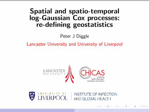
Spatial and spatio-temporallog-Gaussian Cox processes:

re-defining geostatistics

Peter J Diggle

Lancaster University and University of Liverpool

combininghealth information,

computation and statistics

CHICAS

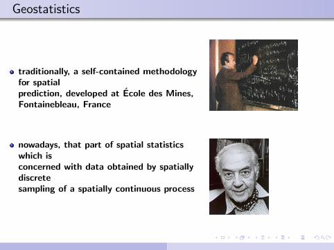
Geostatistics

traditionally, a self-contained methodologyfor spatialprediction, developed at Ecole des Mines,Fontainebleau, France

nowadays, that part of spatial statisticswhich isconcerned with data obtained by spatiallydiscretesampling of a spatially continuous process

Model-based Geostatistics(Diggle, Moyeed and Tawn, 1998)

the application of general principles of statisticalmodelling and inference to geostatistical problems

which means:

− formulate a model for the data

− use likelihood-based methods of inference

− answer the scientific question

Geostatistical data and model : lead pollution in Galicia

5.0 5.5 6.0 6.5 7.0

46.5

47.0

47.5

48.0

X Coord

Y C

oord

S(x) pollution surface

xi sampling location

Yi measured pollution

Yi|S(·) ∼ N(S(xi), τ 2)

Point processes

Stochastic models for arrangements of points in space and/ortime

Scientific focus on understanding why the points are wherethey are:

− absolutely

− and/or relatively

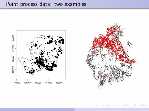
Point process data: two examples

400000 420000 440000 460000 480000

1000

0012

0000

1400

0016

0000

●

●

●

●

●

●

●

●

●

●●

● ●

●●

●

●

●

●

●

●

●

●

●

●

●

●

●

●

●

●

●

●

●

●

●

●

●

●

●

● ●●

●

●

●

●

●

●

●

●

●

●

●

●

●

●

●

●

●

●

●

●

●

●

●

●

●

●

●

●

●

●

●

●

●

●

●

●

●

●

●

●

●

●

●

●

●

●

●

●

●

●

●

●

●

● ●

●

●

●

● ●●

●

●

●

●

●

●

●

●

●

●

●

●

●

●

●

●●

●

●

●

●

●

●

●

●

●

●

●

●

●

●

●

●

●

●

●

●

●

●

●

●

●

●

●

●

●

●

●

●

●

●●

●

●

●●

●

●

●

●

●

●

●

●

●●

●

●

●

●

●

●

●

●

●●

●

●

●

●

●

●●

●

●

●

●

●

●

●

●

●

●

●

●

●

●

●

●

●

●

●

●

●

●

●

●

●

●

●

●

●●

●

●

●

●

●

●

●

●

●

●

●

●

●●

●

●

●

●

●

●

●

●

●

●

●

●

●

●●

●

●

●

●

●

●

●

●

●

●

●

●●

●

●

●

●

●

●

●

●

●

●

● ●

●

●●

●

● ●

●

●

●

●

●

●

●

●

●●

●

●●

●

●

●

●

●

●●

●

●

●

●

●

●

●●

●

●

●

●

●

●

●●

●

●

●●

●

●

●

●

●

●

●

●

●

●

●

●

●

●

●●

●

●

●

●

●

●

●

●

●

●

●

●

●

●

●

●

●

●

●

●

●

●

●

●

●

●

●

●

●

●

●●

●

●

●

●

●

●

●

●●

●

●

●

●

●

●

●

●

●

●

●

●

●

●

●

●

●

●

●

●

●

●

●

●

●

●

●

●

●●

●

●

●

●

●

●

●

●

●

●

●

●

●

●

●

●

●

●

●

●

●

●

●

●

●

●

●

●●

●

●

●

●

●

●

●

●

●

●

●

●

●

●

●

●

●

●

●

●

●

●

●

●

●

●

●

●

●

●

●

●

●●

●

●

●

●

●

●

●

●

●

●

●

●

●

●

●●

●

●

●

●

●

●●

●

●

●

●

●

●

●

●

●

●●

●

●

●

●●

●

●

●

●

●

●

●

●

●

●

●

●

●●

●

●

●

●

●

●

●

●

●

●

●

●

●

●

●

●

●●

●

●

●

●

●

●

●

●

●

●

●

●

●

●

●

●

●

●

●

●

●

●

●

●

●

●

●

●

●

●

●

●

●

●

●

●

●

●

●●

●

●

●

●

●

●

●

●

●

●

●

●

●

●

●

●

●

●

●

●

●

●

●

●

●

●

●

●

●

●●

●

●

●

●

●

●

●

●●

●

●

●

●

●

●

●

●

●

●

●

●

●

●

●

●

●

●

●

●

●

●

●

●

●

●

●

●

●

●

●

●

●●●

●

● ●

●

●

●●

●●

●

●

●

●

●

●

●

●●

●

●

●

●

●

●

●

●

●●

●

●

●

●

●

●●

●

●

●

●

●

●

●

●

●

●

●

●

●

●

●

●

●

●

●

●

●

●

●●

●

●

●

●

●

●

●

●

●

●

●

●

●

●

●

●

●

●

●

●

●

●●

●

●

●

●

●

●

●

●

●

●

●

●

●

●

●

●

●

●

●

●

●

●

●

●

●

●

●

●

●

●●

●

●

●

●

●

●

●

●

●

●

●

●

●

●

●

●

●

●

●

●

●

●

●

●

●

●

●

●

●

●

●

●

●

●

●

●

●

●

●

●

●

●

●

●

●

●

●

●●

●

●

●

●

●

●

●

●

●

●

●

●

●

●●

●

●

●

●

●

●

●●

●●

●

●

●

●

●

●

●

●

●

●

●

●

●

●

●

●

●

●

●

●

●

●

●

●

●

●

●

●

●

●

●

●

●

●

●

●

●

●●

●

●

●

●

●

●

●

●

●

●

●

●

●

●●

●

●

●

●

●●

●

●

●

●

●

●

●

●

●

●

●

●

●

●

●

●

●

●

●

●

●

●

●

●

●

●

●

●

●

●

●

●

●

●

●●

●

●

●

●

●

●

●

●

●

●●

●

●

●

●●

●

●

●

●

●

●

●

●

●

●

●

●

●

●

●

●

●

●

●

●

●

●

●

●

●

●

●

●

●

●●

●

●

●

●

●

●

●

●

●

●

●

●

●

●

●

●

●

●

●

●

●

●

●

●

●

●

●

●

●

●

●

●

● ●

●

●

●

●

●●

●

●

●

●

●

●

●

●

●

●

●

●

●

●●

●

●

●

●

●

●

●

●

●

●

●

●

●

●

●

●

●

●

●

●

●

●

●

●

●

●

●●

●

●

●

●

● ●

●

●

●

●

●

●

●●

●

●

●

●

●

●

●

●

●

●●

●

●

●

●

●

●

●●

●

●

●

●

●●

●

●

●

●

●

●

●

●

●

●

●

●

●

●

●●

●

●

●

●

●

●

●

●

● ●

●

●

●

●

●

●

●

●

●

●●

●●

●

●

●

●

●

●

●

●

●

●

●

●

●

●

●

●

●

●

●

●

●

●

●

●

●

●

●

●

●●●

●

●

●

●

●

●

●

●

●

●

●

●●

●

●

●

●

●

●

●

●

●

●

●

●

●

●

●

●

●

●

●

●

●

●

●

●

●●

●

●●

●

●

●

●

●

●

●

●

●

●

●●

●

●

●

●

●●

●●

●

●

●

●

●

●

●

●

●

●

●●

●

●

●

●

●

●

●

●

●

●

●

●

●

●

●

●

●

●

●

●

●

●

●●

●

●

●

●

●

●

●

●

●

●

●

●

●

●●

●

●

●

●

●

●

●

●

●

●

●

●

●

●

●

●

●

●

●

●

●

●

●

●

●

●

●

●

●

●●

●

●

●

●

●

●

●

●

●

●●

●

●

●

●

●

●

●

●

●

●

●

●

●

●

●

●

●

●

●

●

●

●

●

●●

●

●

●

●

●

●

●

●

●

●

●

●

●

●

●

●

●

●

●

●

●

●

●

●

●

●

●

●

●

●

●

●

●

●

●

●

●

●

●

●

●●●

●

●

●

●

●

●

●

●

●

●

●

●

●

●

●

●

●

●

●

●

●●

●

●

●

●

●

●

●

●

●

●

●

●

●

●

●

●

●

●

●

●

●

●

●●

●

●

●

●

●

●

●

●

●

●

●●

●

●

●

●

●

●

●

●

●

●

●

●

●●

●

●

●

●

●

●

●

●

●

●

●

●

●

●

●

●

●

●

●

●

●

●

●

●

●

●

●

●

●

●●

●●

●

●

●

●●

●

●●●

●

●

●

●

●

●

●

●

●

●

●

●

●

●

●

●● ●

●

●

●

●●

●

●

●

●●

●

●

●

●

●

●

●

●

●

●

●

●

●

●

●

●

●

●

●

●

●

●

●

●

●

●

●

●

●

●

●

●●

●

●

●●

●

●

●

●

●

●●

●

●

●

●

●

●

●

●

●

●

●

●

●

●

●

●

●

●

●

●

●

●●

●

●

●

●

●

●

●

●

●

●●

●

●

●

●

●

●

●

●

●

●

●●

●

●●

●

●

●

●

●

●

●

●

●

●

●

●

●

●

●

●

●

●

● ●

●

●

●

●

●

●

●

●

●

●●

●

●

●

●

●

●

●

●

●

●

●

●

●

●●

●

●●

●

●

●

●

●

●

●

●

●

●

●●

●

●

●

●

●

●

●

●

●

●

●

●

●

●

●

●

●

●

●

●

●●

●●●

●●

●

●

●

●

●●

●

●●

●

●

●

●

●

●

●

●

●

●

●

●

●

●

●

●

●

●

●

●

●

●

●

●

●

●

●

●

●

●

●

●

●●

●

●

●

●

●

●

●

●

●

●

●

●

●

●

●

●

●

●

●

●

●

●

●

●

●

●●

●

●

●

●

●

●

●●

●●

●

●

●

●

● ●

●

●

●

●

●

●

●

●

●

●

●

●●●

●

●

●

●

●

●

●

●

●

●

●

●

●

●

●

●

●

●

●

●

●

●

●

●

●

●●

●

●

●

●

●

●

●

●

●

●

●●

●

●

●

●

●

●

●

●

●

●

● ●

●

●●

●

●

●

●●

●

●

●

●

●

●

●

●

●●

●

●

●

●

●

●

●

●

●

●

●

●●

●

●

●

●

●

●

●

●

●

●●

●

●

●

●

●

●

●

●

●

●

●

●

●

●

●

●

●

●●

●

●

●

●

●

●

●

●

●

●

●

●

●

●

●

●

●

●

●

●

●

●

●

●● ●

●

●

●

●

●

●

●

●

●

●

●

●

●

●

●

●

●

●

●

●

●

●

●

●

●

●●

●

●

●

●●

●

●

●

●

●

●

●

●

●

●

●

●

●

●

●

●

●

●

●

●

●

●

●

●

●●

●

●

●

●

●

●

●

●

●

●

●

●

●

●

●

●

●

●●

●

●

●

●

●

●

●

●

●

●

●

●

●

●

●

●●

●

●

●

●

●

●

●

●

●

●

●

●

●

●

●

●

●

●

●

●

●

●

●

●

●

●

●

●

●

●

●

●

●

●●

●

●

●●

●

●

●

●

●

●

●●

●

●

●

●

●

●

●

●

●

●

●

●

●

●●

●

●

●

●

●●

●

●

●

●

●

●

●

●

●

●

●

●

●

●

●

●●

●

●

●●

●

●

●

●

●

●

●

●

●●

●

●

● ●

●

●

●

●

●

●

●

●

●

●

●

●

●

●

●

●

●

●

●

●

●

●

●

●●

●

●

●

●

●

●

●●

●

●

●

●

●

●

●

●

●

●●

●

●

●

●

●

●

●

●●

●●

●

●

●

●

●

●

●

●

●

●

●

●

●

●

●

●

●

●

●

●

●

●

●

●

●

●

●●

●

●

●●

●

●

●

●

●

●

● ●

● ●

●

●

●

●

●

●

●●

●

●

●

●

●

●

●

●

●

●

●

●

● ●

●

●

●●

●

●

●

●

●

●

●

●

●

●

●

●

●

●

●

●

●

●

●

●

●

●

●

●●

●

●

●

●

●●

●

●

●

●

●

●

●

●

●●

●

●

●

●

●

●

●

●

●

●

●

●

●

●●

●

● ●

●

●

●

●

●

●

●

●

●

●

●●

●

●

●

●

●

●

●

●

●

●

●

●

●

●●

●

●

●

●

●

●

●

●

●

●

●

●

●

●

●

●

●

●

●

●

●

●

●

●

●

●●

●

●

●

●

●

●

●

●

●

●

●

●

●

●

●

●

●

●

●●

●●

●

●

●

●

●

●

●

●

●

●

● ●

●

●

●

●

●

●

●

●

●

●

●

●

●

●

●

●

●

●

●

●

●

●

●

●

●

●

●

●

●

●

●●

●

●

●

●

●

●

●

●

●

●

●

●●

●

●●

●

●

●

●●

●

●

●●

●

●

●

●

●●

●

●

●

●

●

●

●

●

●

●

●

●

●

●

●

●

● ●

●

●

●

●

●

●

●

●

●

●

●

●

●

●

●

●

●

●

●

●

●

●

●

●●

● ●

●

●

●

●

●

●

●

●

●

●

●

●

●

●

●

●

●

●

●

●

●

●

●

●

●

●

●

●

●

●

●

●

●

●●

●

●

●

●

●

●

●

●

●

●

●

●

●

●

●

●

●

●

●

●●

●●

●●

●

●

●

●

●

●

●

●

●

●

●

●

●

●

●

●●

●

●

●● ●

●● ● ●

●

●

●

●

●

●

●

●

●

●

●●

●

●

●

●

●

●

●

●

●

●

●

●

●

●

●

●

●

●

●

●

●

●

●

●

●

●

●

●

●

●

●

●

●

●

●

●

●

●

●

●

●

●

●

●

●

●

●

●

●

●

●

●

●

● ●

●

●●

●

●

●

●

●

●

●

●

●

●

●

●

●

●

●

●

●

●

●

●

●

●

●

●

●

●

●

●

●●

●

●

●

●

●

●

●

●

●

●

●●

●

●

●

●

●

●

●

●

●

●

●

●

●

●

●

●

●

●

●

●●

●

●

●

●

●

●

●

●

●

●

●

●

●

●

●

●

●

● ●

●

●●

●●

●

●

●

●

●

●

●

●

●●

●

●

●

●

●●

●

●

●

●

●

●●

●

●

●

●

●

●

●

●

●

●

●

●

●

●

●

●

●

●

●

●

●

●

●

●

●

●●

●

●

● ●

●

●

●

●

●

●

●

●

●

●

●

●

●

●

●

●

●

●

●●

●●

●

●

●

●

●

●

●

●

●

●

●

●

●

●

●

●

●

●

●

●

●

●

●

●

●

●●

●

●

●

●

●

●

●

●

●

●

●

●

●

●●

●

●

●

●●

●

●●

●

●

●

●

●

●

●

●

●

●

●

●

●

●

●

●

●

●

●

●

●

●

●

●

●

●

●●

●

●

●

●

●

●●

●

●

●

●

●

●

●

●

●

●

●

●

●

●

●

●

●

●

●

●

●

●

●

●●

●

●

●

●

●

●

●

●

●

●

●

●

●

●

●

●

●

●

●

●

●

●

●

●

●

●

●

●

●

●

●

●

●

●

●

●

●●

●

●

●

●

●

● ●

●

●

●

●

●

●

●

●

●

●

●

●

●

●

●

●

●●

●

●

●

●

●

●

●●

●

●

●

●

●

●

●

●

●

●

●

●

●

●

●

●

●

●

●

●

●

●

●

●●

●

●

●

●

●

●

●

●

●

●

●

●

●

●

●

●

●

●

●

● ●

●

●●

●

●

●

●

●

●

●

●

●

●

●

●

●

●

●

●

●

●

●

●

●

●●

●

●

●

●

●

●

●

●

●

●

●

●

●

●

●

●

●

●

●

●

●

●

●

●

●

●

●

●

●

●

●

●

●

●

●

●

●

●

●

●

●

●

●

●

●

●

●●

●

●

● ●

●

●

●

●

●

●

●

●●

● ●

●

●

●

●●

●

●

●

●●

●

●

●

●

●

●

●

●

●

●●

●

●

●

●

●

●

●

●

●

●

●

●

●

●●

●

●

●

●●

●

●

●

●

●

●

●

●●

●

●● ●

●

●

●

●

●

●

●

●

●

●

●

●

●●

●

●

●

●

●

●

●

●

●

●

●●

●

●

●

●

●

●

●

●

●

●

●

●

●● ●

●

●

●

●

●

●●

●

●

●

●●●

●

●

●

●●

●

●

●

●

● ●

●

●

●

●

● ●

●

●

●

●●

●

●

●

●

●

●

●

●

●●

●

● ●

●

●

●

●

●

●

●

●

● ●

●

●

●●

●

●

●

●

●

●

●

●

●

●●

●

●

●

●

● ●

●

●●

●

●

●

●

●

●

●

●

●

●

●

●●

●

●

●

●

●

● ●

●

●

● ●

●

●

●●

●

●

●

●

●●

●

●

●

●

●

●

●

●

●

● ●

●

●●

●

●

●●●

●

●

●

●

●

●

●

●

●

●

●

●

●

●

●

●

●

●

●●

●

●

●

●

●

●

●

●

●

●

●

●

●

●

●

●

●

●

●

●

●

●

●

●

●

●

●

●

●●

●

●

●

●

●

●

●

●

●

●

●

●

●

●

●●

●●●

●

●

●

●

●

●

●

●

●

●●

●●

●●

●●

●

●

●●

●

●

● ●

●

●

●

●

●

●

●

●

●

●●●

●●

●

●

●

●

●●

●

●

●

●

●●

●

●

●

●

●

●

●

●

●

●

●

●

●

●

●

●

●

●

●

●

●

●

●

●

●

●

●● ●

●

●

●

●

●

●

●

●

●

●●●

●

●

●●

●

●

●

●

●

●

●

●

●

●

●

●

●

●

●

●

●

●

●

●

●

●●

●

●

●

●

●

●

●

●

●

●

●

●●

●

●

●

●●

●

●

●

●

●●

●

●

●●

●●

●

●

●

●●

●

●

●

●●

●

●

●

●

●

●

●

●

●●

●

●

●

●

●

●

●

●

●

●

●

●

●

●

●

●

●

●

●

●

●

●

●

●

●

●

●

●

●

●

●

●

●

●●

●

●

●

●

●●

●

●●

●

●

●●

●

●

●

●●

●

●

●

●

●

●

●

●

●●

●

●

●

●●

●●●

●●

●

●

●

●

●

●●

●

●

●

●●

●

●

●●

●

●

●

●●

●

●

●

●

●

●

●

●

●

●

●

●

●

●

●

●

●

●

●

●

●

●

●

●

●●

●

●

●

●

●●

●

●

●

●

●

●

●

●

●

●

●

●

●●●

●

●●●

●

●

●

●

●

●

●

●

●

●

●

●

●

●

●

●

●

●

●

●

●●

●

●

●

●

●

●

● ●

●

●

●

●

●

●

●

●

●

●

●

●

●

●

●

●

●●

●

●

●

●

●

●

●

●

●●

●

●

●

●

● ●

●

●

●

●●

●

●

●

●

●

●

●

●

●

●

●

●●●

●

●

●

●●

●

●

● ●

●

●●

●

●

●

●

●

●

●

●

●

●

●

●

●●

●

●● ●

●

●

●

●

●

●

●

●

●

●

●

●

●

●

●

●

●

●●

●

●

●

●

●

●

●

●

●

●

●

●

●

●

●

●

●

●

●

●

●

●

●●●

●●

●

●

●

●

●

●●●

●

●

●

●●

●

●

●

●

●

●

●

●

●●

●

●

●

●

●

●

●

●

●

●

●

●

●

●

●

●

●

●

●

●

●

●

●

●

●

●

●

●

●

●

●

●

●

●

●

●

● ●

● ●

●

●

●

●

●

●

●

●

●● ●

●

●

●

●

●●

●

●

●●

●

●

●●

●

●

●

●

●●

●

●●

●

●

●

●

●

●

●

●

●

●

●

●

●

●

●

●

●

●

●●

●

●

●

●

●●

●

●●

●

●

●

●

●

●

●●

●

●

●

●

●

●

●

●

●

●

●

●

●

●

●

●

●

●

●

●

●

●

●

●

●

●

●

●

●

●

●

●●

●

●

●

●

●●

●

●

●

●

●

●

●

●

●

●

●

●

●

●●

●

●

●

●

●

●

●

●

●

●

●

●

●

●

●

●●

●

●

●

●

●●

●

●

●

●

●

●

●●

●●

●

●

●

●

●

●

●

●

●

●

●

●

●

●

●

●

●

●

●

●

●

●

●

●

●

●

●

●●

●

●

●

●●

●●

●

●

●●

●

●

● ●

●

●

●

●

●

●●

●

●

●

●

●

●

●

● ●

●

●

● ●

●

●

● ●

●

●

●

●

●

●

●

●

●

●

●

●

●●

●

●●

●

●

●

●

●

●

●

●

●●

●●

●

●

●

●

●

●

●

●

●

●

●

●

●

●

●●

●

●●

●

●

●

● ●●

●●

●

●

●

●

●

●●

●

●

●

●

●

●●

●

●

●

●

●

●

●

●

●

●

●

●

●

●

●

●

●

●

●

●

●

●

●●

●

●

●●

●

●

●

●●

●

●

●

●

●

●

●

●

●●

●

●●

●

●

●

●

●

●

●

●

●●

●

●

●

●

●●

● ●

●

●

●

●

●

●

●

●

●

●

● ●●

●

● ●

●

●

●

●

●

●

●

●

●

●

● ●

●

●

●

●

●

●

●

●

●

●

● ●●

●●

●

●

●● ●

●

●

●

●

●●

●

●

●●

●

●

●

●●

●

●

●

●

●

●

●

●

●

●

●

●●

●

●

●

●

●

●

●

●

●

●

●

●

●

●

●

● ●●

●

●

●●

●●

●

●

●

●

●

●

●●

●

●

●

●

●

●

●●

●●

●

●

●

●

● ●

●

●

●

●

●

●

●

●

●

●

●

●

● ● ●

●

●

●

●

●

●

●

●

●

●

●

● ●

●

●

●●

●

●

●●

●

●

●

●

●●

●

●

●

●

●●

●

●

●

●

●

●

●

●

●

●

●

●

●●

●

●

●

●

●

●●

●

●

●

●

●

●

●●

●●●

●

●

●

●

●

●

●

●

●●

●

●

●

●

●

●

●●

●

●

●

●●●

●

●

●●

●

●

●●

●

●

●

●● ●

●

●

●

●

●

●

●

●

●

●●

●

● ●

●

●

●

●

●●

●

●

●

●

●

●

●● ●

●

●

●●

●●

●

●

●

●

●

●

●

●●

●

●

●

●

●

●

●

●

●

●

●

●

●

●●

●

●

●

●

●●

●

●

●

●

●

●

●

●

●

●

●

●

●●

●

●

●

●●

●

●●

●●

●

●

●

●

●

●

● ●

●

●

●

●

●

●

●

●

●

●

●

●

●

●

●

●

●

●

●

●

●

●

●

●●

●

●

●

●

●

●

●

●

●

●●

●

●

●

●

●

●

● ●

●

●

●

●

●● ●

●

●●●

●

●

●

●

●

●●

●

●

●

●

●

●●

●

●

●

● ●

●

●● ●

●

●

●●

●

●

●

● ●

●

●

●

●

●

●

●

●

●

●●

●

●

●

●

●

●

●

●

●●

●

●

●

●

●

●

●

●

●●●

●

● ●

●

●

●

●

●

●

●

●

●●

●

●●

●

●

●

●

●

●

●

●

●

●

●

●●●

●●

●

●

●

●

●

●

●

●

●

●

●

●

●

●

●●

●

●

●

●

●

●

●

●

●

●

●

●

●

●

●●

●

●●

●

●

●

●

●

●

●

●

●

●●

●

●

●

●

●

●

●

●●

●

●●

●

●●

●

●

●

●

●

●

●

●

●

●

●

●

●

●●

●●

● ●

●

●

●

●

●

● ●

● ●

●

●

●

●

●

●

●

●

●

●

●

●

●

●

●

●

●

●

●

●

●

●

●

●●

●

●●

●

●

●

●

●

●

●

●●●

●

●

●

●

●

●

●

●

●

●

●

●

●

●

●

●

●

●

●

●

● ●● ●

●

●

●

●

●

●

●

●

●

●

●

● ●

●

●

● ●

●

●

● ●

●●

●

●

●

● ●

●

●

●●

●

●

●

●

●

●

●

●●●

● ●

●

●

●

●

●

●

●

●

●

●

●●

●●●

●

●

●●

●

●

●

●

●

●

●

●

●

●

●● ●●

●

●

●

●

●

●

●

●

●

●

●

●

●●

●

● ●

●

●

●

●

●

●

●

●

●

●

●

●

●

●

●●

●

●●

●

●

●

●

●

●

●

●

●●

●

●

●

●

●

●

●

●

●

●

●

●

●

●

●●

●

●

●

●

●

●

●

●

●

●

●

●

●

●

●

●

●

●●

●

●●

●

●

●

●

●

●

●

●●

● ●

●

●

●

●

●

●

●

●

●

●

●

●

●

●

●

●

●

●

●

●

●

●

●

●

●

●

●●

●●

●

●

●

●

●

●

●

●

●

●

●

●

●●●

●

●

●

●●

●

●

●

●

●●

●

●

●

●

●

●

●

●●

●

●●

●

●●

●

●

●

●

●

●

●

●

●

●

●

● ●

●●

●●

●

●

●

● ●●

●

●

●●

●

●

●

●

●●

●

●

●

●

●

●

●

●

●

●

●

●

●

●

●

●

●

●

●

●

●

●

●

●

●

●

●

●

●

●●

●

●

●

●

●

●

●

●

●●

●

●

●

●

●

●

●

●

●

●

●

●

●

●

●

●

●

●

●

●

●

●

●

●

●

●

●

●

●

●

●

●

●

●

●

●

●

●

●

●

●

●

●

●

●

●

●

●

●

●

●

●

●

●

●●

●

●

●

●

●

●

●

●

●

●

●

●

●

●

●●

●

●

●

●

●

●

●

●

●

●

●

●

●

●

●

●●

●

●

●

●

●

●

●●

●

●

●

●

●

●

●

●

●

●

●

●

●

●

●

●

●

●

●●

●

●

●

●

●

● ●

●●

●

●

●

●●

●

●●

●

●

●

●

●

●

●

●

●

●

●

●

●

●

●

●●

●●

●

●

●

●

●

●

●

●

●

●

●

●●

●

●

●

●

●

●

●

●

●

●

●

●

●

●

●

●

● ●

●

●

●

●

●

●

●

●

●

●

●

●

●

●

●

●

●

●

●

●

●

●

●

●

●

● ●●

●

●

●

●

●

●

●●

●●

●●

●

●

●

●

●

●●

●

●

●

●

●

●

●

●

●

●

●

●

●●

●

●

●

●

●

●

●

●

●

●

●

●

●

●

●

●

●

●

●

●

●

●

●

●

●

●

●●

●

●

●

●

●

●

●

●

●

●

●

●

●

●

●

●

●

●

●

●

●

●

●

● ●

●

●

●

●

●

●

●

●

●

●

●

●

●

●

●

●

●

●

●●

●

●

●●

●

●

●

●

●

●

●

●

●

●

●

●

●

● ●●

●

●

●

●

●

●

●

●

●

●

●

●● ●

●

●

●

●

●

●

●

●

●

●

●●

●

●

●

●

●●

●●●

●

●

●

●

●●

●●

●●●

●

●

●

●

●

●

●●

●

●

●

●

●

●

●●

●

●

●

●

●

●

●

●

●

●

●

●

●

●

●

●

●

●

●

●

●

●

●

●

●

●

●

● ●

●●

● ●●

●

●

●

●

●

●

●

●

●

●

●

●

●

●

●●

●

●

●

●

●

●

●●

●

●

●

●

●

●●

●

●

●

●

●●

●

●

●●

●

●

●

●

●

●

●

●●

●

●

●

●

●

●

●

●

●

●

●

●

●

●

●

●

●

●

●

●

●

●

●

●

●

●

●

●

●

●

●

●

●

●

●

●

●

●

●

●

●

● ●

●

●

●

●

●

●●

●

●

●

●

●

●

●

●

●

● ●

●

●

●

●

●

●

●

●

●

●

●

●

●

●

●

●

●

●

●

●

●

●

●

●

●

●●

●

●●

●

●

●

●

●

●

●

●

●

●

●

●

●

●

●

●

●

●

●

●

●

●

●

●

●

●

●

●

●

●

●

●

●

●

●

●

●

●●

● ●●

●

●

●

●

●

●

●

●

●

●

●

●

● ●

●

●

●

●

●

●

●

●●

●●

●

●

●●●

●

●●

●

●

●●

●

●

●

●

●

●

●

●

●

●

●

●

●

●

●

●

●

●

●

●

●

●

●

●●

●

●

●

●

●

●

●

●

●

●

●

●

●

●

●

●

●

●●

●●

● ●

●

●●

●

●

●

●

●

●

●

●

●●

●●

●●

●

●●●

●

●

●

●

●

● ● ●

●

●

●

● ●

●●

●

●

●

●●

●

●

●

●

●

●

●

●

●

●

●●

●

●

●

●

●

●

●

●

● ●

●

●●

●

●

●

●

●

●

●

●

●

●

●

●

●

●

●

●

●

●

●

●

●

●

●

●

●

●

●

●

●●

●

●

●

●

●

●

●

●

●

●

●

●

●

●

●

●●

●

●

●

●

●

●

●

●●

●

●

●●

●●

●

●

●

●

●

●

●

●

●

●

●

●

●

● ●●

●

●

●

●

●

●

●

●

●

●

●●

●

●

●

●

●●

●●

●

●

●

●

●

●

●

●

●

●

●

●

●

●

●

●

●

●

●

●

●

●

●●

●

●

●

●●

●

●

●

●

●

●

●

●

●

●

●

●

●

●

●

●

●

●

●

●●

●

●

●● ●

●

●

●

●

●

●

●

●

●

●

●

●

●

●

●

●

●

●

●

●

●

●

●

●

●●

●

●

●

● ●

●

●

●

●

●

●

●

●●

●●

●●

●

●

●

●

●●

●

●

●

●

●

●

●

●

●

●

●

● ●● ●

●

●

●

●

●

●

●

●

●

●

●

●

●

●

●

●

●●

●

● ●

●

●

●●

●

●

●

●

●

●

●●

●

●

●

●

●

●

●

●

● ●

●

●

●● ●

●

●

●

●●●

●

●

●

●

●

●

●

●

●

●

●●

●

●

●

●

●

●

●

●

●

●●

●

●

●

●

●

●

●●

●●

●

●

●

●

●

●

●

●

●●

●

●

●

●

●

●

●

●

●

●

●

●

●

●

●

●

●

●

●

●

●

●

●

●

●

●

●

●

●

●●

●

●

●

●

●

●

●

●●

●

●● ●

●

●

●

●● ●

●● ●

●

●

●

●

●

● ●

●

●

●

●

●

●

●

●

●

●

●

●

●

●

●

●

●●

●

●

●

●

●

●

●●

● ●

●

●

●●

●

●

●

●

●

●

●

●

●

●

●

●

●● ●

●

●

●●

●

●●

● ●

●

●

●

●

●

●

●

●

●

●

●

●

●

●

●

●

●

●

●

●

●

●●

●

●

●

●

●●

●

●

●

●

●

●

●

●

●

●

●

●

●

●

●

●

●

●

●

●

●

● ●

●

●

●

●

●

●

●

●

●

●

●

●

●

●

●

●

●

●

●

●

●

●

●

●

●

●

●

●●

●

●●

●

●

●

●

●

●●

●

●●

●

●

●

●

●●

●

●●

●

●●

●

●

●

●

●

●●

●

●

●

●

●

●●

●

●●

●

●

●

●

●

● ●

●

●

●

●●

●

●

●

●

●●

●

●●

●

●

●

●

●

●

●●

●●●

●

●

●

●

●

●

●

●

●

●

●

●

●

●

●

●

●

●

●

●●

●

●

●

●

●

●

●

●

●

●●

●

●

●

●

●●

●

●

●

●

●

●●

●

●

●

●

●

●

●

●●

●●

●

●

● ●●

●

●

●

●

●

●●

●

●

●

●

●

●

●

●

●●

●

●

●

●

●

●

●

●●

●● ●

●

●

●

●

●

●

●

●

●

●

●

●

●

●

●

●

●●

●

●●

●

●

●

●

●●

●●

●●

●

●

●

●

●

●●

●

●

●

●

●

●

●

●

●

●●

●

●

●

●

●

●

●● ●

●

●

●

●

●

●●

●

●

●

●

●

●

●

●

●

●

●

●

●

●

●

●

●

●

●

● ●

●

●

●

●

●

●

●●

●

●

●

●

●

●

●

●

●

●●

●

●

●

●●

●

●

●●

●

●

●

●

●

●

●

●

●

●

●●

●

●●

●

●

●

●

●

●

●

●

●

●

●

●

●

●

●

●●

●

●

●

●

●

●

●

●

●

●

●

●

●

●

●

●

●

●

●

●

●

●

●

●

●

●

●●

●

●

●

●

●

●

●

●

●

●

●

●●

●

●

●

●

●

●

●

●

●

●

●

●

●

●

●

●

●

●

●

●

●

●

●

●

●

●●

●

●

●

●

●

●

● ●

●

●

●

●

●●

●●

●

●

●

●

●

●

●

●

●

●

●

●

●

●

●●

●

●

●

●

●

●

●●

●

●

●

●

●

●●

●

●

●

●

●

●

●

●

●●

●

●

●

●

●

● ●

●

●

●

●

●

●

●

●

●

●

●

●

●

●●

●

●

●

●

●

●

●

●●

●

●

●

●

●

●●

●

●

●●

●

●

●

●

●

●

●

●

●

●

●

●

●

●

●

●

●

●

●

●

● ●

●

●

●

●

●

●

●

●

●

●

●

●●

●

●

●

●

●

●●

●●

●

●●

●

●

●

●

●

●

●

●

●

●

●

●

●

●

●

●●

●

●

●

●

●

●

●

●

●

●

●●

●

●

●

●

●

●

●

●

●

●● ●

●●

●

● ●●

●

●

●

●●

●

●

●

●

●

●

●●

●

●

●

●●

●

●

●

●●

●

●

●

●

●

●

●

●

●

●

●

●

●

●

●

●

●●

●

●●●

●

●

●

●

●●

●

●

●

●

●

●

●

●

●

●

●

●

●

●

●

●

●

●

●

●

●

●

●

●

●●

●

●

●

●

●

●

●

●●

●

●●

●

●

●

●

● ●

●

●

●

●

●

●

●

●

●

●●

●

●

●

●

●

●

●

●

●

●

●

●

●

●

●

●

●

●

●

●●

●

●

●

●

●

●

●●

●

●

●

●

●

● ●

●

●

●

●●

●●

●

●

●●

●

●

●

●

●

●

●

●●

●

●

●

●

●

●●

●

●●

●

●

●

●

●

●

●

●

●

●

●

●●

●

●●

●

●

●

●

●

●

●

●

●●●

●

●

●

●

●

●

●

●

●

●

●

●

●

●

●

●

●

●

●

●

●

●

●

●

●

●

●

●

●

●

●●

●

●

●

●

●

●

●

●

●

●

●

●

●

● ●

●●

●

●

●

●

●

●

●

●

●

●

●●

●

●

●

●

●

●

●●

●

●

●

●

●●

●

●

●

●

●

●

●

● ●

● ●

●

●

●

●

●

●

●

●● ●

●

●

●

●

●

●

●

●

●

●

●

●

●

●

●

●

●

● ●

●

●

●

●

●

●

●

●

●

● ●

●

●

●

●

●

●

●

●

●

●

●

●

●

●●

●

●

●

●

●●

●

●

●●

●

●

●

●

●

●

●

●

●

●

●

●

●

●

●

●

●

●

●

●

●

●

●

●

●

●

●

●

●

●

●

●

●

●

●

●

●

●

●

●

●

●

●

●

●

●

●

●

●

●

●

●

●

●

●

●

●

●●

●

●

●

●●

●

●

●

●

●

●

●

●

●

●●

●

●

●

●

●

●

●

●

●●

●

●

●●

●

●

●

●

●

●

●

●

●

●

●

●

●

●

●●

●

●

●

●

●

●● ●

●

●

●

●

●

●

●

●

●

●

●

●

●

●

●

●

●

●

●

●

●

●

●

● ●

●

●

●

●

●

●

●

●

●

● ●

●

●

●●

● ●

●

● ●

●

●

●

●

●

●●

●

●

●

●

●

●

●

●

●

●

●

●

●

●

●

●

●

●●

●

●

●

●

●

●

●

●

●

●

●

●

●

●

●

●●

●

●

●

●

●

●

●●

●

●

●

●

●

●

●

●

●

●

●

●

●

●

●

●

●

●

●

●

●

●

●●

●

●

●

●

●

●

●

●

●

●

●

●

●

●

●

●●

●

●

●

●

●

●

●

●

●

●

●

●

●

●

●

●

●

●

●

●

●

●

●

●

●

●

●

●

●●

●

●

●

●

●

●

●

●

●

●

●

●

●

●

●

●

●

●

●

●

●

●

●

●●

●

●

●

●

●

●

●

●

●

●

●●

●●

●

●

●●

●

●

●

●

●

●

●

●

●

●

●

●

●

●●

●

●

●●

●

●● ● ●

●

●

●

●

●

●

●

●

●

●

●

●

●

●●

●

●

●

●

●

●

●

●

●

●

●

●

●●

●

● ●

●

●

●●

●

●

●

●

●

●

●

●

●

●

●

●

●

●●

●

●

●

●

●

●●

● ●●

●

● ●

●

●

●

●

●

●

●

●

●

●

●

●

●

●

●

●

●

●

●

●

●

●

●

●

●

●

●

●

●

●●

●

●

●

●

●

●

●

●

●

●

●

●

●

●●

●

●

●

●

●

●●

●

●

●

●

●

●

●

●

●

●

●

●

●

●

●

●

●

●

●

●

●

●

●

●

●

●

●

●

●

●

●

●

●

●

●

●

●

●

●

●

●

●

●

●●

●

●

●

●

●

●

●

●

●

●

●

●

●

●

●

●

●

●

●

●●

●

●

●●

●●●●●●●●●

●●●●●

●●●

●●

●●●●●●●●●●●

●●

●

●●●

●●

●

●

●

●

●

●

●●●●

●●●

●●

●●

●●

●●

●●

●●●

●

●●

● ●●

●●

●●●

●

●●

●

●●

●●

●●●

●●

●

●●●●●

●

●●

●●

●●

●●●

●●●●

●

●●

●

●

●●

●

● ●

●●

●●

●●● ●

●

●●●●

●

●●● ●

● ●

●

●

●●

●● ●●●●

●●

●

●●

●

●●

●

●

●●

●●●

●●

●●

●●

●●

●●

●●

●

●

●

●

●●

●

●

●●●●

●●●

●

●●

●●●

●

●●

●

●

●●●

●●●

●

●

●

●

●

●●

●●

●● ●

●

●

●

●

●●●●

●●

●●

●

●

●

●● ●

● ●

●●●

●

●●●●

●

●

●

●●

●●●●●

●●●● ●●

●●

●

●●

●●●

●

●●

●● ●

●

●●

●●

●●

●●●

●●● ● ●

●●●

●●●

●

●

●

●

●

●

●

●

●

● ●

●●

●

●●●

●

●

●●

●

● ●●●

●●●

●

●●

●●

● ●

●

●

●

●

●

●

●

●

●●●

●

●

●●

●

●

●

●●●●

●

●

●●

●

●

●●

●

●●

●

●●●

●●●●●

●●●

●●

●

●●●

●●

●

●

●

●

●●

●

●

●●●

●

●

●

●●

●

●

●

●

●

● ●

●

●

●●

●

●●

●●

●

●●●

●

●

●

●

●●●

●●

●

●●

●●

●

●

●●●

●

●

●

●●

●●

●

●

●

●

● ●

●

●●

●

●

●

●

●

●●

●

●

●

●●

●

●●

●

● ●●

●

●

●

●

●

●

●

●

●

●

●

●

●

●

●●

●●●

●●

●

●

●

●●

●

●●

●

●●

●●

●●

●

●

● ●

●

●●

●●●

●●●

●

●●

●●●

●

●

●

●●

●

●

●

●●●

●●●

●

●●●●●

●

●●●●●

●●

●

●●●

●●●●

●● ●

●

●

●●●●

●

●●

●

●

●● ●●

●

●

●●

●● ●

●●

●●

● ●

●●

●

●

●

●●

●

●

●●

●

●

●

●●

●

●● ●

●

●●

●●

●●●

● ●●

●

●

●●

●

●●

●●

●●●

●

●●

●

●●

●●

●●●●

●●●

●

●

●●

●

●

●●

●●●

●

●●

●●

●●

●●●●

●

● ●●

● ●

● ●

●

●

● ●

●

●

●

Cox process

Poisson process

λ(x) : intensity function

event-locations mutually independent, probability densityproportional to λ(x)

Requires: λ(x) ≥ 0 and∫

A λ(x)dx <∞, for any finite region A

Cox process

λ(x) is unobserved realisation of stochastic process Λ(x)

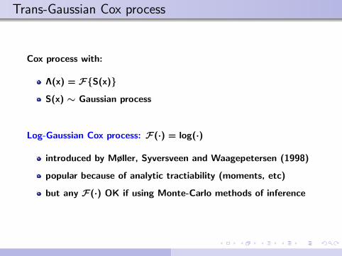
Trans-Gaussian Cox process

Cox process with:

Λ(x) = F{S(x)}

S(x) ∼ Gaussian process

Log-Gaussian Cox process: F(·) = log(·)

introduced by Møller, Syversveen and Waagepetersen (1998)

popular because of analytic tractiability (moments, etc)

but any F(·) OK if using Monte-Carlo methods of inference

LGCP as a geostatistical model

● ●

●●

●

●

●

●

●

●

●

●

●

●

●

●

●

●

●

●

●

● ●

●

●

●

●

●

●

●

●

●

●

●

●

●

●

●

●

●

●

●

●

●

●

●

● ●

●

●

●

●

●

●

●

●

●

●

●

●

●

● ●

●

●

●

●

●

●

●

●

●

●

●

●

●

●

●

●

●

●

●

●

●

●

●

●

●

●

●

●

●

●

●

●

●

●

●

●

●

●

●

●

●

●●

●

●

●

●

●

●

●

●

●

●

●

●

●

●

●

●

●

●

●

●●

●

● ●

●

●

●

●●

●

●

●

●

●

●

●

●

●

●

●

●

●

●

●

●

●

●

●

●

●

●

●

●

●

●

●

●

●

●

●

●

●

●

●

●

●

●

●

●

●

●

●

●

●

●

●

●

●

●

●

● ●

●

●

●

●

●

●

●

●

●

●

●

●

●

●

●

●●

●

●

●

●

●

●

●●

●

●

●

●

●

●

●

●

●

●

●

●

●

●

●

●

●

●

●

●

●

●

●

●

●

●

●

●

●

●

●

●

●

●

●

●

●

LGCP as a geostatistical model

2

2

2

2

1

1

1

5

1

2

4

2

1

4

3

8

5

2

2

6

3

4

5

1

1

0

5

3

7

3

2

2

3

2

4

5

3

11

2

6

1

5

7

10

12

16

5

3

6

2

4

6

5

5

2

6

5

4

3

6

4

4

1

0

LGCP as a geostatistical model

● ●

●●

●

●

●

●

●

●

●

●

●

●

●

●

●

●

●

●

●

● ●

●

●

●

●

●

●

●

●

●

●

●

●

●

●

●

●

●

●

●

●

●

●

●

● ●

●

●

●

●

●

●

●

●

●

●

●

●

●

● ●

●

●

●

●

●

●

●

●

●

●

●

●

●

●

●

●

●

●

●

●

●

●

●

●

●

●

●

●

●

●

●

●

●

●

●

●

●

●

●

●

●

●●

●

●

●

●

●

●

●

●

●

●

●

●

●

●

●

●

●

●

●

●●

●

● ●

●

●

●

●●

●

●

●

●

●

●

●

●

●

●

●

●

●

●

●

●

●

●

●

●

●

●

●

●

●

●

●

●

●

●

●

●

●

●

●

●

●

●

●

●

●

●

●

●

●

●

●

●

●

●

●

● ●

●

●

●

●

●

●

●

●

●

●

●

●

●

●

●

●●

●

●

●

●

●

●

●●

●

●

●

●

●

●

●

●

●

●

●

●

●

●

●

●

●

●

●

●

●

●

●

●

●

●

●

●

●

●

●

●

●

●

●

●

●

LGCP as a geostatistical model

● ●

●●

●

●

●

●

●

●

●

●

●

●

●

●

●

●

●

●

●

● ●

●

●

●

●

●

●

●

●

●

●

●

●

●

●

●

●

●

●

●

●

●

●

●

● ●

●

●

●

●

●

●

●

●

●

●

●

●

●

● ●

●

●

●

●

●

●

●

●

●

●

●

●

●

●

●

●

●

●

●

●

●

●

●

●

●

●

●

●

●

●

●

●

●

●

●

●

●

●

●

●

●

●●

●

●

●

●

●

●

●

●

●

●

●

●

●

●

●

●

●

●

●

●●

●

● ●

●

●

●

●●

●

●

●

●

●

●

●

●

●

●

●

●

●

●

●

●

●

●

●

●

●

●

●

●

●

●

●

●

●

●

●

●

●

●

●

●

●

●

●

●

●

●

●

●

●

●

●

●

●

●

●

● ●

●

●

●

●

●

●

●

●

●

●

●

●

●

●

●

●●

●

●

●

●

●

●

●●

●

●

●

●

●

●

●

●

●

●

●

●

●

●

●

●

●

●

●

●

●

●

●

●

●

●

●

●

●

●

●

●

●

●

●

●

●

LGCP as a geostatistical model

● ●

●●

●

●

●

●

●

●

●

●

●

●

●

●

●

●

●

●

●

● ●

●

●

●

●

●

●

●

●

●

●

●

●

●

●

●

●

●

●

●

●

●

●

●

● ●

●

●

●

●

●

●

●

●

●

●

●

●

●

● ●

●

●

●

●

●

●

●

●

●

●

●

●

●

●

●

●

●

●

●

●

●

●

●

●

●

●

●

●

●

●

●

●

●

●

●

●

●

●

●

●

●

●●

●

●

●

●

●

●

●

●

●

●

●

●

●

●

●

●

●

●

●

●●

●

● ●

●

●

●

●●

●

●

●

●

●

●

●

●

●

●

●

●

●

●

●

●

●

●

●

●

●

●

●

●

●

●

●

●

●

●

●

●

●

●

●

●

●

●

●

●

●

●

●

●

●

●

●

●

●

●

●

● ●

●

●

●

●

●

●

●

●

●

●

●

●

●

●

●

●●

●

●

●

●

●

●

●●

●

●

●

●

●

●

●

●

●

●

●

●

●

●

●

●

●

●

●

●

●

●

●

●

●

●

●

●

●

●

●

●

●

●

●

●

●

Re-defining geostatistics

Old:

unobserved, real-valuedstochastic processS = {S(x) : x ∈ A}

pre-specified locations{xi ∈ A : i = 1, ..., n}measurements

Y = {Yi : i = 1, ..., n} atlocations xi

use model for [S,Y] = [S][Y|S]to predict S

New:

unobserved, real-valuedstochastic processS = {S(x) : x ∈ A}

data D

use model for [S,D] = [S][D|S]to predict S

New definition shifts focus from data to problems

LGCP model-fitting

Ingredients:

latent Gaussian process S

data D

parameters θ

Predictive inference via MCMC or INLA

[θ, S,D] = [θ][S|θ][D|S, θ]⇒ [S|D] =

∫[S|D; θ][θ|D]dθ

∫[S|D; θ][θ|D]dθ ≈ [S|D; θ] ?

Applications

intensity estimation: hickories in Lansing Woods

spatial segregation: BTB in Cornwall

disease atlases: lung cancer mortality in Spain

real-time spatial health surveillance: AEGISS

Intensity estimation: hickories in Lansing Woods

●

●

●●

●

●●●●

●●●

●●

●

●

●

●

●

●●

●

●●

●

●

●

●

●

●●●

●

● ●

●●

● ●

●

●● ● ●

●●

● ● ●●●●

●● ●

●

●

●●●

●●●

●

●●

●

●

●

●● ●

●●●

● ●●●●

●

●

●●●●●

●

●●

●●●●●

●

●●

●●●●

●●

● ●●

●● ●

●●

●● ●●●

●●

●●●

●●

●●●

●●●

● ●●●●

●●

●●

●●●

●●

● ●

●

●●●●●●●

●●●

●

●

●●

●

●●●●

●●●

●●

●●

●

●●●●● ●

● ●

●

●●

●●●

●●●●

●

●

●

●●

●●●●

●●●●

●●

●●● ●

●

●

●

●

●

●●

●●●

●

●●

●

●●

●

● ●●●

●●

●

●●●

●

●

●

●● ●

● ●

●●●●●

●

●

●

●● ●

●

●●●●

●●

●●

●

●

●●●

●

●

●●●

●●●●

●

●

●●

●

●

●

●●

●●

●●

●●

●●●●

●

●●

●

●

● ●

●●

●●●●

●●●●●●

●●●●●

●●

●

● ●

●

●

●●●●

●

●●●

●

●

●

●●●●

●

●

●●●●●

●

●●

● ●

●

● ●

●●●

●

●

● ●●

●●

●

●

●●●

●●●●●

●

●

●●

●

●

●● ●●

●

●

●

●●●

●

●●

●●

● ●

●●

●

●●● ●

●

● ●

●●●●

●● ●●

●●

●●

●● ●

●●

●

●●●●

● ●●

●

●●●

●●

●●

●

●

●

● ●●

●

● ●

●

●●

●

●

●●●

●●●●● ●

●●

●●

●

●●●●

●

● ●

●

●

●

●●●●

●

●●●●●●●●

●

●

●●

●●

●● ●

●●

●●●

●● ●

● ●

●

●

● ●●

●●●●●

●●

●

● ●●●

●

●●

●●

●

●●

●●

●

●

●●

●●

●

●●●

●

●

●

●

●●

●

●

●

●

●

●●

●

●●

●●●

●●

●●●

●●

●

●●●

●●●●● ●●

●

●● ●

●●●

●

●

●●●

●

●● ●●●

●●●● ●

●

●●

●●

●

●

●

● ●

●

●●

●

●●

●

●●

●

●

●●●●● ● ●

●●

●● ●

●

●●●

●●●

●●

●●●

●

●●●

●

●

●●● ●

●●●

●● ●

●

●●

●●

●

●

●

●●

●

●

●●●●●

●

●

●

● ●

●●

●

●●

●●

use data to construct non-parametricestimate of λ(x)

lots of existing methods, butinferential standing unclear

LGCP approach enables predictiveinference

Λ(x) = exp{S(x)}S(·) ∼ SGP(β, σ2, ρ(u))

ρ(u) = exp(−u/φ)

Intensity estimation: Lansing Woods results

Parameter estimation

β

Den

sity

−15 −10 −5 0 5 10 15

0.0

0.5

1.0

1.5

2.0

σ

Den

sity

0.0 0.5 1.0 1.5 2.0 2.5

01

23

4φ

Den

sity

0 10 20 30 40

0.00

0.05

0.10

0.15

Prediction

0 20 40 60 80 100

020

4060

8010

0

0.0

0.2

0.4

0.6

0.8

1.0

●

●

●●

●

●●●●

●●●

●●

●

●

●

●

●

●●●

●●

●●

●

●●

●●●●

● ●

●●● ●

●

●●● ●●●

● ●●●●●

●● ●

●●

●●●●●●

●

●●

●●

●

●● ●

●●●

●●●●●

●●

●●●●●●

●●

●●●●●●

●●

●●●●

●●●●●

●● ●

●●

●●●●●

●●

●●●

●●

●●●●●●

● ●●●●●●

●●

●●● ●

●●●

●

●●●●●●●

●●● ●

●●●

●

●●●●●●●

● ●

●● ●

●●●●● ●

●●

●

●●

●●●

●●●●

●●

●

●●

●●●●

●●●●

●●

●●● ●●

●

●

●

●●● ●●●

●●●

●●●●

● ●●●●●

●●●●●●

●●● ●

●●

●●●●●

●

●

●

●● ●

●

●●●●

●●●●

●

●

●●●●

●●●

●●●●

●

●

●

●●

●

●

●

●●●●

●●

●●

●●●●

●

●●●

●

●●

●●

●●●●

●●●●●●

●●●●●●●

●

● ●

●

●●

●●●●

●●●●

●

●

●●●●

●

●

●●●●●

●

●●

●●●

● ●

●●●

●

●

● ●●

●●●

●●●●

●●●●●

●●

●●●

●

●● ●●

●●

●

●●●●

●●

●●● ●

●●

●

●●● ●

●

● ●●●●

●

●●●●

●●●●●

● ●●●●

●●●●

●●●

●

●●●

●●

●●●

●

●

●●●

●

● ●

●

●●

●

●

●●●

●●●●● ●

●●● ●

●

●●●●

●

● ●●

●

●

●●●●

●

●●●●●●●●

●●

●●●

●

●● ●

●●

●●●

●● ●

● ●

●

●●●●

●●●●●●

●

●

●●●●

●●

●

●●

●

●●●

●●

●

●●

●●

●

●●●●

●●

●

●●

●

●

●

●●

●●

●

●●

●●●●●

●●●

●●●

●●●

●●●●●●●

●

●●●●●●

●

●●●●

●●● ●

●●

●●●● ●

●●

●●●

●

●●

● ●

●

●●

●

●●

●

●●●

●

●●●●● ●●

●●●●●

●●●●

●●●

●●

●●●

●●●●

●

●

●●● ●

●●●

●● ●

●●

●●●

●

●

●

●●

●●

●●●●●

●

●

●● ●

●●●●●

●●

0 20 40 60 80 100

020

4060

8010

0

0.05

0.10

0.15

0.20

0.25

0 20 40 60 80 100

020

4060

8010

00.0

0.2

0.4

0.6

0.8

1.0

●

●

●●

●

●●●●

●●●

●●

●

●

●

●

●

●●●

●●

●●

●

●●

●●●●

● ●

●●● ●

●

●●● ●●●

● ●●●●●

●● ●

●●

●●●●●●

●

●●

●●

●

●● ●

●●●

●●●●●

●●

●●●●●●

●●

●●●●●●

●●

●●●●

●●●●●

●● ●

●●

●●●●●

●●

●●●

●●

●●●●●●

● ●●●●●●

●●

●●● ●

●●●

●

●●●●●●●

●●● ●

●●●

●

●●●●●●●

● ●

●● ●

●●●●● ●

●●

●

●●

●●●

●●●●

●●

●

●●

●●●●

●●●●

●●

●●● ●●

●

●

●

●●● ●●●

●●●

●●●●

● ●●●●●

●●●●●●

●●● ●

●●

●●●●●

●

●

●

●● ●

●

●●●●

●●●●

●

●

●●●●

●●●

●●●●

●

●

●

●●

●

●

●

●●●●

●●

●●

●●●●

●

●●●

●

●●

●●

●●●●

●●●●●●

●●●●●●●

●

● ●

●

●●

●●●●

●●●●

●

●

●●●●

●

●

●●●●●

●

●●

●●●

● ●

●●●

●

●

● ●●

●●●

●●●●

●●●●●

●●

●●●

●

●● ●●

●●

●

●●●●

●●

●●● ●

●●

●

●●● ●

●

● ●●●●

●

●●●●

●●●●●

● ●●●●

●●●●

●●●

●

●●●

●●

●●●

●

●

●●●

●

● ●

●

●●

●

●

●●●

●●●●● ●

●●● ●

●

●●●●

●

● ●●

●

●

●●●●

●

●●●●●●●●

●●

●●●

●

●● ●

●●

●●●

●● ●

● ●

●

●●●●

●●●●●●

●

●

●●●●

●●

●

●●

●

●●●

●●

●

●●

●●

●

●●●●

●●

●

●●

●

●

●

●●

●●

●

●●

●●●●●

●●●

●●●

●●●

●●●●●●●

●

●●●●●●

●

●●●●

●●● ●

●●

●●●● ●

●●

●●●

●

●●

● ●

●

●●

●

●●

●

●●●

●

●●●●● ●●

●●●●●

●●●●

●●●

●●

●●●

●●●●

●

●

●●● ●

●●●

●● ●

●●

●●●

●

●

●

●●

●●

●●●●●

●

●

●● ●

●●●●●

●●

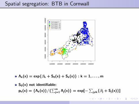
Spatial segregation: BTB in Cornwall

140000 160000 180000 200000 220000 240000

2000

040

000

6000

080

000

1000

0012

0000

●

●

●

●

●

●●

●

●●●●

●

●

●●

●

●

●

●

●

●

●

●● ●

●

●

●●●●

●

●

●

●●●●

●

●●●

●●●

●●●

●●●

●●

●

●●●

●●●

●●

●

●●●

●

●●●●

●● ●

●

● ●●

●●●

●●

●

●

●●

●●

●●●

●●●

●●●●●● ●●●

●●

●●●●

● ●

●

●

●●●●●●●

●●

●

●

●

●

●

●

●●

●

●

●●●

●●

●

●●

●

●●●

● ●

●

●

●●

●●

●●●

●

●

●●●●

●

●

●●●

●

●●● ●

●

● ●●●

●

●●

●

●

● ●●● ●●

●

●

●

● ●

●

●

●●●●

●

●

●

●

●●

●●

●

●

●● ●

●

●

●●●●●●●

●●●●

●●

●●●

●●● ●

●●●●

●●●

●

●●

●●● ●●●●●●●

●

● ●

●●

●

●●●

●

●●

●●●●●●

●

●●●● ●

●●●

●●●

●

●

●

●

●

●●●●●●

●●

●●

●

●●●●●●●●●

●

●

●

●

●●

●

●

●

●

●● ●●

● ●●

●●● ●

●●

●

●

●●●

●

● ●

●

●

●

●●

●● ●

●●

●

●

●

●●●● ●●●

●

●●

●●● ●●

●

●

●

●

●

●

●●

●

●●●

●●

●

●● ●●●●

●

●

●●

●●●●

●●●

●●

●●

●●

●

●●

●

●

●

●

●

●●●

● ●

●

●●

●●●●●●●●●●●

●●

●

●

●●●●●

●

●

●

●

●●●●

●●

●

●

●●●●

●

●

●●

●

●●●●●

●●

●●

●

●

●● ●

●

●●

●

●●●●

●

●

●

●●●

●

●

●●●●

●

●●

●●●

●

●

●

●

●

●●●

●●

●

● ●●●

●

●●●●

●

●●●●●

●●

●

●●●●

●

●

●

●

●

●●

●

●

●

●

●●●

●●

●●

●

●●●

●

●

●●●

●

●

● ●●●●

●

●●●

●●●● ●

●

●

●

●

●

●

●

●

●●

●●

●●●●

●●

●●●●

●

●

●

●

●

●

●

● ●●●●

●

●

●

●

●● ●

●●●

●●●

● ●

●●

●●

●●●

●●

●

●

●

●

●●●

●

●●

●

●

●

●●●

●●●

●

●

●●

●

●

●

●

●●

●

●

● ●

● ●

●●

●●● ●●

●●

●

●●●

●

●

●

●●

●

●

●

●

●

●

●

●

● ●

●●●●● ●

●

●

●●

●●●

●●

●

●

● ●● ●●●●

●●

●● ●●

●●●

●●

●●●

●●

●●

●●

●●●

●

●

●

●

●

●●

●

●

●

●

●

●

●●

●

●

●●

●

●

●

●●●

●

●●●

●●

●●●

●●

●

●●●

●●

●●

●

●

●

●●●

●●

●

●●

●●

●

●●

●

●●●●

●

●

●●

●

●

●

●

●

●●●●●

●●●

●

●●●

●

●

●

●

●●

●●●

●

●●

●

●●

● ●●●●●

●

●

●

●●

●

●

●●

●

●●

●

●

●

●

●

●

●

●

●

●

Genotype 9Genotype 12Genotype 15Genotype 20

Λk(x) = exp{βk + S0(x) + Sk(x)} : k = 1, . . . ,m

S0(x) not identifiable:

pk(x) = {Λk(x)}/{∑m

j=1 Λj(x)} = exp[−∑

j6=k{βj + Sj(x)}]

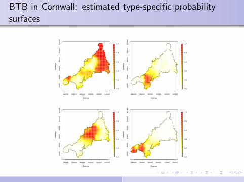
BTB in Cornwall: estimated type-specific probabilitysurfaces

140000 160000 180000 200000 220000 240000

2000

040

000

6000

080

000

1000

0012

0000

Eastings

Nor

thin

gs

0.0

0.2

0.4

0.6

0.8

1.0

140000 160000 180000 200000 220000 240000

2000

040

000

6000

080

000

1000

0012

0000

Eastings

Nor

thin

gs

0.0

0.2

0.4

0.6

0.8

1.0

140000 160000 180000 200000 220000 240000

2000

040

000

6000

080

000

1000

0012

0000

Eastings

Nor

thin

gs

0.0

0.2

0.4

0.6

0.8

1.0

140000 160000 180000 200000 220000 240000

2000

040

000

6000

080

000

1000

0012

0000

Eastings

Nor

thin

gs

0.0

0.2

0.4

0.6

0.8

1.0

BTB in Cornwall: areas of type-specific (0.8+) dominance

P(type k dominates)> 0.6

Dominant type defined as p_k>0.8

type 1type 2type 3type 4

P(type k dominates)> 0.7

P(type k dominates)> 0.8 P(type k dominates)> 0.9

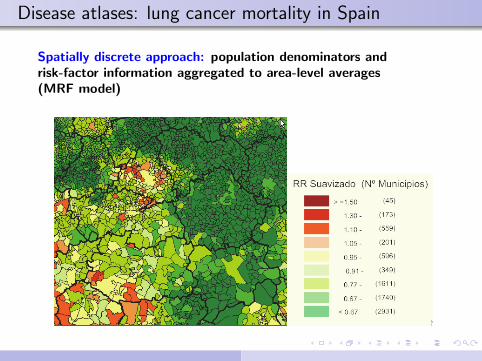
Disease atlases: lung cancer mortality in Spain

Spatially discrete approach: population denominators andrisk-factor information aggregated to area-level averages(MRF model)

Disease atlases: lung cancer mortality in Spain

Spatially continuous approach: population denominators andrisk-factor information in principle at point level (LGCP model)

Λ(x) = d(x) exp{z(x)′β + S(x)}

0.6

0.8

1.0

1.2

1.4

0.0

0.2

0.4

0.6

0.8

1.0

Predicted risk surface P(relative risk > 1.1)

Building spatio-temporal dependence

Separable

ρ(u, v) = ρS(u;α)ρT(v;β)

Non-separable empirical

ρ(u, v) = ρS(u;α;β)ρT(v){1 + f(u, v; θ)}

Non-separable mechanistic

S(x, t) = limδ→0

{∫hδ(u)S(x− u, t− δ)du + Zδ(x, t)

}

In conclusion

1 Statistical modelling should be driven by the underlyingscientific problem, rather than by the format of available data

2 Most (but not all) natural phenomena are spatially continuous

3 Surprisingly many of the problems to which spatial methodscan make a useful contribution reduce to an application ofBayes’ Theorem

[S,D] = [S][D|S]⇒ [S|D]

4 Modelling an unobserved stochastic process and assigning aprior distribution to an unknown parameter are mathematicallyequivalent but scientifically different activities

5 Modelling as a route to empirical prediction and modelling asa route to understanding a physical/biological mechanismdemand different approaches

Acknowledgements

CHICAS, Lancaster University : Paula Moraga, Barry Rowlingson,Ben Taylor

MRC: Methodology Research Grant G0902153

Diggle, P.J., Moraga, P., Rowlingson, B. and Taylor, B. (2013).Spatial and spatio-temporal log-Gaussian Cox processes: extendingthe geostatistical paradigm. Statistical Science, 28, 542–563.