TEMPO2 user manual - Jodrell Bank Observatorypulsar/Resources/tempo2_manual.pdf · TEMPO2 user manual George Hobbs, Russell Edwards Australia Telescope National Facility, CSIRO, PO

TEMPO2 user manual

George Hobbs, Russell EdwardsAustralia Telescope National Facility, CSIRO, PO Box 76, Epping NSW 1710, Australia

(documentation V2.0)

1

Contents

1 INTRODUCTION 6

2 Obtaining and installing tempo2 6

3 A simple example of using tempo2 6

4 Required files 8

4.1 Clock correction files . . . . . . . . . . . . . . . . . . . . . . . . . . . . . . . . . . . . . . . 84.1.1 Updating clock corrections . . . . . . . . . . . . . . . . . . . . . . . . . . . . . . . 9

4.2 Earth Orientation Parameters . . . . . . . . . . . . . . . . . . . . . . . . . . . . . . . . . . 94.3 Time ephemeris . . . . . . . . . . . . . . . . . . . . . . . . . . . . . . . . . . . . . . . . . . 94.4 Planetary ephemeris . . . . . . . . . . . . . . . . . . . . . . . . . . . . . . . . . . . . . . . 104.5 Observatory definitions . . . . . . . . . . . . . . . . . . . . . . . . . . . . . . . . . . . . . . 10

5 Parameter files 10

5.0.1 tpo file format . . . . . . . . . . . . . . . . . . . . . . . . . . . . . . . . . . . . . . 145.0.2 Changing the model epoch . . . . . . . . . . . . . . . . . . . . . . . . . . . . . . . 14

5.1 Jumps . . . . . . . . . . . . . . . . . . . . . . . . . . . . . . . . . . . . . . . . . . . . . . . 155.2 Removing Timing Noise . . . . . . . . . . . . . . . . . . . . . . . . . . . . . . . . . . . . . 155.3 Default values . . . . . . . . . . . . . . . . . . . . . . . . . . . . . . . . . . . . . . . . . . . 15

6 Observation files 15

6.1 Setting dispersion measures . . . . . . . . . . . . . . . . . . . . . . . . . . . . . . . . . . . 176.2 Jodrell Bank Observatory binary format . . . . . . . . . . . . . . . . . . . . . . . . . . . . 17

7 Atmospheric propagation delays 17

8 Command-line arguments 17

8.1 The tempo1 emulation mode . . . . . . . . . . . . . . . . . . . . . . . . . . . . . . . . . . 188.2 Filtering . . . . . . . . . . . . . . . . . . . . . . . . . . . . . . . . . . . . . . . . . . . . . . 188.3 Aliases . . . . . . . . . . . . . . . . . . . . . . . . . . . . . . . . . . . . . . . . . . . . . . . 19

9 The bootstrap fitting algorithm 19

10 Predictive mode 19

10.1 Tempo2 format . . . . . . . . . . . . . . . . . . . . . . . . . . . . . . . . . . . . . . . . . 1910.2 Tempo1 format . . . . . . . . . . . . . . . . . . . . . . . . . . . . . . . . . . . . . . . . . 19

11 Global parameters 20

12 Output formats 20

12.1 general . . . . . . . . . . . . . . . . . . . . . . . . . . . . . . . . . . . . . . . . . . . . . . . 2112.2 general2 . . . . . . . . . . . . . . . . . . . . . . . . . . . . . . . . . . . . . . . . . . . . . . 2112.3 list . . . . . . . . . . . . . . . . . . . . . . . . . . . . . . . . . . . . . . . . . . . . . . . . . 2212.4 stats . . . . . . . . . . . . . . . . . . . . . . . . . . . . . . . . . . . . . . . . . . . . . . . . 22

13 Graphical interfaces 23

13.1 basic . . . . . . . . . . . . . . . . . . . . . . . . . . . . . . . . . . . . . . . . . . . . . . . . 2313.2 calcDM . . . . . . . . . . . . . . . . . . . . . . . . . . . . . . . . . . . . . . . . . . . . . . 2313.3 chisq . . . . . . . . . . . . . . . . . . . . . . . . . . . . . . . . . . . . . . . . . . . . . . . . 2313.4 compare . . . . . . . . . . . . . . . . . . . . . . . . . . . . . . . . . . . . . . . . . . . . . . 2413.5 compareRes . . . . . . . . . . . . . . . . . . . . . . . . . . . . . . . . . . . . . . . . . . . . 2413.6 delays . . . . . . . . . . . . . . . . . . . . . . . . . . . . . . . . . . . . . . . . . . . . . . . 2413.7 errors . . . . . . . . . . . . . . . . . . . . . . . . . . . . . . . . . . . . . . . . . . . . . . . 2513.8 fake . . . . . . . . . . . . . . . . . . . . . . . . . . . . . . . . . . . . . . . . . . . . . . . . 2513.9 gorilla . . . . . . . . . . . . . . . . . . . . . . . . . . . . . . . . . . . . . . . . . . . . . . . 2613.10plk . . . . . . . . . . . . . . . . . . . . . . . . . . . . . . . . . . . . . . . . . . . . . . . . . 27

2

13.11polytest . . . . . . . . . . . . . . . . . . . . . . . . . . . . . . . . . . . . . . . . . . . . . . 2913.12splk . . . . . . . . . . . . . . . . . . . . . . . . . . . . . . . . . . . . . . . . . . . . . . . . 2913.13stridefit . . . . . . . . . . . . . . . . . . . . . . . . . . . . . . . . . . . . . . . . . . . . . . 2913.14transform . . . . . . . . . . . . . . . . . . . . . . . . . . . . . . . . . . . . . . . . . . . . . 30

14 Developing the software 31

14.1 Creating a plug-in . . . . . . . . . . . . . . . . . . . . . . . . . . . . . . . . . . . . . . . . 3114.1.1 A new output format . . . . . . . . . . . . . . . . . . . . . . . . . . . . . . . . . . 3114.1.2 A new graphical interface . . . . . . . . . . . . . . . . . . . . . . . . . . . . . . . . 32

14.2 The main source code . . . . . . . . . . . . . . . . . . . . . . . . . . . . . . . . . . . . . . 34

15 Tempo2 error and warning messages 34

15.1 Error messages . . . . . . . . . . . . . . . . . . . . . . . . . . . . . . . . . . . . . . . . . . 3415.2 Warning messages . . . . . . . . . . . . . . . . . . . . . . . . . . . . . . . . . . . . . . . . 34

16 Common questions 35

17 In progress 35

18 Acknowledgements 35

3

List of Figures

1 a) pre-fit timing residuals for the test data-set and b) post-fit timing residuals. . . . . . . 82 An example of the ‘basic’ graphical interface. A P− P diagram is produced with the pulsar

being analysed highlighted. . . . . . . . . . . . . . . . . . . . . . . . . . . . . . . . . . . . 233 Example of the chisq plug-in for determining the most likely values of the orbital period,

PB, and longitude of periastron, OM. . . . . . . . . . . . . . . . . . . . . . . . . . . . . . 244 The solar system Shapiro delay for PSR J1810−2005 shown using the delays graphical

interface plug-in . . . . . . . . . . . . . . . . . . . . . . . . . . . . . . . . . . . . . . . . . 255 Simulating pulsar timing residuals for a pulsar with a proper motion in right ascension of

200 mas/yr using the fake plugin. . . . . . . . . . . . . . . . . . . . . . . . . . . . . . . . 276 An example of the plk graphical interface in use. The post-fit residuals for PSR J0437−4715

are plotted with 20 observations shown in green and 10 cm observations in red. The whitecircles and black lines indicate arrival times between orbital phases 0.4 and 0.6. . . . . . . 28

7 Example of the splk graphical interface plug-in for showing the pre- and post-fit timingresiduals for multiple pulsar simultaneously. . . . . . . . . . . . . . . . . . . . . . . . . . . 29

8 Example of the stridefit graphical interface plug-in which calculates the pulsar’s disper-sion measure as a function fo time. . . . . . . . . . . . . . . . . . . . . . . . . . . . . . . . 30

4

List of Tables

1 Observatory details . . . . . . . . . . . . . . . . . . . . . . . . . . . . . . . . . . . . . . . . 112 Pulsar parameters that can be entered in a parameter file . . . . . . . . . . . . . . . . . . 123 Binary parameters that can be entered in a parameter file . . . . . . . . . . . . . . . . . . 134 Flags in arrival time files . . . . . . . . . . . . . . . . . . . . . . . . . . . . . . . . . . . . . 165 Commands that may be included in an arrival time file . . . . . . . . . . . . . . . . . . . . 17

5

1 INTRODUCTION

Tempo2 is a new version of the tempo pulsar timing software. An overview of the software is provided inHobbs, Edwards & Manchester (2006; MNRAS 369 655). A second paper provides mathematical detailsof the algorithms used in the software (Edwards, Hobbs & Manchester 2006; currently available fromastro-ph). A third paper will describe how tempo2 can be used to simulate the effects of gravitationalwaves on pulsar timing residuals. A summary of the basic features can also be found in Hobbs, Edwards& Manchester (2006; in press CHJAA).This document provides full usage instructions for tempo2.

2 Obtaining and installing tempo2

The tempo2 software and documentation can be obtained from http://www.atnf.csiro.au/research/

pulsar/ppta/tempo2. Click on the “Download” option to download the software to your local machine.This software requires compilation before it will run. Up-to-date installation instructions are available ina README file with the download.Note: tempo2 makes heavy use of “long double” precision in its calculations. Most compiler/architecturecombinations support long doubles of 80 or 128 bits in size, which is sufficient. Tempo2 has beensuccessfully tested under Linux-gcc/x86, Solaris/SPARC and Mac OS 10.4-gcc/PowerPC. Unfortunately,some systems only provide 64-bit long doubles (i.e. identical to a standard ”double”); these include MacOS 10.3.9 and earlier, and many Windows compilers. While parts of the source code make reference toa software quad-precision library, this feature is no longer functional.

3 A simple example of using tempo2

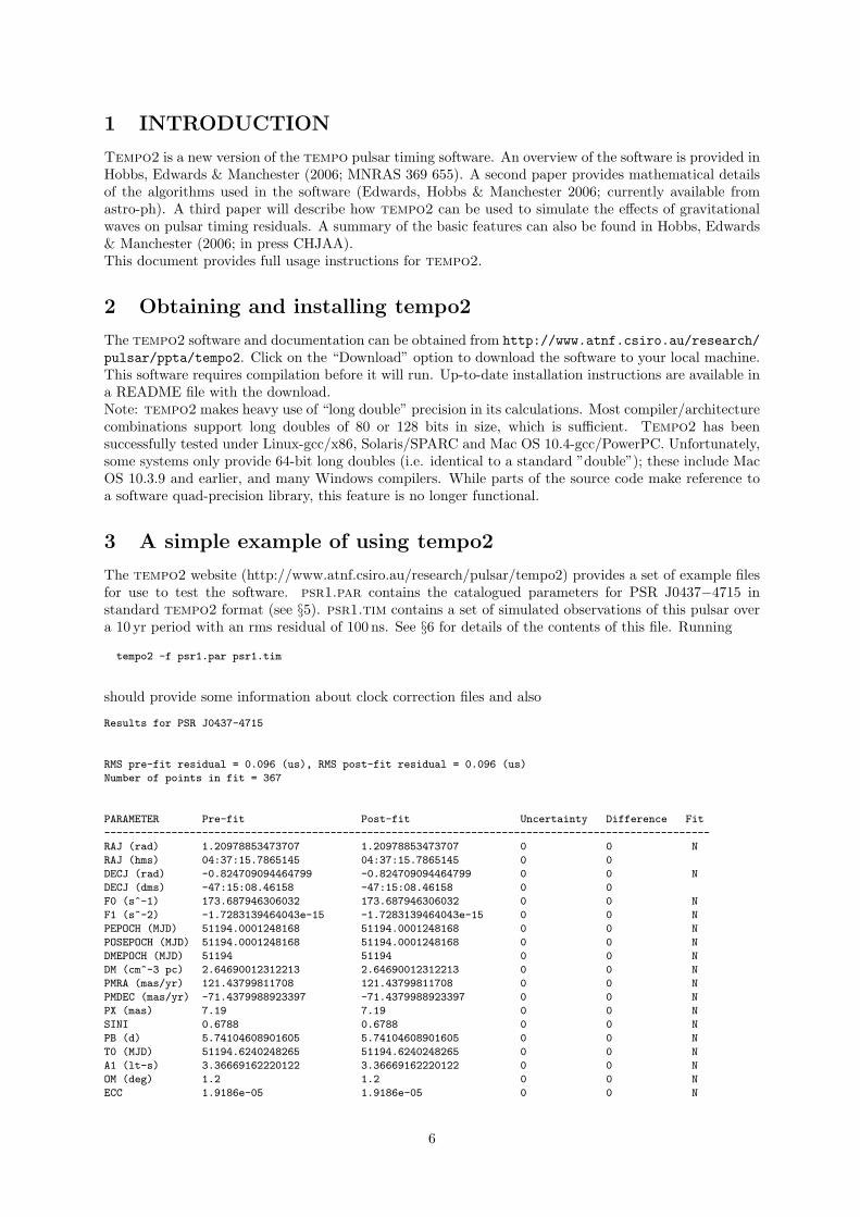
The tempo2 website (http://www.atnf.csiro.au/research/pulsar/tempo2) provides a set of example filesfor use to test the software. psr1.par contains the catalogued parameters for PSR J0437−4715 instandard tempo2 format (see §5). psr1.tim contains a set of simulated observations of this pulsar overa 10 yr period with an rms residual of 100 ns. See §6 for details of the contents of this file. Running

tempo2 -f psr1.par psr1.tim

should provide some information about clock correction files and also

Results for PSR J0437-4715

RMS pre-fit residual = 0.096 (us), RMS post-fit residual = 0.096 (us)

Number of points in fit = 367

PARAMETER Pre-fit Post-fit Uncertainty Difference Fit

---------------------------------------------------------------------------------------------------

RAJ (rad) 1.20978853473707 1.20978853473707 0 0 N

RAJ (hms) 04:37:15.7865145 04:37:15.7865145 0 0

DECJ (rad) -0.824709094464799 -0.824709094464799 0 0 N

DECJ (dms) -47:15:08.46158 -47:15:08.46158 0 0

F0 (s^-1) 173.687946306032 173.687946306032 0 0 N

F1 (s^-2) -1.7283139464043e-15 -1.7283139464043e-15 0 0 N

PEPOCH (MJD) 51194.0001248168 51194.0001248168 0 0 N

POSEPOCH (MJD) 51194.0001248168 51194.0001248168 0 0 N

DMEPOCH (MJD) 51194 51194 0 0 N

DM (cm^-3 pc) 2.64690012312213 2.64690012312213 0 0 N

PMRA (mas/yr) 121.43799811708 121.43799811708 0 0 N

PMDEC (mas/yr) -71.4379988923397 -71.4379988923397 0 0 N

PX (mas) 7.19 7.19 0 0 N

SINI 0.6788 0.6788 0 0 N

PB (d) 5.74104608901605 5.74104608901605 0 0 N

T0 (MJD) 51194.6240248265 51194.6240248265 0 0 N

A1 (lt-s) 3.36669162220122 3.36669162220122 0 0 N

OM (deg) 1.2 1.2 0 0 N

ECC 1.9186e-05 1.9186e-05 0 0 N

6

PBDOT (10^-12) 3.64 3.64 0 0 N

OMDOT (deg/yr) 0.0159999997519168 0.0159999997519168 0 0 N

M2 0.236 0.236 0 0 N

START (MJD) 50640.9281162413 49350.5129309451 0 -1290.4 N

FINISH (MJD) 52088.8971386924 53000.5197060478 0 911.62 N

TRACK (MJD) 0 0 0 0 N

TZRMJD 51204.6438924841 51204.6438924841 0 0 N

TZRFRQ (MHz) 1413.39997808495 1413.39997808495 0 0 N

---------------------------------------------------------------------------------------------------

Binary model: DD

Mass function = 0.001243113190 +- 0.000000000000 solar masses

Minimum companion mass = 0.1403 solar masses

Median companion mass = 0.1637 solar masses

Maximum companion mass = 0.3493 solar masses

MTOT derived from sin i and m2 = 1.8186068413766

Inclination angle (deg) = 42.74994182955 (+ 0 - 0)

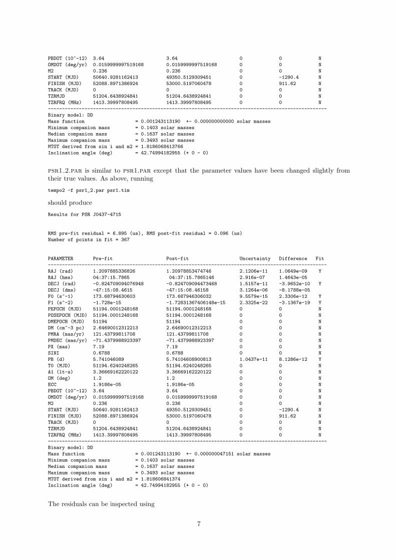
psr1 2.par is similar to psr1.par except that the parameter values have been changed slightly fromtheir true values. As above, running

tempo2 -f psr1_2.par psr1.tim

should produce





---------------------------------------------------------------------------------------------------

RAJ (rad) 1.2097885336826 1.20978853474746 2.1206e-11 1.0649e-09 Y

RAJ (hms) 04:37:15.7865 04:37:15.7865146 2.916e-07 1.4643e-05

DECJ (rad) -0.824709094076948 -0.824709094473468 1.5157e-11 -3.9652e-10 Y

DECJ (dms) -47:15:08.4615 -47:15:08.46158 3.1264e-06 -8.1788e-05

F0 (s^-1) 173.68794630603 173.687946306032 9.5579e-15 2.3306e-12 Y

F1 (s^-2) -1.728e-15 -1.72831367406148e-15 2.3325e-22 -3.1367e-19 Y

PEPOCH (MJD) 51194.0001248168 51194.0001248168 0 0 N

POSEPOCH (MJD) 51194.0001248168 51194.0001248168 0 0 N

DMEPOCH (MJD) 51194 51194 0 0 N

DM (cm^-3 pc) 2.64690012312213 2.64690012312213 0 0 N

PMRA (mas/yr) 121.43799811708 121.43799811708 0 0 N

PMDEC (mas/yr) -71.4379988923397 -71.4379988923397 0 0 N

PX (mas) 7.19 7.19 0 0 N

SINI 0.6788 0.6788 0 0 N

PB (d) 5.741046089 5.74104608900813 1.0437e-11 8.1286e-12 Y

T0 (MJD) 51194.6240248265 51194.6240248265 0 0 N

A1 (lt-s) 3.36669162220122 3.36669162220122 0 0 N

OM (deg) 1.2 1.2 0 0 N

ECC 1.9186e-05 1.9186e-05 0 0 N

PBDOT (10^-12) 3.64 3.64 0 0 N

OMDOT (deg/yr) 0.0159999997519168 0.0159999997519168 0 0 N

M2 0.236 0.236 0 0 N

START (MJD) 50640.9281162413 49350.5129309451 0 -1290.4 N

FINISH (MJD) 52088.8971386924 53000.5197060478 0 911.62 N


TZRMJD 51204.6438924841 51204.6438924841 0 0 N

TZRFRQ (MHz) 1413.39997808495 1413.39997808495 0 0 N

---------------------------------------------------------------------------------------------------

Binary model: DD







The residuals can be inspected using

7

Figure 1: a) pre-fit timing residuals for the test data-set and b) post-fit timing residuals.

tempo2 -gr plk -f psr1_2.par psr1.tim

which should produce a plot of the pre-fit residuals as shown in Figure 1a. Pressing ’2’ on the plot willshow the post-fit residuals (Figure 1b).

4 Required files

Tempo2 requires certain files in order to run correctly. These files are provided with the download andare discussed in the following sections.

4.1 Clock correction files

Times of arrival provided to tempo2 are recorded against local observatory clocks. These times differfrom those recorded against a uniform clock, firstly because observatory clocks are typically maintained inapproximate synchrony with Coordinated Universal Time (UTC), which itself is not uniform, and secondlybecause they deviate from ideal UTC owing to deviations in uniformity in the underlying frequencystandard (usually a hydrogen maser). The ultimate aim of the clock correction process is to transformall site arrival times to a chosen realisation of TT (Terrestrial Time), which in an ideal realisation is auniform clock ticking SI seconds on the geoid. By default this is TT(TAI), which (since 1971) differsfrom UTC by a constant offset plus an integer number of leap seconds. Alternative realisations of TTcan be specified using the the CLOCK keyword in the parameter file.The clock correction process proceeds entirely on the basis of linear interpolation of user-supplied tab-ulations of the difference between named pairs of clocks, as a function of Modified Julian Day (MJD)1.These files reside in the directory $TEMPO2/clock. Lines beginning with the hash character (#) aretreated as comments. The first line must be a comment specifying the name of the clock to convertfrom, the name of the clock to convert to, and an optional “badness” value (which defaults to 1). Forexample, the following specifies that the values in the file can be added to times measured against theParkes clock (“UTC(PKS)”) to transform them to the frame of the Global Positioning System (GPS)clock (“UTC(GPS)”).

# UTC(PKS) UTC(GPS) 10

Non-comment lines consist of a sequence of pairs of MJDs and offsets (in seconds), specifying the differencebetween the second and first clocks as a function of date. For example:

50844.72917 -7.49068e-07

50845.77083 -7.47637e-07

50846.81250 -7.46650e-07

...

1The frame in which the MJD is measured is not specified: it is assumed that clock offsets and drift rates are smallenough that if t′ = t + f(t) then t ' t′ − f(t′).

8

The spacing of the dates need not be any specific value, or even be regular. For most purposes roughlydaily values are suitable.All files ending in .clk in $TEMPO2/clock are read by Tempo2 when it starts executing. Then, givena TOA to transform, it obtains the name of the clock against which it was measured based upon namespecified in the observatory database (§4.5), given the observatory code recorded in the TOA file. Giventhe source and destination clocks, tempo2 must then choose a selection of clock correction tables (from.clk files) to use for the transformation. This is firstly attempted by consulting the list of pre-definedtransformation paths, which are defined using CLK CORR CHAIN entries in the parameter file. Forexample, the following tells tempo2 to convert from UTC(PKS) to TT(TAI) using tables defined inpks2gps.clk, gps2utc.clk,utc2tai.clk and tai2tt tai.clk:

CLK_CORR_CHAIN pks2gps gps2utc utc2tai tai2tt_tai

This parameter may be specified multiple times. Tempo2 will attempt to apply each path in the orderin which they were specified (which may fail if the MJD of the TOA is outside the range of componenttables).If no applicable pre-defined paths are found, tempo2 find the “best” possible path using all of theavailable tables. Here “best” means the path for which the sum of badness values is minimized. Tie-breaking is arbitrary. This path is then appended to the global list of pre-defined paths. Since tempo2always checks this list before attempting automatic path construction, subsequent transformations willalways use this path if it is applicable, even if the MJDs of some TOAs would have allowed for a “better”path. Caution is therefore advised in using the automatic path construction feature when multiple pathsexist.

4.1.1 Updating clock corrections

The distribution of tempo2 includes several useful files containing corrections based on the BIPM’sCircular T (offsets between UTC and its various realisations, as well as the GPS clock) and the IERSBulletin C (announcing leap seconds). A suite of ancillary software is available on the tempo2 website,which provides among other things a means for parsing Circular T to update the relevant clock correctionfiles (update clkcorr). This program can also parse clock monitoring data from the Parkes Observatory.Interested parties are invited to contribute code for the parsing of clock data from other sources.

4.2 Earth Orientation Parameters

To compute the Roemer delay, the position of the observatory must be known. This depends not only onthe Earth’s orbit, but on the Earth’s orientation and rotation. The necessary parameters are obtainedby interpolation of the “C05” series of Earth Orientation Parameters (EOPs) from the IERS. The file$TEMPO2/earth/README specifies the web address for downloading the latest EOPs. The user may op-tionally select to emulate the algorithm of tempo (which neglects polar motion and uses an out of dateprecession/nutation model) for transforming the observatory coordinates to the celestial frame, using theT2C METHOD parameter; in this case $TEMPO2/clock/ut1.dat (in the same format as the correspondingfile for tempo) is used.

4.3 Time ephemeris

The pulse arrival times at the observatory at transformed to the arrival time at the solar system barycentre(SSB). In this transformation the Einstein delay, which describes the combined effect of gravitiatonalredshift and time dilation due to the motion of the Earth and other bodies, must be taken in to account.This transformation converts the site arrival time from TT to a coordinate time at the SSB, known asBarycentric Coordinate Time (TCB). Optionally, for backward compatibility with tempo the user mayalso choose to use a scaled version of this frame in which the mean drift relative to TT is divided out:this is nominally (but incorrectly; see Paper II) referred to as TDB. This is accomplished by specifying“UNITS TDB” in the parameter file.The Einstein delay is computed using a polynomial approximation to the numerical evaulation of the timedilation integral as provided by Irwin & Fukushima (1999). It lives in $TEMPO2/ephemeris/TIMEEPH short.te405.For reproducing results obtained with tempo, the user may also chose to use the Fairhead & Bretagnon(1990) version of this integral (stored at $TEMPO2/ephemeris/TDB.1950.2050) by specifying ”TIMEEPHFB90” in the pulsar parameter file.

9

4.4 Planetary ephemeris

In order to correct the arrival time to the solar system’s barycentre, tempo2 requires a solar systemephemeris. By default the JPL ephemeris DE200 is chosen. Different JPL ephemerides may be selectedusing the EPHEM FILE command in the parameter file. For example,

EPHEM_FILE /pulsar/psr/runtime/tempo//tempo_ephem/DE405.1950.2050

would select the DE405 JPL ephemeris. If the full-path is defined from $TEMPO2/ephemeris then theDE405 ephemeris could be selected from

EPHEM DE405

4.5 Observatory definitions

It is necessary for tempo2 to know the coordinates of the observatory. In the original TEMPO a file,obsys.dat, was used that contained the coordinates of each observatory and a single-character identifyingcode. This code was used in the arrival time file. Unfortunately, different users used different codes for thesame observatory and therefore the arrival time files were not transferable between different installationsof TEMPO. To avoid this, tempo2 provides a read-only database of observatories, each identified bya short, non-cryptic mnemonic. This resides in $TEMPO/observatory/observatories.dat. In addition,for backwards compatability or for experimental use, further defintitions can be placed in extra files:tempo2 parses every file in $TEMPO/observatory/. Each line should contain 5–6 whitespace-separatedparameters. These are, in order, the x, y and z geocentric coordinates (in metres), a one-word namefor the observatory, a few-character mnemonic and optionally the name of the clock associated with theobservatory (used to refer to the relevant clock-correction tables). If not supplied, the clock name isconstructed as UTC(xxx) where xxx is the observatory mnemonic.For full accuracy, observatory coordinates should be specified in the International Terrestrial ReferenceSystem. Geodetic coordinates (as optionally used by tempo, given as latitude and longitude in degreesin the form dddmmss.ss, and height in metres) may be specified, in which case tempo2 will detect thisand convert them to the ITRF on the assumption that they refer to the GRS80 geoid. The convertedcoordinates are displayed and execution is halted for the user to add the converted coordinates to theobservatories database (or not! the accuracy of the conversion and the assumption of GRS80 may bedubious).NOTE: The mnemonics in observatories.dat have not been finalised. Please let G. Hobbs or R. Edwardsknow if you prefer another mnemonic for your observatory.The current observatory file is listed in Table 1.

5 Parameter files

The parameter files have the same design as in the earlier tempo implementations. Each of the pulsarparameters has a label, a value and may have an uncertainty on the value and a flag indicating whethertempo2 should fit for this parameter or whether this parameter should be held constant (0 = default= hold constant; 1 = fit). These labels are described in Table 2. An example of a parameter file forPSR J0437−4715 taken from the catalogue and fitting for various parameters:

PSRJ J0437-4715

RAJ 04:37:15.7865145 1 7.000e-07

DECJ -47:15:08.461584 1 8.000e-06

DM 2.6469 1.000e-04

PEPOCH 51194.000

F0 173.6879489990983 1 3.000e-13

F1 -1.728314E-15 1 1.600e-20

PMRA 121.438 6.000e-03

PMDEC -71.438 7.000e-03

BINARY DD

PB 5.741046 1 3.000e-06

ECC 1.9186E-5 1 5.000e-09

A1 3.36669157 1 1.400e-07

T0 51194.6239 1 8.000e-04

10

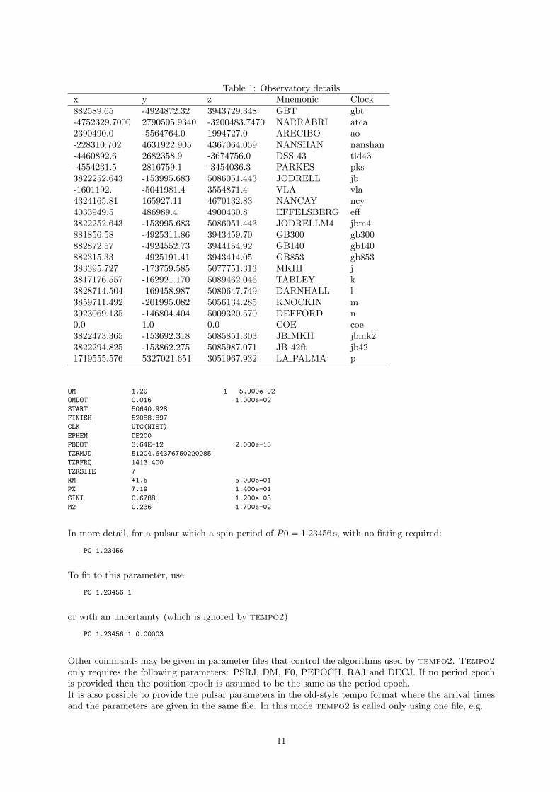
Table 1: Observatory detailsx y z Mnemonic Clock882589.65 -4924872.32 3943729.348 GBT gbt-4752329.7000 2790505.9340 -3200483.7470 NARRABRI atca2390490.0 -5564764.0 1994727.0 ARECIBO ao-228310.702 4631922.905 4367064.059 NANSHAN nanshan-4460892.6 2682358.9 -3674756.0 DSS 43 tid43-4554231.5 2816759.1 -3454036.3 PARKES pks3822252.643 -153995.683 5086051.443 JODRELL jb-1601192. -5041981.4 3554871.4 VLA vla4324165.81 165927.11 4670132.83 NANCAY ncy4033949.5 486989.4 4900430.8 EFFELSBERG eff3822252.643 -153995.683 5086051.443 JODRELLM4 jbm4881856.58 -4925311.86 3943459.70 GB300 gb300882872.57 -4924552.73 3944154.92 GB140 gb140882315.33 -4925191.41 3943414.05 GB853 gb853383395.727 -173759.585 5077751.313 MKIII j3817176.557 -162921.170 5089462.046 TABLEY k3828714.504 -169458.987 5080647.749 DARNHALL l3859711.492 -201995.082 5056134.285 KNOCKIN m3923069.135 -146804.404 5009320.570 DEFFORD n0.0 1.0 0.0 COE coe3822473.365 -153692.318 5085851.303 JB MKII jbmk23822294.825 -153862.275 5085987.071 JB 42ft jb421719555.576 5327021.651 3051967.932 LA PALMA p

OM 1.20 1 5.000e-02

OMDOT 0.016 1.000e-02

START 50640.928

FINISH 52088.897

CLK UTC(NIST)

EPHEM DE200

PBDOT 3.64E-12 2.000e-13

TZRMJD 51204.64376750220085

TZRFRQ 1413.400

TZRSITE 7

RM +1.5 5.000e-01

PX 7.19 1.400e-01

SINI 0.6788 1.200e-03

M2 0.236 1.700e-02

In more detail, for a pulsar which a spin period of P0 = 1.23456 s, with no fitting required:

P0 1.23456

To fit to this parameter, use

P0 1.23456 1

or with an uncertainty (which is ignored by tempo2)

P0 1.23456 1 0.00003

Other commands may be given in parameter files that control the algorithms used by tempo2. Tempo2only requires the following parameters: PSRJ, DM, F0, PEPOCH, RAJ and DECJ. If no period epochis provided then the position epoch is assumed to be the same as the period epoch.It is also possible to provide the pulsar parameters in the old-style tempo format where the arrival timesand the parameters are given in the same file. In this mode tempo2 is called only using one file, e.g.

11

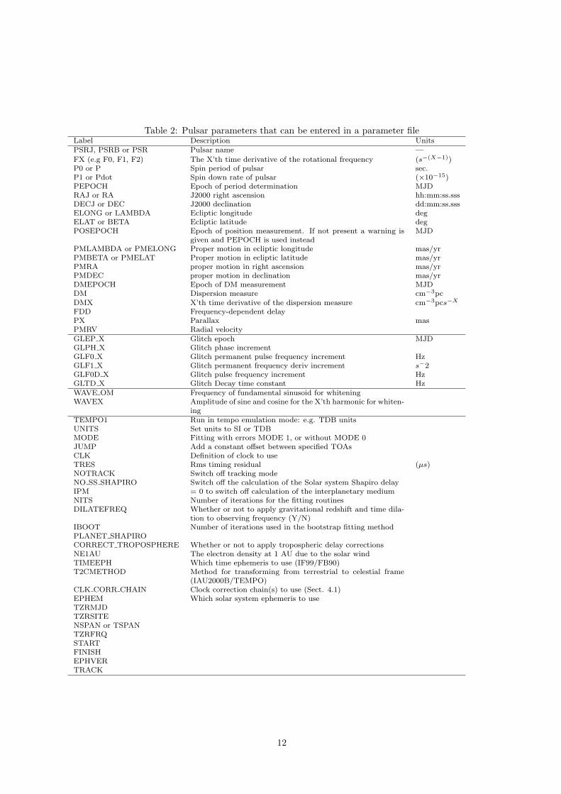
Table 2: Pulsar parameters that can be entered in a parameter fileLabel Description UnitsPSRJ, PSRB or PSR Pulsar name —

FX (e.g F0, F1, F2) The X’th time derivative of the rotational frequency (s−(X−1))P0 or P Spin period of pulsar sec.P1 or Pdot Spin down rate of pulsar (×10−15)PEPOCH Epoch of period determination MJDRAJ or RA J2000 right ascension hh:mm:ss.sssDECJ or DEC J2000 declination dd:mm:ss.sssELONG or LAMBDA Ecliptic longitude degELAT or BETA Ecliptic latitude degPOSEPOCH Epoch of position measurement. If not present a warning is

given and PEPOCH is used insteadMJD

PMLAMBDA or PMELONG Proper motion in ecliptic longitude mas/yrPMBETA or PMELAT Proper motion in ecliptic latitude mas/yrPMRA proper motion in right ascension mas/yrPMDEC proper motion in declination mas/yrDMEPOCH Epoch of DM measurement MJDDM Dispersion measure cm−3pcDMX X’th time derivative of the dispersion measure cm−3pcs−X

FDD Frequency-dependent delayPX Parallax masPMRV Radial velocityGLEP X Glitch epoch MJDGLPH X Glitch phase incrementGLF0 X Glitch permanent pulse frequency increment HzGLF1 X Glitch permanent frequency deriv increment s−2GLF0D X Glitch pulse frequency increment HzGLTD X Glitch Decay time constant HzWAVE OM Frequency of fundamental sinusoid for whiteningWAVEX Amplitude of sine and cosine for the X’th harmonic for whiten-

ingTEMPO1 Run in tempo emulation mode: e.g. TDB unitsUNITS Set units to SI or TDBMODE Fitting with errors MODE 1, or without MODE 0JUMP Add a constant offset between specified TOAsCLK Definition of clock to useTRES Rms timing residual (µs)NOTRACK Switch off tracking modeNO SS SHAPIRO Switch off the calculation of the Solar system Shapiro delayIPM = 0 to switch off calculation of the interplanetary mediumNITS Number of iterations for the fitting routinesDILATEFREQ Whether or not to apply gravitational redshift and time dila-

tion to observing frequency (Y/N)IBOOT Number of iterations used in the bootstrap fitting methodPLANET SHAPIROCORRECT TROPOSPHERE Whether or not to apply tropospheric delay correctionsNE1AU The electron density at 1 AU due to the solar windTIMEEPH Which time ephemeris to use (IF99/FB90)T2CMETHOD Method for transforming from terrestrial to celestial frame

(IAU2000B/TEMPO)CLK CORR CHAIN Clock correction chain(s) to use (Sect. 4.1)EPHEM Which solar system ephemeris to useTZRMJDTZRSITENSPAN or TSPANTZRFRQSTARTFINISHEPHVERTRACK

12

Table 3: Binary parameters that can be entered in a parameter fileLabel Description UnitsBINARY Binary model (BT/ELL1/DD/MSS)A1 Projected semi-major axis of orbit lt-secPB Orbital period daysECC or E Eccentricity of orbit —T0 Epoch of periastron MJDOM Longitude of periastron degreesTASC Epoch of ascending node MJDEPS1 ECC× sin(OM) for ELL1 model —EPS2 ECC× cos(OM) for ELL1 model —OMDOT Rate of advance of periastron (deg/yr)PBDOT 1st time derivative of binary period (10−12)A1DOT or XDOT Rate of change of projected semi-major axis (10−12)SINI Sine of inclination angleM2 Companion mass (solar masses)XPBDOT Rate of change of orbital period minus GR predictionA1DOTEDOT or ECCDOT Rate of change of eccentricityOMDOT Periastron advance degrees/yrPBDOT 1st time derivative of binary periodPBX X’th time derivative of binary periodGAMMA post-Keplerian ’gamma’ term sDR Relativistic deformation of the orbitDTH Relativistic deformation of the orbitA0 Aberration parameter A0B0 Aberration parameter B0BP Tensor multi-scalar parameter beta-primeBPP Tensor multi-scalar parameter beta-prime-primeDTHETA Relativistic deformation of the orbitXOMDOT Rate of periastron advance minus GR prediction deg/yrAFACA1DOT or XDOTTASC Epoch of ascending node MJDEPS1DOTEPS2DOTKOMKINSHAPMAXMTOT Total system mass solar massesBPJEP XBPJPH XBPJA1 XBPJEC XBPJOM XBPJPB X

tempo2 -gr plk myfile.tempo

where the first line in the file contains flags with ’1’ to indicate that the parameter should be fit and ’0’for not fitting:

Column Parameter

1 Phase

2 P0

3 P1

4 P2

5 RAJ

6 DECJ

7 PMRA

8 PMDEC

9 A1

10 ECC

11 T0

12 PB

13 OM

14 OMDOT

15 GAMMA

16 DM

13

17 PX

18 PBDOT

19 M1 (not implemented)

20 SINI

21 MTOT

22 M2

23 DTHETA

24 BP (not implemented)

25 BPP (not implemented)

27 Binary model: 0 = none, 1 = BT, 2 = EH, 3 = DD, 4 = DDGR,

5 = H88, 6 = BT+, 7 = DDT, 8 = DD+, 9 = 2 BT orbits

The actual parameter values are given on three extra lines. The second line in the file gives

Columns Parameter

1-12 Pulsar name

21-40 RAJ in the form hhmmss.ss

41-60 DECJ in the form ddmmss.ss

61-70 PMRA

71-80 PMDEC

The third line gives

Columns Parameter

2-20 P0

21-40 P1

41-60 PEPOCH as Julian date

61-70 P2

71-80 PX

The fourth line gives

Columns Parameter

9-20 DM

Further lines provide the binary parameters (not implemented yet).

5.0.1 tpo file format

Both the parameters and the arrival times may be provided in a single file. The first line of this file mustbe

HEAD

followed by the parameters in the same format as above. These are followed by

TOAS

and a list of arrival times.

5.0.2 Changing the model epoch

It is possible to convert the period epoch from that given in the parameter file using the -epoch commandon the command line. For instance -epoch 52000 will update the period epoch, rotational frequency andits first derivative to the new epoch using the inputted values of F0, F1 and F2. Can use -epoch centre

(or -epoch center) to set to the centre of the data span. -epoch left will set the epoch to the firstobservation.

14

5.1 Jumps

It is often necessary to fit for a constant offset between two sets of arrival times. For instance, thetemplates used to determine arrival times at different frequencies may not be perfectly aligned or anoffset may exist between the arrival times provided by different observatories. The command JUMP in theparameter file is used to define jumps.JUMP MJD v1 v2 will provide a jump between all TOAs with MJDs between v1 and v2 compared to allthe other TOAs.JUMP FREQ v1 v2 will section all TOAs with observing frequencies between v1 and v2 MHz.JUMP TEL id will section all TOAs observed with telescope ‘id’.JUMP NAME str will section all TOAs with observation IDs that contain the string ‘str’.JUMP flag val will select all TOAs with specified flag (e.g. -o) and value val.

5.2 Removing Timing Noise

Even with accurate spin and positional parameters the residuals for some (particularly the young) pul-sars contain remnant structures. Some of these structures are understood: cusps, for instance, signifysudden changes in the pulsar’s spin rate during a glitch, sinusoidal oscillations can represent unmodelledcompanions (such as planets) or the pulsar precessing. However, many of the structures seen in theresiduals are still not understood and are known as “timing noise”. To obtain the most accurate pulsar’spositional and proper motion parameters (and dispersion measure) it is essential to remove this timingnoise. This has traditionally been carried out by fitting higher order pulsar rotational derivative terms.More recently, Hobbs et al. (2004) described a method for fitting harmonically related sinusoids.

5.3 Default values

6 Observation files

For each pulsar an arrival time file must be created that contains all the site-arrival-times2 (i.e. the pulsearrival time at the observatory for each observation3). These files can take the form of the old Parkes–or Jodrell–style tempo files or may use a new formatting structure.The current tempo2 format is identified with

FORMAT 1

at the start of the observation file. Each observation line can be entered in a “free-format” manner (thereis no limit on the number of decimal places or characters supplied for each parameter). The file has thefollowing form:

file freq sat satErr siteID <flags>

where the flags are listed in Table 4. It is important for the TOAs to be given to high precision. tempo2reads all parameters with ‘long double’ precision. Other undefined flags may be used in the arrival timefiles. These flags can provide any information and could be used, for example, in determining coloursused for plotting with a personal graphical interface. An example observation file is given below.

FORMAT 1

C ../archives/w040205_062810.cFTp 3072.52800000 53040.27037033597299853 10.07000 7 -i WBC_10

../archives/w040206_070831.cFTp 3092.99900000 53041.31851839551620031 1.16000 7 -i WBC_10

C ../archives/w040206_084839.cFTp 3068.03800000 53041.38807867413299846 9.97000 7 -i WBC_10









../archives/n2004-06-27-04:13:58.FTp 685.24900000 53183.18848980008860039 0.06000 7 -i nCPSR2_50

2site-arrival-times can be obtained from pulse profiles and a standard template using software packages such as pat.3note: the “pulse” arrival time is measured by the summation of many thousands of individual pulses from the pulsar.

15

Table 4: Flags in arrival time filesFlag Parameter Typedm DM (cm−3pc) floatp Phase offset floatt Telescope identifier string




The pat software in the psrchive package has been updated to output arrival time files using this (orearlier) formats.A list of available commands that can be included in an arrival time file are provided in table 5. Note that,when writing out a new arrival time file from tempo2 (using a plugin such as plk, for example - see Sec-tion 13.10), most of these commands will not be replicated, but are instead directly executed. (EFLOOR,EMIN, EMAX and EQUAD for example will be absorbed in the TOA uncertainties.) The exception tothis is EFAC, which is written to the tim-file without affecting the uncertainties. (GLOBAL EFAC,T2EFAC and EFAC are combined into a single EFAC value, though.)

The old Parkes–style structure contains a label indicating the observation (such as a file name containingthe folded profile), the observing frequency (MHz), the site–arrival–time (MJD), a phase offset (µs), theuncertainty on the TOA (µs) and an identification flag for the telescope used. These identification flagsare defined by the user and differ between users. For example,

f981016_092219.FT 0 0 1374.000 51102.3925603118473 0.00 138.00 7

tempo2 can read arrival times in the “Parkes”, “Princeton” and “ITOA” formats. All these formats are“fixed-format” and are defined as:

Princeton Format

columns item

1-1 Observatory code (1-character)

2-2 Must be blank

16-24 Observing frequency (MHz)

25-44 TOA (decimal point must be in column 30 or 31)

45-53 TOA uncertainty

69-78 DM correction (NOT IMPLEMENTED IN TEMPO2)

Parkes Format

columns item

1-1 Must be blank


35-55 TOA (decimal point must be in column 42)

56-63 Phase offset (fraction of P0, added to TOA)


80-80 Observatory (1-character)

ITOA Format

columns item

1-2 ignored, but must not be blank

10-28 TOA (decimal point must be in column 15)



46-55 DM correction (NOT IMPLEMENTED IN TEMPO2)

58-59 Observatory (2-characters)

16

Table 5: Commands that may be included in an arrival time fileCommand MeaningEFAC x Multiply uncertainties by xT2EFAC -backend dfb x Multiply TOA uncertainties with flag “-backend dfb” by xGLOBAL EFAC x Multiply all TOA uncertainties by x. If for some or all of the

TOAs an “EFAC y” is present as well, then those TOAs will bemultiplied by x × y.

EMAX x Ignore TOAs with uncertainties greater than x µsEMIN x Ignore TOAs with uncertainties less than x µsEFLOOR x Put uncertainties of less than x µs to x µsEND Ignore all remaining lines in the arrival time fileEQUAD x Additional uncertainty in us, added in quadratureFMAX x Ignore TOAs at frequencies greater than xFMIN x Ignore TOAs at frequencies less than xINCLUDE x Include the arrival times in file xINFO x Identify all following points with a given highlighting codeMODE MODE 0 (default) implies that the TOA error is not taken into

account during the fitting procedure. MODE 1 uses the uncer-tainties (see section on fitting)

NOSKIP End of SKIP statementPHASE x Add phase jumpSIGMA x Set uncertainties of following TOAs to x µsSKIP Skip all lines until NOSKIP is readTIME x Add x seconds to following TOAsTRACK x Tracks phase wrap-arounds if time step is less than x days

6.1 Setting dispersion measures

In some situations the dispersion measure is measured accurately for every observation. This informationcan be provided to tempo2 by adding -dm DMval on the end of each arrival time line in the .tim file. Ifthis is not present then the dispersion measure in the .par file is used instead.

6.2 Jodrell Bank Observatory binary format

It is also possible to provide pulse arrival times in the Jodrell Bank format binary file that containingbarycentric arrival times. For instance a typical usage would be:

tempo2 -f psrav.eph psrav.bat -jbo -delete psrav.del

7 Atmospheric propagation delays

(to be written)

8 Command-line arguments

tempo2 has a number of options that can be controlled from the command line. Options include:

• -debug, provides output useful for identifying problems with the software

• -delete fname, delete the observations listed in the file fname by their site-arrival times or obser-vations name.

• -clock x, define the clock in conversion to TT as X

• -epoch x, set the epoch of the parameter file to be MJD x

17

• -f x.par y.tim specifies the parameter (.par) and arrival time (.tim) files to use for subsequentprocessing. If only a .tim file is present (without -f option) then the parameter file will be assumedto be y.par.

• -filter x, filters the set of observations (see below).

• -fit x, turn on fitting for parameter ’x’ (this command-line option can be repeated for multipleparameters)

• -gr x, use the ’x’ graphical interface

• -h, displays help information

• -jbo, expect input in the Jodrell Bank psrav.bat format

• -list lists information about the residuals, time delays etc. that have been used by tempo2.

• -machine x define the processor being used

• -model . . .

• -name x define the pulsar name to be ’x’ - ignoring what is in the parameter file.

• -newpar produces a new .par file from the fitted parameters

• -nobs re-defines the maximum number of observations to be stored simultaneously in memory.

• -nofit switch off the fitting algorithms

• -noWarnings switch off displaying warnings.

• -npsr re-defines the maximum number of pulsars to be stored simultaneously in memory.

• -output name uses the ’name’ plugin instead of displaying the standard tempo2 output.

• -polyco runs tempo2 in predictive mode.

• -pre only calculates the pre-fit residuals

• -residuals outputs the residuals to a file called “residuals.dat”.

• -set X a, set the parameter X to the value ‘a’ (ignoring the value in the parameter file)

• -tempo1 enables tempo1 compatibility mode

8.1 The tempo1 emulation mode

In the tempo1 compatibility mode the following parameters are automatically set (these can also be setmanually in the parameter file):

• UNITS TDB

• TIMEEPH FB90 TIMEEPH

• DILATEFREQ N

• PLANET SHAPIRO N

• T2CMETHOD TEMPO

• CORRECT TROPOSHPHERE N

• NE SW 9.961

• ECLIPTIC OBLIQUITY 84381.412

8.2 Filtering

If is often useful to be able to filter the observation file before processing. For instance, an observer mayuse multiple back-end systems or observatories. These can be defined using “flags”:






If all the WBC 10 and nCPSR2 20 observations should be ignored then use

tempo2 -f mypar.par mytim.tim -filter "-i nCPSR2_20 -i WBC_10"

18

8.3 Aliases

Occasionally the user must repeatedly run the same tempo2 command which contains multiple arguments.This can be simplified using aliases. Aliases are placed in a file called $TEMPO2/alias.dat as follows:

-jodrell -f psrav.eph psrav.bat -jbo -del psrav.del

-quick -newpar -gr plk

The user can then type

tempo2 -jodrell -gr plk

instead of

tempo2 -f psrav.eph psrav.bat -jbo -del psrav.del -gr plk

9 The bootstrap fitting algorithm

Bootstrapping fitting methods can produce more realistic parameter values and uncertainties when signif-icant correlations between parameters are present. The bootstrapping method implemented in tempo2estimates the uncertainty on a parameter by 1) randomly selecting observations to produce a new datasetof the same length as the original (the observations are selected with replacement; ie. in the new datasetsome of the original observations will be omitted while others will be replicated), 2) recalculating theparameter and 3) repeating as many times as possible.

10 Predictive mode

For on-line and off-line folding of pulsar data tempo2 can produce a set of polynomial coefficients topredict the pulse phase at any given time. After a standard tempo2 fit has been carried out, theparameters will include the following

• tzrmjd: a reference TOA calculated as the first site-arrival-time with an MJD greater than PE-POCH. The residual after fitting is subsequently removed from tzrmjd to produce a site-arrival-timethat produces zero residual,

• tzrfrq: The frequency of the arrival time corresponding to tzrmjd,

• tzrsite: The telescope site code corresponding to tzrmjd.

Tempo2 can be used to produce predictions in a new format or in a new format.

10.1 Tempo2 format

(To be written)

10.2 Tempo1 format

Example usage:

tempo2 -f 0437-4715.par -polyco "53000 53001 300 12 8 pks 1400.0" -tempo1

will request that tempo2 makes a prediction for J0437-4715 from MJDs 53000 to 53001 with each dividedinto segments each of nspan = 300 minutes. The number of coefficients for use in the fitting, ncoeff = 12.The maximum hour angle range for the prediction, maxha = 8. The observatory site for the predictionis site code = pks at an observing frequency of freq = 1400.0. Therefore, the format used in defininingthe prediction is

-polyco "mjd1 mjd2 nspan ncoeff maxha site_code freq"

19

(note the use of the quote marks around the parameters). Tempo2 should produce a file(polyco new.dat) that takes the form of tempo1. For instance,

0437-4715 27-Dec-03 123000.00 53000.52083333330 2.646966 0.269 -7.575

27109839749.228820 173.687948999098 atca 960 12 600.000 0.5593 0.1742

-5.42287549188530393e-08 1.29656588048219029e-01 -8.73567925939434345e-05

-3.77430102018454689e-08 3.61675384452316159e-11 -5.30580886494090104e-16

-2.11398949708346726e-17 7.50678735870179551e-22 7.17204723641224429e-24

-2.20834139169245321e-28 -1.38834331804078410e-30 6.03780300115982370e-35

Tempo2 also produces a file (newpolyco.dat) which has the same parameters, but listed to moredecimal places. Each parameter is listed on an individual line.note: the tempo1 software switches off clock corrections in predictive mode. To emulate

this the CLK flag in the parameter file should be set to CLK UNCORR.

11 Global parameters

(To be written)

12 Output formats

The default output format provides the pre- and post-fit rms residuals, the number of points in the fitand, if a weighted fit has been carried out, the reduced χ2-value of the fit. For each parameter, thevalues of the pre- and post-fit parameters are listed alongside the uncertainty in the post-fit value andthe difference between the pre- and post-fit values. A flag indicates whether the parameter was includedin the fit. For binary systems, the default output format also provides details on the binary model andlists, if possible, the mass function, minimum, median and maximum companion masses, the total systemmass and the inclination angle. An example is given below,





---------------------------------------------------------------------------------------------------

RAJ (rad) 1.2097885336826 1.20978853474746 2.1206e-11 1.0649e-09 Y

RAJ (hms) 04:37:15.7865 04:37:15.7865146 2.916e-07 1.4643e-05

DECJ (rad) -0.824709094076948 -0.824709094473468 1.5157e-11 -3.9652e-10 Y

DECJ (dms) -47:15:08.4615 -47:15:08.46158 3.1264e-06 -8.1788e-05

F0 (s^-1) 173.68794630603 173.687946306032 9.5579e-15 2.3306e-12 Y

F1 (s^-2) -1.728e-15 -1.72831367406148e-15 2.3325e-22 -3.1367e-19 Y

PEPOCH (MJD) 51194.0001248168 51194.0001248168 0 0 N

POSEPOCH (MJD) 51194.0001248168 51194.0001248168 0 0 N

DMEPOCH (MJD) 51194 51194 0 0 N

DM (cm^-3 pc) 2.64690012312213 2.64690012312213 0 0 N

PMRA (mas/yr) 121.43799811708 121.43799811708 0 0 N

PMDEC (mas/yr) -71.4379988923397 -71.4379988923397 0 0 N

PX (mas) 7.19 7.19 0 0 N

SINI 0.6788 0.6788 0 0 N

PB (d) 5.741046089 5.74104608900813 1.0437e-11 8.1286e-12 Y

T0 (MJD) 51194.6240248265 51194.6240248265 0 0 N

A1 (lt-s) 3.36669162220122 3.36669162220122 0 0 N

OM (deg) 1.2 1.2 0 0 N

ECC 1.9186e-05 1.9186e-05 0 0 N

PBDOT (10^-12) 3.64 3.64 0 0 N

OMDOT (deg/yr) 0.0159999997519168 0.0159999997519168 0 0 N

M2 0.236 0.236 0 0 N

START (MJD) 50640.9281162413 49350.5129309451 0 -1290.4 N

FINISH (MJD) 52088.8971386924 53000.5197060478 0 911.62 N


TZRMJD 51204.6438924841 51204.6438924841 0 0 N

20

TZRFRQ (MHz) 1413.39997808495 1413.39997808495 0 0 N

---------------------------------------------------------------------------------------------------

Binary model: DD







Other output formats have been developed and can be used as plug-ins, e.g.

tempo2 -output NAME -f ...

where NAME is the name of the output format. The plug-ins provided with tempo2 are listed below.

12.1 general

The general output format allows the user to detemine, in a general manner, the presentation of thefitted parameters. For instance,

tempo2 -output general -s "\{NORAD\}{ALL\_f}{TAB 20}\& {ALL\_p} {TAB 50}\\\\\\n" -f psr.par psr.tim

will produce output in a LATEXformat:

RAJ (rad) & 18:02:05.33496(12) \\

DECJ (rad) & -21:24:03.72(6) \\

F0 (s^-1) & 79.066424253435(18) \\

F1 (s^-2) & -4.574E-16(13) \\

PEPOCH (MJD) & 52855 \\

POSEPOCH (MJD) & 52855 \\

DMEPOCH (MJD) & 52855 \\

DM (cm^-3 pc) & 149.666066 \\

PB (d) & 0.69888924320(20) \\

A1 (lt-s) & 3.718853847 \\

TASC (MJD) & 52595.795078543 \\

EPS1 & 1.0412e-06 \\

EPS2 & 2.3924e-06 \\

START (MJD) & 52605.162 \\

FINISH (MJD) & 53565.334 \\

TRACK (MJD) & 0 \\

TZRMJD & 52883.440856822 \\

TZRFRQ (MHz) & 1390 \\

Options are also available to increase the uncertainties by a given factor. To change the parameters listed,to change the string displayed if a parameter has not been set and to change the number of decimal placesoutput.

12.2 general2

This output format is similar to the general output described above. However, this output providesaccess to values calculated for each observation:

{sat} site-arrival-times

{bat} barycentric arrival times

{clock0 -> clock4} various clock correction values

{shapiro} the solar Shapiro delay

{shapiroJ} the Shapiro delay due to Juptier

{shapiroS} the Shapiro delay due to Saturn

{shapiroV} the Shapiro delay due to Venus

{shapiroU} the Shapiro delay due to Uranus

{shapiroN} the Shapiro delay due to Neptune

{tropo} the tropospheric delay

{roemer} the solar system Roemer delay

{tt} correction to TT

21

{tt2tb} correction from TT to TB

{earth_ssb} magnitude of vector from Earth to barycentre

{earth_ssb1} magnitude of ’x’ component from Earth to barycentre

{earth_ssb2} magnitude of ’y’ component from Earth to barycentre

{earth_ssb3} magnitude of ’z’ component from Earth to barycentre

{sun_earth1} magnitude of ’x’ component from Sun to Earth

{sun_earth2} magnitude of ’y’ component from Sun to Earth

{sun_earth3} magnitude of ’z’ component from Sun to Earth

{ism} interstellar medium dispersion delay

{elev} Source elevation

{npulse} pulse number

{clock} complete clock corrections to TT

{ipm} interplanetary medium dispersion delay

{freq} observing frequency

{pre} prefit timing residual in seconds

{pre_phase} prefit timing residual in phase

{post} postfit timing residual in seconds

{post_phase} postfit timing residual in phase

{err} TOA error

{binphase} binary phase

For example, to display the barycentric arrival times, the Shapiro delay due to Jupiter and the post-fitresidual, use

tempo2 -output general2 -f par.par tim.tim -s "{bat} {shapiroJ} {post}\n"

12.3 list

The list output lists the basic parameters that are being used in the tempo2 calculations.For example: tempo2 -output list -f msp1.par msp1.tim will list

1. the site arrival times

2. pre- and post-fit residuals

3. clock correction to UTC

4. barycentric arrival time

5. other clock corrections

6. the solar system Shapiro delay

7. the dispersion measure time delays due to the interstellar and planetary medium

8. the Roemer delay

9. ephemeris values for the position of the Sun with respect to the solar system barycentre

10. ephemeris values for the earth-moon barycentre with respect to the solar system barycentre

11. ephemeris values for the moon with respect to the Earth

12. the position of the observatory with respect to the centre of the Earth

13. a 3-vector pointing at the pulsar from the observatory

12.4 stats

Provides information on the residuals and observations such as the median TOA uncertainty for differentobserving frequencies.For example: tempo2 -output stats -f gh.par gh.tim will give

Number of TOAs in fit = 227

Residual = 0.000985 (us)

Earliest arrival time at MJD 53041.318518

Most recent arrival time at MJD 53248.801042

Span = 207.5 days

Observing frequencies = 1429.29 3099.00

22

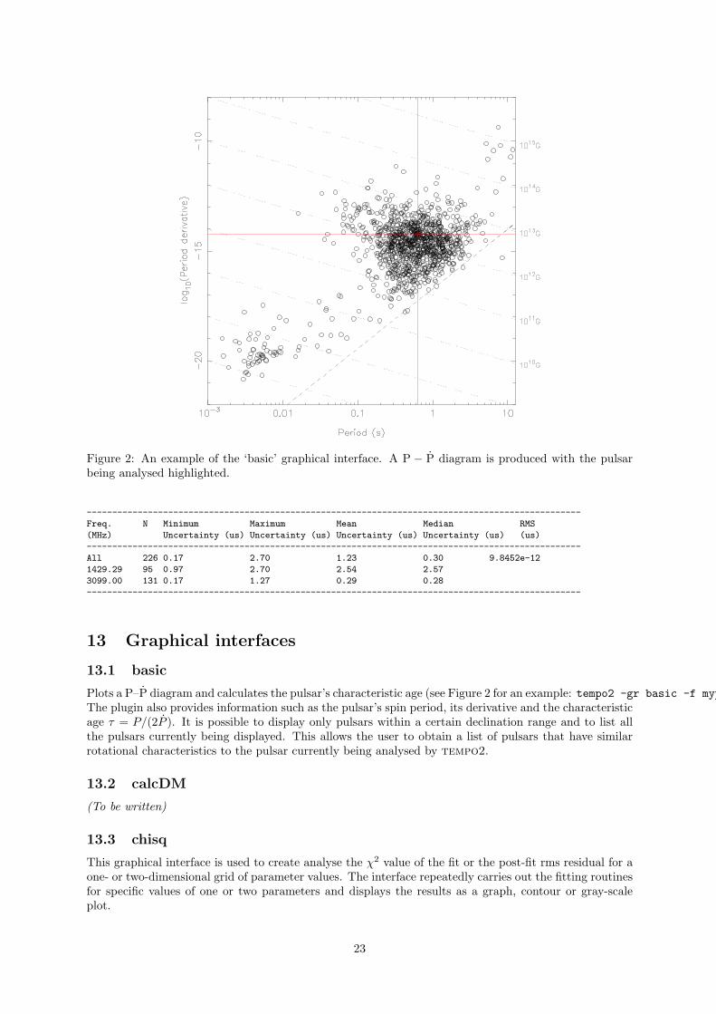
Figure 2: An example of the ‘basic’ graphical interface. A P − P diagram is produced with the pulsarbeing analysed highlighted.

-------------------------------------------------------------------------------------------------

Freq. N Minimum Maximum Mean Median RMS

(MHz) Uncertainty (us) Uncertainty (us) Uncertainty (us) Uncertainty (us) (us)

-------------------------------------------------------------------------------------------------

All 226 0.17 2.70 1.23 0.30 9.8452e-12

1429.29 95 0.97 2.70 2.54 2.57

3099.00 131 0.17 1.27 0.29 0.28

-------------------------------------------------------------------------------------------------

13 Graphical interfaces

13.1 basic

Plots a P–P diagram and calculates the pulsar’s characteristic age (see Figure 2 for an example: tempo2 -gr basic -f mypar.par

The plugin also provides information such as the pulsar’s spin period, its derivative and the characteristicage τ = P/(2P ). It is possible to display only pulsars within a certain declination range and to list allthe pulsars currently being displayed. This allows the user to obtain a list of pulsars that have similarrotational characteristics to the pulsar currently being analysed by tempo2.

13.2 calcDM

(To be written)

13.3 chisq

This graphical interface is used to create analyse the χ2 value of the fit or the post-fit rms residual for aone- or two-dimensional grid of parameter values. The interface repeatedly carries out the fitting routinesfor specific values of one or two parameters and displays the results as a graph, contour or gray-scaleplot.

23

Figure 3: Example of the chisq plug-in for determining the most likely values of the orbital period, PB,and longitude of periastron, OM.

This plugin is based on the “parmap” program developed by Swinburne University.

13.4 compare

Graphical interface used to compare the residuals obtained using two different parameter (.par) files.For instance, different solar system ephemeris could be defined in the parameter files and the resultscompared using this interface.

13.5 compareRes

(To be written)

13.6 delays

This interface allows the user to inspect the clock corrections and propagation time delays that tempo2has applied in order to obtain barycentric arrival times. See Figure 4 (tempo2 -gr delays -f mypar.par mytim.tim).The following key strokes are possible

q quit

y-1 (’y’ followed by ’1’) plot first clock correction

y-2 (’y’ followed by ’2’) plot second clock correction

y-3 plot third clock correction

y-4 plot fourth clock correction

y-5 plot fifth clock correction

y-6 plot UT1

y-7 plot Shapiro delay due to Sun

y-8 plot dispersion delay in solar system

y-9 plot dispersion delay in ISM

y-0 plot Roemer delay

y-a plot pre-fit residuals

y-b plot post-fit residuals

y-c plot Shapiro delay due to Jupiter

24

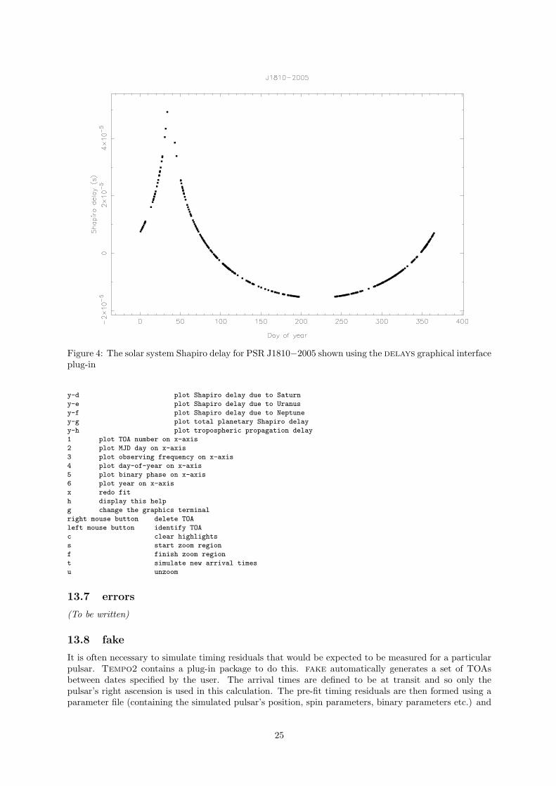
Figure 4: The solar system Shapiro delay for PSR J1810−2005 shown using the delays graphical interfaceplug-in

y-d plot Shapiro delay due to Saturn

y-e plot Shapiro delay due to Uranus

y-f plot Shapiro delay due to Neptune

y-g plot total planetary Shapiro delay

y-h plot tropospheric propagation delay

1 plot TOA number on x-axis

2 plot MJD day on x-axis

3 plot observing frequency on x-axis

4 plot day-of-year on x-axis

5 plot binary phase on x-axis

6 plot year on x-axis

x redo fit

h display this help

g change the graphics terminal

right mouse button delete TOA

left mouse button identify TOA

c clear highlights

s start zoom region

f finish zoom region

t simulate new arrival times

u unzoom

13.7 errors

(To be written)

13.8 fake

It is often necessary to simulate timing residuals that would be expected to be measured for a particularpulsar. Tempo2 contains a plug-in package to do this. fake automatically generates a set of TOAsbetween dates specified by the user. The arrival times are defined to be at transit and so only thepulsar’s right ascension is used in this calculation. The pre-fit timing residuals are then formed using aparameter file (containing the simulated pulsar’s position, spin parameters, binary parameters etc.) and

25

subtracted from the original simulated arrival times. This procedure is iterated until the residuals arezero. These arrival times can subsequently be modified by 1) the addition of Gaussian noise and 2) theaddition of simulated timing noise. Upon running the fake plugin, the user is asked to provide

• The number of days between observations

• The number of observations on a given day

• The maximum absolute hour angle allowed

• Whether the user required random or regular hour angle coverage

• The initial MJD for the simulated TOAs

• The final MJD for the simulated TOAs

• The rms of Gaussian noise to be added to the TOAs

• Whether red noise should be added to simulate timing noise

If the red noise option is selected, the user is also requested to provide

• The power law index for the red noise

• The power law amplitude

• A random number seed

• Whether the residuals should be smoothed

• Whether a cubic should be added to the residuals

The red noise is simulated as a shot-noise process obtained by summing many sinusoids with randomphase, but with amplitudes given by the requested power-law spectrum.The following example simulates a pulsar with a large proper motion:

1. Produce a parameter file similar to (called testfake.par)

PSRJ J1730-2304

RAJ 17:30:21.6483

DECJ -23:04:31.4

POSEPOCH 51500.0

PMRA 200

PEPOCH 51500.0

F0 123.110289179797

F1 -3.0631E-16

DM 9.611

CLK UTC(NIST)

EPHEM DE200

2. Run tempo2 -gr fake testfake.par

3. Follow on screen instructions

4. The fake plug-in will produce an arrival time file called testfake.simulate

5. In the parameter file change the PMRA back to zero

6. Run tempo2 -gr plk -f testfake.par testfake.simulate

The result should be similar to that shown in Figure 5.note: this code was based on the fake software originally developed by Duncan Lorimer and updated bySimon Johnston

13.9 gorilla

(To be written)

26

Figure 5: Simulating pulsar timing residuals for a pulsar with a proper motion in right ascension of200 mas/yr using the fake plugin.

13.10 plk

plk provides the user with a graphical interface that plots pre-fit and post-fit timing residuals versusparameters such as day, TOA number, binary phase or observing frequency. It is based on the plkstandalone package written for the original TEMPO, but has been significantly enhanced. The profilescorresponding to TOAs may be viewed and the TOAs deleted or identified using mouse clicks. Phasejumps can easily be added and the data refit in order to improve the timing model. A simple menusystem allows the user to change the fitted parameters and to produce new arrival time and parameterfiles. This graphical interface only works in single-pulsar mode. An example of the output is shown inFigure 6 (usage: tempo2 -gr plk -f mypar.par mytim.tim).Options available are:

b Bin TOAs within certain time bin

c Change fitting parameters

C run unix command with filenames for highlighted observations

ctrl-c Toggle between period epoch and centre for the reference epoch

d (or right mouse) delete point

D (or middle mouse) view profile

ctrl-D delete highlighted points

e multiply all TOA errors by given amount

f finish of zoom section

F run FITWAVES

ctrl-F remove FITWAVES curve from residuals

g change graphics device

G change gridding on graphics device

h this help file

H highlight points with specific flag in .tim file

i (or left mouse) identify point

j draw line between each points

l list all data points in zoomed region

L add label to plot

ctrl-l add line to plot

m measure distance between two points

M toggle removing mean from the residuals

27

Figure 6: An example of the plk graphical interface in use. The post-fit residuals for PSR J0437−4715are plotted with 20 observations shown in green and 10 cm observations in red. The white circles andblack lines indicate arrival times between orbital phases 0.4 and 0.6.

ctrl-m toggle menu bar

o obtain/highlight all points currently in plot

p Change model parameter values

P write new .par file

ctrl-P Toggle fitting versus pulse phase

q quit

r Reset (reload .par and .tim file)

s start of zoom section

S save a new .tim file

ctrl-S Overplot Shapiro delay

u unzoom

U unhighlight selected points

v view profiles for highlighted points

V define the user parameter

ctrl-V for pre-fit plotting, decompose the timing model fits

w toggle fitting using weights

x redo fit using post-fit parameters

ctrl-X place periodic marks on the x-scale

y Rescale y-axis only

z Zoom using mouse

+ add positive phase jump

- add negative phase jump

ctrl-= add period to add residuals above cursor

< in zoom mode include previous observation

> in zoom mode include next observation

1 plot pre-fit residuals vs date

2 plot post-fit residuals vs date

3 plot pre-fit residuals vs orbital phase

4 plot post-fit residuals vs orbital phase

5 plot pre-fit residuals serially

6 plot post-fit residuals serially

7 plot pre-fit residuals vs day of year

8 plot post-fit residuals vs day of year

9 plot pre-fit residuals vs frequency

a plot post-fit residuals vs frequency

28

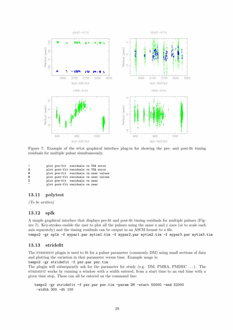
Figure 7: Example of the splk graphical interface plug-in for showing the pre- and post-fit timingresiduals for multiple pulsar simultaneously.

! plot pre-fit residuals vs TOA error

@ plot post-fit residuals vs TOA error

# plot pre-fit residuals vs user values

$ plot post-fit residuals vs user values

% plot pre-fit residuals vs year

^ plot post-fit residuals vs year

13.11 polytest

(To be written)

13.12 splk

A simple graphical interface that displays pre-fit and post-fit timing residuals for multiple pulsars (Fig-ure 7). Key-strokes enable the user to plot all the pulsars using the same x and y axes (or to scale eachaxis separately) and the timing residuals can be output in an ASCII format to a file.tempo2 -gr splk -f mypar1.par mytim1.tim -f mypar2.par mytim2.tim -f mypar3.par mytim3.tim

13.13 stridefit

The stridefit plugin is used to fit for a pulsar parameter (commonly DM) using small sections of dataand plotting the variation in that parameter versus time. Example usage is:tempo2 -gr stridefit -f psr.par psr.tim

The plugin will subsequently ask for the parameter for study (e.g. DM, PMRA, PMDEC . . . ). Thestridefit works by running a window with a width entered, from a start time to an end time with agiven time step. These can all be entered on the command line:

tempo2 -gr stridefit -f psr.par psr.tim -param DM -start 50000 -end 52000

-width 300 -dt 100

29

Figure 8: Example of the stridefit graphical interface plug-in which calculates the pulsar’s dispersionmeasure as a function fo time.

The stridefit plugin will produce a graph of the parameter versus time. Clicking on any point will listthe points that were used in deriving the parameter. If there is reason to believe that any particularpoint is in error (for instance trying to obtain a DM value with only one observing frequency) then thepoint can be deleted using the right mouse button.An example stridefit output is shown in Figure 8.After plotting the following key strokes may be used

h provides help

1 zero x-value for first point

2 centre points

3 toggle plotting day/year

u rescale the axes

q quit

f fit a straight line to a region selected by the mouse

F fit and remove a straight line

r redo the stridefit

e re-enter the MJD of the end point

s re-enter the MJD of the start point

S change the font-size for plotting

n enter the minimum number of observations required for a point

g set the graphical device

w re-enter the width of the fit region

t re-enter the time step

A (or left mouse) identify closest point

X (or right mouse) delete closest point

z zoom using the mouse

l list all the values

L list all the values and ouput to file

13.14 transform

Transforms a tempo1 parameter file into a tempo2-compatable file.

tempo2 -gr transform tempo1.par tempo2.par [back]

30

where the back command is used to convert from tempo2 to tempo1.

14 Developing the software

The plug-in features of tempo2 implies that users can add to the functionality of tempo2 by producingtheir own plug-in. In this section, we first discuss how such plug-ins can be produced. We also provide afew notes for users who are interested in developing the actual main source code and become part of thetempo2 development team.

14.1 Creating a plug-in

Plug-ins are relatively easy to create in C or C++. These plug-ins may use other libraries such as pgplot,tcl/tk or qt. As described above, plug-ins can be created to change the output format or as a graphicalinterface.

14.1.1 A new output format

When an “output-format” plug-in is used, the tempo2 software reads in the specified parameter andobservation files, carries out the standard techniques to obtain pre- and post-fit timing residuals andtheir corresponding parameter values and then passes control to the output-format software to displaythe results. An example output format (in C) is as follows:

#include <stdio.h>

#include <stdlib.h>

#include <string.h>

#include <math.h>

#include "tempo2.h" /* Essential for a tempo2 plugin */

extern "C" int tempoOutput(pulsar *psr,int npsr,char timFile[][MAX_FILELEN],char parFile[][MAX_FILELEN])

{

int i;

printf("Pulsar name = %s\n",psr[0].name);

printf("Pulsar spin-frequency = %Lg\n",psr[0].param[param_f].val[0]);

for (i=0;i<psr[0].nobs;i++)

printf("Residual = %.14f\n",(double)psr[0].obsn[i].residual);

}

This plug-in displays the pulsar’s name (obtained from the parameter file), its post-fit spin-frequency andthe post-fit timing residuals on the screen. The software is built around a structure called pulsarwhich is defined in tempo2.h. The most important definitions in this structure are

char *name; /* The pulsar name */

char *binaryModel; /* The binary model (e.g. T2/BT/ELL1 ...) */

double ne_sw; /* The electron density at 1AU due to the solar wind */

int fitMode; /* = 1 if fitting with errors, 0 = not fitting with errors */

int nobs; /* Number of observations */

int nits; /* Number of iterations used for the fit */

int ipm; /* = 1 if the interplanetary DM correction is used, 0 otherwise */

An array of pulsars is defined and therefore, in order to display the name of the first three pulsarsanalysed:

printf("pulsar 1 = %s\n",psr[0].name);



The structure also includes an array of parameters (param) which are defined as

param_raj,param_decj,param_f,param_pepoch,param_posepoch,

param_dmepoch,param_dm,param_pmra,param_pmdec,param_px,

param_sini,param_pb,param_t0,param_a1,param_om,param_pmrv,

param_ecc,param_edot,param_xpbdot,param_pbdot,param_a1dot,

31

param_omdot,param_tasc,param_eps1,param_eps2,param_m2,param_gamma,

param_mtot,param_glep,param_glph,param_glf0,param_glf1,

param_glf0d,param_gltd,param_start,param_finish,param_track,param_bp,param_bpp,

param_tzrmjd,param_tzrfrq,param_fdd,param_dr,param_dtheta,param_tspan,

param_bpjep,param_bpjph,param_bpja1,param_bpjec,param_bpjom,param_bpjpb,

param_wave_om,param_kom,param_kin,param_shapmax,param_dth,param_a0,

param_b0,param_xomdot,param_afac,param_eps1dot,param_eps2dot,param_tres

For each parameter, the user can obtain

char **label; /* Label about this parameter */

char **shortlabel; /* Label about this parameter without units */

longdouble *val; /* Value of parameter */

longdouble *err; /* Uncertainty on parameter value */

int *fitFlag; /* = 1 if fitting required */

int *paramSet; /* = 1 if parameter has been set */

longdouble *prefit; /* Pre-fit value of the parameter */

longdouble *prefitErr; /* Pre-fit value of the uncertainty */

int aSize; /* Number of elements in the array for this parameter */

Each parameter is stored as an array with each element of the array typically storing time derivatives ofthe parameter. For instance, to obtain the value of the spin-frequency and its first two derivatives:

printf("values = %Lg %Lg %Lg\n",psr[0].param[param_f].val[0],

psr[0].param[param_f].val[1],psr[0].param[param_f].val[2]);

(Note: ’C’ requires the symbol ’%Lg’ or ’%Lf’ to display values in ’long double’ precision.The ‘pulsar’ structure also contains the set of observations and corresponding parameters. The observa-tion structure contains (other less-common parameters are defined in the tempo2.h file)

longdouble sat; /* Site arrival time */

longdouble bat; /* Barycentric arrival time */

int deleted; /* = 1 if observation has been deleted */

longdouble prefitResidual; /* Pre-fit residual */

longdouble residual; /* residual */

double freq; /* Frequency of observation (in MHz) */

double freqSSB; /* Frequency of observation in barycentric frame (in Hz) */

double toaErr; /* Error on TOA (in us) */

char fname[MAX_FILELEN]; /* Name of data file giving TOA */

char telID[100]; /* Telescope ID */

longdouble correctionTT_TB; /* Correction to TDB/TCB */

double einsteinRate; /* Derivative of correctionTT_TB */

longdouble correctionTT_Teph; /* Correction to Teph */

longdouble correctionUT1; /* Correction from site TOA to UT1 */

double shapiroDelaySun; /* Shapiro Delay due to the Sun */

double shapiroDelayJupiter; /* Shapiro Delay due to Jupiter */

double shapiroDelaySaturn; /* Shapiro Delay due to Saturn */

double shapiroDelayUranus; /* Shapiro Delay due to Uranus */

double shapiroDelayNeptune; /* Shapiro Delay due to Neptune */

double troposphericDelay; /* Delay due to neutral refraction in atmosphere */

double tdis1; /* Interstellar dispersion measure delay */

double tdis2; /* Dispersion measure delay due to solar system */

longdouble roemer; /* Roemer delay */

For instance, in order to display the site arrival-time, the barycentric arrival-time, and the Solar Shapirodelay for each observation:

for (i=0;i<psr[0].nobs;i++)

printf("values = %Lf %Lf %f\n",psr[0].obsn[i].sat,psr[0].obsn[i].bat,psr[0].obsn[i].shapiroDelaySun);

14.1.2 A new graphical interface

When a graphical interface is used, tempo2 checks the command-line arguments, initialises the memoryand then passes control to the graphical interface. The reading of the parameter and observation files,calculating barycentric arrival times, obtaining residuals, fitting and displaying the output must all bedone within the graphical interface. The following tempo2 functions are commonly called:

32

readParfile(...) /* Read the parameter file */

readTimfile(...) /* Read the observation file */

preProcess(...) /* Needs to be called after reading the

parameter and observation files */

formBatsAll(...) /* Forms the barycentric arrival times */

formResiduals(...) /* Forms the timing residuals */

doFit(...) /* Calls the fitting algorithms */

textOutput(...) /* The standard output display */

An example of a simple interface would be

#include <stdio.h>

#include <string.h>

#include <stdlib.h>

#include <math.h>

#include "tempo2.h"

using namespace std;

/* The main function called from the TEMPO2 package is ’graphicalInterface’ */

/* Therefore this function is required in all plugins */

extern "C" int graphicalInterface(int argc,char *argv[],pulsar *psr,int *npsr)

{

char parFile[MAX_PSR][MAX_FILELEN];

char timFile[MAX_PSR][MAX_FILELEN];

int i;

double globalParameter;

*npsr = 1; /* For a graphical interface that only shows results for one pulsar */

printf("Graphical Interface: name\n");

printf("Author: author\n");

printf("Version: version number\n");

/* Obtain the .par and the .tim file from the command line */

if (argc==4) /* Only provided .tim name */

{

strcpy(timFile[0],argv[3]);

strcpy(parFile[0],argv[3]);

parFile[0][strlen(parFile[0])-3] = ’\0’;

strcat(parFile[0],"par");

}

/* Obtain all parameters from the command line */

for (i=2;i<argc;i++)

{

if (strcmp(argv[i],"-f")==0)

{

strcpy(parFile[0],argv[i+1]);

strcpy(timFile[0],argv[i+2]);

}

}

readParfile(psr,parFile,timFile,*npsr); /* Load the parameters */

readTimfile(psr,timFile,*npsr); /* Load the arrival times */

preProcess(psr,*npsr,argc,argv);

for (i=0;i<2;i++) /* Do two iterations for pre- and post-fit residuals*/

{

formBatsAll(psr,*npsr); /* Form the barycentric arrival times */

formResiduals(psr,*npsr,0.0); /* Form the residuals */

if (i==0) doFit(psr,*npsr,&globalParameter,0,0); /* Do the fitting */

else textOutput(psr,*npsr,globalParameter,0,0,0,""); /* Display the output */

}

/* Now you have the parameters and residuals */

/* which can be displayed or plotted */

return 0;

33

}

14.2 The main source code

The tempo2 software can be obtained from the ATNF CVS repository soft atnf/tempo2 (pleasecontact members of the ATNF pulsar group for more information). To install type

> make install

The plug-ins provided with the source code are stored in soft atnf/tempo2/plugin and the docu-mentation in soft atnf/tempo2/documentation.

15 Tempo2 error and warning messages

Errors result from serious problems with the pulsar analysis which may not be able to complete at all.Warnings indicate possible problems in the analysis. Generally, the analysis will keep going.

15.1 Error messages

File handling errors

• ERROR [FILE1]: No .tim file given on command line

• ERROR [FILE2]: No .par file given on command line

• ERROR [FILE3]: Unable to open parfile X for pulsar Y

• ERROR [FILE4]: Unable to open timefile X

• ERROR [FILE5]: Unable to open file OBSERVATORY_CLOCK_2_UTC_NIST

• ERROR [FILE6]: Unable to open the leap second file

• ERROR [FILE7]: Unable to open OBSYS.DAT

Parameter file errors

• ERROR [PAR1]: Have not set a period epoch in X

Clock errors

• ERROR: Too many lines in ut1 file -- increase array size in tai2tdb

• ERROR [CLK2] Must increase MAX_CLKCORR

• ERROR [CLK3], must increase size of MAX_LEAPSEC

• ERROR [CLK4]: Date X out of range of TDB-TDT table

Ephemeris errors

• ERROR [EPHEM1]: Ephemeris file X not loaded

15.2 Warning messages

Parameter file warnings

• WARNING [PAR2]: Have not set a position epoch in X. The period epoch will be used

instead

Clock warnings

• Warning [CLK1]: MJD later than last entry in time.dat. Imprecise clock corrections

will be applied

34

16 Common questions

Our web-page provides a feedback form that allows the user to alert the software developers of anyproblems in the software.

1. How do I cite tempo2 in my publication? For basic tempo2 usage, please give a reference toHobbs, Edwards & Manchester (2006; submitted to MNRAS). For details of the timing model pleaserefer to Edwards, Hobbs & Manchester (2006; in preparation).

2. How do I increase the number of observations that can be loaded in tempo2? Use “-nobsX” on the command line where X is the number of observations required (the current default is10000 observations).

17 In progress

Tempo2 is continually being developed. We are currently developing the following

• A set of plug-ins to simulate the effects of gravitational wave sources on pulsar timing residuals andto place limits on the existence of any such gravitational wave sources in real pulsar timing data.

18 Acknowledgements

The tempo2 package is based on the original tempo Fortran code. This software was developed overmany years by multiple authors including J. Taylor, R. Manchester, D. Nice, W. Peters, J. Weisberg, A.Irwin and N. Wex. We thank the Australian pulsar community, J. Weisberg, D. Lorimer and M. Kramerfor suggestions and comments on tempo2.

35

Documents

TEMPO2 user manual - Jodrell Bank Observatorypulsar/Resources/tempo2_manual.pdf · TEMPO2 user manual George Hobbs, Russell Edwards Australia Telescope National Facility, CSIRO, PO