Embed Size (px)
Citation preview
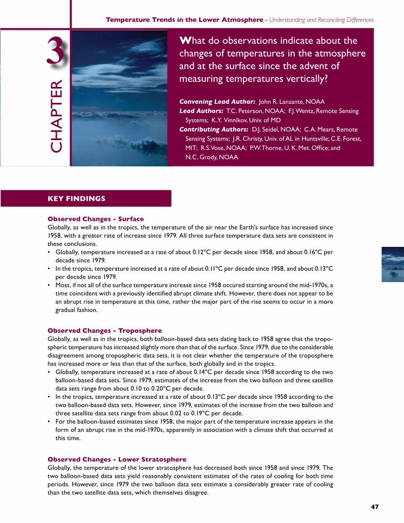
Temperature Trends in the Lower Atmosphere - Understanding and Reconciling Differences
What do observations indicate about the changes of temperatures in the atmosphere and at the surface since the advent of measuring temperatures vertically?
Convening Lead Author: John R. Lanzante, NOAALead Authors: T.C. Peterson, NOAA; F.J. Wentz, Remote Sensing Systems; K.Y. Vinnikov, Univ. of MDContributing Authors: D.J. Seidel, NOAA; C.A. Mears, Remote Sensing Systems; J.R. Christy, Univ. of AL in Huntsville; C.E. Forest, MIT; R.S. Vose, NOAA; P.W. Thorne, U. K. Met. Office; and N.C. Grody, NOAA
CH
APT
ER3
PB �7
KEy F�nd�nGS
observed Changes - SurfaceGlobally, as well as in the tropics, the temperature of the air near the Earth’s surface has increased since 1958, with a greater rate of increase since 1979. All three surface temperature data sets are consistent in these conclusions.• Globally, temperature increased at a rate of about 0.12ºC per decade since 1958, and about 0.16ºC per
decade since 1979.• In the tropics, temperature increased at a rate of about 0.11ºC per decade since 1958, and about 0.13ºC
per decade since 1979.• Most, if not all of the surface temperature increase since 1958 occured starting around the mid-1970s, a
time coincident with a previously identified abrupt climate shift. However, there does not appear to be an abrupt rise in temperature at this time, rather the major part of the rise seems to occur in a more gradual fashion.
observed Changes - TroposphereGlobally, as well as in the tropics, both balloon-based data sets dating back to 1958 agree that the tropo-spheric temperature has increased slightly more than that of the surface. Since 1979, due to the considerable disagreement among tropospheric data sets, it is not clear whether the temperature of the troposphere has increased more or less than that of the surface, both globally and in the tropics.• Globally, temperature increased at a rate of about 0.14ºC per decade since 1958 according to the two
balloon-based data sets. Since 1979, estimates of the increase from the two balloon and three satellite data sets range from about 0.10 to 0.20ºC per decade.
• In the tropics, temperature increased at a rate of about 0.13ºC per decade since 1958 according to the two balloon-based data sets. However, since 1979, estimates of the increase from the two balloon and three satellite data sets range from about 0.02 to 0.19ºC per decade.
• For the balloon-based estimates since 1958, the major part of the temperature increase appears in the form of an abrupt rise in the mid-1970s, apparently in association with a climate shift that occurred at this time.
observed Changes - Lower StratosphereGlobally, the temperature of the lower stratosphere has decreased both since 1958 and since 1979. The two balloon-based data sets yield reasonably consistent estimates of the rates of cooling for both time periods. However, since 1979 the two balloon data sets estimate a considerably greater rate of cooling than the two satellite data sets, which themselves disagree.
The U.S. Climate Change Science Program Chapter 3
�8 �9�8 �9
1. BACKGRoUnd
In this chapter we describe changes in tempera-ture at the surface and in the atmosphere based on four basic types of products derived from observations: surface, radiosonde, satellite and reanalysis. However, we limit our discussion of reanalysis products given their more problem-atic nature for use in trend analysis (see Chapter 2); only a few such trend values are presented for illustrative purposes.
Each of these four generic types of measure-ments consists of multiple data sets prepared by different teams of data specialists. The data sets are distinguished from one another by differences in the details of their construction. Each type of measurement system as well as each particular data set has its own unique strengths and weaknesses. Because it is dif-ficult to declare a particular data set as being “the best,” it is prudent to examine results de-rived from more than one “credible” data set of each type. Also, comparing results from more than one data set provides a better idea of the uncertainties or at least the range of results. In the interest of clarity and conciseness, we have
chosen to display and perform calculations for a representative subset of all available data sets. We consider these to be the “state of the art” data sets of their type, based on our collective expert judgment.
In selecting data sets for use in this report, we limit ourselves to those products that are being actively updated and for which temporal homo-geneity is an explicit goal in the construction, as these are important considerations for their use in climate change assessment. By way of a literature review, we discuss additional data sets not used in this report. Since some data sets are derivatives of earlier ones, we mention this where appropriate. One should not misconstrue the exclusion of a data set from this report as an invalidation of that product. Indeed, some of the excluded data sets have proved to be quite valuable in the past and will continue to be so into the future.
Most of the analyses that we have performed involve data that were averaged over a large region, such as the entire globe or the tropics. The spatial averaging process is complicated by the fact that the locations (gridpoints or
CHAPTER 3: Recommendations
• Although considerable progress has been made in explaining the causes of discrepancies be-tween upper-air datasets, both satellite and balloon-based, continuing steps should be taken to thoroughly assess and improve methods used to remove time-varying biases that are responsible for these discrepancies.
• New observations should be made available in order to provide more redundancy in climate monitoring. Activities should include both the introduction of new observational platforms as well as the necessary processing of data from currently under-utilized platforms. For example, Infraed Radiation (IR) and GPS satellite observations have not been used to any great extent, the former owing to complications when clouds are present and the latter owing to a short period of record. Additionally, the introduction of a network of climate-quality reference stations that include reference radiosondes, would place future climate monitoring on a firmer basis.
• Globally, the rate of cooling since 1958 is about 0.37ºC per decade based on the two balloon data sets. Since 1979, estimates of this decrease are about 0.65ºC per decade for the two balloon data sets, and from about 0.33 to 0.45º C per decade for the two satellite data sets.
• The bulk of the stratospheric temperature decrease occurred from about the late 1970s to the middle 1990s. It is unclear whether the decrease was gradual or occurred in abrupt steps in the first few years after each major volcanic eruption.
Each type of measurement system as well as each particular dataset has its own unique strengths and weaknesses.
�8 �9
Temperature Trends in the Lower Atmosphere - Understanding and Reconciling Differences
�8 �9
stations) at which data values are available can vary fundamentally by data type (see Chapter 2 for details) and, even for a given type, between data production teams. In an effort towards more consistency, the spatial averages we use represent the weighted average of zonal aver-ages1 (i.e., averages around an entire latitude line or zone), where the weights are the cosine of latitude2. This insures that the different latitude zones are given equal treatment across all data sets.
This chapter begins with a discussion of the four different data types, introducing some temperature data sets for each type, and then discussing their time histories averaged over the globe. Later we present more detail, concentrat-ing on the analysis of temperature trends for two eras: (1) the period since the widespread availability of radiosonde observations in 1958, and (2) since the introduction of satellite data in 1979. We compare overall temperature trends from different measurement systems and then go into more detail on trend variations in the horizontal and vertical.
2. SURFACE TEMPERATURES
2.1 Land-based Temperature dataOver land, temperature data come from fixed weather observing stations with thermometers housed in special instrument shelters. Records of temperature from many thousands of such stations exist. Chapter 2 outlines the difficul-ties in developing reliable surface temperature data sets. One concern is the variety of changes that may affect temperature measurements at an individual station. For example, the ther-mometer or instrument shelter might change, the time of day when the thermometers are read might change, or the station might move. These problems are addressed through a variety of procedures (see Peterson et al., 1998 for a review) that are generally quite successful at re-
1 The zonal averages, which were supplied to us by each data set production team, differ among data sets. We allowed each team to use their judgment as how to best produce these from the available gridpoint or station values in each latitude zone.
2 The cosine factor weights lower latitudes more than higher ones, to account for the fact that lines of longi-tude converge towards the poles. As a result, a zonal band in lower latitudes encompasses more area than a comparably sized band (in terms of latitude/longitude dimensions) in higher latitudes.
moving the effects of such changes at individual stations (e.g., Vose et al., 2003 and Peterson, 2006) whether the changes are documented in the metadata or detected via statistical analysis using data from neighboring stations as well (Aguilar et al., 2003). Subtle or widespread impacts that might be expected from urbaniza-tion or the growth of trees around observing sites might still contaminate a data set. These problems are addressed either actively in the data processing stage (e.g., Hansen et al., 2001) or through data set evaluation to ensure as much as possible that the data are not biased3 (e.g., Jones et al., 1990; Peterson, 2003; Parker, 2004; Peterson and Owen, 2005).
2.2 Marine Temperature dataData over the ocean come from moored buoys, drifting buoys, volunteer observing ships, and satellites. Historically, ships have provided most of the data, but in recent years an increas-ing number of buoys have been used, placed primarily in data-sparse areas away from ship-ping lanes. In addition, satellite data are often used after 1981. Many of the ships and buoys take both air temperature observations and sea surface temperature (SST) observations. Night marine air temperature (NMAT) observations have been used to avoid the problem that the Sun’s heating of the ship’s deck can make the thermometer reading greater than the actual air temperature. Where there are dense ob-servations of NMAT and SST, over the long term they track each other very well. However, since marine observations in an area may only be taken a few times per month, SST has the advantage over air temperature in that water temperature changes much more slowly than that of air. Also, there are twice as many SST observations as NMAT from the same platforms as SSTs are taken during both the day and night and SST data are supplemented in data sparse
3 Changes in regional land use such as deforestation, aforestation, agricultural practices, and other regional changes in land use are not addressed in the develop-ment of these data sets. While modeling studies have suggested over decades to centuries these affects can be important on regional space scales (Oleson et al., 2004), we consider these effects to be those of an external forcing to the climate system and are treated as such by many groups in the simulation of climate using the models described in Chapter 5. To the ex-tent that these effects could be large enough to have a measurable influence on global temperature, these changes will be detected by the land-based surface network.
Data over the ocean come from moored
buoys, drifting buoys, volunteer observing ships, and satellites.
The U.S. Climate Change Science Program Chapter 3
50 5150 51
areas by drifting buoys which do not take air temperature measurements. Accordingly, only having a few SST observations in a grid box for a month can still provide an accurate measure of the average temperature of the month.
2.3 Global Surface Temperature dataCurrently, there are three main groups creating global analyses of surface temperature (see Table 3.1), differing in the choice of available data that are utilized as well as the manner in which these data are synthesized. Since the network of surface stations changes over time, it is necessary to assess how well the avail-able observations monitor global or regional temperature. There are three ways in which to make such assessments (Jones, 1995). The first is using “frozen grids” where analysis using only those grid boxes with data present in the sparsest years is used to compare to the full data set results from other years (e.g., Parker et al., 1994). The results generally indicate very small errors on multi-annual timescales (Jones, 1995). The second technique is sub-sampling a spatially complete field, such as model output, only where in situ observations are available. Again the errors are small (e.g., the standard errors are less than 0.06ºC for the observing period 1880 to 1990; Peterson et al., 1998b). The third technique is comparing optimum averaging, which fills in the spatial field using covariance matrices, eigenfunctions or struc-ture functions, with other analyses. Again, very small differences are found (Smith et al., 2005). The fidelity of the surface temperature record is further supported by work such as Peterson et al. (1999) which found that a rural subset of
global land stations had almost the same global trend as the full network and Parker (2004) that found no signs of urban warming over the period covered by this report.
2.3.1 noaa ncdcThe National Oceanic and Atmospheric Ad-ministration (NOAA) National Climatic Data Center (NCDC) integrated land and ocean data set (see Table 3.1) is derived from in situ data. The SSTs come from the International Compre-hensive Ocean-Atmosphere Data Set (ICOADS) SST observations release 2 (Slutz et al., 1985; Woodruff et al., 1998; Diaz et al., 2002). Those that pass quality control tests are averaged into monthly 2° grid boxes (Smith and Reynolds, 2003). The land surface air temperature data come from the Global Historical Climatology Network (GHCN) (Peterson and Vose, 1997) and are averaged into 5° grid boxes. A recon-struction approach is used to create complete global coverage by combining together the faster and slower time-varying components of temperature (van den Dool et al., 2000; Smith and Reynolds, 2005).
2.3.2 nasa gissThe NASA Goddard Institute for Space Stud-ies (GISS) produces a global air temperature analysis (see Table 3.1) known as GISTEMP using land surface temperature data primarily from GHCN and the U.S. Historical Climatol-ogy Network (USHCN; Easterling, et al., 1996). The NASA team modifies the GHCN/USHCN data by combining at each location the time records of the various sources and adjusting the non-rural stations in such a way that their long-term trends are consistent with those from neighboring rural stations (Hansen et al., 2001). These meteorological station measurements over land are combined with in situ sea sur-face temperatures and Infrared Radiation (IR) satellite measurements for 1982 to the present (Reynolds and Smith, 1994; Smith et al., 1996) to produce a global temperature index (Hansen et al., 1996).
2.3.3 UK HadCRUT2v The UK global land and ocean data set (Had-CRUT2v, see Table 3.1) is produced as a joint effort by the Climatic Research Unit of the University of East Anglia and the Hadley Centre of the UK Meteorological (Met) Office.
The fact that a rural subset of global land stations had almost the same trend as the full set of stations, indicates that urbanization is not a significant contributor to the global temperature trend.
50 51
Temperature Trends in the Lower Atmosphere - Understanding and Reconciling Differences
50 51
The land surface air temperature data are from Jones and Mo-berg (2003) of the Cli-matic Research Unit. The global SST fields are produced by the Hadley Centre using a blend of COADS and Met Office data bank in situ observations (Rayner, et al., 2003). The integrated data set is known as Had-CRUT2v (Jones and Moberg, 2003)4. The temperature anoma-lies were calculated on a 5°x5° grid box basis. Within each grid box, the temporal variability of the observations has been adjusted to ac-count for the effect of changing the number of stations or SST observations in individual grid-box temperature time series (Jones et al., 1997, 2001). There is no reconstruction of data gaps because of the problems of introducing biased interpolated values.
2.3.4 synopsis of surface daTa seTs
Since the three chosen data sets utilize many of the same raw observations, there is a degree of interdependence. Nevertheless, there are some differences among them as to which observing sites are utilized. An important advantage of surface data is the fact that at any given time there are thousands of thermometers in use that contribute to a global or other large-scale aver-age. Besides the tendency to cancel random er-rors, the large number of stations also greatly fa-cilitates temporal homogenization since a given station may have several “near-neighbors” for “buddy-checks.” While there are fundamental differences in the methodology used to create the surface data sets, the differing techniques with the same data produce almost the same re-sults (Vose et al., 2005a). The small differences in deductions about climate change derived
4 Although global and hemispheric temperature time series created using a technique known as optimal averaging (Folland et al., 2001a; Parker et al., 2004), which provides estimates of uncertainty in the time series, including the effects of data gaps and uncer-tainties related to bias corrections or uncorrected biases, are available, we have used the data in their more basic form, for consistency with the other data sets.
from the surface data sets are likely to be due mostly to differences in construction methodol-ogy and global averaging procedures.
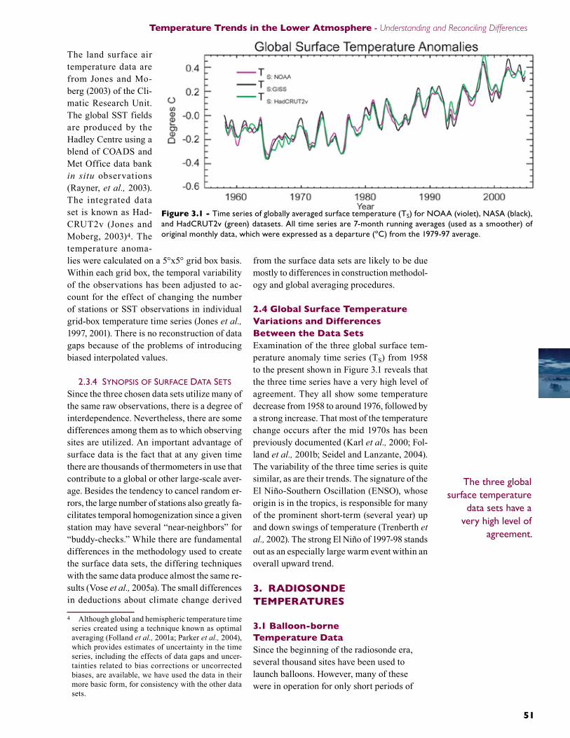
2.� Global Surface Temperature Variations and differences Between the data SetsExamination of the three global surface tem-perature anomaly time series (TS) from 1958 to the present shown in Figure 3.1 reveals that the three time series have a very high level of agreement. They all show some temperature decrease from 1958 to around 1976, followed by a strong increase. That most of the temperature change occurs after the mid 1970s has been previously documented (Karl et al., 2000; Fol-land et al., 2001b; Seidel and Lanzante, 2004). The variability of the three time series is quite similar, as are their trends. The signature of the El Niño-Southern Oscillation (ENSO), whose origin is in the tropics, is responsible for many of the prominent short-term (several year) up and down swings of temperature (Trenberth et al., 2002). The strong El Niño of 1997-98 stands out as an especially large warm event within an overall upward trend.
3. RAd�oSondE TEMPERATURES
3.1 Balloon-borne Temperature dataSince the beginning of the radiosonde era, several thousand sites have been used to launch balloons. However, many of these were in operation for only short periods of
Figure 3.1 - Time series of globally averaged surface temperature (TS) for NOAA (violet), NASA (black), and HadCRUT2v (green) datasets. All time series are 7-month running averages (used as a smoother) of original monthly data, which were expressed as a departure (ºC) from the 1979-97 average.
The three global surface temperature
data sets have a very high level of
agreement.
The U.S. Climate Change Science Program Chapter 3
52 5352 53
Our Name
Web PageName Given by Producers Producers
Surface
NOAA http://www.ncdc.noaa.gov/oa/climate/monitoring/gcag/gcag.html
ER-GHCN-ICOADS NOAA’s National Climatic Data Center (NCDC)
NASA http://www.giss.nasa.gov/data/update/gistemp/graphs/
Land+Ocean Temperature NASA’s Goddard Institute for Space Studies (GISS)
HadCRUT2v http://www.cru.uea.ac.uk/cru/data/temperature
HadCRUT2v Climatic Research Unit of the University of East Anglia and the Hadley Centre of the UK Met Office
RadiosondeRATPAC http://www.ncdc.noaa.gov/oa/cab/ratpac/
RATPAC NOAA’s: Air Resources Laboratory (ARL), Geophysical Fluid Dynamics Laboratory (GFDL), and National Climatic Data Center (NCDC)
HadAT2 http://www.hadobs.org/
HadAT2 Hadley Centre of the UK Met Office
Satellite
Temperature of the Lower Troposphere
T2LT-UAH http://vortex.nsstc.uah.edu/data/msu/t2lt
TLT University of Alabama in Huntsville (UAH)
T2LT-RSS http://www.remss.com/msu/msu_data_description.html
TLT Remote Sensing System, Inc. (RSS)
Temperature of the Middle Troposphere
T2-UAHhttp://vortex.nsstc.uah.edu/data/msu/t2
TMT University of Alabama in Huntsville (UAH)
T2-RSShttp://www.remss.com/msu/msu_data_description.html
TMT Remote Sensing System, Inc. (RSS)
T2-UMdhttp://www.atmos.umd.edu/~kostya/CCSP/
Channel 2 University of Maryland and NOAA/NESDIS (UMd)
Temperature of the Middle Troposphere minus Stratospheric Influences
T*G (global) T*T (tropics)http://www.ncdc.noaa.gov/oa/climate/research/ fu-mt-uah-monthly-anom.txt (UAH)
http://www.ncdc.noaa.gov/oa/climate/research/ fu-mt-rss-monthly-anom.txt (RSS)
T(850-300) University of Washington, Seattle (UW) and NOAA’s Air Resources Laboratory (ARL)
Temperature of the Lower Stratosphere
T4-UAHhttp://vortex.nsstc.uah.edu/data/msu/t4
TLS University of Alabama in Huntsville (UAH)
T4-RSShttp://www.remss.com/msu/msu_data_description.html
TLS Remote Sensing System, Inc. (RSS)
Reanalysis
NCEP50http://wesley.ncep.noaa.gov/reanalysis.html
NCEP50 National Centers for Environmental Prediction (NCEP), NOAA, and the National Center for Atmospheric Research (NCAR)
ERA40http://www.ecmwf.int/research/era
ERA40 European Centre for Medium-Range Weather Forecasts (ECMWF)
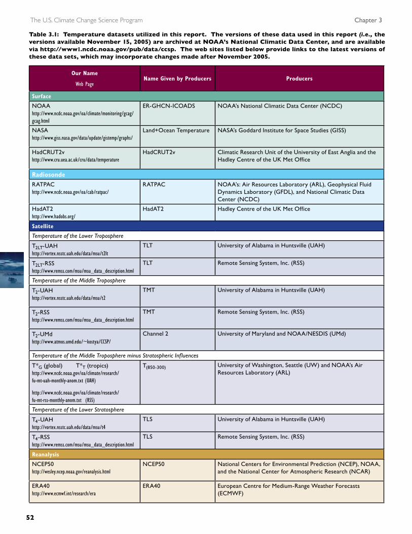
Table 3.1: Temperature datasets utilized in this report. The versions of these data used in this report (i.e., the versions available november 15, 2005) are archived at noAA’s national Climatic data Center, and are available via http://www1.ncdc.noaa.gov/pub/data/ccsp. The web sites listed below provide links to the latest versions of these data sets, which may incorporate changes made after november 2005.
52 53
Temperature Trends in the Lower Atmosphere - Understanding and Reconciling Differences
52 53
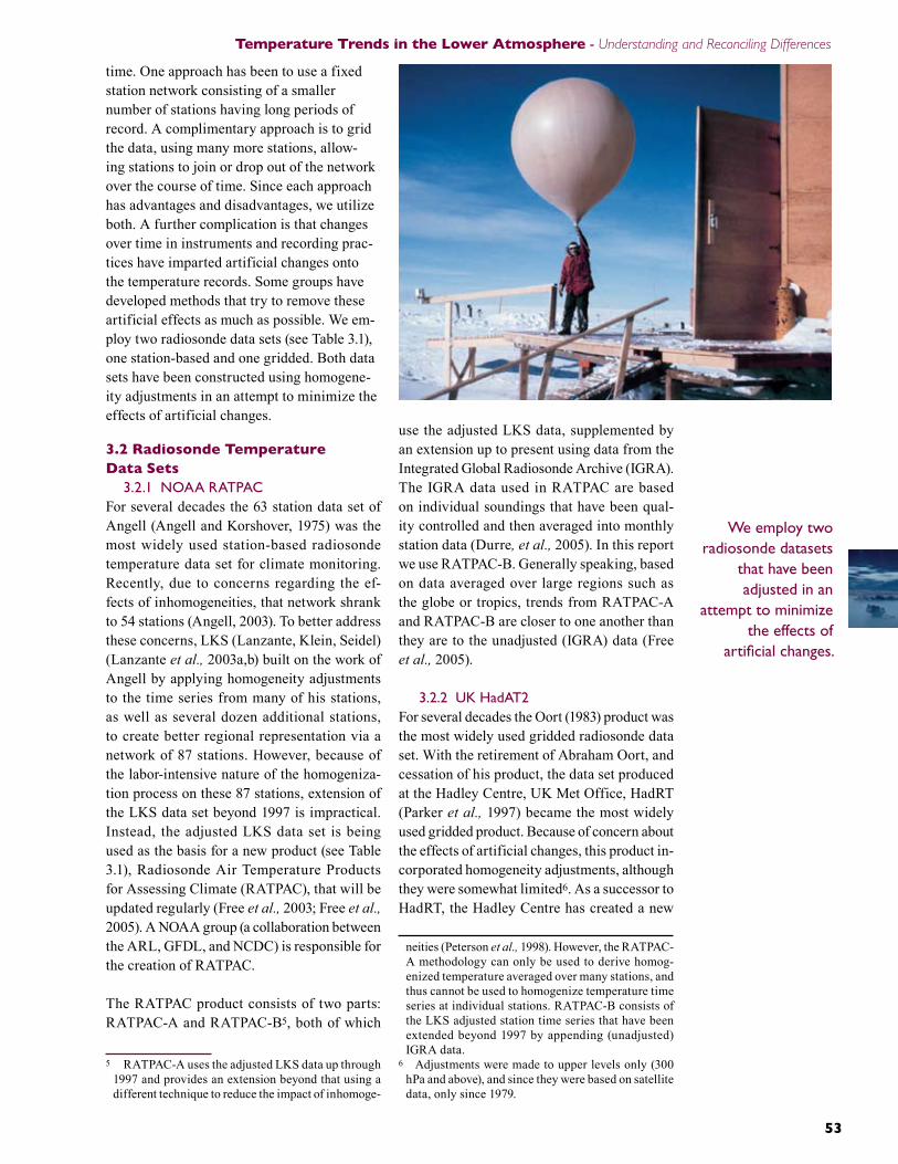
time. One approach has been to use a fixed station network consisting of a smaller number of stations having long periods of record. A complimentary approach is to grid the data, using many more stations, allow-ing stations to join or drop out of the network over the course of time. Since each approach has advantages and disadvantages, we utilize both. A further complication is that changes over time in instruments and recording prac-tices have imparted artificial changes onto the temperature records. Some groups have developed methods that try to remove these artificial effects as much as possible. We em-ploy two radiosonde data sets (see Table 3.1), one station-based and one gridded. Both data sets have been constructed using homogene-ity adjustments in an attempt to minimize the effects of artificial changes.
3.2 Radiosonde Temperature data Sets
3.2.1 noaa raTpacFor several decades the 63 station data set of Angell (Angell and Korshover, 1975) was the most widely used station-based radiosonde temperature data set for climate monitoring. Recently, due to concerns regarding the ef-fects of inhomogeneities, that network shrank to 54 stations (Angell, 2003). To better address these concerns, LKS (Lanzante, Klein, Seidel) (Lanzante et al., 2003a,b) built on the work of Angell by applying homogeneity adjustments to the time series from many of his stations, as well as several dozen additional stations, to create better regional representation via a network of 87 stations. However, because of the labor-intensive nature of the homogeniza-tion process on these 87 stations, extension of the LKS data set beyond 1997 is impractical. Instead, the adjusted LKS data set is being used as the basis for a new product (see Table 3.1), Radiosonde Air Temperature Products for Assessing Climate (RATPAC), that will be updated regularly (Free et al., 2003; Free et al., 2005). A NOAA group (a collaboration between the ARL, GFDL, and NCDC) is responsible for the creation of RATPAC.
The RATPAC product consists of two parts: RATPAC-A and RATPAC-B5, both of which
5 RATPAC-A uses the adjusted LKS data up through 1997 and provides an extension beyond that using a different technique to reduce the impact of inhomoge-
use the adjusted LKS data, supplemented by an extension up to present using data from the Integrated Global Radiosonde Archive (IGRA). The IGRA data used in RATPAC are based on individual soundings that have been qual-ity controlled and then averaged into monthly station data (Durre, et al., 2005). In this report we use RATPAC-B. Generally speaking, based on data averaged over large regions such as the globe or tropics, trends from RATPAC-A and RATPAC-B are closer to one another than they are to the unadjusted (IGRA) data (Free et al., 2005).
3.2.2 UK HadAT2For several decades the Oort (1983) product was the most widely used gridded radiosonde data set. With the retirement of Abraham Oort, and cessation of his product, the data set produced at the Hadley Centre, UK Met Office, HadRT (Parker et al., 1997) became the most widely used gridded product. Because of concern about the effects of artificial changes, this product in-corporated homogeneity adjustments, although they were somewhat limited6. As a successor to HadRT, the Hadley Centre has created a new
neities (Peterson et al., 1998). However, the RATPAC-A methodology can only be used to derive homog-enized temperature averaged over many stations, and thus cannot be used to homogenize temperature time series at individual stations. RATPAC-B consists of the LKS adjusted station time series that have been extended beyond 1997 by appending (unadjusted) IGRA data.
6 Adjustments were made to upper levels only (300 hPa and above), and since they were based on satellite data, only since 1979.
Our Name
Web PageName Given by Producers Producers
Surface
NOAA http://www.ncdc.noaa.gov/oa/climate/monitoring/gcag/gcag.html
ER-GHCN-ICOADS NOAA’s National Climatic Data Center (NCDC)
NASA http://www.giss.nasa.gov/data/update/gistemp/graphs/
Land+Ocean Temperature NASA’s Goddard Institute for Space Studies (GISS)
HadCRUT2v http://www.cru.uea.ac.uk/cru/data/temperature
HadCRUT2v Climatic Research Unit of the University of East Anglia and the Hadley Centre of the UK Met Office
RadiosondeRATPAC http://www.ncdc.noaa.gov/oa/cab/ratpac/
RATPAC NOAA’s: Air Resources Laboratory (ARL), Geophysical Fluid Dynamics Laboratory (GFDL), and National Climatic Data Center (NCDC)
HadAT2 http://www.hadobs.org/
HadAT2 Hadley Centre of the UK Met Office
Satellite
Temperature of the Lower Troposphere
T2LT-UAH http://vortex.nsstc.uah.edu/data/msu/t2lt
TLT University of Alabama in Huntsville (UAH)
T2LT-RSS http://www.remss.com/msu/msu_data_description.html
TLT Remote Sensing System, Inc. (RSS)
Temperature of the Middle Troposphere
T2-UAHhttp://vortex.nsstc.uah.edu/data/msu/t2
TMT University of Alabama in Huntsville (UAH)
T2-RSShttp://www.remss.com/msu/msu_data_description.html
TMT Remote Sensing System, Inc. (RSS)
T2-UMdhttp://www.atmos.umd.edu/~kostya/CCSP/
Channel 2 University of Maryland and NOAA/NESDIS (UMd)
Temperature of the Middle Troposphere minus Stratospheric Influences
T*G (global) T*T (tropics)http://www.ncdc.noaa.gov/oa/climate/research/ fu-mt-uah-monthly-anom.txt (UAH)
http://www.ncdc.noaa.gov/oa/climate/research/ fu-mt-rss-monthly-anom.txt (RSS)
T(850-300) University of Washington, Seattle (UW) and NOAA’s Air Resources Laboratory (ARL)
Temperature of the Lower Stratosphere
T4-UAHhttp://vortex.nsstc.uah.edu/data/msu/t4
TLS University of Alabama in Huntsville (UAH)
T4-RSShttp://www.remss.com/msu/msu_data_description.html
TLS Remote Sensing System, Inc. (RSS)
Reanalysis
NCEP50http://wesley.ncep.noaa.gov/reanalysis.html
NCEP50 National Centers for Environmental Prediction (NCEP), NOAA, and the National Center for Atmospheric Research (NCAR)
ERA40http://www.ecmwf.int/research/era
ERA40 European Centre for Medium-Range Weather Forecasts (ECMWF)
Table 3.1: Temperature datasets utilized in this report. The versions of these data used in this report (i.e., the versions available november 15, 2005) are archived at noAA’s national Climatic data Center, and are available via http://www1.ncdc.noaa.gov/pub/data/ccsp. The web sites listed below provide links to the latest versions of these data sets, which may incorporate changes made after november 2005.
We employ two radiosonde datasets
that have been adjusted in an
attempt to minimize the effects of
artificial changes.
The U.S. Climate Change Science Program Chapter 3
5� 555� 55
product (HadAT2, see Table 3.1) that uses all available digital radiosonde data for a larger network of almost 700 stations having relatively long records7. Identification and adjustment of inhomogeneities was accomplished by way of comparison of neighboring stations.
3.2.3 synopsis of radiosonde daTa seTs
The two chosen data sets differ fundamentally
7 High quality small station subsets, such as Lanz-ante et al. (2003a) and the Global Climate Observing System Upper Air Network, were used as a skeletal network from which to define a set of adequately similar station series used in homogenization. The data set is designed to impart consistency in both space and time and, by using radiosonde neighbors rather than satellites or reanalyses, minimizes the chances of introducing spurious changes related to the introduction of satellite data and their subsequent platform changes (Thorne et al., 2005).
in their selection of sta-tions in that the NOAA data set uses a relatively small number of highly scrut inized stat ions, while the UK data set uses a considerably larg-er number of stations. Compared to the surface, far fewer thermometers are in use at any given time (hundreds or less) so there is less opportu-nity for random errors to cancel, but more impor-tantly, there are far fewer suitable “neighbors” to aid in temporal homog-enization. While both products incorporate a common building-block data set (Lanzante et al., 2003a), their methods of construction differ considerably. Any dif-ferences in deductions about climate change derived from them could be attributed to both the differing raw inputs as well as differing con-struction methodologies. Concerns about poor temporal homogeneity
are much greater than for surface data. Indeed, it is unlikely that a recently identified cooling bias in radiosonde data (Sherwood, et al., 2005; Randal and Wu, 2006) has been completely removed by the adjustment process.
3.3 Global Radiosonde Temperature Variations and differences Between the data Sets
3.3.1 Troposphere
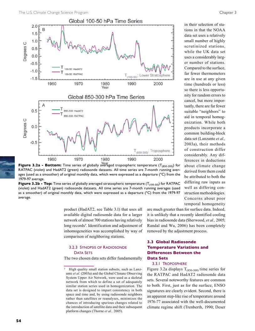
Figure 3.2a displays T(850-300) time series for the RATPAC and HadAT2 radiosonde data sets. Several noteworthy features are common to both. First, just as for the surface, ENSO signatures are clearly evident. Second, there is an apparent step-like rise of temperature around 1976-77 associated with the well-documented climate regime shift (Trenberth, 1990; Deser
Figure 3.2a - Bottom: Time series of globally averaged tropospheric temperature (T(850-300)) for RATPAC (violet) and HadAT2 (green) radiosonde datasets. All time series are 7-month running aver-ages (used as a smoother) of original monthly data, which were expressed as a departure (ºC) from the 1979-97 average.Figure 3.2b - Top: Time series of globally averaged stratospheric temperature (T(100-50)) for RATPAC (violet) and HadAT2 (green) radiosonde datasets. All time series are 7-month running averages (used as a smoother) of original monthly data, which were expressed as a departure (ºC) from the 1979-97 average.
5� 55
Temperature Trends in the Lower Atmosphere - Understanding and Reconciling Differences
5� 55
et al., 2004). Third, there is a long-term rise in temperatures, although a considerable amount of it may be due to the step-like change (Seidel and Lanzante, 2004). To a first approximation, both data sets display these features similarly and there is very little systematic difference between the two. Although a major component of the RATPAC product is used in the construc-tion of the HadAT2 data set, it should be kept in mind that the former utilizes a much smaller network of stations, although the length of the station records tends to be relatively long. If the good agreement is not fortuitous, this suggests that the reduced RATPAC station network pro-vides representative spatial sampling8.
3.3.2 loWer sTraTosphere
Figure 3.2b displays global temperature anom-aly time series of T(100-50) from the RATPAC and HadAT2 radiosonde data sets. Several noteworthy features are common to both data sets. First is the prominent signature of three climatically important volcanic eruptions: Mt. Agung (March 1963), El Chichón (April 1982), and Mt. Pinatubo (June 1991). Temperatures rise rapidly as volcanic aerosols are injected into the stratosphere and remain elevated for about 2-3 years before diminishing. There is some ambiguity as to whether the temperatures return to their earlier values or whether they experience step-like falls in the post-volcanic period for the latter two volcanoes, particularly Mt. Pinatubo (Pawson et al., 1998; Lanzante et al., 2003a; Seidel and Lanzante, 2004). Second, there are small amplitude variations associated with the tropical quasi-biennial oscillation (QBO) with a period of ~ 2-3 years (Seidel et al., 2004). Third, there is a downward trend, although there is some doubt as to whether the temperature decrease is best described by a linear trend over the period of record. For one thing, the temperature series prior to about 1980 exhibits little or no decrease in tempera-ture. After that, the aforementioned step-like drops represent a viable alternative to a linear decrease (Seidel and Lanzante, 2004).In spite of similarities among data sets, closer examination reveals some important differ-ences. There is a rather large difference between
8 This result is consistent with the relatively large spatial scales represented by a single radiosonde sta-tion at this level on an annual time scale demonstrated by Wallis (1998) and Thorne et al. (2005).
RATPAC and HadAT2 time series for the peak volcanic warming associated with Mt. Agung in 1963. This may be a reflection of differences in spatial sampling because the horizontal pattern of the response is not uniform (Free and Angell, 2002). More noteworthy for estimates of climate change are some subtle systematic differences between the two data sets that vary over time. A closer examination reveals that the RATPAC product tends to have higher temperatures than the HadAT2 product from approximately 1963-85, with the RATPAC product having lower values before and after this time period9. As we will see later, this yields a slightly greater decreasing trend for the RATPAC product. Poorer agreement between the RATPAC and HadAT2 products in the stratosphere compared to the troposphere is not unexpected because of the fact that artificial jumps in temperature induced by changes in radiosonde instruments and measurement systems tend to increase in magnitude from the near-surface upwards (Lan-zante et al., 2003b). More details on this issue are given in Chapter 4, Section 2.1.
9 It is worth noting that prominent artificial step-like drops, many of which were associated with the adoption of a particular type of radiosonde (Vaisala), were found in stratospheric temperatures at Austra-lian and western tropical Pacific stations in the mid to late 1980s by Parker et al. (1997), Stendel et al. (2000), and Lanzante et al. (2003a). Differences in consequent homogeneity adjustments around this time could potentially explain a major part of the difference between the NOAA and UK products, although this has not been demonstrated.
The U.S. Climate Change Science Program Chapter 3
56 5756 57
�. SATELL�TE-dER�VEd TEMPERATURES
�.1 Microwave Satellite dataThree groups, employing different method-ologies, have developed satellite Microwave Sounding Unit (MSU) climate data sets (see Table 3.1) derived from NOAA polar-orbiting satellites. We do not present results from a fourth group (Prabhakara et al., 2000), which developed yet another methodology, since they are not continuing to work on MSU climate analyses and are not updating their time series. One of the main issues that is addressed dif-ferently by the groups is the inter-calibration between the series of satellites, and is discussed in Chapters 2 and 4.
�.2 Microwave Satellite data Sets4.2.1 uniV. of alabama in hunTsVille (uah)
The first group to produce MSU climate prod-ucts, by adjusting for the differences between satellites and the effects of changing orbits (di-urnal drift), was UAH. Their approach (Christy et al., 2000; Christy et al., 2003) uses both an offset adjustment to allow for the systematic average differences between satellites and a non-linear hot target temperature10 calibration to create a homogeneous series. The UAH data set has products corresponding to three temperature measures: T2LT, T2, and T4 (see Chapter 2 for definitions of these measures). In this report, we use the most up-to-date versions available to us at the time, which is version 5.1 of the UAH data set for T2, and T4, and version 5.2 for T2LT
11.
4.2.2 remoTe sensing sysTems (rss)After carefully studying the methodology of the UAH team, another group, RSS, created their own data sets for T2 and T4 using the same input data but with modifications to the adjustment procedure (Mears et al., 2003), two of which are particularly noteworthy: (1) the method of inter-calibration from one satellite to the next
10 In fact, two targets are used, both with temperatures that are presumed to be well known. These are cold space, pointing away from the Earth, Moon, or Sun, and an onboard hot target.
11 The version number for T2LT differs from that for T2, and T4 because an error, which was found to affect the former (and was subsequently corrected), does not affect the latter two measures. This error was discovered by Mears and Wentz (2005).
and (2) the computation of the needed correc-tion for the daily cycle of temperature. While the second modification has little effect on the overall global trend differences between the two teams, the first is quite important in this regard. Recently, the RSS team has created its own version of T2LT (Mears and Wentz, 2005) and in doing so discovered a methodological error in the corresponding temperature measure of UAH. The UAH T2LT product used in this re-port is based on their corrected method. In this report, we use version 2.1 of the RSS data.
4.2.3 uniVersiTy of maryland (umd)A very different approach (Vinnikov et al., 2004) was developed by a team involving col-laborators from the University of Maryland and the NOAA National Environmental Satellite, Data, and Information Service (NESDIS) and was used to estimate globally averaged tem-perature trends (Vinnikov and Grody, 2003). After further study, they developed yet another new method (Grody et al., 2004; Vinnikov et al., 2006). As done by the other two groups, the UMd team’s methodology also recalibrates the instruments based on overlapping data between the satellites. However, the manner in which they perform this recalibration differs. Also, in both versions they do not adjust for diurnal drift directly, but average the data from ascending and descending orbits. In their second approach, they substantially altered the manner in which target temperatures are used in their recalibra-tion. The effect of their revision was to reduce the global temperature trends derived from their data from 0.22-0.26 to 0.20ºC/decade. In this most recent version of their data set, which we use in this report, they apply the nonlinear adjustment of Grody et al. (2004) and estimate the diurnal cycle as described in Vinnikov et al. (2006). The UMd group produces only a measure of T2, hence there is no stratospheric product (T4) or one corresponding to the lower troposphere (T2LT).
�.3 Synopsis of Satellite data SetsThe relationship among satellite data sets is fundamentally different from that for surface or radiosonde products. For satellites, different data sets use virtually the same raw inputs so that any differences in derived measures are due to construction methodology. The excel-lent coverage provided by the orbiting sensors,
For satellites, different data sets use virtually the same raw inputs so that any differences in derived measures are due to construction methodology.
56 57
Temperature Trends in the Lower Atmosphere - Understanding and Reconciling Differences
56 57
more than half the Earth’s surface daily, is a major advantage over in situ observations. The disadvantage is that while in situ observations rely on data from many hundreds or thousands of individual thermometers every day, provid-ing a beneficial redundancy, the satellite data typically come from only one or two instru-ments at a given time. Therefore, any problem impacting the data from a single satellite can adversely impact the entire climate record. The lack of redundancy, compounded by occasional premature satellite failure that limits the time of overlapping measurements from successive satellites, elevates the issue of temporal homo-geneity to the overwhelming explanation for any differences in deductions about climate change derived from the three data sets.
�.� Global Satellite Temperature Variations and differences Between the data Sets
4.4.1 TemperaTure of The Troposphere
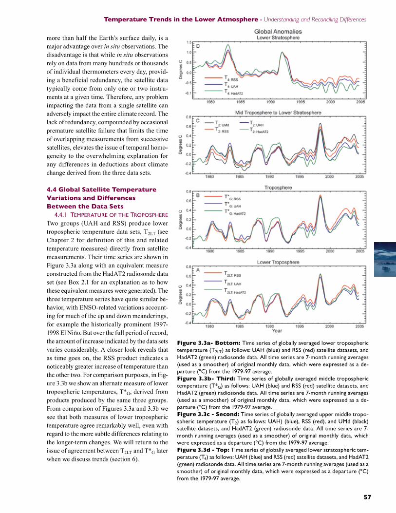
Two groups (UAH and RSS) produce lower tropospheric temperature data sets, T2LT (see Chapter 2 for definition of this and related temperature measures) directly from satellite measurements. Their time series are shown in Figure 3.3a along with an equivalent measure constructed from the HadAT2 radiosonde data set (see Box 2.1 for an explanation as to how these equivalent measures were generated). The three temperature series have quite similar be-havior, with ENSO-related variations account-ing for much of the up and down meanderings, for example the historically prominent 1997-1998 El Niño. But over the full period of record, the amount of increase indicated by the data sets varies considerably. A closer look reveals that as time goes on, the RSS product indicates a noticeably greater increase of temperature than the other two. For comparison purposes, in Fig-ure 3.3b we show an alternate measure of lower tropospheric temperatures, T*G, derived from products produced by the same three groups. From comparison of Figures 3.3a and 3.3b we see that both measures of lower tropospheric temperature agree remarkably well, even with regard to the more subtle differences relating to the longer-term changes. We will return to the issue of agreement between T2LT and T*G later when we discuss trends (section 6).
Figure 3.3a- Bottom: Time series of globally averaged lower tropospheric temperature (T2LT) as follows: UAH (blue) and RSS (red) satellite datasets, and HadAT2 (green) radiosonde data. All time series are 7-month running averages (used as a smoother) of original monthly data, which were expressed as a de-parture (ºC) from the 1979-97 average.Figure 3.3b- Third: Time series of globally averaged middle tropospheric temperature (T*G) as follows: UAH (blue) and RSS (red) satellite datasets, and HadAT2 (green) radiosonde data. All time series are 7-month running averages (used as a smoother) of original monthly data, which were expressed as a de-parture (ºC) from the 1979-97 average.Figure 3.3c - Second: Time series of globally averaged upper middle tropo-spheric temperature (T2) as follows: UAH) (blue), RSS (red), and UMd (black) satellite datasets, and HadAT2 (green) radiosonde data. All time series are 7-month running averages (used as a smoother) of original monthly data, which were expressed as a departure (ºC) from the 1979-97 average.Figure 3.3d - Top: Time series of globally averaged lower stratospheric tem-perature (T4) as follows: UAH (blue) and RSS (red) satellite datasets, and HadAT2 (green) radiosonde data. All time series are 7-month running averages (used as a smoother) of original monthly data, which were expressed as a departure (ºC) from the 1979-97 average.
The U.S. Climate Change Science Program Chapter 3
58 5958 59
Time series corresponding to the temperature of the upper middle troposphere (T2) are shown in Figure 3.3c. The products represented in this figure are the same as for the lower troposphere, except that an additional product, that from the UMd group is available. Again, all of the time series have similar behavior with regard to the year-to-year variations. However, closer examination shows that two of the products (UMd and RSS satellite data) indicate consid-erable temperature increase over the period of record, whereas the other two (UAH satellite and HadAT2 radiosonde) indicate slight warm-ing only. A more detailed discussion of the differences between the various products can be found in Chapter 4.
We note that all of the curves for the vari-ous tropospheric temperature series (Figures 3.3a-c) exhibit remarkably similar shape over the period of record. For the common time period, the satellite measures are similar to the tropospheric layer-averages computed from radiosonde data. The important differences between the various series are with regard to the more subtle long-term evolution over time, which manifests itself as differences in linear trend, discussed later in more detail.
4.4.2 TemperaTure of The loWer sTraTosphere
Figure 3.3d shows the temperature of the lower stratosphere (T4); note that there is no product from the UMd team for this layer. The dominant features for this layer are the major volcanic eruptions: El Chichón in 1982 and Mt. Pinatubo in 1991. As discussed above, the volcanic aero-sols tend to warm the stratosphere for about 2-3 years before diminishing. In contrast, ENSO events have little influence on the stratospheric temperature. Both products show that the strato-spheric temperature has decreased considerably since 1979, as compared to the lesser amount of increase that is seen in the troposphere. The T4-RSS product shows somewhat less overall decrease than the T4-UAH product, in large part as a result of the fact that the former increases relative to the latter from about 1992-94. As was the case for the troposphere, the radiosonde series show a greater decrease than the satellite data. Again, the satellite and radiosonde series for the lower-stratosphere exhibit the same general behavior over time.
5. REAnALyS�S TEMPERATURE “dATA”
A number of agencies from around the world have produced reanalyses based on different schemes for different time periods. We focus on two of the most widely referenced, which cover a longer time period than the others (see Table 3.1). The NCEP50 reanalysis represents a collaborative effort between NOAA’s National Centers for Environmental Prediction (NCEP) and the National Center for Atmospheric Re-search (NCAR). For the NCEP50 reanalysis, gridded air temperatures at the surface and aloft are available from 1958 to present. Using a completely different system, the European Center for Medium-Range Weather Forecasts (ECMWF) has produced similar gridded data from September 1957 to August 2002 called ERA40. Reanalyses are “hybrid products,” utilizing raw input data of many types, as well as complex mathematical models to combine these data. For more detailed information on the reanalyses, see Chapter 2. As the reanalysis output does not represent a different observing platform, a separate assessment of reanalysis data will not be made.
6. CoMPAR�SonS BETWEEn d�FFEREnT LAyERS And oBSERV�nG PLATFoRMS
6.1 during the Radiosonde Era, 1958 to the Present
6.1.1 global
As shown in earlier sections, globally averaged temperature time series indicate increasing temperature at the surface and in the tropo-sphere with decreases in the stratosphere over the course of the last several decades. It is desir-able to derive some estimates of the magnitude of the rate of these changes. The widely-used, least-squares, linear trend technique is adopted for this purpose with the explicit caveat that long-term changes in temperature are not nec-essarily linear, as there may be departures in the form of periods of enhanced or diminished change, either linear or nonlinear, as well as abrupt, step-like changes12. While it has been
12 For example, the tropospheric linear trends in the periods 1958-1979 and 1979-2003 were shown to be much less than the trend for the full period (1958-2003), based on one particular radiosonde data set (Thorne et al., 2005), due to the abrupt rise in tem-
Global average time series indicate increasing temperature at the surface and in the troposphere with decreases in the stratosphere over the course of the last several decades.
58 59
Temperature Trends in the Lower Atmosphere - Understanding and Reconciling Differences
58 59
shown that such constructs are plausible, it is nevertheless difficult to prove that they provide a better fit to the data, over the time periods addressed in this report, than the simple linear model (Seidel and Lanzante, 2004). Additional discussion on this topic can be found in Ap-pendix A.
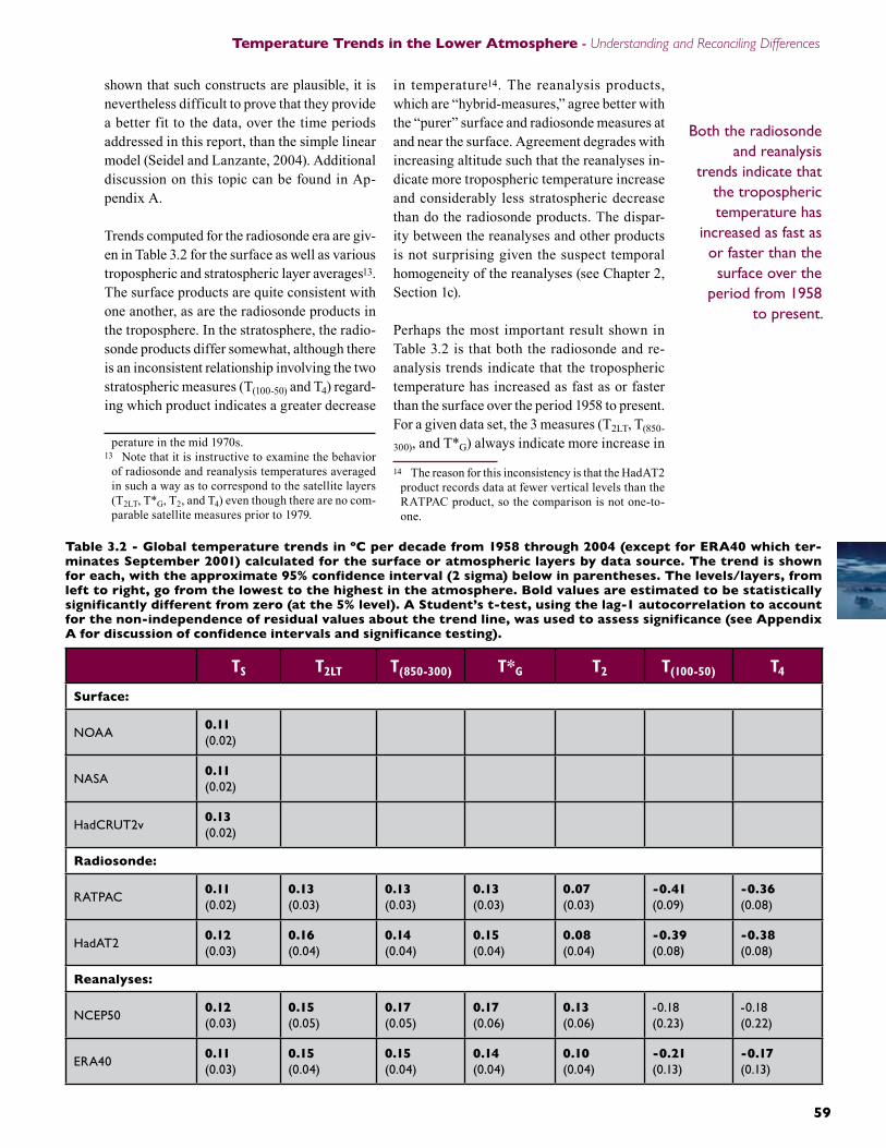
Trends computed for the radiosonde era are giv-en in Table 3.2 for the surface as well as various tropospheric and stratospheric layer averages13. The surface products are quite consistent with one another, as are the radiosonde products in the troposphere. In the stratosphere, the radio-sonde products differ somewhat, although there is an inconsistent relationship involving the two stratospheric measures (T(100-50) and T4) regard-ing which product indicates a greater decrease
perature in the mid 1970s.13 Note that it is instructive to examine the behavior
of radiosonde and reanalysis temperatures averaged in such a way as to correspond to the satellite layers (T2LT, T*G, T2, and T4) even though there are no com-parable satellite measures prior to 1979.
in temperature14. The reanalysis products, which are “hybrid-measures,” agree better with the “purer” surface and radiosonde measures at and near the surface. Agreement degrades with increasing altitude such that the reanalyses in-dicate more tropospheric temperature increase and considerably less stratospheric decrease than do the radiosonde products. The dispar-ity between the reanalyses and other products is not surprising given the suspect temporal homogeneity of the reanalyses (see Chapter 2, Section 1c).
Perhaps the most important result shown in Table 3.2 is that both the radiosonde and re-analysis trends indicate that the tropospheric temperature has increased as fast as or faster than the surface over the period 1958 to present. For a given data set, the 3 measures (T2LT, T(850-
300), and T*G) always indicate more increase in
14 The reason for this inconsistency is that the HadAT2 product records data at fewer vertical levels than the RATPAC product, so the comparison is not one-to-one.
TS T2LT T(850-300) T*G T2 T(100-50) T4
Surface:
NOAA 0.11(0.02)
NASA0.11(0.02)
HadCRUT2v0.13(0.02)
Radiosonde:
RATPAC0.11(0.02)
0.13(0.03)
0.13(0.03)
0.13(0.03)
0.07(0.03)
-0.�1(0.09)
-0.36(0.08)
HadAT20.12(0.03)
0.16(0.04)
0.1�(0.04)
0.15(0.04)
0.08(0.04)
-0.39(0.08)
-0.38(0.08)
Reanalyses:
NCEP500.12(0.03)
0.15(0.05)
0.17(0.05)
0.17(0.06)
0.13(0.06)
-0.18(0.23)
-0.18(0.22)
ERA400.11(0.03)
0.15(0.04)
0.15(0.04)
0.1�(0.04)
0.10(0.04)
-0.21(0.13)
-0.17(0.13)
Table 3.2 - Global temperature trends in ºC per decade from 1958 through 200� (except for ERA�0 which ter-minates September 2001) calculated for the surface or atmospheric layers by data source. The trend is shown for each, with the approximate 95% confidence interval (2 sigma) below in parentheses. The levels/layers, from left to right, go from the lowest to the highest in the atmosphere. Bold values are estimated to be statistically significantly different from zero (at the 5% level). A Student’s t-test, using the lag-1 autocorrelation to account for the non-independence of residual values about the trend line, was used to assess significance (see Appendix A for discussion of confidence intervals and significance testing).
Both the radiosonde and reanalysis
trends indicate that the tropospheric temperature has
increased as fast as or faster than the surface over the
period from 1958 to present.
The U.S. Climate Change Science Program Chapter 3
60 6160 61
the troposphere than at the surface, although this is usually not true when the T2 measure is considered. The reason for the inconsistency involving T2 is because of contributions to the layer that it measures from stratospheric cool-ing, an effect first recognized by Spencer and Christy (1992) (see discussion of this issue in Chapters 2 and 4). The development of T*G as a global measure, and its counterpart, T*T for the tropics (Fu et al., 2004; Fu and Johanson, 2005; Johanson and Fu, 2006) was an attempt to remove the confounding effects of the stratosphere using a statistical approach (see Chapter 2).
6.1.2 land Vs. ocean
The annual average temperature of most of the land and ocean surface increased during the ra-diosonde era, with the exception of parts of the North Atlantic Ocean, the North Pacific Ocean, and a few smaller areas. With a few exceptions, such as the west coast of North America, trends in land air temperature in coastal regions are generally consistent with trends in SST over neighboring ocean areas (Houghton et al., 2001). Because bias adjustments are performed separately for land and ocean areas, before merging to create a global product, it is unlikely that the land-ocean consistency is an artifact of the construction methods used in the vari-ous surface analyses. However, land air tem-peratures did increase somewhat more rapidly than SSTs in some regions during the past two decades. Possibly related to this is the fact that since the mid-1970s, whether due to anthropo-genic or natural causes, El Niño has frequently been in its “warm” phase, which tends to bring higher than normal temperatures to much of North America, among other regions, which have had strong temperature increases over the past few decades (Hurrell, 1996). Also, when global temperatures are rising or falling, the global mean land temperature tends to both rise and fall faster than the ocean, which has a tremendous heat storage capacity (Waple and Lawrimore, 2003). The physical reasons for these differences between land and ocean are given in Chapter 1.
6.1.3 marine air Vs. sea surface TemperaTure
In ocean areas, it is natural to consider whether the temperature of the air and that of the ocean
surface (SST) increases or decreases at the same rate. Several studies have examined this ques-tion. Overall, on seasonal and longer scales, the SST and marine air temperature generally move at about the same rate globally and in many ocean basin scale regions (Bottomley et al., 1990; Parker et al., 1995; Folland et al., 2001b; Rayner et al., 2003). However, differences be-tween SST and marine air temperature in the tropics were noted by Christy et al. (1998) and then examined in more detail by Christy et al. (2001). The latter study found that tropical SST increased more than NMAT from 1979 -1999 derived from the Tropical Atmosphere Ocean (TAO) array of tropical buoys and transient marine ship observations. Over the satellite era, some unexplained differences in these trends were also noted by Folland et al. (2003) in parts of the tropical south Pacific using the Rayner et al. (2003) NMAT data set which incorporates new corrections for the effect on NMAT of increasing deck (and hence measure-ment) heights.
6.1.4 minimum Vs. maximum TemperaTures oVer land
Daily minimum temperature increased about twice as fast as daily maximum temperature over global land areas during the radiosonde era (Karl et al., 1993; Easterling et al., 1997; Folland et al, 2001b). Vose et al. (2005b) con-firmed this using a more spatially complete data set, but also found that during the satellite era maximum and minimum temperatures have been rising at nearly the same rate. In addition, their rate of warming increased near the start of the satellite era, consistent with the evolution of surface temperatures as depicted in Fig. 3.1. The causes of this asymmetric warming during the radiosonde era are still debated, but many of the areas with greater increases of minimum temperatures correspond to those where cloudi-ness appears to have increased over the period as a whole (Dai et al., 1999; Henderson-Sell-ers, 1992; Sun and Groisman, 2000; Groisman et al., 2004). This makes physical sense since clouds tend to cool the surface during the day by reflecting incoming solar radiation, and warm the surface at night by absorbing and reradiating infrared radiation back to the surface.
The surface temperature increase has accelerated in recent decades while the tropospheric increase has decelerated.
60 61
Temperature Trends in the Lower Atmosphere - Understanding and Reconciling Differences
60 61
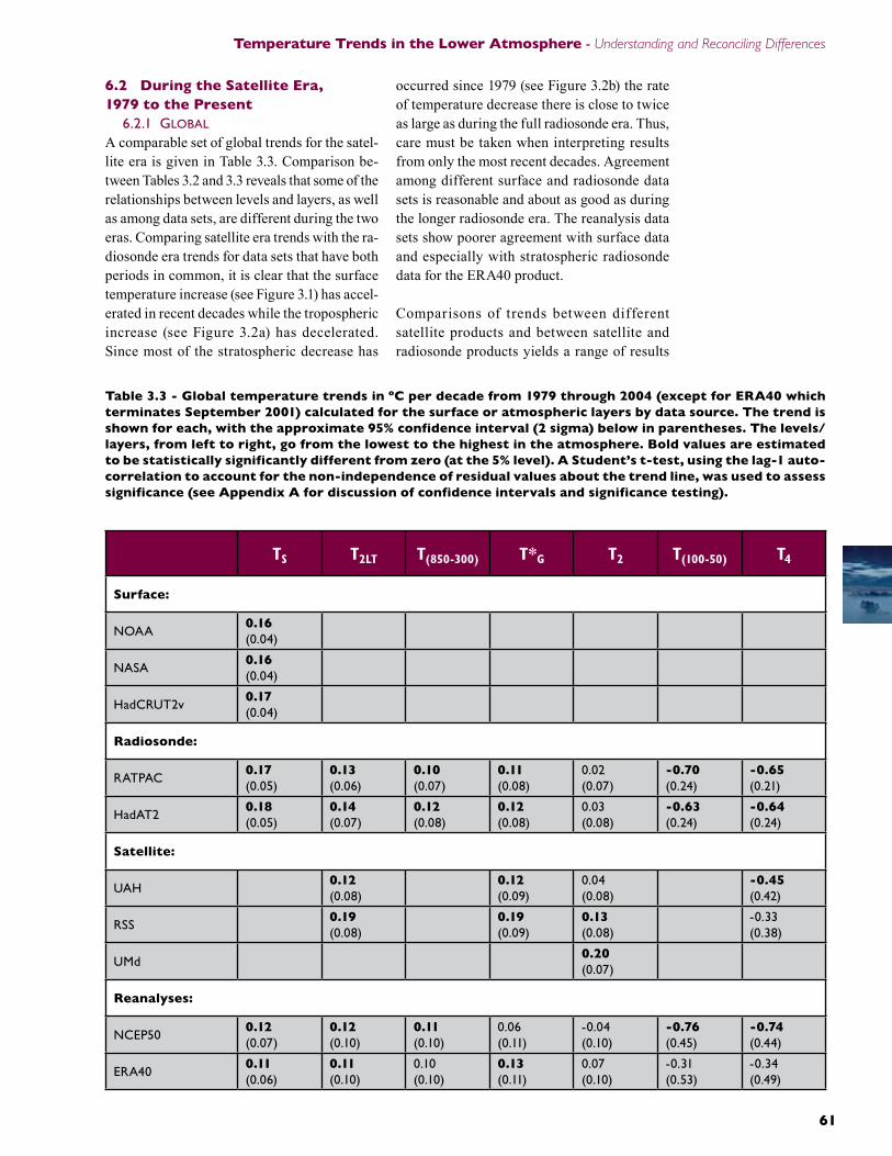
6.2 during the Satellite Era, 1979 to the Present
6.2.1 global
A comparable set of global trends for the satel-lite era is given in Table 3.3. Comparison be-tween Tables 3.2 and 3.3 reveals that some of the relationships between levels and layers, as well as among data sets, are different during the two eras. Comparing satellite era trends with the ra-diosonde era trends for data sets that have both periods in common, it is clear that the surface temperature increase (see Figure 3.1) has accel-erated in recent decades while the tropospheric increase (see Figure 3.2a) has decelerated. Since most of the stratospheric decrease has
occurred since 1979 (see Figure 3.2b) the rate of temperature decrease there is close to twice as large as during the full radiosonde era. Thus, care must be taken when interpreting results from only the most recent decades. Agreement among different surface and radiosonde data sets is reasonable and about as good as during the longer radiosonde era. The reanalysis data sets show poorer agreement with surface data and especially with stratospheric radiosonde data for the ERA40 product.
Comparisons of trends between different satellite products and between satellite and radiosonde products yields a range of results
TS T2LT T(850-300) T*G T2 T(100-50) T4
Surface:
NOAA 0.16(0.04)
NASA0.16(0.04)
HadCRUT2v0.17(0.04)
Radiosonde:
RATPAC0.17(0.05)
0.13(0.06)
0.10(0.07)
0.11(0.08)
0.02(0.07)
-0.70(0.24)
-0.65(0.21)
HadAT20.18(0.05)
0.1�(0.07)
0.12(0.08)
0.12(0.08)
0.03(0.08)
-0.63(0.24)
-0.6�(0.24)
Satellite:
UAH0.12 (0.08)
0.12(0.09)
0.04(0.08)
-0.�5(0.42)
RSS0.19(0.08)
0.19(0.09)
0.13(0.08)
-0.33(0.38)
UMd0.20(0.07)
Reanalyses:
NCEP500.12(0.07)
0.12(0.10)
0.11(0.10)
0.06(0.11)
-0.04(0.10)
-0.76(0.45)
-0.7�(0.44)
ERA400.11(0.06)
0.11(0.10)
0.10(0.10)
0.13(0.11)
0.07(0.10)
-0.31(0.53)
-0.34(0.49)
Table 3.3 - Global temperature trends in ºC per decade from 1979 through 200� (except for ERA�0 which terminates September 2001) calculated for the surface or atmospheric layers by data source. The trend is shown for each, with the approximate 95% confidence interval (2 sigma) below in parentheses. The levels/layers, from left to right, go from the lowest to the highest in the atmosphere. Bold values are estimated to be statistically significantly different from zero (at the 5% level). A Student’s t-test, using the lag-1 auto-correlation to account for the non-independence of residual values about the trend line, was used to assess significance (see Appendix A for discussion of confidence intervals and significance testing).
The U.S. Climate Change Science Program Chapter 3
62 6362 63
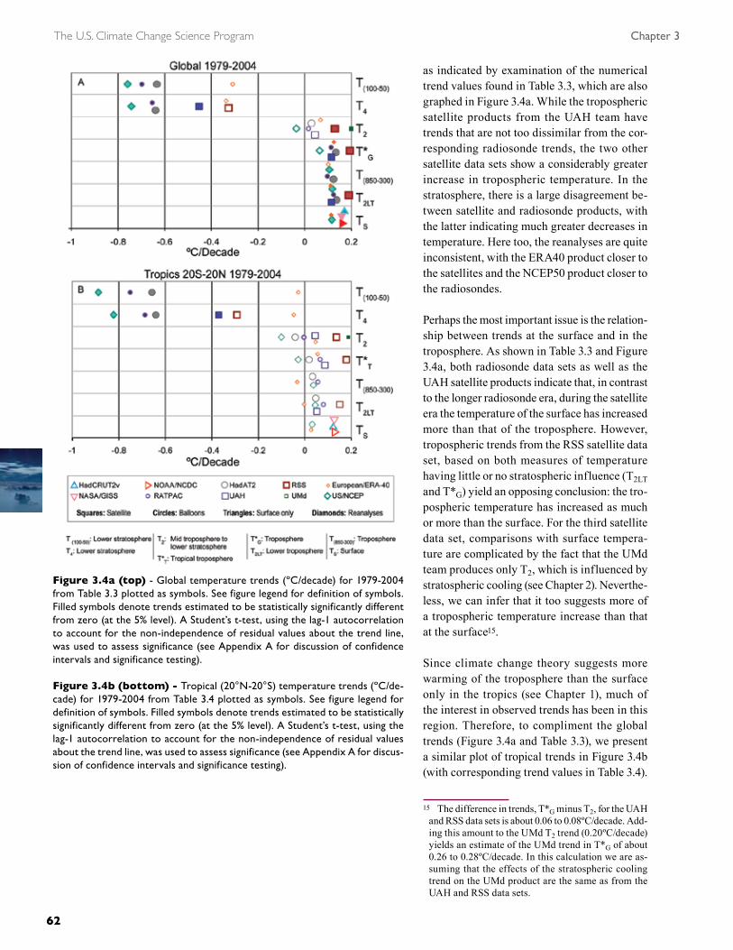
as indicated by examination of the numerical trend values found in Table 3.3, which are also graphed in Figure 3.4a. While the tropospheric satellite products from the UAH team have trends that are not too dissimilar from the cor-responding radiosonde trends, the two other satellite data sets show a considerably greater increase in tropospheric temperature. In the stratosphere, there is a large disagreement be-tween satellite and radiosonde products, with the latter indicating much greater decreases in temperature. Here too, the reanalyses are quite inconsistent, with the ERA40 product closer to the satellites and the NCEP50 product closer to the radiosondes.
Perhaps the most important issue is the relation-ship between trends at the surface and in the troposphere. As shown in Table 3.3 and Figure 3.4a, both radiosonde data sets as well as the UAH satellite products indicate that, in contrast to the longer radiosonde era, during the satellite era the temperature of the surface has increased more than that of the troposphere. However, tropospheric trends from the RSS satellite data set, based on both measures of temperature having little or no stratospheric influence (T2LT and T*G) yield an opposing conclusion: the tro-pospheric temperature has increased as much or more than the surface. For the third satellite data set, comparisons with surface tempera-ture are complicated by the fact that the UMd team produces only T2, which is influenced by stratospheric cooling (see Chapter 2). Neverthe-less, we can infer that it too suggests more of a tropospheric temperature increase than that at the surface15.
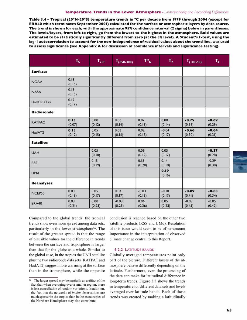
Since climate change theory suggests more warming of the troposphere than the surface only in the tropics (see Chapter 1), much of the interest in observed trends has been in this region. Therefore, to compliment the global trends (Figure 3.4a and Table 3.3), we present a similar plot of tropical trends in Figure 3.4b (with corresponding trend values in Table 3.4).
15 The difference in trends, T*G minus T2, for the UAH and RSS data sets is about 0.06 to 0.08ºC/decade. Add-ing this amount to the UMd T2 trend (0.20ºC/decade) yields an estimate of the UMd trend in T*G of about 0.26 to 0.28ºC/decade. In this calculation we are as-suming that the effects of the stratospheric cooling trend on the UMd product are the same as from the UAH and RSS data sets.
Figure 3.�a (top) - Global temperature trends (ºC/decade) for 1979-2004 from Table 3.3 plotted as symbols. See figure legend for definition of symbols. Filled symbols denote trends estimated to be statistically significantly different from zero (at the 5% level). A Student’s t-test, using the lag-1 autocorrelation to account for the non-independence of residual values about the trend line, was used to assess significance (see Appendix A for discussion of confidence intervals and significance testing).
Figure 3.�b (bottom) - Tropical (20°N-20°S) temperature trends (ºC/de-cade) for 1979-2004 from Table 3.4 plotted as symbols. See figure legend for definition of symbols. Filled symbols denote trends estimated to be statistically significantly different from zero (at the 5% level). A Student’s t-test, using the lag-1 autocorrelation to account for the non-independence of residual values about the trend line, was used to assess significance (see Appendix A for discus-sion of confidence intervals and significance testing).
62 63
Temperature Trends in the Lower Atmosphere - Understanding and Reconciling Differences
62 63
Compared to the global trends, the tropical trends show even more spread among data sets, particularly in the lower stratosphere16. The result of the greater spread is that the range of plausible values for the difference in trends between the surface and troposphere is larger than that for the globe as a whole. Similar to the global case, in the tropics the UAH satellite plus the two radiosonde data sets (RATPAC and HadAT2) suggest more warming at the surface than in the troposphere, while the opposite
16 The larger spread may be partially an artifact of the fact that when averaging over a smaller region, there is less cancellation of random variations. In addition, the fact that the networks of in situ observations are much sparser in the tropics than in the extratropics of the Northern Hemisphere may also contribute.
conclusion is reached based on the other two satellite products (RSS and UMd). Resolution of this issue would seem to be of paramount importance in the interpretation of observed climate change central to this Report.
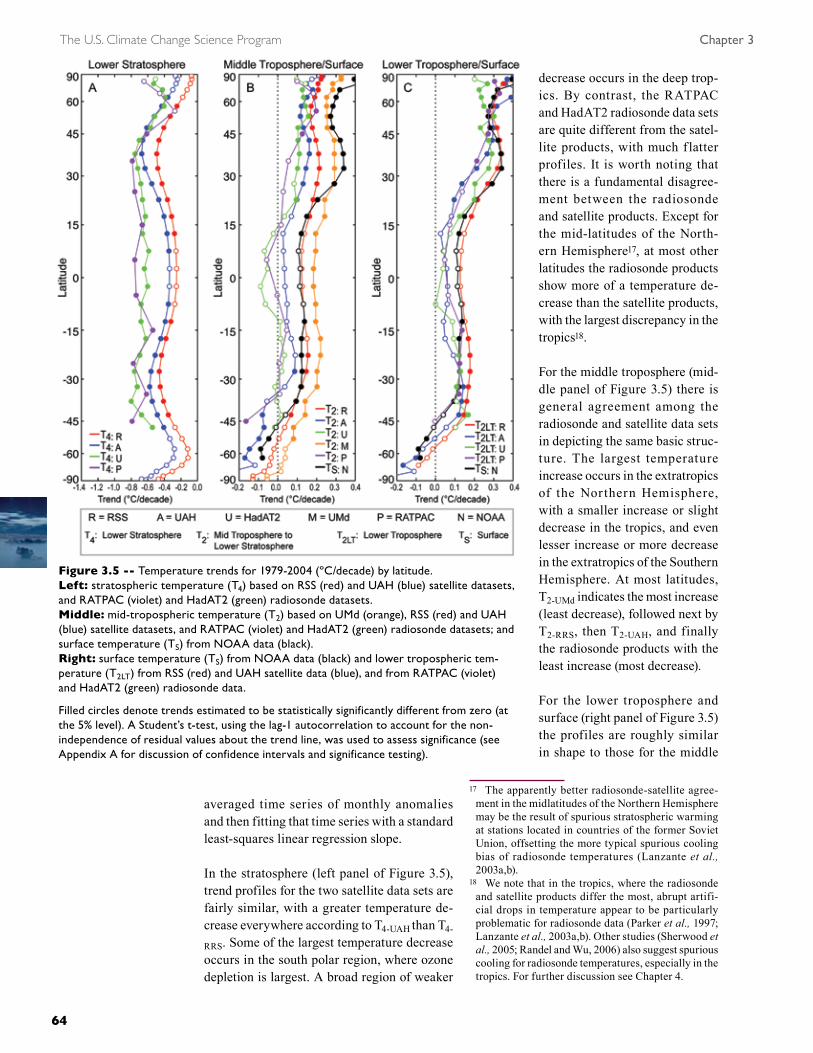
6.2.2 laTiTude bands
Globally averaged temperatures paint only part of the picture. Different layers of the at-mosphere behave differently depending on the latitude. Furthermore, even the processing of the data can make for latitudinal difference in long-term trends. Figure 3.5 shows the trends in temperature for different data sets and levels averaged over latitude bands. Each of these trends was created by making a latitudinally
TS T2LT T(850-300) T*G T2 T(100-50) T4
Surface:
NOAA 0.13(0.15)
NASA0.13(0.15)
HadCRUT2v0.12(0.17)
Radiosonde:
RATPAC0.13(0.07)
0.08(0.12)
0.06(0.14)
0.07(0.15)
0.00(0.14)
-0.75(0.36)
-0.69(0.29)
HadAT20.15(0.12)
0.05(0.15)
0.03(0.16)
0.02(0.18)
-0.04(0.17)
-0.66(0.30)
-0.6�(0.31)
Satellite:
UAH0.05 (0.18)
0.09(0.19)
0.05(0.17)
-0.37(0.28)
RSS0.15(0.19)
0.18(0.20)
0.14(0.18)
-0.29(0.30)
UMd0.19(0.16)
Reanalyses:
NCEP500.03(0.16)
0.05(0.17)
0.04(0.17)
-0.03(0.18)
-0.10(0.17)
-0.89(0.41)
-0.83(0.34)
ERA400.03(0.21)
0.00(0.23)
-0.03(0.25)
0.06(0.26)
0.05(0.23)
-0.03(0.45)
-0.05(0.42)
Table 3.� – Tropical (20ºn-20ºS) temperature trends in ºC per decade from 1979 through 200� (except for ERA�0 which terminates September 2001) calculated for the surface or atmospheric layers by data source. The trend is shown for each, with the approximate 95% confidence interval (2 sigma) below in parentheses. The levels/layers, from left to right, go from the lowest to the highest in the atmosphere. Bold values are estimated to be statistically significantly different from zero (at the 5% level). A Student’s t-test, using the lag-1 autocorrelation to account for the non-independence of residual values about the trend line, was used to assess significance (see Appendix A for discussion of confidence intervals and significance testing).
The U.S. Climate Change Science Program Chapter 3
6� 656� 65
averaged time series of monthly anomalies and then fitting that time series with a standard least-squares linear regression slope.
In the stratosphere (left panel of Figure 3.5), trend profiles for the two satellite data sets are fairly similar, with a greater temperature de-crease everywhere according to T4-UAH than T4-
RRS. Some of the largest temperature decrease occurs in the south polar region, where ozone depletion is largest. A broad region of weaker
decrease occurs in the deep trop-ics. By contrast, the RATPAC and HadAT2 radiosonde data sets are quite different from the satel-lite products, with much flatter profiles. It is worth noting that there is a fundamental disagree-ment between the radiosonde and satellite products. Except for the mid-latitudes of the North-ern Hemisphere17, at most other latitudes the radiosonde products show more of a temperature de-crease than the satellite products, with the largest discrepancy in the tropics18.
For the middle troposphere (mid-dle panel of Figure 3.5) there is general agreement among the radiosonde and satellite data sets in depicting the same basic struc-ture. The largest temperature increase occurs in the extratropics of the Northern Hemisphere, with a smaller increase or slight decrease in the tropics, and even lesser increase or more decrease in the extratropics of the Southern Hemisphere. At most latitudes, T2-UMd indicates the most increase (least decrease), followed next by T2-RRS, then T2-UAH, and finally the radiosonde products with the least increase (most decrease).
For the lower troposphere and surface (right panel of Figure 3.5) the profiles are roughly similar in shape to those for the middle
17 The apparently better radiosonde-satellite agree-ment in the midlatitudes of the Northern Hemisphere may be the result of spurious stratospheric warming at stations located in countries of the former Soviet Union, offsetting the more typical spurious cooling bias of radiosonde temperatures (Lanzante et al., 2003a,b).
18 We note that in the tropics, where the radiosonde and satellite products differ the most, abrupt artifi-cial drops in temperature appear to be particularly problematic for radiosonde data (Parker et al., 1997; Lanzante et al., 2003a,b). Other studies (Sherwood et al., 2005; Randel and Wu, 2006) also suggest spurious cooling for radiosonde temperatures, especially in the tropics. For further discussion see Chapter 4.
Figure 3.5 -- Temperature trends for 1979-2004 (ºC/decade) by latitude. Left: stratospheric temperature (T4) based on RSS (red) and UAH (blue) satellite datasets, and RATPAC (violet) and HadAT2 (green) radiosonde datasets.Middle: mid-tropospheric temperature (T2) based on UMd (orange), RSS (red) and UAH (blue) satellite datasets, and RATPAC (violet) and HadAT2 (green) radiosonde datasets; and surface temperature (TS) from NOAA data (black).Right: surface temperature (TS) from NOAA data (black) and lower tropospheric tem-perature (T2LT) from RSS (red) and UAH satellite data (blue), and from RATPAC (violet) and HadAT2 (green) radiosonde data. Filled circles denote trends estimated to be statistically significantly different from zero (at the 5% level). A Student’s t-test, using the lag-1 autocorrelation to account for the non-independence of residual values about the trend line, was used to assess significance (see Appendix A for discussion of confidence intervals and significance testing).
6� 65
Temperature Trends in the Lower Atmosphere - Understanding and Reconciling Differences
6� 65
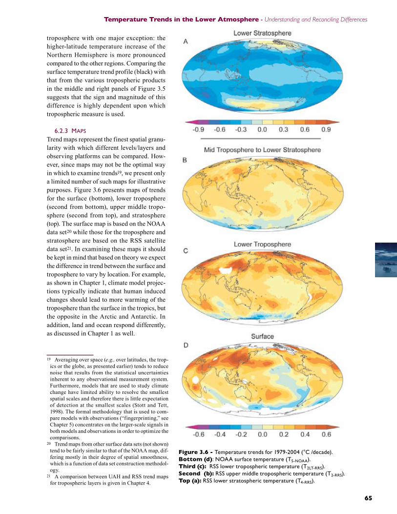
troposphere with one major exception: the higher-latitude temperature increase of the Northern Hemisphere is more pronounced compared to the other regions. Comparing the surface temperature trend profile (black) with that from the various tropospheric products in the middle and right panels of Figure 3.5 suggests that the sign and magnitude of this difference is highly dependent upon which tropospheric measure is used.
6.2.3 maps
Trend maps represent the finest spatial granu-larity with which different levels/layers and observing platforms can be compared. How-ever, since maps may not be the optimal way in which to examine trends19, we present only a limited number of such maps for illustrative purposes. Figure 3.6 presents maps of trends for the surface (bottom), lower troposphere (second from bottom), upper middle tropo-sphere (second from top), and stratosphere (top). The surface map is based on the NOAA data set20 while those for the troposphere and stratosphere are based on the RSS satellite data set21. In examining these maps it should be kept in mind that based on theory we expect the difference in trend between the surface and troposphere to vary by location. For example, as shown in Chapter 1, climate model projec-tions typically indicate that human induced changes should lead to more warming of the troposphere than the surface in the tropics, but the opposite in the Arctic and Antarctic. In addition, land and ocean respond differently, as discussed in Chapter 1 as well.
19 Averaging over space (e.g., over latitudes, the trop-ics or the globe, as presented earlier) tends to reduce noise that results from the statistical uncertainties inherent to any observational measurement system. Furthermore, models that are used to study climate change have limited ability to resolve the smallest spatial scales and therefore there is little expectation of detection at the smallest scales (Stott and Tett, 1998). The formal methodology that is used to com-pare models with observations (“fingerprinting,” see Chapter 5) concentrates on the larger-scale signals in both models and observations in order to optimize the comparisons.
20 Trend maps from other surface data sets (not shown) tend to be fairly similar to that of the NOAA map, dif-fering mostly in their degree of spatial smoothness, which is a function of data set construction methodol-ogy.
21 A comparison between UAH and RSS trend maps for tropospheric layers is given in Chapter 4.
Figure 3.6 - Temperature trends for 1979-2004 (°C /decade).Bottom (d): NOAA surface temperature (TS-NOAA).Third (c): RSS lower tropospheric temperature (T2LT-RRS).Second (b): RSS upper middle tropospheric temperature (T2-RRS).Top (a): RSS lower stratospheric temperature (T4-RRS).
The U.S. Climate Change Science Program Chapter 3
66 6766 67
The trend maps indicate both similarities and differences between the surface and tropospheric trend patterns. There is a rough correspondence in patterns between the two. The largest temperature increase occurs in the extra-tropics of the Northern Hemisphere, particularly over landmasses. A decrease or smaller increase is found in the high latitudes of the Southern Hemisphere as well as in the eastern tropical Pacific. Note the general cor-respondence between the above noted features in Figures 3.6c,d and the zonal trend profiles (middle and right panels of Figure 3.5). Note that the temperature of the mid troposphere to lower stratosphere is somewhat of a hybrid measure, being affected most strongly by the troposphere, but with a non-negligible influence by the stratosphere.
In contrast to the surface and troposphere, a temperature decrease is found almost every-where in the stratosphere (Figure 3.6a). The largest decrease is found in the midlatitudes of the Northern Hemisphere and the South Polar Region, with a smaller decrease in the tropics. Again note the correspondence between the main features of the trend map (Figure 3.6a) and the corresponding zonal trend profiles (left panel of Figure 3.5).
7. CHAnGES �n VERT�CAL STRUCTURE
7.1 Vertical Profiles of TrendsUp to this point, our vertical comparisons have contrasted trends of surface temperature with trends based on different layer-averaged temperatures. Layers are useful because the averaging process tends to reduce noise. The use of layer-averages is also driven by the limitations of satellite measurement systems that are unable to provide much vertical detail. However, as illustrated in Chapter 1, changes in various forcing agents can lead to more com-plex changes in the vertical. Radiosonde data, because of their greater vertical resolution, are much better suited for this than currently avail-able satellite data.Figure 3.7 shows vertical profiles of trends from the RATPAC and HadAT2 radiosonde data sets for temperature averaged over the globe (top) or tropics (bottom) for the radiosonde (left) and satellite (right) eras. The trend values of Figure
3.7 are also given in Table 3.5. Each graph has profiles for the two radiosonde data sets. The tropics are of special interest because many cli-mate models suggest that under global warming scenarios trends should increase from the lower troposphere upwards, maximizing in the upper troposphere (see Chapters 1 and 5).
For the globe, the figure indicates that during the longer period the tropospheric temperature increased slightly more than that of the surface. By contrast, for the globe during the satellite era, the surface temperature increased more than that of the troposphere. Both data sets agree reasonably well in these conclusions. For the tropics, the differences between the two eras are more pronounced. For the longer period there is good agreement between the two data sets in that the temperature increase is smaller at the surface and maximized in the upper tro-posphere. The largest disagreement between data sets and least amount of tropospheric temperature increase is seen in the tropics dur-ing the satellite era. For the RATPAC product, the greatest temperature increase occurs at the surface with a slight increase (or decrease) in the lower and middle troposphere followed by somewhat larger increase in the upper tropo-sphere. The HadAT2 product also shows largest increase at the surface, with a small increase in the troposphere, however, it lacks a distinct return to increase in the upper troposphere. In summary, the two data sets have fairly similar profiles in the troposphere with the exception of the tropics during the satellite era22. For the stratosphere, the decrease in temperature is noticeably greater for both the globe and the tropics during the satellite than radiosonde era as expected (see Figure 3.2b). Some of the larg-est discrepancies between data sets are found in the stratosphere.
7.2 Lapse RatesTemperature usually decreases in the tropo-sphere going upward from the surface. Lapse rate is defined as the rate of decrease in temper-ature with increasing altitude and is a measure of the stability of the atmosphere23. Most of the
22 However, the differences between data sets may not be meaningful since they are small compared to the statistical uncertainty estimates (see Table 3.5 and discussion in Appendix A).
23 A larger lapse rate implies more unstable conditions and a greater tendency towards vertical mixing of
From 1958 to the present, the tropospheric temperature increased slightly more than that of the surface, but from 1979 to the present, the surface temperature increased more than that of the troposphere.
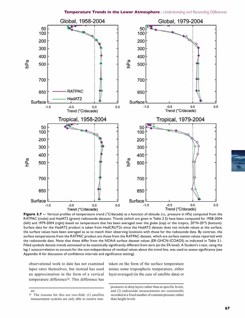
66 67
Temperature Trends in the Lower Atmosphere - Understanding and Reconciling Differences
66 67
observational work to date has not examined lapse rates themselves, but instead has used an approximation in the form of a vertical temperature difference24. This difference has
air.24 The reasons for this are two-fold: (1) satellite
measurement systems are only able to resolve tem-
taken on the form of the surface temperature minus some tropospheric temperature, either layer-averaged (in the case of satellite data) or
peratures in deep layers rather than at specific levels, and (2) radiosonde measurements are consistently recorded at a fixed number of constant pressure rather than height levels.
Figure 3.7 -- Vertical profiles of temperature trend (°C/decade) as a function of altitude (i.e., pressure in hPa) computed from the RATPAC (violet) and HadAT2 (green) radiosonde datasets. Trends (which are given in Table 3.5) have been computed for 1958-2004 (left) and 1979-2004 (right) based on temperature that has been averaged over the globe (top) or the tropics, 20ºN-20ºS (bottom). Surface data for the HadAT2 product is taken from HadCRUT2v since the HadAT2 dataset does not include values at the surface; the surface values have been averaged so as to match their observing locations with those for the radiosonde data. By contrast, the surface temperatures from the RATPAC product are those from the RATPAC dataset, which are surface station values reported with the radiosonde data. Note that these differ from the NOAA surface dataset values (ER-GHCN-ICOADS) as indicated in Table 3.1. Filled symbols denote trends estimated to be statistically significantly different from zero (at the 5% level). A Student’s t-test, using the lag-1 autocorrelation to account for the non-independence of residual values about the trend line, was used to assess significance (see Appendix A for discussion of confidence intervals and significance testing).
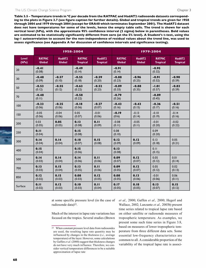
The U.S. Climate Change Science Program Chapter 3
68 6968 69
at some specific pressure level (in the case of radiosonde data)25.
Much of the interest in lapse rate variations has focused on the tropics. Several studies (Brown
25 When constant pressure level data from radiosondes are used, the resulting lapse rate quantity may be influenced by changes in the thickness (i.e., average temperature) of the layer. However, some calculations by Gaffen et al. (2000) suggest that thickness changes do not have very much influence. Therefore, we con-sider vertical temperature differences to be a suitable approximation of lapse rate
et al., 2000; Gaffen et al., 2000; Hegerl and Wallace, 2002; Lanzante et al., 2003b) present time series related to tropical lapse rate based on either satellite or radiosonde measures of tropospheric temperature. As examples, we present some such time series in Figure 3.8, based on measures of lower tropospheric tem-perature from three different data sets. Some essential low-frequency characteristics are common to all. A considerable proportion of the variability of the tropical lapse rate is associ-
1958-2004 1979-2004
Level(hPa)
RATPAC Global
HadAT2Global
RATPAC Tropical
HadAT2Tropical
RATPAC Global
HadAT2Global
RATPAC Tropical
HadAT2Tropical
20 -0.�1(0.08)
-0.�9(0.14)
-0.91(0.14)
-0.95(0.32)
30 -0.�8(0.09)
-0.57(0.10)
-0.55(0.18)
-0.59(0.20)
-0.88(0.23)
-0.96(0.25)
-0.91(0.52)
-0.90(0.59)
50 -0.53(0.12)
-0.55(0.12)
-0.63(0.22)
-0.52(0.23)
-0.89(0.33)
-0.88(0.35)
-1.01(0.57)
-0.83(0.59)
70 -0.�8(0.11)
-0.58(0.22)
-0.79(0.26)
-0.89(0.45)
100 -0.23(0.06)
-0.25(0.06)
-0.18(0.06)
-0.27(0.07)
-0.�3(0.16)
-0.�3(0.15)
-0.36(0.17)
-0.51(0.16)
150 -0.05(0.06)
-0.04(0.06)
0.05(0.07)
-0.01(0.06)
-0.19(016)
-0.13(0.14)
-0.10(0.19)
-0.14(0.16)
200 0.03(0.05)
0.05(0.05)
0.13(0.08)
0.11(0.09)
-0.08(0.11)
-0.05(0.11)
-0.01(0.20)
-0.02(0.22)
250 0.11(0.04)
0.15(0.08)
0.08(0.10)
0.09(0.20)
300 0.1�(0.04)
0.1�(0.04)
0.18(0.07)
0.15(0.08)
0.12(0.09)
0.12(0.09)
0.13(0.18)
0.05(0.21)
400 0.15(0.04)
0.15(0.06)
0.13(0.08)
0.11(0.15)
500 0.1�(0.03)
0.1�(0.04)
0.1�(0.06)
0.11(0.06)
0.09(0.07)
0.12(0.07)
0.05(0.12)
0.01(0.14)
700 0.13(0.03)
0.15(0.04)
0.13(0.05)
0.11(0.06)
0.09(0.05)
0.12(0.07)
0.05(0.12)
0.02(0.13)
850 0.12(0.02)
0.15(0.03)
0.08(0.03)
0.12(0.05)
0.08(0.05)
0.13(0.06)
-0.01(0.06)
0.06(0.11)
Surface 0.11(0.02)
0.12(0.03)
0.10(0.03)
0.11(0.04)
0.17(0.05)
0.18(0.05)
0.13(0.07)
0.15(0.12)
Table 3.5 – Temperature trends in ºC per decade from the RATPAC and HadAT2 radiosonde datasets correspond-ing to the plots in Figure 3.7 (see figure caption for further details). Global and tropical trends are given for 1958 through 200� and 1979 through 200� (except for ERA�0 which terminates September 2001). The HadAT2 dataset does not have temperatures for some of the levels, hence the empty table cells. The trend is shown for each vertical level (hPa), with the approximate 95% confidence interval (2 sigma) below in parentheses. Bold values are estimated to be statistically significantly different from zero (at the 5% level). A Student’s t-test, using the lag-1 autocorrelation to account for the non-independence of residual values about the trend line, was used to assess significance (see Appendix A for discussion of confidence intervals and significance testing).
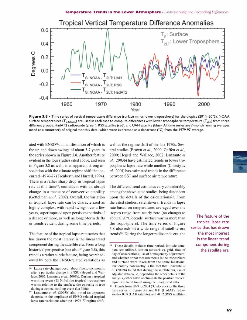
68 69
Temperature Trends in the Lower Atmosphere - Understanding and Reconciling Differences
68 69
ated with ENSO26, a manifestation of which is the up and down swings of about 3-7 years in the series shown in Figure 3.8. Another feature evident in the four studies cited above, and seen in Figure 3.8 as well, is an apparent strong as-sociation with the climate regime shift that oc-curred ~1976-77 (Trenberth and Hurrell, 1994). There is a rather sharp drop in tropical lapse rate at this time27, coincident with an abrupt change in a measure of convective stability (Gettelman et al., 2002). Overall, the variation in tropical lapse rate can be characterized as highly complex, with rapid swings over a few years, superimposed upon persistent periods of a decade or more, as well as longer-term drifts or trends evident during some time periods.
The feature of the tropical lapse rate series that has drawn the most interest is the linear trend component during the satellite era. From a long historical perspective (see also Figure 3.8), this trend is a rather subtle feature, being overshad-owed by both the ENSO-related variations as
26 Lapse rate changes occur about five to six months after a particular change in ENSO (Hegerl and Wal-lace, 2002; Lanzante et al., 2003b). During a tropical warming event (El Niño) the tropical troposphere warms relative to the surface; the opposite is true during a tropical cooling event (La Niña).
27 Lanzante et al. (2003b) also noted an apparent decrease in the amplitude of ENSO-related tropical lapse rate variations after the ~1976-77 regime shift.
well as the regime shift of the late 1970s. Sev-eral studies (Brown et al., 2000; Gaffen et al., 2000; Hegerl and Wallace, 2002; Lanzante et al., 2003b) have estimated trends in lower tro-pospheric lapse rate while another (Christy et al., 2001) has estimated trends in the difference between SST and surface air temperature.
The different trend estimates vary considerably among the above-cited studies, being dependent upon the details of the calculations28. From the cited studies, satellite-era trends in lapse rate based on temperatures averaged over the tropics range from nearly zero (no change) to about 0.20ºC/decade (surface warms more than the troposphere). The time series of Figure 3.8 also exhibit a wide range of satellite-era trends29. During the longer radiosonde era, the
28 These details include: time period, latitude zone, data sets utilized, station network vs. grid, time of day of observations, use of homogeneity adjustment, and whether or not measurements in the troposphere and surface were taken from the same locations. Particularly noteworthy is the fact that Lanzante et al. (2003b) found that during the satellite era, use of adjusted data could, depending the other details of the analysis, either halve or eliminate the positive tropical lapse rate trend found using the unadjusted data.
29 Trends from 1979 to 2004 (ºC /decade) for the three time series in Figure 3.8 are: 0.11 (HadAT2 radio-sonde), 0.08 (UAH satellite), and -0.02 (RSS satellite).
Figure 3.8 - Time series of vertical temperature difference (surface minus lower troposphere) for the tropics (20°N-20°S). NOAA surface temperatures (TS-NOAA) are used in each case to compute differences with lower tropospheric temperature (T2LT) from three different groups: HadAT2 radiosonde (green), RSS satellite (red), and UAH satellite (blue). All time series are 7-month running averages (used as a smoother) of original monthly data, which were expressed as a departure (ºC) from the 1979-97 average.
The feature of the tropical lapse rate
series that has drawn the most interest is the linear trend component during
the satellite era.
The U.S. Climate Change Science Program Chapter 3
70 PB
various studies found trends of opposite sign (i.e., air temperature at the surface increases more slowly than that of air aloft) and show less sensitivity, with a range of values of near-zero to about -0.05ºC/decade30.
Spatial variations in lapse rate trends have also been examined. During the satellite era, some have found predominantly increasing trends in the tropics (Gaffen et al., 2000; Brown et al., 2000) while others have found a greater mix-ture, with more areas of negative trends (Hegerl and Wallace, 2002; Lanzante et al., 2003b). Outside of the tropics, both Hegerl and Wal-lace (2002) and Lanzante et al. (2003b) found complex spatial patterns of trend. Lanzante et al. (2003b) also found considerable local sensi-tivity to homogeneity adjustment in the tropics and even more so over the extra-tropics of the Southern Hemisphere, which is quite sparsely sampled.
While the first two of these trends are statistically significant at the 5% level, the third is not (see Ap-pendix A for discussion of significance testing).
30 The trend from 1958 to 2004 for the HadAT2 radio-sonde series shown in Figure 3.8 is -0.02ºC/decade. This trend is not statistically significant at the 5% level (see Appendix A for discussion of significance testing).
Satellite-era trends in lapse rate based on temperatures averaged over the tropics range from nearly zero (no change) to about 0.20ºC/decade (surface warms more than the troposphere).