Noise Temperature induced by Atmosphere and Weather on

JPL D-32584

Atmospheric Noise Temperature Induced by Clouds and Other Weather Phenomenaat SHF Band (1-45 GHz) Prepared for the United States Air Force Spectrum Efficient Technologies for Test and Evaluation Advanced Range Telemetry Edwards Air Force Base, California

Christian Ho, Stephen Slobin

and Kelly Gritton

August 11, 2005

Atmospheric Noise Temperature Induced by Clouds and

Other Weather Phenomena at SHF Band (1-45 GHz)

Prepared for: Department of The Air Force

Spectrum Efficient Technologies for Test and Evaluation (TE)

Advanced Range Telemetry (ARTM)

Edwards Air Force Base, California

JPL Task Plan Number 81-7849

PRDA 000-05-C-1PKD.

FY2005

Prepared by:

Christian Ho, Stephen Slobin

and Kelly Gritton

JET PROPULSION LABORATORY,

California Institute of Technology

Pasadena, California 91109

August 11, 2005

2

Acknowledgements

The authors would like to thank the Test Resource Management Center

(TRMC) Test and Evaluation/Science and

Technology (T&E/S&T) Program for their support on this study.

This work is funded by

the T&E/S&T Program through the NASA Contracting Office (NMO715600)

under the contract (81-7849).

We are indebted to the former Executing Agent, Saul Ortigoza and

Deputy Executing Agent, Ronald Streich from Department of The Air Force

Spectrum Efficient Technologies (SET) for Test and Evaluation (TE)

Advanced Range Telemetry (ARTM)

Edwards Air Force Base, California

We also thank for approving the public release of this report by the Air Force

Flight Test Center Public Affairs Office under number PA 07135.

This research was carried out at the Jet Propulsion Laboratory, California

Institute of Technology, and was sponsored by the Department of the Air Force

through an agreement with the National Aeronautics and Space Administration.

3

Table of Contents

Abstract

1. Introduction

2. Background

3. Fundamental Theory

4. Antenna Noise

5. Noise from Atmospheric Gaseous Radiation

5.1. Radiation Theory

5.2. Application to the Clear Atmosphere

6. Sky Noise due to Clouds

7. Sky Noise due to Rain

8. Application to Air Force Benchmark Scenarios

8.1. Case 1, East Coast - Patuxent River

8.2. Case 2, West Coast – Pt. Mugu

8.3. G/T Reduction

9. Conclusions

References

Tables

Figure Captions

Figures

4

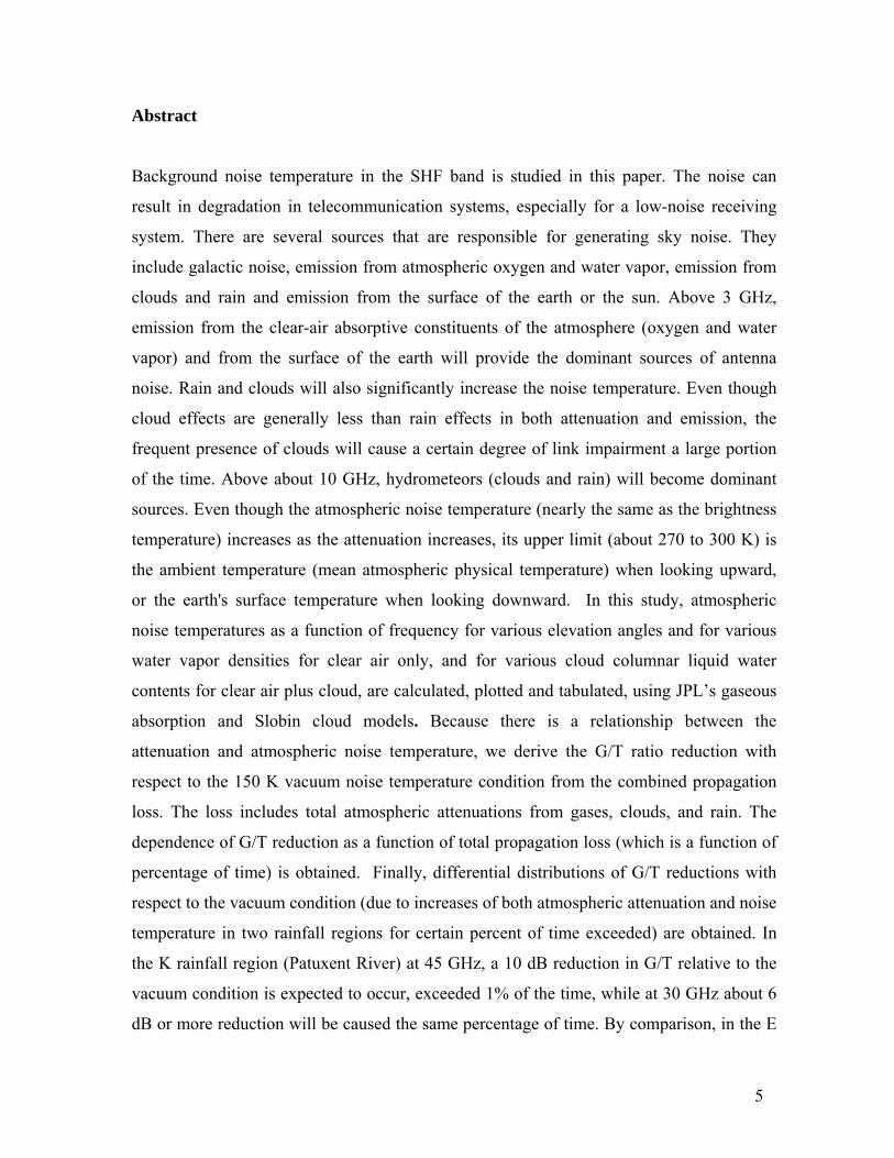
Abstract

Background noise temperature in the SHF band is studied in this paper. The noise can

result in degradation in telecommunication systems, especially for a low-noise receiving

system. There are several sources that are responsible for generating sky noise. They

include galactic noise, emission from atmospheric oxygen and water vapor, emission from

clouds and rain and emission from the surface of the earth or the sun. Above 3 GHz,

emission from the clear-air absorptive constituents of the atmosphere (oxygen and water

vapor) and from the surface of the earth will provide the dominant sources of antenna

noise. Rain and clouds will also significantly increase the noise temperature. Even though

cloud effects are generally less than rain effects in both attenuation and emission, the

frequent presence of clouds will cause a certain degree of link impairment a large portion

of the time. Above about 10 GHz, hydrometeors (clouds and rain) will become dominant

sources. Even though the atmospheric noise temperature (nearly the same as the brightness

temperature) increases as the attenuation increases, its upper limit (about 270 to 300 K) is

the ambient temperature (mean atmospheric physical temperature) when looking upward,

or the earth's surface temperature when looking downward. In this study, atmospheric

noise temperatures as a function of frequency for various elevation angles and for various

water vapor densities for clear air only, and for various cloud columnar liquid water

contents for clear air plus cloud, are calculated, plotted and tabulated, using JPL’s gaseous

absorption and Slobin cloud models. Because there is a relationship between the

attenuation and atmospheric noise temperature, we derive the G/T ratio reduction with

respect to the 150 K vacuum noise temperature condition from the combined propagation

loss. The loss includes total atmospheric attenuations from gases, clouds, and rain. The

dependence of G/T reduction as a function of total propagation loss (which is a function of

percentage of time) is obtained. Finally, differential distributions of G/T reductions with

respect to the vacuum condition (due to increases of both atmospheric attenuation and noise

temperature in two rainfall regions for certain percent of time exceeded) are obtained. In

the K rainfall region (Patuxent River) at 45 GHz, a 10 dB reduction in G/T relative to the

vacuum condition is expected to occur, exceeded 1% of the time, while at 30 GHz about 6

dB or more reduction will be caused the same percentage of time. By comparison, in the E

5

rainfall region (West Coast), a 6 dB G/T reduction relative to the vacuum condition will

appear at 45 GHz, exceeded 1 % of the time, while for 30 GHz only about 3 dB reduction

will occur.

6

1. Introduction

In the previous report [1], we find that in the SHF band the atmospheric gaseous

absorption and other weather-related phenomena are the main sources which cause

microwave attenuation. However, any natural absorbing medium in the atmosphere

which interacts with the transmitted radio wave will not only produce signal attenuation,

but will also be a source of thermal noise power radiation [2]. Thus, effects of

atmosphere and weather on SHF signals are like a double-edged sword. On one hand,

atmosphere and weather phenomena such as clouds, fog, and rain can cause attenuation

of microwaves through absorption, resulting in a reduction of the receiving system’s

effective gain, G. On another hand, these media radiate radio noise to the background,

causing the increase in the system noise temperature, T. As a final result, the G/T ratio of

the receiving system will decrease [3]. Thus, for a very-low-noise communications

receiver, the background noise temperature radiated by the atmosphere is the most

important factor in the design and performance of the system.

There are several sources that contribute radio noise at SHF band. For a downlink, when

a low-noise ground receiver receives an SHF band signal from a spacecraft or aircraft, at

the same time it also receives noise from the sources shown in Figure 1. These include

the cosmic background (2.7 K), galactic noise, emission from atmospheric gases (oxygen

and water vapor), emissions from clouds and rain, emission from the surface of the earth

or the sun, etc. For an uplink as shown in Figure 2, the spacecraft or aircraft receives SHF

signals from the ground transmitter, and also emissions upward from atmospheric gases,

from clouds and rain, and from the earth's surface (including land, bodies of water, and

vegetation, etc).

The atmosphere may be regarded as a medium which consists of gaseous, liquid, and

solid constituents. Among the liquid and solid constituents, the hydrometeors (clouds,

rain, snow, ice) are the dominant factor in the microwave region, while other particles,

such as dust, smoke and sand, are of minor importance. If the absorption and

transmission properties of the atmosphere are considered, it is generally sufficient to take

7

into account the atmosphere up to a height of about 50 km, although hydrometeors are

rarely found above 15 km. The main gaseous constituents of the atmosphere are nitrogen,

oxygen, argon, carbon dioxide (making up 99.999 volume % of dry air), and water vapor,

which is a variable constituent. Among these gases, only oxygen and water vapor cause

absorption in the microwave region, while gases which have no electric or magnetic

dipole moment do not absorb microwaves. Weather related phenomena, such as clouds

and rain can also significantly increase the noise temperature. The maximum noise

temperature can be as high as the ambient temperature of the absorbing medium (about

270 to 300 K).

Besides the thermal noise radiated from the atmosphere and weather related cloud, fog,

and rain, there are also some other noise sources, such as extra-terrestrial and man-made

made noise. Extra-terrestrial sources include those from sun, moon, cosmic background

and galaxy. The man-made noise sources include those from business activity, electrical

and electronic equipment, power lines, internal engine ignition, and emission from other

communication systems, etc. All these radiations from natural (terrestrial and extra-

terrestrial) and man-made sources are referred to as radio noise, or sky noise. These

noises will directly couple to the receiving system at the SHF band. As a result, the sky

noise will be added to the system noise through an increase in the antenna temperature of

the receiver.

In this report, we will review all related studies of atmospheric noise temperature due to

gases and weather phenomena for both theory and experiment. We will pay attention to

cloud effects on attenuation and noise temperature in the SHF band because very few

studies can be found on this topic. We will use JPL’s gaseous absorption model and the

Slobin’s cloud model [3] to calculate atmospheric noise temperatures as a function of

frequency for various elevation angles and for various water vapor densities (for clear air

only) and for various cloud columnar liquid water contents (for clear-air and cloud

combined cases). These results will be applied to two Air Force benchmark sites. As a

final production, the effects on receiving system G/T reduction as a function of percent of

time will be presented.

8

2. Background

Radio noise emitted by a distant star can be a source of information in radio astronomy

[4], while that emitted from earth's surface can be used for remote sensing. However,

these noises may be a limiting factor for communication systems.

At frequencies below 1 GHz, radio noise caused by atmospheric radiation is less than a

few Kelvins. This is negligible when compared with a receiving system with a noise

temperature of several hundred Kelvins. However, In the SHF band, the radio noise

caused by atmospheric emission increases significantly with increasing frequency. At

some frequencies and elevation angles, the noise temperature can be as high as 300 K.

This background temperature can not be neglected and needs to be considered in

receiving system design.

The data rate of a communication link is proportional to received Eb/No (energy per

bit/system noise temperature), which is a function of the distance, EIRP, pointing,

atmospheric loss, other losses, and system noise temperature.

Eb/No is furthermore proportional to the ratio of receiving antenna G-eff/T-op, where

G-eff (dBi) = G-vac (dBi) – A-atm (dB)

T-op(K) = T-vac (K) + T-atm (K)

and G-eff is the effective antenna gain, G-vac is vacuum antenna gain, A-atm is the

atmospheric loss, T-op is the system operating noise temperature, T-vac is the vacuum

noise temperature, and T-atm is the atmospheric noise temperature. Thus, the change of

G/T ratio with respect to a vacuum atmosphere condition is given by

Δ(G/T) w.r.t.vacuum = –A-atm (dB) –10 x log[(T-vac +T-atm)/(T-vac)] (1)

9

where the minus sign means that increases in both of A-atm and T-atm will cause a

decrease of G/T. For a low noise receiving system (T-vac is low), T-atm is the most

important source of the G/T decrease.

3. Fundamental Theory

The noise power received at a given frequency usually is expressed by the so-called

brightness temperature, or noise temperature, which is a measure of the power being

radiated in a given band by this source in the direction of the receiving antenna, and is

equal to the physical temperature of a blackbody (perfect absorber) emitting the same

power in that band.

In general, the noise power received by an antenna is the sum of the emitted power of the

source in the direction of the antenna within the frequency band of interest, and the power

from the surrounding medium which is reflected by an object or reflecting surface

towards the direction of the antenna. These powers are further attenuated by the medium

between the antenna and the reflecting surface. Thus, the brightness temperature is a

background temperature in certain direction. It is nothing to do with the receiving antenna

vacuum system noise temperature or antenna gain.

The radio noise emitted from the atmosphere in thermodynamic equilibrium, from

Kirchoff’s Law, is equal to its absorption, and this equality holds for all frequencies. The

brightness temperature, tb, (in astronomy [4] which is referred as the background

temperature observed by a ground antenna in a given direction through the atmosphere),

in a fixed frequency band, is given by radiative transfer theory [5]

tb = t(l)κ(l)e−τ (l)dl + t∞e−τ∞

0

∞∫

(2)

where optical depth is

τ(l) = κ(l')dl'0

l∫ (3)

10

which is an integral along the path from a radiating parcel to any point to the ground.

dτ(l) = κ(l)dl , where κ(l) is the absorption coefficient, a function of atmospheric

species, its abundance, temperature, pressure, height, and the frequency, is the cosmic

background noise temperature from infinity with an optical depth

t∞τ ∞. For a

homogeneous, isothermal atmosphere, κ(l) = κ , the mean absorption coefficient, and

t(l) = tm , the mean physical temperature.

Thus the optical depth through the total path isτ(l) = κl . The equation (2) becomes

tb = tm e−κlκdl0

l0∫ + t∞e−τ ∞

(4)

where the integration covers all radiative atmospheric elements from the ground to the

top of atmosphere l0l0

, tm is the ambient temperature, κ is the absorption coefficient, and τ

is the optical depth to the point under consideration, There is a relation between the τ and

the attenuation, A (in dB), due to the gaseous absorption over the path. At SHF band, the

last term in above equation reducing to 2.7 K, the cosmic background component (unless

the sun is in the beam of the antenna), will be neglected.

Thus, the equation is further reduced to

tb = tm (1− e−τ 0 ) = tm(1− e−κl0 ) = tm (1−10−

A(dB)10 ) = tm (1−1/L) K (5)

where L = eτ 0 = eκl0 = eA / 4.34 =10A /10, is a linear loss factor due to the atmospheric

absorption. We can see that when L becomes very large, tb will be equal to tm. Thus, the

tm is the upper limit of tb.

The attenuation, dB, of a lossy medium can be calculated from the loss factor L as

dBLA 10log10= (6)

11

The mean ambient temperature, tm, ranges from about 260 to 280 K, depending mostly on

the height above the surface of the primary radiating atmospheric component. For

example, water vapor is concentrated primarily close to the earth's surface, so its mean

physical temperature is somewhat higher than that of the oxygen component. Thus,

equation (5) sets up the relationship between the attenuation caused by the atmospheric

absorption at any height and the brightness temperature due to the radiation. Figure 3

shows the noise temperature as a function of total path attenuation for the range of values

of tm from 270 K to 280 K. The noise temperature approaches ‘saturation’, i.e., the value

of tm, fairly quickly above attenuation values of about 10 dB. Below that value the

selection of tm is not very critical. The centerline (tm=275 K) serves as the best prediction

curve for tb. The noise temperature rises quickly with attenuation level. It is 56 K for 1

dB attenuation, 137 K for 3 dB attenuation, and 188 K for 5 dB attenuation. There is a

further relationship to determine the value of tm from the surface temperature measured,

ts, when a total zenith atmospheric attenuation is fixed.

Ktt sm 5012.1 −= (7)

Figure 4 summarizes the median expected noise levels produced by sources of external

radio noise in the frequency range applicable to practical space communications [6, 7].

Noise levels are expressed in terms of both noise temperature, ta, (right vertical axis), and

noise factor, Fa (dB) (left vertical axis). The noise contributions from atmospheric

gaseous noise at elevation angles of 0o and 90o (curves E(0), and E(90) are shown). We

can see that above 1 GHz, the absorptive constituents of the atmosphere, i.e. oxygen,

water vapor, and rain (curves E), act as dominant noise sources and can reach a

maximum value of 290 K under extreme conditions. The Sun is a strong variable noise

source, reaching values of 10,000 K and higher when observed with a narrow beamwidth

(<0.5o) antenna directed at Sun (curve D), under quiet Sun conditions. The cosmic

background noise level of 2.7 K (curve F) is very low and is not a factor of concern in

space communications.

12

The flat-earth approximation is often used to calculate atmospheric attenuation at

elevation angles other than at zenith (vertical, looking upward). When zenith atmospheric

loss is L0 or A0(dB), for a horizontally stratified atmosphere, then

A(θ) = A0 /sinθ (8)

and

L(θ) = L01/sinθ (9)

the brightness temperature at an elevation angle θ is given by

tb(θ) = tm(1−10−A0 (dB) /(10sinθ )) = tm(1−1/L01/sinθ ) (10)

For elevation angles greater than 30o, the error compared to round-earth calculations is

much less than 1 % [5]. This equation can be used for brightness temperature estimates

quite accurately down to an elevation angle of 10°, with an error of less than 2 %. This

will be discussed further in Section 6.

4. Antenna Noise

A telecommunication system designer must be concerned with noise sources which are

both man-made and naturally occurring. Radio and sky noise is emitted by both terrestrial

and extraterrestrial matter. Observed noise causes an increase in the receiving antenna

temperature leading to an increase in the overall system noise.

There are two common parameters which are most useful for communication system

performance evaluation, noise figure, Fa in dB, and noise temperature, ta in K. Noise

figure and noise temperature are related by the following equation:

dBttF a

a ⎟⎟⎠

⎞⎜⎜⎝

⎛+=

0

1log10 (11)

where t0 is the ambient reference temperature of 290 K.

13

Antenna noise is conveniently treated in terms of noise temperature, since the two

parameters are linearly related. In circuit theory the noise power, pn, which is transferred

to a matched load is

pn = kBTb watts (12)

where kB is Boltzmann’s constant, T is antenna noise temperature in (degree) Kelvin, and

b is the bandwidth in Hertz. Thermal radiation power flux from gaseous atmosphere is

given by the Rayleigh-Jeans approximation to Planck’s equation

Pn =2kBT

λ2 = 22.2kBTf 2 watts /Hz /m2 /Rad2 (13)

where f is the frequency in GHz.

For the uplink, the earth-viewing antenna observes the earth’s surface emission and

atmospheric radiation. Usually, the observed noise is a complex function of atmospheric

and surface temperature, elevation angle, frequency, and antenna gain. For the earth

surface, the land has higher brightness temperature, while the sea has lower brightness

temperature in the main antenna beam.

For the downlink, which is the case we will deal with in this study, a receiving antenna

on the ground sees the energy from both the antenna main beam and the side lobes. Thus,

the noise sources are not necessarily in direct line of sight and they can come from all

directions. For an antenna at a high elevation angle, it mainly receives the sky noise from

the antenna boresight direction, while at low elevation angle, thermal noise emission

from the earth’s surface will be increasingly observed in the antenna’s side lobes.

The antenna temperature is defined as its gain coupling with the background temperature

in all directions as shown in Figure 5. It depends on antenna gain and brightness

temperature in the pointing direction:

Tr =Gr (θ)tb

mainlobe∫ (θ)dΩ + Gr (θ)tb

sidebeam∫ (θ)dΩ

Gr (θ)Ω∫ dΩ

(14)

14

where Tr = antenna temperature, K

Gr = receiver’s antenna gain pattern (dimensionless)

tb = brightness temperature, K

dΩ = solid angle ( dΩΩ∫ = sinθ0

2π∫0π∫ dθdφ = 4π )

θ = polar angle (0° - 180°)

φ = azimuth angle (0° - 360°).

Tsky in Figure 5 is extra-terrestrial noise temperature from cosmic background and

ta is background temperature from atmospheric radiation with an optical depth τ from an

atmospheric parcel. The integration is over the entire sphere and includes the antenna’s

mainbeam and sidelobes.

Noise from individual sources such as atmospheric gases, the sun, the Earth’s surface,

etc, is usually given in terms of their brightness temperature. The antenna temperature is

the convolution of the antenna pattern and the brightness temperature of the sky and

ground. For antennas whose patterns encompass a single distributed source, the antenna

temperature and brightness temperature are the same.

5. Noise from Atmospheric Gaseous Radiation

5.1. Radiation Theory

When radio waves pass through an atmosphere, the waves suffer molecular absorption

and scattering at centimeter and millimeter wavelengths [5,6,7,8]. On Earth, the gaseous

absorption is due primarily to atmospheric water vapor and oxygen. There are 29

absorption lines for H2O up through 1097 GHz, and 44 lines for O2 up through 834 GHz.

Relatively narrow and weaker ozone (O3) lines are above 100 GHz. Between 120 GHz

and 1097 GHz, water vapor plays a serious role in radio wave attenuation. For

frequencies greater than 70 GHz, other gases can also contribute an attenuation in the

absence of water vapor; however, their spectral lines are usually too weak to affect

propagation [5,8,9,10]

15

The principal interaction mechanism between radio waves and gaseous constituents is

molecular absorption and emission from molecules. Accurate predictions of atmospheric

attenuation and emission can be determined from radiative transfer calculations.

Absorption of radio waves results from a quantum level change in the rotational energy

of molecules. Spectral lines of absorption and emission occur when a quantized system,

such as a molecule, interacts with an electromagnetic radiation field and makes a

transition between two quantum states of the system. The resonant frequency flm is [5,10]

flm = (El − Em) /h (15)

where El and Em are energy levels of final and initial rotational energy state, h is the

Plank constant.

The general expression for the absorption coefficient κ( f , f lm) may be written as

{ } ),(||3

8),( 2//23

lmlmlkTEkTEi

lm ffLgeehcQ

fnff ml φμπκ −− −= (16)

where ni is the number of absorbing molecules per unit volume for ith species, μ the total

dipole moment, gl the statistical weight of the lower state, φlm the transition matrix

element, L( f , f lm) a function describing the line shape, and Q the partition function.

The volume absorption coefficient κ describes the interaction of radiation with the

absorbing matter. κ is a function of the density of the absorbing substance, atmospheric

temperature, and pressure. Optical depth is an integration of absorption coefficient κ

along the path, which is dimensionless and can be expressed in a unit “neper” (logarithms

to base e) or dB (logarithms to base 10). 1 Np = 4.34 dB. The absorption coefficient κ can

be determined through the experimental measurements of power spectral line of

absorption or theoretical calculation of energy transition between any quantum state.

Then the brightness temperature can be calculated using the radiative transfer equation as

shown in Equation (2). Brightness temperature is used here to refer to the temperature of

the sky in a particular direction as seen by an antenna of infinitely narrow beamwidth. It

is similar to the brightness in radio astronomy for describing the flux per unit solid angle

per Hertz from an extended source.

16

5.2. Application to the Clear Atmosphere:

The gaseous constituents of Earth’s atmosphere interact with a radio wave through a

molecular absorption process that results in attenuation of the signal. Absorption of

electromagnetic energy by gaseous molecules usually involves the interaction of electric

or magnetic incident waves with an electric or magnetic dipole. H2O and O2 are the two

major atmospheric constituents for radio wave absorption in the microwave band. The

oxygen molecule has a permanent magnetic moment arising from two unpaired electron

spins. Magnetic interaction produces a family of rotation lines around 60 GHz and an

isolated line at 118.8 GHz. Uncondensed water is a molecule with an electric dipole.

Through an electric interaction with the incident electric field, it produces rotational lines

at 22.2, 183.3, and 323.8 GHz and at several frequencies in the far-infrared band. Each of

the absorption spectral lines has a certain width because the energy levels vary when

molecules are in motion. Among the various factors causing line broadening, atmospheric

pressure broadening is the most important in the microwave band. The same absorption

process will produce the thermal noise power radiation that is dependent on the intensity

of the absorption.

Radiation and absorption from atmospheric molecules is heavily dependent on

atmospheric structure, including its temperature, pressure, composition, abundance, etc.

The Earth’s atmosphere consists of N2, O2, and several minor gases. A standard

atmosphere model can be found in references [11, 12].

Surface Pressure: 1013 mb (average)

Surface Density: ~1.29 kg/m3

Average temperature: ~300 K

Diurnal temperature range: 210 K to 320 K

Mean molecular weight: 28.61 g/mole

Atmospheric composition (by volume):

Major: Nitrogen (N2) - 78.09%; Oxygen (O2) - 20.95%;

Argon (Ar) - 0.93%; Carbon Dioxide (C O2) - 0.03% ;

17

Minor (ppm): Water vapor (H2O) - ~40 – 40,000 (variable); Neon (Ne) - 20;

Helium (He) - 5.2; Methane (CH4) - 1.5; ; Krypton (Kr) - 1.1;

Hydrogen (H2) - 1.0; Nitrous oxide (N2O) - 0.6;

Carbon Monoxide (CO) - 0.2; Ozone (O3) - < 0.05; Xenon (Xe) - 0.09,

We can see that the most variable component of the atmosphere is water vapor (H2O).

The saturation vapor pressure is a very strong function of temperature. For example, the

saturation partial pressure of water vapor (over water) is 6.108 mbar at 0°C, 12.27 mbar

at 10°C, 17.04 mbar at 15°C, 23.37 mbar at 20°C, 42.43 mbar at 30°C, and 73.78 mbar at

40°C. For the U.S. standard model atmosphere at sea level (15°C, 1013.25 mbar), water

vapor at 100% relative humidity constitutes about 1.7% by volume.

Each atmospheric component has a different scale height. Attenuation scale height is

defined as that height at which the specific attenuation (dB/km) is 1/e of its surface value,

assuming an exponential decrease with height above the surface. Pressure scale heights

are somewhat different, however. For example, below 120 km, all compositions have a

similar pressure scale heights (N2 ~ 8.7 km; O2 ~ 9.0 km; Ar ~9.2 km). Above 120 km

(which is entering the thermosphere), scale heights almost double for these gases. Atomic

gases, O and H occur as larger concentrations at 100 km altitude. In this study, because

we are interested in the surface atmospheric attenuation, we only consider gaseous

density and scale heights near the surface of planets. Water vapor has an attenuation

scale height of approximately 2 km, although due to incomplete mixing it may vary

considerably from this value under actual conditions. Oxygen has an attenuation scale

height of about 5.4 km, and is more completely mixed than is water vapor. Additionally,

it can be shown [3] that the attenuation through the entire real atmosphere with a scale

height h, is equal to that of a fictitious atmosphere of thickness h, with uniform

homogeneous density equal to the surface density of the real atmosphere.

The major atmospheric gases that emit electromagnetic noise are also oxygen and water

vapor. The sky noise temperature for oxygen and water vapor, for an infinitely narrow

beam, at various elevation angles, is calculated by direct application of the radiative

18

transfer equation, at frequencies between 1 and 45 GHz. Figures 6 through 11 (6 figures)

summarize the results of atmospheric noise temperature as a function of frequency for

elevation angles of 90, 45, 30, 20, 10, 5, and 0 degrees. These six figures cover six

surface water vapor densities (also called absolute humidity, AH) of 0, 3, 7.5, 10, 13, and

17 g/m3. The US standard atmosphere [12] has a surface water vapor density of about 7.7

g/m3, although 7.5 g/m3 is used here in all calculations for an "average clear atmosphere".

A density of 7.5 g/m3 results from a surface temperature of 15 C and a relative humidity

of about 58%.

The atmospheric noise temperatures shown in the figures are the brightness temperatures

seen by a ground-based receiver, excluding the cosmic noise contribution of 2.7 K or

other extra-terrestrial sources for frequencies between 1 and 45 GHz. The curves are

calculated for the atmospheric gases oxygen and water vapor for seven different elevation

angles from θ = 90° (zenith) to θ = 0° (horizon). Figures are chosen to represent a

completely dry atmosphere (0 g/m3), a fairly dry atmosphere (3.0 g/m3 of water vapor),

an average atmosphere (7.5 g/m3), a moist atmosphere (13 g/m3), and a very moist

atmosphere (17 g/m3). For 0, 3, and 7.5 g/m3, a surface temperature of 15 C is assumed,

but for higher absolute humidity, higher temperatures were chosen to keep the required

relative humidity below an arbitrary value of 65%. For AH = 10 g/m3 and 13 g/m3 a

surface temperature of 25 C was chosen. For 17 g/m3 a surface temperature of 35 C was

chosen. At or above 12° elevation angle, a flat earth model is used for atmospheric

absorption integration along the slant path. Below 12° elevation a round-earth model is

used.

Atmospheric noise temperatures are also calculated as a function of frequency for various

water vapor densities as shown in Figures 12 through 22 (11 figures). In each figure,

there are eight different water vapor densities (0, 3, 7.5, 10, 13, 15, 17, and 21 g/m3)

which correspond to different surface temperatures and relative humidities (RH). These

values are summarized in Table 1.

19

The eleven figures cover eleven elevation angles of 90°, 45°, 30°, 20°, 15°, 10°, 5°, 3°,

2°, 1°, and 0.5°. To fit the Air Force’s scenarios, we have paid attenuation to low

elevation angle values. We have limited the lowest elevation to 0.5 degrees, which is

consistent with the lowest elevation of Nexrad weather radar beams. Again, at elevation

angles below 12 degrees, a spherical earth model has been used.

For all the calculations, the model assumed is one of a horizontally stratified (doesn't

change with lateral offset) atmosphere, even though a spherical earth model is used. The

total pressure is that for the standard atmosphere (1013 mb = 101.3 kPa) at sea level with

the water vapor pressure added to it. This will give values of 1013 mb, 1017 mb, 1023

mb, and 1037 mb for 0 g/ m3 (dry air and O2 only), 3 g/ m3, 7.5 g/m3, and 17 g/ m3 water

vapor respectively. An exponential decrease of absolute humidity with height is assumed,

with a scale height of 2 km. The decrease in pressure of the dry atmosphere is also

governed by an exponential law, whereas the decrease in temperature (6.5°C per km) is

linear down to a temperature of about 217 K (-56.15 °C), and then remains constant at

217 K above that height (at about 10.25 km above sea level). Under these assumptions

the zenith noise temperature calculated from humidity, temperature and pressure data at

the surface is evaluated. These data are in reasonable agreement with the limited amount

of experimental data available. We note that the zenith brightness temperature calculated

here is not accurate if atmospheric inversion of temperature and humidity occur.

6. Sky Noise due to Clouds [3,13,14]

Cloud radiation is an important phenomenon in addition to gaseous radiation. Clouds

may be present 50% of the time as a yearly average, or continuously for periods of weeks

on end. Although cloud noise temperature and attenuation are typically less than those

for rain, rain is present only 5% to 8% in most temperate locales. Thus from the point of

view of percent of time, the cloud effects cannot be neglected at SHF band.

Sky noise from clouds can be determined from radiative transfer approximation methods

in much the same way as described for gaseous radiation. Once the temperature and

20

cloud absorption coefficient variations along the path are defined, the noise temperature

due to the clouds alone, tc, can be determined directly from the cloud attenuation:

tc = tm 1−10−

Ac (dB)10

⎛

⎝ ⎜ ⎜

⎞

⎠ ⎟ ⎟ K (17)

where tm is the mean cloud path physical temperature, and Ac is the total path attenuation

through the clouds, in dB. Equation (17) gives the magnitude of noise temperature

contributed by clouds alone. This temperature can not directly be added to the noise

temperature caused by atmospheric gaseous radiation to obtain total noise temperature

from both atmospheric gases and clouds. However, the total noise temperature can be

calculated through the combination of both attenuations by

tatm = tm 1−10−

Ag +Ac

10⎛

⎝ ⎜ ⎜

⎞

⎠ ⎟ ⎟ K (18)

where atmospheric gaseous attenuation Ag and cloud attenuation Ac are in dB.

Because the noise temperature due to the cloud has the direct relationship with cloud

attenuation as shown above, we need to study the attenuation through the cloud layers

first. The cloud attenuation can be calculated using the procedure listed in ITU-R

recommendation P.840 [14].

To obtain the attenuation due to clouds for a given probability value, we can use the total

columnar content of liquid water L (kg/m2), which is an integration of liquid water

density (kg/m3) along a column with a cross section of 1 m2 from the surface to the top of

clouds, or, equivalently, mm of precipitable water for a given site to yield:

A = LKl/sinθ dB for 90° ≥ θ ≥ 5° (19)

where θ is the elevation angle and Kl is the specific attenuation coefficient

[(dB/km)/(g/m3)] as defined in P.840 [14], which is a function of signal frequency and

temperature (which controls the cloud liquid water density). Based on the L values from

21

world statistical maps [13], attenuation values due to clouds at any location can be

calculated.

Slobin [3] has provided calculations of cloud attenuation and cloud noise temperature for

several locations in the continental United States, Alaska, and Hawaii, using radiative

transfer methods and a four-layer cloud model. Extensive data on cloud characteristics,

such as type, thickness, and coverage, were gathered from twice-daily radiosonde

measurements and hourly temperature and relative humidity profiles.

Twelve cloud types are studied in the Slobin model [3], based on their liquid water

content, cloud thickness, and base heights above the surface. Several of the more intense

cloud types include two cloud layers, and the combined effects of both are included in the

model. Table 2 lists seven of the Slobin cloud types, labeled here from light, thin clouds

to very heavy clouds, and shows the characteristics of each. The case numbers listed in

the table correspond to the numbers assigned by Slobin [3].

The total zenith (90° elevation angle) attenuation was calculated by radiative transfer

methods for frequencies from 4 to 50 GHz for each of the cloud types. Table 3 presents a

summary of zenith cloud attenuation for several of the frequency bands of interest. The

values include the clear air gaseous attenuation also. The values at C-band and Ku-band

are less than 1 dB, even for the most intense cloud types.

The Slobin model also developed annual cumulative distributions of cloud attenuation for

specified cloud regions at fifteen frequencies from 8.5 to 90 GHz. Slobin divided the U.S.

into fifteen regions of statistically “consistent” clouds. The region boundaries are highly

stylized and should be interpreted liberally. Some boundaries coincide with major

mountain ranges (Cascades, Rockies, and Sierra Nevada), and similarities may be noted

between the cloud regions and the rain rate regions of the Global Rainfall Model [15,16].

Each cloud region is characterized by observations at a particular National Weather

Service observation station. The locations of the observation sites are shown with their

three-letter identifiers on the map. For each of these stations, an “average year” was

22

selected on the basis of rainfall measurements. The “average year” was taken to be the

one in which the year’s monthly rainfall distribution best matched the 30-year average

monthly distribution. Hourly surface observations for the “average year” for each station

were used to derive cumulative distributions of zenith attenuation and noise temperature

due to oxygen, water vapor, and clouds, for a number of frequencies ranging from 8.5 to

90 GHz.

When Slobin [3] calculated the cumulative distributions, the following procedure was

used:

• For each hour’s observations, the attenuation of each reported cloud layer (up to four)

was calculated based on the layer’s water particle density, thickness, and temperature.

The attenuation due to water vapor and oxygen was also found using the reported

surface conditions.

• Total attenuation and noise temperature due to all cloud layers and gases were

calculated for sixteen possible cloud configurations, corresponding to all

combinations of cloud presence or absence at the four layer heights.

• Cumulative probability distributions for attenuation and noise temperature were

calculated using the reported percent-coverage values corresponding to each layer.

For example, if the percentage of coverage was 60 percent for layer 1 and 20 percent

for layer 2, then the probability of various configurations of clouds present in the

antenna beam would be as follows:

No clouds present: (1.0-0.6)(1.0-0.2)=0.32 Layer 1 clouds only present: (0.6)(1.0-0.2)=0.48 Layer 2 clouds only present: (1.0-0.6)(0.2)=0.08 Clouds in both layers present: (0.6)(0.2)=0.12

The distributions give the percent of the time that cloud attenuation is the given value or

less. For example, on the Miami plot, the cloud attenuation was 0.6 dB or less for 0.5

(50%) of the time at 32 GHz. Values of attenuation in the distribution range 0 to 0.5 (0 to

50%) may be regarded as the range of clear sky effects. The value of attenuation at 0% is

the lowest value observed for the test year.

23

The attenuations for zenith paths can be extended to slant paths using the cosecant law.

Such extension will probably lead to overestimation at low elevation angles and small

percentage of time. This is because clouds with large vertical development have less

thickness for slant paths than for zenith paths. At time percentages where rain effects

become significant (usually cumulative distributions greater than 95%, effects exceeded

5% of the year or less), the attenuation and noise temperature due to the rain should be

considered also.

For low elevation angles (typically below about 10 degrees), the effect of the round earth

must be considered. At higher elevation angles, it is sufficiently accurate to use a flat-

earth model, where the path length through any atmosphere constituent (of a fixed scale

height) can be modeled as 1/sinθ and the normalized path length at zenith is 1.0

airmasses. Figure 23 shows a cartoon of the flat-earth and round-earth atmospheric

models. In the flat-earth model, the number of airmasses (=1.0 at zenith) traversed at an

elevation angle θ is equal to 1/sin(θ). For the round-earth model, the situation can be

significantly more complicated. It can be seen that for atmospheric constituents of the

same scale height (same homogeneous layer at the surface), the path length for the round-

earth model is always less than for the flat-earth model, for the same elevation angle θ.

Additionally, for a cloud layer elevated above the surface with the same thickness as a

water vapor or oxygen layer at the surface, the path length through the cloud (AM2) is

always less than that through the surface layer (AM1). This is because the cloud layer is

"curved over" more relative to the beam passing through it than is the surface layer, at the

same elevation angle. Thus the path through the cloud is steeper than through the surface

layer.

For calculations made in this report (for oxygen, water vapor, and clouds), the flat-earth

model is used at elevations of 12 degrees and above, and a round-earth model is used

below 12 degrees. For the purposes of path length calculation, water vapor is assumed to

lie in a homogeneous layer 2.0 km thick above the surface, and oxygen is assumed to lie

in a homogeneous layer 5.4 km thick above the surface. For all cloud calculations it is

assumed that a single cloud layer has 100% sky coverage, and the cloud layer is 2 km

24

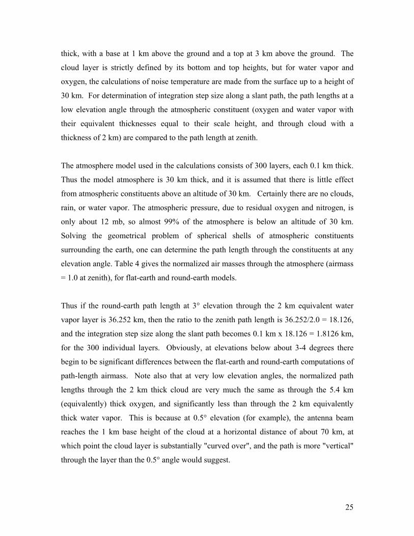
thick, with a base at 1 km above the ground and a top at 3 km above the ground. The

cloud layer is strictly defined by its bottom and top heights, but for water vapor and

oxygen, the calculations of noise temperature are made from the surface up to a height of

30 km. For determination of integration step size along a slant path, the path lengths at a

low elevation angle through the atmospheric constituent (oxygen and water vapor with

their equivalent thicknesses equal to their scale height, and through cloud with a

thickness of 2 km) are compared to the path length at zenith.

The atmosphere model used in the calculations consists of 300 layers, each 0.1 km thick.

Thus the model atmosphere is 30 km thick, and it is assumed that there is little effect

from atmospheric constituents above an altitude of 30 km. Certainly there are no clouds,

rain, or water vapor. The atmospheric pressure, due to residual oxygen and nitrogen, is

only about 12 mb, so almost 99% of the atmosphere is below an altitude of 30 km.

Solving the geometrical problem of spherical shells of atmospheric constituents

surrounding the earth, one can determine the path length through the constituents at any

elevation angle. Table 4 gives the normalized air masses through the atmosphere (airmass

= 1.0 at zenith), for flat-earth and round-earth models.

Thus if the round-earth path length at 3° elevation through the 2 km equivalent water

vapor layer is 36.252 km, then the ratio to the zenith path length is 36.252/2.0 = 18.126,

and the integration step size along the slant path becomes 0.1 km x 18.126 = 1.8126 km,

for the 300 individual layers. Obviously, at elevations below about 3-4 degrees there

begin to be significant differences between the flat-earth and round-earth computations of

path-length airmass. Note also that at very low elevation angles, the normalized path

lengths through the 2 km thick cloud are very much the same as through the 5.4 km

(equivalently) thick oxygen, and significantly less than through the 2 km equivalently

thick water vapor. This is because at 0.5° elevation (for example), the antenna beam

reaches the 1 km base height of the cloud at a horizontal distance of about 70 km, at

which point the cloud layer is substantially "curved over", and the path is more "vertical"

through the layer than the 0.5° angle would suggest.

25

For the calculations carried out in this report, it was assumed that all atmospheric

constituents (water vapor, oxygen, clouds) follow a flat-earth path-length law at elevation

angles down to and including 12°, and follow their individual round-earth laws (Table 4)

below 12° elevation.

The curve-fit expressions for path length through the atmosphere, relative to a zenith path

length are given by the expression: AM(θ) = a0 + a1 * θ + a2 * θ2 + .....+a6 * θ6, where

θ is elevation angle in degrees. The best-fit coefficients for these round-earth expressions

below 12° elevation, for the three atmosphere constituents, are listed in Table 5.

For example, if the zenith path length through the cloud is 2.0 km, then the path length at

3° elevation is 17.260 * 2 km = 34.520 km, as per the table above. The curve-fit equation

for cloud air mass (path length = 2.0 * AM[3°]) yields 17.376 * 2 km = 34.752 km. This

curve-fit value agrees with the rigorous geometrical calculation to within 1%. For use in

the equation of radiative transfer, the path length integration element dl along a slant

path, becomes dl*AM(θ) instead of the flat-earth dl/sin(θ).

In calculating the attenuation caused by clouds using the Slobin cloud model [3], some

considerations need to be taken care as follows:

It is important to collect the most precise cloud water density data possible. If more

accurate estimations of local conditions are desired, statistics of cloud liquid water can

also be derived using cloud detection algorithms along with radiosonde data.

Radiosondes do not explicitly measure cloud liquid water, but these algorithms can

provide an empirical relationship between meteorological conditions at a sounding level

and the amount of cloud liquid water density present at that location.

Columnar cloud liquid water (or "precipitable" water) is sometimes represented in mm

rather than kg/m2. By using the identity that 1 gram of water occupies a volume of 1 cm3

it can be shown that 1 kg/m2 = 1000 g/m2 = 1000 cm3/m2 = 1000 cm3/10000 cm2 = 0.1 cm

= 1.0 mm.

26

In the Slobin model, cloud liquid water content is discussed in terms of water particle

density in units of g/m3. In this case the density must be multiplied by the clouds overall

thickness. Assuming no local cloud thickness data is available, a good typical value is

about 1-2 km. When a quick calculation of cloud attenuation is desired for a generic

location it is suggested to use a columnar liquid content of 0.5 kg/m2. This is equivalent

to a cloud liquid water content of 0.5 g/m3, 1 km thick, or 0.25 g/m3, 2 km thick, etc.

This value represents a good “rule of thumb” though in extreme cases the value could be

significantly higher. The relationship between cloud liquid water content and cloud

columnar liquid is: columnar liquid (kg/m2) = cloud LWC:(g/m3) x cloud thickness (km).

The elevation angle scaling term used in the model is a simple 1/sin(θ) relationship. This

is a reasonable approximation for elevation angles above about 10°. At elevation angles

below about 10° an additional effect must be considered. The 1/sin(θ) relationship

assumes that clouds are infinitely wide. As a result, at very low elevation angles the path

length through the clouds is unrealistically long (many tens of kilometers). In reality,

scattered and broken clouds typically only extend several kilometers in width. Therefore,

a physical limit to the path length should be imposed when performing low elevation

angle calculations.

After calculating the attenuations due to clouds as shown in Table 3, Slobin used the

equations (2) to calculate the cloud noise temperature for several locations in the U.S.,

Alaska, and Hawaii. The temperature and cloud absorption coefficient variations along

the path must be defined, and equations (5) can be applied. Table 6 summarizes the

zenith (90° elevation angle) sky noise temperature as calculated by Slobin for several

frequencies of interest. Note that the temperatures shown in the table are a combination

of noise from both cloud and atmospheric gases, not from clouds alone.

Based on annual cumulative distributions of zenith cloud attenuations generated from a

statistical study, Slobin [3] also developed annual cumulative distributions of zenith noise

27

temperature for specified regions at 5 frequencies from 10 to 90 GHz. Figure 24 shows an

example of the distributions at a frequency of 30 GHz for five cloud regions, ranging

from very dry, clear Yuma, Arizona, to very wet, cloudy Lihue, Hawaii. Figures 25, 26,

27, and 28 (from left panel to right panel) show examples of zenith noise temperature

cumulative distributions for eight of the cloud regions, Lihue, Fairbanks, Yuma, San

Diego, Oakland, Denver, New York, and Miami, at frequencies of 10, 18, 32, 44, and 90

GHz [3]. It can be seen from the curves that the noise temperature at zenith for 90 GHz

(for low cumulative distributions associated with clear sky conditions) may be lower than

for 44 GHz. This is the case for very low zenith brightness temperatures, which means

that the water vapor content is very low (lower than about 3.0 g/m3).

The distributions give the percent of the time when the noise temperature is the given

value or less. For example, at Denver, the noise temperature was 12 K or less for 50% of

the time at 32 GHz. Values of noise temperature in the distribution range 0 to 50% may

be regarded as the range of clear sky conditions. The value of noise temperature at 0% is

the lowest value observed for the test year. Cumulative distributions in the range of 50%

to 95% are considered to be cloudy, with no rain. Cumulative distributions greater than

95% are considered to include rain, although no rain information is included in the curves

shown (Figures 24-28).

We also studied the dependence of noise temperature on cloud morphology. In Figure 29,

a cartoon shows three types of scenarios of cloud radiation for various cloud heights,

thicknesses, and liquid water contents (LWC, g/m3). Calculation results in Figures 30

through 32 show the dependence of cloud radiation on cloud height, while cloud

thickness and LWC are fixed. Figures 33 through 35 show dependence of noise

temperature on cloud thickness for a fixed cloud base height and LWC. Figures 36

through 46 show dependence of noise temperature on cloud LWC for 0, 0.2, 0.4, 0.6, 0.8,

and 1.0 g/m3 with a fixed cloud thickness (2 km), base height (1 km) and AH (water

vapor) value. The eleven figures cover elevation angles of 90°, 45°, 30°, 20°, 15°, 10°,

5°, 3°, 2°, 1°, and 0.5°. The relationships between liquid water content and columnar

liquid for clouds with 2 km thickness are listed in Table 7.

28

7. Sky Noise due to Rain [15,16]

The water constituents which are found in the atmosphere in a solid or liquid state are

rain, snow, hail, cloud or fog. The absorption of microwaves by hydrometeors does not

occur, as in the case for gases, by rotational and vibrational transitions of the molecules,

but by reaction with the free and bound charged particles of the medium. Therefore, there

are no resonances, but a continuous increase of the attenuation with frequency until there

is a saturation in the millimeter wave region. Especially at higher frequencies, both

absorption and scattering contribute to the attenuation, but only absorption to the

emission of noise.

Information on attenuation (which includes absorption and scattering effects) due to rain

at various elevation angles and for various frequencies at SHF band can be found in our

previous study [1]. The severity of radio signal loss through the rain is strongly

dependent on the local rainfall rates, rain cloud heights, and signal frequencies.

Applying the ITU rain attenuation models [15,16] to the studied frequency band (1-45

GHz), attenuations along paths with various elevation angles through the rain region can

be calculated. The rain attenuation model shows that total specific attenuation rate, γR, is

a function of rain fall rate, R, as

γR = kRα in dB /km (20)

where two coefficients α and k are functions of signal’s frequency and elevation angle

and have been experimentally determined in the model. Rain attenuation can be obtained

by γR timing the path length, L (km) through the rain.

Sky noise from rain can be determined from radiative transfer equation in much same

way as given for the sky noise due to clouds. In the most areas, rain usually occurs in a

period less than 5% of time. At very small percentage of time, rainfall rate can be very

high. The attenuation on radio signals can reach to several tens of dB. If the attenuation

due to such phenomena can be evaluated, then the brightness temperature contribution

may be estimated, by adding the attenuations from rain, cloud and gaseous atmosphere

29

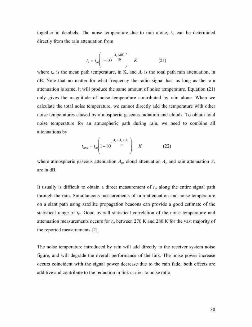
together in decibels. The noise temperature due to rain alone, tr, can be determined

directly from the rain attenuation from

tr = tm 1−10−

Ar (dB)10

⎛

⎝ ⎜ ⎜

⎞

⎠ ⎟ ⎟ K (21)

where tm is the mean path temperature, in K, and Ar is the total path rain attenuation, in

dB. Note that no matter for what frequency the radio signal has, as long as the rain

attenuation is same, it will produce the same amount of noise temperature. Equation (21)

only gives the magnitude of noise temperature contributed by rain alone. When we

calculate the total noise temperature, we cannot directly add the temperature with other

noise temperatures caused by atmospheric gaseous radiation and clouds. To obtain total

noise temperature for an atmospheric path during rain, we need to combine all

attenuations by

tatm = tm 1−10−

Ag +Ac +Ar

10⎛

⎝ ⎜ ⎜

⎞

⎠ ⎟ ⎟ K (22)

where atmospheric gaseous attenuation Ag, cloud attenuation Ac and rain attenuation Ar

are in dB.

It usually is difficult to obtain a direct measurement of tm along the entire signal path

through the rain. Simultaneous measurements of rain attenuation and noise temperature

on a slant path using satellite propagation beacons can provide a good estimate of the

statistical range of tm. Good overall statistical correlation of the noise temperature and

attenuation measurements occurs for tm between 270 K and 280 K for the vast majority of

the reported measurements [2].

The noise temperature introduced by rain will add directly to the receiver system noise

figure, and will degrade the overall performance of the link. The noise power increase

occurs coincident with the signal power decrease due to the rain fade; both effects are

additive and contribute to the reduction in link carrier to noise ratio.

30

8. Application to Air Force Benchmark Scenarios We will apply our calculations into two Air Force benchmark sites (U. S. east coast,

Patuxent River, Maryland, and U.S. west coast, Pt. Mugu [Laguna Peak], California) [1].

At first we need to collect all radio climatological data for the two sites. Radio

climatologic parameter maps are shown in Figures 47 through 50 [17]. World statistical

maps at 1% of time exceeded water vapor density in winter (February) and in summer

(August) are shown in Figures 47 and 48 [18]. A cloud columnar liquid water map at 1%

of the year exceeded is shown in Figure 49, while the map for 10% of the year exceeded

is shown in Figure 50. Figure 51 is the rain region distribution map for the United States.

Table 8 shows all radio parameters at the four Air Force benchmark sites for our

calculations (Patuxent River, and three west coast sites).

Cloud attenuation strongly depends on liquid water density and percent of time of

occurrence. For example, at the east coast Patuxent River site, a columnar liquid water

content of 1.2 kg/m2 is exceeded 1% of the time, while at the west coast Laguna Peak

site, 0.5 kg/m2 is exceeded 1% of the time.

8.1. Case 1 (East Coast - Patuxent River) [1]

At the Naval Test Range at Patuxent River, MD (commonly referred to as "PAX River"

or simply PAX), the primary receiving antennas are 8-foot diameter (operating at 1.4–2.4

GHz) just off the Chesapeake Bay, slightly inland. The antennas are approximately 80–

100 feet above ground level. The approximate coordinates of the station are:

38°18’ N, 76°24’ W, antenna elevation = 30 m

For this site, calculations were carried out using an elevation of sea level.

An important worst case flight profile has a jet aircraft take off and fly out to sea at

altitudes that can range from 1000 to 50,000 ft and go out as far as the radio horizon. We

have listed all radio climatologic parameters in Table 8 for the benchmark cases.

31

8.1.1. Atmospheric Gaseous (clear air only) [11,17,19]: Figure 52 shows calculation

results of atmospheric noise temperature for clear-air only at Patuxent River with a water

vapor density of 21 g/m3, exceeded 1% of the time (see Figure 48).

8.1.2. Clouds Included [3,13,14]: Figure 53 shows calculation results of atmospheric

noise temperature for clear air (21 g/m3 water vapor) plus cloud at Patuxent River with a

cloud columnar liquid of 1.2 kg/m2, exceeded 1% of the time (see Figure 49). Table 9

shows noise temperatures due to clear air only with 21 g/m3 water vapor, and with 1.2

kg/m2 clouds added.

8.1.3. Rain Included [15,16]: For the east coast Patuxent River, the rainfall climatic zone

in the ITU model is designed as K region. The rainfall rate as a function of percent of

time is

RK = 4.17p−0.418 +1.6 log p /0.001( )log3 0.3/ p( )[ mm /h] (23)

The rainfall distribution can be extended beyond 0.3% to such greater percentages of the

time pc at which the rainfall rate is assumed to approach zero, using the expression:

R( p) = R(0.3%) log(pc / p)log(pc /0.3)

⎡

⎣ ⎢

⎤

⎦ ⎥

2

mm /h (24)

For K region, pc is 5(%), while for E region, pc is 3(%).

Figure 54 shows specific attenuation rate, γR, as a function of percentage of time

exceeded at K region, while Figure 55 shows the zenith attenuation for a percent of time

exceeded due to rain alone with an assumption that rain path length is 4 km. Zenith noise

temperature for a percent of time exceeded due to rain alone is shown in Figure 56. A 275

K mean path temperature is used for this calculation. Both figures give the differential

distributions of attenuation and noise temperatures around 1% of time exceeded. Actual

attenuation and noise temperature should be greater than what showed in the Figure after

including gas and cloud effects.

32

8.2. Case 2 (West Coast – Pt. Mugu) [1]

The second benchmark location is the Naval Weapons Center at Pt. Mugu, CA.

Operations at this West Coast site often experience fog and ducting phenomena. There

are two receiving antenna sites in the center. The first is on a low mountain called Laguna

Peak. The antenna coordinates approximately are:

34° 6' N, 119 °4’ W, elevation = 400 m

The second antenna location is on San Nicholas Island:

33° 15' N, 119 °31' W, elevation = 300 m

For both of these sites, noise temperature calculations were carried out using an elevation

of sea level.

8.2.1. Atmospheric Gaseous (clear air only) [11,17,19]: Figure 57 shows calculation

results of atmospheric noise temperature for clear-air only at the West Coast location

with a water vapor density of 15 g/m3, exceeded 1% of the time (see Figure 48).

8.2.2. Clouds Included [3,13,14]: Figure 58 shows calculation results of atmospheric

noise temperature for clear air (15 g/m3) plus cloud at West Coast location with a cloud

columnar liquid of 0.5 kg/m2, exceeded 1% of the time (see Figure 49). Table 10 shows

noise temperatures due to clear air only with 15 g/m3 water vapor, and with 0.5 kg/m2

clouds added..

8.2.3. Rain Included [15,16]: For three west coastal sites around southern California:

Laguna peak, San Nicholas Island, and Edwards Air Force Base, their rainfall climatic

zone in ITU model is designed as E region. The rainfall rate as a function of percent of

time is

RE = 2.0p−0.466 + 0.5 log p /0.001( )log3 0.3/ p( )[ mm /h] (25)

Figure 59 shows specific attenuation rate, γR, as a function of percentage of time

exceeded at E region, while Figure 60 shows the differential distribution of zenith

attenuation for a percent of time exceeded due to rain alone with an a 4 km rain path

33

length. Differential distribution of zenith noise temperature for a percent of time

exceeded due to rain alone at E region is shown in Figure 61. We can see that at 1% of

time exceeded for 30 GHz, attenuation is 0.56 dB, while noise temperature is 33 K.

8.3. G/T reduction

Important application of all studies shown in previous sections is in finding the effects on

the G/T ratio by both atmospheric attenuation and noise temperature [3].

In calculating G/T ratio changes, from equation (1), we have

⎥⎥⎦

⎤

⎢⎢⎣

⎡⎟⎟⎠

⎞⎜⎜⎝

⎛−++=Δ−

−10

)(

... 1011log10)(dBA

vac

mtotvacuumtrw

tot

Tt

ATG (26)

where Atot is the total atmospheric attenuation (including gas, cloud and rain

attenuations). The first term in right side of equation (26) is contribution from total

atmospheric attenuation alone, while the second term is the contribution from

atmospheric noise temperature. Increases in both terms will cause a reduction of G/T

ratio with respect to the vacuum condition. Figure 62 shows G/T ratio reduction with

respect to the vacuum condition as a function of total path attenuation for various low

noise receivers with vacuum noise temperatures (Tvac) from 150 K to 250 K. A straight

line running diagonally shows the relationship between G/T reduction with respect to the

vacuum condition for attenuation only (due to attenuation increase alone). Actual changes

of G/T with respect to the vacuum condition as shown in Figure 62 are caused from two

types of contributions: attenuation and atmospheric noise increases. We can see,

however, that when the attenuation is greater than 10 dB, the noise temperature becomes

closer to the ambient temperature (here 275 K is used), and the G/T changes with respect

to the vacuum condition are nearly constant (roughly about 4 dB above the diagonal line).

This difference is due to the contribution from noise temperature alone. However, the

reduction is also dependent on the receiver’s vacuum noise temperature.

Based on relationship between attenuation and G/T reduction shown in equation (26) and

Figure 62, we calculate the dependence of G/T reduction on percentage of time. Figure

34

63 shows the differential distribution of the G/T reduction with respect to the vacuum

condition as a function of percent of time exceeded at Region K (Patuxent River). To

calculate these changes of G/T ratio, we have assumed a 150 K (T-vac) vacuum system

temperature and a 275 K (tm) mean path temperature. In calculating total atmospheric

attenuation, we have included all weather conditions: 7.5 g/m3 surface absolute humidity,

a 1.2 kg/m2 cloud columnar liquid water content, and a 4 km rain path length. Rain

attenuation as shown in Figures 55 and 60 has a dependence on percent of time and is a

dominant attenuation factor at small percent of time. At large percent of time exceeded,

only attenuations from gases and clouds exist, even their values can be small. Due to both

atmospheric attenuation (gas, cloud and rain) and noise temperature, at 45 GHz, 10 dB

reduction in G/T ratio may be exceeded 1% of the time, while at 30 GHz about 6 dB

reduction will occur the same percentage of time. Thus, in the K region, 99% of the time

the G/T reduction relative to the vacuum condition is less than 10 dB for 45 GHz, and 6

dB for 30 GHz.

Figure 64 shows the differential distribution of the G/T reduction with respect to the

vacuum condition as a function of percent of time exceeded in Region E (West coast). All

parameters used here are the same as in Figure 63, except a 0.5 kg/m2 cloud columnar

LWC and an E region rainfall rate. We can see that there is a lower reduction of G/T ratio

with respect to the vacuum condition. 1% of time there is more than 6 dB in G/T

reduction relative to the vacuum condition at 45 GHz, while at 30 GHz only about 3 dB

reduction may be exceeded.

9. Conclusions In this study, the background noise temperature induced by atmospheric gases, clouds

and other weather phenomena are presented. The effects on the reduction of the ratio of

system gain and temperature at SHF band are reviewed, investigated and applied to two

Air Force benchmark cases. Earth’s atmosphere, which is a natural absorption medium

not only produces the signal attenuation, but also is a source of thermal noise power

radiation when it interacts with the transmitted radio wave. For a very low noise

communications receiver, the background noise temperature radiated by the atmospheric

35

gases, clouds and rain is an important factor in the design and performance of the system.

The antenna noise from 1 GHz to 3 GHz is dominated by either galactic noise, emission

from atmospheric oxygen, emission from rain and cloud, or depending on the antenna

side-lobes, emission from the surface of the earth or the sun. Above 3 GHz, emission

from the absorptive constituents of the atmosphere (water vapor, oxygen and

hydrometeors) and from the surface of the earth will provide the dominant sources of

antenna noise. Precipitation and clouds will also significantly increase the noise

temperature. Above about 10 GHz, hydrometeors (when present) and the other absorptive

atmospheric constituents will become dominant sources. In the bands of strong gaseous

absorption (e.g., at 22 GHz for water vapor) or at low elevation angles, the noise

temperature will closely approach the ambient temperature of the absorbing medium

(usually less than about 290 K).

In this study, atmospheric noise temperatures as a function of frequency for various

elevation angles and for various water vapor densities for clear air only and for various

cloud columnar liquid water contents for cloud included are calculated, plotted and

tabulated, using JPL’s gaseous absorption and Slobin cloud models. Because there is a

relationship between the attenuation and atmospheric noise temperature, we derive the

G/T reduction with respect to the vacuum condition from the combined propagation loss.

The loss includes total atmospheric attenuation from gases, clouds and rain. The

dependence of G/T reduction as a function of total propagation loss is obtained. Finally,

differential distribution of G/T ratio reduction with respect to the vacuum condition due

to increases of both atmospheric attenuation and noise temperature at both rainfall

regions for a percent of time exceeded are obtained. In rain region K (Patuxent River), at

45 GHz, more than 10 dB reduction in G/T ratio may be exceeded 1% of time, while at

30 GHz a 6 dB or more reduction will occur at the same percentage of time. For

comparison, in the E rainfall region (West Coast), a 6 dB or more G/T reduction relative

to the vacuum condition can occur at 45 GHz, 1 % of the time, while for 30 GHz a 3 dB

or more reduction will occur.

36

References

1. Ho, C., C. Wang, K. Angkasa, and K. Gritton, Estimation of Microwave Power Margin Losses Due to Earth’s Atmosphere and Weather in the Frequency Range of 3–30 GHz, Prepared for the United States Air Force Spectrum Efficient Technologies for Test and Evaluation Advanced Range Telemetry Edwards Air Force Base, California, JPL Publication D-27879, 2004.

2. Ippolito, L.J., Propagation Effects Handbook for Satellite Systems Design, Fifth Edition, NASA Reference Publication 1082, 2000.

3. Slobin, S.D., Microwave noise temperature and attenuation of clouds: Statistics of these effects at various sites in the United States, Alaska, and Hawaii, Radio Sci., Vol 17, p1443-1454, 1982.

4. Kraus, J.D., Radio astronomy, 2nd Ed., Cygnus-Quasar Books, 1986.

5. Water, J.W., Absorption and emissions by atmospheric gases, Methods of Experimental Physics, Vol.12B, Radio Telescope, Ed. M.L.Meeks, Academic Press, New York, 1976.

6. CCIR, Radio emission from natural source in the frequency range above 50 MHz, Report 720-2, 1986.

7. Radio noise, ITU-R P372-8, 2003.

8. Smith, E.K., Centimeter and millimeter wave attenuation and brightness temperature due to atmospheric oxygen and water vapor, Radio Sci., Vol. 17, p1455-1464, 1982.

9. Liebe, H.J., An updated model for millimeter wave propagation in moist air, Radio Sci., 20, 1069, 1985.

10. Ulaby, F.T, R.K.Moore, and A.K. Fung, Microwave Interaction with atmospheric constituents, pp 256, in Microwave Remote Sensing: Active and Passive, Vol 1: Microwave Remote Sensing Fundamentals and Radiometry, ed. by F.T. Ulaby et al., Addison-Wesley Publishing Company, Inc., 1981.

11. Reference standard atmosphere for gaseous attenuation, ITU-R P.835-4, 2003.

12. National Oceanic and Amospheric Administration, U.S. Standard Atmosphere - 1976, adopted by the United States Committee on Extension to the Standard Atmosphere, Washington, U.S. Govt. Print. Off., 1976.

13. Water vapor: Surface density and total columnar content, ITU-R P.836, 2003.

14. Attenuation due to clouds and fog, ITU-R P.840, 2003.

15. Characteristics of precipitation for propagation modeling, ITU-R P.837, 2003.

16. Specific attenuation model for rain for use in prediction methods, ITU-R P.838, 2003.

17. The radio refractive index: its formula and refractivity data, ITU-R P.453-9, 2001.

37

18. Bean, B.R, and E.J. Dutton, Radio Meteorology, National Bureau of Standards Monograph 92, 1966.

19. Attenuation by Atmospheric Gases, Recommendation ITU-R P.676-4, 1999.

38

Figure Captions

Figure 1. A cartoon illustrating a downlink communication from a spacecraft or aircraft

to a ground low noise receiver. Emissions from atmospheric gases, clouds, rain, surface

earth, sun and cosmic background can be received by an upward looking antenna,

causing the increase of noise temperature of the receiver.

Figure 2. A sketch showing an uplink scenario from a ground transmitter to a spacecraft

or aircraft. Besides receiving the signal from the transmitter, the aircraft will also receive

the upward emission from atmospheric gases, clouds and rain, emissions from earth

surface, land and water body, etc.

Figure 3. The relationship between total signal attenuation and atmospheric noise

temperature as shown in equation (5). Three curves correspond to three different ambient

(mean path) temperatures. Below the 10 dB the noise temperature increases rapidly with

increasing attenuation, while above the 10 dB, the noise temperature increases slowly to

reach their ambient temperatures.

Figure 4. Radio emissions (brightness temperature and noise factor) between 0.1 and 100

GHz. Noise sources include radiation from atmospheric gases at elevation angles 0 and

90 degree (E), Sun with 1° beamwidth (D), cosmic background radiation (F). At lower

frequency, there are man-made emission (A) and galactic noise (C and B). [Reference 7]

Figure 5. Radio emission seen by an upward-looking beam antenna. Antenna temperature

is the convolution of background brightness temperature and antenna gain in all

directions.

Figures 6-11: (6 figures) Atmospheric noise temperature as a function of frequency

for clear air (no clouds) with 6 different values of surface absolute humidity (0 to 17

g/m3), each figure for elevation angles ranging from 90 degrees to 0 degrees.

39

Figure 6. Atmospheric noise temperature as a function of frequency for a clear and dry

atmosphere (AH = 0 g/m3) for various elevation angles. The noise mainly comes from the

radiation of oxygen. A surface temperature of T = 15 C and sea level atmospheric

pressure are used for the calculation.

Figure 7. Atmospheric noise temperature as a function of frequency for a clear

atmosphere with various elevation angles. A slight water vapor (AH = 3 g/m3) is applied

here. Both radiation from oxygen and water vapor make the contribution to noise

temperature.


atmosphere with various elevation angles. A median level of water vapor density (AH =

7.5 g/m3) is applied here. At 0° elevation angle, the noise temperature reaches 280 K at

20 GHz.


atmosphere with various elevation angles. A moist water vapor density (AH = 10 g/m3)

is applied here.


atmosphere with various elevation angles. A more moist water vapor density (AH = 13

g/m3) is applied here. At 0° elevation angle, the noise temperature reaches nearly 300 K

at 20 GHz.


atmosphere with various elevation angles. A very moist water vapor density (AH = 17

g/m3) is applied here. At 0° elevation angle, a noise temperature of 300 K is exceeded at

20 GHz.

Figures 12-22: (11 figures) Atmospheric noise temperature as a function of

frequency for clear air (no clouds) at 11 elevation angles, each figure for various

40

amounts of surface absolute humidity ranging from 0 to 21 g/m3. The receiving

station height (HT) is 0 km above mean sea level (MSL)


atmosphere with various water vapor densities (0, 3, 7.5, 10, 13, 15, 17, and 21 g/m3) at

zenith (90° elevation angle). Note that an enlarged vertical scale is used for this plot.


atmosphere with various water vapor densities at 45° elevation angle. Note that an

enlarged vertical scale is used for this plot.


atmosphere with various water vapor densities at 30° elevation angle. Note that an

enlarged vertical scale is used for this plot.


atmosphere with various water vapor densities at 20° elevation angle.









41






atmosphere with various water vapor densities at 0.5° elevation angle.

Figure 23. Flat-earth and round-earth atmosphere models, which are used for calculating

airmass for water vapor, oxygen, and clouds along a low-elevation non-zenith path. The

flat-earth model is accurate for a path with elevation angle greater than 12°, while the

round-earth model can be used for lower elevation paths through the atmosphere.

Figure 24. Cumulative distribution of zenith atmospheric noise temperature at 30 GHz at

five locations [Reference 3]

Figure 25. Cumulative distribution of zenith atmospheric noise temperature for five

frequency bands (10, 18, 32, 44, and 90 GHz) at Lihue, Hawaii (left panel) and

Fairbanks, Alaska (right panel) [Reference 3]


frequency bands (10, 18, 32, 44, and 90 GHz) at Yuma, Arizona (left panel) and San

Diego, California (right panel) [Reference 3]


frequency bands (10, 18, 32, 44, and 90 GHz) at Oakland, California(left panel) and

Denver, Colorado (right panel) [Reference 3]

42


frequency bands (10, 18, 32, 44, and 90 GHz) at New York, NY (left panel) and Miami,

Florida (right panel) [Reference 3]

Figure 29. A cartoon showing three types of cloud distributions for the following noise

temperature calculation on cloud effects. Clouds may have different height, thickness and

liquid water contents.

Figures 30-35: (6 figures) Atmospheric noise temperature as a function of

frequency, clear air with surface absolute humidity of 7.5 g/m3, and 6 cloud cases

with various base heights above the ground, thicknesses and cloud liquid water

contents.

Figure 30. Atmospheric noise temperature as a function of frequency for various

elevation angles due to cloud height changes. Cloud has a base height of 1 km, 1 km

thickness and 0.2 g/m3 LWC. The background atmosphere has a 7.5 g/m3 water vapor

density and a 15 C temperature.


elevation angles due to cloud height changes. Cloud has a base height of 3 km with fixed

thickness and LWC as in Figure 29.


elevation angles due to cloud height changes. Cloud has a base height of 5 km with fixed

thickness and LWC as in Figure 29.


elevation angles due to cloud thickness changes. Cloud has a base height of 1 km, 1 km

thickness and 0.5 g/m3 LWC. The background atmosphere has a 7.5 g/m3 water vapor

density and a 15 C temperature.

43


elevation angles due to cloud thickness changes. Cloud has a fixed base height and LWC

as in Figure 32, but a 3 km thickness.


elevation angles due to cloud thickness changes. Cloud has a fixed base height and LWC

as in Figure 32, but a 5 km thickness.

Figures 36-46 (11 figures) Atmospheric noise temperature as a function of

frequency, for clear air with surface absolute humidity of 7.5 g/m3 and 2 km scale

height, and a single cloud layer of 2 km thickness with liquid water contents ranging

from 0 g/m3 to 1.0 g/m3, at 11 elevation angles ranging from 90 degrees to 0.5

degrees.


atmosphere plus clouds with various cloud liquid water contents (0, 0.2, 0.4, 0.6, 0.8 and

1.0 g/m3) at zenith (90° elevation angle). Cloud has a base height of 1 km and 2 km

thickness. Background atmosphere has 7.5 g/m3 water vapor density.



1.0 g/m3) at 45° elevation angle.







44





















1.0 g/m3) at 0.5° elevation angle.

Figure 47. Northern American map of surface water vapor density (g/m3) at 1% of time

exceeded in winter (February) [Reference 18].

45

Figure 48. Northern American map of surface water vapor density (g/m3) at 1% of time

exceeded in summer (August). [Reference 18]

Figure 49. World map of normalized total columnar content of cloud liquid water (kg/m2)

for 1% of the year exceeded, which is an integration of liquid water density, M, in kg/m3

along a column with a cross section of 1 m2 from the surface to the top of clouds.

[Reference 14]

Figure 50. World map of normalized total columnar content of cloud liquid water (kg/m2)

for 10% of the year exceeded. [Reference 14]

Figure 51. Northern America rain zone map. While most of southern California areas are

in rain fall zone E, Patuxent river at east coast is in zone K. [Reference 14]

Figures 52 and 53: East Coast (Patuxent River) atmospheric noise temperature as a

function of frequency, for clear-air only at 1% of time exceeded, and for clear-air

plus clouds, both at 1% of time exceeded.

Figure 52 Atmospheric noise temperature as a function of frequency for various elevation

angles for clear-air only at Patuxent River. An extreme moist atmosphere with water

vapor density (or AH) of 21 g/m3 (at 1% of time exceeded), which corresponds to a

surface temperature of 35 C, relative humidity (RH) of 52.93%, and atmospheric pressure

of 1013.25 mb at sea level are used.


elevation angles for clear-air plus clouds at Patuxent River. An extreme moist atmosphere

with water vapor density of 21 g/m3 and cloud columnar liquid water content of 1.2

kg/m2 (both at 1% of time exceeded) are used.

46

Figure 54. Specific attenuation coefficient, γR (dB/km) as a function of percent of time

exceeded for various radio frequencies at region K (Patuxent River). coefficient

magnitude is dependent on rainfall rate and frequency.

Figure 55. A differential distribution of zenith rain attenuation as a function of percent of

time exceeded for various radio frequencies at region K. Zenith rain path has a 4 km

length. Attenuation magnitude is dependent on rainfall rate and frequency.

Figure 56. A differential distribution of zenith atmospheric noise temperature due to the

rain as a function of percent of time exceeded for various radio frequencies at region K.

The noise temperature magnitude is dependent on rainfall rate, attenuation and frequency.

Figures 57 and 58: West Coast (Pt. Mugu) atmospheric noise temperature as a

function of frequency, for clear-air only at 1% of time exceeded, and for clear-air

plus clouds, both at 1% of time exceeded


elevation angles for clear-air only at West Coast. A moist atmosphere with water vapor

density of 15 g/m3 (at 1% of time exceeded), which corresponds to the surface

temperature of 27 C, relative humidity of 58.11 %, and atmospheric pressure of 1013.25

mb at sea level are used.


elevation angles for clear-air plus clouds at West Coast. A moist atmosphere with water

vapor density of 15 g/m3 and moderate cloud columnar liquid water content of 0.5 kg/m2

(both at 1% of time exceeded) are used for the calculation.

Figure 59. Specific attenuation coefficient, γR (dB/km) as a function of percent of time

exceeded for various radio frequencies at region E. The coefficient magnitude is

dependent on rainfall rate and frequency.

47

Figure 60. A differential distribution of zenith rain attenuation as a function of percent of

time exceeded for various radio frequencies at region E. Zenith rain path has a 4 km

length. Attenuation magnitude is dependent on rainfall rate and frequency.

Figure 61. A differential distribution of zenith atmospheric noise temperature due to the

rain as a function of percent of time exceeded for various radio frequencies at region E.

The noise temperature magnitude is dependent on rainfall rate, attenuation and frequency.

Figure 62. The reduction of G/T ratio with respect to the vacuum condition as a function

of atmospheric attenuation for various low noise receiver. The system vacuum noise

temperature can be as low as 150, 170, 190, 210, 230, 250 K. The mean path temperature

is assumed to be 275 K. The straight line running diagonally gives the G/T reduction with

respect to the vacuum condition due to atmospheric attenuation alone. Actual changes

relative to vacuum condition are due to both effects of atmospheric attenuation and noise

temperature increases.

Figure 63. A differential distribution of G/T ratio reduction with respect to the vacuum

condition due to increases of both atmospheric attenuations and noise temperature at

Region K (Patuxent River) for a percent of time exceeded. Total atmospheric attenuations

used here include gaseous absorption, cloud attenuation and rain attenuation as shown in

Figure 54. To calculate the zenith G/T ratio changes relative to the vacuum condition,

following parameters have been used: Cloud LWC = 1.2 kg/m2, AH = 7.5 g/m3, T-vac =

150 K, tm = 275 K.

Figure 64. A differential distribution of G/T ratio reduction with respect to the vacuum

condition due to increases of both atmospheric attenuation and noise temperature at

Region E (West Coast) for a percent of time exceeded. Total atmospheric attenuations

used here include gaseous absorption, cloud attenuation and rain attenuation as shown in

Figure 59. To calculate the G/T ratio changes relative to the vacuum condition, following

parameters have been used: Cloud LWC = 0.5 kg/m2, AH = 7.5 g/m3, T-vac = 150 K, tm =

275 K.

48

49

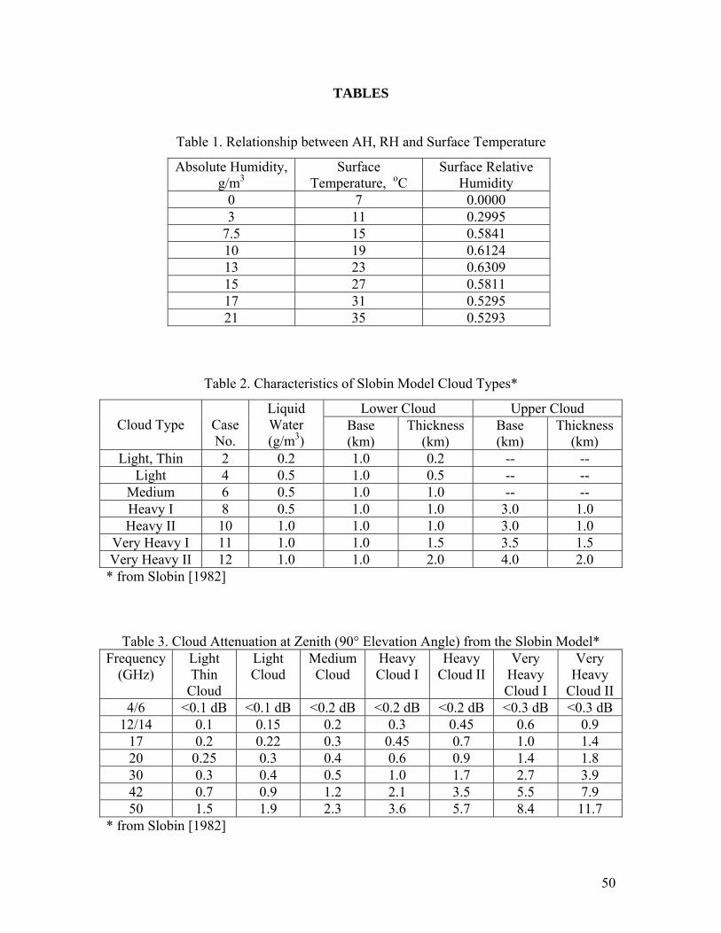
TABLES

Table 1. Relationship between AH, RH and Surface Temperature

Absolute Humidity, g/m3

Surface Temperature, oC

Surface Relative Humidity

0 7 0.0000 3 11 0.2995

7.5 15 0.5841 10 19 0.6124 13 23 0.6309 15 27 0.5811 17 31 0.5295 21 35 0.5293

Table 2. Characteristics of Slobin Model Cloud Types*

Lower Cloud Upper Cloud Cloud Type

Case No.

Liquid Water (g/m3)

Base (km)

Thickness (km)

Base (km)

Thickness (km)

Light, Thin 2 0.2 1.0 0.2 -- -- Light 4 0.5 1.0 0.5 -- --

Medium 6 0.5 1.0 1.0 -- -- Heavy I 8 0.5 1.0 1.0 3.0 1.0 Heavy II 10 1.0 1.0 1.0 3.0 1.0

Very Heavy I 11 1.0 1.0 1.5 3.5 1.5 Very Heavy II 12 1.0 1.0 2.0 4.0 2.0

* from Slobin [1982]

Table 3. Cloud Attenuation at Zenith (90° Elevation Angle) from the Slobin Model* Frequency

(GHz) Light Thin

Cloud

Light Cloud

Medium Cloud

Heavy Cloud I

Heavy Cloud II

Very Heavy Cloud I

Very Heavy

Cloud II 4/6 <0.1 dB <0.1 dB <0.2 dB <0.2 dB <0.2 dB <0.3 dB <0.3 dB

12/14 0.1 0.15 0.2 0.3 0.45 0.6 0.9 17 0.2 0.22 0.3 0.45 0.7 1.0 1.4 20 0.25 0.3 0.4 0.6 0.9 1.4 1.8 30 0.3 0.4 0.5 1.0 1.7 2.7 3.9 42 0.7 0.9 1.2 2.1 3.5 5.5 7.9 50 1.5 1.9 2.3 3.6 5.7 8.4 11.7


50

Table 4. Normalized Airmasses for Flat-Earth and Round-Earth Models Normalized Airmass for Round Earth Model Elevation

Angle, deg Flat Earth,

1/sin(θ) Water Vapor, Scale height=2.0km

Oxygen, Scale height=5.4km

Cloud, base =1km, top =2km, 2km thick

90 1.000 1.000 1.000 ----- 30 2.000 1.999 1.997 ----- 20 2.924 2.920 2.915 ----- 15 3.864 3.855 3.841 ----- 12 4.810 4.793 4.766 4.777 10 5.759 5.730 5.682 5.702 8 7.185 7.129 7.038 7.074 6 9.567 9.435 9.226 9.307 5 11.474 11.248 10.901 11.033 4 14.336 13.903 13.273 13.502 3 19.107 18.126 16.826 17.260 2 28.654 25.693 22.516 23.372

1.5 38.202 32.054 26.694 27.814 1.0 57.299 41.692 32.189 33.258 0.5 114.593 56.749 39.387 38.746

Table 5. Best-fit Coefficients for Round-Earth Expressions (Below 12 Degrees Elevation)

Constant Water Vapor, scale height = 2.0 km

Oxygen, scale height = 5.4 km

Cloud, base = 1 km, top = 3 km, 2 km thick

a0 77.809 48.793 46.062 a1 -50.2205269 -21.4312154 -15.3831656 a2 17.7024858 5.6619839 2.3175156 a3 -3.5261501 -0.9160630 -0.1067986 a4 0.3933954 0.0880003 -0.0094930 a5 -0.0228348 -0.0045792 0.0011618 a6 0.0005356 0.0000990 -0.0000328

51

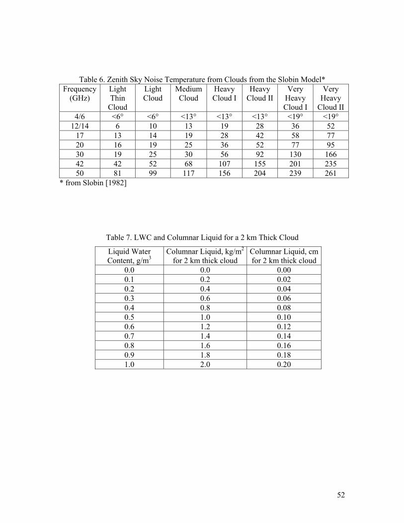
52

Table 6. Zenith Sky Noise Temperature from Clouds from the Slobin Model* Frequency

(GHz) Light Thin

Cloud

Light Cloud

Medium Cloud

Heavy Cloud I

Heavy Cloud II

Very Heavy Cloud I

Very Heavy

Cloud II 4/6 <6° <6° <13° <13° <13° <19° <19°

12/14 6 10 13 19 28 36 52 17 13 14 19 28 42 58 77 20 16 19 25 36 52 77 95 30 19 25 30 56 92 130 166 42 42 52 68 107 155 201 235 50 81 99 117 156 204 239 261


Table 7. LWC and Columnar Liquid for a 2 km Thick Cloud

Liquid Water Content, g/m3

Columnar Liquid, kg/m2

for 2 km thick cloud Columnar Liquid, cm for 2 km thick cloud

0.0 0.0 0.00 0.1 0.2 0.02 0.2 0.4 0.04 0.3 0.6 0.06 0.4 0.8 0.08 0.5 1.0 0.10 0.6 1.2 0.12 0.7 1.4 0.14 0.8 1.6 0.16 0.9 1.8 0.18 1.0 2.0 0.20

Table 8. Radio Parameters at Four Case Study Areas

Radio Parameters Applied Ranges Patuxent River Laguna Peak San Nicholas Island Edwards AFB

February 310 N-units 330 N-units 330 N-units 320 N-units Refractive Index August 360 N-units 345 N-units 350 N-units 330 N-units

February 40 N-units 45 N-units 45 N-units 40 N-units Refractivity Gradient August 50 N-units 55 N-units 60 N-units 45 N-units

February, 1.0% 9 g/m3 10.4 g/m3 10.5 g/m3 9.9 g/m3 Water Vapor Content August, 1.0% 21 g/m3 15 g/m3 15.2 g/m3 14.5 g/m3

Zone K E E E

0.1% of Time 12 mm/h 6.2 mm/h 6.2 mm/h 6.2 mm/h

Rainfall Zone and

Rainfall Rate 1.0% of Time 2.5 mm/h 1.8 mm/h 1.8 mm/h 1.8 mm/h

1.0% of Time 1.2 kg/m2 0.5 kg/m2 0.5 kg/m2 0.4 kg/m2 Cloud Liquid Water Columnar

Content 10% of Time 0.4 kg/m2 0.2 kg/m2 0.2 kg/m2 0.2 kg/m2

Radio Climatic Zone

Inland, Coastal or Sea

A1 A1 B A2

Surface Duct 10% 15% 15% 10% Ducting Occurrence Rate Elevated Duct 10% 50% 50% 10%

53

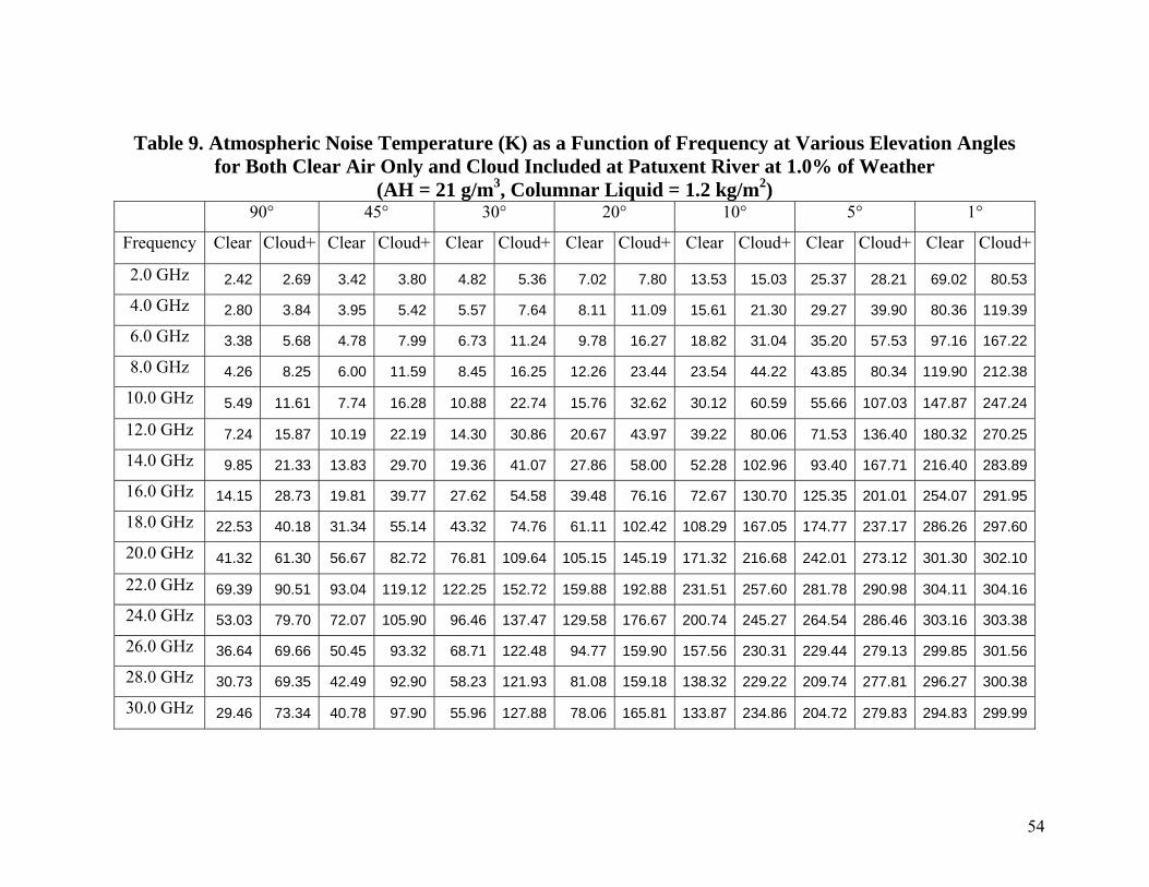
Table 9. Atmospheric Noise Temperature (K) as a Function of Frequency at Various Elevation Angles for Both Clear Air Only and Cloud Included at Patuxent River at 1.0% of Weather

(AH = 21 g/m3, Columnar Liquid = 1.2 kg/m2) 90° 45° 30° 20° 10° 5° 1°

Frequency Clear Cloud+ Clear Cloud+ Clear Cloud+ Clear Cloud+ Clear Cloud+ Clear Cloud+ Clear Cloud+

2.0 GHz 2.42 2.69 3.42 3.80 4.82 5.36 7.02 7.80 13.53 15.03 25.37 28.21 69.02 80.53

4.0 GHz 2.80 3.84 3.95 5.42 5.57 7.64 8.11 11.09 15.61 21.30 29.27 39.90 80.36 119.39

6.0 GHz 3.38 5.68 4.78 7.99 6.73 11.24 9.78 16.27 18.82 31.04 35.20 57.53 97.16 167.22

8.0 GHz 4.26 8.25 6.00 11.59 8.45 16.25 12.26 23.44 23.54 44.22 43.85 80.34 119.90 212.38

10.0 GHz 5.49 11.61 7.74 16.28 10.88 22.74 15.76 32.62 30.12 60.59 55.66 107.03 147.87 247.24

12.0 GHz 7.24 15.87 10.19 22.19 14.30 30.86 20.67 43.97 39.22 80.06 71.53 136.40 180.32 270.25

14.0 GHz 9.85 21.33 13.83 29.70 19.36 41.07 27.86 58.00 52.28 102.96 93.40 167.71 216.40 283.89

16.0 GHz 14.15 28.73 19.81 39.77 27.62 54.58 39.48 76.16 72.67 130.70 125.35 201.01 254.07 291.95

18.0 GHz 22.53 40.18 31.34 55.14 43.32 74.76 61.11 102.42 108.29 167.05 174.77 237.17 286.26 297.60

20.0 GHz 41.32 61.30 56.67 82.72 76.81 109.64 105.15 145.19 171.32 216.68 242.01 273.12 301.30 302.10

22.0 GHz 69.39 90.51 93.04 119.12 122.25 152.72 159.88 192.88 231.51 257.60 281.78 290.98 304.11 304.16

24.0 GHz 53.03 79.70 72.07 105.90 96.46 137.47 129.58 176.67 200.74 245.27 264.54 286.46 303.16 303.38

26.0 GHz 36.64 69.66 50.45 93.32 68.71 122.48 94.77 159.90 157.56 230.31 229.44 279.13 299.85 301.56

28.0 GHz 30.73 69.35 42.49 92.90 58.23 121.93 81.08 159.18 138.32 229.22 209.74 277.81 296.27 300.38

30.0 GHz 29.46 73.34 40.78 97.90 55.96 127.88 78.06 165.81 133.87 234.86 204.72 279.83 294.83 299.99

54

Table 10. Atmospheric Noise Temperature (K) as a Function of Frequency at Various Elevation Angles for Both Clear Air Only and Cloud Included at West Coast at 1.0% of Weather

(AH = 15 g/m3, Columnar Liquid = 0.5 kg/m2) 90° 45° 30° 20° 10° 5° 1°

Frequency Clear Cloud+ Clear Cloud+ Clear Cloud+ Clear Cloud+ Clear Cloud+ Clear Cloud+ Clear Cloud+

2.0 GHz 2.41 2.53 3.41 3.57 4.80 5.03 6.99 7.33 13.47 14.11 25.25 26.46 68.47 73.46

4.0 GHz 2.70 3.15 3.82 4.44 5.38 6.26 7.83 9.11 15.08 17.52 28.25 32.85 77.13 95.00

6.0 GHz 3.14 4.12 4.43 5.80 6.24 8.17 9.07 11.86 17.46 22.76 32.66 42.52 89.70 124.79

8.0 GHz 3.78 5.49 5.33 7.74 7.51 10.88 10.92 15.76 20.97 30.07 39.13 55.71 107.14 159.26

10.0 GHz 4.70 7.33 6.62 10.30 9.32 14.46 13.52 20.89 25.89 39.56 48.04 72.26 129.36 193.91

12.0 GHz 5.99 9.71 8.43 13.64 11.85 19.09 17.16 27.47 32.70 51.47 60.12 92.18 156.40 225.27

14.0 GHz 7.90 12.88 11.10 18.04 15.57 25.18 22.48 36.04 42.50 66.54 76.99 116.02 188.66 251.35

16.0 GHz 11.03 17.41 15.47 24.30 21.64 33.75 31.07 47.96 57.94 86.71 102.32 145.52 226.39 271.53

18.0 GHz 17.12 24.95 23.91 34.63 26.39 47.71 47.26 66.98 85.69 116.94 143.93 184.68 265.81 285.72

20.0 GHz 31.02 40.09 42.86 55.01 33.23 74.58 81.61 102.14 138.81 166.52 209.35 235.78 290.95 293.53

22.0 GHz 52.58 62.53 71.42 84.24 43.46 111.39 128.16 147.00 197.94 217.52 259.74 271.07 295.82 295.99

24.0 GHz 40.04 52.43 54.95 71.23 58.69 95.27 102.10 127.85 166.68 197.41 236.10 259.24 294.36 295.15

26.0 GHz 27.92 43.06 38.67 58.93 95.51 79.62 74.25 108.49 128.02 174.34 197.41 242.01 288.30 293.26

28.0 GHz 23.79 41.48 33.06 56.83 74.52 76.91 64.17 105.05 112.70 169.85 179.18 238.03 282.46 292.20

30.0 GHz 23.13 43.31 32.16 59.26 53.13 80.02 62.53 108.95 110.09 174.63 175.77 241.72 280.68 291.99

55

Figure 1

56

Figure 2

57

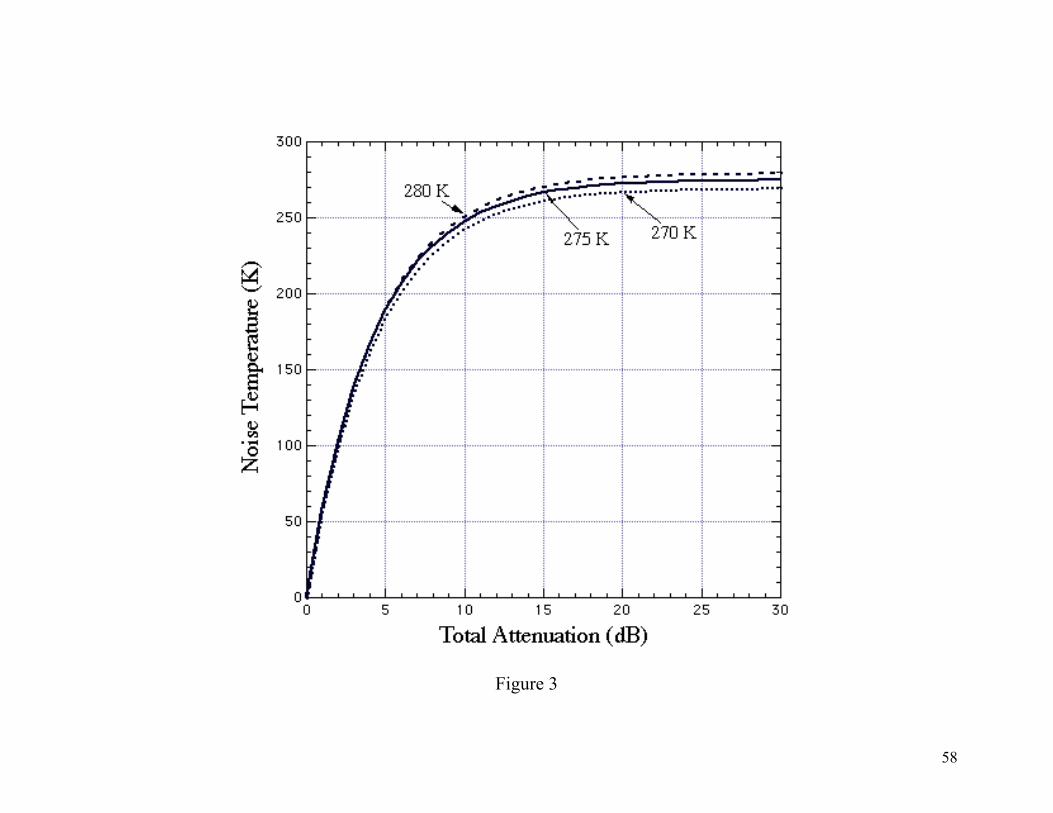
Figure 3

58

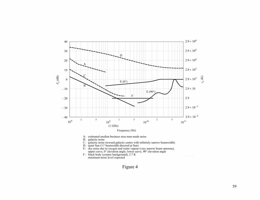
FI

59

0372-03

A

E (0°)

D

C

B

E (90°)F

2 5 2 5 2 5109108 1010 1011

0

10

20

30

40

– 40

– 30

– 20

– 10

t (K

)a

Fa versus freq 011 Hz)

F (d

B)

a

Frequency (Hz)(1 GHz)

2.9 × 10

2.9

2.9 × 106

2.9 × 105

2.9 × 104

2.9 × 103

2.9 × 102

2.9 × 10 –1

2.9 × 10 –2

1

GURE 3uency (108 to 1

ABCDE

F

: estimated median business area man-made noise: galactic noise: galactic noise (toward galactic centre with infinitely narrow beamwidth): quiet Sun (½° beamwidth directed at Sun): sky noise due to oxygen and water vapour (very narrow beam antenna);: upper curve, 0° elevation angle; lower curve, 90° elevation angle: black body (cosmic background), 2.7 K minimum noise level expected

Figure 4

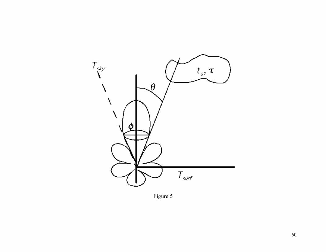
Figure 5

60

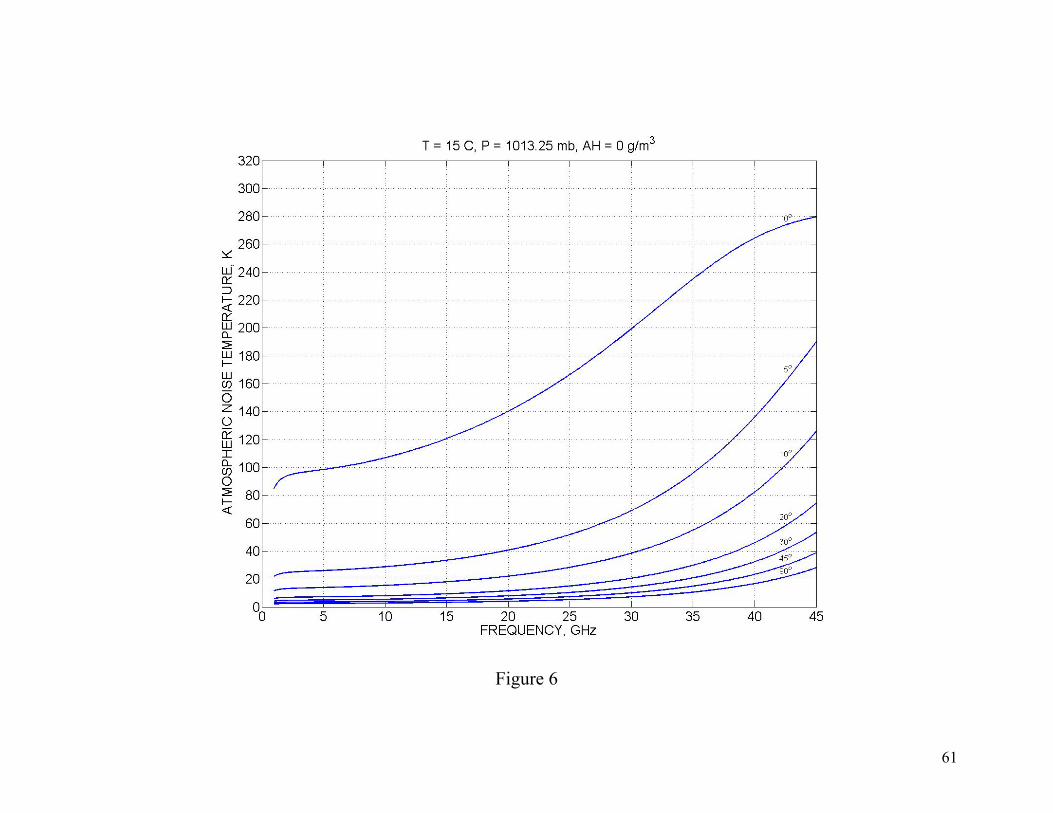
Figure 6

61

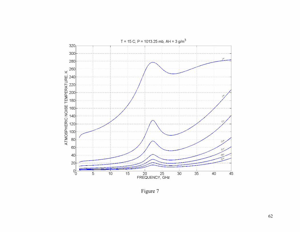
Figure 7

62

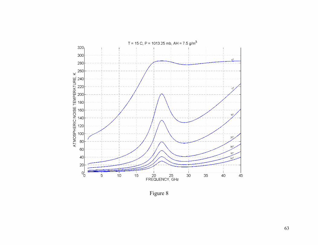
Figure 8

63

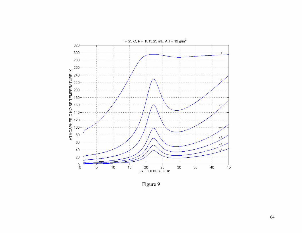
Figure 9

64

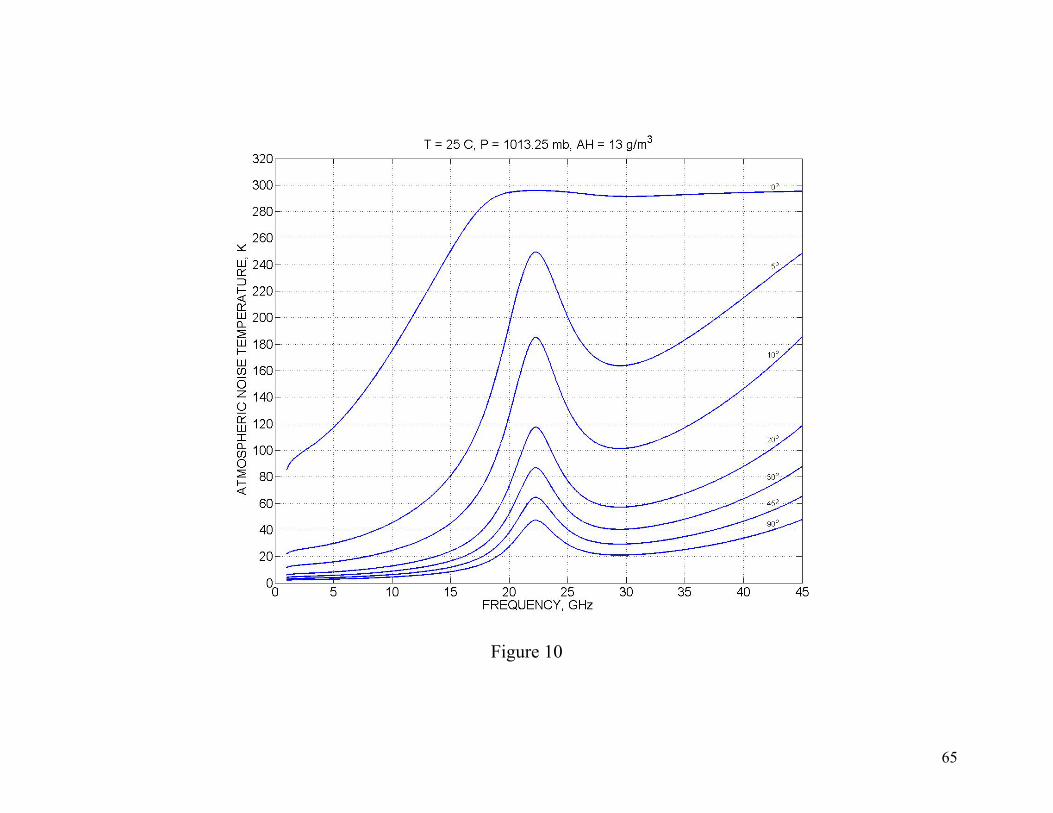
Figure 10

65

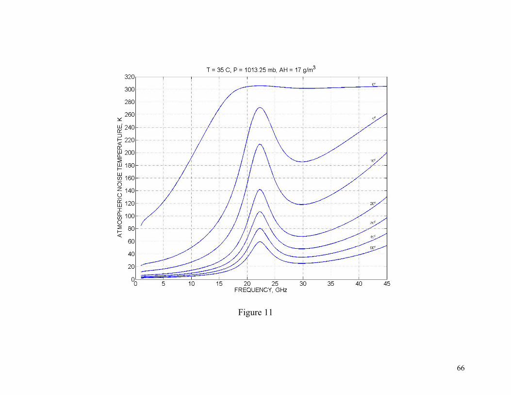
Figure 11

66

Figure 12

67

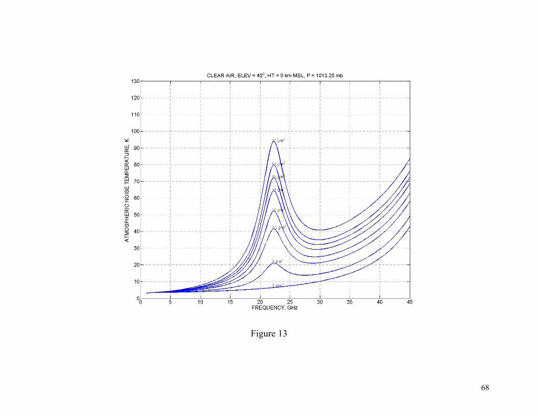
Figure 13

68

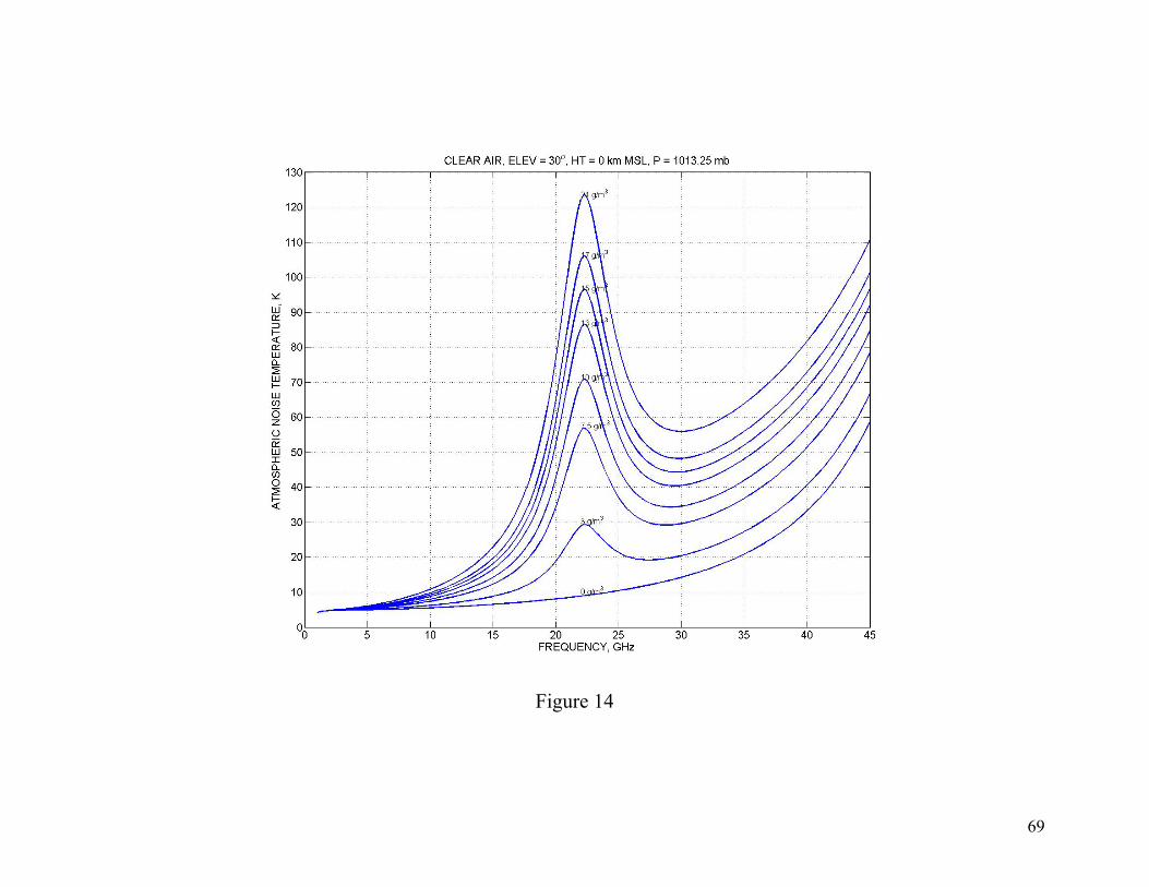
Figure 14

69

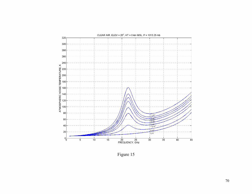
Figure 15

70

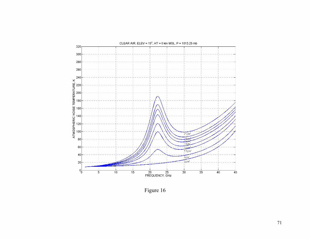
Figure 16

71

Figure 17

72

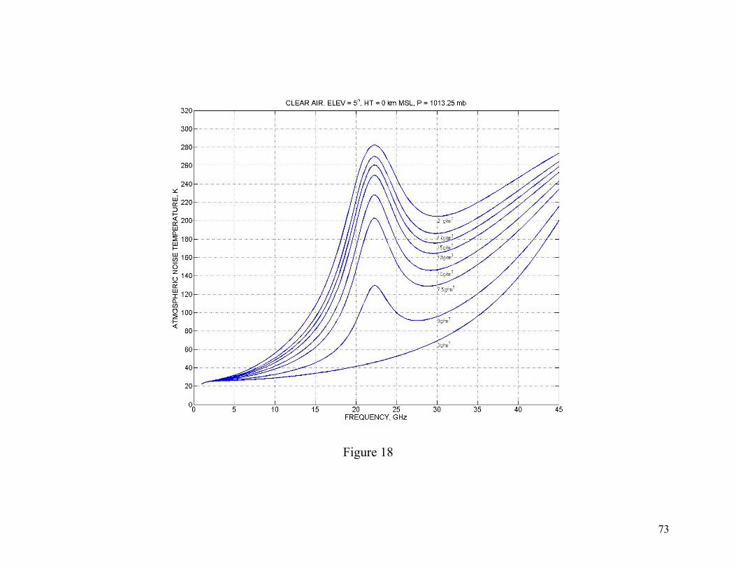
Figure 18

73

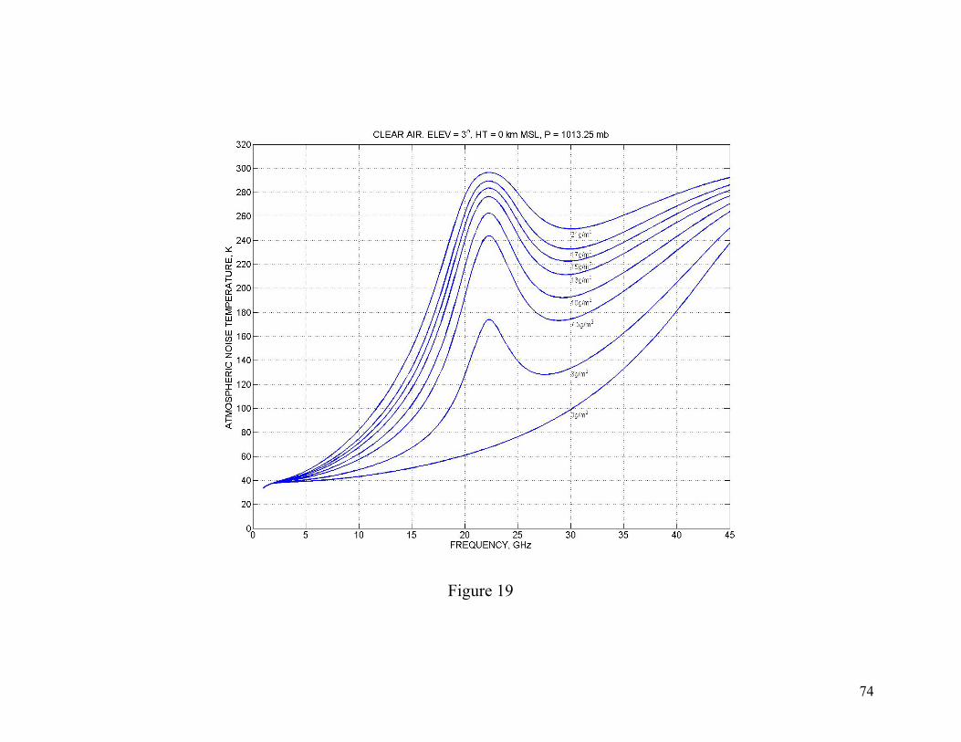
Figure 19

74

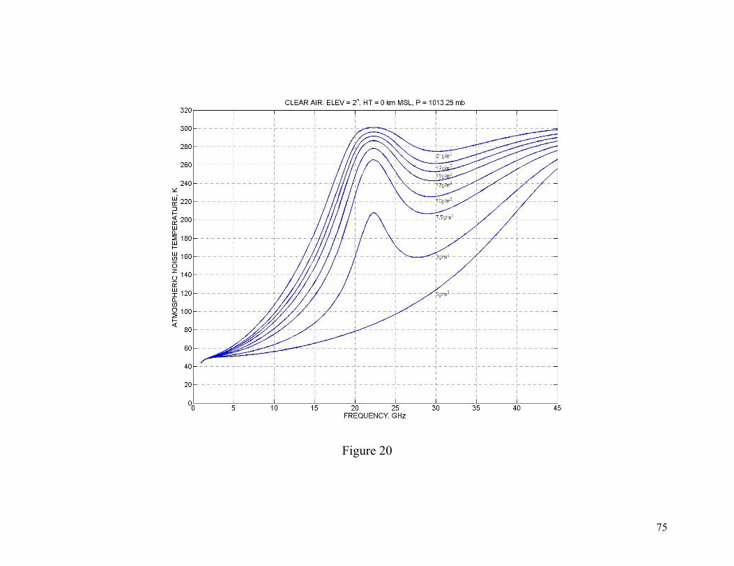
Figure 20

75

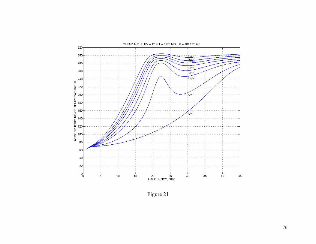
Figure 21

76

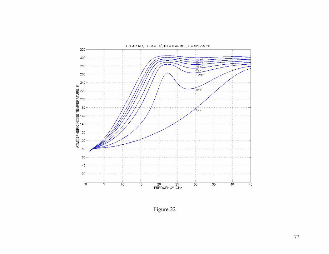
Figure 22

77

Figure 23

78

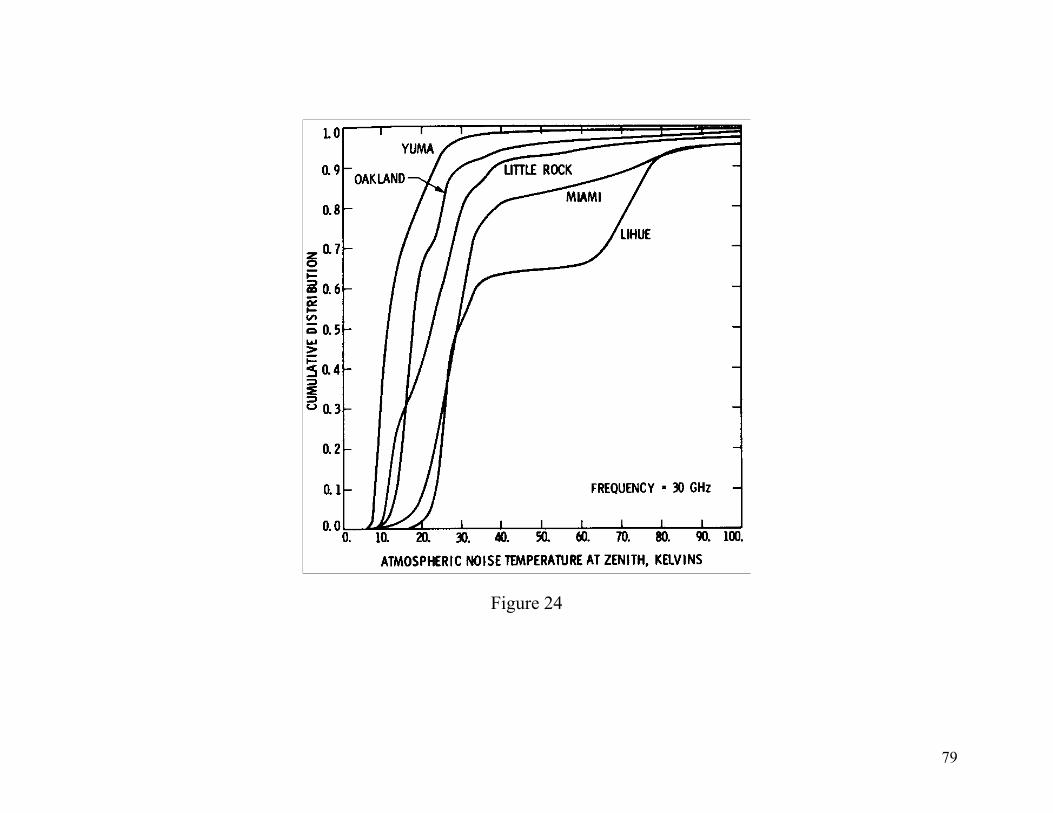
Figure 24

79

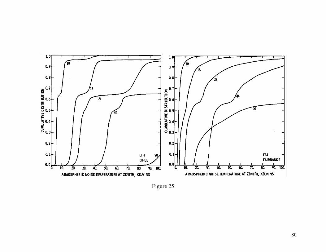
Figure 25

80

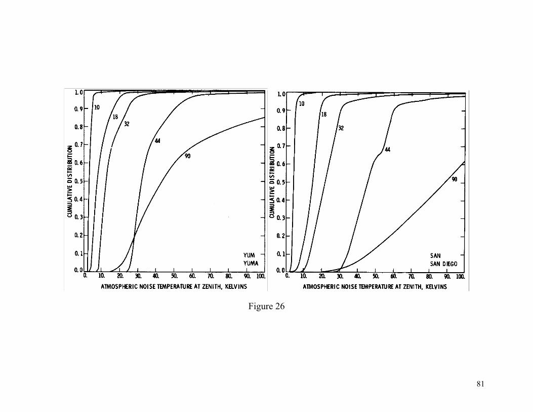
Figure 26

81

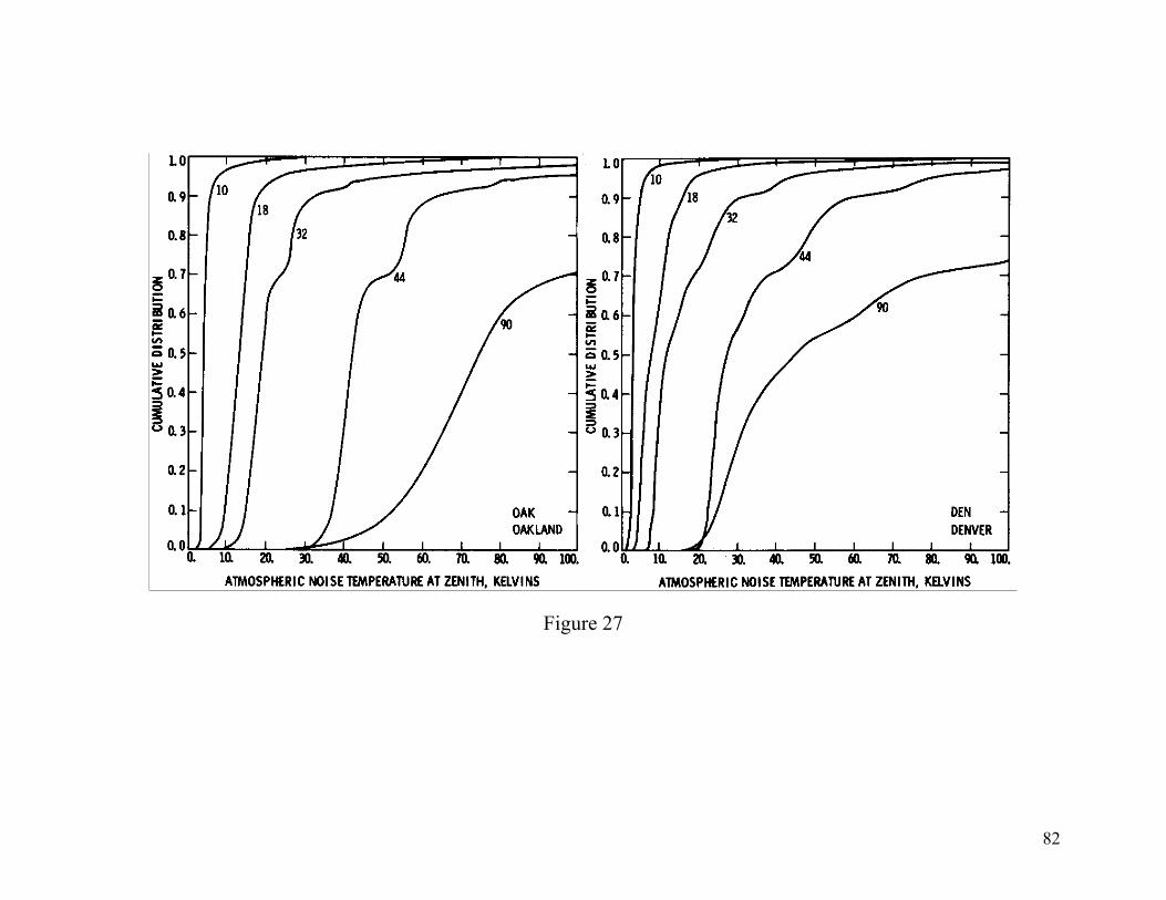
Figure 27

82

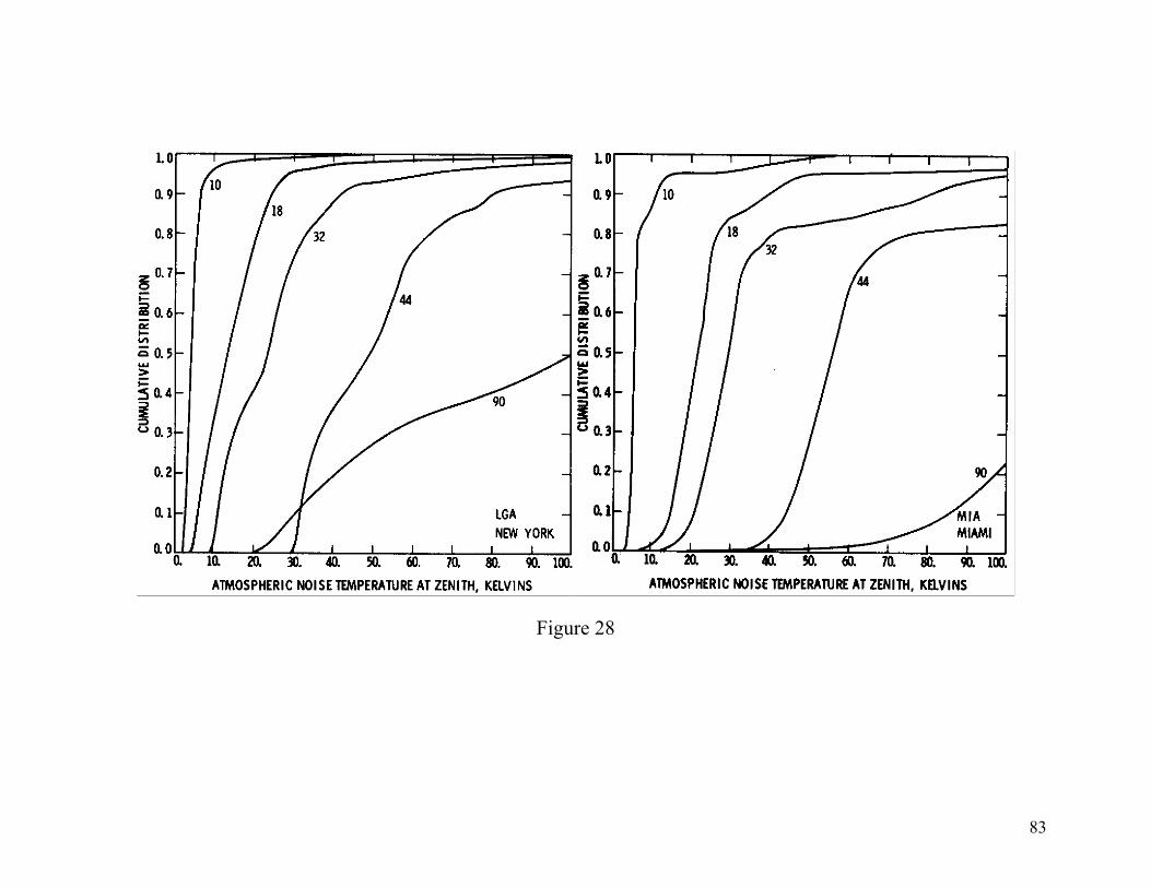
Figure 28

83

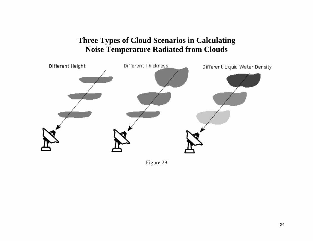
Three Types of Cloud Scenarios in Calculating Noise Temperature Radiated from Clouds

Figure 29

84

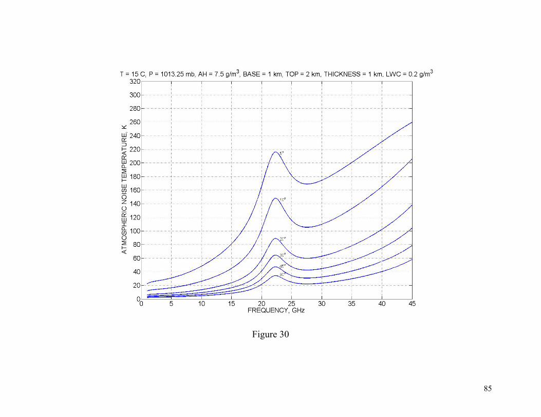
Figure 30

85

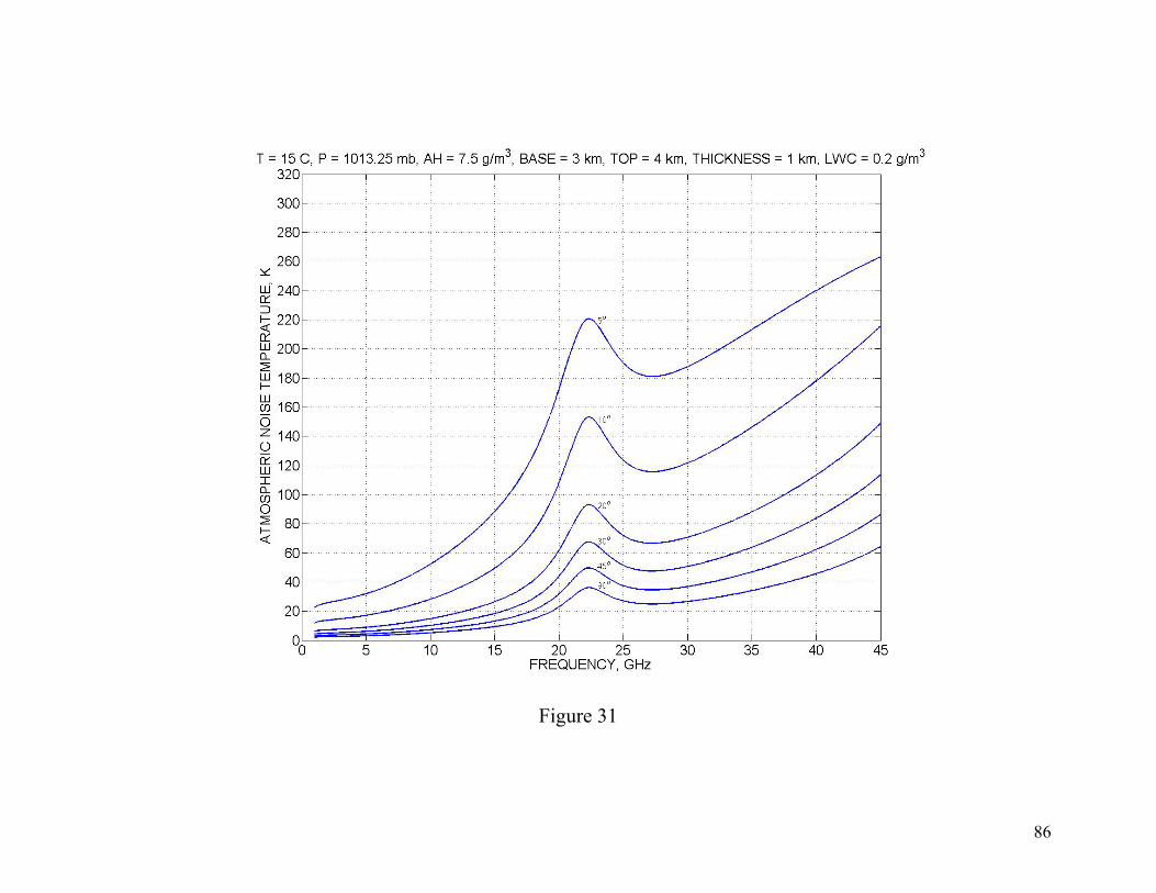
Figure 31

86

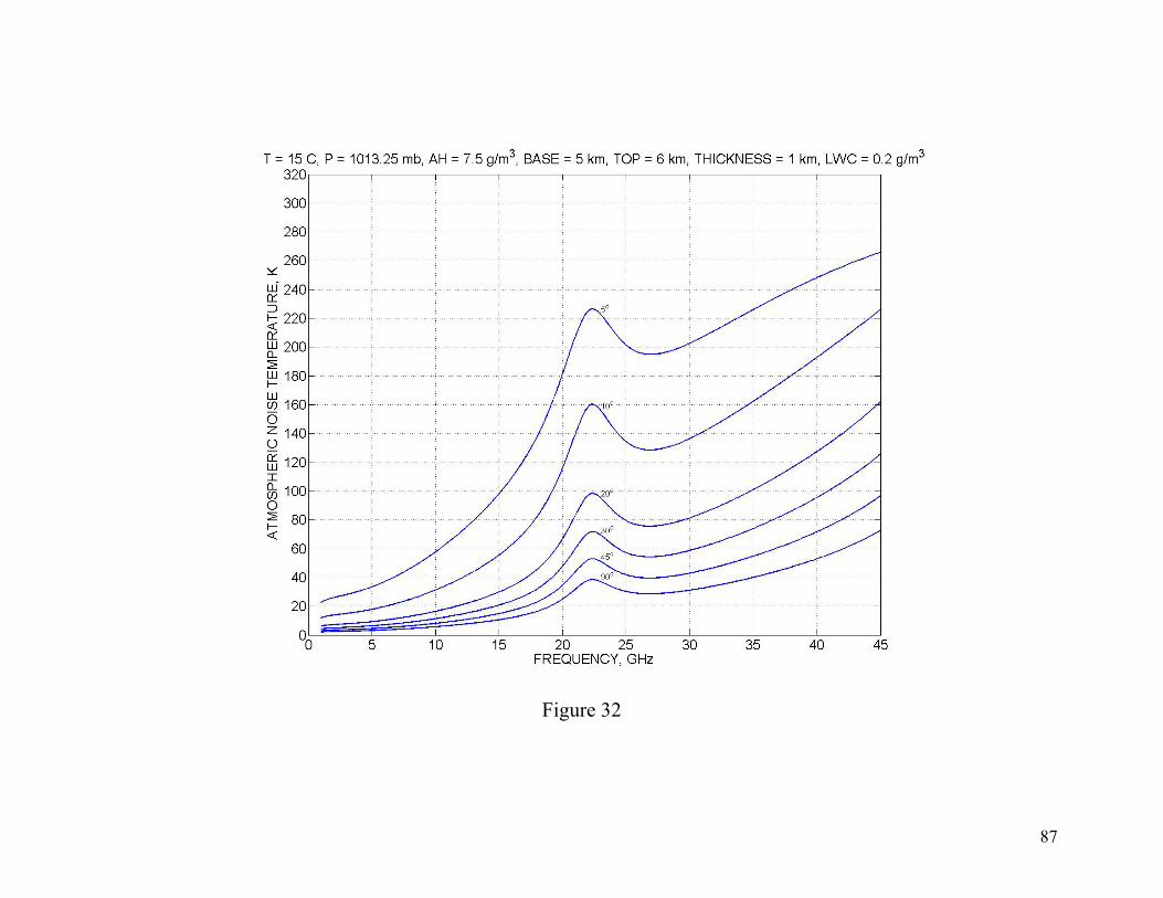
Figure 32

87

Figure 33

88

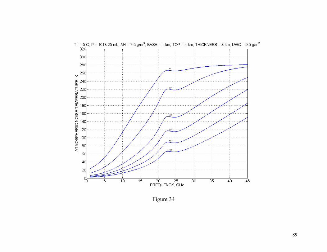
Figure 34

89

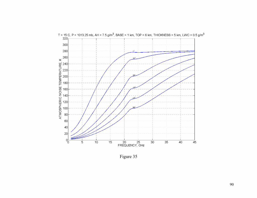
Figure 35

90

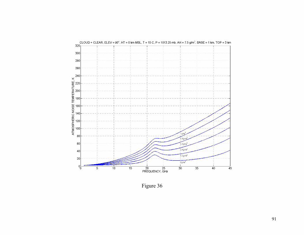
Figure 36

91

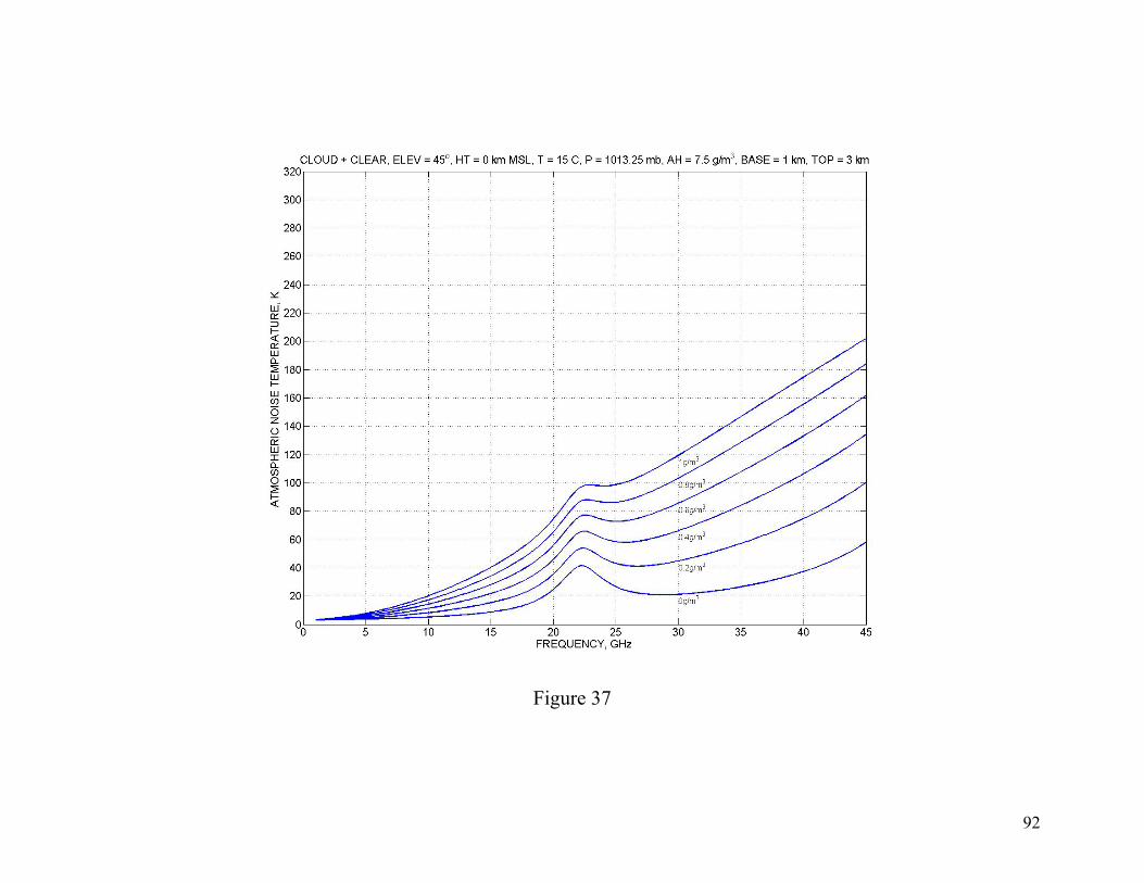
Figure 37

92

Figure 38

93

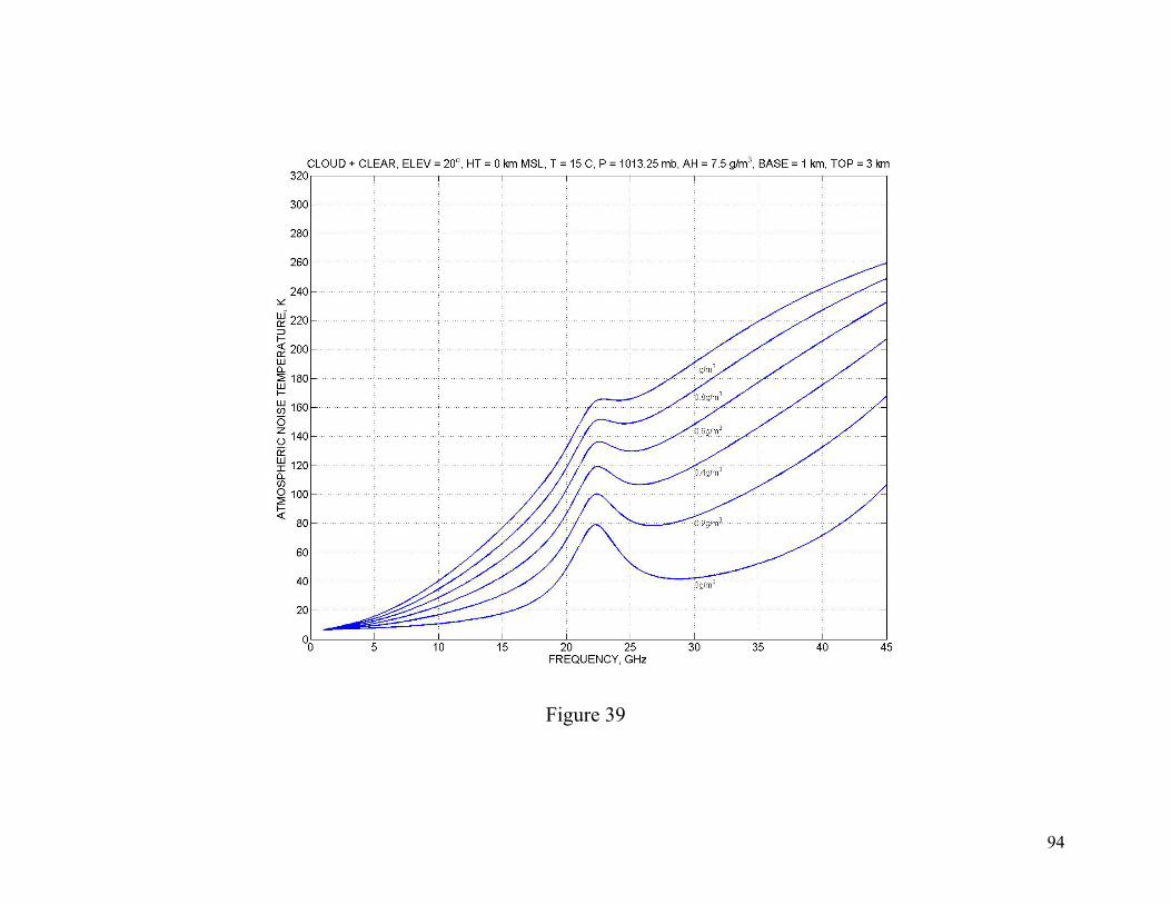
Figure 39

94

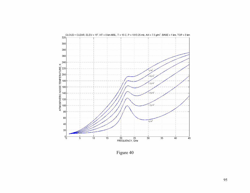
Figure 40

95

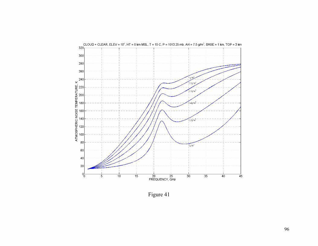
Figure 41

96

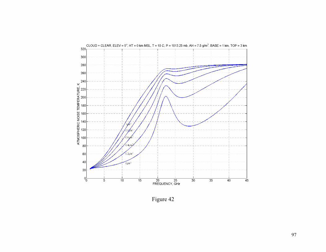
Figure 42

97

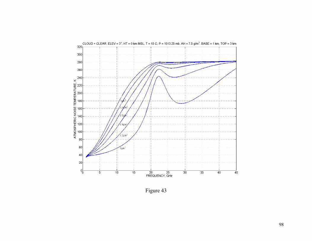
Figure 43

98

Figure 44

99

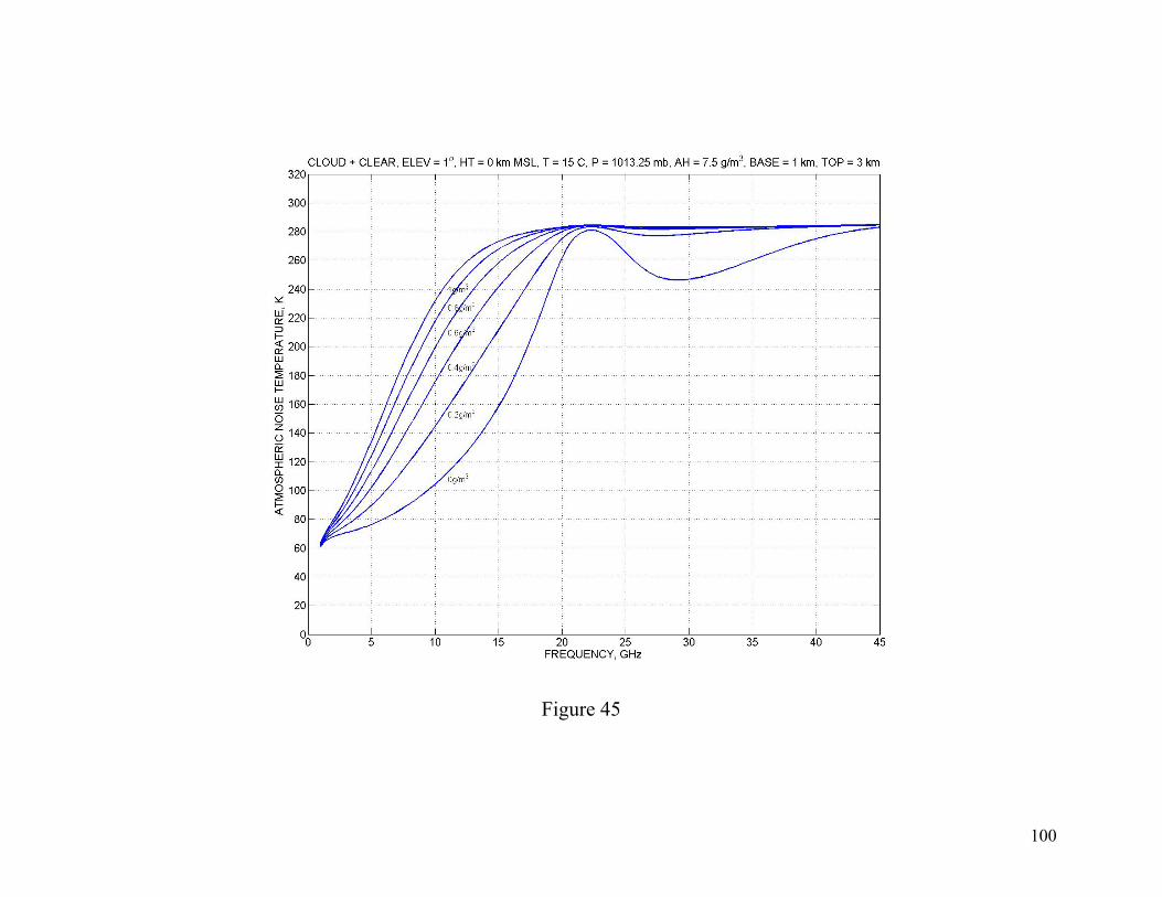
Figure 45

100

Figure 46

101

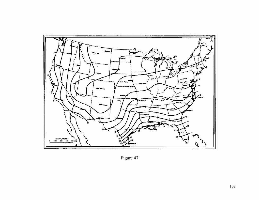
Figure 47

102

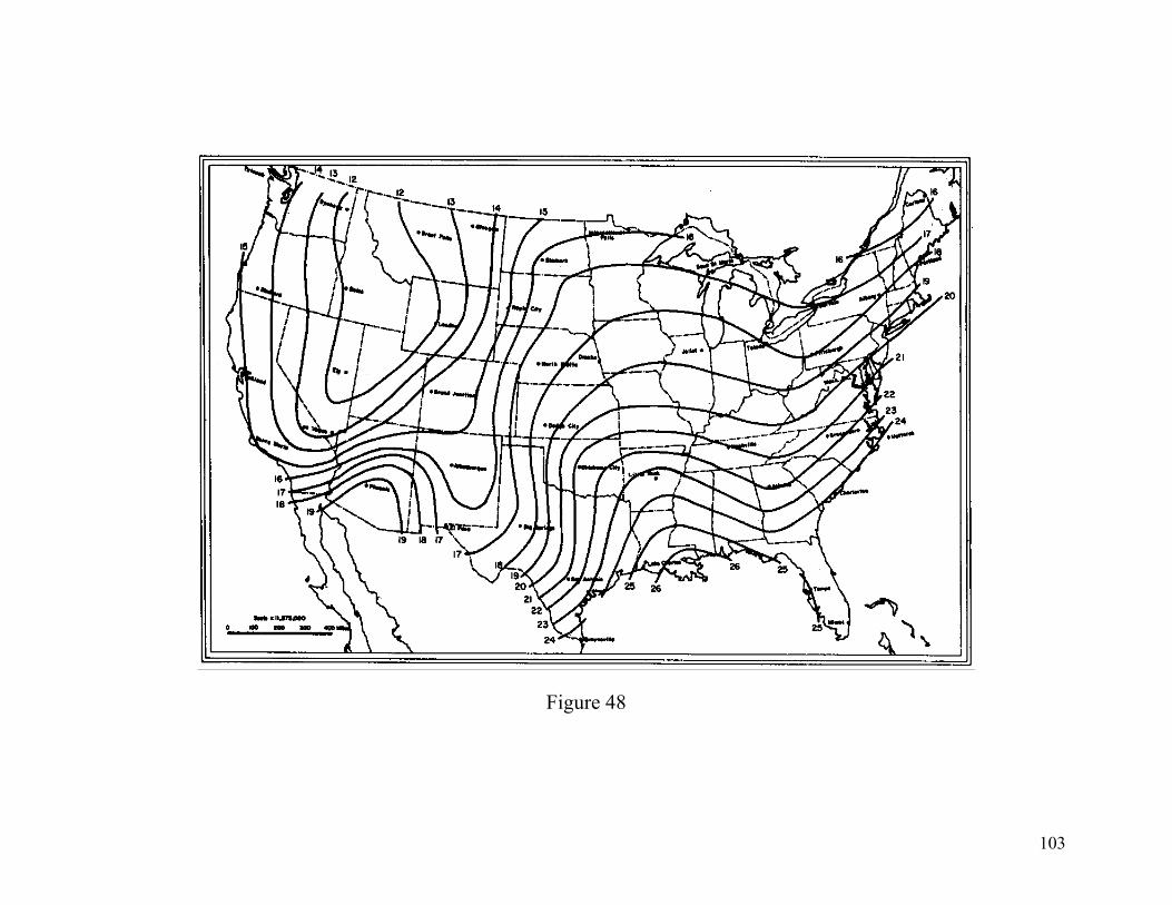
Figure 48

103

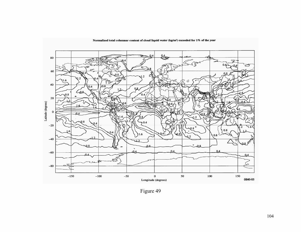
Figure 49

104

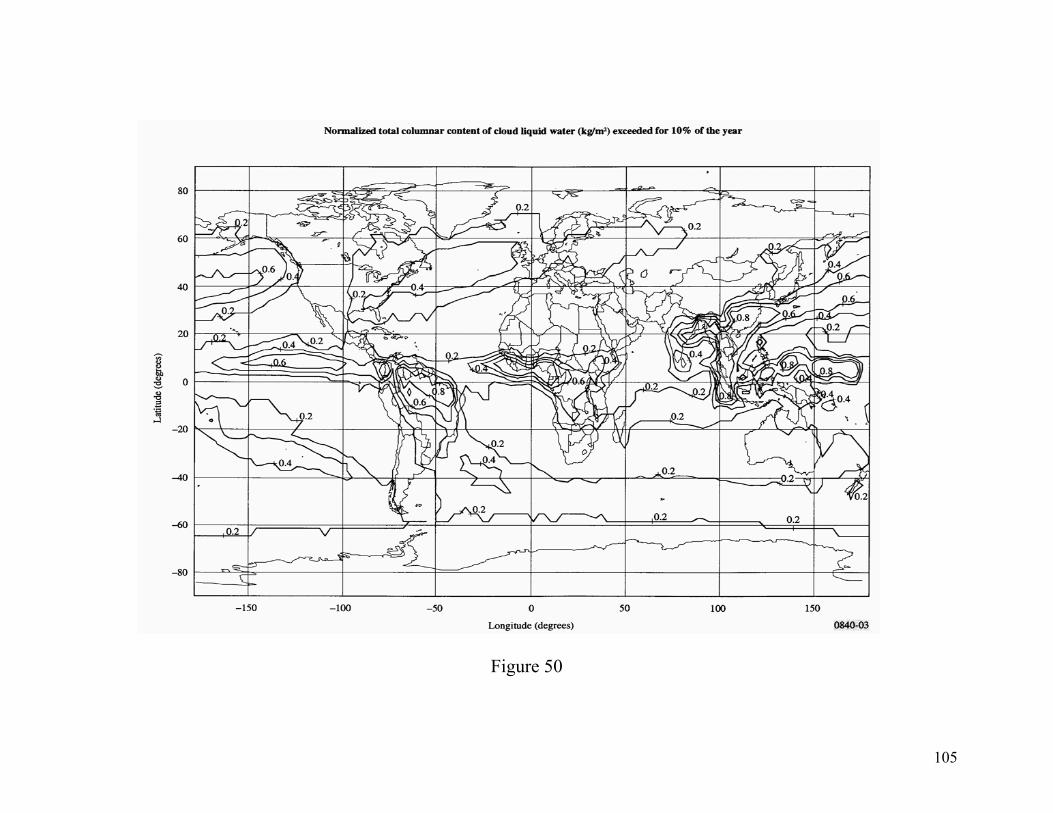
Figure 50

105

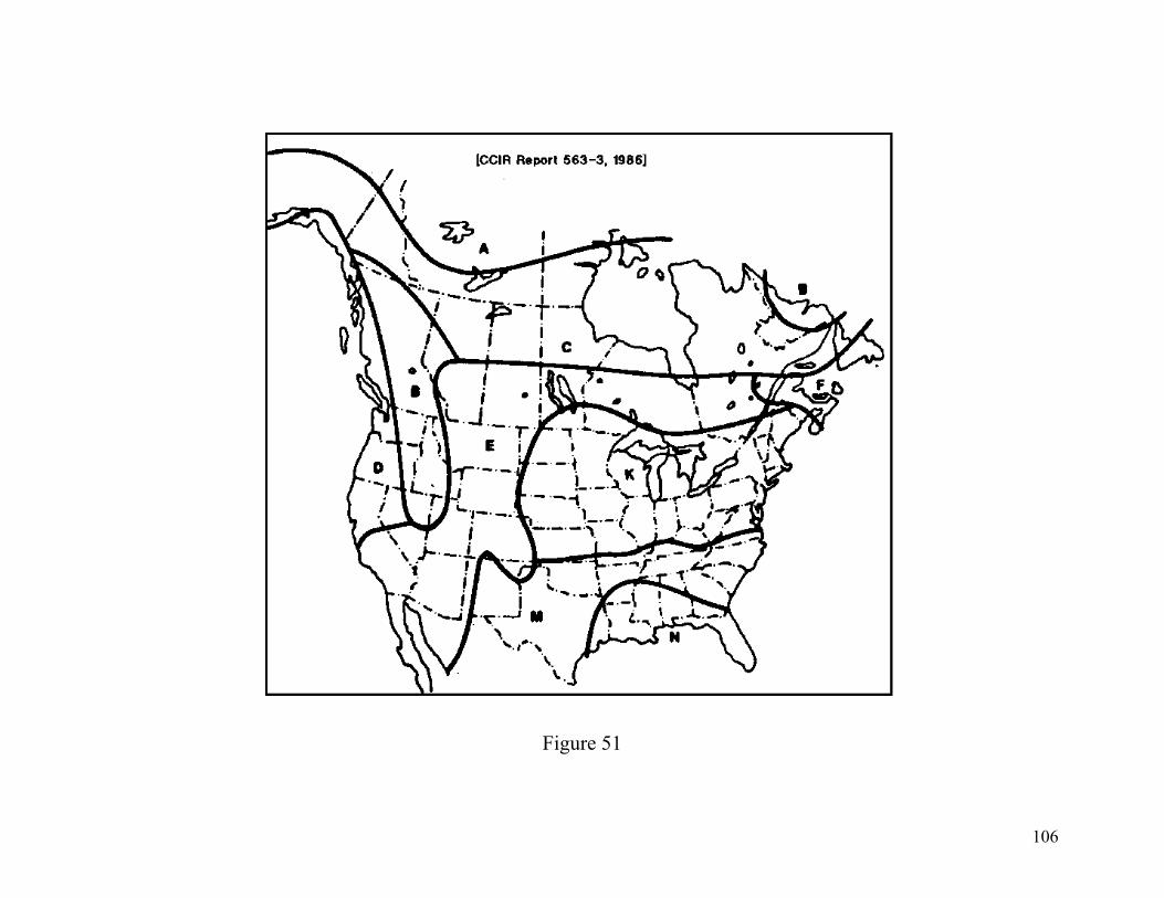
Figure 51

106

Figure 52

107

108

Figure 53

10-6

10-5

10-4

10-3

10-2

10-1

100

101

Spec

ific

Atte

nuat

ion,

γ R (d

B/k

m)

0.12 3 4 5 6 7 8 9

12 3 4

Percentage of Time Exceeded, p (%)

Rainfall Zone: K Region

2 GHz

6 GHz

10 GHz

15 GHz

25 GHz

30 GHz

45 GHz

Figure 54

109

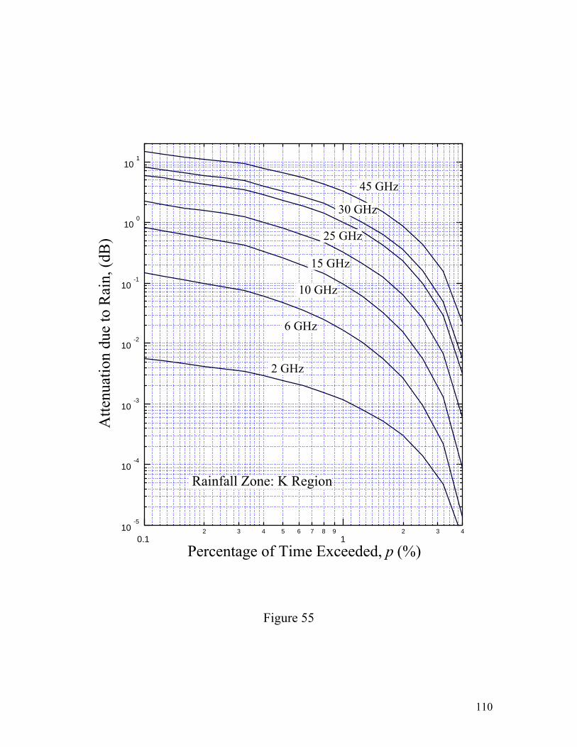
10-5

10-4

10-3

10-2

10-1

100

101

Atte

nuat

ion

due

to R

ain,

(dB

)

0.12 3 4 5 6 7 8 9

12 3 4



2 GHz

6 GHz

10 GHz

15 GHz

25 GHz

30 GHz

45 GHz

Figure 55

110

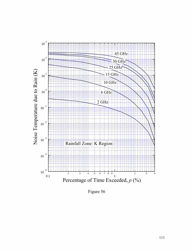
10-5

10-4

10-3

10-2

10-1

100

101

102

103

Noi

se T

empe

ratu

re d

ue to

Rai

n (K

)

0.12 3 4 5 6 7 8 9

12 3 4



2 GHz

6 GHz

10 GHz

15 GHz

25 GHz 30 GHz

45 GHz

Figure 56

111

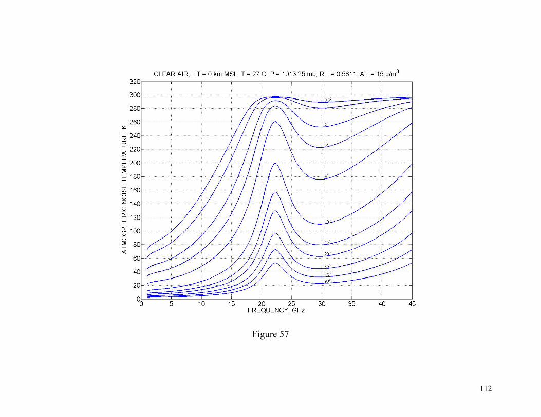
Figure 57

112

113

Figure 58

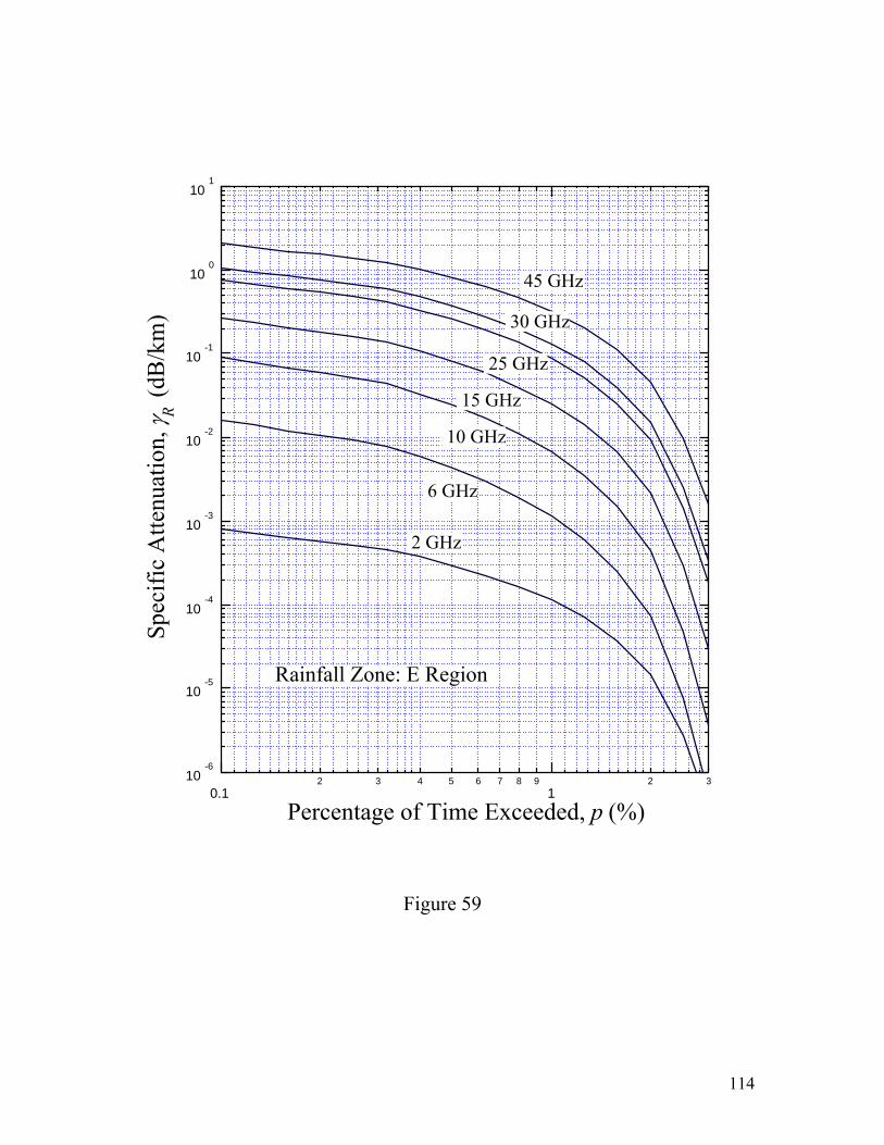
10-6

10-5

10-4

10-3

10-2

10-1

100

101

Spec

ific

Atte

nuat

ion,

γ R (d

B/k

m)

0.12 3 4 5 6 7 8 9

12 3


Rainfall Zone: E Region

2 GHz

6 GHz

10 GHz

15 GHz

25 GHz

30 GHz

45 GHz

Figure 59

114

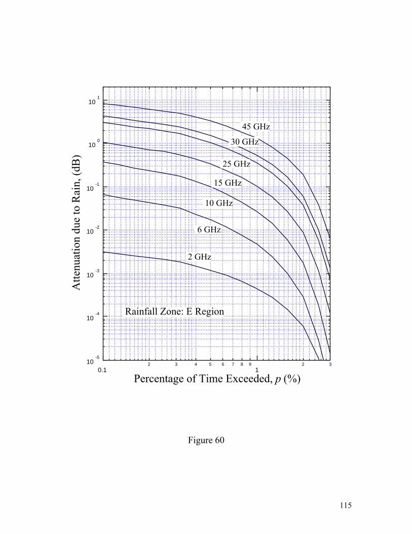
10-5

10-4

10-3

10-2

10-1

100

101

Atte

nuat

ion

due

to R

ain,

(dB

)

0.12 3 4 5 6 7 8 9

12 3



2 GHz

6 GHz

10 GHz

15 GHz

25 GHz

30 GHz

45 GHz

Figure 60

115

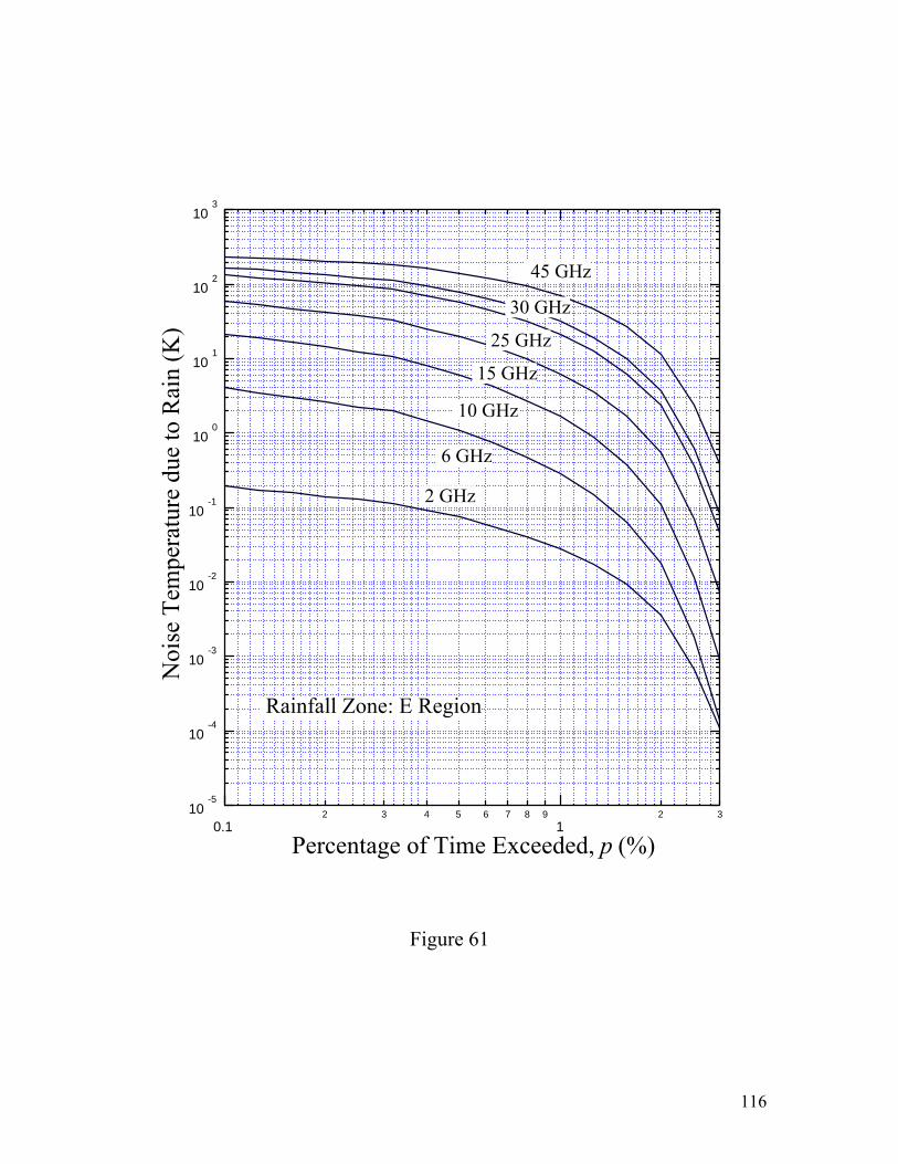
10-5

10-4

10-3

10-2

10-1

100

101

102

103

Noi

se T

empe

ratu

re d

ue to

Rai

n (K

)

0.12 3 4 5 6 7 8 9

12 3



2 GHz

6 GHz

10 GHz

15 GHz

25 GHz

30 GHz

45 GHz

Figure 61

116

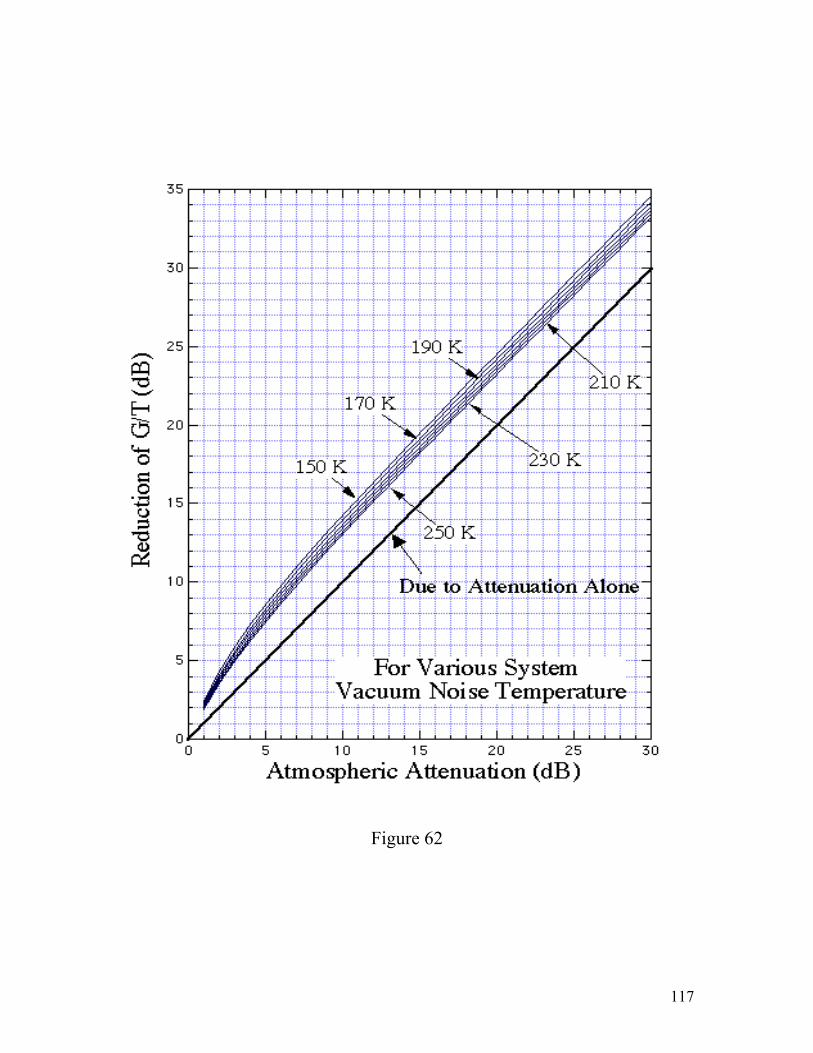
Figure 62

117

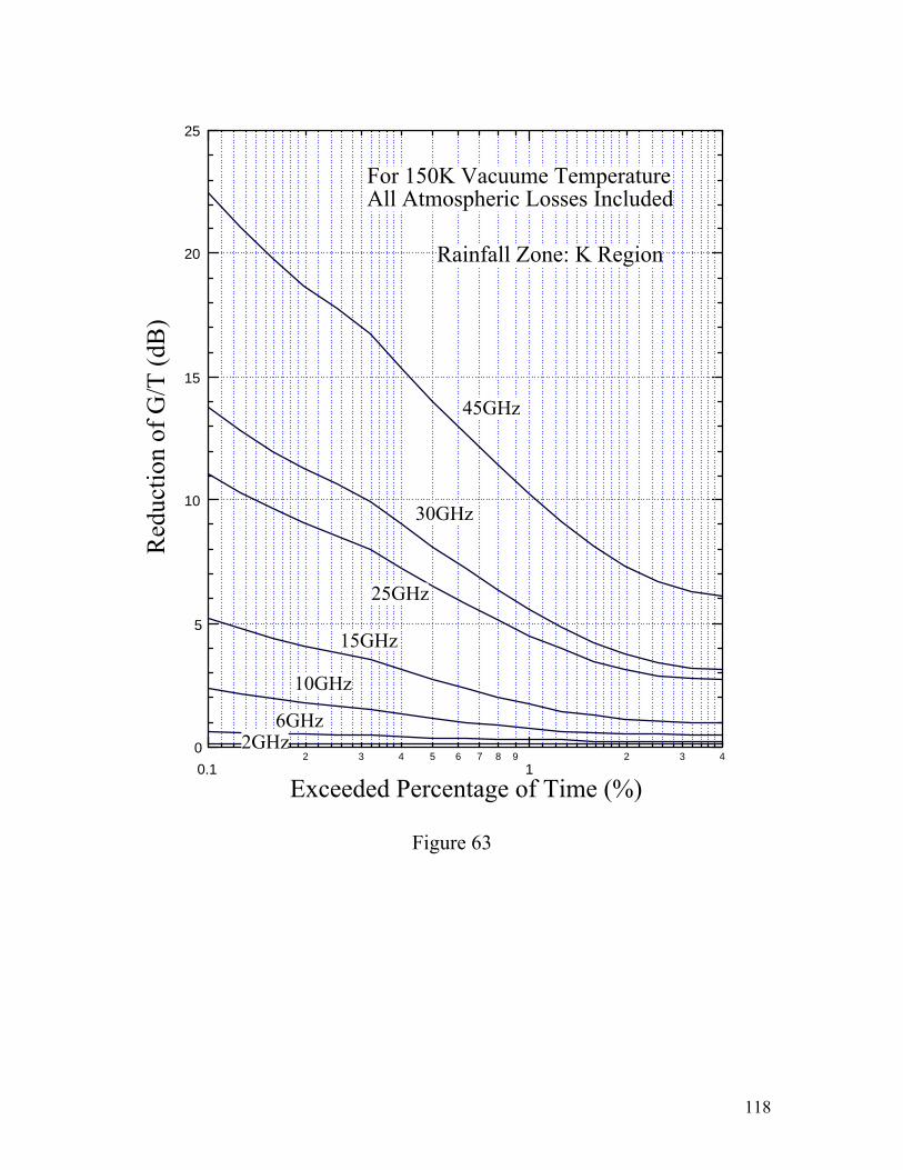
25

20

15

10

5

0

Red

uctio

n of

G/T

(dB

)

0.12 3 4 5 6 7 8 9

12 3 4

Exceeded Percentage of Time (%)

45GHz

30GHz

25GHz

15GHz

10GHz

6GHz2GHz

For 150K Vacuume TemperatureAll Atmospheric Losses Included


Figure 63

118

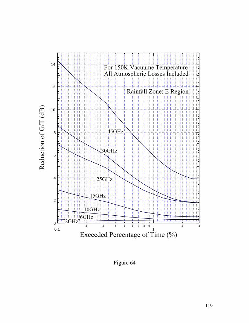
14

12

10

8

6

4

2

0

Red

uctio

n of

G/T

(dB

)

0.12 3 4 5 6 7 8 9

12 3

Exceeded Percentage of Time (%)

45GHz

30GHz

25GHz

15GHz

10GHz6GHz

2GHz

For 150K Vacuume TemperatureAll Atmospheric Losses Included


Figure 64

119

Documents

Noise Temperature induced by Atmosphere and Weather on