Technology, Prices, and the Derived Demand for EnergyAuthor(s): Ernst R. Berndt and David O. WoodSource: The Review of Economics and Statistics, Vol. 57, No. 3 (Aug., 1975), pp. 259-268Published by: The MIT PressStable URL: http://www.jstor.org/stable/1923910 .Accessed: 12/01/2011 12:18

Your use of the JSTOR archive indicates your acceptance of JSTOR's Terms and Conditions of Use, available at .http://www.jstor.org/page/info/about/policies/terms.jsp. JSTOR's Terms and Conditions of Use provides, in part, that unlessyou have obtained prior permission, you may not download an entire issue of a journal or multiple copies of articles, and youmay use content in the JSTOR archive only for your personal, non-commercial use.

Please contact the publisher regarding any further use of this work. Publisher contact information may be obtained at .http://www.jstor.org/action/showPublisher?publisherCode=mitpress. .

Each copy of any part of a JSTOR transmission must contain the same copyright notice that appears on the screen or printedpage of such transmission.

JSTOR is a not-for-profit service that helps scholars, researchers, and students discover, use, and build upon a wide range ofcontent in a trusted digital archive. We use information technology and tools to increase productivity and facilitate new formsof scholarship. For more information about JSTOR, please contact support@jstor.org.

The MIT Press is collaborating with JSTOR to digitize, preserve and extend access to The Review ofEconomics and Statistics.

http://www.jstor.org

The Review of Economics and Statistics

VOL. LVII AUGUST 1975 NUMBER 3

TECHNOLOGY, PRICES, AND THE DERIVED DEMAND FOR ENERGY

Ernst R. Berndt and David 0. Wood*

I. Introduction

INDUSTRIAL demand for energy is essen- tially a derived demand: the firm's demand

for energy as an input is derived from the de- mand for the firm's output. Inputs other than energy typically also enter the firm's production process. Since firms tend to choose that bundle of inputs which minimizes the total cost of pro- ducing a given level of output, the derived de- mand for inputs, including energy, depends on the level of output, the substitution possibilities among inputs allowed by the production tech- nology, and the relative prices of all inputs.

Empirical studies typically have not simulta- neously considered the derived demand for en- ergy and nonenergy inputs. Studies of industrial energy demand have been restricted in one of two ways: (1) by focussing attention solely on the level of output and ignoring input prices (Darmstadter et al. 1971), Dupree and West (1972), Morrison and Readling (1968), Na- tional Energy Board (1971), National Petro- leum Council (1971) (Schurr et al. 1960), or (2) by confining the analysis to output and the demand response of some particular energy type to a change in its own price and perhaps that of close energy substitutes, but neglecting the prices of all nonenergy inputs (Anderson 1971), Baxter and Rees (1968), Mount, Chap-

man, and Tyrrell (1973). In a similar fashion, empirical studies of demand for nonenergy in- puts have excluded from their concern the role of energy prices. For example, the voluminous literature on determinants of investment behav- ior typically either (i) restricts attention to changes in output and ignores all input prices (the "accelerator" models), or (ii) expands the analysis to output and the prices of capital and labor services, but ignores the possible role of all intermediate inputs including energy (the "neoclassical" models). To our knowledge, no empirical study has explicitly investigated cross-substitution possibilities between energy and nonenergy inputs.1

The absence of studies on substitution possi- bilities between energy and nonenergy inputs becomes particularly apparent if one is inter- ested in deriving implications of increasingly scarce and higher priced energy inputs. Con- sider the effect of higher priced energy on cor- porate investment behavior. If energy and cap- ital are substitutable, ceteris paribus, then higher priced energy will increase the demand for new capital goods. If energy and capital are complementary, however, then ceteris paribus, higher priced energy will dampen the demand for energy and the demand for new plant and equipment. More generally, if it were found that possibilities for substitution between en- ergy and nonenergy inputs are extremely lim- ited, then we might expect that the adjustment by industry to higher priced energy will be somewhat difficult, that unit cost may rise con- siderably, that the composition of output may shift away from energy intensive products, and

Received for publication March 26, 1974. Revision ac- cepted for publication December 30, 1974.

* The authors are indebted to G. Chris Archibald, W. Erwin Diewert, David L. Dorenfeld, John H. Helliwell, Dale W. Jorgenson, L. J. Lau, and N. E. Savin for their helpful comments. The views expressed in this paper, how- ever, are those of the authors. Mr. Berndt acknowledges research support from the University of British Columbia and the Ford Foundation Energy Policy Project. Both au- thors acknowledge the research assistance of Eli Appel- baum, Sandra Dean, Bruce Kendall, and Muhammad Khalid.

1 Parks (1971) has investigated substitution possibilities between capital, labor, and three intermediate goods, but does not specify energy as a separate input.

[ 259 ]

260 THE REVIEW OF ECONOMICS AND STATISTICS

that significant changes in the underlying tech- nological structure may be required.

In this paper we report results of an attempt to characterize more completely the structure of technology in United States manufacturing, 1947-1971, by providing evidence on the possi- bilities for substitution between energy and nonenergy inputs. Our principal finding is that technological possibilities for substitution be- tween energy and nonenergy inputs are present, but to a somewhat limited extent. Specifically, we find that (i) energy demand is price respon- sive - the own price elasticity is about -.5; (ii) energy and labor are slightly substitutable - the Allen partial elasticity of substitution be- tween energy and labor (a-EL) is about 0.65; and (iii) energy and capital are complementary - a-E. is about -3.2. We also consider the va- lidity of the value added specification typically used in studies of production and investment behavior, and find that our data do not support this specification.

II. Theoretical Model and Stochastic Specification

We assume that there exists in United States manufacturing a twice differentiable aggregate production function relating the flow of gross output Y to the services of four inputs: capital (K), labor (L), energy (E), and all other in- termediate materials (M). Further, we assume that production is characterized by constant re- turns to scale and that any technical change af- fecting K, L, E, and M is Hicks-neutral. Cor- responding to such a production function there exists a cost function which reflects the production technology. In its general form we write this cost function as G - G (Y, PK, PL, PE, PM), where G is total cost, and P., PL, PE, and PM are the input prices of K, L, E, and M, respectively.

For purposes of estimation we must employ a specific functional form for G. We choose to specify a highly general functional form, one that places no a priori restrictions on the Allen partial elasticities of substitution and one that can be interpreted as a second order approxi- mation to an arbitrary twice-differentiable cost function. A variety of functional forms satisfy these requirements - the generalized Leontief, generalized Cobb-Douglas, and translog cost

functions all are sufficiently flexible.2 We arbi- trarily choose to employ the translog cost func- tion. For our four-input KLEM model, we write this cost function with symmetry and constant returns to scale imposed as

In G = In ao + In y + aKInPK +? tLInPL

+ aE lnPE + aM In PM + - YKK (In PK)2 2

+ YKL In PK In PL + 7KEI n PK In PE

+ YKMI n PK In PM + - YLL (In PL )2 2

+ YLEI n P1I in PE + YLM In PL in PM 1

+ YEE (In pE)2 + YEM In PE In PM

1

+ ? YMm (InPM)2. (1) 2

Linear homogeneity in prices imposes the fol- lowing restrictions on (1)

aK + aL + aE + aM 1

YKK + YKL + YKE + YKM = 0

YKL + YLL + YLE + YLM 0

YKE + YLE + YEE + YEM ?

YKM + YLM + YEM + YMM 0 (2)

Assuming perfect competition in the factor mar- kets, we treat input prices as fixed. Given the level of output, cost minimizing input demand functions are derived as follows. First we loga- rithmically differentiate (1),

aInG OG Pi a In P, OPi G

j K,L,E,M

and then, using Shephard's Lemma,3 OG

Xi ap,$i-K,L,E,M

we obtain the KLEM input demand equations PKK

MK G = aK + YKK In PK + YKL In PL G + YKE In PE + YKM In PM

PLL ML G = OL + YKL In PK + YLL In PL

+ ?YLE n PE + YLM In PM (3)

2 The generalized Leontief cost function is discussed by Diewert (1971), the generalized Cobb-Douglas by Diewert (1973a) and the translog by Christensen, Jorgenson, and Lau (1971, 1973).

3 For further discussion, see Diewert (1974).

THE DERIVED DEMAND FOR ENERGY 261

P.oE X0 G ac + EYKE ln PK + yLEIln PL

? YEE In PE + YEM In PM

PMM Mm a + ?YKM In PK + YLM In PL

? YEM In PE + ymm In PM

where the total cost G = PKK + PLL + PE E + PMM. The Mi are of course the cost shares of the inputs in the total cost of producing Y.

Uzawa (1962) has derived the Allen partial elasticities of substitution (AES) between in- puts i and j as

G Gij GiGj

where OG 02G

Gi ap, i aPi oPi

and by definition, o-ij =u-i. With the translog cost function the AES are

y,q, + M%2 - M =ri 7Zi+ X, i- K,LE,M (4)

Yv + Hi Mi ~~~~~(5) C0-i Y MjMj i, j K, L,E,M, i 1,.

These AES are not constrained to be constant but may vary with the values of the cost shares.

The price elasticity of demand for factors of production, Eij, is conventionally defined as

Ei ln xi Oln Pj

where output quantity and all other input prices are fixed. Allen (1938) has shown that the AES are analytically related to the price elasticities of demand for factors of production

E.ij Mj a-ij. (6)

Hence even though -ij = ji, in general Eij #, Eji.

We characterize the structure of technology in United States Manufacturing 1947-1971 by estimating the input demand equations (3) sub- ject to the restrictions imposed by linear homo- geneity in prices (2). Such an empirical imple- mentation requires that our translog model (3) be imbedded within a stochastic framework. We assume that deviations of the cost shares from the logarithmic derivatives of the translog cost function are the result of random errors in cost minimizing behavior; we append to each

of the equations in (3) an additive disturbance term. Since the cost shares of the four equations in (3) always sum to unity, the sum of the dis- turbances across the four equations is zero at each observation. This implies that the distur- bance covariance matrix is singular and non- diagonal. We arbitrarily drop the disturbance from the MK equation and specify that the dis- turbance column vector e(t),

E(t) [EL(t) EE (t) EM(t)]

is independently and identically normally dis- tributed with mean vector zero and nonsingular covariance matrix Ql, t 1, ... . T.

At the level of an individual firm it may be reasonable to assume that the supply of inputs is perfectly elastic, and therefore that input prices can be taken as fixed. At the more aggre- gated industry level, however, input prices are less likely to be exogenous. Since the level of aggregation in this study is that of total United States manufacturing, it may be inappropriate for us to assume that prices are exogenous and that the regressors in (3) are uncorrelated with the disturbances. If our estimation procedure is to provide consistent estimates of the param- eters in (3), this possible simultaneity must be taken into account. We have chosen as our estimation procedure the method of instrumen- tal variables: We regress each of the regressors in (3) on a set of variables considered exoge- nous to the United States manufacturing sector, and employ the fitted values from these "first stage" regressions as instruments in place of the regressors in (3).4

Since the disturbance covariance matrix of the four equation model (3) is singular, we could arbitrarily drop the M, equation and es- timate the remaining three equations by three- stage least squares (3SLS). The problem with this procedure is that the 3SLS estimates may not be invariant to the equation deleted. Invari- ance can be attained, however, by iterating the 3SLS procedure until the estimated coefficients and residual covariance matrix converge. For this reason we employ the iterative three-stage least squares (I3SLS) estimator. The I3SLS es-

4 Since linear homogeneity in prices (2) is imposed, we can rewrite the regressors in (3) as logarithms of the price ratios. We form values of the instruments as fitted values from the regressions of ln (PL/PK), ln (PE/PK), and ln (PM/PK) on the exogenous variables.

262 THE REVIEW OF ECONOMICS AND STATISTICS

timator is consistent and asymptotically effi- cient, but in finite samples it provides coefficient estimates which in general differ numerically from those of the full information maximum likelihood estimator.5

III. Data Construction and Sources

The data required for I3SLS estimation of the KLEM translog cost function in United States manufacturing 1947-1971 are the prices and cost shares of the four inputs and values for the exogenous variables used in forming the in- struments.

Following procedures outlined by Christen- sen-Jorgenson (1969), we construct the rental price of capital services P. from nonresidential structures and producers' durable equipment, taking account of variations in effective tax rates and rates of return, depreciation, and cap- ital gains. We then construct quantity indexes of K by Divisia aggregation of capital services from nonresidential structures and producers' durable equipment. Finally, we compute the value of capital services as the product of the quantity index K and the rental price PK. A more detailed discussion of procedures used in constructing these capital price and quantity in- dexes is found in Berndt and Christensen (1973b).

Since data on labor compensation are readily available, we obtain an estimate of PL by first concentrating on our measure of L. We con- struct our measure of labor services L as a Di- visia index of production ("blue collar") and nonproduction ("white collar") labor man- hours, adjusted for quality changes using the educational attainment indexes of Christensen- Jorgenson (1970). Our measure of the value of labor services is total compensation to employ- ees in United States manufacturing, adjusted for the earnings of proprietors. We then com- pute PL as adjusted total labor compensation divided by L. A more detailed discussion of methodology and data sources used in the con- struction of the labor price and quantity indexes is presented in Berndt-Christensen (1974).

We next construct annual price and quantity indexes for energy and other intermediate ma- terials in United States manufacturing 1947-

1971. Annual interindustry flow tables measur- ing flows of goods and services from 25 produc- ing sectors to 10 consuming sectors and five categories of final demand, in both current and constant dollars, are presented in Faucett (1973).6 Based on these tables, we construct annual quantity indexes of E as Divisia quan- tity indexes of coal, crude petroleum, refined petroleum products, natural gas, and electricity purchased by establishments in United States manufacturing. We then compute the value of energy purchases as the sum of current dollar purchases of these five energy types. Finally, we form the price index PR as the value of total energy purchases divided by E.

Annual quantity indexes of M are con- structed from the Faucett interindustry flow tables as Divisia quantity indexes of nonenergy intermediate good purchases by establishments in United States manufacturing from agricul- ture, non-fuel mining, and construction; manu- facturing excluding petroleum products; trans- portation; communications, trade, and services; water and sanitary services; and foreign coun- tries (imports). We then compute the value of total nonenergy intermediate good purchases as the sum of current dollar purchases of all these nonenergy intermediate goods. Finally, we form the price index PM as the value of total nonen- ergy intermediate good purchases divided by M.

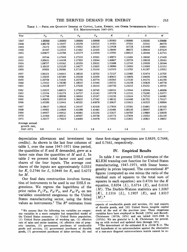
In tables 1 and 2 we tabulate price, quantity, and cost shares of K, L, E, and M, and total input cost. Looking at the first four columns of table 1, we note that over the 1947-1971 time period the prices of K, E, and M rose less rap- idly than the price of L. The slower growth rates of PE and PK are due partly to actions of the federal government, particularly the price ceilings on certain energy types and the favor- able tax treatment given corporations investing in new plant and equipment (the accelerated

5See Dhrymes (1973).

6 The interindustry flow tables described in Faucett (1973) are based on data from the annual Bureau of Mines Minerals Yearbook, the Census of Minerals Industries (1954, 1958, 1963 and 1967), the Census of Manufacturers (1947, 1954, 1958, 1963 and 1967), the U.S. Department of Commerce Input-Output Tables (1947, 1958, 1963), Annual Surveys of Manufacturers, and a variety of secondary sources. This set of accounts was developed with support from the Ford Foundation Energy Policy Project and the Mathematics and Computation Laboratory, Office of Pre- paredness, General Services Administration.

THE DERIVED DEMAND FOR ENERGY 263

TABLE 1.- PRICE AND QUANTITY INDEXES OF CAPITAL, LABOR, ENERGY, AND OTHER INTERMEDIATE INPUTS -

U.S. MANUFACTURING 1947-1971

Year PK PL PB PM K L E M

1947 1.00000 1.00000 1.00000 1.00000 1.00000 1.00000 1.00000 1.00000 1948 1.00270 1.15457 1.30258 1.05525 1.14103 .97501 .92932 .88570 1949 .74371 1.15584 1.19663 1.06225 1.23938 .92728 1.01990 .94093 1950 .92497 1.23535 1.21442 1.12430 1.28449 .98675 1.08416 1.07629 1951 1.04877 1.33784 1.25179 1.21694 1.32043 1.08125 1.18144 1.13711

1952 .99744 1.37949 1.27919 1.19961 1.40073 1.13403 1.18960 1.17410 1953 1.00653 1.43458 1.27505 1.19044 1.46867 1.20759 1.28618 1.30363 1954 1.08757 1.45362 1.30356 1.20612 1.52688 1.13745 1.29928 1.18144 1955 1.10315 1.51120 1.34277 1.23835 1.58086 1.19963 1.33969 1.32313 1956 .99606 1.58186 1.37154 1.29336 1.62929 1.23703 1.41187 1.35013

1957 1.06321 1.64641 1.38010 1.30703 1.72137 1.23985 1.52474 1.35705 1958 1.15619 1.67389 1.39338 1.32699 1.80623 1.16856 1.44656 1.25396 1959 1.30758 1.73430 1.36756 1.30774 1.82065 1.25130 1.54174 1.41250 1960 1.25413 1.78280 1.38025 1.33946 1.81512 1.26358 1.56828 1.40778 1961 1.26328 1.81977 1.37630 1.34319 1.83730 1.24215 1.59152 1.39735

1962 1.26525 1.88531 1.37689 1.34745 1.84933 1.29944 1.65694 1.48606 1963 1.32294 1.93379 1.34737 1.33143 1.87378 1.32191 1.76280 1.59577 1964 1.32798 2.00998 1.38969 1.35197 1.91216 1.35634 1.76720 1.64985 1965 1.40659 2.05539 1.38635 1.37542 1.98212 1.43460 1.81702 1.79327 1966 1.45100 2.13441 1.40102 1.41878 2.10637 1.53611 1.92525 1.90004

1967 1.38617 2.20616 1.39197 1.42428 2.27814 1.55581 2.03881 1.95160 1968 1.49901 2.33869 1.43388 1.43481 2.41485 1.60330 2.08997 2.08377 1969 1.44957 2.46412 1.46481 1.53356 2.52637 1.64705 2.19889 2.10658 1970 1.32464 2.60532 1.45907 1.54758 2.65571 1.57894 2.39503 2.03230 1971 1.20177 2.76025 1.64689 1.54978 2.74952 1.52852 2.30803 2.18852

Average annual growth rate, 1947-1971 0.8 4.3 2.1 1.8 4.3 1.8 3.5 3.3

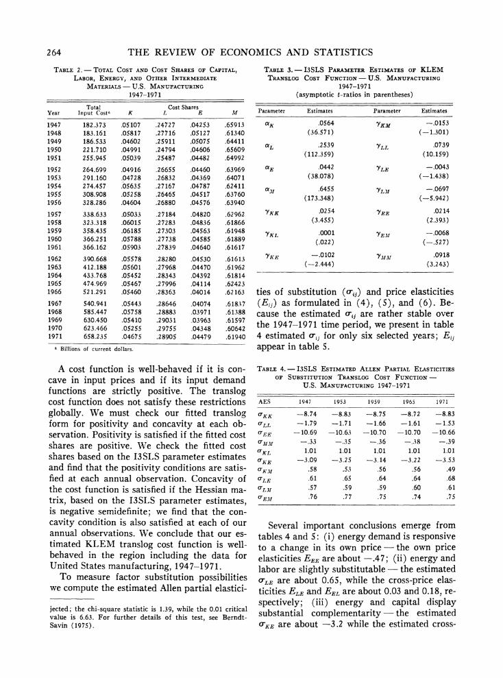
depreciation allowances and investment tax credits). As shown in the last four columns of table 1, over the same 1947-1971 time period, the quantities of E and K demanded, grew at a faster rate than the quantities of M and L. In table 2 we present total factor cost and cost shares of the four inputs. The average cost shares of the inputs are approximately 0.0535 for K, 0.2744 for L, 0.0448 for E, and 0.6272 for M.

Our final data construction involves forma- tion of instruments to be used in our I3SLS re- gressions. We regress the logarithms of the price ratios PL/IP., PE/PK, and PM/PK on ten variables considered exogenous to the United States manufacturing sector, using the fitted values as instruments.7 The R2 estimates from

these first-stage regressions are 0.8839, 0.7648, and 0.7661, respectively.

IV. Empirical Results

In table 3 we present I3SLS estimates of the KLEM translog cost function for United States manufacturing, 1947-1971, with linear homo- geneity in prices imposed. The conventional R2 figures (computed as one minus the ratio of the residual sum of squares to the total sum of squares in each equation) are 0.4736 for the K equation, 0.8204 (L), 0.6714 (E), and 0.6161 (M). The Durbin-Watson statistics are 1.3087 (K), 2.1516 (L), 1.1907 (E), and 1.8517 (M) .8

7 We assume that the following ten variables are exogen- ous variables in a more complete but unspecified model of the United States economy: (1) United States population, (2) United States population of working age, (3) effective rate of sales and excise taxation, (4) effective rate of prop- erty taxation, (5) government purchases of nondurable goods and services, (6) government purchases of durable goods, (7) government purchases of labor services, (8) real

exports of nondurable goods and services, (9) real exports of durable goods, and (10) United States tangible capital stock at the end of the previous year. These exogenous variables have been employed in Berndt (1974) and Berndt- Christensen (1973b, 1974) and are tabled 1929-1968 in (1973b). We are grateful to L. R. Christensen for provid- ing us with revised and updated data through 1971.

8 The determinant of the estimated Q is .35268 E-11. The null hypothesis of no autocorrelation against the alternative of a non-zero diagonal autocovariance matrix cannot be re-

264 THE REVIEW OF ECONOMICS AND STATISTICS

TABLE 2. TOTAL COST AND COST SHARES OF CAPITAL,

LABOR, ENERGY, AND OTHER INTERMEDIATE

MATERIALS - U.S. MANUFACTURING

1947-1971

Total Cost Shares Year Input Costa K L E M

1947 182.373 .05107 .24727 .04253 .65913 1948 183.161 .05817 .27716 .05127 .61340 1949 186.533 .04602 .25911 .05075 .64411 1950 221.710 .04991 .24794 .04606 .65609 1951 255.945 .05039 .25487 .04482 .64992

1952 264.699 .04916 .26655 .04460 .63969 1953 291.160 .04728 .26832 .04369 .64071 1954 274.457 .05635 .27167 .04787 .62411 1955 308.908 .05258 .26465 .04517 .63760 1956 328.286 .04604 .26880 .04576 .63940

1957 338.633 .05033 .27184 .04820 .62962 1958 323.318 .06015 .27283 .04836 .61866 1959 358.435 .06185 .27303 .04563 .61948 1960 366.251 .05788 .27738 .04585 .61889 1961 366.162 .05903 .27839 .04640 .61617

1962 390.668 .05578 .28280 .04530 .61613 1963 412.188 .05601 .27968 .04470 .61962 1964 433.768 .05452 .28343 .04392 .61814 1965 474.969 .05467 .27996 .04114 .62423 1966 521.291 .05460 .28363 .04014 .62163

1967 540.941 .05443 .28646 .04074 .61837 1968 585.447 .05758 .28883 .03971 .61388 1969 630.450 .05410 .29031 .03963 .61597 1970 623.466 .05255 .29755 .04348 .60642 1971 658.235 .04675 .28905 .04479 .61940

a Billions of current dollars.

A cost function is well-behaved if it is con- cave in input prices and if its input demand functions are strictly positive. The translog cost function does not satisfy these restrictions globally. We must check our fitted translogr form for positivity and concavity at each ob- servation. Positivity is satisfied if the fitted cost shares are positive. We check the fitted cost shares based on the I3SLS parameter estimates and find that the positivity conditions are satis- fied at each annual observation. Concavity of the cost function is satisfied if the Hessian ma- trix, based on the I3SLS parameter estimates, is negative semidefinite; we find that the con- cavity condition is also satisfied at each of our annual observations. We conclude that our es- timated KLEM translog cost function is well- behaved in the region including the data for United States manufacturing, 1947-1971.

To measure factor substitution possibilities we compute the estimated Allen partial elastici-

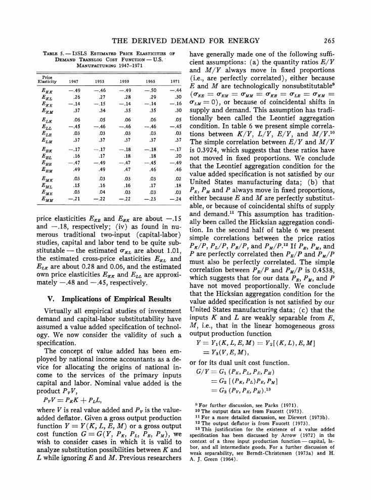
ties of substitution (crij) and price elasticities (Eij) as formulated in (4), (5), and (6). Be- cause the estimated crij are rather stable over the 1947-1971 time period, we present in table 4 estimated (ria for only six selected years; Eij appear in table 5.

Several important conclusions emerge from tables 4 and 5: (i) energy demand is responsive to a change in its own price - the own price elasticities EEE are about -.47; (ii) energy and labor are slightly substitutable - the estimated aLE are about 0.65, while the cross-price elas- ticities ELE and EEL are about 0.03 and 0.18, re- spectively; (iii) energy and capital display substantial complementarity - the estimated a-KE are about -3.2 while the estimated cross-

TABLE 3. - I3SLS PARAMETER ESTIMATES OF KLEM TRANSLOG COST FUNCTION - U.S. MANUFACTURING

1947-1971 (asymptotic t-ratios in parentheses)

Parameter Estimates Parameter Estimates

aK .0564 YKM -.0153

(36.571) (-1.301)

aL .2539 'YL .0739 (112.359) (10.159)

aE .0442 YLE -.0043

(38.078) (-1.438)

am1 .6455 YLM -.0697 (173.348) (-5.942)

YIKK .0254 'EE .0214 (3.455) (2.393)

hYKL .0001 'YEM -.0068 (.022) (-.527)

YKE -.0102 Y.i.t1i .0918 (-2.444) (3.243)

TABLE 4. - I3SLS ESTIMATED ALLEN PARTIAL ELASTICITIES

OF SUBSTITUTION TRANSLOG COST FUNCTION -

U.S. MANUFACTURING 1947-1971

AES 1947 1953 1959 1965 1971

C -KK -8.74 -8.83 -8.75 -8.72 -8.83

0ILL -1.79 -1.71 -1.66 -1.61 -1.53 r,FE -10.69 -10.63 -10.70 -10.70 -10.66

0MMI -.33 -.35 -.36 -.38 -.39

CrKL 1.01 1.01 1.01 1.01 1.01

KEF -3.09 -3.25 -3.14 -3.22 -3.53

0-KM .58 .53 .56 .56 .49

0"LE .61 .65 .64 .64 .68

ol,1.ll .57 .59 .59 .60 .61

0E1I .76 .77 .75 .74 .75

jected; the chi-square statistic is 1.39, while the 0.01 critical value is 6.63. For further details of this test, see Berndt- Savin (1975).

THE DERIVED DEMAND FOR ENERGY 265

TABLE 5. - I3SLS ESTIMATED PRICE ELASTICITIES OF

DEMAND TRANSLOG COST FUNCTION -U.S.

MANUFACTURING 1947-1971

Price Elasticity 1947 1953 1959 1965 1971

EKK -.49 -.46 -.49 -.50 -.44

EKL .26 .2 7 .28 .29 .30

EKE -.14 -.15 -.14 -.14 -.16 EKM .37 .34 .35 .35 .30

ELK .06 .05 .06 .06 .05 ELL -.45 -.46 -.46 -.46 -.45

ELE .03 .03 .03 .03 .03 ELM .37 .37 .37 .37 .37

EEK -.17 -.17 -.18 -.18 -.17

EEL .16 .17 .18 .18 .20 EEE -.47 -.49 -.47 -.45 -.49

EEM .49 .49 .47 .46 .46

EMK .03 .03 .03 .03 .02

EML .15 .16 .16 .17 .18

EME .03 .04 .03 .03 .03 EMM -.21 -.22 -.22 -.23 -.24

price elasticities EKE and EEK are about -.15 and -.18, respectively; (iv) as found in nu- merous traditional two-input (capital-labor) studies, capital and labor tend to be quite sub- stitutable - the estimated crKL are about 1.01, the estimated cross-price elasticities EKL and ELK are about 0.28 and 0.06, and the estimated own price elasticities EKK and ELL are approxi- mately -.48 and -.45, respectively.

V. Implications of Empirical Results

Virtually all empirical studies of investment demand and capital-labor substitutability have assumed a value added specification of technol- ogy. We now consider the validity of such a specification.

The concept of value added has been em- ployed by national income accountants as a de- vice for allocating the origins of national in- come to the services of the primary inputs capital and labor. Nominal value added is the product PvV,

PVV = PKK+PLL,

where V is real value added and P, is the value- added deflator. Given a gross output production function Y = Y(K, L, E, M) or a gross output cost function G = G(Y, PK, PL, PEI PM), we wish to consider cases in which it is valid to analyze substitution possibilities between K and L while ignoring E and M. Previous researchers

have generally made one of the following suffi- cient assumptions: (a) the quantity ratios E/Y and M/Y always move in fixed proportions (i.e., are perfectly correlated), either because E and M are technologically nonsubstitutable9 (TEE EM = CMM = CKE = OLE = OKM

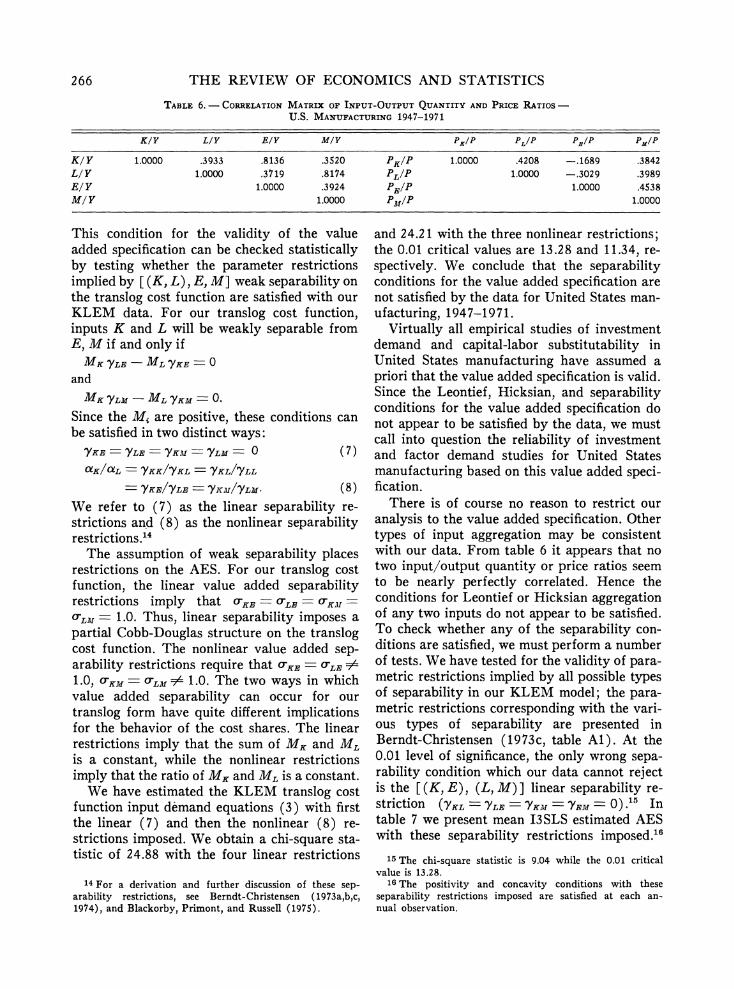
OrLM 0), or because of coincidental shifts in supply and demand. This assumption has tradi- tionally been called the Leontief aggregation condition. In table 6 we present simple correla- tions between K/Y, L/Y, E/Y, and M/Y.'0 The simple correlation between E/Y and M/Y is 0.3924, which suggests that these ratios have not moved in fixed proportions. We conclude that the Leontief aggregation condition for the value added specification is not satisfied by our United States manufacturing data; (b) that PE, PM and P always move in fixed proportions, either because E and M are perfectly substitut- able, or because of coincidental shifts of supply and demand." This assumption has tradition- ally been called the Hicksian aggregation condi- tion. In the second half of table 6 we present simple correlations between the price ratios PK/P, PL/P, PO/P, and PM/P.'2 If Ps, PM, and P are perfectly correlated then PI/P and PM/P must also be perfectly correlated. The simple correlation between PE/P and PM/P is 0.4538, which suggests that for our data PE, PM, and P have not moved proportionally. We conclude that the Hicksian aggregation condition for the value added specification is not satisfied by our United States manufacturing data; (c) that the inputs K and L are weakly separable from E, M, i.e., that in the linear homogeneous gross output production function

Y =Y1 (K, L, E, M) = Yg [ (K, L),I El M] N Y3(V, E, M),

or for its dual unit cost function. G/Y - GI (PK, PL, PE, PM)

- G2 [ (PK, PL) PE, PM] - G3 (PV, PE, PM1) .13

For further discussion, see Parks (1971). 10The output data are from Faucett (1973). 11 For a more detailed discussion, see Diewert (1973b). 12 The output deflator is from Faucett (1973). 13 This justification for the existence of a value added

specification has been discussed by Arrow (1972) in the context of a three input production function - capital, la- bor, and all intermediate goods. For a further discussion of weak separability, see Berndt-Christensen (1973a) and H. A. J. Green (1964).

266 THE REVIEW OF ECONOMICS AND STATISTICS

TABLE 6. - CORRELATION MATRIX OF INPUT-OUTPUT QUANTITY AND PRICE RATIOS -

U.S. MANUFACTURING 1947-1971

K/Y L/Y EIY M/Y PK/P PLIP PE/P Pf/P

K/Y 1.0000 .3933 .8136 .3520 PKIP 1.0000 .4208 -.1689 .3842 L/ Y 1.0000 .3719 .8174 PLIP 1.0000 -.3029 .3989 E/ Y 1.0000 .3924 PEIP 1.0000 .4538 M/ Y 1.0000 PM/P 1.0000

This condition for the validity of the value added specification can be checked statistically by testing whether the parameter restrictions implied by [ (K, L), E, M] weak separability on the translog cost function are satisfied with our KLEM data. For our translog cost function, inputs K and L will be weakly separable from E, M if and only if

MK YLE - ML YKE 0 and

MK YLM - ML YKM -0

Since the M, are positive, these conditions can be satisfied in two distinct ways:

YKE =YLE YKAI MYLM 0 (7) aK/aL YKKI/KL =YKL/YLL

YKE/IYLE -YKJ/IYLM- (8) We refer to (7) as the linear separability re- strictions and (8) as the nonlinear separability restrictions.'4

The assumption of weak separability places restrictions on the AES. For our translog cost function, the linear value added separability restrictions imply that CRKE - LE RKMAr

o-LAI = 1.0. Thus, linear separability imposes a partial Cobb-Douglas structure on the translog cost function. The nonlinear value added sep- arability restrictions require that RKE = OLE # 1.0, 'KM= o-Lm 74 1.0. The two ways in which value added separability can occur for our translog form have quite different implications for the behavior of the cost shares. The linear restrictions imply that the sum of MK and ML is a constant, while the nonlinear restrictions imply that the ratio of MK and ML is a constant.

We have estimated the KLEM translog cost function input demand equations (3) with first the linear (7) and then the nonlinear (8) re- strictions imposed. We obtain a chi-square sta- tistic of 24.88 with the four linear restrictions

and 24.21 with the three nonlinear restrictions; the 0.01 critical values are 13.28 and 11.34, re- spectively. We conclude that the separability conditions for the value added specification are not satisfied by the data for United States man- ufacturing, 1947-1971.

Virtually all empirical studies of investment demand and capital-labor substitutability in United States manufacturing have assumed a priori that the value added specification is valid. Since the Leontief, Hicksian, and separability conditions for the value added specification do not appear to be satisfied by the data, we must call into question the reliability of investment and factor demand studies for United States manufacturing based on this value added speci- fication.

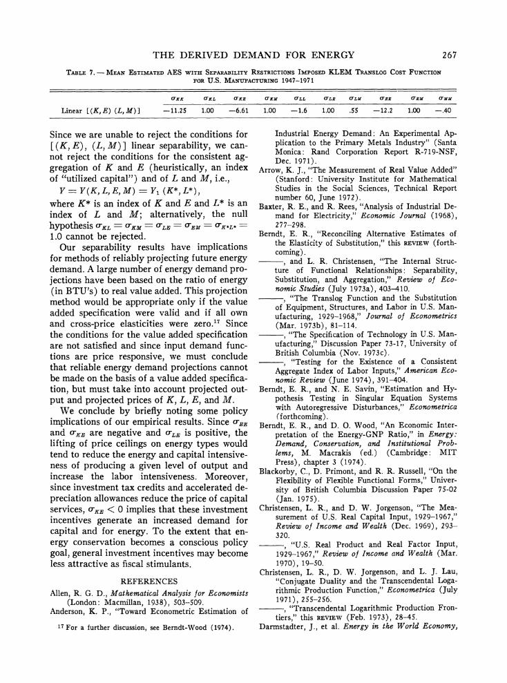
There is of course no reason to restrict our analysis to the value added specification. Other types of input aggregation may be consistent with our data. From table 6 it appears that no two input/output quantity or price ratios seem to be nearly perfectly correlated. Hence the conditions for Leontief or Hicksian aggregation of any two inputs do not appear to be satisfied. To check whether any of the separability con- ditions are satisfied, we must perform a number of tests. We have tested for the validity of para- metric restrictions implied by all possible types of separability in our KLEM model; the para- metric restrictions corresponding with the vari- ous types of separability are presented in Berndt-Christensen (1973c, table Al). At the 0.01 level of significance, the only wrong sepa- rability condition which our data cannot reject is the [(K, E), (L, M)] linear separability re- striction (YKL -

-LE YKJ = YEM 0) .- In table 7 we present mean I3SLS estimated AES with these separability restrictions imposed.'6

14 For a derivation and further discussion of these sep- arability restrictions, see Berndt-Christensen (1973a,b,c, 1974), and Blackorby, Primont, and Russell (1975).

15 The chi-square statistic is 9.04 while the 0.01 critical value is 13.28.

16 The positivity and concavity conditions with these separability restrictions imposed are satisfied at each an- nual observation.

THE DERIVED DEMAND FOR ENERGY 267

TABLE 7. - MEAN ESTIMATED AES WITH SEPARABILITY RESTRICTIONS IMPOSED KLEM TRANSLOG COST FUNCTION

FOR U.S. MANUFACTURING 1947-1971

CXX CXL CXE CXM CLL CLE CLM CXX CEM CMM

Linear [(K,E) (L,M)] -11.25 1.00 -6.61 1.00 -1.6 1.00 .55 -12.2 1.00 -.40

Since we are unable to reject the conditions for [(K, E), (L, M)] linear separability, we can- not reject the conditions for the consistent ag- gregation of K and E (heuristically, an index of "utilized capital") and of L and M, i.e.,

Y = Y(K, L, E, M) = Y, (K*, L*),

where K* is an index of K and E and L* is an index of L and M; alternatively, the null hypothesis CKL = KM = CL =EM = KL

1.0 cannot be rejected. Our separability results have implications

for methods of reliably projecting future energy demand. A large number of energy demand pro- jections have been based on the ratio of energy (in BTU's) to real value added. This projection method would be appropriate only if the value added specification were valid and if all own and cross-price elasticities were zero.17 Since the conditions for the value added specification are not satisfied and since input demand func- tions are price responsive, we must conclude that reliable energy demand projections cannot be made on the basis of a value added specifica- tion, but must take into account projected out- put and projected prices of K, L, E, and M.

We conclude by briefly noting some policy implications of our empirical results. Since oEE

and o-KE are negative and -LE iS positive, the lifting of price ceilings on energy types would tend to reduce the energy and capital intensive- ness of producing a given level of output and increase the labor intensiveness. Moreover, since investment tax credits and accelerated de- preciation allowances reduce the price of capital services, OKE < 0 implies that these investment incentives generate an increased demand for capital and for energy. To the extent that en- ergy conservation becomes a conscious policy goal, general investment incentives may become less attractive as fiscal stimulants.

REFERENCES Allen, R. G. D., Mathematical Analysis for Economists

(London: Macmillan, 1938), 503-509. Anderson, K. P., "Toward Econometric Estimation of

17 For a further discussion, see Berndt-Wood (1974).

Industrial Energy Demand: An Experimental Ap- plication to the Primary Metals Industry" (Santa Monica: Rand Corporation Report R-719-NSF, Dec. 1971).

Arrow, K. J., "The Measurement of Real Value Added" (Stanford: University Institute for Mathematical Studies in the Social Sciences, Technical Report number 60, June 1972).

Baxter, R. E., and R. Rees, "Analysis of Industrial De- mand for Electricity," Economic Journal (1968), 2 77-298.

Berndt, E. R., "Reconciling Alternative Estimates of the Elasticity of Substitution," this REVIEW (forth- coming).

, and L. R. Christensen, "The Internal Struc- ture of Functional Relationships: Separability, Substitution, and Aggregation," Review of Eco- nomic Studies (July 1973a), 403-410.

,"The Translog Function and the Substitution of Equipment, Structures, and Labor in U.S. Man- ufacturing, 1929-1968," Journal of Econometrics (Mar. 1973b), 81-114.

, "The Specification of Technology in U.S. Man- ufacturing," Discussion Paper 73-17, University of British Columbia (Nov. 1973c).

, "Testing for the Existence of a Consistent Aggregate Index of Labor Inputs," American Eco- nomic Review (June 1974), 391-404.

Berndt, E. R., and N. E. Savin, "Estimation and Hy- pothesis Testing in Singular Equation Systems with Autoregressive Disturbances," Econometrica (forthcoming).

Berndt, E. R., and D. 0. Wood, "An Economic Inter- pretation of the Energy-GNP Ratio," in Energy: Demand, Conservation, and Institutional Prob- lems, M. Macrakis (ed.) (Cambridge: MIT Press), chapter 3 (1974).

Blackorby, C., D. Primont, and R. R. Russell, "On the Flexibility of Flexible Functional Forms," Univer- sity of British Columbia Discussion Paper 75-02 (Jan. 1975).

Christensen, L. R., and D. W. Jorgenson, "The Mea- surement of U.S. Real Capital Input, 1929-1967," Review of Income and Wealth (Dec. 1969), 293- 320.

, "U.S. Real Product and Real Factor Input, 1929-1967," Review of Income and Wealth (Mar. 1970), 19-50.

Christensen, L. R., D. W. Jorgenson, and L. J. Lau, "Conjugate Duality and the Transcendental Loga- rithmic Production Function," Econometrica (July 1971), 255-256.

, "Transcendental Logarithmic Production Fron- tiers," this REVIEW (Feb. 1973), 28-45.

Darmstadter, J., et al. Energy in the World Economy,

268 THE REVIEW OF ECONOMICS AND STATISTICS

Resources for the Future, Inc. (Baltimore: Johns Hopkins Press, 1971).

Dhrymes P. J., "Small Sample Asymptotic Relations Between Maximum Likelihood and 3SLS Estima- tors," Econometrica (Mar. 1973), 357-364.

Diewert, W. E., "An Application of the Shephard Dual- ity Theorem: A Generalized Leontief Production Function," Journal of Political Economy (May/ June 1971), 481-507.

, "Separability and the Generalized Cobb-Doug- las Utility Function" (Ottawa: Department of Manpower and Immigration, Jan. 1973a), mimeo.

, "Hicks' Aggregation Theorem and the Existence of a Real Value Added Function" (Ottawa: De- partment of Manpower and Immigration, Jan. 1973b), mimeo.

'"Applications of Duality Theory" in Frontiers of Quantitative Economics, M. Intrilligator and David Kendrick (eds.) (Amsterdam: North-Hol- land, 1974), vol. 2.

Dupree, W. and J. West, "United States Energy Through the Year 2000," U.S. Department of the Interior (Washington: U.S. Government Printing Office, Dec. 1972).

Jack Faucett Associates, "Data Development for the I-0 Energy Model: Final Report" (Chevy Chase, Maryland: Jack Faucett Associates, Inc., May 1973).

Green, H. A. J., Aggregation in Economic Analysis: An Introductory Survey (Princeton: Princeton University Press, 1974).

Morrison, W. E., and C. L. Readling, "An Energy Model for the United States," Bureau of Mines, U.S. Department of the Interior, Information Cir- cular 8384 (Washington: U.S. Government Print- ing Office, 1968).

Mount, T. D., L. D. Chapman, and T. J. Tyrrell, "Elec- tricity Demand in the United States: An Econo- metric Analysis," ORNL-NSF-EP-49 (Oak Ridge, Tennessee: Oak Ridge National Laboratory (June 1973).

National Energy Board, Energy Supply and Demand in Canada and Export Demand for Canadian Energy, 1966 to 1990 (Ottawa: Information Canada, 1971).

National Petroleum Council, U.S. Energy Outlook: An Initial Appraisal, 1971-1985 (Washington: Na- tional Petroleum Council, 1-3, 1971).

Parks, R. W., "Price Responsiveness of Factor Utiliza- tion in Swedish Manufacturing, 1870-1950," this REVIEW (May 1971), 129-139.

Schurr, S. H., et al. Energy in the American Economy, 1850-1975, Resources for the Future, Inc. (Balti- more: Johns Hopkins Press, 1960).

Uzawa, H., "Production Functions with Constant Elas- ticities of Substitution," Review of Economic Studies (Oct. 1962), 291-299.