Embed Size (px)
Citation preview
Munich Personal RePEc Archive
Effective Demand and Prices of
Production: An Evolutionary Approach
Rotta, Tomas
Goldsmiths College, University of London, UK
1 January 2020
Online at https://mpra.ub.uni-muenchen.de/97910/
MPRA Paper No. 97910, posted 08 Jan 2020 09:47 UTC
EFFECTIVE DEMAND AND PRICES OF PRODUCTION:
AN EVOLUTIONARY APPROACH
TOMÁS N. ROTTA
Goldsmiths College, University of London, UK
Institute of Management Studies
ABSTRACT
In this paper I develop an innovative evolutionary framework to integrate Keynes’ short-
run principle of effective demand and the formation of long-run prices of production in
Classical Political Economy. At the intersection of Keynes, Marx, and Kalecki, my
evolutionary framework integrates effective demand, functional income distribution, profit
rate equalization, technological diffusion, and the gravitation towards prices of production.
My approach bridges two gaps at once: the absence of the short-run principle of effective
demand in Classical Political Economy; and the absence of technological diffusion, profit
rate equalization, and the formation of long-run prices of production in Keynes and
Kalecki. To formalize the feedback effects between individual decisions taken at the micro
level and the unintended social outcomes at the macro level I develop a simple model using
replicator dynamics from evolutionary Game Theory. My approach offers a better
understanding of how effective demand determines the rate of exploitation, the
equalization of profit rates, and the convergence of market prices towards prices of
production.
Key words: Effective Demand, Prices of Production, Marx, Keynes, Kalecki
JEL codes: B51, C73, D20*
*Author’s note: The author thanks Duncan Foley, Ozlem Onaran, Zoe Sherman, Engelbert Stockhammer, Simon
Mohun, Eckhard Hein, Ian Seda, Bruno Höfig, Pedro Loureiro, David Eisnitz, and Everest Lindesmith for their
comments and suggestions on previous versions. An earlier version of this paper appeared in the Greenwich Political
Economy Centre (GPERC) working paper series: https://gala.gre.ac.uk/id/eprint/15511/
[1]
1. Introduction
In this paper I develop an innovative evolutionary framework to integrate Keynes’ short-run
principle of effective demand and the formation of long-run prices of production in Classical Political
Economy. At the intersection of Keynes, Marx, and Kalecki, my evolutionary framework integrates
effective demand, functional income distribution, profit rate equalization, technological diffusion, and the
gravitation of market prices towards prices of production.
The incorporation of Keynes’ principle of effective demand into the framework of Classical
Political Economy offers a better understanding of how aggregate demand determines the rate of
exploitation, the behavior of profit rates, and the formation of prices of production in the long run. My
approach therefore bridges two gaps at once. The first gap relates to the absence of the short-run principle
of effective demand in Classical Political Economy, most markedly in the canonical works of Smith, Say,
Ricardo, and Mill. The usual procedure in Classical Political Economy was to employ Say’s Law in either
one of its two versions, namely Say’s Identity or Say’s Equality, hence downgrading aggregate demand to
a passive role (Becker and Baumol 1952; Baumol 1977, 1999; Robison 1947; Shoul 1957; Foley 1985).
The second gap relates to the absence of technological diffusion, profit rate equalization, and the formation
of long-run prices of production in the works of Keynes and Kalecki. Neither Keynes nor Kalecki showed
how competition at the micro level would equalize profit rates and converge market prices towards prices
of production in the long run.
My framework draws from Marx’s insights in chapters IX and XV in Capital III, from Keynes’
principle of effective demand, and from Kalecki’s insights on macroeconomic aggregates. In my approach,
aggregate demand determines the amount of value realized. And profit rates equalize across sectors as long
as profitability responds negatively to the capital committed to production in each sector. Over-supply in
one sector will erode profits in that sector and firms will search for more profitable opportunities elsewhere.
[2]
Once effective demand is brought into Classical Political Economy, the distinction between the
source of value and the determination of the quantitity of value becomes crucial. In this paper I take the
Marxist stance that value is the social form of labor in capitalism, whose quantity is determined by the
abstract labor time socially necessary to reproduce commodities. As Rubin ([1928]1972) noted, the term
“socially necessary” has a double meaning. It means socially necessary in the supply-side sense that the
existing technology and cost structures determine what and how firms can produce. But “socially
necessarily” also has a demand-side dimension under which value needs social validation to become value
in the first place. Hence, the “socially necessary” character of value determination must be understood at
the intersection of supply and demand aspects. There is, therefore, no such a thing as non-realized values,
for value must be realized to be conceptualized as value. Value that is not realized is not value: “It is only
by being exchanged that the products of labour acquire a socially uniform objectivity as values” (Marx
[1887]1990, p.166), as the “different kinds of individual labour represented in these particular use values,
in fact, become labour in general, and in this way social labour, only by actually being exchanged” (Marx
[1859]1989, p. 286).
A central feature of my approach is the distinction between the ex ante and the ex post rates of
exploitation. Marx ([1894]1994, p.352-353) himself introduced this distinction in chapter XV of Capital
III where he theorized the difference between “immediate exploitation” at the point of production, which
is the source of value, and “realized exploitation” at the point of exchange, which determines the quantity
of value. The distinction between the ex ante and the ex post rates of exploitation is what allows for the
integration of Keynes’ principle of effective demand, as well as Kalecki’s macroeconomic aggregates, into
the Marxist framework of accumulation and distribution.
In my framework I additionally introduce competition at the firm level through cost-reducing
technological progress. And because the real wage in endogenous to aggregate demand, the Okishio (1961)
theorem no longer holds. Okishio (1961) had originally demonstrated that in a Marxist framework with an
exogenous real wage, technical change will lead the average profit rate not to fall but in fact to rise. In my
[3]
evolutionary approach, on the contrary, technical change can reduce profitability over the long run even if
it temporarily raises profit rates for the initial adopters.
In this paper I build on the existing scholarship and develop an evolutionary model that closely
mimics Marx’s original insights on exploitation, accumulation, and technological progress in volume III of
Capital. I build a simple model using replicator dynamics from evolutionary Game Theory to describe the
competitive selection that occurs simultaneously at the micro intra-sector and at the macro inter-sector
levels. The replicator dynamics describe an updating process with random interactions in which behaviors
with higher payoffs proliferate. It is a useful device to mimic the competitive struggle for survival in natural
and social environments, for it models the process of equilibration by tracking the results of individual
interactions (Bowles 2006; Gintis 2009; Prado 2006, 2002). The proposed framework formalizes key
aspects of the Classical Political Economy approach to accumulation and profitability in an adaptive system,
in which agents control their actions but not the aggregate consequences of their individual decisions. Micro
decisions produce unintended macro outcomes that then feed back again into micro decisions.
My framework brings together the principle of effective demand from Keynes, the theory of value
from Classical Political Economy, and the evolutionary approach to modelling from Game Theory. It
therefore allows us to integrate Keynes’, Marx’, and Kalecki’s insights on profit equalization, prices of
production, and the role of aggregate demand in the realization of value and surplus value. By incorporating
Keynes’ principle of effective demand into the Classical Political Economy theory of value and distribution,
I am able to offer a better understanding of how aggregate demand determines the behavior of profit rates
and of prices of production in the longer run.
2. Effective Demand and Say’s Law
The principle of effective demand remains a hotly debated concept even within the post-Keynesian
tradition. In this paper I follow Chick (1983), Hayes (2019; 2007), Hartwig (2007), Allain (2009), and
[4]
Casarosa (1981) in their understanding of effective demand as the firms’ effective commitment to
production. Given the technology and cost structure, effective demand refers to how expected profitability
determines supply and employment decisions at the beginning of the production period. Hence, this ex ante
commitment to produce is not identical to the ex post aggregate expenditures with consumption and
investment. Effective demand is the firms’ profit-maximizing expected proceeds, an ex ante concept
relating to expectations but revised in line with ex post realized incomes. Even though aggregate demand
and aggregate expenditure are not identical, they can be equal when ex ante expectations are fulfilled ex
post, but not otherwise. Therefore, “effective demand is an unfortunate term, for it really refers to the output
that will be supplied; in general there is no assurance that it will also be demanded” (Chick 1983, p.65).
In Kalecki’s work effective demand is featured but is not identical to that of Keynes. Assuming
workers do not save, the capitalists’ aggregate expenditures with investment and consumption goods
determine the level of aggregate profits. Workers spend what they get, while capitalists get what they spend.
Real aggregate gross profit is determined entirely at the macro level, while income and output are set in the
interaction between the micro and macro levels (Kriesler 1989). Kalecki derives his theory of effective
demand from the national account identities and from the fact that capitalists decide their expenditures but
not their incomes. As in Keynes, investment is autonomous from savings, and changes in income ensure
that savings accommodate to the level of investment.
In Marxist theory the principle of effective demand means that the expected profit rate determines
the firms’ constant and variable capitals advanced at the beginning of the production period, as well as the
firms’ supply of commodities in the current production period. Market prices can change during the
production period, but output changes only in the transition from one production period to the next. The
beginning-of-period expenditures, which comprise the firms’ effective commitment to production, will then
realize the values created at the end of the previous production period. Because the economy is structured
as a chain of production periods (or circuits of capital as Marx put it), the ex ante aggregate demand at the
[5]
beginning of a production period is also at the same time the expenditure that realizes ex post the values
created in the preceding production period.
In the works of Smith, Say, and Ricardo − on the contrary − growth, cycles, and recessions were
not demand-driven but actually supply-driven phenomena. With notable exceptions such as Marx and
Malthus, Say’s Law was a key element at the core of Classical Political Economy. Ricardo often claimed
in many of his writings that cycles are not caused by aggregate demand deficiency but in fact by
miscalculations about what to produce and in what proportions. The crucial issue was therefore not a lack
of aggregate demand but a temporary mismatch between the composition of aggregate demand and
aggregate supply, solved through the continuous movement of capitals across sectors. Say and Ricardo
attributed economic crisis not to oversupply but in fact to underproduction (Béraud and Numa 2018; Kates
1997; Becker and Baumol 1952; Baumol 1977, 1999; Vianello 1989).
Becker and Baumol (1952) and Baumol (1977; 1999) were the first to notice the ambiguity of the
term ‘Say’s Law’ in Classical Political Economy. This ambiguity is present in Say’s own work and further
reproduced by James Mill, David Ricardo, Marx, Keynes, Oskar Lange, and also by Kalecki. Becker and
Baumol pointed out that Say’s Law actually has two versions, one stronger (Say’s Identity) and one weaker
(Say’s Equality). They proposed the following definitions:
(i) Walras’ Law: Total demand (including the demand for money) equals total supply
(including the supply of money). This is just a definition; no direction of causality is
implied between supply and demand.
(ii) Say’s Identity (stronger version): Total supply automatically becomes, and is identical to,
total demand. This happens because no one ever wants to hold cash, so all sales incomes
are immediately spent on other goods and services. The demand for money does not affect
aggregate demand, supply, or income. Money is just a veil. Recessions and cycles can
occur but are entirely supply-driven.
[6]
(iii) Say’s Equality (weaker version): Demand is supply-led and the equilibrium between
aggregate demand and aggregate supply is stable, such that deviations from it are possible
but self-correcting. Because of supply-side issues such as coordination problems and
miscalculations, recessions and cycles are possible though brief. Money can be used as a
store of value, and as a medium of exchange the supply of money is determined
endogenously.
Say’s Law in either of its two versions and Keynes’ principle of effective demand determine in
very different ways the direction of causality between the core elements of Marxist theory (Trigg 2006).
An example of this is the direction of causality between aggregate demand and the profit rate. A substantial
branch of the Marxist tradition would assign the profit rate as the cause and demand as the effect, which
amounts to deploying Say’s Law and making the economy supply-led. Discussions of the tendency of the
profit rate to fall feature this type of reasoning. For underconsumptionists, on the contrary, the profit rate is
the effect and aggregate demand is the cause, in which case the profit rate becomes itself endogenous to
demand.
Because of his death in 1883, Marx left unfinished the drafts of the second and third volumes of
Capital. Engels later edited and published the manuscripts in the 1890s, but the connections between
effective demand, exploitation, and accumulation were left incomplete. Since the advent of Keynesian and
Kaleckian macroeconomics in the 1930s, heterodox scholars have attempted to offer new insights into how
the theory of effective demand relates to Marx’s theory of value and accumulation (Shaikh 2016, 1989;
Foley 1985, 1983; Baran and Sweezy 1968), but a comprehensive model is still needed.
In the next section I discuss how effective demand determines the realization of values and the
equalization of profit rates in the formation of prices of production.
[7]
3. Exploitation, Profit Rate Equalization, and Production Prices
In chapter IX of Capital III, Marx theorized the equalization of profit rates and the formation of
long-run prices of production. In chapter XV of the same volume, Marx then considered the difference
between the ex ante and ex post rates of exploitation, explicitly mentioning the role of aggregate
expenditures (consumption plus investment) in the realization of exploitation:
The conditions for immediate exploitation and for the realization of that exploitation are not
identical. Not only are they separate in time and space, they are also separate in theory. The former
is restricted only by the society's productive forces, the latter by the proportionality between the
different branches of production and by the society's power of consumption. And this is determined
… by the power of consumption within a given framework of antagonistic conditions of distribution
[…]. It is further restricted by the drive for accumulation, the drive to expand capital and produce
surplus-value on a larger scale (Marx [1894]1994, p.352-353 – emphasis added).
In the 1930s, Kalecki built on Marx’s insights to claim that the volume of real aggregate gross
profit is determined at the macro level by the capitalists’ aggregate expenditures. Assuming workers do not
save, capitalists cannot realize more surplus value in the aggregate than their own expenditures (Sardoni
2009; 1989). No matter how large the ex ante rate of exploitation in the production sphere, the capitalist
class can only realize an ex post rate of exploitation that makes total profits match their own expenditures.
Kalecki, however, did not explain how profit rates would equalize across sectors and hence ignored prices
of production in his analysis (Jossa 1989; Vianello 1989).
The gravitation of market prices toward prices of production has been the object of rigorous study
in the Marxist literature. These studies offer a level of technical detail that is much more precise than the
numerical and verbal examples that Marx offered in volumes II and III of Capital. In this literature there is
an agreement on three main results: (i) profit rates do not always equalize and thus prices of production
cannot always function as stable attractors for market prices (Harris 1972; Nikaido 1983, 1985; Flaschel
[8]
and Semmler 1985; Boggio 1985, 1990; Kubin 1990; Duménil and Lévy 1999, 1995; Prado 2006); (ii)
market prices that ensure balanced reproduction across sectors are not necessarily the set of prices that can
also ensure profit rate equalization (Cockshott 2017); (iii) free capital mobility and competition among
capitals lead to the equalization of profit rates, while free labor mobility and competition among workers
lead to the equalization of the rates of exploitation (Foley 2018; Cogliano 2011).
On the empirical side of the literature (Scharfenaker and Foley 2017; Scharfenaker and Semieniuk
2017; Fröhlich 2013; Farjoun and Machover 1983) there has been a growing consensus that profitability
converges not to a single uniform profit rate but actually to a statistical equilibrium distribution of profit
rates with a tent shape around a single peak. Shaikh (2016) shows, however, that profit rates on new
investment projects (what Keynes labeled the ‘marginal efficiency of capital’) tend to equalize over time.
Scharfenaker and Foley (2017), in particular, developed a model based on thermodynamics and quantal
responses to explain the tent-shaped distribution of profit rates across firms. My evolutionary approach
does not explain the statistical distribution of profit rates but it does provide a theoretical framework in
which effective demand realizes the values created in production and determines the behavior of profit rates
in the long run.
Building on top of the existing literature, in the next sections I develop my evolutionary model of
accumulation and competition amid technological progress. First, I formalize the macro inter-sector
competition through which the aggregate and growing monetary capital of an economy is continuously
redistributed between two sectors: sector I produces the means of production and sector II produces the
final consumption good. The continuous redirection of monetary capital between sectors takes place
according to profit rate differentials. Second, I formalize the micro intra-sector competition in which
individual firms within each sector compete against each other via cost-reducing technical change.
Innovations are gradually adopted based on profit rate differentials within sectors. I then close the model
using the principle of effective demand and make exploitation, profit, and growth all dependent upon the
level of aggregate demand. Profit rates equalize and market prices converge toward production prices. At
[9]
the end I present computer simulations, an analysis of the evolutionary stability of the long-run equilibria,
and an explanation of the conditions under which market prices converge to prices of production.
4. Macro Inter-Sector Competition
The economy-wide circuit of capital, which starts and ends with capital in the form of money, and
which represents the production period during time 𝑡 can be summarized through the aggregation in (1).
Variables with primes (′) are ex post (after production has taken place) while variables without primes are
ex ante (before production takes place):
𝑀𝑡 − 𝐶𝑡 { 𝐿𝑃𝑀𝑃 … 𝑃 … 𝐶𝑡′ − 𝑀𝑡′ (1)
An initial amount of monetary capital 𝑀𝑡 purchases two types of commodities as inputs 𝐶𝑡: labor
power (LP) and means of production (MP). During the subsequent production phase (… 𝑃 …) labor power
creates more value than its own. The difference between the value that labor power creates and the value
of labor power itself is the surplus value. The total value of the gross output 𝐶𝑡′ contains the new value
added created by productive workers plus the pre-existing value transferred from the means of production.
The gross output exchanges for a sum of money represented by the aggregate gross expenditures 𝑀𝑡′. The
extra value that workers create and for which they receive no compensation is the basis for the gross profits ∆𝑀𝑡 = 𝑀𝑡′ − 𝑀𝑡 in the system.
The economy comprises two sectors, each producing a single type of output using both labor power
and means of production. Sector I supplies a homogenous type of means of production. Sector II supplies
a homogenous type of final consumption good. Economic events take place temporally, therefore the
overlap of any two consecutive circuits of capital can be represented as follows:
[10]
𝑀𝑡 − 𝐶𝑡 { 𝐿𝑃𝑀𝑃 … 𝑃 … 𝐶𝑡′ − 𝑀𝑡′ 𝑀𝑡+1 − 𝐶𝑡+1 { 𝐿𝑃𝑀𝑃 … 𝑃 … 𝐶𝑡+1′ − 𝑀𝑡+1′
(2)
The new circuit formally repeats the preceding one. The crucial causal relation is then that between
the total value realized 𝑀𝑡′ at the end of the first circuit and the total monetary capital 𝑀𝑡+1 advanced at the
beginning of the following circuit. Because of its supply-led principle, Say’s Law in any of its versions
would mean that causality runs from 𝑀𝑡 to 𝑀𝑡′ and then to 𝑀𝑡+1. The principle of effective demand, on the
contrary, implies that the direction of causality actually runs from the ex ante demand 𝑀𝑡+1 at the beginning
of the new production period to the realization of the total value 𝑀𝑡′ at the end of the previous production
period.
There is no fixed capital in this economy, so non-labor inputs are circulating capital only. The
means of production that enter as inputs in sectors I and II are the previous output of sector I in the preceding
production period. Technology is represented by a linear production structure with fixed coefficients and
constant returns to scale. Using 𝑎𝑗𝑖 to indicate the quantity of input 𝑗 per unit of output 𝑖, the matrix of
input-output coefficients is:
𝐴 = [𝑎𝑗𝑖] = [𝑎11 𝑎120 0 ] with 0 ≤ 𝑎𝑗𝑖 < 1 (3)
Using 𝑙𝑖 to indicate the quantity of labor hours per unit of output in sector 𝑖, 𝑟𝑖,𝑡 to indicate the
within-sector profit rate per unit of output, 𝑝𝑖 to indicate the market price per unit of output, and 𝑤 to
indicate the money wage per work hour, then per unit of output we have [𝑝𝑗,𝑡−1𝑎𝑗𝑖 + 𝑤𝑙𝑖](1 + 𝑟𝑖,𝑡) = 𝑝𝑖,𝑡.
For each sector the price system is:
[11]
[𝑝1,𝑡−1𝑎11 + 𝑤𝑙1](1 + 𝑟1,𝑡) = 𝑝1,𝑡
[𝑝1,𝑡−1𝑎12 + 𝑤𝑙2](1 + 𝑟2,𝑡) = 𝑝2,𝑡
(4)
The first term inside the brackets on the left-hand side represents constant capital, and the second
term represents variable capital or the value of labor power, both in money terms. Their summation [𝑝𝑗,𝑡−1𝑎𝑗𝑖 + 𝑤𝑙𝑖] is the unit cost. Competition within each sector then simultaneously determines profit
rates and prices.
Although the nominal wage per work hour 𝑤 is exogenously given by the bargaining power
between workers and capitalists, the real wage 𝑤𝑝2,𝑡 in terms of quantities of the consumption good produced
in sector II is determined endogenously. As in the “New Interpretation” (Foley 2018), values are expressed
in money terms and workers get their money wages and spend it as they like, not bound to any real wage
specified in terms of a bundle of goods. Labor supply and credit are assumed not to be binding constraints
on growth.
In each sector there is a collection of several firms and each of them can switch between sectors
depending on the average profitability �̅�𝑖,𝑡. Capitalists commit their capitals to where they expect to profit
the most. But once firms flow into a sector aiming at the prevailing �̅�𝑖,𝑡 they will immediately and
unintentionally alter this average profitability. Supposing a very large collection of firms in the economy,
we can normalize the total number of firms to unity and then consider only the evolution of population
shares, with 𝑓1,𝑡 representing the fraction committed to sector I and 𝑓2,𝑡 the fraction committed to sector II:
𝑀𝑡 = 𝑓1,𝑡𝑀𝑡 + 𝑓2,𝑡𝑀𝑡 = 𝑀1,𝑡 + 𝑀2,𝑡 with 𝑓1,𝑡 + 𝑓2,𝑡 = 1 (5)
Outputs 𝑥𝑖,𝑡 supplied by each sector are the sectoral monetary capitals advanced divided by the
respective unit costs. Sectoral supply expands when more monetary capital is advanced in the sector at the
beginning of the production period, and it contracts when capitalists withdraw their initial expenditures:
[12]
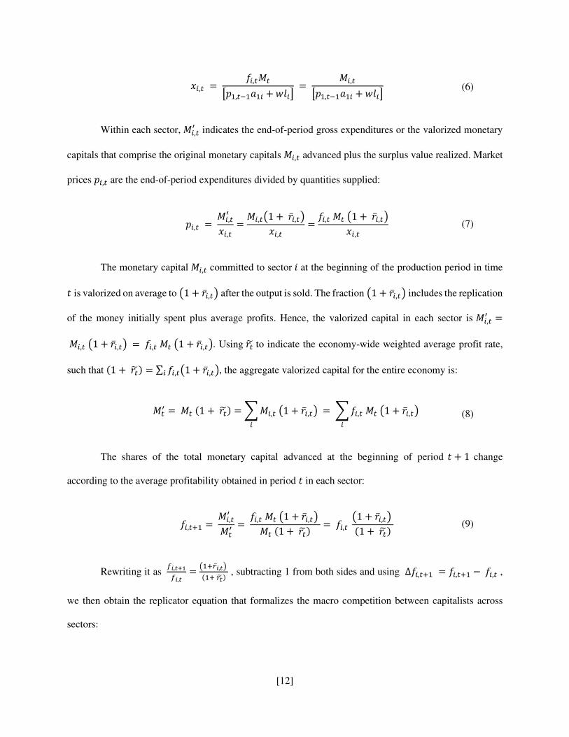
𝑥𝑖,𝑡 = 𝑓𝑖,𝑡𝑀𝑡[𝑝1,𝑡−1𝑎1𝑖 + 𝑤𝑙𝑖] = 𝑀𝑖,𝑡[𝑝1,𝑡−1𝑎1𝑖 + 𝑤𝑙𝑖] (6)
Within each sector, 𝑀𝑖,𝑡′ indicates the end-of-period gross expenditures or the valorized monetary
capitals that comprise the original monetary capitals 𝑀𝑖,𝑡 advanced plus the surplus value realized. Market
prices 𝑝𝑖,𝑡 are the end-of-period expenditures divided by quantities supplied:
𝑝𝑖,𝑡 = 𝑀𝑖,𝑡′𝑥𝑖,𝑡 = 𝑀𝑖,𝑡(1 + �̅�𝑖,𝑡)𝑥𝑖,𝑡 = 𝑓𝑖,𝑡 𝑀𝑡 (1 + �̅�𝑖,𝑡)𝑥𝑖,𝑡 (7)
The monetary capital 𝑀𝑖,𝑡 committed to sector 𝑖 at the beginning of the production period in time 𝑡 is valorized on average to (1 + �̅�𝑖,𝑡) after the output is sold. The fraction (1 + �̅�𝑖,𝑡) includes the replication
of the money initially spent plus average profits. Hence, the valorized capital in each sector is 𝑀𝑖,𝑡′ = 𝑀𝑖,𝑡 (1 + �̅�𝑖,𝑡) = 𝑓𝑖,𝑡 𝑀𝑡 (1 + �̅�𝑖,𝑡). Using 𝑟�̃� to indicate the economy-wide weighted average profit rate,
such that (1 + 𝑟�̃�) = ∑ 𝑓𝑖,𝑡(1 + �̅�𝑖,𝑡)𝑖 , the aggregate valorized capital for the entire economy is:
𝑀𝑡′ = 𝑀𝑡 (1 + 𝑟�̃�) = ∑ 𝑀𝑖,𝑡 (1 + �̅�𝑖,𝑡) 𝑖 = ∑ 𝑓𝑖,𝑡 𝑀𝑡 (1 + �̅�𝑖,𝑡) 𝑖 (8)
The shares of the total monetary capital advanced at the beginning of period 𝑡 + 1 change
according to the average profitability obtained in period 𝑡 in each sector:
𝑓𝑖,𝑡+1 = 𝑀𝑖,𝑡′𝑀𝑡′ = 𝑓𝑖,𝑡 𝑀𝑡 (1 + �̅�𝑖,𝑡) 𝑀𝑡 (1 + 𝑟�̃�) = 𝑓𝑖,𝑡 (1 + �̅�𝑖,𝑡) (1 + 𝑟�̃�) (9)
Rewriting it as 𝑓𝑖,𝑡+1𝑓𝑖,𝑡 = (1+�̅�𝑖,𝑡) (1+ 𝑟�̃�) , subtracting 1 from both sides and using Δ𝑓𝑖,𝑡+1 = 𝑓𝑖,𝑡+1 − 𝑓𝑖,𝑡 ,
we then obtain the replicator equation that formalizes the macro competition between capitalists across
sectors:
[13]
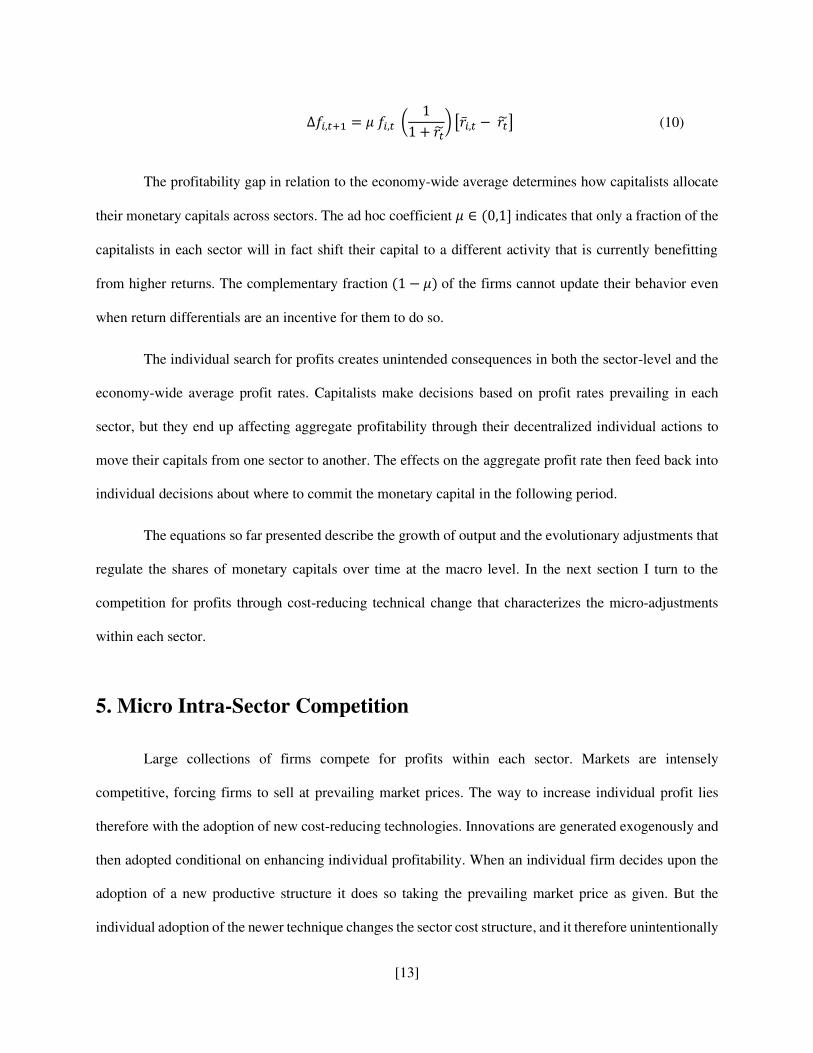
Δ𝑓𝑖,𝑡+1 = 𝜇 𝑓𝑖,𝑡 ( 11 + 𝑟�̃�) [�̅�𝑖,𝑡 − 𝑟�̃�] (10)
The profitability gap in relation to the economy-wide average determines how capitalists allocate
their monetary capitals across sectors. The ad hoc coefficient 𝜇 ∈ (0,1] indicates that only a fraction of the
capitalists in each sector will in fact shift their capital to a different activity that is currently benefitting
from higher returns. The complementary fraction (1 − 𝜇) of the firms cannot update their behavior even
when return differentials are an incentive for them to do so.
The individual search for profits creates unintended consequences in both the sector-level and the
economy-wide average profit rates. Capitalists make decisions based on profit rates prevailing in each
sector, but they end up affecting aggregate profitability through their decentralized individual actions to
move their capitals from one sector to another. The effects on the aggregate profit rate then feed back into
individual decisions about where to commit the monetary capital in the following period.
The equations so far presented describe the growth of output and the evolutionary adjustments that
regulate the shares of monetary capitals over time at the macro level. In the next section I turn to the
competition for profits through cost-reducing technical change that characterizes the micro-adjustments
within each sector.
5. Micro Intra-Sector Competition
Large collections of firms compete for profits within each sector. Markets are intensely
competitive, forcing firms to sell at prevailing market prices. The way to increase individual profit lies
therefore with the adoption of new cost-reducing technologies. Innovations are generated exogenously and
then adopted conditional on enhancing individual profitability. When an individual firm decides upon the
adoption of a new productive structure it does so taking the prevailing market price as given. But the
individual adoption of the newer technique changes the sector cost structure, and it therefore unintentionally
[14]
affects the market price. The new market price then operates as a signal for the remaining firms to also
adopt the cost-reducing technique. Each sector will thus display a production structure that is a combination
of firms producing with the new technique and firms still producing with the old technique.
The economy has three evolutionary processes taking place concurrently. The first is the
evolutionary diffusion of new techniques in the sector producing means of production. The second is the
evolutionary diffusion of new techniques in the sector producing final consumption goods. The third is the
evolutionary distribution of the growing aggregate monetary capital between sectors. An individual
decision to adopt a new technique thus triggers a chain of reactions and feedback effects that no individual
capitalist can anticipate. Externalities exist in this economy given that firms do not fully internalize the
social consequences of their individual actions.
The prevailing technique of production is represented in the set of four technical parameters
(𝑎11𝑜 , 𝑎12𝑜 , 𝑙1𝑜, 𝑙2𝑜). An innovation (𝑎11𝑛 , 𝑎12𝑛 , 𝑙1𝑛, 𝑙2𝑛) can imply the use of more of labor power and means of
production, less of both inputs, or more of one input and less of the other (superscript 𝑜 for ‘old’ and 𝑛 for
‘new’ technique). Rearranging the price equations in (4) we get the profit rate per unit produced using the
old technology:
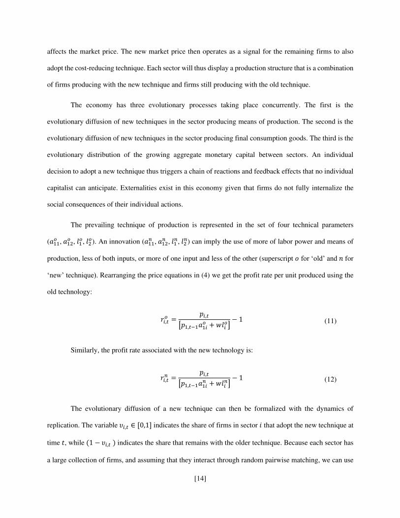
𝑟𝑖,𝑡𝑜 = 𝑝𝑖,𝑡[𝑝1,𝑡−1𝑎1𝑖𝑜 + 𝑤𝑙𝑖𝑜] − 1 (11)
Similarly, the profit rate associated with the new technology is:
𝑟𝑖,𝑡𝑛 = 𝑝𝑖,𝑡[𝑝1,𝑡−1𝑎1𝑖𝑛 + 𝑤𝑙𝑖𝑛] − 1 (12)
The evolutionary diffusion of a new technique can then be formalized with the dynamics of
replication. The variable 𝜐𝑖,𝑡 ∈ [0,1] indicates the share of firms in sector 𝑖 that adopt the new technique at
time 𝑡, while (1 − 𝜐𝑖,𝑡 ) indicates the share that remains with the older technique. Because each sector has
a large collection of firms, and assuming that they interact through random pairwise matching, we can use
[15]
a simple replicator equation for the diffusion of innovations. Normalizing population sizes to unity allows
us to work with population shares in each sector as follows:
𝜐𝑖,𝑡+1 = 𝜐𝑖,𝑡 + 𝜐𝑖,𝑡(1 − 𝜐𝑖,𝑡)[𝑟𝑖,𝑡𝑛 − 𝑟𝑖,𝑡𝑜 ] ∆𝜐𝑖,𝑡+1 = 𝜐𝑖,𝑡(1 − 𝜐𝑖,𝑡)[𝑟𝑖,𝑡𝑛 − 𝑟𝑖,𝑡𝑜 ] ∆𝜐𝑖,𝑡+1 = 𝜐𝑖,𝑡[𝑟𝑖,𝑡𝑛 − �̅�𝑖,𝑡] (13)
The term 𝜐𝑖,𝑡(1 − 𝜐𝑖,𝑡) is the variance of the firms within each sector and the term [𝑟𝑖,𝑡𝑛 − 𝑟𝑖,𝑡𝑜 ] is
the differential replication selection, so that the updating process is payoff monotonic. The third line in
equation (13) follows from the fact that the average profit rate in each sector is: �̅�𝑖,𝑡 = (𝜐𝑖,𝑡)[𝑟𝑖,𝑡𝑛 ] +(1 − 𝜐𝑖,𝑡)[𝑟𝑖,𝑡𝑜 ]. Technical change and its evolutionary diffusion imply that older and newer cost structures coexist
until the newer technique completely replaces the older one. Given the monetary capital 𝑀𝑖,𝑡 committed to
each sector, the new quantities supplied can be found by dividing the monetary capital advanced by the
mixed cost structure:
𝑥𝑖,𝑡 = 𝑀𝑖,𝑡(𝜐𝑖,𝑡)[𝑝1,𝑡−1𝑎1𝑖𝑛 + 𝑤𝑙𝑖𝑛] + (1 − 𝜐𝑖,𝑡)[𝑝1,𝑡−1𝑎1𝑖𝑜 + 𝑤𝑙𝑖𝑜] (14)
The supply equation in (14) thus replaces the supply equation in (6), which only applied to
production under a single technology. Average rates of profit in each sector now depend on the prevailing
market prices and on the linear combination between older and newer techniques:
�̅�𝑖,𝑡 = 𝑝𝑖,𝑡(𝜐𝑖,𝑡)[𝑝1,𝑡−1𝑎1𝑖𝑛 + 𝑤𝑙𝑖𝑛] + (1 − 𝜐𝑖,𝑡)[𝑝1,𝑡−1𝑎1𝑖𝑜 + 𝑤𝑙𝑖𝑜] − 1 = ∆𝑀𝑖,𝑡𝑀𝑖,𝑡 (15)
As soon as profit rates in each sector change from their previous position they trigger intra-sector
competition via the micro replicator dynamic in equation (13) as well as inter-sector competition via the
macro replicator dynamic in equation (10). The out-of-equilibrium adjustments and the evolution of the
[16]
system over time explicitly reflect the interplay of unintended social consequences of uncoordinated
individual actions. In the next section I analyze the stationary states that might prevail in the long run.
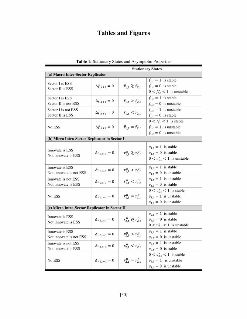
6. Long-Run Equilibria and Evolutionary Stability
The model becomes more intuitive if we focus on the trajectories of the three replicator
equations (𝑓1,𝑡, 𝜐1,𝑡, 𝜐2,𝑡) toward their long-run stationary states. Stationary states are those states at which
the replicator reaches a fixed point with no further changes in the replication process (∆𝑓1,𝑡 = 0, ∆𝜐1,𝑡 =0, ∆𝜐2,𝑡 = 0). The crucial procedure is to know which strategies are going to prevail asymptotically when 𝑡 → ∞.
In an evolutionary game with replicator dynamics we know that the evolutionarily stable strategies
prevail over the long run. An evolutionarily stable strategy (ESS) is a best response to itself and hence it is
a symmetric Nash equilibrium that is also asymptotically stable in its respective replicator equation.
Evolutionary stability implies both self-correction and asymptotic attractiveness (i.e., it is a stable attractor),
hence the system converges over time to a stationary point that is evolutionarily stable (Bowles 2006; Gintis
2009; Elaydi 2005; Scheinerman 2000).
In Table 1 I summarize the stationary states and asymptotic properties of each replicator equation.
Note that in the macro inter-sector dynamic, when there is no ESS, the system converges to an interior
stable solution 𝑓1∗ such that average profit rates are equalized asymptotically across sectors. In this case,
profit rates are not just equal across sectors but truly equalized in the sense that the equality in sector
profitability is evolutionarily stable. In the Appendix I provide a formal stability analysis of the stationary
states.
[Table 1 about here]
[17]
Because the technical coefficients in the input-output matrix are exogenous but not constant, a
strategy that was an ESS before the technical change might not be an ESS after the innovation is introduced.
As long as we have exogenous innovations brought into the system, the ESS’s themselves will change over
time. The closure imposed on the system will determine which strategies are ESS, which long-run
equilibrium will prevail, and whether or not the stationary state will be stable. In the next section I use
Keynes’ principle of effective demand as the model closure.
7. Effective Demand and the Realization of Value
In this section I offer a model closure in which the realization of value and surplus value is
endogenous and dependent upon Keynes’ principle of effective demand. Once effective demand is brought
into the framework the realized rate of exploitation, the profit rates and, hence, the distribution of income
between wages and profits become dependent upon the demand side.
Because effective demand determines the amount of surplus value realized and hence the ex post
rates of exploitation, profitability becomes sensitive to the amount of monetary capital committed to each
sector. Profit rates equalize as long as the average profit rate of a sector increases less than the competing
profit rate when the firms committing their capital to that sector increase their share in the population, or
simply d�̅�1,𝑡d𝑓1,𝑡 < d�̅�2,𝑡d𝑓1,𝑡 . In the Appendix I show under what parameter values this stability condition is met.
In the circuit of capital that Marx developed the total expenditures on labor power and means of
production take place at the beginning of each production period. This implies that constant capital and
variable capital are both advanced before production takes place. The hours worked per unit of output, 𝑙𝑖, then generate the value added that corresponds to the summation of wages and profits. Workers in sector 𝑖 produce 𝑤𝑙𝑖(1 + 𝑒𝑖,𝑡) of value added per unit of output but only get back the value of their labor power
corresponding to 𝑤𝑙𝑖, leaving the surplus 𝑒𝑖,𝑡𝑤𝑙𝑖 to the firms hiring them. The realized rate of exploitation 𝑒𝑖,𝑡 is endogenous to the level of effective demand.
[18]
The wage share in the overall value added is 𝑉𝑉+𝑆 = 11+𝑒, in which V is the value of labor power (the
total wage bill advanced in the economy), S is realized surplus value or profits, 𝑒 = 𝑆𝑉 is the economy-wide
rate of exploitation, and V+S is the flow of value added in the economy. Profits originate from unpaid labor
time. Hence:
𝑀𝑖,𝑡′ = [𝑝1,𝑡−1𝑎1𝑖 + 𝑤𝑙𝑖(1 + 𝑒𝑖,𝑡)]𝑥𝑖,𝑡 ∆𝑀𝑖,𝑡 = 𝑀𝑖,𝑡′ − 𝑀𝑖,𝑡 = 𝑒𝑖,𝑡 𝑤𝑙𝑖 𝑥𝑖,𝑡
(16)
(17)
This particular relation between profitability and exploitation derives from the fact that the price
system is such that 𝑝𝑖,𝑡 = 𝑝1,𝑡−1𝑎1i + 𝑤𝑙𝑖 + 𝑒𝑖,𝑡𝑤𝑙𝑖 = [𝑝1,𝑡−1𝑎1i + 𝑤𝑙𝑖](1 + 𝑟𝑖,𝑡). Rearranging terms and
solving for the profit rate gives us:
𝑟𝑖,𝑡 = 𝑒𝑖,𝑡1 + (𝑝1,𝑡−1𝑤 ) (𝑎1𝑖𝑙𝑖 )
(18)
Equation (18) is the usual Marxist relation in which the profit rate is the rate of exploitation divided
by one plus the organic composition of capital. The organic composition is, in turn, the relative price 𝑝1,𝑡−1𝑤
times the technical composition 𝑎1𝑖𝑙𝑖 between constant and variable capital.
Once firms begin to adopt technological innovations, the mixed productive structure requires
weighting the surplus value produced by the respective shares of firms employing the newer and older
technologies. Equations (19) and (20) replace equations (16) and (17) as soon as a new technique is
introduced:
𝑀𝑖,𝑡′ = {(𝜐𝑖,𝑡)[𝑝1,𝑡−1𝑎1𝑖𝑛 + 𝑤𝑙𝑖𝑛(1 + 𝑒𝑖,𝑡)] + (1 − 𝜐𝑖,𝑡)[𝑝1,𝑡−1𝑎1𝑖𝑜 + 𝑤𝑙𝑖𝑜(1 + 𝑒𝑖,𝑡)]}𝑥𝑖,𝑡
∆𝑀𝑖,𝑡 = 𝑀𝑖,𝑡′ − 𝑀𝑖,𝑡 = {(𝜐𝑖,𝑡)[𝑤𝑙𝑖𝑛𝑒𝑖,𝑡] + (1 − 𝜐𝑖,𝑡)[𝑤𝑙𝑖𝑜𝑒𝑖,𝑡]}𝑥𝑖,𝑡
(19)
(20)
[19]
Increments in the share of firms adopting the new technology (𝜐𝑖,𝑡) can reduce or increase the
average profit rate prevailing in a sector. But the final effect on profitability can only be known after the
repricing of both the means of production and the final consumption good.
The central issue is the determination of the aggregate demand, the surplus value realized, and the
endogenous rates of exploitation. In this closure I opt for the neo-Keynesian autonomous investment
function à la Joan Robinson (1962; see also Dutt 2011; 1990; Marglin 1984) which assumes that firms
operate at full capacity utilization and that the amount of monetary capital committed to the investment
good sector is a function of past profitability. The parameters 𝛾𝑖 indicate the sensitivity of ex ante
investment demand to the observed profit rates in each sector, and the autonomous component is simply
the investment carried out in the previous period (𝑀1,𝑡−1′ ). Given that there are firms operating with the
newer and older technologies simultaneously in each sector, we have that:
𝑀1,𝑡+1 = 𝑀1,𝑡′ = 𝑀1,𝑡−1′ + 𝛾1{(𝜐1,𝑡)[𝑟1,𝑡−1𝑛 ] + (1 − 𝜐1,𝑡)[𝑟1,𝑡−10 ]} 𝑀1,𝑡−1
+ 𝛾2{(𝜐2,𝑡)[𝑟2,𝑡−1𝑛 ] + (1 − 𝜐2,𝑡)[𝑟2,𝑡−10 ]} 𝑀2,𝑡−1
(21)
The monetary capital 𝑀1,𝑡+1 effectively committed to production in sector I at the beginning of
period 𝑡 + 1 reflects the capitalists’ expected profitability in that sector. Expected profitability is based on
the realized profit rate in the previous period. Keynes’ principle of effective demand implies that causality
runs from 𝑀1,𝑡+1 at the beginning of production period in 𝑡 + 1 to 𝑀1,𝑡′ at the end of production period in 𝑡. The monetary capital 𝑀1,𝑡+1 advanced is the ex ante demand at the beginning of period 𝑡 + 1, and as
such it simultaneously comprises the expenditure 𝑀1,𝑡′ necessary to realize the value produced in sector I at
the end of the previous production period 𝑡.
In sector II, likewise, the monetary capital 𝑀2,𝑡+1 effectively committed to production at the
beginning of period 𝑡 + 1 reflects the capitalists’ expected profitability for that sector. Supposing that
workers do not save and that there is no consumption credit, the total expenditure 𝑀2,𝑡′ with the consumption
[20]
goods produced in sector II is simply the total wage bill in the economy. At the beginning of period 𝑡 + 1,
capitalists commit to sector II an amount of monetary capital proportional to the aggregate consumption of
out wages realized in the previous production period 𝑡. Given that the wage bills in each sector must be
weighted by the shares of firms using the old and the new technologies, we have that:
𝑀2,𝑡+1 = 𝑀2,𝑡′ = {(𝜐1,𝑡)[𝑤𝑙1𝑛] + (1 − 𝜐1,𝑡)[𝑤𝑙10]} 𝑥1,𝑡 +
{(𝜐2,𝑡)[𝑤𝑙2𝑛] + (1 − 𝜐2,𝑡)[𝑤𝑙20]} 𝑥2,𝑡
(22)
Therefore, effective demand at the beginning of period 𝑡 + 1 is 𝑀𝑡+1 = 𝑀1,𝑡+1 + 𝑀2,𝑡+1 =𝑀1,𝑡′ + 𝑀2,𝑡′ , in which the second equality follows directly from equations (5) and (9). The endogenous rates
of exploitation 𝑒𝑖,𝑡 within each sector are the sector surplus values realized over the nominal wage bill
advanced:
𝑒𝑖,𝑡 = 𝑀𝑖,𝑡+1 − 𝑀𝑖,𝑡{(𝜐𝑖,𝑡)[𝑤𝑙𝑖𝑛] + (1 − 𝜐𝑖,𝑡)[𝑤𝑙𝑖0]} 𝑥𝑖,𝑡 = 𝑀𝑖,𝑡′ − 𝑀𝑖,𝑡{(𝜐𝑖,𝑡)[𝑤𝑙𝑖𝑛] + (1 − 𝜐𝑖,𝑡)[𝑤𝑙𝑖0]} 𝑥𝑖,𝑡 (23)
The rates of exploitation in each sector depend directly on the level of aggregate demand from
equations (21) and (22). In qualitative terms, profits originate from surplus value. The principle of effective
demand then also implies that in quantitative terms the determination runs from profits (or realized surplus
value) to realized exploitation. Even though profits originate qualitatively from surplus value at the point
of production, under the principle of effective demand the amount of profits is the quantity of surplus value
realized at the point of exchange.
In some neo-Kaleckian models (as in Dutt 1990, 1984; Marglin 1984; Badhuri and Marglin 1990)
the markup is exogenous and prices are fixed per unit of output; thus income distribution between wages
and profits is exogenous. Effective demand determines the level of aggregate output and income via
quantity adjustments. But this is not the case in Marx’s circuit of capital because the beginning-of-period
[21]
aggregate expenditures on wages and means of production are advanced capital, and are therefore already
set at their nominal levels at the start of each production period.
8. Model Simulation
To simulate the model it is necessary to fix parameters and initial conditions. As I show in the
Appendix, the long-run stationary state is dependent on the parameter values but independent from the
arbitrary initial conditions.
In this example the initial technical coefficients are set to (𝑎11𝑜 , 𝑎12𝑜 , 𝑙1𝑜, 𝑙2𝑜) = (0.2, 0.1, 0.7, 0.7)
representing the old technology. The nominal wage 𝑤 is set to 10 dollars per work hour and only 𝜇=20%
of the firms migrate to another sector in each period according to inter-sector average profitability
differentials. The initial aggregate monetary capital 𝑀𝑡=1 is set to 100 dollars, and the initial distribution is
set at 60% to sector I (𝑓1,𝑡=1 = 0.6) and 40% to sector II (𝑓2,𝑡=1 = 0.4). The means of production are
initially priced at 50 dollars per unit (𝑝1,𝑡=0 = 50). For the investment function I set 𝛾1 = 𝛾2 = 0.5, and
investment demand begins at 50 dollars (𝑀1,𝑡=1′ = 50).
The model is set to run for 400 production periods. For the first 49 rounds the trajectories evolve
without technical change. At period 𝑡 = 50 I introduce an innovation in sector II that increases labor
productivity by 100% while increasing the use of machines by 100% per unit of output, hence
(𝑎11𝑜 , 𝑎12𝑛 , 𝑙1𝑜, 𝑙2𝑛) = (0.2, 0.2, 0.7, 0.35). This machine-intensive labor-saving innovation generates a strong
increase in the technical composition of capital in the sector producing the consumption good. At time 𝑡 =100 I introduce an innovation in sector I that increases labor productivity by 150% and the use of machines
by 100% per unit of output such that (𝑎11𝑛 , 𝑎12𝑛 , 𝑙1𝑛, 𝑙2𝑛) = (0.4, 0.2, 0.28, 0.35). This innovation implies a
strong machine-intensive labor-saving technical change in the sector producing the means of production.
[22]
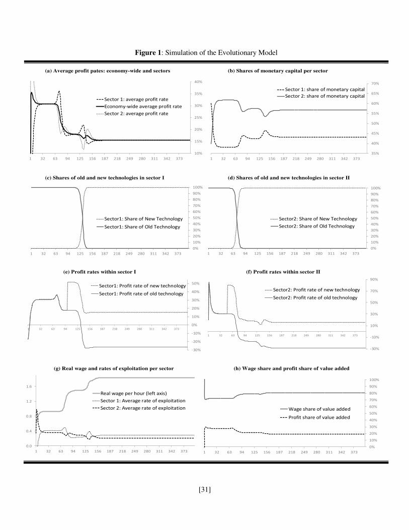
[Figure 1 about here]
In Figure 1 I report simulation results for key variables. Panel (a) shows the equalization of profit
rates over time, such that the economy-wide average profit rate is a stable attractor to the sector profit rates.
Panel (b) shows the movement of firms across sectors in search of higher returns. Panels (c) and (d) show
the shares of firms operating with the old and new technologies within each sector. Panel (e) and (f) show
the profit rates of firms employing the old and new technologies within each sector. The uncoordinated
implementation of the new technologies increases the profit rate only for those firms initially adopting the
innovation, but the gradual diffusion of the new technologies results in lower levels of profitability for all
firms over time. Panel (g) shows the real wage and the average rates of exploitation in both sectors. Because
the nominal wage is constant and the new technology reduces the price of the consumption good, the real
wage rises over time. Hence, the gains from technology reduce the rate of exploitation. Finally, panel (f)
shows the wage and profit shares of value added for the entire economy. Corresponding to an increase in
the real wage, the wage share also rises over time. The reduction in the price of production of the
consumption good leads the real wage to rise faster than the productivity of labor, contributing to the fall
in the average rate of profit.
9. Final Remarks
In this paper I developed an innovative evolutionary approach to integrate the principle of effective
demand from Keynes, the macroeconomic aggregates from Kalecki, and the formation of long-run prices
of production from Classical Political Economy. My approach combines the replicator dynamics from
evolutionary Game Theory and Marx’s model of a competitive economy with technical change. In an
evolutionary setting the replicator dynamics offers a behavioral microfoundation for spontaneous and path-
[23]
dependent interactions of multiple uncoordinated agents. The replicator equation allows for the
formalization, in real time, of the feedback effects between decisions planned at the micro level and the
unintended social outcomes at the macro level. Externalities are present in this setting as uncoordinated
agents do not internalize the social consequences of their individual actions.
My framework demonstrates how aggregate demand determines the realization of values, the
distribution of income between wages and profits, the equalization of profit rates, the diffusion of new
techniques, and the convergence of market prices to prices of production. My evolutionary approach
therefore offers a clearer and more precise presentation of Marx’s system in Capital III. In particular, I
bring together the formation of prices of production amid technological progress (as in chapter IX) and the
role of aggregate demand in the realization of value (as in chapter XV).
Contrary to the Okishio theorem, which only holds under an exogenous real wage, technical change
can lead profit rates to fall. Once the real wage is endogenous to aggregate demand, technical change
increases the profit rate of early adopters. But competition and the diffusion of the new technique can reduce
profitability over time if the repricing of means of production and consumption goods increases the real
wage faster than the productivity of labor. As Basu (2019) demonstrated, because technical change impacts
both the real wage and the productivity of labor, the trend of the profit rate derives from the relation between
these two factors. Okishio’s theorem only holds true if labor productivity rises faster than the real wage,
and hence technological change causes the profit rate to rise over time. But if technical change causes the
real wage to rise faster than labor productivity, the profit rate will fall. For the rate of exploitation to increase
systematically over time the model would need to include equations for the labor market, allowing for the
existence of involuntary unemployment and job insecurity. This extension of the model will be pursued in
further work.
Keynes’ principle of effective demand thus offers a better and more complete understanding of
how aggregate demand determines the rates of exploitation, the rates of profit, the functional distribution
[24]
of income, the diffusion of technological innovation, and the gravitation of market prices toward prices of
production in a competitive economy.
References
Allain, O. (2009). Effective Demand and Short-Term Adjustments in the General Theory. Review of Political Economy 21, pp.1–22.
Baran, P. and Sweezy, P. (1968). Monopoly Capital: An Essay on the American Economic and Social Order. New York, Monthly Review Press.
Basu, D. (2019). Reproduction and Crises in Capitalist Economies. In M. Vidal, T. Smith, T. Rotta, P. Prew.
The Oxford Handbook of Karl Marx, pp.279-298. New York: Oxford University Press.
Baumol, W. (1999). Say's Law. Journal of Economic Perspectives 13(1) pp.195–204.
Baumol, W. (1977). Say's (at Least) Eight Laws. Economica 44, pp.145-162.
Becker, G. and Baumol, W. (1952). The Classical Monetary Theory: The Outcome of the Discussion.
Economica 76, pp.355-376.
Béraud, A. and Numa, G. (2018). Beyond Says Law: The Significance of J. B. Say’s Monetary Views.
Journal of the History of Economic Thought 40 (2), pp.217-241.
Bhaduri, A. and Marglin, S. (1990). Unemployment and the Real Wage: The Economic Basis for Contesting
Political Ideologies. Cambridge Journal of Economics 14(4), pp.375-393.
Boggio, L. (1990). The Dynamic Stability of Production Prices: A Synthetic Discussion of Models and
Results. Political Economy: Studies in the Surplus Approach, volume 6, numbers 1-2, pp.47-
58.
Boggio, L. (1985). On the Stability of Production Prices. Metroeconomica 37(3), pp.241–267.
Bowles, S. (2006). Microeconomics: Behavior, Institutions, and Evolution. Princeton University Press,
New Jersey.
Casarosa, C. (1981) The Microfoundations of Keynes’s Aggregate Supply and Expected Demand Analysis.
Economic Journal 91, pp.188–194.
Chick, V. (1983). Macroeconomics After Keynes. Oxford: Philip Allan.
Cockshott, P. (2017). Sraffa’s Reproduction Prices Versus Prices of Production: Probability and Convergence. World Review of Political Economy 8(1), pp.35-55.
Cogliano, J. (2011). Smith's ‘Perfect Liberty' and Marx's Equalized Rate of Surplus-Value. New School for Social Research Working Papers No.08.
Duménil, G. and Lévy,D. (1999). Being Keynesian in the Short Term and Classical in the Long Term: The
Traverse to Classical Long-Term Equilibrium, Manchester School, 67(6), pp.684–716.
[25]
Duménil, G. and Lévy, D. (1995). Structural Change and Prices of Production. Structural Change and Economic Dynamics 6(4), pp.397-434.
Dutt, A. K. (2011). The Role of Aggregate Demand in Classical-Marxian Models of Economic
Growth. Cambridge Journal of Economics 35(2), pp.357-382.
Dutt, A. K. (1990). Growth, Distribution and Uneven Development. Cambridge, UK: Cambridge University
Press.
Dutt, A. K. (1984). Stagnation, Income Distribution and Monopoly Power. Cambridge Journal of Economics 8(1), pp.25-40.
Elaydi, S. N. (2005). An Introduction to Difference Equations. New York: Springer.
Farjoun, F. and Machover, M. (1983). Laws of Chaos: A Probabilistic Approach to Political Economy.
London: Verso.
Flaschel, P. and Semmler, W. (1985). The Dynamic Equalization of Profit Rates for Input-Output Models
with Fixed Capital. In: Semmler, W. (ed) Lecture Notes in Economics and Mathematical Systems. Heildelberg: Spring Verlag.
Foley, D. (2018). The New Interpretation After 35 years. Review of Radical Political Economics 50(3), pp.
559–568.
Foley, D. (1985). Say's Law in Marx and Keynes. In: Cahiers d'Économie Politique, n.10-11, pp. 183-194.
Foley, D. (1983). Money and Effective Demand in Marx’s Scheme of Expanded Reproduction. In: Desai,
P. (ed) Marxism, Central Planning, and the Soviet Economy: Essays in Honor of Alexander Erlich. Cambridge: MIT Press, pp.19-33.
Fröhlich, N. (2013). Labour Values, Prices of Production and the Missing Equalisation Tendency of Profit
Rates: Evidence from the German Economy. Cambridge Journal of Economics 37(5),
pp.1107-1126.
Gintis, H. (2009). Game Theory Evolving. New Jersey: Princeton University Press.
Harris, D. (1972). On Marx’s Scheme of Reproduction and Accumulation. Journal of Political Economy
80(3), part 1, pp.505-522.
Hartwig, J. (2007). Keynes vs. the Post Keynesians on the Principle of Effective Demand. European Journal of the History of Economic Thought 14, pp.725–739.
Hayes, M. G. (2019) John Maynard Keynes: The Art of Choosing the Right Model. Cambridge, UK: Polity
Press.
Hayes, M. G. (2007) The Point of Effective Demand. Review of Political Economy 19, pp.55–80.
Jossa, B. (1989). Class Struggle and Income Distribution in Kaleckian Theory. In Sebastiani, M. (ed)
Kalecki’s Relevance Today. London: Palgrave Macmillan, pp.142-159.
Kates, S. (1997) On the True Meaning of Say’s Law. Eastern Economic Journal 23(2), pp.191-202.
Kriesler, P. (1989). Methodological Implications of Kalecki's Microfoundations. In Sebastiani, M. (ed)
Kalecki’s Relevance Today. London: Palgrave Macmillan, pp.121-141.
[26]
Kubin, I. (1990). Market Prices and Natural Prices: A Model with a Value Effectual Demand. Political Economy: Studies in the Surplus Approach 6(1-2), pp.175-192.
Marglin, S. A. (1984). Growth, Distribution and Prices. Cambridge, MA, Harvard University Press.
Marx, K. ([1859]1989) A Contribution to the Critique of Political Economy. In: Karl Marx, Frederick
Engels: Collected Works: 29. Moscow: International Publishers Co Inc.,U.S., pp. 258–420.
Marx, K. ([1887]1990) Capital: Volume I. London: Penguin Books.
Marx, K. ([1894]1994). Capital: Volume III. London: Penguin Books.
Nikaido, H. (1985). Dynamics of Growth and Capital Mobility in Marx’s Scheme of Reproduction. Journal of Economics 45(3), pp.197-218.
Nikaido, H. (1983). Marx on Competition. Journal of Economics 43(4), pp.337-362.
Okishio, N. (1961). Technical Change and the Rate of Profit. Kobe Economic Review, vol. 7, pp.85-99.
Prado, E. F. S. (2006). Uma Formalização da Mão Invisível. Estudos Econômicos 36, pp.47-65.
Prado, E. F. S. (2002). Geração, Adoção e Difusão de Técnicas de Produção - Um Modelo Baseado em
Marx. Análise Econômica 38, pp. 67-80.
Robinson, J. (1947). An Essay on Marxian Economics. London: Macmillan.
Robinson, J. (1962). Essays in the Theory of Economic Growth. London: Macmillan.
Rubin, I. I. ([1928]1972). Essays on Marx's Theory of Value. Detroit: Black and Red.
Sardoni, C. (2009). The Marxian Schemes of Reproduction and the Theory of Effective Demand.
Cambridge Journal of Economics 33(1), pp.161–173.
Sardoni, C. (1989) Some Aspects of Kalecki's Theory of Profits: its Relationship to Marx's Schemes of
Reproduction. In Sebastiani, M. (ed) Kalecki’s Relevance Today. London: Palgrave
Macmillan, pp.206-2019.
Scheinerman, E. R. (2000) Invitation to Dynamical Systems. New Jersey: Prentice-Hall.
Scharfenaker, E. and Foley, D. (2017) Quantal Response Statistical Equilibrium in Economic Interactions:
Theory and Estimation. Entropy 19(9), pp.1-15.
Scharfenaker and Semieniuk (2016). A Statistical Equilibrium Approach to the Distribution of Profit Rates.
Metroeconomica 68(3), pp.465–499.
Shaikh, A. (2016) Capitalism: Competition, Conflict, Crisis. London: Oxford University Press.
Shaikh, A. (1989) Accumulation, Finance, and Effective Demand and Marx, Keynes and Kalecki. In:
Semmler, W. (ed) Financial Dynamics and Business Cycles: New Perspectives. New York:
M. E. Sharpe, pp.65-86.
Shoul, B. (1957). Karl Marx and Say’s Law. Quarterly Journal of Economics 71(4), pp.611-629.
Trigg, A. (2006). Marxian Reproduction Schema. London: Routledge.
[27]
Vianello, F. (1989). Effective Demand and the Rate of Profits: Some Thoughts on Marx, Kalecki and Sraffa.
In Sebastiani, M. (ed) Kalecki’s Relevance Today. London: Palgrave-Macmillan, pp.206-
2019.
[28]
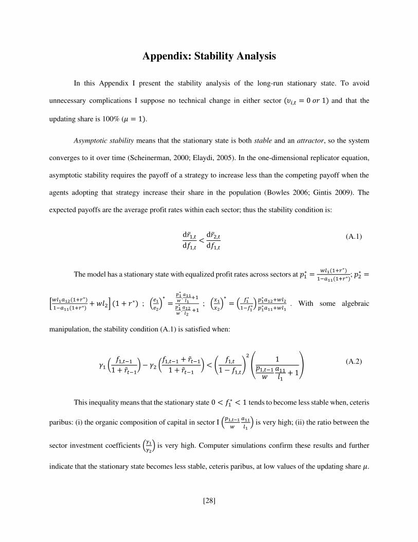
Appendix: Stability Analysis
In this Appendix I present the stability analysis of the long-run stationary state. To avoid
unnecessary complications I suppose no technical change in either sector (𝜐𝑖,𝑡 = 0 𝑜𝑟 1) and that the
updating share is 100% (𝜇 = 1).
Asymptotic stability means that the stationary state is both stable and an attractor, so the system
converges to it over time (Scheinerman, 2000; Elaydi, 2005). In the one-dimensional replicator equation,
asymptotic stability requires the payoff of a strategy to increase less than the competing payoff when the
agents adopting that strategy increase their share in the population (Bowles 2006; Gintis 2009). The
expected payoffs are the average profit rates within each sector; thus the stability condition is:
d�̅�1,𝑡d𝑓1,𝑡 < d�̅�2,𝑡d𝑓1,𝑡 (A.1)
The model has a stationary state with equalized profit rates across sectors at 𝑝1∗ = 𝑤𝑙1(1+𝑟∗)1−𝑎11(1+𝑟∗); 𝑝2∗ =[𝑤𝑙1𝑎12(1+𝑟∗)1−𝑎11(1+𝑟∗) + 𝑤𝑙2] (1 + 𝑟∗) ; (𝑒1𝑒2)∗ = 𝑝1∗𝑤 .𝑎11𝑙1 +1𝑝1∗𝑤 .𝑎12𝑙2 +1 ; (𝑥1𝑥2)∗ = ( 𝑓1∗1−𝑓1∗) 𝑝1∗𝑎12+𝑤𝑙2𝑝1∗𝑎11+𝑤𝑙1 . With some algebraic
manipulation, the stability condition (A.1) is satisfied when:
𝛾1 ( 𝑓1,𝑡−11 + �̃�𝑡−1) − 𝛾2 (𝑓1,𝑡−1 + �̃�𝑡−11 + �̃�𝑡−1 ) < ( 𝑓1,𝑡1 − 𝑓1,𝑡)2 ( 1𝑝1,𝑡−1𝑤 𝑎11𝑙1 + 1) (A.2)
This inequality means that the stationary state 0 < 𝑓1∗ < 1 tends to become less stable when, ceteris
paribus: (i) the organic composition of capital in sector I (𝑝1,𝑡−1𝑤 𝑎11𝑙1 ) is very high; (ii) the ratio between the
sector investment coefficients (𝛾1𝛾2) is very high. Computer simulations confirm these results and further
indicate that the stationary state becomes less stable, ceteris paribus, at low values of the updating share 𝜇.
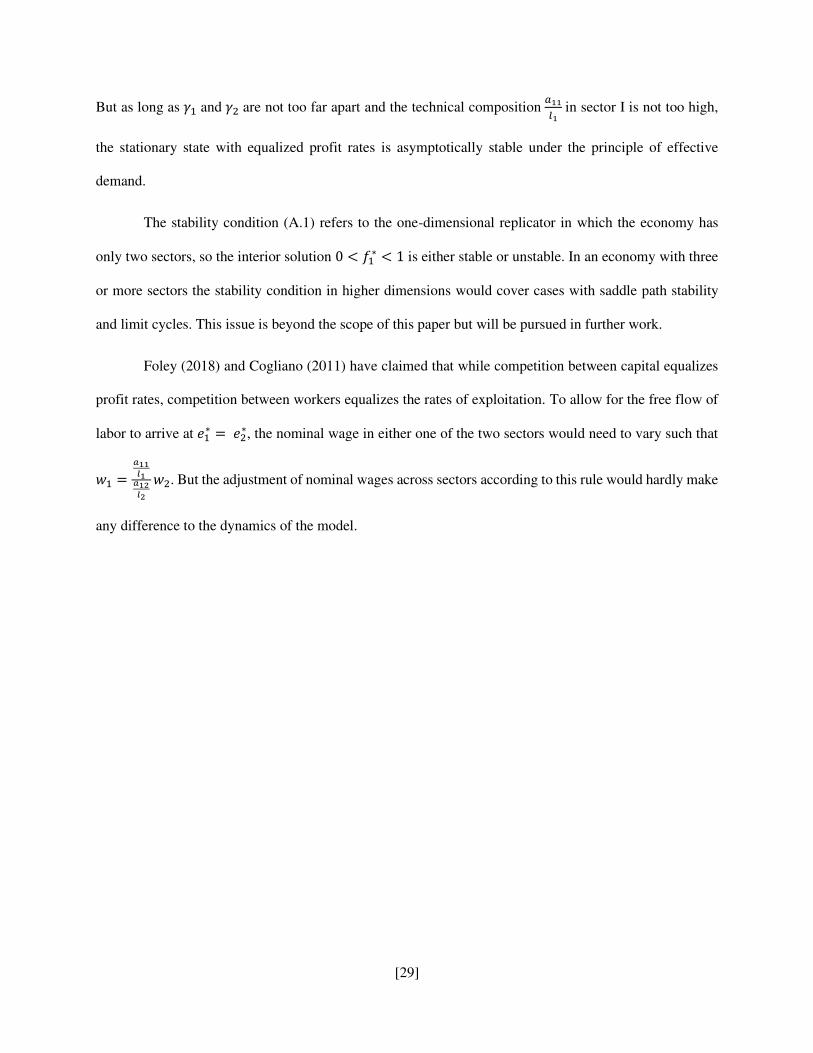
[29]
But as long as 𝛾1 and 𝛾2 are not too far apart and the technical composition 𝑎11𝑙1 in sector I is not too high,
the stationary state with equalized profit rates is asymptotically stable under the principle of effective
demand.
The stability condition (A.1) refers to the one-dimensional replicator in which the economy has
only two sectors, so the interior solution 0 < 𝑓1∗ < 1 is either stable or unstable. In an economy with three
or more sectors the stability condition in higher dimensions would cover cases with saddle path stability
and limit cycles. This issue is beyond the scope of this paper but will be pursued in further work.
Foley (2018) and Cogliano (2011) have claimed that while competition between capital equalizes
profit rates, competition between workers equalizes the rates of exploitation. To allow for the free flow of
labor to arrive at 𝑒1∗ = 𝑒2∗, the nominal wage in either one of the two sectors would need to vary such that
𝑤1 = 𝑎11𝑙1𝑎12𝑙2 𝑤2. But the adjustment of nominal wages across sectors according to this rule would hardly make
any difference to the dynamics of the model.
[30]
Tables and Figures
Table 1: Stationary States and Asymptotic Properties
Stationary States (a) Macro Inter-Sector Replicator
Sector I is ESS
Sector II is ESS Δ𝑓𝑖,𝑡+1 = 0 �̅�1,𝑡 ≷ �̅�2,𝑡
𝑓1,𝑡 = 1 is stable 𝑓1,𝑡 = 0 is stable 0 < 𝑓𝑖,𝑡∗ < 1 is unstable
Sector I is ESS
Sector II is not ESS Δ𝑓𝑖,𝑡+1 = 0 �̅�1,𝑡 > �̅�2,𝑡
𝑓1,𝑡 = 1 is stable 𝑓1,𝑡 = 0 is unstable
Sector I is not ESS
Sector II is ESS Δ𝑓𝑖,𝑡+1 = 0 �̅�1,𝑡 < �̅�2,𝑡
𝑓1,𝑡 = 1 is unstable 𝑓1,𝑡 = 0 is stable
No ESS Δ𝑓𝑖,𝑡+1 = 0 �̅�1,𝑡 = �̅�2,𝑡
0 < 𝑓𝑖,𝑡∗ < 1 is stable 𝑓1,𝑡 = 1 is unstable 𝑓1,𝑡 = 0 is unstable
(b) Micro Intra-Sector Replicator in Sector I
Innovate is ESS
Not innovate is ESS ∆𝜐1,𝑡+1 = 0
𝑟1,𝑡𝑛 ≷ 𝑟1,𝑡𝑜
𝜐1,𝑡 = 1 is stable 𝜐1,𝑡 = 0 is stable 0 < 𝑣1,𝑡∗ < 1 is unstable
Innovate is ESS
Not innovate is not ESS ∆𝜐1,𝑡+1 = 0 𝑟1,𝑡𝑛 > 𝑟1,𝑡𝑜
𝜐1,𝑡 = 1 is stable 𝜐1,𝑡 = 0 is unstable
Innovate is not ESS
Not innovate is ESS ∆𝜐1,𝑡+1 = 0 𝑟1,𝑡𝑛 < 𝑟1,𝑡𝑜
𝜐1,𝑡 = 1 is unstable 𝜐1,𝑡 = 0 is stable
No ESS ∆𝜐1,𝑡+1 = 0 𝑟1,𝑡𝑛 = 𝑟1,𝑡𝑜
0 < 𝑣1,𝑡∗ < 1 is stable 𝜐1,𝑡 = 1 is unstable 𝜐1,𝑡 = 0 is unstable
(c) Micro Intra-Sector Replicator in Sector II
Innovate is ESS
Not innovate is ESS ∆𝜐2,𝑡+1 = 0
𝑟2,𝑡𝑛 ≷ 𝑟2,𝑡𝑜
𝜐2,𝑡 = 1 is stable 𝜐2,𝑡 = 0 is stable 0 < 𝑣2,𝑡∗ < 1 is unstable
Innovate is ESS
Not innovate is not ESS ∆𝜐2,𝑡+1 = 0 𝑟2,𝑡𝑛 > 𝑟2,𝑡𝑜
𝜐2,𝑡 = 1 is stable 𝜐2,𝑡 = 0 is unstable
Innovate is not ESS
Not innovate is ESS ∆𝜐2,𝑡+1 = 0 𝑟2,𝑡𝑛 < 𝑟2,𝑡𝑜
𝜐2,𝑡 = 1 is unstable 𝜐2,𝑡 = 0 is stable
No ESS ∆𝜐2,𝑡+1 = 0 𝑟2,𝑡𝑛 = 𝑟2,𝑡𝑜
0 < 𝑣2,𝑡∗ < 1 is stable 𝜐2,𝑡 = 1 is unstable 𝜐1,𝑡 = 0 is unstable
[31]
Figure 1: Simulation of the Evolutionary Model
(a) Average profit pates: economy-wide and sectors (b) Shares of monetary capital per sector
(c) Shares of old and new technologies in sector I (d) Shares of old and new technologies in sector II
(e) Profit rates within sector I (f) Profit rates within sector II
(g) Real wage and rates of exploitation per sector (h) Wage share and profit share of value added
10%
15%
20%
25%
30%
35%
40%
1 32 63 94 125 156 187 218 249 280 311 342 373
Sector 1: average profit rate
Economy-wide average profit rate
Sector 2: average profit rate
35%
40%
45%
50%
55%
60%
65%
70%
1 32 63 94 125 156 187 218 249 280 311 342 373
Sector 1: share of monetary capital
Sector 2: share of monetary capital
0%
10%
20%
30%
40%
50%
60%
70%
80%
90%
100%
1 32 63 94 125 156 187 218 249 280 311 342 373
Sector1: Share of New Technology
Sector1: Share of Old Technology
0%
10%
20%
30%
40%
50%
60%
70%
80%
90%
100%
1 32 63 94 125 156 187 218 249 280 311 342 373
Sector2: Share of New Technology
Sector2: Share of Old Technology
-30%
-20%
-10%
0%
10%
20%
30%
40%
50%
1 32 63 94 125 156 187 218 249 280 311 342 373
Sector1: Profit rate of new technology
Sector1: Profit rate of old technology
-30%
-10%
10%
30%
50%
70%
90%
1 32 63 94 125 156 187 218 249 280 311 342 373
Sector2: Profit rate of new technology
Sector2: Profit rate of old technology
0.0
0.4
0.8
1.2
1.6
1 32 63 94 125 156 187 218 249 280 311 342 373
Real wage per hour (left axis)
Sector 1: Average rate of exploitation
Sector 2: Average rate of exploitation
0%
10%
20%
30%
40%
50%
60%
70%
80%
90%
100%
1 32 63 94 125 156 187 218 249 280 311 342 373
Wage share of value added
Profit share of value added