Embed Size (px)
Citation preview

Technological Change and
the Dynamics of Industries

© M.F. van Dijk, ‘s-Gravenhage 2000
ISBN: 90 5278 285 7Universitaire Pers Maastricht
Technological Change and
the Dynamics of Industries
Theoretical Issues and
Empirical Evidence from
Dutch Manufacturing
PROEFSCHRIFT
ter verkrijging van de graad van doctor aande Universiteit Maastricht,op gezag van de Rector Magnificus, Prof.dr. A.C. Nieuwenhuijzen Krusemanvolgens het besluit van het College van Decanen, in het openbaar te verdedigenop donderdag 19 oktober 2000 om 16.00 uur
door
Machiel François van Dijk
Promotores:Prof.dr. W.E. Steinmueller (University of Sussex, United Kingdom)Prof.dr. H.H.G. Verspagen
Beoordelingscommissie:Prof.dr. R. CowanProf.dr. G. Dosi (Scuola Superiore Sant’Anna, Italia)Prof.dr. L.L.G. Soete
Contents
Chapter 1 Introduction.........................................................................................1
Chapter 2 Empirical Regularities in Dutch Manufacturing...............................11
2.1 Introduction...............................................................................................112.2 The data.....................................................................................................122.3 Stylised facts and the Dutch manufacturing sector...................................16
2.3.1 Firm level .............................................................................................162.3.2 Manufacturing level .............................................................................242.3.3 Industry level ........................................................................................31
2.4 Conclusions...............................................................................................39Appendix 1: List of industries in the SN database...........................................40Appendix 2: Histograms of the industry-level variables selectedin section 2.3.3 ................................................................................................. 43
Chapter 3 Survey of Selected Theories.............................................................45
3.1 Introduction...............................................................................................453.2 Equil ibrium models...................................................................................46
3.2.1 Static equilibrium models....................................................................473.2.2 The ‘Bounds’ approach........................................................................503.2.3 Dynamic equil ibrium models...............................................................523.2.4 Theoretical and empirical limitations of equilibrium models..............54
3.3. Technological regimes.............................................................................573.3.1 Literature overview ..............................................................................583.3.2 Empirical evidence on innovative patterns..........................................653.3.3 Technological regimes and industrial dynamics inevolutionary models......................................................................................673.3.4 Conclusion............................................................................................70
3.4 Product life cycles.....................................................................................713.4.1 Literature overview ..............................................................................713.4.2 Klepper’s model ...................................................................................783.4.3 Conclusion............................................................................................83
3.5 Appraisal ...................................................................................................833.6 Conclusions...............................................................................................86
Chapter 4 Technological Regimes and Industry Life Cycles in DutchManufacturing.....................................................................................................87
4.1 Introduction...............................................................................................874.2 Technological regimes..............................................................................88
4.2.1 The hypotheses.....................................................................................884.2.2 Classification of industries...................................................................914.2.3 The results............................................................................................934.2.4 Conclusion..........................................................................................101
4.3 Industry li fe cycles..................................................................................1034.3.1 The hypotheses...................................................................................1044.3.2 Classification of industries................................................................. 1084.3.3 The hypotheses tested ........................................................................1104.3.4 Conclusion..........................................................................................118
4.4 Combined analysis..................................................................................1204.5 Conclusions.............................................................................................127Appendix: list of industries with their technological regime andevolutionary stage..........................................................................................129
Chapter 5 Technological diffusion patterns and their effects on industrialdynamics ...........................................................................................................133
5.1 Introduction.............................................................................................1335.2 The diffusion of new product technologies............................................134
5.2.1 Modelling diffusion dynamics: Shy’s approach................................1355.2.2 A note on firm growth........................................................................136
5.3 The model................................................................................................1395.3.1 Competitiveness of firms...................................................................1405.3.2 Exit rules ............................................................................................1415.3.3 Evolution of fi rm size.........................................................................1425.3.4 Imitation .............................................................................................143
5.4 Simulation results....................................................................................1465.5 Interaction between adoption regimes and technological regimes.........1595.6 Conclusions.............................................................................................170
Chapter 6 Conclusions.....................................................................................173
6.1 Summary ................................................................................................. 1746.2 Suggestions for future research...............................................................178
References.........................................................................................................181
Nederlandse samenvatting ................................................................................191
Acknowledgements...........................................................................................197
Curriculum vitea...............................................................................................199


1
Chapter 1
Introduction
Industrial landscapes exhibit high degrees of diversity. In all developedcountries, we observe a substantial cross-sectional variety in the ways in whichthe activities of producers are organised in meeting the demands of theircustomers. Consider, for example, the large variances in sectoral structures.Whereas some industries accommodate only a small number of large enterprisesthat are hardly ever challenged by entering firms, other sectors are much morecharacterised by a large population of small firms that continuously rejuvenatesitself through the process of entry and exit. Interestingly, this observation goestogether with some remarkable similarities between countries. Chemicals and oilrefinery are typical examples of industries dominated by a few large firms,whereas sectors such as textiles and wooden products show much lower levelsof sales concentration in most of the industrialised countries.
Besides the large diversity of the industrial landscape, we also observe that thislandscape is subject to substantial change over time. The rise and fall of someindustries and, within these industries, the evolving patterns of entry, exit, andgrowth and decline of firms continuously alter the industrial landscape at thevarious levels of analysis. For instance, in the United States the automobileindustry initially experienced a rapid increase in the number of producers, butwhile market sales were stil l increasing, a sharp reduction in the number of fi rmstook place. Nowadays, the number of f irms in this industry has more or lessstabilised at a low level, which naturally implies rather high concentrationlevels.
Traditionally, such high concentration levels have been among the mainconcerns of anti-trust policies. A high concentration of sales in an industry isusually associated with substantial market power of the firms in the industryand, consequently, with a suboptimal economic performance (in terms of
2
welfare). Many economic policies therefore reflect the idea that having anindustry structure characterised by the presence of many firms is the best way tominimise the market power of individual firms and hence to maximise economicperformance. Obviously, the justification of these policies is strongly based onthe following two hypotheses: (1) high concentration levels imply low levels ofcompetition, and (2) maximising competition guarantees optimal economicperformance.
From a theoretical point of view, these two hypotheses can be seriouslyquestioned. Concentration levels do not necessarily indicate the intensity ofindustrial competition. Although we may observe a small number of large firmsin an industry, competition between them, or the competitive pressures frompotential entrants, may still be considerable. Even if the concentration level ofan industry is found to be high for many subsequent years, still a large share ofthe market may have been transferred within the group of continuing firms orfrom these continuing firms to entrants. Finally, one could even argue thatincreasing competitive pressures might force inefficient firms to exit the market,leading to an increase in concentration levels.
The second hypothesis asserts that maximal competition assures optimaleconomic performance. Although this may perhaps maximise the economicperformance of an industry in the short run, one may question whether suchhighly competitive markets maximise economic performance in the long run aswell , as fierce competition may hamper technological progress. High levels ofcompetition could adversely effect firms’ endeavours to be innovative in twoways. First, fierce competition may suppress profits so much that firms cannotfinance their investments in research and development from their retainedearnings. Second, the profits resulting from successful innovation may quicklybe eroded in highly competitive markets. Consequently, if f irms expect theycannot sufficiently reap the potential benefits from their innovations, they may,in the worst case, decide to refrain from investing in research and developmentat all.
In order to assess the validity of these arguments, and thus to evaluate theappropriateness of anti-trust policies, empirical research is obviously of utmostimportance. Empirical analyses of, for instance, the relationships betweenconcentration, competition and technological change may learn us more aboutthe existence and significance of the trade-off between the short-run and long-run economic performance of an industry. Since the outcomes of such analyses
3
could directly be used for welfare analysis and economic policy making,empirical research in industrial economics can already be fully justified onpurely normative grounds.
On positive grounds, the legitimacy of empirical exercises in industrialeconomics is undisputed as well . As in many other scientific disciplines,theoretical and empirical work are strongly related in two ways. By exploringdatabases we may find empirical regularities that could provide a useful startingpoint for the identification of the phenomena to be explained. As such, empiricalwork contributes to the initial setting of a theoretical research agenda.Alternatively, by confronting theoretical conceptualisations with empirical datawe are able to evaluate the explanatory powers of the models underinvestigation. If necessary, the output of such analyses can in turn be used tofurther improve, expand or redirect theoretical work in industrial economics.
In conclusion, on both normative and positive grounds, empirical research isessential for the analytical rigour and practical relevance of industrial economicsas a scientific discipline. Naturally, sound empirical research in this fieldimposes strong requirements on the availabil ity of economic data. However, formany decades industrial economists had to rely on case studies and on ratherhighly aggregated cross-sectional data. The availability of only this type of datahas indeed affected the research agenda in this era. Since these data did notallow for empirical research on the long-run impact of, e.g., entry and exit, orthe transfer of market shares within the group of continuing firms1, not mucheffort was taken to develop or advance theoretical frameworks analysing thecauses and consequences of these phenomena. Instead, theoretical work mainlyconcentrated on static equilibrium analyses of industry structures with thestructure-conduct-performance framework, originally developed by EdwardMason and Joe Bain in the 1950s, as the dominant paradigm. In this approach,industrial competition is regarded as a static phenomenon, i.e., as a state ofaffairs, of which the intensity can simply be assessed by a set of structuralattributes.
However, over the last fifteen years the quality and availabili ty of economic datahas substantially improved. Especially the increased availability of longitudinalfirm-level databases has greatly enlarged the scope of empirical research in
1 Case studies could, of course, allow for studying these matters. However, as Baldwin
(1995) argues, their limited scope precludes the type of generalisations that social sciencedemands.
4
industrial economics. The availability of these data has made it possible forresearchers to follow the characteristics of a large number of f irms over time.This opportunity does not only allow for studying patterns of birth, growth anddeath of individual firms, but also for an analysis of the cumulative effect ofentry, exit, and variations in sizes or market shares of continuing firms.Furthermore, it has become possible to analyse differences between industriesconcerning these cumulative effects, and to investigate how industries changeover time.
The increased availabil ity of these longitudinal firm-level databases has indeedled to a large amount of empirical work taking advantage of the opportunitiesmentioned above. This work has resulted in a number of robust empirical resultsthat are hard to reconcile with the assumptions and analytical results of theconventional static equilibrium theories. For instance, it has been observed thatin virtually all industries entry and exit of firms occur simultaneously. Thisresult is at odds with models in which the entry process is viewed as amechanism by which the industry adjusts itself to changing exogenousconditions. A second example is the coexistence of firms of various sizes inrather narrowly defined industries. Many industries exhibit a fairly skewed andstable distribution of firm sizes, indicating that at any point in time large as wellas small firms simultaneously inhabit the industry. This observation seeminglyrejects the notion of the optimal firm size found in textbook models on industrialorganisation. The final example concerns the persistence of asymmetric firmperformances. The ‘ fact’ that, e.g., profitability differentials between firms inthe same industry are persistent over time suggest that profitability levels do notconverge to some ‘normal’ equilibrium rate of return.
These empirical findings constitute an important reason for the increased interestin dynamic approaches that we observe in the recent theoretical literature onindustrial economics. However, the idea of analysing industrial economics froma dynamic perspective is certainly not new. In the early days of this discipline,prominent economists such as Adam Smith, Alfred Marshall and JosephSchumpeter started from a dynamic approach as well in theorising about theorganisation of manufacturing industries. Intra-industry competition was clearlyviewed by them as a dynamic process, i.e., a process causing continuous change,driven by the entry, exit and growth and decline of profit-seeking firms.
The increased scope of empirical research, together with the evidence it hasbrought forward, is certainly not the only reason for the upsurge of dynamic
5
approaches in industrial economic theory. Especially in the last two decades,technological change is increasingly being acknowledged as an endogenousprocess driving industrial competition and economic growth. Since the industrialrevolution, technological change has obviously always been an importanteconomic phenomenon, but for many decades it has mostly been regarded as anexogenous factor in models of industrial economics. These models simplyassume that the exogenously created knowledge related to any innovation flowsaround freely and hence does not effect competition between fi rms.
In reality, however, both bounded rationality and the tacit nature oftechnological knowledge prevent that new knowledge spills over rapidly,enabling innovative firms to enjoy at least temporaril y higher (disequilibrium)profits. In fact, the opportunity to enjoy these profits provides the economicincentives to firms’ search for technological improvements. Competitionbetween firms is therefore largely driven by the process of technological change,continuously disturbing the economic status quo. Obviously, this rejects thenotion of competition as a static concept underlying the mainstream equil ibriummodels. The inabili ty to incorporate (technological) competition as anendogenous, perturbing process has therefore led to an increasing dissatisfactionwith these models and, consequently, to an increasing and renewed interest intheoretical approaches in which the dynamics of industrial competition areendogenously driven by the process of technological change.
These theoretical approaches can roughly be categorised in two groups. The firstone focuses on technological regimes. A technological regime can be defined asa particular combination of opportunity, appropriabil ity, cumulativenessconditions and properties of the knowledge base that underlies the innovativeand productive activities in an industry and explains how these activities areorganised in an industry. The second group of theories focuses on product orindustry li fe cycles. These theories start from the observation that mostsuccessful products go through a number of distinct stages over their lives, andaim to explain how the structural and dynamic properties of the industry co-evolve with these product life cycles.
Given the presence of these theoretical frameworks embodying the dynamicinteraction between industrial competition and technological change, and giventhe increased availabili ty of longitudinal firm-level data, it is actually quitesurprising that until now the opportunity of testing these theories with thelongitudinal micro-data has hardly been taken advantage of. Most of the
6
empirical work using these data focussed on revealing some strong empiricalregularities, but one of the main issues in industrial economics, explaining theobserved cross-sectional differences, has hardly been addressed so far. Thisvirtually unexploited opportunity constitutes the primary objective of this thesis:to explain how and, by using firm-level data on Dutch manufacturing,investigate empirically whether the technological regime framework and theproduct life cycle approach can explain the observed differences betweenindustries with regard to their structural and dynamic properties.
Understanding whether and how technological regimes and product life cyclesshape the structures and the dynamics of industries is important for a number ofreasons. As mentioned already, the evidence derived from longitudinaldatabases suggests that existing conventional theories are in need ofimprovement. Probably the main reason why these equil ibrium theories arehardly corroborated by the data is that they mostly neglect the process oftechnological change. Since both the technological regime framework and theproduct life cycle approach explicitly recognise technological change as themajor determinant of the competitive process, empirical evidence supporting orrejecting these theories could at least indicate which directions to explore andwhich directions to discard in the further development of industrial economictheory.
From a policy point of view, understanding how technological regimes andproduct life cycles affect the competitive process is important as well. As wehave argued before, the justification of economic policies rely substantially onwhat we know, both theoretically and empirically, about the competitive processwithin industries. As an example, consider again the concerns of anti-trustpolicies regarding high concentration levels. The assumption underlying thesepolicies is that high levels of sales concentration indicate a lack of competition.However, both the technological regime framework and the product li fe cycleapproach can provide certain conditions under which intense technologicalcompetition and oligopolistic market structures are naturally conjoined.
For instance, a technological regime with high appropriabil ity andcumulativeness conditions and characterised by tacit and complex knowledge ismuch more conducive to technological competition driven by large andestablished firms than to a competitive process driven by small firms. But alsothe product life cycle approach depicts a specific evolutionary stage in whichdynamic increasing returns to technological change becomes an important

7
determinant of the competitive process. As these models show, the outcome ofsuch a competitive process necessarily implies strongly increasing concentrationlevels. Although under these circumstances market structures will notcorrespond to the textbook conditions of perfect competition, the typicalconcerns of anti-trust policies regarding the adverse effects of highconcentration levels on industrial competition may still be largely misplaced.
In conclusion, understanding whether and how technological regimes andproduct life cycles shape the structures and the dynamics of industries is ofsubstantial importance to both the theory of industrial economics and thepractical implications of this theory for policy. We believe therefore that thepresent thesis will provide a valuable contribution to the empirical foundations,as well as to our theoretical understanding and the practical relevance ofindustrial economics. In what follows, the structure of this dissertation and theunderlying research methodology will be presented.
Since the regularities provided by earlier empirical research using longitudinaldatabases are the starting point of this thesis, chapter 2 wil l investigate whetherthe previously obtained ‘stylised facts’ 2 are also observed in the Dutchmanufacturing sector. As such, chapter 2 aims to serve three objectives. The firstone is to describe the database we have used in this dissertation. We will providesome general information regarding, e.g., the variables that are included, thenumber of firms and the period it captures, and present some descriptivestatistics of the dataset. Further, we will pay attention to one specific limitationof the database, namely its observation threshold: only firms with at least twentyemployees are included in the database. The second objective of chapter 2 is toprovide a survey of the stylised facts that empirical work in industrial economicshave provided so far. Finally, we will investigate whether these stylised facts areobserved in the Dutch manufacturing sector as well .
Chapter 3 surveys the theoretical l iterature on industrial economics, anddemonstrates how the selected theories may explain variances in the structuraland dynamic properties of industries. The main focus of this chapter will be onthe theoretical issues regarding the technological regime framework and theproduct life cycle approach, but chapter 3 will also include an overview of the
2 Because the notion of stylised facts is perhaps slightly confusing, we would like to
emphasise that using the terminology of stylised facts merely represents our way ofcharacterising the process and outcome of creating broad characterisations of availablepatterns in the data.

8
equilibrium models. Although these models have dominated the literature onindustrial economics for a considerable time, we will demonstrate that theequilibrium approaches and their related assumptions inherently involve sometheoretical and empirical li mitations. We will t hen argue that the technologicalregime framework and the product li fe cycle approach are conceptually muchmore appropriate in providing plausible explanations for the structures anddynamics of industries, as they both embody elements such as boundedrationality and technological uncertainty that are close to empirical substance.
Finally, chapter 3 will demonstrate how the technological regime frameworkand the product li fe cycle approach may explain the observed structural anddynamic differences between industries. The basic arguments are as follows.Given different technological regimes, i.e., different combinations ofopportunity, appropriabil ity, cumulativeness conditions and properties of theknowledge base underlying the innovative and productive activities, theresulting different patterns of innovative activities are likely to affect thestructural and dynamic properties of industries. Alternatively, theories andmodels on product life cycles explain and depict the evolution of an industry’sstructural and dynamic properties over its li fetime. Based on this approach, theobserved cross-sectional differences may be explained by the differentevolutionary stages that the industries occupy.
By using the longitudinal firm-level database on Dutch manufacturing, chapter 4will investigate the extent to which the technological regime framework and theproduct life cycle approach can actually explain the cross-sectional variances instructures and dynamics. From both theoretical frameworks we wil l fi rst derive anumber of hypotheses. Next, we will classify the industries in the sampleaccording to their underlying technological regime and the evolutionary stagethey occupy. For the classification of the industries into regimes we will use ataxonomy of technology classes offered by Malerba et al. (1995). Ideally, someexogenous criteria would be used for the classification of industries intoevolutionary stages as well. However, since these are not available, we will haveto base our classification on the revealed patterns of some variables denoting theevolutionary stage of the industries in the sample. Based on these classifications,we will then test the hypotheses for the technological regime framework and theproduct life cycle approach individually. Finally, we will perform a number ofregression analyses in this chapter to investigate the extent to which theseapproaches collectively account for differences between industries, and whetherany interaction effects can be observed between them.

9
Although the technological regime framework and the industry li fe cycleapproach provide plausible explanations for differences in the structures anddynamics of industries, we believe that both these theories still ignore a numberof crucial elements. First of all, models on product li fe cycles generally focus onthe emergence and evolution of only one product and its associated technology.However, in many industries we observe that firms repeatedly introduce oradopt new product technologies that replace the older ones. Second, both theseapproaches do not explicitly consider differences in the technological propertiesof the goods produced by the industries. Finally, in models on technologicalregimes and on industry li fe cycles the growth of a firm is generally determinedby its relative (technological) performance. However, empirical studies on firmgrowth do not provide much evidence supporting such a relationship. Most ofthese studies suggest that the size of a firm generally follows a random walkwith a declining positive drift.
In chapter 5 we will introduce a model on industry dynamics that attempts toinclude these three elements. As in Shy (1996), the degree of substitutabilitybetween the quality and the network size of a technology and the degree ofcompatibil ity of succeeding technologies are the key determinants of thesimulation model presented here. However, Shy (1996) mainly limits his focusto the demand side, as he investigates how varying consumer preferences overtechnology advance and network size effects the timing and frequency of newtechnology adoption. Our focus in chapter 5 will be on the relation between thedemand side and the supply side. Given variations in consumer preferences overquality and network sizes, and different degrees of compatibility betweensucceeding technologies, we will investigate whether the resulting differences inthe timing and frequency of new technology adoptions affect the dynamics ofthe population of supplying firms. This would be an important result, because ifthe industrial properties are indeed related to the diffusion patterns, our modelmay provide an additional explanation for the observed structural and dynamicdifferences between industries.
Since we believe that it is of equal interest that the emergent properties of ourmodel are close to empirical substance, we will also investigate in this chapterwhether the results of our model are consistent with the stylised facts thatempirical research in industrial economics has put forward so far. Finally, byvarying a number of parameters reflecting the technological regime conditions,

10
we will i nvestigate whether the results of our model are significantly differentunder various technological regimes.
Chapter 6 concludes this dissertation by summarising the main results and bypresenting some concluding remarks. Further, we will suggest some directionsfor future research in this final chapter.
11
Chapter 2
Empirical Regularities in Dutch Manufacturing
2.1 Introduction
In the last fifteen years, the increased availability of micro-level data has led tonumerous studies on firm and industry dynamics using longitudinal datasets.The possibili ty to follow a large number of individual firms over time allowedresearchers to study the dynamics of industries without having to relyexclusively on case studies. As a result, the empirical foundations of industrialdynamics have been greatly enhanced at all three levels of aggregation. At thefirm level, these data have provided evidence regarding patterns of birth, growthand death of individual firms and their potential determinants. At the industrylevel, we have been able to fully assess the impact of dynamic changes inindustries by, for instance, measuring the cumulative effect of entry and exit,and the turbulence caused by variations in sizes and market shares of continuingfirms. Finally, at the sectoral (i.e., manufacturing) level we have been able todirectly compare different industries with respect to their dynamics, andinvestigate their structural evolution. Together, these empirical studies have ledto a rich set of stylised facts in the field of industrial economics.
This collection of stylised facts is employed to construct the framework of thischapter in the following way. First, the presentation of the stylised facts aims toprovide a survey of the most important results empirical literature in industrialeconomics has put forward so far. Second, testing for the presence of thesestylised facts in the Dutch manufacturing sector learns us the similarities anddifferences between the manufacturing sector in the Netherlands andmanufacturing sectors in other countries. Finally, it gives us the opportunity toprovide a detailed description of the dataset that we use throughout this thesis.The next section starts with this.
12
2.2 The data
Recently, Statistics Netherlands (SN) has made it possible for researchers togain access to a firm-level longitudinal dataset. In this section we will describethe SN manufacturing database that we will use throughout this thesis. We willprovide some general information about the database (e.g., the period itcaptures, the number of f irms), and pay attention to the specific limitations of it,especially with regard to its truncation of certain types of observations.
The SN manufacturing database captures all firms with more than twentyemployees (working 15 hours or more weekly) that have been active in theDutch manufacturing sector between 1978 and 1992. In total, there are 10,246firms in the dataset, of which 2,558 firms are present throughout the wholeperiod. These continuing firms on average capture 53.5 and 52.4 percent of,respectively, total manufacturing employment and value of production. Theremaining firms are only temporaril y present in the dataset. Although thesefirms enter and exit the database, defining them as greenfield entrants andclosedown exiters is not appropriate in most of the cases. The majority of theentering and exiting firms appears or disappears because of passing thethreshold of twenty employees. For the period from 1986 and onwards, SNprovides aggregated statistics of the specific reasons why firms respectivelyenter or exit the database. Over this period, on average only 8.9 percent and 21.1percent of the firms entering and exiting the database were greenfield entrants orclosedown exiters.
Unfortunately, the firm-level data we have access to do not allow us todistinguish the entry and exit categories in detail . We are only able to identifyfirms that enter and exit for other reasons than greenfield entry, closedown exit,and passing the observation threshold. Whenever firms enter of exit because ofthese ‘other’ reasons (such as mergers, acquisitions or administrative reasons)SN assigns an additional variable to these firms. However, this variable does notspecify which of these reasons applies. Hence, we can only distinguish firmsthat enter or exit for ‘normal’ reasons (i.e., new firms that really enter, existingfirms that really close down and firms passing the observation threshold) fromfirms that enter or exit for ‘other’ reasons (which is never real entry or real exit).To give an example: when two firms merge in a certain year, we observe in thatyear two firms exiting for an ‘other’ reason, and one firm entering for an ‘other’reason in the following year.
13
Although most of the firms enter and exit the dataset because of passing theobservation threshold, we will still label them as entrants and exiters. We couldhave called them, e.g., pseudo-entrants and pseudo-exiters, but for conveniencewe have simply named them entrants and exiters. Certainly, any empirical testaiming to identify, for instance, the determinants of the entry and exit decisionwould be highly inappropriate when these groups of f irms are considered. Forcross-sectional purposes however, studying the impact of the entry and exitprocess still makes sense. If , for example, an industry is conducive to entrantswe may well assume that it is less difficult for small firms to grow and pass theobservation threshold, to stay above the threshold, and to obtain a significantmarket share in that industry compared to other industries. We believe thereforethat for the purpose of comparing different industries the use of statisticsmeasuring the impact of the entry and exit process is useful, despite the presenceof the observation threshold.
Hence, we will use the following definitions throughout this thesis. An entrant isa firm present in the dataset for one or more years, but absent in 1978. Its year ofentry is the year in which it is observed for the first time. If a firm is present forone or more years, but absent in 1992, we label it an exiter. Its year of exit is theyear in which it is observed for the last time. Excluded from the groups ofentering and exiting firms are firms that enter and exit the dataset because ofmergers, acquisitions or administrative reasons. Finally, an incumbent orcontinuing firm is defined as a firm that is present in 1978 and in 1992.
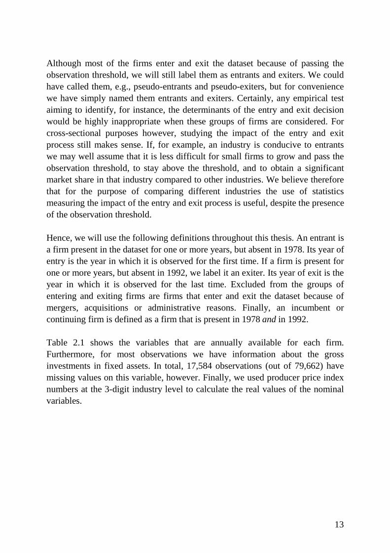
Table 2.1 shows the variables that are annually available for each firm.Furthermore, for most observations we have information about the grossinvestments in fixed assets. In total, 17,584 observations (out of 79,662) havemissing values on this variable, however. Finally, we used producer price indexnumbers at the 3-digit industry level to calculate the real values of the nominalvariables.
14
Table 2.1: L ist and description of var iables available in the SN database
Variable Description
Class of manufacturing All firms are allocated to a 4-digit industry, according to StatisticsNetherlands’ standard classification of industries as of 1974. If afirm is active in more than one industry it is allocated to theindustry from where it receives most of its revenues
Number of employees The number of employees working more than 15 hours a week,employed by the end of September
Industrial sales The revenues from sell ing goods manufactured in-house or byothers, provided they are on the payroll of the firm
Total value of production The sum of industrial sales, activated costs (i.e., costs made for theinternal production of capital goods for internal use), changes inthe stock of final products and other revenues
Total consumption value The sum of industrial purchases, changes in the stock of rawmaterials, usage of energy and other costs
Value added Total production value minus total consumption value
Indirect taxes Sum of indirect taxes (excluding value added tax) and levies lessoperating subsidies received
Labour costs The sum of gross wages and salaries paid by the firm
Gross result Value added minus labour costs and indirect taxes
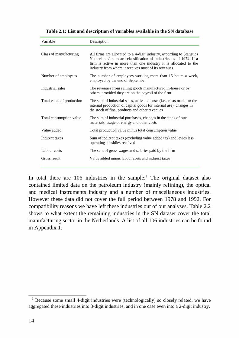
In total there are 106 industries in the sample.1 The original dataset alsocontained limited data on the petroleum industry (mainly refining), the opticaland medical instruments industry and a number of miscellaneous industries.However these data did not cover the full period between 1978 and 1992. Forcompatibil ity reasons we have left these industries out of our analyses. Table 2.2shows to what extent the remaining industries in the SN dataset cover the totalmanufacturing sector in the Netherlands. A list of all 106 industries can be foundin Appendix 1.
1 Because some small 4-digit industries were (technologically) so closely related, we have
aggregated these industries into 3-digit industries, and in one case even into a 2-digit industry.
15
Table 2.2: Compar ison of the SN database with total Dutch manufactur ing
Number offirms
Value of production (mln. guilders)
Employment(x 1000)
Investments infixed assets
(mln. guilders)
Year SampleTotalmanuf. Sample
Totalmanuf. Sample
Totalmanuf. Sample
Totalmanuf.
1978 5444 . 145535 180984 819 998 6595 .1979 5411 . 160984 201194 815 987 6741 .1980 5377 . 171630 219283 807 974 7297 .1981 5209 . 184384 233868 773 949 6691 .1982 5006 . 185277 240214 733 911 6668 .1983 4987 44167 192700 248746 705 870 7076 .1984 4893 43586 212420 274616 695 849 8917 .1985 4951 44846 224905 280894 709 860 10444 149981986 4965 44742 217122 260156 725 872 11959 163281987 5080 45735 214838 257907 732 882 12786 165111988 5295 46736 229713 272780 732 889 11789 156571989 5517 48215 248572 295163 751 902 12955 160701990 5593 49240 255370 303753 764 920 13286 175151991 5868 50798 258769 309752 765 917 12852 168191992 6066 51661 260972 308674 757 910 12725 15856
Note: The numbers of firms for the total manufacturing sector were obtained from the website ofSN (http://statline.cbs.nl); before 1983 these numbers were not available. The data on the value ofproduction, employment and investments for total manufacturing were taken from the nationalaccounts statistics, also provided by SN. Before 1985 the investments figures from were notavailable for the manufacturing sector separately.
Although the vast majority (around 89 percent) of the manufacturing firmsemploys less than twenty workers, the firms in the dataset cover approximatelyeighty percent of total manufacturing value of production and employment, andabout 75 percent of total investments. Hence, the exclusion of firms with lessthan twenty employees does not have a major effect (in terms of production,employment and investments) on the representation of the Dutch manufacturingsector, at least in a quantitative sense. Still , the exclusion may affect the typicalpatterns of entry and exit by small firms, as observed in the empirical l iterature.For instance, it has often been noticed that hazard rates of entering firms declinewith firm age and initial f irm size. But these observations are based on empiricalstudies exploring firm-level databases that include firms of all sizes. Does theexclusion of firms with less than twenty employees affect these and otherempirical regularities? The next section wil l deal with this question.
16
2.3 Stylised facts and the Dutch manufacturing sector
As mentioned in the introduction of this chapter, the increased availability ofmicro-level longitudinal databases has led to a rich set of stylised facts inindustrial economics. This section will select a number of these stylised factsand investigate whether they can also be found for the population of Dutchmanufacturing firms having more than twenty employees. The selection ofstylised facts is based on a number of criteria. The first and most obvious one isthat the stylised fact selected should be testable, given the available variables ofthe SN dataset. Hence, stylised facts involving, for instance, research anddevelopment expenditures, patent applications, and advertisement expendituresare excluded in advance. The second criterion is related to the limitations of theSN dataset with regard to the observation threshold. We will try to select andtest some stylised facts that should indicate to what extent the regularitiesemerging from, for instance, the entry and exit process are affected by theexclusion of firms with less than twenty employees. The third and last selectioncriterion is related to the relevance of the stylised fact for the objectives of thisthesis. Certainly this is an arbitrary task, but given the large amount of empiricalresearch output of especially the last decade a selection had to be made here.
The presentation of the selected stylised facts will be organised as follows. First,we will focus on the regularities observed at the firm level. These include, e.g.,survival patterns, persistency in performance levels, and the evolution of f irmsizes. Then we will zoom out to study the impact of the firm level regularities atthe aggregate level of the manufacturing sector. Here, we will look for stylisedfacts related to, e.g., size distributions, or the aggregate impact of entry and exit.Finally, we will t ry to identify the stylised facts at the industry level that havebeen established so far in industrial economics. Since the aim of the presentchapter is to provide a survey of the stylised facts in industrial economics, wewill not elaborate on theoretical considerations regarding the observedrelationships.
2.3.1 Firm level
Let us start at the beginning of a firm’s li fe. Obviously, as many studies2 haveshown, the first years are the most difficult for the newborn firm. Entrants aretypically small , and commence their operations at relatively low productivity
2 For an extensive overview see Caves (1998).
17
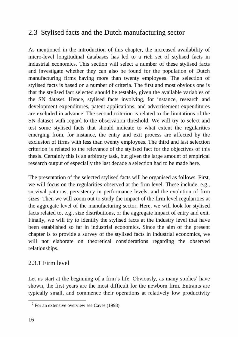
levels (Baldwin, 1995). Thus infant mortality rates are high, but for a givenentry cohort exit rates decline over time. Besides the negative relationshipbetween exit rates and age, the initial size of entrants also seems to have apositive impact on the probability to survive, whereas survivors’ growth ratesare often observed to be negatively related to initial size and age (see Dosi et al.,1997, and Geroski, 1995).
0,3
0,4
0,5
0,6
0,7
0,8
0,9
1,0
1 2 3 4 5 6 7 8 9 10 11 12 13 14
Y ears af ter entry
Rel
ativ
e to
ave
rage
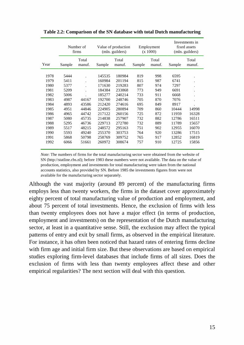
Relati ve producti v i ty Relati ve si ze
Figure 2.1: Average relative size and productivity of entrants
We will first consider the relative size and productivity of entrants. Figure 2.1displays the ratio of the mean value of the size (number of employees) andproductivity (value added per employee) of entrants divided by the mean of allfirms in Dutch manufacturing. On average, the size of entrants is 36 percent ofthe size of existing firms in the first year of birth, gradually growing to 57percent after 14 years. In a similar exercise, but with a dataset containing firmsof all sizes, Baldwin (1995) found entrants to start at 17 percent of the Canadianmanufacturing average, increasing to 33 percent after a decade. Further, hefound that the productivity of entrants averaged about 73 percent ofmanufacturing average at birth, increasing to 100 percent after ten years. In ourdata, we see that the average initial productivity is higher (89 percent ofmanufacturing average), but after fourteen years entrants are also on average asproductive as all manufacturing firms.
18
0
2
4
6
8
10
12
14
1 2 3 4 5 6 7 8 9 10 11 12 13
Y ears af ter entry
Per
cen
t
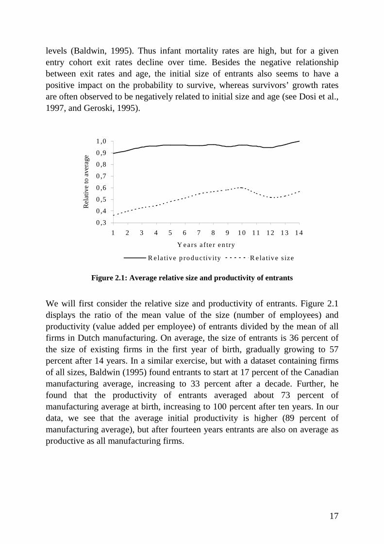
Figure 2.2: Average exit rates of entrants by years after entry
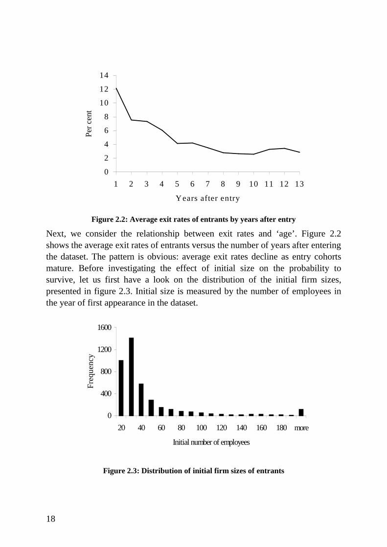
Next, we consider the relationship between exit rates and ‘age’ . Figure 2.2shows the average exit rates of entrants versus the number of years after enteringthe dataset. The pattern is obvious: average exit rates decline as entry cohortsmature. Before investigating the effect of initial size on the probabil ity tosurvive, let us first have a look on the distribution of the initial firm sizes,presented in figure 2.3. Initial size is measured by the number of employees inthe year of first appearance in the dataset.
0
400
800
1200
1600
20 40 60 80 100 120 140 160 180 more
Initial number of employees
Fre
qu
en
cy
Figure 2.3: Distr ibution of initial firm sizes of entrants

19
As figure 2.3 shows, most firms enter the database employing approximately 30workers. More precisely, the median number of employees at the year ofentering is equal to 31, whereas the mean equals 52.5 employees (with astandard error of 1.86). Next, we have estimated the following logit model forall appropriate entry cohorts:
Surv = β1 + β2 ln (ini_empl) + ε, (2.1)
where Surv = 0 if a firm exits before 1992 and 1 otherwise. The variableini_empl denotes the number of employees of each firm in its year of entry.Table 2.3 shows the regression statistics.
Table 2.3: Regression analysis of survival on initial size
Entry cohort Constant Initial size -2 log L
1979 -1.18 (0.54) 0.23 (0.15)* 614.681980 0.51 (0.73) -0.25 (0.22) 421.161981 -0.33 (0.68) 0.08 (0.18) 357.401982 -1.32 (0.65)** 0.35 (0.17)** 393.571983 -1.06 (0.48)** 0.34 (0.13)** * 660.231984 -0.73 (0.69) 0.28 (0.18) 404.211985 0.26 (0.68) 0.06 (0.18) 386.781986 -1.38 (0.86) 0.49 (0.23)** 321.291987 -0.62 (0.83) 0.39 (0.23)* 375.681988 -0.02 (0.83) 0.25 (0.23) 395.041989 -0.96 (0.78) 0.48 (0.22)** 447.951990 -2.50 (1.14)** 1.01 (0.33)** 314.011991 -1.77 (1.19) 1.07 (0.35)** * 398.45
All entry cohorts -0.13 (0.18) 0.20 (0.05)** * 6343.5
Firms present in 1978 -1.63 (0.13)** * 0.34 (0.03)** * 7364.0
Note: Standard errors in parentheses* significant at the 10%-level** significant at the 5%-level** * significant at the 1%-level
The results of table 2.3 show that there is some mixed evidence for a positiveeffect of initial size on the probability to survive. For five entry cohorts we havefound estimates for β2 that were not significantly different from zero at the 10percent level.3 The other entry cohorts did show a significant effect of initialsize. When all entry cohorts were pooled together, the effect of initial size was
3 This is based on the calculation of the probabili ty of obtaining (by chance alone) a chi-
square statistic (for testing the hypothesis that the parameter estimate is zero) greater inabsolute value than that observed given that the true parameter is zero.
20
significant at the 1 percent level. In order to compare the regularities of theseentry cohorts with all the firms present in 1978, we have run regression (2.1) forthese firms as well , where ini_empl is the number of employees in 1978. Here,we also found a significant positive effect of size on the probabili ty to survive(see the last row of table 2.3).
Finally, we examine whether initial size and age indeed have a negative impacton the growth rates of surviving entrants. For all surviving entrants (i.e., entrantsstill present in 1992), we have estimated the following model by ordinary leastsquares:
−1
lnt
t
empl
empl = β1 + β2 ln (ini_empl) +β3 ln (aget) + ε , (2.2)
where empl t is equal to the number of workers employed by the firm at year = t,and aget is equal to the number of years a firm is present in the dataset atyear = t. As the results in table 2.4 show, initial size and age indeed have asignificant4 negative effect on the growth of surviving entrants, although theparameter estimates are very small .
Table 2.4: Regression analysis of post-entry growth rates of survivingentrants on initial size and age
Constant Initial size Age Adjusted R2
0.135 (0.010) -0.024 (0.002) -0.007 (0.003) 0.010
Note: Standard errors in parentheses.
In conclusion, we see that the stylised facts related to entering firms can also befound in the SN data on Dutch manufacturing. Despite the uncertainty we havewith regard to e.g. the age of f irms appearing in the dataset, still the regularitiesobserved in the empirical l iterature for real entrants are also found for firmsentering the SN dataset: exit rates decline as entry cohorts mature, theprobability to survive is positively related to the initial size of entrants andfinally, the growth of surviving entrants is negatively related to their initial sizeand age.
For continuing firms, similar studies of patterns of firm growth are found in theempirical l iterature. Especially those studying the relationship between growth
4 All coeff icients are significant at 1 percent level, according to a t-test to test the hypothesisthat the parameter is zero.

21
and size are often led by investigations related to the validity of Gibrat’s ‘Law ofProportionate Effect’ . This ‘Law’ basically states that in each period theexpected value of the increment to a firm’s size is proportional to the currentsize of the firm (Sutton, 1997). More formally, let x (t) denote the size of a firmat time t, then Gibrat’s Law states:
x (t + 1) − x (t) = εt x (t), (2.3)
where the random variable εt denotes the proportionate rate of growth. Moststudies5, however, reject this law. For instance, Evans (1987a, 1987b) found thatfirm growth and its variance decreases with both firm size and age for a sampleof U.S. manufacturing firms. Do these empirically observed departures fromGibrat’s Law also apply to Dutch manufacturing firms? Obviously, therelationship between the growth of continuing firms (i.e., firms present in 1978and 1992) and their age cannot be studied here, however we can investigate therelation between growth rates and sizes.
Similar to Evans (1987b), we regressed the average annual growth rate ofemployment for each continuing firm on the logarithm of its number ofemployees in 1978. Hence, we have
[ln (empl1992 ) – ln (empl1978 )] / 14 = β1 + β2 ln (empl1978) + ε . (2.4)
The ordinary least squares estimate of β2 gives a value of –0.013, with a t-valueof –17.7. 6 Alternatively, we run a similar regression taking the annual growthrates as the dependent variable. Hence, we have
ln (emplt+1) – ln (empl t) = β1 + β2 ln (empl t) + ε , (2.5)
Here, the estimate for β2 equals –0.009, with a t-value of –12.6.7 Hence, bothtests corroborate the findings mentioned by Sutton (1997) that the growth ofcontinuing firms declines with their sizes. Consequently, we reject Gibrat’sLaw, since β2 is significantly different from zero.8
5 See Sutton (1997) for an extensive overview.6 The parameter estimate for β1 is equal to 0.058, with a t-value of 18.3; the adjusted R2 is
equal to 0.11.7 Here, the parameter estimate for β1 is equal to 0.042, with a t-value of 12.9; the adjusted
R2 is equal to 0.005.8 To see why β2 = 0 is consistent with Gibrat’s Law, rewrite (2.3) as: x (t + 1) / x (t) = 1 + εt.
22
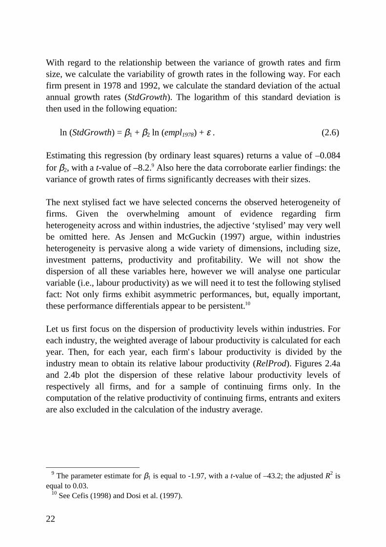
With regard to the relationship between the variance of growth rates and firmsize, we calculate the variability of growth rates in the following way. For eachfirm present in 1978 and 1992, we calculate the standard deviation of the actualannual growth rates (StdGrowth). The logarithm of this standard deviation isthen used in the following equation:
ln (StdGrowth) = β1 + β2 ln (empl1978) + ε . (2.6)
Estimating this regression (by ordinary least squares) returns a value of –0.084for β2, with a t-value of –8.2.9 Also here the data corroborate earlier findings: thevariance of growth rates of firms signif icantly decreases with their sizes.
The next stylised fact we have selected concerns the observed heterogeneity offirms. Given the overwhelming amount of evidence regarding firmheterogeneity across and within industries, the adjective ‘stylised’ may very wellbe omitted here. As Jensen and McGuckin (1997) argue, within industriesheterogeneity is pervasive along a wide variety of dimensions, including size,investment patterns, productivity and profitability. We will not show thedispersion of all these variables here, however we will analyse one particularvariable (i.e., labour productivity) as we will need it to test the following stylisedfact: Not only firms exhibit asymmetric performances, but, equally important,these performance differentials appear to be persistent.10
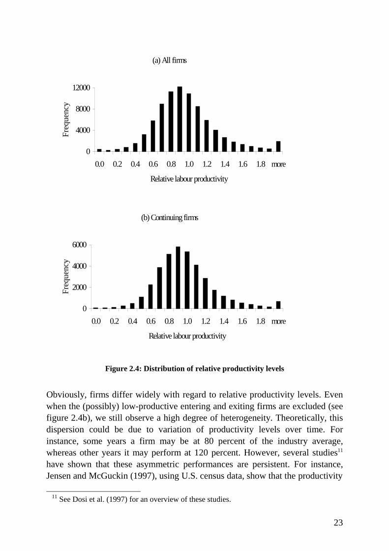
Let us first focus on the dispersion of productivity levels within industries. Foreach industry, the weighted average of labour productivity is calculated for eachyear. Then, for each year, each firm' s labour productivity is divided by theindustry mean to obtain its relative labour productivity (RelProd). Figures 2.4aand 2.4b plot the dispersion of these relative labour productivity levels ofrespectively all firms, and for a sample of continuing firms only. In thecomputation of the relative productivity of continuing firms, entrants and exitersare also excluded in the calculation of the industry average.
9 The parameter estimate for β1 is equal to -1.97, with a t-value of –43.2; the adjusted R2 is
equal to 0.03.10 See Cefis (1998) and Dosi et al. (1997).
23
(a) All firms
0
4000
8000
12000
0.0 0.2 0.4 0.6 0.8 1.0 1.2 1.4 1.6 1.8 more
Relative labour productivity
Fre
quen
cy
(b) Continuing firms
0
2000
4000
6000
0.0 0.2 0.4 0.6 0.8 1.0 1.2 1.4 1.6 1.8 more
Relative labour productivity
Fre
quen
cy
Figure 2.4: Distr ibution of relative productivity levels
Obviously, firms differ widely with regard to relative productivity levels. Evenwhen the (possibly) low-productive entering and exiting firms are excluded (seefigure 2.4b), we stil l observe a high degree of heterogeneity. Theoretically, thisdispersion could be due to variation of productivity levels over time. Forinstance, some years a firm may be at 80 percent of the industry average,whereas other years it may perform at 120 percent. However, several studies11
have shown that these asymmetric performances are persistent. For instance,Jensen and McGuckin (1997), using U.S. census data, show that the productivity
11 See Dosi et al. (1997) for an overview of these studies.
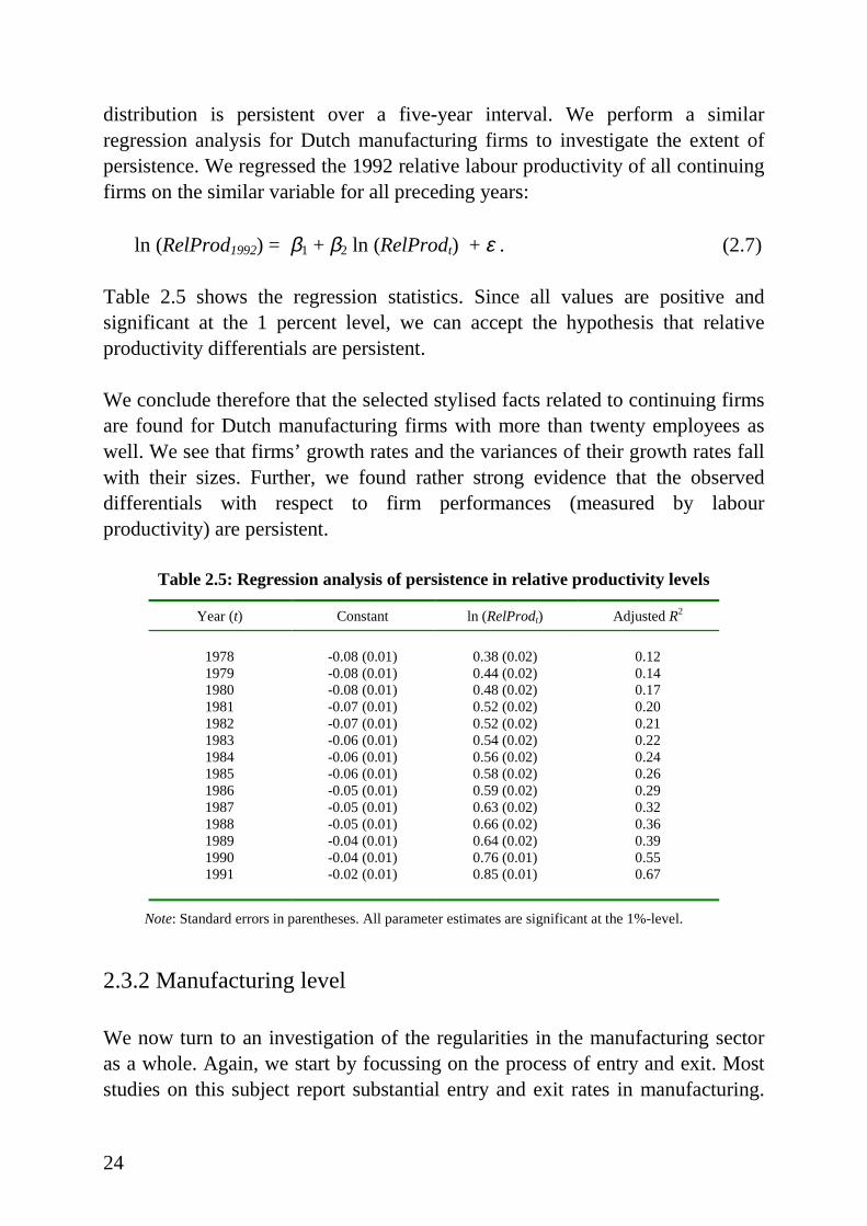
24
distribution is persistent over a five-year interval. We perform a similarregression analysis for Dutch manufacturing firms to investigate the extent ofpersistence. We regressed the 1992 relative labour productivity of all continuingfirms on the similar variable for all preceding years:
ln (RelProd1992) = β1 + β2 ln (RelProdt) + ε . (2.7)
Table 2.5 shows the regression statistics. Since all values are positive andsignificant at the 1 percent level, we can accept the hypothesis that relativeproductivity differentials are persistent.
We conclude therefore that the selected stylised facts related to continuing firmsare found for Dutch manufacturing firms with more than twenty employees aswell . We see that firms’ growth rates and the variances of their growth rates fallwith their sizes. Further, we found rather strong evidence that the observeddifferentials with respect to firm performances (measured by labourproductivity) are persistent.
Table 2.5: Regression analysis of persistence in relative productivity levels
Year (t) Constant ln (RelProdt) Adjusted R2
1978 -0.08 (0.01) 0.38 (0.02) 0.121979 -0.08 (0.01) 0.44 (0.02) 0.141980 -0.08 (0.01) 0.48 (0.02) 0.171981 -0.07 (0.01) 0.52 (0.02) 0.201982 -0.07 (0.01) 0.52 (0.02) 0.211983 -0.06 (0.01) 0.54 (0.02) 0.221984 -0.06 (0.01) 0.56 (0.02) 0.241985 -0.06 (0.01) 0.58 (0.02) 0.261986 -0.05 (0.01) 0.59 (0.02) 0.291987 -0.05 (0.01) 0.63 (0.02) 0.321988 -0.05 (0.01) 0.66 (0.02) 0.361989 -0.04 (0.01) 0.64 (0.02) 0.391990 -0.04 (0.01) 0.76 (0.01) 0.551991 -0.02 (0.01) 0.85 (0.01) 0.67
Note: Standard errors in parentheses. All parameter estimates are significant at the 1%-level.
2.3.2 Manufacturing level
We now turn to an investigation of the regularities in the manufacturing sectoras a whole. Again, we start by focussing on the process of entry and exit. Moststudies on this subject report substantial entry and exit rates in manufacturing.
25
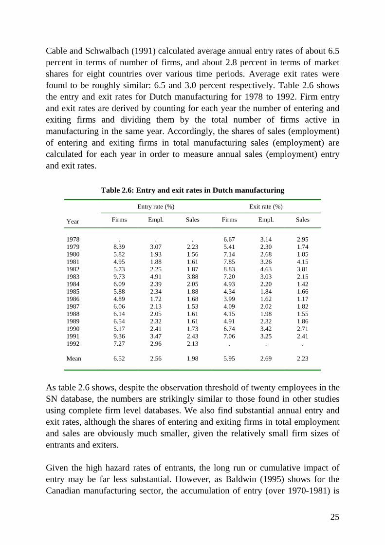
Cable and Schwalbach (1991) calculated average annual entry rates of about 6.5percent in terms of number of firms, and about 2.8 percent in terms of marketshares for eight countries over various time periods. Average exit rates werefound to be roughly similar: 6.5 and 3.0 percent respectively. Table 2.6 showsthe entry and exit rates for Dutch manufacturing for 1978 to 1992. Firm entryand exit rates are derived by counting for each year the number of entering andexiting firms and dividing them by the total number of firms active inmanufacturing in the same year. Accordingly, the shares of sales (employment)of entering and exiting firms in total manufacturing sales (employment) arecalculated for each year in order to measure annual sales (employment) entryand exit rates.
Table 2.6: Entry and exit rates in Dutch manufacturing
Entry rate (%) Exit rate (%)
Year Firms Empl. Sales Firms Empl. Sales
1978 . . . 6.67 3.14 2.951979 8.39 3.07 2.23 5.41 2.30 1.741980 5.82 1.93 1.56 7.14 2.68 1.851981 4.95 1.88 1.61 7.85 3.26 4.151982 5.73 2.25 1.87 8.83 4.63 3.811983 9.73 4.91 3.88 7.20 3.03 2.151984 6.09 2.39 2.05 4.93 2.20 1.421985 5.88 2.34 1.88 4.34 1.84 1.661986 4.89 1.72 1.68 3.99 1.62 1.171987 6.06 2.13 1.53 4.09 2.02 1.821988 6.14 2.05 1.61 4.15 1.98 1.551989 6.54 2.32 1.61 4.91 2.32 1.861990 5.17 2.41 1.73 6.74 3.42 2.711991 9.36 3.47 2.43 7.06 3.25 2.411992 7.27 2.96 2.13 . . .
Mean 6.52 2.56 1.98 5.95 2.69 2.23
As table 2.6 shows, despite the observation threshold of twenty employees in theSN database, the numbers are strikingly similar to those found in other studiesusing complete firm level databases. We also find substantial annual entry andexit rates, although the shares of entering and exiting firms in total employmentand sales are obviously much smaller, given the relatively small firm sizes ofentrants and exiters.
Given the high hazard rates of entrants, the long run or cumulative impact ofentry may be far less substantial. However, as Baldwin (1995) shows for theCanadian manufacturing sector, the accumulation of entry (over 1970-1981) is
26
of a considerable magnitude. The number of entrants alive in 1981 equalled 35.5percent of the 1970 firm population, while their number of employees was equalto 10.9 percent of total 1970 employment. The magnitude of exit was found tobe substantial as well : 35.0 percent in terms of f irm numbers, 10.5 in terms ofemployment.
Calculating these numbers for Dutch manufacturing over 1978-1992 also showsa significant cumulative impact of entry and exit. In 1992, 43.0 percent of allfirms are firms that were not present in 1978, collectively capturing 22.4 percentof total 1992 employment and 19.5 percent of total 1992 sales. Hence, althoughentrants are typically small and have high hazard rates, those that survive arecollectively able to obtain a significant market share in time. Further, thenumber of firms that were present in 1978, but absent in 1992 equals 39.1percent of the total population of firms in 1978. Their shares in 1978employment and sales were 23.5 and 23.3 percent, respectively.
To summarise, when measured over the full period (1978-1992) the Dutchmanufacturing sector is characterised by high turnover of market shares due tofirms entering and exiting the database. However, this is not the only source ofturbulence, of course. Within the population of continuing firms, the turnoverdue to changing market shares may also substantially contribute to thereallocation of market shares. To measure this source of turbulence, we firstcalculated for each continuing firm the absolute change (between 1992 and1978) of its share in total sales of the industry in which it is allocated. Next, foreach industry we calculated the sum of these changes, and divided this by two.Finally, we computed the average of this number over the 106 industries. Basedon these calculations we find that in the Dutch manufacturing sector, on average15.5 percent of industrial market share is reallocated between continuing firmsover the period 1978-1992. This number is very close to the 16.0 percent foundby Baldwin (1995) for the Canadian manufacturing sector, measured likewiseover the period 1970-1979.
Potentially, the observed turbulence could substantially contribute to aggregateproductivity growth at the industry level. If market shares are generallytransferred from the less productive to the more productive firms in an industry,aggregate productivity will rise due to this simple Darwinian selectionmechanism. However, individual firms may also contribute to aggregateproductivity growth by increasing their productive eff iciency. As Baldwin(1995) shows, the contribution of turnover to productivity in Canadian
27
manufacturing is substantial when the cumulated or long run impact of entry andexit is taken into account. Depending on the assumptions related to thereplacement patterns between entrants, exiters, and incumbents, he found thatbetween 40 to 50 percent of aggregate productivity growth could be attributed tothe turnover process. Another study by Haltiwanger (1997)12 found similarvalues for all U.S. manufacturing industries, although his decomposition methodwas slightly different from Baldwin’s. In what follows we will decomposeaggregate productivity growth in order to calculate the contribution of turnoverto aggregate productivity growth in Dutch manufacturing.
Labour productivity at the firm level (Prodi,t) is again measured as the real valueadded per employee. The average labour productivity in 1978 and 1992 is thenthe output (sales) share weighted sum of the productivity levels of all firms inDutch manufacturing (denoted by AvgProd1978 and AvgProd1992). Let Shcont,t
denote the output share (in total manufacturing) of a continuing firm at t,Shext,1978 the output share of an exiting firm in 1978, and Shent,1992 the outputshare of an entering firm in 1992. Based on Haltiwanger (1997) we decomposegrowth of average labour productivity (AvgProd1992 - AvgProd1978) into thefollowing five components:
1. A within effect: within firm productivity growth weighted by initial outputshares
( )[ ]∑ −cont
contcontcont ProdProdSh 1978,1992,1978,
2. A between firm effect: changing output shares weighted by the deviation ofinitial firm productivity and initial average manufacturing productivity
( )( )[ ]∑ −−cont
contcontcont AvgProdProdShSh 19781978,1978,1992,
3. A covariance term: the sum of f irm productivity growth times firm sharechange
( )( )[ ]∑ −−cont
contcontcontcont ProdProdShSh 1978,1992,1978,1992,
12 This study decomposed total factor productivity growth, whereas Baldwin (1995)
decomposed aggregate growth of labour productivity.
28
4. An entry effect: the end year share weighted sum of the difference betweenproductivity of entering firms and initial average manufacturing productivity
( )∑ −ent
entent AvgProdProdSh 19781992,1992,
5. An exit effect: the initial share weighted sum of the difference between initialaverage manufacturing productivity and productivity of exiting fi rms
( )∑ −ext
extext ProdAvgProdSh 1978,19781978,
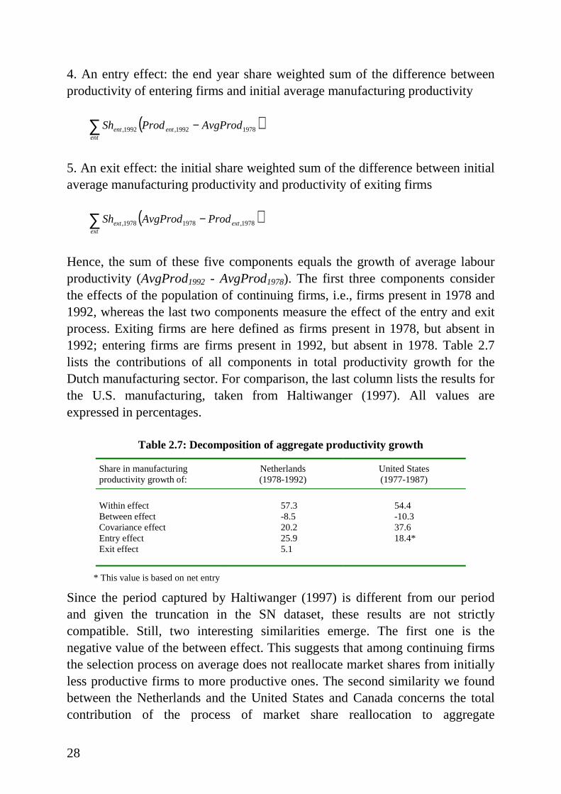
Hence, the sum of these five components equals the growth of average labourproductivity (AvgProd1992 - AvgProd1978). The first three components considerthe effects of the population of continuing firms, i.e., firms present in 1978 and1992, whereas the last two components measure the effect of the entry and exitprocess. Exiting firms are here defined as firms present in 1978, but absent in1992; entering firms are firms present in 1992, but absent in 1978. Table 2.7lists the contributions of all components in total productivity growth for theDutch manufacturing sector. For comparison, the last column lists the results forthe U.S. manufacturing, taken from Haltiwanger (1997). All values areexpressed in percentages.
Table 2.7: Decomposition of aggregate productivity growth
Share in manufacturingproductivity growth of:
Netherlands(1978-1992)
United States(1977-1987)
Within effect 57.3 54.4Between effect -8.5 -10.3Covariance effect 20.2 37.6Entry effect 25.9 18.4*Exit effect 5.1
* This value is based on net entry
Since the period captured by Haltiwanger (1997) is different from our periodand given the truncation in the SN dataset, these results are not strictlycompatible. Still, two interesting similarities emerge. The first one is thenegative value of the between effect. This suggests that among continuing firmsthe selection process on average does not reallocate market shares from initiall yless productive firms to more productive ones. The second similarity we foundbetween the Netherlands and the United States and Canada concerns the totalcontribution of the process of market share reallocation to aggregate
29
productivity growth. Since all but the ‘within’ component capture changes inmarket shares, this turnover contribution can be calculated as [100 percent – the‘within’ share]. For the Netherlands, this equals 42.7 percent, which is similar tothe values between 40 to 50 percent found in the earlier mentioned studies. Oneimportant difference between the US and Dutch manufacturing is found for theeffects of entry and exit. In Dutch manufacturing, especially the entry of f irmswith high productivity levels substantially contributed to aggregate productivitygrowth.13
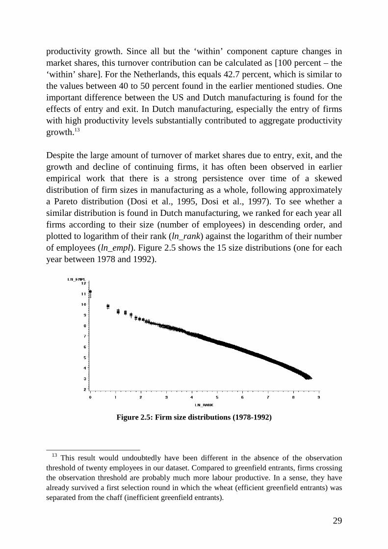
Despite the large amount of turnover of market shares due to entry, exit, and thegrowth and decline of continuing firms, it has often been observed in earlierempirical work that there is a strong persistence over time of a skeweddistribution of f irm sizes in manufacturing as a whole, following approximatelya Pareto distribution (Dosi et al., 1995, Dosi et al., 1997). To see whether asimilar distribution is found in Dutch manufacturing, we ranked for each year allfirms according to their size (number of employees) in descending order, andplotted to logarithm of their rank (ln_rank) against the logarithm of their numberof employees (ln_empl). Figure 2.5 shows the 15 size distributions (one for eachyear between 1978 and 1992).
Figure 2.5: Firm size distr ibutions (1978-1992)
13 This result would undoubtedly have been different in the absence of the observation
threshold of twenty employees in our dataset. Compared to greenfield entrants, firms crossingthe observation threshold are probably much more labour productive. In a sense, they havealready survived a first selection round in which the wheat (eff icient greenfield entrants) wasseparated from the chaff (inefficient greenfield entrants).
30
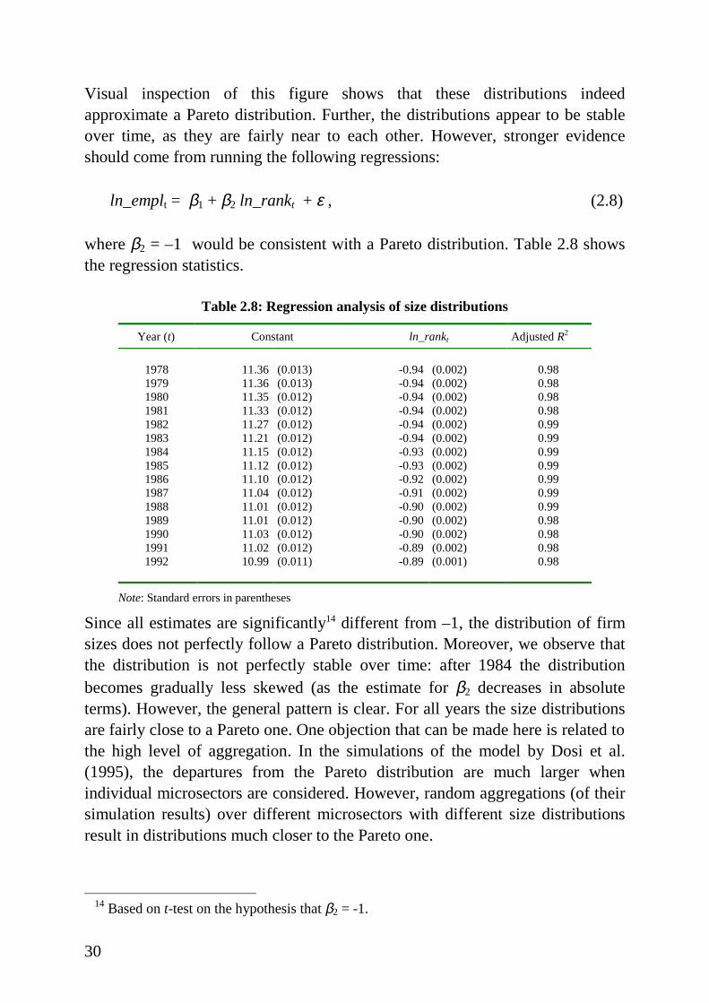
Visual inspection of this figure shows that these distributions indeedapproximate a Pareto distribution. Further, the distributions appear to be stableover time, as they are fairly near to each other. However, stronger evidenceshould come from running the following regressions:
ln_empl t = β1 + β2 ln_rankt + ε , (2.8)
where β2 = –1 would be consistent with a Pareto distribution. Table 2.8 showsthe regression statistics.
Table 2.8: Regression analysis of size distr ibutions
Year (t) Constant ln_rankt Adjusted R2
1978 11.36 (0.013) -0.94 (0.002) 0.981979 11.36 (0.013) -0.94 (0.002) 0.981980 11.35 (0.012) -0.94 (0.002) 0.981981 11.33 (0.012) -0.94 (0.002) 0.981982 11.27 (0.012) -0.94 (0.002) 0.991983 11.21 (0.012) -0.94 (0.002) 0.991984 11.15 (0.012) -0.93 (0.002) 0.991985 11.12 (0.012) -0.93 (0.002) 0.991986 11.10 (0.012) -0.92 (0.002) 0.991987 11.04 (0.012) -0.91 (0.002) 0.991988 11.01 (0.012) -0.90 (0.002) 0.991989 11.01 (0.012) -0.90 (0.002) 0.981990 11.03 (0.012) -0.90 (0.002) 0.981991 11.02 (0.012) -0.89 (0.002) 0.981992 10.99 (0.011) -0.89 (0.001) 0.98
Note: Standard errors in parentheses
Since all estimates are significantly14 different from –1, the distribution of f irmsizes does not perfectly follow a Pareto distribution. Moreover, we observe thatthe distribution is not perfectly stable over time: after 1984 the distributionbecomes gradually less skewed (as the estimate for β2 decreases in absoluteterms). However, the general pattern is clear. For all years the size distributionsare fairly close to a Pareto one. One objection that can be made here is related tothe high level of aggregation. In the simulations of the model by Dosi et al.(1995), the departures from the Pareto distribution are much larger whenindividual microsectors are considered. However, random aggregations (of theirsimulation results) over different microsectors with different size distributionsresult in distributions much closer to the Pareto one.
14 Based on t-test on the hypothesis that β2 = -1.

31
Therefore, disaggregating the manufacturing sector into the 106 industries in theSN database may show size distributions less stable and less close to the Paretodistribution than the one for the manufacturing as a whole. Also the otherregularities and statistics shown in this section are derived from themanufacturing sector as a whole, concealing possible differences between theindustries. In the next section we will disaggregate the manufacturing sector andfocus on the differences between the industries.
2.3.3 Industry level
Given the objectives of this thesis, the most important stylised fact discussed inthis chapter is related to the observed differences between industries. Manystudies have observed that variables like capital intensity, advertising intensity,R&D intensity, concentration, and entry and exit rates differ widely acrosssectors, observations that are indeed at the very origin of the birth of industrialeconomics as a discipline (Dosi et al., 1997). At the end of this section we willshow the specific distributions of a number of selected variables over theindustries in the SN database. But first we wil l investigate whether the data onDutch manufacturing support cross-sectional relationships that have beenobserved in earlier empirical research.
Compared to the evidence obtained at the firm and manufacturing level,empirical evidence on cross-sectional relationships at the industry level is ratherthin. Most of this evidence addresses the (theoretical) determinants of entry andmarket share turnover among incumbents, the relation between entry and exitrates, and the determinants of industry-level profitability. As we will show, aconsiderable part of the evidence is ‘negative’ , i.e., it shows that someexplanatory variables have repeatedly been found to be insignificant. Especiallyin cases where, from a standard theoretical point of view, these variables aresupposed to have considerable explanatory powers, negative results are naturallyequally interesting.
But first we will deal with a general phenomenon that has been observed bymany studies on entry and exit, i.e., the strong correlation between entry and exitrates (Geroski, 1995). For the Dutch manufacturing sector this relationshipexists as well: for the correlation between the industry averages of annual salesentry and exit rates we found a (Pearson) correlation coefficient of 0.58 (0.76when firm entry and exit rates are correlated). When cumulative entry and exitrates are considered, we also find significantly positive relationships: 0.23
32
between cumulative firm entry and exit, and a correlation coefficient of 0.52when cumulative sales entry and exit rates are considered.15 Hence, at theindustry level high entry rates are associated with high exit rates, regardless ofhow the entry and exit rates are measured.
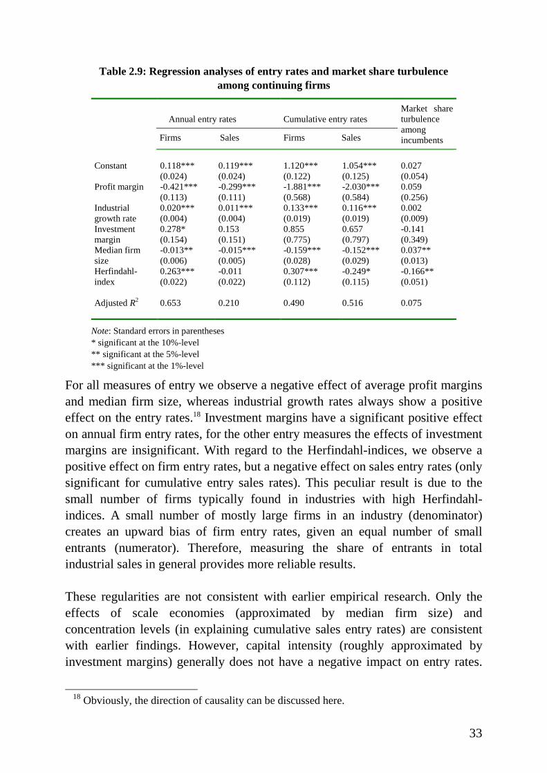
With regard to the determinants of gross entry, earlier research has shown thatprofitability does not seem to have a significant effect on attracting entrants.Obviously, this observation is at odds with standard models of the entry process,in which high profits are supposed to attract profit-seeking entrants. Mixedresults were obtained for the effect of industry growth, whereas capital intensity,scale economies and concentration levels were found to have a negative effecton gross entry.16 Since we have several ways to measure the entry process, wewill analyse the regression results of each of the entry measures on the following‘determinants’ . For profitability, we use the industry mean of profits over sales.Since we have no data on capital stock, we will use the industry mean ofinvestments over sales as a proxy for capital intensity. For scale economies, weuse a proxy as well, which is (the log of) the median firm size in an industry.Finally, for concentration levels we use the average Herfindahl-index of anindustry.17 Table 2.9 lists the results of the (ordinary least squares) regressionanalysis.
15 All these correlations have p-values less than 0.01. This p-value (of a correlation r) is
obtained by treating the statistic
)1(
)2(2r
nrt
−
−=
as having a Student' s t distribution with (n-2) degrees of freedom, where n is the number ofobservations. The p-value of the correlation r is the probabili ty of obtaining (by chance alone)a Student' s t-statistic greater in absolute value than the observed statistic t.
16 See Schmalensee (1989), Malerba and Orsenigo (1994), Dosi et al. (1995), and Geroski(1995).
17 The Herfindahl-index is calculated as the sum of the squared market shares. Using thecollective market share of the four largest firms as an alternative measure for concentrationdoes not significantly change the results.
33
Table 2.9: Regression analyses of entry rates and market share turbulenceamong continuing firms
Annual entry rates Cumulative entry rates
Firms Sales Firms Sales
Market shareturbulenceamongincumbents
Constant 0.118** *(0.024)
0.119** *(0.024)
1.120** *(0.122)
1.054** *(0.125)
0.027(0.054)
Profit margin -0.421** *(0.113)
-0.299** *(0.111)
-1.881** *(0.568)
-2.030** *(0.584)
0.059(0.256)
Industrialgrowth rate
0.020** *(0.004)
0.011** *(0.004)
0.133** *(0.019)
0.116** *(0.019)
0.002(0.009)
Investmentmargin
0.278*(0.154)
0.153(0.151)
0.855(0.775)
0.657(0.797)
-0.141(0.349)
Median firmsize
-0.013**(0.006)
-0.015** *(0.005)
-0.159** *(0.028)
-0.152** *(0.029)
0.037**(0.013)
Herfindahl-index
0.263** *(0.022)
-0.011(0.022)
0.307** *(0.112)
-0.249*(0.115)
-0.166**(0.051)
Adjusted R2 0.653 0.210 0.490 0.516 0.075
Note: Standard errors in parentheses* significant at the 10%-level** significant at the 5%-level** * significant at the 1%-level
For all measures of entry we observe a negative effect of average profit marginsand median firm size, whereas industrial growth rates always show a positiveeffect on the entry rates.18 Investment margins have a significant positive effecton annual firm entry rates, for the other entry measures the effects of investmentmargins are insignificant. With regard to the Herfindahl-indices, we observe apositive effect on firm entry rates, but a negative effect on sales entry rates (onlysignificant for cumulative entry sales rates). This peculiar result is due to thesmall number of firms typically found in industries with high Herfindahl-indices. A small number of mostly large firms in an industry (denominator)creates an upward bias of firm entry rates, given an equal number of smallentrants (numerator). Therefore, measuring the share of entrants in totalindustrial sales in general provides more reliable results.
These regularities are not consistent with earlier empirical research. Only theeffects of scale economies (approximated by median firm size) andconcentration levels (in explaining cumulative sales entry rates) are consistentwith earlier findings. However, capital intensity (roughly approximated byinvestment margins) generally does not have a negative impact on entry rates.
18 Obviously, the direction of causali ty can be discussed here.
34
And instead of an insignificant effect of profitabil ity on gross entry rates, weobserve a significantly negative relationship.
Of course, an exercise like this should be taken with some caution. Explainingthe entry rates derived from the SN database is in fact explaining the extent towhich small firms are able to grow and pass the observation threshold of twentyemployees (annual entry rates) and the extent to which they are able to surviveand gain market share (cumulative entry rates). Therefore, the independentvariables mostly reflect the growth opportunities for entrants. Interpreted assuch, it can well be explained why we observe a negative relationship betweenprofitability and our ‘entry rates’ . Perhaps high profits initiall y attract manyentrants, but if many of these entrants have difficulties in surviving they maynever exceed the observation threshold of twenty employees. And the moredifficult it i s for entrants to survive and grow, the less competition theincumbents face and hence the more they are able to retain their high profitlevels, ceteris paribus. In this interpretation, high profits simply reflect theappropriability conditions in an industry and, consequently, the opportunities foryoung and small firms to survive and grow.
With regard to the stylised facts related to the determinants of turbulence amongincumbents19, earlier empirical research20 has shown that variables related to thelevel of international competition and conditions related to technology and to thedemand side explain a great deal of the differences among industries inincumbents’ market share mobili ty. Since these variables cannot be extractedfrom the SN dataset, the only appropriate variables we can include in theanalysis are those we also included in analysing the entry rates. But the evidenceon the explanatory powers of these variables is rather thin. No study so far hasconvincingly shown that any of these variables significantly explains the amountof turbulence among incumbents in an industry. As shown by the low adjustedR2, displayed in the last column of table 2.9, in Dutch manufacturing thesevariables together do not explain much of the variation of incumbents’ mobilityin market shares as well. Only median firm size (positive) and the Herfindahl-index (negative) are statistically significant in explaining the market shareturbulence among incumbents.
19 Measured as half the sum of the absolute changes in market shares for all continuing
firms in an industry between 1978 and 1992.20 See Baldwin and Rafiquzzaman (1995) and Baldwin and Caves (1998).
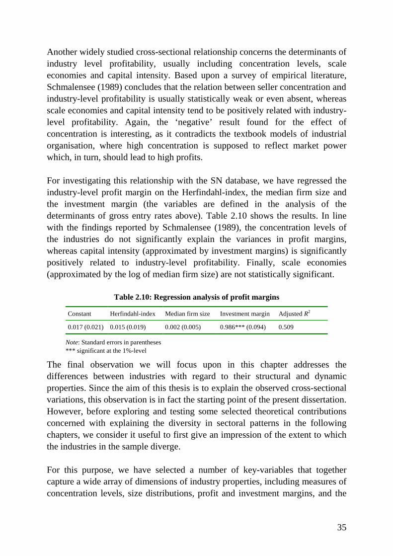
35
Another widely studied cross-sectional relationship concerns the determinants ofindustry level profitabil ity, usually including concentration levels, scaleeconomies and capital intensity. Based upon a survey of empirical li terature,Schmalensee (1989) concludes that the relation between seller concentration andindustry-level profitability is usually statistically weak or even absent, whereasscale economies and capital intensity tend to be positively related with industry-level profitability. Again, the ‘negative’ result found for the effect ofconcentration is interesting, as it contradicts the textbook models of industrialorganisation, where high concentration is supposed to reflect market powerwhich, in turn, should lead to high profits.
For investigating this relationship with the SN database, we have regressed theindustry-level profit margin on the Herfindahl-index, the median firm size andthe investment margin (the variables are defined in the analysis of thedeterminants of gross entry rates above). Table 2.10 shows the results. In linewith the findings reported by Schmalensee (1989), the concentration levels ofthe industries do not significantly explain the variances in profit margins,whereas capital intensity (approximated by investment margins) is significantlypositively related to industry-level profitabili ty. Finally, scale economies(approximated by the log of median firm size) are not statistically significant.
Table 2.10: Regression analysis of profit margins
Constant Herfindahl-index Median firm size Investment margin Adjusted R2
0.017 (0.021) 0.015 (0.019) 0.002 (0.005) 0.986** * (0.094) 0.509
Note: Standard errors in parentheses*** significant at the 1%-level
The final observation we will focus upon in this chapter addresses thedifferences between industries with regard to their structural and dynamicproperties. Since the aim of this thesis is to explain the observed cross-sectionalvariations, this observation is in fact the starting point of the present dissertation.However, before exploring and testing some selected theoretical contributionsconcerned with explaining the diversity in sectoral patterns in the followingchapters, we consider it useful to first give an impression of the extent to whichthe industries in the sample diverge.
For this purpose, we have selected a number of key-variables that togethercapture a wide array of dimensions of industry properties, including measures ofconcentration levels, size distributions, profit and investment margins, and the
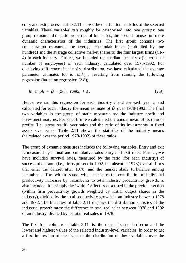
36
entry and exit process. Table 2.11 shows the distribution statistics of the selectedvariables. These variables can roughly be categorised into two groups: onegroup measures the static properties of industries, the second focuses on moredynamic characteristics of the industries. The first group contains twoconcentration measures: the average Herfindahl-index (multiplied by onehundred) and the average collective market shares of the four largest firms (CR-4) in each industry. Further, we included the median firm sizes (in terms ofnumber of employees) of each industry, calculated over 1978-1992. Fordisplaying differences in the size distribution, we have calculated the averageparameter estimates for ln_ranki, t, resulting from running the followingregression (based on regression (2.8)):
ln_empl i,t = β1 + β2 ln_ranki,t + ε . (2.9)
Hence, we ran this regression for each industry i and for each year t, andcalculated for each industry the mean estimate of β2 over 1978-1992. The finaltwo variables in the group of static measures are the industry profit andinvestment margins. For each firm we calculated the annual mean of its ratio ofprofits (i.e., gross result) over sales and the ratio of its investments in fixedassets over sales. Table 2.11 shows the statistics of the industry means(calculated over the period 1978-1992) of these ratios.
The group of dynamic measures includes the following variables. Entry and exitis measured by annual and cumulative sales entry and exit rates. Further, wehave included survival rates, measured by the ratio (for each industry) ofsuccessful entrants (i.e., firms present in 1992, but absent in 1978) over all firmsthat enter the dataset after 1978, and the market share turbulence amongincumbents. The ‘within’ share, which measures the contribution of individualproductivity increases by incumbents to total industry productivity growth, isalso included. It is simply the ‘within’ effect as described in the previous section(within firm productivity growth weighted by initial output shares in theindustry), divided by the total productivity growth in an industry between 1978and 1992. The final row of table 2.11 displays the distribution statistics of theindustrial growth rates: the difference in total real sales between 1978 and 1992of an industry, divided by its total real sales in 1978.
The first four columns of table 2.11 list the mean, its standard error and thelowest and highest values of the selected industry-level variables. In order to geta first impression of the shape of the distribution of these variables over the
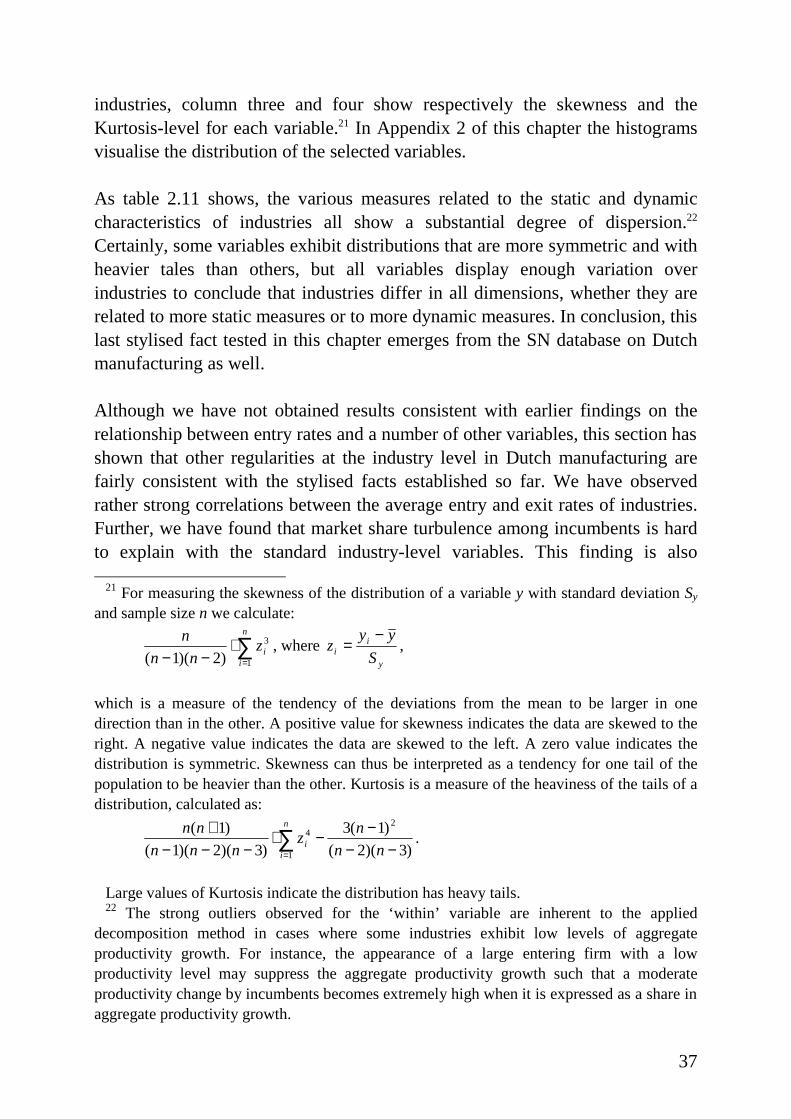
37
industries, column three and four show respectively the skewness and theKurtosis-level for each variable.21 In Appendix 2 of this chapter the histogramsvisualise the distribution of the selected variables.
As table 2.11 shows, the various measures related to the static and dynamiccharacteristics of industries all show a substantial degree of dispersion.22
Certainly, some variables exhibit distributions that are more symmetric and withheavier tales than others, but all variables display enough variation overindustries to conclude that industries differ in all dimensions, whether they arerelated to more static measures or to more dynamic measures. In conclusion, thislast stylised fact tested in this chapter emerges from the SN database on Dutchmanufacturing as well .
Although we have not obtained results consistent with earlier findings on therelationship between entry rates and a number of other variables, this section hasshown that other regularities at the industry level in Dutch manufacturing arefairly consistent with the stylised facts established so far. We have observedrather strong correlations between the average entry and exit rates of industries.Further, we have found that market share turbulence among incumbents is hardto explain with the standard industry-level variables. This finding is also
21 For measuring the skewness of the distribution of a variable y with standard deviation Sy
and sample size n we calculate:
∑=
⋅−−
n
iiz
nn
n
1
3
)2)(1(, where
y
ii S
yyz
−= ,
which is a measure of the tendency of the deviations from the mean to be larger in onedirection than in the other. A positive value for skewness indicates the data are skewed to theright. A negative value indicates the data are skewed to the left. A zero value indicates thedistribution is symmetric. Skewness can thus be interpreted as a tendency for one tail of thepopulation to be heavier than the other. Kurtosis is a measure of the heaviness of the tails of adistribution, calculated as:
∑= −−
−−⋅−−−
+ n
ii nn
nz
nnn
nn
1
24
)3)(2(
)1(3
)3)(2)(1(
)1(.
Large values of Kurtosis indicate the distribution has heavy tails.22 The strong outliers observed for the ‘within’ variable are inherent to the applied
decomposition method in cases where some industries exhibit low levels of aggregateproductivity growth. For instance, the appearance of a large entering firm with a lowproductivity level may suppress the aggregate productivity growth such that a moderateproductivity change by incumbents becomes extremely high when it is expressed as a share inaggregate productivity growth.
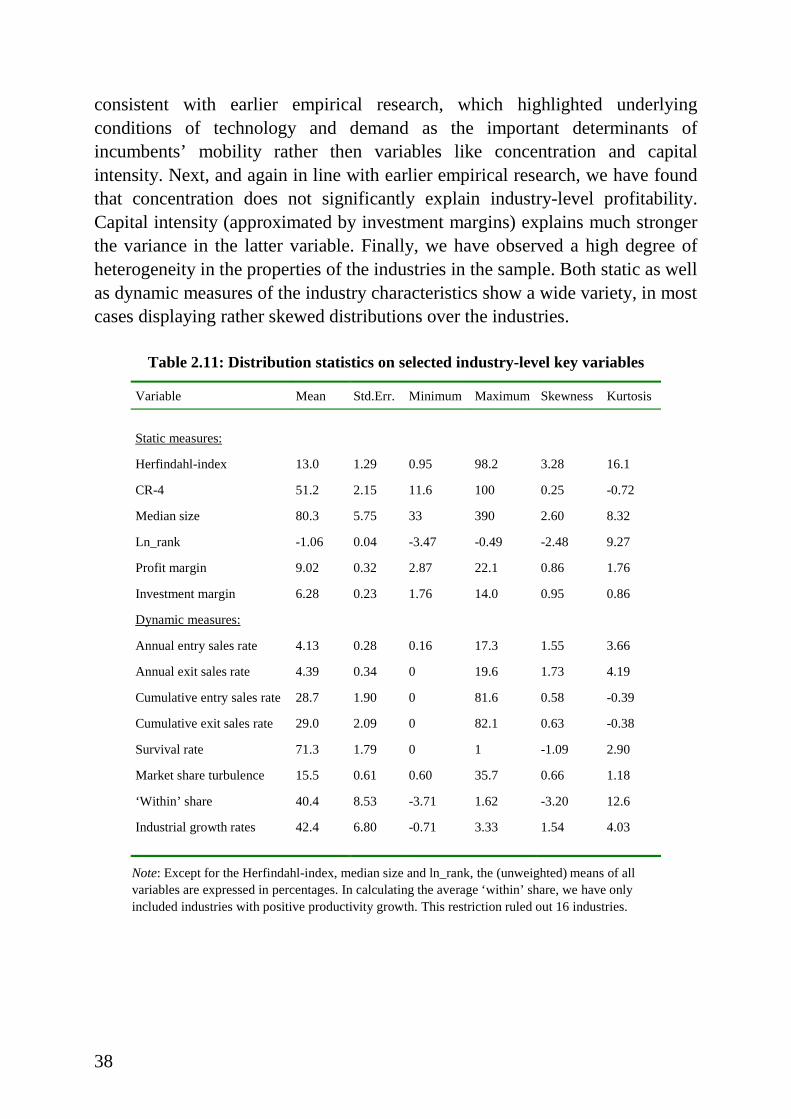
38
consistent with earlier empirical research, which highlighted underlyingconditions of technology and demand as the important determinants ofincumbents’ mobility rather then variables like concentration and capitalintensity. Next, and again in line with earlier empirical research, we have foundthat concentration does not significantly explain industry-level profitabil ity.Capital intensity (approximated by investment margins) explains much strongerthe variance in the latter variable. Finally, we have observed a high degree ofheterogeneity in the properties of the industries in the sample. Both static as wellas dynamic measures of the industry characteristics show a wide variety, in mostcases displaying rather skewed distributions over the industries.
Table 2.11: Distr ibution statistics on selected industry-level key variables
Variable Mean Std.Err. Minimum Maximum Skewness Kurtosis
Static measures:
Herfindahl-index 13.0 1.29 0.95 98.2 3.28 16.1
CR-4 51.2 2.15 11.6 100 0.25 -0.72
Median size 80.3 5.75 33 390 2.60 8.32
Ln_rank -1.06 0.04 -3.47 -0.49 -2.48 9.27
Profit margin 9.02 0.32 2.87 22.1 0.86 1.76
Investment margin 6.28 0.23 1.76 14.0 0.95 0.86
Dynamic measures:
Annual entry sales rate 4.13 0.28 0.16 17.3 1.55 3.66
Annual exit sales rate 4.39 0.34 0 19.6 1.73 4.19
Cumulative entry sales rate 28.7 1.90 0 81.6 0.58 -0.39
Cumulative exit sales rate 29.0 2.09 0 82.1 0.63 -0.38
Survival rate 71.3 1.79 0 1 -1.09 2.90
Market share turbulence 15.5 0.61 0.60 35.7 0.66 1.18
‘Within’ share 40.4 8.53 -3.71 1.62 -3.20 12.6
Industrial growth rates 42.4 6.80 -0.71 3.33 1.54 4.03
Note: Except for the Herfindahl-index, median size and ln_rank, the (unweighted) means of allvariables are expressed in percentages. In calculating the average ‘within’ share, we have onlyincluded industries with positive productivity growth. This restriction ruled out 16 industries.
39
2.4 Conclusions
Given the empirical nature of this thesis and the extensive use of the SNmanufacturing database throughout it, this chapter illuminated three importantissues related to empirical research in industrial economics. First of all, we havedescribed in detail the firm-level data on which a major part of the research inthis dissertation is based. Second, by presenting a number of selected stylisedfacts we aimed to highlight some robust empirical results that have beenestablished so far in industrial economics. Especially in the last fifteen years, theincreased access to firm-level data has resulted in a collection of results thatwere found to be rather invariant across countries and over time. Finally, wehave investigated whether these stylised facts could also be found in Dutchmanufacturing.
Two important results emerge from this chapter. The first is that the regularitiesemerging from the SN manufacturing database are to a large extent consistentwith the stylised facts in industrial economics. Whether we look at firm-levelregularities, their aggregate impact on the manufacturing sector, or regularitiesat the industry level, practically all of them seem to be consistent with earlierempirical findings in industrial economics. The second result is in fact alreadycaptured by the first one, but is still mentioned separately here because of itsessence for the research in this thesis. We have shown that industries widelydiffer in virtually all dimensions observable in the data. Certainly, this result isfar from new. In fact, it constitutes the origin of industrial economics as adiscipline. However, despite the presence of a number of theoreticalcontributions that potentially can explain the observed differences, not mucheffort has been done so far in testing these theories with the increasinglyavailable firm-level data.
As mentioned already in chapter one, the aim of this thesis is to fill this gap. Inchapter 4 we will use the SN database to empirically test some theories that mayexplain the observed differences between industries with regard to theirstructural and dynamic properties. But first, the next chapter will elaborate onthese theoretical contributions.

40
Appendix 1: List of industries in the SN database
Food products
Production, processing and preserving of meat and meat productsManufacture of dairy productsProcessing and preserving of f ish and fish productsManufacture of grain mill productsManufacture of vegetable and animal oils and fatsProcessing and preserving of fruit and vegetablesManufacture of bakery productsManufacture of sugar, cacao, chocolate and sugar confectionery
Beverages, tobacco, and food nec*
Manufacture of prepared animal feedsManufacture of other food products necDistil ling, rectifying and blending of spirits; ethyl alcohol productionManufacture of malt liquors and maltManufacture of soft drinksManufacture of tobacco products
Textile products and wearing apparel
Preparation and spinning of wool fibres, weaving of woolPreparation and spinning of cotton fibres, weaving of cottonManufacture of tricot and stockingsFinishing of textilesManufacture of carpets and rugsManufacture of made-up textile articles, except apparelManufacture of other textiles necManufacture of wearing apparel, dressing and dyeing of fur
Leather products
Tanning and dressing of leatherManufacture of luggage, handbags and the like, saddlery and harnessManufacture of footwear
Wood and wood products
Sawmill ing and planing of wood, manufacture of veneer sheets, plywood, laminboard,particleboard and other panels and boardsCarpentry and manufacture of densified wood and parquet flooring blocksManufacture of wooden containersManufacture of other products of wood, manufacture of articles of cork, straw and plaitingmaterialsManufacture of furniture, except metal furniture
Paper and paper products
Manufacture of paper and paperboardManufacture of other articles of paper and paperboardManufacture of corrugated paper and paperboard

41
Printing and publishing
Printing of newspapersPrinting of booksOffset printingChemigrafical and fotoli thografical firmsOther printingPublishing of newspapersPublishing of periodicalsPublishing of booksOther publishingBookbinding
Chemicals, chemical products, yarns and fibres
Manufacture of fertili sersManufacture of synthetic resinManufacture of dyestuffs and colouring mattersManufacture of chemical raw materials necManufacture of paints, varnishes and similar coatings, printing inkManufacture of pharmaceuticals and medicinal chemicalsManufacture of soap and detergents, cleaning and polishing preparations, perfumes and toiletpreparationsManufacture of chemical pesticidesManufacture of other chemical products nec
Rubber and plastic products
Manufacture of rubber productsManufacture of plastic products
Building materials, earthenware and glass
Manufacture of bricks and tilesManufacture of ceramicsManufacture of cement and limeManufacture of articles of concrete and cementManufacture of other non-metalli c mineral products necManufacture of glass and glass products
Basic and fabricated metal products
Manufacture of basic metalsIron, steel and non-ferrous metal foundriesForging, pressing, stamping and roll -forming of metalManufacture of metal fasteners, cables, springs and the likeManufacture of tanks, reservoirs and pipelinesManufacture of steel and non-ferrous metal doors, windows, walls and the likeMetal construction necManufacture of metal furnitureManufacture of metal packingsManufacture of heating and boilers, except electricalManufacture of other fabricated metal products necForging, treatment and coating of metals
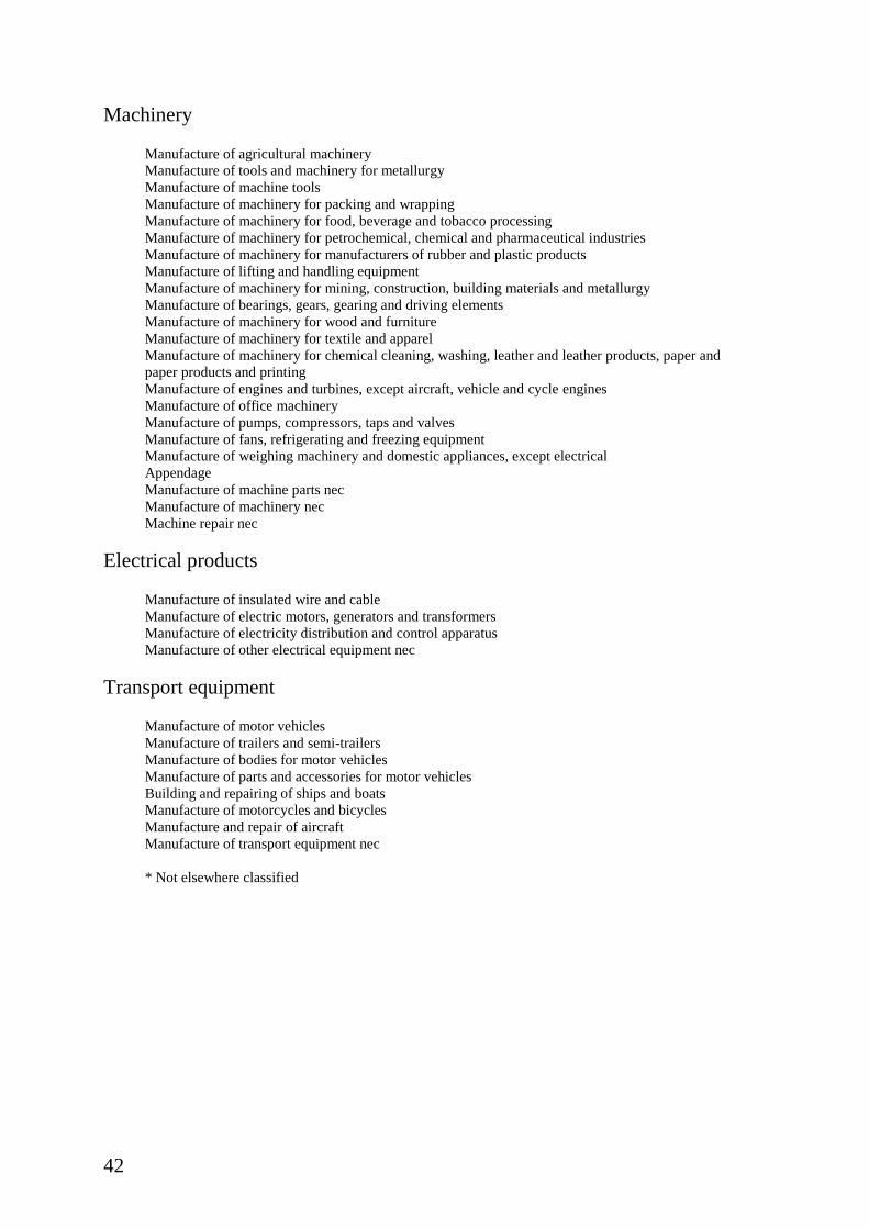
42
Machinery
Manufacture of agricultural machineryManufacture of tools and machinery for metallurgyManufacture of machine toolsManufacture of machinery for packing and wrappingManufacture of machinery for food, beverage and tobacco processingManufacture of machinery for petrochemical, chemical and pharmaceutical industriesManufacture of machinery for manufacturers of rubber and plastic productsManufacture of lifting and handling equipmentManufacture of machinery for mining, construction, building materials and metallurgyManufacture of bearings, gears, gearing and driving elementsManufacture of machinery for wood and furnitureManufacture of machinery for textile and apparelManufacture of machinery for chemical cleaning, washing, leather and leather products, paper andpaper products and printingManufacture of engines and turbines, except aircraft, vehicle and cycle enginesManufacture of office machineryManufacture of pumps, compressors, taps and valvesManufacture of fans, refrigerating and freezing equipmentManufacture of weighing machinery and domestic appliances, except electricalAppendageManufacture of machine parts necManufacture of machinery necMachine repair nec
Electrical products
Manufacture of insulated wire and cableManufacture of electric motors, generators and transformersManufacture of electricity distribution and control apparatusManufacture of other electrical equipment nec
Transport equipment
Manufacture of motor vehiclesManufacture of trailers and semi-trailersManufacture of bodies for motor vehiclesManufacture of parts and accessories for motor vehiclesBuilding and repairing of ships and boatsManufacture of motorcycles and bicyclesManufacture and repair of aircraftManufacture of transport equipment nec
* Not elsewhere classified
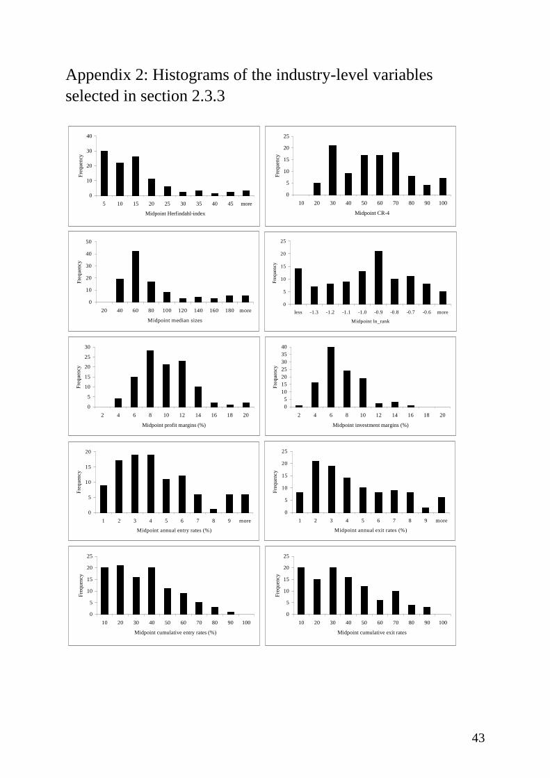
43
Appendix 2: Histograms of the industry-level variablesselected in section 2.3.3
0
10
20
30
40
5 10 15 20 25 30 35 40 45 more
Midpoint Herfindahl-index
Fre
quen
cy
0
5
10
15
20
25
10 20 30 40 50 60 70 80 90 100
Midpoint CR-4
Fre
quen
cy
0
10
20
30
40
50
20 40 60 80 100 120 140 160 180 more
Midpoint median sizes
Fre
quen
cy
0
5
10
15
20
25
less -1.3 -1.2 -1.1 -1.0 -0.9 -0.8 -0.7 -0.6 more
Midpoint ln_rank
Fre
quen
cy
0
5
10
15
20
25
30
2 4 6 8 10 12 14 16 18 20
Midpoint profit margins (%)
Fre
quen
cy
05
10152025303540
2 4 6 8 10 12 14 16 18 20
Midpoint investment margins (%)
Fre
quen
cy
0
5
10
15
20
1 2 3 4 5 6 7 8 9 more
Midpoint annual entry rates (%)
Fre
quen
cy
0
5
10
15
20
25
1 2 3 4 5 6 7 8 9 more
M idpoint annual exit rates (%)
Fre
quen
cy
0
5
10
15
20
25
10 20 30 40 50 60 70 80 90 100
Midpoint cumulative entry rates (%)
Fre
quen
cy
0
5
10
15
20
25
10 20 30 40 50 60 70 80 90 100
Midpoint cumulative exit rates
Fre
quen
cy
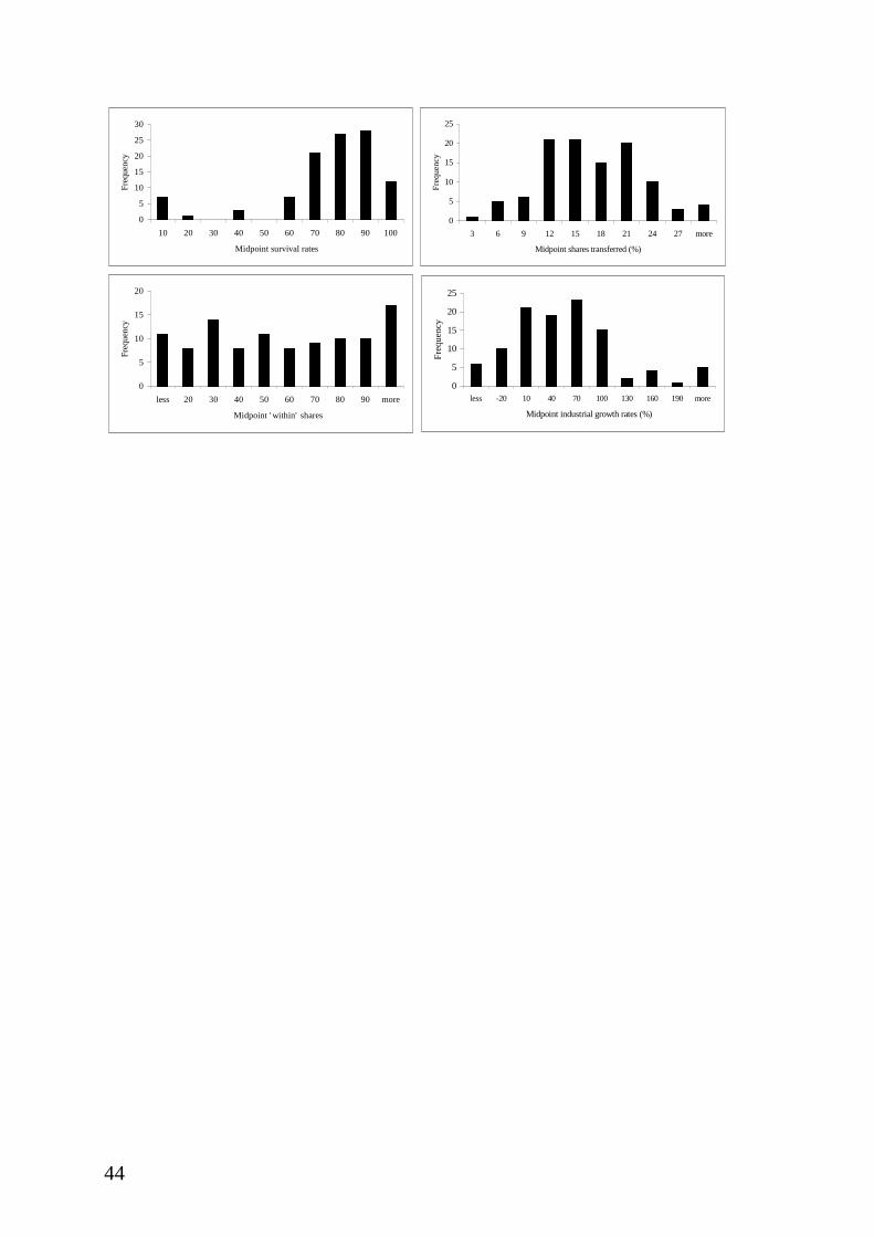
44
0
5
10
15
20
25
30
10 20 30 40 50 60 70 80 90 100
Midpoint survival rates
Fre
quen
cy
0
5
10
15
20
25
3 6 9 12 15 18 21 24 27 more
Midpoint shares transferred (%)
Fre
quen
cy
0
5
10
15
20
less 20 30 40 50 60 70 80 90 more
Midpoint ' within' shares
Fre
quen
cy
0
5
10
15
20
25
less -20 10 40 70 100 130 160 190 more
Midpoint industrial growth rates (%)
Fre
quen
cy
45
Chapter 3
Survey of Selected Theories
3.1 Introduction
In the early days of industrial economics as a discipline, competition withinindustries was clearly viewed as a dynamic process. Although Alfred Marshallhas laid the foundations of the partial equilibrium analysis found in manytextbooks, he acknowledged that dynamics, rather than statics, should be themain concern of economics. Marshall’s view is best reflected by his famousanalogy of the young trees in the forest of which many succumb, but those fewthat survive gradually grow and replace the older ones. And as in the forest,“ …in almost every trade there is a constant rise and fall of large businesses…”(Marshall , 1936, p. 316).
By describing competition as a process mainly involving the dynamicinnovations of the entrepreneur, Joseph Schumpeter (1912, 1942) even morerejected the idea of competition as a static concept. In Schumpeter’s view,economic processes are organic: changes come from within the system. In thissystem, the entrepreneur is a key figure, an active agent of economic progresswho induces economic development by actively searching for and carrying out‘new combinations’ in production (Ekelund and Hébert, 1990).
Marshall and Schumpeter’s acknowledgements of the dynamics of thecompetitive process were virtually discarded in the subsequent developments inindustrial economics. Instead, priority was given to analytical tractability and,consequently, attention shifted to essentially static equilibrium analyses ofindustrial structures, which constituted the dominant paradigm in industrialeconomics for many decades. However, the research methodology underlyingthis paradigm inherently involves some theoretical and empirical limitations.
46
Especially technological change, generally acknowledged to be a major enginedriving economic growth, is diff icult to embody properly in equil ibrium models.In section 2 of this chapter we will focus on these models and explain how theequilibrium approach limits the theoretical and empirical analysis of industrialeconomics.
Perhaps because of these limitations we recently observe a renewed interest indisequilibrium phenomena that is starting to change the conventional way ofanalysing industries (Dosi et al., 1997). The recently obtained empiricalevidence on the persistence of heterogeneity and turbulence, as discussed in theprevious chapter, undoubtedly contributed to this renewed and increasinginterest. The remainder of this chapter wil l focus on two of these rather recentlydeveloped theoretical approaches that may help to explain the observeddifferences between industries with regard to their structural and dynamicproperties. The first one, which will be described in section 3, is the frameworkof technological regimes. A technological regime can be defined as a particularcombination of opportunity, appropriability, cumulativeness conditions andproperties of the knowledge base underlying the innovative and productiveactivities of an industry. Given differences in these conditions, different patternsof innovative activities are likely to emerge which, in turn, may affect thestructures and dynamics of industries. However, cross-sectional differencesbetween industries may also stem from the different evolutionary stages theseindustries occupy. Explanations of this type can be derived from theories onproduct or industry li fe cycles. This is the second recently developed theoreticalapproach upon which we will focus in this chapter.
3.2 Equilibrium models
This section aims to give a brief overview of the equilibrium approaches inindustrial economics. It is divided in four parts. First we will describe the staticequilibrium models, including the structure-conduct-performance approach andthe game-theoretical contributions. Second, we will pay attention to the ‘bounds’approach, developed by John Sutton. Because of its explicit aim to construct anempirically testable framework, applicable to a wide range of industries, wehave devoted a complete subsection to this approach. Third, we will focus on theclass of dynamic equilibrium models. Fourth, and finally, we will discuss thetheoretical and empirical li mitations of the equilibrium models in industrialeconomics.
47
3.2.1 Static equilibrium models
For a number of decades the structure-conduct-performance (SCP) approach,developed by Mason and Bain1, was the dominant paradigm in industrialeconomics. Based upon neo-classical theory, as well as upon empirical work2,this paradigm postulates causal relationships between the structure of anindustry, the conduct of f irms in the industry, and their economic performance.Structure refers to the environment within which firms operate, and includeselements like the number and size distribution of buyers and sellers, the level ofproduct differentiation, and the height of entry barriers. The fact that structuralconditions may provide the latitude to act in some other way than being a ‘price-taker’ in the market leads to the assumption that structure influences conduct.The variety of behaviours that might be realised due to weak structuralfoundations for competition might, in fact, be very large and include collusivebehaviour, price discrimination, et cetera. Regardless of the non-competitivebehaviour employed, the assumption of the SCP approach was that, becausefirms are profit maximising, the result would be detectable differences in theperformance of these firms in the market and, in particular, in the allocativeineff iciency compared to perfect competition.
Hence, in its simplest form, the exogenously determined structural properties ofan industry govern the conduct of f irms, which in turn determines the economicperformance of a market. More sophisticated versions of this framework alsorecognise causal relationships in opposite directions. For instance, entry-deterring practices by existing firms (conduct) are aimed to discourage entrantsand will thus affect the ultimate structure of an industry. Also, the level ofproduct differentiation is likely to be affected by the marketing strategies of thefirms. Although recognising the interaction between the elements has made theSCP paradigm more realistic, it has also posed new problems related to theempirical work in this area. As Schmalensee (1989) argues:“ … in the long-runequilibria with which cross-section studies must be primarily concerned,essentially all variables that have been employed in such studies are logicallyendogenous. This means that there are in general no theoretically exogenous
1 See Bain (1956) and Mason (1957).2 For instance, see Bain (1951, 1954), or Weiss (1974) for a survey.
48
variables that can be used as instruments to identify and estimate any structuralequation.” (Schmalensee, 1989, p. 954).3
Mostly due to this fundamental endogeneity problem, the interests of themainstream industrial economists shifted from empirical research to moretheoretical founded contributions. Most of these theoretical contributions camefrom the Chicago School during the 1970s and from the New IndustrialEconomists during the 1980s. Whereas the starting point of the SCP paradigmwas imperfect competition, the Chicago School asserts that perfect competitionhas substantial explanatory power (Martin, 1994). In their view, market powermay only exist temporarily, unless supported by government interference. Aparticularly important point of contention of the Chicago School was thepresumed effect of a competitive ‘ fringe’ , even in industries that are structurallyhighly concentrated. Bork (1978), for example, criticised many of the classicantitrust decisions because of their failure to consider the impact of competitors,even though they held a relatively small share of the market. In essence, theargument of the Chicago School was that structure reflected relative efficiencyand that larger firms were large because they were more eff icient than rivals.4 If ,however, these larger firms proceeded to the ‘conduct’ stage of the SCP modelin ways that prove antithetical to competitive behaviour, the smaller fi rms wouldhave a significant impact on the market.5 By breaking the link between structureand conduct, the Chicago school undermined the theoretical consistency of theSCP model.
Subsequent research in industrial economics in the 1980s shifted back theattention from perfect markets to essentially oligopolistic market structures. Thisschool, labelled New Industrial Economics or New Industrial Organisation, iseven more based on neo-classical theory than the SCP tradition. However, NewIndustrial Economists consider conduct as the key element rather than structure.
3 The empirical foundations of the structure-performance link were also attacked by a
variety of studies contesting Bain' s original findings. For an overview, see chapter 9 ofScherer (1980).
4 See Demsetz (1973).5 A similar argument is derived from the theory of contestable markets (Baumol et al.,
1982). Assuming that there are no sunk costs and that an existing dominant firm will notdecrease its price if an entrants comes in, this theory claims that the only way the dominantfirm can keep an entrant out is to set a price that yields zero economic profit. Hence, even inhighly concentrated markets the force of potential competition is enough to yield the sameperformance as a competitive market (Martin, 1994).

49
This emphasis on behaviour is reflected by the extensive use of game theory6 inNew Industrial Economics. The strength of these game-theoretical models is theabil ity to formally incorporate in an elegant way the strategic interactionsbetween players (usually fi rms in an oligopolistic setting). For instance, duopolymodels, such as the Cournot and Stackelberg (leader-follower) models, are setup as non-cooperative games in which the players’ strategies consist of settingquantities as a function of the other player’s quantity setting. The outcome ofsuch a game (in terms of, e.g., market shares) is a Nash-equil ibrium, i.e., aconfiguration of strategies in which no player has an incentive to change itsstrategy given the other players’ strategies. Other applications of game theory inindustrial economics include models of collusive behaviour, productdifferentiation, innovation and patent races, and predatory pricing strategies.7
Despite the novelty of formally embodying strategic interactions, theseapplications of game theory have not enabled us to say much more on theworking of oligopolistic markets than that could be said on the basis of earliertheory (Fisher, 1989). Many outcomes are still possible. Another objection isthat the results of such game-theoretic analyses tend to depend delicately on theprecise form of the underlying game (Sutton, 1991). Further, these form-specificfactors, such as the information partition among the players, are usually diff icultto map into empirical categories that hold across a range of different industries.
One way to overcome this latter diff iculty is to tailor-make a model to fit a morenarrowly defined environment. Such a modell ing strategy is likely to increasethe degree of precision of predictions, but by definition it will li mit the breadthof applications. Acknowledging this trade-off, Sutton (1991, 1998) aims to finda middle way that has come to be known as the ‘bounds’ approach. Rather thanpredicting some unique equilibrium outcome, this approach aims to predict a setof outcomes that can be supported as an equilibrium outcome of a wide class ofmodels that may all be plausible a priori. In game-theoretical terms, such anexercise “ …results in a partitioning of the space of outcomes into two sets: theset of points that can be supported as equilibria…and the set of points thatcannot.” (Sutton, 1998, p.7). For instance, with regard to market concentration,this approach aims to specify a lower bound to the equilibrium level ofconcentration that holds across a broad set of different industries instead ofpredicting precise levels of market concentration for a limited set of industries.
6 Initially already introduced in economics in the 1940s by Von Neumann and Morgenstern
(1944).7 Chapter 13 of Rasmussen (1989) gives on overview of these applications.
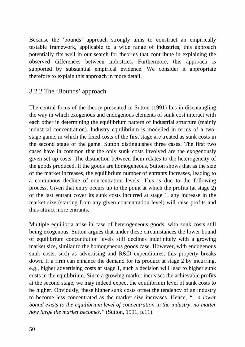
50
Because the ‘bounds’ approach strongly aims to construct an empiricallytestable framework, applicable to a wide range of industries, this approachpotentially fits well in our search for theories that contribute in explaining theobserved differences between industries. Furthermore, this approach issupported by substantial empirical evidence. We consider it appropriatetherefore to explain this approach in more detail.
3.2.2 The ‘Bounds’ approach
The central focus of the theory presented in Sutton (1991) lies in disentanglingthe way in which exogenous and endogenous elements of sunk cost interact witheach other in determining the equilibrium pattern of industrial structure (mainlyindustrial concentration). Industry equilibrium is modelled in terms of a two-stage game, in which the fixed costs of the first stage are treated as sunk costs inthe second stage of the game. Sutton distinguishes three cases. The first twocases have in common that the only sunk costs involved are the exogenouslygiven set-up costs. The distinction between them relates to the heterogeneity ofthe goods produced. If the goods are homogeneous, Sutton shows that as the sizeof the market increases, the equil ibrium number of entrants increases, leading toa continuous decline of concentration levels. This is due to the followingprocess. Given that entry occurs up to the point at which the profits (at stage 2)of the last entrant cover its sunk costs incurred at stage 1, any increase in themarket size (starting from any given concentration level) will raise profits andthus attract more entrants.
Multiple equilibria arise in case of heterogeneous goods, with sunk costs stillbeing exogenous. Sutton argues that under these circumstances the lower boundof equilibrium concentration levels stil l declines indefinitely with a growingmarket size, similar to the homogeneous goods case. However, with endogenoussunk costs, such as advertising and R&D expenditures, this property breaksdown. If a firm can enhance the demand for its product at stage 2 by incurring,e.g., higher advertising costs at stage 1, such a decision will l ead to higher sunkcosts in the equilibrium. Since a growing market increases the achievable profitsat the second stage, we may indeed expect the equilibrium level of sunk costs tobe higher. Obviously, these higher sunk costs offset the tendency of an industryto become less concentrated as the market size increases. Hence, “ …a lowerbound exists to the equilibrium level of concentration in the industry, no matterhow large the market becomes.” (Sutton, 1991, p.11).
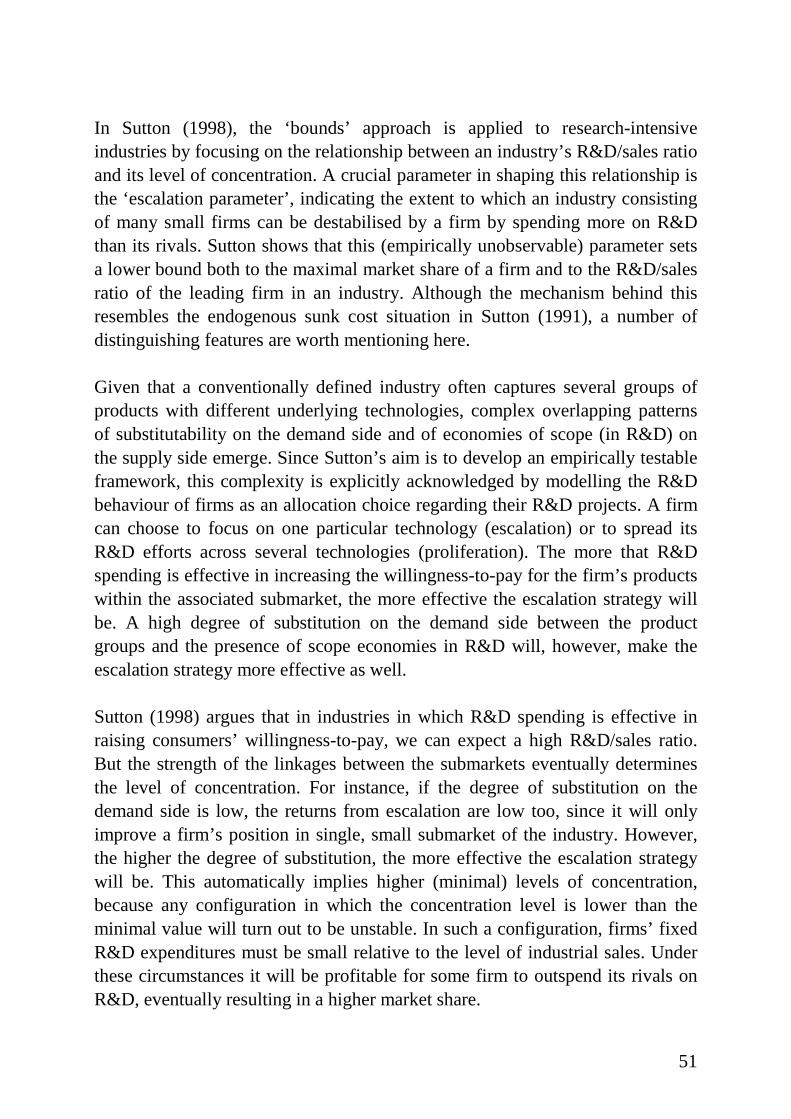
51
In Sutton (1998), the ‘bounds’ approach is applied to research-intensiveindustries by focusing on the relationship between an industry’s R&D/sales ratioand its level of concentration. A crucial parameter in shaping this relationship isthe ‘escalation parameter’ , indicating the extent to which an industry consistingof many small firms can be destabilised by a firm by spending more on R&Dthan its rivals. Sutton shows that this (empirically unobservable) parameter setsa lower bound both to the maximal market share of a firm and to the R&D/salesratio of the leading firm in an industry. Although the mechanism behind thisresembles the endogenous sunk cost situation in Sutton (1991), a number ofdistinguishing features are worth mentioning here.
Given that a conventionally defined industry often captures several groups ofproducts with different underlying technologies, complex overlapping patternsof substitutability on the demand side and of economies of scope (in R&D) onthe supply side emerge. Since Sutton’s aim is to develop an empirically testableframework, this complexity is explicitly acknowledged by modell ing the R&Dbehaviour of firms as an allocation choice regarding their R&D projects. A firmcan choose to focus on one particular technology (escalation) or to spread itsR&D efforts across several technologies (proliferation). The more that R&Dspending is effective in increasing the wil lingness-to-pay for the firm’s productswithin the associated submarket, the more effective the escalation strategy willbe. A high degree of substitution on the demand side between the productgroups and the presence of scope economies in R&D will, however, make theescalation strategy more effective as well.
Sutton (1998) argues that in industries in which R&D spending is effective inraising consumers’ will ingness-to-pay, we can expect a high R&D/sales ratio.But the strength of the linkages between the submarkets eventually determinesthe level of concentration. For instance, if the degree of substitution on thedemand side is low, the returns from escalation are low too, since it will onlyimprove a firm’s position in single, small submarket of the industry. However,the higher the degree of substitution, the more effective the escalation strategywill be. This automatically implies higher (minimal) levels of concentration,because any configuration in which the concentration level is lower than theminimal value wil l turn out to be unstable. In such a configuration, firms’ fixedR&D expenditures must be small relative to the level of industrial sales. Underthese circumstances it wil l be profitable for some firm to outspend its rivals onR&D, eventually resulting in a higher market share.
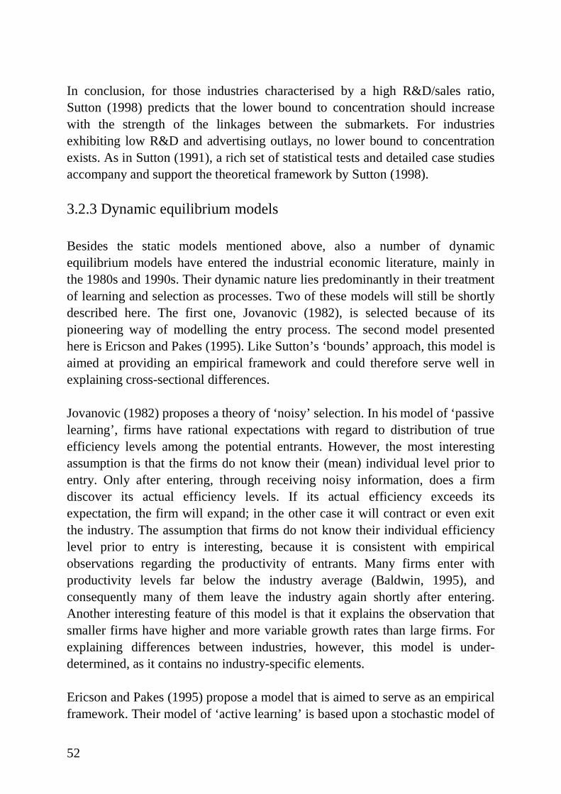
52
In conclusion, for those industries characterised by a high R&D/sales ratio,Sutton (1998) predicts that the lower bound to concentration should increasewith the strength of the linkages between the submarkets. For industriesexhibiting low R&D and advertising outlays, no lower bound to concentrationexists. As in Sutton (1991), a rich set of statistical tests and detailed case studiesaccompany and support the theoretical framework by Sutton (1998).
3.2.3 Dynamic equilibrium models
Besides the static models mentioned above, also a number of dynamicequilibrium models have entered the industrial economic literature, mainly inthe 1980s and 1990s. Their dynamic nature lies predominantly in their treatmentof learning and selection as processes. Two of these models will stil l be shortlydescribed here. The first one, Jovanovic (1982), is selected because of itspioneering way of modell ing the entry process. The second model presentedhere is Ericson and Pakes (1995). Like Sutton’s ‘bounds’ approach, this model isaimed at providing an empirical framework and could therefore serve well inexplaining cross-sectional differences.
Jovanovic (1982) proposes a theory of ‘noisy’ selection. In his model of ‘passivelearning’ , firms have rational expectations with regard to distribution of trueeff iciency levels among the potential entrants. However, the most interestingassumption is that the firms do not know their (mean) individual level prior toentry. Only after entering, through receiving noisy information, does a firmdiscover its actual eff iciency levels. If its actual efficiency exceeds itsexpectation, the firm will expand; in the other case it will contract or even exitthe industry. The assumption that firms do not know their individual efficiencylevel prior to entry is interesting, because it is consistent with empiricalobservations regarding the productivity of entrants. Many firms enter withproductivity levels far below the industry average (Baldwin, 1995), andconsequently many of them leave the industry again shortly after entering.Another interesting feature of this model is that it explains the observation thatsmaller firms have higher and more variable growth rates than large firms. Forexplaining differences between industries, however, this model is under-determined, as it contains no industry-specific elements.
Ericson and Pakes (1995) propose a model that is aimed to serve as an empiricalframework. Their model of ‘active learning’ is based upon a stochastic model of
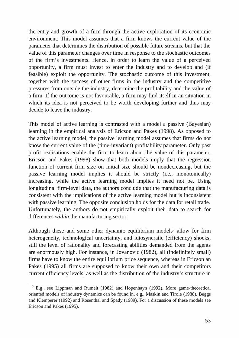
53
the entry and growth of a firm through the active exploration of its economicenvironment. This model assumes that a firm knows the current value of theparameter that determines the distribution of possible future streams, but that thevalue of this parameter changes over time in response to the stochastic outcomesof the firm’s investments. Hence, in order to learn the value of a perceivedopportunity, a firm must invest to enter the industry and to develop and (iffeasible) exploit the opportunity. The stochastic outcome of this investment,together with the success of other firms in the industry and the competitivepressures from outside the industry, determine the profitabili ty and the value ofa firm. If the outcome is not favourable, a firm may find itself in an situation inwhich its idea is not perceived to be worth developing further and thus maydecide to leave the industry.
This model of active learning is contrasted with a model a passive (Bayesian)learning in the empirical analysis of Ericson and Pakes (1998). As opposed tothe active learning model, the passive learning model assumes that firms do notknow the current value of the (time-invariant) profitabili ty parameter. Only pastprofit realisations enable the firm to learn about the value of this parameter.Ericson and Pakes (1998) show that both models imply that the regressionfunction of current firm size on initial size should be nondecreasing, but thepassive learning model implies it should be strictly (i.e., monotonically)increasing, while the active learning model implies it need not be. Usinglongitudinal firm-level data, the authors conclude that the manufacturing data isconsistent with the implications of the active learning model but is inconsistentwith passive learning. The opposite conclusion holds for the data for retail trade.Unfortunately, the authors do not empirically exploit their data to search fordifferences within the manufacturing sector.
Although these and some other dynamic equil ibrium models8 allow for firmheterogeneity, technological uncertainty, and idiosyncratic (efficiency) shocks,still the level of rationali ty and forecasting abil ities demanded from the agentsare enormously high. For instance, in Jovanovic (1982), all (indefinitely small )firms have to know the entire equil ibrium price sequence, whereas in Ericson anPakes (1995) all firms are supposed to know their own and their competitorscurrent efficiency levels, as well as the distribution of the industry’s structure in
8 E.g., see Lippman and Rumelt (1982) and Hopenhayn (1992). More game-theoretical
oriented models of industry dynamics can be found in, e.g., Maskin and Tirole (1988), Beggsand Klemperer (1992) and Rosenthal and Spady (1989). For a discussion of these models seeEricson and Pakes (1995).
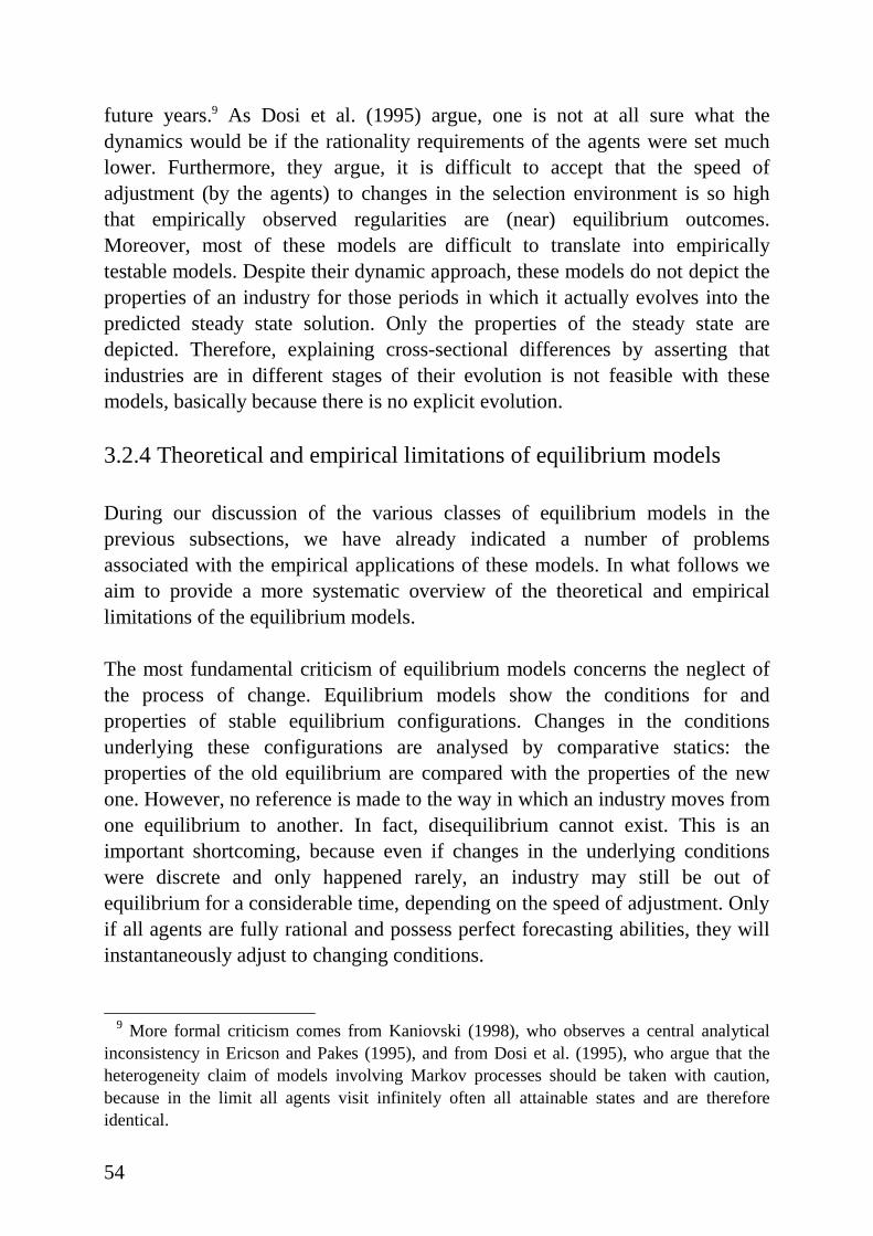
54
future years.9 As Dosi et al. (1995) argue, one is not at all sure what thedynamics would be if the rationality requirements of the agents were set muchlower. Furthermore, they argue, it is difficult to accept that the speed ofadjustment (by the agents) to changes in the selection environment is so highthat empirically observed regularities are (near) equilibrium outcomes.Moreover, most of these models are difficult to translate into empiricallytestable models. Despite their dynamic approach, these models do not depict theproperties of an industry for those periods in which it actually evolves into thepredicted steady state solution. Only the properties of the steady state aredepicted. Therefore, explaining cross-sectional differences by asserting thatindustries are in different stages of their evolution is not feasible with thesemodels, basically because there is no explicit evolution.
3.2.4 Theoretical and empirical limitations of equilibrium models
During our discussion of the various classes of equilibrium models in theprevious subsections, we have already indicated a number of problemsassociated with the empirical applications of these models. In what follows weaim to provide a more systematic overview of the theoretical and empiricallimitations of the equili brium models.
The most fundamental criticism of equil ibrium models concerns the neglect ofthe process of change. Equilibrium models show the conditions for andproperties of stable equilibrium configurations. Changes in the conditionsunderlying these configurations are analysed by comparative statics: theproperties of the old equilibrium are compared with the properties of the newone. However, no reference is made to the way in which an industry moves fromone equil ibrium to another. In fact, disequilibrium cannot exist. This is animportant shortcoming, because even if changes in the underlying conditionswere discrete and only happened rarely, an industry may still be out ofequilibrium for a considerable time, depending on the speed of adjustment. Onlyif all agents are fully rational and possess perfect forecasting abili ties, they willinstantaneously adjust to changing conditions.
9 More formal criti cism comes from Kaniovski (1998), who observes a central analytical
inconsistency in Ericson and Pakes (1995), and from Dosi et al. (1995), who argue that theheterogeneity claim of models involving Markov processes should be taken with caution,because in the limit all agents visit infinitely often all attainable states and are thereforeidentical.

55
However, behaviourists10 have stressed that human beings are not perfectlyrational. In many real-li fe situations, “ …decision problems are too complex tocomprehend and therefore firms cannot maximize over the set of all conceivablealternatives. Relatively simple decision rules and procedures are used to guideaction…” (Nelson and Winter, 1982, p.35). Therefore, whenever the equil ibriumconditions of an industry change, the industry will be temporarily out ofequilibrium as firms will need time to adapt to the new situation. Again, if theequilibrium conditions seldom change, equilibrium analysis may still beappropriate, provided that the industry is in equilibrium most of the time. Buttechnological and institutional changes, both from within the industry as well asfrom outside the industry, continuously alter the conditions underlying theequilibrium configurations.
Technological change, generally acknowledged to be a major determinant ofeconomic growth, is especially difficult to embody properly in equil ibriummodels. The usual way of incorporating technological change in these modelsstarts by assuming that technological change is exogenous to the economicsystem, and that, because of perfect information, the new knowledge associatedwith the innovation is immediately available to all firms. Given theseassumptions, any innovation is immediately taken up by the firms andoptimally11 implemented in their production processes. As mentioned before,this necessarily implies that the relevant decision-makers within the firms knowall the available production techniques and, equally important, how to applythem. Further, they will need to know the prices of all inputs, regardless of thescale on which these are hired. Finally, they will have to have the cognitiveabil ities to assess all the available techniques in order to select the one thatminimises costs.
Obviously, this view on the innovative process has received a great deal ofcriticism. First of all , many firms devote resources to research and developmentin order to enhance their technological knowledge base. Since a large number ofinnovations are the outcome of these research and development activities,technological progress is endogenous rather than exogenous to the industry.Even in cases in which new technological knowledge becomes available to firmsthrough research efforts from outside their industry, still they will have toundertake efforts to obtain and implement the knowledge. As such, the
10 Most notably Herbert Simon; see Simon (1959, 1965).11 In terms of cost minimisation.

56
implementation of the exogenously available knowledge is an endogenousprocess as well.
This brings us to the second point of criticism, namely the diffusion of newtechnological knowledge. Equilibrium models assume that whenever aninnovation is introduced in an industry, the knowledge related to the innovationflows around freely and competitors can thus rapidly incorporate the newknowledge. This assumption assures that any disequil ibrium in the industry isonly short-lived. However, it is plausible that both the tacit nature oftechnological knowledge and the bounded rationality of entrepreneurs preventnew knowledge from spilling over rapidly to competitors. As Nelson and Winter(1982) argue, a large component of technological knowledge is tacit, meaningthat it cannot be articulated in codified forms such as blueprints or writteninstructions. But even if every new technology were fully specified inblueprints, bounded rationality would still li mit the speed of diffusion.Entrepreneurs, like any other human being, do not have the cognitive powers toknow and assess all the options available to them. Instead, the subjectivelycreate a highly simpli fied model of their environment. Therefore, entrepreneursvary in their perception of technological developments and their alertness tothese developments. Together with the tacitness of knowledge this obviouslyhinders the rapid transfer of technological knowledge from innovators toimitators.
Because of the duration and imperfections of the knowledge diffusion process,innovative firms are able to enjoy at least temporaril y higher (disequilibrium)profits. In fact, the opportunity to enjoy these profits provides the economicincentives to firms’ search for technological improvements. But also in thisrespect the assumption of perfect information is obviously not plausible andeven invalid. The innovative process involves some fundamental uncertainty,entailing the existence of techno-economic problems whose solution proceduresare not known and the impossibility of precisely tracing consequences to actions(Dosi, 1988b). Consequently, entrepreneurs will sometimes make mistakes inthis process or, at the minimum, behave in a way that is inconsistent with theassumption of rational profit maximisation. Of course, future profitopportunities may stil l be the main reason why firms engage in research anddevelopment, however a positive outcome of their search activities is neverguaranteed a priori.
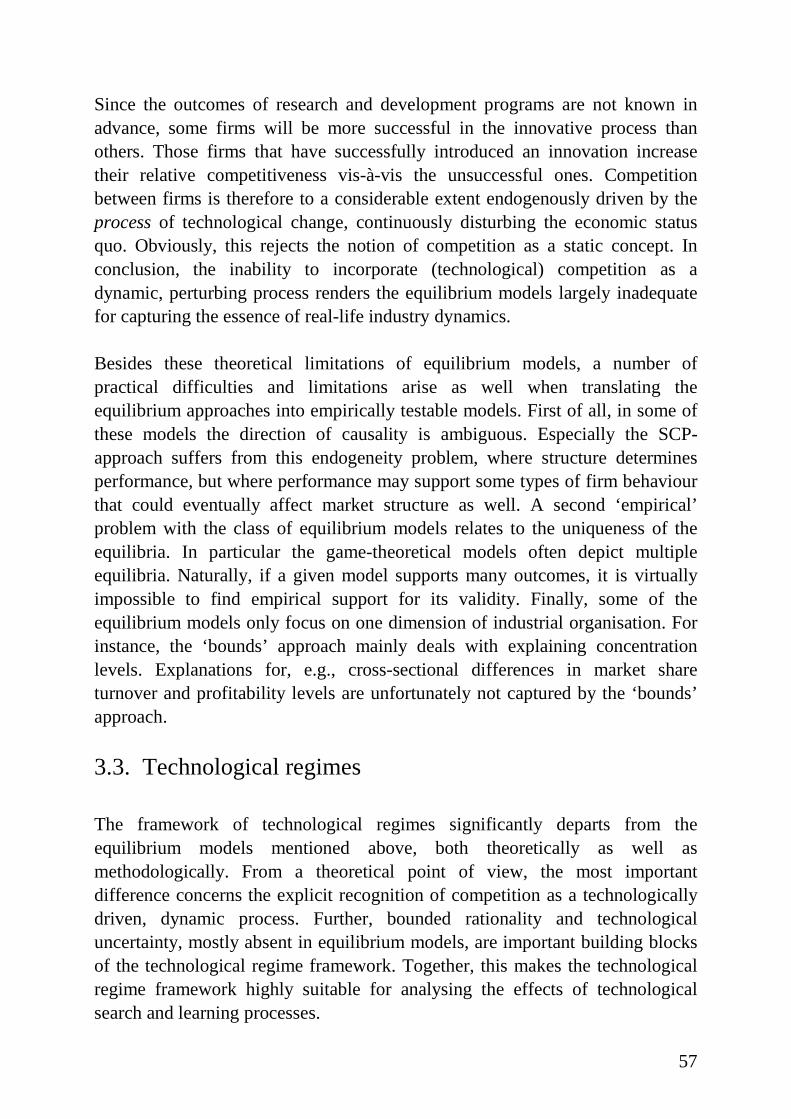
57
Since the outcomes of research and development programs are not known inadvance, some firms will be more successful in the innovative process thanothers. Those firms that have successfully introduced an innovation increasetheir relative competitiveness vis-à-vis the unsuccessful ones. Competitionbetween firms is therefore to a considerable extent endogenously driven by theprocess of technological change, continuously disturbing the economic statusquo. Obviously, this rejects the notion of competition as a static concept. Inconclusion, the inability to incorporate (technological) competition as adynamic, perturbing process renders the equil ibrium models largely inadequatefor capturing the essence of real-life industry dynamics.
Besides these theoretical limitations of equilibrium models, a number ofpractical diff iculties and limitations arise as well when translating theequilibrium approaches into empirically testable models. First of all , in some ofthese models the direction of causali ty is ambiguous. Especially the SCP-approach suffers from this endogeneity problem, where structure determinesperformance, but where performance may support some types of f irm behaviourthat could eventually affect market structure as well. A second ‘empirical’problem with the class of equil ibrium models relates to the uniqueness of theequilibria. In particular the game-theoretical models often depict multipleequilibria. Naturally, if a given model supports many outcomes, it is virtuallyimpossible to find empirical support for its validity. Finally, some of theequilibrium models only focus on one dimension of industrial organisation. Forinstance, the ‘bounds’ approach mainly deals with explaining concentrationlevels. Explanations for, e.g., cross-sectional differences in market shareturnover and profitabili ty levels are unfortunately not captured by the ‘bounds’approach.
3.3. Technological regimes
The framework of technological regimes significantly departs from theequilibrium models mentioned above, both theoretically as well asmethodologically. From a theoretical point of view, the most importantdifference concerns the explicit recognition of competition as a technologicallydriven, dynamic process. Further, bounded rationality and technologicaluncertainty, mostly absent in equilibrium models, are important building blocksof the technological regime framework. Together, this makes the technologicalregime framework highly suitable for analysing the effects of technologicalsearch and learning processes.

58
The main difference in methodology between the equilibrium approaches andthe technological regime framework can best be described by the distinctionbetween formal and appreciative theorising, first brought forward by Nelson andWinter (1982). Formal theorising aims to set up a framework that enables one toexplore, find and check logical connections between economic variables and todisplay possible causal mechanisms for particular phenomena. In formaltheorising, analytical tractability is more important than minimising theintellectual distance from what is known empirically. Appreciative theorisingtends to stay much closer to empirical substance. Here, theories are primarilyconceptual tools of inquiry, and the focus is on the endeavour in which thesetools are applied in explaining why certain economic events have happened.Although some overlap exists, it can be argued that formal theorising is the mainmethodological tool used in equilibrium models, whereas appreciative theorisingmuch more underlies the technological regime framework.12
Given its theoretical and methodological foundations, the technological regimeframework potentially serves well i n providing realistic explanations for theobserved differences between industries. In this section we will thereforeelaborate on the technological regime framework. We will first focus on theevolution of the notion of technological regimes within the literature oneconomics and technological change. Attention will be paid to the differentviews on the role of technological opportunity and the role of knowledge indetermining the rate and direction of technological change. Further, the role ofinstitutional and market forces in selecting and establishing technologicalregimes will be considered. Second, we will present a short overview ofempirical research on the relationship between technological regimes and theintersectoral variety in the rates and forms of organisation of innovations.Finally, we will examine the contribution of a number of evolutionary models tounderstanding the relationship between the structural and dynamic properties ofan industry and its underlying technological regime.
3.3.1 Literature overview
Not surprisingly, this overview of the literature on technological regimes startswith a discussion on the work of Joseph Schumpeter. During his life,
12 For a discussion of the linkages between formal and appreciative theorising, see Nelson
(1994).
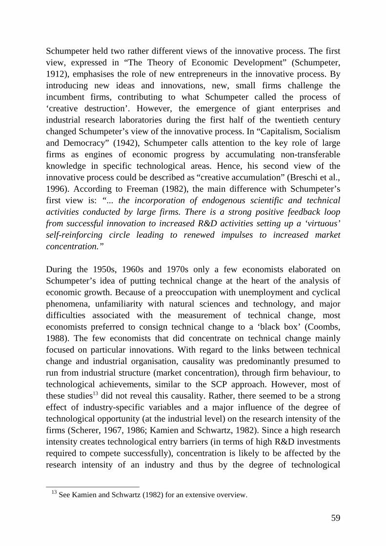
59
Schumpeter held two rather different views of the innovative process. The firstview, expressed in “The Theory of Economic Development” (Schumpeter,1912), emphasises the role of new entrepreneurs in the innovative process. Byintroducing new ideas and innovations, new, small firms challenge theincumbent firms, contributing to what Schumpeter called the process of‘creative destruction’ . However, the emergence of giant enterprises andindustrial research laboratories during the first half of the twentieth centurychanged Schumpeter’s view of the innovative process. In “Capitalism, Socialismand Democracy” (1942), Schumpeter calls attention to the key role of largefirms as engines of economic progress by accumulating non-transferableknowledge in specific technological areas. Hence, his second view of theinnovative process could be described as “creative accumulation” (Breschi et al.,1996). According to Freeman (1982), the main difference with Schumpeter’sfirst view is: “ ... the incorporation of endogenous scientific and technicalactivities conducted by large firms. There is a strong positive feedback loopfrom successful innovation to increased R&D activities setting up a ‘virtuous’self-reinforcing circle leading to renewed impulses to increased marketconcentration.”
During the 1950s, 1960s and 1970s only a few economists elaborated onSchumpeter’s idea of putting technical change at the heart of the analysis ofeconomic growth. Because of a preoccupation with unemployment and cyclicalphenomena, unfamili arity with natural sciences and technology, and majordifficulties associated with the measurement of technical change, mosteconomists preferred to consign technical change to a ‘black box’ (Coombs,1988). The few economists that did concentrate on technical change mainlyfocused on particular innovations. With regard to the links between technicalchange and industrial organisation, causality was predominantly presumed torun from industrial structure (market concentration), through firm behaviour, totechnological achievements, similar to the SCP approach. However, most ofthese studies13 did not reveal this causality. Rather, there seemed to be a strongeffect of industry-specific variables and a major influence of the degree oftechnological opportunity (at the industrial level) on the research intensity of thefirms (Scherer, 1967, 1986; Kamien and Schwartz, 1982). Since a high researchintensity creates technological entry barriers (in terms of high R&D investmentsrequired to compete successfully), concentration is likely to be affected by theresearch intensity of an industry and thus by the degree of technological
13 See Kamien and Schwartz (1982) for an extensive overview.
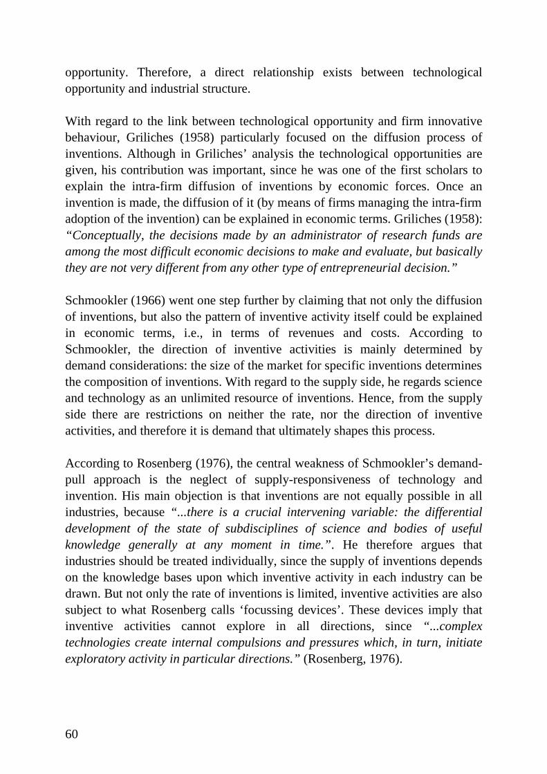
60
opportunity. Therefore, a direct relationship exists between technologicalopportunity and industrial structure.
With regard to the link between technological opportunity and firm innovativebehaviour, Griliches (1958) particularly focused on the diffusion process ofinventions. Although in Griliches’ analysis the technological opportunities aregiven, his contribution was important, since he was one of the first scholars toexplain the intra-firm diffusion of inventions by economic forces. Once aninvention is made, the diffusion of it (by means of firms managing the intra-fi rmadoption of the invention) can be explained in economic terms. Grili ches (1958):“ Conceptually, the decisions made by an administrator of research funds areamong the most difficult economic decisions to make and evaluate, but basicallythey are not very different from any other type of entrepreneurial decision.”
Schmookler (1966) went one step further by claiming that not only the diffusionof inventions, but also the pattern of inventive activity itself could be explainedin economic terms, i.e., in terms of revenues and costs. According toSchmookler, the direction of inventive activities is mainly determined bydemand considerations: the size of the market for specif ic inventions determinesthe composition of inventions. With regard to the supply side, he regards scienceand technology as an unlimited resource of inventions. Hence, from the supplyside there are restrictions on neither the rate, nor the direction of inventiveactivities, and therefore it is demand that ultimately shapes this process.
According to Rosenberg (1976), the central weakness of Schmookler’s demand-pull approach is the neglect of supply-responsiveness of technology andinvention. His main objection is that inventions are not equally possible in allindustries, because “ ...there is a crucial intervening variable: the differentialdevelopment of the state of subdisciplines of science and bodies of usefulknowledge generally at any moment in time.” . He therefore argues thatindustries should be treated individually, since the supply of inventions dependson the knowledge bases upon which inventive activity in each industry can bedrawn. But not only the rate of inventions is limited, inventive activities are alsosubject to what Rosenberg calls ‘ focussing devices’ . These devices imply thatinventive activities cannot explore in all directions, since “ ...complextechnologies create internal compulsions and pressures which, in turn, initiateexploratory activity in particular directions.” (Rosenberg, 1976).

61
Nelson and Winter (1977) agree that, even under a wide range of demandconditions, some powerful intra project heuristics could apply that guide theevolution of certain technologies in a particular direction. They call thesedirections ‘natural trajectories’ , and introduce the notion of a technologicalregime. A technological regime reflects the (perceived) boundaries oftechnological opportunities for further innovations and defines the trajectories tothose boundaries. Like Rosenberg, they also recognise that underlying themovement along the natural trajectories involves “ ... a certain knowledge on thepart of the technicians, engineers, scientists, involved in the relevant inventiveactivity.” (Nelson and Winter, 1977, p.60). One key property of the knowledgebase that may differ across industries is the extent to which scientific knowledgeunderpins the relevant technologies. That is, in some industries the role ofscience may be limited: the knowledge may then be quite specific and “ mayinvolve more art and feel than science” (Nelson and Winter, 1977, p.60).However, in other industries science may play a major role in the process oftechnological change, providing generic knowledge relevant to the specifictechnologies.
Dosi (1982, 1988a) elaborates on both the natural trajectories and thecharacteristics of the knowledge base. To start with the latter, Dosi (1988a)distinguishes three aspects of knowledge: (1) the level of specificity, (2) thelevel of tacitness, and (3) the extent to which the knowledge is publiclyavailable. The first aspect is quite similar to the property of the knowledge baseput forward by Nelson and Winter (1977), i.e., knowledge can be universal andwidely applicable, or more specific to particular ‘ways of doing things’ . Thesecond aspect has to do with the extent to which the knowledge is well codified,or whether it is more tacit, learned mainly through practice. The third aspectrelates to the fact that some knowledge is open and public, e.g., scientific andtechnical publications, whereas other knowledge is more private, either becauseit is protected by secrecy or patents which represents a choice behaviour offirms, or because it is tacit, which may either represent a choice not to‘articulate’ the knowledge (akin to secrecy), or may be inherent in the processby which the knowledge needs to be exchanged or ‘ taught’ .
With regard to Rosenberg’s focussing devices, and Nelson and Winter’stechnological regimes and natural trajectories, Dosi (1982) adds to theirconcepts the notion of ‘ technological trajectories’ and ‘ technologicalparadigms’ . Similar to what a ‘scientific paradigm’ does in science in general14,
14 See Kuhn (1962).

62
a technological paradigm sets out the relevant technological problems, and thepattern of solving these problems that are based on selected principles derivedfrom natural sciences and on selected material technologies. A technologicalparadigm thus “ …embodies strong prescriptions on the directions of technicalchange to pursue and those to neglect.” (Dosi, 1982, p.152). These directionsare then the technological trajectories, defined as the patterns of problem solvingactivities on the ground of a technological paradigm. Typical examples oftechnological paradigms and trajectories can be found in chemical processes,power generation, aircraft technology, microelectronic technology (Nelson andWinter, 1977; Saviotti and Metcalfe, 1984; Sahal, 1985), and in biotechnology(Orsenigo, 1989).
An interesting question posed by Dosi (1982) is what actually determines theemergence and establishment of a technological paradigm. Selection by marketmechanism is not likely to be very strong ex ante, given the intrinsic uncertaintyassociated with the outcome of a technological paradigm.15 Dosi (1982, p.155):“ Other, more specific variables are li kely to come into play such as (1) theeconomic interests of the organizations involved in R&D in these newtechnological areas, (2) their technological history, the fields of their expertise,etc.; (3) institutional variables ‘strictu sensu’ such as public agencies, themil itary, etc.” The market is more selective ex post and within a technologicalparadigm. After a technological paradigm is selected and the technologicaltrajectories have been defined, the market operates as (1) a selecting deviceamong the range of products in which the technologies have been incorporated,and (2) as a signalling device, inducing producers to respond through technicaladvance, but mainly within the boundaries of the existing technologicaltrajectory. New technological paradigms emerge “ ...either in relation to newopportunities opened-up by scientific developments or to the increasingdifficulty in going forward on a given technological directory...” (Dosi, 1982,p.157).
Dosi (1988a) suggests that the empirically observed inter-sectoral differences inthe rates and forms of organisation of innovations can be explained by0differences in paradigm-specific opportunities.16 Since opportunities forinnovation depend on the stage of development of a technological paradigm (bydefinition, the establishment of a new paradigm increases both the scope and theease with which potential innovations can be achieved), unevenly distributed
15 See also Freeman (1974).16 Scherer (1967, 1986) and Kamien and Schwartz (1982) provide similar suggestions.

63
degrees of development across sectors can explain the inter-sectoral differenceswith regard to innovations.
However, there are also differences between technological paradigms. Oneaspect in which technological paradigms differ (and, related, the opportunitiesfor innovation) has already been mentioned, i.e., the underlying properties of theknowledge base. But differences in the paradigm-specific opportunities may alsostem from “ ...(1) the ‘ease’ with which technological advances, howeverdefined, can be achieved; (2) different possibil ities for the innovator toappropriate economic benefits from it in terms of profits, market shares, etc.;and (3) different degrees of cumulativeness of technological advances...” (Dosi,1988b, p.233). The ‘ease’ with which technological advances can be achieved ina certain sector depends on, for instance, the extent to which that sector candraw from the knowledge base and the technological advances of its suppliersand customers. Appropriability refers to the possibility of innovators to reap theprofits from their innovations and to protect it from imitation. Possibleappropriability devices17 are patents, secrecy, lead times, costs and time requiredfor duplication, learning curve effects, superior sales efforts, and differentialtechnical efficiency due to scale economies. Several studies18 have shown thatthe combination of these devices, as well as the overall degree ofappropriability, differs between sectors. Finally, dynamic returns to innovativeeffort or auto-correlated probabilities of innovative success, indicating thecumulativeness of technological advance19, may differ between sector because ofdifferences in the cognitive nature of the learning process (e.g., learning bydoing). It depends on the extent to which the underlying technology iscumulative, i.e., the extent to which “ ...today’s technical advances build fromand improve upon the technology that was available at the start of the period,and tomorrow’s in turn builds on today’s.” (Nelson, 1995, p.74).
For a clear understanding of the differences between technological paradigmsand technological regimes, it is perhaps useful to express our view on thedistinction between the two concepts. A technological paradigm defines thetechnological opportunities for further innovations and channels the direction oftechnological activities within a paradigm (i.e., the technological trajectories).The emergence and establishment of a technological paradigm is mainlydetermined by institutional factors, whereas market selection is more important
17 See Levin et al. (1984).18 See Dosi (1988a) for an overview of these studies.19 See also Teece (1982, 1986).

64
within a paradigm (i.e., along the technological trajectories). Finally, eachtechnological paradigm is characterised by a particular combination of thefollowing elements: (1) the ‘ease’ of achieving technological advances, (2) thelevel of appropriability, (3) the level of cumulativeness, and (4) the properties ofthe knowledge base, common to specific activities of innovation and productionand shared by the population of f irms undertaking those activities.
This particular combination of opportunity, appropriabili ty, cumulativenessconditions and properties of the knowledge base in turn determines thetechnological regime, which specifies the economic logic governing theintroduction and adoption of the paradigm-specific technologies. Hence, atechnological paradigm defines the opportunities of the innovative processmainly in technological terms, whereas a technological regime consists of theeconomic opportunities and constraints.To explain how a technological regime specifies the economic logic governingthe introduction and adoption of paradigm-specific technologies, usually twocombinations of opposite regime conditions are analysed in the li terature ontechnological regimes. The first one is characterised by low appropriability andcumulativeness conditions, and the knowledge is mainly specific, codified andsimple.20 All these conditions facilitate innovative activities by young and smallfirms. Low appropriabil ity conditions impede the persistence of high profitsassociated with previous innovations and, as a consequence, they impose abarrier to growth to previously successful innovators. And becausecumulativeness is low, previously successful innovators cannot benefit fromdynamic increasing returns to their innovative efforts. Finally, the properties ofthe knowledge base contribute to potentially high spillover levels. When theknowledge underlying an innovation is specific21, codified and simple, it spillsover rather easily, which facili tates imitation by other firms.
Therefore, when appropriability and cumulativeness conditions are low, and theknowledge is mainly specific, codified and simple we can expect the pattern ofinnovative activities to be characterised by the constant inflow of newentrepreneurs with new ideas, products and processes, continuously challengingthe established firms and wiping out their quasi rents associated with previousinnovations. Since such a pattern resembles the first one of Schumpeter’s twoviews on the innovative process (as set out at the beginning of this subsection), a
20 Opportunity conditions are assumed to be similar in these two regimes.21 In the sense that generically applicable scientific knowledge plays a minor role.

65
regime with such underlying conditions is often called a Schumpeter Mark I(SM-I) regime.
This SM-I regime is contrasted with a technological regime where the threeconditions are reversed. Here, appropriability and cumulativeness conditions arehigh, whereas the knowledge is mainly generic, tacit and complex. Under theseconditions, the patterns of innovative activities are likely to be dominated bylarge and established firms. High appropriabil ity conditions facilitate thepersistence of high profits associated with previous innovations. Therefore,previously successful innovators will have sufficient financial means to expandtheir operations. Further, because of high cumulativeness the previouslysuccessful innovators can explore dynamic increasing returns to their innovativeefforts, which reinforces their innovative successes. Finally, the properties of theknowledge base impede other firms to imitate successful innovators, becausegeneric, tacit and complex knowledge by definition implies low spillover levels.
Since the pattern of innovative activities resulting from such conditions is likelyto be characterised by the dominance of large and established firms and by high(technological) entry barriers, this regime closely resembles Schumpeter’ssecond view on the innovative process. Therefore, a regime with highappropriability and cumulativeness conditions and with generic, tacit andcomplex knowledge conditions is called a Schumpeter Mark II (SM-II ) regime.
In conclusion, the conditions defining a technological regime provide a set ofeconomic opportunities and constraints for the population of innovative firms.As such, the technological regime framework provides a plausible theoreticalexplanation for the inter-sectoral variety in the rates and forms of organisation ofinnovations. To what extent the empirical literature on technological regimessupports this explanation will be investigated in the next subsection.
3.3.2 Empirical evidence on innovative patterns
The most important empirical work in this area can be found in Malerba et al.(1995) and Breschi et al. (1996). By using patent data for four countries(Germany, France, United Kingdom and Italy) for the period 1968-1986,Malerba et al. (1995) construct a group of indicators of the Schumpeter Mark Iand Schumpeter Mark II patterns of innovative activities, and call these patternsrespectively ‘widening’ and ‘deepening’ . Next, they group the empirical proxiesinto four types: concentration of innovative activities, size of the innovating

66
firms, change over time in the hierarchy of innovators, and the relevance of newinnovators. After applying these indicators to 33 technological classes, theauthors find the following results.
First, patterns of innovative activities differ systematically across technologicalclasses. Second, they observe that across countries, remarkable similaritiesemerge in the patterns of innovative activities for each technological class. Inthe same technological class the indicators approximately have the same valuesacross countries. Third, two groups of technological classes can be defined, inwhich innovative activities are organised according to the widening and thedeepening patterns of innovative activities. In general, mechanical andtraditional sectors show a widening pattern, whereas chemicals and electronicsbetter show a deepening pattern. Especially the second result “ ...suggestsstrongly that ‘ technological imperatives’ and technology-specific factors(closely linked to technological regimes) play a major role in determining thepatterns of innovative activities...” (Malerba et al., 1995, p.47).22
Breschi et al. (1996) estimate the impact of a number of technological regimevariables on Schumpeterian patterns of innovation (defined by the specificcombination of entry, stabili ty and concentration of the innovating firms). Theyfind considerable evidence for the existence of a relationship between sectoralpatterns of technical change and the nature of the underlying technologicalregime. Especially the deepening patterns of innovative activities seem to berelated to high degrees of cumulativeness and appropriability, and highimportance of basic sciences relative to applied sciences. Another interestingconclusion is that widening patterns of innovation are associated to either veryhigh or very low opportunity conditions. The authors explain this result by theambiguous effects of opportunity conditions on concentration. High levels ofopportunity facilitate the entry of new innovative firms, which leads to anincrease in the population of innovation and thus lower concentration levels. Butalso low opportunities can have a negative effect on concentration by impedingthe persistence of major differences in innovative rates among firms.
In conclusion, both of these papers provide evidence for the hypothesis that arelation exists between the pattern of innovative activities in a sector and itsunderlying technological regime. However, although the previously mentionedauthors have used some demographic indicators, they have only employed these
22 Malerba et al. (1996) perform a similar analysis with a different dataset, however theresults are “ remarkably consistent” .
67
indicators to the population of f irms registered in patent databases. The questionthat naturally follows concerns whether a similar relationship exists between thestructural and dynamic properties of the full population of firms in an industryand its underlying technological regime.
3.3.3 Technological regimes and industrial dynamics in evolutionarymodels
Such a relationship, running in first approximation from the latter to the former,has indeed been suggested by, e.g., Nelson and Winter (1982), Winter (1984)and Dosi et al. (1995). Nelson and Winter (1982) have developed a number ofmodels that capture some elements of technological regimes. Without going intodetails, the main results derived from the simulations of these models are thefollowing. In general, higher opportunities for innovation (parameterised by ahigher growth of latent productivity, i.e., the movement of the set of newtechnological possibil ities created outside the industry) lead to higherconcentration levels. The model’s explanation for this is that if one firm issuccessful in R&D, it will create a larger advantage of that firm over non-successful innovators in case of high latent productivity growth.
Being successful in R&D is modelled as a random process, in which a firmreceives a draw from a distribution of technological opportunities. Since higherlatent productivity growth is reflected by the distribution of opportunities, the‘productivity jump’ of a successful innovator will therefore be higher whenlatent productivity growth is high. This, in turn, leads to a higher expansion ofthe firm (in the model, net investments are a function of price-cost margin,which is positively related to productivity levels). Another important result isthat a lower ease of imitation (implying higher appropriabili ty) leads to a higherultimate concentration level of the industry. The explanation is quitestraightforward: if it is hard for firms to imitate the technology of an innovator,the latter will be able to reap the benefits from its innovation longer than in caseof easy imitation, and will therefore expand more rapidly.23
Nelson and Winter (1982) admit that the exclusion of entry of new fi rms in theirmodels might be an important omission. Winter (1984) overcomes this omission
23 Both this and the previous result were found if the industry was relatively unconcentrated
initially. Industries that were initially already concentrated were found to remain very stablewith regard to concentration, regardless of the parameter setting.

68
by presenting an extension of one of the models presented in Nelson and Winter(1982), in which the role of innovative entry on industry evolution is examinedunder two different technological regimes. The first regime is labelled‘entrepreneurial’ , and resembles more or less Schumpeter’s earlier view of theinnovative process, as expressed in “The Theory of Economic Development” .Schumpeter’s later view, expressed in “Capitalism, Socialism and Democracy”underlies the ‘ routinised’ technological regime. These different regimes arerepresented by different parameter settings24, such that an entrepreneurial regimeis favourable to innovative entry and unfavourable to innovative activity byestablished firms. In a routinised regime these conditions are reversed, of course.
The two most important parameters are the relative importance of externally andinternally generated innovations, and the degree of comprehensiveness of asingle innovation. Externally generated innovations, which are more importantin the entrepreneurial regime, are the result of ‘background’ R&D activity that isrelevant to the industry’s technology but is not funded by the industry itself (asopposed to internally generated innovations). Hence, this first parameterbasically reflects differences with respect to properties of the knowledge baserelevant to the industry. The second parameter relates to cumulativenessconditions. In the entrepreneurial regime, an innovation is comprehensive in thesense that if a firm is successful in innovating, the firm’s new productivity levelis equal to the productivity level associated with the new technique it found. Inthe routinised regime, however, the new productivity level is the geometricmean of the level associated with the innovation and the level associated withthe old technique. Including some additional assumptions with regard to theproductivity growth of the old technique, actual innovative entry is tended to beconfined to the early stages of the industry’s development in the routinisedregime. In later stages, “ ...the potential innovative entrant faces the handicapthat the single good idea represented by his one non-comprehensive innovationtends not to be enough to permit him to match the efficiency of the establishedcompetition...” (Winter, 1984, p.221).
The simulation runs show a number of interesting results. With regard to theratio of adopted innovations associated with new entry and the innovations byestablished firms, the simulations clearly show that in the entrepreneurial regimethe majority of innovations arise from the entry of new firms, as opposed to the
24 More specifically, the parameters governing the rate of innovative entry and the
productivity level resulting from an innovation have different values between the tworegimes.
69
routinised regime. Further, the total number of innovations in the routinised caseis much higher than in the entrepreneurial regime, which offsets their moreincremental nature. Hence, by the end of the run productivity is substantiallyhigher in the routinised case. Finally, in the entrepreneurial regime the industrystructure is much less concentrated and less profitable at the end of the run thanin the routinised regime.
The final model discussed here is by Dosi et al. (1995). In this model,technological regimes (together with ‘market regimes’ , indicating the relativespeed at which selection occurs) are used to explain the empirically observedintersectoral variety in the industrial structures and dynamics. In the model, eachtechnological regime is defined by the stochastic processes determining the‘competitiveness’ of entrants and incumbents. For instance, in one regime,called Schumpeter Mark I, the competitiveness of incumbents remains the onethey were endowed with at their birth. Hence, in this regime they never learn, asopposed to the Schumpeter Mark II regime. Here, learning by incumbents ishighly cumulative: in each period the competitiveness of incumbents isstochastically augmented by a factor that is positively related to their relativecompetitiveness (i.e., vis-à-vis the average competitiveness of the industry).Thus, in Schumpeter II regimes, ‘success breeds success’ . Finally, anIntermediate Regime is defined, in which the competitiveness of incumbentsessentially follows a random walk with a positive drift.
Interestingly, the simulation results show that within a Schumpeter I regimesome intertemporally stable, but lowly concentrated, structures emerge. This isnot the case for the other two regimes that display an irregular long-termcyclical pattern. In a Schumpeter II regime, however, the average time that theindustries spend in highly concentrated structure is longer than in anIntermediate regime. Hence, disruptions occur less frequently under SchumpeterII , but they induce major discontinuities when they occur. With regard to firmsize distributions, the simulations show that the less skewed size distributionappear under Schumpeter I regimes, whereas the most skewed appear underSchumpeter II .
Besides these comparisons between the three regimes, the experiments by Dosiet al. (1995) also allow for an analysis of different parameter settings within theregimes. Three parameters are considered here: the technological opportunitiesfor incumbents, the technological opportunities for entrants, and the level ofmarket selection. In general, higher opportunities for incumbents lead to a

70
smaller population of firms, higher concentration, and lower marketturbulence.25 Higher technological opportunities for entrants lead to exactlyopposite results: a higher number of firms, lower concentration, and highermarket turbulence. Finally, a higher level of market selection has a negativeeffect on the number of firms, and a positive effect on concentration.26 Hence,higher selective market forces (more ‘eff icient’ markets) “ ...tend to yield, inevolutionary environments, more concentrated market structures, rather thanmore ‘perfect’ ones in the standard sense.” (Dosi et al., 1995, p.13).
3.3.4 Conclusion
This section has shown that the technological regime approach provides a soundframework for explaining the inter-sectoral variety in the rates and forms oforganisation of innovative activities. By explicitly recognising competition as adynamic process, and by allowing for bounded rationality and technologicaluncertainty, the theoretical foundations of the technological framework arebased on very realistic assumptions. Given these assumptions, the technologicalregime frameworks explains the sectoral asymmetries in innovative activities bydifferences in opportunity, appropriability, cumulativeness and knowledgeconditions underlying the innovative activities. As we have shown, thisexplanation is supported by substantial evidence from empirical research thatfocussed on the structure and dynamics of the population of innovating firms.
The evolutionary models discussed in the previous subsection also depict atheoretical relationship between the structural and dynamic properties of the fullpopulation of firms in an industry and its underlying technological regime. Inchapter 4 we will test whether such a relationship can also be establishedempirically. However, differences in the structural and dynamic patternsbetween industries may also stem from the fact that the industries are at differentstages of their life cycle. In the next section we will elaborate on how theorieson product or industry li fe cycles depict the evolution of industries.
25 Measured as the sum of the absolute changes in market shares.26 No clear relationship was found between market selection and turbulence.
71
3.4 Product li fe cycles
The product life cycle approach starts from the observation that most successfulproducts exhibit a life cycle that basically consists of four subsequent stages:introduction, expansion, consolidation, and contraction. When the product isintroduced, sales are low and prices are high, but in the expanding stage salesincrease rapidly and prices fall significantly. Both trends level off in theconsolidating stage, after which sales start to fall during the contracting stage;for prices the trend is less clear during this stage. These regularities in itself mayhave important implications for firms marketing their products27, but from theperspective of this chapter, the most interesting aspects of the product life cycleare the co-evolving structural and dynamic properties of the industry. Thissection will present the most important contributions to the literature on productor industry li fe cycles.
3.4.1 Literature overview
In the late thirties, Joseph Schumpeter28 already observed that after theintroduction of a major product innovation, a strong ‘band-wagon’ effect oftenappears, followed by the entry of many new firms into the rapidly expandingsectors, attracted by the high profits associated with innovations. However, theentry of new firms leads to an erosion of profit rates, and as the industry maturesand its product becomes standardised, a shift to cost-saving innovations occursand the exploitation of scale economies becomes more important, leading to areduction in the number of f irms in the industry. In the subsequent decades, anumber of detailed industry studies29 have confirmed and refined theseregularities. For instance, the evolutionary patterns of automobiles, car tires,televisions and television picture tubes, penicillin, typewriters, and commercialaircraft for trunk carriers all showed a sharp shakeout, together with a peak ofentry rates in the initial build-up of the industry and negligible entry shortly afterthe shakeout. Furthermore, these studies observed that market shares tend tostabilise over time, with a general dominance of the earliest entrants in theseindustries (Klepper, 1997).
27 See e.g., Dean (1950), Levitt (1965), or Hayes and Wheelwright (1979a and 1979b).28 See Schumpeter (1939).29 See Klepper (1997), and Klepper and Simons (1999) for a detailed overview of these
studies.
72
Textbook models of perfect and monopolistic competition are not able toreproduce these regularities. The main reason for this is that such models arestatic, whereas the product life cycle is essentially a dynamic process. But evenapplying comparative static analysis could not show the patterns described bythe product life cycle framework. Suppose the product life cycle would besimulated in a model of perfect competition by an exogenously shifting demandcurve. In such models the relationship between demand and the number of f irmswould always be positive and linear: ceteris paribus, the change in the number offirms is always equal to the total change in demand divided by the costminimising size of the representative firm.
In the framework of the product life cycle, however, this relationship is not sostraightforward. There can even be an increase in demand and a simultaneousreduction in the number of f irms in the industry. This last regularity can bereproduced only by an (again) exogenously changing production function suchthat the average cost minimising size of the representative firm increases. Still,this would not reflect the empirically observed gradual standardisation of theindustry’s product over its life cycle, simply because in models of perfectcompetition the products are assumed to be homogeneous. Models ofmonopolistic competition could reproduce this result by imposing a decreasingelasticity of the firm’s individual demand curve. But then again the adjustmentneeded to reproduce the different regularities of the different stages of theproduct life cycle would have to be imposed on the model.
In conclusion, static models of industrial organisation require arbitraryassumptions to reproduce the regularities of the different evolutionary stages ofan industry by exogenously changing the relevant parameters of the model. Butthese models cannot explain why these parameters change over the life cycle ofan industry. An approach for modelling and analysing the relationships betweenthe product life cycle, the co-evolving nature of technological change and theirimpact on industrial dynamics that does not require such arbitrary assumptionswould obviously be much more satisfactory.
73
In line with Klepper and Simons (1999), we divide the most importantcontributions in modelling and analysing these relationships30 in two ‘schools’ .The first one, labelled ‘event theories’ presumes a well -defined technologicalevent or development that increases the value of experience of some firms. Thesecond school, called ‘competitive advantage theories’ , emphasises firmheterogeneity coupled with intensifying competition over time. Both approachesshow how a shakeout of firms can take place in the evolution of the industry.We will first discuss the event theories.
The first important contributions in the event theories have been provided byWilli am Abernathy and James Utterback31, by introducing the notion of adominant design. In their view, new industries are initially characterised byuncertainty about the product’s technology and the user preferences. In this‘experimental’ stage market shares often change rapidly between successfulinnovators and less efficient rivals, with firms mainly competing on productinnovations. However, as both producers and consumers gradually select thedesired features of the product, the opportunities for improving the productdecrease. At this stage a ‘dominant design’ emerges that sets the standards forthe product. “ A dominant design…is synthesized from more fragmentedtechnological innovations introduced independently in prior products and testedand often modified by users of those prior products.” (Suárez and Utterback,1995, p.418) Typical examples of emerging dominant designs can be found inthe typewriter industry, automobiles, television and picture tubes and thetransistor industry.
Obviously, the technological event here is the emergence of a dominant designthat shifts the terms of technological competition in an industry. In this stage,firm survival is largely determined by the abil ity to adapt to the newtechnological environment. Firms that are not able to eff iciently produce thedominant design are forced to exit. Further, entry and survival rates decline too,because (1) the opportunities for new product designs are depleted, and (2) theexperience, knowledge and reputation build up by earlier entrants have becomeimportant competitive assets, reducing the relative competitiveness of the new
30 Naturally, the product li fe cycle concept has also been studied by other economic
disciplines. We have mentioned already some contributions from the business literature (seefootnote 27), but also in the international trade literature the product li fe cycle has beenemployed; see Vernon (1966, 1979). However, we will only discuss the literature on productli fe cycles in industrial economics.
31 See, for instance, Utterback and Abernathy (1975) and Abernathy and Utterback (1978).

74
entrants and thus decreasing their survival chances. Together with the increasingexit of fi rms not sufficiently adapting to the new technological environment, thisleads to a shakeout of firms in the industry.
After the emergence of a dominant design, exit still continues, as surviving firmsgradually shift their attention from product improvements to means of producingmore eff iciently by investing in capital-intensive production methods. Thisincreases the minimum eff icient size of firms in the industry, which forces firmsbelow this size to exit as well . Eventually, the industry consolidates as theopportunities for improving the production process are depleted. Hence, processinnovations occur less frequently and become more incremental, causing marketshares to stabilise.
An important condition for the emergence of a single dominant product design isthat the consumers of the product have similar demands. Obviously, not allmarkets satisfy this condition. Windrum and Birchenhall (1998) provide threecounterexamples of mature markets characterised by divergent consumer needs(camera, musical ampli fier and personal computer markets) which all havedifferentiated into a number of market niches. Moreover, they observe, evenwithin these niches alternative designs may compete. For instance, within thegroup of professional photographers, a variety of f ilm formats, lenses andshutter mechanisms are being used. In their simulation model, embodyingcoevolutionary, interpopulation dynamics of consumer and firm learning, theyaim to analyse under what conditions such a pattern of multiple niches is likelyto emerge. The authors’ simulation experiments are based on differences in theinitial number of f irms to consumer types. The results show that in most of thesimulation runs the market converges to more than one consumer type servicedby multiple firms. Only in some cases a single dominant design emerges. Thelikelihood of this event decreases as the initial number of f irms to consumertypes increases. Hence, the authors conclude that the emergence of a singledominant design is not more than a ‘special case’ .
Within the event theories, the model by Jovanovic and MacDonald (1994) offersan alternative technological event that shifts the terms of competition in theindustry. Instead of the emergence of a dominant design, a major inventionemanating from outside the industry eventually causes the shakeout of f irm. Theintuition behind their model is as follows. At the moment the invention arrives, agroup of firms trying to exploit the invention will enter the industry. Bothincumbents and entrants will try to implement the invention, but only the

75
successful ones will be able to decrease their costs and expand to a greateroptimal size. Being successful is determined by a random process, in which themore experienced incumbents have a higher probability to implement theinnovation than the post-invention entrants. The output growth and decliningprices resulting from the expansion of successful firms render technologicallaggards unprofitable and force them to exit the industry. Since entry does notoccur after the introduction of the invention, the exit of the laggards constitutesthe shakeout in their model.
In the comparative advantage theories, shakeouts are due to a process ofcontinuously increasing competition instead of the emergence of a dominantdesign or a radical invention. Within these theories, the organisational ecologyapproach focuses on non-technological competition. Organisational ecology32
primarily studies the evolution of heterogeneous populations of organisationalforms, but it departs from the traditional organisational theories by focussingmuch more on the population of organisational forms rather than on thebehaviour of individual organisations. An important assumption in this theory isthat organisations are relatively inert, i.e., they adapt rather slow to changes inthe selection environment. Competition (for scarce resources) and legitimation(the social acceptance of an organisational form) determine the evolutionarypattern of populations. The strength of both these forces depends on the densityof the population in the following way. The closer the number of organisationsis to the maximum number of organisations supported by the resourceenvironment (the so-called carrying capacity), the more intensive the selectiveforces will be.
The most interesting aspect from the point of view of this thesis is the predictedrelationship between density on the one hand, and founding and survival rates oforganisational forms on the other. In the early stage of the evolution of apopulation, founding and survival rates wil l be low due to the absence ofsufficient legitimacy. But as legitimacy increases over time, both founding andsurvival rates will grow up to a point where the carrying capacity of theenvironment is approached. At this point the increased competition for thescarce resources will cause founding and survival rates to decline again.
As with the product li fe cycle theories, organisational ecology could explaindifferences between industries by asserting that industries are in different stages
32 Hannan and Freeman (1989) and Hannan and Carroll (1992) are the basic references forstudies in this field.
76
of their evolution. However, we have not included the organisational ecologyapproach in our empirical analysis for the following reason. The organisationalecology approach strongly focuses on the emergence and coexistence ofdifferent organisation forms of f irms, but with the available data it is virtuallyimpossible to distinguish these different organisational forms. Therefore, despitethe focus on non-equilibrium interactions and the recognition of heterogeneityand bounded rationality, we have not explored the empirical opportunities of theorganisational ecology approach.
Comparative advantage theories embodying increasing technologicalcompetition can be found in Gort and Klepper (1982), Klepper and Graddy(1990), and Klepper (1996). Gort and Klepper construct a theory of theevolution of a new industry to explain the history of the diffusion of 46products. They distinguish five evolutionary stages with respect to the numberof producers in a prototypical new industry. The commercial introduction of anew product marks the beginning of stage I. Stage II is defined as the period ofsharp increase in the number of producers, whereas in stage III the number ofentrants more or less balances the number of exiting firms. Stage IV then is theperiod of negative net entry, and the final stage V is the second period ofapproximately zero net entry. However, Gort and Klepper do not consider thefirst and the final stage and thus apply their following model only to stages II ,III , and IV.
By definition, in every period the expected number of entrants is equal to theprobability of entry of each potential entrant, multiplied by the number ofpotential entrants. The probability of entry depends on information on newproduct technology, including the potential rewards of entry. The informationstems from two sources: (1) non-transferable information emanating fromexperience in production by existing firms, and (2) information emanating fromsources outside the set of current producers. The first type of information has anegative effect on the probability of entry, since it provides an advantage ofincumbents over entrants and hence operates as an entry barrier. Because thesecond type of information reduces the value of accumulated experience ofincumbents, it has a positive effect on entry. In the early stages of the productli fe cycle, most innovations are based on the second type of technologicalinformation, whereas at later stages the innovations emanate more from theaccumulated stock of experience of existing firms.
77
Therefore, entry rates are high in the early stage of an industry, when thenumber of firms is relatively low and, consequently, profits are high. But as theindustry matures, three forces reduce the entry of f irms: (1) the accumulation ofexperience by existing firms, (2) the decrease in profit rates resulting from anincrease in the number of producers, and (3) a gradual reduction in thepopulation of potential entrants that have not yet entered the market. Eventuallya point of zero net entry is reached, but as the above mentioned processcontinues, entry rates are stil l falling and exit rates will rise sharply, because theincreasing competition compresses profit margins and forces less eff icient firmsto leave the market. Gort and Klepper (1982) find substantial support for theirhypotheses in analysing the 46 product histories. However, as they state in theirconclusion: “ We view many of these inferences as only first steps towarddeveloping a theory of the evolution of industries.” (Gort and Klepper, 1982,p.651).
In this respect, Klepper and Graddy (1990) could be seen as a second step indeveloping such a comparative advantage theory. After reanalysing the data setassembled by Gort and Klepper, they establish three evolutionary stages, againwith respect to the number of f irms in a new industry: first it grows, thendeclines sharply, and finally it levels off .33 Based on this and other inferencesabout output and prices, Klepper and Graddy construct a model, which aims atexplaining the observed regularities. In comparison with Gort and Klepper(1982), the model by Klepper and Graddy focuses more on individual firms.They assume that the limited number of potential entrants differ in the averagecosts and product quali ty, and that cost reductions only occur immediately afterentry by means of imitating more eff icient rivals. All firms in the industrychange their capacity in each period at a rate that is determined by their averagecost relative to the prices.
Including some other assumptions, Klepper and Graddy (1990) show that theirmodel is “ capable of explaining the fall in price, the rise in output, and theeventual levelling off of both that characterizes the evolution of new industries.”(Klepper and Graddy, 1990, p. 39). According to the model, in the early stage ofa new industry, when prices are relatively high, the number of f irms increasesbecause all firms are profitable, and consequently no prior entrants exit theindustry. But as the price decreases, firms with high cost levels will eventuallymake losses and therefore exit the industry. At some point, the price wil l attain alevel at which profitable entry is no longer possible, causing entry to cease. With
33 Hence, these stages resemble respectively stages II , IV and V of Gort and Klepper (1982).
78
exit still continuing, the number of fi rms in the industry drops significantly, untileventually price levels off , which stabilises the number of firms.
Although the model by Klepper and Graddy is capable of reproducing manyempirical regularities concerning the evolution of new industries, the authorsadmit that their model is highly simpli fied, excluding factors as innovation byincumbents, scale economies, and strategic behaviour. Further, the gradual shiftover time from product innovations to process innovations, as observed by forinstance Schumpeter (1939), is absent in their model as well. The model byKlepper (1996) does include many of these issues. Furthermore, it allows for thederivation of a number of testable hypotheses, as will be shown in the nextchapter. For these reasons we believe that Klepper (1996) provides the mostappropriate conceptual tool to study empirically the relation between theevolutionary stages of industries and their structural and dynamic properties.The next subsection will highlight the most important features of this model.
3.4.2 Klepper’s model
The basic idea of Klepper’s model is to depict the evolution of a new,technologically progressive industry. In this model, all the decisions of the firmsare made to maximise current expected profits. For firm i in period t, theexpected profit E (Πit) can be expressed as:
E (Πit) = [si + g (rdit)] G - F - rdit +
[Qit-1(Qt/Qt-1) + ∆qit] × [pt - c + l (rcit)] - rcit - m (∆qit) (3.1)
In the first part of this expression, [si + g (rdit)] is the probability of f irm ideveloping a product innovation. This probabil ity is determined by two factors.The first one is the firm’s innovative expertise si, with which it is randomlyendowed at its birth and which remains constant over time.34 The second factoris the firm’s spending on product R&D, i.e., rdit. The function g (rdit) reflects thefirm-specific opportunities for product innovation. The following conditionsapply:
34 The cumulative distribution function H (s) , from which the innovation expertise si is
drawn, is the same for the potential entrants in each period.
79
(i) g’ (rdit) > 0 ,∀ rdit ≥ 0(ii ) g’’ (rdit) < 0 ,∀ rdit ≥ 0(iii) g’ (0) G > 1(iv) ∀ t , ∃ i s.t. si = smax
(v) si + g (rdit) ≤ 1
G denotes the one-period gross monopoly profit from offering a distinct productvariant achieved by a successful product innovation. The innovators sells thedistinctive variant of the product at a higher price than the price of the standardproduct, but the monopoly profits are only made for one period, because otherfirms monitor all the innovations at some fixed costs35 F and subsequentlyimitate the innovation without any additional costs. After one period, all productinnovations are copied and incorporated in the standard product. It is assumedthat F > [si + g (rdit)] G - rdit for all rdit. Hence, all firms must produce thestandard product in order to have nonnegative profits. Condition (ii i) ensuresthat rdit > 0 for all i, t.
The second part of expression (3.1) denotes the firm’s net profit from producingthe standard product after subtracting its spending on process R&D, rcit, and thecosts of adjusting its output, m (∆qit). Qt, the total quantity demanded, expandsover time as the price of the standard product, pt, falls over time. A keyassumption is that incumbents can maintain their market share at no additionalcosts. Therefore, they experience a rise in their sales from Qit-1 in period t - 1 toQit-1(Qt/Qt-1) in period t, where Qt/Qt-1 is the growth in total quantity demanded.If it wants to increase its output further (i.e., increasing its market share), it mustincur an adjustment cost of m (∆qit), where ∆qit is the expansion in its outputabove Qit-1(Qt/Qt-1). The function m (∆qit) is such that m’ (0) = 0, m’ (∆qit) > 0for all ∆qit > 0, and m’’ (∆qit) > 0 for all ∆qit ≥ 0. Hence, increasing market shareis assumed to be subject to increasing marginal adjustment costs.
The function l (rcit), reflecting the opportunities for process R&D, is assumed toasymptotically approach an upper bound as rcit increases. Furthermore it reflectsdiminishing returns. Hence, l’ (rcit) > 0 and l’ ’ (rcit) < 0 for all rcit ≥ 0. Becauseof the assumption that l’ (0) Qmin > 1, where Qmin is the smallest level of outputever produced by any firm, rcit > 0 for all i, t. Finally, the average cost of
35 According to Klepper (1996), these monitoring costs F have to be incurred by a firm “ in
order to be able to imitate costlessly the innovations of its rivals, which is required to marketa distinctive product variant and also the standard product...” .
80
producing the standard product36 is assumed to be independent of Qit and equalto c - l (rcit). Thus if no firm spends money on process R&D, the average cost ofproducing the standard product is equal to c, and it is the same for every firm.
If the expected profits are negative, incumbents will exit the industry. Entrantswill only enter if the expected profits are positive. In each period t there is alimited number of potential entrants Kt. For entrants, expression (3.1) applies aswell , with Qit-1 equal to zero. It is assumed that all firms are atomistic and pricetakers, and the market is cleared in every period. In every period firms decide onhow much will be spent on product R&D, process R&D, and the expansion inmarket share to maximise current expected profits. As we have discussed insection 3.2.4, this is a strong assumption, that conflicts with the more realisticassumption of bounded rationality. On the other hand, the behaviouralassumptions of Klepper (1996) are much less strong than the assumptionsunderlying the dynamics equil ibrium models as discussed in section 3.2.3,because the agents in Klepper’s model are assumed to be myopic instead ofknowing all future states of the industry.
In Klepper (1996), the most important results of the model are formalised in tenpropositions. The next chapter will derive and test hypotheses that are based ononly four of these propositions, because the other six are related to issues forwhich data is unavailable. Hence, only the propositions that are relevant for theempirical analysis of the next chapter are given below.
Proposition I Initially the number of entrants may rise or decline, buteventually it will decline to zero.
To prove this proposition, first the first-order conditions for maximisingexpected current profits are derived by differentiating (1) with respect to rdit ,rcit , and ∆qit:
36 Here, Klepper follows Flaherty (1980): average cost in period t is a function of only
process R&D in period t . However, as Klepper argues: “ If all process improvements wereassumed to be costlessly imitated one period after they were introduced, firm differences inaverage costs would still be a function of only differences in contemporaneous firm spendingon process R&D. ... This change would not affect the model. Even if cost differences wereallowed to cumulate, it would only reinforce the advantages of the largest firms.”
81
g’ (rdit*) G = 1 (3.2)
[Qit-1(Qt/Qt-1) + ∆qit* ] l’ (rcit
*) = 1 (3.3)
m’ (∆qit*) = pt - c + l (rcit
*) , (3.4)
where an asterisk denotes optimal values. Since it is assumed thatF > [si + g (rdit)] G - rdit for all rdit, a necessary condition for nonnegativeexpected profits is:
pt - c + l (rcit*) > 0 (3.5)
This last expression assures that m’ (∆qit*) > 0 through expression (3.4) and,
consequently, that ∆qit* > 0. Hence all firms that remain in the market in period
t increase their market share. Another implication is that the firm’s incrementalprofit earned from product R&D remains constants over time, since rdit
* isdefined by (3.2) and is the same for all firms. Let VEit
* = ∆qit* [pt - c + l (rcit
*)] -rcit
* - m (∆qit*) denote the entrant’s incremental profit earned from the standard
product. Differentiating VEit* with respect to pt yields:
dVEit* / dpt = ∂VEit
* / ∂pt = ∆qit* (3.6)
Given that ∆qit* > 0 and that pt falls over time, VEit
* must fall over time as well .Thus the marginal entrant must earn greater incremental profit from productinnovation over time, which can only be achieved by a higher innovativeexpertise si. Hence, over time the minimum innovative expertise required forentry must rise. As long as this minimum level is lower than or equal to smax,then E (Πit
*) ≥ 0 for potential entrants with smax. In that case E (Πit*) > 0 for all
prior entrants with smax, because they spent more on process R&D and havelower average cost therefore. This can be shown by rewriting (3.3) asQit l’ (rcit
*) = 1, and since Qit > Qit-1, and l’’ (rcit) < 0, it follows that rcit > rcit-1.As a consequence, no incumbent firm with smax will exit the industry. In fact,they will want to expand their market share, but because this cannot happenindefinitely, some incumbents will have to exit the industry. This requires adecrease in pt such that E (Πit
*) < 0 for some incumbents with smax. After thatpoint, potential entrants even with smax will be unable to earn positive profits,and no further entry will occur.
82
Proposition I I Initially, the number of firms may rise over time, buteventually it will decline steadily.
In proving proposition I, it was shown that pt must fall over time by a suff icientamount to cause some firms to exit in every period. Secondly, it was also shownthat after some time entry ceases. Hence, eventually the number of f irms willdecline.
Proposition II I As each firm grows large, eventually the change in itsmarket share will decline over time.
If ∆qit declines in time, ∆qit / Qt will decline, because Qt is nondecreasing overtime. As expression (3.4) indicates, ∆qit is based on pt - c + l (rcit). Since rcit
grows in time, l (rcit) will grow as well , but eventually it will approach its upperbound. However, pt falls over time, and therefore pt - c + l (rcit), the profitmargin on the standard product, decreases as well . Consequently, ∆qit declinesin time.
Klepper’s next five propositions are all related to issues such as the number ofproduct innovations, and the amount spent on product and process R&D. Asmentioned before, the absence of data on these variables impedes the derivationof testable hypotheses.37 Therefore, these propositions are skipped, which leadsus to the fourth proposition considered here (proposition 9 in Klepper’s article).
Proposition IV For each period, firm average cost varies inversely withfirm output.
Klepper (1996, p.578): “ Since rcit varies directly with Qit and l’ (rcit) > 0 for allrcit , it follows directly that c - l (rcit) varies inversely with Qit .”
Let us shortly summarise the model. Its main implication is that the industry willeventually evolve to an oligopoly. The earliest successful entrants engage inR&D and start growing. This increases their returns from R&D, because theoutput in which they can embody their innovations rises. Initiall y, i.e., in theexpanding stage, firms enter, but at some point the price is driven down to alevel at which (profitable) entry is no longer possible. Exit stil l continues, as for
37 Audretsch (1987) however found significant differences between industries in differentevolutionary stages with respect to R&D and skill i ntensity “ consistent with the assumptionsof the empirical literature.” (Audretsch, 1987, p. 306).
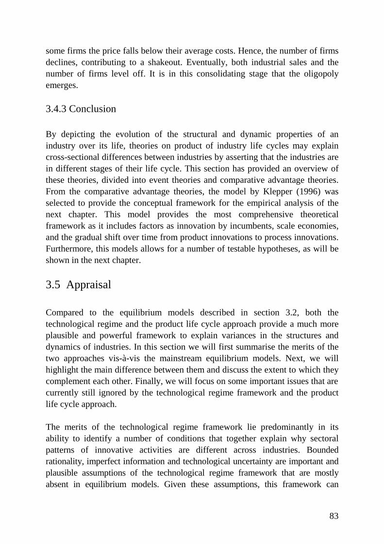
83
some firms the price falls below their average costs. Hence, the number of firmsdeclines, contributing to a shakeout. Eventually, both industrial sales and thenumber of firms level off . It is in this consolidating stage that the oligopolyemerges.
3.4.3 Conclusion
By depicting the evolution of the structural and dynamic properties of anindustry over its life, theories on product of industry li fe cycles may explaincross-sectional differences between industries by asserting that the industries arein different stages of their life cycle. This section has provided an overview ofthese theories, divided into event theories and comparative advantage theories.From the comparative advantage theories, the model by Klepper (1996) wasselected to provide the conceptual framework for the empirical analysis of thenext chapter. This model provides the most comprehensive theoreticalframework as it includes factors as innovation by incumbents, scale economies,and the gradual shift over time from product innovations to process innovations.Furthermore, this models allows for a number of testable hypotheses, as will beshown in the next chapter.
3.5 Appraisal
Compared to the equilibrium models described in section 3.2, both thetechnological regime and the product life cycle approach provide a much moreplausible and powerful framework to explain variances in the structures anddynamics of industries. In this section we will first summarise the merits of thetwo approaches vis-à-vis the mainstream equilibrium models. Next, we willhighlight the main difference between them and discuss the extent to which theycomplement each other. Finally, we will focus on some important issues that arecurrently stil l ignored by the technological regime framework and the productli fe cycle approach.
The merits of the technological regime framework lie predominantly in itsabil ity to identify a number of conditions that together explain why sectoralpatterns of innovative activities are different across industries. Boundedrationality, imperfect information and technological uncertainty are important andplausible assumptions of the technological regime framework that are mostlyabsent in equili brium models. Given these assumptions, this framework can

84
explain why the creation and diffusion of technological knowledge is anendogenous process that produces winners and losers among the firms involved inresearch and development activities. As we have argued in section 3.2.4, byassuming that new technological knowledge arrives exogenously, information isperfect and entrepreneurs are perfectly rational, equil ibrium models lack thepossibili ty of modelling the competitive process driven by endogenoustechnological change. Hence, by endogenising technological change andidentifying technological innovativeness as a major determinant of the competitiveprocess, the technological regime approach provides a much more comprehensiveand plausible framework for analysing the structural and dynamic properties ofindustries than the equili brium models.
The strength of the product or industry li fe cycle approach lies in its ability toendogenise the evolution of an industry over its lifetime. More specifically, itanalyses how the terms of (technological) competition change through theformative stages of an industry, and how these changes effect the industry’sstructural and dynamic properties. To some extent, equilibrium models could beused as well to analyse different equilibrium properties of industries underdifferent competitive and technological38 conditions. However, these modelswould not able to explain why the competitive and technological conditionschange over time. This is an important omission, because many new industrieshave shown rather similar evolutionary patterns, suggesting that the competitiveprocess changed in a systematic way as these industries matured. Since modelson product life cycles do explain how these changes arise, they provide a muchbetter tool to analyse the evolution of industries than the mainstream equil ibriummodels.
In conclusion, compared to the mainstream equilibrium models we consider thetechnological regime and the product life cycle approach much more appropriateand plausible theoretical frameworks for explaining and analysing industrialdynamics. But how do the technological regime framework and the product orli fe approach compare to each other? In our view, these theoretical bodies arehighly complementary. The technological regime framework explains structuraldifferences in industrial dynamics between industries, whereas the product lifecycle approach explains temporal differences in industrial dynamics withinindustries. In general, the technological regime framework does not distinguishthe various stages through which new industries evolve. Reversely, the productli fe cycle approach does not distinguish differences in, e.g., cumulativeness
38 In terms of different specifications of the production function.
85
conditions between industries. Within the product life cycle approach, thecomparative advantage models certainly acknowledge the cumulative nature ofthe innovative process. But no reference is made to the effect of differentdegrees of cumulativeness on the evolutionary patterns of the industries.
Since these two approaches are highly complementary, there seems to be a greatpotential for combining the technological regime framework and the product lifecycle approach. To a large extent the deficiencies of the former can be overcomeby the latter, and vice versa. The result of such an attempt to combine the twoframeworks may be a model that allows for a direct comparison between the lifecycle patterns of new industries with different underlying technological regimeconditions. However, when the present models of the technological regime andthe product life cycle approach were taken as a starting point for such acombined model, a number of important issues would still be ignored.
First of all, models of product life cycles generally focus on the emergence andevolution of only one product and its associated technology. However, in manyindustries we observe that firms repeatedly introduce or adopt new producttechnologies that replace the older ones. Second, both these approaches do notexplicitly consider differences in the technological properties of the goodsproduced by the industries. Finally, in models on technological regimes and onindustry li fe cycles the growth of a firm is generally determined by its relative(technological) performance. However, empirical studies on firm growth do notprovide much evidence supporting such a relationship. Most of these studiessuggest that the size of a firm generally follows a random walk with a decliningpositive drift.39
In conclusion, although the present models of the technological regime and theproduct life cycle approach still ignore a number of interesting issues, webelieve they provide a comprehensive and plausible framework to analyse thestructural and dynamic properties of industries. Furthermore, we expect thatfuture efforts to combine them will prove valuable, as these two approaches arehighly complementary. A preliminary attempt to combine some parts of thetechnological regime framework and the product life cycle approach and toovercome their present shortcomings is presented in chapter 5 of this thesis.
39 See Geroski (1998).
86
3.6 Conclusions
In our search for theoretical contributions that may explain the observeddifferences across industries in a dynamic and comprehensive way, we haveselected two approaches and described them thoroughly in this chapter. In ourview, both the technological regime framework as well as the product life cycleapproach are highly appropriate conceptual tools to study empirically thedifferences in cross-section regularities, as they both embody elements such asfirm heterogeneity and technological uncertainty that are close to empiricalsubstance. With regard to their potential power to explain differences instructures and dynamics between industries, we have argued the following.
The technological regime framework asserts that patterns of innovative activitiesare determined by the combination of opportunity, appropriabil ity andcumulativeness conditions, and properties of the technological knowledge baseunderlying these activities. If entry, survival, growth and exit patterns are relatedto the rates and forms of organisation of innovations, then the observed inter-sectoral variety in structures and dynamics can be explained by differences inthe underlying technological regimes. Alternatively, theories and models onproduct life cycles explain and depict the evolution of an industry’s structuraland dynamic properties over its lifetime. Based on this approach, the observedcross-sectional differences can be explained by the different evolutionary stagesthat industries occupy. To what extent these theories can actually account for thecross-sectional variances will be investigated in the next chapter.
87
Chapter 4
Technological Regimes and Industry Life Cyclesin Dutch Manufacturing
4.1 Introduction
The empirical li terature in industrial economics has indeed been greatly enrichedby the increased availabil ity of longitudinal firm-level databases. As we haveshown in chapter 2, the exploration of such databases has resulted in a collectionof strong empirical regularities that seem to hold over different countries, aswell as over different time periods. One of these regularities concerns theobserved variances in the structures and dynamics of industries. However, untilnow the opportunity to test theories explaining these cross-sectional differenceswith the available longitudinal firm-level data has hardly been exploited. Usingthe SN database, the present chapter aims to exploit this opportunity byinvestigating whether the technological regime framework and the product lifecycle approach can explain the observed differences between industries withregard to their structural and dynamic properties.
This chapter is structured as follows. In section 4.2, we will investigate theempirical relationship between industrial dynamics and technological regimes.After deriving a number of hypotheses from the theoretical framework andclassifying the industries according to their technological regime, we will testwhether the differences suggested by the technological regime frameworkactually exist. The structure of section 4.3 is rather similar. A number ofhypotheses, derived from Klepper (1996), will be tested to see whetherindustries in different evolutionary stages show different regularities, andwhether these regularities are in line with Klepper’s model. In section 4.4 wewill use regression analyses to investigate the extent to which the selected
88
theoretical approaches simultaneously account for differences betweenindustries, and whether any interaction effects can be observed between them.Section 4.5 concludes this chapter.
4.2 Technological regimes
As argued in the previous chapter, the main contribution of the technologicalregime framework is that it suggests an explanation for the observed inter-sectoral variety in the rates and forms of organisation of innovations. Empiricalevidence supporting this explanation can be found in Malerba et al. (1995) andBreschi et al. (1996). However, these studies only focused on structural anddynamic differences in the populations of innovative firms in relation to theunderlying technological regimes. The question that naturally follows concernswhether a similar relationship exists between the structural and dynamicproperties of the full population of f irms in an industry and its underlyingtechnological regime.
The aim of the present section is to answer this question. It is structured asfollows. First, we will shortly summarise the main characteristics of thetechnological regime framework, and formulate a number of hypotheses derivedfrom this framework. Second, we will present how we have classified theindustries in the SN database according to their technological regime. Finally,we will t est the hypotheses with the firm-level data at hand.
4.2.1 The hypotheses
The previous chapter already discussed in detail the literature on technologicalregimes. Before formulating the hypotheses, let us briefly summarise the mostimportant issues on the technological regime framework from which thehypotheses will be derived. A technological regime can be defined as aparticular combination of opportunity, appropriabil ity, cumulativenessconditions and properties of the knowledge base, common to specific activitiesof innovation and production and shared by the population of f irms undertakingthose activities. Opportunity conditions refer to the likelihood of innovating,given a certain research effort. Appropriabil ity conditions reflect the possibilit iesof protecting innovations from imitation and of appropriating the profits from aninnovation. Cumulativeness conditions refer to the extent to which theinnovative successes of individual firms are serially correlated. Finally, with
89
regard to the properties of the knowledge base, the following three aspects ofknowledge can be distinguished: (1) the level of specificity, (2) the level oftacitness, and (3) the extent to which the knowledge is publicly available.
In the literature on technological regimes, two regimes with opposite underlyingconditions are usually distinguished. These metaphorical archetypes correspondto the two rather opposite views on the innovative process that Schumpeter heldduring his life. The two regimes are labelled Schumpeter Mark I (SM-I) andSchumpeter Mark II (SM-II). Since opportunity conditions do not necessarilydiffer between the regimes, the differences between them are mainly related todifferences in appropriabili ty, cumulativeness conditions and patterns of accessto knowledge. A SM-I regime is characterised by low appropriabili ty andcumulativeness conditions, and the knowledge is mainly specific, codified andsimple. In a SM-II regime, these three conditions are reversed: appropriabili tyand cumulativeness conditions are high, whereas the knowledge is mainlygeneric, tacit and complex.
In the presentation of hypotheses that follows, we will base the formulations ofthe hypotheses on these two archetypes. We will propose one group of industriesin which the SM-I regime underlies the innovative and productive activities, anda second group in which the SM-II regime prevails. Based on the differences inthe appropriabil ity, cumulativeness and knowledge conditions, we willhypothesise significant differences between the two groups of industries withregard to a number of selected variables. These differences can be classified intwo major categories. The first category addresses differences in static measures,such as the firm size distribution, whereas the second category more reflectdifferences in the dynamic properties of the industry, e.g., the process of entryand exit. We will first derive some hypotheses related to the static inter-industrydifferences.
As argued in chapter 3, in a typical SM-I industry we can expect the pattern ofinnovative activities to be characterised by the constant inflow of newentrepreneurs with new ideas, products and processes, continuously challengingthe established firms and wiping out their quasi-rents associated with previousinnovations. Such an industry is therefore likely to be characterised by thepresence of many small firms and low entry barriers (Malerba et al., 1995). InSM-II industries, this situation is reversed: large firms prevail , (technological)entry barriers are high, and the high profit rates of incumbent firms arepersistent. Additionally, Audretsch (1997) suggests that the degree of capital
90
intensity also shapes the technological regimes: a routinised technologicalregime (which resembles a SM-II regime) is more capital intensive than anentrepreneurial technological regime (SM-I regime). All together, thesecharacterisations allow us to derive the following hypotheses:
Hypothesis 1 The share of small firms is higher in SM-I industries thanin SM-II industries.
Hypothesis 2 Concentration levels are lower SM-I industries than inSM-II industries.
Hypothesis 3 Entry barriers are lower in SM-I industries than in SM-IIindustries.
Hypothesis 4 Capital intensity is lower in SM-I industries than in SM-IIindustries.
Hypothesis 5 In SM-I industries, profit rates are lower than in SM-IIindustries.
Hypothesis 6 In SM-I industries, entrants are more productive thanincumbents, whereas in SM-II industries incumbents are moreproductive than entrants.
This last hypothesis reflects the relative advantage that entrants should haveover incumbents in SM-I industries, and vice versa for SM-II industries. Hence,hypothesis 6 tests for differences between entrants and incumbents within eachtechnological regime.
With respect to variances in the dynamic properties of industries, differences inthe stability of the firm population can be measured by looking at the amount ofturnover (in terms of shifts in market shares) due to entry and exit. Moreover,the turbulence within the group of incumbent firms can be examined here: SM-Iindustries are expected to show a less stable population of incumbent firms thanSM-II industries. This leads to the following hypotheses:
Hypothesis 7 In SM-I industries, the amount of turnover due to entryand exit is higher than in SM-II industries.

91
Hypothesis 8 The turbulence within the group of incumbent firms ishigher in SM-I industries than in SM-II industries.
Another potential difference between the two groups of industries concerns theshare of the entry and exit process in the total growth in productivity. Given thenature of the two regimes, we can expect the contribution this process toproductivity growth to be higher in SM-I industries, and the contribution ofincumbents to be higher in SM-II industries. Hence, we can derive the followinghypothesis:
Hypothesis 9 The contribution of the entry and exit process toproductivity growth is higher in SM-I industries than in SM-IIindustries, and vice versa for incumbents’ contributions.
In section 4.2.3, these hypotheses will be tested. But first we will explain howwe have classif ied the industries into the groups of SM-I and SM-II regimes.
4.2.2 Classification of industries
As mentioned in chapter 3, previous empirical research used data on innovationactivities performed by the firms to study the technological regime of anindustry. Unfortunately, the SN database does not include variables indicatingthe innovative activities of the firm. We therefore have to rely on the results ofprevious empirical research to classify our industries into a group of SM-I and agroup of SM-II industries.
The classification of industries into technological regimes that we propose isbased on the taxonomy presented in Malerba et al. (1995).1 Although thistaxonomy does not directly rest on differences with regard to the underlyingappropriability, cumulativeness, and knowledge conditions, the appliedindicators of innovative activity strongly suggest major differences between thetechnological classes according to the widening (SM-I) and the deepening(SM-II) pattern. And, as mentioned in chapter 3, Breschi et al. (1996) found thatthese patterns are, in turn, related to the conditions of the underlyingtechnological regime.
1 See section 3.3.2 of the previous chapter for the details of this taxonomic exercise.
92
Since the 33 technological classes do not always match the industries in oursample, we unfortunately had to exclude those industries for which no evidenceexisted regarding their underlying technological regime. Hence, only industriesthat are unambiguously SM-I and SM-II (according to Malerba et al., 1995) areconsidered in the analysis that follows. Although even for this group ofindustries there may not be a strict conceptual correspondence between atechnology class and an industry, we believe this does not cause a majordistortion in mapping the technology classes to industries. Furthermore, giventhe strong similarities across the four European countries investigated byMalerba et al. (1995), we do not expect that a similar exercise based on patentdata for the Dutch manufacturing sector will l ead to a different taxonomy oftechnological classes. Finally, given the substantial overlap in the time periodsof the dataset by Malerba et al, (1968-1986) and our dataset (1978-1992), we donot believe that the small differences in these time periods will bias the results.
According to the proposed criterion, our total sample of 106 industries is dividedin 60 SM-I industries and 18 SM-II industries. The remaining 28 industries areexcluded from the analysis in this section. This group of industries mainlyinvolves the manufacturing of food products, which could not be classified in adistinct category in the analysis by Malerba et al (1995)2, and the printingindustries, which was simply not included in their analysis. The complete list ofindustries and the technological regimes to which they have been allocated canbe found in the Appendix of this chapter, as well as the list of excludedindustries.
Before turning to the next section, in which we will test the proposedhypotheses, we would like to repeat our remarks made in chapter 2 with regardto the truncation of the SN database. The point we raised there is that theconsequence of this truncation is that our ‘entering’ and ‘exiting’ firms aremainly firms crossing the observation threshold. It might seem awkward then topropose a number of hypotheses related to the process of entry and exit.However, if, for instance, the regime of an industry is favourable to new andsmall firms, it is likely that it is easier for these firms to grow and pass theobservation threshold than in an industry with a regime favourable to large andestablished firms. To put more strongly, excluding firms with less than twentyemployees, even if involving an inevitable censoring of observations, is notlikely to distort the entry and exit characteristics associated with the two
2 Malerba et al. (1995) put the food and tobacco industry into a group labelled ‘othertechnological classes’ .
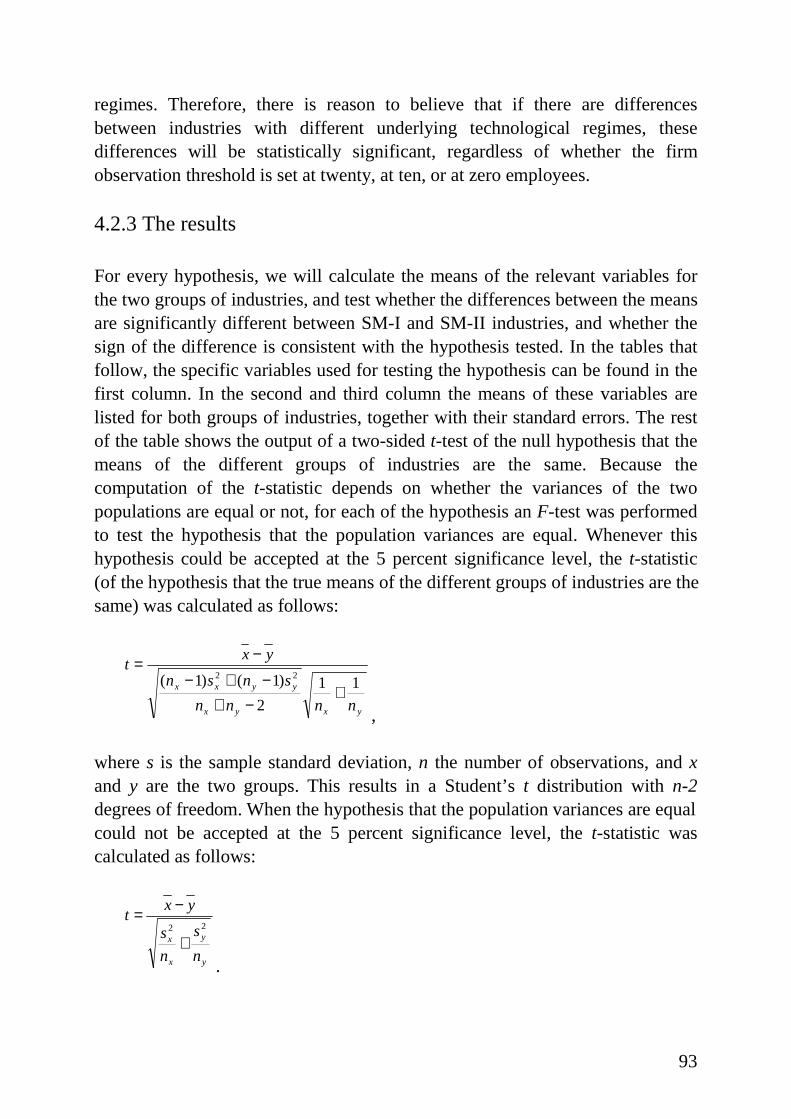
93
regimes. Therefore, there is reason to believe that if there are differencesbetween industries with different underlying technological regimes, thesedifferences will be statistically significant, regardless of whether the firmobservation threshold is set at twenty, at ten, or at zero employees.
4.2.3 The results
For every hypothesis, we will calculate the means of the relevant variables forthe two groups of industries, and test whether the differences between the meansare significantly different between SM-I and SM-II industries, and whether thesign of the difference is consistent with the hypothesis tested. In the tables thatfollow, the specific variables used for testing the hypothesis can be found in thefirst column. In the second and third column the means of these variables arelisted for both groups of industries, together with their standard errors. The restof the table shows the output of a two-sided t-test of the null hypothesis that themeans of the different groups of industries are the same. Because thecomputation of the t-statistic depends on whether the variances of the twopopulations are equal or not, for each of the hypothesis an F-test was performedto test the hypothesis that the population variances are equal. Whenever thishypothesis could be accepted at the 5 percent significance level, the t-statistic(of the hypothesis that the true means of the different groups of industries are thesame) was calculated as follows:
yxyx
yyxx
nnnn
snsn
yxt
11
2
)1()1( 22
+−+
−+−
−=
,
where s is the sample standard deviation, n the number of observations, and xand y are the two groups. This results in a Student’s t distribution with n-2degrees of freedom. When the hypothesis that the population variances are equalcould not be accepted at the 5 percent significance level, the t-statistic wascalculated as follows:
y
y
x
x
n
s
n
s
yxt
22
+
−=
.
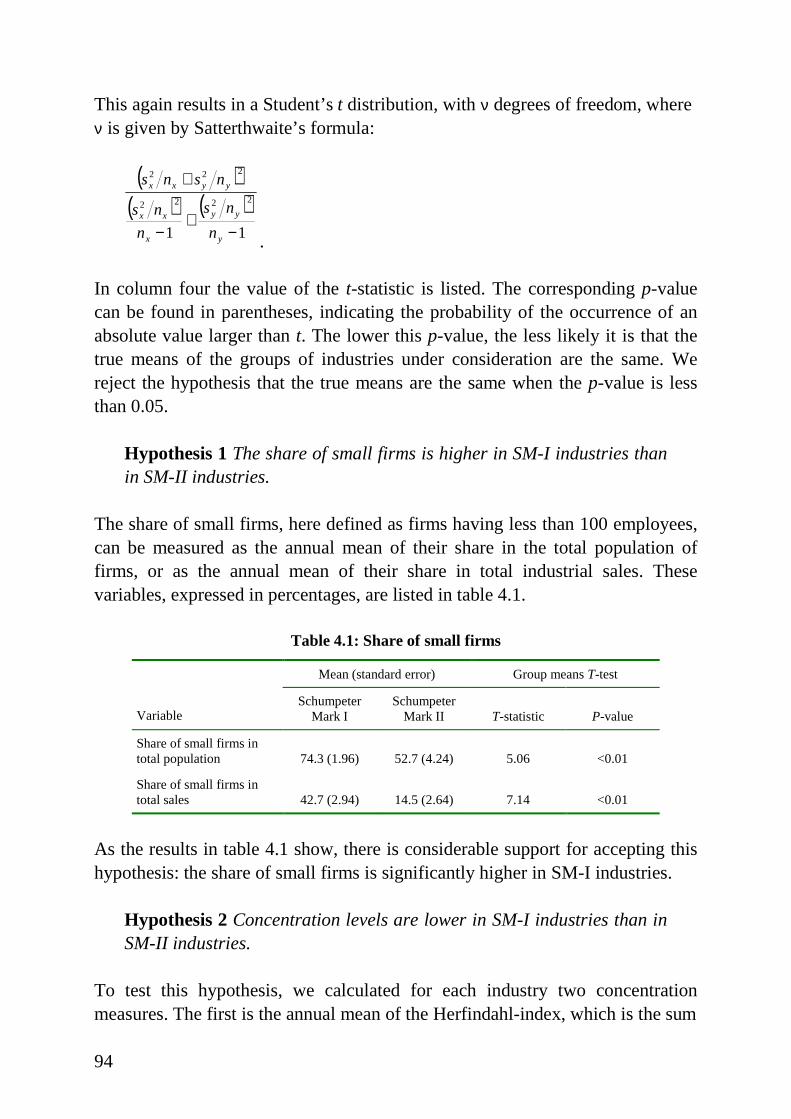
94
This again results in a Student’s t distribution, with ν degrees of freedom, where ν is given by Satterthwaite’s formula:
( )( ) ( )
11
2222
222
−+
−
+
y
yy
x
xx
yyxx
n
ns
n
ns
nsns
.
In column four the value of the t-statistic is listed. The corresponding p-valuecan be found in parentheses, indicating the probabili ty of the occurrence of anabsolute value larger than t. The lower this p-value, the less likely it is that thetrue means of the groups of industries under consideration are the same. Wereject the hypothesis that the true means are the same when the p-value is lessthan 0.05.
Hypothesis 1 The share of small firms is higher in SM-I industries thanin SM-II industries.
The share of small firms, here defined as firms having less than 100 employees,can be measured as the annual mean of their share in the total population offirms, or as the annual mean of their share in total industrial sales. Thesevariables, expressed in percentages, are listed in table 4.1.
Table 4.1: Share of small firms
Mean (standard error) Group means T-test
VariableSchumpeter
Mark ISchumpeter
Mark II T-statistic P-value
Share of small firms intotal population 74.3 (1.96) 52.7 (4.24) 5.06 <0.01
Share of small firms intotal sales 42.7 (2.94) 14.5 (2.64) 7.14 <0.01
As the results in table 4.1 show, there is considerable support for accepting thishypothesis: the share of small firms is significantly higher in SM-I industries.
Hypothesis 2 Concentration levels are lower in SM-I industries than inSM-II industries.
To test this hypothesis, we calculated for each industry two concentrationmeasures. The first is the annual mean of the Herfindahl-index, which is the sum
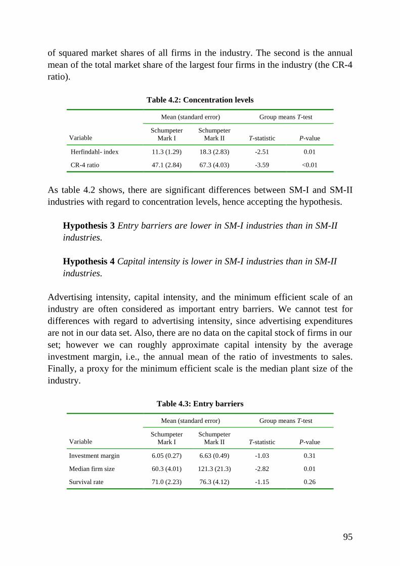
95
of squared market shares of all firms in the industry. The second is the annualmean of the total market share of the largest four firms in the industry (the CR-4ratio).
Table 4.2: Concentration levels
Mean (standard error) Group means T-test
VariableSchumpeter
Mark ISchumpeter
Mark II T-statistic P-value
Herfindahl- index 11.3 (1.29) 18.3 (2.83) -2.51 0.01
CR-4 ratio 47.1 (2.84) 67.3 (4.03) -3.59 <0.01
As table 4.2 shows, there are significant differences between SM-I and SM-IIindustries with regard to concentration levels, hence accepting the hypothesis.
Hypothesis 3 Entry barriers are lower in SM-I industries than in SM-IIindustries.
Hypothesis 4 Capital intensity is lower in SM-I industries than in SM-IIindustries.
Advertising intensity, capital intensity, and the minimum eff icient scale of anindustry are often considered as important entry barriers. We cannot test fordifferences with regard to advertising intensity, since advertising expendituresare not in our data set. Also, there are no data on the capital stock of f irms in ourset; however we can roughly approximate capital intensity by the averageinvestment margin, i.e., the annual mean of the ratio of investments to sales.Finally, a proxy for the minimum eff icient scale is the median plant size of theindustry.
Table 4.3: Entry barr iers
Mean (standard error) Group means T-test
VariableSchumpeter
Mark ISchumpeter
Mark II T-statistic P-value
Investment margin 6.05 (0.27) 6.63 (0.49) -1.03 0.31
Median firm size 60.3 (4.01) 121.3 (21.3) -2.82 0.01
Survival rate 71.0 (2.23) 76.3 (4.12) -1.15 0.26
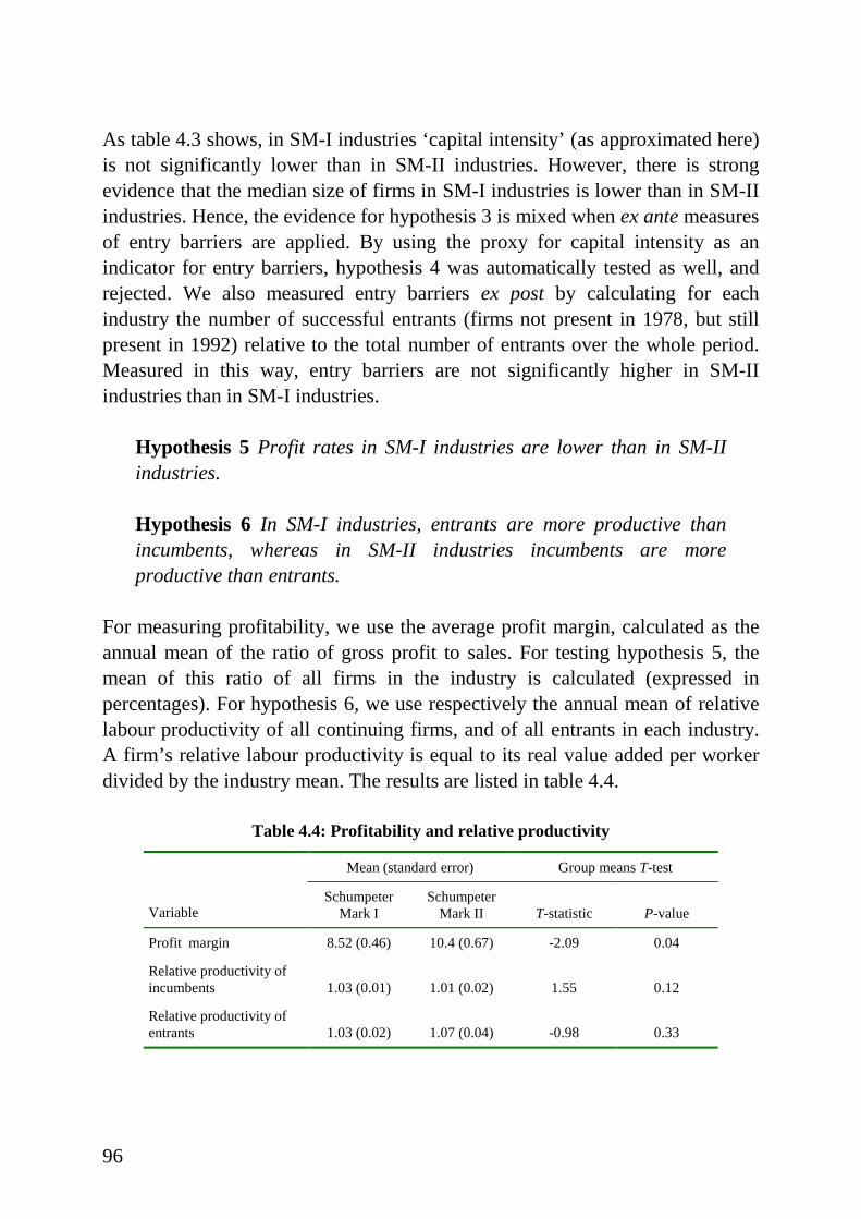
96
As table 4.3 shows, in SM-I industries ‘capital intensity’ (as approximated here)is not significantly lower than in SM-II industries. However, there is strongevidence that the median size of firms in SM-I industries is lower than in SM-IIindustries. Hence, the evidence for hypothesis 3 is mixed when ex ante measuresof entry barriers are applied. By using the proxy for capital intensity as anindicator for entry barriers, hypothesis 4 was automatically tested as well , andrejected. We also measured entry barriers ex post by calculating for eachindustry the number of successful entrants (firms not present in 1978, but stillpresent in 1992) relative to the total number of entrants over the whole period.Measured in this way, entry barriers are not significantly higher in SM-IIindustries than in SM-I industries.
Hypothesis 5 Profit rates in SM-I industries are lower than in SM-IIindustries.
Hypothesis 6 In SM-I industries, entrants are more productive thanincumbents, whereas in SM-II industries incumbents are moreproductive than entrants.
For measuring profitabili ty, we use the average profit margin, calculated as theannual mean of the ratio of gross profit to sales. For testing hypothesis 5, themean of this ratio of all firms in the industry is calculated (expressed inpercentages). For hypothesis 6, we use respectively the annual mean of relativelabour productivity of all continuing firms, and of all entrants in each industry.A firm’s relative labour productivity is equal to its real value added per workerdivided by the industry mean. The results are listed in table 4.4.
Table 4.4: Profitabili ty and relative productivity
Mean (standard error) Group means T-test
VariableSchumpeter
Mark ISchumpeter
Mark II T-statistic P-value
Profit margin 8.52 (0.46) 10.4 (0.67) -2.09 0.04
Relative productivity ofincumbents 1.03 (0.01) 1.01 (0.02) 1.55 0.12
Relative productivity ofentrants 1.03 (0.02) 1.07 (0.04) -0.98 0.33
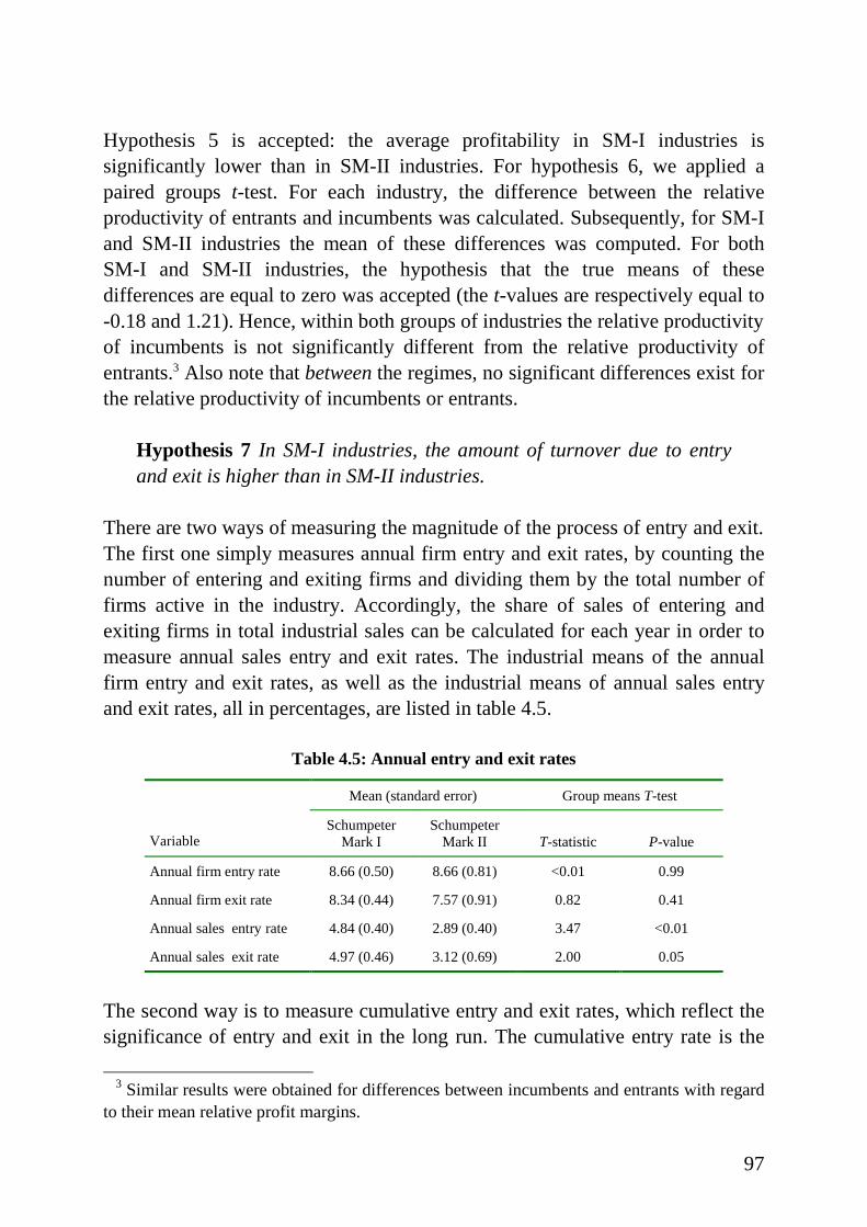
97
Hypothesis 5 is accepted: the average profitabil ity in SM-I industries issignificantly lower than in SM-II industries. For hypothesis 6, we applied apaired groups t-test. For each industry, the difference between the relativeproductivity of entrants and incumbents was calculated. Subsequently, for SM-Iand SM-II industries the mean of these differences was computed. For bothSM-I and SM-II industries, the hypothesis that the true means of thesedifferences are equal to zero was accepted (the t-values are respectively equal to-0.18 and 1.21). Hence, within both groups of industries the relative productivityof incumbents is not significantly different from the relative productivity ofentrants.3 Also note that between the regimes, no significant differences exist forthe relative productivity of incumbents or entrants.
Hypothesis 7 In SM-I industries, the amount of turnover due to entryand exit is higher than in SM-II industries.
There are two ways of measuring the magnitude of the process of entry and exit.The first one simply measures annual firm entry and exit rates, by counting thenumber of entering and exiting firms and dividing them by the total number offirms active in the industry. Accordingly, the share of sales of entering andexiting firms in total industrial sales can be calculated for each year in order tomeasure annual sales entry and exit rates. The industrial means of the annualfirm entry and exit rates, as well as the industrial means of annual sales entryand exit rates, all in percentages, are listed in table 4.5.
Table 4.5: Annual entry and exit rates
Mean (standard error) Group means T-test
VariableSchumpeter
Mark ISchumpeter
Mark II T-statistic P-value
Annual firm entry rate 8.66 (0.50) 8.66 (0.81) <0.01 0.99
Annual firm exit rate 8.34 (0.44) 7.57 (0.91) 0.82 0.41
Annual sales entry rate 4.84 (0.40) 2.89 (0.40) 3.47 <0.01
Annual sales exit rate 4.97 (0.46) 3.12 (0.69) 2.00 0.05
The second way is to measure cumulative entry and exit rates, which reflect thesignificance of entry and exit in the long run. The cumulative entry rate is the
3 Similar results were obtained for differences between incumbents and entrants with regard
to their mean relative profit margins.
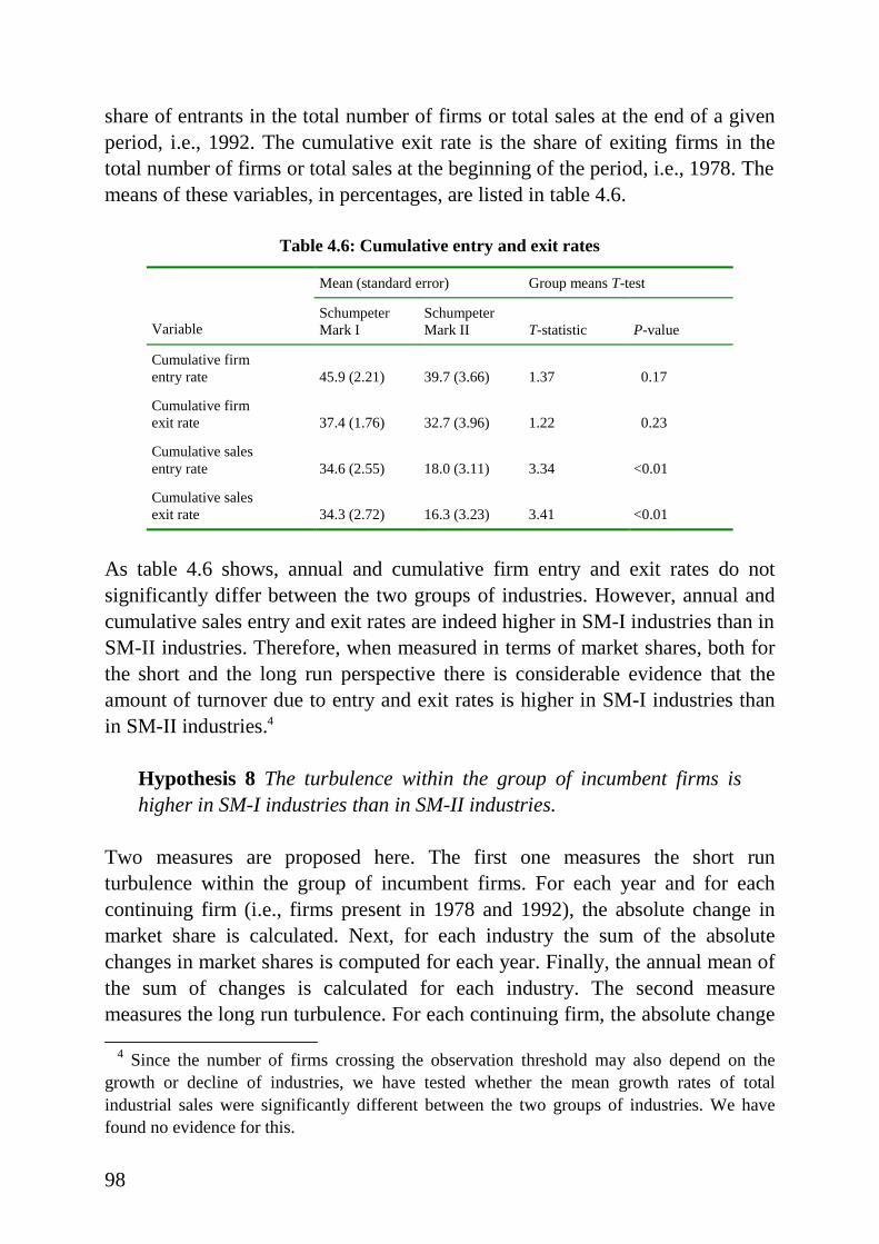
98
share of entrants in the total number of f irms or total sales at the end of a givenperiod, i.e., 1992. The cumulative exit rate is the share of exiting firms in thetotal number of fi rms or total sales at the beginning of the period, i.e., 1978. Themeans of these variables, in percentages, are listed in table 4.6.
Table 4.6: Cumulative entry and exit rates
Mean (standard error) Group means T-test
VariableSchumpeterMark I
SchumpeterMark II T-statistic P-value
Cumulative firmentry rate 45.9 (2.21) 39.7 (3.66) 1.37 0.17
Cumulative firmexit rate 37.4 (1.76) 32.7 (3.96) 1.22 0.23
Cumulative salesentry rate 34.6 (2.55) 18.0 (3.11) 3.34 <0.01
Cumulative salesexit rate 34.3 (2.72) 16.3 (3.23) 3.41 <0.01
As table 4.6 shows, annual and cumulative firm entry and exit rates do notsignificantly differ between the two groups of industries. However, annual andcumulative sales entry and exit rates are indeed higher in SM-I industries than inSM-II industries. Therefore, when measured in terms of market shares, both forthe short and the long run perspective there is considerable evidence that theamount of turnover due to entry and exit rates is higher in SM-I industries thanin SM-II industries.4
Hypothesis 8 The turbulence within the group of incumbent firms ishigher in SM-I industries than in SM-II industries.
Two measures are proposed here. The first one measures the short runturbulence within the group of incumbent firms. For each year and for eachcontinuing firm (i.e., firms present in 1978 and 1992), the absolute change inmarket share is calculated. Next, for each industry the sum of the absolutechanges in market shares is computed for each year. Finally, the annual mean ofthe sum of changes is calculated for each industry. The second measuremeasures the long run turbulence. For each continuing firm, the absolute change
4 Since the number of f irms crossing the observation threshold may also depend on thegrowth or decline of industries, we have tested whether the mean growth rates of totalindustrial sales were significantly different between the two groups of industries. We havefound no evidence for this.
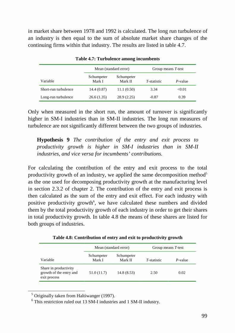
99
in market share between 1978 and 1992 is calculated. The long run turbulence ofan industry is then equal to the sum of absolute market share changes of thecontinuing firms within that industry. The results are listed in table 4.7.
Table 4.7: Turbulence among incumbents
Mean (standard error) Group means T-test
VariableSchumpeter
Mark ISchumpeter
Mark II T-statistic P-value
Short-run turbulence 14.4 (0.87) 11.1 (0.50) 3.34 <0.01
Long-run turbulence 26.6 (1.35) 28.9 (2.25) -0.87 0.39
Only when measured in the short run, the amount of turnover is significantlyhigher in SM-I industries than in SM-II industries. The long run measures ofturbulence are not signif icantly different between the two groups of industries.
Hypothesis 9 The contribution of the entry and exit process toproductivity growth is higher in SM-I industries than in SM-IIindustries, and vice versa for incumbents’ contributions.
For calculating the contribution of the entry and exit process to the totalproductivity growth of an industry, we applied the same decomposition method5
as the one used for decomposing productivity growth at the manufacturing levelin section 2.3.2 of chapter 2. The contribution of the entry and exit process isthen calculated as the sum of the entry and exit effect. For each industry withpositive productivity growth6, we have calculated these numbers and dividedthem by the total productivity growth of each industry in order to get their sharesin total productivity growth. In table 4.8 the means of these shares are listed forboth groups of industries.
Table 4.8: Contr ibution of entry and exit to productivity growth
Mean (standard error) Group means T-test
VariableSchumpeter
Mark ISchumpeter
Mark II T-statistic P-value
Share in productivitygrowth of the entry andexit process
51.0 (11.7) 14.8 (8.53) 2.50 0.02
5 Originally taken from Haltiwanger (1997).6 This restriction ruled out 13 SM-I industries and 1 SM-II industry.
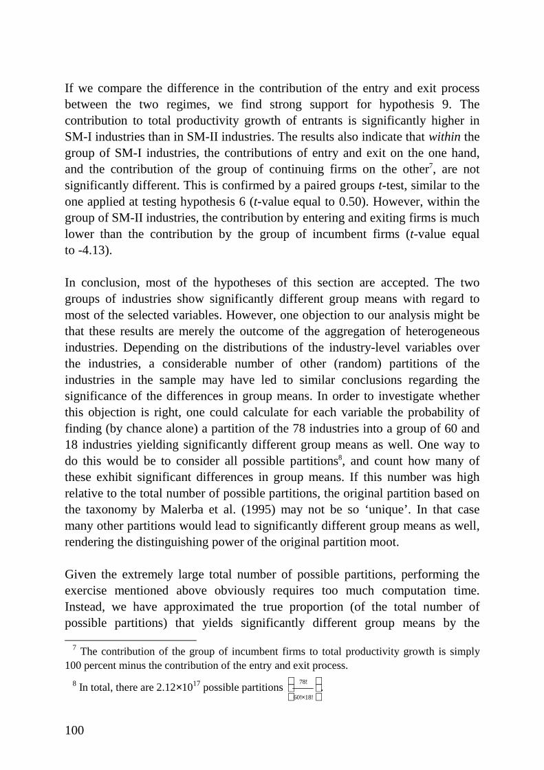
100
If we compare the difference in the contribution of the entry and exit processbetween the two regimes, we find strong support for hypothesis 9. Thecontribution to total productivity growth of entrants is significantly higher inSM-I industries than in SM-II industries. The results also indicate that within thegroup of SM-I industries, the contributions of entry and exit on the one hand,and the contribution of the group of continuing firms on the other7, are notsignificantly different. This is confirmed by a paired groups t-test, similar to theone applied at testing hypothesis 6 (t-value equal to 0.50). However, within thegroup of SM-II industries, the contribution by entering and exiting firms is muchlower than the contribution by the group of incumbent firms (t-value equalto -4.13).
In conclusion, most of the hypotheses of this section are accepted. The twogroups of industries show significantly different group means with regard tomost of the selected variables. However, one objection to our analysis might bethat these results are merely the outcome of the aggregation of heterogeneousindustries. Depending on the distributions of the industry-level variables overthe industries, a considerable number of other (random) partitions of theindustries in the sample may have led to similar conclusions regarding thesignificance of the differences in group means. In order to investigate whetherthis objection is right, one could calculate for each variable the probabil ity offinding (by chance alone) a partition of the 78 industries into a group of 60 and18 industries yielding significantly different group means as well. One way todo this would be to consider all possible partitions8, and count how many ofthese exhibit significant differences in group means. If this number was highrelative to the total number of possible partitions, the original partition based onthe taxonomy by Malerba et al. (1995) may not be so ‘unique’ . In that casemany other partitions would lead to significantly different group means as well ,rendering the distinguishing power of the original partition moot.
Given the extremely large total number of possible partitions, performing theexercise mentioned above obviously requires too much computation time.Instead, we have approximated the true proportion (of the total number ofpossible partitions) that yields significantly different group means by the
7 The contribution of the group of incumbent firms to total productivity growth is simply100 percent minus the contribution of the entry and exit process.
8 In total, there are 2.12×10¹⁷ possible partitions
× !18!60
!78.
101
following procedure. In total 25,000 times, we have randomly divided the 78industries into a group of 60 and a group of 18 industries, and counted thenumber of times the means of the industry-level variables9 were significantlydifferent between the two subgroups. For each variable, table 4.9 lists thepercentage of cases in which the mean of the 60 industries group is significantlylower than the mean of the 18 industries group, and the percentage of cases inwhich the opposite holds.10 Hence, the sum of these percentages approximatesthe probabili ty of f inding by chance alone a partition yielding significantlydifferent group means (regardless of their signs).
As the results in table 4.9 show, the proportion of cases in which the randomgrouping procedure leads to significantly different group means consistent withthe technological regime framework is quite low. And given that the variablesare not perfectly correlated, we can expect the number of cases in which themeans of a selection of these variables are simultaneously different andconsistent with the technological regime framework to be even much lower.11 Inconclusion, the results of this random grouping procedure provide additionalevidence that the criterion based on the taxonomy by Malerba et al. (1995)constitutes a significant determinant of structural and dynamic differencesbetween industries.
4.2.4 Conclusion
The main conclusion from the analysis of this section is that the results indeedsuggest that the structural and dynamic properties of the industries are stronglyrelated to their underlying technological regimes. Obviously, the two groups ofindustries show considerable differences with regard to most of the selectedvariables, which in all cases have the right sign, and thus corroborate thehypotheses. For only a few variables the differences are not significant. Let usshortly summarise the results.
9 We have omitted the variables that tested for differences within the technological regimes,
as these variables are not included in hypotheses that test for differences between the SM-Iand SM-II groups.
10 Based on the t-test described in section 4.2.3.11 In fact, none of the 25,000 random partitions exhibited a sequence of group means test
results for the 19 variables identical to the sequence derived from the original analysis of thissection.
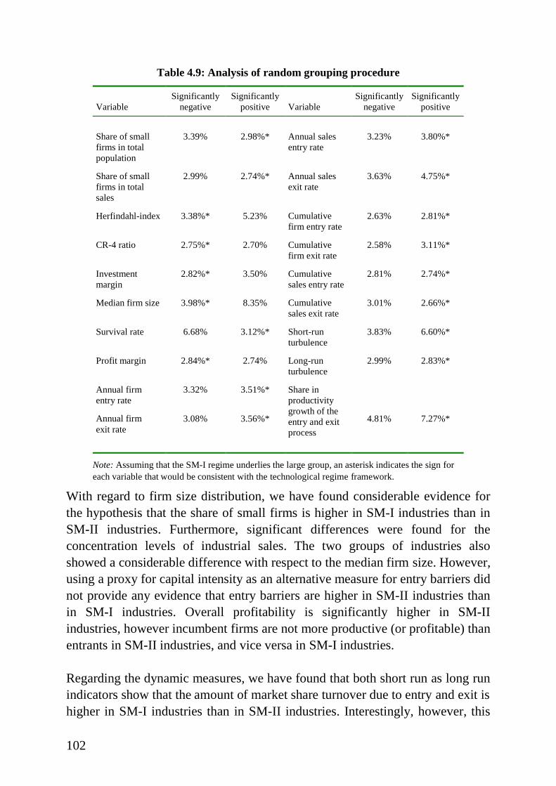
102
Table 4.9: Analysis of random grouping procedure
VariableSignificantly
negativeSignificantly
positive VariableSignificantly
negativeSignificantly
positive
Share of smallfirms in totalpopulation
3.39% 2.98%* Annual salesentry rate
3.23% 3.80%*
Share of smallfirms in totalsales
2.99% 2.74%* Annual salesexit rate
3.63% 4.75%*
Herfindahl-index 3.38%* 5.23% Cumulativefirm entry rate
2.63% 2.81%*
CR-4 ratio 2.75%* 2.70% Cumulativefirm exit rate
2.58% 3.11%*
Investmentmargin
2.82%* 3.50% Cumulativesales entry rate
2.81% 2.74%*
Median firm size 3.98%* 8.35% Cumulativesales exit rate
3.01% 2.66%*
Survival rate 6.68% 3.12%* Short-runturbulence
3.83% 6.60%*
Profit margin 2.84%* 2.74% Long-runturbulence
2.99% 2.83%*
Annual firmentry rate
3.32% 3.51%*
Annual firmexit rate
3.08% 3.56%*
Share inproductivitygrowth of theentry and exitprocess
4.81% 7.27%*
Note: Assuming that the SM-I regime underlies the large group, an asterisk indicates the sign foreach variable that would be consistent with the technological regime framework.
With regard to firm size distribution, we have found considerable evidence forthe hypothesis that the share of small firms is higher in SM-I industries than inSM-II industries. Furthermore, significant differences were found for theconcentration levels of industrial sales. The two groups of industries alsoshowed a considerable difference with respect to the median firm size. However,using a proxy for capital intensity as an alternative measure for entry barriers didnot provide any evidence that entry barriers are higher in SM-II industries thanin SM-I industries. Overall profitability is significantly higher in SM-IIindustries, however incumbent firms are not more productive (or profitable) thanentrants in SM-II industries, and vice versa in SM-I industries.
Regarding the dynamic measures, we have found that both short run as long runindicators show that the amount of market share turnover due to entry and exit ishigher in SM-I industries than in SM-II industries. Interestingly, however, this
103
goes together with the evidence that firm entry and exit rates did not differsignificantly between the two groups of industries. The measures of turbulencewithin the group of incumbent firms showed some mixed results. This variablewas only significantly different when measured as year to year changes. If thefull period was taken into account, the turbulence within the group ofincumbents is approximately the same for SM-I and SM-II industries. Finally,the contribution of the entry and exit process to total productivity growth ishigher in SM-I industries than in SM-II industries.
These results show that technological regimes to a considerable extent explaindifferences between industries with regard to their structural and dynamicproperties. In our view, the results of this analysis are strong enough to supportto “ …interpretations leaning toward an evolutionary approach [which]emphasize sector/technology-specific patterns and invariances in the way agentslearn…as determinants of both structures and dynamics.” (Dosi et al., 1997,p.19). In the next section we will i nvestigate to what extent differences betweenindustries can be explained by the different evolutionary stages they occupy.
4.3 Industry life cycles
This section attempts to interpret the observed differences between industrieswith regard to their structural and dynamic properties by relating them withtheoretical conceptualisations regarding industry li fe cycles. By asserting thatindustries subsequently go through their stages of birth, growth, maturity anddecline, theories on product or industrial life cycles could explain the observeddifferences in the following way. If each of these evolutionary stages of anindustry has its own structural and dynamic properties, then cross-sectionaldifferences between industries may stem from the different evolutionary stagesthose industries are in. This section aims to find empirical evidence for thisexplanation by posing the following question: can differences betweenindustries be explained by the different evolutionary stages they occupy?
In order to answer this question, we will derive and test a number of hypothesesbased upon Klepper’s model, as presented in chapter 3. The structure of thissection will be as follows. First, we will briefly explain how we will employKlepper’s model in the empirical analysis of this section, and present thehypotheses derived from this model. Next, we will present how we haveassigned the evolutionary stages to the industries in the SN database, and discuss
104
some restrictions the data may impose on testing the hypotheses. Finally, wewill t est the hypotheses and discuss the results.
4.3.1 The hypotheses
As mentioned in chapter 3, the most important feature of Klepper’s model is thedynamic increasing returns from technological change. The model emphasisesdifferences in firm innovative capabilities, and the importance of f irm size inappropriating the returns from innovation to explain regularities concerning howentry, exit, market structure, and innovation vary from the birth oftechnologically progressive industries through maturity. The main implication ofthis model is that the industry will eventually evolve to an oligopoly. Theearliest successful entrants engage in R&D and start growing. This increasestheir returns from R&D, because the output in which they can embody theirinnovations rises. Initiall y, i.e., in the expanding stage, firms enter, but at somepoint the price is driven down to a level at which (profitable) entry is no longerpossible. Exit stil l continues, as for some firms the price falls below theiraverage costs. Hence, the number of f irms declines, contributing to a shakeout.Eventually, both industrial sales and the number of f irms level off . Theoligopoly emerges in this consolidating stage.
Unfortunately, the time span of the SN manufacturing database does not allowfor studying the full evolution of the industries in the sample. In fact, it is likelythat most of these industries have already reached maturity. Furthermore, thelevel of aggregation of the sampled industries may in some cases be too high toinvestigate the impact of life cycles of individual products. Therefore, we do notaim to directly test the model. Rather, we try to investigate whether basicallymature industries exhibit distinct evolutionary stages as well, and whetherdynamic increasing returns to technological change underlie the emergence ofthese stages. For instance, the obsolescence of the prevailing design of a good,or a radical change in the technology used to produce it may initiate a newevolutionary pattern in a mature industry, resembling the li fe cycle of a newindustry. Hence, we will employ Klepper’s model as a conceptual tool to answerthe following questions: (1) Do industries in different stages show differentregularities? (2) Are these observed regularities in line with the regularitiespredicted by Klepper’s model? (3) Can the observed differences be explained bydynamic increasing returns from technological change?
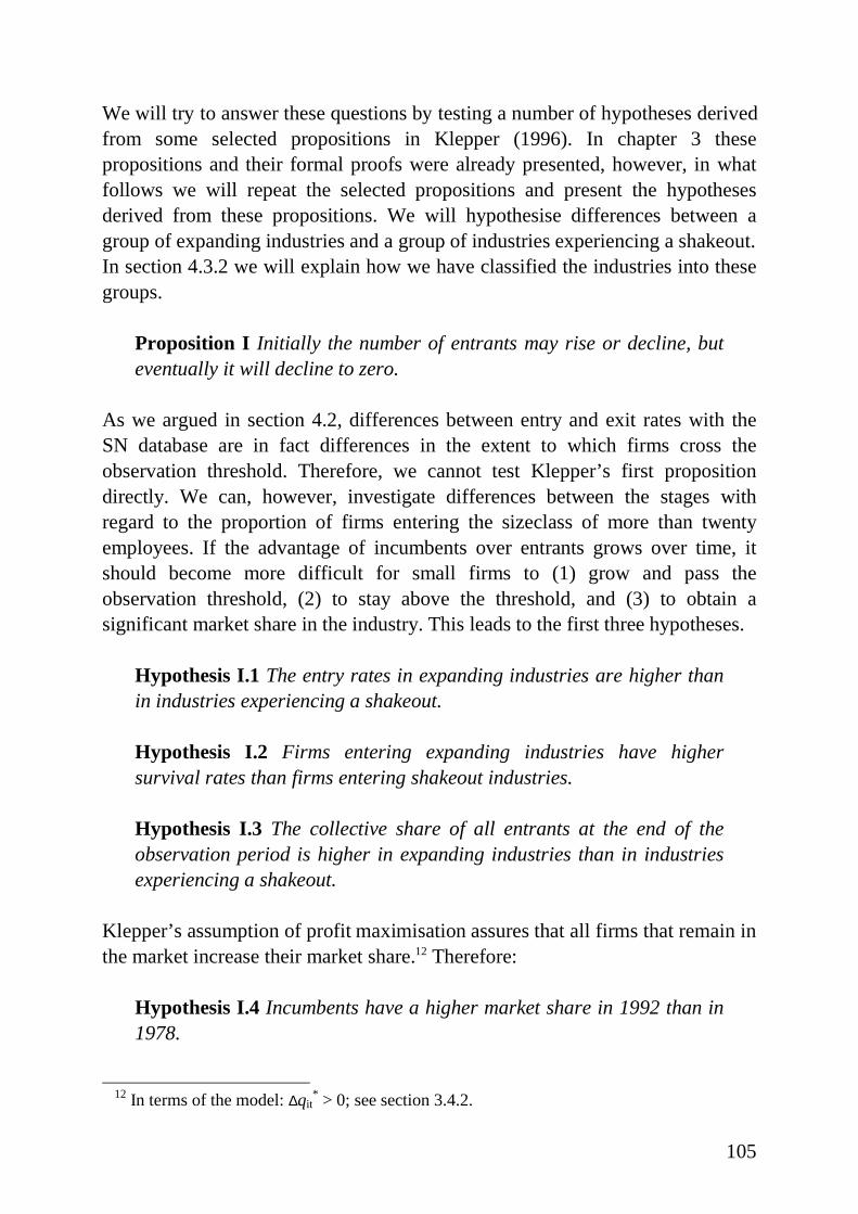
105
We will try to answer these questions by testing a number of hypotheses derivedfrom some selected propositions in Klepper (1996). In chapter 3 thesepropositions and their formal proofs were already presented, however, in whatfollows we will repeat the selected propositions and present the hypothesesderived from these propositions. We will hypothesise differences between agroup of expanding industries and a group of industries experiencing a shakeout.In section 4.3.2 we will explain how we have classified the industries into thesegroups.
Proposition I Initially the number of entrants may rise or decline, buteventually it will decline to zero.
As we argued in section 4.2, differences between entry and exit rates with theSN database are in fact differences in the extent to which firms cross theobservation threshold. Therefore, we cannot test Klepper’s first propositiondirectly. We can, however, investigate differences between the stages withregard to the proportion of firms entering the sizeclass of more than twentyemployees. If the advantage of incumbents over entrants grows over time, itshould become more difficult for small firms to (1) grow and pass theobservation threshold, (2) to stay above the threshold, and (3) to obtain asignificant market share in the industry. This leads to the first three hypotheses.
Hypothesis I.1 The entry rates in expanding industries are higher thanin industries experiencing a shakeout.
Hypothesis I.2 Firms entering expanding industries have highersurvival rates than firms entering shakeout industries.
Hypothesis I.3 The collective share of all entrants at the end of theobservation period is higher in expanding industries than in industriesexperiencing a shakeout.
Klepper’s assumption of profit maximisation assures that all f irms that remain inthe market increase their market share.12 Therefore:
Hypothesis I.4 Incumbents have a higher market share in 1992 than in1978.
12 In terms of the model: ∆qit
* > 0; see section 3.4.2.
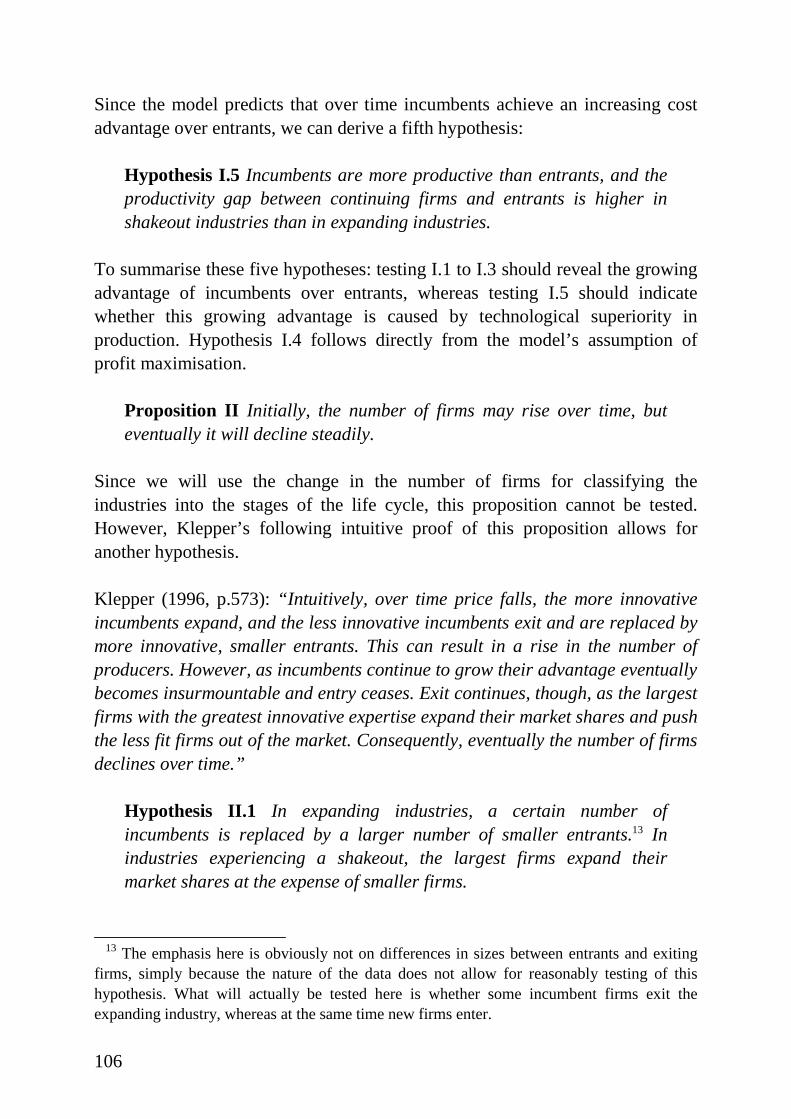
106
Since the model predicts that over time incumbents achieve an increasing costadvantage over entrants, we can derive a fifth hypothesis:
Hypothesis I.5 Incumbents are more productive than entrants, and theproductivity gap between continuing firms and entrants is higher inshakeout industries than in expanding industries.
To summarise these five hypotheses: testing I.1 to I.3 should reveal the growingadvantage of incumbents over entrants, whereas testing I.5 should indicatewhether this growing advantage is caused by technological superiority inproduction. Hypothesis I.4 follows directly from the model’s assumption ofprofit maximisation.
Proposition I I Initially, the number of firms may rise over time, buteventually it will decline steadily.
Since we will use the change in the number of firms for classifying theindustries into the stages of the life cycle, this proposition cannot be tested.However, Klepper’s following intuitive proof of this proposition allows foranother hypothesis.
Klepper (1996, p.573): “ Intuitively, over time price falls, the more innovativeincumbents expand, and the less innovative incumbents exit and are replaced bymore innovative, smaller entrants. This can result in a rise in the number ofproducers. However, as incumbents continue to grow their advantage eventuallybecomes insurmountable and entry ceases. Exit continues, though, as the largestfirms with the greatest innovative expertise expand their market shares and pushthe less fit firms out of the market. Consequently, eventually the number of firmsdeclines over time.”
Hypothesis I I .1 In expanding industries, a certain number ofincumbents is replaced by a larger number of smaller entrants.13 Inindustries experiencing a shakeout, the largest firms expand theirmarket shares at the expense of smaller firms.
13 The emphasis here is obviously not on differences in sizes between entrants and exiting
firms, simply because the nature of the data does not allow for reasonably testing of thishypothesis. What will actually be tested here is whether some incumbent firms exit theexpanding industry, whereas at the same time new fi rms enter.

107
Proposition II I As each firm grows large, eventually the change in itsmarket share will decline over time.
The prediction that the continuing firm’s growth in market share declines overtime can easily be tested with the available data. However, testing whether theprofit margin on the standard product decreases is more difficult. In the model,the profit margin is defined as price minus average cost of production. The latterare negatively dependent on the amount spent on process R&D. Since there is nodata on any of these variables, the profit margin (total profits before taxes overtotal sales) is taken as a proxy for the profit rate. This leads to the followinghypotheses.
Hypothesis II I .1 The growth of continuing firms’ market shares ispositively related to their profit rates.
Hypothesis II I .2 Profit rates are higher in expanding industries than inindustries experiencing a shakeout.
Hypothesis II I .3 The growth of market shares of continuing firms ishigher in expanding industries than in industries experiencing ashakeout.
Proposition IV For each period, firm average cost varies inversely withfirm output.
This proposition implies that in each period small firms are less productive thanlarge firms, basically because of scale economies in process R&D. Hence, thefollowing hypothesis can be derived.
Hypothesis IV.1 For each period, large firms are more productive thansmall f irms.
In section 4.3.3 we will test these hypotheses and discuss the results. But firstwe will explain how we have classified the industries into their evolutionarystages.
108
4.3.2 Classification of industries
Given the characteristics of the SN dataset, a number of problems arise.Obviously, the major problem is that the entire evolutionary history of eachindustry cannot be observed, i.e., the origin of the industries occur before thefirst year of observation. Therefore, it cannot be tested whether the industriesevolve according to the pattern predicted by Klepper’s model. Instead, we willattempt to locate the industries in the sample in terms of the evolutionary stagethat they occupy in Klepper’s framework.14 This is facilitated by the relativelylong period over which the fi rms are observed in the dataset.
Ideally, some independent proxies, such as the growth rate of patents, would beused to determine the evolutionary stage the industry is in. Since these, or anyother data that would allow us to exogenously classify the industries, are notavailable, we will have to base our classification on the revealed patterns ofsome variables denoting the evolution of the industries in the sample.Obviously, such an endogenous classification will , to some extent, limit ourempirical analysis. However, we can still investigate whether the industrypatterns, denoted by variables other than the ones used for classifying theindustries, are consistent with the regularities predicted by Klepper’s model. Ifwe would find that the patterns are indeed consistent, such results would provideevidence, albeit circumstantial, that differences in regularities between industriesin different stages can be explained by dynamic increasing returns totechnological change.
We propose a combination of the following two variables to determine in whichstage an industry is: the growth rate of the total number of firms and the growthrate of the sum of their total industrial real sales, both measured over the fullperiod (i.e., 1978-1992). A standard t-test was applied to determine whethereach of these growth rates was significantly different from zero. Table 4.10explains how each industry is classified into the stage of its evolution. Inparentheses the number of industries in each category is listed.
14 This methodology is very similar to Audretsch (1987).
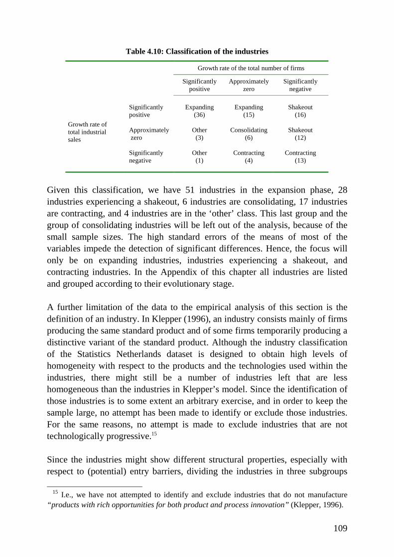
109
Table 4.10: Classification of the industr ies
Growth rate of the total number of firms
Significantlypositive
Approximatelyzero
Significantlynegative
Significantlypositive
Expanding(36)
Expanding(15)
Shakeout(16)
Approximately zero
Other(3)
Consolidating(6)
Shakeout(12)
Growth rate oftotal industrialsales
Significantlynegative
Other(1)
Contracting(4)
Contracting(13)
Given this classification, we have 51 industries in the expansion phase, 28industries experiencing a shakeout, 6 industries are consolidating, 17 industriesare contracting, and 4 industries are in the ‘other’ class. This last group and thegroup of consolidating industries will be left out of the analysis, because of thesmall sample sizes. The high standard errors of the means of most of thevariables impede the detection of significant differences. Hence, the focus wil lonly be on expanding industries, industries experiencing a shakeout, andcontracting industries. In the Appendix of this chapter all i ndustries are listedand grouped according to their evolutionary stage.
A further limitation of the data to the empirical analysis of this section is thedefinition of an industry. In Klepper (1996), an industry consists mainly of f irmsproducing the same standard product and of some firms temporarily producing adistinctive variant of the standard product. Although the industry classificationof the Statistics Netherlands dataset is designed to obtain high levels ofhomogeneity with respect to the products and the technologies used within theindustries, there might still be a number of industries left that are lesshomogeneous than the industries in Klepper’s model. Since the identification ofthose industries is to some extent an arbitrary exercise, and in order to keep thesample large, no attempt has been made to identify or exclude those industries.For the same reasons, no attempt is made to exclude industries that are nottechnologically progressive.15
Since the industries might show different structural properties, especially withrespect to (potential) entry barriers, dividing the industries in three subgroups
15 I.e., we have not attempted to identify and exclude industries that do not manufacture
“ products with rich opportunities for both product and process innovation” (Klepper, 1996).
110
could create some bias. For instance, if by coincidence the group of expandingindustries contains a large number of industries with high entry barriers, then theresults of testing a hypothesis for differences between the group of industrieswith respect to entry rates will be unreliable. Therefore, we have compared thethree groups with respect to the means of capital intensity, approximated by theratio of investments to sales, and median firm size. Because the means of thesevariables do not differ significantly between the three groups, there is lessreason to believe that the proposed division leads to a bias with respect todifferent structural properties of the groups of industries.
4.3.3 The hypotheses tested
In this section, the ten hypotheses will be tested. For each hypothesis, thespecific variables used for testing wil l be defined. Subsequently, the results ofthe test wil l be reported, together with a short discussion on their consistencywith the model. Although Klepper’s model does not deal with the evolution ofindustries after consolidation (the total quantity demanded expands over time), itmight be interesting to see to what extent the group of contracting industriesdiffers from the other groups. Therefore, for each hypothesis the values of thespecific variables for the contracting industries will be listed as well.
In each of the following tables that show the results of testing for differencesbetween the groups of industries, the mean and its standard error of the specificvariable wil l be listed in the second column. The rest of the table shows theoutput of a t-test of the null hypothesis that the means of the different groups ofindustries are the same.16 In the third and fourth column the values of thet-statistic wil l be listed. The corresponding p-values can be found in parentheses,indicating the probabili ty of the occurrence of a value larger than t. We rejectthe hypothesis that the true means are the same when the p-value is less than0.05.
Hypothesis I.1 The entry rates in expanding industries are higher thanin industries experiencing a shakeout.
For each industry, the mean of annual gross entry rates, defined as the number ofentrants in a certain year divided by the total number of firms present at thebeginning of the year, is calculated.
16 For the details of this test, see section 4.2.3 of this chapter.

111
Table 4.11: Firm entry rates
T-statistic (p-value) of a T-test for mean differences
Industry stage Mean (Std.Err.) vs. Shakeout-industries vs. Contracting industries
Expansion 9.81 (0.72) 4.06 (<0.01) 1.15 (0.25)
Shakeout 6.48 (0.39) -1.46 (0.16)
Contraction 8.20 (1.10)
As the t-statistic indicates, the gross entry rates are indeed significantly higher inexpanding industries than in industries experiencing a shakeout of firms. Hence,this hypothesis is accepted. Contracting industries show intermediate values forthis variable, but with the highest standard error of the mean. The mean of thegross entry rates of contracting industries is not significantly different from themeans of the groups of expanding and shakeout industries.
To some extent the acceptance of this hypothesis may seem too obvious: onecould argue that it is not surprising to see higher entry rates in industries inwhich the total number of f irms grows, as compared to industries in which thisnumber declines. However, the classification of industries is based on net entry,whereas this hypothesis tests for differences with regard to gross entry. Hence,in principle shakeout industries may even show higher entry rates thanexpanding industries. In that case of course the exit rates of shakeout industrieswould have to significantly exceed the exit rates of expanding industries as well .
Table 4.12, in which we have displayed the means of annual firm exit rates,shows that this is not the case after all. On average, firm exit rates are notsignificantly higher in industries experiencing a shakeout than the exit rates forthe group of expanding industries. But the interesting conclusion is then stillthat, exactly as in Klepper’s model, a shakeout of firms is not caused by anincrease in exit rates, but by a significant reduction in the number of firmsentering the industry.
Another argument against the acceptance of this hypothesis might be thatexpanding industries have higher growth rates (in terms of sales) then industriesexperiencing a shakeout, and that therefore entry rates are higher as well.However, if this were true, contracting industries would have to show the lowestentry rates. Since this is not the case, the lowest entry rates of shakeout

112
industries may be interpreted as circumstantial evidence for an advantage ofincumbents over entrants in this group of industries.
Table 4.12: Firm exit rates
T-statistic (p-value) of a T-test for mean differences
Industry stage Mean (Std.Err.) vs. Shakeout-industries vs. Contracting industries
Expansion 7.87 (0.81) -0.01 (0.99) -1.83 (0.07)
Shakeout 7.88 (0.47) -2.99 (<0.01)
Contraction 10.6 (0.90)
Finally, one could argue that the emergence of niches, for instance throughspecialisation, has been much higher in expanding industries. However, this isnot confirmed by the latest standard classification of industries, introduced byStatistics Netherlands in 1993. When the total sales of a new product, initiallyassigned to existing industries, become suff iciently high, Statistics Netherlandsintroduces a new 4-digit industry. If this has happened relatively often inexpanding industries, it could explain the higher entry and survival rates. This isnot the case, however. About one fifth of the group of expanding industries hasbeen spli t up in two or more new 4-digit industries17, equal to the proportion ofthe group of shakeout industries that have been subdivided in 1993.
Hypothesis I.2 Firms entering expanding industries have highersurvival rates than firms entering shakeout industries.
The variable used here is the industrial mean of the survival rates. It iscalculated (for each industry) as the number of successful entrants (firms notpresent in 1978, but still present in 1992) relative to the total number of entrantsover the whole period.
Table 4.13: Survival rates
T-statistic (p-value) of a T-test for mean differences
Industry stage Mean (Std.Err.) vs. Shakeout-industries vs. Contracting industries
Expansion 77.1 (1.82) 3.46 (<0.01) 2.24 (0.04)
Shakeout 61.1 (4.28) -0.76 (0.45)
Contraction 66.1 (4.60)
17 As compared to the 1974 classification used in the present analysis.
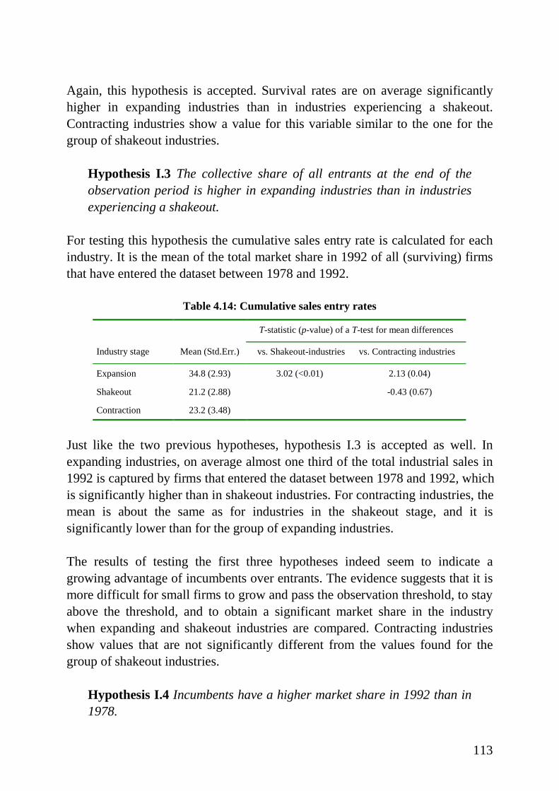
113
Again, this hypothesis is accepted. Survival rates are on average significantlyhigher in expanding industries than in industries experiencing a shakeout.Contracting industries show a value for this variable similar to the one for thegroup of shakeout industries.
Hypothesis I.3 The collective share of all entrants at the end of theobservation period is higher in expanding industries than in industriesexperiencing a shakeout.
For testing this hypothesis the cumulative sales entry rate is calculated for eachindustry. It is the mean of the total market share in 1992 of all (surviving) firmsthat have entered the dataset between 1978 and 1992.
Table 4.14: Cumulative sales entry rates
T-statistic (p-value) of a T-test for mean differences
Industry stage Mean (Std.Err.) vs. Shakeout-industries vs. Contracting industries
Expansion 34.8 (2.93) 3.02 (<0.01) 2.13 (0.04)
Shakeout 21.2 (2.88) -0.43 (0.67)
Contraction 23.2 (3.48)
Just like the two previous hypotheses, hypothesis I.3 is accepted as well . Inexpanding industries, on average almost one third of the total industrial sales in1992 is captured by fi rms that entered the dataset between 1978 and 1992, whichis signif icantly higher than in shakeout industries. For contracting industries, themean is about the same as for industries in the shakeout stage, and it issignificantly lower than for the group of expanding industries.
The results of testing the first three hypotheses indeed seem to indicate agrowing advantage of incumbents over entrants. The evidence suggests that it ismore diff icult for small firms to grow and pass the observation threshold, to stayabove the threshold, and to obtain a significant market share in the industrywhen expanding and shakeout industries are compared. Contracting industriesshow values that are not significantly different from the values found for thegroup of shakeout industries.
Hypothesis I.4 Incumbents have a higher market share in 1992 than in1978.
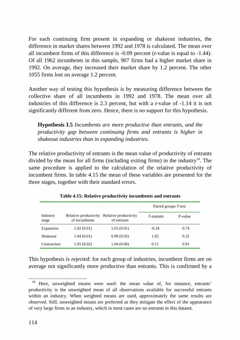
114
For each continuing firm present in expanding or shakeout industries, thedifference in market shares between 1992 and 1978 is calculated. The mean overall i ncumbent firms of this difference is -0.09 percent (t-value is equal to -1.44).Of all 1962 incumbents in this sample, 907 firms had a higher market share in1992. On average, they increased their market share by 1.2 percent. The other1055 firms lost on average 1.2 percent.
Another way of testing this hypothesis is by measuring difference between thecollective share of all incumbents in 1992 and 1978. The mean over allindustries of this difference is 2.3 percent, but with a t-value of -1.14 it is notsignificantly different from zero. Hence, there is no support for this hypothesis.
Hypothesis I.5 Incumbents are more productive than entrants, and theproductivity gap between continuing firms and entrants is higher inshakeout industries than in expanding industries.
The relative productivity of entrants is the mean value of productivity of entrantsdivided by the mean for all firms (including exiting firms) in the industry18. Thesame procedure is applied to the calculation of the relative productivity ofincumbent firms. In table 4.15 the mean of these variables are presented for thethree stages, together with their standard errors.
Table 4.15: Relative productivity incumbents and entrants
Paired groups T-test
Industrystage
Relative productivityof incumbents
Relative productivityof entrants
T-statistic P-value
Expansion 1.02 (0.01) 1.03 (0.01) -0.34 0.74
Shakeout 1.04 (0.01) 0.99 (0.05) 1.02 0.32
Contraction 1.05 (0.02) 1.04 (0.06) 0.11 0.91
This hypothesis is rejected: for each group of industries, incumbent firms are onaverage not significantly more productive than entrants. This is confirmed by a
18 Here, unweighted means were used: the mean value of, for instance, entrants’
productivity is the unweighted mean of all observations available for successful entrantswithin an industry. When weighted means are used, approximately the same results areobserved. Still , unweighted means are preferred as they mitigate the effect of the appearanceof very large firms in an industry, which in most cases are no entrants in this dataset.
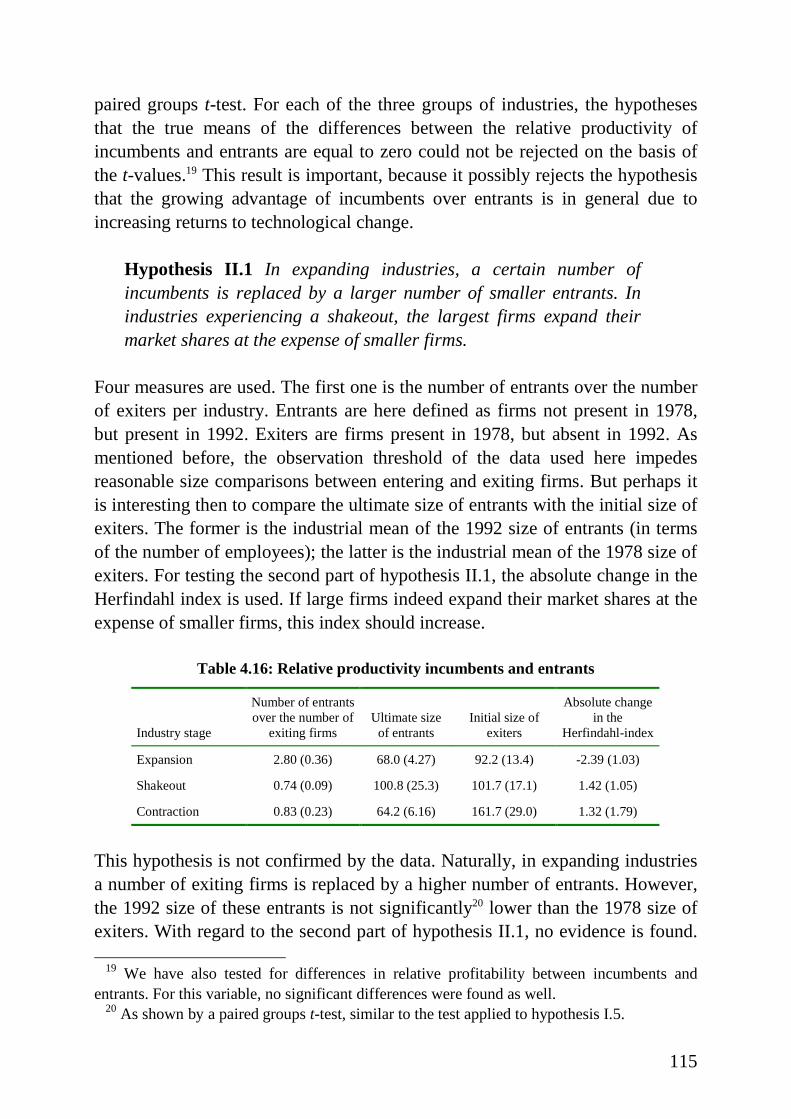
115
paired groups t-test. For each of the three groups of industries, the hypothesesthat the true means of the differences between the relative productivity ofincumbents and entrants are equal to zero could not be rejected on the basis ofthe t-values.19 This result is important, because it possibly rejects the hypothesisthat the growing advantage of incumbents over entrants is in general due toincreasing returns to technological change.
Hypothesis I I .1 In expanding industries, a certain number ofincumbents is replaced by a larger number of smaller entrants. Inindustries experiencing a shakeout, the largest firms expand theirmarket shares at the expense of smaller firms.
Four measures are used. The first one is the number of entrants over the numberof exiters per industry. Entrants are here defined as firms not present in 1978,but present in 1992. Exiters are firms present in 1978, but absent in 1992. Asmentioned before, the observation threshold of the data used here impedesreasonable size comparisons between entering and exiting firms. But perhaps itis interesting then to compare the ultimate size of entrants with the initial size ofexiters. The former is the industrial mean of the 1992 size of entrants (in termsof the number of employees); the latter is the industrial mean of the 1978 size ofexiters. For testing the second part of hypothesis II .1, the absolute change in theHerfindahl index is used. If large firms indeed expand their market shares at theexpense of smaller firms, this index should increase.
Table 4.16: Relative productivity incumbents and entrants
Industry stage
Number of entrantsover the number of
exiting firmsUltimate sizeof entrants
Initial size ofexiters
Absolute changein the
Herfindahl-index
Expansion 2.80 (0.36) 68.0 (4.27) 92.2 (13.4) -2.39 (1.03)
Shakeout 0.74 (0.09) 100.8 (25.3) 101.7 (17.1) 1.42 (1.05)
Contraction 0.83 (0.23) 64.2 (6.16) 161.7 (29.0) 1.32 (1.79)
This hypothesis is not confirmed by the data. Naturally, in expanding industriesa number of exiting firms is replaced by a higher number of entrants. However,the 1992 size of these entrants is not significantly20 lower than the 1978 size ofexiters. With regard to the second part of hypothesis II .1, no evidence is found.
19 We have also tested for differences in relative profitabili ty between incumbents andentrants. For this variable, no significant differences were found as well .
20 As shown by a paired groups t-test, similar to the test applied to hypothesis I.5.

116
On average, the Herfindahl index does not increase significantly in shakeoutindustries. An interesting observation is that in contracting industries, the initialsize of exiters is significantly larger than the ultimate size of entrants.
Hypothesis II I .1 The growth of continuing firms’ market shares ispositively related to their profit rates.
For each continuing firm present in the group of expanding and shakeoutindustries, the change in market share between 1978 and 1992 was calculated.Then, again for each firm, the average profit rate was calculated by the sum ofreal profits (between 1978 and 1992) divided by the sum of real sales over thesame period. This average profit rate of each incumbent was then divided by theaverage industrial profit rate for continuing firms to calculate the relativeprofitability of each continuing firm. To test hypothesis III .1, the correlationcoefficient between the change in market share and the log of relativeprofitability was calculated. Although the coefficient is significantly positive atthe 1 percent level, its value of 0.11 is not high. But despite this low value, thehypothesis is accepted.
Hypothesis II I .2 Profit rates are higher in expanding industries than inindustries experiencing a shakeout.
The profit rates are approximated by the profit margin: the total profits (beforetaxes) over total sales. Then for each industry the mean of these profit margins iscalculated.
Table 4.17: Profit margins
T-statistic (p-value) of a T-test for mean differences
Industry stage Mean (Std.Err.) vs. Shakeout-industries vs. Contracting industries
Expansion 9.48 (0.42) 0.51 (0.61) 2.42 (0.02)
Shakeout 9.10 (0.67) 1.60 (0.12)
Contraction 7.35 (0.88)
Because the differences are insignificant between expansion and shakeout,hypothesis III .2 is not accepted. Contracting industries exhibit the lowest profitrates, which are significantly lower than the profit rates of expanding industries.
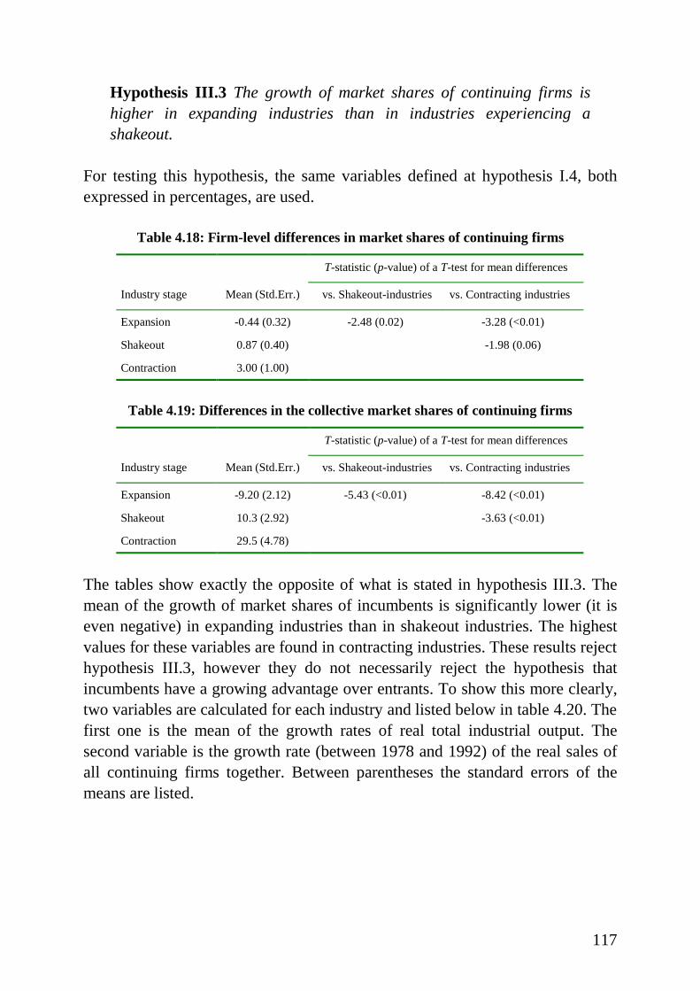
117
Hypothesis II I .3 The growth of market shares of continuing firms ishigher in expanding industries than in industries experiencing ashakeout.
For testing this hypothesis, the same variables defined at hypothesis I.4, bothexpressed in percentages, are used.
Table 4.18: Firm-level differences in market shares of continuing firms
T-statistic (p-value) of a T-test for mean differences
Industry stage Mean (Std.Err.) vs. Shakeout-industries vs. Contracting industries
Expansion -0.44 (0.32) -2.48 (0.02) -3.28 (<0.01)
Shakeout 0.87 (0.40) -1.98 (0.06)
Contraction 3.00 (1.00)
Table 4.19: Differences in the collective market shares of continuing firms
T-statistic (p-value) of a T-test for mean differences
Industry stage Mean (Std.Err.) vs. Shakeout-industries vs. Contracting industries
Expansion -9.20 (2.12) -5.43 (<0.01) -8.42 (<0.01)
Shakeout 10.3 (2.92) -3.63 (<0.01)
Contraction 29.5 (4.78)
The tables show exactly the opposite of what is stated in hypothesis III .3. Themean of the growth of market shares of incumbents is significantly lower (it iseven negative) in expanding industries than in shakeout industries. The highestvalues for these variables are found in contracting industries. These results rejecthypothesis III .3, however they do not necessarily reject the hypothesis thatincumbents have a growing advantage over entrants. To show this more clearly,two variables are calculated for each industry and listed below in table 4.20. Thefirst one is the mean of the growth rates of real total industrial output. Thesecond variable is the growth rate (between 1978 and 1992) of the real sales ofall continuing firms together. Between parentheses the standard errors of themeans are listed.
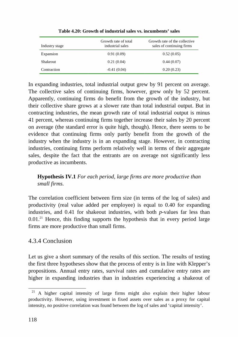
118
Table 4.20: Growth of industr ial sales vs. incumbents’ sales
Industry stageGrowth rate of total
industrial salesGrowth rate of the collective
sales of continuing firms
Expansion 0.91 (0.09) 0.52 (0.05)
Shakeout 0.21 (0.04) 0.44 (0.07)
Contraction -0.41 (0.04) 0.20 (0.23)
In expanding industries, total industrial output grew by 91 percent on average.The collective sales of continuing firms, however, grew only by 52 percent.Apparently, continuing firms do benefit from the growth of the industry, buttheir collective share grows at a slower rate than total industrial output. But incontracting industries, the mean growth rate of total industrial output is minus41 percent, whereas continuing firms together increase their sales by 20 percenton average (the standard error is quite high, though). Hence, there seems to beevidence that continuing firms only partly benefit from the growth of theindustry when the industry is in an expanding stage. However, in contractingindustries, continuing firms perform relatively well in terms of their aggregatesales, despite the fact that the entrants are on average not significantly lessproductive as incumbents.
Hypothesis IV.1 For each period, large firms are more productive thansmall f irms.
The correlation coefficient between firm size (in terms of the log of sales) andproductivity (real value added per employee) is equal to 0.40 for expandingindustries, and 0.41 for shakeout industries, with both p-values far less than0.01.21 Hence, this finding supports the hypothesis that in every period largefirms are more productive than small firms.
4.3.4 Conclusion
Let us give a short summary of the results of this section. The results of testingthe first three hypotheses show that the process of entry is in line with Klepper’spropositions. Annual entry rates, survival rates and cumulative entry rates arehigher in expanding industries than in industries experiencing a shakeout of
21 A higher capital intensity of large firms might also explain their higher labour
productivity. However, using investment in fixed assets over sales as a proxy for capitalintensity, no positive correlation was found between the log of sales and ‘capital intensity’ .
119
firms. Apparently, for entrants it becomes more diff icult to survive and grow asthe industry matures. The model’s explanation for this is that the advantage ofincumbents over entrants grows over time. However, as the results of testinghypothesis I.5 show, this is not reflected by a higher productivity of continuingfirms.
No evidence was found for the hypothesis I.4: on average changes in marketshares are very small for continuing firms, and about half of them actually losemarket share. Hypothesis II .1 was rejected as well: in expanding industries anumber of exiting firms are replaced by a higher number of entrants, but thelatter are not significantly smaller than the former. Further, in the group ofshakeout industries the Herfindahl-index does not increase significantly,suggesting that large firms do not grow at the expense of small firms.Hypothesis III .1 was accepted, because a positive correlation was found betweenthe growth of market share of continuing firms (in expanding and shakeoutindustries) and their average profit rates. Hypothesis III .2 could not be accepted,since on average the profit rates between the group of expanding industries andshakeout industries do not significantly differ. Hypothesis III .3 was rejected,because in expanding industries continuing firms on average lose market share,whereas in industries experiencing a shakeout they gain on average. The finalhypothesis (IV.1) was accepted, because a fairly strong positive correlation wasfound between labour productivity and the size of the firm (in terms of output),suggesting that large firms are indeed more productive than small fi rms.
Returning to the three questions posed in section 4.3.1, the analysis of thissection has shown that the answer to the first question is affirmative: industriesin different stages show different regularities. The second question (are theobserved regularities in line with the regularities predicted by the model?)cannot be answered so easily, because the evidence is mixed. On the one hand,no (or only weak) evidence was found for the hypotheses that focused on theexpansion of market shares of continuing firms, or on the differences of profitrates between expanding and shakeout industries. On the other hand, the testresults of hypotheses I.1 to I.3 seem to confirm Klepper’s prediction of agrowing advantage of incumbents over entrants, since the results suggest that isit more difficult for small firms to enter, survive, and grow in industriesexperiencing a shakeout. Further, we have found evidence that a shakeout offirms is not caused by an increase in exit rates, but rather by a significantreduction in the number of f irms entering the industry. This finding is againconsistent with the model by Klepper. Finally, large firms were found to be
120
more productive than small firms. Hence, to some extent the observedregularities are in line with Klepper’s predictions.
However, no evidence was found for the part of Klepper’s model that actuallyexplains the emerging regularities of new, technologically progressiveindustries. It is dynamic increasing returns to technological change that drivesKlepper’s model, but on average incumbent firms were not found to be moreproductive or profitable than entrants when mature industries are considered.Therefore, the answer to the third question seems to be no: although industries indifferent stages show different regularities, and although the observed(differences in) regularities are to some extent in line with Klepper’s model,they cannot generally be explained by dynamic increasing returns totechnological change. However, the significant differences between the groupsof industries in different stages that were observed for many of the variables,indicate that distinguishing industries on the basis of their evolutionary stagestill makes sense. Furthermore, there is some evidence for a growing advantageof incumbents over entrants, even though incumbents are not significantly moreproductive than entrants.
4.4 Combined analysis
Since there are a number of variables that are theoretically explained by both theframework of technological regimes and the product life cycle, it might beinteresting to investigate empirically the extent to which these two approachescan simultaneously account for differences in these variables across industries,and to see whether there is any interaction between them. The most appropriateway to investigate this is to run regressions in which the independent variablesare dummies denoting the technological regime and the evolutionary stage of theindustries. An interesting opportunity of applying such a regression analysis isthat we can now also include those industries that were left out in the previoussections (e.g., the 28 industries that were omitted in the analysis of section 4.2because their technological regime was unknown), and see whether theseindustries have some special properties in common. Therefore, all 106 industriespresent in the SN database wil l be included in the regression analysis thatfollows. Table 4.21 shows how the technological regimes and the evolutionarystage are distributed over the industries.
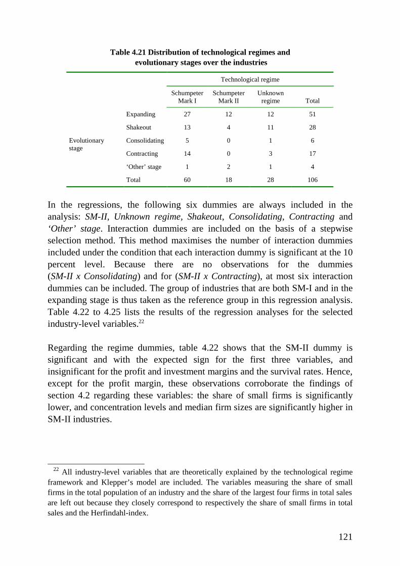
121
Table 4.21 Distr ibution of technological regimes and evolutionary stages over the industr ies
Technological regime
SchumpeterMark I
SchumpeterMark II
Unknownregime Total
Expanding 27 12 12 51
Shakeout 13 4 11 28
Consolidating 5 0 1 6
Contracting 14 0 3 17
‘Other’ stage 1 2 1 4
Evolutionarystage
Total 60 18 28 106
In the regressions, the following six dummies are always included in theanalysis: SM-II , Unknown regime, Shakeout, Consolidating, Contracting and‘Other’ stage. Interaction dummies are included on the basis of a stepwiseselection method. This method maximises the number of interaction dummiesincluded under the condition that each interaction dummy is significant at the 10percent level. Because there are no observations for the dummies(SM-II x Consolidating) and for (SM-II x Contracting), at most six interactiondummies can be included. The group of industries that are both SM-I and in theexpanding stage is thus taken as the reference group in this regression analysis.Table 4.22 to 4.25 lists the results of the regression analyses for the selectedindustry-level variables.22
Regarding the regime dummies, table 4.22 shows that the SM-II dummy issignificant and with the expected sign for the first three variables, andinsignificant for the profit and investment margins and the survival rates. Hence,except for the profit margin, these observations corroborate the findings ofsection 4.2 regarding these variables: the share of small firms is significantlylower, and concentration levels and median firm sizes are significantly higher inSM-II industries.
22 All i ndustry-level variables that are theoretically explained by the technological regime
framework and Klepper’s model are included. The variables measuring the share of smallfirms in the total population of an industry and the share of the largest four firms in total salesare left out because they closely correspond to respectively the share of small firms in totalsales and the Herfindahl-index.
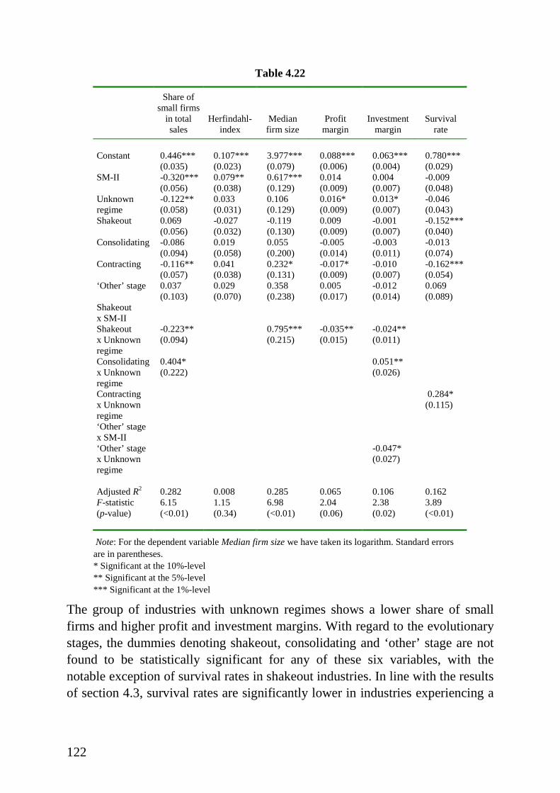
122
Table 4.22
Share ofsmall firms
in totalsales
Herfindahl-index
Medianfirm size
Profitmargin
Investmentmargin
Survivalrate
Constant 0.446** *(0.035)
0.107** *(0.023)
3.977** *(0.079)
0.088** *(0.006)
0.063** *(0.004)
0.780** *(0.029)
SM-II -0.320** *(0.056)
0.079**(0.038)
0.617** *(0.129)
0.014(0.009)
0.004(0.007)
-0.009(0.048)
Unknownregime
-0.122**(0.058)
0.033(0.031)
0.106(0.129)
0.016*(0.009)
0.013*(0.007)
-0.046(0.043)
Shakeout 0.069(0.056)
-0.027(0.032)
-0.119(0.130)
0.009(0.009)
-0.001(0.007)
-0.152** *(0.040)
Consolidating -0.086(0.094)
0.019(0.058)
0.055(0.200)
-0.005(0.014)
-0.003(0.011)
-0.013(0.074)
Contracting -0.116**(0.057)
0.041(0.038)
0.232*(0.131)
-0.017*(0.009)
-0.010(0.007)
-0.162** *(0.054)
‘Other’ stage 0.037(0.103)
0.029(0.070)
0.358(0.238)
0.005(0.017)
-0.012(0.014)
0.069(0.089)
Shakeoutx SM-IIShakeoutx Unknownregime
-0.223**(0.094)
0.795** *(0.215)
-0.035**(0.015)
-0.024**(0.011)
Consolidatingx Unknownregime
0.404*(0.222)
0.051**(0.026)
Contractingx Unknownregime
0.284*(0.115)
‘Other’ stagex SM-II‘Other’ stagex Unknownregime
-0.047*(0.027)
Adjusted R2 0.282 0.008 0.285 0.065 0.106 0.162F-statistic(p-value)
6.15(<0.01)
1.15(0.34)
6.98(<0.01)
2.04(0.06)
2.38(0.02)
3.89(<0.01)
Note: For the dependent variable Median firm size we have taken its logarithm. Standard errorsare in parentheses.* Significant at the 10%-level** Significant at the 5%-level** * Significant at the 1%-level
The group of industries with unknown regimes shows a lower share of smallfirms and higher profit and investment margins. With regard to the evolutionarystages, the dummies denoting shakeout, consolidating and ‘other’ stage are notfound to be statistically significant for any of these six variables, with thenotable exception of survival rates in shakeout industries. In line with the resultsof section 4.3, survival rates are significantly lower in industries experiencing a
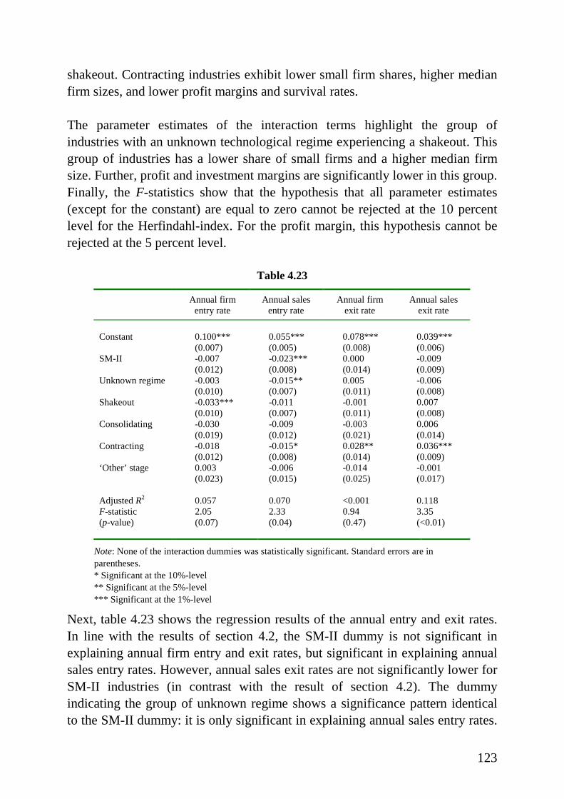
123
shakeout. Contracting industries exhibit lower small firm shares, higher medianfirm sizes, and lower profit margins and survival rates.
The parameter estimates of the interaction terms highlight the group ofindustries with an unknown technological regime experiencing a shakeout. Thisgroup of industries has a lower share of small firms and a higher median firmsize. Further, profit and investment margins are significantly lower in this group.Finally, the F-statistics show that the hypothesis that all parameter estimates(except for the constant) are equal to zero cannot be rejected at the 10 percentlevel for the Herfindahl-index. For the profit margin, this hypothesis cannot berejected at the 5 percent level.
Table 4.23
Annual firmentry rate
Annual salesentry rate
Annual firmexit rate
Annual salesexit rate
Constant 0.100** *(0.007)
0.055** *(0.005)
0.078** *(0.008)
0.039** *(0.006)
SM-II -0.007(0.012)
-0.023** *(0.008)
0.000(0.014)
-0.009(0.009)
Unknown regime -0.003(0.010)
-0.015**(0.007)
0.005(0.011)
-0.006(0.008)
Shakeout -0.033** *(0.010)
-0.011(0.007)
-0.001(0.011)
0.007(0.008)
Consolidating -0.030(0.019)
-0.009(0.012)
-0.003(0.021)
0.006(0.014)
Contracting -0.018(0.012)
-0.015*(0.008)
0.028**(0.014)
0.036** *(0.009)
‘Other’ stage 0.003(0.023)
-0.006(0.015)
-0.014(0.025)
-0.001(0.017)
Adjusted R2 0.057 0.070 <0.001 0.118F-statistic(p-value)
2.05(0.07)
2.33(0.04)
0.94(0.47)
3.35(<0.01)
Note: None of the interaction dummies was statistically significant. Standard errors are inparentheses.* Significant at the 10%-level** Significant at the 5%-level** * Significant at the 1%-level
Next, table 4.23 shows the regression results of the annual entry and exit rates.In line with the results of section 4.2, the SM-II dummy is not significant inexplaining annual firm entry and exit rates, but significant in explaining annualsales entry rates. However, annual sales exit rates are not significantly lower forSM-II industries (in contrast with the result of section 4.2). The dummyindicating the group of unknown regime shows a significance pattern identicalto the SM-II dummy: it is only significant in explaining annual sales entry rates.

124
The shakeout dummy is only significantly negative for firm entry rates,confirming the results of section 4.3. Consolidating industries and industries inthe ‘other’ stage do not show any significant differences regarding annual entryand exit rates. However, in contracting industries, entry rates (in term of sales)are significantly lower and exit rates are significantly higher. Finally, note thatthe values for the adjusted R2 for all four variables and the value of theF-statistic for annual firm exit rates are quite low.
Table 4.24
Cumulativefirm entry rate
Cumulativesales entry rate
Cumulative firmexit rate
Cumulativesales exit rate
Constant 0.566** *(0.026)
0.425** *(0.030)
0.320** *(0.023)
0.310** *(0.031)
SM-II -0.118** *(0.042)
-0.211** *(0.049)
0.021(0.039)
-0.183** *(0.058)
Unknown regime -0.012(0.042)
-0.116** *(0.041)
0.050(0.038)
-0.129** *(0.046)
Shakeout -0.211** *(0.042)
-0.137** *(0.041)
0.080**(0.038)
0.007(0.047)
Consolidating -0.162** *(0.064)
-0.105(0.076)
-0.012(0.058)
-0.004(0.078)
Contracting -0.204** *(0.042)
-0.173** *(0.050)
0.162** *(0.039)
0.142** *(0.057)
‘Other’ stage -0.043(0.077)
-0.032(0.091)
0.038(0.097)
-0.100(0.109)
Shakeoutx SM-II
0.202*(0.112)
Shakeoutx Unknown regime
-0.123*(0.070)
-0.152**(0.063)
Consolidatingx Unknown regimeContractingx Unknown regime
0.392** *(0.122)
‘Other’ stagex SM-II
-0.316**(0.139)
‘Other’ stagex Unknown regime
0.591** *(0.212)
Adjusted R2 0.374 0.214 0.203 0.315F-statistic(p-value)
9.95(<0.01)
5.75(<0.01)
4.35(<0.01)
6.36(<0.01)
Note: Standard errors are in parentheses.* Significant at the 10%-level** Significant at the 5%-level** * Significant at the 1%-level
With regard to cumulative sales entry and exit rates, the figures in table 4.24confirm our findings of section 4.2 that these measures are significantly lower inSM-II industries. However, with regard to cumulative firm entry and exit ratesthe results suggest a significance pattern opposite to section 4.2. Here, we find
125
that firm entry rates are significantly lower in SM-II industries, whereascumulative firm exit rates are not significantly lower in this group of industries.The dummy denoting the group of unknown regimes is negatively significant forthe cumulative sales entry rates and exit rates. The dummies denoting the groupof shakeout and contracting industries show rather similar significance patterns:cumulative entry rates are lower and cumulative exit rates are higher in thesetwo groups. The group of shakeout industries with an unknown technologicalregime shows significantly lower cumulative firm entry and exit rates. Finally,compared to the previous two groups of variables, the values of the adjusted R2
and the F-statistic are much higher.
Table 4.25 shows the regression statistics of the final four industry-levelvariables. In line with the findings of section 4.2, short run market shareturbulence among incumbents is significantly lower in SM-II industries, whereaslong run turbulence is not. Further, the contribution of the entry and exit processin aggregate productivity growth is significantly lower in SM-II industries. Thedummy denoting the group of industries with unknown regime is (negatively)significant in explaining both short and long run turbulence among incumbents.The group of shakeout and consolidating industries show a higher growth of thecollective market share of incumbents and a lower share of the entry and exitprocess in aggregate productivity growth. In contracting industries, long runturbulence and the market share growth of incumbents are significantly higher,whereas for the industries in the ‘other’ stage only the long run turbulenceamong incumbents was found to be significantly higher.
For two out of the four variables in table 4.25, the group of unknown regimeindustries experiencing a shakeout stands out again. This interaction term issignificantly positive in explaining long run turbulence among incumbents andsignificantly negative in explaining the collective market share growth ofincumbents. Finally, note that for the regression of the last dependent variable oftable 4.25 (the share of the entry and exit process in aggregate productivitygrowth) the hypothesis that all parameter but the constant are equal to zero couldnot be rejected at the 10 percent level.
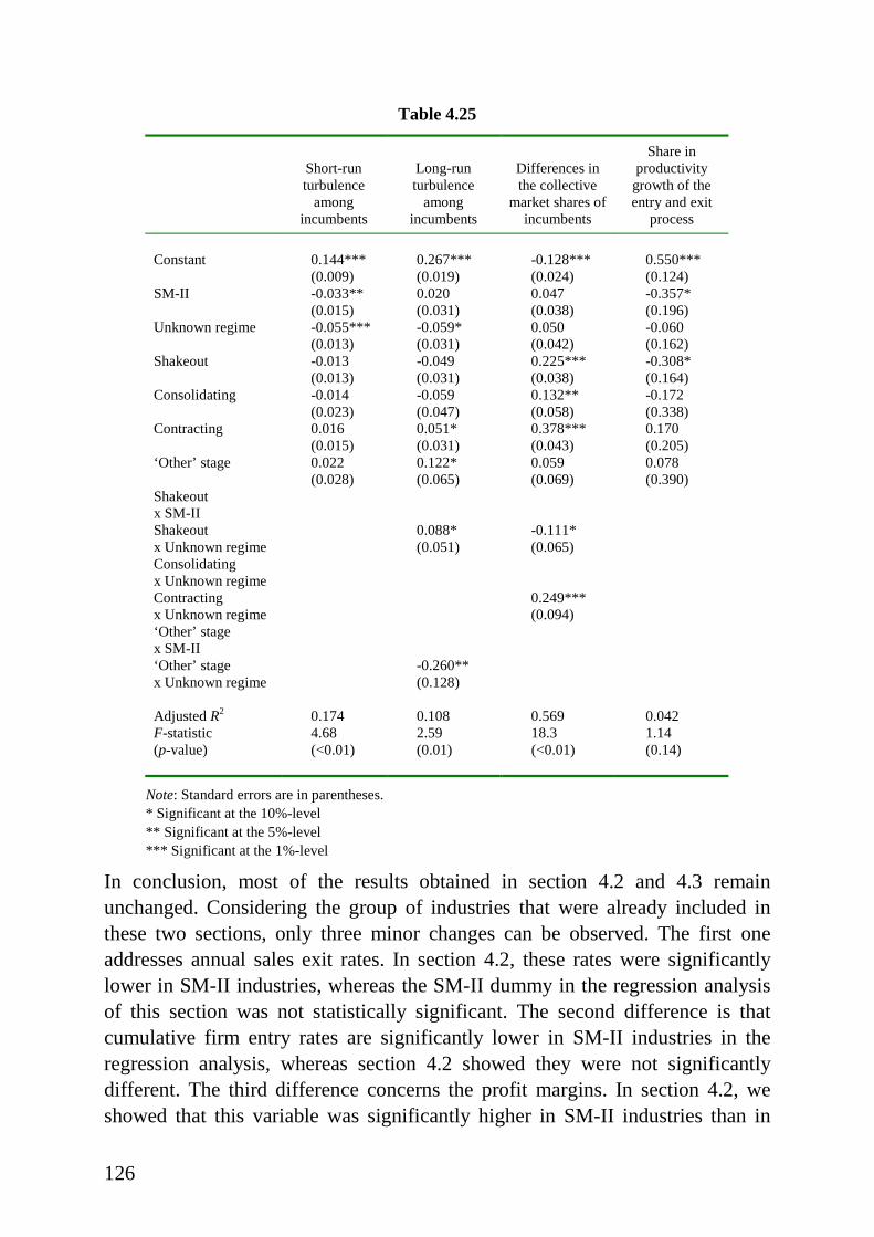
126
Table 4.25
Short-runturbulence
amongincumbents
Long-runturbulence
amongincumbents
Differences inthe collective
market shares ofincumbents
Share inproductivitygrowth of theentry and exit
process
Constant 0.144** *(0.009)
0.267** *(0.019)
-0.128** *(0.024)
0.550** *(0.124)
SM-II -0.033**(0.015)
0.020(0.031)
0.047(0.038)
-0.357*(0.196)
Unknown regime -0.055** *(0.013)
-0.059*(0.031)
0.050(0.042)
-0.060(0.162)
Shakeout -0.013(0.013)
-0.049(0.031)
0.225** *(0.038)
-0.308*(0.164)
Consolidating -0.014(0.023)
-0.059(0.047)
0.132**(0.058)
-0.172(0.338)
Contracting 0.016(0.015)
0.051*(0.031)
0.378** *(0.043)
0.170(0.205)
‘Other’ stage 0.022(0.028)
0.122*(0.065)
0.059(0.069)
0.078(0.390)
Shakeoutx SM-IIShakeoutx Unknown regime
0.088*(0.051)
-0.111*(0.065)
Consolidatingx Unknown regimeContractingx Unknown regime
0.249** *(0.094)
‘Other’ stagex SM-II‘Other’ stagex Unknown regime
-0.260**(0.128)
Adjusted R2 0.174 0.108 0.569 0.042F-statistic(p-value)
4.68(<0.01)
2.59(0.01)
18.3(<0.01)
1.14(0.14)
Note: Standard errors are in parentheses.* Significant at the 10%-level** Significant at the 5%-level** * Significant at the 1%-level
In conclusion, most of the results obtained in section 4.2 and 4.3 remainunchanged. Considering the group of industries that were already included inthese two sections, only three minor changes can be observed. The first oneaddresses annual sales exit rates. In section 4.2, these rates were significantlylower in SM-II industries, whereas the SM-II dummy in the regression analysisof this section was not statistically significant. The second difference is thatcumulative firm entry rates are significantly lower in SM-II industries in theregression analysis, whereas section 4.2 showed they were not significantlydifferent. The third difference concerns the profit margins. In section 4.2, weshowed that this variable was significantly higher in SM-II industries than in
127
SM-I industries, whereas in the regression analysis of the present section thedummy denoting the group of SM-II industries was not significantly different.
When we look at the industries that were initially not included in the analysis,we observed the following results. First, the group of industries for which thetechnological regime was unknown showed some interesting properties. In thisgroup, the share of small firms, annual and cumulative sales entry rates andturbulence among incumbents are lower, whereas profit and investment marginswere found to be higher than in the reference group. Hence, for these variablesthe group with unknown regimes resembles the archetypical SM-II regime.However, the insignificant results for the other variables (most notablyconcentration levels and the contribution of the entry and exit process toaggregate productivity growth) do not correspond to the theoretical SM-IIregime.
Second, the group of contracting industries showed some structural properties(low share of small firms, high median firm size) that may indicatecircumstances conducive to large firms. In this group, selective forces seem tobe rather strong: low profit margins, low entry and survival rates and high exitrates. Finally, the interaction terms highlighted the group of industries with anunknown technological regime experiencing a shakeout. This group has thefollowing properties in common. Small fi rms have a minor share in the industry,the median size of the firm is high, and profit and investment margins are low.Regarding the dynamic properties, we observed for this group low cumulativefirm entry and exit rates, but a high long run market share turbulence amongincumbents. Incidentally, the other interaction terms were significant too, butnone of them exhibited a systematically different pattern vis-à-vis the referencegroup of industries.
4.5 Conclusions
Starting from the hypothesis that differences between industries can beexplained by underlying structural differences (i.e., different technologicalregimes) as well as by temporal differences (i.e., differences in the evolutionarystages of the industries), this chapter has shown that the data indeed provideevidence for both types of explanations. The analysis of section 4.2 stronglysuggested that differences in the structural and dynamic properties of industriesare closely related to the set of opportunity, appropriabili ty, cumulativeness andknowledge conditions underlying the innovative activities in an industry. And
128
although the model by Klepper (1996) is primarily intended to depict theevolution of technologically progressive industries, section 4.3 has shown thatapplying the model to (basically mature) manufacturing industries in general,i.e., without any reference to their technological progressiveness, provides someinteresting results. Industries in different evolutionary stages indeed showdifferent regularities, which are partly in line with Klepper’s model. Especiallydifferences in the entry and survival rates of industries corroborate Klepper’shypothesis of a growing advantage of incumbents over entrants. Further, wehave found circumstantial evidence that a shakeout of firms is not caused by anincrease in exit rates, but rather by a significant reduction in the number of f irmsentering the industry. This finding is again consistent with the model byKlepper. Apart from some minor differences, the regression analysis of section4.4, which investigated the interaction between the two theoretical approaches,generally confirmed the results of section 4.2 and 4.3.
Further analyses, directly using proxies for the actual opportunity,appropriability, cumulativeness and conditions of knowledge accumulation todetermine the technological regime, or the actual age of an industry togetherwith, e.g., the growth rate of patents to determine an industry’s evolutionarystage would certainly provide a stronger basis for testing whether technologicalregimes and industry li fe cycles explain the observed differences betweenindustries. However, we believe that the analysis presented here has providedimportant evidence on the links between technological regimes, patterns ofinnovation, industry li fe cycles and industrial dynamics.

129
Appendix: list of industries with their technological regimeand evolutionary stage
IndustryTechnologicalregime
Evolutionarystage
Finishing of textiles Schumpeter Mark I ExpandingManufacture of carpets and rugs Schumpeter Mark I ExpandingManufacture of made-up textile articles, except apparel Schumpeter Mark I ExpandingManufacture of other non-metalli c mineral products nec* Schumpeter Mark I ExpandingManufacture of glass and glass products Schumpeter Mark I ExpandingIron, steel and non-ferrous metal foundries Schumpeter Mark I ExpandingManufacture of tanks, reservoirs and pipe-lines Schumpeter Mark I ExpandingManufacture of steel and non-ferrous metal doors,windows, walls and the like
Schumpeter Mark I Expanding
Metal construction nec Schumpeter Mark I ExpandingManufacture of metal furniture Schumpeter Mark I ExpandingForging, treatment and coating of metals Schumpeter Mark I ExpandingManufacture of agricultural machinery Schumpeter Mark I ExpandingManufacture of machine-tools Schumpeter Mark I ExpandingManufacture of machinery for packing and wrapping Schumpeter Mark I ExpandingManufacture of machinery for food, beverage and tobaccoprocessing
Schumpeter Mark I Expanding
Manufacture of machinery for manufacturers of rubberand plastic products
Schumpeter Mark I Expanding
Manufacture of lifting and handling equipment Schumpeter Mark I ExpandingManufacture of machinery for textile and apparel Schumpeter Mark I ExpandingManufacture of machinery for chemical cleaning,washing, leather and leather products, paper and paperproducts and printing
Schumpeter Mark I Expanding
Manufacture of pumps, compressors, taps and valves Schumpeter Mark I ExpandingManufacture of fans, refrigerating and freezing equipment Schumpeter Mark I ExpandingAppendage Schumpeter Mark I ExpandingManufacture of machine parts nec Schumpeter Mark I ExpandingManufacture of machinery nec Schumpeter Mark I ExpandingManufacture of trailers and semi-trailers Schumpeter Mark I ExpandingManufacture of bodies for motor vehicles Schumpeter Mark I ExpandingManufacture of transport equipment nec Schumpeter Mark I ExpandingManufacture of other textiles nec Schumpeter Mark I ShakeoutTanning and dressing of leather Schumpeter Mark I ShakeoutManufacture of luggage, handbags and the like, saddleryand harness
Schumpeter Mark I Shakeout
Manufacture of wooden containers Schumpeter Mark I ShakeoutManufacture of other products of wood, manufacture ofarticles of cork, straw and plaiting materials
Schumpeter Mark I Shakeout
Manufacture of furniture, except metal furniture Schumpeter Mark I ShakeoutManufacture of cement and lime Schumpeter Mark I ShakeoutManufacture of articles of concrete and cement Schumpeter Mark I ShakeoutForging, pressing, stamping and roll -forming of metal Schumpeter Mark I ShakeoutManufacture of metal fasteners, cables, springs and thelike
Schumpeter Mark I Shakeout
Manufacture of heating and boilers, except electrical Schumpeter Mark I ShakeoutManufacture of other fabricated metal products nec Schumpeter Mark I ShakeoutMachine repair nec Schumpeter Mark I ShakeoutCarpentry and manufacture of densified wood and parquetflooring blocks
Schumpeter Mark I Consolidating
Manufacture of ceramics Schumpeter Mark I Consolidating

130
IndustryTechnologicalregime
Evolutionarystage
Manufacture of basic metals Schumpeter Mark I ConsolidatingManufacture of tools and machinery for metallurgy Schumpeter Mark I ConsolidatingManufacture of bearings, gears, gearing and drivingelements
Schumpeter Mark I Consolidating
Preparation and spinning of wool fibres, weaving of wool Schumpeter Mark I ContractingPreparation and spinning of cotton fibres, weaving ofcotton
Schumpeter Mark I Contracting
Manufacture of tricot and stockings Schumpeter Mark I ContractingManufacture of wearing apparel, dressing and dyeing offur
Schumpeter Mark I Contracting
Manufacture of footwear Schumpeter Mark I ContractingSawmill ing and planing of wood, manufacture of veneersheets, plywood, laminboard, particle board and otherpanels and boards
Schumpeter Mark I Contracting
Manufacture of bricks and tiles Schumpeter Mark I ContractingManufacture of metal packings Schumpeter Mark I ContractingManufacture of machinery for petrochemical, chemicaland pharmaceutical industries
Schumpeter Mark I Contracting
Manufacture of machinery for wood and furniture Schumpeter Mark I ContractingManufacture of engines and turbines, except aircraft,vehicle and cycle engines
Schumpeter Mark I Contracting
Manufacture of office machinery Schumpeter Mark I ContractingManufacture of weighing machinery and domesticappliances, except electrical
Schumpeter Mark I Contracting
Building and repairing of ships and boats Schumpeter Mark I ContractingManufacture of machinery for mining, construction,building materials and metallurgy
Schumpeter Mark I ‘Other’ stage
Manufacture of synthetic resin Schumpeter Mark II ExpandingManufacture of dye-stuffs and colouring matters Schumpeter Mark II ExpandingManufacture of chemical raw materials nec Schumpeter Mark II ExpandingManufacture of paints, varnishes and similar coatings,printing ink
Schumpeter Mark II Expanding
Manufacture of pharmaceuticals and medicinal chemicals Schumpeter Mark II ExpandingManufacture of other chemical products nec Schumpeter Mark II ExpandingManufacture of plastic products Schumpeter Mark II ExpandingManufacture of electric motors, generators andtransformers
Schumpeter Mark II Expanding
Manufacture of electricity distribution and controlapparatus
Schumpeter Mark II Expanding
Manufacture of other electrical equipment nec Schumpeter Mark II ExpandingManufacture of motor vehicles Schumpeter Mark II ExpandingManufacture of parts and accessories for motor vehicles Schumpeter Mark II ExpandingManufacture of soap and detergents, cleaning andpolishing preparations, perfumes and toilet preparations
Schumpeter Mark II Shakeout
Manufacture of chemical pesticides Schumpeter Mark II ShakeoutManufacture of rubber products Schumpeter Mark II ShakeoutManufacture of motorcycles and bicycles Schumpeter Mark II ShakeoutManufacture of fertili sers Schumpeter Mark II ‘Other’ stageManufacture of insulated wire and cable Schumpeter Mark II ‘Other’ stageProcessing and preserving of f ish and fish products Unknown regime ExpandingManufacture of bakery products Unknown regime ExpandingManufacture of other food products nec Unknown regime ExpandingManufacture of malt liquors and malt Unknown regime ExpandingManufacture of other articles of paper and paperboard Unknown regime ExpandingManufacture of corrugated paper and paperboard Unknown regime ExpandingOffset printing Unknown regime ExpandingChemigrafical and fotoli thografical firms Unknown regime Expanding

131
IndustryTechnologicalregime
Evolutionarystage
Other printing Unknown regime ExpandingPublishing of books Unknown regime ExpandingOther publishing Unknown regime ExpandingManufacture and repair of aircraft Unknown regime ExpandingProduction, processing and preserving of meat and meatproducts
Unknown regime Shakeout
Manufacture of grain mill products Unknown regime ShakeoutManufacture of vegetable and animal oils and fats Unknown regime ShakeoutProcessing and preserving of fruit and vegetables Unknown regime ShakeoutManufacture of sugar, cacao, chocolate and sugarconfectionery
Unknown regime Shakeout
Manufacture of prepared animal feeds Unknown regime ShakeoutManufacture of soft drinks Unknown regime ShakeoutManufacture of tobacco products Unknown regime ShakeoutManufacture of paper and paperboard Unknown regime ShakeoutPrinting of newspapers Unknown regime ShakeoutPublishing of newspapers Unknown regime ShakeoutBookbinding Unknown regime ConsolidatingManufacture of dairy products Unknown regime ContractingDistil ling, rectifying and blending of spirits; ethyl alcoholproduction
Unknown regime Contracting
Printing of books Unknown regime ContractingPublishing of periodicals Unknown regime ‘Other’ stage
* not elsewhere classified

133
Chapter 5
Technological diffusion patterns and their effectson industrial dynamics
5.1 Introduction
Both the technological regime framework and the industry li fe cycle approachare able to explain variations in industry structures and dynamics. The previouschapter has shown that opportunity, appropriability, cumulativeness andknowledge conditions underlying the industrial innovative process, as well asthe evolutionary stage of the industrial life cycle affect the structural anddynamic properties of an industry. However, as we have mentioned in section3.5, in our view these theories still ignore a number of crucial elements. First ofall , models of product life cycles generally focus on the emergence andevolution of only one product and its associated technology. However, in manyindustries we observe that firms repeatedly introduce or adopt new producttechnologies that replace the older ones. Second, both the technological regimeand the industry li fe cycle approach do not explicitly consider differences in thetechnological properties of the goods produced by the industries. Finally, inmodels on technological regimes and on industry li fe cycles the growth of a firmis generally determined by its relative (technological) performance. However,empirical studies on firm growth do not provide much evidence supporting sucha relationship. Most of these studies suggest that the size of a firm generallyfollows a random walk with a declining positive drift.1
In this chapter we wil l introduce a model on industry dynamics that attempts toinclude these three elements. As in Shy (1996), the degree of substitutability
1 See Geroski (1998).

134
between the quality and the network size of a technology and the degree ofcompatibil ity of succeeding technologies are the key determinants of thesimulation model presented here. However, Shy (1996) mainly limits his focusto the demand side, as he investigates how varying consumer preferences overtechnology advance and network size effects the timing and frequency of newtechnology adoption. Our focus will be on the relation between the demand sideand the supply side. Given variations in purchaser preferences over quality andnetwork sizes, and different degrees of compatibility between succeedingtechnologies, we will investigate how the resulting differences in the timing andfrequency of new technology adoptions by purchasers effect the dynamics of thepopulation of supplying firms. Furthermore, we will investigate whether theseeffects are different under various technological regimes.
The structure of the chapter is as follows. The next section presents theconceptual basis of the model. Based on Shy (1996), we will explain howvariations in consumer preferences over quality and network sizes of producttechnologies and different degrees of compatibility between succeedingtechnologies affect the timing and frequency of new technology adoptions.Further, we will elaborate on some theoretical and empirical issues concerningfirm growth. Section three formally presents the model, of which the simulationresults will be analysed in section four. Section five focuses on how these resultsare effected when different technological regime conditions are considered.Section six concludes this chapter.
5.2 The diffusion of new product technologies
As mentioned in the introduction, one of the objectives of the industry modelpresented in this chapter is to include a repeating process of new technologyadoptions. An interesting option of including such a process is that, by varyingthe parameters determining the diffusion patterns, the model can be used toinvestigate whether differences in the diffusion of new technologies affect thestructural and dynamic properties of an industry. This would be an importantresult, because if the industrial properties are indeed related to the diffusionpatterns, our model may provide an additional explanation for the observedstructural and dynamic differences between industries.
Obviously, we will first need a theoretical framework that explains howdifferences in the diffusion patterns of new product technologies may arise.Although there is a considerable amount of literature on modelling diffusion
135
dynamics2, in our view the model by Shy (1996) provides the most appropriateframework for analysing the determinants of diffusion patterns. In this model,the degree of substitutabili ty between the quality and the network size of atechnology and the degree of compatibility of succeeding technologies are thekey variables determining the timing and frequency of new technologyadoptions. In what follows we will briefly explain the logic behind Shy’s model.
5.2.1 Modelli ng diffusion dynamics: Shy’s approach
Shy (1996) describes the consumer dynamics within an overlapping generationsframework. In the model, the generation of entering consumers chooses whetherto purchase a certain product based on an old technology already used by anolder generation of consumers or whether to purchase the product based on thenew technology with a higher quality. The young generation chooses the newtechnology if the utilit y from the high quality technology, combined with thesize of the network associated with the new technology, overtakes the utilityfrom the old technology with its associated network size. The size of thenetwork of the new technology is the sum the population size of the younggeneration and a certain percentage of the old generation of users. Thispercentage is determined by the degree of compatibility between the old andnew technology. Hence, the higher the compatibility, the larger the network sizeassociated with the new technology will be. Shy (1996) then shows that adecrease in the degree of compatibility between new and old technologies willincrease the duration of each technology. Further, by varying the degree ofsubstitution between the quality and the network size of a technology, he showsthat the duration of each adopted technology is lower and the frequency oftechnology adoptions is higher the more consumers value quality and networksize as substitutes rather than complements.
Hence, his focus on consumer preferences helps us understand “…whytechnology is replaced more often in some industries than in others…” (Shy,1996, p.786). He also asserts that his model is general enough to capture avariety of market structures. That is, he shows that both a persistent monopoly,as well as a more competitive market structure with the entry of a new firmwhenever a new technology becomes available3, is consistent with his model.The aim of our model is to further elaborate on the evolution of the supply side
2 See Stoneman (1991) for an overview of these models.3 Shy (1996) assumes that the new firm is endowed with a one period patent right on the
new technology, allowing it to (temporarily) charge a monopoly price.
136
of industries experiencing repeated adoption of new technologies. Althoughprevious models on technological change and industry evolution haveinvestigated issues such as the evolution of the firm population4 or the diffusionprocess of (subsequent) innovations5, they have not explicitly linked these twoprocesses such that causality runs from the latter to the former. Hence, thesemodels have not analysed the effect of technology diffusion patterns on thedynamics of the firm population. The model presented in this chapter attempts tofill this hiatus.
In conclusion, the model by Shy (1996) provides the theoretical basis of the firsttwo distinguishing elements that are included in our model on industry dynamics(i.e., the repeated adoption of new product technologies, and differences intechnological properties of the goods produced). The next subsection will focuson the process governing firm growth that constitutes the third distinguishingelement of our model.
5.2.2 A note on firm growth
In virtually all evolutionary models on industrial dynamics some type ofreplicator dynamics is employed to depict the evolution of the size of a firm.The basic assumption underlying this mechanism is that the selection processallocates market share from the less eff icient firms to the more eff icient ones.Hence, in its simplest form this replication concept states that the growth of afirm over a certain period is proportional to its relative competitiveness.However, there are a number of reasons why in practice such a relationship maynot be very strong. Let us briefly summarise these reasons.
The growth or decline of a firm is ultimately a managerial decision: themanagement decides on how much to invest and how many workers to hire orlay off . Many factors may influence the final outcome of this decision. Pastperformance is certainly one of them. Besides creating the necessary funds, highprofits in the past are a signal of a firm’s competitiveness, creating confidenceamong the management and the potential investors. However, high profits mayalso indicate a lag in mobilising effective competition, reflecting a windfall gainfrom being properly positioned to take advantage of a change in level orcharacter of demand. In this last case the high profits may have resulted from
4 See, e.g., Nelson and Winter (1982), Winter (1984) and Dosi et al. (1995).5 See, e.g., Davies (1979), Iwai, (1984a, 1984b), Reinganum (1981), Silverberg and Lehnert
(1993), Silverberg and Verspagen (1994a, 1994b).

137
mere chance, and are not likely to be as persistent as profits resulting fromhaving been superior to competitors.
But probably more important than a firm’s past competitiveness in the growthdecision are the expectations of a firm regarding the state of the economy, thecondition of the industry, a firm’s own performance, et cetera. There are manyreasons why firms may have different expectations. First of all , the prospectsmay differ between industries. When an industry is expected to grow rapidly, afirm will be more inclined to expand than when prospects are less optimistic forthe industry. Second, firms within the same industry could have differentinformation sets on which the decision to grow is based. Third, even if f irmswould have the same information, still they may perceive and interpret itdifferently, leading to different expectations.
Naturally, different expectations lead to different decisions. Moreover, firmsmay have different ambitions regarding their (ultimate) sizes or market shares.Some firms may indeed be driven by enormous ambitions and try to capture thetotal market as much as possible. But other firms may be less ambitious. Theiraim could be to acquire a certain amount of profits, and if this goal is reached ata certain size they may decide to keep the size approximately fixed. Perhaps thedesire to grow is present latently, but if it is not strong enough no seriousattempts will be made to fulfil this desire. Finally, the situation on the marketsfor labour and capital goods may differ across industries. A shortage oflabourers with skills necessary for a specific firm probably hinders a firm’sdesire to expand.
Combining the potential differences in expectations, ambitions and inputmarkets makes anticipating the growth paths of firms very diff icult. As Geroski(1998) argues, the growth of a firm may very well be understood, but also behard to describe or predict with any precision. Perhaps for these reasonseconometric work on the growth of f irms usually find that firm size essentiallyfollows a random walk. Only some significantly negative effects of initial sizeand age on corporate growth are frequently observed, but usually these effectsare not very large (Geroski, 1998).
As shown in chapter 2, in Dutch manufacturing these regularities are alsoobserved. We have also found that initial size and firm age (at least the proxy wehave used for the age of entering firms) have a significant negative effect onfirm growth. But the main question here concerns the extent to which the
138
relative competitiveness of firms can explain their growth rates. In order toanswer this question we will run two regressions for all continuing firms, inwhich we will employ the relative labour productivity (RelProd) of a firm todenote its relative competitiveness. For a given year this variable is calculated asa firm’s individual labour productivity (value added per employee) divided bythe weighted industry average for that year. The first regression we will runtakes the actual annual growth rate of the firms as the dependent variable, thesecond one takes the average growth rate of the firm over the period 1978-1992.Hence, we have:
ln (emplt+1) – ln (empl t) = β1 + β2 ln (RelProdt) + ε , (5.1)
[ln (empl1992 ) – ln (empl1978 )] / 14 = β1 + β2 ln (RelProd1978) + ε , (5.2)
The following table lists the results of the regression analyses.
Table 5.1: Regression analyses of firm growth on relative productivity
Regression β1 β2 Adjusted R2
(5.1) 0.005 (0.001) 0.048 (0.002) 0.017
(5.2) 0.004 (0.001) 0.012 (0.002) 0.012
Note: Standard errors in parentheses. All parameter estimates are significant at the 1%-level.
Although the parameter estimates for relative labour productivity are significantin both regressions, they do not explain more than two percent of the totalvariance in firms’ growth rates. This clearly confirms that the patterns of f irmgrowth are only weakly influenced by selective pressures. We concludetherefore that relative competitiveness only plays a limited role in explaining thegrowth patterns of f irms. In our view, this result is enough to abstain from anattempt to model the growth process of a firm on the basis of past or currentperformance levels.
In the model that follows, we will thus refrain from employing some type ofreplicator dynamics in modelling firm growth. Instead, we will model theevolution of the size of a firm as following a random walk, however with adeclining positive drift. In this way we assure that the process governing firmgrowth is a priori consistent with the stylised fact that growth rates arenegatively correlated to the firm’s age. Of course, the relative competitivenessof a firm will matter in the model, but only in determining the probability ofsurvival. Therefore, in this model it is really a matter of survival of the fittest, as
139
opposed to expansion of the fittest. Modelling firm growth in this way alsoallows us to investigate whether replicator dynamics are essential inevolutionary models on industry dynamics, or whether random firm growth canlead to realistic results as well .
After having described the two most distinguishing features of the model, i.e., itsfocus on the repeated adoption of new technologies in relation to the dynamicsof the firm population, and the modelling of f irm growth as an essentiallyrandom process, we now turn to the technical details of the model.
5.3 The model
Consider an industry where in each discrete time period t, t = 0, 1, 2,…, the firmpopulation consists of N (t) firms. All firms in the industry are producing acertain product that is defined by its functional characteristics. An essentialassumption in the model is that the function the product performs can be basedon different technologies. For instance, both the standard compact cassettes aswell as the compact disc (CD) are sound recording media, however analoguerecording technology underlies the compact cassette, whereas a CD is recordedusing digital technology. However, our notion of a product also extends toproducer or capital goods. An example here could be industrial lathes, which canbe manually operated or operated by computer numeric control (CNC)technology.
Every period a random number of new firms enter the industry according to aPoisson process6 with arrival rate ρent. At birth, each firm i is endowed with afirm-specific organisational competitiveness level λi, a product technology Ψ,and a size si. The organisational competitiveness level λi is a random genotypevariable7 that sets for each firm a potential li mit to its actual competitiveness,creating some (initial) heterogeneity among firms with regard to theirorganisational capabilit ies. As mentioned, this variable may limit the firm’sactual competitiveness, but whether it actually does depends on its technologicalcompetitiveness that is calculated as follows.
6 For practical reasons, we have adopted the Poisson process here and approximated it by
five hundred Bernoulli t rials every period. For analytical convenience, the arrival rate is keptconstant over the simulation period.
7 This variable is generated as follows. Let x ~ N (µλ ,σλ). Then λi =max{0 ; x} if x ≤ µλ ,and λi =max{0 ; 2µλ-x} if x > µλ.
140
5.3.1 Competitiveness of fi rms
Assume that at every period Κ product technologies are available. At birth,every firm is randomly endowed with a technology Ψ (Ψ = 1, 2,…,Κ), such thatthe probabili ty of receiving a given technology is equal to 1 / (Κ). Thesetechnologies are ranked according to their intrinsic quali ty level QΨ, such thatQΚ > QΚ-1 >…> Q1. Further, there is a class of old technologies Ψ = 0 that allhave an intrinsic quality level Q0. Every β1 periods a pioneering entrant orincumbent introduces a new, intrinsically better product technology that hasbecome available due to exogenous technological change. This introductioncauses all technologies to drop one level in their intrinsic quality. Hence, thenewly introduced technology becomes Κ (the technology with the highestquality level QΚ), and Ψ = 1 becomes part of the class of old technologies Ψ = 0and degrades to the intrinsic quality level Q0. Although our model embodiesintra-firm technology diffusion (firms can employ more than one producttechnology simultaneously) we will first explain the evolution of some essentialvariables for a single-technology firm.
A firm’s technological competitiveness TCi,Ψ (t) depends on the intrinsic qualityQΨ of the product technology it is applying and the total share ΓΨ of thistechnology in the industry in the following way:
TCi,Ψ (t) = α ΓΨ (t)+ (1-α) QΨ (t), (5.3)
where 0 ≤ α ≤ 1, and Q0 ≤ QΨ ≤ 1. The parameter α is essential here, as itdetermines the strength of the network externalities on the demand side. Thehigher α, the more the total market share of a technology determines the firm’stechnological competitiveness.
Combining the organisational competitiveness λi with the technologicalcompetitiveness TCi,Ψ (t) gives the potential competitiveness PCi,Ψ (t) of a firm,which is:
PCi,Ψ (t) = min { TCi,Ψ (t) ; λi } . (5.4)
Hence, a firm’s potential competitiveness is either bounded by its organisationalor its technological competitiveness. We could have modelled organisational
141
and technological competitiveness as (imperfect) substitutes, but this wouldhave implied that, e.g., a firm with a very low level of organisationalcompetitiveness may still survive as long as it has a high level of technologicalcompetitiveness. We believe that such a situation is not realistic, as firms willalways need a certain level of organisational skil ls in order to manage themanufacturing and selling of their products. Furthermore, by modell ingorganisational and technological competitiveness as complementary, we excludein advance the awkward possibility that the organisational and technologicalskills of the firms will be negatively correlated in the simulation results.
Finally, a firm’s actual competitiveness Ci,Ψ (t) evolves according to thefollowing moving average process:
Ci,Ψ (t) = θ Ci,Ψ (t-1) + (1-θ) PCi,Ψ (t), (5.5)
where 0 ≤ θ ≤ 1, and Ci (t) = β2 λi for all firms that enter at period t. Theparameter β2 puts an entrant at an initiall y disadvantageous and possibly evenhazardous position. To some extent such an entry process corresponds toJovanovic (1982). Even firms with very low competitiveness levels may decideto enter the industry, simply because they do not know their truecompetitiveness prior to their entry. Only by actually entering they can gathersome evidence regarding their real capabilities, which may subsequentlyeventuate in a rapid exodus of entrants with low competitiveness levels. It is alsoconsistent with the empirical evidence on the entry process.8
5.3.2 Exit rules
If the actual competitiveness is below a certain fraction ΦL of the industryaverage C , or if size drops below the minimum level s, a firm dies withprobability one, a higher productivity level reduces the probabili ty of exitingPexit (t). Survival is guaranteed for the next period if relative competitivenessexceeds an upper level ΦH. Hence, we have
Pexit, i (t) = 0
if Ci,Ψ (t) ≥ ΦH C (t) (5.6a)
8 See Caves (1998) for an extensive overview.

142
Pexit, i (t) = 3
)()(
)()(
LH
H
β
Φ−Φ−Φ
tctc
tctc i
if ΦL C (t) < Ci,Ψ (t) < ΦH C (t) (5.6b)
Pexit, i (t) = 1
if Ci,Ψ (t) ≤ ΦL C (t), or if si (t) ≤ s. (5.6c)
These exit rules can be interpreted as a mixture of voluntary and forced exit. Ifrelative competitiveness is lower than ΦL, or if firm size drops below theminimum level s, firms go bankrupt and are thus forced to exit. However, forthose firms that observe that their relative competitiveness lies between ΦL andΦH, the exit decision is voluntary. Depending on their aspiration level, some ofthem may decide to continue, whereas others may voluntaril y leave the industryand perhaps try their chances elsewhere.
5.3.3 Evolution of fi rm size
As mentioned before, all firms are initially endowed with a fixed size si. Weinterpret this size as a firm’s sales capacity and assume for convenience thatfirms always operate at full capacity. All surviving firms grow each periodaccording to a random process, however their mean growth rates asymptoticallyreach zero as they mature. The process governing firm growth is
( )[ ]6
)()(4
551)(
)1(βχβ ββ +++=
+ −− tata
i
i ii eets
ts , (5.7)
where ai,t denotes the age of firm i at t. The variable χ is randomly drawn from anormal distribution with mean µχ = 0 and variance σχ , β4 sets the averagegrowth rate of firms at the age of zero. This growth rate gradually declines as thefirm matures, a process of which the pace is determined by β5 . Finally, β6
assures that even at a high age the size of a firm is stil l subject to randomshocks.
143
5.3.4 Imitation
The description of the model, so far, has only considered firms employing oneproduct technology. But, as mentioned, the model also allows for firmsemploying several technologies simultaneously. Let Ψ = A denote the firm’sintrinsically best technology. As long as A < Κ, a firm may have the opportunityto imitate an intrinsically better technology. Every period, firms randomlyreceive an imitation draw according to a Poisson process9 with arrival rate ρim.Receiving an imitation draw means that the firm acquires the knowledge ofemploying one intrinsically better technology. This process is arranged such thaton average a firm with a given market share10 zi would receive ρim [zi + β7 (1-zi)]imitation draws in every β1 periods, where 0 ≤ β7 ≤ 1. The parameter β7 sets theinequality between firms with different sizes with regard to receiving animitation draw. If β7 = 1 all firms have equal probabilities to imitate, if β7 = 0the probabili ty to imitate is proportional to a firm’s market share.
If an imitation draw is received, the probabili ty of acquiring the knowledge ofgiven other product technology is equal to 1 / (Κ − A).11 Every firm that hasobtained an opportunity reallocates every period a share ωi (t) of its totalcapacity from its worst available technology Ψ = L (i.e., the technology with thelowest technological competitiveness) to its best available technology Ψ = H(i.e., the technology with the highest technological competitiveness).12 The sizeof this reallocation share ωi (t) is determined by:
ωi (t) = β8 [TCi,H (t) − TCi,L (t)] (1 + η ), (5.8)
9 Again approximated by Bernoulli trials.10 By market share we mean the firm’s share in the total capacity of the industry. Hence, we
have ∑=)(
)()()(tN
iii tststz .
11 The randomness of this process essentially reflects a bound to the agents’ rationali ty,combined with some degree of technological uncertainty. Hence, the combination of theseelements may lead to erroneous decisions of f irms with regard to the allocation of theirimitation efforts.
12 Note that what we call here the ‘best’ technology is not necessarily the technology withthe highest intrinsic quali ty.
144
where β8 is a system parameter (0 ≤ β8 ≤ 1), and η is a random variable13 drawnfrom a normal distribution with mean µη = 0 and variance ση . Hence, onaverage the share that is reallocated increases with the difference in thetechnological competitiveness between the worst and the best available producttechnology.
Whenever capacity is reallocated, part of it gets lost because of adjustment costs.If we denote si,L as the capacity allocated to the worst product technology, si,H asthe capacity allocated to the best product technology, si as the total capacity of
the firm (i.e., ∑=
H
Lis
ψψ, ), and ∆si ( = si (t + 1) − si (t)) as the capacity growth of the
firm, we have:
si,H (t + 1) = si,H (t) + β9 min{ ωi (t) si (t); si,L (t)} + ∆si
if ∆si > 0, (5.9a)
si,H (t + 1) = si,H (t) + β9 max{ ωi (t) si (t) ; si,L (t) + ∆si ; 0} +
min{ ∑−
=
1
,
H
Lis
ψψ + ∆si ; 0}
if ∆si ≤ 0, (5.9b)
si,L (t + 1) = max{ min{si,L (t) + ∆si − ωi (t)si (t); si,L (t) − ωi (t)si (t)} ; 0} ,
(5.10)
where 0 ≤ β9 ≤ 1. This parameter arranges the fraction of the transferred capacitythat gets lost whenever reallocated. Expression (5.9a) says that if the capacity ofthe firm grows, it allocates first of all i ts growth to the best technology. Second,the firm reallocates capacity from the worst technology according to the amountdetermined by (5.8). If this amount is not available, it takes away all the capacity
13 Again, bounded rationality and technological uncertainty justify the randomness of this
process.

145
that remained for the worst technology14, and adds it to the capacity of the besttechnology.
Expression (5.9b) deals with cases of negative growth of total capacity. In sucha case the firm first withdraws the change in capital from the worst technology.If that is not sufficient, it will subsequently take away capacity from the secondworst, the third worst, et cetera. Only if even the capacity of the second besttechnology H − 1 is divested, the firm will necessarily have to withdraw theremaining part of its total capacity decline ∆si from its best technology. If ,however, si,L (t) is stil l positive after subtracting (formally adding) ∆si , the firmwill reallocate again capacity from the worst to the best technology, possiblebounded by si,L (t) + ∆si . Expression (5.10) gives the amount of capacityavailable for the worst technology after having gone through the process ofreallocation.
With regard to the competitiveness and survival probabili ties, we in fact regard afirm employing more than one product technology as a ‘mother’ firm consistingof several subfirms, each of them employing one technology. The actualcompetitiveness of each subfirm still evolves according to (5.5). Hence, theorganisational competitiveness of the mother firm still applies to all thesubfirms. Given the reallocation rules, it may happen therefore that a firm shiftspart of its capacity to a certain technology because of its higher technologicalcompetitiveness, whereas the actual competitiveness derived from thistechnology is still bounded by the organisational competitiveness. This can bejustified in two ways. First, we could argue that in this way a firm protects itselffor the long run. Somewhere in the future the technological competitiveness ofthe worst technology may fall below the organisational competitiveness if newtechnologies are introduced, in which case the technological competitivenesswill be binding. In order to avoid this a firm may decide already now to transfersome capacity to the best technology. Second, we could assume that a firm onlyhas fuzzy information with regard to its competitiveness. For instance, it mayerroneously think it could perform better by switching to a better producttechnology.
14 For simplicity, we assume that in such a case the firm only in that period does not
consider reallocation from the second worst to the best technology.
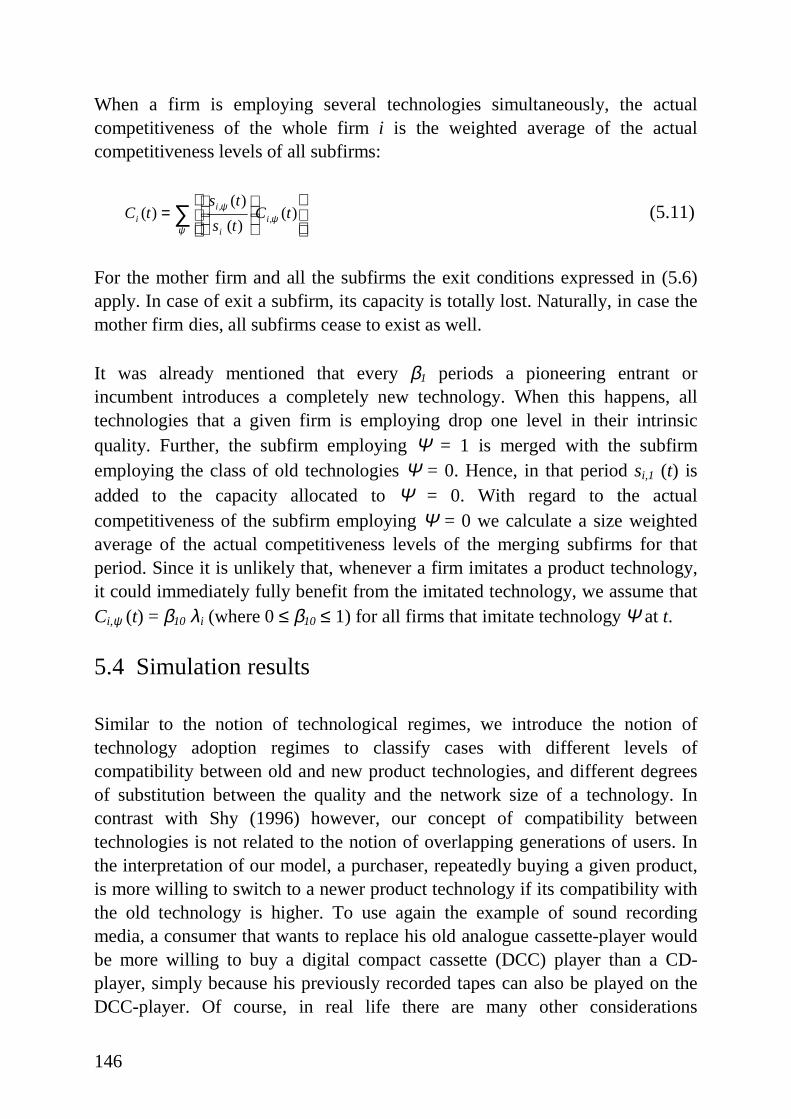
146
When a firm is employing several technologies simultaneously, the actualcompetitiveness of the whole firm i is the weighted average of the actualcompetitiveness levels of all subfirms:
∑
=
ψψ
ψ )()(
)()( ,
, tCts
tstC i
i
ii (5.11)
For the mother firm and all the subfirms the exit conditions expressed in (5.6)apply. In case of exit a subfirm, its capacity is totally lost. Naturally, in case themother fi rm dies, all subfirms cease to exist as well .
It was already mentioned that every β1 periods a pioneering entrant orincumbent introduces a completely new technology. When this happens, alltechnologies that a given firm is employing drop one level in their intrinsicquality. Further, the subfirm employing Ψ = 1 is merged with the subfirmemploying the class of old technologies Ψ = 0. Hence, in that period si,1 (t) isadded to the capacity allocated to Ψ = 0. With regard to the actualcompetitiveness of the subfirm employing Ψ = 0 we calculate a size weightedaverage of the actual competitiveness levels of the merging subfirms for thatperiod. Since it is unlikely that, whenever a firm imitates a product technology,it could immediately fully benefit from the imitated technology, we assume thatCi,ψ (t) = β10 λi (where 0 ≤ β10 ≤ 1) for all firms that imitate technology Ψ at t.
5.4 Simulation results
Similar to the notion of technological regimes, we introduce the notion oftechnology adoption regimes to classify cases with different levels ofcompatibil ity between old and new product technologies, and different degreesof substitution between the quali ty and the network size of a technology. Incontrast with Shy (1996) however, our concept of compatibility betweentechnologies is not related to the notion of overlapping generations of users. Inthe interpretation of our model, a purchaser, repeatedly buying a given product,is more willing to switch to a newer product technology if its compatibility withthe old technology is higher. To use again the example of sound recordingmedia, a consumer that wants to replace his old analogue cassette-player wouldbe more wil ling to buy a digital compact cassette (DCC) player than a CD-player, simply because his previously recorded tapes can also be played on theDCC-player. Of course, in real l ife there are many other considerations
147
involved, but purely for the sake of compatibil ity this consumer would find aDCC player easier than a CD player. Or let us consider a case in which a firm isconsidering to switch from a manually operated lathe to a CNC operated one. Ifthe CNC lathe requires worker skills that are very different from the skil lsnecessary for manually operated lathes, the much more advanced CNC lathe isquite incompatible with the old fashioned manually controlled workbench,which could seriously hinder the adoption of this new technology.
In the model, we will simulate different compatibility levels by varying thedifferences in the intrinsic quality levels QΨ between succeeding producttechnologies. High compatibili ty between a new and an old technology thenimplies a high difference in their intrinsic quali ty levels. For simulating variousdegrees of substitution between the quality and the network size of a technology,we will use the parameter α, which sets the relative importance of atechnology’s share in the market.
We will simulate three different adoption regimes, in which the number ofproduct technologies available is equal to three (K = 3). The first one will belabelled ‘quality regime’ : in this regime, quality and network size are perfectsubstitutes. This is arranged by setting parameter α equal to zero. Hence,technological competitiveness is only determined by the intrinsic quality of atechnology. Further, in this regime new technologies are highly compatible withold technologies. This situation is obtained by setting the intrinsic quality levelsas follows: Q3 = 1, Q2 = 0.5, and Q1 = 0.25.
The second technology adoption regime, labelled ‘ intermediate regime’ ischaracterised by again perfect substitutability of quality and network size, buthere new technologies are less compatible with old technologies than in thequality regime. The lower compatibility of succeeding technologies is obtainedby decreasing the differences in their intrinsic quality levels: Q3 = 1, Q2 = 0.75,and Q1 = 0.5. Thus, compared to the quality regime, the second best technologyis more competitive vis-à-vis the best technology available.
The settings of the third adoption regime (the ‘network’ regime) are such thatquality and network size are to some extent complementary, with α = 0.5.Further, Q3 = 1, Q2 = 0.75, and Q1 = 0.5. Under this regime, technologicalcompetitiveness is also determined by the market share of a technology. The

148
other parameters remain constant across the three technology adoptionregimes.15
Although the three adoption regimes we analyse here are not perfectly consistentwith the cases described by Shy (1996), we can still base our expectations withregard to the outcomes of the simulations on the predictions of his model.According to Shy (1996), whenever new technologies are perfectly compatiblewith old technologies, the new technologies are adopted each period. Further, adecrease in the degree of compatibility between new and old technologies wouldincrease the duration of each technology. Based on this, we may expect that theduration of a technology is higher in the intermediate regime than in the qualityregime.
Further, Shy (1996) concludes that when newer technologies are not perfectlycompatible with older technologies, new technologies are never adopted ifconsumers treat network size and technological advance as perfectcomplements, but may be adopted if they are treated as perfect substitutes.Therefore, we may expect from our simulations that duration will be highestunder the network regime, although eventually newer technologies wil l beadopted, given that our parameters are not consistent with perfectcomplementarity between network size and quality.16 Finally, we may expect tosee that new technologies are not always adopted whenever they appear in boththe quali ty and, more li kely, in the intermediate regime. In both these regimesthere is perfect substitutability between quality and network size and imperfectcompatibil ity. However, Shy’s result (of technologies being skippedoccasionally under these conditions) very much relies on his notion ofcompatibil ity. Therefore, some scepticism with regard to this expectation isappropriate.
Figure 5.1a to 5.1c show the evolution of the market share of successive producttechnologies for the three adoption regimes, resulting from one simulation run of5000 periods. As figure 5.1a shows, in the quality regime technologies have arather short life. Whenever a new technology is introduced, it quickly replaces
15 The values of the other parameters are: N (0) = 40, ρE = 0.15, µλ = 1, σλ = 0.1, si = 250,
β1 = 500, Q0 = 0, θ = 0.99, β2 = 0.6, ΦL = 0.6 , ΦH = 1, s= 25, β3 = 10, β4 = 0.01, β5 = 0.0069,σχ = 0.1, β6 = 0.01, ρim = 20, β7 = 0.1, β8 = 0.1, ση = 0.5, β9 = 0.05, and β10 = 0.8. The resultsof the simulations are robust to small changes in the levels of all parameters.
16 However, when α is set equal to one, the simulations of our model indeed show that newtechnologies are never adopted.
149
the previous technology and starts to dominate the market until again a newtechnology becomes available. In the intermediate regime, the replacementprocess is considerably slower, implying a longer duration of technologies (seefigure 5.1b). Under this regime, none of the technologies persistently capturesthe entire market. The last figure shows that under the network regime, after avery short period of coexistence, one technology always dominates the marketuntil it becomes obsolete17, after which it is quickly replaced by a newtechnology that again dominates until its obsolescence. Thus, the outcomes ofthe simulations are fairly comparable to Shy’s predictions. The duration oftechnologies is higher when compatibil ity between new and old technologies islower. However, both under the quality regime as well under the intermediateregime, new technologies are always adopted.18 Only under the network regimenew technologies are never adopted until the existing dominant technology hasbecome obsolete (i.e., until i ts intrinsic quality level QΨ has dropped to Q0).
How do the populations of f irms evolve under these different regimes, and arethere significant differences between the regimes? Figures 5.2 and 5.3 show theevolution of the number of firms and the concentration levels. Under the quali tyregime, we observe a gradually declining number of f irms and increasingconcentration levels. The intermediate regime exhibits a gradually growingpopulation of f irms with decreasing concentration levels. Finally, under thenetwork regime we see on average a growing population of f irms, however thegrowth rates fluctuate considerably. Further, new technology adoptions in thenetwork regime are associated with a sharp decrease in the number of firms.
These figures, derived from one simulation run for each regime, indeed showthat the regimes differ with regard to the population dynamics. But for a betterassessment of the significance of these differences we calculated a number ofstatistics on the basis of the output of ten runs per regime19, shown in table 5.2.
17 I.e., until it becomes part of the class of old technologies.18 As mentioned before, this is due to the different notion of compatibility in Shy (1996).19 In order to keep the datasets at a reasonable size we have sampled each run only every 50
periods.
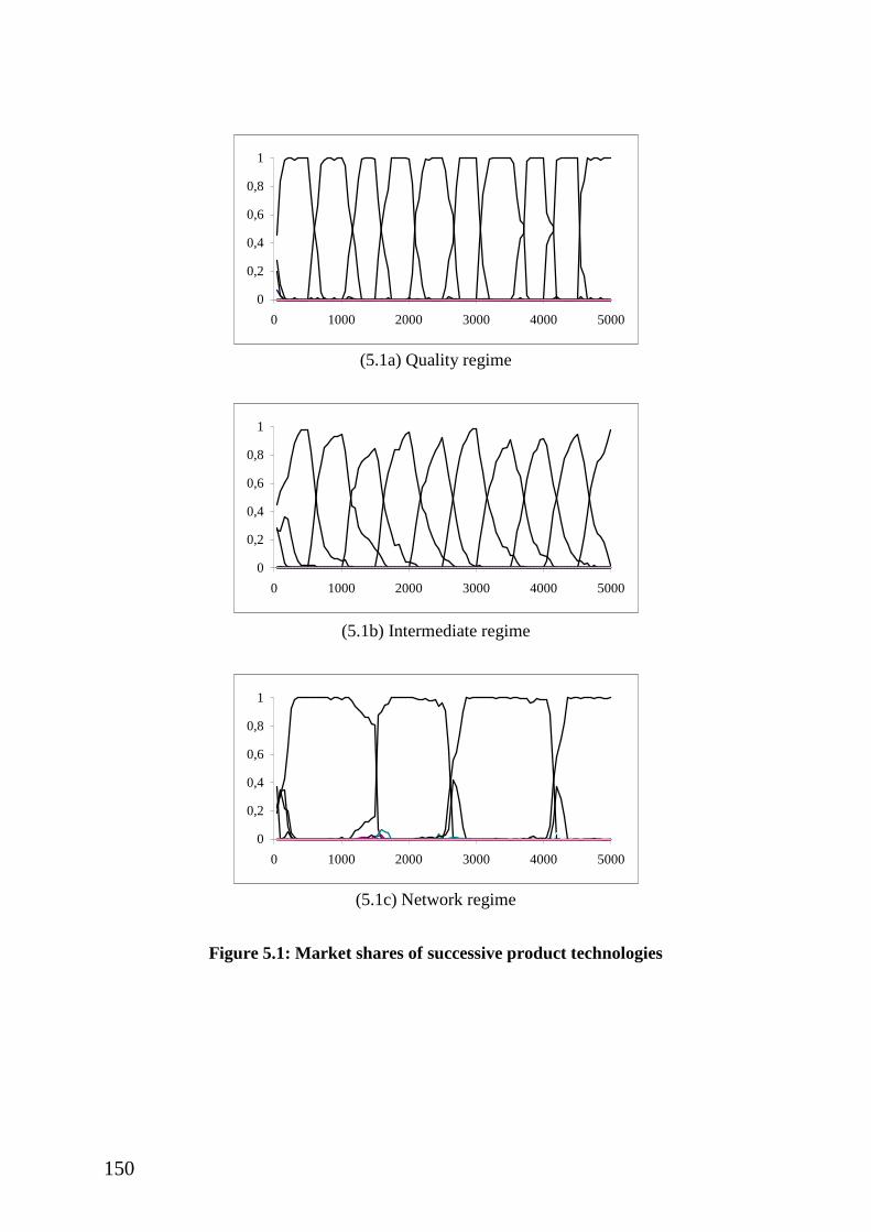
150
0
0,2
0,4
0,6
0,8
1
0 1000 2000 3000 4000 5000
(5.1a) Quali ty regime
0
0,2
0,4
0,6
0,8
1
0 1000 2000 3000 4000 5000
(5.1b) Intermediate regime
0
0,2
0,4
0,6
0,8
1
0 1000 2000 3000 4000 5000
(5.1c) Network regime
Figure 5.1: Market shares of successive product technologies
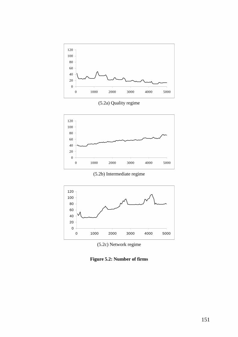
151
0
20
40
60
80
100
120
0 1000 2000 3000 4000 5000
(5.2a) Quali ty regime
0
20
40
60
80
100
120
0 1000 2000 3000 4000 5000
(5.2b) Intermediate regime
0
20
40
60
80
100
120
0 1000 2000 3000 4000 5000
(5.2c) Network regime
Figure 5.2: Number of firms
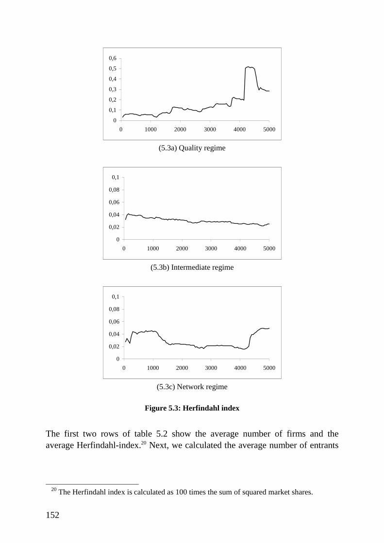
152
0
0,1
0,2
0,3
0,4
0,5
0,6
0 1000 2000 3000 4000 5000
(5.3a) Quali ty regime
0
0,02
0,04
0,06
0,08
0,1
0 1000 2000 3000 4000 5000
(5.3b) Intermediate regime
0
0,02
0,04
0,06
0,08
0,1
0 1000 2000 3000 4000 5000
(5.3c) Network regime
Figure 5.3: Herfindahl index
The first two rows of table 5.2 show the average number of firms and theaverage Herfindahl-index.20 Next, we calculated the average number of entrants
20 The Herfindahl index is calculated as 100 times the sum of squared market shares.
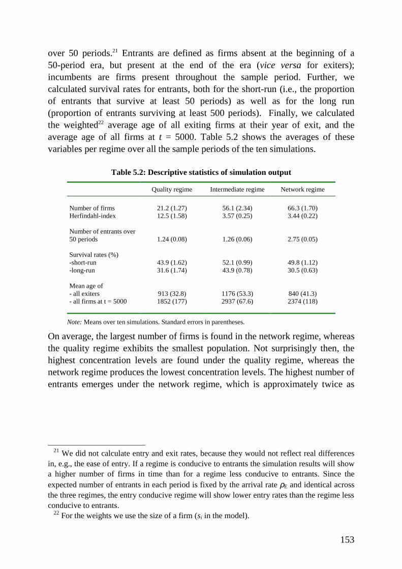
153
over 50 periods.21 Entrants are defined as firms absent at the beginning of a50-period era, but present at the end of the era (vice versa for exiters);incumbents are firms present throughout the sample period. Further, wecalculated survival rates for entrants, both for the short-run (i.e., the proportionof entrants that survive at least 50 periods) as well as for the long run(proportion of entrants surviving at least 500 periods). Finally, we calculatedthe weighted22 average age of all exiting firms at their year of exit, and theaverage age of all firms at t = 5000. Table 5.2 shows the averages of thesevariables per regime over all the sample periods of the ten simulations.
Table 5.2: Descriptive statistics of simulation output
Quali ty regime Intermediate regime Network regime
Number of firms 21.2 (1.27) 56.1 (2.34) 66.3 (1.70)Herfindahl-index 12.5 (1.58) 3.57 (0.25) 3.44 (0.22)
Number of entrants over50 periods 1.24 (0.08) 1.26 (0.06) 2.75 (0.05)
Survival rates (%)-short-run 43.9 (1.62) 52.1 (0.99) 49.8 (1.12)-long-run 31.6 (1.74) 43.9 (0.78) 30.5 (0.63)
Mean age of- all exiters 913 (32.8) 1176 (53.3) 840 (41.3)- all firms at t = 5000 1852 (177) 2937 (67.6) 2374 (118)
Note: Means over ten simulations. Standard errors in parentheses.
On average, the largest number of fi rms is found in the network regime, whereasthe quali ty regime exhibits the smallest population. Not surprisingly then, thehighest concentration levels are found under the quality regime, whereas thenetwork regime produces the lowest concentration levels. The highest number ofentrants emerges under the network regime, which is approximately twice as
21 We did not calculate entry and exit rates, because they would not reflect real differences
in, e.g., the ease of entry. If a regime is conducive to entrants the simulation results will showa higher number of f irms in time than for a regime less conducive to entrants. Since theexpected number of entrants in each period is fixed by the arrival rate ρE and identical acrossthe three regimes, the entry conducive regime will show lower entry rates than the regime lessconducive to entrants.
22 For the weights we use the size of a firm (si in the model).
154
high as under the other regimes.23 Concerning the survival rates, we see that theintermediate regime produces the highest probability for entrants to survive,both for the short run as well as the long run. The lowest short-run survival ratesemerge under the quality regime. Long-run survival rates for the quali ty and thenetwork regime are virtually similar.
The average age of exiting firms is highest under the intermediate regime, andlowest under the network regime. Further, at the end of the simulation the oldestpopulation is found under the intermediate regime, whereas the youngestpopulation is found under the quality regime.
All these results suggest that the three adoption regimes induce cross-sectionaldifferences in the structural and dynamic properties of the population of firms.As such, our model indeed provides an additional explanation for theempirically observed sectoral variances. Although this result in itself is veryimportant, we believe it is of equal interest that our model is also consistent withthe stylised facts that empirical research in industrial economics has put forwardso far. Among these “facts” , the most essential for our model are: (i) persistenceof market turbulence due to entry and exit, (ii ) high infant mortality, negativelycorrelated with firm age, (iii ) growth rates of firms that fall with age and withsize, (iv) persistence of asymmetric performances, and (v) skewed and stablesize distributions. We will therefore conclude this section by investigatingwhether our model is able to reproduce these stylised facts.
From the results that we have already mentioned in this section, it is obviousthat the model reproduces the first stylised fact. Under all regimes, there ispersistent market turbulence due to entry and exit. The second stylised fact (highinfant mortality, negatively correlated with firm age) also emerges, except forthe quali ty regime. Figure 5.4 shows the probability of exiting over the fullsimulation period given the age cohort24 of an entrant for each regime.
23 Note that we only sample every 50 periods. Therefore, despite the identical entry arrival
rate of 0.15 per period, the three regimes produce different numbers of entrants due tovariations in the number of f irms that die before being observed in the sample. Hence, thisnumber can be interpreted as a ‘very short run’ survival rate.
24 Each age cohort covers 50 simulation periods.

155
0,0
0,2
0,4
0,6
0,8
1,0
0 1000 2000 3000 4000 5000
quality regime intermediate regime network regime
Figure 5.4: hazard rate as a function of age
Under the quality regime, infant mortality initiall y declines with age, howeverno entrant is able to live for more than approximately 4,500 periods. This leadsto a rise in hazard rates for entrants with ages exceeding 4,000 periods. Theother two regimes show very similar hazard rates that indeed decline as entrantsmature. Hence, both the intermediate regime and the network regime reproducethis second stylised fact.
The third stylised fact (growth rates of firms that fall with age and with size) isof course imposed on the model by equation (5.7). Still, it might be interestingto learn about the emerging econometric regularities of the model. As in Dosi etal. (1995), we therefore run a number of regressions of the following form:
( ))(ln)(ln)(ln)(ln)(
)(ln 3210 tatsqtaqtsqq
ts
Ttsiiii
i
i +++=
+, (5.12)
for t = 50, 100, …, 5000 and T = 50 (regression 5.12a), and for t = 500, 1000,…, 5000 and T = 500 (regression 5.12b). The results are listed in table 5.3.
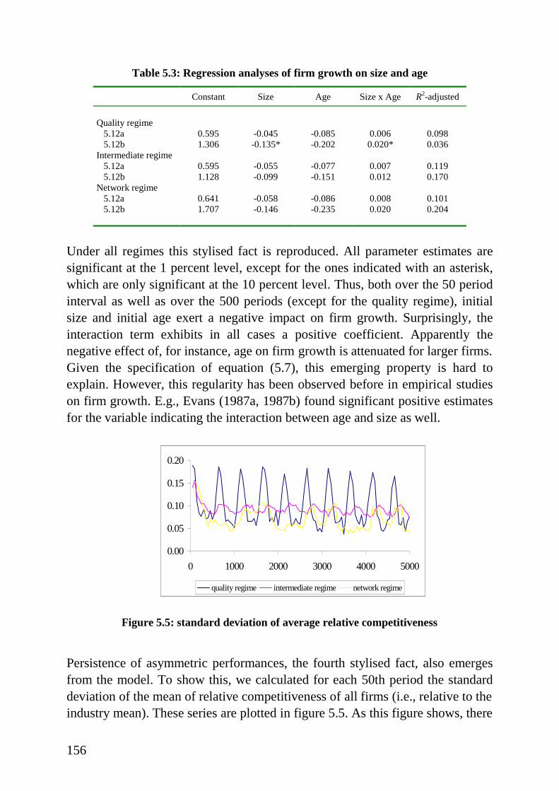
156
Table 5.3: Regression analyses of firm growth on size and age
Constant Size Age Size x Age R2-adjusted
Quali ty regime 5.12a 0.595 -0.045 -0.085 0.006 0.098 5.12b 1.306 -0.135* -0.202 0.020* 0.036Intermediate regime 5.12a 0.595 -0.055 -0.077 0.007 0.119 5.12b 1.128 -0.099 -0.151 0.012 0.170Network regime 5.12a 0.641 -0.058 -0.086 0.008 0.101 5.12b 1.707 -0.146 -0.235 0.020 0.204
Under all regimes this stylised fact is reproduced. All parameter estimates aresignificant at the 1 percent level, except for the ones indicated with an asterisk,which are only significant at the 10 percent level. Thus, both over the 50 periodinterval as well as over the 500 periods (except for the quali ty regime), initialsize and initial age exert a negative impact on firm growth. Surprisingly, theinteraction term exhibits in all cases a positive coefficient. Apparently thenegative effect of, for instance, age on fi rm growth is attenuated for larger firms.Given the specification of equation (5.7), this emerging property is hard toexplain. However, this regularity has been observed before in empirical studieson firm growth. E.g., Evans (1987a, 1987b) found significant positive estimatesfor the variable indicating the interaction between age and size as well .
0.00
0.05
0.10
0.15
0.20
0 1000 2000 3000 4000 5000
quality regime intermediate regime network regime
Figure 5.5: standard deviation of average relative competitiveness
Persistence of asymmetric performances, the fourth stylised fact, also emergesfrom the model. To show this, we calculated for each 50th period the standarddeviation of the mean of relative competitiveness of all firms (i.e., relative to theindustry mean). These series are plotted in figure 5.5. As this figure shows, there
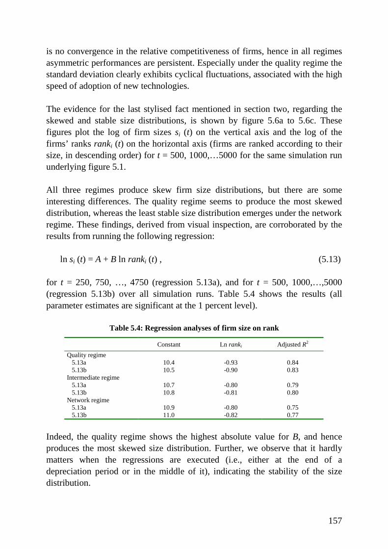
157
is no convergence in the relative competitiveness of f irms, hence in all regimesasymmetric performances are persistent. Especially under the quali ty regime thestandard deviation clearly exhibits cyclical fluctuations, associated with the highspeed of adoption of new technologies.
The evidence for the last stylised fact mentioned in section two, regarding theskewed and stable size distributions, is shown by figure 5.6a to 5.6c. Thesefigures plot the log of firm sizes si (t) on the vertical axis and the log of thefirms’ ranks ranki (t) on the horizontal axis (firms are ranked according to theirsize, in descending order) for t = 500, 1000,…5000 for the same simulation rununderlying figure 5.1.
All three regimes produce skew firm size distributions, but there are someinteresting differences. The quali ty regime seems to produce the most skeweddistribution, whereas the least stable size distribution emerges under the networkregime. These findings, derived from visual inspection, are corroborated by theresults from running the following regression:
ln si (t) = A + B ln ranki (t) , (5.13)
for t = 250, 750, …, 4750 (regression 5.13a), and for t = 500, 1000,…,5000(regression 5.13b) over all simulation runs. Table 5.4 shows the results (allparameter estimates are significant at the 1 percent level).
Table 5.4: Regression analyses of firm size on rank
Constant Ln ranki Adjusted R2
Quali ty regime 5.13a 10.4 -0.93 0.84 5.13b 10.5 -0.90 0.83Intermediate regime 5.13a 10.7 -0.80 0.79 5.13b 10.8 -0.81 0.80Network regime 5.13a 10.9 -0.80 0.75 5.13b 11.0 -0.82 0.77
Indeed, the quality regime shows the highest absolute value for B, and henceproduces the most skewed size distribution. Further, we observe that it hardlymatters when the regressions are executed (i.e., either at the end of adepreciation period or in the middle of it), indicating the stability of the sizedistribution.
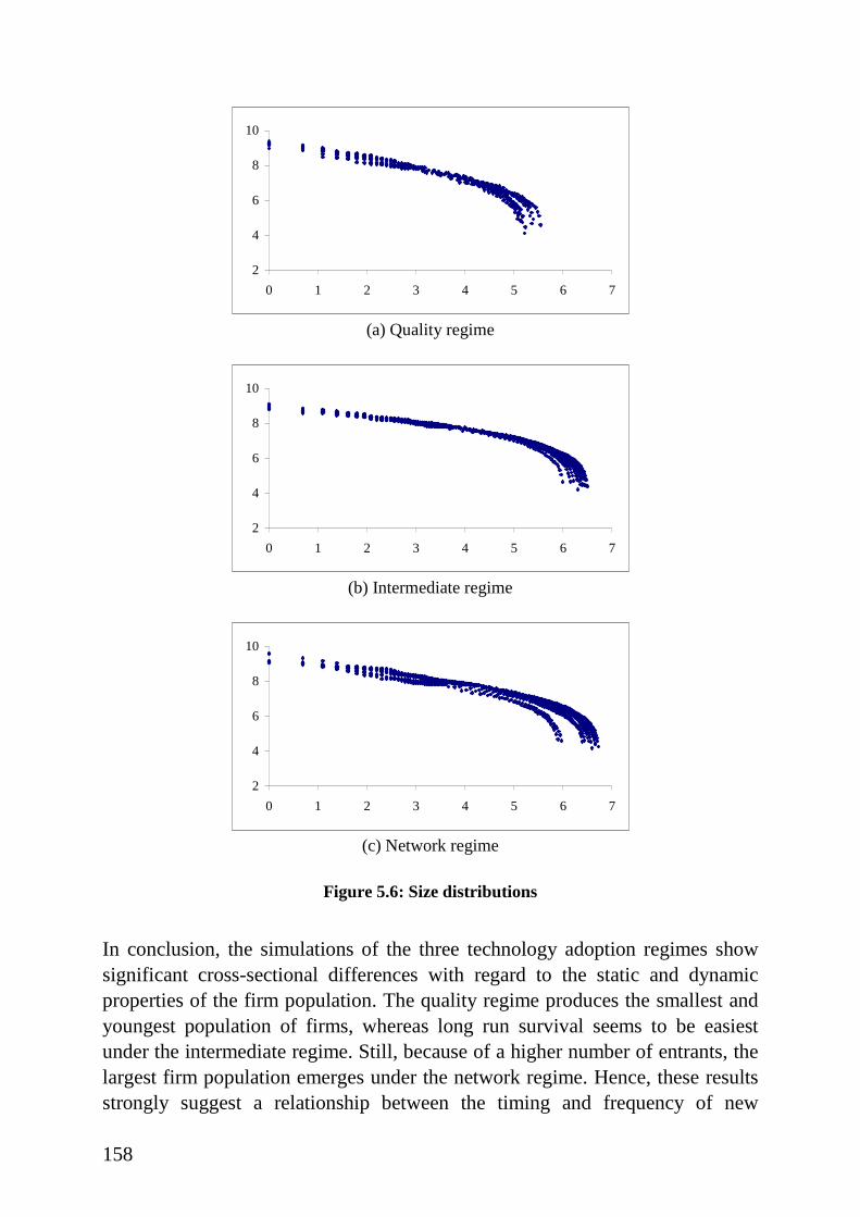
158
2
4
6
8
10
0 1 2 3 4 5 6 7
(a) Quali ty regime
2
4
6
8
10
0 1 2 3 4 5 6 7
(b) Intermediate regime
2
4
6
8
10
0 1 2 3 4 5 6 7
(c) Network regime
Figure 5.6: Size distr ibutions
In conclusion, the simulations of the three technology adoption regimes showsignificant cross-sectional differences with regard to the static and dynamicproperties of the firm population. The quality regime produces the smallest andyoungest population of firms, whereas long run survival seems to be easiestunder the intermediate regime. Still , because of a higher number of entrants, thelargest firm population emerges under the network regime. Hence, these resultsstrongly suggest a relationship between the timing and frequency of new
159
technology adoptions and the dynamics of the firm population. Furthermore, themodel is consistent with a number of stylised facts observed in the empiricalliterature.
5.5 Interaction between adoption regimes and technologicalregimes
As mentioned in the introduction, one of the aims of our model was to introducedemand side considerations as an alternative to more supply side orientedexplanations for industrial demography, such as the concept of technologicalregimes. By varying a number of parameters determining the technologicalcompetitiveness of f irms, we have designed three technology adoption regimesand investigated the differences in the firm population between these regimes.However, to some extent our model allows also for investigating the impact ofdifferent technological regimes on the industrial demography, and theinteraction between adoption regimes and technological regimes. The presentsection will deal with these issues. By selecting and varying a number ofparameters reflecting the level of cumulativeness and spillovers25 oftechnological knowledge, we will run and compare several simulations ofdifferent technological regimes under the three technology adoption regimes.
Chapter 3 has shown that the conditions determining the technological regimehave a strong impact on the patterns of innovative activities of an industry, aswell as on the ease and the impact of imitation. Since in our model innovation isexogenous, we cannot fully simulate the different conditions underlyingtechnological regimes. Only to the extent that these conditions apply to ease andimpact of imitation we can analyse the effect of different technological regimesin our model.
To investigate whether our model is still able to produce the regularitiespredicted by the technological regime framework, we first have to identify theparameters reflecting the cumulativeness and spillover conditions. Forcumulativeness we have to find the variable that indicates best to what extent theacquisition of knowledge is a cumulative process. We propose to vary the
25 For simplicity, we will reduce the number of conditions determining a technological
regime to only two: cumulativeness and spill over effects. The latter captures both theappropriabili ty and knowledge conditions from the original technological regime framework.Hence, differences in the opportunity levels regarding innovations are not considered here.
160
parameter governing the ‘penalty’ rates for continuing firms (β10). This penaltyrate can be interpreted as a measure indicating to what extent the knowledge andexperiences of a firm with its existing product technologies carry over to thenew technology it adopts. For instance, if β10 is equal to β2 (the penalty rate forentrants), the subfirm adopting the new technology starts at a competitivenesslevel equal to that of an entrant.26 In this case the subfirm has no directadvantage over entrants with regard to the new technology (the accumulatedexperience with its existing technologies does not carry over to the subfirm withthe new technology). However, the higher β10 (relative to β2), the more theknowledge of new technology is based on the knowledge of previoustechnologies, and hence the more a new subfirm benefits from its accumulatedexperience vis-à-vis new firms entering with the same technology.27
For varying the spillover effects, it seems natural to vary the parameterdetermining the probabilit y to receive an imitation draw (i.e., ρim). Since wehave defined the process of imitating as acquiring the knowledge of applying asuperior technology, this parameter reflects the ease of knowledge of newproduct technologies to flow to imitators. However, this parameter only reflectsspillovers between continuing firms, not from continuing firms to entrants. Ofcourse, in a strict sense, entrants are considered as continuing firms in the modelfrom the moment they have entered. Thus, when the arrival rate of imitations ishigher, the very young firms have a higher probability to receive an imitationdraw as well . On the other hand, since more continuing firms will imitate, theaverage competitiveness level will be higher, which decreases the probabil ity forentrants to survive. Several simulation runs with different imitation arrival ratesindeed show that this last effect dominates: higher levels of spil lovers generallylead to less (successful) entry, ceteris paribus. Since this inconsistency is due tothe fact that entrants do not directly benefit from higher spillover levels, weconsider it appropriate to increase the arrival rate of entrants (ρent) too whenspillovers levels are higher. In that case, more entrants have access to the
26 I.e., relative to the firms’ genotype organisational competitiveness levels λi.27 Of course, it may happen occasionally that an entrant with a certain technology receives
an imitation draw quickly after it has entered. If β10 is high, this entrant will also benefit fromits experience with the inferior technology, despite the short time it has been employing it.This will not seriously effect the results however, because the overall competitiveness of thisentrant is at least for some time also determined by the competitiveness of the subfirmemploying the inferior technology for which the entry penalty rate β2 is still effective. Besidesthat, this firm already employed the initial technology successfully and therefore must possesssome crucial knowledge about it.
161
knowledge necessary to imitate an existing technology. The entering firms willthen also benefit directly from high spil lover conditions.
In the next experiments we will consider three levels of cumulativeness andspillover conditions (low, medium, high) for each of the technology adoptionregimes of the previous section. The specific parameter settings are as follows.Low cumulativeness means no direct advantage for subfirms relative to entrants(β10 = β2 = 0.6). Medium levels correspond to the parameter settings of theprevious section (β10 = 0.8), whereas high cumulativeness levels are set byβ10 = 1. With regard to spil lover effects, low levels of spillovers are set byρI = 10 and ρent = 0.1. Medium levels again correspond to the parameter settingsof the previous section (hence, ρI = 20 and ρent = 0.15). High spilloverconditions are set by ρI = 30 and ρent = 0.2.
Hence, for each adoption regime we will consider nine different combinations ofcumulativeness and spill over conditions. To get a general impression of theeffect of varying the cumulativeness and spil lover conditions, we will show themeans and their standard errors of the same variables listed in table 5.2 underthese various conditions over ten simulation runs (except for the number ofentrants).28 For an assessment of the significance of the effects of differentcumulativeness and spill over conditions, and to investigate the extent to whichthese conditions interact, we will additionally perform the following regressionanalyses. Each of the six variables will be regressed on a number of dummyvariables, indicating the various cumulativeness and spillover conditions and thepotential interaction between them. More specific, for each adoption regime wewill estimate the following equation:
Y = β1 + β2 Cm_l + β3 Cm_h + β4 Sp_l + β5 Sp_h + β6 (Cm_l x Sp_l) +
β7 (Cm_l x Sp_h) + β8 (Cm_h x Sp_l) + β9 (Cm_h x Sp_h) + ε , (5.14)
where Y is the dependent variable under consideration, Cm_l equals one ifcumulativeness conditions are low and zero otherwise, Cm_h equals one ifcumulativeness is high and zero otherwise, Sp_l equals one if spilloverconditions are low and zero otherwise, and Sp_h equals one if spillovers are high
28 We will not display the evolution of market shares of succeeding technologies for the
different technological regime conditions, because these patterns hardly show any differenceswithin each technology adoption regime.
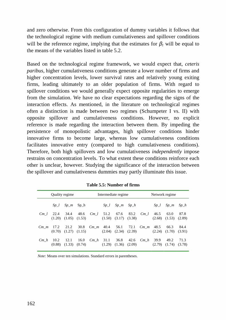
162
and zero otherwise. From this configuration of dummy variables it follows thatthe technological regime with medium cumulativeness and spillover conditionswill be the reference regime, implying that the estimates for β1 will be equal tothe means of the variables listed in table 5.2.
Based on the technological regime framework, we would expect that, ceterisparibus, higher cumulativeness conditions generate a lower number of firms andhigher concentration levels, lower survival rates and relatively young exitingfirms, leading ultimately to an older population of firms. With regard tospillover conditions we would generally expect opposite regularities to emergefrom the simulation. We have no clear expectations regarding the signs of theinteraction effects. As mentioned, in the literature on technological regimesoften a distinction is made between two regimes (Schumpeter I vs. II) withopposite spillover and cumulativeness conditions. However, no explicitreference is made regarding the interaction between them. By impeding thepersistence of monopolistic advantages, high spillover conditions hinderinnovative firms to become large, whereas low cumulativeness conditionsfacilitates innovative entry (compared to high cumulativeness conditions).Therefore, both high spil lovers and low cumulativeness independently imposerestrains on concentration levels. To what extent these conditions reinforce eachother is unclear, however. Studying the significance of the interaction betweenthe spillover and cumulativeness dummies may partly il luminate this issue.
Table 5.5: Number of firms
Quali ty regime Intermediate regime Network regime
Sp_l Sp_m Sp_h Sp_l Sp_m Sp_h Sp_l Sp_m Sp_h
Cm_l 22.4(1.20)
34.4(1.05)
48.6(1.53)
Cm_l 51.2(1.50)
67.6(3.17)
83.2(3.38)
Cm_l 46.5(2.68)
63.0(1.53)
87.8(2.89)
Cm_m 17.2(0.70)
21.2(1.27)
30.8(1.15)
Cm_m 40.4(2.04)
56.1(2.34)
72.1(2.39)
Cm_m 48.5(2.24)
66.3(1.70)
84.4(3.91)
Cm_h 10.2(0.88)
12.1(1.33)
16.0(0.74)
Cm_h 31.1(1.29)
36.8(1.36)
42.6(2.09)
Cm_h 39.9(2.79)
49.2(1.74)
71.3(3.78)
Note: Means over ten simulations. Standard errors in parentheses.
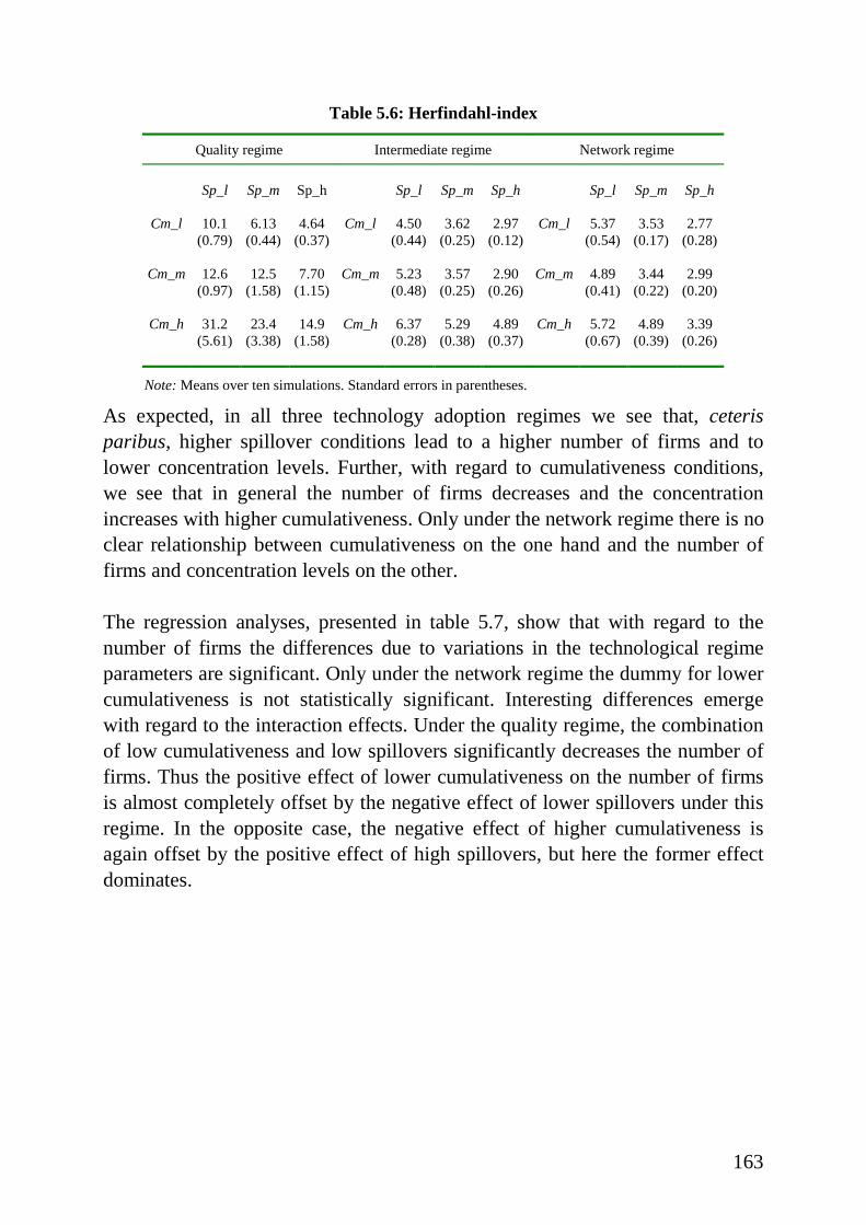
163
Table 5.6: Herfindahl-index
Quali ty regime Intermediate regime Network regime
Sp_l Sp_m Sp_h Sp_l Sp_m Sp_h Sp_l Sp_m Sp_h
Cm_l 10.1(0.79)
6.13(0.44)
4.64(0.37)
Cm_l 4.50(0.44)
3.62(0.25)
2.97(0.12)
Cm_l 5.37(0.54)
3.53(0.17)
2.77(0.28)
Cm_m 12.6(0.97)
12.5(1.58)
7.70(1.15)
Cm_m 5.23(0.48)
3.57(0.25)
2.90(0.26)
Cm_m 4.89(0.41)
3.44(0.22)
2.99(0.20)
Cm_h 31.2(5.61)
23.4(3.38)
14.9(1.58)
Cm_h 6.37(0.28)
5.29(0.38)
4.89(0.37)
Cm_h 5.72(0.67)
4.89(0.39)
3.39(0.26)
Note: Means over ten simulations. Standard errors in parentheses.
As expected, in all three technology adoption regimes we see that, ceterisparibus, higher spillover conditions lead to a higher number of f irms and tolower concentration levels. Further, with regard to cumulativeness conditions,we see that in general the number of f irms decreases and the concentrationincreases with higher cumulativeness. Only under the network regime there is noclear relationship between cumulativeness on the one hand and the number offirms and concentration levels on the other.
The regression analyses, presented in table 5.7, show that with regard to thenumber of firms the differences due to variations in the technological regimeparameters are significant. Only under the network regime the dummy for lowercumulativeness is not statistically significant. Interesting differences emergewith regard to the interaction effects. Under the quality regime, the combinationof low cumulativeness and low spillovers significantly decreases the number offirms. Thus the positive effect of lower cumulativeness on the number of f irmsis almost completely offset by the negative effect of lower spil lovers under thisregime. In the opposite case, the negative effect of higher cumulativeness isagain offset by the positive effect of high spil lovers, but here the former effectdominates.
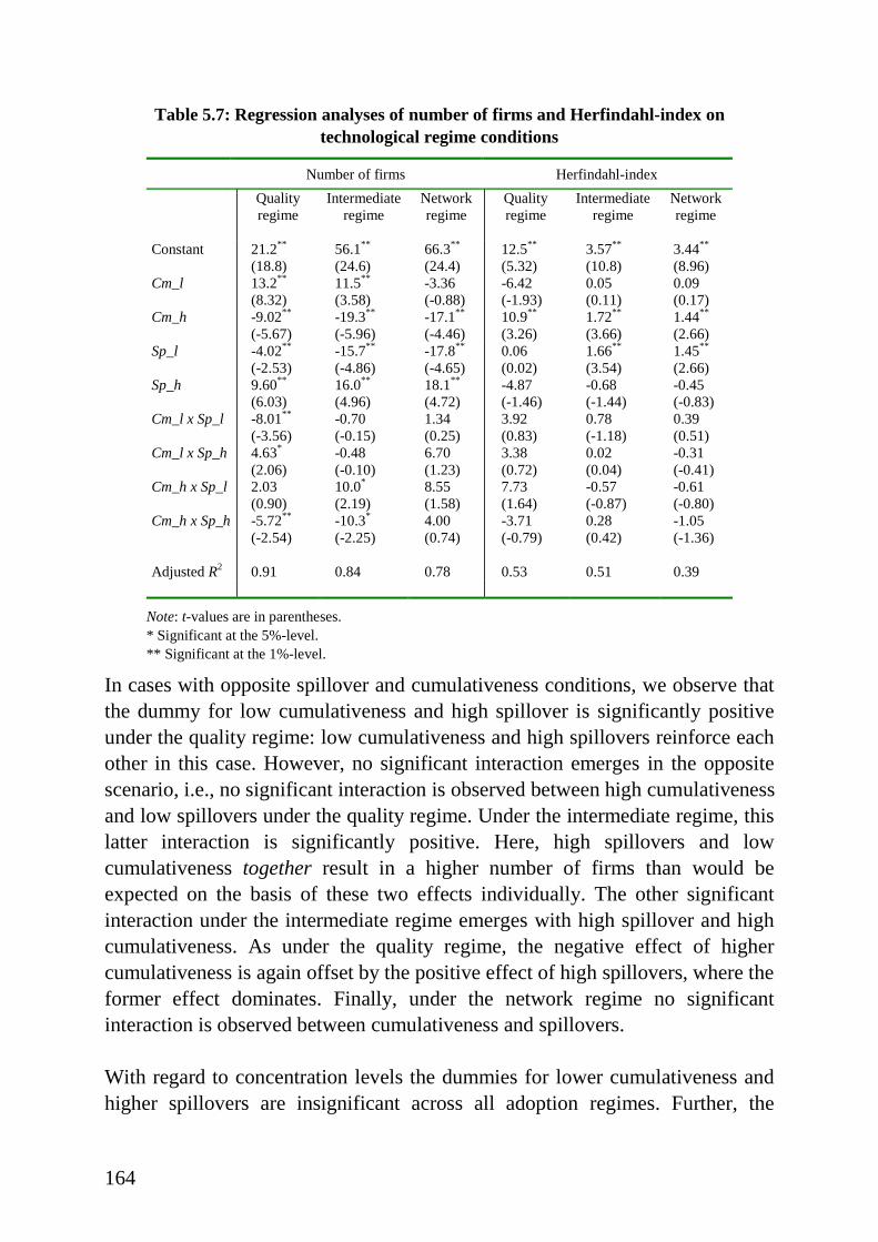
164
Table 5.7: Regression analyses of number of firms and Herfindahl-index ontechnological regime conditions
Number of firms Herfindahl-index
Quali tyregime
Intermediateregime
Networkregime
Quali tyregime
Intermediateregime
Networkregime
Constant 21.2**
(18.8)56.1**
(24.6)66.3**
(24.4)12.5**
(5.32)3.57**
(10.8)3.44**
(8.96)Cm_l 13.2**
(8.32)11.5**
(3.58)-3.36(-0.88)
-6.42(-1.93)
0.05(0.11)
0.09(0.17)
Cm_h -9.02**
(-5.67)-19.3**
(-5.96)-17.1**
(-4.46)10.9**
(3.26)1.72**
(3.66)1.44**
(2.66)Sp_l -4.02**
(-2.53)-15.7**
(-4.86)-17.8**
(-4.65)0.06(0.02)
1.66**
(3.54)1.45**
(2.66)Sp_h 9.60**
(6.03)16.0**
(4.96)18.1**
(4.72)-4.87(-1.46)
-0.68(-1.44)
-0.45(-0.83)
Cm_l x Sp_l -8.01**
(-3.56)-0.70(-0.15)
1.34(0.25)
3.92(0.83)
0.78(-1.18)
0.39(0.51)
Cm_l x Sp_h 4.63*
(2.06)-0.48(-0.10)
6.70(1.23)
3.38(0.72)
0.02(0.04)
-0.31(-0.41)
Cm_h x Sp_l 2.03(0.90)
10.0*
(2.19)8.55(1.58)
7.73(1.64)
-0.57(-0.87)
-0.61(-0.80)
Cm_h x Sp_h -5.72**
(-2.54)-10.3*
(-2.25)4.00(0.74)
-3.71(-0.79)
0.28(0.42)
-1.05(-1.36)
Adjusted R2 0.91 0.84 0.78 0.53 0.51 0.39
Note: t-values are in parentheses.* Significant at the 5%-level.** Significant at the 1%-level.
In cases with opposite spillover and cumulativeness conditions, we observe thatthe dummy for low cumulativeness and high spillover is significantly positiveunder the quality regime: low cumulativeness and high spillovers reinforce eachother in this case. However, no significant interaction emerges in the oppositescenario, i.e., no significant interaction is observed between high cumulativenessand low spillovers under the quality regime. Under the intermediate regime, thislatter interaction is significantly positive. Here, high spillovers and lowcumulativeness together result in a higher number of firms than would beexpected on the basis of these two effects individually. The other significantinteraction under the intermediate regime emerges with high spillover and highcumulativeness. As under the quality regime, the negative effect of highercumulativeness is again offset by the positive effect of high spil lovers, where theformer effect dominates. Finally, under the network regime no significantinteraction is observed between cumulativeness and spil lovers.
With regard to concentration levels the dummies for lower cumulativeness andhigher spillovers are insignificant across all adoption regimes. Further, the
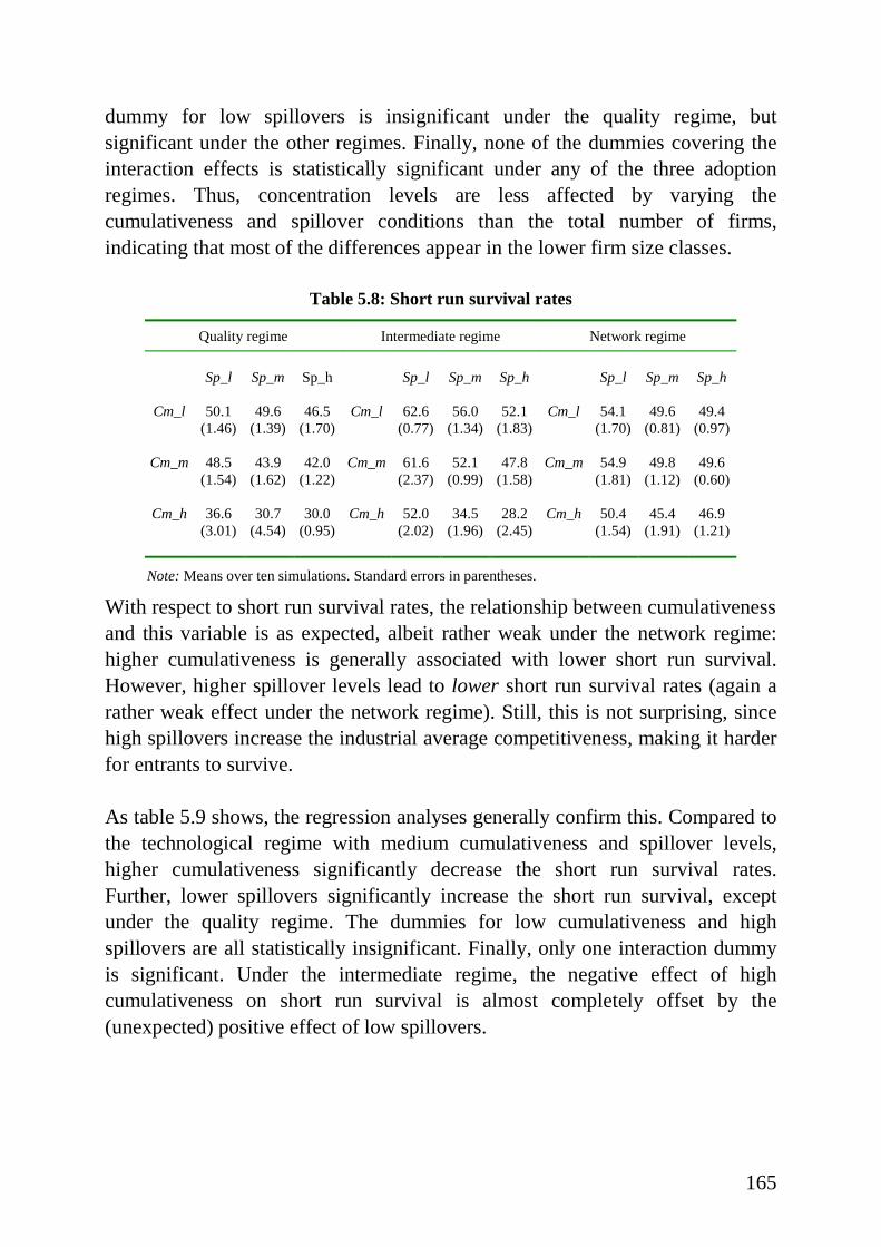
165
dummy for low spillovers is insignificant under the quality regime, butsignificant under the other regimes. Finally, none of the dummies covering theinteraction effects is statistically significant under any of the three adoptionregimes. Thus, concentration levels are less affected by varying thecumulativeness and spill over conditions than the total number of firms,indicating that most of the differences appear in the lower firm size classes.
Table 5.8: Short run survival rates
Quali ty regime Intermediate regime Network regime
Sp_l Sp_m Sp_h Sp_l Sp_m Sp_h Sp_l Sp_m Sp_h
Cm_l 50.1(1.46)
49.6(1.39)
46.5(1.70)
Cm_l 62.6(0.77)
56.0(1.34)
52.1(1.83)
Cm_l 54.1(1.70)
49.6(0.81)
49.4(0.97)
Cm_m 48.5(1.54)
43.9(1.62)
42.0(1.22)
Cm_m 61.6(2.37)
52.1(0.99)
47.8(1.58)
Cm_m 54.9(1.81)
49.8(1.12)
49.6(0.60)
Cm_h 36.6(3.01)
30.7(4.54)
30.0(0.95)
Cm_h 52.0(2.02)
34.5(1.96)
28.2(2.45)
Cm_h 50.4(1.54)
45.4(1.91)
46.9(1.21)
Note: Means over ten simulations. Standard errors in parentheses.
With respect to short run survival rates, the relationship between cumulativenessand this variable is as expected, albeit rather weak under the network regime:higher cumulativeness is generally associated with lower short run survival.However, higher spillover levels lead to lower short run survival rates (again arather weak effect under the network regime). Still , this is not surprising, sincehigh spillovers increase the industrial average competitiveness, making it harderfor entrants to survive.
As table 5.9 shows, the regression analyses generally confirm this. Compared tothe technological regime with medium cumulativeness and spillover levels,higher cumulativeness significantly decrease the short run survival rates.Further, lower spillovers significantly increase the short run survival, exceptunder the quality regime. The dummies for low cumulativeness and highspillovers are all statistically insignificant. Finally, only one interaction dummyis significant. Under the intermediate regime, the negative effect of highcumulativeness on short run survival is almost completely offset by the(unexpected) positive effect of low spillovers.
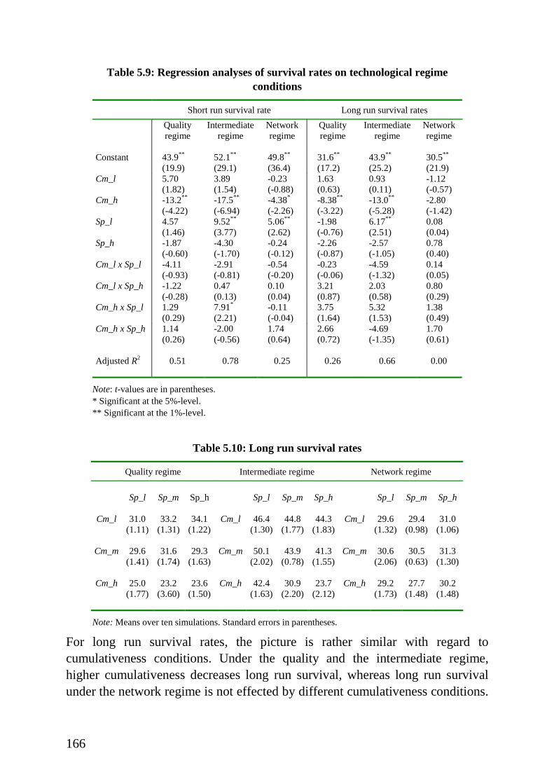
166
Table 5.9: Regression analyses of survival rates on technological regimeconditions
Short run survival rate Long run survival rates
Quali tyregime
Intermediateregime
Networkregime
Quali tyregime
Intermediateregime
Networkregime
Constant 43.9**
(19.9)52.1**
(29.1)49.8**
(36.4)31.6**
(17.2)43.9**
(25.2)30.5**
(21.9)Cm_l 5.70
(1.82)3.89(1.54)
-0.23(-0.88)
1.63(0.63)
0.93(0.11)
-1.12(-0.57)
Cm_h -13.2**
(-4.22)-17.5**
(-6.94)-4.38*
(-2.26)-8.38**
(-3.22)-13.0**
(-5.28)-2.80(-1.42)
Sp_l 4.57(1.46)
9.52**
(3.77)5.06**
(2.62)-1.98(-0.76)
6.17**
(2.51)0.08(0.04)
Sp_h -1.87(-0.60)
-4.30(-1.70)
-0.24(-0.12)
-2.26(-0.87)
-2.57(-1.05)
0.78(0.40)
Cm_l x Sp_l -4.11(-0.93)
-2.91(-0.81)
-0.54(-0.20)
-0.23(-0.06)
-4.59(-1.32)
0.14(0.05)
Cm_l x Sp_h -1.22(-0.28)
0.47(0.13)
0.10(0.04)
3.21(0.87)
2.03(0.58)
0.80(0.29)
Cm_h x Sp_l 1.29(0.29)
7.91*
(2.21)-0.11(-0.04)
3.75(1.64)
5.32(1.53)
1.38(0.49)
Cm_h x Sp_h 1.14(0.26)
-2.00(-0.56)
1.74(0.64)
2.66(0.72)
-4.69(-1.35)
1.70(0.61)
Adjusted R2 0.51 0.78 0.25 0.26 0.66 0.00
Note: t-values are in parentheses.* Significant at the 5%-level.** Significant at the 1%-level.
Table 5.10: Long run survival rates
Quali ty regime Intermediate regime Network regime
Sp_l Sp_m Sp_h Sp_l Sp_m Sp_h Sp_l Sp_m Sp_h
Cm_l 31.0(1.11)
33.2(1.31)
34.1(1.22)
Cm_l 46.4(1.30)
44.8(1.77)
44.3(1.83)
Cm_l 29.6(1.32)
29.4(0.98)
31.0(1.06)
Cm_m 29.6(1.41)
31.6(1.74)
29.3(1.63)
Cm_m 50.1(2.02)
43.9(0.78)
41.3(1.55)
Cm_m 30.6(2.06)
30.5(0.63)
31.3(1.30)
Cm_h 25.0(1.77)
23.2(3.60)
23.6(1.50)
Cm_h 42.4(1.63)
30.9(2.20)
23.7(2.12)
Cm_h 29.2(1.73)
27.7(1.48)
30.2(1.48)
Note: Means over ten simulations. Standard errors in parentheses.
For long run survival rates, the picture is rather similar with regard tocumulativeness conditions. Under the quality and the intermediate regime,higher cumulativeness decreases long run survival, whereas long run survivalunder the network regime is not effected by different cumulativeness conditions.
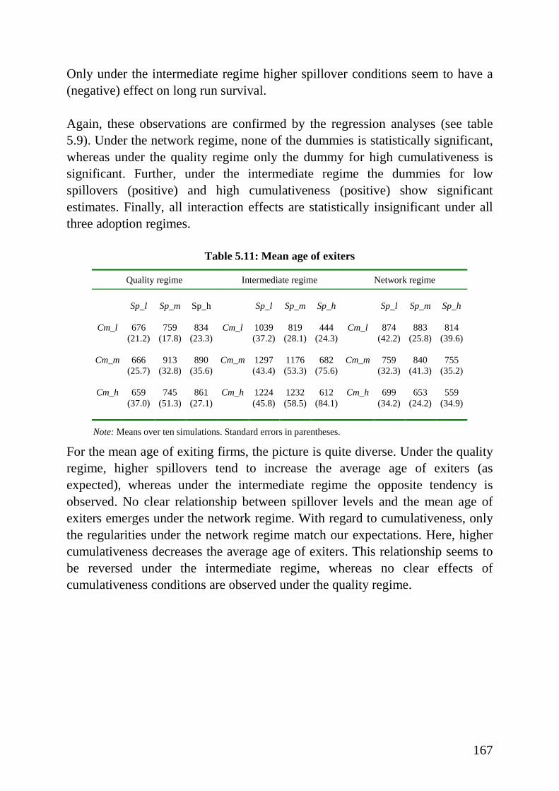
167
Only under the intermediate regime higher spillover conditions seem to have a(negative) effect on long run survival.
Again, these observations are confirmed by the regression analyses (see table5.9). Under the network regime, none of the dummies is statistically significant,whereas under the quality regime only the dummy for high cumulativeness issignificant. Further, under the intermediate regime the dummies for lowspillovers (positive) and high cumulativeness (positive) show significantestimates. Finally, all interaction effects are statistically insignificant under allthree adoption regimes.
Table 5.11: Mean age of exiters
Quali ty regime Intermediate regime Network regime
Sp_l Sp_m Sp_h Sp_l Sp_m Sp_h Sp_l Sp_m Sp_h
Cm_l 676(21.2)
759(17.8)
834(23.3)
Cm_l 1039(37.2)
819(28.1)
444(24.3)
Cm_l 874(42.2)
883(25.8)
814(39.6)
Cm_m 666(25.7)
913(32.8)
890(35.6)
Cm_m 1297(43.4)
1176(53.3)
682(75.6)
Cm_m 759(32.3)
840(41.3)
755(35.2)
Cm_h 659(37.0)
745(51.3)
861(27.1)
Cm_h 1224(45.8)
1232(58.5)
612(84.1)
Cm_h 699(34.2)
653(24.2)
559(34.9)
Note: Means over ten simulations. Standard errors in parentheses.
For the mean age of exiting firms, the picture is quite diverse. Under the qualityregime, higher spillovers tend to increase the average age of exiters (asexpected), whereas under the intermediate regime the opposite tendency isobserved. No clear relationship between spillover levels and the mean age ofexiters emerges under the network regime. With regard to cumulativeness, onlythe regularities under the network regime match our expectations. Here, highercumulativeness decreases the average age of exiters. This relationship seems tobe reversed under the intermediate regime, whereas no clear effects ofcumulativeness conditions are observed under the quality regime.
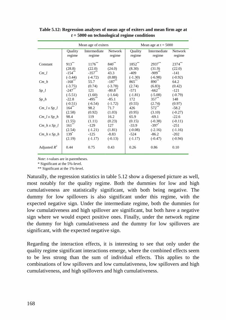
168
Table 5.12: Regression analyses of mean age of exiters and mean firm age att = 5000 on technological regime condit ions
Mean age of exiters Mean age at t = 5000
Quali tyregime
Intermediateregime
Networkregime
Quali tyregime
Intermediateregime
Networkregime
Constant 913**
(28.8)1176**
(22.0)840**
(24.0)1852**
(8.30)2937**
(31.9)2374**
(22.0)Cm_l -154**
(-3.44)-357**
(-4.72)43.3(0.88)
-409(-1.30)
-909**
(-6.98)-141(-0.92)
Cm_h -168**
(-3.75)55.7(0.74)
-187**
(-3.78)865**
(2.74)890**
(6.83)64.2(0.42)
Sp_l -247**
(-5.51)121(1.60)
-80.8**
(-1.64)-571(-1.81)
-662**
(-5.08)-121(-0.79)
Sp_h -22.8(-0.51)
-495**
(-6.54)-85.1(-1.72)
172(0.55)
357**
(2.74)148(0.97)
Cm_l x Sp_l 164**
(2.58)98.2(0.92)
71.7(1.03)
426(0.95)
572**
(3.10)-58.2(-0.27)
Cm_l x Sp_h 98.4(1.55)
119(1.11)
16.2(0.23)
65.9(0.15)
-69.1(-0.38)
-22.6(-0.11)
Cm_h x Sp_l 161**
(2.54)-129(-1.21)
127(1.81)
-33.9(-0.08)
-397*
(-2.16)-251(-1.16)
Cm_h x Sp_h 139*
(2.19)-125(-1.17)
-8.83(-0.13)
-524(-1.17)
-86.2(-0.47)
-202(-0.94)
Adjusted R2 0.44 0.75 0.43 0.26 0.86 0.10
Note: t-values are in parentheses.* Significant at the 5%-level.** Significant at the 1%-level.
Naturally, the regression statistics in table 5.12 show a dispersed picture as well,most notably for the quality regime. Both the dummies for low and highcumulativeness are statistically significant, with both being negative. Thedummy for low spillovers is also significant under this regime, with theexpected negative sign. Under the intermediate regime, both the dummies forlow cumulativeness and high spillover are significant, but both have a negativesign where we would expect positive ones. Finally, under the network regimethe dummy for high cumulativeness and the dummy for low spillovers aresignificant, with the expected negative sign.
Regarding the interaction effects, it is interesting to see that only under thequality regime significant interactions emerge, where the combined effects seemto be less strong than the sum of individual effects. This applies to thecombinations of low spil lovers and low cumulativeness, low spillovers and highcumulativeness, and high spillovers and high cumulativeness.
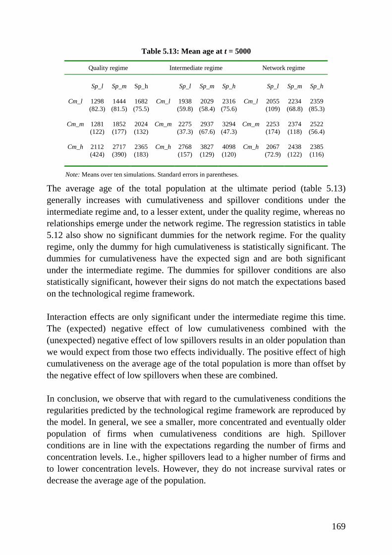
169
Table 5.13: Mean age at t = 5000
Quali ty regime Intermediate regime Network regime
Sp_l Sp_m Sp_h Sp_l Sp_m Sp_h Sp_l Sp_m Sp_h
Cm_l 1298(82.3)
1444(81.5)
1682(75.5)
Cm_l 1938(59.8)
2029(58.4)
2316(75.6)
Cm_l 2055(109)
2234(68.8)
2359(85.3)
Cm_m 1281(122)
1852(177)
2024(132)
Cm_m 2275(37.3)
2937(67.6)
3294(47.3)
Cm_m 2253(174)
2374(118)
2522(56.4)
Cm_h 2112(424)
2717(390)
2365(183)
Cm_h 2768(157)
3827(129)
4098(120)
Cm_h 2067(72.9)
2438(122)
2385(116)
Note: Means over ten simulations. Standard errors in parentheses.
The average age of the total population at the ultimate period (table 5.13)generally increases with cumulativeness and spillover conditions under theintermediate regime and, to a lesser extent, under the quality regime, whereas norelationships emerge under the network regime. The regression statistics in table5.12 also show no significant dummies for the network regime. For the qualityregime, only the dummy for high cumulativeness is statistically significant. Thedummies for cumulativeness have the expected sign and are both significantunder the intermediate regime. The dummies for spillover conditions are alsostatistically significant, however their signs do not match the expectations basedon the technological regime framework.
Interaction effects are only significant under the intermediate regime this time.The (expected) negative effect of low cumulativeness combined with the(unexpected) negative effect of low spil lovers results in an older population thanwe would expect from those two effects individually. The positive effect of highcumulativeness on the average age of the total population is more than offset bythe negative effect of low spil lovers when these are combined.
In conclusion, we observe that with regard to the cumulativeness conditions theregularities predicted by the technological regime framework are reproduced bythe model. In general, we see a smaller, more concentrated and eventually olderpopulation of f irms when cumulativeness conditions are high. Spilloverconditions are in line with the expectations regarding the number of f irms andconcentration levels. I.e., higher spillovers lead to a higher number of f irms andto lower concentration levels. However, they do not increase survival rates ordecrease the average age of the population.
170
A possible explanation for this is that the benefits of the incumbents from highspillovers are such that they easily imitate and survive, thereby increasing theindustrial average competitiveness. This process leads both to an eventuallyolder population, as well as to hard survival conditions for entrants. Anotherreason for this inconsistency with the technological regime framework is thatour model does not allow for analysing the effect of the technological regimeconditions on differences between the innovative activities of incumbents andentrants. Innovation is exogenous in our model, and perhaps endogenising theinnovation process would make our model more consistent with thetechnological regime framework.
Finally, we observe that the regularities emerging under the network regime arethe least affected by variations in spil lover and cumulativeness conditions. Theinteraction effects between spillovers and cumulativeness are never significantunder the network regime as well. Apparently, the emerging regularities underthis regime are mainly determined by the network externalities among users andthe resulting diffusion patterns of new product technologies. Under the qualityand intermediate regime, we have found some significant interaction effects,however they do not appear to systematically affect the results.
5.6 Conclusions
This chapter has shown that differences in the timing and frequency of newproduct technology adoptions provide an additional explanation for sectoralvariations in the dynamics of the firm population. Assuming that varyingconsumer preferences over technology advance and network size effects, anddifferent degrees of compatibili ty between succeeding technologies explain whyin some industries technologies are more often replaced than in others (see Shy,1996), we analysed, by means of a simulation model, how the differentreplacement patterns would effect the dynamics of the firm population. Wedesigned and investigated three different technology adoption regimes with thefollowing underlying conditions: (i) a quality regime, in which quality andnetwork size are regarded as perfect substitutes and new product technologiesare highly compatible with old technologies, (ii ) an intermediate regime, inwhich new product technologies are less compatible with old technologies, butwhere quality and network size are still regarded as perfect substitutes, and (iii )a network regime, in which network size and quali ty are regarded ascomplementary. By modell ing the growth of a firm’s competitiveness as afunction of both the quali ty level and the market share of the product

171
technologies it employs, and by tuning the parameters of this function to arrangethe adoption regimes, the model produced the following results.
First of all, three rather different replacement patterns of technologies emerge.In the quality regime, technologies are continuously and rather quickly replacedby superior technologies as soon as they become available. In the intermediateregime, newer technologies stil l always replace older ones, but the duration of atechnology is higher than under the quality regime. Finally, in the networkregime eventually one technology always dominates the market until it becomesobsolete (despite the presence of superior technologies), after which it is quicklyreplaced by a new technology that again dominates until its obsolescence.
The second result is that the replacement patterns of product technologiesclearly affect the dynamics of the firm population. The quality regime producesthe smallest, but most dynamic population of f irms, whereas the largest firmpopulation emerges under the network regime. The intermediate regime exhibitsthe most stable population of firms, where long run survival is relatively easy.
The third result is that for all three regimes the model is able to reproduce anumber of important stylised facts from industrial organisation. The modelproduces persistence of market turbulence due to entry and exit; high infantmortality, negatively correlated with firm age; growth rates of f irms that fallwith age and with size; persistence of asymmetric performances; and skewedand relatively stable size distributions.
The fourth result is that all these outcomes are obtained in the absence ofreplicator dynamics. There is no explicit relationship in our model between afirm’s relative competitiveness and its growth rate. The only selectionmechanism in our model is that a minimum level of relative competitiveness isrequired in order to survive. This rather simple mechanism turns out to besufficient to produce meaningful results, consistent with the previouslymentioned stylised facts.
The fifth and final result is derived from running the model under differenttechnological regimes, represented by various cumulativeness and spilloverconditions. In general, we see a smaller, more concentrated and eventually olderpopulation of f irms when cumulativeness conditions are high. These regularitiesare in line with the technological regime framework. Spil lover conditions,however, are only partly consistent with this framework. Higher spillovers

172
indeed lead to a higher number of f irms and lower concentration levels.However, they do not generally increase survival rates or decrease the averageage of the population. The explanation for this is found in the trivial effect ofhigh spillover conditions on the competitiveness of incumbent firms vis-à-visentrants. High spillover conditions enable more continuing firms to imitate,which increases the industrial average competitiveness. This, in turn,deteriorates the general conditions for entrants and makes it more difficult forthem to survive. Finally, we observed that the regularities emerging under thenetwork regime are the least affected by varying cumulativeness and spilloverconditions.
Endogenising the innovation process could make our model more consistentwith the technological regime framework. Since innovation is exogenous in ourmodel, we cannot analyse the effect of the technological regime conditions ondifferences between the innovative activities of incumbents and entrants.Perhaps future efforts in this direction will enable us to better assess theinteraction between the demand side oriented adoption regimes and the moresupply side oriented technological regimes.

173
Chapter 6
Conclusions
This dissertation has focussed on variances in the structural and dynamicproperties of manufacturing industries. For many decades we have knownempirically that industries differ widely in, for example, concentration levels,capital intensity, and entry and exit rates. And for many decades industrialeconomists, trying to find theoretical explanations for these observed differences,have mainly relied upon theories involving stable equili brium solutions. Recentlyhowever, the increased access to firm-level databases has led to a number of robustempirical results that are hard to reconcile with the assumptions underlying themainstream equili brium theories and models of industrial economics, and with theresults these models produce. Probably therefore we observe an increasing interestin theoretical alternatives based on more realistic assumptions regarding firmbehaviour and the process of technological change. As such, these alternativetheoretical frameworks may provide plausible explanations for the cross-sectionalvariations in the structures and dynamics of industries.
The major objective of this dissertation was to find and test for explanationsderived from these rather recently developed theoretical frameworks. Byexploring the theoretical and empirical l iterature in industrial economics, byusing a longitudinal firm-level database, and by developing and simulating amodel on industrial dynamics, we obtained the following results. Empirically,we have shown that both the technological regime framework as well as theproduct or industry li fe cycle approach can explain differences betweenindustries. Further, our model has shown that differences in the timing andfrequency of new technology adoptions provide an additional explanation for thestructural and dynamic differences between industries. In the next section wewill briefly summarise the main chapters of this dissertation. In the second andfinal section of this chapter we will suggest some directions for future researchin industrial economics.
174
6.1 Summary
Given the empirical nature of this thesis and the extensive use of the StatisticsNetherlands manufacturing database throughout it, chapter 2 has illuminatedthree important issues related to empirical research in industrial economics. Firstof all, we have described in detail the firm-level data on which a major part ofthe research in this dissertation is based. Second, by presenting a number ofselected stylised facts we have aimed to highlight some robust results that havebeen established in industrial economics. Especially in the last fifteen years, theincreased access to firm-level data has resulted in a collection of results thatwere found to be rather invariant across countries and over time. Finally, wehave investigated whether these stylised facts could also be found in Dutchmanufacturing.
Two important results emerged from this chapter. The first one was that theregularities emerging from the SN manufacturing database were to a large extentconsistent with the stylised facts of industrial economics. Whether we looked atfirm-level regularities, their aggregate impact on the manufacturing sector, orregularities at the industry level, practically all of them seemed to be consistentwith earlier empirical findings in industrial economics. To mention just a few,we have found hazard rates of entering firms and growth rates of survivingentrants declining with age and (initial) size; persistence of productivitydifferentials between firms in the same industry; skewed but rather stabledistributions of firm sizes; and finally, significantly positive correlationsbetween entry and exit rates across industries.
The second result of chapter 2 concerns the observation that Dutchmanufacturing industries widely differ in virtually all dimensions observable inthe data. Although this result is far from new, we have argued that, despite thepresence of a number of theoretical contributions that potentially can explain theobserved differences, not much effort has been done in testing these theorieswith the increasingly available firm-level data. As such, this unexploitedopportunity constituted one of the main objectives of this dissertation: toinvestigate empirically which theoretical frameworks can explain the cross-sectional differences.
Based on the results of chapter 2, chapter 3 has selectively surveyed thetheoretical literature in industrial economics. In our search for theoretical
175
contributions that may explain the observed differences across industries in adynamic and comprehensive way, we have selected two approaches anddescribed them thoroughly in this chapter. We have argued that both thetechnological regime framework as well as the product li fe cycle approach arehighly appropriate conceptual tools to study empirically the differences in cross-sectional regularities, as they both embody elements such as firm heterogeneityand technological uncertainty that are close to empirical substance. With regardto their potential power to explain differences in structures and dynamicsbetween industries, we have argued the following.
The technological regime framework asserts that sectoral patterns of innovativeactivities are determined by the combination of opportunity, appropriability andcumulativeness conditions, and properties of the technological knowledge baseunderlying these activities. If entry, survival, growth and exit patterns are relatedto the rates and forms of organisation of innovations, then the observed inter-sectoral variety in structures and dynamics can be explained by differences inthe underlying technological regimes. Alternatively, theories and models onproduct life cycles explain and depict the evolution of an industry’s structuraland dynamic properties over its lifetime. Based on this approach, the observedcross-sectional differences can be explained by the different evolutionary stagesthat industries occupy.
To what extent these theories could actually account for the cross-sectionalvariances was investigated in chapter 4. The first part of this chapter aimed tofind empirical evidence for the technological regime framework. Based on thisframework, we derived a number of hypotheses and tested these with thelongitudinal firm-level data we had access to. This empirical analysis stronglysuggested that differences in the structural (e.g., concentration levels) anddynamic (e.g., entry and exit rates) properties of industries are closely related tothe set of opportunity, appropriability, cumulativeness and knowledgeconditions underlying the innovative activities in an industry.
The second part of chapter 4 investigated whether the cross-sectional variationsin structures and dynamics of industries could be explained by the differentevolutionary stages the industries occupied. Based on a model by Klepper(1996), we again derived and tested a number of hypotheses. AlthoughKlepper’s model is primarily intended to depict the evolution of technologicallyprogressive industries, the second part of chapter 4 has shown that applying themodel to (basically mature) manufacturing industries in general, i.e., without
176
any reference to their technological progressiveness, provides some interestingresults. Industries in different evolutionary stages indeed show differentregularities, which are partly in line with Klepper’s model. Especiallydifferences in the entry and survival rates of industries corroborate Klepper’shypothesis of a growing advantage of incumbents over entrants. Further, wehave found evidence that a shakeout of firms is mainly caused by a reduction inentry rates, rather than an increase in exit rates. Again, this finding is consistentwith Klepper’s model. Apart from some minor differences, the regressionanalyses of the third and final part of chapter 4, which investigated theinteraction between the two theoretical approaches, generally confirmed theresults of the separate investigations.
In chapter 5 we have introduced a simulation model on industry dynamics. Thismodel embodies three elements that, in our view, are not properly acknowledgedby the technological regime framework and the product life cycle approach.First of all, models on product life cycles generally focus on the emergence andevolution of only one product and its associated technology. However, in manyindustries we observe that firms repeatedly introduce or adopt new producttechnologies that replace the older ones. Second, both these approaches do notexplicitly consider differences in the technological properties of the goodsproduced by the industries. Finally, in models on technological regimes and onindustry li fe cycles the growth of a firm is generally determined by its relative(technological) performance. However, empirical studies on firm growth do notprovide much evidence supporting such a relationship. Most of these studiessuggest that the size of a firm generally follows a random walk with a decliningpositive drift.
As mentioned, the model presented in chapter 5 includes these three elements.But the most interesting feature of this model is that it provides an additionalexplanation for sectoral variations in the structures and dynamics of the firmpopulation in the following way. Assuming that varying consumer preferencesover technology advance and network size effects, and different degrees ofcompatibil ity between succeeding technologies explain why in some industriestechnologies are more often replaced than in others (see Shy, 1996), our modelshowed how the different replacement patterns effect the structures anddynamics of the firm population.
More precisely, we designed and investigated three different technologyadoption regimes with the following underlying conditions: (i) a quality regime,
177
in which quality and network size are regarded as perfect substitutes and newproduct technologies are highly compatible with old technologies, (ii ) anintermediate regime, in which new product technologies are less compatiblewith old technologies, but where quality and network size are stil l regarded asperfect substitutes, and (iii ) a network regime, in which network size and quali tyare regarded as complementary. By modelling the growth of a firm’scompetitiveness as a function of both the quality level and the market share ofthe product technology it employs, and by tuning the parameters of this functionto arrange the adoption regimes, the model produced the following results.
First of all, three rather different replacement patterns of technologies emerged.In the quality regime, technologies are continuously and rather quickly replacedby superior technologies as soon as they become available. In the intermediateregime, newer technologies stil l always replace older ones, but the duration of atechnology is higher than under the quality regime. Finally, in the networkregime eventually one technology always dominates the market until it becomesobsolete (despite the presence of superior technologies), after which it is quicklyreplaced by a new technology that again dominates until i ts obsolescence.
The second result was that the replacement patterns of product technologiesclearly affected the dynamics of the firm population. The quality regimeproduced the smallest, but most dynamic population of f irms, whereas thelargest firm population emerged under the network regime. The intermediateregime exhibited the most stable population of firms, where long run survival isrelatively easy. The third result was that for all three regimes the model is ableto reproduce a number of important stylised facts from industrial organisation.The model produces persistence of market turbulence due to entry and exit; highinfant mortality, negatively correlated with firm age; growth rates of firms thatfall with age and with size; persistence of asymmetric performances; andskewed and relatively stable size distributions.
The fourth result was that all these outcomes were obtained in the absence ofreplicator dynamics. There is no explicit relationship in our model between afirm’s relative competitiveness and its growth rate. The only selectionmechanism in our model is that a minimum level of relative competitiveness isrequired in order to survive. This rather simple mechanism turned out to besufficient to produce meaningful results, consistent with the previouslymentioned stylised facts.
178
The fifth and final result was derived from running the model under differenttechnological regimes, represented by various cumulativeness and spilloverconditions. In general, we saw a smaller, more concentrated and eventually olderpopulation of f irms when cumulativeness conditions are high. These regularitiesare in line with the technological regime framework. Spil lover conditions,however, were only partly consistent with this framework. Higher spilloversindeed led to a higher number of firms and lower concentration levels. However,they did not generally increase survival rates or decreased the average age of thepopulation. The explanation for this was found in the trivial effect of highspillover conditions on the competitiveness of incumbent firms vis-à-visentrants. High spillover conditions enable more continuing firms to imitate,which increases the industrial average competitiveness. This, in turn,deteriorates the general conditions for entrants and makes it more difficult forthem to survive. Finally, we observed that the regularities emerging under thenetwork regime are the least affected by varying cumulativeness and spilloverconditions.
In conclusion, this dissertation has shown that theoretical approaches involvingdisequilibrium, bounded rationality and technological uncertainty provideplausible and empirically supported explanations for one of the main issues inindustrial economics, namely the differences in structural and dynamicproperties of industries.
6.2 Suggestions for future research
In what ways can we further improve the empirical and theoretical foundationsof industrial economics? Obviously, more data would be the moststraightforward way to strengthen the empirical foundations. Although thelongitudinal firm-level data at hand has already greatly enriched our knowledgeabout the firm-level dynamics and their impact at the level of the industry, stillmore information regarding investment behaviour, research and development,strategic all iances, et cetera, could further improve our understanding ofindustrial dynamics.
Regarding the empirical analyses of chapter 4, more data could certainlystrengthen the results. For instance, variables indicating the actual opportunity,appropriability, cumulativeness and conditions of knowledge accumulation todetermine the technological regime, or the actual age of an industry togetherwith, e.g., the growth rate of patents to determine an industry’s evolutionary

179
stage, would undoubtedly provide a stronger basis for testing whethertechnological regimes and industry li fe cycles explain the observed differencesbetween industries.
Concerning the theoretical foundations of industrial economics, we have arguedin chapter 3 that the technological regime framework and the product life cycleapproach are highly appropriate conceptual tools for studying industrialdynamics. Given their focus on the process of technological change and the co-evolving structural and dynamic properties of the industries, these twoframeworks provide useful starting points in theorising on industrial economics.Advancing these theories therefore seems a fruitful and promising direction tobe explored in industrial economics.
At present, such efforts are already being undertaken by scholars working ontechnological regimes. Marsil i (1999), for instance, argues that the concept ofappropriability conditions does not clearly distinguish differences in the easewith which internal and external firms can access a certain pool of technologicalopportunities. She introduces the notion of technological entry barriers in orderto capture the dynamics of industrial competition driven by firms from outsidethe industry more accurately than the concept of appropriabil ity, which appliesto competitors from both inside and outside the industry.
The product or industry li fe cycle approach can also be fruitfully extended in ourview. One could, for instance, include networks of exchange relationships thatfirms build up in time with their (financial) suppliers and customers. Besidesdynamic increasing returns to technological change underlying present models,mutual learning and declining transaction costs associated with maintaining anetwork of exchange relationships may provide an additional growingcompetitive advantage of incumbent firms over entrants as the industry matures.
With regard to our model presented in chapter 5, we have already suggested oneway of advancing our framework. Since innovation is exogenous in our model,we cannot analyse the effect of the technological regime conditions ondifferences between the innovative activities of incumbents and entrants. Hence,endogenising the innovation process could make our model more suitable foranalysing the effects of various technological regime conditions. Furthermore, itmay allow us to model technological entry barriers as well in order to take intoaccount the suggestions made by Marsili (1999).
180
Another possibili ty to improve the behavioural assumptions of our model, and infact of many more models on industry dynamics, is to further investigate thedeterminants of firm growth. As we have argued in chapter 5, econometricestimations regarding firm growth on the basis of relative firm performance (interms of productivity or profitabili ty) usually explain only a very small part of thetotal variance in growth rates (Geroski, 1998). For the outsider, the evolution ofthe size of a firm essentially follows a random walk. But what happens in theminds of the insiders? After all, the growth of a firm (in terms of capital and labourincreases) is ultimately a managerial decision. But when exactly does themanagement of a firm decide to expand its capacity and, equally interesting, withhow much will it increase (or decrease) the capacity of the firm? Attempts toidentify the quantitative and quali tative variables that underlie the growthdecisions of firms are very important as they may substantially improve thebehavioural foundations of agent based models on industrial dynamics.
The final suggestion we make in this section regards the scope of industrialeconomics. Most theoretical and empirical work in industrial economics focuseson manufacturing. However, in most industrialised countries the share ofmanufacturing in the gross domestic product is far less than the share of theservices sector. It seems important therefore to enlarge the scope to industriesproducing services or, more general, immaterial goods. One could, for example,investigate whether technological regime conditions also apply to patterns ofinnovative activities in services industries. Further, one can look for typical lifecycle phenomena (such as shakeouts) in these sectors. Finally, one could elaborateon the innovative processes in services industries. Many services are characterisedby the phenomenon that the supplier and the demander have to meet physically inorder to perform a transaction. Hence, for this type of services production andconsumption takes place simultaneously. Is it possible then to distinguish productinnovations from process innovations?
Empirical research on services industries, based on longitudinal firm-level data,may answer some interesting questions as well. For instance, do the empiricalregularities observed in manufacturing industries also emerge in servicesindustries? An answer to this question should illuminate additional similarities anddifferences between manufacturing and services industries. Furthermore, onecould investigate whether and explain why services industries differ with regard totheir structural and dynamic properties. Whether such an investigation wouldresemble the present dissertation remains an interesting question.
181
References
Abernathy, W. and Utterback, J. (1978): “Patterns of Industrial Innovation” .Technology Review 80: 41-47.
Audretsch, D. (1987): “An Empirical Test of the Industry Life Cycle”.Weltwirtschaftliches Archiv 123 (2): 297-308.
Audretsch, D. (1997), “Technological Regimes, Industrial Demography and theEvolution of Industrial Structures” . Industrial and Corporate Change 6 (1):49-82.
Bain, J. (1951): “Relation of Profit Rate to Industrial Concentration: AmericanManufacturing 1936-40” . Quarterly Journal of Economics 65: 293-324.
Bain, J. (1954): “Economies of Scale, Concentration, and the Condition of Entryin Twenty Manufacturing Industries” . American Economic Review 44: 15-39.
Bain, J. (1956): “Barriers to New Competition” . Cambridge, MA: HarvardUniversity Press.
Baldwin, J. (1995): “The Dynamics of Industrial Competition: A NorthAmerican Perspective”. Cambridge: Cambridge University Press.
Baldwin, J. and Caves, R. (1998): “ International Competition and IndustrialPerformance: Allocative Efficiency, Productive Eff iciency, and Turbulence” . In:“The Economics and Politics of International Trade”. Gary Cook, (ed.) London:Routledge: 57-84.
Baldwin, J. and Rafiquzzaman, M. (1995): “Restructuring in the CanadianManufacturing Sector from 1970 to 1990: Industry and Regional Dimensions ofJob Turnover” . Research Paper Series 78, Analytical Studies Branch, StatisticsCanada.

182
Baumol, W., Panzar, J. and Wil lig, R. (1982): “Contestable Markets and theTheory of Industry Structure”. New York: Harcourt Brace Jovanovich.
Beggs, A. and Klemperer, P. (1992): “Multi-Period Competition with SwitchingCosts” . Econometrica 60: 651-666.
Breschi, S., Malerba, F. and Orsenigo, L. (1996): “Technological Regimes andSchumpeterian Patterns of Innovation” . Paper prepared for the Meeting of theJosef A. Schumpeter Society, Stockholm, June 1996.
Bork, R. (1978): “The Antitrust Paradox” . New York: Basic Books.
Cable, J. and Schwalbach, J. (1991): “ International Comparisons of Entry andExit” . In: Geroski, P. and Schwalbach, J. (eds.): “Entry and MarketContestability” . Oxford: Blackwell: 257-281.
Caves, R. (1998): “ Industrial Organization and New Findings on the Turnoverand Mobility of Firms” . Journal of Economic Literature 36: 1947-1982.
Cefis, E. (1998): “Persistence in Profitability and in Innovative Activities” .Paper presented at the European Meeting on Applied Evolutionary Economicsheld in Grenoble, June 1999.
Coombs, R. (1988): “Technological opportunities and industrial organisation” .In: Dosi, G., C. Freeman, R. Nelson, G. Silverberg and L. Soete (eds.):“Technical Change and Economic Theory” . London: Frances Pinter: 295-308.
Davies, S. (1979): “The Diffusion of Process Innovations” . Cambridge:Cambridge University Press.
Dean, J. (1950): “Pricing Policies for New Products” . Harvard Business Review28: 45-53.
Demsetz, H. (1973): “ Industry Structure, Market Rivalry, and Public Policy” .Journal of Law and Economics 16: 1-9.
Dosi, G. (1982): “Technological Paradigms and Technological Trajectories” .Research Policy 11: 147-162.
183
Dosi, G. (1988a): “Sources, Procedures and Microeconomic Effect ofInnovation” . Journal of Economic Literature 26: 1120-1171.
Dosi, G. (1988b): “The Nature of the Innovative Process” . In: Dosi, G., C.Freeman, R. Nelson, G. Silverberg and L. Soete (eds.): “Technical Change andEconomic Theory” . London: Frances Pinter: 221-238.
Dosi, G., O Marsili, L. Orsenigo and R. Salvatore (1995), ‘Learning, MarketSelection and the Evolution of Industrial Structures’ . Small Business Economics7, 411-436.
Dosi, G., F. Malerba, O. Marsil i and L. Orsenigo (1997), ‘ Industrial Structuresand Dynamics: Evidence, Interpretations and Puzzles’ . Industrial and CorporateChange 6 (1): 3-24.
Ekelund, R., and Hébert, R. (1990): “A History of Economic Theory andMethod” . Singapore: McGraw-Hill .
Ericson, R., and Pakes, A. (1995): “Markov-Perfect Industry Dynamics: AFramework for Empirical Work” . Review of Economic Studies 62: 53-82.
Ericson, R., and Pakes, A. (1998): “Empirical Implications of AlternativeModels of Firm Dynamics” . Journal of Economic Theory 79: 1-45.
Evans, D. (1987a): “Tests of Alternative Theories of Firm Growth” . Journal ofPolitical Economy 95 (4) 657-674.
Evans, D. (1987b): “The Relationship between Firm Growth, Size, and Age:Estimates for 100 Manufacturing Industries” . Journal of Industrial Economics35 (4): 567-581.
Fisher, F. (1989): “Games economists play: a noncooperative view” . RandJournal of Economics 20 (1): 113-124.
Flaherty, M. (1980): “ Industry Structure and Cost-Reducing Investment.”Econometrica 48 (5): 1187-1209.
184
Freeman, C. (1974): “The Economics of Industrial Innovation” .Harmondsworth: Penguin.
Freeman, C. (1982). “The Economics of Industrial Innovation” . London:Frances Pinter.
Geroski, P. (1995): “What do we know about entry?” International Journal ofIndustrial Organization 13: 421-440.
Geroski, P. (1998): “The growth of firms in theory and in practice” . Paperprepared for the 1998 DRUID Conference on “Competencies, Governance andEntrepreneurship” .
Griliches, Z. (1958): “Research Costs and Social Returns: Hybrid Corn andRelated Innovations” . Journal of Poli tical Economy 66: 419-431.
Gort, M. and Klepper, S. (1982): “Time paths in the diffusion of productinnovations” . The Economic Journal 92: 630-653.
Haltiwanger, J. (1997): “Measuring and Analyzing Aggregate Fluctuations: TheImportance of Building from Microeconomic Evidence.” St. Louis Fed. ReserveBank Econ. Review 79 (3): 55-77.
Hannan, M. and Carroll, G. (1992): “Dynamics of organizational populations:density, legitimation and competition” . New York: Oxford University Press.
Hannan, M. and Freeman, J. (1989): “Organizational ecology” . Cambridge, MA:Harvard University Press.
Hayes, R. and Wheelwright, S. (1979a): “Link Manufacturing Process andProduct Life Cycles” . Harvard Business Review 57: 133-140.
Hayes, R. and Wheelwright, S. (1979b): “The Dynamics of Process-Product LifeCycles” . Harvard Business Review 57: 127-136.
Hopenhayn, H. (1992): “Entry, Exit, and Firm Dynamics in the Long Run” .Econometrica 60: 1127-1150.
185
Iwai, K. (1984a): “Schumpeterian Dynamics. An Evolutionary Model ofInnovation and Imitation” . Journal of Economic Behavior and Organization 5:159-190.
Iwai, K. (1984b): “Schumpeterian Dynamics, Part II . Technological Progress,Firm Growth and ‘Economic Selection’” . Journal of Economic Behavior andOrganization 5: 321-351.
Jensen, J., and McGuckin, R. (1997): “Firm performance and Evolution:Empirical Regularities in the US Microdata”. Industrial and Corporate Change6 (1): 25-47.
Jovanovic, B. (1982): “Selection and the evolution of industry” . Econometrica50 (3): 649-670.
Jovanovic, B. and MacDonald, G. (1994): “The Life Cycle of a CompetitiveIndustry” . Journal of Political Economy 102 (2): 322-347.
Kamien, M. and Schwartz, N. (1982): “Market Structure and Innovation” .Cambridge: Cambridge University Press.
Kaniovski, Y. (1998): “ Interdependent Search and Industry Dynamics: onEricson and Pakes (1995)” . IIASA Interim Report IR-98-031.
Klepper, S. (1996): “Entry, Exit, Growth, and Innovation over the Product LifeCycle”. American Economic Review 86 (3): 562-583.
Klepper, S. (1997): “ Industry Life Cycles” . Industrial and Corporate Change 6(1): 145-181.
Klepper, S. and Graddy, E. (1990): “The evolution of new industries and thedeterminants of market structure”. RAND Journal of Economics 21 (1): 27-44.
Klepper, S. and Simons, K. (1999): “ Industry Shakeouts and TechnologicalChange”. Paper presented at the European Meeting on Applied EvolutionaryEconomics held in Grenoble, June 1999.
Kuhn, T. (1962): “The Structure of Scientific Revolutions” . Chicago: ChicagoUniversity Press.

186
Levin, R. et al. (1984): “Survey research on R&D appropriabili ty andtechnological opportunity. Part 1: Appropriability” . New Haven: YaleUniversity Press.
Levitt, T. (1965): “Exploit the Product Life Cycle”. Harvard Business Review18: 81-94.
Lippman, S. and Rummelt, R. (1982): “Uncertain Immitabil ity: An Analysis ofInterfirm Differences Under Competition” . Bell Journal of Economics 13: 418-438.
Marshall , A. (1936): “Principles of Economics” (8th edition). London:Macmill an.
Marsili, O. (1999): “The Anatomy and Evolution of Industries. Technologicalchange and industrial dynamics” . SPRU , University of Sussex (unpublisheddissertation).
Malerba, F. and Orsenigo, L (1994): “The Dynamics and Evolution ofIndustries” . IIASA Working Paper WP-94-120.
Malerba, F., and L. Orsenigo (1995), “Schumpeterian patterns of innovation” .Cambridge Journal of Economics 19, 47-65.
Malerba, F., and L. Orsenigo (1996), ‘Schumpeterian patterns of innovation aretechnology specific’ . Research Policy 25 (3), 451-478.
Martin, S. (1994): “ Industrial Economics. Economic Analysis and PublicPolicy” . Prentice-Hall, New Jersey.
Maskin, E. and Tirole, J. (1988): “A Theory of Dynamic Oligopoly: I and II ” .Econometrica 56: 549-600.
Mason, E. (1957): “Economic Concentration and Monopoly Problem.Cambridge, MA: Harvard University Press.

187
Nelson, R. (1994): “What has been the Matter with Neoclassical GrowthTheory?” In: Silverberg, G. and Soete, L. (eds.): “ The Economics of Growthand Technical Change”. Aldershot: Edward Elgar Publishing Limited.
Nelson, R. (1995): “Recent Evolutionary Theorizing About Economic Change”.Journal of Economic Literature 13: 48-90.
Nelson, R. and Winter, S. (1977): “ In search of a useful theory of innovation” .Research Policy 6: 36-76.
Nelson, R. and Winter, S. (1982): “An Evolutionary Theory of EconomicChange”. Cambridge: Harvard University Press.
Neumann, J. Von, and Morgenstern, O. (1944): “The Theory of Games andEconomic Behavior” . New York: Wiley.
Orsenigo, L. (1989): “The Emergence of Biotechnology: Institutions andMarkets in Industrial Innovation” . London: Pinter Publishers.
Rasmussen, E. (1989): “Games and Information: an introduction to gametheory” . Oxford: Basil Blackwell .
Reinganum, J. (1981): “On the Diffusion of New Technology: a game theoreticapproach” . Review of Economic Studies 48: 395-405.
Rosenberg, N. (1976): “Perspectives on technology” . Cambridge: CambridgeUniversity Press.
Rosenthal, R. and Spady, R. (1989): “Duopoly with both Ruin and Entry” .Canadian Journal of Economics 22: 834-851.
Sahal, D. (1985): “Technology Guide-Posts and Innovation Avenues” . ResearchPolicy 14 (2): 61-82.
Saviotti, P. and Metcalfe, S. (1984): “A Theoretical Approach to theConstruction of Technological Output Indicators” . Research Policy 13 (3): 141-151.
188
Scherer, F. (1967): “Market Structure and the Employment of Scientists andEngineers” . American Economic Review 57: 524-531.
Scherer, F. (1980): “ Industrial Market Structure and Economic Performance”(2nd edition). Boston: Houghton Miff lin Company.
Scherer, F. (1986): “ Innovation and Growth. Schumpeterian Perspectives” .Cambridge: MIT Press.
Schmalensee, R. (1989): “ Inter-Industry Studies of Structure and Performance”.In: Schmalensee, R. and Willig, R., (eds.): “Handbook of IndustrialOrganization, Volume II ” . Amsterdam: North-Holland Publishing Co.: 951-1009.
Schmookler, J. (1966): “ Invention and Economic Growth” . Cambridge: HarvardUniversity Press.
Schumpeter, J. (1912), “The Theory of Economic Development” . Oxford:Oxford University Press.
Schumpeter J. (1939): “Business Cycles: a Theoretical, Historical and StatisticalAnalysis of the Capitalist Process” . New York: McGraw-Hil l.
Schumpeter, J. (1942), “Capitalism, Socialism and Democracy” . New York:Harper and Brothers.
Shy, O. (1996): “Technology revolutions in the presence of networkexternalities” . International Journal of Industrial Organization 14: 785-800.
Silverberg, G., and Lehnert, D. (1993): “Long waves and ‘evolutionary chaos’ ina simple Schumpeterian model of embodied technical change”. StructuralChange and Economic Dynamics 4: 9-37.
Silverberg, G., and Verspagen, B. (1994a): “Collective learning, innovation andgrowth in a boundedly rational, evolutionary world” . Journal of EvolutionaryEconomics 4: 207-226.

189
Silverberg, G., and Verspagen, B. (1994a): “Learning, innovation and economicgrowth: a long-run model of industrial dynamics” . Industrial and CorporateChange 3: 199-223.
Simon, H. (1959): “Theories of Decision Making in Economics” . AmericanEconomic Review 49: 253-283.
Simon, H. (1965): “Administrative Behavior” . New York: Free Press.
Stoneman, P. (1991): “Technological Diffusion: The Viewpoint of EconomicTheory” . In: Mathias, P. and Davis, J. (eds.): “ Innovation and technology inEurope: From the eighteenth century to the present day. The Nature ofIndustrialization series” . Oxford and Cambridge: Blackwell : 162-184.
Suárez, F. and Utterback, J. (1995): “Dominant Designs and the Survival ofFirms” . Strategic Management Journal 16: 415-430.
Sutton, J. (1991): “Sunk Costs and Market Structure”. Cambridge, MA: MITPress.
Sutton, J. (1997): “Gibrat’s Legacy” . Journal of Economic Literature 35: 40-59.
Sutton, J. (1998): “Technology and Market Structure”. Cambridge, MA: MITPress.
Teece, D. (1982): “Toward an Economic Theory of the Multiproduct Firms” .Journal of Economic Behaviour and Organisation 3 (1): 39-63.
Teece, D. (1986): “Profiting from Technological Innovation” . Research Policy15 (6): 285-306.
Utterback, J. and Abernathy, W. (1975): “A Dynamic Model of Process andProduct Innovation” . Omega 3 (6): 639-656.
Vernon, R. (1966): “ International Investment and International Trade in theProduct Life Cycle”. Quarterly Journal of Economics 80: 190-207.
Vernon, R. (1979): “The Product Life Cycle Hypothesis in a New InternationalEnvironment” . Oxford Bulletin of Economics and Statistics 41: 255-267.
190
Weiss, L. (1974): “The Concentration-Profits Relationship and Antitrust” . In:Goldschmid, H., Mann, H. and Weston, J. (eds.): “ Industrial Concentration: TheNew Learning” . Boston: Little Brown.
Windrum, P. and Birchenhall , C. (1998): “ Is Life Cycle Theory a Special Case?Dominant Designs and the Emergence of Market Niches throughCoevolutionary Learning” . Structural Change and Economic Dynamics 9: 109-134.
Winter, S. (1984): ‘Schumpeterian Competition in Alternative TechnologicalRegimes’ . Journal of Economic Behavior and Organization 5: 287-320.

191
Nederlandse samenvatting
Industriële landschappen vertonen een grote diversiteit. In alle moderneeconomieën zijn er substantiële verschillen waar te nemen in de industriëleorganisatie van de bedrijfstakken. Sommige bedrijfstakken worden gedomineerddoor een klein aantal grote ondernemingen, waarvan de samenstelli ng zich in deloop van de tijd nauweli jks wijzigt. Maar er zijn evengoed bedrijfstakken tevinden die veel meer gekenmerkt worden door een grote populatie van kleineondernemingen, en waarin een continu proces van toe- en uittreding ervoor zorgtdat de ondernemingspopulatie zichzelf steeds vernieuwt. Opmerkeli jk is dat erzich hierbij sterke overeenkomsten voordoen tussen verschillende landen. Zozijn de chemische en de olieverwerkende industrie typische bedrijfstakken die inveel landen gedomineerd worden door slechts een klein aantal groteondernemingen, terwijl de textiel en de houtverwerkende industrie een veellagere concentratie van ondernemingen kennen in de meeste geïndustrialiseerdelanden.
Naast de grote diversiteit van het industriële landschap zien we ook dat ditlandschap sterk onderhevig is aan veranderingen over de tijd. De opkomst enneergang van sommige industrieën en, binnen deze industrieën, deintertemporele variaties in toe- en uittreding van bedrijven, zorgen ervoor dat hetindustriële landschap zich voortdurend wijzigt. In de eerste twintig jaar van hetbestaan van de Amerikaanse automobielindustrie bijvoorbeeld nam het aantalbedrijven in deze sector sterk toe, maar terwijl de totale omzet van deze marktnog steeds groeide was er in de daaropvolgende decennia een sterke daling tezien in het aantal producenten. Vandaag de dag vertoont deze industrie een hogeconcentratiegraad en doen zich nog nauweli jks veranderingen voor in het(kleine) aantal automobielproducenten.
Binnen de economische wetenschap houdt het vakgebied industriële organisatiezich voor een belangrijk deel bezig met het verklaren van de waargenomencross-sectionele en intertemporele verschillen. Jarenlang hebben wetenschappersop dit gebied hun theoretische verklaringen veelal gebaseerd op modellen die

192
uitgaan van stabiele evenwichtsconcepten. Recentelijk echter heeft detoegenomen beschikbaarheid van longitudinale data op ondernemingsniveau (dezogenaamde microdata) tot een aantal robuuste empirische resultaten geleid diemoeili jk te verenigen zijn met zowel de veronderstell ingen die ten grondslagliggen aan de gevestigde evenwichtsmodellen, als met de resultaten die dezemodellen genereren. Well icht om deze reden zien we een toenemendebelangstelling voor alternatieve theorieën die uitgaan van meer realistischeveronderstell ingen met betrekking tot het gedrag van ondernemingen en hetproces van technologische veranderingen. Gegeven deze meer realistischeuitgangspunten mag verwacht worden dat dergeli jke alternatieve theorieën beterin staat zijn om de structurele en dynamische verschillen tussen bedrijfstakkengeloofwaardig te verklaren.
De belangrijkste doelstelling van dit proefschrift was het afleiden en toetsen vanverklaringen voor de structurele en dynamische verschillen tussen bedrijfstaken,gebaseerd op deze vrij recent ontwikkelde theoretische raamwerken. Devolgende werkwijze is daarbij gevolgd. Na een inleidend eerste hoofdstuk,waarin onder meer het mogeli jke belang en het kader van ditproefschriftonderzoek zijn uiteengezet, zijn in hoofdstuk 2 drie zaken aan bodgekomen die van essentieel belang zijn voor met name het empirisch gedeeltevan dit proefschrift. Ten eerste is in hoofdstuk 2 een gedetail leerde beschrijvinggegeven van de longitudinale microdata van de Nederlandse industrie waaropeen groot gedeelte van dit proefschriftonderzoek is gebaseerd. Ten tweede is indit hoofdstuk een aantal belangrijke resultaten geselecteerd uit de empirischeonderzoeksliteratuur op het gebied van industriële organisatie. Ten derdeonderzocht hoofdstuk 2 of deze empirische resultaten ook voor de Nederlandseindustrie te vinden waren.
De twee belangrijkste conclusies voortkomend uit hoofdstuk 2 zijn als volgt.Allereerst is aangetoond dat de karakteristieken van de Nederlandse industriëlesector voor een groot gedeelte consistent zijn met bevindingen die eerderempirisch onderzoek in andere landen heeft opgeleverd. Zowel op het niveauvan de onderneming, de bedrijfstak, als de gehele industrie komen vrijwel alleresultaten overeen met eerdere empirische bevindingen op het gebied vanindustriële organisatie. Zo is onder meer het volgende aangetoond: defaalkansen van toetreders en de groeivoet van ‘overlevende’ toetreders dalenmet de leeftijd van de onderneming en haar (initiële) grootte; persistentie vanproductiviteitsverschillen tussen bedrijven binnen dezelfde bedrijfstak; scheve,
193
maar stabiele verdelingen van de grootte van ondernemingen; en, ten slotte, eensignificante, positieve correlatie tussen toe- en uittredingspercentages.
De tweede conclusie uit hoofdstuk 2 betreft de bevinding dat, voor vrijwel elkevariabele beschikbaar in de data, bedrijfstakken binnen de Nederlandse industrieop uitgebreide schaal verschillen van elkaar. Hoewel dit resultaat verre vannieuw is, is dit resultaat toch apart naar voren gehaald vanwege het belang ervanvoor het doel van dit proefschrift, nameli jk het zoeken naar en testen vanverklaringen voor verschillen in de structuur en dynamiek van bedrijfstakken.
Uitgaande van de resultaten gevonden in hoofdstuk 2 is er in hoofdstuk 3 eenselectie gemaakt van theoretische modellen die de gevonden verschillen tussenbedrijfstakken plausibel kunnen verklaren. Nadat eerst een overzicht is gegevenvan de bestaande evenwichtsmodellen en er op hun theoretische en empirischetekortkomingen is gewezen, zijn in hoofdstuk 3 twee theoretische benaderingengeselecteerd en uitvoerig beschreven, te weten het technologisch regimeraamwerk en de productlevenscyclus benadering. Deze benaderingen hebbenmet elkaar gemeen dat ze beiden uitgaan van realistische veronderstellingen,zoals heterogeniteit van bedrijven en substantiële onzekerheid met betrekkingtot technologische veranderingen. Mede om deze reden zijn deze tweetheoretische benaderingen zeer geschikt als conceptuele bases voor empirischonderzoek naar structurele en dynamische verschillen tussen bedrij fstakken. Metbetrekking tot hun verklarend vermogen is het volgende in hoofdstuk 3beargumenteerd.
Het technologisch regime raamwerk gaat ervan uit dat de dynamiek vaninnovatieve activiteiten binnen een bepaalde bedrijfstak bepaald wordt door eencombinatie van economische en technologische factoren. Deze factoren bestaanuit (1) de technologische mogeli jkheden, (2) de toeëigenbaarheid van winstenuit innovaties, (3) de mate waarin innovaties cumulatief zijn en (4) de specifiekeeigenschappen van de technologische kennisbasis van de betreffende bedrij fstak.Een technologisch regime wordt dan gedefinieerd als de specifieke combinatievan deze factoren. Als er binnen een bedrijfstak een verband bestaat tussenbijvoorbeeld de mate van toe- en uittreding of de slaag- en groeikansen vanjonge ondernemingen enerzijds, en de dynamiek van innovatieve activiteitenanderzijds, dan kunnen structurele en dynamische verschillen tussenbedrijfstakken verklaard worden door verschil len in het onderliggendetechnologisch regime condities. De productlevenscyclus benadering, op haarbeurt, verklaart het verloop van de structurele en dynamische eigenschappen
194
gedurende de verschil lende fasen van de levenscyclus van een bedrijfstak.Uitgaande van deze benadering kunnen cross-sectionele verschillen tussenbedrijfstakken verklaard worden door de verschil lende fasen waarin dezebedrijfstakken zich bevinden.
Of deze theoretische benaderingen ook daadwerkeli jk de gevonden verschillentussen bedrijfstakken kunnen verklaren is onderzocht in hoofdstuk 4. In heteerste deel van dit hoofdstuk werd een aantal hypothesen afgeleid van hettechnologisch regime raamwerk en vervolgens werden deze hypothesenempirisch getoetst met behulp van de beschikbare longitudinale microdata. Deuitkomsten van deze analyses suggereerden inderdaad dat verschillen instructurele kenmerken (zoals markconcentratie) en dynamische eigenschappen(zoals de mate van toe- en uittreding) sterk gerelateerd zijn aan verschil len in hetonderliggende technologisch regime condities. Het tweede deel van hoofdstuk 4onderzocht of de verschillen tussen bedrijfstakken verklaard kunnen wordendoor de verschillende evolutionaire stadia waarin de bedrijfstakken zichbevinden. Hierbij vormde het model uit Klepper (1996) de conceptuele basisvoor de te toetsen hypothesen. Het belangrijkste resultaat van deze analyse wasdat bedrijfstakken die zich in verschil lende fasen bevonden inderdaad significantverschillende eigenschappen vertoonden die, voor een belangrijk deel,overeenkwamen met de uitkomsten van het model van Klepper. Vooral degeconstateerde verschil len in toetreding en overlevingskansen van jongeondernemingen ondersteunen Klepper’s hypothese van een toenemend voordeelvan gevestigde ondernemingen ten opzichte van toetreders. Tevenssuggereerden de resultaten dat een shakeout voornameli jk veroorzaakt wordtdoor een afname in het aantal toetreders in plaats van een toename van in hetaantal uittreders. Ook dit resultaat is consistent met het model van Klepper.
Zowel het technologisch regime raamwerk als de productlevenscyclusbenadering kunnen derhalve voor een belangrijk deel de geconstateerdeverschillen tussen bedrijfstakken verklaren. In de inleiding van hoofdstuk 5werd echter geconstateerd dat er nog drie belangrijke elementen zijn die doorbeide theoretische raamwerken onvolledig erkend worden. Ten eerste werdvastgesteld dat productlevenscyclusmodellen zich in het algemeen richten op deintroductie en evolutie van slechts één product en de bijbehorende technologie.Echter, in veel bedrijfstakken zien we dat bedrijven herhaaldelijk nieuweproducttechnologieën introduceren of adopteren. Ten tweede werd geconstateerddat beide benaderingen niet expliciet rekening houden met verschil len in detechnologische eigenschappen van de geproduceerde goederen. Ten slotte

195
veronderstellen beide theoretische benaderingen dat de groei van eenonderneming bepaald wordt door haar relatieve (technologisch) prestatieniveau.Empirische studies naar de groei van ondernemingen ondersteunen echternauwelijks een dergeli jke relatie. Het merendeel van deze studies suggereert datde evolutie van de grootte van een onderneming het best benaderd wordt dooreen stochastisch proces, zij het met een positieve maar afnemende gemiddeldegroeivoet.
In de rest van hoofdstuk 5 werd een theoretisch model geïntroduceerd dat welexpliciet rekening houdt met de bovengenoemde drie elementen. Debelangrijkste eigenschap van dit model is dat het een additionele verklaringgeeft voor sectorale verschillen in de structurele en dynamische eigenschappenvan de populatie van bedrijven. Daarbij is uitgegaan van de veronderstelling dater twee factoren zijn die het adoptieproces van nieuwe technologieën verklaren.De eerste betreft verschillen in de preferenties van consumenten met betrekkingtot substitueerbaarheid van de technologische geavanceerdheid van een nieuwetechnologie enerzijds en de netwerkeffecten ervan anderzijds. De tweede factorbetreft de mate waarin nieuwe technologieën compatibel zijn met ouderetechnologieën. Shy (1996) toont aan dat deze factoren inderdaad kunnenverklaren waarom technologieën in sommige bedrijfstakken vaker wordenvervangen dan in andere. Het model uit hoofdstuk 5 laat vervolgens zien datverschillen in de wijze waarin opeenvolgende technologieën zich verspreidenbinnen een bedrijfstak een duidelijk effect hebben op de structurele en dedynamische kenmerken van de bedrijfstak. Een belangrijke bijkomstigheid is datde resultaten die dit model genereert verder volledig consistent zijn met deresultaten die eerder empirisch onderzoek op het gebied van industriëleorganisatie heeft opgeleverd.
Concluderend kan gesteld worden dat dit proefschrift heeft aangetoond dattheoretische benaderingen die uitgaan van technologische onzekerheid, beperkterationaliteit en die niet gebonden zijn aan stringente evenwichtsconceptenplausibele en empirisch ondersteunde verklaringen geven voor het bestaan vanstructurele en dynamische verschil len tussen bedrijfstakken.


197
Acknowledgements
Many people have contributed to the completion of this dissertation, bothdirectly, by providing me with useful comments, thoughts and suggestions, aswell as indirectly, by creating a stimulating and pleasant working environment. Iwould therefore like to express my gratitude to all my friends and my (ex-)colleagues that I have been working with over the last four years. Due to thecombination of (possible) oblivion and risk aversion I am not giving a full li st ofnames here, but I am sure that all the people to whom these acknowledgementsare addressed are aware of their inclusion.
A number of people deserve special attention here, though. First of all , I wouldlike to thank Robin Cowan, Luc Soete and Giovanni Dosi for being part of thejury. Second, I would like to thank Wilma Coenegrachts for helping me out ofadministrative problems many times. Thirdly, I owe much gratitude to mysupervisors Bart Verspagen en Edward Steinmueller. I truly enjoyed working withthem and I would like to thank them both for their invaluable contributionsthrough all the stages of the process that has led to the completion of this disser-tation. In this respect I would like to thank Giovanni Dosi again for supervisingmy work while I was visiting IIASA.
Approximately 99 percent of the time I spent on writing this dissertation I had thepleasure to enjoy the company of Önder Nomaler. Fortunately, this companywent far beyond merely sharing the office. The many interesting discussions wehave had and the many times he has helped me out of all sorts of troubles havenot only made a substantial contribution to this thesis, but have also led to a veryspecial friendship. I would therefore like to sincerely thank him for all hiscontributions and for the great time we have had over the last four years.
Ten slotte wil i k van deze gelegenheid gebruik maken om mijn famili e, en mijnouders in het bijzonder, te bedanken voor hun liefde en steun waarop ik nietalleen de afgelopen vier jaar, maar feitelijk al mijn hele leven op mag rekenen.Het hebben van zo’n stevig fundament beschouw ik als een enorm grootvoorrecht waar ik hen zeer dankbaar voor ben.

198

199
Curriculum vitea
Machiel van Dijk werd op 24 februari 1972 geboren in Dordrecht. In 1990behaalde hij het diploma voor Voortgezet Wetenschappelijk Onderwijs aan hetTitus Brandsmacollege in Dordrecht. Aansluitend studeerde hij AlgemeneEconomie aan de Erasmus Universiteit Rotterdam. In 1996 behaalde hij hetdoctoraal diploma in deze afstudeerrichting, waarna hij assistent in opleidingwerd aan het Maastricht Economic Research Institute on Innovation andTechnology (MERIT), verbonden aan de economische faculteit van deUniversiteit Maastricht. Sinds 1 april 2000 is hij wetenschappelijk medewerkervan het Centraal Planbureau in Den Haag.
Machiel van Dijk was born on February 24, 1972 in Dordrecht. In 1990 hegraduated from secundary school, after which he studied General Economics atthe Erasmus Universiteit Rotterdam. After his graduation in 1996, he started hisPh.D. thesis at the Maastricht Economic Research Institute on Innovation andTechnology (MERIT), which is based at the Economics Faculty of theUniversiteit Maastricht. Since April 1, 2000 he is a researcher at the CPBNetherlands Bureau for Economic Policy Analysis in Den Haag.