Technical Paper - Mixing Analysis of a Newtonion Fluid

7/21/2019 Technical Paper - Mixing Analysis of a Newtonion Fluid

http://slidepdf.com/reader/full/technical-paper-mixing-analysis-of-a-newtonion-fluid 1/7

chemical engineering research and design 8 6 ( 2 0 0 8 ) 1434–1440

Contents lists available at ScienceDirect

Chemical Engineering Research and Design

j o u r n a l h o m e p a g e : w w w . e l s e v i e r . c o m / l o c a t e / c h e r d

Mixing analysis of a Newtonian fluid in a 3D planetary

pin mixer

Robin Kay Connelly a,∗, James Valenti-Jordan b

a Department of Food Science, University of Wisconsin-Madison, 1605 Linden Dr., Madison, WI 53706, USAb Campbell Soup Company, 1 Campbell Place, Mail Stop 210, Camden, NJ 08103, USA

a b s t r a c t

The mixograph is a planetary pin mixer that has been used for decades to evaluate the mixing tolerance and large

strain rheology of hydrated flour. In this work, computational fluid dynamics (CFD) has been used to gain greater

understanding of the mixing action of this mixer by evaluating both local and global measures of mixing using

particle tracking. In this study, mixing of a highly viscous, Newtonian corn syrup is simulated. Segregation scale,

length of stretch and efficiency are used to evaluate the mixer. It is shown that this planetary pin mixer does not

experience as much axial mixing as cross-sectional mixing over the same time span. Additionally, it is observed that

some pin positions are more efficient than others. These results are being used to compare this mixer with other

mixers used for similar purposes in the food industry.

© 2008 The Institution of Chemical Engineers. Published by Elsevier B.V. All rights reserved.

Keywords: Planetary pin mixer; Mixograph; Computational fluid dynamics; CFD; Mixing analysis; Mixing efficiency

1. Introduction

The mixograph (National Instruments, Lincoln, NE, USA) is a

planetary pin mixer used to evaluate the mixing tolerance

of hydrated wheat flour dough in the food industry. It is a

four-pin planetary pin mixer with three stationary pins, where

the moving pins travel on an epitrochoid path. Two separate

groups have looked at the motion of the mixograph inde-

pendent of the response curve (Buchholz, 1990; Steele et al.,

1990). In this study, the mixing profile of the mixograph-style

reomixer (Reomix Instruments, Lund, Sweden) is looked at

using a Newtonian corn syrup. The reomixer is used as analternative to the 10g of flour mixograph and differs from

the mixograph only in the specific spacing of the pins and

walls.

Theresultsprovided by this instrument consist of thereac-

tion torque on thebaseof themixing bowl causedby the forces

that have been applied to the stationary pins and walls of the

bowl by the dough as it is moved by the planetary pins. These

results are used to determine the point of peak development

and the mixing tolerance of the dough, which is related to

the development of the gluten protein structure during hydra-

tion and mixing. A more fundamental understanding of the

∗ Corresponding author. Tel.: +1 608 262 8033; fax: +1 608 262 6872.E-mail address: [email protected] (R.K. Connelly).Received20 August 2008; Accepted 27 August 2008

results is possible when types of forces acting on the dough

within the mixing chamber are known. One tool that is help-

ful in resolving these forces is computational fluid dynamics

(CFD). Previous studies have looked at a 2D cross-section of

the mixograph ( Jongen, 2000; Jongen et al., 2003). This study

continues into 3D where the effect of the angled bottom of

the bowl is incorporated and the full 3D mixing profile is

analysed.

CFDmixing studies withother mixing geometrieshavecov-

ered topics such as comparison of mixers through numerical

simulation (Rauline et al., 1998, 2000; Jongen, 2000; Jongen et

al., 2003; Connelly and Kokini, 2007a,b), assessment of mix-ing effectiveness (Tanguy et al., 1992, 1996, 1997; Bertrand et

al., 1994; Wong and Manas-Zloczower, 1994; Yang and Manas-

Zloczower, 1994; Yang et al., 1994; Connelly and Kokini, 2004,

2006) and design and optimization of improved mixing ele-

ments (Liuetal.,2006). During these studies,various measures

of mixing have been used or developed to help assess how

well the mixing has taken place. In this study, we will be mak-

ing use of some of these mixing assessment tools (Connelly

and Kokini, 2007b), which are available in the finite element

method (FEM) CFDprogramPolyflow (Fluent Inc.,Lebanon, NH,

USA).

0263-8762/$ – see front matter © 2008 The Institution of Chemical Engineers. Published by Elsevier B.V. All rights reserved.doi:10.1016/j.cherd.2008.08.023

http://www.sciencedirect.com/science/journal/02638762

mailto:[email protected]

http://localhost/var/www/apps/conversion/tmp/scratch_5/dx.doi.org/10.1016/j.cherd.2008.08.023

http://localhost/var/www/apps/conversion/tmp/scratch_5/dx.doi.org/10.1016/j.cherd.2008.08.023

mailto:[email protected]

http://www.sciencedirect.com/science/journal/02638762



chemical engineering research and design 8 6 ( 2 0 0 8 ) 1434–1440 1435

Nomenclature

c average concentration

c j, c

j concentration of the points in the jth pair

D dimension

D rate of strain tensor

e efficiency of mixing F deformation gradient tensor

j index variable

Ls scale of segregation

ˆ m current orientation unit vector

M number of pairs of material points

N number of material points

r distance between a pair of points

R(|r|) Eulerian coefficient of correlation

S2 sample variance

t time

v velocity vector

x position of a fluid element at time, t

X initial position of a fluid element

Greek letters

distance beyond which there is no correlation

length of stretch

arithmetic mean of the length of stretch

motion as function of time and initial position

2. Model description

2.1. Geometry, pin motion, mesh and boundary

conditions

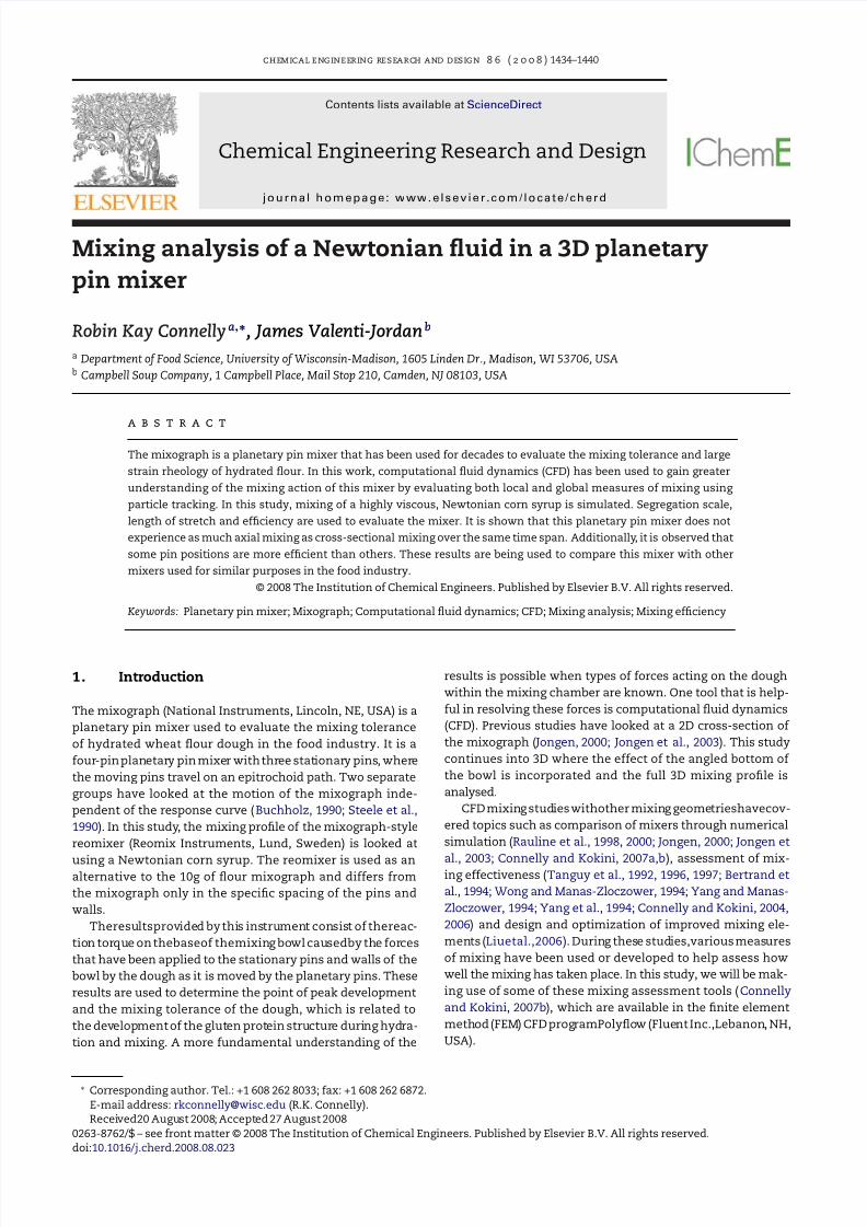
The mixer geometry is modelled as filled to 50 ml and the

meshes are shown in Fig. 1. The mesh elements are triangular

prisms. In the standard reference frame, the darker pins are

the moving pins, which follow an epitrochoid (planetary) pin

path, while the lighter pins are the stationary pins. The pin

motion is accounted for in the simulations using the mesh

superposition technique (Avalosse, 1996; Avalosse and Rubin,

2000). In order to simplify the pinpaths so that themesh could

be created to provide a consistent pin shape and volume at

every time step with this approach, the simulation is con-

Fig. 1 – Geometry and mesh where the pins with the light

grey tops are stationary in the standard reference frame.

ducted in the rotating reference frame (RRF). The wall of the

vessel and the “stationary” pins were set to rotate counter-

clockwise around the central vertical axis at the rate of the

primary gear (88 rpm), while the “moving” pins were set to

rotate clockwise around their vertical planetary axis at the

rate of the secondary gear (66 rpm). This approach also allows

the true epitrochoid (planetary) pin path to be modelled more

easily and the mesh to be better refined in the areas near thepins.

The 2D horizontal cross-section mesh selected as a start-

ing point for the 3D mesh was created such that the pin shape

remained a nearly constant hexagon made up of six trian-

gular elements with a time step of 0.0227 s that moved the

pins one element along the pin path. The 2D mesh was also

subjected to a mesh discretization and time step study using

quadratic FEM interpolation for velocity and linear continuous

FEM interpolation for pressure, where it was found that the

difference in the solution was only 2–3% along the pin paths

when themeshdensity wasincreased 16 times andonly about

0.14% if a four times smaller time step is used. Therefore, this

mesh was deemed adequate for use in this study. Also, analy-sis of the difference between the initial time steps on start-up

of the simulation and the results when those pin positions

were repeated showed that the results from the first 0.1 s of

the simulation should not be used for steady-state analysis,

due to start-up effects ( Jordan, 2006).

Globe Corn Syrup 011420 (Corn Products, Westchester,

IL), was selected as the test fluid because the single

proportionality constantof Newtonian viscositywas lesscom-

putationally difficult to simulate. Also, its viscosity lies in the

range of observed viscosities exhibited by developing dough

(Dhanasekharan et al., 1999). This corn syrup has a Newto-

nian viscosity of 5400 cP and a density of 1.409g/cm3 at 49 ◦C.

A no slip boundary condition was used at the walls and on thepins. The top surface was given a full slip boundary condition

but was otherwise constrained to maintain a flat shape.

The flow and mixing simulation was done using the FEM

CFD package Polyflow 3.10.2 (Fluent Inc., Lebanon, NH) with

a mesh created using Gambit 2.3 and post-processed using

Fieldview 10F (Intelligent Light, Rutherford, NJ). The simula-

tion was run on an IBM IntelliStation Z Pro with dual Intel

Xeon 3.4 GHz–64 bit processors and 6 GB RAM running Red

Hat Enterprise Linux WS 3. The 3D simulation was done using

mini-element velocity and linear pressure FEM interpolations.

With these FEM interpolation types, the problem size was

1.4 GB and took a CPU time of 12.68 h.

2.2. Particle tracking and visualizations

In orderto analyse theabilityof thereomixer to fully distribute

the fluid over the entire domain, the fate 10,000 initially ran-

domly distributed material points were studied over 360 time

steps for a total simulation time of 8.182s. In order to track

these points over time, Polyflow and its mixing post-processor,

Polystat, were usedto track the positionsof the 10,000 material

points over all the time steps using the flow profile solutions.

The trajectories of the massless material points or particles

were calculated by the time integration of the equation x = v

using a fourth order explicit Runge-Kutta scheme within an

element with local rather than global coordinates. The time

step was sized such that the final position in crossing an ele-

ment is always on the element boundary so that the element

coordinates maybe transformed to the localcoordinatesof the

next element to be crossed before continuing the integration.



1436 chemical engineering research and design 8 6 ( 2 0 0 8 ) 1434–1440

Fig. 2 – Horizontal mixing analysis: data at (a) 0, (b) 120, (c) 240, and (d) 360 time steps.

The sum of the steps when transformed to global coordinates

gives the successive positions of the particles in real space

(Debbaut et al., 1997; Ishikawa et al., 2001). The default of

an average of three steps to cross an element was chosen

for the time integration, with the particle positions and kine-

matic parameters recorded at the same time intervals as used

between pin positions. The results were visually inspected to

illustrate the flow profile within the mixer, as well as quanti-

tatively analysed to provide standard mixing indicators over

the entire flow field.

One analysis studied the mixing in the horizontal plane.

The randomly distributed material points were initially

divided along the x = 0 plane and arbitrarily assigned a con-centration value of 1 (light grey) or 0 (dark grey). A pictorial

representation of this division is shown in Fig. 2a. Comple-

tion of mixing is visually indicated by a random distribution

of light and dark grey points over the entire flow domain. In

a second analysis, several cutting planes were used to alter-

nate between zones of randomly distributed points initially

assigned a concentration value of 1 (light grey) or 0 (dark grey)

in order to determine the extent of vertical mixing because

low vertical mixing was expected in this geometry. The cut-

ting planes are located at a height of 1, 3, 5, 7, 9, 11, 13, 15,

17, and 19.698 mm, which created 11 sub-regions in the flow

domain, as shown in Fig. 3a.

2.3. Measures of mixing

The information generated from producing the visual depic-

tions of the mixing above were also analysed statistically. The

scale of segregation is a statistical measure of the mean dis-

tance from a point atwhich it is equally probable to find a light

grey point as a dark grey point. The positions of the particles

at any given time were used to calculate the value of the scale

of segregation, which is defined as (Dankwertz, 1952; Tadmore

and Gogos, 1979; Brodkey, 1985; Chella, 1994):

Ls =

0

R(|r|) d|r|,

Fig. 3 – Vertical mixing analysis: results at (a) 0 and (b) 360

time steps.




where

R(|r|) =

M

j=1(c j − c) · (c

j − c)

MS2 .

R(|r|) is the Eulerian coefficient of correlation between con-

centrations of pairs of points in the mixer separated by |r|

where R(0)=1 for points having the same correlation andR( )=0atlarge |r| where there is no correlation.The number of

pairs is M = N(N−1)/2 where N is the number of points and S2

is the sample variance. The concentration of the points in the

jth pair is c j

and c j , while c is the average concentration. The

minimum value occurs when the initially segregated particles

become randomly distributed and is a function of the number

of particles tracked and the size of the flow domain. Calcula-

tion of thescaleof segregationwas done at each recorded time

step in orderto track theevolutionof this parameterovertime.

If there are dead spots or faults in the flow that create areas

of the mixer where parts of the initially segregated material

cannot reach, this parameter will not be able to reduce to the

minimum value. In addition, the segregation scale is a globalaverage value that cannot pinpoint the exact location, size or

number of local flow defects (Dankwertz, 1952; Tadmore and

Gogos, 1979; Brodkey, 1985; Chella, 1994).

The 10,000 points were also used to follow the lamellar

mixing parameters, including length of stretch and efficiency

(Ottino et al., 1979, 1981; Ottino andChella, 1983; Ottino, 1989).

Given a motion x= (X, t) where initially X= (X, 0) for an

infinitesimal material line segment dx=F·dX located at posi-

tionx at time t andthe deformation tensoris F=, thelength

of stretch of a material line is defined as = |dx| /|dX|. The

arithmetic mean of the length of stretch, , has been shown

to be directly related to the geometric mean striation thick-

ness and is a measure of the growth of the interfacial area(Alvarez et al., 1998; Muzzio et al., 2000; Zalc et al., 2002). An

exponential increase in the length of stretch over time is a

necessary requirement for effective mixing (Ottino, 1989). The

local or instantaneous efficiency of mixing for isochoric flows

is defined as

e =/

(D : D)1/2 =

−D : ˆ m ˆ m

(D : D)1/2 =

D ln /Dt

(D : D)1/2 ,

where D is the rate of strain tensor, ˆ m is the current orienta-

tion unit vector and (D:D)1/2 is the limit of −D : ˆ m ˆ m according

to Cauchy–Schwarz’s inequality (Ottino et al., 1979, 1981). The

efficiency canbe thought of as the fraction of the energy dissi-

pated locally that is used to stretch a fluid element at a given

instant in a purely viscous fluid (Ottino, 1989) and falls in the

range {−1, 1}. A value of −1 would indicate that all the energy

dissipated was used to shorten the length of the material line,

in effect completely unmixing it, while a value of 1 indicates

that all the energy dissipated was used to stretch the material

line. The time-averaged efficiency is defined as (Ottino, 1989):

e = 1t

t0 e dt.

Typical behaviour of the time averaged mixing efficiency

ranges from the decay of the efficiency with time as t−1 for

flows with no reorientation such as the simple shearing flows,to flows with some periodic reorientation but still decaying

on average with time as t−1, to the optimum case for mixing,

which is flows with strong reorientation that have a positive,

constant average value of the efficiency (Ottino, 1989).

3. Results

3.1. Topographical mixing analysis and scale of

segregation

Fig. 2a shows the initial conditions of the 10,000 data points

discussed above. Fig. 2b and c shows the progression of the

mixing as bulk rotational flow has started in the mixer andareas where the pins have travelled are showing significantly

more blending of the differently shaded points. In Fig. 2d, the

mixing has approached completion at 360 timesteps, based on

optical verification. The main effect holding back the comple-

tion of the mixing is that the points at the walls have not been

displaced much. This lack of movement is due to fluid bound-

ary layers near the wall where there is a no slip boundary

condition, and has been seen experimentally in similar mix-

ers (Gouillart et al., 2007; Thiffeault et al., 2008). This has been

shown to reduce the overall mixing effectiveness for similar

mixers from exponential to power law (Gouillart et al., 2007;

Thiffeault et al., 2008).

When the mixing is analysed using the segregation scale,

the results in Fig. 4 show that most of the mixing takes

place early in the simulation. When a single dark grey par-

ticle invades a large volume of light grey particles, the average

distance for the light grey points to the nearest dark grey

point drops drastically. Therefore, the initial large drop in

segregation scale is expected and observed in Fig. 3. Over-

all, the segregation scale reduces to a nearly constant value

of ∼0.8mm by 270 time steps, which is near the minimum

possible with the level of discrimination available with 10,000

points.

Next, the vertical mixing capability of the reomixer is anal-

ysed. The 11 zones of alternating colour at time zero are

shown in Fig. 3a. As mixing progresses, only minimal mixing

is observed. In Fig. 3b, the points are just beginning to show

blending after 360 time steps. These results show that there is

relatively little vertical mixing in comparison to the amount

of horizontal mixing in the reomixer occurs during the 8.182s

simulated here. However, the slow vertical mixing seen in the

simulation should still provide significant vertical distributive

mixing in the normal run time of this mixer, which is on the

order to 10 min.

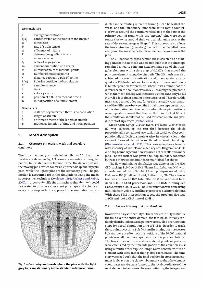
The initial segregation scale value for the axial mixing case

shown in Fig. 5 was much lower than initial value for the hor-

izontal mixing analysis due to the effect of the initial multiple

layers. However, the initial slope was much lower, so that the

Fig. 4 – Segregation scale of vertically divided particles for

analysis of horizontal mixing.




Fig. 5 – Segregation scale of horizontally divided particles

for analysis of axial mixing.

Fig. 6 – Log of the length of stretch.

value after 360 time steps was higher than that of the hori-

zontal mixing analysis case. There was also little indication of

levelling off to a constant value within the timeframe of the

simulation.

Fig. 5 also shows that thesegregation scale data was mildly

oscillating along its decline. The period of the oscillations was

every 20 time steps, which was the same frequency that the

mixer takes to produce a geometrically similar orientation.

This indicates some periodic reorientation or “un-mixing” of

the material being mixed.

The oscillations were also present in the results shown in

Fig. 4, but are much easier to see with this narrow segrega-tion scale range. These results were not unexpected since the

straight vertical pins did not provide any vertical pumping

and the simplification of a fixed, flat shape for the top sur-

face used in the simulation further constrains vertical motion

of the fluid.

3.2. Length of stretch and efficiency

The purpose of tracking the length of stretch is to under-

stand how much the material is being stretchedin a particular

region. Thelength of stretch is a measure of how mucha mate-

rial point, conceptualized as an infinitesimal line, is stretched

over time. The length of stretch was tracked over time and

recorded in Fig. 6 as the logarithm of the value of the stretch.

It showed good mixing represented by a logarithmic increase

in the length of stretch (Avalosse and Rubin, 2000). The stan-

dard deviation also increased with time because there were

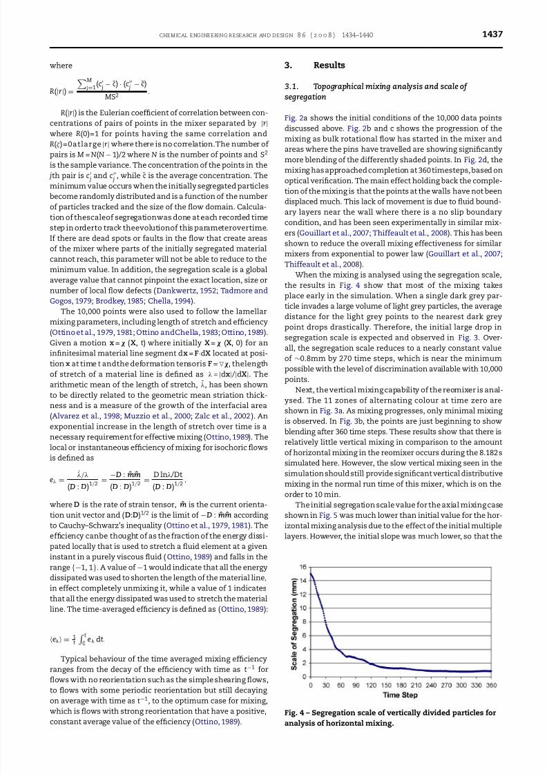
Fig. 7 – Length of stretch distribution at 360 time steps.

some points that did not experience much stretch, especially

along the walls as shown in Fig. 7.

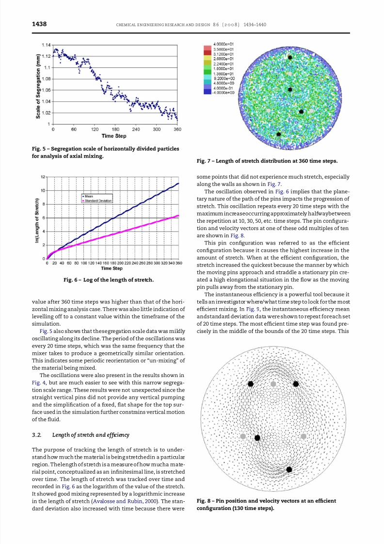
The oscillation observed in Fig. 6 implies that the plane-tary nature of the path of the pins impacts the progression of

stretch. This oscillation repeats every 20 time steps with the

maximum increaseoccurring approximately halfwaybetween

the repetition at 10, 30, 50, etc. time steps. The pin configura-

tion and velocity vectors at one of these odd multiples of ten

are shown in Fig. 8.

This pin configuration was referred to as the efficient

configuration because it causes the highest increase in the

amount of stretch. When at the efficient configuration, the

stretch increased the quickest because the manner by which

the moving pins approach and straddle a stationary pin cre-

ated a high elongational situation in the flow as the moving

pin pulls away from the stationary pin.The instantaneous efficiency is a powerful tool because it

tells an investigator where/what time step to look for the most

efficient mixing. In Fig. 9, the instantaneous efficiency mean

andstandard deviation data were shown to repeat foreach set

of 20 time steps. The most efficient time step was found pre-

cisely in the middle of the bounds of the 20 time steps. This

Fig. 8 – Pin position and velocity vectors at an efficient

configuration (130 time steps).




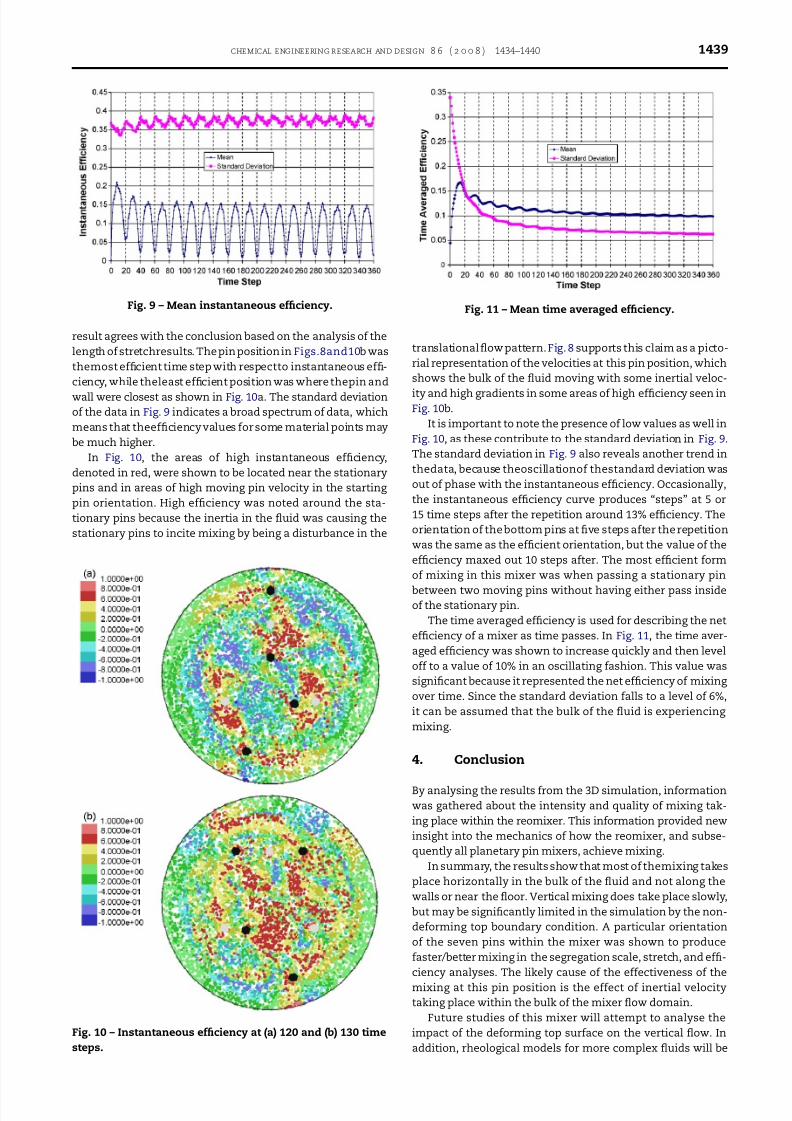
Fig. 9 – Mean instantaneous efficiency.

result agrees with the conclusion based on the analysis of the

length of stretchresults. The pin position in Figs.8and10b was

themost efficient time step with respectto instantaneous effi-

ciency, while theleast efficient position was where thepin and

wall were closest as shown in Fig. 10a. The standard deviationof the data in Fig. 9 indicates a broad spectrum of data, which

means that theefficiency values for some material points may

be much higher.

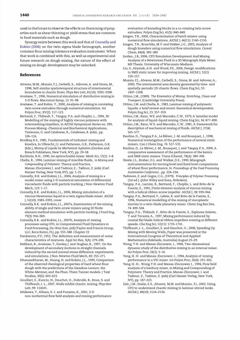
In Fig. 10, the areas of high instantaneous efficiency,

denoted in red, were shown to be located near the stationary

pins and in areas of high moving pin velocity in the starting

pin orientation. High efficiency was noted around the sta-

tionary pins because the inertia in the fluid was causing the

stationary pins to incite mixing by being a disturbance in the

Fig. 10 – Instantaneous efficiency at (a) 120 and (b) 130 time

steps.

Fig. 11 – Mean time averaged efficiency.

translational flow pattern. Fig. 8 supports this claim as a picto-

rial representation of the velocities at this pin position, which

shows the bulk of the fluid moving with some inertial veloc-

ity and high gradients in some areas of high efficiency seen inFig. 10b.

It is important to note the presence of low values as well in

Fig. 10, as these contribute to the standard deviation in Fig. 9.

The standard deviation in Fig. 9 also reveals another trend in

thedata, because theoscillationof thestandard deviation was

out of phase with the instantaneous efficiency. Occasionally,

the instantaneous efficiency curve produces “steps” at 5 or

15 time steps after the repetition around 13% efficiency. The

orientation of the bottom pins at five steps after the repetition

was the same as the efficient orientation, but the value of the

efficiency maxed out 10 steps after. The most efficient form

of mixing in this mixer was when passing a stationary pin

between two moving pins without having either pass insideof the stationary pin.

The time averaged efficiency is used for describing the net

efficiency of a mixer as time passes. In Fig. 11, the time aver-

aged efficiency was shown to increase quickly and then level

off to a value of 10% in an oscillating fashion. This value was

significant because it represented the net efficiency of mixing

over time. Since the standard deviation falls to a level of 6%,

it can be assumed that the bulk of the fluid is experiencing

mixing.

4. Conclusion

By analysing the results from the 3D simulation, informationwas gathered about the intensity and quality of mixing tak-

ing place within the reomixer. This information provided new

insight into the mechanics of how the reomixer, and subse-

quently all planetary pin mixers, achieve mixing.

In summary, the results show that most of themixing takes

place horizontally in the bulk of the fluid and not along the

walls or near the floor. Vertical mixing does take place slowly,

but may be significantly limited in the simulation by the non-

deforming top boundary condition. A particular orientation

of the seven pins within the mixer was shown to produce

faster/better mixing in the segregation scale, stretch, and effi-

ciency analyses. The likely cause of the effectiveness of the

mixing at this pin position is the effect of inertial velocity

taking place within the bulk of the mixer flow domain.

Future studies of this mixer will attempt to analyse the

impact of the deforming top surface on the vertical flow. In

addition, rheological models for more complex fluids will be




used in thefuture to observe the effects on themixing of prop-

erties such as shear thinning or yield stress that are common

in food materials such as dough.

Synergy exists between this work and that of Connelly and

Kokini (2006) on the twin sigma blade farinograph, another

common flour mixing tolerance evaluation instrument. When

that work is combined with this, as well as experimental and

future research on dough mixing, the nature of the effect of mixing on dough development may be unlocked.

References

Alvarez, M.M., Muzzio, F.J., Cerbelli, S., Adrover, A. and Giona, M.,1998, Self-similar spatiotemporal structure of intermaterialboundaries in chaotic flows. Phys Rev Lett, 81(16): 3395–3398.

Avalosse, T., 1996, Numerical simulation of distributive mixing in3-D flows. Macromol Symp, 12: 91–98.

Avalosse, T. and Rubin, Y., 2000, Analysis of mixing in corotating twin screw extruders through numerical simulation. IntPolym Proc, XV(2): 117–123.

Bertrand, F., Thibault, F., Tanguy, P.A. and Choplin, L., 1994, 3D

Modelling of the mixing of highly viscous polymers withintermeshing impellers, in AIChE Symposium Series no. 299,Process Mixing -Chemical and Biochemical Applications,Tatterson, G. and Calabrese, R., Calabrese, R. (eds) , pp.106–116.

Brodkey, R.S., 1985, Fundamentals of turbulent mixing andkinetics, In Ulbrecht, J.J. and Patterson, G.K., Patterson, G.K.(Eds.), Mixing of Liquids by Mechanical Agitation (Gordon andBreach Publishers, New York, NY), pp. 29–58.

Buchholz, R.H., 1990, An epitrochoidal mixer. Math Sci, 15(1): 1–8.Chella, R., 1994, Laminar mixing of miscible fluids, in Mixing and

Compounding of Polymers: Theory and Practice,Manas-Zloczower, I. and Tadmor, Z., Tadmor, Z. (eds) (CarlHanser Verlag, New York, NY), pp. 1–25.

Connelly, R.K. and Kokini, J.L., 2004, Analysis of mixing in amodel mixer using 2-D numerical simulation of differentialviscoelastic fluids with particle tracking. J Non-Newton FluidMech, 123: 1–17.

Connelly, R.K. and Kokini, J.L., 2006, Mixing simulation of aviscous Newtonian liquid in a twin sigma blade mixer. AIChE

J, 52(10): 3383–3393, coverConnelly, R.K. and Kokini, J.L., 2007a, Examination of the mixing

ability of single and twin screw mixers using 2D finiteelement method simulation with particle tracking. J Food Eng,79(3): 956–969.

Connelly, R.K. and Kokini, J.L., 2007b, Analysis of mixing processes using CFD, in Computational Fluid Dynamics inFood Processing, Da-Wen Sun, (ed) (Taylor and Francis Group,LLC, Boca Raton, FL), pp. 555–588. Chapter 23

Dankwertz, P.V., 1952, The definition and measurement of somecharacteristics of mixtures. Appl Sci Res, 3(A): 279–296.

Debbaut, B., Avalosse, T., Dooley, J. and Hughes, K., 1997, On thedevelopment of secondary motions in straight channelsinduced by the second normal stress difference: experimentsand simulations. J Non-Newton Fluid Mech, 69: 255–271.

Dhanasekharan, M., Huang, H. and Kokini, J.L., 1999, Comparisonof the observed rheological properties of hard wheat flourdough with the predictions of the Giesekus-Leonov, theWhite-Metzner, and the Phan-Thien Tanner models. J TextStudies, 30(5): 603–623.

Gouillart, E., Kuncio, N., Dauchot, O., Dubrulle, B., Roux, S. andThiffeault, J.-L., 2007, Walls inhibit chaotic mixing. Phys RevLett, 99: 114501.

Ishikawa, T., Kihara, S.-I. and Funatsu, K., 2001, 3-Dnon-isothermal flow field analysis and mixing performance

evaluation of kneading blocks in a co-rotating twin screwextruders. Polym Eng Sci, 41(5): 840–849.

Jongen, T.R., 2000, Characterization of batch mixers using numerical flow simulations. AIChE J, 46(11): 2140–2150.

Jongen, T.R., Bruschke, M.V. and Dekker, J.G., 2003, Analysis of dough kneaders using numerical flow simulations. CerealChem, 84(4): 383–389.

Jordan., J.B., 2006, CFD Simulation Development And Mixing

Analysis of a Newtonian Fluid in a 3D Mixograph Style Mixer.MS Thesis. University of Wisconsin-Madison.

Liu, S., Hrymak, A.N. and Wood, P.E., 2006, Design modificationsto SMX static mixer for improving mixing. AIChE J, 52(1):150–157.

Muzzio, F.J., Alvarez, M.M., Cerbelli, S., Giona, M. and Adrover, A.,2000, The intermaterial area density generated by time- andspatially-periodic 2D chaotic flows. Chem Eng Sci, 55:1497–1508.

Ottino, J.M., (1989). The Kinematics of Mixing: Stretching, Chaos and

Transport. (Cambridge University Press).Ottino, J.M. and Chella, R., 1983, Laminar mixing of polymeric

liquids: a brief review and recent theoretical developments.Polym Eng Sci, 23: 357–359.

Ottino, J.M., Ranz, W.E. and Macosko, C.W., 1979, A lamellar model

for analysis of liquid–liquid mixing. Chem Eng Sci, 34: 877–890.Ottino, J.M., Ranz, W.E. and Macosko, C.W., 1981, A framework for

description of mechanical mixing of fluids. AIChE J, 27(4):565–577.

Rauline, D., Tanguy, P.A., Le Blévec, J.-M. and Bousquet, J., 1998,Numerical investigation of the performance of several staticmixers. Can J Chem Eng, 76: 527–535.

Rauline, D., Le Blévec, J.-M., Bousquet, J. and Tanguy, P.A., 2000, Acomparative assessment of the performance of the kenicsand SMX static mixers. Trans IChemE, 78(A): 389–396.

Steele, J.L., Brabec, D.L. and Walker, D.E., 1990, Mixographinstrumentation for moving bowl and fixed bowl comparisonsof wheat flour performance, In Proceedings of the Food Processing

Automation Conference , pp. 224–234.Tadmore, Z. and Gogos, C.G., (1979). Principles of Polymer Processing

(1st ed.). (John Wiley and Sons, Hoboken).Tanguy, P.A., Lacroix, R., Bertrand, F., Choplin, L. and Brito-de la

Fuente, E., 1992, Finite element analysis of viscous mixing with a helical ribbon-screw impeller. AIChE J, 38: 939–944.

Tanguy, P.A., Bertrand, F., Labrie, R. and Brito-de la Fuente, E.,1996, Numerical modelling of the mixing of viscoplasticslurries in a twin-blade planetary mixer. Chem Eng Res Des,74: 499–504.

Tanguy, P.A., Thibault, F., Brito-de la Fuente, E., Espinosa-Solares,T. and Tecante, A., 1997, Mixing performance induced bycoaxial flat blade-helical ribbon impellers rotating at differentspeeds. Che Eng Sci, 52(11): 1733–1741.

Thiffeault, J.-L., Gouillart, E. and Dauchot, O., 2008, Speeding UpMixing with Moving Walls, Paper was presented at theInternational Congress of Theoretical and AppliedMathematics (Adelaide, Australia) August 25–29.

Wong, T.H. and Manas-Zloczower, I., 1994, Two-dimensionaldynamic study of the distributive mixing in an internal mixer.Int Polym Proc, IX(1): 3–10.

Yang, H.-H. and Manas-Zloczower, I., 1994, Analysis of mixing performance in a VIC mixer. Int Polym Proc, IX(4): 291–302.

Yang, H.-H., Wong, T.H. and Manas-Zloczower, I., 1994, Flow fieldanalysis of a banbury mixer, in Mixing and Compounding of Polymers: Theory and Practice, Manas-Zloczower, I. andTadmor, Z., Tadmor, Z. (eds) (Carl Hanser Verlag, New York,NY), pp. 187–223.

Zalc, J.M., Szalai, E.S., Alvarez, M.M. and Muzzio, F.J., 2002, Using CFD to understand chaotic mixing in laminar stirred tanks.AIChE J, 48(10): 2124–2134.

Documents

Technical Paper - Mixing Analysis of a Newtonion Fluid