University of South Florida University of South Florida

Scholar Commons Scholar Commons

Graduate Theses and Dissertations Graduate School

November 2019

Simulation and Experimental Investigation of Fluid Mixing Simulation and Experimental Investigation of Fluid Mixing

Enhancement with Orifice Plate Enhancement with Orifice Plate

Mohammed Al Busaidi University of South Florida

Follow this and additional works at: https://scholarcommons.usf.edu/etd

Part of the Other Education Commons

Scholar Commons Citation Scholar Commons Citation Al Busaidi, Mohammed, "Simulation and Experimental Investigation of Fluid Mixing Enhancement with Orifice Plate" (2019). Graduate Theses and Dissertations. https://scholarcommons.usf.edu/etd/8616

This Thesis is brought to you for free and open access by the Graduate School at Scholar Commons. It has been accepted for inclusion in Graduate Theses and Dissertations by an authorized administrator of Scholar Commons. For more information, please contact scholarcommons@usf.edu.

Simulation and Experimental Investigation of Fluid Mixing Enhancement with Orifice Plate

by

Mohammed Al Busaidi

A thesis submitted in partial fulfillment

of the requirements for the degree of

Master of Science in Mechanical Engineering

Department of Mechanical Engineering

College of Engineering

University of South Florida

Major Professor: Rasim Guldiken, Ph.D.

David Murphy, Ph.D.

Andres Tejada-Martinez, Ph.D.

Date of Approval:

October 28, 2019

Keywords: Fluid Mechanics, Mixing Efficiency, Microfluidics

Copyright © 2019, Mohammed Al Busaidi

Dedication

I would like to dedicate this thesis to all of my family including my parents, brothers and

sisters. They have helped me in every way possible and supported me through the pursuit of my

Master’s degree.

Acknowledgments

Special thanks to Dr. Andres Tejada-Martinez for his knowledge contribution to the

simulation part of my research. He has cleared doubts that I had about how fluid flow simulation

operates. Great appreciation to Dr. David Murphy for his knowledge in experimental analysis

and for providing me with papers that have helped me complete this thesis. I would also like to

thank Dr. Murphy for allowing me to borrow equipment from his lab that was needed to conduct

the experiments. Also credits to Dr. Rasim Guldiken for his continued support during my pursuit

for this degree. This would not have been possible without his help and supervision during my

studies.

iv

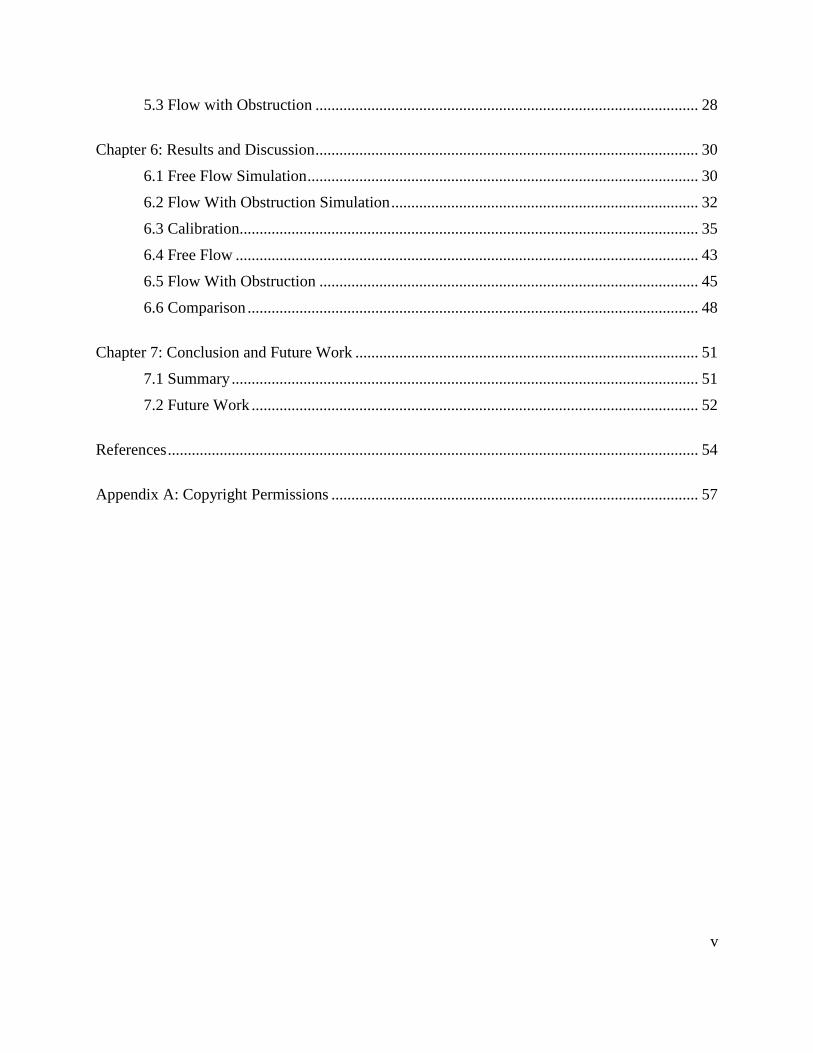
Table of Contents

List of Tables ................................................................................................................................. vi

List of Figures .............................................................................................................................. viii

Abstract ........................................................................................................................................... x

Chapter 1: Introduction ................................................................................................................... 1

1.1 Motivation ..................................................................................................................... 1

1.2 Thesis Organization ...................................................................................................... 2

Chapter 2: Fluid Mixing and Measurement Methods ..................................................................... 4

2.1 Mixing Methods ............................................................................................................ 4

2.2 Measurement Methods .................................................................................................. 6

Chapter 3: Simulation of Two Fluids Through a Pipe .................................................................. 10

3.1 Geometric Model ........................................................................................................ 10

3.2 Meshing....................................................................................................................... 11

3.3 Set Up.......................................................................................................................... 14

3.4 Simulation With Orifice Plate ..................................................................................... 15

Chapter 4: Sensor Calibration ....................................................................................................... 18

4.1 About the Sensor ......................................................................................................... 18

4.2 Set Up.......................................................................................................................... 19

4.3 Mixing of Two Different Colored Mixtures of Water ................................................ 21

Chapter 5: Light Reflection and Mixing ....................................................................................... 23

5.1 Geometrical Set Up ..................................................................................................... 23

5.2 Flow Mechanics .......................................................................................................... 24

v

5.3 Flow with Obstruction ................................................................................................ 28

Chapter 6: Results and Discussion ................................................................................................ 30

6.1 Free Flow Simulation .................................................................................................. 30

6.2 Flow With Obstruction Simulation ............................................................................. 32

6.3 Calibration................................................................................................................... 35

6.4 Free Flow .................................................................................................................... 43

6.5 Flow With Obstruction ............................................................................................... 45

6.6 Comparison ................................................................................................................. 48

Chapter 7: Conclusion and Future Work ...................................................................................... 51

7.1 Summary ..................................................................................................................... 51

7.2 Future Work ................................................................................................................ 52

References ..................................................................................................................................... 54

Appendix A: Copyright Permissions ............................................................................................ 57

vi

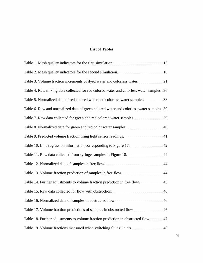
List of Tables

Table 1. Mesh quality indicators for the first simulation. ..................................................13

Table 2. Mesh quality indicators for the second simulation. .............................................16

Table 3. Volume fraction increments of dyed water and colorless water. .........................21

Table 4. Raw mixing data collected for red colored water and colorless water samples. .36

Table 5. Normalized data of red colored water and colorless water samples. ...................38

Table 6. Raw and normalized data of green colored water and colorless water samples. .39

Table 7. Raw data collected for green and red colored water samples. .............................39

Table 8. Normalized data for green and red color water samples. ....................................40

Table 9. Predicted volume fraction using light sensor readings. .......................................41

Table 10. Line regression information corresponding to Figure 17. .................................42

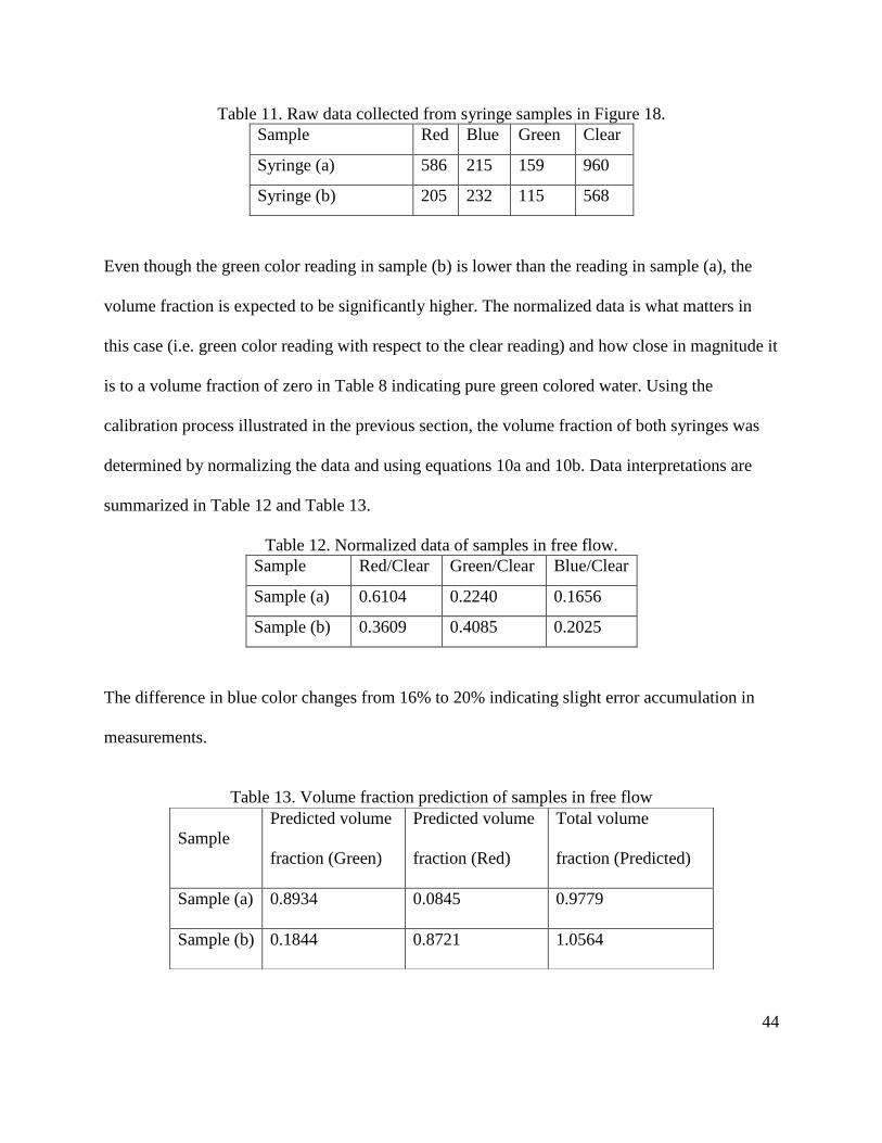
Table 11. Raw data collected from syringe samples in Figure 18. ....................................44

Table 12. Normalized data of samples in free flow. ..........................................................44

Table 13. Volume fraction prediction of samples in free flow ..........................................44

Table 14. Further adjustments to volume fraction prediction in free flow. .......................45

Table 15. Raw data collected for flow with obstruction. ...................................................46

Table 16. Normalized data of samples in obstructed flow .................................................46

Table 17. Volume fraction predictions of samples in obstructed flow ..............................46

Table 18. Further adjustments to volume fraction prediction in obstructed flow. .............47

Table 19. Volume fractions measured when switching fluids’ inlets. ...............................48

vii

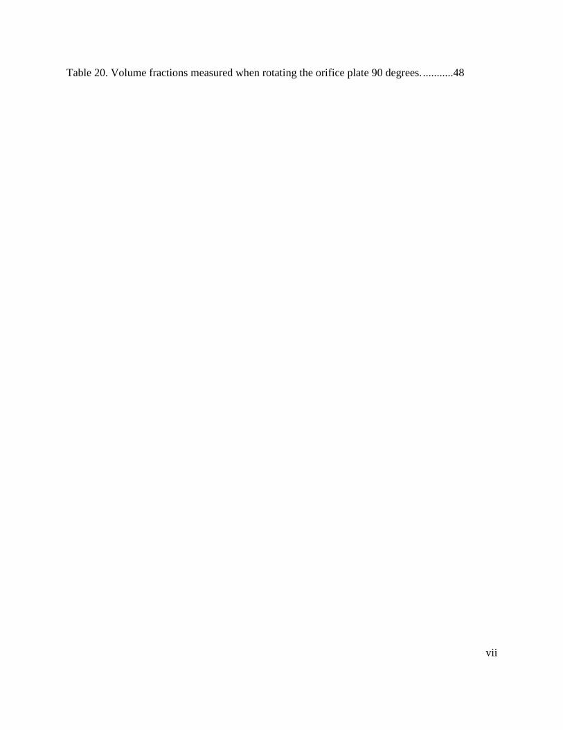
Table 20. Volume fractions measured when rotating the orifice plate 90 degrees. ...........48

viii

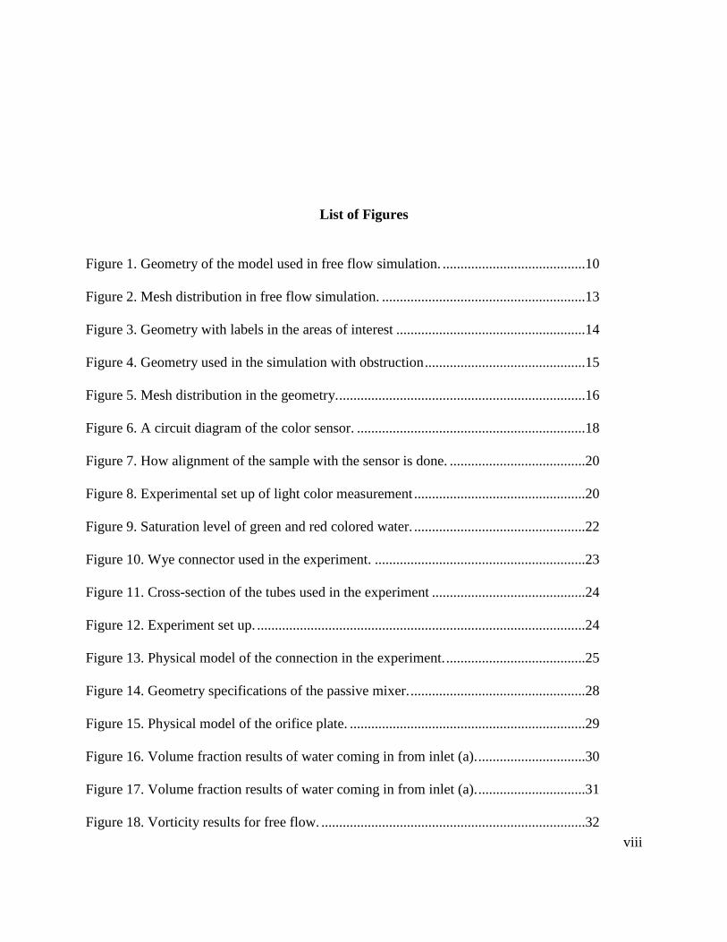
List of Figures

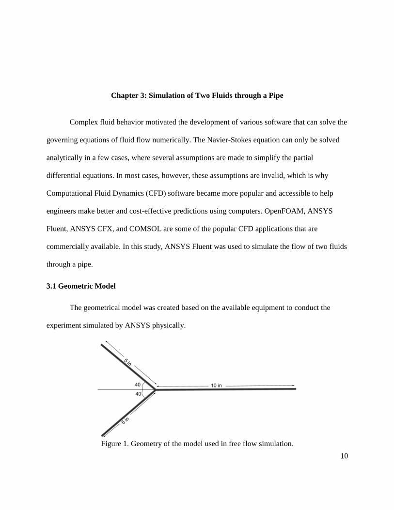
Figure 1. Geometry of the model used in free flow simulation. ........................................10

Figure 2. Mesh distribution in free flow simulation. .........................................................13

Figure 3. Geometry with labels in the areas of interest .....................................................14

Figure 4. Geometry used in the simulation with obstruction .............................................15

Figure 5. Mesh distribution in the geometry. .....................................................................16

Figure 6. A circuit diagram of the color sensor. ................................................................18

Figure 7. How alignment of the sample with the sensor is done. ......................................20

Figure 8. Experimental set up of light color measurement ................................................20

Figure 9. Saturation level of green and red colored water. ................................................22

Figure 10. Wye connector used in the experiment. ...........................................................23

Figure 11. Cross-section of the tubes used in the experiment ...........................................24

Figure 12. Experiment set up. ............................................................................................24

Figure 13. Physical model of the connection in the experiment. .......................................25

Figure 14. Geometry specifications of the passive mixer. .................................................28

Figure 15. Physical model of the orifice plate. ..................................................................29

Figure 16. Volume fraction results of water coming in from inlet (a). ..............................30

Figure 17. Volume fraction results of water coming in from inlet (a). ..............................31

Figure 18. Vorticity results for free flow. ..........................................................................32

ix

Figure 19. Results of the simulation with obstruction of fluid from inlet (a). ...................33

Figure 20. Results of the simulation with obstruction of fluid from inlet (b). ...................34

Figure 21.Vorticity of flow with obstruction.. ...................................................................35

Figure 22. Volume fraction of fluid from inlet (a) along the top surface. .........................36

Figure 23. Graphical representation of Table 4 .................................................................37

Figure 24. Linear regression models of measured and predicted volume fractions. .........42

Figure 25. Samples collected from free flow on both sides. ..............................................43

Figure 26. Samples collected from both sides of the obstructed flow. ..............................45

Figure 27. Experimental set up. .........................................................................................49

Figure 28. Volume fraction distribution. ...........................................................................51

x

Abstract

Current experimental and simulation fluid mixing studies aim to increase mixing

efficiency and incorporate various measurement methods to quantify mixing. In this thesis,

comprehensive simulation and experimental studies were carried out to investigate the effects of

an orifice plate on mixing. Mixing efficiency is measured through the correlation of volume

fraction to color light reflectivity, as dyes were introduced to the fluids being mixed. Volume

fractions close to 0.5 indicate high mixing performance, and the efficiency declines as volume

fractions depart from 0.5. It was found that fluids in a small diameter tube do not mix due to the

absence of eddies or swirling motions. Measurements were taken at regions away from the

centerline of the tube and volume fractions of 0.85 and 0.91 were obtained.

Fluids have shown significant mixing performance when passing through the orifice plate. The

regions where samples were taken after the obstruction were maintained and volume fractions of

0.59 and 0.45 were recorded. Simulation results were also analyzed and compared against

experimental results. The simulation was then used to investigate vorticity effects on mixing in

and around the plate. Results show that higher vorticity occurs in the plate and that is where

higher mixing performance is observed when volume fraction results are displayed. This

indicates that an orifice plate is an effective passive mixing method to implement in a flow for

wide variety of applications.

1

Chapter 1: Introduction

Fluid mixing is used in many industries such as chemical, pharmaceutical, pulp and paper

and oil and gas. In 1989, low efficiency mixing costs ranged from $1 billion to $10 billion in the

U.S. alone [1]. Therefore, significant effort has been focused on researching more efficient

mixers.

Mixing can be defined as the reduction of inhomogeneity while achieving the desired

result [1]. Fluid mixing can be classified into two main categories: active and passive. Active

mixing involves the use of an external power source, such as a motor. On the other hand, passive

mixing is purely dependent on the geometry of the flow and how it can be manipulated to

maximize mixing efficiency at low costs. The benefit of passive mixing is that it is cost-effective

and mixing activity can be achieved without power sources. However, the downside is that it

does not compete with active mixing in performance [2]. In small diameter tubes, mixing is

challenging due to low Reynold’s number resulting in laminar flow.

1.1 Motivation

The motive behind the research in fluid mixing is the development of an optimal drug

composition against liver tumor. The drug works by mixing two fluids using two syringes and a

connector, where the hole in the connector is adjustable. Mixing the two fluids using this method

requires time for efficient mixing and energy to stroke the fluids back and forth; this has

2

motivated the engineering department to research and develop a comfortable and more

convenient method to mix the two fluids.

Given the importance of the process, a passive mixer was proposed to mix the fluids

promptly and effortlessly. The idea of the passive mixer is to allow the fluid to flow through a

smaller diameter hole while changing direction. Fluids have shown mixing activity when they

change direction [3]. They also start to form vortices at high velocities even at low Reynold’s

number [4-9].

Since mixing is not a well-defined quantity, a new way of measuring mixing was

investigated, where different color dyes are introduced to the fluids and the wavelength of the

reflected light is analyzed to determine the volume fraction of the fluid.

1.2 Thesis Organization

This thesis is organized in such a manner that presents the simulation work and

experiments conducted during the research. An additional chapter has been reserved to illustrate

how the sensor was calibrated and to determine the volume fraction of a fluid sample. The

organization of this thesis is as follows.

Chapter 2: This chapter discusses what other researchers have done in the field and their

way of measuring mixing. It outlines the advantages and disadvantages of the methods

used for measurement and as well as the method used in this research.

Chapter 3: Computational Fluid Dynamics software has many components that can be

modified to simulate the desired experiment. This chapter discusses setting up the

simulation before it was allowed to run and additional details such as the geometry of the

model, boundary conditions and numerical specifications.

3

Chapter 4: The calibration of the sensor is a lengthy process and requires effort. How the

sensor was calibrated and correlated with the volume fraction is discussed in this chapter.

Chapter 5: This chapter discusses the experimental set up used, the methods used to

collect samples and measure them, and the mechanics of the flow along with the

calculations such as calculating Reynold’s number at different sections of the flow and

the conservation of mass principle.

Chapter 6: This is an outline of the results obtained from all experiments including

simulations. In this chapter, the results and their interpretations are discussed. The results

of different experiments are analyzed and compared to each other.

Chapter 7: A conclusion of all the discussions and results in this research. Also, a future

work section outlines what can be researched further in this study.

4

Chapter 2: Fluid Mixing and Measurement Methods

Quantifying mixing is challenging and researchers have correlated different physical quantities

that can indicate whether a fluid is adequately mixed. Moreover, fluid mixing is not a well define

quantity, which means that there are no physical quantities that can perfectly describe how much

two fluids have mixed.

2.1 Mixing Methods

In general, there are two classes of mixing. An example of active mixing is using a

surface acoustic wave (SAW) to push two fluids in a micro-channel to merge into one fluid [10].

This works by merging two fluids through a wye connector and allowing them to flow in a

microchannel, where one fluid dominates the top portion and the other fluid dominates the

bottom portion of the channel. Multiple experiments were carried out to compare the effects of

using one SAW and two SAW’s with free flow. All measurements were taken at a region of

interest for all experiments and better mixing was extrapolated from the results [11].

Yang et al. designed and manufactured a micromixer that uses ultrasonic vibrations to

enhance mixing. The device is made up of two inlets and one outlet separated by a mixing

chamber. The mixing chamber is made up of a piezoelectric material, where square waves are

generated to it to excite movement. Multiple experiments were carried out, where the frequency

of vibration varies to investigate the optimal frequency for mixing efficiency. There was no

5

mixing activity that can be observed for vibrations below 8 kHz, however, as the power input

increased, the fluids showed higher mixing surface area even at constant frequencies [12].

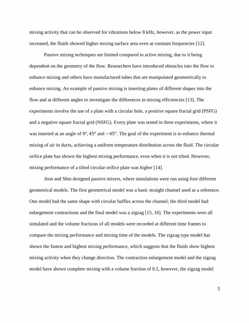
Passive mixing techniques are limited compared to active mixing, due to it being

dependent on the geometry of the flow. Researchers have introduced obstacles into the flow to

enhance mixing and others have manufactured tubes that are manipulated geometrically to

enhance mixing. An example of passive mixing is inserting plates of different shapes into the

flow and at different angles to investigate the differences in mixing efficiencies [13]. The

experiments involve the use of a plate with a circular hole, a positive square fractal grid (PSFG)

and a negative square fractal grid (NSFG). Every plate was tested in three experiments, where it

was inserted at an angle of 0°, 45° and −45°. The goal of the experiment is to enhance thermal

mixing of air in ducts, achieving a uniform temperature distribution across the fluid. The circular

orifice plate has shown the highest mixing performance, even when it is not tilted. However,

mixing performance of a tilted circular orifice plate was higher [14].

Jeon and Shin designed passive mixers, where simulations were run using four different

geometrical models. The first geometrical model was a basic straight channel used as a reference.

One model had the same shape with circular baffles across the channel; the third model had

enlargement contractions and the final model was a zigzag [15, 16]. The experiments were all

simulated and the volume fractions of all models were recorded at different time frames to

compare the mixing performance and mixing time of the models. The zigzag type model has

shown the fastest and highest mixing performance, which suggests that the fluids show highest

mixing activity when they change direction. The contraction enlargement model and the zigzag

model have shown complete mixing with a volume fraction of 0.5, however, the zigzag model

6

was completely mixed in 22.5 seconds compared to the contraction enlargement model that was

mixed in 23 seconds [3].

The results of the experiments carried out suggest that active mixers have a higher mixing

efficiency, however, active mixers can be challenging to implement in some situations and they

require an energy source. Passive mixers have shown decent mixing performance and they only

require manipulation of the flow geometry. Experiments have proved that mixing performance is

at its peak when two fluids change direction [3], which is why an orifice plate was designed and

introduced at a 45-degree angle.

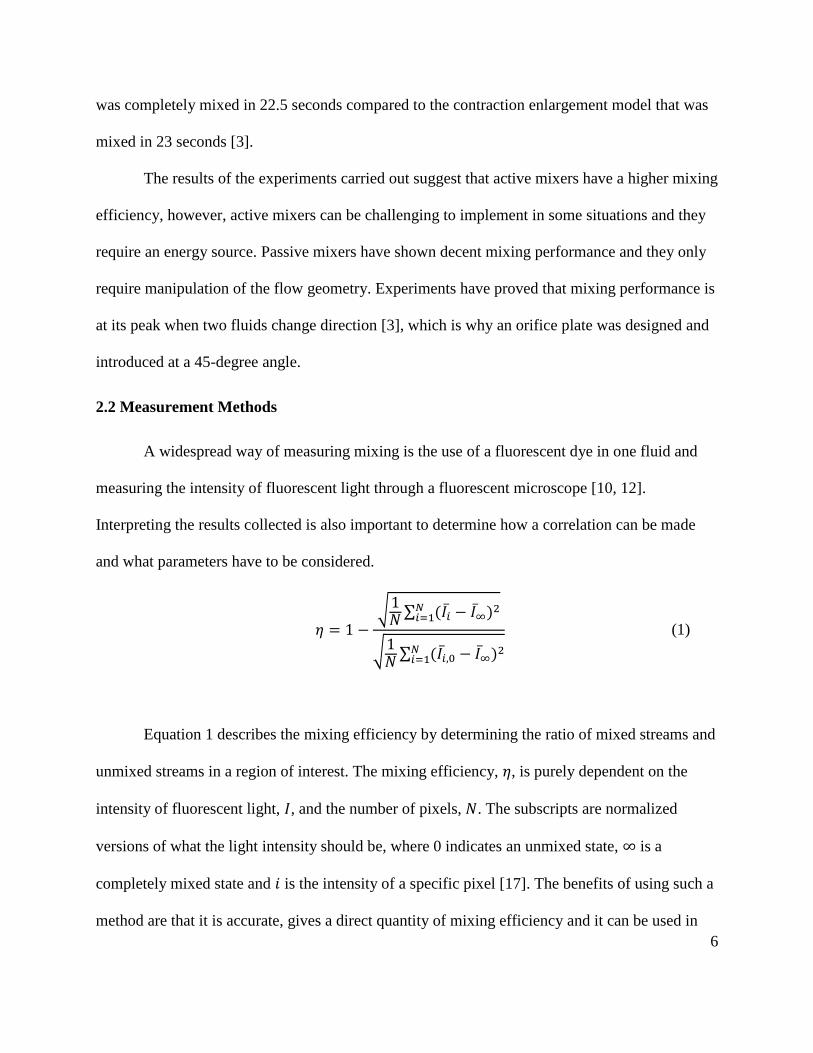
2.2 Measurement Methods

A widespread way of measuring mixing is the use of a fluorescent dye in one fluid and

measuring the intensity of fluorescent light through a fluorescent microscope [10, 12].

Interpreting the results collected is also important to determine how a correlation can be made

and what parameters have to be considered.

𝜂 = 1 −√1𝑁∑ (𝐼�̅� − 𝐼∞̅)2𝑁𝑖=1

√1𝑁∑ (𝐼�̅�,0 − 𝐼∞̅)2𝑁𝑖=1

(1)

Equation 1 describes the mixing efficiency by determining the ratio of mixed streams and

unmixed streams in a region of interest. The mixing efficiency, 𝜂, is purely dependent on the

intensity of fluorescent light, 𝐼, and the number of pixels, 𝑁. The subscripts are normalized

versions of what the light intensity should be, where 0 indicates an unmixed state, ∞ is a

completely mixed state and 𝑖 is the intensity of a specific pixel [17]. The benefits of using such a

method are that it is accurate, gives a direct quantity of mixing efficiency and it can be used in

7

very small diameter tubes. Drawbacks include a high number of pixels has to be used to obtain

accurate measurements and the equipment required are expensive. Yang et al. have used the

same methodology to monitor the mixing activity inside the mixing chamber but failed to obtain

quantitative results [12].

Mixing performance can also be estimated by measuring temperature. Two fluids of

different temperatures will show a uniform temperature distribution when perfectly mixed and

high-temperature gradients when they are unmixed [18]. Liang Teh et al. introduced an

important parameter that can be calculated to describe mixing performance.

Θ =

𝑇𝐻 − 𝑇𝑎,𝑎𝑣𝑒𝑇𝑎,𝑚𝑎𝑥 − 𝑇𝑎,𝑚𝑖𝑛

(2)

Equation 2 is used to describe the mixing performance of two fluids (both being air in

this experiment) coming from two different inlets, where one fluid is at a high temperature and

another is at a low temperature. 𝑇𝐻 is the temperature of the hot air, 𝑇𝑎,𝑎𝑣𝑒 is the average

temperature of the air in the mixed channel, 𝑇𝑎,𝑚𝑎𝑥 is the maximum temperature in the channel,

and 𝑇𝑎,𝑚𝑖𝑛 is the minimum temperature in the channel [13]. The equation shows that if the

difference between the maximum and minimum temperature is high, the mixing performance

will be lower and vice versa. This is an excellent method to calculate mixing performance

because it provides a quantitative parameter for mixing and it can be compared to mixing

performance in other experiments. However, using temperature to calculate mixing performance

introduces a significant error that is not accounted for, which is the conduction of heat transfer.

Using this method assumes that heat is transferred by pure advection and it can only be used for

fluids with identical thermal coefficients.

8

A simple way of measuring mixing is by using different color dyes and judging visually

using the naked eye to determine how much two fluids have mixed [3]. This is not an effective

method as there are no quantitative results and it is challenging to compare mixing performances

if they are close. However, it was used in this case only to validate simulation results [3].

Another method was a visual judgment of mixing an acid and a base [19]. The experiment

involves the use of an acid-base indicator reaction inside a colorless tank and an operator can

monitor the mixing activity and the decolorization process is compared against an RGB scale to

determine the mixing performance [20]. Using an RGB scale removes the subjectivity of using

the naked eye. This method is a good way of monitoring mixing on a large scale and it can also

be used to detect segregated regions and dead zones. The disadvantage of this method is that it is

limited to acid-base mixing.

As mentioned above, there are many ways to measure mixing as it is not measured

directly but correlated with other parameters that can be measured. Researchers have used

fluorescent light intensity, temperature and as well as other parameters that were not mentioned

to estimate how well two fluids have mixed. Other than obtaining quantitative results,

researchers also used these methods to monitor mixing activity in real-time.

A new way of mixing that will be further explained in this thesis is measuring the color of the

reflected light to determine the volume fraction of a fluid in a mixture. Colors of objects reflect a

particular wavelength of light that can be perceived as a color. The wavelength that is being

reflected can be measured using a sensor and analyzed to determine the volume fraction of a

fluid in a mixture when a color dye is introduced to the fluid. This gives an accurate

measurement of the volume fraction and only one sample is needed to determine both volume

9

fractions. However, this only works for colorless liquids as certain dyes need to be introduced to

them and obtaining a sample in a region of interest from the flow can be challenging.

10

Chapter 3: Simulation of Two Fluids through a Pipe

Complex fluid behavior motivated the development of various software that can solve the

governing equations of fluid flow numerically. The Navier-Stokes equation can only be solved

analytically in a few cases, where several assumptions are made to simplify the partial

differential equations. In most cases, however, these assumptions are invalid, which is why

Computational Fluid Dynamics (CFD) software became more popular and accessible to help

engineers make better and cost-effective predictions using computers. OpenFOAM, ANSYS

Fluent, ANSYS CFX, and COMSOL are some of the popular CFD applications that are

commercially available. In this study, ANSYS Fluent was used to simulate the flow of two fluids

through a pipe.

3.1 Geometric Model

The geometrical model was created based on the available equipment to conduct the

experiment simulated by ANSYS physically.

Figure 1. Geometry of the model used in free flow simulation.

11

The geometrical model in Figure 1 was created in DesignModeler, where two fluids were

set to flow simultaneously, merging into a single flow. Both fluids flowed for the same length of

5 inches and have mixed in a 10-inch channel with a constant diameter of 0.125 inches. The

model created is two dimensional, which indicates no changes will be captured in the z-direction.

A 2-D model significantly decreases the intensity of computation, saving simulation time for the

flow and this works because only data in the x and y directions are of interest. A circular pipe

can be modeled as a 2-dimensional member by making the edge equal to the diameter of the

pipe, and then the edge of 0.125 inches can be used as the hydraulic diameter when calculating

Reynold’s number for the flow.

3.2 Meshing

How a mesh is defined plays a crucial role in the computation of the flow. A coarse mesh

will take less time to simulate but will yield inaccurate results. On the other hand, a fine mesh

will yield accurate results but will require more computation time. ANSYS provides mesh

statistics to be able to judge if the mesh is valid. The statistics of interest in this simulation are

orthogonal quality, aspect ratio, and skewness [21].

ANSYS automatically calculates the orthogonal quality of every cell.

𝐴𝑖 ∙ 𝑓𝑖|𝐴𝑖| |𝑓𝑖|

(3a)

𝐴𝑖 ∙ 𝑐𝑖|𝐴𝑖| |𝑐𝑖|

(3b)

Equations 3a and 3b are used to calculate the orthogonal quality of the cell. 𝐴𝑖 is the area vector

of a face and 𝑓𝑖 is the distance from the centroid of the cell to the edge. 𝑐𝑖 is the distance from the

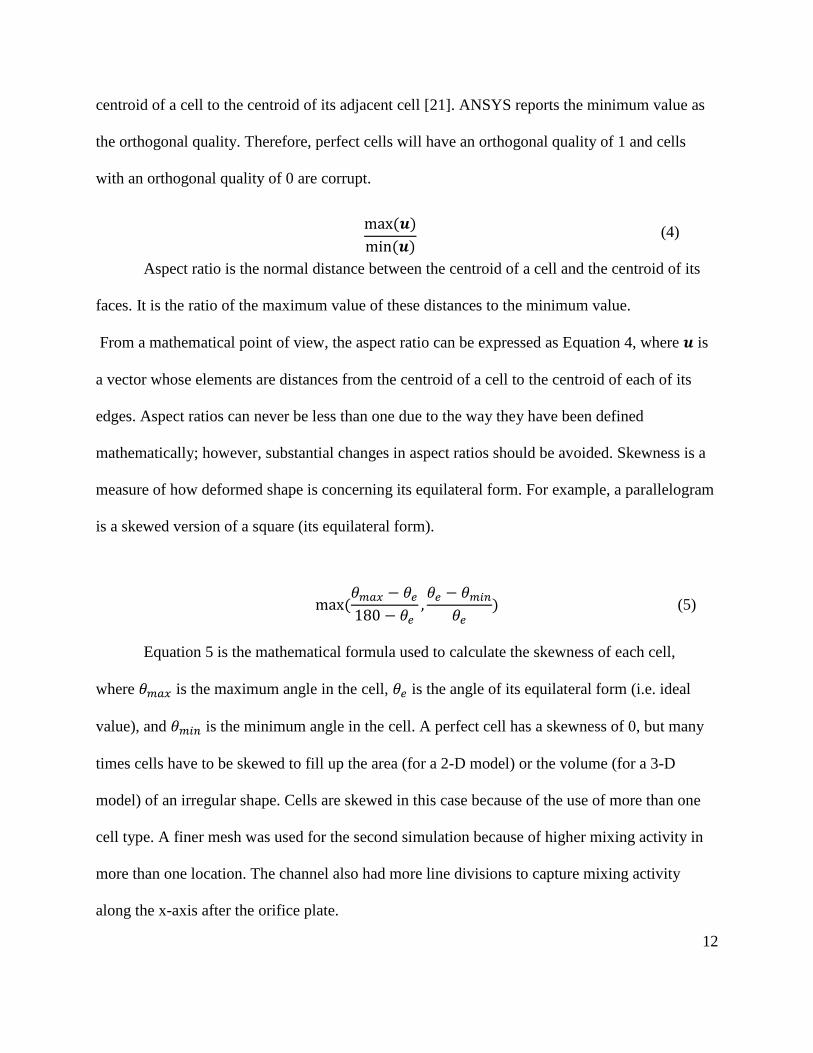
12

centroid of a cell to the centroid of its adjacent cell [21]. ANSYS reports the minimum value as

the orthogonal quality. Therefore, perfect cells will have an orthogonal quality of 1 and cells

with an orthogonal quality of 0 are corrupt.

Aspect ratio is the normal distance between the centroid of a cell and the centroid of its

faces. It is the ratio of the maximum value of these distances to the minimum value.

From a mathematical point of view, the aspect ratio can be expressed as Equation 4, where 𝒖 is

a vector whose elements are distances from the centroid of a cell to the centroid of each of its

edges. Aspect ratios can never be less than one due to the way they have been defined

mathematically; however, substantial changes in aspect ratios should be avoided. Skewness is a

measure of how deformed shape is concerning its equilateral form. For example, a parallelogram

is a skewed version of a square (its equilateral form).

Equation 5 is the mathematical formula used to calculate the skewness of each cell,

where 𝜃𝑚𝑎𝑥 is the maximum angle in the cell, 𝜃𝑒 is the angle of its equilateral form (i.e. ideal

value), and 𝜃𝑚𝑖𝑛 is the minimum angle in the cell. A perfect cell has a skewness of 0, but many

times cells have to be skewed to fill up the area (for a 2-D model) or the volume (for a 3-D

model) of an irregular shape. Cells are skewed in this case because of the use of more than one

cell type. A finer mesh was used for the second simulation because of higher mixing activity in

more than one location. The channel also had more line divisions to capture mixing activity

along the x-axis after the orifice plate.

max (𝒖)

min (𝒖) (4)

max (

𝜃𝑚𝑎𝑥 − 𝜃𝑒180 − 𝜃𝑒

,𝜃𝑒 − 𝜃𝑚𝑖𝑛

𝜃𝑒) (5)

13

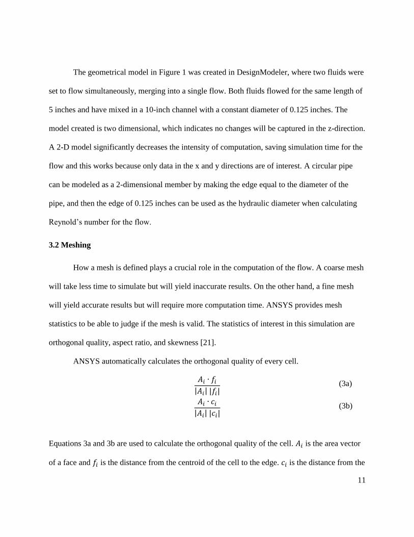
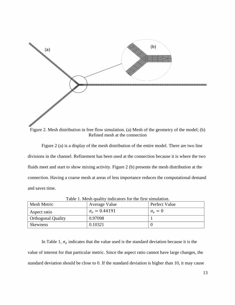
Figure 2. Mesh distribution in free flow simulation. (a) Mesh of the geometry of the model; (b)

Refined mesh at the connection

Figure 2 (a) is a display of the mesh distribution of the entire model. There are two line

divisions in the channel. Refinement has been used at the connection because it is where the two

fluids meet and start to show mixing activity. Figure 2 (b) presents the mesh distribution at the

connection. Having a coarse mesh at areas of less importance reduces the computational demand

and saves time.

Table 1. Mesh quality indicators for the first simulation.

Mesh Metric Average Value Perfect Value

Aspect ratio 𝜎𝑒 = 0.44191 𝜎𝑒 = 0

Orthogonal Quality 0.97098 1

Skewness 0.10321 0

In Table 1, 𝜎𝑒 indicates that the value used is the standard deviation because it is the

value of interest for that particular metric. Since the aspect ratio cannot have large changes, the

standard deviation should be close to 0. If the standard deviation is higher than 10, it may cause

14

some computing difficulties. Orthogonal quality of the cells has an average value very close to 1

and a minimum value of 0.71109, which is decent for this simulation. The minimum value of

orthogonal quality should be higher than 0.01, and the average value should be significantly

higher. Since most cells are equilateral shapes, skewness has an average value close to 0 and a

maximum, reasonable value of 0.62627. A maximum value higher than 0.95 in skewness may

lead to computations diverging [21]. Mesh metric indicators are very close to their ideal values

as the model investigated is 2-Dimensional.

3.3 Set Up

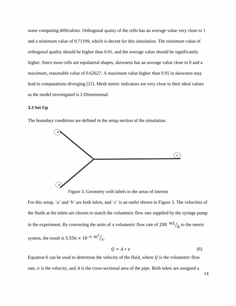
The boundary conditions are defined in the setup section of the simulation.

Figure 3. Geometry with labels in the areas of interest

For this setup, ‘a’ and ‘b’ are both inlets, and ‘c’ is an outlet shown in Figure 3. The velocities of

the fluids at the inlets are chosen to match the volumetric flow rate supplied by the syringe pump

in the experiment. By converting the units of a volumetric flow rate of 200 𝑚𝐿 ℎ⁄ to the metric

system, the result is 5.556 × 10−8 𝑚3

𝑠⁄ .

𝑄 = 𝐴 ∗ 𝑣 (6)

Equation 6 can be used to determine the velocity of the fluid, where 𝑄 is the volumetric flow

rate, 𝑣 is the velocity, and 𝐴 is the cross-sectional area of the pipe. Both inlets are assigned a

15

velocity of 7.017 × 10−3𝑚 𝑠⁄ . The simulation was then allowed to run for 10,000-time steps,

where each time step represents 0.001 seconds, totaling 10 seconds. A time step this small has

been chosen to keep the Courant number at a low value throughout the iterations as ANSYS

automatically stops the simulation once the Courant number exceeds 250 indicating divergence.

𝐶 =

𝑢 ⋅ Δ𝑡

Δ𝑥

(7)

Equation 7 is used to calculate the Courant number, where u is the wave speed of the system, Δ𝑡

is the time step and Δ𝑥 is the grid spacing, which relates to the mesh.

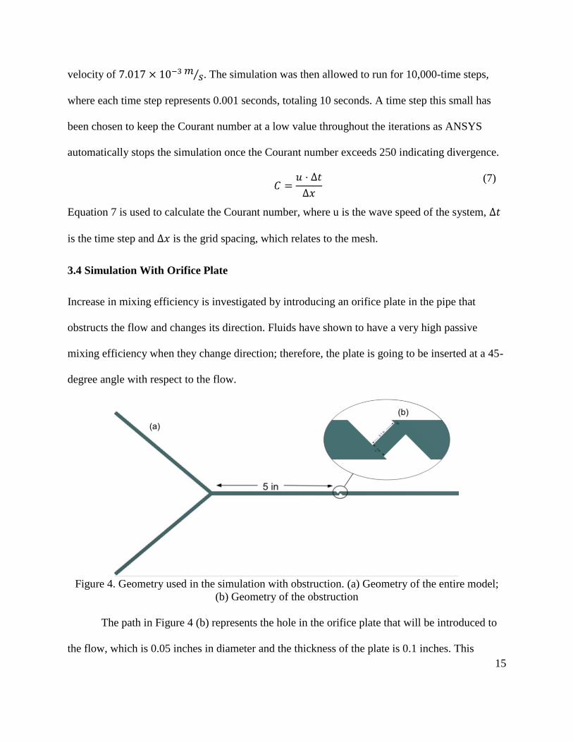
3.4 Simulation With Orifice Plate

Increase in mixing efficiency is investigated by introducing an orifice plate in the pipe that

obstructs the flow and changes its direction. Fluids have shown to have a very high passive

mixing efficiency when they change direction; therefore, the plate is going to be inserted at a 45-

degree angle with respect to the flow.

Figure 4. Geometry used in the simulation with obstruction. (a) Geometry of the entire model;

(b) Geometry of the obstruction

The path in Figure 4 (b) represents the hole in the orifice plate that will be introduced to

the flow, which is 0.05 inches in diameter and the thickness of the plate is 0.1 inches. This

16

simulation was conducted in comparison to the first simulation to understand how an orifice

plate can improve mixing efficiency. Other than the obstruction located 5 inches away from the

junction, all other parameters remain the same except the mesh distribution.

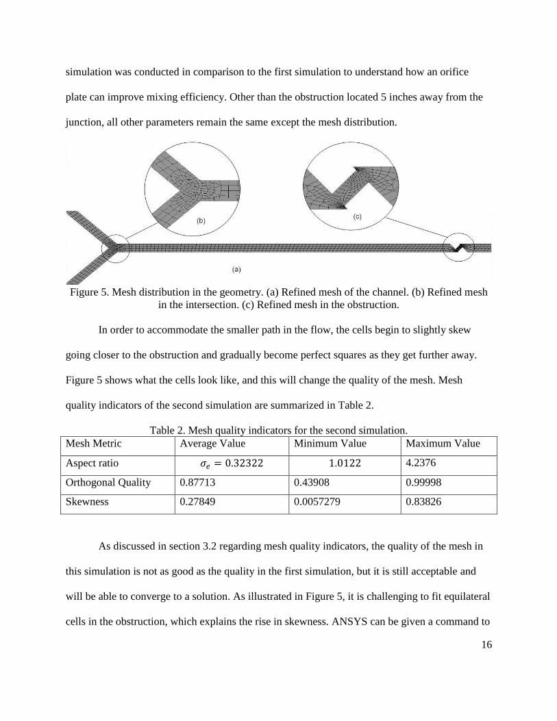
Figure 5. Mesh distribution in the geometry. (a) Refined mesh of the channel. (b) Refined mesh

in the intersection. (c) Refined mesh in the obstruction.

In order to accommodate the smaller path in the flow, the cells begin to slightly skew

going closer to the obstruction and gradually become perfect squares as they get further away.

Figure 5 shows what the cells look like, and this will change the quality of the mesh. Mesh

quality indicators of the second simulation are summarized in Table 2.

Table 2. Mesh quality indicators for the second simulation.

Mesh Metric Average Value Minimum Value Maximum Value

Aspect ratio 𝜎𝑒 = 0.32322 1.0122 4.2376

Orthogonal Quality 0.87713 0.43908 0.99998

Skewness 0.27849 0.0057279 0.83826

As discussed in section 3.2 regarding mesh quality indicators, the quality of the mesh in

this simulation is not as good as the quality in the first simulation, but it is still acceptable and

will be able to converge to a solution. As illustrated in Figure 5, it is challenging to fit equilateral

cells in the obstruction, which explains the rise in skewness. ANSYS can be given a command to

17

highly smooth out the mesh and that matches it with the mesh shown in Figure 2 for the rest of

the model.

18

Chapter 4: Sensor Calibration

4.1 About the Sensor

There are multiple parameters that can be measured to define how well two fluids are

mixed. For instance, the intensity of fluorescent light detected, where a fluorescent dye needs to

be dissolved in one of the fluids [10]. In addition, mixing can be measured by quantifying the

volume fraction of one of the fluids in a mixed stream. In this study, the experiments carried out

uses the latter methodology to measure the mixing ratio by introducing different color dyes into

both fluids and using a color sensor.

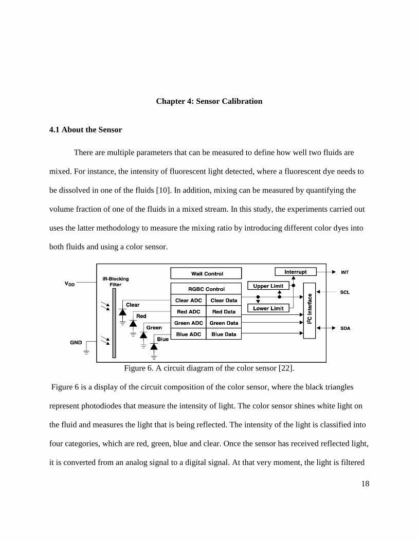
Figure 6. A circuit diagram of the color sensor [22].

Figure 6 is a display of the circuit composition of the color sensor, where the black triangles

represent photodiodes that measure the intensity of light. The color sensor shines white light on

the fluid and measures the light that is being reflected. The intensity of the light is classified into

four categories, which are red, green, blue and clear. Once the sensor has received reflected light,

it is converted from an analog signal to a digital signal. At that very moment, the light is filtered

19

through three color filters, which are red, green and blue; the total value of unfiltered light that

goes through the channel is also recorded. The sensor then reports the intensity of each filtered

color [22]. To improve accuracy, only red, green, and blue dyes are used in the following

experiments. Afterward, a correlation between the volume fraction and color reading can be

assessed.

The sensor used is very sensitive that factors other than light intensity may result in

inaccurate date. For instance, any air or body movements close to the sensor’s location may

result changing the readings. This means that the following conditions have to be maintained the

same for all measurements.

1. Movements around the sensor

2. Lighting in the room

3. Distance between the sensor and the sample

4. Volume of media

5. Position of the sample under the sensor

6. Dye saturation in the media

4.2 Set Up

Initially, mixtures are made in beakers containing water and food coloring dyes. The

mixture is stirred until it is visually evident that the food coloring has entirely dissolved in the

liquid. Consequently, a sample is taken and placed in a cell dish. The computer is placed away

from the sensor not to interfere with the data with any movements while measuring the sample.

The number of lights turned on in the room stayed the same to keep the light absorption

contribution the same throughout all samples. Also, an adjustable clamp is used to ensure that the

20

position of the sensor is constant throughout all measurements. The volume of the water and dye

saturation may change; however, every time a new mixture is made, the sensor is calibrated

using these mixtures for all future measurements. The saturation of dyes was challenging to

control because they are in a paste form and not a liquid.

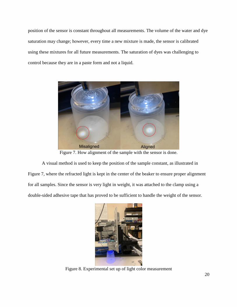
Figure 7. How alignment of the sample with the sensor is done.

A visual method is used to keep the position of the sample constant, as illustrated in

Figure 7, where the refracted light is kept in the center of the beaker to ensure proper alignment

for all samples. Since the sensor is very light in weight, it was attached to the clamp using a

double-sided adhesive tape that has proved to be sufficient to handle the weight of the sensor.

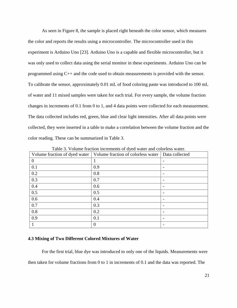
Figure 8. Experimental set up of light color measurement

21

As seen in Figure 8, the sample is placed right beneath the color sensor, which measures

the color and reports the results using a microcontroller. The microcontroller used in this

experiment is Arduino Uno [23]. Arduino Uno is a capable and flexible microcontroller, but it

was only used to collect data using the serial monitor in these experiments. Arduino Uno can be

programmed using C++ and the code used to obtain measurements is provided with the sensor.

To calibrate the sensor, approximately 0.01 mL of food coloring paste was introduced to 100 mL

of water and 11 mixed samples were taken for each trial. For every sample, the volume fraction

changes in increments of 0.1 from 0 to 1, and 4 data points were collected for each measurement.

The data collected includes red, green, blue and clear light intensities. After all data points were

collected, they were inserted in a table to make a correlation between the volume fraction and the

color reading. These can be summarized in Table 3.

Table 3. Volume fraction increments of dyed water and colorless water.

Volume fraction of dyed water Volume fraction of colorless water Data collected

0 1 -

0.1 0.9 -

0.2 0.8 -

0.3 0.7 -

0.4 0.6 -

0.5 0.5 -

0.6 0.4 -

0.7 0.3 -

0.8 0.2 -

0.9 0.1 -

1 0 -

4.3 Mixing of Two Different Colored Mixtures of Water

For the first trial, blue dye was introduced to only one of the liquids. Measurements were

then taken for volume fractions from 0 to 1 in increments of 0.1 and the data was reported. The

22

same procedure was repeated using red and green dyes. The dyes used are not manufactured to

be purely monochromatic and this will introduce a slight error, but an engineering judgment was

made to use the primary colors, which are red, green and blue to simplify the interpretation of the

data. It was found that many factors still contribute to the data being collected and an adjustment

has been made to the way the data has been collected to eliminate these factors, using two

different colored liquids. The results and adjustments will be discussed further in chapter 6 of

this thesis.

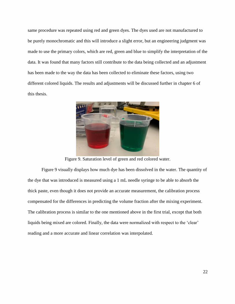
Figure 9. Saturation level of green and red colored water.

Figure 9 visually displays how much dye has been dissolved in the water. The quantity of

the dye that was introduced is measured using a 1 mL needle syringe to be able to absorb the

thick paste, even though it does not provide an accurate measurement, the calibration process

compensated for the differences in predicting the volume fraction after the mixing experiment.

The calibration process is similar to the one mentioned above in the first trial, except that both

liquids being mixed are colored. Finally, the data were normalized with respect to the ‘clear’

reading and a more accurate and linear correlation was interpolated.

23

Chapter 5: Light Reflection and Mixing

In the previous chapter, a well-defined calibration has been done, which leads to the next

step of mixing fluids in a flow and determining the factors that affect the efficiency of mixing of

two fluids. A controlled flow can be generated using a syringe pump. In this experiment, a Cole

Parmer syringe pump was used, where it is able to push two syringes at the same time and at the

same rate specified by the user.

5.1 Geometrical Set Up

The flow geometry used is identical to the geometry presented in section 3.1. A tube with

a circular-cross section of diameter 0.125 inches was used. The tubes were soft enough that they

can be cut using scissors to the length desired.

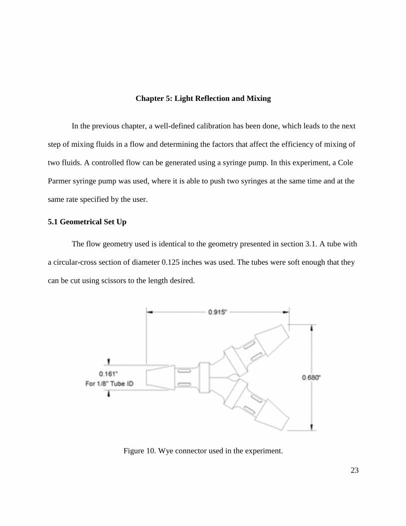
Figure 10. Wye connector used in the experiment.

24

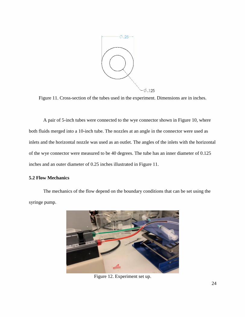
Figure 11. Cross-section of the tubes used in the experiment. Dimensions are in inches.

A pair of 5-inch tubes were connected to the wye connector shown in Figure 10, where

both fluids merged into a 10-inch tube. The nozzles at an angle in the connector were used as

inlets and the horizontal nozzle was used as an outlet. The angles of the inlets with the horizontal

of the wye connector were measured to be 40 degrees. The tube has an inner diameter of 0.125

inches and an outer diameter of 0.25 inches illustrated in Figure 11.

5.2 Flow Mechanics

The mechanics of the flow depend on the boundary conditions that can be set using the

syringe pump.

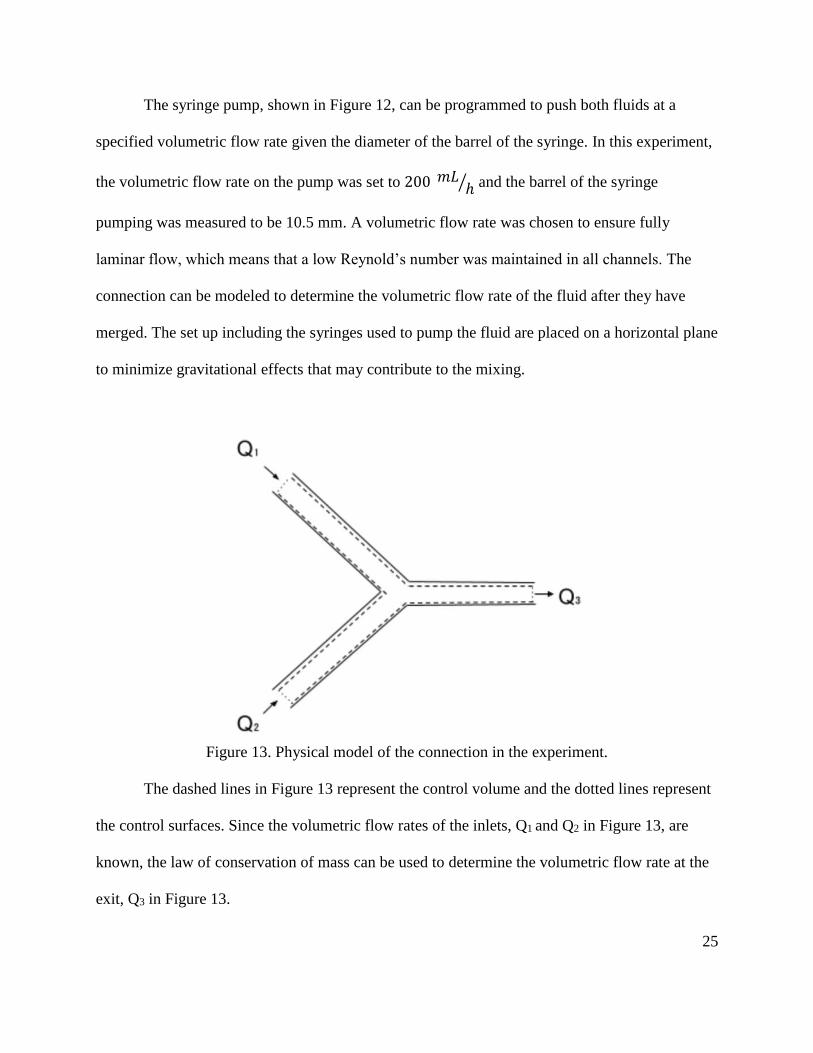
Figure 12. Experiment set up.

25

The syringe pump, shown in Figure 12, can be programmed to push both fluids at a

specified volumetric flow rate given the diameter of the barrel of the syringe. In this experiment,

the volumetric flow rate on the pump was set to 200 𝑚𝐿 ℎ⁄ and the barrel of the syringe

pumping was measured to be 10.5 mm. A volumetric flow rate was chosen to ensure fully

laminar flow, which means that a low Reynold’s number was maintained in all channels. The

connection can be modeled to determine the volumetric flow rate of the fluid after they have

merged. The set up including the syringes used to pump the fluid are placed on a horizontal plane

to minimize gravitational effects that may contribute to the mixing.

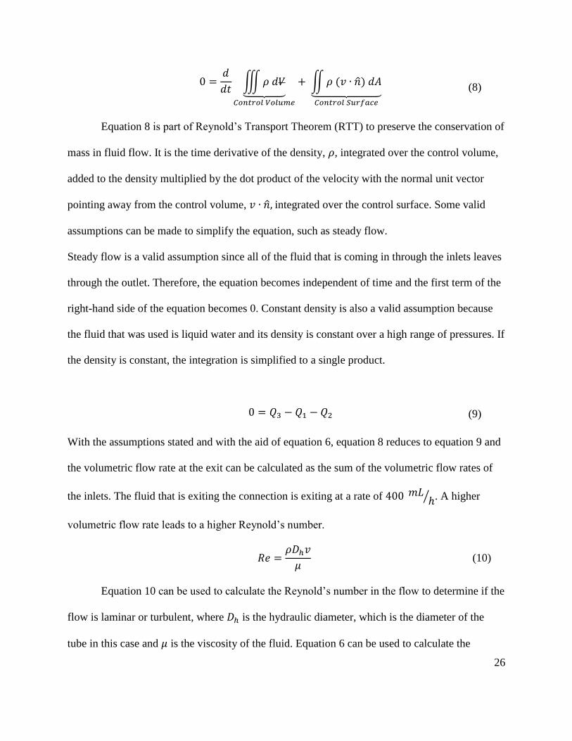
Figure 13. Physical model of the connection in the experiment.

The dashed lines in Figure 13 represent the control volume and the dotted lines represent

the control surfaces. Since the volumetric flow rates of the inlets, Q1 and Q2 in Figure 13, are

known, the law of conservation of mass can be used to determine the volumetric flow rate at the

exit, Q3 in Figure 13.

26

0 =

𝑑

𝑑𝑡∭𝜌 𝑑𝑉⏟

𝐶𝑜𝑛𝑡𝑟𝑜𝑙 𝑉𝑜𝑙𝑢𝑚𝑒

+ ∬𝜌 (𝑣 ∙ �̂�) 𝑑𝐴⏟ 𝐶𝑜𝑛𝑡𝑟𝑜𝑙 𝑆𝑢𝑟𝑓𝑎𝑐𝑒

(8)

Equation 8 is part of Reynold’s Transport Theorem (RTT) to preserve the conservation of

mass in fluid flow. It is the time derivative of the density, 𝜌, integrated over the control volume,

added to the density multiplied by the dot product of the velocity with the normal unit vector

pointing away from the control volume, 𝑣 ∙ �̂�, integrated over the control surface. Some valid

assumptions can be made to simplify the equation, such as steady flow.

Steady flow is a valid assumption since all of the fluid that is coming in through the inlets leaves

through the outlet. Therefore, the equation becomes independent of time and the first term of the

right-hand side of the equation becomes 0. Constant density is also a valid assumption because

the fluid that was used is liquid water and its density is constant over a high range of pressures. If

the density is constant, the integration is simplified to a single product.

0 = 𝑄3 − 𝑄1 − 𝑄2 (9)

With the assumptions stated and with the aid of equation 6, equation 8 reduces to equation 9 and

the volumetric flow rate at the exit can be calculated as the sum of the volumetric flow rates of

the inlets. The fluid that is exiting the connection is exiting at a rate of 400 𝑚𝐿 ℎ⁄ . A higher

volumetric flow rate leads to a higher Reynold’s number.

𝑅𝑒 =

𝜌𝐷ℎ𝑣

𝜇 (10)

Equation 10 can be used to calculate the Reynold’s number in the flow to determine if the

flow is laminar or turbulent, where 𝐷ℎ is the hydraulic diameter, which is the diameter of the

tube in this case and 𝜇 is the viscosity of the fluid. Equation 6 can be used to calculate the

27

velocity of the merged flow to be 3.5 𝑚𝑚 𝑠⁄ given the volumetric flow rate and cross-sectional

area at the output. Inserting the numbers into equation 9 yields 12.49 and that indicates that the

flow is fully laminar. The viscosity and density of water at room temperature were used, which

are 8.9 ∗ 10−4 Pa and 998 𝑘𝑔

𝑚3⁄ respectively.

The needle syringes that go through the tube, seen in Figure 12, are used to gather

samples to be measured using the light sensor. The syringe is inserted so that the needle is less

than halfway through the pipe. For such a small diameter, it is difficult to pick up a sample that is

at the right or left inner surfaces of the tube. However, the syringe was only inserted at a point

where the fluid has already passed to not interfere with the fluid while it is flowing. Before

puncturing the tube, the syringe was stopped and started again after the syringe was ready to pick

up a sample. Pulling the flanges on the syringe would cause the two fluids to mix by causing

turbulence, which is why the outlet was covered instead for the syringe pump to build up

pressure inside the tube and cause the fluids to flow into the barrels. The pressure in the tube will

push out the plunger while the fluids start to occupy the barrel, this ensures that the speed at

which the fluid flows is going to be equal to the speed of the syringe pump and that will not

contribute to any mixing activity.

Once the samples have been gathered, 2 mL of the fluid was placed in the cell dish under

the color sensor to determine the volume fraction of that sample. A sample of 2 mL was used

because it is the same volume used in the calibration. A volume fraction of 0.5 indicates that the

fluids have completely mixed and a volume fraction closer to 1 indicates that the fluids have not

mixed very well. The region at the tip of the flow is invalid for measurement since the two fluids

28

cannot start pumping at the exact same time and one of the fluids will dominate the volume

fraction.

5.3 Flow with Obstruction

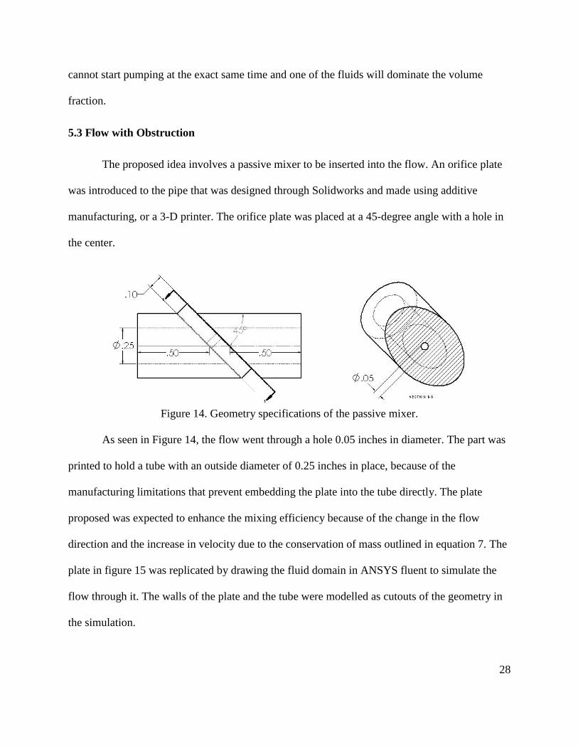
The proposed idea involves a passive mixer to be inserted into the flow. An orifice plate

was introduced to the pipe that was designed through Solidworks and made using additive

manufacturing, or a 3-D printer. The orifice plate was placed at a 45-degree angle with a hole in

the center.

Figure 14. Geometry specifications of the passive mixer.

As seen in Figure 14, the flow went through a hole 0.05 inches in diameter. The part was

printed to hold a tube with an outside diameter of 0.25 inches in place, because of the

manufacturing limitations that prevent embedding the plate into the tube directly. The plate

proposed was expected to enhance the mixing efficiency because of the change in the flow

direction and the increase in velocity due to the conservation of mass outlined in equation 7. The

plate in figure 15 was replicated by drawing the fluid domain in ANSYS fluent to simulate the

flow through it. The walls of the plate and the tube were modelled as cutouts of the geometry in

the simulation.

29

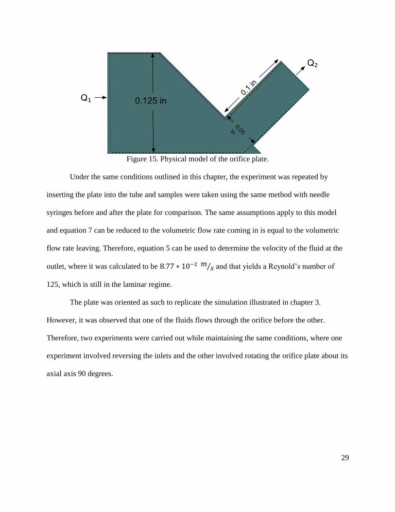
Figure 15. Physical model of the orifice plate.

Under the same conditions outlined in this chapter, the experiment was repeated by

inserting the plate into the tube and samples were taken using the same method with needle

syringes before and after the plate for comparison. The same assumptions apply to this model

and equation 7 can be reduced to the volumetric flow rate coming in is equal to the volumetric

flow rate leaving. Therefore, equation 5 can be used to determine the velocity of the fluid at the

outlet, where it was calculated to be 8.77 ∗ 10−2 𝑚 𝑠⁄ and that yields a Reynold’s number of

125, which is still in the laminar regime.

The plate was oriented as such to replicate the simulation illustrated in chapter 3.

However, it was observed that one of the fluids flows through the orifice before the other.

Therefore, two experiments were carried out while maintaining the same conditions, where one

experiment involved reversing the inlets and the other involved rotating the orifice plate about its

axial axis 90 degrees.

30

Chapter 6: Results and Discussion

In this chapter, the results of all simulations and experiments are presented, and their

interpretations are discussed. The results of the simulation are also validated through the

experiment, and the effect of obstructing the flow is investigated to demonstrate the increase in

mixing efficiency.

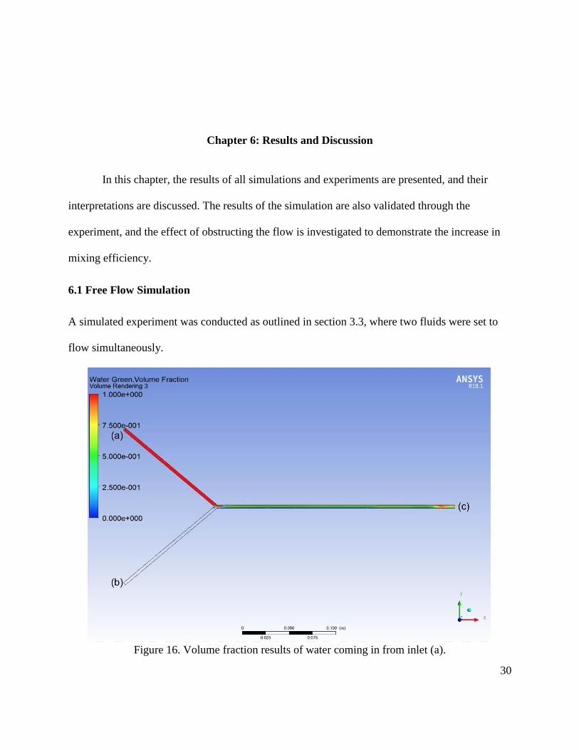
6.1 Free Flow Simulation

A simulated experiment was conducted as outlined in section 3.3, where two fluids were set to

flow simultaneously.

Figure 16. Volume fraction results of water coming in from inlet (a).

31

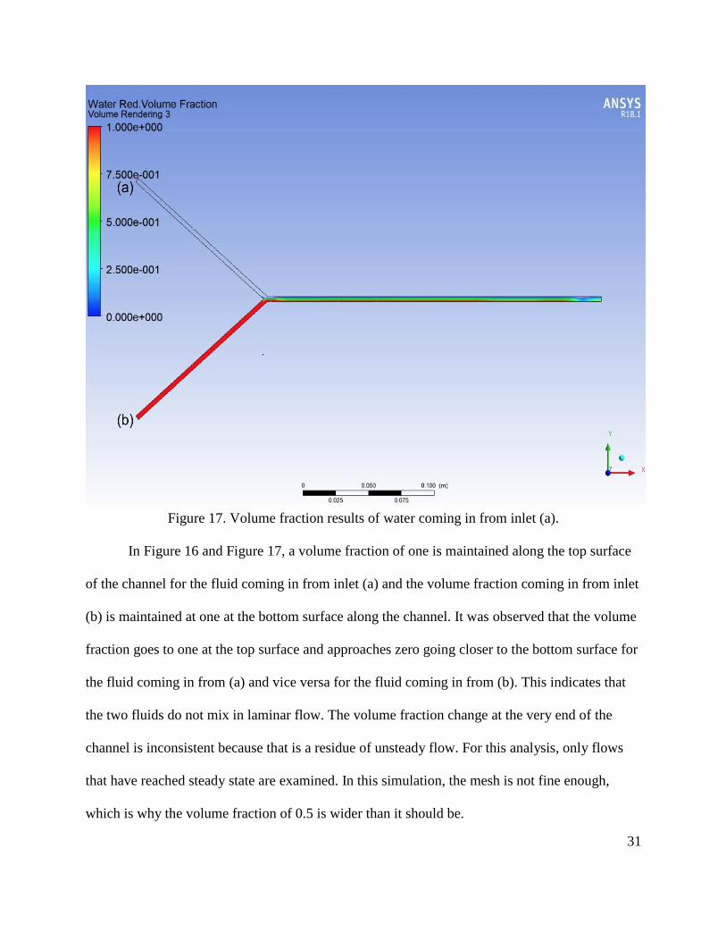
Figure 17. Volume fraction results of water coming in from inlet (a).

In Figure 16 and Figure 17, a volume fraction of one is maintained along the top surface

of the channel for the fluid coming in from inlet (a) and the volume fraction coming in from inlet

(b) is maintained at one at the bottom surface along the channel. It was observed that the volume

fraction goes to one at the top surface and approaches zero going closer to the bottom surface for

the fluid coming in from (a) and vice versa for the fluid coming in from (b). This indicates that

the two fluids do not mix in laminar flow. The volume fraction change at the very end of the

channel is inconsistent because that is a residue of unsteady flow. For this analysis, only flows

that have reached steady state are examined. In this simulation, the mesh is not fine enough,

which is why the volume fraction of 0.5 is wider than it should be.

32

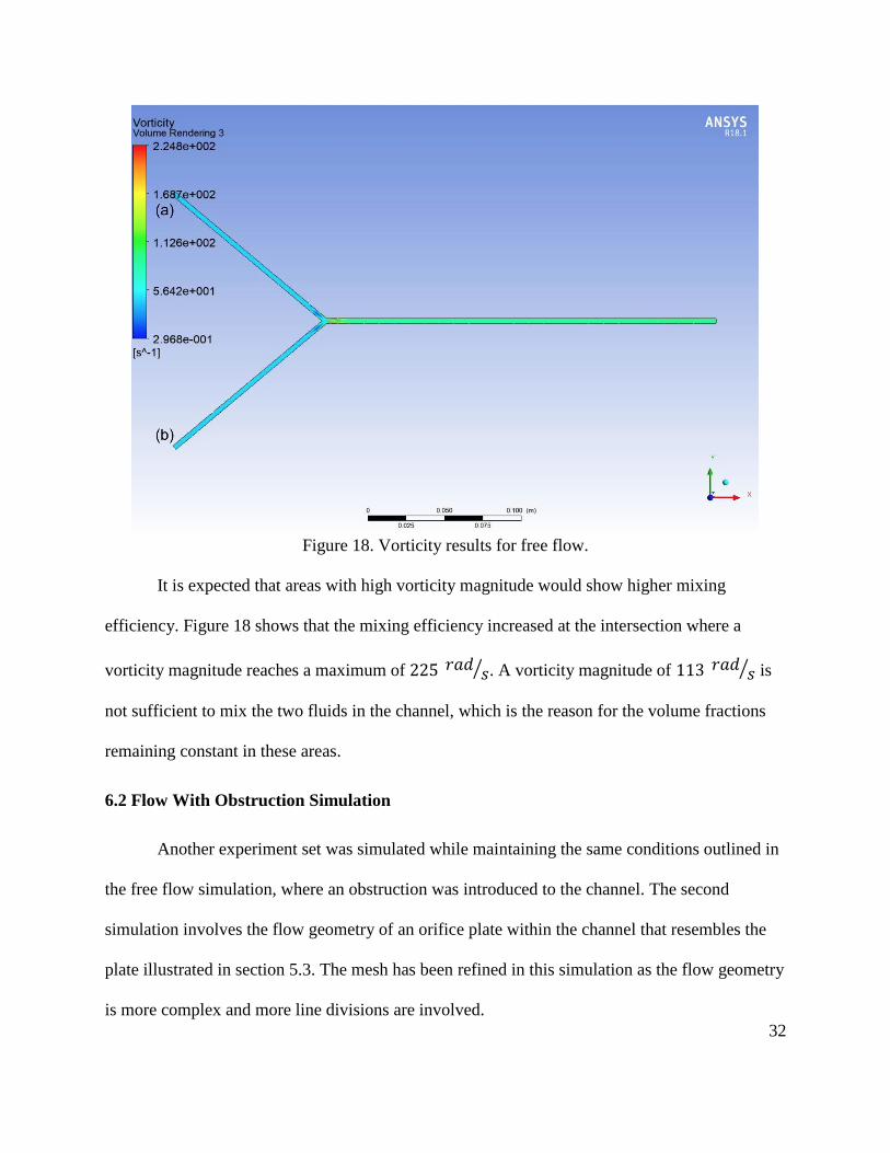
Figure 18. Vorticity results for free flow.

It is expected that areas with high vorticity magnitude would show higher mixing

efficiency. Figure 18 shows that the mixing efficiency increased at the intersection where a

vorticity magnitude reaches a maximum of 225 𝑟𝑎𝑑 𝑠⁄ . A vorticity magnitude of 113 𝑟𝑎𝑑 𝑠⁄ is

not sufficient to mix the two fluids in the channel, which is the reason for the volume fractions

remaining constant in these areas.

6.2 Flow With Obstruction Simulation

Another experiment set was simulated while maintaining the same conditions outlined in

the free flow simulation, where an obstruction was introduced to the channel. The second

simulation involves the flow geometry of an orifice plate within the channel that resembles the

plate illustrated in section 5.3. The mesh has been refined in this simulation as the flow geometry

is more complex and more line divisions are involved.

33

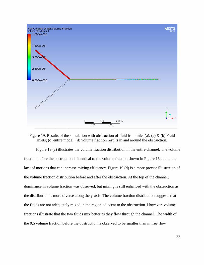
Figure 19. Results of the simulation with obstruction of fluid from inlet (a). (a) & (b) Fluid

inlets; (c) entire model; (d) volume fraction results in and around the obstruction.

Figure 19 (c) illustrates the volume fraction distribution in the entire channel. The volume

fraction before the obstruction is identical to the volume fraction shown in Figure 16 due to the

lack of motions that can increase mixing efficiency. Figure 19 (d) is a more precise illustration of

the volume fraction distribution before and after the obstruction. At the top of the channel,

dominance in volume fraction was observed, but mixing is still enhanced with the obstruction as

the distribution is more diverse along the y-axis. The volume fraction distribution suggests that

the fluids are not adequately mixed in the region adjacent to the obstruction. However, volume

fractions illustrate that the two fluids mix better as they flow through the channel. The width of

the 0.5 volume fraction before the obstruction is observed to be smaller than in free flow

34

simulation because of the finer mesh that is able to capture higher resolution results. However,

the results are very similar and that can be another method of validating the results of the

simulation, where the same results were obtained when using a refined mesh.

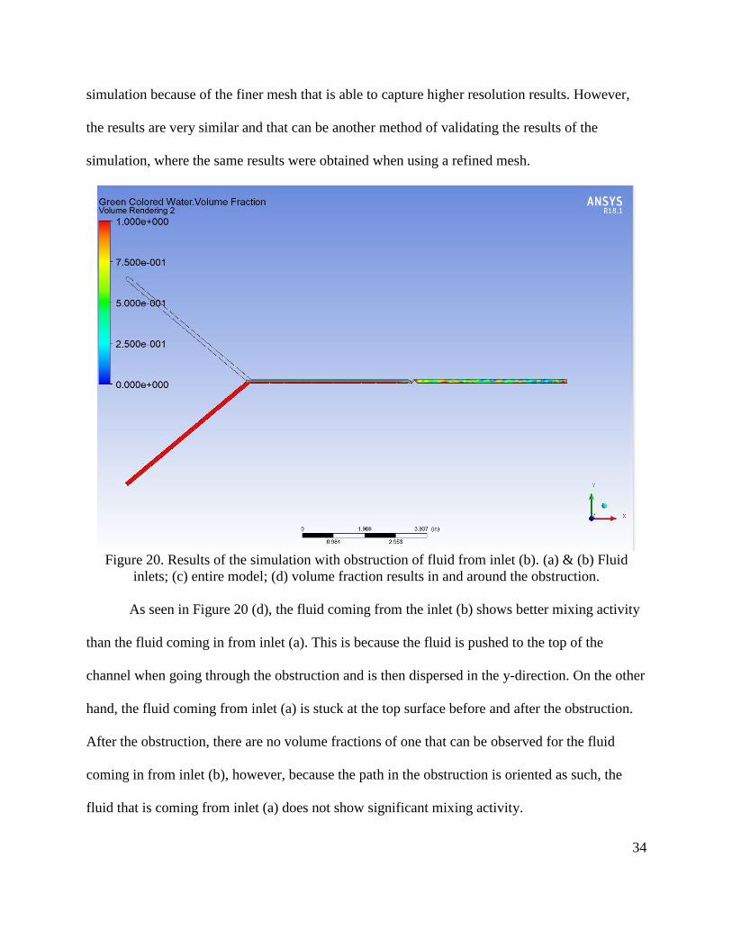
Figure 20. Results of the simulation with obstruction of fluid from inlet (b). (a) & (b) Fluid

inlets; (c) entire model; (d) volume fraction results in and around the obstruction.

As seen in Figure 20 (d), the fluid coming from the inlet (b) shows better mixing activity

than the fluid coming in from inlet (a). This is because the fluid is pushed to the top of the

channel when going through the obstruction and is then dispersed in the y-direction. On the other

hand, the fluid coming from inlet (a) is stuck at the top surface before and after the obstruction.

After the obstruction, there are no volume fractions of one that can be observed for the fluid

coming in from inlet (b), however, because the path in the obstruction is oriented as such, the

fluid that is coming from inlet (a) does not show significant mixing activity.

35

The plate can be oriented depending on what fluid is targeted to be mixed. Inserting

another plate that is oriented 90 degrees counter-clockwise from the one shown in Figures 19 and

20 can enhance the mixing further. Depending on the orientation, it is expected to observe one of

the fluids being mixed more efficiently than the other.

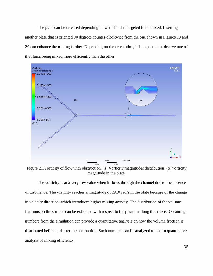
Figure 21.Vorticity of flow with obstruction. (a) Vorticity magnitudes distribution; (b) vorticity

magnitude in the plate.

The vorticity is at a very low value when it flows through the channel due to the absence

of turbulence. The vorticity reaches a magnitude of 2910 rad/s in the plate because of the change

in velocity direction, which introduces higher mixing activity. The distribution of the volume

fractions on the surface can be extracted with respect to the position along the x-axis. Obtaining

numbers from the simulation can provide a quantitative analysis on how the volume fraction is

distributed before and after the obstruction. Such numbers can be analyzed to obtain quantitative

analysis of mixing efficiency.

36

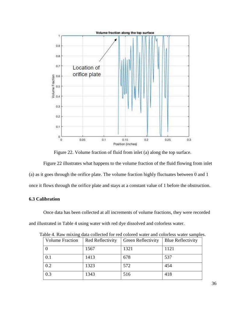
Figure 22. Volume fraction of fluid from inlet (a) along the top surface.

Figure 22 illustrates what happens to the volume fraction of the fluid flowing from inlet

(a) as it goes through the orifice plate. The volume fraction highly fluctuates between 0 and 1

once it flows through the orifice plate and stays at a constant value of 1 before the obstruction.

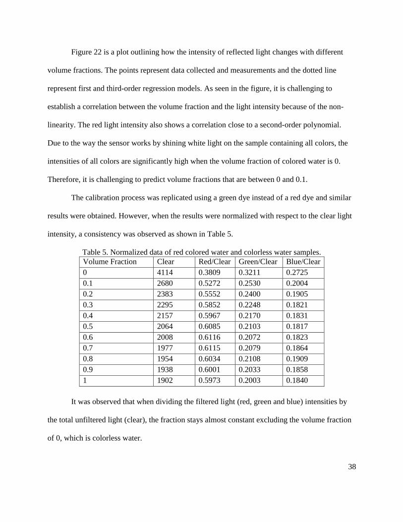
6.3 Calibration

Once data has been collected at all increments of volume fractions, they were recorded

and illustrated in Table 4 using water with red dye dissolved and colorless water.

Table 4. Raw mixing data collected for red colored water and colorless water samples.

Volume Fraction Red Reflectivity Green Reflectivity Blue Reflectivity

0 1567 1321 1121

0.1 1413 678 537

0.2 1323 572 454

0.3 1343 516 418

37

Table 4 (continued)

0.4 1287 468 395

0.5 1256 434 375

0.6 1228 416 366

0.7 1209 411 368.5

0.8 1179 412 373

0.9 1163 394 360

1 1136 381 350

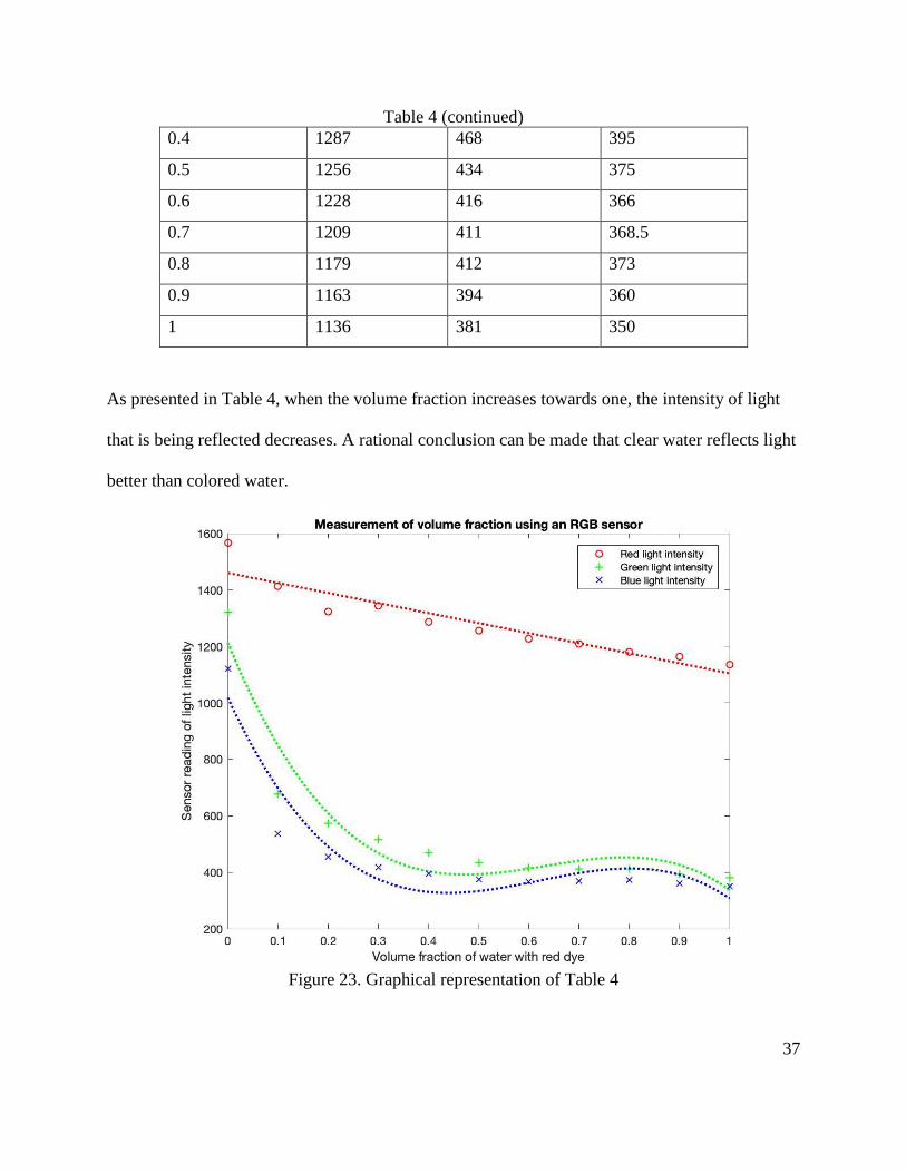
As presented in Table 4, when the volume fraction increases towards one, the intensity of light

that is being reflected decreases. A rational conclusion can be made that clear water reflects light

better than colored water.

Figure 23. Graphical representation of Table 4

38

Figure 22 is a plot outlining how the intensity of reflected light changes with different

volume fractions. The points represent data collected and measurements and the dotted line

represent first and third-order regression models. As seen in the figure, it is challenging to

establish a correlation between the volume fraction and the light intensity because of the non-

linearity. The red light intensity also shows a correlation close to a second-order polynomial.

Due to the way the sensor works by shining white light on the sample containing all colors, the

intensities of all colors are significantly high when the volume fraction of colored water is 0.

Therefore, it is challenging to predict volume fractions that are between 0 and 0.1.

The calibration process was replicated using a green dye instead of a red dye and similar

results were obtained. However, when the results were normalized with respect to the clear light

intensity, a consistency was observed as shown in Table 5.

Table 5. Normalized data of red colored water and colorless water samples.

Volume Fraction Clear Red/Clear Green/Clear Blue/Clear

0 4114 0.3809 0.3211 0.2725

0.1 2680 0.5272 0.2530 0.2004

0.2 2383 0.5552 0.2400 0.1905

0.3 2295 0.5852 0.2248 0.1821

0.4 2157 0.5967 0.2170 0.1831

0.5 2064 0.6085 0.2103 0.1817

0.6 2008 0.6116 0.2072 0.1823

0.7 1977 0.6115 0.2079 0.1864

0.8 1954 0.6034 0.2108 0.1909

0.9 1938 0.6001 0.2033 0.1858

1 1902 0.5973 0.2003 0.1840

It was observed that when dividing the filtered light (red, green and blue) intensities by

the total unfiltered light (clear), the fraction stays almost constant excluding the volume fraction

of 0, which is colorless water.

39

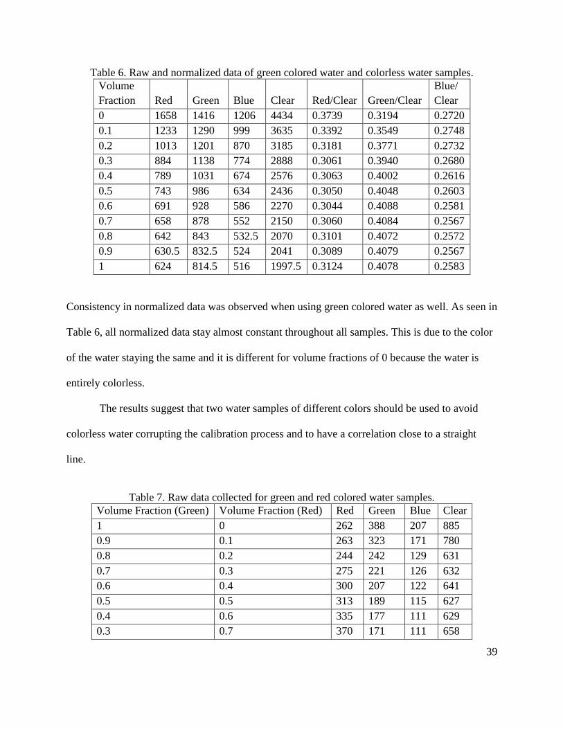
Table 6. Raw and normalized data of green colored water and colorless water samples.

Volume

Fraction Red Green Blue Clear Red/Clear Green/Clear

Blue/

Clear

0 1658 1416 1206 4434 0.3739 0.3194 0.2720

0.1 1233 1290 999 3635 0.3392 0.3549 0.2748

0.2 1013 1201 870 3185 0.3181 0.3771 0.2732

0.3 884 1138 774 2888 0.3061 0.3940 0.2680

0.4 789 1031 674 2576 0.3063 0.4002 0.2616

0.5 743 986 634 2436 0.3050 0.4048 0.2603

0.6 691 928 586 2270 0.3044 0.4088 0.2581

0.7 658 878 552 2150 0.3060 0.4084 0.2567

0.8 642 843 532.5 2070 0.3101 0.4072 0.2572

0.9 630.5 832.5 524 2041 0.3089 0.4079 0.2567

1 624 814.5 516 1997.5 0.3124 0.4078 0.2583

Consistency in normalized data was observed when using green colored water as well. As seen in

Table 6, all normalized data stay almost constant throughout all samples. This is due to the color

of the water staying the same and it is different for volume fractions of 0 because the water is

entirely colorless.

The results suggest that two water samples of different colors should be used to avoid

colorless water corrupting the calibration process and to have a correlation close to a straight

line.

Table 7. Raw data collected for green and red colored water samples.

Volume Fraction (Green) Volume Fraction (Red) Red Green Blue Clear

1 0 262 388 207 885

0.9 0.1 263 323 171 780

0.8 0.2 244 242 129 631

0.7 0.3 275 221 126 632

0.6 0.4 300 207 122 641

0.5 0.5 313 189 115 627

0.4 0.6 335 177 111 629

0.3 0.7 370 171 111 658

40

Table 7 (continued)

0.2 0.8 417 172 115 708

0.1 0.9 473 169 117 762

0 1 530 167 118 818

Table 8. Normalized data for green and red color water samples.

Volume fraction (Red) Red/Clear Green/Clear Blue/Clear

0 0.2960 0.4384 0.2339

0.1 0.3372 0.4141 0.2192

0.2 0.3867 0.3835 0.2044

0.3 0.4348 0.3494 0.1992

0.4 0.4680 0.3229 0.1903

0.5 0.4992 0.3014 0.1834

0.6 0.5326 0.2814 0.1765

0.7 0.5623 0.2599 0.1687

0.8 0.5890 0.2429 0.1624

0.9 0.6207 0.2218 0.1535

1 0.6479 0.2042 0.1443

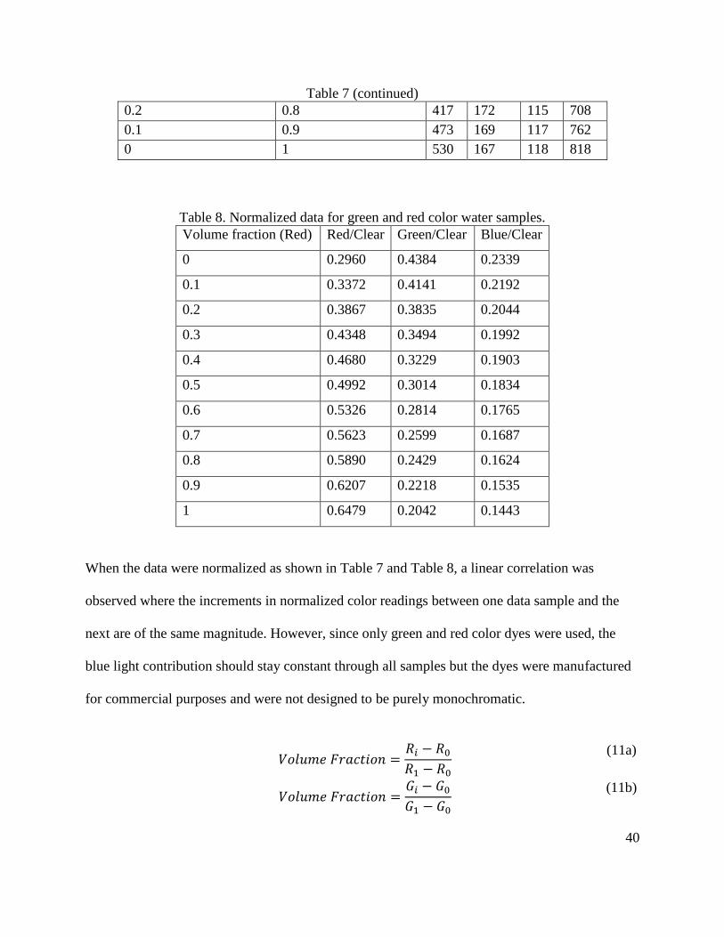
When the data were normalized as shown in Table 7 and Table 8, a linear correlation was

observed where the increments in normalized color readings between one data sample and the

next are of the same magnitude. However, since only green and red color dyes were used, the

blue light contribution should stay constant through all samples but the dyes were manufactured

for commercial purposes and were not designed to be purely monochromatic.

𝑉𝑜𝑙𝑢𝑚𝑒 𝐹𝑟𝑎𝑐𝑡𝑖𝑜𝑛 =𝑅𝑖 − 𝑅0𝑅1 − 𝑅0

𝑉𝑜𝑙𝑢𝑚𝑒 𝐹𝑟𝑎𝑐𝑡𝑖𝑜𝑛 =𝐺𝑖 − 𝐺0𝐺1 − 𝐺0

(11a)

(11b)

41

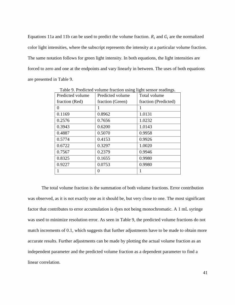
Equations 11a and 11b can be used to predict the volume fraction. 𝑅𝑖 and 𝐺𝑖 are the normalized

color light intensities, where the subscript represents the intensity at a particular volume fraction.

The same notation follows for green light intensity. In both equations, the light intensities are

forced to zero and one at the endpoints and vary linearly in between. The uses of both equations

are presented in Table 9.

Table 9. Predicted volume fraction using light sensor readings.

Predicted volume

fraction (Red)

Predicted volume

fraction (Green)

Total volume

fraction (Predicted)

0 1 1

0.1169 0.8962 1.0131

0.2576 0.7656 1.0232

0.3943 0.6200 1.0143

0.4887 0.5070 0.9958

0.5774 0.4153 0.9926

0.6722 0.3297 1.0020

0.7567 0.2379 0.9946

0.8325 0.1655 0.9980

0.9227 0.0753 0.9980

1 0 1

The total volume fraction is the summation of both volume fractions. Error contribution

was observed, as it is not exactly one as it should be, but very close to one. The most significant

factor that contributes to error accumulation is dyes not being monochromatic. A 1 mL syringe

was used to minimize resolution error. As seen in Table 9, the predicted volume fractions do not

match increments of 0.1, which suggests that further adjustments have to be made to obtain more

accurate results. Further adjustments can be made by plotting the actual volume fraction as an

independent parameter and the predicted volume fraction as a dependent parameter to find a

linear correlation.

42

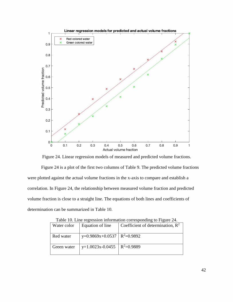
Figure 24. Linear regression models of measured and predicted volume fractions.

Figure 24 is a plot of the first two columns of Table 9. The predicted volume fractions

were plotted against the actual volume fractions in the x-axis to compare and establish a

correlation. In Figure 24, the relationship between measured volume fraction and predicted

volume fraction is close to a straight line. The equations of both lines and coefficients of

determination can be summarized in Table 10.

Table 10. Line regression information corresponding to Figure 24.

Water color Equation of line Coefficient of determination, R2

Red water y=0.9869x+0.0537 R2=0.9892

Green water y=1.0023x-0.0455 R2=0.9889

43

To reduce the error further, the actual volume fractions were found using the equations of the

lines. High coefficients of determination indicate that the results obtained are accurate.

6.4 Free Flow

Under the conditions discussed in Chapter 5, the flow was implemented and

measurements were obtained.

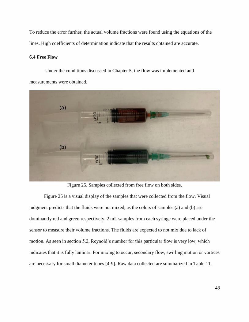
Figure 25. Samples collected from free flow on both sides.

Figure 25 is a visual display of the samples that were collected from the flow. Visual

judgment predicts that the fluids were not mixed, as the colors of samples (a) and (b) are

dominantly red and green respectively. 2 mL samples from each syringe were placed under the

sensor to measure their volume fractions. The fluids are expected to not mix due to lack of

motion. As seen in section 5.2, Reynold’s number for this particular flow is very low, which

indicates that it is fully laminar. For mixing to occur, secondary flow, swirling motion or vortices

are necessary for small diameter tubes [4-9]. Raw data collected are summarized in Table 11.

44

Table 11. Raw data collected from syringe samples in Figure 18.

Sample Red Blue Green Clear

Syringe (a) 586 215 159 960

Syringe (b) 205 232 115 568

Even though the green color reading in sample (b) is lower than the reading in sample (a), the

volume fraction is expected to be significantly higher. The normalized data is what matters in

this case (i.e. green color reading with respect to the clear reading) and how close in magnitude it

is to a volume fraction of zero in Table 8 indicating pure green colored water. Using the

calibration process illustrated in the previous section, the volume fraction of both syringes was

determined by normalizing the data and using equations 10a and 10b. Data interpretations are

summarized in Table 12 and Table 13.

Table 12. Normalized data of samples in free flow.

Sample Red/Clear Green/Clear Blue/Clear

Sample (a) 0.6104 0.2240 0.1656

Sample (b) 0.3609 0.4085 0.2025

The difference in blue color changes from 16% to 20% indicating slight error accumulation in

measurements.

Table 13. Volume fraction prediction of samples in free flow

Sample

Predicted volume

fraction (Green)

Predicted volume

fraction (Red)

Total volume

fraction (Predicted)

Sample (a) 0.8934 0.0845 0.9779

Sample (b) 0.1844 0.8721 1.0564

45

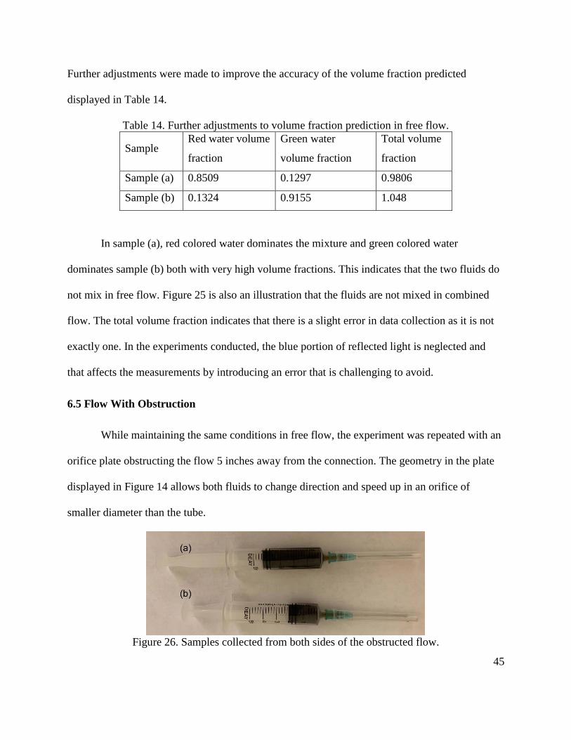
Further adjustments were made to improve the accuracy of the volume fraction predicted

displayed in Table 14.

Table 14. Further adjustments to volume fraction prediction in free flow.

Sample Red water volume

fraction

Green water

volume fraction

Total volume

fraction

Sample (a) 0.8509 0.1297 0.9806

Sample (b) 0.1324 0.9155 1.048

In sample (a), red colored water dominates the mixture and green colored water

dominates sample (b) both with very high volume fractions. This indicates that the two fluids do

not mix in free flow. Figure 25 is also an illustration that the fluids are not mixed in combined

flow. The total volume fraction indicates that there is a slight error in data collection as it is not

exactly one. In the experiments conducted, the blue portion of reflected light is neglected and

that affects the measurements by introducing an error that is challenging to avoid.

6.5 Flow With Obstruction

While maintaining the same conditions in free flow, the experiment was repeated with an

orifice plate obstructing the flow 5 inches away from the connection. The geometry in the plate

displayed in Figure 14 allows both fluids to change direction and speed up in an orifice of

smaller diameter than the tube.

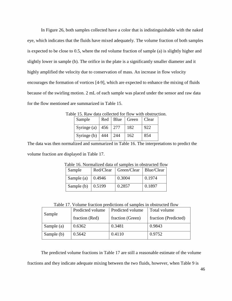
Figure 26. Samples collected from both sides of the obstructed flow.

46

In Figure 26, both samples collected have a color that is indistinguishable with the naked

eye, which indicates that the fluids have mixed adequately. The volume fraction of both samples

is expected to be close to 0.5, where the red volume fraction of sample (a) is slightly higher and

slightly lower in sample (b). The orifice in the plate is a significantly smaller diameter and it

highly amplified the velocity due to conservation of mass. An increase in flow velocity

encourages the formation of vortices [4-9], which are expected to enhance the mixing of fluids

because of the swirling motion. 2 mL of each sample was placed under the sensor and raw data

for the flow mentioned are summarized in Table 15.

Table 15. Raw data collected for flow with obstruction.

Sample Red Blue Green Clear

Syringe (a) 456 277 182 922

Syringe (b) 444 244 162 854

The data was then normalized and summarized in Table 16. The interpretations to predict the

volume fraction are displayed in Table 17.

Table 16. Normalized data of samples in obstructed flow

Sample Red/Clear Green/Clear Blue/Clear

Sample (a) 0.4946 0.3004 0.1974

Sample (b) 0.5199 0.2857 0.1897

Table 17. Volume fraction predictions of samples in obstructed flow

Sample Predicted volume

fraction (Red)

Predicted volume

fraction (Green)

Total volume

fraction (Predicted)

Sample (a) 0.6362 0.3481 0.9843

Sample (b) 0.5642 0.4110 0.9752

The predicted volume fractions in Table 17 are still a reasonable estimate of the volume

fractions and they indicate adequate mixing between the two fluids, however, when Table 9 is

47

compared to Table 7 in the calibration process, the error is still noticeable for volume fractions

near 0.5. Therefore, the adjustments were made and closer approximations of the volume

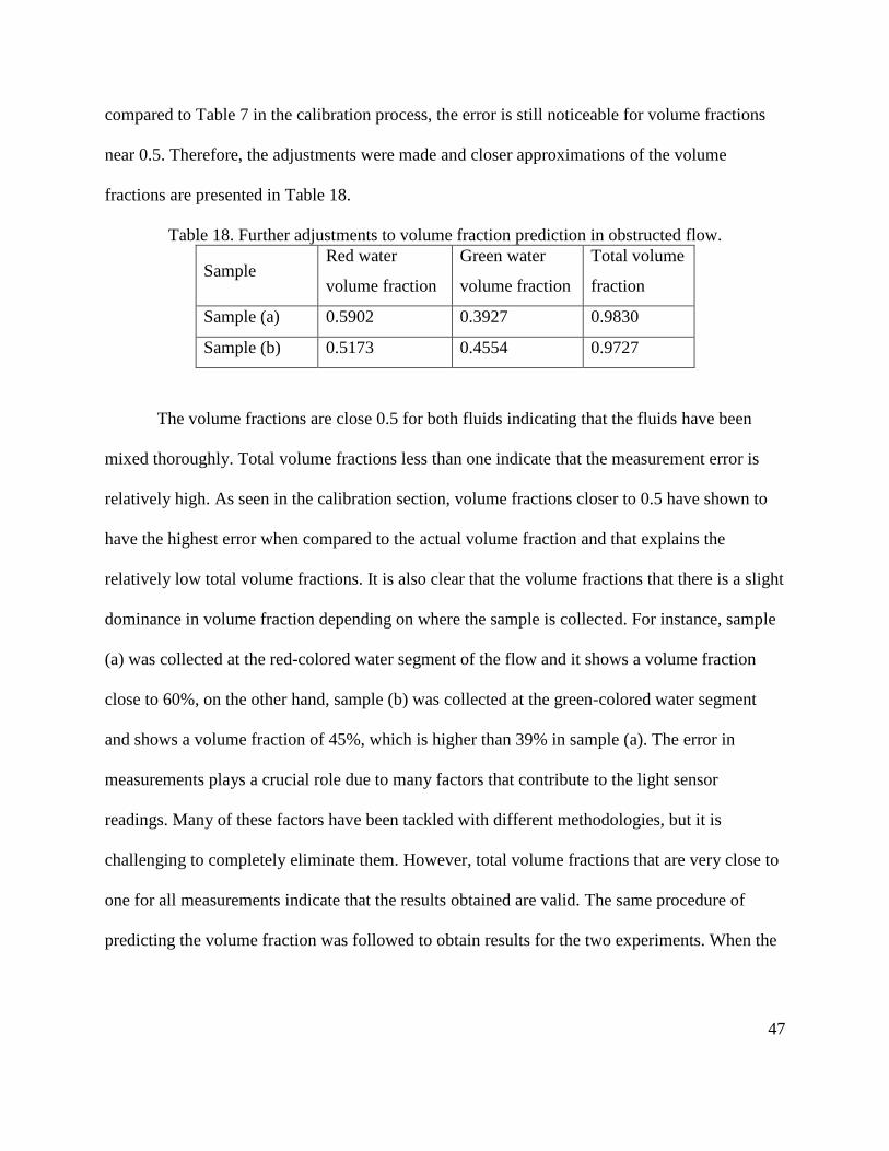
fractions are presented in Table 18.

Table 18. Further adjustments to volume fraction prediction in obstructed flow.

Sample Red water

volume fraction

Green water

volume fraction

Total volume

fraction

Sample (a) 0.5902 0.3927 0.9830

Sample (b) 0.5173 0.4554 0.9727

The volume fractions are close 0.5 for both fluids indicating that the fluids have been

mixed thoroughly. Total volume fractions less than one indicate that the measurement error is

relatively high. As seen in the calibration section, volume fractions closer to 0.5 have shown to

have the highest error when compared to the actual volume fraction and that explains the

relatively low total volume fractions. It is also clear that the volume fractions that there is a slight

dominance in volume fraction depending on where the sample is collected. For instance, sample

(a) was collected at the red-colored water segment of the flow and it shows a volume fraction

close to 60%, on the other hand, sample (b) was collected at the green-colored water segment

and shows a volume fraction of 45%, which is higher than 39% in sample (a). The error in

measurements plays a crucial role due to many factors that contribute to the light sensor

readings. Many of these factors have been tackled with different methodologies, but it is

challenging to completely eliminate them. However, total volume fractions that are very close to

one for all measurements indicate that the results obtained are valid. The same procedure of

predicting the volume fraction was followed to obtain results for the two experiments. When the

48

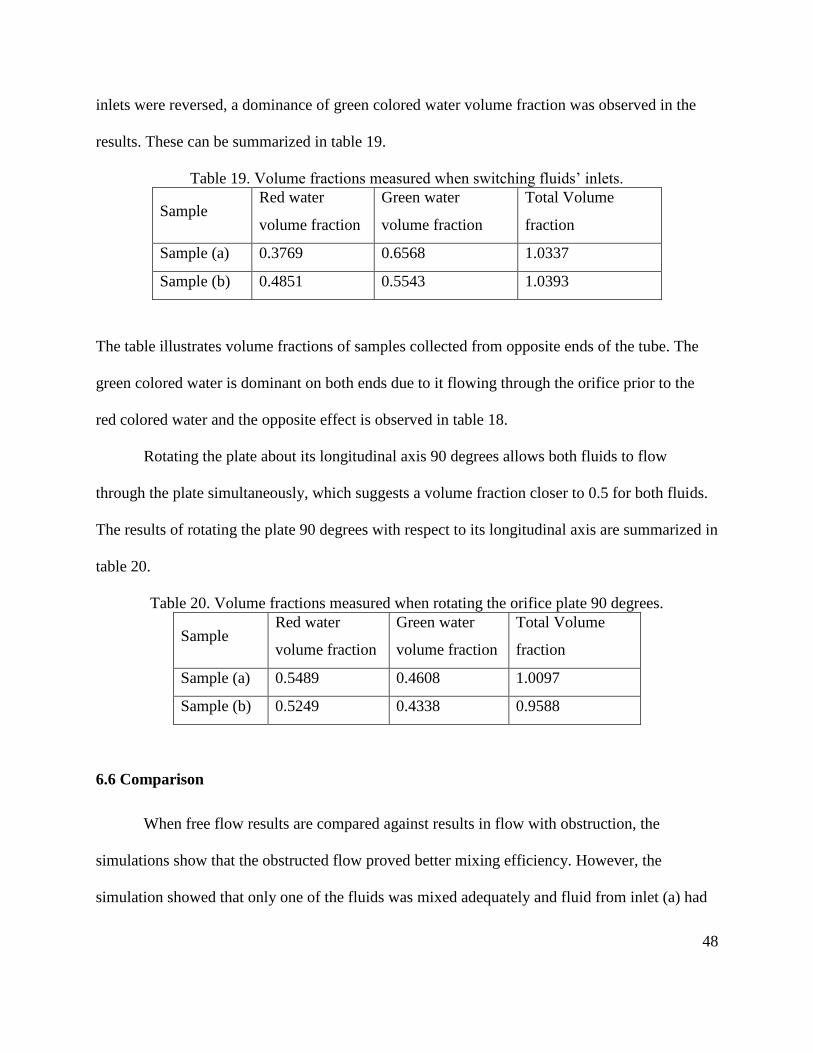
inlets were reversed, a dominance of green colored water volume fraction was observed in the

results. These can be summarized in table 19.

Table 19. Volume fractions measured when switching fluids’ inlets.

Sample Red water

volume fraction

Green water

volume fraction

Total Volume

fraction

Sample (a) 0.3769 0.6568 1.0337

Sample (b) 0.4851 0.5543 1.0393

The table illustrates volume fractions of samples collected from opposite ends of the tube. The

green colored water is dominant on both ends due to it flowing through the orifice prior to the

red colored water and the opposite effect is observed in table 18.

Rotating the plate about its longitudinal axis 90 degrees allows both fluids to flow

through the plate simultaneously, which suggests a volume fraction closer to 0.5 for both fluids.

The results of rotating the plate 90 degrees with respect to its longitudinal axis are summarized in

table 20.

Table 20. Volume fractions measured when rotating the orifice plate 90 degrees.

Sample Red water

volume fraction

Green water

volume fraction

Total Volume

fraction

Sample (a) 0.5489 0.4608 1.0097

Sample (b) 0.5249 0.4338 0.9588

6.6 Comparison

When free flow results are compared against results in flow with obstruction, the

simulations show that the obstructed flow proved better mixing efficiency. However, the

simulation showed that only one of the fluids was mixed adequately and fluid from inlet (a) had

49

a constant volume fraction of one along the top surface. When analyzing the experiment results

for the flow with obstruction, it was observed that volume fractions of red colored water after the

obstruction were dominant. It is expected to see higher volume fractions of red colored water

since the obstruction was oriented in a way that pushes the mixture towards it.

When the inlets were reversed, green colored water was dominant in both sides of the

mixtures. When the plate was rotated 90 degrees the plate has illustrated optimum mixing, where

volume fractions were the closest to 0.5, which indicates the highest mixing efficiency among

the three cases. In all cases, sample (a) is collected at the same location radially shown in figure

13 that is adjacent to the red colored water inlet. Sample (b) is also collected at the same location

radially in all experiments. However, the axial location of the needle syringes changes to collect

samples after the orifice plate for the flow of obstruction and in the axial location is arbitrary for

the free flow experiment (flow without an orifice plate).

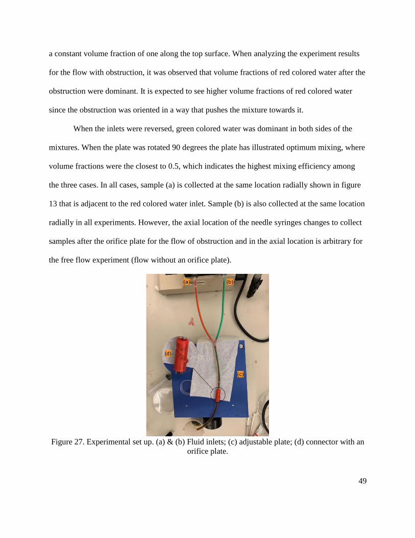
Figure 27. Experimental set up. (a) & (b) Fluid inlets; (c) adjustable plate; (d) connector with an

orifice plate.

50

Figure 25 is an illustration of how the orifice plate was introduced to the flow. A section

cut of Figure 25 (d) is presented in figure 14, where the dashed lines represent the path of cut that

the fluids were pushed through. Both fluids are being pushed towards the left of the tube, where

the red-colored water was running and that explains the higher volume fraction of red colored

water. The results obtained from this experiment are in accordance with the results obtained in

the simulation of obstructed flow. As can be seen in Figure 25, there were some air bubbles in

the flow that can contribute to error accumulation due to surface tension and the plate cannot be

oriented as precise as the simulation geometrical model.

The free flow simulation agrees with the free flow experiment, where both fluids’

behaviors are laminar and move in a straight line without showing any mixing activity. The case

is identical in the obstructed flow simulation and experiment before the fluids reach the

obstruction. The simulations were conducted mainly to look at the vorticity magnitudes in the

flow and around the obstruction, as vorticity is challenging to measure in such a small diameter

tube.

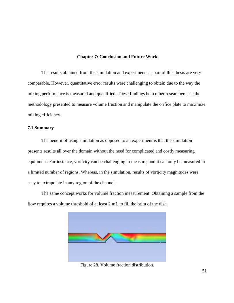
51

Chapter 7: Conclusion and Future Work

The results obtained from the simulation and experiments as part of this thesis are very

comparable. However, quantitative error results were challenging to obtain due to the way the

mixing performance is measured and quantified. These findings help other researchers use the

methodology presented to measure volume fraction and manipulate the orifice plate to maximize

mixing efficiency.

7.1 Summary

The benefit of using simulation as opposed to an experiment is that the simulation

presents results all over the domain without the need for complicated and costly measuring

equipment. For instance, vorticity can be challenging to measure, and it can only be measured in

a limited number of regions. Whereas, in the simulation, results of vorticity magnitudes were

easy to extrapolate in any region of the channel.

The same concept works for volume fraction measurement. Obtaining a sample from the

flow requires a volume threshold of at least 2 mL to fill the brim of the dish.

Figure 28. Volume fraction distribution.

52

As seen in Figure 28, the simulation is capable of displaying the results everywhere in the

channel, whereas the experiment was only able to capture an average volume fraction over a 2

mL volume of fluid at the top and bottom regions of the channel.

7.2 Future Work

The ideas presented in this thesis have a significant opportunity for improvement and

research. Given the new development of enhancing the efficiency of mixing and measuring the

volume fraction, new research opportunities are available. Obstructing the flow gives rise to

issues that need to be analyzed. The parameters can then be modified by analyzing the inputs and

outputs to optimize the process.

The orifice plate, comparable to all obstructions, introduces a noticeable pressure drop in

the flow. Pressure drops require the use of a more powerful pump yielding a higher cost. The

effects of the shape of the orifice, the orientation of the plate and the number of orifices can be

investigated and experimented with minimizing the pressure drop in the flow. Such

investigations are challenging due to the difficulty of measuring pressure drop.

It was observed that the two fluids do not mix before the obstruction initially, which is

illustrated in Figure 25. However, when the fluids were left in the tube for an extended period,

the color of the fluid indicated that the two fluids have mixed but no quantitative results were

collected. This is an opportunity for further research to investigate the time it takes for the fluids

to mix in static or quasi-static state, where volume fractions are measured at different times to

determine how long does it take for the fluids to reach a steady state.

Correlating the volume fraction with color readings was limited to the use of primary

colors in this thesis. While this has proved to be an effective method to measure volume fraction,

53

it can be improved further. All three primary colors can be incorporated in the calibration process

to obtain a more accurate correlation. By doing this, the measurement error will be minimized

because it does not assume that the color dye used is purely monochromatic, and it will allow the

use of a wide range of color dyes. Also, the adjustment results presented in Table 18 can be

avoided. Furthermore, the method used to measure the volume fractions can be used with

cameras that have embedded RGB sensors to monitor and measure mixing efficiency promptly

and more accurately.

Overall, research in these areas can optimize the measurement process and mixing

efficiency of two fluids in any flow.

54

References

[1] E. L. Paul, V. A. Atiemo-Obeng, and S. M. Kresta, Handbook of industrial mixing:

science and practice. John Wiley & Sons, 2004.

[2] C.-Y. Lee, C.-L. Chang, Y.-N. Wang, and L.-M. Fu, "Microfluidic mixing: a review,"

International journal of molecular sciences, vol. 12, no. 5, pp. 3263-3287, 2011.

[3] W. Jeon and C. B. Shin, "Design and simulation of passive mixing in microfluidic

systems with geometric variations," Chemical engineering journal, vol. 152, no. 2-3, pp. 575-

582, 2009.

[4] D. Bothe, C. Stemich, and H.-J. Warnecke, "Fluid mixing in a T-shaped micro-mixer,"

Chemical Engineering Science, vol. 61, no. 9, pp. 2950-2958, 2006.

[5] M. Engler, N. Kockmann, T. Kiefer, and P. Woias, "Numerical and experimental

investigations on liquid mixing in static micromixers," Chemical Engineering Journal, vol. 101,

no. 1-3, pp. 315-322, 2004.

[6] I. Glasgow, J. Batton, and N. Aubry, "Electroosmotic mixing in microchannels," Lab on

a Chip, vol. 4, no. 6, pp. 558-562, 2004.

[7] H. Yu, S. Xiao, H. Chen, and S. Fan, "Influence of flow velocity profile on mixing in

micromixer," Nanotechnology and Precision Engineering, vol. 3, no. 4, pp. 290-294, 2005.

[8] Y. Zhao, Y. Ying, G. Chen, and Q. Yuan, "Characterization of micro-mixing in T-shaped

micro-mixer," JOURNAL OF CHEMICAL INDUSTRY AND ENGINEERING-CHINA-, vol. 57,

no. 8, p. 1884, 2006.

55

[9] E. A. Mansur, Y. Mingxing, W. Yundong, and D. Youyuan, "A state-of-the-art review of

mixing in microfluidic mixers," Chinese Journal of Chemical Engineering, vol. 16, no. 4, pp.

503-516, 2008.

[10] M. C. Jo and R. Guldiken, "Dual surface acoustic wave-based active mixing in a

microfluidic channel," Sensors and Actuators A: Physical, vol. 196, pp. 1-7, 2013.

[11] M. Tan, L. Yeo, and J. Friend, "Rapid fluid flow and mixing induced in microchannels

using surface acoustic waves," EPL (Europhysics Letters), vol. 87, no. 4, p. 47003, 2009.

[12] Z. Yang, S. Matsumoto, H. Goto, M. Matsumoto, and R. Maeda, "Ultrasonic micromixer

for microfluidic systems," Sensors and Actuators A: Physical, vol. 93, no. 3, pp. 266-272, 2001.

[13] A. L. Teh, Y. H. Siow, W. M. Chin, C. M. Chia, and J. J. Foo, "Thermal mixing

enhancement of a free cooling/heating system with a 2D space-filling plate," Applied Thermal

Engineering, vol. 89, pp. 946-957, 2015.

[14] S. Shaaban, "Optimization of orifice meter's energy consumption," Chemical Engineering

Research and Design, vol. 92, no. 6, pp. 1005-1015, 2014.

[15] A. A. S. Bhagat, E. T. Peterson, and I. Papautsky, "A passive planar micromixer with

obstructions for mixing at low Reynolds numbers," Journal of micromechanics and

microengineering, vol. 17, no. 5, p. 1017, 2007.

[16] M. Oddy, J. Santiago, and J. Mikkelsen, "Electrokinetic instability micromixing,"

Analytical chemistry, vol. 73, no. 24, pp. 5822-5832, 2001.

[17] T.-D. Luong, V.-N. Phan, and N.-T. Nguyen, "High-throughput micromixers based on

acoustic streaming induced by surface acoustic wave," Microfluidics and nanofluidics, vol. 10,

no. 3, pp. 619-625, 2011.

56

[18] H. Suzuki, K. Nagata, Y. Sakai, and T. Hayase, "Direct numerical simulation of turbulent

mixing in regular and fractal grid turbulence," Physica Scripta, vol. 2010, no. T142, p. 014065,

2010.

[19] F. Cabaret, S. Bonnot, L. Fradette, and P. A. Tanguy, "Mixing time analysis using

colorimetric methods and image processing," Industrial & engineering chemistry research, vol.

46, no. 14, pp. 5032-5042, 2007.

[20] G. Delaplace, L. Bouvier, A. Moreau, R. Guérin, and J.-C. Leuliet, "Determination of

mixing time by colourimetric diagnosis—Application to a new mixing system," Experiments in

fluids, vol. 36, no. 3, pp. 437-443, 2004.

[21] ANSYS, "ANSYS Fluent User’s Guide," no. 15.0, pp. 128-132, 2013.

[22] TAOS, "TCS3472 COLOR LIGHT-TO-DIGITAL CONVERTER with IR FILTER

DataSheet," 2012.

[23] Arduino, "Arduino Uno Datasheet."

57

Appendix A: Copyright Permissions

Permission to use figure 6 as part of my thesis was granted by the company TAOS, which is now

part of AMS. The figure a circuit diagram of the TCS34725 color sensor used for volume

fraction measurements.

Permission to use figure 10 as part of my thesis was granted by the company McMaster-Carr.

The figure is a CAD drawing of the wye-connector used in the experiment.