Analysis of Thermal Mixing in T-Junctions Using Fluid ... · right angles, creating a mixing region of fluid both around and downstream of the junction resulting inT- temperature

Abstract—T-junctions are present in a wide range of industry and facilitate the mixing of fluids that are often at different temperatures. Temperature fluctuations introduced during the mixing process can result in thermal fatigue and consequently structural failure in the pipework. Predicting the magnitudes and locations of the stresses allows one to prevent and/or mitigate potential issues. A number of studies have investigated the fluid dynamics of T-junctions but very few have researched the impacts of the resulting flow field on the enveloping pipe materials especially where temperature fluctuations are significant. The present study employs steady-state one-way fluid-structure interaction analysis to determine the stress response of the pipework in a thermal-mixing T-junction situation. Firstly, the numerical flow field is simulated using CFD and validated against experimental data. Then, the effects of the fluid force fields on the pipe walls are modelled using structural analysis to predict the resulting stresses.

Index Terms—CFD, fluid-structure interaction, thermal fatigue, T-junctions

I. INTRODUCTION hermal mixing of fluids at different temperatures is common within industry such as nuclear power plants

[1]. This often occurs in regions of pipe-work connected at right angles, creating a mixing region of fluid both around and downstream of the T-junction resulting in temperature gradients along the pipe walls [2]. Consequently, significant thermal stresses are introduced within the pipe material [2]. These temperature gradients and accompanying thermal stresses and strains fluctuate with the complex flow pattern generated at the T-junction [2,3,4]. This produces thermal fatigue, which negatively promotes crack initiation followed by catastrophic crack propagation [5]. The lifetime of components are significantly impacted by this phenomenon [6]. With respect to nuclear power plants, there has been several well-documented and potentially serious thermal fatigue failure incidents in, for example, the sodium-cooled fast reactor ‘PHENIX’ in 1991, the French ‘PWR Civaux 1’ in 1998, and the Japanese ‘PWR Tsuruga-2’ in 1999 and ‘Tomari-2’ in 2003 [1].

Currently, engineering industry design guidelines

Manuscript received November 20, 2017. Participation at the conference was supported in part by the Institution

of Mechanical Engineers (IMechE) and the Mechanical Engineering Class Grant at the University of Dundee.

Andrew R. Gow was a student at the University of Dundee, UK. He is now a graduate mechanical engineer at Mott MacDonald, Glasgow, UK. (email: [email protected])

Salim M. Salim is with the University of Dundee, DD1 4HN, UK. (phone: 44-01382381378; e-mail: [email protected] ).

concerning thermal fatigue phenomena in T-junctions are not fully comprehensive [3]. The ability to predict thermal stripping in advance would be highly beneficial within industrial settings [7]; it would facilitate the institution of effective and targeted monitoring of potential thermal fatigue sites as well as to indicate where fatigue-susceptible welds should not be positioned [8]. To predict thermal fatigue phenomena, one could experimentally investigate the magnitudes of the temperature changes induced in the pipe walls as well as the spatial distribution of these temperatures [9]. Alternatively, computational fluid-structure interaction (FSI) simulations can be utilized to predict the magnitudes of the thermal stresses and their distributions.

Majority of published work have focused on the analysis of fluid flow in T-junctions without considering the resulting thermal stresses on the pipe walls [10, 11], which the present study aims to address. One-way FSI technique is implemented and to ensure confidence in the numerical predictions, the flow field is validated against experimental data produced by Naik-Nimbalkar et al. [9].

The geometry set-up investigated in the experimental validation paper are summarized in Fig. 1 and Table 1; the difference between the two conditions is the velocity ratio (the ratio of the velocity of the hot water to the cold water) as well as the diameter of the branch (vertical) pipe.

In Fig. 1, the arrows indicate direction of fluid flow. The length of the inlet is 1.2 times the diameter. The diameter of the main pipe may be referred to as ‘D’ and Line 1 is located at 0.5 D horizontal distance from the midline of the branch pipe and Line 2 is located at 1.25 D horizontal distance from the midline of the branch pipe. These are regions within the domains where the temperature profiles are physically measured in the experiment.

Fig. 1. Geometry of domain, with Line 1 and Line 2 marked.

Two velocity ratios of 0.5 and 4 were investigated and are referred to Case 1 and Case 2 respectively, with the corresponding boundary conditions shown in Table 1.

Analysis of Thermal Mixing in T-Junctions Using Fluid-Structure Interaction

Andrew R. Gow, and Salim M. Salim, CEng, MIMechE, Member, IAENG

T

Proceedings of the International MultiConference of Engineers and Computer Scientists 2018 Vol II IMECS 2018, March 14-16, 2018, Hong Kong

ISBN: 978-988-14048-8-6 ISSN: 2078-0958 (Print); ISSN: 2078-0966 (Online)

IMECS 2018

TABLE 1

EXPERIMENTAL CONDITIONS

Case no. Velocity ratio Main pipe Branch pipe (Vh/Vc) Diameter Velocity ‘Vc’ Temperature ‘Tc’ Diameter Velocity ‘Vh’ Temperature ‘Th’ (m) (m/s) (K) (m) (m/s) (K) 1 0.5 0.05 1.00 303 0.025 0.50 318

2 4.0 0.05 0.33 303 0.015 1.32 318

II. METHODOLOGY A. Computational Domain

The computational domain consists of two components: a

fluid domain (the fluid flow through the pipes and the T-junction) and a solid domain (the pipe-work). Careful attention was considering in creating the fluid-domain lengths ensuring absence of entrance or exit effects within the simulation [6]. Naik-Nimbalkar et al. concluded that there are practically no entrance or exit effects when the fluid domain is modelled as shown in Fig. 1. [9].

The fluid (water) properties are presented in Table 2.

TABLE 2 FLUID PROPERTIES (WATER)

Fluid Property Value Density 998.2 kg/m3

Specific heat 4182 J/kg.K Thermal conductivity 0.6 W/m.K Viscosity 0.001003 kg/m.s

The thickness of the pipe material was arbitrarily chosen to be 1 mm which is common for pipe-work materials. Steel was selected as the material for the pipe-work since this is commonly used within T-junction set-ups and hence results gained during this analysis would have wide applicability. The properties of steel are presented in Table 3.

TABLE 3 PIPE MATERIAL PROPERTIES (STEEL)

Material Property Value Density 7850 kg/m3

Young’s modulus 2.0 GPa Poisson’s ratio 0.3 Tensile and compressive yield strength 250 MPa Coefficient of thermal expansion* 1.2 x 10-5 C-1 * Zero thermal strain reference temperature is 22 °C B. Mesh and Physics Set-Up

The ANSYS computer package utilises a finite-volume method (FVM) when simulating fluid-flow behaviour. The generated mesh for the fluid domain is presented in Fig. 2. With reference to Fig. 1, Naik-Nimbalkar et al. indicated that Zone 2 of the fluid flow would require a much finer mesh than the other zones [9], therefore, an element size of 3.0 mm was utilised in Zone 2. Zones 1 and 3 were meshed with a slightly less fine mesh. Furthermore, it is recommended in cases such as those being investigated here,

that a structured layer of cells with high aspect ratio (diminutive perpendicular to the wall, but large in the flow direction) are placed around the periphery of the fluid-domain [14]. Such structured layers of cells in this region of high flow field gradients allow accurate representation of flow phenomena at the boundary [14]. This accuracy is essential because it is the information at this boundary region (particularly temperature and pressure fields) that is ‘linked’ to the solid domain in one-way FSI analyses and causes the resulting material stresses and strains that we are keen to investigate to predict effects of thermal fatigue. Fig. 3 provides a visual demonstration of the generated mesh. The fluid domain consists of 244459 elements (Case 1) and 240050 elements (Case 2).

Fig. 2 illustrates a layer of 5 cells with high aspect ratio (where the thickness decreases with radial distance from the centre) follow the periphery of the fluid domain; such a mesh allows the encapsulation of the flow at the periphery.

Fig. 2. Fluid domain mesh. Note the finer mesh in Zone 2.

Fig. 3. Fluid domain mesh. The exit of the main pipe is demonstrated (the

entrances to the main and branch pipe are identical).

Fig. 4. Solid domain mesh.



IMECS 2018

The ANSYS software package utilises a finite-element method (FEM) for the calculation of stresses and strains in the solid domain as opposed to FVM for the fluid domain. Fig. 4 demonstrates the pipe-work mesh utilized in this study. The solid domain consists of 11196 elements (Case 1) and 10513 elements (Case 2).

The realizable k−ε turbulence model is selected because it performs well in thermal mixing cases and is accompanied by ‘third-order MUSCL’ discretizations for momentum, turbulent kinetic energy, turbulent dissipation rate and energy. The default ‘SIMPLE’ pressure-velocity coupling scheme was retained.

III. RESULTS

The flow simulation results of the current investigation are illustrated qualitatively below. Fig. 5 and Fig. 6 show the thermal distributions of Case 1 (with velocity ratio 0.5) and Case 2 (with velocity ratio 4.0) respectively.

Fig. 5. Numerical results of the steady-state temperature distribution

through the mid-plane of the flow field for Case 1.

Fig. 6. Numerical results of the steady-state temperature distribution

through the mid-plane of the flow field for Case 2.

As expected, the extent of in the hot incoming stream and consequently the mixing region is larger for Case 2 due to the bigger velocity ratio, Vh/Vc (4.0 vs. 0.5) when compared to Case 1. Better thermal mixing is achieved in Case 2.

Fig. 7, 8 and 9 quantitavely compares the simulated results (FSI data) against experimental data produced by Naik-Nimbalkar et al. No experimental measurements were recorded along Line 2 of Case 2.

Note that the normalized temperature is expressed as:

(T-Tc) / (Th-Tc) (1)

Y is the distance from Lines 1 or 2 (i.e. the center of the horizontal pipe) to the point of measurement and R is the radius of the main pipe as set up in the experiment. Refer to Fig. 1 and Table 1.

Fig. 7. Simulated vs. experimental data of steady state temperature

distribution along Line 1 of Case 1.





It can be observed that the predicted results are in very good agreement with experimental data when the velocity ratio is low (i.e. Fig. 7 and 8), but when the ratio increases there is a larger discrepancy (Fig. 9). This is likely explained that as the velocity ratio increases, so does the turbulence mixing which is not captured sufficiently with the employed turbulence model and could be improved by more robust turbulence modelling approaches such as Large Eddy Simulation (LES) instead.

The temperature distributions throughout the pipework and the associated von-Mises stress distribution for both velocity ratios: Case 1 (Vh/Vc = 0.5) and Case 2 (Vh/Vc = 4.0) are demonstrated in Fig. 10 on the following page.



IMECS 2018

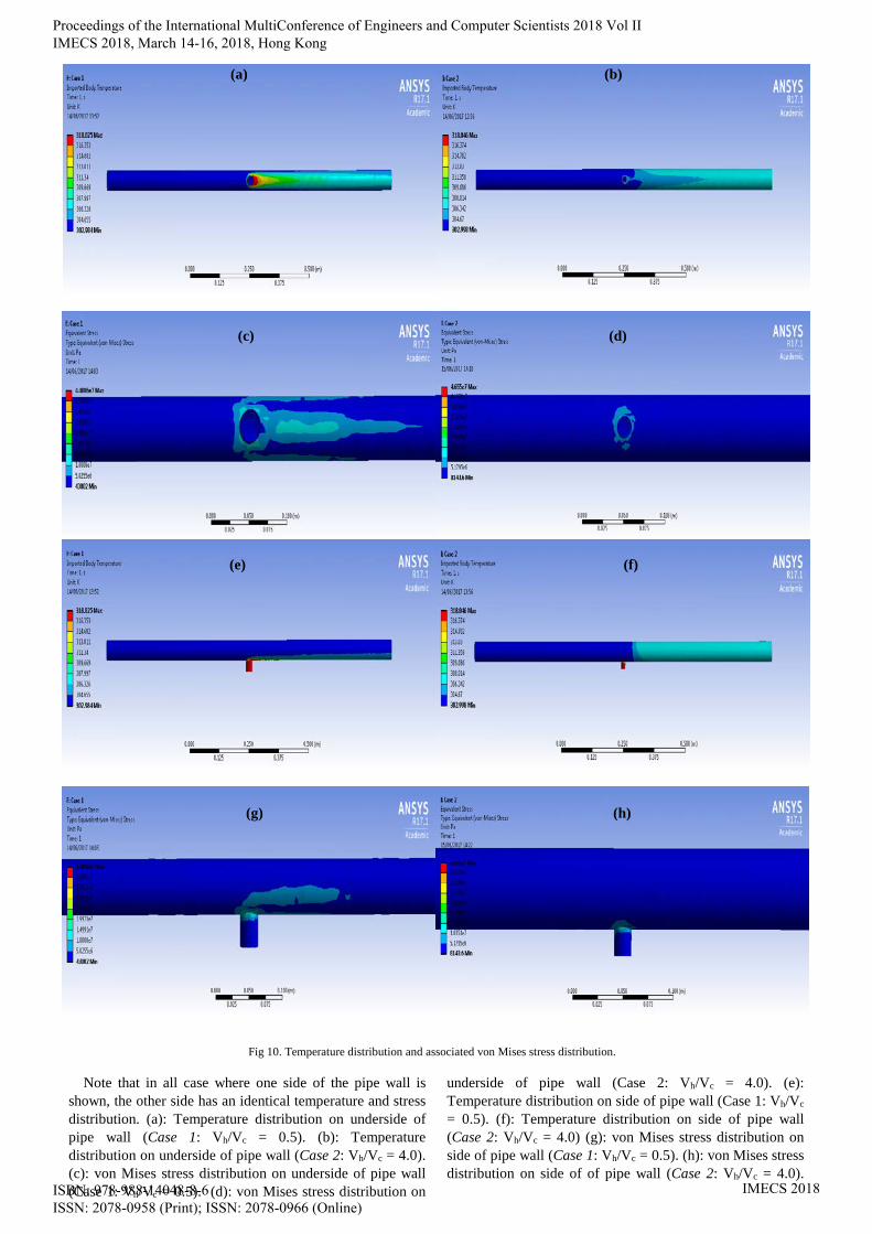
Fig 10. Temperature distribution and associated von Mises stress distribution.

Note that in all case where one side of the pipe wall is

shown, the other side has an identical temperature and stress distribution. (a): Temperature distribution on underside of pipe wall (Case 1: Vh/Vc = 0.5). (b): Temperature distribution on underside of pipe wall (Case 2: Vh/Vc = 4.0). (c): von Mises stress distribution on underside of pipe wall (Case 1: Vh/Vc = 0.5). (d): von Mises stress distribution on

underside of pipe wall (Case 2: Vh/Vc = 4.0). (e): Temperature distribution on side of pipe wall (Case 1: Vh/Vc = 0.5). (f): Temperature distribution on side of pipe wall (Case 2: Vh/Vc = 4.0) (g): von Mises stress distribution on side of pipe wall (Case 1: Vh/Vc = 0.5). (h): von Mises stress distribution on side of of pipe wall (Case 2: Vh/Vc = 4.0).

(g)

(h)

(a) (b)

(d) (c)

(f) (e)



IMECS 2018

From Fig. 10, it can be seen that in both cases, there is a temperature distribution through the main pipe wall at the downstream location (i.e. away from the hot fluid inlet). For Case 1 (Vh/Vc = 0.5), the temperature increases occur on the bottom of the pipe in the plane of the branch-pipe entrance, whereas for Case 2 (Vh/Vc = 4.0), the hot ‘jet’ of fluid entering the main flow introduces a temperature increase throughout the whole circumference of the downstream portion of the pipe. The von Mises stress distributions are different also, whereas the magnitudes are similar. For Case 1, the stress is in the range 5-15 MPa and presents as a ring around the joint between the main pipe and branch pipe as well as a distinctive ‘trident’ pattern along the main pipe, emanating from the branch-pipe in the down-stream direction. For Case 2, the stress is in the range 5-15 MPa and this stress is localized in a ring around the joint between the main and main pipe. Therefore, based upon the two cases here, it can be concluded that the magnitudes of thermal stress do not depend upon the velocity ratio between branch and main pipe, although the distributions will differ; additionally, the latter are seen to be not easily predictable based on analysis of the temperature fields in the pipe-work.

The stress magnitudes and distributions are important in a thermal fatigue analysis. The former is important because the thermal fatigue is more likely to occur in higher stress states; material data exists concerning the likelihood of thermal fatigue for given stress magnitudes. The distribution of stress is important because it permits focused monitoring of the pipe-work for potential crack development; furthermore, certain features are more susceptible to thermal fatigue and their placement should be avoided in sites where thermal fatigue is more likely. With respect to the latter issue, it is certainly noteworthy that the joint between the main and branch pipe of T-junctions are often welded together; thus, for the two cases here, it can be concluded that thermal fatigue of the weld could potentially be an important issue owing to a ring of stress in this region.

IV. CONCLUSION Thermal fatigue induced during thermal-mixing at T-junctions is a significant problem that can lead to cracking and failure of the junction with associated impacts on the many industries in which these structures are utilized. There is a need to predict this phenomenon so that targeted monitoring may be instituted and the placement of fatigue-prone elements (such as welds) can be controlled. Computational fluid-structure analyses can accomplish this and, indeed, are increasingly being utilized now in these cases.

This report presented the results obtained by a steady-state one-way fluid-structure interaction analyses concerning thermal-mixing (303 K and 318 K) in T-junctions. There is a distinct lack of experimental data in the available literature concerning the induced temperature distributions and stresses within pipe-work in these cases; however, there is fluid experimental data available for thermal-mixing T-junction cases. Accordingly, a study by Naik-Nimbalkar et al. was used as the basis to confirm the validity of the results

in this report. It is seen that the fluid flow was captured well by the ANSYS software package since the temperature distributions generally closely matched those obtained by Naik-Nimbalkar et al. There were some (albeit small) discrepancies for Case 2 although the report author believes that a more refined mesh, or perhaps the use of a more complex turbulence model, would alleviate these discrepancies. In any case, it can thus be reasonably assumed that the computational analysis of the pipe-work provided sound results. Naik-Nimbalkar et al. stipulated that the steady-state temperature increase through the mid-plane of the flow in Case 1 did not propagate through the diameter of the flow; this finding is confirmed via computational results. Additionally, Naik-Nimbalkar et al. determined that, for Case 2, the temperature would increase across the whole diameter of the mid-plane. This finding was also confirmed via computational analyses.

There is much further work to be conducted,. Firstly, this investigation utilized steady-state computational analyses. These analyses provide information on the distribution and magnitudes of temperature fields and stress; these do provide useful information as elucidated above. However, transient analyses allow the investigation of the cyclic nature of the stresses over a given time-frame; the frequency and nature of the stress cycles are other important factors in thermal fatigue analysis. Secondly, it would be prudent to investigate whether other turbulence models would provide more accurate results and whether changes in mesh types and sizes had any significant impact upon the results. Thirdly, the investigation here only analyzed two cases of differing velocity ratios in a T-junction of fixed dimensions (with one simulated material) where the temperatures at the two inlets were constant. It would be exceptionally useful to analyze a wide range of factors so that more general conclusions could be drawn; such conclusions could then be applied to the safe and efficient design of T-junctions used for thermal mixing processes.

REFERENCES [1] S. Qian, J. Frith and N. Kasahara, “Classification of Flow Patterns in

Angled T-Junctions for the Evaluation of High Cycle Thermal Fatigue,” Journal of Pressure Vessel Technology, vol. 137, pp. 213011-213017, 2015.

[2] M. Lakshmiraju and J. Cui, “Numerical Modelling of Transient Thermal Mixing,” International Journal of Latest Research in Science and Technology, vol. 3, pp. 80-89, 2014.

[3] M. Kamaya and A. Nakamura, “Thermal stress analysis for fatigue damage evaluation at a mixing tee,” Nuclear Engineering and Design, vol. 241, p. 2674–2687, 2011.

[4] K. Miyoshi, A. Nakamura, Y. Utanohara and N. Takenaka, “An investigation of wall temperature characteristics to evaluate thermal fatigue at a T-junction,” Mechanical Engineering Journal, vol. 1, pp. 1-12, 2014.

[5] M. J. Jhung, “Assessment of Thermal Fatigue in Mixing Tee by FSI analysis,” Nuclear Engineering and Technology, vol. 45, pp. 99-106, 2013.

[6] O. Costa and L. Cizelj, “Approach, Thermal Fatigue Assessment: A Two-Dimensional,” in 20th International Conference: Nuclear Energy for New Europe 2011, Bovec, 2011.

[7] S. Kim, J. Choi, M. Kim, N. Huh and J. Lee, “Evaluation of fatigue damage induced by thermal stripping in a T-junction using the three-dimensional coupling method and frequency response method,” in Transactions of the Korean Nuclear Society Autumn Meeting, Gyeongju, 2012.

[8] H. Lee, J. Kim and B. Yoo, “Assessment of Fatigue and Fracture on a Tee-Junction of LMFBR Piping Under Thermal Stripping



IMECS 2018

Phenomenon,” Journal of Korean Nuclear Society , vol. 31, pp. 267-275, 1999.

[9] V. S. Naik-Nimbalkar, A. W. Patwardhan, I. Banerjee, G. Padmakumar and G. Vaidyanathan, “Thermal mixing in T-junctions,” Chemical Engineering Science, vol. 65, pp. 5901-5911, 2010.

[10] G. Nimadge, “CFD Analysis of Flow through T-Junction An overview,” International Journal for Scientific Research & Development, vol. 4, pp. 2321-2329, 2016.

[11] S. Tawade and A. Suryavanashi, “A Review on Thermal Stress in Mixing Tee Junction Using FSI,” International Journal of Innovative Research in Science, Engineering and Technology, vol. 4, pp. 2420-2427, 2015.

[12] M. J. Jhung and H. Ko, “FSI Analysis of Mixing Tee for Thermal Fatigue,” in Transactions of the Korean Nuclear Society Autumn Meeting , Gyeongju, 2012.

[13] J. Tu, G. Yeoh and C. Liu, “Governing Equations for CFD - Fundamentals,” in Computational Fluid Dynamics: A Practical Approach, 2nd ed., Amsterdam, Elsevier, 2013, pp. 61-118.

[14] H. Lee, “Meshing,” in Finite Element Simulations with ANSYS Workbench 16, Mission, SDC Publications, 2015, pp. 327-364.



IMECS 2018

Documents

Analysis of Thermal Mixing in T-Junctions Using Fluid ... · right angles, creating a mixing region of fluid both around and downstream of the junction resulting inT- temperature