Technical Note: Review of methods for linear least-squares fitting of

Atmos. Chem. Phys., 8, 5477–5487, 2008www.atmos-chem-phys.net/8/5477/2008/© Author(s) 2008. This work is distributed underthe Creative Commons Attribution 3.0 License.

AtmosphericChemistry

and Physics

Technical Note: Review of methods for linear least-squares fitting ofdata and application to atmospheric chemistry problems

C. A. Cantrell

National Center for Atmospheric Research Atmospheric Chemistry Division 1850 Table Mesa Drive Boulder,CO 80305, USA

Received: 13 February 2008 – Published in Atmos. Chem. Phys. Discuss.: 1 April 2008Revised: 11 August 2008 – Accepted: 15 August 2008 – Published: 12 September 2008

Abstract. The representation of data, whether geophysi-cal observations, numerical model output or laboratory re-sults, by a best fit straight line is a routine practice in thegeosciences and other fields. While the literature is full ofdetailed analyses of procedures for fitting straight lines tovalues with uncertainties, a surprising number of scientistsblindly use the standard least-squares method, such as foundon calculators and in spreadsheet programs, that assumes nouncertainties in thex values. Here, the available proceduresfor estimating the best fit straight line to data, including thoseapplicable to situations for uncertainties present in both thex andy variables, are reviewed. Representative methods thatare presented in the literature for bivariate weighted fits arecompared using several sample data sets, and guidance ispresented as to when the somewhat more involved iterativemethods are required, or when the standard least-squares pro-cedure would be expected to be satisfactory. A spreadsheet-based template is made available that employs one methodfor bivariate fitting.

1 Introduction

Representation of the relationship betweenx (independent)andy (dependent) variables by a straight line (or other func-tion) is a routine process in scientific and other disciplines.Often the parameters (slope andy-intercept) of such a fittedline can be related to fundamental physical quantities. It istherefore very important that the parameters accurately rep-resent the data collected, and that uncertainties in the param-eters are estimated and applied correctly or the results of thefitting process and thus the scientific study could be misin-terpreted.

Correspondence to:C. A. Cantrell([email protected])

The approaches to fitting straight lines to collections ofx−y data pairs can be broadly grouped into two categories:the “standard” least-squares methods in which the distancesbetween the fitted line and the data in they-direction are min-imized, and the “bivariate” least-squares methods in whichthe perpendicular distances between the fitted line and thedata are minimized. A third method, similar to the secondbut less commonly employed, involves minimization of theareas of the right triangles formed by the data point and theline. In all of these methods, weights may be also applied tothe data to account for the differing uncertainties in the indi-vidual points. In “standard” least-squares, the weighting per-tains to they-variables only, whereas in “bivariate” methods,weights can be assigned for thex- andy-variables indepen-dently. There is widely varying terminology for these proce-dures in the literature that can be confusing to the non-expert.Authors have used terms such as major axis regression, re-duced major axis regression, ordinary least-squares, maxi-mum likelihood, errors in variables, rigorous least-squares,orthogonal regression and total least-squares. Herein, theterms “standard” and “bivariate” will be used to denote thesetwo categories of fitting methods. This paper does, however,present a detailed reference list of available methods and ap-plications presented in the literature.

For demonstration and testing purposes, two data sets fromthe literature were employed. First, the well-known data ofPearson (1901) with weights suggested by York (1966) wereused (see Table 1 and Fig. 1). The data values are similar tothose that might be encountered in a laboratory study or ac-quired in atmospheric measurements, but with rather extremeweights that range 3 orders of magnitude as the data rangesabout a factor of five. This data set has the advantage thatthe exact results of the bivariate fit are known and reportedin the literature, and one that is frequently used as a test fornew fitting methods.

Published by Copernicus Publications on behalf of the European Geosciences Union.

http://creativecommons.org/licenses/by/3.0/

5478 C. A. Cantrell: Least squares fitting

25 of 32

Pearson's Data with York's Weights

X Data

0 2 4 6 8

Y D

ata

0

2

4

6

8

data

standard least squares

standard least squares w/ weights

Williamson-York, Neri et al.

Krane and Schecter

Figure 1.

Fig. 1. Linear fits to the data of Pearson [1901] with weights sug-gested by York [1966] (“Pearson-York” data set, shown in Table 1).The weights have been plotted asσ values (wi=1/σ2

i). Fit parame-

ters are shown in Table 2.

Table 1. Example data “Pearson’s data with York’s weights” forcomparison of fitting procedures described in the text.

x wx y wy

1 0.0 1000.0 5.9 1.02 0.9 1000.0 5.4 1.83 1.8 500.0 4.4 4.04 2.6 800.0 4.6 8.05 3.3 200.0 3.5 20.06 4.4 80.0 3.7 20.07 5.2 60.0 2.8 70.08 6.1 20.0 2.8 70.09 6.5 1.8 2.4 100.010 7.4 1.0 1.5 500.0

A second data set was created by selecting random num-bers from Gaussian distributions and adding them to basevalues, which were numbers 1 through 100 (see Fig. 2). Ini-tially, the Gaussian distributions were set with means of zero,and standard deviations of 10 units plus 30% of the basevalue, but other tests were performed with different amountsof constant and proportional uncertainty. These data weremeant to represent those that would result from an inter-comparison of two instruments measuring the same quantity,which have baseline noise of 10 units (1 sigma), measure-ment uncertainties that are well above the baseline of 30%(1 sigma), and nominal “true” values from 1 to 100 units.This data set has the characteristic that in the absence ofnoise, or if the noise is properly dealt with, the best fit lineshould have a slope of one, and an intercept of zero.

26 of 32

Synthetic Data with Random Noise (10+30%)

X Data

-50 0 50 100 150 200

Y D

ata

-50

0

50

100

150

200

250data

standard least squares

standard least squares w/ weights

Williamson-York, Neri et al.

Krane and Schecter

1:1

Figure 2.

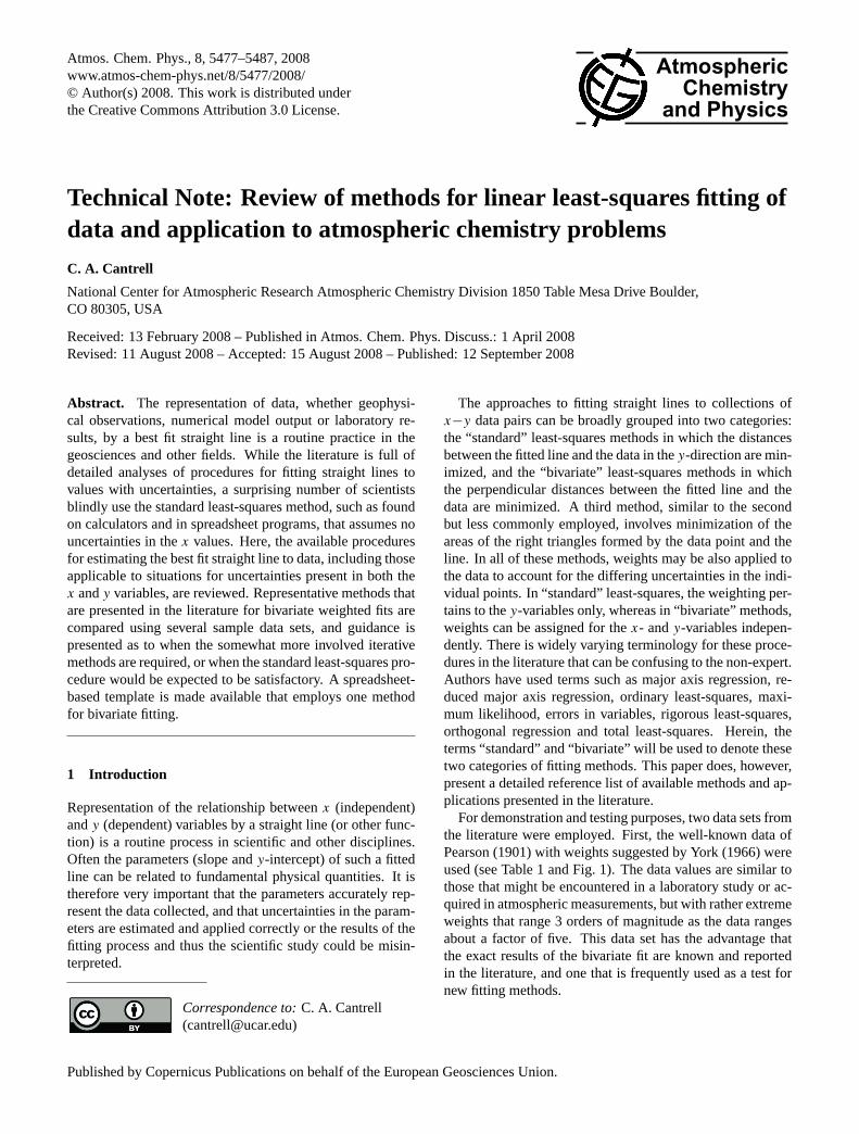
Fig. 2. Linear fits to data generated by sampling a Gaussian functionwith standard deviation of 10 units plus 30%, and adding the noiseto the numbers 1 through 100. Fit parameters are shown in Table 3.

Next, the methods were applied to two examples of au-thentic data to demonstrate specifically the value of bivariatemethods, and to point out how and when they should be ap-plied.

This review and recommendation does not attempt to bemathematically nor statistically rigorous. The reader is re-ferred to the referenced literature for such details. The pur-pose here is to provide operational information for the scien-tific user of these routines, and to provide guidance for thechoice of routine to be utilized.

Note that there is not universal agreement in the uses ofsymbols for the measuredx andy values and the calculatedslope and intercept that appear in the literature. The reader iscautioned in this regard. In this paper,xi andyi (lower caseitalics) refer to the measuredx andy values,m refers to theslope of the best fit line, andb is they-axis intercept. Othersymbols are defined throughout the paper.

2 Standard least-squares

The equations for a line that best describesx−y data pairswhen all of the measurement error may be assumed to re-side in they-variable (i.e. thex values are exact or nearlyso) is readily available and easily derived (e.g. Bevington,1969). The fitted line then becomes a “predicted” value fory

given a value forx. The usual method involves minimizingthe sum of squares of the differences between the fitted lineand the data points in they-direction (although minimiza-tion of other quantities has been used). The slope,m, andy-intercept,b, of this best-fit line can be represented in termsof summations of computations performed on then measured

Atmos. Chem. Phys., 8, 5477–5487, 2008 www.atmos-chem-phys.net/8/5477/2008/

C. A. Cantrell: Least squares fitting 5479

Table 2. Comparison of fit parameters using various weighting and fitting procedures for Pearson’s data with York’s weights (reproduced inTable 1).

Reference order Slope Std err Slope % diff Intercept Std err Intcpt % diff

Std Least-Squaresy−x –0.53958 0.0421 12.3 5.7612 0.189 5.1x−y –0.56589 0.0442 17.8 5.8617 0.216 7.0

Std Lst-Sqrs w/wgtsy−x –0.61081 – 27.1 6.1001 – 11.3x−y –0.66171 – 37.7 6.4411 – 17.5

Williamson-Yorky−x –0.48053 0.0706 0 5.4799 0.359 0x−y –0.48053 0.0706 0 5.4799 0.359 0

Neri et al.y−x –0.48053 – 0 5.4799 – 0x−y –0.48053 – 0 5.4799 – 0

Reedy−x –0.48053 0.0706 1×10−7 5.4799 0.359 6×10−8

x−y –0.48053 – 3×10−7 5.4799 – 1×10−7

Macdonaldy−x –0.48053 – 5×10−6 5.4799 – 2×10−6

x−y –0.48053 – 5×10−5 5.4799 – 8×10−6

Lybanony−x –0.48053 – 2×10−6 5.4799 – 5×10−7

x−y – – – – – –

Krane and Schectery−x –0.46345 – 3.6 5.3960 – 1.5x−y –0.55049 – 14.6 5.8163 – 6.1

data pairs,x1, y1, x2, y2, . . . ,xn, yn.

m =n∑

xiyi −∑

xi

∑yi

n∑

x2i −

(∑xi

)2b =

∑x2i

∑yi −

∑xi

∑xiyi

n∑

x2i −

(∑xi

)2 (1)

The6 symbols refer to the summation of the quantity overall n values, and the subscript,i, denotes the individual mea-suredx andy values. The uncertainties in the slope and in-tercept can also be calculated.

σm =

√∑y2i −b

∑yi−m

∑xiyi

n−2√n∑

x2i −

(∑xi

)2 σb = σm

√∑x2i

n(2)

Another useful quantity is the correlation coefficient (alsocalled the Pearson Correlation Coefficient), which providesan index of the degree of correlation between thex andy

data.

rxy =n∑

xiyi−∑

xi

∑yi√(

n∑

x2i −

(∑xi

)2) (n∑

y2i −

(∑yi

)2) (3)

It is usually the case that not all the data points have the sameuncertainty. Thus, it is desired that data with least uncertaintyhave the greatest influence on the slope and intercept of thefitted line. This is accomplished by weighting each of thepoints with a factor,wi , which is often assumed (and demon-strated mathematically to yield the best unbiased linear fitparameters, if set) equal to the inverse of the variance of the

y-values (σ 2yi). It could include estimates of all sources of

uncertainty in they-values. Other weighting procedures arealso possible. The formulas for the slope and intercept aremodified as shown to include data weights.

m =

∑wi

∑wixiyi −

∑wixi

∑wiyi∑

wi

∑wix

2i −

(∑wixi

)2b =

∑wix

2i

∑wiyi −

∑wixi

∑wixiyi∑

wi

∑wix

2i −

(∑wixi

)2 (4)

These formulas are readily programmed, or exist as availablespreadsheet or calculator functions, and can be routinely ap-plied to fitting of straight lines tox−y data sets.

The standard least-squares method was applied with andwithout weights, using Eqs. (1) and (4), to the two test datasets (“Pearson-York” and “synthetic data”) for comparisonwith the bivariate methods (see Tables 2 and 3). Note thatwhen there are significantx andy errors, that standard least-squares yields erroneous slopes. For the “synthetic data”, theslope was usually too small, whereas for the “Pearson-York”data, the slope was too large (compared to the Williamson-York and Neri et al. methods, discussed below).

3 Methods when bothx and y have errors

The application of fitting procedures that account for uncer-tainties in both thex- and y- variables is somewhat morecomplex. This is because minimization of the distance be-tween data points and a fitted line in thex- andy-directionshas not yielded to analytical solutions. Iterative approachesare therefore required. Several equation forms have been

www.atmos-chem-phys.net/8/5477/2008/ Atmos. Chem. Phys., 8, 5477–5487, 2008


Table 3. Comparison of fit parameters using various weighting and fitting procedures for synthetic data with random errors (see text).

Reference order Slope Std err Slope % diff Intercept Std err Intcpt % diff

Std Least-Squaresy−x 0.64455 0.0802 37.7 15.5840 5.068 526x−y 1.62395 0.2022 57.0 –33.2653 10.818 810

Std Lst-Sqrs w/wgtsy−x 0.51688 – 50.0 3.12330 – 185x−y 1.45084 – 40.3 –25.7369 – 604

Williamson-Yorky−x 1.03409 0.1004 0 –3.65745 3.369 0x−y 1.03409 0.1004 0 –3.65745 3.369 0

Neri et al.y−x 1.03409 – 0 –3.65745 – 0x−y 1.03409 – 0 –3.65745 – 0

Reedy−x 1.03409 – 0 –3.65745 – 0x−y 1.03409 – 0 –3.65745 – 1×10−9

Krane and Schectery−x 0.63716 – 38.4 3.73640 – 202x−y 1.69288 – 63.7 –16.2079 – 343

proposed and discussed (Barker and Diana, 1974; Borcherdsand Sheth, 1995; Brauers and Finlayson-Pitts, 1997; Bruz-zone and Moreno, 1998; Chong, 1991, 1994; Christian andTucker, 1984; Christian et al., 1986; Gonzalez et al., 1992;Irwin and Quickenden, 1983; Jones, 1979; Kalantar, 1990,1991; Krane and Schecter, 1982; Leduc, 1987; Lybanon,1984ab, 1985; Macdonald and Thompson, 1992; MacTag-gart and Farwell, 1992; Markovsky and Van Huffel, 2007;Moreno, 1996; Neri et al., 1990, 1991; Orear, 1982; Pasa-choff, 1980; Pearson, 1901; Press et al., 1992a,b; Reed,1990; Riu and Rius, 1995; Squire et al., 1990; Williamson,1968; York, 1966, 1969; York et al., 2004). This list is largeto provide a comprehensive reference for the reader. Whilethese approaches are not as convenient as the straightforwardequations applicable to standard least-squares, they can eas-ily be programmed using standard languages or spreadsheetprogram routines.

In assessing the impacts of errors on linear fits, normal(Gaussian) distributions of the errors are assumed. This is areasonable assumption for most real-world situations, but itshould be recognized that formulations for error estimates ofthe slope and intercept of the fits will be different for othererror distributions.

Some representative examples of exact and approximateprocedures (discussed below) from the literature were ap-plied to the sample data sets, and the results of the fits areshown in Tables 2 and 3. In each case, slopes and interceptswere derived by fittingy on x, and by exchanging thex andy variables, thus fittingx ony. The slopes and intercepts forthe latter case were made comparable to those of the formercase by calculating the equivalent values fory=mx+b (sincex=y/m−b/m, thenm′=1/m andb′

= − b/m). For methodsthat properly account for errors in both variables, the fit pa-rameters by these two approaches should be identical (i.e.m′

from fitting x on y should equalm from fitting y on x, andsimilarly for b′ andb). This is termed invariance to exchange

of x and y. Proper fitting methods should also be invari-ant to change of scale (i.e. fit parameters do not depend onthe choice of units forx andy). Several numerical digits areshown in Tables 2 and 3, not all significant, so that the resultsfrom the various methods can be accurately compared.

The method described by York (1966; 1968) and Yorket al. (2004) was applied to the sample data sets. This in-volves iteratively solving the following equations (Eq. 5).This method allows for correlation between thex andy er-rors, indicated byri (different than therxy in Eq. 3), whichis set to zero in the present case (i.e. errors are assumed to beuncorrelated).

b = y − m x m=∑

WiβiVi∑WiβiUi

x =∑

Wixi

/∑Wi y=

∑Wiyi

/∑Wi

Ui = xi − x Vi=yi−y Wi=wxiwyi

wxi+m2wyi−2mriαi

βi = Wi

[Ui

wyi+

mVi

wxi− (mUi + Vi)

riαi

]αi =

√wxiwyi

(5)

The procedure is to assume a starting value form, calcu-lateWi, Ui, Vi , αi , andβi , and then calculate a revised valuefor m. This process is repeated untilm changes by somesmall increment according to the accuracy desired. This is asimpler implementation of an earlier method of York (1966),which was described in York (1969) and York et al. (2004),and is the same as the method of Williamson (1968), if thex andy errors are uncorrelated (i.e.ri=0). The method ofWilliamson (1968) has been praised in the literature (Mac-Taggert and Farwell, 1992; Kalantar, 1990) as being effi-ciently able to converge to the correct answer. Other ap-proaches (including the earlier York method), may not al-ways converge or may be slow to do so, depending on thespecific data set. As with standard least-squares, one can per-form bivariate fits without weighting. This is done by makingall the weights the same (e.g. 1).

The uncertainties in the slope and intercept can also be cal-culated. Among various methods discussed in the literature



(Cecchi, 1991; Kalantar, 1992; Kalantar et al., 1995; Morenoand Bruzzone, 1993; Reed, 1990, 1992; Sheth et al., 1996;Williamson, 1968; York et al., 2004), the following formsappear to lead to correct estimates of the fit parameter uncer-tainties (after York et al. (2004) with some algebraic manip-ulation).

σ 2b =

1∑Wi

+(x + β

)2σ 2

m σ 2m =

1∑Wi

(βi−β

)2std errb=

√σ 2

b

√S

n−2 std errm=√

σ 2m

√S

n−2

β =∑

Wiβi

/∑Wi

S =∑

[yi − (mxi + b)]2

(6)

The quantity√

S/(n − 2) is a “goodness of fit” parameter.

Its expected value is unity. Its deviation from unity can beused to adjust the weighting factors (in a global sense), butthe bivariate slope and intercept will not be affected.

Another straightforward method is that of Neri etal. (1989). This involves minimization of the shortest dis-tance between the fitted line and that data points, and as-sumes thex andy errors are uncorrelated. The followingequations are utilized.∑

Wixi(mxi + b − yi) −∑ W2

i m(mxi+b−yi )2

wxi= 0

b =∑

Wi (yi − mxi)/∑

Wi

Wi =wxiwyi

wxi+m2wyi

(7)

In this method, an initialm is guessed (such as from stan-dard least-squares or by inspection),b is calculated (secondequation in Eq. 7), and thenm is adjusted to minimize theleft hand side of the first equation in Eq. (7). The process isrepeated until the left side of the first equation in Eq. (7) issatisfactorily close to zero. The Williamson-York and Neri etal. methods give identical results for the slope and interceptof the two test data sets.

Four other methods give results that are reasonably closeto the above results, but are not exactly the same, and donot always give the same slope on exchange of thex andy

variables. These approximate methods may be satisfactoryfor many applications.

Reed (1992) suggests finding roots of the followingquadratic expression.

g(m) = Am2+ Bm + C = 0

A =

∑ W2i UiVi

wxi

B =∑

W2i

(U2

i

wyi

−V 2

i

wxi

)C =−

∑ W2i UiVi

wyi

(8)

This equation is solved form by the quadratic formula,

m =

(−B ±

√B2 − 4AC

)/2A, where the choice of roots

is refined by comparison with standard least-squares or byinspection.

Macdonald and Thompson (1992) describe a number ofcases for which their method is applicable. They have madeavailable a FORTRAN program that applies their procedures,which provides nearly exact results for the Pearson-York dataset. Similarly, Lybanon (1984) presents a detailed methodthat also yields results very close to those of the “exact”methods. Krane and Schecter (1982) put forward a methodproposed by Barker and Diana (1974) and discussed by oth-ers (Irwin and Quickenden, 1983; Orear, 1984; Lybanon,1984b) that is called “effective variance”. One begins withEq. (4), but the weights,wi , are adjusted to the followingform.

wi =wxiwyi

wxi + m2wyi

(9)

This is same as York’sWi value with uncorrelated errors.Sincem appears in the formula for the weight, an iterativeprocess is required, in which an initialm value is guessed,wi is calculated, followed by calculation of a revisedm. Theresult differs from the “exact” methods for the Pearson-Yorkdata set by a few percent, but it is more accurate than thestandard least-squares. This method does not retrieve thesame slope and intercept when thex- and y-variables areexchanged. The errors are larger with the “synthetic” dataset.

Press et al. (1992a,b) present a method called “maximumlikelihood estimation” and include a routine written in C orFORTRAN for its implementation. This is also discussed byTitterington and Halliday (1979). York et al. (2004) demon-strate that their method and “maximum likelihood estima-tion” are mathematically identical. Brauers and Finlayson-Pitts (1997) applied the Press et al. method to analysis ofkinetic data.

The methods of Williamson (1968), York (1969), York etal. (2004) and Neri et al. (1989) all agree and appear to pro-vide the exact answer to the best fit for the Pearson-York dataset. The approaches of Reed (1992), Macdonald and Thomp-son (1992), and Lybanon (1984) provide results very close tothe exact ones. The “effective variance” method performsreasonably well for the Pearson-York data set, but poorer forthe synthetic data. Because of this variability in performance,it should be used with caution.

4 Comparing the methods

A more detailed examination of the behavior of bivariateand standard least-squares as a function of the random noiseadded in the “synthetic data” was performed. The purposehere is to advise the reader when the more involved bivariatemethods should be used or when the standard least-squaresare expected to provide satisfactory values for the fit parame-ters. A series of calculations was performed in which randomnoise was sampled from Gaussian distributions with varyingconstant and proportional standard deviations (like the sec-ond test data set used above). Standard least-squares (without



27 of 32

Synthetic Data Fit Summary

r

0.0 0.2 0.4 0.6 0.8 1.0

mfi

t /

me

xp

ecte

d

-0.2

0.0

0.2

0.4

0.6

0.8

1.0

1.2

1.4

1.6Bivariate

Standard LS, x & y errors

Standard LS, y errors only

Pearson-York std LS

0.90 0.95 1.000.85

1.00

1.15

Figure 3.

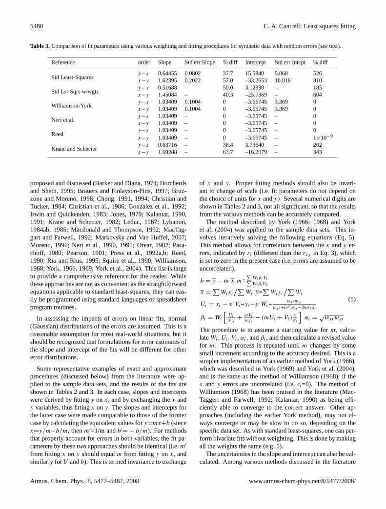
Fig. 3. Ratio of fitted to expected slopes (mfit/mexpected) from stan-dard least-squares and the Williamson-York bivariate method versusr-values from Eq. (3). Errors in both thex andy variables lead tosystematic errors in the slope from standard least-squares. Slopesfrom the bivariate method show no such systematic variation withr.

weights) were applied to the data sets, as was the method ofWilliamson-York. The values ofr (Eq. 3) were also calcu-lated. This test has the advantage that the “correct” slope andintercept are known (1 and 0, respectively). Note that the er-rors are normally distributed, which may not necessarily bethe case in “real” data sets.

Figure 3 showsmfit/mexpectedversusr of the best fit linesusing standard least-squares when proportional uncertaintiesof zero to 50% and/or constant uncertainties of up to 50units were applied to thex-data, they-data, or both. Stan-dard least-squares performs well by retrieving slopes close tounity (the expected value) when errors are applied to they-data only. However, when errors are added to thex-variableeither alone or with errors added to they-variable, the slopesof the best fit lines from standard least-squares are signifi-cantly less than unity. The ratio of the fitted slope to that ex-pected is approximately equal to|r|. This is true even whenr values are very small. The normal interpretation of thesesmall r values is that the data are uncorrelated and cannotbe represented by a linear relationship. In this case, how-ever, we know that there is a linear relationship betweenx

andy because of the way the data were constructed. TheF

statistics for the standard fits indicate that they are statisti-cally significant at the 95% confidence level for all but thosecorresponding to the 3 smallestr values.

Applying the Williamson-York bivariate method to thesame data sets, leads to slopes within about 20% of the ex-pected value of unity. Note that this is the case even whenthe data are very noisy and thus correlation coefficients aresmall. Values much closer to the expected value are retrievedwhen the data is less noisy (see inset in Fig. 3). These fits

were performed with 100 data points. If the sizes of the datasets are increased, the error (scatter) in the slope decreasesaccordingly. As an example, for a constant error of 28 units,the average error in the slope (5 repetitions) decreases from19% to 6% to less than 1% as the number of data points goesfrom 100 to 1000 to 10 000 (an approximate

√n relation-

ship).Knowing that the bivariate methods are an improvement

over standard least-squares when there are errors in thex-variable is a start, but can the information gathered be usedto indicate when the extra trouble of the bivariate fit is calledfor, versus when standard least-squares will suffice. Figure 3shows that there is a rather robust relationship between thesystematic error in the slope from standard least-squares andthe absolute value of the correlation coefficient (as expected,comparing Eqs. 1 and 3). For errors in both variables, thefractional error in the standard least-squares slope is approx-imately 1–|r|. Thus, a quick calculation of the correlationcoefficient can give a rough indication of the error in the de-rived standard least-squares slope for data with comparableerrors in both variables. If this error in the slope is outsidethe needs of the task at hand, then a bivariate approach shouldbe employed. For unusual weighting situations (such as thePearson-York data), it is probably best to always use robustbivariate methods, since the impact of such weights on the fitparameters is not intuitive (although in this specific case, thestandard least-squares slope is only in error by 12%). Whenthe error in they-variable is much greater than the error inx-variable, then standard least-squares performs better thanindicated by the calculatedr value.

5 Application to actual observations

Two authentic sets of data from the TRACE-P campaign(TRansport And Chemistry Experiment – Pacific) were se-lected for application of these fitting procedures. TRACE-Pinvolved two aircraft (the NASA DC-8 and P3-B) as plat-forms for observations primarily in the western Pacific Oceanbasic. The observations used here are gas-phase formalde-hyde (CH2O) concentrations collected by Alan Fried and col-leagues aboard the NASA DC-8 aircraft (Fried et al., 2003),and peroxy radical concentrations (HO2+RO2) collected bythe author and colleagues aboard the NASA P-3B aircraft(Cantrell et al., 2003). These data represent very typical sit-uations that might require the fitting procedures discussedhere.

The details of the measurement techniques and the model-ing approaches can be found in the references cited above.Briefly, CH2O was measured in the NASA DC-8 aircraftin a low-pressure cell with multi-pass optics (100 m pathtotal optical path) using a tunable lead salt diode infraredlaser as the source. A spectral line near 2831.6 cm−1 wasscanned and the second harmonic spectrum (after subtractionof the background) was related to the ambient concentration



through addition of known mixtures of CH2O in zero air tothe instrument inlet. The measurements were corrected for asmall interference from methanol. The estimated uncertaintyof the measurements was 15%, and detection limits typicallyranged from 50 to 80 pptv (parts per trillion by volume). Oneminute average retrieved concentrations ranged from –47 to10 665 pptv. Concentrations measured below the detectionlimit were used as observed in the fits described here.

HO2+RO2 concentrations were measured on the NASA P-3B aircraft and were determined by conversion to gas-phasesulfuric acid through the addition of reagent gases NO andSO2 to the instrument inlet. The sulfuric acid product wasionized by reaction with negatively charged nitrate ions. Theproduct and reagent ions were quantified by quadrupole massspectrometry. Calibrations were performed using quantita-tive photolysis of water vapor at 184.9 nm. The estimateduncertainty for these data was 17% and the detection lim-its were 2–5 pptv. Concentrations below the detection limitwere used as observed in the fits described here.

CH2O and HO2+RO2 concentrations were estimated by aphotochemical box model with inputs of key parameters con-strained by the observations (Crawford et al., 1999; Olson etal., 2004). The time-dependent model is run for several daysto diurnal steady state. Monte Carlo calculations yielded un-certainty estimates of 20% for modeled CH2O and 30% forHO2+RO2.

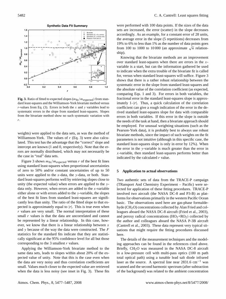
Figure 4 shows the measured CH2O concentrations ver-sus those estimated by the constrained box model on lin-ear scales (4466 data pairs). The inset plots show the highrange of concentrations (>500 pptv, lower right) and the dataplotted on logarithmic scales (upper left). The lines repre-sent different methods of fitting the data. The solid line isa weighted bivariate fit to all of the data with the measure-ments weighted using a variance of the square of 15% ofthe concentration plus 50 pptv, and the model results usinga variance of the square of 20% of the concentration. Theslope is near unity (1.054, standard error=0.0144) and they-intercept is small (1.283, standard error=2.046), in agree-ment with assessments by Fried et al. (2003) and Olson etal. (2004). The correlation coefficient squared,r2 is 0.856.The long dashed line is a standard unweighted least-squaresfit which yields a slope of 1.462 (standard error=0.0090) anda y-intercept of –44.6 (standard error 3.16). It appears thatthe line is being unduly weighted by the handful of pointsat high concentrations in which the model systematically un-derestimates the observations, leading to a larger slope thanthe bivariate method. The medium dashed line is a weightedleast-squares fit (Eq. 4), with weights calculated using the“effective variance” method (Eq. 9). Its slope is 0.873 andthe y-intercept is 20.1. Finally, the short dashed line is aweighted least-squares fit (equation 4) with weights in the y-direction only (i.e.wi=wyi). The slope for this fit is 0.811(std err=0.012) and they-intercept is 22.4 (std err=2.14).These fits mostly have slopes of unity within the combinedmeasurement-model uncertainties (0.25, 1σ), with the ex-

28 of 32

CH2O measurement-model comparison

CH2O, pptv (model)

0 200 400 600 800 1000

CH

2O

, p

ptv

(m

eas

ure

me

nt)

0

200

400

600

800

1000

2000 4000 6000 8000 10000

2000

4000

6000

8000

10000

1 10 100 1000 100001

10

100

1000

10000

Figure 4.

Fig. 4. Comparison of measured formaldehyde concentrations withthose estimated from a constrained box model during the TRACE-P campaign (after Fried et al., 2003; Olson et al., 2004). The datapoints are divided into two groups: those corresponding to measure-ments below 500 pptv (small points), and those for measurementsabove 500 pptv (large points). The main window (on linear scales)shows results of linear fits using four approaches: solid line, bivari-ate weighted fit to all data; long dash, standard unweighted least-squares fit; medium dash, fit using weighted standard least-squares(Eq. 4) with weights calculated using effective variance; and shortdash, fit using weighted standard least-squares with weights in they-direction only. The lower right inset shows the fit lines and dataon expandedx- andy-scales (linear). The upper left inset shows thefull range of data on logarithmic scales. See text for fit parametersand discussion.

ception of the standard unweighted least-squares fit. Theintercepts are all within the detection limit of the measure-ments (around 50 pptv). The large slope retrieved with thestandard unweighted approach could lead one to make theassessment that there are missing processes in the model,errors in the measurements, or both. While it does appearthat there are statistically significant differences between themeasurements and the model at high concentrations, thesmall number of outliers should not significantly change thefit of the entire data set. Eliminating data pairs with mea-surements greater than 4000 pptv, results in bivariate fit slopeand y-intercept values of 1.041 and 2.476, respectively. Theweighted standard fits change by small amounts as well. Theunweighted standard fit, though, yields slope and y-interceptvalues of 1.248 and –5.744, respectively. This is a signif-icant change and shows how susceptible the standard fit isto a small number of outliers (the term outlier is used hereto mean data that are not described well by the bivariate fitline).

The impact of outliers on the various fit methods is demon-strated further. To the full data set are added numbers of datapairs (up to 1000) for whichx is 50 and y is 5000. A secondtrial added data pairs withx values of 5000x andy values



29 of 32

1 10 100 1000

fit

slo

pe

-0.2

0.0

0.2

0.4

0.6

0.8

1.0

1.2

1.4

1.6

1 10 100 1000

fit

y-a

xis

in

terc

ep

t

0

200

400

600

800

1000

Number of outliers added

1 10 100 1000

r 2

0.0

0.2

0.4

0.6

0.8

1.0

Figure 5.

Fig. 5. Impacts of added data outliers to the formaldehyde datasetpresented in Fig. 4. Shown are slopes (top panel), intercepts (middlepanel), and correlation coefficients (bottom panel) of various fits asimpacted by adding extra points, in amounts indicated on thex-axis,to the dataset that are clearly outliers. Eight collections of fit param-eters are shown for 1, 10, 100, and 1000 outliers added. Four collec-tions had outliers equal tox=50,y=5000 (dark gray); the other fourhad outliers equal tox=5000,y=50 (light gray). The circles in thetop two panels represent parameters derived from weighted bivari-ate fits; the downward pointing triangles represent parameters de-rived from Eq. (4) using effective variance; the squares represent pa-rameters derived from Eq. (4) with weights in the y-direction only;and the diamonds represent parameters derived from unweightedstandard least-squares. The values on they-axis (corresponding tox=0.8) are those derived from the original formaldehyde data withno added outliers.

of 50. These results are summarized in Fig. 5. It can beseen that outliers above the fit line have little impact on thebivariate and the other weighted fit slopes, even when thenumber of outliers approaches 20% of the data. The stan-dard unweighted least-squares fit is affected moderately byoutliers above the fit line. Outliers below the fit line impactall of the fits greatly except the bivariate. In fact, as shownbefore, the bivariate fit procedure continues to perform welleven when ther2 parameter indicates that thex andy dataare completely uncorrelated. While there have been vari-

30 of 32

HO2+RO

2 measurement-model comparison

HO2+RO2, pptv (model)

0 20 40 60 80 100 120

HO

2+

RO

2,

pp

tv (

meas

ure

men

t)

0

20

40

60

80

100

120

Figure 6.

Fig. 6. Fits of HO2+RO2 measurements versus constrained boxmodel estimates. The lines are four different fit approaches: solidline, bivariate weighted fit to all data; long dash, standard un-weighted least-squares fit; medium dash, fit using weighted stan-dard least-squares (Eq. 4) with weights calculated using effectivevariance; and short dash, fit using weighted standard least-squareswith weights in they-direction only.

ous techniques put forward to eliminate outliers (e.g. theQ-test, Dean and Dixon, 1951) that can applied, these exercisesshow that the bivariate fit method is relatively insensitive tooutliers.

As mentioned earlier, and discussed by Fried et al. (2003),there appears to be a change in the ratio of measurement tomodel values from near unity at lower concentrations to wellabove unity at higher concentrations. As one approach, thedata were separated into two groups for measured values be-low and above 500 pptv, and each group was fit separately.The bivariate slope of the low concentration group is 0.789,while the bivariate slope of the high concentration group is1.403. An alternate method is to fit the ratio of measure-ment to model ([CH2O]meas/[CH2O]model) versus measure-ment value. Separating into two groups as before leads toa bivariate slope of 0.00607 for the low concentration group(i.e. moderate dependence of the ratio on the concentration)and an intercept of 0.797 (the ratio at the limit of zero con-centration). The slope for the high concentration group is0.000679 and the intercept is 1.290. It seems that there couldbe atmospheric processes missing from the model or instru-mental issues affecting the measurements in the high concen-tration regime that need to be addressed (in agreement withFried et al., 2003).

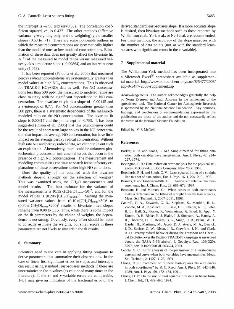
Fits of measured versus modeled HO2+RO2 are shownalong with the data in Fig. 6. The solid line is a bivari-ate fit weighted using variances for the measurements thatare the square of 20% of the concentration plus 5, and us-ing variances for the model results that are the square of30% of model values. Its slope is 0.961 (std err=0.015) and



the intercept is –2.96 (std err=0.35). The correlation coef-ficient squared,r2, is 0.437. The other methods (effectivevariance, y-weighting only, and no weighting) yield smallerslopes (0.63 to .71). There are some noticeable outliers inwhich the measured concentrations are systematically higherthan the modeled ones at low modeled concentrations. Elim-ination of these data does not greatly affect the bivariate fit.A fit of the measured to model ratios versus measured val-ues yields a moderate slope (–0.00864) and an intercept nearunity (1.053).

It has been reported (Faloona et al., 2000) that measuredperoxy radical concentrations are systematically greater thanmodel values at high NOx concentrations. This is observedfor TRACE-P HO2+RO2 data as well. For NO concentra-tions less than 500 pptv, the measured to modeled ratios areclose to unity with no significant dependence on NO con-centration. The bivariate fit yields a slope of –0.00145 anda y-intercept of 0.77. For NO concentrations greater than500 pptv, there is a systematic dependence of the measured-modeled ratio on the NO concentration. The bivariate fitslope is 0.00317 and they-intercept is –0.785. It has beensuggested (Olson et al., 2006) that this phenomenon couldbe the result of short term large spikes in the NO concentra-tion that impact the average NO concentration, but have littleimpact on the average peroxy radical concentration. Withouthigh rate NO and peroxy radical data, we cannot rule out suchan explanation. Alternatively, there could be unknown pho-tochemical processes or instrumental issues that occur in thepresence of high NO concentrations. The measurement andmodeling communities continue to search for satisfactory ex-planations of these observations under high NO conditions.

Does the quality of fits obtained with the bivariatemethods depend strongly on the selection of weights?This was examined using the CH2O measurements andmodel results. The best estimate for the variance ofthe measurements is (0.15×[CH2O]meas+50)2, and for themodel values is (0.20×[CH2O]model)

2. Varying the mea-sured variance values from (0.10×[CH2O]meas+50)2 to(0.30×[CH2O]meas+200)2 results in bivariate fitted slopesranging from 0.88 to 1.15. Thus, while there is some impacton the fit parameters by the choice of weights, the depen-dence is not strong. Obviously, every effort should be madeto correctly estimate the weights, but small errors in theseparameters are not likely to invalidate the fit results.

6 Summary

Scientists need to use care in applying fitting programs toderive parameters that summarize their observations. In thecase of linear fits, significant errors in slopes and interceptscan result using standard least-squares methods if there areuncertainties in thex-values (as cautioned many times in theliterature). If thex- andy-variable errors are comparable,1–|r| may give an indication of the fractional error of the

derived standard least-squares slope. If a more accurate slopeis desired, then bivariate methods such as those reported byWilliamson et al., York et al., or Neri et al. are recommended.For these methods, the accuracy of the slope improves withthe number of data points (not so with the standard least-squares with significant errors in thex-variable).

7 Supplemental material

The Williamson-York method has been incorporated intoa Microsoft Excel® spreadsheet available as supplemen-tal material.http://www.atmos-chem-phys.net/8/5477/2008/acp-8-5477-2008-supplement.zip

Acknowledgements.The author acknowledges gratefully the helpof Norm Evensen and Andi Andreae in the refinement of thespreadsheet tool. The National Center for Atmospheric Researchis sponsored by the National Science Foundation. Any opinions,findings, and conclusions or recommendations expressed in thispublication are those of the author and do not necessarily reflectthe views of the National Science Foundation.

Edited by: V. F. McNeill

References

Barker, D. R. and Diana, L. M.: Simple method for fitting datawhen both variables have uncertainties, Am. J. Phys., 42, 224–227, 1974.

Bevington, P. R.: Data reduction error analysis for the physical sci-ences, McGraw-Hill Book Company, New York, 1969.

Borcherds, P. H. and Sheth, C. V.: Least squares fitting of a straightline to a set of data points, Eur. J. Phys. 16, 1, 204–210, 1995.

Brauers, T. and Finlayson-Pitts, B. J.: Analysis of relative rate mea-surements, Int. J. Chem. Kin., 29, 665–672, 1997.

Bruzzone H. and Moreno, C.: When errors in both coordinatesmake a difference in the fitting of straight lines by least squares,Meas. Sci. Technol., 9, 2007–2011, 1998.

Cantrell, C. A., Edwards, G. D., Stephens, S., Mauldin, R. L.,Zondlo, M. A., Kosciuch, E., Eisele, F. L., Shetter, R. E., Lefer,B. L., Hall, S., Flocke, F., Weinheimer, A. Fried, E. Apel, Y.Kondo, D. R. Blake, N. J. Blake, I. J. Simpson, A., Bandy, A.R., Thornton, D. C., Heikes, B. G., Singh, H. B., Brune, W. H.,Harder, H., Martinez, M., Jacob, D. J., Avery, M. A., Barrick,J. D., Sachse, G. W., Olson, J. R., Crawford, J. H., and Clark,A. D.: Peroxy radical behavior during the Transport and Chemi-cal Evolution over the Pacific (TRACE-P) campaign as measuredaboard the NASA P-3B aircraft, J. Geophys. Res., 108(D20),8797, doi:10.1029/2003JD003674, 2003.

Cecchi, G. C.: Error analysis of the parameters of a least-squaresdetermined curve when both variables have uncertainties, Meas.Sci. Technol., 2, 1127–1128, 1991.

Chong, D. P.: Comment on “Linear least-squares fits with errorsin both coordinates” by B. C. Reed, Am. J. Phys. 57, 642–646,1989, Am. J. Phys., 59, 472–474, 1991.

Chong, D. P.: On the use of least squares to fit data in linear form,J. Chem. Ed., 71, 489–490, 1994.


http://www.atmos-chem-phys.net/8/5477/2008/acp-8-5477-2008-supplement.zip

http://www.atmos-chem-phys.net/8/5477/2008/acp-8-5477-2008-supplement.zip


Christian, S. D. and Tucker, E. E.: Analysis with the microcom-puter. 5. General least-squares with variable weighting, Am.Lab., 16(2), 18–18, 1984.

Christian, S. D., Tucker, E. E., and Enwall, E.: Least-squares anal-ysis: A primer, Am. Lab., 18, 41–49, 1986.

Crawford, J., Davis, D., Olson, J., Chen, G., Liu, S., Gregory, G.,Barrick, J., Sachse, G., Sandholm, S., Heikes, B., Singh, H., andBlake, D.: Assessment of upper tropospheric HOx sources overthe tropical Pacific based on NASA GTE/PEM data: Net effecton HOx and other photochemical parameters, J. Geophys. Res.,104(D13), 16 255–16 273, 1999.

Dean, R. B. and Dixon, W. J.: Simplified statistics forsmall numbers of observations, Anal. Chem., 23, 636–638,doi:10.1021/ac60052a025, 1951.

Faloona, I., Tan, D., Brune, W. H., Jaegle, L., Jacob, D. J., Kondo,Y., Koike, M., Chatfield, R., Pueschel, R., Ferry, G., Sachse, G.,Vay, S., Anderson, B., Hannon, J., and Fuelberg, H.: Observa-tions of HOx and its relationship with NOx in the upper tropo-sphere during SONEX, J. Geophys. Res., 105(D3), 3771–3783,2000.

Fried, A., Crawford, J., Olson, J., Walega, J., Potter, W., Wert, B.,Jordan, C., Anderson, B., Shetter, R., Lefer, B., Blake, D., Blake,N., Meinardi, S., Heikes, B., O’Sullivan, D., Snow, J., Fuelberg,H., Kiley, C. M., Sandholm, S., Tan, D., Sachse, G., Singh,H., Faloona, I., Harward, C. N., and Carmichael, G. R.: Air-borne tunable diode laser measurements of formaldehyde duringTRACE-P: Distributions and box model comparisons, J. Geo-phys. Res., 108(D20), 8798, doi:10/1029/2003JD003451, 2003.

Gonzalez, A. G., Marquez, A., and Fernandez Sanz, J.: An iter-ative algorithm for consistent and unbiased estimation of linearregression parameters when there are errors in both thex andy

variables, Computers Chem., 16(1), 25–27, 1992.Irwin, J. A. and Quickenden, T. I.: Linear least squares treatement

when there are errors in bothx andy, J. Chem. Ed., 60(5), 711–712, 1983.

Jones, T. A.: Fitting straight lines when both variables are subject toerror. I. Maximum likelihood and least-squares estimation, Math.Geo., 11(1), 1–25, 1979.

Kalantar, A. H.: Weighted least squares evaluation of slope fromdata having errors in both axes, Trends in Anal. Chem., 9(1),149–151, 1990.

Kalantar, A. H.: Kerrich’s method fory=αx data when bothy andx are uncertain, J. Chem Ed., 68(1), 368–370, 1991.

Kalantar, A. H.: Straight-line parameters’ errors propagated fromthe errors in both coordinates, Meas. Sci. Technol., 3, 1113–1113, 1992.

Kalantar, A. H., Gelb, R. I., and Alper, J. S.: Biases in summarystatistics of slopes and intercepts in linear regression with errorsin both variables, Talanta, 42(4), 597–603, 1995.

Krane, K. S. and Schecter, L.: Regression line analysis, Am. J.Phys., 50(1), 82–84, 1982.

Leduc, D. J.: A comparative analysis of the reduced major axistechnique of fitting lines to bivariate data, Can. J. For. Res., 17,654–659, 1987.

Lybanon, M.: A better least-squares method when both variableshave uncertainties, Am. J. Phys., 52(1), 22–26, 1984a.

Lybanon, M.: Comment on “Least squares when both variableshave uncertainties”, Am. J. Phys., 52(3), 276–278, 1984b.

Lybanon, M.: A simple generalized least-squares algorithm, Comp.

Geosci., 11, 501–508, 1985.Macdonald, J. R. and Thompson, W. J.: Least-squares fitting when

both variables contain errors: Pitfalls and possibilities, Am. J.Phys., 60(1), 66–73, 1992.

MacTaggart, D. L. and Farwell, S. O.: Analytical use of linear re-gression, Part II: Statistical error in both variables, J. AOAC Intl.,75(4), 608–614, 1992.

Markovsky, I. and Van Huffel, S.: Overview of total least-squaresmethods, Sig. Proc., 87, 2283–2302, 2007.

Moreno, C., and Bruzzone, H.: Parameters’ variances of a least-squares determined straight line with errors in both coordinates,Meas. Sci. Technol., 4, 635–636, 1993.

Moreno, C.: A least-squares-based method for determining the ratiobetween two measured quantities, Meas. Sci. Technol., 7, 137–141,1996.

Neri, F., G. Saitta, and S. Chiofalo: An accurate and straightforwardapproach to line regression analysis of error-affected experimen-tal data, J. Phys. E: Sci. Inst., 22, 215–217, 1989.

Neri, F., Patane, S., and Saitta, G.: Error-affected experimental dataanalysis: application to fitting procedure, Meas. Sci. Technol., 1,1007–1010, 1990.

Olson, J. R., Crawford, J. H., Chen, G., Fried, A., Evans, M. J.,Jordan, C. E., Sandholm, S. T., Davis, D. D., Anderson, B.E., Avery, M. A., Barrick, J. D., Black, D. R., Brune, W. H.,Eisele, F. L., Flocke, F., Harder, H., Jacob, D. J., Kondo, Y.,Lefer, B. L., Martinez, M., Mauldin, R. L., Sachse, G. W., Shet-ter, R. E., Singh, H. B., Talbot, R. W., and Tan, D.: Testingfast photochemical theory during TRACE-P based on measure-ments of OH, HO2, and CH2O, J. Geophys. Res., 109, D15S10,doi:10.1029/2003JD004278, 2004.

Olson, J. R., Crawford, J. H., Chen, G., Brune, W. H., Faloona,I. C., Tan, D., Harder, H., and Martinez, M.: A reevaluation ofairborne HOx observations from NASA field campaigns, J. Geo-phys. Res., 111, D10301, doi: 10.1029/2005/JD006617, 2006.

Orear, J.: Least squares when both variables have uncertainties,Am. J. Phys., 50, 912–916, 1982; Erratum, Am. J. Phys., 52,278–278, 1984.

Pasachoff, J. M.: Applicability of least-squares formula, Am. J.Phys., 48(10), 800–800, 1980.

Pearson, K.: On lines and planes of closet fit to systems of points inspace, Philos. Mag., 2(2), 559–572, 1901.

Press, W. H., Teukolsky, S. A., Vetterling, W. T., and Flannery, B. P.:Numerical Recipes in C, 2nd ed., Cambridge University Press,1992a.

Press, W. H., Teukolsky, S. A., Vetterling, W. T., and Flannery, B.P.: Numerical Recipes in Fortran, 2nd ed., Cambridge UniversityPress, 1992b.

Reed, B. C.: Linear least-squares fits with errors in both coordi-nates, Am. J. Phys., 57(3), 642–646, 1989; Erratum, Am J. Phys.,58(2), 189–189, 1990.

Reed, B. C.: Linear least-squares fits with errors in both coordi-nates. II: Comments on parameter variances, Am. J. Phys., 60(1),59–62, 1992.

Riu, J. and Rius, F. X.: Univariate regression models with errors inboth axes, J. Chemometrics, 9, 343–362, 1995.

Sheth, C. V. A.: Ngwengwe, and P. H. Borcherds, Least squaresfitting of a straight line to a set of data points: II: Parameter vari-ances, Eur. J. Phys., 17(2), 322–326, 1996.

Squire, P. T.: Comment on “Linear least-squares fits with errors



in both coordinates” by B. C. Reed, Am. J. Phys. 57, 642–646,1989, Am. J. Phys., 58(12), 1209–1209, 1990.

Titterington, D. M. and Halliday, A. N.: On the fitting of parallelisochrones and the method of maximum likelihood, Chem. Geol.26, 183–195, 1979.

Williamson, J. H.: Least-squares fitting of a straight line, Can. J.Phys., 46, 1845–1847, 1968.

York, D.: Least-squares fitting of a straight line, Can. J. Phys., 44,1079–1086, 1966.

York, D.: Least squares fitting of a straight line with correlated er-rors, Earth and Planet. Sci. Lett., 5, 320–324, 1969.

York, D., Evensen, N. M., Lopez Martinez, M., and De BasabeDelgado, J.: Unified equations for the slope, intercept, and stan-dard errors of the best straight line, Am J. Phys., 72(3), 367–375,2004.


Documents

Technical Note: Review of methods for linear least-squares fitting of