Embed Size (px)
Citation preview

Lecture (14,15)Lecture (14,15)
More than one Variable,More than one Variable,Curve Fitting, Curve Fitting,
and and Method of Least Squares Method of Least Squares

Two Variables Two Variables
Often two variables are in some way connected.
Observation of the pairs: X Y
X1 Y1X2 Y2. .. .. .Xn Yn

CovarianceCovariance
The covariance gives the some information about the extent to which the two random variables influence each other.
1
1
2 2
1
( , ) { { }} { { }}
( , ) { . } { }. { }
it is computed from the sample as,
1( , ) ( )( )
if x=y
1( , ) ( )( )
1( )
n
i
n
i
n
xi
Cov x y E x E x E y E y
Cov x y E x y E x E y
Cov x y x x y yn
Cov x x x x x xn
x xn

Example Covariance
0
1
2
3
4
5
6
7
0 1 2 3 4 5 6 7
x y xxi yyi ( xix )( yiy )
0 3 -3 0 0 2 2 -1 -1 1 3 4 0 1 0 4 0 1 -3 -3 6 6 3 3 9
3x 3y 7
4.15
7)))((
),cov( 1
n
yyxxyx
i
n
ii What does this
number tell us?

Pearson’s R
• Covariance does not really tell us anything– Solution: standardise this measure
• Pearson’s R: standardise by adding std to equation:
),cov( yx
cov( , )xy
x y
x y

Correlation CoefficientCorrelation Coefficient
1
2 2
1 1
( , ) { { }} { { }}( , )
it is computed from the sample as,
1( )( )
( , )( , )
1 1( ) ( )
1 ( , ) 1
if x=y
( , ) 1
( , ) 0 there is no relation betw
x y x y
n
i
n nx y
i i
Cov x y E x E x E y E yx y
x x y yCov x y n
x y
x x y yn n
x y
x x
x y
een x and y
( , ) 1 there is a perfect reverse relation between x and yx y

Correlation Coefficient (Cont.)Correlation Coefficient (Cont.)
- 1 0 0 1 0 2 0 3 0
X
- 4 0
- 2 0
0
2 0
4 0
6 0
Y
0 20 40 60 80 100
X
0
0.2
0.4
0.6
0.8
Y
0 2 0 4 0 6 0 8 0 1 0 0
X
0
2 0
4 0
6 0
8 0
1 0 0
Y
-60 -40 -20 0 20 40 60
X
-60
-40
-20
0
20
40
60
Y
( , ) 0x y ( , )x y
( , )x y ( , ) 1x y

Procedure of Best Fitting (Step 1) Procedure of Best Fitting (Step 1)
How to find out the relation between the two variables?
1. Make observation of the pairs: X Y
X1 Y1X2 Y2. .. .. .Xn Yn

Procedure of Best Fitting (Step 2)Procedure of Best Fitting (Step 2)
2. Make plot of the observations.
It is always difficult to decide whether a curved line fits nicely to a set of data.
Straight lines are preferable.
We change the scale to obtain straight lines.
-40 -20 0 20 40
X
-40
-20
0
20
40
60
80
Y

Method of Least Square (Step 3)Method of Least Square (Step 3)
3. Specify a straight line relation.Y=a+bX
We need to find a and b that minimises the square of the differences between the line and the observed data.
-40 -20 0 20 40
X
-40
-20
0
20
40
60
80
Y
Y=a+bX

Step 3 (cont.)
find best fit of a line in a cloud of observations: Principle of least squares
ε
y = ax + bε = residual error
= , true value= , predicted value
iyy
min)ˆ(
1
2
n
yyn
ii

Method of Least Square (Step 4)Method of Least Square (Step 4)
2
1
2
1
2 2
1
2
The sum of the squared deviation is equal to,
( , ) ( )
Values and for which is minimum,
( , ) ( , )0 and 0
( ) 0
2 ( ) ( ) 0
n
i ii
n
i ii
n
i i i ii
i
S a b y a bx
a b S
S a b S a b
a b
y a bxa
y y a bx a bxa
y
a
2
1
2
[2 ( )] ( ) 0n
i i ii
i
y a bx a bxa a
y
a
2[ ( ) ( ) ii i i
yy a bx a bx
a a
1
1
1
1
1 1
] 2( ) 0
2[ ( )] 2( ) 0
2 2( ) 0
( ) 0
0
n
ii
n
i i ii
n
i ii
n
i ii
n n
i ii i
a bx
y a bx a bxa
y a bx
y a bx
y na b x
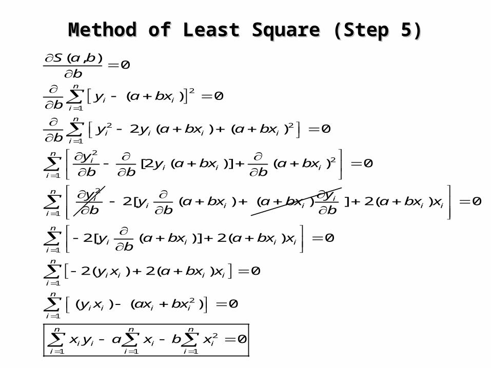
Method of Least Square (Step 5)Method of Least Square (Step 5)
2
1
2 2
1
22
1
2
( , )0
( ) 0
2 ( ) ( ) 0
[2 ( )] ( ) 0
n
i ii
n
i i i ii
ni
i i ii
i
S a b
b
y a bxb
y y a bx a bxb
yy a bx a bx
b b b
y
b
2[ ( ) ( ) ii i i
yy a bx a bx
b b
1
1
1
2
1
2
1 1 1
] 2( ) 0
2[ ( )] 2( ) 0
2( ) 2( ) 0
( ) ( ) 0
0
n
i ii
n
i i i ii
n
i i i ii
n
i i i ii
n n n
i i i ii i i
a bx x
y a bx a bx xb
y x a bx x
y x ax bx
x y a x b x

Method of Least Square (Step 6)Method of Least Square (Step 6)
2
1
2 2
1
22
1
2
( , )0
( ) 0
2 ( ) ( ) 0
[2 ( )] ( ) 0
n
i ii
n
i i i ii
ni
i i ii
i
S a b
b
y a bxb
y y a bx a bxb
yy a bx a bx
b b b
y
b
2[ ( ) ( ) ii i i
yy a bx a bx
b b
1
1
1
2
1
2
1 1 1
] 2( ) 0
2[ ( )] 2( ) 0
2( ) 2( ) 0
( ) ( ) 0
0
n
i ii
n
i i i ii
n
i i i ii
n
i i i ii
n n n
i i i ii i i
a bx x
y a bx a bx xb
y x a bx x
y x ax bx
x y a x b x

Method of Least Square (Step 7)Method of Least Square (Step 7)
2
1 1 1 12
2
1 1
n n n n
i i i i ii i i i
n n
i ii i
y x x x ya
n x x
1 1 12
2
1 1
n n n
i i i ii i i
n n
i ii i
n x y y xb
n x x
y a bx

ExampleExample
X y
1 1
3 2
4 4
6 4
8 5
9 7
11 8
14 9
We have the following eight pairs of observations:

Example (Cont.) Example (Cont.)
xi yi Xi^2 xi.yi Yi^2
1 1 1 1 1
3 2 9 6 4
4 4 16 16 16
6 4 36 24 16
8 5 64 40 25
9 7 81 63 49
11 8 121 88 64
14 9 196 126 81
56 40 524 364 256
7 5 65.5 45.5 32
Construct the least square line:
1/n
N=8
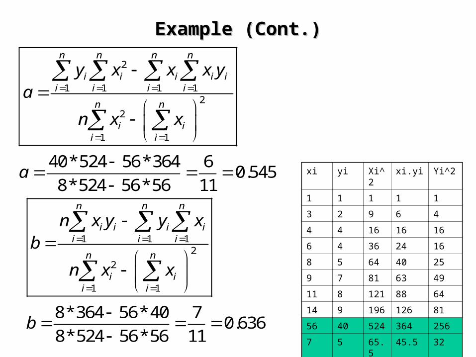
Example (Cont.)Example (Cont.)
2
1 1 1 12
2
1 1
40*524 56*364 60.545
8*524 56*56 11
n n n n
i i i i ii i i i
n n
i ii i
y x x x ya
n x x
a
1 1 12
2
1 1
8*364 56*40 70.636
8*524 56*56 11
n n n
i i i ii i i
n n
i ii i
n x y y xb
n x x
b
xi yi Xi^2
xi.yi Yi^2
1 1 1 1 1
3 2 9 6 4
4 4 16 16 16
6 4 36 24 16
8 5 64 40 25
9 7 81 63 49
11 8 121 88 64
14 9 196 126 81
56 40 524 364 256
7 5 65.5 45.5 32

Example (Cont.)Example (Cont.)
0 4 8 12 16
X
0
2
4
6
8
10
Y
Equation Y = 0.545+ 0.636 * X
Number of data points used = 8
Average X = 7
Average Y = 5

i 1 2 3 4 5
xi 2.10 6.22 7.17 10.5 13.7
yi 2.90 3.83 5.98 5.71 7.74
Example (2)
7416238
1626
3201392
6939
5
1
5
1
5
1
2
5
1
. yx
. y
. x
. x
iii
ii
ii
ii
4023.0
69.3951
3.392
)16.26)(69.39(51
7.238
038.269.39
51
3.392
)7.238)(69.39(51
)3.392)(16.26(51
2
2
b
a
x. . y 402300382

Example (3)

Excel Application
• See Excel
Covariance and the Correlation Coefficient
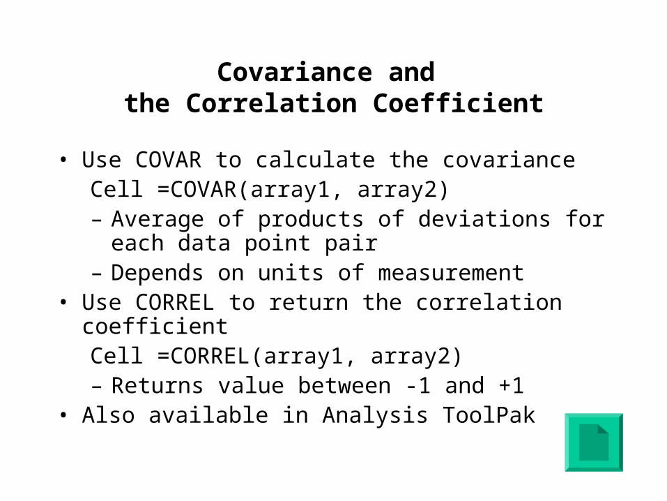
• Use COVAR to calculate the covarianceCell =COVAR(array1, array2)– Average of products of deviations for each
data point pair– Depends on units of measurement
• Use CORREL to return the correlation coefficient Cell =CORREL(array1, array2)– Returns value between -1 and +1
• Also available in Analysis ToolPak

Analysis ToolPak
• Descriptive Statistics• Correlation• Linear Regression• t-Tests• z-Tests• ANOVA• Covariance
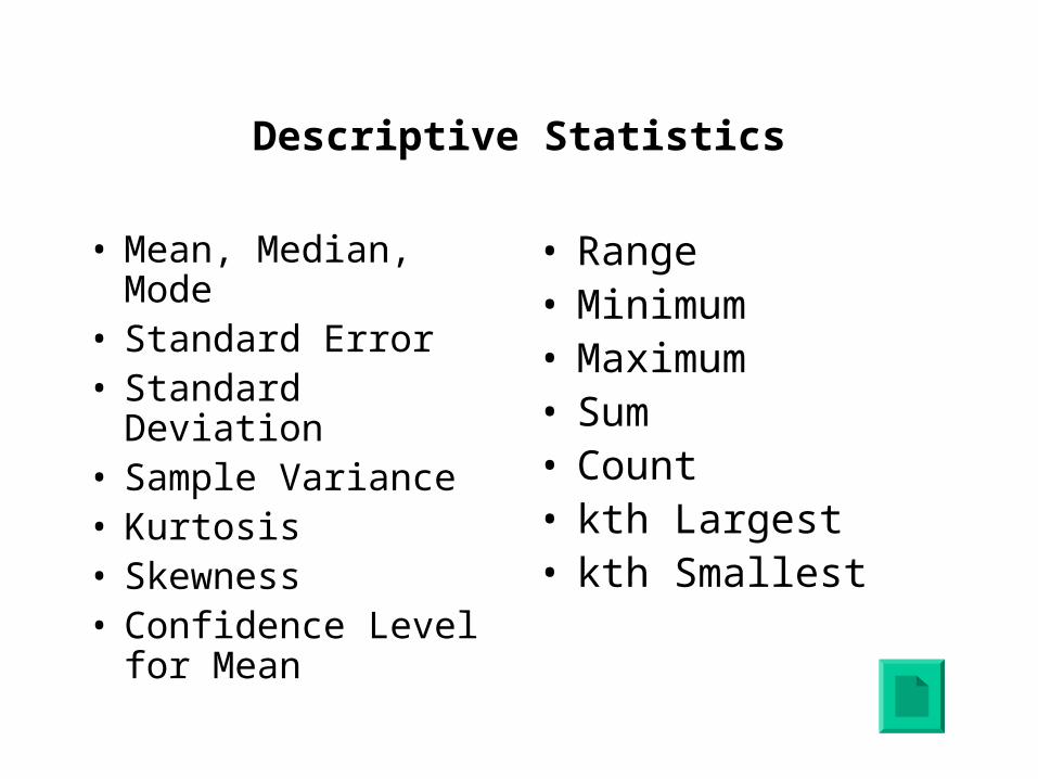
Descriptive Statistics
• Mean, Median, Mode
• Standard Error• Standard Deviation• Sample Variance• Kurtosis• Skewness• Confidence Level
for Mean
• Range• Minimum• Maximum• Sum• Count• kth Largest• kth Smallest

Correlation and Regression
• Correlation is a measure of the strength of linear association between two variables– Values between -1 and +1– Values close to -1 indicate strong negative
relationship– Values close to +1 indicate strong positive
relationship– Values close to 0 indicate weak relationship
• Linear Regression is the process of finding a line of best fit through a series of data points– Can also use the SLOPE, INTERCEPT, CORREL and
RSQ functions
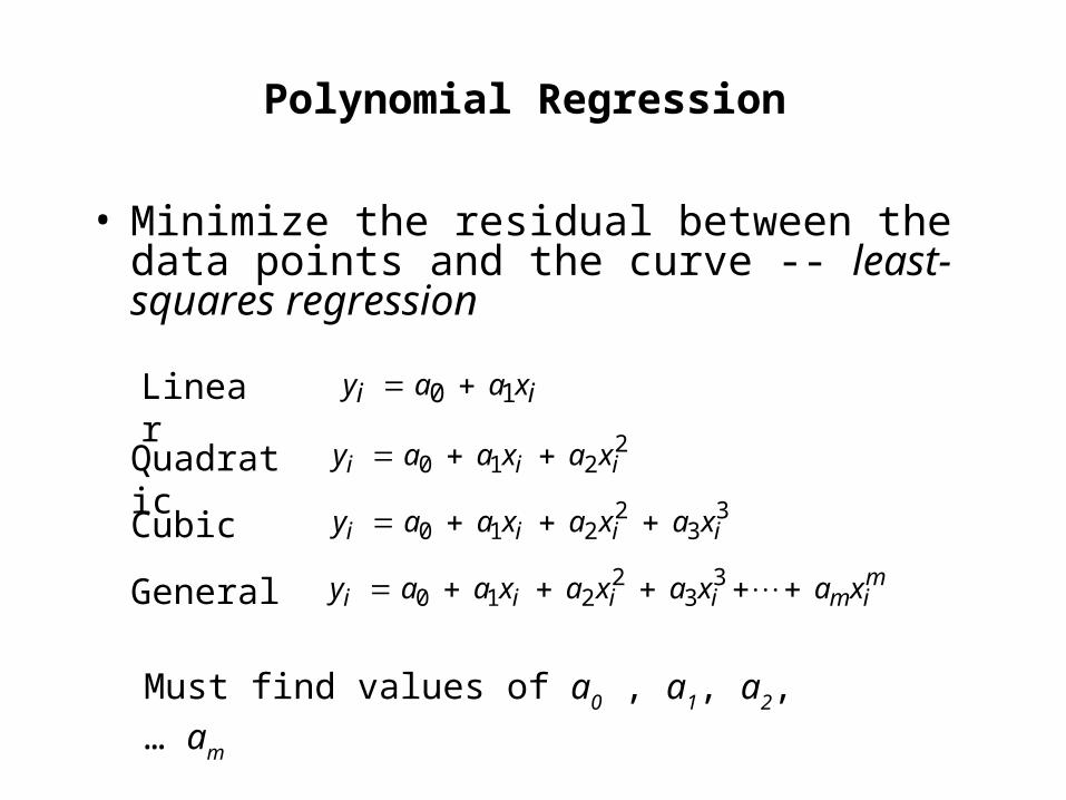
Polynomial Regression
• Minimize the residual between the data points and the curve -- least-squares regression
Must find values of a0 , a1, a2, … am
ii x a a y 10 Linear
2210 iii x a x a a y Quadratic
33
2210 iiii x a x a x a a y Cubic
General mimiiii x ax a x a x a a y 3
32
210

Polynomial Regression
• Residual
)( 33
2210
mimiiiii x a x a x a x a a = ye
n
i=
mm
n
i=ir x a x a x ax a a y = e = S
1
233
2210
1
2 )]([
• Sum of squared residuals
• Minimize by taking derivatives

Polynomial Regression
• Normal Equations
n
i=i
mi
n
i=ii
n
i=ii
n
i=i
mn
i=
mi
n
i=
mi
n
i=
mi
n
i=
mi
n
i=
mi
n
i=i
n
i=i
n
i=i
n
i=
mi
n
i=i
n
i=i
n
i=i
n
i=
mi
n
i=i
n
i=i
yx
yx
yx
y
a
a
a
a
xxxx
xxxx
xxxx
xxxn
1
1
2
1
1
2
1
0
1
2
1
2
1
1
1
1
2
1
4
1
3
1
2
1
1
1
3
1
2
1
11
2
1
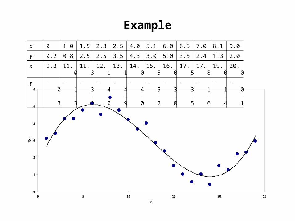
Example
x 0 1.0 1.5 2.3 2.5 4.0 5.1 6.0 6.5 7.0 8.1 9.0
y 0.2 0.8 2.5 2.5 3.5 4.3 3.0 5.0 3.5 2.4 1.3 2.0
x 9.3 11.0 11.3 12.1 13.1 14.0 15.5 16.0 17.5 17.8 19.0 20.0
y -0.3 -1.3 -3.0 -4.0 -4.9 -4.0 -5.2 -3.0 -3.5 -1.6 -1.4 -0.1
-6
-4
-2
0
2
4
6
0 5 10 15 20 25
x
f(x)

Example
n
i=ii
n
i=ii
n
i=ii
n
i=i
n
i=i
n
i=i
n
i=i
n
i=i
n
i=i
n
i=i
n
i=i
n
i=i
n
i=i
n
i=i
n
i=i
n
i=i
n
i=i
n
i=i
n
i=i
yx
yx
yx
y
a
a
a
a
xxxx
xxxx
xxxx
xxxn
1
3
1
2
1
1
3
2
1
0
1
6
1
5
1
4
1
3
1
5
1
4
1
3
1
2
1
4
1
3
1
2
1
1
3
1
2
1
369943
26037
9316
301
82235181167127801472752835846342
712780147275283584634223060
2752835846342230606229
84634223060622924
3
2
1
0
.
.
.
.
a
a
a
a
....
....
....
...
x 0 1.0 1.5 2.3 2.5 4.0 5.1 6.0 6.5 7.0 8.1 9.0
y 0.2 0.8 2.5 2.5 3.5 4.3 3.0 5.0 3.5 2.4 1.3 2.0
x 9.3 11.0 11.3 12.1 13.1 14.0 15.5 16.0 17.5 17.8 19.0 20.0
y -0.3 -1.3 -3.0 -4.0 -4.9 -4.0 -5.2 -3.0 -3.5 -1.6 -1.4 -0.1
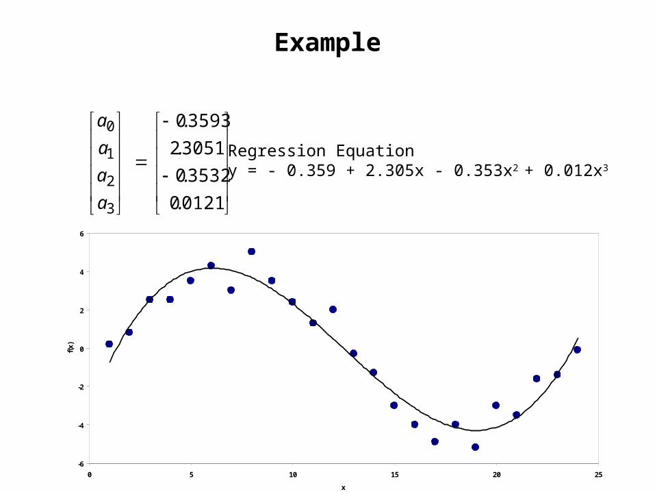
Example
01210
35320
30512
35930
3
2
1
0
.
.
.
.
a
a
a
a
Regression Equationy = - 0.359 + 2.305x - 0.353x2 + 0.012x3
-6
-4
-2
0
2
4
6
0 5 10 15 20 25
x
f(x)
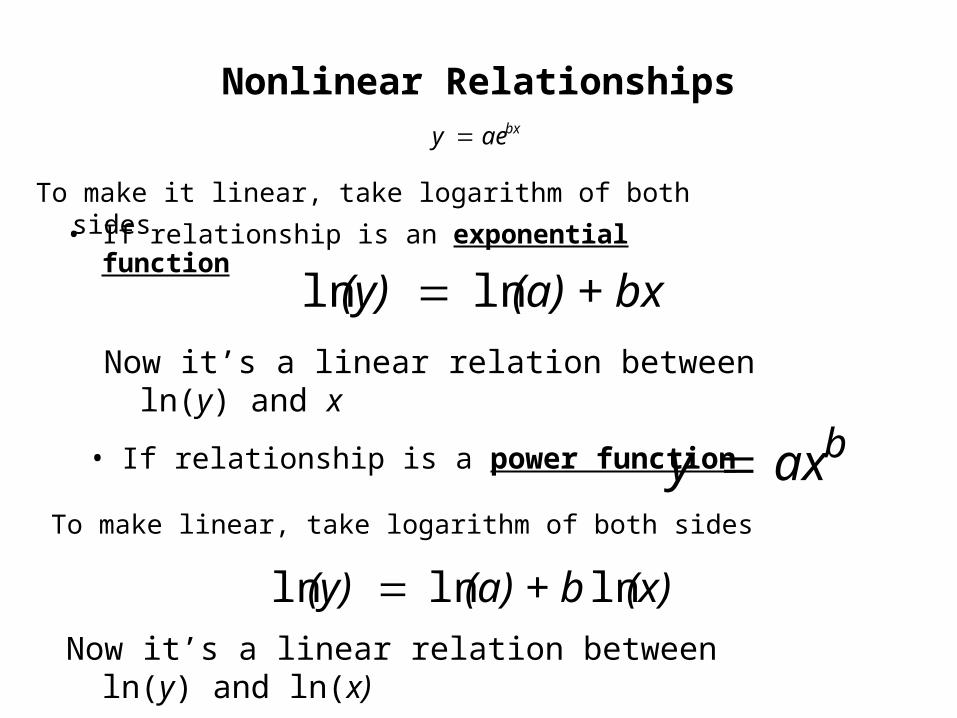
Nonlinear Relationships
• If relationship is an exponential function
To make it linear, take logarithm of both sides
bx aey
(a) + bx (y) lnln
b axy To make linear, take logarithm of both sides
(x)(a) + b (y) lnlnln
Now it’s a linear relation between ln(y) and x
Now it’s a linear relation between ln(y) and ln(x)
• If relationship is a power function

Examples
• Quadratic curve
– Flow rating curve:• q = measured discharge, • H = stage (height) of water behind outlet
• Power curve
– Sediment transport: • c = concentration of suspended sediment• q = river discharge
– Carbon adsorption: • q = mass of pollutant sorbed per unit mass of carbon, • C = concentration of pollutant in solution
b aqc
b axy
2210 x ax a ay
2210 H aH a aq
ncKq
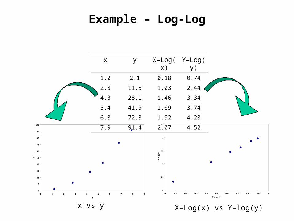
Example – Log-Log
x y X=Log(x)
Y=Log(y)
1.2 2.1 0.18 0.74
2.8 11.5 1.03 2.44
4.3 28.1 1.46 3.34
5.4 41.9 1.69 3.74
6.8 72.3 1.92 4.28
7.9 91.4 2.07 4.52
0
10
20
30
40
50
60
70
80
90
100
0 1 2 3 4 5 6 7 8 9
x
y
x vs y
0
0.5
1
1.5
2
2.5
0 0.1 0.2 0.3 0.4 0.5 0.6 0.7 0.8 0.9 1
X=Log(x)
Y=
Lo
g(y
)
X=Log(x) vs Y=log(y)

Example – Log-Log
n
i=ii
n
i=i
n
i=i
n
i=i
n
i=i
YX
Y
B
a
XX
Xn
1
1
1
2
1
1
431lnln
119ln
014ln
348ln
5
1
5
1
5
1
5
1
5
1
25
1
2
5
1
5
1
. )(y)(x YX
. ) (y Y
. )(x X
. )(x X
iii
iii
ii
ii
ii
ii
ii
ii
431
119
014348
3486
.
.
B
a
..
.
Using the X’s and Y’s, not the original x’s and y’s

Example – Carbon Adsorption
ncKq
q = pollutant mass sorbed per carbon massC = concentration of pollutant in solution, K = coefficient n = measure of the energy of the reaction
cnKq 101010 log log log

Example – Carbon Adsorption
ncKq
Linear axes: K = 74.702, and n = 0.2289
0
50
100
150
200
250
300
350
0 100 200 300 400 500 600
C
q

0
0.5
1
1.5
2
2.5
3
0 0.5 1 1.5 2 2.5 3
X=Log(c)
Y=
Lo
g(q
)
Example – Carbon Adsorption
cnKq 101010 log log log
Logarithmic axes: logK = 1.8733, K = 101.6733 = 74.696, n = 0.2289
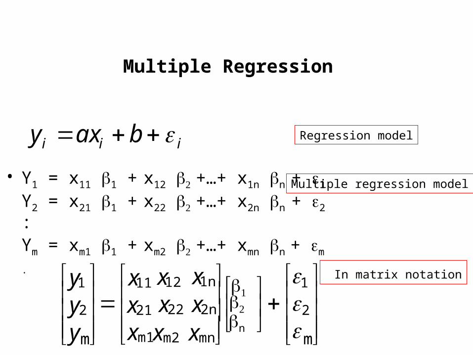
Multiple Regression
• Y1 = x11 1 + x12 +…+ x1n n + 1
Y2 = x21 1 + x22 +…+ x2n n + 2
:Ym = xm1 1 + xm2 +…+ xmn n+ m
.
iii baxy Regression model
m
2
1
m1
21
11
m
2
1
xxx
yyy
n
12x22x 2nx
1nx
m2x mnx
Multiple regression model
In matrix notation

m
2
1
m1
21
11
m
2
1
x
x
x
y
y
y
n
12x
22x 2nx1nx
m2x mnx
Multiple Regression (cont.)
Observed data = design matrix * parameters + residuals
XY