Embed Size (px)
Citation preview
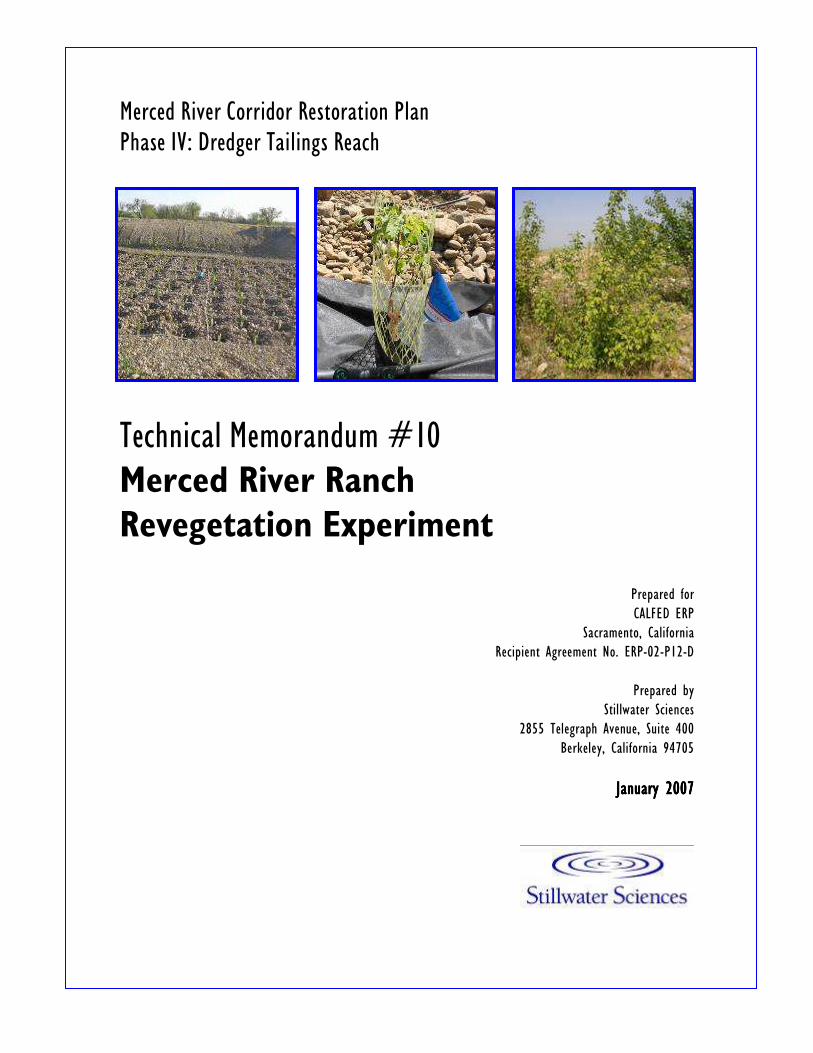
Merced River Corridor Restoration Plan Phase IV: Dredger Tailings Reach
Technical Memorandum #10
Merced River Ranch
Revegetation Experiment
Prepared for CALFED ERP
Sacramento, California Recipient Agreement No. ERP-02-P12-D
Prepared by Stillwater Sciences
2855 Telegraph Avenue, Suite 400 Berkeley, California 94705
January 2007January 2007January 2007January 2007

For more information or copies of this Technical Memorandum, please contact:
Stillwater Sciences
2855 Telegraph Avenue, Suite 400
Berkeley, CA 94705
stillwatersci.com
(510) 848-8098
Suggested citation: Stillwater Sciences. 2006. Merced River Ranch revegetation
experiment. Prepared by Stillwater Sciences, Berkeley, California, for CALFED,
Sacramento, California.

Table of Contents
i Merced River Ranch Revegetation Experiment
Table of Contents
1 INTRODUCTION ............................................................................... 1
1.1 Study Area ........................................................................................... 1
1.2 Restoration Planning .......................................................................... 3
1.3 Site Revegetation ................................................................................. 4
1.4 Experiment Goals and Approach ..................................................... 5
2 METHODS .......................................................................................... 7
2.1 Experimental Design .......................................................................... 7
2.2 Data Collection .................................................................................. 10 2.2.1 Site Conditions ........................................................................ 10 2.2.2 Survival ................................................................................... 11 2.2.3 Growth .................................................................................... 12 2.2.4 Water Potential ....................................................................... 12 2.2.5 Weed Percent Cover ................................................................ 13
2.3 Statistical Analyses ........................................................................... 13 2.3.1 Initial Size Analysis ................................................................ 13 2.3.2 Growth Analysis ..................................................................... 14 2.3.3 Water Potential Analysis of Variance ..................................... 15 2.3.4 Survival and Hazard Analysis ................................................ 16 2.3.5 Cox Proportional Hazard Model ............................................. 16
3 RESULTS ........................................................................................... 21
3.1 Site Conditions .................................................................................. 21 3.1.1 Soil Texture and Nutrients ..................................................... 21 3.1.2 Depth to Groundwater, River Stage, and Pond Stage ............ 22 3.1.3 Temperature ............................................................................ 23
3.2 Plant Size and Growth ..................................................................... 24 3.2.1 Initial Size at Planting ............................................................ 24 3.2.2 Plant Growth Timing.............................................................. 26 3.2.3 Patterns in Plant Growth between Treatment Groups ........... 26 3.2.4 ANCOVA Models of 3-Year Diameter Increment Growth .... 27
3.3 Water Potential .................................................................................. 29

Table of Contents
ii Merced River Ranch Revegetation Experiment
3.4 Plant Survival .................................................................................... 32 3.4.1 Survival and Hazard Patterns ................................................ 32 3.4.2 First-Year Survival (2004) ...................................................... 33 3.4.3 Second-Year Survival (2005) .................................................. 36 3.4.4 Third-Year Survival (2006) .................................................... 39
3.5 Weed Percent Cover ......................................................................... 40
4 DISCUSSION.................................................................................... 43
4.1 Treatment/Non-treatment Effects and Revegetation
Recommendations ............................................................................ 43 4.1.1 Initial Size ............................................................................... 43 4.1.2 Block and Relative Elevation above Groundwater .................. 44 4.1.3 Irrigation ................................................................................. 45 4.1.4 Weed Reduction ...................................................................... 46 4.1.5 Soil Amendments .................................................................... 47
4.2 Species Responses ............................................................................. 48 4.2.1 Acer negundo .......................................................................... 48 4.2.2 Fraxinus latifolia ..................................................................... 48 4.2.3 Populus fremontii .................................................................... 49 4.2.4 Quercus lobata ........................................................................ 49
5 REFERENCES .................................................................................... 51
6 FIGURES ........................................................................................... 55
APPENDIX A SOIL ANALYSIS REPORTS ............................................................... A-1
APPENDIX B INITIAL CONDITIONS ANOVA RESULTS AND PAIRWISE
COMPARISONS ................................................................................... B-1
APPENDIX C EXPERIMENTAL SCHEDULE ........................................................... C-1
LIST OF TABLES
Table 2-1. Revegetation experiment hypotheses, treatments, and treatment levels............... 8 Table 2-2. As-built experimental plot elevations. .................................................................... 9 Table 3-1. Soil analytes at each experimental block. ............................................................. 22 Table 3-2. Average, minimum, and maximum groundwater, river stage, and pond stage
elevations (m NGVD). .......................................................................................... 22 Table 3-3. Monthly average temperatures at the MRR (°C). ................................................. 24 Table 3-4. Initial seedling height, diameter and number of leaves at planting time (means
±1SE) by plot (block and relative elevation). ....................................................... 25 Table 3-5. End of year height and diameter (mean±1 SE) for all species. ............................. 27

Table of Contents
iii Merced River Ranch Revegetation Experiment
Table 3-6. Top five candidate ANCOVA models of factor influences on diameter growth
increment. ............................................................................................................. 28 Table 3-7. Parameter estimates for the best ANCOVA models for each species. ................. 29 Table 3-8. Average water potentials (MPa) (±1SE) ................................................................ 31 Table 3-9. Water potential sample sizes. ............................................................................... 31 Table 3-10. ANOVA models for pre-dawn and afternoon water potential. ......................... 32 Table 3-11. End-of-year survival by species and irrigation treatment for all three years. ... 33 Table 3-12. Pearson Correlation Matrix for the three explanatory variables: initial height,
diameter, and number of leaves. .......................................................................... 34 Table 3-13. Year 1 top five candidate Cox models for each species. ..................................... 34 Table 3-14. Parameter estimates, hazard ratio (HR), and HR confidence limits for the best
Year 1 Cox survival model for each species. ....................................................... 35 Table 3-15. Year 2 top five candidate Cox models for each species. ..................................... 37 Table 3-16. Parameter estimates, hazard ratio (HR), and HR confidence limits for the best
Year 2 Cox survival model for each species. ....................................................... 38 Table 3-17. Year 3 top five candidate Cox models for each species. ..................................... 39 Table 3-18. Parameter estimates, hazard ratio (HR), and HR confidence limits for the best
Year 3 Cox survival model for each species. ....................................................... 40 Table 3-19. Percent of non-weed reduction plants within each weed cover class. ............... 41 Table 3-20. Weed species identified in experimental plots. .................................................. 42
LIST OF FIGURES
Figure 1. Merced River watershed and project location.
Figure 2. Typical conditions of the Merced River Ranch resulting from historical dredging
operations.
Figure 3. Locations of experiment plots, groundwater monitoring wells, staff gauges, and access
roads at the Merced River Ranch.
Figure 4. Experimental block design.
Figure 5. Photographs of experimental design, subjects, and treatments.
Figure 6. 2004 groundwater elevations, river stage and swale pond stage.
Figure 7. 2005 groundwater elevations, river stage and swale pond stage.
Figure 8. 2006 groundwater elevations and river stage.
Figure 9. Temperatures at the control area during 2004.
Figure 10. Temperatures at the control area during 2005.
Figure 11. Temperatures at the control area during 2006.
Figure 12. Notched boxplots illustrating the distributions of initial seedling condition (height,
basal diameter and no. of leaves) at planting for each species in Block 1 and Block 2
high, mid, and low elevation plots.
Figure 13. Year 1 leaf-out timing for seedlings of each species.
Figure 14. Year 1 and Year 2 relative seasonal growth timing for all species.
Figure 15. Seedling height growth by irrigation treatment.
Figure 16. Seedling basal diameter growth by irrigation treatment.
Figure 17. Seedling height growth by distance to groundwater.
Figure 18. Seedling basal diameter growth by distance to groundwater.
Figure 19. Final seedling growth by irrigation level.
Figure 20. Final seedling growth by elevation level.
Figure 21. Xylem water potential values for irrigation treatment groups in Year 2 (2005).

Table of Contents
iv Merced River Ranch Revegetation Experiment
Figure 22. Xylem water potential values for high and low treatment groups in Year 2 (2005).
Figure 23. Final cohort survival by irrigation treatment.
Figure 24. Final hazard rate by irrigation treatment.
Figure 25. Final hazard rate by distance to groundwater.
Figure 26. Year 2 cohort survival by irrigation treatment.
Figure 27. Year 2 cohort survival by distance to groundwater.
Figure 28. Year 3 cohort survival by irrigation treatment.
Figure 29. Year 3 cohort survival by distance to groundwater.
Introduction
1 Merced River Ranch Revegetation Experiment
1 INTRODUCTION
The Merced River Ranch revegetation experiment has been undertaken as a
component of the Merced River Corridor Restoration Plan - Phase IV Project
(CALFED ERP-02-P12-D), which is intended to evaluate strategies for channel and
floodplain restoration within the context of the contemporary flow regime. The
Phase IV Project focuses on restoration planning activities on the Merced River
Ranch (MRR), located at the uppermost end of the Merced River Dredger Tailings
Reach (Figure 1). The Dredger Tailings Reach (DTR) has been severely impacted by
historic gold dredger mining and alteration of the natural hydrograph by upstream
dams. The reach is also the primary spawning area in the Merced River for fall-run
Chinook salmon (Oncorhynchus tshawytscha), an important management species for
the California Department of Fish and Game (CDFG), and potentially steelhead (O.
mykiss), which is listed as threatened under the Federal Endangered Species Act.
This technical memorandum reports the results of the three-year MRR revegetation
experiment and develops revegetation recommendations for inclusion in
restoration planning documents prepared for the Phase IV Project.
1.11.11.11.1 Study AreaStudy AreaStudy AreaStudy Area
The Merced River is a tributary to the San Joaquin River in the southern portion of
California’s Central Valley (Figure 1a). The river, which drains an approximately
3,305-km2 (1,276-mi2) watershed, originates in Yosemite National Park and flows
southwest through the Sierra Nevada range before joining the San Joaquin River
140 km (87 mi) south of the City of Sacramento. Elevations in the watershed range
from 3,960 m (13,000 ft) at its crest to 15 m (49 ft) at the confluence with the San
Joaquin River. The DTR of the Merced River extends from Crocker-Huffman Dam
(river mile [RM] 52) to approximately 1.9 km (1.2 mi) downstream of the Snelling
Road Bridge (RM 45.2), a reach of approximately 11.6 km (7.2 mi) (Figure 1b and c).
The 129 ha (318 ac) MRR is located in the upstream portion of the DTR (RM 51 to
50) and was purchased by California Department of Fish and Game (CDFG) in 1998
as a source of coarse sediment for future river restoration projects and as a
floodplain restoration site.
The hydrology of the Merced River has been altered by water supply requirements
and flood control operations, which together have reduced flood frequency,

Introduction
2 Merced River Ranch Revegetation Experiment
reduced peak flow magnitude, altered seasonal flow patterns, and reduced the
temporal variability of flows. These changes in hydrologic conditions have altered
the frequency, duration, and magnitude of floodplain inundation, and reduced the
frequency of sediment transport and bed mobilization, but, in conjunction with a
lack of sediment supply, have caused bed scour and armoring in the remaining
flood events (Stillwater Sciences 2001).
Since 1926, sediment supply from the upper 81 percent of the watershed has been
intercepted at the original Exchequer Dam and then the New Exchequer Dam. This
interception has eliminated the vast majority of the river’s historical sediment
supply, thus depriving the river of a basic element necessary to maintain
geomorphic equilibrium.
In addition to the effects of flow regulation and loss of sediment supply from the
upper watershed, this reach has been extensively modified by gold dredging. In
the early-to-mid twentieth century, gold dredges excavated the river channel,
floodplain, and valley floor. The dredges had earthmoving capacities of 1.4–3.4
million cubic yards/year and excavated the channel and floodplain deposits to
bedrock, usually at a depth of 20–36 feet (Clark 1998). After recovering the gold,
the dredgers redeposited the remaining tailings in long rows, often roughly parallel
to the river channel, on the floodplain (Figure 2). Although they were originally
thought to consist of fine sand and gravel overlain by cobbles and boulders
(Goldman 1964) extending to the original dredging depths, recent surveys indicate
that the tailings piles exhibit little stratification (URS 2004b). As a result of gold
dredging, the channel has been depleted of coarse sediment, the adjacent
floodplain has been raised and covered with dredger tailings piles, and soil and
fine sediment have been washed downstream. An estimated 3.22 million cubic
yards (2.46 million m3) of dredger tailings currently cover approximately 305 acres
(1,236,000 m2) of the riparian corridor of the DTR (URS 2004b).
Sparse, weedy herbaceous vegetation consisting largely of non-native grasses and
forbs dominates the large expanse of tailing surfaces and floodplain area of the
MRR. Native riparian vegetation is typically restricted to narrow bands adjacent to
the river, measuring 33 m (100 ft) or less in width on each bank of the river, and
linear patches confined to swales within the dredger tailings (Whitlow and Bahre
1984, Stillwater Sciences 2002). The dominant vegetation along the narrow river
banks is a mix of individual or small patches of valley oak (Quercus lobata) and
mixed willow (Salix spp.), with cottonwood forest, grassland, riparian scrub, and
off-channel marsh habitat generally located farther away from the river (Stillwater
Sciences 2002). In some areas, dredging operations left behind low-lying swales
between tailing piles. Several of these swales, subsequently referred to as swale
ponds, are connected to a perennial or seasonal groundwater supply and support a
variety of wetland vegetation types (primarily freshwater emergent marsh,

Introduction
3 Merced River Ranch Revegetation Experiment
seasonal wetland, open water/ponds, mixed willow, and cottonwood forest). Most
of the smaller, linear patches of riparian scrub and forest in the swale ponds are
dominated by narrow-leaf willow (Salix exigua) with edible fig (Ficus carica),
California wild grape (Vitas californica), and Himalaya blackberry (Rubus discolor) as
common associated species (Stillwater Sciences 2001, URS 2006a). The deepest,
wettest swale ponds support cattail (Typha spp.) marsh habitat and/or perennial
ponds. These swale ponds support floating plants, such as various duckweeds
(Lemnaceae) and water fern (Azolla filiculoides). The introduced water hyacinth
(Eichhornia crassipes) also occurs in some swale ponds. Many of the swale ponds
also contain beds of submergent macrophytes. Marsh pennywort (Hydrocotyle
ranunculoides) forms dense beds in some shallower swale ponds (Stillwater Sciences
2001).
1.21.21.21.2 Restoration PlanningRestoration PlanningRestoration PlanningRestoration Planning
The Phase IV Project, and therefore MRR revegetation experiment, stem from the
larger Merced River Corridor Restoration Plan (MRCRP). Funded by the CALFED
Ecosystem Restoration Program, the intent of the MRCRP was to provide a
technically sound, publicly supported, and implementable plan to improve
ecological function in the Merced River corridor from Crocker-Huffman Dam (RM
52) to the confluence with the San Joaquin River (RM 0). Crocker-Huffman Dam is
the downstream-most dam on the Merced River and the upstream limit of
anadromous fish access. The MRCRP (Stillwater Sciences 2002) identifies
restoration objectives and provides management recommendations based on
current scientific understanding of the Merced River with input from the Merced
River Stakeholders (MRS), Merced River Technical Advisory Committee (MRTAC),
and the broader public. Since a broad spectrum of interests, represented by the
MRS, MRTAC, and public, provided input to the restoration objectives, they
address not only geomorphic and ecological restoration in the river, but also the
concerns of local citizens, landowners, and other stakeholders.
To guide reach-scale restoration efforts and address various anthropogenic impacts
to the DTR, the MRCRP identified the following objectives for the DTR (Stillwater
Sciences 2002):
• balance sediment supply and transport capacity to allow the accumulation
and retention of channel bed material suitable for spawning and to prevent
riparian vegetation encroachment;
• restore floodplain functions to improve the establishment of riparian
vegetation and the quality of riparian habitat;
• increase in-channel habitat complexity to improve aquatic habitat for native
aquatic species; and
• scale low-flow and bankfull channel geometry to current flow conditions.

Introduction
4 Merced River Ranch Revegetation Experiment
The Phase IV Project begins to address the MRCRP objectives through the design of
pilot floodplain and channel restoration experiments. The Phase IV project
includes conducting: 1) DTR- and MRR-scale studies of current conditions to
provide the basis for and to inform the design of restoration actions (Stillwater
Sciences 2004a, b and c; URS 2004a and b; Stillwater Sciences 2005, 2006; URS
2006a); and 2) experiments to test actions that will initiate the restoration of natural
ecosystem function at the MRR to the extent feasible. The project will provide
transferable scientific information to reduce uncertainty in future restoration
design on the Merced and potentially in other rivers in the Central Valley. For
example, removal of the tailings from the floodplain has the potential to yield
multiple restoration opportunities and ecosystem benefits, but the detailed impacts
of such restoration activities are largely unknown. The Phase IV Project
experiments, of which the revegetation experiment is one, are designed to increase
the collective scientific understanding of the potential for dredger tailings removal
and re-use (e.g., as material to use as fill during channel reconstruction or for gravel
augmentation), and is intended to improve restoration effectiveness and reduce
project uncertainty when implementing restoration actions in the future.
1.31.31.31.3 Site RevegetationSite RevegetationSite RevegetationSite Revegetation
Revegetation will be an essential component of floodplain restoration at the MRR
to ameliorate the factors currently limiting vegetation and habitat quality. The
impacted hydrology, sediment supply, and floodplain conditions of the DTR
strongly affect riparian vegetation and habitat extent, floristic and structural
composition, and health in the following ways:
1) Replacement of native riparian vegetation by dredger tailings. Most of the natural
riparian vegetation in the reach was removed and replaced by piles of dredger
tailings. Throughout the DTR riparian vegetation is currently limited to narrow
bands along the river channel and fragmented patches in low-lying areas
among the dredger tailings piles (Whitlow and Bahre 1984, Stillwater Sciences
2001).
2) Altered flood regime. Recruitment of new plants is hindered by reduced flood
magnitude and alteration of flood timing as a result of flow regulation. Limited
floodplain inundation and the shift of peak flows from spring to winter has
resulted in: a) inadequate wetting of appropriate recruitment sites during the
spring seed release period and, b) flow recession rates too steep to allow
seedlings to develop adequate root systems to ensure survival and vigorous
growth in the first growing season (Stillwater Sciences 2001, Stella 2005).
3) Reduced sediment supply. Recruitment of new plants is hindered by reduced
sediment supply as a result of a dam which is located upstream of the reach.
The reduction in sediment supply has reduced the deposition of fine sediment

Introduction
5 Merced River Ranch Revegetation Experiment
on the floodplain during flood events, thus reducing the creation of suitable
substrates for seedling germination (Stillwater Sciences 2001).
4) Degraded floodplain substrates. The river channel in the dredger tailings reach is
confined by piles of dredger tailings which have replaced the natural floodplain
soils. The cobble dredger tailing piles contain very little soil (Whitlow and
Bahre 1984, URS 2004a), provide a poor growing substrate for vegetation, and
likely retain very little water moisture.
5) Increased floodplain elevation. The piles of dredger tailings have increased the
floodplain elevation along the river, further limiting inundation of the
floodplain by flood flows (URS 2004b). In addition, it is believed that the
dredger mining process and water diversion have severely altered groundwater
patterns at the site. As a result, very little water is available to growing plants
beyond the immediate channel margin.
Even under restored floodplain conditions, natural recruitment of pioneer riparian
plant species is not expected to significantly contribute to the development of a
self-sustaining, diverse riparian corridor (Stillwater Sciences 2001, Stella 2005). The
morphological changes to the river channel and floodplain that result from
restoration are not expected to lead to sufficient process change to create
recruitment-friendly conditions. While restored floodplain conditions will improve
natural recruitment potential over existing conditions by increasing the frequency
of floodplain inundation, active revegetation of restored floodplains will be
necessary to recreate a riparian corridor that provides multiple ecosystem benefits.
Active revegetation will also be needed on the large areas of the floodplain that are
too far from the river to experience flooding under the regulated flow regime.
Future revegetation efforts will, therefore, need to be extensive and will include
improving substrate conditions, planting propagules of local origin (seed, cuttings,
and seedlings), irrigating and maintaining planted areas during initial
establishment, and fostering and monitoring natural recruitment.
1.41.41.41.4 Experiment Goals and ApproachExperiment Goals and ApproachExperiment Goals and ApproachExperiment Goals and Approach
The results of other riparian revegetation can be used to some extent to inform and
guide revegetation planning at the MRR, but riparian revegetation efforts in the
Central Valley, particularly on floodplains covered or formerly covered in dredger
tailings, have had mixed results (AMFSTP 2002). Part of the problem is the lack of
formal monitoring data that has been collected on past revegetation efforts. While
increasing numbers of studies and revegetation efforts are being designed and
implemented to increase understanding of issues affecting riparian revegetation
and incorporate more formalized monitoring (e.g., CDWR and CDFG 2003a and b,
Stella et al. 2003, AMFSTP 2004, CDWR 2004, Kiparsky 2005, Souza Environmental
Solution et al. 2005, Stella 2005), few projects have the time or funding to conduct

Introduction
6 Merced River Ranch Revegetation Experiment
revegetation in an experimental setting where multiple factors are tested and
monitored.
Because of the large extent of planned revegetation efforts (Stillwater Sciences
2005) and uncertainty in how site conditions will affect revegetation performance,
the pilot riparian revegetation experiment was included in the Phase IV project.
The experiment is also a response to the recommendations of the Merced River
Adaptive Management Forum to improve the linkages between scientific input and
project design, conduct active experiments with revegetation design when the
opportunity exists, and increase the amount of transferable information generated
from the Merced River (AMFSTP 2002 and 2004).
The goals and objectives of the revegetation experiment were developed with the
long-term intention of improving revegetation effort effectiveness. The overarching
goals of the experiment are to: 1) increase scientific understanding of factors
limiting the success of riparian revegetation on restored floodplains, and 2) provide
transferable scientific information that will reduce the scientific uncertainty in
future revegetation projects.
The objectives of the revegetation experiment are to:
• assess the influence of different design parameters to determine the most
effective and efficient revegetation techniques on floodplains within the MRR
once the tailing piles have been removed;
• develop vegetation-related recommendations for the restoration design of the
MRR; and
• assist in the adaptive management of the Phase IV and other restoration
projects on the Merced River and other Central Valley rivers by informing the
revegetation of floodplains currently covered in tailing piles and by refining
hypotheses that could be tested during or through future revegetation projects.
This experiment tests the effects of initial size, depth to groundwater, irrigation
duration, and weed reduction on the survival, growth, and water potential of four
native riparian tree species. The experimental areas were designed to provide the
substrate textures and range of floodplain elevations likely to occur once the tailing
piles have been removed for restoration purposes. The range of experimental
treatments considered was refined following conversations with several
revegetation practitioners in the Central Valley and a review of the literature; final
treatments were selected to inform several of the primary uncertainties in
revegetation success. The final design was a balance between the range of
treatments, the number of statistically required replicates, and logistical and cost
constraints. The experiment was initiated in April 2004 and concluded in October
2006.
Methods
7 Merced River Ranch Revegetation Experiment
2 METHODS
2.12.12.12.1 Experimental DesignExperimental DesignExperimental DesignExperimental Design
The MRR revegetation experiment tests the effects of groundwater depth, irrigation
duration, and weed reduction treatments on water stress, survival, and growth of
Fremont cottonwood (Populus fremontii), box elder (Acer negundo), Oregon ash
(Fraxinus latifolia), and valley oak (Quercus lobata). These species are dominant or
co-dominant components of Central Valley mixed riparian forests. They exhibit
different life history traits and occur within a predictable range of geomorphic
recruitment positions on river banks and floodplains (Stillwater Sciences 2001,
Stillwater Sciences 2003, Stella et al. 2003, Vaghti and Greco in press, Greco et al. in
review). At the MRR, these species have been found to occur naturally at
elevations between 86 and 91 m (282 and 299 ft) (KSN, unpublished data),
primarily at relative elevations of approximately 0.61–4.57 m (2–15 ft) above
summer baseflow water surface elevation and presumed groundwater levels
(Stillwater Sciences 2001, Stella et al. 2003). Throughout this report, these four
species are abbreviated using the first two letters of their genus and species name:
Acer negundo = ACNE; Fraxinus latifolia = FRLA; Populus fremontii = POFR; Quercus
lobata = QULO. Hypotheses, experimental treatments, and treatment levels are
listed in Table 2-1.

Methods
8 Merced River Ranch Revegetation Experiment
Table Table Table Table 2222----1111.... Revegetation experiment hypotheses, treatments, and treRevegetation experiment hypotheses, treatments, and treRevegetation experiment hypotheses, treatments, and treRevegetation experiment hypotheses, treatments, and treatment levels.atment levels.atment levels.atment levels.
Hypothesis Experimental
treatments Treatment levels
Merced River Ranch floodplains restored to
functional elevations will provide shorter distances to
groundwater, resulting in increased establishment
and survival of revegetated plants.
Floodplain
elevation
Floodplain plots at:
1. Low,
2. middle, or
3. high relative
elevations
Controlling weeds in the immediate vicinity of
plantings increases plant survival and growth
because of reduced competition from herbaceous
plants.
Weed
reduction
Weed reduction:
1. applied
2. not applied
Irrigating seedlings and cuttings after planting will
increase survival and growth because of reduced
moisture stress. Plants will require irrigation for at
least one year to become established. Plants irrigated
for greater than one year will demonstrate increased
survival over plants irrigated for only one year.
Irrigation
Drip irrigation during
the growing season for:
1. one,
2. two, or
3. three years
The hypotheses and factors tested in the experiment were developed in response to
the establishment needs of pioneer riparian tree species and designed to answer
some of the primary current unknowns in floodplain revegetation specific to
dredge tailing areas (AMFSTP 2002). Experimental treatments were refined based
on the planting plans, experiences, and results of other Central Valley revegetation
efforts on restored floodplain surfaces (J. Bair, pers. comm.; D. Boucher, pers. comm.;
CDWR and CDFG 2003a and b; CDWR 2004; K. Dulik, pers. comm.; W. Moise, pers.
comm.; J. Souza, pers. comm.; Souza Environmental Solution et al. 2005).
Two experimental areas (Block 1 and Block 2) were graded on the MRR in areas
that were representative of overall site conditions but that did not require the
disturbance of wetland habitat or high-quality riparian vegetation (Figure 3). Two
experimental block areas were used in an attempt to account for intra-site
variability in uncontrolled physical environmental factors. A groundwater
monitoring well was installed at each block location just prior to plot excavation
(Figure 3). Low, middle, and high relative elevation treatment plots were
excavated at each block in April 2004 in relation to the groundwater elevation at
that time, and were designed to be 1, 2, and 4 m above groundwater, respectively
(Figures 3 and 4). These elevations were selected to replicate the range of
floodplain relative elevations likely to occur once the tailing piles have been
removed for restoration purposes (URS 2006b). Following plot excavation and
planting (which required the use of heavy equipment), and the results of
groundwater monitoring (see Section 3.1.2), final relative elevations (at plant bases)
above groundwater varied somewhat from the initial design. Table 2-2 reports the
final, as-built elevation at each experimental plot, and includes the abbreviation

Methods
9 Merced River Ranch Revegetation Experiment
convention for each relative elevation plot that is used throughout this report.
Monitoring of the two groundwater wells has revealed that groundwater levels
remain relatively stable throughout the year (see Section 3.1.2).
Table Table Table Table 2222----2222. . . . AsAsAsAs----built built built built experimental plot elevationexperimental plot elevationexperimental plot elevationexperimental plot elevations.s.s.s.
Experimental PlotExperimental PlotExperimental PlotExperimental Plot (Plot (Plot (Plot (Plot Abbreviation)Abbreviation)Abbreviation)Abbreviation)
ElevationElevationElevationElevation (NGVD)(NGVD)(NGVD)(NGVD) Depth toDepth toDepth toDepth to GroundwaterGroundwaterGroundwaterGroundwater****
m (ft)m (ft)m (ft)m (ft) m (ft)m (ft)m (ft)m (ft)
Block 1 Low (B1L) 87.54 (287.2) 0.6 (1.97)
Middle (B1M) 89.16 (292.5) 2.2 (7.22)
High (B1H) 90.54 (297.1) 3.6 (11.81)
Block 2 Low (B2L) 88.52 (290.4) 0.7 (2.30)
Middle (B2M) 89.69 (294.3) 1.9 (6.23)
High (B2H) 91.80 (301.2) 4.0 (13.12)
*based on average (2004 and 2005) groundwater elevation at each block (see
Table 3-2)
Each relative elevation plot contained 10 replicates of each species/irrigation/weed
reduction treatment combination, for a subtotal of 240 plants per elevation plot. A
total of 1,440 individual plants were planted using container stock or cuttings (see
below) and monitored for the experiment. Sixty of each species were planted
randomly on 2 m-centers in each relative elevation treatment plot (Figure 5a). This
spacing was selected to prevent interactions and/or competition between the root
systems of the plants for the duration of the experiment while minimizing the size
of the experimental plots, which needed to be excavated using heavy equipment. A
backhoe was required to dig the planting holes, which were approximately 0.61–
0.92 m (2–3 ft) deep, because of the large substrate size. Approximately 0.01 m3
(0.35 ft3) of commercial source topsoil was added to every planting hole to improve
the existing, extremely poor soil conditions (see Section 3.1.1). Fremont
cottonwood was planted as 0.61–0.92 m (2–3 ft) long cuttings while box elder,
Oregon ash, and valley oak were planted as approximately 1 year-old container
stock (Figure 5b–d). Cottonwood cuttings were collected at the MRR by River
Partners; valley oak acorns were collected near Oakdale, CA and grown by the
USDA Forest Service in Davis, CA; Oregon ash and box elder seeds were collected
on the Tuolumne River and grown by Circuit Rider Productions in Windsor, CA.
Cuttings and container stock were placed into planting holes and backfilled with
the added topsoil and tailings. Protective plastic mesh sleeves were placed around
each plant upon planting to reduce potential impacts from herbivory (Figure 5).
Because of the coarse substrate, high summer temperatures at the site, and a late
initial planting time, all plants were irrigated during the first year of the
experiment. A drip irrigation system, using water from the Merced River, supplied
7.5 L (2 gal) of water per hour to all plants during each irrigation session. The
irrigation system was run 4 to 6 hours per day, 3 days per week during the growing

Methods
10 Merced River Ranch Revegetation Experiment
season (April through October). Frequent watering was required due to the very
low water retention of the tailings substrate. Before the second year of the
experiment, irrigation treatments were re-assigned randomly to all surviving trees,
stratified by species. Irrigation was shut-off (i.e., drip emitters were plugged) to
one-third of the surviving trees (stratified by treatment), while the other two-thirds
were assigned a second year of irrigation. A further reassignment of irrigation
treatment was applied randomly to 50% of the remaining plants prior to the start of
the 2006 growing season to determine which surviving trees were given a third
year of irrigation.
Weed reduction treatments were also randomly assigned to all species. Plants with
weed reduction had a 1 m2 black fabric weed control mat installed at planting and
manual weed removal during the growing season within a 1 m2 area around the
plant (Figure 5a, b, and c). Plants with no weed reduction had no weed control mat
or manual weed removal; weeds were allowed to grow to the extent that they did
not invade weed-reduction-treatment plants.
2.22.22.22.2 Data Data Data Data CollectionCollectionCollectionCollection
Project monitoring was conducted primarily during the plant growing season
(April through October) of 2004, 2005 and 2006. A variety of physical site
conditions were monitored, including substrate texture and nutrients, groundwater
elevation, swale pond and river stage, and ambient air temperature. Plant survival,
growth, and vigor were monitored as the primary response variables to the
experimental treatments. Xylem water potential was monitored to quantify plant
responses to relative elevation and irrigation treatments. Weed percent cover was
monitored to evaluate the effects of the weed reduction treatment. Specific
monitoring methods are described in the following subsections.
2.2.1 Site Conditions
Soil texture and nutrients were measured to evaluate their potential to limit
revegetation success and to inform future revegetation efforts. Substrate texture
was measured at the MRR during an earlier Phase IV project study (URS 2004b).
Soil samples were collected at each experimental block prior to planting and sent to
a lab for analysis of total nitrogen, phosphorous, and sulphur, as well as soil
minerals such as potassium, calcium, magnesium, copper, and zinc.
Depth to groundwater, river stage, and swale pond stage were monitored during
the growing season at the MRR to document river/groundwater interactions that
may influence the planning and performance of revegetation efforts. Depth to
groundwater was monitored weekly at the two monitoring wells on the MRR
(Figure 3) from April 12–November 12, 2004 and March 31–November 25, 2005, and

Methods
11 Merced River Ranch Revegetation Experiment
monitored continuously from April 28–November 3, 2006. In 2004 and 2005 a
water level meter (Solinst Mini 101) was used to measure the distance to
groundwater from the top of each monitoring well. The height of the well from
was subtracted from the measured depth during data processing. In 2006, Solinst
Gold Water-level dataloggers were installed in each well to continuously record
groundwater level. This data was corrected for the depth of the well and for
barometric pressure. The stage of the Merced River at the MRR was monitored
continuously with a water level logger (Global Water WL16) (Figure 3) from April
21, 2004 through December 31, 2005. In 2006, due to an equipment malfunction, a
stage-discharge rating curve was developed to estimate stage from flows measured
at the Merced ID Crocker-Huffman gauge. A staff gauge was installed in one of the
swale ponds at the MRR (Figure 3) and monitored weekly from April 12–November
12, 2004 and March 31–November 25, 2005. During data processing, all
groundwater and stage data was adjusted to National Geodetic Vertical Datum of
1929 (NGVD29) using elevation data collected with survey-grade GPS equipment at
each piece of monitoring equipment (i.e., the end of the pressure transducer, the
bottom of the staff gauge, and the top and bottom of each groundwater monitoring
well).
Temperature was monitored at relative elevation treatment plots and in one control
location to: 1) document seasonal temperature conditions at the MRR; 2) evaluate
differences between experimental areas; and 3) evaluate the effects on temperature
on plant survival and growth. Outdoor temperature data loggers (Onset HOBO
Pro RH/Temp) that continuously record data were installed in the middle of each
experimental block and in one control area at the beginning of the experiment on
April 12, 2004. These three data loggers were removed on August 18, 2004, as
instrument drift was suspected, in order to calibrate them with each other and with
four additional data loggers. On April 12, 2005, all seven data loggers were
deployed (one control and one in each relative elevation treatment plot) and
recorded data through November 3, 2006.
Several permanent photo monitoring stations were established at each relative
elevation plot at the initiation of the experiment in order to document conditions
and changes at the experimental plots. A digital photograph was taken at each
photo monitoring station during growth and vigor monitoring efforts.
2.2.2 Survival
Plant survival was monitored weekly during the growing season in 2004 and 2005,
and twice a month in 2006. Each plant was inspected and recorded as Alive, Dead,
or Stressed on field datasheets. Plants listed as Dead were tested by scratching
through the bark at the base to reveal any living tissue and flagged if verified as
dead. The irrigation system was inspected and maintained during the survival
monitoring efforts. All Stressed plants were categorized as Alive prior to data

Methods
12 Merced River Ranch Revegetation Experiment
analysis. Where plants were erroneously recorded as Dead and later found to be
Alive, weekly monitoring results were compared with monthly growth and vigor
monitoring results (which were more detailed monitoring efforts; see Section 2.2.3)
and corrected. Approximately 40 such corrections were made to the data (out of
1,440 plants) and were primarily necessitated by data collection errors (e.g.,
survival status was recorded for the adjacent plant) or because the above-ground
portions of some plants died back completely, only to resprout later in the season
from the roots or lowest portion of the trunk.
2.2.3 Growth
Plant growth and vigor were monitored monthly during the first growing season of
the experiment (2004), every other month during 2005, and twice during 2006. The
height and basal diameter of each living plant was measured to quantify growth.
The height of the longest living stem (from the ground surface to stem apex) was
measured using meter sticks and recorded in centimeters. Where crown die-back
occurred, we measured height to the top of the live crown. Basal diameter was
measured at the base of the primary stem/trunk above the root mound using a
caliper and recorded in millimeters. During the first year of the experiment, the
number of leaves on each plant was counted as an additional measure of growth.
This practice was discontinued in Year 2 as there were too many leaves on
surviving trees to complete the monitoring on schedule.
A qualitative assessment of each plant’s vigor was also made during these
monitoring efforts. The following vigor codes were used: (0) dead; (1) extreme
stress or damage; (2) appears stressed or diseased; (3) stable, healthy; (4) active
growth, robust. These vigor codes were useful to field technicians in describing
plant conditions, but were not used in any subsequent data analyses.
2.2.4 Water Potential
The water status of a plant can be evaluated by measuring its xylem water potential
(Boyer 1967, Boyer 1995). Xylem water potential was measured on a randomly
selected subset of surviving trees in B1L and B1H on June 1 and September 18, 2005
using a pressure chamber instrument (PMS Instruments Model 670). Both
monitoring efforts consisted of pre-dawn and afternoon sampling events. Pre-dawn
sampling occurred between 3 and 6 AM; afternoon sampling of the same plants
occurred the same day between 1 and 4 PM. At each sampling event, a leaf or
small terminal branch was cut from each sampled tree, placed immediately in a
moist plastic bag, and stored in a cooler until it was placed in the pressure
chamber. The chamber was slowly pressurized until water was visually detected at
the cut surface. Pressure was recorded in megapascals (MPa) and is reported as a
negative value to capture the water potential of the plant being sampled rather
than the pressure in the chamber (Boyer 1967).
Methods
13 Merced River Ranch Revegetation Experiment
2.2.5 Weed Percent Cover
The effects of the weed reduction treatment were evaluated by monitoring weed
percent cover at each plant once each year during the height of the growing season.
Aerial percent cover of all weed (i.e., non-planted) species was visually estimated
within a 1 m2 plot around each plant. A modified Braun-Blanquet (1965) cover
class system was used, and includes the following classes: 0=0%, 1=1–5%; 2=6–10%;
3=11–25%; 4=26–50%; 5=51–75%; 6=76–100%. Plants in the weed reduction
treatment had a cover class of 0. Species composition within each plot was
recorded during the 2005 percent cover monitoring to document the most prolific
weed species and the presence of non-native versus native weed species. To
evaluate potential temperature effects of the weed reduction mats, substrate
temperatures were intermittently recorded at the base of weed reduction and non-
weed reduction treatment plants using a handheld infrared thermometer.
2.32.32.32.3 Statistical AnalysesStatistical AnalysesStatistical AnalysesStatistical Analyses
All data were entered into a project database (Access 2003, Microsoft) and checked
for errors. The database was used to conduct primary queries of the data and
calculate summary statistics. All other statistical tests were conducted in S-Plus
(Version 6.1, Insightful Corp., Seattle, WA).
2.3.1 Initial Size Analysis
In order to evaluate the results of final size and growth rate calculations (see
below), we first analyzed whether seedlings and cuttings varied significantly in
initial size (height, basal diameter and number of leaves upon planting) by the
location where they were planted. The basic unit of analysis was the 6 planting
plots (2 blocks x 3 relative elevation levels). Relative elevation, block, weed
reduction and irrigation were not tested as separate factors since the planting
effectively occurred before any treatments were experienced by the plants. Each
species was analyzed separately since seedling morphologies varied at planting
(e.g., POFR were planted as cuttings). We used analysis of variance (ANOVA)
models to test whether seedlings differed in initial height, basal diameter, and
number of leaves by plot. For tests in which initial size or leaf number varied by
plot at a p<0.05 significance level, we conducted post-hoc pairwise comparisons to
identify which plot(s) had extreme distributions. Group means were compared
using simultaneous 95% confidence intervals calculated using the Tukey method
(Zar 1999).

Methods
14 Merced River Ranch Revegetation Experiment
2.3.2 Growth Analysis
Growth over the duration of the experiment was plotted from seasonal monitoring data.
We generated plots of cumulative height and basal diameter over the three years, and
number of leaves for the first growing season. Data plotted were only from plants that
were alive at each survey date. We also plotted relative growth of the three size metrics
(height, basal diameter, number of leaves) for each species to evaluate the seasonal
timing of biomass allocation. The change in each metric over the growing season was
normalized relative to its maximum value (resulting in units of proportion change over
time) and all three metrics plotted on a common time axis.
We evaluated treatment influences on growth using analysis of covariance (ANCOVA)
models. Each species was tested individually because of gross differences in growth
rates and tree morphology. The dependent variable chosen for the ANCOVA models
was basal diameter increment from initial planting to November 2006, the end of the
third growing season. We chose this as the best growth measurement for several
reasons. Increment was chosen rather than final values to account for differences in
seedling size at planting. Basal diameter increment was a good representative growth
measure because it was correlated with height increment for each species (Pearson
correlations for ACNE=0.76, FRLA=0.73, POFR=0.89 and QULO=0.50). Unlike height,
however, basal diameter was not a problematic growth metric for any species. Height
values decreased over the experiment for many ACNE stems because of crown dieback,
and initial height, which is subtracted from final values to calculate increment, was
meaningless for POFR because this species was planted as cuttings.
Independent variables in the ANCOVA growth models included the treatment variables
of interest, which were elevation, weed control, and number of years irrigated. In
addition to these, we included two environmental covariates that may influence growth:
(1) planting block; and (2) initial basal diameter at planting, which we hypothesized may
have had some additional growth influence, even after its correlation with final basal
diameter was eliminated in the increment calculation.
For model development and selection we adopted Akaike’s Information Criteria
(AIC) as detailed by Burnham and Anderson (1998). Initially we specified models
with all combination of treatment variables of interest (main effects plus
interactions for elevation, weed control and number of years irrigated); this
resulted in 23 candidate models per species. To this candidate set we compared
another model that represented the best fit when the environmental covariates
‘block’ and initial basal diameter were included. Models were compared using
their AIC values, which maximizes the likelihood using Kullback-Leibler distance
and penalizes overly-complex models (Burnham and Anderson 1998).
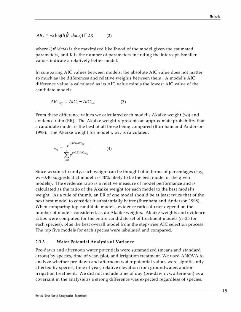
AIC is calculated as:
Methods
15 Merced River Ranch Revegetation Experiment
KdatalAIC 2))|ˆ(log(2 +−= θ (2)
where l( θ̂ |data) is the maximized likelihood of the model given the estimated
parameters, and K is the number of parameters including the intercept. Smaller
values indicate a relatively better model.
In comparing AIC values between models, the absolute AIC value does not matter
so much as the differences and relative weights between them. A model’s AIC
difference value is calculated as its AIC value minus the lowest AIC value of the
candidate models:
minAICAICAIC idiff −= (3)
From these difference values we calculated each model’s Akaike weight (wi) and
evidence ratio (ER). The Akaike weight represents an approximate probability that
a candidate model is the best of all those being compared (Burnham and Anderson
1998). The Akaike weight for model i, wi , is calculated:
∑=
−
−
=n
p
AIC
AIC
ipdiff
idiff
e
ew
1
)5.0(
)5.0(
(4)
Since wi sums to unity, each weight can be thought of in terms of percentages (e.g.,
wi =0.40 suggests that model i is 40% likely to be the best model of the given
models). The evidence ratio is a relative measure of model performance and is
calculated as the ratio of the Akaike weight for each model to the best model’s
weight. As a rule of thumb, an ER of one model should be at least twice that of the
next best model to consider it substantially better (Burnham and Anderson 1998).
When comparing top candidate models, evidence ratios do not depend on the
number of models considered, as do Akaike weights. Akaike weights and evidence
ratios were computed for the entire candidate set of treatment models (n=23 for
each species), plus the best overall model from the step-wise AIC selection process.
The top five models for each species were tabulated and compared.
2.3.3 Water Potential Analysis of Variance
Pre-dawn and afternoon water potentials were summarized (means and standard
errors) by species, time of year, plot, and irrigation treatment. We used ANOVA to
analyze whether pre-dawn and afternoon water potential values were significantly
affected by species, time of year, relative elevation from groundwater, and/or
irrigation treatment. We did not include time of day (pre-dawn vs. afternoon) as a
covariant in the analysis as a strong difference was expected regardless of species,

Methods
16 Merced River Ranch Revegetation Experiment
time of year, or treatment level. We conducted post-hoc pair-wise contrasts of
simultaneous 95% confidence intervals using the Tukey method to see which
covariants had the strongest influences on the ANOVA significance levels.
2.3.4 Survival and Hazard Analysis
We analyzed influences on plant survival from the experimental treatment levels,
testing each species independently because of obvious differences in survival
patterns. Seedling survival was analyzed separately in each of the three years
because of the imposition of a new irrigation treatment in both 2005 and 2006,
which resulted in 3 irrigation levels for the experiment: 1, 2, or 3 years. For each
growing season, survivorship over time was calculated for each treatment group
using Kaplan-Meier non-parametric estimations to account for censored
observations (Machin et al. 2006). From the survival curves we plotted the
empirical hazard rate in order to evaluate changes in mortality risk over time for
different species and treatments. The hazard function describes the temporal
change in the instantaneous death rate experienced by individuals in a sample per
unit of time; it is expressed in units of deaths individual-at-risk-1 time-1 (Zens and
Peart 2003). We generated empirical hazard plots using a cubic-B spline first
derivative (predict.smooth.spline function in S-Plus) fit to the inverse of the
Kaplan-Meier survival function (T. Therneau, pers. comm.). The empirical hazard
plots were used to evaluate how the baseline hazard rates (i.e., the force of
mortality) varied over time and between species and experimental units (Burnham
and Rexstad 1993, Dunlap et al. 1994, Pletcher and Curtsinger 2000, Tableman et al.
2004).
2.3.5 Cox Proportional Hazard Model
We analyzed differences in seedling survival between treatment levels in each year
of the experiment using a Cox proportional hazard model. The Cox model, which
is commonly used in the health sciences (Vittinghoff et al. 2005, Machin et al. 2006),
is a flexible regression model for assessing the effects of multiple predictors on
time-to-event data (time-to-death or machine failure, for example). The model is
non-parametric with respect to the distribution of survival times, a feature that
makes the Cox model very flexible for representing complex mortality patterns. A
primary assumption in the Cox model is that the ratio of the hazard rate, or
instantaneous risk of death, between groups does not change with time. This
means that though the number of individuals in each group that die at any time
may vary, the death totals are proportional between groups at all times. This is a
reasonable assumption if mortality is affected by a treatment factor but is also
influenced by environmental factors that vary in intensity over time. In the Cox
model, the linear predictors are linked through log transformation of the hazard
ratio:
Methods
17 Merced River Ranch Revegetation Experiment
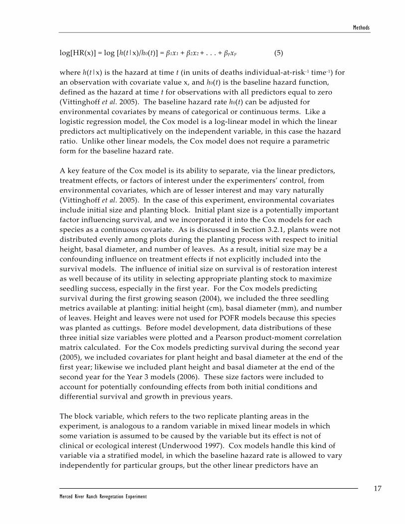
log[HR(x)] = log [h(t|x)/h0(t)] = β1x1 + β2x2 + . . . + βpxp (5)
where h(t|x) is the hazard at time t (in units of deaths individual-at-risk-1 time-1) for
an observation with covariate value x, and h0(t) is the baseline hazard function,
defined as the hazard at time t for observations with all predictors equal to zero
(Vittinghoff et al. 2005). The baseline hazard rate h0(t) can be adjusted for
environmental covariates by means of categorical or continuous terms. Like a
logistic regression model, the Cox model is a log-linear model in which the linear
predictors act multiplicatively on the independent variable, in this case the hazard
ratio. Unlike other linear models, the Cox model does not require a parametric
form for the baseline hazard rate.
A key feature of the Cox model is its ability to separate, via the linear predictors,
treatment effects, or factors of interest under the experimenters’ control, from
environmental covariates, which are of lesser interest and may vary naturally
(Vittinghoff et al. 2005). In the case of this experiment, environmental covariates
include initial size and planting block. Initial plant size is a potentially important
factor influencing survival, and we incorporated it into the Cox models for each
species as a continuous covariate. As is discussed in Section 3.2.1, plants were not
distributed evenly among plots during the planting process with respect to initial
height, basal diameter, and number of leaves. As a result, initial size may be a
confounding influence on treatment effects if not explicitly included into the
survival models. The influence of initial size on survival is of restoration interest
as well because of its utility in selecting appropriate planting stock to maximize
seedling success, especially in the first year. For the Cox models predicting
survival during the first growing season (2004), we included the three seedling
metrics available at planting: initial height (cm), basal diameter (mm), and number
of leaves. Height and leaves were not used for POFR models because this species
was planted as cuttings. Before model development, data distributions of these
three initial size variables were plotted and a Pearson product-moment correlation
matrix calculated. For the Cox models predicting survival during the second year
(2005), we included covariates for plant height and basal diameter at the end of the
first year; likewise we included plant height and basal diameter at the end of the
second year for the Year 3 models (2006). These size factors were included to
account for potentially confounding effects from both initial conditions and
differential survival and growth in previous years.
The block variable, which refers to the two replicate planting areas in the
experiment, is analogous to a random variable in mixed linear models in which
some variation is assumed to be caused by the variable but its effect is not of
clinical or ecological interest (Underwood 1997). Cox models handle this kind of
variable via a stratified model, in which the baseline hazard rate is allowed to vary
independently for particular groups, but the other linear predictors have an

Methods
18 Merced River Ranch Revegetation Experiment
equally-proportional effect on the stratified groups. This is a useful feature to
avoid making unwarranted assumptions of proportional hazards for the
stratification variable that could bias the treatment effect estimates. However,
stratified Cox models cannot estimate parameter values for the stratification
variable; therefore this feature is appropriate for variables for which the specific
effect size is not of interest. In this experiment, planting block was included as a
stratified variable for each species’ Cox model.
For each species we developed best explanatory Cox models of plant survival using
an AIC model selection process similar to the growth models described above. As
with the growth models, we initially specified a candidate set of 23 models of
interest, one for each combination of treatment variables and their interactions.
Block was included as a stratification variable. We also generated a ‘best’ model
that resulted from an AIC-optimization of all possible variables, including the three
initial size variables of height, basal diameter and number of leaves at planting. As
with the growth models, we compared the candidate models for each species using
their AIC values, Akaike weights and evidence ratios.
For the best model of each species (those with the highest Akaike weights), we
interpreted the effects of each explanatory variable via the hazard ratio.
Proceeding from equation (5), the hazard ratio for a model predictor is the
exponentiated coefficient estimate for that predictor. For a binary predictor (e.g.,
weed control), the resulting hazard ratio indicates the proportionally greater (for
HR>1) or lesser (for HR<1) mortality risk of one treatment versus another. For
continuous variables such as initial size, the HR indicates the proportional effect on
mortality risk of a one-unit increase in the predictor variable (e.g., an incremental
height increase of 1 cm).
We used the confidence limits for the hazard ratio and the change-in-estimate
method to evaluate the ecological importance of each variable in the final Cox
survival models. The AIC-based model selection method is somewhat liberal as to
parameter inclusion compared to frequentist-based methods (Burnham and
Anderson 2000); therefore it is especially important to evaluate the magnitude and
ecological importance of any particular variable. In a Cox model, the confidence
limits of the hazard ratio are well-suited for this process; these are calculated by
exponentiating the confidence limits of the parameter estimate (Vittinghoff et al.
2005). A hazard ratio equal to 1 for a particular variable (i.e., a parameter estimate =
e) indicates no difference in mortality risk between groups. Therefore, if the hazard
ratio is close to unity and/or the 95% confidence limits of the hazard ratio bracket 1,
one may conclude that a factor has little effect on survival.
The change-in-estimate method is another way to assess the ecological importance
of factors included in the final Cox survival models (Machin et al. 2006). This

Methods
19 Merced River Ranch Revegetation Experiment
strategy compares an estimate of the hazard ratio from a full model with
environmental covariates to that from a simpler model with only the design factors
of interest (i.e., treatment variables). If the ratio of the two estimates is greater than
C or smaller than 1/C, the change is considered practically or clinically important
and the extra variables are retained in the final Cox model. The constant C reflects
the researcher’s judgment of what constitutes an acceptable level of confoundment
that must be adjusted for; in practice, it is often set at C=1.1 and 1/C = 0.9, or 10% of
a hazard ratio estimate (Maldonado and Greenland 1993, Machin et al. 2006). For
each of the best survival models determined using the AIC-based selection process,
we evaluated the coefficient estimates compared to simpler models to determine
which coefficients were not practically important for plant survival, using a C value
of 1.1.


Results
21 Merced River Ranch Revegetation Experiment
3 RESULTS
3.13.13.13.1 Site ConditionsSite ConditionsSite ConditionsSite Conditions
3.1.1 Soil Texture and Nutrients
A study of tailing pile texture and volume at the MRR found the tailing piles to be
a heterogeneous mix of cobbles and boulders in a matrix of gravel, sand and silt
(URS 2004b). Minimal stratigraphic differentiation was observed in the tailing
piles, with the exception of a shallow(0.2 m [0.7 ft]) surface layer of large cobles
and boulders (URS 2004b). The depth of the study test pits (between 3 and 8 m [10
and 26 ft] deep) and the condition of the excavated revegetation experimental plots
suggest that restored floodplains, upon which revegetation will be conducted, will
have approximately the same texture as the tailing piles, with the exception of the
coarse surface layer, which will be removed during restoration.
There may be a sufficient volume of fine material recovered during the floodplain
restoration process to improve soil conditions somewhat before revegetation
begins. From the 2004 study results, it was estimated that approximately 5.5% of
the tailings is composed of material less than 2 mm (texturally designated as
medium sand, fine sand, silt and clay). Conceptual restoration plans for the MRR
call for the removal of, on average, 4.6 m (15 ft) of tailings from the floodplain
portion of the site (Stillwater Sciences 2005). Sorting this volume of tailings could
potentially recover enough fine material to cover the restored MRR floodplain with
0.2 to 0.3 m (9 to 10 in) of sand, silt, and clay (G. Strnad, pers. comm.). While this
fine sediment could improve substrate conditions prior to revegetation, it is also
the size material that is most likely to be contaminated with mercury (Stillwater
Sciences 2004). For this reason, material being considered for re-use at the MRR
will need to be batch-tested for mercury (Stillwater Sciences 2004). Only batches of
fine material found to be below or within the range of natural background mercury
levels (50–80 ng/g) for California’s Central Valley (Bouse et al. 1996) should be used
in appropriate areas of the floodplain not prone to frequent river inundation or on
higher terrace surfaces above the 100-year floodplain.
Soil analyses of both experimental blocks indicated that soils were highly disturbed
(low micronutrient and zinc levels), but not necessarily to a level likely to critically

Results
22 Merced River Ranch Revegetation Experiment
limit plant establishment (M. Buttress, pers. comm.). Table 3-1 summarizes the
results of soil analyses for Block 1 and Block 2.
Table Table Table Table 3333----1111. . . . Soil analytesSoil analytesSoil analytesSoil analytes at each expeat each expeat each expeat each experimental block.rimental block.rimental block.rimental block.
AnalyteAnalyteAnalyteAnalyte Block 1Block 1Block 1Block 1 Block 2Block 2Block 2Block 2
Organic matter (%) 2.6 0.7
Nitrogen (ppm) 5 3
Phosphorus – weak bray (ppm) 13 7
Potassium (% cation saturation) 2.3 1.8
Magnesium (% cation saturation) 35.0 32.6
Calcium (% cation saturation) 56.0 64.5
Sodium (% cation saturation) 0.7 1.1
Zinc (ppm) 0.5 0.3
Boron (ppm) 0.3 0.2
pH 6.6 7.0
Soils at Block 1 had coarser texture and higher levels of most nutrients than Block
2, but in general the ranges of nutrient levels were similar at both blocks (Appendix
A). Soil at Block 1 was considered to have low to medium organic matter while soil
at Block 2 had very low organic matter (M. Buttress, pers. comm.). Both blocks had
very low nitrogen, phosphorus, sodium, and zinc, low potassium; and high
magnesium levels (see Appendix A).
3.1.2 Depth to Groundwater, River Stage, and Pond Stage
Groundwater elevations at the two monitoring wells, river stage, and swale pond
stage in 2004, 2005 and 2006 are presented in Figures 6–8 and summarized in Table
3-2.
Table Table Table Table 3333----2222. . . . Average, minimum, and maximum groAverage, minimum, and maximum groAverage, minimum, and maximum groAverage, minimum, and maximum groundwater, river stage, and undwater, river stage, and undwater, river stage, and undwater, river stage, and swale swale swale swale pond pond pond pond stage stage stage stage elevationselevationselevationselevations over the experiment monitoring periodover the experiment monitoring periodover the experiment monitoring periodover the experiment monitoring period (m (m (m (m NGVD)NGVD)NGVD)NGVD)....
LocationLocationLocationLocation
2004200420042004 2005200520052005 2006200620062006
AverageAverageAverageAverage (ft NGVD)(ft NGVD)(ft NGVD)(ft NGVD)
RangeRangeRangeRange (ft NGVD)(ft NGVD)(ft NGVD)(ft NGVD)
AverageAverageAverageAverage (ft NGVD)(ft NGVD)(ft NGVD)(ft NGVD)
RangeRangeRangeRange (ft NGVD)(ft NGVD)(ft NGVD)(ft NGVD)
AverageAverageAverageAverage (ft NGVD)(ft NGVD)(ft NGVD)(ft NGVD)
RangeRangeRangeRange (ft NGVD)(ft NGVD)(ft NGVD)(ft NGVD)
River Stage 84.4
(276.8) 84.2–85.0
(276.2–278.8) 84.7
(277.8) 84.3–85.9
(276.3–281.6) 85.0
(278.6) 84.4–85.6
(276.6–280.7)
Groundwater at Block 1
86.9 (285.0)
86.7–87.1 (284.5–285.7)
87.0 (285.5)
87.0–87.1 (285.3–285.7)
87.1 (285.6)
87.0–87.2 (285.3–285.8)
Groundwater at Block 2
87.7 (287.8)
87.6 –87.9 (287.5–288.5)
87.9 (288.3)
87.9–88.0 (288.2–288.9)
88.0 (288.4)
87.9–88.1 (288.3–288.7)
Swale Pond Stage
87.9 (288.2)
87.7–88.0 (287.8–288.8)
87.9 (288.4)
87.5—88.1 (287.2–289.1)
N/A N/A

Results
23 Merced River Ranch Revegetation Experiment
River stage was approximately 84.4 m (276.6 ft) during summer and fall baseflows
in both 2004 and 2005, and 84.6 m (277.5 ft) in 2006 (Figures 6–8). Short increases in
river stage were seen in May and October 2004 (to 85.0 m and 84.6 m, respectively)
and corresponded with scheduled flow releases from upstream dams designed to
improve salmon outmigration and emigration conditions. Sustained high stages
from March to May 2005, ranging from 85.9 m (281.6 ft) to 84.9 m (278.5 ft), and
April to July 2006, ranging from 85.6 m to 85.2 m (280.7 ft to 279.3 ft), were results
of flow releases due to higher-than-average winter rain and snow fall.
Groundwater elevations, and therefore depth to groundwater (see Table 2-2),
fluctuated very little over the monitoring period (Figures 6–8). Over three years,
from their lowest to highest recorded levels, groundwater varied no more than 0.4
m (1.3 ft) and 0.4 m (1.2 ft) at Block 1 and Block 2, respectively. The groundwater
table showed little response or relationship to river flow conditions and appears to
be perched 2.5 to 3.4 m (8.0 to 11.0 ft) above summer and fall baseflows (Figures 6–
8).
The monitored swale pond was inundated year-round, as were all of the larger
ponds at the site (Z. Diggory, pers. obs.). Pond stage levels remained relatively
stable over the monitoring period, fluctuating no more than 0.3 m (1.0 ft) in 2004
and 0.6 m (2.0 ft) in 2005 (pond stage was not consistently monitored in 2006), and
showed no response to river flow conditions (Figure 6–8).
3.1.3 Temperature
Temperature was originally monitored, in part, to evaluate potential differences in
temperature between experimental plots. In 2004, B1M was an average of 0.3 °C
warmer than the control area and 0.8 °C warmer than B2M. B2M was an average of
0.5 °C warmer than the control area. In 2005, B1M was 0.9 °C warmer than the
control area. There were no consistent differences between other monitored areas
in 2005. Despite B1M being consistently warmer than other monitored areas, in
general, daily average temperatures were not remarkably different between areas.
For example, on July 16, 2005, one of the hottest days that year, the daily average
temperature ranged from 32.9 to 33.8 °C between areas, a difference of 0.9 °C. The
typical calibration error value specified for the data loggers by the manufacturer is
± 0.2 °C.
Because of the small differences between experimental plots, only temperature
from the control area is presented and discussed below. Daily average, minimum,
and maximum temperatures from 2004–2006 are presented in Figures 9–11.
Monthly average temperatures are summarized in Table 3-3.

Results
24 Merced River Ranch Revegetation Experiment
Table Table Table Table 3333----3333. . . . Monthly average temperatures at the MRRMonthly average temperatures at the MRRMonthly average temperatures at the MRRMonthly average temperatures at the MRR ((((±1SE±1SE±1SE±1SE) during the experiment ) during the experiment ) during the experiment ) during the experiment ((((°C°C°C°C))))....
2004200420042004 2005200520052005 2006200620062006
JanJanJanJan – – 8.4 (±0.3)
FebFebFebFeb – – 10.0 (±0.6)
MarMarMarMar – – 9.7 (±0.4)
AprAprAprApr 18.6 (±1.0) 15.3 (±0.4) 14.7 (±0.5)
MaMaMaMayyyy 20.6 (±0.4) 19.8 (±0.6) 21.3 (±0.6)
JunJunJunJun 24.3 (±0.4) 22.6 (±0.5) 26.2 (±0.6)
JulJulJulJul 27.2 (±0.3) 29.1 (±0.4) 29.6 (±0.6)
AugAugAugAug 25.6 (±0.6) 27.1 (±0.4) 25.4 (±0.3)
SeptSeptSeptSept – 21.5 (±0.4) 22.4 (±0.5)
OctOctOctOct – 17.2 (±0.4) 15.9 (±0.4)
NovNovNovNov – 11.9 (±0.4 –
DecDecDecDec – 9.3 (±0.6) –
During the experimental monitoring periods, monthly average temperatures were
lowest in January (8.4 ±0.3 °C in 2006) and highest in July (28.6±0.7 °C). At the
control area, daily temperatures ranged from 3.3 °C (on April 18) to 42.5 °C (on
August 11) in 2004; from -3.9 °C (on November 27) to 42.9 °C (on July 14) in 2005;
and from -3.4 °C (on February 16) to 45.9 °C (on July 23) in 2006.
3.23.23.23.2 Plant Size and GrowthPlant Size and GrowthPlant Size and GrowthPlant Size and Growth
3.2.1 Initial Size at Planting
The initial height, basal diameter and number of leaves of each species at the time
of planting varied substantially by planting plot; these differences are summarized
in Table 3-4. Boxplots of initial size means and distributions are presented in
Figure 12.

Results
25 Merced River Ranch Revegetation Experiment
Table Table Table Table 3333----4444. . . . Initial seedling height, Initial seedling height, Initial seedling height, Initial seedling height, basal basal basal basal diameter and number of leaves at planting time (means diameter and number of leaves at planting time (means diameter and number of leaves at planting time (means diameter and number of leaves at planting time (means ±1SE) ±1SE) ±1SE) ±1SE) by plot (block by plot (block by plot (block by plot (block and and and and relative elevationrelative elevationrelative elevationrelative elevation))))....
VVVVariableariableariableariable SSSSpeciespeciespeciespecies B1HB1HB1HB1H B1MB1MB1MB1M B1LB1LB1LB1L B2HB2HB2HB2H B2MB2MB2MB2M B2LB2LB2LB2L
Height (cm)
ACNE 26.7 (±1.5) 27.5 (±1.5) 31.2 (±1.5) 28.1 (±1.4) 24.9 (±1.3) 28.2 (±1.3)
FRLA 6.3 (±0.3) 4.2 (±0.3) 5.4 (±0.4) 6.4 (±0.4) 5.3 (±0.4) 6.1 (±0.3)
POFR 47.9 (±1.1) 45.1 (±1.1) 46.1 (±1.2) 48.5 (±1.1) 45.6 (±0.8) 44.7 (±1.1)
QULO 42 (±1.4) 45 (±1.2) 42.3 (±1.1) 48.9 (±1.3) 44.9 (±1.3) 45.1 (±1.3)
Basal Diameter (mm)
ACNE 3.1 (±0.1) 3.1 (±0.1) 3.3 (±0.1) 3.1 (±0.1) 2.9 (±0.1) 3.1 (±0.1)
FRLA 2.4 (±0.1) 2.3 (±0.1) 2.1 (±0) 2.4 (±0.1) 2.2 (±0.1) 2.2 (±0.1)
POFR 14.4 (±0.5) 12.8 (±0.4) 14.8 (±0.4) 17 (±0.6) 7.7 (±0.2) 13.2 (±0.4)
QULO 4.6 (±0.2) 5.6 (±0.2) 5.7 (±0.2) 4.8 (±0.1) 5 (±0.1) 4.1 (±0.1)
Number of Leaves
ACNE 5.2 (±0.2) 5.7 (±0.3) 5.6 (±0.2) 4.2 (±0.3) 4.2 (±0.2) 3.9 (±0.3)
FRLA 3.8 (±0.3) 3.2 (±0.3) 3 (±0.4) 2 (±0.2) 1.1 (±0.1) 2.4 (±0.2)
POFR 0 (±0) 0 (±0) 0 (±0) 0 (±0) 0 (±0) 0 (±0)
QULO 28.1 (±1.6) 29.2 (±1.6) 25.1 (±1.4) 39.5 (±1.7) 35 (±1.9) 32.1 (±1.5)
Analysis of variance tests indicate that for most species and variables (initial
height, basal diameter and number of leaves), there were significant differences in
mean values by plot at an α=0.05 level (see Appendix B). This may be a function of
large differences in planting stock between plots, or of large sample sizes (n=60),
which would result in sufficient resolution to detect very small differences among
plots.
Of the significantly different factors analyzed, and follow-up pairwise
comparisons, the strongest differences in initial conditions were:
1. POFR cutting basal diameter differed by plot (F5,345=56.21, p=<0.001). Follow up
pairwise comparisons indicated that cuttings in B2M had smaller basal
diameters (by approximately 6 to 10 mm) than in other plots (Figure 12g and
Appendix B).
2. FRLA seedling leaf number differed by plot (F5,345=14.57, p=<0.001); seedlings in
B2M had fewer leaves (by approximately 1 to 3 leaves) than in other plots
(Figure 12j and Appendix B).
3. ACNE seedling leaf number differed by plot (F5,345=10.38, p=<0.001); seedlings in
B1L had more leaves (by approximately 1 to 2 leaves) than in other plots (Figure
12i and Appendix B).
4. QULO seedling height and leaf number differed by plot (F5,345=3.92, p=0.002 and
F5,345=10.49, p=<0.001); seedlings in B2H were taller (by approximately 5 to 8 cm)
and had more leaves (by approximately 10 to 15 leaves) than in other plots
(Figures 12d, 12e and Appendix B).
The smaller basal diameters of POFR cuttings in plot B2M (7.7±0.2 mm) relative to
other plots (Table 3-4 and Figure 12), in particular, is notable. In this plot, FRLA
seedlings had the lowest mean number of leaves at planting (1.1±0.1) as well. B2M
was the last experimental plot to be planted and it is likely that, despite attempts to

Results
26 Merced River Ranch Revegetation Experiment
randomize cuttings and container stock, field crews were left with the smallest cuttings
and less than ideal FRLA container stock at the end of the planting effort.
3.2.2 Plant Growth Timing
All species began to grow new leaves approximately ten weeks after planting (Figure 13;
see Appendix C for week dates). Leaf-out for POFR began sooner than the other species,
and POFR trees had double the mean number of leaves at the end of the first growing
season compared to QULO, and four times that of ACNE and FRLA. Because the four
species have different leaf morphologies (e.g., ACNE and FRLA have compound leaves),
raw leaf numbers do not give good indications of leaf area differences between species.
In contrast to the other species, POFR continued to accumulate leaves at a rapid rate
throughout the first growing season. QULO leaf accumulation slowed abruptly after the
18th week (mid-August; see Appendix C), whereas the other three species continued
accumulating leaves through late October. As discussed in Section 2.2.5 (Methods), the
number of leaves was not tracked in subsequent years.
Relative timing of leaf-out, height growth and basal diameter growth varied by species,
but three species showed consistent timing patterns between the first and second years
(Figure 14). Early in the growing season, most tree species allocate biomass first to
height, then to basal diameter increment (Oliver and Larson 1996). This pattern is
believed to be an adaptation to competition for light as plants race to the top of the
canopy following bud break. Height growth preceded basal diameter increment for
ACNE, FRLA and POFR in the first growing season (2004), and for ACNE and FRLA in
the second. Height and basal diameter growth progressed apace for QULO in both
years and height growth trailed basal diameter growth for POFR in the second year.
Leaf-out trailed height growth in the first year for all species except FRLA, for which
both processes occurred simultaneously.
3.2.3 Patterns in Plant Growth between Treatment Groups
Over the course of the experiment, growth was greatest for POFR, followed by ACNE,
with slower growth rates for FRLA and QULO (Table 3-5). In the first year, POFR
seedlings had the greatest increase in height, followed by ACNE, QULO, and FRLA. In
the second year, ACNE growth was greater than that of the other species. After 3 years,
mean height for POFR was greatest. 38% of ACNE alive at the end of the experiment
experienced crown dieback (Stillwater Sciences, unpublished data), resulting in lower live
crown heights compared to Year 2. Basal diameter growth over the course of the
experiment was greatest for POFR, followed by ACNE, QULO, and FRLA.

Results
27 Merced River Ranch Revegetation Experiment
Table Table Table Table 3333----5555. . . . EndEndEndEnd----ofofofof----year height and year height and year height and year height and basal basal basal basal diameter (mean±1 SE) for all species.diameter (mean±1 SE) for all species.diameter (mean±1 SE) for all species.diameter (mean±1 SE) for all species.
Growth MeasureGrowth MeasureGrowth MeasureGrowth Measure YearYearYearYear ACNEACNEACNEACNE FRLAFRLAFRLAFRLA POFRPOFRPOFRPOFR QULOQULOQULOQULO
Height (cm)
Year 1 87.0±1.5 46.8±1.8 125.2±3.4 85.7±2.0
Year 2 193.2±3.5 95.3±3.2 183.4±5.5 113.3±2.
Year 3 177.0±8.0 118.1±3.7 226.2±9.1 120.2±2.6
Basal Diameter (mm)
Year 1 14.0±0.4 6.2±0.2 18.7±0.4 9.0±0.1
Year 2 24.5±0.5 13.2±0.4 29.4±0.9 14.3±0.2
Year 3 29.1±1.1 17.7±0.6 42.0±2.1 18.7±0.5
Growth patterns did not vary systematically by treatment factors, but some factors were
important for individual species. Figures 15 and 16 show height and basal diameter
growth over the 3-year experiment by irrigation treatments, and Figures 17 and 18 show
height and basal diameter growth by elevation level. No positive irrigation effect (i.e.,
higher growth with increased irrigation duration) is apparent until the third year, and
only then for ACNE basal diameter. Differences in growth between elevation levels are
more apparent (Figures 17 and 18). In general, growth is greater for stems on lower
surfaces compared to upper surfaces. However, in many cases the differences are not
proportional between the treatments, and the middle levels had either higher or lower
growth than the other two levels. Differences in growth between weed control
treatments were not shown because they were minimal.
In contrast to the treatment effects, the largest growth influence was due to planting
plot, as evidenced in large differences between combinations of block and elevation level
(with no consistent elevation trend). When growth patterns are compared by treatment
and planting block, differences are larger due to block than to either elevation or
irrigation. Figure 19 shows final plant size (2006) by irrigation and block, and Figure 20
shows final plant size by elevation and block. The only consistently positive effect of
increased irrigation duration occurred for QULO, and the only increasingly negative
effect of depth to groundwater was for FRLA.
3.2.4 ANCOVA Models of 3-Year Basal Diameter Increment Growth
The ANCOVA basal diameter growth models confirmed that planting location had the
greatest influence on growth throughout the experiment. Table 3-6 shows the top five
candidate models for each species. Elevation and/or block were the most common
factors in the top model for all species. Elevation was the best explanatory factor for
FRLA, and block was best for POFR. For ACNE, block, elevation, and initial basal
diameter were important, with an interaction between the latter two variables. For
QULO, all treatment factors were included in the best model, with initial basal diameter
and interactions between block and elevation, and weed control and irrigation as well.
For QULO especially, absolute values of growth differences were not great for any factor
(Figures 15–20).

Results
28 Merced River Ranch Revegetation Experiment
Table Table Table Table 3333----6666. . . . Top five candidate ANCOVA models of factor influences on Top five candidate ANCOVA models of factor influences on Top five candidate ANCOVA models of factor influences on Top five candidate ANCOVA models of factor influences on basal diameterbasal diameterbasal diameterbasal diameter growth igrowth igrowth igrowth increment.ncrement.ncrement.ncrement.
model deviance K AIC delta weights ER parameters
ACNEACNEACNEACNE
1 1462.02 5 1472.36 0.00 1.00 1.00 (Intercept)+elev+iDiam+block+elev:iDiam
2 1483.80 4 1492.03 19.67 0.00 0.00 (Intercept)+elev+weed+elev:weed
3 1483.68 5 1494.02 21.66 0.00 0.00 (Intercept)+elev+weed+irrigate+elev:weed
4 1490.00 2 1494.07 21.70 0.00 0.00 (Intercept)+elev
5 1490.24 2 1494.31 21.95 0.00 0.00 (Intercept)+irrigate
FRLAFRLAFRLAFRLA
1 1165.49 2 1169.56 0.00 0.20 1.00 (Intercept)+elev
2 1164.29 3 1170.43 0.87 0.13 0.65 (Intercept)+elev+weed
3 1162.84 4 1171.08 1.52 0.09 0.47 (Intercept)+elev+weed+elev:weed
4 1165.48 3 1171.63 2.07 0.07 0.36 (Intercept)+elev+irrigate
5 1167.66 2 1171.73 2.17 0.07 0.34 (Intercept)+weed
POFRPOFRPOFRPOFR
1 1274.29 2 1278.38 0.00 0.33 1.00 (Intercept)+block
2 1276.25 2 1280.34 1.96 0.12 0.38 (Intercept)+elev
3 1277.22 2 1281.31 2.93 0.08 0.23 (Intercept)+irrigate
4 1277.26 2 1281.34 2.96 0.07 0.23 (Intercept)+weed
5 1275.73 3 1281.91 3.53 0.06 0.17 (Intercept)+elev+weed
QULOQULOQULOQULO
1 1811.18 8 1827.70 0.00 1.00 1.00 (Intercept)+elev+weed+irrigate+block+iDiam+block:elev+weed:irrigate
2 1872.11 4 1880.26 52.56 0.00 0.00 (Intercept)+weed+irrigate+weed:irrigate
3 1871.40 5 1881.61 53.92 0.00 0.00 (Intercept)+elev+weed+irrigate+weed:irrigate
4 1878.92 2 1882.96 55.26 0.00 0.00 (Intercept)+irrigate
5 1878.92 2 1882.96 55.27 0.00 0.00 (Intercept)+elev
The best model for ACNE and QULO were much better than any other model (Table
3-6). Parameter estimates for the coefficients of each species’ best model are shown in
Table 3-7. For the top models Akaike weights and evidence ratios were close to unity
for both species, indicating an overwhelmingly better fits than other candidate models
(Table 3-6). For FRLA, the top model including only the elevation term was 20% likely
given the candidate set (Akaike weight), and about 35% better than the next best model
(evidence ratio). Using the rule of thumb of a two-time ER, the top three FRLA models
are reasonable approximations. Elevation is the most common factor in all these models;
the elevation parameter estimate in the best model is negative, indicating that as depth
to groundwater increased, growth decreased (Table 3-7, Figure 20). For POFR, the best
model containing only the block variable was 33% likely given the candidate set and
67% better than the next best model, which had elevation as the sole explanatory factor.
Because of interaction terms, interpretation of the trend in the continuous variables (i.e.,
the sign of the parameter estimates for elevation, irrigation duration, and initial basal
diameter) is problematic. For QULO, the estimate for initial basal diameter is negative,
indicating that growth was less for larger plants (Table 3-7). This is counter to our
initial expectations. However, the biological importance of this relationship is suspect,
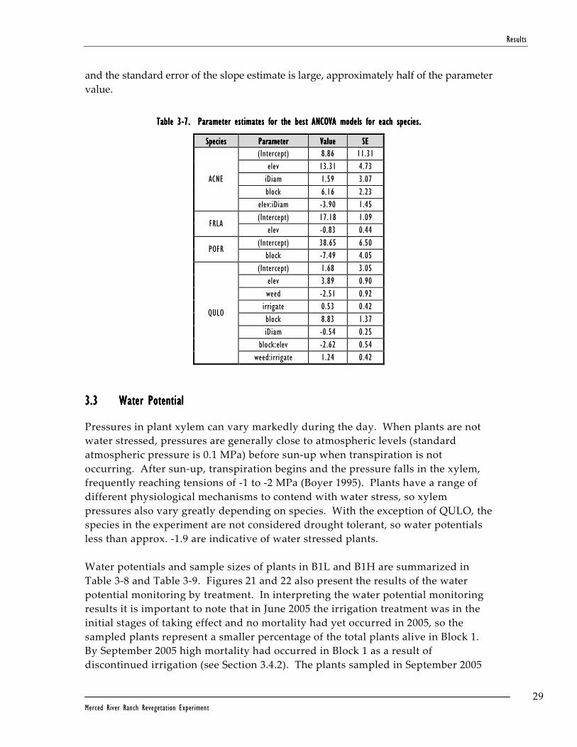
Results
29 Merced River Ranch Revegetation Experiment
and the standard error of the slope estimate is large, approximately half of the parameter
value.
Table Table Table Table 3333----7777. . . . Parameter estimates for the best ANCOVA models for each species.Parameter estimates for the best ANCOVA models for each species.Parameter estimates for the best ANCOVA models for each species.Parameter estimates for the best ANCOVA models for each species.
SpeciesSpeciesSpeciesSpecies ParParParParameterameterameterameter ValueValueValueValue SESESESE
ACNE
(Intercept) 8.86 11.31
elev 13.31 4.73
iDiam 1.59 3.07
block 6.16 2.23
elev:iDiam -3.90 1.45
FRLA (Intercept) 17.18 1.09
elev -0.83 0.44
POFR (Intercept) 38.65 6.50
block -7.49 4.05
QULO
(Intercept) 1.68 3.05
elev 3.89 0.90
weed -2.51 0.92
irrigate 0.53 0.42
block 8.83 1.37
iDiam -0.54 0.25
block:elev -2.62 0.54
weed:irrigate 1.24 0.42
3.33.33.33.3 Water PotentialWater PotentialWater PotentialWater Potential
Pressures in plant xylem can vary markedly during the day. When plants are not
water stressed, pressures are generally close to atmospheric levels (standard
atmospheric pressure is 0.1 MPa) before sun-up when transpiration is not
occurring. After sun-up, transpiration begins and the pressure falls in the xylem,
frequently reaching tensions of -1 to -2 MPa (Boyer 1995). Plants have a range of
different physiological mechanisms to contend with water stress, so xylem
pressures also vary greatly depending on species. With the exception of QULO, the
species in the experiment are not considered drought tolerant, so water potentials
less than approx. -1.9 are indicative of water stressed plants.
Water potentials and sample sizes of plants in B1L and B1H are summarized in
Table 3-8 and Table 3-9. Figures 21 and 22 also present the results of the water
potential monitoring by treatment. In interpreting the water potential monitoring
results it is important to note that in June 2005 the irrigation treatment was in the
initial stages of taking effect and no mortality had yet occurred in 2005, so the
sampled plants represent a smaller percentage of the total plants alive in Block 1.
By September 2005 high mortality had occurred in Block 1 as a result of
discontinued irrigation (see Section 3.4.2). The plants sampled in September 2005

Results
30 Merced River Ranch Revegetation Experiment
were thus a much larger percentage of the total plants alive, indicating that they
were the heartier, better established individuals or, in the case of un-irrigated
FRLA, the only individuals left alive to sample (Table 3-9).
Pre-dawn water potential values were influenced by species, time of year, relative
elevation above groundwater, and month-relative elevation above groundwater
interactions (Table 3-10). Afternoon water potential values were significantly
influenced by species only (Table 3-10). Post-hoc pair-wise comparisons of
simultaneous 95% confidence intervals indicate that, with both pre-dawn and
afternoon values, POFR was the species driving the significant differences. In
general, POFR had higher water potentials (i.e., better water status) than the other
species. This difference and high pre-dawn values regardless of relative elevation
or irrigation treatment level suggest that POFR plantings (at least those that
survived to September 2005) had the deepest rooting system and had reached a
reliable groundwater source.
While irrigation and relative elevation treatment did not have significant effects on
water potential values, results were suggestive of an effect. ACNE and FRLA
demonstrated the predicted directional response to relative elevation and irrigation
treatment (i.e., higher potentials/less water stress in the low relative elevation plot
and when irrigated than in the high relative elevation plot and when not irrigated)
in both June and September. QULO demonstrated no response to relative elevation
or irrigation in June and the predicted responses in September (Figures 21 and 22).
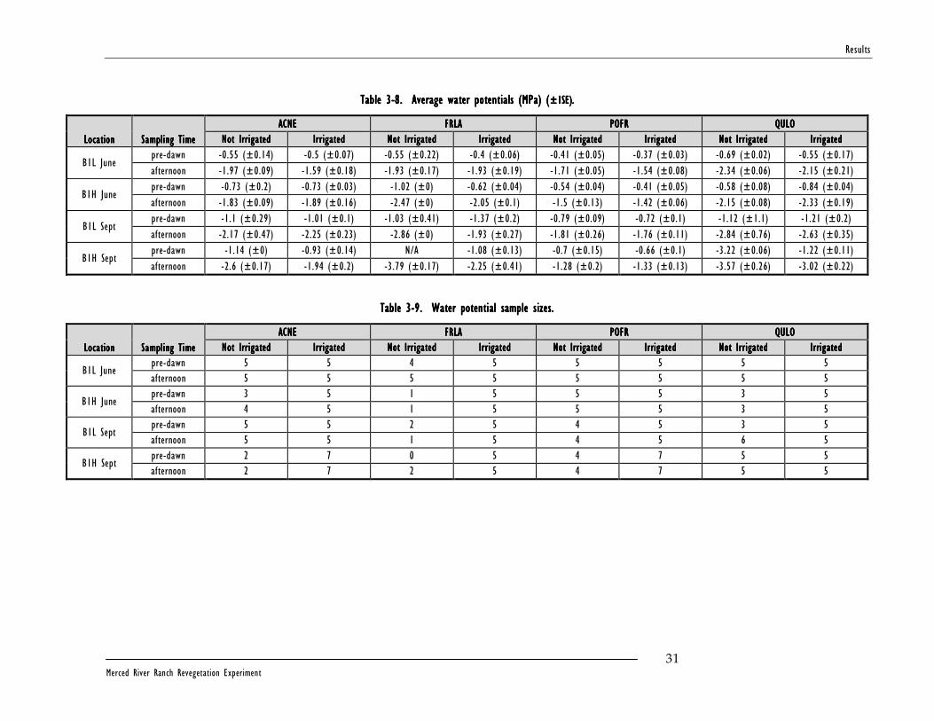
Results
31 Merced River Ranch Revegetation Experiment
Table Table Table Table 3333----8888. . . . Average water potentials (MPa) (Average water potentials (MPa) (Average water potentials (MPa) (Average water potentials (MPa) (±1SE)±1SE)±1SE)±1SE)....
LocationLocationLocationLocation Sampling TimeSampling TimeSampling TimeSampling Time
ACNEACNEACNEACNE FRLAFRLAFRLAFRLA POFRPOFRPOFRPOFR QULOQULOQULOQULO
Not IrrigatedNot IrrigatedNot IrrigatedNot Irrigated IrrigatedIrrigatedIrrigatedIrrigated Not IrrigatedNot IrrigatedNot IrrigatedNot Irrigated IrrigatedIrrigatedIrrigatedIrrigated Not IrrigatedNot IrrigatedNot IrrigatedNot Irrigated IrrigatedIrrigatedIrrigatedIrrigated Not IrrigatedNot IrrigatedNot IrrigatedNot Irrigated IrrigatedIrrigatedIrrigatedIrrigated
B1L June pre-dawn -0.55 (±0.14) -0.5 (±0.07) -0.55 (±0.22) -0.4 (±0.06) -0.41 (±0.05) -0.37 (±0.03) -0.69 (±0.02) -0.55 (±0.17)
afternoon -1.97 (±0.09) -1.59 (±0.18) -1.93 (±0.17) -1.93 (±0.19) -1.71 (±0.05) -1.54 (±0.08) -2.34 (±0.06) -2.15 (±0.21)
B1H June pre-dawn -0.73 (±0.2) -0.73 (±0.03) -1.02 (±0) -0.62 (±0.04) -0.54 (±0.04) -0.41 (±0.05) -0.58 (±0.08) -0.84 (±0.04)
afternoon -1.83 (±0.09) -1.89 (±0.16) -2.47 (±0) -2.05 (±0.1) -1.5 (±0.13) -1.42 (±0.06) -2.15 (±0.08) -2.33 (±0.19)
B1L Sept pre-dawn -1.1 (±0.29) -1.01 (±0.1) -1.03 (±0.41) -1.37 (±0.2) -0.79 (±0.09) -0.72 (±0.1) -1.12 (±1.1) -1.21 (±0.2)
afternoon -2.17 (±0.47) -2.25 (±0.23) -2.86 (±0) -1.93 (±0.27) -1.81 (±0.26) -1.76 (±0.11) -2.84 (±0.76) -2.63 (±0.35)
B1H Sept pre-dawn -1.14 (±0) -0.93 (±0.14) N/A -1.08 (±0.13) -0.7 (±0.15) -0.66 (±0.1) -3.22 (±0.06) -1.22 (±0.11)
afternoon -2.6 (±0.17) -1.94 (±0.2) -3.79 (±0.17) -2.25 (±0.41) -1.28 (±0.2) -1.33 (±0.13) -3.57 (±0.26) -3.02 (±0.22)
Table Table Table Table 3333----9999. . . . Water potential sampWater potential sampWater potential sampWater potential sample sizes.le sizes.le sizes.le sizes.
LocationLocationLocationLocation Sampling TimeSampling TimeSampling TimeSampling Time
ACNEACNEACNEACNE FRLAFRLAFRLAFRLA POFRPOFRPOFRPOFR QULOQULOQULOQULO
Not IrrigatedNot IrrigatedNot IrrigatedNot Irrigated IrrigatedIrrigatedIrrigatedIrrigated Not IrrigatedNot IrrigatedNot IrrigatedNot Irrigated IrrigatedIrrigatedIrrigatedIrrigated Not IrrigatedNot IrrigatedNot IrrigatedNot Irrigated IrrigatedIrrigatedIrrigatedIrrigated Not IrrigatedNot IrrigatedNot IrrigatedNot Irrigated IrrigatedIrrigatedIrrigatedIrrigated
B1L June pre-dawn 5 5 4 5 5 5 5 5
afternoon 5 5 5 5 5 5 5 5
B1H June pre-dawn 3 5 1 5 5 5 3 5
afternoon 4 5 1 5 5 5 3 5
B1L Sept pre-dawn 5 5 2 5 4 5 3 5
afternoon 5 5 1 5 4 5 6 5
B1H Sept pre-dawn 2 7 0 5 4 7 5 5
afternoon 2 7 2 5 4 7 5 5

Results
32 Merced River Ranch Revegetation Experiment
Table Table Table Table 3333----10101010. . . . ANOVA models for preANOVA models for preANOVA models for preANOVA models for pre----dawn and afternoon watedawn and afternoon watedawn and afternoon watedawn and afternoon water potential.r potential.r potential.r potential.
Model FactorModel FactorModel FactorModel Factor DDDDegrees of egrees of egrees of egrees of ffffreedomreedomreedomreedom
SSSSum of um of um of um of squaressquaressquaressquares MMMMean squareean squareean squareean square FFFF----RatioRatioRatioRatio Pr(F)Pr(F)Pr(F)Pr(F)
PrePrePrePre----DawnDawnDawnDawn
Species 3 0.615121 0.201707 16.3696 <0.001
Month 1 1.266324 1.266324 102.7689 <0.001
Elevation 1 0.060560 0.060560 4.9148 0.028
Month:Elevation 1 0.083874 0.083874 6.8068 0.010
Residuals 133 1.638832 0.012322
AfternoonAfternoonAfternoonAfternoon
Species 3 0.318675 0.106225 12.27087 <0.001
Residuals 142 1.229250 0.008657
3.43.43.43.4 Plant SurvivalPlant SurvivalPlant SurvivalPlant Survival
3.4.1 Survival and Hazard Patterns
Plant mortality over the course of the experiment varied substantially between
species and was strongly influenced by both the treatment variables and the
environmental covariates for initial size. In general, mortality was influenced most
strongly by initial planting size in the first year, by irrigation treatment in the
second year, and by relative elevation in the third year. It is likely that this
temporal change in the primary drivers of mortality is the result of the interaction
of the treatment regimes with the plants’ growth patterns and changing
vulnerability profiles over time. Figure 23 shows plant mortality over the course of
the experiment for the different irrigation groups, and Table 3-11 summarizes
survival at the end of each growing season for those groups. Figure 24 shows the
empirical instantaneous hazard rate (deaths individuals-at-risk-1 time-1) among
irrigation treatments, and Figure 25 shows the hazard rate among elevation
treatments. The most consistent contrast in hazard rate in the second year was
between the two irrigation treatments (Figure 24). In the third year (2006), the
elevation group hazard plots show a higher mortality rate for ACNE in the high
plots, and for POFR and QULO in the high and medium elevation plots (Table
3-11).
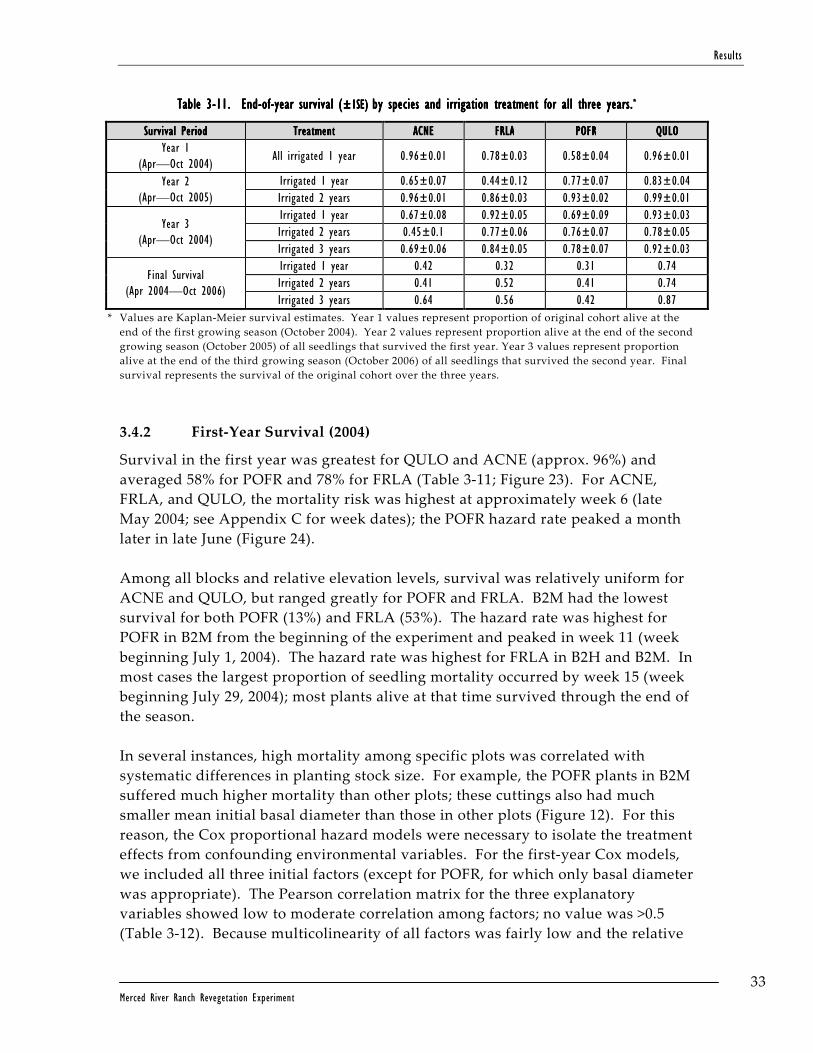
Results
33 Merced River Ranch Revegetation Experiment
Table Table Table Table 3333----11111111. . . . EndEndEndEnd----ofofofof----year survival year survival year survival year survival ((((±1SE)±1SE)±1SE)±1SE) by species and irrigation treatment for all three years.by species and irrigation treatment for all three years.by species and irrigation treatment for all three years.by species and irrigation treatment for all three years.****
Survival PeriodSurvival PeriodSurvival PeriodSurvival Period TreatmentTreatmentTreatmentTreatment ACNEACNEACNEACNE FRLAFRLAFRLAFRLA POFRPOFRPOFRPOFR QULOQULOQULOQULO
Year 1 (Apr—Oct 2004)
All irrigated 1 year 0.96±0.01 0.78±0.03 0.58±0.04 0.96±0.01
Year 2 (Apr—Oct 2005)
Irrigated 1 year 0.65±0.07 0.44±0.12 0.77±0.07 0.83±0.04
Irrigated 2 years 0.96±0.01 0.86±0.03 0.93±0.02 0.99±0.01
Year 3 (Apr—Oct 2004)
Irrigated 1 year 0.67±0.08 0.92±0.05 0.69±0.09 0.93±0.03
Irrigated 2 years 0.45±0.1 0.77±0.06 0.76±0.07 0.78±0.05
Irrigated 3 years 0.69±0.06 0.84±0.05 0.78±0.07 0.92±0.03
Final Survival (Apr 2004—Oct 2006)
Irrigated 1 year 0.42 0.32 0.31 0.74
Irrigated 2 years 0.41 0.52 0.41 0.74
Irrigated 3 years 0.64 0.56 0.42 0.87
* Values are Kaplan-Meier survival estimates. Year 1 values represent proportion of original cohort alive at the
end of the first growing season (October 2004). Year 2 values represent proportion alive at the end of the second
growing season (October 2005) of all seedlings that survived the first year. Year 3 values represent proportion
alive at the end of the third growing season (October 2006) of all seedlings that survived the second year. Final
survival represents the survival of the original cohort over the three years.
3.4.2 First-Year Survival (2004)
Survival in the first year was greatest for QULO and ACNE (approx. 96%) and
averaged 58% for POFR and 78% for FRLA (Table 3-11; Figure 23). For ACNE,
FRLA, and QULO, the mortality risk was highest at approximately week 6 (late
May 2004; see Appendix C for week dates); the POFR hazard rate peaked a month
later in late June (Figure 24).
Among all blocks and relative elevation levels, survival was relatively uniform for
ACNE and QULO, but ranged greatly for POFR and FRLA. B2M had the lowest
survival for both POFR (13%) and FRLA (53%). The hazard rate was highest for
POFR in B2M from the beginning of the experiment and peaked in week 11 (week
beginning July 1, 2004). The hazard rate was highest for FRLA in B2H and B2M. In
most cases the largest proportion of seedling mortality occurred by week 15 (week
beginning July 29, 2004); most plants alive at that time survived through the end of
the season.
In several instances, high mortality among specific plots was correlated with
systematic differences in planting stock size. For example, the POFR plants in B2M
suffered much higher mortality than other plots; these cuttings also had much
smaller mean initial basal diameter than those in other plots (Figure 12). For this
reason, the Cox proportional hazard models were necessary to isolate the treatment
effects from confounding environmental variables. For the first-year Cox models,
we included all three initial factors (except for POFR, for which only basal diameter
was appropriate). The Pearson correlation matrix for the three explanatory
variables showed low to moderate correlation among factors; no value was >0.5
(Table 3-12). Because multicolinearity of all factors was fairly low and the relative
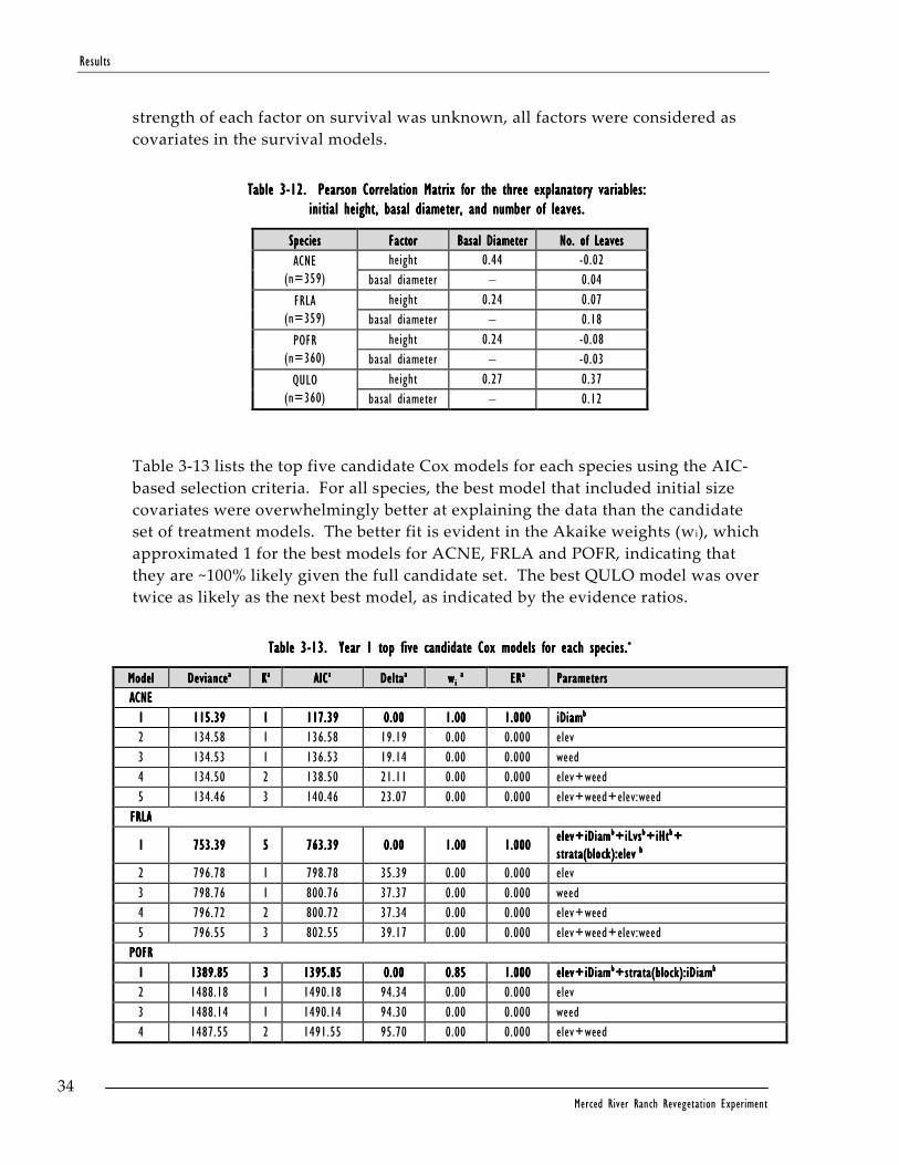
Results
34 Merced River Ranch Revegetation Experiment
strength of each factor on survival was unknown, all factors were considered as
covariates in the survival models.
Table Table Table Table 3333----12121212. . . . Pearson Correlation Matrix for the three explanatory variables: Pearson Correlation Matrix for the three explanatory variables: Pearson Correlation Matrix for the three explanatory variables: Pearson Correlation Matrix for the three explanatory variables: initial height, initial height, initial height, initial height, basal basal basal basal diameter, and number of leaves.diameter, and number of leaves.diameter, and number of leaves.diameter, and number of leaves.
SpeciesSpeciesSpeciesSpecies FactorFactorFactorFactor Basal Basal Basal Basal DiameterDiameterDiameterDiameter No. of LeavesNo. of LeavesNo. of LeavesNo. of Leaves
ACNE (n=359)
height 0.44 -0.02
basal diameter – 0.04
FRLA (n=359)
height 0.24 0.07
basal diameter – 0.18
POFR (n=360)
height 0.24 -0.08
basal diameter – -0.03
QULO (n=360)
height 0.27 0.37
basal diameter – 0.12
Table 3-13 lists the top five candidate Cox models for each species using the AIC-
based selection criteria. For all species, the best model that included initial size
covariates were overwhelmingly better at explaining the data than the candidate
set of treatment models. The better fit is evident in the Akaike weights (wi), which
approximated 1 for the best models for ACNE, FRLA and POFR, indicating that
they are ~100% likely given the full candidate set. The best QULO model was over
twice as likely as the next best model, as indicated by the evidence ratios.
Table Table Table Table 3333----13131313. . . . Year 1 top five candidate Cox models for each species.Year 1 top five candidate Cox models for each species.Year 1 top five candidate Cox models for each species.Year 1 top five candidate Cox models for each species.****
ModelModelModelModel DevianceDevianceDevianceDevianceaaaa KKKKaaaa AICAICAICAIC aaaa DeltaDeltaDeltaDeltaaaaa wwww i i i i aaaa ERERERERaaaa ParametersParametersParametersParameters
ACNEACNEACNEACNE
1111 115.39115.39115.39115.39 1111 117.39117.39117.39117.39 0.000.000.000.00 1.001.001.001.00 1.0001.0001.0001.000 iDiamiDiamiDiamiDiambbbb
2 134.58 1 136.58 19.19 0.00 0.000 elev
3 134.53 1 136.53 19.14 0.00 0.000 weed
4 134.50 2 138.50 21.11 0.00 0.000 elev+weed
5 134.46 3 140.46 23.07 0.00 0.000 elev+weed+elev:weed
FRLAFRLAFRLAFRLA
1111 753.39753.39753.39753.39 5555 763.39763.39763.39763.39 0.000.000.000.00 1.001.001.001.00 1.0001.0001.0001.000 elev+iDiamelev+iDiamelev+iDiamelev+iDiambbbb+iLvs+iLvs+iLvs+iLvsbbbb+iHt+iHt+iHt+iHtbbbb++++ strata(block):elevstrata(block):elevstrata(block):elevstrata(block):elev bbbb
2 796.78 1 798.78 35.39 0.00 0.000 elev
3 798.76 1 800.76 37.37 0.00 0.000 weed
4 796.72 2 800.72 37.34 0.00 0.000 elev+weed
5 796.55 3 802.55 39.17 0.00 0.000 elev+weed+elev:weed
POFRPOFRPOFRPOFR
1111 1389.851389.851389.851389.85 3333 1395.851395.851395.851395.85 0.000.000.000.00 0.850.850.850.85 1.0001.0001.0001.000 elev+iDiamelev+iDiamelev+iDiamelev+iDiambbbb+strata(block):iD+strata(block):iD+strata(block):iD+strata(block):iDiamiamiamiambbbb
2 1488.18 1 1490.18 94.34 0.00 0.000 elev
3 1488.14 1 1490.14 94.30 0.00 0.000 weed
4 1487.55 2 1491.55 95.70 0.00 0.000 elev+weed

Results
35 Merced River Ranch Revegetation Experiment
ModelModelModelModel DevianceDevianceDevianceDevianceaaaa KKKKaaaa AICAICAICAIC aaaa DeltaDeltaDeltaDeltaaaaa wwww i i i i aaaa ERERERERaaaa ParametersParametersParametersParameters
5 1487.54 3 1493.54 97.69 0.00 0.000 elev+weed+elev:weed
QULOQULOQULOQULO
1111 142.17142.17142.17142.17 1111 144.17144.17144.17144.17 0.000.000.000.00 0.440.440.440.44 1.0001.0001.0001.000 weedweedweedweed
2 142.17 1 144.17 0.00 0.44 1.000 weed
3 143.96 1 145.96 1.78 0.18 0.410 elev
4 141.21 2 145.21 1.03 0.26 0.596 elev+weed
5 140.89 3 146.89 2.71 0.11 0.258 elev+weed+elev:weed
* The best model for each species is indicated in bold font. a Deviance is the residual model deviance; K is the number of model parameters estimated; AIC is Akaike
Information Criteria; Delta is the AIC difference; wi is Akaike weights; and ER is the evidence ratio. See text for
explanation of these values. b Initial size measures: iDiam=initial basal diameter; iHt=initial height; iLvs=initial number of leaves. Strata(block)
is the inclusion of the stratified block variable in the Cox model.
Table 3-14 shows the parameter values, hazard ratios, and HR confidence limits for
all parameters included in the best model for each species. For each estimated
model parameter, the corresponding hazard ratio represents the proportional
difference in mortality for two seedlings that differed in treatment groups for a
binary variable or a one-unit difference in increment for a continuous variable.
Strong effects are indicated by hazard ratios much less or much greater than one,
and the precision of the effect size is noted by the confidence intervals. Intervals
that contain one indicate indeterminate or no effect on mortality by a variable.
Table Table Table Table 3333----14141414. . . . Parameter estimates, hazard ratio (HR), and HR confidence limits for the best Year 1 Cox survival modelParameter estimates, hazard ratio (HR), and HR confidence limits for the best Year 1 Cox survival modelParameter estimates, hazard ratio (HR), and HR confidence limits for the best Year 1 Cox survival modelParameter estimates, hazard ratio (HR), and HR confidence limits for the best Year 1 Cox survival model for each species.for each species.for each species.for each species.****
SpeciesSpeciesSpeciesSpecies ParameterParameterParameterParameter CoefficientCoefficientCoefficientCoefficient EstimateEstimateEstimateEstimate Coefficient SECoefficient SECoefficient SECoefficient SE Hazard RatioHazard RatioHazard RatioHazard Ratio
Lower 95% Lower 95% Lower 95% Lower 95% CLCLCLCL
Upper 95% Upper 95% Upper 95% Upper 95% CLCLCLCL
ACNEACNEACNEACNE iDiamiDiamiDiamiDiam ----1.501.501.501.50 0.520.520.520.52 0.220.220.220.22 0.080.080.080.08 0.620.620.620.62
FRLAFRLAFRLAFRLA
elev 0.10 0.10 1.11 0.91 1.36
iDiam -0.51 0.32 0.60 0.32 1.13
iLvsiLvsiLvsiLvs ----0.280.280.280.28 0.080.080.080.08 0.760.760.760.76 0.650.650.650.65 0.890.890.890.89
iHtiHtiHtiHt ----0.130.130.130.13 0.050.050.050.05 0.880.880.880.88 0.800.800.800.80 0.970.970.970.97
strata(block):elev 0.20 0.10 1.23 1.01 1.50
POFRPOFRPOFRPOFR
elevelevelevelev 0.170.170.170.17 0.070.070.070.07 1.181.181.181.18 1.021.021.021.02 1.361.361.361.36
iDiamiDiamiDiamiDiam ----0.220.220.220.22 0.030.030.030.03 0.810.810.810.81 0.760.760.760.76 0.850.850.850.85
strata(block):iDiam -0.06 0.03 0.95 0.90 1.00
QULOQULOQULOQULO weed -0.47 0.30 0.63 0.35 1.12
* Parameters that have a substantial effect on plant mortality are indicated in bold font.
The best Cox survival models for the 2004 growing season are dominated by initial
size parameters, indicating that this boundary condition was the most important
factor controlling mortality risk during the first year. For ACNE, a 1 mm increment
in basal diameter corresponds to a hazard ratio of 0.22. This means that a seedling
of basal diameter 2 mm will be 4-5 times as likely to die in the first year as one with

Results
36 Merced River Ranch Revegetation Experiment
a basal diameter of 3 mm. Though the survival probability will still be relatively
high (>80%) for the smaller plants, a five-fold increase in the risk of mortality may
translate into substantial losses in a horticultural restoration scenario, depending
on the size distribution of planting stock. For POFR, initial basal diameter was also
the
most important factor in the first year, with a hazard ratio of 0.81. Though this
represents only a 19% difference in mortality between two seedlings with a 1 mm
basal diameter differential, the POFR cuttings varied greatly in basal diameter and
suffered large losses the first year among the smaller size classes (Figure 23). The
best POFR model also included elevation, with a hazard ratio of 1.18, indicating
that plants increase their mortality risk 18% for every additional meter they are
planted above the water table. An interaction term between the stratified block
variable and initial basal diameter is also included in the model but does not have a
large effect on mortality (HR=0.95).
For FRLA seedlings, an incremental increase in stem height of 1 cm results in a 12%
lower probability of mortality, whereas an individual with one more leaf than
another seedling will have a 24% lower mortality risk in the first year (recall that
FRLA seedlings initially had only 1 to 4 leaves upon planting). Other factors in
that model were not important. For QULO, weed control was retained as the sole
predictor in the final Cox model, with a hazard ratio of 0.63 indicating a 47% lower
mortality risk in the weed control group over controls. However, the confidence
limits for this variable contain 1, indicating that treatment difference are not
detectable at the 0.05 probability level. Therefore for this species no treatment
factor or environmental covariate was a good predictor of mortality in the first
year.
3.4.3 Second-Year Survival (2005)
Seedling survival in Year 2 was analyzed separately from the first year because of
the imposition of a new treatment factor. Beginning in the early spring, the drip
irrigation system was removed from a third of the plants that had survived the first
year in order to test the effects of continued irrigation on plant survival and
growth. This factor proved to be the largest determinant of mortality in the second
year; in fact unirrigated FRLA survival dropped below 50% (Figure 26). In contrast,
differences in planting elevation and weed control had little effect (Figure 27). For
the plants that were irrigated for two years, survival in 2005 ranged among species
86–99%; survival within this group was higher than in the unirrigated group by
31% for ACNE, 42% for FRLA, and 16% for both POFR and QULO (Table 14).
Hazard plots indicate that mortality peaked between weeks 65–70 (July 14, 2005–
August 18, 2005), and the greatest differences were between irrigated and
unirrigated groups (Table 3-11, Figures 24 and 25). Unlike in Year 1, mortality in
Year 2 was greater in the second half of the growing season and did not subside
following the death of vulnerable plants. Mortality was also higher for all species
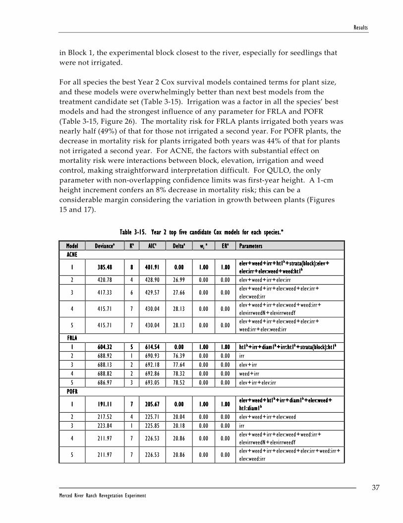
Results
37 Merced River Ranch Revegetation Experiment
in Block 1, the experimental block closest to the river, especially for seedlings that
were not irrigated.
For all species the best Year 2 Cox survival models contained terms for plant size,
and these models were overwhelmingly better than next best models from the
treatment candidate set (Table 3-15). Irrigation was a factor in all the species’ best
models and had the strongest influence of any parameter for FRLA and POFR
(Table 3-15, Figure 26). The mortality risk for FRLA plants irrigated both years was
nearly half (49%) of that for those not irrigated a second year. For POFR plants, the
decrease in mortality risk for plants irrigated both years was 44% of that for plants
not irrigated a second year. For ACNE, the factors with substantial effect on
mortality risk were interactions between block, elevation, irrigation and weed
control, making straightforward interpretation difficult. For QULO, the only
parameter with non-overlapping confidence limits was first-year height. A 1-cm
height increment confers an 8% decrease in mortality risk; this can be a
considerable margin considering the variation in growth between plants (Figures
15 and 17).
Table Table Table Table 3333----15151515. . . . Year 2 top five candidate Cox models for each species.Year 2 top five candidate Cox models for each species.Year 2 top five candidate Cox models for each species.Year 2 top five candidate Cox models for each species.****
ModelModelModelModel DevianceDevianceDevianceDevianceaaaa KKKKaaaa AICAICAICAIC aaaa DeltaDeltaDeltaDeltaaaaa wwww i i i i aaaa ERERERERaaaa ParametersParametersParametersParameters
ACNEACNEACNEACNE
1111 385.48385.48385.48385.48 8888 401.91401.91401.91401.91 0.000.000.000.00 1.001.001.001.00 1111.00.00.00.00 elev+weed+irr+ht1elev+weed+irr+ht1elev+weed+irr+ht1elev+weed+irr+ht1bbbb+strata(block):elev++strata(block):elev++strata(block):elev++strata(block):elev+ elev:irr+elev:weed+weed:ht1elev:irr+elev:weed+weed:ht1elev:irr+elev:weed+weed:ht1elev:irr+elev:weed+weed:ht1bbbb
2 420.78 4 428.90 26.99 0.00 0.00 elev+weed+irr+elev:irr
3 417.33 6 429.57 27.66 0.00 0.00 elev+weed+irr+elev:weed+elev:irr+ elev:weed:irr
4 415.71 7 430.04 28.13 0.00 0.00 elev+weed+irr+elev:weed+weed:irr+ elevirrweedN+elevirrweedY
5 415.71 7 430.04 28.13 0.00 0.00 elev+weed+irr+elev:weed+elev:irr+ weed:irr+elev:weed:irr
FRLAFRLAFRLAFRLA
1111 604.32604.32604.32604.32 5555 614.54614.54614.54614.54 0.000.000.000.00 1.001.001.001.00 1.001.001.001.00 ht1ht1ht1ht1bbbb+irr+diam1+irr+diam1+irr+diam1+irr+diam1bbbb+irr:ht1+irr:ht1+irr:ht1+irr:ht1bbbb+strata(block):ht1+strata(block):ht1+strata(block):ht1+strata(block):ht1bbbb
2 688.92 1 690.93 76.39 0.00 0.00 irr
3 688.13 2 692.18 77.64 0.00 0.00 elev+irr
4 688.82 2 692.86 78.32 0.00 0.00 weed+irr
5 686.97 3 693.05 78.52 0.00 0.00 elev+irr+elev:irr
POFRPOFRPOFRPOFR
1111 191.11191.11191.11191.11 7777 205.67205.67205.67205.67 0.000.000.000.00 1.001.001.001.00 1.001.001.001.00 elev+weed+ht1elev+weed+ht1elev+weed+ht1elev+weed+ht1bbbb+irr+diam1+irr+diam1+irr+diam1+irr+diam1bbbb+elev:weed++elev:weed++elev:weed++elev:weed+ ht1:diam1ht1:diam1ht1:diam1ht1:diam1bbbb
2 217.52 4 225.71 20.04 0.00 0.00 elev+weed+irr+elev:weed
3 223.84 1 225.85 20.18 0.00 0.00 irr
4 211.97 7 226.53 20.86 0.00 0.00 elev+weed+irr+elev:weed+weed:irr+ elevirrweedN+elevirrweedY
5 211.97 7 226.53 20.86 0.00 0.00 elev+weed+irr+elev:weed+elev:irr+weed:irr+ elev:weed:irr

Results
38 Merced River Ranch Revegetation Experiment
ModelModelModelModel DevianceDevianceDevianceDevianceaaaa KKKKaaaa AICAICAICAIC aaaa DeltaDeltaDeltaDeltaaaaa wwww i i i i aaaa ERERERERaaaa ParametersParametersParametersParameters
QULOQULOQULOQULO
1111 166.73166.73166.73166.73 5555 176.91176.91176.91176.91 0.000.000.000.00 1.001.001.001.00 1.001.001.001.00 elev+irr+ht1elev+irr+ht1elev+irr+ht1elev+irr+ht1bbbb+elev:irr+elev:ht1+elev:irr+elev:ht1+elev:irr+elev:ht1+elev:irr+elev:ht1bbbb
2 191.99 1 194.01 17.10 0.00 0.00 irr
3 188.53 3 194.60 17.69 0.00 0.00 elev+irr+elev:irr
4 191.67 2 195.70 18.80 0.00 0.00 weed+irr
5 191.78 2 195.82 18.91 0.00 0.00 elev+irr
* The best model for each species is indicated in bold font.
a Deviance is the residual model deviance; K is the number of model parameters estimated; AIC is Akaike
Information Criteria; Delta is the AIC difference; wi is Akaike weights; and ER is the evidence ratio. See text
for explanation of these values. b Size after the first year: diam1= Year 1 final basal diameter; ht1=Year 1 final height. Strata(block) is the
inclusion of the stratified block variable in the Cox model.
Table Table Table Table 3333----16161616. . . . Parameter estimates, hazard ratio (HR), and HR confidence limits for the best Year 2 Cox survival model Parameter estimates, hazard ratio (HR), and HR confidence limits for the best Year 2 Cox survival model Parameter estimates, hazard ratio (HR), and HR confidence limits for the best Year 2 Cox survival model Parameter estimates, hazard ratio (HR), and HR confidence limits for the best Year 2 Cox survival model for each species.for each species.for each species.for each species.****
SpeciesSpeciesSpeciesSpecies ParameterParameterParameterParameter CoefficientCoefficientCoefficientCoefficient EstimateEstimateEstimateEstimate Coefficient SECoefficient SECoefficient SECoefficient SE
Hazard Hazard Hazard Hazard RatioRatioRatioRatio
LoLoLoLower 95% wer 95% wer 95% wer 95% CLCLCLCL
Upper 95% Upper 95% Upper 95% Upper 95% CLCLCLCL
ACNE
elev -0.08 0.26 0.93 0.56 1.55
weed -0.52 0.48 0.60 0.23 1.53
irr -0.46 0.31 0.63 0.35 1.15
ht1 -0.03 0.01 0.98 0.96 0.99
strata(block):elev 0.49 0.16 1.64 1.19 2.25
elev:irr -0.54 0.22 0.59 0.38 0.90
elev:weed -0.31 0.12 0.73 0.58 0.93
weed:ht1 0.01 0.01 1.01 1.00 1.03
FRLA
ht1 -0.04 0.01 0.96 0.94 0.98
irr -0.72 0.21 0.49 0.32 0.75
diam1 -0.07 0.08 0.94 0.80 1.09
irr:ht1 -0.01 0.01 0.99 0.97 1.00
strata(block):ht1 0.01 0.01 1.01 1.00 1.02
POFR
elev 0.36 0.22 1.43 0.93 2.21
weed 0.52 0.39 1.68 0.78 3.61
ht1 0.00 0.02 1.00 0.95 1.05
irr -0.82 0.21 0.44 0.29 0.67
diam1 0.28 0.14 1.32 1.00 1.74
elev:weed -0.38 0.18 0.68 0.48 0.97
ht1:diam1 0.00 0.00 1.00 1.00 1.00
QULO
elev -0.78 0.55 0.46 0.16 1.35
irr -0.25 0.52 0.78 0.28 2.19
ht1 -0.08 0.03 0.92 0.86 0.99
elev:irr -0.62 0.32 0.54 0.29 1.01
elev:ht1 0.01 0.01 1.01 0.99 1.03
* Parameters that have a substantial effect on plant mortality are indicated in bold font.
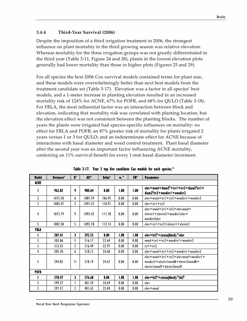
Results
39 Merced River Ranch Revegetation Experiment
3.4.4 Third-Year Survival (2006)
Despite the imposition of a third irrigation treatment in 2006, the strongest
influence on plant mortality in the third growing season was relative elevation.
Whereas mortality for the three irrigation groups was not greatly differentiated in
the third year (Table 3-11, Figure 24 and 28), plants in the lowest elevation plots
generally had lower mortality than those in higher plots (Figures 25 and 29).
For all species the best 2006 Cox survival models contained terms for plant size,
and these models were overwhelmingly better than next best models from the
treatment candidate set (Table 3-17). Elevation was a factor in all species’ best
models, and a 1-meter increase in planting elevation resulted in an increased
mortality risk of 124% for ACNE, 67% for POFR, and 68% for QULO (Table 3-18).
For FRLA, the most influential factor was an interaction between block and
elevation, indicating that mortality risk was correlated with planting location, but
the elevation effect was not consistent between the planting blocks. The number of
years the plants were irrigated had species-specific influences on mortality: no
effect for FRLA and POFR; an 87% greater risk of mortality for plants irrigated 2
years versus 1 or 3 for QULO; and an indeterminate effect for ACNE because of
interactions with basal diameter and weed control treatment. Plant basal diameter
after the second year was an important factor influencing ACNE mortality,
conferring an 11% survival benefit for every 1-mm basal diameter increment.
Table Table Table Table 3333----17171717. . . . Year 3 top five candidate Cox models for each species.Year 3 top five candidate Cox models for each species.Year 3 top five candidate Cox models for each species.Year 3 top five candidate Cox models for each species.****
ModelModelModelModel DevianceDevianceDevianceDevianceaaaa KKKKaaaa AICAICAICAIC aaaa DeltaDeltaDeltaDeltaaaaa wwww i i i i aaaa ERERERERaaaa ParametersParametersParametersParameters
ACNEACNEACNEACNE
1111 962.02962.02962.02962.02 9999 980.64980.64980.64980.64 0.000.000.000.00 1.001.001.001.00 1.001.001.001.00 elev+weed+diam2elev+weed+diam2elev+weed+diam2elev+weed+diam2bbbb+irr1+irr2+diam2+irr1+irr2+diam2+irr1+irr2+diam2+irr1+irr2+diam2bbbbirr1+irr1+irr1+irr1+ diam2diam2diam2diam2bbbbirr2+weedirr1+weedirr2irr2+weedirr1+weedirr2irr2+weedirr1+weedirr2irr2+weedirr1+weedirr2
2 1075.30 6 1087.59 106.95 0.00 0.00 elev+weed+irr1+irr2+weedirr1+weedirr2
3 1085.47 3 1091.55 110.91 0.00 0.00 elev+irr1+irr2
4 1073.79 9 1092.42 111.78 0.00 0.00 elev+weed+irr1+irr2+elev:weed+ elevirr1+elevirr2+weedirr1elev+ weedirr2elev
5 1082.58 5 1092.78 112.14 0.00 0.00 elev+irr1+irr2+elevirr1+elevirr2
FRLAFRLAFRLAFRLA
1111 287.41287.41287.41287.41 3333 293.53293.53293.53293.53 0.000.000.000.00 1.001.001.001.00 1.001.001.001.00 eleeleeleelev+ht2v+ht2v+ht2v+ht2bbbb+strata(block)+strata(block)+strata(block)+strata(block) bbbb:elev:elev:elev:elev
2 305.86 5 316.17 22.64 0.00 0.00 weed+irr1+irr2+weedirr1+weedirr2
3 312.43 2 316.49 22.97 0.00 0.00 irr1+irr2
4 305.70 6 318.13 24.60 0.00 0.00 elev+weed+irr1+irr2+weedirr1+weedirr2
5 294.82 11 318.19 24.67 0.00 0.00 elev+weed+irr1+irr2+elev:weed+weedirr1+ weedirr2+elevirr1weedN+elevirr2weedN+ elevirr1weedY+elevirr2weedY
POFRPOFRPOFRPOFR
1111 370.47370.47370.47370.47 3333 376.60376.60376.60376.60 0.000.000.000.00 1.001.001.001.00 1.001.001.001.00 elev+ht2elev+ht2elev+ht2elev+ht2bbbb+strata(block)+strata(block)+strata(block)+strata(block) bbbb:ht2:ht2:ht2:ht2bbbb
2 399.27 1 401.29 24.69 0.00 0.00 elev
3 397.57 2 401.63 25.04 0.00 0.00 elev+weed

Results
40 Merced River Ranch Revegetation Experiment
ModelModelModelModel DevianceDevianceDevianceDevianceaaaa KKKKaaaa AICAICAICAIC aaaa DeltaDeltaDeltaDeltaaaaa wwww i i i i aaaa ERERERERaaaa ParametersParametersParametersParameters
4 397.19 3 403.33 26.73 0.00 0.00 elev+weed+elev:weed
5 397.98 3 404.11 27.51 0.00 0.00 elev+irr1+irr2
QULOQULOQULOQULO
1111 376.99376.99376.99376.99 5555 387.18387.18387.18387.18 0.000.000.000.00 0.980.980.980.98 1.001.001.001.00 elev+ht2elev+ht2elev+ht2elev+ht2bbbb+irr1+irr2+diam2+irr1+irr2+diam2+irr1+irr2+diam2+irr1+irr2+diam2bbbb
2 391.06 3 397.14 9.96 0.01 0.01 elev+irr1+irr2
3 390.97 4 399.10 11.92 0.00 0.00 elev+weed+irr1+irr2
4 389.47 5 399.66 12.48 0.00 0.00 elev+irr1+irr2+elevirr1+elevirr2
5 389.81 5 400.00 12.82 0.00 0.00 elev+weed+irr1+irr2+elev:weed
* The best model for each species is indicated in bold font.
a Deviance is the residual model deviance; K is the number of model parameters estimated; AIC is Akaike
Information Criteria; Delta is the AIC difference; wi is Akaike weights; and ER is the evidence ratio. See text for
explanation of these values. b Size after the second year: diam2= Year 2 final basal diameter; ht2=Year 2 final height. Strata(block) is the
inclusion of the stratified block variable in the Cox model.
Table Table Table Table 3333----18181818. . . . Parameter estimates, hazard ratio (HR), and HR confideParameter estimates, hazard ratio (HR), and HR confideParameter estimates, hazard ratio (HR), and HR confideParameter estimates, hazard ratio (HR), and HR confidence limits for the best Year 3 Cox survival model nce limits for the best Year 3 Cox survival model nce limits for the best Year 3 Cox survival model nce limits for the best Year 3 Cox survival model for each species.for each species.for each species.for each species.****
SpeciesSpeciesSpeciesSpecies ParameterParameterParameterParameter CoefficientCoefficientCoefficientCoefficient EstimateEstimateEstimateEstimate Coefficient SECoefficient SECoefficient SECoefficient SE
Hazard Hazard Hazard Hazard RatioRatioRatioRatio
Lower 95% Lower 95% Lower 95% Lower 95% CLCLCLCL
Upper 95% Upper 95% Upper 95% Upper 95% CLCLCLCL
ACNEACNEACNEACNE
elevelevelevelev 0.810.810.810.81 0.090.090.090.09 2.242.242.242.24 1.891.891.891.89 2.662.662.662.66
weed 0.10 0.11 1.11 0.89 1.38
diam2diam2diam2diam2 ----0.120.120.120.12 0.020.020.020.02 0.890.890.890.89 0.0.0.0.86868686 0.920.920.920.92
irr1 0.46 0.41 1.59 0.71 3.55
irr2irr2irr2irr2 0.580.580.580.58 0.250.250.250.25 1.791.791.791.79 1.091.091.091.09 2.932.932.932.93
diam2irr1 0.00 0.02 1.00 0.96 1.03
diam2irr2 -0.04 0.01 0.96 0.94 0.99
weedirr1 -0.07 0.15 0.93 0.70 1.25
weedirr2weedirr2weedirr2weedirr2 ----0.200.200.200.20 0.080.080.080.08 0.820.820.820.82 0.700.700.700.70 0.950.950.950.95
FRLAFRLAFRLAFRLA
elev -0.04 0.13 0.96 0.75 1.24
ht2 -0.02 0.00 0.98 0.97 0.99
strata(block):elevstrata(block):elevstrata(block):elevstrata(block):elev 0.290.290.290.29 0.130.130.130.13 1.341.341.341.34 1.041.041.041.04 1.731.731.731.73
POFRPOFRPOFRPOFR
elevelevelevelev 0.510.510.510.51 0.140.140.140.14 1.671.671.671.67 1.271.271.271.27 2.202.202.202.20
ht2 -0.02 0.01 0.98 0.97 0.99
strata(block):ht2 -0.01 0.01 0.99 0.98 1.00
QULOQULOQULOQULO
elevelevelevelev 0.520.520.520.52 0.130.130.130.13 1.681.681.681.68 1.291.291.291.29 2.182.182.182.18
ht2 -0.01 0.01 0.99 0.98 1.00
irr1irr1irr1irr1 0.620.620.620.62 0.220.220.220.22 1.871.871.871.87 1.221.221.221.22 2.862.862.862.86
irr2 -0.22 0.13 0.80 0.62 1.04
diam2 -0.09 0.05 0.91 0.82 1.02
* Parameters that have a substantial effect on plant mortality are indicated in bold font.
3.53.53.53.5 Weed Percent CoverWeed Percent CoverWeed Percent CoverWeed Percent Cover
Weed percent cover monitoring revealed an increase in weeds between 2004 and
2005 where no weed reduction was provided. Table 3-19 summarizes the percent
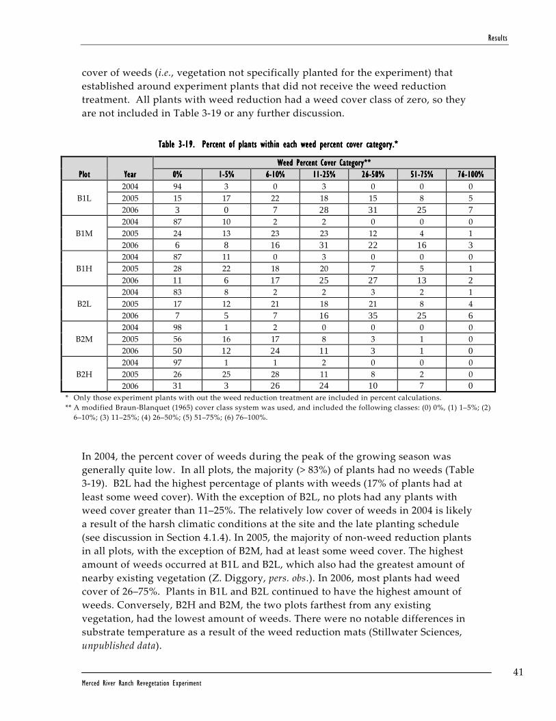
Results
41 Merced River Ranch Revegetation Experiment
cover of weeds (i.e., vegetation not specifically planted for the experiment) that
established around experiment plants that did not receive the weed reduction
treatment. All plants with weed reduction had a weed cover class of zero, so they
are not included in Table 3-19 or any further discussion.
Table Table Table Table 3333----19191919. . . . Percent of plants Percent of plants Percent of plants Percent of plants withinwithinwithinwithin each weed each weed each weed each weed percent percent percent percent cover cover cover cover categorycategorycategorycategory....****
PlotPlotPlotPlot YearYearYearYear
WWWWeed eed eed eed Percent CPercent CPercent CPercent Cover over over over Category**Category**Category**Category**
0%0%0%0% 1111----5%5%5%5% 6666----10%10%10%10% 11111111----25%25%25%25% 26262626----50%50%50%50% 51515151----75%75%75%75% 76767676----100%100%100%100%
B1L
2004 94 3 0 3 0 0 0
2005 15 17 22 18 15 8 5
2006 3 0 7 28 31 25 7
B1M
2004 87 10 2 2 0 0 0
2005 24 13 23 23 12 4 1
2006 6 8 16 31 22 16 3
B1H
2004 87 11 0 3 0 0 0
2005 28 22 18 20 7 5 1
2006 11 6 17 25 27 13 2
B2L
2004 83 8 2 2 3 2 1
2005 17 12 21 18 21 8 4
2006 7 5 7 16 35 25 6
B2M
2004 98 1 2 0 0 0 0
2005 56 16 17 8 3 1 0
2006 50 12 24 11 3 1 0
B2H
2004 97 1 1 2 0 0 0
2005 26 25 28 11 8 2 0
2006 31 3 26 24 10 7 0 * Only those experiment plants with out the weed reduction treatment are included in percent calculations.
** A modified Braun-Blanquet (1965) cover class system was used, and included the following classes: (0) 0%, (1) 1–5%; (2)
6–10%; (3) 11–25%; (4) 26–50%; (5) 51–75%; (6) 76–100%.
In 2004, the percent cover of weeds during the peak of the growing season was
generally quite low. In all plots, the majority (> 83%) of plants had no weeds (Table
3-19). B2L had the highest percentage of plants with weeds (17% of plants had at
least some weed cover). With the exception of B2L, no plots had any plants with
weed cover greater than 11–25%. The relatively low cover of weeds in 2004 is likely
a result of the harsh climatic conditions at the site and the late planting schedule
(see discussion in Section 4.1.4). In 2005, the majority of non-weed reduction plants
in all plots, with the exception of B2M, had at least some weed cover. The highest
amount of weeds occurred at B1L and B2L, which also had the greatest amount of
nearby existing vegetation (Z. Diggory, pers. obs.). In 2006, most plants had weed
cover of 26–75%. Plants in B1L and B2L continued to have the highest amount of
weeds. Conversely, B2H and B2M, the two plots farthest from any existing
vegetation, had the lowest amount of weeds. There were no notable differences in
substrate temperature as a result of the weed reduction mats (Stillwater Sciences,
unpublished data).

Results
42 Merced River Ranch Revegetation Experiment
Field technicians identified the most prevalent weeds to species or, if required
characters for identification were not present, to genus. These species, and whether
or not they are native to California, are listed in Table 3-20.
Table Table Table Table 3333----20202020. . . . Weed species identified in experimental plots.Weed species identified in experimental plots.Weed species identified in experimental plots.Weed species identified in experimental plots.****
Latin NameLatin NameLatin NameLatin Name Common NameCommon NameCommon NameCommon Name Native?Native?Native?Native?
Amsinckia menzeisii Rancher's fireweed Y
Avena fatua Wild oat N
Brassica nigra Black mustard N
Bromus hordeaceus Soft chess N
Bromus madritensis Foxtail chess N
Calandrinia ciliata Red maids Y
Cichorium intybus Chicory N
Conium maculatum Poison hemlock N
Cynodon dactylon Bermuda grass N
Cyperus squarrosus Bearded flatsedge Y
Datura wrightii Sacred datura Y
Eragrostis pectinacea Lovegrass Y
Eremocarpus setigerus Turkey mullein Y
Erodium cicutarium Storksbill, Filaree N
Ficus carica Edible fig N
Galium parisiense Wall bedstraw N
Hypochaeris glabra Smooth cat's-ear N
Lotus purshianus Spanish clover Y
Medicago polymorpha California burclover N
Phacelia cicutaria Phacelia Y
Populus fremontii Fremont cottonwood Y
Raphanus raphanistrum Wild radish N
Rubus discolor Himalayan blackberry N
Rumex sp. Dock Y&N
Salix sp. Willow Y
Senecio vulgaris Common groundsel N
Silybum marianum Milk thistle N
Sonchus asper ssp. asper Prickly sow thistle N
Sorghum halepense Johnsongrass N
Vicia sativa Vetch N
* In this case, a weed was defined as any plant not specifically planted
for the experiment.

Discussion
43 Merced River Ranch Revegetation Experiment
4 DISCUSSION
4.14.14.14.1 Treatment/Treatment/Treatment/Treatment/NonNonNonNon----treatment Effectstreatment Effectstreatment Effectstreatment Effects and and and and Revegetation Revegetation Revegetation Revegetation RecommendationsRecommendationsRecommendationsRecommendations
4.1.1 Initial Size
The initial size of cuttings and container stock had a strong effect on first year
survival and growth of most species (Section 3.2.1 and 3.4.2). ACNE and POFR
survival in Year 1 were positively correlated with initial basal diameter, with a 78%
(ACNE) and 19% (POFR) lower mortality risk with every 1-mm basal diameter
increment in planting stock (Table 3-14). FRLA seedlings in the first year were
highly sensitive to initial height and number of leaves, with a 12% lower mortality
risk with every 1 cm increase in height and a 24% lower mortality risk with one
additional leaf (Table 3-14). QULO seedling mortality was not sensitive to initial
size in the first year, but in the second year, relative mortality risk decreased
approximately 8% with every 1-cm increment in height at the beginning of the
growing season (Table 3-16). Though size was a factor in Year 3 survival models
(Table 3-18), the factor had a negligible influence on mortality (i.e., the hazard ratio
was ~1). While it may seem intuitive that plant size would influence survival,
explicitly modeling the effect via the Cox proportional hazard model allows for
quantification of both the predicted survival rate for other restoration projects, and
the range of planting stock size that would result in the lowest mortality (see
Section 4.3.1).
To ensure that adequate survival rates are achieved, we recommend that all
cuttings and container stock used in MRR revegetation efforts meet the size
thresholds indicated in the logistic regression survival models. ACNE container
stock should have basal diameters ≥2.5 mm (0.1 in), which should result in 95%
survival in the first year. To facilitate achieving a target of 80% survival in the first
year, FRLA container stock should be greater than 12.0 cm (4.7 in) tall. POFR
cuttings should have basal diameters >15.0 mm (>0.6 in); 80% survival is predicted
for cuttings of this size. No size recommendations resulted from QULO survival
models, but this experiment established that >90% survival can be achieved in the
first year for seedlings with size distributions of 45.0 (±1.0) cm height and 5.0 (±0.3)
mm basal diameter. Where these size thresholds are not met for particular species,
cuttings or container stock should be rejected and/or grown out in the nursery until
they reach adequate sizes.

Discussion
44 Merced River Ranch Revegetation Experiment
4.1.2 Block and Relative Elevation above Groundwater
Elevation above groundwater and, to a lesser extent, experimental block were
found to be important influences on survival in the third year, but not in the
previous two years. For ACNE, POFR and QULO, plant mortality risk in the third
year was 67–124% greater for every meter increment increase in elevation above
groundwater. In the first two years, there were block/elevation combinations that
were more, or less, conducive to plant survival than others, but no systematic
relationship with elevation. From the Cox survival models, these effects appear to
be due more to differences in initial size in the first year, and irrigation treatment
in the second year.
Similarly, negative growth effects were associated with elevation, particularly for
FRLA and for POFR in Block 1 (Figure 20). However, FRLA growth reduction with
elevation was modest, approximately 0.8 mm reduced for every 1 m gain in
elevation above groundwater, and block, not elevation, was the most important
factor in the POFR basal diameter growth model (Table 3-7). Interestingly, height
growth effects due to elevation appear to be stronger in the first year; lower
elevation plants are taller at the end of the first year for all species (Figure 17).
However, in the second and third years, surviving plants no longer show the same
systematic stratification by relative elevation. Because mortality over the course of
the experiment gradually reduces the sample size and potentially skews the
distributions with regards to growth, it is difficult to isolate the growth treatment
effects.
The significant effect of relative elevation on survival in the third year may be a
result of plant roots having finally reached permanent groundwater at the lower
elevation treatment plots. If this is the case, we could expect that on lower
floodplain surfaces (<2 m above groundwater) two years of irrigation may be
sufficient to establish all species. On higher surfaces (>2 m), three or more years
may be necessary to establish ACNE and POFR. It appears that POFR is better than
ACNE at establishing at higher floodplain elevations (Figure 29), perhaps through
a combination of higher root growth (allowing more plants at the 2 m elevation
level to access groundwater) or through better drought tolerance. ACNE crowns
experienced high rates of dieback (Figure 17), which is both an indicator of drought
stress and a functional adaptation that decreases transpiring area.
Based on these results, and with the goals of minimizing the need for irrigation and
promoting long-term survival of revegetated plants, we recommend that
floodplains at the MRR be restored to elevations less than or not much greater than
2 m above groundwater. “Drowning” of riparian trees from exceedingly high
groundwater levels is not expected to limit plant survival on the restored
floodplain. Stella (2005) showed no ill-effects of saturated soils on the growth and
Discussion
45 Merced River Ranch Revegetation Experiment
survival of POFR and willow species for up to 60 days. Revegetation monitoring of
the lower Clear Creek Floodway Rehabilitation Project found higher survival of
plantings where groundwater depths were shallow and concluded that shallow
depths to groundwater were even more critical in areas with coarse substrate than
with alluvial soils (Souza Environmental Solutions et al. 2005). There are, of course,
other factors that will need to be considered in determining appropriate restored
floodplain elevations, and they will be evaluated in MRR restoration planning
documents (e.g., Stillwater Sciences 2005).
4.1.3 Irrigation
The lack of a significant relative elevation effect in the first two years may be the
result of the overwhelming effect of the irrigation treatment on plant survival. This
factor was a strong determinant of survival in the second year, when irrigation was
stopped for one group of plants (Table 3-16, Figures 23, 24 and 26). For plants with
ongoing irrigation in Year 2, end-of-season survival was high, ranging among
species from 86–99% (Table 3-11). For those plants that had irrigation shut off in
Year 2, survival ranged from 44–83% (Table 3-11). In Year 2, the difference in
ACNE and QULO survival rates between irrigation treatment levels (Table 3-11)
represents an important threshold since many permits and/or performance criteria
require restoration projects to achieve and maintain 80% survival of plantings.
Irrigation did not have a significant effect on growth or water potential values
(Tables 3-7 and 3-11). The influence of irrigation on survival suggests that
irrigation provides sufficient benefits to plants (such as accelerated root growth
and/or adequate water supply) that they are able to overcome, or are no longer
adversely affected by, greater distances to groundwater. By the third year,
however, irrigation treatment had a minor effect on survival except for ACNE
(Table 3-11 and Table 3-17, Figure 28).
Final survival among the irrigation groups indicates the benefit of irrigating at least
two years for FRLA and POFR, one year for QULO, and at least three years for
ACNE to achieve the greatest marginal value of survival. There were small
differences in survival rates for FRLA and POFR irrigated 2 versus 3 years. QULO
irrigated for only one growing season still retained 74% survival at the end of the
third year (Table 3-11). For ACNE, plants watered three years had a 23% greater
survival rate than those watered two years; therefore for this species a longer
irrigation plan is warranted.
The strong effect of irrigation on Year 2 survival but not on growth or Year 3
survival (Figures 15, 16 and 28) suggests that supplying irrigation is critical to the
successful establishment of re-vegetated plants over a range of relative elevations,
but not necessarily to their longer-term development. In this case, irrigation may
be necessary to achieve the survival rates required by restoration project

Discussion
46 Merced River Ranch Revegetation Experiment
environmental compliance documents and permits, but may not be as useful in
meeting growth and/or canopy density objectives or requirements.
Based on these results, we recommend that at least two years of irrigation be
provided to all species regardless of floodplain elevation. On higher surfaces (>2
m), three or more years of irrigation may be necessary, particularly to establish
ACNE and POFR. Where irrigation is to be provided at the MRR, we recommend
the use of a drip irrigation system. The drip irrigation system used for the
experiment was inexpensive, easy to install, and required minimal maintenance.
We also believe that the use of drip irrigation, rather than overhead sprinklers or
flood irrigation, limited the establishment of weed species in the experimental
areas. The MRR property has riparian water rights associated with it, so water can
be pumped from the Merced River during the irrigation season at no cost, so long
as a USFWS-approved fish screen is installed at the pump intact. During the
experiment the irrigation system was run by two gas-powered pumps. While this
was sufficient for the experiment, the risk of theft and/or vandalism of the pumps
is high and the small size of the fuel tanks constrain how long the pumps can run.
For these reasons, we recommend that housing for the irrigation pumps, valves,
and filters be constructed to protect the system from vandalism and theft. We also
recommend that, if feasible, electricity be provided to the MRR in order to power
the irrigation pumps and an automatic timer for the irrigation system.
4.1.4 Weed Reduction
Weed reduction did not emerge as a significant predictor of growth or mortality,
except as a minor influence on QULO growth (Table 3-7). The lack of effect on
survival is somewhat surprising, since weeds have been reported as having severe
negative impacts on other revegetation projects in the Central Valley, but may be
explained by the harsh conditions at the MRR and/or the late start of the
experiment. In comparison with most floodplains, the MRR does not support much
herbaceous vegetation. The coarse substrate and extreme summer temperatures
appear to restrict the establishment of perennial herbaceous vegetation, although
annual species do establish after the winter and spring rains. It could be that the
harsh site conditions inhibit weed establishment to the extent that weeds cannot
out-compete planted vegetation, particularly container stock which is usually one
to two years old at outplanting. Weeds may have been further restricted in the
experimental areas due to the late start date of the experiment. The experiment was
started in April 2004, several months later than planned due to permit schedules.
As a result, the newly excavated experimental areas were not exposed to winter
and spring rainfall that could have supported the establishment of greater amounts
of weeds. This explanation is supported qualitatively by the observation that the
vast majority of weeds in Year 1 occurred immediately adjacent to irrigation
emitters. Our experimental results suggest that, at the MRR, plants installed as

Discussion
47 Merced River Ranch Revegetation Experiment
cuttings or as at least one-year old seedlings are large enough to escape many of
the competitive impacts of herbaceous weeds.
Information about the potential impact of weeds on future revegetation efforts at
the MRR has also come from the observations of field technicians. These
observations provide insight into potential vectors for non-native invasive weed
introduction and suggest actions that may be taken to minimize the negative
impacts of weeds on future revegetation efforts. For example, where potting soil
(which was placed in each planting hole at the start of the experiment) was
delivered at the site, a thick cover of weeds established quickly. This suggests that
the potting soil may have been contaminated with weed seed or that the improved
substrate conditions dramatically facilitated weed establishment. Therefore, we
recommend that any soil amendment brought to the site, such as topsoil or wood
chips, should be certified as sterilized and/or weed-free. Since this is difficult to
document, we recommend that, when feasible, organic material from on-site, such
as salvaged sand and wood chips from trees grubbed during restoration
implementation, be used for soil amendments rather than imported material.
Material from on-site may well contain weed seed, but its use would prevent the
introduction of new weed species and potentially harmful bacteria or fungi.
Weed monitoring indicated that cottonwood and willow seedlings are frequent
“weeds” in the experimental areas (Table 3-20), further suggesting that improved
conditions provided by soil amendments and irrigation will facilitate the
recruitment of both native and non-native species. Weed control mats or some
other weed control activity may be required in areas that are expected to support a
vigorous cover of weeds, such as wet spots, areas with sand substrates, or where
existing vegetation is nearby.
Several noxious weed species were observed along the experiment access roads,
indicating that vehicles traveling into the site are likely responsible for their
introduction. To minimize the introduction of non-native invasive weed species to
the MRR, we recommend that vehicular access to the site be restricted to the
greatest extent possible. Vehicles that must enter the site for restoration and/or
revegetation purposes should be required to spray down or brush off their tires
beforehand.
4.1.5 Soil Amendments
Soil analyses indicate that floodplain substrates could be improved with the
addition of organic matter (Appendix A). We recommend that organic matter
produced during floodplain restoration activities, such as wood chips from tress
and shrubs that are grubbed prior to tailing excavation, be salvaged and applied to
areas where revegetation is planned. Organic matter from on-site is preferable to
compost from outside the restoration area, as foreign compost could be

Discussion
48 Merced River Ranch Revegetation Experiment
contaminated with weed seed (see Section 4.1.4) and harmful bacteria or fungus (G.
Strnad, pers. comm.). Seeding newly restored areas with native herbaceous species
will also increase the organic content of floodplain substrates and facilitate soil
development.
Soil nutrient analyses suggest that current levels of nitrogen, phosphorus,
potassium, zinc and boron are so low at the site that they could inhibit the growth
of plantings or naturally recruited plants (M. Buttress, pers. comm.). Additions of
nitrogen, phosphate (P2O5), potash (K2O), zinc, and boron (which should be added
with caution) should increase nutrient levels and improve soil fertility on the
restored floodplains (Appendix A). In Block 1, adding gypsum to restored areas
should increase calcium levels and counteract the negative effects of high
magnesium levels, such as poor drainage and reduced potassium availability. In
Block 2, the addition of sulfur should improve plant vigor. Appendix A provides
guidelines for nutrient additions and rates of application. Nutrient applications
must be conducted with care to ensure that amendments do not affect groundwater
or Merced River water quality. In addition, the need for fertilizer should be
balanced with the expected increase in weeds resulting from improved soil nutrient
conditions.
4.24.24.24.2 Species ResponsesSpecies ResponsesSpecies ResponsesSpecies Responses
4.2.1 Acer negundo
ACNE container stock was considered to be in good condition at planting.
In general, ACNE demonstrated some of the highest survival and growth rates in
the experiment, although some plants experienced dramatic crown die-back in Year
3. Physiologically, ACNE benefited from additional irrigation, particularly at
higher relative elevations, but likely reached groundwater in lower relative
elevation plots. In general, survival, growth, and water potential data from this
experiment indicate that, with three years of irrigation and/or short distances to
groundwater, ACNE demonstrates good survival within the first three years
following revegetation. Under harsher conditions (e.g., drought, extreme
temperatures, or greater distances to groundwater), ACNE trees may experience
dramatic annual dieback. While they appear to re-sprout from the base once
conditions improve (e.g., temperatures decrease or water supply increases), annual
ACNE die-back may limit a revegetation project’s potential to meet canopy or
vegetative cover objectives.
4.2.2 Fraxinus latifolia
FRLA container stock was in poor condition at planting, and this strongly affected
first year survival rates. Once plants were established, or were given at least two
years of irrigation, survival rates improved markedly. FRLA water potential values

Discussion
49 Merced River Ranch Revegetation Experiment
demonstrated strong and predictable responses to irrigation and relative elevation
treatments. FRLA showed the greatest pre-dawn/afternoon difference in water
potential. This result, in combination with the high mortality of non-irrigated
individuals, suggests that FRLA is not efficient at controlling water loss. In
general, the results from this experiment indicate that, if outplanted in good
condition (i.e., at least 12 cm tall) and provided with at least two years of irrigation
and short distances to groundwater, FRLA demonstrates good survival within the
first three years following revegetation.
4.2.3 Populus fremontii
POFR cuttings were in variable condition at planting. High mortality of cuttings
less than 15 mm indicates that initial deficiencies in basal diameter can have large
effects on POFR survival, and subsequently on restoration success and cost for this
species. POFR water potentials were always the highest and showed little difference
between treatments. This suggests that POFR (at least those that survived to August
2005) had the deepest rooting system of the four species and had reached a reliable
groundwater source regardless of plot elevation at the time of sampling. In
general, the results from this experiment indicate that, if outplanted in good
condition (i.e., at least 15 mm in basal diameter) and provided with at least two
years of irrigation and/or short distances to groundwater, POFR demonstrates good
survival within the first three years following revegetation. In addition, the
dramatic growth demonstrated by many POFR plants during the experiment
suggests that this species can be important during revegetation to provide canopy
and vegetative cover quickly.
4.2.4 Quercus lobata
QULO container stock was in good condition at planting. QULO consistently had
the highest survival rates and slowest growth of all the species in the experiment.
Low pre-dawn water potential values for QULO suggest that, at the time of
sampling, the species was not particularly deep-rooted (i.e., it had not reached
groundwater). This species is expected to eventually grow a very deep tap root,
but in the meantime it is able to tolerate the most water stress of the four species.
In general, the results from this experiment indicate that, if outplanted in good
condition and provided with at least one year of irrigation, QULO demonstrates
excellent survival within the first three years following revegetation. The
consistently high survival and drought tolerance of this species suggest that QULO
will be critical to future revegetation to provide gradual but long-term
improvements in canopy and vegetative cover.


References
51 Merced River Ranch Revegetation Experiment
5 REFERENCES
AMFSTP (Adaptive Management Forum Scientific and Technical Panel). 2002.
Merced River adaptive management forum report. USFWS Anadromous Fish
Restoration Program and CALFED Bay-Delta Program, Sacramento, CA.
AMFSTP (Adaptive Management Forum Scientific and Technical Panel). 2004.
Final report: adaptive management forum for large-scale channel and riverine
habitat restoration projects. USFWS Anadromous Fish Restoration Program and
CALFED Bay-Delta Program, Sacramento, CA.
Bouse, R.M., M.D. Hornberger, S.N. Luoma. 1996. Sr and Nd compositions and
trace element concentrations in San Francisco Bay cores to distinguish sediment
deposited from hydraulic gold mining and mercury mining (abstract). EOS,
Transactions of the American Geophysical Union 77:201.
Boyer, J.S. 1967. Leaf water potentials measured with a pressure chamber. Plant
Physiology 42:133-137.
Boyer, J.S. 1995. Measuring the water status of plants and soils. Academic Press,
Inc., San Diego, CA.
Braun-Blanquet, J. 1965. Plant sociology: the study of plant communities. Hafner,
London.
Burnham, K.P. and D.R. Anderson. 1998. Model selection and inference: a practical
information-theoretic approach. Springer, New York.
Burnham, K.P. and E.A. Rexstad. 1993. Modeling heterogeneity in survival rates of
banded waterfowl. Biometrics 49:1194-1208.
Clark, W.B. 1998. Gold districts of California. Bulletin No. 193. California
Division of Mines and Geology, Sacramento, California.199 pp.

References
52 Merced River Ranch Revegetation Experiment
CDWR (California Department of Water Resources). 2004. Merced River Salmon
Habitat Enhancement Project, Ratzlaff Reach: vegetation sampling transect data.
CDWR, Fresno, CA.
CDWR (California Department of Water Resources) and CDFG (California
Department of Fish and Game). 2003a. Revised revegetation plan: Merced River
Salmon Habitat Enhancement Project, Robinson Reach. CDWR, Fresno, CA.
CDWR (California Department of Water Resources) and CDFG (California
Department of Fish and Game). 2003b. Monitoring plan: Merced River Salmon
Habitat Enhancement Project, Robinson Reach. CDWR, Fresno, CA.
Dunlap, J.M., P.E. Heilman, and R.F. Stettler. 1994. Genetic variation and
productivity of Populus trichocarpa and its hybrids. Two-year survival and growth
of native black cottonwood clones from four river valleys in Washington. Canadian
Journal of Forest Research-Revue 24:1539-1549.
Goldman, H. B. 1964. Sand and gravel in California: an inventory of deposits.
Part B - Central California. Bulletin No. 180-B. California Department of Mines
and Geology, Sacramento.
Greco, S.E., E.H. Girvetz, E.W. Larsen, J.P. Mann, and C. Lowney. In review. A
method to model a relative elevation topographic surface of a large alluvial river
floodplain and riparian ecological applications.
Kiparsky, M. (ed.). 2005. Getting results: integrating science and management to
achieve system-level responses. A summary for managers and scientists of the 3rd
biennial CALFED Science Conference, October 4-6, 2004, Sacramento, CA.
CALFED Science Program, Sacramento, CA.
Machin, D., Y.B. Cheung and M.K.B Parmar. 2006. Survival analysis: a practical
approach. 2nd edition. John Wiley and Sons, Inc., West Sussex, England.
Maldonado, G. and S. Greenland. 1993. Simulation study of confounder-selection
strategies. American Journal of Epidemiology 138(11): 923-936.
Oliver, C.D. and B.L. Larson. 1996. Forest stand dynamics: update edition. John
Wiley and Sons, Inc., New York. 520 p.
Pletcher, S.D. and J.W. Curtsinger. 2000. The influence of environmentally induced
heterogeneity on age-specific genetic variance for mortality rates. Genetical
Research 75:321-329.

References
53 Merced River Ranch Revegetation Experiment
Souza Environmental Solutions, Terrestrial Connections, and N.C. Schwertman.
2005. 2004 riparian revegetation monitoring report for the lower Clear Creek
floodway rehabilitation project. Prepared for Western Shasta Resource
Conservation District, Anderson, CA.
Stella, J.C., J.Vick, and B.K. Orr. 2003. Riparian vegetation dynamics on the Merced
River. Proceedings of the Riparian Habitat and Floodplains Conference. March 12-
14, 2001. Sacramento, California.
Stella JC. 2005. A field-calibrated model of pioneer riparian tree recruitment for the
San Joaquin Basin, CA. University of California, Berkeley, Berkeley, CA.
Stillwater Sciences. 2001. Merced River Corridor Restoration Plan Baseline Studies
Volume II: Geomorphic and riparian vegetation investigations. Prepared by
Stillwater Sciences, Berkeley, California for CALFED, Sacramento, California.
Stillwater Sciences. 2002. Merced River Corridor Restoration Plan. Prepared by
Stillwater Sciences, Berkeley, California, for CALFED, Sacramento, California.
Stillwater Sciences. 2004a. Channel and floodplain surveys of the Merced River
Dredger Tailings Reach. Stillwater Sciences, Berkeley, CA.
Stillwater Sciences. 2004b. Sediment transport model of the Merced River Dredger
Tailings Reach. Stillwater Sciences, Berkeley, CA.
Stillwater Sciences. 2004c. Mercury assessment of the Merced River Ranch.
Stillwater Sciences, Berkeley, CA.
Stillwater Sciences. 2005. Conceptual restoration design for the Merced River
Ranch, Vol. I: conceptual design report. Stillwater Sciences, Berkeley, CA.
Stillwater Sciences. 2006. Baseline monitoring of the Merced River Dredger Tailings
Reach. Stillwater Sciences, Berkeley, CA.
Tableman, M., J.S. Kim and S. Portnoy. 2004. Survival Analysis Using S: Analysis of
Time-to-Event Data. In Texts in Statistical Science. Chapman & Hall/CRC, Boca
Raton. 260 p.
Underwood, A.J. 1997. Experiments in ecology: their logical design and
interpretation using analysis of variance. Cambridge University Press, Cambridge,
UK.

References
54 Merced River Ranch Revegetation Experiment
URS Corporation. 2004a. Hydraulic model of the Merced River Dredger Tailings
Reach. Prepared for Stillwater Sciences, Berkeley, CA.
URS Corporation. 2004b. Volume and texture analysis of the Merced River dredger
tailings. Prepared for Stillwater Sciences, Berkeley, CA.
URS Corporation. 2006a. Final jurisdictional wetland delineation for the Merced
River Ranch. Prepared for Stillwater Sciences, Berkeley, CA.
URS Corporation. 2006b. Merced River Ranch floodplain restoration project near
Snelling, Merced County, California: 75% design drawings and specifications.
Prepared for Stillwater Sciences, Berkeley, CA.
Vaghti, M.G. and S.E. Greco. In press. Riparian vegetation of the Great Valley. In
Barbour, M, T. Keeler-Wolf, and J. Major (editors). Terrestrial Vegetation of
California, 3rd Edition
Vittinghoff, E., D.V. Glidden, S.C. Shiboski, C.E. McCulloch. 2005. Regression
methods in biostatistics: linear, logistic, survival, and repeated measures models
(Statistics for Biology and Health). Springer Science and Business Media, New
York, NY.
Whitlow, T.H. and C.J. Bahre. 1984. Plant succession on Merced River dredge
spoils. Pages 68-74 in R.E. Warner and K.M. Hendrix, editors. California riparian
systems: ecology, conservation, and productive management. University of
California Press, Berkeley, CA.
Zar, J.H. 1999. Biostatistical analysis, 4th edition. Prentice Hall, Upper Saddle
River, New Jersey.
Zens, M.S. and D.R. Peart. 2003. Dealing with death data: individual hazards,
mortality and bias. Trends in Ecology & Evolution 18:366-373.

Figures
55 Merced River Ranch Revegetation Experiment
6 FIGURES


Appendix A
A-1 Riparian Revegetation Experiment for the Merced River Ranch
A p p e n d i x A
SOIL ANALYSIS REPORTS

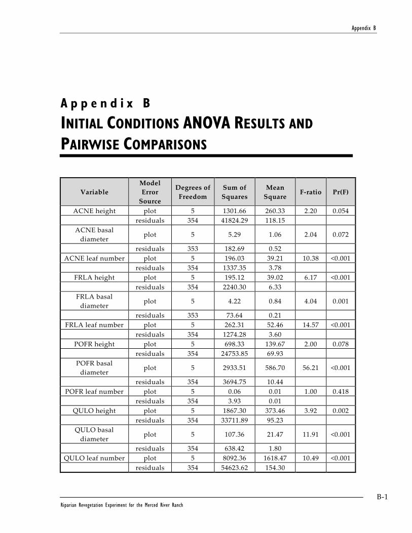
Appendix B
B-1 Riparian Revegetation Experiment for the Merced River Ranch
A p p e n d i x B
INITIAL CONDITIONS ANOVA RESULTS AND
PAIRWISE COMPARISONS
Variable
Model
Error
Source
Degrees of
Freedom
Sum of
Squares
Mean
Square F-ratio Pr(F)
ACNE height plot 5 1301.66 260.33 2.20 0.054
residuals 354 41824.29 118.15
ACNE basal
diameter plot 5 5.29 1.06 2.04 0.072
residuals 353 182.69 0.52
ACNE leaf number plot 5 196.03 39.21 10.38 <0.001
residuals 354 1337.35 3.78
FRLA height plot 5 195.12 39.02 6.17 <0.001
residuals 354 2240.30 6.33
FRLA basal
diameter plot 5 4.22 0.84 4.04 0.001
residuals 353 73.64 0.21
FRLA leaf number plot 5 262.31 52.46 14.57 <0.001
residuals 354 1274.28 3.60
POFR height plot 5 698.33 139.67 2.00 0.078
residuals 354 24753.85 69.93
POFR basal
diameter plot 5 2933.51 586.70 56.21 <0.001
residuals 354 3694.75 10.44
POFR leaf number plot 5 0.06 0.01 1.00 0.418
residuals 354 3.93 0.01
QULO height plot 5 1867.30 373.46 3.92 0.002
residuals 354 33711.89 95.23
QULO basal
diameter plot 5 107.36 21.47 11.91 <0.001
residuals 354 638.42 1.80
QULO leaf number plot 5 8092.36 1618.47 10.49 <0.001
residuals 354 54623.62 154.30

Appendix B
B-2 Merced River Ranch Revegetation Experiment
(
(
(
(
(
(
(
(
(
(
(
(
(
(
(
)
)
)
)
)
)
)
)
)
)
)
)
)
)
)
B1H-B1L
B1H-B1M
B1H-B2H
B1H-B2L
B1H-B2M
B1L-B1M
B1L-B2H
B1L-B2L
B1L-B2M
B1M-B2H
B1M-B2L
B1M-B2M
B2H-B2L
B2H-B2M
B2L-B2M
-12 -8 -4 0 4 8 12
simultaneous 95 % confidence limits, Tukey method
response variable: init.ht
(
(
(
(
(
(
(
(
(
(
(
(
(
(
(
)
)
)
)
)
)
)
)
)
)
)
)
)
)
)
B1H-B1L
B1H-B1M
B1H-B2H
B1H-B2L
B1H-B2M
B1L-B1M
B1L-B2H
B1L-B2L
B1L-B2M
B1M-B2H
B1M-B2L
B1M-B2M
B2H-B2L
B2H-B2M
B2L-B2M
-0.6 -0.3 0.0 0.3 0.6
simultaneous 95 % confidence limits, Tukey method
response variable: init.diam
(
(
(
(
(
(
(
(
(
(
(
(
(
(
(
)
)
)
)
)
)
)
)
)
)
)
)
)
)
)
B1H-B1L
B1H-B1M
B1H-B2H
B1H-B2L
B1H-B2M
B1L-B1M
B1L-B2H
B1L-B2L
B1L-B2M
B1M-B2H
B1M-B2L
B1M-B2M
B2H-B2L
B2H-B2M
B2L-B2M
-2.0 -1.0 0.0 1.0 2.0 3.0
simultaneous 95 % confidence limits, Tukey method
response variable: init.lvs
ACNE Initial Size, 95% Conf Intervals by Plot
(
(
(
(
(
(
(
(
(
(
(
(
(
(
(
)
)
)
)
)
)
)
)
)
)
)
)
)
)
)
B1H-B1L
B1H-B1M
B1H-B2H
B1H-B2L
B1H-B2M
B1L-B1M
B1L-B2H
B1L-B2L
B1L-B2M
B1M-B2H
B1M-B2L
B1M-B2M
B2H-B2L
B2H-B2M
B2L-B2M
-3.5 -2.0 -0.5 1.0 2.5
simultaneous 95 % confidence limits, Tukey method
response variable: init.ht
(
(
(
(
(
(
(
(
(
(
(
(
(
(
(
)
)
)
)
)
)
)
)
)
)
)
)
)
)
)
B1H-B1L
B1H-B1M
B1H-B2H
B1H-B2L
B1H-B2M
B1L-B1M
B1L-B2H
B1L-B2L
B1L-B2M
B1M-B2H
B1M-B2L
B1M-B2M
B2H-B2L
B2H-B2M
B2L-B2M
-0.6 -0.3 0.0 0.2 0.4 0.6
simultaneous 95 % confidence limits, Tukey method
response variable: init.diam
(
(
(
(
(
(
(
(
(
(
(
(
(
(
(
)
)
)
)
)
)
)
)
)
)
)
)
)
)
)
B1H-B1L
B1H-B1M
B1H-B2H
B1H-B2L
B1H-B2M
B1L-B1M
B1L-B2H
B1L-B2L
B1L-B2M
B1M-B2H
B1M-B2L
B1M-B2M
B2H-B2L
B2H-B2M
B2L-B2M
-1.5 0.0 1.0 2.0 3.0 4.0
simultaneous 95 % confidence limits, Tukey method
response variable: init.lvs
FRLA Initial Size, 95% Conf Intervals by Plot

Appendix B
B-3 Riparian Revegetation Experiment for the Merced River Ranch
(
(
(
(
(
(
(
(
(
(
(
(
(
(
(
)
)
)
)
)
)
)
)
)
)
)
)
)
)
)
B1H-B1L
B1H-B1M
B1H-B2H
B1H-B2L
B1H-B2M
B1L-B1M
B1L-B2H
B1L-B2L
B1L-B2M
B1M-B2H
B1M-B2L
B1M-B2M
B2H-B2L
B2H-B2M
B2L-B2M
-8 -4 0 2 4 6 8 10
simultaneous 95 % confidence limits, Tukey method
response variable: init.ht
(
(
(
(
(
(
(
(
(
(
(
(
(
(
(
)
)
)
)
)
)
)
)
)
)
)
)
)
)
)
B1H-B1L
B1H-B1M
B1H-B2H
B1H-B2L
B1H-B2M
B1L-B1M
B1L-B2H
B1L-B2L
B1L-B2M
B1M-B2H
B1M-B2L
B1M-B2M
B2H-B2L
B2H-B2M
B2L-B2M
-6 -2 0 2 4 6 8 10
simultaneous 95 % confidence limits, Tukey method
response variable: init.diam
(
(
(
(
(
(
(
(
(
(
(
(
(
(
(
)
)
)
)
)
)
)
)
)
)
)
)
)
)
)
B1H-B1L
B1H-B1M
B1H-B2H
B1H-B2L
B1H-B2M
B1L-B1M
B1L-B2H
B1L-B2L
B1L-B2M
B1M-B2H
B1M-B2L
B1M-B2M
B2H-B2L
B2H-B2M
B2L-B2M
-0.10 -0.04 0.0 0.04 0.08
simultaneous 95 % confidence limits, Tukey method
response variable: init.lvs
POFR Initial Size, 95% Conf Intervals by Plot
(
(
(
(
(
(
(
(
(
(
(
(
(
(
(
)
)
)
)
)
)
)
)
)
)
)
)
)
)
)
B1H-B1L
B1H-B1M
B1H-B2H
B1H-B2L
B1H-B2M
B1L-B1M
B1L-B2H
B1L-B2L
B1L-B2M
B1M-B2H
B1M-B2L
B1M-B2M
B2H-B2L
B2H-B2M
B2L-B2M
-14 -10 -6 -2 2 4 6 8
simultaneous 95 % confidence limits, Tukey method
response variable: init.ht
(
(
(
(
(
(
(
(
(
(
(
(
(
(
(
)
)
)
)
)
)
)
)
)
)
)
)
)
)
)
B1H-B1L
B1H-B1M
B1H-B2H
B1H-B2L
B1H-B2M
B1L-B1M
B1L-B2H
B1L-B2L
B1L-B2M
B1M-B2H
B1M-B2L
B1M-B2M
B2H-B2L
B2H-B2M
B2L-B2M
-2.0 -1.0 0.0 1.0 2.0
simultaneous 95 % confidence limits, Tukey method
response variable: init.diam
(
(
(
(
(
(
(
(
(
(
(
(
(
(
(
)
)
)
)
)
)
)
)
)
)
)
)
)
)
)
B1H-B1L
B1H-B1M
B1H-B2H
B1H-B2L
B1H-B2M
B1L-B1M
B1L-B2H
B1L-B2L
B1L-B2M
B1M-B2H
B1M-B2L
B1M-B2M
B2H-B2L
B2H-B2M
B2L-B2M
-25 -15 -5 0 5 10 15
simultaneous 95 % confidence limits, Tukey method
response variable: init.lvs
QULO Initial Size, 95% Conf Intervals by Plot


Appendix C
C-1 Riparian Revegetation Experiment for the Merced River Ranch
A p p e n d i x C
EXPERIMENTAL SCHEDULE
Week
Beginning
Experiment
Week
Week
Beginning
Experiment
Week
Week
Beginning
Experiment
Week
Week
Beginning
Experiment
Week
4/15/2004 0 12/9/2004 34 8/4/2005 68 3/30/2006 102
4/22/2004 1 12/16/2004 35 8/11/2005 69 4/6/2006 103
4/29/2004 2 12/23/2004 36 8/18/2005 70 4/13/2006 104
5/6/2004 3 12/30/2004 37 8/25/2005 71 4/20/2006 105
5/13/2004 4 1/6/2005 38 9/1/2005 72 4/27/2006 106
5/20/2004 5 1/13/2005 39 9/8/2005 73 5/4/2006 107
5/27/2004 6 1/20/2005 40 9/15/2005 74 5/11/2006 108
6/3/2004 7 1/27/2005 41 9/22/2005 75 5/18/2006 109
6/10/2004 8 2/3/2005 42 9/29/2005 76 5/25/2006 110
6/17/2004 9 2/10/2005 43 10/6/2005 77 6/1/2006 111
6/24/2004 10 2/17/2005 44 10/13/2005 78 6/8/2006 112
7/1/2004 11 2/24/2005 45 10/20/2005 79 6/15/2006 113
7/8/2004 12 3/3/2005 46 10/27/2005 80 6/22/2006 114
7/15/2004 13 3/10/2005 47 11/3/2005 81 6/29/2006 115
7/22/2004 14 3/17/2005 48 11/10/2005 82 7/6/2006 116
7/29/2004 15 3/24/2005 49 11/17/2005 83 7/13/2006 117
8/5/2004 16 3/31/2005 50 11/24/2005 84 7/20/2006 118
8/12/2004 17 4/7/2005 51 12/1/2005 85 7/27/2006 119
8/19/2004 18 4/14/2005 52 12/8/2005 86 8/3/2006 120
8/26/2004 19 4/21/2005 53 12/15/2005 87 8/10/2006 121
9/2/2004 20 4/28/2005 54 12/22/2005 88 8/17/2006 122
9/9/2004 21 5/5/2005 55 12/29/2005 89 8/24/2006 123
9/16/2004 22 5/12/2005 56 1/5/2006 90 8/31/2006 124
9/23/2004 23 5/19/2005 57 1/12/2006 91 9/7/2006 125
9/30/2004 24 5/26/2005 58 1/19/2006 92 9/14/2006 126
10/7/2004 25 6/2/2005 59 1/26/2006 93 9/21/2006 127
10/14/2004 26 6/9/2005 60 2/2/2006 94 9/28/2006 128
10/21/2004 27 6/16/2005 61 2/9/2006 95 10/5/2006 129
10/28/2004 28 6/23/2005 62 2/16/2006 96 10/12/2006 130
11/4/2004 29 6/30/2005 63 2/23/2006 97 10/19/2006 131
11/11/2004 30 7/7/2005 64 3/2/2006 98 10/26/2006 132
11/18/2004 31 7/14/2005 65 3/9/2006 99 11/2/2006 133
11/25/2004 32 7/21/2005 66 3/16/2006 100
12/2/2004 33 7/28/2005 67 3/23/2006 101