23 June 2015 JC DP 2015 01

Technical Discussion Paper

Risk, Performance Scenarios and Cost Disclosures

In Key Information Documents for

Packaged Retail and Insurance-based Investment Products (PRIIPs)

Table of Contents

Practical information .............................................................................................................................. 4

Executive Summary ................................................................................................................................. 5

1 Introduction .................................................................................................................................... 7

Purpose of this Discussion Paper ............................................................................................ 7 1.1

Next steps ............................................................................................................................... 7 1.2

2 Risk and Reward .............................................................................................................................. 8

General .................................................................................................................................... 8 2.1

Common issues for both the risk indicator and performance scenarios ................................ 9 2.2

2.2.1 Distribution of returns .................................................................................................... 9

2.2.2 Choice of model, choice of parameters ........................................................................ 11

2.2.3 Time value of money – what represents a loss for the retail investor? ....................... 13

2.2.4 Timeframe of the risk and reward information ............................................................ 15

Construction of a Risk Indicator ............................................................................................ 16 2.3

2.3.1 Measurement of Risk .................................................................................................... 17

2.3.2 Translation of risk measures into risk indicators .......................................................... 28

2.3.3 Merging the main risks into a Summary Risk Indicator (SRI) ........................................ 31

Performance scenarios ......................................................................................................... 44 2.4

2.4.1 Feedback from the public consultation on JC/DP/2014/02 .......................................... 44

2.4.2 How to choose performance scenarios: discussion about different approaches......... 45

2.4.3 Assessment of different approaches ............................................................................ 47

2.4.4 How to construct performance scenarios: methodological details to be prescribed in the regulation and input required ................................................................................................ 48

3 Costs .............................................................................................................................................. 52

Identifying the costs .............................................................................................................. 52 3.1

3.1.1 Funds ............................................................................................................................. 53

2

3.1.2 Life-insurance products................................................................................................. 72

3.1.3 Structured products, derivative, CFD & SPVs ............................................................... 83

Aggregating the costs ............................................................................................................ 96 3.2

3.2.1 Summary indicators ...................................................................................................... 97

ANNEXES ............................................................................................................................................. 115

A RIY taking into account biometric cash flows ............................................................................. 115

B RIY taking into account biometric benefits(Option 2 in relation to cash flows to be considered) 117

D Specific issues in relation to SPVs ............................................................................................... 124

3

Practical information

EBA, EIOPA, and ESMA (the ESAs) welcome comments on this Technical Discussion Paper on Risk, Performance Scenarios and Cost Disclosures in Key Information Documents for Packaged Retail and Insurance-based Investment Products (PRIIPs).

The discussion paper is available on the websites of the three ESAs. Comments on this discussion paper can be sent using the response form, via the ESMA website under the heading ‘Your input/Consultations’ by 17 August 2015.

Contributions not received in Word, or sent to an email address, or after the deadline, will not be processed.

It is important to note that although you may not be able to respond to each and every question, the ESAs would encourage partial responses from stakeholders on those questions that they believe are most relevant to them.

Publication of responses

All contributions received will be published following the close of the consultation, unless you request otherwise. A standard confidentiality statement in an email message will not be treated as a request for non-disclosure. A confidential response may be requested from us in accordance with the ESAs’ rules on public access to documents.1 We may consult you if we receive such a request. Any decision we make not to disclose the response is reviewable by the Board of Appeal of the ESAs and the European Ombudsman.

Data protection

Information on data protection can be found on the different ESAs’ websites under the heading ‘Legal notice’.

1 See https://eiopa.europa.eu/about-eiopa/legal-framework/public-access-to-documents/index.html.

4

Executive Summary

This Technical Discussion Paper aims to collect views on the possible methodologies to determine and display risks, performance and costs in the Key Information Document (KID) for PRIIPs. The paper is split in a section on risk and reward and a section on costs.

Risk and Reward

Three risks are considered for the risk indicator: market, credit and liquidity risk. The PRIIPs Sub Group assessed multiple approaches for risk indicators in the last year. This Technical Discussion Paper reports back on these approaches. The main part presents the four approaches that are being considered as viable. The first approach is a qualitatively based indicator which combines credit and market risk, complemented by a quantitative market risk measure. The second approach is an indicator which separates market risk and credit risk. Market risk in this indicator is assessed by a quantitative volatility measure and credit risk is assessed by a qualitative external credit rating. The third approach is an indicator based on quantitative market and credit risk measures and is calculated by using forward looking simulation models. The fourth and final approach is a two-level indicator where the first level roughly separates products based on their qualitative characteristics and the second level specifies the risk based on a quantitative assessment.

Another four approaches are highlighted for performance scenarios. The first approach is to let the manufacturer of a PRIIP decide which scenarios to present in the KID (the so called what-if: manufacturer choice). A second approach is to prescribe which scenarios should be included in the KID. The third approach is one that takes probabilities of outcomes into account in the scenario selection. The fourth approach that is described is a combination of the previous approaches.

Costs

The cost section start with the aim to identify the different types of costs of the different types of PRIIPs (in particular, funds, structured products and life-insurance products), and identify the specific issues related to the calculation of some of these costs (e.g. transaction costs and performance fees, notably in the case of funds, or cost related to biometric risk premium in the case of life-insurance products).

Its second part aims to assess the different possible ways of aggregating these different types of costs, including the different possible definitions of the overall cost ratio (summary cost indicator), and the possible ways of calculating the cumulative effect of costs.

The list of costs identified in the case of funds is inspired by the UCITS example, but it includes different types of costs that were excluded from the “ongoing charges figure” of UCITS (e.g. transaction costs). This list is detailed and benefits from the experience of the CESR guidelines on the methodology for calculation of the ongoing charges figure in the Key Investor Information Document.

The list of costs identified in the case of life-insurance products makes it clear that, as opposed to investment funds, the definition of the different types of costs of this type of PRIIPs is not

5

harmonised within the EU. This list distinguishes between the case of unit-linked products and with-profit contracts. It also highlights that there are some specific issues related to the costs of life-insurance products, including the way of handling the (costs of) biometric risk premium of these products, the allocation of costs in the case of with-profits contracts, and the costs related to embedded guarantees and options.

The list of costs identified in the case of structured products emphasizes the fact that the main part of these costs is included in the price of the product and that the estimate of the fair value of the product is therefore needed to calculate its costs. The different types of costs of SPVs are also discussed in this part.

Two main possible approaches for aggregating the costs of the different types of PRIIPs are presented: Reduction in Yield (RIY) and Total Cost Ratio (TCR).

The total cost ratio means that the costs of operating a PRIIP are aggregated and presented as an annual percentage rate on the investment. Specific issues related to the TCR in the case of different types of PRIIPs are discussed (e.g. the most appropriate definition of the denominator of this ratio) and the extent to which the principles that govern the use of the ongoing charges figure of UCITS could apply to the TCR if applied to the different types of PRIIPs.

Reduction in Yield is a method for expressing the overall impact of costs in terms of their negative impact on a notional ‘gross’ yield for a product. It is currently implemented in different national markets, and notably in the case of life-insurance products. Specific issues related to the RIY and TCR in the case of the different types of PRIIPs are discussed (e.g. the yield assumption(s) to be taken, the way it handles the biometric benefits).

With respect to the cumulative effects of costs, the assumptions on growth rates and the interaction with the reward section of the KID are discussed.

6

1 Introduction

Purpose of this Discussion Paper 1.1

This Technical Discussion Paper aims to provide stakeholders with an opportunity to comment on certain specific technical areas related to risk, performance and cost information that are required for the Regulatory Technical Standards (RTS) to be developed by the European Supervisory Authorities (ESAs: EBA, EIOPA and ESMA) pursuant to Article 8(5) of the Regulation 1286/2014 on Key Information Documents for Packaged Retail and Insurance-based Investment Products (hereafter, PRIIPs Regulation).2

This follows a broader and less technical first Discussion Paper (JC/DP/2014/02)3. This Technical Discussion Paper does not provide full feedback on the responses to the first Discussion Paper, but includes some feedback on those areas of the first Discussion Paper that address topics also covered here.

Next steps 1.2

The ESAs expect to follow this Technical Discussion Paper with a final Consultation Paper setting out the draft RTS under Article 8 in the autumn of 2015. Separate Consultation Papers will also be published for the RTS under Articles 10 and 13.

The draft RTS on Article 8 will then be finalised and be submitted to the European Commission by 31 March 2016, as set out in the PRIIPs Regulation.

2 See http://www.europarl.europa.eu/sides/getDoc.do?type=TA&reference=P7-TA-2014-0357&language=EN&ring=A7-2013-0368. 3 See http://www.eba.europa.eu/documents/10180/899036/JC+DP+2014+02+-+PRIIPS+Discussion+Paper.pdf.

7

2 Risk and Reward

General 2.1

Article 8 (3) of the PRIIPs Regulation requires a section titled “What are the risks and what could I get in return?” consisting of a brief description of the risk-reward profile of the PRIIP comprising amongst others the following elements:

(i) a summary risk indicator, supplemented by a narrative explanation of that indicator;

(ii) its main limitations and a narrative explanation of the risks which are materially relevant to the PRIIP and which are not adequately captured by the summary risk indicator; and

(iii) appropriate performance scenarios, and the assumptions to produce them.

The goal of the summary risk indicator is to provide retail investors with an indication of the overall risk of the PRIIP in relation to other PRIIPs. The goal of including performance scenarios in the KID is to provide information about potential outcomes of the product, complementing the information provided in the description of how the product performs and in the risk indicator.

From the perspective of consumers’ protection, the content of the KID should at first aim at reducing the asymmetry of information between consumers and manufacturers.

Additionally, the KID is viewed as complementary pre-contractual information which supplements the information provided to a consumer (e.g. via financial intermediary or other information sources).The KID shall not be the sole and unique source of information. Its purpose is to serve in the pre-contractual phase where consumers are deciding which product to buy. From that perspective, the KID aims to provide clear information on material terms and allow comparison between products so as to broaden the perspective of investment of a consumer and help him select the product which best matches his interests, risk profile and objectives.

Risk in general is a difficult concept as it is linked to perception. As such and from this perspective, what matters is what risk implies from the point of view of a consumer. In the Discussion Paper published in November (JC/DP/2014/02), two dimensions of risk have been identified. These are (i) the possibility of capital loss and (ii) the uncertainty of the returns. These dimensions were operationalised in Key Questions to consumers in the Discussion Paper (p.23 and 24).

If the dimensions of risks are considered to be potential loss and uncertainty of returns there are different measures that are related to these dimensions. Approaches that fall under the concept of risk might focus on the question which is either:

• how much money could be lost based on the level of confidence assuming that the market

would behave in accordance with a set of given assumptions (this can be covered by downside measures such as VaR or Expected Shortfall) or

8

• how returns are dispersed and whether the investment value can change dramatically (measured in volatility) which in turn may impact upwards or downwards the value of capital a consumer may get back following redemption or maturity of its investment.

The ESAs have identified three main risks in the Discussion Paper as material for the PRIIPs in scope. These risks are the market risk, the credit risk, and the liquidity risk. Extended details on these three risks can be found further in this Paper (please refer to section 2.3). It is important to flag that due to the wide scope of PRIIPs it may be necessary to amend or create variations of proposed methodological approaches in order to cover all products.

The sections 2.2, 2.3 and 2.4 below give an overview of the concepts of risk and performance and the technicalities related to these concepts. This paper will not address the presentational formats of the summary risk indicators and the performance scenarios.

Common issues for both the risk indicator and performance scenarios 2.2

There are a number of general aspects that relate to both the risk indicator and the performance scenarios. These aspects are discussed in this section. In section 2.2.1 the distribution of returns is discussed. Section 2.2.2 deals with specifications of the model and the parameters. The time value of money is discussed in section 2.2.3. Finally, a shared general aspect is the discussion in relation to the timeframe(s) used for determining the risk and the performance of a PRIIP. This is discussed in section 2.2.4.

2.2.1 Distribution of returns

Many quantitative measures of market risk and methods of calculating performance scenarios are based on an estimation of the distribution of returns at a given time frame. This section focuses on the possible approaches to get to a distribution of returns. When considering the different uses of the distribution of returns for the different sections in the KID (ordering products in terms of risk vs selecting specific points of the distribution and showing the estimated performance), it might be worthwhile to consider using different approaches for these two sections. However, should a modelling approach be used for both computing a risk measure and developing performance scenarios, a single approach is preferable.

Feedback from the public consultation on JC/DP/2014/02 2.2.1.1

Opinions of the respondents to the Discussion Paper on the choice of parametric or non-parametric methods diverge: some argue that estimation based on the statistics of historical data are simpler and more reliable and more difficult to manipulate than estimation through parametric or semi parametric models. Others argue that the predictive power of such an estimate is weak, the result is subject to sampling errors and moreover that such an approach is not widely used by financial institutions. Some respondents mention that many stochastic models used for pricing financial market instruments are validated by prudential supervisory authorities. All respondents suggest that the simpler the approach taken to modelling, the better.

9

The comments and suggestions of the respondents concentrate on the modelling of the dynamics of the marginal distribution of the main risk factors (equity prices, bond yields, volatility of prices and/or bond yields, etc.) but did not raise the matter of how to estimate these parameters or how to estimate the correlation of those risk factors.

The respondents did address concerns for certain products: notably certain life-insurance products where the interplay of investment performance and other factors (such as consumer behaviour) may be important.

Estimations of distribution of returns 2.2.1.2

Estimations of a distribution of returns can be achieved by calculating the distribution of returns for a particular product from a sample of observed series of financial data or by calculating the distribution of returns using forward stochastic modelling of risk factors. Five distinct approaches to the estimation of the distribution of returns have been considered:

a) Distribution of returns directly obtained from historical data b) Stochastic modelling based on parameters estimated from historical data c) Stochastic modelling based on parameters estimated from current market prices of

derivatives and other forward looking contracts d) Stochastic modelling based on predefined parameters e) Stochastic modelling based on parameters chosen by the manufacturer

The first choice to be made is whether to use historical data or forward simulation to construct the distribution of returns. If forward simulation is chosen, the regulatory technical standards need to outline how to choose the model and the parameters required. The first choice is described below, whereas the second question is considered in the next section.

The above mentioned methods have been considered from the perspective of ease of specification, ease of standardisation, ease of implementation, ease of supervision and “accuracy”. Historical methods are easily standardised (the standards need to specify estimation methods and statistical tests on samples) and are relatively easy to supervise but may not be the most accurate as the future does not necessarily reflect the past and there may not be enough independent periods to estimate returns over a long time horizon. Modelling approaches, whether reliant on current market data, historical data or manufacturer’s data, may be the more accurate at estimating the distribution of potential returns, but are difficult to standardise and supervise. Furthermore, a modelling approach is the most costly option, both for the manufacturer and supervisory authorities. Modelling with predefined parameters is the easiest to standardise and the easiest to supervise but it introduces potential issues for regulators with respect to ensuring that the right parameters are used in the right context at the right time.

The methods of estimating distributions have been considered for all products falling under the scope of PRIIPs. Certain approaches to estimating returns may be well-suited for one class of products but difficult or not applicable for a different class. The use of historical data is problematic for structured products where the parameters of the product are chosen in the context of the

10

current environment. A modelling approach may be problematic for products if the product depends on factors not included in the model.

Question 1: Please state your preference on the general approach how a distribution of returns should be established for the risk indicator and performance scenarios´ purposes. Include your considerations and caveats.

2.2.2 Choice of model, choice of parameters

At this point, it is useful to define what is meant by “model” in the context of generating a distribution of returns using a simulation. A model explains, in a precise way, how the price or level of a market observable changes from one point in time to another. The model may include a deterministic component (e.g. an expected rate of growth) and a random component or random components. The model chosen as the basis for any forward simulation should be made with an understanding of how market risk will be measured and how the performance scenarios will be constructed and presented. It may also be desirable to allow for a particular choice of model based on the underlying asset (e.g. Black-Scholes or Heston for equity assets, Hull-White or Libor Market Model for interest rate assets).

All models require some parameters to be set for the model to produce results. A simple model is one which says that the price change over one day consists of a deterministic component and a random component chosen from a log-normal distribution. The model parameters, which determine the risk of the asset, are the deterministic component and the variance or spread of the log-normal distribution.

In order to achieve an appropriate level of objectivity, the methodology to estimate the distribution of returns, as well as the rules to select the input variables, need to be standardised. However, considering the different types of products in scope and to allow for financial innovation (both in products as well as in estimation techniques), some degree of flexibility would still be necessary

There are two possible choices with regard to the specification of the model: prescribe the model to be used or allow the manufacturers to use whichever model they consider the most appropriate. The advantage of prescribing a model (e.g. assuming all risk factors follow a random walk with a time-homogenous variance otherwise known as Black-Scholes) is simple and ensures that we are comparing all products of a particular class on a similar basis. The disadvantage is that particular risk factors may have distributions inconsistent with this model. This could create biased comparisons amongst product classes. In addition, the results of the prescribed model may be inconsistent with the results obtained from the internal model used by the manufacturer to understand a product. In such situations, the regulation would not achieve the goal of reducing the asymmetry in understanding between the manufacturer and the customer. On the other hand, allowing manufacturers to choose the most appropriate model has the advantage that the assumed process is probably better matched to what is observed as it is in the interest of the firms to understand how their products are likely to perform. The disadvantage is that without some degree of supervision,

11

manufacturers could choose an inappropriate model that gives an inaccurate appraisal of the risk of the product.

The choice of whether to prescribe a model or not depends in part on the risk measure chosen. If the risk measure depends critically on the tail of the distribution (e.g. at 95% or 99% confidence level), then the choice of model is more important than if the risk measure is based on a measure of width (volatility) or a measure closer to the mean of the distribution (e.g. at 75% or 80% confidence level).

Each model or methodology will require the specification of a number of parameters. Typically there is a parameter or group of parameters which govern how the average price (or level) of a particular risk factor changes with time, another parameter or group of parameters which govern the variability of the risk factor and, if needed, a parameter or group of parameters which describe the correlation between the price and its variability.

The choice of the parameters that determine the expected level of return are discussed in a later section.

The parameters that determine the variability can be estimated from historical data, based on current expectations derived from current market prices, prescribed by a central authority or left to the judgment of the manufacturer. The first two methods for estimating parameters do not require much prescription, but do require some supervision to ensure that results are comparable across manufacturers. They also allow for the variability in different asset behaviours in different markets. Prescription of parameters probably necessitates prescription of a simple model with relatively few parameters with limited capacity to adjust parameters that capture the nature of a particular asset in a particular market. Allowing firms the freedom to choose parameters may require greater supervision to ensure that parameters are chosen with the intent of portraying the true risk of a product to its potential investor. Again, some principles to limit the discretion of the manufacturer could be included in the technical standards.

Parameters that describe the correlation between level and variability exist in complex models. The choice of these parameters needs to be considered when manufacturers are allowed to choose the most appropriate model. In this case, the parameters could be set according to historical performance, current market prices or at the discretion of the manufacturer.

Question 2: How should the regulatory technical standards define a model and the method of choosing the model parameters for the purposes of calculating a risk measure and determining performance under a variety of scenarios?

What should be the criteria used to specify the model? Should the model be prescribed or left to the discretion of the manufacturer?

What should be the criteria used to specify the parameters? Should the parameters be left to the discretion of the manufacturer, specified to be in accordance with historical or current market values or set by a supervisory authority?

12

2.2.3 Time value of money – what represents a loss for the retail investor?

The concern of the customer is the real term value of the investment in the future – is this value the monetary value or the ability of the customer to use the value of the investment to purchase goods and services. Even though most customers have difficulty with the concept of the time value of money, it is a key financial concept and or critical importance for products with long holding periods.

The information provided by certain risk measures (Value at Risk – VaR, Expected Shortfall) depends – ES) depend on the level against which loss is measured and any assumptions regarding how the average performance of the asset(s) underlying a product changes with time. The information provided by probabilistic performance scenarios similarly depends on any assumptions regarding how the average performance of an asset or assets underlying a product changes with time. A simple illustration of this issue is the performance of an equity fund measured assuming that the fund value increases with the time horizon measured against the price paid. In this case, the risk is decreasing with the time horizon. Similarly, the performance at a 90% confidence level will increase with time.

The concern of the customer is the value of the investment in the future – this is of critical importance for products with long holding periods.

With regards to the level against which performance is measured there are two factors which could be considered leading to 3 choices:

a. The amount invested without any adjustment b. The amount invested grown at the risk-free growth rate c. The amount invested grown the rate of inflation

Should any of the latter 3 choices be preferred, the specification of the relevant rates could be left to the discretion of the manufacturer, chosen according to historical data, chosen according to current market expectations or prescribed by an authority - supervisory authorities (e.g. EIOPA), central banks and/or market instruments. Inflation rates can also be obtained from a number of sources, some of which differ amongst what inflation is measured.

Question 3: Please state your view on what benchmark should be used and why. Are there specific products or underlying investments for which a specific growth rate would be more or less applicable?

Considering that risk and return are related - investors demand more (potential) return for riskier assets - manufacturers and academics have identified that different assets have different expected growth rates depending on their risk (described as risk premiums). Risk premiums can have a dramatic influence on the performance of an asset regardless of the level against which risk or performance is measured. These risk premiums are thought to be time-dependent and dependent on economic conditions. Therefore, defining appropriate risk premiums parameters may be particularly important for performance scenarios. For the risk indicator purposes, as comparison is the more relevant aspect, accurate estimation of this premium is not so relevant.

13

A similar decision to the one above needs to be made with respect to the expected growth of an asset’s value over time. In general, prudential standards require financial institutions to rely on risk-neutral growth rates for the purposes of calculating capital requirements. From the customer’s perspective, the asset will grow at the risk neutral rate adjusted by a risk premium. With respect to the specification of asset growth rates, there are several choices that can be considered:

a. The asset grows at the risk free rate (with the hypothesis that the risk-premium is equal to zero)

b. The asset grows at the risk free rate adjusted for an asset specific risk premiums (with the hypothesis that the risk premium is different from zero and constant)

c. The asset grows at the risk free rate adjusted for an asset specific risk premiums adjusted for current market conditions (with the hypothesis that the risk premium is different from zero and time dependent).

The risk premiums can be estimated from historical data, left to the discretion of the manufacturer or prescribed by an authority. There are advantages and disadvantages for each approach. Historical data, if used appropriately, may give the best estimate; manufacturers may be best placed to understand which risk premium is likely to apply to their products; and specification by a supervisory authority ensures a consistent approach across all manufacturers. All three methods of determining risk premiums present challenges indeed, manufacturers may choose a value which presents their products in the best possible light but is not realized; and supervisory authorities are not better placed to estimate risk premiums than the manufacturer. Historical estimations may not apply in the future, given that there is evidence that risk premiums are not consistent over time. Moreover, historical risk premiums can be negative in certain circumstances4. Risk premiums can be applied in situations where the risk premium is not earned by the investor.5

Further, the inclusion of a risk premium within a model can bias estimate of a product’s risk and performance. Risk premiums directly impact the performance of a product should there be a correlation between expected variability and level (e.g. a local volatility model introduces a correlation between the equity growth rate and the variability of equity prices with higher growth rates correlated with lower variability). The inclusion of equity premiums could result in a lower variability than might be expected from current market prices.

With regard to performance, there is a question of whether the performance scenario is meant to be as close to reality as possible. Real asset returns include a risk-neutral rate adjusted by a risk premium. In theory, a realistic estimation of performance should thus include the risk premium. The difficulty is that, ab initio, one does not know what risk premium applies in the immediate future. There is a bias if one does not include a risk premium for a particular asset, there is a bias if one includes a risk premium and biases the choice of product for a period when the risk premiums have changed.

4 Recent studies conducted by Riccardo Rebonato at PIMCO suggest that bond premiums are negative during the initial stages of a recovery from a recessionary period (Quant Europe, 2015). 5 Work by Elroy Dimson suggests that during the past 15 years, equity risk premiums are principally earned through the dividend so the application of equity risk premiums should only be considered when the investor receives the dividend.

14

In case risk premiums are used it is important to sufficiently separate the asset classes and prescribe the risk premium that is attached to that specific asset class. As the risk premiums change over time it is important that these premiums are being evaluated from time to time.

Question 4: What would be the most reasonable approach to specify the growth rates? Would any of these approaches not work for a specific type of product or underlying investment?

2.2.4 Timeframe of the risk and reward information

A focus of the KID is the presentation of the risk of a product should the product be held for the recommended time.

Products under the scope of the PRIIPs Regulation, however, have several characteristics which can impact the level of risk through time. The general considerations are products which have a fixed maturity versus those that allow the customer to determine the exit point and for those products which have a fixed maturity whether the customer can easily exit the position during its lifetime at a market dependent price. The question which arises is whether both the risk measure and the performance scenarios need to present the changes in the risk and performance due the interaction of the product characteristics with the time that the product will be held.

For open-ended products, the variability of returns at a particular time horizon will generally decrease as one nears the fixed time horizon. The potential loss of open-ended products will generally increase as the horizon increases. The potential loss at a fixed time horizon could increase or decrease depending on the actual evolution of asset prices.

For products with a predetermined pay-out at a fixed time horizon and daily liquidity, the variability of the returns will decrease as the time to maturity decreases as the expected return becomes more and more certain. However, should the customer wish to exit prior to maturity, the variability of the payoff could be quite large even if the payoff at maturity is a fixed value. The potential loss at a fixed time horizon could increase or decrease depending on the actual evolution of asset prices.

Reflection of time frame in the risk indicator 2.2.4.1

As risk for the same product may be different depending on the investment horizon considered, a decision has to be made about what investment horizon should be reflected in the risk indicator.

The question of how to present the risk at intermediate times between the purchase date and the recommended time horizon could be handled in a number of different ways:

a. Show the risk indicator and performance scenarios for several intermediate times as well as the recommended holding period

b. Construct a risk indicator based on different observations of the risk indicator at different time horizons (e.g. average of the indicator, maximum level of the indicator)

c. Show the risk indicator for the recommended holding period, but include a warning or narrative text that explains the possible variation in risk over time.

15

Considering that the KID includes a reference to a “Recommended holding period”, and an “intended market” to which the product is directed (that might consider the investment horizon), and for simplicity of the presentation (to avoid overload of information that may confuse some investor), it seems appropriate to build the risk indicator adapted to the recommended holding period stated by the manufacturer in the KID, including additional information or warnings about the limitations of the indicator (e.g. the risk level assigned is only accurate if the product is kept to the recommended holding period).

Performance scenarios may be used to provide additional insight on differences in potential performance linked to investment horizons. Some methodological issues arise however to present performance in intermediate scenarios (see section 2.4).

Question 5: Please state your view on what time frame or frames should the Risk Indicator and Performance Scenarios be based

Feedback from the public consultation on JC/DP/2014/02 2.2.4.2

In general, the responses to the Discussion Paper indicated that for the performance scenarios it is important to consider the diverse spectrum of PRIIPs in scope. A distinction is made between fixed term products and products that are open-ended. For products that are open-ended the respondents acknowledge it is desirable to have a standardised recommended holding period (such as the 5-year period for UCITS) to enable comparison. For fixed term products respondents indicated that due to the assumed buy-and-hold strategy the recommended holding period should be the term of the product. In general, the preference was to have a flexible approach and only for open-ended products a standardised holding period should be defined. In addition to this holding period respondents preferred to align the performance scenarios with the cost scenarios and indicated that it would be interesting and useful to consumers to show multiple holding periods in the performance scenarios. There was no specific feedback on the recommended holding period in relation to the risk indicator.

Construction of a Risk Indicator 2.3

Several steps need to be taken before the three main risks can be converted into a summary risk indicator. The first step is to decide how to measure the different types of risk. This is discussed for every type of risk in the sections 2.3.1. Once a decision has been made as to how to measure risk it is important to translate the risk into an indicator. This is discussed in section 2.3.2. The next step is to assemble the main types of risk into a summary risk indicator. Currently four approaches to do so are discussed in section 2.3.3. Finally, it needs to be decided how to present the indicator. This last step is not part of this Technical Discussion Paper.

As for the methodological approaches described below it is important that a balance is found on the level of prescriptiveness on the measures (i.e. to which extent the regulators may prescribe assumptions and parameters in relation to a risk methodology). It is also relevant to balance the

16

level of complexity of the methodology with the results obtained. Furthermore, the complexity of implementation should be considered thoroughly. This aspect of implementation is relevant both at the level of the supervisors as well as at the level of the market participants. Cost in that respect is a key issue in implementation.

As introduced in the Discussion Paper there are a number of criteria that are taken into account in the assessment of the proposed methodologies. These criteria are listed in the table below:

Criteria for assessing underlying methodologies Reliable The information within the KID is reliable where it provides a fair estimate of the actual

risks and costs involved. Robust The measurement of risk, reward and costs should not be easy to manipulate. It should

be an objective representation of the risk, reward and costs that are being measured. Stable The output of the measurements needs to be relatively stable. It is important that risk

or cost indicators are reliable forecasts, and that they are not overly sensitive to relatively minor changes in conditions.

Applicable The measurements should be applicable to all types of PRIIPs. Where a measurement (e.g. of historic volatility) is available for some PRIIPs but not available for those without a track record, or might be a misleading measure for some, effective methodologies for combining or synthesizing different measures in an objective way may be necessary.

Comparable The measurements should lead to values that are comparable amongst different types of PRIIPs.

Discriminatory If it is not possible to differentiate between PRIIPs, a measure loses its purpose. It needs to be clear that a certain measured output is below or above another measured output. Therefore it is important that the indicator provides discriminatory output.

Feasible/ Proportional

An indicator or measure that is overly sophisticated in relation to the granularity and accuracy of the information included in the KID could be seen as disproportionate. This does not imply that the simplest or least costly option should always be selected.

Supervision Will it be possible for regulators to assess whether product manufacturers are complying with any proposed prescribed methodology?

2.3.1 Measurement of Risk

The three main risks described in the Discussion Paper were accompanied with different measures. These measures have been assessed. The results of this assessment can be found in this section.

Market risk 2.3.1.1

This section discusses the possible measures of market risk. It is not intended to describe the whole methodology for the Risk Indicator (see section 2.3.3). It focuses on the high level description of

17

market risk6, considered to be PRIIPs´ most relevant risk, and possible ways to give a value to that risk.

Feedback from the public consultation on JC/DP/2014/02

Many respondents indicated that due to the differences of characteristics of the products in scope it is important to remain open to differentiation in the methodology for the different types of products. This includes that for some type of products volatility based measures would be more suitable than downside based measures. There are also some respondents which argue that a measure of market risk should be based on a downside measure as it better reflects how consumers perceive risk. For the downside measures the VaR was mentioned more often than the ES. Finally, there were some respondents who indicated that figures do not automatically reflect the risk of a PRIIP and that it would be more useful to look at the characteristics of the products and to use a measure that is based on the qualitative aspects of the PRIIP.

High-level description of possible market risk measures

In the Discussion Paper multiple market risk measures were analysed. As shown above, most respondents favour a volatility based approach followed by proponents of a VaR based measure with the qualitative based approach being the least preferable. In this section a high level description of the different market risk measures is provided.

Volatility is an example of a measure which aims at quantifying the variation of value of an asset whereas VaR and Expected Shortfall are examples of measures aiming at quantifying the potential loss of capital.

One of the options presented in the Discussion Paper was to combine different qualitative measures to proxy the market risk of a PRIIP. The measures described therein were, among others,(i) the type of underlying, (ii) the level of diversification, (iii) the amount of leverage and (iv) the exposure to foreign currencies. One partly qualitative risk indicator is now introduced (see section 2.3.3) which uses product characteristics to proxy the risk of a PRIIP.

Another option described in the Discussion Paper, this time of a quantitative nature, was historical (ex-post) volatility on traded products. This measure is already widely used in the context of the existing methodology for the UCITS SRRI. Volatility is a measure that is closely related to the perception of risk referred to as “uncertainty”. As indicated in the previous section, a number of Discussion Paper respondents favour a comparable approach to UCITS. However, because volatility in itself does not sufficiently capture the impact of any (conditional) capital protection common to a lot of PRIIPs, this Technical Discussion Paper envisages the use of a modified version of the current UCITS methodology.

6 The DP defined market risk as “the risk of changes in the value of the PRIIP due to movements in the value of the underlying assets or reference values.“

18

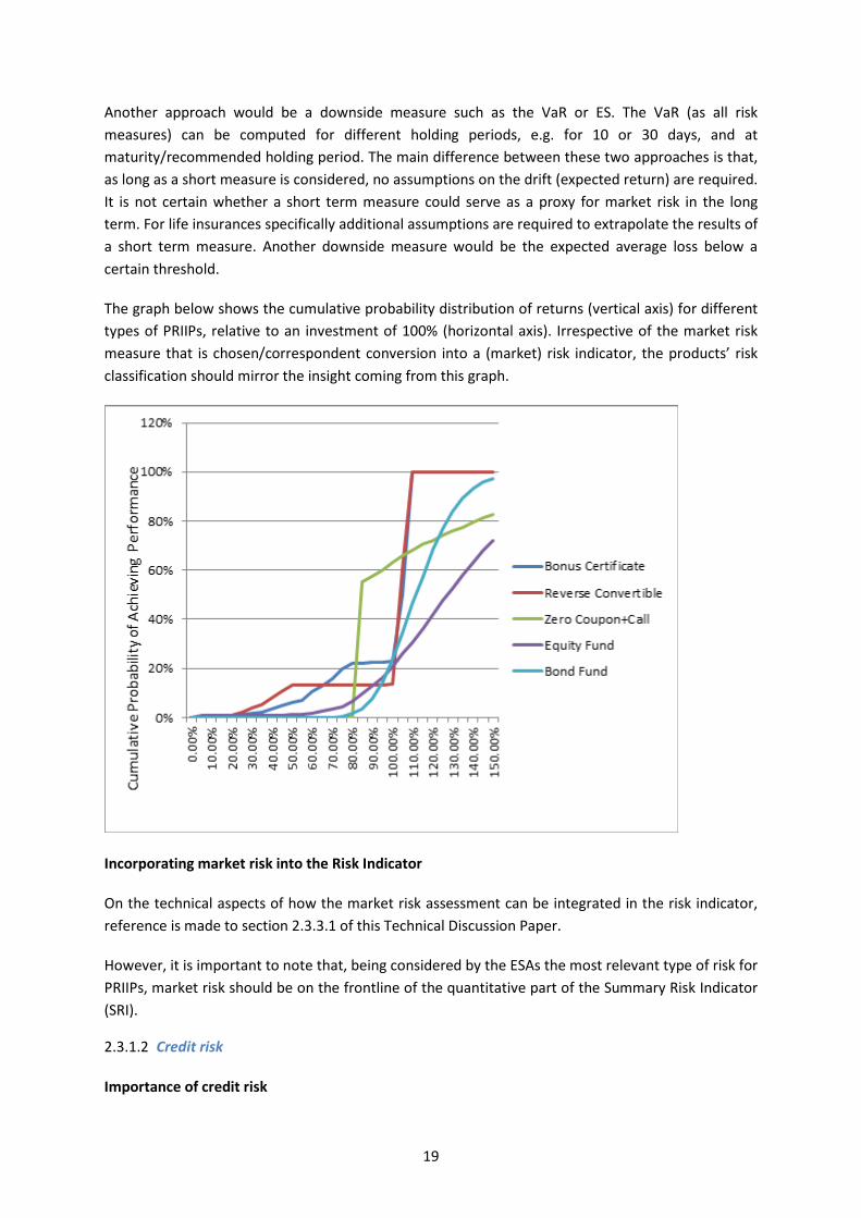
Another approach would be a downside measure such as the VaR or ES. The VaR (as all risk measures) can be computed for different holding periods, e.g. for 10 or 30 days, and at maturity/recommended holding period. The main difference between these two approaches is that, as long as a short measure is considered, no assumptions on the drift (expected return) are required. It is not certain whether a short term measure could serve as a proxy for market risk in the long term. For life insurances specifically additional assumptions are required to extrapolate the results of a short term measure. Another downside measure would be the expected average loss below a certain threshold.

The graph below shows the cumulative probability distribution of returns (vertical axis) for different types of PRIIPs, relative to an investment of 100% (horizontal axis). Irrespective of the market risk measure that is chosen/correspondent conversion into a (market) risk indicator, the products’ risk classification should mirror the insight coming from this graph.

Incorporating market risk into the Risk Indicator

On the technical aspects of how the market risk assessment can be integrated in the risk indicator, reference is made to section 2.3.3.1 of this Technical Discussion Paper.

However, it is important to note that, being considered by the ESAs the most relevant type of risk for PRIIPs, market risk should be on the frontline of the quantitative part of the Summary Risk Indicator (SRI).

Credit risk 2.3.1.2

Importance of credit risk

19

The assessment of credit risk7 is important for PRIIPs where an entity has a direct contractual obligation to pay to the consumer (a) certain amount(s) (at maturity, at least) whether or not depending on the evolution of the underlying assets. If the credit risk is linked to the underlying assets where the PRIIP is invested in, it is assumed that such credit risk is reflected in the PRIIP’s market risk (eg. actively managed UCITS investing in bonds). In some cases however, it could be appropriate to assess the credit risk attached to the underlying investment independently from market risk8. Credit risk could be mitigated in some situations such as when there is a guarantee or a compensation scheme (such as the deposit compensation scheme) in place or when appropriate collateral is provided.

Depending on the creditworthiness of the counterparty, credit risk could be the most important risk consumers are facing when investing in some PRIIPs. Therefore, the ESAs lean towards the incorporation of credit risk in the risk indicator rather than presenting it in a separate narrative. However, the possibility to nuance or to comment in a narrative the assessment of credit risk emerging from the risk indicator may not need to be excluded.

Feedback from the public consultation on JC/DP/2014/02

The Discussion Paper (p. 28-29) explored qualitative as well as quantitative measures for evaluating credit risk. Qualitative measures or features included the credit rating and prudential supervision, as well as different products’ features such as risk spreading, level of seniority, secured or unsecured nature and deposit/insurance guarantee schemes. Quantitative measures included the issuer´s credit spread or CDS spread and credit value at risk.

Feedback from respondents on quantitative credit risk measures is predominantly negative for several reasons: credit or CDS spreads are not available for all manufacturers and require a liquid bond or CDS market; spreads may be impacted by elements other than credit risk evolution, such as liquidity, and the different impacts are hard to isolate; spreads may be highly volatile, possibly leading to a very unstable risk measure. It is acknowledged that credit VaR is not applied by all PRIIPs´ manufacturers and is a very model dependent exercise which could jeopardise the consistency and comparability of the risk indicator.

To a large extent there is a preference amongst respondents for the use of qualitative measures for credit risk, especially credit ratings, if available. Credit ratings are seen as objective, generally accepted, stable and accessible measures of credit risk that can easily be applied by market participants and supervised by regulators. But some respondents point out the value of other qualitative or generic measures such as prudential supervision, deposit/insurance guarantee and segregation, particularly if no credit ratings are available.

7 The DP defined credit risk as “the risk of loss on investment arising from the obligor´s failure to meet some/all his contractual obligations. The obligor could include the issuer of the PRIIP.” 8 For instance a unit linked insurance contract where the proceeds are invested in a government bond, a “capital protected” structured investment fund where the proceeds are to a large extent invested in a bond portfolio that should deliver at maturity the repayment of the invested amount, or an investment fund that makes use of efficient portfolio techniques or financial derivative contracts such as a total return swap.

20

High level description of possible credit risk measures

Quantitative credit risk measures

Credit spreads or Credit Default Swap spreads

The main advantages of credit spreads or CDS spreads are that these spreads are specific per issuer; they are real time indicators of market’s perception of credit risk and are objective information, determined by market parties. If there are no CDS or corporate bonds outstanding, spreads could be derived from spreads on peer companies, but this may reduce the objectivity of the assessment. However, there are several disadvantages in relation to their use as a risk measure:

• the accuracy of the measure may be questioned, as especially the impact of liquidity on the height of these measures is difficult to isolate;

• the spreads may be volatile (real time information), implying that there should be appropriate rules regarding the consequences of frequent shifts; on the other hand, this volatility could be an advantage if it accurately represents a change in credit risk;

• the spreads are a relevant measure only to the extent that there is a liquid bond or CDS market; not all manufacturers have listed bonds or quoted CDS, especially small manufacturers.

Credit value at risk

Measuring credit value at risk is a highly technical exercise that is neither widespread nor standardised across all PRIIPs´ manufacturers; therefore, it is deemed inappropriate for evaluating the credit risk for the purpose of the PRIIPs KID.

Qualitative credit risk measures

An important source for the evaluation of credit risk, credit ratings reflect the opinion of independent experts based on their own internal analysis, and are, in many instances, the only overall credit risk assessment which retail investors have access to. Advantages are their objectivity, as they are provided by an external party, relative stability and comparability (see further) and ease of application and supervision. However, there are also some drawbacks:

• they have been criticised after the financial crisis (i.e. an overreliance upon credit ratings), but measures have been taken on a European level;

• not all PRIIPs´ manufacturers have a credit rating (especially small manufacturers); credit risk could be derived from the rating of peer companies but this could reduce the objectivity of the assessment;

• credit ratings may not reflect as promptly a change in credit risk as information directly derived from market data.

Other qualitative or generic features that have been discussed are the prudential framework, sovereign/non sovereign nature of the counterparty, risk diversification, level of seniority and term of the product.

21

The ESAs have also discussed some credit risk mitigation features that might neutralize or reduce the credit risk on the original obligor and shift the risk to a third party or to other assets. Some possible credit risk mitigation measures have been discussed: third party guarantee, deposit/insurance guarantee schemes and segregation/collateral9.

The ESAs consider that credit ratings could be used as a primary measure of overall credit risk. The standardised approach for credit risk assessment under the capital adequacy framework could serve as a benchmark10. This measure may, however, need to be combined with other qualitative features to take into account the specific situation of some PRIIPs with credit risk mitigating factors, such as PRIIPs with a statutory segregation obligation, PRIIPs where appropriate collateral is provided or PRIIPs where the payment obligations are protected by a guarantee scheme. Another qualitative feature that may be considered is whether the fact that an obligor is subject to a prudential framework could be qualified as a mitigating factor justifying a more favourable credit risk assessment (all supervised entities are allowed certain credit class or more). Entities subject to prudential framework need to comply with minimal solvency, liquidity or leverage requirements and prudential supervision, which could lower the default risk. However, the recent financial crisis has shown that entities subject to prudential supervision are not infallible; moreover, debt conversion or reduction has been introduced as a resolution instrument (“bail-in”) for credit institutions and investment firms (Directive 2014/59/EU of the European Parliament and of the Council of 15 May 2014 establishing a framework for the recovery and resolution of credit institutions and investment firms and amending several Directives).11.

For manufacturers or obligors for which credit ratings or the aforementioned mitigating factors are not available, the credit risk could be assessed on the basis of an analysis of credit ratings of comparable obligors. This last option could however introduce subjectivity into the credit risk assessment. It could also be considered to put the absence of a credit rating on par with a certain level of credit risk.

9 PRIIPs where the invested assets are segregated from the rest of the assets of the manufacturer and where those segregated assets constitute a security in case the manufacturer defaults or PRIIPs where collateral is provided to offset or reduce credit risk on the obligor could require a different credit risk assessment. Reference could be made to article 275 of Directive 2009/138/EC of the European Parliament and of the Council of 25 November 2009 on the taking-up and pursuit of the business of Insurance and Reinsurance (“Solvency II Directive”) or to situations where collateral is provided on a purely contractual basis. However, for purely contractually organized collateral this feature may be difficult to put in practice (item 43 of the ESMA guidelines dd. 12 December 2012 for competent authorities and UCITS management companies on ETF’s and other UCITS issues that could serve as a benchmark ; at the minimum, it could be requested that collateral needs to be deposited on a segregated account opened with an entity subject to a prudential framework, that the assets are pledged to the consumers and that the market value of the collateral corresponds to the obligations under the PRIIP as calculated on a periodically/daily basis). 10 Under the standardized approach, Regulation (EU) No 575/2013 of the European Parliament and of the Council of 26 June 2013 on prudential requirements for credit institutions and investment firms and amending Regulation (EU) No 648/2012 (“CRR Regulation”) identifies different types of credit risk exposure (e.g. to central governments, credit institutions and corporates) and six credit quality steps for each type of exposure. These different credit quality steps correspond to different risk weightings (ranging from 0% to 20%, 50%, 100% and 150%). 11 Entities subject to prudential framework need to comply with minimal solvency, liquidity or leverage requirements and prudential supervision, what could lower the default risk. However, the recent financial crisis has shown that entities subject to prudential supervision are not infallible; moreover debt conversion or reduction has been introduced as a resolution instrument (“bail-in”) for credit institutions and investment firms (Directive 2014/59/EU of the European Parliament and of the Council of 15 May 2014 establishing a framework for the recovery and resolution of credit institutions and investment firms and amending several Directives).

22

It is important to point out that what is being proposed by the ESAs is to use the CRA ratings as an input parameter for the summary risk indicator, rather than a concrete proposal to display the credit rating as output of the summary risk indicator.

Regarding the comparability of credit ratings, the ESAs refer to the mapping exercise they have undertaken in the context of the CRR Regulation12 and the Solvency II Directive13 in order to assign the various ratings to different credit quality steps. The ESAs have also taken into account the international request for reducing overreliance on CRAs (cfr. a.o. FSB high-level principles of 27 October 2010 and art. 5b CRA Regulation14). This request is especially targeted to regulated entities and other professional financial market participants who are facing an investment decision. The PRIIPs´ context is different as retail consumers are considering an investment. The ESAs further refer to the report they published in February 2014 on mechanistic references to credit ratings in the ESAs’ guidelines and recommendations15. It is acknowledged in the report that the standardised approach of the capital adequacy framework and the EBA guidelines on the mapping of credit assessments to credit quality steps could appear to constitute sole or mechanistic reliance. But the ESAs have identified mitigating factors and have considered it not appropriate to repeal or amend the guidelines to remove references to external ratings.

If the use of credit ratings as input parameter for the risk indicator would qualify as “mechanistic reliance”, it can be examined if mitigating factors could be foreseen to limit the effect of mechanistic overreliance, such as the assignment of a risk class that depends on multiple elements, one of which could be a credit rating, the possibility for the product manufacturer, on the basis of an internal assessment, to assign a higher credit risk or risk class than implied by the credit rating, or linking a range of credit ratings to a specific risk class to limit the mechanistic effect of a specific rating change.

Finally, the ESAs point out that it is important to follow closely the work that is being done by the Basel Committee on Banking Supervision, which has published on the 22nd December 2014 a consultative paper and proposed revisions to the standardized approach for credit risk16. It can be assessed whether risk drivers that may in the future be used in the context of the standardized approach for credit risk can also be applied to the evaluation of credit risk of PRIIPs. However, final orientations by the Basel Committee may be taken after the deadline for the delivery of the RTS under Article 8 of the PRIIPs Regulation.

Depending on the choice of indicator (see section 2.3.2), credit risk could be measured by either credit ratings or credit spreads. One of the described indicators use credit spreads or CDS spreads for the assessment of credit risk and use the change in spread and the loss given default via simulation

12 Regulation 575/2013 (art. 136(1) and (3)) gives a mandate to the ESAs to map the different credit ratings in order to assign the different rating outcomes of the credit rating agencies to the different credit quality steps under the standardized approach. 13 Cfr. art. 109a Solvency II Directive for the purpose of the calculation of the capital requirements under the standard formula. 14 Art. 5b CRA Regulation requires the ESAs not to refer to credit ratings in their guidelines, recommendations and draft technical standards where such references have the potential to trigger sole or mechanistic reliance on credit ratings by the competent authorities, the sectoral competent authorities, regulated entities or other financial market participants. 15 http://www.esma.europa.eu/content/Discussion-Paper-Key-Information-Documents-Packaged-Retail-and-Insurance-based-Investment-Pr 16 http://www.bis.org/bcbs/publ/d307.pdf.

23

as an input in the return distribution of the PRIIP. Again, these quantitative credit risk measures may need to be complemented with additional qualitative measures of credit risk.

Question 6: Do you have any views on these considerations on the assessment of credit risk, and in particular regarding the use of credit ratings?

2.3.1.3 Liquidity risk

The products in scope vary significantly. On the one hand there are highly liquid products where the customer can decide to buy or sell at the then prevailing price and without the application of any penalty fee, on a regular basis (up to an intraday basis). On the other hand there exist fixed term products with no given or committed liquidity and potential substantial penalties, should the customer decide to sell the product earlier than the fixed maturity.

The question of what shall be measured with regards to liquidity is the first element to clarify. Liquidity risk has been defined in the Discussion Paper as (i) the absence of a sufficiently active market on which the PRIIP can be traded or (ii) the absence of equivalent arrangements. Liquidity risk is considered when a PRIIP cannot be sold or redeemed, based on the absence of an active market or equivalent arrangement and/or may be redeemed but subject to penalty fees in addition to potential other impacts on the market value of the PRIIP. These points raise questions as to whether the PRIIP can be cashed-in during its life in a reasonable time and/or at its investment value.

Feedback from the public consultation on JC/DP/2014/02

Views are shared among respondents to the Discussion Paper; most underline the fact that liquidity is a feature of a given product, as much as its investment strategy and objectives are, and would rather qualify questions around liquidity as being part of a profile or liquidity level rather than a liquidity risk. They explain further that a low liquidity as well as an uncertain liquidity level of a product does not necessarily entail a liquidity risk. Financing infrastructure, as an example, requires long term investment; the illiquid nature of such investment in addition renders impossible a good or high liquidity of a product referencing such an asset. Some respondents to the Discussion Paper further mention that some products (such as, but not limited, to structured products) are buy-and-hold investments, implying that on a general basis and as per such products, consumers would not redeem early, but at maturity. However, the respondents recognized that beyond the liquidity profile of a product, liquidity can become a risk under certain conditions. It would be the case to the extent that a product’s underlying assets, which are deemed liquid, become illiquid under specific market conditions. They also point out situations whereby disinvestment of a product comes with penalties and/or disinvestment is made at a “discounted price”. This includes the time to access the amount of cash payable to the consumer following redemption or termination of a product. In addition hereto some underline that, depending on the products, and although a secondary market exists or for other, whether the product is listed or whether market makers provide liquidity, these “liquidity options” do not guarantee that the product may be redeemed early nor do they guarantee that additional costs or penalties will not impact the value of the redemption amount. At that point, liquidity or potential illiquidity, if not understood or if impracticable under certain conditions although options exist, may become a risk in a time where a consumer may, for personal reasons or

24

based on specific market conditions, want to disinvest early. Both the liquidity risk and the liquidity profile of a product shall be disclosed under the KID.

As such, the following information, based on respondents’ answers to the Discussion Paper appears to be material information that shall be provided to the consumer. Such information relates to:

• the redemption or termination of an investment as per the applicable legal documentation on an on-going basis;

• the existence of a secondary market or of liquidity provided by market makers; • the expected period of time between a redemption request or termination order and the

effective receipt, by a consumer, of the proceeds, in addition to • any applicable costs in the case of an early termination.

Liquidity risk vs liquidity profile

It is important to distinguish liquidity risk from the liquidity profile of a product. The liquidity profile refers to characteristics of the product. These are factual information about (a) the liquidity level of the product (if any, such as a daily or quarterly redemption dates as an example) and (b) the conditions to disinvest (such as the notice period of redemption, or applicable exit fees or in kind or cash redemption, as an illustration). The liquidity profile of a product may make it less easy to redeem or sell the PRIIP during its life in a reasonable time due to the “unknown liquidity” of some products and/or to an uncertain value of the redemption amount due to penalty fees or other mechanism impacting downward the market value of a PRIIP.

The liquidity profile of a product may be correlated to the liquidity of the underlying assets, implying that the liquidity of a product shall be consistent with the average liquidity of the underlying assets. This is the case when a disinvestment from a product supposes the liquidation of part or all of the underlying assets, unless new subscription(s) match(es) the redemption request(s).

The liquidity profile of a product may, however, be disconnected from the liquidity of the underlying assets to the extent that a disinvestment of the product does not imply the sale of part or all of the underlying assets. This is the case when (a) market makers offer liquidity in relation to a specific product, subject to conditions (such as a commitment to a maximum bid/ask spread under normal conditions but for the avoidance of doubt, it shall be noted that market makers might provide liquidity and do not have an obligation to commit to do so, unless otherwise specified in the applicable agreement), or when (b) the product is traded on a secondary market, implying that each consumer selling order shall be matched by one or several buying order(s), subject again to potential fees and/or penalties, being understood that there is no guarantee of liquidity which may then vary upon market conditions.

The liquidity profile of a product shall be presented in the KID under the section “what is this product”. Under the section “How long should I hold it and can I take money out early” the recommended holding period as any applicable costs (including any penalties) required in relation to the then redemption or early redemption (if not already disclosed under the costs section under the reference “exit costs”), will be disclosed.

25

The liquidity risk of a product shall be presented in the KID´s risk section, either as one of the elements considered to classify the product in the risk scale of the summary indicator, and/or as a narrative or warning below the indicator.

Question 7: Do you agree that liquidity issues should be reflected in the risk section, in addition to clarifications provided in other section of the KID?

High level description of possible measures of liquidity risk

Here is an overview and short description of the different liquidity measures that have been considered.

Quantitative liquidity measures

The bid-offer spread

The bid-offer spread is the difference between the bid price and offer price of a financial instrument and is often used as a liquidity measure for listed securities. In a frictionless world there would be no difference between the bid and ask price of a security. The bid-offer spread would in such case be zero. Consequently, one could say that the lower the spread, the less friction is present at the market.

Sometimes this spread is presented as a percentage of the offer price (such is called the percent spread).

100% ∗ 𝑜𝑓𝑓𝑒𝑟 𝑝𝑟𝑖𝑐𝑒 − 𝑏𝑖𝑑 𝑝𝑟𝑖𝑐𝑒

𝑜𝑓𝑓𝑒𝑟 𝑝𝑟𝑖𝑐𝑒

A part of the bid-offer spread is assumed to be costs (please refer Section 3 on Costs) and not solely reflecting the liquidity risk of the product. There is no clear methodology to distinguish the costs from the liquidity impact. Therefore, if such a measure would be selected, it would show that costs considerations are included in the measurement of liquidity risk. A main disadvantage of the bid-offer spread is that it can only be measured when there is a market in place for the PRIIPs, where both the bid and ask prices are known. For example, some MTF or platforms owned by manufacturers might not always show both the bid and the ask prices. This also implies that for a large part of the PRIIPs this measure cannot be applied. Furthermore, the spread in itself is not a sufficient indicator of liquidity risk since it needs to be compared with the size of the transaction. Different bid-ask spreads could be available for different sizes of orders. A size-weighted approach to assess liquidity risk seems too complicated for assessing liquidity risk.

The average volume traded

This measure is obvious in a sense that it is easy to calculate the average number of trades per time period when this information is known. However, it seems only applicable to PRIIPs that are listed and transferable (such as securities or UCITS). Insurance based products for instance, are not transferable, liquidity being only provided in such cases by the manufacturer. Especially in those cases the main question of a retail consumer would not be ‘how fast can I exit the product’ but rather ‘under what conditions (e.g. how much will it cost me) can I exit the product’. Also, the

26

conditions under which a product can be exited early are described in a different section of the KID, ‘How long should I hold it and can I take money out early?’

Furthermore, an active market in place for the PRIIP is a prerequisite. For newly established AIFs there is no track record on the average volume traded. This also implies that it is not possible to calculate this measure for these types of PRIIPs which on average do not fall into the most liquid category.

Number of market makers excluding the manufacturer

This measure also assumes that the PRIIP is transferable and traded at a given market price. It also assumes that the market allows multiple market makers to be present. The number of market makers is easily identifiable but the number per se does not say anything about their efforts to actually provide liquidity to the then specific market. For example, a large number of market makers present in the market does not necessarily mean that the product is liquid and a small number of market makers does not necessarily mean that the product is illiquid. In practice it is usually the manufacturer who is the market maker for structured products and sometimes allows one other specialist to be a market maker. As such, the number of existing market makers should not be used as an indication of liquidity risk.

Liquidity of the underlying investments

This could also be used as a measure. However, here again the above mentioned liquidity measures should or could be used to indicate the liquidity of the underlying, bringing in the exact same difficulties as described above. An additional limitation in relation to identifying the liquidity risk of a product on the basis of its underlying investments has to do with the fact that although the underlying investments might be very liquid, the product bought by the retail consumer might not. As a consequence, this measure shall not be considered for the purpose of assessing the product´s liquidity risk.

Summarising, there are several quantitative ways to measure liquidity. However, all of them require a secondary market. No quantitative model has been developed yet to become a standard. Based on the above, it appears that the quantitative measures listed are not appropriate indicators of a product’s liquidity risk.

Qualitative liquidity measures

The preferred method for identifying the liquidity risk of a PRIIP seems to be qualitative in nature. The possibility and the conditions (including fees and penalties) under which a PRIIP can be exit early are included in different sections of the KID (such as “How long should I hold it and can I take money out early?”).

This suggests that liquidity could be assumed if (i) a product is traded or will be traded on a regulated market or MTF (ii) a liquidity provider exists (either manufacturer or other parties) (iii) market rules ensure liquidity under normal conditions and/or, (iv) when regular redemption dates are offered throughout the life of the product under normal market conditions.

27

Using only qualitative criteria has some limitations. First, there is no measure of when a market is “sufficiently active”. This element would need some quantitative threshold to be defined in relation to criteria (i) and (ii) (minimum daily volume, maximum bid-offer spread…). However, defining this threshold is difficult. For bid-offer spread, costs would be included in the liquidity definition, and this is controversial.

In relation to costs or penalties it could be argued that if costs or penalties are excessive, even though there is theoretical liquidity, there is still risk for the consumer to lose part of his investment if he decides to redeem early, and liquidity risk exists. On the other hand, there are arguments against considering that high costs or penalties justify labelling a product as illiquid, such as the difficulty of defining a threshold and that information may be duplicated as it is presented in other sections.

Question 8: Do you consider that qualitative measures such as the ones proposed are appropriate or that they need to be supplemented with some quantitative measure to some extent? Should cost and exit penalties for early redemptions be considered a component of the liquidity risk and hence, be used to define a product as liquid or not for the KID purpose?

2.3.2 Translation of risk measures into risk indicators

This section elaborates on alternative options to construct a Summary Risk Indicator to be displayed in the PRIIP´s KID. The analysis follows from the presentation done over the preceding sections of the different measures (qualitative and quantitative) for the main risks (market, credit and liquidity) and the decisions at stake upon conversion of such measures into a proper indicator of those risks:

a) for each type of risk, whether to use purely qualitative or purely quantitative measures, or rather a combination of both types of measures;

b) whether market and credit risk should be measured separately (using different scales that may be shown separately) and possible ways to combine them, in this case, to get an overall integrated risk classification.

In alternative to a “single dimension” or a “multi-dimensional” risk indicator (one for market risk and another one for credit risk), one could also think of a “2 level” type of indicator, where the “2nd level” is aimed at refining the information content as per the “1st level”, with a view to improve its discriminatory power.

The next important decision regarding the risk indicator is related to the choice of its scale/scales, i.e., the definition of the boundaries of low, medium and high risk.

The ESAs have selected four preferred types of risk indicators, including possible amendments, believed to correspond better to the requirements set in the PRIIPs Regulation; the process to select these particular indicator types has included the review of a variety of approaches, some already being used (or consulted) in a number of institutions/countries in Europe, and others that have emerged within the work of the Joint Committee itself and the Consultative Expert Group (CEG). All

28

of these approaches to construct a risk indicator have been judged on the basis of their strengths and weaknesses, with a view to maximum fulfilment of the eligibility criteria that has been put forward in the Discussion Paper: Applicability, Discrimination, Comparability, Reliability, Robustness, Stability, Feasibility and Supervision. However, it should be noted that full assessment of the pre-selected approaches has not been completed yet.

In order to better assess preselected approaches, calculations are being made by the ESAs for each of them using product testing. The exercise is not yet finished as details of the potential regulation of each approach are still under discussion. However, some initial results have been assembled so far.

Disregarded Risk Indicators 2.3.2.1

The ESAs have also analyzed a few risk indicators which were deemed as not so suitable in the PRIIPs context - below is an overview of those indicators and the reasons why they have not been selected.

UCITS Risk Indicator (without any adjustment)

The risk indicator currently used for UCITS KII is based on the volatility of the fund. Volatility is estimated using generally the weekly past returns of the fund and then rescaled to a yearly basis. The returns relevant for the computation of volatility are gathered from a sample period covering the last 5 years of the life of the fund. For structured funds (funds which provide investors, at certain predetermined dates, algorithm-based contingent payoffs linked to the performance of underlying assets), as per displayed in Box 8 of CESR/10-673 guidelines, a 99% VaR at maturity is first calculated through historical simulation of the fund´s returns, and then transformed into the corresponding annualized returns volatility measure, according to the usual square root rule. All UCITS funds are ranked over a scale from 1 to 7, according to their increasing level of (historical or ex-post) volatility.

Using the (absolutely not adjusted) UCITS methodology has not been considered a viable option on the grounds that the indicator only takes market risk into consideration, whereas for PRIIPs in scope other than investment funds, credit risk is considered to be a relevant risk and ways to incorporate it in the indicator need to be explored. On the other hand, even for the purpose of assessing market risk, if the basic historical volatility measure has definitely some limitations in regards to fixed term PRIIPs, given that past returns volatility is not necessarily a good indicator of the return dispersion at maturity, the end-of-maturity approach adopted in some cases (e.g. structured funds) could also significantly bias the return dispersion that happens during the life of the product.

However, an indicator including a market risk measure derived from the one used currently in the UCITS context is being considered in the current Technical Discussion Paper, under the second preselected approach.

Purely qualitative indicator

Qualitative risk indicators employ a combination of simple product features (e.g. capital protection, currency exposure, type of underlying, tenor, prudential status, external rating of the product or the

29

issuer, seniority), to display the risks attached to PRIIPs in a standardised way, that may give retail clients a clear insight into the product´s main risk profile.

Different advantages and disadvantages have been identified for the purely qualitative risk indicators. On the plus side, they tend to be easy to implement and supervise (being not dependent on the estimation of the future distribution of returns, which always requires certain assumptions), imposing no significant costs, and provide substantial flexibility; they are also relatively stable, given that basic product features such as the ones outlined do not change throughout the product´s life and they are applicable to all types of PRIIPs. On the negative side, approaching the risk indicator with purely qualitative risk measures (market risk included) requires the use of certain judgment calls, given that the relative impact of each product feature on the risk profile may be difficult to assess, making it not so accurate or easy to check an indicator, while providing little discriminatory power, especially regarding the middle categories. In addition, it is indisputable that in the particular case of market risk, different quantitative measures are available, that are commonly accepted market practices and would provide a more reliable and robust measure of the risk.

Taking the above into account, purely qualitative risk indicators have been judged non suitable in the PRIIPs´ context, at this stage; however, an indicator combining a quantitative measure for market risk with some products´ qualitative features is being considered in the current Technical Discussion Paper, under the first preselected approach.

Guise model

The Guise model is a mixed quantitative/qualitative indicator: market risk is based on expected shortfall above certain level, complemented with qualitative measures such as the level of capital protection and prudential supervision status.

This risk measurement model has been in use in the Netherlands since 2002 - the risk indicator is focused on market risk, measured using the expected loss suffered with a maximum 10% probability and the capital protection/guarantee level (100%, above 80% or less), but credit risk is also taken into account, with guarantees being considered in the calculations, as long as the manufacturer or guarantor is under prudential supervision and the capital guarantee amounts to 90% or higher. The expected shortfall can be determined with the help of Monte Carlo simulation. In case the PRIIP has a sufficient history, one can use its historical returns and volatility. In other cases, predefined parameters are used.

There are five risk categories in total, going from ‘very little’ to ‘very large’, with a difference being made between products that ‘build assets’ and debt-products.

Building asset products Very little Pay-out of the initial investment fully guaranteed Little Pay-out of 80% or more of the initial investment guaranteed; AND ES >95% Fairly large Less than 80% of the initial investment guaranteed; AND ES >90% Large 75%<ES<90% Very large ES <75%

30

This model has been appraised as a concrete example of one of the possible ways to combine quantitative and qualitative measures of risk; however, on the face of its main limitations (e.g. credit risk handling, difficult application in the case of particularly complex products), it has eventually been decided to continue exploring ways of combining both types of measures in a broader way, using as a basis the three pre-selected approaches presented below, but also taking in due care potential amendments. In particular, in the following pre-selected risk indicator approaches, the preference highlighted in previous sections for a qualitative credit risk measure based on external credit ratings has been looked upon. However, similarly to what happens with the Guise model, among the amendments that can be envisaged to the pre-selected approaches, it may be possible to discuss the use of a market risk measure related to expected shortfall, i.e., to consider an average of a certain portion of the return distribution, as opposed to a single point (VaR).

2.3.3 Merging the main risks into a Summary Risk Indicator (SRI)

The types of risk indicators that have been selected as preferred approaches have certain features in common, in regards to the weight and measurement of the three main risks, which the ESAs reckon to be of the essence:

a) Market risk is at the core of the indicator and is quantitatively measured b) Credit risk is integral qualitative part of the indicator c) Liquidity risk can be assessed by qualitative criteria

Market risk has been considered the most important risk for most PRIIPs in scope, which is strong enough a reason to preclude its measurement through exclusively qualitative measures, notwithstanding the fact that for some PRIIPs qualitative measures may prove to be accurate and robust measures of market risk (e.g. possibility that “loss” exceeds the invested amount).

Still, for some PRIIPs, credit risk could end up being the most important risk consumers are facing, implying that it would potentially be inappropriate to develop a summary risk indicator that does not incorporate it. That is why the ESAs are leaning towards the incorporation of credit risk in the risk indicator, whether single or multidimensional, rather than presenting it in a separate narrative. However, the possibility to nuance or to display the credit risk in a narrative is not explicitly excluded. On the technical aspects of how the credit risk assessment can be integrated in the risk indicator, reference is made to the previous section on credit risk.

Regarding liquidity risk, there has been a debate as to whether it could or should impact the risk indicator or alternatively be disclosed through a narrative or warning. As it stands, three alternative options remain in relation to the presentation of the liquidity risk of a product:

• The liquidity risk could be combined with the other risk measures to define the overall risk level. An add-on within the market risk measure could be proposed. This would mean that if the market risk measure puts the product in class two, and the product is illiquid, the risk indicator should classify the product in class three or higher.

• The liquidity risk could be flagged to consumers by adding a warning to the indicator stating what the level of liquidity of the product is.

• The liquidity risk of a product could be explained in a narrative next to the indicator.

31

In principle, some of the above mentioned options could also be combined. For instance, an add-on could typically be combined with a narrative, in order to provide consumers with an appropriate amount of transparency.

It is important to bear in mind also that the level one text refers to a summary risk indicator, which combines the different risks of importance for the consumer in a summary format.

Integrating risks 2.3.3.1

Feedback from the public consultation of JC/DP/2014/02

Two thirds of respondents were sceptical as to the feasibility of integrating the three risks together (including the EBA BSG and the EIOPA IRSG). It was noted that the underlying risks could be difficult to compare, and that not all risk dimensions would be equal across different types of PRIIPs. In addition, the integration would raise further technical issues, such as how these should be weighted (e.g. equal or different weights) or how correlations should be taken into account. Also, it was argued that consumers would not be able to apply their own weights/importance regarding the three risks, as this might differ among individual consumers. The separation of risks, on the other hand, would allow consumers to see the different risks on their own.

Among the respondents who favoured the integration of market, credit and liquidity risks, many of them did not say whether this should be done through the use of a single integrated visual element or still allow for the possibility of a split up of the three risks. It was argued that a single integrated risk indicator would aid transparency and be more comprehensible for consumers. Thus, comparability between different PRIIPs would also be enhanced. Moreover, a separation of risks could overemphasise some of the risks. One issue that was raised regarding the integration of the risks into one single indicator concerned the weights that should be applied - a number of respondents favoured equal weights, while only few would see room to apply different weights.

Most of these respondents would favour to measure market risk quantitatively while credit and liquidity risk should rather be qualitatively assessed. Few respondents would further prefer to only indicate market risk and credit risk separately, while omitting liquidity risk. A small number of respondents would go a step further and only show a single non-integrated risk element, i.e., market risk. The remaining risks would only be shown in a narrative format in that case. Especially respondents from the insurance industry argued that for insurance products only market risk should show in the risk indicator.

The ESAs have taken the above mentioned comments in due consideration; indeed, given the diverging views on the integration of PRIIPs´ main risks - market, credit and liquidity - both possibilities of a single aggregated and a multidimensional risk indicator (that is, showing different risks separately) are explored in the current Technical Discussion Paper. However, in this second option, it may be necessary to add an overall risk assessment to the split between the different types of risk. Upcoming results from Phase II of Consumer Testing will be further taken into account in the ESAs´ s final proposal of the draft Regulatory Technical Standards of Article 8.

Considering the above and the discussions in previous sections, below is a more in depth analysis of the four types of risk indicators selected by the ESAs as possible candidates for the KID´s SRI.

32

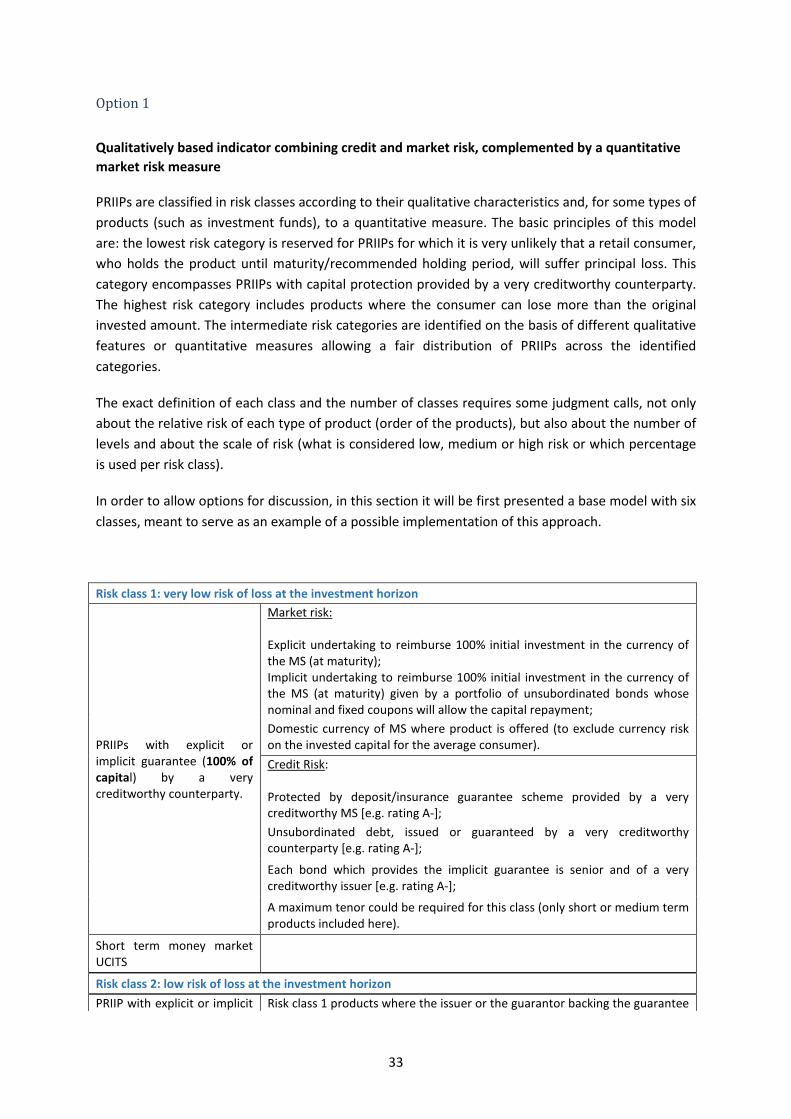
Option 1

Qualitatively based indicator combining credit and market risk, complemented by a quantitative market risk measure

PRIIPs are classified in risk classes according to their qualitative characteristics and, for some types of products (such as investment funds), to a quantitative measure. The basic principles of this model are: the lowest risk category is reserved for PRIIPs for which it is very unlikely that a retail consumer, who holds the product until maturity/recommended holding period, will suffer principal loss. This category encompasses PRIIPs with capital protection provided by a very creditworthy counterparty. The highest risk category includes products where the consumer can lose more than the original invested amount. The intermediate risk categories are identified on the basis of different qualitative features or quantitative measures allowing a fair distribution of PRIIPs across the identified categories.

The exact definition of each class and the number of classes requires some judgment calls, not only about the relative risk of each type of product (order of the products), but also about the number of levels and about the scale of risk (what is considered low, medium or high risk or which percentage is used per risk class).

In order to allow options for discussion, in this section it will be first presented a base model with six classes, meant to serve as an example of a possible implementation of this approach.

Risk class 1: very low risk of loss at the investment horizon

PRIIPs with explicit or implicit guarantee (100% of capital) by a very creditworthy counterparty.

Market risk: Explicit undertaking to reimburse 100% initial investment in the currency of the MS (at maturity); Implicit undertaking to reimburse 100% initial investment in the currency of the MS (at maturity) given by a portfolio of unsubordinated bonds whose nominal and fixed coupons will allow the capital repayment; Domestic currency of MS where product is offered (to exclude currency risk on the invested capital for the average consumer). Credit Risk: Protected by deposit/insurance guarantee scheme provided by a very creditworthy MS [e.g. rating A-]; Unsubordinated debt, issued or guaranteed by a very creditworthy counterparty [e.g. rating A-];

Each bond which provides the implicit guarantee is senior and of a very creditworthy issuer [e.g. rating A-];

A maximum tenor could be required for this class (only short or medium term products included here).

Short term money market UCITS

Risk class 2: low risk of loss at the investment horizon PRIIP with explicit or implicit Risk class 1 products where the issuer or the guarantor backing the guarantee

33

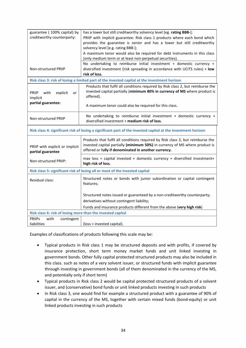
guarantee ( 100% capital) by creditworthy counterparty:

has a lower but still creditworthy solvency level [eg. rating BBB-]; PRIIP with implicit guarantee: Risk class 1 products where each bond which provides the guarantee is senior and has a lower but still creditworthy solvency level [e.g. rating BBB-]; A maximum tenor would also be required for debt instruments in this class (only medium term or at least non-perpetual securities).

Non-structured PRIIP No undertaking to reimburse initial investment + domestic currency + diversified investment (risk spreading in accordance with UCITS rules) + low risk of loss.

Risk class 3: risk of losing a limited part of the invested capital at the investment horizon

PRIIP with explicit or implicit partial guarantee:

Products that fulfil all conditions required by Risk class 2, but reimburse the invested capital partially (minimum 80% in currency of MS where product is offered).

A maximum tenor could also be required for this class.

Non-structured PRIIP No undertaking to reimburse initial investment + domestic currency + diversified investment + medium risk of loss.

Risk class 4: significant risk of losing a significant part of the invested capital at the investment horizon

PRIIP with explicit or implicit partial guarantee

Products that fulfil all conditions required by Risk class 3, but reimburse the invested capital partially (minimum 50%) in currency of MS where product is offered or fully if denominated in another currency.

Non-structured PRIIP: max loss = capital invested + domestic currency + diversified investment+ high risk of loss.

Risk class 5: significant risk of losing all or most of the invested capital

Residual class: Structured notes or bonds with junior subordination or capital contingent features;

Structured notes issued or guaranteed by a non-creditworthy counterparty; derivatives without contingent liability; Funds and insurance products different from the above (very high risk) Risk class 6: risk of losing more than the invested capital PRIIPs with contingent liabilities (loss > invested capital).

Examples of classifications of products following this scale may be:

• Typical products in Risk class 1 may be structured deposits and with profits, if covered by insurance protection, short term money market funds and unit linked investing in government bonds. Other fully capital protected structured products may also be included in this class. such as notes of a very solvent issuer, or structured funds with implicit guarantee through investing in government bonds (all of them denominated in the currency of the MS, and potentially only if short term)

• Typical products in Risk class 2 would be capital protected structured products of a solvent issuer, and (conservative) bond funds or unit linked products investing in such products

• In Risk class 3, one would find for example a structured product with a guarantee of 90% of capital in the currency of the MS, together with certain mixed funds (bond-equity) or unit linked products investing in such products

34

• In Risk class 4, one can find a structured product in a foreign currency, a structured note with a guarantee of 70%, a perpetual note or an equity fund.

• In Risk class 5, highly leveraged AIFs or long options and warrants • In Risk class 6, short options and IRS

Alternative ways to define and measure levels of loss (to be applied only for non-structured PRIIPs with diversified investment) may be set up as follows:

1st alternative => average loss

• for products with recommended investment horizon up to 10 years, average loss at the recommended investment horizon simulated on 20 years of historical rolling monthly data

• for products with recommended investment horizon over 10 years, the historical observation period is extended to the double of the investment horizon

• missing history is substituted by market indices, peer indices, similar products • low is below 5%, medium is below 20%, high is below 50%

2nd alternative => volatility

• annualised volatility of the underlying calculated using ten years of monthly returns • missing history is substituted by market indices, peer indices, similar products • for absolute return funds, the maximum between historical volatility and the volatility limit

is used • for total return funds, life cycle funds and maturity funds, the maximum between historical

volatility and the volatility of the riskiest asset mix (possible in the future) is used • low is below 2%, medium is below 10%, high is below 30%

3rd alternative => SRRI (UCITS current indicator)

• low risk: SRRI 1-2 • medium risk: SRRI 3 • high risk: SRRI 4-5 • very high risk: SRRI 6-7

Other possible variations of the boundaries between risk classes and alternative scales

• Creditworthiness thresholds: o Complementary mitigating factors may be taken into account such as the presence of

collateral or segregation (cfr. section on credit risk), which may lead to a more favourable credit risk assessment;

o Alternative credit risk assessments may be considered for credit institutions and insurance undertakings without credit rating due to prudential supervision.

• Money market funds may be eliminated from Risk class 1 as there is no explicit or implicit guarantee.

• Limits in tenors. More severe limits may be required for all classes (ex: 3 years for Class 1, 5 years for Class 2, 10 years for Class 3). On the contrary, limited tenor may only be required for non-public counterparties or PRIIPs not protected by deposit/insurance guarantee fund,

35

or tenor limit might be eliminated except for perpetual instruments (not admitted in Classes under 4).

• Partial guarantee allowed in Class 3 may be higher (90%), or permitted only for short term products. In parallel, partial guarantee in Class 4 may also be higher.

• Low, medium and high risk may be defined using a different scale. Note that it is important to align the risk scale defined with other measures with the one used for funds to avoid any incoherence.

• Finally, the scale may be adapted to a different number of levels (expanded to 7 levels, potentially more difficult to calibrate, or reduced to 5 risk classes).

A “five risk classes” indicator would have less discriminatory power but added simplicity. For this purpose, Class 5 would include, together with the products with contingent liabilities, highly leveraged products and all derivatives. Class 4 would then be defined as the residual class.

The main advantages of this approach are:

• it takes into account low probability but high impact events by focusing for a large set of PRIIPs on the worst case (market risk) scenario (likelihood of suffering complete or nearly complete loss of the principal) and avoids moral hazard issues due to underrating of extreme events that could be the consequence of a purely quantitative approach.

• Applicability/Comparability: it allows the classification of all PRIIPs in product type groups on the basis of a limited number of risk-related criteria, without having the need to dispose for all PRIIPs of appropriate market data that may not always be available, and making them easily comparable.

• Feasibility: it is easy to implement by the industry, the criteria being relatively easy to apply by all product manufacturers, both well sophisticated financial groups and small manufacturers.

• Robustness: it is objective and independent from the manufacturer (it relies less on assumptions or calculations by the manufacturer), hence it is difficult to manipulate.

• Supervision: it is easy to supervise, the criteria can be applied without difficulty, reducing the implementation costs for the supervisory authorities.

The main limitations of an approach with high reliance on qualitative measures are:

• Reliability: the indicator is focused on the possibility of certain levels of losses but is not able to measure the likeliness of the different loss outcomes for a large part of PRIIPs. The combination of qualitative features inevitably implies to a certain extent judgment - the relative impact of each feature on the risk profile may be difficult to assess.

• Discrimination: the indicator is not able to discriminate certain product types on the basis of the market risk before maturity, notably fully guaranteed products, which are discriminated on the basis of credit risk.

Question 9: Please state your views on the most appropriate criteria and risk levels´ definition in case this approach was selected.

36

Option 2

Indicator separating assessment of market risk - quantitative measure based on volatility - and credit risk - qualitative measure, external credit ratings

Market and credit risks are assessed separately, over two different scales, and combined such as to produce a two dimensional risk indicator. As far as credit risk is concerned, the indicator differentiates products among 7 risk classes, going from A to G, on the basis of the issuer´s or guarantor´s credit rating. The credit risk grading grid has been designed to be consistent with the generic classification used by major rating agencies (e.g. Standard & Poor´s, Moody´s, Fitch).

The viability of this option in legal terms could require further analysis, since, as mentioned, the level one text refers to a summary risk indicator (in the single), which combines the different risks of importance for the consumer in a summary format, and there is some discussion as to whether an indicator that shows market and credit risk separately can comply with this obligation. The discussion of this option here does not address this point.

Market risk is assessed in a purely quantitative way, based, to a very big extent, on the methodology currently in place for UCITS, implying that products are classified in one of 7 risk classes, according to their volatility. However, as mentioned before, for products that have a (conditional) capital guarantee, volatility in itself might not be an appropriate measure of risk. In fact, the current UCITS´ guidelines already advocate a special treatment for structured UCITS, under a Black-Scholes´ VaR based volatility calculation.

Considering PRIIPs´ two main features – a level of capital protection at maturity, if any, and an exposure to the performance of one or several underlying assets – this indicator splits their market risk in the corresponding two components, the “bond” one and the “risky” one,

• Bond component risk contribution = % capital guarantee x tenor x rate volatility • Risky component risk contribution = % capital at risk x delta x underlying volatility,

such that the product´s aggregate volatility is given by the sum of both. This aggregate volatility figure is calculated for a very short holding period, 5 or 20 days, and then scaled to an annual volatility (multiplied by square root of time).

One can already see that in the case of fully capital protected products, the contribution to risk given by the “risky component” is zero, risk being given by “tenor x rate volatility” alone.

So, there is a two tier rationale underlying the indicator, whose market risk measure is essentially volatility based: 1) the volatility of a product´s bond component can be fairly approximated by the volatility of the corresponding zero coupon bond and 2) the product´s sensitivity to the moves of the underlying asset(s) can be assessed by computing its delta(s) – accordingly, this second component uses the so-called delta approximation to compute volatility. Since the indicator was designed to be consistent with the UCITS methodology, it uses 5 year realized volatilities of the various assets underlying PRIIPs; and it also combines that historical data with forward looking one (delta/implied volatilities).

37

The indicator´s major advantages are:

• Reliability: It is close to a full valuation approach, since to get deltas (for some products) one needs all the same technology that is required for valuing the whole product (e.g. option pricing).

• Feasibility: Risk statistics are easy to obtain provided deltas can be properly calculated, (which presumably manufacturers do already, for hedging purposes). Accordingly, for the asset management industry it would not involve significant additional costs, as it is related to current practice.

On the other hand, its main disadvantages are:

• New risk measure that has not been put to test: lack of theoretical or academic support. • Applicability: short term risk measure based on market values may not be applicable to all

products in scope (notably insurance products and those for which no reliable daily valuations are available).

• Reliability: the delta approximation approach applies well only for basic capital guaranteed structured products (i.e. composed of a risk free bond and one simple call option on a single underlying) but less well for other structured products, and nonlinear products in general.

• Robustness: the fact that some risk factors are neglected (notably volatility and correlation) leads to inaccurate risk estimates (too high or too low, for products with capital protection in particular), potentially increasing gaming.

• Supervision: delta calculation would require supervisors to check the pricing of the products.

Possible variations of the indicator may be envisaged

For the credit risk measure, some refinements such as the ones proposed in previous sections (see section 2.3.1.2 about credit risk measures) could be applied, namely stricter requirements on number of CRAs assigning a given rating, and alternative credit risk assessments for credit institutions and insurance undertakings without credit rating due to prudential supervision. It is also possible to refer to ongoing work by Basel Committee on replacement of credit ratings by quantitative indicators.

As for market risk, if volatility was to be preferred as a risk measure, and given the limited use of delta, as discussed, it could be derived from any kind of forward looking simulation.

Otherwise, the CESR guidelines on the methodology for the calculation of the synthetic risk and reward indicator in the KIID (CESR / 10-673) have suggested (Box 8) a way of accommodating a volatility based approach of the risk measure to some types of products (structured funds in that case) for which a VaR based measure of risk seems more appropriate, using the Black and Scholes modelling framework. The extent to which this type of approach could be extended to different types of PRIIPs could be further investigated.

In addition, it might be argued that for those PRIIPs for which a volatility based measure does not seem relevant, notably because of their specific volatility cycle (e.g. Real estate or private equity funds), one could set up normalized values of the risk measure / indicator.

38

Question 10: Please state your views on the required parameters and possible amendments to this indicator.

Option 3

Indicator based on quantitative market and credit risk measures calculated using forward looking simulation models

Several alternatives have been proposed within this framework.

On the one hand, an approach developed by the structured products industry in Germany, in place since 2005, based on the 99% VaR calculated with the help of a Monte Carlo simulation. It is a full valuation approach, given that all the product´s relevant risk components (credit risk premium, underlying prices, implied volatility, foreign exchange rates, interest rate - with their constant correlations assumed) are identified and simulated for a common defined holding period (e.g. 10 days and/or 1 year), on the basis of historical data (normally distributed returns of risk factors given by 2 years realized volatilities and correlations and zero drifts). The product is classified into one of the 5 risk classes, depending on the derived VaR.

The indicator rests on the major premise that comparability of risks can only be achieved if an identical holding period for all products is set and applied. Short time risk is used for the risk classification.

On the other hand, modelling using longer time frames has also been proposed. Under these approaches, returns are simulated for the whole investment horizon (standard end of maturity, but if the risk of the product varies over time, then different holding periods are considered).

Irrespective of the time frame used to calculate returns, there are some key decisions that have to be taken for this approach, in relation to the use of standard assumptions, to ensure consistency and comparability:

• The standardization may apply to the parameters used, that may be defined per asset class level. In order to get reasonable and stable parameters - expected returns, VaR/cov of the risk factors, as well as risk-free rates and FX rates - long series of historical data may be used (such as 30 years), or an independent entity (regulator) may set and review them regularly.

• Standardization may also be required for models governing the evolution of risk factors. Alternatively, some freedom may be left to manufacturers to use their internal pricing models, in so far as they are coherent with the common parameters set. When the return distribution cannot be analytically derived, Monte Carlo simulations should be used, leaving down to regulators the recommendation regarding environmental parameters (e.g. length of time step) and to manufacturers the choice of the stochastic processes.

• Discretion may be left to manufacturers regarding the choice of model and/or parameters, within certain guidelines or principles.

Finally, different statistical measures can be calculated from the previously generated distribution of returns. Downside measures are favoured under these approaches (that is, measures considering

39

the loss part of the distribution) but symmetrical measures such as volatility can easily be computed too. The following alternatives have been mentioned:

• a VaR measure, either with a 99% or a 95% confidence level. • a combination of the average of the 20% worst cases (expected shortfall) and the expected

returns of the distribution. • a 50% expected shortfall.

Based on the derived products´ distribution for the market risk factors, credit risk may be integrated in different ways:

• Incorporating credit spread volatility into the product´s return distribution. • Incorporating issuer default scenarios into the distribution of returns, according to the

default probability (and recovery assumptions) derived either from credit ratings or from credit spreads or other quantitative risk measures. Credit spreads, for instance, may be directly inferred from the outstanding issuers´ bonds or, should there be no sufficient number available, approximated by the issuer rating. If no such rating is available, the credit spread can be proxy from peer companies.

• Measuring credit risk over a separate scale (using external credit ratings) and showing both market and credit risk scales separately, and, if deemed necessary, using the maximum of both scales as the overall indicator (similar to the solution proposed for the previous approach).

The integration of credit risk using the first two alternatives leads to one product return distribution, hence total risk can easily be computed as VaR or ES (or volatility).

For this third approach, main advantages identified are:

• Applicability: in general, the approach may be neutral across all products in scope, given that all relevant risk factors are taken into account.

• Reliability: full valuation approach grounded on well-established research and industry application for risk valuation and management; compatible with consumers´ risk perceptions (loss and uncertainty).

• Discrimination: potentially high, since it delivers a complete distribution of returns from which VaR as well as other statistical measures (such as ES or volatility) can be derived.

• Robustness: high in case of decision in favour of parameters and model prescription. However, though prescriptive approaches offer consistency, there are a number of drawbacks, notably in relation to the significant level of market changes that happen over time, such that parameters choices rapidly become inappropriate, as well as difficulties in setting parameters covering 100% of PRIIPs. On the other hand, for firms using internal pricing models, market pressure and existing regulatory oversight may allow reasonable comparison between manufacturers.

• Comparability: results are comparable once parameters and models are determined.

Main disadvantages of this third approach are:

40

• Feasibility: possibly high initial implementation costs for manufacturers; complexity of risk calculation dependent on product´s complexity.

• Supervision: possibly high initial implementation costs for regulators, further requiring parameter setting and updating.

Question 11: Please state your views on the appropriate details to regulate this approach, should it be selected.

Possible amendments to this approach

One variation to this third approach is a forward looking model that uses the end of maturity as the default holding period, but if risk of a product varies over time, then different holding periods will be shown to reflect the change of risk over time. This approach would use a calculation method based on Monte Carlo and a prescribed ‘model world’ (such as Black Scholes) for all products in order to have comparable results. If manufacturers can prove that internal models are equivalent to the prescribed model world and lead to equivalent risk indicators, their own internal models can be used. As for product parameters, this approach assumes that regulators decide upon them as much as possible.

The market risk factors that are to be taken into account are all relevant factors that determine the risk for the respective holding periods; 1) structured products: underlying prices, volatilities of implied volatility, foreign exchange rates, interest rates, credit spreads and general assumption of constant correlations; 2) simple products such as normal funds: analytical risk, e.g. historical risk; 3) dynamic investment strategies: benchmark investments; additional description of algorithms. As for dynamic investment strategies; for some investment funds and insurance products: clear description of strategies, risk premiums, cost reimbursement schemes and algorithms in order to enable outsiders to replicate the risk calculation; because of competitiveness reasons no public disclosure of precise algorithms (disclosure only to regulators).

The credit risk factors can be integrated into the simulation via a Poisson distribution considering the default risk of a PRIIP, e.g. very low for insurance products where guarantee schemes need to be considered.

Possible extensions of this approach include:

• Comparisons and back testing - Proposal for continuing comparisons of products, back testing rules and incentives e.g. as in CRR in order to calibrate and develop the model and parameters ( regulator should decide on this).

• Proposal to set-up a public database - PRIIPs models which include all public pieces of information, e.g. risk factor mappings and risk premiums, in order to enable outsiders to replicate the risk calculations.

Question 12: Please state your views on the general principles of this approach, should it be selected. How would you like to see the risk measure and parameters, why?

41

Option 4

“Two-level” indicator

The “first level” of such an indicator would distinguish products in a very broad or simplified dimension (for instance, products where capital is at risk, from those with capital protection, or those where consumers may lose more than capital invested). The “second level” could be used to provide retail consumers with a finer grained insight of the information contained in the “first level”, therefore enabling them with an additional “tool” to better discriminate products classified in the same “first level”. This approach might enable the use different methodologies to be applied to different types of products in relation to the “second level”. Whereas the first level may differentiate the products merely on characteristics (max. capital at loss), the division at the second level could be based on a more quantitative measure (such as a volatility or loss based measure as described above).

The main advantage of a two level indicator is that it provides more possibility to discriminate amongst products. In case the risk indicator would only contain 7 buckets, it would imply that many products with different levels of ‘risk’ would fall in the same bucket, making the discrimination purpose of the PRIIPs Regulation less easy to achieve. A major disadvantage is the comparability between classes. How would the risks of the different level 2 relate to each other? Furthermore, it is difficult to compare products if they are first segregated on the basis of a general product characteristic. Finally, it is difficult to foresee whether consumers would understand such a two level indicator. This should result from the results from the Consumer Testing.

Question 13: Please state your views on the potential use of a two-level indicator. What kind of differentiators should be set both for the first level and the second level of such an indicator?

Scale of the Risk Indicator 2.3.3.2

Irrespective of the fact that the risk level is being assessed on a quantitative and/or on a qualitative basis, as per the decided risk indicator, one must think of a way to define the proper scale of the indicator, i.e. the number, designation and limits of each risk class or “bucket”. The definition of the scale of the risk indicator is seen as paramount, having a direct impact on its comparability and discrimination properties. The decision is all the more relevant considering the fact that, as the number of risk buckets increases, the improved discrimination power of the indicator comes quite probably at the expense of its comparability.

Some of the quantitatively based risk indicators currently used in the marketplace have set up the boundaries in order to reflect the economic risk of products, such that capital protected ones, for instance, would always fall in the lower class(es), as opposed to, say, illiquid and more volatile assets, that would need to classify on the higher risk classes. These boundaries have been determined on the basis of long term risk estimates of benchmark assets, raising the question as to how frequently they should be re-assessed.

As an example, the short term VaR based risk indicator used in Germany since 2005 classifies investment products over a scale of 5 classes, where 1 is called “conservative” and 5 is defined as “speculative”. The risk classes were defined in the following way:

42

• Class 1 was defined to cover short term bonds for highly rated issuers and medium term European government bonds (7-10 years). (VaR limit €250)

• Class 2 was designed to cover pan-European real estate investment, an investment in gold and a diversified commodity investment. (VaR limit €750)

• Class 3 was based on well diversified equity indices or low volatile blue chips. (VaR limit €1.250)

• Class 4 was calibrated to cover blue chip stocks. (VaR limit €1.750) • Class 5 should cover volatile stock investments and also highly leveraged products.

Correspondingly, the current 1 to 7 buckets scale used by the UCITS risk indicator, volatility based, implies a more conservative definition of risk - equity funds, for example, may in general terms be found in level 5 or 6 (that is not medium risk).

Risk indicators of a qualitative nature tend to use letters, rather than numeric scales. Credit risk, notably, if assessed on the basis of external credit ratings, can be classified in classes A (Prime) to G (Imminent Default).

So far, the analysis about how to determine the risk scale to use in the risk indicator is not concluded yet.

Question 14: Do you have suggestions or concrete proposals on which risk scale to use and where or how the cut-off points should be determined?

43

Performance scenarios 2.4

From a consumer behavioural perspective, a lot of research shows that consumers have a strong preference for getting information on the expected returns of an investment. This is recognized not only in literature but also by the wide use of expected returns in performance scenarios found in marketing material. Therefore, showing possible outcomes of the product is an important part of the KID to standardise and to display explicitly.

On the other hand, research shows that individuals have difficulties in perceiving the relationship between risk and return and apparently understand returns better than risks. Framing effects and emotional factors may affect both return and risk perception. Therefore, when representing the performances of financial products special attention needs to be paid to the way financial information is represented, to avoid misinterpretations.

The decisions to make about the representation of the product performance in the KID can be structured in steps. The first step is to decide on how to choose the scenarios (hypothetical scenarios, a probabilistic approach or a combination of both). The second step is to decide on how to construct the scenarios (methodological issues about how to actually generate or compute the performance in each scenario). For the third and final step one needs to decide on how to present the scenarios. In this Technical Discussion Paper focus is on the first two steps. Consumer research is being carried out in parallel, to inform the decisions about presentation.

As a preliminary reflection, the elements below are relevant for the performance scenarios:

• to reduce manufacturer discretion as far as possible in the selection of scenarios, in order to increase comparability of different KIDs and avoid the risk of arbitrary choices of the manufacturer, potentially resulting in performance information that does not appropriately reflect realistic possible outcomes of the product.

• to present helpful information to consumers, while avoiding the risk of anchoring to the numbers presented in this KID´s section, confusing scenarios with a promise of a future result

2.4.1 Feedback from the public consultation on JC/DP/2014/02

In relation to the first step (how to choose scenarios) two basic approaches in this area were already included in the Discussion Paper: ”what if” hypothetical scenarios vs probabilistic approach.

Most of the respondents were in favour of hypothetical scenarios, but there was also a relevant number of respondents who preferred a probabilistic approach. In favour of hypothetical scenarios, respondents argued that this approach provides a clear explanation about how the product works. A probabilistic approach may confuse the consumer and makes it more difficult and costly than necessary to produce the KID. However, respondents who favoured a probabilistic approach argued that it provides helpful information to consumers as it enables them to assess the likeliness of the returns presented, whereas hypothetical scenarios may suggest to the customer that the scenarios are equally probable or that the middle scenario is the most likely. Finally, some respondents defended that information about performance should include past or historical performance.

44

As for the second step (how to construct the scenarios), most respondents supported presenting performance information as net of costs, since it was seen as a more valuable information for consumers, whereas gross figures may be misleading as they cannot be achieved. However, some respondents defended gross performance (considering that it would present the mechanics of the product more clearly, and enable better comparison), or showing both gross and net figures in the performance section. A particular area considered problematic was the treatment of insurance premium (in defence of excluding insurance premium in the performance scenario). Finally, several respondents flagged the importance of consistency between the performance scenarios´ section and the costs´ section.

2.4.2 How to choose performance scenarios: discussion about different approaches

Considering the feedback received on the Discussion Paper and ongoing discussions, the ESAs are still analysing both general approaches previously discussed and seek in additional input about the options to regulate in detail each approach in this Technical Discussion Paper.

First, possible approaches are described and some options to regulate or further define them are explored, including a combination of different options. Second, a summary of the main strengths and weaknesses of each approach is presented, reflecting the current analysis of the ESAs on this topic. Section 2.4.4 below will deal in detail with how to construct the scenarios in each approach and possible details of the regulation that would be required for each one.

What-if or hypothetical scenarios 2.4.2.1

This approach shows the client how the product will perform under different market conditions (what would happen if…). The scenarios are then the market situations that are selected to show future performance. No indication is provided about the likelihood of each situation. However, some information about the criteria, on the basis of which the negative/neutral/positive scenarios are built, could be given to the investors (e.g. hypotheses on the growth rate/performance of the underlying investments, or the length of return time series in case of historical scenario). In this way, the meaning of each scenario and the way in which they differentiate from each other could be more understandable for investors.

There are different ways to select the market conditions that need to be shown. One could essentially leave the choice of the scenarios to the manufacturer (what-if manufacturers choice) while another one could prescribe under which market conditions the performance scenarios need to be reflected (what-if prescribed). The approach taken could be different for different types of products (e.g. it might be useful to select those market conditions in which products that have specific features will be triggered such as knock-out of early redemption).

With the previously stated element of manufacturer´s discretion, the following options within hypothetical scenarios are proposed.

What- if: manufacturers choice approach

This approach leaves the responsibility and flexibility of selecting the scenarios with the manufacturers within certain high level guiding principles. These principles may be defined in a

45

similar way to current UCTIS KII guidelines. In short, these guidelines require manufacturers to select at least three scenarios to illustrate how the pay-out works, showing an unfavourable, a medium and a favourable outcome, as well as additional scenarios showing the impact of specific features of the product if needed. The examples shall be based on reasonable assumptions about future market conditions and the information shall follow the overriding principle of being fair, clear and not misleading.

What- if: prescribed approach

This option aims to define certain standardized scenarios, without any implication about their likelihood, which would be used by all manufacturers and all types of products in order to make performance information fully comparable and reduce discretion of manufacturers in selecting scenarios. The main difficulty of this option is to be able to find scenarios that are meaningful for very different types of products, and that may keep on being appropriate over time. A decision on what risk factors to consider for each type of product needs to be made.

Probabilistic approach 2.4.2.2

The second approach consists of defining the scenarios according to the likelihood of the possible returns. The scenarios could be defined by percentiles of the product return distribution and would be the same across all products and manufacturers. It should be stressed that the represented probabilities are cumulative and refer to parts of the return distributions (i.e. the tails in case of negative/positive scenarios) and not to specific points.

The probability of each scenario may or may not be disclosed in the KID. Although information on the probability of each scenario may be valuable for the consumer to understand this section, it is potentially difficult for consumers to interpret the information on probabilities correctly. Evidence obtained from the consumer testing will be considered to make that decision.

Lastly, with respect to the presentation of performance it could be useful to add some warnings, which put on evidence that reported performance scenarios are subject to statistical errors and model risk; moreover, it could be stressed that the scenarios may shift over time.

Combination of approaches 2.4.2.3

Another possible option would be a combination of the proposed approaches (e.g. prescribe two scenarios and leave one scenario up to the manufacturer that demonstrates the specific characteristics of the product). Or even, considering a scenario based on probability (combined with some standardised scenario) and a further one adapted to the product, to show how a special feature of the product may impact results.

In particular it may be appropriate to include, whichever final approach is selected, a scenario showing the event covered by the insurance element. That would be coherent with the presentation of insurance premium as a cost. An example would be for a life insurance product to present a scenario in which the policyholder dies.

46

2.4.3 Assessment of different approaches

What-if: manufacturer choice 2.4.3.1

What-if scenarios selected by the manufacturer are useful to demonstrate the product characteristics, which may be specifically helpful for nonlinear pay-offs.

Consumers face difficulties interpreting performance information. In this kind of scenarios, one of the difficulties is that consumers may interpret that all scenarios presented are equally likely or that the middle one is the most likely.

The representativeness of scenarios selected under a what-if approach does not depend on a model (i.e., not subject to model risk). However, there is no guarantee that the picture it provides of the product is accurate or realistic, as it depends on the choices of the manufacturer. This approach is relatively easy to manipulate and comparability is low because manufacturers can choose different scenarios.

Implementation by manufacturers is relatively easy and no significant costs are expected. These kinds of scenarios are very stable and would not trigger revision of the KIDs, as they are selected to reflect the functioning and features of the product, which do not change.

From a regulatory/supervisory perspective, this approach is relatively easy to regulate (only high principles are needed) and to supervise as no calculations need to be checked. However, it might be difficult to supervise whether the chosen scenarios are reasonable.

What-if: prescribed approach 2.4.3.2

In a what-if approach with prescribed scenarios consumers get comparable information that may reflect different aspects of the product and may help them understand the functioning and risk of the product if they are well defined. A prescriptive approach reduces the risk of manufacturers manipulating this element. Additionally, these scenarios are also quite stable and easy to implement (no significant costs, but some limited costs to implement an historical scenario).

However, it is very difficult to set scenarios that can provide useful and relevant information for all PRIIPs in scope (from an equity based CFD to a bond fund or a with profit insurance contract). Relevant risk factors need to be identified. Different scenarios (in particular if growth assumptions are considered) may need to be defined to accommodate for different underlying assets and different pay-offs. However, comparability may be difficult in this case across different types of products.

Regulators are responsible for the definition and monitoring of the scenarios. Periodic revisions of the scenarios may be necessary to keep them meaningful if market conditions change.

Finally, under a predefined approach there is a risk of manufacturers designing their product to optimize presentation given the predefined scenarios that may introduce distortions in the market.

47

Probabilistic approach 2.4.3.3

Presenting scenarios that are selected according to their probability helps consumers to assess which return can reasonably be expected and may provide a more realistic picture of products, in particular for those products that only provide good returns in extreme situations.

On the other hand, consumers may face difficulties interpreting these kinds of scenarios as they may be seen as a promise. In particular, presenting a negative scenario with no potential losses may lead consumers to believe there is no risk at all. Hence, presentation issues, and in particular, the narratives explaining the information provided, need to be carefully designed, should this approach be selected.

Estimation of future events is very difficult, in particular with long term horizons. The reliability of the information in a probability approach depends on methodological assumptions and input data used for modelling performance. Whereas for risk measurement the impact of the risk premiums may be less relevant (because the aim is to compare products), economically meaningful estimates of performance scenarios need more realistic assumptions on the risk premium.

Potential biases are particularly relevant if the probability of each scenario is disclosed.

Probability approaches may be robust and comparable as the same scenarios are defined for all products with no discretion for manufacturer. However, the underlying methodologies and assumptions may need to be sufficiently standardised to fully achieve this goal.

A probability approach requires a methodology that may be costly to implement. In addition, scenarios chosen by probability are less stable than in other approaches, as changes in the market conditions may trigger revision of thresholds, as the likelihood of the different outcomes changes. Revision of KID may also imply higher costs for this option. Similar modelling methodology may already be in place for the risk indicator, reducing implementation costs, although methodologies required may differ to some extent.

From a regulatory/supervisory perspective, a probabilistic approach is relatively easy to set if a normative approach is used, whereas a more prescriptive approach may increase difficulty. Additionally, supervising the implementation needs more resources compared to other approaches.

Question 15: Please express your views on the assessment described above and the relative relevance of the different criteria that may be considered.

2.4.4 How to construct performance scenarios: methodological details to be prescribed in the regulation and input required

Definition and number of scenarios 2.4.4.1

What–if: manufacturer choice

If this approach were adopted, the initial proposal would be to replicate UCITS guidelines on performance scenarios.

48

Question 16: Do you think that these principles are sufficient to avoid the risks of manufacturers presenting a non-realistic performance picture of the product? Do you think that they should be reinforced?

What- if: prescribed approach

If this approach is adopted, the regulation should define appropriate scenarios that may be valid and meaningful for all PRIIPs. Options to define standard scenarios that have been proposed are:

a) An historical scenario: Past performance over the last x years - where x may be the recommended holding period, or a graphical presentation of historical outcomes in different periods - for instance, what would have been the performance of the product if it had been launched weekly in the last 10 years?

b) Set a predefined growth rate/performance of the underlying investment(s). For example: showing what would happen if the underlying price goes up 10%, 0% and falls 10%. In case of several underlying investments, this % may be applied as an average performance of the underlying assets or as the performance of the relevant one (worst performing is a worst-off for example). As it is very difficult to define reasonable % for different products, it may be necessary to define different scenarios for different types of products and to keep them updated. The % may be based on an assumed growth rate per asset class. (e.g. a 5.5% growth rate for equities and a 3% growth rate for corporate debt etcetera).

Question 17: Do you think the options presented would represent appropriate performance scenarios? What other standardized scenarios may be fixed?

Probability approach

A first step for a probabilistic approach is to set a distribution of returns for the period over which the performance scenario is displayed. For this specific discussion we refer to section 2.2.1. The other main issue to set in this approach is to define the percentiles of the distribution that would be shown as negative, neutral and positive scenarios.

For instance, consider the following three scenarios: a pessimistic scenario as the 10th percentile of the distribution, a neutral scenario as the 50th percentile and an optimistic scenario as the 90th percentile. In the answers to the Discussion Paper other percentiles have been mentioned, such as the 25th and the 75th.

Question 18: Which percentiles do you think should be set?

Combined approach

Examples of possible combinations of scenarios are the following:

a) An historical scenario + a pessimistic scenario (set as 10th percentile based on probabilistic approach) + a predefined rise in the underlying asset (e.g. the drift of the underlying asset) + an additional scenario to illustrate specific features of the products not illustrated before.

49

b) A positive scenario (maximum the 90th percentile) + a worst case scenario + a predefined evolution of the underlying asset (+/- x%, defined according to the type of assets) + an insurance event.

c) Probability approach (three scenarios) + an insurance event.

Question 19: Do you have any views on possible combinations?

Other methodological issues to calculate performance in each scenario 2.4.4.2

Inclusion of credit risk events in the scenarios

Performance scenarios may be defined to inform about potential return in different market circumstances or they may also include credit events of the issuer or counterparty. The second alternative implies that in certain products the negative scenario would be the issuer default.

Question 20: Do you think that credit events should be considered in the performance scenarios?

Inclusion of specific redemption events in the scenarios

Performance of a product may be influenced by voluntary or triggered redemption events. A voluntary redemption event would be the redemption of a life insurance product before the term of the contract. A trigger redemption event would occur when the condition of the product´s characteristic has taken place. Examples are auto-callable products that are being called and knock-out products that reach the knock out level.

In the case performance scenarios are presented only for the recommended holding period, such specific redemption scenarios may be particularly meaningful. Another alternative could be to include performance information on different holding periods, defined to show the impact of specific redemption events.

Question 21: Do you think that such redemption events should be considered in the performance scenarios?

Investment horizon of the scenarios

Performance scenarios will present potential return at the recommended holding period. In addition, it is being considered to present performance information also for different holding periods as a way to show consumers the potential difference in return if they decide to exit earlier.

That would mean that each scenario should be defined for different moments of time and performance should be calculated for each of these moments. The simplest way to define the scenario over time would be to define a constant evolution (for instance a 2% annual growth each year). However, this assumption may be problematic for certain products as it may give the impression of a more stable behaviour than in reality.

50

Calculating performance in the interim periods may also be problematic for certain products, in particular, for products with a fixed term where early exit is not guaranteed or products with low liquidity. The initial proposal would be to present the estimated fair value of such products at each time period defined (1, 3 and 5 years, for example), completed with a warning of the limitations of these figures.

Question 22: Do you think that performance in the case of exit before the recommended holding period should be shown? Do you think that fair value should be the figure shown in the case of structured products, other bonds or AIFs? Do you see any other methodological issues in computing performance in several holding periods?

51

3 Costs

Identifying the costs 3.1

Establishing a list that would be as comprehensive as possible of the different types of costs of the different types of PRIIPs is a pre-requisite for aggregating these costs in summary indicators. Indeed, the output of the parallel workflow on the presentation of costs, as well as the results of the consumer testing, might lead to the decision of splitting one aggregating indicator in different types of indicators (related to on-going costs, Entry/Exit cost, etc.), in addition to the presentation of one overall summary indicator taking into account all the different types of costs. Identifying the costs is also important to reach a more standardized view on the calculation of each type of costs, among the different types of PRIIPs, and therefore the calculation of the aggregated indicator(s). This is what the present section intends to do in relation to a) funds b) life-insurance products and c) structured products and SPVs. Because the terms designating the different types of costs might differ from one sector to another and from member state to another, it is of a paramount importance, so as to avoid double-counting to establish the principle that if one type of costs is for one sector in one member state covered by two or more types of costs as referred to in the present section, this type of cost is only accounted for once in the calculation of the summary indicators which are based on it. In addition to identifying the costs, the important information to be discussed in this section is the main features each of these types of costs, that is:

• when and how often it is charged; • what is the basis of this charge (percentage of premium, percentage of individual

reserve/fund, fixed amount, etc.); • is it conditional or unconditional?

The following section will discuss the aggregating of the costs. Aggregating the costs is not an easy issue precisely because the features of the different types of cost differ. Put in another way, the aggregation of the costs means transforming these different cost types into one of them.

52

3.1.1 Funds

General issues

In the case of a fund which is an umbrella, each constituent compartment or sub-fund shall be treated separately for the purpose of this section, but any charges attributable to the fund as a whole shall be apportioned among all of the sub-funds on a basis that is fair to all investors.

List of costs to be taken into account 3.1.1.1

The following list is indicative but not exhaustive of the types of costs that shall be taken into account in the amount to be disclosed in the case of funds:

Entry-Exit costs

These costs include entry / exit charges or commissions, or any other amount paid directly by the investor or deducted from a payment received by or due to the investor17.

The following list is indicative but not exhaustive of the types of entry-exit costs that shall be taken into account in the amount to be disclosed:

(a) Up front initial costs (e.g. distribution fees, loading costs, constitution costs, marketing costs, subscription fee);

(b) Acquisition costs.18

Question 23: Are the two types of entry costs listed here clear enough? Should the list be further detailed or completed (notably in the case of acquisition costs)? Should some of these costs included in the on-going charges? On-going charges

In the context of the KID, ‘ongoing charges’ are payments deducted from the assets of a fund where such deductions are required or permitted by national law and regulation, the fund rules or instrument of incorporation of the fund, or its prospectus. The figure to be disclosed in the KID shall be based on the total of all such payments made over a specific period.

The ongoing charges figure shall include all types of cost borne by the fund, whether they represent expenses necessarily incurred in its operation, or the remuneration of any party connected with it or providing services to it. These costs may be expressed or calculated in a variety of ways (e.g. a flat fee, a proportion of assets, a charge per transaction, etc.). The costs included in the ongoing charges might be divided into those costs which are fixed and those which are optional or variable, as performance fees and transaction costs.

17 Including costs such as fees to be paid to the commercial register in the case of close end funds (in particular real estate AiFs). 18 Please note that acquisition costs may have several layers (introduction, one fixed fee, %percentage of purchase).

53

As the KID is a pre-contractual document, the cost disclosure shall be ex-ante. However, it might be considered that the disclosure of some types of variable costs be revised when the KID in its entirety has to be revised (please see the corresponding part of the RTS).

The following list is indicative but not exhaustive of the types of ongoing charges that, if they are deducted from the assets of a fund, shall be taken into account in the amount to be disclosed:

(a) all payments to the following persons, including any person to whom they have delegated any function:

• the management company of the fund • directors or partners of the fund if an investment company • the depositary • the custodian(s) • any investment adviser.

Question 24: How should the list be completed? Do you think this list should explicitly mention carried interest in the case of private equity funds?

(b) all payments to any person providing outsourced services to any of the above, including:

• providers of valuation and fund accounting services • shareholder service providers, such as the transfer agent and broker dealers that are record

owners of the fund’ shares and provide sub-accounting services to the beneficial owners of those shares;

• providers of collateral management services; • providers of prime-brokerage services; • providers of property management services (if applicable -e.g. administrative maintenance,

operation and litigation costs for Real Estate AIFs).

Question 25: Should these fees be further specified?

(c) registration fees, regulatory fees and similar charges, including passporting fees;

Question 26: Should these fees be further specified? The “recovering fees” cover the following situation: when an investor receives income from foreign investments, the third-country government may heavily tax it. Investors may be entitled to reclaim the difference but they will still lose money in the recovering process (fee to be paid).

(d) recovering fees for specific treatment of gain and losses;

Question 27: Should these fees be further specified? The “recovering fees” cover the following situation: when an investor receives income from foreign investments, the third-country government may heavily tax it. Investors may be entitled to reclaim the difference but they will still lose money in the recovering process (fee to be paid).

54

(e) audit fees

(f) payments to legal and professional advisers;

(g) any costs of distribution, to the extent that these payments are known to the PRIIP manufacturer;

Question 28: This list is taken from the CESR guidelines on cost disclosure for UCITS. What is missing in the case of retail AIFs (real estate funds, private equity funds)?

In the case of private equity funds, would it be relevant to include a breakdown of flows, distinguishing those (“out”) paid by the fund for the proper functioning of its financial portfolio management from those (“in”) paid by the target company for the provision of advisory services. This breakdown would allow to clarify real costs for investors (instead of only indicating the net amount), knowing that “in” will be deducted from “out”).

In the case of costs of distribution, would this need to be detailed depending on the type of costs of distribution? To what extent are these costs different from the distribution fees mentioned in the Entry costs above?

(h) a performance-related fee payable to the management company or any investment or sub-

investment adviser (please see below for a more detailed analysis on these costs);

(i) financing costs, including interest on borrowing (including those provided by related parties);

Question 29: Which are the specific issues in relation to this type of costs?

(j) costs of capital guarantee or capital protection19;

Question 30: Is it relevant to include this type of costs in the costs to be disclosed in the on-going charges? Which are the specific issues in relation to this type of costs? Which definition of Costs for capital guarantee or capital protection would you suggest? (Contribution for deposit insurance or cost of external guarantor?)

(k) payments to third parties to meet costs necessarily incurred in connection with the acquisition or disposal of any asset for the fund’ portfolio, whether those costs are explicit (e.g. brokerage charges, taxes and linked charges) or implicit (e.g. costs of dealing in fixed-interest securities, market impact costs);

19 The guarantee might be granted to the investor through different types of contractual arrangements comprising up-front or ongoing payments: a guarantee given by a bank or a financial instrument such as a financial option with premiums paid upfront or each year, under fixed or variable terms depending on market conditions (in some equity funds, the payment equals the dividend of the underlying assets). In both cases, the cost to be disclosed might be computed as the total amount of premiums paid or as the positive difference between this amount and the « pure » premium defined as the fair value of the guarantee assuming no transaction costs or arbitrage (SEC’s approach).

55

• in relation to transaction-based payments made to any of the persons listed in (a) or (b), in respect of which the recipient is not accountable to the fund; all such amounts shall be taken into account in the published figure;

• please see below for a more detailed methodology for the calculation of these costs.

(l) payments incurred for the holding of financial derivative instruments;

Question 31: Which are the specific issues in relation to this type of costs? Should the scope of these costs be narrowed to administrative costs in connection with investments in derivative instruments? In that respect, it could be argued that margin calls itself should not be considered as costs. The possible rationale behind this reasoning would be that margin calls may result in missed revenues, since no return is realized on the cash amount that is deposited, and that:

i) No actual amount is paid to a third party. Hence, one could argue whether these should be defined as costs of investing from a fundamental point of view.

ii) It would be very challenging to quantify the actual missed revenue amount. Assumptions would be needed on the rate of return that would be realized on the deposited cash amount. Daily fluctuations in margin account balances will add to the complexity of required calculations.

(m) the value of goods or services received by the management company or any connected person in exchange for placing of dealing orders).

Question 32: Which are the specific issues in relation to this type of costs? Should this type of costs be further detailed/ defined?

(n) the costs of acquiring or disposing of units in UCITS or AIFs, which shall be taken into account in accordance with below:

• Where a fund invests a substantial proportion of its assets in UCITS or AIFs, its (total expense ratio) TCR/(Reduction in yield) RIY figure shall take account of the ongoing charges incurred in the underlying UCITS/AIFs. The following shall be included in the calculation:

• if the underlying is a UCITS its most recently available ongoing charges figure shall be used; this may be the figure published by the UCITS or its operator or management company, or a figure calculated by a reliable third-party source if more up-to-date than the published figure;

• the (total expense ratio) TCR /RIY figure may be reduced to the extent that there is any arrangement in place (and that is not already reflected in the fund’s profit and loss account) for the investing fund to receive a rebate or retrocession of charges from the underlying AIF/UCITS;

• in cases where subscription and / or redemption fees are payable by the fund in relation to the acquisition or disposal of units in an underlying UCITS/AIF, the monetary value of those fees shall be aggregated for the period under review and taken into account in the calculation of the (total expense ratio) TCR figure/RIY.

56

(o) the costs of acquiring or disposing of units in a PRIIP other than UCITS or AIFs, which shall be taken into account in accordance with below:

• where a fund invests in a PRIIP other than UCITS or AIFs, its (total expense ratio) TCR /RIY figure shall take account of the ongoing charges incurred in the underlying PRIIP. Its most recently available (total expense ratio) TCR /RIY figure shall be included in the calculation;

• the (total expense ratio) TCR /RIY figure may be reduced to the extent that there is any arrangement in place (and that is not already reflected in the fund’s profit and loss account) for the investing fund to receive a rebate or retrocession of charges from the underlying PRIIP;

• in cases where subscription and / or redemption fees are payable by the fund in relation to the acquisition or disposal of units in an underlying PRIIP, the monetary value of those fees shall be aggregated for the period under review and taken into account in the calculation of the (total expense ratio) TCR /RIY.

(p) the costs of acquiring or disposing of units in an investment product other than a PRIIP, which shall be taken into account in accordance with below:

• the PRIIP manufacturer shall either use any published information that represents a reasonable substitute for the (total expense ratio) TCR /RIY figure (e.g. a total expense ratio/RIY published by a reliable source) or else shall make a best estimate of its maximum level based on scrutiny of the investment product’s current prospectus and most recently published report and accounts;

(q) Under a fee-sharing agreement, the management company or another party may be meeting, in whole or in part, operating costs that should normally be included in the (total expense ratio) TCR /RIY figure.

• Any remuneration of the management company (or another person) that derives from such fee-sharing agreements shall be taken into account and added to the total (total expense ratio) TCR /RIY. Possible examples include the remuneration of a management company through a fee-sharing agreement with a broker on transaction costs, or with a custodian on stock-lending income;

• There is generally no need to take into account fee-sharing agreements on expenses that are already accounted for in the (total expense ratio) TCR /RIY disclosure (for example, the remuneration of a management company through a fee-sharing agreement with a fund which is captured under paragraph (a) above). However, in the specific case of a fund investing in other UCITS/AIFs, any fee-sharing agreement between the management company of the fund and the UCITS/AIFs or its operator or management company shall be taken into account if it is not already captured under paragraph (l) below.

(r) Earnings from efficient portfolio management techniques if they are not paid into the portfolio: A PRIIP manufacturer can use the securities contained in a portfolio to earn additional income through, for example, stock lending, repo, collateral swaps and reverse repo. To ensure a level playing field across PRIIPs, these earnings should be reported as a cost to the investor if they are not paid into the portfolio as they reduce the potential return earned by the investor;

57

(s) Implicit costs incurred by structured funds: please see the corresponding discussion in the “structured products” part of the cost section;

(t) Dividends served by the shares held in the portfolio of the funds: if an investor buys a unit or share of an equity fund, the investor is normally entitled to a proportion of the dividends served by the shares held in the portfolio. Should the dividends not accrue to the fund and therefore its unit-holders eventually, this should be regarded as a cost. On the other hand (please also see the “structured products” part of the cost section), when an investor is investing money into a structured note, the pay-off which is indexed on the performance of an underlying basket of shares, he will not receive the dividends paid out by those shares, because the investor is not the beneficial owner of the underlying shares and is therefore not entitled to receive the corresponding dividends. In such a situation, not receiving the dividends should not be considered as a cost (even though it can be seen as a opportunity cost, compared to a scenario where the investor uses the same amount of money to buy the underlying shares directly).

Question 33: How to deal with the uncertainty if, how and when the dividend will be paid out to the investors? Do you agree that dividends can be measured ex-post and estimated ex-ante and that estimation of future dividends for main indices are normally available?

Specific issues related to certain types of costs 3.1.1.2

Some costs cannot be exactly predicted in advance. In particular this applies to transaction costs and performance fees. The precise cost depends, respectively, on the number of transactions per year and the performance of the fund compared to the benchmark20. The mechanism for displaying the cost in the KID needs to allow for the fact that these costs cannot be accurately forecast. The following sections analyse these types of costs in more detail. Although this type of cost cannot be predicted with confidence, transaction costs and performance fees impact on investor returns and should be included in the list of costs to be disclosed under the requirements of the PRIIPs Regulation. Not disclosing these costs would lead to investors not seeing a (possibly significant) part of the costs incurred by their investment. This approach is also fully consistent with the cost disclosure requirements of MiFID II.

It is worth noting that the feedback received by the ESAs on transaction costs from the Discussion Paper (DP) published in November 201421 showed that a large number of respondents were of the view that the interaction between the MiFID II regulatory framework and/or the level 1 PRIIPs Regulation implied that transaction costs should be taken into account in the cost disclosure under the PRIIPs Requirements. However several stakeholders identified specific technical issues as regards the disclosure of certain components of transaction costs (such as market impact costs or bid-ask spread). These specific issues are precisely discussed in the following paragraphs of this section.

20 Which may be coupled with a high watermark 21 JC/DP/2014/02 Discussion paper on Key Information Documents for Packaged Retail and Insurance-based Investment Products (PRIIPs) published on 17 November 2014.

58

On performance fees, some respondents pointed out that any ex ante measure of these costs would be error prone. However, while suggesting various presentation options of performance fees, notably including the UCITs example, most respondents noted that performance fees should be disclosed to investors, because it could largely affect the investment decision.

1. Transaction costs (costs referred to in (k) above)

a. Identification and suggested calculation methods of the different components of transaction costs

Transaction costs are costs that are indirect expenses incurred when buying or selling assets. They can include explicit costs such as broker commissions and implicit costs such as the bid-ask spread (the difference between the price at which someone is prepared to buy a security and the price for which they will sell the same security). Whilst these are costs incurred when transacting in underlying investments within the PRIIP, they can potentially significantly reduce returns. Transaction costs reflect the investment strategy of the asset manager and will potentially be higher for actively managed funds. Because the PRIIPs Regulation requires the disclosure of all direct and indirect costs, the following section assesses how such disclosure should be presented in the case of transaction costs.

This section relates to the transaction costs for funds. However the issue of the disclosure of transaction costs is also relevant for other types of PRIIPs (please refer to the corresponding parts of this paper).

Transaction costs include explicit costs such as broker commissions and transaction taxes. They also include implicit costs such as bid-ask spreads and market impact costs. Where funds invest in other funds, they incur entry and exit charges, which may be implicit or explicit, depending on the pricing mechanism. The section below discusses how these different types of costs might be calculated or estimated.

Question 34: Is this description comprehensive?

i) Explicit costs

a. Broker commissions

Broker commissions are the fees paid to brokers to execute a trade in a financial instrument.

For trades in equities and several other financial instruments (for example mutual funds, ETF’s and options), the fund or portfolio manager receives an invoice on which the broker commissions are specified. This means that these commissions can easily be identified and reported by the manager.

There are other types of trades where there is no invoiced broker commission, but brokers receive remuneration through the bid-ask spread. These are discussed under implicit costs.

Question 35: Can you identify any difficulties with calculating and presenting explicit broker commissions? How can explicit broker commissions best be calculated ex-ante?

59

b. Transaction Taxes

A transaction tax is a levy placed on a specific financial transaction.

These taxes exist in several different countries and are not uniform. One example of a transaction tax is stamp duty, which is charged on the purchase of certain securities in the UK and Ireland. Stamp duty is settled by the broker and invoiced separately to the fund in the same way as broker commissions.

Transaction taxes are similar to broker commissions, with the difference that they are paid to a public body, not to a private firm. However they represent costs that are incurred by investors in the fund. Unlike other taxes, they are paid directly from the assets of the fund based on transactions initiated by the fund manager, and do not depend on the tax position of the underlying investor.

Questions 36: How can the total of costs related to transaction taxes best be calculated? How should this be done to give the best estimate ex-ante? Are there other explicit costs relating to transactions that should be identified? Do you think that ticket fees (booking fees paid to custody banks that are billed separately from the annual custodian fee paid for depositing the securities) should be added to this list?

ii) Implicit costs

a. Bid-Ask spread

The bid-ask spread is the difference between the price at which a trader is able to sell a financial instrument and the price at which the trader can buy the same instrument. The bid-mid spread is the element that includes cost from the perspective of the owner of a PRIIP who is trying to sell the investment. The mid-offer spread is the element that includes cost from the perspective of a buyer of the PRIIP22.

There are two considerations when assessing the transaction costs associated with bid-ask spreads. The first is how to calculate the precise spread cost at any point in time. In some markets spread costs are relatively straightforward to observe. For example quote-driven equity markets have a continuous, published bid-ask spread during trading hours. Order-driven equity markets publish a best bid and offer, which can be observed. However, OTC markets, such as many bond markets, are less transparent, and it may be hard to observe the precise spread on an instrument at any point in time.

The second consideration is how to disclose the different elements of the bid-ask spread. In some markets such as bonds, derivatives, swaps and transactions on foreign exchange markets, there are few or no explicit costs. Costs such as broker commissions are embedded within the bid-ask spread

22 The bid-ask spread may be asymmetric hence it may not be readily apparent how to split the cost from the perspective of the buyer and the cost from the perspective of the seller. As an example, an out-of-the-money option may have a theoretical value of £0.01 and bid-ask spread of £0.00-0.25. Hence the cost to the seller is 100% of the investment value and the cost to the buyer is 2500% of the investment value.

60

rather than being charged separately. This might give the impression to investors that no broker commissions are generated by transactions in these instruments. However, the amount of such costs actually borne by the investor is usually a part of the spread. The part of the spread that makes up the broker commissions depends on the type of product.

Reporting these costs is important in order not to create an imbalance between the transaction costs of different products and asset classes. If explicit costs are reported while implicit costs are not reported, this could result in certain products appearing cheaper than others without actually being so.

One solution to disclose such costs could be to disclose the implicit costs including the implicit broker commission in which case no estimation of broker commission would be required. An alternative would be to attempt to split out the component of spread that represents the broker commission.

In this regard, broker commissions included in the spread of bonds are to be distinguished from those included in the spread of other financial instruments.

Broker commissions included in the spread of bonds

The market where commissions embedded in the bid-ask spread is most prevalent is the over-the counter (OTC) market for debt securities (bonds). There are three different ways of making the broker commissions included in the spread of bonds transparent:

i. The entire market switches to gross pricing, making the broker commissions explicit and possible to identify and report;

ii. The fund or portfolio manager makes their own estimate of the broker commissions incurred in the spread of the transaction (the manager should keep records of the methodology used to make the estimates - this could be based on a statistically significant sample of trades).

Question 37: As regards the abovementioned estimate, can the fair value approach be used?23

iii. The fund or portfolio manager calculates the spread through a centrally designed table

based on different categories of bonds (AAA Government, Corporate, etc.). For example, 50% of the spread for each bond type might be considered broker commission. An example24 of a predefined table is presented below. This table may have to be updated on a regular basis, which may imply an ongoing supervision. The difficulty with such a table might be that spreads are security specific and vary depending on market

23 One could also argue that all fund managers either have their own dealing desk or sub-contract this to other dealing desks. Since the principle of Best Execution is paramount, the dealers should know the typical spread in the securities with which they deal. 24 Table designed by the Federation of the Dutch Pension Funds. This table is part of an advice to all Dutch pension funds and gives a method for calculating and reporting transaction costs. Please note that this is not already a suggestion for how this should be done, but only an example of how it could be done.

61

conditions (e.g. volatility and liquidity, order size…), which would therefore imply presenting not only one fixed table Bond transaction costs Product Costs (%) AAA Government bonds 0,10 EMU Government bonds 0,35 Corporate bonds 0,35 High yield (Global and EURO) 0,50 Emerging Markets Bonds 0,50

The assumption that about 50% of the spread is made up of broker commissions is a crude way of calculating the broker commissions paid in order to trade bonds.

Broker commissions included in other financial instruments

The broker commissions are also usually included in the spread of several other financial instruments. For example foreign exchange costs are costs related to trading on the foreign exchange market (Forex). There is no standardized way by which transaction costs are charged by brokers on Forex. Forex brokers use single mark-ups, fixed spreads and flexible spreads with mark-ups included in them. Besides this, Forex brokers are often dealers that actually carry market risk. For parties that act as dealers, it might be hard to distinguish between commissions and the spread. The same goes for other products such as most derivatives and swaps.

Question 38: Can you identify any other difficulties with calculating and presenting the bid-ask spread? Do you believe broker commissions included in the spread should be disclosed? If so, which of the above mentioned approaches do you think would be more suitable for ex-ante calculations or are there alternative methods not explored above?

b. Market Impact Costs

Market impact cost is a measure of the amount that the market moves against a trader while executing an order. It refers to the change in the market price due to supply/demand imbalances as a result of a trade. Some orders are executed in a single transaction. However, many orders need to be executed through multiple transactions. Market impact is relevant for this type of order. The market impact is how much additionally a trader must pay over the initial price when buying, or receives under the initial price when selling, due to market slippage, in other words the cost incurred because the transaction(s) itself changed the price of the asset. When an order is executed through multiple transactions, the effect of a trader continually buying or selling a security may be that the price of the security moves in a way that would not be captured by calculating the spread on each individual transaction.

The relevance of calculating market impact can be illustrated by an example. If the spread of a share is 1% for 10,000 traded but 1.5% for 500,000 traded, a trader with an order for 500,000 has two

62

options. They might deal the entire order in a single transaction, incurring the 1.5% spread. Alternatively they might try to work the order over a period so as not to pay the larger spread. Over this period, the market might move adversely so that whilst the spread paid on each individual transaction is 1% or less, the total cost to the client is greater, since the reference price has changed. If market impact is not disclosed as a transaction cost, there is an incentive for traders to break up orders into small transactions and incur small spreads on each transaction, even though this may lead to a greater total cost for the client.

In some markets, particularly equity markets, transaction cost analysts and brokers calculate market impact costs and estimate expected costs. However as discussed in the section on bid-ask spread, there may be challenges in calculating such costs for bonds and other types of investments.

Question 39: Do you believe that market impact costs should be part of the costs presented under the PRIIPs regulation? If so, how can the market impact costs best be calculated? How should this be done to give the best estimate ex-ante?

c. Entry- and exit charges paid by funds

If a fund trades in units or shares of another fund, it will be charged entry and exit charges. Some specific part of entry- and exit charges are payments to open-ended funds to compensate for the effect of transaction costs incurred when rebalancing the fund portfolio, in order not to disadvantage existing shareholders’ interests in that fund. Typically, when an investor wants to invest in a fund, that fund will have to rebalance their portfolio because of the newly attracted capital, in so far as the fund is not able to net incoming and outgoing investments. The same goes when investors leave a particular fund, because that fund will typically have to rebalance its assets in order to compensate for the outflow of capital. The costs related to this rebalancing are charged to the incoming or exiting investors. There are two different ways of charging entry- and exit charges.

i. Dual Pricing

Some funds use dual pricing which allows the fund manager to set, within limits, the prices at which units in the fund are created or redeemed. The ask price represents the costs of buying the fund’s investments, while the bid price represents the proceeds from selling the fund’s investments. The spread charged on a dual priced fund should reflect the actual spread from dealing in the underlying investments

ii. Single Pricing

Some funds use a single price at which all units are traded. There are two different methods to compensate for effect of the in- and outflow by investors in the fund. These two methods result in two different ways of charging the cost.

Dilution Levy

One way of charging entry- and exit charges to investors is by charging an additional charge on top of the NAV. This charge is called a dilution levy and is charged separately on top of the price representing NAV.

Swing Pricing (both “partial swing pricing” and “full swing pricing”)

63

Swing pricing is a mechanism by which the NAV is adjusted if there is any net capital activity, either inflow or outflow. There are two different ways of undertaking swing pricing. Under the first, known as “full” swinging, the NAV is adjusted each time there is any net capital activity. The direction of the swing is determined by the net flows of the day, either flows in or out. The second is known as “partial” swinging. This means that the process is triggered and the NAV swung, only when the net capital activity exceeds a predefined threshold.

Funds investing in other funds may incur transaction costs when they deal. For the three different methods described above, there will be different ways in which the transaction cost is incurred. Where a dilution levy is charged, this should be a transparent, explicit transaction cost. Where a dual price is used, this will be similar to a bid-ask spread (see section on implicit costs above). Where swing pricing is used, it may be less transparent to the investing fund whether it has incurred a transaction cost, and what the scale of that cost is.

For funds that receive investments from other funds, these pricing methods create a risk of double counting of transaction costs. The costs paid by investors entering or exiting need to be deducted from the total transaction costs paid by the fund.

There may also be an issue that it is hard to predict whether a dilution levy will be charged or a swing price used. This may need to be addressed through assessing the average costs expected to be incurred.

Question 40: How should entry- and exit charges be calculated considering the different ways of charging these charges? How should this be done to give the best estimate ex-ante? Can you identify any other problems related to calculating and presenting entry- and exit fees?

b. Suggested Methodology for a calculation of the overall transaction costs25

Having regard to the list of identified components of transaction costs in the previous section, and the calculation issues some of them are likely to raise, the following is one possible methodology to calculate the overall transaction costs.

Transaction cost disclosure will need to strike a balance between achieving accuracy sufficient to be of value to consumers and the cost of obtaining accurate information. While some information is readily available, there may be substantial costs associated with collecting other types of information on an accurate basis.

There are broadly two ways to disclose transaction costs: one is to disclose the actual costs that are incurred when transacting (based on a set methodology); the other is to create standardised models of costs for particular types of transactions, and for firms to apply these to all of the transactions that they undertake. Given the advantages and disadvantages with each approach, it may be attractive to use a hybrid of the two methodologies.

25 This section notably draws on the joint DWP / FCA Call for Evidence into Transaction Cost Disclosure (March 2015) http://www.fca.org.uk/static/documents/discussion-papers/dp15-02.pdf, which considered these issues.

64

Standardised models

Academic research has often tended to use standardised models of some description to estimate the unit transaction cost for transactions in a particular type of security, and then multiplied those unit transaction costs by the volume of transactions undertaken by a fund. In this way, researchers come up with an estimate of transaction costs.

One approach to the disclosure of transaction costs is to operate a model like this that can be used by all market participants to estimate their transaction costs. The unit transaction costs could be provided centrally, or could be developed at manufacturer level according to clear principles and a methodology set down centrally or in the Regulatory technical standards.

ESAs will investigate the extent to which it would be preferable to choose between using central costs or let manufacturers develop their own model for different asset classes. Where the model is developed at manufacturer level, a principles-based regime is likely to be preferable, given the complexity and risk of creating arbitrage opportunities.

This approach has a number of attractions to it; it is comparatively easy to calculate the transaction costs for any portfolio or combination of portfolios, without undertaking analysis of actual market trades or prices. The asset manager takes all of their transactions, categorises each transaction into a standard category and then uses a standard number to calculate the implied cost of each transaction. This makes it a lower cost approach, which might be especially relevant for small players. It would also be relatively straightforward to audit such an approach, and it would remove the risk of perverse incentives to under-estimate individual transaction costs.

The main disadvantage with such an approach is that it does not capture the actual costs incurred by the manager. This will reduce the value of the disclosure as it will give limited ability to put pressure on providers to get value for money from their transaction costs. These estimated transaction costs would also be static (at least for a period of time), as the standard models would only be updated from time to time. It may also require significant set-up costs on the part of regulator(s) or manufacturer to establish the relevant categories (which would need to be more granular than “asset class”), and then ongoing costs to maintain these.

Actual costs

There are some areas where it should be straightforward to calculate the actual transaction costs. An example of this is an explicit cost such as dealing commission. However in other areas, for example for some types of implicit costs, as aforementioned, calculation of actual costs may be significantly more complex and subject to interpretation and errors.

Disclosure of actual costs should give consumers a better understanding of the true costs of transacting. It would also be clearer which costs were within the control of the fund manager.

If disclosure reports were only to present actual costs, there would need to be clear definitions of all of these costs to ensure consistency. Fund managers could be permitted to use snapshots or sampling to identify an actual cost which could be applied across all transactions of a similar type in

65

a given reporting year, but care would need to be taken to ensure that costs were genuinely representative.

However, this increases the risk that the rules would not be resilient to changes in market practice or structure, or that the rules would unintentionally incentivise or disincentivise certain behaviours. There is also the risk that rules would be costly to implement, but create disclosure information that has a spurious level of accuracy.

If actual costs are used as the basis for reporting, and if implicit costs such as market impact are reported, there is the potential that sometimes reportable transaction costs might be negative (where for example a fund is a small seller while there is a large buyer in the market). This may be chance, or it may reflect the investment strategy or dealing style of the asset manager. It might be more informative for reports to highlight aggregated costs, subtracting negative costs from positive ones. Alternatively, it might be more helpful to report negative costs separately from positive ones.

Hybrid approach

Another potential option is to allow a hybrid approach between reporting actual costs and reporting costs via a standardised model.

This would enable firms to report actual costs in some areas while reporting modelled costs in other areas. Firms could be required to use actual costs for some categories, or given the option as to when they should use actual costs, and when they could use standard numbers. Such an approach should reduce the complexity of reporting actual costs, particularly for some types of assets, while keeping as far as possible a report of the actual costs incurred.

The construction of such a hybrid approach may be attractive in that it obtains most of the benefits of reporting actual costs while ensuring the costs of producing the information are proportionate.

A risk associated with this approach is that firms might report whichever of actual or standardised costs is lower. The lack of incentive to control costs which are reported using a standardised model would remain. There may also not be sufficient incentive for firms to move from a standardised model towards actual cost reporting.

There are two ways that a hybrid approach could be operated. One is to set out a series of principles within which firms are expected to operate. The other is to define in some detail how each type of cost should be treated. Given the complexity and risk of creating arbitrage opportunities, a principles-based approach is likely to be preferable.

Portfolio turnover

Portfolio turnover is the most important contextual information for transaction costs.

Portfolio turnover can be used to calculate unit transaction costs i.e. how much each unit of turnover cost, which is likely to be of use for considering value for money and for benchmarking.

66

There are different methodologies for calculating portfolio turnover, which may be broadly described as adjusting the actual turnover for transactions that relate to flows into and out of the product26.

The turnover, and therefore the transaction costs, of passively managed assets will usually be much lower than for actively managed assets. However portfolio turnover will also vary widely between actively managed funds, including those of a given provider, depending on whether the manager pursues a buy-and-hold strategy or a much more active approach.

Possible Principles of the calculation

The transaction cost could be calculated by multiplying:

Portfolio Turnover Rate (PTR) * Average Transaction Cost.

There are different possible methodologies to calculate PTR. One possible definition is:

(fund purchases + fund sales) / average fund size27

This definition does not incorporate purchases or sales of units.

The Average Transaction Cost would be calculated as the sum of explicit costs such as taxes and commissions and implicit costs such as spreads.

One underlying issue of this methodology is the extent to which asset managers are able to calculate the spreads. It may be reasonable to assume that the dealers within any institution, who have best execution obligations, should know a typical spread within the bonds or equities or other instruments with which they deal every day. In some asset classes, such as equities, there are reasonably consistent, published estimates of market impact, although in others there are no such estimates available.

The period of calculation could be varied within available data sets but one could suggest a 30 day period to smooth differences in the spread from day to day.

It would make sense to smooth the transaction costs over the last x years to give a better guide to the future. The suggested value of x could be 3.

Specific cases

Where a fund has less than three years data, the average over the period with data should be used.

26 The SEC has notably suggested a definition in 2009(http://www.sec.gov/rules/final/2009/33-8998.pdf) in developing a “summary prospectus”, while a definition of PTR has also been set from 2004 at EU level in the context of the simplified prospectus (http://eur-lex.europa.eu/legal-content/EN/TXT/PDF/?uri=CELEX:32004H0384R%2801%29&from=EN). 27 However a manager would not know ex ante the sum of purchases and sales and the size of their fund at the start, middle and end of their financial year.

67

If the fund is a new fund, an estimate of a typical transaction cost should be reported. This estimate could make use of a relevant benchmark of the envisaged portfolio.

Question 41: Which other technical specifications would you suggest adding to the abovementioned methodology? Which other technical issues do you identify as regards the implementation of the methodology?

68

2. Performance fees (costs referred to in (h) above)

A performance-related fee is a fee that an investor’s investment may be charged by the investment manager that manages the assets. This fee is normally based on a percentage of the increase in the fund’s value and is in addition to the annual management charges.

The definition of performance fees by IOSCO28 in its final report on elements of international regulatory standards on fees and expenses of investment funds is the following:

“A performance fee is a variable fee linked to the “performance” of a fund. A performance fee can for example be based on a share of the capital gains or the capital appreciation of the fund’s net asset value or any portion of the fund’s net asset value as compared to an appropriate index of securities or other measure of investment performance. It is charged to the fund by the Fund operator. It aims at creating an incentive for the Fund operator to optimize the performance of the fund.” In addition the footnote states: “The “performance” of a fund should be understood in a very wide scope here to encompass any kind of variable fee. It includes capital appreciation as well as any income linked to the fund’s assets (e.g., dividends). It should be assessed with reference to a target ‘performance.’”.

It is also commonly recognized that there are two possible models of performance fees: the absolute model (high water mark) and the relative model (when performance fees are computed on the basis of comparison between the fund’s performance and the benchmark/hurdle rate).

Question 42: Do you think that an explicit definition of performance fees should be included? Do you think the definition by IOSCO is relevant in the specific context of the cost disclosure of the PRIIPs Regulation?

The challenge that arises for a pre-contractual document such as the KID is that while the performance fee formula might be known in advance of the purchase of the investment, the likelihood and scale of any such fees will not be. However, where costs are presented against relevant performance scenarios it might be argued that these costs might be disclosed (please see below).

Rate of returns / growth rates

The KID must include cost disclosures to show the compound impact of costs on the capital investment. This implies that an assumption on rates of return on the investment needs to be set. But this is also important where different elements of the cost structure vary differently according to the performance of the investment, as for performance fees. One straightforward approach would be to use the assumptions on returns as referred to in the rewards section of the KID (performance scenarios)29.

28 https://www.iosco.org/library/pubdocs/pdf/IOSCOPD178.pdf 29 Also see section II. a. i. for more discussions with regard to assumptions on growth rates.

69

Question 43: What would be the appropriate assumption for the rate of returns, in general and in the specific case of the calculation of performance fees? Suggested Methodologies for the calculation of performance fees Option 1: performance fees shown in performance scenarios This first option considers that it is best showing to the investor the effect of performance fees together with the performance in the performance scenarios section of the KID. Under this approach, performance fees would not be included in the total cost indicator in the cost section. The drawback of this exemption is that it is difficult to justify excluding this type of costs related to performance from the total cost indicator while keeping in all the other types of costs, including some of them which might also be partly related to performance. The merit of this approach is that it is practically easy to implement and the impact of performance fees might be well understood by the investor. A text accompanying the performance scenario might be needed to highlight that performance fees are included (as costs) in the figures that are shown. Option 2: ex ante estimate of performance fees included in the cost indicator Another approach is to include an ex ante estimate of performance fees in the total cost indicator, using the past values of performance fees as a guide for future. This might notably imply smoothing an historical calculation of the performance fees of the fund over the last Y reported financial years. The setting up of the value of Y is difficult, because there is no obvious answer to that question. Values of 3 or 5 years might be envisaged, but a more tailored approach might be considered. The merits of this approach is to make the calculation of performance fees consistent with the calculation of all the other types of costs, while not creating an explicit exemption which is hard to justify. The drawback of this approach is that the calculation of the estimate might be error prone, because the predictability of this type of cost might be poor in some cases. However, because the KID includes performance scenarios, the predictability power of which might be also not as high as expected in some cases, it might be argued that the Level 1 Legislation has already made the choice to include in the KID some type of information that might not be fully certain in all cases. In this option, and while also including performance fees in the summary cost indicator, several presentation options of performance fees are possible, including showing performance fees as incidental costs in the break-down of costs, or including it in the on-going costs figure. A possible concrete proposal (based on the UCITS approach)30 for the calculation of performance fees under this option is the following:

a) The performance fees shall be computed on the basis of historical data covering the last XX years. The average annual performance fees shall be computed in percentage terms;

30 CESR’s guidelines on the SRRI – CESR/10-673: http://www.esma.europa.eu/system/files/10_673.pdf

70

b) For funds/share classes where a full performance fees history, as required sub a), is not available (i.e. because the fund/share classes is new or the fund’s terms have changed due to the introduction of the performance fee or the change of one of its parameters), the abovementioned method, shall be adjusted according to the following steps:

1) Take the relevant available history of the performance fees of the fund/ share class; 2) For any years for which data is not available:

a) estimate the return of the fund/ share class;

For new funds, their return should be estimated using the return of a comparable fund or of a peer group31. The estimated return should be gross of all the costs charged to the new fund. Therefore peer group’s returns need to be adjusted adding the average relevant costs charged according to the funds rules of the new fund. For instance, in case of a new class with a different fees structure, the returns of the existing class should be adjusted taking into account the costs of the new class.

b) In case of relative performance fees model, take into account the historical series of the benchmark/hurdle rate.

3) compute the fees from the beginning of the sample period, as required sub a), until the date of availability of the actual performance fees data of the fund, applying the relevant algorithm to the abovementioned historical series;

4) Concatenate both performance fees series to one series over the full sample period as required sub a);

5) Compute the performance fees according sub a methodology (average of annual

performance fees). Option 3: indication of performance fees as costs excluded from the total cost indicator A third option is to use an ex ante estimate of performance fees, using the past values of performance fees as a guide for future, while abstaining from the inclusion of performance fees in the total cost indicator. Performance fees would be indicated in a separate line in the cost section, distinguishing them as costs to be paid under certain conditions only. The calculation of performance fees could be computed in the same manner as presented in Option 2, using one of the two concrete proposals, i.e. either basing the calculations on historical data or combining historical data with estimates. As in option 2, and as for every estimate, it needs to be

31 such as: Lipper; Morningstar; Fideuram.

71

recognized that the calculation of the estimate might be error prone, because the predictability of this cost might be poor in some cases. The merit of this option is that performance fees would be clearly identifiable as costs, which have to be paid under certain specific conditions. The drawback of this option is that the cost indictor would not encompass all costs which could potentially appear. Therefore performance fees should be indicated below the total cost indicator, in order to allow investors to understand easily that these costs might potentially need to be added to the total costs. In this option, several presentation options of performance fees are possible, including showing performance fees as incidental costs in the break-down of costs, or including it in the on-going costs figure. Question 44: Which option do you favor? Do you identify another possible approach to the disclosure and calculation of performance fees in the context of the KID?

3.1.2 Life-insurance products

General issues 3.1.2.1

It is first worth noting that the feedback received by the ESAs on the cost disclosure of life-insurance products from the Discussion Paper (DP) published in November 201432 showed that respondents acknowledged that these products involve implicit costs for which no generally acknowledged measure exists so far, and therefore the main challenge would be to make the costs of these PRIIPs transparent and to introduce standardised calculation methods that will ensure comparability of investor information in a way equivalent to the current rules applying to other types of PRIIPs, including UCITS. Some respondents acknowledged that insurance products often include other benefits, such as insurance protection, aside from the investment performance. Some of these respondents were of the view that the premium for these insurance benefits should not be considered as a cost (these respondents considered this premium as a compensation for additional benefits for the coverage of biometric risks), while other respondents on the contrary argued that these costs should be included in the cost disclosure presentation options and/or in the summary cost indicator or indicators. Other respondents pointed out that in the case of unit-linked contracts, it was in their view critical to include the fees charged on the assets of the units themselves to the fees charges on the contract itself as it is already the case for funds of funds.

32 JC/DP/2014/02 Discussion paper on Key Information Documents for Packaged Retail and Insurance-based Investment Products (PRIIPs) published on 17 November 2014.

72

Biometric risk premium

Background discussion

For insurance PRIIPs, one of the key features is that the computation of the amount of the insurance premium is based upon numerous factors such as biometric risks for the whole population of insured or guarantees offered by the insurance undertaking (they may include an actuarial safety margin above the pure premium which equals expected claims, which may be the source for profit sharing between policy holder and insurer, a charge to cover both the costs of “prudentially” required capital and the expenses incurred by the management of the company). The premium paid by the investor does not directly derive from the aggregation of costs borne by the insurance undertaking and depending on the product may not easily be split in a pure premium and an amount of costs without using models and hypothesis on possible future payoffs and their probability to occur. In addition, the cost/benefit balance for policyholders may be affected ex post by profit-sharing mechanisms (either contractual or legal) among the whole population of policyholders of a given product. Such mechanisms make the ex ante computation of costs more difficult.

Moreover, life insurance contracts may mix this insurance guarantee with an investment element, composed of units of account (i.e. underlying investment options) sometimes combined with an additional guarantee similar to a put option that can be exercised upon occurrence of a given event affecting the policyholder (e.g. disability/morbidity, death, retirement, etc.).

One of the challenges identified is to give an overview of all these different elements in terms of costs to the investor. The consumer will be informed separately in the KID about the product features of life insurance PRIIPs, notably information in the section on ‘what is this product’ specifically related to the insurance cover provided by the PRIIP.

Given that the consumer will expect the costs section to cover all costs, the costs related to the insurance cover should be included there. Apart from the total aggregate cost disclosure for the PRIIP as a whole, a breakout showing costs specific to the insurance cover could also be included.

Where insurance risk premiums are to be considered as costs, or a part of these premiums so identified, this should also be reflected in the reward part of the KID. Namely, a specific performance scenario reflecting the benefits of the insurance cover for the consumer (e.g. a scenario that would show the benefits incurred by the contract in the case of the death of the insured person) should be considered.

It should also be noted that for certain biometric risks (for example disability/morbidity cover) premiums are often calculated separately from other parts of the contract. While the insurance cover in these cases may legally be part of the same contract as the investment element it behaves technically like a separate contract.

While some stakeholders have argued that the risk premium is not a cost, excluding costs related to the provision of risk cover could cause different types of problems. The risk premium is not an exact number, the actuaries can calculate it using different mortality tables, and different assumptions (namely about the actuarial safety margin). Therefore an insurance company could offer a product the investment part of which is very cheap, but which would include a very expensive risk element

73

(which would contain in reality most of the costs of the product). This would be a way of circumventing the disclosure requirements of the PRIIPs Regulation

Possible approaches to the treatment of biometric risk premiums

As mentioned in the previous section, specific features of life-insurance PRIIPs are the biometric risk premiums that are needed to cover the statistical risk of benefit payments with regard to the insurance cover. In order to address the issue whether biometric risk premiums shall be included in an aggregate cost indicator or not two broad options have been identified:

Option 1: The full biometric risk premium is not included within the aggregate cost indicator, while the biometric risk premiums and/or the cost part of these could be shown separately e.g. by disclosing a separate RIY- or TCR-indicator for biometric risk premiums (see discussion below).

Option 2: Consider the full biometric risk premium as cost.

Discussion of the options:

Considering the full biometric risk premium as cost (option 2) would reflect the idea that the biometric risk premium might be seen as cost for the insurance cover and should then be included in a cost indicator that aims at the disclosure of the cumulative effect of all costs. This could be also interpreted as being fully in line with the level 1 PRIIPs Regulation. But biometric risk premiums are different from other types of costs. They are not linked to the costs of the investment element of life insurance contracts and policy holders get benefit payments from insurance cover in return for them that do not exist for other types of PRIIPs. Therefore including the full biometric risk premium in the aggregated cost indicator without a clear indication that these costs relate to both insurance and investment elements could lead to the conclusion that costs associated to the investment process could be systematically higher for life insurance products compared to other PRIIPs. Therefore the objective of fair comparability between the different types of PRIIPs might not be easy to achieve. For fair comparability the biometric risk premium might also be deemed a ‘price’ rather than a cost (that is, made up of a cost element and a ‘fair value’ element for the cover in question).

Excluding the full biometric risk premiums from the aggregated cost indicator (option 1) may therefore be seen as an appropriate alternative. However, there is some debate as to the consistency with the PRIIPs Regulation of any exclusion of costs related to the provision of the insurance benefits, which calls for all costs to be shown in an aggregated form. This option also would have a major drawback: life insurers could circumvent the cost disclosure by shifting cost charges into the biometric risk premiums. While local requirements (e.g. profit-sharing imposed by law) could strongly discourage such behaviour, it might be difficult to systematically rely on these to avoid this kind of manipulation. One solution, also allowing costs related to biometric risk premiums to be aggregated, could be to require set assumptions on best estimate death (or other biometrical) probabilities in order to split biometric risk premiums in a fair value ("pure premium") and a margin.

This could include disclosing a separate indicator for biometric risk premiums calculated consistently with the aggregate cost indicator. If e.g. for the aggregate cost indicator a RIY- or TCR-approach is used this would mean to disclose a separate RIY- or TCR-indicator for biometric risk premiums such that the sum of both indicators would be equivalent to option 2. If a life insurer shifted cost charges

74

to the biometric risk premiums this would be transparent as the sum of both indicators would not change.

As aforementioned, in some cases the biometric insurance cover is offered as separate rider that is calculated independently from the main insurance. A separate risk-rider could as well be offered as separate contract that would not fall under the PRIIPs-regulation and where no investment element would be associated with a risk rider.

Question 45: Which of the above mentioned options 1 and 2 for the calculation of aggregate costs would you prefer? Do you agree with above mentioned assumptions on the specificities of the costs of life-insurance products? How should the breakdown of costs showing costs specific to the insurance cover be specified? Do you think that risk-type riders (e.g. term or disability or accident insurances) have to be disregarded in the calculation of the aggregated cost indicator? How shall risk-type rider be defined in this context? (one possible approach might be: A risk-type rider in this context is an additional insurance cover without a savings element, which has separate contractual terms and separate premiums and that the customer is not obliged to buy as a compulsory part of the product).

Possible approaches to the cash flows to be considered for the aggregated cost indicator

It is specific to life insurance PRIIPs that on the benefit side cash flows in relation to insurance cover (death benefits or other biometric benefits) and cash flows in relation to an investment process (endowment benefits) are considered. In relation to the cash flows that shall be considered for the calculation of the aggregated cost indicator, the following two options have been identified:

Option 1: consider the scenario in which the insured biometric risk does not occur, i.e. only consider premium cash flows and endowment benefit cash flows, both with probability 1.

Option 2: Consider all cash flows – premiums, biometric benefit cash flows and endowment benefit cash flows – weighted with the probability of their occurrence.

Please note that this issue is also relevant in the context of the following “aggregating the costs” section and is further discussed there.

Allocation of costs in the case of with-profit contracts A separate challenge arises in relation to ‘with-profit’ contracts, where some costs that are not deducted from the premiums of each contract may be passed to policy holders via profit sharing mechanisms. Please see the following related part of this section.

List of costs to be taken into account 3.1.2.2

Life-insurance PRIIPs (in general) The following list is indicative but not exhaustive of the types of costs that shall be taken into account in the amount to be disclosed in the case of all life-insurance products.

75

For the sake of consistency and comparability with the other types of PRIIPs, the following lists of entry costs and on-going costs include the different types of costs that might be borne at the level of the life-insurance product (individual contract), taking into account not only the direct costs borne by the consumer but also the costs related to his individual contract borne at the level of the insurance company (costs that might not be explicitly split between individual contracts). Entry Costs These are all cost connected to contracting a life-insurance PRIIP. These costs include:

(a) Up front initial costs such as acquisition costs; (b) Structuring costs; (c) Marketing, sales and distribution (please note that these may be included in the acquisition

costs); (d) Processing / operating costs, including those related to biometric risk cover e.g. medical

check-ups; (e) Costs for biometrical risks; (f) Costs of embedded options33 (early surrender, guaranteed interest rate for future

premiums, etc.) and other related implicit costs; (g) Costs of holding required capital (fully distributed cost or incremental cost)34.

Question 46: Do you think this list is comprehensive? Should these different types of costs be further defined?

There is no uniform approach to the calculation of these costs. These costs may be charged on the initial investment, the possible supplementary investment; and on the regular and/or fixed investment. In the last case it could be appropriate to account these costs for as ongoing costs. A specific issue relates to the “costs for biometrical risks”. As mentioned before, the definition of such costs is not obvious. If these costs mean the costs of the guaranteed capital or pension in case of death, disability, etc., it is covered by a specific premium paid to the insurer. However the detailed structure of such a premium is prudential information (which does not mean that the cost indicator should not take it into account). As mentioned before, on the other hand, if these types of costs are removed from the calculation of the cost indicator, it should also be removed from the calculation of the risk and reward indicator in the dedicated section of the KID, which raises other types of issues. There may be a similar issue for cost of embedded options and guaranties. If the investor is charged a premium for embedded options and guaranties he gets a benefit in return for this charge that is realized in certain scenarios. From the perspective of the investor charges for embedded guaranties

33 In line with the choice made to disclose the cost of capital protection for funds and structured products. 34 Please note that this type of costs might be in some cases built into other charges.

76

and options therefore are not a loss like other kinds of cost (at least to the extent this charges cover only the fair value of the embedded options and guarantees). However in many cases, the price of embedded options is not explicitly charged by the insurer (for example the guarantee on early surrender value of a contract), though it is clear that the behaviour of policyholder with this guarantee has an impact on the financial performance of the general fund of the insurer.

In any case if charges for embedded options and guarantees shall be considered as cost consistency to the treatment of structured products and other PRIIPs with similar options and guarantees should be ensured35.More specifically, there are often several guarantees and options built into life insurance contracts, e.g. a guaranteed interest rate and the option for surrender.

A guaranteed interest rate can influence costs in “bad” scenarios as it limits the possible margin of the insurer. This may appropriately be taken into account by showing cost indicators for several performance scenarios (including “bad” scenarios).

Surrender options could theoretically be taken into account in cost indicators by the use of surrender probabilities. But this does not seem to be appropriate as from the view of a single policy holder a cost indicator that is based on the assumptions that he will surrender with a certain probability is meaningless. As costs in the event of early redemption may be significantly higher than in the event of regular termination of the contract a solution might be to show several numbers (e.g. one for regular termination after 30 years, one for surrender after 20 years and one for surrender after 10 years). But more importantly surrender should be treated in the section titled "How long should I hold it and can I take money out early?" and not under the costs section. Surrender fees cannot be accounted for twice and they already have to be shown under Article 8 g (iii) of the PRIIPs Regulation.

Besides surrender life insurance contracts may comprise a lot of other contingent options (e.g. the option for top up payments; options for interruption of premium payments; options for funds shifting in unit-linked products).

Question 47: Do you agree that guaranteed interest rate and surrender options should be handled in the above mentioned way? Do you know other contractual options, which have to be considered? If yes how?

35 To illustrate this point, let’s imagine two consumers investing 100€ in two substitutable PRIIPs (at least from the consumer’s perspective). The first investor pays a premium in a life insurance contract having a capital protection and a profit sharing clause (90% of the return of the general fund of the insurer) and a second one invest in a fund with a capital protection and a 10% performance fee, both paying 5% upfront fee. 95€ are invested in both funds such that after one year, the investors get: 95 + 90% * max(Underlying_Asset_Value – 95,0). The main question is therefore: should we disclose the cost of the underlying financial option (capital protection) for those two substitutable PRIIPS, when such cost is implicitly paid by the underlying funds? If we choose the SEC’s approach which is based on the difference between the price of the protection and its fair value accounted by the issuer, the insurer should not disclose as a cost the fair value of embedded option. If he chooses to edge his risk by a protection granted by a third party (reinsurer, bank, etc.) or an hedging portfolio, he should only disclose the difference between the price of the protection or of the hedging portfolio and the fair value of the embedded option, which amounts to a transaction cost.

77

Question 48: Should the methodology for the calculation of these costs be further specified? Ongoing Costs One approach is to set up a differentiation between on-going “fix” costs and “variable” costs for the investor. ‘’Fix” costs are costs which will necessarily incur to the investor:

• Administrative costs: administration of the contracts (usually assessed as a maximal costs), financial administration of the contract36 (for some management methods, fix costs amply to the contract and are known before subscription);

• Costs of holding required capital (fully distributed costs or incremental costs)37. As a contrary, some individual costs (variable costs) do not automatically apply, because they are linked to the individual behaviour of the investor (but they are known before subscription).

• Profit sharing38 between policyholders and shareholders for contracts eligible to participation bonus/with-profit: the part of the profits not distributed to policyholders should be projected on each economic scenario; it should be noted that in some countries not only profits from investments are shared between policy holders and the insurance company but profits from prudent biometric assumptions, prudent cost assumptions and other sources may be shared too. In some countries, yearly cost bonuses are widespread which are financed from prudential margins in cost assumptions. These cost bonuses behave like a deduction from explicit cost charges used for the calculation of premiums. The cost reducing effect of this part of profit participation should be shown. For cost profits it would be wrong to add that part of profits that is not distributed to policyholders to the overall costs as this would result in double counting of costs. The profit participation could also be added as a part of the gross reward (rather than deducting if from the costs). Example: Let us assume that the premium contains an explicit cost charge of 50 Euros. Let us further assume that the actual cost of the insurer is only 30 Euro and the resulting cost profit of 20 Euros is split evenly between policyholder and insurer, i.e. the policyholder gets a profit participation of 10 Euros and the insurer can keep 10 Euros cost profit. In this example the total cost charge for the policyholder is 40 Euros (50 Euro charged to the premium minus 10 Euros refunded by profit participation). It would be wrong to add the insurers share in the cost profit (10 Euros) to the cost charge in the premium (50 Euros)

36 In order to be consistent with the ongoing costs for funds, transaction costs should be disclosed when they are deducted from financial result of the management of the underlying funds to be shared between the policyholder and the insurer according to the profit sharing obligation (contractual or legal basis). 37 Please note that this type of costs might be in some cases built into other charges. 38 Please also refer to the subsection “Profit sharing“ in the “general issues” part of the Summary Indicators section.

78

as this would result in overall costs of 60 Euros instead of 40 Euros. However obviously, this issue is not easy to solve ex ante.

• Underlying fund reallocation: Fees charged by the insurance undertaking when the investor decides to reallocate capital from an underlying fund (unit of account or euro-denominated contract) to another underlying fund (unit of account or euro-denominated contract). This is usually presented as a percentage of the reallocated amount of as a fix fare. A cost can also be applied for automatic fund reallocation;

• Costs on supplementary or regular payment: a fix or variable charge can be applied on each regular or supplementary payment (notably in relation to individual contract changes (changes of the insured sum, changes of the premium, changes in the method of payment, exemption from payment …).

Question 49: Do you think this list and breakdown is comprehensive? There is no uniform approach to calculation. In general, different approaches are combined, in each of which during the entire contributory or non-contributory contract term administrative costs are charged in percentage of gross premiums or the insured sum. Sometimes administrative costs are charged an annual fee (unit cost). In relation to individual costs mentioned above, insofar as relevant transactions will be charged extra, both can be found, absolute values as well as a percentage of the total / sum insured. Question 50: Should the methodology for the calculation of these costs be further specified? How?

• Costs for managing the insurance cover.

A specific issue is related to costs for managing the insurance cover (Costs related to biometric risk, which are embedded in the product structure, i.e. administrative costs that are related to the insurance cover, as costs for medical checks). – Please also see the paragraph above and the specific issues raised by biometric risk premiums.

Question 51: Should the methodology for the calculation of these costs be further specified? How? Exit Costs These costs include fees and penalties in case the insured withdraw a certain amount. In some cases, this are not technically an early-exit since insurance contracts do not always have a fix term (but rather a recommended holding period). Moreover, exit costs can apply for the part of investment which is withdrawn only (not the whole capital). It is worth noting that the possibility of early surrender might bring about very significant costs for the insurer under certain economic circumstances as this option, in many life insurance contracts having guaranteed surrender values, is similar to an American put option where the strike is raised each year according to the profit allocation between policyholders and shareholders, the price of

79

such option being fully supported by the general fund of the insurer (it is usually not recognized in the mathematical provision in the contract).

The calculation might be based on the reduction of the surrender value. However Exit costs are usually fix and known by the investor, as a percentage of the amount withdrawn. The early redemption fees cover administration costs connected to early redemption and may also be linked to the calculation of biometric risk benefits.

Question 52: Should the methodology for the calculation of these costs be further specified?

Early redemption costs

The PRIIPs Regulation requires a product manufacturer to set out the consequences of early redemption in a separate section of the KID (see section 9.6 below). Retail investors can be charged a fee where they choose to withdraw their investment before the contractual holding period, or in other words ‘early termination’. This raises the question as to whether such fees should be shown in the costs section of the KID for PRIIPs (please note however that these fees are actually already shown in some member states).39

For life-insurance products, early redemption fees/penalties can be quite high and complex (the fees may vary depending on how long the investor has remained invested and early redemption fees/penalties may be caused by the insurance cover rather than the investment element). It might be important to show the effect of early termination in the cost section as this will allow the investor of the long-term investment nature of an Insurance PRIIPs investment. Furthermore, it could help consumers more effectively compare products. However, for insurance contracts where the surrender option has a guaranteed surrender value (not pure unit-linked contracts), the effect of this “fee” is to reduce the surrender value in case of early redemption. For such contracts, it is questionable whether early redemption fee/penalty should be disclosed as an exit cost (and expressed as a percentage of the surrender value), for it is already recognized in the cost of the embedded options of the insurance policy. Such an issue might well be much more general than the only case of life-insurance products. One additional question is how to present these costs. One option would be to show the costs over different time horizons up to and including the holding period of the product.40

Unit-linked (and hybrid) life-insurance products In addition to the costs previously listed for all life-insurance products, there are some specific on-going costs to be taken into account in the case of unit-linked and hybrid life-insurance products:

39 There is a difference between the early redemption life-insurance products and the early redemption of structured products. In the case of the former, early redemption might be discouraged by the presence of explicit early redemption fees. In the case of the latter, the cost of early redemption is a bid-mid spread charged to the investor which is not necessarily dependent on when the investor decides to exit. 40 Please refer to the part on the cumulative effect of costs.

80

These costs include fund related costs, which are costs taken by the investment company and that influence the performance (asset based fees, depositary fee, performance fee, ongoing administrative costs, choice of underlying (costs for switching and shifting). The calculation of these costs is often performed using annual unit-costs, as a percentage of the premium paid, or as a percentage of the assets of the fund. Question 53: Should the methodology for the calculation of these costs be further specified? How? Do fund related costs also exist for with profit life insurance products? In addition to the management fees of the underlying funds, the fund related costs would more specifically include the following list of costs:

(a) Costs on underlying funds reallocation: costs charged by the insurer when the investor decides to reallocate capital from an underlying fund (unit of account or currency-denominated contract) to another underlying fund (unit of account or euro-denominated contract). These costs can be calculated as a percentage of the reallocated amount or as a fixed fare. These costs include:

i. Costs on automatic underlying funds reallocation: Costs charged by the insurer when the policyholder subscribes to an automatic service of underlying funds reallocation in a given context (e.g. ‘stop loss’ in case of sharp drop of the value, ‘securing investment gains’, ‘scheduled switches’, etc.). These costs are generally not paid per operation but globally, and charged by the insurer on the premium invested;

(b) UCITS, EMTN, structured funds, some types of AIFs: Unit-linked insurance contracts offer investors the possibility of investing in UCITS, EMTN, structured funds, and some types of retail and insured funds. These underlying funds are manufactured by asset managers. An agreement can be signed by the asset manager acting as the allocation manager and the asset manager acting as the manufacturer of the UCITS, EMTN or any other structured fund. The management of underlying funds is indirectly charged to the policyholder by the asset manager, who includes these costs in the valuation of the surrender value of underlying funds;

Question 54: How to ensure that the look-through approach is consistent with what is applied in the case of funds of funds?

- Specific case of Real estate funds: Real estate funds invested as units of account in a unit-linked insurance contract are designed to acquire and manage various property assets. Investments in shares of real estate funds may be remunerated as dividends that indirectly include all or part of the cost of the management of these funds.

Question 55: Should the methodology for the calculation of these costs be further specified? With-profit (and hybrid) life-insurance products

81

For with-profits life-insurance PRIIPs, certain cost elements are not deducted from the premiums of the individual contract but are passed to policy holders via profit sharing mechanisms. These costs need to be considered in the costs to be disclosed at the level of the contract.

Profit sharing

For with-profit-policies investment profits usually are shared between insurer and policy holders. The part that is not distributed to policy holders represents a cost from the perspective of the policy holders.

In some Member States profits from other sources (e.g. risk profits and cost profits that result from prudent assumptions in the calculation of premiums) are shared too. If explicit cost bonuses are declared they behave like a deduction from costs.

Profit-sharing-mechanisms vary across Member States. Usually there are regulatory minimum requirements concerning the extent to which profits have to be distributed to policy holders. But often these minimum requirements, e.g. on sharing of investment profits, do not apply on a per contract level.

Profit from investments

It is not obvious how to project the part of future profits from investments that are not distributed to policy holders and can therefore be seen as cost from the perspective of policy holders. A conservative approach could be to base projections on regulatory minimum requirements. But due to competition in reality profit sharing may be substantially higher than minimum requirements. Other solutions could be based on historic data or the current business strategy of the insurer.

Profits from prudent cost assumptions

In some Member States it is widespread that every year explicit cost bonuses are distributed to policy holders. These cost bonuses behave like variable cost deductions. As the KID shall show both fix and variable costs it seems appropriate to consider cost bonuses as cost deductions.

Profits from prudent biometric assumptions

The appropriate treatment of risk bonuses arising from prudent biometric assumptions will depend on the decision whether biometric risk premiums are included in the summary cost indicator or not. If biometric risk premiums shall be shown in the summary cost indicator it could be appropriate to deduct expected risk bonuses from biometric risk premiums.

Question 56: Which above mentioned or further options do you support, and why? More generally, how to measure costs that are passed to policy holders via profit participation mechanisms? Would you say that they are known to the insurance company? Do you think an estimate based on the previous historical data is the most appropriate methodology for the calculation of these costs?

82

In addition to the costs previously listed for all life-insurance products, there are also some specific on-going costs to be taken into account in the case of with-profit (capital endowment) and hybrid life-insurance products: (a) Costs for managing capital investments: these are personnel costs for the administration of the capital investments; structuring and restructuring costs, costs for new investments, transaction costs, deposit fees; In relation to the expenses for the management of investments for separate administration costs will be charged in general. Since these expenses reduce the investment result, the policyholder will contribute towards these costs by reduced profit sharing. (b) Surcharges according to methods of regular payment chosen (annual vs. monthly; instalment charge): In general annual premium income is assumed. If the premium is actually paid semi-annually, quarterly basis or monthly, this calculation is no longer correct. Strictly speaking the difference occurring here are not costs, but interest income contribution due to late payment. In general, the calculation takes the form of a percentage surcharge of gross contribution in case of periodic premiums and payment of contributions for periods less than a year. Question 57: Is this type of costs really specific to with-profit life-insurance products? Do you agree that these costs should be accounted for as on-going costs? Question 58: Do you think the list of costs of life-insurance products presented above is comprehensive? Which types of costs should be added?

3.1.3 Structured products41, derivative, CFD & SPVs42

General issues In the case of structured products, derivatives and CFDs there is a lack of transparency regarding the cost components since some costs are embedded in the purchase price and may not be easily identifiable.

There are two possible approaches to the disclosure of the costs when the cost is fully contained in the purchase price:

41 Please note that structured funds do not fall within the remit of this section (please refer to the section “funds”), except for embedded costs where the structured products regime does apply to structured funds, as referred to in item (s) of on-going charges for funds in section I. a. i. 42 In the present paper SPV is an abbreviation meaning instruments issues by Special Purpose Vehicles, as defined in Article 4 (1) of the PRIIPs Regulation.

83

• Introduce a distinction between the investment’s price and the margin/fees that have been incorporated in the price. Retail investors may not need to know the breakdown of fees and costs, but they should at least know the general amount of margin/fees incorporated in the purchase price of a structured product, derivative or CFD.

For example, if a manufacturer sells a structured EMTN at 1,000€, he should disclose in the KID that 3% (30€) of the purchase price is a sales commission and 2% (20€) of the acquisition price will be absorbed upfront to recompense the manufacturer for the costs the manufacturer incurs when structuring the note. The result is that 95% (950€) of the acquisition price will be invested in the note: there are 5% costs (however, of this 95%, part may serve to invest in a bond and part may serve to invest in a derivative; in both cases there may be a commission included in the acquisition price of the bond or the derivative).

One could argue that a product may have higher cost in one firm but provide a higher participation compared to another with lower costs but lower participation. However, this would not justify not disclosing these costs. The performance of the product will be shown in the reward section of the KID.

• An alternative solution is to establish cost disclosures on the basis of the ‘fair value’ or ‘intrinsic value’ of the product. The ‘fair value’ is the value of the liability that the manufacturer records on its balance sheet when the product is sold. The difference between the amount received and the ‘fair value’ is the revenue received by the manufacturer and can be thought of as the cost of the product. For the example listed above, the ‘fair value’ of the product might be 950€ and the cost might therefore be 50€.

If all the costs are properly identified these two approaches should lead to the same results.

Question 59: To what extent are those two approaches similar and should lead to the same results?

One limitation that applies to both approaches is that there is no guarantee that without a prescriptive approach two manufacturers would agree on the costs of such products. The issue with a fee/cost disclosure framework is that manufacturers could, for similar products and sales channels, account or claim different levels of structuring costs, and indeed sales commissions. The issue with a ‘fair value’ framework is that sophisticated models, dependent on calibration mechanisms, are used to estimate the ‘fair value’ (even if the manufacturers should have a model in place to estimate the fair value at least for accounting purposes). While manufacturers should have a model in place to estimate the fair value at least for pricing and accounting purposes, without a standard mechanism for estimating the ‘fair value,’ there is no guarantee that two manufacturers of the same product would agree as to the ‘fair value’ of that product43. However, national experiences have shown that this might actually not be the case, the views of manufacturers tending to converge as the number of bilateral contacts with regulators on the estimation of the fair value will grow and the setting up

43 (i.e. different manufacturers will show different fair values for the same products, based on their view of markets, interest rates, dividend yield, equity market performance, funding need, calculation methodology for viewing their own credit risk, etc.).

84

of parameters for that purpose become more stable among manufacturers. Including in the KID a statement indicating that these are estimates calculated by the manufacturer according to his internal models, may be an appropriate way of addressing this issue.

It might also be argued that another limitation of the ‘fair value’ approach is that some costs are not included in the ‘fair value.’ Firstly, most approaches to derivatives valuation assume that there are no trading costs incurred in hedging operations (the basic concept of a derivative valuation model is that the derivative can be replaced by dynamic positions in market securities – equities and/or bonds – for no cost). As this is not the case, the parameters used to value the derivative are adjusted to account for the cost of hedging and the ‘fair value’ may include an estimate of the transaction costs borne by the manufacturer. Secondly, the manufacturer may actually receive revenue as the money received for a structured product may represent cheaper funding than alternate means (e.g. equity and/or alternate forms of debt). This difference in funding results in revenue, which is generally not disclosed to the purchaser as part of the cost. However one could argue that this is not a cost (an opportunity cost). Thirdly, the ‘fair value’ can vary over time so that if the ‘fair value’ is disclosed at the time of purchase, different purchasers of the same product may see different costs depending on the ‘fair value’ at the time of purchase (there might be also a difference to be made between PRIIPs sold on the primary market and on the secondary market).

In spite of these different drawbacks, it is unclear whether there is a real alternative approach to fair value in relation to the disclosure of costs of structured products.

The potential specific case of structured deposits is not addressed in the following parts. However the structured deposits that benefit from external guarantee might deserve a specific treatment in terms of cost disclosure.

Questions 60: In comparison to structured products, do you see any specificity of costs of structured deposits? Do you think that the potential external guarantees of structured deposits might just have to be taken into account in the estimation of the fair value of these products? The specific case of SPVs is discussed in Annex C. It is worth noting that the feedback received by the ESAs on the cost disclosure of structured products from the Discussion Paper (DP) published in November 201444 showed that respondents acknowledged that these products involve implicit costs for which no generally acknowledged measure exists so far, and therefore the main challenge would be to make the costs of these PRIIPs transparent and to introduce standardised calculation methods that will ensure comparability of investor information in a way equivalent to the current rules applying to other types of PRIIPs, including UCITS. Some respondents indicated that the Issuer Estimated Value as a one-off estimation at the time of structuring the product is a feasible approach to disclose costs of structured products, and these respondents were of the view that it is standard in several countries, including Germany and the US.

44 JC/DP/2014/02 Discussion paper on Key Information Documents for Packaged Retail and Insurance-based Investment Products (PRIIPs) published on 17 November 2014.

85

These same respondents notably argued that it must be calculated on the date when the product conditions are determined and that the IEV should include the expected issuer margin and, where applicable, a sales commission.

List of costs to be taken into account 3.1.3.1

The following is an indicative but not exhaustive list of the types of costs and charges that shall be taken into account in the amount to be disclosed. A. Entry costs

These costs include initial charges or commissions, or any other amount paid directly by the investor or deducted from a payment received by or due to the investor.

Entry costs for structured products, derivatives and CFDs include:

(a) Sales commissions; (b) Structuring costs, including market-making costs (spread) and settlement costs; (c) Hedging costs (to ensure that the manufacturer is able to replicate the performance

of the derivative component of the structured product – these costs include transaction costs);

(d) Legal fees; (e) Costs for capital guarantee or capital protection; (f) Implicit premium paid to the issuer.

Question 61: Do you agree with the above mentioned list of entry costs? Which of these costs are embedded in the price? Should we differentiate between “delta 1” and “option based” structured products? In which cases do you think that some of these costs might not be known to the manufacturer? Which of these types of costs should be further defined?

It might be the case that not all these costs are currently necessarily “unitized” by the manufacturer when pricing the product. Firms with wide retail outfits may have already determined models to account for legal costs at the transaction level, unitized hedging costs and settlement costs but it may not be the case of all issuers / dealers. Prices of exotic payoffs (such as Autocalls or Reverse Convertibles) will often be estimated by the dealer based on a portfolio hedging methodology and influenced by the size of the deal, the timing of the request, etc.. This might specifically be the case for certain costs such as:

• Hedging costs: especially for products that may not be individually hedged by purchasing an option/an asset in the market but rather hedged on a portfolio basis by combining various risks on the books;

• Legal fees: There are platform costs such as Base prospectus, legal opinions, tax opinions that are conducted at the business level.

On the other hand on a unitized basis, certain costs are easily seized such as: Sales commission (if known), costs for capital protection and certain hedging costs such as balance sheet/funding

86

costs linked to holding the hedging asset on the balance sheet, and product level legal costs (listing prospectus, supplements, legal and tax opinions). When products are delta-one and encompass rebalancing of underlying components over the life of the product, it might be the case that some of the hedging costs and spreads are on-going and must be disclosed on running basis rather than upfront. B. On-going costs

(a) Costs related to coupon payments; (b) Costs of the underlying, if any.

It might be the case that for some manufacturers part of these costs are taken into account in the price of the product.

In relation to the costs of the underlying, it will be necessary for the KID to disclose the costs of the product due to the required hedging strategy (this notably refers to bid/offers borne by the manufacturer when replicating the rebalancing of an index/basket (and charged within the product), or to the borrowing on a given stock if going short).

Question 62: To what extent do you think these types of costs should be further defined and detailed? In the case of a contract-for-difference (CFD), additional types of costs will usually exist and impact the effective return. These costs will include:

(a) Commissions charged by CFD providers (general commission or a commission on each trade (i.e. on opening and closing a contract)45;

(b) Costs related to CFD trading such as bid-ask spreads, daily and overnight financing costs, account management fees and taxes.

C. Exit costs

(a) Proportional fees; (b) Bid-mid spread paid by the purchaser to sell the product and any penalties for early exit.

In many markets, the product issuer is the only counterparty who will buy the product on the secondary market. Thus, the bid price might not reflect the real value of the product if there is only one available counterparty. If the price is not reflecting the real value of the product a question remains whether the difference should be considered as a cost from the investor point of view.

45 Please note that this type of cost could be included in the “(a) sales commissions” type of Entry cost mentioned before.

87

Question 63: How would you estimate ex ante the spread referred to above in (b), in the case the product is listed as in the case it is not? Should maximum spreads, when available, be considered? Should the term “proportional fees” be further defined? Which definition would you suggest?

Early redemption costs

The PRIIPs Regulation requires a product manufacturer to set out the consequences of early redemption in a separate section of the KID. Retail investors can be charged a fee where they choose to withdraw their investment before the contractual holding period, or in other words ‘early termination’. This raises the question as to whether such fees should be shown in the costs section of the KID for PRIIPs (please note however that these fees are actually already shown in some member states). 46

For structured products the bid price quoted to a seller includes the impact of market performance to date and bid-mid spread. It is not easy for investors to understand how the amount they receive is impacted by the bid-mid spread. Therefore it is important to show the bid-mid spread charged for early termination as it will allow investors to compare manufacturers. However giving an estimate of this spread will be challenging as dealers may be able to offer tighter spread at certain time of day or depending on the structure of their books. Further it is challenging to ascertain on day 1 what the spread may be: there may be changes in market circumstances making it potentially difficult to exit of a given position from a hedging point of view.

D. Other: the loss of interest on the amount invested between the purchase date of the product and the strike date (or commencement date) of the product might also have to be considered.

Other more general questions:

64. Do you agree with the list of costs outlined above? Which types of costs would require more precise definitions? To what extent should the methodology be prescriptive in the definition and calculation methodologies of the different types of costs?

65. Would you include other cost components?

66. Under which hypothesis should the costs of the underlying be included?

67. How would you deal with the issue of the amortization of the entry costs during the life of the product? For derivatives it will be notably important to define what the invested capital is, in order to calculate percentages. The possibilities include: the amount paid (i.e. option premium price or initial margin/collateral) or the exposure (to be defined for optional derivatives). Do you see other possible approaches on this specific point?

46 There is a difference between the early redemption life-insurance products and the early redemption of structured products. In the case of the former, early redemption might be discouraged by the presence of explicit early redemption fees. In the case of the latter, the cost of early redemption is a bid-mid spread charged to the investor which is not necessarily dependent on when the investor decides to exit.

88

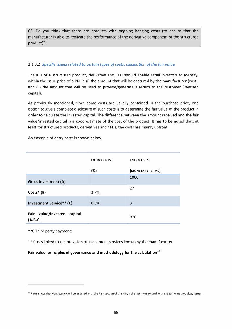
68. Do you think that there are products with ongoing hedging costs (to ensure that the manufacturer is able to replicate the performance of the derivative component of the structured product)?

Specific issues related to certain types of costs: calculation of the fair value 3.1.3.2

The KID of a structured product, derivative and CFD should enable retail investors to identify, within the issue price of a PRIIP, (i) the amount that will be captured by the manufacturer (cost), and (ii) the amount that will be used to provide/generate a return to the customer (invested capital).

As previously mentioned, since some costs are usually contained in the purchase price, one option to give a complete disclosure of such costs is to determine the fair value of the product in order to calculate the invested capital. The difference between the amount received and the fair value/invested capital is a good estimate of the cost of the product. It has to be noted that, at least for structured products, derivatives and CFDs, the costs are mainly upfront.

An example of entry costs is shown below.

ENTRY COSTS

(%)

ENTRYCOSTS

(MONETARY TERMS)

Gross investment (A) 1000

Costs* (B) 2.7% 27

Investment Service** (C) 0.3% 3

Fair value/invested capital (A-B-C)

970

* % Third party payments

** Costs linked to the provision of investment services known by the manufacturer

Fair value: principles of governance and methodology for the calculation47

47 Please note that consistency will be ensured with the Risk section of the KID, if the later was to deal with the same methodology issues.

89

There is a need to establish common principles and methodologies to estimate the fair value of structured products (and derivatives and CFDs) notably in order to allow for the comparability of products.

The fair value policy that would govern the measurement of the fair value should set a series of rules covering, among others, the following areas:

(a) Governance; (b) Methodology for the calculation of the fair value.

Such rules should aim at outlining a valuation process that:

(a) complies with the applicable accounting standards, so that the fair value is the same as the value of the liability that the manufacturer records on its balance sheet when the product is sold;

(b) makes sure that internal pricing models for PRIIPs are consistent with the methodologies, modelling and standards used by the manufacturer to value his own portfolio under the hypothesis that the product is available for sale or held for trading;

(c) is consistent with the level of complexity of the product and the type of underlying ; (d) takes into account the issuer credit risk and the uncertainty about the underlying; (c) sets the parameters to identify an active market in order to avoid risk mispricing that

could lead in extreme cases to significantly inaccurate estimates;

In the case of subscription products, the reference time for valuation should be close to the beginning of the subscription period and criteria to update such values, in case of very long offering periods or when you have high volatility in the markets, has to be defined. The subscription period for structured notes is usually several weeks long and therefore the values of the components (the zero-coupon bond and the derivative contract) are changing continuously during the subscription period. Therefore, if the subscription price is not adjusted accordingly, structuring costs will vary during the subscription period. On the other hand, each investor will have the same product terms so it might be difficult to communicate that they are paying different structuring costs.

It is also necessary to set the criteria in the case where preliminary terms or preliminary subscription prices are used, such as in the case of a certificate where the reference value of the underlying is fixed at the end of the offering period. Indeed, the use of preliminary terms means that the final terms of structured products are not confirmed until after the subscription period has ended. Therefore, if the use of preliminary terms is allowed, it is strictly speaking not possible to calculate the exact value of the structuring cost ex ante.

Valuation techniques may need to be calibrated over time, in order to reflect, for instance, the macroeconomic evolutions.

Several approaches are possible in relation to the calculation of the fair value.

One approach is to use the existing regulations in relation to the pricing of assets and liabilities. The regulatory standards mandated by the PRIIPs Regulation could then include an harmonized

90

version of these regulations. In this regard, the following list of principles and pricing rules could be used.

Proposals of general principles of governance

1. The management board should approve the valuation policy defining the relating scope.

2. The valuation policy should ensure that the fair price is calculated consistently with the procedure approved by the management board.

3. The valuation procedure should be periodically reviewed and updated if necessary, following periodic reporting.

4. The risk management function should, if needed, provide appropriate support to the valuation process concerning exposures to assets requiring complex evaluation such as structured securities and derivatives.

Proposal of a methodology for the calculation of the fair value

The fair price should be computed having regard to sound and reliable data. According to the international accounting standard (IFRS 13)48, the fair value of a structured product should be determined on the basis of:

(a) Market prices, if available or efficiently formed; (b) Internal pricing models using market values which are indirectly connected to the

product, derived from products with similar characteristics (comparable approach); (c) Internal pricing models based on inputs which are not derived directly from market

data for which estimations and assumptions must be formulated (market-to-model approach)49.

Given the nature of the KID for structured products, derivatives and CFDs, market prices are often not available. If the fair value cannot be derived from market prices, it should be estimated using a valuation technique that is able to represent properly the different factors affecting the product payoff structure making maximum use of market data.

In particular, valuation techniques should normally include:

(a) the use of recent arm’s length market transactions between knowledgeable, professional counterparties;

(b) reference to the current market price of another instrument that is substantially the same;

(c) discounted cash flow analysis; (d) option pricing models.

48 Please note that under IRFS 13, for derivatives which are exchange traded, the price used for fair value measurement is usually the market exchange price on the measurement date (IFRS 13.77,79). The fair value of non-exchange traded derivatives (e.g. OTC) is generally based on the income approach (which is explained in IFRS 13.B10). 49 In case of lack of consistent pricing models, prices received from the counterparties.

91

Mathematical models for the valuation of derivatives, structured product and CFDs describe the evolution of the underlying asset/s properly taking into account the different risk factors, by using standards generally recognised and accepted in the market. In addition they have to take into account the different product payoff features (such as worst of, best of, rainbow features).

A preliminary step could be to define the assumptions of the model in relation with:

• the number and type of model components (static vs. stochastic distributions); • the number of stochastic variables and complexity of modelled behaviour; • the type of solution of the model (closed solutions, numerical solutions, Monte Carlo

techniques); • the type of calibration of the model (historical data (backward looking), data implied in the

market prices (forward looking)).

In addition it is necessary to define common rules for the main pricing parameters. The main parameters are the following:

i. the expected return (e.g. risk premium) and volatility of the underlying and correlations among the underlying securities (if there is more than one underlying security);

Implied volatility is usually preferred since it is derived from current market prices and it is not affected by the past performance as the historical data.

ii. interest rates and yield curves;

Market quoted interest rates are usually available for the main currencies. The risk free yield curve of the currency denominated product has to be used. Usually the euro swap curve is used for euro denominated products.

iii. the credit risk (related to the issuer default risk).

There are different data that could be used as a proxy of the credit risk. Usually market data such as CDS spread or credit spread are available. Nonetheless in case of unavailability or lack of reliability of market indicators, comparable data can often be used. If market data are not available some general criteria have to be identified to tackle with this issue. Adjustments to the model should be made in relation to identified issues:

• close out/bid offer price; • model risk; • parameters uncertainty; • liquidity valuation adjustment; • future funding and investing costs.

The robustness of estimates must be checked testing the data used for the computation. In this context ECB standards for reviewing the calculation of the fair value exposures of credit institutions should be taken into account.

92

However, the interaction between the approach suggested here under the PRIIPs framework and the approach taken by prudential Regulators that have already oversight of all components of models used to estimate capital requirements in the CRD IV framework50, will have to be carefully scrutinized.

Indeed the calculation of the fair value of any derivative product will require a model or combination of models (which can be used to relate the value of the derivative to the market observables on which it depends) and the value for certain parameters which may not be readily observable in the market (e.g. equity-interest rate correlation). There are many types of models available (simple Black-Scholes, Black-Scholes with a local volatility surface, stochastic volatility, GARCH, …).

Often, firms use a variety of models opting to use more complicated models for only those products whose value depends on factors not captured in simpler models.

There are a variety of calibration techniques available for determining model parameters from market prices – and these calibration techniques may themselves depend on parameters chosen by the firm. For example, firms can decide to use options in a calibration process where they limit the strikes to be those strikes where the option’s dependence on the underlying price sits in a particular range. Further they may exclude certain maturities if the properties of the option prices at those maturities bias the calibration process unnecessarily.

It is worth noting that a firm’s choice has to be approved by the relevant prudential authority if the model is used in estimating the capital required for the firm as part of a CRD IV permission. Were the PRIIPs regulatory technical standards to mandate a particular choice for a model and a calibration scheme, that might raise questions about the interaction with the established prudential regime, even though the objectives of the two pieces of legislation are very different.

It is also suggested to disclose hedging costs of structured products (as identified in the Identifying the costs section) explicitly, notably to ensure a level playing field with other types of PRIIPs where transaction costs are disclosed. Therefore the suggested methodology in this section goes beyond the corresponding SEC regulatory framework51.

Finally, the extent to which the aforementioned principle based approach of the calculation of the fair value should be supplemented by independent price verification (third party or regulator) could be further investigated. In that respect, it may be argued that as long as governance principles are implemented, independent price verification and setting up public databases are not necessary.

Questions:

69. Do you agree with the general framework outlined above?

50 Notably Article 105(10) to 105(13) of Regulation 575/2013 on prudential requirements for credit institutions and investment firms. 51 US Regulation S-K Items 201, 501, and 505.

93

70. Which criteria should be chosen to update the values in the KID when input data change significantly?

71. As the evolution of underlying asset/s should be taken into account, are there specific issues to be tackled with in relation to specific types of underlying? To what extent should the RTS be prescriptive on the risk premium?

72. Are you aware of any other assumptions to be set?

73. Having in mind that most of the applied models in banking are forward looking (e.g. using implied volatility instead of historical volatility) which are the pros and cons of backward looking approach and forward looking approach?

74. Do you think that there are other risk free curves that could be considered?

75. Do you think that there are other market data that could be used to determine the credit risk? Do you think that implied credit spreads from other issuer bonds (other than structured products) could be used?

76. How would you determine the credit risk in the absence of market data and which are the criteria to identify the comparable?

77. How would you include the counterparty risk in the valuation? Would you include specific models to include counterparty risk in valuation (CVA models)? How would you consider the counterparty risk for pure derivatives?

78. In which circumstances do you think parameters cannot be computed/estimated using market data? What would you suggest to deal with this issue?

79. Would it be meaningful to prescribe specific pricing models for structured products, derivatives and CFDs? If yes which are the pros and cons of parametric and non-parametric models?

Possible alternative approaches to the calculation of fair values for structured products:

A prescriptive approach to the calculation of fair values for structured products?

A prescriptive approach to the calculation of fair values for structured products would entail specifying in great detail52:

(a) the valuation model used for a structured products or its components; (b) the valuation method to implement the model, and;

52 This is notably one of the differences with the principle-based approach.

94

(c) the input parameters for the specific model.

While it may seem viable and preferable at first, there are too many degrees of freedom that a framework (set of rules) would have to cover.

In general, as aforementioned, the calculation of a fair value should use an appropriate pricing model. Within this model, certain assumptions about the future dynamics of the underlying risk factors need to be made. Two of these assumptions53 are that volatility is constant over time and trading costs do not exist. It is common knowledge, that these two assumptions are not met in practice. That is why - among others - we see a maturity and strike-dependent implied volatility in exchange-traded options with significant bid-ask spreads. There are several extensions to the Black-Scholes model (and several other pricing models) that try to capture the empirical observations e.g. by specifying a separate stochastic process for the volatility or by making time a stochastic variable.

Considering the multitude of models, it seems impossible to prescribe a specific model for each and every possible derivative structure, especially since the modelling world evolves over time to account for new empirical observations.

The pricing model should be able to reproduce the observable market prices of other financial instruments, i.e. interest rate swaps, traded options, etc. This principle can – of course – only be applied in cases where there are observable market instruments. If e.g. there are no traded options for a specific underlying, the (market) implied volatility cannot be assessed. A trader would form an estimate on the expected future volatility and would add or subtract a buffer (depending on whether he is buying or selling volatility) in order to cover potential misjudgements. A general, formalized process to come up with a reasonable assumption cannot be imagined. If using e.g. historical estimates, the results would most probably be biased and the implied costs not reliable. An approach using potentially other comparable companies with listed options as a proxy could be easily manipulated.

Even if market inputs are observable, their reliability or information value for a specific instrument can only be judged ex post from an external perspective in an intensive review process. During the calibration, a trader may ignore market information that he deems unreliable (e.g. indicative quotes that do not represent real trading opportunity) or unimportant (e.g. observable short-term volatility for a longer-term product) for the product at hand. Prescribing ex ante concrete measures about how to determine an input parameter exactly can lead to unrealistic, systematically biased and wrong estimates.

Hence a prescriptive approach setting up in full details of the parameters and valuation modelling to be computed to calculate fair values could lead to comparable and robust but not reliable cost estimates and indicators. Therefore it is proposed not to consider it in the PRIIPs framework and to opt for a principle-based approach, as described in the previous parts of this section.

53 In the classic Black-Scholes model

95

Aggregating the costs 3.2

General issues

The PRIIP manufacturer shall:

• be responsible for the calculation of the TCR/RIY/cumulative effect of costs figures and for its accurate statement in the KID;

• establish procedures that are consistent with this methodology and are adequately documented;

• keep records of each calculation for a period of x years after the last date on which that version of the KID was available to be issued.

Question 80: What should be the value of x? (in the case of UCITS, x=5, but the extent to which this is appropriate for other types of PRIIPs, notably life-insurance products, is unclear).

A separate calculation shall be performed for each share class, but if the units of two or more classes rank pari passu, a single calculation may be performed for them.

Question 81: Should this principle be further explained / detailed? Should the terms “rank pari passu” be adapted to fit the different types of PRIIPs?

Information about the TCR/RIY/ cumulative effect figures that were applicable during previous years / periods should be published at the location (e.g. the management company’s website) which is specified in the KID as the general source of further information for investors who require it.

Monetary vs Percentage terms

The PRIIP manufacturer shall disclose its costs expressed in monetary and percentage terms. This means that an assumption has to be made on the initial invested amount in order to present a costs figure expressed in monetary terms.

This initial invested amount shall be consistent among the different types of PRIIPs, and also be used to show the compound effect of costs.

It is suggested that the initial invested amount taken into account for the calculation of cost figures is 1 000 euros (or the minimum amount of subscription foreseen for the product?).

Question 82: What should be the relevant figure for the initial invested amount to be taken into account for the calculation of cost figures? Should a higher initial investment amount be taken into account not to overestimate the impact of fixed costs? How should the situation of products with regular payments be taken into account for that specific purpose? (Would an invested amount of 1 000 euros per period of time be a relevant figure?)

96

PRIIPs with a variety of possible outcomes depending on some features of the investor Question 83: For some life-insurance products, the costs will differ on the age of the customer and other parameters. How to take into account this specific type of PRIIPs for the purpose of aggregating the costs? Should several KIDs for several ages be considered?

3.2.1 Summary indicators

Please note as a general remark that because the previous section of this paper intends to list the different types of costs for each type of PRIIP, the present section does not enter into the question of the possible presentation of the cost disclosure into separate figures comprising aggregated entry costs, aggregated ongoing costs and aggregated exit costs figures. These figures could be calculated using the same methodology detailed as follows for TCR or RIY. One important issue of the present section is the extent to which a common summary indicator can be set for all the different types of PRIIPs. It would be indeed hardly understandable for the investor that the summary cost indicator is a total cost ratio for one type of PRIIP, and a Reduction in Yield indicator in the case of another type of PRIIP. The purpose of this section is therefore to investigate how to set up this common cost summary indicator that would apply to all types of PRIIPs, using a comparable methodology. When TCR and RIY methodologies are discussed it shall therefore be clear that these methodologies are considered in so far as they could be applied to all types of PRIIPs.

Total Cost Ratio (TCR) 3.2.1.1

General issues The total cost ratio means that the costs of operating a PRIIP are aggregated and presented as an annual percentage rate on investment. This can be done on an ex ante or ex post basis, depending on the principles provided for the cost estimation in the previous section.. The ‘TCR’ mentioned in the present section under the PRIIPs Regulation would differ from the ‘TER’ that was used before it was replaced by the OCF (the latter did not include different types of costs). Therefore it is necessary to establish a new term, which could be for example ‘The total cost ratio’ (TCR) (However, other terms could be used, including “total product costs”, to emphasize the fact that, for example, all distribution costs might not be included in this ratio for all PRIIPs). Under section 3 of the KII implementing Regulation, the ongoing charges figure for UCITS has to be calculated at least once a year, on an ex-post basis. Where it is considered unsuitable to use the ex-post figure because of a material change (e.g. an increase in management fees) or where the fund is new to the market, an estimate may be used instead until reliable ex-post figures becomes available.

97

A TCR figure needs to be adjusted to also include other costs (upfront costs, for instance), for instance by using an assumption to ‘annualise’ these costs (amortize them). In this case a ‘total aggregate’ figure can be derived.

The final figure would be sensitive to the scenarios or assumptions chosen, but could be used to illustrate total aggregate costs and compare between products (in so far as the assumptions used are standardised across all PRIIPs). The rate of return should be chosen in order to be consistent with the scenarios presented in the ‘performance scenarios’ section.

In the case of some derivatives, attention should be paid where the (recommended) holding period may be one day or even less.

Question 84: Do you agree with the abovementioned considerations? Which difficulties do you identify in the annualisation of costs?

Methodology for the calculation of the different types of costs to be included in the TCR

The methodology for the calculation of the TCR could distinguishes between 1) the types of costs to be included in the numerator of the TCR (these are the different types costs identified in the Identifying the costs previous section) 2) the different possible definitions of the denominator of the TCR54.

In respect to 2) the different possible definitions that have been identified are notably the followings:

• The average net investment; • The average net assets (notably in the case of funds); • The invested amount.

These different options are further discussed in the next paragraphs regarding the possible issues relating to the implementation of the TCR approach to the different types of costs of the different types of PRIIPs. The first and the second options mentioned above are further described below:

The TCR for PRIIPs is there calculated as the annualized ratio between all costs paid directly or indirectly by the investor and the average value of the investment over a specific investment horizon. For the definition of the investment horizon, the (minimum) recommended holding period of the PRIIP or another period of time can be used.

54 Having in mind that one single definition of this denominator for all PRIIPs is targeted to ensure comparability between products.

98

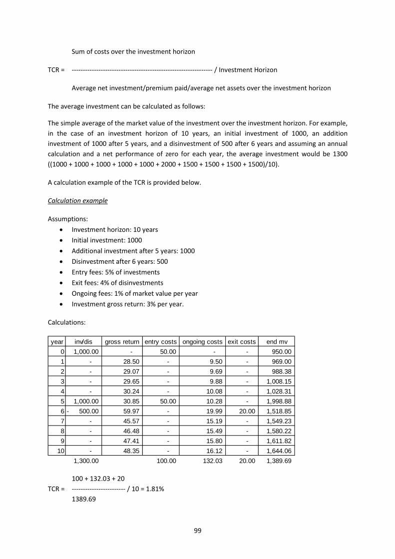
Sum of costs over the investment horizon

TCR = --------------------------------------------------------------- / Investment Horizon

Average net investment/premium paid/average net assets over the investment horizon

The average investment can be calculated as follows:

The simple average of the market value of the investment over the investment horizon. For example, in the case of an investment horizon of 10 years, an initial investment of 1000, an addition investment of 1000 after 5 years, and a disinvestment of 500 after 6 years and assuming an annual calculation and a net performance of zero for each year, the average investment would be 1300 ((1000 + 1000 + 1000 + 1000 + 1000 + 2000 + 1500 + 1500 + 1500 + 1500)/10).

A calculation example of the TCR is provided below.

Calculation example

Assumptions: • Investment horizon: 10 years • Initial investment: 1000 • Additional investment after 5 years: 1000 • Disinvestment after 6 years: 500 • Entry fees: 5% of investments • Exit fees: 4% of disinvestments • Ongoing fees: 1% of market value per year • Investment gross return: 3% per year.

Calculations:

100 + 132.03 + 20 TCR = ------------------------ / 10 = 1.81% 1389.69

year inv/dis gross return entry costs ongoing costs exit costs end mv0 1,000.00 - 50.00 - - 950.00 1 - 28.50 - 9.50 - 969.00 2 - 29.07 - 9.69 - 988.38 3 - 29.65 - 9.88 - 1,008.15 4 - 30.24 - 10.08 - 1,028.31 5 1,000.00 30.85 50.00 10.28 - 1,998.88 6 500.00- 59.97 - 19.99 20.00 1,518.85 7 - 45.57 - 15.19 - 1,549.23 8 - 46.48 - 15.49 - 1,580.22 9 - 47.41 - 15.80 - 1,611.82

10 - 48.35 - 16.12 - 1,644.06 1,300.00 100.00 132.03 20.00 1,389.69

99

Possible issues relating to the implementation of the TCR approach to the different types of costs of the different types of PRIIPs Entry-Exit costs If the entry-exit costs are to be included in the TCR, several assumptions are needed to annualize these costs:

(c) a chosen holding period chosen to amortize the costs; (d) an amortization methodology (linear?).

Question 85: Which other assumptions would be needed there? In the case of life-insurance products, to what extent should the amortization methodology related to the amortization methodology of the premium calculation? To what extent should the chosen holding period be related to the recommended holding period? Funds The Entry-exit costs ratio to be included in the TCR could be the ratio of the total of these amortized costs to the average net assets of the fund. The figure shall be expressed as a percentage rounded to two decimal places. Question 86: This definition of the ratio is taken from the CESR guidelines on cost disclosure for UCITS. Is it appropriate also in the case of retail AIFs? Should it be amended? Another approach to calculate these costs is to calculate the ratio of the total of these amortized costs to the invested amount in the fund. However in that case the question remains as to how to aggregate this ratio with the on-going charges ratio. Another possible approach could be to use the ratio between the total amount of costs over the holding period and the average net investment (assumed during the whole period, in order to take into account future additional investments, partial withdrawals, payments (i.e. programmed investments or disinvestments)). Do you think this approach would be appropriate?

It is to be noted that a PRIIP manufacturer will already be required to disclose in the KID, as per the Regulation, a recommended holding period. In respect of the cost section, providing information on total aggregate costs to illustrate their cumulative impact also implies estimating costs over a future time period, which should be consistent with any recommended holding period otherwise disclosed. The aggregation of costs into a percentage figure for the purposes of comparison could therefore depend on the same holding period assumptions, so as to allow an appropriate amortization of one-off costs or other similar technique for combining costs.

Life-insurance products

The entry-exit costs to be included in the TCR could be the ratio of the total of these amortized costs to the premium paid (or invested amount, or the value of the life-insurance product, gross or net of capital invested; or the expected economic value of the contract). The figure shall be expressed as a percentage to two decimal places.

100

Question 87: What would be other options to define the TCR ratio in the case of life-insurance products? What about the case of regular payments or regular increasing? Which definition would you favour? How to ensure a level playing field and a common definition with the other types of PRIIPs in this regard? Another possible approach could be to use the ratio between the total amount of costs over the holding period and the average net investment (assumed during the whole period, in order to take into account future additional investments, partial withdrawals, payments (i.e. programmed investments or disinvestments)). Do you think this approach would be appropriate? To what extent do these possible calculation methodologies fit the case of insurance products with regular payments? For insurance policies having a guaranteed surrender value, it might be the case that early redemption penalties should not be considered as exit costs to the extent they are already taken into account in the estimation of the cost of embedded options. The main difficulty in computing total expense for insurance contracts that are not purely unit-linked, lies in the fact that the costs depend on economic scenario assumptions as well as on other assumptions concerning early surrender behaviour of policyholders, asset portfolio rebalancing or profit sharing (see below).

It is to be noted that a PRIIP manufacturer will already be required to disclose in the KID, as per the Regulation, a recommended holding period. In respect of the cost section, providing information on total aggregate costs to illustrate their cumulative impact also implies estimating costs over a future time period, which should be consistent with any recommended holding period otherwise disclosed. The aggregation of costs into a percentage figure for the purposes of comparison could therefore depend on the same holding period assumptions, so as to allow an appropriate amortisation of one-off costs or other similar technique for combining costs. However in that case, because PRIIPs manufacturers may have different recommended holding periods, even for a similar type of PRIIP, it would not be easy to compare the resulting cost ratios.

Structured products & SPVs

In the case of structured products the TCR could in practice equal the ratio of the Entry-Exit costs to the value of the products (or to the invested amount), because the on-going charges figure approximately equals zero55. However in some cases structured products can include on-going costs.

From the perspective of the issuer, all costs are represented by the difference between the sum paid by the buyer of the structured product and the fair value of the liability recognized on the balance sheet of the manufacturer. This is analogous to an entry cost discussed in the context of funds or life-insurance products. However, it is the only cost incurred by the buyer of a structured product.

55 But on-going charges should of course always be included in the TCR.

101

To provide the cost as a TCR or RIY number, the cost may have to be annualized. This could be accomplished by assuming annual compounding and using the maturity/holding period of the structured product to convert the cost to an annual percentage which represents a reduction in yield or total expense ratio. Several issues arise through the use of such a methodology for a structured product. Firstly, it is not clear whether the cost derived from the fair value is the true cost (certain costs may be included in parameters used to calculate the fair value and, as such, be recognized in the P/L of the trading desk that is managing the manufacturer’s exposure to market risk factors through a hedging strategy). Secondly, the payoff of a structured product is calculated using the total sum paid by the purchaser and the performance of the referenced market assets. This methodology assumes that the fair value is the true price of purchasing a particular investment strategy. Please note that these comments also apply to the calculation of the fair value per se (please see the dedicated part of this paper).

Question 88: What would be other options to define the TCR ratio in the case of structured products? Do you identify other specific issues in relation to the TCR if applied to structured products? Another possible approach could be to use the ratio between the total amount of costs over the holding period and the average net investment (assumed during the whole period, in order to take into account future additional investments, partial withdrawals, payments (i.e. programmed investments or disinvestments)). Do you think this approach would be appropriate? For derivatives, it might be the case that it is necessary to further define the concept of investment to be used as denominator of the ratio. Possibilities include the use of the actual sums paid and received (i.e. initial margins, variation margins, collateral postings, various payoffs, etc.) or the use of the exposure (i.e. market value of the derivative underlying). Do you think these approaches would be appropriate?

On-going charges Funds

Methodology for calculation of the TCR (except for new funds)

The TCR figure could be the ratio of the total discloseable costs to the average net assets of the fund, calculated according to this section. The figure shall be expressed as a percentage to two decimal places.

Question 89: This definition of the ratio is taken from the CESR guidelines on cost disclosure for UCITS. Is it appropriate also in the case of retail AIFs? Should it be amended? Another possible approach could be to use the ratio between the total amount of costs over the holding period and the average net investment (assumed during the whole period, in order to take into account future additional investments, partial withdrawals, payments (i.e. programmed investments or disinvestments)). Do you think this approach would be appropriate?

Apart from its first submission as a pre-contractual information for new funds, the ongoing charges figure shall be calculated at least once a year, on an ex-post basis. Where it is considered unsuitable to use the ex-post figure because of a material change (e.g. an increase in management fees), an

102

estimate may be used instead until reliable ex-post figures reflecting the impact of the material change become available.

The ex-post figure shall be based on recent cost calculations which the management company has determined on reasonable grounds to be appropriate for that purpose. The figure may be based on the costs set out in the fund’ statement of operations published in its latest annual or half-yearly report, if this is sufficiently recent; if it is not, a comparable calculation based on the costs charged during a more recent 12-month period shall be used instead.

The costs are assessed on an ‘all taxes included’ basis, which means that the gross value of expenses shall be used.

The average net assets shall relate to the same period as the costs, and be calculated using figures based on the fund’ net assets at each calculation of the NAV (e.g. daily NAVs where this is the normal frequency of calculation approved by the fund competent authority).

Where the costs attributable to an underlying UCITS/AIF are to be taken into account:

• the ongoing charges figure (or equivalent) of each underlying UCITS/AIF is pro-rated according to the proportion of the fund’ net asset value which that UCITS/AIF represents at the relevant date (being the date at which the fund figures are taken);

• all the pro-rated figures are added to the total cost figure of the investing fund itself, thus presenting a single total.

Methodology for calculation of the TCR for new funds

In place of ex-post data, estimates shall be used in the calculation of the different types of costs;

For funds which charge a fixed all-inclusive fee, that figure shall be displayed (provided it includes all costs to be presented under the PRIIPs cost disclosure requirements);

For funds which set a cap or maximum on the amount that can be charged, (and provided it includes all costs to be presented under the PRIIPs cost disclosure requirements) where instead that figure shall be disclosed so long as the management company gives a commitment to respect the published figure and to absorb any costs that would otherwise cause it to be exceeded.

If, in the management company’s opinion, expressing a figure to two decimal places would be likely to suggest a spurious degree of accuracy to investors, it shall be sufficient to express that figure to one decimal place;

The management company shall ensure that the accuracy of the estimated figure is kept under review. The management company shall determine when it is appropriate to begin using ex-post figures rather than an estimate; but in any case it shall, no later than 12 months after the date on which units were first offered for sale in any Member State, review the accuracy of the estimate by calculating a figure on an ex-post basis.

103

Question 90: These different aforementioned principles are taken from the CESR guidelines on cost disclosure for UCITS. Is it also appropriate in the PRIIPs context?

Life-insurance products Question 91: To what extent do the principles and methodologies presented for funds in the case of on-going charges apply to life-insurance products?

The cost of embedded options of life insurance products could be estimated in the following way:

• given an economic scenario generator for the main types of assets; • a rule for the rebalancing of the asset portfolio; • a rule for the profit sharing and a model of the early surrender of policyholder (all those

rules and models being disclosed to the supervision authority under Solvency II framework)

The insurer generates a large number of payoff scenarios corresponding to the options embedded in the contract (early surrender, guaranteed interest rate on initial and/or future premiums, etc.).

The insurer then determines an optimal portfolio of financial assets (with a possible rebalancing at each time period, possibly assuming transaction costs) whose payoffs are as close as possible to the projected payoffs (according to a given norm, the so-called “replicating portfolio”).

The price of the initial portfolio is expected to give an estimation of the cost of the embedded option.

This approach has some drawbacks (numerical stability, unknown convergence properties, difficulty to take account of extreme scenarios for VaR computation purposes) and was abandoned by most insurers.

The main approach used today (for embedded value or Solvency II purposes) is based on the assumption that the price of the embedded option is approximated by the expected present value of payoffs given by economic scenarios generated according to a risk-neutral probability.

The total costs could thus be estimated by computing the expected present value of future profits of the insurer arising from the management of the contract and the expected value of its future operational expenses (also calculated according to a model disclosed under Solvency II framework).

Question 92: Do you think this methodology should be further detailed? To what extent do you think this methodology is appropriate and feasible (notably in terms of calibration of the model)? It might indeed be considered that valuation models for Solvency II usually are not likely to be designed for per contract calculations. Life insurers may restrict the calculation of technical provisions in the Solvency II-Balance-Sheet to homogenous risk groups. Furthermore they are allowed to use simplified calculation methods if the error is immaterial at the portfolio level. As profit sharing mechanisms in many countries are applied on the company level and not on a per contract level,

104

projected cash flows from future discretionary benefits will not easily be broken down on a per product or even a per contract basis with the existing Solvency II-Valuation-Models.

Reduction in Yield (RIY) 3.2.1.2

General issues

RIY is a method for expressing the overall impact of costs in terms of their negative impact on a notional ‘gross’ yield for a product.

A RIY figure for a product can combine different cost elements (e.g. up front and exit costs, ongoing costs, performance fees) for comparison purposes. Different assumed scenarios would give different RIY figures, as RIY takes into account such factors as:

(a) the amount invested (where fees might vary by investment size);

(b) the length of the investment / recommended holding period (where penalty fees might vary according to the investment term, and where the overall relative impact of different fees varies according to the investment term);

(c) and the annual rate of investment return (some fees will vary in their impact depending on performance). In particular the calculation of the RIY requires the computation – based on the previous assumptions - of two different internal rates of return:

a. - the return i1 (whose calculation is based on the gross cash flows); b. - and the return i2 (calculated taking into account the net cash flows)

The difference between the two rates (i2 – i1) represents the cumulative effect of all costs.

In general terms, the calculation of i1 and i2 would be based on the following equations:

(1) S0 = GCF1 / (1+i1) + GCF2 / (1+i1)2 + …. + GCFn / (1+i1)n

(2) (S0 – EC) = NCF1 / (1+i2) + NCF2 / (1+i2)2 + …. + NCFn / (1+i2)n

Where:

S0 = is the sum/premium invested/paid (in the case of regular premium, S0 is the present value of the premiums).

GCFx = are the gross cash flows of the investment based upon the assumptions on performance

EC = are the entry costs charged at t=0

NCFx = are the net cash flow of the investment, based upon the assumptions on performance deducted the ongoing costs and the exit costs

105

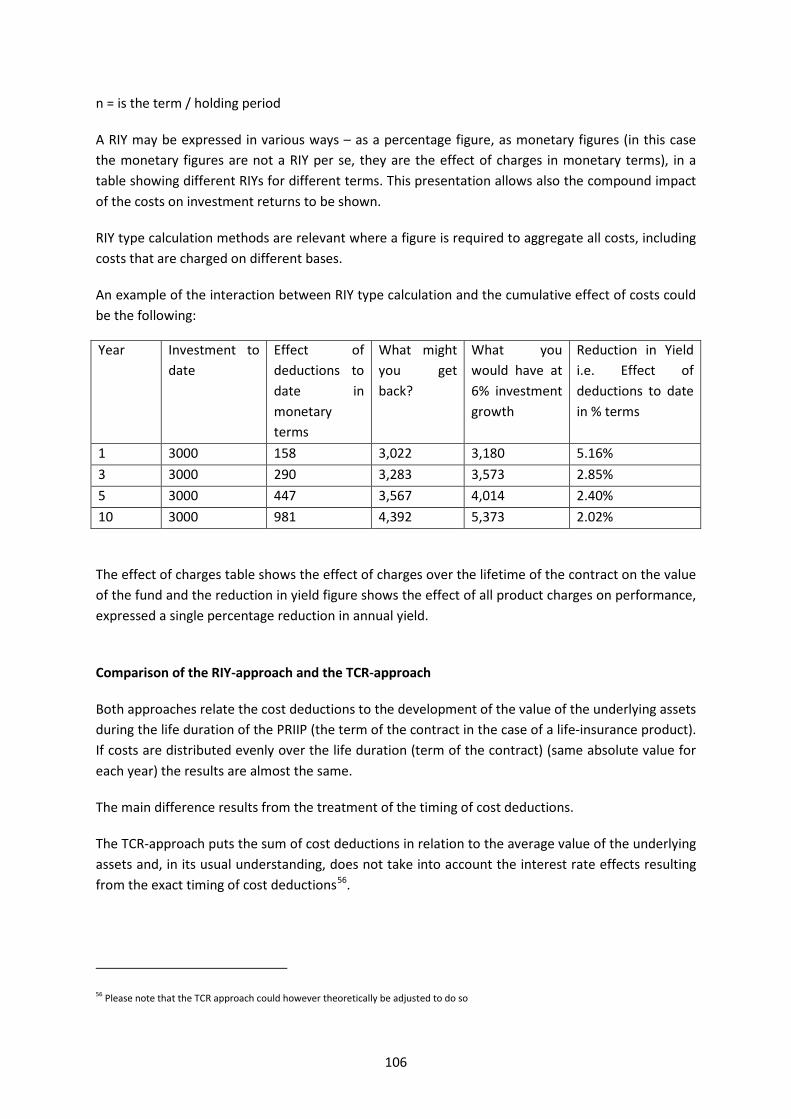
n = is the term / holding period

A RIY may be expressed in various ways – as a percentage figure, as monetary figures (in this case the monetary figures are not a RIY per se, they are the effect of charges in monetary terms), in a table showing different RIYs for different terms. This presentation allows also the compound impact of the costs on investment returns to be shown.

RIY type calculation methods are relevant where a figure is required to aggregate all costs, including costs that are charged on different bases.

An example of the interaction between RIY type calculation and the cumulative effect of costs could be the following:

Year Investment to date

Effect of deductions to date in monetary terms

What might you get back?

What you would have at 6% investment growth

Reduction in Yield i.e. Effect of deductions to date in % terms

1 3000 158 3,022 3,180 5.16% 3 3000 290 3,283 3,573 2.85% 5 3000 447 3,567 4,014 2.40% 10 3000 981 4,392 5,373 2.02%

The effect of charges table shows the effect of charges over the lifetime of the contract on the value of the fund and the reduction in yield figure shows the effect of all product charges on performance, expressed a single percentage reduction in annual yield.

Comparison of the RIY-approach and the TCR-approach

Both approaches relate the cost deductions to the development of the value of the underlying assets during the life duration of the PRIIP (the term of the contract in the case of a life-insurance product). If costs are distributed evenly over the life duration (term of the contract) (same absolute value for each year) the results are almost the same.

The main difference results from the treatment of the timing of cost deductions.

The TCR-approach puts the sum of cost deductions in relation to the average value of the underlying assets and, in its usual understanding, does not take into account the interest rate effects resulting from the exact timing of cost deductions56.

56 Please note that the TCR approach could however theoretically be adjusted to do so

106

The basic idea of the RIY-approach is to assess how much the internal rate of return for the customer is reduced due to costs. In contrast to the TCR-approach it therefore takes the timing of cost deductions implicitly into account. The more the benefit at maturity is decreased due to costs the higher the RIY is. This is not always true for the TCR-approach. Therefore in this respect, the impact of costs on the benefit at maturity is shown more accurately by the RIY-approach.

The difference between both approaches is illustrated by the examples in the Annex “Comparison of RIY- and TCR-approach” (in case of life-insurance contracts). In both examples the sum of cost deductions is 1200. In the first example these costs are distributed evenly over all years. In the second example these costs are charged up-front. If a performance greater than zero is assumed, the endowment benefit at maturity is lower in the second example. While the TCR is almost the same in both examples the RIY is significantly higher in the second example reflecting the negative impact of up-front cost deductions on the endowment benefit at maturity.

This is very important especially for life insurance PRIIPs where upfront costs are often huge. In the calculation example assumed upfront costs are 4% of the sum of premiums. In some Member States they often are even higher than 7% of the sum of premiums.

Possible issues relating to the implementation of the RIY approach to the different types of costs of the different types of PRIIPs

Funds The case of funds does not seem to raise specific issues as long as the different types of costs have been identified and estimated (please see previous section). Question 93: Do you identify any specific issue in relation to the implementation of the RIY approach to funds? Structured products

In relation to the calculation of RIY in the case of structured products, there might be an issue regarding embedded costs and costs that are in fact a loss of opportunity for the investors (for instance dividends or lending fees that should accrue to the investment product but are taken by the manufacturer, or the value of goods or services that are given or rendered to the manufacturer).

Indeed, contrary to other costs, it is not straightforward to take them into account when the net performance is measured (otherwise, the costs could be double counted. Because the impact of these costs is that the amount to be invested is reduced, the (gross) performance already takes into account these costs).

This could mean that there may be a difference between a total cost ratio and a reduction in yield approach for such products with embedded costs and products with loss of opportunity costs. In a total cost ratio approach, these costs can be taken into account and could be qualified as entry costs (embedded costs) or ongoing costs (ongoing loss of opportunity) (however with a warning that they

107

cannot be subtracted from the gross performance). In a reduction in yield approach it seems that these costs are difficult to take into account because the gross performance or yield already takes it into account (because the performance is calculated on the basis of the net invested amount rather than the gross invested amount).

In order to take them into account in a RIY approach, the value of these costs may need to be added to the original investment value and the yield reduction caused by these costs would correspond to the original value of the costs plus their assumed return.

Question 94: In addition to the abovementioned issues and the issues raised in relation to TCR when applied to structured products, do you identify any other specific issue in relation to the implementation of the RIY approach to structured products? Life-insurance products

Introduction

It may be argued that the RIY fits well the specifics of life insurance contracts:

• Costs charged to premiums are usually fixed at the inception of the contract and often cannot be changed during the term of the contract;

• costs in premiums are often calculated in relation to different kinds of parameters even in one product (fixed amounts, percent of premiums, per thousand of insured sum, ...);

• costs may be very heterogeneous across different contracts and even across different years in one contract

Due to these specific distributing costs at the company level, allocating costs to single contracts is not an easy option for life insurance contracts.

The main advantages of the RIY-approach are the followings:

• Individual costs charged to the single contract are transformed to one number; • It takes the timing of the cost withdrawals into account. If e.g. a certain sum of costs is

deducted upfront the endowment benefit at maturity may differ materially from the endowment benefit for a scenario where the same sum of costs is distributed evenly to each year of the term. This is very relevant because in some Member States upfront costs of life insurance contracts often are very high. The RIY-indicator takes appropriately these timing effects into account.

General Framework

The basic idea of the Reduction in yield (RIY) approach is to quantify how far the annual yield of a PRIIP in relation to gross premiums is reduced by costs.

An alternative approach could be based on the question how far the annual yield in relation to net premiums has to be increased to compensate for costs. Both approaches produce very similar – but different - results. The difference between both approaches is similar to the question which

108

denominator shall be used in the TCR-methodology. In the following text we only describe the first approach.

The calculation of the RIY (in this “gross premium approach”) requires the following steps:

Step 1: Project benefit payments on certain performance assumptions taking into account all costs, future profit sharing and guarantees.

Step 2: Calculate an internal rate of return r in relation to gross premiums and projected benefit payments from step 1 and another internal rate of return i for a cost free scenario. The difference i – r is the reduction in yield. Costs proportional to the value of assets under management may be simply added to i – r if not already considered in i – r.

Within the framework described above the following two approaches, which correspond to the two options regarding the cash flows to be considered, are described in more details:

RIY without taking into account biometric benefits (Option 1 in relation to cash flows to be considered – please refer to the “general issues” subsection of the Identifying the costs section)

Let denote EB the endowment benefit at maturity of the contract projected in step 1 and GP1, … , GPn the gross premiums payable until maturity.

Calculation of r:

Let denote r the internal rate of return in relation to the endowment benefit EB and the gross premiums GP1, … , GPn.

Calculation of i:

Let denote NP1, … , NPn the net premiums derived from gross premiums GP1, … , GPn by deducting costs, i.e. NPj = GPj - Cj , where Cj are the costs for time period j. Then i is defined as internal rate of return in relation to the endowment benefit EB and net premiums NP1, … , NPn .

Alternative for the calculation of i:

Instead of calculating i in relation to net premiums the endowment benefit could be recalculated for a cost free scenario (with all other assumptions unchanged). Then i can be defined as internal rate of return in relation to the projected endowment benefit in the cost free scenario and gross premiums.

Costs proportional to the value of underlying assets:

If certain parts of the costs are proportional to the value of underlying assets (e.g. costs for administration and management of assets; insurers margin in profits from investments,…) the corresponding cost ratio i’ may be simple added to i – r instead of including these costs in Cj . The reduction in yield then is i – r + i’.

Handling of biometric risk premiums

109

If full biometric risk premiums shall be included in the summary cost indicator (option 2 for treatment of biometric risk premiums – please see the “general issues” subsection of the Identifying the costs section), the biometric risk premium could be included into Cj. In this case the biometric risk premium could be reduced by expected risk bonuses that might be credited to policy holders within the profit sharing mechanism.

If full biometric risk premiums shall not be included in the summary cost indicator (option 1 for treatment of biometric risk premiums) they need to be excluded from Cj . If in this case a separate RIY-indicator for biometric risk premiums shall be disclosed it would equal j – (i + i’), where j is the performance of the underlying assets. Therefore the RIY-indicator for biometric risk premiums is that part of the difference between the performance of the underlying assets and the yield for the customer in relation to gross premiums and endowment benefit that is not covered by the reduction in yield due to costs and hence stems from biometric risk premiums.

Advantages of RIY without taking into account biometric benefits:

• RIY-approaches following option 1 in relation to the cash flows to be considered are already in place in several Member States;

• Yield numbers in relation to endowment benefits at maturity are transparent and understandable. The customer usually relates yield numbers to the investment part of a life insurance contract that is defined by the endowment benefit only. Customers usually look at death benefits as different scenario and would not understand a reduction in yield that mixes both using probability weighted cash flows including biometric benefits;

• Restricting the calculation of yield numbers to endowment benefits reduces the number of variables in the calculation compared to approaches where probability weighted cash flows are used, thus improving comparability of results.

• Considering only endowment benefits is more consistent to other PRIIPs-products than life insurance products. For other PRIIPS-products premium payments may also stop and the investment capital may be paid out before the regular end of the contract in the event of death. Nevertheless it is not discussed to compute RIY-numbers for such products considering death probabilities;

• Moreover cash flows weighted with probabilities do not give an accurate view for a single contract. The numbers are only applicable to large pools of customers. As described above a single customer thinks in scenarios - not probabilities. A single customer either dies or does not die but he does not die gradually year by year as probability weights would assume;

• The approach is easy to implement. Defining RIY-numbers on the basis of probability weighted cash flows would be much more burdensome for the insurers and supervisory authorities as best estimate assumptions on death probabilities and other biometric probabilities must be set. In some Member States a wide variety of products with very different best estimate probabilities exist.

Disadvantages of RIY without consideration of biometric benefits:

• It is not obvious how to handle annuity life products as there is no fix term.

110

However, a solution could be to treat the accumulation phase and the pay-out phase of annuities differently. While the described approach can easily be applied to the accumulation phase of an annuity product during the pay-out phase a reduction-in-pay-approach might be more appropriate. Another solution could be to assume that the policy holder dies when he reaches the statistical life expectancy.

RIY taking into account biometric benefits (Option 2 in relation to cash flows to be considered – please refer to the “general issues” subsection of the Identifying the costs section)

Calculation of the i

The “i” is the yield or yields (in case of multiple scenarios) of the underlying assets in the performance scenario(s).

Calculation of the r

The r is the IRR which balances two stochastic cash-flows:

1. (projected) inpayments (gross premiums) made by the client, get by the provider weighted by the probabilities of each payments (these are in the most cases the survival probabilities)

2. (projected) outpayments (benefits) made by the provider, get by the client weighted by the probabilities of each benefits (these are partly death, partly survival probabilities, that can be also others)

(For technical details and complementary explanations please see the Technical Appendix)

Other issues 3.2.1.3

Life-insurance products

Performance assumptions

For the calculation of the aggregated cost indicator performance assumptions may be needed. For the choice of these assumptions the following principles should be applied:

• Performance assumptions should be consistent with the scenarios shown in the performance scenarios section of the KID;

• The performance assumptions should reflect the risk/reward profile of the product. This can vary substantially between different life insurance products (with-profit-policies vs. pure unit linked products vs. mixed products)

Furthermore the following questions arise:

• Shall only one performance assumption be considered are shall several performance scenarios be considered?

• Shall the performance assumptions relate to the performance of the underlying assets or – in the case of with-profit-products – to the yield that is credited to the policy holder?

111

Single performance assumption vs. several performance assumptions

Option 1: Only one performance assumption is used

Advantage: there is only one cost indicator.

Disadvantages: • It may look like the performance assumption is promised or at least very likely to happen; • The cost indicator may vary between different performance assumptions. This cannot be

shown with only one performance assumption; • If the performance assumption changes, then all the product cost indicators will change

immediately, which could not be understood by the investors. If there are more scenarios, the frequency of the changes may be smaller.

Option 2: Several performance assumptions (e.g. 0%, 3%, 6%; an even number of assumptions might be preferable as otherwise the middle scenario could be misinterpreted as an expected scenario)

Advantages/Disadvantages: these are just the opposite as for option 1.

Assumptions on performance of underlying assets vs. assumptions on yield credited to policy holders

Option 1:

Performance assumptions relate to the rate that is credited to the policy holder (e.g. the credited rate that the insurer has currently declared could be used).

Advantage: • This may be easy to implement, especially if the current declaration is used; • The use of the current declaration would automatically be consistent with the current

business practice of the insurer.

Disadvantages: • The current declaration is not necessarily indicative for future years; • If the insurers margin in profits from investments is considered as cost and shall be shown in

the cost indicator assumptions on the performance of the underlying assets are needed anyway;

• For unit linked policies there is no credited rate as policy holders participate directly in the profits from the underlying assets.

Option 2:

Performance assumptions relate to the performance of underlying assets

Advantage

• This approach can be applied to unit-linked policies too;

112

• performance assumptions on the underlying assets are needed anyway if the insurers margin in investment profits shall be shown as part of the cost indicator

Disadvantages • For with-profit-policies usually a certain performance of the underlying assets does not

automatically translate into a certain yield that is credited to the policyholders as the latter depends on profit-sharing-mechanisms that may involve the discretion of the insurer and smoothing-mechanisms. Furthermore with-profit-policies are usually equipped with financial guarantees that may influence the yield credited to policy holders as well. Therefore in the “real world” the performance of the underlying assets and the credited rate may differ substantially in single years. Therefore it is not obvious how future benefits may be projected realistically on the basis of assumptions on the performance of underlying assets (see next section).

Assumptions on the term of the policy

Cost indicators can depend heavily on the term of a life insurance contract. Therefore which term shall be assumed is a key decision to be made.

Option 1: only one term (approximately the average term on the market) is used Advantage: Only one cost indicator is needed.

Disadvantages: the average term – and so the cost indicator – can be totally different from the client’s real term (an so his real cost indicator)

Option 2: Illustrate cost indicators for several terms (e.g. 10, 20, 30 years)

Advantage: The dependency of cost indicators on the term is shown. The client can look at the number that fits best his needs.

Disadvantage: Several cost indicators are needed.

Option 3: Produce more than one KID. Create a number of sample customers with different terms and create a KID for each.

Options 3 could solve the disadvantage of Option 2.

A specific problem is the question how to treat lifelong life insurance policies. In this case option 3 might be helpful. For example a term based on statistic life expectancy might be applied in this case. Another solution would be to consider it a savings product, where the surrender value is the benefit, so we calculate the cost indicator with this assumption (e.g. 20 year term).

Cumulative effects of costs 3.2.1.4

General issues

Rate of returns / growth rates

113

The KID must include cost disclosures to show the compound impact of costs on the capital investment and on returns.

With respect to returns, it needs to be defined whether these are calculated on the basis of the gross or net investment, knowing that for the net investments costs are deducted from the gross investment.

With respect to growth, an assumption on rates of return on the investment needs to be set. This may be important also where different elements of the cost structure vary differently according to the performance of the investment. One approach would be to assume 0% growth – in effect to disregard this factor. Otherwise, a common rate for purposes of comparison could be established, or rates used that reflect viable outcomes for each PRIIP (reflecting also growth rates illustrated in the performance scenario section of the KID). Making a non-zero assumption for rates of return could be more accurate for consumers when consider the impact the costs will have on their investment. However, the use of rates of return for the costs section may be problematic if no such rates are assumed in the performance scenario section. The use of rate of return assumptions therefore needs to be considered jointly in connection with the selection of options for showing performance scenarios.

The calculation of the cumulative effect of costs is such that if the calculation of the summary indicator (TCR, RIY, etc.) is fixed, and if the issue of the setting of specific assumptions (growth rate, time period) to estimate this cumulative effect is also solved, then the calculation per se of the cumulative effect does not raise in itself specific issues.

There are several issues with setting growth parameters. Of primary importance is that growth parameters depend on economic conditions and may require frequent or relatively frequent revision which could lead to frequent revision of KIDs. Of secondary importance are that growth parameters may need to be specified by both asset class and geographic locus of the asset and that growth rates may impact the performance of products differently

Question 95: Do you agree with the above-mentioned assessment? Should the calculation basis for returns be the net investment amount (i.e. costs deducted)? Do you identify specific issues in relation to the calculation per se of the cumulative effect of costs?

114

ANNEXES

A RIY taking into account biometric cash flows

RIY taking into account biometric benefits (Option 2 in relation to cash flows to be considered – please refer to the “general issues” subsection of the Identifying the costs section)

Calculation of the i

The “i” is the yield or yields (in case of multiple scenarios) of the underlying assets in the performance scenario(s).

Calculation of the r

The r is the IRR which balances two stochastic cash-flows:

3. (projected) inpayments (gross premiums) made by the client, get by the provider

weighted by the probabilities of each payments (these are in the most cases the survival probabilities)

4. (projected) outpayments (benefits) made by the provider, get by the client weighted by the probabilities of each benefits (these are partly death, partly survival probabilities, that can be also others)

(For technical details and complementary explanations please see the Technical Appendix)

Remarks:

• Gross premiums quite often are unchanged during the term of the policy, but sometimes it is changing (mainly increasing) e.g. because of the expected inflation. We should take into account the changes only if it is compulsory for the client. If (s)he can refuse it, we calculate with the unchanged premiums;

• The benefits also contain the profit-sharing or returns on reserves, and the different bonuses contingently promised by the provider;

• in this approach the (net) risk premium considered not as a cost, because the client will get for it an equivalent (in expected value), however contingent benefit. (Option 3 for treatment of risk premiums);

• the probabilities used in the cash flow, are real probabilities (means: different from 0% and 100%), if the contract contains explicitly that the benefit is contingent, depends on the occurrence of certain event (e.g. death or maturity). It means, that in case of an endowment policy we use death and survival probabilities, but in case of a simple savings account only 100% or 0%, which means: not using probabilities;

• The TCR indicator can be seen as a special case of the RIY indicator. It is optimized to calculate a single premium, one year old contract, where the main costs are determined mainly as percentage of the invested capital. It could be argued that it is easy to use RIY into this special case, but it is not easy to generalize a TCR approach into a more complex situation.

115

Defining probabilities, and risk premium - risk premium as separate RIY indicator

If in the contract have to use probabilities different from 0% and 100%, it can cause problems. Practically all life insurances have to use them, although their role is smaller in case of unit-linked policies, but quite important in case of traditional life assurances as endowment policies. (See details in the Annex)

The problem is that (in many cases) the value of the survival probabilities increase, then the r will also decrease, so the cost indicator increases. So the interest of the provider is to use as low survival (=high death) probabilities, as possible (but sometimes – e.g. in case of annuities - just the opposite is true). It is true in case of the most insurance policies.

To handle this problem it is suggested to quantify the used risk premium – also as a reduction in yield indicator. The method is the following: one could seek the IRR of the pure investment product, without biometric risks. In this case, the result will be a new IRR (r’), which will be lower than r, just because it handles the risk premium as cost. So the difference of the r’ and r will be the risk premium as a RIY indicator.

The RIY risk premium indicator = r-r’

If a provider will set high death probabilities, than the RIY risk premium indicator will be high, so the client will be able to decide whether it is good or not for him/her this price for the death protection. The client even can compares the risk premium indicators of different providers for the same protection – in the same framework, as the costs, so the providers start also to compete to each other not only in cost, but in risk premium also.

However this approach is the best to handle the problem, other approaches also possible: • the regulator defines probabilities for calculating the cost indicator. This can be quite

simple, e.g. using the 90% of the qx-s of the 2014 population mortality table. This doesn’t mean, that the regulator prescribes a mortality table for the premium calculation, but only for calculating the cost indicator. It is also clear, that this method shows lower the cost indicator of a provider who uses smaller death probabilities, so it is advantageous for these undertakings, if the mortality profit is not shared with the clients. If it is shared, then the opposite can be true.

• the provider free to use any probabilities, but it has to publish them with justification. However these probabilities have to be identical with the probabilities the undertaking have used during the premium calculation.

• it is the national regulator duty and task to prescribe the method have to use.

Advantages of RIY taking into account biometric benefits:

• this is the most general approach ; • in case of traditional life assurances it gives the most exact result. • In case of annuities, this is the only possible solution.

Disadvantages of RIY taking

• there is not used yet in practice

116

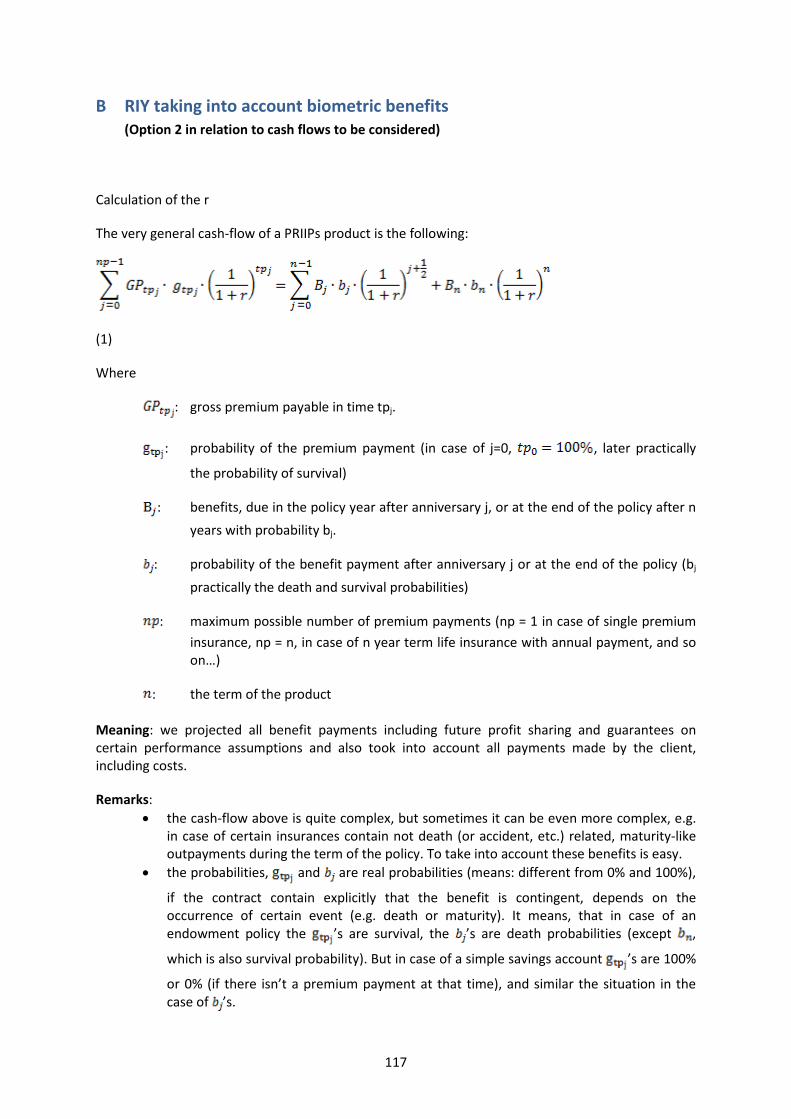
B RIY taking into account biometric benefits (Option 2 in relation to cash flows to be considered)

Calculation of the r

The very general cash-flow of a PRIIPs product is the following:

(1)

Where

: gross premium payable in time tpj.

: probability of the premium payment (in case of j=0, , later practically

the probability of survival)

: benefits, due in the policy year after anniversary j, or at the end of the policy after n years with probability bj.

: probability of the benefit payment after anniversary j or at the end of the policy (bj practically the death and survival probabilities)

: maximum possible number of premium payments (np = 1 in case of single premium insurance, np = n, in case of n year term life insurance with annual payment, and so on…)

: the term of the product

Meaning: we projected all benefit payments including future profit sharing and guarantees on certain performance assumptions and also took into account all payments made by the client, including costs.

Remarks: • the cash-flow above is quite complex, but sometimes it can be even more complex, e.g.

in case of certain insurances contain not death (or accident, etc.) related, maturity-like outpayments during the term of the policy. To take into account these benefits is easy.

• the probabilities, and are real probabilities (means: different from 0% and 100%),

if the contract contain explicitly that the benefit is contingent, depends on the occurrence of certain event (e.g. death or maturity). It means, that in case of an endowment policy the ’s are survival, the ’s are death probabilities (except ,

which is also survival probability). But in case of a simple savings account ’s are 100%

or 0% (if there isn’t a premium payment at that time), and similar the situation in the case of ’s.

117

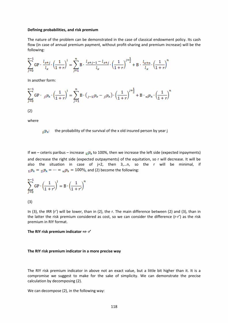
Defining probabilities, and risk premium

The nature of the problem can be demonstrated in the case of classical endowment policy. Its cash flow (in case of annual premium payment, without profit-sharing and premium increase) will be the following:

In another form:

(2)

where

: the probability of the survival of the x old insured person by year j

If we – ceteris paribus – increase to 100%, then we increase the left side (expected inpayments) and decrease the right side (expected outpayments) of the equitation, so r will decrease. It will be also the situation in case of j=2, then 3,…n, so the r will be minimal, if

, and (2) become the following:

(3)

In (3), the IRR (r’) will be lower, than in (2), the r. The main difference between (2) and (3), than in the latter the risk premium considered as cost, so we can consider the difference (r-r’) as the risk premium in RIY format.

The RIY risk premium indicator =r- r’

The RIY risk premium indicator in a more precise way

The RIY risk premium indicator in above not an exact value, but a little bit higher than it. It is a compromise we suggest to make for the sake of simplicity. We can demonstrate the precise calculation by decomposing (2).

We can decompose (2), in the following way:

118

(4)

where

: decomposition of the gross premium.

: net risk premium out of the j gross premium. It is the product of a sum at risk and a death probability. The sum at risk is the difference of the death benefit and the reserve, the death probability is the probability that an x year old insured (x the age at policy inception) die just between j and j+1.

: the savings premium with costs.

: decomposition of the death benefit.

: the cumulated savings (practically the reserve of the policy). .

: sum at risk in year j.

The (4) contain two cash-flows, (5) and (6):

(5)

and

(6)

The (5) is a pure savings product. In case of maturity, the client will get the whole amount, but if (s)he dies earlier, (s)he will get the savings so far. The (6) is a pure risk product – practically the equality equitation for this. This is not a classical term policy which is supposed to be part of an endowment policy together with a pure endowment.

The r for (5) and (6) will be the same as for (2) and each other. It means, that we suppose that the risk element in (6) was calculated with the internal rate of return of (2). This is reasonable. So the

119

internal rate of return for the cash-flow with death benefits (2) is the same as for a pure savings cash-flow (6).

We will get the exact r’, if we put into (5) the risk premiums as costs, i.e. without death benefits.

(7)

If we put , then (7) also become (3).

To calculate r’ with (3), without (7) means, that the RIY risk premium will not be exact (probable a little bit higher, than the real), but the RIY cost indicator remain exact. We think it is worth to make a little simplification ((3), without (7)) in the calculation of RIY risk indicator.

Annuities

In case of annuities there are special parameters for (1): • np=1 (single premium) • ’s are survival probabilities

In case of simple life annuity (1) become the following:

(8)

where ω is the maximum possible age.

In case of annuities there is not a separate RIY risk premium indicator, and have to use the probabilities as used in the premium calculation.

120

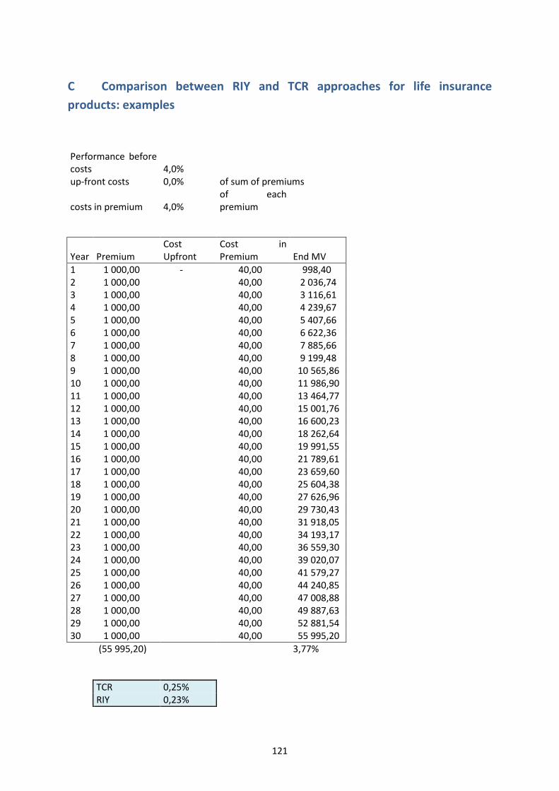
C Comparison between RIY and TCR approaches for life insurance products: examples

Performance before costs 4,0%

up-front costs 0,0% of sum of premiums

costs in premium 4,0% of each premium

Year Premium

Cost Upfront

Cost in Premium End MV

1 1 000,00 - 40,00 998,40 2 1 000,00

40,00 2 036,74

3 1 000,00

40,00 3 116,61 4 1 000,00

40,00 4 239,67

5 1 000,00

40,00 5 407,66 6 1 000,00

40,00 6 622,36

7 1 000,00

40,00 7 885,66 8 1 000,00

40,00 9 199,48

9 1 000,00

40,00 10 565,86 10 1 000,00

40,00 11 986,90

11 1 000,00

40,00 13 464,77 12 1 000,00

40,00 15 001,76

13 1 000,00

40,00 16 600,23 14 1 000,00

40,00 18 262,64

15 1 000,00

40,00 19 991,55 16 1 000,00

40,00 21 789,61

17 1 000,00

40,00 23 659,60 18 1 000,00

40,00 25 604,38

19 1 000,00

40,00 27 626,96 20 1 000,00

40,00 29 730,43

21 1 000,00

40,00 31 918,05 22 1 000,00

40,00 34 193,17

23 1 000,00

40,00 36 559,30 24 1 000,00

40,00 39 020,07

25 1 000,00

40,00 41 579,27 26 1 000,00

40,00 44 240,85

27 1 000,00

40,00 47 008,88 28 1 000,00

40,00 49 887,63

29 1 000,00

40,00 52 881,54 30 1 000,00 40,00 55 995,20

(55 995,20)

3,77%

TCR 0,25%

RIY 0,23%

121

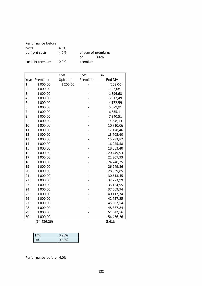
Performance before costs 4,0%

up-front costs 4,0% of sum of premiums

costs in premium 0,0% of each premium

Year Premium

Cost Upfront

Cost in Premium End MV

1 1 000,00 1 200,00 - (208,00) 2 1 000,00

- 823,68

3 1 000,00

- 1 896,63 4 1 000,00

- 3 012,49

5 1 000,00

- 4 172,99 6 1 000,00

- 5 379,91

7 1 000,00

- 6 635,11 8 1 000,00

- 7 940,51

9 1 000,00

- 9 298,13 10 1 000,00

- 10 710,06

11 1 000,00

- 12 178,46 12 1 000,00

- 13 705,60

13 1 000,00

- 15 293,82 14 1 000,00

- 16 945,58

15 1 000,00

- 18 663,40 16 1 000,00

- 20 449,93

17 1 000,00

- 22 307,93 18 1 000,00

- 24 240,25

19 1 000,00

- 26 249,86 20 1 000,00

- 28 339,85

21 1 000,00

- 30 513,45 22 1 000,00

- 32 773,99

23 1 000,00

- 35 124,95 24 1 000,00

- 37 569,94

25 1 000,00

- 40 112,74 26 1 000,00

- 42 757,25

27 1 000,00

- 45 507,54 28 1 000,00

- 48 367,84

29 1 000,00

- 51 342,56 30 1 000,00 - 54 436,26

(54 436,26)

3,61%

TCR 0,26%

RIY 0,39%

Performance before 4,0%

122

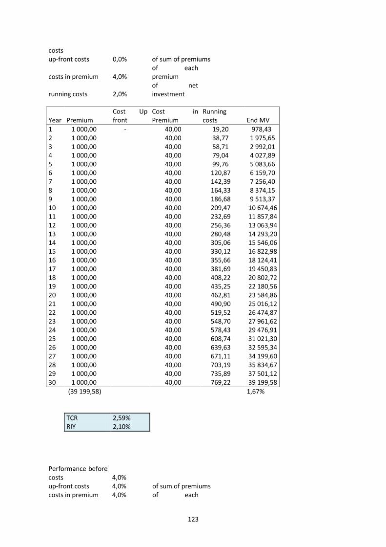
costs up-front costs 0,0% of sum of premiums

costs in premium 4,0%

of each premium

running costs 2,0%

of net investment

Year Premium

Cost Up front

Cost in Premium

Running costs End MV

1 1 000,00 - 40,00 19,20 978,43 2 1 000,00

40,00 38,77 1 975,65

3 1 000,00

40,00 58,71 2 992,01 4 1 000,00

40,00 79,04 4 027,89

5 1 000,00

40,00 99,76 5 083,66 6 1 000,00

40,00 120,87 6 159,70

7 1 000,00

40,00 142,39 7 256,40 8 1 000,00

40,00 164,33 8 374,15

9 1 000,00

40,00 186,68 9 513,37 10 1 000,00

40,00 209,47 10 674,46

11 1 000,00

40,00 232,69 11 857,84 12 1 000,00

40,00 256,36 13 063,94

13 1 000,00

40,00 280,48 14 293,20 14 1 000,00

40,00 305,06 15 546,06

15 1 000,00

40,00 330,12 16 822,98 16 1 000,00

40,00 355,66 18 124,41

17 1 000,00

40,00 381,69 19 450,83 18 1 000,00

40,00 408,22 20 802,72

19 1 000,00

40,00 435,25 22 180,56 20 1 000,00

40,00 462,81 23 584,86

21 1 000,00

40,00 490,90 25 016,12 22 1 000,00

40,00 519,52 26 474,87

23 1 000,00

40,00 548,70 27 961,62 24 1 000,00

40,00 578,43 29 476,91

25 1 000,00

40,00 608,74 31 021,30 26 1 000,00

40,00 639,63 32 595,34

27 1 000,00

40,00 671,11 34 199,60 28 1 000,00

40,00 703,19 35 834,67

29 1 000,00

40,00 735,89 37 501,12 30 1 000,00 40,00 769,22 39 199,58

(39 199,58)

1,67%

TCR 2,59%

RIY 2,10%

Performance before costs 4,0%

up-front costs 4,0% of sum of premiums costs in premium 4,0% of each

123

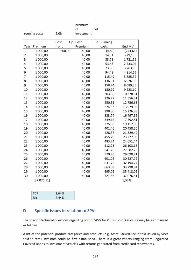
premium

running costs 2,0% of net investment

Year Premium

Cost Up front

Cost in Premium

Running costs End MV

1 1 000,00 1 200,00 40,00 (4,80) (244,61) 2 1 000,00

40,00 14,31 729,13

3 1 000,00

40,00 33,78 1 721,56 4 1 000,00

40,00 53,63 2 733,04

5 1 000,00

40,00 73,86 3 763,95 6 1 000,00

40,00 94,48 4 814,65

7 1 000,00

40,00 115,49 5 885,52 8 1 000,00

40,00 136,91 6 976,96

9 1 000,00

40,00 158,74 8 089,35 10 1 000,00

40,00 180,99 9 223,10

11 1 000,00

40,00 203,66 10 378,61 12 1 000,00

40,00 226,77 11 556,31

13 1 000,00

40,00 250,33 12 756,63 14 1 000,00

40,00 274,33 13 979,98

15 1 000,00

40,00 298,80 15 226,83 16 1 000,00

40,00 323,74 16 497,62

17 1 000,00

40,00 349,15 17 792,81 18 1 000,00

40,00 375,06 19 112,86

19 1 000,00

40,00 401,46 20 458,26 20 1 000,00

40,00 428,37 21 829,49

21 1 000,00

40,00 455,79 23 227,05 22 1 000,00

40,00 483,74 24 651,44

23 1 000,00

40,00 512,23 26 103,18 24 1 000,00

40,00 541,26 27 582,79

25 1 000,00

40,00 570,86 29 090,81 26 1 000,00

40,00 601,02 30 627,79

27 1 000,00

40,00 631,76 32 194,27 28 1 000,00

40,00 663,09 33 790,84

29 1 000,00

40,00 695,02 35 418,05 30 1 000,00 40,00 727,56 37 076,51

(37 076,51)

1,33%

TCR 2,64%

RIY 2,44%

D Specific issues in relation to SPVs

The specific technical questions regarding cost of SPVs for PRIIPs Cost Disclosure may be summarized as follows:

A list of the potential product categories and products (e.g. Asset Backed Securities) issued by SPVs sold to retail investors could be first established. There is a great variety ranging from Regulated Covered Bonds to investment vehicles with returns generated from credit card repayments.

124

For the purpose of the PRIIPs Regulation one can focus on SPVs that deliver traditional equity linked payoffs with some levels of capital protection to retail investors.

In that context, an SPV is a special purpose entity whose only business is to issue debt securities (Notes) and to enter into financial transactions. The Company will typically use the issue proceeds of the Notes to purchase certain assets. The assets are usually securities issued by a third-party issuer, but could take the form of other assets (such as shares or cash deposits).

In addition, the SPV typically enters into a swap agreement with a Dealer under the terms of which the SPV pays the returns of the assets against the return of an Equity structured pay-off.

For some Notes, there will not be any assets and the SPV will only enter into a swap agreement. When this is the case, the SPV pays all investment proceeds to the derivatives counterparty in exchange for the equity pay-off, and the obligations of the counterparty are collateralized under a CSA (credit support annex) agreement.

The assets and the swap agreement will generally be the only assets available to the SPV to fund its payment obligations under the notes.

For some notes, the amount payable on the maturity date may be less than the original investment and may even be zero. Typically, the higher the potential return on the notes, the greater the risk of loss attached to those notes will be.

For certain notes, the investor is entitled to receive at least 100 per cent. of the principal amount of the notes on the maturity date, subject to the credit risk of the obligor of the assets and Collateral posted by the swap counterparty (if any) and to the credit risk of the Custodian, the Principal Paying Agent, the Paying Agent(s) and the Counterparty to the swap agreement (if there is one). If there is a default on those assets, or by the Custodian, the Principal Paying Agent, the Paying Agent(s) or the Counterparty under the Swap Agreement, investors are likely to lose some or all of their money.

The costs of an SPV are best illustrated in a diagram of the cash flows between all entities and intermediaries involved in the creation, management and termination of an SPV:

125

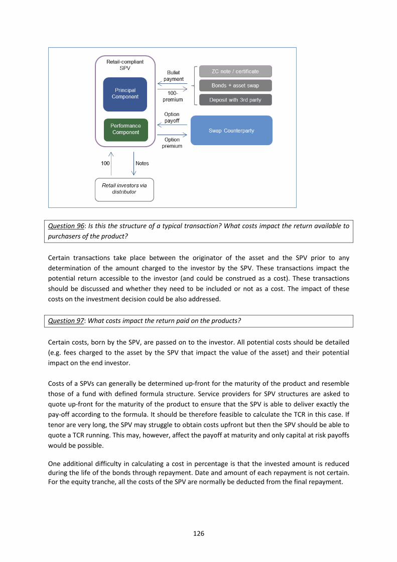
Question 96: Is this the structure of a typical transaction? What costs impact the return available to purchasers of the product?

Certain transactions take place between the originator of the asset and the SPV prior to any determination of the amount charged to the investor by the SPV. These transactions impact the potential return accessible to the investor (and could be construed as a cost). These transactions should be discussed and whether they need to be included or not as a cost. The impact of these costs on the investment decision could be also addressed. Question 97: What costs impact the return paid on the products?

Certain costs, born by the SPV, are passed on to the investor. All potential costs should be detailed (e.g. fees charged to the asset by the SPV that impact the value of the asset) and their potential impact on the end investor. Costs of a SPVs can generally be determined up-front for the maturity of the product and resemble those of a fund with defined formula structure. Service providers for SPV structures are asked to quote up-front for the maturity of the product to ensure that the SPV is able to deliver exactly the pay-off according to the formula. It should be therefore feasible to calculate the TCR in this case. If tenor are very long, the SPV may struggle to obtain costs upfront but then the SPV should be able to quote a TCR running. This may, however, affect the payoff at maturity and only capital at risk payoffs would be possible.

One additional difficulty in calculating a cost in percentage is that the invested amount is reduced during the life of the bonds through repayment. Date and amount of each repayment is not certain. For the equity tranche, all the costs of the SPV are normally be deducted from the final repayment.

126

Question 98: What are the potential difficulties in calculating costs of an SPV investment using a TCR approach?

This implies to look at all potential costs and understand how they would fit into a TCR framework.

Question 99: What are the potential difficulties in calculating costs of an SPV investment using a RIY approach?

This implies to look at all potential costs and understand how they fit into a RIY framework. There is a potential complication if the valuation of the asset in the RIY approach differs from the valuation of the asset as reported by the SPV.

127