Discussion Papers in Economics

DP 11/16

School of Economics University of Surrey

Guildford Surrey GU2 7XH, UK

Telephone +44 (0)1483 689380 Facsimile +44 (0)1483 689548 Web www.econ.surrey.ac.uk

ISSN: 1749-5075

VELOCITY IN THE LONG RUN: MONEY AND STRUCTURAL TRANSFORMATION

By

Antonio Mele

(University of Surrey)

& Radoslaw Stefanski

(University of St. Andrews and University of Oxford)

Velocity in the Long Run:

Money and Structural Transformation1

Antonio MeleUniversity of Surrey

Radoslaw StefanskiUniversity of St. Andrews and University of Oxford (OxCarre)

July 28, 2016

Abstract

Monetary velocity declines as economies grow. We argue that this is due to the process of

structural transformation - the shift of workers from agricultural to non-agricultural production

associated with rising income. A calibrated, two-sector model of structural transformation with

monetary and non-monetary trade accurately generates the long run monetary velocity of the

US between 1869 and 2013 as well as the velocity of a panel of 92 countries between 1980 and

2010. Three lessons arise from our analysis: 1) Developments in agriculture, rather than non-

agriculture, are key in driving monetary velocity; 2) Inflationary policies are disproportionately

more costly in richer than in poorer countries; and 3) Nominal prices and inflation rates are not

‘always and everywhere a monetary phenomenon’: the composition of output influences money

demand and hence the secular trends of price levels.

JEL codes: O1; O4; E4; E5; N1

Keywords: structural transformation, monetary shares, velocity, agricultural productivity, non-

monetary exchange

1 We would like to thank Martin Ellison, Alexander Berentsen, Fernando Martin, Domenico Ferraro, BertholdHerrendorf, Joe Kaboski, Marti Mestieri, Rachel Ngai, Edward C. Prescott, Todd Schoellman, Akos Valentyni,Gustavo Ventura, Xiaodong Zhu, and all other participants of the Structural Transformation Workshop at ArizonaState University as well as seminar participants at the University of Oxford and the University of St Andrews forhelpful comments and suggestions. All errors are our own.

Corresponding author: Radoslaw (Radek) Stefanski, School of Economics and Finance - Castlecliffe, TheScores - University of St Andrews, Fife KY16 9AR, United Kingdom. Email address: radek.stefanski@gmail.com;rls7@st-andrews.ac.uk

1 Introduction

How does a country’s long-run money demand change with its economic development? An exten-

sive literature2 finds that for broad enough measures of the money stock and over long periods of

time, increases in income per capita tend to be associated with increases in the money-to-GDP ratio

or, equivalently, a falling monetary velocity.3 The possible sources of this stylized fact have been

widely debated and include institutional changes, financial innovations, improvements in communi-

cation and information-gathering technologies as well as changes in the composition of output.4

Perhaps surprisingly, this research has been almost entirely empirical in nature, which has made it

challenging to quantify the role played by individual channels.5 In this paper we address this gap

by constructing and calibrating a model of long-run monetary demand, and we use the model to

quantify the role played by a single mechanism potentially driving the income-velocity relationship:

structural transformation. This process, also known as industrialization, is the change in the com-

position of an economy’s employment and output, from agricultural towards non-agricultural goods,

associated with economic growth. Whilst structural transformation is certainly known to influence

money demand (see for example Jonung (1983), Friedman (1959) or Chandavarkar (1977)), no the-

oretical models of the process exist, and the quantitative importance of this channel is unclear. We

use a calibrated model to show how structural transformation influences money demand over the

development process and that quantitatively this channel is the main driver of within and across

country differences in long-run monetary velocity.

The suggested mechanism is simple. Agriculture - especially traditional agriculture - is largely a

non-monetary sector. As is argued by Chandavarkar (1977), this is true for at least three reasons.

First, agricultural workers are often compensated in kind, either through share-cropping or other

informal credit arrangements. Second, households in poorer countries tend to home-produce their

agricultural consumption. Third, the agricultural setting is conductive to barter transactions.6

2 See for example Wicksell (1936), Warburton (1949), Friedman (1959), Bordo and Jonung (1981, 1987), Jonung(1983) or Ireland (1991).

3 Income velocity of money, V , is defined as the ratio of gross domestic product, Y (measured in current prices,P ) to the nominal money stock, M : V ≡ P×Y

M. This implies that the inverse of velocity is simply the money-share:

V −1 = MP×Y

. Velocity is thus a convenient measure of how money demand compares to income, with lower money

demand relative to income translating into higher velocity and viceversa. This also means that a rising money shareis equivalent to a falling velocity.

4 Wicksell (1936), for example, argues that this trend stems from an increase in the prominence of organizedmarkets, a shift from home to market production as well as the increase in both worker specialization and thecomplexity of goods. Friedman and Schwartz (1963) suggest that real money balances are luxury goods and hencehave an income elasticity larger than unity. Bordo and Jonung (1987, 1990) emphasize institutional changes andfinancial innovations as systematically influencing velocity over long periods, whilst Townsend (1987) and Goodfriend(1991) highlight that improvements in communications and information-gathering technologies can contribute to afalling velocity. Finally, Friedman (1959), Chandavarkar (1977) and Jonung (1983), assert that the composition of aneconomy can be important in driving money demand.

5 One notable exception is Ireland (1994), who constructs a theoretical model of changes in the compositionof monetary aggregates. Our paper instead focuses on the changes in the total share of money-stock-to-GDP andabstracts from compositional effects.

6 Since most individuals wish to consume as varied a bundle of food as possible, most household-producers will wishto consume the agricultural goods of other household-producers in addition to their own. Thus, double coincidenceof wants is easy to achieve when traders meet and thus the probability of barter is likely to be relatively high.

3

The non-agriculture sector, however, tends to be far more complex and hence is more likely to need

money to enable exchange.7 As an economy grows, its structure will change from one dominated

by a (predominantly non-monetary) agricultural sector towards one dominated by a (predominantly

monetary) non-agricultural sector. This changing composition of the economy results in a rising

demand for money, a rising money-to-GDP ratio and consequently a falling monetary velocity.

To capture the above mechanisms, we build a simple model with two sectors: agriculture, which

produces goods traded without money, and non-agriculture, in which an endogenous share of goods

is exchanged using money. The demand for money in the non-agricultural sector is introduced

through a cash-in-advance constraint on consumption goods following Cole and Kocherlakota (1998).

Building on a long-tradition of models exemplified by Herrendorf et al. (2014), Buera and Kaboski

(2012), Gollin et al. (2002), Restuccia et al. (2008), Yang and Zhu (2013) and Stefanski (2014a,b),

structural transformation is generated by non-homothetic preferences: consumers have a subsistence

level of agricultural consumption. Intuitively, households need to eat a minimum quantity of food

to survive. In poor countries where agricultural productivity tends to be low, more workers need to

be employed in the agricultural sector in order to produce enough food to satisfy subsistence needs.

A poor economy is thus dominated by non-monetary agriculture and most transactions take place

without money. As agricultural productivity increases, less workers are needed to satisfy subsistence

consumption, prompting workers to migrate into the non-agricultural sector and thus increasing

that sector’s share in total employment and output. Given that a part of non-agricultural goods

are traded with money, the shift in the composition of the economy towards the non-agricultural

sector will result in an increase in monetary transactions, an increase in the money-to-GDP ratio

and hence in a lower velocity.

The model is calibrated to match the 1869-2013 patterns of US growth, structural transformation

and monetary supply. Our simple framework replicates several features of the long run data including

agricultural labor shares, GDP per worker, sectoral prices, nominal interest rates and aggregate

inflation. Most importantly, the model reproduces the evolution of the US long run money-to-GDP

ratio over 140 years, capturing nearly 91% of the variation in the data. A similarly calibrated one-

sector model fails to replicate observed money-share, as it is unable to match the observed price

dynamics - and in particular the so-called ‘Great-Deflation’ of the late 19th century. The model

also accurately predicts the variability in velocity across countries. Keeping preference parameters

of the US, we recalibrate the model to a panel of 92 countries between 1980 and 2010. The model

accurately captures cross-country differences in incomes, employment shares, interest rates and

inflation rates. It also does well in reproducing velocities and does exceptionally well in replicating

the income-velocity relationship.8

7 Crucially, there are more varieties of goods in the non-agricultural sector. Thus, the probability that an economicsprofessor - for example - can barter his output for the services of a car mechanic is far lower than the probability thattwo farmers producing different types of vegetables may wish to trade. For an in-depth discussion on this transactionsrole of money see Ostroy and Starr (1990).

8 In particular, a one percent increase in GDP per worker is found to increase the money-to-GDP ratio by 0.14percentage points in both the data and the model.

4

The multi-sector framework, and in particular the reallocation of workers from agriculture to

non-agriculture, is the key driver of our results. To illustrate this point, we perform a number

of exercises that isolate individual channels affecting monetary velocity, like variation in monetary

growth rates, productivity growth rates and productivity levels. We also extend the baseline model

to allow for heterogenous endowments of capital across countries.9 Quantitatively, we find that

differences in agricultural productivity levels are the key source of cross-country variation in velocity

since they influence the size of the non-agricultural, predominantly-monetary sector. A one-sector

version of our model without structural transformation fails entirely in capturing across and within

country variation in monetary velocity.

Finally, we examine how the costs of suboptimal monetary policies vary with income. Inflation is

more costly in richer countries than in poorer countries - where the monetary part of the economy is

smaller and therefore distortions from the inflation tax are less damaging. For example, a hyperinfla-

tion of approximately 400% a year in a poor country like Zimbabwe (where GDP per worker is 2% of

that of the US) will have negligible welfare costs. By contrast, the same hyperinflation in a country

like Argentina (30% of US GDP per worker) will have very large welfare costs. Argentinean incomes

would have to rise by approximately 25% to deliver the same expected flow utility as without the

hyperinflation. The low cost of inflation in poorer countries may help explain why poorer countries

tend to have much higher inflation rates than richer countries.

There are three main lessons from our work. First, monetary velocity is not constant over the

development process but falls with income. Most of the existing explanations of this observation

are rooted in the non-agricultural sector - and focus on factors such as financial innovation or

the expansion of the banking sector. The surprising finding of this paper is that the evolution of

monetary velocity is driven almost exclusively by developments in the agricultural sector. It is the

variation in agricultural productivity that influences the size of the non-agricultural sector and in

turn influences monetary demand and hence velocity. Second, since velocity depends systematically

on the composition of output - a country’s price levels and inflation rates may not ‘always and

everywhere be a monetary phenomenon’ (Friedman and Schwartz, 1963). The price level in an

economy, P , is defined as P ≡ (M/Y )V where M is the money stock, Y is output and V is

velocity. Two countries, with identical money stocks and identical output levels - but with different

output compositions - will have entirely different velocities, V , and hence different price levels. The

message to researchers from these findings is that a one sector model cannot be successfully used to

understand the long run dynamics of monetary velocity and hence the evolution of price levels or

inflation rates. These findings should also be of interest to policymakers in developing countries who

may have overlooked the importance of the agricultural sector in their monetary policy decisions.

Finally, the third lesson of this paper is that the cost of inefficient monetary policy varies with

income and is higher in richer countries than in poorer countries. An inflation tax offers a relatively

9 Capital is largely a credit good and so a variation in capital stock levels can influence the demand for moneyand hence velocity.

5

cheap source of income to poor-country governments, and its distortive effects are relatively small in

economies that are dominated by large, non-monetary, agricultural sectors. This may help explain

why we observe persistently higher inflation in poorer countries than in richer countries - despite

recommendations of strong anti-inflationary policies by international financial institutions such as

the International Monetary Fund (IMF).10

In the next section we document the main facts regarding structural transformation, monetary

velocity and the extent of non-monetary production in agriculture. In section 3, we construct and

solve our simple baseline model. In section 4 we calibrate the model to the experience of the United

States and in section 5 we show the results for the US. Section 6 carries out the cross-country analysis

by examining how the model performs in international, cross-country data and by running a number

of counterfactuals to quantify the importance of the different mechanisms of the model. Section 7

examines the different costs of inflation in rich and poor countries. Finally, section 8 offers some

concluding remarks on the importance of our findings.

2 Facts

In this section we present three stylized facts. First, there is a positive relationship between the

money to GDP ratio (or the inverse of monetary velocity) and income per capita. Second, the

proportion of workers employed in agriculture tends to fall as income rises. Finally, non-monetary

activities are most prevalent in countries with large agricultural sectors. These facts taken together

suggest that as countries grow richer, they tend to use more money relative to the size of their

economy, and that this process is potentially linked with the decline of a predominantly non-monetary

sector - agriculture.11

Money Shares We are interested in the pattern of the ratio of the stock of money to nominal

GDP, over time and across countries.12 It is therefore crucial to define exactly what we mean by

the stock of money. Throughout the paper all classifications of monetary data follow the definitions

set out by the IMF in the International Financial Statistics (IFS). The IFS classifies money into ever

broadening bands from M0 to M3.13 We are not directly interested in the narrowest definition of

the monetary stock such as M0 or M1: as argued by Ireland (1994), economies undergo a change in

10 Weisbrot et al. (2009), for example, examine existing IMF loan agreements with 41 developing countries in 2009.They find that the IMF took a stance on monetary policy in 25 of these countries and in 22 of those 25 countries itrecommended a contractionary or anti-inflationary monetary policy.

11 See Appendix A for details of sources and construction of all data.12 From now on, unless otherwise stated, we will only refer to money share relative to the GDP instead of referring

to (the inverse of) velocity. This saves repetition and - in our eyes - the money share has a cleaner and more intuitiveinterpretation than velocity.

13 The narrowest definition of money stock, M0, is the value of currency and deposits in the central bank. Thenext classification, M1, includes all of M0 as well as transferable deposits and electronic currency. Next, M2, includesM1 but also measures time and savings deposits, foreign currency transferable deposits, certificates of deposit andsecurities repurchase agreements. Finally, M3, includes M2 as well as travelers checks, foreign currency time deposits,commercial paper and shares of mutual/market funds.

6

BDI

ETHZWE

MWICAFTZA

NPL

NER

MDGGIN

UGA

BFA

LBR

TGO

TCD

BGD

GNBKHMSLE

LSO

RWA

ZMB

SOM

MLI

KEN

LAO

VNM

BEN

TJK

GMBCIVSTPSENGHAKGZNGA

HTI

COMAFG

COG

CHN

MDA

IND

PNG

CMR

CPV

BTN

MRT

LKA

GEO

PAKIDNMNG

PHL

ARM

GNQ

AGO

BOL

MAR

NIC

SLB

YEM

GUY

AZE

ALB

PRYUKRHNDMDV

THAEGY

FJI

DJI

NAM

VCT

SWZSRB

BIH

VUT

PERKAZ

MKD

SYR

ECU

SLVTUN

WSMGTM

PAN

BLRIRQDOM

MUS

COL

BRA

BWA

BGRURY

LVA

MYS

CHLDZAJAM

RUS

ZAF

ARG

TURESTLTUVEN

LCA

TKM

TONCRIBLZHRVPOL

JOR

IRNSURSVK

GAB

LBN

MEX

CYP

HUN

PRT

CZEKOR

MLT

SVN

OMN

LBYTTO

NZLBHRGRC

SAU

GBRESPBRBFINDNK

ISR

BHS

JPN

SWE

KWTCANDEU

SGP

AUSIRL

CHE

FRAITANLDAUTBEL

NORBRNUSA

ISLQAT

LUX

ARE

Average: 1980−2010

6

12

25

50

100

200

400

800M

oney

Sha

re, %

.008 .016 .03 .06 .12 .25 .5 1 2 4

GDP per worker (PPP), USA=1

(a) M2/GDP and GDP per capita (1990 PPP USD).Cross-section data, 1980-2010 average.

Share of M2in GDP, US

20

40

60

80

100

Mo

ney

Sh

are,

%

1870 1890 1910 1930 1950 1970 1990 2010 Year

(b) US Data, 1869-2013.

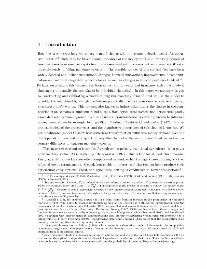
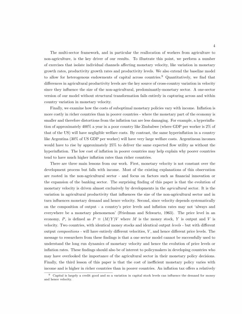
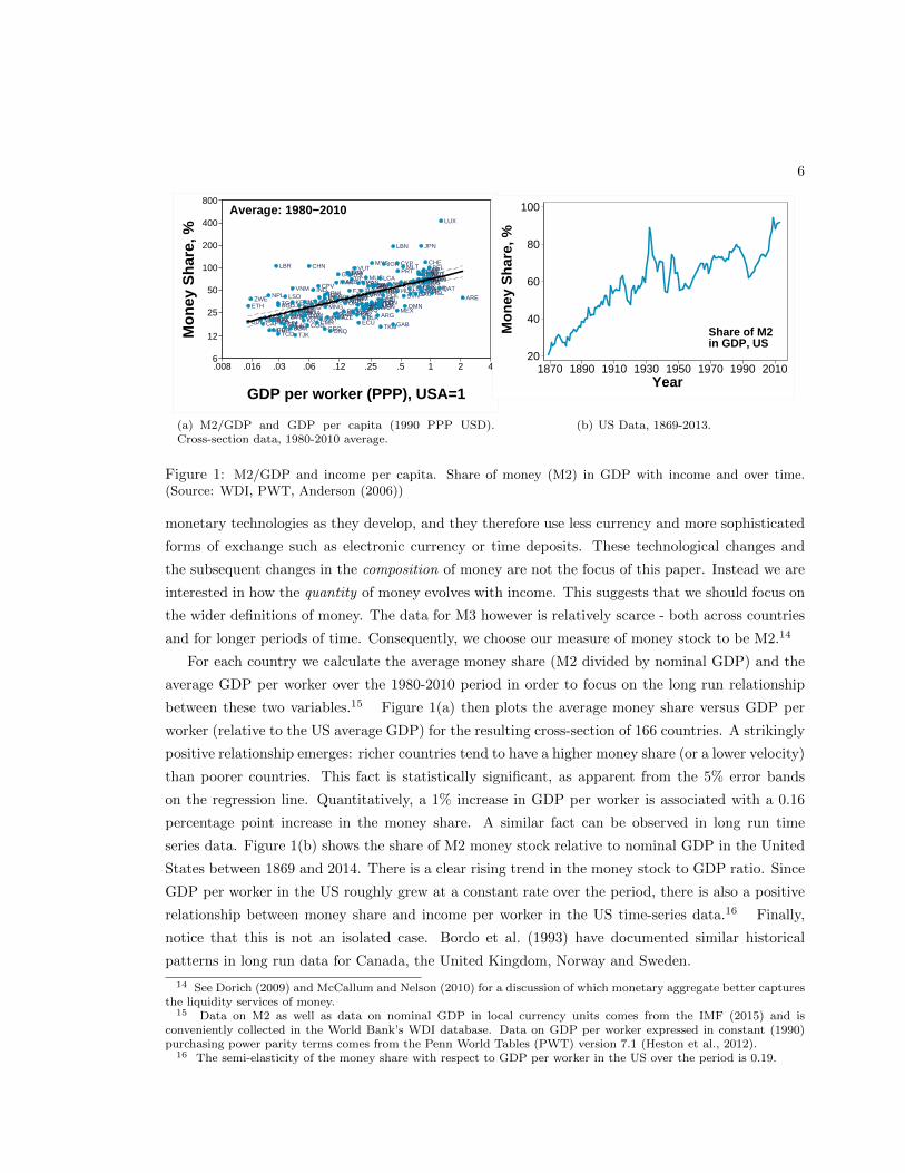
Figure 1: M2/GDP and income per capita. Share of money (M2) in GDP with income and over time.(Source: WDI, PWT, Anderson (2006))

monetary technologies as they develop, and they therefore use less currency and more sophisticated

forms of exchange such as electronic currency or time deposits. These technological changes and

the subsequent changes in the composition of money are not the focus of this paper. Instead we are

interested in how the quantity of money evolves with income. This suggests that we should focus on

the wider definitions of money. The data for M3 however is relatively scarce - both across countries

and for longer periods of time. Consequently, we choose our measure of money stock to be M2.14

For each country we calculate the average money share (M2 divided by nominal GDP) and the

average GDP per worker over the 1980-2010 period in order to focus on the long run relationship

between these two variables.15 Figure 1(a) then plots the average money share versus GDP per

worker (relative to the US average GDP) for the resulting cross-section of 166 countries. A strikingly

positive relationship emerges: richer countries tend to have a higher money share (or a lower velocity)

than poorer countries. This fact is statistically significant, as apparent from the 5% error bands

on the regression line. Quantitatively, a 1% increase in GDP per worker is associated with a 0.16

percentage point increase in the money share. A similar fact can be observed in long run time

series data. Figure 1(b) shows the share of M2 money stock relative to nominal GDP in the United

States between 1869 and 2014. There is a clear rising trend in the money stock to GDP ratio. Since

GDP per worker in the US roughly grew at a constant rate over the period, there is also a positive

relationship between money share and income per worker in the US time-series data.16 Finally,

notice that this is not an isolated case. Bordo et al. (1993) have documented similar historical

patterns in long run data for Canada, the United Kingdom, Norway and Sweden.

14 See Dorich (2009) and McCallum and Nelson (2010) for a discussion of which monetary aggregate better capturesthe liquidity services of money.

15 Data on M2 as well as data on nominal GDP in local currency units comes from the IMF (2015) and isconveniently collected in the World Bank’s WDI database. Data on GDP per worker expressed in constant (1990)purchasing power parity terms comes from the Penn World Tables (PWT) version 7.1 (Heston et al., 2012).

16 The semi-elasticity of the money share with respect to GDP per worker in the US over the period is 0.19.

7

COD

MOZ

ZWE

BDI

ETHMWI

CAF

TZANPL

NER

MDG

UGA

BFA

SOM

KHMLBR

TGO

TCD

BGD

GIN

GNB

SLE

LSO

RWA

VNMZMB

LAOMLI

KEN

BEN

GMB

CIV

TJK

SEN

GHA

NGA

HTI

AFG

KGZ

COG

COM

CHN

UZB

STP

MDA

IND

PNG

CMR

BTN

CPV

MRT

LKA

GEO

GNQ

PAKIDN

PHL

ARM

AGO

BOL

MNG

MAR

NIC

SLB

YEM

GUY

AZE

PRY

ALB

UKR

HND

BIH

MDV

THA

EGY

FJI

VCT

SWZ

SRB

VUT

PER

KAZ

NAM

MKD

SYRECU

SLV

DJI

TUN

WSM

GTM

BLR

PANDOMMUS

COL

BRA

BWA

BGRIRQURYLVAUSSR

MYS

CHL

DZA

JAM

RUSZAFYUGARGLTUEST

TUR

CUB

VEN

LCA

TON

CRI

HRV

BLZPOL

TKM

JOR

IRN

SUR

SVK

GAB

LBN

MEX

CYPHUNPRT

CSKCZE

KOR

SVNMLT

OMN

LBYTTONZL

BHR

GRCSAU

GBRBRBESPFINDNKISRBHSJPNSWECAN

KWTSGPAUSDEUCHE

IRL

FRAITANLDAUTBELNORUSA

ISL

QATLUXBRNARE

1/64 1/32 1/16 1/8 1/4 1/2 1 2 4

Average: 1980−2010

0

20

40

60

80

100A

gr. E

mp.

Sha

re, %

PPP GDP per worker, USA=1

(a) Cross Section

0%

20%

40%

60%

80%

1860 1880 1900 1920 1940 1960 1980 2000

Shar

e of

Em

ploy

men

t (%

)

Agriculture Services

Industry

Source: Feldstein (1988), WDI

Employment Shares, US

(b) USA

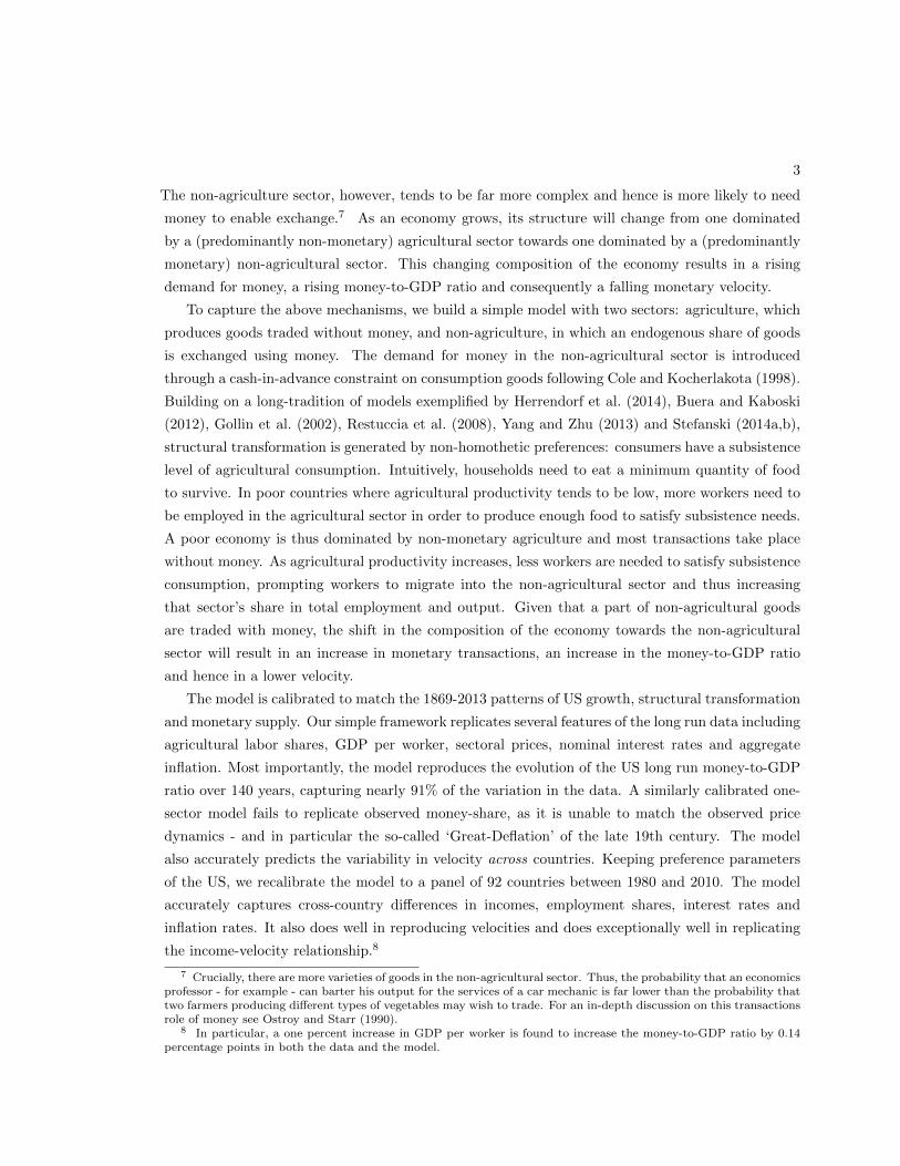
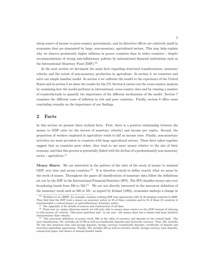
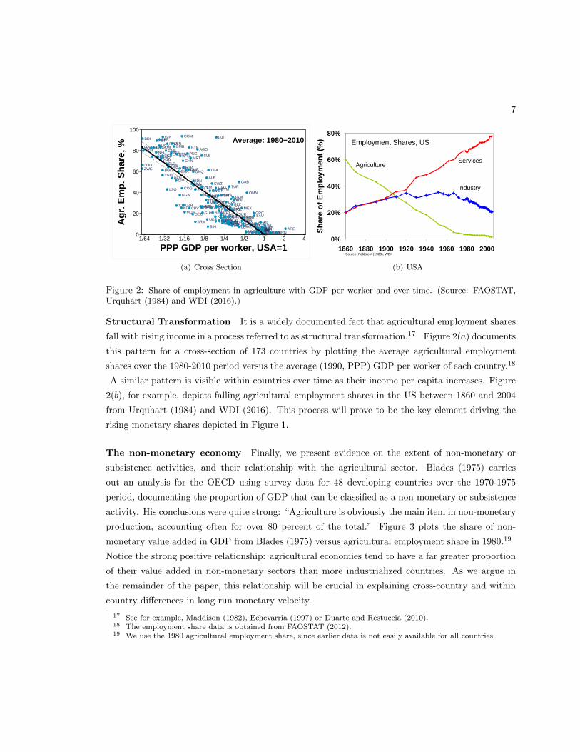
Figure 2: Share of employment in agriculture with GDP per worker and over time. (Source: FAOSTAT,Urquhart (1984) and WDI (2016).)

Structural Transformation It is a widely documented fact that agricultural employment shares

fall with rising income in a process referred to as structural transformation.17 Figure 2(a) documents

this pattern for a cross-section of 173 countries by plotting the average agricultural employment

shares over the 1980-2010 period versus the average (1990, PPP) GDP per worker of each country.18

A similar pattern is visible within countries over time as their income per capita increases. Figure

2(b), for example, depicts falling agricultural employment shares in the US between 1860 and 2004

from Urquhart (1984) and WDI (2016). This process will prove to be the key element driving the

rising monetary shares depicted in Figure 1.

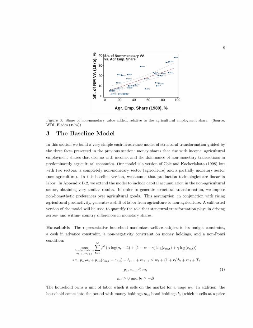
The non-monetary economy Finally, we present evidence on the extent of non-monetary or

subsistence activities, and their relationship with the agricultural sector. Blades (1975) carries

out an analysis for the OECD using survey data for 48 developing countries over the 1970-1975

period, documenting the proportion of GDP that can be classified as a non-monetary or subsistence

activity. His conclusions were quite strong: “Agriculture is obviously the main item in non-monetary

production, accounting often for over 80 percent of the total.” Figure 3 plots the share of non-

monetary value added in GDP from Blades (1975) versus agricultural employment share in 1980.19

Notice the strong positive relationship: agricultural economies tend to have a far greater proportion

of their value added in non-monetary sectors than more industrialized countries. As we argue in

the remainder of the paper, this relationship will be crucial in explaining cross-country and within

country differences in long run monetary velocity.

17 See for example, Maddison (1982), Echevarria (1997) or Duarte and Restuccia (2010).18 The employment share data is obtained from FAOSTAT (2012).19 We use the 1980 agricultural employment share, since earlier data is not easily available for all countries.

8

AGO

ARG

BEN

BFA

BWA

CIV

CMR

DOM

ECU

GUY

IND

IRN

IRQ

JAM

JOR

KENKOR

MEX

MLI

MOZ

MRT

MUS

MYS

NICPHL

SEN

SLE

SWZ

THA

UGA

VEN

VNM

ZMB

Sh. of Non−monetary VAvs. Agr Emp. Share

0

10

20

30

40

Sh.

of N

M V

A (

1975

), %

0 20 40 60 80 100

Agr. Emp. Share (1980), %

Figure 3: Share of non-monetary value added, relative to the agricultural employment share. (Source:WDI, Blades (1975))

3 The Baseline Model

In this section we build a very simple cash-in-advance model of structural transformation guided by

the three facts presented in the previous section: money shares that rise with income, agricultural

employment shares that decline with income, and the dominance of non-monetary transactions in

predominantly agricultural economies. Our model is a version of Cole and Kocherlakota (1998) but

with two sectors: a completely non-monetary sector (agriculture) and a partially monetary sector

(non-agriculture). In this baseline version, we assume that production technologies are linear in

labor. In Appendix B.2, we extend the model to include capital accumulation in the non-agricultural

sector, obtaining very similar results. In order to generate structural transformation, we impose

non-homothetic preferences over agricultural goods. This assumption, in conjunction with rising

agricultural productivity, generates a shift of labor from agriculture to non-agriculture. A calibrated

version of the model will be used to quantify the role that structural transformation plays in driving

across- and within- country differences in monetary shares.

Households The representative household maximizes welfare subject to its budget constraint,

a cash in advance constraint, a non-negativity constraint on money holdings, and a non-Ponzi

condition:

maxat, cm,t, cn,t,bt+1,mt+1

∞∑t=0

βt (α log(at − a) + (1− α− γ) log(cm,t) + γ log(cn,t))

s.t. pa,tat + pc,t(cm,t + cn,t) + bt+1 +mt+1 ≤ wt + (1 + rt)bt +mt + Tt

pc,tcm,t ≤ mt (1)

mt ≥ 0 and bt ≥ −B

The household owns a unit of labor which it sells on the market for a wage wt. In addition, the

household comes into the period with money holdings mt, bond holdings bt (which it sells at a price

9

1+ rt) and it receives a helicopter transfer of money from the government of Tt. Given this income,

the household purchases agricultural goods at (at the price pa,t) as well as non-agricultural goods

cm,t and cn,t (at the price pc,t). It also purchases bonds bt+1 that promise to pay out 1+rt+1 dollars

next period, and chooses its (non-negative) stock of money, mt+1, for the next period. We assume

that there are two kinds of non-agricultural goods: those that can be bought without money (cnt )

and those that must be bought with money (cm,t). This establishes a role for money: the household

needs to put aside a part of its income, mt+1, each period in order to be able to buy monetary goods

in the following period. To capture this idea, we impose the cash-in-advance (CIA) constraint (25)

on cm,t goods. Only cash held from the previous period can be used to purchase monetary goods in

the current period and cash transfers from government can only be used in the subsequent period.

Finally, we impose a lower bound, −B, on bond holdings to avoid Ponzi schemes.

Households have non-homothetic preferences for agricultural goods at. In other words, there ex-

ists a subsistence level of agriculture, a, that must be consumed every period. Intuitively, households

need to obtain a minimum quantity of food or calories in order to survive. A crucial assumption of

our model is that agriculture is a non-cash good. The intuition here is that agriculture - especially

traditional agriculture - is often characterized by compensation in kind or subsistence production.

Farmers - especially in poorer countries - often work for landlords as sharecroppers and get paid in

kind for their efforts, or produce much of their food at home for their own consumption (Blades,

1975). Furthermore, barter is far more likely in agriculture than in non-agriculture, as most people

wish to eat a varied basket of foods. Thus, when two agricultural producers (or households) meet to

trade, double coincidence of wants for agricultural products is relatively likely. As such, little to no

cash is needed to obtain agricultural goods in poorer countries. Of course, the above assumption is

a simplification and in richer countries, cash will be far more readily used in the agricultural sector.

However, in richer countries, the agricultural sector will also tend to be very small - and hence

the influence of agricultural money demand on the overall money demand will also be very small.

Therefore, as a first approximation, the assumption that all agricultural goods are traded without

money is a reasonable one.

Money use in non-agriculture, however, will be important, since a double coincidence of wants

in that sector is far less likely. Due to the massive variety of goods produced in non-agriculture,

the probability that two randomly matching producers or consumers (say an economist and a car

mechanic) would want each other’s services will be far smaller. As such, money becomes necessary

to overcome this mismatch problem. Of course, some goods in non-agriculture are nonetheless still

traded without cash using credit arrangements or payments in kind (e.g. employer-provided cars,

housing, health insurance etc.). Hence, following Chari et al. (1996b), in our model a fixed proportion

γ of non-agricultural goods do not require cash.20

20 In Appendix B.2, we follow Cole and Kocherlakota (1998) by adding capital to the model, and show that if wetreat investment as a non-monetary, credit good we can go a long way in endogenizing the cash-credit split of thenon-agricultural sector.

10

Firms There are two representative firms: agricultural (a) and non-agricultural (c). Each firm s =

a, c, hires labor, Ls,t, and produces output, Ys,t, using a simple linear technology that combines labor

with exogenous, sector-specific total factor productivity, Bs,t. The profit maximization problems are:

maxLs,t

ps,tYs,t − wtLs,t s.t. Ys,t = Bs,tLs,t. (2)

Output of non-agricultural firms, Yc,t, can be sold as both a monetary and a non-monetary good,

whereas all agricultural output is assumed to be non-monetary.

Money Supply The government is assumed to have a so-called helicopter monetary policy:

Mt+1 = Tt+1 +Mt. (3)

Market Clearing Finally, in each period, markets clear in a standard fashion.

at = Ya,t, cm,t + cn,t = Yc,t

mt = Mt, bt = 0 (4)

La,t + Lc,t = 1.

Competitive Equilibrium For a given monetary policy, {Tt}∞t=0, a competitive equilibrium in

this economy is a sequence of prices, {pa,t, pc,t, wt, rt}, and quantities, {at, cm,t, cn,t, bt,mt, La,t, Lc,t}∞t=0,

such that (1) given prices and monetary policy, households and firms solve their optimization prob-

lem, (2) the government budget constraint is satisfied and (3) markets clear.

Solution The first order conditions for the household are given by:

at:αβt

at − a= λtpa,t; cm,t:

(1− α− γ)βt

cm,t= pc,t(λt + µt); cn,t:

γβt

cn,t= pc,tλt (5)

bt+1: λt = (1 + rt+1)λt+1; mt+1: λt = λt+1 + µt+1 (6)

CIA: µt(pc,tcm,t −mt) = 0 and µt ≥ 0 (7)

In the above, λt and µt are multipliers on the budget and CIA constraints respectively. The

firms’ first-order conditions are:

La,t: pa,tBa,t = wt and Lc,t: pc,tBc,t = wt. (8)

The market clearing conditions are given by the equations in (4). Finally, the transversality condi-

tions for the above problem are:

lim inft→∞

λt(bt+1 + B) = 0 and lim inft→∞

λtmt+1 = 0. (9)

11

Following Cole and Kocherlakota (1998), we solve the model by imposing the following assump-

tion on interest rates:

Assumption 3.1. Assume that interest rates are always positive, i.e. rt > 0.

The consequence of the above assumption is that the CIA constraint always binds since there is

a positive opportunity cost of holding money.21 We impose this assumption for two reasons. First

and most importantly, despite recent negative nominal interest rates, this paper’s focus is the very

long run, and long-run interest rates have tended to be positive. Second, imposing this assumption

allows us to find a simple, analytic and unique solution.

Given a sequence of government policies and Assumption 3.1 (so that the CIA constraint holds

with equality), equations (5)-(8), in addition to the market clearing conditions, characterize the

competitive equilibrium. In particular, sectoral employment is given by:

La,t =ατt + (1− α− γ(1− τt))

aBa,t

1− (α+ γ)(1− τt)and Lc,t = 1− La,t, (10)

where τt ≡ 1β

Mt+1

Mt. Non-agricultural output is divided between cash and non-cash goods:

cn,t = (1− φt)Yc,t and cm,t = φtYc,t, (11)

where φt =1−α−γ

(1−α−γ)+γτt. Finally, sectoral prices are

pa,t =Mt

φtBa,tLc,tand pc,t =

Mt

φtBc,tLc,t(12)

and the nominal interest rate and wage rate are

rt = τt − 1 and wt =Mt

φtLc,t. (13)

The impact of non-homothetic preferences on agricultural employment can be seen in equation

(10). When productivity in agriculture, Ba,t, is low, a large fraction of the labor force must work

in agriculture in order to produce enough food for subsistence. As productivity in agriculture

increases the subsistence level can be met with a smaller fraction of the population working in the

agricultural sector resulting in a shift of workers from agriculture to non-agriculture. In other words,

from equation (10), ∂La,t/∂Ba,t < 0.

Next, notice that the composition of the economy affects sectoral prices. Since sectoral em-

ployment shares depend on agricultural productivity, from equations (10) and (12), we can write

∂ps,t/∂Ba,t < 0, s = a, c. In other words, ceteris paribus, prices of agricultural and non-agricultural

goods decline with rising agricultural productivity and hence with structural transformation. Thus

it is not only monetary factors that drive nominal prices, as has been suggested by the literature

21 To see this divide the equations in (6) by each other to obtain the expression for interest rates, rt+1 =µt+1

λt+1.

Thus, the nominal interest rate is positive if and only if money yields liquidity services (µt+1 > 0). In particular, ifthe nominal interest rate is positive, the CIA constraint is binding.

12

(Friedman and Schwartz, 1963), but real factors also play a crucial role. Rising agricultural pro-

ductivity changes the composition of the economy, and hence influences the nominal price of goods.

This feature of the model is particularly important at the early stages of industrialization. In section

5, we show that this process was key in generating the so-called “Great Deflation” in the late 19th

century United States.

Finally, notice that monetary policy has an impact both on sectoral employment and the con-

sumption of monetary goods. By choosing the transfers, the government directly controls the evolu-

tion of the money stock in the economy, Mt, and hence the variable τt, which determines how costly

it is to hold cash from one period to another. From equation (13), the higher the τt, the higher the

nominal interest rate, and hence the greater the opportunity cost of holding cash. Thus, higher τt

results in workers shifting away from cash dominated sectors, ∂Lc,t/∂τt < 0 and consumers consum-

ing less cash goods, ∂cm,t/∂τt < 0. This first channel highlights a new cost of monetary policy in

this two-sector CIA model - higher inflation taxes can reverse or delay structural transformation.

Interestingly, the impact of monetary policy on the size of the agricultural sector is itself dependent

on the level of agricultural productivity, given that∂(∂La,t/∂τt)

∂Ba,t> 0. In other words, an inflation

tax in a country with higher agricultural productivity will have a greater distortionary effect than

in a country with lower productivity. Countries with high agricultural productivity have larger

non-agricultural and hence monetary sectors. The inflation tax will hence impact a larger fraction

of those economies. This suggests that the same policies will have different effects in rich and poor

countries. We quantify these effects in section 7, where we look at the welfare cost of inflation.

Optimality The distortion in this environment arises - as in the standard CIA model - from the

lag between households being paid their wage income and their ability to buy non-agricultural cash

goods with that income (Cole and Kocherlakota, 1998). In particular, households can only use

last period’s money holdings to purchase current period non-agricultural cash goods. This forces

households to hold a low-yield asset (money) instead of a higher yield asset (bonds) in order to

have money holdings to purchase cash goods in the future. Thus, as long as nominal interest rates

are positive (i.e., the CIA constraint binds), the economy will not reach the first best. If, however,

nominal interest rates were set to zero, then households would be indifferent between being paid

today or being paid in the future (and indeed between holding money and a bond), and the distortion

associated with the trading arrangement would be eliminated.22 Hence, since the CIA binds if and

only if rt > 0, and, as we showed above, rt = τt − 1, we need τt → 1 to eliminate the distortion. In

other words, we need to implement the Friedman rule, i.e. we must have Mt+1

Mt→ β.23

22 More specifically, money does not expand the production possibility frontier. As such, the Pareto optimalallocations can be found by solving the corresponding social planner’s problem without money. It is then easy to showthat the decentralized problem and the social planner’s problem are identical when nominal interest rates are zero.

23 A word of caution is needed here. Whilst it is true that as τt → 1, the equilibrium allocations approach thePareto optimal allocations, directly setting τt = 1 in equations (10)-(13) violates Assumption 3.1. It is relatively easyto show that it is nonetheless true that the allocations and prices implied by the above equations when τt = 1 are alsoa competitive equilibrium. However, as is argued by Cole and Kocherlakota (1998), an equilibrium such as this (i.e.one where rt = 0) can be achieved with a large set of monetary policies - including but not restricted to the policy

13

Velocity The share of monetary stock relative to the nominal GDP (or the inverse of monetary

velocity) can be written as:

V −1t =

Mt

pa,tat + pc,tCt=

φtpc,tCt

pa,tat + pc,tCt

= φtLc,t. (14)

The first equality follows by definition. The second equality follows from the assumption that the

CIA constraint binds, and from equation (11), which splits non-agricultural consumption into its

monetary and non-monetary components. The final equality follows from equations (10)-(13).

There are two channels driving the money share. First, the term φt determines what proportion

of non-agriculture is bought with cash. This variable itself is influenced by the preference parameter,

γ, which captures (in a reduced form) the non-monetary activity in the non-agricultural sector, as

well as by τt. Since ∂φt/∂τt < 0, a higher inflation tax results in households wanting to purchase

fewer cash goods, which in turn lowers money demand and the money share. Second, the money

share crucially and positively depends on Lc,t - the share of employment in the non-agricultural

sector. As a greater proportion of workers shifts to a largely cash sector, the share of money in the

economy rises - and the velocity falls.

From (14), two facts of interest emerge. First, since higher agricultural productivity results in

greater non-agricultural employment, it also implies a higher money share. In other words,∂V −1

t

∂Bat

> 0.

Second, a higher inflation tax means it is more costly to hold cash, which leads to a lower employment

share in non-agriculture (as workers move away from a cash to a non-cash sector) and a lower φt (as

consumers want to consume less cash goods). Together this means that the money share decreases

in response to a higher τt so that∂V −1

t

∂τt< 0.

These two facts highlight that both monetary policy and agricultural productivity can influence

a country’s monetary demand and hence monetary shares. We quantify the role that each of these

channels play in explaining within and across country variation in monetary shares, by calibrating

the model in the next section.

4 US Calibration

We calibrate the model to the experience of the United States between 1869 and 2012.24 Follow-

ing Solow (1956), we measure the growth of technological residuals with production functions. In

particular, measured productivity in the agricultural (Ba,t) and non-agricultural sectors (Bc,t) is:

Ba,t =Ya,t

La,tand Bc,t =

Yc,t

Lc,t. (15)

Mt+1/Mt = β. Thus, whilst the limit is indeed an equilibrium, Pareto optimal and can be implemented with a policyτt = 1, it is not necessarily unique as other monetary policies could also sustain zero nominal interest rates.

24 See Appendix A for details of sources and construction of all data.

14

M2 per worker, US

.01

.1

1

1019

90=1

1870 1890 1910 1930 1950 1970 1990 2010 Year

Filtered Unfiltered

(a) Smoothed and unsmoothed money stock (M2),US

1.02

1.04

1.06

1.08

1.1

1.12

τ

1870 1890 1910 1930 1950 1970 1990 2010 Year

(b) Implicit monetary distortion τ , US

Figure 4: The evolution of the money stock in the US.

In Appendix A we explain how we construct constant price sectoral value added (Ya,t and Yc,t), total

labor force and agricultural employment data for the US between 1869 and 2013. We then calculate

sequences of sectoral labor productivity in the data for each sector using equation (15). Next, we

smooth these resulting sequences using a Hodrick-Prescott filter with smoothing parameter 100, and

calculate the annualized growth rate of the smoothed labor productivity in each sector between 1869

and 2013.25 We find that annualized growth rate of labor productivity for the period in agriculture

was 2.657%, and in non-agriculture 1.276%. We normalize Ba,1869 = Bc,1869 = 1 and assume that

productivity in each sector grows at the corresponding annualized average. Letting ga ≡ 1+0.02657

and gc ≡ 1 + 0.01276, we define sectoral productivity in our model as:

Ba,t = gt−1869a and Bc,t = gt−1869

c . (16)

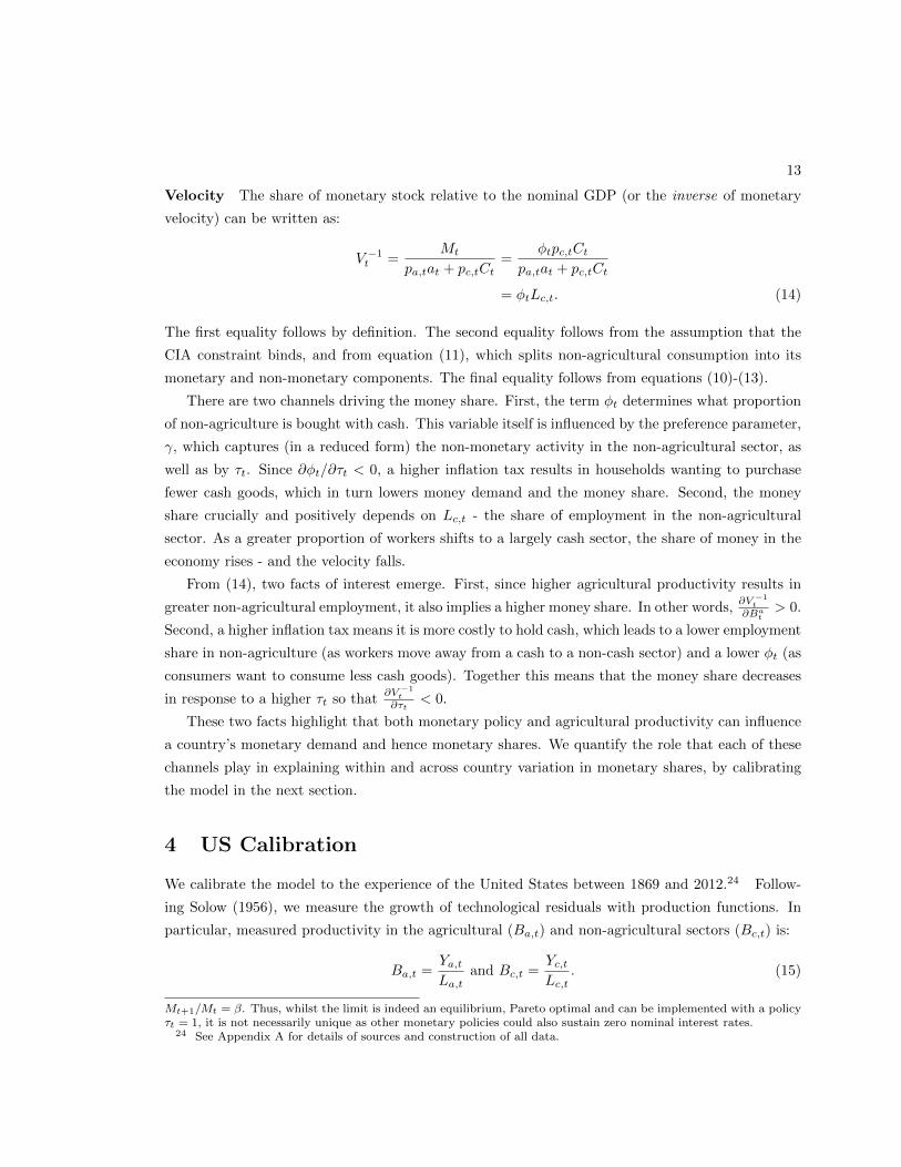
We take the sequence of money stock per worker, {Mt}2014t=1869, directly from the data as an

exogenous input. We follow Anderson (2006) in the construction of the long run money stock. Since

the labor force is assumed constant in the model, we divide our sequence of money by the size of

the labor force in the US and smooth the resulting sequence using the HP filter with smoothing

parameter 100. The resulting money stock per worker is presented in Figure 4.

We then turn to the discount factor, β. Recall that the nominal interest rate, rt, satisfies

rt = τt − 1, where τt =1β

Mt+1

Mt. Thus, β = 1

1+rt

Mt+1

Mt. Taking the nominal interest rate from Officer

and Williamson (2016b), and combining it with monetary growth rates in the US, we calculate

the average of the right hand side of this equation between 1980 and 2012 to obtain a value of

β = 0.972.26 Given β and the sequence of Mt we calculate the series of monetary wedges {τ}2013t=1869

using the formula τt ≡ 1β

Mt+1

Mt.

Finally, we calibrate the variables γ, α and a. The calibration of γ follows Chari et al. (1996a).

25 Here the annualized growth of a sequence xt between periods T and T +N is given by(

xT+N

xT

) 1N − 1.

26 The average nominal interest rate and monetary growth rate for 1980-2012 is 7.95% and 4.97% respectively.

15

Parameter Values Target

Ba,1869,Bc,1869 1 Normalization.

ga − 1 0.02657Annualized growth rate of (HP-Smoothed) agricultural laborproductivity in US, 1869-2012. See Appendix for detailedsources.

{Ba,t}2013t=1869 Ba,t = gta Constant, exogenous sectoral productivity growth.

gc − 1 0.01276Annualized growth rate of (HP-Smoothed) non-agriculturallabor productivity in US, 1869-2012. See Appendix fordetailed sources.

{Bc,t}2013t=1869 Bc,t = gtc Constant, exogenous sectoral productivity growth.

{Mt}2014t=1869 {·} M2 money stock from IMF (2015), Rasche (1990), Friedmanand Schwartz (1963) and Carter et al., eds (2006).

β 0.972 Money growth rate and nominal interest rate in 1980.

{τt}2013t=1869 τt =1β

Mt+1

MtConstructed from above.

γ 0.2339 Money share in non-agricultural value added, 1980.α 0.00003626 Employment share in agriculture in 1980.a 0.641 Employment share in agriculture in 2012.

Table 1: Calibrated parameters

In particular, this parameter determines the importance of cash versus non-cash goods in the non-

agricultural sector. In our model, the share of cash goods in non-agriculture, call it sMt , is given by:

sMt ≡ pC,tcm,t

pC,t(cm,t + cn,t)= φt =

1

1 + γ1−α−γ τt

. (17)

Solving for γ, we obtain γ = 1−α

1+sMt

1−sMtτt

. Taking the average of the right hand side between 1980

and 2012, we obtain γ = 0.23(1 − α).27 Notice that α determines the long run employment share

in agriculture, whilst a determines the initial employment in agriculture (given the normalization

Ba,1869 = 1). We take the agricultural employment share in 1980 and 2012 directly from the

data (3.5% and 1.5% respectively). We then plug these values into equation (10) and obtain two

additional equations. Together these two equations with the equation for γ yield the following

parameter values: a = 0.641, α = 0.00003626 and γ = 0.2339. All the parameters from the above

calibration are summarized in Table 1. We can then use equations (10)-(13) to obtain solutions to

the model which we review below.

5 US Results

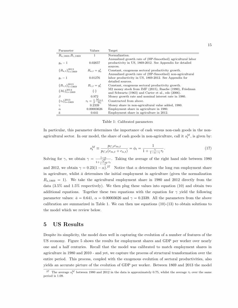
Despite its simplicity, the model does well in capturing the evolution of a number of features of the

US economy. Figure 5 shows the results for employment shares and GDP per worker over nearly

one and a half centuries. Recall that the model was calibrated to match employment shares in

agriculture in 1980 and 2010 - and yet, we capture the process of structural transformation over the

entire period. This process, coupled with the exogenous evolution of sectoral productivities, also

yields an accurate picture of the evolution of GDP per worker. Between 1869 and 2013 the model

27 The average sMt between 1980 and 2012 in the data is approximately 0.75, whilst the average τt over the sameperiod is 1.09.

16

US AgriculturalEmployment Share

Data

Model

0

20

40

60

Em

plo

ymen

t S

har

e, %

1870 1890 1910 1930 1950 1970 1990 2010 Year

(a) Agricultural Employment Share, US

GDP per worker, US

0

.5

1

1.5

1990

=1

1870 1890 1910 1930 1950 1970 1990 2010 Year

Model Data

(b) GDP per worker, US

Figure 5: Simulations and data for US prices, 1869-2012.

predicts an average annualized labor productivity growth rate of 1.8%, versus 1.7% in the data.

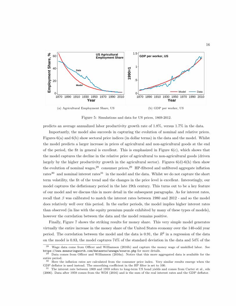
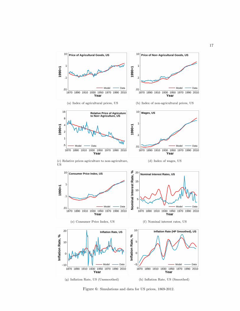
Importantly, the model also succeeds in capturing the evolution of nominal and relative prices.

Figures 6(a) and 6(b) show sectoral price indices (in dollar terms) in the data and the model. Whilst

the model predicts a larger increase in prices of agricultural and non-agricultural goods at the end

of the period, the fit in general is excellent. This is emphasized in Figure 6(c), which shows that

the model captures the decline in the relative price of agricultural to non-agricultural goods (driven

largely by the higher productivity growth in the agricultural sector). Figures 6(d)-6(h) then show

the evolution of nominal wages,28 consumer prices,29 HP-filtered and unfiltered aggregate inflation

rates30 and nominal interest rates31 in the model and the data. Whilst we do not capture the short

term volatility, the fit of the trend and the changes in the price level is excellent. Interestingly, our

model captures the deflationary period in the late 19th century. This turns out to be a key feature

of our model and we discuss this in more detail in the subsequent paragraphs. As for interest rates,

recall that β was calibrated to match the interest rates between 1980 and 2012 - and so the model

does relatively well over this period. In the earlier periods, the model implies higher interest rates

than observed (in line with the equity premium puzzle exhibited by many of these types of models),

however the correlation between the data and the model remains positive.

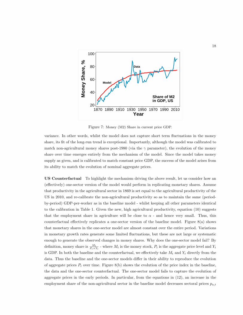
Finally, Figure 7 shows the striking results for money share. This very simple model generates

virtually the entire increase in the money share of the United States economy over the 140-odd year

period. The correlation between the model and the data is 0.91, the R2 in a regression of the data

on the model is 0.83, the model captures 74% of the standard deviation in the data and 54% of the

28 Wage data come from Officer and Williamson (2016b) and capture the money wage of unskilled labor. Seehttps://www.measuringworth.com/datasets/uswage/source.php for more details.

29 Data comes from Officer and Williamson (2016a). Notice that this more aggregated data is available for theentire period.

30 Here the inflation rates are calculated from the consumer price index. Very similar results emerge when theGDP deflator is used instead. The smoothing coefficient in the HP filter is set to 100.

31 The interest rate between 1869 and 1959 refers to long-term US bond yields and comes from Carter et al., eds(2006). Data after 1959 comes from the WDI (2016) and is the sum of the real interest rates and the GDP deflator.

17

Price of Agricultural Goods, US

.01

.1

1

10

1990

=1

1870 1890 1910 1930 1950 1970 1990 2010 Year

Model Data

(a) Index of agricultural prices, US

Price of Non−Agricultural Goods, US

.01

.1

1

10

1990

=1

1870 1890 1910 1930 1950 1970 1990 2010 Year

Model Data

(b) Index of non-agricultural prices, US

Relative Price of Agricutureto Non−Agriculture, US

.5

1

2

4

8

16

1990

=1

1870 1890 1910 1930 1950 1970 1990 2010 Year

Model Data

(c) Relative prices agriculture to non-agriculture,US

Wages, US

.01

.1

1

10

1990

=1

1870 1890 1910 1930 1950 1970 1990 2010 Year

Model Data

(d) Index of wages, US

Consumer Price Index, US

.01

.1

1

10

1990

=1

1870 1890 1910 1930 1950 1970 1990 2010 Year

Model Data

(e) Consumer Price Index, US

Nominal Interest Rates, US

0

5

10

15

20

No

min

al In

tere

st R

ate,

%

1870 1890 1910 1930 1950 1970 1990 2010 Year

Model Data

(f) Nominal interest rates, US

Inflation Rate, US

−10

0

10

20

Infl

atio

n R

ate,

%

1870 1890 1910 1930 1950 1970 1990 2010 Year

Model Data

(g) Inflation Rate, US (Unsmoothed)

Inflation Rate (HP Smoothed), US

−5

0

5

10

Infl

atio

n R

ate,

%

1870 1890 1910 1930 1950 1970 1990 2010 Year

Model Data

(h) Inflation Rate, US (Smoothed)

Figure 6: Simulations and data for US prices, 1869-2012.

18

Share of M2in GDP, US

Data

Model

20

40

60

80

100

Mo

ney

Sh

are,

%

1870 1890 1910 1930 1950 1970 1990 2010 Year

Figure 7: Money (M2) Share in current price GDP.

variance. In other words, whilst the model does not capture short term fluctuations in the money

share, its fit of the long-run trend is exceptional. Importantly, although the model was calibrated to

match non-agricultural money shares post-1980 (via the γ parameter), the evolution of the money

share over time emerges entirely from the mechanism of the model. Since the model takes money

supply as given, and is calibrated to match constant price GDP, the success of the model arises from

its ability to match the evolution of nominal aggregate prices.

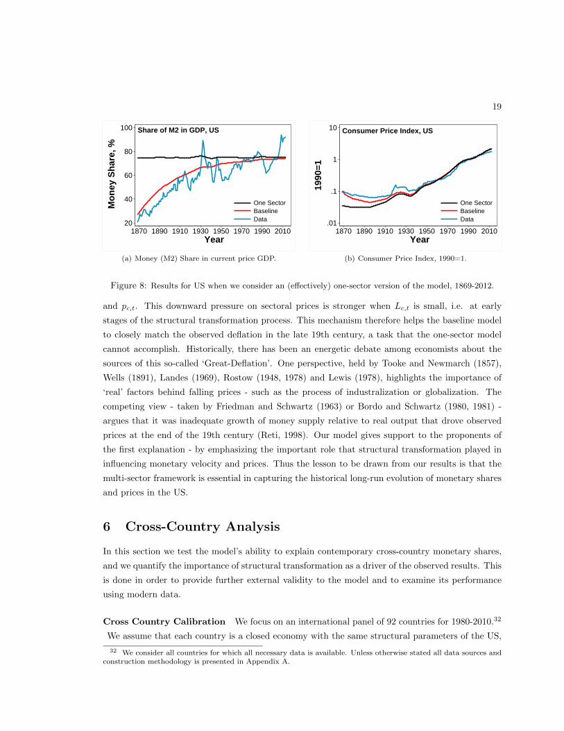
US Counterfactual To highlight the mechanism driving the above result, let us consider how an

(effectively) one-sector version of the model would perform in replicating monetary shares. Assume

that productivity in the agricultural sector in 1869 is set equal to the agricultural productivity of the

US in 2010, and re-calibrate the non-agricultural productivity so as to maintain the same (period-

by-period) GDP-per-worker as in the baseline model - whilst keeping all other parameters identical

to the calibration in Table 1. Given the new, high agricultural productivity, equation (10) suggests

that the employment share in agriculture will be close to α - and hence very small. Thus, this

counterfactual effectively replicates a one-sector version of the baseline model. Figure 8(a) shows

that monetary shares in the one-sector model are almost constant over the entire period. Variations

in monetary growth rates generate some limited fluctuations, but these are not large or systematic

enough to generate the observed changes in money shares. Why does the one-sector model fail? By

definition, money share is Mt

Pt×Yt- where Mt is the money stock, Pt is the aggregate price level and Yt

is GDP. In both the baseline and the counterfactual, we effectively take Mt and Yt directly from the

data. Thus the baseline and the one-sector models differ in their ability to reproduce the evolution

of aggregate prices Pt over time. Figure 8(b) shows the evolution of the price index in the baseline,

the data and the one-sector counterfactual. The one-sector model fails to capture the evolution of

aggregate prices in the early periods. In particular, from the equations in (12), an increase in the

employment share of the non-agricultural sector in the baseline model decreases sectoral prices pa,t

19

Share of M2 in GDP, US

20

40

60

80

100

Mo

ney

Sh

are,

%

1870 1890 1910 1930 1950 1970 1990 2010 Year

One SectorBaselineData

(a) Money (M2) Share in current price GDP.

Consumer Price Index, US

.01

.1

1

10

1990

=1

1870 1890 1910 1930 1950 1970 1990 2010 Year

One SectorBaselineData

(b) Consumer Price Index, 1990=1.

Figure 8: Results for US when we consider an (effectively) one-sector version of the model, 1869-2012.

and pc,t. This downward pressure on sectoral prices is stronger when Lc,t is small, i.e. at early

stages of the structural transformation process. This mechanism therefore helps the baseline model

to closely match the observed deflation in the late 19th century, a task that the one-sector model

cannot accomplish. Historically, there has been an energetic debate among economists about the

sources of this so-called ‘Great-Deflation’. One perspective, held by Tooke and Newmarch (1857),

Wells (1891), Landes (1969), Rostow (1948, 1978) and Lewis (1978), highlights the importance of

‘real’ factors behind falling prices - such as the process of industralization or globalization. The

competing view - taken by Friedman and Schwartz (1963) or Bordo and Schwartz (1980, 1981) -

argues that it was inadequate growth of money supply relative to real output that drove observed

prices at the end of the 19th century (Reti, 1998). Our model gives support to the proponents of

the first explanation - by emphasizing the important role that structural transformation played in

influencing monetary velocity and prices. Thus the lesson to be drawn from our results is that the

multi-sector framework is essential in capturing the historical long-run evolution of monetary shares

and prices in the US.

6 Cross-Country Analysis

In this section we test the model’s ability to explain contemporary cross-country monetary shares,

and we quantify the importance of structural transformation as a driver of the observed results. This

is done in order to provide further external validity to the model and to examine its performance

using modern data.

Cross Country Calibration We focus on an international panel of 92 countries for 1980-2010.32

We assume that each country is a closed economy with the same structural parameters of the US,

32 We consider all countries for which all necessary data is available. Unless otherwise stated all data sources andconstruction methodology is presented in Appendix A.

20

AFG

AREARG

AUSAUTBHR

BHS

BLZ

BOL

BRB

BWA

CANCHE

CHL

CIV

CMR

COG

COLCRI

CYP

DNK

DOM

DZAECU

EGY

ESPFIN

FJI

FRA

GAB

GBR

GHA

GMB

GRC

GTM

GUY

HND

IDN

IND

IRL

IRN

ISLISR

ITA

JAM

JOR

JPN

KEN

KOR

KWT

LCA

MAR

MDVMEX

MLT

MRT

MUS

MYS

NGA

NIC

NLDNORNZL

OMN

PAK

PER

PHL

PNG

PRT

PRY

QAT

SAU

SEN

SGP

SLV

SUR

SWE

SWZ

SYR

TGOTHA

TON

TTO

TUN

TUR

URY

USA

VCT

VEN

VUT

ZAF

ZMB

Agricultural Employment Share,Average 1980−2010

0

.2

.4

.6

.8

1

Dat

a

0 .1 .2 .3 .4 .5 .6 .7 .8 .9 1 Model

(a) Agricultural Employment Share, Average 1980-2010

AFG

ARE

ARG

AUSAUT

BHRBHS

BLZ

BOL

BRB

BWA

CANCHE

CHL

CIV

CMRCOG

COL

CRI

CYP

DNK

DOMDZA

ECUEGY

ESPFIN

FJI

FRA

GAB

GBR

GHAGMB

GRC

GTM

GUYHND

IDNIND

IRL

IRN

ISLISR

ITA

JAMJOR

JPN

KEN

KOR

KWT

LCA

MARMDV

MEXMLT

MRT

MUSMYS

NGA

NIC

NLDNOR

NZLOMN

PAK

PER

PHLPNG

PRT

PRY

QAT

SAU

SEN

SGP

SLV

SUR

SWE

SWZSYR

TGO

THA

TON

TTO

TUN

TURURY

USA

VCT

VEN

VUT

ZAF

ZMB

1/64

1/32

1/16

1/8

1/4

1/2

1

2

4

8

1/64 1/32 1/16 1/8 1/4 1/2 1 2 4 8

PPP GDP per worker,Average 1980−2010USA=1

Dat

a

Model

(b) GDP per worker, Average 1980-2010

Figure 9: Simulations and data for cross-section of the average for 1980-2010. Line depicts 45 degrees.

with the exception of sectoral productivity and monetary policy. Money stock per worker in each

country and each year is taken directly from the data. We assume that labor productivity in sector

s and in country i grows at a constant rate, gis − 1, and is given by:

Bis,t = Bi

s × (gis)t−1980. (18)

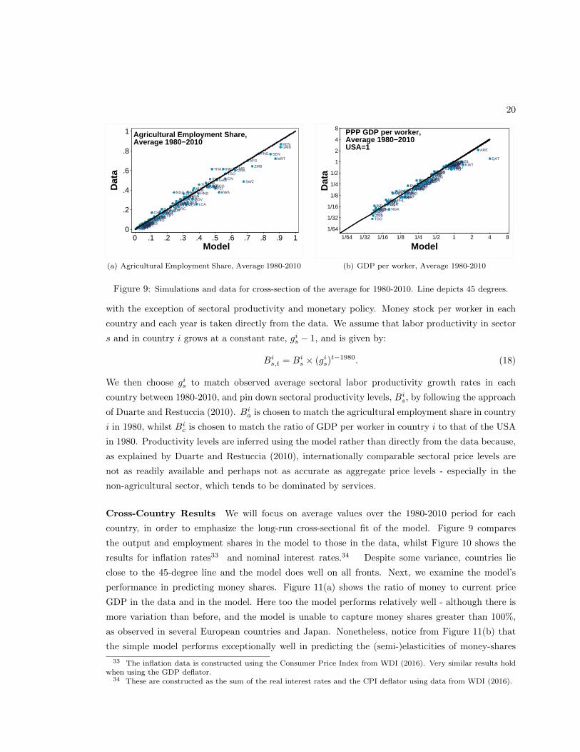
We then choose gis to match observed average sectoral labor productivity growth rates in each

country between 1980-2010, and pin down sectoral productivity levels, Bis, by following the approach

of Duarte and Restuccia (2010). Bia is chosen to match the agricultural employment share in country

i in 1980, whilst Bic is chosen to match the ratio of GDP per worker in country i to that of the USA

in 1980. Productivity levels are inferred using the model rather than directly from the data because,

as explained by Duarte and Restuccia (2010), internationally comparable sectoral price levels are

not as readily available and perhaps not as accurate as aggregate price levels - especially in the

non-agricultural sector, which tends to be dominated by services.

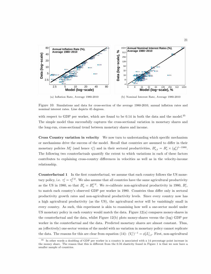
Cross-Country Results We will focus on average values over the 1980-2010 period for each

country, in order to emphasize the long-run cross-sectional fit of the model. Figure 9 compares

the output and employment shares in the model to those in the data, whilst Figure 10 shows the

results for inflation rates33 and nominal interest rates.34 Despite some variance, countries lie

close to the 45-degree line and the model does well on all fronts. Next, we examine the model’s

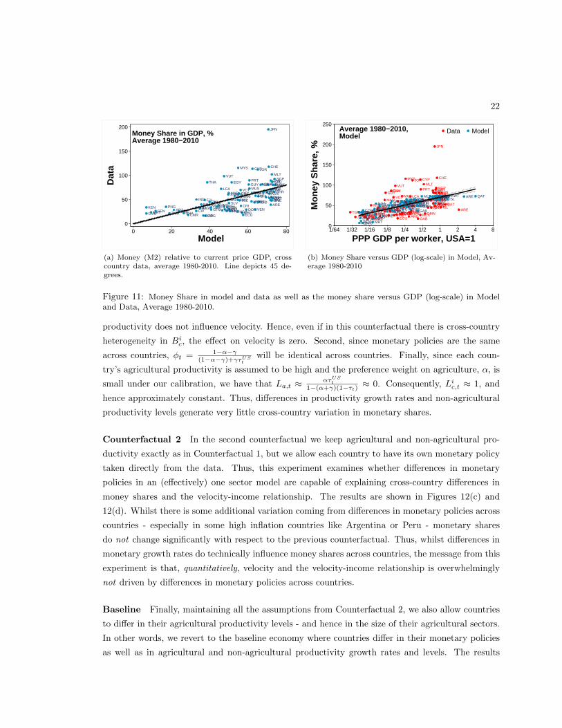
performance in predicting money shares. Figure 11(a) shows the ratio of money to current price

GDP in the data and in the model. Here too the model performs relatively well - although there is

more variation than before, and the model is unable to capture money shares greater than 100%,

as observed in several European countries and Japan. Nonetheless, notice from Figure 11(b) that

the simple model performs exceptionally well in predicting the (semi-)elasticities of money-shares

33 The inflation data is constructed using the Consumer Price Index from WDI (2016). Very similar results holdwhen using the GDP deflator.

34 These are constructed as the sum of the real interest rates and the CPI deflator using data from WDI (2016).

21

ARE

ARG

AUS

AUTBHR

BHS

BLZ

BOL

BRB

BWA

CAN

CHE

CHL

CIVCMR

COG

COLCRI

CYP

DNK

DOMDZA

ECU

EGY

ESP

FIN FJIFRAGAB GBR

GHA

GMB

GRCGTM

GUY

HNDIDN

IND

IRL

IRN

ISL

ISR

ITA

JAM

JOR

KEN

KOR

KWTLCA

MARMDV

MEX

MLT

MRT

MUS

MYS

NGA

NIC

NLD

NOR NZL

OMN

PAK

PER

PHL

PNG

PRT

PRY

QATSAU

SEN

SGP

SLV

SUR

SWE

SWZSYR

TGOTHA

TONTTO

TUN

TUR

URY

USAVCT

VEN

VUT

ZAF

ZMB

Annual Inflation Rate (%),Average 1980−2010

2.5

5

10

20

40

80

Dat

a (lo

g−sc

ale)

2.5 5 10 20 40 80 Model (log−scale)

(a) Inflation Rate, Average 1980-2010

AFG ARG

AUS

AUT

BHRBHS

BLZ

BOL

BRBBWA

CAN

CHE

CHL

CIVCMR COG

COLCRI

CYP

DNK

DOM

DZA

ECU

EGYESP

FINFJIFRA

GAB

GBR

GHAGMB

GRCGTMGUYHNDIDN

IND

IRL

IRN

ISL

ISR

ITA

JAM

JOR

JPN

KEN

KORKWTLCA

MARMDV

MEX

MLT

MRTMUS

MYS

NGA

NIC

NLD

NOR

NZL

OMN

PER

PHLPNG

PRT

PRY

QAT

SEN

SGP

SUR

SWESWZ

SYR

TGO

THATONTTO

TUN

URY

USA

VCT

VEN

VUTZAF

ZMB

Annual Nominal Interest Rates (%) ,Average 1980−2010

4

8

16

32

64

128

256

512

1024

Dat

a (lo

g−sc

ale)

, %

4 8 16 32 64 128 256 512 1024

Model (log−scale), %

(b) Nominal Interest Rate, Average 1980-2010

Figure 10: Simulations and data for cross-section of the average 1980-2010, annual inflation rates andnominal interest rates. Line depicts 45 degrees.

with respect to GDP per worker, which are found to be 0.14 in both the data and the model.35

The simple model thus successfully captures the cross-sectional variation in monetary shares and

the long-run, cross-sectional trend between monetary shares and income.

Cross Country variation in velocity We now turn to understanding which specific mechanism

or mechanisms drive the success of the model. Recall that countries are assumed to differ in their

monetary policies M it (and hence τ it ) and in their sectoral productivities, Bi

s,t = Bis × (gis)

t−1980.

The following two counterfactuals quantify the extent to which variations in each of these factors

contributes to explaining cross-country differences in velocities as well as in the velocity-income

relationship.

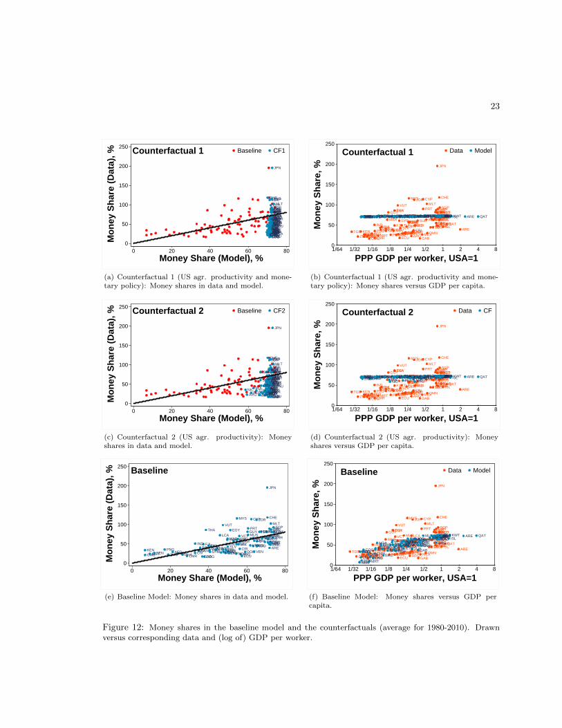
Counterfactual 1 In the first counterfactual, we assume that each country follows the US mone-

tary policy, i.e. τ it = τUSt . We also assume that all countries have the same agricultural productivity

as the US in 1980, so that Bia = BUS

a . We re-calibrate non-agricultural productivity in 1980, Bic,

to match each country’s observed GDP per worker in 1980. Countries thus differ only in sectoral

productivity growth rates and non-agricultural productivity levels. Since every country now has

a high agricultural productivity (as the US), the agricultural sector will be vanishingly small in

every country. As such, this experiment is akin to examining how well a one-sector model under

US monetary policy in each country would match the data. Figure 12(a) compares money-shares in

the counterfactual and the data, whilst Figure 12(b) plots money-shares versus the (log) GDP per

worker in the counterfactual and the data. Predicted monetary shares are almost constant. Thus,

an (effectively) one-sector version of the model with no variation in monetary policy cannot replicate

the data. The reasons for this are clear from equation (14): (V it )

−1 = φitL

ic,t. First, non-agricultural

35 In other words a doubling of GDP per worker in a country is associated with a 14 percentage point increase inthe money share. The reason that this is different from the 0.16 elasticity found in Figure 1 is that we now have asmaller sample of countries.

22

AFGARE

ARG

AUS

AUT

BHR

BHSBLZBOL

BRB

BWA

CAN

CHE

CHL

CIVCMR COG

COLCRI

CYP

DNK

DOM

DZA

ECU

EGY ESP

FINFJI

FRA

GAB

GBR

GHAGMB

GRC

GTM

GUY

HNDIDN

IND

IRL

IRN ISL

ISR

ITAJAM

JOR

JPN

KEN

KOR

KWTLCA

MAR

MDVMEX

MLT

MRT

MUS

MYS

NGANIC

NLD

NOR

NZL

OMN

PAK

PER

PHLPNG

PRT

PRY

QATSAU

SEN

SGP

SLV

SUR

SWE

SWZ

SYR

TGO

THA

TONTTO

TUN

TUR

URY

USAVCT

VEN

VUT

ZAF

ZMB

Money Share in GDP, %Average 1980−2010

0

50

100

150

200

Dat

a

0 20 40 60 80

Model

(a) Money (M2) relative to current price GDP, crosscountry data, average 1980-2010. Line depicts 45 de-grees.

KENTGOZMBSEN

IND

CIVGMBCOG

GHA

PNGMRT

IDNPAK

CMRAFGNGA

EGY

MDVPHL

SWZ

BOLNIC

MARVCT

GUYTHA

PRY

FJIHND

VUT

BWASLV

SYRTUN

PERDOM

MUS

ECUGTM TON

MYS

COL

CHL

LCA

URYJAMDZA

TUR

ZAF

ARGVEN

BLZ

JOR

IRN

GAB

CYP

MEXCRI

SUR

PRT

OMN

KOR

MLT

NZL

GBR

JPN

DNK

ESPISR

FINBHS

GRC

SWE

IRL

CAN

BRB

SGP

AUSFRABHR ITA

TTO

CHE

NORSAU

USAAUTNLD

ISL

KWT

ARE

QAT

KEN

TGO

ZMBSEN

INDCIV

GMB

COGGHA

PNGMRT

IDNPAKCMRAFG

NGAEGYMDVPHL

SWZBOLNICMARVCTGUY

THAPRY

FJIHNDVUTBWA

SLVSYRTUNPERDOMMUSECU

GTMTONMYSCOL

CHL

LCA

URYJAMDZA

TUR

ZAFARGVENBLZJOR

IRNGAB

CYP

MEXCRISURPRT

OMN

KORMLTNZLGBRJPNDNKESPISRFINBHS

GRC

SWEIRLCANBRBSGPAUSFRABHRITATTO

CHENORSAUUSAAUTNLD

ISLKWT ARE QAT

1/64 1/32 1/16 1/8 1/4 1/2 1 2 4 8

Average 1980−2010,Model

0

50

100

150

200

250

Mon

ey S

hare

, %

PPP GDP per worker, USA=1

Data Model

(b) Money Share versus GDP (log-scale) in Model, Av-erage 1980-2010

Figure 11: Money Share in model and data as well as the money share versus GDP (log-scale) in Modeland Data, Average 1980-2010.

productivity does not influence velocity. Hence, even if in this counterfactual there is cross-country

heterogeneity in Bic, the effect on velocity is zero. Second, since monetary policies are the same

across countries, φt = 1−α−γ(1−α−γ)+γτUS

twill be identical across countries. Finally, since each coun-

try’s agricultural productivity is assumed to be high and the preference weight on agriculture, α, is

small under our calibration, we have that La,t ≈ ατUSt

1−(α+γ)(1−τt)≈ 0. Consequently, Li

c,t ≈ 1, and

hence approximately constant. Thus, differences in productivity growth rates and non-agricultural

productivity levels generate very little cross-country variation in monetary shares.

Counterfactual 2 In the second counterfactual we keep agricultural and non-agricultural pro-

ductivity exactly as in Counterfactual 1, but we allow each country to have its own monetary policy

taken directly from the data. Thus, this experiment examines whether differences in monetary

policies in an (effectively) one sector model are capable of explaining cross-country differences in

money shares and the velocity-income relationship. The results are shown in Figures 12(c) and

12(d). Whilst there is some additional variation coming from differences in monetary policies across

countries - especially in some high inflation countries like Argentina or Peru - monetary shares

do not change significantly with respect to the previous counterfactual. Thus, whilst differences in

monetary growth rates do technically influence money shares across countries, the message from this

experiment is that, quantitatively, velocity and the velocity-income relationship is overwhelmingly

not driven by differences in monetary policies across countries.

Baseline Finally, maintaining all the assumptions from Counterfactual 2, we also allow countries

to differ in their agricultural productivity levels - and hence in the size of their agricultural sectors.

In other words, we revert to the baseline economy where countries differ in their monetary policies

as well as in agricultural and non-agricultural productivity growth rates and levels. The results

23

AFGARE

ARG

AUS

AUT

BHR

BHSBLZBOL

BRB

BWA

CAN

CHE

CHL

CIVCMRCOG

COLCRI

CYP

DNK

DOM

DZA

ECU

EGYESP

FINFJI

FRA

GAB

GBR

GHAGMB

GRC

GTM

GUY

HNDIDNIND

IRL

IRNISL

ISR

ITAJAM

JOR

JPN

KEN

KOR

KWTLCA

MAR

MDVMEX

MLT

MRT

MUS

MYS

NGANIC

NLD

NORNZL

OMNPAK

PER

PHLPNG

PRT

PRY

QATSAU

SEN

SGP

SLV

SURSWE

SWZ

SYR

TGO

THA

TONTTOTUN

TURURY

USAVCT

VEN

VUT

ZAF

ZMB

Counterfactual 1

0

50

100

150

200

250

Mo

ney

Sh

are

(Dat

a), %

0 20 40 60 80

Money Share (Model), %

Baseline CF1

(a) Counterfactual 1 (US agr. productivity and mone-tary policy): Money shares in data and model.

AFGARE

ARG

AUS

AUT

BHR

BHSBLZBOL

BRB

BWA

CAN

CHE

CHL

CIVCMRCOG

COLCRI

CYP

DNK

DOM

DZA

ECU

EGY ESP

FINFJI

FRA

GAB

GBR

GHAGMB

GRC

GTM

GUY

HNDIDNIND

IRL

IRN ISL

ISR

ITAJAM

JOR

JPN

KEN

KOR

KWTLCA

MAR

MDVMEX

MLT

MRT

MUS

MYS

NGANIC

NLD

NORNZL

OMN

PAK

PER

PHLPNG

PRT

PRY

QATSAU

SEN

SGP

SLV

SURSWE

SWZ

SYR

TGO

THA

TONTTOTUN

TURURY

USAVCT

VEN

VUT

ZAF

ZMB

AFG AREARG AUSAUTBHRBHSBLZBOL BRBBWA CANCHECHLCIV CMRCOG COL CRICYP DNKDOMDZAECUEGY ESPFINFJI FRAGAB GBRGHAGMB GRCGTMGUYHNDIDNIND IRLIRN ISLISRITAJAMJOR JPNKEN KOR KWTLCAMARMDV MEXMLTMRT MUSMYSNGA NIC NLDNORNZLOMNPAK PERPHLPNG PRTPRY QATSAUSEN SGPSLV SUR SWESWZ SYRTGO THA TON TTOTUN TURURY USAVCT VENVUT ZAFZMB

1/64 1/32 1/16 1/8 1/4 1/2 1 2 4 8

Counterfactual 1

0

50

100

150

200

250

Mo

ney

Sh

are,

%

PPP GDP per worker, USA=1

Data Model

(b) Counterfactual 1 (US agr. productivity and mone-tary policy): Money shares versus GDP per capita.

AFGARE

ARG

AUS

AUT

BHR

BHSBLZBOL

BRB

BWA

CAN

CHE

CHL

CIVCMRCOG

COLCRI

CYP

DNK

DOM

DZA

ECU

EGYESP

FINFJI

FRA

GAB

GBR

GHAGMB

GRC

GTM

GUY

HNDIDNIND

IRL

IRNISL

ISR

ITAJAM

JOR

JPN

KEN

KOR

KWTLCA

MAR

MDVMEX

MLT

MRT

MUS

MYS

NGANIC

NLD

NORNZL

OMNPAK

PER

PHLPNG

PRT

PRY

QATSAU

SEN

SGP

SLV

SURSWE

SWZ

SYR

TGO

THA

TONTTOTUN

TURURY

USAVCT

VEN

VUT

ZAF

ZMB

Counterfactual 2

0

50

100

150

200

250

Mo

ney

Sh

are

(Dat

a), %

0 20 40 60 80

Money Share (Model), %

Baseline CF2

(c) Counterfactual 2 (US agr. productivity): Moneyshares in data and model.

AFGARE

ARG

AUS

AUT

BHR

BHSBLZBOL

BRB

BWA

CAN

CHE

CHL

CIVCMRCOG

COLCRI

CYP

DNK

DOM

DZA

ECU

EGY ESP

FINFJI

FRA

GAB

GBR

GHAGMB

GRC

GTM

GUY

HNDIDNIND

IRL

IRN ISL

ISR

ITAJAM

JOR

JPN

KEN

KOR

KWTLCA

MAR

MDVMEX

MLT

MRT

MUS

MYS

NGANIC

NLD

NORNZL

OMN

PAK

PER

PHLPNG

PRT

PRY

QATSAU

SEN

SGP

SLV

SURSWE

SWZ

SYR

TGO

THA

TONTTOTUN

TURURY

USAVCT

VEN

VUT

ZAF

ZMB

AFG AREARG

AUSAUTBHRBHSBLZBOL

BRBBWA CANCHECHLCIV CMRCOG COL CRICYP DNKDOMDZAECUEGY ESPFINFJI FRAGAB GBRGHAGMB GRCGTMGUYHNDIDNIND IRLIRN ISLISRITAJAMJOR JPNKEN KOR KWTLCAMARMDV MEX

MLTMRT MUSMYSNGANIC

NLDNORNZLOMNPAKPER

PHLPNG PRTPRY QATSAUSEN SGPSLV SURSWESWZ SYRTGO THA TON TTOTUN

TURURYUSAVCT VENVUT ZAF

ZMB

1/64 1/32 1/16 1/8 1/4 1/2 1 2 4 8

Counterfactual 2

0

50

100

150

200

250

Mo

ney

Sh

are,

%

PPP GDP per worker, USA=1

Data CF

(d) Counterfactual 2 (US agr. productivity): Moneyshares versus GDP per capita.

AFGARE

ARG

AUS

AUT

BHR

BHSBLZBOL

BRB

BWA

CAN

CHE

CHL

CIVCMR COG

COLCRI

CYP

DNK

DOM

DZA

ECU

EGY ESP

FINFJI

FRA

GAB

GBR

GHAGMB

GRC

GTM

GUY

HNDIDNIND

IRL

IRN ISL

ISR

ITAJAM

JOR

JPN

KEN

KOR

KWTLCA

MAR

MDVMEX

MLT

MRT

MUS

MYS

NGANIC

NLD

NORNZL

OMNPAK

PER

PHLPNG

PRT

PRY

QATSAU

SEN

SGP

SLV

SURSWE

SWZ

SYR

TGO

THA

TONTTOTUN

TURURY

USAVCT

VEN

VUT

ZAF

ZMB

Baseline

0

50

100

150

200

250

Mo

ney

Sh

are

(Dat

a), %

0 20 40 60 80

Money Share (Model), %

(e) Baseline Model: Money shares in data and model.

AFGARE

ARG

AUS

AUT

BHR

BHSBLZBOL

BRB

BWA

CAN

CHE

CHL

CIVCMRCOG

COLCRI

CYP

DNK

DOM

DZA

ECU

EGY ESP

FINFJI

FRA

GAB

GBR

GHAGMB

GRC

GTM

GUY

HNDIDNIND

IRL

IRN ISL

ISR

ITAJAM

JOR

JPN

KEN

KOR

KWTLCA

MAR

MDVMEX

MLT

MRT

MUS

MYS

NGANIC

NLD

NORNZL

OMN

PAK

PER

PHLPNG

PRT

PRY

QATSAU

SEN

SGP

SLV

SURSWE

SWZ

SYR

TGO

THA

TONTTOTUN

TURURY

USAVCT

VEN

VUT

ZAF

ZMB AFG

ARE

ARG

AUSAUTBHRBHS

BLZ

BOL

BRB

BWA

CANCHECHL

CIV CMRCOG

COLCRICYP

DNK

DOMDZAECU

EGY

ESPFIN

FJI

FRA

GAB

GBR

GHA

GMB

GRC

GTM

GUY

HNDIDN

IND

IRL

IRN

ISLISRITA

JAMJOR

JPN

KEN

KORKWT

LCAMARMDV MEX

MLT

MRT

MUSMYSNGA

NIC

NLDNORNZL

OMNPAK

PERPHL

PNG

PRTPRY

QATSAU

SEN

SGP

SLV SUR

SWE

SWZ

SYR

TGOTHA

TON

TTOTUN

TUR

URYUSA

VCTVEN

VUT

ZAF

ZMB

1/64 1/32 1/16 1/8 1/4 1/2 1 2 4 8

Baseline

0

50

100

150

200

250

Mo

ney

Sh

are,

%

PPP GDP per worker, USA=1

Data Model

(f) Baseline Model: Money shares versus GDP percapita.

Figure 12: Money shares in the baseline model and the counterfactuals (average for 1980-2010). Drawnversus corresponding data and (log of) GDP per worker.

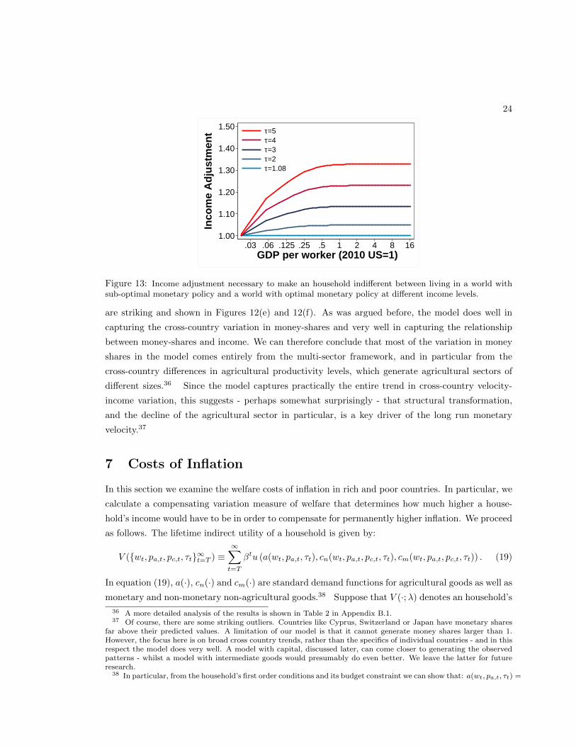
24

1.00

1.10

1.20

1.30

1.40

1.50

Inco

me

Ad

just

men

t

.03 .06 .125 .25 .5 1 2 4 8 16 GDP per worker (2010 US=1)

τ=5τ=4τ=3τ=2τ=1.08

Figure 13: Income adjustment necessary to make an household indifferent between living in a world withsub-optimal monetary policy and a world with optimal monetary policy at different income levels.

are striking and shown in Figures 12(e) and 12(f). As was argued before, the model does well in

capturing the cross-country variation in money-shares and very well in capturing the relationship

between money-shares and income. We can therefore conclude that most of the variation in money

shares in the model comes entirely from the multi-sector framework, and in particular from the

cross-country differences in agricultural productivity levels, which generate agricultural sectors of

different sizes.36 Since the model captures practically the entire trend in cross-country velocity-

income variation, this suggests - perhaps somewhat surprisingly - that structural transformation,

and the decline of the agricultural sector in particular, is a key driver of the long run monetary

velocity.37

7 Costs of Inflation

In this section we examine the welfare costs of inflation in rich and poor countries. In particular, we

calculate a compensating variation measure of welfare that determines how much higher a house-

hold’s income would have to be in order to compensate for permanently higher inflation. We proceed

as follows. The lifetime indirect utility of a household is given by:

V ({wt, pa,t, pc,t, τt}∞t=T ) ≡∞∑t=T

βtu (a(wt, pa,t, τt), cn(wt, pa,t, pc,t, τt), cm(wt, pa,t, pc,t, τt)) . (19)

In equation (19), a(·), cn(·) and cm(·) are standard demand functions for agricultural goods as well as

monetary and non-monetary non-agricultural goods.38 Suppose that V (·;λ) denotes an household’s

36 A more detailed analysis of the results is shown in Table 2 in Appendix B.1.37 Of course, there are some striking outliers. Countries like Cyprus, Switzerland or Japan have monetary shares

far above their predicted values. A limitation of our model is that it cannot generate money shares larger than 1.However, the focus here is on broad cross country trends, rather than the specifics of individual countries - and in thisrespect the model does very well. A model with capital, discussed later, can come closer to generating the observedpatterns - whilst a model with intermediate goods would presumably do even better. We leave the latter for futureresearch.

38 In particular, from the household’s first order conditions and its budget constraint we can show that: a(wt, pa,t, τt) =

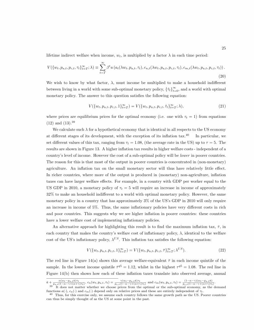
25

lifetime indirect welfare when income, wt, is multiplied by a factor λ in each time period:

V ({wt, pa,t, pc,t, τt}∞t=T ;λ) ≡∞∑t=T

βtu (at(λwt, pa,t, τt), cn,t(λwt, pa,t, pc,t, τt), cm,t(λwt, pa,t, pc,t, τt)) .

(20)

We wish to know by what factor, λ, must income be multiplied to make a household indifferent

between living in a world with some sub-optimal monetary policy, {τt}∞t=0, and a world with optimal

monetary policy. The answer to this question satisfies the following equation:

V ({wt, pa,t, pc,t, 1}∞t=T ) = V ({wt, pa,t, pc,t, τt}∞t=T ;λ), (21)

where prices are equilibrium prices for the optimal economy (i.e. one with τt = 1) from equations

(12) and (13).39

We calculate such λ for a hypothetical economy that is identical in all respects to the US economy

at different stages of its development, with the exception of its inflation tax.40 In particular, we

set different values of this tax, ranging from τt = 1.08, (the average rate in the US) up to τ = 5. The

results are shown in Figure 13. A higher inflation tax results in higher welfare costs - independent of a

country’s level of income. However the cost of a sub-optimal policy will be lower in poorer countries.

The reason for this is that most of the output in poorer countries is concentrated in (non-monetary)

agriculture. An inflation tax on the small monetary sector will thus have relatively little effect.

In richer countries, where more of the output is produced in (monetary) non-agriculture, inflation

taxes can have larger welfare effects. For example, in a country with GDP per worker equal to the

US GDP in 2010, a monetary policy of τt = 5 will require an increase in income of approximately

32% to make an household indifferent to a world with optimal monetary policy. However, the same

monetary policy in a country that has approximately 3% of the US’s GDP in 2010 will only require

an increase in income of 5%. Thus, the same inflationary policies have very different costs in rich

and poor countries. This suggests why we see higher inflation in poorer countries: these countries

have a lower welfare cost of implementing inflationary policies.

An alternative approach for highlighting this result is to find the maximum inflation tax, τ , in

each country that makes the country’s welfare cost of inflationary policy, λ, identical to the welfare

cost of the US’s inflationary policy, λUS . This inflation tax satisfies the following equation:

V ({wt, pa,t, pc,t, 1}∞t=T ) = V ({wt, pa,t, pc,t, τ}∞t=T ;λUS). (22)

The red line in Figure 14(a) shows this average welfare-equivalent τ in each income quintile of the

sample. In the lowest income quintile τ q5 = 1.12, whilst in the highest τ q5 = 1.08. The red line in

Figure 14(b) then shows how each of these inflation taxes translate into observed average, annual

a+α(wt−pa,ta)τt

pa,t(1−α−γ+(α+γ)τt), cn(wt, pa,t, τt) =

γ(wt−pa,ta)τtpc,t(1−α−γ+(α+γ)τt)

and cm(wt, pa,t, τt) =(1−α−γ)(wt−pa,ta)

pc,t(1−α−γ+(α+γ)τt).

39 It does not matter whether we choose prices from the optimal or the sub-optimal economy, as the demandfunctions a(·), cn(·) and cm(·) depend only on relative prices and these are entirely independent of τt.

40 Thus, for this exercise only, we assume each country follows the same growth path as the US. Poorer countriescan thus be simply thought of as the US at some point in the past.

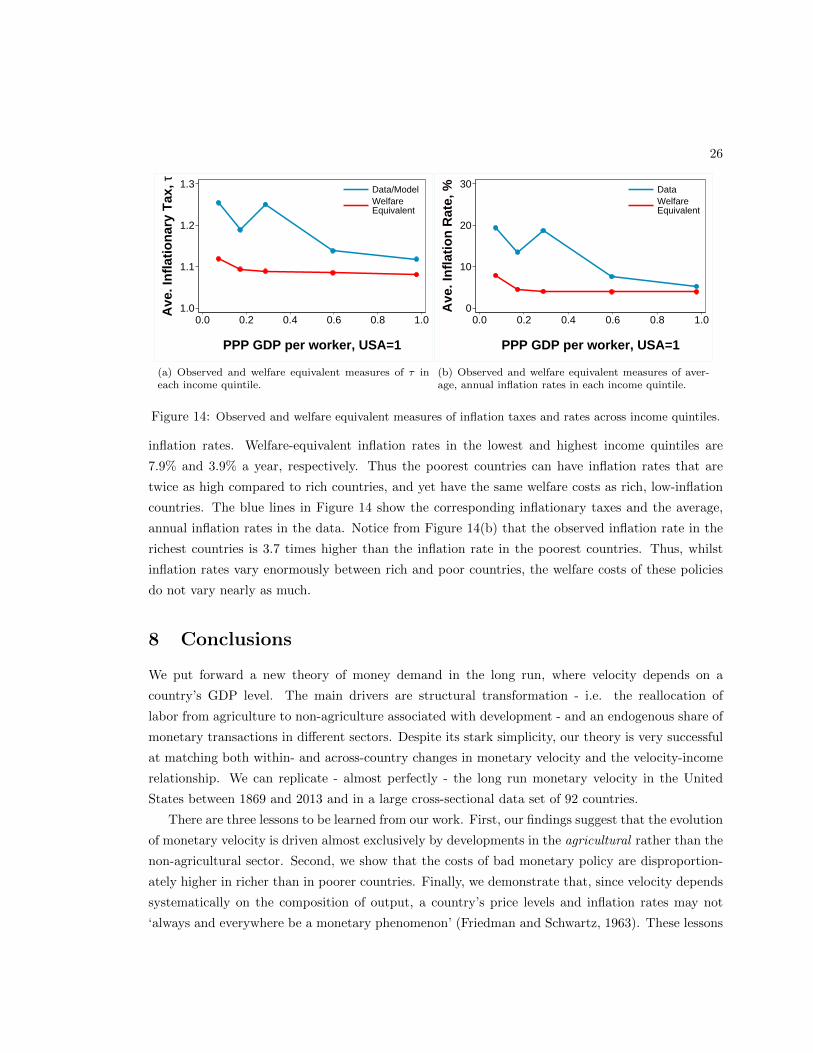
26

1.0

1.1

1.2

1.3

Ave

. In

flat

ion

ary

Tax

, τ

0.0 0.2 0.4 0.6 0.8 1.0

PPP GDP per worker, USA=1

Data/ModelWelfare Equivalent

(a) Observed and welfare equivalent measures of τ ineach income quintile.

0

10

20

30

Ave

. In

flat

ion

Rat

e, %

0.0 0.2 0.4 0.6 0.8 1.0

PPP GDP per worker, USA=1

DataWelfare Equivalent

(b) Observed and welfare equivalent measures of aver-age, annual inflation rates in each income quintile.

Figure 14: Observed and welfare equivalent measures of inflation taxes and rates across income quintiles.

inflation rates. Welfare-equivalent inflation rates in the lowest and highest income quintiles are

7.9% and 3.9% a year, respectively. Thus the poorest countries can have inflation rates that are

twice as high compared to rich countries, and yet have the same welfare costs as rich, low-inflation

countries. The blue lines in Figure 14 show the corresponding inflationary taxes and the average,

annual inflation rates in the data. Notice from Figure 14(b) that the observed inflation rate in the

richest countries is 3.7 times higher than the inflation rate in the poorest countries. Thus, whilst

inflation rates vary enormously between rich and poor countries, the welfare costs of these policies

do not vary nearly as much.

8 Conclusions

We put forward a new theory of money demand in the long run, where velocity depends on a

country’s GDP level. The main drivers are structural transformation - i.e. the reallocation of

labor from agriculture to non-agriculture associated with development - and an endogenous share of

monetary transactions in different sectors. Despite its stark simplicity, our theory is very successful

at matching both within- and across-country changes in monetary velocity and the velocity-income

relationship. We can replicate - almost perfectly - the long run monetary velocity in the United

States between 1869 and 2013 and in a large cross-sectional data set of 92 countries.

There are three lessons to be learned from our work. First, our findings suggest that the evolution

of monetary velocity is driven almost exclusively by developments in the agricultural rather than the

non-agricultural sector. Second, we show that the costs of bad monetary policy are disproportion-

ately higher in richer than in poorer countries. Finally, we demonstrate that, since velocity depends

systematically on the composition of output, a country’s price levels and inflation rates may not

‘always and everywhere be a monetary phenomenon’ (Friedman and Schwartz, 1963). These lessons

27

should be of utmost interest to central bankers, especially in developing countries, who may down-

play the role of the agricultural sector in their policy decisions. Moreover, our findings may help

explain why we observe persistently higher inflation rates in poorer countries than in richer countries

- despite strong anti-inflationary policies recommended by international institutions. Finally, our

results are also important to researchers, as they highlight that one-sector models cannot be success-

fully used to understand the long run dynamics of monetary velocity and nominal price levels. Our

work on the evolution of long-run monetary velocity thus offers key insights into understanding the

secular trends in sectoral and aggregate price levels, with strong implications for policy and future

research.

28

A Data Appendix

A.1 US Data

GDP (PPP) and Labor Force Data We use data from Penn World Tables version 7.1. (see

Heston et al. (2012)) to construct annual time series of PPP-adjusted GDP in constant 1990

prices, PPP-adjusted GDP per worker in 1990 constant prices, and total employment between 1950-

2010. For each country, we construct total employment L using the variables Population (POP),

PPP Converted GDP Chain per worker at 2005 constant prices (RGDPWOK), and PPP Con-

verted GDP Per Capita (Chain Series) at 2005 constant prices (RGDPCH) as L = (RGDPCH ×POP )/RGDPWOK. We then construct PPP-adjusted GDP in constant 2005 prices using the

variables “PPP Converted GDP Per Capita (Laspeyres), derived from growth rates of c, g, i, at

2005 constant prices (RGDPL)” and “Population (POP)” as GDPK = RGDPL× POP . We then

re-base the 2005 data to 1990 prices.

We extend the labor force and GDP data calculated above back in time for the period 1869-1950

using growth rates from Maddison (2007) . In particular, we calculate the pre-1950 growth rates for

Maddison’s GDP measure (in 1990 Geary-Khamis dollars) and use it to extend the GDP measure

calculate above. We also calculate the population growth rates from Maddison’s data and assume

that the growth rate of the labor force pre-1950 is the same as the growth rate of the population

(which is true if the labor force to population ratio stays constant over time). We then use these

population growth rates to extend the labor force data calculated above back in time. Finally, we

extend the series for GDP and labor force forward in time between 2011 and 2014 using growth rates

for labor force and constant price PPP GDP from the WDI (2016). The series for PPP-adjusted

GDP per worker in constant prices is then computed as y = GDP/L.

Agricultural and Non-Agricultural Employment We construct contemporary (1980-2014)

agricultural employment share using data from the FAOSTAT (2012) by taking the ratio of econom-

ically active population (labor force) in agriculture to total economically active population (labor

force). For the US, we then combine this with the agricultural employment share from Alvarez-

Cuadrado and Poschke (2011) for 1869-1980. Missing data is interpolated. We then obtain total

employment in agriculture by multiplying the agricultural employment shares calculated above by

the labor force data found in the previous paragraph. Non-agricultural employment is then the dif-

ference between total employment and agricultural employment. These are the La,t and Lc,t referred

to in the main body of the text.

Labor Productivity Growth Rates To calculate sectoral labor productivity growth rates for

our cross-sectional experiment we use constant price sectoral value added data in local currency

units from the UN (2008), sectoral employment shares from FAOSTAT (2012) and labor force data

from Heston et al. (2012). We multiply the employment shares by the labor force data to calculate

29

sectoral employment and then use this data to calculate sectoral labor productivities for agriculture

and non-agriculture in each country between 1980 and 2010. Next, we HP-filter these series (using a

smoothing parameter of 100), and for each country, i, and sector s = a, c we calculate an annualized

average sectoral labor productivity growth rate, gis − 1.

Sectoral Value Added, Constant price For the period 1970-2014 we construct constant price

(1990) value added data for agriculture and total value added from UN (2008). We then extend this

data for the US backwards using sectoral growth rates. First, we obtain constant price agricultural

and total value added data for the period 1947-1970 from the 10-sector database constructed by

Timmer et al. (2014) and use this data to extend our value added measures back to 1947. Then,

we extend these concatenated data back to 1869 using the Historical National Accounts database

constructed by the Timmer et al. (2014). This database provides historical constant price indices

of GNP for agriculture and the total economy. Missing values are interpolated. Notice that - like

Duarte and Restuccia (2010) - we do not directly use the resulting series in our model. Instead, we

use the above constant (1990) price agricultural and total value added data to calculate constant

price shares of agricultural value added in total value added. Then, in order to remain consistent

with out aggregate GDP data calculated above, we multiply these constant price shares by the

aggregate PPP GDP data calculated above. This gives us a consistent estimate of 1990 value added

of agriculture. Subtracting this estimate from the GDP PPP gives us an estimate of non-agricultural

value added. These are the Ya,t and Yc,t referred to in the main body of the text.

US Sectoral prices Sectoral prices between 1929 and 2013 for the United States are obtained

by dividing sectoral value added in current prices (obtained from the BEA and (Timmer et al.,

2014)) by constant price sectoral value added (calculated above). Obtaining pre-1929 prices is more

complicated. In particular, as far as we know, no dependable series of data on sectoral prices exists.

As such, we use nominal wheat prices obtained from Table Cc205-266 in Carter et al., eds (2006)

to extend the agricultural price index back in time between 1869 and 1929. Then, using data on

constant- and current-price aggregate GDP, constant price sectoral value added and the agricultural

price index calculated above, we can infer a non-agricultural price index as well. In particular,

multiplying the constant-price agricultural value added by the agricultural price index, gives us an

estimate of current price agricultural value added, pa,tYa,t. We can then subtract this from current

price GDP, to obtain an estimate of current price non-agricultural value added, pc,tYc,t. Then, taking

the ratio of current price non-agricultural value added to constant price non-agricultural value added

we obtain an estimate of the price index of the non-agricultural sector.

Money We follow Anderson (2006) in the construction of the long run money stock series for the

US. The source of the data for the years 1959-2014 are lines 34 and 35 in the International Financial

30

Statistics (IMF, 2015).41 For the year 1948-1958 we use data constructed by Rasche (1990) and

available online on the Historical Statistics of the United States website (Carter et al., eds, 2006).

We extend this for 1869-1947 using data from Friedman and Schwartz (1963) also reported in the

Historical Statistics of the United States.42

Aggregate Capital We follow Kuralbayeva and Stefanski (2013) and Caselli (2005) in construct-

ing capital and make use of the perpetual inventory method. Capital is accumulated according to:

Kt+1 = (1− δ)Kt + It, (23)

where It is investment and δ is the depreciation rate. We measure It from the PWT 7.1 as real

aggregate investment in PPP terms.43 As is standard, we compute the initial capital stock K0 as

I0/(g+ δ), where I0 is the value of the above investment series in the first period that it is available,

and g is the average geometric growth rate for the investment series in the first twenty years the

data is available. Finally, we set the depreciation rate, δ, to 0.0496 to match the depreciation rates

in the US.44 The results are not very sensitive to choices in either δ, g or initial capital stock. The

above process gives us sequences of capital stocks, Kt, derived from PWT data.

We extend our US capital data back in time using Piketty (2014) who provides data on the

capital-output ratio in the US between 1770 and 2010 (measured in current-period prices). We

consider only the reproducible part of his capital measure by subtracting the value of land from

his measure of ‘national capital’. The resulting capital series corresponds much more closely to our

modern measure of capital (Jones, 2015). We use the implied growth rates in the capital-output

ratio from Piketty (2014) to extend our capital-output ratio data backwards in time and maintain

comparability. We find that the implied (reproducible) capital-output ratio in the US in 1869 (in

current-period prices) was approximately 1.97. This is of course is a very crude estimate and should

be approached cautiously - nonetheless this is the best we can do over this long time horizon.

TFP growth rates In the version of the model with capital, we use total factor productivity

growth rates of the non-agricultural sector directly from the data. To calculate these, we assign all

capital in the economy to the non-agricultural sector. Then, taking Yc,t, Lc,t and Kt from the above,

and using the country-specific capital share, ν, the TFP in non-agriculture in a country is simply

41 Notice, that for 1980-2014 this coincides with the WDI data used earlier.42 Notice that Friedman and Schwartz (1963) have slightly different definitions of monetary aggregates to those

currently used. According to Anderson (2006), Friedman and Schwartz’s ‘M4 resembles, in many respects, the FederalReserve’s current M2’ and ‘(h)ence, from an economic viewpoint, Friedman and Schwartz’s M4 and the currentlypublished Federal Reserve M2 aggregates are more similar than first appearances might suggest’. As such, for the1898-1947 period - when it is available - we use Friedman and Schwartz’s measure of M4. For the period 1869-1897only the M3 measure is available. As such, we use the growth rate of M3, to extend the data back in time.

43 So that It ≡ RGDPL ·POP ·KI, where RGDPL is real income per capita obtained with the Laspeyres method,POP is the population and KI is the investment share in real income. In the above we have re-based RGDPL into1990 dollars.

44 The value of δ is chosen so that the average ratio of depreciation to GDP using the constructed capital stockseries matches the average ratio of depreciation to GDP in the data over the corresponding period. The OECDsAnnual National Accounts report depreciation in the data as “Consumption of Fixed Capital.”

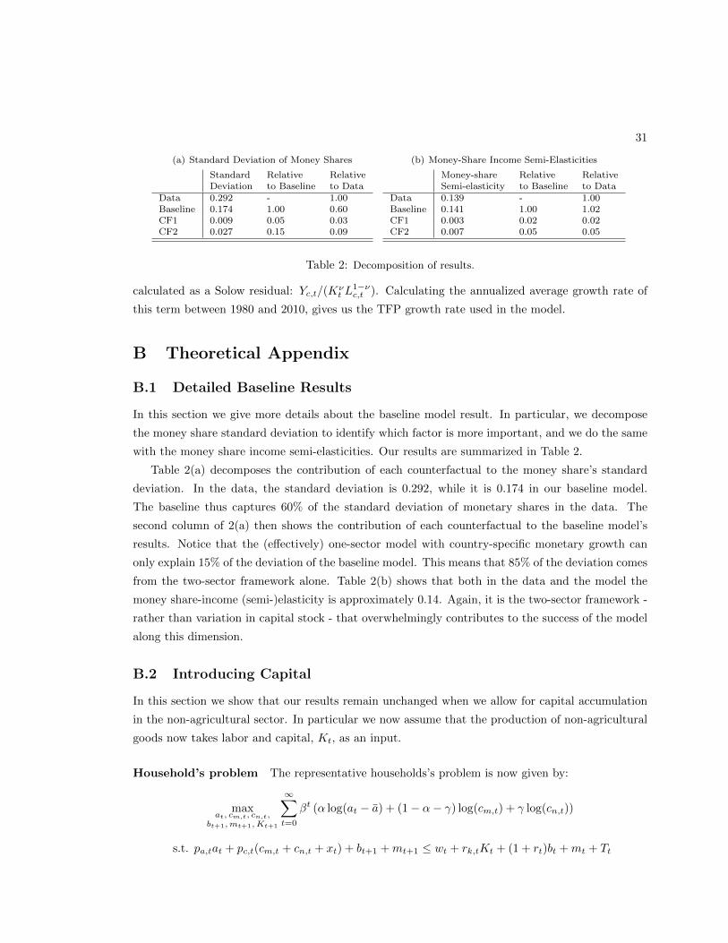
31

(a) Standard Deviation of Money Shares

Standard Relative RelativeDeviation to Baseline to Data

Data 0.292 - 1.00Baseline 0.174 1.00 0.60CF1 0.009 0.05 0.03CF2 0.027 0.15 0.09

(b) Money-Share Income Semi-Elasticities

Money-share Relative RelativeSemi-elasticity to Baseline to Data

Data 0.139 - 1.00Baseline 0.141 1.00 1.02CF1 0.003 0.02 0.02CF2 0.007 0.05 0.05

Table 2: Decomposition of results.

calculated as a Solow residual: Yc,t/(Kνt L

1−νc,t ). Calculating the annualized average growth rate of

this term between 1980 and 2010, gives us the TFP growth rate used in the model.

B Theoretical Appendix

B.1 Detailed Baseline Results

In this section we give more details about the baseline model result. In particular, we decompose

the money share standard deviation to identify which factor is more important, and we do the same

with the money share income semi-elasticities. Our results are summarized in Table 2.

Table 2(a) decomposes the contribution of each counterfactual to the money share’s standard

deviation. In the data, the standard deviation is 0.292, while it is 0.174 in our baseline model.

The baseline thus captures 60% of the standard deviation of monetary shares in the data. The

second column of 2(a) then shows the contribution of each counterfactual to the baseline model’s

results. Notice that the (effectively) one-sector model with country-specific monetary growth can

only explain 15% of the deviation of the baseline model. This means that 85% of the deviation comes

from the two-sector framework alone. Table 2(b) shows that both in the data and the model the

money share-income (semi-)elasticity is approximately 0.14. Again, it is the two-sector framework -

rather than variation in capital stock - that overwhelmingly contributes to the success of the model

along this dimension.

B.2 Introducing Capital

In this section we show that our results remain unchanged when we allow for capital accumulation

in the non-agricultural sector. In particular we now assume that the production of non-agricultural

goods now takes labor and capital, Kt, as an input.

Household’s problem The representative households’s problem is now given by:

maxat, cm,t, cn,t,

bt+1,mt+1, Kt+1

∞∑t=0

βt (α log(at − a) + (1− α− γ) log(cm,t) + γ log(cn,t))

s.t. pa,tat + pc,t(cm,t + cn,t + xt) + bt+1 +mt+1 ≤ wt + rk,tKt + (1 + rt)bt +mt + Tt

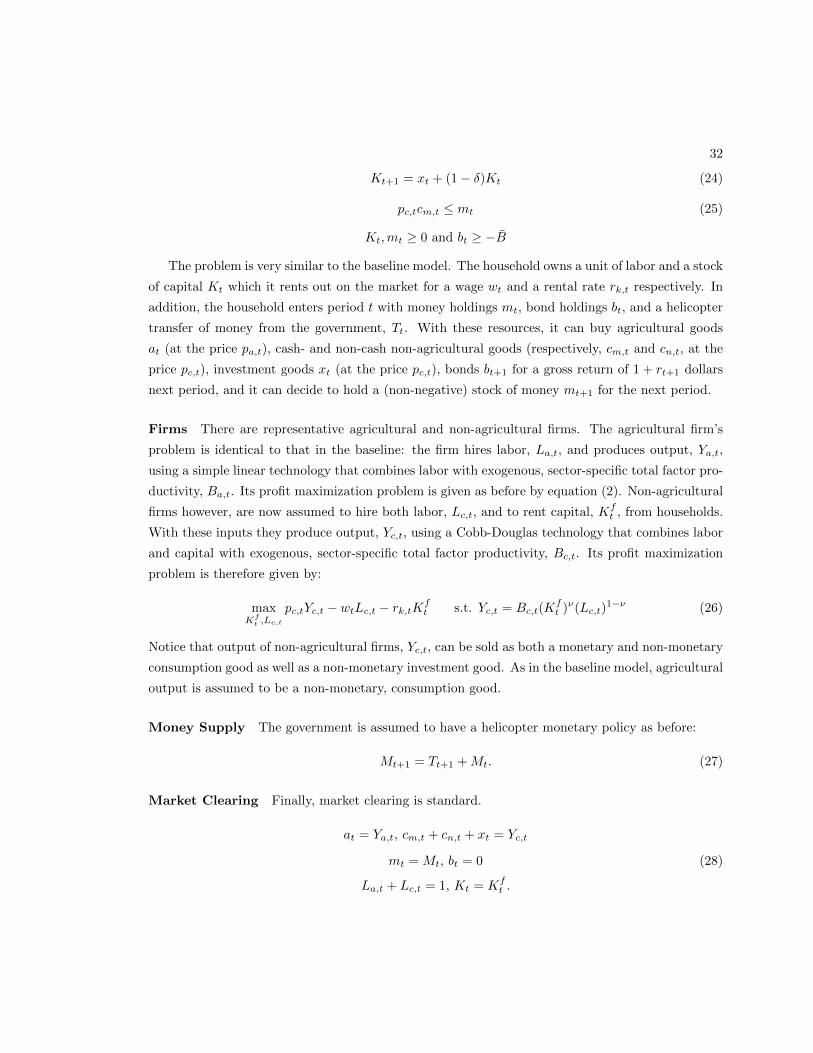
32

Kt+1 = xt + (1− δ)Kt (24)

pc,tcm,t ≤ mt (25)

Kt,mt ≥ 0 and bt ≥ −B

The problem is very similar to the baseline model. The household owns a unit of labor and a stock

of capital Kt which it rents out on the market for a wage wt and a rental rate rk,t respectively. In

addition, the household enters period t with money holdings mt, bond holdings bt, and a helicopter

transfer of money from the government, Tt. With these resources, it can buy agricultural goods

at (at the price pa,t), cash- and non-cash non-agricultural goods (respectively, cm,t and cn,t, at the

price pc,t), investment goods xt (at the price pc,t), bonds bt+1 for a gross return of 1 + rt+1 dollars

next period, and it can decide to hold a (non-negative) stock of money mt+1 for the next period.

Firms There are representative agricultural and non-agricultural firms. The agricultural firm’s

problem is identical to that in the baseline: the firm hires labor, La,t, and produces output, Ya,t,

using a simple linear technology that combines labor with exogenous, sector-specific total factor pro-

ductivity, Ba,t. Its profit maximization problem is given as before by equation (2). Non-agricultural

firms however, are now assumed to hire both labor, Lc,t, and to rent capital, Kft , from households.

With these inputs they produce output, Yc,t, using a Cobb-Douglas technology that combines labor

and capital with exogenous, sector-specific total factor productivity, Bc,t. Its profit maximization

problem is therefore given by:

maxKf

t ,Lc,t

pc,tYc,t − wtLc,t − rk,tKft s.t. Yc,t = Bc,t(K

ft )

ν(Lc,t)1−ν (26)

Notice that output of non-agricultural firms, Yc,t, can be sold as both a monetary and non-monetary

consumption good as well as a non-monetary investment good. As in the baseline model, agricultural

output is assumed to be a non-monetary, consumption good.

Money Supply The government is assumed to have a helicopter monetary policy as before:

Mt+1 = Tt+1 +Mt. (27)

Market Clearing Finally, market clearing is standard.

at = Ya,t, cm,t + cn,t + xt = Yc,t

mt = Mt, bt = 0 (28)

La,t + Lc,t = 1, Kt = Kft .

33

Solution We follow the same solution strategy as in the baseline model. In particular, we assume

that nominal interest rates are always positive and we use the first order conditions of the household

and firms problems, in combination with the market clearing conditions and the evolution of money

by government to obtain three equations that (together with transversality conditions for bonds,

capital and money) pin down the equilibrium solutions of the problem.

The first equation defines a split of non-agricultural consumption between monetary and non-

monetary goods. Defining Ct ≡ cm,t + cn,t = Yc,t − (Kt+1 − (1− δ)Kt) we can write:

cn,t = (1− φt)Ct and cm,t = φtCt, (29)

where φt =1−α−γ

(1−α−γ)+γτt. Second, given initial capital endowment, K0, the path of capital is pinned

down by a transversality condition and the following Euler Equation:

τt+1

τt

φt+1

φt

Ct+1

Ct= β

(νBc

t+1(Kt+1)ν−1(Lc

t+1)1−ν + 1− δ

). (30)

Finally, employment in the non-agricultural sector, Lc,t, is determined by the following:

ατt(1− Lc,t)− a

Ba,t

=(1− ν)(1− α− γ)Bc,tK

νt (Lc,t)

−ν

φtCt. (31)

We solve the model following the strategy of Echevarria (1997). We assume that after some

point in time, T , the variables Mt, Ba,t and Bc,t grow at constant rates (gm − 1, ga − 1 > 0 and

gc − 1 respectively) and hence τt → τ and φt → φ converge to constants. Given these assumptions,

the role of the non-homotheticity disappears in the limit as limt→∞a

Ba,t= 0 in equation (31).

The model thus converges asymptotically to a balanced growth path where capital, investment and

non-agricultural consumption grow at the rate g1

1−νc , agricultural consumption grows at a rate ga

and employment in agriculture and non-agriculture are constant. Consequently, we can re-write the

model in terms of variables that are stationary in the long run. In particular, defining kt ≡ Kt/B1

1−ν

c,t

and ct ≡ Ct/B1

1−ν

c,t equations (30) and (31) become:(Bc,t+1

Bc,t

) 11−ν ct+1

ct

τt+1

τt

φt+1

φt= β

(νkν−1

t+1 (Lct+1)

1−ν + 1− δ)

and (32)

ατtφt

(1− Lc,t)− aBa,t

=(1− ν)(1− α− γ)kνt (Lc,t)

−ν

(1− δ)kt −(

Bc,t+1

Bc,t

) 11−ν

kt+1 + kνt (Lc,t)1−ν

(33)

Since limt→∞a

Ba,t= 0, using the above it is easy to show that kt → k∗ and Lc

t → L∗c , where:

L∗c =

(1− ν)

(g

11−νc − β(1− δ)

)(g

11−νc − β(1− δ)

)+ α

1−α−γ τ φ

(g

11−νc (1− βν)− β(1− δ)(1− ν)

) , and (34)

k∗ = β− 11−ν (g

11−νc − β(1− δ))

11−ν ν

11−ν L∗

c . (35)

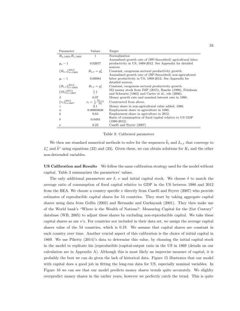
34

Parameter Values Target

Ba,1869,Bc,1869 1 Normalization

ga − 1 0.02657Annualized growth rate of (HP-Smoothed) agricultural laborproductivity in US, 1869-2012. See Appendix for detailedsources.

{Ba,t}2013t=1869 Ba,t = gta Constant, exogenous sectoral productivity growth.

gc − 1 0.00984Annualized growth rate of (HP-Smoothed) non-agriculturallabor productivity in US, 1869-2012. See Appendix fordetailed sources.

{Bc,t}2013t=1869 Bc,t = gtc Constant, exogenous sectoral productivity growth.

{Mt}2014t=1867 {·} M2 money stock from IMF (2015), Rasche (1990), Friedmanand Schwartz (1963) and Carter et al., eds (2006).

β 0.97 Money growth rate and nominal interest rate in 1980.

{τt}2013t=1867 τt =1β

Mt+1

MtConstructed from above.

γ 0.1 Money share in non-agricultural value added, 1980.α 0.00003626 Employment share in agriculture in 1980.a 0.64 Employment share in agriculture in 2012.

δ 0.0493Ratio of consumption of fixed capital relative to US GDP(1980-2012).

ν 0.23 Caselli and Feyrer (2007)

Table 3: Calibrated parameters

We then use standard numerical methods to solve for the sequences kt and Lc,t that converge to

L∗c and k∗ using equations (32) and (33). Given these, we can obtain solutions for Kt and the other

non-detrended variables.

US Calibration and Results We follow the same calibration strategy used for the model without

capital. Table 3 summarizes the parameters’ values.

The only additional parameters are δ, ν and initial capital stock. We choose δ to match the

average ratio of consumption of fixed capital relative to GDP in the US between 1980 and 2012

from the BEA. We choose a country specific ν directly from Caselli and Feyrer (2007) who provide

estimates of reproducible capital shares for 54 countries. They start by taking aggregate capital

shares using data from Gollin (2002) and Bernanke and Gurkaynak (2001). They then make use

of the World bank’s “Where is the Wealth of Nations?: Measuring Capital for the 21st Century”

database (WB, 2005) to adjust these shares by excluding non-reproducible capital. We take these

capital shares as our ν’s. For countries not included in their data set, we assign the average capital

shares value of the 54 countries, which is 0.19. We assume that capital shares are constant in

each country over time. Another crucial aspect of this calibration is the choice of initial capital in

1869. We use Piketty (2014)’s data to determine this value, by choosing the initial capital stock

in the model to replicate his (reproducible-)capital-output ratio in the US in 1869 (details on our

calculation are in Appendix A). Although this is most likely an imprecise measure of capital, it is

probably the best we can do given the lack of historical data. Figure 15 illustrates that our model

with capital does a good job in fitting the long-run data for US, especially nominal variables. In

Figure 16 we can see that our model predicts money shares trends quite accurately. We slighlty

overpredict money shares in the earlier years, however we perfectly catch the trend. This is quite

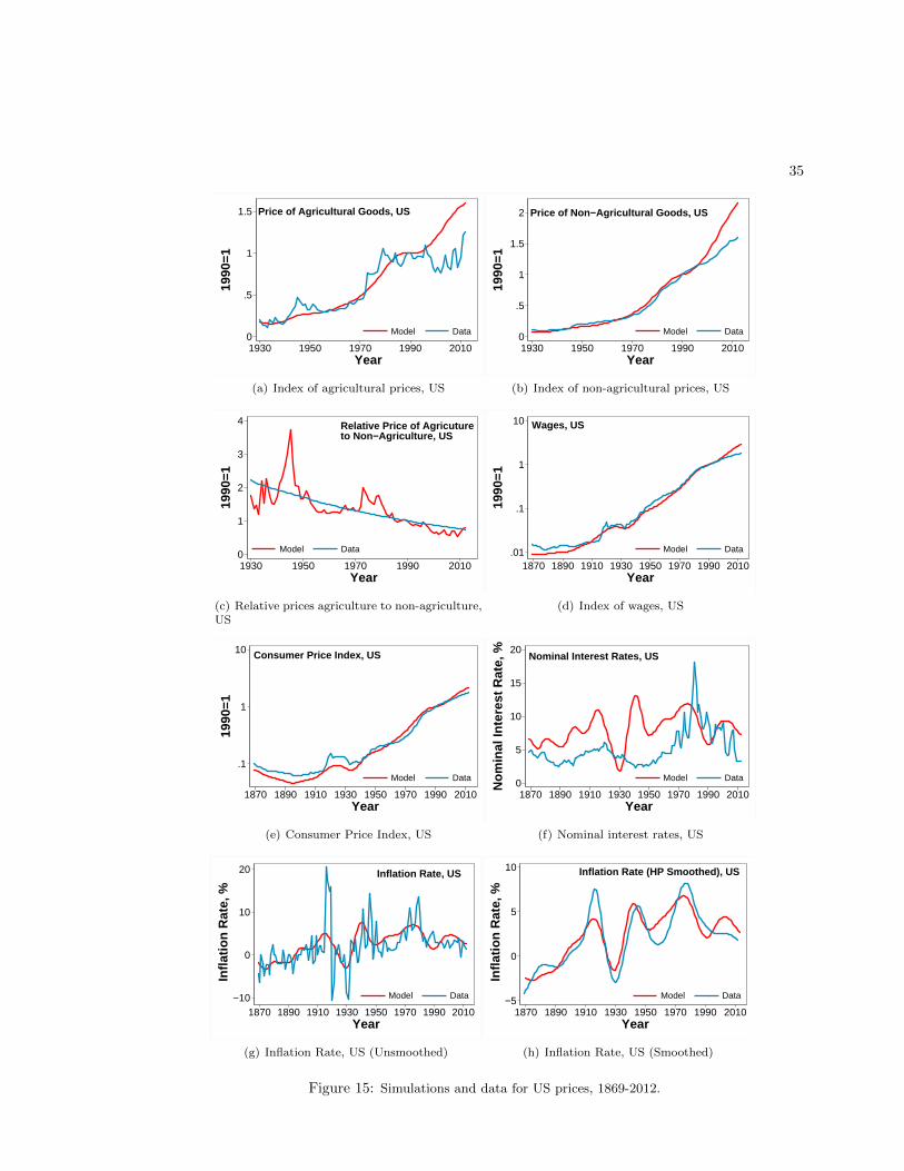
35

Price of Agricultural Goods, US

0

.5

1

1.519

90=1

1930 1950 1970 1990 2010 Year

Model Data

(a) Index of agricultural prices, US

Price of Non−Agricultural Goods, US

0

.5

1

1.5

2

1990

=1

1930 1950 1970 1990 2010 Year

Model Data

(b) Index of non-agricultural prices, US

Relative Price of Agricutureto Non−Agriculture, US

0

1

2

3

4

1990

=1

1930 1950 1970 1990 2010 Year

Model Data

(c) Relative prices agriculture to non-agriculture,US

Wages, US

.01

.1

1

10

1990

=1

1870 1890 1910 1930 1950 1970 1990 2010 Year

Model Data

(d) Index of wages, US

Consumer Price Index, US

.1

1

10

1990

=1

1870 1890 1910 1930 1950 1970 1990 2010 Year

Model Data

(e) Consumer Price Index, US

Nominal Interest Rates, US

0

5

10

15

20

No

min

al In

tere

st R

ate,

%

1870 1890 1910 1930 1950 1970 1990 2010 Year

Model Data

(f) Nominal interest rates, US

Inflation Rate, US

−10

0

10

20

Infl

atio

n R

ate,

%

1870 1890 1910 1930 1950 1970 1990 2010 Year

Model Data

(g) Inflation Rate, US (Unsmoothed)

Inflation Rate (HP Smoothed), US

−5

0

5

10

Infl

atio

n R

ate,

%

1870 1890 1910 1930 1950 1970 1990 2010 Year

Model Data

(h) Inflation Rate, US (Smoothed)

Figure 15: Simulations and data for US prices, 1869-2012.

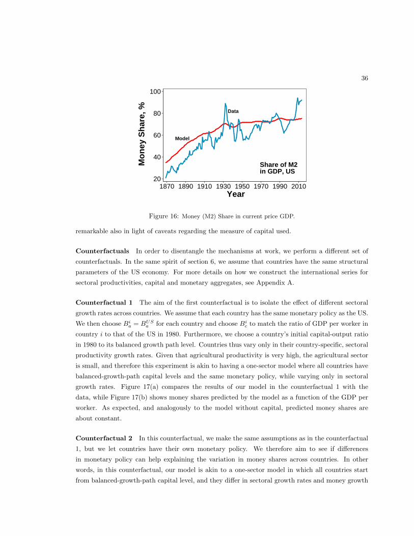
36

Share of M2in GDP, US

Data

Model

20

40

60

80

100

Mo

ney

Sh

are,

%

1870 1890 1910 1930 1950 1970 1990 2010 Year

Figure 16: Money (M2) Share in current price GDP.

remarkable also in light of caveats regarding the measure of capital used.

Counterfactuals In order to disentangle the mechanisms at work, we perform a different set of

counterfactuals. In the same spirit of section 6, we assume that countries have the same structural

parameters of the US economy. For more details on how we construct the international series for

sectoral productivities, capital and monetary aggregates, see Appendix A.

Counterfactual 1 The aim of the first counterfactual is to isolate the effect of different sectoral

growth rates across countries. We assume that each country has the same monetary policy as the US.

We then choose Bia = BUS

a for each country and choose Bic to match the ratio of GDP per worker in

country i to that of the US in 1980. Furthermore, we choose a country’s initial capital-output ratio

in 1980 to its balanced growth path level. Countries thus vary only in their country-specific, sectoral

productivity growth rates. Given that agricultural productivity is very high, the agricultural sector

is small, and therefore this experiment is akin to having a one-sector model where all countries have

balanced-growth-path capital levels and the same monetary policy, while varying only in sectoral

growth rates. Figure 17(a) compares the results of our model in the counterfactual 1 with the

data, while Figure 17(b) shows money shares predicted by the model as a function of the GDP per

worker. As expected, and analogously to the model without capital, predicted money shares are

about constant.

Counterfactual 2 In this counterfactual, we make the same assumptions as in the counterfactual

1, but we let countries have their own monetary policy. We therefore aim to see if differences

in monetary policy can help explaining the variation in money shares across countries. In other

words, in this counterfactual, our model is akin to a one-sector model in which all countries start

from balanced-growth-path capital level, and they differ in sectoral growth rates and money growth

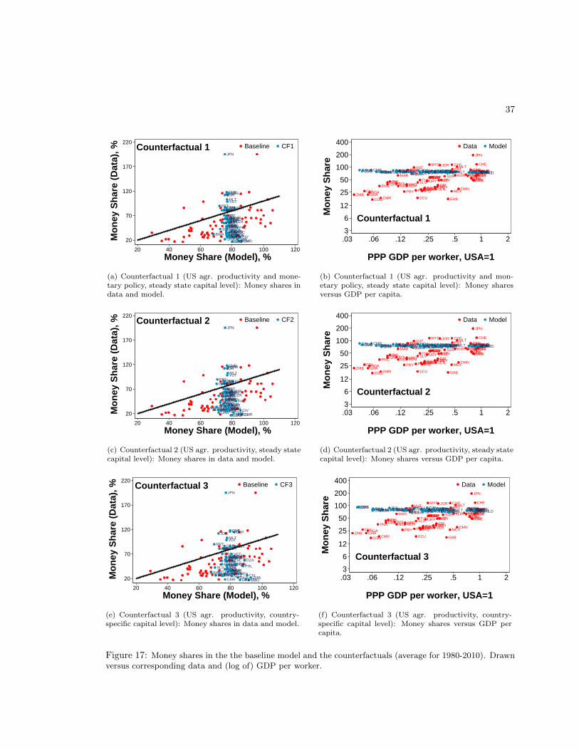
37

AUS

AUT

BHR

BHSBLZBOL

BWA

CHE

CHL

CIVCMRCOG

COLCRI

CYP

DNK

DOM

DZA

ECU

EGYESP

FIN

FRA

GAB

GBR

GHA

GRC

GTM

GUY

HNDIDN

IRL

IRN

IRQ

ISR

ITAJAM

JOR

JPN

KORMAR

MDVMEX

MLT

MYS

NGANIC

NLD

OMN

PAK

PER

PHLPNG

PRT

PRY

SLV

SUR

SWE

THA

TON

TUN

TUR

URY

VCT

VEN

VUT

ZAF

ZMB

Counterfactual 1

20

70

120

170

220

Mo

ney

Sh

are

(Dat

a), %

20 40 60 80 100 120

Money Share (Model), %

Baseline CF1

(a) Counterfactual 1 (US agr. productivity and mone-tary policy, steady state capital level): Money shares indata and model.

AUSAUT

BHRBHSBLZ

BOLBWA

CHE

CHL

CIV

CMRCOG

COLCRI

CYP

DNK

DOM

DZA

ECU

EGY ESP

FINFRA

GAB

GBR

GHA

GRC

GTM

GUY

HNDIDN

IRLIRN

IRQ

ISRITA

JAM

JOR

JPN

KORMAR

MDV

MEX

MLTMYS

NGA

NIC

NLD

OMN

PAK

PER

PHLPNG

PRT

PRY

SLV

SURSWE

THA

TON

TUN

TUR

URY

VCT

VEN

VUT

ZAF

ZMB

AUSAUTBHRBHSBLZBOLBWA CHECHLCIV CMRCOG COL CRICYP DNKDOMDZAECUEGY ESPFINFRAGAB GBRGHA GRCGTMGUYHNDIDN IRLIRNIRQ ISRITAJAM JOR JPNKORMARMDV MEX MLTMYSNGA NIC

NLDOMNPAK PERPHLPNG PRTPRY SLV SUR SWETHA TONTUN TURURYVCT VENVUT ZAFZMB

Counterfactual 13

6

12

25

50

100

200

400

Mo

ney

Sh

are

.03 .06 .12 .25 .5 1 2

PPP GDP per worker, USA=1

Data Model

(b) Counterfactual 1 (US agr. productivity and mon-etary policy, steady state capital level): Money sharesversus GDP per capita.

AUS

AUT

BHR

BHSBLZBOL

BWA

CHE

CHL

CIVCMRCOG

COLCRI

CYP

DNK

DOM

DZA

ECU

EGYESP

FIN

FRA

GAB

GBR

GHA

GRC

GTM

GUY

HNDIDN

IRL

IRN

IRQ

ISR

ITAJAM

JOR

JPN

KORMAR

MDVMEX

MLT

MYS

NGANIC

NLD

OMN

PAK

PER

PHLPNG

PRT

PRY

SLV

SUR

SWE

THA

TON

TUN

TUR

URY

VCT

VEN

VUT

ZAF

ZMB

Counterfactual 2

20

70

120

170

220

Mo

ney

Sh

are

(Dat

a), %

20 40 60 80 100 120

Money Share (Model), %

Baseline CF2

(c) Counterfactual 2 (US agr. productivity, steady statecapital level): Money shares in data and model.

AUSAUT

BHRBHSBLZ

BOLBWA

CHE

CHL

CIV

CMRCOG

COLCRI

CYP

DNK

DOM

DZA

ECU

EGY ESP

FINFRA

GAB

GBR

GHA

GRC

GTM

GUY

HNDIDN

IRLIRN

IRQ

ISRITA

JAM

JOR

JPN

KORMAR

MDV

MEX

MLTMYS

NGA

NIC

NLD

OMN

PAK

PER

PHLPNG

PRT

PRY

SLV

SURSWE

THA

TON

TUN

TUR

URY

VCT

VEN

VUT

ZAF

ZMB

AUSAUTBHRBHSBLZBOL BWACHECHLCIV CMRCOG COL CRI CYP DNKDOMDZAECUEGY ESPFINFRAGAB GBRGHA GRCGTMGUYHNDIDN IRLIRNIRQ ISRITAJAM JOR JPNKORMARMDV MEX MLTMYSNGA NIC NLDOMNPAK PER

PHLPNG PRTPRY SLV SUR SWETHA TONTUN TURURYVCT VENVUT ZAFZMB

Counterfactual 23

6

12

25

50

100

200

400

Mo

ney

Sh

are

.03 .06 .12 .25 .5 1 2

PPP GDP per worker, USA=1

Data Model

(d) Counterfactual 2 (US agr. productivity, steady statecapital level): Money shares versus GDP per capita.

AUS

AUT

BHR

BHSBLZBOL

BWA

CHE

CHL

CIVCMR COG

COLCRI

CYP

DNK

DOM

DZA

ECU

EGYESP

FIN

FRA

GAB

GBR

GHA

GRC

GTM

GUY

HNDIDN

IRL

IRN

IRQ

ISR

ITAJAM

JOR

JPN

KORMAR

MDVMEX

MLT

MYS

NGANIC

NLD

OMN

PAK

PER

PHLPNG

PRT

PRY

SLV

SUR

SWE

THA

TON

TUN

TUR

URY

VCT

VEN

VUT

ZAF

ZMB

Counterfactual 3

20

70

120

170

220

Mo

ney

Sh

are

(Dat

a), %

20 40 60 80 100 120

Money Share (Model), %

Baseline CF3

(e) Counterfactual 3 (US agr. productivity, country-specific capital level): Money shares in data and model.

AUSAUT

BHRBHSBLZ

BOLBWA

CHE

CHL

CIV

CMRCOG

COLCRI

CYP

DNK

DOM

DZA

ECU

EGY ESP

FINFRA

GAB

GBR

GHA

GRC

GTM

GUY

HNDIDN

IRLIRN

IRQ

ISRITA

JAM

JOR

JPN

KORMAR

MDV

MEX

MLTMYS

NGA

NIC

NLD

OMN

PAK

PER

PHLPNG

PRT

PRY

SLV

SURSWE

THA

TON

TUN

TUR

URY

VCT

VEN

VUT

ZAF

ZMB

AUSAUTBHRBHSBLZBOLBWA

CHECHLCIVCMR

COG COL CRICYP DNKDOMDZAECUEGY ESPFIN FRA

GABGBRGHA GRCGTMGUYHNDIDN IRLIRN

IRQ ISRITAJAM JOR JPNKORMARMDVMEXMLTMYSNGA NIC NLDOMNPAK PER

PHLPNGPRTPRY SLV SUR SWETHA TONTUN

TURURYVCT VENVUT ZAFZMB

Counterfactual 33

6

12

25

50

100

200

400

Mo

ney

Sh

are

.03 .06 .12 .25 .5 1 2

PPP GDP per worker, USA=1

Data Model

(f) Counterfactual 3 (US agr. productivity, country-specific capital level): Money shares versus GDP percapita.

Figure 17: Money shares in the the baseline model and the counterfactuals (average for 1980-2010). Drawnversus corresponding data and (log of) GDP per worker.

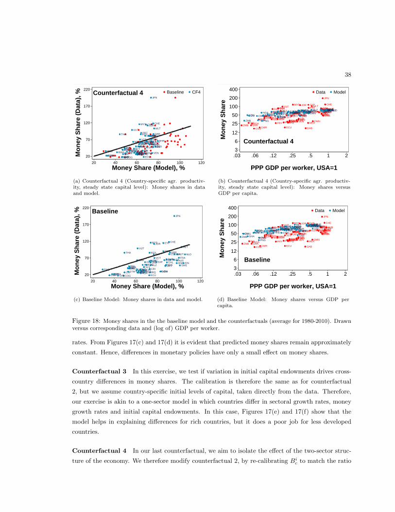
38

AUS

AUT

BHR

BHSBLZBOL

BWA

CHE

CHL

CIVCMRCOG

COLCRI

CYP

DNK

DOM

DZA

ECU

EGY ESP

FIN

FRA

GAB

GBR

GHA

GRC

GTM

GUY

HNDIDN

IRL

IRN

IRQ

ISR

ITAJAM

JOR

JPN

KORMAR

MDVMEX

MLT

MYS

NGANIC

NLD

OMN

PAK

PER

PHLPNG

PRT

PRY

SLV

SUR

SWE

THA

TON

TUN

TUR

URY

VCT

VEN

VUT

ZAF

ZMB

Counterfactual 4

20

70

120

170

220

Mo

ney

Sh

are

(Dat

a), %

20 40 60 80 100 120

Money Share (Model), %

Baseline CF4

(a) Counterfactual 4 (Country-specific agr. productiv-ity, steady state capital level): Money shares in dataand model.

AUSAUT

BHRBHSBLZ

BOLBWA

CHE

CHL

CIV

CMRCOG

COLCRI

CYP

DNK

DOM

DZA

ECU

EGY ESP

FINFRA

GAB

GBR

GHA

GRC

GTM

GUY

HNDIDN

IRLIRN

IRQ

ISRITA

JAM

JOR

JPN

KORMAR

MDV

MEX

MLTMYS

NGA

NIC

NLD

OMN

PAK

PER

PHLPNG

PRT

PRY

SLV

SURSWE

THA

TON

TUN

TUR

URY

VCT

VEN

VUT

ZAF

ZMB

AUSAUTBHRBHSBLZ

BOLBWA

CHECHL

CIV CMRCOGCOL CRICYP DNKDOMDZAECUEGY ESPFINFRA

GAB

GBR

GHA

GRCGTM

GUYHND

IDN

IRLIRNIRQ ISRITA

JAMJOR JPNKOR

MARMDV MEXMLT

MYSNGA NIC NLDOMN

PAKPER

PHL

PNG

PRTPRY SLVSUR

SWE

THATONTUN

TUR

URYVCTVEN

VUTZAF

ZMB

Counterfactual 43

6

12

25

50

100

200

400

Mo

ney

Sh

are

.03 .06 .12 .25 .5 1 2

PPP GDP per worker, USA=1

Data Model

(b) Counterfactual 4 (Country-specific agr. productiv-ity, steady state capital level): Money shares versusGDP per capita.

AUS

AUT

BHR

BHSBLZBOL

BWA

CHE

CHL

CIVCMR COG

COLCRI

CYP

DNK

DOM

DZA

ECU

EGY ESP

FIN

FRA

GAB

GBR

GHA

GRC

GTM

GUY

HNDIDN

IRL

IRN

IRQ

ISR

ITAJAM

JOR

JPN

KORMAR

MDVMEX

MLT

MYS

NGANIC

NLD

OMN

PAK

PER

PHLPNG

PRT

PRY

SLV

SUR

SWE

THA

TON

TUN

TUR

URY

VCT

VEN

VUT

ZAF

ZMB

Baseline

20

70

120

170

220

Mo

ney

Sh

are

(Dat

a), %

20 40 60 80 100 120

Money Share (Model), %

(c) Baseline Model: Money shares in data and model.

AUSAUT

BHRBHSBLZ

BOLBWA

CHE

CHL

CIV

CMRCOG

COLCRI

CYP

DNK

DOM

DZA

ECU

EGY ESP

FINFRA

GAB

GBR

GHA

GRC

GTM

GUY

HNDIDN

IRLIRN

IRQ

ISRITA

JAM

JOR

JPN

KORMAR

MDV

MEX

MLTMYS

NGA

NIC

NLD

OMN

PAK

PER

PHLPNG

PRT

PRY

SLV

SURSWE

THA

TON

TUN

TUR

URY

VCT

VEN

VUT

ZAF

ZMB

AUSAUTBHRBHSBLZ

BOLBWA

CHECHL

CIV

CMR

COGCOL CRI

CYPDNK

DOMDZAECUEGY

ESPFINFRA

GAB

GBR

GHA

GRC

GTM

GUY

HNDIDN

IRL

IRNIRQISRITA

JAM JORJPNKOR

MARMDV MEX

MLT

MYSNGA NIC

NLD

OMNPAK

PERPHL

PNG

PRT

PRY SLV SUR

SWE

THA

TONTUN TUR

URYVCT VEN

VUTZAF

ZMB

Baseline3

6

12

25

50

100

200

400

Mo

ney

Sh

are

.03 .06 .12 .25 .5 1 2

PPP GDP per worker, USA=1

Data Model

(d) Baseline Model: Money shares versus GDP percapita.

Figure 18: Money shares in the the baseline model and the counterfactuals (average for 1980-2010). Drawnversus corresponding data and (log of) GDP per worker.

rates. From Figures 17(c) and 17(d) it is evident that predicted money shares remain approximately

constant. Hence, differences in monetary policies have only a small effect on money shares.

Counterfactual 3 In this exercise, we test if variation in initial capital endowments drives cross-

country differences in money shares. The calibration is therefore the same as for counterfactual

2, but we assume country-specific initial levels of capital, taken directly from the data. Therefore,

our exercise is akin to a one-sector model in which countries differ in sectoral growth rates, money

growth rates and initial capital endowments. In this case, Figures 17(e) and 17(f) show that the

model helps in explaining differences for rich countries, but it does a poor job for less developed

countries.

Counterfactual 4 In our last counterfactual, we aim to isolate the effect of the two-sector struc-

ture of the economy. We therefore modify counterfactual 2, by re-calibrating Bic to match the ratio

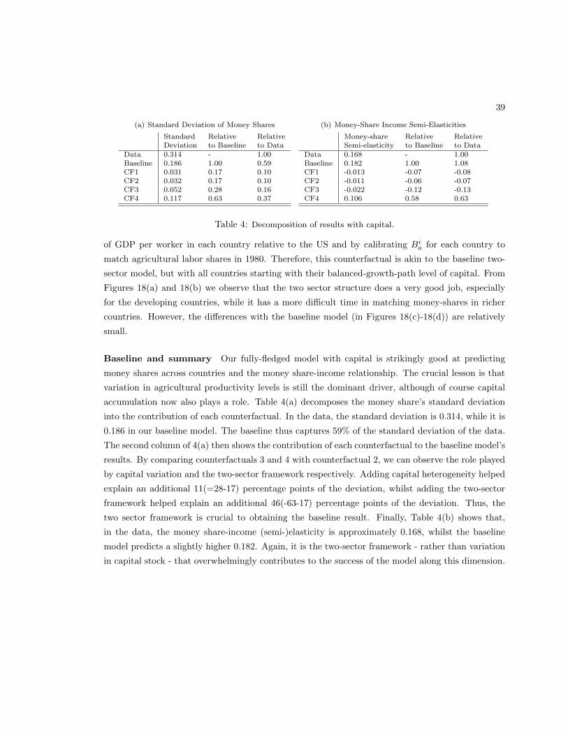
39

(a) Standard Deviation of Money Shares

Standard Relative RelativeDeviation to Baseline to Data

Data 0.314 - 1.00Baseline 0.186 1.00 0.59CF1 0.031 0.17 0.10CF2 0.032 0.17 0.10CF3 0.052 0.28 0.16CF4 0.117 0.63 0.37

(b) Money-Share Income Semi-Elasticities

Money-share Relative RelativeSemi-elasticity to Baseline to Data

Data 0.168 - 1.00Baseline 0.182 1.00 1.08CF1 -0.013 -0.07 -0.08CF2 -0.011 -0.06 -0.07CF3 -0.022 -0.12 -0.13CF4 0.106 0.58 0.63

Table 4: Decomposition of results with capital.

of GDP per worker in each country relative to the US and by calibrating Bia for each country to

match agricultural labor shares in 1980. Therefore, this counterfactual is akin to the baseline two-

sector model, but with all countries starting with their balanced-growth-path level of capital. From

Figures 18(a) and 18(b) we observe that the two sector structure does a very good job, especially

for the developing countries, while it has a more difficult time in matching money-shares in richer

countries. However, the differences with the baseline model (in Figures 18(c)-18(d)) are relatively

small.

Baseline and summary Our fully-fledged model with capital is strikingly good at predicting

money shares across countries and the money share-income relationship. The crucial lesson is that

variation in agricultural productivity levels is still the dominant driver, although of course capital

accumulation now also plays a role. Table 4(a) decomposes the money share’s standard deviation

into the contribution of each counterfactual. In the data, the standard deviation is 0.314, while it is

0.186 in our baseline model. The baseline thus captures 59% of the standard deviation of the data.

The second column of 4(a) then shows the contribution of each counterfactual to the baseline model’s

results. By comparing counterfactuals 3 and 4 with counterfactual 2, we can observe the role played

by capital variation and the two-sector framework respectively. Adding capital heterogeneity helped

explain an additional 11(=28-17) percentage points of the deviation, whilst adding the two-sector

framework helped explain an additional 46(-63-17) percentage points of the deviation. Thus, the

two sector framework is crucial to obtaining the baseline result. Finally, Table 4(b) shows that,

in the data, the money share-income (semi-)elasticity is approximately 0.168, whilst the baseline

model predicts a slightly higher 0.182. Again, it is the two-sector framework - rather than variation

in capital stock - that overwhelmingly contributes to the success of the model along this dimension.

40

References

Alvarez-Cuadrado, Francisco and Markus Poschke, “Structural Change Out of Agriculture:

Labor Push versus Labor Pull,” American Economic Journal: Macroeconomics, 2011, 3 (3), 127–

58.

Anderson, Richard G., “Monetary Aggregates (CJ),” in Susan B. Carter, Scott Sigmund Gartner,

Michael R. Haines, Alan L. Olmstead, Richard Sutch, and Gavin Wright, eds., Historical Statistics

of the United States, Earliest Times to the Present: Millennial Edition, Cambridge University

Press, 2006.

Bernanke, B.S. and R. Gurkaynak, “Is Growth Exogenous? Taking Mankiw, Romer and Weil

Seriously,” NBER Macroeconomic Annual, 2001.

Blades, Derek W., “Subsistence activities in the national accounts of developing countries with

special reference to Latin America,” Review of Income and Wealth, 1975, 21 (4), 391–410.

Bordo, Michael D. and Anna J. Schwartz, “Money and Prices in the Nineteenth Century: An

Old Debate Rejoined,” The Journal of Economics History, March 1980, 40 (1), 61–67.

and , “Money and Prices in the 19th Century: Was Thomas Tooke Right?,” Explorations in

Economic History, 1981, 18, 97–121.

and Lars Jonung, “The Long Run Behavior of the Income Velocity of Money in Five Advanced

Countries: 1870-1975: An Institutional Approach,” Economic inquiry, Jan 01 1981, 19 (1), 96.

Last updated - 2013-02-23.

and , The Long-Run Behuvibr of the Velocity of Circulation: The International Evidence,

Cambridge University Press, 1987.

and , “The long-run behavior of velocity: The institutional approach revisited,” Journal of

Policy Modeling, 1990, 12 (2), 165–197.

, , and Pierre Siklos, “The Common Development of Institutional Change as Measured by

Income Velocity: A Century of Evidence from Industrialized Countries,” NBER Working Paper

No. 4379, 1993.

Buera, Francisco J. and Joseph P. Kaboski, “Scale and the Origins of Structural Change,”

Journal of Economic Theory, March 2012, 147 (2), 684712.

Carter, Susan B., Scott Sigmund Gartner, Michael R. Haines, Alan L. Olmstead,

Richard Sutch, and Gavin Wright, eds, Historical Statistics of the United States, Earli-

est Times to the Present: Millennial Edition, Cambridge University Press, 2006.

41

Caselli, Francesco, “Accounting for Cross-country income Differences,” in Philippe Aghion and

Steven N. Durlauf, eds., Handbook of Economic Growth, Volume 1A., Elsevier B.V., 2005, pp. 680–

738.

and James Feyrer, “The Marginal Product of Capital,” Quarterly Journal of Economics, 2007,

122 (2).

Chandavarkar, Anand G., “Monetization of Developing Economies,” Staff Papers (International

Monetary Fund), 1977, 24 (3), 665–721.

Chari, V.V., Larry E. Jones, and Rodolfo E. Manuelli, “Inflation, growth, and financial

intermediation,” Proceedings, 1996, (May), 41–58.

, Lawrence J. Christiano, and Patrick J. Kehoe, “Optimality of the Friedman rule in

economies with distorting taxes.,” Journal of Monetary Economics, 1996, 37, 203–223.

Cole, Harold L. and Narayana Kocherlakota, “Zero Nominal Interest Rates: Why Theyre

Good and How to Get Them,” Federal Reserve Bank of Minneapolis Quarterly Review, 1998,

22(2), 210.

Dorich, Jose, “Resurrecting the Role of Real Money Balance Effects,” Staff Working Papers 09-24,

Bank of Canada 2009.

Duarte, M. and D. Restuccia, “The Role of the Structural Transformation in Aggregate Pro-

ductivity,” The Quarterly Journal of Economics, 2010, 125(1), 129–173.

Echevarria, C., “Changes in Sectoral Composition Associated with Economic Growth,” Interna-

tional Economic Review, 1997, 38.

FAOSTAT, Food and Agriculture Organization of the United Nations Database 2012.

Friedman, Milton, “The Demand for Money: Some Theoretical and Empirical Results,” The

American Economic Review, Papers and Proceedings, 1959, Vol. 49, 525–527.

and Anna J. Schwartz, A Monetary History of the United States, 1867-1960, Princeton Uni-

versity Press, 1963.

Gollin, Douglas, “Getting Income Shares Right,” Journal of Political Economy, April 2002, 110

(2), 458–474.

, Stephen Parente, and Richard Rogerson, “The Role of Agriculture in Development,”

American Economic Review, 2002, 92(2), 160–164.

Goodfriend, Marvin, “Money, Credit, Banking, and Payments System Policy,” Federal Reserve

Bank of Richmond Economic Review, January/February 1991, 77, 7–23.

42

Herrendorf, Berthold, Richard Rogerson, and Akos Valentinyi, “Growth and Structural

Transformation,” in Philippe Aghion and Steven N. Durlauf, eds., Handbook of Economic Growth,

North Holland, 2014, chapter 6, p. 855.

Heston, Alan, Robert Summers, and Bettina Aten, Penn World Table Version 7.1 Center

for International Comparisons of Production, Income and Prices at the University of Pennsylvania

2012.

IMF, “IMF International Financial Statistics, 1948-2015,” UK Data Service 2015.

Ireland, P., “Money and Growth: An Alternative Approach,” American Economic Review, March

1994, 84 (1), 47–65.

Ireland, Peter N., “Financial Evolution and the Long-Run Behavior of Velocity: New Evidence

from U.S. Regional Data,” FRB Richmond Economic Review, November/December 1991, 77 (6),

16–26.

Jones, Charles I., “Pareto and Piketty: The Macroeconomics of Top Income and Wealth Inequal-

ity,” Journal of Economic Perspectives, 2015, 29 (1), 29–46.

Jonung, L., “Monetization and the Behavior of Velocity in Sweden, 1871-l 913,” Explorations in

Economic History, 1983, 20, 418–439.

Kuralbayeva, Karlygash and Radoslaw Stefanski, “Windfalls, Structural Transformation and

Specialization,” Journal of International Economics, 2013, 90, 273–301.

Landes, David S., The Unbound Prometheus: Technological Change and Industrial Development

in Western Europe from 1750 to the Present, Cambridge University Press, 1969.

Lewis, W. A., Growth and Fluctuations 1870-1913., George Allen and Unwin, 1978.

Maddison, A, Phases of Capitalist Development, Oxford: Oxford University Press, 1982.

Maddison, Angus, “Historical Statistics for the World Economy: 1-2003 AD,” 2007.

McCallum, Bennett T. and Edward Nelson, “Chapter 3 - Money and Inflation: Some Critical

Issues?,” in Benjamin M. Friedman and Michael Woodford, eds., Handbook of Monetary Eco-

nomics, Vol. 3 of Handbook of Monetary Economics, Elsevier, 2010, pp. 97 – 153.

Officer, Lawrence H. and Samuel H. Williamson, “The Annual Consumer Price Index for the

United States, 1774-2014,” MeasuringWorth 2016.

and , “Annual Wages in the United States, 1774-Present,”

http://www.measuringworth.com/uswages/ 2016.

43

Ostroy, Joseph M. and Ross M. Starr, “Chapter 1 The transactions role of money,” in “Hand-

book of Monetary Economics,” Vol. 1, Elsevier, 1990, pp. 3 – 62.

Piketty, Thomas, Capital in the Twenty-first Century, Harvard University Press, 2014.

Rasche, Robert H., “Demand Functions for Measures of U. S. Money and Debt,” Financial Sectors

in Open Economies: Empirical Analysis and Policy Issues, 1990.

Restuccia, Diego, Dennis Tao Yang, and Xiaodong Zhu, “Agriculture and Aggregate Produc-

tivity: A Quantitative Cross-Country Analysisy,” Journal of Monetary Economics, 2008, 55(2),

234–250.

Reti, Steven P., Silver and gold : the political economy of International Monetary Conferences,

1867-1892, Greenwood Press, 1998.

Rostow, W. W., British Economy of the Nineteenth Century, Calrendon Press, 1948.

, The World Economy: History and Prospects, University of Texas Press, 1978.

Solow, Robert M., “A Contribution to the Theory of Economic Growth,” The Quarterly Journal

of Economics, 1956, 70, 65–94.

Stefanski, Radoslaw, “Dirty Little Secrets: Inferring Fossil-Fuel Subsidies from Patterns in Emis-

sion Intensities,” OxCarre Working Papers, 2014, 134.

, “Structural Transformation and the Oil Price,” Review of Economic Dynamics, 2014, 17 (3),

458–504.

Timmer, M.P., G.J. de Vries, and K. de Vries, “Patterns of Structural Change in Developing

Countries.,” GGDC research memorandum 149, 2014.

Tooke, T. and W. Newmarch, A History of Prices, Vol. 6, Longman, Brown, Green, 1857.

Townsend, Robert M., “Economic Organization with Limited Communication,” American Eco-

nomic Review, December 1987, 77, 954–970.

UN, National Accounts Statistics database 2008.

Urquhart, Michael, “The employment shift to services: Where did it come from?,” Monthly Labor

Review, 1984, 107, 15–22.

Warburton, Clarck, “The Secular Trend in Monetary Ve,” Quarterly Journal of Economics, Febru-

ary 1949, 63.

WB, Where Is the Wealth of Nations?, The World Bank, 2005. doi:10.1596/978-0-8213-6354-6.

WDI, “World Development Indicators,” 2016.

44

Weisbrot, Mark, Rebecca Ray, Jake Johnston, Jose Antonio Cordero, and Juan Antonio

Montecino, “IMF-Supported Macroeconomic Policies and the World Recession: A Look at Forty-

One Borrowing Countries,” CEPR Reports, October 2009.

Wells, David A., Recent Economic Changes and Their Effect on Production and Distribution of

Wealth and Well-Being of Society, D. Appleton and Co., 1891.

Wicksell, Knut, Interest And Prices, Macmillan And Company Limited, 1936.

Yang, Dennis Tao and Xiaodong Zhu, “Modernization of Agriculture and Long Term Growth,”

Journal of Monetary Economics, 2013, 60 (3).