Embed Size (px)
Citation preview
Su
pp
lem
en
t to
Vo
lum
e 2
4www.newsteelconstruction.com
TECHNICAL DIGEST 2016
Technical Digest2016
4 Modular Construction Hybrid modular systems using a steel-framed podium
6 LTB (Part 1) A brief history of LTB
8 LTB (Part 2) LTB in the Eurocodes - Back to the Future
10 Tee sections The design of tee sections in bending to BS 5950 and to BS EN 1993-1-1
12 Destabilising loads The management of destabilising loads in BS 5950 and BS EN 1993-1-1
14 Weld design Design of fillet welds and partial penetration butt welds using the directional method
16 Responsibilities Responsibilities in steel frame design
18 LTB (Part 3) Lateral torsional bucking - additional Eurocode provisions
20 Steel subgrades The selection of steel subgrade using BS EN 1993-1-10 and the UK National Annex
22 Biaxial stress Use of EN 1993-1-5 section 4 and 10 for biaxial stress
24 Advisory Desk AD 393: Minimum requirements for column splices in accordance with Eurocodes AD 394: New rules on the selection of Execution Class for structural steel AD 395: Nominally pinned connections and axial forces AD 396: Tying resistance of flexible end plates in one-sided connections AD 397: UK NA to BS EN 1991-1-3: General Actions - Snow loads AD 398: Net area for staggered holes in accordance with Eurocode 3 AD 399: Design of partial penetration butt welds in accordance with BS EN 1993-1-8 AD 400: The degree of shear connection in composite beams and SCI P405 AD 401: Appropriate anchorage of parallel decking AD 402: Design of end plate joints made with preloaded bolts subject to coincident shear and tension
These and other steelwork articles can be downloaded from the New Steel Construction Website at www.newsteelconstruction.com
EDITOR Nick Barrett Tel: 01323 422483 [email protected]
DEPUTY EDITOR Martin Cooper Tel: 01892 538191 [email protected]
PRODUCTION EDITOR Andrew Pilcher Tel: 01892 553147 [email protected]
PRODUCTION ASSISTANT Alastair Lloyd Tel: 01892 553145 [email protected]
COMMERCIAL MANAGER Fawad Minhas Tel: 01892 553149 [email protected]
NSC IS PRODUCED BY BARRETT BYRD ASSOCIATES ON BEHALF OF THE BRITISH CONSTRUCTIONAL STEELWORK ASSOCIATION AND STEEL FOR LIFE IN ASSOCIATION WITH THE STEEL CONSTRUCTION INSTITUTE
The British Constructional Steelwork Association Ltd4 Whitehall Court, Westminster, London SW1A 2ESTelephone 020 7839 8566 Website www.steelconstruction.orgEmail [email protected]
Steel for Life Ltd4 Whitehall Court, Westminster, London SW1A 2ESTelephone 020 7839 8566 Website www.steelforlife.orgEmail [email protected]
The Steel Construction InstituteSilwood Park, Ascot, Berkshire SL5 7QNTelephone 01344 636525 Fax 01344 636570Website www.steel-sci.comEmail [email protected]
CONTRACT PUBLISHER & ADVERTISING SALESBarrett, Byrd Associates7 Linden Close, Tunbridge Wells, Kent TN4 8HHTelephone 01892 524455Website www.barrett-byrd.com
EDITORIAL ADVISORY BOARDMs S McCann-Bartlett (Chair)Mr N Barrett; Mr G Couchman, SCI; Mr C Dolling, BCSA;Ms S Gentle, SCI; Ms N Ghelani, Mott MacDonald;Mr R Gordon; Ms K Harrison, Heyne Tillett Steel;Ms B Romans, Bourne Construction Engineering;Mr G H Taylor, Caunton Engineering;Mr A Palmer, BuroHappold Engineering;Mr O Tyler, Wilkinson Eyre Architects
The role of the Editorial Advisory Board is to advise on the overall style and content of the magazine.
New Steel Construction welcomes contributions on any suitable topics relating to steel construction. Publication is at the discretion of the Editor. Views expressed in this publication are not necessarily those of the BCSA, SCI, or the Contract Publisher. Although care has been taken to ensure that all information contained herein is accurate with relation to either matters of fact or accepted practice at the time of publication, the BCSA, SCI and the Editor assume no responsibility for any errors or misinterpretations of such information or any loss or damage arising from or related to its use. No part of this publication may be reproduced in any form without the permission of the publishers.
All rights reserved ©2017. ISSN 0968-0098
Contents

3NSCTechnical Digest 2016
Introduction
For further information about steel construction and Steel for Life please visit www.steelconstruction.info or www.steelforlife.org
Steel for Life is a wholly owned subsidiary of BCSA
Gold sponsors: AJN Steelstock Ltd | Ficep UK Ltd | Kingspan Limited | National Tube Stockholders and Cleveland Steel & Tubes | ParkerSteel | Peddinghaus Corporation | voestalpine Metsec plc | Wedge Group Galvanizing Ltd
Silver sponsors: Hadley Group, Building Products Division | Jack Tighe Ltd
Bronze sponsors: BAPP Group of Companies | Barnshaw Section Benders Limited | Hempel | Joseph Ash Galvanizing | Kaltenbach Limited | Kloeckner Metals UK | Sherwin-Williams | Tension Control Bolts Ltd | Voortman Steel Machinery
BARRETTSTEEL LIMITED
Headline sponsors:
Keeping designers up-to-date
The steel construction sector has an unrivalled reputation for keeping engineers and architects fully up-to-date with all the technical guidance they need
to take advantage of the many benefits of steel in their designs. There are multiple sources for this information – notably the steelconstruction.info website which should be the first port of call when seeking support – and one of the most popular has for many years been the pages of New Steel Construction, where Advisory Desk Notes and longer Technical Articles from the sector’s own experts are among the best read sections of the magazine.
All of these articles can also be found on www.newsteelconstruction.com but we have responded to requests to bring them together in a separate format with this publication, the first in what is intended will be an annual series of Technical Digests.
This document, available in downloadable pdfs or for online viewing, contains all of the AD Notes and Technical Articles from the steel construction sector published in NSC during 2016.
AD Notes reflect recent developments in technical standards or new knowledge that designers need to be made aware of. Some of them arise because a question is being frequently asked of the steel sector’s technical advisers. They have always been recognised as essential reading for all involved in the design of constructional steelwork.
The longer Technical Articles offer more detailed insights into what designers need to know to do their jobs, often sparked by legislative changes or changes to codes and standards. Sometimes it is simply felt that it would be helpful if a lot of relatively minor changes, perhaps made over a period of time, were brought together in one place, so a technical update is needed.
The content of both AD Notes and Technical Articles needs to be known and understood by designers. Both can provide early warnings to designers that something has changed, and they need to know at least this much about it – further detailed information would always be available via the steel sector’s other advisory routes. We hope you find this new publication of value.
Nick Barrett - Editor
4 NSCTechnical Digest 2016
Modular construction
Modular construction has established itself in the UK for medium and high-rise residential buildings, such as student residences and hotels, in which there is often need to provide open plan space at the ground floor level and for basement car parking. The structural system generally adopted is to support the modules on a steel-framed podium or transfer structure in which the beams align with the load-bearing walls of the modules and columns are placed at multiples of the module width. This article reviews some of the design considerations in planning modular buildings when supported by a steel framework and is based on the results of a recent research project called MODCONS, which was carried out with support from the European Commission.
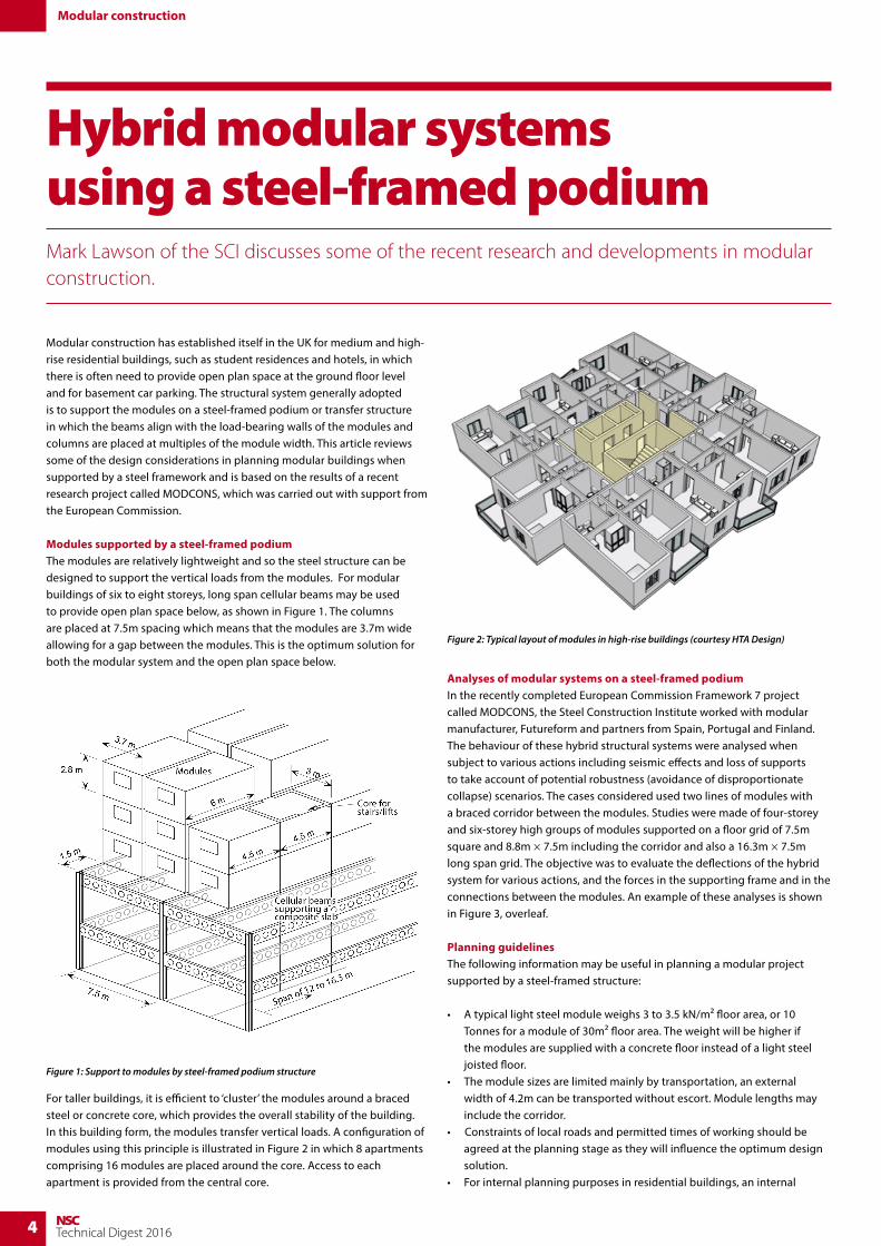
Modules supported by a steel-framed podiumThe modules are relatively lightweight and so the steel structure can be designed to support the vertical loads from the modules. For modular buildings of six to eight storeys, long span cellular beams may be used to provide open plan space below, as shown in Figure 1. The columns are placed at 7.5m spacing which means that the modules are 3.7m wide allowing for a gap between the modules. This is the optimum solution for both the modular system and the open plan space below.
For taller buildings, it is efficient to ‘cluster’ the modules around a braced steel or concrete core, which provides the overall stability of the building. In this building form, the modules transfer vertical loads. A configuration of modules using this principle is illustrated in Figure 2 in which 8 apartments comprising 16 modules are placed around the core. Access to each apartment is provided from the central core.
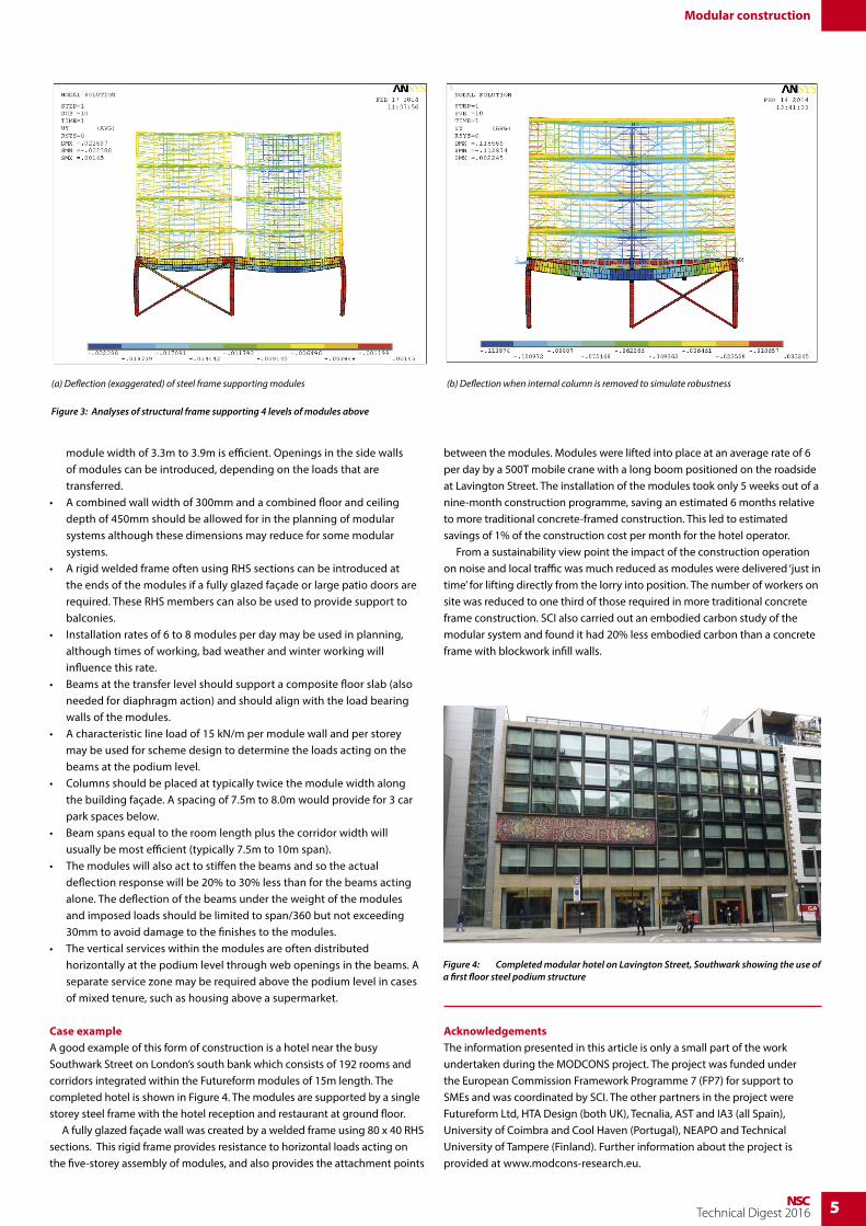
Analyses of modular systems on a steel-framed podiumIn the recently completed European Commission Framework 7 project called MODCONS, the Steel Construction Institute worked with modular manufacturer, Futureform and partners from Spain, Portugal and Finland. The behaviour of these hybrid structural systems were analysed when subject to various actions including seismic effects and loss of supports to take account of potential robustness (avoidance of disproportionate collapse) scenarios. The cases considered used two lines of modules with a braced corridor between the modules. Studies were made of four-storey and six-storey high groups of modules supported on a floor grid of 7.5m square and 8.8m × 7.5m including the corridor and also a 16.3m × 7.5m long span grid. The objective was to evaluate the deflections of the hybrid system for various actions, and the forces in the supporting frame and in the connections between the modules. An example of these analyses is shown in Figure 3, overleaf. Planning guidelinesThe following information may be useful in planning a modular project supported by a steel-framed structure:
• A typical light steel module weighs 3 to 3.5 kN/m2 floor area, or 10 Tonnes for a module of 30m2 floor area. The weight will be higher if the modules are supplied with a concrete floor instead of a light steel joisted floor.
• The module sizes are limited mainly by transportation, an external width of 4.2m can be transported without escort. Module lengths may include the corridor.
• Constraints of local roads and permitted times of working should be agreed at the planning stage as they will influence the optimum design solution.
• For internal planning purposes in residential buildings, an internal
Hybrid modular systems using a steel-framed podiumMark Lawson of the SCI discusses some of the recent research and developments in modular construction.
Figure 1: Support to modules by steel-framed podium structure
Figure 2: Typical layout of modules in high-rise buildings (courtesy HTA Design)
5NSCTechnical Digest 2016
Modular construction
module width of 3.3m to 3.9m is efficient. Openings in the side walls of modules can be introduced, depending on the loads that are transferred.
• A combined wall width of 300mm and a combined floor and ceiling depth of 450mm should be allowed for in the planning of modular systems although these dimensions may reduce for some modular systems.
• A rigid welded frame often using RHS sections can be introduced at the ends of the modules if a fully glazed façade or large patio doors are required. These RHS members can also be used to provide support to balconies.
• Installation rates of 6 to 8 modules per day may be used in planning, although times of working, bad weather and winter working will influence this rate.
• Beams at the transfer level should support a composite floor slab (also needed for diaphragm action) and should align with the load bearing walls of the modules.
• A characteristic line load of 15 kN/m per module wall and per storey may be used for scheme design to determine the loads acting on the beams at the podium level.
• Columns should be placed at typically twice the module width along the building façade. A spacing of 7.5m to 8.0m would provide for 3 car park spaces below.
• Beam spans equal to the room length plus the corridor width will usually be most efficient (typically 7.5m to 10m span).
• The modules will also act to stiffen the beams and so the actual deflection response will be 20% to 30% less than for the beams acting alone. The deflection of the beams under the weight of the modules and imposed loads should be limited to span/360 but not exceeding 30mm to avoid damage to the finishes to the modules.
• The vertical services within the modules are often distributed horizontally at the podium level through web openings in the beams. A separate service zone may be required above the podium level in cases of mixed tenure, such as housing above a supermarket.
Case exampleA good example of this form of construction is a hotel near the busy Southwark Street on London’s south bank which consists of 192 rooms and corridors integrated within the Futureform modules of 15m length. The completed hotel is shown in Figure 4. The modules are supported by a single storey steel frame with the hotel reception and restaurant at ground floor. A fully glazed façade wall was created by a welded frame using 80 x 40 RHS sections. This rigid frame provides resistance to horizontal loads acting on the five-storey assembly of modules, and also provides the attachment points
between the modules. Modules were lifted into place at an average rate of 6 per day by a 500T mobile crane with a long boom positioned on the roadside at Lavington Street. The installation of the modules took only 5 weeks out of a nine-month construction programme, saving an estimated 6 months relative to more traditional concrete-framed construction. This led to estimated savings of 1% of the construction cost per month for the hotel operator. From a sustainability view point the impact of the construction operation on noise and local traffic was much reduced as modules were delivered ‘just in time’ for lifting directly from the lorry into position. The number of workers on site was reduced to one third of those required in more traditional concrete frame construction. SCI also carried out an embodied carbon study of the modular system and found it had 20% less embodied carbon than a concrete frame with blockwork infill walls.
(a) Deflection (exaggerated) of steel frame supporting modules (b) Deflection when internal column is removed to simulate robustness
Figure 3: Analyses of structural frame supporting 4 levels of modules above
Acknowledgements The information presented in this article is only a small part of the work undertaken during the MODCONS project. The project was funded under the European Commission Framework Programme 7 (FP7) for support to SMEs and was coordinated by SCI. The other partners in the project were Futureform Ltd, HTA Design (both UK), Tecnalia, AST and IA3 (all Spain), University of Coimbra and Cool Haven (Portugal), NEAPO and Technical University of Tampere (Finland). Further information about the project is provided at www.modcons-research.eu.
Figure 4: Completed modular hotel on Lavington Street, Southwark showing the use of a first floor steel podium structure

6 NSCTechnical Digest 2016
A brief history of LTBDavid Brown of the SCI reviews the (relatively) recent history of lateral torsional buckling of beams. Part 1 includes a reminder of the underlying structural mechanics and the transition from theory into BS 449 and BS 5950. Part 2 looks at the comparison with BS EN 1993-1-1 and gazes into the near future.
In the beginning - Euler Almost all buckling begins with Euler. Leonhard Euler (1707 – 1783) was a Swiss mathematician and physicist. In structural engineering he is most famous for identifying the elastic critical buckling load for a column. In the Eurocode, this load
is called Ncr and is expressed as Ncr =π2 EI
L2 . This is a purely theoretical
load, as it assumes infinite material strength and assumes the strut is perfectly straight – neither of which is true. The obvious connection with a beam is that the compression flange is rather like a strut – if the web and tension flange are ignored. In a beam, the resistance to lateral buckling of the compression flange is generated by:• The lateral bending resistance of the compression flange,• The tension flange, which restrains the compression flange, being
connected by the web,• The torsional stiffness of the section.The elastic critical buckling moment for a beam is analogous to the Euler load for struts, but rather more complicated because of the additional contributions. In the Eurocode, this moment is called Mcr. The elastic critical stress for a beam is simply the moment divided by modulus. In the same way as a strut, the elastic critical moment is a theoretical moment, assuming infinitely strong material, and a perfectly straight beam.
From Euler to allowable stress – Messers Ayrton, Perry and RobertsonIn 1886, Ayreton and Perry related the elastic critical stress to a failure stress, allowing for an initial imperfection (lack of straightness) and limited to the yield strength of the material. They did not resolve what the initial imperfections should be. In 1925, Robertson developer the Ayrton-Perry formula, establishing im-perfection values on the basis of experimental tests. This work was adopted
as a basis of the strut curves (and LTB curves) in BS 449 and BS 153 (the bridge design Standard). Sadly, the reference to Ayrton seems to have been dropped and the expression became commonly known as the Perry-Robert-son formula. Although the precise form of the Perry-Robertson curve depends on the Perry factor assumed, Figure 1 shows the relationship between the elastic critical stress and the Perry-Robertson curve. It should be noted that there is no plateau in Figure 1. The Perry-Robertson formula is an elastic approach and is based on failure when the stress at the extreme fibre of the section reaches yield. At low slenderness, one might expect plastic behaviour, where the whole cross section reaches yield. At low slenderness therefore, the Perry-Robertson curve is quite conservative.
Application to LTB of fabricated beamsThe salient paper is by Kerensky, Flint and Brown (sadly, no relation) of 1956, where they described the basis of design for beams and plate girders in the revised bridge Standard, BS 153. This important paper was used to prepare the design guidance in the 1969 (metric) version of BS 449. The first step is to establish the elastic critical stress in bending. Kerensky, Flint and Brown (KFB) present the critical stress for a symmetrical I section as
fb,crit =π2EIyh
2ZxL2
1
γ1+
4GKL2
π2EIyh2{ }Even without describing the variables, the comparison with the commonly-used expression for Mcr in the Eurocode is clear – the physics has not changed. KFB proposed using the Perry-Robertson formula to establish an allowable stress as it had “evolved in conjunction with extensive tests and has a background of satisfactory application in design”. The problem at low slenderness remained to be solved – by curve fitting. KFB proposed a plateau extending to a slenderness of l/ry of 60, and then joining (with a straight line) to the Perry-Robertson curve at l/ry = 100. KFB noted that this led to a maximum ‘overstress’ (compared to the Perry-Robertson stress) of 13%. KFB recognised that for certain cross sections, the ‘elastic’ background to the approach could “seriously penalise” the use of such members. The problem is more noticeable when the member has a higher ‘shape factor’,
which is plastic modulus
elastic modulus.
However, as they were covering plate girders, where the shape factor could be as low as 1.0, the basic formula was not modified.
Transition of KFB proposals into BS 449 for rolled sectionsIn BSI papers of 1969, notes are provided on the amendments to BS 449 – which included the conversion to metric units, but of more interest to this discussion, also describe the development of the LTB rules that appear in BS 449. The basis for the BS 449 curve is the KFB paper, simplified for building designers and modified to account for the shape factor of the rolled I sections commonly used. Firstly, the KFB formula for the critical stress is simplified. With approximations for various variables, the expression for the elastic critical stress becomesFigure 1: Elastic critical stress and Perry-Robertson – S355 steel
LTB (Part 1)

7NSCTechnical Digest 2016
:
Elastic critical stress =1675 1
201 +
IT
ryDlry
22
( ) ( )In BS 449, this is given the symbol “A”, and (if anyone can find an old copy of BS 449) appears over Table 7. In clause 20 of BS 449, this value of A is described as the elastic critical stress for girders with equal moment of inertia about the major axis – i.e. a symmetrical section. For unsymmetrical sections, the calculation of the elastic critical stress is modified. The BS 449 drafters then dealt with the problems with the Perry-Robertson curve at low slenderness. A slightly different plateau length was proposed by extending the plateau until the Perry-Robertson stress was exceeded by the 13% described in the KFB paper, but also allowing for a shape factor of 1.15 for rolled sections. The product of these two factors is 1.13 × 1.15 = 1.3. Thus the plateau was extended until the Perry-Robertson stress was exceeded by 30%. Although KFB proposed the intersection with the Perry-Robertson curve at l/ry = 100, the drafters of BS 449 modified this to a point when the critical stress was 17/1.2 tonsf/in2, or 233 N/mm2. The actual slenderness at this intersection point varies with D/T. This results in the curve (for one specific beam, with D/T = 24) shown in Figure 2. Note that the bending stresses have been normalised by dividing by the yield strength, to give a reduction factor. The slenderness is plotted against slenderness (l/ry ) and non-dimensional slenderness (to assist future comparisons) The form of the BS 449 curve may be confirmed by simply plotting values in any one column from Table 3a.
Observations on the BS 449 approach to LTBBS 449 has a simple approach to LTB. The look-up table is simple to use, but rather more complicated to embed in a spreadsheet or other program. It might also be noted that the plateau seems relatively long (The Eurocode plateau is limited to a non-dimensional slenderness of 0.4, or l/ry = 32). Finally we note that BS 449 had no way of dealing with non-uniform moment, which was a major change introduced in BS 5950.
Bring on BS 5950 As long ago as 1969, a committee was appointed to prepare a successor to BS 449 as a limit state code. Note that the metric version of BS 449 had only just been issued! In a background document to BS 5950, the comment is made that the new code is based on the same underlying theory as BS 449. The new rules took account of moment gradient (an improvement), but it was noted that the results of the new procedures were more conservative, especially at low slenderness. Perhaps one might expect this looking at the optimistic plateau length in Figure 2. In the background document, the elastic critical
moment ME is expressed as ME =π
L
EIyGJ
γ1 +
π2EH
L2GJ , which should
again look familiar.
Having calculated an elastic critical stress, BS 5950 determines an allowable bending strength using the Perry-Robertson formula, found in B.2.1 of BS 5950. The Perry factor and Robertson Constant are given. The formulation of the expressions in B.2.3 has a plateau length of λLT0 .
For S355 steel, λLT0 = 0.4π2 E
py
0.5
= 30.6( )In Eurocode terms, this is equivalent to a non-dimensional slenderness of 0.38. The comparison between the LTB curves in BS 449 and BS 5950 (for a beam with D/T = 24) is shown in Figure 3.
The BS 5950 buckling curve is generally significantly lower than that in BS 449. Designers of a certain age may recall the general view that resistances had reduced. To some degree, this would have been offset by the change to a limit state code, when the load factor was approximately 1.55 compared to the 1.7 in BS 449. In comparisons made in 1979, it was noted that BS 449 “gives wide variations in the factor of safety” in some circumstances “which are below what is generally considered appropriate”, so perhaps the reductions in resistance are not surprising. In 1989, Amendment 8 to BS 449 was published with a revised Table 3a. For the specific beam used in this comparison, Figure 4 now shows the reduction factor as given in the revised Table. Perhaps as might be expected, the form of the curve given by Amendment 8 very closely follows that given in BS 5950. SCI has not been able to locate background documents giving the expressions behind the Amendment 8 curves – Figure 4 is simply plotted from the values in the Standard. It is not inconceivable that the Amendment follows the BS 5950 expressions, but with some allowance for the different factors of safety. If the Amendment 8 curve is plotted at 90% of its value, there is close correspondence with the BS 5950 curve – and 1.55/1.7 = 0.91. Of particular note is the much reduced plateau length compared to BS 449.
The second major change in BS 5950 was the introduction of methods to deal with a non-uniform moment, via the mLT factor in Table 18. Technical exposition on the treatment of non-uniform moments appeared in AD 251 and is not repeated here. In Part 2, the comparisons are extended to the Eurocode, with a forward-looking view of the future LTB formulae.
Figure 2: Normalised stresses vs slenderness
Figure 3: Comparison between BS 449 and BS 5950 LTB curves
Figure 4: Comparison between BS 449, BS 5950 and BS 449 Amendment 8
LTB {Part 1)

8 NSCTechnical Digest 2016
LTB (Part 2)
LTB in the Eurocodes – Back to the FutureIn Part 1, David Brown of the SCI looked at comparisons between lateral torsional buckling in BS 449 and BS 5950. In Part 2, the comparison is extended to the current Eurocode – and what might happen as the Eurocode is revised.
There have been several articles on BS EN 1993-1-1 and lateral torsional buckling, covering numerical examples and the calculation of the C1 factor to deal with non-uniform bending moment diagrams. The emphasis has always been that the physics has not changed, a truth which should have been reinforced when the background to BS 449 and BS 5950 was reviewed in Part 1. The Eurocode is perhaps clearer than previous steel design codes. LTB is always based on the elastic critical moment – it was in BS 449 and BS 5590; this is now explicit in EC3. The criticism of the European Standard is that expressions for Mcr are not given in the Standard – according to other Europeans, this is expected to be known by designers, or extracted from other resources – something that the Standard does not need to provide. The closed formula is complicated, just like the expression for the elastic critical stress in BS 449, but at least there are software tools and freely available software to calculate this moment. The physics of a non-uniform moment is dealt with by the C1 factor, with a second adjustment via the ƒ factor (but only if using the special case for rolled sections in 6.3.2.3). Perhaps as expected, with more test data available and many more numerical simulations possible, the Eurocode allows more finesse within the buckling curves. Instead of the one single curve in BS 449 and BS 5950, four curves are available, depending on the cross-section. The Eurocode is further complicated with two families of buckling curves; the “general case” in clause 6.3.2.2 and a set of expressions for rolled sections (called “special” in this article). If verifying a rolled section, the “special” set of expressions in clause 6.3.2.3 are highly recommended, especially with a non-uniform bending moment, as the calculated resistance is significantly higher than that calculated using the “general case”. A comparison between the LTB curves from BS 5950, the “general case” and the “special case” is shown in Figure 5. For the particular beam examined, the “general case” and “special case” use curves c and d respectively.
The EC3 “special case” curve has a similar plateau length to BS 5950, but then provides a larger resistance at all slenderness. The increase in resistance in the Eurocode may appear small in Figure 5, but may be as much as 25% and more for some beam profiles. The increase in resistance is more significant as slenderness increases. The conservatism of the “general case” can also be seen in Figure 5; the plateau is short (limited to a slenderness of 0.2) and then a reduced resistance compared to the “special case”. The difference between the “general case” and the “special case” for rolled sections becomes more significant for non-uniform bending moments, since the beneficial effect of ƒ from clause 6.3.2.3(2) can only be applied to the “special case”. Figure 6 shows the comparison with a triangular bending moment diagram (C1 = 1.77, mLT = 0.6). In BS 5950, the influence of mLT is outside the calculation of the bending resistance Mb ; the curve shows the effective reduction factor after allowing for mLT . The increase in resistance calculated using the “special case” is up to 50% higher than that determined using the “general case”.
Where to next?The Eurocodes are currently being revised, with a target date around 2020 for an amendment. It is likely that the LTB curves will be amended, though this is by no means certain. There is much discussion to be undertaken before the amendment is released. Accompanying the amended Standard will be a revised UK National Annex, which will mean the UK (where allowed) can influence the final outcome within our shores. The proposed buckling curves may have more theoretical justification than the current set of expressions. As with most work associated with the development of design Standards, the majority of the enthusiasm tends to come from those with an academic background. Perhaps academic colleagues have the time and opportunity to make a contribution, but it certainly influences the final output. At present, it is far too early to be confident any detail in the Figure 5: Comparison between BS 5950 and EC3; uniform bending moment diagram
1.20
1.00
0.80
0.60
0.40
0.20
0.000.00 0.50 1.00 1.50 2.00 2.50
Non-dimensional slenderness
BS 5950 EC3 General Case EC3 Special Case
Redu
ctio
n fa
ctor
Figure 6: Comparison between BS 5950 and EC3; Triangular bending moment diagram
1.20
1.00
0.80
0.60
0.40
0.20
0.000.00 0.50 1.00 1.50 2.00
Non-dimensional slenderness
E�ective BS 5950 EC3 General Case EC3 Special Case
Redu
ctio
n fa
ctor

9NSCTechnical Digest 2016
LTB (Part 2)
amendment, so the discussion from now on becomes rather less reliable. The proposed amendment dispenses with the “general case” and the “special case” in favour of a single set of curves. A comparison between the two formulations is shown above, for beams where h/b < 2 (i.e. curve b in the current Standard).
In the proposed equations, φ depends on the shape of the bending moment diagram, rather like kc in the current formulation. The value of the imperfection factor, αLT becomes a variable which depends on the ratio between the major and minor axis elastic moduli rather than a constant, and approaches the value currently given for minor axis flexural buckling. In addition to the slenderness for lateral torsional buckling, the minor axis slenderness for flexural buckling, λz , becomes an important part of the proposed process. A further notable change is that the plateau only extends to a slenderness of 0.2 (which is the same as the flexural buckling curve). The proposed LTB curves deliver higher resistances than the “general case”, but are less attractive than the “special case”. A general comparison between the current rules and the proposed amendments is not possible, as the effect varies with the beam profile and the shape of the bending moment diagram. Figure 7 shows the comparison for a 457 × 191 × 98 UB with a triangular bending moment diagram; the difference between the “special case” and the proposed rules is marginal – what’s not to like? Figure 8 shows the comparison for the same beam with a uniform bending moment diagram. In this comparison the different plateau lengths are clearly seen; the proposed rules deliver a reduced resistance across the full range of slenderness, compared to the “special case”. Figure 9 also shows a rather less attractive comparison, for a 305 × 165 × 40 UB with a bending moment diagram due to a UDL. The proposed rules deliver less resistance than the “special case” across the whole range of slenderness. For this beam and loading, at high slenderness the proposed rules deliver only 84% of the current “special case” resistance, which is a significant reduction.
A perfect storm approaching?At the same time as amendments to the resistance functions are being discussed, research is also underway considering the γM1 value, which is used when calculating buckling resistance. The current recommended value in the Eurocode (which is adopted in the UK National Annex) is 1.0. It seems likely that some increase in reliability will be proposed – which may be to increase the γM1 value directly, or the same effect may be achieved by further adjustments to the resistance functions. There remains much debate before agreement is reached, but there is a strong possibility that LTB resistances will be reduced in 2020 – a combination of the revised formulae and the effect of an increase in γM1. The practical effect of changes to the resistance functions will mean that existing Eurocode design software and design aids, such as the Blue Book, will need to be updated, even if (in some circumstances) the change is small. As was demonstrated in Figure 9, the potential change in resistance could be significant – it would be inappropriate to continue to use out-of-date resources. LTB checks appear in very many SCI publications as part of worked examples, so the task of revision is certainly not trivial. Perhaps the more significant concern is change to the Eurocodes when
many designers are still not using them, or are in the early stages of transition. Although the Eurocodes have been available since 2005 (and so changes in 2020 after 15 years in use are perhaps not unreasonable), for many ‘late adopters’ the 2020 revisions may seem rather early. A concluding reminder – the proposals are not yet agreed, so may well change before the amendment. The effect of the UK National Annex may also change the comparisons made in this article. No doubt nearer the time there will be plenty of articles looking at the impact of whatever is finally agreed.
αLT 0.34 0.16Wel,y
Wel,z
≤ 0.49
ϕLT 0.5 1 + αLT ( λLT - βλLT,0 ) + βλLT2[ ] 0.5 1 + φ αLT ( λz - 0.2 ) + λLT
2λLT
2
λz2[ ]
χLTϕLT + ϕLT
2 - βλLT2
1
ϕLT + ϕLT2 - φλLT
2
φ
f 1 - 0.5 ( 1 - kc ) 1 - 2 ( λLT - 0.8 )2[ ]
Variable Current (”Special Case”) Proposed
( )
αLT 0.34 0.16Wel,y
Wel,z
≤ 0.49
ϕLT 0.5 1 + αLT ( λLT - βλLT,0 ) + βλLT2[ ] 0.5 1 + φ αLT ( λz - 0.2 ) + λLT
2λLT
2
λz2[ ]
χLTϕLT + ϕLT
2 - βλLT2
1
ϕLT + ϕLT2 - φλLT
2
φ
f 1 - 0.5 ( 1 - kc ) 1 - 2 ( λLT - 0.8 )2[ ]
Variable Current (”Special Case”) Proposed
( )
αLT 0.34 0.16Wel,y
Wel,z
≤ 0.49
ϕLT 0.5 1 + αLT ( λLT - βλLT,0 ) + βλLT2[ ] 0.5 1 + φ αLT ( λz - 0.2 ) + λLT
2λLT
2
λz2[ ]
χLTϕLT + ϕLT
2 - βλLT2
1
ϕLT + ϕLT2 - φλLT
2
φ
f 1 - 0.5 ( 1 - kc ) 1 - 2 ( λLT - 0.8 )2[ ]
Variable Current (”Special Case”) Proposed
( )
Figure 7: Comparison between existing and proposed EC3 rules; 457 × 191 × 98; triangular bending moment diagram
1.20
1.00
0.80
0.60
0.40
0.20
0.000.00 0.50 1.00 1.50 2.00
Non-dimensional slenderness
EC3 Special Case Proposed EC3
Redu
ctio
n fa
ctor
Figure 8: Comparison between existing and proposed EC3 rules; 457 × 191 × 98; uniform bending moment diagram
1.20
1.00
0.80
0.60
0.40
0.20
0.000.00 0.50 1.00 1.50 2.00 2.50
Non-dimensional slenderness
EC3 Special Case Proposed EC3
Redu
ctio
n fa
ctor
Figure 9: Comparison between existing and proposed EC3 rules; 305 × 165 × 40; bending moment diagram from a UDL
1.20
1.00
0.80
0.60
0.40
0.20
0.000.00 0.50 1.00 1.50 2.00 2.50 3.00
Non-dimensional slenderness
EC3 Special Case Proposed EC3
Redu
ctio
n fa
ctor
10 NSCTechnical Digest 2016
Tee sections
The design of tee sections in bendingAlthough tees might not be an ideal choice to resist bending, sometimes they are selected for their architectural merit. To assist when tees must be used, David Brown of the SCI describes the design approach to BS 5950-1 and to BS EN 1993-1-1.
If members are subject to bending, structural engineers will probably recommend beams with flanges, or hollow sections. Tees used to resist bending are unlikely to appear as a preferred solution, but if they must be used, they must be verified to the design Standard. This article looks at the verification of a Tee used as a cantilever, perhaps as the exposed steelwork supporting a canopy. Especially with Tees cut from universal beams, the long narrow web means that the section is Class 4. The focus of this article is lateral-torsional buckling, assuming that cross-sectional checks have been completed. Numerical examples are presented, considering Class 3 and Class 4 sections.
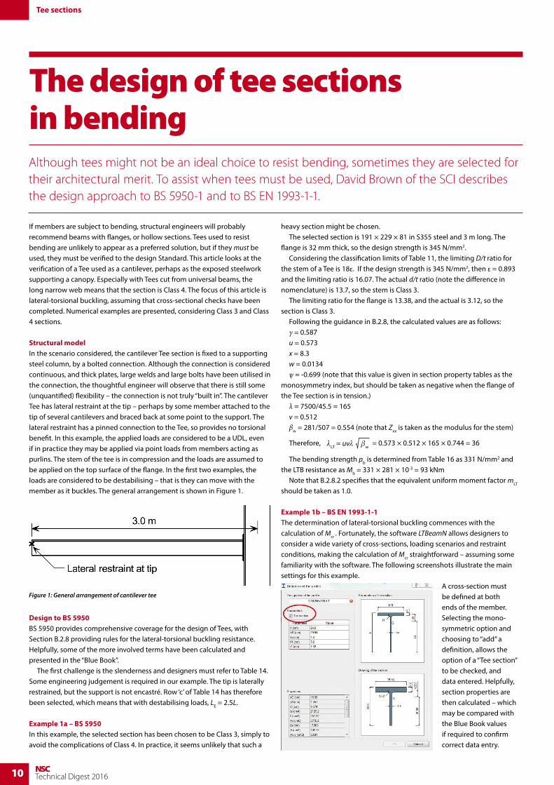
Structural modelIn the scenario considered, the cantilever Tee section is fixed to a supporting steel column, by a bolted connection. Although the connection is considered continuous, and thick plates, large welds and large bolts have been utilised in the connection, the thoughtful engineer will observe that there is still some (unquantified) flexibility – the connection is not truly “built in”. The cantilever Tee has lateral restraint at the tip – perhaps by some member attached to the tip of several cantilevers and braced back at some point to the support. The lateral restraint has a pinned connection to the Tee, so provides no torsional benefit. In this example, the applied loads are considered to be a UDL, even if in practice they may be applied via point loads from members acting as purlins. The stem of the tee is in compression and the loads are assumed to be applied on the top surface of the flange. In the first two examples, the loads are considered to be destabilising – that is they can move with the member as it buckles. The general arrangement is shown in Figure 1.
Design to BS 5950BS 5950 provides comprehensive coverage for the design of Tees, with Section B.2.8 providing rules for the lateral-torsional buckling resistance. Helpfully, some of the more involved terms have been calculated and presented in the “Blue Book”. The first challenge is the slenderness and designers must refer to Table 14. Some engineering judgement is required in our example. The tip is laterally restrained, but the support is not encastré. Row ‘c’ of Table 14 has therefore been selected, which means that with destabilising loads, LE = 2.5L.
Example 1a – BS 5950In this example, the selected section has been chosen to be Class 3, simply to avoid the complications of Class 4. In practice, it seems unlikely that such a
heavy section might be chosen. The selected section is 191 × 229 × 81 in S355 steel and 3 m long. The flange is 32 mm thick, so the design strength is 345 N/mm2. Considering the classification limits of Table 11, the limiting D/t ratio for the stem of a Tee is 18ε. If the design strength is 345 N/mm2, then ε = 0.893 and the limiting ratio is 16.07. The actual d/t ratio (note the difference in nomenclature) is 13.7, so the stem is Class 3. The limiting ratio for the flange is 13.38, and the actual is 3.12, so the section is Class 3. Following the guidance in B.2.8, the calculated values are as follows: γ = 0.587 u = 0.573 x = 8.3 w = 0.0134 ψ = -0.699 (note that this value is given in section property tables as the monosymmetry index, but should be taken as negative when the flange of the Tee section is in tension.) λ = 7500/45.5 = 165 v = 0.512 βw = 281/507 = 0.554 (note that Zxx is taken as the modulus for the stem)
Therefore, λLT = uvλ βw= 0.573 × 0.512 × 165 × 0.744 = 36
The bending strength pb is determined from Table 16 as 331 N/mm2 and the LTB resistance as Mb = 331 × 281 × 10-3 = 93 kNm Note that B.2.8.2 specifies that the equivalent uniform moment factor mLT should be taken as 1.0.
Example 1b – BS EN 1993-1-1The determination of lateral-torsional buckling commences with the calculation of Mcr . Fortunately, the software LTBeamN allows designers to consider a wide variety of cross-sections, loading scenarios and restraint conditions, making the calculation of Mcr straightforward – assuming some familiarity with the software. The following screenshots illustrate the main settings for this example.
A cross-section must be defined at both ends of the member. Selecting the mono-symmetric option and choosing to “add” a definition, allows the option of a “Tee section” to be checked, and data entered. Helpfully, section properties are then calculated – which may be compared with the Blue Book values if required to confirm correct data entry.
Figure 1: General arrangement of cantilever tee

11NSCTechnical Digest 2016
Tee sections
Loading can be applied at any point, but in this example, the load has been applied at the top of the section. This is a destabilising load, as it is above the shear centre.
The support has been fixed at the left hand end (as drawn), and a lateral restraint introduced at the tip.
LTBeamN can then calculate Mcr , and present a 3-D view of the buckled shape.
In this example, Mcr = 1085 kNm. Following the usual Eurocode procedure,
281 × 103 × 345
1085 × 106
Wy ƒy
Mcr
λLT = = = 0.299
Only the “General case” of 6.3.2.2 may be used, so from Table 6.4, curve ‘d’ is selected, which means in Table 6.3, αLT = 0.76. Completing the maths, χLT = 0.924 Therefore, Mb = 0.924 × 281 × 103 × 345 × 10-6 = 89.6 kNm – which compares well with the value of 93 kNm according to BS 5950.
Example 2a – BS 5950In this example, the chosen section is 191 × 229 × 45 in S355 steel and 3 m long. The flange is 17.7 mm thick, so the design strength is 345 N/mm2. The d/t ratio for this section is 22.1, so the stem is Class 4. Advisory Desk note AD 311i gives advice for Class 4 sections, recommending the calculation of a reduced design strength – effectively making the section Class 3.
The reduced design strength 18 × 0.893
22.1= 345 × = 182.5 N/mm2
2
( )
Following the same process as outlined in example 1a: γ = 0.612 u = 0.576 x = 14.1 w = 0.00486 ψ = -0.706 λ = 7500/42.9 = 175 v = 0.682 βw = 152/269 = 0.565 Therefore, λLT = uvλ βw = 0.576 × 0.682 × 175 × 0.752 = 51.7
The bending strength pb is determined by calculation from Annex B.2.1 as 169 N/mm2 and the LTB resistance as Mb = 169 × 152 × 10-3 = 25.7 kNm
Example 2b – BS EN 1993-1-1Introducing the revised cross section into LTBeamN, yields Mcr = 231 kNm According to Table 5.2 of BS EN 1993-1-1, the limiting outstand for elements in compression is 14ε for a Class 3 section, where ε = 0.825. Thus the limiting length of web in compression is 14 × 0.825 × 10.5 = 121 mm from the neutral axis, making an overall depth of 175.7mm. The effective cross section is shown in Figure 2.The modulus of this reduced cross section can be determined by hand, or LTBeamN can be used to calculate the properties of the revised section. Simply reducing the overall depth of the section to 175.7 mm in LTBeamN gives the revised elastic modulus as 88.0 × 103 mm3.
Proceeding in the usual way, 88.0 × 103 × 345
231 × 106
Wy ƒy
Mcr
λLT = = = 0.363
Completing the maths, χLT = 0.877 Therefore, Mb = 0.877 × 88.0 × 103 × 345 × 10-6 = 26.6 kNm – which compares with the value of 25.7 kNm according to BS 5950.
Example 3a – BS 5950Example 3 is the same as example 2, but the loads are not destabilising. From Table 14, LE = 0.9L. Following the same process as outlined in example 2a: γ, u, x, w, ψ, βw all as example 2a λ = 2700/42.9 = 62.9 v = 1.392
Therefore, λLT = uvλ βw = 0.576 × 1.392 × 62.9 × 0.752 = 37.9
At this short slenderness, there is no reduction for lateral-torsional buckling, so the bending strength is the reduced design strength, 182.5 N/mm2. The LTB resistance is therefore Mb = 182.5 × 152 × 10-3 = 27.7 kNm
Example 3b = BS EN 1993-1-1With the loads applied at the shear centre, LTBeamN gives Mcr = 235 kNm, which leads to Mb = 26.7 kNm
ObservationsThe contrast between examples 2 and 3 is possibly the most surprising, as the huge difference in the effective length does not result in a significant difference in the resistance. Although the effective length varies in the BS 5950 approach, the influence of the factor v means that the slenderness for lateral-torsional buckling does not change so significantly. Within the Eurocode approach, the difference between the two examples is simply the location of the applied loads, which only varies by 9 mm. The loads are only slightly destabilising, so the limited change in lateral-torsional buckling resistance is to be expected.
ConclusionsAs expected, both design Standards give a reasonably consistent result. With access to appropriate software, some designers may find the Eurocode approach more straightforward, though specifying the correct supports, restraints and loading is essential.
i AD 311: T-sections in bending – stem in compression Available from http://www.steelbiz.org/
Figure 2: Gross and effective cross sections

12 NSCTechnical Digest 2016
The management of destabilising loadsAlthough destabilising loads on unrestrained beams may be infrequent in orthodox building structures, they are sometimes found in domestic construction and can be quite common in steelwork supporting industrial equipment. David Brown looks at the provisions in BS 5950 and BS EN 1993-1-1.
Is the load destabilising?The common definition of a destabilising load is if the load is free to move with the flange, it’s a destabilising load. BS 5950 describes the situation in clause 4.3.4 as when both the load and the flange are free to deflect laterally. The situation is shown in Figure 1.
In the destabilising load condition, the vertical load has moved with the compression flange, which is deflecting laterally. The vertical load is eccentric to the shear centre and the resulting moment encourages further lateral deflection of the flange. The stress due to the lateral bending of the flange is increased, which means the beam is closer to buckling than it would be without the additional moment. Figure 1 also shows the effect of a load applied which is a stabilising load. In this case, the load produces a restoring moment, which serves to reduce the lateral bending of the compression flange; the load may be increased before the onset of buckling. Destabilising loads are relatively common in steelwork supporting equipment, where there may be no floor to provide restraint. Equipment supported on multiple beams may still be a destabilising load, if all the beams can buckle in the same direction and the load can move, as shown in Figure 2.
BS 5950 provisionsBS 5950 deals with destabilising loads by increasing the effective length, LE, as specified in Table 13. The effective length of the beam is really the effective length of the all-important unrestrained compression flange. With a beam loaded in the conventional sense, it is easy to visualise the compression flange from a bird’s eye view, and consider the fixity at the end of the beam flange. Full rotational fixity leads to shorter effective lengths and less fixity leads to larger effective lengths. For a comparison with BS EN 1993-1-1, it will be assumed that both flanges are free to rotate on plan. Sometimes this is known as a fork end support, as indicated in Figure 3 – the beam has vertical and lateral support, but nothing stops the flanges rotating on plan.
With a beam supported in this way, Table 13 of BS 5950 indicates that the effective length LE is 1.0 LLT under normal conditions, and 1.2 LLT if the loads are destabilising. This is the only provision that BS 5950 makes for destabilising loads; from then on, the process of determining a lateral torsional buckling resistance follows the normal rules. Before leaving Table 13, the condition with the compression flange unrestrained should be noted. This is the case often encountered in domestic construction when beams sit on padstones. Two options are offered in Table 13; when the bottom flange is positively connected to the support and secondly when the beam simply sits on the support with no positive connection. If one imagines looking again with a bird’s eye view of the top flange, an unrestrained compression flange can deform laterally even at the support. As shown in Figure 4, the effective length is increased in this situation. Table 13 specifies 1.2 LLT + 2D for the normal loading condition and 1.4 LLT + 2D when loads are destabilising. Finally, note that clause 4.3.4 alerts the designer to the possibility of destabilising loads, but in all other cases specifies that the normal loading condition be assumed. In BS 5950 therefore, there is no way of allowing for the beneficial effects of stabilising loads.
Destabilising load condition Stabilising load condition
Figure 2: Possible load arrangements supporting equipment
Figure 3: Beam with fork end supports
Destabilising loads
Figure 1: Load arrangements
13NSCTechnical Digest 2016
BS EN 1993-1-1 provisionsWithin the Eurocode approach, the impact of the load position is accounted for in the determination of Mcr which may be calculated by a closed expression or determined using software. If designers conclude that the loads are destabilising, the general form of the closed expression (for a beam with fork end supports) is shown below.
+Mcr = C1 + ( C2zg )2 – C2zg
π2Elz
L2 ( )lw
lz
L2GlT
π2Elz
This expression is fully defined in NCCI ; of interest to this discussion is the C2 value and the zg dimension. Rather like the C1 value, the C2 value depends on the shape of the bending moment diagram. Values for both factors can be obtained from NCCI. Two simple loading conditions and the values of C1 and C2 are given in Table 1, for a simply supported beam.
Loading condition C1
C2
UDL 1.13 0.45
Central point load 1.35 0.63
The dimension zg is the distance from the shear centre to the point of load application. As shown in Figure 5, in the conventional orientation, if the load is applied to the top flange (a destabilising load), zg is positive. If the load is stabilising, applied below the shear centre, zg is negative.
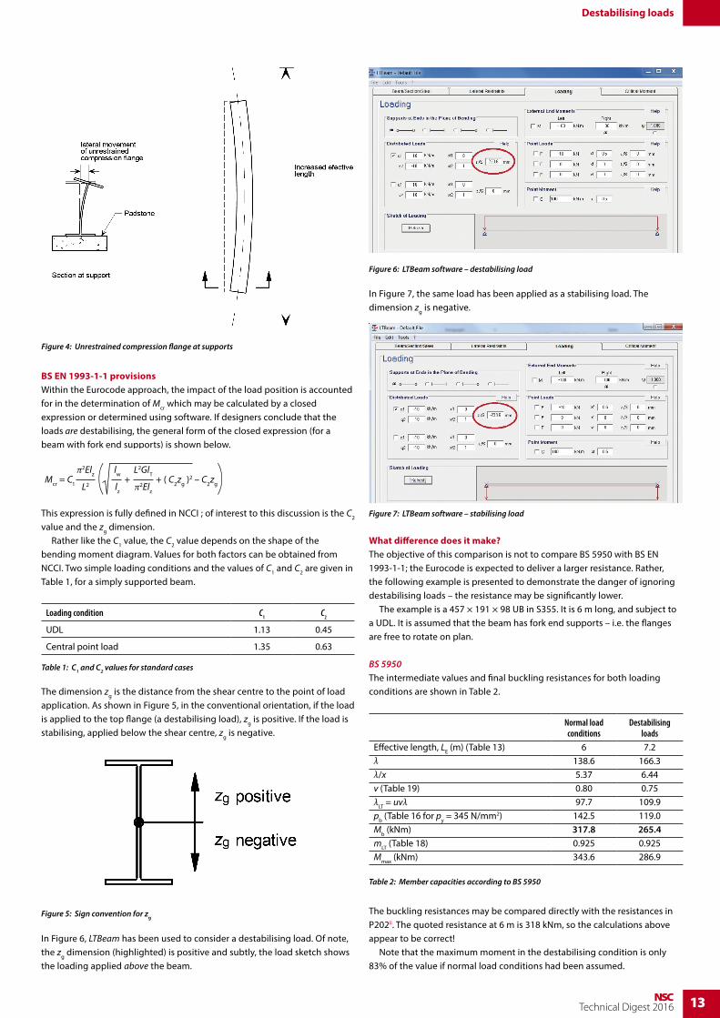
In Figure 6, LTBeam has been used to consider a destabilising load. Of note, the zg dimension (highlighted) is positive and subtly, the load sketch shows the loading applied above the beam.
In Figure 7, the same load has been applied as a stabilising load. The dimension zg is negative.
What difference does it make?The objective of this comparison is not to compare BS 5950 with BS EN 1993-1-1; the Eurocode is expected to deliver a larger resistance. Rather, the following example is presented to demonstrate the danger of ignoring destabilising loads – the resistance may be significantly lower. The example is a 457 × 191 × 98 UB in S355. It is 6 m long, and subject to a UDL. It is assumed that the beam has fork end supports – i.e. the flanges are free to rotate on plan.
BS 5950The intermediate values and final buckling resistances for both loading conditions are shown in Table 2.
Normal load conditions
Destabilising loads
Effective length, LE (m) (Table 13) 6 7.2λ 138.6 166.3λ/x 5.37 6.44v (Table 19) 0.80 0.75λLT = uvλ 97.7 109.9pb (Table 16 for py = 345 N/mm2) 142.5 119.0Mb (kNm) 317.8 265.4mLT (Table 18) 0.925 0.925Mmax (kNm) 343.6 286.9
The buckling resistances may be compared directly with the resistances in P202ii. The quoted resistance at 6 m is 318 kNm, so the calculations above appear to be correct! Note that the maximum moment in the destabilising condition is only 83% of the value if normal load conditions had been assumed.
Figure 4: Unrestrained compression flange at supports
Figure 5: Sign convention for zg
Table 1: C1 and C2 values for standard cases
Figure 6: LTBeam software – destabilising load
Figure 7: LTBeam software – stabilising load
Destabilising loads
Table 2: Member capacities according to BS 5950
14 NSCTechnical Digest 2016
BS EN 1993-1-1A similar exercise may be completed for BS EN 1993-1-1, as shown in Table 3 for three loading conditions. The load is assumed to be applied at the outside of the flange for both the stabilising and destabilising conditions. Mcr was calculated using LTBeam and by the expression above; both values are shown in Table 3.
In this case, if loads are destabilising, the resistance is again only 82% of the resistance if the loads are applied at the shear centre. Note that if the loads were stabilising, the resistance shows an enhancement of 17%.
General observationsThis article has attempted to warn designers about the dangers of undiagnosed destabilising loads – whichever Standard is used, the lateral torsional buckling resistance is reduced significantly. The Eurocode allows the benefit of stabilising loads to be calculated, which may be an advantage in that relatively uncommon design situation. This exercise also demonstrates that the BS 5950 approach of increasing the effective length by 20% is a good approximation to allow for the effect of destabilising loads. If Mb is recalculated according to the Eurocode, but with a buckling length of 7.2 m, the resistance is 348 kNm, which compares favourably with the precise calculation of 338 kNm. To increase the buckling length by 20% is a good rule of thumb when selecting an initial section, as the Eurocode resistance tables can then be used directly. To verify members to the Eurocode, an initial section is necessary, so that the dimension zg can be determined. Finally, this exercise considered destabilising loads applied to the top flange. If equipment is supported from stools, themselves on top of the beams, it may be prudent to increase the zg dimension further, to allow for the increased destabilising effect.
i AD 311: T-sections in bending – stem in compression Available from http://www.steelbiz.org/ii P202 Section properties and member capacities to BS 5950-1
Normal load (applied at shear
centre)
Destabilising load (applied at
top flange)
Stabilising load (applied at bottom
flange)
Dimension zg (mm) 0 223.6 -223.6
Mcr (kNm) (LTBeam) 537 398 724
Mcr (kNm) (expression) 535 402 712
λLT 1.20 1.39 1.03
χLT (αLT = 0.49) 0.525 0.434 0.621
χLT,Mod 0.536 0.440 0.632
Mb (kNm) 412.4 338.5 486.2
Table 3: Member resistance according to BS EN 1993-1-1
Design of fillet welds and partial penetration butt weldsRichard Henderson of the SCI discusses the directional method for the design of fillet welds and partial penetration butt welds and shows how the combined stress formula is related to Von Mises’ failure criterion. The weld design rules can be applied in all cases.
IntroductionA simple rule of thumb approach to sizing partial penetration butt welds carrying longitudinal shear has sometimes been used where the resistance is based on the average shear stress used for checking the shear resistance of beam webs: 0.6py in BS 5950 or fy/√3 in EN 1993-1-1. This confusingly led to a lower shear resistance than that found when sizing the weld using the specified design strength. In what follows, the directional method in EN 1993-1-8 is discussed and examples of weld design are presented, showing the rule of thumb approach to be conservative and inappropriate.
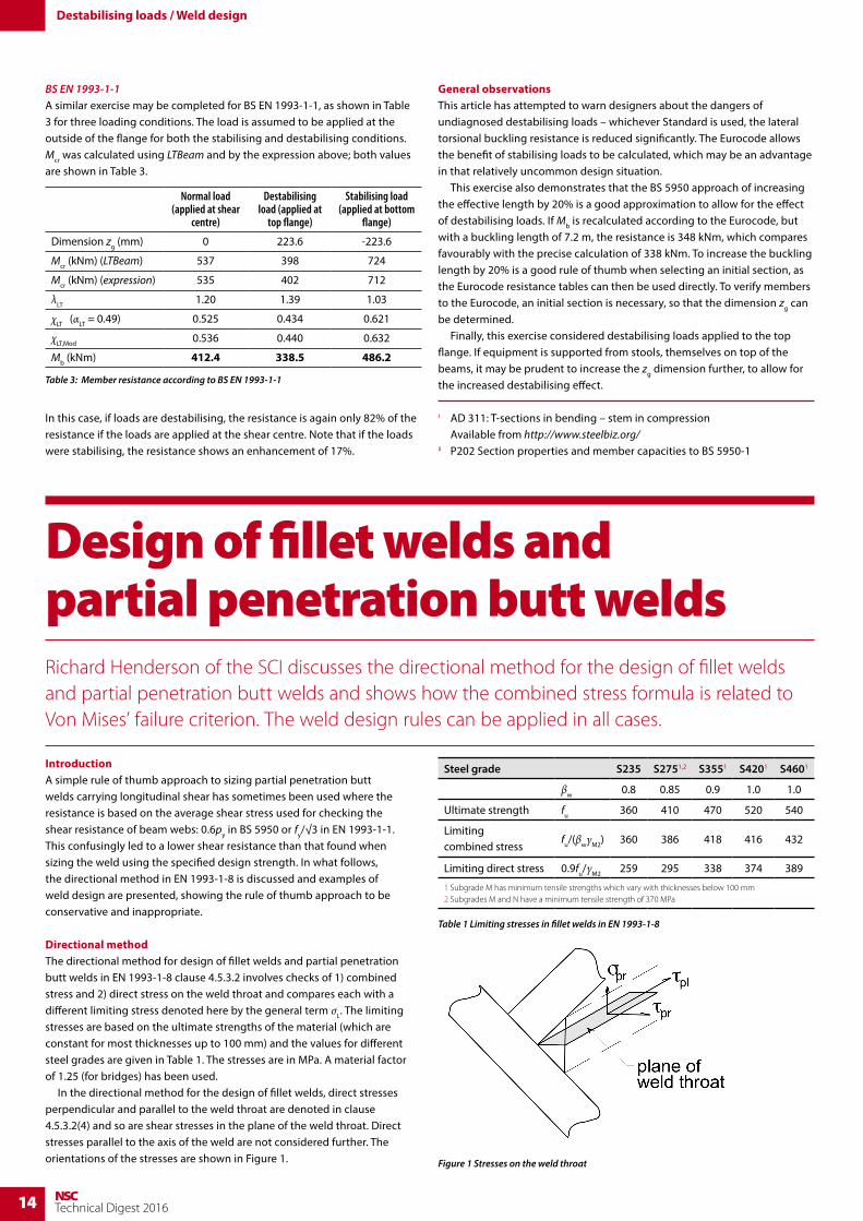
Directional methodThe directional method for design of fillet welds and partial penetration butt welds in EN 1993-1-8 clause 4.5.3.2 involves checks of 1) combined stress and 2) direct stress on the weld throat and compares each with a different limiting stress denoted here by the general term σL. The limiting stresses are based on the ultimate strengths of the material (which are constant for most thicknesses up to 100 mm) and the values for different steel grades are given in Table 1. The stresses are in MPa. A material factor of 1.25 (for bridges) has been used. In the directional method for the design of fillet welds, direct stresses perpendicular and parallel to the weld throat are denoted in clause 4.5.3.2(4) and so are shear stresses in the plane of the weld throat. Direct stresses parallel to the axis of the weld are not considered further. The orientations of the stresses are shown in Figure 1.
Table 1 Limiting stresses in fillet welds in EN 1993-1-8
Steel grade S235 S2751,2 S3551 S4201 S4601
βw 0.8 0.85 0.9 1.0 1.0
Ultimate strength fu 360 410 470 520 540
Limiting combined stress
fu/(βwγM2) 360 386 418 416 432
Limiting direct stress 0.9fu/γM2 259 295 338 374 389
1 Subgrade M has minimum tensile strengths which vary with thicknesses below 100 mm2 Subgrades M and N have a minimum tensile strength of 370 MPa
Figure 1 Stresses on the weld throat
Destabilising loads / Weld design

15NSCTechnical Digest 2016
The formula in EN 1993-1-8 is
σ2pr + 3(τ2
pr + τ2pl)
≤ σL( )0.5(1)
where the direct stress is perpendicular to the weld throat and the shear stresses are in the perpendicular (transverse) and parallel (longitudinal) directions. In equation (1), the subscript “pr” has been used instead of the EN 1993-1-8 symbol “⊥” and “pl” instead of “||”. In designing partial penetration butt welds, the designer determines the penetration required and the fabricator chooses the weld preparation to achieve the penetration specified, based on his welding processes and the corresponding weld procedures.
Von Mises’ failure criterionThe EC3 formula for the combined stress on a weld is based on the Von Mises failure criterion which is usually expressed in terms of principal stresses (orientated such that there are no coincident shear stresses). The standard expression is:
(σ1 – σ2)2 + (σ2 – σ3)
2 + (σ3 – σ1)2 ≤ 2σL
2
where σ1 , σ2 and σ3 are the principal stresses in three orthogonal directions and σL is a limiting stress. In the design of joints with essentially linear welds between plates, the stress in the through thickness direction is zero (see figure 2) so for the biaxial stress state, the equation becomes: (σ1 – σ2)
2 + σ22 + (– σ1)
2 ≤ 2σL2 (2)
The failure criterion in equation (2) is expressed in terms of principal stresses which are related to coincident direct and shear stresses using the transformation equations illustrated by Mohr’s circle of stress.
In general, orthogonal stresses σx and σy and coincident shear stress τxy are present and principal stresses are given by:
σ1 = + τ2xy
σx+σy
2+
σx–σy
2( )2
σ2 = + τ2
xy
σx+σy
2–
σx–σy
2( )2
where the square root term is the radius of the Mohr’s circle and its centre is at ½(σx + σy). If the transformations are made, the formulae in equations (1) and (2) are algebraically identical when σy equals zero.
Limiting stressesThe Von Mises failure criterion is often expressed in terms of the yield strength of the material. However, in the Eurocode, in the design of fillet welds and partial penetration butt welds, as we have seen in Table 1, for lower steel grades, the limiting strength is allowed to be a higher value, between the yield strength and the ultimate strength of the material. Interestingly, for higher strength steels, the inclusion of the material factor of 1.25 means that the limiting stress is less than the yield strength of the material. For S355 steel, the limiting direct stress is less than the yield strength for material 40 mm thick or less. Engineers who remember designing to BS 5950-1: 1990 will recall the requirement to check the stress on the fusion line of partial penetration butt welds and limit it to 0.7py in shear or 1.0py in tension. This check was no longer a requirement in the 2000 update of the code. Comparisons of the limiting shear stress with the values for combined stress assuming pure shear (ie σpr in equation (1) is zero) in Table 2 show that the limiting stresses in the Eurocode are higher for the lower strength grades and lower for the higher strength grades.
Examples(1) A weld in pure shear is carrying a force of 1.27 kN/mm in grade S355 material. A partial penetration Vee butt weld is to be used. What depth of weld penetration is required? The shear stress on the weld of 250 MPa gives a weld throat to BS 5950 of 5.1 mm. Design to BS 5950: 1990 used a design strength pw of 255 MPa on the weld throat. However the shear stress on the fusion line was also limited to 0.7py = 249 MPa resulting in the same weld size. Using the directional method in EC3, all the components of stress are zero except for the shear stress parallel to the axis of the weld (τpl) so substituting in equation (1), the design shear stress is 418/√3 MPa (241 MPa) and the weld size is 5.3 mm (see Figure 4 over page).If the principal stresses are calculated in each case, we find the following for the weld to BS 5950: 2000. The shear stress is 250 MPa and the direct stresses σx and σy are both zero. The principal stresses are therefore equal to ± 250 MPa. Substituting in equation (2) for the failure criterion, the limiting stress is 250 x √3 = 433 MPa. This is higher than 418 MPa, the limiting stress to EC3, where the principal stresses are ± 241 MPa.
Figure 2: Stresses in plate elements
Figure 3: Mohr’s circle of stress
Table 2: Comparison of Limiting shear stresses EC3 and BS 5950: 1990
Steel grade S235 S275 S355 S420 S460
Limiting combined stress
fu/(βwγM2) 360 386 418 416 432
Combined stress (shear only)
fL /√3 208 223 241 240 249
Limiting shear stress: BS 5950: 1990
0.7fy 165 193 249 294 322
Design Strength1: BS 5950: 2000
– – 220 250 200 –
1 Matching electrodes
Weld design
16 NSCTechnical Digest 2016
(2) A second example of welds in pure shear is a lap joint transferring tension between plates in S355 material 20 mm thick, through longitudinal welds. It will be assumed that the edges of the plate are to be prepared for a partial penetration Vee butt weld. The thickness of the plates and length of the welds is such that it is assumed the direct stresses due to the eccentricity moment can be neglected.
1200 kN is to be transferred through welds on each edge of the plate with an effective length of 400 mm. The longitudinal shear stress per mm of
weld is 1200 / (2 x 400) = 1.5 kN/mm. The penetration required is 1.5 × 10³ × √3/418 = 6.2 mm. The size of weld throat to BS 5950: 2000 would be 1.5 x 10³ / 250 = 6.0 mm.
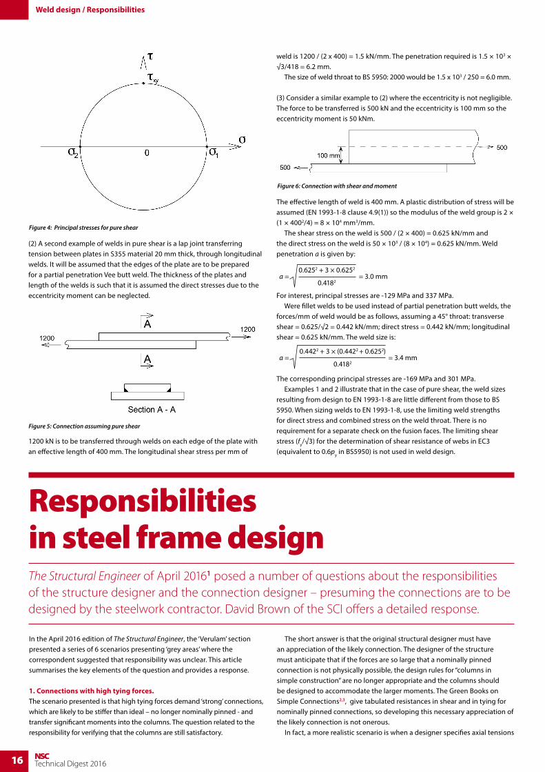
(3) Consider a similar example to (2) where the eccentricity is not negligible. The force to be transferred is 500 kN and the eccentricity is 100 mm so the eccentricity moment is 50 kNm.
The effective length of weld is 400 mm. A plastic distribution of stress will be assumed (EN 1993-1-8 clause 4.9(1)) so the modulus of the weld group is 2 × (1 × 4002/4) = 8 × 104 mm3/mm. The shear stress on the weld is 500 / (2 × 400) = 0.625 kN/mm and the direct stress on the weld is 50 × 103 / (8 × 10⁴) = 0.625 kN/mm. Weld penetration a is given by:
= 3.0 mma = 0.6252 + 3 × 0.6252
0.4182
For interest, principal stresses are -129 MPa and 337 MPa. Were fillet welds to be used instead of partial penetration butt welds, the forces/mm of weld would be as follows, assuming a 45° throat: transverse shear = 0.625/√2 = 0.442 kN/mm; direct stress = 0.442 kN/mm; longitudinal shear = 0.625 kN/mm. The weld size is:
= 3.4 mma = 0.4422 + 3 × (0.4422 + 0.6252)
0.4182
The corresponding principal stresses are -169 MPa and 301 MPa. Examples 1 and 2 illustrate that in the case of pure shear, the weld sizes resulting from design to EN 1993-1-8 are little different from those to BS 5950. When sizing welds to EN 1993-1-8, use the limiting weld strengths for direct stress and combined stress on the weld throat. There is no requirement for a separate check on the fusion faces. The limiting shear stress (fy/√3) for the determination of shear resistance of webs in EC3 (equivalent to 0.6py in BS5950) is not used in weld design.
Figure 4: Principal stresses for pure shear
Figure 5: Connection assuming pure shear
Figure 6: Connection with shear and moment
Responsibilities in steel frame designThe Structural Engineer of April 20161 posed a number of questions about the responsibilities of the structure designer and the connection designer – presuming the connections are to be designed by the steelwork contractor. David Brown of the SCI offers a detailed response.
In the April 2016 edition of The Structural Engineer, the ‘Verulam’ section presented a series of 6 scenarios presenting ‘grey areas’ where the correspondent suggested that responsibility was unclear. This article summarises the key elements of the question and provides a response.
1. Connections with high tying forces. The scenario presented is that high tying forces demand ‘strong’ connections, which are likely to be stiffer than ideal – no longer nominally pinned - and transfer significant moments into the columns. The question related to the responsibility for verifying that the columns are still satisfactory.
The short answer is that the original structural designer must have an appreciation of the likely connection. The designer of the structure must anticipate that if the forces are so large that a nominally pinned connection is not physically possible, the design rules for “columns in simple construction” are no longer appropriate and the columns should be designed to accommodate the larger moments. The Green Books on Simple Connections2,3, give tabulated resistances in shear and in tying for nominally pinned connections, so developing this necessary appreciation of the likely connection is not onerous. In fact, a more realistic scenario is when a designer specifies axial tensions
Weld design / Responsibilities

17NSCTechnical Digest 2016
in the beams that are not tying forces – for some reason they are ‘real’ forces. Immediately, this is at variance with the concept of “simple” or nominally pinned connections, which are “shear only”. Although nominally pinned connections can be verified for shear and, as an entirely separate check, a tying force, the Green Books do not contain any design rules for the combination of shear and axial forces. In the original question, it was suggested that BS 5950 was “a little hazy” about requiring the connection flexibilities to
be checked to ensure that they comply with the frame design concepts. Not so – clause 2.1.2.1 requires that “in each case the details of the joints should be such as to fulfil the assumptions made in the relevant design method” although it might be argued that BS 5950 does not specify how stiffness is to be calculated. It might also be said that BS 5950 puts the onus on the connection designer to meet the structure designer’s assumptions, but this cannot be reasonable or sensible if those assumptions are unrealistic. The Eurocodes place the responsibility squarely with the original designer. To paraphrase BS EN 1993-1-1 clause 5.1.2, the effects of the behaviour of the joints… must be taken into account when they are significant. In clause 5.5.1(2), “the calculation model and basic assumptions should reflect…. the anticipated type of behaviour of the cross sections, members, joints and bearings”. This leads on to BS EN 1993-1-8, where rules are presented to calculate joint stiffness and compare this with limits on nominally pinned, semi-rigid and rigid behaviour. Rather than follow the calculation procedure, the Eurocode points out that a joint may be classified on the basis of “experience of previous satisfactory performance in similar
cases”, which seems a more attractive option if that experience exists. In the UK, designers have the advantage that the National Annex notes that connections designed in accordance with the principles in the Green Book on Simple Connections3 (Figure 1) are nominally pinned, without justification by calculation of stiffness.
2. Flange to web welds in a plate girder. This question has reached SCI on a number of occasions. The responsibility lies with the designer of the member, not the connection designer.
3. Joint resistances in hollow section trusses. The situation described was when checked by the connection designer, the joints required expensive stiffening (although it was really strengthening that was required). When the truss designer has selected members, the joint resistance has also been set. Joints should be checked as part of the design process, as judicious choice of members and geometry can lead to nodes which do not need strengthening. As the question in Verulam noted, there is published guidance on this specific subject in Steel Industry Guidance Note SN484. All these guidance notes are available on Steelbiz. Although checking joint resistance can appear daunting (see Figure 2 showing part of BS EN 1993-1-8), software is available. Free software can be obtained from Tata Steel Tubes, in Corby – the contact number is listed on SN48.
4. Holding Down Bolts and foundation design. The question focused on the design responsibility when holding down bolts are in tension. As the original contributor noted, this is covered in Steel Industry Guidance Note SN515. Once the loads in the anchors have been calculated by the steelwork contractor, it is for the consulting engineer to design and specify the anchorage arrangement and the base reinforcement. Managing significant base shear deserves careful thought, especially as the UK appears to have an almost unique approach to detailing this interface. Other countries tend to use anchors solidly cast in (so therefore cast with rather more precision than is typical in the UK) and have a mere smear of grout. In the UK, we use bolts cast in conical or cylindrical formers
Figure 1: One of the Eurocode ‘Green Books’
Figure 2: Typical joint checks from BS EN 1993-1-8
Type of joint Design resistance
N1
b1
t1
h1
t0h0
b0
θ1
Chord face failure β ≤ 0,85
N1,Rd = + 4 1-β /γm5
kn fy0t02
(1-β) sinθ1( )2η
sinθ1
Chord side wall buckling 1) β = 1.0 2)
N1,Rd = + 10t0 /γm5
kn fbt0
sinθ1( )2h1
sinθ1
Brace failure β ≥ 0,85
N1,Rd = fyit1(2h1-4t1+2beff)/γM5
Punching shear 0,85 ≤ β ≤ (1-1/γ)
N1,Rd = + 2be,p /γm5
fy0t0
3sinθ1( )2h1
sinθ1
Responsibilities

18 NSCTechnical Digest 2016
to allow for significant movement, and generally a significant thickness of grout, as shown in Figure 3 – which may be deeper in practice due to the variability of the concrete levels. The baseplate tends to have 6 mm oversize holes – so it is unlikely that all the bolts are in bearing on the plate. Friction may transfer shear, as may the bolts, but for significant base shear additional measures may be justified. This may be to consider the grouting operation as special, rather than mundane, and ensure the final result is as specified. More elaborate measures might involve locating the whole base in a pocket, or welding a shear nib on the underside (to be located in a pocket in the foundation).
5. Nominally pinned connections invalidate the original assumption of full fixity to the column. In this situation, the designer had assumed an effective length of 0.7L for the column, yet the permitted connections are nominally pinned, with only shear loads provided. The scenario seems unlikely – the choice of 0.7L must have been based on full fixity at both ends – both ends held in position and restrained in direction according to Table 22 of BS 5950. But nominally pinned connections do not provide full restraint in direction, so a longer effective length would be the correct choice. In the scenario described, it seems the original designer has made an error in choosing the effective length. Practice probably varies amongst designers, but an effective length equal to the system length or an effective length factor of 0.85 are common choices when nominally pinned connections are anticipated.
6. High shear and bending. The last situation presented in Verulam was a member with high shear – sufficiently high to reduce the moment capacity. In the (hopefully hypothetical) scenario, the necessary strengthening was considered to be part of the connection design. Clearly, the connection plays no part in the combination of member design forces and the responsibility for selecting a member with sufficient strength lies squarely with the structure designer. A relatively common (real) situation is when a floor plan is prepared, possibly indicating certain shear loads for major beams, but also with a general note stating that if no force is given, the connection must be designed for a certain minimum shear. This note can easily become too general, with the connections for small beams supposed to be designed for a shear force that exceeds the resistance of the beam itself. In general, the critical check for a beam is likely to be the bending resistance or deflection, with the shear force no more than about 60% of the beam’s shear resistance. High shears at the end of a beam are generally only produced if there is a concentrated load near the end of the beam.
You can lead a horse to water …The proverb continues … but you can’t make them drink. There are very many resources available covering the sorts of topics raised in Verulam, if only designers knew of them and read them. A good place to start is the Steel Industry Guidance Notes (SIGNS), which cover a wide variety of topics. Searching for “SIGNS” on Steelbiz will produce a complete list, which could form the background to a succinct library of “good practice” guidance. You can also go to www.newsteelconstruction.com and search the Advisory Desk articles.
1 Volume 94, Issue 4. The Institution of Structural Engineers, April 20162 Joints in steel construction: Simple Connections, SCI and BCSA, 20093 Joints in steel construction: Simple joints to Eurocode 3, SCI and BCSA, 20144 SN48 Design of welded joints using structural hollow sections. Available on Steelbiz5 SN51 Design responsibility – simple connections. Available on Steelbiz
Figure 3: Typical base detail
Lateral torsional buckling – additional Eurocode provisionsDavid Brown of the SCI discusses the Eurocode rules when the effect of LTB may be ignored, and the simplified rules for buildings.
All designers will appreciate that there is a range of slenderness known as the ‘plateau length’, where there is no reduction for lateral torsional buckling – illustrated in Figure 1. In the Eurocode, the plateau length is given by λLT,0 and has the value of 0.2 if using clause 6.3.2.2 and the value of 0.4 if using clause 6.3.2.3 and the UK National Annex. If λLT is calculated, and found to be less than the plateau length, then there is no reduction for LTB. This (fairly obvious) point is confirmed in the first part of
clause 6.3.2.2(4), which states that if λLT ≤ λLT,0 lateral torsional buckling checks may be ignored and only cross sectional checks apply. There is some uncertainty which value of λLT,0 was intended in this clause (0.2 or 0.4), so it is hoped that the forthcoming revision will provide some clarity. The second part of clause 6.3.2.2(4) is rather more interesting,
stating that LTB may be ignored if < λLT,02
MEd
Mcr
. MEd is the design
Responsibilities / LTB (Part 3)
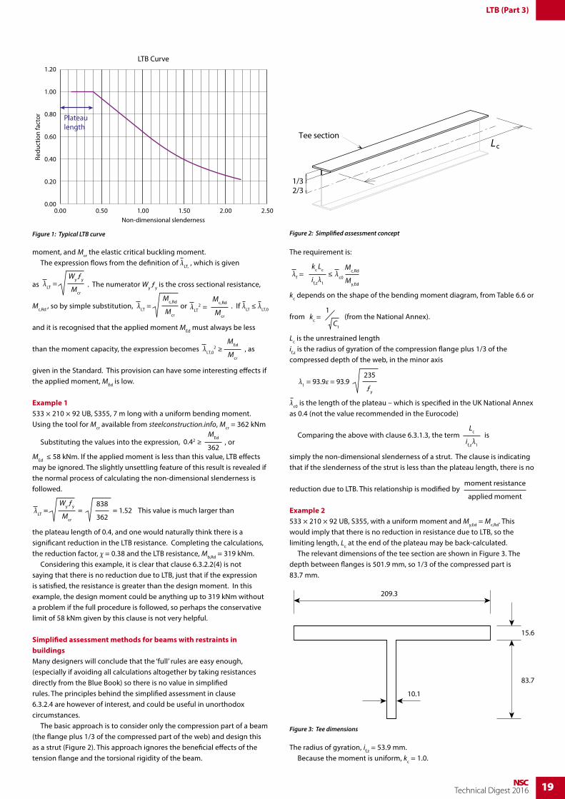
19NSCTechnical Digest 2016
moment, and Mcr the elastic critical buckling moment. The expression flows from the definition of λLT, , which is given
as λLT =Wy ƒy
Mcr
. The numerator Wy ƒy is the cross sectional resistance,
Mc,Rd , so by simple substitution, λLT =Mc,Rd
Mcr
or λLT2 =
Mc,Rd
Mcr
. If λLT ≤ λLT,0
and it is recognised that the applied moment MEd must always be less
than the moment capacity, the expression becomes λLT,02 ≥
MEd
Mcr
, as
given in the Standard. This provision can have some interesting effects if the applied moment, MEd is low.
Example 1533 × 210 × 92 UB, S355, 7 m long with a uniform bending moment. Using the tool for Mcr available from steelconstruction.info, Mcr = 362 kNm
Substituting the values into the expression, 0.42 ≥MEd
362 , or
MEd ≤ 58 kNm. If the applied moment is less than this value, LTB effects may be ignored. The slightly unsettling feature of this result is revealed if the normal process of calculating the non-dimensional slenderness is followed.
λLT =Wy ƒy
Mcr
=838
362= 1.52 This value is much larger than
the plateau length of 0.4, and one would naturally think there is a significant reduction in the LTB resistance. Completing the calculations, the reduction factor, χ = 0.38 and the LTB resistance, Mb,Rd = 319 kNm. Considering this example, it is clear that clause 6.3.2.2(4) is not saying that there is no reduction due to LTB, just that if the expression is satisfied, the resistance is greater than the design moment. In this example, the design moment could be anything up to 319 kNm without a problem if the full procedure is followed, so perhaps the conservative limit of 58 kNm given by this clause is not very helpful.
Simplified assessment methods for beams with restraints in buildingsMany designers will conclude that the ‘full’ rules are easy enough, (especially if avoiding all calculations altogether by taking resistances directly from the Blue Book) so there is no value in simplified rules. The principles behind the simplified assessment in clause 6.3.2.4 are however of interest, and could be useful in unorthodox circumstances. The basic approach is to consider only the compression part of a beam (the flange plus 1/3 of the compressed part of the web) and design this as a strut (Figure 2). This approach ignores the beneficial effects of the tension flange and the torsional rigidity of the beam.
The requirement is:
λf =kc Lc
if,zλ1
≤Mc,Rd
My,Ed
λc0
kc depends on the shape of the bending moment diagram, from Table 6.6 or
from kc =1
C1
(from the National Annex).
Lc is the unrestrained lengthif,z is the radius of gyration of the compression flange plus 1/3 of the compressed depth of the web, in the minor axis λ1 = 93.9ε = 93.9
235
ƒy
λc0 is the length of the plateau – which is specified in the UK National Annex as 0.4 (not the value recommended in the Eurocode)
Comparing the above with clause 6.3.1.3, the term Lc
if,zλ1
is
simply the non-dimensional slenderness of a strut. The clause is indicating that if the slenderness of the strut is less than the plateau length, there is no
reduction due to LTB. This relationship is modified by moment resistance
applied moment
Example 2533 × 210 × 92 UB, S355, with a uniform moment and My,Ed = Mc,Rd. This would imply that there is no reduction in resistance due to LTB, so the limiting length, Lc at the end of the plateau may be back-calculated. The relevant dimensions of the tee section are shown in Figure 3. The depth between flanges is 501.9 mm, so 1/3 of the compressed part is 83.7 mm.
The radius of gyration, if,z = 53.9 mm. Because the moment is uniform, kc = 1.0.
Figure 1: Typical LTB curve
Plateaulength
LTB Curve
Non-dimensional slenderness
Redu
ctio
n fa
ctor
1.20
1.00
0.80
0.60
0.40
0.20
0.000.00 0.50 1.00 1.50 2.00 2.50
1/32/3
Tee sectionLc
Figure 2: Simplified assessment concept
Figure 3: Tee dimensions
209.3
10.1
15.6
83.7
LTB (Part 3)
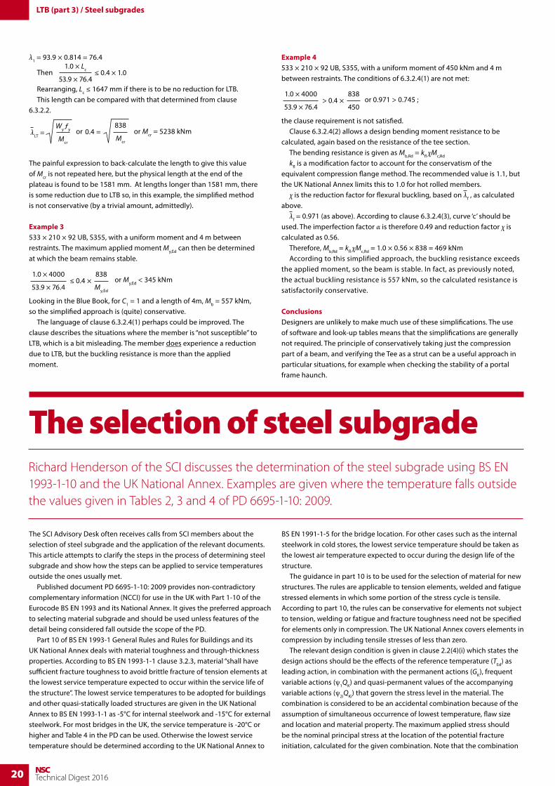
20 NSCTechnical Digest 2016
λ1 = 93.9 × 0.814 = 76.4
Then 1.0 × Lc
53.9 × 76.4≤ 0.4 × 1.0
Rearranging, Lc ≤ 1647 mm if there is to be no reduction for LTB. This length can be compared with that determined from clause 6.3.2.2.
λLT = Wy ƒy
Mcr
or 0.4 = 838
Mcr
or Mcr = 5238 kNm
The painful expression to back-calculate the length to give this value of Mcr is not repeated here, but the physical length at the end of the plateau is found to be 1581 mm. At lengths longer than 1581 mm, there is some reduction due to LTB so, in this example, the simplified method is not conservative (by a trivial amount, admittedly).
Example 3533 × 210 × 92 UB, S355, with a uniform moment and 4 m between restraints. The maximum applied moment My,Ed can then be determined at which the beam remains stable.
≤ 0.4 × 838
My,Ed
1.0 × 4000
53.9 × 76.4 or My,Ed < 345 kNm
Looking in the Blue Book, for C1 = 1 and a length of 4m, Mb = 557 kNm, so the simplified approach is (quite) conservative. The language of clause 6.3.2.4(1) perhaps could be improved. The clause describes the situations where the member is “not susceptible” to LTB, which is a bit misleading. The member does experience a reduction due to LTB, but the buckling resistance is more than the applied moment.
Example 4533 × 210 × 92 UB, S355, with a uniform moment of 450 kNm and 4 m between restraints. The conditions of 6.3.2.4(1) are not met:
> 0.4 × 838
450
1.0 × 4000
53.9 × 76.4 or 0.971 > 0.745 ;
the clause requirement is not satisfied. Clause 6.3.2.4(2) allows a design bending moment resistance to be calculated, again based on the resistance of the tee section. The bending resistance is given as Mb,Rd = kfl χMc,Rd kfl is a modification factor to account for the conservatism of the equivalent compression flange method. The recommended value is 1.1, but the UK National Annex limits this to 1.0 for hot rolled members. χ is the reduction factor for flexural buckling, based on λf , as calculated above. λf = 0.971 (as above). According to clause 6.3.2.4(3), curve ‘c’ should be used. The imperfection factor α is therefore 0.49 and reduction factor χ is calculated as 0.56. Therefore, Mb,Rd = kfl χMc,Rd = 1.0 × 0.56 × 838 = 469 kNm According to this simplified approach, the buckling resistance exceeds the applied moment, so the beam is stable. In fact, as previously noted, the actual buckling resistance is 557 kNm, so the calculated resistance is satisfactorily conservative.
ConclusionsDesigners are unlikely to make much use of these simplifications. The use of software and look-up tables means that the simplifications are generally not required. The principle of conservatively taking just the compression part of a beam, and verifying the Tee as a strut can be a useful approach in particular situations, for example when checking the stability of a portal frame haunch.
The selection of steel subgradeRichard Henderson of the SCI discusses the determination of the steel subgrade using BS EN 1993-1-10 and the UK National Annex. Examples are given where the temperature falls outside the values given in Tables 2, 3 and 4 of PD 6695-1-10: 2009.
The SCI Advisory Desk often receives calls from SCI members about the selection of steel subgrade and the application of the relevant documents. This article attempts to clarify the steps in the process of determining steel subgrade and show how the steps can be applied to service temperatures outside the ones usually met. Published document PD 6695-1-10: 2009 provides non-contradictory complementary information (NCCI) for use in the UK with Part 1-10 of the Eurocode BS EN 1993 and its National Annex. It gives the preferred approach to selecting material subgrade and should be used unless features of the detail being considered fall outside the scope of the PD. Part 10 of BS EN 1993-1 General Rules and Rules for Buildings and its UK National Annex deals with material toughness and through-thickness properties. According to BS EN 1993-1-1 clause 3.2.3, material “shall have sufficient fracture toughness to avoid brittle fracture of tension elements at the lowest service temperature expected to occur within the service life of the structure”. The lowest service temperatures to be adopted for buildings and other quasi-statically loaded structures are given in the UK National Annex to BS EN 1993-1-1 as -5°C for internal steelwork and -15°C for external steelwork. For most bridges in the UK, the service temperature is -20°C or higher and Table 4 in the PD can be used. Otherwise the lowest service temperature should be determined according to the UK National Annex to
BS EN 1991-1-5 for the bridge location. For other cases such as the internal steelwork in cold stores, the lowest service temperature should be taken as the lowest air temperature expected to occur during the design life of the structure. The guidance in part 10 is to be used for the selection of material for new structures. The rules are applicable to tension elements, welded and fatigue stressed elements in which some portion of the stress cycle is tensile. According to part 10, the rules can be conservative for elements not subject to tension, welding or fatigue and fracture toughness need not be specified for elements only in compression. The UK National Annex covers elements in compression by including tensile stresses of less than zero. The relevant design condition is given in clause 2.2(4)(i) which states the design actions should be the effects of the reference temperature (TEd) as leading action, in combination with the permanent actions (GK), frequent variable actions (ψ1QK) and quasi-permanent values of the accompanying variable actions (ψ2iQKi) that govern the stress level in the material. The combination is considered to be an accidental combination because of the assumption of simultaneous occurrence of lowest temperature, flaw size and location and material property. The maximum applied stress should be the nominal principal stress at the location of the potential fracture initiation, calculated for the given combination. Note that the combination
LTB (part 3) / Steel subgrades
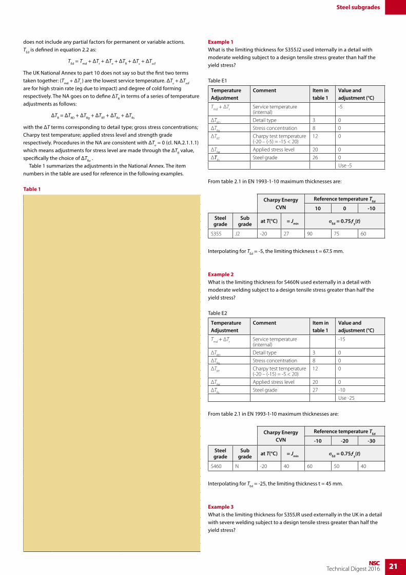
21NSCTechnical Digest 2016
does not include any partial factors for permanent or variable actions.TEd is defined in equation 2.2 as:
TEd = Tmd + ΔTr + ΔTσ + ΔTR + ΔTε + ΔTεcf
The UK National Annex to part 10 does not say so but the first two terms taken together: (Tmd + ΔTr ) are the lowest service temperature. ΔTε + ΔTεcf are for high strain rate (eg due to impact) and degree of cold forming respectively. The NA goes on to define ΔTR in terms of a series of temperature adjustments as follows:
ΔTR = ΔTRD + ΔTRg + ΔTRT + ΔTRσ + ΔTRs
with the ΔT terms corresponding to detail type; gross stress concentrations; Charpy test temperature; applied stress level and strength grade respectively. Procedures in the NA are consistent with ΔTσ = 0 (cl. NA.2.1.1.1) which means adjustments for stress level are made through the ΔTR value, specifically the choice of ΔTRσ . Table 1 summarizes the adjustments in the National Annex. The item numbers in the table are used for reference in the following examples.
Example 1What is the limiting thickness for S355J2 used internally in a detail with moderate welding subject to a design tensile stress greater than half the yield stress?
Table E1
Temperature Adjustment
Comment Item in table 1
Value and adjustment (°C)
Tmd
+ ΔTr
Service temperature (internal)
-5
ΔTRD
Detail type 3 0
ΔTRg
Stress concentration 8 0
ΔTRT
Charpy test temperature (-20 – (-5) = -15 < 20)
12 0
ΔTRσ Applied stress level 20 0
ΔTRs
Steel grade 26 0
Use -5
From table 2.1 in EN 1993-1-10 maximum thicknesses are:
Charpy Energy CVN
Reference temperature TEd
10 0 -10
Steel grade
Sub grade at T(°C) = Jmin σEd = 0.75ƒy(t)
S355 J2 -20 27 90 75 60
Interpolating for TEd = -5, the limiting thickness t = 67.5 mm.
Example 2What is the limiting thickness for S460N used externally in a detail with moderate welding subject to a design tensile stress greater than half the yield stress?
Table E2
Temperature Adjustment
Comment Item in table 1
Value and adjustment (°C)
Tmd
+ ΔTr
Service temperature (internal)
-15
ΔTRD
Detail type 3 0
ΔTRg
Stress concentration 8 0
ΔTRT
Charpy test temperature (-20 – (-15) = -5 < 20)
12 0
ΔTRσ Applied stress level 20 0
ΔTRs
Steel grade 27 -10
Use -25
From table 2.1 in EN 1993-1-10 maximum thicknesses are:
Charpy Energy CVN
Reference temperature TEd
-10 -20 -30
Steel grade
Sub grade at T(°C) = Jmin σEd = 0.75ƒy(t)
S460 N -20 40 60 50 40
Interpolating for TEd = -25, the limiting thickness t = 45 mm.
Example 3What is the limiting thickness for S355JR used externally in the UK in a detail with severe welding subject to a design tensile stress greater than half the yield stress?
Adjustments for detail type (NA.2.1.1.1.2 and Table NA.1)
Detail Item ΔTRD
Unwelded As rolled, ground or machined surfaces 1 +30°C
Mechanically fastened joints or flame cut edges 2 +20°C
Welded Generally (described as ‘moderate’ in the PD) 3 0°C
Attachment; transverse weld toe: length >150 mm; width ≤ 50mm (described as ‘severe’ in the PD)
4 -20°C
Attachment; transverse weld toe: length >150 mm; width > 50mm (described as ‘very severe’ in the PD)
5 -30°C
Member fabricated from plates: transverse butt weld
6 -20°C
Rolled section: transverse butt weld 7 -30°C
Adjustment for gross stress concentration (Table NA.2)
Stress concentration factor ΔTRg
Guidance on stress concentration factors is given in PD 6695-1-9:2008
1 8 0°C
1.5 9 -10°C
2 10 -20°C
3 11 -30°C
Adjustment for Charpy test temperature (Table NA.3)
General (except bridges conforming to BS EN 1993-2). Obtain intermediate values by linear interpolation. The maximum difference between the Charpy test temperature and T
Ed = (T
md + ΔT
r ) should be limited.
T – (Tmd + ΔTr ) ΔTRT
≤ 20°C 12 0°C
25°C 13 -10°C
30°C 14 -20°C
35°C 15 -30°C
Further restriction on joint types apply: see the NA
> 35 ≤ 40°C 16 -40°C
> 40°C 17 Not permitted
Bridges conforming to BS EN 1993-2 ≤ 20°C 18 0°C
> 20°C 19 Not permitted
Adjustment for applied stress (Table NA.4)
σEd ΔTRσ
0.75ƒy(t) 20 0°C
Use the values for 0.75 ƒy(t) but adjusted
for lower values of σEd
. Linear interpolation may be used for intermediate values.
0.5ƒy(t) 21 0°C
0.3ƒy(t) 22 +10°C
0.15ƒy(t) 23 +20°C
≤ 0 24 +30°C
Adjustment for steel grade (Table NA.5)
steel grade TRs
< S355 25 +10°C
S355 26 0°C
> S355 27 -10°C
Table 1
Steel subgrades
22 NSCTechnical Digest 2016
Table E3
Temperature Adjustment
Comment Item in table 1
Value and adjustment (°C)
Tmd
+ ΔTr
Service temperature (internal)
-15
ΔTRD
Detail type 4 -20
ΔTRg
Stress concentration 8 0
ΔTRT
Charpy test temperature (20 – (-15) = 35)
15 -30
ΔTRσ Applied stress level 20 0
ΔTRss
Steel grade 26 0
Use -65
Table 2.1 in EN 1993-1-10 does not have thicknesses for temperatures as low as this. However, such values are given in PD6695-1-10.
Charpy Energy CVN
Reference temperature TEd
-50 -60 -70
Steel grade
Sub grade at T(°C) = Jmin σEd = 0.75ƒy(t)
S355 JR 20 27 10 10 5
Interpolating for TEd = -65, the limiting thickness t = 7.5 mm.
Example 4What is the limiting thickness for S355J2 used externally where the service temperature is -40°C in a detail with moderate welding subject to a design tensile stress just less than 0.3 times the yield stress?
Table E4
Temperature Adjustment
Comment Item in table 1
Value and adjustment (°C)
Tmd
+ ΔTr
Service temperature (internal)
-40
ΔTRD
Detail type 3 0
ΔTRg
Stress concentration 8 0
ΔTRT
Charpy test temperature (-20 – (-40) = 20)
12 0
ΔTRσ Applied stress level 22 +10
ΔTRs
Steel grade 26 0
Use -30
From table 2.1 in EN 1993-1-10, maximum thicknesses are:
Charpy Energy CVN
Reference temperature TEd
-20 -30 -40
Steel grade
Sub grade at T(°C) = Jmin σEd = 0.75ƒy(t)
S355 J2 -20 27 50 40 35
The limiting thickness t = 40 mm.
Example 5What is the limiting thickness for S355JR used in a bridge where the service temperature is -20°C in a detail with moderate welding subject to a design tensile stress just less than 0.3 times the yield stress?
Table E5
Temperature Adjustment
Comment Item in table 1
Value and adjustment (°C)
Tmd
+ ΔTr
Service temperature (internal)
-20
ΔTRD
Detail type
ΔTRg
Stress concentration
ΔTRT
Charpy test temperature (20 – (-20) = 40 > 20)
19 Not permitted
ΔTRσ Applied stress level
ΔTRs
Steel grade
Use of the proposed sub grade is not permitted. Comparison of the results from examples 1 to 5 with the tables in PD6695-1-10 will show that the same values appear.
ConclusionThe determination of the maximum thickness for a given material subgrade and set of conditions has been illustrated, using EN 1993-1-10 and its National Annex and can be seen to correspond to the values given in PD6695-1-10. It is noted in the JRC Scientific and Technical Report EUR 23510 EN – 2008 entitled Commentary and worked examples to EN 1993-1-10 by Sedlacek et al, September 2008, in section 1.4.3(1) that “As EN 1993-1-10, section 2 has been developed for structures subjected to fatigue (such) as bridges … , its use for buildings where fatigue plays a minor role would be extremely safe sided.”
Use of EN 1993-1-5 section 4 and 10 for biaxial stressChris Hendy, head of Bridge Design and Technology at Atkins and Chairman of SCI’s Steel Bridge Group discusses the background to a proposed change to the rules for the design of plates subject to biaxial compression according to BS EN 1993-1-5. This article was written before the recent issue of a relevant draft for public comment (16/30340641 DC. BS EN 1993-1-5 AMD1).
1. IntroductionGenerally, section 10 of EN 1993-1-5 will not be required in design and the effective width method of section 4 of EN 1993-1-5 will be used in preference. However, where the geometrical conditions for the use of the effective width method are not met or where the combination of stresses (e.g. biaxial stress) are
not covered by section 4, it may be necessary to use section 10. This latter case can arise, for example, in box girder bridges at transverse support diaphragms where there is local load introduction, such as at intermediate piers or stay cable supports. In such cases, it is also possible to adapt the rules of section 4 to include biaxial effects, but EN 1993-1-5 currently gives no rules for this situation.
Steel subgrades / Biaxial stress

23NSCTechnical Digest 2016
The choice of design method leads to two important observations that designers should be aware of as follows:
(i) Section 10 takes no account of the beneficial shedding of load from overstressed panels and stiffeners so is mostly conservative by comparison with section 4, although not always (see ii). The choice of method can therefore have a large impact on steel tonnage. A particular difficulty occurs when the majority of the length of bridge sees uniaxial direct stress but local zones of flange (e.g. adjacent to diaphragms) see biaxial direct stress. This leads to different designers taking different approaches which are essentially: (a) use section 4 throughout, without corrections for biaxial stress locations; (b) use section 4 throughout, making corrections for biaxial stress locations; (c) use section 4 generally and section 10 for biaxial stress locations; (d) use section 10 throughout. Reference 1 provides some guidance on the comparison of the methods.
At this stage, this note merely draws attention to the fact that method (a) is not conservative, method (b) is appropriate provided that suitable assumptions for the interaction are made and methods (c) and (d) are likely to lead to ever increasing quantities.
Method (b) could be informed by ECCS publication 44, section 2.625 for example, which recommends an interaction of the utilisations of the two direct stress such that the square root sum of the squares of the utilisations is less than unity. It was not however written with the express intent of then using EN 1993-1-5 for the further interaction of this combined utilisation with shear in section 7. Alternatively, the affected element could be checked for biaxial stress using section 10 to subsequently determine a reduction factor for that element for subsequent use in section 4 and 7. Detailing such calculation methods are outside the scope of the note.
(ii) EN1993-1-5 section 10 is typically more conservative than section 4, but is unconservative for cases of biaxial compression and should not be used for such cases in its current format. The sections below identify the problem and propose an interim modification until EN 1993-1-5 is itself modified.
2. Biaxial compression – the problem in EN 1993-1-5 section 10Depending on plate slenderness, the behaviour under biaxial compression varies as follows:
(i) Where there is no tendency for buckling (stocky plates), the behaviour is accurately predicted by the Von Mises yield criterion:
)(σx,Ed
fy /γM1
+2
)(σz,Ed
fy /γM1
2
–σx,Ed
fy /γM1
σz,Ed
fy /γM1
+ 3 )( τEd
fy /γM1
2
≤ 1.0
In essence the presence of biaxial stress provides confinement which
means that the allowable compressive stress in one direction may be increased by applying compressive stress in the other. Stresses in excess of yield can be reached.
(ii) For very high slenderness, the interaction between compressive stresses is essentially that for elastic buckling and is linear. The material strength itself is not relevant.
(iii) For intermediate slenderness, the behaviour is intermediate to the above and has to be determined by non-linear theory.
These three cases of interaction are shown in Figure 1. EN 1993-1-5 chooses to use a form of the Von Mises equivalent stress criterion for verifying plates under in-plane stress fields, whether stocky or slender, via (10.5):
The reduction factors ρx and ρz are introduced to allow for buckling. Their inclusion in all denominators means that the interaction between stresses is always convex, whilst at high slenderness it is known that the interaction should be almost linear as mentioned above. In simple terms, by applying the reduction factors ρx and ρz to the negative term (when both direct
stresses are positive and compressive), this beneficial term becomes large and too much benefit is taken from it. The results of EN 1993-1-5 (10.5) are shown for a square plate in biaxial compression with varying slenderness (b/t ratio) in Figure 2 and compared with the results of the German DIN 18800-3 code. It can be seen that at high slenderness, b/t=100, the EN 1993-1-5 prediction is still very convex, while the DIN code has a linear interaction. From non-linear studies it is known that EN 1993-1-5 is unsafe in this case and DIN 18800-3 is conservative. It is evident some correction is needed to the rules of EN 1993-1-5 for biaxial compression at high slenderness.
3. Biaxial compression – the interim correction to EN 1993-1-5 section 10The following amendments should be made to EN 1993-1-5 section 10 until such time as the standard is itself modified. The amendments reduce the benefit of the negative term in expression (10.5) by eliminating the reduction factor terms in its denominator when both direct stresses are compressive. For this reason, the method of clause 10(5)a) should not then be used because the reduction factor is always automatically applied to all the stresses.
The method in EN 1993-1-5 clause 10(5)a) should not be used.In clause 10(5)b), expression (10.5) should be replaced with the following:
where:V = (ρx ρz) when σx,Ed and σz,Ed are both compressive, or V = 1.0 otherwise.
References1. Hendy, C R, Murphy, C.J, Designers’ Guide to EN1993-2: Design of steel
structures Part 2, Steel bridges, Thomas Telford (2007)
For more information on the Steel Bridge Group go to http://steel-sci.org/the-steel-bridge-group.html
Figure 1: Different types of interaction for biaxial compression
Material theory,stocky plate
Non-linear buckling theory,slender plate
Linear buckling theory
(i)
(iii)
(ii)
equivalent stress hypothesis
linear buckling theory
(i)
(iii)
(ii)
upper bound
lower bound
1.0
1.00
σz.norm
σx.norm
Material theory,stocky plate
Non-linear buckling theory,slender plate
Linear buckling theory
(i)
(iii)
(ii)
equivalent stress hypothesis
linear buckling theory
(i)
(iii)
(ii)
upper bound
lower bound
1.0
1.00
σz.norm
σx.norm
)( σx,Ed
ρx fy /γM1
+2
)( σz,Ed
ρzfy /γM1
2
–σx,Ed
ρx fy /γM1
σz,Ed
ρzfy /γM1
+ 3 )( τEd
χwfy /γM1
2
≤ 1.0
DIN 18800-3 EN 1993-1-5
)( σx,Ed
ρx fy /γM1
+2
)( σz,Ed
ρzfy /γM1
2
–σx,Ed
ρx fy /γM1
σz,Ed
ρzfy /γM1
+ 3 )( τEd
χwfy /γM1
2
≤ 1.0V
Figure 2: Interaction for biaxial compression according to DIN 18800-3 and EN 1993-1-5
Biaxial stress
24 NSCTechnical Digest 2016
designers when specifying the Execution requirements for steel structures. Four Execution Classes were identified – Class 4 being the most onerous. Orthodox buildings are typically Class 2. Some years after its publication, the European committees responsible for the design (BS EN 1993-1-1) and Execution (BS EN 1090-2) standards for structural steel recognised that the recommendations for the selection of Execution Class would be better placed in the design standard, BS EN 1993-1-1. The work to move this guidance is now complete and the British Standards Institute (BSI) recently published a revised version of BS EN 1993-1-1 together with a new National Annex NA+A1:2014 to BS EN 1993-1-1:2005+A1:2014 (issued June 2015). BS EN 1993-1-1:2005+A1:2014 now contains a new normative ‘Annex C – Selection of Execution Class’. There are a couple of major differences between the recommendations in Annex C of BS EN 1993-1-1 and those given in Annex B of BS EN 1090-2. The first difference is that the Annex C is normative and engineers must use the approach given in the standard. The guidance given in Annex B of BS EN 1090-2 was informative and engineers could either adopt the guidance or use an alternative approach. The second change concerns the approach for selecting Execution Class. The relationship in Annex C is based on Consequences Class (CC)/Reliability Class (RC), type of loading and the grade of steel. Production Class has been removed. The new Annex C of BS EN 1993-1-1:2005+A1:2014 also contains provisions for national determination. These allow member states to recommend an alternative approach to the selection of Execution Class and to place limitations on the use of Execution Class 1. The UK’s approach for
the selection of Execution Class is given in Clause NA.2.27.3 and Table NA.4. of the revised National Annex to BS EN 1993-1-1. Table NA.4. is reproduced below. Note that the broad division in the table is between structures subject to fatigue, and those where fatigue is not a design consideration. EXC2 is the anticipated Class for most building structures. Bridges, being subject to fatigue, will generally be Execution Class 3. The use of EXC1 is not encouraged by the standard or the UK National Annex. The standard states that EXC1 “is not endorsed for general use.” and the National Annex notes that the use of EXC1 “might result in a higher probability of structural failure than is normally accepted for most structures in the UK” Although BS EN 1090-2:2008+A1:2011 has not yet been amended to remove Annex B, it is recommended that the selection of Execution Class should be based on the recommendations given in ‘normative’ Annex C of BS EN 1993-1-1:2005+A1:2014 and its supporting National Annex.
Contact: Dr David MooreTel: 0207 7478122Email: [email protected]
Clause 6.2.7.1(14) of BS EN 1993-1-8:2005 specifies minimum requirements for component in bearing type splices. The Standard specifies splice material to be provided to transmit at least 25% of the maximum compressive force in the column. This requirement can be satisfied relatively easily in medium rise structures. For very large structures, accumulating load from a number of storeys, the compression in the column can be very significant, resulting in large and expensive splice details. It is understood that the requirements in the Eurocode are to provide a degree of continuity of stiffness about both axes. Previously, UK designers would have observed the recommended detailing practice in the Green Books, where minimum component sizes were specified to achieve this continuity of stiffness. SCI recommend that if the Eurocode rules lead to splices which are significantly larger than previous practice, the issue should be discussed between the connection designer and the Engineer with responsibility for the overall design. It may be that agreement can be reached to detail the splices in a way which meets the essential requirements, which are:• To provide a connection capable of carrying the design forces. The
design forces should include the second order effects described in Advisory Desk notes 243, 244 and 314;
• To ensure the members are held accurately in position relative to each other;
• To provide a degree of continuity of stiffness about both axes;• To provide sufficient strength and stiffness to hold the upper column
shaft during erection;• To provide resistance in tension, if the structure is to be designed for
vertical tying.As many designers will be aware, the Eurocodes are to be revised; this clause, and 6.2.7.1(13) covering non-bearing splices, have been proposed for revision. Unfortunately, any revisions are some years away, so to wait for the revised Standard is not a solution.
Contact: Abdul MalikTel: 01344636525Email: [email protected]
AD 393: Minimum requirements for column splices in accordance with Eurocodes
Advisory Desk 2016
Until recently, the process for determining Execution Class for structural steel was based on the approach given in BS EN 1090-2:2008+A1:2011 (issued August 2011). This approach has now been superseded by an alternative method given in BS EN 1993-1-1:2005+A1:2014 (issued June 2015) and the amendment to its accompanying National Annex. BS EN 1090-2 introduced the concept of Execution Class as an aid to
AD 394: New rules on the selection of Execution Class for structural steel
Parts of BS EN 1993 which are applicable to the design of the structure (1)
All relevant Parts except Part 1-9 or Part 1-12
All relevant Parts including Part 1-9 and/or Part 1-12
Other Eurocodes applicable to the design of the structure(1) (in addition to BS EN 1990 and BS EN 1991)
Required – – BS EN 1998
Optional BS EN 1994 BS EN 1994 BS EN 1994
Execution Class RC1, CC1,RC2, CC2
Minimum EXC2
Generally EXC3
Generally EXC3
RC3, CC3 EXC3 Minimum EXC3
Minimum EXC3
Note: (1) or a distinct, clearly identifiable zone of a structure.
Advisory Desk
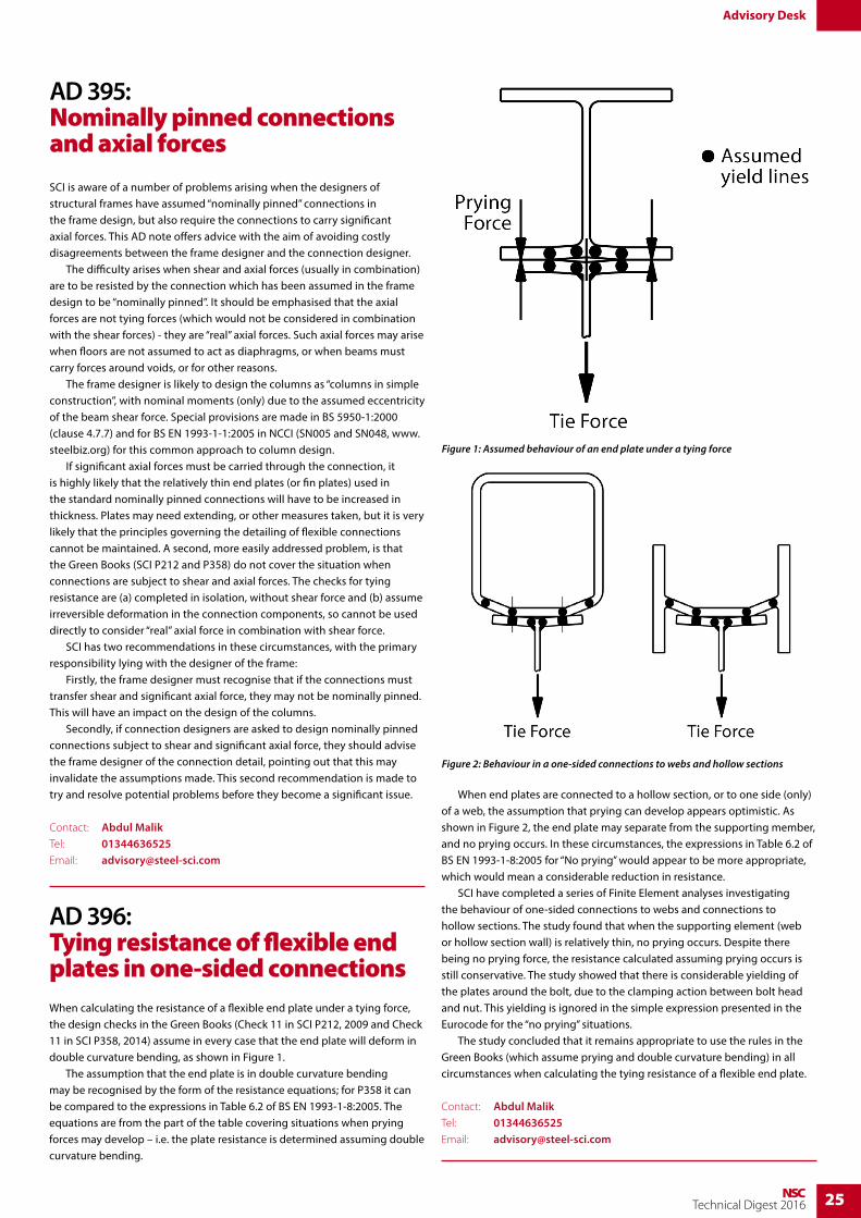
25NSCTechnical Digest 2016
Advisory Desk
When calculating the resistance of a flexible end plate under a tying force, the design checks in the Green Books (Check 11 in SCI P212, 2009 and Check 11 in SCI P358, 2014) assume in every case that the end plate will deform in double curvature bending, as shown in Figure 1. The assumption that the end plate is in double curvature bending may be recognised by the form of the resistance equations; for P358 it can be compared to the expressions in Table 6.2 of BS EN 1993-1-8:2005. The equations are from the part of the table covering situations when prying forces may develop – i.e. the plate resistance is determined assuming double curvature bending.
AD 396: Tying resistance of flexible end plates in one-sided connections
SCI is aware of a number of problems arising when the designers of structural frames have assumed “nominally pinned” connections in the frame design, but also require the connections to carry significant axial forces. This AD note offers advice with the aim of avoiding costly disagreements between the frame designer and the connection designer. The difficulty arises when shear and axial forces (usually in combination) are to be resisted by the connection which has been assumed in the frame design to be “nominally pinned”. It should be emphasised that the axial forces are not tying forces (which would not be considered in combination with the shear forces) - they are “real” axial forces. Such axial forces may arise when floors are not assumed to act as diaphragms, or when beams must carry forces around voids, or for other reasons. The frame designer is likely to design the columns as “columns in simple construction”, with nominal moments (only) due to the assumed eccentricity of the beam shear force. Special provisions are made in BS 5950-1:2000 (clause 4.7.7) and for BS EN 1993-1-1:2005 in NCCI (SN005 and SN048, www.steelbiz.org) for this common approach to column design. If significant axial forces must be carried through the connection, it is highly likely that the relatively thin end plates (or fin plates) used in the standard nominally pinned connections will have to be increased in thickness. Plates may need extending, or other measures taken, but it is very likely that the principles governing the detailing of flexible connections cannot be maintained. A second, more easily addressed problem, is that the Green Books (SCI P212 and P358) do not cover the situation when connections are subject to shear and axial forces. The checks for tying resistance are (a) completed in isolation, without shear force and (b) assume irreversible deformation in the connection components, so cannot be used directly to consider “real” axial force in combination with shear force. SCI has two recommendations in these circumstances, with the primary responsibility lying with the designer of the frame: Firstly, the frame designer must recognise that if the connections must transfer shear and significant axial force, they may not be nominally pinned. This will have an impact on the design of the columns. Secondly, if connection designers are asked to design nominally pinned connections subject to shear and significant axial force, they should advise the frame designer of the connection detail, pointing out that this may invalidate the assumptions made. This second recommendation is made to try and resolve potential problems before they become a significant issue.
Contact: Abdul MalikTel: 01344636525Email: [email protected]
AD 395: Nominally pinned connections and axial forces
When end plates are connected to a hollow section, or to one side (only) of a web, the assumption that prying can develop appears optimistic. As shown in Figure 2, the end plate may separate from the supporting member, and no prying occurs. In these circumstances, the expressions in Table 6.2 of BS EN 1993-1-8:2005 for “No prying” would appear to be more appropriate, which would mean a considerable reduction in resistance. SCI have completed a series of Finite Element analyses investigating the behaviour of one-sided connections to webs and connections to hollow sections. The study found that when the supporting element (web or hollow section wall) is relatively thin, no prying occurs. Despite there being no prying force, the resistance calculated assuming prying occurs is still conservative. The study showed that there is considerable yielding of the plates around the bolt, due to the clamping action between bolt head and nut. This yielding is ignored in the simple expression presented in the Eurocode for the “no prying” situations. The study concluded that it remains appropriate to use the rules in the Green Books (which assume prying and double curvature bending) in all circumstances when calculating the tying resistance of a flexible end plate.
Contact: Abdul MalikTel: 01344636525Email: [email protected]
Figure 1: Assumed behaviour of an end plate under a tying force
Figure 2: Behaviour in a one-sided connections to webs and hollow sections
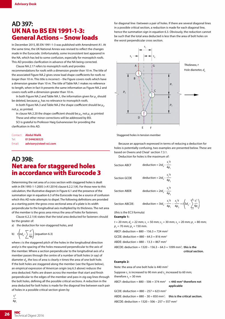
26 NSCTechnical Digest 2016
for diagonal line i between a pair of holes. If there are several diagonal lines in a possible critical section, a reduction is made for each diagonal line, hence the summation sign in equation 6.3. Obviously, the reduction cannot be such that the total area deducted is less than the area of bolt holes on the worst perpendicular cross section.
Because an approach expressed in terms of reducing a deduction for holes is potentially confusing, two examples are presented below. These are based on Owens and Cheal1 section 7.3.1. Deduction for holes is the maximum of:
Section ABCF deduction = 2td0 -s1
2t
4p1
Section GCDE deduction = 2td0 -s2
2t
4p2
Section ABDE deduction = 2td0 -s3
2t
4p3
Section ABCDE: deduction = 3td0 -s1
2t
4p1
= t 3d0 -si
2
4pi∑-
s22t
4p2
2
i=1( )
(this is the EC3 formula)Example 1:
t = 20 mm; d0 = 22 mm; s1 = 50 mm; s2 = 30 mm; s3 = 20 mm; p1 = 80 mm; p2 = 70 mm; p3 = 150 mm.
ABCF: deduction = 880 – 156.3 = 724 mm2
GCDE: deduction = 880 – 64.3 = 816 mm2
ABDE: deduction = 880 – 13.3 = 867 mm2
ABCDE: deduction = 1320 – 156.3 – 64.3 = 1099 mm2; this is the critical section.
Example 2:
Note: the area of one bolt hole is 440 mm2
Suppose s1 is increased to 90 mm and s2 increased to 60 mm; therefore s3 = 30 mm
ABCF: deduction = 880 – 506 = 374 mm2 < 440 mm2 therefore not applicable
GCDE: deduction = 880 – 257 = 623 mm2
ABDE: deduction = 880 – 30 = 850 mm2; this is the critical section.
ABCDE: deduction = 1320 – 506 – 257 = 557 mm2
Advisory Desk
In December 2015, BS EN 1991-1-3 was published with Amendment A1. At the same time, the UK National Annex was revised to reflect the changes made in the Eurocode. Unfortunately, some inconsistent text appeared in the NA, which has led to some confusion, especially for monopitch roofs. This AD provides clarification in advance of the NA being corrected. Clause NA.2.17 refers to monopitch roofs and provides recommendations for roofs with a dimension greater than 10 m. The title of the associated Figure NA.2 gives snow load shape coefficients for roofs no longer than 10 m. This title is incorrect – the Figure covers roofs which have a dimension greater than 10 m. The title of Table NA.1 makes no reference to length, when in fact it presents the same information as Figure NA.2 and covers roofs with a dimension greater than 10 m. In both Figure NA.2 and Table NA.1, the information given for μ2 should be deleted, because μ2 has no relevance to monopitch roofs. In both Figure NA.3 and Table NA.2 the shape coefficient should be μ2, not μ1 as printed. In clause NA.2.20 the shape coefficient should be μ4, not μ3 as printed These and other minor corrections will be addressed by BSI. SCI is grateful to Professor Haig Gulvanessian for providing the clarification in this AD.
Contact: Abdul MalikTel: 01344636525Email: [email protected]
AD 397: UK NA to BS EN 1991-1-3: General Actions – Snow loads
AD 398: Net area for staggered holes in accordance with Eurocode 3Determining the net area of a cross section with staggered holes is dealt with in EN 1993-1-1:2005 (+A1:2014) clause 6.2.2.1(4). For those new to this calculation, the illustrative diagram in Figure 6.1 and the presence of the summation sign in equation 6.3 of the Eurocode may be a source of confusion which this AD note attempts to dispel. The following definitions are provided as a starting point: the gross cross sectional area of a plate is its width perpendicular to the longitudinal axis multiplied by its thickness. The net area of the member is the gross area minus the area of holes for fasteners. Clause 6.2.2.1(4) states that the total area deducted for fasteners should be the greater of:a) the deduction for non-staggered holes, and
b) t nd0 -s2
4p∑( ) (equation 6.3)
where s is the staggered pitch of the holes in the longitudinal direction and p is the spacing of the holes measured perpendicular to the axis of the member. Where a section perpendicular to the longitudinal axis of a member passes through the centre of a number of bolt holes (n say) of diameter d0, the loss of area is clearly n times the area of one bolt hole. If the bolt holes are staggered along the member (see the figure below), an empirical expression of American origin (eq 6.3 above) reduces the area deducted. Paths are drawn across the member that start and finish perpendicular to the edges of the member and pass in zig-zag lines through the bolt holes, defining all the possible critical sections. A reduction in the area deducted for bolt holes is made for the diagonal line between each pair of holes in a possible critical section given by
si2
4pi

27NSCTechnical Digest 2016
Reference
1 Owens & Cheal, Structural Steelwork Connections, Butterworths 1989
Contact: Richard HendersonTel: 01344636525Email: [email protected]
AD 399: Design of partial penetration butt welds in accordance with BS EN 1993-1-8
Partial penetration butt welds are covered by Clause 4.7.2, which directs the designer to ‘use the method for a deep penetration fillet weld” given in clause 4.5.2(3). Clause 4.5.2(3) really concerns only the definition of the throat, and leaves the designer unsure of how the design resistance is to be calculated. Partial penetration welds are considered to be less ductile than full penetration welds and therefore many design Standards require that they are to be treated in the same way as fillet welds. This is the principle behind the advice in clause 4.7.2. Unless rotation is suitably restrained, eccentricity must be taken into account when calculating the stress in the weld. Examples of details where eccentricity is introduced in partial penetration butt welds are shown in Figure 4.9 of BS EN 1993-1-8. Eccentricity need not be considered if the weld is used as part of a weld group around the perimeter of a structural hollow section (clause 4.12(3)). It is reasonable to assume that there is no eccenticity if the welded element is part of a member which itself cannot rotate at the joint – for example if a partial penetration weld is used to connect the flange of a beam to an end plate. In the numerical example which follows, it is assumed that rotation cannot take place.
ThroatThe throat of a partial penetration butt weld is the distance from the root to the external face of the weld, as described in clause 4.5.2(1). Examples are shown in figure 1.
Common practice is to either (a) assume the penetration (and hence the design throat) is less than the preparation, or (b) to conduct weld procedure trials to demonstrate what penetration can consistently be achieved. The first approach was encouraged by the 1990 version of BS 5950, where clause 6.6.6.2 specified a reduction of 3 mm for V and bevel welds. Clause 6.9.2 of the 2000 version of BS 5950 specifies no reduction but refers to the depth of penetration, which may be more or less than the preparation.
Design resistanceIt is recommended the the directional method of clause 4.5.3.2(6) is used when calculating the resistance of a partial penetration butt weld. Assuming there is no longitudinal stress, the direct stress must be resolved into a
Advisory Desk
perpendicular stress on the throat, σ⊥ and a shear stress on the throat, τ⊥. Expression 4.1 of BS EN 1993-1-8 requires that the combination of perpendicular stresses are verified and also limits the perpendicular stress. With no longitudinal stress on the weld throat, the verifications become:
(σ⊥2 + 3τ⊥2)0.5 ≤fu
βWγM2 and
σ⊥ ≤
0.9fu
γM2
In case (b) of figure 1, assuming the applied force is 2000 N/mm, and the throat is 9 mm, the components of force become: σ⊥ = 2000 Cos(33)/9 = 186 N/mm2 and τ⊥ = 2000 Sin(33)/9 = 121 N/mm2
The combined check of shear and perpendicular stress, with βw = 0.9 for S355 (taken from Table 4.1) becomes:
(1862 + 3(121)2)0.5 = 280 N/mm2. The limit is 4700.9 × 1.25
= 418 N/mm2
The perpendicular stress σ⊥ is 186 N/mm2; the limit is 0.9 × 470
1.25
= 338 N/mm2
Of course, if a standard fillet weld is verified by the same process, using an angle to the throat of 45°, it can be demonstrated that the resistances are those quoted in the Blue Book1 for a transverse weld.
Reference
1 Steel building design: Design data. In accordance with Eurocodes and UK
National Annexes (P363). SCI, Reprinted 2015.
Contact: Abdul MalikTel: 01344636525Email: [email protected]
a a
a
33°
(a) (b) (c)
Figure 1: Throat (a) of partial penetration welds
AD 400: The degree of shear connection in composite beams and SCI P405
The stud resistances presented in both BS 5950-3.1 (as amended in 2010) and BS EN 1994-1-1 are lower than those given in the previous British Standard. This has resulted in many composite beam designs (that were previously satisfactory) becoming impossible to verify because the maximum number of studs that can be accommodated on a beam is often less than the number of studs needed to satisfy rules for minimum degree of shear connection. The rules given in SCI P4051 complement those given in BS EN 1994-1-1 by allowing the user to take into account more parameters (affecting the requirements for shear connection) than are explicitly covered by the Eurocode. This means that, in many cases, the problems encountered by designers in satisfying the minimum degree of shear connection requirements can be overcome. P405 offers minimum degree of shear connection rules that are tailored to a range of cases:
• Both propped and unpropped construction.• Both transverse and parallel decking cases are covered as the deck
orientation can have a significant impact on the required degree of shear connection.
• Beams that are only part utilised in bending (because their design is governed by serviceability considerations).
• Beams that carry high levels of loading, as found in plant rooms.• Cellular beams, i.e. beams with regularly spaced, large circular web
openings.The lower bound minimum degree of shear connection of 40% that is specified in BS EN 1994-1-1 and BS 5950-3.1 is modified in P405 accounting for the parameters indicated above. However, there remains a need for an absolute limit, to avoid the shear studs going beyond their elastic range under SLS loading. This is to prevent cumulative plastic deformation of the shear connection under repeated loading.
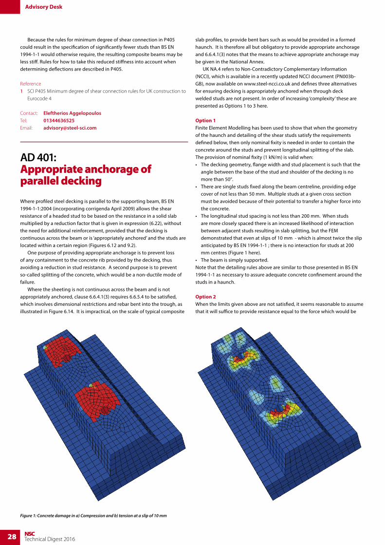
28 NSCTechnical Digest 2016
slab profiles, to provide bent bars such as would be provided in a formed haunch. It is therefore all but obligatory to provide appropriate anchorage and 6.6.4.1(3) notes that the means to achieve appropriate anchorage may be given in the National Annex. UK NA.4 refers to Non-Contradictory Complementary Information (NCCI), which is available in a recently updated NCCI document (PN003b-GB), now available on www.steel-ncci.co.uk and defines three alternatives for ensuring decking is appropriately anchored when through deck welded studs are not present. In order of increasing ‘complexity’ these are presented as Options 1 to 3 here.
Option 1Finite Element Modelling has been used to show that when the geometry of the haunch and detailing of the shear studs satisfy the requirements defined below, then only nominal fixity is needed in order to contain the concrete around the studs and prevent longitudinal splitting of the slab. The provision of nominal fixity (1 kN/m) is valid when:• The decking geometry, flange width and stud placement is such that the
angle between the base of the stud and shoulder of the decking is no more than 50°.
• There are single studs fixed along the beam centreline, providing edge cover of not less than 50 mm. Multiple studs at a given cross section must be avoided because of their potential to transfer a higher force into the concrete.
• The longitudinal stud spacing is not less than 200 mm. When studs are more closely spaced there is an increased likelihood of interaction between adjacent studs resulting in slab splitting, but the FEM demonstrated that even at slips of 10 mm - which is almost twice the slip anticipated by BS EN 1994-1-1 ; there is no interaction for studs at 200 mm centres (Figure 1 here).
• The beam is simply supported.Note that the detailing rules above are similar to those presented in BS EN 1994-1-1 as necessary to assure adequate concrete confinement around the studs in a haunch. Option 2When the limits given above are not satisfied, it seems reasonable to assume that it will suffice to provide resistance equal to the force which would be
Figure 1: Concrete damage in a) Compression and b) tension at a slip of 10 mm
Advisory Desk
Because the rules for minimum degree of shear connection in P405 could result in the specification of significantly fewer studs than BS EN 1994-1-1 would otherwise require, the resulting composite beams may be less stiff. Rules for how to take this reduced stiffness into account when determining deflections are described in P405.
Reference
1 SCI P405 Minimum degree of shear connection rules for UK construction to
Eurocode 4
Contact: Eleftherios AggelopoulosTel: 01344636525Email: [email protected]
AD 401: Appropriate anchorage of parallel decking
Where profiled steel decking is parallel to the supporting beam, BS EN 1994-1-1:2004 (incorporating corrigenda April 2009) allows the shear resistance of a headed stud to be based on the resistance in a solid slab multiplied by a reduction factor that is given in expression (6.22), without the need for additional reinforcement, provided that the decking is continuous across the beam or is ‘appropriately anchored’ and the studs are located within a certain region (Figures 6.12 and 9.2). One purpose of providing appropriate anchorage is to prevent loss of any containment to the concrete rib provided by the decking, thus avoiding a reduction in stud resistance. A second purpose is to prevent so-called splitting of the concrete, which would be a non-ductile mode of failure. Where the sheeting is not continuous across the beam and is not appropriately anchored, clause 6.6.4.1(3) requires 6.6.5.4 to be satisfied, which involves dimensional restrictions and rebar bent into the trough, as illustrated in Figure 6.14. It is impractical, on the scale of typical composite
needed to ‘unfold’ the profile if it were subject to transverse tension, as this sets a limit to the containment provided by the profiled decking. It can readily be calculated that a 60 mm deep profile, 0.9 mm thick, grade S450, with plastic hinges top and bottom, will unfold at less than 4 kN/m. Fixings at 250 mm centres, which is also a spacing close enough to ensure reasonable proximity to the zone of influence of any one stud, should suffice to provide this level of fixity. With thicker decking, the bearing resistance of the screw or nail will improve more than commensurately with the demands made on it. With a profile depth less than 60 mm, a more relaxed view can be taken, as the studs should normally be at least 95 mm in height (100 mm, if welded direct to the beam), reducing the need for containment. It seems reasonable to provide fixings at 250 mm, as for the deeper profile.
Option 3The third option open to designers is to provide additional reinforcement in the haunch, in accordance with BS EN 1994-1-1, clause 6.6.5.4.
Contact: Graham CouchmanTel: 01344636525Email: [email protected]
AD 402: Design of end plate joints made with preloaded bolts subject to coincident shear and tension.Advisory Desk note AD373 gave a summary of the checks required on connections subject to combined shear and tension. This AD note discusses the behaviour of such a connection in more detail. Where a preloaded bolt in a joint is subject to a tensile force, the preload is theoretically not affected but the clamping force between the plates is reduced. This is based on the assumption that the bolt acts as a spring and the plates are infinitely stiff. In reality, the plates are not infinitely stiff and the clamping force is only reduced by 80% of the applied tension. Where a bolted joint consisting of end plates and preloaded bolts is subject to both shear and
Search for Advisory Desk articles on newsteelconstruction.com
Use the search bar at the top of every page of newsteelconstruction.com to search out Advisory Desk articles by name, number or subject, or list them (most recent first) by hovering over Technical in the main menu and selecting
Advisory Desk from the resulting pop-up menu.
ksnμ
γM3
Fs,Rd = Fp,C – 0.8Ft,Ed,ser ( )
ksnμ
γM3
Fp,C – 0.8Ft,Ed =1.0 × 1.0 × 0.4
1.25× (137.2 – 50) = 27.9kNFs,Rd = ( )
Advisory Desk
tension, the applied tension reduces the clamping force between the faying surfaces and the shear resistance of the joint is therefore also reduced. Bolted joints designed with preloaded bolts are categorized in Table 3.2 of BS EN 1993-1-8:2005 either as shear connections: B (slip-resistant at serviceability), C (slip-resistant at ultimate) or as tension connections: E (preloaded). If a joint of the type described is subject to both shear and tension, and it is necessary to eliminate slip at either serviceability or ultimate limit states (category B or C), additional preload is required in the joint which may mean additional bolts to ensure no slip occurs. Clause 3.9.2 deals with this issue and formulae for the design slip resistance per bolt are given in equations 3.8a and 3.8b for category B and C connections respectively. In each case, the bolt preloading force is reduced by 80% of the tension force in the bolt as result of the design value of the loading (effect of actions), to allow for the flexibility of the end plates. For example, for the serviceability case, equation (3.8a) is:
Prying action results in an increased bolt tension and an equal and opposite compression between the plates in the joint. There is therefore no reduction in clamping force due to prying and Ft,Ed does not need to include any prying force. Consider an end plate joint made with eight M20 grade 8.8 bolts subject to a shear of 200 kN and a coincident tension of 500 kN. If we assume the holes are normal, there is one friction plane, the friction surface is class B and the joint is class C, the preloading force in a bolt is 137.2 kN. The tension per bolt is 62.5 kN so the reduction in preload per bolt is 50 kN. The design slip resistance of a grade 8.8 or 10.9 preloaded bolt is given in clause 3.9.1(2) as:
The design shear divided by the design slip resistance is 200/27.9 = 7.2 so eight bolts are required. If no tension were present, six bolts would be sufficient to carry the design shear force.
Contact: Richard HendersonTel: 01344636525Email: [email protected]

SIGN UP FOR YOUR FREE SUBSCRIPTION
TO NSC MAGAZINE
NSC magazine is available free of charge in a paper format for the UK and Ireland as well as in a digital format for use on tablets, smartphones and desktop computers.
A regularly updated website also carries news of steel construction issues and projects, as well as the NSC digital library containing the current issue and archives.
Here’s how to register for your copy
If you already have an account:• Login using the normal
‘Login / create account’ button in the top left corner (If you cannot remember your password, use the ‘Email new password’ button)
• Go to the ‘Toolbox’ sidebar menu on the lower left hand side
• Select ‘My Pro� le’
• Tick the box to receive either digital or printed NSC magazine, or both
• Click ‘Save’
If you don’t have an account:• Click the ‘Login / create
account’ button in the top left corner
• Click the ‘Create an account’ blue link in the Login box
• Enter the required details to create an account
• Tick the box to receive either digital or printed NSC magazine, or both
• Click ‘Save’
or
Email your details to [email protected]
Visit www.steelconstruction.info