Tax Evasion and Economic Growth∗

Jordi Caballé† Judith Panadés‡

June 2000

Abstract

In this paper we analyze how the tax compliance policy affects the rate ofeconomic growth. We consider a model of overlapping generations in which thepaths of all the macroeconomic variables are endogenously determined and weperform the comparative statics analysis of changes in both the probability ofinspection and the penalty fee imposed on tax evaders. We also show the non-optimality from the growth viewpoint of an inspection policy inducing truthfulrevelation of income for exogenously given levels of both the penalty and thetax rates. Finally, we show that ”hanging evaders with probability zero” isthe most growth enhancing policy among all the inspection policies inducinghonest behavior by the taxpayers.

JEL classification code: H26, O41.

Keywords: Tax Evasion, Endogenous Growth, Fiscal Policy.

∗ Financial support from the Spanish Ministry of Education through grant PB96-1160-C02-02and the Generalitat of Catalonia through grant SGR98-62 is gratefully acknowledged. We wantto thank Inés Macho, Pau Olivella, and a referee of this journal for their valuable suggestions. Ofcourse, they should not bear any responsibility for the remaining errors.

† Unitat de Fonaments de l’Anàlisi Econòmica and CODE. Universitat Autònoma de Barcelona.‡ Unitat de Fonaments de l’Anàlisi Econòmica. Universitat Autònoma de Barcelona.

Correspondence address: Jordi Caballé. Universitat Autònoma de Barcelona. Departamentd’Economia i d’Història Econòmica. Edifici B. 08193 Bellaterra (Barcelona). Spain.

1 Introduction

The aim of this paper is to analyze how the tax compliance policy affects the rateof economic growth. It is well known that proportional taxation matters for growthsince taxes distort the accumulation of capital. It is usually found in standard growthmodels with infinite horizon that the rate at which either physical or human capitalis accumulated increases with their private return (see, among many others, Lucas(1988), Lucas (1990), and Rebelo (1991)) and, hence, high tax rates on income aretypically associated with low growth rates.Moreover, in overlapping generation models displaying endogenous growth,

individuals face a finite life span and the capital accumulation is a direct consequenceof the saving of the young individuals who earn a wage in exchange of the labor theyhire to the firms. In this kind of models young individuals must purchase all thecapital installed in the economy during the next period. Therefore, an increase inthe income tax rate reduces the disposable income of the workers and, thus, capitalaccumulation becomes also slower. Furthermore, since the after-tax interest ratedecreases, savings will also fall provided the elasticity of intertemporal substitutionis high enough to generate a saving function that is increasing in the interest rates(see Jones and Manuelli (1992)).On the other hand, taxation is also affecting the process of economic growth since

it generates resources to finance the supply of the productive inputs provided by thegovernment (see, for instance, Barro (1990) and Turnovsky (1997)). Such inputs takeusually the form of public goods, like roads or public education. Since firms are notcharged by the use of these public goods, government spending plays the role of anexternality for the productive sector. Such an externality ends up being a engine ofendogenous growth since the resulting aggregate production function could display anuniformly high marginal productivity from private capital, and this makes perpetualcapital accumulation possible (see Jones and Manuelli (1990)). Therefore, as pointedby Barro (1990), there is a tension between the role of taxation in disincentiving theaccumulation of capital and the role of the public spending financed by these taxesin raising the return from private capital and, hence, the speed of accumulation.Obviously, an effective tax system must be enforceable, that is, it must provide

incentives to the taxpayers for tax compliance. Without these incentives nobodywould pay taxes voluntarily in a competitive economy. Therefore, it seems pertinentto have a closer look to the instruments that allow the government to enforce the taxsystem. The two complementary instruments available to the tax collecting agencyin order to enforce the tax legislation are the inspections and the fines imposed ontax evaders. We thus analyze the effects of changes in the parameters characterizingthese two policy instruments on the rate of economic growth. To this end, we have toconsider a dynamic general equilibrium model in which the paths of aggregate output,wages, interest rates, saving and consumption are all endogenously determined. Weshould mention at this point that the literature has paid little attention to the

1

macroeconomic implications of tax evasion.1

Our general equilibrium approach forces us to an extreme stylization of theeconomy under study. Thus, we consider an overlapping generations model withproduction à la Diamond (1965) for which we parametrize both preferences andtechnologies. In such an economy young individuals obtain an income accruingfrom the labor services they supply to the firms. There is a proportional tax ondeclared labor income and collected taxes will finance productive inputs supplied bythe government. Note that we have then all the elements necessary to reproduce thetension between government revenues and public spending since collected taxes willdiscourage savings whereas public spending will raise the marginal productivity ofprivate capital.We will assume that under-reporting of income is a risky and illegal activity.

Agents are investigated with positive probability and, if a taxpayer is caught evading,she must pay a proportional penalty on the amount of evaded taxes, as in Yitzhaki(1974). The proceeds from penalties levied to the tax payers that are caught under-reporting are also used to finance public capital. Therefore, the enforcement policyhas real effects since it generates funds to finance public capital formation throughtwo channels: (i) it makes taxpayers to behave more honestly so that they end uppaying more taxes and (ii) it generates additional resources accruing from the finespaid by audited evaders.The combination of the penalty fee, the audit probability, and the tax rate

determines not only the amount of declared income, but also the amount of laborincome saved which will be used for consumption in the next period. Such asaving determines the private capital installed in the economy that, together withpublic capital, determines in turn the evolution of all the remaining macroeconomicvariables. The economy will end up displaying a balanced growth path which isparametrized by its corresponding endogenous rate of long-term growth.Our main findings include the comparative statics of the two tax compliance

instruments on the aforementioned endogenous rate of long-term growth. Sucha comparative statics is generally ambiguous and depends on the importance ofpublicly provided inputs in the production process. Such an ambiguity arises since theconfigurations of probability of audit and penalty for under-reporting that increaseoverall tax revenues will also increase growth through the public capital formationchannel. However, since a greater overall tax revenue means less disposable incomefor individuals, there will be less saving, less investment, and lower rates of growth.Obviously, the net effect on growth will generally depend on the relative elasticity ofoutput with respect to the two types of capital.In our analysis the combination of the audit probability and the penalty fee

determines whether individuals become partial evaders, total evaders (i.e., they

1The papers of Peacock and Shaw (1982), Ricketts (1984), Lai and Chang (1988), Lai, Chang andChang (1995) and Chang and Lai (1996) are among the few exceptions that introduce macroeconomicconsiderations in the analysis of tax evasion. However, all these papers rely on variants of thetraditional Keynesian (IS-LM) model in which neither the dynamics nor the maximizing behaviourof consumers are made explicit. Moreover, they concentrate the analysis on the relationship betweentax evasion and total tax collection.

2

do not even fill their income report), or honest taxpayers (i.e., they declare theirtotal income). We characterize the effects on long-term growth of changing thetax compliance parameters in the previous three scenarios and, in some cases, wecan make the result of the comparative statics exercises independent of the relativeproductivity of the two types of capital. For instance, when taxpayers behavehonestly, an increase in the penalty rate has no consequences whereas an increase inthe probability of inspection amounts to incur in a useless additional cost associatedwith the inspection effort. Such a waste of resources immediately translates into lowerspeed of accumulation in equilibrium.We also provide two other results also found in partial equilibrium analyses

of the tax evasion problem. The first one refers to the non-optimality from thegrowth viewpoint of an inspection policy inducing truthful revelation of income forexogenously given levels of both the penalty and the tax rates. This result followssince, if there is truthful revelation, then a slight reduction in the costly inspectioneffort reduces negligibly the amount of collected taxes whereas the resources liberatedby the tax collection agency can be devoted to the provision of growth enhancingpublic services. The second result refers to the growth maximizing combinationof the two instruments. Such a combination depends on how productive is publiccapital relative to private capital. In particular, if inducing complete tax complianceis optimal, then a policy with an arbitrarily high penalty fee and a low inspectionprobability allows the implementation of a growth rate arbitrarily close to that of aneconomy without tax evasion.The paper is organized as follows. Section 2 presents the taxpayer optimization

problem. Section 3 determines the equilibrium of the economy from the interactionamong consumers, firms and the government. Section 4 analyzes the implications ofthe tax enforcement policy for economic growth. Section 5 concludes the paper.

2 The Tax Evasion Problem

Let us consider an overlapping generations (OLG) economy populated by a continuumof identical individuals living for two periods. A new generation is born in each periodand there is no population growth. Generations are indexed by the period in whichthey are born. Individuals own a unit of labor when they are young (the first periodof their lives) and this unit of labor is supplied inelastically to the firms in exchangeof a wage. Labor income is subjected to a proportional tax and the tax rate isτ ∈ (0, 1). An individual of generation t declares a level xt of labor income duringthe first period of life. Therefore, the amount of taxes paid voluntarily will be τxt.Since tax evasion is possible, xt might be less than the real wage wt. With probabilityp ∈ (0, 1) individuals are subjected to investigation by the tax authority and, if suchan investigation takes place, the tax collecting agency detects the true labor incomeearned by the taxpayer. In such a case, the taxpayer will have to pay a proportionalpenalty rate π > 1 on the amount of evaded taxes τ (wt − xt). Note that, even ifthere is no uncertainty in our model, the tax authority must audit an individualto indisputably certify that she is an evader and to impose her the correspondingpenalty.

3

Our specification of the tax evasion problem is thus the same as in Yitzhaki (1974)since the penalty is imposed on evaded taxes while Allingham and Sandmo (1972)assume instead that the penalty is on undeclared income. Note however that, ifthe tax rate τ is exogenously given, all our analysis can be adapted to the setup ofAllingham and Sandmo by replacing the penalty rate π by bπ /τ , where bπ would bethe penalty rate on unreported income.We now introduce two doses of realism in the tax system in order to prevent

counterfactual behavior by the taxpayers. First, if an individual has declared morethan her true labor income, and this individual is audited, then the excess taxcontribution is just returned. In other words, the penalty rate applying to ”negative”tax evasion is 1. Under such an assumption, no individual will declare more thanher true wage because excess tax contribution is in fact a risky investment having anegative risk premium.2

Second, the tax legislation does not feature a ”loss offset”. This means that thetax rate applying to negative income is zero. Hence, the tax code establishes thatonly agents declaring positive income must fill the tax form and pay the correspondingtaxes on declared income. Note that individuals not filling the tax form are in factimplicitly declaring that they have earned a labor income equal to zero.The sequence of events is the following. First, young individuals work and receive

their wages. Then, they fill the report where they voluntarily declare the labor incomethey have earned and they pay the corresponding taxes. Consumption in the firstperiod of life takes place. Let st denote the income disposable after an individualhas consumed and paid the taxes on declared income. Then, the potential inspectionoccurs with probability p. Obviously, the effective saving of an agent which has notbeen audited is st while the saving of an audited agent will be st−πτ (wt − xt). Thegross rate of return on the amount effectively saved is Rt+1. Capital income willbe consumed when individuals are old (i.e., in the second period of life). An oldindividual does not have any other source of income and thus her consumption willbe Rt+1 (st − πτ (wt − xt)) if she has been audited, or Rt+1st if she has not. Since theinspection occurs after consumption has taken place, taxing the income of old agentsis not enforceable and, therefore, capital income is tax exempt.The following table summarizes the sequence of events within each period of life:

2Recall that risk averse agents take risky positions if and only if the associated risk premium isstrictly positive (see Arrow (1970)).

4

First period of lifeIndividuals work.Wages are paid.

Individuals declare their labor incomeand pay the corresponding taxes.Young consumption takes place.

Tax inspection occurs with probability pand the corresponding penalty is paid.

Capital market opens andeffective saving takes place.

Second period of life

Return on saving is paid.

Old consumption takes place.

The preferences of an agent of generation t are represented by the time-additiveVon Neumann-Morgenstern utility function

u¡C1t

¢+ δE

³u³ eC2

t+1

´´, (1)

where C1t denotes consumption in the individual’s first period of life (young

consumption) and eC2t+1 is the random consumption in the second period of life

(old consumption). The random variable eC2t+1 takes two values, C

2At+1 and C2N

t+1,which correspond to old consumption if the individual has been audited, and oldconsumption if she has not been audited, respectively. The parameter δ > 0 is thediscount factor.Therefore, an individual of generation t chooses both the declared income

xt ∈ [0, wt] and the intended saving st in order to solve the following program:

Max©u¡C1t

¢+ (1− p) δu

¡C2Nt+1

¢+ pδu

¡C2At+1

¢ª, (2)

subject toC1t = wt − τxt − st,

C2Nt+1 = Rt+1st, and

C2At+1 = Rt+1 (st − πτ (wt − xt)) .

For tractability we will assume that the expected utility representation u islogarithmic, i.e., u (C) = lnC. The analysis can be generalized to an isoelasticutility, u (C) = C1−σ−1

1−σ with σ > 0. However, this generalization will yield a savingfunction that will not be independent of the interest rate and this will substantiallycomplicate the analysis. In fact, the relationship between saving and the interestrate is an unsolved empirical question and to build a model abstracting from sucha relationship is thus a reasonable, defensive position.3 Clearly, our results will be

3It should be noticed that the Von Neumann-Morgenstern utility function (1) is time-additive,homothetic, and exhibits a saving function that is independent of the interest rate if and only if uis logarithmic.

5

qualitatively similar if we assume instead isoelastic utilities having a parameter σsufficiently close to 1. As we will see, a policy leading to greater enforcement (due toan increase either in p or in π) will modify the long-term interest rate and, thus, ifsaving were not independent of the interest rate, we will have a new channel throughwhich the tax compliance policy could influence the rate of capital accumulation.

Lemma 1 The solution to the individual’s optimization program (2) is given by

xt = Xwt, and st = Swt,

where

X =

⎧⎪⎪⎪⎪⎪⎪⎪⎪⎨⎪⎪⎪⎪⎪⎪⎪⎪⎩

0 if pπ ≤ (τ + δ) p

τ(1 + δ) + δ(1− τ)p,

(1− p)τ(1 + δpπ)− (1− pπ)(pδ + τ)

pτ(π − 1)(1 + δ)if (τ+δ)p

τ(1+δ)+δ(1−τ)p < pπ < 1,

1 if pπ ≥ 1,

(3)

and

S =

⎧⎪⎪⎪⎪⎪⎪⎪⎪⎪⎪⎨⎪⎪⎪⎪⎪⎪⎪⎪⎪⎪⎩

S1 if pπ ≤ (τ + δ) p

τ(1 + δ) + δ(1− τ)p,

πδ(1− p)(1− τ)

(π − 1)(1 + δ)if

(τ + δ) p

τ(1 + δ) + δ(1− τ)p< pπ < 1,

δ(1− τ)

(1 + δ)if pπ ≥ 1,

(4)

with

S1 =(δ + (1 + δ(1− p))πτ) +

p(δ + (1 + δ(1− p))πτ)2 − 4δπτ(1− p)(1 + δ)

2(1 + δ). (5)

Proof. See the appendix.

Notice that intended saving before tax inspection st and reported income xt areboth linear in actual wages. From (3) we see that the condition for obtaining aninterior solution for declared income, xt ∈ (0, wt) , can be rewritten as

(τ + δ)

τ(1 + δ) + δ(1− τ)p< π <

1

p. (6)

It should be pointed out that the inequalities in (6) are satisfied by a plausibleparameter configuration like

τ = 0.25, π = 3, p = 0.05, δ = 0.425. (7)

6

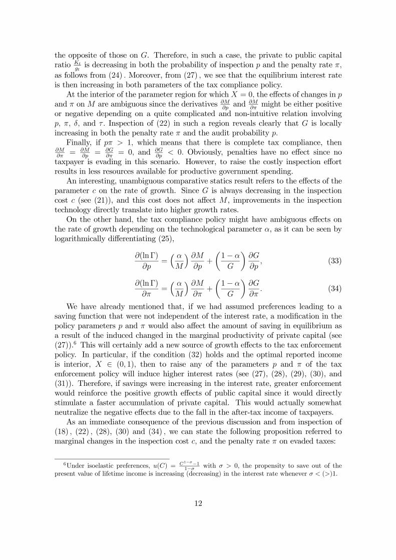
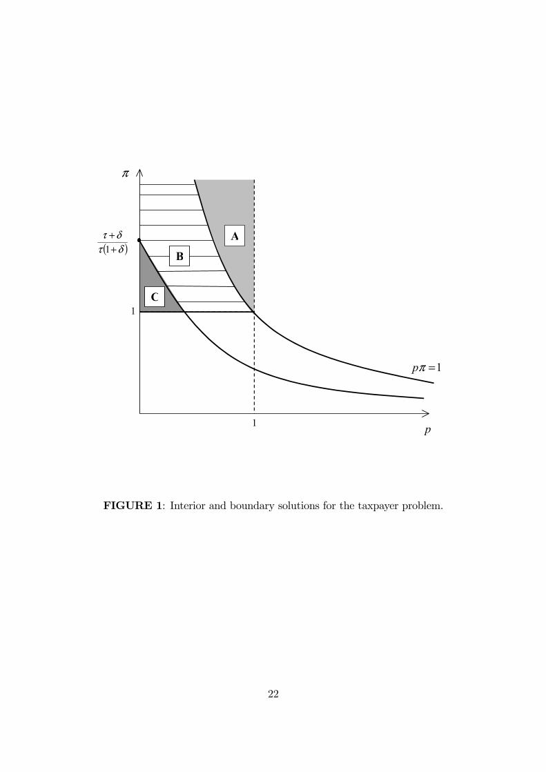
Figure 1 shows the regions of the parameters p and π for which we obtain eitherinterior or corner solutions for the declared income xt. In the interior of region B,the optimal solution satisfies xt ∈ (0, wt) whereas xt = wt in region A and xt = 0in region C. The function of p defining the frontier between regions B and C is thedecreasing and convex hyperbole given by the first expression in (6) . Note that such

an expression becomes equal to (τ+δ)τ(1+δ)

whenever p = 0. The frontier between regionsA and B is clearly another hyperbole given by the locus satisfying pπ = 1. Therefore,for a given value of p ∈ (0, 1), it is clear that the set of values of the penalty rate πfor which xt ∈ (0, wt) constitutes an open interval (π, π) with

π =(τ + δ)

τ(1 + δ) + δ(1− τ)p∈µ1,1

p

¶and π = 1

p. Moreover, for a given value of the penalty rate π > 1, the set of values of

the audit probability p for which xt ∈ (0, wt) constitutes also an open interval¡p, p¢

with p = 1π. The infimum p of this interval is equal to zero when the mild condition

π ≥ (τ + δ)

τ(1 + δ)(8)

is imposed whereas p ∈ ¡0, 1π

¢when the weak inequality in (8) does not hold.

[Insert Figure 1 about here]

The following partial derivatives concerning the behavior of both the propensityto declare X and the propensity to save S for an interior solution are obtained from(3) and (4):

∂X

∂p=

πδ(1− τ)

τ(π − 1)(1 + δ)> 0,

∂X

∂π=

δ(1− p)(1− τ)

τ(π − 1)2(1 + δ)> 0,

∂S

∂p=−δπ(1− τ)

(π − 1)(1 + δ)< 0,

∂S

∂π=−δ(1− p)(1− τ)

(π − 1)2(1 + δ)< 0.

As expected, reported income is increasing in both the probability of investigationand the penalty rate π. Since individuals increase the income reported with p and π,this immediately translates into a decrease of intended saving.The effects of marginal changes in the policy parameters on the propensity to save

S when pπ < (τ+δ)pτ(1+δ)+δ(1−τ)p can be obtained directly from implicitly differentiating

the fist order condition of problem (2) . Since xt = 0 in such a parameter region, thefirst order condition with respect to st is

−u0 (wt − st)] + (1− p)Rt+1u0 (Rt+1st) + pRt+1u

0 (Rt+1 (st − πτwt)) = 0. (9)

7

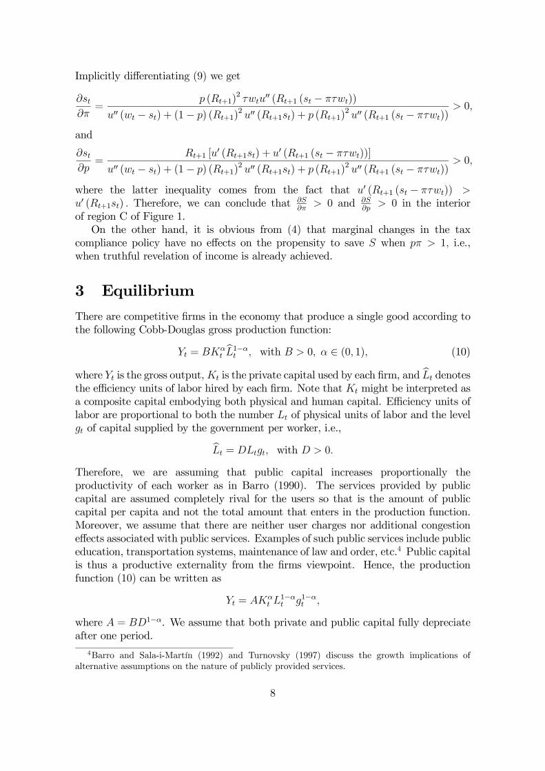
Implicitly differentiating (9) we get

∂st∂π

=p (Rt+1)

2 τwtu00 (Rt+1 (st − πτwt))

u00 (wt − st) + (1− p) (Rt+1)2 u00 (Rt+1st) + p (Rt+1)

2 u00 (Rt+1 (st − πτwt))> 0,

and

∂st∂p

=Rt+1 [u

0 (Rt+1st) + u0 (Rt+1 (st − πτwt))]

u00 (wt − st) + (1− p) (Rt+1)2 u00 (Rt+1st) + p (Rt+1)

2 u00 (Rt+1 (st − πτwt))> 0,

where the latter inequality comes from the fact that u0 (Rt+1 (st − πτwt)) >u0 (Rt+1st) . Therefore, we can conclude that

∂S∂π

> 0 and ∂S∂p

> 0 in the interiorof region C of Figure 1.On the other hand, it is obvious from (4) that marginal changes in the tax

compliance policy have no effects on the propensity to save S when pπ > 1, i.e.,when truthful revelation of income is already achieved.

3 Equilibrium

There are competitive firms in the economy that produce a single good according tothe following Cobb-Douglas gross production function:

Yt = BKαtbL1−αt , with B > 0, α ∈ (0, 1), (10)

where Yt is the gross output,Kt is the private capital used by each firm, and bLt denotesthe efficiency units of labor hired by each firm. Note that Kt might be interpreted asa composite capital embodying both physical and human capital. Efficiency units oflabor are proportional to both the number Lt of physical units of labor and the levelgt of capital supplied by the government per worker, i.e.,bLt = DLtgt, with D > 0.

Therefore, we are assuming that public capital increases proportionally theproductivity of each worker as in Barro (1990). The services provided by publiccapital are assumed completely rival for the users so that is the amount of publiccapital per capita and not the total amount that enters in the production function.Moreover, we assume that there are neither user charges nor additional congestioneffects associated with public services. Examples of such public services include publiceducation, transportation systems, maintenance of law and order, etc.4 Public capitalis thus a productive externality from the firms viewpoint. Hence, the productionfunction (10) can be written as

Yt = AKαt L

1−αt g1−αt ,

where A = BD1−α. We assume that both private and public capital fully depreciateafter one period.

4Barro and Sala-i-Martín (1992) and Turnovsky (1997) discuss the growth implications ofalternative assumptions on the nature of publicly provided services.

8

Taking gt as given, the optimal demands for private capital and workers by firmsmust satisfy the first order conditions for profit maximization

wt = A(1− α)Kαt L

−αt g1−αt , (11)

andRt = AαKα−1

t L1−αt g1−αt . (12)

Given the constant returns to scale assumption, competitive firms will make zeroprofits and its number remains thus indeterminate. We normalize the number offirms to one per worker. Hence, equilibrium in the labor market implies that Lt = 1for all t. Therefore, (11) and (12) become in equilibrium

wt = A(1− α)Kαt g

1−αt , (13)

andRt = AαKα−1

t g1−αt . (14)

On the other hand, equilibrium in the capital market implies that effective savingmust be equal to the private capital installed in the next period,

Kt+1 = (1− p)st + p(st − πτ (wt − xt)). (15)

Since in this large economy a fraction p of individuals is subjected to tax investigation,the first term on the RHS of (15) is the effective saving of the non-audited populationwhereas the second term is the effective saving of the audited population. Substitutingst and xt by their optimal values given in Lemma 1, (15) becomes

Kt+1 =Mwt, (16)

whereM = S − pπτ(1−X). (17)

Note that M > 0 since effective saving after inspection is strictly positive. Using (3)and (4) to substitute for X, and S, we get the following explicit expression for M :

M =

⎧⎪⎪⎪⎪⎪⎪⎪⎪⎪⎨⎪⎪⎪⎪⎪⎪⎪⎪⎪⎩

S1 − pπτ if pπ ≤ (τ + δ) p

τ(1 + δ) + δ(1− τ)p,

πδ(1− τ)(1− 2p+ p2π)

(π − 1)(1 + δ)if

(τ + δ) p

τ(1 + δ) + δ(1− τ)p< pπ < 1,

δ (1− τ)

1 + δif pπ ≥ 1,

(18)

where S1 is given in (5) .The government finances the stock of public capital by means of both the

proportional taxes on declared income and the penalty fees collected from the auditedtaxpayers in the previous period. We assume that the government faces a proportional

9

inspection cost c per unit of audited income. Therefore, the budget constraint of thegovernment is

gt+1 = (1− p)τxt + p(τxt + πτ(wt − xt))− cpwt, (19)

where the first term on the RHS of (19) are the taxes paid by the non-auditedtaxpayers, the second term are the taxes plus the penalty fees paid by auditedtaxpayers, and the last term is the cost associated with tax inspection. Substitutingthe equilibrium value of xt given in Lemma 1, we get

gt+1 = Gwt, (20)

whereG = (1− pπ)τX + pπτ − cp. (21)

We can use (3) to get an explicit expression for G in terms of the exogenousparameters,

G =

⎧⎪⎪⎪⎪⎪⎨⎪⎪⎪⎪⎪⎩

p (πτ − c) if pπ ≤ (τ+δ)pτ(1+δ)+δ(1−τ)p ,

(1−pπ)(τ(π−1)+δπτ(1−p)−δ(1−pπ))(π−1)(1+δ) + pπτ − cp if (τ+δ)p

τ(1+δ)+δ(1−τ)p < pπ < 1,

τ − cp if pπ ≥ 1.

(22)

We will assume that τ > c since this assumption, together with the fact thatX ∈ [0, 1], ensures that G is strictly positive. That is, if the unitary cost of inspectionc is lower than the tax rate, the tax system always generates resources for positivepublic spending. Plugging (13) into (20) we obtain

gt+1 = GA(1− α)Kαt g

1−αt ,

which can be rewritten as

gt+1gt

= GA(1− α)

µKt

gt

¶α

. (23)

Furthermore, divide (16) by (20) and get

Kt

gt=

M

G, (24)

so that (23) becomes

Γ ≡ gt+1gt

= GA(1− α)

µM

G

¶α

= A(1− α)MαG1−α. (25)

Therefore, the gross rate of growth Γ of public spending is constant for all t along anequilibrium path. Hence, combining (13) and (24) we get

wt = A(1− α)

µM

G

¶α

gt, (26)

10

and, thus, wages also grow at the same gross rate Γ. Since the reported income xtand the intended savings st are proportional to wages, and the same occurs with theseveral consumptions, as dictated by the constraints of problem (2), all these variablesalso grow at the rate Γ. Finally, from (14) and (24) , the equilibrium interest rate isconstant and equal to

Rt = Aα

µG

M

¶1−α. (27)

Note that this economy is always in a balanced growth path and thus displaysno transition. This should not be surprising since the constant returns to scaleassumption, together with the fact that public spending is proportional to installedcapital (see (24)), implies that the model becomes of the Ak type. Recall that theinfinite horizon versions of the Ak models of Barro (1990) and Rebelo (1991) did notdisplay transition either.

4 Growth Effects of the Tax Compliance Policy

The effects of changes in the tax enforcement parameters on the gross rate Γ ofeconomic growth are exclusively determined by the induced changes in M and G asit can be seen from (25). The following partial derivatives for interior solutions canbe obtained from (18) and (22) after some tedious algebra:

∂M

∂π= −δ(1− pπ)(1− τ)(p(π − 2) + 1)

(π − 1)2(1 + δ)< 0, (28)

∂M

∂p=−2δπ(1− τ)(1− pπ)

(π − 1)(1 + δ)< 0, (29)

∂G

∂π=

δ(1− pπ)(1− τ)(p(π − 2) + 1)(π − 1)2(1 + δ)

> 0, (30)

∂G

∂p=2δπ(1− τ)(1− pπ)− c(1 + δ)(π − 1)

(π − 1)(1 + δ). (31)

The sign of the last partial derivative is ambiguous. However, ∂G∂p

> 0 if and only if

2δπ(1− τ)(1− pπ) > c(1 + δ)(π − 1). (32)

This condition is satisfied whenever the unitary cost of inspection is sufficiently lowfor given values of p and π. For instance, the parameter configuration in (7) exhibitsa positive derivative of G with respect to p if and only if c < 0.553. This is a mildrestriction indeed since a reasonable calibration of the model would place the valueof c around 0.03.5 Under condition (32) , the qualitative effects of p and π on M are

5Let us mention incidentally that, if the parameter values are set according to (7), c = 0.03,α = 0.34, and A = 11, the resulting values of the gross rate of growth and of the gross interest rateper period would be Γ = 1.49 and R = 2.53, respectively. If we view a period in our model as having

a length of 25 years, the corresponding net interest rate per year, r ≡ (R)1/25 − 1 , would be 3.77%,and the yearly net rate of growth, γ ≡ (Γ)1/25 − 1 , would be 1.61%.

11

the opposite of those on G. Therefore, in such a case, the private to public capitalratio Kt

gtis decreasing in both the probability of inspection p and the penalty rate π,

as follows from (24) . Moreover, from (27) , we see that the equilibrium interest rateis then increasing in both parameters of the tax compliance policy.At the interior of the parameter region for whichX = 0, the effects of changes in p

and π onM are ambiguous since the derivatives ∂M∂pand ∂M

∂πmight be either positive

or negative depending on a quite complicated and non-intuitive relation involvingp, π, δ, and τ . Inspection of (22) in such a region reveals clearly that G is locallyincreasing in both the penalty rate π and the audit probability p.Finally, if pπ > 1, which means that there is complete tax compliance, then

∂M∂π

= ∂M∂p

= ∂G∂π

= 0, and ∂G∂p

< 0. Obviously, penalties have no effect since notaxpayer is evading in this scenario. However, to raise the costly inspection effortresults in less resources available for productive government spending.An interesting, unambiguous comparative statics result refers to the effects of the

parameter c on the rate of growth. Since G is always decreasing in the inspectioncost c (see (21)), and this cost does not affect M , improvements in the inspectiontechnology directly translate into higher growth rates.On the other hand, the tax compliance policy might have ambiguous effects on

the rate of growth depending on the technological parameter α, as it can be seen bylogarithmically differentiating (25),

∂(lnΓ)

∂p=³ α

M

´ ∂M

∂p+

µ1− α

G

¶∂G

∂p, (33)

∂(lnΓ)

∂π=³ α

M

´ ∂M

∂π+

µ1− α

G

¶∂G

∂π. (34)

We have already mentioned that, if we had assumed preferences leading to asaving function that were not independent of the interest rate, a modification in thepolicy parameters p and π would also affect the amount of saving in equilibrium asa result of the induced changed in the marginal productivity of private capital (see(27)).6 This will certainly add a new source of growth effects to the tax enforcementpolicy. In particular, if the condition (32) holds and the optimal reported incomeis interior, X ∈ (0, 1), then to raise any of the parameters p and π of the taxenforcement policy will induce higher interest rates (see (27), (28), (29), (30), and(31)). Therefore, if savings were increasing in the interest rate, greater enforcementwould reinforce the positive growth effects of public capital since it would directlystimulate a faster accumulation of private capital. This would actually somewhatneutralize the negative effects due to the fall in the after-tax income of taxpayers.As an immediate consequence of the previous discussion and from inspection of

(18) , (22) , (28), (30) and (34) , we can state the following proposition referred tomarginal changes in the inspection cost c, and the penalty rate π on evaded taxes:

6Under isoelastic preferences, u(C) = C1−σ−11−σ with σ > 0, the propensity to save out of the

present value of lifetime income is increasing (decreasing) in the interest rate whenever σ < (>)1.

12

Proposition 2 (a) The rate of growth Γ is decreasing in the unitary inspection costc.(b) The rate of growth Γ is not affected by marginal changes in the penalty rate π

when pπ > 1.(c) Consider a tax compliance policy pair (p, π) such that there is under-reporting

of income, i.e., pπ < 1. If α is sufficiently close to zero, then the rate of growth Γ islocally increasing in the penalty rate π.(d) Consider a tax compliance policy pair (p, π) such that X ∈ (0, 1). If α is

sufficiently close to one, then the rate of growth Γ is locally decreasing in the penaltyrate π.

Clearly, the parameter α measures the importance of private capital in theproduction process. If α is close to one, then the contribution of government spendingto aggregate output is small so that, at an interior solution, a decrease in the penaltyrate will reduce the resources devoted to government spending while it will increaseprivate capital accumulation (M will increase). The latter effect will dominate thereduction in public resources due to the decrease inG. The converse argument applieswhen α is close to zero.We should point out that the nature of the two instruments available to the tax

authority is quite different. Usually, the tax legislation establishes the levels of boththe tax rate τ and the penalty rate π on evaded taxes whereas the probability p ofinspection depends on the effort made by the tax collection agency. Such an effortis not verifiable and, therefore, an specific value of p cannot be enforced by law.Moreover, the probability p of inspection can be almost instantaneously adjustedby the tax authority whereas the modification of the penalty rate should undergo arather lengthy parliamentary process. Therefore, let us assume now that the penaltyrate is fixed at a finite level, and consider a tax authority trying to maximize the rateof economic growth for a given tax rate. The following proposition establishes thenon-desirability from the growth viewpoint of auditing policies inducing taxpayers tobe honest.

Proposition 3 For every given finite value of π, the rate Γ of economic growth isnever maximized by selecting an audit probability p which induces taxpayers to declaretheir true labor income.

Proof. See the appendix.

The intuition behind the previous proposition is quite obvious. First, note thatcondition (32) does not hold when the expected penalty rate pπ takes a value around1 and, according to (31), G is locally decreasing in p in such a case. Then, givena finite penalty rate and an initial position of complete tax compliance, the taxcollection agency may increase G (the government revenues) by reducing, say, thenumber of tax inspectors whereas the induced reduction in M (the private capitalaccumulation) is almost zero around p = 1

π(see (29)).

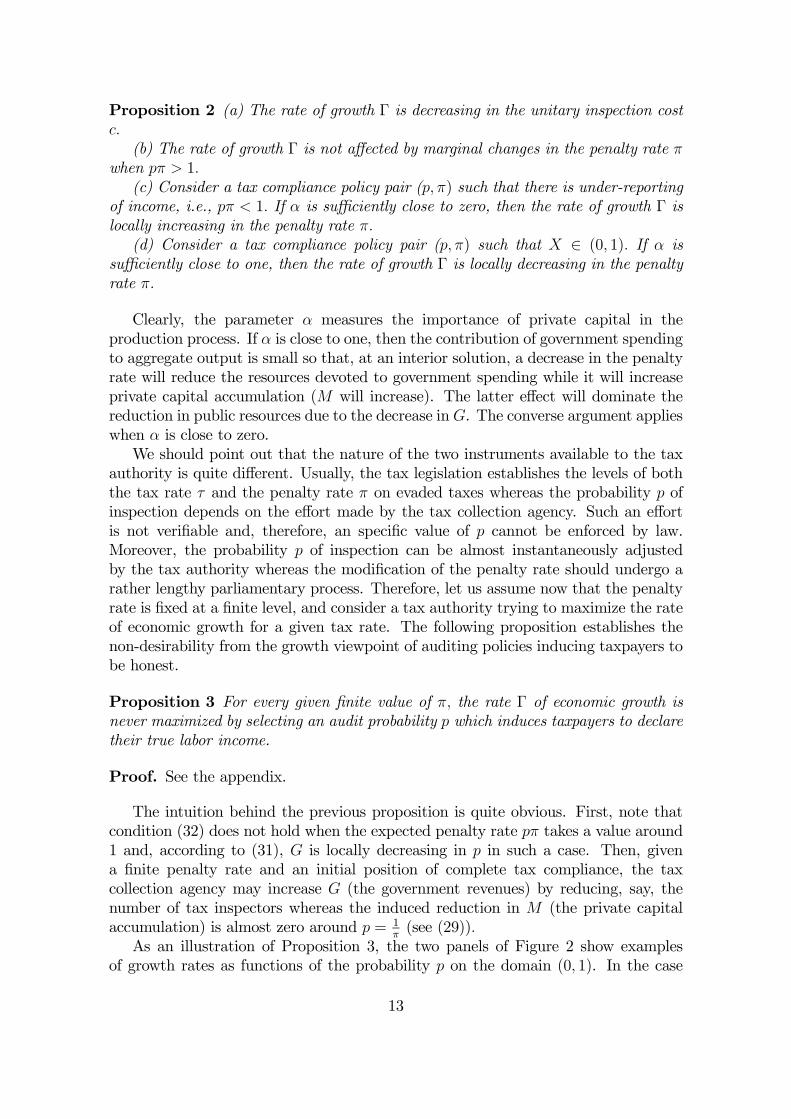
As an illustration of Proposition 3, the two panels of Figure 2 show examplesof growth rates as functions of the probability p on the domain (0, 1). In the case

13

considered in Panel 2A, we obtain a kind of Laffer curve, and growth is maximizedwhen the audit probability is p = 0.0775 ∈ ¡p, p¢. However, Panel 2B shows asituation in which public spending is so unproductive (α = 0.9) that the growth rateis strictly decreasing in p on the whole domain. Note that the two plotted functionsare strictly decreasing in

¡1π− ε, 1

¢for some ε > 0.

[Insert Figure 2 about here]

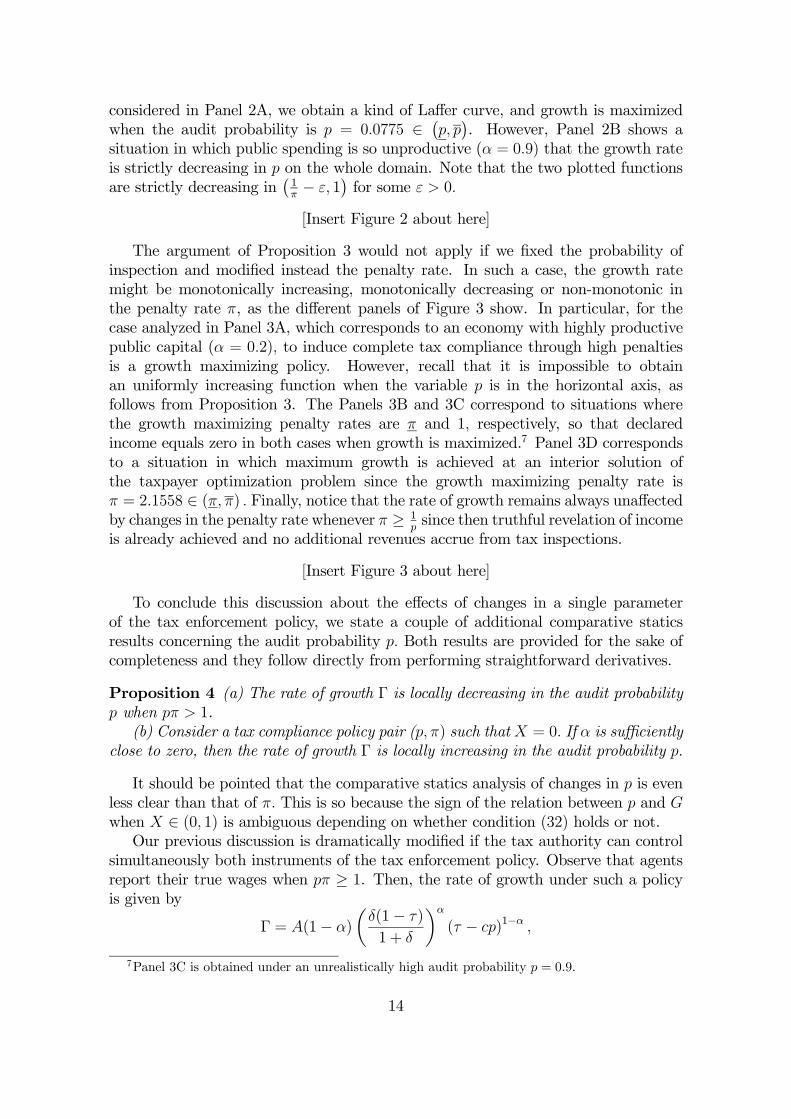
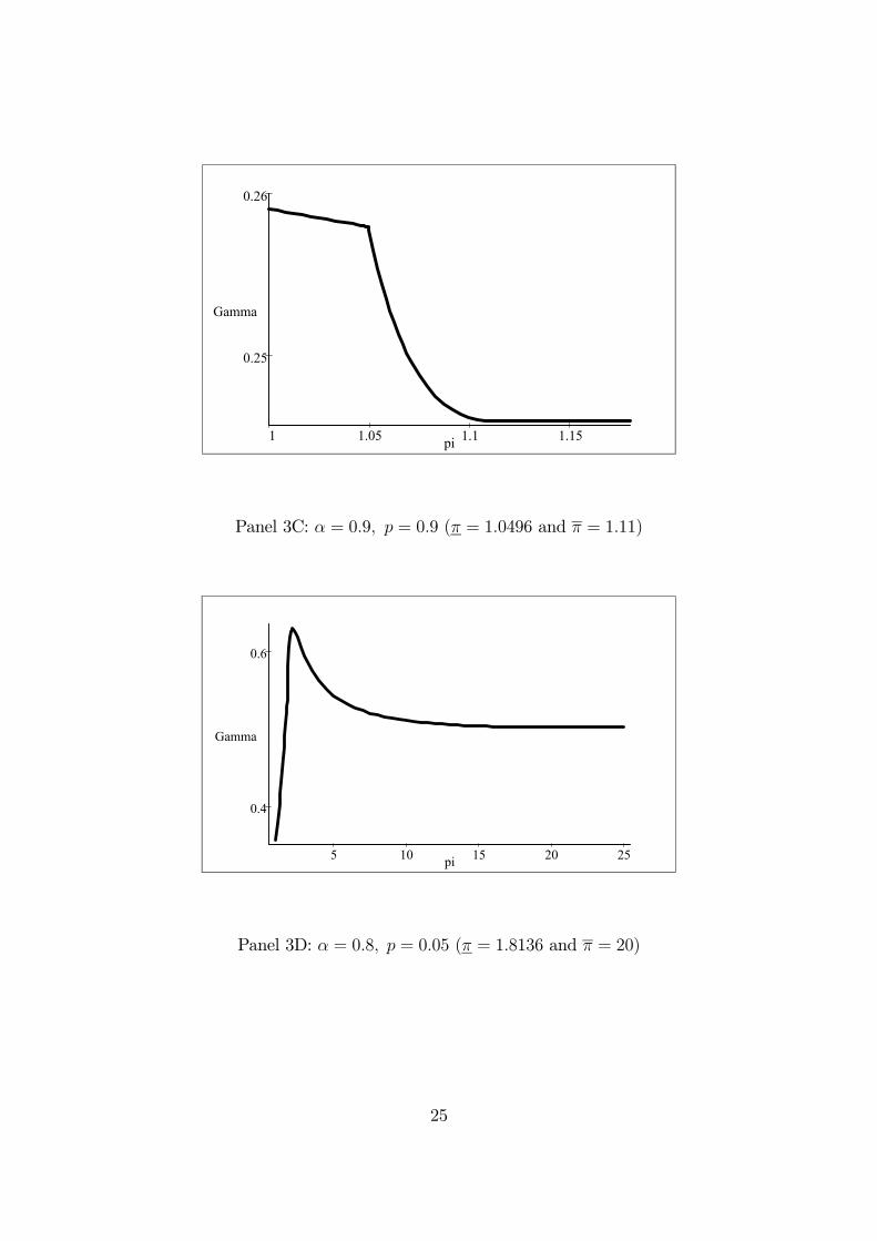
The argument of Proposition 3 would not apply if we fixed the probability ofinspection and modified instead the penalty rate. In such a case, the growth ratemight be monotonically increasing, monotonically decreasing or non-monotonic inthe penalty rate π, as the different panels of Figure 3 show. In particular, for thecase analyzed in Panel 3A, which corresponds to an economy with highly productivepublic capital (α = 0.2), to induce complete tax compliance through high penaltiesis a growth maximizing policy. However, recall that it is impossible to obtainan uniformly increasing function when the variable p is in the horizontal axis, asfollows from Proposition 3. The Panels 3B and 3C correspond to situations wherethe growth maximizing penalty rates are π and 1, respectively, so that declaredincome equals zero in both cases when growth is maximized.7 Panel 3D correspondsto a situation in which maximum growth is achieved at an interior solution ofthe taxpayer optimization problem since the growth maximizing penalty rate isπ = 2.1558 ∈ (π, π) . Finally, notice that the rate of growth remains always unaffectedby changes in the penalty rate whenever π ≥ 1

psince then truthful revelation of income

is already achieved and no additional revenues accrue from tax inspections.

[Insert Figure 3 about here]

To conclude this discussion about the effects of changes in a single parameterof the tax enforcement policy, we state a couple of additional comparative staticsresults concerning the audit probability p. Both results are provided for the sake ofcompleteness and they follow directly from performing straightforward derivatives.

Proposition 4 (a) The rate of growth Γ is locally decreasing in the audit probabilityp when pπ > 1.(b) Consider a tax compliance policy pair (p, π) such that X = 0. If α is sufficiently

close to zero, then the rate of growth Γ is locally increasing in the audit probability p.

It should be pointed that the comparative statics analysis of changes in p is evenless clear than that of π. This is so because the sign of the relation between p and Gwhen X ∈ (0, 1) is ambiguous depending on whether condition (32) holds or not.Our previous discussion is dramatically modified if the tax authority can control

simultaneously both instruments of the tax enforcement policy. Observe that agentsreport their true wages when pπ ≥ 1. Then, the rate of growth under such a policyis given by

Γ = A(1− α)

µδ(1− τ)

1 + δ

¶α

(τ − cp)1−α ,

7Panel 3C is obtained under an unrealistically high audit probability p = 0.9.

14

as follows from (18), (22) and (25). Such a growth rate is strictly decreasing in p andit is clear that a growth rate arbitrarily close to

Γ∗ = A(1− α)

µδ(1− τ)

1 + δ

¶α

τ 1−α (35)

can be implemented by means of a complete tax compliance policy displaying aprobability p of inspection arbitrarily low and a penalty rate π arbitrarily high withpπ ≥ 1 (see Figure 1). Such a policy consisting on ”hanging evaders with probabilityzero” has received attention in the theoretical literature on tax evasion when thegovernment seeks to maximize its revenues (see, among many others, Kolm (1973)).8

It is easy to check algebraically from (18) and (22) that, if X ∈ (0, 1) thenM > δ(1−τ)1+δ

and G < τ . Hence, the desirability from the growth viewpoint of complete taxcompliance will depend on whether the technological parameter α is high or low, as itcan bee seen from comparing (25) with (35). In particular, to induce honest behaviorby the taxpayers is desirable whenever public capital is very productive, i.e., when αis sufficiently close to zero. The following proposition summarizes more precisely theresults:

Proposition 5 (a) Consider the set of tax compliance policies inducing true reportsof labor income, that is, policies satisfying pπ ≥ 1. Then, the supremum of the set ofrates of growth associated with such policies is Γ∗. Moreover, for all ε > 0, there existsa policy pair (p(ε), π(ε)), with p(ε) ·π(ε) = 1, such that the rates of growth associatedwith the policies (p(ε), π), with π ≥ π(ε), are equal to Γ∗ − ε. Furthermore, thefunction p(ε) is strictly increasing while π(ε) is strictly decreasing, and lim

ε→0p(ε) = 0

while limε→0

π(ε) =∞.

(b)If α is sufficiently close to zero, then there exists a policy pair (p, π) inducingcomplete tax compliance that displays faster economic growth than any other policyinducing tax evasion. Conversely, if α is sufficiently close to one, then there exists apolicy pair (p, π) inducing tax evasion that displays faster economic growth than anyother policy inducing complete tax compliance.

Let us point out that Proposition 3 does not contradict the first sentence in part(b) of Proposition 5. In the former we were keeping fixed the penalty rate at a finitelevel whereas in the latter both p and π were moving simultaneously in oppositedirections with π tending to infinity and p tending to zero. Obviously, the growthrate given in (35) is never achieved by a complete compliance policy but it is justarbitrarily approximated.

5 Summary and Final Remarks

We have developed a simple OLG model to analyze the implications for economicgrowth of different tax compliance policies. A crucial assumption of our model is

8Moreover, Friedland, Maital and Rutenberg (1978) have documented the effectiveness of suchan extreme policy in their experimental work.

15

that both private and public capital are needed for production. We have shownthat the effects of greater enforcement depend on the relative productivity of thesetwo types of capital. Even if greater enforcement leads to a reduction of savingsince individuals will enjoy less disposable income, the overall effect might be growthenhancing. This is so because enforcement generates resources that are used tofinance public capital formation. Public capital becomes a source of endogenousgrowth because allows private capital to keep its marginal productivity at a highlevel and, thus, it stimulates savings. We also show that the symmetry between thetwo instruments of tax enforcement that we have considered is far from complete. Inthis respect, we have seen that the policy of ”hanging evaders with probability zero”,that consists on imposing very high penalties to evaders with a very low probabilityof inspection, is the one that allows the government to better approximate the highestgrowth rate among all the policies inducing honest behavior. Moreover, for a givenlevel of penalties, long-term growth is never maximized for a probability of inspectioninducing truthful revelation of income since the marginal cost of such in inspectioneffort is always greater than the marginal revenue generated by such a policy.It should be noticed that in this paper we have conducted just a positive analysis

of the growth effects of changes in the tax enforcement policy. The normative analysisin an OLG model like ours will depend on the objective function of the social plannerand, in particular, on the weights assigned to each generation in his objective function.It is indeed very easy to construct examples illustrating how the preferences of thesocial planner might conflict with the objective of maximizing economic growth.9

Due to the extreme simplicity of the model we have just considered, manyextensions are possible. We just mention four of them.The first one refers to the explicit recognition of involuntary mistakes in the

process of filling the tax form (see Rubinstein (1979)). In this case, the penalty fee ondetected tax evaders should be set at a moderate level since both the inefficiency andthe inequality generated by severe penalties applied infrequently could be politicallyunbearable. The analysis could give rise then to an endogenous penalty rate, and itwill thus provide further support for the non-optimality of complete tax compliancein the spirit of our Proposition 3. The relevance of such a proposition relies indeed onthe fact that legislators do not set very severe penalties on tax evaders since they areperhaps aware that many taxpayers commit unverifiable mistakes by accident whenthey fill their tax forms. Therefore, fines cannot tend to infinity, which conformswith the assumption of Proposition 3. However, this extension would require agentsworking for more than one period since the repeated interaction between taxpayersand the tax collecting agency would be now a key element of the model.The second extension would be to consider inspection policies for which the

probability of an audit depends on the income declared as in Reinganum and Wilde(1985). These authors show that net fiscal revenues could increase by appropriatelydesigning a policy belonging to that class. The growth implications of those inspectionpolicies remain thus unexplored.Third, in our model growth is achieved by means of the accumulation of both

private and public capital. However, there are other ways in which sustained growth

9Some examples are available under request to the autors.

16

can be achieved, like for instance through human capital accumulation (see, amongmany others, Caballé and Santos (1993)). An advantage of the models displayingan explicit mechanism of human capital formation that raised the efficiency unitsof labor is that labor and public capital could be more properly distinguished.Note that in our model the exponents for labor and public capital are the same.Moreover, even if we reinterpreted private capital as a composite input embodyingboth physical and human capital, these two kinds of capital would be considered asperfect substitutes (see Rebelo (1991)). Therefore, in both cases we are making quiterestrictive assumptions indeed. The analysis of changes in the tax compliance policyon such richer models of human capital accumulation could also provide insights onboth the short-run and the long-run effects. This is so because those models typicallydisplay some transitional dynamics while such a dynamics is absent in the modelconsidered in this paper.Finally, since in our model inspection occurs in every period after consumption has

taken place, the income of old agents cannot be audited and, hence, capital incomeis not taxed. A more general OLG model, like one with more periods of life (as inAuerbach and Kotlikoff (1987)) or the one of perpetual youth of Blanchard (1985),would allow us to consider taxation on capital income as well. In this context, tofight against evasion will have direct effects on the interest rate that will affect inturn both savings and the rate of capital accumulation.

17

APPENDIX

Proof of Lemma 1. To obtain the solution for the individual’s problem (2) wemust first assume that the solution is interior, that is, xt ∈ (0, wt) . In this case, thefirst order conditions with respect to xt and st yield, after some tedious algebra, thefollowing solution:

xt =

µ(1− p)τ(1 + δpπ)− (1− pπ)(pδ + τ)

pτ(π − 1)(1 + δ)

¶wt, (A1)

and

st =

µπδ(1− p)(1− τ)

(π − 1)(1 + δ)

¶wt.

It can be checked from (A1) that such a conjectured solution satisfies in fact xt > 0if and only if

pπ >(τ + δ) p

τ(1 + δ) + δ(1− τ)p. (A2)

On the other hand, it can be seen from manipulating (A1) that a necessary andsufficient condition for xt < wt is

pπ < 1. (A3)

Since xt ∈ [0, wt] as a consequence of the aforementioned tax code, we have that xt = 0when (A1) is non-positive, which means that the agent will not fill the tax form insuch a circumstance. Hence, to obtain the solution for problem (2) when condition(A2) does not hold, we impose xt = 0 and solve the maximization problem for st. Thecorresponding optimal propensity to save is then given in (5) . Furthermore, xt = wt

when pπ ≥ 1 so that, in such a case, we solve the maximization problem (2) for stafter imposing xt = wt in its constraints.

Proof of Proposition 3. Observe that the gross growth rate Γ is a continuousfunction of the inspection probability p for all p ∈ (0, 1). Hence, we only have to provethat there exist a number ε ∈ (0, 1

π− p) such that the rate of growth Γ is strictly

decreasing in p on the interval¡1π− ε, 1

¢. We will first prove that the derivative ∂Γ

∂p

is strictly negative for p ∈ ¡ 1π, 1¢. Notice that X = 1 when p ∈ ¡ 1

π, 1¢. Thus, from

(18) and (22), it holds that M = δ(1−τ)1+δ

, G = τ − cp, and

Γ = A(1− α)

µδ(1− τ)

1 + δ

¶α

(τ − cp)1−α , (A4)

as follows from evaluating (25) in such a parameter region. Clearly, (A4) is strictlydecreasing in p. Next, since Γ has continuous derivatives with respect to p on

¡p, 1

π

¢,

we must compute the left derivative of Γ with respect to p at 1π. In order to compute

limp→(1/π)−

∂Γ∂pwe only have to evaluate the derivative of (25) at an interior solution and

take the limit as p tends to 1π. From (29) and (31) we obtain lim

p→(1/π)−∂M∂p= 0 and

18

limp→(1/π)−

∂G∂p= −c < 0 . Therefore, from (33), we get lim

p→(1/π)−∂(lnΓ)∂p

< 0 .We have thus

proved that for some ε > 0 the rate of growth is strictly decreasing in the interval¡1π− ε, 1

¢and, hence, a policy inducing complete tax compliance cannot be growth

maximizing. .

19

References

[1] Allingham, M. G. and A. Sandmo (1972). ”Income Tax Evasion: A TheoreticalAnalysis.” Journal of Public Economics 1, 323-38.

[2] Arrow, K. (1970). ”Essays in the. Theory of Risk Bearing” (chapter 3), NorthHolland, Amsterdam.

[3] Auerbach A.J. and L.J. Kotlikoff (1987). ”Dynamic Fiscal Policy”, CambridgeUniversity Press, NY.

[4] Barro, R. J. (1990). ”Government Spending in a Simple Model of EndogenousGrowth.” Journal of Political Economy 98, S103-S125.

[5] Barro, R. J. and X. Sala-i-Martin (1992). ”Public Finance in Models of EconomicGrowth.” Review of Economic Studies 59, 645-661.

[6] Blanchard, O.J (1985). ”Debt, Deficits, and Finite Horizons.” Journal of PoliticalEconomy 93: 223-247.

[7] Caballé, J. and M. S. Santos (1993). ”On Endogenous Growth with Physical andHuman Capital”. Journal of Political Economy 101, 1042-1067.

[8] Chang, W. Y. and C. C. Lai (1996). ”The Implication of Efficiency Wages onTax Evasion and Tax Collections.” Public Finance Quarterly, 24, 163-172.

[9] Diamond, P. A. (1965). ”National Debt in a Neoclassical Growth Model.”American Economic Review 55, 1126-1150.

[10] Friedland, N., S. Maital, and A. Rutenberg, (1978). ”A Simulation Study ofIncome Tax Evasion.” Journal of Public Economics 10, 107-116.

[11] Jones, L., and R. Manuelli (1990). ”A Convex Model of Economic Growth:Theory and Policy Implications.” Journal of Political Economy 98: 1008-1038.

[12] Jones, L., and R. Manuelli (1992). ”Finite Lifetimes and Growth.” Journal ofEconomic Theory 58: 171-197.

[13] Kolm, S. C. (1973). ”A Note on Optimum Tax Evasion.” Journal of PublicEconomics 2, 265-270.

[14] Lai, C. C., J. J. Chang, and W. Y. Chang, (1995). ”Tax Evasion and EfficientBargains.” Public Finances/Finances Publiques 50, 96-105.

[15] Lai, C. C., and W. Y. Chang, (1988). ”Tax Evasion and Tax Collections: anAggregate Demand - Aggregate Supply Analysis.” Public Finances/FinancesPubliques 43, 138-146.

20

[16] Lucas, R. (1988). ”On the Mechanics of Economic Development.” Journal ofMonetary Economics 22: 3-42.

[17] Lucas, R. (1990). ”Supply-Side Economics: An Analytical Review.” OxfordEconomic Papers 42: 293-316.

[18] Peacock, A., and G. K. Shaw, (1982) ”Tax Evasion and Tax Revenue Loss.”Public Finances/Finances Publiques 37, 269-278.

[19] Rebelo, S. (1991). ”Long-Run Policy Analysis and Long-Run Growth.” Journalof Political Economy 99, 500-521.

[20] Reinganum, J. F, and L. L. Wilde (1985). ”Income Tax Compliance in aPrincipal-Agent Framework” Journal of Public Economics 26, 1-18.

[21] Ricketts, M. (1984). ”On the Simple Macroeconomics of Tax Evasion:an Elaboration of the Peacock-Shaw Approach.” Public Finances/FinancesPubliques 39, 420-424.

[22] Rubinstein, P. (1979). ”An Optimal Conviction Policy for Offenses that MayHave Been Committed by Accident ” In Brams S., J. Schotter, and G.Shwodiauer, eds., Applied Game Theory. Physica-Verlag, Wuerzburg, Germany,406-413.

[23] Turnovsky, S.J. (1997). ”Fiscal Policy in a Growing Economy with PublicCapital.” Macroeconomic Dynamics 1, 615-639.

[24] Yitzhaki, S. (1974). ”A Note on Income Tax Evasion: A Theoretical Analysis.”Journal of Public Economics 3, 201-202.

21

π

1=πp

1

1

( )δτδτ

++

1

C

B

A

p

FIGURE 1: Interior and boundary solutions for the taxpayer problem.

22

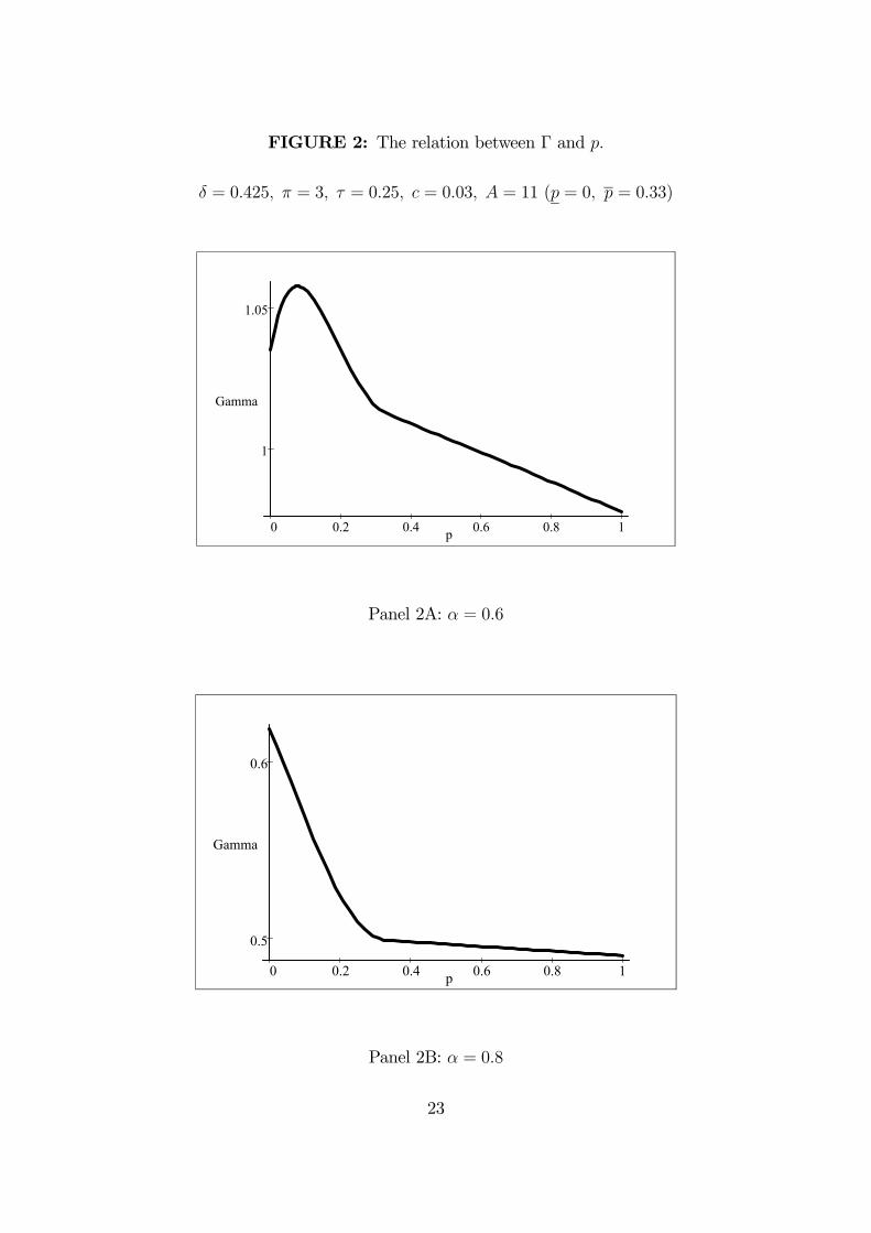
FIGURE 2: The relation between Γ and p.

δ = 0.425, π = 3, τ = 0.25, c = 0.03, A = 11 (p = 0, p = 0.33)

1

1.05

Gamma

0 0.2 0.4 0.6 0.8 1p

Panel 2A: α = 0.6

0.5

0.6

Gamma

0 0.2 0.4 0.6 0.8 1p

Panel 2B: α = 0.8

23

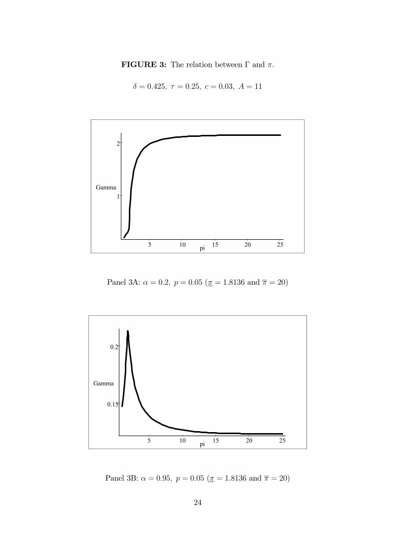
FIGURE 3: The relation between Γ and π.

δ = 0.425, τ = 0.25, c = 0.03, A = 11

1

2

Gamma

5 10 15 20 25pi

Panel 3A: α = 0.2, p = 0.05 (π = 1.8136 and π = 20)

0.15

0.2

Gamma

5 10 15 20 25pi

Panel 3B: α = 0.95, p = 0.05 (π = 1.8136 and π = 20)

24

0.25

0.26

Gamma

1 1.05 1.1 1.15pi

Panel 3C: α = 0.9, p = 0.9 (π = 1.0496 and π = 1.11)

0.4

0.6

Gamma

5 10 15 20 25pi

Panel 3D: α = 0.8, p = 0.05 (π = 1.8136 and π = 20)

25