Pursuit and Evasion: Evolutionary Dynamics and …naomi/publications/2010/PaiLeoGNC10.pdfPursuit and Evasion: Evolutionary Dynamics and Collective Motion ... pursuit and evasion games

AIAA Guidance, Navigation, and Control Conf., Toronto, Ontario, Canada, 2010

Pursuit and Evasion: Evolutionary Dynamics and

Collective Motion

Darren Pais∗ and Naomi E. Leonard†

Princeton University, Princeton, NJ, 08544, U.S.A.

Pursuit and evasion strategies are used in both biological and engineered settings; com-mon examples include predator-prey interactions among animals, dogfighting aircraft, carchases, and missile pursuit with target evasion. In this paper, we consider an evolutionarygame between three strategies of pursuit (classical, constant bearing, motion camouflage)and three strategies of evasion (classical, random, optical-flow based). Pursuer and evaderagents are modeled as self-propelled steered particles with constant speed and strategy-dependent heading control. We use Monte-Carlo simulations and theoretical analysis toshow convergence of the evolutionary dynamics to a pure strategy Nash equilibrium ofclassical pursuit vs. classical evasion. Here, evolutionary dynamics serve as a powerful toolin determining equilibria in complicated game-theoretic interactions. We extend our workto consider a novel pursuit and evasion based collective motion scheme, motivated by col-lective pursuit and evasion in locusts. We present simulations of collective dynamics andpoint to several avenues for future work.

I. Introduction

Pursuit and evasion behaviors, widely observed in nature, play a critical role in predator foraging, preysurvival, mating and territorial battles in several species. Pursuit-evasion contests were studied exten-

sively by Isaacs1 from a game-theoretic perspective in the context of differential games. In engineering,pursuit and evasion games have received much attention, particularly in the context of missile guidance andavoidance2,3 and aircraft pursuit and evasion.4,5 The book by Nahin6 provides a review of the topic alongwith relevant historical background.

The pervasiveness of pursuit and evasion in nature suggests the examination of winning strategies froman evolutionary perspective. Here one can think of a strategy as a control law that a particular pursuer(evader) employs to capture (escape). Correlates of evolutionary ‘fitness’ (fitness is proportional to repro-ductive or survival rate), such as time-to-capture, provide natural metrics that connect the dynamics ofindividual pursuer-evader pairs to evolutionary dynamics of populations comprising individuals playing dif-ferent strategies. Stable equilibria or winning strategies of such evolutionary dynamics (sometimes calledevolutionarily stable strategies or ESS7) point to strategies or behaviors one would expect to observe innature. Further, such strategies are often solutions (Nash equilibria) to constrained optimization problems,or to games with complicated structure such as stochastic payoff matrices.

Recently, Wei et al.8 used the evolutionary approach to study pursuit games, with dynamics derivedin the paper by Justh and Krishnaprasad.9 The authors8,9 use Monte-Carlo simulations and analyticalcalculations to study three pursuit strategies competing against a field of deterministic or random nonreactiveevasive strategies. The three chosen pursuit strategies (classical, constant bearing and motion camouflage)are biologically inspired. The authors show convergence of an evolutionary dynamics game between thethree strategies to pure motion camouflage and motivate this result by empirical observations of hoverflies,dragonflies and bats10 applying this technique.

In the present paper we build on the work in Ref. 8 by studying the coevolution of the three strategiesof pursuit from Ref. 8 playing against three distinct evasive strategies, two of which are reactive strategies.We use Monte-Carlo simulations and theoretical analysis to show convergence to an equilibrium of classical∗Ph.D. Candidate, Mechanical and Aerospace Engineering, J-32 Engineering Quadrangle, and AIAA Student Member.†Edwin S. Wilsey Professor, Mechanical and Aerospace Engineering, D-234 Engineering Quadrangle.

1 of 14

American Institute of Aeronautics and Astronautics

pursuit versus classical evasion. We point out that extending the ‘games against nature’ approach8 tocompetitions between two sets of strategies does not result in a motion camouflage as the winning pursuitstrategy, as in Ref. 8. Indeed, the environment of evasive strategies that a pursuer population encounters iscritical in determining the winning pursuit strategy. As a result, analysis of strategy spaces different againfrom those studied in the present paper will yield other interesting evolutionary outcomes.

We further explore the winning strategies (classical pursuit and classical evasion) in a collective motionmodel with agents pursuing and evading designated neighbors on a cyclical interaction topology. This workis motivated by collective motion in cannibalistic locusts11 and has strong parallels to prior work in cyclicpursuit.12–14 Simulation results suggest a rich set of solutions for this collective motion model.

The outline of this paper is as follows. Section II describes the planar dynamics for pursuit and evasiveagents and the different pursuit and evasion strategies under consideration. In Section III we study theevolutionary dynamics of the two populations. Section IV focuses on the collective motion model with thewinning strategies. We conclude and provide directions for future work in Section V .

NOTATION: For notational convenience, the Euclidean plane R2 is identified with the complex planeC. Thus (x, y) ∈ R2 ≡ x+ iy ∈ C. For two complex numbers c1, c2 ∈ C, the complex inner product is definedas 〈c1, c2〉 := Re(c1c∗2), the real part of c1c∗2, where c∗2 is the complex conjugate of c2. |c1| is the complexmodulus of c1. 1N represents an N × 1 vector of ones. The (i, j) element of a matrix A is denoted aij . MT

denotes the transpose of matrix M and M# denotes the element-wise inverse of M , i.e. m#ij = 1/mij . For

a column vector x, xj denotes the j’th element of x.

II. Dynamics of Pursuit and Evasion

We study a two-agent planar pursuit and evasion problem where each agent is modeled as a self-propelledsteered particle with constant speed and with angular velocity determined by the interaction between theparticles. We consider three pursuit behaviors: classical, constant bearing and motion camouflage, andthree evasive behaviors: classical, random motion, and optical-flow based.15 The choice of the three pursuitbehaviors is motivated by work in Refs. 8 and 9, where it is proved that if the speed of the pursuer isgreater than that of the evader, the pursuer captures the evader in finite time. Here ‘capture’ means thatthe Euclidean distance between the pursuer and evader reaches a designated minimum. Consider a pursuerand an evader moving on the complex plane with positions rP = xP + iyP ∈ C and rE = xE + iyE ∈ C andheadings θP ∈ S1 and θE ∈ S1, respectively. The dynamics of the two-agent system are given by

rP = eiθP , θP = uP

rE = νeiθE , θE = uE .(1)

Here, the speed of the pursuer is normalized to be 1 and the evader has a constant positive speed ν < 1. Wedefine the baseline vector8 r as the relative position of pursuer with respect to evader, i.e.,

r = rP − rE .

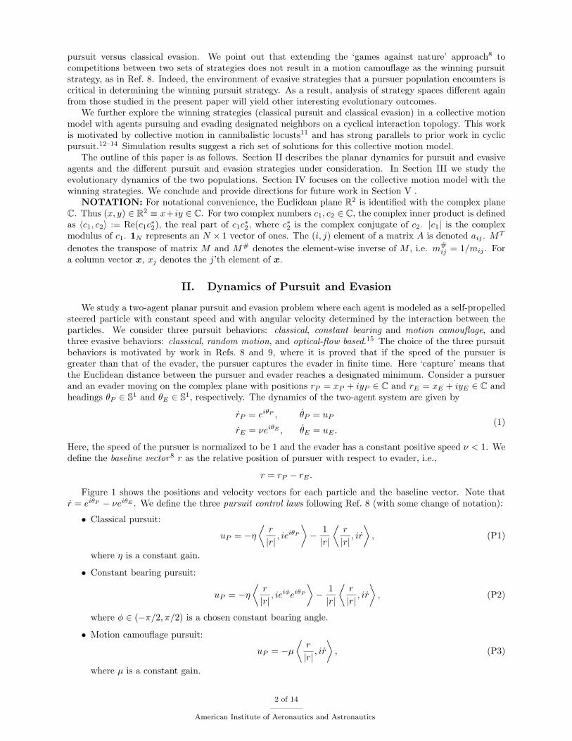
Figure 1 shows the positions and velocity vectors for each particle and the baseline vector. Note thatr = eiθP − νeiθE . We define the three pursuit control laws following Ref. 8 (with some change of notation):

• Classical pursuit:

uP = −η⟨r

|r|, ieiθP

⟩− 1|r|

⟨r

|r|, ir

⟩, (P1)

where η is a constant gain.

• Constant bearing pursuit:

uP = −η⟨r

|r|, ieiφeiθP

⟩− 1|r|

⟨r

|r|, ir

⟩, (P2)

where φ ∈ (−π/2, π/2) is a chosen constant bearing angle.

• Motion camouflage pursuit:

uP = −µ⟨r

|r|, ir

⟩, (P3)

where µ is a constant gain.

2 of 14


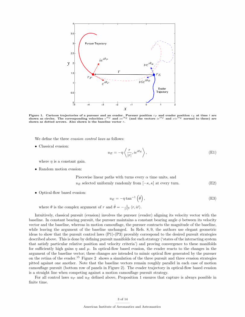
Figure 1. Cartoon trajectories of a pursuer and an evader. Pursuer position rP and evader position rE at time t areshown as circles. The corresponding velocities eiθP and νeiθE (and the vectors ieiθP and νieiθE normal to these) areshown as dotted arrows. Also shown is the baseline vector r.

We define the three evasion control laws as follows:

• Classical evasion:

uE = −η⟨r

|r|, ieiθE

⟩, (E1)

where η is a constant gain.

• Random motion evasion:

Piecewise linear paths with turns every α time units, anduE selected uniformly randomly from [−κ, κ] at every turn. (E2)

• Optical-flow based evasion:uE = −η tan−1

(θ), (E3)

where θ is the complex argument of r and θ = − 1|r|2 〈r, ir〉.

Intuitively, classical pursuit (evasion) involves the pursuer (evader) aligning its velocity vector with thebaseline. In constant bearing pursuit, the pursuer maintains a constant bearing angle φ between its velocityvector and the baseline, whereas in motion camouflage, the pursuer contracts the magnitude of the baseline,while leaving the argument of the baseline unchanged. In Refs. 8, 9, the authors use elegant geometricideas to show that the pursuit control laws (P1)-(P3) provably correspond to the desired pursuit strategiesdescribed above. This is done by defining pursuit manifolds for each strategy (‘states of the interacting systemthat satisfy particular relative position and velocity criteria’) and proving convergence to these manifoldsfor sufficiently high gains η and µ. In optical-flow based evasion, the evader reacts to the changes in theargument of the baseline vector; these changes are intended to mimic optical flow generated by the pursueron the retina of the evader.15 Figure 2 shows a simulation of the three pursuit and three evasion strategiespitted against one another. Note that the baseline vectors remain roughly parallel in each case of motioncamouflage pursuit (bottom row of panels in Figure 2). The evader trajectory in optical-flow based evasionis a straight line when competing against a motion camouflage pursuit strategy.

For all control laws uP and uE defined above, Proposition 1 ensures that capture is always possible infinite time.

3 of 14


P

P

P P

P

P P

P

P

E

E

E

E

E

E

E

E

E

Figure 2. Simulated trajectories of each of the nine pairs of competing pursuit and evasive strategies. The rowscorrespond to pursuit control laws (P1), (P2) and (P3) respectively and the columns correspond to evasive controllaws (E1), (E2) and (E3) respectively. For example, the plot in the middle corresponds to constant bearing pursuit vs.random motion evasion. The starting positions are indicated with ‘P’ and ‘E’. In all plots the evader starts at the originwith θE(0) = 0. The pursuers in columns 1 and 3 start at rP (0) = 5 + 3i with a heading θP (0) = π. In the second columnthe pursuers start at random orientations and with random headings. The straight lines in each plot are snapshots ofthe baseline vector at specific points in time.

Proposition 1. Consider dynamics (1) and control laws (P1)-(P3) and (E1)-(E3). For every capture radiusε > 0 and every initial condition rP (0), rE(0) such that |r(0)| = |rP (0) − rE(0)| > ε, there exists a finitecapture time T such that |r(T )| = ε.

Proof. Refer to Refs. 8, 9 for proof. Note that the evasive controls (E1)-(E3) satisfy the continuity andboundedness assumptions so that the proof extends to these cases.

The central question we ask in this paper is which strategies win out in a coevolutionary contest betweenthe three proposed pursuit strategies and the three proposed evasive strategies? In Ref. 8 the authorsstudied the evolutionary dynamics of the three pursuit strategies (P1)-(P3) playing against an environmentof nonreactive deterministic or random evasive strategies such as (E2). In the following section we consideran evolutionary scenario in which the pursuit strategies coevolve with reactive evasive strategies (E1) and(E3) as well.

III. Evolutionary Dynamics

To gain insight into the consequences of evolutionary competition between a population of pursuers anda population of evaders, we cast the problem in the framework of evolutionary dynamics (c.f. Refs. 7,16,17).The key idea here is that individuals in a population play a certain strategy that determines their payoff orfitness. This fitness can be a function of the environment, the strategies of other individuals, the frequencies

4 of 14


or distribution of competing strategies in the environment (known as frequency dependence) and the densityof individuals present in a region (density dependence), among other factors. Strategies with higher fitnessbecome widespread in a population, and can eventually take over the population; strategies with lowerfitness become diminished and might eventually go extinct. Here we consider frequency dependence in acompetition between a population of pursuers and a population of evaders. The population of pursuers andthe population of evaders are assumed to be composed of individuals playing strategies (employing controllaws) (P1)-(P3) and (E1)-(E3), respectively. Fitnesses are determined by the cumulative effect of severalone-on-one contests between pursuers and evaders such that a long time-to-capture for a particular contestcorresponds to a high evader fitness and a low pursuer fitness.

Consider a pursuer population represented by the population vector p =[p1 p2 p3

]T. Here pi,

i ∈ {1, 2, 3}, corresponds to the fraction of individuals in the population playing strategy (Pi). Hence thevector p is restricted to the 2-simplex defined by ∆2 =

{p | pT13 = 1 and pi ≥ 0, ∀i

}. Similarly, the evader

population is represented by the population vector q =[q1 q2 q3

]Twhich is also restricted to ∆2. The

fitness vectors for the pursuer and evader populations are denoted by fP ∈ R3+ and fE ∈ R3

+ respectively,where fPi is the fitness of pursuit strategy (Pi) and fEj is the fitness of evasive strategy (Ej) . Definepopulation mean fitness by fP = pTfP and fE = qTfE .

We can now write down a discrete update equation for each population that depends on the relativefitnesses of the different strategies in that population. For transition from generation g to generation g + 1,we have for i = 1, 2, 3 and j = 1, 2, 3:

pi(g + 1) = pi(g)fPi

fP

qj(g + 1) = qj(g)fEj

fE.

(2)

One can verify that the equations (2) ensure that each population vector remains in the simplex ∆2. Intu-itively, strategies with fitness greater than the population mean fitness are favored. Given an expression forthe fitness vectors, we can study the outcomes of the dynamics (2). As in Ref. 8 we use time-to-capture as ameasure of fitness. The fitness of the set of pursuer strategies fP depends on the distribution of evaders inthe population q and fE depends on the distribution of pursuers in the population p. This implies that theequations (2) are coupled. We simulate the evolutionary dynamics (2) using Monte-Carlo calculations thatdetermine fitnesses. We then perform a theoretical analysis.

III.A. Monte-Carlo Simulations

We follow the setup in Ref. 8 for our Monte-Carlo experiments. The important step is the constructionof the capture time matrix T ∈ R3×3 such that tij > 0 represents the time-to-capture for pursuit strategy(Pi) competing against evasive strategy (Ej). Proposition 1 gives us that all elements of T are positive andfinite. To construct T , we perform nine simulations, one for each element of T , such that each simulationhas a pursuer and an evader starting from the same initial conditions. In each simulation the evader startsat the origin with a heading of zero. The pursuer’s initial position is chosen from a uniform distributionon the square [−10, 10] × [−10, 10], and its initial heading from a uniform distribution on S1. The otherparameters are the same for each simulation: η = µ = 10, ν = .6, ε = 0.05, φ = 0.3, α = 0.2, and κ = 2.The results presented here remain qualitatively consistent for reasonable variations of these parameters. Adetailed study of the effect of each parameter on capture times is a direction of future work.

For each generation, we compute ten time matrices Tk, k ∈ {1, . . . , 10}, such that each matrix correspondsto a different choice of pursuer initial conditions and evader random trajectory for column 2. The average

matrix T is defined by tij =110

10∑k=1

tkij . Let T (g) denote the average time matrix computed at generation

g. Letting matrices M(g) = T#

(g) and N(g) = TT

(g), the fitness vectors are defined by

fP (g) = M(g)q(g)

fE(g) = N(g)p(g).(3)

5 of 14


The inverse and direct relationships between the time matrix and fitness for pursuers and evaders, re-spectively, ensure that high capture times have asymmetric fitness consequences for pursuers and evaders.Equations (3) also encode the frequency dependence and coupling of the evolutionary dynamics (2) since thefitness of a pursuer (evader) strategy depends on the population distribution of evader (pursuer) strategies.Another way of interpreting equations (3) is from the perspective of a focal pursuer (evader) employing aspecific strategy in a given generation. The expected fitness of this individual depends on expected interac-tions with each evasive (pursuit) strategy, which in turn depends on the population distribution of evaders(pursuers).

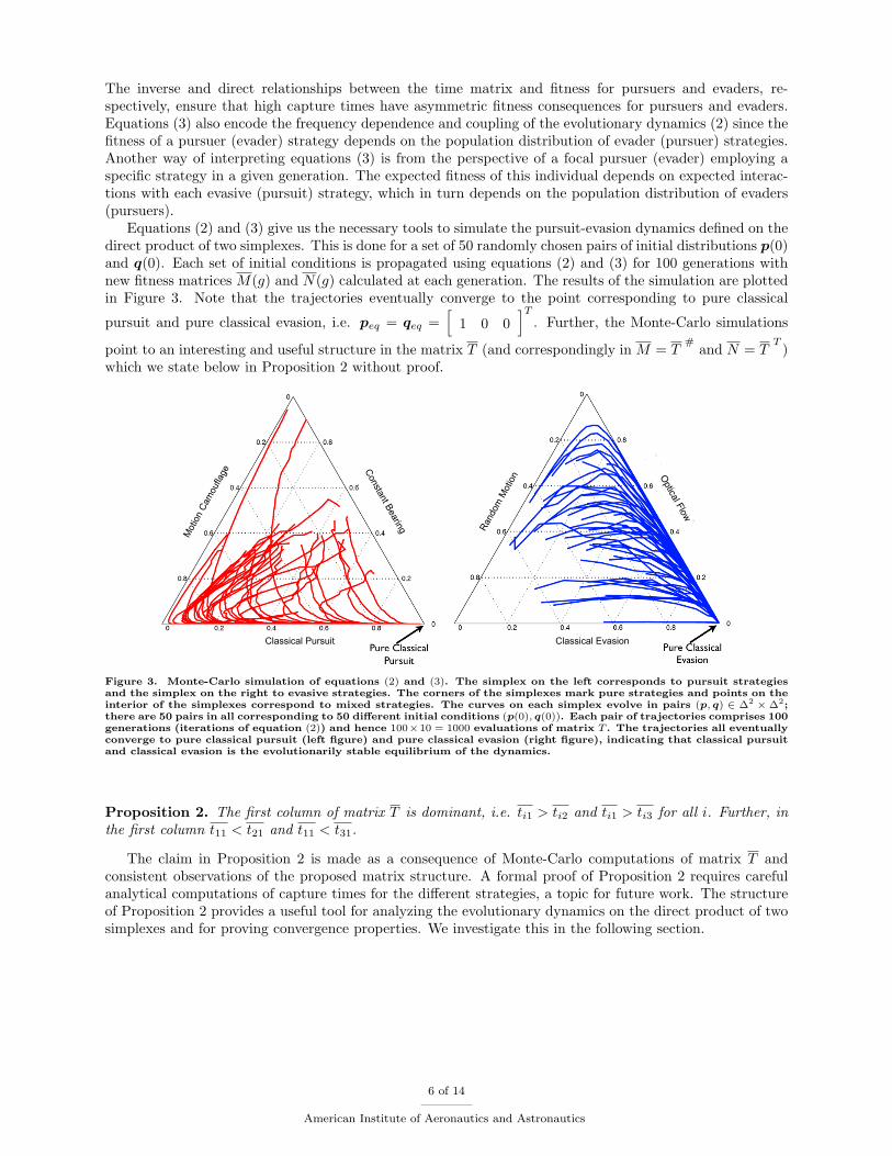
Equations (2) and (3) give us the necessary tools to simulate the pursuit-evasion dynamics defined on thedirect product of two simplexes. This is done for a set of 50 randomly chosen pairs of initial distributions p(0)and q(0). Each set of initial conditions is propagated using equations (2) and (3) for 100 generations withnew fitness matrices M(g) and N(g) calculated at each generation. The results of the simulation are plottedin Figure 3. Note that the trajectories eventually converge to the point corresponding to pure classical

pursuit and pure classical evasion, i.e. peq = qeq =[

1 0 0]T

. Further, the Monte-Carlo simulations

point to an interesting and useful structure in the matrix T (and correspondingly in M = T#

and N = TT

)which we state below in Proposition 2 without proof.

Motio

n C

am

oufla

ge

Classical Pursuit

Consta

nt B

earin

g Random

Motio

n

Classical Evasion

Rela

tive H

eadin

g C

hange

Optical Flow

Figure 3. Monte-Carlo simulation of equations (2) and (3). The simplex on the left corresponds to pursuit strategiesand the simplex on the right to evasive strategies. The corners of the simplexes mark pure strategies and points on theinterior of the simplexes correspond to mixed strategies. The curves on each simplex evolve in pairs (p, q) ∈ ∆2 ×∆2;there are 50 pairs in all corresponding to 50 different initial conditions (p(0), q(0)). Each pair of trajectories comprises 100generations (iterations of equation (2)) and hence 100×10 = 1000 evaluations of matrix T . The trajectories all eventuallyconverge to pure classical pursuit (left figure) and pure classical evasion (right figure), indicating that classical pursuitand classical evasion is the evolutionarily stable equilibrium of the dynamics.

Proposition 2. The first column of matrix T is dominant, i.e. ti1 > ti2 and ti1 > ti3 for all i. Further, inthe first column t11 < t21 and t11 < t31.

The claim in Proposition 2 is made as a consequence of Monte-Carlo computations of matrix T andconsistent observations of the proposed matrix structure. A formal proof of Proposition 2 requires carefulanalytical computations of capture times for the different strategies, a topic for future work. The structureof Proposition 2 provides a useful tool for analyzing the evolutionary dynamics on the direct product of twosimplexes and for proving convergence properties. We investigate this in the following section.

6 of 14


III.B. Theoretical Analysis

For some small time step ∆t > 0, we can rewrite the equations (2) as follows:

1∆t

(pi(g + 1)− pi(g)) = pi(g)fPi − fP

∆t fP1

∆t(qj(g + 1)− qj(g)) = qj(g)

fEj − fE∆t fE

.

In the limit ∆t→ 0, we get

pi = pifPi − fP

∆t fP

qj = qjfEj − fE

∆t fE.

Applying a further timescale change8 we finally arrive at the set of differential equations

pi =pi

fP

(fPi − fP

)qj =

qj

fE

(fEj − fE

).

(4)

Consider a constant matrix T that obeys the structure of Proposition 2. Further let M = T# and N = TT .Defining fitness vectors fP = Mq and fE = Np analogous to equation (3), and substituting into (4) we get

pi =pi

pTMq

((Mq)i − pTMq

)qj =

qjqTNp

((Np)j − qTNp

).

(5)

Equations (5) are a form of the replicator dynamics18 for two interacting populations with fitnesses defined bylinear functions of the population distributions. Critical to arriving at equations (5) is the assumption thatT is constant and thus M and N are constant. This is motivated by a ‘law of large numbers’ argument.8

Further, the assumption makes the analysis of equations (5) tractable, and hence allows us to formallyinvestigate the convergence shown in the Monte-Carlo experiments.

The system of equations (5) is a four-dimensional system evolving on ∆2×∆2. There are several possiblesolutions of the dynamics on these simplexes. For instance, all vertex pairs (pairs of pure strategies) are fixedpoints. Further, a strategy that is initially absent does not ever emerge, i.e., pi(0) = 0 =⇒ pi(t) = 0, ∀t,and the same holds for qj (replicator dynamics are said to be non-innovative – we do not consider mutationshere). Given the structure of the matrices M and N from Proposition 2, we investigate the dynamics ofequations (5).

In order to investigate the coupled replicator dynamical system (5), we first study the simpler singlepopulation replicator dynamics given by

qi =qi

qTf

(fi − qTf

), for i = 1, 2, 3. (6)

The fitness functions for the system of equations (6) are assumed to satisfy the following properties:

• Property 1: fi ≡ fi(t), i = 1, 2, 3, are each distinct functions of time, i.e., fi 6= fj pointwise. If this werenot the case then populations i and j would be indistinguishable from the perspective of evolutionarydynamics.

• Property 2: The functions fi(t) are each globally Lipschitz, bounded and positive for all t ≥ 0.

• Property 3: The functions fi(t) have a single dominant fitness; without loss of generality, f3(t) > f2(t)and f3(t) > f1(t) for all t ≥ 0.

7 of 14


Lemma 1. Assume initial conditions are restricted to the domain D ={q ∈ ∆2|q3 > 0

}. The dynamics

(6), satisfying Properties 1-3, have a unique asymptotically stable equilibrium point qeq =[

0 0 1]T

attracting all initial conditions in D.

Proof. We first show that the domain D is an invariant set with respect to the dynamics (6). All boundariesof D are clearly invariant since qi ∈ {0, 1} =⇒ qi = 0. Thus ∆2 is invariant. We have left to show thatq3(0) > 0 =⇒ q3(t) > 0 for all t > 0. To do this consider

q3 =q3f3

qTf− q3 ≥ −q3.

This implies for all t > 0,q3(t) ≥ q3(0)e−t > 0.

Using the constraint qT13 = 1, we restate the dynamics (6) as a two-dimensional system,

q1 =q1

f(f31(t)(q1 − 1) + f32(t)q2)

q2 =q2

f(f32(t)(q2 − 1) + f31(t)q1) ,

(7)

where f32(t) = f3(t) − f2(t) > 0, f31(t) = f3(t) − f1(t) > 0, and f = qTf = f3 − q1f31 − q2f32. Also(q1, q2) ∈ D where the invariant domain D is rewritten as D = {(q1, q2) | q1 ≥ 0, q2 ≥ 0, q1 + q2 < 1}. Onecan check that the only three equilibrium points of the system (7) in ∆2 (given properties (1)-(3)) are thevertices (qeq1, qeq2) = (0, 0), (0, 1), (1, 0), of which (0, 0) is the only equilibrium in D.

Linearization about the (0, 0) equilibrium gives the dynamics,[q1

q2

]=

[−f31/f3 0

0 −f32/f3

][q1

q2

].

This non-autonomous linear system in diagonal form can be solved easily as

qi(t) = qi(0)exp(−∫ t

0

f3i(t)f3(t)

dt

), i = 1, 2.

For i = 1, 2, limt→∞

qi(t) = 0 and hence the (0, 0) equilibrium point of the non-autonomous system (7) is locallyasymptotically stable by Theorem 4.13 of Ref. 19.

To prove that the invariant domain D is the region of attraction for the asymptotically stable (0, 0)equilibrium point of (7), we use a Lyapunov function V = q1 + q2. V is positive definite on D with a uniqueminimum: V = 0 ⇐⇒ q1 = q2 = 0. We compute

V = q1 + q2 =1

f(q1f31 + q2f32)(q1 + q2 − 1) < 0.

Since V is negative definite on the domain D, by Theorem 4.9 of Ref. 19 we have that D is the regionof attraction for the equilibrium point qeq1 = 0, qeq2 = 0 (and qeq3 = 1). Hence the equilibrium point

qeq =[

0 0 1]T

is the asymptotically stable limit for all q(0) ∈ D.

Note that the case of Lemma 1 with each fi constant is considered in Ref. 8. We now return to thecoupled two populations set of equations (5) and state the main theorem of this section. Here we employthe dominant structure of matrix T from Proposition 2 to prove convergence.

Theorem 1. Assume initial conditions are restricted to the domain D2 ={

(p, q) ∈ ∆2 ×∆2|p1 > 0, q1 > 0}

.Let matrix T satisfy Proposition 2 with M = T# and N = TT . Then, the coupled replicator dynamics (5)

have a unique asymptotically stable equilibrium point peq = qeq =[

1 0 0]T

attracting all initialconditions in D2.

8 of 14


Proof. The invariance of the domain D2 with respect to the dynamics (5) follows from the invariance ofthe domain D in the proof of Lemma 1. The column dominant structure of matrix T implies that thefirst element of the fitness vector fE = Np = TTp is dominant. That is, regardless of the populationdistribution p at any time instant, fE1 > fE2 and fE1 > fE3. Hence we can apply Lemma 1 to concludethat regardless of the evolution of the population vector p, the population vector q will asymptotically

converge to qeq =[

1 0 0]T

.Asymptotic stability implies that for every ε > 0 there exists a time t1 ≥ 0 such that t > t1 =⇒

‖q − qeq‖ < ε. Based on the calculations in Lemma 2 of the Appendix, we let

ε = min{

2(m11 −m21)(m11 −m21) + ‖M‖1

,2(m11 −m31)

(m11 −m31) + ‖M‖1

}.

For this choice of ε we are guaranteed that for all t > t1 the fitness vector fP = Mq preserves the orderingfP1 > fP2 and fP1 > fP3. Hence we can apply Lemma 1 again to the dynamics of p to conclude that after

time t1, the population vector p will also asymptotically converge to peq =[

1 0 0]T

.

Motio

n C

am

oufla

ge

Classical Pursuit

Consta

nt B

earin

g Random

Motio

n

Classical Evasion

Rela

tive H

eadin

g C

hange

Optical Flow

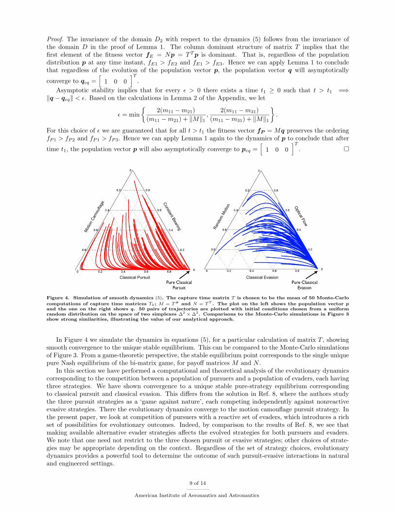
Figure 4. Simulation of smooth dynamics (5). The capture time matrix T is chosen to be the mean of 50 Monte-Carlo

computations of capture time matrices Tk; M = T# and N = TT . The plot on the left shows the population vector pand the one on the right shows q. 50 pairs of trajectories are plotted with initial conditions chosen from a uniformrandom distribution on the space of two simplexes ∆2 ×∆2. Comparisons to the Monte-Carlo simulations in Figure 3show strong similarities, illustrating the value of our analytical approach.

In Figure 4 we simulate the dynamics in equations (5), for a particular calculation of matrix T , showingsmooth convergence to the unique stable equilibrium. This can be compared to the Monte-Carlo simulationsof Figure 3. From a game-theoretic perspective, the stable equilibrium point corresponds to the single uniquepure Nash equilibrium of the bi-matrix game, for payoff matrices M and N .

In this section we have performed a computational and theoretical analysis of the evolutionary dynamicscorresponding to the competition between a population of pursuers and a population of evaders, each havingthree strategies. We have shown convergence to a unique stable pure-strategy equilibrium correspondingto classical pursuit and classical evasion. This differs from the solution in Ref. 8, where the authors studythe three pursuit strategies as a ‘game against nature’, each competing independently against nonreactiveevasive strategies. There the evolutionary dynamics converge to the motion camouflage pursuit strategy. Inthe present paper, we look at competition of pursuers with a reactive set of evaders, which introduces a richset of possibilities for evolutionary outcomes. Indeed, by comparison to the results of Ref. 8, we see thatmaking available alternative evader strategies affects the evolved strategies for both pursuers and evaders.We note that one need not restrict to the three chosen pursuit or evasive strategies; other choices of strate-gies may be appropriate depending on the context. Regardless of the set of strategy choices, evolutionarydynamics provides a powerful tool to determine the outcome of such pursuit-evasive interactions in naturaland engineered settings.

9 of 14


We now shift focus to employing pursuit and evasive behaviors for collective motion. In the followingsection we examine classical pursuit and classical evasion as this pair constitutes the evolutionary equilibriumof our strategy space.

IV. Collective Motion

The multi-agent dynamics described in this section are motivated in part by work done by Bazazi etal11 (further analyzed by Romanczuk et al20). These authors study social forging in groups of cannibalisticmigratory locusts: individuals pursue other conspecifics in front of them and evade individuals approachingfrom behind. We do not intend to mimic the collective dynamics observed in Ref. 11, rather we studythe outcomes of collective dynamics of steered particles exhibiting classical pursuit and evasive behaviorssimultaneously.

Consider a system of N agents indexed by j = 1, . . . , N , each having position rj = xj + iyj and headingθj . The agents are steered particles with constant speed v > 0 and steering control uj . Similar to equations(1), the kinematics of the agents are given by

rj = veiθj , θj = uj . (8)

For each agent we define baseline vectors bj+ = rj+1− rj and bj− = rj−1− rj . Note that j+ 1 and j− 1 aredefined mod N ; i.e., bN+ = r1 − rN and b1− = rN − r1. The control law uj is given by

uj = ujP + ujE

= K

⟨ieiθj ,

bj+‖bj+‖

⟩− βK

⟨ieiθj ,

bj−‖bj−‖

⟩,

(9)

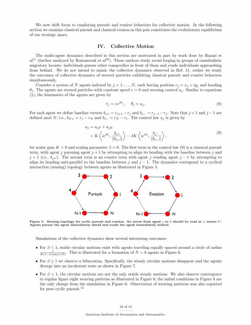
for scalar gain K > 0 and scaling parameter β > 0. The first term in the control law (9) is a classical pursuitterm, with agent j pursuing agent j + 1 by attempting to align its heading with the baseline between j andj + 1 (i.e., bj+). The second term is an evasive term with agent j evading agent j − 1 by attempting toalign its heading anti-parallel to the baseline between j and j − 1. The dynamics correspond to a cyclicalinteraction (sensing) topology between agents as illustrated in Figure 5.

Figure 5. Sensing topology for cyclic pursuit and evasion. An arrow from agent j to k should be read as ‘j senses k’.Agents pursue the agent immediately ahead and evade the agent immediately behind.

Simulations of the collective dynamics show several interesting outcomes:

• For β < 1, stable circular motions exist with agents traveling equally spaced around a circle of radiusv

K(1−β) sin(π/N) . This is illustrated for a formation of N = 8 agents in Figure 6.

• For β ≥ 1 we observe a bifurcation. Specifically, the steady circular motions disappear and the agentsdiverge into an incoherent state as shown in Figure 7.

• For β < 1, the circular motions are not the only stable steady motions. We also observe convergenceto regular figure eight weaving patterns as illustrated in Figure 8; the initial conditions in Figure 8 arethe only change from the simulation in Figure 6. Observation of weaving patterns was also reportedfor pure cyclic pursuit.12

10 of 14


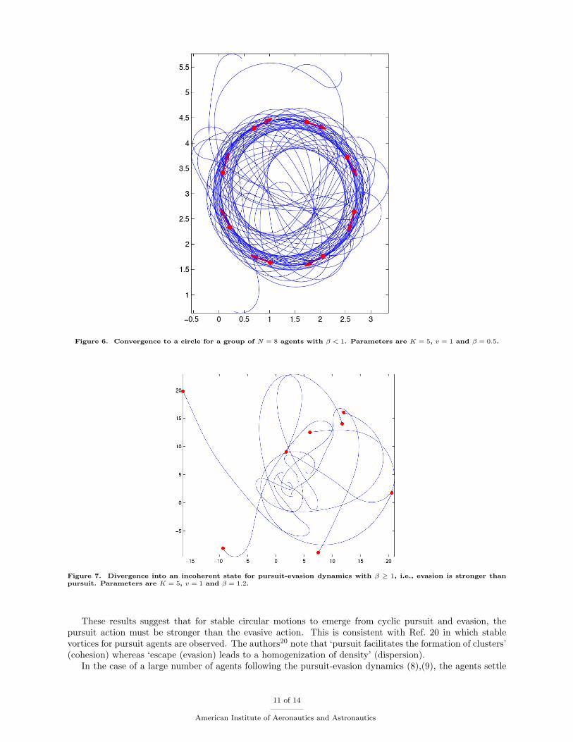
Figure 6. Convergence to a circle for a group of N = 8 agents with β < 1. Parameters are K = 5, v = 1 and β = 0.5.

Figure 7. Divergence into an incoherent state for pursuit-evasion dynamics with β ≥ 1, i.e., evasion is stronger thanpursuit. Parameters are K = 5, v = 1 and β = 1.2.

These results suggest that for stable circular motions to emerge from cyclic pursuit and evasion, thepursuit action must be stronger than the evasive action. This is consistent with Ref. 20 in which stablevortices for pursuit agents are observed. The authors20 note that ‘pursuit facilitates the formation of clusters’(cohesion) whereas ‘escape (evasion) leads to a homogenization of density’ (dispersion).

In the case of a large number of agents following the pursuit-evasion dynamics (8),(9), the agents settle

11 of 14


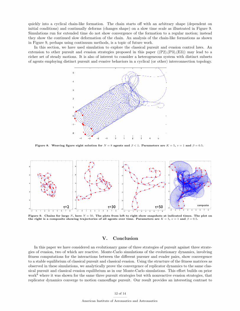
quickly into a cyclical chain-like formation. The chain starts off with an arbitrary shape (dependent oninitial conditions) and continually deforms (changes shape) on a slow time scale as illustrated in Figure 9.Simulations run for extended time do not show convergence of the formation to a regular motion; insteadthey show the continued slow deformation of the chain. An analysis of the chain-like formations as shownin Figure 9, perhaps using continuum methods, is a topic of future work.

In this section, we have used simulation to explore the classical pursuit and evasion control laws. Anextension to other pursuit and evasion strategies proposed in this paper ((P2),(P3),(E3)) may lead to aricher set of steady motions. It is also of interest to consider a heterogeneous system with distinct subsetsof agents employing distinct pursuit and evasive behaviors in a cyclical (or other) interconnection topology.

Figure 8. Weaving figure eight solution for N = 8 agents and β < 1. Parameters are K = 5, v = 1 and β = 0.5.

Figure 9. Chains for large N, here N = 50. The plots from left to right show snapshots at indicated times. The plot onthe right is a composite showing trajectories of all agents over time. Parameters are K = 5, v = 1 and β = 0.5.

V. Conclusion

In this paper we have considered an evolutionary game of three strategies of pursuit against three strate-gies of evasion, two of which are reactive. Monte-Carlo simulations of the evolutionary dynamics, involvingfitness computations for the interactions between the different pursuer and evader pairs, show convergenceto a stable equilibrium of classical pursuit and classical evasion. Using the structure of the fitness matrices asobserved in these simulations, we analytically prove the convergence of replicator dynamics to the same clas-sical pursuit and classical evasion equilibrium as in our Monte-Carlo simulations. This effort builds on priorwork8 where it was shown for the same three pursuit strategies but with nonreactive evasion strategies, thatreplicator dynamics converge to motion camouflage pursuit. Our result provides an interesting contrast to

12 of 14


the earlier result8 and further illustrates that the consequences of evolutionary dynamics depend significantlyon the space of strategies considered. Evolutionary dynamics are a useful tool for finding Nash equilibria andevolutionary stable strategies in complex interactions and games. Using strategy spaces different again fromthose in this paper may lead to a richer set of outcomes, including, for example, mixed strategy solutions asopposed to the pure strategy equilibrium shown here.

Motivated by the outcome of the evolutionary game studied in this paper and by the behavior ofcannabilistic locusts, we have investigated a novel control scheme involving agents performing simultane-ous pursuit and evasion on cyclical interaction topologies. In the case that the pursuit gain is larger than theevasion gain, simulations indicate local convergence to circular motion formations of specified radius as wellas local convergence to more complex weaving patterns. Exploring the use of different pursuit and evasivebehaviors and corresponding collective outcomes is a topic of future work.

Appendix

Lemma 2. Let q ∈ ∆2, qeq =[

1 0 0]T

and fP = Mq, where M = T# and T satisfies Proposition 2.

Then ‖q − qeq‖ < ε =⇒ fP1 > fP2 and fP1 > fP3, where ε ≤ min{

2(m11−m21)(m11−m21)+‖M‖1 ,

2(m11−m31)(m11−m31)+‖M‖1

}.

Proof. ‖q − qeq‖1 < ε =⇒ q1 > 1− ε2 , q2 <

ε2 and q3 <

ε2 . Suppose that

ε ≤ 2(m11 −m21)(m11 −m21) + ‖M‖1

=⇒ ε <2(m11 −m21)

(m11 −m21) + (m22 +m23)

=⇒ (m11 −m21)(

1− ε

2

)> (m22 +m23)

ε

2=⇒ (m11 −m21)q1 > m22q2 +m23q3

=⇒ (m11 −m21)q1 > m22q2 +m23q3 −m12q2 −m13q3

=⇒[m11 m12 m13

]Tq >

[m21 m22 m23

]Tq, or fP1 > fP2. (10)

Similarly one can show that

ε ≤ 2(m11 −m31)(m11 −m31) + ‖M‖1

=⇒ fP1 > fP3. (11)

Combining (10) and (11) we get the desired result.

Acknowledgments

The authors gratefully acknowledge support from ONR grant N00014-09-1-1074. DP is also supportedby the Gordon Wu and Martin Summerfield Princeton graduate engineering fellowships.

References

1Isaacs, R., Differential Games: A Mathematical Theory with Applications to Warfare and Pursuit, Control and Opti-mization, Dover Publications, 1999.

2Pontani, M. and Conway, B., “Optimal interception of evasive missile warheads: numerical solution of the differentialgame,” Journal of Guidance Control and Dynamics, Vol. 31, No. 4, 2008, pp. 1111–1122.

3Karelahti, J., Virtanen, K., and Raivio, T., “Near-optimal missile avoidance trajectories via receding horizon control,”Journal of Guidance Control and Dynamics, Vol. 30, No. 5, 2007, pp. 1287.

4Raivio, T. and Ehtamo, H., “Visual aircraft identification as a pursuit-evasion game,” Journal of Guidance, Control andDynamics, Vol. 23, No. 4, 2000, pp. 701–708.

5Neuman, F., “On the approximate solution of complex combat games.” Journal of Guidance, Control, and Dynamics,Vol. 13, No. 1, 1990, pp. 128–136.

6Nahin, P., Chases and Escapes: The Mathematics of Pursuit and Evasion, Princeton University Press, 2007.

13 of 14


7Smith, J., Evolution and the Theory of Games, Cambridge University Press, 1982.8Wei, E., Justh, E., and Krishnaprasad, P., “Pursuit and an evolutionary game,” Proceedings of the Royal Society A,

Vol. 465, No. 2105, 2009, pp. 1539.9Justh, E. and Krishnaprasad, P., “Steering laws for motion camouflage,” Proceedings of the Royal Society A, Vol. 462,

No. 2076, 2006, pp. 3629.10Ghose, K., Horiuchi, T. K., Krishnaprasad, P. S., and Moss, C. F., “Echolocating bats use a nearly time-optimal strategy

to intercept prey,” PLoS Biology, Vol. 4, No. 5, 04 2006, pp. e108.11Bazazi, S., Buhl, J., Hale, J., Anstey, M., Sword, G., Simpson, S., and Couzin, I., “Collective motion and cannibalism in

locust migratory bands,” Current Biology, Vol. 18, No. 10, 2008, pp. 735–739.12Marshall, J., Coordinated autonomy: Pursuit formations of multivehicle systems, Ph.D. thesis, University of Toronto

Toronto, Ontario, Canada, 2005.13Marshall, J., Broucke, M., and Francis, B., “Pursuit formations of unicycles,” Automatica, Vol. 42, No. 1, 2006, pp. 3–12.14Marshall, J., Broucke, M., and Francis, B., “Formations of vehicles in cyclic pursuit,” IEEE Transactions on Automatic

Control , Vol. 49, No. 11, 2004, pp. 1963–1974.15Srinivasan, M. V. and Zhang, S., “Visual motor computations insects,” Annual Review of Neuroscience, Vol. 27, No. 1,

2004, pp. 679–696.16Nowak, M., Evolutionary Dynamics: Exploring the Equations of Life, The Belknap Press of Harvard University Press,

2006.17Hofbauer, J. and Sigmund, K., “Evolutionary game dynamics,” Bulletin-American Mathematical Society, Vol. 40, No. 4,

2003, pp. 479–520.18Taylor, P. and Jonker, L., “Evolutionary stable strategies and game dynamics,” Mathematical Biosciences, Vol. 40, No.

1-2, 1978, pp. 145–156.19Khalil, H., Nonlinear Systems, Prenctice Hall, 2002.20Romanczuk, P., Couzin, I., and Schimansky-Geier, L., “Collective motion due to individual escape and pursuit response,”

Physical Review Letters, Vol. 102, No. 1, 2009, pp. 10602.

14 of 14


Documents

Pursuit and Evasion: Evolutionary Dynamics and …naomi/publications/2010/PaiLeoGNC10.pdfPursuit and Evasion: Evolutionary Dynamics and Collective Motion ... pursuit and evasion games