Embed Size (px)
Citation preview
https://doi.org/10.1007/s10846-020-01275-0
Task-Space Admittance Controller with Adaptive Inertia MatrixConditioning
Mariana de Paula Assis Fonseca1 · Bruno Vilhena Adorno2 · Philippe Fraisse3
Received: 1 July 2020 / Accepted: 8 October 2020© The Author(s) 2021
AbstractWhenrobots physically interact with the environment, compliant behaviors should be imposed to prevent damages to allentities involved in the interaction. Moreover, during physical interactions, appropriate pose controllers are usually basedon the robot dynamics, in which the ill-conditioning of the joint-space inertia matrix may lead to poor performance oreven instability. When the control is not precise, large interaction forces may appear due to disturbed end-effector poses,resulting in unsafe interactions. To overcome these problems, we propose a task-space admittance controller in which theinertia matrix conditioning is adapted online. To this end, the control architecture consists of an admittance controller inthe outer loop, which changes the reference trajectory to the robot end-effector to achieve a desired compliant behavior;and an adaptive inertia matrix conditioning controller in the inner loop to track this trajectory and improve the closed-loop performance. We evaluated the proposed architecture on a KUKA LWR4+ robot and compared it, via rigorousstatistical analyses, to an architecture in which the proposed inner motion controller was replaced by two widely used ones.The admittance controller with adaptive inertia conditioning presents better performance than with a controller based onthe inverse dynamics with feedback linearization, and similar results when compared to the PID controller with gravitycompensation in the inner loop.
Keywords Dynamic control · Adaptive control · Admittance control · Robot manipulator · Ill-conditioning ·Dual quaternion
1 Introduction
When robots interact with the environment, whether withobjects or humans, the closed-loop behavior should be
Bruno Vilhena [email protected]
Mariana de Paula Assis [email protected]
Philippe [email protected]
1 Graduate Program in Electrical Engineering, UniversidadeFederal de Minas Gerais (UFMG), Av. Antonio Carlos 6627,31270-901, Belo Horizonte-MG, Brazil
2 Department of Electrical and Electronic Engineering,School of Engineering, The University of Manchester,Sackville Street, Manchester, M13 9PL, UK
3 LIRMM UMR 5506 CNRS, Universite de Montpellier (UM),161 rue Ada Montpellier, 34392, Montpellier, France
safe for all agents and physical structures involved in theinteraction [1], which means that it is crucial to control howthe robot responds to the interaction and also its dynamicbehavior when moving to accomplish a given task.
Impedance and admittance controllers [2] are usually themost appropriate ones for a safe interaction [3] becausesuitable compliant behavior is achieved by controlling theapparent robot impedance. These controllers are commonlyused in a control architecture where there is an impedanceor admittance in an outer loop, and a motion controller inan inner loop [4–7]. Considering this architecture, a suitablemotion controller is based on the robot dynamic model asit enables more accurate analyses and helps in the synthesisof the robot dynamic behavior [8]. In those controllers, thejoint space inertia matrix (JSIM) plays an important role inthe control of the robot’s dynamic behavior [9, 10], whichalso affects safety.
Although it is well-known that the JSIM is positive defi-nite independently of the robot configuration, this propertydoes not guarantee the good conditioning of the matrix[11]. The links of a serial manipulator are connected in a
Journal of Intelligent & Robotic Systems (2021) 101: 41
/ Published online: 4 February 2021
way that each link in the kinematic chain is carried by itspredecessors while carrying all successive links in the chain.As a result, the equivalent inertia of the links is extremelydisparate, and this difference increases with the number oflinks, regardless if they are identical or not [9, 12], whichleads to the ill-conditioning of the JSIM.
When the JSIM is ill-conditioned (i.e., it has a large con-dition number), small perturbations in the system can pro-duce large changes in the numerical solutions [12], influen-cing the control performance [11], which in turn may affectsafety. For instance, imprecise end-effector motion controlcan result in large interaction wrenches when the robot inter-acts with highly rigid environments, which may result indamage to either the robot or the environment. Also, depen-ding on the control design, an ill-conditioned inertia matrixmay lead to closed-loop instability, which may yield dan-gerous movements that would harm the human or causedamage to the environment.
Despite the fact that this ill-conditioning is intrinsic toserial kinematic chains [9], its effects can be mitigated andtherefore the control performance can be enhanced. How-ever, this problem is mostly neglected by researchers andjust a few have worked on a solution for it [11, 13].
In order to circumvent the ill-condition problem, Shenand Featherstone propose to use a PD controller with gravitycompensation [11]. The PD controller is not affected by theill-conditioning of the JSIM since it directly converts thejoint position/velocity error to the drive torque. Yet, accor-ding to the authors, other controllers that have completeknowledge about the robot dynamics should achieve betteraccuracy.
To benefit from the complete dynamic model in thecontrol law whilst alleviating the effects of the JSIM’s ill-conditioning, an alternative is to add a well-conditionedconstant positive definite matrix to it in the Euler-Lagrangeequation. However, this addition could lead to steady-stateerror in the closed-loop system due to the introduction ofdisturbances in the robot model that are not compensated bythe control law. Even though the added matrix is constant,the resultant disturbance depends on the robot accelerationand, therefore, is time-varying, which means that addingan integrator to the control law would not be sufficient tosolve the steady-state error problem. More specifically, ifthe actual robot’s inertia matrix is given by M = M + A,where M is the nominal robot’s JSIM and A is a positivedefinite matrix, the actual dynamic model is given by
τ = Mq + Cq + g = Mq + Cq + g + w,
where w = Aq is the time-varying disturbance [14].Another option is to add a positive definite variable
matrix that varies according to the JSIM conditioning,
without adding excessive inaccuracy to the nominal model.This matrix should be adapted during the robot motion,which inspires the use of an adaptive controller. In thiscontext, we address the problem of task-space admittancecontrol with adaptive inertia matrix conditioning, thusensuring good performance and safe closed-loop behaviorduring physical interactions.
1.1 State of the Art
1.1.1 Impedance/Admittance Controllers
Pure motion control is usually insufficient to handle physi-cal contacts between the robot and the environment, spe-cially if the environment is rigid, because of the large con-tact wrenches arising from the interactions [15]. Therefore,some works have largely relied on the use of force con-trollers to minimize the interaction forces [1]. However,traditional force controllers tend to increase the robot stiff-ness to obtain high bandwidth and position accuracy, whichmay result in poor compliance and even instability. There-fore, force controllers are not the best choice for a good andsafe interaction [16]. Impedance and admittance controllers,on the other hand, have shown to be more appropriateto handle interactions [3], ensuring a suitable compliantbehavior by controlling the apparent robot impedance.
Hogan [2] proposed the first impedance controller tocontrol dynamic interactions between a manipulator and theenvironment in cases involving interaction forces that arenot orthogonal to motions, in which pure force controllersare not adequate. By changing the robot impedance to matchthe desired interaction impedance, safety is improved,which has motivated many researchers to use impedancecontrollers when physical interactions are required.
For instance, Erhart et al. [17] extend an impedance-based controller to dual-arm mobile manipulators to limitundesired internal forces caused by kinematic errors dueto uncertainties in the object geometry and manipulators.In order to accomplish that, the motion of the arms areseparated from the motion of the mobile base to decrease thecomputational cost and also to, using a potential function,minimize the propagation of the base disturbances to themanipulators. Experiments were performed only in thehorizontal plane. Lee et al. [18] also present an impedancecontroller that considers a dual-arm system as a singlemanipulator, whose end-effector motion is defined by therelative motion between the two end-effectors. Thus, usinga relative Jacobian, the impedance controller is reduced to asingle controller for both arms. Two different arms are usedto perform a writing task, in which one arm holds a platewhile the other writes on it.
In the context of human-robot interactions, Sieberet al. [19] propose the use of an impedance controller in
J Intell Robot Syst (2021) 101: 41Page 2 of 1941
a manipulation task performed by a team composed of ahuman and multiple robots. By means of a master-slavearchitecture, the human coordinates the robots formation,and the desired trajectory is designed according to themanipulated object geometry. However, small deviations inthe trajectory result in internal forces, and thus impedancecontrollers are used in each manipulator to prevent damageseither to the robots or to the object. A major drawbackof that work is that only the end-effectors positions areconsidered, therefore the internal torques due to orientationuncertainties are not explicitly taken into account.
More concerned with multiple tasks, Hoffman et al. [20]propose a multi-priority impedance controller that considerstask priorities inside a Quadratic Programming (QP) optimi-zation framework that allows equality and inequality cons-traints. This architecture is useful when more than onetask must be dealt with simultaneously, such as controllingthe end-effectors of a humanoid robot while keepingthe balance. Moreover, equality and inequality constraintsenable the definition of joint limits, collision avoidance,etc., directly in the control law.
Admittance controllers, which are dual to impedancecontrollers, have also been used in applications wherethe manipulator physically interacts with the environment.Throughout the literature, admittance controllers have beencalled position-based impedance controllers, velocity-basedimpedance controllers, or, ambiguously, impedance con-trollers [21]. Currently, a more widely accepted definition isthat impedance controllers are the ones in which the robotvelocity is measured, yielding a wrench as a control signal.Conversely, in admittance controllers, a contact wrench ismeasured and mapped to a velocity that must be imposed tothe robot [21].
Thanks to the ability to handle stiff impedances inaddition to enabling non-back drivable and heavy robots tohave a compliant behavior, admittance controllers are oftenused in wearable and industrial robots [21, 22]. Navarroet al. [23] propose an adaptive damping controller (a specialtype of admittance controller) that fulfills the ISO10218,a standard that has some requirements to guarantee safetyin human-robot interactions with industrial robots. Thecontroller was validated on a manipulator equipped witha robotic hand in a collaborative screwing application.Cherubini et al. [24] developed a collaborative human-robotmanufacturing cell for homokinetic joint assembly, in whichpre-taught trajectories are deformed to comply with externalwrenches using an admittance controller. As a result, thehuman workload is reduced, and a risk analysis indicatesthat their approach is compatible with safety standards.
Tarbouriech et al. [25] propose an admittance controllerfor a collaborative dual-arm manipulation of bulky objects.Computer vision is used to detect where the human isin contact with the object, and an admittance controller
makes the bimanual manipulator move according to thisinformation. As the gravity effects are canceled during themanipulation, the human makes an effort only to movethe object, without needing to sustain it. Agravante et al.[26] combine a visual servoing controller to an admittancecontroller to achieve a human-robot collaborative task ofcarrying a flat surface while preventing an object on top ofit from falling. Since they used Euler angles to representorientations, the controller is restricted to small rotationsdue to representational singularities [27].
To avoid the representational singularity problemwhen performing six-degree-of-freedom (DOF) impedance/admittance control, Caccavale et al. [4] propose to usethe imaginary part of a unit quaternion to represent rota-tions and formulate a geometrically consistent stiffness forinfinitesimal displacements. Notwithstanding, they use twodistinct control laws for the position and orientation, andtheir approach presents the topological obstruction prob-lem [28], which may trap the closed-loop system within anunstable equilibrium set. That work is later extended [5] topropose a controller in which the stiffness is proved to begeometrically consistent for finite displacements. Caccavaleet al. [5] applied that controller in a dual-arm manipulation,considering internal and external wrenches. Nonetheless,the new controller still carries the topological obstructionissue.
1.1.2 Adaptive Controllers
Since common admittance controller architectures rely oninner motion controllers, special care must be taken ifthe robot is torque-actuated because the JSIM may beill-conditioned, as discussed in the previous section. Toovercome this drawback, we propose to use an adaptivecontroller that adjusts the JSIM conditioning online, thusimproving the closed-loop performance.
Although adaptive control has been extensively studied,very few authors have tackled the problem of adaptingthe JSIM conditioning. For instance, Slotine and Li [29]propose an adaptive control law for robots with dynamicsuncertainties. Moreover, they show that although the estima-ted parameters do not converge to the real parameters, theclosed-loop system is asymptotically stable. They firstaddress the problem in joint space and then extend the solu-tion to the Cartesian space.
Cheah et al. [30, 31] extend the work of Slotine and Li[29] to tackle not only dynamic but also kinematic uncer-tainties. They show that the robot end-effector can convergeto the desired trajectory, despite the uncertain dynamic andkinematic parameters, which are updated online by adaptivelaws. Liu et al. [32] propose a task-space adaptive Jacobiancontroller that is asymptotically stable in the Lyapunovsense and consider the dynamics, kinematics, and also the
J Intell Robot Syst (2021) 101: 41 Page 3 of 19 41
actuator dynamics, which was not considered by any of theprevious works.
Passivity-based adaptive controllers, such as the onesproposed by Slotine and Li [29] and Cheah et al. [30, 31],rely on approximate transpose-Jacobian feedback to trackthe manipulator end-effector [33]. Although those control-lers achieve asymptotic stability, their performance is notgood over the entire robot configuration space. Since theclosed-loop response varies with the manipulator configura-tion [33], it is not possible to define fixed gains that result infixed closed-loop poles. Moreover, those controllers lead tononlinear and coupled error dynamics, and thus it is hard toquantify the system performance. Controllers based on theinverse dynamics, on the other hand, yield linear and de-coupled error dynamics when the robot parameters are per-fectly known. Thus, Wang and Xie [33] propose an adaptiveinverse dynamics controller for robots with unknown dyna-mic and kinematic parameters, but the controller requiresthe measurements of the joints accelerations, which are notnecessary for the passivity-based controllers. As a result,the adaptive inverse dynamics controller is more sensitive tonoise.
Both passivity-based and inverse-dynamics based adap-tive controllers use the fact that both kinematic and dynamicmodels are linear in the parameters and utilize a regressor inthe parameter update laws. However, computing the regres-sor matrix is expensive for manipulators with a high numberof DOF. Thus, Hanlei [34] proposes a computationallyefficient adaptive control law based on the Newton-Eulerrecursive algorithm.
Passivity-based controllers have some advantages whencompared to inverse dynamics controllers. For example, theydo not require the inversion of the estimated inertia matrix.However, those laws usually do not guarantee that the esti-mated inertia matrix is positive definite, which results in phy-sically inconsistent results, or even well-conditioned [35].To overcome the lack of positiveness guarantee, one strategyis to ensure that the estimated parameters are positive toobtain a positive definite estimated inertia matrix. This canbe done by defining an appropriate convex region, whoseinterior defines the set of admissible positive parameters,and then using a projection algorithm to ensure that theparameters remain inside that region [30]. Nevertheless,in discrete implementations, the estimated parameters mayescape from that region, thus Wang and Xie [35] propose anapproach that guarantees the positiveness of the estimatedparameters while retaining the stability of the closed-loopsystem. Still, they observed that when the parameter updateis too fast, the algorithm cannot project the estimatedparameters into the region of admissible parameters.
Despite the vast literature on adaptive control, to the bestof our knowledge, none of them consider the improvementof the JSIM conditioning.
1.2 Statement of Contributions and Organizationof the Paper
We propose a task-space admittance controller withadaptive inertia matrix conditioning that consists of:
– an admittance controller using the dual quaternion (DQ)logarithmic mapping in the outer loop to improve theinteraction between the robot and the environment,imposing a desired impedance behavior;
– a task-space adaptive controller (TAC) in the innerloop that ensures the improvement in the JSIM’sconditioning.
We also present experimental results and rigorous sta-tistical analyses, based on a hypothesis-testing framework,to compare the performance of the proposed architecture(admittance + TAC) with two classic controllers used in theinner loop, together with the admittance controller in theouter loop: an inverse dynamic with feedback linearization(TIDFL) controller and a PID with gravity compensation(TPID).
Furthermore, our approach is free from topologicalobstructions, in which the closed-loop system can betrapped into unstable equilibria, and is simple to implement.
This work builds upon our previous works [13, 14], inwhich we have proposed a joint-space adaptive controllerto compensate for the uncertainties introduced by a matrixthat we add to the JSIM to improve its conditioning. Thecurrent approach extends those previous works to the task-space and integrates it to a task-space admittance controllerthat we have briefly introduced as an extended abstract inthe Workshop Applications of Dual Quaternion Algebra toRobotics, which happened at ICAR 2019 [7].
The paper is organized as follows. Section 2 presents abrief mathematical background, whereas Section 3 presentsthe admittance control law using the DQ logarithmic map-ping. Section 4 introduces the TAC and the two other task-space motion controllers that are used for comparison pur-poses, namely TIDFL and TPID. Section 5 presents the ex-perimental results as well as the statistical analyses compar-ing the three controllers. Finally, Section 6 presents the finalremarks and perspectives of future works.
2Mathematical Background
When designing task-space controllers, the mathematicalrepresentation of rigid motions plays an important role,since a poor choice may lead, for instance, to representa-tional singularities [27]. In the last decades, several workshave shown that dual quaternion algebra presents severaladvantages over other mathematical tools for robot mod-eling and control, most notably when the task-space is
J Intell Robot Syst (2021) 101: 41Page 4 of 1941
considered [36]. For instance, unit dual quaternions havea compact representation, requiring only eight parame-ters, whereas homogeneous transformation matrices (HTM)need twelve if the fourth constant row is discarded, present-ing thus a smaller computational effort concerning multi-plications and additions. Moreover, the unit DQ does nothave representational singularities, as well as the HTM, andthe coefficients of a DQ can be used directly in the controllaw. This is a great convenience since the use of other tradi-tional methods based on HTM may require the extraction ofgeometrical parameters, which in turn can lead to represen-tational singularities. Another advantage of DQ is the factthat it has strong algebraic properties and can be used to rep-resent, in addition to rigid motions, wrenches, twists, andgeometric primitives such as Plucker lines and planes. [37]
Thanks to the aforementioned advantages, we use dualquaternion algebra throughout the paper.
2.1 Quaternions and Dual Quaternions
Quaternions can be understood as an extension of imaginarynumbers, in which the three imaginary components obey[38]
ı2 = j2 = k2 = ı j k = −1,
and the set of quaternions is defined as
H h1 + ıh2 + jh3 + kh4 : h1, h2, h3, h4 ∈ R
.
Given H h = h1 + ıh2 + jh3 + kh4, the real part of h isRe (h) h1, and Im (h) ıh2+ jh3+kh4 is the imaginarypart, such that h = Re (h)+ Im (h), whereas the quaternionconjugate is given by h∗ = Re (h) − Im (h). The subset ofpure quaternions is defined as Hp h ∈ H : Re (h) = 0,and the subset of unit quaternions is defined as S3 h ∈H : hh∗ = 1.
The multiplication between real matrices and quaternionsis sometimes necessary, and thus appropriate operators areneeded. Given H h = h1 + ıh2 + jh3 + kh4, the operatorvec4 : H → R
4 is defined as
vec4 h [h1 h2 h3 h4
]T, (1)
such that, given a, b ∈ H, the Hamilton operators−H 4,
+H 4 :
H → R4×4 satisfy [39]
vec4 (ab) = +H 4(a) vec4 b (2)
= −H 4(b) vec4 a. (3)
Moreover, given Hp p = ıp1+jp2+kp3, the operatorvec3 : Hp → R
3 is defined as
vec3 p [p1 p2 p3
]T. (4)
Analogously to quaternions, the dual quaternion set isdefined as
H h1 + εh2 : h1, h2 ∈ H, ε = 0, ε2 = 0
,
where ε is the nilpotent dual unit [40]. The subset of pureDQ is defined as
Hp (h1 + εh2) ∈ H : Re (h1) = Re (h2) = 0
whereas the set of unit DQ is defined as S h ∈ H : hh∗ = 1
, in which h∗ = h∗
1 + εh∗2 [37]. The set
S equipped with the standard multiplication form the groupSpin(3)R
3 of rigid motions [41].Similarly to quaternions, given the DQ
a = a1 + ıa2 + j a3 + ka4 + ε(a5 + ıa6 + j a7 + ka8
)
and the pure DQ
b = ıb1 + j b2 + kb3 + ε(ıb4 + j b5 + kb6
),
the operators vec8 : H → R8 and vec6 : Hp → R
6 aredefined as [37]
vec8 a = [a1 a2 a3 a4 a5 a6 a7 a8
]T, (5)
vec6 b = [b1 b2 b3 b4 b5 b6
]T. (6)
Given u = [u1 u2 u3 u4 u5 u6 u7 u8
]Tand v =[
v1 v2 v3 v4 v5 v6]T
, the inverse mappings vec8 : R8 →H and vec6 : R6 → Hp are given by
vec8u = u1 + u2 ı + u3j + u4k + ε(u5 + u6 ı + u7j + u8k
), (7)
vec6v = v1 ı + v2j + v3k + ε(v4 ı + v5j + v6k
). (8)
2.2 Dual Quaternion Logarithmic Mapping
Considering a translation p =(ıpx + jpy + kpz
)∈ Hp
and a rotation r = (cos (φ/2) + n sin (φ/2)) ∈ S3, with
φ ∈ [0, 2π) being the rotation angle around the rotation axis
n =(ınx + jny + knz
)∈ S
3 ∩ Hp, the unit DQ x ∈ Sthat combines both p and r is given by
x = r + ε1
2pr, (9)
whose logarithm is [39]
log x = nφ2 + ε
p2 . (10)
J Intell Robot Syst (2021) 101: 41 Page 5 of 19 41
The DQ logarithmic mapping can be used to translate thespacial difference xc
d x∗cxd between two poses xc, xd ∈
S, as in (9), to the origin [42]. More specifically,
xc → xd =⇒ xcd → 1 =⇒ log xc
d → 0.
Moreover, letting y log x, the time derivatives of y and x
are related by means of the matrix Q8(x) ∈ R
8×6 as [43]
vec8 x = Q8(x)
vec6 y, (11)
where vec8 (·) and vec6 (·) transform the DQ into a vector,as in (5) and (6), respectively, and
Q8(x) =
[Q4 (r) 04×3
12
+H 4 (p) Q4 (r)
−H 4 (r) Qp
], (12)
with 0m×n ∈ Rm×n being a matrix of zeros,
+H +4 (·) being
the Hamilton operator as in (2), and
Qp =[01×3
I 3
], (13)
with Im ∈ Rm×m being the identity matrix. In addition,
Q4 (r) =
⎡⎢⎢⎣
−r2 −r3 −r4
γ n2x + γnxny γ nxnz
γ nynx γ n2y + γnynz
γ nznx γ nzny γ n2z +
⎤⎥⎥⎦ , (14)
where ri is the ith component of the quaternion r , and
γ = r1 − , (15)
=
1, if φ = 0sin(φ/2)
φ/2 , otherwise.(16)
The generalized wrench log ∈ R6 related to the
logarithm is given by
log GTlog
(x)ς , (17)
where R6 ς = [
f T mT]T
is the wrench related to[vT ωT
]T, with f , m ∈ R
3 being the force and moment,and v, ω ∈ R
3 being the linear and angular velocities,
respectively. From[vT ωT
]T = Glog(x)
vec6 y, we use
the relations vec4 r = Q4 (r) ddt
vec3 (nφ/2) [43], withvec4 (·) and vec3 (·) being the operators defined in (1) and
(4), respectively, and ω = 2I 3×4−H 4 (r∗) vec4 r [39], with
−H 4 (·) being the Hamilton operator as in (3), to find byinspection that
Glog(x)[
03×3 2I 3
2I 3×4−H 4 (r∗)Q4 (r) 03×3
],
where I 3×4 [03×1 I 3×3
].
3 Admittance Control Law
In order to have a safe interaction between a robot manipu-lator and the environment, we propose a control architecturethat guarantees a compliant behavior while achieving goodend-effector pose accuracy. To obtain a compliant behavioron industrial manipulators, admittance controllers arefrequently used since those robots are usually characterizedby a stiff and non-backdrivable mechanical structure [44], inwhich an admittance controller ensures better performancethan impedance controllers [21]. Moreover, when a highpositioning accuracy is desirable, an admittance controller isalso more adequate as it usually achieve smaller steady-stateerrors in the end-effector pose than impedance controllers.Thus, aiming at high accuracy and a compliant behaviorof industrial manipulators, an admittance controller is moreadequate and hence used in this paper.
Considering the desired end-effector pose xd ∈ S, ourproposed architecture consists of an admittance controllerin the outer loop that modifies xd according to the externalwrench, which is measured at the robot end-effector, andoutputs a compliant pose xc ∈ S that satisfies the desiredapparent impedance. A torque motion controller is used inthe inner loop to control the end-effector pose according tothe reference trajectory given by xc, as illustrated in Fig. 1.
Analogously to the work of Caccavale et al. [4], thedesired apparent impedance is achieved by imposing theclosed-loop dynamics given by
Md ycd + Bd yc
d + Kdycd = −c
log,
where Md, Bd, Kd ∈ R6×6 are the apparent desired inertia,
damping, and stiffness positive definite matrices, ycd
vec6
(log xc
d
) ∈ R6 in which the logarithm is given by (10),
with S xcd x∗
cxd . The external generalized wrench,with respect to frame Fc, transformed to be consistentwith the logarithmic mapping according to (17) is given byc
log = GTlog
(xc
d
)ςc. Since the wrench ςeff ∈ R
6 read bythe force/torque sensor at the robot end-effector is givenwith respect to the end-effector frame, the transformation toexpress it in the compliant frame Fc is given by
ςc = vec6(rc
eff
(vec6ς
eff)rc∗
eff
),
where rceff = r∗
creff, with reff ∈ S3 being the orientation of
the end-effector with respect to the fixed reference frame,and vec6 (·) being the operator defined in (8).
The admittance controller is dual to the impedancecontroller, in which the contact wrench is measured and thecontroller output is the acceleration. Thus, the admittancecontrol law is given by
ycd = M−1
d
(−Bd yc
d − Kdycd
− clog
). (18)
J Intell Robot Syst (2021) 101: 41Page 6 of 1941
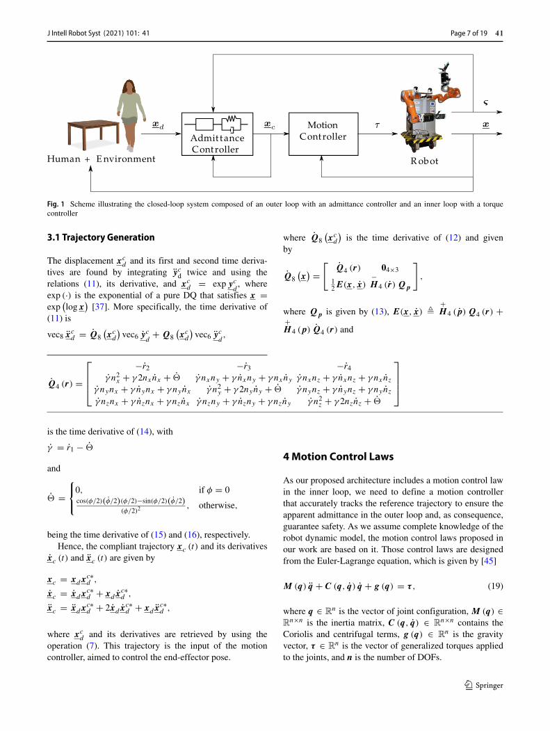
Fig. 1 Scheme illustrating the closed-loop system composed of an outer loop with an admittance controller and an inner loop with a torquecontroller
3.1 Trajectory Generation
The displacement xcd and its first and second time deriva-
tives are found by integrating ycd twice and using the
relations (11), its derivative, and xcd = exp yc
d, where
exp (·) is the exponential of a pure DQ that satisfies x =exp
(log x
)[37]. More specifically, the time derivative of
(11) is
vec8 xcd = Q8
(xc
d
)vec6 yc
d+ Q8
(xc
d
)vec6 yc
d,
where Q8(xc
d
)is the time derivative of (12) and given
by
Q8(x) =
[Q4 (r) 04×3
12E(x, x)
−H 4 (r)Qp
],
where Qp is given by (13), E(x, x) +H 4 (p) Q4 (r) +
+H 4 (p) Q4 (r) and
Q4 (r) =
⎡⎢⎢⎣
−r2 −r3 −r4
γ n2x + γ 2nxnx + γ nxny + γ nxny + γ nxny γ nxnz + γ nxnz + γ nxnz
γ nynx + γ nynx + γ nynx γ n2y + γ 2nyny + γ nynz + γ nynz + γ nynz
γ nznx + γ nznx + γ nznx γ nzny + γ nzny + γ nzny γ n2z + γ 2nznz +
⎤⎥⎥⎦
is the time derivative of (14), with
γ = r1 −
and
=⎧⎨⎩
0, if φ = 0cos(φ/2)(φ/2)(φ/2)−sin(φ/2)(φ/2)
(φ/2)2 , otherwise,
being the time derivative of (15) and (16), respectively.Hence, the compliant trajectory xc (t) and its derivatives
xc (t) and xc (t) are given by
xc = xdxc∗d ,
xc = xdxc∗d + xd xc∗
d ,
xc = xdxc∗d + 2xd xc∗
d + xd xc∗d ,
where xcd and its derivatives are retrieved by using the
operation (7). This trajectory is the input of the motioncontroller, aimed to control the end-effector pose.
4Motion Control Laws
As our proposed architecture includes a motion control lawin the inner loop, we need to define a motion controllerthat accurately tracks the reference trajectory to ensure theapparent admittance in the outer loop and, as consequence,guarantee safety. As we assume complete knowledge of therobot dynamic model, the motion control laws proposed inour work are based on it. Those control laws are designedfrom the Euler-Lagrange equation, which is given by [45]
M (q) q + C (q, q) q + g (q) = τ , (19)
where q ∈ Rn is the vector of joint configuration, M (q) ∈
Rn×n is the inertia matrix, C (q, q) ∈ R
n×n contains theCoriolis and centrifugal terms, g (q) ∈ R
n is the gravityvector, τ ∈ R
n is the vector of generalized torques appliedto the joints, and n is the number of DOFs.
J Intell Robot Syst (2021) 101: 41 Page 7 of 19 41
We discuss, in the following, an adaptation of twoclassic task-space motion controllers that are based on(19) and on the differential forward kinematics; namely,the task-space inverse dynamics with feedback lineariza-tion (TIDFL) and task-space PID controller with gravitycompensation (TPID). The adaptation consists of using unitDQ to represent the end-effector pose, which offers someadvantages, as discussed in Section 2. Then, we propose anadaptive controller to improve the JSIM conditioning.
4.1 Task-Space Inverse Dynamics with FeedbackLinearization
One common task-space controller for torque-actuatedrobots is based on the inverse dynamics with feedbacklinearization [45]; that is,
u = M (q) aq + C (q, q) q + g (q) , (20)
where the control input u τ ∈ Rn is applied to the joints
and aq q ∈ Rn is the control input designed to stabilize
the linearized closed-loop system.Since we seek a task-space controller, the control law for
the linearized closed-loop system is defined as
aq = J+ (ax − J q), (21)
where J+ is the Moore–Penrose pseudoinverse of theJacobian matrix J ∈ R
8×n and ax vec8 x is given by
ax = vec8 xc − KD vec8 ˙x − KP vec8 x − KI
∫ t
0 vec8 xdt, (22)
where KD, KP , KI ∈ R8×8 are positive definite gain
matrices and x x−xc denotes the end-effector error, withxc ∈ S ⊂ H being the compliant end-effector pose [46].
The torque of each joint calculated from (20) can bevery disparate due to the difference in the singular values ofM (q), leading to poor closed-loop behavior, as we show inthe results in Section 5. For instance, if the configuration-dependent inertia along a specific joint is very small,no matter how large the position/velocity error or PID-coefficients are, the correction torque applied on that jointwill be still small compared to the dominant torque, whichmay result in some undesired stationary error [11, 14].
4.2 Task-Space PID Controller with GravityCompensation
To improve the closed-loop system dynamic behavior injoint space, Shen and Featherstone [11] propose to usea PD with gravity compensation, which is proved to bestable [46], as it directly converts the joint-space error tothe joint torques, without using the JSIM, and therefore is
not affected by its ill-conditioning [11]. We adapted theircontroller to be in task-space and use unit DQ to representthe end-effector pose. Moreover, we added an integral termto it. Thus, the TPID is given by
u = J+ax + g (q) , (23)
with ax given by (22).Shen and Featherstone [11] emphasizes that, although
controllers such as (23) do not use the JSIM, whichmitigates the problem caused by the JSIM ill-conditioning,a controller that takes into consideration the whole dynamicmodel of the system should achieve better accuracy.
4.3 Task-Space Adaptive JSIM ConditioningController
Targeting a task-space control law that is able to achieve agood accuracy by using torque inputs, an adequate alterna-tive to the previously widely used control structures is touse an adaptive controller in which a carefully chosen pos-itive definite matrix D ∈ R
n×n is added to the JSIM toimprove its conditioning without adding excessive inaccu-racy to the nominal model. Since the inertia matrix dependson the robot configuration, it is difficult to choose D before-hand, and thus it should be adapted during the robot motion,which motivates the use of an adaptive controller.
A typical adaptive controller is composed of a control lawand an adaptation law. Thus, assuming full knowledge ofthe robot kinematics and dynamics, and that only the matrixD needs to be estimated, we propose a task-space adaptivecontrol law based on the one by Cheah et al. [31], which isgiven by
u = J T ax + v(q, q, qr , qr
)+ Y(q, qr
)a, (24)
where ax is given by (22), v(q, q, qr , qr
) ∈ Rn
is a vector containing the known dynamic model—i.e.,v(q, q, qr , qr
) = M (q) qr +C (q, q) qr +g (q)—, where
qr = J+ vec8 xr ,
qr = J+ (vec8 xr − J q),
in which
vec8 xr = vec8 xc − α vec8 x,
vec8 xr = vec8 xc − α vec8 ˙x,
with α being a positive constant. The matrix Y(q, qr
) ∈R
n×n is the regressor that depends on the choice of D andon the parameter vector a ∈ R
n to be estimated.
4.3.1 Adaptive JSIM Conditioning
In order to define the adaptation law, we first choose thepositive definite matrix D that is added to the JSIM aiming
J Intell Robot Syst (2021) 101: 41Page 8 of 1941
to improve its conditioning.1 Therefore, knowing that theinertia matrix M M (q) can be decomposed into M =USUT , where each column ui , with i ∈ 1, . . . , n, ofU ∈ O (n) contains the left singular vectors of M andS ∈ R
n×n contains the singular values of M [47], wedefine D = UDUT as a positive definite matrix, whereR
n×n D = diag(d1, . . . , dn) is a suitable diagonal matrix[13].
Since the condition number of M is given by cond (M) σ1M /σnM , where σ1M and σnM are the maximum andminimum singular values of M , respectively, thus M+D =U(S + D)UT implies
cond(M + D) = (σ1M+σ1
D)
(σnM+σn
D).
If cond(M + D) < cond(M), then
σ1M + σ1D
σnM + σnD
<σ1M
σnM
=⇒ σ1D
σnD
<σ1M
σnM
=⇒ cond(D)
< cond (M) .
(25)
Therefore, for the condition number of the sum(M + D
)be smaller than the one of M , the matrix D must be betterconditioned than M [13].
Considering the robot dynamic model (19) in which thematrix D is added to the nominal JSIM, and knowing thatthe model is linear in a set of parameters and its linearcombinations [30], we can write
[M (q) + D
]qr + C (q, q) qr + g (q)
= M (q) qr + C (q, q) qr + g (q)︸ ︷︷ ︸v(q,q,qr ,qr )
+ Y(q, qr
)a,
which implies Y(q, qr
)a = Dqr , with a ∈ R
n being thevector of parameters.
In (24), the vector a contains the estimated values of a,and thus the goal is to enforce Y
(q, qr
)a = Dqr , with
a = [a1 · · · an
]Tbeing the singular values of D. Since
D = UDUT =n∑
i=1
uiuTi ai,
the regressor is given by Y(q, qr
) = [y1 · · · yn
], where
yi = uiuTiqr .
In order to enforce the estimated parameters in a to bepositive and also to have a matrix D that fulfills condition(25), we first define a convex region corresponding to the
1From a physical point of view, improving the conditioning number ofthe inertia matrix is equivalent to changing the inertial impedance ofthe closed-loop system. More specifically, the system will have moreuniform inertial characteristics.
admissible parameter set [35]. Thus, variable lower (βmin)and upper (βmax) bounds are defined as a function of thesingular values of the JSIM such that σnM < βmin = βmax <
σ1M . The convex region of admissible parameters is definedas [13]
ηmin ≤ a ≤ ηmax
,
where
ηmax 1nβmax − diag (0, . . . , n − 1) 1nδ,
ηmin 1nβmax − diag (1, . . . , n) 1nδ,
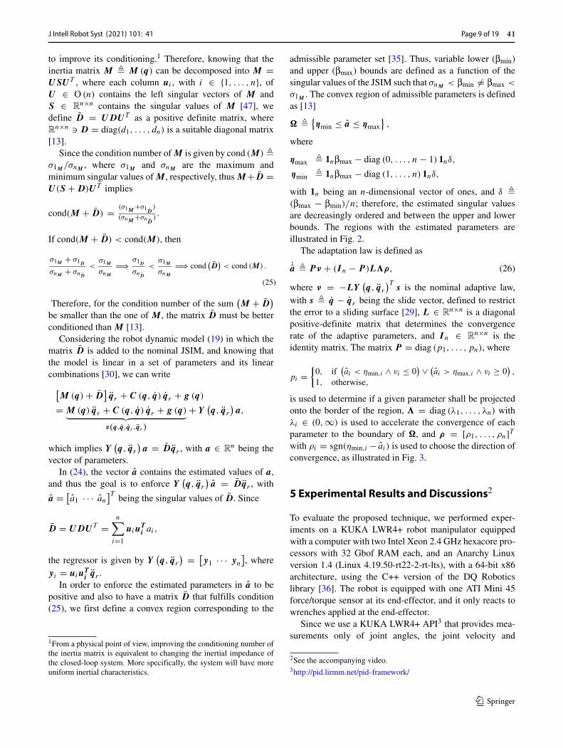
with 1n being an n-dimensional vector of ones, and δ (βmax − βmin)/n; therefore, the estimated singular valuesare decreasingly ordered and between the upper and lowerbounds. The regions with the estimated parameters areillustrated in Fig. 2.
The adaptation law is defined as
˙a Pν + (In − P )Lρ, (26)
where ν = −LY(q, qr
)Ts is the nominal adaptive law,
with s q − qr being the slide vector, defined to restrictthe error to a sliding surface [29], L ∈ R
n×n is a diagonalpositive-definite matrix that determines the convergencerate of the adaptive parameters, and In ∈ R
n×n is theidentity matrix. The matrix P = diag (p1, . . . , pn), where
pi =
0, if(ai < ηmin,i ∧ νi ≤ 0
) ∨ (ai > ηmax,i ∧ νi ≥ 0
),
1, otherwise,
is used to determine if a given parameter shall be projectedonto the border of the region, = diag (λ1, . . . , λn) withλi ∈ (0, ∞) is used to accelerate the convergence of eachparameter to the boundary of , and ρ = [ρ1, . . . , ρn]Twith ρi = sgn(ηmin,i − ai ) is used to choose the direction ofconvergence, as illustrated in Fig. 3.
5 Experimental Results and Discussions2
To evaluate the proposed technique, we performed exper-iments on a KUKA LWR4+ robot manipulator equippedwith a computer with two Intel Xeon 2.4 GHz hexacore pro-cessors with 32 Gbof RAM each, and an Anarchy Linuxversion 1.4 (Linux 4.19.50-rt22-2-rt-lts), with a 64-bit x86architecture, using the C++ version of the DQ Roboticslibrary [36]. The robot is equipped with one ATI Mini 45force/torque sensor at its end-effector, and it only reacts towrenches applied at the end-effector.
Since we use a KUKA LWR4+ API3 that provides mea-surements only of joint angles, the joint velocity and
2See the accompanying video.3http://pid.lirmm.net/pid-framework/
J Intell Robot Syst (2021) 101: 41 Page 9 of 19 41
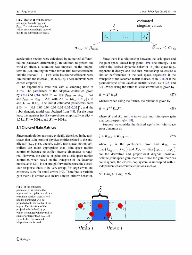
Fig. 2 Region with the lowerand upper bounds βmin andβmax. The estimated singularvalues are decreasingly orderedinside the subregions of size δ
acceleration vectors were calculated by numerical differen-tiation (backward differencing). In addition, to prevent thewind-up effect, a saturation was imposed on the integralterm in (22), limiting the value for the first four coefficientsinto the interval [−1, 1] while the last four coefficients werelimited into the interval [−0.06, 0.06]. These intervals werechosen empirically.
The experiments were run with a sampling time of5 ms. The parameters of the adaptive controller, givenby (24) and (26), were α = 0.5, βmin = σnM + σ
and βmax = σ1M − σ , with σ = (σnM + σ1M
)/10,
and L = 0.1I 7. The initial estimated parameters were
a [0] = [0.1 0.05 0.04 0.03 0.02 0.02 0.02
]T, and the
robot dynamic model was obtained from [48]. For the outerloop, the matrices in (18) were chosen empirically as Md =1.5I 6, Bd = 300I 6, and Kd = 100I 6.
5.1 Choice of Gain Matrices
Since manipulation tasks are typically described in the task-space, that is, in terms of physical entities related to the end-effector (e.g., pose, wrench, twist), task-space motion con-trollers are more appropriate than joint-space motioncontrollers because no explicit inverse kinematics is requi-red. However, the choice of gains for a task-space motioncontroller, when based on the transpose of the Jacobianmatrix, as in (24), is not straightforward because the closed-loop response tends to be very abrupt for large errors andextremely slow for small errors [49]. Therefore, a variablegain matrix is desirable to ensure a more uniform behavior.
Since there is a relationship between the task-space andthe joint-space closed-loop gains [49], one strategy is todefine the desired dynamic behavior in joint-space (e.g.,exponential decay) and use that relationship to ensure asimilar performance in the task-space, regardless if thetranspose of the Jacobian matrix is used, as in (24), or if thepseudoinverse of the Jacobian matrix is used, as in (23) and(21). When using the latter, this transformation is given by
K = J+KqJ , (27)
whereas when using the former, the relation is given by
K = J+T KqJ+, (28)
where K and Kq are the task-space and joint-space gainmatrices, respectively [49].
Suppose we consider the desired equivalent joint-spaceerror dynamics as
¨q + KDq˙q + KPq q = 0, (29)
where q is the joint-space error and KDq =diag
(kDq1
, . . . , kDqn
)and KPq = diag
(kPq1
, . . . , kPqn
)
are the derivative and proportional diagonal positive-definite joint-space gain matrices. Since the gain matricesare diagonal, the closed-loop system is uncoupled with n
independent characteristic equations such as
ri2 + kDqi
ri + kPqi= 0,
Fig. 3 If the estimatedparameter ai is outside theregion and the update ν makes itto remain outside, then pi = 0and the parameter will beprojected onto the border of theregion. The direction of theprojection is defined by ρi ,which is changed whenever ai issmaller or larger than ηmin,i . Ifpi = 1, then the nominaladaptation law is used
J Intell Robot Syst (2021) 101: 41Page 10 of 1941
for all i ∈ 1, · · · , n, with two roots given by
ri1,2 = −kDqi±√
k2Dqi
−4kPqi
2
If k2Dqi
= 4kPqi, then ri1 = ri2 = −kDqi
/2 and thus the
solution to (29) is given by
qi (t) = ci1eri t + ci2 te
ri t ,
with ci1 , ci2 ∈ R. Hence, the error decreases exponentially.Thus, we have chosen the equivalent joint-space gains
as KDq = 10I 7 and KPq = 25I 7, for all torquecontrollers, which satisfies the relation k2
Dqi= 4kPqi
, for
all i ∈ 1, . . . , n, and the integral gain has been chosenempirically as KIq = 10I 7. Consequently, as we wish a
dynamic behavior equivalent to ¨q + KDq˙q + KPq q = 0,
the gains KP , KI , and KD for the controllers (20)—(22)and (23) have been found by using the transformation (27).Similarly, the equivalent task-space gains for the controller(24)—(26) are found according to the transformation (28).
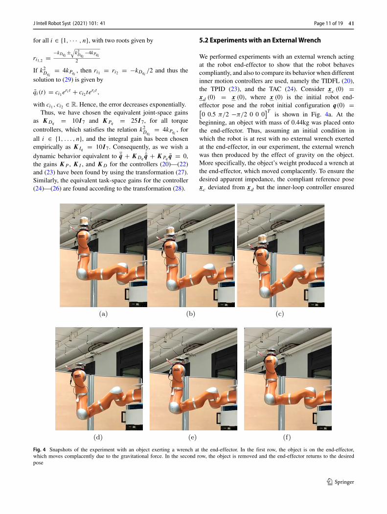
5.2 Experiments with an External Wrench
We performed experiments with an external wrench actingat the robot end-effector to show that the robot behavescompliantly, and also to compare its behavior when differentinner motion controllers are used, namely the TIDFL (20),the TPID (23), and the TAC (24). Consider xc (0) =xd (0) = x (0), where x (0) is the initial robot end-effector pose and the robot initial configuration q(0) =[0 0.5 π/2 −π/2 0 0 0
]Tis shown in Fig. 4a. At the
beginning, an object with mass of 0.44kg was placed ontothe end-effector. Thus, assuming an initial condition inwhich the robot is at rest with no external wrench exertedat the end-effector, in our experiment, the external wrenchwas then produced by the effect of gravity on the object.More specifically, the object’s weight produced a wrench atthe end-effector, which moved complacently. To ensure thedesired apparent impedance, the compliant reference posexc deviated from xd but the inner-loop controller ensured
Fig. 4 Snapshots of the experiment with an object exerting a wrench at the end-effector. In the first row, the object is on the end-effector,which moves complacently due to the gravitational force. In the second row, the object is removed and the end-effector returns to the desiredpose
J Intell Robot Syst (2021) 101: 41 Page 11 of 19 41
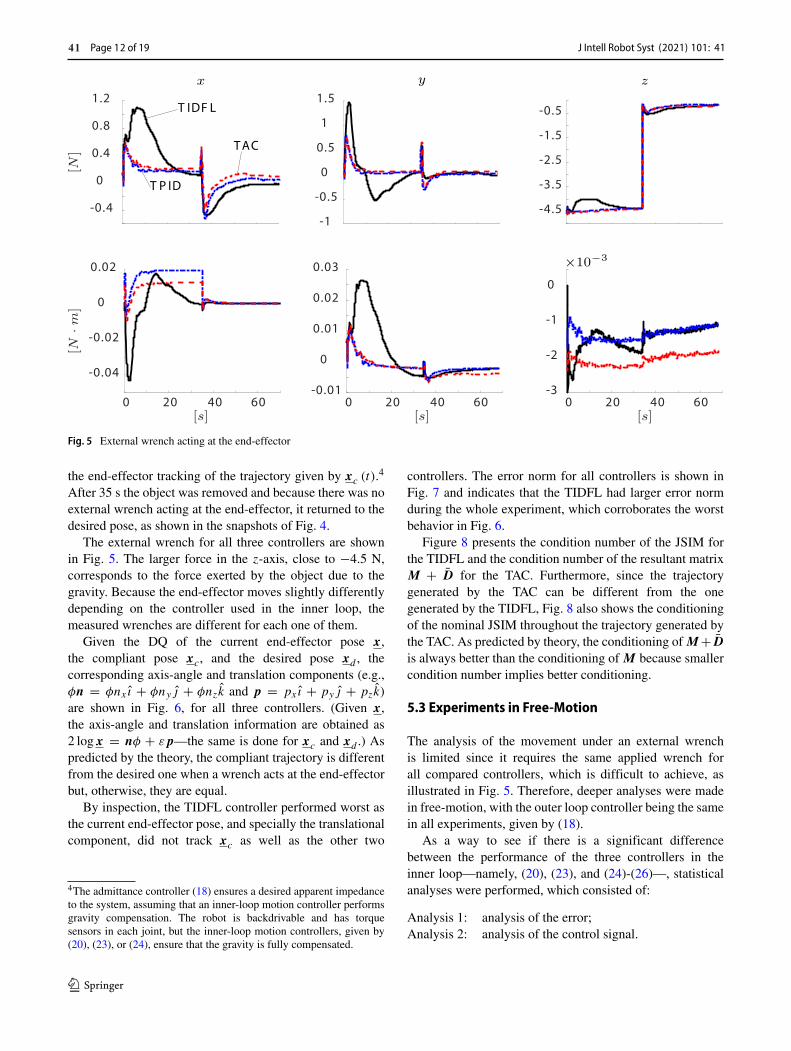
Fig. 5 External wrench acting at the end-effector
the end-effector tracking of the trajectory given by xc (t).4
After 35 s the object was removed and because there was noexternal wrench acting at the end-effector, it returned to thedesired pose, as shown in the snapshots of Fig. 4.
The external wrench for all three controllers are shownin Fig. 5. The larger force in the z-axis, close to −4.5 N,corresponds to the force exerted by the object due to thegravity. Because the end-effector moves slightly differentlydepending on the controller used in the inner loop, themeasured wrenches are different for each one of them.
Given the DQ of the current end-effector pose x,the compliant pose xc, and the desired pose xd , thecorresponding axis-angle and translation components (e.g.,φn = φnx ı + φnyj + φnzk and p = pxı + pyj + pzk)are shown in Fig. 6, for all three controllers. (Given x,the axis-angle and translation information are obtained as2 log x = nφ + εp—the same is done for xc and xd .) Aspredicted by the theory, the compliant trajectory is differentfrom the desired one when a wrench acts at the end-effectorbut, otherwise, they are equal.
By inspection, the TIDFL controller performed worst asthe current end-effector pose, and specially the translationalcomponent, did not track xc as well as the other two
4The admittance controller (18) ensures a desired apparent impedanceto the system, assuming that an inner-loop motion controller performsgravity compensation. The robot is backdrivable and has torquesensors in each joint, but the inner-loop motion controllers, given by(20), (23), or (24), ensure that the gravity is fully compensated.
controllers. The error norm for all controllers is shown inFig. 7 and indicates that the TIDFL had larger error normduring the whole experiment, which corroborates the worstbehavior in Fig. 6.
Figure 8 presents the condition number of the JSIM forthe TIDFL and the condition number of the resultant matrixM + D for the TAC. Furthermore, since the trajectorygenerated by the TAC can be different from the onegenerated by the TIDFL, Fig. 8 also shows the conditioningof the nominal JSIM throughout the trajectory generated bythe TAC. As predicted by theory, the conditioning of M +D
is always better than the conditioning of M because smallercondition number implies better conditioning.
5.3 Experiments in Free-Motion
The analysis of the movement under an external wrenchis limited since it requires the same applied wrench forall compared controllers, which is difficult to achieve, asillustrated in Fig. 5. Therefore, deeper analyses were madein free-motion, with the outer loop controller being the samein all experiments, given by (18).
As a way to see if there is a significant differencebetween the performance of the three controllers in theinner loop—namely, (20), (23), and (24)-(26)—, statisticalanalyses were performed, which consisted of:
Analysis 1: analysis of the error;Analysis 2: analysis of the control signal.
J Intell Robot Syst (2021) 101: 41Page 12 of 1941
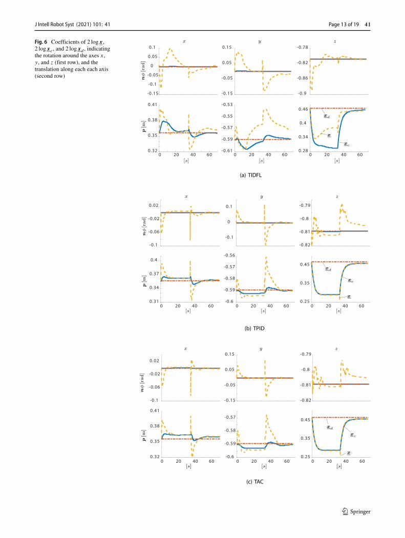
Fig. 6 Coefficients of 2 log x,2 log xc, and 2 log xd , indicatingthe rotation around the axes x,y, and z (first row), and thetranslation along each each axis(second row)
J Intell Robot Syst (2021) 101: 41 Page 13 of 19 41
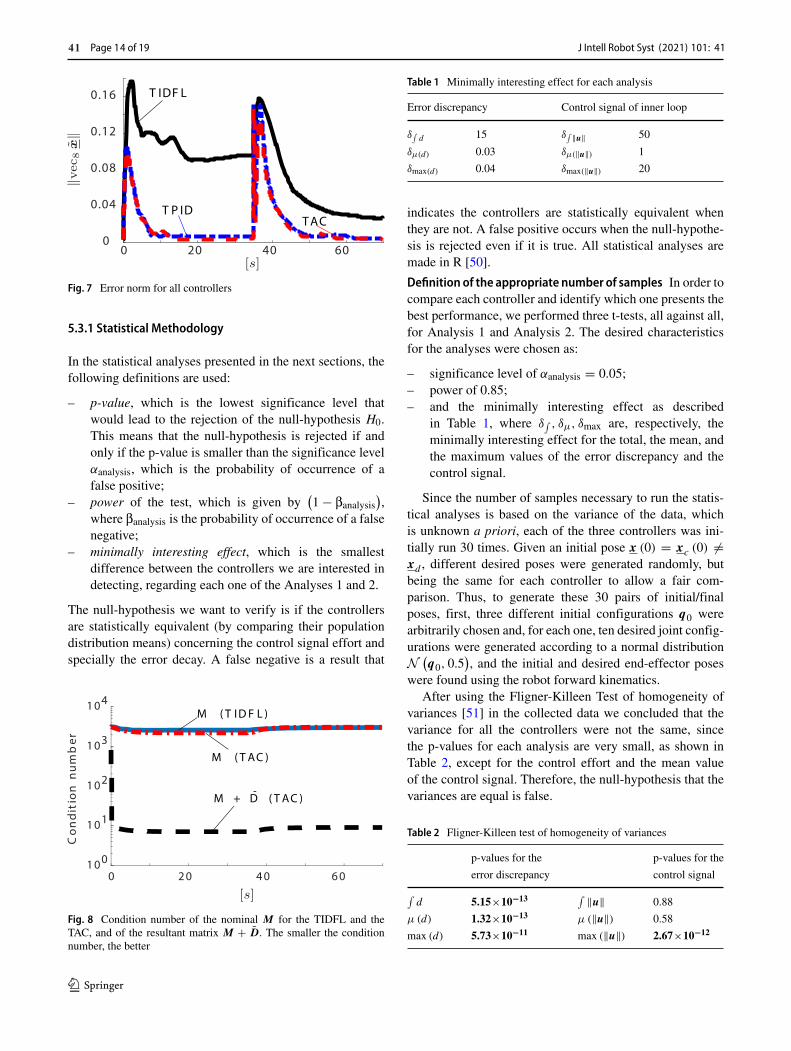
Fig. 7 Error norm for all controllers
5.3.1 Statistical Methodology
In the statistical analyses presented in the next sections, thefollowing definitions are used:
– p-value, which is the lowest significance level thatwould lead to the rejection of the null-hypothesis H0.This means that the null-hypothesis is rejected if andonly if the p-value is smaller than the significance levelαanalysis, which is the probability of occurrence of afalse positive;
– power of the test, which is given by(1 − βanalysis
),
where βanalysis is the probability of occurrence of a falsenegative;
– minimally interesting effect, which is the smallestdifference between the controllers we are interested indetecting, regarding each one of the Analyses 1 and 2.
The null-hypothesis we want to verify is if the controllersare statistically equivalent (by comparing their populationdistribution means) concerning the control signal effort andspecially the error decay. A false negative is a result that
Fig. 8 Condition number of the nominal M for the TIDFL and theTAC, and of the resultant matrix M + D. The smaller the conditionnumber, the better
Table 1 Minimally interesting effect for each analysis
Error discrepancy Control signal of inner loop
δ∫ d 15 δ∫ ‖u‖ 50
δμ(d) 0.03 δμ(‖u‖) 1
δmax(d) 0.04 δmax(‖u‖) 20
indicates the controllers are statistically equivalent whenthey are not. A false positive occurs when the null-hypothe-sis is rejected even if it is true. All statistical analyses aremade in R [50].
Definition of the appropriate number of samples In order tocompare each controller and identify which one presents thebest performance, we performed three t-tests, all against all,for Analysis 1 and Analysis 2. The desired characteristicsfor the analyses were chosen as:
– significance level of αanalysis = 0.05;– power of 0.85;– and the minimally interesting effect as described
in Table 1, where δ∫ , δμ, δmax are, respectively, theminimally interesting effect for the total, the mean, andthe maximum values of the error discrepancy and thecontrol signal.
Since the number of samples necessary to run the statis-tical analyses is based on the variance of the data, whichis unknown a priori, each of the three controllers was ini-tially run 30 times. Given an initial pose x (0) = xc (0) =xd , different desired poses were generated randomly, butbeing the same for each controller to allow a fair com-parison. Thus, to generate these 30 pairs of initial/finalposes, first, three different initial configurations q0 werearbitrarily chosen and, for each one, ten desired joint config-urations were generated according to a normal distributionN(q0, 0.5
), and the initial and desired end-effector poses
were found using the robot forward kinematics.After using the Fligner-Killeen Test of homogeneity of
variances [51] in the collected data we concluded that thevariance for all the controllers were not the same, sincethe p-values for each analysis are very small, as shown inTable 2, except for the control effort and the mean valueof the control signal. Therefore, the null-hypothesis that thevariances are equal is false.
Table 2 Fligner-Killeen test of homogeneity of variances
p-values for the p-values for the
error discrepancy control signal
∫d 5.15×10⁻¹³
∫ ‖u‖ 0.88
μ (d) 1.32×10⁻¹³ μ (‖u‖) 0.58
max (d) 5.73×10⁻¹¹ max (‖u‖) 2.67×10⁻¹²
J Intell Robot Syst (2021) 101: 41Page 14 of 1941
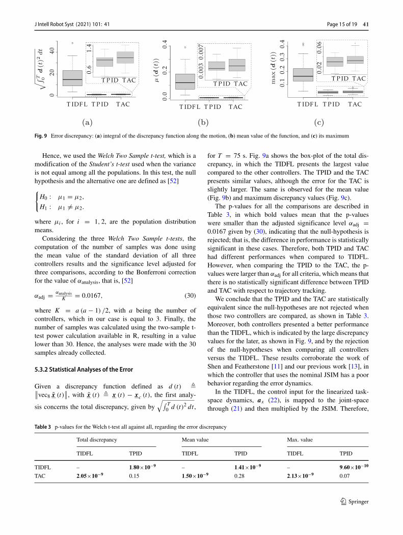
Fig. 9 Error discrepancy: (a) integral of the discrepancy function along the motion, (b) mean value of the function, and (c) its maximum
Hence, we used the Welch Two Sample t-test, which is amodification of the Student’s t-test used when the varianceis not equal among all the populations. In this test, the nullhypothesis and the alternative one are defined as [52]
H0 : μ1 = μ2,
H1 : μ1 = μ2.
where μi , for i = 1, 2, are the population distributionmeans.
Considering the three Welch Two Sample t-tests, thecomputation of the number of samples was done usingthe mean value of the standard deviation of all threecontrollers results and the significance level adjusted forthree comparisons, according to the Bonferroni correctionfor the value of αanalysis, that is, [52]
αadj = αanalysisK
= 0.0167, (30)
where K = a (a − 1) /2, with a being the number ofcontrollers, which in our case is equal to 3. Finally, thenumber of samples was calculated using the two-sample t-test power calculation available in R, resulting in a valuelower than 30. Hence, the analyses were made with the 30samples already collected.
5.3.2 Statistical Analyses of the Error
Given a discrepancy function defined as d (t) ∥∥vec8 x (t)∥∥, with x (t) x (t) − xc (t), the first analy-
sis concerns the total discrepancy, given by√∫ T
0 d (t)2 dt ,
for T = 75 s. Fig. 9a shows the box-plot of the total dis-crepancy, in which the TIDFL presents the largest valuecompared to the other controllers. The TPID and the TACpresents similar values, although the error for the TAC isslightly larger. The same is observed for the mean value(Fig. 9b) and maximum discrepancy values (Fig. 9c).
The p-values for all the comparisons are described inTable 3, in which bold values mean that the p-valueswere smaller than the adjusted significance level αadj =0.0167 given by (30), indicating that the null-hypothesis isrejected; that is, the difference in performance is statisticallysignificant in these cases. Therefore, both TPID and TAChad different performances when compared to TIDFL.However, when comparing the TPID to the TAC, the p-values were larger than αadj for all criteria, which means thatthere is no statistically significant difference between TPIDand TAC with respect to trajectory tracking.
We conclude that the TPID and the TAC are statisticallyequivalent since the null-hypotheses are not rejected whenthose two controllers are compared, as shown in Table 3.Moreover, both controllers presented a better performancethan the TIDFL, which is indicated by the large discrepancyvalues for the later, as shown in Fig. 9, and by the rejectionof the null-hypotheses when comparing all controllersversus the TIDFL. These results corroborate the work ofShen and Featherstone [11] and our previous work [13], inwhich the controller that uses the nominal JSIM has a poorbehavior regarding the error dynamics.
In the TIDFL, the control input for the linearized task-space dynamics, ax (22), is mapped to the joint-spacethrough (21) and then multiplied by the JSIM. Therefore,
Table 3 p-values for the Welch t-test all against all, regarding the error discrepancy
Total discrepancy Mean value Max. value
TIDFL TPID TIDFL TPID TIDFL TPID
TIDFL – 1.80×10⁻⁹ – 1.41×10⁻⁹ – 9.60×10⁻¹⁰
TAC 2.05×10⁻⁹ 0.15 1.50×10⁻⁹ 0.28 2.13×10⁻⁹ 0.07
J Intell Robot Syst (2021) 101: 41 Page 15 of 19 41
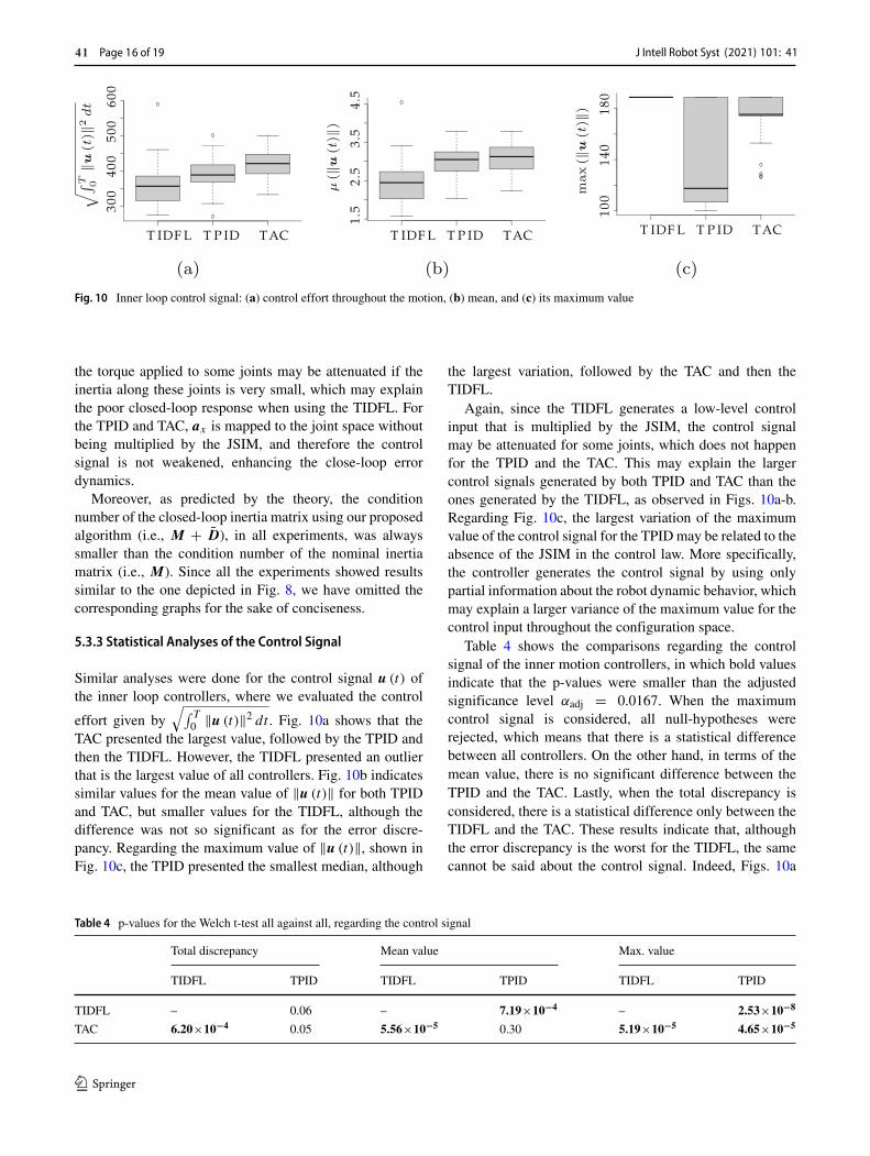
Fig. 10 Inner loop control signal: (a) control effort throughout the motion, (b) mean, and (c) its maximum value
the torque applied to some joints may be attenuated if theinertia along these joints is very small, which may explainthe poor closed-loop response when using the TIDFL. Forthe TPID and TAC, ax is mapped to the joint space withoutbeing multiplied by the JSIM, and therefore the controlsignal is not weakened, enhancing the close-loop errordynamics.
Moreover, as predicted by the theory, the conditionnumber of the closed-loop inertia matrix using our proposedalgorithm (i.e., M + D), in all experiments, was alwayssmaller than the condition number of the nominal inertiamatrix (i.e., M). Since all the experiments showed resultssimilar to the one depicted in Fig. 8, we have omitted thecorresponding graphs for the sake of conciseness.
5.3.3 Statistical Analyses of the Control Signal
Similar analyses were done for the control signal u (t) ofthe inner loop controllers, where we evaluated the control
effort given by√∫ T
0 ‖u (t)‖2 dt . Fig. 10a shows that theTAC presented the largest value, followed by the TPID andthen the TIDFL. However, the TIDFL presented an outlierthat is the largest value of all controllers. Fig. 10b indicatessimilar values for the mean value of ‖u (t)‖ for both TPIDand TAC, but smaller values for the TIDFL, although thedifference was not so significant as for the error discre-pancy. Regarding the maximum value of ‖u (t)‖, shown inFig. 10c, the TPID presented the smallest median, although
the largest variation, followed by the TAC and then theTIDFL.
Again, since the TIDFL generates a low-level controlinput that is multiplied by the JSIM, the control signalmay be attenuated for some joints, which does not happenfor the TPID and the TAC. This may explain the largercontrol signals generated by both TPID and TAC than theones generated by the TIDFL, as observed in Figs. 10a-b.Regarding Fig. 10c, the largest variation of the maximumvalue of the control signal for the TPID may be related to theabsence of the JSIM in the control law. More specifically,the controller generates the control signal by using onlypartial information about the robot dynamic behavior, whichmay explain a larger variance of the maximum value for thecontrol input throughout the configuration space.
Table 4 shows the comparisons regarding the controlsignal of the inner motion controllers, in which bold valuesindicate that the p-values were smaller than the adjustedsignificance level αadj = 0.0167. When the maximumcontrol signal is considered, all null-hypotheses wererejected, which means that there is a statistical differencebetween all controllers. On the other hand, in terms of themean value, there is no significant difference between theTPID and the TAC. Lastly, when the total discrepancy isconsidered, there is a statistical difference only between theTIDFL and the TAC. These results indicate that, althoughthe error discrepancy is the worst for the TIDFL, the samecannot be said about the control signal. Indeed, Figs. 10a
Table 4 p-values for the Welch t-test all against all, regarding the control signal
Total discrepancy Mean value Max. value
TIDFL TPID TIDFL TPID TIDFL TPID
TIDFL – 0.06 – 7.19×10⁻⁴ – 2.53×10⁻⁸
TAC 6.20×10⁻⁴ 0.05 5.56×10⁻⁵ 0.30 5.19×10⁻⁵ 4.65×10⁻⁵
J Intell Robot Syst (2021) 101: 41Page 16 of 1941
and b suggest that, in general, the TIDFL generates smallercontrol signals. This can be related to the use of the JSIMin the control law, which attenuates the control signal alongjoints that have smaller equivalent inertia.
6 Conclusion and Final Remarks
This paper proposed a task-space admittance controller withan adaptation of the JSIM conditioning. The architectureconsists of an admittance controller in the outer loop, toensure a compliant robot behavior in case of interaction, andan adaptive motion controller in the inner loop that guaran-tees that the adapted JSIM is always better conditioned thanthe nominal one throughout the whole robot configurationspace. The controllers are based on DQ algebra, whichprevents the occurrence of representational singularities.Moreover, this architecture was compared with one in whichthe motion controller in the inner loop is replaced by othertwo widely used motion controllers, namely the TIDFL andthe TPID.
Statistical analyses were performed with the robot infree-motion to evaluate the tracking error and the controlsignal. The results of the Welch t-tests, together with theexplanatory analyses, showed that the TIDFL presented theworst behavior regarding the error dynamics, whereas theTPID and the TAC presented similar results. This situationcan be explained by the ill-conditioning of the inertiamatrix. If the inertia along specific joints is very small,no matter how large the position/velocity error or PID-coefficients are, the correction torques generated by theTIDFL will be still small because they lie in the rangespace of the JSIM, which may be ill-conditioned and thusattenuate the control signals associated to small eigenvalues.For the TPID and TAC, the low-level control inputs arenot multiplied by the JSIM and thus are not attenuated,alleviating the problem.
Experiments done under a contact wrench acting onthe end-effector showed that the robot moves compliantlyaccording to a desired apparent impedance, which isimposed by the admittance controller in the outer loop. BothTPID and TAC followed the compliant trajectory, muchmore accurately than the TIDFL.
The proposed admittance controller, although simple andeffective, has a stiffness term that is geometrically inconsis-tent with the six-DOF tasks. Moreover, it suffers from theunwinding phenomenon, in which the end-effector posemay be close to the desired pose and yet rotate through largeangles before reaching the equilibrium [28]. Furthermore,the adaptive controller has shown good results, but we havenot proved the system closed-loop stability, which is anongoing work. Due to the insertion of disturbances in theinertia matrix during the adaptation law, the steady-state
error may be affected, especially if the JSIM conditioning isoverly changed.
Future works will be focused on the formal proof ofclosed-loop stability when using the proposed algorithm,taking into consideration the effects of the added matrix inthe control performance. Moreover, the outer loop will alsobe modified to deal with the unwinding problem and to usea stiffness matrix that is geometrically consistent with thetask.
Supplementary Information The online version contains supplemen-tary material available at (10.1007/s10846-020-01275-0).
Acknowledgments This work was supported by the Coordenacao deAperfeicoamento de Pessoal de Nıvel Superior (CAPES), ConselhoNacional de Desenvolvimento Cientıfico e Tecnologico (CNPq) underGrant 424011/2016-6 and Grant 303901/2018-7, and the CentreNational de la Recherche Scientifique (CNRS).
Open Access This article is licensed under a Creative CommonsAttribution 4.0 International License, which permits use, sharing,adaptation, distribution and reproduction in any medium or format, aslong as you give appropriate credit to the original author(s) and thesource, provide a link to the Creative Commons licence, and indicateif changes were made. The images or other third party material inthis article are included in the article’s Creative Commons licence,unless indicated otherwise in a credit line to the material. If materialis not included in the article’s Creative Commons licence and yourintended use is not permitted by statutory regulation or exceedsthe permitted use, you will need to obtain permission directly fromthe copyright holder. To view a copy of this licence, visit http://creativecommonshorg/licenses/by/4.0/.
References
1. Cherubini, A., Crosnier, A., Fraisse, P., Navarro, B., Passama,R., Sorour, M.: Research on cobotics at the LIRMM IDH group.In: ICRA Workshop IC3 - Industry of the future: Collaborative,connected, cognitive, vol hal-015233, Singapore, pp 1–5 (2017).https://hal.archives-ouvertes.fr/hal-01523305
2. Hogan, N.: Impedance control: An approach to manipulation. J.Dyn. Syst. Meas. Control. 107(1), 1–7 (1985). https://doi.org/10.1115/1.3140702. https://asmedigitalcollection.asme.org/dynamicsystems/article/107/1/1/400604/Impedance-Control-An-Approach-to-Manipulation-Part
3. Kimmel, M., Hirche, S.: Active safety control for dynamic human-robot interaction. In: 2015 IEEE/RSJ international conferenceon intelligent robots and systems (IROS), pp 4685–4691. IEEE(2015). http://ieeexplore.ieee.org/document/7354044/
4. Caccavale, F., Natale, C., Siciliano, B., Villani, L.: Six-DOF impe-dance control based on angle/axis representations. IEEE Trans.Robot. Autom. 15(2), 289–300 (1999). https://doi.org/10.1109/70.760350. http://ieeexplore.ieee.org/document/760350/
5. Caccavale, F., Chiacchio, P., Marino, A., Villani, L.: Six-DOFimpedance control of dual-arm cooperative manipulators. IEEE/ASME Transactions on Mechatronics 13(5), 576–586 (2008).https://doi.org/10.1109/TMECH.2008.2002816. http://ieeexplore.ieee.org/document/4639601/
6. Dietrich, A., Bussmann, K., Petit, F., Kotyczka, P., Ott, C.,Lohmann, B., Albu-Schaffer, A.: Whole-body impedance control
J Intell Robot Syst (2021) 101: 41 Page 17 of 19 41
of wheeled mobile manipulators: Stability analysis and experi-ments on the humanoid robot Rollin’ Justin. Auton. Robot. 40(3),505–517 (2016). https://doi.org/10.1007/s10514-015-9438-z
7. Fonseca, M.P.A., Adorno, B.V., Fraisse, P.: Task-space impedancecontroller using dual quaternion logarithm. In: Workshop onapplications of dual quaternion algebra to robotics, pp 1–2 (2019).https://zenodo.org/record/3566610#.Xe9X4NF7nDE
8. Yang, C., Ma, H., Fu, M.: Robot kinematics and dynamics mod-eling. In: Advanced technologies in modern robotic applications,pp 27–48. Springer, Singapore (2016)
9. Featherstone, R.: An empirical study of the joint space inertiamatrix. The International Journal of Robotics Research 23(9),859–871 (2004). https://doi.org/10.1177/0278364904044869.http://journals.sagepub.com/doi/10.1177/0278364904044869
10. Shah, S.V., Saha, S.K., Dutt, J.K.: A new perspective towardsdecomposition of the generalized inertia matrix of multi-body systems. Multibody System Dynamics 43(2), 97–130(2018). https://doi.org/10.1007/s11044-017-9581-8. http://link.springer.com/10.1007/s11044-017-9581-8
11. Shen, Y., Featherstone, R.: The effect of Ill-conditioned inertiamatrix on controlling manipultor robot. In: Proceedings of the2003 australasian conference on robotics & automation, pp 1–6.Australian Robotics and Automation Association (2003). http://hdl.handle.net/1885/87130
12. Agarwal, A., Shah, S.V., Bandyopadhyay, S., Saha, S.K.:Dynamics of serial kinematic chains with large number ofdegrees-of-freedom. Multibody System Dynamics 32(3), 273–298 (2014). https://doi.org/10.1007/s11044-013-9386-3. http://link.springer.com/10.1007/s11044-013-9386-3
13. Fonseca, M.P.A., Adorno, B.V., Fraisse, P.: An adaptive controllerwith guarantee of better conditioning of the robot manipulatorjoint-space inertia matrix. In: 2019 19th International conferenceon advanced robotics (ICAR), vol 111, pp 111–116. IEEE (2019).https://ieeexplore.ieee.org/document/8981558/
14. Fonseca, M.P.A., Adorno, B.V., Fraisse, P.: Design of an adaptivecontroller to improve the condition number of the inertia matrix ofserial manipulators. In: Proceedings XXII congresso brasileiro deautomatica, pp 1–8 (2018). http://www.swge.inf.br/proceedings/paper/?P=CBA2018-0982
15. Villani, L., Schutter, J.D.: Force control. In: Siciliano, B., Khatib,O. (eds.) Springer handbook of robotics, vol 53, pp 161–185.Springer, Berlin, Heidelberg (2008)
16. Ju, Z., Yang, C., Ma, H.: Kinematics modeling and experimentalverification of baxter robot. In: Proceedings of the 33rd chinesecontrol conference, CCC 2014, pp 8518–8523 (2014)
17. Erhart, S., Sieber, D., Hirche, S.: An impedance-based controlarchitecture for multi-robot cooperative dual-arm mobile manipu-lation. In: 2013 IEEE/RSJ international conference on intelligentrobots and systems, pp 315–322. IEEE, Tokyo (2013). http://ieeexplore.ieee.org/document/6696370/
18. Lee, J., Chang, P.H., Jamisola, R.S.: Relative impedancecontrol for dual-arm robots performing asymmetric bimanualtasks. IEEE Trans. Ind. Electron. 61(7), 3786–3796 (2014).https://doi.org/10.1109/TIE.2013.2266079. http://ieeexplore.ieee.org/document/6523093/
19. Sieber, D., Music, S., Hirche, S.: Multi-robot manipulationcontrolled by a human with haptic feedback. In: 2015 IEEE/RSJinternational conference on intelligent robots and systems (IROS),vol 2015-Decem, pp 2440–2446. IEEE (2015). http://ieeexplore.ieee.org/document/7353708/
20. Hoffman, E.M., Laurenzi, A., Muratore, L., Tsagarakis, N.G.,Caldwell, D.G.: Multi-priority cartesian impedance controlbased on quadratic programming optimization. In: 2018 IEEEInternational Conference on Robotics and Automation (ICRA),pp 309–315. IEEE, Brisbane (2018). https://ieeexplore.ieee.org/document/8462877/
21. Keemink, A.Q.L., van der Kooij, H., Stienen, A.H.A.: Admit-tance control for physical human-robot interaction. Int. J.Robot. Res. 37(11), 1421–1444 (2018). https://doi.org/10.1177/0278364918768950
22. Ferraguti, F., Talignani Landi, C., Sabattini, L., Bonfe, M.,Fantuzzi, C., Secchi, C.: A variable admittance control strategy forstable physical human-robot interaction. Int. J. Robot. Res. 38(6),747–765 (2019). https://doi.org/10.1177/0278364919840415
23. Navarro, B., Cherubini, A., Fonte, A., Passama, R., Poisson, G.,Fraisse, P.: An ISO10218-compliant adaptive damping controllerfor safe physical human-robot interaction. In: 2016 IEEEInternational Conference on Robotics and Automation (ICRA),pp 3043–3048. IEEE (2016). http://ieeexplore.ieee.org/document/7487468/
24. Cherubini, A., Passama, R., Crosnier, A., Lasnier, A., Fraisse,P.: Collaborative manufacturing with physical human-robot inter-action. Robot. Comput. Integr. Manuf. 40, 1–13 (2016). https://doi.org/10.1016/j.rcim.2015.12.007. http://linkinghub.elsevier.com/retrieve/pii/S0736584515301769
25. Tarbouriech, S., Navarro, B., Fraisse, P., Crosnier, A., Cherubini,A., Salle, D.: Admittance control for collaborative dual-arm mani-pulation, pp 198–204. https://doi.org/10.1109/icar46387.2019.8981624 (2020)
26. Agravante, D.J., Cherubini, A., Bussy, A., Gergondet, P., Kheddar,A.: Collaborative human-humanoid carrying using vision andhaptic sensing. In: 2014 IEEE international conference on roboticsand automation (ICRA), pp 607–612. IEEE (2014). http://ieeexplore.ieee.org/document/6906917/
27. Siciliano, B., Sciavicco, L., Villani, L., Oriolo, G. Robotics:Modelling, Planning and Control. Advanced Textbooks in Controland Signal Processing, 1st edn. Springer London, London(2009)
28. Bhat, S.P., Bernstein, D.S.: A topological obstruction to globalasymptotic stabilization of rotational motion and the unwindingphenomenon. In: Proceedings of the 1998 American ControlConference. ACC (IEEE Cat. No.98CH36207), vol 5, pp 2785–2789. IEEE (1998)
29. Slotine, J.-J.E., Li, W.: On the Adaptive Control of Robot Manip-ulators. The International Journal of Robotics Research 6(3), 49–59 (1987). https://doi.org/10.1177/027836498700600303. http://journals.sagepub.com/doi/10.1177/027836498700600303
30. Cheah, C.C., Liu, C., Slotine, J.J.E.: Adaptive Tracking Controlfor Robots with Unknown Kinematic and Dynamic Properties.The International Journal of Robotics Research 25(3), 283–296(2006). https://doi.org/10.1177/0278364906063830
31. Cheah, C.C., Liu, C., Slotine, J.J.E.: Adaptive Jacobian TrackingControl of Robots With Uncertainties in Kinematic, Dynamicand Actuator Models. IEEE Trans. Autom. Control 51(6), 1024–1029 (2006). https://doi.org/10.1109/TAC.2006.876943. http://ieeexplore.ieee.org/document/1643374/
32. Liu, C., Cheah, C.C., Slotine, J.J.E.: Adaptive Jacobian trackingcontrol of rigid-link electrically driven robots based on visualtask-space information. Automatica 42(9), 1491–1501 (2006).https://doi.org/10.1016/j.automatica.2006.04.022
33. Wang, H., Xie, Y.: Adaptive inverse dynamics control of robotswith uncertain kinematics and dynamics. Automatica 45(9), 2114–2119 (2009). https://doi.org/10.1016/j.automatica.2009.05.011
34. Hanlei, W.: On the recursive implementation of adaptive controlfor robot manipulators. In: Proceedings of the 29th chinese controlconference, pp 2154–2161 (2010)
35. Wang, H., Xie, Y.: On the uniform positive definiteness of theestimated inertia for robot manipulators. In: IFAC ProceedingsVolumes, vol 44, pp 4089–4094. IFAC (2011). https://pdfs.semanticscholar.org/edca/de54c1d78449a61b2d199ce46c4f2a347e69.pdf
J Intell Robot Syst (2021) 101: 41Page 18 of 1941
36. Adorno, B.V., Marinho, M.M.: DQ robotics: a library for robotmodeling and control using dual quaternion algebra. IEEE Robo-tics & Automation Magazine, pp 0–0. arXiv:1910.11612 (2019)
37. Adorno, B.V.: Robot Kinematic Modeling and Control Based onDual Quaternion Algebra - Part I : Fundamentals. https://hal.archives-ouvertes.fr/hal-01478225/document (2017)
38. Hamilton, W.R.: On Quaternions, Or On a New System ofImaginaries in Algebra. Philosophical Magazine Series 3 25(163),10–13 (1844). https://doi.org/10.1080/14786444408644923
39. Adorno, B.V.: Two-arm Manipulation: From Manipulators toEnhanced Human-Robot Collaboration [Contribution a la manip-ulation a deux bras : des manipulateurs a la collaborationhomme-robot]. Ph.D. Thesis, Universite Montpellier II. https://tel.archives-ouvertes.fr/tel-00641678/document (2011)
40. Clifford: Preliminary sketch of biquaternions. Proc. Lond. Math.Soc. s1-4(1), 381–395 (1873). https://doi.org/10.1112/plms/s1-4.1.381
41. Selig, J.M.: Geometric Fundamentals of Robotics. Springer, NewYork (2005)
42. Figueredo, L.F.C., Adorno, B.V., Ishihara, J.Y., Borges, G.A.:Robust kinematic control of manipulator robots using dual quater-nion representation. In: 2013 IEEE International Conferenceon Robotics and Automation, pp 1949–1955. IEEE, Karlsruhe(2013). http://ieeexplore.ieee.org/document/6630836/
43. Savino, H.J., Pimenta, L.C.A., Shah, J.A., Adorno, B.V.: Poseconsensus based on dual quaternion algebra with applicationto decentralized formation control of mobile manipulators. J.Franklin Inst. 357(1), 142–178 (2020). https://linkinghub.elsevier.com/retrieve/pii/S0016003219307161
44. Landi, C.T., Ferraguti, F., Sabattini, L., Secchi, C., Fantuzzi, C.:Admittance control parameter adaptation for physical human-robot interaction. In: 2017 IEEE International Conference onRobotics and Automation (ICRA), pp 2911–2916. IEEE (2017).http://ieeexplore.ieee.org/document/7989338/
45. Spong, M.W., Hutchinson, S., Vidyasagar, M.: Robot Modelingand Control. John Wiley & Sons, Inc, Hoboken (2006)
46. Kelly, R., Santibanez, V., Lorıa, A.: Control of Robot Manipula-tors in Joint Space. Springer, Leipzig (2005)
47. Chen, C.-T. In: Sedra, A.S., Ligthner, M.R. (eds.) Linear SystemTheory and Design, 3rd edn. Oxford University Press, New York(1999)
48. Katsumata, T., Navarro, B., Bonnet, V., Fraisse, P., Cros-nier, A., Venture, G.: Optimal exciting motion for fastrobot identification. Application to contact painting tasks withestimated external forces. Robot. Auton. Syst. 113, 149–159 (2019). https://doi.org/10.1016/j.robot.2018.11.021. https://linkinghub.elsevier.com/retrieve/pii/S0921889017307091
49. Pham, H.L., Adorno, B.V., Perdereau, V., Fraisse, P.: Set-point control of robot end-effector pose using dual quater-nion feedback. Robot. Comput. Integr. Manuf. 52(2016), 100–110 (2018). https://doi.org/10.1016/j.rcim.2017.11.003. https://linkinghub.elsevier.com/retrieve/pii/S0736584516301831
50. Peng, R.D.: R Programming for Data Science. Lean Publish-ing, British Columbia (2016). https://leanpub.com/rprogramming%5Cnhttp://leanpub.com/rprogramming
51. Crawley, M.J.: The r book. John Wiley & Sons Ltd,Hoboken (2007). https://www.wiley.com/en-br/The+R+Book-p-9780470515068
52. Montgomery, D.C. Design and Analysis of Experiments, 5th edn.John Wiley & Sons, Inc., Hoboken (2001). http://doi.wiley.com/10.1002/qre.458
Publisher’s Note Springer Nature remains neutral with regard tojurisdictional claims in published maps and institutional affiliations.
Mariana de Paula Assis Fonseca graduated in Automation andControl Engineering in 2013, at the Universidade Federal de MinasGerais (UFMG), Brazil. She received her Masters Degree also fromUFMG, in 2017, in Electrical Engineering, and is currently a Ph.D.candidate in Electrical Engineering at UFMG. She spent one year atLIRMM, in Montpellier, France, as an assistant engineer from theCNRS, and is currently a member of the Mechatronics, Control andRobotics (MACRO) research group at UFMG.
Bruno Vilhena Adorno received the B.S. degree in mechatronicsengineering and the M.S. degree in electrical engineering from theUniversity of Brasilia, Brasilia, Brazil, in 2005 and 2008, respectively,and the Ph.D. degree in automatic and microelectronic systems fromthe University of Montpellier, Montpellier, France, in 2011. He iscurrently a Senior Lecturer in Robotics with the Department ofElectrical and Electronic Engineering at The University of Manchester(UoM), Manchester, United Kingdom. Before joining the UoM, he wasan Associate Professor with the Department of Electrical Engineeringat the Federal University of Minas Gerais, Belo Horizonte, Brazil. Hiscurrent research interests include both practical and theoretical aspectsrelated to robot kinematics, dynamics, and control with applicationsto mobile manipulators, humanoids, and cooperative manipulationsystems.
Philippe Fraisse received the master’s degree in electrical engineeringfrom the Ecole Normale Superieure de Cachan, Cachan, France, in1988, and the Ph.D. degree in automatic control from the University ofMontpellier, Montpellier, France, in 1994. He is currently a Professorwith the Robotics Department, University of Montpellier. His researchinterests include physical human-robot interaction, humanoid robotics,robotics for rehabilitation, and mobile manipulators.
J Intell Robot Syst (2021) 101: 41 Page 19 of 19 41