Tariffs and the Expansion of the American

Pig Iron Industry, 1870-1940

Kanda Naknoi ∗

University of Connecticut

Preliminary and Incomplete

February 2017

Abstract

This study quantifies the benefit of the protection of the American pig iron in-dustry in 1870-1940. We illustrate that despite the presence of dynamic learning,fluctuations of demand and costs including transport costs could result in declinesin competitiveness. Transport costs played a crucial role because their large declinesoccurred before the US output surpassed that the UK output in 1890. A hypothet-ical removal of pig iron duty in 1883-1888 would result in a 50-70 percent loss inthe US output.

Key words: Pig iron trade, protection, transport costs

∗Department of Economics, University of Connecticut, 365 Fairfield Way, Storrs, CT 06269. Email:kanda.naknoi@uconn.edu. I would like to thank Gavin Wright for advice and support. I am indebted tocomments from Avner Greif, David Hummels, Kris Mitchener, Paul Rhode, Slavi Slavov, Asaf Zussman,and participants in seminars in Stanford, UC Irvine, the 2007 NBER Summer Institute, and the 2011UC Conference on New Perspectives on the Great Specialization. The remaining errors are entirely myown.

1 Introduction

Pig iron is a major intermediate input for iron and steel products, which play an important

role in the American industrialization (Wright, 1990; Irwin, 2003). The US pig iron

industry received protection in the form of duty from the 1820s, long before discoveries of

rich iron ore deposits and an innovation that greatly improved efficiency. By 1890, output

of pig iron in the US surpassed that of Great Britain, and subsequently the US became

the leading producer of pig iron. In 1913, the pig iron duty was removed but it was

reintroduced in 1922. However, the degree to which the US pig iron industry benefited

from protection remains an open question.

The literature has framed the question as the infant-industry hypothesis, which con-

sists of two parts. Did the US pig iron industry require protection to survive on such

a large scale that learning could take place? If so, was dynamic learning subsequently

realized? Irwin (2000a) and Davis and Irwin (2008) examined this question for the ante-

bellum period, and found that the majority of US pig iron output would have survived a

free trade regime. Hence, these studies dismiss the need to quantify the dynamic learning

effect, which were found in other industries such as the steel rail (Head, 1994).1

This study revisits this question over the postbellum period, from 1870 to 1940. We

explore this period for three reasons. First, the US did not surpass the UK in terms of

output until 1890. Second, the innovation that greatly improved efficiency took place in

1An alternative method to test an infant-industry hypothesis is to use a probability model to assessthe likelihood of a rise of a new industry behind tariff wall, such as Irwin (2000b)

1

1870, and that might have contributed to industry-wide learning by doing. Finally, time

series of price, input costs and transport costs display large fluctuations over this period.

The time series variations are highly useful for investigating the dynamic properties of the

industry. We supplement the estimation in Davis and Irwin (2008) with the estimation

of learning, as in Head (1994). We proceed in the following steps.

First, we estimate the elasticity of equilibrium output in response to price of imported

pig iron from the UK, controlling for cost shocks and demand shocks, as done in Davis

and Irwin (2008). This framework is from Grossman (1986), who assumes imperfect

substitution between imported and domestically produced products. The elasticity is

found to be 1.17, which is close to 1.41 in Davis and Irwin (2008).

Next, we estimate the scale of the dynamic learning effect on the US pig iron price,

using the lagged cumulative output beginning from 1846 as the measure of experience. By

doing so we do not overestimate the effect of learning from 1870, since learning could take

place in the antebellum period. We find evidence for learning, and the implied learning

rate is 20 percent. In other words, doubling the experience lowers price of the US pig

iron by 20 percent. This learning rate is the same as the estimate for the semiconductor

industry in Irwin and Klenow (1994). However, we do not find evidence for learning

spillover from the UK producers.

Finally, we simulate the counter-factual free trade regime beginning in 1870, taking

into account dynamic learning. Since costs fluctuated a great deal, the impact of a removal

of pig iron duty is sensitive to the timing of removal. A removal in 1870 would reduce

2

output about 40 percent, but a removal in 1885 would remove output about 70 percent,

with or without learning. Note that the quantitative impact of learning is extremely small;

therefore, much of learning had likely taken place in the antebellum period. The period

over which pig iron duty was critical to the industry is the years 1883-1888. A removal

of pig iron duty over this period would create a 50-70 percent loss in output. Hence, our

study provides evidence that protection was necessary for the US pig iron industry before

the US output surpassed the UK output.

What contributed to the decline in competitiveness of the US pig iron in 1883-1888?

The answer is a large decline in trans-Atlantic transport costs. From 1870 to 1990,

transport costs in ad valorem terms fell at the rate of 1.5 percentage point per year.

However, it fell about twice that rate or 3.2 percentage point per year in 1883-1888.

For input costs, imported coal price increased but the US coal price decreased over this

period. At the same time, price of iron ore fluctuated over this period with downward

trend. Thus, costs of intermediate inputs were not the primary cause of the decline in

competitiveness.

Our findings contrast with early work by Taussig (1915) and Temin (1964) on the

postbellum period, which viewed the effects of tariffs on the industry as marginal. Sun-

dararajan (1970), and Baack and Ray (1973), in contrast, find that tariffs significantly

helped expand the domestic pig iron industry in the post-bellum period. Our result is in

line with the finding by Allen (1979), that the productivity of the US pig iron industry

rose substantially after the 1880s.

3

The next section explains the estimation methodology. We describe the data and

estimation results in Section 3. The counter-factual exercise is in Section 4, and Section

5 concludes.

2 The Methodology

I follow Grossman (1986), who assume imperfect substitution of domestic and imported

products. The domestic demand for US pigk iron is determined by its price, price of

imported pig iron from the UK and demand shocks:

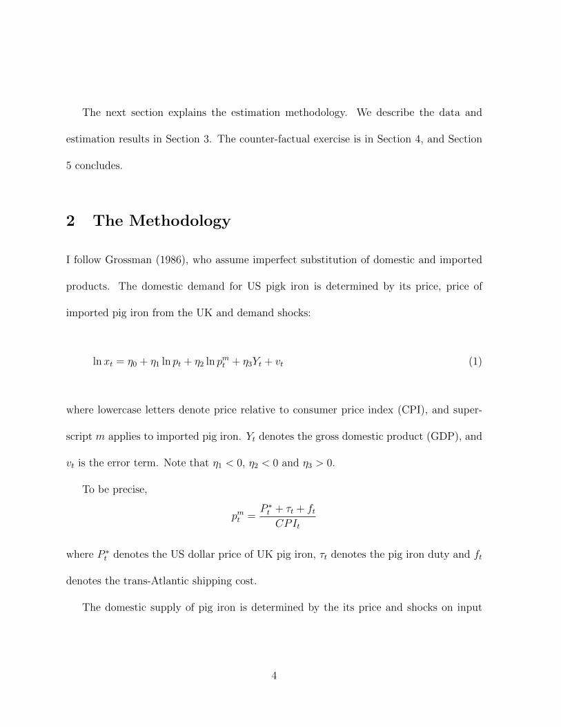
lnxt = η0 + η1 ln pt + η2 ln pmt + η3Yt + vt (1)

where lowercase letters denote price relative to consumer price index (CPI), and super-

script m applies to imported pig iron. Yt denotes the gross domestic product (GDP), and

vt is the error term. Note that η1 < 0, η2 < 0 and η3 > 0.

To be precise,

pmt =P ∗t + τt + ftCPIt

where P ∗t denotes the US dollar price of UK pig iron, τt denotes the pig iron duty and ft

denotes the trans-Atlantic shipping cost.

The domestic supply of pig iron is determined by the its price and shocks on input

4

price as follows:

ln yt = ε0 + ε1 ln pt + ε2 ln pct + ut, (2)

where superscript c denotes an intermediate input, such as coal, imported coal and iron

ore. ut is the error term. Note that ε1 > 0 and ε2 < 0.

In equilibrium, yt = xt = qt. Thus, Equations (1) and (2) yield the following estimating

equation:

ln qt = γ0 + γ1 ln pmt + γ2 lnYt + γ3pct + ht, (3)

where the elasticities are written in terms of demand and supply elasticities:

γ1 =η2ε1ε1 − η1

> 0

γ2 =η3ε1ε1 − η1

> 0

γ3 = − η1ε2ε1 − η1

< 0

In particular, γ1 governs the impacts of protection on output. Moreover, the benefits

of protection could accumulate over time through learning-by-doing. In the case of the

US pig iron industry, besides the invention of the pneumatic or Bessemer process by

Williams Kelly and Henry Bessemer, “hard driving” has received considerable attention

5

as the major innovation increasing the productivity (Allen, 1979; Temin, 1964). The

hard driving technique was pioneered in 1870, and further improved in the 1880s and

1890s. This technique allows a large amount of hot air to flow into blast furnaces at high

pressure, in order to speed up the smelting process. It helps increase output per furnace,

but adding this hard driving feature to a furnace requires a large sum of capital (Berck,

1978).

According to Berck (1978), constructing a new hard-driven furnace in Chicago in 1887

would have incurred the fixed cost ranging from 180,000 to 250,000 dollars. However,

that would have saved the variable cost and yielded profits as high as 130,000 dollars

in one year. Given that the estimated annual capacity of a hard-driven furnace was

43,500-52,690 gross tons, this was highly profitable but risky business, because redeeming

the fixed cost depended on fluctuations of demand. However, pig iron duty reduced the

riskiness by restricting competition with imports and allowing the domestic producers to

sell at a high price to recover the fixed cost.

As a consequence, the US producers could produce up to their furnace capacity when

a positive demand shock occurred. The economies of scale at the plant level were, there-

fore, a direct benefit from protection. Indirect effects of protection are the spillovers of

learning-by-doing at the industry level. Spillovers were made possible by the institu-

tions for learning, namely the professional associations that published their reports and

provided places to exchange knowledge among engineers and iron masters. The most

6

notable of these was the American Iron and Steel Association established in 1864.2 Other

related organizations were the American Institute of Mining Engineers and the United

States Association of Charcoal Iron Workers. The Transactions of the American Institute

of Mining Engineers was first published in 1871, and the United States Association of

Charcoal Iron Workers’ Journal was published in 1880 (Gordon, 1996). Through these in-

stitutions, spillovers of learning led to further cost-saving techniques and achievements of

industry-wide economies of scale. Consequently, pig iron producers became price-setters

in imperfectly competitive markets, and operated at a large scale, along the same line

as the endogenous growth theory (Romer, 1986). For this reason, we employ the most

common measure of economies of scale in the literature, namely the cumulative industry

output (Irwin and Klenow, 1994).

The most direct way to estimate it is to estimate a relationship between the cost curve

and cumulative output. However, cost data are not available, so we indirectly estimate

this from price data, as in Head (1994). Assume that firms are price-setters. Hence, price

is the product of markup and marginal cost. With imperfect competition, the markup

depends on the demand elasticity, hence demand shock term can capture the markup.

Specifically, the estimation equation becomes:

ln pt = α0 + α1 lnEt + α2 ln pct + α3 ln pot + α4 lnYt + nt (4)

2The original name was the American Iron and Associates.

7

Et is cumulative industry output from 1846 up to period t−1. Yt or the GDP also proxies

other macro shocks other than demand shocks, namely shocks on the cost of capital, labor

costs and productivity. nt is the stochastic component. Note that αi > 0 for i > 1. If

there are dynamic learning effects, α1 < 0 will hold. In the literature, one commonly used

concept is the so-called “learning rate.” It is the rate at which the marginal cost drops

following doubling cumulative output. Formally, learning rate is calculated as 1 − 2α1 .

It is critical to use cumulative industry output from the antebellum years, because

learning, if it exists, could have begun from an early stage of the industry. By incor-

porating this possibility, we do not overestimate the impact of learning in early years of

our sample. It is also plausible that there are spillovers of learning from the UK through

migration of workers. Let E∗t be cumulative industry output in the UK up to the last

period. Then, the estimation equation becomes:

ln pt = α0 + α1 lnEt + α?1 lnE∗t + α2 ln pct + α3 ln pot + α4 lnYt + n?t (5)

After the estimation, we simulate a counter-factual free trade regime from 1870 by

setting τt = 0 for all t. Thus, the percentage change in the domestic price of imported

pig iron becomes:

dpmtpmt

=P ∗t + f

P ∗t + τt + ft

− 1 < 0 (6)

8

Then, the hypothetical output under free trade is:

qfreet =

(1 + γ1

dpmtpmt

)qt (7)

Next, we calculate the hypothetical output without the learning effect from 1871 as:

For the year 1870, qnolearnt = qfreet . The reason is that Et−2 for t = 1870 is the

accumulated output from 1846 to 1868, which was given as the initial condition. In other

words, the producers have learned from experience up to 1868 regardless of whether free

trade is adopted.

3 The Data and Empirical Results

3.1 The Data

Figure 1 provides the annual movements of the US pig iron output in comparison with

the UK pig iron output. The annual output of the domestic pig iron doubled in every

decade from 1870 to 1890. The US output increased from 1.7 million gross tons in 1870

to 3.8 million gross tons in 1880, and it became 9.2 million gross tons in 1890. In fact,

the US surpassed Great Britain and became the world leading pig iron producer in 1890.

At this point, the US share in world production was 34.4 percent, whereas that of Great

Britain was 29.4 percent. The industry slowed down during the depression in the 1890s

but resumed its growth in the end of the century.

9

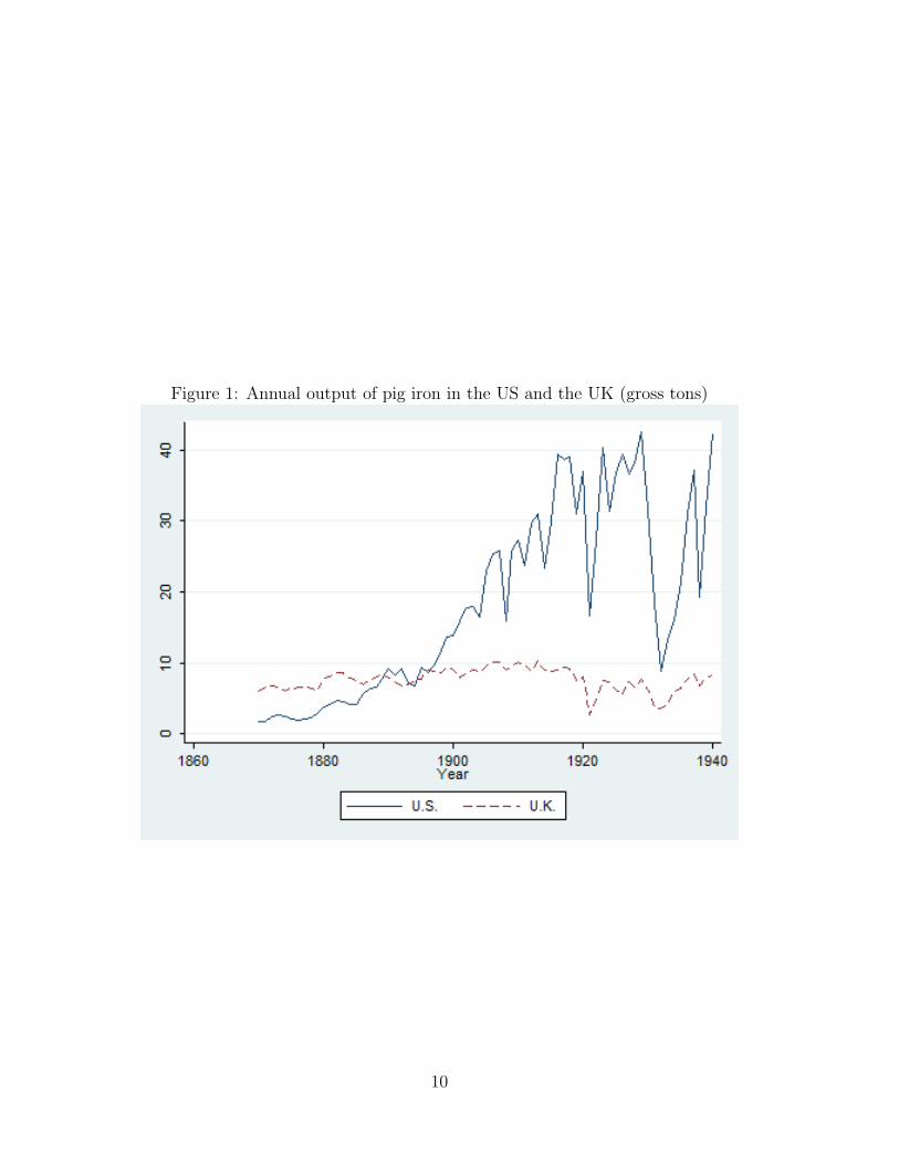
Figure 1: Annual output of pig iron in the US and the UK (gross tons)

10

In the early twentieth century, the US pig iron production continued to expand, al-

though there were declines in production in 1908, 1911 and 1914. In 1913 when the pig

iron duty was temporarily removed, the US accounted for approximately 40 percent of

world production. The US share of world production reached its peak at 60 percent in

1918. After the industry recovered from the Great Depression in 1933, it returned to its

pre-depression level in 1937. By 1940, the US pig iron output had tripled its 1900 level

to 42 million gross tons. In contrast, in 1940 the UK production remained approximately

the same as its 1900 level, which was only one-fifth of US output in 1940.

The US pig iron was produced mostly for domestic demand. The US was a net

importer almost all the time and her export remained below 3 percent of production. The

US was Britain’s one of the most important importers until the mid 1880s. In 1894, the

US became a net exporter of pig iron for the first time. The US producers continued to

produce for domestic demand throughout 1940, although the US became a net exporter

of pig iron sporadically.

The domestic prices of the US and UK pig iron are displayed in Figure 2. The trans-

Atlantic shipping costs and pig iron duty are included in this comparison. The US prices

are no.1 Foundry price at Philadelphia for 1870-89, and Bessemer price at Chicago for

1890-1940. The UK price of pig iron is no.1 Foundry price at Cleveland for 1870-89, and

Cleveland Bessemer price for 1890-1940. These particular varieties are chosen to make the

domestic and imported varieties are comparable, since pig iron is a differentiated products

11

industry.3

While the production expanded rapidly in 1870-1990, the domestic price of US pig iron

fell from an average value of 29.63 dollars per gross ton during the 1870s to 21.59 dollars

per gross ton during the 1880s. The average price declined sharply to 13.27 dollars per

gross ton during the 1890s. In the early twentieth century, the domestic price bounced

back to its previous level on average. The average price in the 1900s was 18.70 dollars per

gross ton. It subsequently rose to 21.46 dollars per gross ton in the 1910s and to 24.25

dollars per gross ton in the 1920s. In the 1930s, the price declined to 19.19 dollars per

gross ton. The relatively high price in the early twentieth century suggest a possibility

of monopoly pricing scheme, which could have resulted from the formation of the United

States Steel Corporation in 1901.

It is evident that, on average, the US pig iron was priced higher than imported pig

iron from the UK in the first two decades. It is clear that the price of imported pig iron

in the US was lower than the US price until 1887. Then, it exceeded the price of domestic

pig iron throughout the following 15 years, until 1913. Shortly after the abolition of pig

iron duty in 1913, the two prices were approximately equal despite the fluctuations. From

1913, the price of UK pig iron in the US remained higher than the US price almost all

the time.

As indicated in Figure 2, the protective nature of pig iron duty against the UK pig iron

became the most apparent from 1888. However, there were still imports of pig iron from

3There are various grades of pig iron being categorized by chemical contents.

12

Figure 2: Domestic price of US and UK pig iron (dollar per gross ton)

13

the UK in this period. The imports of pig iron in this period were mainly for consumption

in the Atlantic and Pacific coastal areas. Throughout the 1910s, the share of imports to

Atlantic and Pacific ports accounted for more than 90 percent of the total imports 4. The

primary reason for this is the high costs of shipping pig iron from the inland furnaces to

the coastal areas. This pattern of imports is consistent with the decline of production

in New York-New Jersey. Unlike inland producers, the seaboard area producers are not

naturally protected by inland transport costs, so they faced tough foreign competition.

Next, Figure 3 displays the pig iron duty and its equivalent ad valorem rate. The pig

iron duty was in effect through the sample period except for from 1913 to 1921, when the

duty was temporarily abolished. The ad valorem rate is calculated as the ratio of collected

duties to the price of imported pig iron. It is preferable to the duties as a measure of

protectiveness, because it reflects changes in effective tariffs without changes in tariff laws

(Temin, 1964; and Sundararajan, 1970).5

The duty was specific regardless of types or qualities until January 1, 1939. The duty

on pig iron was 7 dollars per gross ton from 1870 to 1872; then it was 6.30 dollars per

gross ton from 1872 to 1875. From 1875 to 1883, the rate was increased back to 7.00

dollars per gross ton. It was again reduced to 6.72 dollars per gross ton from 1883 to

1894. Then, it was reduced to 4 dollars per gross ton from 1894 to 1909, and 2.50 dollars

per gross ton from 1909 to 1913, where the pig iron duties were removed. However, the

4The imports statistics by ports of entry are from Foreign Commerce and Navigation of the UnitedStates, Bureau of the Census.

5Sundararajan (1970) suggests using “effective protection rate” as a proxy for protection. The corre-lation of his measured effective protection rate and ad valorem rate is as high as 0.93.

14

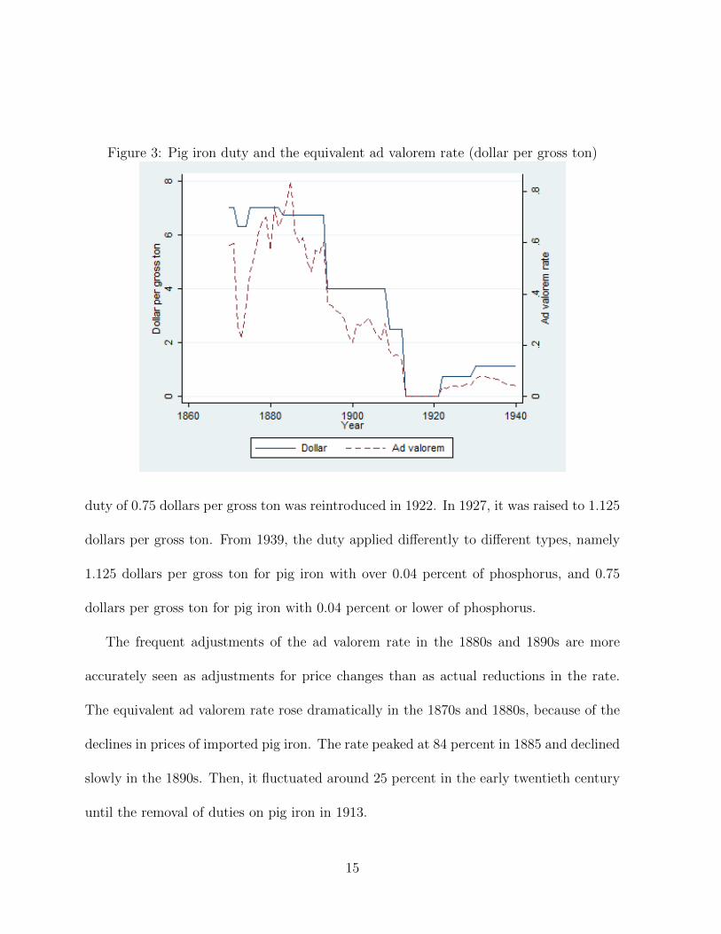
Figure 3: Pig iron duty and the equivalent ad valorem rate (dollar per gross ton)

duty of 0.75 dollars per gross ton was reintroduced in 1922. In 1927, it was raised to 1.125

dollars per gross ton. From 1939, the duty applied differently to different types, namely

1.125 dollars per gross ton for pig iron with over 0.04 percent of phosphorus, and 0.75

dollars per gross ton for pig iron with 0.04 percent or lower of phosphorus.

The frequent adjustments of the ad valorem rate in the 1880s and 1890s are more

accurately seen as adjustments for price changes than as actual reductions in the rate.

The equivalent ad valorem rate rose dramatically in the 1870s and 1880s, because of the

declines in prices of imported pig iron. The rate peaked at 84 percent in 1885 and declined

slowly in the 1890s. Then, it fluctuated around 25 percent in the early twentieth century

until the removal of duties on pig iron in 1913.

15

The pig iron duty was reintroduced in 1922 to protect manufactures in the seaboard

areas. To be precise, New York and New Jersey were not naturally protected by high

transport costs and thus faced tough foreign competition (Berglund and Wright, 1929:

Sundararajan, 1970). The equivalent ad valorem rates remained below 10 percent from

1922 to 1940. The reason lies on the fact that the US producers had long replaced the UK

as the main supplier for the US market. Although the domestic suppliers sometimes could

not meet the entire domestic demand for pig iron, import market share in consumption

remained lower than 2 percent for most of the time from 1889. In 1922, the import market

share became as low as 1.30 percent.

The protective nature of the pig iron duty was apparent in the first half of 1870 and

the 1880s, since the US pig iron was more expensive than imported pig iron over these

periods. However, there were still imports of UK pig iron in this period. The imports of

pig iron in this period were mainly for consumption in the Atlantic and Pacific coastal

areas. Throughout the 1910s, the share of imports to Atlantic and Pacific ports accounted

for more than 90 percent of the total imports 6. The primary reason for this is likely the

inland shipping costs.

Finally, Figure 4 displays the shipping cost. The ad valorem rate is calculated as

the ratio of the dollar shipping charge to the domestic price of imported pig iron from

the UK. Trans-Atlantic shipping costs for pig iron are from two sources. First, Inwood

and Kaey (2015) provides trans-Atlantic shipping costs for pig iron from Lancashire to

6The imports statistics by ports of entry are from Foreign Commerce and Navigation of the UnitedStates, Bureau of the Census.

16

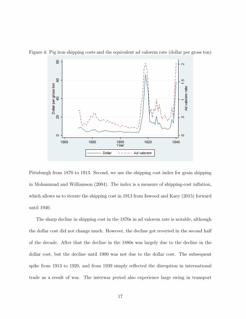
Figure 4: Pig iron shipping costs and the equivalent ad valorem rate (dollar per gross ton)

Pittsburgh from 1870 to 1913. Second, we use the shipping cost index for grain shipping

in Mohammad and Williamson (2004). The index is a measure of shipping-cost inflation,

which allows us to iterate the shipping cost in 1913 from Inwood and Kaey (2015) forward

until 1940.

The sharp decline in shipping cost in the 1870s in ad valorem rate is notable, although

the dollar cost did not change much. However, the decline got reverted in the second half

of the decade. After that the decline in the 1880s was largely due to the decline in the

dollar cost, but the decline until 1900 was not due to the dollar cost. The subsequent

spike from 1913 to 1920, and from 1939 simply reflected the disruption in international

trade as a result of war. The interwar period also experience large swing in transport

17

costs.

3.2 Empirical results

3.2.1 Elasticity of Output

Table 1 reports the OLS estimation results. Column 1 is the specification in Equation

(3), and Columns 2-4 includes one-period lag of explanatory variables and the lagged

dependent variable, to allow dynamic adjustments. The estimated coefficients all have

expect signs and they are statistically significant, except for those for price of coal and

price of iron ore in Columns 2 and 4. The test for serial correlation is the Durbin Watson

Alternative (DWA) test, since it is possible that price of imported pig iron is endogenous

to domestic output.

Next we explore a two-step estimation procedure by instrumenting the price of im-

ported pig iron with GDP, exchange rate and pig iron duty. Our choice of instruments

(IV) are motivated by the following reasons. First, it follows the trade literature in the

sense that it includes an exogenous trade frictions variable. In addition, the exchange

rate and GDP are macro variables which affect expenditure on other goods that requires

imported pig iron as input.

The IV regression results are reported in Table 2. The hypothetical of serial correlation

is rejected. The coeffient of price of imported pig iron is significant in Columns 1 and

2. The values are 0.46 and 0.56, respectively. However, the price of imported column

18

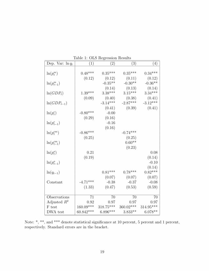
Table 1: OLS Regression Results

Dep. Var: ln qt (1) (2) (3) (4)

ln(pmt ) 0.48*** 0.35*** 0.35*** 0.34***(0.12) (0.12) (0.11) (0.12)

ln(pmt−1) -0.35** -0.30** -0.36**(0.14) (0.13) (0.14)

ln(GDPt) 1.39*** 3.38*** 3.15*** 3.34***(0.09) (0.40) (0.38) (0.41)

ln(GDPt−1) -3.14*** -2.87*** -3.12***(0.41) (0.39) (0.41)

ln(pct) -0.80*** -0.00(0.29) (0.16)

ln(pct−1) -0.16(0.16)

ln(pcmt ) -0.86*** -0.74***(0.25) (0.25)

ln(pcmt−1) 0.60**(0.23)

ln(pot ) 0.21 0.08(0.19) (0.14)

ln(pot−1) -0.10(0.14)

ln(qt−1) 0.81*** 0.78*** 0.82***(0.07) (0.07) (0.07)

Constant -4.71*** -0.38 -0.37 -0.08(1.33) (0.47) (0.53) (0.59)

Observations 71 70 70 70Adjusted R2 0.92 0.97 0.97 0.97F test 160.09*** 318.75*** 360.02*** 314.95***DWA test 60.842*** 6.896*** 3.833** 6.078**

Note: *, **, and *** denote statistical significance at 10 percent, 5 percent and 1 percent,respectively. Standard errors are in the bracket.

19

continues to give statistical significant coefficient with an expected sign, where as other

input prices do not. The sign of other coefficients are also expected. For this reason, we

use Column 2 to calculate the elasticity of output with respect to price of imported pig

iron. The long-run elasticity is (0.56− 0.15)/(1− 0.71) = 1.17. This value is close to 1.41

in Davis and Irwin (2008).

Next, we include the World War dummy in the estimation, because the World Wars

disrupted international trade. The World War dummy is 1 for the years are 1914-1918,

1939 and 1940, and 0 otherwise. The results are in Table 3. Surprising, the World War

did not have significant impacts on the US pig iron output. This implies that the impacts

of wars have been reflected by rising shipping cost and aggregate demand shocks.

3.2.2 Dynamic Learning

Since the estimating equation is based on cost accounting, apart from the lagged cumu-

lative output, we are not concerned with endogeneity of input prices. Hence, we estimate

dynamic learning equation using simple OLS.

In Table 4, all coefficients have expected signs except for price of imported coal.

However, the World War dummy has a significant and positive effect on cost of price of pig

iron. Hence, we use Column 3 and 4 to obtain the learning rate. Specifically, the learning

coefficient is -0.44 and -0.26, and statistically significant. The implied learning rate is 0.36

and 0.20, respectively. We choose 0.20 in our counter-factual exercise as a conservative

value. This is also the same as the 20-percent learning rate in the semiconductor industry

20

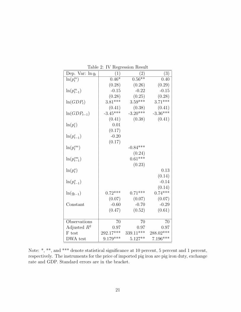
Table 2: IV Regression Result

Dep. Var: ln qt (1) (2) (3)ln(pmt ) 0.46* 0.56** 0.40

(0.28) (0.26) (0.29)ln(pmt−1) -0.15 -0.22 -0.15

(0.28) (0.25) (0.28)ln(GDPt) 3.81*** 3.59*** 3.71***

(0.41) (0.38) (0.41)ln(GDPt−1) -3.45*** -3.20*** -3.36***

(0.41) (0.38) (0.41)ln(pct) 0.01

(0.17)ln(pct−1) -0.20

(0.17)ln(pcmt ) -0.84***

(0.24)ln(pcmt−1) 0.61***

(0.23)ln(pot ) 0.13

(0.14)ln(pot−1) -0.14

(0.14)ln(qt−1) 0.72*** 0.71*** 0.74***

(0.07) (0.07) (0.07)Constant -0.60 -0.70 -0.29

(0.47) (0.52) (0.61)

Observations 70 70 70Adjusted R2 0.97 0.97 0.97F test 292.17*** 339.11*** 288.02***DWA test 9.179*** 5.127** 7.196***

Note: *, **, and *** denote statistical significance at 10 percent, 5 percent and 1 percent,respectively. The instruments for the price of imported pig iron are pig iron duty, exchangerate and GDP. Standard errors are in the bracket.

21

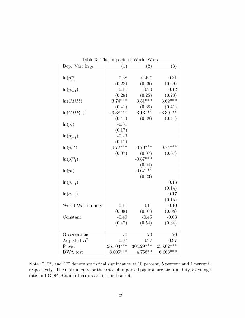
Table 3: The Impacts of World Wars

Dep. Var: ln qt (1) (2) (3)

ln(pmt ) 0.38 0.49* 0.31(0.28) (0.26) (0.29)

ln(pmt−1) -0.11 -0.20 -0.12(0.28) (0.25) (0.28)

ln(GDPt) 3.74*** 3.51*** 3.62***(0.41) (0.38) (0.41)

ln(GDPt−1) -3.38*** -3.13*** -3.30***(0.41) (0.38) (0.41)

ln(pct) -0.01(0.17)

ln(pct−1) -0.23(0.17)

ln(pcmt ) 0.72*** 0.70*** 0.74***(0.07) (0.07) (0.07)

ln(pcmt−1) -0.87***(0.24)

ln(pot ) 0.67***(0.23)

ln(pot−1) 0.13(0.14)

ln(qt−1) -0.17(0.15)

World War dummy 0.11 0.11 0.10(0.08) (0.07) (0.08)

Constant -0.49 -0.45 -0.03(0.47) (0.54) (0.64)

Observations 70 70 70Adjusted R2 0.97 0.97 0.97F test 261.03*** 304.29*** 255.62***DWA test 8.805*** 4.758** 6.668***

Note: *, **, and *** denote statistical significance at 10 percent, 5 percent and 1 percent,respectively. The instruments for the price of imported pig iron are pig iron duty, exchangerate and GDP. Standard errors are in the bracket.

22

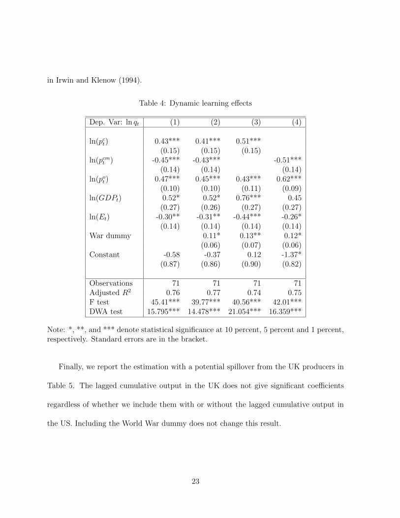
in Irwin and Klenow (1994).

Table 4: Dynamic learning effects

Dep. Var: ln qt (1) (2) (3) (4)

ln(pct) 0.43*** 0.41*** 0.51***(0.15) (0.15) (0.15)

ln(pcmt ) -0.45*** -0.43*** -0.51***(0.14) (0.14) (0.14)

ln(pot ) 0.47*** 0.45*** 0.43*** 0.62***(0.10) (0.10) (0.11) (0.09)

ln(GDPt) 0.52* 0.52* 0.76*** 0.45(0.27) (0.26) (0.27) (0.27)

ln(Et) -0.30** -0.31** -0.44*** -0.26*(0.14) (0.14) (0.14) (0.14)

War dummy 0.11* 0.13** 0.12*(0.06) (0.07) (0.06)

Constant -0.58 -0.37 0.12 -1.37*(0.87) (0.86) (0.90) (0.82)

Observations 71 71 71 71Adjusted R2 0.76 0.77 0.74 0.75F test 45.41*** 39.77*** 40.56*** 42.01***DWA test 15.795*** 14.478*** 21.054*** 16.359***

Note: *, **, and *** denote statistical significance at 10 percent, 5 percent and 1 percent,respectively. Standard errors are in the bracket.

Finally, we report the estimation with a potential spillover from the UK producers in

Table 5. The lagged cumulative output in the UK does not give significant coefficients

regardless of whether we include them with or without the lagged cumulative output in

the US. Including the World War dummy does not change this result.

23

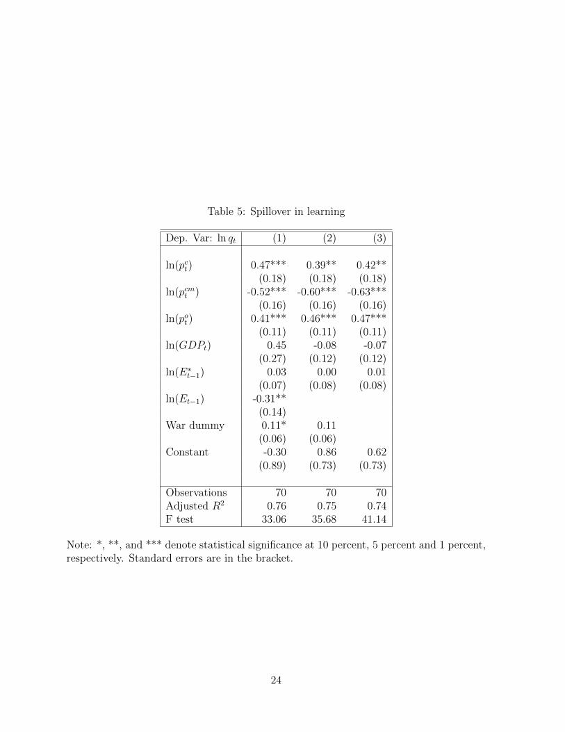
Table 5: Spillover in learning

Dep. Var: ln qt (1) (2) (3)

ln(pct) 0.47*** 0.39** 0.42**(0.18) (0.18) (0.18)

ln(pcmt ) -0.52*** -0.60*** -0.63***(0.16) (0.16) (0.16)

ln(pot ) 0.41*** 0.46*** 0.47***(0.11) (0.11) (0.11)

ln(GDPt) 0.45 -0.08 -0.07(0.27) (0.12) (0.12)

ln(E∗t−1) 0.03 0.00 0.01

(0.07) (0.08) (0.08)ln(Et−1) -0.31**

(0.14)War dummy 0.11* 0.11

(0.06) (0.06)Constant -0.30 0.86 0.62

(0.89) (0.73) (0.73)

Observations 70 70 70Adjusted R2 0.76 0.75 0.74F test 33.06 35.68 41.14

Note: *, **, and *** denote statistical significance at 10 percent, 5 percent and 1 percent,respectively. Standard errors are in the bracket.

24

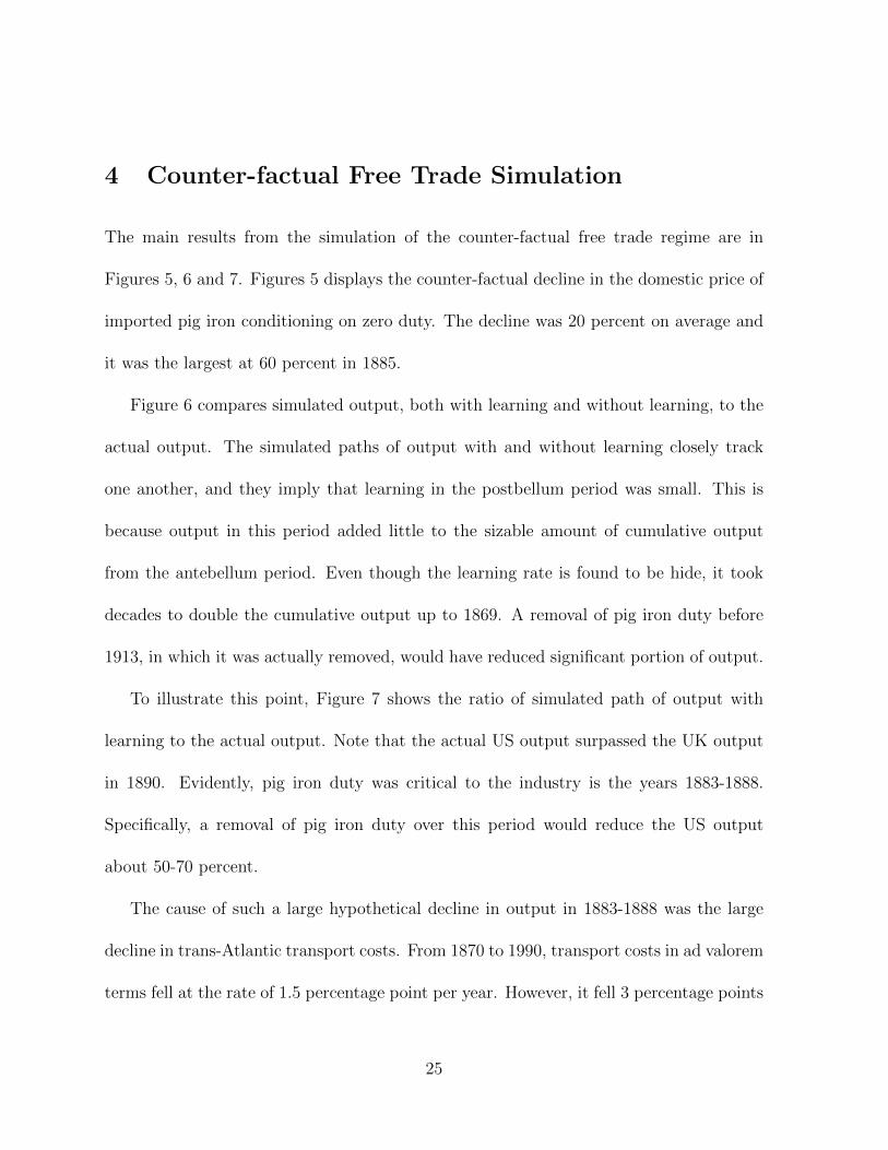
4 Counter-factual Free Trade Simulation

The main results from the simulation of the counter-factual free trade regime are in

Figures 5, 6 and 7. Figures 5 displays the counter-factual decline in the domestic price of

imported pig iron conditioning on zero duty. The decline was 20 percent on average and

it was the largest at 60 percent in 1885.

Figure 6 compares simulated output, both with learning and without learning, to the

actual output. The simulated paths of output with and without learning closely track

one another, and they imply that learning in the postbellum period was small. This is

because output in this period added little to the sizable amount of cumulative output

from the antebellum period. Even though the learning rate is found to be hide, it took

decades to double the cumulative output up to 1869. A removal of pig iron duty before

1913, in which it was actually removed, would have reduced significant portion of output.

To illustrate this point, Figure 7 shows the ratio of simulated path of output with

learning to the actual output. Note that the actual US output surpassed the UK output

in 1890. Evidently, pig iron duty was critical to the industry is the years 1883-1888.

Specifically, a removal of pig iron duty over this period would reduce the US output

about 50-70 percent.

The cause of such a large hypothetical decline in output in 1883-1888 was the large

decline in trans-Atlantic transport costs. From 1870 to 1990, transport costs in ad valorem

terms fell at the rate of 1.5 percentage point per year. However, it fell 3 percentage points

25

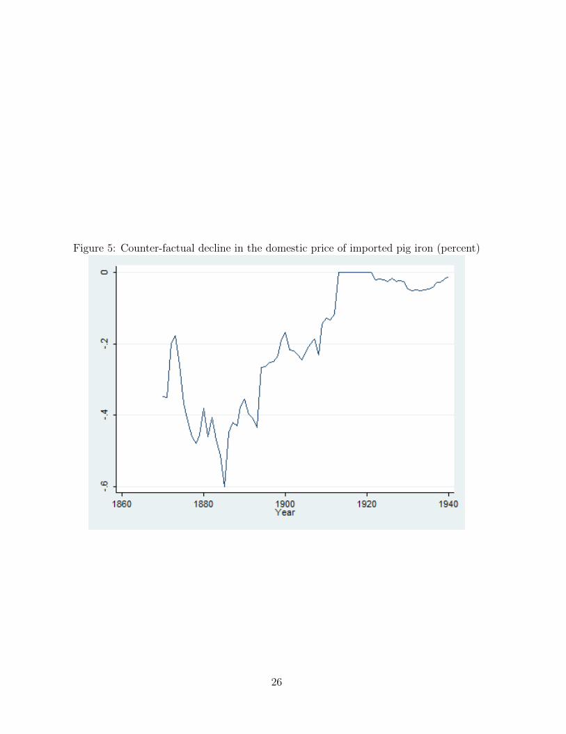
Figure 5: Counter-factual decline in the domestic price of imported pig iron (percent)

26

Figure 6: Simulated paths of US pig iron output and actual output (gross ton)

27

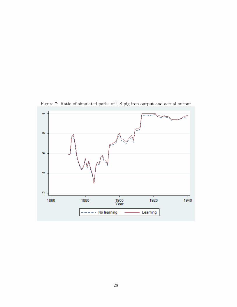
Figure 7: Ratio of simulated paths of US pig iron output and actual output

28

per year in 1883-1888. For input costs, imported coal price increased but the US coal

price decreased over this period. At the same time, price of iron ore fluctuated over this

period with downward trend. Thus, we could not argue that costs of intermediate inputs

were the cause of the decline in competitiveness.

5 Concluding remarks

This study provides evidence that protection was necessary for the US pig iron industry

before the US output surpassed the UK output in 1890. Despite evidence for learning by

doing, fluctuations of costs especially shipping costs could make protection necessary for

the majority of production of pig iron output in the US.

The simulation results should also be interpreted with caution, since we ignore the

geographical aspect of the US pig iron industry. Besides protection, a fraction of the

industry was naturally protected by high inland transport costs. Even without protection,

some inland producers would be able to continue their production and keep accumulating

experience and knowledge in the absence of unfavorable shocks.

Having concluded that the US pig iron industry expanded behind the tariff wall, our

study does not imply that developing countries today will surely enjoy the benefits from

protection in the same way. The primary reason is that the economic system today is

far different from the past. For instance, the fall of transport costs have made countries

prone to foreign competition, and a large-scale investment in import-competing industries

29

has become riskier than in the past. These factors may partially contribute to the failure

of protectionist policy.

A Data appendix

A.1 Pig iron data

The annual time series of pig iron production (imports and exports) includes Ferro-alloys

production (imports and exports). US figures are from Taussig (1915), Some Aspects of

the Tariff Question, and the Annual Statistical Report, American Iron and Steel Associ-

ation, various issues. British figures, the composition by grades, and world total are from

Carr, J. C. and W. Taplin (1962), History of the British Steel Industry.

Prices of domestic pig iron are taken from the Statistical Abstract of the US and the

Annual Statistical Report, American Iron and Steel Association, various issues. They

are no. 1 Foundry price at Philadelphia for 1870-85, and Bessemer price at Chicago for

1886-1940. The UK prices of pig iron are from Taussig (1915) and the Annual Statistical

Report, American Iron and Steel Association. They are no. 1 Foundry price at Cleveland

for 1870-85, and Bessemer price at Cleveland for 1886-1940.

Volume of exports and imports of pig iron are from the Statistical Abstract of the

U.S., various issues. Trading partner countries are from the Annual Statistical Report,

American Iron and Steel Association, various issues. Pig iron duty is from Taussig (1915),

Berglund and Wright (1929), and Metal Statistics, American Metal Market Daily Iron

30

and Steel Report, various issues.

A.2 Shipping cost data

Trans-Atlantic shipping costs for pig iron are from two sources. First, Inwood and Kaey

(2015) provides trans-Atlantic shipping costs for pig iron from Lancashire to Pittsburgh

from 1870 to 1913. Second, we use the shipping cost index for grain shipping in Moham-

mad and Williamson (2004). The index is a measure of shipping-cost inflation, which

allows us to iterate the shipping cost in 1913 from Inwood and Kaey (2015) forward until

1940.

A.3 Other data

Old range non-Bessemer ore price, bituminous coal domestic price and its import price,

are from various issues of the Statistical Abstract of the US. The consumer price index

is taken from the Historical Statistics of the United States: Colonial Times to 1970,

Bicentennial Edition, US Department of Commerce, Bureau of the Census.

The exchange rate data are from Economic History Services (EH.net).

References

Allen, R. C. (1979). International competition in iron and steel, 1850-1913. Journal of

Economic History 87 (4), 911–937.

Allen, R. C. (1981). Accounting for price changes: American steel rails, 1879-1910.

Journal of Political Economy 89 (3), 512–528.

Baack, B. D. and E. J. Ray (1973). Tariff policy and comparative advantage in the iron

and steel industry: 1870-1929. Explorations in Economic History 11, 3–23.

Berck, P. (1978). Hard driving and efficiency: Iron production in 1890. Journal of

Economic History 38 (4), 879–900.

Burglund, A. and P. G. Wright (1929). The Tariff on Iron and Steel. Washington, D.C.:

The Institute of Economics of The Brookings Institution.

Carr, J. and W. Taplin (1962). History of the British Steel Industry. Cambridge, Mas-

sachusetts: Harvard University Press.

Clemens, M. A. and J. G. Williamson (2001). A tariff-growth paradox? protection’s

impact the world around 1875-1997. NBER Working Paper 8459.

David, P. A. and G. Wright (1997). Increasing returns and the genesis of American

resource abundance. Industrial and Corporate Change 6 (2), 203–245.

Davis, J. H. and D. A. Irwin (2008). The antebellum US iron industry: Domestic

production and foreign competition. Explorations in Economic History 45, 254–

269.

Gordon, R. (1996). American Iron, 1607-1900. Baltimore and London: Johns Hopkins

University Press.

Grossman, G. M. (1986). Imports as a cause of injury: The case of the US steel industry.

Journal of International Economics 30 (3/4), 201–224.

Harley, K. C. (2001). The antebellum tariff: Different products or competing sources?

a comment on Irwin and Temin. Journal of Economic History 61 (3), 799–805.

Head, K. (1994). Infant industry protection in the steel rail industry. Journal of Inter-

national Economics 37 (1), 141–165.

Helpman, E. (1984). Increasing returns, imperfect markets, and trade theory. In

R. Jones and P. Kenen (Eds.), Handbook of International Economics. New York:

North-Holland Publishing Company.

Inwood, K. and I. Keay (2015). Transport costs and trade volumes: Evidence from the

trans-atlantic iron trade, 18701913. Journal of Economic History 75 (1), 95–124.

Irwin, D. A. (2000a). Could the United States iron industry have survived free trade

after the civil war? Explorations in Economic History 37, 278–299.

Irwin, D. A. (2000b). Did late-nineteenth-century US tariffs promote infant industries?

evidence from the tinplate industry. Journal of Economic History 60 (2), 335–360.

Irwin, D. A. (2003). Explaining America’s surge in manufactured exports, 1880-1913.

Review of Economics and Statistics 85 (2), 364–376.

Isard, P. (1948). Some locational factors in the iron and steel industry since the early

nineteenth century. Journal of Political Economy 56 (3), 203–217.

Jeans, J. S. (1906). The Iron Trade of Great Britain. London: Methuen and Co.

Mitchell, B. R. (1988). British Historical Statistics. Cambridge University Press.

Romer, P. M. (1986). Increasing returns and long-run growth. Journal of Political

Economy 94 (5), 1002–1037.

Romer, P. M. (1990). Endogenous technological change. Journal of Political Econ-

omy 98 (5), S71–S102.

Sundararajan, V. (1970). The impact of the tariff on some selected products of the US

iron and steel industry, 1870-1914. Quarterly Journal of Economics 84 (4), 590–610.

Taussig, F. W. (1915). Some Aspects of the Tariff Question. Harvard University Press.

Temin, P. (1964). Iron and Steel in Nineteenth-Century America: An Economic Inquiry.

The M.I.T. Press.

Wright, G. (1990). The origins of American industrial success, 1879-1940. American

Economic Review 80 (4), 651–668.