Embed Size (px)
Citation preview
1
NewEdition
December 26, 2015
User Manual
TALYS-1.8A nuclear reaction program
Arjan KoningStephane HilaireStephane Goriely

2
c© User Manual2015 A.J. Koning, All rights reservedOn cover page: a platypus.
First edition: December 26, 2015
Contents
Contents i
Preface ix
1 Introduction 1
1.1 From TALYS-1.0 to TALYS-1.2 . . . . . . . . . . . . . . . . . . . . . . . .. . . . . . 4
1.2 From TALYS-1.2 to TALYS-1.4 . . . . . . . . . . . . . . . . . . . . . . . .. . . . . . 5
1.3 From TALYS-1.4 to TALYS-1.6 . . . . . . . . . . . . . . . . . . . . . . . .. . . . . . 7
1.4 From TALYS-1.6 to TALYS-1.8 . . . . . . . . . . . . . . . . . . . . . . . .. . . . . . 8
1.5 How to use this manual . . . . . . . . . . . . . . . . . . . . . . . . . . . . . .. . . . . 9
2 Installation and getting started 11
2.1 The TALYS package . . . . . . . . . . . . . . . . . . . . . . . . . . . . . . . . .. . . 11
2.2 Installation . . . . . . . . . . . . . . . . . . . . . . . . . . . . . . . . . . . .. . . . . 12
2.3 Verification . . . . . . . . . . . . . . . . . . . . . . . . . . . . . . . . . . . . .. . . . 13
2.4 Getting started . . . . . . . . . . . . . . . . . . . . . . . . . . . . . . . . . .. . . . . . 13
3 Nuclear reactions: General approach 15
3.1 Reaction mechanisms . . . . . . . . . . . . . . . . . . . . . . . . . . . . . .. . . . . . 19
3.1.1 Low energies . . . . . . . . . . . . . . . . . . . . . . . . . . . . . . . . . . .. 19
3.1.2 High energies . . . . . . . . . . . . . . . . . . . . . . . . . . . . . . . . . .. . 21
3.2 Cross section definitions . . . . . . . . . . . . . . . . . . . . . . . . . .. . . . . . . . 22
3.2.1 Total cross sections . . . . . . . . . . . . . . . . . . . . . . . . . . . .. . . . . 23
3.2.2 Exclusive cross sections . . . . . . . . . . . . . . . . . . . . . . . .. . . . . . 23
i
ii CONTENTS
3.2.3 Binary cross sections . . . . . . . . . . . . . . . . . . . . . . . . . . .. . . . . 27
3.2.4 Total particle production cross sections . . . . . . . . . .. . . . . . . . . . . . 28
3.2.5 Residual production cross sections . . . . . . . . . . . . . . .. . . . . . . . . . 29
3.3 Spectra and angular distributions . . . . . . . . . . . . . . . . . .. . . . . . . . . . . . 29
3.3.1 Discrete angular distributions . . . . . . . . . . . . . . . . . .. . . . . . . . . 30
3.3.2 Exclusive spectra . . . . . . . . . . . . . . . . . . . . . . . . . . . . . .. . . . 30
3.3.3 Binary spectra . . . . . . . . . . . . . . . . . . . . . . . . . . . . . . . . .. . 32
3.3.4 Total particle production spectra . . . . . . . . . . . . . . . .. . . . . . . . . . 32
3.3.5 Double-differential cross sections . . . . . . . . . . . . . .. . . . . . . . . . . 33
3.4 Fission cross sections . . . . . . . . . . . . . . . . . . . . . . . . . . . .. . . . . . . . 33
3.5 Recoils . . . . . . . . . . . . . . . . . . . . . . . . . . . . . . . . . . . . . . . . .. . 35
3.5.1 Qualitative analysis . . . . . . . . . . . . . . . . . . . . . . . . . . .. . . . . . 35
3.5.2 General method . . . . . . . . . . . . . . . . . . . . . . . . . . . . . . . . .. . 35
3.5.3 Quantitative analysis . . . . . . . . . . . . . . . . . . . . . . . . . .. . . . . . 36
3.5.4 The recoil treatment in TALYS . . . . . . . . . . . . . . . . . . . . .. . . . . . 37
3.5.5 Method of average velocity . . . . . . . . . . . . . . . . . . . . . . .. . . . . . 39
3.5.6 Approximative recoil correction for binary ejectilespectra . . . . . . . . . . . . 39
4 Nuclear models 41
4.1 Optical model . . . . . . . . . . . . . . . . . . . . . . . . . . . . . . . . . . . .. . . . 41
4.1.1 Spherical OMP: Neutrons and protons . . . . . . . . . . . . . . .. . . . . . . . 43
4.1.2 Spherical dispersive OMP: Neutrons . . . . . . . . . . . . . . .. . . . . . . . . 49
4.1.3 Spherical OMP: Complex particles . . . . . . . . . . . . . . . . .. . . . . . . 50
4.1.4 Semi-microscopic optical model (JLM) . . . . . . . . . . . . .. . . . . . . . . 52
4.1.5 Systematics for non-elastic cross sections . . . . . . . .. . . . . . . . . . . . . 54
4.2 Direct reactions . . . . . . . . . . . . . . . . . . . . . . . . . . . . . . . . .. . . . . . 54
4.2.1 Deformed nuclei: Coupled-channels . . . . . . . . . . . . . . .. . . . . . . . . 54
4.2.2 Distorted Wave Born Approximation . . . . . . . . . . . . . . . .. . . . . . . 57
4.2.3 Odd nuclei: Weak coupling . . . . . . . . . . . . . . . . . . . . . . . .. . . . 57
4.2.4 Giant resonances . . . . . . . . . . . . . . . . . . . . . . . . . . . . . . .. . . 58
4.3 Gamma-ray transmission coefficients . . . . . . . . . . . . . . . .. . . . . . . . . . . . 59
4.3.1 Gamma-ray strength functions . . . . . . . . . . . . . . . . . . . .. . . . . . . 60
4.3.2 Renormalization of gamma-ray strength functions . . .. . . . . . . . . . . . . . 61
CONTENTS iii
4.3.3 Photoabsorption cross section . . . . . . . . . . . . . . . . . . .. . . . . . . . 62
4.4 Pre-equilibrium reactions . . . . . . . . . . . . . . . . . . . . . . . .. . . . . . . . . . 63
4.4.1 Exciton model . . . . . . . . . . . . . . . . . . . . . . . . . . . . . . . . . .. 63
4.4.2 Photon exciton model . . . . . . . . . . . . . . . . . . . . . . . . . . . .. . . 76
4.4.3 Pre-equilibrium spin distribution . . . . . . . . . . . . . . .. . . . . . . . . . . 77
4.4.4 Continuum stripping, pick-up, break-up and knock-out reactions . . . . . . . . . 78
4.4.5 Angular distribution systematics . . . . . . . . . . . . . . . .. . . . . . . . . . 81
4.5 Compound reactions . . . . . . . . . . . . . . . . . . . . . . . . . . . . . . .. . . . . 83
4.5.1 Binary compound cross section and angular distribution . . . . . . . . . . . . . 83
4.5.2 Width fluctuation correction factor . . . . . . . . . . . . . . .. . . . . . . . . . 86
4.6 Multiple emission . . . . . . . . . . . . . . . . . . . . . . . . . . . . . . . .. . . . . . 92
4.6.1 Multiple Hauser-Feshbach decay . . . . . . . . . . . . . . . . . .. . . . . . . . 92
4.6.2 Multiple pre-equilibrium emission . . . . . . . . . . . . . . .. . . . . . . . . . 93
4.7 Level densities . . . . . . . . . . . . . . . . . . . . . . . . . . . . . . . . . .. . . . . 96
4.7.1 Effective level density . . . . . . . . . . . . . . . . . . . . . . . . .. . . . . . 97
4.7.2 Collective effects in the level density . . . . . . . . . . . .. . . . . . . . . . . 110
4.7.3 Microscopic level densities . . . . . . . . . . . . . . . . . . . . .. . . . . . . . 112
4.8 Fission . . . . . . . . . . . . . . . . . . . . . . . . . . . . . . . . . . . . . . . . .. . . 113
4.8.1 Level densities for fission barriers . . . . . . . . . . . . . . .. . . . . . . . . . 113
4.8.2 Fission transmission coefficients . . . . . . . . . . . . . . . .. . . . . . . . . . 114
4.8.3 Transmission coefficient for multi-humped barriers .. . . . . . . . . . . . . . . 115
4.8.4 Class II/III states . . . . . . . . . . . . . . . . . . . . . . . . . . . . .. . . . . 116
4.8.5 Fission barrier parameters . . . . . . . . . . . . . . . . . . . . . .. . . . . . . 117
4.8.6 WKB approximation . . . . . . . . . . . . . . . . . . . . . . . . . . . . . .. . 118
4.8.7 Fission fragment properties . . . . . . . . . . . . . . . . . . . . .. . . . . . . . 118
4.9 Thermal reactions . . . . . . . . . . . . . . . . . . . . . . . . . . . . . . . .. . . . . . 125
4.9.1 Capture channel . . . . . . . . . . . . . . . . . . . . . . . . . . . . . . . .. . 125
4.9.2 Other non-threshold reactions . . . . . . . . . . . . . . . . . . .. . . . . . . . 125
4.10 Direct capture . . . . . . . . . . . . . . . . . . . . . . . . . . . . . . . . . .. . . . . . 127
4.11 Populated initial nucleus . . . . . . . . . . . . . . . . . . . . . . . .. . . . . . . . . . 127
4.12 Astrophysical reaction rates . . . . . . . . . . . . . . . . . . . . .. . . . . . . . . . . . 127
4.13 Medical isotope production . . . . . . . . . . . . . . . . . . . . . . .. . . . . . . . . . 129
iv CONTENTS
4.13.1 Production and depletion of isotopes . . . . . . . . . . . . .. . . . . . . . . . . 129
4.13.2 Initial condition and stopping power . . . . . . . . . . . . .. . . . . . . . . . . 132
4.13.3 Nuclear reaction and decay rates . . . . . . . . . . . . . . . . .. . . . . . . . . 133
4.13.4 Activities . . . . . . . . . . . . . . . . . . . . . . . . . . . . . . . . . . .. . . 134
5 Nuclear structure and model parameters 135
5.1 General setup of the database . . . . . . . . . . . . . . . . . . . . . . .. . . . . . . . . 135
5.2 Nuclear masses and deformations . . . . . . . . . . . . . . . . . . . .. . . . . . . . . 135
5.3 Isotopic abundances . . . . . . . . . . . . . . . . . . . . . . . . . . . . . .. . . . . . . 136
5.4 Discrete level file . . . . . . . . . . . . . . . . . . . . . . . . . . . . . . . .. . . . . . 137
5.5 Deformation parameters . . . . . . . . . . . . . . . . . . . . . . . . . . .. . . . . . . 138
5.6 Level density parameters . . . . . . . . . . . . . . . . . . . . . . . . . .. . . . . . . . 140
5.7 Resonance parameters . . . . . . . . . . . . . . . . . . . . . . . . . . . . .. . . . . . 142
5.8 Gamma-ray parameters . . . . . . . . . . . . . . . . . . . . . . . . . . . . .. . . . . . 142
5.9 Thermal cross sections . . . . . . . . . . . . . . . . . . . . . . . . . . . .. . . . . . . 143
5.10 Optical model parameters . . . . . . . . . . . . . . . . . . . . . . . . .. . . . . . . . . 144
5.11 Fission parameters . . . . . . . . . . . . . . . . . . . . . . . . . . . . . .. . . . . . . 145
5.12 Integral validation library . . . . . . . . . . . . . . . . . . . . . .. . . . . . . . . . . . 149
5.13 Decay data library . . . . . . . . . . . . . . . . . . . . . . . . . . . . . . .. . . . . . . 149
5.14 Best TALYS input parameters . . . . . . . . . . . . . . . . . . . . . . .. . . . . . . . 149
6 Input description 151
6.1 Basic input rules . . . . . . . . . . . . . . . . . . . . . . . . . . . . . . . . .. . . . . 152
6.2 Keywords . . . . . . . . . . . . . . . . . . . . . . . . . . . . . . . . . . . . . . . .. . 153
6.2.1 Four main keywords . . . . . . . . . . . . . . . . . . . . . . . . . . . . . .. . 154
6.2.2 Basic physical and numerical parameters . . . . . . . . . . .. . . . . . . . . . 158
6.2.3 Optical model . . . . . . . . . . . . . . . . . . . . . . . . . . . . . . . . . .. . 177
6.2.4 Direct reactions . . . . . . . . . . . . . . . . . . . . . . . . . . . . . . .. . . . 200
6.2.5 Compound nucleus . . . . . . . . . . . . . . . . . . . . . . . . . . . . . . .. . 202
6.2.6 Gamma emission . . . . . . . . . . . . . . . . . . . . . . . . . . . . . . . . .. 206
6.2.7 Pre-equilibrium . . . . . . . . . . . . . . . . . . . . . . . . . . . . . . .. . . . 215
6.2.8 Level densities . . . . . . . . . . . . . . . . . . . . . . . . . . . . . . . .. . . 223
6.2.9 Fission . . . . . . . . . . . . . . . . . . . . . . . . . . . . . . . . . . . . . . .238
CONTENTS v
6.2.10 Medical isotope production . . . . . . . . . . . . . . . . . . . . .. . . . . . . . 245
6.2.11 Output . . . . . . . . . . . . . . . . . . . . . . . . . . . . . . . . . . . . . . .248
6.2.12 Energy-dependent parameter adjustment . . . . . . . . . .. . . . . . . . . . . . 264
6.2.13 Input parameter table . . . . . . . . . . . . . . . . . . . . . . . . . .. . . . . . 266
7 Verification and validation, sample cases and output 277
7.1 Robustness test with DRIP . . . . . . . . . . . . . . . . . . . . . . . . . .. . . . . . . 277
7.2 Robustness test with MONKEY . . . . . . . . . . . . . . . . . . . . . . . .. . . . . . 277
7.3 Validation with sample cases . . . . . . . . . . . . . . . . . . . . . . .. . . . . . . . . 278
7.3.1 Sample 1: All results for 14 MeV n +93Nb . . . . . . . . . . . . . . . . . . . . 280
7.3.2 Sample 2: Excitation functions:208Pb (n,n’), (n,2n), (n,p) etc. . . . . . . . . . . 311
7.3.3 Sample 3: Comparison of compound nucleus WFC models: 10 keV n +93Nb . . 317
7.3.4 Sample 4: Recoils: 20 MeV n +28Si . . . . . . . . . . . . . . . . . . . . . . . . 320
7.3.5 Sample 5: Fission cross sections: n +232Th . . . . . . . . . . . . . . . . . . . . 322
7.3.6 Sample 6: Continuum spectra at 63 MeV for Bi(n,xp)...Bi(n,xα) . . . . . . . . . 326
7.3.7 Sample 7: Pre-equilibrium angular dist. and multiplepre-equilibrium emission . 330
7.3.8 Sample 8: Residual production cross sections: p +natFe up to 100 MeV . . . . . 334
7.3.9 Sample 9: Spherical optical model and DWBA: n +208Pb . . . . . . . . . . . . 336
7.3.10 Sample 10: Coupled-channels rotational model: n +28Si . . . . . . . . . . . . . 338
7.3.11 Sample 11: Coupled-channels vibrational model: n +74Ge . . . . . . . . . . . . 340
7.3.12 Sample 12: Inelastic spectra at 20 MeV: Direct + Preeq+ GR + Compound . . . 341
7.3.13 Sample 13: Gamma-ray intensities:208Pb(n, nγ) and208Pb(n, 2nγ) . . . . . . . 342
7.3.14 Sample 14: Fission yields for238U . . . . . . . . . . . . . . . . . . . . . . . . . 344
7.3.15 Sample 15: Photonuclear reactions: g +90Zr . . . . . . . . . . . . . . . . . . . 347
7.3.16 Sample 16: Different optical models : n +120Sn . . . . . . . . . . . . . . . . . 348
7.3.17 Sample 17: Different level density models : n +99Tc . . . . . . . . . . . . . . . 350
7.3.18 Sample 18: Astrophysical reaction rates : n +187Os . . . . . . . . . . . . . . . . 354
7.3.19 Sample 19: Unresolved resonance range parameters: n+ 136Ba . . . . . . . . . 357
7.3.20 Sample 20: Maxwellian averaged cross section at 30 keV: n + 138Ba . . . . . . . 358
7.3.21 Sample 21: Medical isotope production with p +100Mo . . . . . . . . . . . . . 359
7.3.22 Sample 22: Calculations up to 500 MeV for p +209Bi . . . . . . . . . . . . . . 360
7.3.23 Sample 23: Neutron multiplicities and fission yieldsfor n + 242Pu . . . . . . . . 362
7.3.24 Sample 24: Local parameter adjustment for n +93Nb . . . . . . . . . . . . . . . 363
vi CONTENTS
7.3.25 Sample 25: Direct neutron capture for n +89Y . . . . . . . . . . . . . . . . . . 367
7.3.26 Sample 26: Different alpha-particle optical model potentials: alpha +165Ho . . . 368
7.3.27 Sample 27: Low energy resonance data for n +107Ag . . . . . . . . . . . . . . . 371
8 Computational structure of TALYS 375
8.1 General structure of the source code . . . . . . . . . . . . . . . . .. . . . . . . . . . . 375
8.1.1 machine . . . . . . . . . . . . . . . . . . . . . . . . . . . . . . . . . . . . . . .375
8.1.2 constants . . . . . . . . . . . . . . . . . . . . . . . . . . . . . . . . . . . . .. 376
8.1.3 talysinput . . . . . . . . . . . . . . . . . . . . . . . . . . . . . . . . . . . .. . 376
8.1.4 talysinitial . . . . . . . . . . . . . . . . . . . . . . . . . . . . . . . . . .. . . . 376
8.1.5 talysreaction . . . . . . . . . . . . . . . . . . . . . . . . . . . . . . . . .. . . 376
8.1.6 natural . . . . . . . . . . . . . . . . . . . . . . . . . . . . . . . . . . . . . . .376
8.1.7 ecis06t . . . . . . . . . . . . . . . . . . . . . . . . . . . . . . . . . . . . . . .376
8.2 Input: talysinput . . . . . . . . . . . . . . . . . . . . . . . . . . . . . . . .. . . . . . . 377
8.2.1 readinput . . . . . . . . . . . . . . . . . . . . . . . . . . . . . . . . . . . . .. 377
8.2.2 input1 . . . . . . . . . . . . . . . . . . . . . . . . . . . . . . . . . . . . . . . .377
8.2.3 input2, input3, input4, input5, input6 . . . . . . . . . . . .. . . . . . . . . . . 378
8.2.4 checkkeyword . . . . . . . . . . . . . . . . . . . . . . . . . . . . . . . . . .. 378
8.2.5 checkvalue . . . . . . . . . . . . . . . . . . . . . . . . . . . . . . . . . . . .. 378
8.3 Initialisation: talysinitial . . . . . . . . . . . . . . . . . . . . .. . . . . . . . . . . . . 378
8.3.1 particles . . . . . . . . . . . . . . . . . . . . . . . . . . . . . . . . . . . . .. . 379
8.3.2 nuclides . . . . . . . . . . . . . . . . . . . . . . . . . . . . . . . . . . . . . .. 379
8.3.3 thermalxs . . . . . . . . . . . . . . . . . . . . . . . . . . . . . . . . . . . . .. 388
8.3.4 grid . . . . . . . . . . . . . . . . . . . . . . . . . . . . . . . . . . . . . . . . . 389
8.3.5 mainout . . . . . . . . . . . . . . . . . . . . . . . . . . . . . . . . . . . . . . .390
8.3.6 timer . . . . . . . . . . . . . . . . . . . . . . . . . . . . . . . . . . . . . . . . 391
8.4 Nuclear models: talysreaction . . . . . . . . . . . . . . . . . . . . .. . . . . . . . . . 391
8.4.1 basicxs . . . . . . . . . . . . . . . . . . . . . . . . . . . . . . . . . . . . . . .392
8.4.2 preeqinit . . . . . . . . . . . . . . . . . . . . . . . . . . . . . . . . . . . . .. 396
8.4.3 excitoninit . . . . . . . . . . . . . . . . . . . . . . . . . . . . . . . . . . .. . 397
8.4.4 compoundinit . . . . . . . . . . . . . . . . . . . . . . . . . . . . . . . . . .. . 397
8.4.5 astroinit . . . . . . . . . . . . . . . . . . . . . . . . . . . . . . . . . . . . .. . 397
8.4.6 reacinitial . . . . . . . . . . . . . . . . . . . . . . . . . . . . . . . . . . .. . . 397
CONTENTS vii
8.4.7 incident . . . . . . . . . . . . . . . . . . . . . . . . . . . . . . . . . . . . . .. 397
8.4.8 exgrid . . . . . . . . . . . . . . . . . . . . . . . . . . . . . . . . . . . . . . . .399
8.4.9 recoilinit . . . . . . . . . . . . . . . . . . . . . . . . . . . . . . . . . . . .. . 399
8.4.10 direct . . . . . . . . . . . . . . . . . . . . . . . . . . . . . . . . . . . . . . .. 399
8.4.11 preeq . . . . . . . . . . . . . . . . . . . . . . . . . . . . . . . . . . . . . . . .400
8.4.12 population . . . . . . . . . . . . . . . . . . . . . . . . . . . . . . . . . . .. . 408
8.4.13 compnorm . . . . . . . . . . . . . . . . . . . . . . . . . . . . . . . . . . . . .409
8.4.14 comptarget . . . . . . . . . . . . . . . . . . . . . . . . . . . . . . . . . . .. . 409
8.4.15 binary . . . . . . . . . . . . . . . . . . . . . . . . . . . . . . . . . . . . . . .. 413
8.4.16 angdis . . . . . . . . . . . . . . . . . . . . . . . . . . . . . . . . . . . . . . .. 415
8.4.17 multiple . . . . . . . . . . . . . . . . . . . . . . . . . . . . . . . . . . . . .. . 415
8.4.18 channels . . . . . . . . . . . . . . . . . . . . . . . . . . . . . . . . . . . . .. . 419
8.4.19 totalxs . . . . . . . . . . . . . . . . . . . . . . . . . . . . . . . . . . . . . .. . 419
8.4.20 spectra . . . . . . . . . . . . . . . . . . . . . . . . . . . . . . . . . . . . . .. 419
8.4.21 massdis . . . . . . . . . . . . . . . . . . . . . . . . . . . . . . . . . . . . . .. 419
8.4.22 residual . . . . . . . . . . . . . . . . . . . . . . . . . . . . . . . . . . . . .. . 422
8.4.23 totalrecoil . . . . . . . . . . . . . . . . . . . . . . . . . . . . . . . . . .. . . . 422
8.4.24 normalization . . . . . . . . . . . . . . . . . . . . . . . . . . . . . . . .. . . . 422
8.4.25 thermal . . . . . . . . . . . . . . . . . . . . . . . . . . . . . . . . . . . . . .. 422
8.4.26 output . . . . . . . . . . . . . . . . . . . . . . . . . . . . . . . . . . . . . . .. 423
8.4.27 finalout . . . . . . . . . . . . . . . . . . . . . . . . . . . . . . . . . . . . . .. 424
8.4.28 astro . . . . . . . . . . . . . . . . . . . . . . . . . . . . . . . . . . . . . . . .. 425
8.4.29 endf . . . . . . . . . . . . . . . . . . . . . . . . . . . . . . . . . . . . . . . . .425
8.5 Programming techniques . . . . . . . . . . . . . . . . . . . . . . . . . . .. . . . . . . 426
8.6 Changing the array dimensions . . . . . . . . . . . . . . . . . . . . . .. . . . . . . . . 427
9 Outlook and conclusions 431
Bibliography 432
A Log file of changes since the release of TALYS-1.0 493
B Log file of changes since the release of TALYS-1.2 505
C Log file of changes since the release of TALYS-1.4 513

viii CONTENTS
D Log file of changes since the release of TALYS-1.6 523
E Derivation of the isotope production equations 529
F TERMS AND CONDITIONS FOR COPYING, DISTRIBUTION AND MODIFI CATION 531
Index 535
Preface
TALYS is a nuclear reaction program created at NRG Petten, the Netherlands and CEA Bruyeres-le-Chatel, France. The idea to make TALYS was born in 1998, whenwe decided to implement our combinedknowledge of nuclear reactions into one single software package. Our objective is to provide a completeand accurate simulation of nuclear reactions in the 1 keV-200 MeV energy range, through an optimalcombination of reliable nuclear models, flexibility and user-friendliness. TALYS can be used for theanalysis of basic scientific experiments or to generate nuclear data for applications.
Like most scientific projects, TALYS is always under development. Nevertheless, at certain mo-ments in time, we freeze a well-defined version of TALYS and subject it to extensive verification andvalidation procedures. You are now reading the manual of version 1.8.
Many people have contributed to the present state of TALYS: In no particular order, and realizingthat we probably forget someone, we thank Jacques Raynal forextending the ECIS-code according toour special wishes and for refusing to retire, Jean-Paul Delaroche and Olivier Bersillon for theoreticalsupport, Emil Betak, Vivian Demetriou and Connie Kalbach for input on the pre-equilibrium models,Dimitri Rochman for helping to apply this code even more thaninitially thought possible, Eric Bauge forextending the optical model possibilities of TALYS, PascalRomain, Emmeric Dupont and Michael Bor-chard for specific computational advice and code extensions, Steven van der Marck for careful readingof this manual, Roberto Capote and Mihaela Sin for input on fission models, Yi Xu for his direct capturemodel, Gilles Noguere for a better implementation of the unresolved resonance range model, NataliaDzysiuk for parameter optimization, Vasily Simutkin and Michail Onegin to help implementing the GEFmodel for fission yields by Schmidt and Jurado, Arjan Plompen, Jura Kopecky and Robin Forrest fortesting many of the results of TALYS, and Mark Chadwick, PhilYoung and Mike Herman for helpfuldiscussions and for providing us the motivation to compete with their software.
TALYS-1.8 falls in the category of GNU General Public License software. Please read the releaseconditions on the next page. Although we have invested a lot of effort in the validation of our code, wewill not make the mistake to guarantee perfection. Therefore, in exchange for the free use of TALYS: Ifyou find any errors, or in general have any comments, corrections, extensions, questions or advice, wewould like to hear about it. You can reach us [email protected], if you need us personally, but questionsor information that is of possible interest to all TALYS users should be send to the mailing [email protected]. The webpage for TALYS iswww.talys.eu.
Arjan Koning
Stephane Hilaire
Stephane Goriely
ix

x
TALYS release terms
TALYS-1.8 is copylefted free software: you can redistribute it and/or modify it under the terms of theGNU General Public License as published by the Free SoftwareFoundation, see http://www.gnu.org.
This program is distributed in the hope that it will be useful, but WITHOUT ANY WARRANTY;without even the implied warranty of MERCHANTABILITY or FITNESS FOR A PARTICULAR PUR-POSE. See the GNU General Public License in Appendix F for more details.
In addition to the GNU GPLtermswe have a fewrequests:
• When TALYS is used for your reports, publications, etc., please make a proper reference to thecode. At the moment this is:A.J. Koning, S. Hilaire and M.C. Duijvestijn, “TALYS-1.0”,Proceedings of the InternationalConference on Nuclear Data for Science and Technology, April 22-27, 2007, Nice, France, editorsO.Bersillon, F.Gunsing, E.Bauge, R.Jacqmin, and S.Leray,EDP Sciences, 2008, p. 211-214.
• Please inform us about, or send, extensions you have built into TALYS. Of course, proper creditwill be given to the authors of such extensions in future versions of the code.
• Please send us a copy/preprint of reports and publications in which TALYS is used. This will helpus to maintain the TALYS-bibliography [133]-[748].
xi
Chapter 1Introduction
TALYS is a computer code system for the analysis and prediction of nuclear reactions. The basic objec-tive behind its construction is the simulation of nuclear reactions that involve neutrons, photons, protons,deuterons, tritons,3He- and alpha-particles, in the 1 keV - 200 MeV energy range and for target nuclidesof mass 12 and heavier. To achieve this, we have implemented asuite of nuclear reaction models into asingle code system. This enables us to evaluate nuclear reactions from the unresolved resonance rangeup to intermediate energies.
There are two main purposes of TALYS, which are strongly connected. First, it is anuclear physicstool that can be used for the analysis of nuclear reaction experiments. The interplay between experimentand theory gives us insight in the fundamental interaction between particles and nuclei, and precise mea-surements enable us to constrain our models. In return, whenthe resulting nuclear models are believedto have sufficient predictive power, they can give an indication of the reliability of measurements. Themany examples we present at the end of this manual confirm thatthis software project would be nowherewithout the existing (and future) experimental database.
After the nuclear physics stage comes the second function ofTALYS, namely as anuclear datatool: Either in a default mode, when no measurements are available, or after fine-tuning the adjustable pa-rameters of the various reaction models using available experimental data, TALYS cangeneratenucleardata for all open reaction channels, on a user-defined energyand angle grid, beyond the resonance region.The nuclear data libraries that are constructed with these calculated and experimental results provide es-sential information for existing and new nuclear technologies. Important applications that rely directlyor indirectly on data generated by nuclear reaction simulation codes like TALYS are: conventional andinnovative nuclear power reactors (GEN-IV), transmutation of radioactive waste, fusion reactors, accel-erator applications, homeland security, medical isotope production, radiotherapy, single-event upsets inmicroprocessors, oil-well logging, geophysics and astrophysics.
Before this release, TALYS has already been extensively used for both basic and applied science.A large list of TALYS-related publications is given in Refs.[133]-[748]. We have ordered these refer-ences per topic, see the top of the bibliography, which should give a good indication of what the codecan be used for.
The development of TALYS used to follow the “first completeness, then quality” principle. This
1
2 CHAPTER 1. INTRODUCTION
certainly should not suggest that we use toy models to arriveat some quick and dirty results since severalreaction mechanisms coded in TALYS are based on theoreticalmodels whose implementation is onlypossible with the current-day computer power. It rather means that, in our quest for completeness, wetry to divide our effort equally among all nuclear reaction types. The precise description ofall possiblereaction channels in a single calculational scheme is such an enormous task that we have chosen, to putit bluntly, not to devote several years to the theoretical research and absolutely perfect implementationof one particular reaction channel which accounts for only afew millibarns of the total reaction crosssection. Instead, we aim to enhance the quality of TALYS equally over the whole reaction range andalways search for the largest shortcoming that remains after the last improvement. We now think that“completeness and quality” has been accomplished for several important parts of the program. Thereward of this approach is that with TALYS we can cover the whole path from fundamental nuclearreaction models to the creation of complete data libraries for nuclear applications, with the obvious sidenote that the implemented nuclear models will always need tobe upgraded using better physics. Anadditional long-term aim is full transparency of the implemented nuclear models, in other words, anunderstandablesource program, and a modular coding structure.
The idea to construct a computer program that gives a simultaneous prediction of many nuclearreaction channels, rather than a very detailed descriptionof only one or a few reaction channels, is notnew. Well-known examples of all-in-one codes from the past decades are GNASH [2], ALICE [3],STAPRE [4], and EMPIRE [5]. They have been, and are still, extensively used, not only for academicalpurposes but also for the creation of the nuclear data libraries that exist around the world. GNASH andEMPIRE are still being maintained and extended by the original authors, whereas various local versionsof ALICE and STAPRE exist around the world, all with different extensions and improvements. TALYSis new in the sense that it has recently been written completely from scratch (with the exception ofone very essential module, the coupled-channels code ECIS), using a consistent set of programmingprocedures.
As specific features of the TALYS package we mention
• In general, an exact implementation of many of the latest nuclear models for direct, compound,pre-equilibrium and fission reactions.
• A continuous, smooth description of reaction mechanisms over a wide energy range (0.001- 200MeV) and mass number range (12< A < 339).
• Completely integrated optical model and coupled-channelscalculations by the ECIS-06 code [6].
• Incorporation of recent optical model parameterisations for many nuclei, both phenomenological(optionally including dispersion relations) and microscopical.
• Total and partial cross sections, energy spectra, angular distributions, double-differential spectraand recoils.
• Discrete and continuum photon production cross sections.
• Excitation functions for residual nuclide production, including isomeric cross sections.
• An exact modeling of exclusive channel cross sections, e.g.(n, 2np), spectra, and recoils.
3
• Automatic reference to nuclear structure parameters as masses, discrete levels, resonances, leveldensity parameters, deformation parameters, fission barrier and gamma-ray parameters, generallyfrom the IAEA Reference Input Parameter Library [163].
• Various width fluctuation models for binary compound reactions and, at higher energies, multipleHauser-Feshbach emission until all reaction channels are closed.
• Various phenomenological and microscopic level density models.
• Various fission models to predict cross sections and fission fragment and product yields, and neu-tron multiplicities.
• Models for pre-equilibrium reactions, and multiple pre-equilibrium reactions up to any order.
• Generation of parameters for the unresolved resonance range.
• Reconstruction of resonance range into pointwise cross sections using tabulated resonance param-eters.
• Astrophysical reaction rates using Maxwellian averaging.
• Medical isotope production yields as a function of accelerator energy and beam current.
• Option to start with an excitation energy distribution instead of a projectile-target combination,helpful for coupling TALYS with intranuclear cascade codesor fission fragment studies.
• Use of systematics if an adequate theory for a particular reaction mechanism is not yet availableor implemented, or simply as a predictive alternative for more physical nuclear models.
• Automatic generation of nuclear data in ENDF-6 format (not included in the free release).
• Automatic optimization to experimental data and generation of covariance data (not included inthe free release).
• A transparent source program.
• Input/output communication that is easy to use and understand.
• An extensive user manual.
• A large collection of sample cases.
The central message is that we always provide a complete set of answers for a nuclear reaction, forall open channels and all associated cross sections, spectra and angular distributions. It depends on thecurrent status of nuclear reaction theory, and our ability to implement that theory, whether these answersare generated by sophisticated physical methods or by a simpler empirical approach. With TALYS, acomplete set of cross sections can already be obtained with minimal effort, through a four-line input fileof the type:
projectile nelement Femass 56energy 14.
4 CHAPTER 1. INTRODUCTION
which, if you are only interested in reasonably good answersfor the most important quantities, will giveyou all you need. If you want to be more specific on nuclear models, their parameters and the level ofoutput, you simply add some of the more than 340 keywords thatcan be specified in TALYS. We thusdo not ask you to understand the precise meaning of all these keywords: you can make your input file assimple or as complex as you want. Let us immediately stress that we realize the danger of this approach.This ease of use may give the obviously false impression thatone gets agood description ofall thereaction channels, with minimum reaction specification, asif we would have solved virtually all nuclearreaction problems (in which case we would have been famous).Unfortunately, nuclear physics is notthat simple. Clearly, many types of nuclear reactions are very difficult to model properly and can not beexpected to be covered by simple default values. Moreover, other nuclear reaction codes may outperformTALYS on particular tasks because they were specifically designed for one or a few reaction channels.In this light, Section 7.3 is very important, as it contains many sample cases which should give theuser an idea of what TALYS can do. We wish to mention that the above sketched method for handlinginput files was born out of frustration: We have encountered too many computer codes containing animplementation of beautiful physics, but with an unnecessary high threshold to use the code, since itsinput files are supposed to consist of a large collection of mixed, and correlated, integer and real values,for which valuesmustbe given, forcing the user to first read the entire manual, which often does notexist.
1.1 From TALYS-1.0 to TALYS-1.2
On December 21, 2007 the first official version of the code, TALYS-1.0, was released. Since then, thecode has undergone changes that fall in the usual two categories: significant extensions and correctionsthat may affect a large part of the user community, and several small bug fixes. As appendix to thismanual, we add the full log file of changes since the release ofTALYS-1.0. Here we list the mostimportant updates:
• Further unification of microscopic structure information from Hartree-Fock-Bogolyubov (HFB)calculations. Next to masses, HFB deformation parameters are now also provided. The latestHFB-based tabulated level densities for both the ground state and fission barriers were included inthe structure database. Another new addition is a database of microscopic particle-hole densitiesfor preequilibrium calculations.
• Introduction of more keywords for adjustment. Often, theseare defined relative to the defaultvalues, and thus often have a default value of 1. This is convenient since one does not have to lookup the current value of the parameter if it is to be changed by acertain amount. Instead, givinge.g. aadjust 41 93 1.04means multiplying the built-in value for the level density parametera by1.04. Such keywords are now available for many parameters ofthe optical model, level density,etc., enabling easy sensitivity and covariance analyses with TALYS.
• An alternative fission model has been added, or more precisely, revived. Pascal Romain and col-leagues of CEA Bruyeres-le-Chatel has been more successfulto fit actinide data with older TALYS
1.2. FROM TALYS-1.2 TO TALYS-1.4 5
options for fission (present in versions of the code before the first released beta version TALYS-0.64) using effective level densities, than with the newer options with explicit collective enhance-ment for the level densities[8, 9]. Therefore we decided to re-include that option again, throughthecolldamp keyword. Also his corrections for the class-II states were adopted. We generally usethis option now for our actinide evaluations, until someoneis able to do that with the newer fissionmodels built in the code.
• Average resonance parameters for the unresolved resonancerange are calculated.
• More flexibility has been added for cases where TALYS fails tofit experimental data. It is nowpossible to normalize TALYS directly to experimental or evaluated data for each reaction channel.This is not physical, but needed for several application projects.
• Perhaps the most important error was found by Arjan Plompen and Olivier Bersillon. In the dis-crete level database of TALYS-1.0, the internal conversioncoefficients were wrongly applied to thegamma-ray branching ratios. A new discrete level database has been generated and internal con-version is now correctly taken into account. In some cases, this affects the production of discretegamma lines and the cross section for isomer production.
• TALYS can be turned into a ”pure” optical model program with the keywordomponly y. Afterthe optical model calculation and output it then skips the calculation for all nonelastic reactionchannels. In this mode, TALYS basically becomes a driver forECIS.
• It is now possible to save and use your best input parameters for a particular isotope in the struc-ture database (helpful for data evaluation). With thebest keyword these parameter settings canautomatically be invoked. We include part of our collectionin the current version.
• Pygmy resonance parameters for gamma-ray strength functions can be included.
To accommodate all this, plus other options, the following new keywords were introduced:aadjust, seepage 227,rvadjustF , see page 192,avadjustF, see page 193,rvdadjustF , see page 194,avdadjustF,see page 194,rvsoadjustF, see page 195,avsoadjustF, see page 195,best, see page 174,colldamp, seepage 224,coulomb, see page 183,epr, see page 213,fiso, see page 211,gamgamadjust, see page 210,gnadjust, see page 237,gpadjust, see page 237,gpr, see page 214,hbstate, see page 241,jlmmode,see page 179,micro, see page 113,ompenergyfile, see page 258,omponly, see page 180,phmodel,see page 235,radialmodel, see page 180,rescuefile, see page 176,s2adjust, see page 233,soswitch,see page 184,spr, see page 213,strengthM1, see page 207,urr , see page 204,xsalphatherm, see page174,xscaptherm, see page 173,xsptherm, see page 174.
1.2 From TALYS-1.2 to TALYS-1.4
On December 23, 2009 the second official version of the code, TALYS-1.2, was released. Since then, thecode has undergone changes that fall in the usual two categories: significant extensions and correctionsthat may affect a large part of the user community, and several small bug fixes. As appendix to this
6 CHAPTER 1. INTRODUCTION
manual, we add the full log file of changes since the release ofTALYS-1.2. Here we list the mostimportant updates:
• A new phenomenological model for break-up reactions by Connie Kalbach was included. Thismodel is documented in an unpublished report to the FENDL-3 meeting at the IAEA, december2010, and resolves some of the cross section prediction problems that were observed in earlierversions of TALYS. The contribution can be scaled by a normalization factor (Cbreak keyword).
• The alpha double-folding potential by Demetriou et al[22] was added as an option.
• Several deuteron OMP’s were added to provide a better prediction of deuteron reaction cross sec-tions and transmission coefficients.
• As part of the output of the binary reaction information, thecompound nucleus formation crosssection as a function of spin and parity is now also printed.
• TALYS is now able to produce unresolved resonance range (URR) parameters with a higher qualitythan that of TALYS-1.2, thanks to modelling and programminghelp by Gilles Noguere, CEA-Cadarache, and testing by Paul Koehler, ORNL.
• We increased the flexibility of using level densities. Up to TALYS-1.2, it was possible to choosebetween 5 level density models, which were then used forall nuclides in the calculation. It is nowpossible to choose one of these 5 level density modelsper nuclide, e.g. the Constant Temperaturemodel for the target nucleus and the Backshifted Fermi Gas model for the compound nucleus. Theldmodel andcolenhancekeywords have been extended with (optional) Z,A identifiers.
• We have added the possibility to print the direct, pre-equilibrium and compound components ofeach cross section in the output files, in order to check whichreaction mechanism is responsible fordifferent parts of the excitation function. This can be enabled with the newcomponentskeyword.
• It is now possible to calculate the Maxwellian averaged cross section (MACS) at a user-definedenergy. By using theastroE keyword, one can for example compare TALYS with experimental 30keV averaged capture cross sections.
• We have included the possibility to calculate the so-calledeffective cross section for integral activa-tion measurements, by folding the excitation functions by an experimental flux. Intalys/structure/flux,we have stored more than 40 spectra which have been used in past activation benchmarks.
For TALYS-1.4 the following new keywords were introduced:Cbreak, see page 221,deuteronomp,see page 198,rwadjustF , see page 193,awadjustF, see page 194,rwdadjustF , see page 194,awdad-justF, see page 195,rwsoadjustF, see page 196,awsoadjustF, see page 196,integral, see page 257,urrnjoy , see page 204,components, see page 262,astroE, see page 172,astroT, see page 172, whilethe possibilities ofalphaomp, see page 199,ldmodel, see page 223,colenhance, see page 223, wereextended.
It is worthwhile to mention here that the structure databasehas almost not changed since therelease of version 1.2. The only exceptions are thestructure/mass/hfbdirectory, which contains the
1.3. FROM TALYS-1.4 TO TALYS-1.6 7
latest Hartree-Fock-Bogolyubov + Skyrme-based theoretical masses, and thestructure/fluxdirectory,which contains a collection of experimental neutron spectra for the calculation of effective integral crosssections.
1.3 From TALYS-1.4 to TALYS-1.6
On December 28, 2011 the third official version of the code, TALYS-1.4, was released. Since then, thecode has undergone changes that fall in the usual two categories: significant extensions and correctionsthat may affect a large part of the user community, and several small bug fixes. As appendix to thismanual, we add the full log file of changes since the release ofTALYS-1.4. Here we list the mostimportant updates:
• The activity of all residual products can be given in the output. This means that TALYS can nowdirectly be used for medical isotope production with accelerators through the use of theproduc-tion keyword. For this the decay data library is added to the TALYS structure database. Excitationfunctions are thus automatically transferred into isotopeproduction rates in MBq or Ci, as a func-tion of time. Various extra keywords for this are included for flexibility.
• Part of the GEF code for fission yields, by Schmidt and Jurado,has been translated into FORTRANand into a TALYS subroutine by Vasily Simutkin and Michail Onegin. This now allows the calcu-lation of fission yields and fission neutron multiplicities as a function of Z, N, A and the number ofemitted neutrons, while the calculation of fission neutron spectra will be done in a future versionof TALYS. GEF is designed to produce this information starting from an excited state of a fissilesystem. Hence, the TALYS-GEF combination can now give estimates for these fission quantitiesin the case of multi-chance fission.
• Non-equidistant binning for the excitation energy grid wasintroduced. The excitation energiescan now be tracked on a logarithmic grid, and has now become the default. It allows to use lessexcitation energy bins while not losing precision. The old situation of TALYS-1.4 and before canbe invoked with the newequidistant keyword, but from now on the default will beequidistant n.Especially for cross sections above 100 MeV the improvementis significant in terms of smoothnessand more reliable absolute values.
• Thanks to the previous improvement, TALYS can now technically be used up to 1 GeV. For this,the Koning-Delaroche OMP was extended as well.
• A radiative capture model for the direct capture cross section was added.
• An extra option for the pre-equilibrium spin distribution was included, see thepreeqspinkeyword.
• The energy keyword has been made more flexible, avoiding long files with energy values to beconstructed by the user.
• About 70 keywords can now have energy-dependent values. After the keyword and its value aregiven in the input, an energy range can be specified over whichthe corresponding model parameter
8 CHAPTER 1. INTRODUCTION
is altered. Hence, it is for example possible to have a (usual) constant value for the optical modelradiusrV , but to increase its value between e.g. 6 and 10 MeV, through asimple addition on theinput line.
For TALYS-1.6 the following new keywords were introduced:equidistant, see page 161,disctable, seepage 163,Tljadjust , see page 196,branch, see page 164,racap, see page 212,sfexp, see page 212,sfth, see page 213,ldmodelracap, see page 212,Vinf , see page 192,Ejoin , see page 191,w3adjust,see page 187,w4adjust, see page 187,incadjust, see page 182,Liso, see page 164,fisfeed, see page250, production, see page 245,Ebeam, see page 246,Eback, see page 246,Tcool, see page 248,Tirrad , see page 248,rho, see page 247,Ibeam, see page 246,Area, see page 246,radiounit , see page247,yieldunit , see page 247,cpang, see page 184,egradjust, see page 209,ggradjust, see page 209,sgradjust, see page 209,epradjust, see page 214,gpradjust, see page 215,spradjust, see page 214,E0adjust, see page 231,Exmatchadjust, see page 230,Tadjust, see page 231,fisbaradjust, see page240, fishwadjust, see page 240,fymodel, see page 244,outfy, see page 244,gefran, see page 244,while the possibilities ofpreeqspin, see page 217,ldmodel, see page 223, were extended.
1.4 From TALYS-1.6 to TALYS-1.8
On December 23, 2013 the fourth official version of the code, TALYS-1.6, was released. Since then, thecode has undergone changes that fall in the usual two categories: significant extensions and correctionsthat may affect a large part of the user community, and several small bug fixes. As appendix to thismanual, we add the full log file of changes since the release ofTALYS-1.6. Here we list the mostimportant updates:
• Low energy resonance cross sections were added to the output. For this, the resonance keywordwas introduced. Ifresonance y, TALYS will read in resonance parameters, from various possiblesources, and call the RECENT code of Red Cullen’s PREPRO package[23]. Low energy pointwiseresonance cross sections are added to channels like total, elastic, fission and capture. Choices foradoption of resonance parameters from various libraries can be made with thereslib keyword,which can be equal to default, endfb7.1, jeff3.1, jendl4.0.In addition, use can be made of Cullen’sSIGMA1 code, for resonance broadening, and GROUPIE, for groupwise cross sections.
• The stand-alone Fortran version of the GEF code was added as asubroutine to enable, in principle,the evaporation of fission fragments by TALYS. For this, TALYS “loops over itself””, i.e. it isrestarted internally for every excited fission fragment. The results are not yet good however. Theoption for this isfymodel 3. In principle, quantities like the neutron spectrum for evaporatedfission fragments, nubar etc. are available now.
• The range of elements that is allowed in the input is extendedup to Z=124, with nuclear symbolsRg(111), Cn(112), Fl(114) and Lv(116), B3(113), B5(115), B7-9(117-119), C0-4(120-124).
• More models (strength 6, 7, 8for gamma-ray strength functions are added.
1.5. HOW TO USE THIS MANUAL 9
• More models (alphaomp 6, 7, 8for the alpha optical model potential are added.alphaomp 6, i.e.of Avrigeanu et al [25] is now the default alpha OMP potential.
For TALYS-1.8 the following new keywords were introduced:pshiftadjust, see page 232,resonance,see page 205,Tres, see page 206,group, see page 205,reslib, see page 205,bestend, see page 175,E1file, see page 211,Estop, see page 168,popMeV, see page 167,bestbranch, see page 175,breakup-model, see page 221,outbinspectra, see page 254,ffspin, see page 244,skipCN, see page 206, whilethe possibilities ofstrength, see page 207,element, see page 154,alphaomp, see page 199,fymodel,see page 244, were extended.
1.5 How to use this manual
Although we would be honored if you would read this manual from the beginning to the end, we canimagine that not all parts are necessary, relevant or suitable to you. For example if you are just aninterested physicist who does not own a computer, you may skip
Chapter 2: Installation guide.
while everybody else probably needs Chapter 2 to use TALYS. Acomplete description of all nuclearmodels and other basic information present in TALYS, as wellas the description of the types of crosssections, spectra, angular distributions etc. that can be produced with the code can be found in the nextthree chapters:
Chapter 3: A general discussion of nuclear reactions and thetypes of observables that can beobtained.
Chapter 4: An outline of the theory behind the various nuclear models that are implemented inTALYS.
Chapter 5: A description of the various nuclear structure parameters that are used.
If you are an experienced nuclear physicist and want to compute your own specific cases directly after asuccessful installation, then instead of reading Chapters3-5 you may go directly to
Chapter 6: Input description.
The next chapter we consider to be quite important, since it contains ready to use starting points (samplecases) for your own work. At the same time, it gives an impression of what TALYS can be used for. Thatand associated matters can be found in
Chapter 7: Output description, sample cases and verification and validation.
People planning to enter the source code for extensions, changes or debugging, may be interested in

10 CHAPTER 1. INTRODUCTION
Chapter 8: The detailed computational structure of TALYS.
Finally, this manual ends with
Chapter 9: Conclusions and ideas for future work.
Chapter 2Installation and getting started
2.1 The TALYS package
In what follows we assume TALYS will be installed on a Unix/Linux operating system. In total, you willneed about 6 Gb of free disk space to install TALYS. (This rather large amount of memory is almost com-pletely due to microscopic level density, radial density, gamma and fission tables in the nuclear structuredatabase. Since these are, at the moment, not the default models for TALYS you could omit these if totalhard disk storage poses a problem.) If you obtain the entire TALYS package from www.talys.eu, youshould do
• tar zxvf talys.tar
and the total TALYS package will be automatically stored in thetalys/directory. It contains the followingdirectories and files:
- READMEoutlines the contents of the package.
- talys.setupis a script that takes care of the installation.
- source/contains the source code of TALYS: 316 Fortran subroutines,and the filestalys.cmb,mom.cmb, gef.cmb, gefsubdcl2.cmb, which contains all variable declarations and common blocks.This includes the fileecis06t.f. This is basically Jacques Raynal’s code ECIS-06, which we havetransformed into a subroutine and have slightly modified to enable communication with the rest ofTALYS.
- structure/contains the nuclear structure database in various subdirectories. See Chapter 5 for moreinformation.
- doc/contains the documentation: this manual in postscript and pdf format and the description ofECIS-06.
11
12 CHAPTER 2. INSTALLATION AND GETTING STARTED
- samples/contains the input and output files of the sample cases.
The code has so far been tested by us on various Unix/Linux systems, so we can not guarantee that itworks on all operating systems, although we know that some users have easily installed TALYS underWindows. The only machine dependencies we can think of are the directory separators ’/’ we use inpathnames that are hardwired in the code. If there is any dependence on the operating system, theassociated statements can be altered in the subroutinemachine.f. Also, the output of the execution timein timer.fmay be machine dependent. The rest of the code should work on any computer.
TALYS has been tested for the following compilers and operating systems:
• Fujitsu/Lahey Fortran90/95 compiler on various Linux systems
• g95 Fortran compiler on various Linux systems
• gfortran Fortran compiler on various Linux systems
• Portland pgf95 Fortran compiler on various Linux systems
• Intel ifort Fortran compiler on various Linux systems
• Workshop 6.2 Fortran90 compiler on the SUN workstation
2.2 Installation
The installation of TALYS is straightforward. For a Unix/Linux system, the installation is expected to behandled by thetalys.setupscript, as follows
• edit talys.setupand set the first two variables: the name of your compiler and the place where youwant to store the TALYS executable.
• talys.setup
If this does not work for some reason, we here provide the necessary steps to do the installation manually.For a Unix/Linux system, the following steps should be taken:
• chmod -R u+rwX talys to ensure that all directories and files have read and write permission andthe directories have execute permission. (This may no longer be needed, since these permissionsare usually only disabled when reading from a CD or DVD).
• cd talys/source
• Ensure that TALYS can read the nuclear structure database. This is done in subroutinemachine.f.If talys.setuphas not already replaced the path name inmachine.f, do it yourself. We think this isthe only Unix/Linux machine dependence of TALYS. Apart froma few trivial warning messagesfor ecis06t.f, we expect no complaints from the compiler.
2.3. VERIFICATION 13
• f95 -c *.f
• f95 *.o -o talys
• mv talys ∼/bin (assuming you have a∼/bin directory which contains all executables that can becalled from any working directory)
After you or talys.setuphave completed this, type
• rehash, to update your table with commands.
The above commands represent the standard compilation options. Consult the manual of your compilerto get an enhanced performance with optimization flags enabled. The only restriction for compilation isthatecis06t.fshouldnot be compiled in double precision.
2.3 Verification
If TALYS is installed, testing the sample cases is the logical next step. Thesamples/directory containsthe scriptverify that runs all the test cases. Each sample case has its own subdirectory, which containsa subdirectoryorg/, where we stored the input files andour calculated results, obtained with the Fu-jitsu/Lahey v8.0 compiler on Linux Red Hat Enterprise 6. It also contains a subdirectorynew, wherewe have stored the input files only and where theverify script will produceyour output files. A fulldescription of the keywords used in the input files is given inChapter 6. Section 7.3 describes all samplecases in full detail. Note that under Linux/Unix, in each subdirectory a file with differences with ouroriginal output is created.
Should you encounter error messages upon running TALYS, like ’killed’ or ’segmentation fault’,then probably the memory of your processor is not large enough (i.e. smaller than 256 Mb). Edittalys.cmband reduce the value ofmemorypar.
2.4 Getting started
If you have created your own working directory with an input file named e.g.input, then a TALYS cal-culation can easily be started with:
talys < input > output
where the namesinput andoutputare not obligatory: you can use any name for these files.

14 CHAPTER 2. INSTALLATION AND GETTING STARTED
Chapter 3Nuclear reactions: General approach
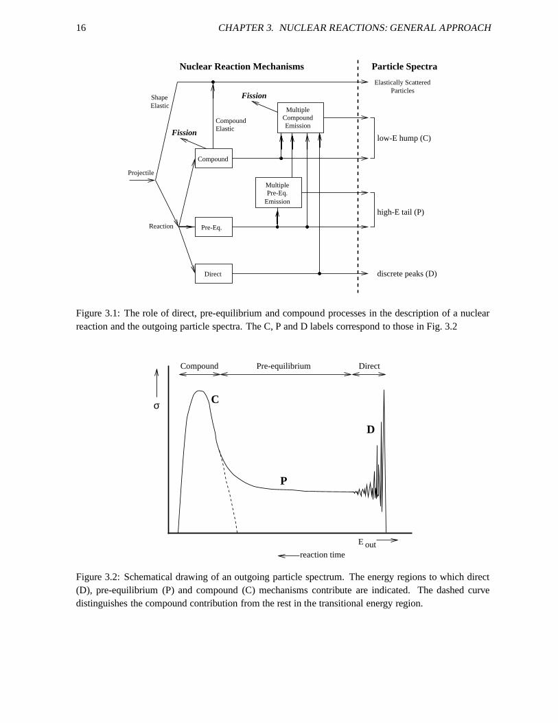
An outline of the general theory and modeling of nuclear reactions can be given in many ways. Acommon classification is in terms of time scales: short reaction times are associated with direct reactionsand long reaction times with compound nucleus processes. Atintermediate time scales, pre-equilibriumprocesses occur. An alternative, more or less equivalent, classification can be given with the numberof intranuclear collisions, which is one or two for direct reactions, a few for pre-equilibrium reactionsand many for compound reactions, respectively. As a consequence, the coupling between the incidentand outgoing channels decreases with the number of collisions and the statistical nature of the nuclearreaction theories increases with the number of collisions.Figs. 3.1 and 3.2 explain the role of the differentreaction mechanisms during an arbitrary nucleon-induced reaction in a schematic manner. They will allbe discussed in this manual.
This distinction between nuclear reaction mechanisms can be obtained in a more formal way bymeans of a proper division of the nuclear wave functions intoopen and closed configurations, as detailedfor example by Feshbach’s many contributions to the field. This is the subject of several textbooks andwill not be repeated here. When appropriate, we will return to the most important theoretical aspects ofthe nuclear models in TALYS in Chapter 4.
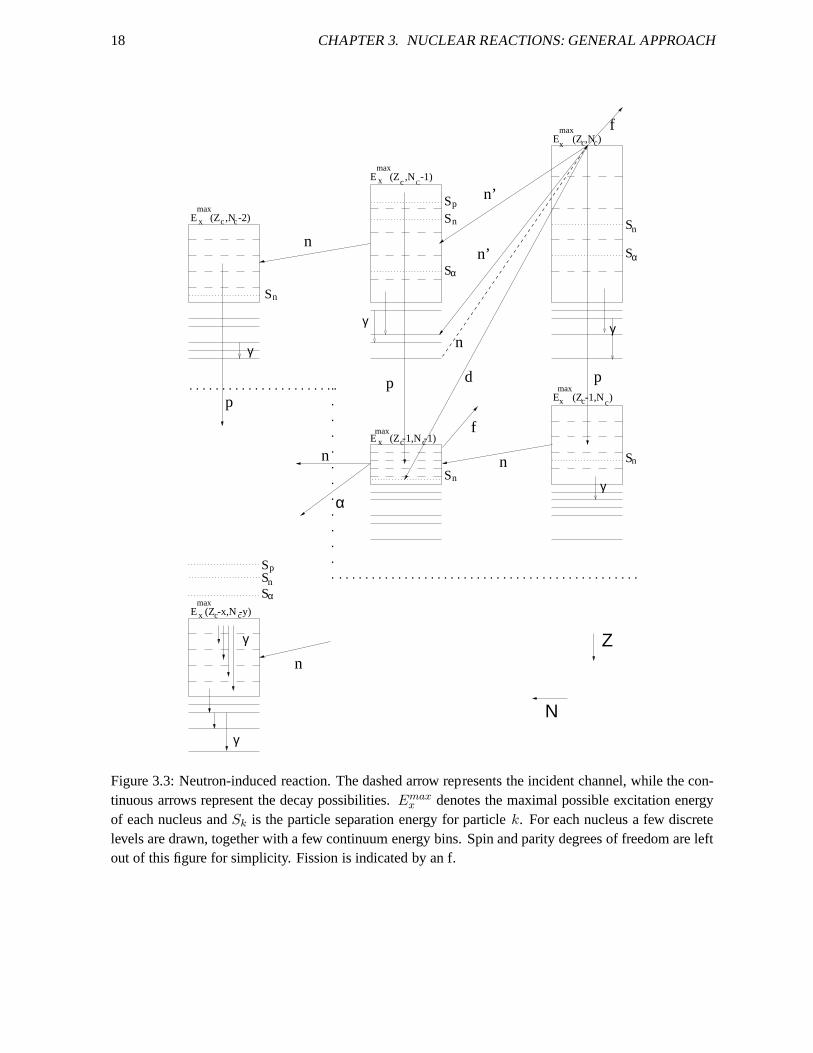
When discussing nuclear reactions in the context of a computer code, as in this manual, a differentstarting point is more appropriate. We think it is best illustrated by Fig. 3.3. A particle incident on atarget nucleus will induce severalbinary reactions which are described by the various competing reactionmechanisms that were mentioned above. The end products of the binary reaction are the emitted particleand the corresponding recoiling residual nucleus. In general this is, however, not the end of the process.A total nuclear reaction may involve a whole sequence of residual nuclei, especially at higher energies,resulting from multiple particle emission. All these residual nuclides have their own separation energies,optical model parameters, level densities, fission barriers, gamma strength functions, etc., that mustproperly be taken into account along the reaction chain. Theimplementation of this entire reaction chainforms the backbone of TALYS. The program has been written in away that enables a clear and easyinclusion of all possible nuclear model ingredients for anynumber of nuclides in the reaction chain. Ofcourse, in this whole chain the target and primary compound nucleus have a special status, since they
15
16 CHAPTER 3. NUCLEAR REACTIONS: GENERAL APPROACH
MultiplePre-Eq.
Emission
Pre-Eq.
Fission
Fission
MultipleCompoundEmission
discrete peaks (D)
Compound
low-E hump (C)Elastic
Projectile
ElasticShape
Reaction
Particle Spectra
Elastically Scattered Particles
Nuclear Reaction Mechanisms
high-E tail (P)
Compound
Direct
Figure 3.1: The role of direct, pre-equilibrium and compound processes in the description of a nuclearreaction and the outgoing particle spectra. The C, P and D labels correspond to those in Fig. 3.2
σ
Compound DirectPre-equilibrium
C
P
D
Eoutreaction time
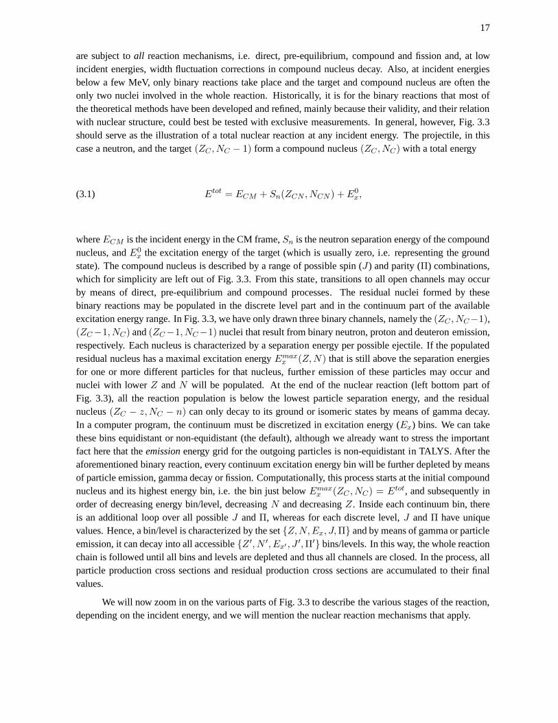
Figure 3.2: Schematical drawing of an outgoing particle spectrum. The energy regions to which direct(D), pre-equilibrium (P) and compound (C) mechanisms contribute are indicated. The dashed curvedistinguishes the compound contribution from the rest in the transitional energy region.
17
are subject toall reaction mechanisms, i.e. direct, pre-equilibrium, compound and fission and, at lowincident energies, width fluctuation corrections in compound nucleus decay. Also, at incident energiesbelow a few MeV, only binary reactions take place and the target and compound nucleus are often theonly two nuclei involved in the whole reaction. Historically, it is for the binary reactions that most ofthe theoretical methods have been developed and refined, mainly because their validity, and their relationwith nuclear structure, could best be tested with exclusivemeasurements. In general, however, Fig. 3.3should serve as the illustration of a total nuclear reactionat any incident energy. The projectile, in thiscase a neutron, and the target(ZC , NC − 1) form a compound nucleus(ZC , NC) with a total energy
(3.1) Etot = ECM + Sn(ZCN , NCN ) + E0x,
whereECM is the incident energy in the CM frame,Sn is the neutron separation energy of the compoundnucleus, andE0
x the excitation energy of the target (which is usually zero, i.e. representing the groundstate). The compound nucleus is described by a range of possible spin (J) and parity (Π) combinations,which for simplicity are left out of Fig. 3.3. From this state, transitions to all open channels may occurby means of direct, pre-equilibrium and compound processes. The residual nuclei formed by thesebinary reactions may be populated in the discrete level partand in the continuum part of the availableexcitation energy range. In Fig. 3.3, we have only drawn three binary channels, namely the(ZC , NC−1),(ZC−1, NC) and(ZC−1, NC−1) nuclei that result from binary neutron, proton and deuteronemission,respectively. Each nucleus is characterized by a separation energy per possible ejectile. If the populatedresidual nucleus has a maximal excitation energyEmax
x (Z,N) that is still above the separation energiesfor one or more different particles for that nucleus, further emission of these particles may occur andnuclei with lowerZ andN will be populated. At the end of the nuclear reaction (left bottom part ofFig. 3.3), all the reaction population is below the lowest particle separation energy, and the residualnucleus(ZC − z,NC − n) can only decay to its ground or isomeric states by means of gamma decay.In a computer program, the continuum must be discretized in excitation energy (Ex) bins. We can takethese bins equidistant or non-equidistant (the default), although we already want to stress the importantfact here that theemissionenergy grid for the outgoing particles is non-equidistant in TALYS. After theaforementioned binary reaction, every continuum excitation energy bin will be further depleted by meansof particle emission, gamma decay or fission. Computationally, this process starts at the initial compoundnucleus and its highest energy bin, i.e. the bin just belowEmax
x (ZC , NC) = Etot, and subsequently inorder of decreasing energy bin/level, decreasingN and decreasingZ. Inside each continuum bin, thereis an additional loop over all possibleJ andΠ, whereas for each discrete level,J andΠ have uniquevalues. Hence, a bin/level is characterized by the setZ,N,Ex, J,Π and by means of gamma or particleemission, it can decay into all accessibleZ ′, N ′, Ex′ , J ′,Π′ bins/levels. In this way, the whole reactionchain is followed until all bins and levels are depleted and thus all channels are closed. In the process, allparticle production cross sections and residual production cross sections are accumulated to their finalvalues.
We will now zoom in on the various parts of Fig. 3.3 to describethe various stages of the reaction,depending on the incident energy, and we will mention the nuclear reaction mechanisms that apply.
18 CHAPTER 3. NUCLEAR REACTIONS: GENERAL APPROACH
n
d
f
f
n’
n’n
p
n
p
S
S
S
SS
γ
γ
.
n
n
α
.
.
.
.
.
.
.
.
.
.
.
.. . . . . . . . . . . . . . . . . . . . . . .
. . . . . . . . . . . . . . . . . . . . . . . . . . . . . . . . . . . . . . . . . . . . . .
Ζ
Ν
p
n
n
Sn
Sp
S
SSp
γ
γ
γ
γ
max
x
max
x
maxx
max
x
max
x
max
x
E (Z -1,N -1)
E (Z -x,N -y)
E (Z ,N )
c
c c
c
c c
c c
cE (Z ,N -2)
CE (Z ,N -1)
E (Z -1,N )c
c
α
Snn
α
n
α
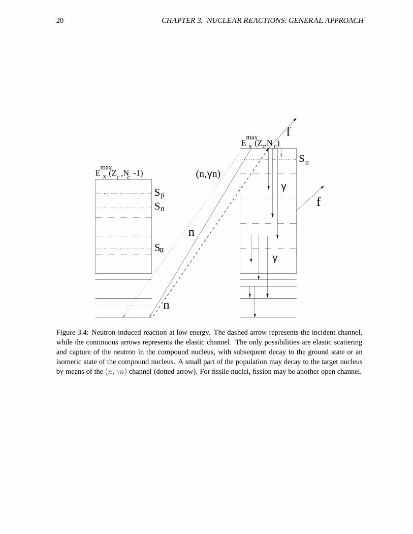
Figure 3.3: Neutron-induced reaction. The dashed arrow represents the incident channel, while the con-tinuous arrows represent the decay possibilities.Emax
x denotes the maximal possible excitation energyof each nucleus andSk is the particle separation energy for particlek. For each nucleus a few discretelevels are drawn, together with a few continuum energy bins.Spin and parity degrees of freedom are leftout of this figure for simplicity. Fission is indicated by an f.
3.1. REACTION MECHANISMS 19
3.1 Reaction mechanisms
In the projectile energy range between 1 keV and several hundreds of MeV, the importance of a particularnuclear reaction mechanism appears and disappears upon varying the incident energy. We will nowdescribe the particle decay scheme that typically applies in the various energy regions. Because of theCoulomb barrier for charged particles, it will be clear thatthe discussion for low energy reactions usuallyconcerns incident neutrons. In general, however, what follows can be generalized to incident chargedparticles. The energy ranges mentioned in each paragraph heading are just meant as helpful indications,which apply for a typical medium mass nucleus.
3.1.1 Low energies
Elastic scattering and capture (E< 0.2 MeV)
If the energy of an incident neutron is below the excitation energy of the first inelastic level, and if thereare no(n, p), etc. reactions that are energetically possible, then the only reaction possibilities are elasticscattering, neutron capture and, for fissile nuclides, fission. At these low energies, only the(ZC , NC −1)
and(ZC , NC) nuclides of Fig. 3.3 are involved, see Fig. 3.4. First, the shape (or direct) elastic scatteringcross section can directly be determined from the optical model, which will be discussed in Section 4.1.The compound nucleus, which is populated by a reaction population equal to the reaction cross section,is formed at one single energyEtot = Emax
x (ZC , NC) and a range ofJ,Π-values. This compoundnucleus either decays by means of compound elastic scattering back to the initial state of the targetnucleus, or by means of neutron capture, after which gamma decay follows to the continuum and todiscrete states of the compound nucleus. The competition between the compound elastic and capturechannels is described by the compound nucleus theory, whichwe will discuss in Section 4.5. To beprecise, the elastic and capture processes comprise the first binary reaction. To complete the descriptionof the total reaction, the excited(ZC , NC) nucleus, which is populated over its whole excitation energyrange by the primary gamma emission, must complete its decay. The highest continuum bin is depletedfirst, for all J andΠ. The subsequent gamma decay increases the population of thelower bins, beforethe latter are depleted themselves. Also, continuum bins that are above the neutron separation energySn of the compound nucleus contribute to the feeding of the(n, γn) channel. This results in a weakcontinuous neutron spectrum, even though the elastic channel is the only true binary neutron channel thatis open. The continuum bins and the discrete levels of the compound nucleus are depleted one by one, indecreasing order, until the ground or an isomeric state of the compound nucleus is reached by subsequentgamma decay. If a nuclide is fissile, fission may compete as well, both from the initial compound stateEmax
x (ZC , NC) and from the continuum bins of the compound nucleus, the latter resulting in a(n, γf)
cross section. Both contributions add up to the so called first-chance fission cross section.
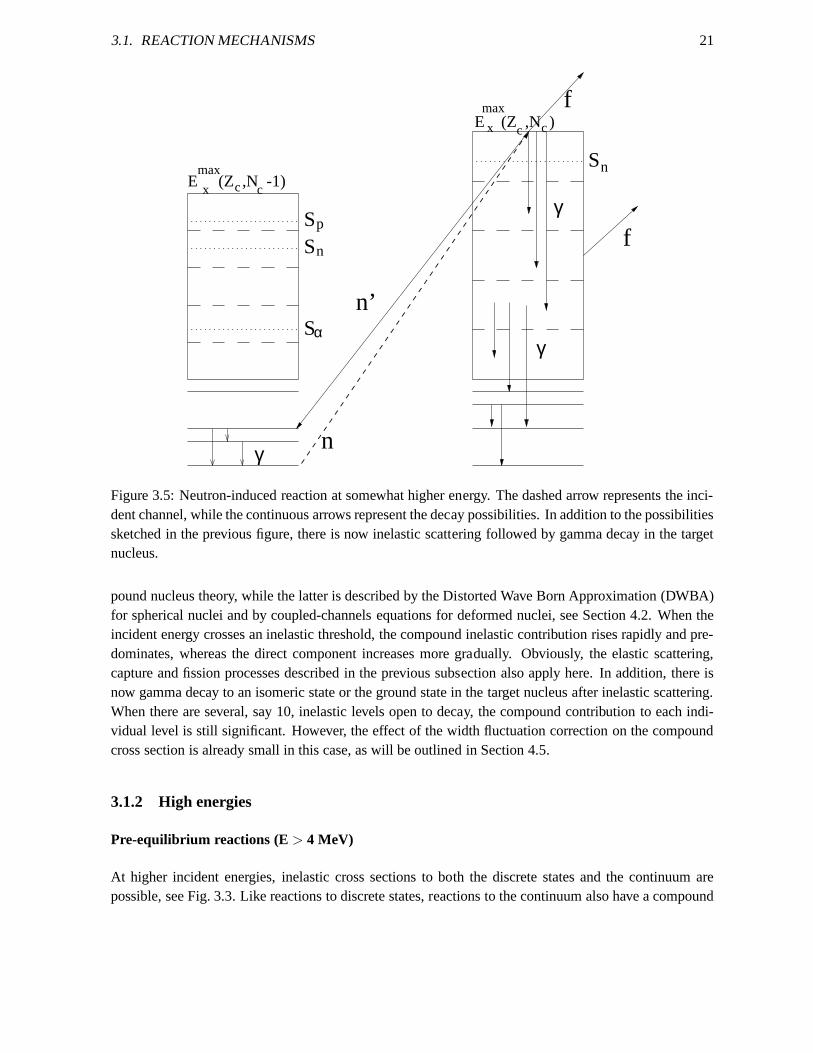
Inelastic scattering to discrete states (0.2< E < 4 MeV)
At somewhat higher incident energies, the first inelastic channels open up, see Fig. 3.5. Reactions tothese discrete levels have a compound and a direct component. The former is again described by the com-
20 CHAPTER 3. NUCLEAR REACTIONS: GENERAL APPROACH
n
f
S
Sp
S
γ
γf
Sn
n
(n,γn)maxx c c
E (Z ,N -1)
maxx c cE (Z ,N )
n
α
Figure 3.4: Neutron-induced reaction at low energy. The dashed arrow represents the incident channel,while the continuous arrows represents the elastic channel. The only possibilities are elastic scatteringand capture of the neutron in the compound nucleus, with subsequent decay to the ground state or anisomeric state of the compound nucleus. A small part of the population may decay to the target nucleusby means of the(n, γn) channel (dotted arrow). For fissile nuclei, fission may be another open channel.
3.1. REACTION MECHANISMS 21
n
f
n’S
Sp
S
Sn
γ
γf
γ
max
x c cE (Z ,N -1)
max
x c cE (Z ,N )
α
n
Figure 3.5: Neutron-induced reaction at somewhat higher energy. The dashed arrow represents the inci-dent channel, while the continuous arrows represent the decay possibilities. In addition to the possibilitiessketched in the previous figure, there is now inelastic scattering followed by gamma decay in the targetnucleus.
pound nucleus theory, while the latter is described by the Distorted Wave Born Approximation (DWBA)for spherical nuclei and by coupled-channels equations fordeformed nuclei, see Section 4.2. When theincident energy crosses an inelastic threshold, the compound inelastic contribution rises rapidly and pre-dominates, whereas the direct component increases more gradually. Obviously, the elastic scattering,capture and fission processes described in the previous subsection also apply here. In addition, there isnow gamma decay to an isomeric state or the ground state in thetarget nucleus after inelastic scattering.When there are several, say 10, inelastic levels open to decay, the compound contribution to each indi-vidual level is still significant. However, the effect of thewidth fluctuation correction on the compoundcross section is already small in this case, as will be outlined in Section 4.5.
3.1.2 High energies
Pre-equilibrium reactions (E > 4 MeV)
At higher incident energies, inelastic cross sections to both the discrete states and the continuum arepossible, see Fig. 3.3. Like reactions to discrete states, reactions to the continuum also have a compound
22 CHAPTER 3. NUCLEAR REACTIONS: GENERAL APPROACH
and a direct-like component. The latter are usually described by pre-equilibrium reactions which, bydefinition, include direct reactions to the continuum. Theywill be discussed in Section 4.4. Also non-elastic channels to other nuclides, through charge-exchange, e.g. (n, p), and transfer reactions, e.g.(n, α), generally open up at these energies, and decay to these nuclides can take place by the same direct,pre-equilibrium and compound mechanisms. Again, the channels described in the previous subsectionsalso apply here. In addition, gamma decay to ground and isomeric states of all residual nuclides occurs.When many channels open up, particle decay to individual states (e.g. compound elastic scattering)rapidly becomes negligible. For the excitation of a discrete state, the direct component now becomespredominant, since that involves no statistical competition with the other channels. At about 15 MeV,the total compound cross section, i.e. summed over all final discrete states and the excited continuum, ishowever still larger than the summed direct and pre-equilibrium contributions.
Multiple compound emission (E> 8 MeV)
At incident energies above about the neutron separation energy, the residual nuclides formed after thefirst binary reaction contain enough excitation energy to enable further decay by compound nucleusparticle emission or fission. This gives rise to multiple reaction channels such as(n, 2n), (n, np), etc.For higher energies, this picture can be generalized to manyresidual nuclei, and thus more complexreaction channels, as explained in the introduction of thisChapter, see also Fig. 3.3. If fission is possible,this may occur for all residual nuclides, which is known as multiple chance fission. All excited nuclideswill eventually decay to their isomeric and ground states.
Multiple pre-equilibrium emission (E > 40 MeV)
At still higher incident energies, above several tens of MeV, the residual nuclides formed after binaryemission may contain so much excitation energy that the presence of furtherfast particles inside thenucleus becomes possible. These can be imagined as stronglyexcited particle-hole pairs resulting fromthe first binary interaction with the projectile. The residual system is then clearly non-equilibrated and theexcited particle that is high in the continuum may, in addition to the first emitted particle, also be emittedon a short time scale. This so-called multiple pre-equilibrium emission forms an alternative theoreticalpicture of the intra-nuclear cascade process, whereby now not the exact location and momentum of theparticles is followed, but instead the total energy of the system and the number of particle-hole excitations(exciton number). In TALYS, this process can be generalizedto any number of multiple pre-equilibriumstages in the reaction by keeping track of all successive particle-hole excitations, see Section 4.6.2. Forthese incident energies, the binary compound cross sectionbecomes small: the non-elastic cross sectionis almost completely exhausted by primary pre-equilibriumemission. Again, Fig. 3.3 applies.
3.2 Cross section definitions
In TALYS, cross sections for reactions to all open channels are calculated. Although the types of most ofthese partial cross sections are generally well known, it isappropriate to define them for completeness.
3.2. CROSS SECTION DEFINITIONS 23
This section concerns basically the book-keeping of the various cross sections, including all the sumrules they obey. The particular nuclear models that are needed to obtain them are described in Chapter 4.Thus, we do not yet give the definition of cross sections in terms of more fundamental quantities. Unlessotherwise stated, we use incident neutrons as example in what follows and we consider only photons(γ), neutrons (n), protons (p), deuterons (d), tritons (t), helium-3 particles (h) and alpha particles (α)as competing particles. Also, to avoid an overburdening of the notation and the explanation, we willpostpone the competition of fission to the last section of this Chapter.
3.2.1 Total cross sections
The most basic nuclear reaction calculation is that with theoptical model, which will be explained inmore detail in Section 4.1. Here, it is sufficient to summarize the relations that can be found in manynuclear reaction textbooks, namely that the optical model yields thereaction cross sectionσreac and, inthe case of neutrons, thetotal cross sectionσtot and theshape-elastic cross sectionσshape−el. They arerelated by
(3.2) σtot = σshape−el + σreac.
If the elastic channel is, besides shape elastic scattering, also fed by compound nucleus decay, the lat-ter component is a part of the reaction cross section and is called thecompound elastic cross sectionσcomp−el. With this, we can define thetotal elastic cross sectionσel,
(3.3) σel = σshape−el + σcomp−el,
and thenon-elastic cross sectionσnon−el,
(3.4) σnon−el = σreac − σcomp−el,
so that we can combine these equations to give
(3.5) σtot = σel + σnon−el.
The last equation contains the quantities that can actuallybe measured in an experiment. We also notethat the competition between the many compound nucleus decay channels ensures thatσcomp−el rapidlydiminishes for incident neutron energies above a few MeV, inwhich caseσnon−el becomes practicallyequal toσreac.
A further subdivision of the outcome of a nuclear reaction concerns the breakdown ofσnon−el: thiscross section contains all the partial cross sections. For this we introduce the exclusive cross sections,from which all other cross sections of interest can be derived.
3.2.2 Exclusive cross sections
In this manual, we call a cross sectionexclusivewhen the outgoing channel is precisely specified bythe type and number of outgoing particles (+ any number of photons). Well-known examples are the
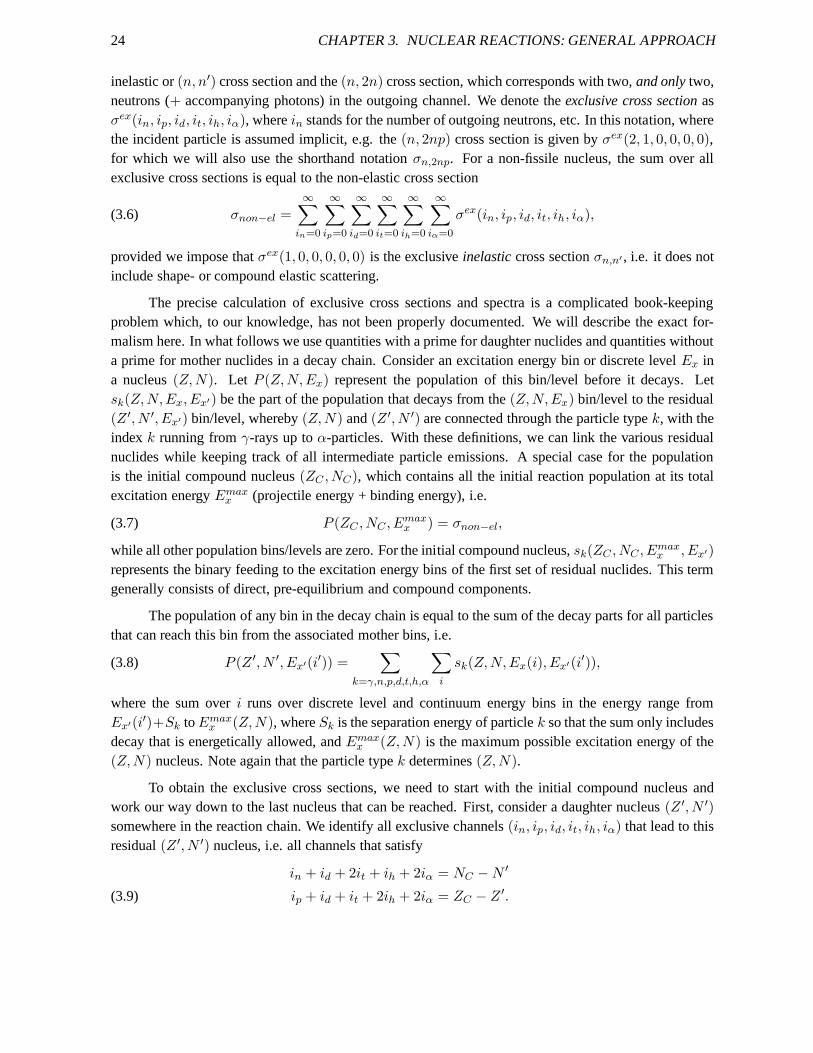
24 CHAPTER 3. NUCLEAR REACTIONS: GENERAL APPROACH
inelastic or(n, n′) cross section and the(n, 2n) cross section, which corresponds with two,and onlytwo,neutrons (+ accompanying photons) in the outgoing channel. We denote the exclusive cross sectionasσex(in, ip, id, it, ih, iα), wherein stands for the number of outgoing neutrons, etc. In this notation, wherethe incident particle is assumed implicit, e.g. the(n, 2np) cross section is given byσex(2, 1, 0, 0, 0, 0),for which we will also use the shorthand notationσn,2np. For a non-fissile nucleus, the sum over allexclusive cross sections is equal to the non-elastic cross section
(3.6) σnon−el =∞∑
in=0
∞∑
ip=0
∞∑
id=0
∞∑
it=0
∞∑
ih=0
∞∑
iα=0
σex(in, ip, id, it, ih, iα),
provided we impose thatσex(1, 0, 0, 0, 0, 0) is the exclusiveinelasticcross sectionσn,n′ , i.e. it does notinclude shape- or compound elastic scattering.
The precise calculation of exclusive cross sections and spectra is a complicated book-keepingproblem which, to our knowledge, has not been properly documented. We will describe the exact for-malism here. In what follows we use quantities with a prime for daughter nuclides and quantities withouta prime for mother nuclides in a decay chain. Consider an excitation energy bin or discrete levelEx ina nucleus(Z,N). Let P (Z,N,Ex) represent the population of this bin/level before it decays. Letsk(Z,N,Ex, Ex′) be the part of the population that decays from the(Z,N,Ex) bin/level to the residual(Z ′, N ′, Ex′) bin/level, whereby(Z,N) and(Z ′, N ′) are connected through the particle typek, with theindexk running fromγ-rays up toα-particles. With these definitions, we can link the various residualnuclides while keeping track of all intermediate particle emissions. A special case for the populationis the initial compound nucleus(ZC , NC), which contains all the initial reaction population at its totalexcitation energyEmax
x (projectile energy + binding energy), i.e.
(3.7) P (ZC , NC , Emaxx ) = σnon−el,
while all other population bins/levels are zero. For the initial compound nucleus,sk(ZC , NC , Emaxx , Ex′)
represents the binary feeding to the excitation energy binsof the first set of residual nuclides. This termgenerally consists of direct, pre-equilibrium and compound components.
The population of any bin in the decay chain is equal to the sumof the decay parts for all particlesthat can reach this bin from the associated mother bins, i.e.
(3.8) P (Z ′, N ′, Ex′(i′)) =∑
k=γ,n,p,d,t,h,α
∑
i
sk(Z,N,Ex(i), Ex′(i′)),
where the sum overi runs over discrete level and continuum energy bins in the energy range fromEx′(i′)+Sk toEmax
x (Z,N), whereSk is the separation energy of particlek so that the sum only includesdecay that is energetically allowed, andEmax
x (Z,N) is the maximum possible excitation energy of the(Z,N) nucleus. Note again that the particle typek determines(Z,N).
To obtain the exclusive cross sections, we need to start withthe initial compound nucleus andwork our way down to the last nucleus that can be reached. First, consider a daughter nucleus(Z ′, N ′)
somewhere in the reaction chain. We identify all exclusive channels(in, ip, id, it, ih, iα) that lead to thisresidual(Z ′, N ′) nucleus, i.e. all channels that satisfy
in + id + 2it + ih + 2iα = NC − N ′
ip + id + it + 2ih + 2iα = ZC − Z ′.(3.9)
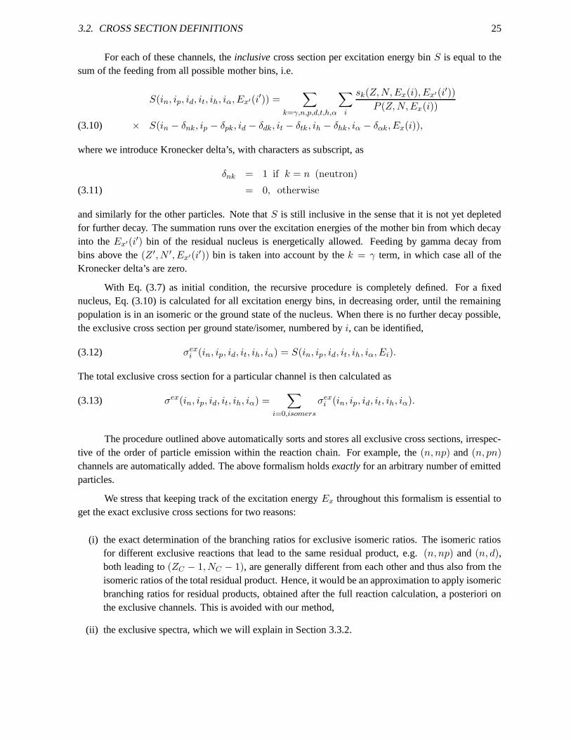
3.2. CROSS SECTION DEFINITIONS 25
For each of these channels, theinclusivecross section per excitation energy binS is equal to thesum of the feeding from all possible mother bins, i.e.
S(in, ip, id, it, ih, iα, Ex′(i′)) =∑
k=γ,n,p,d,t,h,α
∑
i
sk(Z,N,Ex(i), Ex′(i′))
P (Z,N,Ex(i))
× S(in − δnk, ip − δpk, id − δdk, it − δtk, ih − δhk, iα − δαk, Ex(i)),(3.10)
where we introduce Kronecker delta’s, with characters as subscript, as
δnk = 1 if k = n (neutron)
= 0, otherwise(3.11)
and similarly for the other particles. Note thatS is still inclusive in the sense that it is not yet depletedfor further decay. The summation runs over the excitation energies of the mother bin from which decayinto theEx′(i′) bin of the residual nucleus is energetically allowed. Feeding by gamma decay frombins above the(Z ′, N ′, Ex′(i′)) bin is taken into account by thek = γ term, in which case all of theKronecker delta’s are zero.
With Eq. (3.7) as initial condition, the recursive procedure is completely defined. For a fixednucleus, Eq. (3.10) is calculated for all excitation energybins, in decreasing order, until the remainingpopulation is in an isomeric or the ground state of the nucleus. When there is no further decay possible,the exclusive cross section per ground state/isomer, numbered byi, can be identified,
(3.12) σexi (in, ip, id, it, ih, iα) = S(in, ip, id, it, ih, iα, Ei).
The total exclusive cross section for a particular channel is then calculated as
(3.13) σex(in, ip, id, it, ih, iα) =∑
i=0,isomers
σexi (in, ip, id, it, ih, iα).
The procedure outlined above automatically sorts and stores all exclusive cross sections, irrespec-tive of the order of particle emission within the reaction chain. For example, the(n, np) and (n, pn)
channels are automatically added. The above formalism holdsexactlyfor an arbitrary number of emittedparticles.
We stress that keeping track of the excitation energyEx throughout this formalism is essential toget the exact exclusive cross sections for two reasons:
(i) the exact determination of the branching ratios for exclusive isomeric ratios. The isomeric ratiosfor different exclusive reactions that lead to the same residual product, e.g.(n, np) and (n, d),both leading to(ZC − 1, NC − 1), are generally different from each other and thus also from theisomeric ratios of the total residual product. Hence, it would be an approximation to apply isomericbranching ratios for residual products, obtained after thefull reaction calculation, a posteriori onthe exclusive channels. This is avoided with our method,
(ii) the exclusive spectra, which we will explain in Section3.3.2.
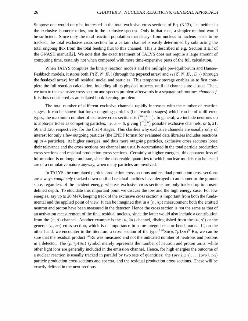
26 CHAPTER 3. NUCLEAR REACTIONS: GENERAL APPROACH
Suppose one would only be interested in the total exclusive cross sections of Eq. (3.13), i.e. neither inthe exclusive isomeric ratios, nor in the exclusive spectra. Only in that case, a simpler method wouldbe sufficient. Since only the total reaction population thatdecays from nucleus to nucleus needs to betracked, the total exclusive cross section for a certain channel is easily determined by subtracting thetotal ongoing flux from the total feeding flux to this channel.This is described in e.g. Section II.E.f ofthe GNASH manual[2]. We note that the exact treatment of TALYS does not require a large amount ofcomputing time, certainly not when compared with more time-expensive parts of the full calculation.
When TALYS computes the binary reaction models and the multiple pre-equilibrium and Hauser-Feshbach models, it stores bothP (Z,N,Ex) (through thepopexclarray) andsk(Z,N,Ex, Ex′) (throughthe feedexclarray) for all residual nuclei and particles. This temporary storage enables us to first com-plete the full reaction calculation, including all its physical aspects, until all channels are closed. Then,we turn to the exclusive cross section and spectra problem afterwards in a separate subroutine:channels.f.It is thus considered as an isolated book-keeping problem.
The total number of different exclusive channels rapidly increases with the number of reactionstages. It can be shown that form outgoing particles (i.e. reaction stages) which can be ofk differenttypes, the maximum number of exclusive cross sections is
(m+k−1m
)
. In general, we include neutrons upto alpha-particles as competing particles, i.e.k = 6, giving
(m+5m
)
possible exclusive channels, or 6, 21,56 and 126, respectively, for the first 4 stages. This clarifies why exclusive channels are usually only ofinterest for only a few outgoing particles (the ENDF format for evaluated data libraries includes reactionsup to 4 particles). At higher energies, and thus more outgoing particles, exclusive cross sections loosetheir relevance and the cross sections per channel are usually accumulated in the total particle productioncross sections and residual production cross sections. Certainly at higher energies, this apparent loss ofinformation is no longer an issue, since the observable quantities to which nuclear models can be testedare of a cumulative nature anyway, when many particles are involved.
In TALYS, the cumulated particle production cross sectionsand residual production cross sectionsare alwayscompletelytracked down until all residual nuclides have decayed to an isomer or the groundstate, regardless of the incident energy, whereas exclusive cross sections are only tracked up to a user-defined depth. To elucidate this important point we discuss the low and the high energy case. For lowenergies, say up to 20 MeV, keeping track of the exclusive cross section is important from both the funda-mental and the applied point of view. It can be imagined that in a(n, np) measurement both the emittedneutron and proton have been measured in the detector. Hencethe cross section isnot the same as that ofan activation measurement of the final residual nucleus, since the latter would also include a contributionfrom the(n, d) channel. Another example is the(n, 2n) channel, distinguished from the(n, n′) or thegeneral(n, xn) cross section, which is of importance in some integral reactor benchmarks. If, on theother hand, we encounter in the literature a cross section ofthe type120Sn(p, 7p18n)96Ru, we can besure that the residual product96Ru was measured and not the indicated number of neutrons and protonsin a detector. The(p, 7p18n) symbol merely represents the number of neutron and proton units, whileother light ions are generally included in the emission channel. Hence, for high energies the outcome ofa nuclear reaction is usually tracked in parallel by two setsof quantities: the(proj, xn), . . . (proj, xα)
particle production cross sections and spectra, and the residual production cross sections. These will beexactly defined in the next sections.
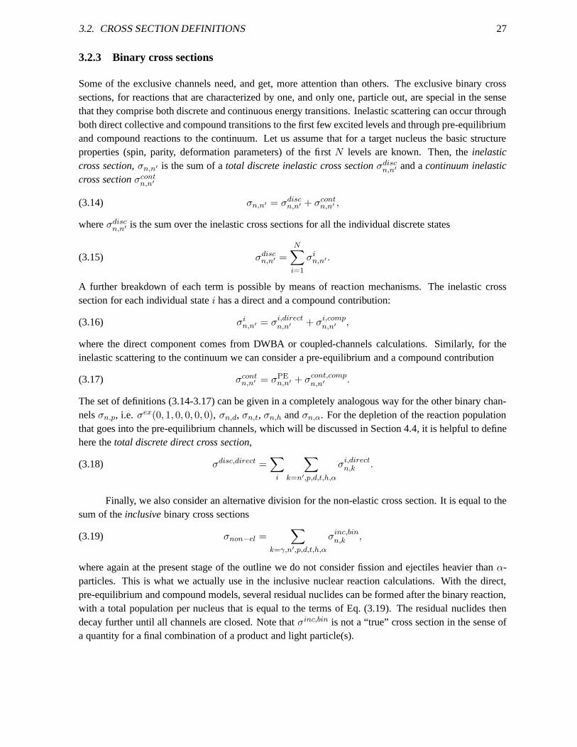
3.2. CROSS SECTION DEFINITIONS 27
3.2.3 Binary cross sections
Some of the exclusive channels need, and get, more attentionthan others. The exclusive binary crosssections, for reactions that are characterized by one, and only one, particle out, are special in the sensethat they comprise both discrete and continuous energy transitions. Inelastic scattering can occur throughboth direct collective and compound transitions to the firstfew excited levels and through pre-equilibriumand compound reactions to the continuum. Let us assume that for a target nucleus the basic structureproperties (spin, parity, deformation parameters) of the first N levels are known. Then, theinelasticcross section, σn,n′ is the sum of atotal discrete inelastic cross sectionσdisc
n,n′ and acontinuum inelasticcross sectionσcont
n,n′
(3.14) σn,n′ = σdiscn,n′ + σcont
n,n′ ,
whereσdiscn,n′ is the sum over the inelastic cross sections for all the individual discrete states
(3.15) σdiscn,n′ =
N∑
i=1
σin,n′ .
A further breakdown of each term is possible by means of reaction mechanisms. The inelastic crosssection for each individual statei has a direct and a compound contribution:
(3.16) σin,n′ = σi,direct
n,n′ + σi,compn,n′ ,
where the direct component comes from DWBA or coupled-channels calculations. Similarly, for theinelastic scattering to the continuum we can consider a pre-equilibrium and a compound contribution
(3.17) σcontn,n′ = σPE
n,n′ + σcont,compn,n′ .
The set of definitions (3.14-3.17) can be given in a completely analogous way for the other binary chan-nelsσn,p, i.e. σex(0, 1, 0, 0, 0, 0), σn,d, σn,t, σn,h andσn,α. For the depletion of the reaction populationthat goes into the pre-equilibrium channels, which will be discussed in Section 4.4, it is helpful to definehere thetotal discrete direct cross section,
(3.18) σdisc,direct =∑
i
∑
k=n′,p,d,t,h,α
σi,directn,k .
Finally, we also consider an alternative division for the non-elastic cross section. It is equal to thesum of theinclusivebinary cross sections
(3.19) σnon−el =∑
k=γ,n′,p,d,t,h,α
σinc,binn,k ,
where again at the present stage of the outline we do not consider fission and ejectiles heavier thanα-particles. This is what we actually use in the inclusive nuclear reaction calculations. With the direct,pre-equilibrium and compound models, several residual nuclides can be formed after the binary reaction,with a total population per nucleus that is equal to the termsof Eq. (3.19). The residual nuclides thendecay further until all channels are closed. Note thatσinc,bin is not a “true” cross section in the sense ofa quantity for a final combination of a product and light particle(s).
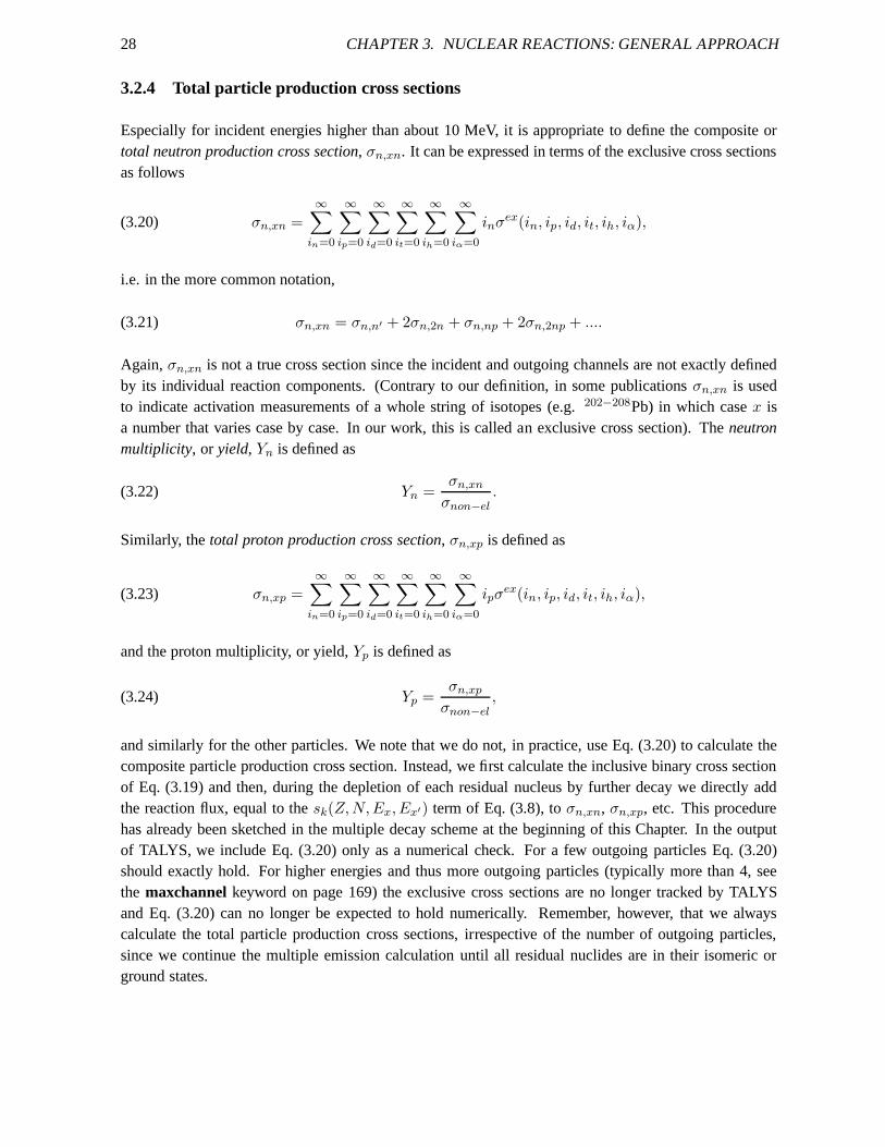
28 CHAPTER 3. NUCLEAR REACTIONS: GENERAL APPROACH
3.2.4 Total particle production cross sections
Especially for incident energies higher than about 10 MeV, it is appropriate to define the composite ortotal neutron production cross section, σn,xn. It can be expressed in terms of the exclusive cross sectionsas follows
(3.20) σn,xn =∞∑
in=0
∞∑
ip=0
∞∑
id=0
∞∑
it=0
∞∑
ih=0
∞∑
iα=0
inσex(in, ip, id, it, ih, iα),
i.e. in the more common notation,
(3.21) σn,xn = σn,n′ + 2σn,2n + σn,np + 2σn,2np + ....
Again,σn,xn is not a true cross section since the incident and outgoing channels are not exactly definedby its individual reaction components. (Contrary to our definition, in some publicationsσn,xn is usedto indicate activation measurements of a whole string of isotopes (e.g.202−208Pb) in which casex isa number that varies case by case. In our work, this is called an exclusive cross section). Theneutronmultiplicity, or yield, Yn is defined as
(3.22) Yn =σn,xn
σnon−el.
Similarly, thetotal proton production cross section, σn,xp is defined as
(3.23) σn,xp =∞∑
in=0
∞∑
ip=0
∞∑
id=0
∞∑
it=0
∞∑
ih=0
∞∑
iα=0
ipσex(in, ip, id, it, ih, iα),
and the proton multiplicity, or yield,Yp is defined as
(3.24) Yp =σn,xp
σnon−el,
and similarly for the other particles. We note that we do not,in practice, use Eq. (3.20) to calculate thecomposite particle production cross section. Instead, we first calculate the inclusive binary cross sectionof Eq. (3.19) and then, during the depletion of each residualnucleus by further decay we directly addthe reaction flux, equal to thesk(Z,N,Ex, Ex′) term of Eq. (3.8), toσn,xn, σn,xp, etc. This procedurehas already been sketched in the multiple decay scheme at thebeginning of this Chapter. In the outputof TALYS, we include Eq. (3.20) only as a numerical check. Fora few outgoing particles Eq. (3.20)should exactly hold. For higher energies and thus more outgoing particles (typically more than 4, seethe maxchannelkeyword on page 169) the exclusive cross sections are no longer tracked by TALYSand Eq. (3.20) can no longer be expected to hold numerically.Remember, however, that we alwayscalculate the total particle production cross sections, irrespective of the number of outgoing particles,since we continue the multiple emission calculation until all residual nuclides are in their isomeric orground states.
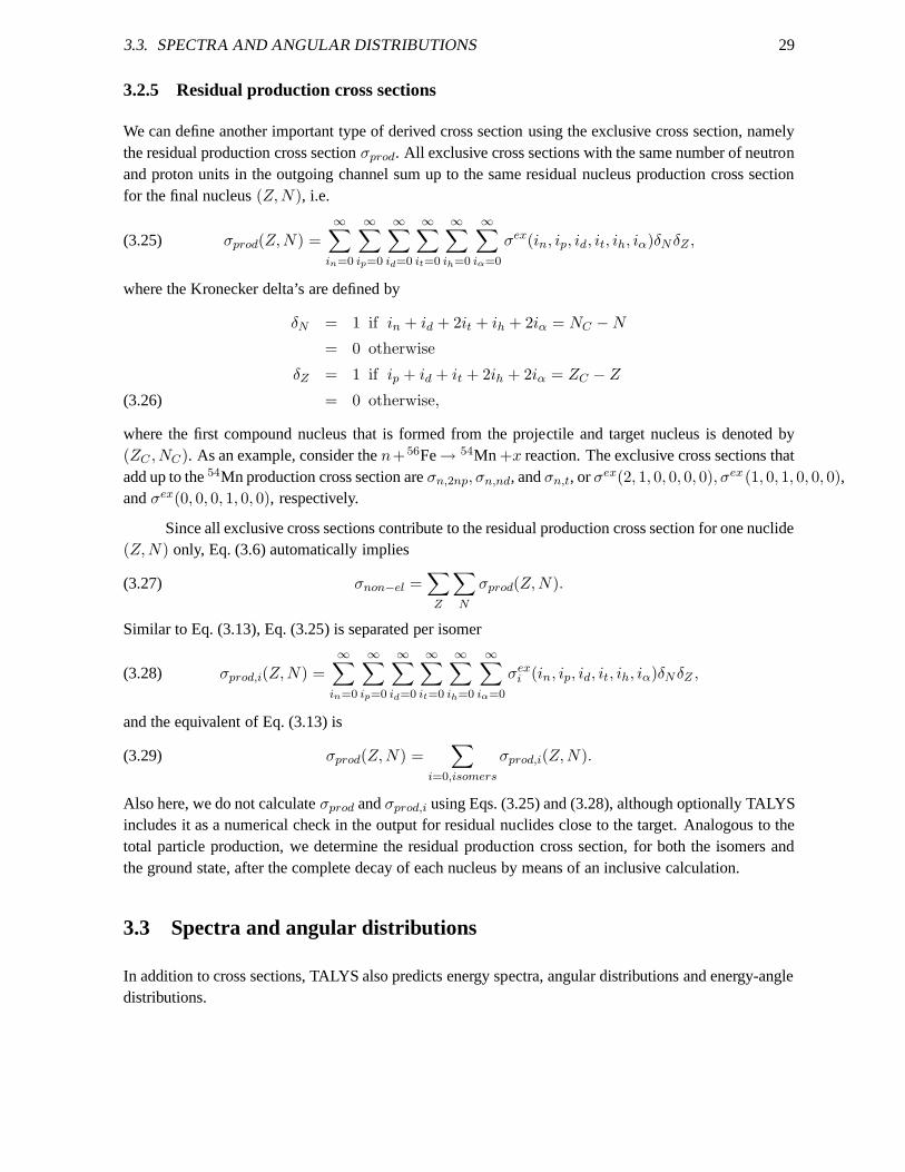
3.3. SPECTRA AND ANGULAR DISTRIBUTIONS 29
3.2.5 Residual production cross sections
We can define another important type of derived cross sectionusing the exclusive cross section, namelythe residual production cross sectionσprod. All exclusive cross sections with the same number of neutronand proton units in the outgoing channel sum up to the same residual nucleus production cross sectionfor the final nucleus(Z,N), i.e.
(3.25) σprod(Z,N) =
∞∑
in=0
∞∑
ip=0
∞∑
id=0
∞∑
it=0
∞∑
ih=0
∞∑
iα=0
σex(in, ip, id, it, ih, iα)δNδZ ,
where the Kronecker delta’s are defined by
δN = 1 if in + id + 2it + ih + 2iα = NC − N
= 0 otherwise
δZ = 1 if ip + id + it + 2ih + 2iα = ZC − Z
= 0 otherwise,(3.26)
where the first compound nucleus that is formed from the projectile and target nucleus is denoted by(ZC , NC). As an example, consider then+56Fe→ 54Mn +x reaction. The exclusive cross sections thatadd up to the54Mn production cross section areσn,2np, σn,nd, andσn,t, orσex(2, 1, 0, 0, 0, 0), σex(1, 0, 1, 0, 0, 0),andσex(0, 0, 0, 1, 0, 0), respectively.
Since all exclusive cross sections contribute to the residual production cross section for one nuclide(Z,N) only, Eq. (3.6) automatically implies
(3.27) σnon−el =∑
Z
∑
N
σprod(Z,N).
Similar to Eq. (3.13), Eq. (3.25) is separated per isomer
(3.28) σprod,i(Z,N) =
∞∑
in=0
∞∑
ip=0
∞∑
id=0
∞∑
it=0
∞∑
ih=0
∞∑
iα=0
σexi (in, ip, id, it, ih, iα)δNδZ ,
and the equivalent of Eq. (3.13) is
(3.29) σprod(Z,N) =∑
i=0,isomers
σprod,i(Z,N).
Also here, we do not calculateσprod andσprod,i using Eqs. (3.25) and (3.28), although optionally TALYSincludes it as a numerical check in the output for residual nuclides close to the target. Analogous to thetotal particle production, we determine the residual production cross section, for both the isomers andthe ground state, after the complete decay of each nucleus bymeans of an inclusive calculation.
3.3 Spectra and angular distributions
In addition to cross sections, TALYS also predicts energy spectra, angular distributions and energy-angledistributions.
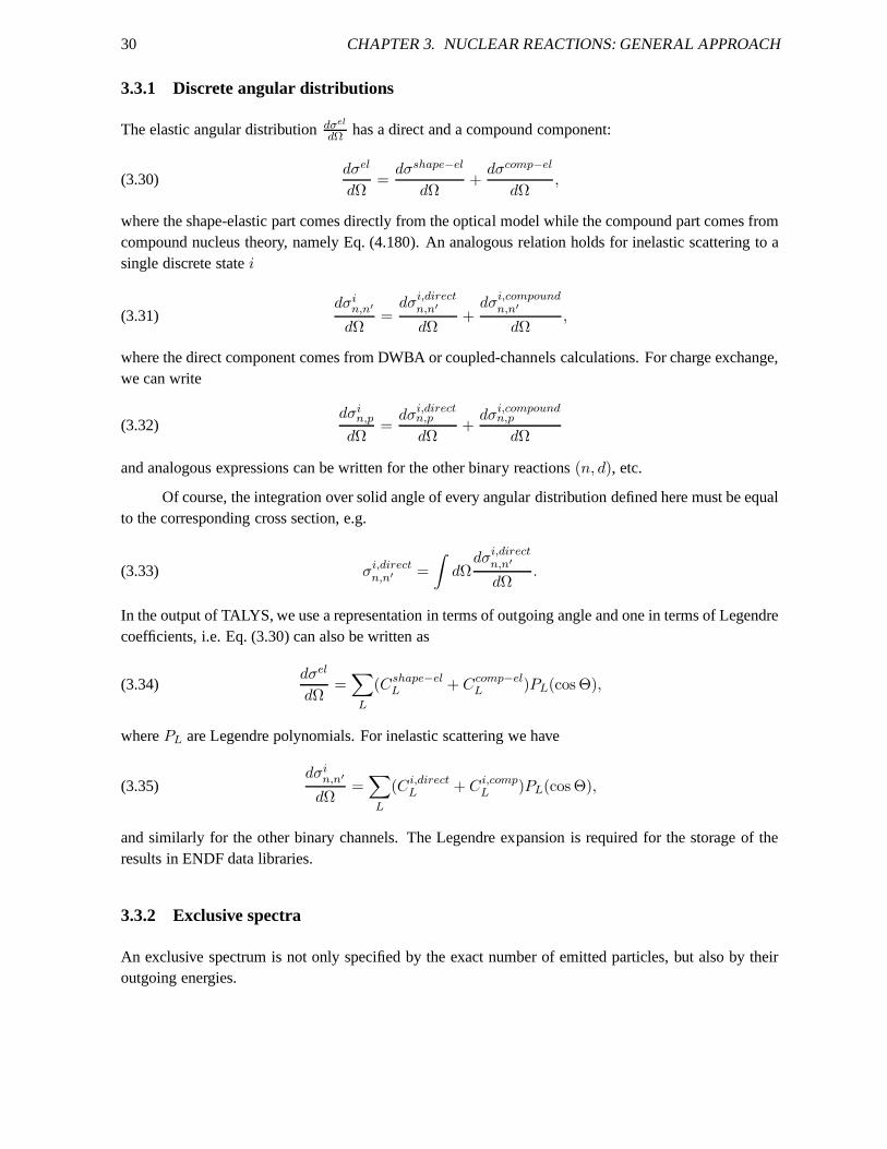
30 CHAPTER 3. NUCLEAR REACTIONS: GENERAL APPROACH
3.3.1 Discrete angular distributions
The elastic angular distributiondσel
dΩ has a direct and a compound component:
(3.30)dσel
dΩ=
dσshape−el
dΩ+
dσcomp−el
dΩ,
where the shape-elastic part comes directly from the optical model while the compound part comes fromcompound nucleus theory, namely Eq. (4.180). An analogous relation holds for inelastic scattering to asingle discrete statei
(3.31)dσi
n,n′
dΩ=
dσi,directn,n′
dΩ+
dσi,compoundn,n′
dΩ,
where the direct component comes from DWBA or coupled-channels calculations. For charge exchange,we can write
(3.32)dσi
n,p
dΩ=
dσi,directn,p
dΩ+
dσi,compoundn,p
dΩ
and analogous expressions can be written for the other binary reactions(n, d), etc.
Of course, the integration over solid angle of every angulardistribution defined here must be equalto the corresponding cross section, e.g.
(3.33) σi,directn,n′ =
∫
dΩdσi,direct
n,n′
dΩ.
In the output of TALYS, we use a representation in terms of outgoing angle and one in terms of Legendrecoefficients, i.e. Eq. (3.30) can also be written as
(3.34)dσel
dΩ=∑
L
(Cshape−elL + Ccomp−el
L )PL(cos Θ),
wherePL are Legendre polynomials. For inelastic scattering we have
(3.35)dσi
n,n′
dΩ=∑
L
(Ci,directL + Ci,comp
L )PL(cos Θ),
and similarly for the other binary channels. The Legendre expansion is required for the storage of theresults in ENDF data libraries.
3.3.2 Exclusive spectra
An exclusive spectrum is not only specified by the exact number of emitted particles, but also by theiroutgoing energies.
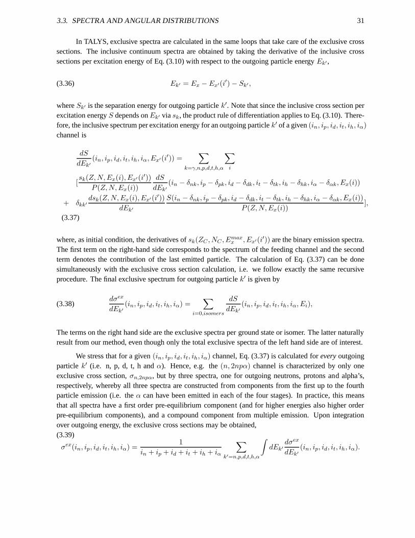
3.3. SPECTRA AND ANGULAR DISTRIBUTIONS 31
In TALYS, exclusive spectra are calculated in the same loopsthat take care of the exclusive crosssections. The inclusive continuum spectra are obtained by taking the derivative of the inclusive crosssections per excitation energy of Eq. (3.10) with respect tothe outgoing particle energyEk′ ,
(3.36) Ek′ = Ex − Ex′(i′) − Sk′ ,
whereSk′ is the separation energy for outgoing particlek′. Note that since the inclusive cross section perexcitation energyS depends onEk′ via sk, the product rule of differentiation applies to Eq. (3.10).There-fore, the inclusive spectrum per excitation energy for an outgoing particlek′ of a given(in, ip, id, it, ih, iα)
channel is
dS
dEk′
(in, ip, id, it, ih, iα, Ex′(i′)) =∑
k=γ,n,p,d,t,h,α
∑
i
[sk(Z,N,Ex(i), Ex′(i′))
P (Z,N,Ex(i))
dS
dEk′
(in − δnk, ip − δpk, id − δdk, it − δtk, ih − δhk, iα − δαk, Ex(i))
+ δkk′
dsk(Z,N,Ex(i), Ex′(i′))
dEk′
S(in − δnk, ip − δpk, id − δdk, it − δtk, ih − δhk, iα − δαk, Ex(i))
P (Z,N,Ex(i))],
(3.37)
where, as initial condition, the derivatives ofsk(ZC , NC , Emaxx , Ex′(i′)) are the binary emission spectra.
The first term on the right-hand side corresponds to the spectrum of the feeding channel and the secondterm denotes the contribution of the last emitted particle.The calculation of Eq. (3.37) can be donesimultaneously with the exclusive cross section calculation, i.e. we follow exactly the same recursiveprocedure. The final exclusive spectrum for outgoing particle k′ is given by
(3.38)dσex
dEk′
(in, ip, id, it, ih, iα) =∑
i=0,isomers
dS
dEk′
(in, ip, id, it, ih, iα, Ei),
The terms on the right hand side are the exclusive spectra perground state or isomer. The latter naturallyresult from our method, even though only the total exclusivespectra of the left hand side are of interest.
We stress that for a given(in, ip, id, it, ih, iα) channel, Eq. (3.37) is calculated foreveryoutgoingparticle k′ (i.e. n, p, d, t, h andα). Hence, e.g. the(n, 2npα) channel is characterized by only oneexclusive cross section,σn,2npα, but by three spectra, one for outgoing neutrons, protons and alpha’s,respectively, whereby all three spectra are constructed from components from the first up to the fourthparticle emission (i.e. theα can have been emitted in each of the four stages). In practice, this meansthat all spectra have a first order pre-equilibrium component (and for higher energies also higher orderpre-equilibrium components), and a compound component from multiple emission. Upon integrationover outgoing energy, the exclusive cross sections may be obtained,(3.39)
σex(in, ip, id, it, ih, iα) =1
in + ip + id + it + ih + iα
∑
k′=n,p,d,t,h,α
∫
dEk′
dσex
dEk′
(in, ip, id, it, ih, iα).
32 CHAPTER 3. NUCLEAR REACTIONS: GENERAL APPROACH
3.3.3 Binary spectra
Similar to the cross sections, the exclusive spectra determine various other specific spectra of interest.The exclusiveinelastic spectrumis a special case of Eq. (3.38)
(3.40)dσn,n′
dEn′
=dσex
dEn′
(1, 0, 0, 0, 0, 0).
Since Eq. (3.37) represents an energy spectrum, it includesby definition only continuum transitions, i.e.it does not include the binary reactions to discrete states.Hence, upon integration, Eq. (3.40) only givesthe continuum inelastic cross section of Eq. (3.14):
(3.41) σcontn,n′ =
∫
dEn′
dσn,n′
dEn′
.
Similar relations hold for the binary(n, p), (n, d), (n, t), (n, h) and(n, α) spectra. The contributions tothe binary spectra generally come from pre-equilibrium andcontinuum compound spectra.
3.3.4 Total particle production spectra
Similar to the total particle production cross sections, the compositeor total neutron spectrumcan beexpressed in terms of exclusive spectra as follows
(3.42)dσn,xn
dEn′
=∞∑
in=0
∞∑
ip=0
∞∑
id=0
∞∑
it=0
∞∑
ih=0
∞∑
iα=0
dσex
dEn′
(in, ip, id, it, ih, iα),
i.e. in the other notation,
(3.43)dσn,xn
dEn′
=dσn,n′
dEn′
+dσn,2n
dEn′
+dσn,np
dEn′
+dσn,2np
dEn′
+ ....
Similar relations hold for the(n, xp), etc. spectra. Note that, in contrast with Eq. (3.20), the multiplicityis already implicit in the exclusive spectra.
Again, in practice we do not use Eq. (3.42) to calculate the composite spectra but instead add thedsk(Z,N,Ex, Ex′)/dEk′ term that appears in Eq. (3.37) to the composite spectra while depleting allnuclides in an inclusive calculation. We do use Eq. (3.42) asa numerical check in the case of a fewoutgoing particles. Finally, integration of the total neutron spectrum and addition of the binary discretecross section gives the total particle production cross section
(3.44) σn,xn =
∫
dEn′
dσn,xn
dEn′
+ σdiscn,n′,
and similarly for the other particles.
3.4. FISSION CROSS SECTIONS 33
3.3.5 Double-differential cross sections
The generalization of the exclusive spectra to angular dependent cross sections is done by means of theexclusive double-differential cross sections
(3.45)d2σex
dEk′dΩ(in, ip, id, it, ih, iα),
which are obtained by either physical models or systematics. Integration over angles yields the exclusivespectrum
(3.46)dσex
dEk′
(in, ip, id, it, ih, iα) =
∫
dΩd2σex
dEk′dΩ(in, ip, id, it, ih, iα).
The other relations are analogous to those of the spectra, e.g. the inelastic double-differential crosssection for the continuum is
(3.47)d2σn,n′
dEn′dΩ=
d2σex
dEn′dΩ(1, 0, 0, 0, 0, 0),
and the total neutron double-differential cross section can be expressed as
(3.48)d2σn,xn
dEn′dΩ=
∞∑
in=0
∞∑
ip=0
∞∑
id=0
∞∑
it=0
∞∑
ih=0
∞∑
iα=0
d2σex
dEn′dΩ(in, ip, id, it, ih, iα).
For theexclusivecalculation, the angular information is only tracked for the first particle emission. Thereason is that for incident energies up to about 20 to 30 MeV, only the first emitted particle deviates froman isotropic angular distribution. Multiple compound emission to the continuum is essentially isotropic.The isotropic contribution to the exclusive double-differential spectrum is then simply determined bythe part of the corresponding cross section that comes from Hauser-Feshbach decay. At higher incidentenergies, where the approximation of only one forward-peaked particle becomes incorrect, the interestin exclusive spectra, or for that matter, the computationalcheck of Eq. (3.48), is no longer there. Thepresence of multiple pre-equilibrium emission at energiesabove several tens of MeV requires that weinclude angular information for every emitted particle in the total double-differential cross section, i.e.the left-hand side of Eq. (3.48). Again, this is all tracked correctly in the full inclusive calculation.
3.4 Fission cross sections
For clarity, we have kept the fission channel out of the discussion so far. The generalization to a picture inwhich fission is possible is however not too difficult. For fissile nuclides, the first expression that needsgeneralization is that of the non-elastic cross section expressed as a sum of exclusive cross sections,Eq. (3.6). It should read
(3.49) σnon−el =
∞∑
in=0
∞∑
ip=0
∞∑
id=0
∞∑
it=0
∞∑
ih=0
∞∑
iα=0
σex(in, ip, id, it, ih, iα) + σf ,
34 CHAPTER 3. NUCLEAR REACTIONS: GENERAL APPROACH
where thetotal fissioncross sectionσf is the sum over exclusive fission cross sections
(3.50) σf =
∞∑
in=0
∞∑
ip=0
∞∑
id=0
∞∑
it=0
∞∑
ih=0
∞∑
iα=0
σexf (in, ip, id, it, ih, iα),
whereσexf (in, ip, id, it, ih, iα) represents the cross section for fissioningafter the emission ofin neutrons,
ip protons, etc. Well-known special cases areσn,f = σexf (0, 0, 0, 0, 0, 0), σn,nf = σex
f (1, 0, 0, 0, 0, 0)
andσn,2nf = σexf (2, 0, 0, 0, 0, 0), which are also known as first-chance, second-chance and third-chance
fission cross section, respectively. Eq. (3.50) is more general in the sense that it also includes cases whereparticles other than neutrons can be emitted before the residual nucleus fissions, e.g.(n, npf), whichmay occur at higher incident energies.
The generalization of the non-elastic cross section of Eq. (3.19) is
(3.51) σnon−el =∑
k=γ,n′,p,d,t,h,α
σinc,binn,k + σbin
f ,
whereσbinf represents fission from the initial compound state (i.e. excluding (n, γf) processes).
Analogous to Eq. (3.25), we can define a cross section for eachfissioning residual product
(3.52) σfisprod(Z,N) =
∞∑
in=0
∞∑
ip=0
∞∑
id=0
∞∑
it=0
∞∑
ih=0
∞∑
iα=0
σexf (in, ip, id, it, ih, iα)δNδZ .
At higher energies, the meaning ofσfisprod(Z,N) is more relevant than the exclusive fission cross sections.
Consequently, for the total fission cross section we have
(3.53) σf =∑
Z
∑
N
σfisprod(Z,N).
What remains to be explained is howσexf is computed. First, we need to add to Eq. (3.8) a term
we denote bysf (Z,N,Ex(i)), which is the part of the population that fissions from the(Z,N,Ex(i))
bin. Hence, for fissile nuclides we have
(3.54) P (Z,N,Ex(i)) = sf (Z,N,Ex(i)) +∑
k=γ,n,p,d,t,h,α
∑
i
sk(Z,N,Ex(i), Ex′(i′)).
where in this case the sum overi runs over discrete levels and continuum bins from 0 toEx(i)−Sk. Theexclusive fission cross sectionσex
f is
(3.55) σexf (in, ip, id, it, ih, iα) =
∑
i
sf (Z,N,Ex(i))
P (Z,N,Ex(i))S(in, ip, id, it, ih, iα, Ex(i)).
wherei runs from 0 toEmaxx (Z,N). The rest of the calculation of the exclusive particle crosssection
proceeds exactly as before. Eq. (3.10) is now automaticallydepleted from the fission cross section (3.55),in the sense that thesk terms alone, summed overγ and particles only, no longer add up to the populationP .
3.5. RECOILS 35
Finally, the exclusive fission cross sections are also accompanied by spectra. For example, the firsttwo neutrons emitted in the(n, 2nf) channel (third-chance fission) are described by an outgoingneutronspectrum. The exclusive spectrum of outgoing particlek′ in a fission channel is
(3.56)dσex
f
dEk′
(in, ip, id, it, ih, iα) =∑
i
sf (Z,N,Ex(i))
P (Z,N,Ex(i))
dS
dEk′
(in, ip, id, it, ih, iα),
while the exclusive particle spectra are again described byEq. (3.37). For double-differential spectra, theusual generalization holds. We also repeat here that the total (observable) fission cross section is alwayscalculated by letting reaction population go into the fission channel from each(Z,N,Ex, J,Π) channeluntil all nuclides have ended up in their ground or isomeric state, irrespective of the user request for anexclusive channel calculation.
3.5 Recoils
3.5.1 Qualitative analysis
In a nuclear reaction code, the calculations are usually performed in the center of mass (CM) frame, whilethe experimental data are obtained in the Laboratory (LAB) frame. It is therefore necessary to performa transformation either by (i) expressing the experimentaldata in the CM frame or by (ii) expressing theCM model results in the LAB frame. Of course, the cross sections are the same in both frames, but thespectra are certainly different. The best example is given by the elastic peak in an emission spectrumwhich is a Dirac delta peak in the CM frame and rather looks like a Gaussian when measured experimen-tally. The reason for this, apart from the fact that the projectile beam is not perfectly mono-energetic,is that the composite system has a velocity in the LAB frame before decay occurs. Consequently if oneconsiders the emission of an ejectile with a well defined energy in the CM frame, the ejectile energy inthe LAB frame will not be unique because of all the CM emissionangles. More precisely, a maximumejectile energy will be obtained when the emission occurs at0, and a minimum will be obtained at180, together with all the intermediate situations. Dealing with this situation is simple if only one nu-cleus decays, but if two particles are sequentially emitted, the first emission probabilities create a velocitydistribution of the residual nuclei in the LAB frame. One must first loop over these velocities before onecan compute the secondary emission.
3.5.2 General method
As mentioned in section 3.2.2, in TALYS each nucleus that candecay is described by an arrayP (Z,N,Ex)
which gives the population in a bin/level with excitation energyEx of the nucleus(Z,N). A special caseis the initial compound nucleus which contains all the initial reaction population at its total excitationenergyEmax
x . For the kinematics of the binary reactions, it is necessaryto keep track of the velocitiesand moving directions of these nuclei in the LAB frame, so that we can reconstruct the LAB spectrafrom the decays in the CM frame. We therefore have to add in principle three dimensions to theP array.The first one to keep track of the recoil energy, and the two other ones for the emission angles. However,such book-keeping would become very time consuming, especially for high energies.
36 CHAPTER 3. NUCLEAR REACTIONS: GENERAL APPROACH
Hence, we only take into account the recoil energies and the usualΘ angle and define anotherarrayPrec(Z,N,Ex, Er,Θr) which indicates the fraction of the total populationP (Z,N,Ex) movingwith the kinetic energyEr in the directionΘr with respect to the beam direction in the LAB frame.Obviously,
(3.57) P (Z,N,Ex) =∑
Er bins
∑
Θr bins
Prec(Z,N,Ex, Er,Θr).
Again, the initial compound nucleus(ZC , NC) is a special one. Its kinetic energyE0r in the LAB
frame is unique and is given by
(3.58) E0r =
√
(E2p + 2MpEp + M2
C) − MC ,
whereEp is the projectile kinetic energy in the LAB,Mp the projectile mass andMC the compoundnucleus mass, and it moves in the beam direction (i.e. 0). Before any emission is calculated, the initialreaction population is stored in the array elementPrec(Zc, Nc, E
maxx , E0
r , 0). As explained before, thepopulation of the residual nuclei bins are calculated by looping over all possible ejectiles, emissionenergies and angles in the CM frame. Therefore, each time we decay from a mother bin to a residual bin,we know exactly what fraction of the total bin population is emitted in a given CM (energy,angle) bin.We then simply couple the CM emission energies and angles with the CM kinetic energy and movingdirection in the LAB frame to determine simultaneously the ejectile double-differential spectrum in theLAB and the residual nucleus population in the corresponding LAB (energy,angle) bin. This may seemsimple from a qualitative point of view, it is however not trivial to implement numerically and can betime consuming.
3.5.3 Quantitative analysis
From now on, for simplicity, we assume that the kinematics ofthe binary reactions can be consideredas a classical process, i.e. we excludeγ decay and relativistic kinematics in the recoil calculation. Wehere consider the emission of a given ejectile from a given energy bini of the decaying nucleus(Z,N)
which moves with a given velocityvcm (or kinetic energyEcm) in the directionΘcm with respect tothe beam direction. The total population that is going to decay isP (Z,N,Ei) and the fraction of thispopulation moving with the velocityvcm in the directionΘcm is given byPrec(Z,N,Ei, Ecm,Θcm). Wecan determine the total emitted flux for a given emission energy and a given emission angle in the CMframe. In practice, we rather decay from a initial bin to a residual bin in a given angular bin in the CMframe. If recoil effects are neglected we directly derive from such a decay an energy bin[ECM
low , ECMup ]
and an angular bin[ΘCMlow ,ΘCM
up ] in which the total fluxΦCMej is emitted. Accounting for recoil effects
requires an intermediate step to share the available energy∆E (difference between the energy bins of theinitial nucleus and final nucleus) among the ejectile with massmej and the residual nucleus with massMR.
To do this, we use the classical relation
(3.59) −→v LABej = −→v cm + −→v CM
ej ,
3.5. RECOILS 37
which connects the LAB velocity−→v LABej of the ejectile with its velocity−→v CM
ej in the CM frame and theCM frame velocity−→v cm. We need to connect−→v CM
ej with ∆E.
This can be done upon writing
(3.60) ∆E =1
2mej(
−→v CMej )2 +
1
2MR(−→v CM
R )2,
where−→v CMR is the residual nucleus velocity in the CM frame, and using the relation
(3.61) mej−→v CM
ej + mR−→v CM
R =−→0 .
Combining(3.60) and(3.61) yields
(3.62) vCMej =
√
2MR
mej(mej + MR)∆E,
which reduces to the classical relation
(3.63) vCMej =
√
2∆E
mej,
if recoil effects are neglected (i.e. in the limitMR → +∞).
Once this connection is established, Eq. (3.59) is used to determine the velocity and angle of boththe emitted light particle and the residual nucleus by simple projections on the LAB axis.
Hence, given a decay situation in the CM frame, we can reconstruct both the energy and angle ofemission in the LAB frame. We now have to determine the link between the double-differential decaycharacteristics in both frames. The solution is well known (see Ref. [7] for instance) and consists ofusing a Jacobian which accounts for the modification of an elementary solid angledΩ in the CM framewhen going into the LAB frame. However, in TALYS we have to employ another method because we donot generally calculate decays for well defined energies andangles but rather for a given energy bin andangular bin. Moreover, since we do not account for the azimuthal angle, we may also encounter someproblems when calculating recoil for secondary emission. Indeed, only the first binary process has theazimuthal symmetry with respect to the beam direction.
3.5.4 The recoil treatment in TALYS
The way the double-differential spectra are calculated by TALYS in the LAB frame from those obtainedin the CM frame is illustrated in Fig. 3.6. As stressed in Chapter 3, the emission energy grid for theoutgoing particles is non-equidistant. Moreover, one has to keep in mind that the total fluxΦ(i, j) in anenergy-angular bin(i, j) is connected with the double differential cross sectionxs(i, j) by
(3.64) Φ(i, j) = xs(i, j)∆E(i)∆cosΘ(j).
Consequently, it is appropriate to locate the grid points using an energy-cosine grid. As an example, inFig. 3.6, we consider the decay in the CM bin defined by the energy interval[2, 3] and the cosine interval
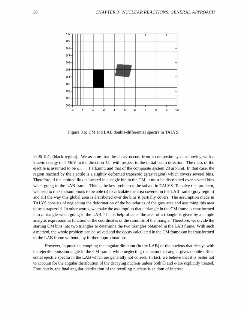
38 CHAPTER 3. NUCLEAR REACTIONS: GENERAL APPROACH
Figure 3.6: CM and LAB double-differential spectra in TALYS.
[0.25, 0.5] (black region). We assume that the decay occurs from a composite system moving with akinetic energy of 1 MeV in the direction 45 with respect to the initial beam direction. The mass of theejectile is assumed to beme = 1 arb.unit, and that of the composite system20 arb.unit. In that case, theregion reached by the ejectile is a slightly deformed trapezoid (gray region) which covers several bins.Therefore, if the emitted flux is located in a single bin in theCM, it must be distributed over several binswhen going to the LAB frame. This is the key problem to be solved in TALYS. To solve this problem,we need to make assumptions to be able (i) to calculate the area covered in the LAB frame (gray region)and (ii) the way this global area is distributed over the binsit partially covers. The assumption made inTALYS consists of neglecting the deformation of the boundaries of the grey area and assuming this areato be a trapezoid. In other words, we make the assumption thata triangle in the CM frame is transformedinto a triangle when going in the LAB. This is helpful since the area of a triangle is given by a simpleanalytic expression as function of the coordinates of the summits of the triangle. Therefore, we divide thestarting CM bins into two triangles to determine the two triangles obtained in the LAB frame. With sucha method, the whole problem can be solved and the decay calculated in the CM frame can be transformedto the LAB frame without any further approximations.
However, in practice, coupling the angular direction (in the LAB) of the nucleus that decays withthe ejectile emission angle in the CM frame, while neglecting the azimuthal angle, gives double differ-ential ejectile spectra in the LAB which are generally not correct. In fact, we believe that it is better notto account for the angular distribution of the decaying nucleus unless bothΘ andφ are explicitly treated.Fortunately, the final angular distribution of the recoiling nucleus is seldom of interest.
3.5. RECOILS 39
3.5.5 Method of average velocity
As mentioned above, we do not loop over the angular distribution of the decaying nucleus. This is equiv-alent to replacing the arrayPrec(Z,N,Ei, Er,Θr) by Prec(Z,N,Ei, Er). Then, we only have to keeptrack of the velocities of the nucleus that is going to decay,i.e. we have to loop over theEr bins to re-construct both the ejectile and residual nuclei spectra. Another approximation that we have implementedas an option (recoilaverage y) consists of using an average velocity before this reconstruction, a methodfirst applied by Chadwick et al. [10, 11]. This approach avoids the loop over theEr bins altogether andreduces the calculation time. However, for high energies, this might be too crude an approximation.
3.5.6 Approximative recoil correction for binary ejectile spectra
Maybe you are not interested in a full recoil calculation, but merely want to correct the outgoing particlespectra for the recoil of the nucleus. In that case you may usethe following method which is implementedin TALYS for just that purpose and which is outlined below.
The assumptions are made that (i) only binary emission takes place, and that (ii ) emission onlyoccurs under 0o. Hence, this approximation is basically expected to be valid for angle-integrated spectraonly. The CM to LAB conversion of the ejectile spectra takes under these conditions the following simpleform:
(3.65) Elabej =
MR
MC∆E +
mejMp
M2C
Ep + 2
√
mejMRMp
M3C
Ep ∆E,
in whichElabej is the LAB ejectile energy. This correction is applied to thefull ejectile spectrum including
the multiple emission contributions. Hence, the approximation is rather crude. It saves, however, a lotof computer time. Since the high-energy tail originates completely from binary emission, this tail iscorrectly converted to the LAB system. Furthermore, the correction is small at low energies where thelargest contributions from multiple emission reside.

40 CHAPTER 3. NUCLEAR REACTIONS: GENERAL APPROACH
Chapter 4Nuclear models
Fig. 4.1 gives an overview of the nuclear models that are included in TALYS. They can generally becategorized into optical, direct, pre-equilibrium, compound and fission models, all driven by a compre-hensive database of nuclear structure and model parameters. We will first describe the optical modeland the various models for direct reactions that are used. Next, we give an outline of the various pre-equilibrium models that are included. Then, we describe compound nucleus models for both binary andmultiple emission, and level densities, which are important ingredients of pre-equilibrium and compoundmodels. Finally, we give an outline of the fission models.
4.1 Optical model
The central assumption underlying the optical model is thatthe complicated interaction between anincident particle and a nucleus can be represented by a complex mean-field potential, which divides thereaction flux into a part covering shape elastic scattering and a part describing all competing non-elasticchannels. Solving the Schrodinger equation numerically with this complex potential yields a wealth ofvaluable information. First, it returns a prediction for the basic observables, namely the elastic angulardistribution and polarisation, the reaction and total cross section and, for low energies, thes, p-wavestrength functions and the potential scattering radiusR′. The essential value of a good optical model isthat it can reliably predict these quantities for energies and nuclides for which no measurements exist.Also, the quality of the not directly observable quantitiesthat are provided by the optical model has anequally important impact on the evaluation of the various reaction channels. Well-known examples aretransmission coefficients, for compound nucleus and multi-step compound decay, and the distorted wavefunctions that are used for direct inelastic reactions and for transitions to the continuum that describestatistical multi-step direct reactions. Also, the reaction cross sections that are calculated with the opticalmodel are crucial for the semi-classical pre-equilibrium models.
All optical model calculations are performed by ECIS-06 [6], which is used as a subroutine inTALYS.
41
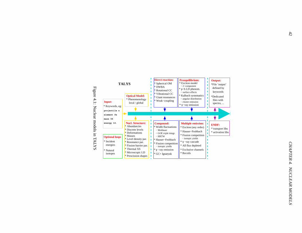
42C
HA
PT
ER
4.N
UC
LEA
RM
OD
ELS
* Exciton model* Spherical OM* DWBA* Rotational CC* Vibrational CC* Giant resonances
* p−h LD phenom.
* γ−ray emission
− angular distribution − cluster emission
* Kalbach systematics
* Width fluctuations − Moldauer − GOE triple integr. − HRTW
* Hauser−Feshbach* Fission competition
− isotopic yields
* −ray emissionγ* GC+ Ignatyuk
* Fission competition* Hauser−Feshbach
* Exciton (any order)
* Exclusive channels
− isotopic yields
* −ray cascadeγ* All flux depleted
* Recoils
* Discrete levels* Abundancies
* Deformations* Masses* Level density par.* Resonance par.* Fission barrier par.* Thermal XS* Microscopic LD* Prescission shapes
*File ’output’
spectra, ... files with*Dedicated
keywords defined by
* transport libs* activation libs
* Weak−coupling
element fe
mass 56
projectile n
energy 14.
* Keywords, eg: local / global* Phenomenology
Input:
Optical Model:
Nucl. Structure:
Direct reaction: Preequilibrium: Output:
ENDF:Multiple emission:Compound:
− surface effects
− 2−component
Optional loops
* Incident
* Natural
energies
isotopes
TALYSFigure
4.1:N
uclearm
odelsin
TALY
S
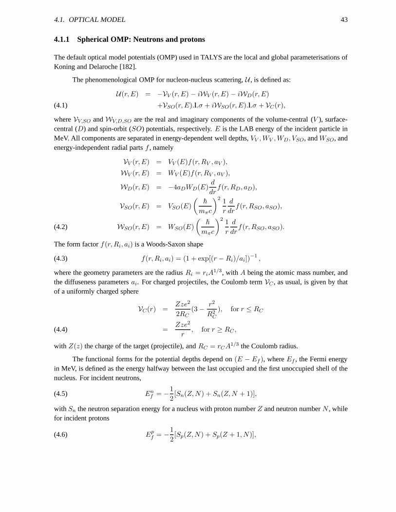
4.1. OPTICAL MODEL 43
4.1.1 Spherical OMP: Neutrons and protons
The default optical model potentials (OMP) used in TALYS arethe local and global parameterisations ofKoning and Delaroche [182].
The phenomenological OMP for nucleon-nucleus scattering,U , is defined as:
U(r,E) = −VV (r,E) − iWV (r,E) − iWD(r,E)
+VSO(r,E).l.σ + iWSO(r,E).l.σ + VC(r),(4.1)
whereVV,SO andWV,D,SO are the real and imaginary components of the volume-central(V ), surface-central (D) and spin-orbit (SO) potentials, respectively.E is the LAB energy of the incident particle inMeV. All components are separated in energy-dependent welldepths,VV ,WV ,WD, VSO, andWSO, andenergy-independent radial partsf , namely
VV (r,E) = VV (E)f(r,RV , aV ),
WV (r,E) = WV (E)f(r,RV , aV ),
WD(r,E) = −4aDWD(E)d
drf(r,RD, aD),
VSO(r,E) = VSO(E)
(
~
mπc
)2 1
r
d
drf(r,RSO, aSO),
WSO(r,E) = WSO(E)
(
~
mπc
)2 1
r
d
drf(r,RSO, aSO).(4.2)
The form factorf(r,Ri, ai) is a Woods-Saxon shape
(4.3) f(r,Ri, ai) = (1 + exp[(r − Ri)/ai])−1 ,
where the geometry parameters are the radiusRi = riA1/3, with A being the atomic mass number, and
the diffuseness parametersai. For charged projectiles, the Coulomb termVC , as usual, is given by thatof a uniformly charged sphere
VC(r) =Zze2
2RC(3 − r2
R2C
), for r ≤ RC
=Zze2
r, for r ≥ RC ,(4.4)
with Z(z) the charge of the target (projectile), andRC = rCA1/3 the Coulomb radius.
The functional forms for the potential depths depend on(E − Ef ), whereEf , the Fermi energyin MeV, is defined as the energy halfway between the last occupied and the first unoccupied shell of thenucleus. For incident neutrons,
(4.5) Enf = −1
2[Sn(Z,N) + Sn(Z,N + 1)],
with Sn the neutron separation energy for a nucleus with proton numberZ and neutron numberN , whilefor incident protons
(4.6) Epf = −1
2[Sp(Z,N) + Sp(Z + 1, N)],
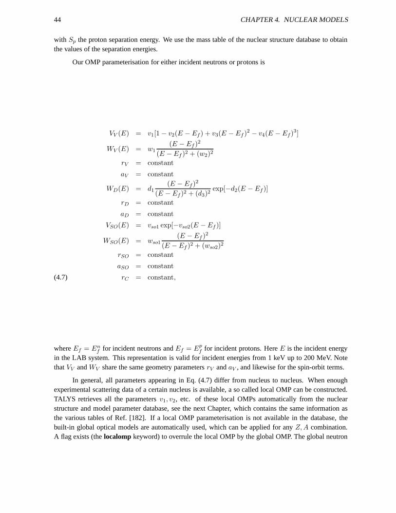
44 CHAPTER 4. NUCLEAR MODELS
with Sp the proton separation energy. We use the mass table of the nuclear structure database to obtainthe values of the separation energies.
Our OMP parameterisation for either incident neutrons or protons is
VV (E) = v1[1 − v2(E − Ef ) + v3(E − Ef )2 − v4(E − Ef )3]
WV (E) = w1(E − Ef )2
(E − Ef )2 + (w2)2
rV = constant
aV = constant
WD(E) = d1(E − Ef )2
(E − Ef )2 + (d3)2exp[−d2(E − Ef )]
rD = constant
aD = constant
VSO(E) = vso1 exp[−vso2(E − Ef )]
WSO(E) = wso1(E − Ef )2
(E − Ef )2 + (wso2)2
rSO = constant
aSO = constant
rC = constant,(4.7)
whereEf = Enf for incident neutrons andEf = Ep
f for incident protons. HereE is the incident energyin the LAB system. This representation is valid for incidentenergies from 1 keV up to 200 MeV. NotethatVV andWV share the same geometry parametersrV andaV , and likewise for the spin-orbit terms.
In general, all parameters appearing in Eq. (4.7) differ from nucleus to nucleus. When enoughexperimental scattering data of a certain nucleus is available, a so called local OMP can be constructed.TALYS retrieves all the parametersv1, v2, etc. of these local OMPs automatically from the nuclearstructure and model parameter database, see the next Chapter, which contains the same information asthe various tables of Ref. [182]. If a local OMP parameterisation is not available in the database, thebuilt-in global optical models are automatically used, which can be applied for anyZ,A combination.A flag exists (thelocalomp keyword) to overrule the local OMP by the global OMP. The global neutron
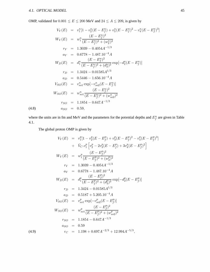
4.1. OPTICAL MODEL 45
OMP, validated for0.001 ≤ E ≤ 200 MeV and24 ≤ A ≤ 209, is given by
VV (E) = vn1 [1 − vn
2 (E − Enf ) + vn
3 (E − Enf )2 − vn
4 (E − Enf )3]
WV (E) = wn1
(E − Enf )2
(E − Enf )2 + (wn
2 )2
rV = 1.3039 − 0.4054A−1/3
aV = 0.6778 − 1.487.10−4A
WD(E) = dn1
(E − Enf )2
(E − Enf )2 + (dn
3 )2exp[−dn
2 (E − Enf )]
rD = 1.3424 − 0.01585A1/3
aD = 0.5446 − 1.656.10−4A
VSO(E) = vnso1 exp[−vn
so2(E − Enf )]
WSO(E) = wnso1
(E − Enf )2
(E − Enf )2 + (wn
so2)2
rSO = 1.1854 − 0.647A−1/3
aSO = 0.59,(4.8)
where the units are in fm and MeV and the parameters for the potential depths andEnf are given in Table
4.1.
The global proton OMP is given by
VV (E) = vp1 [1 − vp
2(E − Epf ) + vp
3(E − Epf )2 − vp
4(E − Epf )3]
+ VC .vp1
[
vp2 − 2vp
3(E − Epf ) + 3vp
4(E − Epf )2]
WV (E) = wp1
(E − Epf )2
(E − Epf )2 + (wp
2)2
rV = 1.3039 − 0.4054A−1/3
aV = 0.6778 − 1.487.10−4A
WD(E) = dp1
(E − Epf )2
(E − Epf )2 + (dp
3)2
exp[−dp2(E − Ep
f )]
rD = 1.3424 − 0.01585A1/3
aD = 0.5187 + 5.205.10−4A
VSO(E) = vpso1 exp[−vp
so2(E − Epf )]
WSO(E) = wpso1
(E − Epf )2
(E − Epf )2 + (wp
so2)2
rSO = 1.1854 − 0.647A−1/3
aSO = 0.59
rC = 1.198 + 0.697A−2/3 + 12.994A−5/3,(4.9)
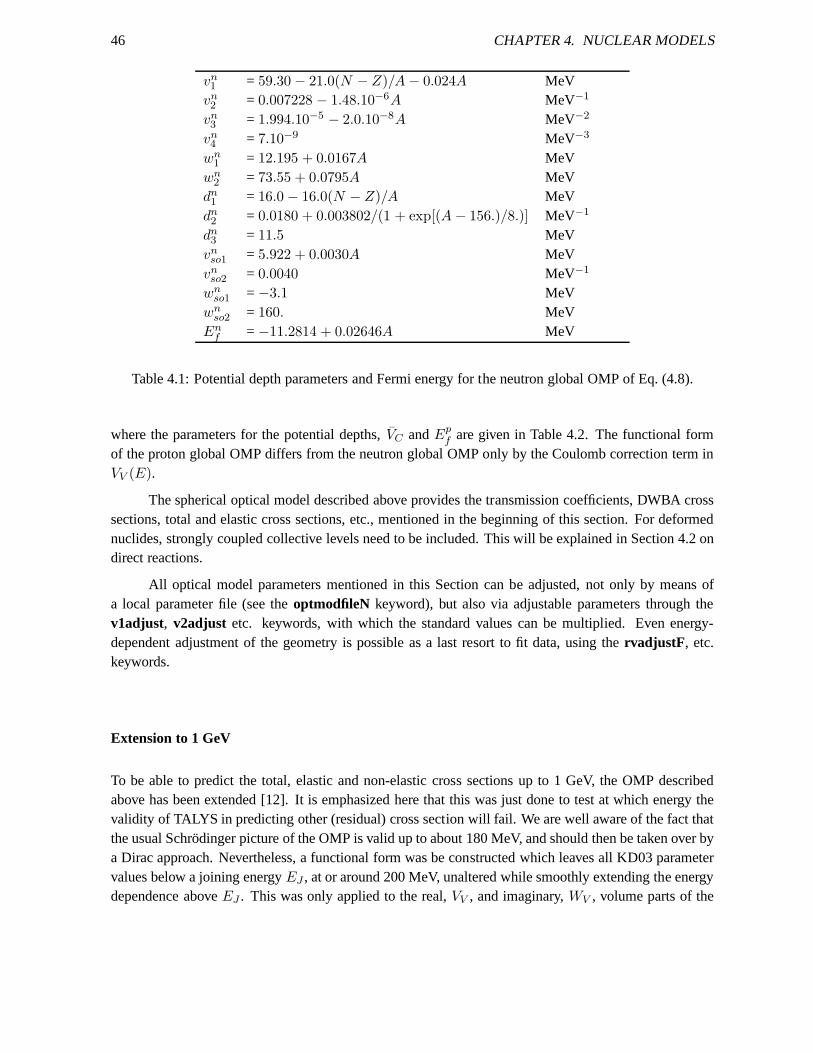
46 CHAPTER 4. NUCLEAR MODELS
vn1 = 59.30 − 21.0(N − Z)/A − 0.024A MeV
vn2 = 0.007228 − 1.48.10−6A MeV−1
vn3 = 1.994.10−5 − 2.0.10−8A MeV−2
vn4 = 7.10−9 MeV−3
wn1 = 12.195 + 0.0167A MeV
wn2 = 73.55 + 0.0795A MeV
dn1 = 16.0 − 16.0(N − Z)/A MeV
dn2 = 0.0180 + 0.003802/(1 + exp[(A − 156.)/8.)] MeV−1
dn3 = 11.5 MeV
vnso1 = 5.922 + 0.0030A MeV
vnso2 = 0.0040 MeV−1
wnso1 = −3.1 MeV
wnso2 = 160. MeV
Enf = −11.2814 + 0.02646A MeV
Table 4.1: Potential depth parameters and Fermi energy for the neutron global OMP of Eq. (4.8).
where the parameters for the potential depths,VC andEpf are given in Table 4.2. The functional form
of the proton global OMP differs from the neutron global OMP only by the Coulomb correction term inVV (E).
The spherical optical model described above provides the transmission coefficients, DWBA crosssections, total and elastic cross sections, etc., mentioned in the beginning of this section. For deformednuclides, strongly coupled collective levels need to be included. This will be explained in Section 4.2 ondirect reactions.
All optical model parameters mentioned in this Section can be adjusted, not only by means ofa local parameter file (see theoptmodfileN keyword), but also via adjustable parameters through thev1adjust, v2adjust etc. keywords, with which the standard values can be multiplied. Even energy-dependent adjustment of the geometry is possible as a last resort to fit data, using thervadjustF , etc.keywords.
Extension to 1 GeV
To be able to predict the total, elastic and non-elastic cross sections up to 1 GeV, the OMP describedabove has been extended [12]. It is emphasized here that thiswas just done to test at which energy thevalidity of TALYS in predicting other (residual) cross section will fail. We are well aware of the fact thatthe usual Schrodinger picture of the OMP is valid up to about180 MeV, and should then be taken over bya Dirac approach. Nevertheless, a functional form was be constructed which leaves all KD03 parametervalues below a joining energyEJ , at or around 200 MeV, unaltered while smoothly extending the energydependence aboveEJ . This was only applied to the real,VV , and imaginary,WV , volume parts of the
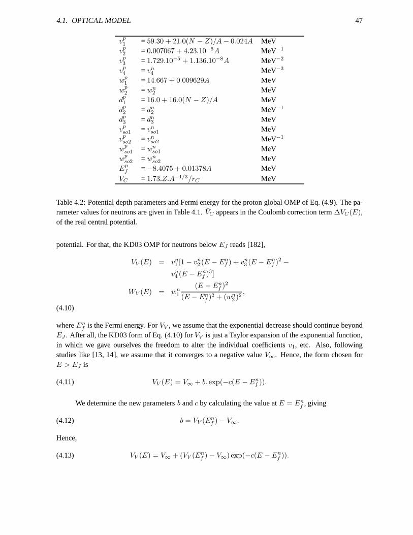
4.1. OPTICAL MODEL 47
vp1 = 59.30 + 21.0(N − Z)/A − 0.024A MeV
vp2 = 0.007067 + 4.23.10−6A MeV−1
vp3 = 1.729.10−5 + 1.136.10−8A MeV−2
vp4 = vn
4 MeV−3
wp1 = 14.667 + 0.009629A MeV
wp2 = wn
2 MeVdp1 = 16.0 + 16.0(N − Z)/A MeV
dp2 = dn
2 MeV−1
dp3 = dn
3 MeVvpso1 = vn
so1 MeVvpso2 = vn
so2 MeV−1
wpso1 = wn
so1 MeVwp
so2 = wnso2 MeV
Epf = −8.4075 + 0.01378A MeV
VC = 1.73.Z.A−1/3/rC MeV
Table 4.2: Potential depth parameters and Fermi energy for the proton global OMP of Eq. (4.9). The pa-rameter values for neutrons are given in Table 4.1.VC appears in the Coulomb correction term∆VC(E),of the real central potential.
potential. For that, the KD03 OMP for neutrons belowEJ reads [182],
VV (E) = vn1 [1 − vn
2 (E − Enf ) + vn
3 (E − Enf )2 −
vn4 (E − En
f )3]
WV (E) = wn1
(E − Enf )2
(E − Enf )2 + (wn
2 )2,
(4.10)
whereEnf is the Fermi energy. ForVV , we assume that the exponential decrease should continue beyond
EJ . After all, the KD03 form of Eq. (4.10) forVV is just a Taylor expansion of the exponential function,in which we gave ourselves the freedom to alter the individual coefficientsv1, etc. Also, followingstudies like [13, 14], we assume that it converges to a negative valueV∞. Hence, the form chosen forE > EJ is
(4.11) VV (E) = V∞ + b. exp(−c(E − Enf )).
We determine the new parametersb andc by calculating the value atE = Enf , giving
(4.12) b = VV (Enf ) − V∞.
Hence,
(4.13) VV (E) = V∞ + (VV (Enf ) − V∞) exp(−c(E − En
f )).
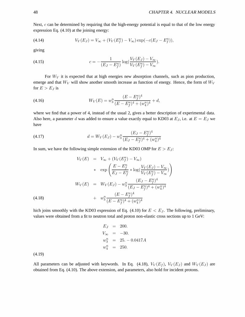
48 CHAPTER 4. NUCLEAR MODELS
Next, c can be determined by requiring that the high-energy potential is equal to that of the low energyexpression Eq. (4.10) at the joining energy:
(4.14) VV (EJ ) = V∞ + (VV (Enf ) − V∞) exp(−c(EJ − En
f )),
giving
(4.15) c = − 1
(EJ − Enf )
log(VV (EJ ) − V∞
VV (Enf ) − V∞
).
For WV it is expected that at high energies new absorption channels, such as pion production,emerge and thatWV will show another smooth increase as function of energy. Hence, the form ofWV
for E > EJ is
(4.16) WV (E) = wn3
(E − Enf )4
(E − Enf )4 + (wn
4 )4+ d,
where we find that a power of 4, instead of the usual 2, gives a better description of experimental data.Also here, a parameterd was added to ensure a value exactly equal to KD03 atEJ , i.e. atE = EJ wehave
(4.17) d = WV (EJ) − wn3
(EJ − Enf )4
(EJ − Enf )4 + (wn
4 )4
In sum, we have the following simple extension of the KD03 OMPfor E > EJ :
VV (E) = V∞ + (VV (Enf ) − V∞)
∗ exp
(
E − Enf
EJ − Enf
∗ log(VV (EJ) − V∞
VV (Enf ) − V∞
)
)
WV (E) = WV (EJ ) − wn3
(EJ − Enf )4
(EJ − Enf )4 + (wn
4 )4
+ wn3
(E − Enf )4
(E − Enf )4 + (wn
4 )4(4.18)
hich joins smoothly with the KD03 expression of Eq. (4.10) for E < EJ . The following, preliminary,values were obtained from a fit to neutron total and proton non-elastic cross sections up to 1 GeV:
EJ = 200.
V∞ = −30.
wn3 = 25. − 0.0417A
wn4 = 250.
(4.19)
All parameters can be adjusted with keywords. In Eq. (4.18),VV (Ef ), VV (EJ ) and WV (EJ ) areobtained from Eq. (4.10). The above extension, and parameters, also hold for incident protons.
4.1. OPTICAL MODEL 49
4.1.2 Spherical dispersive OMP: Neutrons
The theory of the nuclear optical model can be reformulated in terms of dispersion relations that connectthe real and imaginary parts of the optical potential, and wehave added an option in TALYS to take theminto account. These dispersion relations are a natural result of the causality principle that a scatteredwave cannot be emitted before the arrival of the incident wave. The dispersion component stems directlyfrom the absorptive part of the potential,
(4.20) ∆V(r,E) =Pπ
∫ ∞
−∞
W(r,E′)
E′ − EdE′,
whereP denotes the principal value. The total real central potential can be written as the sum of aHartree-Fock termVHF (r,E) and the the total dispersion potential∆V(r,E)
(4.21) V(r,E) = VHF (r,E) + ∆V(r,E).
SinceW(r,E) has a volume and a surface component, the dispersive addition is,
∆V(r,E) = ∆VV (r,E) + ∆VD(r,E)
= ∆VV (E)f(r,RV , aV ) − 4aD∆VD(E)d
drf(r,RD, aD)(4.22)
where the volume dispersion term is given by
(4.23) ∆VV (E) =Pπ
∫ ∞
−∞
WV (E′)
E′ − EdE′,
and the surface dispersion term is given by
(4.24) ∆VD(E) =Pπ
∫ ∞
−∞
WD(E′)
E′ − EdE′.
Hence, the real volume well depth of Eq. (4.2) becomes
(4.25) VV (E) = VHF (E) + ∆VV (E),
and the real surface well depth is
(4.26) VD(E) = ∆VD(E).
In general, Eqs. (4.23)-(4.24) cannot be solved analytically. However, under certain plausible conditions,analytical solutions exist. Under the assumption that the imaginary potential is symmetric with respectto the Fermi energyEF ,
(4.27) W (EF − E) = W (EF + E),
whereW denotes either the volume or surface term, we can rewrite thedispersion relation as,
(4.28) ∆V (E) =2
π(E − EF )P
∫ ∞
EF
W (E′)
(E′ − EF )2 − (E − EF )2dE′,
50 CHAPTER 4. NUCLEAR MODELS
from which it easily follows that∆V (E) is skew-symmetric aroundEF ,
(4.29) ∆V (E + EF ) = −∆V (E − EF ),
and hence∆V (EF ) = 0. This can then be used to rewrite Eq. (4.20) as
∆V (E) = ∆V (E) − ∆V (EF )
=Pπ
∫ ∞
−∞W (E′)(
1
E′ − E− 1
E′ − EF)dE′
=E − EF
π
∫ ∞
−∞
W (E′)
(E′ − E)(E′ − EF )dE′.(4.30)
For the Hartree-Fock term we adopt the usual form forVV (E) given in Eq. (4.7). The dispersion integralsfor the functions for absorption can be calculated analytically and are included as options in ECIS-06.This makes the use of a dispersive optical model parameterization completely equivalent to that of anon-dispersive OMP: the dispersive contributions are calculated automatically once the OMP parametersare given. Upon comparison with a nondispersive parameterization, we find thatv1 is rather different (asexpected) and thatrV , aV , v2, v3, w1 andw2 are slightly different. We have included dispersive sphericalneutron OMP parameterization for about 70 nuclides (unpublished). They can be used with the keyworddispersion y.
4.1.3 Spherical OMP: Complex particles
For deuterons, tritons, Helium-3 and alpha particles, we use a simplification of the folding approach ofWatanabe [15], see Ref. [16]. We take the nucleon OMPs described in the previous section, either localor global, as the basis for these complex particle potentials.
Deuterons
For deuterons, the real central potential depth at incidentenergyE is
(4.31) V deuteronV (E) = V neutron
V (E/2) + V protonV (E/2),
and similarly forWV andWD. For the spin-orbit potential depth we have
(4.32) V deuteronSO (E) = (V neutron
SO (E) + V protonSO (E))/2,
and similarly forWSO. For the radius and diffuseness parameter of the real central potential we have
rdeuteronV = (rneutron
V + rprotonV )/2,
adeuteronV = (aneutron
V + aprotonV )/2,(4.33)
and similarly for the geometry parameters of the other potentials.
Note that several of these formulae are somewhat more general than necessary, since the nucleonpotentials mostly have geometry parameters, and also potential depths such asVSO, which are equal for
4.1. OPTICAL MODEL 51
neutrons and protons (aD is an exception). The general formulae above have been implemented to alsoaccount for other potentials, if necessary.
We are well aware of the fact that others have constructed specific potentials for deuterons thatmay outperform the Watanabe-type potential described here. Therefore, we have also added the deuteronpotentials of Daehnick et al. [17], Bojowald et al.[18], Hanet al.[19], and Haixia An et al.[20] as options.
Tritons
For tritons, the real central potential depth at incident energyE is
(4.34) V tritonV (E) = 2V neutron
V (E/3) + V protonV (E/3),
and similarly forWV andWD. For the spin-orbit potential depth we have
(4.35) V tritonSO (E) = (V neutron
SO (E) + V protonSO (E))/6,
and similarly forWSO. For the radius and diffuseness parameter of the real central potential we have
rtritonV = (2rneutron
V + rprotonV )/3,
atritonV = (2aneutron
V + aprotonV )/3,(4.36)
and similarly for the geometry parameters of the other potentials.
Helium-3
For Helium-3, the real central potential depth at incident energyE is
(4.37) V Helium−3V (E) = V neutron
V (E/3) + 2V protonV (E/3),
and similarly forWV andWD. For the spin-orbit potential depth we have
(4.38) V Helium−3SO (E) = (V neutron
SO (E) + V protonSO (E))/6,
and similarly forWSO. For the radius and diffuseness parameter of the real central potential we have
rHelium−3V = (rneutron
V + 2rprotonV )/3,
aHelium−3V = (aneutron
V + 2aprotonV )/3,(4.39)
and similarly for the geometry parameters of the other potentials.
Alpha particles
For alpha’s, the real central potential depth at incident energyE is
(4.40) V alphasV (E) = 2V neutron
V (E/4) + 2V protonV (E/4),
52 CHAPTER 4. NUCLEAR MODELS
and similarly forWV andWD. For the spin-orbit potential depth we have
(4.41) V alphasSO (E) = W alphas
SO (E) = 0.
For the radius and diffuseness parameter of the real centralpotential we have
ralphasV = (rneutron
V + rprotonV )/2,
aalphasV = (aneutron
V + aprotonV )/2,(4.42)
and similarly for the geometry parameters of the other potentials.
As extra options the alpha potentials by McFadden and Satchler [21] and Demetriou et al [22] areavailable.
All optical model parameters for complex particles can be altered via adjustable parameters throughthe v1adjust, rvadjust etc. keywords, with which the standard values can be multiplied. Also localenergy-dependent adjustment of the geometry is possible asa last resort to fit data, using thervadjustF ,etc. keywords.
4.1.4 Semi-microscopic optical model (JLM)
Besides the phenomenological OMP, it is also possible to perform TALYS calculations with the semimi-croscopic nucleon-nucleus spherical optical model potential as described in [28]. We have implementedEric Bauge’s MOM code [163] as a subroutine to perform so called Jeukenne-Lejeune-Mahaux (JLM)OMP calculations. The optical model potential of [28] and its extension to deformed and unstable nucleihas been widely tested [28, 29, 30, 31, 32] and produces predictions from A=30 to 240 and for energiesranging from 10 keV up to 200 MeV. MOM stands for “Modele Optique Microscopique” in French,or “Microscopic Optical Model” in English. In this version of TALYS, only spherical JLM OMP’s areincluded.
The MOM module reads the radial matter densities from the nuclear structure database and per-forms the folding of the Nuclear Matter (NM) optical model potential described in [28] with the densitiesto obtain a local OMP. This is then put in the ECIS-06 routine to compute observables by solving theSchrodinger equation for the interaction of the projectile with the aforementioned OMP. The OMP’sare calculated by folding the target radial matter density with an OMP in nuclear matter based on theBruckner-Hartree-Fock work of Jeukenne, Lejeune and Mahaux [33, 34, 35, 36]. This NM OMP wasthen phenomenologically altered in [28, 37] in order to improve the agreement of predicted finite nucleiobservables with a large set of experimental data. These improvements consist in unifying the low andhigh energy parameterizations of the NM interaction in [37], and in studying the energy variations of thepotential depth normalization factors in [28]. These factors now include non-negligible normalizations ofisovector components [28] that are needed in order to account simultaneously for (p,p) and (n,n) elasticscattering as well as (p,n)IAS quasi-elastic scattering. The final NM potential for a givennuclear matterdensityρ = ρn − ρp and asymmetryα = (ρn + ρp)/ρ reads
4.1. OPTICAL MODEL 53
UNM (E)ρ,α = λV (E)[
V0(E) ± λV 1(E)αV1(E)]
+ iλW (E)[
W0(E) ± λW1(E)αW1(E)]
,(4.43)
with E the incident nucleon energy,E = E−Vc (whereVc is the Coulomb field),V0, V1, W0, andW1 the real isoscalar, real isovector, imaginary isoscalar, and imaginary isovector NM OMP componentsrespectively, andλV , λV 1, λW , andλW1 the real (isoscalar+isovector), real isovector, imaginary, andimaginary isovector normalization factors respectively.The values ofλV , λV 1, λW , andλW1 given in[28] read
(4.44) λV (E) = 0.951 + 0.0008 ln(1000E) + 0.00018 [ln(1000E)]2
λW (E) =
[
1.24 −[
1 + e(E−4.52.9
)]−1]
[
1 + 0.06 e−(E−14
3.7 )2]
×[
1 − 0.09 e−(E−80
78)2]
[
1 +
(
E − 80
400
)
Θ(E − 80)
]
(4.45)
(4.46) λV 1(E) = 1.5 − 0.65[
1 + eE−1.3
3
]−1
λW1(E) =
[
1.1 + 0.44
[
1 +(
eE−40
50.9
)4]−1]
×[
1 − 0.065 e−(E−40
13)2] [
1 − 0.083 e−(E−200
80)2]
.(4.47)
with the energyE expressed in MeV. As stated in [28], in the 20 to 50 MeV range, the uncertaintiesrelated toλV , λV 1, λW , andλW1 are estimated to be 1.5%, 10%, 10%, and 10%, respectively. Outsidethis energy range, uncertainties are estimated to be 1.5 times larger.
In order to apply the NM OMP to finite nuclei an approximation had to be performed. This isthe Local Density Approximation (LDA) where the local valueof the finite nucleus OMP is taken tobe the NM OMP value for the local finite nucleus density:UFN (r) = UNM (ρ(r)). Since this LDAproduces potentials with too small rms radii, the improved LDA, which broadens the OMP with a Gaus-sian form factor (4.48), is introduced. In [37, 28] different prescriptions for the improved Local Densityapproximation are compared and LDA range parameters are optimized.
(4.48) UFN(r,E) = (t√
π)−3
∫
UNM (ρ(r′), E)
ρ(r′)exp(−|~r − ~r′|2/t2r)ρ(r′)d~r′,
54 CHAPTER 4. NUCLEAR MODELS
with t the range of the Gaussian form factor. Thetr = 1.25 fm and ti = 1.35 fm values werefound [28] to be global optimal values for the real and imaginary ranges, respectively.
Finally, since no spin-orbit (SO) potential exists betweena nucleon and NM, the Scheerbaum [38]prescription was selected in [37], coupled with the phenomenological complex potential depthsλvso , andλwso . The SO potential reads
(4.49) U son(p)(r) = (λvso(E) + iλvso(E))
1
r
d
dr
(
2
3ρp(n) +
1
3ρn(p)
)
,
with
(4.50) λvso = 130 exp(−0.013E) + 40
and
(4.51) λwso = −0.2 (E − 20).
All JLM OMP parameters can be altered via adjustable parameters through thelvadjust, lwadjust etc.keywords, with which the standard values can be multiplied.
4.1.5 Systematics for non-elastic cross sections
Since the reaction cross sections for complex particles as predicted by the OMP have not been tested andrely on a relatively simple folding model, we added a possibility to estimate the non-elastic cross sectionsfrom empirical expressions. The adoptedtripathi.f subroutine that provides this does not coincide withthe published expression as given by Tripathi et al. [39], but checking our results with the publishedfigures of Ref. [39] made us decide to adopt this empirical model as an option. We sometimes use itfor deuterons up to alpha-particles. A high-quality OMP forcomplex particles would make this optionredundant.
4.2 Direct reactions
Various models for direct reactions are included in the program: DWBA for (near-)spherical nuclides,coupled-channels for deformed nuclides, the weak-coupling model for odd nuclei, and also a giant res-onance contribution in the continuum. In all cases, TALYS drives the ECIS-06 code to perform thecalculations. The results are presented as discrete state cross sections and angular distributions, or ascontributions to the continuum.
4.2.1 Deformed nuclei: Coupled-channels
The formalism outlined in the previous section works, theoretically, for nuclides which are sphericaland, in practice, for nuclides which are not too strongly deformed. In general, however, the more general
4.2. DIRECT REACTIONS 55
coupled-channels method should be invoked to describe simultaneously the elastic scattering channeland the low-lying states which are, due to their collective nature, strongly excited in inelastic scattering.These collective excitations can be described as the resultof static or dynamic deformations, which causethe homogeneous neutron-proton fluid to rotate or vibrate. The associated deformation parameters canbe predicted from a (semi-)microscopic model or can be derived from an analysis of the experimentalangular distributions.
The coupled-channels formalism for scattering and reaction studies is well known and will notbe described in this manual. For a detailed presentation, werefer to Ref. [40]. We will only state themain aspects here to put the formalism into practice. Refs. [41] and [42] have been used as guidance. Ingeneral various different channels, usually the ground state and several inelastic states, are included ina coupling scheme while the associated coupled equations are solved. In ECIS-06, this is done in a socalled sequential iterative approach [6]. Besides Ref. [6], Ref. [43] is also recommended for more insightin the use of the ECIS code.
Various collective models for deformed nuclei exist. Note that the spherical optical model ofEq. (4.2) is described in terms of the nuclear radiusRi = riA
1/3. For deformed nuclei, this expressionis generalized to include collective motions. Various models have been implemented in ECIS-06, whichenables us to cover many nuclides of interest. We will describe the ones that can be invoked by TALYS.The collective models are automatically applied upon reading the deformation parameter database, seeSection 5.5.
Symmetric rotational model
In the symmetric rotational model, the radii of the different terms of the OMP are expressed as
(4.52) Ri = riA1/3
1 +∑
λ=2,4,....
βλY 0λ (Ω)
,
where theβλ’s are permanent, static deformation parameters, and theY functions are spherical har-monics. The quadrupole deformationβ2 plays a leading role in the interaction process. Higher orderdeformationsβλ (with λ = 4, 6, ...) are systematically smaller in magnitude thanβ2. The inclusion ofβ4 andβ6 deformations in coupled-channels calculations produces changes in the predicted observables,but in general, onlyβ2 andβ4 are important in describing inelastic scattering to the first few levels in arotational band. For even-even nuclides like184W and232Th, the symmetric rotational model providesa good description of the lowest0+, 2+, 4+ (and often6+, 8+, etc.) rotational band. The nuclear modeland parameter database of TALYS specifies whether a rotational model can be used for a particular nu-cleus, together with the included levels and deformation parameters. Either a deformation parameterβλ
or a deformation lengthδλ = βλriA1/3 may be given. The latter one is generally recommended since
it has more physical meaning thanβλ and should not depend on incident energy (whileri may, in someoptical models, depend on energy). We takeδλ equal for the three OMP componentsVV , WV andWD
and take the spin-orbit potential undeformed. The same holds for the vibrational and other collectivemodels.
By default, TALYS uses the global optical model by Soukhovitskii et al. [44] for actinides. For
56 CHAPTER 4. NUCLEAR MODELS
rotational non-fissile nuclides, if no specific potential isspecified through one of the various input meth-ods, we take our local or global spherical potential and subtract 15% from the imaginary surface potentialparameterd1, if rotational or vibrational levels are included in the coupling scheme.
Harmonic vibrational model
A vibrational nucleus possesses a spherically symmetric ground state. Its excited states undergo shapeoscillations about the spherical equilibrium model. In theharmonic vibrational model, the radii of thedifferent terms of the OMP are expressed as
(4.53) Ri = riA1/3
1 +∑
λµ
αλµY µλ (Ω)
,
where theαλµ operators can be related to the coupling strengthsβλ, describing the vibration amplitudewith multipolarity λ. Expanding the OMP to first or second order with this radius gives the OMP ex-pressions for the excitation of one-phonon (first order vibrational model) and two-phonon (second ordervibrational model) states [6]. For vibrational nuclei, theminimum number of states to couple is two.For even-even nuclei, we generally use the(0+, 2+) coupling, where the2+ level is a one-quadrupolephonon excitation. The level scheme of a vibrational nucleus (e.g.110Pd) often consists of a one-phononstate (2+) followed by a(0+, 2+, 4+) triplet of two-phonon states. When this occurs, all levels are in-cluded in the coupling scheme with the associated deformation lengthδ2 (or deformation parameterβ2).If the 3− and5− states are strongly collective excitations, that is whenβ3 andβ5 are larger than 0.1,these levels may also be included in the coupling scheme. An example is120Sn [45], where the low lying(0+, 2+, 3−, 4+, 5−) states can all be included as one-phonon states in a single coupling scheme.
Again, if no specific potential is specified through one of thevarious input methods, we take ourlocal or global spherical potential and subtract 15% from the imaginary surface potential parameterd1.
Vibration-rotational model
For certain nuclides, the level scheme consists not only of one or more rotational bands, but also of oneor more vibrational bands that can be included in the coupling scheme. An example is238U , where manyvibrational bands can be coupled. In Chapter 5 on nuclear model parameters, it is explained how suchcalculations are automatically performed by TALYS. Depending on the number of levels included, thecalculations can be time-consuming.
Asymmetric rotational model
In the asymmetric rotational model, in addition to the spheroidal equilibrium deformation, the nucleuscan oscillate such that ellipsoidal shapes are produced. Inthis model the nucleus has rotational bandsbuilt on the statically deformed ground state and on theγ-vibrational state. The radius is now angular
4.2. DIRECT REACTIONS 57
dependent,
(4.54) Ri(Θ) = riA1/3
[
1 + β2 cos γY 02 (Ω) +
√
1
2β2 sin γ(Y 2
2 (Ω) + Y −22 (Ω)) + β4Y
04 (Ω)
]
,
where we restrict ourselves to a few terms. The deformation parametersβ2, β4 andγ need to be specified.24Mg is an example of a nucleus that can be analyzed with the asymmetric rotational model. Mixingbetween bands is not yet automated as an option in TALYS.
4.2.2 Distorted Wave Born Approximation
The Distorted Wave Born Approximation (DWBA) is only valid for small deformations. Until the adventof the more general coupled-channels formalism, it was the commonly used method to describe inelasticscattering, for both weakly and strongly coupled levels. Nowadays, we see DWBA as a first ordervibrational model for small deformation, with only a singleiteration to be performed for the coupled-channels solution. (See, however Satchler [46] for the exact difference between this so called distortedwave method and DWBA). The interaction between the projectile and the target nucleus is modeled bythe derivative of the OMP for elastic scattering times a strength parameter. The latter, the deformationparameterβλ, is then often used to vary the overall magnitude of the crosssection (which is proportionalto β2
λ).
In TALYS, we use DWBA
(a) if a deformed OMP is not available. This applies for the spherical OMPs mentioned in the pre-vious Section, which are all based on elastic scattering observables only. Hence, if we have notconstructed a coupled-channels potential, TALYS will automatically use (tabulated or systemati-cal) deformation parameters for DWBA calculations.
(b) if a deformed OMP is used for the first excited states only.For the levels that do not belong tothat basic coupling scheme, e.g. for the many states at somewhat higher excitation energy, we useDWBA with (very) small deformation parameters.
4.2.3 Odd nuclei: Weak coupling
Direct inelastic scattering off odd-A nuclei can be described by the weak-coupling model [47], whichassumes that a valence particle or hole interacts only weakly with a collective core excitation. Hence themodel implies that the nucleon inelastic scattering by the odd-A nucleus is very similar to that by theeven core alone, i.e. the angular distributions have a similar shape. LetL be the spin of the even corestate, andJ0 andJ the spin of the ground and excited state, respectively, of the odd-A nucleus, resultingfrom the angular momentum coupling. Then, the spinsJ of the multiplet states in the odd-A nucleusrange from|L − J0| to (L + J0). If the strength of the inelastic scattering is characterized by the squareof the deformation parametersβ2
L,J , then the sum of allβ2L,J or σ(E) for the transitions in the odd-A
nucleus should be equal to the valueβ2L or σ(E) for the single transition in the even core nucleus:
(4.55)∑
J
β2L,J = β2
L,∑
J
σJ0→J = σ0→L,
58 CHAPTER 4. NUCLEAR MODELS
where the symbol0 → L indicates a transition between the ground state to the excited state with spinLin the even core nucleus. The deformation parametersβ2
L,J are now given by
(4.56) β2L,J =
2J + 1
(2J0 + 1)(2L + 1)β2
L.
In practice, the DWBA cross sections are calculated for the real mass of the target nucleus and at the exactexcitation energies of the odd-A states, but for the even-core spinL and with deformation parametersβL,J .
We stress that our weak-coupling model is not full-proof. First of all, there are always two choicesfor the even-even core. The default used in TALYS (by means ofthe keywordcore -1) is to use theeven-even core obtained by subtracting a nucleon, but the other choice (core 1), to obtain the even-evencore by adding a nucleon, may sometimes be more appropriate.The next uncertainty is the choice oflevels in the odd-A core. We select the levels that are closest to the excitation energy of the even-spinstate of the even-even core. Again, this may not always be themost appropriate choice. A future optionis to designate these levels manually.
4.2.4 Giant resonances
The high-energy part of the continuum spectra are generallydescribed by pre-equilibrium models. Thesemodels are essentially of a single-particle nature. Upon inspection of continuum spectra, some structurein the high-energy tail is observed that can not be accountedfor by the smooth background of the single-particle pre-equilibrium model. For example, many 14 MeV inelastic neutron spectra show a little humpat excitation energies around 6-10 MeV. This structure is due to collective excitations of the nucleus thatare known as giant resonances [48, 49]. We use a macroscopic,phenomenological model to describegiant resonances in the inelastic channel. For each multipolarity, an energy weighted sum rule (EWSR)Sℓ applies,
(4.57) Sℓ =∑
i
Eℓ,iβ2ℓ,i = 57.5A−5/3l(2l + 1) MeV,
whereEℓ,i is the excitation energy of thei-th state with multipolarityℓ. The summation includes allthe low-lying collective states, for eachℓ, that have already been included in the coupled-channels orDWBA formalism. The EWSR thus determines the remaining collective strength that is spread over thecontinuum. Our treatment is phenomenological in the sense that we perform a DWBA calculation withECIS-06 for each giant resonance state and spread the cross section over the continuum with a Gaussiandistribution. The central excitation energy for these states and the spreading width is different for eachmultipolarity and has been empirically determined. For thegiant monopole resonance (GMR) EWSRwe have
(4.58) S0 = 23A−5/3 MeV,
with excitation energy and width
(4.59) E0,GMR = 18.7 − 0.025A MeV, ΓGMR = 3 MeV.
4.3. GAMMA-RAY TRANSMISSION COEFFICIENTS 59
The EWSR for the giant quadrupole resonance (GQR) is
(4.60) S2 = 575A−5/3MeV,
with
(4.61) E0,GQR = 65A−1/3MeV, ΓGQR = 85A−2/3MeV.
The EWSR for the giant octupole resonance is
(4.62) S3 = 1208A−5/3MeV,
which has a low-energy (LEOR) and a high-energy (HEOR) component. Following Kalbach [49], weassume
(4.63) S3,LEOR = 0.3S3, S3,HEOR = 0.7S3,
with excitation energy and width
(4.64) E0,LEOR = 31A−1/3MeV, ΓLEOR = 5MeV,
and
(4.65) E0,HEOR = 115A−1/3MeV, ΓHEOR = 9.3 − A/48MeV,
respectively. We also take as width for the actual Gaussian distributionΓGauss = 0.42Γℓ.
The contribution from giant resonances is automatically included in the total inelastic cross sec-tion. The effect is most noticeable in the single- and double-differential energy spectra.
4.3 Gamma-ray transmission coefficients
Gamma-ray transmission coefficients are important for the description of the gamma emission channelin nuclear reactions. This is an almost universal channel since gamma rays, in general, may accompanyemission of any other emitted particle. Like the particle transmission coefficients that emerge from theoptical model, gamma-ray transmission coefficients enter the Hauser-Feshbach model for the calculationof the competition of photons with other particles.
The gamma-ray transmission coefficient for multipolarityℓ of type X (whereX = M or E) isgiven by
(4.66) TXℓ(Eγ) = 2πfXℓ(Eγ)E2ℓ+1γ ,
whereEγ denotes the gamma energy andfXℓ(Eγ) is the energy-dependent gamma-ray strength function.
60 CHAPTER 4. NUCLEAR MODELS
4.3.1 Gamma-ray strength functions
We have included 4 models for the gamma-ray strength function. The first is the so-called Brink-Axeloption [50], in which a standard Lorentzian form describes the giant dipole resonance shape, i.e.
(4.67) fXℓ(Eγ) = KXℓσXℓEγΓ2
Xℓ
(E2γ − E2
Xℓ)2 + E2
γΓ2Xℓ
,
whereσXℓ, EXℓ andΓXℓ are the strength, energy and width of the giant resonance, respectively, and
(4.68) KXℓ =1
(2ℓ + 1)π2~2c2.
At present, we use the Brink-Axel option for all transition types other thanE1. ForE1 radiation,the default option used in TALYS is the generalized Lorentzian form of Kopecky and Uhl [51],
(4.69) fE1(Eγ , T ) = KE1
[
EγΓE1(Eγ)
(E2γ − E2
E1)2 + E2
γ ΓE1(Eγ)2+
0.7ΓE14π2T 2
E3E1
]
σE1ΓE1,
where the energy-dependent damping widthΓ(Eγ) is given by
(4.70) ΓE1(Eγ) = ΓE1
E2γ + 4π2T 2
E2E1
,
andT is the nuclear temperature given by[52]
(4.71) T =
√
En + Sn − ∆ − Eγ
a(Sn),
whereSn is the neutron separation energy,En the incident neutron energy,∆ the pairing correction (seethe Section on level densities) anda the level density parameter atSn.
ForE1-transitions, GDR parameters for various individual nuclides exist. These are stored in thenuclear structure database of TALYS, see Chapter 5. Certainnuclides have a split GDR, i.e. a second setof Lorentzian parameters. For these cases, the incoherent sum of two strength functions is taken. For alltransitions other thanE1, systematic formulae compiled by Kopecky [163], for the resonance parametersare used. ForE1 transitions for which no tabulated data exist, we use(4.72)σE1 = 1.2×120NZ/(AπΓE1) mb, EE1 = 31.2A−1/3+20.6A−1/6 MeV, ΓE1 = 0.026E1.91
E1 MeV.
ForE2 transitions we use(4.73)σE2 = 0.00014Z2EE2/(A
1/3ΓE2) mb, EE2 = 63.A−1/3 MeV, ΓE2 = 6.11 − 0.012A MeV.
For multipole radiation higher thanE2, we use
(4.74) σEℓ = 8.10−4σE(ℓ−1), EEℓ = EE(ℓ−1) ΓEℓ = ΓE(ℓ−1),
4.3. GAMMA-RAY TRANSMISSION COEFFICIENTS 61
ForM1 transitions we use
(4.75) fM1 = 1.58A0.47 at 7 MeV, EM1 = 41.A−1/3 MeV, ΓM1 = 4 MeV,
where Eq. (4.67) thus needs to be applied at 7 MeV to obtain theσM1 value. For multipole radiationhigher thanM1, we use
(4.76) σMℓ = 8.10−4σM(ℓ−1), EMℓ = EM(ℓ−1) ΓMℓ = ΓM(ℓ−1),
For all cases, the systematics can be overruled with user-defined input parameters.
In addition to the GDR contribution above, we can include Pygmy resonances by adding anothercontribution of the form (4.67) to the strength function. The Pygmy resonance parameters do not have adefault but can be given through theepr, etc. keywords, see page 213.
There are also two microscopic options forE1 radiation. Stephane Goriely calculated gamma-ray strength functions according to the Hartree-Fock BCS model (strength 3) and the Hartree-Fock-Bogolyubov model (strength 4), see also Ref. [163]. Since these microscopical strenght functions,which we will call fHFM, have not been adjusted to experimental data, we add adjustment flexibilitythrough a scaling function, i.e.
(4.77) fE1(Eγ) = fnorfHFM(Eγ + Eshift)
where by defaultfnor = 1 andEshift = 0 (i.e. unaltered values from the tables). The energy shiftEshift
simply implies obtaining the level density from the table ata different energy. Adjustingfnot andEshift
together gives enough adjustment flexibility.
4.3.2 Renormalization of gamma-ray strength functions
At sufficiently low incident neutron energies, the average radiative capture widthΓγ is due entirely tothe s-wave interaction, and it isΓγ at the neutron separation energySn that is often used to normalizegamma-ray transmission coefficients [53]. TheΓγ values are, when available, read from our nuclearstructure database. For nuclides for which no experimentalvalue is available, we use an interpolationtable by Kopecky [54] for40 < A < 250, the simple form
(4.78) Γγ = 1593/A2 eV,
for A > 250, while we apply no gamma normalization forA < 40.
The s-wave radiation width may be obtained by integrating the gamma-ray transmission coeffi-cients over the density of final states that may be reached in the first step of the gamma-ray cascade. Thenormalization is then carried out as follows
(4.79)2πΓγ
D0= Gnorm
∑
J
∑
Π
∑
Xℓ
J+ℓ∑
I′=|J−ℓ|
∑
Π′
∫ Sn
0dEγTXℓ(Eγ)ρ(Sn − Eγ , I ′,Π′)f(X,Π′, ℓ),
whereD0 is the average resonance spacing andρ is the level density. TheJ,Π sum is over the compoundnucleus states with spinJ and parityΠ that can be formed withs-wave incident particles, andI ′,Π′
62 CHAPTER 4. NUCLEAR MODELS
denote the spin and parity of the final states. The multipole selection rules aref(E,Π′, ℓ) = 1 ifΠ = Π′(−1)ℓ, f(M,Π′, ℓ) = 1 if Π = Π′(−1)ℓ+1, and 0 otherwise. It is understood that the integraloverdEγ includes a summation over discrete states.Gnorm is the normalization factor that ensures theequality (4.79). In practice, the transmission coefficients (4.66) are thus multiplied byGnorm beforethey enter the nuclear reaction calculation.Gnorm can be specified by the user. The default is the valuereturned by Eq. (4.79). IfGnorm = 1 is specified, no normalization is carried out and strength functionspurely determined from giant resonance parameters are taken. Other values can be entered forGnorm,e.g. for fitting of the neutron capture cross section. Normalisation per multipolarity can be performed byadjusting theσXℓ values in the input, see Chapter 6.
4.3.3 Photoabsorption cross section
TALYS requires photo-absorption cross sections for photo-nuclear reactions and for pre-equilibriumgamma-ray emission. Following Chadwick et al. [55], the photo-absorption cross section is given by
(4.80) σabs(Eγ) = σGDR(Eγ) + σQD(Eγ).
The GDR component is related to the strength functions outlined above. It is given by
(4.81) σGDR(Eγ) =∑
i
σE1(EγΓE1,i)
2
(E2γ − E2
E1,i)2 + E2
γΓ2E1,i
,
where the parameters where specified in the previous subsection. The sum overi is over the number ofparts into which the GDR is split.
The quasi-deuteron componentσQD is given by
(4.82) σQD(Eγ) = LNZ
Aσd(Eγ)f(Eγ).
Here,σd(Eγ) is the experimental deuteron photo-disintegration cross section, parameterized as
(4.83) σd(Eγ) = 61.2(Eγ − 2.224)3/2
E3γ
,
for Eγ > 2.224 MeV and zero otherwise. The so-called Levinger parameter isL = 6.5 and the Pauli-blocking function is approximated by the polynomial expression
(4.84) f(Eγ) = 8.3714.10−2−9.8343.10−3Eγ +4.1222.10−4E2γ−3.4762.10−6E3
γ +9.3537.10−9E4γ
for 20 < Eγ < 140 MeV,
(4.85) f(Eγ) = exp(−73.3/Eγ)
for Eγ < 20 MeV, and
(4.86) f(Eγ) = exp(−24.2348/Eγ )
for Eγ > 140 MeV.
4.4. PRE-EQUILIBRIUM REACTIONS 63
4.4 Pre-equilibrium reactions
It is now well-known that the separation of nuclear reactionmechanisms into direct and compound istoo simplistic. As Fig. 3.2 shows, the cross section as predicted by the pure compound process is toosmall with respect to measured continuum spectra, and the direct processes described in the previoussection only excite the discrete levels at the highest outgoing energies. Furthermore, the measured an-gular distributions in the region between direct and compound are anisotropic, indicating the existenceof a memory-preserving, direct-like reaction process. Apparently, as an intermediate between the twoextremes, there exists a reaction type that embodies both direct- and compound-like features. Thesereactions are referred to aspre-equilibrium, precompoundor, when discussed in a quantum-mechanicalcontext,multi-step processes. Pre-equilibrium emission takes place after the first stageof the reactionbut long before statistical equilibrium of the compound nucleus is attained. It is imagined that the inci-dent particle step-by-step creates more complex states in the compound system and gradually loses itsmemory of the initial energy and direction. Pre-equilibrium processes cover a sizable part of the reactioncross section for incident energies between 10 and (at least) 200 MeV. Pre-equilibrium reactions havebeen modeled both classically and quantum-mechanically and both are included in TALYS.
4.4.1 Exciton model
In the exciton model (see Refs. [181, 56, 57] for extensive reviews), the nuclear state is characterized atany moment during the reaction by the total energyEtot and the total number of particles above and holesbelow the Fermi surface. Particles (p) and holes (h) are indiscriminately referred to as excitons. Further-more, it is assumed that all possible ways of sharing the excitation energy between different particle-holeconfigurations with the same exciton numbern = p + h have equal a-priori probability. To keep trackof the evolution of the scattering process, one merely traces the temporal development of the excitonnumber, which changes in time as a result of intranuclear two-body collisions. The basic starting pointof the exciton model is a time-dependent master equation, which describes the probability of transitionsto more and less complex particle-hole states as well as transitions to the continuum (emission). Uponintegration over time, the energy-averaged emission spectrum is obtained. These assumptions makes theexciton model amenable for practical calculations. The price to be paid, however, is the introduction of afree parameter, namely the average matrix element of the residual two-body interaction, occurring in thetransition rates between two exciton states. When this matrix element is properly parameterized, a verypowerful model is obtained.
Qualitatively, the equilibration process of the excited nucleus is imagined to proceed as follows,see Fig. 4.2. After entering the target nucleus, the incident particle collides with one of the nucleons ofthe Fermi sea, with depthEF . The formed state withn = 3 (2p1h), in the case of a nucleon-inducedreaction, is the first that is subject to particle emission, confirming the picture of the exciton model as acompound-like model rather than a direct-like model. Subsequent interactions result in changes in thenumber of excitons, characterized by∆n = +2 (a new particle-hole pair) or∆n = −2 (annihilation ofa particle-hole pair) or∆n = 0 (creation of a different configuration with the same excitonnumber). Inthe first stage of the process, corresponding to low exciton numbers, the∆n = +2 transitions are pre-dominant. Apart from transitions to more complex or less complex exciton states, at any stage there is a
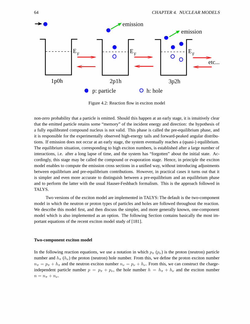
64 CHAPTER 4. NUCLEAR MODELS
EF E
FE
F
1p0h 2p1h 3p2h
etc...
h: holep: particle
emissionemission
Figure 4.2: Reaction flow in exciton model
non-zero probability that a particle is emitted. Should this happen at an early stage, it is intuitively clearthat the emitted particle retains some “memory” of the incident energy and direction: the hypothesis ofa fully equilibrated compound nucleus is not valid. This phase is called the pre-equilibrium phase, andit is responsible for the experimentally observed high-energy tails and forward-peaked angular distribu-tions. If emission does not occur at an early stage, the system eventually reaches a (quasi-) equilibrium.The equilibrium situation, corresponding to high exciton numbers, is established after a large number ofinteractions, i.e. after a long lapse of time, and the systemhas “forgotten” about the initial state. Ac-cordingly, this stage may be called the compound or evaporation stage. Hence, in principle the excitonmodel enables to compute the emission cross sections in a unified way, without introducing adjustmentsbetween equilibrium and pre-equilibrium contributions. However, in practical cases it turns out that itis simpler and even more accurate to distinguish between a pre-equilibrium and an equilibrium phaseand to perform the latter with the usual Hauser-Feshbach formalism. This is the approach followed inTALYS.
Two versions of the exciton model are implemented in TALYS: The default is the two-componentmodel in which the neutron or proton types of particles and holes are followed throughout the reaction.We describe this model first, and then discuss the simpler, and more generally known, one-componentmodel which is also implemented as an option. The following Section contains basically the most im-portant equations of the recent exciton model study of [181].
Two-component exciton model
In the following reaction equations, we use a notation in which pπ (pν) is the proton (neutron) particlenumber andhπ (hν ) the proton (neutron) hole number. From this, we define the proton exciton numbernπ = pπ + hπ and the neutron exciton numbernν = pν + hν . From this, we can construct the charge-independent particle numberp = pπ + pν , the hole numberh = hπ + hν and the exciton numbern = nπ + nν .
4.4. PRE-EQUILIBRIUM REACTIONS 65
The temporal development of the system can be described by a master equation, describing thegain and loss terms for a particular class of exciton states,see [181]. Integrating the master equationover time up to the equilibration timeτeq yields the mean lifetime of the exciton stateτ that can be usedto calculate the differential cross section [58]. The primary pre-equilibrium differential cross section forthe emission of a particlek with emission energyEk can then be expressed in terms ofτ , the composite-nucleus formation cross sectionσCF, and an emission rateWk,
dσPEk
dEk= σCF
pmaxπ∑
pπ=p0π
pmaxν∑
pν=p0ν
Wk(pπ, hπ, pν , hν , Ek)τ(pπ, hπ, pν , hν)
× P (pπ, hπ, pν , hν),(4.87)
where the factorP represents the part of the pre-equilibrium population thathas survived emissionfrom the previous states and now passes through the(pπ, hπ, pν , hν) configurations, averaged over time.Expressions for all quantities appearing in this expression will be detailed in the rest of this Section. Theinitial proton and neutron particle numbers arep0
π = Zp, andp0ν = Np, respectively withZp (Np) the
proton (neutron) number of the projectile. For any exciton state in the reaction process,hπ = pπ−p0π and
hν = pν−p0ν , so that for primary pre-equilibrium emission the initial hole numbers areh0
π = h0ν = 0. For
e.g. a neutron-induced reaction, the initial exciton number is given byn0 = n0ν = 1 (0pπ0hπ1pν0hν ),
but only pre-equilibrium gamma emission can occur from thisstate (nucleon emission from this state isessentially elastic scattering and this is already coveredby the optical model). Particle emission onlyoccurs fromn = 3 (2p1h) and higher exciton states. We use a hardwired value ofpmax
π = pmaxν = 6 as
the upper limit of the summation, see [181]. We use the never-come-back approximation, i.e. throughoutthe cascade one neglects the interactions that decrease theexciton number, although the adopted solutionof Eq. (4.87) does include transitions that convert a protonparticle-hole pair into a neutron pair and viceversa. The maximum valuespmax
π andpmaxν thus entail an automatic separation of the pre-equilibrium
population and the compound nucleus population. The latteris then handled by the more adequateHauser-Feshbach mechanism. We now discuss the various ingredients of Eq. (4.87).
A. Reaction cross sections The basic feeding term for pre-equilibrium emission is the compoundformation cross sectionσCF, which is given by
(4.88) σCF = σreac − σdirect,
where the reaction cross sectionσreac is directly obtained from the optical model andσdirect is the sumof the cross sections for direct reactions to discrete states σdisc,direct as defined in Eq. (3.18), and forgiant resonances, see Section 4.2.4.
B. Emission rates and particle-hole state densities The emission rateWk has been derived by Clineand Blann [59] from the principle of microreversibility, and can easily be generalized to a two-componentversion [60]. The emission rate for an ejectilek with relative massµk and spinsk is
Wk(pπ, hπ, pν , hν , Ek) =2sk + 1
π2~3µkEkσk,inv(Ek)
× ω(pπ − Zk, hπ, pν − Nk, hν , Etot − Ek)
ω(pπ, hπ, pν , hν , Etot),(4.89)
66 CHAPTER 4. NUCLEAR MODELS
whereσk,inv(Ek) is the inverse reaction cross section, again calculated with the optical model,Zk (Nk)is the charge (neutron) number of the ejectile andEtot is the total energy of the composite system.
For the particle-hole state densityω(pπ, hπ, pν , hν , Ex) we use the expression of Betak and Dobes [60,61]. Their formula is based on the assumption of equidistantlevel spacing and is corrected for the ef-fect of the Pauli exclusion principle and for the finite depthof the potential well. The two-componentparticle-hole state density is
ω(pπ, hπ, pν , hν , Ex) =gnππ gnν
ν
pπ!hπ!pν !hν !(n − 1)!(U − A(pπ, hπ, pν , hν))n−1
× f(p, h, U, V ),(4.90)
wheregπ andgν are the single-particle state densities,A the Pauli correction,f the finite well function,andU = Ex − Pp,h with Pp,h Fu’s pairing correction [62],
Pp,h = ∆ − ∆
[
0.996 − 1.76
(
n
ncrit
)1.6
/
(
Ex
∆
)0.68]2
if Ex/∆ ≥ 0.716 + 2.44
(
n
ncrit
)2.17
,
= ∆ otherwise,(4.91)
with
(4.92) ncrit = 2gTcrit ln 2,
whereTcrit = 2√
∆/14g/3.5 andg = gπ + gν . The pairing energy∆ for total level densities is given by
(4.93) ∆ = χ12√A
,
where hereA is the mass number andχ = 0, 1 or 2 for odd-odd, odd or even-even nuclei. The Paulicorrection term is given by
A(pπ, hπ, pν , hν) =[max(pπ, hπ)]2
gπ+
[max(pν , hν)]2
gν
− p2π + h2
π + pπ + hπ
4gπ− p2
ν + h2ν + pν + hν
4gν.(4.94)
For the single-particle state densities we take
(4.95) gπ = Z/15, gν = N/15,
which is, through the relationshipg = aπ2/6, in line with the values for our total level density parametera, see Eq. (4.242), and also provides a globally better description of spectra than the generally adoptedg = A/13.
4.4. PRE-EQUILIBRIUM REACTIONS 67
The finite well functionf(p, h,Ex, V ) accounts for the fact that a hole cannot have an energybelow that of the bottom of the potential well depthV . It is given by
(4.96) f(p, h,Ex, V ) = 1 +
h∑
i=1
(−1)i(
h
i
)[
Ex − iV
Ex
]n−1
Θ(Ex − iV ),
whereΘ is the unit step function. Note thatf is different from 1 only for excitation energies greater thanV . In the original version of Betak and Dobes,V is given by the depthEf of the Fermi well. This wasgeneralized by Kalbach [63, 49] to obtain an effective method to include surface effects in the first stageof the interaction, leading to a harder pre-equilibrium spectrum. For the first stage the maximum depthof the hole should be significantly reduced, since in the surface region the potential is shallower than inthe interior. This automatically leaves more energy to be adopted by the excited particle, yielding moreemission at the highest outgoing energies. We use the following functional form forV in terms of theprojectile energyEp and the massA,
V = 22 + 16E4
p
E4p + (450/A1/3)4
MeV for h = 1 and incident protons,
V = 12 + 26E4
p
E4p + (245/A1/3)4
MeV for h = 1 and incident neutrons,
V = Ef = 38 MeV for h > 1.(4.97)
See Ref. [181] for a further justification of this parameterisation.
C. Lifetimes The lifetimeτ of exciton state(pπ, hπ, pν , hν) in Eq. (4.87) is defined as the inverse sumof the total emission rate and the various internal transition rates,
τ(pπ, hπ, pν , hν) = [λ+π (pπ, hπ, pν , hν) + λ+
ν (pπ, hπ, pν , hν)
+ λ0πν(pπ, hπ, pν , hν) + λ0
νπ(pπ, hπ, pν , hν) + W (pπ, hπ, pν , hν)]−1,(4.98)
whereλ+π (λ+
ν ) is the internal transition rate for proton (neutron) particle-hole pair creation,λ0πν (λ0
νπ)is the rate for the conversion of a proton (neutron) particle-hole pair into a neutron (proton) particle-holepair, andλ−
π (λ−ν ) is the rate for particle-hole annihilation. These transition rates will be discussed in
Sec. 4.4.1. The total emission rateW is the integral of Eq. (4.89) over all outgoing energies, summedover all outgoing particles,
(4.99) W (pπ, hπ, pν , hν) =∑
k=γ,n,p,d,t,h,α
∫
dEkWk(pπ, hπ, pν , hν , Ek).
The final ingredient of the exciton model equation, Eq. (4.87), is the part of the pre-equilibrium popula-tionP that has survived emission from all previous steps and has arrived at the exciton state(pπ, hπ, pν , hν).The expression forP is somewhat more complicated than that of the depletion factor that appears in theone-component exciton model [57]. For two components, contributions from both particle creationandcharge exchange reactions need to be taken into account, whereas transitions that do not change theexciton number cancel out in the one-component model.
68 CHAPTER 4. NUCLEAR MODELS
For the(pπ, hπ, pν , hν) state,P is given by a recursive relation:
P (pπ, hπ, pν , hν) = P (pπ − 1, hπ − 1, pν , hν)Γ+π (pπ − 1, hπ − 1, pν , hν) (A)
+ P (pπ, hπ, pν − 1, hν − 1)Γ+ν (pπ, hπ, pν − 1, hν − 1) (B)
+ [P (pπ − 2, hπ − 2, pν + 1, hν + 1)Γ′+π (pπ − 2, hπ − 2, pν + 1, hν + 1)
+ P (pπ − 1, hπ − 1, pν , hν)Γ′+ν (pπ − 1, hπ − 1, pν , hν)]
× Γ0νπ(pπ − 1, hπ − 1, pν + 1, hν + 1) (C + D)
+ [P (pπ, hπ, pν − 1, hν − 1)Γ′+π (pπ, hπ, pν − 1, hν − 1)
+ P (pπ + 1, hπ + 1, pν − 2, hν − 2)Γ′+ν (pπ + 1, hπ + 1, pν − 2, hν − 2)]
× Γ0πν(pπ + 1, hπ + 1, pν − 1, hν − 1) (E + F ).
(4.100)
This relation contains 6 distinct feeding terms: (A) creation of a proton particle-hole pair from the(pπ −1, hπ−1, pν , hν) state, (C) creation of a proton particle-hole pair from the(pπ−2, hπ−2, pν +1, hν +1)
state followed by the conversion of a neutron particle-holepair into a proton particle-hole pair, and (D)creation of a neutron particle-hole pair from the(pπ − 1, hπ − 1, pν , hν) state followed by its conversioninto a proton particle-hole pair. The three remaining terms(B), (E), and (F) are obtained by changingprotons into neutrons and vice versa. The probabilities of creating new proton or neutron particle-holepairs and for converting a proton (neutron) pair into a neutron (proton) pair are calculated as follows:
Γ+π (pπ, hπ, pν , hν) = λ+
π (pπ, hπ, pν , hν)τ(pπ, hπ, pν , hν),
Γ+ν (pπ, hπ, pν , hν) = λ+
ν (pπ, hπ, pν , hν)τ(pπ, hπ, pν , hν),
Γ′+π (pπ, hπ, pν , hν) = λ+
π (pπ, hπ, pν , hν)τ ′(pπ, hπ, pν , hν),
Γ′+ν (pπ, hπ, pν , hν) = λ+
ν (pπ, hπ, pν , hν)τ ′(pπ, hπ, pν , hν),
Γ0πν(pπ, hπ, pν , hν) = λ0
πν(pπ, hπ, pν , hν)τ(pπ, hπ, pν , hν),
Γ0νπ(pπ, hπ, pν , hν) = λ0
νπ(pπ, hπ, pν , hν)τ(pπ, hπ, pν , hν),
τ ′(pπ, hπ, pν , hν) = [λ+π (pπ, hπ, pν , hν) + λ+
ν (pπ, hπ, pν , hν)
+ W (pπ, hπ, pν , hν)]−1.
(4.101)
The use ofτ ′ in the probabilityΓ′+π (Γ′+
ν ), to create a new proton (neutron) particle-hole pair preceding anexchange interaction, originates from the approximation that only one exchange interaction is allowedin each pair-creation step. The appropriate lifetime in this case consists merely of pair creation andemission rates [58].
The initial condition for the recursive equations is
(4.102) P (p0π, h0
π, p0ν , h0
ν) = 1,
after whichP can be solved for any configuration.
To calculate the pre-equilibrium spectrum, the only quantities left to determine are the internaltransition ratesλ+
π , λ+ν , λ0
πν andλ0νπ.
4.4. PRE-EQUILIBRIUM REACTIONS 69
D. Internal transition rates The transition rateλ+π for the creation of a proton particle-hole pair is
given by four terms, accounting forpπ, hπ, pν andhν scattering that leads to a new(pπ, hπ) pair,
λ+π (pπ, hπ, pν , hν) =
1
ω(pπ, hπ, pν , hν , Etot)
[
∫ Lpπ2
Lpπ1
λ1pππ(u)ω(pπ − 1, hπ, pν , hν , Etot − u)ω(1, 0, 0, 0, u)du
+
∫ Lhπ2
Lhπ1
λ1hππ(u)ω(pπ, hπ − 1, pν , hν , Etot − u)ω(0, 1, 0, 0, u)du
+
∫ Lpν2
Lpν1
λ1pνπ(u)ω(pπ, hπ, pν − 1, hν , Etot − u)ω(0, 0, 1, 0, u)du
+
∫ Lhν2
Lhν1
λ1hνπ(u)ω(pπ, hπ, pν , hν − 1, Etot − u)ω(0, 0, 0, 1, u)du],(4.103)
where the first and third term represent particle scatteringand the second and fourth term hole scattering.The integration limits correct for the Pauli exclusion principle,
Lpπ1 = A(pπ + 1, hπ + 1, pν , hν) − A(pπ − 1, hπ, pν , hν),
Lpπ2 = Etot − A(pπ − 1, hπ , pν , hν),
Lhπ1 = A(pπ + 1, hπ + 1, pν , hν) − A(pπ, hπ − 1, pν , hν),
Lhπ2 = Etot − A(pπ, hπ − 1, pν , hν),
Lpν1 = A(pπ, hπ, pν + 1, hν + 1) − A(pπ, hπ, pν − 1, hν),
Lpν2 = Etot − A(pπ, hπ, pν − 1, hν),
Lhν1 = A(pπ + 1, hπ + 1, pν , hν) − A(pπ, hπ, pν , hν − 1),
Lhν2 = Etot − A(pπ, hπ, pν , hν − 1),(4.104)
which demands that (a) the minimal energy available to the scattering particle or hole creating a newparticle-hole pair equals the Pauli energy of the final stateminus the Pauli energy of the inactive particlesand holes not involved in the scattering process, and (b) themaximal energy available equals the totalexcitation energy minus the latter Pauli energy.
The termλ1pππ(u) is the collision probability per unit time for a proton-proton interaction leading
to an additional proton particle-hole pair. In general, thecorresponding term for a hole is obtainedby relating it to the particle collision probability through the accessible state density of the interactingparticles and holes,
(4.105) λ1hππ(u) = λ1p
ππ(u)ω(1, 2, 0, 0, u)
ω(2, 1, 0, 0, u).
Similarly, λ1pνπ(u) is the collision probability per unit time for a neutron-proton interaction leading to an
additional proton particle-hole pair, and for the corresponding hole term we have
(4.106) λ1hνπ(u) = λ1p
νπ(u)ω(1, 1, 0, 1, u)
ω(1, 1, 1, 0, u).
70 CHAPTER 4. NUCLEAR MODELS
The transition rate for conversion of a proton particle-hole pair into a neutron pair is
λ0πν(pπ, hπ, pν , hν) =
1
ω(pπ, hπ, pν , hν , Etot)
∫ Lpπ2
Lpπ1
λ1p1hπν (u)
ω(pπ − 1, hπ − 1, pν , hν , Etot − u)ω(1, 1, 0, 0, u)du,(4.107)
with integration limits
Lpπ1 = A(pπ, hπ, pν , hν) − A(pπ − 1, hπ − 1, pν , hν)
Lpπ2 = Etot − A(pπ − 1, hπ − 1, pν , hν).(4.108)
The termλ1p1hπν is the associated collision probability. Interchangingπ andν in Eqs. (4.103-4.108) gives
the expressions forλ+ν , λ1h
νν , λ1hπν andλ0
νπ.
We distinguish between two options for the collision probabilities:
D1. Effective squared matrix element
Expressing the transition rate in terms of an effective squared matrix element has been used inmany exciton model analyses. Also in TALYS, it is one of the options for our calculations and compar-isons with data. The collision probabilities of Eqs. (4.103) and (4.107) are determined with the aid ofFermi’s golden rule of time-dependent perturbation theory, which for a two-component model gives
λ1pππ(u) =
2π
~M2
ππω(2, 1, 0, 0, u),
λ1hππ(u) =
2π
~M2
ππω(1, 2, 0, 0, u),
λ1pνπ(u) =
2π
~M2
νπω(1, 1, 1, 0, u),
λ1hνπ(u) =
2π
~M2
νπω(1, 1, 0, 1, u),
λ1p1hπν (u) =
2π
~M2
πνω(0, 0, 1, 1, u),(4.109)
where the relations (4.105)-(4.106) have been applied. Interchangingπ and ν gives the expressionsfor λ1p
νν , λ1hνν , λ1p
πν , λ1hπν , andλ1p1h
νπ . Here, theM2ππ, etc. are average squared matrix elements of the
residual interaction, which are assumed to depend on the total energyEtot of the whole compositenucleus only. Such a matrix element thus represents a trulyeffectiveresidual interaction, whereby allindividual residual interactions taking place inside the nucleus can be cast into an average form for thesquared matrix element to which one assigns a globalEtot-dependence a posteriori.
The average residual interaction inside the nucleus is not necessarily the same for like and unlikenucleons. The two-component matrix elements are given, in terms of an averageM2, by
M2ππ = RππM2,
M2νν = RννM
2,
M2πν = RπνM
2,
M2νπ = RνπM2.(4.110)
4.4. PRE-EQUILIBRIUM REACTIONS 71
In TALYS, we take
(4.111) Rνν = 1.5, Rνπ = Rππ = Rπν = 1.,
which is in line with the, more parameter-free, optical model based exciton model that we describe later.Note that this deviates somewhat from the parameters adopted in Ref. [181]. The current parameteriza-tion gives slightly better performance for cross section excitation functions. In TALYS, the above param-eters are adjustable (Rpinu, etc. keywords) with Eq. (4.111) as default. The following semi-empiricalexpression for the squared matrix element has been shown to work for incident energies between 7 and200 MeV [181]:
(4.112) M2 =C1Ap
A3
[
7.48C2 +4.62 × 10⁵
( Etot
n.Ap+ 10.7C3)3
]
.
Eq. (4.112) is a generalization of older parameterisationssuch as given in Refs. [58, 49], which applyin smaller (lower) energy ranges. HereC1, C2 andC3 are adjustable constants (see theM2constant,M2limit andM2shift keywords) that are all equal to 1 by default, andAp is the mass number of theprojectile, which allows generalization for complex-particle reactions. Again, Eq. (4.112) is slightlydifferent (10%) from the expression given in Ref. [181] to allow for better fits of excitation functions.
Finally, for matrix element based transition rates and equidistant particle-hole level densities, theintegrals in the transition rates can be approximated analytically [58], giving
λπ+(pπ, hπ, pν , hν) =2π
~
g2π
2n(n + 1)
[
Etot − A(pπ + 1, hπ + 1, pν , hν)]n+1
[Etot − A(pπ, hπ, pν , hν)]n−1
× (nπgπM2ππ + 2nνgνM2
πν)f(p + 1, h + 1, Etot, V )
λν+(pπ, hπ, pν , hν) =2π
~
g2ν
2n(n + 1)
[
Etot − A(pπ, hπ, pν + 1, hν + 1)]n+1
[Etot − A(pπ, hπ, pν , hν)]n−1
× (nνgνM2νν + 2nπgπM2
νπ)f(p + 1, h + 1, Etot, V )
λπν(pπ, hπ, pν , hν) =2π
~M2
πν
pπhπ
ng2νf(p, h,Etot, V )
[
Etot − Bπν(pπ, hπ, pν , hν)
Etot − A(pπ, hπ, pν , hν)
]n−1
× (2[Etot − Bπν(pπ, hπ, pν , hν)]
+ n|A(pπ, hπ, pν , hν) − A(pπ − 1, hπ − 1, pν + 1, hν + 1)|)
λνπ(pπ, hπ, pν , hν) =2π
~M2
νπ
pνhν
ng2πf(p, h,Etot, V )
[
Etot − Bνπ(pπ, hπ, pν , hν)
Etot − A(pπ, hπ, pν , hν)
]n−1
× (2[Etot − Bνπ(pπ, hπ, pν , hν)]
+ n|A(pπ, hπ, pν , hν) − A(pπ + 1, hπ + 1, pν − 1, hν − 1)|),(4.113)
with
Bπν(pπ, hπ, pν , hν) = max[A(pπ, hπ, pν , hν), A(pπ − 1, hπ − 1, pν + 1, hν + 1)]
Bνπ(pπ, hπ, pν , hν) = max[A(pπ, hπ, pν , hν), A(pπ + 1, hπ + 1, pν − 1, hν − 1)].(4.114)
which is also included as an option. The default is however touse the numerical solutions for the in-ternal transition rates. This analytical solution requires a value forM2 that is 20% larger than that of
72 CHAPTER 4. NUCLEAR MODELS
Eq. (4.112), which apparently is the energy-averaged effect of introducing such approximations.
D2. Collision rates based on the optical model
Instead of modeling the intranuclear transition rate by an average squared matrix element, one mayalso relate the transition rate to the average imaginary optical model potential depth [181]. The collisionprobabilities, when properly averaged over all particle-hole configurations as in Eq. (4.103), in principlewould yield a parameter free expression for the transition rate.
The average well depthWi can be obtained by averaging the total imaginary part of the potentialW over the whole volume of the nucleus
(4.115) Wi(E) =
∫
Wi(r,E)ρ(r)dr∫
ρ(r)dr,
whereρ represents the density of nuclear matter for which we take the form factorf(r,R, a) of thevolume part of the optical model potential, given by the usual Woods-Saxon shape of Eq. (4.3). The totalimaginary potential is given by
(4.116) Wi(r,E) = WV,i(E)f(r,RV,i, aV,i) − 4aD,iWD,i(E)d
drf(r,RD,i, aD,i).
Next, we define aneffectiveimaginary optical potential [181] related to nucleon-nucleon collisions innuclear matter:
(4.117) W effi (E) = Comp Wi(E).
We use as best overall parameter
(4.118) Comp = 0.55.
This parameter can be adjusted with theM2constantkeyword, which serves as a multiplier for the valuegiven in Eq. (4.118). The collision probabilities are now related as follows to theeffectiveimaginaryoptical potential:
λ1pππ(u) =
1
4
2W effp (u − S(p))
~
λ1hππ(u) =
1
4
2W effp (u − S(p))
~
ω(1, 2, 0, 0, u)
ω(2, 1, 0, 0, u)
λ1pνπ(u) =
3
4
2W effn (u − S(n))
~
λ1hνπ(u) =
3
4
2W effn (u − S(n))
~
ω(1, 1, 0, 1, u)
ω(1, 1, 1, 0, u)
λ1p1hνπ (u) =
1
2
2W effn (u − S(n))
~,(4.119)
and similarly for the components ofλ+ν andλ0
νπ. The transition rates for the exciton model are thenobtained by inserting these terms in Eqs. (4.103) and (4.107). Apart from Eq. (4.118), a parameter-freemodel is obtained.
4.4. PRE-EQUILIBRIUM REACTIONS 73
One-component exciton model
The one-component exciton model has been made redundant by the more flexible and physically morejustified two-component model. Nevertheless, it is included as an option since it connects to many olderpre-equilibrium studies and thus may be helpful as comparison. In the one-component exciton model,the pre-equilibrium spectrum for the emission of a particlek at an energyEk is given by
(4.120)dσPE
k
dEk= σCF
pmax∑
p=p0
Wk(p, h,Ek)τ(p, h),
wherepmax = 6 andσCF are defined as below Eq. (4.87). For the initial particle number p0 we havep0 = Ap with Ap the mass number of the projectile. In general, the hole number h = p − p0 inEq. (4.120), so that the initial hole number is always zero, i.e. h0 = 0 for primary pre-equilibriumemission.
The emission rateWk is
(4.121) Wk(p, h,Ek) =2sk + 1
π2~3µkEkσk,inv(Ek)
ω(p − Ak, h,Etot − Ek)
ω(p, h,Etot)Qk(p),
with all quantities explained below Eq. (4.89), andAk is the mass number of the ejectile andQk(p) is afactor accounting for the distinguishability of neutrons and protons [64]
Qk(p) =(p − Ak)!
p!
p−Nk∑
pπ=Zk
(Z
A)nπ−Zk(
A
N)nν−Nk
1
hπ!hν !
1
(pπ − Zk)!(pν − Nk)!
/
p−Nk∑
pπ=Zk
(Z
A)nπ(
N
A)nν
1
pπ!pν !hπ!hν !
.(4.122)
For gamma’s we setQγ(p) = 1.
Finally, ω(p, h,Ex) is the particle-hole state density for which we use the one-component expres-sion by Betak and Dobes [61], again corrected for the effect of the Pauli exclusion principle and for thefinite depth of the potential well. The one-component particle-hole state density has a simpler form thanthat of Eq. (4.90),
(4.123) ω(p, h,Ex) =gn
p!h!(n − 1)![Ex − A(p, h)]n−1f(p, h,Ex, V ),
whereg = A/15 is the single-particle state density and
(4.124) A(p, h) =[max(p, h)]2
g− p2 + h2 + p + h
4g,
is the Pauli correction factor. The finite well functionf is given by Eq. (4.96).
To obtain the lifetimesτ(p, h) that appear in Eq. (4.120), we first define the total emission rateW (p, h) as the integral of Eq. (4.121) over all outgoing energies, summed over all outgoing particles:
(4.125) W (p, h) =∑
k=γ,n,p,d,t,h,α
∫
dEkWk(p, h,Ek).
74 CHAPTER 4. NUCLEAR MODELS
As mentioned already, we have implemented the never-come-back solution of the master equation.This is based on the assumption that at the beginning of the cascade one neglects the interactions thatdecrease the exciton number. Then, for the one-component model the expression for the lifetime is (seee.g. Ref. [57])
(4.126) τ(p, h) =1
λ+(p, h) + W (p, h)Dp,h,
whereDp,h is a depletion factor that accounts for the removal of reaction flux, through emission, by theprevious stages
(4.127) Dp,h =
p−1∏
p′=p0
λ+(p′, h′)
λ+(p′, h′) + W (p′, h′),
with againh′ = p′ − p0. The initial case of Eq. (4.126) is
(4.128) τ(p0, h0) =1
λ+(p0, h0) + W (p0, h0).
To calculate the pre-equilibrium spectrum, the only quantity left to determine is the internal transitionrateλ+(p, h) from state(p, h) to state(p + 1, h + 1). The general definition ofλ+(p, h) is
λ+(p, h) =1
ω(p, h,Etot)[
∫ Lp2
Lp1
duλ1p(u)ω(p − 1, h,Etot − u)ω(1, 0, u)
+
∫ Lh2
Lh1
duλ1h(u)ω(p, h − 1, Etot − u)ω(0, 1, u)].(4.129)
where the two terms account for particle and hole scattering, respectively, and the integration limits
Lp1 = A(p + 1, h + 1) − A(p − 1, h)
Lp2 = Etot − A(p − 1, h)
Lh1 = A(p + 1, h + 1) − A(p, h − 1)
Lh2 = Etot − A(p, h − 1),(4.130)
correct for the Pauli exclusion principle.
We again distinguish between two options:
1. Effective squared matrix element
The collision probabilities are determined with the aid of Fermi’s golden rule of time-dependentperturbation theory, which for the one-component model are
λ1p(u) =2π
~M2ω(2, 1, u)
λ1h(u) =2π
~M2ω(1, 2, u),(4.131)
4.4. PRE-EQUILIBRIUM REACTIONS 75
with M2 the average squared matrix element of the residual interaction. In the one-component model,“forbidden” transitions are taken into account, so that a squared matrix element smaller than that ofEq. (4.112) of the two-component model is needed to compensate for these transitions. We find that forthe one-component model we need to multiplyM2 of Eq. (4.112) by 0.5 to obtain a global comparisonwith data that is closest to our two-component result, i.e.
(4.132) M2 =0.5C1Ap
A3
[
7.48C2 +4.62 × 10⁵
( Etot
n.Ap+ 10.7C3)3
]
.
For completeness, we note that the transition rate can be well approximated by an analytical form asdiscussed in Refs. [65, 61, 63]. The result is
(4.133) λ+(p, h) =2π
~M2 g3
2(n + 1)
[
Etot − A(p + 1, h + 1)]n+1
[Etot − A(p, h)]n−1 f(p + 1, h + 1, Etot, V ).
However, the overall description of experimental data obtained with the one-component model is how-ever worse that that of the two-component model, so we rarelyuse it.
2. Collision rates based on the optical model
Also in the one-component model the transition rates can be related to the effective nucleon-nucleon interactionσ and thereby to the imaginary optical potential,
λ1p(u) =1
2
2W eff(u − S)
~
λ1h(u) =1
2
2W eff(u − S)
~
ω(1, 2, u)
ω(2, 1, u),(4.134)
with S the separation energy of the particle. Since the one-component model makes no distinctionbetween neutron and proton particle-hole pairs,W eff
V is evaluated as follows,
(4.135) W effi (E) = 0.5Comp Wi(E),
analogous to the multiplication with a factor 0.5 forM2.
Energy width representation The formalism given above, i.e. Eqs. (4.120), (4.121) and (4.126),forms a representation in which the time appears, i.e. the dimensions ofW (p, h) andτ(p, h) are [s]−1
and [s] respectively. An alternative expression for the exciton model that is often used is in terms ofenergy widths. Since this may be more recognisable to some users we also give it here. The partialescape widthΓ↑
k(p, h,Ek) is related to the emission rate by
(4.136) Γ↑k(p, h,Ek) = ~Wk(p, h,Ek).
76 CHAPTER 4. NUCLEAR MODELS
Integrated over energy we have
(4.137) Γ↑k(p, h) = ~Wk(p, h),
and the total escape width is
(4.138) Γ↑(p, h) =∑
k=γ,n,p,d,t,h,α
Γ↑k(p, h) = ~W (p, h).
The damping widthΓ↓ is related to the internal transition rate by
(4.139) Γ↓(p, h) = ~λ+(p, h).
Defining the total width by
(4.140) Γtot(p, h) = Γ↓(p, h) + Γ↑(p, h),
we can rewrite the exciton model cross section (4.120) as
(4.141)dσPE
k
dEk= σCF
pmax∑
p=p0
Γ↑k(p, h,Ek)
Γtot(p, h)
p−1∏
p′=p0
Γ↓(p′, h′)
Γtot(p′, h′)
.
In the output file of TALYS, the results for the various quantities in both the time and the energy widthrepresentation are given.
In sum, the default model used by TALYS is the two-component exciton model with collisionprobabilities based on the effective squared matrix element of Eq. (4.112).
4.4.2 Photon exciton model
For pre-equilibrium photon emission, we have implemented the model of Akkermans and Gruppelaar [66].This model gives a simple but powerful simulation of the direct-semidirect capture process within theframework of the exciton model. Analogous to the particle emission rates, the continuumγ-ray emissionrates may be derived from the principle of detailed balance or microscopic reversibility, assuming thatonly E1-transitions contribute. This yields(4.142)
Wγ(p, h,Eγ) =E2
γ
π2~3c2
σγ,abs(Eγ)
ω(p, h,Etot)
(
g2Eγω(p − 1, h − 1, Ex − Eγ)
g(n − 2) + g2Eγ+
gnω(p, h,Ex − Eγ)
gn + g2Eγ
)
whereσγ,abs(Eγ) is the photon absorption cross section of Eq. (4.80). The initial particle-hole configura-tion in Eq. (4.120) isn0 = 1 (1p0h) for photon emission. For “direct”γ-ray emission in nucleon-inducedreactions only the second term between brackets (n = 1) contributes. The “semi-direct”γ-ray emission(n = 3) consists of both terms.
The emission rate (4.142) is included in Eqs. (4.120) and (4.125) so that the pre-equilibrium photoncross section automatically emerges.
4.4. PRE-EQUILIBRIUM REACTIONS 77
For the two-component model, we use
Wγ(pπ, hπ, pν , hν , Eγ) =E2
γ
π2~3c2
σγ,abs(Eγ)
ω(pπ, hπ, pν , hν , Etot)
× (g2Eγ
12 [ω(pπ − 1, hπ − 1, pν , hν , Ex − Eγ) + ω(pπ, hπ, pν − 1, hν − 1, Ex − Eγ)]
g(n − 2) + g2Eγ
+gnω(pπ, hπ, pν , hν , Ex − Eγ)
gn + g2Eγ).(4.143)
4.4.3 Pre-equilibrium spin distribution
Since the exciton model described above does not provide a spin distribution for the residual states afterpre-equilibrium emission, a model needs to be adopted that provides the spin population in the continuumin binary reactions. TALYS provides two options for this. The default is to adopt the compound nucleusspin distribution (described in Section 4.5) also for the excited states resulting from pre-equilibriumemission. Another option that has been quite often used in the past is to assign a spin distribution tothe particle-hole state density. For that, we adopt the usual decomposition of the state density into aJ-dependent part and an energy-dependent part,
(4.144) ρ(p, h, J,Ex) = (2J + 1)Rn(J)ω(p, h,Ex).
The functionRn(J) represents the spin distribution of the states in the continuum. It is given by
(4.145) Rn(J) =2J + 1
π1/2n3/2σ3exp
[
−(J + 12 )2
nσ2
]
,
and satisfies, for any exciton numbern,
(4.146)∑
J
(2J + 1)Rn(J) = 1.
The used expression for the spin cut-off parameterσ is [67],
(4.147) σ2 = 0.24nA2
3 ,
whereA is the mass number of the nucleus. Similarly, for the two-component particle-hole level densitywe have
(4.148) ρ(pπ, hπ, pν , hν , J,Ex) = (2J + 1)Rn(J)ω(pπ, hπ, pν , hν , Ex).
In practice, with this option (preeqspin y) the residual states formed by pre-equilibrium reactions wouldbe multiplied byRn a posteriori. There are various arguments to prefer the compound nucleus spindistribution, so we use that default.
78 CHAPTER 4. NUCLEAR MODELS
4.4.4 Continuum stripping, pick-up, break-up and knock-out reactions
For pre-equilibrium reactions involving deuterons, tritons, Helium-3 and alpha particles, a contributionfrom the exciton model is automatically calculated with theformalism of the previous subsections. Itis however well-known that for nuclear reactions involvingprojectiles and ejectiles with different par-ticle numbers, mechanisms like stripping, pick-up, break-up and knock-out play an important role andthese direct-like reactions are not covered by the exciton model. Therefore, Kalbach [68] developed aphenomenological contribution for these mechanisms, which we have included in TALYS. In total, thepre-equilibrium cross section for these reactions is givenby the sum of an exciton model (EM), nucleontransfer (NT), and knock-out (KO) contribution:
(4.149)dσPE
k
dEk=
dσEMk
dEk+
dσNTk
dEk+
dσKOk
dEk
where the contribution from the exciton model was outlined in the previous subsection.
Transfer reactions
The general differential cross section formula for a nucleon transfer reaction of the typeA(a, b)B is
dσNTa,b
dEb=
2sb + 1
2sa + 1
Ab
Aa
Ebσb,inv(Eb)
AaK
(
Aa
Ea + Va
)2n( C
AB
)n
× Na
(
2ZA
AA
)2(Za+2)hπ+2pν
ωNT (pπ, hπ, pν , hν , U)(4.150)
where
Ca = 5500 for incident neutrons,
= 3800 for incident charged particles,(4.151)
Na =1
80Eafor pickup,
=1
580√
Eafor stripping,
=1
1160√
Eafor exchange.(4.152)
K is an enhancement factor taking into account the fact that d, t and 3-He are loosely bound:
K = 12 for (N,α),
= 12 − 11Ea − 20
Eafor (α,N) and Ea > 20,
= 1 otherwise,(4.153)
whereN stands for either neutron or proton. The well depthVa is set at
(4.154) Va = 12.5Aa MeV,
4.4. PRE-EQUILIBRIUM REACTIONS 79
and represents the average potential drop seen by the projectile between infinity and the Fermi level. Thepossible degrees of freedom for the reaction are all included in the residual state densityωNT (pπ, hπ, pν , hν , U).Since we do not use this model to describe exchange reactionsin inelastic scattering, there is no need tosum the various terms of Eq. (4.150) overpπ, as in Ref. [68]. The exciton numbers are automatically de-termined by the transfer reaction, i.e.n = |Aa−Ab|, nπ = hπ = |Za−Zb|, nν = hν = |Na−Nb|, pπ =
pν = 0. The accessible state density that is directly determined by the reaction isω(pπ, hπ, pν , hν , U),given by Eq. (4.90). The total residual state density however also takes into account more complexconfigurations that can be excited by the transfer reaction.It is given by
ωNT (pπ, hπ, pν , hν , U) =3∑
i=0
3−i∑
j=0
(XNT )i+jω(pπ + i, hπ + i, pν + j, hν + j, U)
+
pπ∑
i=0
hπ∑
j=0
pν∑
k=0
hν∑
l=0
ω(pπ − i, hπ − j, pν − k, hν − l, U)Θ(i + j + k + l − 1
2)(4.155)
The first term allows that up to three particle-hole pairs canbe excited in a transfer reaction. The factorXNT represents the probability for exciting such a pair and is given by
(4.156) XNT =7√
Ea/Aa
V1A2A
(p2ν + p2
π + h2ν + 1.5h2
π)
For neutrons and protons we adopt forV1 the value given by Eq.(4.97), for deuterons and tritons we takeV1=17 MeV, and for Helium-3 and alpha particles we takeV1=25 MeV. The finite well depth correctionfor Eq. (4.155) are made using a well depth of
V = V1
(
2Z
A
)
if nπ = 0
= V1 otherwise.(4.157)
The second term of Eq. (4.155) allows for transfer of nucleons at the Fermi level. Here, the Heavisidefunction is merely used to avoid double counting ofω(pπ, hπ, pν , hν , U).
Knockout reactions
For (nucleon, α) reactions a knockout contribution is added. The general differential cross sectionformula for a knockout reaction of the typeA(a, b)B is
dσKOa,b
dEb=
σa,inv(Ea)
14(2sb + 1)AbEbσb,inv(Eb)
× Pbgagb [U − AKO(pa, hb)]∑
c=a,b(2sc + 1)Ac 〈σc〉 (Emax + 2Bcoul,c)(Emax − Bcoul,c)2gag2b/6gc
(4.158)
wherePb is the probability of exciting ab-type particle-hole pair,Emax is the maximum emission energy,andBcoul,c is the Coulomb barrier for a particle c. The average inverse cross section〈σc〉 is given by
(4.159) 〈σc〉 =
∫ Emax
Bcoul,c
dEσc(E)
80 CHAPTER 4. NUCLEAR MODELS
For the knockout model, the single-particle state density parameters for the cluster degrees of freedomg
represent the number of cluster states per unit energy. The relevant values are given by
(4.160) gn = N/13, gp = Z/13, gα = A/208 MeV.
The Pauli correction factorAKO is given by
(4.161) AKO(pa, hb) =1
2g2a
− 1
2g2b
The probabilities for exciting the various particle-hole pairs are
Pn =NA − φZA
AA − 2φZA + φZA/2
Pp =ZA − φZA
AA − 2φZA + φZA/2
Pα =φZA/2
AA − 2φZA + φZA/2(4.162)
The factorsφ are a kind of pre-formation parameters [68]. The following values are adopted
NA ≤ 116 : φ = 0.08
116 ≤ NA < 126 : φ = 0.02 + 0.06(126 − NA)/10
126 ≤ NA < 129 : φ = 0.02 + 0.06(NA − 126)/3
129 ≤ NA : φ = 0.08
(4.163)
Break-up reactions
For reactions induced by complex particles, break-up may play an important role. This holds especiallyfor weakly bound projectiles like deuterons. Break-up is here defined as having a projectile fragmentemerge from the reaction in a relatively narrow peak centered close to the beam velocity and stronglydirected toward forward angles. For deuterons only, a simple model by Kalbach has been included [69].This leads to an extra contribution in the (d,n) and (d,p) channels.
The centroid energy of the breakup peak, in MeV, is given by
(4.164) ǫ0 =Ab
Aa
(
ǫa − Ba,b −ZaZA
9.5
)
+ZbZB
9.5,
whereǫa represents the channel energy (the energy of both the emitted particle and the recoiling nucleusin the center of mass), andBa,b is the binding energy in the projectile for the indicated breakup channel(2.224 MeV for deuterons). The peak is assumed to be described by a Gaussian line shape with a widthparameter of
(4.165) Γ = 1.15 + 0.12Ea − AA
140,
4.4. PRE-EQUILIBRIUM REACTIONS 81
whereEa is the laboratory energy of the incident deuteron, and the width parameter is given in MeV.The break-up cross section is assumed to be
(4.166) σBU = Kd,b(A
1/3A + 0.8)2
1 + exp(13−Ea
6 ),
where the normalization factors are
Kd,n = 18,
Kd,p = 21.(4.167)
Finally, the differential break-up cross section is given by
(4.168)dσBU
a,b
dEb= σBU
1
Γ√
2πexp
(
−(ǫ0 − Eb)2
Γ2
)
.
In the output, we have stored the break-up contribution in the column “knockout” (which is normallyonly used for nucleon-induced reactions with alpha particles as ejectiles).
The stripping, pick-up, break-up and knock-out contributions can be adjusted with theCstrip andCknock keywords.
4.4.5 Angular distribution systematics
A sound pre-equilibrium theory should, besides the angle-integrated spectra, also describe the smoothforward peaked angular distributions in the continuum. A physics method to do so will be included in afuture version of TALYS (multi-step direct reactions). Semi-classical models, such as the exciton model,have always had some problems to describe angular distributions (essentially because it is based on acompound-like concept instead of a direct one [70]). A powerful phenomenological method is givenby Kalbach [71]. It is based on experimental information only and the insight that in general, a pre-equilibrium process consists of a forward peaked part (multi-step direct) and an isotropic part (multi-stepcompound), and that the angular distributions are fairly structureless and all look alike. The Kalbachformula for the double-differential cross section for a projectile a and an ejectileb is
(4.169)d2σa,xb
dEbdΩ=
1
4π
[
dσPE
dEb+
dσcomp
dEb
]
a
sinh(a)[cosh(a cos Θ) + fMSD(Eb) sinh(a cos Θ)]
wheredσPE
dEbanddσcomp
dEbare the angle-integrated pre-equilibrium and compound spectra, respectively, and
fMSD is the so-called multi-step direct or pre-equilibrium ratio:
(4.170) fMSD(Eb) =dσPE
dEb/
[
dσPE
dEb+
dσcomp
dEb
]
which thus increases from practically 0 at very low emissionenergy to 1 at the highest emission energies.Hence, once the angle-integrated spectra are known, the parametera determines the angular distribution.
82 CHAPTER 4. NUCLEAR MODELS
Kalbach parameterized it as
a(e′a, e′b) = 0.04
E1e′b
e′a+ 1.8 × 10⁻⁶(
E1e′b
e′a)3 + 6.7 × 10⁻⁷Mamb(
E3e′b
e′a)4,
E1 = min(e′a, 130MeV)
E3 = min(e′a, 41MeV)
e′b = Eb + Sb
e′a = Ea + Sa.
Ma = 1 for neutrons, protons, deuterons, tritons and Helium − 3
= 0 for alpha′s
mb = 1 for protons, deuterons, tritons and Helium − 3
=1
2for neutrons
= 2 for alpha′s
Sb = 15.68(AC − AB) − 28.07
[
(NC − ZC)2
AC− (NB − ZB)2
AB
]
− 18.56(A2/3C − A
2/3B ) + 33.22
[
(NC − ZC)2
A4/3C
− (NB − ZB)2
A4/3B
]
− 0.717
[
Z2C
A1/3C
− Z2B
A1/3B
]
+ 1.211
[
Z2C
AC− Z2
B
AB
]
− Ib
Id = 2.225
It = 8.482
Ih = 7.718
Iα = 28.296,(4.171)
Here,Ea andEb are the incident and the outgoing energy, respectively. ThenumberMa represents theincident particle, whilemb represents the outgoing particle, C is a label for the compound nucleus, B forthe final nucleus and the Myers and Swiatecki mass formula [72] for spherical nuclides should be usedhere to determine the separation energyS. Finally Ib is the energy required to break the emitted particleup into its constituents.
Since we calculate the pre-equilibrium and compound cross sections explicitly (and actually onlyusefMSD for ENDF-6 data libraries), Eq. (4.169) can be reduced to a formula for the double-differentialpre-equilibrium cross section
(4.172)d2σPE
a,xb
dEbdΩ=
1
4π
dσPE
dEb
a
sinh(a)exp(a cos Θ),
to which the isotropic compound angular distribution can beadded. In sum, given the angle-integratedspectrumdσPE
dEbby some physics model, the double-differential cross section is returned quite simply and
reasonably accurate by Eq. (4.172).
4.5. COMPOUND REACTIONS 83
4.5 Compound reactions
The term compound nucleus reaction is commonly used for two different mechanisms: (i) the processof the capture of the projectile in the target nucleus to forma compound nucleus, which subsequentlyemits a particle or gamma, (ii) the multiple emission process of highly excited residual nuclei formedafter the binary reaction. The latter, which is known as multiple compound emission, will be explainedin Section 4.6. We first treat the binary compound nucleus reaction that plays a role at low incidentenergy. It differs from the multiple compound emission at two important points: (a) the presence ofwidth fluctuation corrections and (b) non-isotropic, though still symmetric, angular distributions.
4.5.1 Binary compound cross section and angular distribution
In the compound nucleus picture, the projectile and the target nucleus form a compound nucleus with atotal energyEtot and a range of values for the total spinJ and parityΠ. The following energy, angularmomentum and parity conservation laws need to be obeyed,
Ea + Sa = Ea′ + Ex + Sa′ = Etot
s + I + l = s′ + I ′ + l′ = J
π0Π0(−1)l = πfΠf (−1)l′
= Π.(4.173)
The compound nucleus formula for the binary cross section isgiven by
σcompαα′ = Dcomp π
k2
lmax+I+s∑
J=mod(I+s,1)
1∑
Π=−1
2J + 1
(2I + 1)(2s + 1)
J+I∑
j=|J−I|
j+s∑
l=|j−s|
J+I′∑
j′=|J−I′|
j′+s′∑
l′=|j′−s′|
× δπ(α)δπ(α′)T J
αlj(Ea)⟨
T Jα′l′j′(Ea′)
⟩
∑
α′′,l′′,j′′ δπ(α′′)⟨
T Jα′′l′′j′′(Ea′′)
⟩W Jαljα′l′j′,(4.174)
In the above equations, the symbols have the following meaning:
Ea = projectile energy
s = spin of the projectile
π0 = parity of the projectile
l = orbital angular momentum of the projectile
j = total angular momentum of the projectile
δπ(α) = 1, if (−1)lπ0Π0 = Π and 0 otherwise
α = channel designation of the initial system of projectile andtarget nucleus:α = a, s,Ea, E
0x, I,Π0, wherea is the projectile type andE0
x the excitation energy of the targetnucleus (usually zero)
84 CHAPTER 4. NUCLEAR MODELS
lmax = maximum l-value for projectile
Sa = separation energy
Ea′ = ejectile energy
s′ = spin of the ejectile
πf = parity of the ejectile
l′ = orbital angular momentum of the ejectile
j′ = total angular momentum of the ejectile
δπ(α′) = 1, if (−1)l′
πfΠf = Π and 0 otherwise
α′ = channel designation of the final system of ejectile and residual nucleus:α′ = a′, s′, Ea′ , Ex, I ′,Πf, wherea′ is the ejectile type,Ex the excitation energy of the residualnucleus
I = spin of the target nucleus
Π0 = parity of the target
I ′ = spin of the residual nucleus
Πf = parity of the residual nucleus
Π = parity of the compound system
J = total angular momentum of the compound system
Dcomp = depletion factor to account for direct and pre-equilibriumeffects
k = wave number of relative motion
T = transmission coefficient
W = width fluctuation correction (WFC) factor, see the next Section.
In order to let Eq. (4.174) represent the general case, we have denoted the outgoing transmission coeffi-
cient by⟨
T Jα′l′j′
⟩
. For this, two cases can be distinguished. If the excitationenergyEx, that is implicit
in the definition of channelα′, corresponds to a discrete state of the final nucleus, then wesimply have
(4.175)⟨
T Jα′l′j′(Ea′)
⟩
= T Jα′l′j′(Ea′)
andE′a′ is exactly determined by Eq. (4.173). Forα′ channels in whichEx is in the continuum, we have
an effective transmission coefficient for an excitation energy bin with width∆Ex,
(4.176)⟨
T Jα′l′j′(Ea′)
⟩
=
∫ Ex+ 1
2∆Ex
Ex−1
2∆Ex
dEx′ρ(Ex′ , J,Π)T Jα′l′j′(Ea′)
4.5. COMPOUND REACTIONS 85
whereρ is the level density, which will be discussed in Section 4.7,andT is evaluated at an emissionenergyEa′ that corresponds to the middle of the excitation energy bin,i.e. Ea′ = Etot − Ex − Sa′ .Hence, both transitions to discrete states and transitionsto the whole accessible continuum are coveredby the sum overα′ in Eq. (4.174). The normalization factorDcomp is
(4.177) Dcomp = [σreac − σdisc,direct − σPE]/σreac
This indicates that in TALYS we assume that direct and compound contributions can be added incoher-ently. This formula forDcomp is only applied for weakly coupled channels that deplete theflux, such ascontributions from DWBA or pre-equilibrium. In the case of coupled-channels calculations for the dis-crete collective states, the transmission coefficients of Eq. (4.174) are automatically reduced by ECIS-06to account for direct effects and TALYS only subtracts the direct cross section for the weakly coupledlevels (DWBA), i.e. if
(4.178) σdisc,direct = σdisc,cc + σdisc,DWBA
then
(4.179) Dcomp = [σreac − σdisc,DWBA − σPE]/σreac
TALYS also computes the compound nucleus formula for the angular distribution. It is given by
(4.180)dσcomp
αα′ (θ)
dΩ=∑
L
CcompL PL(cos Θ),
wherePL are Legendre polynomials. The Legendre coefficientsCcompL are given by
CcompL = Dcomp π
k2
∑
J,Π
2J + 1
(2I + 1)(2s + 1)
J+I∑
j=|J−I|
j+s∑
l=|j−s|
J+I′∑
j′=|J−I′|
j′+s′∑
l′=|j′−s′|
× δπ(α)δπ(α′)T J
αlj(Ea)⟨
T Jα′l′j′(Ea′)
⟩
∑
α′′,l′′,j′′ δπ(α′′)⟨
T Jα′′l′′j′′(Ea′′)
⟩W Jαljα′l′j′A
JIljI′l′j′;L,(4.181)
where the Blatt-Biedenharn factorA is given by
AJIljI′l′j′;L =
(−1)I′−s′−I+s
4π(2J + 1)(2j + 1)(2l + 1)(2j′ + 1)(2l′ + 1)
(ll00|L0)W(JjJj; IL)W(jjll;Ls)(
l′l′00|L0)
W(Jj′Jj′; I ′L)W(j′j′l′l′;Ls′),(4.182)
where( | ) are Clebsch-Gordan coefficients andW are Racah coefficients.
Formulae (4.174) and (4.180-4.182) show that the width fluctuation correction factors and theangular distribution factors depend on all the angular momentum quantum numbers involved, and thushave to be re-evaluated each time inside all the summations.We generally need these formulae forrelatively low incident energy, where the WFC has a significant impact and where the compound nucleuscross section to each individual discrete state is large enough to make its angular distribution of interest.
86 CHAPTER 4. NUCLEAR MODELS
For projectile energies above several MeV (we generally take the neutron separation energy for safety),the width fluctuations have disappeared, meaning thatW J
αljα′l′j′ = 1 for all channels. Then for theangle-integrated compound cross section, instead of performing the full calculation, Eq. (4.174) can bedecoupled into two parts that represent the incoming and outgoing reaction flux, respectively. It simplifiesto
(4.183) σcompαα′ =
lmax+I+s∑
J=mod(I+s,1)
1∑
Π=−1
σCFJΠ (Etot)
Γα′(Etot, J,Π −→ Ex, I ′,Πf )
Γtot(Etot, J,Π)
whereσCFJΠ is the compound formation cross section per spin and parity:
(4.184) σCFJΠ (Etot) = Dcomp π
k2
2J + 1
(2I + 1)(2s + 1)
J+I∑
j=|J−I|
j+s∑
l=|j−s|
T Jαlj(Ea)δπ(α)
which itself obeys
(4.185)lmax+I+s∑
J=mod(I+s,1)
1∑
Π=−1
σCFJΠ (Etot) = Dcompσreac
The partial decay widths are
(4.186) Γα′(Etot, J,Π −→ Ex, I ′,Πf ) =1
2πρ(Etot, J,Π)
J+I′∑
j′=|J−I′|
j′+s′∑
l′=|j′−s′|
δπ(α′)⟨
T Jα′l′j′(E
′a′)⟩
and the total decay width is
(4.187) Γtot(Etot, J,Π) =∑
α′′
Γα′′(Etot, J,Π −→ Ex, I ′′,Πf )
where we sum over all possible states in the residual nuclides through the sum overα′′. Note that theterm with the compound nucleus level density,2πρ, is present in both Eq. (4.186) and Eq. (4.187) andtherefore does not need to be calculated in practice for Eq. (4.183). A formula similar to Eq. (4.183) isused for multiple emission, see Section 4.6.
In sum, we use Eqs. (4.174) and (4.181) if either width fluctuations (widthfluc y , p. 202) orcompound angular distributions (outangle y, p. 255) are to be calculated and Eq. (4.183) if they are bothnot of interest.
A final note to make here is that the formulae of this whole Section can also be applied for excited(isomeric) target states.
4.5.2 Width fluctuation correction factor
The WFC factorW accounts for the correlations that exist between the incident and outgoing waves.From a qualitative point of view, these correlations enhance the elastic channel and accordingly decrease
4.5. COMPOUND REACTIONS 87
the other open channels. Above a few MeV of projectile energy, when many competing channels areopen, the WFC factor can be neglected and the simple Hauser-Feshbach model is adequate to describethe compound nucleus decay. To explain the WFC factors, we now switch to a more compact notation inwhich we leave outJ and definea = α, l, j andb = α′, l′, j′. With such a notation the compoundnucleus cross section can be written in the compact form
(4.188) σab =π
k2a
TaTb∑
c TcWab
for each combination ofa andb. In general, the WFC factor may be calculated using three differentexpressions, which have all been implemented in TALYS: The Hofmann-Richert-Tepel-Weidenmuller(HRTW) model [73, 74, 75], the Moldauer model [76, 77], and the model using the Gaussian OrthogonalEnsemble (GOE) of Hamiltonian matrices [78]. A comparison between the three models is given inRef. [183].
For each expression, flux conservation implies that
(4.189) Ta =∑
b
TaTb∑
c TcWab
This equation can be used to check the numerical accuracy of the WFC calculation (see theflagcheckkeyword in Chapter 6).
The HRTW method
The simplest approach is the HRTW method. It is based on the assumption that the main effect of thecorrelation between incident and outgoing waves is in the elastic channel. In that case, it is convenientto express the compound nucleus cross section (4.188) as
(4.190) σab =π
k2
VaVb∑
c Vc[1 + δab(Wa − 1)] ,
where theVi’s are effective transmission coefficients that take into account the correlations.
This expression means that only the elastic channel enhancement is described since fora = b,Eq. (4.190) becomes
(4.191) σaa =π
k2a
V 2a
∑
c VcWa
while for a 6= b,
(4.192) σab =π
k2a
VaVb∑
c Vc
An expression for theVi values can be determined from the flux conservation condition
(4.193)∑
b
σab =π
k2a
Ta,
88 CHAPTER 4. NUCLEAR MODELS
which yields using Eq. (4.190)
(4.194) Ta = Va + (Wa − 1)V 2
a∑
c Vc,
or
(4.195) Va =Ta
1 + (Wa−1)VaP
c Vc
.
The only required information is thus the expression forWa, which can be derived from an analysisusing random matrix calculations. In TALYS, the expressionof Ref. [75] is used. It reads
(4.196) Wa = 1 +2
1 + TFa
+ 87
Ta − T∑
c
Tc
2
Ta∑
c
Tc
5
,
with T =
∑
c
T 2c
∑
c
Tc
and the exponentF =
4T
∑
c
Tc
1 +Ta∑
c
Tc
1 +3T∑
c
Tc
.
The result forVa is obtained after iterating Eq. (4.195) several times, starting from the initial value
(4.197) Va(i = 0) =Ta
1 + (Wa − 1)Ta∑
c
Tc
and calculatingVa(i + 1) using
(4.198) Va(i + 1) =Ta
1 + (Wa − 1)Va(i)∑
c
Vc(i)
until Va(i + 1) ≈ Va(i). In a calculation, a few tens of iterations are generally required to reach a stableresult.
For eachJ andΠ, expressions (4.195)-(4.198) only need to be evaluated once. This is done inhrtwprepare.f, before all the loops overl, j, l′ andj′, etc. quantum numbers are performed. For thecalculation ofW J
αljα′l′j′ in Eq. (4.174), which takes place inside all loops, the correct Va andVb are thenaddressed. The WFC factor can then be derived from Eqs. (4.188) and (4.190),
(4.199) Wab =VaVb∑
c Vc[1 + δab(Wa − 1)]
∑
c Tc
TaTb
which is calculated inhrtw.f.
4.5. COMPOUND REACTIONS 89
Moldauer expression
This is the default option for the WFC in TALYS. Moldauer’s expression forWab is based on the assump-tion that aχ2 law with ν degrees of freedom applies for the partial widthsΓ, which can be calculatedfrom a Porter-Thomas distribution. These are associated with transmission coefficients as
(4.200) T =2π 〈Γ〉
D
provided〈Γ〉 << D, whereD is the mean level spacing. The WFC factorWab reads
(4.201) Wab =
(
1 +2δab
νa
)∫ +∞
0
∏
c
(
1 +2Tc x
νc∑
i Ti
)−(δac+δbc+νc/2)
dx
Moldauer has parameterisedν using Monte Carlo calculations, giving
(4.202) νa = 1.78 +(
T 1.212a − 0.78
)
exp
(
−0.228∑
c
Tc
)
In TALYS, the integral in Eq. (4.201) is evaluated numerically. For this, the Gauss-Laguerre methodhas been chosen and we find that 40 integration points are enough to reach convergence, the criterionbeing the flux conservation of Eq. (4.189). As for the HRTW model, the calculation can be split intoparts dependent and independent of the channel quantum numbers. First, inmolprepare.f, for eachJ and
Π, we calculate Eq. (4.202) for all channels and the product∏
c
(
1 +2Tc x
νc∑
i Ti
)−νc/2
that appears in
Eq. (4.201). Inside all the loops, we single out the correcta andb channel and calculate Eq. (4.201) inmoldauer.f.
Eq. (4.201) involves a product over all possible open channels. When the number of channels islarge, the product calculation drastically increases the time of computation, forcing us to consider anothermethod. Many open channels are considered for capture reactions and reactions to the continuum.
A. Capture reactions If the projectile is captured by the target nucleus, the compound nucleus isformed with an excitation energy at least equal to the projectile separation energy in the compoundsystem. Since theγ transmission coefficient calculation involves all the possible states to which a photoncan be emitted from the initial compound nucleus state, the number of radiative open channels is almostinfinite, but each has a very small transmission coefficient.Following Ref. [79], the product over theradiative channels in Eq. (4.201) can be transformed as
(4.203)∏
c∈γ
(
1 +2Tc x
νc∑
i Ti
)−νc/2
≈ limνγ→+∞
(
1 +2Tγ x
νγ∑
i Ti
)−νγ/2
= exp
(
−T effγ x∑
i Ti
)
whereT effγ is given by the procedure sketched in Section 4.3. The derivation is based on the hypothesis
that all the individualTγ are almost identical to0. Therefore, to calculateWab whenb denotes the gammachannel, we setTb = 0 in Eqs. (4.201) and use Eqs. (4.203) to calculate the productfor γ channels.
90 CHAPTER 4. NUCLEAR MODELS
B. Continuum reactions For high excitation energies, it is impossible to describe all the open channelsindividually. It is then necessary to introduce energy binsto discretize the continuum of levels and definecontinuum (or effective) transmission coefficients as
(4.204) Teff (U) =
∫ Emax
Emin
ρ(ε)T (ε)dε,
whereU is generally taken as the middle of the interval[Emin, Emax] andρ is the density of levels underconsideration. This effective transmission coefficient corresponds to an effective number of channelsNeff (U), given by
(4.205) Neff (U) =
∫ Emax
Emin
ρ(ε)dε.
Calculating the product term in Eq. (4.201) is tedious, unless one assumes that the energy variation ofT (ε) is smooth enough to warrant that each of theNeff (U) channels has the same average transmissioncoefficient
(4.206) Tmean(U) =Teff (U)
Neff (U).
Then, the product over the channelsc belonging to such a continuum bin in the Moldauer integralEq. (4.201) can be replaced by a single term, i.e.
(4.207)∏
c
1 +2Tc
νc
∑
i
Ti
x
−νc/2
≈
1 +2Tmean(U)
νmean
∑
i
Ti
x
−Neff (U)νmean/2
,
where
(4.208) νmean = 1.78 +(
T 1.212mean − 0.78
)
exp
(
−0.228∑
c
Tc
)
C. Fission reactions The fission reaction is treated as one global channel, regardless of the nature ofthe fission fragments that result from fission. We will see later on in Section 4.8, how the global fissiontransmission coefficient is calculated. It is however important to state here that the fission transmissioncoefficient is generally greater than 1 since it results froma summation over several fission paths and cantherefore be defined as
(4.209) Tfis(U) =
∫ Emax
Emin
ρfis(ε)Tf (ε)dε.
Of course, one has0 ≤ Tf (ε) ≤ 1, but one can not assume thatTf is constant over the wholeintegration energy range as in the case of continuum reactions. To bypass this problem, instead of using a
4.5. COMPOUND REACTIONS 91
global fission transmission coefficient, we have grouped thevarious components of Eq. (4.209) accordingto their values. Instead of dealing with a global fission transmission coefficient, we useN different globaltransmission coefficients (whereN is an adjustable parameter) such that
(4.210) Tfis(U) =
N∑
i=0
Tfis(i, U)
where
(4.211) Tfis(i, U) =
∫ Emax
Emin
ρfis(ε)Tf (ε)δi,Ndε
andδi,N = 1 is i/N ≤ Tf (ε) ≤ (i + 1)/N and0 otherwise.
In this case one can define, as for continuum reactions, an effective number of channelsNfis(i, U),and useN average fission transmission coefficients defined by
(4.212) Tfismean(i) =Tfis(i, U)
Nfis(i, U).
If N is large enough, theseN average coefficients can be used for the width fluctuation calculationwithout making a too crude approximation.
The GOE triple integral
The two previously described methods to obtainWab are readily obtained since both are relatively simpleto implement. However, in each case, a semi-empirical parameterisation is used. The GOE formulationavoids such a parameterisation, in which sense it is the moregeneral expression. In the GOE approach,Wab reads
(4.213) Wab =
∑
c Tc
8
∫ +∞
0dλ1
∫ +∞
0dλ2
∫ 1
0dλ f(λ1, λ2, λ)
∏
c
(λ1, λ2, λ) gab(λ1, λ2, λ)
with
(4.214) f(λ1, λ2, λ) =λ(1 − λ)|λ1 − λ2|
√
λ1λ2(1 + λ1)(1 + λ2)(λ + λ1)2(λ + λ2)2,
(4.215)∏
c
(λ1, λ2, λ) =∏
c
1 − λTc√
(1 + λ1Tc)(1 + λ2Tc),
92 CHAPTER 4. NUCLEAR MODELS
and
gab (λ1, λ2, λ) = δab(1 − Ta)
(
λ1
1 + λ1Ta+
λ2
1 + λ2Ta+
2λ
1 − λTa
)2
+ (1 + δab)
×[
λ1(1 + λ1)
(1 + λ1Ta)(1 + λ1Tb)+
λ2(1 + λ2)
(1 + λ2Ta)(1 + λ2Tb)+
2λ(1 − λ)
(1 − λTa)(1 − λTb)
]
(4.216)
The numerical method employed to compute this complicated triple integral is explained in Ref. [183].
Also here, a particular situation exists for the capture channel, where we set
(4.217)∏
c∈γ
1 − λTc√
(1 + λ1Tc)(1 + λ2Tc)≈ exp
[
− (2λ + λ1 + λ2)T effγ /2
]
and for the continuum, for which we set
(4.218)∏
c
(λ1, λ2, λ) =∏
c∈continuum
(1 − λ Tc)Nc
√
(1 + λ1Tc)Nc(1 + λ2Tc)Nc
.
Again, for eachJ andΠ, the multiplications that do not depend ona or b are first prepared ingoepre-pare.f, while the actual WFC calculation takes place ingoe.f.
4.6 Multiple emission
At incident energies above approximately the neutron separation energy, the residual nuclides formedafter the first binary reaction are populated with enough excitation energy to enable further decay byparticle emission or fission. This is called multiple emission. We distinguish between two mechanisms:multiple compound (Hauser-Feshbach) decay and multiple pre-equilibrium decay.
4.6.1 Multiple Hauser-Feshbach decay
This is the conventional way, and for incident energies up toseveral tens of MeV a sufficient way, totreat multiple emission. It is assumed that pre-equilibrium processes can only take place in the binaryreaction and that secondary and further particles are emitted by compound emission.
After the binary reaction, the residual nucleus may be left in an excited discrete statei′ or anexcited state within a bini′ which is characterized by excitation energyE′
x(i′), spinI ′ and parityΠ′. The
population of this state or set of states is given by a probability distribution for Hauser-Feshbach decayPHF that is completely determined by the binary reaction mechanism. For a binary neutron-inducedreaction to a discrete statei′, i.e. whenEx′(i′), I ′ andΠ′ have unique values, the residual population isgiven by
(4.219) PHF(Z ′, N ′, Ex′(i′), I ′,Π′) = σi′
n,k′(Etot, I,Π → Ex′(i′), I ′,Π′),
where the non-elastic reaction cross section for a discretestateσi′
n,k′ was defined in Section 3.2.3 andwhere the ejectilek′ connects the initial compound nucleus(ZC , NC) and the residual nucleus(Z ′, N ′).
4.6. MULTIPLE EMISSION 93
For binary reactions to the continuum, the residual population of states characterised by(I ′,Π′) perEx′(i′) bin is given by the sum of a pre-equilibrium and a compound contribution
PHF(Z ′, N ′, Ex′(i′), I ′,Π′) =
∫
dEk′
dσcomp,cont
dEk′
(Etot, I,Π → Ex′(i′), I ′,Π′)
+ Ppre(Z ′, N ′, pmaxπ + 1, hmax
π + 1, pmaxν + 1, hmax
ν + 1, Ex′(i′)),(4.220)
where the integration range overdEk′ corresponds exactly with the bin width ofE′
x(i′) andPpre denotesthe population entering the compound stage after primary preequilibrium emission. The expression forPpre will be given in Eq. (4.224) of the next section. Once the firstgeneration of residual nuclides/stateshas been filled, the picture can be generalized to tertiary and higher order multiple emission.
In general, the populationPHF before decay of a leveli′ or a set of states(I ′,Π′, Ex′(i′)) in bini′ of a nucleus(Z ′, N ′) in the reaction chain is proportional to the feeding, through the ejectilesk′, fromall possible mother binsi with an energyEx(i) in the(Z,N) nuclides, i.e.
PHF(Z ′, N ′, Ex′(i′), I ′,Π′) =∑
I,Π
∑
k′
∑
i
[PHF(Z,N,Ex(i), I,Π)
+ Ppre(Z,N, pmaxπ + 1, hmax
π + 1, pmaxν + 1, hmax
ν + 1, Ex(i))]
× Γk′(Ex(i), I,Π → Ex′(i′), I ′,Π′)
Γtot(Ex(i), I,Π).(4.221)
The appearance of the indicespmaxπ indicates that only the reaction population that has not been emitted
via the (multiple) pre-equilibrium mechanism propagates to the multiple compound stage. Similar toEq. (4.186) the decay widths are given by(4.222)
Γk′(Ex(i), I,Π −→ Ex′(i′), I ′,Π′) =1
2πρ(Ex(i), I,Π)
J+I′∑
j′=|J−I′|
j′+s′∑
l′=|j′−s′|
δπ(α′)⟨
T Jα′l′j′(E
′a′)⟩
.
Again, the term2πρ (compound nucleus level density) of the decay width (4.222)falls out of the multipleemission equation (4.221) and therefore does not need to be calculated in practice. The total decay widthis
(4.223) Γtot(Ex(i), I,Π) =∑
k′′
J+lmax∑
I′′=mod(J+s,1)
1∑
Π′′=−1
∑
i′′
Γk′′(Ex(i), I,Π −→ Ex′′(i′′), I ′′,Π′′).
In sum, the only differences between binary and multiple compound emission are that width fluctuationsand angular distributions do not enter the model and that theinitial compound nucleus energyEtot isreplaced by an excitation energy binEx of the mother nucleus. The calculational procedure, in terms ofsequences of decaying bins, was already explained in Chapter 3.
4.6.2 Multiple pre-equilibrium emission
At high excitation energies, resulting from high incident energies, the composite nucleus is far fromequilibrated and it is obvious that the excited nucleus should be described by more degrees of freedom
94 CHAPTER 4. NUCLEAR MODELS
than justEx, J andΠ. In general, we need to keep track of the particle-hole configurations that areexcited throughout the reaction chain and thereby calculate multiple pre-equilibrium emission up to anyorder. This is accomplished by treating multiple pre-equilibrium emission within the exciton model.This is the default option for multiple pre-equilibrium calculations in TALYS (selected with the keywordmpreeqmode 1). TALYS contains, furthermore, an alternative more approximative model for multiplepre-equilibrium emission (mpreeqmode 2), called thes-wave transmission coefficient method. Bothapproaches are discussed below.
Multiple pre-equilibrium emission within the exciton model
We introduce the pre-equilibrium populationPpre(Z,N, pπ, hπ, pν , hν , Ex(i)) which holds the amountof the reaction population present in a unique(Z,N) nucleus,(pπ, hπ, pν , hν) exciton state and excita-tion energy binEx(i). A special case is the pre-equilibrium population for a particular exciton state afterbinary emission, which can be written as
Ppre(Z ′, N ′, pπ − Zk′ , hπ, pν − Nk′ , hν , Ex′(i′)) =
= σCF(ZC , NC , Etot)Wk′(ZC , NC , Etot, pπ, hπ, pν , hν , Ek′)
× τ(ZC , NC , Etot, pπ, hπ, pν , hν)P (ZC , NC , Etot, pπ, hπ, pν , hν),(4.224)
whereZC (NC) again is the compound nucleus charge (neutron) number andZk′ (Nk′) corresponds tothe ejectile charge (neutron) number. The residual excitation energyEx(i′) is linked to the total energyEtot, the ejectile energyEk′ , and its separation energyS(k′) by Ex(i′) = Etot −Ek′ −S(k′). ThisPpre
represents the feeding term for secondary pre-equilibriumemission. Note that for several particle-holeconfigurations this population is equal to zero.
In general, the pre-equilibrium population can be expressed in terms of the mother nucleus, ex-citation energy bins, and particle-hole configurations from which it is fed. The residual population isgiven by a generalization of Eq. (4.87), in whichσCF(ZC , NC , Etot) is replaced by the population ofthe particle-hole states left after the previous emission stagePpre(Z,N, p0
π, h0π, p0
ν , h0ν , Ex(i)). Since
several combinations of emission and internal transitionsmay lead to the same configuration, a sum-mation is applied over the ejectiles treated in multiple pre-equilibrium (neutrons and protons), over the(p0
π, h0π, p0
ν , h0ν) configurations with which the next step is started and over the mother excitation energy
bins:
Ppre(Z ′, N ′, p′π, h′π, p′ν , h′
ν , Ex′(i′)) =∑
k′=n,p
pmaxπ∑
p0π=1
hmaxπ∑
h0π=1
pmaxν∑
p0ν=1
hmaxν∑
h0ν=1
∑
i
Ppre(Z,N, p0π , h0
π, p0ν , h0
ν , Ex(i))
Wk(Z,N, pπ , hπ, pν , hν , Ex(i), Ek′)τ(Z,N, pπ , hπ, pν , hν , Ex(i))
× P (Z,N, pπ, hπ, pν , hν , Ex(i)),(4.225)
4.6. MULTIPLE EMISSION 95
where the mother and daughter quantities are related by
Z = Z ′ + Zk′ ,
N = N ′ + Nk′ ,
pπ = p′π + Zk′ ,
hπ = h′π,
pν = p′ν + Nk′ ,
hν = h′ν ,
Ex = Ex′(i′) + Ek′ + Sk′.(4.226)
In the computation, we thus need to keep track of every possible (Z ′, N ′, p′π, h′π, p′ν , h′
ν , Ex′(i′)) con-figuration, which is uniquely linked to a mother exciton state (Z,N, pπ, hπ, pν , hν , Ex(i)) through theejectile characterized by(Zk′ , Nk′ , Ek′). The termP (Z,N, pπ , hπ, pν , hν , Ex(i)) represents the part ofthe pre-equilibrium cross section that starts in(Z,N, p0
π , h0π, p0
ν , h0ν , Ex(i)) and survives emission up to
a new particle-hole state(Z,N, pπ, hπ, pν , hν , Ex(i)). Again (see Eq. (4.102)),
(4.227) P (Z,N, p0π, h0
π, p0ν , h
0ν , Ex(i)) = 1,
and the calculation for each newly encountered(Z,N, pπ , hπ, pν , hν , Ex(i)) configuration proceeds ac-cording to Eq. (4.100).
The part ofPpre that does not feed a new multiple pre-equilibrium population automatically goesto the multiple Hauser-Feshbach chain of Eq. (4.221).
The final expression for the multiple pre-equilibrium spectrum is very similar to Eq.( 4.87)
dσMPEk
dEk′
=
pmaxπ∑
p0π=1
hmaxπ∑
h0π=1
pmaxν∑
p0ν=1
hmaxν∑
h0ν=1
∑
i
Ppre(Z,N, p0π , h0
π, p0ν , h0
ν , Ex(i))
pmaxπ∑
pπ=p0π
hmaxπ∑
hπ=h0π
pmaxν∑
pν=p0ν
hmaxν∑
hν=h0ν
Wk(Z,N, pπ, hπ, pν , hν , Ex(i), Ek′)
× τ(Z,N, pπ, hπ, pν , hν , Ex(i)) P (Z,N, pπ , hπ, pν , hν , Ex(i))(4.228)
Multiple pre-equilibrium emission with the s-wave transmission coefficient method
Apart from the exciton model, TALYS offers another, slightly faster, method to determine multiple pre-equilibrium emission [80, 81]. Within this approach the multiple pre-equilibrium spectrum is given by
96 CHAPTER 4. NUCLEAR MODELS
the following expression:
dσMPEk
dEk′
=
pmaxπ∑
p0π=1
hmaxπ∑
h0π=1
pmaxν∑
p0ν=1
hmaxν∑
h0ν=1
∑
i
Ppre(Z,N, p0π, h0
π, p0ν , h
0ν , Ex(i))
1
p0π + p0
ν
ω(Zk′ , h0π, Nk′ , h0
ν , Ek′ + Sk′)ω(p0π − Zk′ , h0
π, p0ν − Nk′ , h0
ν , Ex(i) − Ek′ − Sk′)
ω(p0π, h0
π, p0ν , h0
ν , Ex(i))
× Ts(Ek′)(4.229)
In this approach each residual particle-hole configurationcreated in the primary pre-equilibrium decaymay have one or more excited particles in the continuum. Eachof these excited particles can either beemitted or captured. The emission probability is assumed tobe well represented by the s-wave transmis-sion coefficientTs(Ek′).
4.7 Level densities
In statistical models for predicting cross sections, nuclear level densities are used at excitation energieswhere discrete level information is not available or incomplete. We use several models for the level den-sity in TALYS, which range from phenomenological analytical expressions to tabulated level densitiesderived from microscopic models. The complete details can be found in Ref. [168].
To set the notation, we first give some general definitions. The level densityρ(Ex, J,Π) corre-sponds to the number of nuclear levels per MeV around an excitation energyEx, for a certain spinJ andparity Π. Thetotal level densityρtot(Ex) corresponds to the total number of levels per MeV aroundEx,and is obtained by summing the level density over spin and parity:
(4.230) ρtot(Ex) =∑
J
∑
Π
ρ(Ex, J,Π).
The nuclear levels are degenerate inM , the magnetic quantum number, which gives rise to thetotal statedensityωtot(Ex) which includes the2J + 1 states for each level, i.e.
(4.231) ωtot(Ex) =∑
J
∑
Π
(2J + 1)ρ(Ex, J,Π).
When level densities are given by analytical expressions they are usually factorized as follows
(4.232) ρ(Ex, J,Π) = P (Ex, J,Π)R(Ex, J)ρtot(Ex),
whereP (Ex, J,Π) is the parity distribution andR(Ex, J) the spin distribution. In all but two leveldensity models in TALYS (ldmodel 5,6), the parity equipartition is assumed, i.e.
(4.233) P (Ex, J,Π) =1
2,
However, in our programming, we have accounted for the possibility to adopt non-equal parities, such ase.g. in the case of microscopic level density tables.
4.7. LEVEL DENSITIES 97
4.7.1 Effective level density
We first describe the simplest expressions that are includedin TALYS for level densities. We here usethe term ”effective” to denote that the nuclear collective effects are not explicitly considered, but insteadare effectively included in the level density expression.
The Fermi Gas Model
Arguably the best known analytical level density expression is that of the Fermi Gas model (FGM). It isbased on the assumption that the single particle states which construct the excited levels of the nucleusare equally spaced, and that collective levels are absent. For a two-fermion system, i.e. distinguishingbetween excited neutrons and protons, the total Fermi gas state density reads
(4.234) ωtotF (Ex) =
√π
12
exp[
2√
aU]
a1/4U5/4,
with U defined by
(4.235) U = Ex − ∆,
where the energy shift∆ is an empirical parameter which is equal to, or for some models closely relatedto, the pairing energy which is included to simulate the known odd-even effects in nuclei. The underlyingidea is that∆ accounts for the fact that pairs of nucleons must be separated before each component canbe excited individually. In practice,∆ plays an important role as adjustable parameter to reproduceobservables, and its definition can be different for the various models we discuss here. Eq. (4.234)indicates that throughout this manual we will use both thetrue excitation energyEx, as basic runningvariable and for expressions related to discrete levels, and theeffectiveexcitation energyU , mostly forexpressions related to the continuum.
Eq. (4.234) also contains the level density parametera, which theoretically is given bya =π2
6 (gπ + gν), with gπ (gν ) denoting the spacing of the proton (neutron) single particle states near theFermi energy. In practicea is determined, through Eq. (4.234), from experimental information of thespecific nucleus under consideration or from global systematics. In contemporary analytical models, itis energy-dependent. This will be discussed in more detail below.
Under the assumption that the projections of the total angular momentum are randomly coupled,it can be derived [82] that the Fermi gas level density is
(4.236) ρF (Ex, J,Π) =1
2
2J + 1
2√
2πσ3exp
[
−(J + 12 )2
2σ2
] √π
12
exp[
2√
aU]
a1/4U5/4,
where the first factor12 represents the aforementioned equiparity distribution and σ2 is the spin cut-offparameter, which represents the width of the angular momentum distribution. It depends on excitationenergy and will also be discussed in more detail below. Eq. (4.236) is a special case of the factorization
98 CHAPTER 4. NUCLEAR MODELS
of Eq. (4.232), with the Fermi gas spin distribution given by,
(4.237) RF (Ex, J) =2J + 1
2σ2exp
[
−(J + 12 )2
2σ2
]
.
SummingρF (Ex, J,Π) over all spins and parities yields for the total Fermi gas level density
(4.238) ρtotF (Ex) =
1√2πσ
√π
12
exp[
2√
aU]
a1/4U5/4,
which is, through Eq. (4.234), related to the total Fermi gasstate density as
(4.239) ρtotF (Ex) =
ωtotF (Ex)√
2πσ.
These equations show thatρtotF andρF are determined by three parameters,a, σ and∆. The first two
of these have specific energy dependencies that will now be discussed separately, while we postpone thediscussion of∆ to the Section on the various specific level density models.
In the Fermi gas model, the level density parametera can be derived fromD0, the average s-wave level spacing at the neutron separation energySn, which is usually obtained from the availableexperimental set of s-wave resonances. The following equation can be used:
(4.240)1
D0=
J=I+ 1
2∑
J=|I− 1
2|
ρF (Sn, J,Π)
whereI is the spin of the target nucleus. From this equation, the level density parametera can beextracted by an iterative search procedure.
In the TALYS-output, all quantities of interest are printed, if requested.
The level density parameter a
The formulae described above may suggest a nuclide-specificconstant value for the level density param-etera, and the first level density analyses spanning an entire range of nuclides [83, 84, 85] indeed treateda as a parameter independent of energy. Later, Ignatyuk et al.[86] recognized the correlation betweenthe parametera and the shell correction term of the liquid-drop component of the mass formula. Theyargued that a more realistic level density is obtained by assuming that the Fermi gas formulae outlinedabove are still valid, but that energy-dependent shell effects should be effectively included through anenergy dependent expression fora. This expression takes into account the presence of shell effects atlow energy and their disappearance at high energy in a phenomenological manner. It reads,
(4.241) a = a(Ex) = a
(
1 + δW1 − exp[−γU ]
U
)
.
Here, a is the asymptotic level density value one would obtain in theabsence of any shell effects, i.e.a = a(Ex −→ ∞) in general, but alsoa = a(Ex) for all Ex if δW = 0. The damping parameterγ
4.7. LEVEL DENSITIES 99
Model α β γ1 δglobal
BFM effective 0.0722396 0.195267 0.410289 0.173015BFM collective 0.0381563 0.105378 0.546474 0.743229CTM effective 0.0692559 0.282769 0.433090 0.CTM collective 0.0207305 0.229537 0.473625 0.GSM effective 0.110575 0.0313662 0.648723 1.13208GSM collective 0.0357750 0.135307 0.699663 -0.149106
Table 4.3: Global level density parameters for the phenomenological models
determines how rapidlya(Ex) approachesa. Finally, δW is the shell correction energy. The absolutemagnitude ofδW determines how differenta(Ex) is from a at low energies, while the sign ofδWdetermines whethera(Ex) decreases or increases as a function ofEx.
The asymptotic valuea is given by the smooth form
(4.242) a = αA + βA2/3,
whereA is the mass number, while the following systematical formula for the damping parameter isused,
(4.243) γ =γ1
A1
3
+ γ2.
In Eqs. (4.242)-(4.243),α, β andγ1,2 are global parameters that have been determined to give the bestaverage level density description over a whole range of nuclides. They are given in Table 4.3, where alsothe average pairing correctionδglobal is given. Also,γ2 = 0 by default. Theα andβ parameters can bechanged with thealphald andbetald keywords, see page 226. The parametersγ1 andγ2 can be adjustedwith thegammashell1andgammashell2keywords, see page 227, andδglobal with thePshiftconstantkeyword, see page 232.
We defineδW , expressed in MeV, as the difference between the experimental mass of the nucleusMexp and its mass according to the spherical liquid-drop model massMLDM (both expressed in MeV),
(4.244) δW = Mexp − MLDM.
For the real mass we take the value from the experimental masscompilation [87]. Following Mengoni
100 CHAPTER 4. NUCLEAR MODELS
and Nakajima [88], forMLDM we take the formula by Myers and Swiatecki [72]:
MLDM = MnN + MHZ + Evol + Esur + Ecoul + δ
Mn = 8.07144 MeV
MH = 7.28899 MeV
Evol = −c1A
Esur = c2A2/3
Ecoul = c3Z2
A1/3− c4
Z2
A
ci = ai
[
1 − κ
(
N − Z
A
)2]
, i = 1, 2
a1 = 15.677 MeV
a2 = 18.56 MeV
κ = 1.79
c3 = 0.717 MeV
c4 = 1.21129 MeV
δ = − 11√A
even − even
= 0 odd
=11√A
odd − odd.(4.245)
Eq. (4.241) should in principle be applied at all excitationenergies, unless a different level densityprescription is used at low energies, as e.g. for the CTM. Therefore, a helpful extra note for practicalcalculations is that for small excitation energies, i.e.Ex ≤ ∆, the limiting value of Eq. (4.241) is givenby its first order Taylor expansion
(4.246) limEx−∆→0
a(Ex) = a [1 + γδW ] .
From now on, wherever the level density parametera appears in the formalism, we implicitly assume theform (4.241) fora(Ex).
It is important to define the order in which the various parameters of Eq. (4.241) are calculated inTALYS, because they can be given as an adjustable parameter in the input file, they can be known fromexperiment or they can be determined from systematics.
If the level density parameter at the neutron separation energy a(Sn) is not known from an exper-imentalD0 value, we use the above systematical formulae for the globallevel density parameters. Inthis case, all parameters in Eq. (4.241) are defined anda(Ex) can be completely computed at any exci-tation energy. However, for several nucleia(Sn) can be derived from an experimentalD0 value throughEq. (4.240), and one may want to use this information. In TALYS, this occurs when an input value fora(Sn) is given and whenasys nis set, meaning that instead of using the systematical formulae (4.242)-(4.244) the resonance parameter database is used to determine level density parameters. If we want touse this “experimental”a(Sn) we are immediately facing a constraint: Eq. (4.241) gives the following
4.7. LEVEL DENSITIES 101
condition that must be obeyed
(4.247) a(Sn) = a
[
1 + δW1 − exp(−γ(Sn − ∆))
Sn − ∆
]
This means also thata(Sn), a, δW andγ cannotall be given simultaneously in the input, since it wouldlead to inconsistency. In the case of an experimentala(Sn), at least another parameter must be re-adjusted. The asymptotic level density parametera is the first choice. This is not as strange as it seems atfirst sight. Even though the values forδW depend strongly on the particular theoretical mass model andare merely adopted to reproduce the global trend of shell effects for various regions of the nuclide chart,we do not alter them when going from a global to a local model. Likewise, we feel that it is dangerous toadjustγ1 merely on the basis of discrete level information and the mean resonance spacing at the neutronseparation energy, since its presence in the exponent of Eq.(4.241) may lead to level density values thatdeviate strongly from the global average at high energy.
Hence, ifa(Sn) is given, and alsoγ andδW are given in the input or from tables then the asymp-totic level density parametera is automatically obtained from
(4.248) a = a(Sn)/
[
1 + δW1 − exp(−γ(Sn − ∆))
Sn − ∆
]
Other choices can however be forced with the input file. Ifa(Sn), a andδW are given whileγ is notgiven in the input,γ is eliminated as a free parameter and is obtained by inverting Eq. (4.247),
(4.249) γ = − 1
Sn − ∆ln
[
1 − Sn − ∆
δW(
a
a(Sn)− 1)
]
If δW is the only parameter not given in the input, it is automatically determined by inverting Eq. (4.247),
(4.250) δW =(Sn − ∆)(a(Sn)
a − 1)
1 − exp(−γ(Sn − ∆))
All this flexibility is not completely without danger. SincebothδW anda(Sn) are independently derivedfrom experimental values, it may occur that Eq. (4.249) poses problems. In particular,δW may have asign opposite to[a(Sn) − a]. In other words, if the argument of the natural logarithm is not between 0and 1, our escape route is to return to Eq. (4.243) forγ and to readjustδW through Eq. (4.250.
The recipe outlined above represents a full-proof method todeal with all the parameters of Eq. (4.241),i.e. it always gives a reasonable answer since we are able to invert the Ignatyuk formula in all possibleways. We emphasize that in general, consistent calculations are obtained with Eqs. (4.244), (4.242),(4.243), and when available, a specifica(Sn) value from the tables. The full range of possibilities of pa-rameter specification for the Ignatyuk formula is summarized in Table 4.4. The reason to include all theseparameter possibilities is simple: fitting experiments. Moreover, these variations are not as unphysicalas they may seem: Regardless of whether they are derived fromexperimental data or from microscopicnuclear structure models, the parametersa(Sn), a, δW andγ always have an uncertainty. Hence, as longas the deviation from their default values is kept within bounds, they can be helpful fitting parameters.
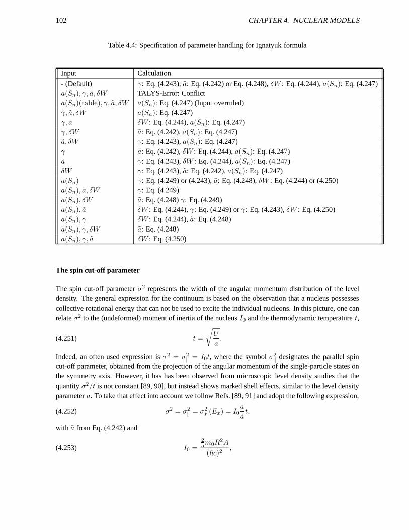
102 CHAPTER 4. NUCLEAR MODELS
Table 4.4: Specification of parameter handling for Ignatyukformula
Input Calculation- (Default) γ: Eq. (4.243),a: Eq. (4.242) or Eq. (4.248),δW : Eq. (4.244),a(Sn): Eq. (4.247)a(Sn), γ, a, δW TALYS-Error: Conflicta(Sn)(table), γ, a, δW a(Sn): Eq. (4.247) (Input overruled)γ, a, δW a(Sn): Eq. (4.247)γ, a δW : Eq. (4.244),a(Sn): Eq. (4.247)γ, δW a: Eq. (4.242),a(Sn): Eq. (4.247)a, δW γ: Eq. (4.243),a(Sn): Eq. (4.247)γ a: Eq. (4.242),δW : Eq. (4.244),a(Sn): Eq. (4.247)a γ: Eq. (4.243),δW : Eq. (4.244),a(Sn): Eq. (4.247)δW γ: Eq. (4.243),a: Eq. (4.242),a(Sn): Eq. (4.247)a(Sn) γ: Eq. (4.249) or (4.243),a: Eq. (4.248),δW : Eq. (4.244) or (4.250)a(Sn), a, δW γ: Eq. (4.249)a(Sn), δW a: Eq. (4.248)γ: Eq. (4.249)a(Sn), a δW : Eq. (4.244),γ: Eq. (4.249) orγ: Eq. (4.243),δW : Eq. (4.250)a(Sn), γ δW : Eq. (4.244),a: Eq. (4.248)a(Sn), γ, δW a: Eq. (4.248)a(Sn), γ, a δW : Eq. (4.250)
The spin cut-off parameter
The spin cut-off parameterσ2 represents the width of the angular momentum distribution of the leveldensity. The general expression for the continuum is based on the observation that a nucleus possessescollective rotational energy that can not be used to excite the individual nucleons. In this picture, one canrelateσ2 to the (undeformed) moment of inertia of the nucleusI0 and the thermodynamic temperaturet,
(4.251) t =
√
U
a.
Indeed, an often used expression isσ2 = σ2‖ = I0t, where the symbolσ2
‖ designates the parallel spincut-off parameter, obtained from the projection of the angular momentum of the single-particle states onthe symmetry axis. However, it has has been observed from microscopic level density studies that thequantityσ2/t is not constant [89, 90], but instead shows marked shell effects, similar to the level densityparametera. To take that effect into account we follow Refs. [89, 91] andadopt the following expression,
(4.252) σ2 = σ2‖ = σ2
F (Ex) = I0a
at,
with a from Eq. (4.242) and
(4.253) I0 =25m0R
2A
(~c)2,
4.7. LEVEL DENSITIES 103
whereR = 1.2A1/3 is the radius, andm0 the neutron mass in amu. This gives
(4.254) σ2F (Ex) = 0.01389
A5/3
a
√aU.
On average, the√
aU/a has the same energy- and mass-dependent behaviour as the temperature√
U/a.The differences occur in the regions with large shell effects. Eq. (4.254) can be altered by means of thespincut keyword, see page 233.
Analogous to the level density parameter, we have to accountfor low excitation energies for whichEq. (4.254) is not defined (Ex ≤ ∆) or less appropriate. This leads us to an alternative methodtodetermine the spin cut-off parameter, namely from the spinsof the low-lying discrete levels. Supposewe want to determine this discrete spin cut-off parameterσ2
d in the energy range where the total leveldensity agrees well with the discrete level sequence, i.e. from a lower discrete levelNL with energyEL
to an upper levelNU with energyEU . It can be derived that
(4.255) σ2d =
1
3∑NU
i=NL(2Ji + 1)
NU∑
i=NL
Ji(Ji + 1)(2Ji + 1).
whereJi is the spin of discrete leveli. Reading these spins from the discrete level file readily gives thevalue forσ2
d. In TALYS, σ2d can be used on a nucleus-by-nucleus basis, when discrete levels are known.
For cases where either Eqs. (4.254) or (4.255) are not applicable, e.g. because there are no discrete levelsandU = Ex − P is negative, we take the systematical formula
(4.256) σ2 =(
0.83A0.26)2
which gives a reasonable estimate for energies in the order of 1-2 MeV.
The final functional form forσ2(Ex) is a combination of Eqs. (4.254) and (4.255). DefiningEd = 1
2(EL + EU ) as the energy in the middle of theNL − NU region, we assumeσ2d is constant up to
this energy and can then be linearly interpolated to the expression given by Eq. (4.254). We choose thematching point to be the neutron separation energySn of the nucleus under consideration, i.e.
σ2(Ex) = σ2d for 0 ≤ Ex ≤ Ed
= σ2d +
Ex − Ed
Sn − Ed(σ2
F (Ex) − σ2d) for Ed ≤ Ex ≤ Sn
= σ2F (Ex) for Ex ≥ Sn.(4.257)
Analogous to the level density parametera, from now on we implicitly assume the energy dependencefor σ2(Ex) wheneverσ2 appears in the formalism.
Constant Temperature Model
In the Constant Temperature Model (CTM), as introduced by Gilbert and Cameron [83], the excitationenergy range is divided into a low energy part from 0 MeV up to amatching energyEM , where the
104 CHAPTER 4. NUCLEAR MODELS
so-called constant temperature law applies and a high energy part aboveEM , where the Fermi gas modelapplies. Hence, for the total level density we have
ρtot(Ex) = ρtotT (Ex), if Ex ≤ EM ,
= ρtotF (Ex), if Ex ≥ EM ,(4.258)
and similarly for the level density
ρ(Ex, J,Π) =1
2RF (Ex, J)ρtot
T (Ex), if Ex ≤ EM ,
= ρF (Ex, J,Π), if Ex ≥ EM .(4.259)
Note that the spin distribution of Eq. (4.237) is also used inthe constant temperature region, includingthe low-energy behaviour for the spin cut-off parameter as expressed by Eq. (4.257).
For the Fermi gas expression, we use the effective excitation energyU = Ex − ∆CTM, where theenergy shift is given by
(4.260) ∆CTM = χ12√A
,
with
χ = 0, for odd − odd,
= 1, for odd − even,
= 2, for even − even.(4.261)
Note that by default no adjustable pairing shift parameter is used in the CTM. In TALYS, the number 12in the enumerator of Eq. (4.260) can be altered using thepairconstant keyword, see page 228. This alsoapplies to the other level density models.
For low excitation energy, the CTM is based on the experimental evidence that the cumulatedhistogramN(Ex) of the first discrete levels can be well reproduced by an exponential law of the type
(4.262) N(Ex) = exp(Ex − E0
T),
which is called the constant temperature law. The nuclear temperatureT andE0 are parameters thatserve to adjust the formula to the experimental discrete levels. Accordingly, the constant temperaturepart of the total level density reads
(4.263) ρtotT (Ex) =
dN(Ex)
dEx=
1
Texp(
Ex − E0
T).
For higher energies, the Fermi gas model is more suitable andthe total level density is given byEq. (4.238). The expressions forρtot
T andρtotF have to be matched at a matching energyEM where they,
and their derivatives, are identical. First, continuity requires that
(4.264) ρtotT (EM ) = ρtot
F (EM ).
4.7. LEVEL DENSITIES 105
Inserting Eq. (4.263) in this equation directly leads to thecondition
(4.265) E0 = EM − T ln[
TρtotF (EM )
]
.
Second, continuity of the derivatives requires that
(4.266)dρtot
T
dEx(EM ) =
dρtotF
dEx(EM ).
Inserting Eq. (4.263) in this equation directly leads to thecondition
(4.267)ρtot
T (EM )
T=
dρtotF
dEx(EM ),
or
(4.268)1
T=
d ln ρtotF
dEx(EM ).
In principle, for all Fermi gas type expressions, includingthe energy dependent expressions fora, σ2,Krot etc., Eq. (4.268) could be elaborated analytically, but in practice we use a numerical approach toallow any level density model to be used in the matching problem. For this, we determine the inversetemperature of Eq. (4.268) numerically by calculatingρtot
F on a sufficiently dense energy grid.
The matching problem gives us two conditions, given by Eqs. (4.265) and (4.268), with threeunknowns:T,E0 andEM . Hence, we need another constraint. This is obtained by demanding that inthe discrete level region the constant temperature law reproduces the experimental discrete levels, i.e.ρtot
T needs to obey
(4.269) NU = NL +
∫ EU
EL
dExρtot(Ex),
or, after inserting Eq. (4.263),
(4.270) NU = NL +
(
exp[EU
T] − exp[
EL
T]
)
exp[−E0
T].
The combination of Eqs. (4.265), (4.268) and (4.270) determinesT,E0 andEM . Inserting Eq. (4.265)in Eq. (4.270) yields:
(4.271) TρtotF (EM ) exp[
−EM
T]
(
exp[EU
T] − exp[
EL
T]
)
+ NL − NU = 0,
from whichEM can be solved by an iterative procedure with the simultaneous use of the tabulated valuesgiven by Eq. (4.268). The levelsNL andNU are chosen such thatρT (Ex) gives the best description ofthe observed discrete states and are stored in the nuclear structure database. For nuclides for which no, ornot enough, discrete levels are given we rely on empirical formula for the temperature. For the effectivemodel,
(4.272) T = −0.22 +9.4
√
A(1 + γδW )

106 CHAPTER 4. NUCLEAR MODELS
and for the collective model
(4.273) T = −0.25 +10.2
√
A(1 + γδW )
whereγ is taken from Eq. (4.243) and Table 4.3. Next, we directly obtain EM from Eq. (4.268) andE0
from Eq. (4.265). Again, Eqs. (4.272) and (4.273) were obtained by fitting all individual values of thenuclides for which sufficient discrete level information exists. In a few cases, the global expression forT leads to a value forEM which is clearly off scale. In that case, we resort to empirical expressions forthe matching energy. For the effective model
(4.274) EM = 2.33 + 253/A + ∆CTM ,
and for the collective model
(4.275) EM = 2.67 + 253/A + ∆CTM ,
after which we obtainT from Eq. (4.268).
The Back-shifted Fermi gas Model
In the Back-shifted Fermi gas Model (BFM) [84], the pairing energy is treated as an adjustable parameterand the Fermi gas expression is used all the way down to 0 MeV. Hence for the total level density wehave
(4.276) ρtotF (Ex) =
1√2πσ
√π
12
exp[
2√
aU]
a1/4U5/4,
and for the level density,
(4.277) ρF (Ex, J,Π) =1
2
2J + 1
2√
2πσ3exp
[
−(J + 12 )2
2σ2
] √π
12
exp[
2√
aU]
a1/4U5/4,
respectively. These expressions, as well as the energy-dependent expressions fora andσ2, contain theeffective excitation energyU = Ex − ∆BFM, where the energy shift is given by
(4.278) ∆BFM = χ12√A
+ δ,
with
χ = −1, for odd − odd,
= 0, for odd − even,
= 1, for even − even,(4.279)
andδ an adjustable parameter to fit experimental data per nucleus.
4.7. LEVEL DENSITIES 107
A problem of the original BFM, which may have hampered its useas the default level densityoption in nuclear model analyses, is the divergence of Eqs. (4.276)-(4.277) whenU goes to zero. Asolution to this problem has been provided by Grossjean and Feldmeier [93], has been put into a practicalform by Demetriou and Goriely [97], and is adopted in TALYS. The expression for the total BFM leveldensity is
(4.280) ρtotBFM(Ex) =
[
1
ρtotF (Ex)
+1
ρ0(t)
]−1
,
whereρ0 is given by
(4.281) ρ0(t) =exp(1)
24σ
(an + ap)2
√anap
exp(4anapt2),
wherean = ap = a/2 andt is given by Eq. (4.251).
With the usual spin distribution, the level density reads
(4.282) ρBFM(Ex, J,Π) =1
2
2J + 1
2σ2exp
[
−(J + 12)2
2σ2
]
ρtotBFM(Ex).
In sum, there are two adjustable parameters for the BFM,a andδ.
The Generalized Superfluid Model
The Generalized Superfluid Model (GSM) takes superconductive pairing correlations into account ac-cording to the Bardeen-Cooper-Schrieffer theory. The phenomenological version of the model [101, 102]is characterized by a phase transition from a superfluid behaviour at low energy, where pairing correla-tions strongly influence the level density, to a high energy region which is described by the FGM. TheGSM thus resembles the CTM to the extent that it distinguishes between a low energy and a high energyregion, although for the GSM this distinction follows naturally from the theory and does not depend onspecific discrete levels that determine a matching energy. Instead, the model automatically provides aconstant temperature-like behaviour at low energies. For the level density expressions, it is useful torecall the general formula for the total level density,
(4.283) ρtot(Ex) =1√2πσ
eS
√D
,
whereS is the entropy andD is the determinant related to the saddle-point approximation. For the GSMthis expression has two forms: one below and one above the so called critical energyUc.
For energies belowUc, the level density is described in terms of thermodynamicalfunctions de-finedat Uc, which is given by
(4.284) Uc = acT2c + Econd.
Here, the critical temperatureTc is
(4.285) Tc = 0.567∆0,
108 CHAPTER 4. NUCLEAR MODELS
where the pairing correlation function is given by
(4.286) ∆0 =12√A
.
This correlation function also determines the condensation energyEcond, which characterizes the de-crease of the superfluid phase relative to the Fermi gas phase. It is given by the expression
(4.287) Econd =3
2π2ac∆
20,
where the critical level density parameterac is given by the iterative equation
(4.288) ac = a
[
1 + δW1 − exp(−γacT
2c )
acT 2c
]
,
which is easily obtained oncea, δW andγ are known. Eq. (4.288) indicates that shell effects are againappropriately taken into account. For the determination ofthe level density we also invoke the expressionfor the critical entropySc,
(4.289) Sc = 2 ac Tc,
the critical determinantDc,
(4.290) Dc =144
πa3
c T 5c ,
and the critical spin cut-off parameterσ2c ,
(4.291) σ2c = 0.01389A5/3 ac
aTc.
Now that everything is specified atUc, we can use the superfluid Equation Of State (EOS) to definethe level density belowUc. For this, we define an effective excitation energy
(4.292) U ′ = Ex + χ∆0 + δ,
where
χ = 2, for odd − odd,
= 1, for odd − even,
= 0, for even − even,(4.293)
andδ is an adjustable shift parameter to obtain the best description of experimental data per nucleus.Note that the convention forχ is again different from that of the BFM or CTM. Defining
(4.294) ϕ2 = 1 − U ′
Uc,
then forU ′ ≤ Uc the quantitiesϕ andT obey the superfluid EOS [101],
(4.295) ϕ = tanh
(
Tc
Tϕ
)
,
4.7. LEVEL DENSITIES 109
which is equivalent to
(4.296) T = 2Tc ϕ
[
ln1 + ϕ
1 − ϕ
]−1
.
The other required functions forU ′ ≤ Uc are the entropyS,
(4.297) S = ScTc
T
(
1 − ϕ2)
= ScTc
T
U ′
Uc,
the determinant D,
(4.298) D = Dc
(
1 − ϕ2) (
1 + ϕ2)2
= DcU ′
Uc
(
2 − U ′
Uc
)2
,
and the spin cut-off parameter
(4.299) σ2 = σ2c
(
1 − ϕ2)
= σ2c
U ′
Uc.
In sum, the level density can now be specified for the entire energy range. ForU ′ ≤ Uc, the total leveldensity is given by
(4.300) ρtotGSM(Ex) =
1√2πσ
eS
√D
,
using Eqs. (4.297)-(4.299). Similarly, the level density is
(4.301) ρGSM(Ex, J,Π) =1
2RF (Ex, J)ρtot
GSM(Ex).
For U ′ ≥ Uc the FGM applies, though with an energy shift that is different from the pairingcorrection of the CTM and BFM. The total level density is
(4.302) ρtotGSM(Ex) =
1√2πσ
√π
12
exp[
2√
aU]
a1/4U5/4,
where the effective excitation energy is defined byU = Ex − ∆GSM , with
(4.303) ∆GSM = Econd − χ∆0 − δ.
The spin cut-off parameter in the high-energy region reads
(4.304) σ2 = I0a
a
√
U
a,
andI0 is given by Eq. (4.253). The level density is given by
(4.305) ρGSM(Ex, J,Π) =1
2RF (Ex, J)ρtot
GSM(Ex).
At the matching energy, i.e., forE′x = Uc − χ∆0 − δ, it is easy to verify that Eqs. (4.300) and
(4.302) match so that the total level density is perfectly continuous. In sum, there are two adjustableparameters for the GSM,a andδ.
110 CHAPTER 4. NUCLEAR MODELS
4.7.2 Collective effects in the level density
All the previously described models do not explicitly account for collective effects. However, it is wellknown that generally the first excited levels of nuclei result from coherent excitations of the fermionsit contains. The Fermi gas model is not appropriate to describe such levels. Nevertheless, the modelspresented so far can still be applied successfully in most cases since they incorporate collectivity in thelevel density in an effective way through a proper choice of the energy-dependent level density parametervalues.
In some calculations, especially if the disappearance of collective effects with excitation energyplays a role (e.g. in the case of fission), one would like to model the collective effects in more detail.It can be shown that the collective effects may be accounted for explicitly by introducing collectiveenhancement factors on top of an intrinsic level densityρF,int(Ex, J,Π). Then the deformed Fermi gaslevel densityρF,def(Ex, J,Π) reads
(4.306) ρF,def(Ex, J,Π) = Krot(Ex)Kvib(Ex)ρF,int(Ex, J,Π),
while the total level densitiesρtotF,def andρtot
F,int are related in the same way.Krot andKvib are called therotational and vibrational enhancement factors, respectively. If Krot andKvib are explicitly accountedfor, ρF,int(Ex, J,Π) should now describe purely single-particle excitations, and can be determined againby using the Fermi gas formula. Obviously, the level densityparametera of ρF,int will be different fromthat of the effective level density described before.
The vibrational enhancement of the level density is approximated [163] by
(4.307) Kvib = exp[δS − (δU/t)],
where δS and δU are changes in the entropy and excitation energy, respectively, resulting from thevibrational modes andT is the nuclear temperature given by Eq. (4.251). These changes are describedby the Bose gas relationships, i.e
δS =∑
i
(2λi + 1)[
(1 + ni) ln(1 + ni) − ni ln ni
]
,
δU =∑
i
(2λi + 1)ωini,(4.308)
whereωi are the energies,λi the multipolarities, andni the occupation numbers for vibrational excita-tions at a given temperature. The disappearance of collective enhancement of the level density at hightemperatures can be taken into account by defining the occupation numbers in terms of the equation
(4.309) ni =exp(−γi/2ωi)
exp(ωi/T ) − 1,
whereγi are the spreading widths of the vibrational excitations. This spreading of collective excitationsin nuclei should be similar to the zero-sound damping in a Fermi liquid, and the corresponding width canbe written as
(4.310) γi = C(ω2i + 4π2T 2).
4.7. LEVEL DENSITIES 111
The value ofC = 0.0075 A1/3 was obtained from the systematics of the neutron resonance densities ofmedium-weight nuclei [94]. We use a modified systematics [163] which includes shell effects to estimatethe phonon energies (in MeV), namely
(4.311) ω2 = 65A−5/6/(1 + 0.05δW ),
for the quadrupole vibrations and
(4.312) ω3 = 100A−5/6/(1 + 0.05δW ),
for the octupole excitations.
An alternative, liquid drop model, estimation of the vibrational collective enhancement factor isgiven by [92]
(4.313) Kvib(Ex) = exp(
0.0555A2
3 t4
3
)
.
Thekvibmodel keyword can be used to choose between these models.
A more important contribution to the collective enhancement of the level density originates fromrotational excitations. Its effect is not only much stronger (Krot ∼ 10 − 100 whereasKvib ∼ 3), but theform for the rotational enhancement depends on the nuclear shape as well. This makes it crucial, amongothers, for the description of fission cross sections.
The expression for the rotational enhancement factor depends on the deformation [163, 95]. Basi-cally, Krot is equal to the perpendicular spin cut-off parameterσ2
⊥,
(4.314) σ2⊥ = I⊥t,
with the rigid-body moment of inertia perpendicular to the symmetry axis given by
(4.315) I⊥ = I0
(
1 +β2
3
)
= 0.01389A5/3
(
1 +β2
3
)
,
whereβ2 is the ground-state quadrupole deformation, which we take from the nuclear structure database.Hence,
(4.316) σ2⊥ = 0.01389A5/3
(
1 +β2
3
)
√
U
a.
For high excitation energies, it is known that the rotational behavior vanishes. To take this intoaccount, it is customary to introduce a phenomenological damping functionf(Ex) which is equal to 1in the purely deformed case and 0 in the spherical case. The expression for the level density is then
ρ(Ex, J,Π) = [1 − f(Ex)]Kvib(Ex)ρF,int(Ex, J,Π) + f(Ex)ρF,def(Ex, J,Π)
= Krot(Ex)Kvib(Ex)ρF,int(Ex, J,Π)(4.317)
where
(4.318) Krot(Ex) = max([σ2⊥ − 1]f(Ex) + 1, 1).
112 CHAPTER 4. NUCLEAR MODELS
The functionf(Ex) is taken as a combination of Fermi functions,
(4.319) f(Ex) =1
1 + exp(Ex−Eg.s.
col
dg.s.col
),
which yields the desired property ofKrot going to 1 for high excitation energy. Little is known about theparameters that govern this damping, although attempts have been made (see e.g. [96]). We arbitrarilytakeEg.s.
col = 30 MeV, dg.s.col = 5 MeV.
Finally, these collective enhancement expressions can be applied to the various phenomenologicallevel density models. The CTM formalism can be extended withexplicit collective enhancement, i.e. thetotal level density reads
ρtot(Ex) = ρtotT (Ex), if Ex ≤ EM ,
= Krot(Ex)Kvib(Ex)ρtotF,int(Ex), if Ex ≥ EM ,(4.320)
and similarly for the level densityρ(Ex, J,Π). Note that the collective enhancement is not applied tothe constant temperature region, since collectivity is assumed to be already implicitly included in thediscrete levels. The matching problem is completely analogous to that described before, although theresulting parametersEM , E0 andT will of course be different.
The BFM can also be extended with explicit collective enhancement, i.e.
(4.321) ρtotBFM(Ex) = Krot(Ex)Kvib(Ex)
[
1
ρtotF,int(Ex)
+1
ρ0(t)
]−1
,
and similarly for the level densityρ(Ex, J,Π). Finally, the GSM can be extended as follows
(4.322) ρtotGSM(Ex) = Krot(Ex)Kvib(Ex)ρtot
GSM,int(Ex).
(In fact, the term “general” in the GSM was originally meant for the collective enhancement).
4.7.3 Microscopic level densities
Besides the phenomenological models that are used in TALYS,there is also an option to employ moremicroscopic approaches. For the RIPL database, S. Goriely has calculated level densities from drip lineto drip line on the basis of Hartree-Fock calculations [98] for excitation energies up to 150 MeV andfor spin values up toI = 30. If ldmodel 4, see page 223, these tables with microscopic level densitiescan be read. Moreover, new energy-, spin- and parity-dependent nuclear level densities based on themicroscopic combinatorial model have been proposed by Hilaire and Goriely [169]. The combinatorialmodel includes a detailed microscopic calculation of the intrinsic state density and collective enhance-ment. The only phenomenological aspect of the model is a simple damping function for the transitionfrom spherical to deformed, see also Eq. (4.317). The calculations make coherent use of nuclear struc-ture properties determined within the deformed Skyrme-Hartree-Fock-Bogolyubov framework. Leveldensities for more than 8500 nuclei are made available in tabular format, for excitation energies up to200 MeV and for spin values up toJ = 49. These level densities are used withldmodel 5.
4.8. FISSION 113
The most recent option, invoked withldmodel 6, is based on temperature-dependent Hartree-Fock-Bogolyubov calculations using the Gogny force [138].
Since these microscopical level densities, which we will call ρHFM, have not been adjusted toexperimental data, we add adjustment flexibility through a scaling function, i.e.
(4.323) ρ(Ex, J, π) = exp(c√
Ex − δ)ρHFM (Ex − δ, J, π)
where by defaultc = 0 andδ = 0 (i.e. unaltered values from the tables). The “pairing shift” δ simplyimplies obtaining the level density from the table at a different energy. The constantc plays a role similarto that of the level density parametera of phenomenological models. Adjustingc andδ together givesadjustment flexibility at both low and higher energies.
For both microscopic level density models, tables for leveldensities on top of the fission barriersare automatically invoked forldmodel 4, 5or 6, when available in the structure database. For nuclidesoutside the tabulated microscopic database, the default Fermi gas model is used.
4.8 Fission
The probability that a nucleus fissions can be estimated by TALYS on both phenomenological and mi-croscopic grounds. Cross sections for (multi-chance) fission can be calculated. For this, various nuclearquantities are required.
4.8.1 Level densities for fission barriers
The level density formulae given in Section 4.7 for the ground state of the nucleus can all be appliedfor the fission barriers. In general, only the ingredients for a few level density expressions change ascompared to the non-fissile case. In TALYS, two methods for fission level densities are programmed.The level densities are used in the calculation of fission transmission coefficients.
Explicit treatment of collective effects
Eq. (4.318) for the rotational enhancement also holds for inner barriers with neutron numberN ≤ 144,which are all assumed to be axially symmetric (specified by the keywordaxtype 1). Inner barriers withN > 144, e.g. the Am-isotopes, are taken to be axially asymmetric (axtype 3), and in that case therotational enhancement is
(4.324) Krot(Ex) = Kasymrot (Ex, β2) = max([
√
π
2σ2⊥(1 − 2β2
3)σ‖ − 1]f(Ex) + 1, 1).
For outer barriers, we apply an extra factor of 2 toKrot, due to the mass asymmetry. For all fissionbarriers, the default parameters for the damping function Eq. (4.319) areU bar
f = 45 MeV, Cbarf = 5
MeV.
The shell correction is also different: For the inner barrier, δW = 1.5 MeV for an axially sym-metric barrier, and 2.5 MeV otherwise. For the other barriers, we take 0.6 MeV in general.
114 CHAPTER 4. NUCLEAR MODELS
Effective treatment of collective effects
Despite being of a more “effective” nature than the approachdescribed above, this method (invoked withcolldamp y) has been more successful in the description of fission crosssections, see e.g. [459]. Anessential aspect is that the damping of collective effects are taken into account in a phenomenologicalway through the level density parametera. The asymptotic level density parametera, see Eq. (4.242) isdamped from its effective limitA/8 to its intrinsic limit A/13 as follows
(4.325) aeff =A
13f(Ex) + a(1 − f(Ex))
where
(4.326) f(Ex) =1
1 + exp−(Ex−Eg.s.
col
dg.s.col
),
with the same values as mentioned below Eq. (4.319). Next, the resultinga(Ex) is used in all equations.After this, an extra rotational enhancement needs only to betaken into account for tri-axial barriers(axtype 2). Instead of Eq. (4.318), this is taken as
(4.327) Krot(Ex) = (U
aeff)1/4(1 − f(Ex)) + f(Ex),
whereaeff = 8a/13 and
(4.328) f(Ex) =1
1 + exp(−12 (Ex − 18)
,
For barriers other than tri-axial,Krot = 1. There is no vibrational enhancement in this model. For theshell correction, for all barriersδW = 2
3 |δW g.s.|. Finally, the spin cut-off parameter (4.257) is multiplied
by(
1 + β2
3
)
as done in Eq. (4.315) for the perpendicular spin cut-off parameter.
4.8.2 Fission transmission coefficients
For fission, the default model implemented in TALYS is based on the transition state hypothesis of Bohrand the Hill-Wheeler expression. This yields transmissioncoefficients that enter the Hauser-Feshbachmodel to compete with the particle and photon transmission coefficients.
Transmission coefficient for one fission barrier
The Hill-Wheeler expression gives the probability of tunneling through a barrier with heightBf andwidth ~ωf for a compound nucleus with excitation energyEx. It reads
(4.329) Tf (Ex) =1
1 + exp[
−2π(Ex−Bf )
~ωf
]

4.8. FISSION 115
For a transition state with excitation energyεi above the top of the same barrier, one has
(4.330) Tf (Ex, εi) =1
1 + exp[
−2π(Ex−Bf−εi)
~ωf
]
which means that the barrier is simply shifted up byεi.
For a compound nucleus with excitation energyEx, spinJ , and parityΠ, the total fission trans-mission coefficient is the sum of the individual transmissions coefficients for each barrier through whichthe nucleus may tunnel, and thus reads in terms of the previously introducedTf (Ex, εi)
(4.331) T J,Πf (Ex) =
∑
i
Tf (Ex, εi)f(i, J,Π) +
∫ Ex
Eth
ρ(ε, J,Π)Tf (Ex, ε)dε
The summation runs over all discrete transition states on top of the barrier andEth marks the beginningof the continuum. In this equation,f(i, J,Π) = 1 if the spin and parity of the transition state equal thatof the compound nucleus and0 otherwise. Moreover,ρ(ε, J,Π) is the level density of fission channelswith spin J and parityΠ for an excitation energyε. The main difference with the usually employedexpressions is that the upper limit in the integration is finite. This expression also enables to definethe number of fission channels by replacingTf (Ex, εi) by 1 in Eq. (4.331). This is needed for widthfluctuation calculations where the fission transmission coefficient is treated as a continuum transmissioncoefficient.
4.8.3 Transmission coefficient for multi-humped barriers
For double humped barriers, the generally employed expression is based on an effective transmissioncoefficientTeff defined by
(4.332) Teff =TATB
TA + TB
whereTA andTB are the transmission coefficients for barrierA and B respectively, calculated withEq. (4.331).
If a triple humped barrier needs to be considered, the expression forTeff reads
(4.333) Teff =TABTC
TAB + TC
whereTAB is given by Eq. (4.332). Consequently, the expression used in TALYS reads
(4.334) Teff =TATBTC
TATB + TATC + TBTC
For any number of barrier, the effective number of fission channels is calculated as in the case forone barrier [183].
116 CHAPTER 4. NUCLEAR MODELS
4.8.4 Class II/III states
Class II (resp. III) states may be introduced when double (resp. triple) humped barriers are considered.In the particular situation where the excitation energyECN of the compound nucleus is lower thanthe barrier heights, fission transmission coefficients display resonant structures which are due to thepresence of nuclear excited levels (Class II) in the second,or in the third (Class III) well of the potentialenergy surface. When such resonant structures occur, the expression for the effective fission transmissioncoefficient has to be modified (generally enhanced).
The way this resonant effect is determined depends on the number of barriers that are considered.
Double humped fission barrier
In the case where two barriers occur, the effective fission transmission coefficientTeff can be written as
(4.335) Teff =TATB
TA + TB× FAB(ECN )
whereFAB(ECN ) is a factor whose value depends on the energy difference between the excitationenergy of the nucleus and that of the a class II state located in the well between barrierA andB. It hasbeen shown [100] that the maximum value ofFAB(E) reaches 4
TA+TBand gradually decreases over an
energy interval defined as the widthΓII of the class II state with excitation energyEII . This is accountedfor using the empirical quadratic expression
(4.336) FAB(E) =4
TA + TB+
(
E − EII
0.5ΓII
)2
×(
1 − 4
TA + TB
)
if EII − 0.5ΓII ≤ E ≤ EII + 0.5ΓII andFAB = 1 otherwise.
Theoretically, this expression is valid for the tunneling through a single double humped barrierwhereas in realistic situations, bothTA andTB are obtained from a summation over several transitionstates. One may thus have largeTA andTB values so that Eq. 4.336 may giveFAB(E) ≤ 1. Sucha situation can only occur for high enough excitation energies for which the individual Hill-Wheelercontributions in Eq. (4.331) are large enough. However, in TALYS, we only consider class II states withexcitation energies lower than the height of the first barrier. Consequently, the resonant effect can onlyoccur if the compound nucleus energyECN is (i) lower than the top of the first barrier and (ii) close to aresonant class II state (EII − 0.5ΓII ≤ ECN ≤ EII + 0.5ΓII ). With such requirements, the individualHill-Wheeler terms are clearly small, andTA + TB ≪ 1.
Triple humped fission barrier
If three barriersA, B and C are considered, the situation is more complicated. In this case, threesituations can occur depending on the positions of the classII and class III states. Indeed the enhancement
4.8. FISSION 117
can be due either to a class II state or to a class III state, buton top of that, a double resonant effect canalso occur if both a class II and a class III state have an excitation energy close to the compound nucleusenergy. For any situation, the enhancement is first calculated for the first and the second barrier givingthe transmission coefficient
(4.337) TABeff = TAB × FAB
with FAB given by Eq. (4.336) as in the previous case.
Next, the eventual coupling with a class III state with energy EIII of width ΓIII is accounted forby generalizing Eq. (4.335) writing
(4.338) TABCeff =
TABeff TC
TABeff + TC
× FABC(ECN )
whereFABC(ECN ) is given by generalizing Eq. (4.336) writing
(4.339) FABC(E) =4
TABeff + TC
+
(
E − EIII
0.5ΓIII
)2
×(
1 − 4
TABeff + TC
)
if EIII − 0.5ΓIII ≤ E ≤ EIII + 0.5ΓIII andFABC = 1 otherwise.
4.8.5 Fission barrier parameters
In TALYS several options are included for the choice of the fission barrier parameters:
1. Experimental parameters [163]: collection of a large setof actinide fission barrier heights andcurvatures for both the inner and outer barrier based on a fit to experimental data, compiled by V.Maslov. Moreover, this compilation contains head band transition states.
2. Mamdouh parameters [106]: set of double-humped fission barrier heights for numerous isotopesderived from Extended Thomas-Fermi plus Strutinsky Integral calculations.
3. Rotating-Finite-Range Model (RFRM) by Sierk [103]: single-humped fission barrier heights aredetermined within a rotating liquid drop model, extended with finite-range effects in the nuclearsurface energy and finite surface-diffuseness effects in the Coulomb energy.
4. Rotating-Liquid-Drop Model (RLDM) by Cohenet al [104].
In the current version of TALYS, the dependence on angular momentum of the fission barriers is dis-carded. If LDM barriers are employed in the calculation, they are corrected for the difference betweenthe ground-state and fission barrier shell correction energy:
(4.340) BLDMf (T ) = BLDM
f (0) − (δWgroundstate − δWbarrier) ∗ g(T )
118 CHAPTER 4. NUCLEAR MODELS
This correction gradually disappears with temperature dueto the washing out of the shell effects [107]:
(4.341) g(T ) =
1 for T < 1.65MeV,
g(T ) = 5.809 exp(−1.066 T ) for T ≥ 1.65MeV.
Shell corrections on top of the fission barrier are generallyunknown. They obviously play an importantrole for the level density as well. Default values are adopted: for subactinidesδWbarrier = 0 MeV, foractinidesδWbarrier,inner = 2.5 MeV andδWbarrier,outer = 0.6 MeV [163].
4.8.6 WKB approximation
As an alternative to the Hill-Wheeler approach, it is also possible to use the WKB approximation tocalculate fission transmission coefficients We use an implementation by Mihaela Sin and Roberto Capoteand refer to Ref. [105] for the full details of this method. Itcan be invoked with the keywordfismodel 5.
4.8.7 Fission fragment properties
Since TALYS-1.6, two models for fission fragments are available, the temperature dependent Brosamodel, and the GEF model.
GEF model
A fission model has been developed model by Schmidt-Jurado [115] It is based on the statistical pop-ulation of states in the fission valleys at the moment of dynamical freeze-out, which is specific to eachcollective degree of freedom. Three fission channels are considered. The separability principle governsthe interplay of macroscopic and microscopic effects. The newly discovered energy-sorting mechanismdetermines the division of intrinsic excitation energy between the fragments at scission and the creationof a strong even-odd effect at large mass asymmetry. This model gives a new insight into several dy-namical times. Most parameters are fixed from independent sources, only about 20 parameters havespecifically been adjusted. Since the parameters of the model are closely related to physical properties ofthe systems, valuable conclusions on the fission process canbe deduced. The good reproduction of mea-sured data and the high predictive power of the code make it useful for applications in nuclear technologyand complement the use of purely empirical models.
Temperature-dependent Brosa model
The description of fission fragment and product yields follows the procedure outlined in Ref. [109]. TheHauser-Feshbach formalism gives a fission cross section perexcitation energy bin for each fissioningsystem. The fission fragment masses and charges are, subsequently, determined per given excitationenergy bin Ex, in a fissioning system FS, characterised by(ZFS, AFS , Ex), for which the fission crosssection exceeds some minimum value. The total fragment massdistribution is given by a sum over all
4.8. FISSION 119
contributing bins weighted with the corresponding fission cross sections:
(4.342) σ(AFF ) =∑
ZF S ,AF S,Ex
σf (ZFS , AFS, Ex)Y (AFF ;ZFS, AFS , Ex),
whereY (AFF ;ZFS , AFS , Ex) is the relative yield of a fission fragment with massAFF originating froma fissioning system. Combining this expression with the result of a fission fragment charge distributioncalculation yields the final production cross section of a fission fragment with massAFF and chargeZFF :
σprod(ZFF , AFF ) =∑
ZF S ,AF S ,Ex
σf (ZFS , AFS , Ex)Y (AFF ;ZFS , AFS , Ex)
×Y (ZFF ;AFF , ZFS , AFS, Ex)(4.343)
Y (ZFF ;AFF , ZFS, AFS , Ex) is the relative yield of a fission fragment with chargeZFF given its massAFF and the fissioning system characterised by(ZFS, AFS , Ex).
In general, an excitation energy distribution is connectedto these fissionfragmentproductioncross sections. In theory, this could be used to deduce the fission product yields through a full evap-oration calculation of the fission fragments. This is not yetpossible in TALYS. Instead a rather crudeapproximation, outlined later in this section, is adopted to estimate the number of post-scission neu-trons emitted from each fragment. This procedure leads to relative yields for the fission product massesY (AFP ;ZFS , AFS , Ex) and chargesY (ZFP ;AFP , ZFS, AFS , Ex) and, hence, to expressions similarto Eq. (4.342) and Eq. (4.343) for the final fission products.
Fission fragment mass distribution
The fission fragment mass distribution is determined with a revised version of the multi-modal randomneck-rupture model (MM-RNRM). The original model has been developed by Brosa to calculate proper-ties of fission fragments at zero temperature [108]. However, fission calculations within TALYS requirefragment mass distributions up to higher temperatures.
In the recent version of the model [109] the temperature is added to the calculation of the potentialenergy landscape of the nucleus. A search for the fission channels in deformation space yields thesuperlong (SL), standard I (ST I), and standard II (ST II) fission barriers and prescission shapes as afunction of temperature. In this manner, the incorporated melting of shell effects naturally gives rise tothe vanishing of the asymmetric fission modes ST I and ST II with increasing excitation energies. Theobtained temperature-dependent fission barrier and prescission shape parameters serve as input for thefragment mass distribution computations in TALYS.
Each mass distribution is a sum over contributions of the three dominant fission modes FM:(4.344)
Y (AFF ;ZFS , AFS , Ex) =∑
FM=SL,STI,STII
WFM(ZFS , AFS , Ex)YFM (AFF ;ZFS , AFS , Ex),
whereWFM (ZFS, AFS , Ex) denotes the weight of a fission mode, andYFM(AFF ;ZFS , AFS , Ex) isthe corresponding mass distribution.Y (AFF ;ZFS , AFS , Ex) can then be substituted in Eq. (4.342) to
120 CHAPTER 4. NUCLEAR MODELS
determine the full fission fragment mass distribution for the reaction under consideration. An analogousexpression can be written down forY (AFP ;ZFS , AFS , Ex).
Each mass distribution calculation is started by determining the relative contributions of the dif-ferent fission modes. These are evaluated with the Hill-Wheeler penetrability through inverted parabolicbarriers using temperature-dependent barrier parametersand, consequently (the reader is referred to [109]for a detailed explanation), ground-state level densities:(4.345)
Tf,FM(ZFS , AFS , Ex) =
∫ ∞
0dǫ ρgs(ZFS , AFS, ǫ)
1
1 + exp[
2π(Bf,F M (ZF S ,AF S ,T (ǫ))+ǫ−Ex)~ωf,F M (ZF S ,AF S ,T (ǫ))
] .
All actinides encounter a double-humped barrier on their way to fission. The effective transmissioncoefficient can be expressed in terms of the transmission coefficient through the first and second barrierdenoted byTA
f andTBf respectively by Eq. (4.332). Since, however, the theoretical inner barrier is much
lower than the outer barrier, the relative contributionWFM (ZFS, AFS , Ex) of the three fission modesmay simply be determined by an equation of the following form:
(4.346) WSL(ZFS , AFS, Ex) =TB
f,SL
TBf,SL + TB
f,STI + TBf,STII
.
Equivalent formulas hold forWSTI(ZFS , AFS, Ex) andWSTII(ZFS , AFS, Ex).
For subactinides it is not possible to calculate the competition between symmetric and asymmetricfission modes, since the computed fission channels exhibit rather broad and strangely shaped outer bar-riers, which makes a parabola fit to these barriers impossible. Hence, the Hill-Wheeler approach cannotbe applied. Fortunately, the SL barriers are much lower thanthe ST barriers. Therefore, in all thesecalculations the asymmetric fission modes are simply discarded and the dominant symmetric SL modeis solely taken into account for subactinides.
The RNRM is employed to calculate the mass distribution per fission mode. An extensive descrip-tion of the RNRM may be found in [108]. Here it is merely attempted to communicate its main ideas. Inthis model, the fission process is regarded as a series of instabilities. After the passage over the barriers,a neck starts to form. If this neck becomes flat its rupture mayhappen anywhere, which means that thepoint of future constriction can shift over the neck. This motion of the dent is called the shift instability.In the instant that the Rayleigh instability starts to deepen the dent, the position of the asymmetry isfrozen and rupture is taking place. The RNRM translates the effect of both mechanisms into measurablequantities.
In order for the shift instability to do its work, a perfectlyflat neck is required. Hence, the so-calledflat-neck parameterisation is introduced: (see Fig. 4.3):
(4.347) ρ(ζ) =
(
r21 − ζ2
)1/2 −r1 ≤ ζ ≤ ζ1
r + a2c(
cosh(
ζ−z+l−r1
a
)
− 1)
ζ1 ≤ ζ ≤ ζ2(
r22 − (2l − r1 − r2 − ζ)2
)1/2ζ2 ≤ ζ ≤ 2l − r1.
The radius of the nucleus is given byρ as a function of a parameterζ in terms of several parameters: thesemilengthl, the neck radiusr, the positionzof the dent, the curvaturec, the extension of the necka, the
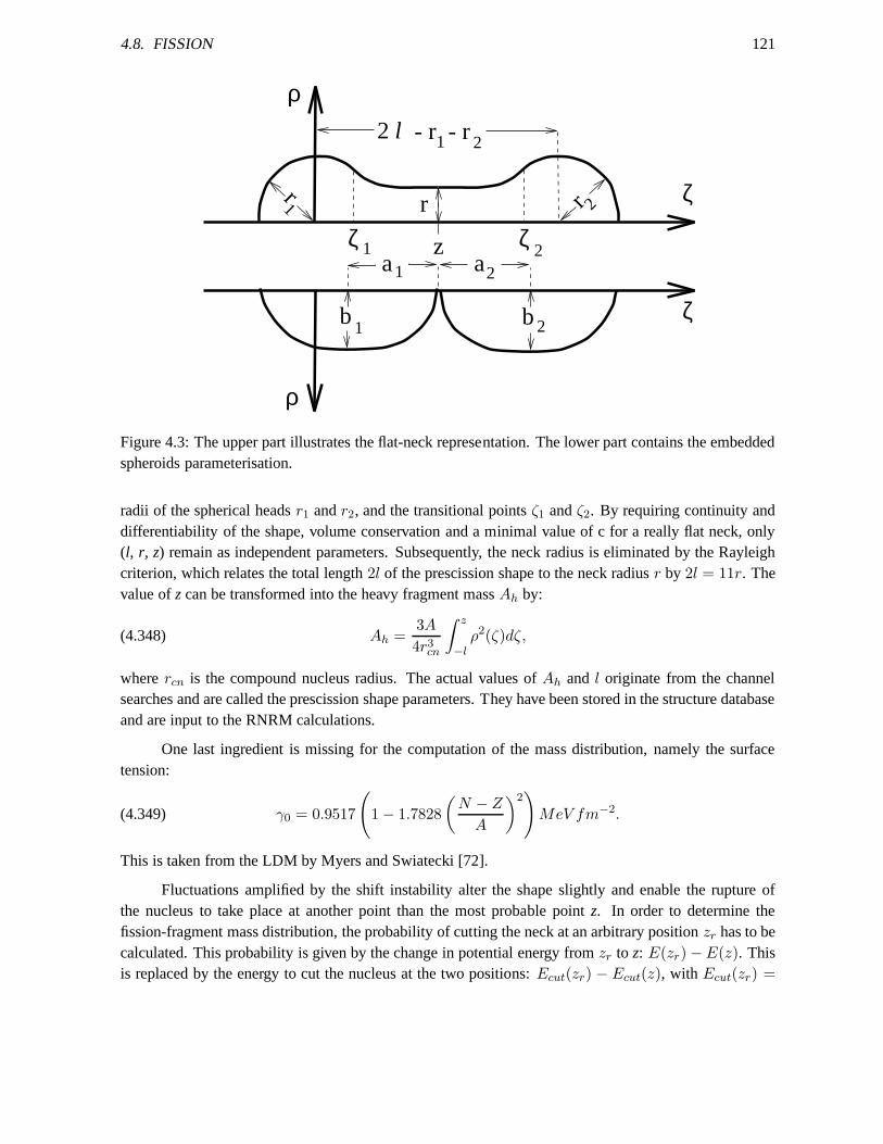
4.8. FISSION 121
1
- r - rl2 1 2
r 2r1
21
ζζ
bb
21
ρ
ρ
ζ
ζ
z
r
a2a
Figure 4.3: The upper part illustrates the flat-neck representation. The lower part contains the embeddedspheroids parameterisation.
radii of the spherical headsr1 andr2, and the transitional pointsζ1 andζ2. By requiring continuity anddifferentiability of the shape, volume conservation and a minimal value of c for a really flat neck, only(l, r, z) remain as independent parameters. Subsequently, the neckradius is eliminated by the Rayleighcriterion, which relates the total length2l of the prescission shape to the neck radiusr by 2l = 11r. Thevalue ofzcan be transformed into the heavy fragment massAh by:
(4.348) Ah =3A
4r3cn
∫ z
−lρ2(ζ)dζ,
wherercn is the compound nucleus radius. The actual values ofAh and l originate from the channelsearches and are called the prescission shape parameters. They have been stored in the structure databaseand are input to the RNRM calculations.
One last ingredient is missing for the computation of the mass distribution, namely the surfacetension:
(4.349) γ0 = 0.9517
(
1 − 1.7828
(
N − Z
A
)2)
MeV fm−2.
This is taken from the LDM by Myers and Swiatecki [72].
Fluctuations amplified by the shift instability alter the shape slightly and enable the rupture ofthe nucleus to take place at another point than the most probable point z. In order to determine thefission-fragment mass distribution, the probability of cutting the neck at an arbitrary positionzr has to becalculated. This probability is given by the change in potential energy fromzr to z: E(zr) − E(z). Thisis replaced by the energy to cut the nucleus at the two positions: Ecut(zr) − Ecut(z), with Ecut(zr) =
122 CHAPTER 4. NUCLEAR MODELS
2πγ0ρ2(zr). The rupture probability is now proportional to the Boltzmann factor:
(4.350) y(AFF ) ∝ exp
(
−2πγ0
(
ρ2(zr) − ρ2(z))
T
)
.
The fragment mass numberAFF can be computed according to the analogue of Eq. (4.348):
(4.351) AFF (zr) =3A
4r3cn
∫ zr
−lρ2(ζ) dζ.
The theoretical yield is finally determined with the following relation in whichY (AFF ) stands for thenormalized fission fragment mass yield:
(4.352) YFM (AFF ;ZFS , AFS , Ex) = y(AFF ) + y(A − AFF ).
In Eq. (4.350) the temperature of the scissioning nucleus must be provided. All calculations of thePES and the crossing of the fission barriers have been isothermal. However, for the RNRM the loss andgain of excitation energy in crossing the barrier is taken into account into a new excitation energy andtemperature at scission:
(4.353) Escissionx = Egroundstate
x + Fdef,scission.
The new excitation energy has two components: the original excitation energy in the ground stateEgroundstate
x and the deformation energy at scissionFdef,scission. Fdef,scission is positive for actinidesand becomes negative in the subactinide region. The new excitation energy is related to a new tempera-tureTscission. However, a new prescission temperature corresponds to a different prescission shape witha somewhat different value forFdef,scission. Therefore, the temperatureTscission has to be determinedin a self-consistent manner together with the final prescission shape. If a prescission shape has a hightemperature or a very long neck, the mass distribution will be broad. Low temperatures and short necksresult in a narrow mass distribution.
Post-scission neutron multiplicities
The mass distribution calculated above belongs to the primary fission fragments. Most fragments, how-ever, are highly excited directly after their creation. They take their share of total excitation energyavailable at scission (4.353). Moreover, they are stronglydeformed, which manifests itself in an extraamount of excitation energy set free when this deformation relaxes towards the ground-state deformationof the fragments by the strong surface tension. The superfluous excitation energy is released during theprocess of post-scission neutron and gamma emission. The neutron emission is responsible for a shift ofthe pre-neutron emission mass distribution to somewhat smaller masses.
The total excitation energy in a newly created fragment withmassAFF results from:
(4.354) Efragmentx (AFF ) = Edef,fragment(AFF ) +
AFF
AEscission
x .
4.8. FISSION 123
Edef,fragment(AFF ) denotes the deformation energy of the fragment, and the second term contains theportion of the thermal energy at scission of the whole fissioning system picked up by the fragment. Theassumption is that the fragment receives a share proportional to its mass.
For the calculation ofEdef,fragment(AFF ) another shape parameterisation is employed: the em-bedded spheroids (see Fig. 4.3). The newborn fragments are modeled as two contacting spheroids withmajor axesa1 anda2, which are linked to2l andzr by:
(4.355) a1 =1
2(r1 + zr), a2 = l − 1
2(r1 + zr).
The minor axesb1 andb2 follow from volume conservation:
(4.356) b21 =
3
4a1
∫ zr
−r1
ρ2dζ, b22 =
3
4a2
∫ 2l−r1
zr
ρ2dζ.
The energy difference of the spheroidally deformed and the spherical fragmentEdef,fragment(AFF ) isgiven by:
Edef,fragment(AFF , ǫ) = Esphsurf(AFF )
(
arcsin(ǫ) + ǫ(
1 − ǫ2)1/2
2ǫ (1 − ǫ2)1/6− 1
)
+
EsphCoul(AFF )
(
(
1 − ǫ2)1/3
2ǫln
(
1 + ǫ
1 − ǫ
)
− 1
)
.(4.357)
The eccentricity is defined as:
(4.358) ǫi =
(
1 −(
bi
ai
)2)1/2
,
andEsphsurf (AFF ) andEsph
Coul(AFF ) represent the LDM surface and the Coulomb energy of a sphericalnucleus obtained from Ref. [110].
The neutron multiplicityνFM(AFF ) for a fragment with massAFF is now derived by finding theroot of the following relation:
(4.359) Efragmentx (AFF ) =
νF M (AF F )∑
n=1
(Sn + ηn) + Eγ .
The separation energySn is calculated from the mass formula [110]. The average kinetic energy of theneutrons is taken to be32 times the fragment temperature, and the energy carried off by γ-raysEγ isapproximately half the separation energy of the first non-evaporated neutron.
The final fission product mass yield per fission mode is given by:
(4.360) YFM(AFP ;ZFS , AFS, Ex) = YFM (AFF −νFM(AFF ))+YFM(A−AFF −νFM(A−AFF )).
124 CHAPTER 4. NUCLEAR MODELS
Fission fragment charge distribution
Unfortunately, the MM-RNRM only yields information on the mass yields of the fission fragments. Pre-dictions of charge distributions are performed in TALYS within a scission-point-model-like approach(Wilkins et al. [111]). Corresponding to each fission fragment massAFF a charge distribution is com-puted using the fact that the probability of producing a fragment with a chargeZFF is given by the totalpotential energy of the two fragment system inside a Boltzmann factor:
(4.361) YFM(ZFF ;AFF , ZFS , AFS , Ex) =exp
(
−E(ZF F ,AF F ,Z,A)T
)
∑
ZF Fiexp
(
−E(ZF Fi,AF F ,Z,A)
T
)
In the original scission-point model this potential energyis integrated over all deformation space. Withinthe MM-RNRM, however, fission channel calculations alreadydefine the deformation at the scissionpoint. Furthermore, a strong coupling between the collective and single particle degrees of freedom isassumed near the scission point. This means that the nucleusis characterised by a single temperatureT .
The potential energy for the creation of one fragment with(ZFF , AFF ) and a second fragmentwith (Z − ZFF , A − AFF ) consists of a sum over the binding energy of the deformed fragments bythe droplet model without shell corrections and their mutual Coulomb repulsion energy as well as thenuclear proximity repulsion energy:
(4.362) E(ZFF , AFF , Z,A) = B(ZFF , AFF ) + B(Z − ZFF , A − AFF ) + ECoul + Vprox.
The single constituents of this formula are defined by the following relations:
B(ZFF , AFF ) = −a1
[
1 − κ
(
AFF − 2ZFF
AFF
)2]
AFF(4.363)
+a2
[
1 − κ
(
AFF − 2ZFF
AFF
)2]
A2
3
FF f(shape)
+3
5
e2
r0
Z2FF
A1
3
FF
g(shape) − π2
2
e2
r0
(
d
r0
)2 Z2FF
AFF(4.364)
ECoul = e2ZFF (Z − ZFF )Sform/(a1 + a2)(4.365)
Vprox = −1.78174πγ0b
21b
22
a1b22 + a2b2
1
(4.366)
The parameters in the binding energy formula are taken from Ref. [110]. The functionf(shape) isthe form factor for the Coulomb term whereasg(shape) denotes the form factor for the surface energy.Sform is the form factor for the Coulomb interaction energy between two spheroids.
The fission product charge distribution is obtained from thecalculated fission fragment chargedistribution by shifting the corresponding fragment massesAFF to the fission product massesAFP withthe aid of the post-scission neutron multiplicityνFM (AFF ):
(4.367) YFM(ZFP ;AFP , ZFS , AFS , Ex) = YFM(ZFF ;AFF − νFM (AFF ), ZFS , AFS , Ex).
Since proton evaporation of the fission fragments is neglected, the charge distribution connected withAFF becomes simply linked to the fission product massAFP .
4.9. THERMAL REACTIONS 125
4.9 Thermal reactions
The Introduction states that TALYS is meant for the analysisof data in the 1 keV - 200 MeV energyregion. The lower energy of 1 keV should not be taken too literally. More accurate is: above the resolvedresonance range. The start of the unresolved resonance range differs from nucleus to nucleus and isrelated to the average resonance spacingD0 or, equivalently, the level density at the binding energy.Generally, the starting energy region is higher for light nuclides than for heavy nuclides. Only beyondthis energy, the optical and statistical models are expected to yield reasonable results, at least for the non-fluctuating cross sections. The lower energies are the domain of R-matrix theory, which describes theresonances. Nevertheless, it would be useful to have a first-order estimate of the non-threshold reactions,not only for the obvious neutron capture channel, but also for the exothermal(n, p), (n, α) and fissionchannels. The fact that a nuclear model calculation in TALYSis only performed down to about 1 keVshould not prevent us to give at least an estimate of the1/v-like behaviour of the excitation function downto 10−5 eV (the lower energy limit in ENDF-6 files). In collaborationwith J. Kopecky, we constructed amethod that provides this.
4.9.1 Capture channel
First, we decide on the lower energy of validity of a TALYS nuclear model calculationEL. Somewhatarbitrarily, we set as defaultEL = D0 when we wish to construct evaluated data libraries, whereD0 istaken from the nuclear model database or, if not present, derived from the level density.EL can also beentered as an input keyword (Elow). Next, we determine the neutron capture cross section at the thermalenergyEth = 2.53.10−8 MeV, either from the experimental database, see Chapter 5, or, if not present,from the systematical relation [112]
(4.368) σn,γ(Eth) = 1.5 × 10⁻³a(Sn − ∆)3.5 mb
with a the level density parameter at the separation energySn and∆ the pairing energy. We assign a1/v, i.e. 1/
√E, dependence to the cross section from10−5 eV to an upper limitE1/v which we set,
again arbitrarily, atE1/v = 0.2EL. The1/v line obviously crossesσn,γ(Eth) atEth. The points atE1/v
andEL are connected by a straight line. The resulting capture cross section then looks like Fig. 4.4. Inreality, the region betweenE1/v andEL is filled with resolved resonances, the only feature we did nottry to simulate.
4.9.2 Other non-threshold reactions
For other reactions with positive Q-values, such as(n, p) and(n, α), only a few experimental values atthermal energy are available and a systematical formula as for (n, γ) is hard to construct. If we do havea value for these reactions at thermal energy, the same method as for capture is followed. If not, weassume that the ratio between the gamma decay width and e.g. the proton decay width is constant forincident energies up toEL. Hence, we determineRp = σn,p/σn,γ atEL, and since we know the thermal(n, γ) value we can produce the (n,p) excitation function down to10−5 eV by multiplying the capturecross section byRp. A similar procedure is applied to all other non-threshold reactions.
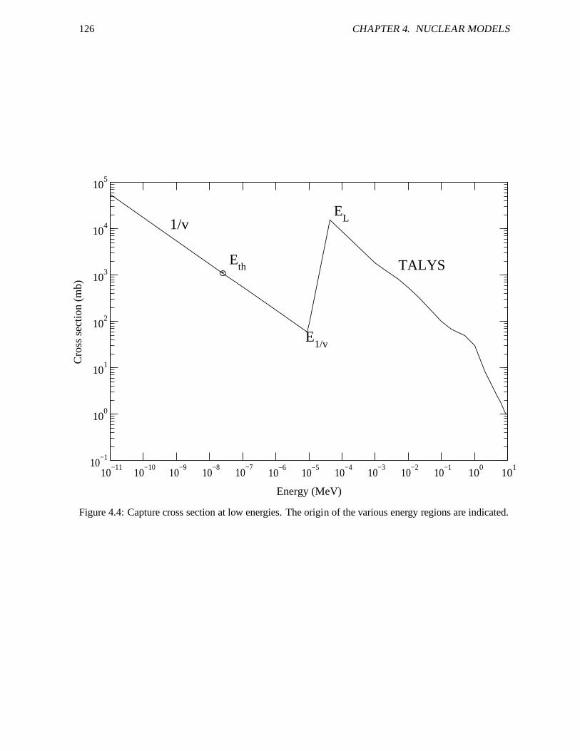
126 CHAPTER 4. NUCLEAR MODELS
10−11
10−10
10−9
10−8
10−7
10−6
10−5
10−4
10−3
10−2
10−1
100
101
Energy (MeV)
10−1
100
101
102
103
104
105
Cro
ss s
ectio
n (m
b)
TALYS
1/v
Eth
E1/v
EL
Figure 4.4: Capture cross section at low energies. The origin of the various energy regions are indicated.
4.10. DIRECT CAPTURE 127
4.10 Direct capture
For light nuclides and (very) neutron-rich nuclides, the direct capture process may have a significantcontribution. Therefore, a direct capture model was implmented, to be activated with theracap keyword,see page 212. More details may become available in future versions of this manual. For the moment werefer to Ref. [139].
4.11 Populated initial nucleus
Usually, a TALYS calculation will concern a projectile witha certain incident energy and a target, ei-ther in its ground or an excited state. For various reasons, we have introduced the possibility to startthe decay from an initial population, i.e. an excited nucleus with a population distributed over excita-tion energy. An example of an interesting application is theneutron spectrum from fission fragments.One could calculate the fragment distribution from fission,e.g. as described in Section 4.8.7 or fromempirical methods, and assume a population per excitation energy and spin, of the excited light andheavy fission fragment (models for such distributions exist, see e.g. Ref. [113]). This distribution canthen be the starting point for a TALYS calculation. The initial population enters the Hauser-Feshbachscheme and the compound nucleus calculation proceeds as usual. The emitted neutrons can be recordedas well as the path from fission fragment to fission product. All relevant nuclear structure quantities areavailable since we simulate the process by a photon-inducedreaction, the only difference being that wedo not excite a single compound nucleus energy but directly fill the continuum bins and discrete levelsaccording to our specified starting population. TALYS can beused in this mode by simply specifyingprojectile 0, see page 154, and providing an energy file as input, see page 155. The initial populationcan be provided at two levels of detail. A full excitation energy-spin-parity population can be given,which is then interpolated on the internal excitation energy scheme of TALYS. Alternatively, only thetotal population per excitation energy can be given, after which the spin-parity-dependent population isdetermined by multiplying it with the spin distribution of Eq. (4.237). For the fission neutron spectrumexample mentioned above, one could loop over all fission fragments (by writing a clever script), sum theresults, and obtain the fission neutron spectrum. There are more applications for this feature, such ascoupling a high-energy intranuclear cascade code with TALYS, the latter taking care of the low energyevaporation part including all its quantum-mechanical conservation rules.
4.12 Astrophysical reaction rates
A complete calculation of astrophysical reaction rates is possible with TALYS. In stellar interiors, nu-clides not only exist in their ground states but also in different thermally excited states and a thermody-namic equilibrium holds locally to a very good approximation. Therefore, most of nuclear astrophysicscalculations have made use of nuclear reaction rates evaluated within the statistical model [114]. Theassumption of a thermodynamic equilibrium combined with the compound nucleus cross sections forthe various excited states then allows to produce Maxwellian-averaged reaction rates, which is importantinput for stellar evolution models. Calculation of stellarreaction rates is obviously not new, but TALYS
128 CHAPTER 4. NUCLEAR MODELS
provides some features which automatically makes the extension to reaction rate calculations very worth-while. In contrast with existing dedicated astrophysical reaction rate codes, the present Chapter showsthat we provide the inclusion of pre-equilibrium reaction mechanism, the detailed competition betweenall open channels, the inclusion of multi-particle emission (neglected in most astrophysics codes), theinclusion of detailed width fluctuation corrections, the inclusion of parity-dependent level densities, theinclusion of coupled channel description for deformed nuclei, and the coherent inclusion of fission chan-nel. Different prescriptions are also used when normalizing nuclear models on available experimentaldata, such as level densities on s-wave spacings or E1 resonance strength on photoabsorption data.
The energies of both the targets and projectiles, as well as their relative energiesE, obey Maxwell-Boltzmann distributions corresponding to the temperatureT at that location (or a black-body Planckspectrum for photons). The astrophysical rate is obtained by integrating the cross section given byEq. (4.174) over a Maxwell-Boltzmann distribution of energies E at the given temperatureT . In ad-dition, in hot astrophysical plasmas, a target nucleus exists in its ground as well as excited states. In athermodynamic equilibrium situation, the relative populations of the various levels of nucleus with spinsIµ and excitation energiesEµ
x obey a Maxwell-Boltzmann distribution. Hence, in the formulae to fol-low, it is understood that the definition of the incidentα channel, see below Eq. (4.174), now includes anexplicit superscriptµ to distinguish between the excited states. The effective stellar rate ofα → α′ in theentrance channel at temperatureT taking due account of the contributions of the various target excitedstates is finally expressed as
NA〈σv〉∗αα′ (T ) =( 8
πm
)1/2 NA
(kT )3/2 G(T )
∫ ∞
0
∑
µ
(2Iµ + 1)
(2I0 + 1)×
σµαα′(E)E exp
(
−E + Eµx
kT
)
dE,(4.369)
wherek is the Boltzmann constant,m the reduced mass of theα channel,NA the Avogadro number, and
(4.370) G(T ) =∑
µ
(2Iµ + 1)/(2I0 + 1) exp(−Eµx/kT )
theT -dependent normalized partition function. Reverse reactions can also be estimated making use ofthe reciprocity theorem [114]. In particular, the stellar photodissociation rates are classically derivedfrom the radiative capture rates by
λ∗(γ,α)(T ) =
(2I + 1)(2j + 1)
(2I ′ + 1)
GI(T )
GI′(T )
(AAa
A′
)3/2( kT
2π~2NA
)3/2×
NA〈σv〉∗(α,γ) e−Qαγ/kT ,(4.371)
whereQαγ is the Q-value of theI0(α, γ)I ′0 capture channel. Note that, in stellar conditions, the reactionrates for targets in thermal equilibrium are usually believed to obey reciprocity since the forward andreverse channels are symmetrical, in contrast to the situation which would be encountered for targets intheir ground states only [114]. In TALYS, the total stellar photodissociation rate is determined from
(4.372) λ∗(γ,j)(T ) =
∑
µ(2Jµ + 1) λµ(γ,α)(T ) exp(−Eµ
x/kT )∑
µ(2Jµ + 1) exp(−Eµx/kT )
,
4.13. MEDICAL ISOTOPE PRODUCTION 129
where the photodissociation rateλµ(γ,α) of stateµ with excitation energyEµ
x is given by
(4.373) λµ(γ,α)(T ) =
∫ ∞
0c nγ(E,T ) σµ
(γ,α)(E) dE ,
wherec is the speed of light,σµ(γ,j)(E) the photodisintegration cross section at energyE, andnγ the
stellarγ-ray distribution well described by the back-body Planck spectrum at the given temperatureT .
In TALYS, if astro y, an appropriate incident energy grid for astrophysical calculations is madewhich overrules any incident energy given by the user.
4.13 Medical isotope production
This section describes the formalism to calculate the production yield of a radioactive nucleus by anuclear reaction. Starting from the general formalism we will introduce realistic approximations andderive simpler equations that hold in basically all cases ofinterest. In TALYS we have implementedonly analytical solutions to the production and depletion equations. This may be generalized in futureversions.
4.13.1 Production and depletion of isotopes
The most general situation is that of the irradiation of a piece of material, consisting of many differentisotopes, which were either present at the start of the irradiation, have been formed, or will be formedduring the irradiation, by either the primary flux of particles, by secondary particles, or by radioactivedecay. If we have a total ofK different isotopes (theoreticallyK may stand for the the entire nuclidechart) and the number of each isotopek is Nk, then the temporal development of such a system isdescribed byK differential equations:
dN1(t)
dt=
K∑
k=1,k 6=1
Λk→1Nk(t) − Λ1N1(t)
. . .
dNi(t)
dt=
K∑
k=1,k 6=i
Λk→iNk(t) − ΛiNi(t)
. . .
dNK(t)
dt=
K∑
k=1,k 6=K
Λk→KNk(t) − ΛKNK(t)(4.374)
In each equation, the first term is a feeding term. In the most general case, various parent nuclides maycontribute to the formation of isotopei, hence the summation over parent nuclidesk, with Λk→i thepartial formation rate for any possible parent isotopek to isotopei. Each partial formation rate can beexpressed as
(4.375) Λk→i = λk→i + Rk→i
130 CHAPTER 4. NUCLEAR MODELS
with λk→i the (partial) radioactive decay rate andRk→i the (partial) nuclear reaction rate for any possibleparent isotopek to isotopei. The second terms of Eq. (4.374) are loss terms due to radioactive decayand nuclear reactions from isotopei to any other isotope. Here the total depletion rate (we interchange“depletion” with “formation” whenever appropriate) for isotopei is
(4.376) Λi = λi + Ri
where the total decay rate for isotopei is
λi =
K∑
k=1,k 6=i
λi→k
and the total nuclear reaction rate for isotopei is
(4.377) Ri =
K∑
k=1,k 6=i
Ri→k
The entire loop overk may run over isotopes in their ground or isomeric states . Theoretically,the sum over reaction rates could include secondary particles (neutrons, photons, alpha particles etc.)formed after the first interaction of the incident beam with the material, over the entire outgoing energyspectrum. Since the number of isotopesi, Ni(t) may appear simultaneously in many equations, due toits possible formation, or depletion, by many different nuclear reactions, it is clear that such a coupledsystem can only be solved by complicated mathematical and computational techniques. In fact, themost exact simulation would involve a Monte Carlo 3D transport calculation in which all primary andsecondary particles are taken into account, including complete cross section libraries for all possibleparticles, coupled with an activation code that keeps trackof the nuclide inventory. If we neglect suchthick target transport issues, a system of equations like (4.374) is often solved by methods developed byBateman [116] and later generalized by Rubinson [117].
Fortunately, the situation is often not as complex as sketched above, since very reasonable approx-imations can be introduced into Eq. (4.374), certainly for charged-particle induced reactions. First, let usstart with the common case of the irradiation of a target which contains of only one natural element at thestart of the irradiation. This set of equations can be then beseparated into a linear combination of contri-butions by each targetisotope. Hence, we solve Eq. (4.374) one by one for each target isotope and addthese contributions at the end to get the answer for the target material. Then, for such a mono-isotopictargetT we have at the start of the irradiation
t = 0 : NT = NT (0)
Ni = 0
. . .
NK = 0(4.378)
Since in practice our target isotope is not radioactive, theloss terms reduce toΛT = RT inEq. (4.374) forNT . Next, if a substantial part of the target is converted into other isotopes, beam
4.13. MEDICAL ISOTOPE PRODUCTION 131
particles may interact with atoms other than the original target atoms. However, this is only a concern forirradiation times of the order of months or longer. For most practical applications, like medical isotopeproduction, we can often assume that the burn-up of the target is small and that the target compositiondoes not change much during the irradiation (this will be confirmed by some of our sample cases). Hence,in addition we will assume there are no nuclear reaction or radioactive decay feeding terms for thetargetisotopeT .
This means that the target isotope is described by the following simple equation
(4.379)dNT (t)
dt= −RT NT (t)
which basically assumes that the only thing that happens to the target material is burn-up through nuclearreactions.
For the isotopes that are produced during the irradiation wecan make similar reasonable assump-tions. We assume there is no loss of aproducedisotope of interest through nuclear reactions with beamparticles, i.e. we assume nuclides are not hit twice (again,this assumption becomes less accurate atvery long irradiation times). This is equivalent to statingthat the isotopes of interest are only producedfrom nuclear reactions on the target isotopes or from decay of other products formed during the irradia-tion. Also, consistent with the assumption for the target isotope that nuclides are not hit twice, we haveΛi = λi for the depletion term, and assume that no other nuclear reactions lead to the isotope of interest.Thus for the produced isotopesi we obtain
(4.380)dNi(t)
dt=
K∑
k=1,k 6=i
λk→iNk(t) + RT→iNT (t) − λiNi(t)
Nuclides often have only one or a few radioactive decay modes. Usually, only beta decay to theground state or an isomer needs to be considered, although insome cases alpha decay may occur as well.If we neglect alpha decay, the summation in the first term above reduces to only one term. Thus, Eq.(4.380) reduces to
(4.381)dNi(t)
dt= λp→iNp(t) + RT→iNT (t) − λiNi(t)
where we now use the subscriptp for the parent isotope, which itself is described by the equation,
(4.382)dNp(t)
dt= RT→pNT (t) − λpNp(t)
where for simplicity we have left out a possible feeding termλg→pNg(t) from its own parent (i.e. thegrandparent of isotopei). It neglects radioactive decay to channels produced by multiple proton emission,e.g. 120Te(p,2p)119Sb and the contribution from its feeding channel120Te(p,2n)119I + 2β+. Althoughthe (p,2p) channel is generally smaller and therefore oftennot relevant for most practical medical isotopeproduction routes, it would be safer that at higher energiesfeeding from radioactive decay is taken intoaccount. For that a more general solution of Eq. (4.374) would have to be implemented, similar tosolutions for neutron-induced problems where processes like e.g. multiple fission yield decay need to be
132 CHAPTER 4. NUCLEAR MODELS
taken into account. For most charged-particle induced reactions of interest, the current approximation isjustified.
If we now use thatNT (t = 0) = NT (0) andNp(t = 0) = Ni(t = 0) = 0, the solutions to theseequations are given by:
NT (t) = NT (0) e−RT t,
Np(t) = NT (0)RT→p
λp − RT[e−RT t − e−λpt],
Ni(t) = NT (0)RT→i
λi − RT[e−RT t − e−λit] + NT (0)
RT→pλp→i
λp − RT
[
e−RT t − e−λit
λi − RT− e−λpt − e−λit
λi − λp
]
.(4.383)
This is derived in the Appendix.
By setting the derivative ofNi(t) to zero, the irradiation time for which a maximal yield is obtainedcan be easily derived:
(4.384) tmax =ln(λi/RT )
λi − RT
The production ofi is restrained by itsβ-decay on the one hand and by the decreasing number of availabletarget atoms on the other hand. Hence, this observabletmax depends on the decay constantλi and thetotal production rateRT .
Now that the analytical formulae for production are set withEq. (4.383), the remaining ingredientsneeded to evaluate Eqs.(4.383) and (4.384) are:N1(0), . . . , NI(0), R, andλ, and this will be done in thenext two sections.
4.13.2 Initial condition and stopping power
The number of target atoms at t=0,Ni(0), for 1 ≤ i ≤ I equals:
(4.385) Ni(0) =NA
ABi ρ Vtar,
whereNA = 6.022 1023 is Avogadro’s number,A is the mass number,Bi is the abundance of isotope iwith
∑Ii Bi = 1, ρ the mass density in [g/cm3], andVtar the active target volume in [cm3]. Vtar is given
by the product of the beam surfaceSbeam in [cm2] and the effective target thickness in [cm], which canbe expressed in terms of the stopping powerdE
dx ,
(4.386) Vtar = Sbeam
∫ Ebeam
Eback
(
dE
dx
)−1
dE,
whereEbeam denotes the incident beam energy andEback is the average projectile energy available atthe backside of the target. If the projectiles travels through the target, the average projectile beam energywill decrease. The amount of energy loss inside the target isdetermined by the target thickness and thestopping power. The integration limitsE1 andE2 are fixed by the requested projectile energy range
4.13. MEDICAL ISOTOPE PRODUCTION 133
inside the target, which is determined by the cross section as function of projectile energy (excitationfunction). This formula neglects the spreading of the beam inside the target.
The stopping power describes the average energy loss of projectiles in the target by atomic colli-sions as a function of their energy in [MeV/cm]. We use the Bethe-Bloch formula [118]:
(4.387)dE
dx= 0.1535 ρ
Z
A
z2p
β2[ln
(
2meγ2v2Wmax
I2
)
− 2β2], MeV/cm
with Z the target charge number, andzp the projectile charge number, whileβ represents a beam particletraveling at a relative velocity
(4.388) β =v
c=
√
Ebeam(Ebeam + 2m0c2)
(Ebeam + m0c2)2,
with rest massm0. Further,me is the electron mass, andγ = 1√1−β2
. The maximum energy transfer in
a single collision,Wmax is given by
(4.389) Wmax = 2mec2(βγ)2,
if the incident particle is much heavier than the electron mass. For the mean excitation potential I asemi-empirical formula is adopted:
(4.390)I
Z= 9.76 + 58.8Z−1.19 eV.
This expression is claimed to be tested only ifZ ≥ 13, but we use it for all values.
4.13.3 Nuclear reaction and decay rates
When the full beam hits the target (i.e., assuming that the beam diameter is smaller than the targetdimensions), the production rate in [atoms/s] of isotopei through the nuclear reaction on the targetisotopeT is given by the following expression
(4.391) RT→i =Ibeam
zp qe
1
Vtar
∫ Ebeam
Eback
(
dE
dx
)−1
σrpi (E) dE
whereIbeam is the beam current in [A] andqe is the electron charge. The factorIbeam/(zpqe) correspondsto the number of projectiles impinging on the target per [s].The residual production cross section ofi in[mb] is denoted byσrp
i (E).
Analogously, the production rate in [s−1] of all reaction channels, from the target, is given by:
(4.392) RT =Ibeam
zp qe
1
Vtar
∫ Ebeam
Eback
(
dE
dx
)−1
(σnon(E) − σin(E)) dE
whereσnon(E) is the non-elastic cross section andσin(E) is the inelastic cross section ofi in [mb],which is nothing else than the residual production cross section σrp
i (E). The differenceσnon(E) −
134 CHAPTER 4. NUCLEAR MODELS
σin(E) provides the probability to create an isotope different from the original target atom in the nuclearreaction.
The decay rate ofi is given by the simple relation
(4.393) λi =ln 2
T1/2i
,
whereT1/2i is the half-life of isotopei in [s]. Theλi in the loss term usually feeds only one or two
different channels, namely by beta decay to the ground stateor isomer of the daughter isotope,
(4.394) λi = λi→d = λg.s.i→d + λiso
i→d
whered denotes the daughter nuclide.
With this, all ingredients of Eq. (4.383) are defined and we may calculate the nuclide inventoryNi(t) at any time during or after the irradiation process.
4.13.4 Activities
With Ni(t) known, the final expression for the activity of the produced isotopei, Ai, as a function of theirradiation timet can now be given by
(4.395) Ai(t) = λi Ni(t).
For small irradiation times the expression forNi(t), Eq. (4.383), behaves as:
(4.396) Ni(t) = NT (0) RT→i t,
and hence the activity ofi as
(4.397) Ai(t) = λi NT (0) RT→i t,
Under these circumstances, the yield scales linearly with the irradiation timet and the production rateRT→i. Only then, the production yield expressed in [MBq/mAh] is ameaningful quantity, which can beused to determine the yield, given a certain irradiation time t=Tirradiation and beam current.
Chapter 5Nuclear structure and model parameters
5.1 General setup of the database
We have aimed to unify the nuclear structure and model parameter database of TALYS as much as possi-ble. In thetalys/structure/directory you can find themasses/, abundance/, levels/, fission/, resonances/,deformation/, optical/, thermal/, gamma/, density/, decay/ integral/andbest/subdirectories. Most subdi-rectories contain about 100 files, where each individual filepoints to a nuclear element and has the namezZZZwhere ZZZ is the charge number of the element. One file contains the info for all the isotopes ofone element. For example, the filetalys/structure/levels/z026contains the discrete levels of all Fe (Z=26)isotopes. As you will see below, the chemical symbol is always present in the file itself, allowing an easysearch. Every directory has this same substructure and alsothe formats in which the data are stored havebeen kept uniform as much as possible.
The nuclear structure database has been created from a collection of “raw” data files, which fora large part come from the Reference Input Parameter LibraryRIPL [163], that we used as a basis forTALYS.
5.2 Nuclear masses and deformations
The nuclear masses are stored in thetalys/structure/masses/directory. In TALYS, we use three differentsources. In order of priority:
• Experimental masses: The Audi Wapstra table (2003) [87]
• Theoretical masses: Goriely’s mass table using either the Skyrme force [119] or the Gogny force,or the Moller mass table [120].
• The Duflo-Zuker mass formula [121], included as a subroutinein TALYS.
135
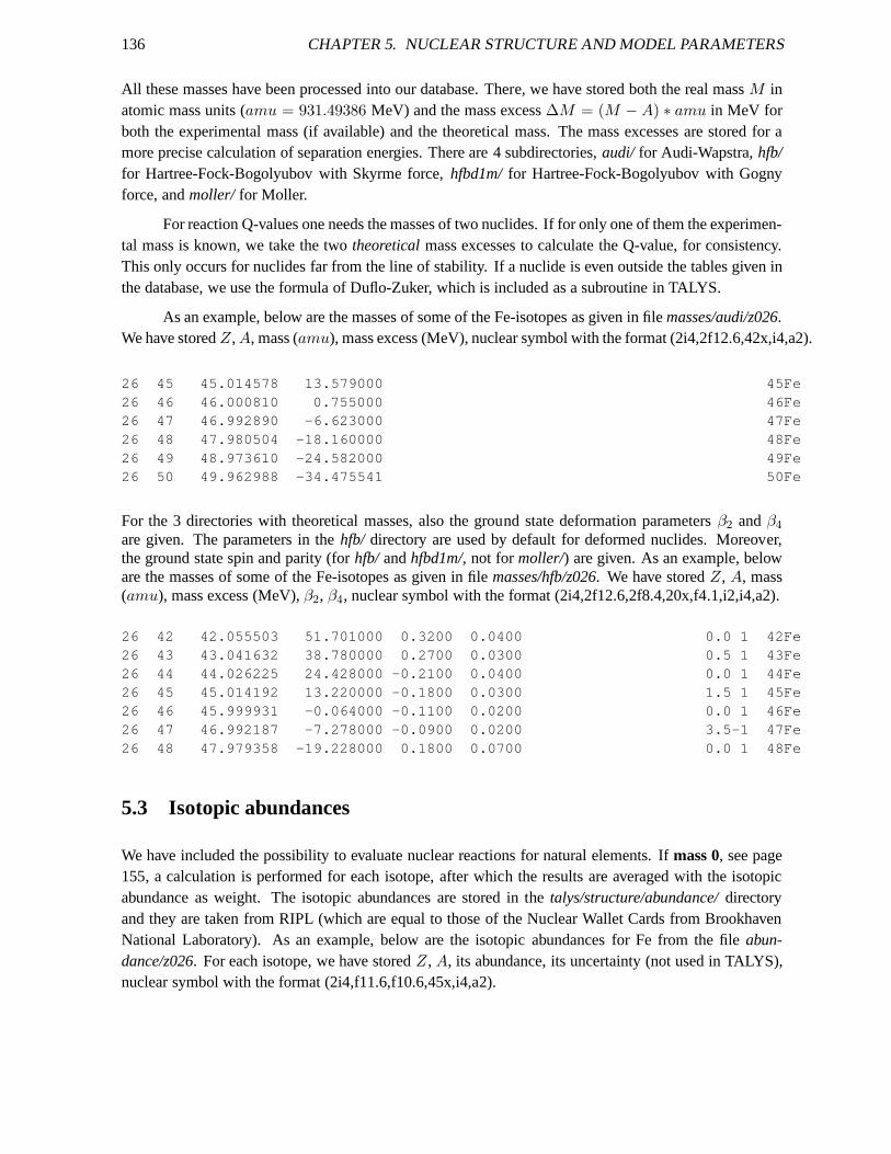
136 CHAPTER 5. NUCLEAR STRUCTURE AND MODEL PARAMETERS
All these masses have been processed into our database. There, we have stored both the real massM inatomic mass units (amu = 931.49386 MeV) and the mass excess∆M = (M − A) ∗ amu in MeV forboth the experimental mass (if available) and the theoretical mass. The mass excesses are stored for amore precise calculation of separation energies. There are4 subdirectories,audi/ for Audi-Wapstra,hfb/for Hartree-Fock-Bogolyubov with Skyrme force,hfbd1m/for Hartree-Fock-Bogolyubov with Gognyforce, andmoller/ for Moller.
For reaction Q-values one needs the masses of two nuclides. If for only one of them the experimen-tal mass is known, we take the twotheoreticalmass excesses to calculate the Q-value, for consistency.This only occurs for nuclides far from the line of stability.If a nuclide is even outside the tables given inthe database, we use the formula of Duflo-Zuker, which is included as a subroutine in TALYS.
As an example, below are the masses of some of the Fe-isotopesas given in filemasses/audi/z026.We have storedZ, A, mass (amu), mass excess (MeV), nuclear symbol with the format (2i4,2f12.6,42x,i4,a2).
26 45 45.014578 13.579000 45Fe26 46 46.000810 0.755000 46Fe26 47 46.992890 -6.623000 47Fe26 48 47.980504 -18.160000 48Fe26 49 48.973610 -24.582000 49Fe26 50 49.962988 -34.475541 50Fe
For the 3 directories with theoretical masses, also the ground state deformation parametersβ2 andβ4
are given. The parameters in thehfb/ directory are used by default for deformed nuclides. Moreover,the ground state spin and parity (forhfb/ andhfbd1m/, not formoller/) are given. As an example, beloware the masses of some of the Fe-isotopes as given in filemasses/hfb/z026. We have storedZ, A, mass(amu), mass excess (MeV),β2, β4, nuclear symbol with the format (2i4,2f12.6,2f8.4,20x,f4.1,i2,i4,a2).
26 42 42.055503 51.701000 0.3200 0.0400 0.0 1 42Fe26 43 43.041632 38.780000 0.2700 0.0300 0.5 1 43Fe26 44 44.026225 24.428000 -0.2100 0.0400 0.0 1 44Fe26 45 45.014192 13.220000 -0.1800 0.0300 1.5 1 45Fe26 46 45.999931 -0.064000 -0.1100 0.0200 0.0 1 46Fe26 47 46.992187 -7.278000 -0.0900 0.0200 3.5-1 47Fe26 48 47.979358 -19.228000 0.1800 0.0700 0.0 1 48Fe
5.3 Isotopic abundances
We have included the possibility to evaluate nuclear reactions for natural elements. Ifmass 0, see page155, a calculation is performed for each isotope, after which the results are averaged with the isotopicabundance as weight. The isotopic abundances are stored in the talys/structure/abundance/directoryand they are taken from RIPL (which are equal to those of the Nuclear Wallet Cards from BrookhavenNational Laboratory). As an example, below are the isotopicabundances for Fe from the fileabun-dance/z026. For each isotope, we have storedZ, A, its abundance, its uncertainty (not used in TALYS),nuclear symbol with the format (2i4,f11.6,f10.6,45x,i4,a2).
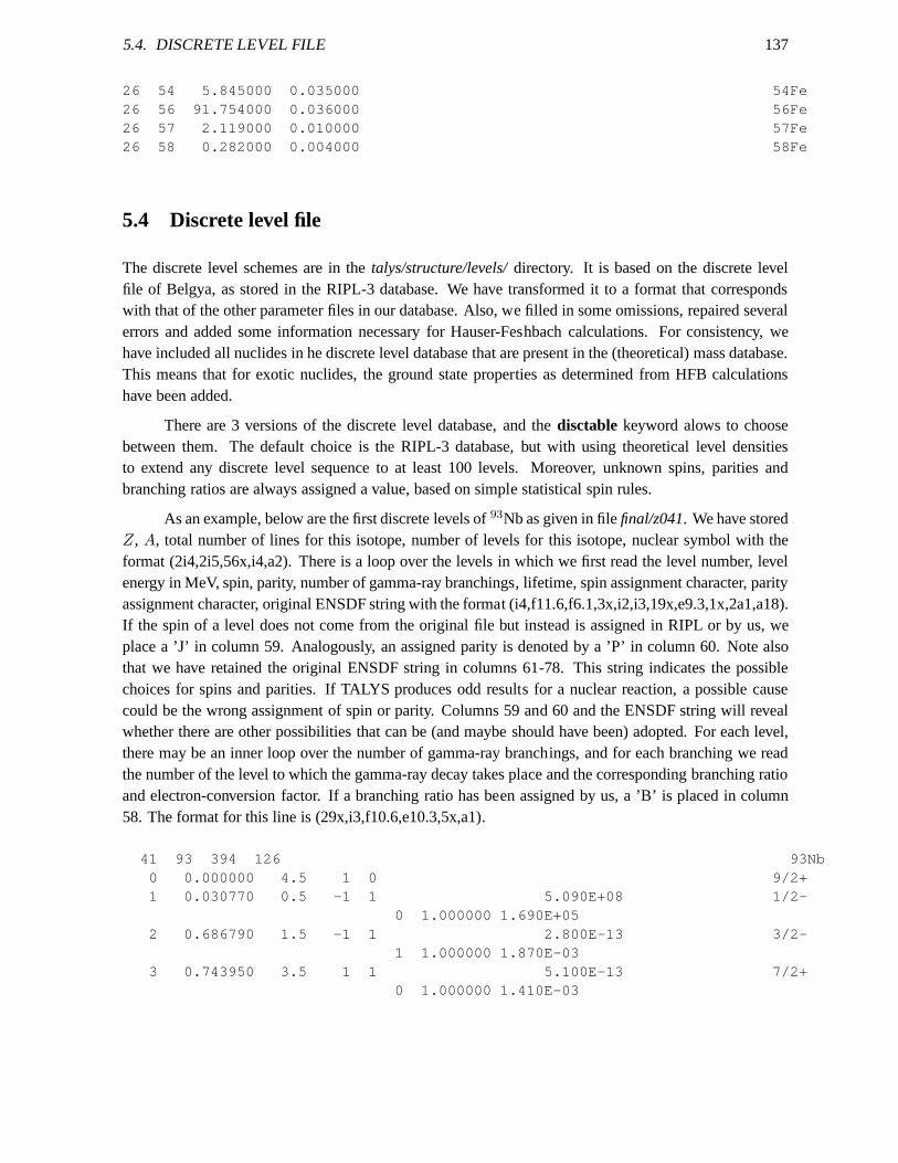
5.4. DISCRETE LEVEL FILE 137
26 54 5.845000 0.035000 54Fe26 56 91.754000 0.036000 56Fe26 57 2.119000 0.010000 57Fe26 58 0.282000 0.004000 58Fe
5.4 Discrete level file
The discrete level schemes are in thetalys/structure/levels/directory. It is based on the discrete levelfile of Belgya, as stored in the RIPL-3 database. We have transformed it to a format that correspondswith that of the other parameter files in our database. Also, we filled in some omissions, repaired severalerrors and added some information necessary for Hauser-Feshbach calculations. For consistency, wehave included all nuclides in he discrete level database that are present in the (theoretical) mass database.This means that for exotic nuclides, the ground state properties as determined from HFB calculationshave been added.
There are 3 versions of the discrete level database, and thedisctable keyword alows to choosebetween them. The default choice is the RIPL-3 database, butwith using theoretical level densitiesto extend any discrete level sequence to at least 100 levels.Moreover, unknown spins, parities andbranching ratios are always assigned a value, based on simple statistical spin rules.
As an example, below are the first discrete levels of93Nb as given in filefinal/z041. We have storedZ, A, total number of lines for this isotope, number of levels forthis isotope, nuclear symbol with theformat (2i4,2i5,56x,i4,a2). There is a loop over the levelsin which we first read the level number, levelenergy in MeV, spin, parity, number of gamma-ray branchings, lifetime, spin assignment character, parityassignment character, original ENSDF string with the format (i4,f11.6,f6.1,3x,i2,i3,19x,e9.3,1x,2a1,a18).If the spin of a level does not come from the original file but instead is assigned in RIPL or by us, weplace a ’J’ in column 59. Analogously, an assigned parity is denoted by a ’P’ in column 60. Note alsothat we have retained the original ENSDF string in columns 61-78. This string indicates the possiblechoices for spins and parities. If TALYS produces odd results for a nuclear reaction, a possible causecould be the wrong assignment of spin or parity. Columns 59 and 60 and the ENSDF string will revealwhether there are other possibilities that can be (and maybeshould have been) adopted. For each level,there may be an inner loop over the number of gamma-ray branchings, and for each branching we readthe number of the level to which the gamma-ray decay takes place and the corresponding branching ratioand electron-conversion factor. If a branching ratio has been assigned by us, a ’B’ is placed in column58. The format for this line is (29x,i3,f10.6,e10.3,5x,a1).
41 93 394 126 93Nb0 0.000000 4.5 1 0 9/2+1 0.030770 0.5 -1 1 5.090E+08 1/2-
0 1.000000 1.690E+052 0.686790 1.5 -1 1 2.800E-13 3/2-
1 1.000000 1.870E-033 0.743950 3.5 1 1 5.100E-13 7/2+
0 1.000000 1.410E-03
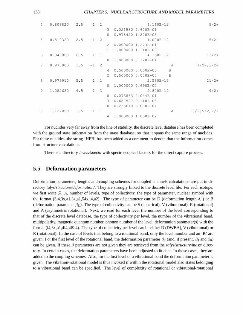
138 CHAPTER 5. NUCLEAR STRUCTURE AND MODEL PARAMETERS
4 0.808820 2.5 1 2 6.160E-12 5/2+3 0.021580 7.670E-010 0.978420 1.200E-03
5 0.810320 2.5 -1 2 1.000E-12 5/2-2 0.000000 1.273E-011 1.000000 1.310E-03
6 0.949800 6.5 1 1 4.360E-12 13/2+0 1.000000 8.120E-04
7 0.970000 1.5 -1 2 J 1/2-,3/2-4 0.500000 0.000E+00 B2 0.500000 0.000E+00 B
8 0.978910 5.5 1 1 2.580E-13 11/2+0 1.000000 7.690E-04
9 1.082680 4.5 1 3 2.800E-12 9/2+8 0.073863 2.044E-013 0.687527 9.110E-030 0.238610 6.080E-04
10 1.127090 1.5 1 1 J 3/2,5/2,7/24 1.000000 1.050E-02
For nuclides very far away from the line of stability, the discrete level database has been completedwith the ground state information from the mass database, sothat it spans the same range of nuclides.For these nuclides, the string ’HFB’ has been added as a comment to denote that the information comesfrom structure calculations.
There is a directorylevels/spectnwith spectroscopical factors for the direct capture process.
5.5 Deformation parameters
Deformation parameters, lengths and coupling schemes for coupled channels calculations are put in di-rectorytalys/structure/deformation/. They are strongly linked to the discrete level file. For eachisotope,we first writeZ, A, number of levels, type of collectivity, the type of parameter, nuclear symbol withthe format (3i4,3x,a1,3x,a1,54x,i4,a2). The type of parameter can be D (deformation lengthδL) or B(deformation parameterβL). The type of collectivity can be S (spherical), V (vibrational), R (rotational)and A (asymmetric rotational). Next, we read for each level the number of the level corresponding tothat of the discrete level database, the type of collectivity per level, the number of the vibrational band,multipolarity, magnetic quantum number, phonon number of the level, deformation parameter(s) with theformat (i4,3x,a1,4i4,4f9.4). The type of collectivity perlevel can be either D (DWBA), V (vibrational) orR (rotational). In the case of levels that belong to a rotational band, only the level number and an ’R’ aregiven. For the first level of the rotational band, the deformation parameterβ2 (and, if present,β4 andβ6)can be given. If theseβ parameters are not given they are retrieved from thetalys/structure/mass/direc-tory. In certain cases, the deformation parameters have been adjusted to fit data. In those cases, they areadded to the coupling schemes. Also, for the first level of a vibrational band the deformation parameter isgiven. The vibration-rotational model is thus invoked if within the rotational model also states belongingto a vibrational band can be specified. The level of complexity of rotational or vibrational-rotational
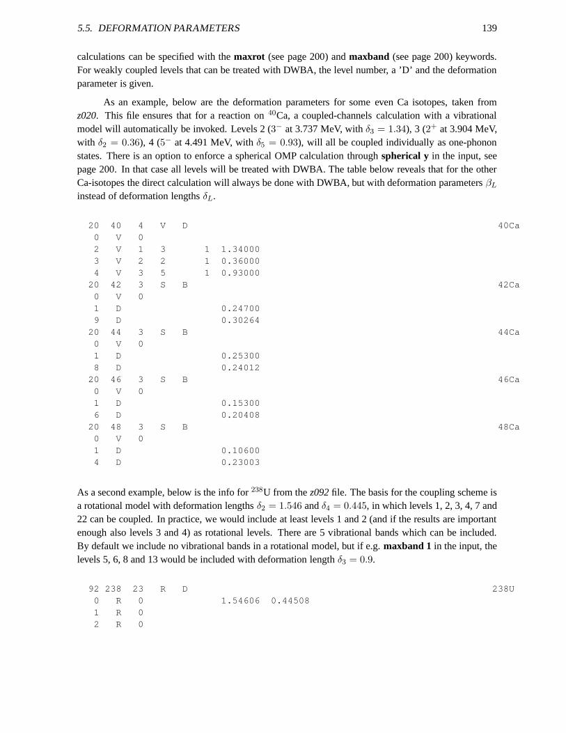
5.5. DEFORMATION PARAMETERS 139
calculations can be specified with themaxrot (see page 200) andmaxband (see page 200) keywords.For weakly coupled levels that can be treated with DWBA, the level number, a ’D’ and the deformationparameter is given.
As an example, below are the deformation parameters for someeven Ca isotopes, taken fromz020. This file ensures that for a reaction on40Ca, a coupled-channels calculation with a vibrationalmodel will automatically be invoked. Levels 2 (3− at 3.737 MeV, withδ3 = 1.34), 3 (2+ at 3.904 MeV,with δ2 = 0.36), 4 (5− at 4.491 MeV, withδ5 = 0.93), will all be coupled individually as one-phononstates. There is an option to enforce a spherical OMP calculation throughspherical y in the input, seepage 200. In that case all levels will be treated with DWBA. The table below reveals that for the otherCa-isotopes the direct calculation will always be done withDWBA, but with deformation parametersβL
instead of deformation lengthsδL.
20 40 4 V D 40Ca0 V 02 V 1 3 1 1.340003 V 2 2 1 0.360004 V 3 5 1 0.93000
20 42 3 S B 42Ca0 V 01 D 0.247009 D 0.30264
20 44 3 S B 44Ca0 V 01 D 0.253008 D 0.24012
20 46 3 S B 46Ca0 V 01 D 0.153006 D 0.20408
20 48 3 S B 48Ca0 V 01 D 0.106004 D 0.23003
As a second example, below is the info for238U from thez092file. The basis for the coupling scheme isa rotational model with deformation lengthsδ2 = 1.546 andδ4 = 0.445, in which levels 1, 2, 3, 4, 7 and22 can be coupled. In practice, we would include at least levels 1 and 2 (and if the results are importantenough also levels 3 and 4) as rotational levels. There are 5 vibrational bands which can be included.By default we include no vibrational bands in a rotational model, but if e.g.maxband 1 in the input, thelevels 5, 6, 8 and 13 would be included with deformation length δ3 = 0.9.
92 238 23 R D 238U0 R 0 1.54606 0.445081 R 02 R 0
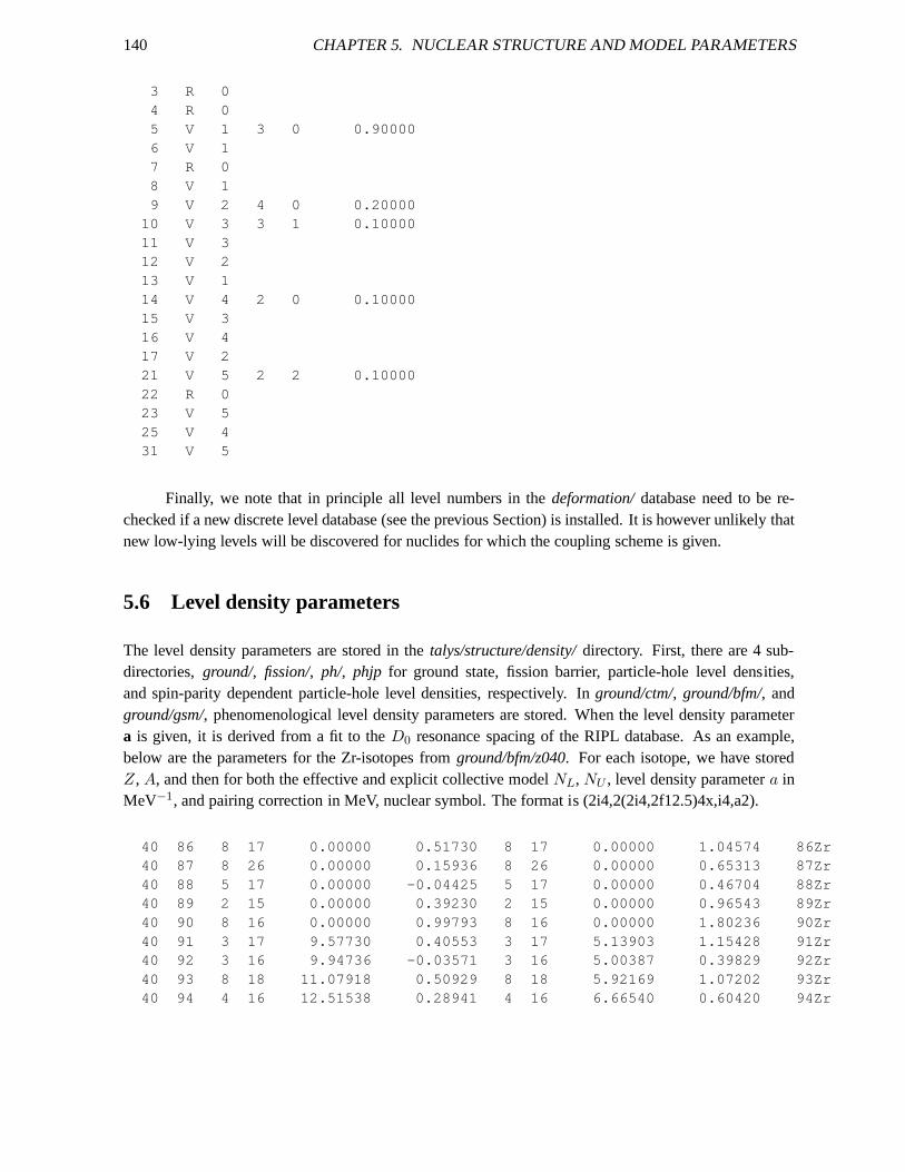
140 CHAPTER 5. NUCLEAR STRUCTURE AND MODEL PARAMETERS
3 R 04 R 05 V 1 3 0 0.900006 V 17 R 08 V 19 V 2 4 0 0.20000
10 V 3 3 1 0.1000011 V 312 V 213 V 114 V 4 2 0 0.1000015 V 316 V 417 V 221 V 5 2 2 0.1000022 R 023 V 525 V 431 V 5
Finally, we note that in principle all level numbers in thedeformation/database need to be re-checked if a new discrete level database (see the previous Section) is installed. It is however unlikely thatnew low-lying levels will be discovered for nuclides for which the coupling scheme is given.
5.6 Level density parameters
The level density parameters are stored in thetalys/structure/density/directory. First, there are 4 sub-directories,ground/, fission/, ph/, phjp for ground state, fission barrier, particle-hole level densities,and spin-parity dependent particle-hole level densities,respectively. Inground/ctm/, ground/bfm/, andground/gsm/, phenomenological level density parameters are stored. When the level density parametera is given, it is derived from a fit to theD0 resonance spacing of the RIPL database. As an example,below are the parameters for the Zr-isotopes fromground/bfm/z040. For each isotope, we have storedZ, A, and then for both the effective and explicit collective model NL, NU , level density parametera inMeV−1, and pairing correction in MeV, nuclear symbol. The format is (2i4,2(2i4,2f12.5)4x,i4,a2).
40 86 8 17 0.00000 0.51730 8 17 0.00000 1.04574 86Zr40 87 8 26 0.00000 0.15936 8 26 0.00000 0.65313 87Zr40 88 5 17 0.00000 -0.04425 5 17 0.00000 0.46704 88Zr40 89 2 15 0.00000 0.39230 2 15 0.00000 0.96543 89Zr40 90 8 16 0.00000 0.99793 8 16 0.00000 1.80236 90Zr40 91 3 17 9.57730 0.40553 3 17 5.13903 1.15428 91Zr40 92 3 16 9.94736 -0.03571 3 16 5.00387 0.39829 92Zr40 93 8 18 11.07918 0.50929 8 18 5.92169 1.07202 93Zr40 94 4 16 12.51538 0.28941 4 16 6.66540 0.60420 94Zr
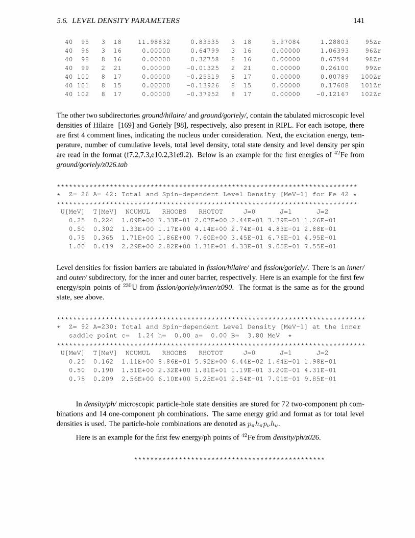
5.6. LEVEL DENSITY PARAMETERS 141
40 95 3 18 11.98832 0.83535 3 18 5.97084 1.28803 95Zr40 96 3 16 0.00000 0.64799 3 16 0.00000 1.06393 96Zr40 98 8 16 0.00000 0.32758 8 16 0.00000 0.67594 98Zr40 99 2 21 0.00000 -0.01325 2 21 0.00000 0.26100 99Zr40 100 8 17 0.00000 -0.25519 8 17 0.00000 0.00789 100Zr40 101 8 15 0.00000 -0.13926 8 15 0.00000 0.17608 101Zr40 102 8 17 0.00000 -0.37952 8 17 0.00000 -0.12167 102Zr
The other two subdirectoriesground/hilaire/andground/goriely/, contain the tabulated microscopic leveldensities of Hilaire [169] and Goriely [98], respectively,also present in RIPL. For each isotope, thereare first 4 comment lines, indicating the nucleus under consideration. Next, the excitation energy, tem-perature, number of cumulative levels, total level density, total state density and level density per spinare read in the format (f7.2,7.3,e10.2,31e9.2). Below is anexample for the first energies of42Fe fromground/goriely/z026.tab
*************************************************** ************************ Z= 26 A= 42: Total and Spin-dependent Level Density [MeV-1] f or Fe 42 **************************************************** ***********************
U[MeV] T[MeV] NCUMUL RHOOBS RHOTOT J=0 J=1 J=20.25 0.224 1.09E+00 7.33E-01 2.07E+00 2.44E-01 3.39E-01 1. 26E-010.50 0.302 1.33E+00 1.17E+00 4.14E+00 2.74E-01 4.83E-01 2. 88E-010.75 0.365 1.71E+00 1.86E+00 7.60E+00 3.45E-01 6.76E-01 4. 95E-011.00 0.419 2.29E+00 2.82E+00 1.31E+01 4.33E-01 9.05E-01 7. 55E-01
Level densities for fission barriers are tabulated infission/hilaire/andfission/goriely/. There is aninner/andouter/subdirectory, for the inner and outer barrier, respectively. Here is an example for the first fewenergy/spin points of230U from fission/goriely/inner/z090. The format is the same as for the groundstate, see above.
*************************************************** ************************** Z= 92 A=230: Total and Spin-dependent Level Density [MeV-1] at the inner
saddle point c= 1.24 h= 0.00 a= 0.00 B= 3.80 MeV **************************************************** *************************
U[MeV] T[MeV] NCUMUL RHOOBS RHOTOT J=0 J=1 J=20.25 0.162 1.11E+00 8.86E-01 5.92E+00 6.44E-02 1.64E-01 1. 98E-010.50 0.190 1.51E+00 2.32E+00 1.81E+01 1.19E-01 3.20E-01 4. 31E-010.75 0.209 2.56E+00 6.10E+00 5.25E+01 2.54E-01 7.01E-01 9. 85E-01
In density/ph/microscopic particle-hole state densities are stored for 72 two-component ph com-binations and 14 one-component ph combinations. The same energy grid and format as for total leveldensities is used. The particle-hole combinations are denoted aspπhπpνhν .
Here is an example for the first few energy/ph points of42Fe fromdensity/ph/z026.
***********************************************
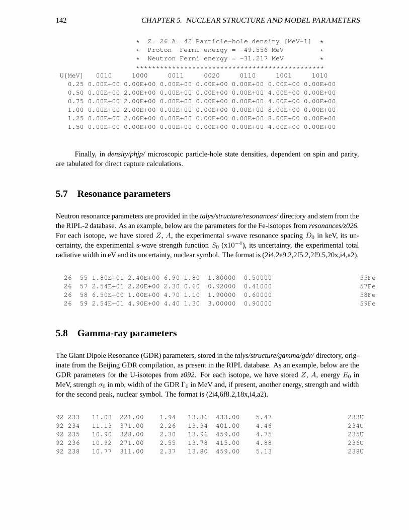
142 CHAPTER 5. NUCLEAR STRUCTURE AND MODEL PARAMETERS
* Z= 26 A= 42 Particle-hole density [MeV-1] ** Proton Fermi energy = -49.556 MeV ** Neutron Fermi energy = -31.217 MeV ************************************************
U[MeV] 0010 1000 0011 0020 0110 1001 10100.25 0.00E+00 0.00E+00 0.00E+00 0.00E+00 0.00E+00 0.00E+0 0 0.00E+000.50 0.00E+00 2.00E+00 0.00E+00 0.00E+00 0.00E+00 4.00E+0 0 0.00E+000.75 0.00E+00 2.00E+00 0.00E+00 0.00E+00 0.00E+00 4.00E+0 0 0.00E+001.00 0.00E+00 2.00E+00 0.00E+00 0.00E+00 0.00E+00 8.00E+0 0 0.00E+001.25 0.00E+00 2.00E+00 0.00E+00 0.00E+00 0.00E+00 8.00E+0 0 0.00E+001.50 0.00E+00 0.00E+00 0.00E+00 0.00E+00 0.00E+00 4.00E+0 0 0.00E+00
Finally, in density/phjp/microscopic particle-hole state densities, dependent on spin and parity,are tabulated for direct capture calculations.
5.7 Resonance parameters
Neutron resonance parameters are provided in thetalys/structure/resonances/directory and stem from thethe RIPL-2 database. As an example, below are the parametersfor the Fe-isotopes fromresonances/z026.For each isotope, we have storedZ, A, the experimental s-wave resonance spacingD0 in keV, its un-certainty, the experimental s-wave strength functionS0 (x10−4), its uncertainty, the experimental totalradiative width in eV and its uncertainty, nuclear symbol. The format is (2i4,2e9.2,2f5.2,2f9.5,20x,i4,a2).
26 55 1.80E+01 2.40E+00 6.90 1.80 1.80000 0.50000 55Fe26 57 2.54E+01 2.20E+00 2.30 0.60 0.92000 0.41000 57Fe26 58 6.50E+00 1.00E+00 4.70 1.10 1.90000 0.60000 58Fe26 59 2.54E+01 4.90E+00 4.40 1.30 3.00000 0.90000 59Fe
5.8 Gamma-ray parameters
The Giant Dipole Resonance (GDR) parameters, stored in thetalys/structure/gamma/gdr/directory, orig-inate from the Beijing GDR compilation, as present in the RIPL database. As an example, below are theGDR parameters for the U-isotopes fromz092. For each isotope, we have storedZ, A, energyE0 inMeV, strengthσ0 in mb, width of the GDRΓ0 in MeV and, if present, another energy, strength and widthfor the second peak, nuclear symbol. The format is (2i4,6f8.2,18x,i4,a2).
92 233 11.08 221.00 1.94 13.86 433.00 5.47 233U92 234 11.13 371.00 2.26 13.94 401.00 4.46 234U92 235 10.90 328.00 2.30 13.96 459.00 4.75 235U92 236 10.92 271.00 2.55 13.78 415.00 4.88 236U92 238 10.77 311.00 2.37 13.80 459.00 5.13 238U
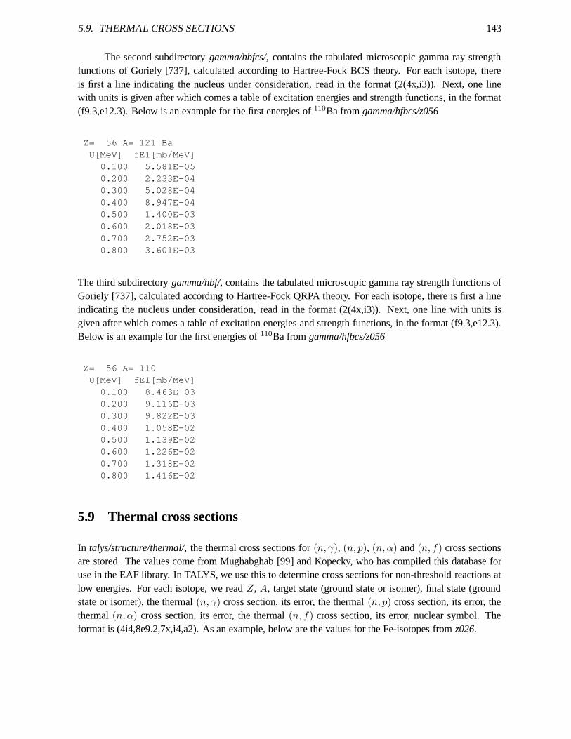
5.9. THERMAL CROSS SECTIONS 143
The second subdirectorygamma/hbfcs/, contains the tabulated microscopic gamma ray strengthfunctions of Goriely [737], calculated according to Hartree-Fock BCS theory. For each isotope, thereis first a line indicating the nucleus under consideration, read in the format (2(4x,i3)). Next, one linewith units is given after which comes a table of excitation energies and strength functions, in the format(f9.3,e12.3). Below is an example for the first energies of110Ba fromgamma/hfbcs/z056
Z= 56 A= 121 BaU[MeV] fE1[mb/MeV]
0.100 5.581E-050.200 2.233E-040.300 5.028E-040.400 8.947E-040.500 1.400E-030.600 2.018E-030.700 2.752E-030.800 3.601E-03
The third subdirectorygamma/hbf/, contains the tabulated microscopic gamma ray strength functions ofGoriely [737], calculated according to Hartree-Fock QRPA theory. For each isotope, there is first a lineindicating the nucleus under consideration, read in the format (2(4x,i3)). Next, one line with units isgiven after which comes a table of excitation energies and strength functions, in the format (f9.3,e12.3).Below is an example for the first energies of110Ba fromgamma/hfbcs/z056
Z= 56 A= 110U[MeV] fE1[mb/MeV]
0.100 8.463E-030.200 9.116E-030.300 9.822E-030.400 1.058E-020.500 1.139E-020.600 1.226E-020.700 1.318E-020.800 1.416E-02
5.9 Thermal cross sections
In talys/structure/thermal/, the thermal cross sections for(n, γ), (n, p), (n, α) and(n, f) cross sectionsare stored. The values come from Mughabghab [99] and Kopecky, who has compiled this database foruse in the EAF library. In TALYS, we use this to determine cross sections for non-threshold reactions atlow energies. For each isotope, we readZ, A, target state (ground state or isomer), final state (groundstate or isomer), the thermal(n, γ) cross section, its error, the thermal(n, p) cross section, its error, thethermal(n, α) cross section, its error, the thermal(n, f) cross section, its error, nuclear symbol. Theformat is (4i4,8e9.2,7x,i4,a2). As an example, below are the values for the Fe-isotopes fromz026.
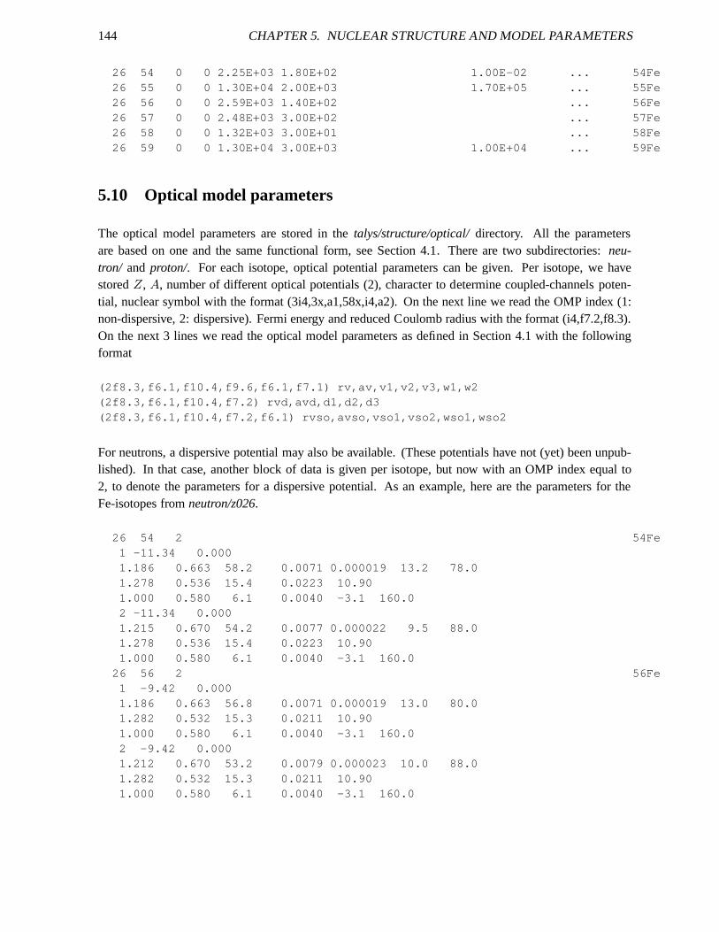
144 CHAPTER 5. NUCLEAR STRUCTURE AND MODEL PARAMETERS
26 54 0 0 2.25E+03 1.80E+02 1.00E-02 ... 54Fe26 55 0 0 1.30E+04 2.00E+03 1.70E+05 ... 55Fe26 56 0 0 2.59E+03 1.40E+02 ... 56Fe26 57 0 0 2.48E+03 3.00E+02 ... 57Fe26 58 0 0 1.32E+03 3.00E+01 ... 58Fe26 59 0 0 1.30E+04 3.00E+03 1.00E+04 ... 59Fe
5.10 Optical model parameters
The optical model parameters are stored in thetalys/structure/optical/directory. All the parametersare based on one and the same functional form, see Section 4.1. There are two subdirectories:neu-tron/ and proton/. For each isotope, optical potential parameters can be given. Per isotope, we havestoredZ, A, number of different optical potentials (2), character to determine coupled-channels poten-tial, nuclear symbol with the format (3i4,3x,a1,58x,i4,a2). On the next line we read the OMP index (1:non-dispersive, 2: dispersive). Fermi energy and reduced Coulomb radius with the format (i4,f7.2,f8.3).On the next 3 lines we read the optical model parameters as defined in Section 4.1 with the followingformat
(2f8.3,f6.1,f10.4,f9.6,f6.1,f7.1) rv,av,v1,v2,v3,w1, w2(2f8.3,f6.1,f10.4,f7.2) rvd,avd,d1,d2,d3(2f8.3,f6.1,f10.4,f7.2,f6.1) rvso,avso,vso1,vso2,wso 1,wso2
For neutrons, a dispersive potential may also be available.(These potentials have not (yet) been unpub-lished). In that case, another block of data is given per isotope, but now with an OMP index equal to2, to denote the parameters for a dispersive potential. As anexample, here are the parameters for theFe-isotopes fromneutron/z026.
26 54 2 54Fe1 -11.34 0.0001.186 0.663 58.2 0.0071 0.000019 13.2 78.01.278 0.536 15.4 0.0223 10.901.000 0.580 6.1 0.0040 -3.1 160.02 -11.34 0.0001.215 0.670 54.2 0.0077 0.000022 9.5 88.01.278 0.536 15.4 0.0223 10.901.000 0.580 6.1 0.0040 -3.1 160.0
26 56 2 56Fe1 -9.42 0.0001.186 0.663 56.8 0.0071 0.000019 13.0 80.01.282 0.532 15.3 0.0211 10.901.000 0.580 6.1 0.0040 -3.1 160.02 -9.42 0.0001.212 0.670 53.2 0.0079 0.000023 10.0 88.01.282 0.532 15.3 0.0211 10.901.000 0.580 6.1 0.0040 -3.1 160.0
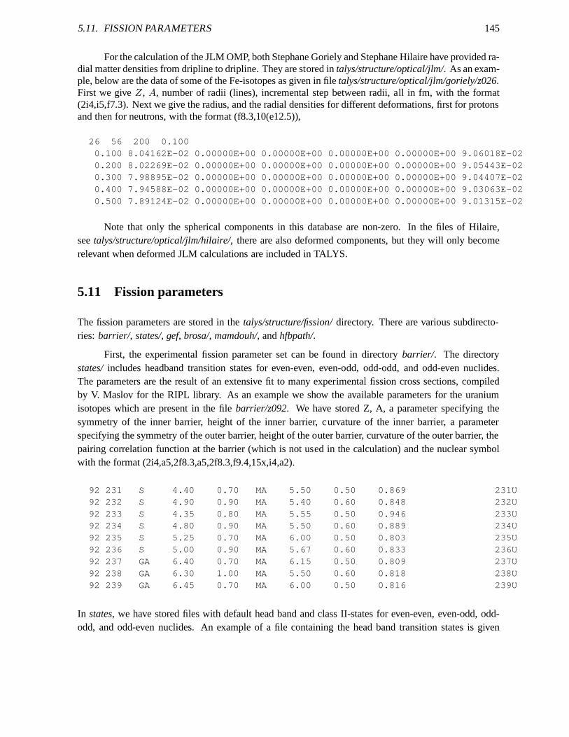
5.11. FISSION PARAMETERS 145
For the calculation of the JLM OMP, both Stephane Goriely andStephane Hilaire have provided ra-dial matter densities from dripline to dripline. They are stored intalys/structure/optical/jlm/. As an exam-ple, below are the data of some of the Fe-isotopes as given in file talys/structure/optical/jlm/goriely/z026.First we giveZ, A, number of radii (lines), incremental step between radii, all in fm, with the format(2i4,i5,f7.3). Next we give the radius, and the radial densities for different deformations, first for protonsand then for neutrons, with the format (f8.3,10(e12.5)),
26 56 200 0.1000.100 8.04162E-02 0.00000E+00 0.00000E+00 0.00000E+00 0. 00000E+00 9.06018E-020.200 8.02269E-02 0.00000E+00 0.00000E+00 0.00000E+00 0. 00000E+00 9.05443E-020.300 7.98895E-02 0.00000E+00 0.00000E+00 0.00000E+00 0. 00000E+00 9.04407E-020.400 7.94588E-02 0.00000E+00 0.00000E+00 0.00000E+00 0. 00000E+00 9.03063E-020.500 7.89124E-02 0.00000E+00 0.00000E+00 0.00000E+00 0. 00000E+00 9.01315E-02
Note that only the spherical components in this database arenon-zero. In the files of Hilaire,seetalys/structure/optical/jlm/hilaire/, there are also deformed components, but they will only becomerelevant when deformed JLM calculations are included in TALYS.
5.11 Fission parameters
The fission parameters are stored in thetalys/structure/fission/directory. There are various subdirecto-ries: barrier/, states/, gef, brosa/, mamdouh/, andhfbpath/.
First, the experimental fission parameter set can be found indirectory barrier/. The directorystates/includes headband transition states for even-even, even-odd, odd-odd, and odd-even nuclides.The parameters are the result of an extensive fit to many experimental fission cross sections, compiledby V. Maslov for the RIPL library. As an example we show the available parameters for the uraniumisotopes which are present in the filebarrier/z092. We have stored Z, A, a parameter specifying thesymmetry of the inner barrier, height of the inner barrier, curvature of the inner barrier, a parameterspecifying the symmetry of the outer barrier, height of the outer barrier, curvature of the outer barrier, thepairing correlation function at the barrier (which is not used in the calculation) and the nuclear symbolwith the format (2i4,a5,2f8.3,a5,2f8.3,f9.4,15x,i4,a2).
92 231 S 4.40 0.70 MA 5.50 0.50 0.869 231U92 232 S 4.90 0.90 MA 5.40 0.60 0.848 232U92 233 S 4.35 0.80 MA 5.55 0.50 0.946 233U92 234 S 4.80 0.90 MA 5.50 0.60 0.889 234U92 235 S 5.25 0.70 MA 6.00 0.50 0.803 235U92 236 S 5.00 0.90 MA 5.67 0.60 0.833 236U92 237 GA 6.40 0.70 MA 6.15 0.50 0.809 237U92 238 GA 6.30 1.00 MA 5.50 0.60 0.818 238U92 239 GA 6.45 0.70 MA 6.00 0.50 0.816 239U
In states, we have stored files with default head band and class II-states for even-even, even-odd, odd-odd, and odd-even nuclides. An example of a file containing the head band transition states is given
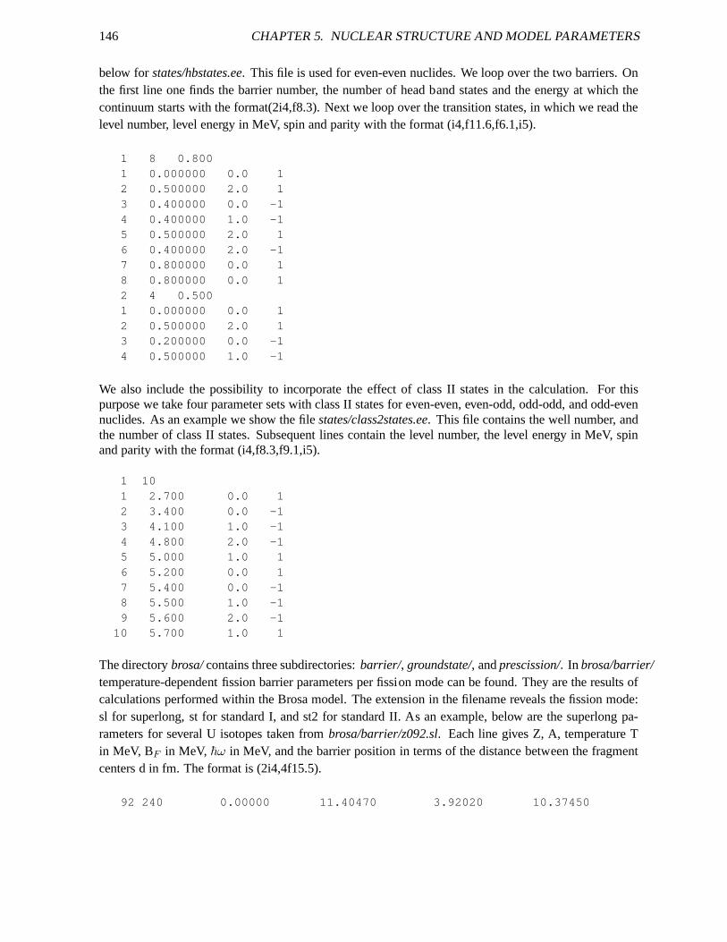
146 CHAPTER 5. NUCLEAR STRUCTURE AND MODEL PARAMETERS
below forstates/hbstates.ee. This file is used for even-even nuclides. We loop over the twobarriers. Onthe first line one finds the barrier number, the number of head band states and the energy at which thecontinuum starts with the format(2i4,f8.3). Next we loop over the transition states, in which we read thelevel number, level energy in MeV, spin and parity with the format (i4,f11.6,f6.1,i5).
1 8 0.8001 0.000000 0.0 12 0.500000 2.0 13 0.400000 0.0 -14 0.400000 1.0 -15 0.500000 2.0 16 0.400000 2.0 -17 0.800000 0.0 18 0.800000 0.0 12 4 0.5001 0.000000 0.0 12 0.500000 2.0 13 0.200000 0.0 -14 0.500000 1.0 -1
We also include the possibility to incorporate the effect ofclass II states in the calculation. For thispurpose we take four parameter sets with class II states for even-even, even-odd, odd-odd, and odd-evennuclides. As an example we show the filestates/class2states.ee. This file contains the well number, andthe number of class II states. Subsequent lines contain the level number, the level energy in MeV, spinand parity with the format (i4,f8.3,f9.1,i5).
1 101 2.700 0.0 12 3.400 0.0 -13 4.100 1.0 -14 4.800 2.0 -15 5.000 1.0 16 5.200 0.0 17 5.400 0.0 -18 5.500 1.0 -19 5.600 2.0 -1
10 5.700 1.0 1
The directorybrosa/contains three subdirectories:barrier/, groundstate/, andprescission/. In brosa/barrier/temperature-dependent fission barrier parameters per fission mode can be found. They are the results ofcalculations performed within the Brosa model. The extension in the filename reveals the fission mode:sl for superlong, st for standard I, and st2 for standard II. As an example, below are the superlong pa-rameters for several U isotopes taken frombrosa/barrier/z092.sl. Each line gives Z, A, temperature Tin MeV, BF in MeV, ~ω in MeV, and the barrier position in terms of the distance between the fragmentcenters d in fm. The format is (2i4,4f15.5).
92 240 0.00000 11.40470 3.92020 10.37450
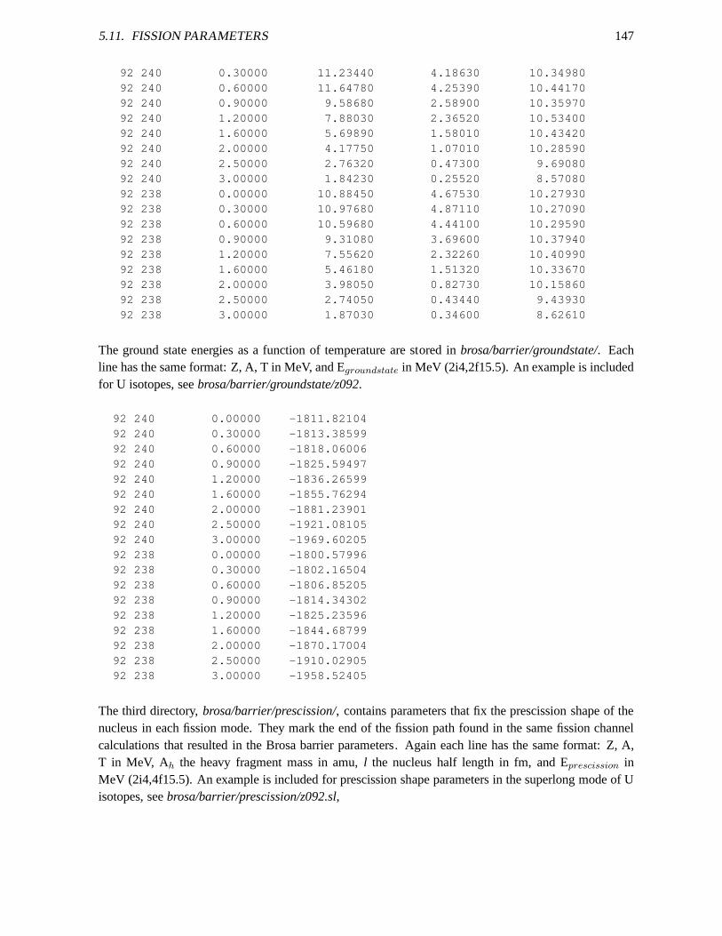
5.11. FISSION PARAMETERS 147
92 240 0.30000 11.23440 4.18630 10.3498092 240 0.60000 11.64780 4.25390 10.4417092 240 0.90000 9.58680 2.58900 10.3597092 240 1.20000 7.88030 2.36520 10.5340092 240 1.60000 5.69890 1.58010 10.4342092 240 2.00000 4.17750 1.07010 10.2859092 240 2.50000 2.76320 0.47300 9.6908092 240 3.00000 1.84230 0.25520 8.5708092 238 0.00000 10.88450 4.67530 10.2793092 238 0.30000 10.97680 4.87110 10.2709092 238 0.60000 10.59680 4.44100 10.2959092 238 0.90000 9.31080 3.69600 10.3794092 238 1.20000 7.55620 2.32260 10.4099092 238 1.60000 5.46180 1.51320 10.3367092 238 2.00000 3.98050 0.82730 10.1586092 238 2.50000 2.74050 0.43440 9.4393092 238 3.00000 1.87030 0.34600 8.62610
The ground state energies as a function of temperature are stored inbrosa/barrier/groundstate/. Eachline has the same format: Z, A, T in MeV, and Egroundstate in MeV (2i4,2f15.5). An example is includedfor U isotopes, seebrosa/barrier/groundstate/z092.
92 240 0.00000 -1811.8210492 240 0.30000 -1813.3859992 240 0.60000 -1818.0600692 240 0.90000 -1825.5949792 240 1.20000 -1836.2659992 240 1.60000 -1855.7629492 240 2.00000 -1881.2390192 240 2.50000 -1921.0810592 240 3.00000 -1969.6020592 238 0.00000 -1800.5799692 238 0.30000 -1802.1650492 238 0.60000 -1806.8520592 238 0.90000 -1814.3430292 238 1.20000 -1825.2359692 238 1.60000 -1844.6879992 238 2.00000 -1870.1700492 238 2.50000 -1910.0290592 238 3.00000 -1958.52405
The third directory,brosa/barrier/prescission/, contains parameters that fix the prescission shape of thenucleus in each fission mode. They mark the end of the fission path found in the same fission channelcalculations that resulted in the Brosa barrier parameters. Again each line has the same format: Z, A,T in MeV, Ah the heavy fragment mass in amu,l the nucleus half length in fm, and Eprescission inMeV (2i4,4f15.5). An example is included for prescission shape parameters in the superlong mode of Uisotopes, seebrosa/barrier/prescission/z092.sl,
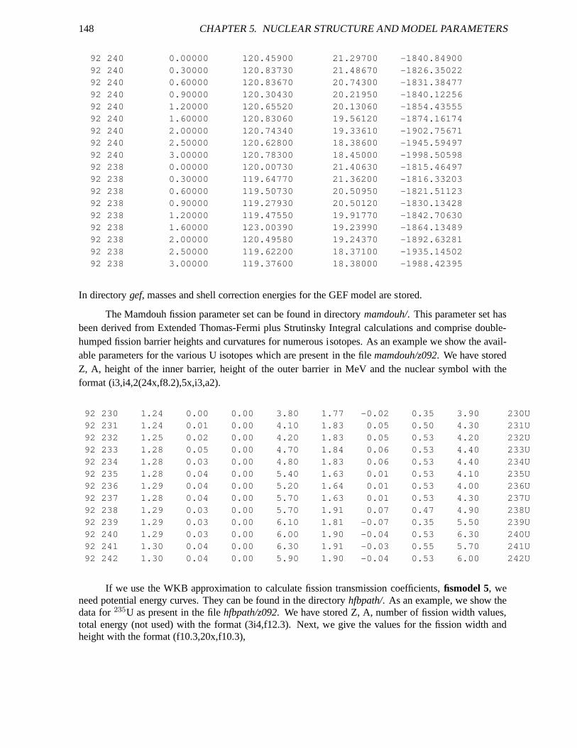
148 CHAPTER 5. NUCLEAR STRUCTURE AND MODEL PARAMETERS
92 240 0.00000 120.45900 21.29700 -1840.8490092 240 0.30000 120.83730 21.48670 -1826.3502292 240 0.60000 120.83670 20.74300 -1831.3847792 240 0.90000 120.30430 20.21950 -1840.1225692 240 1.20000 120.65520 20.13060 -1854.4355592 240 1.60000 120.83060 19.56120 -1874.1617492 240 2.00000 120.74340 19.33610 -1902.7567192 240 2.50000 120.62800 18.38600 -1945.5949792 240 3.00000 120.78300 18.45000 -1998.5059892 238 0.00000 120.00730 21.40630 -1815.4649792 238 0.30000 119.64770 21.36200 -1816.3320392 238 0.60000 119.50730 20.50950 -1821.5112392 238 0.90000 119.27930 20.50120 -1830.1342892 238 1.20000 119.47550 19.91770 -1842.7063092 238 1.60000 123.00390 19.23990 -1864.1348992 238 2.00000 120.49580 19.24370 -1892.6328192 238 2.50000 119.62200 18.37100 -1935.1450292 238 3.00000 119.37600 18.38000 -1988.42395
In directorygef, masses and shell correction energies for the GEF model are stored.
The Mamdouh fission parameter set can be found in directorymamdouh/. This parameter set hasbeen derived from Extended Thomas-Fermi plus Strutinsky Integral calculations and comprise double-humped fission barrier heights and curvatures for numerous isotopes. As an example we show the avail-able parameters for the various U isotopes which are presentin the filemamdouh/z092. We have storedZ, A, height of the inner barrier, height of the outer barrierin MeV and the nuclear symbol with theformat (i3,i4,2(24x,f8.2),5x,i3,a2).
92 230 1.24 0.00 0.00 3.80 1.77 -0.02 0.35 3.90 230U92 231 1.24 0.01 0.00 4.10 1.83 0.05 0.50 4.30 231U92 232 1.25 0.02 0.00 4.20 1.83 0.05 0.53 4.20 232U92 233 1.28 0.05 0.00 4.70 1.84 0.06 0.53 4.40 233U92 234 1.28 0.03 0.00 4.80 1.83 0.06 0.53 4.40 234U92 235 1.28 0.04 0.00 5.40 1.63 0.01 0.53 4.10 235U92 236 1.29 0.04 0.00 5.20 1.64 0.01 0.53 4.00 236U92 237 1.28 0.04 0.00 5.70 1.63 0.01 0.53 4.30 237U92 238 1.29 0.03 0.00 5.70 1.91 0.07 0.47 4.90 238U92 239 1.29 0.03 0.00 6.10 1.81 -0.07 0.35 5.50 239U92 240 1.29 0.03 0.00 6.00 1.90 -0.04 0.53 6.30 240U92 241 1.30 0.04 0.00 6.30 1.91 -0.03 0.55 5.70 241U92 242 1.30 0.04 0.00 5.90 1.90 -0.04 0.53 6.00 242U
If we use the WKB approximation to calculate fission transmission coefficients,fismodel 5, weneed potential energy curves. They can be found in the directory hfbpath/. As an example, we show thedata for235U as present in the filehfbpath/z092. We have stored Z, A, number of fission width values,total energy (not used) with the format (3i4,f12.3). Next, we give the values for the fission width andheight with the format (f10.3,20x,f10.3),
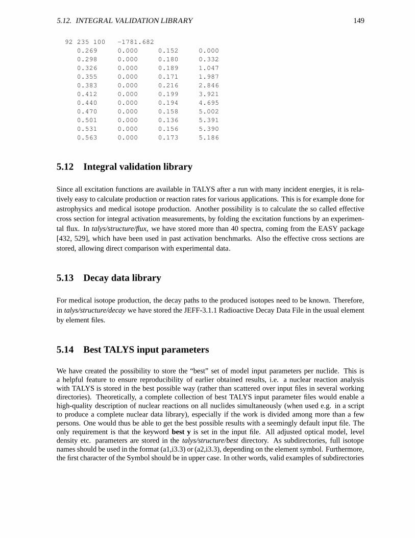
5.12. INTEGRAL VALIDATION LIBRARY 149
92 235 100 -1781.6820.269 0.000 0.152 0.0000.298 0.000 0.180 0.3320.326 0.000 0.189 1.0470.355 0.000 0.171 1.9870.383 0.000 0.216 2.8460.412 0.000 0.199 3.9210.440 0.000 0.194 4.6950.470 0.000 0.158 5.0020.501 0.000 0.136 5.3910.531 0.000 0.156 5.3900.563 0.000 0.173 5.186
5.12 Integral validation library
Since all excitation functions are available in TALYS aftera run with many incident energies, it is rela-tively easy to calculate production or reaction rates for various applications. This is for example done forastrophysics and medical isotope production. Another possibility is to calculate the so called effectivecross section for integral activation measurements, by folding the excitation functions by an experimen-tal flux. In talys/structure/flux, we have stored more than 40 spectra, coming from the EASY package[432, 529], which have been used in past activation benchmarks. Also the effective cross sections arestored, allowing direct comparison with experimental data.
5.13 Decay data library
For medical isotope production, the decay paths to the produced isotopes need to be known. Therefore,in talys/structure/decaywe have stored the JEFF-3.1.1 Radioactive Decay Data File inthe usual elementby element files.
5.14 Best TALYS input parameters
We have created the possibility to store the “best” set of model input parameters per nuclide. This isa helpful feature to ensure reproducibility of earlier obtained results, i.e. a nuclear reaction analysiswith TALYS is stored in the best possible way (rather than scattered over input files in several workingdirectories). Theoretically, a complete collection of best TALYS input parameter files would enable ahigh-quality description of nuclear reactions on all nuclides simultaneously (when used e.g. in a scriptto produce a complete nuclear data library), especially if the work is divided among more than a fewpersons. One would thus be able to get the best possible results with a seemingly default input file. Theonly requirement is that the keywordbest y is set in the input file. All adjusted optical model, leveldensity etc. parameters are stored in thetalys/structure/bestdirectory. As subdirectories, full isotopenames should be used in the format (a1,i3.3) or (a2,i3.3), depending on the element symbol. Furthermore,the first character of the Symbol should be in upper case. In other words, valid examples of subdirectories
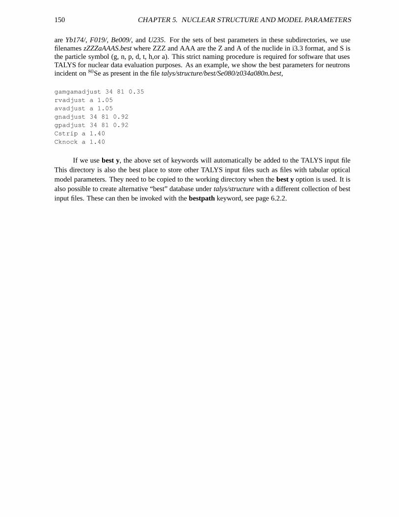
150 CHAPTER 5. NUCLEAR STRUCTURE AND MODEL PARAMETERS
areYb174/, F019/, Be009/, andU235. For the sets of best parameters in these subdirectories, weusefilenameszZZZaAAAS.bestwhere ZZZ and AAA are the Z and A of the nuclide in i3.3 format, and S isthe particle symbol (g, n, p, d, t, h,or a). This strict namingprocedure is required for software that usesTALYS for nuclear data evaluation purposes. As an example, we show the best parameters for neutronsincident on80Se as present in the filetalys/structure/best/Se080/z034a080n.best,
gamgamadjust 34 81 0.35rvadjust a 1.05avadjust a 1.05gnadjust 34 81 0.92gpadjust 34 81 0.92Cstrip a 1.40Cknock a 1.40
If we usebest y, the above set of keywords will automatically be added to theTALYS input fileThis directory is also the best place to store other TALYS input files such as files with tabular opticalmodel parameters. They need to be copied to the working directory when thebest yoption is used. It isalso possible to create alternative “best” database undertalys/structurewith a different collection of bestinput files. These can then be invoked with thebestpathkeyword, see page 6.2.2.
Chapter 6Input description
For the communication between TALYS and its users, we have constructed an input/output method whichshields beginners from all the possible options for nuclearmodel parameters that can be specified inTALYS, while enabling at the same time maximal flexibility for experienced users.
An input file of TALYS consists of keywords and their associated values. Before we list all theinput possibilities, let us illustrate the use of the input by the following example. It represents a minimuminput file for TALYS:
projectile nelement almass 27energy 14.
This input file represents the simplest question that can be asked to TALYS: if a27Al nucleus is hit by 14MeV neutrons, what happens? Behind this simple input file, however, there are more than a few hundreddefault values for the various nuclear models, parameters,output flags, etc., that you may or may notbe interested in. When you use a minimal input file like the oneabove, you leave it to the authors ofTALYS to choose all the parameters and models for you, as wellas the level of detail of the output file.If you want to use specific nuclear models other than the default, adjust parameters or want to have morespecific information in the output file(s), more keywords arerequired. Obviously, more keywords meansmore flexibility and, in the case of adequate use, better results, though often at the expense of increasingthe level of phenomenology. In this Chapter, we will first give the basic rules that must be obeyed whenconstructing an input file for TALYS. Next, we give an outlineof all the keywords, which have beencategorised in several groups. Finally, we summarize all keywords in one table.
151
152 CHAPTER 6. INPUT DESCRIPTION
6.1 Basic input rules
Theoretically, it would be possible to make the use of TALYS completely idiot-proof, i.e. to prevent theuser from any input mistakes that possibly can be made and to continue a calculation with “assumed”values. Although we have invested a relatively large effortin the user-friendliness of TALYS, we havenot taken such safety measures to the extreme limit and ask atleast some minimal responsibility from theuser. Once you have accepted that, only very little effort isrequired to work with the code. Successfulexecution of TALYS can be expected if you remember the following simple rules and possibilities of theinput file:
1. One input line contains one keyword. Usually it is accompanied by only one value, as in the simpleexample given above, but some keywords for model parametersneed to be accompanied by indices(usuallyZ and A) on the same line.
2. A keyword and its value(s)mustbe separated by at least 1 blank character.
3. The keywords can be given in arbitrary order. If, by mistake, you use the same keyword more thanonce, the value of the last one will be adopted. This does not hold for keywords which are labeledwith differentZ andA indices, see the beginning of Section 6.2.
4. All characters can be given in either lowercase or uppercase.
5. A keywordmustbe accompanied by a value. (There is one exception, therotational keyword). Touse default values, the keywords should simply be left out ofthe input file.
6. An input line starting with a# in column 1 is neglected. This is helpful for including commentsin the input file or to temporarily deactivate keywords.
7. A minimal input file always consists of 4 lines and containsthe keywordsprojectile, element,massandenergy. These 4 keywordsmustbe given in any input file.
8. An input line may not exceed 80 characters.
As an example of rules 2, 3, 4 and 6, it can be seen that the following input file is completely equivalentto the one given in the beginning of this Chapter:
# Equivalent input fileenergy 14.projectile nmass 27Element AL#outbasic y
In the following erroneous input file, only the first 2 lines are correct, while rules 2 and 5 are violated inthe other lines.
6.2. KEYWORDS 153
projectile nelement almass27energy
In cases like this, the execution will be stopped and TALYS will give an appropriate error message for thefirst encountered problem. We like to believe that we have covered all such cases and that it is impossibleto let TALYS crash (at least with our compilers, see also Chapter 7), but you are of course invited to proveand let us know about the contrary (Sorry, no cash rewards). Typing errors in the input file will be spottedby TALYS, e.g. if you writeprojjectile n , it will tell you the keyword is not in our list.
6.2 Keywords
The four-line input file given above was an example of a minimum input file for TALYS. In general, youprobably want to be more specific, as in the following example:
projectile nelement nbmass 93energy 1.Ltarget 1relativistic nwidthmode 2outinverse ya 41 93 13.115a 41 94 13.421
which will simulate the reaction of a 1 MeV neutron incident on 93Nb, with the target in its first ex-cited state (Ltarget 1, a 16-year isomer), using non-relativistic kinematics, the HRTW-model for widthfluctuation corrections (widthmode 2) in the compound nucleus calculation, with the particle transmis-sion coefficients and inverse reaction cross sections written on the output file (outinverse y) and withuser-defined level density parametersa for 93Nb and94Nb.
In this Section, we will explain all the possible keywords. We have classified them according totheir meaning and importance. For each keyword, we give an explanation, a few examples, the defaultvalue, and the theoretically allowed numerical range. As the input file above shows, there is usually onevalue per keyword. Often, however, in cases where several residual nuclides are involved, nuclear modelparameters differ from nuclide to nuclide. Then, the particular nuclide under consideration must also begiven in the input line. In general, for these model parameters, we read keyword,Z, A, a physical valueand sometimes a possible further index (e.g. the fission barrier, index for the giant resonance, etc.), allseparated by blanks. As the example above shows for the leveldensity parametera, the same keywordcan appear more than once in an input file, to cover several different nuclides. Again, remember thatall such keywords, if you don’t specify them, have a default value from either the nuclear structure andmodel parameter database or from systematics. The usual reason to change them is to fit experimental
154 CHAPTER 6. INPUT DESCRIPTION
data, to use new information that is not yet in the TALYS database, or simply because the user may notagree with our default values. A final important point to noteis that some keywords induce defaults forother keywords. This may seem confusing, but in practice this is not so. As an example, for a56Fetarget thefissionkeyword is automatically disabled whereas for232Th it is by default enabled. Hence,the default value of thefissionkeyword is mass dependent. In the input description that follows, you willfind a few similar cases. Anyway, you can always find all adopted default values for all parameters atthe top of theoutputfile, see which values have been set by the user or by default, and overrule them ina new input file.
6.2.1 Four main keywords
As explained above there are 4 basic keywords that form the highest level of input. They determine thefundamental parameters for any nuclear reaction induced bya light particle.
projectile
Eight different symbols can be given asprojectile, namelyn, p, d, t, h, a, grepresenting neutron, proton,deuteron, triton,3He, alpha and gamma, respectively, and0, which is used if instead of a nuclear reaction(projectile+ target) we start with an initial population of an excited nucleus.Examples:
projectile n
projectile d
Range: projectile must be equal ton, p, d, t, h, a, gor 0.Default: None.
element
Either the nuclear symbol or the charge numberZ of the target nucleus can be given. Possible values forelementrange from Li (3) to C4 (124). To accomodate target nuclides with Z > 110 the element namesare defined as follows: Rg(111), Cn(112), Fl(114) and Lv(116), B3(113), B5(115), B7-9(117-119), C0-4(120-124). Obviously the symbols, for Z=113,115 and above116 will be changed when official namesare assigned to them.Examples:
element pu
element 41
element V
element B3
6.2. KEYWORDS 155
Range: 3 ≤ element≤ 124 or Li ≤ element≤ C4.Default: None.
mass
The target mass numberA. The case of a natural element can be specified bymass 0. Then, a TALYScalculation for each naturally occurring isotope will be performed (see also theabundancekeyword, p.173), after which the results will be properly weighted and summed.Examples:
mass 239
mass 0
Range: mass 0or 5 < mass≤ 339. The extra condition is that the target nucleus, i.e. the combinationof massandelementmust be present in the mass database, which corresponds to all nuclei between theproton and neutron drip lines.Default: None.
energy
The incident energy in MeV. The user has four possibilities:(1) A single incident energy is specified inthe input as a real number, (2) A filename is specified, where the corresponding file contains a series ofincident energies, with one incident energy per line. Any name can be given to this file, provided it startswith a character, and it is present in your working directory. Option (2) is helpful for the calculation ofexcitation functions or for the creation of nuclear data libraries. Option (2) is mandatory ifprojectile0, i.e., if instead of a nuclear reaction we start with a population of an excited nucleus (see theSpecialcasesbelow). Since TALYS-1.6, there are an additional 2 options which allows to use a whole rangeof incident energies without having to make a file for this: (3) A filename that is predefined by TALYS.This contains a hardwired energy grids with for example for neutrons a finer energy grid at low energiesand a progressively wider grid at high energies. These have the formpE-E.gridwherep is the nameof the projectile, and the twoE’s are the start and end energy in integer form respectively.The .gridspecifies that this concerns a predefined energy grid. An often used example isn0-200.gridwhich is theneutron energy grid of the TENDL library. More energies are used in the eV and keV range while at highenergies automatically a course grid is used. With the filen0-20.gridexactly the same incident energygrid is used, but only up to the final energy of 20 MeV. Finally,option (4) is to give after theenergykeyword 3 numbers: the starting energy, the end energy and the energy step. Next, an equidistant grid ismade based on these 3 numbers.Examples:
energy 140.
energy 0.002
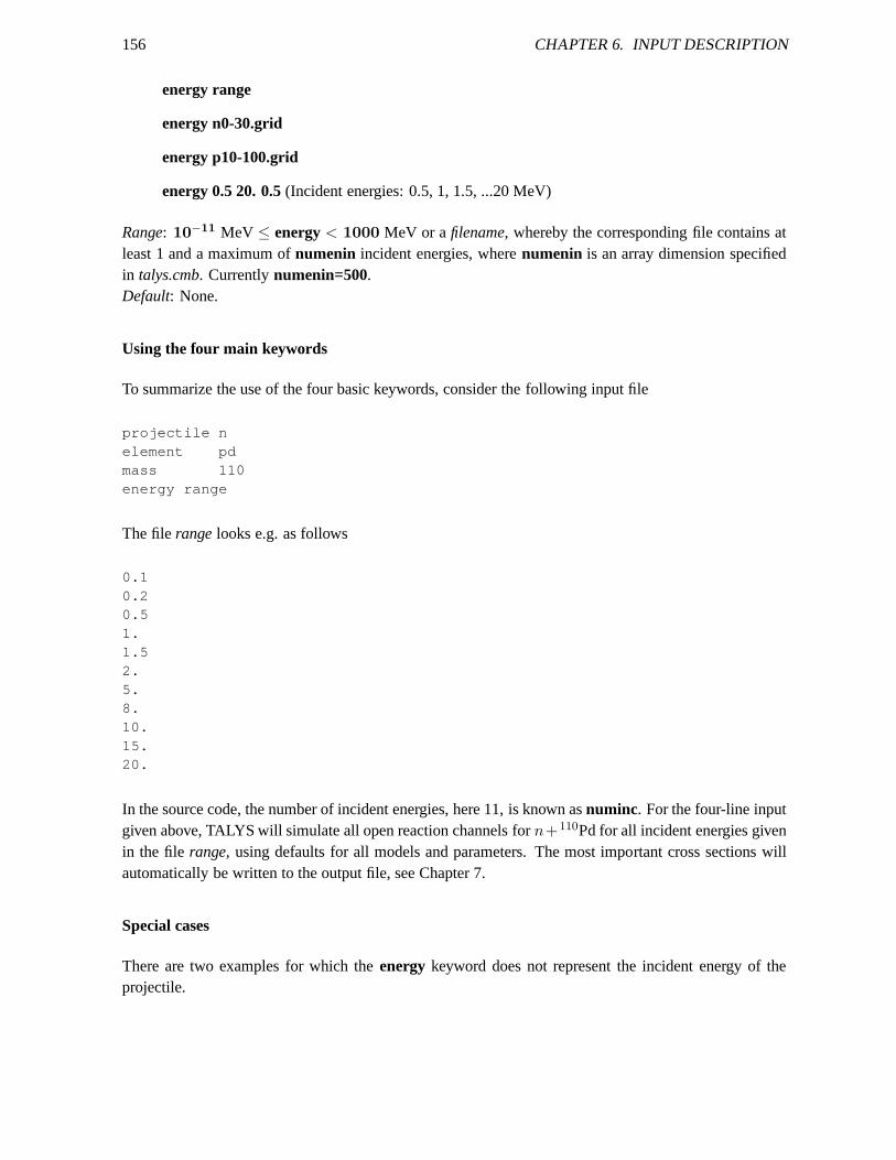
156 CHAPTER 6. INPUT DESCRIPTION
energy range
energy n0-30.grid
energy p10-100.grid
energy 0.5 20. 0.5(Incident energies: 0.5, 1, 1.5, ...20 MeV)
Range: 10−11 MeV ≤ energy< 1000 MeV or afilename, whereby the corresponding file contains at
least 1 and a maximum ofnumenin incident energies, wherenumenin is an array dimension specifiedin talys.cmb. Currentlynumenin=500.Default: None.
Using the four main keywords
To summarize the use of the four basic keywords, consider thefollowing input file
projectile nelement pdmass 110energy range
The filerangelooks e.g. as follows
0.10.20.51.1.52.5.8.10.15.20.
In the source code, the number of incident energies, here 11,is known asnuminc. For the four-line inputgiven above, TALYS will simulate all open reaction channelsfor n+110Pd for all incident energies givenin the file range, using defaults for all models and parameters. The most important cross sections willautomatically be written to the output file, see Chapter 7.
Special cases
There are two examples for which theenergy keyword does not represent the incident energy of theprojectile.
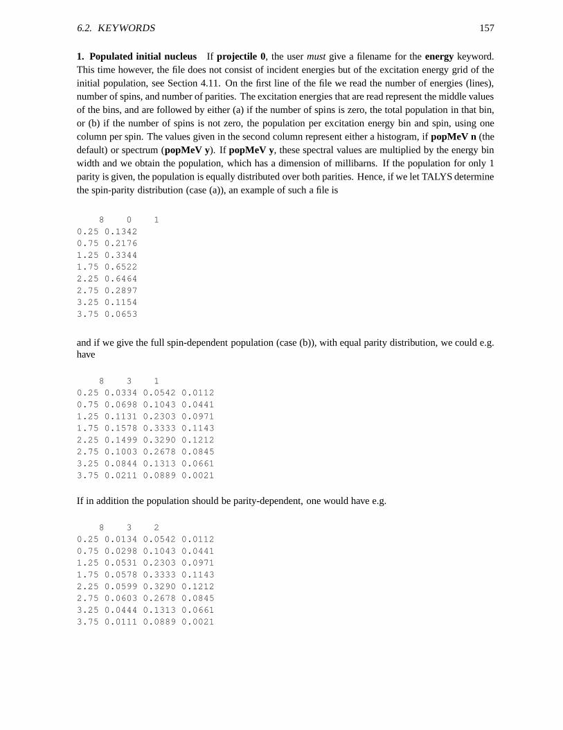
6.2. KEYWORDS 157
1. Populated initial nucleus If projectile 0, the usermustgive a filename for theenergy keyword.This time however, the file does not consist of incident energies but of the excitation energy grid of theinitial population, see Section 4.11. On the first line of thefile we read the number of energies (lines),number of spins, and number of parities. The excitation energies that are read represent the middle valuesof the bins, and are followed by either (a) if the number of spins is zero, the total population in that bin,or (b) if the number of spins is not zero, the population per excitation energy bin and spin, using onecolumn per spin. The values given in the second column represent either a histogram, ifpopMeV n (thedefault) or spectrum (popMeV y). If popMeV y, these spectral values are multiplied by the energy binwidth and we obtain the population, which has a dimension of millibarns. If the population for only 1parity is given, the population is equally distributed overboth parities. Hence, if we let TALYS determinethe spin-parity distribution (case (a)), an example of sucha file is
8 0 10.25 0.13420.75 0.21761.25 0.33441.75 0.65222.25 0.64642.75 0.28973.25 0.11543.75 0.0653
and if we give the full spin-dependent population (case (b)), with equal parity distribution, we could e.g.have
8 3 10.25 0.0334 0.0542 0.01120.75 0.0698 0.1043 0.04411.25 0.1131 0.2303 0.09711.75 0.1578 0.3333 0.11432.25 0.1499 0.3290 0.12122.75 0.1003 0.2678 0.08453.25 0.0844 0.1313 0.06613.75 0.0211 0.0889 0.0021
If in addition the population should be parity-dependent, one would have e.g.
8 3 20.25 0.0134 0.0542 0.01120.75 0.0298 0.1043 0.04411.25 0.0531 0.2303 0.09711.75 0.0578 0.3333 0.11432.25 0.0599 0.3290 0.12122.75 0.0603 0.2678 0.08453.25 0.0444 0.1313 0.06613.75 0.0111 0.0889 0.0021
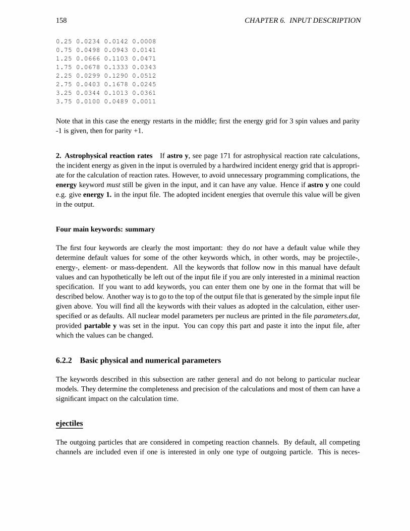
158 CHAPTER 6. INPUT DESCRIPTION
0.25 0.0234 0.0142 0.00080.75 0.0498 0.0943 0.01411.25 0.0666 0.1103 0.04711.75 0.0678 0.1333 0.03432.25 0.0299 0.1290 0.05122.75 0.0403 0.1678 0.02453.25 0.0344 0.1013 0.03613.75 0.0100 0.0489 0.0011
Note that in this case the energy restarts in the middle; firstthe energy grid for 3 spin values and parity-1 is given, then for parity +1.
2. Astrophysical reaction rates If astro y, see page 171 for astrophysical reaction rate calculations,the incident energy as given in the input is overruled by a hardwired incident energy grid that is appropri-ate for the calculation of reaction rates. However, to avoidunnecessary programming complications, theenergykeywordmuststill be given in the input, and it can have any value. Hence ifastro y one coulde.g. giveenergy 1. in the input file. The adopted incident energies that overrule this value will be givenin the output.
Four main keywords: summary
The first four keywords are clearly the most important: they do not have a default value while theydetermine default values for some of the other keywords which, in other words, may be projectile-,energy-, element- or mass-dependent. All the keywords thatfollow now in this manual have defaultvalues and can hypothetically be left out of the input file if you are only interested in a minimal reactionspecification. If you want to add keywords, you can enter themone by one in the format that will bedescribed below. Another way is to go to the top of the output file that is generated by the simple input filegiven above. You will find all the keywords with their values as adopted in the calculation, either user-specified or as defaults. All nuclear model parameters per nucleus are printed in the fileparameters.dat,providedpartable y was set in the input. You can copy this part and paste it into the input file, afterwhich the values can be changed.
6.2.2 Basic physical and numerical parameters
The keywords described in this subsection are rather general and do not belong to particular nuclearmodels. They determine the completeness and precision of the calculations and most of them can have asignificant impact on the calculation time.
ejectiles
The outgoing particles that are considered in competing reaction channels. By default, all competingchannels are included even if one is interested in only one type of outgoing particle. This is neces-
6.2. KEYWORDS 159
sary since there is always competition with other particles, in e.g. Hauser-Feshbach and pre-equilibriummodels, that determines the outcome for the particle under study. Furthermore, reaction Q-values au-tomatically keep channels closed at low incident energies.However, for diagnostic or time-economicalpurposes, or cases where e.g. one is only interested in high-energy(p, p′) and(p, n) multi-step directreactions, one may save computing time and output by skipping certain ejectiles as competing particles.For neutron-induced reactions on actinides up to 20 MeV, setting ejectiles g nis a rather good approx-imation that saves time. Also comparisons with computer codes that do not include the whole range ofparticles will be facilitated by this keyword.Examples:
ejectiles n
ejectiles g n p a
Range: ejectilescan be any combination ofg, n, p, d, t, handa.Default: Include all possible outgoing particles, i.e.ejectiles g n p d t h a
Ltarget
The excited state of the target as given in the discrete leveldatabase. This keyword allows to computecross sections for isomeric targets.Examples:
Ltarget 2
Range: 0 ≤ Ltarget ≤ numlev, wherenumlev is specified in the filetalys.cmb. Currently,numlev=30Default: Ltarget 0, i.e. the target is in its ground state.
maxZ
The maximal number of protons away from the initial compoundnucleus that is considered in a chain ofresidual nuclides. For example, ifmaxZ 3, then for an + 56Fe (Z=26) reaction, the V-isotopes (Z=23)are the last to be considered for further particle evaporation in the multiple emission chain.maxZ isnormally only changed for diagnostic purposes. For example, if you are only interested in the(n, n′),(n, 2n),...(n, xn) residual production cross sections, or the associated discrete gamma ray intensities,maxZ 0 is appropriate. (Note that in this case, the competition of emission of protons up to alphaparticles isstill taken into account for all the nuclides along the(n, xn) chain, only the decay of theresidual nuclides associated with this charged-particle emission are not tracked further).Examples:
maxZ 6
160 CHAPTER 6. INPUT DESCRIPTION
Range: 0 ≤ maxZ ≤ numZ-2, wherenumZ=2+2*memorypar is specified in the filetalys.cmb, wherememorypar=5 for a computer with at least 256 Mb of memory.Default: Continue until all possible reaction channels are closed or until the maximal possible valuefor maxZ is reached (which rarely occurs). By defaultmaxZ=numZ-2 where the parameternumZ isspecified in the filetalys.cmb. This parameter should be large enough to ensure complete evaporation ofall daughter nuclei.
maxN
The maximal number of neutrons away from the initial compound nucleus that is considered in a chain ofnuclides. For example, ifmaxN 3, then for an + 56Fe (N=31) reaction, residual nuclei with N=28 (=31-3) are the last to be considered for further particle evaporation in the multiple emission chain.maxN isnormally only changed for diagnostic or economical purposes.Examples:
maxN 6
Range: 0 ≤ maxN ≤ numN-2, wherenumN=4+4*memorypar is specified in the filetalys.cmb, wherememorypar=5 for a computer with at least 256 Mb of memory.Default: Continue until all possible reaction channels are closed or until the maximal possible valuefor maxN is reached (which rarely occurs). By defaultmaxN=numN-2 where the parameternumN isspecified in the filetalys.cmb. This parameter should be large enough to ensure complete evaporation ofall daughter nuclei.
bins
The number of excitation energy bins in which the continuum of the initial compound nucleus is dividedfor further decay. The excitation energy region between thelast discrete level and the total excitationenergy for the initial compound nucleus is divided intobins energy bins. The resulting bin width thenalso determines that for the neighboring residual nuclei, in the sense that for any residual nucleus weensure that the bins fit exactly between the last discrete level and the maximal possible excitation energy.For residual nuclides far away from the target, a smaller number of bins is automatically adopted. Ifbins0 a simple formula is invoked to take into account the fact thatmore bins are needed when the incidentenergy increases. Instead of a constant number of bins, it isthen incident energy (E) dependent. Morespecifically,nbins 0means
(6.1) Nbins = 30 + 50E2
(E2 + 602)
It is obvious thatbins has a large impact on the computation time.Examples:
bins 25
6.2. KEYWORDS 161
Range: bins = 0 or 2 ≤ bins ≤ numbins, wherenumbins is specified in the filetalys.cmb. Currently,numbins=100Default: bins 40
equidistant
Flag for adopting an equidistant or non-equidistant (logarithmic) excitation energy grid for the contin-uum of each residual nucleus. The latter option makes the calculation more efficient since it uses moreprecision when it is needed.Examples:
equidistant y
equidistant n
Range: y or nDefault: equidistant n
segment
The number of segments to divide the standard emission energy grid. The basic emission energy grid weuse for spectra and transmission coefficient calculations is:
0.001, 0.002, 0.005 MeV0.01, 0.02, 0.05 MeV0.1- 2 MeV : dE= 0.1 MeV2 - 4 MeV : dE= 0.2 MeV4 - 20 MeV : dE= 0.5 MeV
20 - 40 MeV : dE= 1.0 MeV40 - 200 MeV : dE= 2.0 MeV200 - 300 MeV : dE= 5.0 MeVabove 300 MeV : dE=10.0 MeV
This grid is divided into a finer grid by subdividing each interval by segment.Examples:
segment 3
Range: 1 ≤ segment≤ 4. Extra conditions:1 ≤ segment≤ 3 if the maximum incident energy is largerthan 20 MeV,1 ≤ segment≤ 2 if the maximum incident energy is larger than 40 MeV,segment=1if themaximum incident energy is larger than 100 MeV. (These rulesare imposed due to memory limitations).Default: segment 1
162 CHAPTER 6. INPUT DESCRIPTION
maxlevelstar
The number of included discrete levels for thetarget nucleus that is considered in Hauser-Feshbachdecay and the gamma-ray cascade. For nuclides that do not have maxlevelstaravailable in the discretelevel file, we take the last known level as the last discrete level in our calculation.Examples:
maxlevelstar 0
maxlevelstar 12
Range: 0 ≤ maxlevelstar≤ numlev, wherenumlev is specified in the filetalys.cmb. Currently,num-lev=30Default: maxlevelstar 20
maxlevelsres
The number of included discrete levels for allresidualnuclides that is considered in Hauser-Feshbachdecay and the gamma-ray cascade. For nuclides that do not have maxlevelsresavailable in the discretelevel file, we take the last known level as the last discrete level in our calculation. This keyword isoverruled bymaxlevelsbinandmaxlevelstar for specified nuclides.Examples:
maxlevelsres 0
maxlevelsres 12
Range: 0 ≤ maxlevelsres≤ numlev, wherenumlev is specified in the filetalys.cmb. Currently,num-lev=30Default: maxlevelsres 10
maxlevelsbin
The number of included discrete levels for the nuclides resulting from binaryemission that is consideredin Hauser-Feshbach decay and the gamma-ray cascade. For nuclides that do not havemaxlevelsbinavailable in the discrete level file, we take the last known level as the last discrete level in our calculation.On the input line we readmaxlevelsbin, the symbol of the ejectile and the number of levels of theassociated residual nucleus.Examples:
maxlevelsbin a 8
maxlevelsbin p 12
6.2. KEYWORDS 163
Range: 0 ≤ maxlevelsbin≤ numlev, wherenumlev is specified in the filetalys.cmb. Currently,num-lev=30Default: maxlevelsbin g 10, maxlevelsbin n 10, maxlevelsbin p 10, maxlevelsbin d 5, maxlevelsbint 5, maxlevelsbin h 5, maxlevelsbin a 10. The value for the inelastic channel will however always beoverruled by themaxlevelstarkeyword, for the target nucleus, or the value for its default.
Nlevels
The number of included discrete levels for aspecific residualnucleus that is considered in Hauser-Feshbach decay and the gamma-ray cascade. For nuclides thatdo not haveNlevels available in thediscrete level file, we take the last known level as the last discrete level in our calculation. On the inputline we readNlevels, Z, A, and the number of levels.Examples:
Nlevels 41 93 8
Range: 0 ≤ Nlevels≤ numlev, wherenumlev is specified in the filetalys.cmb. Currently,numlev=30Default: Nlevelshas the value specified by the defaults ofmaxlevelstar, maxlevelsbin, andmaxlevel-sres.
disctable
Keyword to change the used discrete level database. The standard discrete level database from RIPL canbe updated with theoretical levels calculated from the microscopic level densities fromldmodel 5, fornuclides with no or few experimental levels. Note thatdisctable 3gives the option to do nuclear reactioncalculations using purely theoretically estimated levels.Examples:
disctable 1: RIPL database with experimental levels + theoretical levels added until the 100thlevel
disctable 2: RIPL database with experimental levels (the only option until TALYS-1.4)
disctable 3: Theoretical levels for all nuclides
Range: 0 ≤ disctable≤ 3Default: disctable 1
levelfile
File with discrete levels. The format of the file is exactly the same as that of the nuclear structure databasetalys/structure/levels/. In practice, the user can copy a file from this database, e.g.z026, to the workingdirectory and change it. In this way, changes in the “official” database are avoided. Note that even if
164 CHAPTER 6. INPUT DESCRIPTION
only changes for one isotope are required, the entire file needs to be copied if for the other isotopes theoriginally tabulated values are to be used. On the input line, we readlevelfile, Z, filename.Examples:
levelfile 26 z026.loc
Range: levelfile can be equal to any filename, provided it starts with a character.Default: If levelfile is not given in the input file, the discrete levels are taken from thetalys/structure/levelsdatabase per nucleus.
Liso
Level number of isomer. This user assigned value can overrule the one determined from the discretelevel file.Examples:
Liso 2
Range: 0 ≤ Liso ≤ numlev, wherenumlev is specified in the filetalys.cmb. Default: Liso not given.
branch
Branching ratio for discrete level to overrule that given bythe discrete level file. With this keyword onecan change for example the ”guessed” branching ratios put inthe discrete level file, or even overrulethe original values from RIPL. On the input line we readbranch, Z, A, mother level, the number ofbranching levels nbr, and next the daughter level and branching ratio for each level up to nbr.Examples:
branch 38 85 7 2 2 0.7 0 0.3: 70% decay of 7th level of85Sr to level 2, and 30% to the groundstate
branch 38 87 17 1 1 1.: 100% decay of 17th level of87Sr to level 1.
Range: 0 ≤ number of levels, mother level, daughter level≤ numlev, wherenumlev is specified inthe filetalys.cmb.Default: branch is not given.
massmodel
Model for nuclear masses. There are 4 theoretical mass models and an analytic formula, see Section 5.2.They are only used when no experimental mass is available or whenexpmass n.Examples:
6.2. KEYWORDS 165
massmodel 0: Duflo-Zuker formula
massmodel 1: Moller table
massmodel 2: Goriely HFB-Skyrme table
massmodel 3: HFB-Gogny D1M table
Range: 0 ≤ massmodel≤ 3Default: massmodel 2
expmass
Flag for using the experimental nuclear mass when available. Useexpmass nto overrule the experimen-tal mass by the theoretical nuclear mass (i.e. the Audi-Wapstra values will not be used). This will thenbe done for all nuclides encountered in the calculation.Examples:
expmass y
expmass n
Range: y or nDefault: expmass y
massnucleus
The mass of the nucleus in amu. Usemassnucleusto overrule the value given in the mass table. On theinput line, we readmassnucleus, Z, A, value.Examples:
massnucleus 41 93 92.12345
massnucleus 94 239 239.10101
Range: A − 1 ≤ massnucleus≤ A+1, whereA is the mass number.Default: massnucleus 0., i.e. the nuclear mass is read from the mass table.
massexcess
The mass excess of the nucleus in MeV. Usemassexcessto overrule the value given in the mass table.On the input line, we readmassexcess, Z, A, value.Examples:
166 CHAPTER 6. INPUT DESCRIPTION
massexcess 41 93 -45.678
massexcess 94 239 39.98765
Range: −500. ≤ massexcess≤ 500.,Default: massexcess 0., i.e. the mass excess is read from the mass table.
isomer
The definition of an isomer in seconds. In the discrete level database, the lifetimes of most of the levelsare given. Withisomer, it can be specified whether a level is treated as an isomer or not. Useisomer 0.to treat all levels, with any lifetime, as isomer and useisomer 1.e38, or any other number larger than thelongest living isomer present in the problem, to include no isomers at all.Examples:
isomer 86400. (86400 sec.=one day)
Range: 0. ≤ isomer≤ 1.e38
Default: isomer 1.(second)
Elow
Lowest incident energy in MeV for which TALYS performs a fullnuclear model calculation. Belowthis energy, cross sections result from inter- and extrapolation using the calculated values atElow andtabulated values and systematics at thermal energy, see Section 4.9. This keyword should only be usedin the case of several incident energies.Examples:
Elow 0.001
Range: 1.e − 6 ≤ Elow ≤ 1.
Default: Elow=D0 for datafiles (endf y), 1.e-6otherwise.
transpower
A limit for considering transmission coefficients in the calculation. Transmission coefficientsTlj smallerthanT0 1
2
× 10−transpower/(2l + 1) are not used in Hauser-Feshbach calculations, in order to reduce thecomputation time.Examples:
transpower 12
Range: 2 ≤ transpower ≤ 20
Default: transpower 5
6.2. KEYWORDS 167
transeps
A limit for considering transmission coefficients in the calculation. Transmission coefficients smallerthantransepsare not used in Hauser-Feshbach calculations, irrespective of the value oftranspower, inorder to reduce the computation time.Examples:
transeps 1.e-12
Range: 0. ≤ transeps≤ 1.
Default: transeps 1.e-8
xseps
The limit for considering cross sections in the calculation, in mb. Reaction cross sections smaller thanxsepsare not used in the calculations, in order to reduce the computation time.Examples:
xseps 1.e-10
Range: 0. ≤ xseps≤ 1000.
Default: xseps 1.e-7
popeps
The limit for considering population cross sections in the multiple emission calculation, in mb. Nuclideswhich, before their decay, are populated with a total cross section less thanpopepsare skipped, inorder to reduce the computation time. Frompopeps, also the criteria for continuation of the decay perexcitation energy bin (variablepopepsA) and per(Ex, J,Π) bin (variablepopepsB) in Hauser-Feshbachcalculations are automatically derived.Examples:
popeps 1.e-6
Range: 0. ≤ popeps≤ 1000.
Default: popeps 1.e-3
popMeV
Flag to use initial population per MeV instead of per histogram, in the case of an excited energy distri-bution to be used withprojectile 0. This keyword is given for backward compatibility. It is nowseenthat it is more natural to input the absolute value of the initial population per continuum bin or level, as
168 CHAPTER 6. INPUT DESCRIPTION
histograms.Examples:
popMeV y
popMeV n
Range: y or nDefault: popMeV n
Estop
Incident energy above which TALYS stops. This keyword is needed to speed up some uncertainty appli-cations involving random TALYS calculations. No matter which incident energies are given in the inputfile, TALYS will stop when the incident energy exceedsEstop.Examples:
Estop 50.
Range: 1.e − 5 ≤ Estop≤ 1000.
Default: Estop 1000.
angles
Number of emission angles for reactions to discrete states.Examples:
angles 18
Range: 1 ≤ angles≤ numang, wherenumang is specified in the filetalys.cmb. Currently,numang=90Default: angles 90
anglescont
Number of emission angles for reactions to the continuum.Examples:
anglescont 18
Range: 1 ≤ anglescont≤ numangcont, wherenumangcontis specified in the filetalys.cmb. Currently,numangcont=36Default: anglescont 36
6.2. KEYWORDS 169
channels
Flag for the calculation and output of all exclusive reaction channel cross sections, e.g.(n, p, (n, 2n),(n, 2npa), etc. Thechannelskeyword can be used in combination with the keywordsoutspectra andoutangle (see next Section) to give the exclusive spectra and angulardistributions.Examples:
channels y
channels n
Range: y or nDefault: channels n
maxchannel
Maximal number of outgoing particles in exclusive channel description, e.g. ifmaxchannel 3, thenreactions up to 3 outgoing particles, e.g.(n, 2np), will be given in the output.maxchannelis only activeif channels y. We emphasize that, irrespective of the value ofmaxchannelandchannels, all reactionchains are, by default, followed until all possible reaction channels are closed to determine cumulativeparticle production cross sections and residual production cross sections.Examples:
maxchannel 2
Range: 0 ≤ maxchannel≤ 8,Default: maxchannel 4
relativistic
Flag for relativistic kinematics.Examples:
relativistic y
relativistic n
Range: y or nDefault: relativistic y
reaction
Flag to disable nuclear reaction calculation. This may be helpful if one is e.g. only interested in a leveldensity calculation. A TALYS run will then last only a few hundreds of a second. (This keyword was
170 CHAPTER 6. INPUT DESCRIPTION
used for the large scale level density analysis of [168]).Examples:
reaction y
reaction n
Range: y or nDefault: reaction y
recoil
Flag for the calculation of the recoils of the residual nuclides and the associated corrections to the light-particle spectra, see Section 3.5.Examples:
recoil y
recoil n
Range: y or nDefault: recoil n
labddx
Flag for the calculation of double-differential cross sections in the LAB system. This is only active ifrecoil y. If labddx n, only the recoils of the nuclides are computed.Examples:
labddx y
labddx n
Range: y or nDefault: labddx n
anglesrec
Number of emission angles for recoiling nuclides. This is only active if recoil y.Examples:
anglesrec 4
Range: 1 ≤ anglesrec≤ numangrec, wherenumangrec is specified in the filetalys.cmb. Currently,numangrec=9Default: anglesrec 9if labddx y, anglesrec 1if labddx n

6.2. KEYWORDS 171
maxenrec
Number of emission energies for recoiling nuclides. This isonly active ifrecoil y.Examples:
maxenrec 4
Range: 1 ≤ maxenrec≤ numenrec, wherenumenrec is specified in the filetalys.cmb. Currently,numenrec=5*memorypar, where we suggestmemorypar=5 for a computer with at least 256 Mb ofmemory.Default: maxenrec 10
recoilaverage
Flag to consider only one average kinetic energy of the recoiling nucleus per excitation energy bin (in-stead of a full kinetic energy distribution). This approximation significantly decreases the calculationtime. This is only active ifrecoil y.Examples:
recoilaverage y
recoilaverage n
Range: y or nDefault: recoilaverage n
channelenergy
Flag to use the channel energy instead of the center-of-massenergy for the emission spectrum.Examples:
channelenergy y
channelenergy n
Range: y or nDefault: channelenergy n
astro
Flag for the calculation of thermonuclear reaction rates for astrophysics, see Section 4.12.Examples:
172 CHAPTER 6. INPUT DESCRIPTION
astro y
astro n
Range: y or nDefault: astro n
astrogs
Flag for treating the target in the ground state only, for astrophysical reaction calculations. In the defaultcase,astrogs n, an average between excited target states will be made. Thiskeyword is only active ifastro y.Examples:
astrogs y
astrogs n
Range: y or nDefault: astrogs n
astroE
Energy, in MeV, for thermonuclear reactions around which Maxwellian averaging should take place.This is only active ifastro y. Actually, specifying this value will automatically activate astro y andastrogs y. Hence, if you require the Maxwellian averaged 30 keV capture cross section, all you needto give is the input line below.astroE may not be specified simultaneously withastroT9. Theenergykeyword must still be given in the TALYS input file, but becomes irrelevant since it concerns an averageover a large number of incident energies.Examples:
astroE 0.03
Range: 0.00001 ≤ astroE ≤ 1..Default: astroE 0.
astroT
Temperature, in units of109 K, for thermonuclear reactions and Maxwellian averaging. This is onlyactive if astro y. Actually, specifying this value will automatically activateastro y. astroT may not bespecified simultaneously withastroE. Theenergykeyword must still be given in the TALYS input file,but becomes irrelevant since it concerns an average over a large number of incident energies.Examples:
6.2. KEYWORDS 173
astroT 0.53
Range: 0.0001 ≤ astroT ≤ 10..Default: astroT 0.
abundance
File with tabulated abundances. Theabundancekeyword is only active for the case of a natural target,i.e. if mass 0. By default, the isotopic abundances are read from the structure database, see Chapter 5.It can however be imagined that one wants to include only the most abundant isotopes of an element, tosave some computing time. Also,abundancemay be used to analyze experimental data for targets of acertain isotopic enrichment. On the input line, we readabundanceand the filename. From each line ofthe file, TALYS readsZ, A and the isotopic abundance with the format (2i4,f11.6). An example of anabundance file, e.g.abnew, different from that of the database, is
82 206 24.10000082 207 22.10000082 208 52.400000
where we have left out the “unimportant”204Pb (1.4%). TALYS automatically normalizes the abun-dances to a sum of 1, leading in the above case to 24.44 % of206Pb, 22.41 % of207Pb and 53.14 % of208Pb in the actual calculation.Examples:
abundance abnew
Range: abundancecan be equal to any filename, provided it is present in the working directory.Default: If abundanceis not given in the input file, abundances are taken fromtalys/structure/abundanceand calculations for all isotopes are performed.
xscaptherm
The thermal capture cross section in millibarn. By default,these are read from the nuclear structuredatabase or taken from systematics. Thexscapthermkeyword gives the possibility to overwrite this byusing the input file.Examples:
xscaptherm 320.2
Range: 10−20 ≤ xscaptherm≤ 10
10
Default: xscaptherm is read from the nuclear structure database or taken from systematics.
174 CHAPTER 6. INPUT DESCRIPTION
xsalphatherm
The thermal(n, α) cross section in millibarn. By default, these are read from the nuclear structuredatabase or taken from systematics. Thexsalphatherm keyword gives the possibility to overwrite thisby using the input file.Examples:
xsalphatherm 0.2
Range: 10−20 ≤ xsalphatherm≤ 10
10
Default: xsalphatherm is read from the nuclear structure database or taken from systematics.
xsptherm
The thermal (n,p) cross section in millibarn. By default, these are read from the nuclear structure databaseor taken from systematics. Thexsptherm keyword gives the possibility to overwrite this by using theinput file.Examples:
xsptherm 0.2
Range: 10−20 ≤ xsptherm ≤ 10
10
Default: xsptherm is read from the nuclear structure database or taken from systematics.
partable
Flag to write the all the model parameters used in a calculation on a separate file,parameters.dat. Thiscan be a very powerful option when one wishes to vary any nuclear model parameter in the input. The fileparameters.dathas the exact input format, so it can be easily copied and pasted into any input file. Thisis helpful for a quick look-up of all the parameters used in a calculation. We have used this ourselves forautomatic (random) TALYS-input generators for e.g. covariance data.Examples:
partable y
partable n
Range: y or nDefault: partable n
best
Flag to use the set of adjusted nuclear model parameters thatproduces the optimal fit for measurementsof all reacion channels of the nuclide under consideration.TALYS will look in the talys/structure/best
6.2. KEYWORDS 175
directory for such a set, see Section 5.14. With the additionof the single linebest y to the input file,TALYS will automatically use all detailed adjusted parameter fits that are stored intalys/structure/best.Examples:
best y
best n
Range: y or nDefault: best n
bestend
Flag to put the best set of parameters at end of input file, instead of at the beginning. Withbestend n,the parameters can be ovverruled later in the input file, while this is no longer possible withbestend y.Obviously, this keyword is only relevant ifbest y.Examples:
bestend y
bestend n
Range: y or nDefault: bestend n
bestbranch
Flag to use the set of adjusted branching ratios for discretelevels.Examples:
bestbranch y
bestbranch n
Range: y or nDefault: bestbranch y
bestpath
Keyword to enable to use your own collection of “best” TALYS input parameters. This directory shouldbe created undertalys/structure/after which the current keyword can be used with that directory name. Inpractice, the user can copy a file from the standardtalys/structure/best/database to his/her own databaseand change it. In this way, changes in the “official” databaseare avoided. See Section 5.14 for the formatof the files in this database.Examples:
176 CHAPTER 6. INPUT DESCRIPTION
bestpath mybest
For this keyword to work, information needs to be present in the talys/structure/mybest/with a formatequal to that of the originaltalys/structure/best/directory, see Section 5.14.Range: bestpath can beequal to any filename, provided it starts with a character. Furthermore, the library must exist in thetalys/structure/directory. This keyword is only active ifbest y.Default: bestpath is equal totalys/structure/best/.
rescuefile
File with incident energy dependent normalization factors. If TALYS is not able to produce the “ultimatefit”, it is possible to invoke a “rescuefile” as a last resort. By giving a table of incident energies andnormalization factors, the result of TALYS can be made exactly equal to that of experimental data, anevaluate data set, or any other data set. The contents of the file consist of a simple x-y table with xthe incident energy and y the normalization factor. A rescuefile can be used for the reactions (n,n’),(n,γ), (n,f), (n,p), (n,d), (n,t), (n,h), (n,’alpha ), (n,2n) and (n,total). To invoke this, the ENDF-6 formatfor MT numbers representing a reaction channel is used, see the sample cases below. Moreover, aglobal multiplication factor can be applied. On the input line, we readrescuefile, reaction identifier (MTnumber), global multiplication factor (optional).Examples:
rescuefile 0 rescue.001 1.01(n,total)
rescuefile 4 rescue.004(n,n’)
rescuefile 16 rescue.016(n,2n)
rescuefile 18 rescue.018 0.995(n,f)
rescuefile 102 rescue.102(n,γ)
rescuefile 103 rescue.103 1.02(n,p)
rescuefile 104 rescue.104(n,d)
rescuefile 105 rescue.105(n,t)
rescuefile 106 rescue.106(n,h)
rescuefile 107 rescue.107(n,α)
Range: rescuefilecan be equal to any filename, provided it starts with a character.Default: no default.
6.2. KEYWORDS 177
nulldev
Path for the null device. The null device is a ”black hole” foroutput that is produced, but not of interestto the user. Some ECIS output files fall in this category. To ensure compatibility with Unix, Linux,Windows and other systems a null device string is used, of which the default setting is given in machine.f.With this keyword, extra flexibility is added. If the null device is properly set in machine.f, this keywordis not needed. On the input line, we readnulldev, filename.Examples:
nulldev /dev/null
nulldev nul
Range: nulldev can be equal to any appropriate filename, provided it starts with a character.Default: The default is set in subroutinemachine.f.
strucpath
Path for the directory with nuclear structure information.With this keyword, extra flexibility is added.Nuclear structure databases other than the default can be invoked with this keyword. If the path nameis properly set in machine.f, this keyword is not needed for standard use. On the input line, we readstrucpath, filename.Examples:
strucpath /home/raynal/mon-structure/
Range: strucpath can be equal to any appropriate directory. The maximum length of the path is 60characters.Default: The default is set in subroutinemachine.f.
6.2.3 Optical model
optmod
File with tabulated phenomenological optical model parameters as a function of energy, see Section 4.1.This can be helpful if one wishes to use an optical model parameterisation which is not hardwired inTALYS. One could write a driver to automatically generate a table with parameters. On the input line,we readoptmod, Z, A, filename, and (optionally) particle type. TALYS first readsthe number of linesto be read with format (8x,i4). Next, from each line of the file, TALYS readsE, v, rv, av, w, rw, aw,vd, rvd, avd, wd, rwd, awd, vso, rvso, avso, wso, rwso, awso, andrc.Examples:
optmod 40 90 ompzr90 d
178 CHAPTER 6. INPUT DESCRIPTION
optmod 94 239 omppu239
Range: optmod can be equal to any filename, provided it starts with a character. The particle type mustbe equal to eithern, p, d, t, h or a. A table of up to 500 incident energies (this is set bynumomp intalys.cmb) and associated parameters can be specified.Default: If the particle type is not given, as in the second example above, neutrons are assumed. Ifopt-mod is not given in the input file, the optical model parameters are taken from thetalys/structure/opticaldatabase per nucleus or, if not present there, from the global optical model.
optmodfileN
File with the neutron optical model parameters of Eq. (4.7).The format of the file is exactly the same asthat of the nuclear structure databasetalys/structure/optical/. In practice, the user can copy a file fromthis database, e.g.z026, to the working directory and change it. In this way, changesin the “official”database are avoided. Note that even if only changes for one isotope are required, the file for the wholeelement needs to be copied if for the other isotopes the originally tabulated values are to be used. On theinput line, we readoptmodfileN, Z, filename.Examples:
optmodfileN 26 z026.loc
Range: optmodfileN can be equal to any filename, provided it starts with a character.Default: If optmodfileN is not given in the input file, the optical model parameters are taken from thetalys/structure/opticaldatabase per nucleus or, if not present there, from the global optical model.
optmodfileP
File with the proton optical model parameters of Eq. (4.7). The format of the file is exactly the same asthat of the nuclear structure databasetalys/structure/optical/. In practice, the user can copy a file fromthis database, e.g.z026, to the working directory and change it. In this way, changesin the “official”database are avoided. Note that even if only changes for one isotope are required, the file for the wholeelement needs to be copied if for the other isotopes the originally tabulated values are to be used. On theinput line, we readoptmodfileP, Z, filename.Examples:
optmodfileP 26 z026.loc
Range: optmodfileP can be equal to any filename, provided it starts with a character.Default: If optmodfileP is not given in the input file, the optical model parameters are taken from thetalys/structure/opticaldatabase per nucleus or, if not present there, from the global optical model.
6.2. KEYWORDS 179
localomp
Flag to overrule the local, nucleus-specific optical model by the global optical model of Eqs. (4.8) or(4.9). This may be helpful to study global mass-dependent trends.Examples:
localomp n
Range: y or nDefault: localomp y, i.e. a nucleus-specific optical model, when available.
dispersion
Flag to invoke the dispersive optical model, see Section 4.1.2. These potentials are only available astabulated neutron local potentials. If not available, TALYS will automatically resort to normal OMP’s.Examples:
dispersion n
Range: y or nDefault: dispersion n.
jlmomp
Flag to use the JLM microscopic optical model potential instead of the phenomenological optical modelpotential, see Section 4.1.4.Examples:
jlmomp n
Range: y or nDefault: jlmomp n , i.e. to use the phenomenological OMP.
jlmmode
Keyword to enable different normalizations for the imaginary potential of the JLM optical model, asexplained in Ref. [1] These different normalizations applyto the constant 0.44 in Eq. (4.47). Thiskeyword is only active if ’jlmomp y’.Examples:
jlmmode 0: standard JLM imaginary potential of Eq. (4.47)
jlmmode 1: 0.44 replaced by1.1 exp(−0.4E1/2)
180 CHAPTER 6. INPUT DESCRIPTION
jlmmode 2: 0.44 replaced by1.25 exp(−0.2E1/2)
jlmmode 3: as jlmmode 2 but withλW (E) twice as large, recommended for energies below 1MeV.
Range: 0 ≤ jlmmode ≤ 3Default: jlmmode 0, i.e. the standard JLM OMP.
radialmodel
Model for radial matter densities in the JLM optical model. There are two options. This keyword is onlyactive if ’jlmomp y’.Examples:
radialmodel 1: HFB-Skyrme based matter densities
radialmodel 2: HFB-Gogny based matter densities
Range: 1 ≤ radialmodel ≤ 2Default: radialmodel 2.
omponly
Flag to let TALYS performonlyan optical model calculation. In this way, TALYS acts simplyas a driverfor ECIS. All non-elastic calculations for the various reaction channels are skipped. This is helpful forsystematic, and quick, testing of optical model potentials.Examples:
omponly y
Range: y or nDefault: omponly n
sysreaction
The types of particles for which the optical model reaction cross section is overruled by values obtainedfrom systematics, see Section 4.1.5. The optical model transmission coefficients will be accordinglynormalized.Examples:
sysreaction p
sysreaction d a
6.2. KEYWORDS 181
Range: sysreactioncan be any combination ofn, p, d, t, h andaDefault: sysreactionis disabled for any particle.Warning: setting e.g.sysreaction pwill thus automatically disable the default setting. If this needs to beretained as well, setsysreaction p d t h a.
statepot
Flag for a different optical model parameterisation for each excited state in a DWBA or coupled-channelscalculation. This may be appropriate if the emission energyof the ejectile, corresponding to a largeexcitation energy, differs considerably from the incidentenergy.Examples:
statepot y
Range: y or nDefault: statepot n
optmodall
Flag for a new optical model calculation for each compound nucleus in the decay chain. In usual mul-tiple Hauser-Feshbach decay, the transmission coefficients for the first compound nucleus are used forthe whole decay chain. When a residual nucleus is far away from the initial compound nucleus, thisapproximation may become dubious. Withoptmodall y, new optical model calculations are performedfor every compound nucleus that is depleted, for all types ofemitted particles.Examples:
optmodall y
Range: y or nDefault: optmodall n
autorot
Flag for automatic rotational coupled-channels calculations, see Section 4.2.1 forA > 150. The dis-crete level file is scanned and an attempt is made to automatically identify the lowest rotational band.Deformation parameters are also read in from the database soautomated coupled-channels calculationscan be performed. This option is possible for the rare earth and actinide region. Note that for all naturalisotopes, the coupling scheme is already given in thetalys/structure/deformationdatabase.Examples:
autorot y
Range: y or nDefault: autorot n
182 CHAPTER 6. INPUT DESCRIPTION
incadjust
Flag to use adjusted optical model parameters for the incident channelandexit channels. Disabling thisflag allows to use a different OMP for the exit channels than for the incident channel, e.g. usingrvadjustn 1.10 together withincadjust n means that the OMP for the incident channel is unaltered, while thatfor the outgoing channel has an adjustrV parameter. This can be used to simulate e.g. temperature-dependent OMP effects.Examples:
incadjust n
Range: y or nDefault: incadjust y
ecissave
Flag for saving ECIS input and output files. This has two purposes: (a) if the next calculation will beperformed with already existing reaction cross sections and transmission coefficients. This is helpfulfor time-consuming coupled-channels calculations, (b) tostudy the ECIS input and output files in detail.ecissavemustbe set toy, if in the next runinccalc n or eciscalc nwill be used. If not, an appropriateerror message will be given and TALYS stops.Examples:
ecissave y
ecissave n
Range: y or nDefault: ecissave n
eciscalc
Flag for the ECIS calculation of transmission coefficients and reaction cross sections for the inversechannels. If this calculation has already been performed ina previous run, and in that previous runecissave yhas been set, it may be helpful to puteciscalc n, which avoids a new calculation. This savestime, especially in the case of coupled-channels calculations. We stress that it is the responsibility of theuser to ensure that the first run of a particular problem is done with ecissave y. You also have to makesure that the same energy grid for inverse channels is used.Examples:
eciscalc y
eciscalc n
6.2. KEYWORDS 183
Range: y or nDefault: eciscalc y
inccalc
Flag for the ECIS calculation of transmission coefficients and reaction cross sections for the incidentchannel. If this calculation has already been performed in aprevious run, and in that previous runecissave yhas been set, it may be helpful to putinccalc n, which avoids a new ECIS calculation. Thissaves time, especially in the case of coupled-channels calculations. We stress that it is the responsibilityof the user to ensure that the first run of a particular problemis done witheciscalc y. If not, an appropriateerror message will be given and TALYS stops. You also have to make sure that the same grid of incidentenergies is used.Examples:
inccalc y
inccalc n
Range: y or nDefault: inccalc y
endfecis
Flag for the ECIS calculation of transmission coefficients and reaction cross sections for the ENDF-6energy grid. If this calculation has already been performedin a previous run, it may be helpful to putendfecis n, which avoids a new calculation. This saves time, especially in the case of coupled-channelscalculations. We stress that it is the responsibility of theuser to ensure that the first run of a particularproblem is done withendfecis yandendfecis y. If not, an appropriate error message will be given andTALYS stops.Examples:
endfecis y
endfecis n
Range: y or nDefault: endfecis y
coulomb
Flag for Coulomb excitation calculation with ECIS, to be used for incident charged particles.Examples:
184 CHAPTER 6. INPUT DESCRIPTION
coulomb y
Range: y or nDefault: coulomb y
cpang
Flag for compound angular distribution calculation for incident charged particles.Examples:
cpang y
Range: y or nDefault: cpang n
soswitch
Energy switch to on-set deformed spin-orbit calculation and sequential iterations in ECIS. For coupled-channels calculations on rotational nuclei, such a switch needs to be made. On the input line, we readsoswitch, value.Examples:
soswitch 1.2
Range: 0.1 ≤ soswitch≤ 10.
Default: soswitch 3.MeV.
v1adjust
Multiplier to adjust the OMP parameter v1 of Eq. (4.7). This keyword can also be used for double-folding and complex particle potentials. On the input line,we readv1adjust, particle symbol, and value.Examples:
v1adjust a 1.12
Range: 0.1 ≤ v1adjust ≤ 10.
Default: v1adjust particle 1.
v2adjust
Multiplier to adjust the OMP parameter v2 of Eq. (4.7). This keyword can only be used for a potentialof the Koning-Delaroche form. On the input line, we readv2adjust, particle symbol, and value.Examples:
6.2. KEYWORDS 185
v2adjust n 0.96
Range: 0.1 ≤ v2adjust ≤ 10. This keyword does not apply to deuterons up to alpha’s.Default: v2adjust particle 1.
v3adjust
Multiplier to adjust the OMP parameter v3 of Eq. (4.7). This keyword can only be used for a potentialof the Koning-Delaroche form. On the input line, we readv3adjust, particle symbol, and value.Examples:
v3adjust p 1.10
Range: 0.1 ≤ v3adjust ≤ 10. This keyword does not apply to deuterons up to alpha’s.Default: v3adjust particle 1.
v4adjust
Multiplier to adjust the OMP parameter v4 of Eq. (4.7). This keyword can only be used for a potentialof the Koning-Delaroche form. On the input line, we readv4adjust, particle symbol, and value.Examples:
v4adjust n 0.98
Range: 0.1 ≤ v4adjust ≤ 10. This keyword does not apply to deuterons up to alpha’s.Default: v4adjust particle 1.
rvadjust
Multiplier to adjust the OMP parameter rv of Eq. (4.7). This keyword can also be used for complexparticle potentials. On the input line, we readrvadjust , particle symbol, and value.Examples:
rvadjust t 1.04
Range: 0.1 ≤ rvadjust ≤ 10.
Default: rvadjust particle 1.
avadjust
Multiplier to adjust the OMP parameter av of Eq. (4.7). This keyword can also be used for complexparticle potentials. On the input line, we readavadjust, particle symbol, and value.Examples:
186 CHAPTER 6. INPUT DESCRIPTION
avadjust d 0.97
Range: 0.1 ≤ avadjust ≤ 10.
Default: avadjust particle 1.
rwadjust
Multiplier to adjust the OMP parameter rw of Eq. (4.7). This keyword can also be used for complexparticle potentials. On the input line, we readrwadjust , particle symbol, and value.Examples:
rwadjust t 1.04
Range: 0.1 ≤ rwadjust ≤ 10.
Default: rwadjust particle 1.
awadjust
Multiplier to adjust the OMP parameter aw of Eq. (4.7). This keyword can also be used for complexparticle potentials. On the input line, we readawadjust, particle symbol, and value.Examples:
awadjust d 0.97
Range: 0.1 ≤ awadjust≤ 10.
Default: awadjust particle 1.
w1adjust
Multiplier to adjust the OMP parameter w1 of Eq. (4.7). This keyword can also be used for double-folding and complex particle potentials. On the input line,we readw1adjust, particle symbol, andvalue.Examples:
w1adjust p 1.10
Range: 0.1 ≤ w1adjust≤ 10.
Default: w1adjust particle 1.
w2adjust
Multiplier to adjust the OMP parameter w2 of Eq. (4.7). This keyword can only be used for a potentialof the Koning-Delaroche form. On the input line, we readw2adjust, particle symbol, and value.Examples:
6.2. KEYWORDS 187
w2adjust n 0.80
Range: 0.1 ≤ w2adjust≤ 10. This keyword does not apply to deuterons up to alpha’s.Default: w2adjust particle 1.
w3adjust
Multiplier to adjust the OMP parameter w3 of Eq. (4.18). Thiskeyword can only be used for the high-energy extension of the Koning-Delaroche form. On the inputline, we readw3adjust, particle symbol,and value.Examples:
w3adjust n 0.80
Range: 0.1 ≤ w3adjust≤ 10. This keyword does not apply to deuterons up to alpha’s.Default: w3adjust particle 1.
w4adjust
Multiplier to adjust the OMP parameter w4 of Eq. (4.18). Thiskeyword can only be used for the high-energy extension of the Koning-Delaroche form. On the inputline, we readw4adjust, particle symbol,and value.Examples:
w4adjust n 0.80
Range: 0.1 ≤ w4adjust≤ 10. This keyword does not apply to deuterons up to alpha’s.Default: w4adjust particle 1.
rvdadjust
Multiplier to adjust the OMP parameter rvd of Eq. (4.7). Thiskeyword can also be used for complexparticle potentials. On the input line, we readrvdadjust , particle symbol, and value.Examples:
rvdadjust d 0.97
Range: 0.1 ≤ rvdadjust ≤ 10.
Default: rvdadjust particle 1.
188 CHAPTER 6. INPUT DESCRIPTION
avdadjust
Multiplier to adjust the OMP parameter avd of Eq. (4.7). Thiskeyword can also be used for complexparticle potentials. On the input line, we readavdadjust, particle symbol, and value.Examples:
avdadjust d 0.97
Range: 0.1 ≤ avdadjust≤ 10.
Default: avdadjust particle 1.
rwdadjust
Multiplier to adjust the OMP parameter rwd of Eq. (4.7). Thiskeyword can also be used for complexparticle potentials. On the input line, we readrwdadjust , particle symbol, and value.Examples:
rwdadjust d 0.97
Range: 0.1 ≤ rwdadjust ≤ 10.
Default: rwdadjust particle 1.
awdadjust
Multiplier to adjust the OMP parameter awd of Eq. (4.7). Thiskeyword can also be used for complexparticle potentials. On the input line, we readawdadjust, particle symbol, and value.Examples:
awdadjust d 0.97
Range: 0.1 ≤ awdadjust≤ 10.
Default: awdadjust particle 1.
d1adjust
Multiplier to adjust the OMP parameter d1 of Eq. (4.7). This keyword can also be used for double-folding and complex particle potentials. On the input line,we readd1adjust, particle symbol, and value.Examples:
d1adjust d 0.97
Range: 0.1 ≤ d1adjust≤ 10.
Default: d1adjust particle 1.
6.2. KEYWORDS 189
d2adjust
Multiplier to adjust the OMP parameter d2 of Eq. (4.7). This keyword can only be used for a potentialof the Koning-Delaroche form. On the input line, we readd2adjust, particle symbol, and value.Examples:
d2adjust n 1.06
Range: 0.1 ≤ d2adjust≤ 10. This keyword does not apply to deuterons up to alpha’s.Default: d2adjust particle 1.
d3adjust
Multiplier to adjust the OMP parameter d3 of Eq. (4.7). This keyword can only be used for a potentialof the Koning-Delaroche form. On the input line, we readd3adjust, particle symbol, and value.Examples:
d3adjust n 1.06
Range: 0.1 ≤ d3adjust≤ 10. This keyword does not apply to deuterons up to alpha’s.Default: d3adjust particle 1.
vso1adjust
Multiplier to adjust the OMP parameter vso1 of Eq. (4.7). This keyword can also be used for complexparticle potentials. On the input line, we readvso1adjust, particle symbol, and value.Examples:
vso1adjust d 1.15
Range: 0.1 ≤ vso1adjust≤ 10.
Default: vso1adjustparticle 1.
vso2adjust
Multiplier to adjust the OMP parameter vso2 of Eq. (4.7). This keyword can only be used for a potentialof the Koning-Delaroche form. On the input line, we readvso2adjust, particle symbol, and value.Examples:
vso2adjust n 1.06
Range: 0.1 ≤ vso2adjust≤ 10. This keyword does not apply to deuterons up to alpha’s.Default: vso2adjustparticle 1.
190 CHAPTER 6. INPUT DESCRIPTION
wso1adjust
Multiplier to adjust the OMP parameter wso1 of Eq. (4.7). This keyword can also be used for complexparticle potentials. On the input line, we readwso1adjust, particle symbol, and value.Examples:
wso1adjust d 1.15
Range: 0.1 ≤ wso1adjust≤ 10.
Default: wso1adjustparticle 1.
wso2adjust
Multiplier to adjust the OMP parameter wso2 of Eq. (4.7). This keyword can only be used for a potentialof the Koning-Delaroche form. On the input line, we readwso2adjust, particle symbol, and value.Examples:
wso2adjust n 1.06
Range: 0.1 ≤ wso2adjust≤ 10. This keyword does not apply to deuterons up to alpha’s.Default: wso2adjustparticle 1.
rvsoadjust
Multiplier to adjust the OMP parameter rvso of Eq. (4.7). This keyword can also be used for complexparticle potentials. On the input line, we readrvsoadjust, particle symbol, and value.Examples:
rvsoadjust d 1.15
Range: 0.1 ≤ rvsoadjust ≤ 10.
Default: rvsoadjust particle 1.
avsoadjust
Multiplier to adjust the OMP parameter avso of Eq. (4.7). This keyword can also be used for complexparticle potentials. On the input line, we readavsoadjust, particle symbol, and value.Examples:
avsoadjust d 1.15
Range: 0.1 ≤ avsoadjust≤ 10.
Default: avsoadjustparticle 1.
6.2. KEYWORDS 191
rwsoadjust
Multiplier to adjust the OMP parameter rwso of Eq. (4.7). This keyword can also be used for complexparticle potentials. On the input line, we readrwsoadjust, particle symbol, and value.Examples:
rwsoadjust d 1.15
Range: 0.1 ≤ rwsoadjust ≤ 10.
Default: rwsoadjust particle 1.
awsoadjust
Multiplier to adjust the OMP parameter awso of Eq. (4.7). This keyword can also be used for complexparticle potentials. On the input line, we readawsoadjust, particle symbol, and value.Examples:
awsoadjust d 1.15
Range: 0.1 ≤ awsoadjust≤ 10.
Default: awsoadjustparticle 1.
rcadjust
Multiplier to adjust the OMP parameter rc of Eq. (4.7). On theinput line, we readrcadjust, particlesymbol, and value.Examples:
rcadjust d 1.15
Range: 0.1 ≤ rcadjust ≤ 10.
Default: rcadjust particle 1.
Ejoin
Joining energyEJ , in MeV, for the original form and high-energy extension of the KD03 OMP, see Eq.(4.18). On the input line, we readEjoin , particle symbol, and value.Examples:
Ejoin n 250.
Range: 0. ≤ Ejoin ≤ 1000..Default: Ejoin 200.
192 CHAPTER 6. INPUT DESCRIPTION
Vinf
Limiting valueV∞ for the real volume potential of Eq. (4.18). This keyword canonly be used for thehigh-energy extension of the Koning-Delaroche form. On theinput line, we readVinf , particle symbol,and value.Examples:
Vinf n -22.
Range: −200. ≤ Vinf ≤ 0..Default: Vinf -30.
rvadjustF
Energy-dependent function to adjust the OMP parameterrV . If physically adequate OMPs fail, suchenergy-dependent adjustment can be invoked as a last resort. As long as the deviation from the originalmodel is not too large, unpleasant surprises in the various reaction channels are avoided. On the inputline, we readrvadjustF , particle symbol, begin energyEb and end energyEe in MeV, maximal deviationD in % , and varianceσ in MeV, of the function. If this keyword is specified,rV will keep its originalconstant value forE < Eb andE > Ee while in between these two values if will be multiplied by thefunction
(6.2) f(E) = 1 + D exp(−(E − Em)2/2σ2) + R
whereEm = (Ee + Eb)/2 and the offset value
(6.3) R = −D exp(−(Ee − Em)2/2σ2)
ensures continuity atEb and Ee. Fig. 6.1 shows an example forrV with an original value of 1.20,which is locally multiplied by the functionf with parametersEb=2, Ee=10, D = 5, σ = 2. Up to10 energy ranges, i.e.rvadjustF keywords, per particle can be used. We suggest however that thekeyword rvadjustF is now replaced by the method explained in Section 6.2.12 forall parameters. WekeeprvadjustF and related OMP keywords for backward compatibility reasons.Examples:
rvadjustF n 2. 10. 5. 2.
Range: The particle symbol should be equal to n, p, d, t, h or a,0 ≤ Eb ≤ 250, 0 ≤ Ee ≤ 250,Eb < Ee, −100 ≤ D ≤ 100, 0 ≤ σ ≤ 100. If σ = 0, then the valueσ = (Ee − Em)/2 will beadopted.Default: rvadjustF is not applied.

6.2. KEYWORDS 193
0 5 10 15E [MeV]
1.16
1.18
1.2
1.22
1.24
1.26
r V [f
m]
Figure 6.1: Energy-dependent radiusrV obtained with thervadjustF keyword
avadjustF
Energy-dependent function to adjust the OMP parameteraV . On the input line, we readavadjustF,particle symbol, begin energyEb and end energyEe in MeV, maximal deviation D in % , and varianceσin MeV, of the function. The same formalism as explained for thervadjustF keyword applies.Examples:
avadjustF n 2. 10. 5. 2.
Range: SeervadjustF keyword.Default: avadjustF is not applied.
rwadjustF
Energy-dependent function to adjust the OMP parameteraV . On the input line, we readrwadjustF ,particle symbol, begin energyEb and end energyEe in MeV, maximal deviation D in % , and varianceσin MeV, of the function. The same formalism as explained for thervadjustF keyword applies.Examples:
rwadjustF n 2. 10. 5. 2.
194 CHAPTER 6. INPUT DESCRIPTION
Range: SeervadjustF keyword.Default: rwadjustF is not applied.
awadjustF
Energy-dependent function to adjust the OMP parameteraV . On the input line, we readawadjustF,particle symbol, begin energyEb and end energyEe in MeV, maximal deviation D in % , and varianceσin MeV, of the function. The same formalism as explained for thervadjustF keyword applies.Examples:
awadjustF n 2. 10. 5. 2.
Range: SeervadjustF keyword.Default: awadjustF is not applied.
rvdadjustF
Energy-dependent function to adjust the OMP parameter rvd.On the input line, we readrvdadjustF ,particle symbol, begin energyEb and end energyEe in MeV, maximal deviation D in % , and varianceσin MeV, of the function. The same formalism as explained for thervadjustF keyword applies.Examples:
rvdadjustF n 2. 10. 5. 2.
Range: SeervadjustF keyword.Default: rvdadjustF is not applied.
avdadjustF
Energy-dependent function to adjust the OMP parameter avd.On the input line, we readavdadjustF,particle symbol, begin energyEb and end energyEe in MeV, maximal deviation D in % , and varianceσin MeV, of the function. The same formalism as explained for thervadjustF keyword applies.Examples:
avdadjustF n 2. 10. 5. 2.
Range: SeervadjustF keyword.Default: avdadjustF is not applied.
rwdadjustF
Energy-dependent function to adjust the OMP parameter rwd.On the input line, we readrwdadjustF ,particle symbol, begin energyEb and end energyEe in MeV, maximal deviation D in % , and varianceσ
6.2. KEYWORDS 195
in MeV, of the function. The same formalism as explained for thervadjustF keyword applies.Examples:
rwdadjustF n 2. 10. 5. 2.
Range: SeervadjustF keyword.Default: rwdadjustF is not applied.
awdadjustF
Energy-dependent function to adjust the OMP parameter awd.On the input line, we readawdadjustF,particle symbol, begin energyEb and end energyEe in MeV, maximal deviation D in % , and varianceσin MeV, of the function. The same formalism as explained for thervadjustF keyword applies.Examples:
awdadjustF n 2. 10. 5. 2.
Range: SeervadjustF keyword.Default: awdadjustF is not applied.
rvsoadjustF
Energy-dependent function to adjust the OMP parameter rvso. On the input line, we readrvsoadjustF,particle symbol, begin energyEb and end energyEe in MeV, maximal deviation D in % , and varianceσin MeV, of the function. The same formalism as explained for thervadjustF keyword applies.Examples:
rvsoadjustF n 2. 10. 5. 2.
Range: SeervadjustF keyword.Default: rvsoadjustF is not applied.
avsoadjustF
Energy-dependent function to adjust the OMP parameter avso. On the input line, we readavsoadjustF,particle symbol, begin energyEb and end energyEe in MeV, maximal deviation D in % , and varianceσin MeV, of the function. The same formalism as explained for thervadjustF keyword applies.Examples:
avsoadjustF n 2. 10. 5. 2.
Range: SeervadjustF keyword.Default: avsoadjustFis not applied.
196 CHAPTER 6. INPUT DESCRIPTION
rwsoadjustF
Energy-dependent function to adjust the OMP parameter rwso. On the input line, we readrwsoadjustF,particle symbol, begin energyEb and end energyEe in MeV, maximal deviation D in % , and varianceσin MeV, of the function. The same formalism as explained for thervadjustF keyword applies.Examples:
rwsoadjustF n 2. 10. 5. 2.
Range: SeervadjustF keyword.Default: rwsoadjustF is not applied.
awsoadjustF
Energy-dependent function to adjust the OMP parameter awso. On the input line, we readawsoadjustF,particle symbol, begin energyEb and end energyEe in MeV, maximal deviation D in % , and varianceσin MeV, of the function. The same formalism as explained for thervadjustF keyword applies.Examples:
awsoadjustF n 2. 10. 5. 2.
Range: SeervadjustF keyword.Default: awsoadjustFis not applied.
Tljadjust
Multiplier to adjust the OMP transmission coefficient perl-value. On the input line, we readTljadjust ,particle symbol, value andl-value.Examples:
Tljadjust n 0.80 0
Range: 0.001 ≤ Tljadjust ≤ 1000.
Default: Tljadjust particle 1. l-value
radialfile
File with radial matter densities. The format of the file is exactly the same as that of the nuclear structuredatabasetalys/structure/optical/jlm/. In practice, the user can copy a file from this database, e.g.z026,to the working directory and change it. In this way, changes in the “official” database are avoided. Notethat even if only changes for one isotope are required, the entire file needs to be copied if for the otherisotopes the originally tabulated values are to be used. On the input line, we readradialfile , Z, filename.Examples:
6.2. KEYWORDS 197
radialfile 26 z026.loc
Range: radialfile can be equal to any filename, provided it starts with a character.Default: If radialfile is not given in the input, radial matter densities are taken from talys/structure/optical/jlm.
lvadjust
Normalization factor for the real central potential for JLMcalculations, see Eq. (4.44). On the input line,we readlvadjust and value.Examples:
lvadjust 1.15
Range: 0.5 ≤ lvadjust ≤ 1.5
Default: lvadjust 1.
lwadjust
Normalization factor for the imaginary central potential for JLM calculations, see Eq. (4.45). On theinput line, we readlwadjust and value.Examples:
lwadjust 1.15
Range: 0.5 ≤ lwadjust ≤ 1.5
Default: lwadjust 1.
lv1adjust
Normalization factor for the real isovector potential for JLM calculations, see Eq. (4.46). On the inputline, we readlv1adjust and value.Examples:
lv1adjust 1.15
Range: 0.5 ≤ lv1adjust ≤ 1.5
Default: lv1adjust 1.
lw1adjust
Normalization factor for the imaginary isovector potential for JLM calculations, see Eq. (4.47). On theinput line, we readlw1adjust and value.Examples:
198 CHAPTER 6. INPUT DESCRIPTION
lw1adjust 1.15
Range: 0.5 ≤ lw1adjust ≤ 1.5
Default: lw1adjust 1.
lvsoadjust
Normalization factor for the real spin-orbit potential forJLM calculations, see Eq. (4.50). On the inputline, we readlvsoadjust and value.Examples:
lvsoadjust 1.15
Range: 0.5 ≤ lvsoadjust≤ 1.5
Default: lvsoadjust 1.
lwsoadjust
Normalization factor for the imaginary spin-orbit potential for JLM calculations, see Eq. (4.51). On theinput line, we readlwsoadjust and value.Examples:
lwsoadjust 1.15
Range: 0.5 ≤ lwsoadjust≤ 1.5
Default: lwsoadjust 1.
deuteronomp
The default deuteron optical model coming from standard Watanabe folding does not always performwell. Therefore, we have included various other options:Examples:
deuteronomp 1: Normal deuteron potential [15]
deuteronomp 2: Deuteron potential of Daehnick et al. [17]
deuteronomp 3: Deuteron potential of Bojowald et al.[18]
deuteronomp 4: Deuteron potential of Han et al.[19]
deuteronomp 5: Deuteron potential of Haixia An et al.[20]
Range: 1 ≤ deuteronomp≤ 5Default: deuteronomp 1
6.2. KEYWORDS 199
alphaomp
Some of our users need a very old alpha optical model potential for their applications, namely that ofMcFadden and Satchler[21]. Therefore, we included an option for that. Also, there is an option to use thedouble folding potential of Demetriou, Grama and Goriely[22], which comes in three different versions.Since 2014, also the alpha OMPs of Avrigeanu et al. [27, 25] and Nolte [26] have been added.Examples:
alphaomp 1: Normal alpha potential
alphaomp 2: Alpha potential of McFadden and Satchler
alphaomp 3: Alpha potential of Ref. [22], table 1.
alphaomp 4: Alpha potential of Ref. [22], table 2.
alphaomp 5: Alpha potential of Ref. [22], dispersive model.
alphaomp 6: Alpha potential of Avrigeanu et al. [25].
alphaomp 7: Alpha potential of Nolte et al. [26].
alphaomp 8: Alpha potential of Avrigeanu et al. [27].
Range: 1 ≤ alphaomp≤ 8Default: alphaomp 1
aradialcor
Normalization factor for the shape of the double-folding alpha potential. This keyword is only relevantfor alphaomp≥ 3. On the input line, we readaradialcor and value.Examples:
aradialcor 1.07
Range: 0.5 ≤ aradialcor ≤ 1.5
Default: aradialcor 1.
adepthcor
Normalization factor for the depth of the double-folding alpha potential. This keyword is only relevantfor alphaomp≥ 3. On the input line, we readadepthcorand value.Examples:
adepthcor 1.07
Range: 0.5 ≤ adepthcor≤ 1.5
Default: adepthcor 1.
200 CHAPTER 6. INPUT DESCRIPTION
6.2.4 Direct reactions
rotational
Flag to enable or disable the rotational optical model for the various particles appearing in the calcula-tion. This flag is to enable or disable coupled-channels calculations for the inverse channels provided acoupling scheme is given in the deformation database. Usingno rotational model at all can be set withanother keyword:spherical y.Examples:
rotational n
rotational n p a
Range: rotational can be any combination ofn, p, d, t, h andaDefault: rotational n p . Warning: setting e.g.rotational a will thus automatically disable the defaultsetting. If this needs to be retained as well, setrotational n p a
spherical
Flag to enforce a spherical OMP calculation, regardless of the availability of a deformed OMP and acoupling scheme. Direct inelastic scattering will then be treated by DWBA.Examples:
spherical n
Range: y or nDefault: spherical n
maxrot
Number of excited levels to be included in a rotational band of a deformed nucleus for coupled-channelscalculations. For example, usemaxrot 4 if the 0+ − 2+ − 4+ − 6+ − 8+ states need to be included.Examples:
maxrot 4
Range: 0 ≤ maxrot ≤ 10Default: maxrot 2
maxband
Maximum number of vibrational bands added to the rotationalcoupling scheme, regardless of the numberof bands specified in the deformation database.Examples:
6.2. KEYWORDS 201
maxband 4
Range: 0 ≤ maxband≤ 10Default: maxband 0
deformfile
File with deformation parameters and coupling schemes. Theformat of the file is exactly the same as thatof the nuclear structure databasetalys/structure/deformation/. In practice, the user can copy a file fromthis database, e.g.z026, to the working directory and change it. In this way, changesin the “official”database are avoided. Note that even if only changes for one isotope are required, the entire file needs tobe copied if for the other isotopes the originally tabulatedvalues are to be used. On the input line, wereaddeformfile, Z, filename.Examples:
deformfile 26 z026.loc
Range: deformfile can be equal to any filename, provided it starts with a character.Default: If deformfile is not given in the input file, discrete levels are taken fromtalys/structure/deformation.
giantresonance
Flag for the calculation of giant resonance contributions to the continuum part of the spectrum. TheGMR, GQR, LEOR and HEOR are included.Examples:
giantresonance y
giantresonance n
Range: y or nDefault: giantresonance yfor incident neutrons and protons,giantresonance notherwise.
core
Integer to denote the even-even core for the weak-coupling model for direct scattering of odd-A nuclei.A value of -1 means the even-even core is determined by subtracting a nucleon from the target nucleus,while a value of +1 means a nucleon is added.Examples:
core 1
Range: -1 or 1Default: core -1
202 CHAPTER 6. INPUT DESCRIPTION
6.2.5 Compound nucleus
compound
Flag for compound nucleus calculation. This keyword can be used to disable compound nucleus evapo-ration if one is for example only interested in high-energy pre-equilibrium spectra.Examples:
compound y
compound n
Range: y or nDefault: compound y
widthfluc
Enabling or disabling width fluctuation corrections (WFC) in compound nucleus calculations, see Sec-tion 4.5.2. Forwidthfluc , the user has 3 possibilities:y, n or a value for the energy above which WFC’sare disabled. The latter option is helpful in the case of a calculation with several incident energies. Then,the user may want to set the width fluctuation off as soon as theincident energy is high enough, in orderto save computing time. We have taken care of this by the default, widthfluc=S, where S is the pro-jectile separation energy (∼ 8 MeV), of the target nucleus. This default is rather safe, since in practicewidth fluctuation corrections are already negligible for incident energies above a few MeV, because thepresence of many open channels reduces the correction to practically zero, i.e. the WFC factors to 1.Note that the disabling of width fluctuations forany incident energy can be accomplished bywidthflucn, which is equivalent towidthfluc 0. or any other energy lower than the (lowest) incident energy.Sim-ilarly, widthfluc y , equivalent towidthfluc 20., will activate width fluctuations for any incident energy.To avoid numerical problems, width fluctuations are never calculated for incident energies beyond 20MeV.Examples:
widthfluc y
widthfluc n
widthfluc 4.5
Range: y or n or 0. ≤ widthfluc < 20.Default: widthfluc is equal to the projectile separation energy S, i.e. width fluctuation corrections areonly used for incident energies below this value.
6.2. KEYWORDS 203
widthmode
Model for width fluctuation corrections in compound nucleuscalculations, see Section 4.5.2.Examples:
widthmode 0: no width fluctuation, i.e. pure Hauser-Feshbach model
widthmode 1: Moldauer model
widthmode 2: Hofmann-Richert-Tepel-Weidenmuller model
widthmode 3: GOE triple integral model
Range: 0 ≤ widthmode≤ 3Default: widthmode 1
fullhf
Flag for Hauser-Feshbach calculation using the full j,l coupling. This keyword can be used to en-able/disable the loop over total angular momentum of the ejectile j′ in Eq. (4.174). Iffullhf n , thetransmission coefficients are averaged over j, reducing thecalculation time of the full Hauser-Feshbachmodel. In practice, the difference with the results from thefull calculation is negligible.Examples:
fullhf y
fullhf n
Range: y or nDefault: fullhf n
eciscompound
Flag for compound nucleus calculation by ECIS-06, done in parallel with TALYS. This keyword is usedfor checking purposes only and does not influence the TALYS results. An ECIS input file is created thatcontains the same discrete levels, level density parameters etc., as the TALYS calculation. The compoundnucleus results given by ECIS can be compared with the results from TALYS, but are not used in TALYS.The results are written on a separate ECIS output file.Examples:
eciscompound y
eciscompound n
Range: y or nDefault: eciscompound n
204 CHAPTER 6. INPUT DESCRIPTION
urr
Flag for the output of unresolved resonance parameters (URR). Since a full compound nucleus modeland all its parameters are included in TALYS, it is only a small step to produce the URR parametersin the output. All calculated parameters, per incident energy, are stored in the fileurr.dat. Energy-dependent tables can be found in the filesurrspacinglj.lLL, with LL the orbital angular momentumin (i2.2) format, for the l,j-dependent neutron spacing,urrneustrengthl.l00for the l-dependent neutronspacing,urrneuwidth.lLLfor the neutron width,urrgamwidth.lLLfor the gamma width,urrfiswidth.lLLfor the fission width, andurrcomwidth.lLL for the competitive width, These can be used for evaluatednuclear data files.Examples:
urr y
urr n
Range: y or nDefault: urr y
lurr
Maximum orbital angular momentum taken into account for URRcalculations. This keyword is onlyactive ifurr y .Examples:
lurr 1
lurr 4
Range: 0 ≤ lurr ≤ numl, wherenuml is specified intalys.cmb(currently lurr=60).Default: lurr 2
urrnjoy
Flag for normalization of URR parameters with NJOY method. This keyword is only active ifurr y . Inaddition to the files mentioned under theurr keyword, a few other files are produced:urrtalys.tot, thecross sections as calculated with the TALYS URR parameters,urrnjoy.tot, the cross sections as calculatedwith the NJOY URR method, andurrratio.tot, containing the ratio between the aforementioned two.Examples:
urrnjoy y
urrnjoy n
Range: y or nDefault: urrnjoy y
6.2. KEYWORDS 205
resonance
Flag for the output of low energy resonance cross sections. If resonance y, TALYS will read in reso-nance parameters, from various possible sources, and call the RECENT code of Red Cullen’s PREPROpackage. Low energy pointwise resonance cross sections will be added to channels like total, elastic,fission and capture.Examples:
resonance y
resonance n
Range: y or nDefault: resonance n
group
Flag for processing pointwise resonance cross sections into energy groups. This keyword is only relevantif resonance y.Examples:
group y
group n
Range: y or nDefault: group n
reslib
Choice for the source of the resonance parameters. This keyword is only relevant ifresonance y.Examples:
reslib default
reslib endfb7.1
reslib jendl4.0
reslib jeff3.2
Range: One of the 4 choices listed above.Default: reslib default
206 CHAPTER 6. INPUT DESCRIPTION
Tres
Temperature, in Kelvin, for the broadening of resonances. This keyword is only relevant ifresonance y.Examples:
Tres 600.
Tres 0.
Range: 0. < Tres < 1.e12Default: Tres 293.16
skipCN
Flag to skip the decay of a compound nucleus altogether. In this way, for example (n,γn) reactions canbe skipped. Furhermore, the flag can be used for debugging purposes or other tests.Examples:
skipCN 40 91
skipCN 92 239
Range: skipCN Z A .Default: skipCN not used.
6.2.6 Gamma emission
gammax
Maximum number ofl-values for gamma multipolarity, wherebyl = 1 stands for M1 and E1 transitions,l = 2 for M2 and E2 transitions, etc.Examples:
gammax 1
Range: 1 ≤ gammax≤ 6Default: gammax 2
gnorm
Normalisation factor for gamma-ray transmission coefficient. This adjustable parameter can be used toscale e.g. the(n, γ) cross section.Examples:
6.2. KEYWORDS 207
gnorm 1.6
gnorm -1. (enforce automatic normalization)
Range: 0. ≤ gnorm ≤ 100.or gnorm -1.Default: gnorm is given by the normalization factor of Eq. (4.79) forstrength 1or 2.
strength
Model forE1 gamma-ray strength function, see Section 4.3. There are 8 possibilities.Examples:
strength 1 : Kopecky-Uhl generalized Lorentzian
strength 2 : Brink-Axel Lorentzian
strength 3 : Hartree-Fock BCS tables
strength 4 : Hartree-Fock-Bogolyubov tables
strength 5 : Goriely’s hybrid model [126]
strength 6 : Goriely T-dependent HFB
strength 7 : T-dependent RMF
strength 8 : Gogny D1M HFB+QRPA
Range: 1 - 8Default: strength 1 for incident neutrons,strength 2 for other incident particles.
strengthM1
Model forM1 gamma-ray strength function. There are two possibilities.Examples:
strengthM1 1 : Use Eq. (4.75)
strengthM1 2 : Normalize theM1 gamma-ray strength function with that ofE1 asfE1/(0.0588A0.878).
Range: 1 - 2Default: strengthM1 2
208 CHAPTER 6. INPUT DESCRIPTION
electronconv
Flag for the application of an electron-conversion coefficient on the gamma-ray branching ratios fromthe discrete level file.Examples:
electronconv y
electronconv n
Range: y or nDefault: electronconv y
egr
Energy of the giant dipole resonance in MeV. On the input line, we readegr, Z, A, value, type ofradiation (the full symbol, i.e. M1, E1, E2, etc.), number ofresonance (optional). If the number of theresonance is not given, it is assumed the keyword concerns the first Lorentzian.Examples:
egr 41 93 16.2 E1
egr 94 239 13.7 E1 2
Range: 1. ≤ egr≤ 100.The optional number of the resonance must be either 1 or 2.Default: egr is read from thetalys/structure/gamma/directory. If the value for the first resonance is notpresent in the directory, it is calculated from systematics, see Section 4.3. If no parameter for the secondresonance is given, this term is omitted altogether.
sgr
Strength of the giant dipole resonance in millibarns. On theinput line, we readsgr, Z, A, value, type ofradiation (the full symbol, i.e. M1, E1, E2, etc.), number ofresonance (optional). If the number of theresonance is not given, it is assumed the keyword concerns the first Lorentzian.Examples:
sgr 41 93 221. E1
sgr 94 239 384. E1 2
Range: 0. ≤ sgr≤ 10000.The optional number of the resonance must be either 1 or 2.Default: sgr is read from thetalys/structure/gamma/directory. If the value for the first resonance is notpresent in the directory, it is calculated from systematics, see Section 4.3. If no parameter for the secondresonance is given, this term is omitted altogether.
6.2. KEYWORDS 209
ggr
Width of the giant dipole resonance in MeV. On the input line,we readggr, Z, A, value, type of radiation(the full symbol, i.e. M1, E1, E2, etc.), number of resonance(optional). If the number of the resonanceis not given, it is assumed the keyword concerns the first Lorentzian.Examples:
ggr 41 93 5.03 E1
ggr 94 239 4.25 E1 2
Range: 1. ≤ ggr ≤ 100.The optional number of the resonance must be either 1 or 2.Default: ggr is read from thetalys/structure/gamma/directory. If the value for the first resonance is notpresent in the directory, it is calculated from systematics, see Section 4.3. If no parameter for the secondresonance is given, this term is omitted altogether.
egradjust
Normalisation factor for the energy of the giant dipole resonance. This parameter can be used as a relativenormalisation instead of the absolute value ofegr.Examples:
egradjust 45 104 0.9
Range: 0.1 ≤ egradjust ≤ 10.Default: egradjust Z A 1..
sgradjust
Normalisation factor for the strength of the giant dipole resonance. This parameter can be used as arelative normalisation instead of the absolute value ofsgr.Examples:
sgradjust 45 104 0.9
Range: 0.1 ≤ sgradjust ≤ 10.Default: sgradjustZ A1..
ggradjust
Normalisation factor for the width of the giant dipole resonance. This parameter can be used as a relativenormalisation instead of the absolute value ofggr.Examples:
210 CHAPTER 6. INPUT DESCRIPTION
ggradjust 45 104 0.9
Range: 0.1 ≤ ggradjust ≤ 10.Default: ggradjustZ A1..
gamgam
The total radiative width,Γγ in eV. On the input line, we readgamgam, Z, A, value.Examples:
gamgam 26 55 1.8
Range: 0. ≤ gamgam≤ 10.Default: gamgamis read from thetalys/structure/resonances/directory, or, if not present there, is takenfrom interpolation, see Section 4.3.
gamgamadjust
Normalisation factor for the average radiative widthΓγ . This parameter can be used to scale e.g. the(n, γ) cross section.Examples:
gamgamadjust 45 104 0.9
Range: 0.1 ≤ gamgamadjust≤ 10.Default: gamgamadjustZ A1..
D0
The s-wave resonance spacingD0 in keV. On the input line, we readD0, Z, A, value.Examples:
D0 26 55 13.
Range: 1.e − 6 ≤ D0≤ 10000.Default: D0 is read from thetalys/structure/resonances/directory.
S0
The s-wave strength functionS0 in units of10−4. On the input line, we readS0, Z, A, value.Examples:
6.2. KEYWORDS 211
S0 26 55 6.90
Range: 0. ≤ S0≤ 10.Default: S0 is read from thetalys/structure/resonances/directory.
etable
ConstantEshift of the adjustment function (4.77) for tabulated gamma strength functions densities, pernucleus. On the input line, we readetable, Z, A, value.Examples:
etable 29 65 -0.6
Range: -10.≤ etable≤ 10.Default: etableZ A0.
ftable
Constantfnor of the adjustment function (4.77) for tabulated gamma strength functions densities, pernucleus. On the input line, we readftable, Z, A, value.Examples:
ftable 29 65 1.2
Range: 0.1≤ ftable ≤ 10.Default: ftableZ A1.
E1file
File with tabulated gamma-ray strength function. The format of the file is the same as that of the nuclearstructure databasetalys/structure/gamma/hfb/. On the input line, we readE1file, Z, A, filename.Examples:
E1file 26 56 gam.loc
Range: E1file can be equal to any filename, provided it starts with a character.Default: If E1file is not given in the input file, the default appplies.
fiso
Correction factor for isospin-forbidden transitions to self-conjugate nuclei [114]. Since isospin-dependentlevel densities are currently not implemented in TALYS, this is a way to handle transitions toZ = N or
212 CHAPTER 6. INPUT DESCRIPTION
Z = N ± 1 nuclei. On the input line, we readfiso, projectileZ, A, value.Examples:
fiso n 20 40 2.2
Range: 0.01≤ fiso≤ 100.Default: If Z = N , fiso 2. for incident neutrons and protons,fiso 5. for incident alpha’s. IfZ = N ± 1,fiso 1.5for incident neutrons, protons and alpha’s. In all other casesfiso 1..
racap
Flag for the inclusion of the direct capture model, for addition to the gamma cross section.Examples:
racap y
racap n
Range: y or nDefault: racap n
ldmodelracap
Level density model for direct capture model. There are 3 options.Examples:
ldmodelracap 1: Spin-parity dependent ph-state densities
ldmodelracap 2: Total ph-state densities
ldmodelracap 3: Spin-parity dependent total level densities (ldmodel 5)
Range: 1 ≤ ldmodelracap≤ 3Default: ldmodelracap 1
sfexp
Experimental spectroscopic factor for direct capture reactions. This keyword is only active ifracapy. On the input line, we readsfexp, Z, A, discrete level, value. The input forZ, A, discrete level, isoptional.Examples:
sfexp 20 40 2 0.1
6.2. KEYWORDS 213
sfexp 2 0.3
sfexp 20 40 0.1
sfexp 0.2
Range: 0. ≤ sfexp≤ 10.Default: sfexp is taken fromtalys/structure/levels/spectn, and if not available there,sfexp Z A level0.347.
sfth
Theoretical spectroscopic factor for direct capture reactions, for levels in the continuum. This keywordis only active ifracap y. On the input line, we readsfth, Z, A, value. The input forZ, A, is optional.Examples:
sfth 20 40 0.1
sfth 0.3
Range: 0. ≤ sfth ≤ 10.Default: sfth Z A0.5.
epr
Energy of the Pygmy resonance in MeV. On the input line, we read epr, Z, A, value, type of radiation(the full symbol, i.e. M1, E1, E2, etc.), number of resonance(optional). If the number of the resonanceis not given, it is assumed the keyword concerns the first Lorentzian.Examples:
epr 41 93 10.2 E1
epr 94 239 8.7 E1 2
Range: 1. ≤ epr ≤ 100.The optional number of the resonance must be either 1 or 2.Default: no default.
spr
Strength of the Pygmy resonance in millibarns. On the input line, we readspr, Z, A, value, type ofradiation (the full symbol, i.e. M1, E1, E2, etc.), number ofresonance (optional). If the number of theresonance is not given, it is assumed the keyword concerns the first Lorentzian.Examples:
214 CHAPTER 6. INPUT DESCRIPTION
spr 41 93 21.6 E1
spr 94 239 3.4 E1 2
Range: 0. ≤ spr ≤ 10000.The optional number of the resonance must be either 1 or 2.Default: no default.
gpr
Width of the Pygmy resonance in MeV. On the input line, we readgpr, Z, A, value, type of radiation(the full symbol, i.e. M1, E1, E2, etc.), number of resonance(optional). If the number of the resonanceis not given, it is assumed the keyword concerns the first Lorentzian.Examples:
gpr 41 93 5.03 E1
gpr 94 239 4.25 E1 2
Range: 0.1 ≤ gpr ≤ 100.The optional number of the resonance must be either 1 or 2.Default: no default.
epradjust
Normalisation factor for the energy of the Pygmy resonance.This parameter can be used as a relativenormalisation instead of the absolute value ofepr.Examples:
epradjust 45 104 0.9
Range: 0.1 ≤ epradjust ≤ 10.Default: epradjust Z A 1..
spradjust
Normalisation factor for the strength of the Pygmy resonance. This parameter can be used as a relativenormalisation instead of the absolute value ofspr.Examples:
spradjust 45 104 0.9
Range: 0.1 ≤ spradjust ≤ 10.Default: spradjust Z A 1..
6.2. KEYWORDS 215
gpradjust
Normalisation factor for the width of the Pygmy resonance. This parameter can be used as a relativenormalisation instead of the absolute value ofgpr.Examples:
gpradjust 45 104 0.9
Range: 0.1 ≤ gpradjust ≤ 10.Default: gpradjust Z A 1..
6.2.7 Pre-equilibrium
preequilibrium
Enabling or disabling the pre-equilibrium reaction mechanism. Forpreequilibrium , the user has 3possibilities:y, n or a value for the starting energy. The latter option is helpful in the case of a calculationwith several incident energies. Then, the user may want to set pre-equilibrium contributions on as soon asthe incident energy is high enough. We have taken care of thisby the default,preequilibrium=Ex(Nm) ,where Ex(Nm) is the excitation energy of the last discrete level Nm of the target nucleus. This default isvery safe, since in practice the pre-equilibrium contribution becomes only sizable for incident energiesseveral MeV higher than Ex(Nm). Note that the disabling of pre-equilibrium forany incident energy canbe accomplished bypreequilibrium n . Similarly, preequilibrium y , equivalent topreequilibrium 0. ,will enable pre-equilibrium for any incident energy.Examples:
preequilibrium y
preequilibrium n
preequilibrium 4.5
Range: y or n or 0. ≤ preequilibrium < 250.Default: preequilibrium is equal to Ex(NL), i.e. pre-equilibrium calculations are included for incidentenergies above the energy of the last discrete level of the target nucleus.
preeqmode
Model for pre-equilibrium reactions. There are four possibilities, see Section 4.4.Examples:
preeqmode 1: Exciton model: Analytical transition rates with energy-dependent matrix element.
preeqmode 2: Exciton model: Numerical transition rates with energy-dependent matrix element.
216 CHAPTER 6. INPUT DESCRIPTION
preeqmode 3: Exciton model: Numerical transition rates with optical model for collision proba-bility.
preeqmode 4: Multi-step direct/compound model
Range: 1 ≤ preeqmode≤ 4Default: preeqmode 2
multipreeq
Enabling or disabling multiple pre-equilibrium reaction mechanism. Formultipreeq, the user has 3possibilities:y, n or a value for the starting energy. The latter option is helpful in the case of a calculationwith several incident energies. Then, the user may want to set multiple pre-equilibrium contributions onas soon as the incident energy is high enough. We have taken care of this by the default,multipreeq 20..This default is very safe, since in practice the multiple pre-equilibrium contribution becomes only sizablefor incident energies a few tens of MeV higher than the default. Note that the disabling of multiple pre-equilibrium for any incident energy can be accomplished bymultipreeq n. Similarly, multipreeq y,equivalent tomultipreeq 0., will activate multiple pre-equilibrium for any incident energy.Examples:
multipreeq y
multipreeq n
multipreeq 40.
Range: y or n or 0. ≤ multipreeq < 250.Default: multipreeq 20., i.e. multiple pre-equilibrium calculations are includedfor incident energiesabove this value. TALYS always setsmultipreeq n if preequilibrium n .
mpreeqmode
Model for multiple pre-equilibrium reactions. There are two possibilities, see Section 4.6.2 for an expla-nation.Examples:
mpreeqmode 1:Multiple exciton model
mpreeqmode 2:Transmission coefficient method
Range: 1 ≤ mpreeqmode≤ 2Default: mpreeqmode 2
6.2. KEYWORDS 217
preeqspin
Flag to use the pre-equilibrium or compound nucleus spin distribution for the pre-equilibrium populationof the residual nuclides. For backward-compatibility withearlier versions of TALYS, the followingoptions are now possible:Examples:
preeqspin n or preeqspin 1: the pre-equilibrium spin distribution is made equal to therelativespin-dependent population after compound nucleus emission
preeqspin 2: the spin distribution from total level densities is adopted
preeqspin yor preeqspin 3: the pre-equilibrium spin distribution is based on particle-hole statedensities
Range: y or n, or 1 ≤ preeqspin≤ 3.Default: preeqspin n
preeqsurface
Flag to use surface corrections in the exciton model.Examples:
preeqsurface y
preeqsurface n
Range: y or nDefault: preeqsurface y
Esurf
Effective well depth for surface effects in MeV in the exciton model, see Eq. (4.97).Examples:
Esurf 25.
Range: 0. ≤ Esurf ≤ Efermi, whereEfermi = 38 MeV is the Fermi well depth.Default: Esurf is given by Eq. (4.97).
preeqcomplex
Flag to use the Kalbach model for pickup, stripping and knockout reactions, in addition to the excitonmodel, in the pre-equilibrium region.Examples:
218 CHAPTER 6. INPUT DESCRIPTION
preeqcomplex y
preeqcomplex n
Range: y or nDefault: preeqcomplex y
twocomponent
Flag to use the two-component (y) or one-component (n) exciton model.Examples:
twocomponent y
twocomponent n
Range: y or nDefault: twocomponent y
pairmodel
Model for pairing correction for pre-equilibrium model.Examples:
pairmodel 1: Fu’s pairing energy correction, see Eq. (4.91).
pairmodel 2: Compound nucleus pairing correction
Range: 1 ≤ pairmodel ≤ 2Default: pairmodel 1
M2constant
Overall constant for the matrix element, or the optical model strength, in the exciton model. The parame-terisation of the matrix element is given by Eq. (4.132) for the one-component model, and by Eq. (4.112)for the two-component model.M2constant is also used to scale the MSD cross section (preeqmode 4).Examples:
M2constant 1.22
Range: 0. ≤ M2constant≤ 100.
Default: M2constant 1.
6.2. KEYWORDS 219
M2limit
Constant to scale the asymptotic value of the matrix elementin the exciton model. The parameterisationof the matrix element is given by Eq. (4.132) for the one-component model, and by Eq. (4.112) for thetwo-component model.Examples:
M2limit 1.22
Range: 0. ≤ M2limit ≤ 100.
Default: M2limit 1.
M2shift
Constant to scale the energy shift of the matrix element in the exciton model. The parameterisation ofthe matrix element is given by Eq. (4.132) for the one-component model, and by Eq. (4.112) for thetwo-component model.Examples:
M2shift 1.22
Range: 0. ≤ M2shift ≤ 100.
Default: M2shift 1.
Rnunu
Neutron-neutron ratio for the matrix element in the two-component exciton model, see Eq. (4.110).Examples:
Rnunu 1.6
Range: 0. ≤ Rnunu ≤ 100.
Default: Rnunu 1.5
Rnupi
Neutron-proton ratio for the matrix element in the two-component exciton model, see Eq. (4.110).Examples:
Rnupi 1.6
Range: 0. ≤ Rnupi ≤ 100.
Default: Rnupi 1.
220 CHAPTER 6. INPUT DESCRIPTION
Rpipi
Proton-proton ratio for the matrix element in the two-component exciton model, see Eq. (4.110).Examples:
Rpipi 1.6
Range: 0. ≤ Rpipi ≤ 100.
Default: Rpipi 1.
Rpinu
Proton-neutron ratio for the matrix element in the two-component exciton model, see Eq. (4.110).Examples:
Rpinu 1.6
Range: 0. ≤ Rpinu ≤ 100.
Default: Rpinu 1.
Rgamma
Adjustable parameter for pre-equilibrium gamma decay.Examples:
Rgamma 1.22
Range: 0. ≤ Rgamma≤ 100.
Default: Rgamma 2.
Cstrip
Adjustable parameter for the stripping or pick-up process,to scale the complex-particle pre-equilibriumcross section per outgoing particle, see Section 4.4.4. On the input line, we readCstrip , particle symbol,and value.Examples:
Cstrip d 1.3
Cstrip a 0.4
Range: 0. ≤ Cstrip ≤ 10.
Default: Cstrip 1.
6.2. KEYWORDS 221
Cknock
Adjustable parameter for the knock-out process, to scale the complex-particle pre-equilibrium cross sec-tion per outgoing particle, see Section 4.4.4. In practice,for nucleon-induced reactions this parameteraffects only alpha-particles. This parameter is however also used as scaling factor for break-up reactions(such as (d,p) and (d,n)). On the input line, we readCknock, particle symbol, and value.Examples:
Cknock a 0.4
Range: 0. ≤ Cknock ≤ 10.
Default: Cknock 1.
Cbreak
Adjustable parameter for the break-up process, to scale thecomplex-particle pre-equilibrium cross sec-tion per outgoing particle, see Section 4.4.4. On the input line, we readCbreak, particle symbol, andvalue.Examples:
Cbreak d 1.3
Cbreak a 0.4
Range: 0. ≤ Cbreak ≤ 10.
Default: Cbreak 1.
breakupmodel
Model for break-up reactions.Examples:
breakupmodel 1: Kalbach model
breakupmodel 2: Avrigeanu model
Range: 1 ≤ breakupmodel≤ 2Default: breakupmodel 1
ecisdwba
Flag for DWBA calculations for multi-step direct calculations. If this calculation has already been per-formed in a previous run, it may be helpful to putecisdwba n, which avoids a new calculation and thus
222 CHAPTER 6. INPUT DESCRIPTION
saves time. We stress that it is the responsibility of the user to ensure that the first run of a particularproblem is done withecisdwba y. If not, an appropriate error message will be given and TALYSstops.Examples:
ecisdwba y
ecisdwba n
Range: y or nDefault: ecisdwba y
onestep
Flag for inclusion ofonly the one-step direct contribution in the continuum multi-step direct model. Thisis generally enough for incident energies up to about 14 MeV,and thus saves computing time.Examples:
onestep y
onestep n
Range: y or nDefault: onestep n
msdbins
The number of emission energy points for the DWBA calculation for the multi-step direct model.Examples:
msdbins 8
Range: 2 ≤ msdbins≤ numenmsd/2-1, wherenumenmsdis specified in the filetalys.cmb. Currently,numenmsd=18Default: msdbins 6
Emsdmin
The minimal emission energy in MeV for the multi-step directcalculation.Examples:
Emsdmin 8.
Range: 0. ≤ EmsdminDefault: Emsdmin is equal toeninc/5.whereeninc is the incident energy.
6.2. KEYWORDS 223
6.2.8 Level densities
ldmodel
Model for level densities. There are 3 phenomenological level density models and 3 options for micro-scopic level densities, see Section 4.7. Since TALYS-1.4, it is possible to choose a level density modelper nuclide considered in the reaction.Examples:
ldmodel 1: Constant temperature + Fermi gas model
ldmodel 2: Back-shifted Fermi gas model
ldmodel 3: Generalised superfluid model
ldmodel 4: Microscopic level densities (Skyrme force) from Goriely’s tables
ldmodel 5: Microscopic level densities (Skyrme force) from Hilaire’s combinatorial tables
ldmodel 6: Microscopic level densities (temperature dependent HFB,Gogny force) from Hilaire’scombinatorial tables
ldmodel 2 41 93: Back-shifted Fermi gas model just for this particular nucleus
Range: 1 ≤ ldmodel≤ 6Default: ldmodel 1
colenhance
Flag to enable or disable explicit collective enhancement of the level density, using theKrot andKvib
factors. This keyword can be used in combination with theldmodel keyword. For fission, ifcolenhancen, collective effects for the ground state are included implicitly in the intrinsic level density, and collectiveeffects on the barrier are determined relative to the groundstate. Since TALYS-1.4, it is possible to enableor disable the collective enhancement per nuclide considered in the reaction.Examples:
colenhance y
colenhance y 41 93
Range: y or nDefault: colenhance yif fission y, colenhance notherwise.
224 CHAPTER 6. INPUT DESCRIPTION
colldamp
Flag for damping of collective effects in effective level density, i.e. in a formulation without explicitcollective enhancement. In practice, this option is only used for fission model parameterization as em-ployed in Bruyeres-le-Chatel actinide evaluations (Pascal Romain). Using it affects also the spin cutoffparameterization. For fission, collective effects for the ground state are included implicitly in the intrinsiclevel density, and collective effects on the barrier are determined relative to the ground state, see Section4.8.1.Examples:
colldamp y
Range: y or nDefault: colldamp n
ctmglobal
Flag to enforce global formulae for the Constant Temperature Model (CTM), see Section 4.7.1. Bydefault, if enough discrete levels are available the CTM will always make use of them for the estimationof the level density at low energies. For an honest comparison with other level density models, andalso to test the predictive power for nuclides for which no discrete levels are known, we have includedthe possibility to perform a level density calculation witha truly global CTM. In practice it means thatthe matching energyEM is always determined from the empirical formula (4.274), while T andE0 aredetermined fromEM through Eqs.(4.268) and (4.265), respectively. This flag isonly relevant ifldmodel1.Examples:
ctmglobal y
Range: y or nDefault: ctmglobal n
spincutmodel
Model for spin cut-off parameter for the ground state level densities, see Section 4.7.1. There are 2expressions.Examples:
spincutmodel 1: σ2 = caa
√
Ua
spincutmodel 2: σ2 = c√
Ua
Range: 1 ≤ spincutmodel≤ 2Default: spincutmodel 1
6.2. KEYWORDS 225
asys
Flag to use all level density parameters from systematics bydefault, i.e. to neglect the connection be-tweena andD0, even if an experimental value is available for the latter.Examples:
asys y
Range: y or nDefault: asys n
parity
Flag to enable or disable non-equiparity level densities. At present, this option only serves to averagetabulated parity-dependent level densities (ldmodel 5, 6) over the two parities (usingparity n ), forcomparison purposes.Examples:
parity y
Range: y or nDefault: parity n for ldmodel 1-4, parity y for ldmodel 5, 6.
a
The level density parametera at the neutron separation energy in MeV−1. On the input line, we reada,Z, A, value.Examples:
a 41 93 11.220
a 94 239 28.385
Range: 1. ≤ a≤ 100.Default: a is read from thetalys/structure/density/directory or, if not present, is calculated from system-atics, see Eq. (4.241).
alimit
The asymptotic level density parametera, for a particular nucleus, in MeV−1, see Eq. (4.241). On theinput line, we readalimit , Z, A, value.Examples:
226 CHAPTER 6. INPUT DESCRIPTION
alimit 41 93 10.8
alimit 94 239 28.010
Range: 1. ≤ alimit ≤ 100.Default: alimit is determined from the systematics given by Eq. (4.242).
alphald
Constant for the global expression for the asymptotic leveldensity parametera, see Eq. (4.242).Examples:
alphald 0.054
Range: 0.01 ≤ alphald ≤ 0.2Default: alphald is determined from the systematics given by Table 4.3, depending on the used leveldensity model.
betald
Constant for the global expression for the asymptotic leveldensity parametera, see Eq. (4.242).Examples:
betald 0.15
Range: −0.5 ≤ betald ≤ 0.5 with the extra condition that ifbetald < 0. thenabs(betald)< alphald(to avoid negativea values).Default: betald is determined from the systematics given by Table 4.3, depending on the used leveldensity model.
gammald
The damping parameter for shell effects in the level densityparameter, for a particular nucleus, inMeV−1, see Eq. (4.241). On the input line, we readgammald, Z, A, value.Examples:
gammald 41 93 0.051
Range: 0. ≤ gammald≤ 1.Default: gammald is determined from either Eq. (4.243) or (4.249).
6.2. KEYWORDS 227
gammashell1
Constant for the global expression for the damping parameter for shell effects in the level density param-eterγ, see Eq. (4.243).Examples:
gammashell1 0.5
gammashell1 0.
Range: 0. ≤ gammashell1≤ 1.Default: gammashell1is determined from the systematics given by Table 4.3.
gammashell2
Constant for the global expression for the damping parameter for shell effects in the level density param-eterγ, see Eq. (4.243).Examples:
gammashell2 0.054
gammashell1 0.
Range: 0. ≤ gammashell2≤ 0.2Default: gammashell2=0.
aadjust
Multiplier to adjust the level density parametera. On the input line, we readaadjust, Z, A and value.Examples:
aadjust 41 93 1.04
Range: 0.5 ≤ aadjust≤ 2.
Default: aadjust Z A1.
shellmodel
Model for liquid drop expression for nuclear mass, to be usedto calculate the shell correction. There are2 expressions.Examples:
shellmodel 1: Myers-Siatecki
228 CHAPTER 6. INPUT DESCRIPTION
shellmodel 2: Goriely
Range: 1 ≤ shellmodel≤ 2Default: shellmodel 1
kvibmodel
Model for the vibrational enhancement of the level density.There are 2 expressions.Examples:
kvibmodel 1: Eq. (4.313)
kvibmodel 2: Eq. (4.307)
Range: 1 ≤ kvibmodel ≤ 2Default: kvibmodel 2
pairconstant
Constant for the pairing energy expression in MeV, see Eq. (4.260).Examples:
pairconstant 11.3
Range: 0. ≤ pairconstant ≤ 30.Default: pairconstant=12.
pair
The pairing correction in MeV. On the input line, we readpair , Z, A, value.Examples:
pair 94 239 0.76
Range: 0. ≤ pair ≤ 10.Default: pair is determined from Eq. (4.278).
deltaW
Shell correction of the mass in MeV, see Eq. (4.241). On the input line, we readdeltaW, Z, A, value,the ground state or fission barrier to which it applies (optional). If the fission barrier is not given or isequal to 0, it concerns the ground state of the nucleus.Examples:
6.2. KEYWORDS 229
deltaW 41 93 0.110
deltaW 94 239 -0.262 1
Range: −20. ≤ deltaW ≤ 20.Default: deltaW is determined from Eq. (4.244).
Nlow
Lower level to be used in the temperature matching problem ofthe Gilbert and Cameron formula. On theinput line, we readNlow, Z, A, value, the ground state or fission barrier to which it applies (optional). Ifthe fission barrier is not given or equal to 0, it concerns the ground state of the nucleus.Examples:
Nlow 41 93 4
Nlow 94 239 2 1
Range: 0 ≤ Nlow ≤ 200Default: Nlow Z A2
Ntop
Upper level to be used in the temperature matching problem ofthe Gilbert and Cameron formula. On theinput line, we readNtop, Z, A, value, the ground state or fission barrier to which it applies (optional). Ifthe fission barrier is not given or equal to 0, it concerns the ground state of the nucleus.Examples:
Ntop 41 93 14
Ntop 94 239 20 1
Range: 0 ≤ Ntop ≤ 200, andNtop ≥ Nlow.Default: Ntop is read from thetalys/structure/density/nmaxdirectory. If not present there,Ntop is equalto the last discrete level used for the Hauser-Feshbach calculation.
Exmatch
The matching energy between the constant temperature and Fermi gas region in MeV, see Eq. (4.264).On the input line, we readExmatch, Z, A, value, the ground state or fission barrier to which it applies(optional). If the fission barrier is not given or is equal to 0, it concerns the ground state of the nucleus.Examples:
Exmatch 41 93 4.213
230 CHAPTER 6. INPUT DESCRIPTION
Exmatch 94 239 5.556 2
Range: 0.1 ≤ Exmatch ≤ 20.Default: Exmatch is determined from Eq. (4.271).
T
The temperature of the Gilbert-Cameron formula in MeV, see Eq. (4.268). On the input line, we readT,Z, A, value, the ground state or fission barrier to which it applies (optional). If the fission barrier is notgiven or is equal to 0, it concerns the ground state of the nucleus.Examples:
T 41 93 0.332
T 94 239 0.673 1
Range: 0.001 ≤ T ≤ 10.Default: T is determined from Eq. (4.268).
E0
The ”back-shift” energy of the four-component formula in MeV, see Eq. (4.265). On the input line, wereadE0, Z, A, value, the ground state or fission barrier to which it applies (optional). If the fissionbarrier is not given or is equal to 0, it concerns the ground state of the nucleus.Examples:
E0 41 93 0.101
E0 94 239 -0.451 1
Range: −10. ≤ E0≤ 10.Default: E0 is determined from Eq. (4.265).
Exmatchadjust
Normalisation factor for the matching energy of the four-component formula. This parameter can be usedas a relative normalisation instead of the absolute value ofT. On the input line, we readExmatchadjust,Z, A, value, the ground state or fission barrier to which it applies (optional). If the fission barrier is notgiven or is equal to 0, it concerns the ground stateExamples:
Exmatchadjust 41 93 0.9
6.2. KEYWORDS 231
Exmatchadjust 94 239 -1.13 1
Range: 0.1 ≤ Exmatchadjust≤ 10.Default: Exmatchadjust Z A1..
Tadjust
Normalisation factor for the temperature of the four-component formula. This parameter can be used asa relative normalisation instead of the absolute value ofT. On the input line, we readTadjust, Z, A,value, the ground state or fission barrier to which it applies(optional). If the fission barrier is not givenor is equal to 0, it concerns the ground stateExamples:
Tadjust 41 93 0.9
Tadjust 94 239 -1.13 1
Range: 0.1 ≤ Tadjust ≤ 10.Default: Tadjust Z A 1..
E0adjust
Normalisation factor for the ”back-shift” energy of the four-component formula. This parameter can beused as a relative normalisation instead of the absolute value ofE0. On the input line, we readE0adjust,Z, A, value, the ground state or fission barrier to which it applies (optional). If the fission barrier is notgiven or is equal to 0, it concerns the ground stateExamples:
E0adjust 41 93 0.9
E0adjust 94 239 -1.13 1
Range: 0.1 ≤ E0adjust≤ 10.Default: E0adjust Z A1..
Pshift
An extra pairing shift for adjustment of the Fermi Gas level density, in MeV. On the input line, we readPshift, Z, A, value.Examples:
Pshift 60 142 0.26
232 CHAPTER 6. INPUT DESCRIPTION
Range: −10. ≤ Pshift ≤ 10.Default: Pshift is determined from Eqs. (4.260), (4.278), or (4.292), depending on the level densitymodel.
Pshiftadjust
Adjustable pairing shift for adjustment of the Fermi Gas level density, in MeV. The difference withPshiftis that the default is 0. On the input line, we readPshiftadjust, Z, A, value.Examples:
Pshiftadjust 60 142 -0.13
Range: −10. ≤ Pshift ≤ 10.Default: Pshift 0..
Pshiftconstant
Global constant for the adjustable pairing shift in MeV.Examples:
Pshiftconstant 1.03
Range: −5. ≤ Pshiftconstant≤ 5.Default: Pshiftconstant=1.09for ldmodel 3 andPshiftconstant=0.otherwise.
Ufermi
ConstantUf of the phenomenological function (4.319) for damping of collective effects, in MeV.Examples:
Ufermi 45.
Range: 0. ≤ Ufermi ≤ 1000.Default: Ufermi 30.
cfermi
Width Cf of the phenomenological Fermi distribution (4.319) for damping of collective effects, in MeV.Examples:
cfermi 16.
Range: 0. ≤ cfermi ≤ 1000.Default: cfermi 10.
6.2. KEYWORDS 233
Ufermibf
ConstantUf of the phenomenological function (4.319) for damping of collective effects on the fissionbarrier, in MeV.Examples:
Ufermibf 90.
Range: 0. ≤ Ufermibf ≤ 1000.Default: Ufermibf 45.
cfermibf
Width Cf of the phenomenological Fermi distribution (4.319) for damping of collective effects on thefission barrier, in MeV.Examples:
cfermibf 16.
Range: 0. ≤ cfermibf ≤ 1000.Default: cfermibf 10.
Rspincut
Global adjustable constant for spin cut-off parameter. Eq.(4.254) is multiplied byRspincut for allnuclides in the calculation.Examples:
Rspincut 0.8
Range: 0. ≤ Rspincut≤ 10.Default: Rspincut 1.
s2adjust
Adjustable constant for spin cut-off parameter per nuclide. Eq. (4.254) is multiplied bys2adjust. On theinput line, we reads2adjust, Z, A, value, fission barrier. If the number of the fission barrier is not givenor is equal to 0, it concerns the ground state.Examples:
s2adjust 41 93 0.8
s2adjust 94 239 1.1 2
234 CHAPTER 6. INPUT DESCRIPTION
Range: 0.01≤ s2adjust≤ 10.Default: s2adjustZ A1.
beta2
Deformation parameter for moment of inertia for the ground state or fission barrier, see Eq. (4.315). Onthe input line, we readbeta2, Z, A, value, fission barrier. If the number of the fission barrier is not givenor is equal to 0, it concerns the ground state.Examples:
beta2 90 232 0.3
beta2 94 239 1.1 2
Range: 0. ≤ beta2< 1.5Default: beta2Z A 0. for the ground state,beta2Z A 0.6 for the first barrier,beta2 0.8for the secondbarrier, andbeta2Z A1. for the third barrier, if present.
Krotconstant
Normalization constant for rotational enhancement for theground state or fission barrier, to be multipliedwith the r.h.s. of Eq. (4.316). On the input line, we readKrotconstant, Z, A, value, fission barrier. Ifthe number of the fission barrier is not given or is equal to 0, it concerns the ground state.Examples:
Krotconstant 90 232 0.4
Krotconstant 94 239 1.1 2
Range: 0.01 ≤ Krotconstant ≤ 100.Default: Krotconstant Z A1.
ctable
Constantc of the adjustment function (4.323) for tabulated level densities, per nucleus. On the input line,we readctable, Z, A, value, and (optionally) fission barrier.Examples:
ctable 29 65 2.8
ctable 92 234 0.1 1
Range: -10.≤ ctable≤ 10.Default: ctable Z A0.
6.2. KEYWORDS 235
ptable
Constantδ of the adjustment function (4.323) for tabulated level densities, per nucleus. On the input line,we readptable, Z, A, value, and (optionally) fission barrier.Examples:
ptable 29 65 -0.6
ptable 92 237 0.2 1
Range: -10.≤ ptable≤ 10.Default: ptable Z A0.
cglobal
Constantc of the adjustment function (4.323) for tabulated level densities, applied for all nuclides at thesame time. Individual cases can be overruled by thectablekeyword. On the input line, we readcglobal,value.Examples:
cglobal 1.5
Range: -10.≤ cglobal≤ 10.Default: cglobal 0.
pglobal
Constantδ of the adjustment function (4.323) for tabulated level densities, applied for all nuclides at thesame time. Individual cases can be overruled by theptable keyword. On the input line, we readpglobal,value.Examples:
pglobal 0.5
Range: -10.eq pglobal ≤ 10Default: pglobal 0.
phmodel
Model for particle-hole state densities.There are two possibilities.Examples:
236 CHAPTER 6. INPUT DESCRIPTION
phmodel 1: Phenomenological particle-hole state densities
phmodel 2: Microscopic particle-hole state densities
Range: 1 ≤ phmodel≤ 2Default: phmodel 1
Kph
Value for the constant of the single-particle level densityparameter, i.e.g = A/Kph, or gπ = Z/Kph
andgν = N/Kph
Examples:
Kph 12.5
Range: 1. ≤ Kph ≤ 100.Default: Kph 15.
g
The single-particle level density parameterg in MeV−1. On the input line, we readg, Z, A, value.Examples:
g 41 93 7.15
g 94 239 17.5
Range: 0.1 ≤ g≤ 100.Default: g = A/Kph
gp
The single-particle proton level density parametergπ in MeV−1. On the input line, we readgp, Z, A,value.Examples:
gp 41 93 3.15
gp 94 239 7.2
Range: 0.1 ≤ gp ≤ 100.Default: gp = Z/Kph
6.2. KEYWORDS 237
gn
The single-particle neutron level density parametergν in MeV−1. On the input line, we readgn, Z, A,value.Examples:
gn 41 93 4.1
gn 94 239 11.021
Range: 0.1 ≤ gn ≤ 100.Default: gn = N/Kph
gpadjust
Multiplier to adjust the partial level density parametergπ. On the input line, we readgpadjust, Z, A andvalue.Examples:
gpadjust 41 93 1.04
Range: 0.5 ≤ gpadjust≤ 2.
Default: gpadjust Z A1.
gnadjust
Multiplier to adjust the partial level density parametergν . On the input line, we readgnadjust, Z, A andvalue.Examples:
gnadjust 41 93 1.04
Range: 0.5 ≤ gnadjust≤ 2.
Default: gnadjust Z A1.
gshell
Flag to include the damping of shell effects with excitationenergy in single-particle level densities.The Ignatyuk parameterisation for total level densities isalso applied to the single-particle level densityparameters.Examples:
gshell y
238 CHAPTER 6. INPUT DESCRIPTION
gshell n
Range: y or nDefault: gshell n
6.2.9 Fission
fission
Flag for enabling or disabling fission. By defaultfission is enabled if the target mass is above 209.Hence, for lower masses, it is necessary to setfission ymanually at high incident energies (subactinidefission).Examples:
fission y
fission n
Range: y or n. Fission is not allowed forA ≤ 56
Default: fission y for A > 209, fission n for A ≤ 209. The default enabling or disabling of fission isthus mass dependent.
fismodel
Model for fission barriers.fismodel is only active iffission y. There are 5 possibilities:Examples:
fismodel 1: “experimental” fission barriers
fismodel 2: theoretical fission barriers, Mamdouh table
fismodel 3: theoretical fission barriers, Sierk model
fismodel 4: theoretical fission barriers, rotating liquid drop
fismodel 5: WKB approximation for fission path model
Range: 1 ≤ fismodel≤ 5Default: fismodel 1
fismodelalt
”Back-up” model for fission barriers, for the case that the parameters of the tables used infismodel 1-2are not available. There are two possibilities:Examples:
6.2. KEYWORDS 239
fismodelalt 3: theoretical fission barriers, Sierk model
fismodelalt 4: theoretical fission barriers, rotating liquid drop model
Range: 3 ≤ fismodelalt≤ 4Default: fismodelalt 4
axtype
Type of axiality of the fission barrier. There are five options:
1: axial symmetry
2: left-right asymmetry
3: triaxial and left-right asymmetry
4: triaxial no left-right asymmetry
5: no symmetry
On the input line, we readaxtype, Z, A, value, fission barrier. If the number of the fission barrier is notgiven or is equal to 0, it concerns the first barrier.Examples:
axtype 90 232 3
axtype 94 239 1 2
Range: 1 ≤ axtype≤ 5Default: axtype 2 for the second barrier andN > 144, axtype 3 for the first barrier andN > 144,axtype 1for the rest.
fisbar
Fission barrier in MeV. On the input line, we readfisbar, Z, A, value, fission barrier. This keywordoverrules the value given in the nuclear structure database. If the number of the fission barrier is notgiven or is equal to 0, it concerns the first barrier.Examples:
fisbar 90 232 5.6
fisbar 94 239 6.1 2
Range: 0. ≤ fisbar ≤ 100.Default: fisbar is read from thetalys/structure/fission/directory, or determined by systematics accordingto the choice offismodel.
240 CHAPTER 6. INPUT DESCRIPTION
fishw
Fission barrier width in MeV. On the input line, we readfishw, Z, A, value, fission barrier. This keywordoverrules the value given in the nuclear structure database. If the number of the fission barrier is notgiven or is equal to 0, it concerns the first barrier.Examples:
fishw 90 232 0.8
fishw 94 239 1.1 2
Range: 0.01 ≤ fishw≤ 10.Default: fishw is read from thetalys/structure/fission/directory or determined by systematics, accordingto the choice offismodel.
fisbaradjust
Normalisation factor for the fission barrier. This parameter can be used as a relative normalisation insteadof the absolute value offisbar. On the input line, we readfisbaradjust, Z, A, value, fission barrier. Ifthe number of the fission barrier is not given or is equal to 0, it concerns the first barrier.Examples:
fisbaradjust 90 232 0.9
fisbaradjust 94 239 1.13 2
Range: 0.1 ≤ fisbaradjust ≤ 10.Default: fisbaradjust Z A 1..
fishwadjust
Normalisation factor for the fission barrier width. This parameter can be used as a relative normalisationinstead of the absolute value offishw. On the input line, we readfishwadjust, Z, A, value, fissionbarrier. If the number of the fission barrier is not given or isequal to 0, it concerns the first barrier.Examples:
fishwadjust 90 232 0.9
fishwadjust 94 239 1.13 2
Range: 0.1 ≤ fishwadjust≤ 10.Default: fishwadjust Z A1..
6.2. KEYWORDS 241
Rtransmom
Normalization constant for moment of inertia for transition states, see Eq. (4.315). On the input line, wereadRtransmom, Z, A, value, fission barrier. If the number of the fission barrier is not given or is equalto 0, it concerns the first barrier.Examples:
Rtransmom 90 232 1.15
Rtransmom 94 239 1.1 2
Range: 0.1 ≤ Rtransmom≤ 10.Default: Rtransmom 0.6for the first barrier,Rtransmom 1.0for the other barriers.
hbstate
Flag to use head band states in fission.Examples:
hbstate y
hbstate n
Range: y or n.Default: hbstate y.
hbtransfile
File with head band transition states. The format of the file is exactly the same as that of the nuclearstructure databasetalys/structure/fission/barrier/. In practice, the user can copy a file from this database,e.g. z092, to the working directory and change it. In this way, changesin the “official” database areavoided. Note that one file in the working directory can only be used for one isotope. On the input line,we readhbtransfile, Z, A, filename.Examples:
hbtransfile 92 238 u238.hb
Range: hbtransfile can be equal to any filename, provided it starts with a character.Default: If hbtransfile is not given in the input file, the head band transition statesare taken from thetalys/structure/fission/statesdatabase.
242 CHAPTER 6. INPUT DESCRIPTION
class2
Flag for the enabling or disabling of class II/III states in fission.class2is only active iffission y.Examples:
class2 y
class2 n
Range: y or nDefault: class2 y
Rclass2mom
Normalization constant for moment of inertia for class II/III states, see Eq. (4.315). On the input line,we readRclass2mom, Z, A, value, fission barrier. If the number of the fission barrier is not given or isequal to 0, it concerns the first barrier well.Examples:
Rclass2mom 90 232 1.15
Rclass2mom 94 239 1.1 2
Range: 0.1 ≤ Rclass2mom≤ 10.Default: Rclass2momZ A 1.
class2width
Width of class II/III states. On the input line, we readclass2width, Z, A, value, fission barrier. If thenumber of the fission barrier is not given or is equal to 0, it concerns the first barrier well.Examples:
class2width 90 232 0.35
class2width 94 239 0.15 2
Range: 0.01 ≤ class2width≤ 10.Default: class2widthZ A0.2
class2file
File with class II/III transition states. The format of the file is exactly the same as that of the nuclearstructure databasetalys/structure/fission/states/. In practice, the user can copy a file from this database,
6.2. KEYWORDS 243
e.g. z092, to the working directory and change it. In this way, changesin the “official” database areavoided. Note that one file in the working directory can only be used for one isotope. On the input line,we readclass2file, Z, A, filename.Examples:
class2file 92 238 u238.c2
Range: class2filecan be equal to any filename, provided it starts with a character.Default: If class2fileis not given in the input file, the head band transition statesare taken from thetalys/structure/fission/statesdatabase.
betafiscor
Factor to adjust the width of the WKB fission path. (only applies forfismodel 5). On the input line, wereadbetafiscor, Z, A, value.Examples:
betafiscor 92 239 1.2
Range: 0.1≤ betafiscor≤ 10.Default: betafiscorZ A 1.
vfiscor
Factor to adjust the height of the WKB fission path. (only applies forfismodel 5). On the input line, wereadvfiscor, Z, A, value.Examples:
vfiscor 92 239 0.9
Range: 0.1≤ vfiscor ≤ 10.Default: vfiscor Z A1.
Rfiseps
Ratio for limit for fission cross section per nucleus. This parameter determines whether the mass distri-bution for a residual fissioning nucleus will be calculated.Cross sections smaller thanRfisepstimes thefission cross section are not used in the calculations, in order to reduce the computation time.Examples:
Rfiseps 1.e-5
Range: 0. ≤ Rfiseps≤ 1.
Default: Rfiseps 1.e-3
244 CHAPTER 6. INPUT DESCRIPTION
fymodel
Model for the calculation of fission yields.Examples:
fymodel 1: Brosa model (the only option until TALYS-1.4)
fymodel 2: GEF model from Schmidt-Jurado [115]
fymodel 3: GEF model from Schmidt-Jurado [115], but evaporation of fission fragments done byHauser-Feshbach model of TALYS
Range: 1 ≤ fymodel ≤ 3Default: fymodel 1
outfy
Detailed output of fission yields from each excited bin.Examples:
outfy y
outfy n
Range: y or nDefault: outfy n
ffspin
Flag to enable a choice between spin dependent excitation functions for excited fission fragments asemerging from GEF, or assignment of spin distributions by TALYS. This only applied tofymodel 3.Examples:
ffspin y
ffspin n
Range: y or nDefault: ffspin n
gefran
Number of random samples for GEF calculation.Examples:

6.2. KEYWORDS 245
gefran 18000
Range: 1000 ≤ gefran ≤ 1000000Default: gefran 50000
massdis
Flag for the calculation of the fission-fragment mass distribution.Examples:
massdis y
massdis n
Range: y or nDefault: massdis n
ffevaporation
Flag to enable phenomenological correction for evaporatedneutrons from fission fragments with theBrosa model.Examples:
ffevaporation y
ffevaporation n
Range: y or nDefault: ffevaporation n
6.2.10 Medical isotope production
production
Flag to calculate medical isotope production.Examples:
production y
production n
Range: y or nDefault: production n
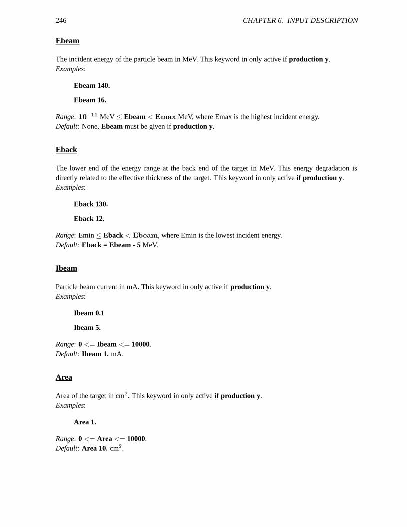
246 CHAPTER 6. INPUT DESCRIPTION
Ebeam
The incident energy of the particle beam in MeV. This keywordin only active ifproduction y.Examples:
Ebeam 140.
Ebeam 16.
Range: 10−11 MeV ≤ Ebeam< Emax MeV, where Emax is the highest incident energy.
Default: None,Ebeammust be given ifproduction y.
Eback
The lower end of the energy range at the back end of the target in MeV. This energy degradation isdirectly related to the effective thickness of the target. This keyword in only active ifproduction y.Examples:
Eback 130.
Eback 12.
Range: Emin≤ Eback < Ebeam, where Emin is the lowest incident energy.Default: Eback = Ebeam - 5MeV.
Ibeam
Particle beam current in mA. This keyword in only active ifproduction y.Examples:
Ibeam 0.1
Ibeam 5.
Range: 0 <= Ibeam <= 10000.Default: Ibeam 1. mA.
Area
Area of the target in cm2. This keyword in only active ifproduction y.Examples:
Area 1.
Range: 0 <= Area <= 10000.Default: Area 10. cm2.

6.2. KEYWORDS 247
rho
Material density of the target in g/cm3. This keyword in only active ifproduction y.Examples:
rho 10.
Range: 0 <= rho <= 100.Default: rho 1. is read from a hardwired material density table.
radiounit
Unit for radioactivity, to be used in the output files for isotope production. This keyword in only activeif production y.The following units are possible:
radiounit Bq : Becquerel
radiounit kBq : kiloBecquerel
radiounit MBq : MegaBecquerel
radiounit GBq : GigaBecquerel
radiounit Ci : Curie
radiounit mCi : milliCurie
radiounit kCi : kiloCurie
Range: radiounit should be equal to one of the units above.Default: radiounit Mbq .
yieldunit
Unit for isotope yield, in weight or number of isotopes. Thiskeyword in only active ifproduction y.The following units are possible:
yieldunit mug: microgram
yieldunit mg: milligram
yieldunit g: gram
yieldunit kg : kilogram
yieldunit num : number of isotopes
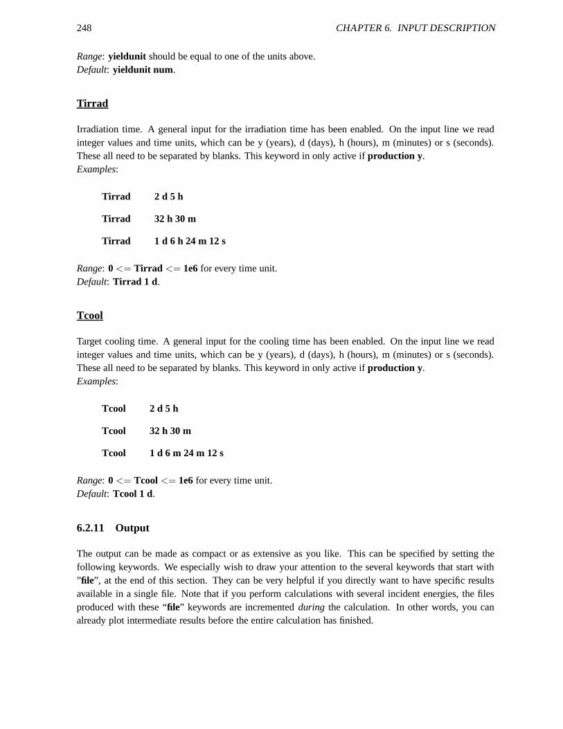
248 CHAPTER 6. INPUT DESCRIPTION
Range: yieldunit should be equal to one of the units above.Default: yieldunit num .
Tirrad
Irradiation time. A general input for the irradiation time has been enabled. On the input line we readinteger values and time units, which can be y (years), d (days), h (hours), m (minutes) or s (seconds).These all need to be separated by blanks. This keyword in onlyactive ifproduction y.Examples:
Tirrad 2 d 5 h
Tirrad 32 h 30 m
Tirrad 1 d 6 h 24 m 12 s
Range: 0 <= Tirrad <= 1e6for every time unit.Default: Tirrad 1 d .
Tcool
Target cooling time. A general input for the cooling time hasbeen enabled. On the input line we readinteger values and time units, which can be y (years), d (days), h (hours), m (minutes) or s (seconds).These all need to be separated by blanks. This keyword in onlyactive ifproduction y.Examples:
Tcool 2 d 5 h
Tcool 32 h 30 m
Tcool 1 d 6 m 24 m 12 s
Range: 0 <= Tcool <= 1e6for every time unit.Default: Tcool 1 d.
6.2.11 Output
The output can be made as compact or as extensive as you like. This can be specified by setting thefollowing keywords. We especially wish to draw your attention to the several keywords that start with”file”, at the end of this section. They can be very helpful if you directly want to have specific resultsavailable in a single file. Note that if you perform calculations with several incident energies, the filesproduced with these “file” keywords are incrementedduring the calculation. In other words, you canalready plot intermediate results before the entire calculation has finished.
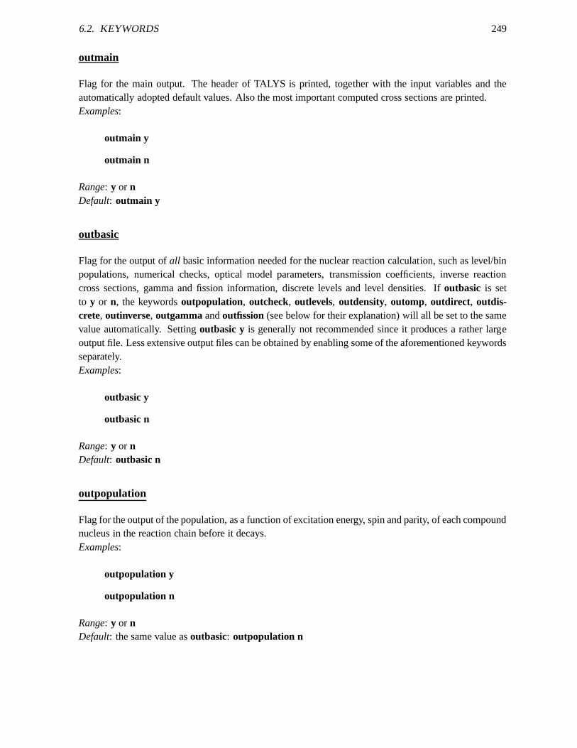
6.2. KEYWORDS 249
outmain
Flag for the main output. The header of TALYS is printed, together with the input variables and theautomatically adopted default values. Also the most important computed cross sections are printed.Examples:
outmain y
outmain n
Range: y or nDefault: outmain y
outbasic
Flag for the output ofall basic information needed for the nuclear reaction calculation, such as level/binpopulations, numerical checks, optical model parameters,transmission coefficients, inverse reactioncross sections, gamma and fission information, discrete levels and level densities. Ifoutbasic is setto y or n, the keywordsoutpopulation, outcheck, outlevels, outdensity, outomp, outdirect, outdis-crete, outinverse, outgammaandoutfission(see below for their explanation) will all be set to the samevalue automatically. Settingoutbasic y is generally not recommended since it produces a rather largeoutput file. Less extensive output files can be obtained by enabling some of the aforementioned keywordsseparately.Examples:
outbasic y
outbasic n
Range: y or nDefault: outbasic n
outpopulation
Flag for the output of the population, as a function of excitation energy, spin and parity, of each compoundnucleus in the reaction chain before it decays.Examples:
outpopulation y
outpopulation n
Range: y or nDefault: the same value asoutbasic: outpopulation n
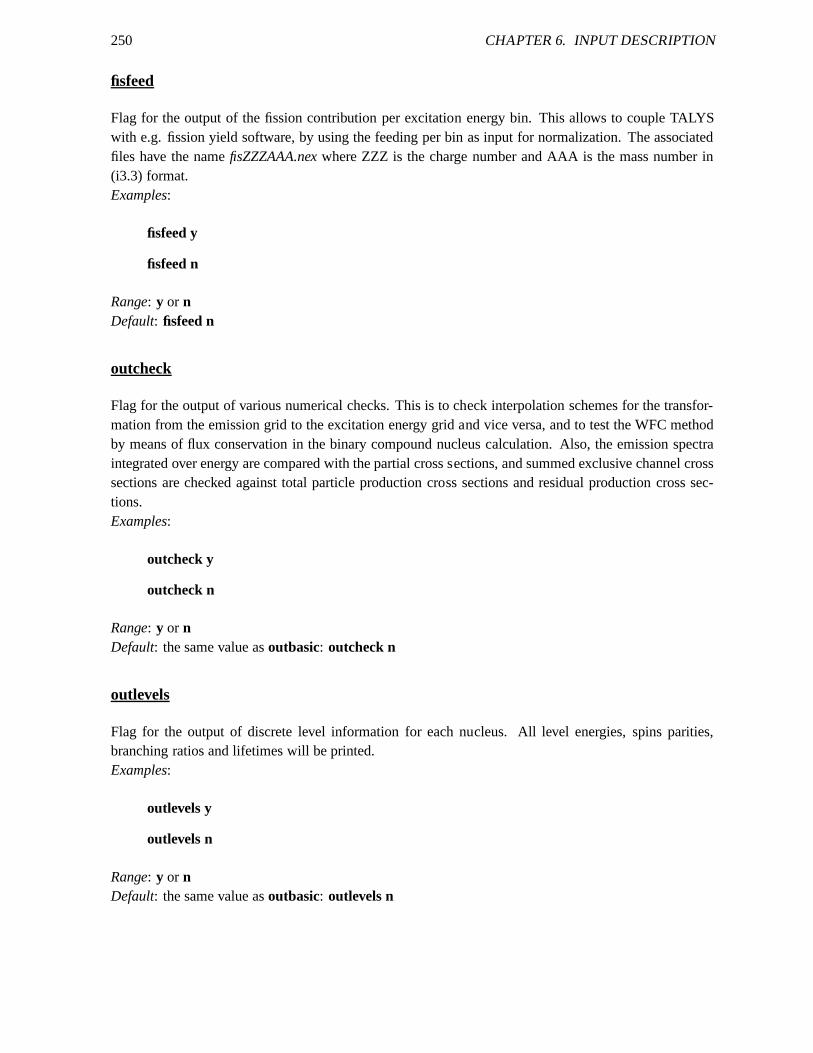
250 CHAPTER 6. INPUT DESCRIPTION
fisfeed
Flag for the output of the fission contribution per excitation energy bin. This allows to couple TALYSwith e.g. fission yield software, by using the feeding per binas input for normalization. The associatedfiles have the namefisZZZAAA.nexwhere ZZZ is the charge number and AAA is the mass number in(i3.3) format.Examples:
fisfeed y
fisfeed n
Range: y or nDefault: fisfeed n
outcheck
Flag for the output of various numerical checks. This is to check interpolation schemes for the transfor-mation from the emission grid to the excitation energy grid and vice versa, and to test the WFC methodby means of flux conservation in the binary compound nucleus calculation. Also, the emission spectraintegrated over energy are compared with the partial cross sections, and summed exclusive channel crosssections are checked against total particle production cross sections and residual production cross sec-tions.Examples:
outcheck y
outcheck n
Range: y or nDefault: the same value asoutbasic: outcheck n
outlevels
Flag for the output of discrete level information for each nucleus. All level energies, spins parities,branching ratios and lifetimes will be printed.Examples:
outlevels y
outlevels n
Range: y or nDefault: the same value asoutbasic: outlevels n
6.2. KEYWORDS 251
outdensity
Flag for the output of level density parameters and level densities for each residual nucleus.Examples:
outdensity y
outdensity n
Range: y or nDefault: the same value asoutbasic: outdensity n
outomp
Flag for the output of optical model parameters for each particle and energy.Examples:
outomp y
outomp n
Range: y or nDefault: the same value asoutbasic: outomp n
outdirect
Flag for the output of the results from the direct reaction calculation of ECIS (DWBA, giant resonancesand coupled-channels).Examples:
outdirect y
outdirect n
Range: y or nDefault: the same value asoutbasic: outdirect n
outinverse
Flag for the output of particle transmission coefficients and inverse reaction cross sections.Examples:
outinverse y
252 CHAPTER 6. INPUT DESCRIPTION
outinverse n
Range: y or nDefault: the same value asoutbasic: outinverse n
outtransenergy
Flag for the output of transmission coefficients sorted per energy (y) or per angular momentum (n).outtransenergy is only active ifoutinverse y.Examples:
outtransenergy y
outtransenergy n
Range: y or nDefault: outtransenergy y
outecis
Flag for keeping the various ECIS output files produced during a TALYS run. This is mainly for diag-nostic purposes.Examples:
outecis y
outecis n
Range: y or nDefault: outecis n
outgamma
Flag for the output of gamma-ray parameters, strength functions, transmission coefficients and reactioncross sections.Examples:
outgamma y
outgamma n
Range: y or nDefault: the same value asoutbasic: outgamma n

6.2. KEYWORDS 253
outpreequilibrium
Flag for the output of pre-equilibrium parameters and crosssections.outpreequilibrium is only activeif preequilibrium y .Examples:
outpreequilibrium y
outpreequilibrium n
Range: y or nDefault: outpreequilibrium n
outfission
Flag for the output of fission parameters, transmission coefficients and partial cross sections.outfissionis only active iffission y.Examples:
outfission y
outfission n
Range: y or nDefault: the same value asoutbasic: outfission n
outdiscrete
Flag for the output of cross sections to each individual discrete state. This is given for both the direct andthe compound component.Examples:
outdiscrete y
outdiscrete n
Range: y or nDefault: the same value asoutbasic: outdiscrete n
adddiscrete
Flag for the addition of energy-broadened non-elastic cross sections for discrete states to the continuumspectra.adddiscreteis only active ifoutspectra y.Examples:

254 CHAPTER 6. INPUT DESCRIPTION
adddiscrete y
adddiscrete n
Range: y or nDefault: adddiscrete y
addelastic
Flag for the addition of energy-broadened elastic cross sections to the continuum spectra. This case istreated separately fromadddiscrete, since sometimes the elastic contribution is already subtracted fromthe experimental spectrum.addelasticis only active ifoutspectra y.Examples:
addelastic y
addelastic n
Range: y or nDefault: the same value asadddiscrete: addelastic y
outspectra
Flag for the output of angle-integrated emission spectra.Examples:
outspectra y
outspectra n
Range: y or nDefault: outspectra y if only one incident energy is given in the input file, andoutspectra n for morethan one incident energy.
outbinspectra
Flag for the output of emission spectra per compound nucleusbin. outbinspectra is only active ifoutspectra yandpopulation y.Examples:
outbinspectra y
outbinspectra n
Range: y or nDefault: outbinspectra n.
6.2. KEYWORDS 255
elwidth
Width of elastic peak in MeV. For comparison with experimental angle-integrated and double-differentialspectra, it may be helpful to include the energy-broadened cross sections for discrete states in the high-energy tail of the spectra.elwidth is the width of the Gaussian spreading that takes care of this. elwidthis only active ifoutspectra yor if ddxmode 1, 2or 3.Examples:
elwidth 0.2
Range: 1.e − 6 ≤ elwidth≤ 100
Default: elwidth 0.5
outangle
Flag for the output of angular distributions for scatteringto discrete states.Examples:
outangle y
outangle n
Range: y or nDefault: outangle n
outlegendre
Flag for the output of Legendre coefficients for the angular distributions for scattering to discrete states.outlegendreis only active ifoutangle y.Examples:
outlegendre y
outlegendre n
Range: y or nDefault: outlegendre n
ddxmode
Option for the output of double-differential cross sections. There are 4 possibilities.Examples:

256 CHAPTER 6. INPUT DESCRIPTION
ddxmode 0: No output.
ddxmode 1: Output per emission energy as a function of angle (angular distributions).
ddxmode 2: Output per emission angle as a function of energy (spectra).
ddxmode 3: Output per emission energy and per emission angle.
Range: 0 ≤ ddxmode≤ 3Default: ddxmode 0. If there is afileddxe keyword, see p. 260, in the input file,ddxmode 1will beset automatically . If there is afileddxa keyword, see p. 261, in the input file,ddxmode 2will be setautomatically. If bothfileddxeandfileddxa are present,ddxmode 3will be set automatically.
outdwba
Flag for the output of DWBA cross sections for the multi-stepdirect model.Examples:
outdwba y
outdwba n
Range: y or nDefault: outdwba n
outgamdis
Flag for the output of discrete gamma-ray intensities. All possible discrete gamma transitions for allnuclei are followed. In the output they are given in tables per nuclide and for each decay from state tostate.Examples:
outgamdis y
outgamdis n
Range: y or nDefault: outgamdis n
outexcitation
Flag for the output of excitation functions, i.e. cross sections as a function of incident energy, such asresidual production cross sections, inelastic cross sections, etc.Examples:
6.2. KEYWORDS 257
outexcitation y
outexcitation n
Range: y or nDefault: outexcitation n if only one incident energy is given in the input file, andoutexcitation y formore than one incident energy.
endf
Flag for the creation of various output files needed for the assembling of an ENDF-6 formatted file.Apart from the creation of various files that will be discussed for the following keywords, a fileendf.totis created which contains the reaction, elastic and total cross sections (calculated by ECIS) on a fineenergy grid. Also a filedecay.Xwill be created, with X the ejectile symbol in (a1) format, that con-tains the discrete gamma decay probabilities for the binaryresidual nuclides. This will be used forgamma-ray production from discrete binary levels. In addition to all the output detailed below, thecontinuum gamma-ray spectra per residual nucleus and incident energy will be stored in filesgamZZZA-AAEYYY.YYY.tot, where where ZZZ is the charge number and AAA is the mass number in (i3.3) format,and YYY.YYY is the incident energy in (f7.3) format. Settingendf y will automatically enable many ofthe “file” keywords given below. All these specific files will be written to output ifendfdetail y, see thenext keyword.Examples:
endf y
endf n
Range: y or nDefault: endf n
integral
Keyword to calculate the effective cross section for integral activation measurements, by folding theexcitation functions by an experimental flux. Intalys/structure/flux, we have stored more than 40 spec-tra, coming from the EASY package [432, 529], which have beenused in past activation benchmarks.Obviously, this keyword does not produce a reliable answer for low energies, since TALYS does notcover the resonance range. On the input line, we readintegral, the cross section filename and the nameof the experimental spectrum. The latter should be equal to the extension of thespectrum. files intalys/structure/flux.Examples:
integral xs010000.L01 tudcucrzr
integral xs200000.tot cf252flux
258 CHAPTER 6. INPUT DESCRIPTION
Range: Both the cross section file and the flux file should exist.Default: integral is not used.
endfdetail
Flag for detailed ENDF-6 information. Certain ENDF-6 data files, usually those for incident charged par-ticles, only require lumped cross sections, spectra etc. and not all the exclusive channels. Theendfdetailkeyword enables to choose between this. For incident neutrons and photons, it is generally assumed thatdetailed ENDF-6 info, such as exclusive channels for all separate MT numbers, is required.Examples:
endfdetail y
endfdetail n
Range: y or nDefault: endfdetail y for incident neutrons and photons,endfdetail n for incident charged particles.
ompenergyfile
File with incident energies to calculate the total, elasticand reaction cross section on a sufficiently preciseenergy grid for ENDF-6 file purposes. On the input line, we read ompenergyfile, filename.Examples:
ompenergyfile energies.omp
Range: ompenergyfilecan be equal to any filename, provided it starts with a character. The incidentenergies should be in the range10−11 MeV to < 250 MeV, whereby theompenergyfilecontains atleast 1 and a maximum ofnumen6 incident energies, wherenumen6 is an array dimension specified intalys.cmb. Currentlynumen6=10000.Default: ompenergyfileis not given in the input file,
filedensity
Flag to write the level density and associated parameters ona separate fileldZZZAAA.tot, where ZZZ isthe charge number and AAA is the mass number in (i3.3) format.filedensity is only active ifoutdensityy.Examples:
filedensity y
filedensity n
Range: y or nDefault: filedensity n
6.2. KEYWORDS 259
fileelastic
Flag to write the elastic angular distribution on a separatefile XXYYY.YYYang.L00, where XX is the par-ticle symbol in (2a1) format (e.g.nn for elastic scattering), and YYY.YYY the incident energy in(f7.3)format. The file contains the angle, and 3 columns containingthe total, shape elastic, and compoundelastic angular distribution, respectively. If in addition outlegendre y, the elastic scattering Legendrecoefficients will be written on a fileXXYYY.YYYleg.L00. This file contains theL-value, and 4 columnscontaining the total, direct, compound and normalized Legendre coefficient.fileelastic is only active ifoutangle y.Examples:
fileelastic y, giving filesnn014.000ang.L00, and (if outlegendre y) nn014.000leg.L00, for an in-cident energy of 14 MeV.
fileelastic n
Range: y or nDefault: fileelastic n
fileangle
Designator for the output of the non-elastic angular distribution of one specific level on a separate filePXYYY.YYYang.LMM, where P and X are the particle symbols in (a1) format for the projectile and ejec-tile, respectively, YYY.YYY is the incident energy in (f7.3) format, and MM is the level number in (i2.2)format. The file contains the angle and 3 columns with the total inelastic, direct inelastic and compoundinelastic angular distribution to the specified level. On the input line we read the level number. Thefileanglekeyword can appear more than once in an input file, one for eachlevel that one is interested in.It will automatically produce files for all ejectiles. If in additionoutlegendre y, the non-elastic scatteringLegendre coefficients will be written on a filePXYYY.YYYleg.LMM. This file contains theL-value, and4 columns containing the total, direct, compound and normalized Legendre coefficient.fileangle is onlyactive ifoutdiscrete yandoutangle y.Examples:
fileangle 2, giving filesnp014.000ang.L02and (outlegendre y) np014.000leg.L02, for the (n, p)
reaction to the second discrete level and an incident energyof 14 MeV, and similarly for the otherejectiles.
Range: 0 < fileangle< numlev. Currently,numlev=30Default: fileanglenot active.
filechannels
Flag to write the exclusive channel cross sections as a function of incident energy on separate files.The files will be calledxsNPDTHA.tot, where N is the neutron number of the exclusive channel, P
260 CHAPTER 6. INPUT DESCRIPTION
the proton number, etc., in (a1) format. For examplexs210000.totcontains the excitation function forσ(n, 2np), if the incident particle was a neutron. The files contain theincident energy and 3 columnswith the exclusive cross section, the associated gamma-rayproduction cross section, and the fraction ofthis cross section relative to the total residual production cross section. If in addition isomers can beproduced, files calledxsNPDTHA.LMMwill be created with MM the isomeric level number in (i2.2)format. If filechannels y, the exclusive binary continuum cross sections, such as continuum inelasticscattering, will also be written to filesPX.con, where P and X are the particle symbols in (a1) format forthe projectile and ejectile, respectively. Ifoutspectra y, the exclusive channel spectra will be written onfilesspNPDTHAEYYY.YYY.totwhere YYY.YYY is the incident energy in (f7.3) format. The files containthe incident energy and 6 columns, with the spectra per outgoing particle type.filechannelsis only activeif channels y.Examples:
filechannels y
filechannels n
Range: y or nDefault: filechannels n
filespectrum
Designator for the output of the composite particle spectrum for a specific particle type on a separatefile. On the input line we read the particle symbols. This willresult in filesXspecYYY.YYY.tot, whereX is the outgoing particle symbol in (a1) format, and YYY.YYYthe incident energy in (f7.3) format.The file contains the emission energy and 5 columns with the total, direct, pre-equilibrium, multiple pre-equilibrium and compound spectrum, respectively.filespectrum is only active ifoutspectra y.Examples:
filespectrum n p a, giving filesnspec014.000.tot, pspec014.000.totandaspec014.000.tot, for anincident energy of 14 MeV.
Range: n p d t h aDefault: filespectrum not active.
fileddxe
Designator for the output of double-differential cross sections per emission energy for a specific parti-cle type. On the input line we read the particle type and the emission energy. This will result in filesXddxYYY.Y.mev, where X is the particle symbol in (a1) format and YYY.Y the emission energy in (f5.1)format. The file contains the emission angle and 5 columns with the total, direct, pre-equilibrium, multi-ple pre-equilibrium and compound spectrum, respectively.Thefileddxe keyword can appear more thanonce in an input file, one for each outgoing energy that one is interested in. If there is at least onefileddxe
6.2. KEYWORDS 261
keyword in the inputddxmode, see p. 255, will automatically be enabled.Examples:
fileddxe n 60.(giving a filenddx060.0.mev).
Range: n p d t h a for the particles and0. - Einc for outgoing energies.Default: fileddxenot active.
fileddxa
Designator for the output of double-differential cross sections per emission angle for a specific parti-cle type. On the input line we read the particle type and the emission angle. This will result in filesXddxYYY.Y.deg, where X is the particle symbol in (a1) format and YYY.Y the emission angle in (f5.1)format. The file contains the emission energy and 5 columns with the total, direct, pre-equilibrium, mul-tiple pre-equilibrium and compound spectrum, respectively. Thefileddxa keyword can appear more thanonce in an input file, one for each outgoing angle that one is interested in. If there is at least onefileddxakeyword in the inputddxmode, see p. 255, will automatically be enabled.Examples:
fileddxa n 30. (giving a filenddx030.0.deg).
Range: n p d t h a for the particles and0. - 180.for outgoing angles.Default: fileddxa not active.
filegamdis
Flag to write the discrete gamma-ray intensities as a function of incident energy to separate files. Thiswill result in files gamZZZAAALYYLMM.tot, where ZZZ is the charge number and AAA is the massnumber in (i3.3) format, YY is the number of the initial discrete state and MM the number of the finaldiscrete state.filegamdis is only active ifoutgamdis y.Examples:
filegamdis y
filegamdis n
Range: y or nDefault: filegamdis n
filetotal
Flag to write all the total cross sections as a function of incident energy on a separate filetotal.tot. Thefile contains the incident energy, and 9 columns containing the non-elastic, total elastic, total, compound
262 CHAPTER 6. INPUT DESCRIPTION
elastic, shape elastic, reaction, compound non-elastic, direct and pre-equilibrium cross section. In ad-dition, the total particle production cross sections will be written on filesXprod.tot, with X the particlesymbol in (a1) format. Finally, separate x-y tables will be made for the total cross section, ontotalxs.tot,the total elastic cross section, onelastic.tot, and the total nonelastic cross section, onnonelastic.tot. file-total is only active ifoutexcitation y or endf y.Examples:
filetotal y
filetotal n
Range: y or nDefault: filetotal n
fileresidual
Flag to write all the residual production cross sections as afunction of incident energy on separate files.The files for the total (i.e. the sum over ground state + isomers) residual production cross sections havethe namerpZZZAAA.totwhere ZZZ is the charge number and AAA is the mass number in (i3.3) format.If a residual nuclide contains one or more isomeric states, there are additional filesrpZZZAAA.LMM,where MM is the number of the isomer (ground state=0) in (i2.2) format. The files contain the incidentenergy and the residual production cross section.fileresidual is only active ifoutexcitation y or endf y.Examples:
fileresidual y
fileresidual n
Range: y or nDefault: fileresidual n
components
Flag to write the direct, pre-equilibrium and compound components of the cross sections in the variousoutput files.Examples:
components y
components n
Range: y or nDefault: components n
6.2. KEYWORDS 263
filerecoil
Flag to write the recoil spectra of the residual nuclides as afunction of incident energy on separatefiles. The files for the recoil spectra have the namerecZZZAAAspecYYY.YYY.totwhere ZZZ is the chargenumber and AAA is the mass number in (i3.3) format and YYY.YYYthe incident energy in (f7.3) format.If in addition flagchannels y, there are additional filesspNPDTHAEYYY.YYY.rec, where N is the neutronnumber of the exclusive channel, P the proton number, etc. The files contain the incident energy and therecoil.Examples:
filerecoil y
filerecoil n
Range: y or nDefault: filerecoil n
filefission
Flag to write all the fission cross sections as a function of incident energy on a separate filefission.tot.The file contains the incident energy and the total fission cross section. If in additionfilechannels y, theexclusive fission cross sections will be written to filesfisNPDTHA.tot, where N is the neutron number ofthe exclusive channel, P the proton number, etc., in (a1) format. For example,fis200000.totcontains theexcitation function forσ(n, 2nf), also known as the third chance fission cross section.filefission is onlyactive iffission y.Examples:
filefission y
filefission n
Range: y or nDefault: filefission n
filediscrete
Designator for the output of the excitation function of one specific non-elastic level on a separate filePX.LMM, where P and X are the particle symbols in (a1) format for the projectile and ejectile, respec-tively, and MM is the level number in (i2.2) format. The file contains the incident energy and 3 columnswith the total inelastic, direct inelastic and compound inelastic cross section to the specified level. On theinput line we read the level number. Thefilediscretekeyword can appear more than once in an input file,one for each level that one is interested in. It automatically produces a file for each ejectile.filediscreteis only active ifoutdiscrete y.Examples:
264 CHAPTER 6. INPUT DESCRIPTION
filediscrete 2, giving filesnn.L02, np.L02, etc. for the excitation functions of (inelastic and other)neutron scattering to the second discrete level.
Range: 0 < filediscrete< numlev. Currently,numlev=30Default: filediscretenot active.
6.2.12 Energy-dependent parameter adjustment
TALYS contains hundreds of parameters and most of them are energy-independent. They are ingredientsof phenomenological models which have been constructed with, indeed, energy-independent parameters.The OMP parameterrV , or the height of the fission barrier,fisbar are examples. There are two reasonsto deviate from this. First, since these models are a phenomenological representation of reality, there isno strict law that these parameters should be energy-independent. Suppose for example that one tries touse a simple Hill-Wheeler expression to approximate fissionpaths coming from microscopic analyses,which are supposedlty built on a better physical basis. Heights and widths of the fission barriers whichare dependent on (in this case, excitation) energy will probably emerge. Then, one may want to use thosein calculations.
A second reason is that if physically adequate models fail tofit experimental data, such energy-dependent adjustment can be invoked as a last resort. As longas the deviation from the original model isnot too large, unpleasant surprises in the various reactionchannels are avoided.
To accomodate this, no less that 65 TALYS keywords (parameters) now have the possibility to beextended with such an energy-dependence.
On the input line, we read the usual keyword and its energy-independent value. If a local variationis required, one adds (1) 4 extra parameters, or (2) a filename, to the input line. With either method amultiplication factor deviating from 1 can be given, as a function of energy. The 4 extra parameters, Ea,Eb, Em and D, drive the following multiplication function
f(E) = 1 + D′ (E − Ea)N
(E − Ea)N + (C − Ea)N, if E < Em
= 1 + D′ (Eb − E)N
(Eb − E)N + (C − Eb)N, if E ≥ Em(6.4)
whereN is currently fixed to 4, and
(6.5) D′ = (D − 1)(1 +1
2
N
)
and
C = Ea +1
2(Em − Ea), if E < Em
C = Em +1
2(Eb − Em), if E ≥ Em(6.6)
An input line would then look as follows:
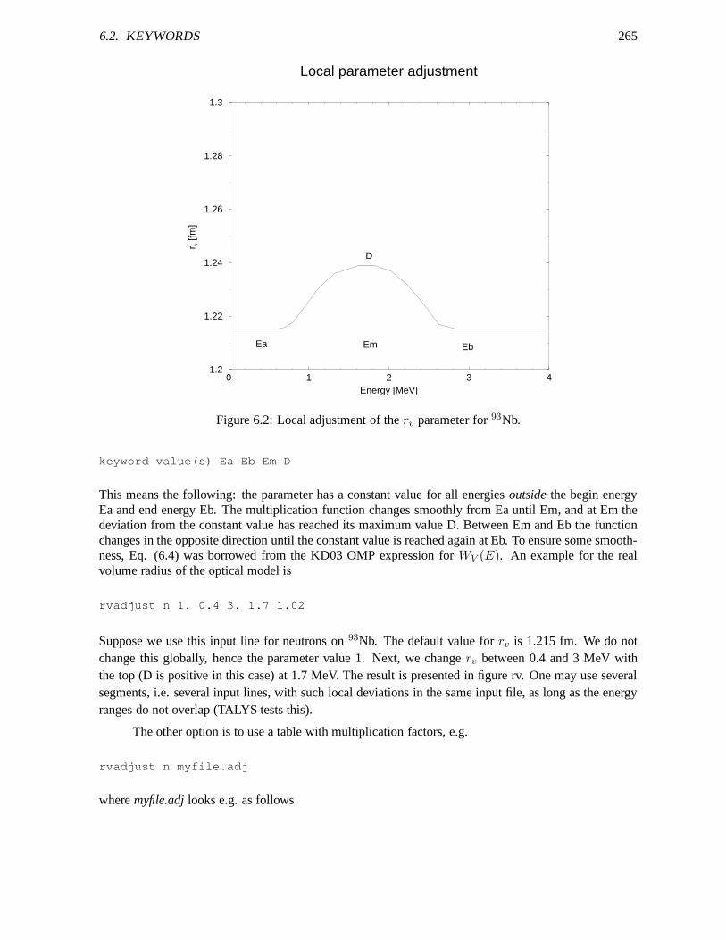
6.2. KEYWORDS 265
0 1 2 3 4Energy [MeV]
1.2
1.22
1.24
1.26
1.28
1.3
r v [fm
]
Local parameter adjustment
Ea EbEm
D
Figure 6.2: Local adjustment of therv parameter for93Nb.
keyword value(s) Ea Eb Em D
This means the following: the parameter has a constant valuefor all energiesoutsidethe begin energyEa and end energy Eb. The multiplication function changes smoothly from Ea until Em, and at Em thedeviation from the constant value has reached its maximum value D. Between Em and Eb the functionchanges in the opposite direction until the constant value is reached again at Eb. To ensure some smooth-ness, Eq. (6.4) was borrowed from the KD03 OMP expression forWV (E). An example for the realvolume radius of the optical model is
rvadjust n 1. 0.4 3. 1.7 1.02
Suppose we use this input line for neutrons on93Nb. The default value forrv is 1.215 fm. We do notchange this globally, hence the parameter value 1. Next, we changerv between 0.4 and 3 MeV withthe top (D is positive in this case) at 1.7 MeV. The result is presented in figure rv. One may use severalsegments, i.e. several input lines, with such local deviations in the same input file, as long as the energyranges do not overlap (TALYS tests this).
The other option is to use a table with multiplication factors, e.g.
rvadjust n myfile.adj
wheremyfile.adjlooks e.g. as follows
266 CHAPTER 6. INPUT DESCRIPTION
0.0 1.0.4. 1.1.7 1.13.0 1.200 1.
which will simply produces a triangle with top at 1.7 MeV. Forsuch simple cases, the use of Eq. (6.4)may be better.
The latter option may be interesting if one manages to fit, in some nuclear structure study, aphenomelogical prescription available in TALYS to a more complex microscopic description of a nuclearprocess. For example, maybe a JLM OMP can be simulated by a Woods-Saxon OMP with energydependent parameters, or a microscopic fission model by a Hill-Wheeler model with energy dependentfission parameters. The resulting fit can then be used as inputfile to TALYS.
The energy-dependent adjustment is currently possible forthe following keywords.
Optical model:avadjust, avdadjust, avsoadjust, awadjust, awdadjust, awsoadjust, d1adjust,d2adjust, d3adjust, lv1adjust, lvadjust, lvsoadjust, lw1adjust, lwadjust, lwsoadjust, rcadjust, rvad-just, rvdadjust, rvsoadjust, rwadjust, rwdadjust, rwsoadjust, tljadjust, v1adjust, v2adjust, v3adjust,v4adjust, vso1adjust, vso2adjust, w1adjust, w2adjust, w3adjust, w4adjust, wso1adjust, wso2adjust,adepthcor,aradialcor
Level density:ctable, krotconstant,ptable, rspincut, s2adjust
Gamma-ray strength function:sgr, sgradjust, spr, spradjust, egr, egradjust, epr, epradjust,etable,ftable, ggr, ggradjust, gnorm, gpr, gpradjust
Pre-equilibrium:cbreak, cknock, cstrip, m2constant
Fission:fisbar, fisbaradjust, fishw, fishwadjust
In a previous version of TALYS, this local adjustment was only applicable for the optical modelparameters, with a different muliplication function, see e.g. rvadjustF on page 192. We now suggest theformalism described above for all parameters.
6.2.13 Input parameter table
From all the keywords given above you can see that certain default values depend on mass, energy orother parameters. In table 6.1 we summarize all these dependencies and give the full table of keywordsincluding their relation with each other.
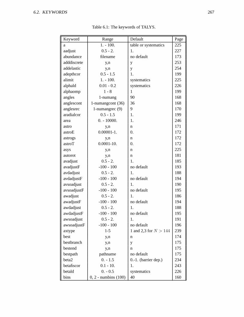
6.2. KEYWORDS 267
Table 6.1: The keywords of TALYS.
Keyword Range Default Pagea 1. - 100. table or systematics 225aadjust 0.5 - 2. 1. 227abundance filename no default 173adddiscrete y,n y 253addelastic y,n y 254adepthcor 0.5 - 1.5 1. 199alimit 1. - 100. systematics 225alphald 0.01 - 0.2 systematics 226alphaomp 1 - 8 1 199angles 1-numang 90 168anglescont 1-numangcont (36) 36 168anglesrec 1-numangrec (9) 9 170aradialcor 0.5 - 1.5 1. 199area 0. - 10000. 1. 246astro y,n n 171astroE 0.00001-1. 0. 172astrogs y,n n 172astroT 0.0001-10. 0. 172asys y,n n 225autorot y,n n 181avadjust 0.5 - 2. 1. 185avadjustF -100 - 100 no default 193avdadjust 0.5 - 2. 1. 188avdadjustF -100 - 100 no default 194avsoadjust 0.5 - 2. 1. 190avsoadjustF -100 - 100 no default 195awadjust 0.5 - 2. 1. 186awadjustF -100 - 100 no default 194awdadjust 0.5 - 2. 1. 188awdadjustF -100 - 100 no default 195awsoadjust 0.5 - 2. 1. 191awsoadjustF -100 - 100 no default 196axtype 1-5 1 and 2,3 forN > 144 239best y,n n 174bestbranch y,n y 175bestend y,n n 175bestpath pathname no default 175beta2 0. - 1.5 0.-1. (barrier dep.) 234betafiscor 0.1 - 10. 1. 243betald 0. - 0.5 systematics 226bins 0, 2 - numbins (100) 40 160
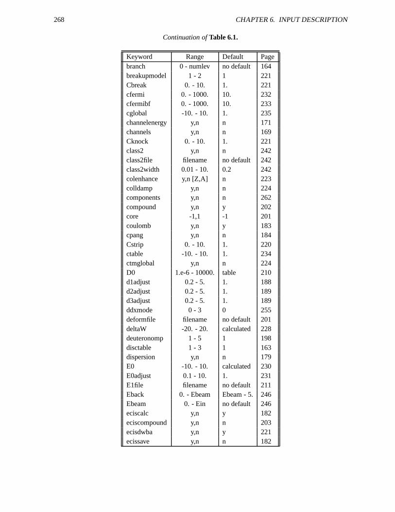
268 CHAPTER 6. INPUT DESCRIPTION
Continuation ofTable 6.1.
Keyword Range Default Pagebranch 0 - numlev no default 164breakupmodel 1 - 2 1 221Cbreak 0. - 10. 1. 221cfermi 0. - 1000. 10. 232cfermibf 0. - 1000. 10. 233cglobal -10. - 10. 1. 235channelenergy y,n n 171channels y,n n 169Cknock 0. - 10. 1. 221class2 y,n n 242class2file filename no default 242class2width 0.01 - 10. 0.2 242colenhance y,n [Z,A] n 223colldamp y,n n 224components y,n n 262compound y,n y 202core -1,1 -1 201coulomb y,n y 183cpang y,n n 184Cstrip 0. - 10. 1. 220ctable -10. - 10. 1. 234ctmglobal y,n n 224D0 1.e-6 - 10000. table 210d1adjust 0.2 - 5. 1. 188d2adjust 0.2 - 5. 1. 189d3adjust 0.2 - 5. 1. 189ddxmode 0 - 3 0 255deformfile filename no default 201deltaW -20. - 20. calculated 228deuteronomp 1 - 5 1 198disctable 1 - 3 1 163dispersion y,n n 179E0 -10. - 10. calculated 230E0adjust 0.1 - 10. 1. 231E1file filename no default 211Eback 0. - Ebeam Ebeam - 5. 246Ebeam 0. - Ein no default 246eciscalc y,n y 182eciscompound y,n n 203ecisdwba y,n y 221ecissave y,n n 182
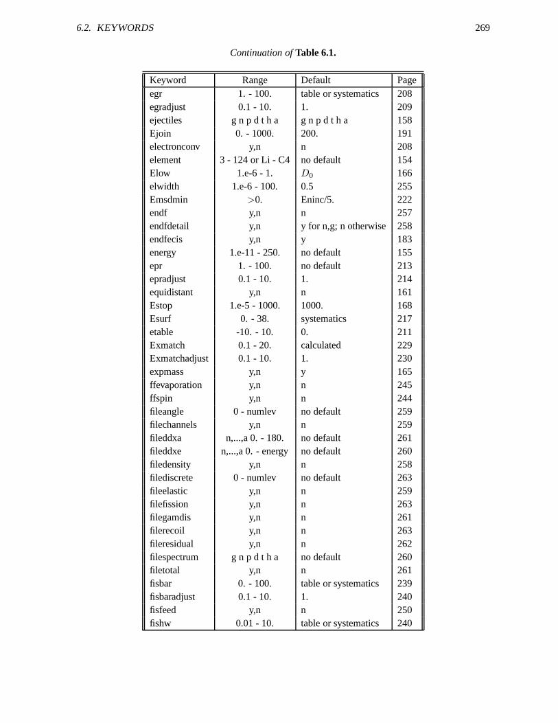
6.2. KEYWORDS 269
Continuation ofTable 6.1.
Keyword Range Default Pageegr 1. - 100. table or systematics 208egradjust 0.1 - 10. 1. 209ejectiles g n p d t h a g n p d t h a 158Ejoin 0. - 1000. 200. 191electronconv y,n n 208element 3 - 124 or Li - C4 no default 154Elow 1.e-6 - 1. D0 166elwidth 1.e-6 - 100. 0.5 255Emsdmin >0. Eninc/5. 222endf y,n n 257endfdetail y,n y for n,g; n otherwise 258endfecis y,n y 183energy 1.e-11 - 250. no default 155epr 1. - 100. no default 213epradjust 0.1 - 10. 1. 214equidistant y,n n 161Estop 1.e-5 - 1000. 1000. 168Esurf 0. - 38. systematics 217etable -10. - 10. 0. 211Exmatch 0.1 - 20. calculated 229Exmatchadjust 0.1 - 10. 1. 230expmass y,n y 165ffevaporation y,n n 245ffspin y,n n 244fileangle 0 - numlev no default 259filechannels y,n n 259fileddxa n,...,a 0. - 180. no default 261fileddxe n,...,a 0. - energy no default 260filedensity y,n n 258filediscrete 0 - numlev no default 263fileelastic y,n n 259filefission y,n n 263filegamdis y,n n 261filerecoil y,n n 263fileresidual y,n n 262filespectrum g n p d t h a no default 260filetotal y,n n 261fisbar 0. - 100. table or systematics 239fisbaradjust 0.1 - 10. 1. 240fisfeed y,n n 250fishw 0.01 - 10. table or systematics 240
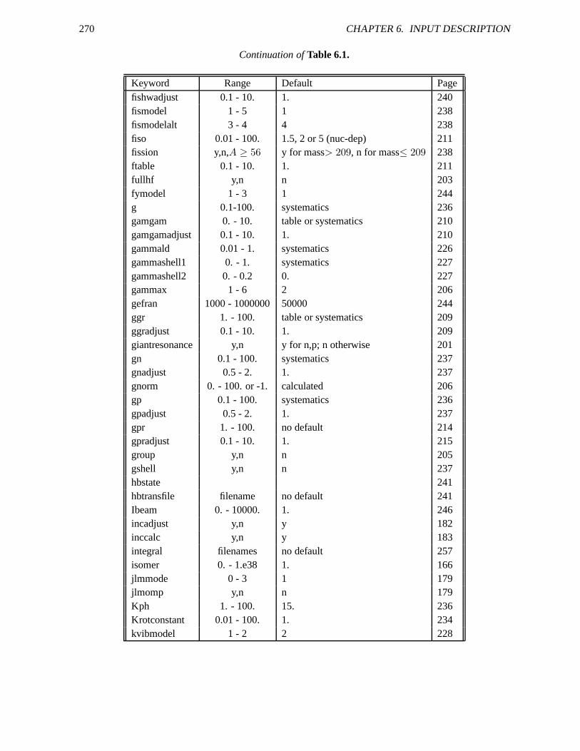
270 CHAPTER 6. INPUT DESCRIPTION
Continuation ofTable 6.1.
Keyword Range Default Pagefishwadjust 0.1 - 10. 1. 240fismodel 1 - 5 1 238fismodelalt 3 - 4 4 238fiso 0.01 - 100. 1.5, 2 or 5 (nuc-dep) 211fission y,n,A ≥ 56 y for mass> 209, n for mass≤ 209 238ftable 0.1 - 10. 1. 211fullhf y,n n 203fymodel 1 - 3 1 244g 0.1-100. systematics 236gamgam 0. - 10. table or systematics 210gamgamadjust 0.1 - 10. 1. 210gammald 0.01 - 1. systematics 226gammashell1 0. - 1. systematics 227gammashell2 0. - 0.2 0. 227gammax 1 - 6 2 206gefran 1000 - 1000000 50000 244ggr 1. - 100. table or systematics 209ggradjust 0.1 - 10. 1. 209giantresonance y,n y for n,p; n otherwise 201gn 0.1 - 100. systematics 237gnadjust 0.5 - 2. 1. 237gnorm 0. - 100. or -1. calculated 206gp 0.1 - 100. systematics 236gpadjust 0.5 - 2. 1. 237gpr 1. - 100. no default 214gpradjust 0.1 - 10. 1. 215group y,n n 205gshell y,n n 237hbstate 241hbtransfile filename no default 241Ibeam 0. - 10000. 1. 246incadjust y,n y 182inccalc y,n y 183integral filenames no default 257isomer 0. - 1.e38 1. 166jlmmode 0 - 3 1 179jlmomp y,n n 179Kph 1. - 100. 15. 236Krotconstant 0.01 - 100. 1. 234kvibmodel 1 - 2 2 228
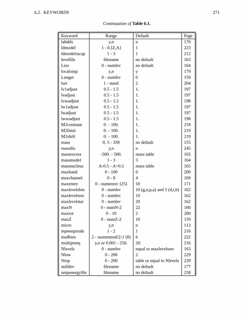
6.2. KEYWORDS 271
Continuation ofTable 6.1.
Keyword Range Default Pagelabddx y,n n 170ldmodel 1 - 6 [Z,A] 1 223ldmodelracap 1 - 3 1 212levelfile filename no default 163Liso 0 - numlev no default 164localomp y,n y 179Ltarget 0 - numlev 0 159lurr 1 - numl 2 204lv1adjust 0.5 - 1.5 1. 197lvadjust 0.5 - 1.5 1. 197lvsoadjust 0.5 - 1.5 1. 198lw1adjust 0.5 - 1.5 1. 197lwadjust 0.5 - 1.5 1. 197lwsoadjust 0.5 - 1.5 1. 198M2constant 0. - 100. 1. 218M2limit 0. - 100. 1. 219M2shift 0. - 100. 1. 219mass 0, 5 - 339 no default 155massdis y,n n 245massexcess -500. - 500. mass table 165massmodel 1 - 3 3 164massnucleus A-0.5 - A+0.5 mass table 165maxband 0 - 100 0 200maxchannel 0 - 8 4 169maxenrec 0 - numenrec (25) 10 171maxlevelsbin 0 - numlev 10 (g,n,p,a) and 5 (d,t,h) 162maxlevelsres 0 - numlev 10 162maxlevelstar 0 - numlev 20 162maxN 0 - numN-2 22 160maxrot 0 - 10 2 200maxZ 0 - numZ-2 10 159micro y,n n 113mpreeqmode 1 - 2 1 216msdbins 2 - numenmsd/2-1 (8) 6 222multipreeq y,n or 0.001 - 250. 20. 216Nlevels 0 - numlev equal to maxlevelsres 163Nlow 0 - 200 2 229Ntop 0 - 200 table or equal to Nlevels 229nulldev filename no default 177ompenergyfile filename no default 258
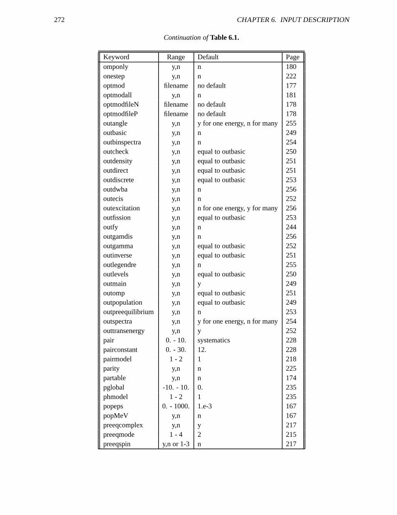
272 CHAPTER 6. INPUT DESCRIPTION
Continuation ofTable 6.1.
Keyword Range Default Pageomponly y,n n 180onestep y,n n 222optmod filename no default 177optmodall y,n n 181optmodfileN filename no default 178optmodfileP filename no default 178outangle y,n y for one energy, n for many 255outbasic y,n n 249outbinspectra y,n n 254outcheck y,n equal to outbasic 250outdensity y,n equal to outbasic 251outdirect y,n equal to outbasic 251outdiscrete y,n equal to outbasic 253outdwba y,n n 256outecis y,n n 252outexcitation y,n n for one energy, y for many 256outfission y,n equal to outbasic 253outfy y,n n 244outgamdis y,n n 256outgamma y,n equal to outbasic 252outinverse y,n equal to outbasic 251outlegendre y,n n 255outlevels y,n equal to outbasic 250outmain y,n y 249outomp y,n equal to outbasic 251outpopulation y,n equal to outbasic 249outpreequilibrium y,n n 253outspectra y,n y for one energy, n for many 254outtransenergy y,n y 252pair 0. - 10. systematics 228pairconstant 0. - 30. 12. 228pairmodel 1 - 2 1 218parity y,n n 225partable y,n n 174pglobal -10. - 10. 0. 235phmodel 1 - 2 1 235popeps 0. - 1000. 1.e-3 167popMeV y,n n 167preeqcomplex y,n y 217preeqmode 1 - 4 2 215preeqspin y,n or 1-3 n 217
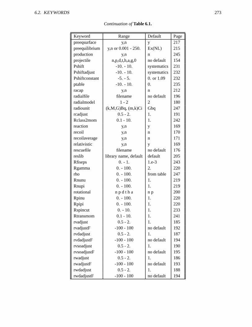
6.2. KEYWORDS 273
Continuation ofTable 6.1.
Keyword Range Default Pagepreeqsurface y,n y 217preequilibrium y,n or 0.001 - 250. Ex(NL) 215production y,n n 245projectile n,p,d,t,h,a,g,0 no default 154Pshift -10. - 10. systematics 231Pshiftadjust -10. - 10. systematics 232Pshiftconstant -5. - 5. 0. or 1.09 232ptable -10. - 10. 0. 235racap y,n n 212radialfile filename no default 196radialmodel 1 - 2 2 180radiounit (k,M,G)Bq, (m,k)Ci Gbq 247rcadjust 0.5 - 2. 1. 191Rclass2mom 0.1 - 10. 1. 242reaction y,n y 169recoil y,n n 170recoilaverage y,n n 171relativistic y,n y 169rescuefile filename no default 176reslib library name, default default 205Rfiseps 0. - 1. 1.e-3 243Rgamma 0. - 100. 2. 220rho 0. - 100. from table 247Rnunu 0. - 100. 1. 219Rnupi 0. - 100. 1. 219rotational n p d t h a n p 200Rpinu 0. - 100. 1. 220Rpipi 0. - 100. 1. 220Rspincut 0. - 10. 1. 233Rtransmom 0.1 - 10. 1. 241rvadjust 0.5 - 2. 1. 185rvadjustF -100 - 100 no default 192rvdadjust 0.5 - 2. 1. 187rvdadjustF -100 - 100 no default 194rvsoadjust 0.5 - 2. 1. 190rvsoadjustF -100 - 100 no default 195rwadjust 0.5 - 2. 1. 186rwadjustF -100 - 100 no default 193rwdadjust 0.5 - 2. 1. 188rwdadjustF -100 - 100 no default 194
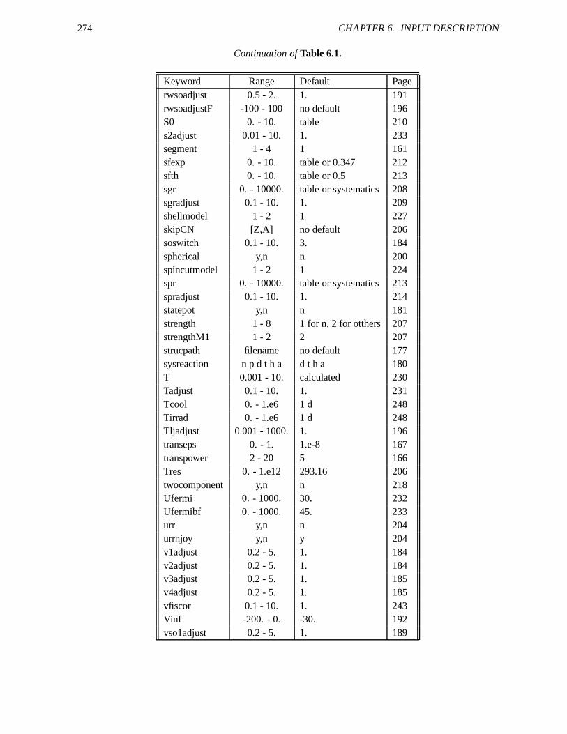
274 CHAPTER 6. INPUT DESCRIPTION
Continuation ofTable 6.1.
Keyword Range Default Pagerwsoadjust 0.5 - 2. 1. 191rwsoadjustF -100 - 100 no default 196S0 0. - 10. table 210s2adjust 0.01 - 10. 1. 233segment 1 - 4 1 161sfexp 0. - 10. table or 0.347 212sfth 0. - 10. table or 0.5 213sgr 0. - 10000. table or systematics 208sgradjust 0.1 - 10. 1. 209shellmodel 1 - 2 1 227skipCN [Z,A] no default 206soswitch 0.1 - 10. 3. 184spherical y,n n 200spincutmodel 1 - 2 1 224spr 0. - 10000. table or systematics 213spradjust 0.1 - 10. 1. 214statepot y,n n 181strength 1 - 8 1 for n, 2 for otthers 207strengthM1 1 - 2 2 207strucpath filename no default 177sysreaction n p d t h a d t h a 180T 0.001 - 10. calculated 230Tadjust 0.1 - 10. 1. 231Tcool 0. - 1.e6 1 d 248Tirrad 0. - 1.e6 1 d 248Tljadjust 0.001 - 1000. 1. 196transeps 0. - 1. 1.e-8 167transpower 2 - 20 5 166Tres 0. - 1.e12 293.16 206twocomponent y,n n 218Ufermi 0. - 1000. 30. 232Ufermibf 0. - 1000. 45. 233urr y,n n 204urrnjoy y,n y 204v1adjust 0.2 - 5. 1. 184v2adjust 0.2 - 5. 1. 184v3adjust 0.2 - 5. 1. 185v4adjust 0.2 - 5. 1. 185vfiscor 0.1 - 10. 1. 243Vinf -200. - 0. -30. 192vso1adjust 0.2 - 5. 1. 189
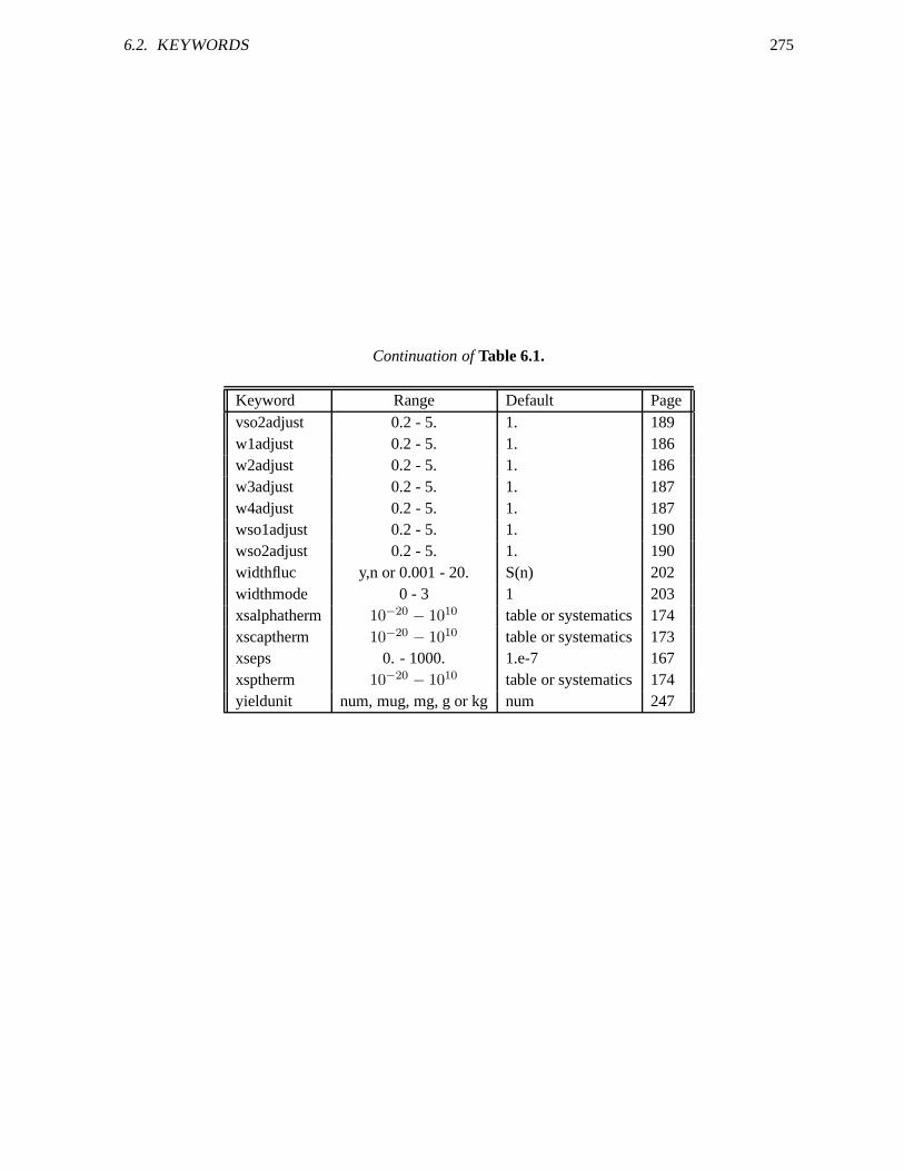
6.2. KEYWORDS 275
Continuation ofTable 6.1.
Keyword Range Default Pagevso2adjust 0.2 - 5. 1. 189w1adjust 0.2 - 5. 1. 186w2adjust 0.2 - 5. 1. 186w3adjust 0.2 - 5. 1. 187w4adjust 0.2 - 5. 1. 187wso1adjust 0.2 - 5. 1. 190wso2adjust 0.2 - 5. 1. 190widthfluc y,n or 0.001 - 20. S(n) 202widthmode 0 - 3 1 203xsalphatherm 10−20 − 1010 table or systematics 174xscaptherm 10−20 − 1010 table or systematics 173xseps 0. - 1000. 1.e-7 167xsptherm 10−20 − 1010 table or systematics 174yieldunit num, mug, mg, g or kg num 247

276 CHAPTER 6. INPUT DESCRIPTION
Chapter 7Verification and validation, sample cases andoutput
TALYS has been tested both formally (”computational robustness”) and by comparison of calculationalresults with experimental data. This will be described in the present Chapter. Also a description of theoutput will be given.
7.1 Robustness test with DRIP
One way to test a nuclear model code is to let it calculate results for a huge number of nuclides, and thewhole range of projectiles and energies. We have written a little code DRIP, not included in the release,that launches TALYS for complete calculations for all nuclides, from dripline to dripline. Besides check-ing whether the code crashes, visual inspection of many curves simultaneously, e.g. (n,2n) excitationfunctions for 50 different targets, may reveal non-smooth behaviour. Various problems, not only in theTALYS source code itself, but also in the nuclear structure database, were revealed with this approach inthe initial development stages.
7.2 Robustness test with MONKEY
Chapter 6 contains a description of the more than 340 keywords that can be used in a problem for TALYS.Some of them are flags which can only be set toy or n. Other keywords can be set to a few or severalinteger values and there are also keywords whose values may cover a quasi-continuous range betweenthe minimum and maximum possible value that we allow for them. Strictly speaking, the total numberof possible input files for TALYS is huge (though theoretically finite, because of the finite precision ofa computer), and obviously only a small subset of them corresponds to physically meaningful cases.Indeed, as with many computer codes it is not too difficult to bring a TALYS calculation to a formallysuccessful end, i.e. without crashing, with an input file that represents a completely unphysical case.
277
278 CHAPTER 7. VERIFICATION AND VALIDATION, SAMPLE CASES AND OUTPUT
Obviously, there is no way to prevent this - the user is supposed to have full responsibility for what sheor he is doing - and we can never anticipate what input files aremade by other users. Nevertheless, totest the robustness of our code, we wrote a little program called MONKEY which remotely simulatesTALYS in the hands of an evil user: It creates an input file for TALYS, using all the keywords, withrandomvalues, and starts a run with it. Each keyword in this input file has a value that remains withinthe allowed (and very broad) range as specified in Chapter 6. If TALYS is compiled with all checkingoptions (i.e. array out-of-bounds checks, divisions by zero, other over/underflow errors, etc.) enabledand runs successfully for thousands of such random input files without crashing, we can at least say wehave testedcomputationalrobustness to some extent, and that wemayhave probed every corner of thecode. We realize that this is not a full-proof method to test TALYS formally on the Fortran level (ifthere exists such a test!), but MONKEY has helped us to discover a few bugs during development whichotherwise would have come to the surface sooner or later. We think it is better thatwefind them first. Theideal result of this procedure would be that TALYS never crashes or stops without giving an appropriateerror message. We emphasize that this test alone does obviously not guarantee any physical quality ofthe results. For that, much more important are the input filesthatare physically meaningful. These arediscussed in the next Section.
7.3 Validation with sample cases
With this manual, we hope to convince you that a large varietyof nuclear reaction calculations can behandled with TALYS. To strengthen this statement, we will discuss many different sample cases. In eachcase, the TALYS input file, the relevant output and, if available, a graphical comparison with experi-mental data will be presented. The description of the first sample case is the longest, since the outputof TALYS will be discussed in complete detail. Obviously, that output description is also applicableto the other sample cases. The entire collection of sample cases serves as (a) verification of TALYS:the sample output files should coincide, apart from numerical differences of insignificant order, with theoutput files obtained on your computer, and (b) validation ofTALYS: the results should be comparableto experimental data for a widely varying set of nuclear reactions. Table 7.1 tells you what to expect interms of computer time, and this shows that it thus may take a while (about two hours on a PC) before allsample cases have finished. Running theverifyscript will be worth the wait, since a successful executionof all sample cases will put you on safer ground for your own calculations. In general, we will explainthe keywords again as they appear in the input files below. If not, consult Table 6.1, which will tell youwhere to find the explanation of a keyword.
Finally, from an extensive number of references [133]-[748], you may deduce whether TALYS isthe appropriate code to perform the calculation you need.
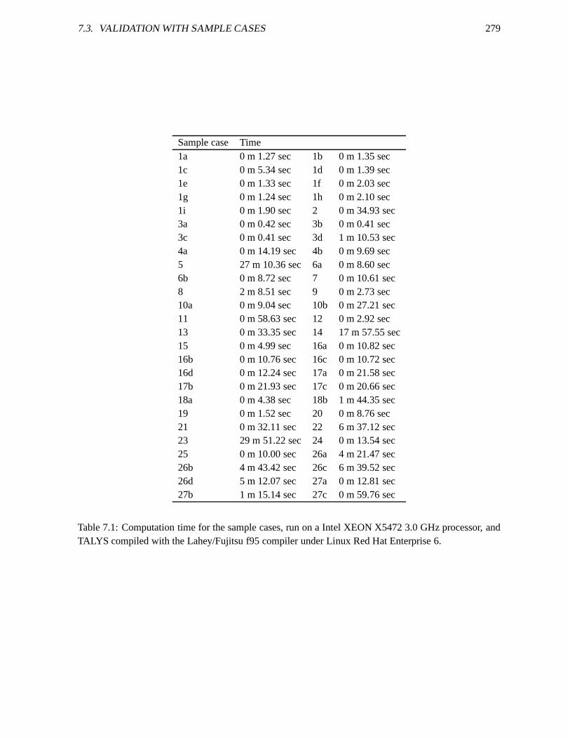
7.3. VALIDATION WITH SAMPLE CASES 279
Sample case Time1a 0 m 1.27 sec 1b 0 m 1.35 sec1c 0 m 5.34 sec 1d 0 m 1.39 sec1e 0 m 1.33 sec 1f 0 m 2.03 sec1g 0 m 1.24 sec 1h 0 m 2.10 sec1i 0 m 1.90 sec 2 0 m 34.93 sec3a 0 m 0.42 sec 3b 0 m 0.41 sec3c 0 m 0.41 sec 3d 1 m 10.53 sec4a 0 m 14.19 sec 4b 0 m 9.69 sec5 27 m 10.36 sec 6a 0 m 8.60 sec6b 0 m 8.72 sec 7 0 m 10.61 sec8 2 m 8.51 sec 9 0 m 2.73 sec10a 0 m 9.04 sec 10b 0 m 27.21 sec11 0 m 58.63 sec 12 0 m 2.92 sec13 0 m 33.35 sec 14 17 m 57.55 sec15 0 m 4.99 sec 16a 0 m 10.82 sec16b 0 m 10.76 sec 16c 0 m 10.72 sec16d 0 m 12.24 sec 17a 0 m 21.58 sec17b 0 m 21.93 sec 17c 0 m 20.66 sec18a 0 m 4.38 sec 18b 1 m 44.35 sec19 0 m 1.52 sec 20 0 m 8.76 sec21 0 m 32.11 sec 22 6 m 37.12 sec23 29 m 51.22 sec 24 0 m 13.54 sec25 0 m 10.00 sec 26a 4 m 21.47 sec26b 4 m 43.42 sec 26c 6 m 39.52 sec26d 5 m 12.07 sec 27a 0 m 12.81 sec27b 1 m 15.14 sec 27c 0 m 59.76 sec
Table 7.1: Computation time for the sample cases, run on a Intel XEON X5472 3.0 GHz processor, andTALYS compiled with the Lahey/Fujitsu f95 compiler under Linux Red Hat Enterprise 6.
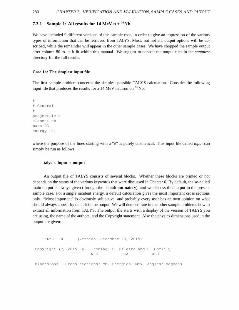
280 CHAPTER 7. VERIFICATION AND VALIDATION, SAMPLE CASES AND OUTPUT
7.3.1 Sample 1: All results for 14 MeV n +93Nb
We have included 9 different versions of this sample case, inorder to give an impression of the varioustypes of information that can be retrieved from TALYS. Most,but not all, output options will be de-scribed, while the remainder will appear in the other samplecases. We have chopped the sample outputafter column 80 to let it fit within this manual. We suggest to consult the output files in thesamples/directory for the full results.
Case 1a: The simplest input file
The first sample problem concerns the simplest possible TALYS calculation. Consider the followinginput file that produces the results for a 14 MeV neutron on93Nb:
## General#projectile nelement nbmass 93energy 14.
where the purpose of the lines starting with a “#” is purely cosmetical. This input file calledinput cansimply be run as follows:
talys < input > output
An output file of TALYS consists of several blocks. Whether these blocks are printed or notdepends on the status of the various keywords that were discussed in Chapter 6. By default, the so-calledmain output is always given (through the defaultoutmain y), and we discuss this output in the presentsample case. For a single incident energy, a default calculation gives the most important cross sectionsonly. “Most important” is obviously subjective, and probably every user has an own opinion on whatshould always appear by default in the output. We will demonstrate in the other sample problems how toextract all information from TALYS. The output file starts with a display of the version of TALYS youare using, the name of the authors, and the Copyright statement. Also the physics dimensions used in theoutput are given:
TALYS-1.8 (Version: December 23, 2015)
Copyright (C) 2015 A.J. Koning, S. Hilaire and S. GorielyNRG CEA ULB
Dimensions - Cross sections: mb, Energies: MeV, Angles: deg rees
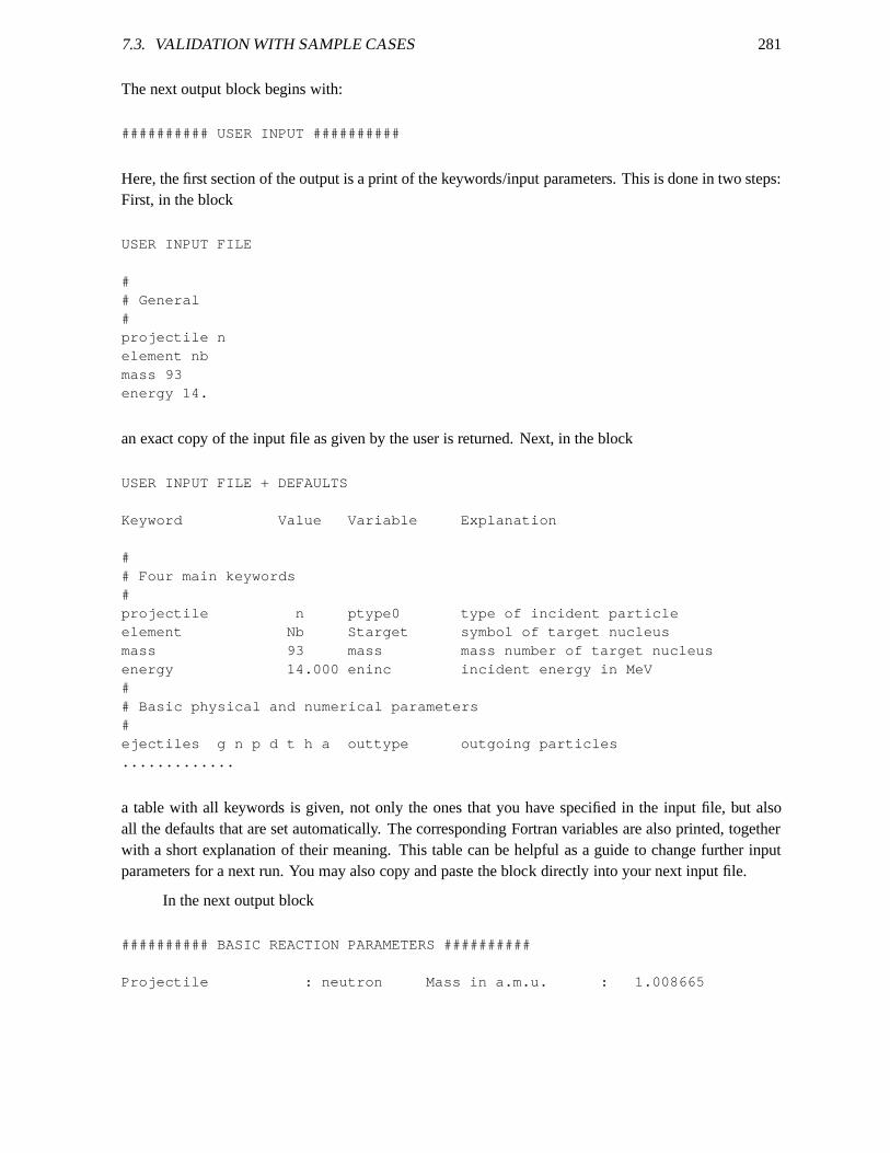
7.3. VALIDATION WITH SAMPLE CASES 281
The next output block begins with:
########## USER INPUT ##########
Here, the first section of the output is a print of the keywords/input parameters. This is done in two steps:First, in the block
USER INPUT FILE
## General#projectile nelement nbmass 93energy 14.
an exact copy of the input file as given by the user is returned.Next, in the block
USER INPUT FILE + DEFAULTS
Keyword Value Variable Explanation
## Four main keywords#projectile n ptype0 type of incident particleelement Nb Starget symbol of target nucleusmass 93 mass mass number of target nucleusenergy 14.000 eninc incident energy in MeV## Basic physical and numerical parameters#ejectiles g n p d t h a outtype outgoing particles.............
a table with all keywords is given, not only the ones that you have specified in the input file, but alsoall the defaults that are set automatically. The corresponding Fortran variables are also printed, togetherwith a short explanation of their meaning. This table can be helpful as a guide to change further inputparameters for a next run. You may also copy and paste the block directly into your next input file.
In the next output block
########## BASIC REACTION PARAMETERS ##########
Projectile : neutron Mass in a.m.u. : 1.008665
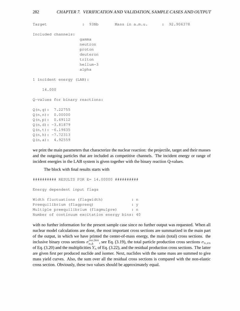
282 CHAPTER 7. VERIFICATION AND VALIDATION, SAMPLE CASES AND OUTPUT
Target : 93Nb Mass in a.m.u. : 92.906378
Included channels:gammaneutronprotondeuterontritonhelium-3alpha
1 incident energy (LAB):
14.000
Q-values for binary reactions:
Q(n,g): 7.22755Q(n,n): 0.00000Q(n,p): 0.69112Q(n,d): -3.81879Q(n,t): -6.19635Q(n,h): -7.72313Q(n,a): 4.92559
we print the main parameters that characterize the nuclear reaction: the projectile, target and their massesand the outgoing particles that are included as competitivechannels. The incident energy or range ofincident energies in the LAB system is given together with the binary reaction Q-values.
The block with final results starts with
########## RESULTS FOR E= 14.00000 ##########
Energy dependent input flags
Width fluctuations (flagwidth) : nPreequilibrium (flagpreeq) : yMultiple preequilibrium (flagmulpre) : nNumber of continuum excitation energy bins: 40
with no further information for the present sample case since no further output was requested. When allnuclear model calculations are done, the most important cross sections are summarized in the main partof the output, in which we have printed the center-of-mass energy, the main (total) cross sections. theinclusive binary cross sectionsσinc,bin
n,k , see Eq. (3.19), the total particle production cross sectionsσn,xn
of Eq. (3.20) and the multiplicitiesYn of Eq. (3.22), and the residual production cross sections. The latterare given first per produced nuclide and isomer. Next, nuclides with the same mass are summed to givemass yield curves. Also, the sum over all the residual cross sections is compared with the non-elasticcross section. Obviously, these two values should be approximately equal.
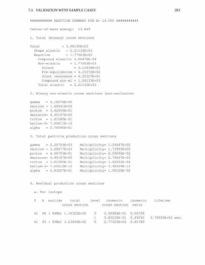
7.3. VALIDATION WITH SAMPLE CASES 283
########### REACTION SUMMARY FOR E= 14.000 ###########
Center-of-mass energy: 13.849
1. Total (binary) cross sections
Total = 3.98195E+03Shape elastic = 2.21132E+03Reaction = 1.77063E+03
Compound elastic= 6.00478E-04Non-elastic = 1.77063E+03
Direct = 3.13938E+01Pre-equilibrium = 4.15372E+02Giant resonance = 6.25327E+01Compound non-el = 1.26133E+03
Total elastic = 2.21132E+03
2. Binary non-elastic cross sections (non-exclusive)
gamma = 4.18076E+00neutron = 1.69541E+03proton = 3.82455E+01deuteron= 4.95187E+00triton = 1.81580E-01helium-3= 7.05611E-10alpha = 2.76590E+01
3. Total particle production cross sections
gamma = 2.20703E+03 Multiplicity= 1.24647E+00neutron = 3.08077E+03 Multiplicity= 1.73993E+00proton = 4.06703E+01 Multiplicity= 2.29694E-02deuteron= 4.95187E+00 Multiplicity= 2.79667E-03triton = 1.81580E-01 Multiplicity= 1.02551E-04helium-3= 7.05612E-10 Multiplicity= 3.98509E-13alpha = 2.83527E+01 Multiplicity= 1.60128E-02
4. Residual production cross sections
a. Per isotope
Z A nuclide total level isomeric isomeric lifetimecross section cross section ratio
41 94 ( 94Nb) 1.18322E+00 0 5.99984E-01 0.507081 5.83234E-01 0.49292 3.76000E+02 sec.
41 93 ( 93Nb) 3.23646E+02 0 2.77623E+02 0.85780
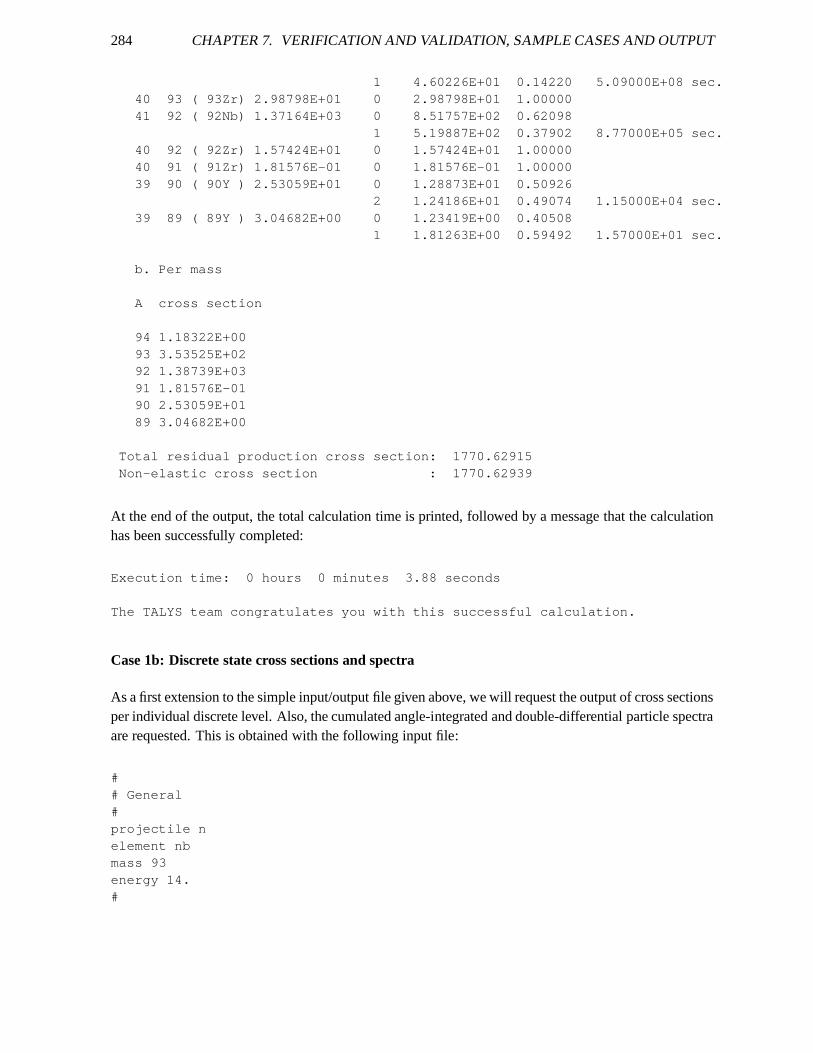
284 CHAPTER 7. VERIFICATION AND VALIDATION, SAMPLE CASES AND OUTPUT
1 4.60226E+01 0.14220 5.09000E+08 sec.40 93 ( 93Zr) 2.98798E+01 0 2.98798E+01 1.0000041 92 ( 92Nb) 1.37164E+03 0 8.51757E+02 0.62098
1 5.19887E+02 0.37902 8.77000E+05 sec.40 92 ( 92Zr) 1.57424E+01 0 1.57424E+01 1.0000040 91 ( 91Zr) 1.81576E-01 0 1.81576E-01 1.0000039 90 ( 90Y ) 2.53059E+01 0 1.28873E+01 0.50926
2 1.24186E+01 0.49074 1.15000E+04 sec.39 89 ( 89Y ) 3.04682E+00 0 1.23419E+00 0.40508
1 1.81263E+00 0.59492 1.57000E+01 sec.
b. Per mass
A cross section
94 1.18322E+0093 3.53525E+0292 1.38739E+0391 1.81576E-0190 2.53059E+0189 3.04682E+00
Total residual production cross section: 1770.62915Non-elastic cross section : 1770.62939
At the end of the output, the total calculation time is printed, followed by a message that the calculationhas been successfully completed:
Execution time: 0 hours 0 minutes 3.88 seconds
The TALYS team congratulates you with this successful calcu lation.
Case 1b: Discrete state cross sections and spectra
As a first extension to the simple input/output file given above, we will request the output of cross sectionsper individual discrete level. Also, the cumulated angle-integrated and double-differential particle spectraare requested. This is obtained with the following input file:
## General#projectile nelement nbmass 93energy 14.#
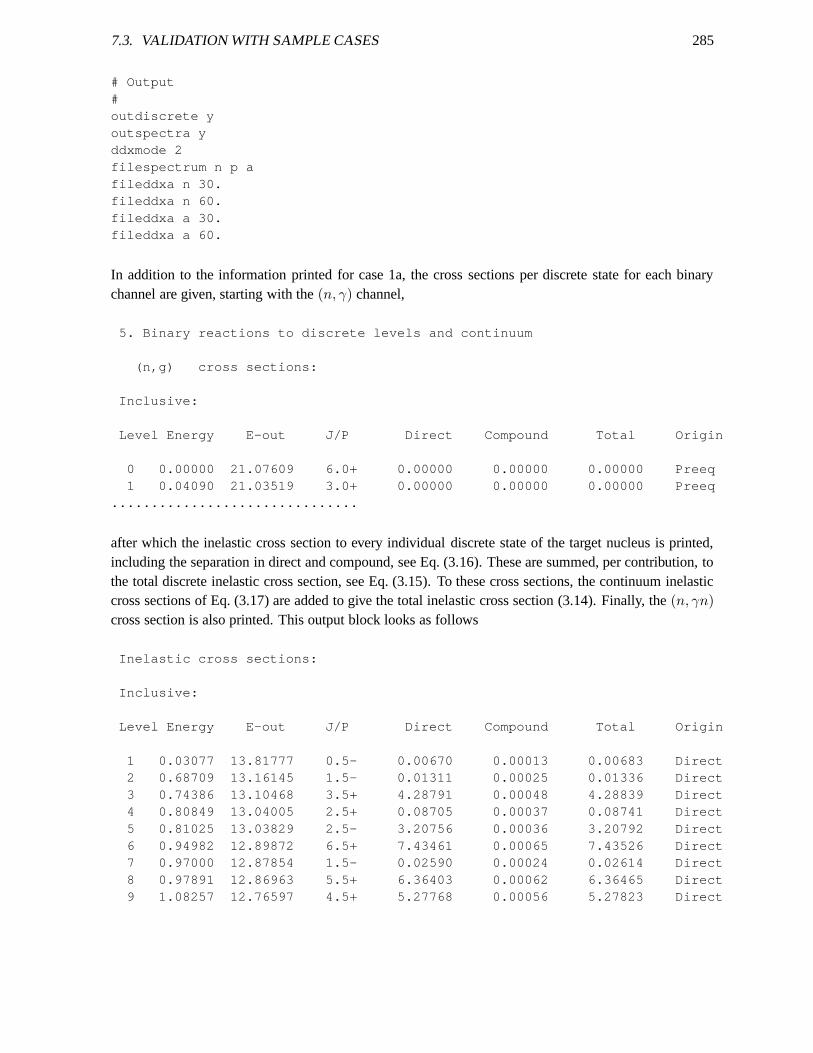
7.3. VALIDATION WITH SAMPLE CASES 285
# Output#outdiscrete youtspectra yddxmode 2filespectrum n p afileddxa n 30.fileddxa n 60.fileddxa a 30.fileddxa a 60.
In addition to the information printed for case 1a, the crosssections per discrete state for each binarychannel are given, starting with the(n, γ) channel,
5. Binary reactions to discrete levels and continuum
(n,g) cross sections:
Inclusive:
Level Energy E-out J/P Direct Compound Total Origin
0 0.00000 21.07609 6.0+ 0.00000 0.00000 0.00000 Preeq1 0.04090 21.03519 3.0+ 0.00000 0.00000 0.00000 Preeq
...............................
after which the inelastic cross section to every individualdiscrete state of the target nucleus is printed,including the separation in direct and compound, see Eq. (3.16). These are summed, per contribution, tothe total discrete inelastic cross section, see Eq. (3.15).To these cross sections, the continuum inelasticcross sections of Eq. (3.17) are added to give the total inelastic cross section (3.14). Finally, the(n, γn)
cross section is also printed. This output block looks as follows
Inelastic cross sections:
Inclusive:
Level Energy E-out J/P Direct Compound Total Origin
1 0.03077 13.81777 0.5- 0.00670 0.00013 0.00683 Direct2 0.68709 13.16145 1.5- 0.01311 0.00025 0.01336 Direct3 0.74386 13.10468 3.5+ 4.28791 0.00048 4.28839 Direct4 0.80849 13.04005 2.5+ 0.08705 0.00037 0.08741 Direct5 0.81025 13.03829 2.5- 3.20756 0.00036 3.20792 Direct6 0.94982 12.89872 6.5+ 7.43461 0.00065 7.43526 Direct7 0.97000 12.87854 1.5- 0.02590 0.00024 0.02614 Direct8 0.97891 12.86963 5.5+ 6.36403 0.00062 6.36465 Direct9 1.08257 12.76597 4.5+ 5.27768 0.00056 5.27823 Direct
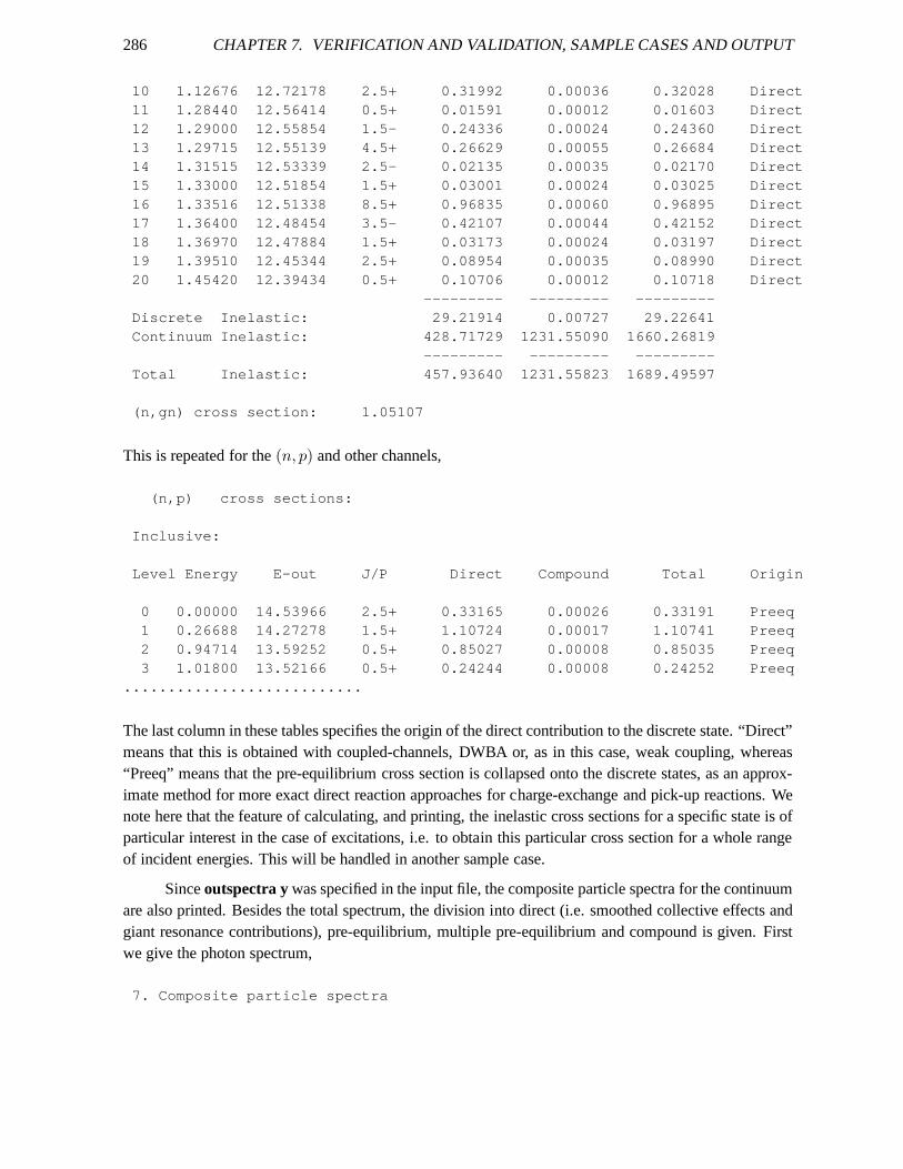
286 CHAPTER 7. VERIFICATION AND VALIDATION, SAMPLE CASES AND OUTPUT
10 1.12676 12.72178 2.5+ 0.31992 0.00036 0.32028 Direct11 1.28440 12.56414 0.5+ 0.01591 0.00012 0.01603 Direct12 1.29000 12.55854 1.5- 0.24336 0.00024 0.24360 Direct13 1.29715 12.55139 4.5+ 0.26629 0.00055 0.26684 Direct14 1.31515 12.53339 2.5- 0.02135 0.00035 0.02170 Direct15 1.33000 12.51854 1.5+ 0.03001 0.00024 0.03025 Direct16 1.33516 12.51338 8.5+ 0.96835 0.00060 0.96895 Direct17 1.36400 12.48454 3.5- 0.42107 0.00044 0.42152 Direct18 1.36970 12.47884 1.5+ 0.03173 0.00024 0.03197 Direct19 1.39510 12.45344 2.5+ 0.08954 0.00035 0.08990 Direct20 1.45420 12.39434 0.5+ 0.10706 0.00012 0.10718 Direct
--------- --------- ---------Discrete Inelastic: 29.21914 0.00727 29.22641Continuum Inelastic: 428.71729 1231.55090 1660.26819
--------- --------- ---------Total Inelastic: 457.93640 1231.55823 1689.49597
(n,gn) cross section: 1.05107
This is repeated for the(n, p) and other channels,
(n,p) cross sections:
Inclusive:
Level Energy E-out J/P Direct Compound Total Origin
0 0.00000 14.53966 2.5+ 0.33165 0.00026 0.33191 Preeq1 0.26688 14.27278 1.5+ 1.10724 0.00017 1.10741 Preeq2 0.94714 13.59252 0.5+ 0.85027 0.00008 0.85035 Preeq3 1.01800 13.52166 0.5+ 0.24244 0.00008 0.24252 Preeq
...........................
The last column in these tables specifies the origin of the direct contribution to the discrete state. “Direct”means that this is obtained with coupled-channels, DWBA or,as in this case, weak coupling, whereas“Preeq” means that the pre-equilibrium cross section is collapsed onto the discrete states, as an approx-imate method for more exact direct reaction approaches for charge-exchange and pick-up reactions. Wenote here that the feature of calculating, and printing, theinelastic cross sections for a specific state is ofparticular interest in the case of excitations, i.e. to obtain this particular cross section for a whole rangeof incident energies. This will be handled in another samplecase.
Sinceoutspectra ywas specified in the input file, the composite particle spectra for the continuumare also printed. Besides the total spectrum, the division into direct (i.e. smoothed collective effects andgiant resonance contributions), pre-equilibrium, multiple pre-equilibrium and compound is given. Firstwe give the photon spectrum,
7. Composite particle spectra
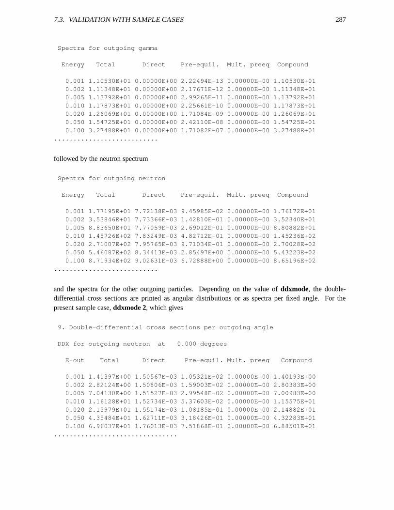
7.3. VALIDATION WITH SAMPLE CASES 287
Spectra for outgoing gamma
Energy Total Direct Pre-equil. Mult. preeq Compound
0.001 1.10530E+01 0.00000E+00 2.22494E-13 0.00000E+00 1. 10530E+010.002 1.11348E+01 0.00000E+00 2.17671E-12 0.00000E+00 1. 11348E+010.005 1.13792E+01 0.00000E+00 2.99265E-11 0.00000E+00 1. 13792E+010.010 1.17873E+01 0.00000E+00 2.25661E-10 0.00000E+00 1. 17873E+010.020 1.26069E+01 0.00000E+00 1.71084E-09 0.00000E+00 1. 26069E+010.050 1.54725E+01 0.00000E+00 2.42110E-08 0.00000E+00 1. 54725E+010.100 3.27488E+01 0.00000E+00 1.71082E-07 0.00000E+00 3. 27488E+01
...........................
followed by the neutron spectrum
Spectra for outgoing neutron
Energy Total Direct Pre-equil. Mult. preeq Compound
0.001 1.77195E+01 7.72138E-03 9.45985E-02 0.00000E+00 1. 76172E+010.002 3.53846E+01 7.73366E-03 1.42810E-01 0.00000E+00 3. 52340E+010.005 8.83650E+01 7.77059E-03 2.69012E-01 0.00000E+00 8. 80882E+010.010 1.45726E+02 7.83249E-03 4.82712E-01 0.00000E+00 1. 45236E+020.020 2.71007E+02 7.95765E-03 9.71034E-01 0.00000E+00 2. 70028E+020.050 5.46087E+02 8.34413E-03 2.85497E+00 0.00000E+00 5. 43223E+020.100 8.71934E+02 9.02631E-03 6.72888E+00 0.00000E+00 8. 65196E+02
...........................
and the spectra for the other outgoing particles. Dependingon the value ofddxmode, the double-differential cross sections are printed as angular distributions or as spectra per fixed angle. For thepresent sample case,ddxmode 2, which gives
9. Double-differential cross sections per outgoing angle
DDX for outgoing neutron at 0.000 degrees
E-out Total Direct Pre-equil. Mult. preeq Compound
0.001 1.41397E+00 1.50567E-03 1.05321E-02 0.00000E+00 1. 40193E+000.002 2.82124E+00 1.50806E-03 1.59003E-02 0.00000E+00 2. 80383E+000.005 7.04130E+00 1.51527E-03 2.99548E-02 0.00000E+00 7. 00983E+000.010 1.16128E+01 1.52734E-03 5.37603E-02 0.00000E+00 1. 15575E+010.020 2.15979E+01 1.55174E-03 1.08185E-01 0.00000E+00 2. 14882E+010.050 4.35484E+01 1.62711E-03 3.18426E-01 0.00000E+00 4. 32283E+010.100 6.96037E+01 1.76013E-03 7.51868E-01 0.00000E+00 6. 88501E+01
................................
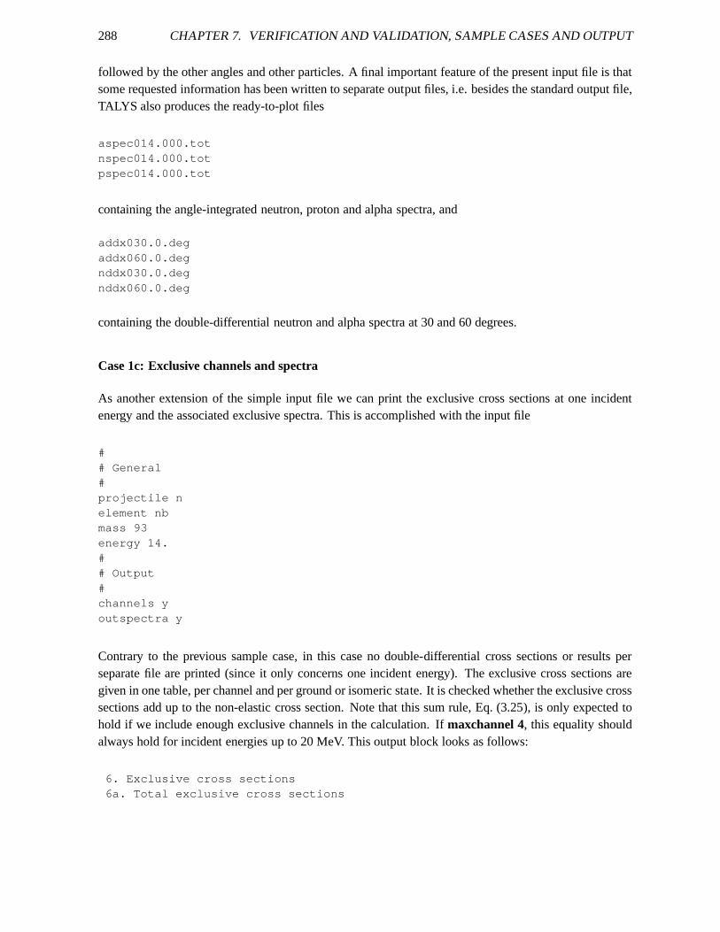
288 CHAPTER 7. VERIFICATION AND VALIDATION, SAMPLE CASES AND OUTPUT
followed by the other angles and other particles. A final important feature of the present input file is thatsome requested information has been written to separate output files, i.e. besides the standard output file,TALYS also produces the ready-to-plot files
aspec014.000.totnspec014.000.totpspec014.000.tot
containing the angle-integrated neutron, proton and alphaspectra, and
addx030.0.degaddx060.0.degnddx030.0.degnddx060.0.deg
containing the double-differential neutron and alpha spectra at 30 and 60 degrees.
Case 1c: Exclusive channels and spectra
As another extension of the simple input file we can print the exclusive cross sections at one incidentenergy and the associated exclusive spectra. This is accomplished with the input file
## General#projectile nelement nbmass 93energy 14.## Output#channels youtspectra y
Contrary to the previous sample case, in this case no double-differential cross sections or results perseparate file are printed (since it only concerns one incident energy). The exclusive cross sections aregiven in one table, per channel and per ground or isomeric state. It is checked whether the exclusive crosssections add up to the non-elastic cross section. Note that this sum rule, Eq. (3.25), is only expected tohold if we include enough exclusive channels in the calculation. If maxchannel 4, this equality shouldalways hold for incident energies up to 20 MeV. This output block looks as follows:
6. Exclusive cross sections6a. Total exclusive cross sections
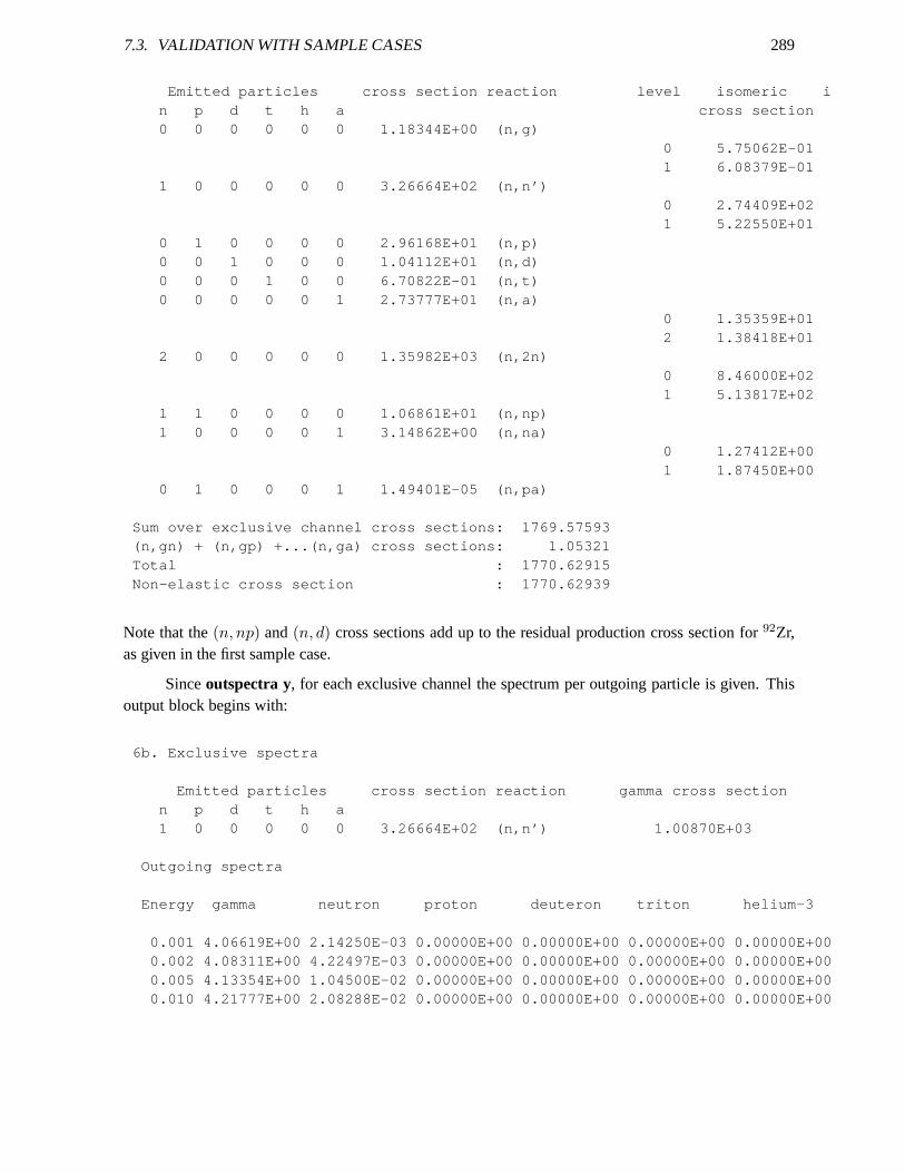
7.3. VALIDATION WITH SAMPLE CASES 289
Emitted particles cross section reaction level isomeric in p d t h a cross section0 0 0 0 0 0 1.18344E+00 (n,g)
0 5.75062E-011 6.08379E-01
1 0 0 0 0 0 3.26664E+02 (n,n’)0 2.74409E+021 5.22550E+01
0 1 0 0 0 0 2.96168E+01 (n,p)0 0 1 0 0 0 1.04112E+01 (n,d)0 0 0 1 0 0 6.70822E-01 (n,t)0 0 0 0 0 1 2.73777E+01 (n,a)
0 1.35359E+012 1.38418E+01
2 0 0 0 0 0 1.35982E+03 (n,2n)0 8.46000E+021 5.13817E+02
1 1 0 0 0 0 1.06861E+01 (n,np)1 0 0 0 0 1 3.14862E+00 (n,na)
0 1.27412E+001 1.87450E+00
0 1 0 0 0 1 1.49401E-05 (n,pa)
Sum over exclusive channel cross sections: 1769.57593(n,gn) + (n,gp) +...(n,ga) cross sections: 1.05321Total : 1770.62915Non-elastic cross section : 1770.62939
Note that the(n, np) and(n, d) cross sections add up to the residual production cross section for 92Zr,as given in the first sample case.
Sinceoutspectra y, for each exclusive channel the spectrum per outgoing particle is given. Thisoutput block begins with:
6b. Exclusive spectra
Emitted particles cross section reaction gamma cross secti onn p d t h a1 0 0 0 0 0 3.26664E+02 (n,n’) 1.00870E+03
Outgoing spectra
Energy gamma neutron proton deuteron triton helium-3
0.001 4.06619E+00 2.14250E-03 0.00000E+00 0.00000E+00 0. 00000E+00 0.00000E+000.002 4.08311E+00 4.22497E-03 0.00000E+00 0.00000E+00 0. 00000E+00 0.00000E+000.005 4.13354E+00 1.04500E-02 0.00000E+00 0.00000E+00 0. 00000E+00 0.00000E+000.010 4.21777E+00 2.08288E-02 0.00000E+00 0.00000E+00 0. 00000E+00 0.00000E+00
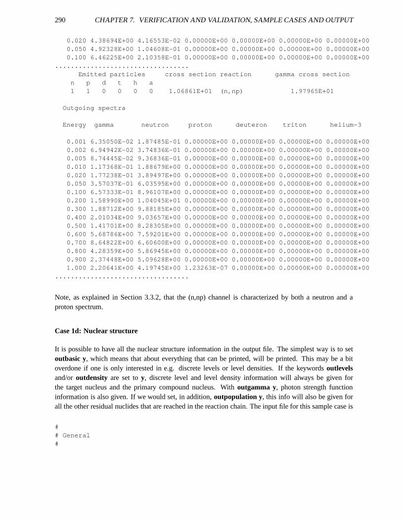
290 CHAPTER 7. VERIFICATION AND VALIDATION, SAMPLE CASES AND OUTPUT
0.020 4.38694E+00 4.16553E-02 0.00000E+00 0.00000E+00 0. 00000E+00 0.00000E+000.050 4.92328E+00 1.04608E-01 0.00000E+00 0.00000E+00 0. 00000E+00 0.00000E+000.100 6.46225E+00 2.10358E-01 0.00000E+00 0.00000E+00 0. 00000E+00 0.00000E+00
..................................Emitted particles cross section reaction gamma cross secti on
n p d t h a1 1 0 0 0 0 1.06861E+01 (n,np) 1.97965E+01
Outgoing spectra
Energy gamma neutron proton deuteron triton helium-3
0.001 6.35050E-02 1.87485E-01 0.00000E+00 0.00000E+00 0. 00000E+00 0.00000E+000.002 6.94942E-02 3.74836E-01 0.00000E+00 0.00000E+00 0. 00000E+00 0.00000E+000.005 8.74445E-02 9.36836E-01 0.00000E+00 0.00000E+00 0. 00000E+00 0.00000E+000.010 1.17368E-01 1.88679E+00 0.00000E+00 0.00000E+00 0. 00000E+00 0.00000E+000.020 1.77238E-01 3.89497E+00 0.00000E+00 0.00000E+00 0. 00000E+00 0.00000E+000.050 3.57037E-01 6.03595E+00 0.00000E+00 0.00000E+00 0. 00000E+00 0.00000E+000.100 6.57333E-01 8.96107E+00 0.00000E+00 0.00000E+00 0. 00000E+00 0.00000E+000.200 1.58990E+00 1.04045E+01 0.00000E+00 0.00000E+00 0. 00000E+00 0.00000E+000.300 1.88712E+00 9.88185E+00 0.00000E+00 0.00000E+00 0. 00000E+00 0.00000E+000.400 2.01034E+00 9.03657E+00 0.00000E+00 0.00000E+00 0. 00000E+00 0.00000E+000.500 1.41701E+00 8.28305E+00 0.00000E+00 0.00000E+00 0. 00000E+00 0.00000E+000.600 5.68786E+00 7.59201E+00 0.00000E+00 0.00000E+00 0. 00000E+00 0.00000E+000.700 8.64822E+00 6.60600E+00 0.00000E+00 0.00000E+00 0. 00000E+00 0.00000E+000.800 4.28359E+00 5.86945E+00 0.00000E+00 0.00000E+00 0. 00000E+00 0.00000E+000.900 2.37448E+00 5.09628E+00 0.00000E+00 0.00000E+00 0. 00000E+00 0.00000E+001.000 2.20641E+00 4.19745E+00 1.23263E-07 0.00000E+00 0. 00000E+00 0.00000E+00
..................................
Note, as explained in Section 3.3.2, that the (n,np) channelis characterized by both a neutron and aproton spectrum.
Case 1d: Nuclear structure
It is possible to have all the nuclear structure informationin the output file. The simplest way is to setoutbasic y, which means that about everything that can be printed, willbe printed. This may be a bitoverdone if one is only interested in e.g. discrete levels orlevel densities. If the keywordsoutlevelsand/oroutdensity are set toy, discrete level and level density information will always be given forthe target nucleus and the primary compound nucleus. Withoutgamma y, photon strength functioninformation is also given. If we would set, in addition,outpopulation y, this info will also be given forall the other residual nuclides that are reached in the reaction chain. The input file for this sample case is
## General#

7.3. VALIDATION WITH SAMPLE CASES 291
projectile nelement nbmass 93energy 14.## Output#outlevels youtdensity youtgamma y
In addition to the output of case 1a, the separation energiesfor the six light particles are printed.
NUCLEAR STRUCTURE INFORMATION FOR Z= 41 N= 52 ( 93Nb)Separation energies:Particle Sneutron 8.83126proton 6.04337deuteron 12.45360triton 13.39081helium-3 15.65202alpha 1.93144
In the next output block, the discrete level scheme is printed for the firstmaxlevelstar levels. The discretelevel info contains level number, energy, spin, parity, branching ratios and lifetimes of possible isomers.It is also indicated whether the spin (J) or parity (P) of a level is experimentally known or whether a valuewas assigned to it (see Section 5.4). The “string” of the original ENSDF database is also given, so thatthe user can learn about possible alternative choices for spin and parity. This output block begins with:
Discrete levels of Z= 41 N= 52 ( 93Nb)
Number Energy Spin Parity Branching Ratio (%) Lifetime(sec ) Assignment
0 0.0000 4.5 +1 0.0308 0.5 - 5.090E+08
---> 0 100.00002 0.6871 1.5 -
---> 1 100.00003 0.7439 3.5 +
---> 0 100.00004 0.8085 2.5 +
---> 3 2.1751---> 0 97.8249
....................................
Sinceoutdensity y, we print all the level density parameters that are involved, as discussed in Section4.7: the level density parameter at the neutron separation energya(Sn), the experimental and theoretical
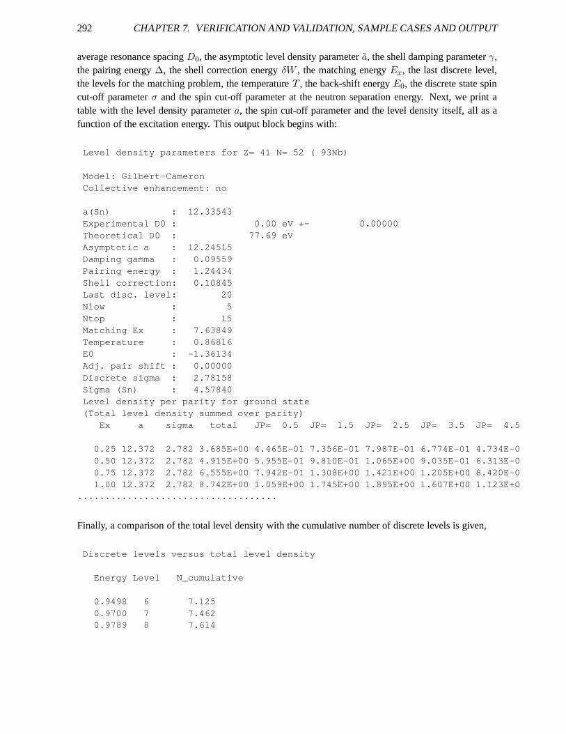
292 CHAPTER 7. VERIFICATION AND VALIDATION, SAMPLE CASES AND OUTPUT
average resonance spacingD0, the asymptotic level density parametera, the shell damping parameterγ,the pairing energy∆, the shell correction energyδW , the matching energyEx, the last discrete level,the levels for the matching problem, the temperatureT , the back-shift energyE0, the discrete state spincut-off parameterσ and the spin cut-off parameter at the neutron separation energy. Next, we print atable with the level density parametera, the spin cut-off parameter and the level density itself, all as afunction of the excitation energy. This output block beginswith:
Level density parameters for Z= 41 N= 52 ( 93Nb)
Model: Gilbert-CameronCollective enhancement: no
a(Sn) : 12.33543Experimental D0 : 0.00 eV +- 0.00000Theoretical D0 : 77.69 eVAsymptotic a : 12.24515Damping gamma : 0.09559Pairing energy : 1.24434Shell correction: 0.10845Last disc. level: 20Nlow : 5Ntop : 15Matching Ex : 7.63849Temperature : 0.86816E0 : -1.36134Adj. pair shift : 0.00000Discrete sigma : 2.78158Sigma (Sn) : 4.57840Level density per parity for ground state(Total level density summed over parity)
Ex a sigma total JP= 0.5 JP= 1.5 JP= 2.5 JP= 3.5 JP= 4.5
0.25 12.372 2.782 3.685E+00 4.465E-01 7.356E-01 7.987E-01 6.774E-01 4.734E-00.50 12.372 2.782 4.915E+00 5.955E-01 9.810E-01 1.065E+00 9.035E-01 6.313E-00.75 12.372 2.782 6.555E+00 7.942E-01 1.308E+00 1.421E+00 1.205E+00 8.420E-01.00 12.372 2.782 8.742E+00 1.059E+00 1.745E+00 1.895E+00 1.607E+00 1.123E+0
....................................
Finally, a comparison of the total level density with the cumulative number of discrete levels is given,
Discrete levels versus total level density
Energy Level N_cumulative
0.9498 6 7.1250.9700 7 7.4620.9789 8 7.614
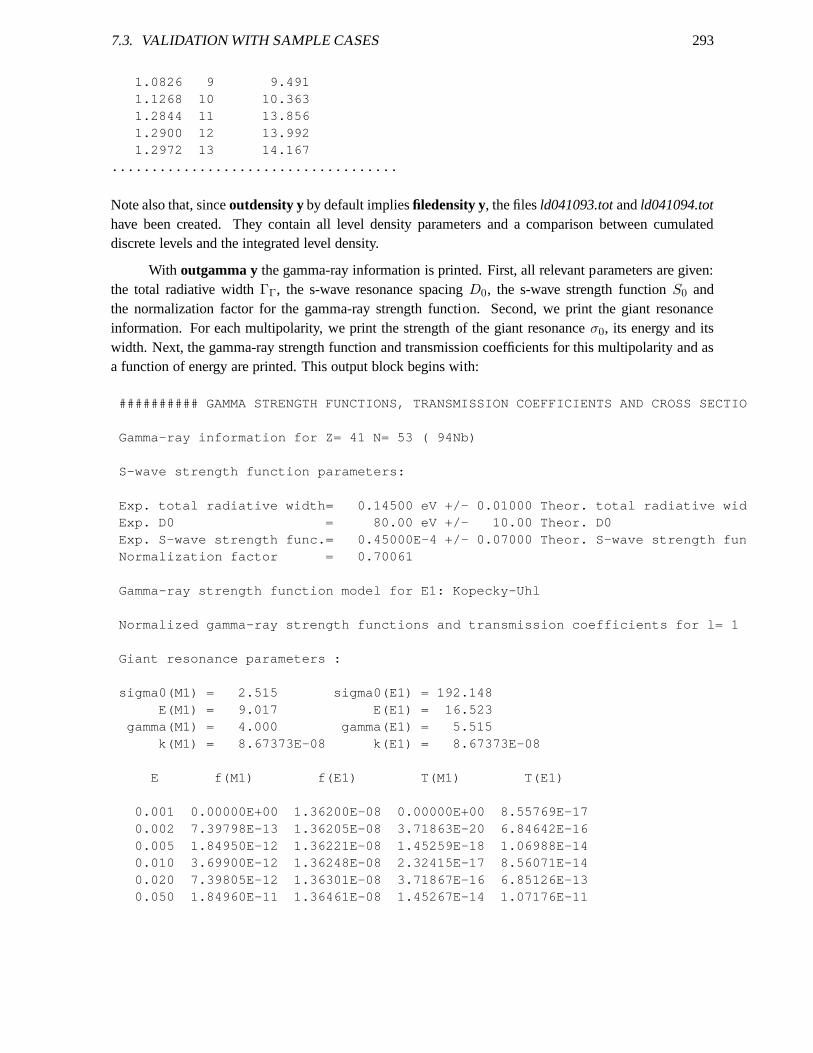
7.3. VALIDATION WITH SAMPLE CASES 293
1.0826 9 9.4911.1268 10 10.3631.2844 11 13.8561.2900 12 13.9921.2972 13 14.167
....................................
Note also that, sinceoutdensity yby default impliesfiledensity y, the filesld041093.totandld041094.tothave been created. They contain all level density parameters and a comparison between cumulateddiscrete levels and the integrated level density.
With outgamma y the gamma-ray information is printed. First, all relevant parameters are given:the total radiative widthΓΓ, the s-wave resonance spacingD0, the s-wave strength functionS0 andthe normalization factor for the gamma-ray strength function. Second, we print the giant resonanceinformation. For each multipolarity, we print the strengthof the giant resonanceσ0, its energy and itswidth. Next, the gamma-ray strength function and transmission coefficients for this multipolarity and asa function of energy are printed. This output block begins with:
########## GAMMA STRENGTH FUNCTIONS, TRANSMISSION COEFFICIENTS AND CROSS SECTIO
Gamma-ray information for Z= 41 N= 53 ( 94Nb)
S-wave strength function parameters:
Exp. total radiative width= 0.14500 eV +/- 0.01000 Theor. to tal radiative widExp. D0 = 80.00 eV +/- 10.00 Theor. D0Exp. S-wave strength func.= 0.45000E-4 +/- 0.07000 Theor. S -wave strength funNormalization factor = 0.70061
Gamma-ray strength function model for E1: Kopecky-Uhl
Normalized gamma-ray strength functions and transmission coefficients for l= 1
Giant resonance parameters :
sigma0(M1) = 2.515 sigma0(E1) = 192.148E(M1) = 9.017 E(E1) = 16.523
gamma(M1) = 4.000 gamma(E1) = 5.515k(M1) = 8.67373E-08 k(E1) = 8.67373E-08
E f(M1) f(E1) T(M1) T(E1)
0.001 0.00000E+00 1.36200E-08 0.00000E+00 8.55769E-170.002 7.39798E-13 1.36205E-08 3.71863E-20 6.84642E-160.005 1.84950E-12 1.36221E-08 1.45259E-18 1.06988E-140.010 3.69900E-12 1.36248E-08 2.32415E-17 8.56071E-140.020 7.39805E-12 1.36301E-08 3.71867E-16 6.85126E-130.050 1.84960E-11 1.36461E-08 1.45267E-14 1.07176E-11
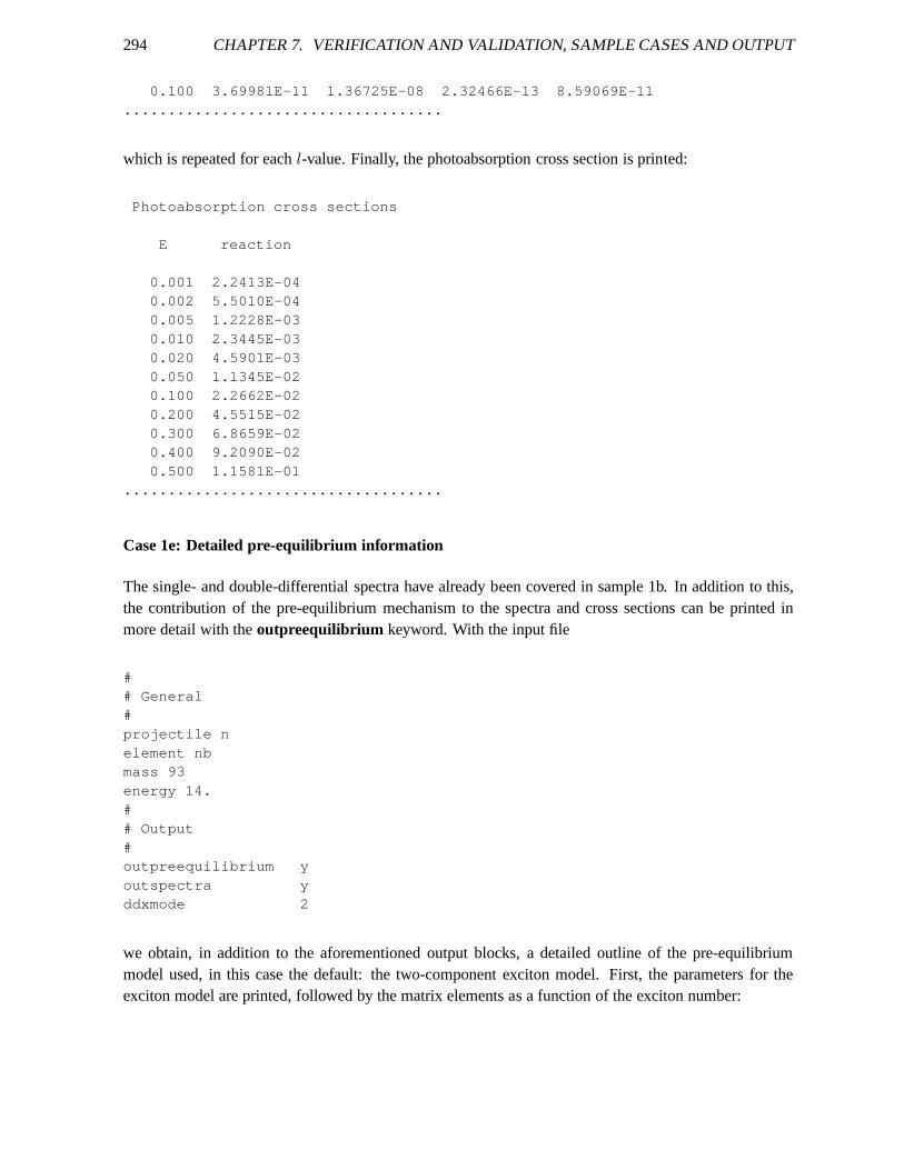
294 CHAPTER 7. VERIFICATION AND VALIDATION, SAMPLE CASES AND OUTPUT
0.100 3.69981E-11 1.36725E-08 2.32466E-13 8.59069E-11....................................
which is repeated for eachl-value. Finally, the photoabsorption cross section is printed:
Photoabsorption cross sections
E reaction
0.001 2.2413E-040.002 5.5010E-040.005 1.2228E-030.010 2.3445E-030.020 4.5901E-030.050 1.1345E-020.100 2.2662E-020.200 4.5515E-020.300 6.8659E-020.400 9.2090E-020.500 1.1581E-01
....................................
Case 1e: Detailed pre-equilibrium information
The single- and double-differential spectra have already been covered in sample 1b. In addition to this,the contribution of the pre-equilibrium mechanism to the spectra and cross sections can be printed inmore detail with theoutpreequilibrium keyword. With the input file
## General#projectile nelement nbmass 93energy 14.## Output#outpreequilibrium youtspectra yddxmode 2
we obtain, in addition to the aforementioned output blocks,a detailed outline of the pre-equilibriummodel used, in this case the default: the two-component exciton model. First, the parameters for theexciton model are printed, followed by the matrix elements as a function of the exciton number:
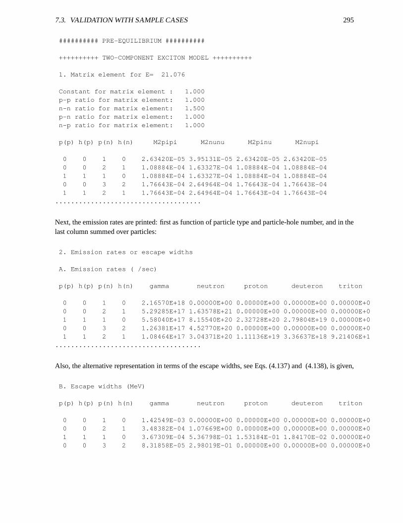
7.3. VALIDATION WITH SAMPLE CASES 295
########## PRE-EQUILIBRIUM ##########
++++++++++ TWO-COMPONENT EXCITON MODEL ++++++++++
1. Matrix element for E= 21.076
Constant for matrix element : 1.000p-p ratio for matrix element: 1.000n-n ratio for matrix element: 1.500p-n ratio for matrix element: 1.000n-p ratio for matrix element: 1.000
p(p) h(p) p(n) h(n) M2pipi M2nunu M2pinu M2nupi
0 0 1 0 2.63420E-05 3.95131E-05 2.63420E-05 2.63420E-050 0 2 1 1.08884E-04 1.63327E-04 1.08884E-04 1.08884E-041 1 1 0 1.08884E-04 1.63327E-04 1.08884E-04 1.08884E-040 0 3 2 1.76643E-04 2.64964E-04 1.76643E-04 1.76643E-041 1 2 1 1.76643E-04 2.64964E-04 1.76643E-04 1.76643E-04
.....................................
Next, the emission rates are printed: first as function of particle type and particle-hole number, and in thelast column summed over particles:
2. Emission rates or escape widths
A. Emission rates ( /sec)
p(p) h(p) p(n) h(n) gamma neutron proton deuteron triton
0 0 1 0 2.16570E+18 0.00000E+00 0.00000E+00 0.00000E+00 0.0 0000E+00 0 2 1 5.29285E+17 1.63578E+21 0.00000E+00 0.00000E+00 0.0 0000E+01 1 1 0 5.58040E+17 8.15540E+20 2.32728E+20 2.79804E+19 0.0 0000E+00 0 3 2 1.26381E+17 4.52770E+20 0.00000E+00 0.00000E+00 0.0 0000E+01 1 2 1 1.08464E+17 3.04371E+20 1.11136E+19 3.36637E+18 9.2 1406E+1
.....................................
Also, the alternative representation in terms of the escapewidths, see Eqs. (4.137) and (4.138), is given,
B. Escape widths (MeV)
p(p) h(p) p(n) h(n) gamma neutron proton deuteron triton
0 0 1 0 1.42549E-03 0.00000E+00 0.00000E+00 0.00000E+00 0.0 0000E+00 0 2 1 3.48382E-04 1.07669E+00 0.00000E+00 0.00000E+00 0.0 0000E+01 1 1 0 3.67309E-04 5.36798E-01 1.53184E-01 1.84170E-02 0.0 0000E+00 0 3 2 8.31858E-05 2.98019E-01 0.00000E+00 0.00000E+00 0.0 0000E+0
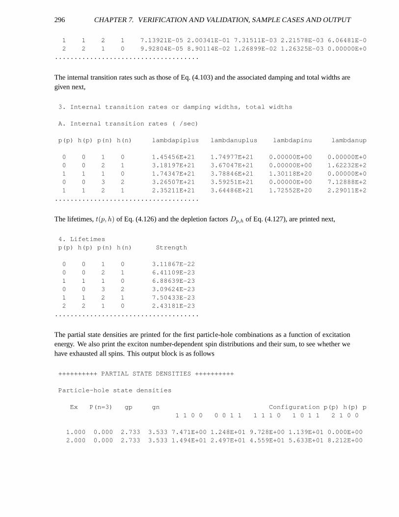
296 CHAPTER 7. VERIFICATION AND VALIDATION, SAMPLE CASES AND OUTPUT
1 1 2 1 7.13921E-05 2.00341E-01 7.31511E-03 2.21578E-03 6.0 6481E-02 2 1 0 9.92804E-05 8.90114E-02 1.26899E-02 1.26325E-03 0.0 0000E+0
.....................................
The internal transition rates such as those of Eq. (4.103) and the associated damping and total widths aregiven next,
3. Internal transition rates or damping widths, total width s
A. Internal transition rates ( /sec)
p(p) h(p) p(n) h(n) lambdapiplus lambdanuplus lambdapinu l ambdanup
0 0 1 0 1.45456E+21 1.74977E+21 0.00000E+00 0.00000E+00 0 2 1 3.18197E+21 3.67047E+21 0.00000E+00 1.62232E+21 1 1 0 1.74347E+21 3.78846E+21 1.30118E+20 0.00000E+00 0 3 2 3.26507E+21 3.59251E+21 0.00000E+00 7.12888E+21 1 2 1 2.35211E+21 3.64486E+21 1.72552E+20 2.29011E+2
.....................................
The lifetimes,t(p, h) of Eq. (4.126) and the depletion factorsDp,h of Eq. (4.127), are printed next,
4. Lifetimesp(p) h(p) p(n) h(n) Strength
0 0 1 0 3.11867E-220 0 2 1 6.41109E-231 1 1 0 6.88639E-230 0 3 2 3.09624E-231 1 2 1 7.50433E-232 2 1 0 2.43181E-23
.....................................
The partial state densities are printed for the first particle-hole combinations as a function of excitationenergy. We also print the exciton number-dependent spin distributions and their sum, to see whether wehave exhausted all spins. This output block is as follows
++++++++++ PARTIAL STATE DENSITIES ++++++++++
Particle-hole state densities
Ex P(n=3) gp gn Configuration p(p) h(p) p1 1 0 0 0 0 1 1 1 1 1 0 1 0 1 1 2 1 0 0
1.000 0.000 2.733 3.533 7.471E+00 1.248E+01 9.728E+00 1.13 9E+01 0.000E+002.000 0.000 2.733 3.533 1.494E+01 2.497E+01 4.559E+01 5.63 3E+01 8.212E+00
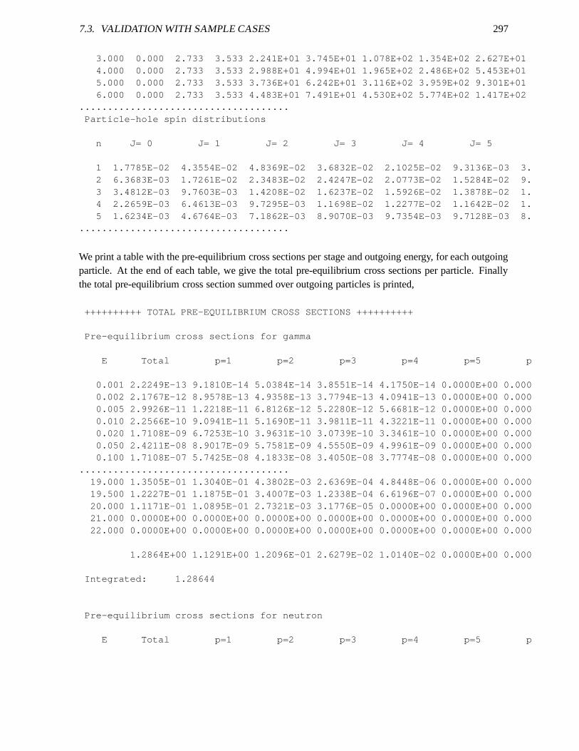
7.3. VALIDATION WITH SAMPLE CASES 297
3.000 0.000 2.733 3.533 2.241E+01 3.745E+01 1.078E+02 1.35 4E+02 2.627E+014.000 0.000 2.733 3.533 2.988E+01 4.994E+01 1.965E+02 2.48 6E+02 5.453E+015.000 0.000 2.733 3.533 3.736E+01 6.242E+01 3.116E+02 3.95 9E+02 9.301E+016.000 0.000 2.733 3.533 4.483E+01 7.491E+01 4.530E+02 5.77 4E+02 1.417E+02
.....................................Particle-hole spin distributions
n J= 0 J= 1 J= 2 J= 3 J= 4 J= 5
1 1.7785E-02 4.3554E-02 4.8369E-02 3.6832E-02 2.1025E-02 9.3136E-03 3.2 6.3683E-03 1.7261E-02 2.3483E-02 2.4247E-02 2.0773E-02 1.5284E-02 9.3 3.4812E-03 9.7603E-03 1.4208E-02 1.6237E-02 1.5926E-02 1.3878E-02 1.4 2.2659E-03 6.4613E-03 9.7295E-03 1.1698E-02 1.2277E-02 1.1642E-02 1.5 1.6234E-03 4.6764E-03 7.1862E-03 8.9070E-03 9.7354E-03 9.7128E-03 8.
.....................................
We print a table with the pre-equilibrium cross sections perstage and outgoing energy, for each outgoingparticle. At the end of each table, we give the total pre-equilibrium cross sections per particle. Finallythe total pre-equilibrium cross section summed over outgoing particles is printed,
++++++++++ TOTAL PRE-EQUILIBRIUM CROSS SECTIONS ++++++++++
Pre-equilibrium cross sections for gamma
E Total p=1 p=2 p=3 p=4 p=5 p
0.001 2.2249E-13 9.1810E-14 5.0384E-14 3.8551E-14 4.1750 E-14 0.0000E+00 0.0000.002 2.1767E-12 8.9578E-13 4.9358E-13 3.7794E-13 4.0941 E-13 0.0000E+00 0.0000.005 2.9926E-11 1.2218E-11 6.8126E-12 5.2280E-12 5.6681 E-12 0.0000E+00 0.0000.010 2.2566E-10 9.0941E-11 5.1690E-11 3.9811E-11 4.3221 E-11 0.0000E+00 0.0000.020 1.7108E-09 6.7253E-10 3.9631E-10 3.0739E-10 3.3461 E-10 0.0000E+00 0.0000.050 2.4211E-08 8.9017E-09 5.7581E-09 4.5550E-09 4.9961 E-09 0.0000E+00 0.0000.100 1.7108E-07 5.7425E-08 4.1833E-08 3.4050E-08 3.7774 E-08 0.0000E+00 0.000
.....................................19.000 1.3505E-01 1.3040E-01 4.3802E-03 2.6369E-04 4.844 8E-06 0.0000E+00 0.00019.500 1.2227E-01 1.1875E-01 3.4007E-03 1.2338E-04 6.619 6E-07 0.0000E+00 0.00020.000 1.1171E-01 1.0895E-01 2.7321E-03 3.1776E-05 0.000 0E+00 0.0000E+00 0.00021.000 0.0000E+00 0.0000E+00 0.0000E+00 0.0000E+00 0.000 0E+00 0.0000E+00 0.00022.000 0.0000E+00 0.0000E+00 0.0000E+00 0.0000E+00 0.000 0E+00 0.0000E+00 0.000
1.2864E+00 1.1291E+00 1.2096E-01 2.6279E-02 1.0140E-02 0 .0000E+00 0.000
Integrated: 1.28644
Pre-equilibrium cross sections for neutron
E Total p=1 p=2 p=3 p=4 p=5 p
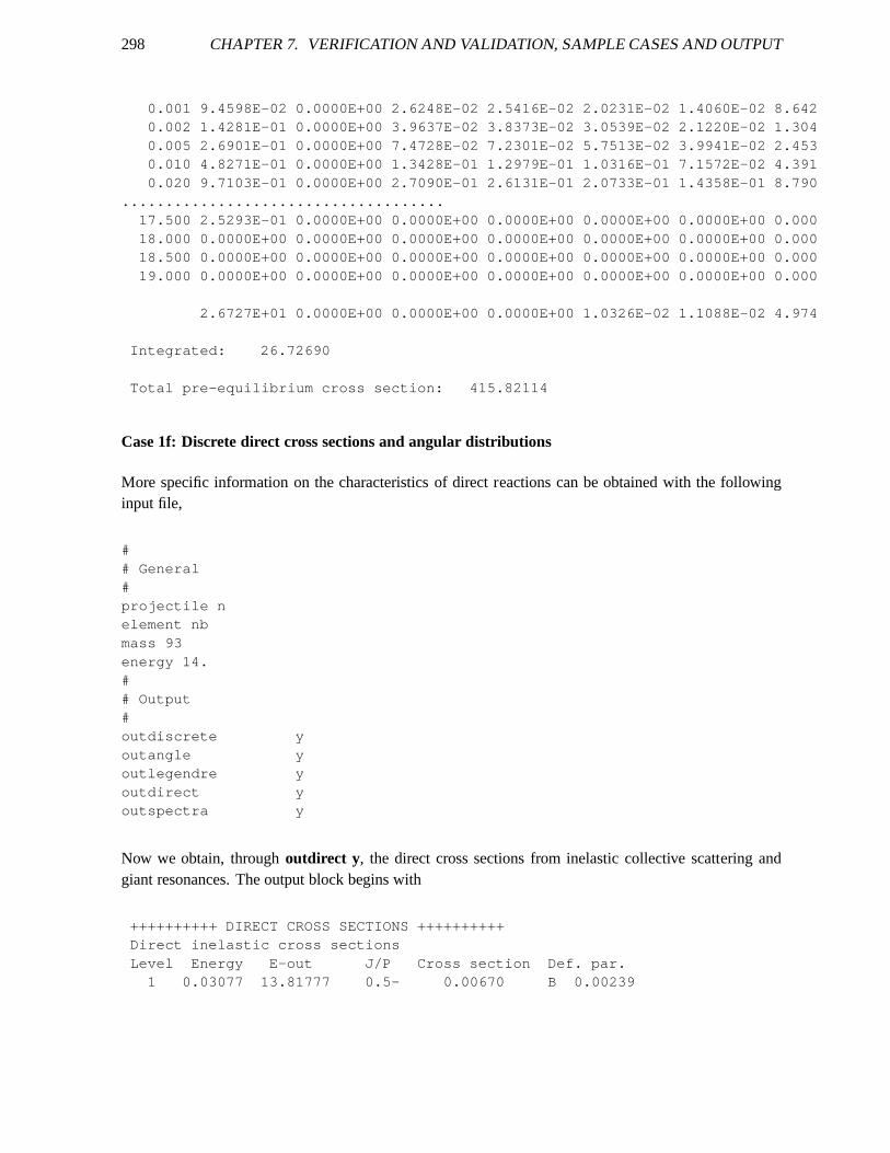
298 CHAPTER 7. VERIFICATION AND VALIDATION, SAMPLE CASES AND OUTPUT
0.001 9.4598E-02 0.0000E+00 2.6248E-02 2.5416E-02 2.0231 E-02 1.4060E-02 8.6420.002 1.4281E-01 0.0000E+00 3.9637E-02 3.8373E-02 3.0539 E-02 2.1220E-02 1.3040.005 2.6901E-01 0.0000E+00 7.4728E-02 7.2301E-02 5.7513 E-02 3.9941E-02 2.4530.010 4.8271E-01 0.0000E+00 1.3428E-01 1.2979E-01 1.0316 E-01 7.1572E-02 4.3910.020 9.7103E-01 0.0000E+00 2.7090E-01 2.6131E-01 2.0733 E-01 1.4358E-01 8.790
.....................................17.500 2.5293E-01 0.0000E+00 0.0000E+00 0.0000E+00 0.000 0E+00 0.0000E+00 0.00018.000 0.0000E+00 0.0000E+00 0.0000E+00 0.0000E+00 0.000 0E+00 0.0000E+00 0.00018.500 0.0000E+00 0.0000E+00 0.0000E+00 0.0000E+00 0.000 0E+00 0.0000E+00 0.00019.000 0.0000E+00 0.0000E+00 0.0000E+00 0.0000E+00 0.000 0E+00 0.0000E+00 0.000
2.6727E+01 0.0000E+00 0.0000E+00 0.0000E+00 1.0326E-02 1 .1088E-02 4.974
Integrated: 26.72690
Total pre-equilibrium cross section: 415.82114
Case 1f: Discrete direct cross sections and angular distributions
More specific information on the characteristics of direct reactions can be obtained with the followinginput file,
## General#projectile nelement nbmass 93energy 14.## Output#outdiscrete youtangle youtlegendre youtdirect youtspectra y
Now we obtain, throughoutdirect y, the direct cross sections from inelastic collective scattering andgiant resonances. The output block begins with
++++++++++ DIRECT CROSS SECTIONS ++++++++++Direct inelastic cross sectionsLevel Energy E-out J/P Cross section Def. par.
1 0.03077 13.81777 0.5- 0.00670 B 0.00239
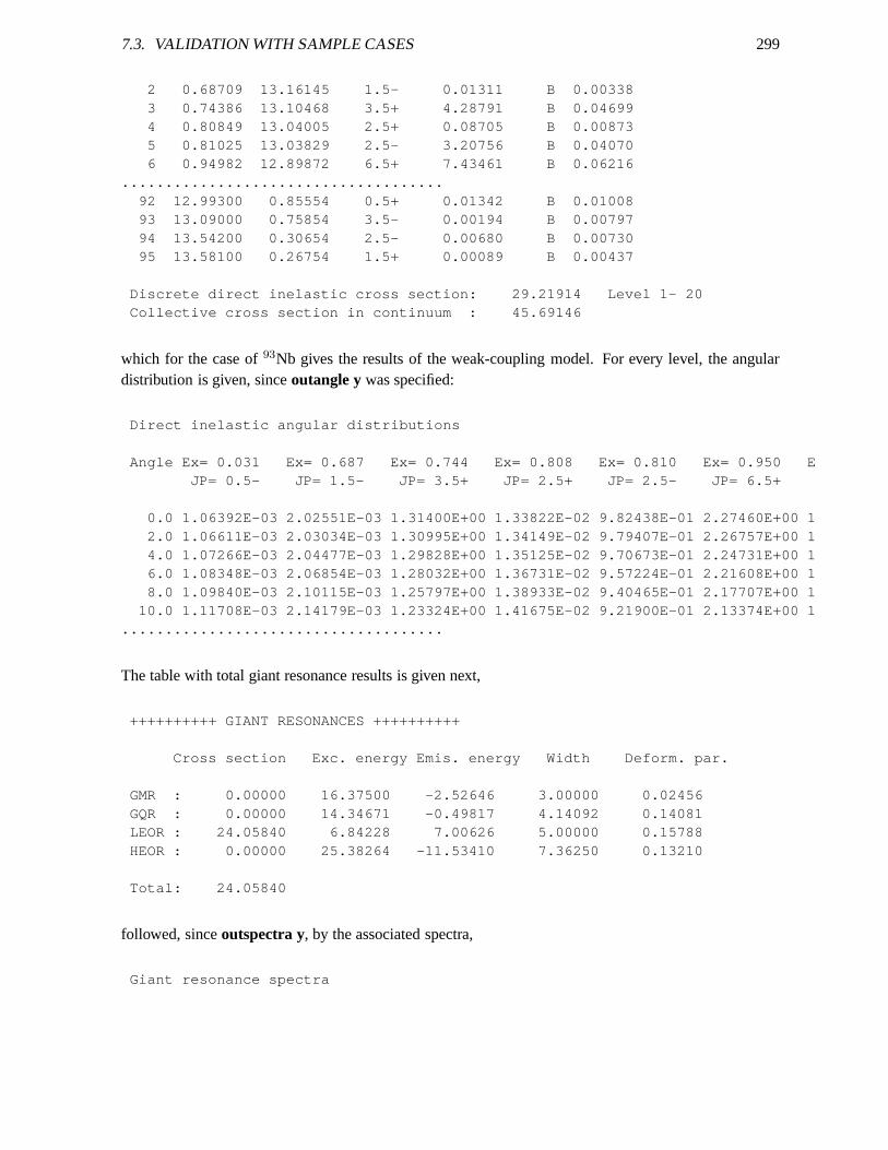
7.3. VALIDATION WITH SAMPLE CASES 299
2 0.68709 13.16145 1.5- 0.01311 B 0.003383 0.74386 13.10468 3.5+ 4.28791 B 0.046994 0.80849 13.04005 2.5+ 0.08705 B 0.008735 0.81025 13.03829 2.5- 3.20756 B 0.040706 0.94982 12.89872 6.5+ 7.43461 B 0.06216
.....................................92 12.99300 0.85554 0.5+ 0.01342 B 0.0100893 13.09000 0.75854 3.5- 0.00194 B 0.0079794 13.54200 0.30654 2.5- 0.00680 B 0.0073095 13.58100 0.26754 1.5+ 0.00089 B 0.00437
Discrete direct inelastic cross section: 29.21914 Level 1- 20Collective cross section in continuum : 45.69146
which for the case of93Nb gives the results of the weak-coupling model. For every level, the angulardistribution is given, sinceoutangle ywas specified:
Direct inelastic angular distributions
Angle Ex= 0.031 Ex= 0.687 Ex= 0.744 Ex= 0.808 Ex= 0.810 Ex= 0.9 50 EJP= 0.5- JP= 1.5- JP= 3.5+ JP= 2.5+ JP= 2.5- JP= 6.5+
0.0 1.06392E-03 2.02551E-03 1.31400E+00 1.33822E-02 9.82 438E-01 2.27460E+00 12.0 1.06611E-03 2.03034E-03 1.30995E+00 1.34149E-02 9.79 407E-01 2.26757E+00 14.0 1.07266E-03 2.04477E-03 1.29828E+00 1.35125E-02 9.70 673E-01 2.24731E+00 16.0 1.08348E-03 2.06854E-03 1.28032E+00 1.36731E-02 9.57 224E-01 2.21608E+00 18.0 1.09840E-03 2.10115E-03 1.25797E+00 1.38933E-02 9.40 465E-01 2.17707E+00 1
10.0 1.11708E-03 2.14179E-03 1.23324E+00 1.41675E-02 9.2 1900E-01 2.13374E+00 1.....................................
The table with total giant resonance results is given next,
++++++++++ GIANT RESONANCES ++++++++++
Cross section Exc. energy Emis. energy Width Deform. par.
GMR : 0.00000 16.37500 -2.52646 3.00000 0.02456GQR : 0.00000 14.34671 -0.49817 4.14092 0.14081LEOR : 24.05840 6.84228 7.00626 5.00000 0.15788HEOR : 0.00000 25.38264 -11.53410 7.36250 0.13210
Total: 24.05840
followed, sinceoutspectra y, by the associated spectra,
Giant resonance spectra
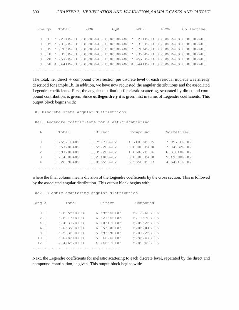
300 CHAPTER 7. VERIFICATION AND VALIDATION, SAMPLE CASES AND OUTPUT
Energy Total GMR GQR LEOR HEOR Collective
0.001 7.7214E-03 0.0000E+00 0.0000E+00 7.7214E-03 0.0000 E+00 0.0000E+000.002 7.7337E-03 0.0000E+00 0.0000E+00 7.7337E-03 0.0000 E+00 0.0000E+000.005 7.7706E-03 0.0000E+00 0.0000E+00 7.7706E-03 0.0000 E+00 0.0000E+000.010 7.8325E-03 0.0000E+00 0.0000E+00 7.8325E-03 0.0000 E+00 0.0000E+000.020 7.9577E-03 0.0000E+00 0.0000E+00 7.9577E-03 0.0000 E+00 0.0000E+000.050 8.3441E-03 0.0000E+00 0.0000E+00 8.3441E-03 0.0000 E+00 0.0000E+00
.....................................
The total, i.e. direct+ compound cross section per discrete level of each residual nucleus was alreadydescribed for sample 1b. In addition, we have now requested the angular distributions and the associatedLegendre coefficients. First, the angular distribution forelastic scattering, separated by direct and com-pound contribution, is given. Sinceoutlegendre yit is given first in terms of Legendre coefficients. Thisoutput block begins with:
8. Discrete state angular distributions
8a1. Legendre coefficients for elastic scattering
L Total Direct Compound Normalized
0 1.75971E+02 1.75971E+02 4.71035E-05 7.95776E-021 1.55728E+02 1.55728E+02 0.00000E+00 7.04232E-022 1.39720E+02 1.39720E+02 1.86062E-06 6.31840E-023 1.21488E+02 1.21488E+02 0.00000E+00 5.49390E-024 1.02659E+02 1.02659E+02 3.25580E-07 4.64241E-02
.....................................
where the final column means division of the Legendre coefficients by the cross section. This is followedby the associated angular distribution. This output block begins with:
8a2. Elastic scattering angular distribution
Angle Total Direct Compound
0.0 6.69554E+03 6.69554E+03 6.12260E-052.0 6.62134E+03 6.62134E+03 6.11570E-054.0 6.40317E+03 6.40317E+03 6.09526E-056.0 6.05390E+03 6.05390E+03 6.06204E-058.0 5.59369E+03 5.59369E+03 6.01725E-05
10.0 5.04824E+03 5.04824E+03 5.96247E-0512.0 4.44657E+03 4.44657E+03 5.89949E-05
.....................................
Next, the Legendre coefficients for inelastic scattering toeach discrete level, separated by the direct andcompound contribution, is given. This output block begins with:
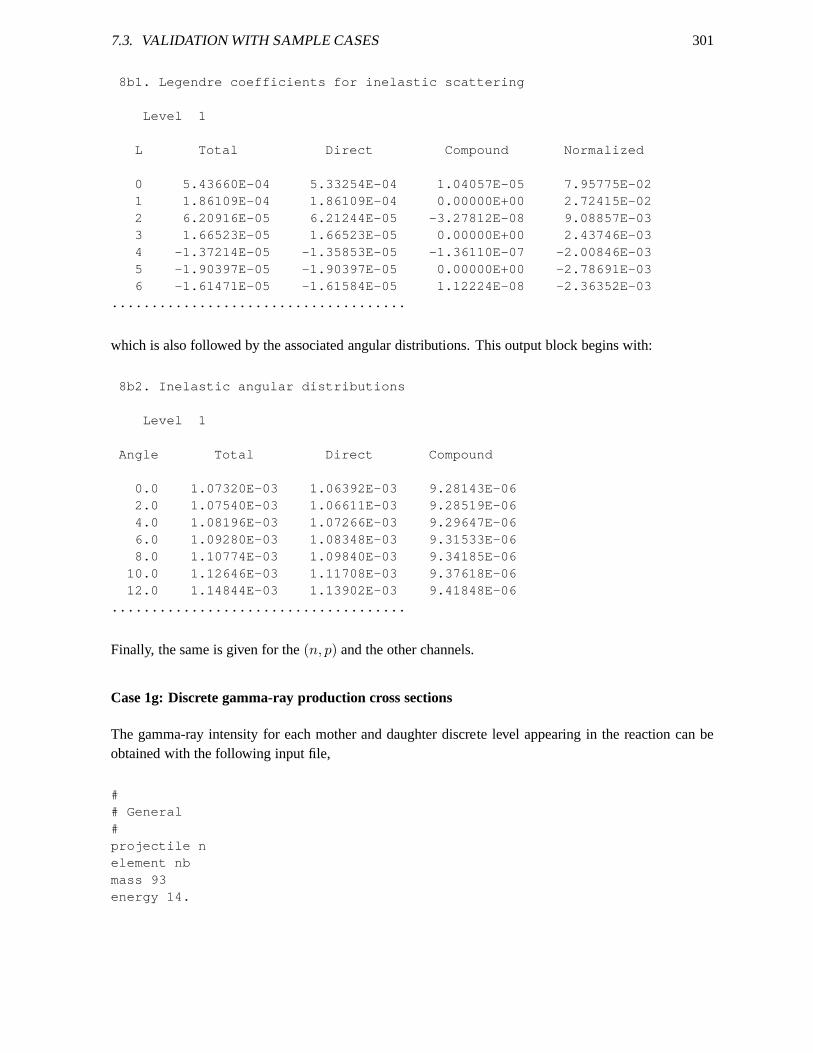
7.3. VALIDATION WITH SAMPLE CASES 301
8b1. Legendre coefficients for inelastic scattering
Level 1
L Total Direct Compound Normalized
0 5.43660E-04 5.33254E-04 1.04057E-05 7.95775E-021 1.86109E-04 1.86109E-04 0.00000E+00 2.72415E-022 6.20916E-05 6.21244E-05 -3.27812E-08 9.08857E-033 1.66523E-05 1.66523E-05 0.00000E+00 2.43746E-034 -1.37214E-05 -1.35853E-05 -1.36110E-07 -2.00846E-035 -1.90397E-05 -1.90397E-05 0.00000E+00 -2.78691E-036 -1.61471E-05 -1.61584E-05 1.12224E-08 -2.36352E-03
.....................................
which is also followed by the associated angular distributions. This output block begins with:
8b2. Inelastic angular distributions
Level 1
Angle Total Direct Compound
0.0 1.07320E-03 1.06392E-03 9.28143E-062.0 1.07540E-03 1.06611E-03 9.28519E-064.0 1.08196E-03 1.07266E-03 9.29647E-066.0 1.09280E-03 1.08348E-03 9.31533E-068.0 1.10774E-03 1.09840E-03 9.34185E-06
10.0 1.12646E-03 1.11708E-03 9.37618E-0612.0 1.14844E-03 1.13902E-03 9.41848E-06
.....................................
Finally, the same is given for the(n, p) and the other channels.
Case 1g: Discrete gamma-ray production cross sections
The gamma-ray intensity for each mother and daughter discrete level appearing in the reaction can beobtained with the following input file,
## General#projectile nelement nbmass 93energy 14.
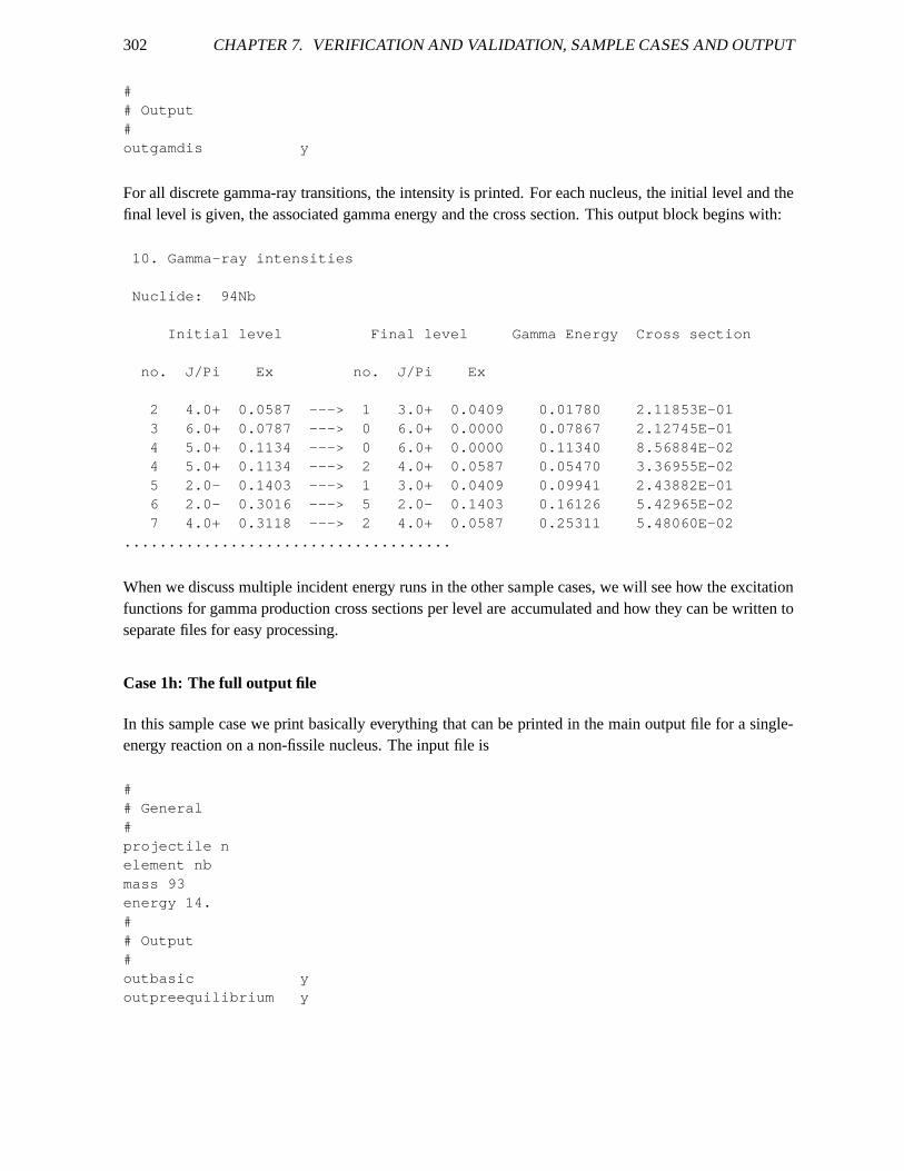
302 CHAPTER 7. VERIFICATION AND VALIDATION, SAMPLE CASES AND OUTPUT
## Output#outgamdis y
For all discrete gamma-ray transitions, the intensity is printed. For each nucleus, the initial level and thefinal level is given, the associated gamma energy and the cross section. This output block begins with:
10. Gamma-ray intensities
Nuclide: 94Nb
Initial level Final level Gamma Energy Cross section
no. J/Pi Ex no. J/Pi Ex
2 4.0+ 0.0587 ---> 1 3.0+ 0.0409 0.01780 2.11853E-013 6.0+ 0.0787 ---> 0 6.0+ 0.0000 0.07867 2.12745E-014 5.0+ 0.1134 ---> 0 6.0+ 0.0000 0.11340 8.56884E-024 5.0+ 0.1134 ---> 2 4.0+ 0.0587 0.05470 3.36955E-025 2.0- 0.1403 ---> 1 3.0+ 0.0409 0.09941 2.43882E-016 2.0- 0.3016 ---> 5 2.0- 0.1403 0.16126 5.42965E-027 4.0+ 0.3118 ---> 2 4.0+ 0.0587 0.25311 5.48060E-02
.....................................
When we discuss multiple incident energy runs in the other sample cases, we will see how the excitationfunctions for gamma production cross sections per level areaccumulated and how they can be written toseparate files for easy processing.
Case 1h: The full output file
In this sample case we print basically everything that can beprinted in the main output file for a single-energy reaction on a non-fissile nucleus. The input file is
## General#projectile nelement nbmass 93energy 14.## Output#outbasic youtpreequilibrium y
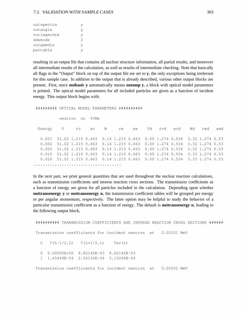
7.3. VALIDATION WITH SAMPLE CASES 303
outspectra youtangle youtlegendre yddxmode 2outgamdis ypartable y
resulting in an output file that contains all nuclear structure information, all partial results, and moreoverall intermediate results of the calculation, as well as results of intermediate checking. Note that basicallyall flags in the ”Output” block on top of the output file are set to y, the only exceptions being irrelevantfor this sample case. In addition to the output that is already described, various other output blocks arepresent. First, sinceoutbasic yautomatically meansoutomp y, a block with optical model parametersis printed. The optical model parameters for all included particles are given as a function of incidentenergy. This output block begins with:
######### OPTICAL MODEL PARAMETERS ##########
neutron on 93Nb
Energy V rv av W rw aw Vd rvd avd Wd rwd awd
0.001 51.02 1.215 0.663 0.14 1.215 0.663 0.00 1.274 0.534 3.3 2 1.274 0.530.002 51.02 1.215 0.663 0.14 1.215 0.663 0.00 1.274 0.534 3.3 2 1.274 0.530.005 51.02 1.215 0.663 0.14 1.215 0.663 0.00 1.274 0.534 3.3 2 1.274 0.530.010 51.02 1.215 0.663 0.14 1.215 0.663 0.00 1.274 0.534 3.3 3 1.274 0.530.020 51.02 1.215 0.663 0.14 1.215 0.663 0.00 1.274 0.534 3.3 3 1.274 0.53
.....................................
In the next part, we print general quantities that are used throughout the nuclear reaction calculations,such as transmission coefficients and inverse reaction cross sections. The transmission coefficients asa function of energy are given for all particles included in the calculation. Depending upon whetherouttransenergy yor outtransenergy n, the transmission coefficient tables will be grouped per energyor per angular momentum, respectively. The latter option may be helpful to study the behavior of aparticular transmission coefficient as a function of energy. The default isouttransenergy n, leading tothe following output block,
########## TRANSMISSION COEFFICIENTS AND INVERSE REACTION CROSS SECTIONS ######
Transmission coefficients for incident neutron at 0.00101 MeV
L T(L-1/2,L) T(L+1/2,L) Tav(L)
0 0.00000E+00 8.82145E-03 8.82145E-031 1.45449E-04 2.56136E-04 2.19240E-04
Transmission coefficients for incident neutron at 0.00202 MeV
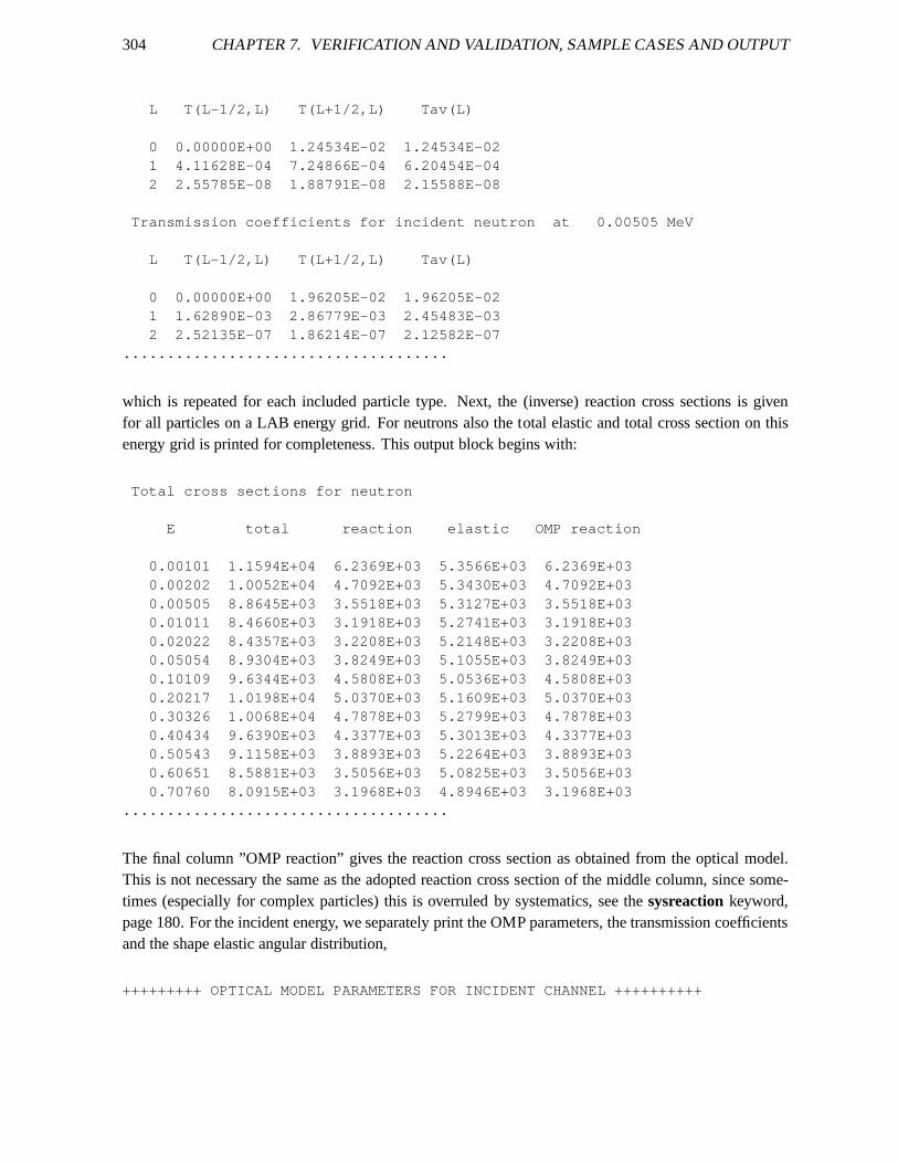
304 CHAPTER 7. VERIFICATION AND VALIDATION, SAMPLE CASES AND OUTPUT
L T(L-1/2,L) T(L+1/2,L) Tav(L)
0 0.00000E+00 1.24534E-02 1.24534E-021 4.11628E-04 7.24866E-04 6.20454E-042 2.55785E-08 1.88791E-08 2.15588E-08
Transmission coefficients for incident neutron at 0.00505 MeV
L T(L-1/2,L) T(L+1/2,L) Tav(L)
0 0.00000E+00 1.96205E-02 1.96205E-021 1.62890E-03 2.86779E-03 2.45483E-032 2.52135E-07 1.86214E-07 2.12582E-07
.....................................
which is repeated for each included particle type. Next, the(inverse) reaction cross sections is givenfor all particles on a LAB energy grid. For neutrons also the total elastic and total cross section on thisenergy grid is printed for completeness. This output block begins with:
Total cross sections for neutron
E total reaction elastic OMP reaction
0.00101 1.1594E+04 6.2369E+03 5.3566E+03 6.2369E+030.00202 1.0052E+04 4.7092E+03 5.3430E+03 4.7092E+030.00505 8.8645E+03 3.5518E+03 5.3127E+03 3.5518E+030.01011 8.4660E+03 3.1918E+03 5.2741E+03 3.1918E+030.02022 8.4357E+03 3.2208E+03 5.2148E+03 3.2208E+030.05054 8.9304E+03 3.8249E+03 5.1055E+03 3.8249E+030.10109 9.6344E+03 4.5808E+03 5.0536E+03 4.5808E+030.20217 1.0198E+04 5.0370E+03 5.1609E+03 5.0370E+030.30326 1.0068E+04 4.7878E+03 5.2799E+03 4.7878E+030.40434 9.6390E+03 4.3377E+03 5.3013E+03 4.3377E+030.50543 9.1158E+03 3.8893E+03 5.2264E+03 3.8893E+030.60651 8.5881E+03 3.5056E+03 5.0825E+03 3.5056E+030.70760 8.0915E+03 3.1968E+03 4.8946E+03 3.1968E+03
.....................................
The final column ”OMP reaction” gives the reaction cross section as obtained from the optical model.This is not necessary the same as the adopted reaction cross section of the middle column, since some-times (especially for complex particles) this is overruledby systematics, see thesysreactionkeyword,page 180. For the incident energy, we separately print the OMP parameters, the transmission coefficientsand the shape elastic angular distribution,
+++++++++ OPTICAL MODEL PARAMETERS FOR INCIDENT CHANNEL ++++++++++
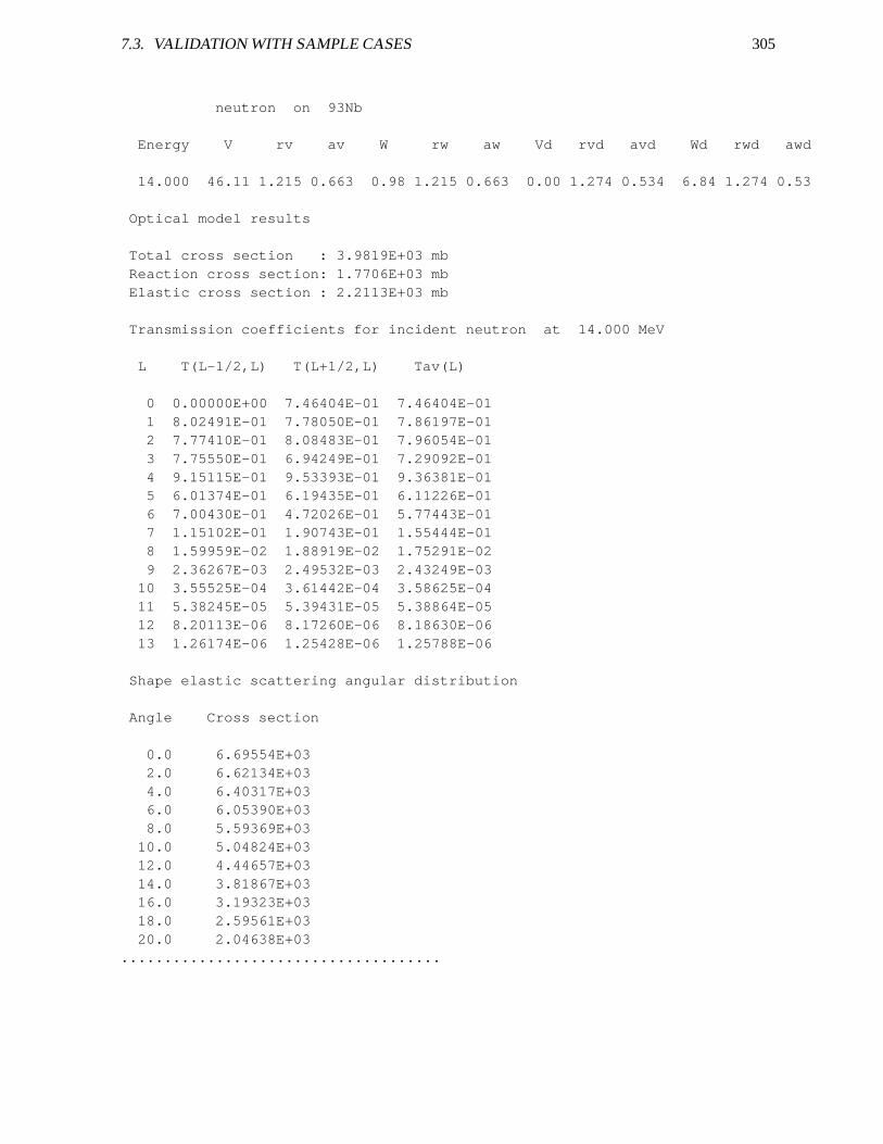
7.3. VALIDATION WITH SAMPLE CASES 305
neutron on 93Nb
Energy V rv av W rw aw Vd rvd avd Wd rwd awd
14.000 46.11 1.215 0.663 0.98 1.215 0.663 0.00 1.274 0.534 6. 84 1.274 0.53
Optical model results
Total cross section : 3.9819E+03 mbReaction cross section: 1.7706E+03 mbElastic cross section : 2.2113E+03 mb
Transmission coefficients for incident neutron at 14.000 M eV
L T(L-1/2,L) T(L+1/2,L) Tav(L)
0 0.00000E+00 7.46404E-01 7.46404E-011 8.02491E-01 7.78050E-01 7.86197E-012 7.77410E-01 8.08483E-01 7.96054E-013 7.75550E-01 6.94249E-01 7.29092E-014 9.15115E-01 9.53393E-01 9.36381E-015 6.01374E-01 6.19435E-01 6.11226E-016 7.00430E-01 4.72026E-01 5.77443E-017 1.15102E-01 1.90743E-01 1.55444E-018 1.59959E-02 1.88919E-02 1.75291E-029 2.36267E-03 2.49532E-03 2.43249E-03
10 3.55525E-04 3.61442E-04 3.58625E-0411 5.38245E-05 5.39431E-05 5.38864E-0512 8.20113E-06 8.17260E-06 8.18630E-0613 1.26174E-06 1.25428E-06 1.25788E-06
Shape elastic scattering angular distribution
Angle Cross section
0.0 6.69554E+032.0 6.62134E+034.0 6.40317E+036.0 6.05390E+038.0 5.59369E+03
10.0 5.04824E+0312.0 4.44657E+0314.0 3.81867E+0316.0 3.19323E+0318.0 2.59561E+0320.0 2.04638E+03
.....................................
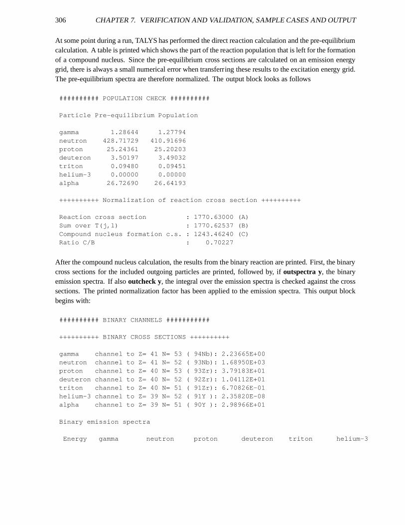
306 CHAPTER 7. VERIFICATION AND VALIDATION, SAMPLE CASES AND OUTPUT
At some point during a run, TALYS has performed the direct reaction calculation and the pre-equilibriumcalculation. A table is printed which shows the part of the reaction population that is left for the formationof a compound nucleus. Since the pre-equilibrium cross sections are calculated on an emission energygrid, there is always a small numerical error when transferring these results to the excitation energy grid.The pre-equilibrium spectra are therefore normalized. Theoutput block looks as follows
########## POPULATION CHECK ##########
Particle Pre-equilibrium Population
gamma 1.28644 1.27794neutron 428.71729 410.91696proton 25.24361 25.20203deuteron 3.50197 3.49032triton 0.09480 0.09451helium-3 0.00000 0.00000alpha 26.72690 26.64193
++++++++++ Normalization of reaction cross section ++++++ ++++
Reaction cross section : 1770.63000 (A)Sum over T(j,l) : 1770.62537 (B)Compound nucleus formation c.s. : 1243.46240 (C)Ratio C/B : 0.70227
After the compound nucleus calculation, the results from the binary reaction are printed. First, the binarycross sections for the included outgoing particles are printed, followed by, ifoutspectra y, the binaryemission spectra. If alsooutcheck y, the integral over the emission spectra is checked against the crosssections. The printed normalization factor has been applied to the emission spectra. This output blockbegins with:
########## BINARY CHANNELS ###########
++++++++++ BINARY CROSS SECTIONS ++++++++++
gamma channel to Z= 41 N= 53 ( 94Nb): 2.23665E+00neutron channel to Z= 41 N= 52 ( 93Nb): 1.68950E+03proton channel to Z= 40 N= 53 ( 93Zr): 3.79183E+01deuteron channel to Z= 40 N= 52 ( 92Zr): 1.04112E+01triton channel to Z= 40 N= 51 ( 91Zr): 6.70826E-01helium-3 channel to Z= 39 N= 52 ( 91Y ): 2.35820E-08alpha channel to Z= 39 N= 51 ( 90Y ): 2.98966E+01
Binary emission spectra
Energy gamma neutron proton deuteron triton helium-3
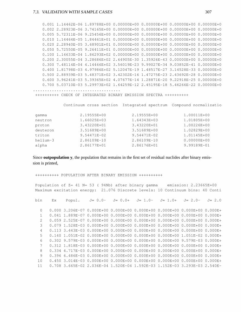
7.3. VALIDATION WITH SAMPLE CASES 307
0.001 1.14462E-06 1.89788E+00 0.00000E+00 0.00000E+00 0. 00000E+00 0.00000E+00.002 2.28923E-06 3.74165E+00 0.00000E+00 0.00000E+00 0. 00000E+00 0.00000E+00.005 5.72311E-06 9.25456E+00 0.00000E+00 0.00000E+00 0. 00000E+00 0.00000E+00.010 1.14464E-05 1.84461E+01 0.00000E+00 0.00000E+00 0. 00000E+00 0.00000E+00.020 2.28940E-05 3.68901E+01 0.00000E+00 0.00000E+00 0. 00000E+00 0.00000E+00.050 5.72550E-05 9.26411E+01 0.00000E+00 0.00000E+00 0. 00000E+00 0.00000E+00.100 1.14633E-04 1.86293E+02 0.00000E+00 0.00000E+00 0. 00000E+00 0.00000E+00.200 2.30055E-04 3.28686E+02 2.64905E-30 1.35926E-43 0. 00000E+00 0.00000E+00.300 7.48114E-04 4.14446E+02 3.56019E-23 9.99027E-34 9. 03852E-41 0.00000E+00.400 1.81798E-03 4.97986E+02 5.12047E-19 1.48517E-27 3. 14528E-33 0.00000E+00.500 2.88939E-03 5.48371E+02 3.42302E-16 1.47275E-23 2. 43692E-28 0.00000E+00.600 3.96241E-03 5.39365E+02 4.07677E-14 1.28871E-20 9. 22918E-25 0.00000E+00.700 5.03710E-03 5.29973E+02 1.64259E-12 2.45195E-18 5. 46266E-22 0.00000E+0
.....................................++++++++++ CHECK OF INTEGRATED BINARY EMISSION SPECTRA ++++++++++
Continuum cross section Integrated spectrum Compound norm alizatio
gamma 2.19555E+00 2.19555E+00 1.00011E+00neutron 1.66025E+03 1.64343E+03 1.01805E+00proton 3.43220E+01 3.43220E+01 1.00226E+00deuteron 3.51689E+00 3.51689E+00 1.02829E+00triton 9.54471E-02 9.54471E-02 1.01145E+00helium-3 2.86109E-10 2.86109E-10 0.00000E+00alpha 2.86177E+01 2.86176E+01 9.99189E-01
Sinceoutpopulation y, the population that remains in the first set of residual nuclides after binary emis-sion is printed,
++++++++++ POPULATION AFTER BINARY EMISSION ++++++++++
Population of Z= 41 N= 53 ( 94Nb) after binary gamma emission: 2.23665E+00Maximum excitation energy: 21.076 Discrete levels: 10 Cont inuum bins: 40 Conti
bin Ex Popul. J= 0.0- J= 0.0+ J= 1.0- J= 1.0+ J= 2.0- J= 2.0
0 0.000 3.206E-07 0.000E+00 0.000E+00 0.000E+00 0.000E+00 0.000E+00 0.000E+1 0.041 1.889E-07 0.000E+00 0.000E+00 0.000E+00 0.000E+00 0.000E+00 0.000E+2 0.059 2.525E-07 0.000E+00 0.000E+00 0.000E+00 0.000E+00 0.000E+00 0.000E+3 0.079 1.528E-03 0.000E+00 0.000E+00 0.000E+00 0.000E+00 0.000E+00 0.000E+4 0.113 3.443E-03 0.000E+00 0.000E+00 0.000E+00 0.000E+00 0.000E+00 0.000E+5 0.140 1.051E-02 0.000E+00 0.000E+00 0.000E+00 0.000E+00 1.051E-02 0.000E+6 0.302 9.579E-03 0.000E+00 0.000E+00 0.000E+00 0.000E+00 9.579E-03 0.000E+7 0.312 1.818E-03 0.000E+00 0.000E+00 0.000E+00 0.000E+00 0.000E+00 0.000E+8 0.334 4.717E-03 0.000E+00 0.000E+00 0.000E+00 0.000E+00 0.000E+00 0.000E+9 0.396 6.486E-03 0.000E+00 0.000E+00 0.000E+00 0.000E+00 0.000E+00 0.000E+
10 0.450 3.014E-03 0.000E+00 0.000E+00 0.000E+00 0.000E+0 0 0.000E+00 0.000E+11 0.708 3.665E-02 2.036E-04 1.520E-04 1.592E-03 1.152E-0 3 3.293E-03 2.540E-
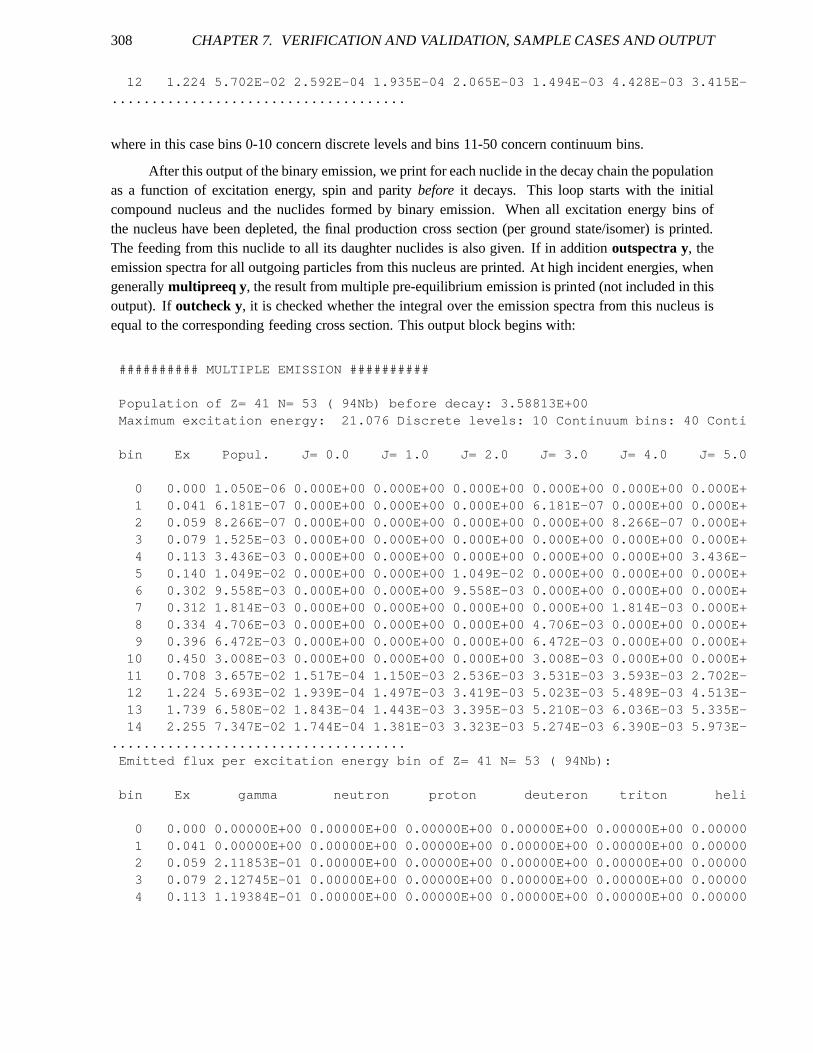
308 CHAPTER 7. VERIFICATION AND VALIDATION, SAMPLE CASES AND OUTPUT
12 1.224 5.702E-02 2.592E-04 1.935E-04 2.065E-03 1.494E-0 3 4.428E-03 3.415E-.....................................
where in this case bins 0-10 concern discrete levels and bins11-50 concern continuum bins.
After this output of the binary emission, we print for each nuclide in the decay chain the populationas a function of excitation energy, spin and paritybefore it decays. This loop starts with the initialcompound nucleus and the nuclides formed by binary emission. When all excitation energy bins ofthe nucleus have been depleted, the final production cross section (per ground state/isomer) is printed.The feeding from this nuclide to all its daughter nuclides isalso given. If in additionoutspectra y, theemission spectra for all outgoing particles from this nucleus are printed. At high incident energies, whengenerallymultipreeq y, the result from multiple pre-equilibrium emission is printed (not included in thisoutput). Ifoutcheck y, it is checked whether the integral over the emission spectra from this nucleus isequal to the corresponding feeding cross section. This output block begins with:
########## MULTIPLE EMISSION ##########
Population of Z= 41 N= 53 ( 94Nb) before decay: 3.58813E+00Maximum excitation energy: 21.076 Discrete levels: 10 Cont inuum bins: 40 Conti
bin Ex Popul. J= 0.0 J= 1.0 J= 2.0 J= 3.0 J= 4.0 J= 5.0
0 0.000 1.050E-06 0.000E+00 0.000E+00 0.000E+00 0.000E+00 0.000E+00 0.000E+1 0.041 6.181E-07 0.000E+00 0.000E+00 0.000E+00 6.181E-07 0.000E+00 0.000E+2 0.059 8.266E-07 0.000E+00 0.000E+00 0.000E+00 0.000E+00 8.266E-07 0.000E+3 0.079 1.525E-03 0.000E+00 0.000E+00 0.000E+00 0.000E+00 0.000E+00 0.000E+4 0.113 3.436E-03 0.000E+00 0.000E+00 0.000E+00 0.000E+00 0.000E+00 3.436E-5 0.140 1.049E-02 0.000E+00 0.000E+00 1.049E-02 0.000E+00 0.000E+00 0.000E+6 0.302 9.558E-03 0.000E+00 0.000E+00 9.558E-03 0.000E+00 0.000E+00 0.000E+7 0.312 1.814E-03 0.000E+00 0.000E+00 0.000E+00 0.000E+00 1.814E-03 0.000E+8 0.334 4.706E-03 0.000E+00 0.000E+00 0.000E+00 4.706E-03 0.000E+00 0.000E+9 0.396 6.472E-03 0.000E+00 0.000E+00 0.000E+00 6.472E-03 0.000E+00 0.000E+
10 0.450 3.008E-03 0.000E+00 0.000E+00 0.000E+00 3.008E-0 3 0.000E+00 0.000E+11 0.708 3.657E-02 1.517E-04 1.150E-03 2.536E-03 3.531E-0 3 3.593E-03 2.702E-12 1.224 5.693E-02 1.939E-04 1.497E-03 3.419E-03 5.023E-0 3 5.489E-03 4.513E-13 1.739 6.580E-02 1.843E-04 1.443E-03 3.395E-03 5.210E-0 3 6.036E-03 5.335E-14 2.255 7.347E-02 1.744E-04 1.381E-03 3.323E-03 5.274E-0 3 6.390E-03 5.973E-
.....................................Emitted flux per excitation energy bin of Z= 41 N= 53 ( 94Nb):
bin Ex gamma neutron proton deuteron triton heli
0 0.000 0.00000E+00 0.00000E+00 0.00000E+00 0.00000E+00 0 .00000E+00 0.000001 0.041 0.00000E+00 0.00000E+00 0.00000E+00 0.00000E+00 0 .00000E+00 0.000002 0.059 2.11853E-01 0.00000E+00 0.00000E+00 0.00000E+00 0 .00000E+00 0.000003 0.079 2.12745E-01 0.00000E+00 0.00000E+00 0.00000E+00 0 .00000E+00 0.000004 0.113 1.19384E-01 0.00000E+00 0.00000E+00 0.00000E+00 0 .00000E+00 0.00000
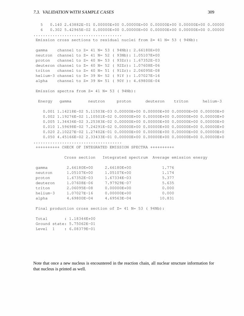
7.3. VALIDATION WITH SAMPLE CASES 309
5 0.140 2.43882E-01 0.00000E+00 0.00000E+00 0.00000E+00 0 .00000E+00 0.000006 0.302 5.42965E-02 0.00000E+00 0.00000E+00 0.00000E+00 0 .00000E+00 0.00000
.....................................Emission cross sections to residual nuclei from Z= 41 N= 53 ( 9 4Nb):
gamma channel to Z= 41 N= 53 ( 94Nb): 2.66180E+00neutron channel to Z= 41 N= 52 ( 93Nb): 1.05107E+00proton channel to Z= 40 N= 53 ( 93Zr): 1.67352E-03deuteron channel to Z= 40 N= 52 ( 92Zr): 1.07608E-06triton channel to Z= 40 N= 51 ( 91Zr): 2.06095E-08helium-3 channel to Z= 39 N= 52 ( 91Y ): 1.07027E-16alpha channel to Z= 39 N= 51 ( 90Y ): 4.69800E-04
Emission spectra from Z= 41 N= 53 ( 94Nb):
Energy gamma neutron proton deuteron triton helium-3
0.001 1.14218E-02 5.11503E-03 0.00000E+00 0.00000E+00 0. 00000E+00 0.00000E+00.002 1.19276E-02 1.10501E-02 0.00000E+00 0.00000E+00 0. 00000E+00 0.00000E+00.005 1.34434E-02 3.25383E-02 0.00000E+00 0.00000E+00 0. 00000E+00 0.00000E+00.010 1.59698E-02 7.24291E-02 0.00000E+00 0.00000E+00 0. 00000E+00 0.00000E+00.020 2.10227E-02 1.27402E-01 0.00000E+00 0.00000E+00 0. 00000E+00 0.00000E+00.050 4.45166E-02 2.33433E-01 0.00000E+00 0.00000E+00 0. 00000E+00 0.00000E+0
.....................................++++++++++ CHECK OF INTEGRATED EMISSION SPECTRA ++++++++++
Cross section Integrated spectrum Average emission energy
gamma 2.66180E+00 2.66180E+00 1.776neutron 1.05107E+00 1.05107E+00 1.174proton 1.67352E-03 1.67334E-03 5.377deuteron 1.07608E-06 7.97929E-07 5.635triton 2.06095E-08 0.00000E+00 0.000helium-3 1.07027E-16 0.00000E+00 0.000alpha 4.69800E-04 4.69563E-04 10.831
Final production cross section of Z= 41 N= 53 ( 94Nb):
Total : 1.18344E+00Ground state: 5.75062E-01Level 1 : 6.08379E-01
Note that once a new nucleus is encountered in the reaction chain, all nuclear structure information forthat nucleus is printed as well.
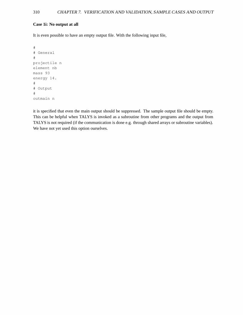
310 CHAPTER 7. VERIFICATION AND VALIDATION, SAMPLE CASES AND OUTPUT
Case 1i: No output at all
It is even possible to have an empty output file. With the following input file,
## General#projectile nelement nbmass 93energy 14.## Output#outmain n
it is specified that even the main output should be suppressed. The sample output file should be empty.This can be helpful when TALYS is invoked as a subroutine fromother programs and the output fromTALYS is not required (if the communication is done e.g. through shared arrays or subroutine variables).We have not yet used this option ourselves.
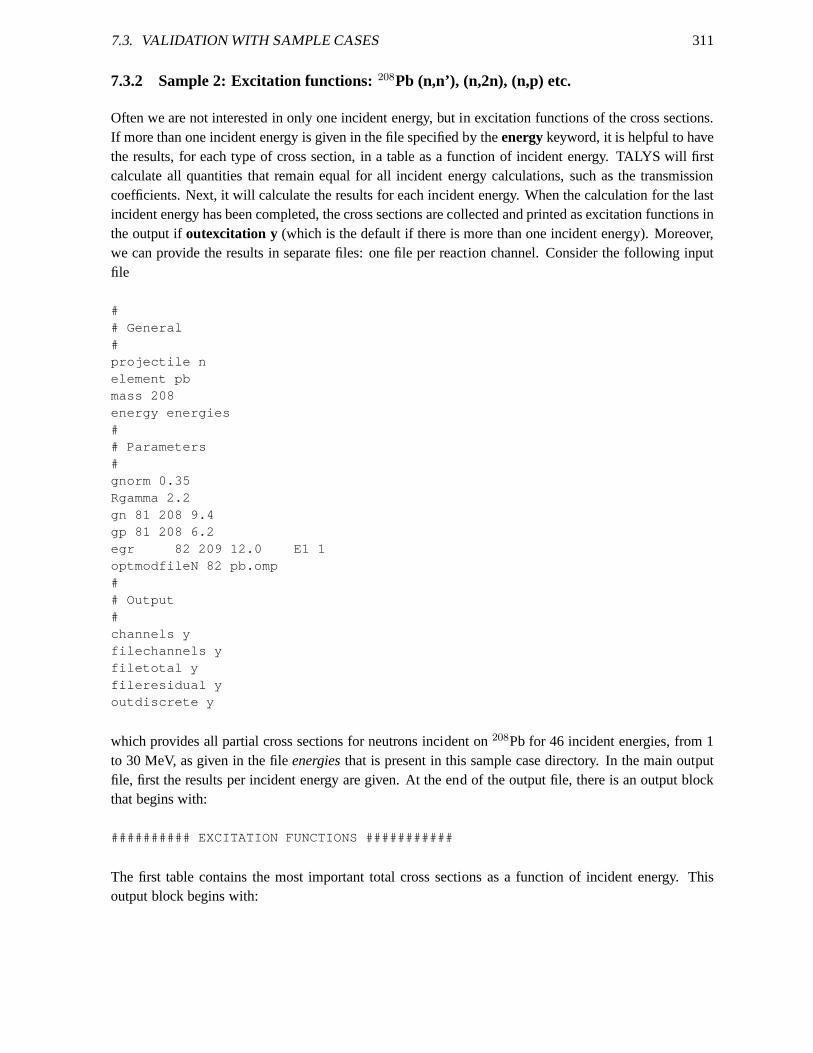
7.3. VALIDATION WITH SAMPLE CASES 311
7.3.2 Sample 2: Excitation functions:208Pb (n,n’), (n,2n), (n,p) etc.
Often we are not interested in only one incident energy, but in excitation functions of the cross sections.If more than one incident energy is given in the file specified by theenergykeyword, it is helpful to havethe results, for each type of cross section, in a table as a function of incident energy. TALYS will firstcalculate all quantities that remain equal for all incidentenergy calculations, such as the transmissioncoefficients. Next, it will calculate the results for each incident energy. When the calculation for the lastincident energy has been completed, the cross sections are collected and printed as excitation functions inthe output ifoutexcitation y (which is the default if there is more than one incident energy). Moreover,we can provide the results in separate files: one file per reaction channel. Consider the following inputfile
## General#projectile nelement pbmass 208energy energies## Parameters#gnorm 0.35Rgamma 2.2gn 81 208 9.4gp 81 208 6.2egr 82 209 12.0 E1 1optmodfileN 82 pb.omp## Output#channels yfilechannels yfiletotal yfileresidual youtdiscrete y
which provides all partial cross sections for neutrons incident on208Pb for 46 incident energies, from 1to 30 MeV, as given in the fileenergiesthat is present in this sample case directory. In the main outputfile, first the results per incident energy are given. At the end of the output file, there is an output blockthat begins with:
########## EXCITATION FUNCTIONS ###########
The first table contains the most important total cross sections as a function of incident energy. Thisoutput block begins with:
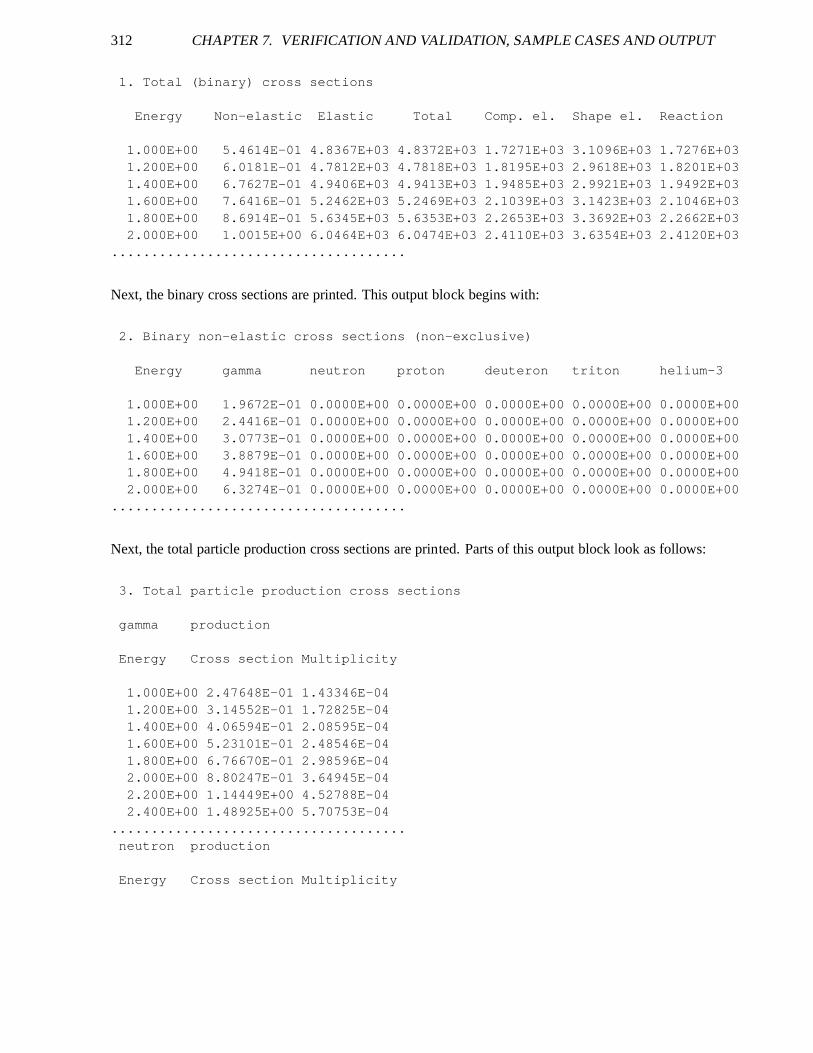
312 CHAPTER 7. VERIFICATION AND VALIDATION, SAMPLE CASES AND OUTPUT
1. Total (binary) cross sections
Energy Non-elastic Elastic Total Comp. el. Shape el. Reacti on
1.000E+00 5.4614E-01 4.8367E+03 4.8372E+03 1.7271E+03 3. 1096E+03 1.7276E+031.200E+00 6.0181E-01 4.7812E+03 4.7818E+03 1.8195E+03 2. 9618E+03 1.8201E+031.400E+00 6.7627E-01 4.9406E+03 4.9413E+03 1.9485E+03 2. 9921E+03 1.9492E+031.600E+00 7.6416E-01 5.2462E+03 5.2469E+03 2.1039E+03 3. 1423E+03 2.1046E+031.800E+00 8.6914E-01 5.6345E+03 5.6353E+03 2.2653E+03 3. 3692E+03 2.2662E+032.000E+00 1.0015E+00 6.0464E+03 6.0474E+03 2.4110E+03 3. 6354E+03 2.4120E+03
.....................................
Next, the binary cross sections are printed. This output block begins with:
2. Binary non-elastic cross sections (non-exclusive)
Energy gamma neutron proton deuteron triton helium-3
1.000E+00 1.9672E-01 0.0000E+00 0.0000E+00 0.0000E+00 0. 0000E+00 0.0000E+001.200E+00 2.4416E-01 0.0000E+00 0.0000E+00 0.0000E+00 0. 0000E+00 0.0000E+001.400E+00 3.0773E-01 0.0000E+00 0.0000E+00 0.0000E+00 0. 0000E+00 0.0000E+001.600E+00 3.8879E-01 0.0000E+00 0.0000E+00 0.0000E+00 0. 0000E+00 0.0000E+001.800E+00 4.9418E-01 0.0000E+00 0.0000E+00 0.0000E+00 0. 0000E+00 0.0000E+002.000E+00 6.3274E-01 0.0000E+00 0.0000E+00 0.0000E+00 0. 0000E+00 0.0000E+00
.....................................
Next, the total particle production cross sections are printed. Parts of this output block look as follows:
3. Total particle production cross sections
gamma production
Energy Cross section Multiplicity
1.000E+00 2.47648E-01 1.43346E-041.200E+00 3.14552E-01 1.72825E-041.400E+00 4.06594E-01 2.08595E-041.600E+00 5.23101E-01 2.48546E-041.800E+00 6.76670E-01 2.98596E-042.000E+00 8.80247E-01 3.64945E-042.200E+00 1.14449E+00 4.52788E-042.400E+00 1.48925E+00 5.70753E-04
.....................................neutron production
Energy Cross section Multiplicity
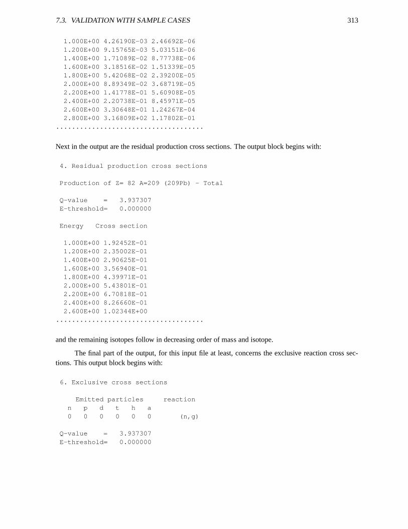
7.3. VALIDATION WITH SAMPLE CASES 313
1.000E+00 4.26190E-03 2.46692E-061.200E+00 9.15765E-03 5.03151E-061.400E+00 1.71089E-02 8.77738E-061.600E+00 3.18516E-02 1.51339E-051.800E+00 5.42068E-02 2.39200E-052.000E+00 8.89349E-02 3.68719E-052.200E+00 1.41778E-01 5.60908E-052.400E+00 2.20738E-01 8.45971E-052.600E+00 3.30648E-01 1.24267E-042.800E+00 3.16809E+02 1.17802E-01
.....................................
Next in the output are the residual production cross sections. The output block begins with:
4. Residual production cross sections
Production of Z= 82 A=209 (209Pb) - Total
Q-value = 3.937307E-threshold= 0.000000
Energy Cross section
1.000E+00 1.92452E-011.200E+00 2.35002E-011.400E+00 2.90625E-011.600E+00 3.56940E-011.800E+00 4.39971E-012.000E+00 5.43801E-012.200E+00 6.70818E-012.400E+00 8.26660E-012.600E+00 1.02344E+00
.....................................
and the remaining isotopes follow in decreasing order of mass and isotope.
The final part of the output, for this input file at least, concerns the exclusive reaction cross sec-tions. This output block begins with:
6. Exclusive cross sections
Emitted particles reactionn p d t h a0 0 0 0 0 0 (n,g)
Q-value = 3.937307E-threshold= 0.000000
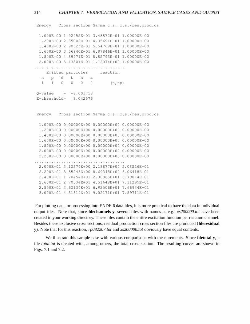
314 CHAPTER 7. VERIFICATION AND VALIDATION, SAMPLE CASES AND OUTPUT
Energy Cross section Gamma c.s. c.s./res.prod.cs
1.000E+00 1.92452E-01 3.48872E-01 1.00000E+001.200E+00 2.35002E-01 4.35691E-01 1.00000E+001.400E+00 2.90625E-01 5.54769E-01 1.00000E+001.600E+00 3.56940E-01 6.97846E-01 1.00000E+001.800E+00 4.39971E-01 8.82793E-01 1.00000E+002.000E+00 5.43801E-01 1.12074E+00 1.00000E+00
.....................................Emitted particles reaction
n p d t h a1 1 0 0 0 0 (n,np)
Q-value = -8.003758E-threshold= 8.042576
Energy Cross section Gamma c.s. c.s./res.prod.cs
1.000E+00 0.00000E+00 0.00000E+00 0.00000E+001.200E+00 0.00000E+00 0.00000E+00 0.00000E+001.400E+00 0.00000E+00 0.00000E+00 0.00000E+001.600E+00 0.00000E+00 0.00000E+00 0.00000E+001.800E+00 0.00000E+00 0.00000E+00 0.00000E+002.000E+00 0.00000E+00 0.00000E+00 0.00000E+002.200E+00 0.00000E+00 0.00000E+00 0.00000E+00
.....................................2.000E+01 3.12374E+00 2.18877E+00 5.08526E-012.200E+01 8.55243E+00 8.69348E+00 6.06418E-012.400E+01 1.70454E+01 2.30865E+01 6.79074E-012.600E+01 2.70534E+01 4.51648E+01 7.31295E-012.800E+01 3.62134E+01 6.92506E+01 7.66934E-013.000E+01 4.31314E+01 9.02171E+01 7.89711E-01
For plotting data, or processing into ENDF-6 data files, it ismore practical to have the data in individualoutput files. Note that, sincefilechannels y, several files with names as e.g.xs200000.tothave beencreated in your working directory. These files contain the entire excitation function per reaction channel.Besides these exclusive cross sections, residual production cross section files are produced (fileresidualy). Note that for this reaction,rp082207.totandxs200000.totobviously have equal contents.
We illustrate this sample case with various comparisons with measurements. Sincefiletotal y, afile total.tot is created with, among others, the total cross section. The resulting curves are shown inFigs. 7.1 and 7.2.
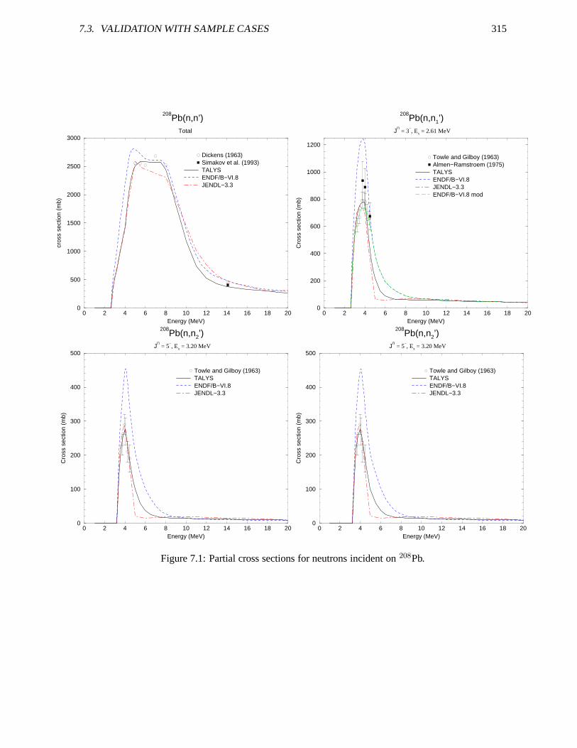
7.3. VALIDATION WITH SAMPLE CASES 315
0 2 4 6 8 10 12 14 16 18 20Energy (MeV)
0
500
1000
1500
2000
2500
3000
cros
s se
ctio
n (m
b)
208Pb(n,n’)
Total
Dickens (1963)Simakov et al. (1993)TALYSENDF/B−VI.8JENDL−3.3
0 2 4 6 8 10 12 14 16 18 20Energy (MeV)
0
200
400
600
800
1000
1200
Cro
ss s
ectio
n (m
b)
208Pb(n,n1’)
JΠ = 3
−, Ex = 2.61 MeV
Towle and Gilboy (1963)Almen−Ramstroem (1975)TALYSENDF/B−VI.8JENDL−3.3ENDF/B−VI.8 mod
0 2 4 6 8 10 12 14 16 18 20Energy (MeV)
0
100
200
300
400
500
Cro
ss s
ectio
n (m
b)
208Pb(n,n2’)
JΠ = 5
−, Ex = 3.20 MeV
Towle and Gilboy (1963)TALYSENDF/B−VI.8JENDL−3.3
0 2 4 6 8 10 12 14 16 18 20Energy (MeV)
0
100
200
300
400
500
Cro
ss s
ectio
n (m
b)
208Pb(n,n2’)
JΠ = 5
−, Ex = 3.20 MeV
Towle and Gilboy (1963)TALYSENDF/B−VI.8JENDL−3.3
Figure 7.1: Partial cross sections for neutrons incident on208Pb.
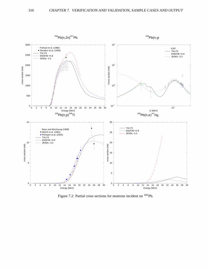
316 CHAPTER 7. VERIFICATION AND VALIDATION, SAMPLE CASES AND OUTPUT
0 2 4 6 8 10 12 14 16 18 20 22 24 26 28 30Energy (MeV)
0
500
1000
1500
2000
2500
3000
cros
s se
ctio
n (m
b)
208Pb(n,2n)
207Pb
Frehaut et al. (1980)Simakov et al. (1993)TALYSENDF/B−VI.8JENDL−3.3
101
E (MeV)
10−1
100
101
102
Cro
ss s
ectio
n (m
b)
208Pb(n,γ)
EXPTALYSENDF/B−VI.8JENDL−3.3
0 2 4 6 8 10 12 14 16 18 20 22 24 26 28 30Energy (MeV)
0
5
10
15
cros
s se
ctio
n (m
b)
208Pb(n,p)
208Tl
Bass and Wechsung (1968)Welch et al. (1981)Plompen et al. (2002)TALYSENDF/B−VI.8JENDL−3.3
0 2 4 6 8 10 12 14 16 18 20 22 24 26 28 30Energy (MeV)
0
5
10
15
20
25
30
cros
s se
ctio
n (m
b)
208Pb(n,α)
205Hg
TALYSENDF/B−VI.8JENDL−3.3
Figure 7.2: Partial cross sections for neutrons incident on208Pb.
7.3. VALIDATION WITH SAMPLE CASES 317
7.3.3 Sample 3: Comparison of compound nucleus WFC models: 10 keV n + 93Nb
In this sample case, we demonstrate the difference between the various models for the width fluctuationcorrection in compound nucleus reactions, as discussed extensively in Ref. [183]. As sample case, wetake 10 keV neutrons incident on93Nb and we ask for various compound nucleus models to calculatecross sections and angular distributions (outangle y), and to put the result for the elastic scatteringangular distribution on a separate file, callednn000.010ang.L00. Since the GOE calculation (widthmode3) is rather time-consuming, we reduce the number of bins to 20for all cases. We wish to check whetherthe flux is conserved in the compound nucleus model for the various WFC models, so we setoutchecky. This means that for each set of quantum numbers, unitarity is checked by means of Eq. (4.189).
Case 3a: Hauser-Feshbach model
The following input file is used
## General#projectile nelement nbmass 93energy 0.01## Parameters#bins 20widthmode 0## Output#outcheck youtangle yfileelastic y
This only new output block, i.e. not discussed before, is
++++++++++ CHECK OF FLUX CONSERVATION OF TRANSMISSION COEFFICIENTS ++++++++++Hauser-Feshbach model
Parity=- J= 3.0 j= 1.5 l= 1 T(j,l)= 7.98822E-03 Sum over outgo ing channelsParity=- J= 4.0 j= 0.5 l= 1 T(j,l)= 4.54100E-03 Sum over outgo ing channelsParity=- J= 4.0 j= 1.5 l= 1 T(j,l)= 7.98822E-03 Sum over outgo ing channelsParity=- J= 5.0 j= 0.5 l= 1 T(j,l)= 4.54100E-03 Sum over outgo ing channelsParity=- J= 5.0 j= 1.5 l= 1 T(j,l)= 7.98822E-03 Sum over outgo ing channelsParity=- J= 6.0 j= 1.5 l= 1 T(j,l)= 7.98822E-03 Sum over outgo ing channels
.....................................
318 CHAPTER 7. VERIFICATION AND VALIDATION, SAMPLE CASES AND OUTPUT
Model σcomp−el
Hauser-Feshbach 2410.89 mbMoldauer 2617.22 mbHRTW 2752.25 mbGOE 2617.12 mb
Table 7.2: Compound elastic cross section for 4 different compound nucleus models for 10 keV neutronsincident on93Nb.
in which the aforementioned unitarity is checked.
Case 3b: Moldauer model
As for case a, but now withwidthmode 1 in the input file.
Case 3c: HRTW model
As for case a, but now withwidthmode 2 in the input file.
Case 3d: GOE model
As for case a, but now withwidthmode 3 in the input file.
Table 7.2 lists the obtained compound nucleus elastic crosssection for the 4 cases.
Fig. 7.3 displays the elastic angular distribution for the 4models. Results like these made usconclude in Ref. [183] that Moldauer’s model, which is closest to the exact GOE result, is the one touse in practical applications, especially when considering the calculation times as printed in Table 7.1.Obviously, this sample case can be extended to one with various incident energies, so that the differencesbetween excitation functions can be studied, see also Ref. [183].
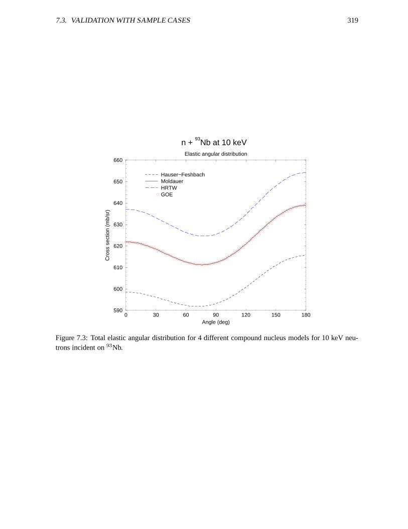
7.3. VALIDATION WITH SAMPLE CASES 319
0 30 60 90 120 150 180Angle (deg)
590
600
610
620
630
640
650
660
Cro
ss s
ectio
n (m
b/sr
)
n + 93
Nb at 10 keVElastic angular distribution
Hauser−FeshbachMoldauerHRTWGOE
Figure 7.3: Total elastic angular distribution for 4 different compound nucleus models for 10 keV neu-trons incident on93Nb.
320 CHAPTER 7. VERIFICATION AND VALIDATION, SAMPLE CASES AND OUTPUT
7.3.4 Sample 4: Recoils: 20 MeV n +28Si
In this sample case, we calculate the recoils of the residualnuclides produced by 20 MeV neutronsincident on28Si reaction. Two methods are compared.
Case 4a: “Exact” approach
In the exact approach, each excitation energy bin of the population of each residual nucleus is describedby a full distribution of kinetic recoil energies. The following input file is used
## General#projectile nelement simass 28energy 20.## Parameters#m2constant 0.70sysreaction p d t h aspherical y## Output#recoil yfilerecoil y
For increasing incident energies, this calculation becomes quickly time-expensive. The recoil calculationyields separate files with the recoil spectrum per residual nucleus, starting withrec, followed by the Z, Aand incident energy, e.g.rec012024spec020.000.tot. Also following additional output block is printed:
8. Recoil spectra
Recoil Spectrum for 29Si
Energy Cross section
0.018 0.00000E+000.053 0.00000E+000.088 0.00000E+00
.....................................0.676 3.21368E+000.720 3.22112E+000.763 3.21215E+00
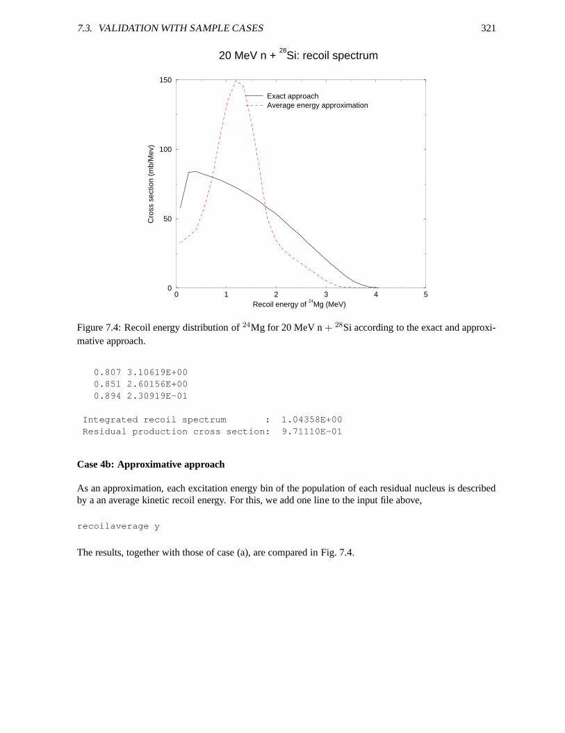
7.3. VALIDATION WITH SAMPLE CASES 321
0 1 2 3 4 5Recoil energy of
24Mg (MeV)
0
50
100
150
Cro
ss s
ectio
n (m
b/M
ev)
20 MeV n + 28
Si: recoil spectrum
Exact approachAverage energy approximation
Figure 7.4: Recoil energy distribution of24Mg for 20 MeV n+ 28Si according to the exact and approxi-mative approach.
0.807 3.10619E+000.851 2.60156E+000.894 2.30919E-01
Integrated recoil spectrum : 1.04358E+00Residual production cross section: 9.71110E-01
Case 4b: Approximative approach
As an approximation, each excitation energy bin of the population of each residual nucleus is describedby a an average kinetic recoil energy. For this, we add one line to the input file above,
recoilaverage y
The results, together with those of case (a), are compared inFig. 7.4.
322 CHAPTER 7. VERIFICATION AND VALIDATION, SAMPLE CASES AND OUTPUT
7.3.5 Sample 5: Fission cross sections: n +232Th
It is well known that a systematic approach for fission is difficult to achieve. It is possible to obtain verysatisfactory fits to fission data with TALYS, but at the expense of using many adjustable input parameters.We are performing extensive model calculations to bring somewhat more structure in the collection offitting parameters. In the meantime, we include here a samplecase for the description of the fission crosssection of232Th. We use the following input file,
## General#projectile nelement Thmass 232energy energies## Models and output#outfission ypartable ybins 40channels yfilechannels ybest y
Note that, although no adjustable parameters are visible above, this is certainly no “default” calculation.Instead, this sample case illustrates the use of so-called “best files”. By using thebest ykeyword, thefile talys/structure/best/Th232/z090a232n.bestis automatically invoked. The contents of that file are
colldamp yasys yclass2 ymaxrot 5gnorm 9.t 90 233 0.41756 1e0 90 233 -0.90113 1exmatch 90 233 5.89461 1t 90 233 0.56780 2e0 90 233 -2.52108 2exmatch 90 233 6.63983 2fisbar 90 233 6.41136 1fishw 90 233 0.61550 1class2width 90 233 0.2 1fisbar 90 233 5.23377 2t 90 232 0.46845e0 90 232 -0.39156Exmatch 90 232 5.55627 0a 90 232 31.90038t 90 232 0.41262 1
7.3. VALIDATION WITH SAMPLE CASES 323
e0 90 232 -1.66339 1exmatch 90 232 6.74958 1t 90 232 0.44833 2e0 90 232 -0.51471 2exmatch 90 232 6.45816 2class2width 90 232 0.10013 1fisbar 90 232 6.31815 2a 90 231 26.62965t 90 231 0.45494e0 90 231 -0.91497exmatch 90 231 4.92684 0t 90 231 0.47007 1e0 90 231 -2.16775 1exmatch 90 231 5.98780 1t 90 231 0.68793 2e0 90 231 -2.79424 2exmatch 90 231 6.74959 2a 90 230 26.21683t 90 230 0.47155e0 90 230 -0.33802exmatch 90 230 5.52092 0t 90 230 0.45039 1e0 90 230 -1.14073 1exmatch 90 230 6.80289 1t 90 230 0.41118 2e0 90 230 -1.25432 2exmatch 90 230 6.52706 2
The above parameters are the usual ones to be adjusted to get good agreement with experimental data:level density and fission parameters for the ground state or on top of the barriers. The resulting filefission.totis plotted together with experimental data in Fig. 7.5.
Due to the presence ofoutfission y in the input file, all nuclear structure related to the fissionprocess is given in the output for the target and the compoundnucleus
Fission information for Z= 90 N=142 (232Th)
Number of fission barriers : 2Number of sets of class2 states : 1
Parameters for fission barrier 1
Type of axiality : 1Height of fission barrier 1 : 5.800Width of fission barrier 1 : 0.900Rtransmom : 0.600Moment of inertia : 87.657Number of head band transition states: 8Start of continuum energy : 0.800
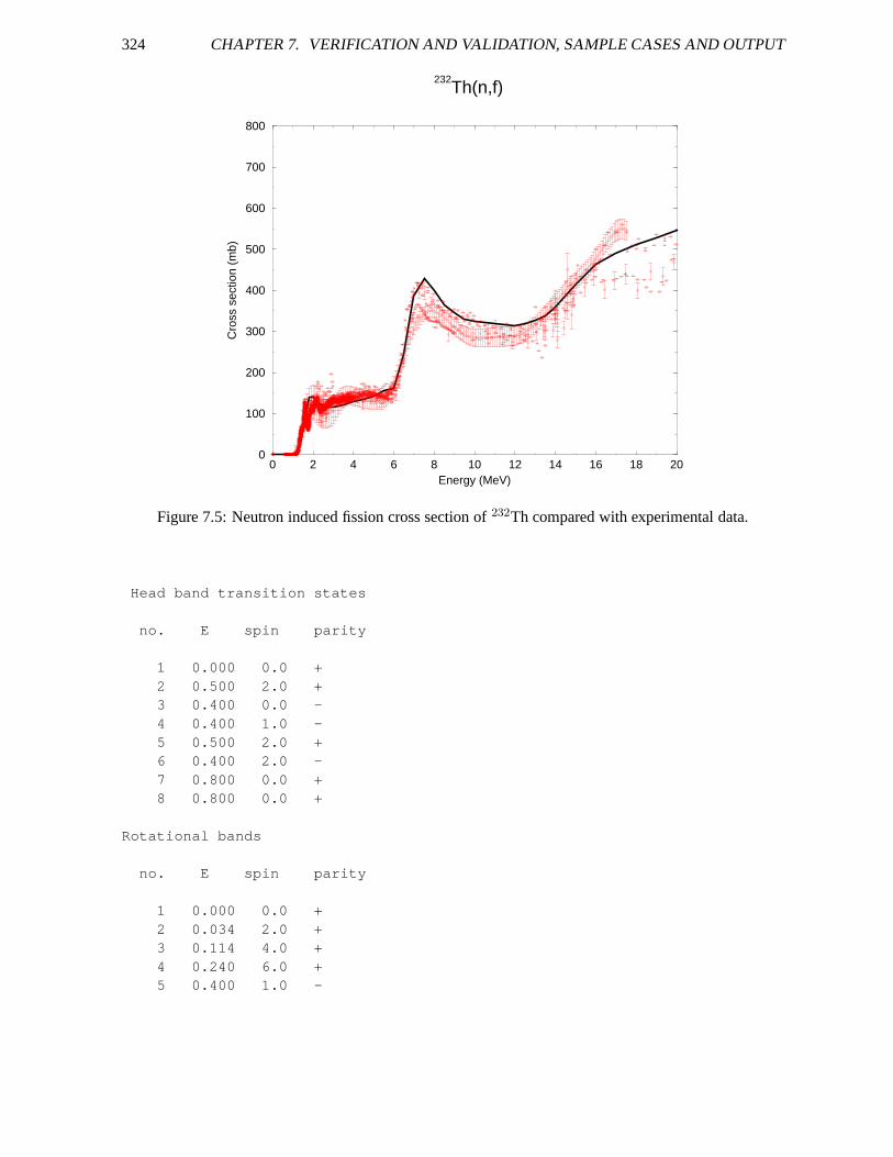
324 CHAPTER 7. VERIFICATION AND VALIDATION, SAMPLE CASES AND OUTPUT
0 2 4 6 8 10 12 14 16 18 20Energy (MeV)
0
100
200
300
400
500
600
700
800
Cro
ss s
ectio
n (m
b)
232Th(n,f)
Figure 7.5: Neutron induced fission cross section of232Th compared with experimental data.
Head band transition states
no. E spin parity
1 0.000 0.0 +2 0.500 2.0 +3 0.400 0.0 -4 0.400 1.0 -5 0.500 2.0 +6 0.400 2.0 -7 0.800 0.0 +8 0.800 0.0 +
Rotational bands
no. E spin parity
1 0.000 0.0 +2 0.034 2.0 +3 0.114 4.0 +4 0.240 6.0 +5 0.400 1.0 -
7.3. VALIDATION WITH SAMPLE CASES 325
6 0.400 2.0 -7 0.411 8.0 +8 0.411 1.0 -9 0.423 2.0 -
10 0.434 3.0 -..................Parameters for fission barrier 2
Type of axiality : 2Height of fission barrier 2 : 6.318Width of fission barrier 2 : 0.600Rtransmom : 1.000Moment of inertia : 154.212Number of head band transition states: 4Start of continuum energy : 0.500
Head band transition states
no. E spin parity
1 0.000 0.0 +2 0.500 2.0 +3 0.200 0.0 -4 0.500 1.0 -
.............
Moreover, the corresponding fission transmission coefficients are printed for all excitation energies en-countered in the calculation
Fission transmission coefficients for Z= 90 N=143 (233Th) a nd an excitation energy of
J T(J,-) T(J,+)
0.5 4.02053E-08 6.51894E-081.5 0.00000E+00 0.00000E+00
.............
The fission information for all residual nuclides can be obtained in the output file as well by addingoutpopulation yto the input file.
326 CHAPTER 7. VERIFICATION AND VALIDATION, SAMPLE CASES AND OUTPUT
7.3.6 Sample 6: Continuum spectra at 63 MeV for Bi(n,xp)...Bi(n,xα)
In this sample case, we calculate angle-integrated and double-differential particle spectra for 63 MeVneutrons on209Bi, see Ref. [422].
Case 6a: Default calculation
The following input file is used
## General#projectile nelement bimass 209energy 63.## Output#ddxmode 2filespectrum n p d t h afileddxa p 20.fileddxa p 70.fileddxa p 110.fileddxa d 20.fileddxa d 70.fileddxa d 110.fileddxa t 20.fileddxa t 70.fileddxa t 110.fileddxa h 20.fileddxa h 70.fileddxa h 110.fileddxa a 20.fileddxa a 70.fileddxa a 110.
Note that we request that angle-integrated spectra for all particles are written on separate files throughfilespectrum n p d t h a. At 20, 70 and 110 degrees, we also ask for the double-differential spectrum forprotons up to alpha-particles. The resulting filespspec063.000.tot, pddx020.0.deg, etc. are presented,together with experimental data, in Figs. 7.6 and 7.7.
Case 6b: Adjusted matrix element
The default results of case (a) for the proton spectra are a bit high. Therefore, as a second version of thissample case, we adjust a pre-equilibrium parameter and add the following to the input above:
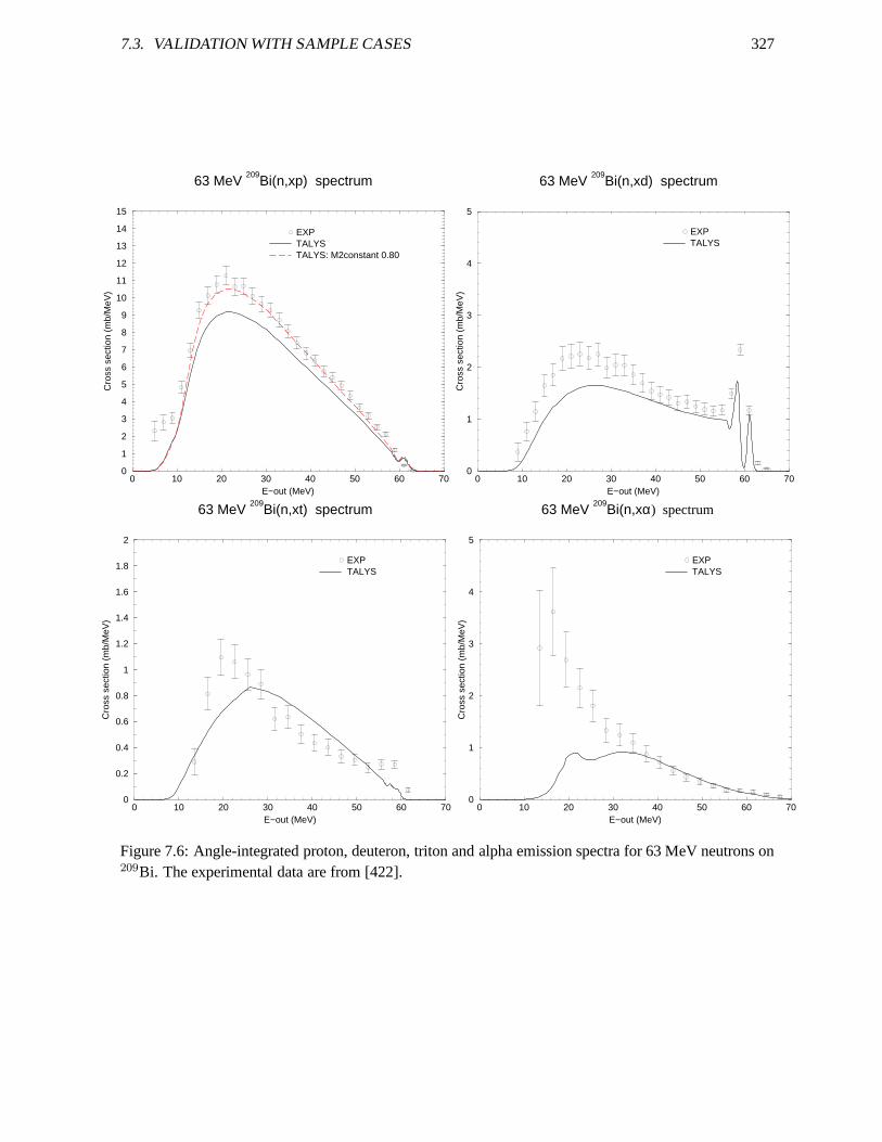
7.3. VALIDATION WITH SAMPLE CASES 327
0 10 20 30 40 50 60 70E−out (MeV)
0
1
2
3
4
5
6
7
8
9
10
11
12
13
14
15
Cro
ss s
ectio
n (m
b/M
eV)
63 MeV 209
Bi(n,xp) spectrum
EXPTALYSTALYS: M2constant 0.80
0 10 20 30 40 50 60 70E−out (MeV)
0
1
2
3
4
5
Cro
ss s
ectio
n (m
b/M
eV)
63 MeV 209
Bi(n,xd) spectrum
EXPTALYS
0 10 20 30 40 50 60 70E−out (MeV)
0
0.2
0.4
0.6
0.8
1
1.2
1.4
1.6
1.8
2
Cro
ss s
ectio
n (m
b/M
eV)
63 MeV 209
Bi(n,xt) spectrum
EXPTALYS
0 10 20 30 40 50 60 70E−out (MeV)
0
1
2
3
4
5
Cro
ss s
ectio
n (m
b/M
eV)
63 MeV 209
Bi(n,xα) spectrum
EXPTALYS
Figure 7.6: Angle-integrated proton, deuteron, triton andalpha emission spectra for 63 MeV neutrons on209Bi. The experimental data are from [422].
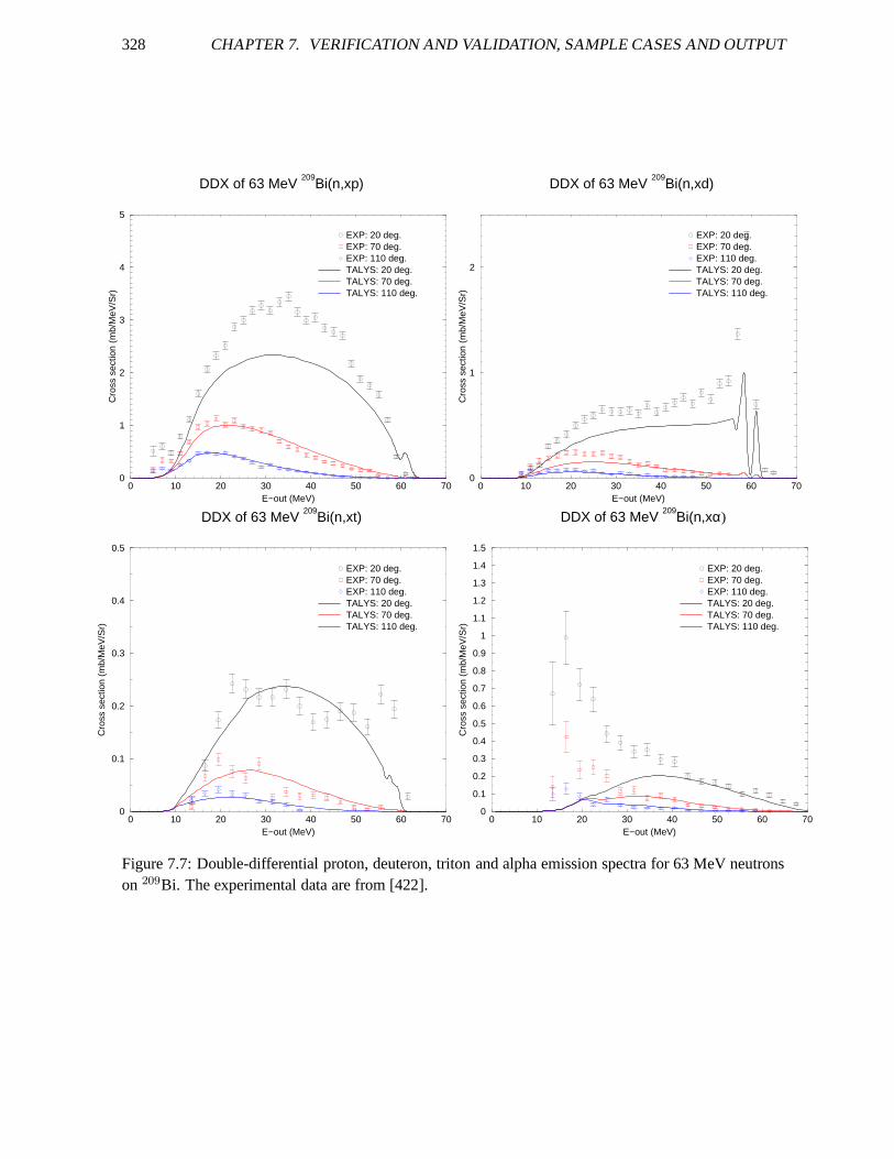
328 CHAPTER 7. VERIFICATION AND VALIDATION, SAMPLE CASES AND OUTPUT
0 10 20 30 40 50 60 70E−out (MeV)
0
1
2
3
4
5
Cro
ss s
ectio
n (m
b/M
eV/S
r)
DDX of 63 MeV 209
Bi(n,xp)
EXP: 20 deg.EXP: 70 deg.EXP: 110 deg.TALYS: 20 deg.TALYS: 70 deg.TALYS: 110 deg.
0 10 20 30 40 50 60 70E−out (MeV)
0
1
2
Cro
ss s
ectio
n (m
b/M
eV/S
r)
DDX of 63 MeV 209
Bi(n,xd)
EXP: 20 deg.EXP: 70 deg.EXP: 110 deg.TALYS: 20 deg.TALYS: 70 deg.TALYS: 110 deg.
0 10 20 30 40 50 60 70E−out (MeV)
0
0.1
0.2
0.3
0.4
0.5
Cro
ss s
ectio
n (m
b/M
eV/S
r)
DDX of 63 MeV 209
Bi(n,xt)
EXP: 20 deg.EXP: 70 deg.EXP: 110 deg.TALYS: 20 deg.TALYS: 70 deg.TALYS: 110 deg.
0 10 20 30 40 50 60 70E−out (MeV)
0
0.1
0.2
0.3
0.4
0.5
0.6
0.7
0.8
0.9
1
1.1
1.2
1.3
1.4
1.5
Cro
ss s
ectio
n (m
b/M
eV/S
r)
DDX of 63 MeV 209
Bi(n,xα)
EXP: 20 deg.EXP: 70 deg.EXP: 110 deg.TALYS: 20 deg.TALYS: 70 deg.TALYS: 110 deg.
Figure 7.7: Double-differential proton, deuteron, tritonand alpha emission spectra for 63 MeV neutronson 209Bi. The experimental data are from [422].

7.3. VALIDATION WITH SAMPLE CASES 329
## Parameters#M2constant 0.80
By decreasingM2constant by 20% (which is a common and acceptable deviation from the average),we favor the pre-equilibrium emission rate over the rate rate, leading to a harder spectrum. The result isshown in Fig. 7.6 for the proton spectrum.
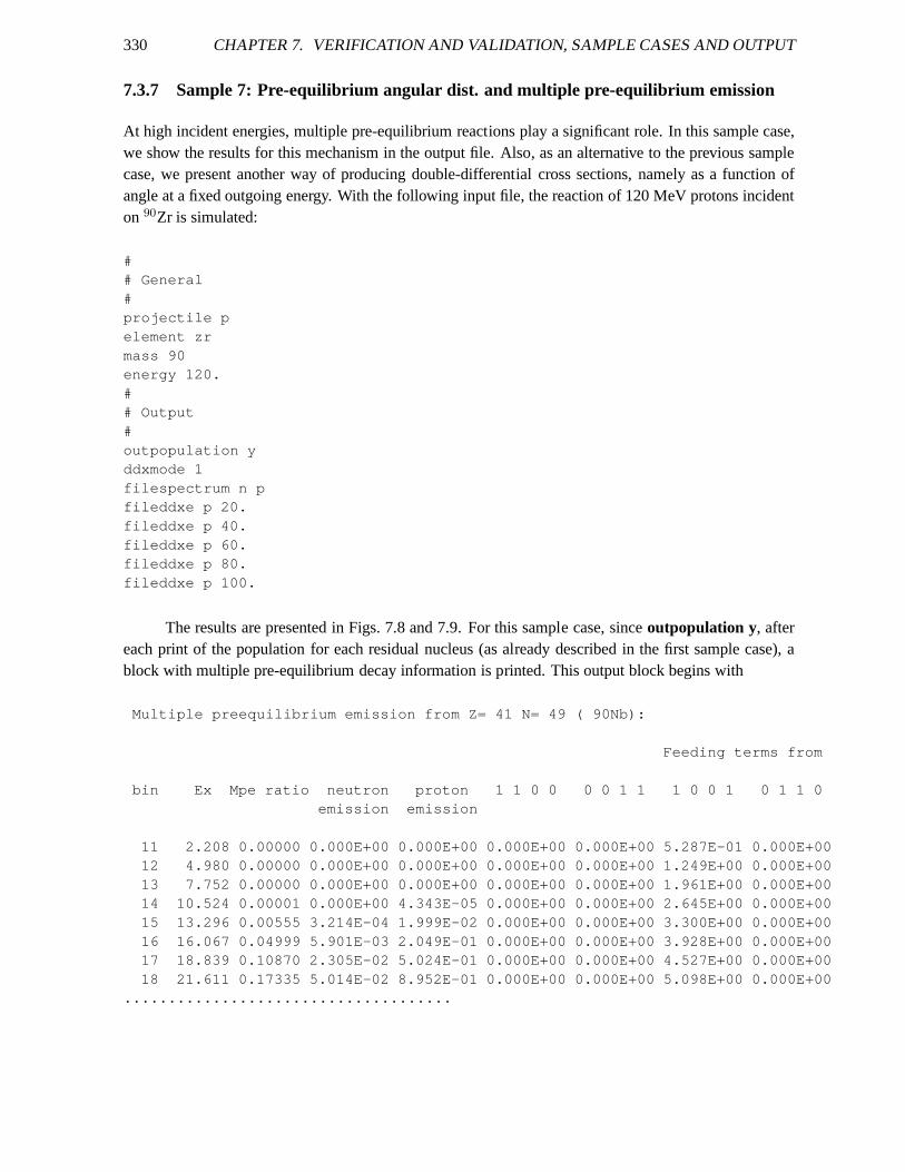
330 CHAPTER 7. VERIFICATION AND VALIDATION, SAMPLE CASES AND OUTPUT
7.3.7 Sample 7: Pre-equilibrium angular dist. and multiplepre-equilibrium emission
At high incident energies, multiple pre-equilibrium reactions play a significant role. In this sample case,we show the results for this mechanism in the output file. Also, as an alternative to the previous samplecase, we present another way of producing double-differential cross sections, namely as a function ofangle at a fixed outgoing energy. With the following input file, the reaction of 120 MeV protons incidenton 90Zr is simulated:
## General#projectile pelement zrmass 90energy 120.## Output#outpopulation yddxmode 1filespectrum n pfileddxe p 20.fileddxe p 40.fileddxe p 60.fileddxe p 80.fileddxe p 100.
The results are presented in Figs. 7.8 and 7.9. For this sample case, sinceoutpopulation y, aftereach print of the population for each residual nucleus (as already described in the first sample case), ablock with multiple pre-equilibrium decay information is printed. This output block begins with
Multiple preequilibrium emission from Z= 41 N= 49 ( 90Nb):
Feeding terms from
bin Ex Mpe ratio neutron proton 1 1 0 0 0 0 1 1 1 0 0 1 0 1 1 0emission emission
11 2.208 0.00000 0.000E+00 0.000E+00 0.000E+00 0.000E+00 5 .287E-01 0.000E+0012 4.980 0.00000 0.000E+00 0.000E+00 0.000E+00 0.000E+00 1 .249E+00 0.000E+0013 7.752 0.00000 0.000E+00 0.000E+00 0.000E+00 0.000E+00 1 .961E+00 0.000E+0014 10.524 0.00001 0.000E+00 4.343E-05 0.000E+00 0.000E+00 2.645E+00 0.000E+0015 13.296 0.00555 3.214E-04 1.999E-02 0.000E+00 0.000E+00 3.300E+00 0.000E+0016 16.067 0.04999 5.901E-03 2.049E-01 0.000E+00 0.000E+00 3.928E+00 0.000E+0017 18.839 0.10870 2.305E-02 5.024E-01 0.000E+00 0.000E+00 4.527E+00 0.000E+0018 21.611 0.17335 5.014E-02 8.952E-01 0.000E+00 0.000E+00 5.098E+00 0.000E+00
.....................................
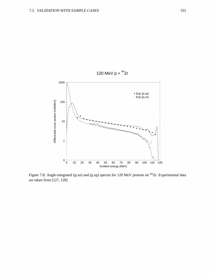
7.3. VALIDATION WITH SAMPLE CASES 331
0 10 20 30 40 50 60 70 80 90 100 110 120Incident energy (MeV)
0
1
10
100
1000
Diff
eren
tial c
ross
sec
tion
(mb/
MeV
)
120 MeV p + 90
Zr
Exp (p,xp)Exp (p,xn)
Figure 7.8: Angle-integrated (p,xn) and (p,xp) spectra for120 MeV protons on90Zr. Experimental dataare taken from [127, 128]
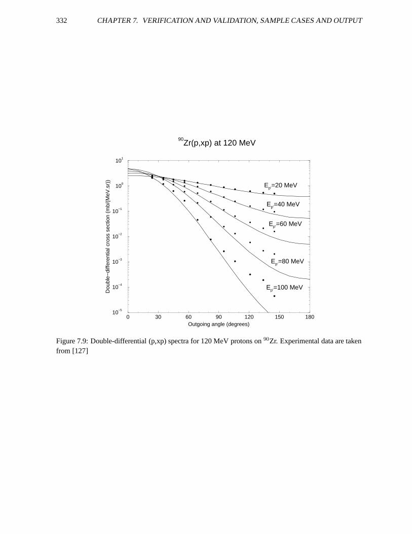
332 CHAPTER 7. VERIFICATION AND VALIDATION, SAMPLE CASES AND OUTPUT
0 30 60 90 120 150 180Outgoing angle (degrees)
10−5
10−4
10−3
10−2
10−1
100
101
Dou
ble−
diffe
rent
ial c
ross
sec
tion
(mb/
(MeV
.sr)
)
90Zr(p,xp) at 120 MeV
Ep’=20 MeV
Ep’=40 MeV
Ep’=60 MeV
Ep’=80 MeV
Ep’=100 MeV
Figure 7.9: Double-differential (p,xp) spectra for 120 MeVprotons on90Zr. Experimental data are takenfrom [127]

7.3. VALIDATION WITH SAMPLE CASES 333
For each continuum bin, with excitation energyEx, we print the fraction of the population that is emit-ted as multiple pre-equilibrium. Also the total neutron andproton emission per residual nucleus isprinted, as well as the feeding terms from previous particle-hole configurations. With this input file, filesnspec120.000.totandpspec120.000.totare created through thefilespectrum n pkeyword. The results aredisplayed in Fig. 7.8. Also, the combination ofddxmode 1and the variousfileddxe keywords generatethepddx100.0.mev, etc. files that are compared with experimental data in Fig. 7.9.
334 CHAPTER 7. VERIFICATION AND VALIDATION, SAMPLE CASES AND OUTPUT
7.3.8 Sample 8: Residual production cross sections: p +natFe up to 100 MeV
In this sample case, we calculate the residual production cross sections for protons onnatFe for incidentenergies up to 100 MeV. A calculation for a natural target is launched, meaning that successive TALYScalculations for each isotope are performed, after which the results are weighted with the natural abun-dance. We restrict ourselves to a calculation with all nuclear model parameters set to their default values.The following input file is used:
## General#projectile pelement femass 0energy energies## Output#fileresidual y
The fileenergiescontains 34 incident energies between 1 and 100 MeV. Obviously, this sample case canbe extended to more incident energies, e.g. up to 200 MeV, by simply adding numbers to theenergiesfile. In that case, we recommend to include more energy bins inthe calculation, (e.g.bins 80) to avoidnumerical fluctuations, although this will inevitably takemore computer time. Note that we have enabledthe fileresidual keyword, so that a separate cross sections file for each final product is produced. Theresults from the filesrp027056.tot, rp027055.tot, rp025054.totandrp025052.totare presented, togetherwith experimental data, in Fig. 7.10.
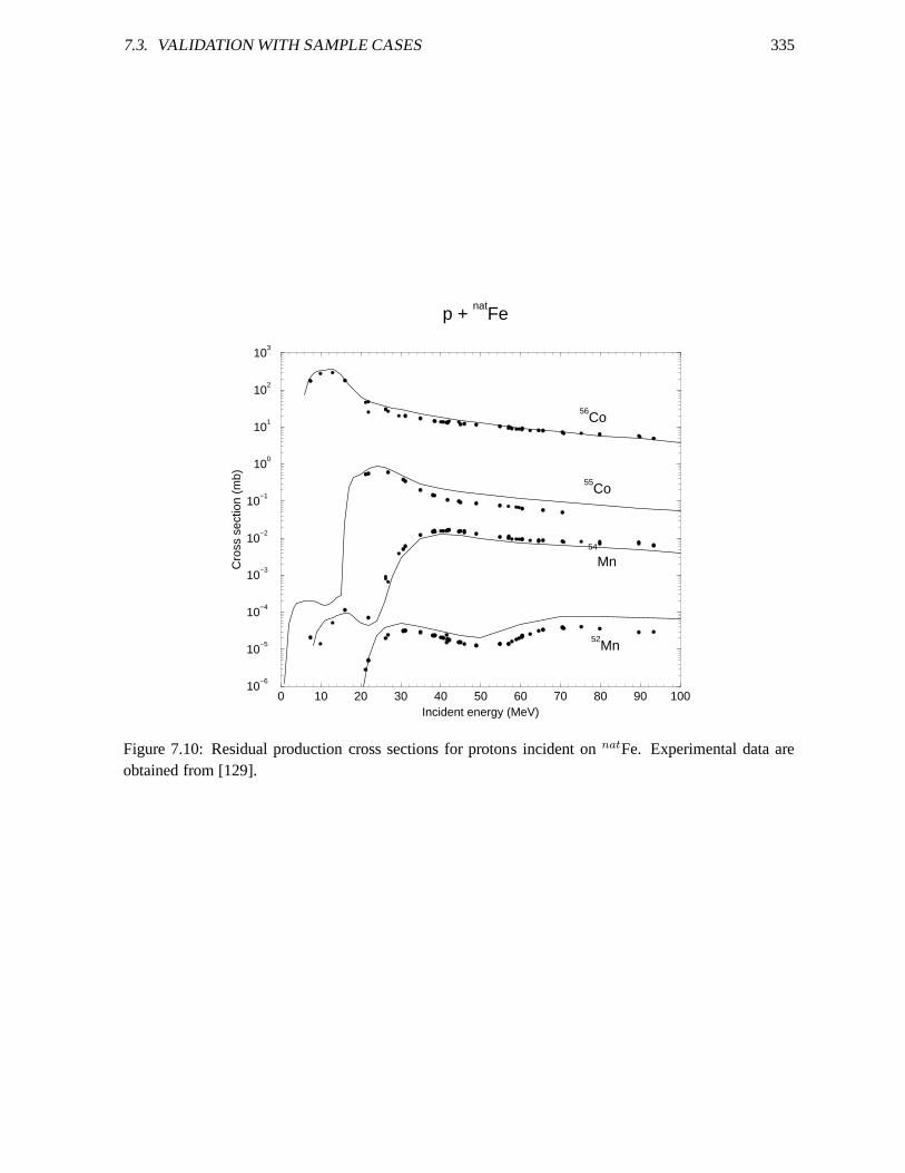
7.3. VALIDATION WITH SAMPLE CASES 335
0 10 20 30 40 50 60 70 80 90 100Incident energy (MeV)
10−6
10−5
10−4
10−3
10−2
10−1
100
101
102
103
Cro
ss s
ectio
n (m
b)
p + nat
Fe
56Co
55Co
54
Mn
52Mn
Figure 7.10: Residual production cross sections for protons incident onnatFe. Experimental data areobtained from [129].
336 CHAPTER 7. VERIFICATION AND VALIDATION, SAMPLE CASES AND OUTPUT
7.3.9 Sample 9: Spherical optical model and DWBA: n +208Pb
Three types of optical model calculations are included in the set of sample cases. In this first one,we treat208Pb as a spherical nucleus and request calculations for the elastic angular distributions andinelastic angular distributions at a few incident energies. This is accomplished with the input file
## General#projectile nelement pbmass 208energy energies## Avoid unnecessary calculations and output#ejectiles npreequilibrium ncompound nmaxZ 0maxN 0bins 5fileresidual nfiletotal n## Output#outangle yfileelastic yfileangle 1fileangle 2
where the fileenergiesconsists of the energies 11., 13.7, 20., 22., and 25.7 MeV (for which experimen-tal data exists). The keywordfileelastic yhas created the filesnn011.000ang.L00, etc. which containthe elastic scattering angular distribution and are compared with experimental data in Fig. 7.11. Withfileangle 1andfileangle 2we have created the filesnn010.000ang.L01, etc. with the inelastic scatteringangular distribution to the first and second discrete state.These are also plotted in Figs. 7.11. Note thatthe keywords in the middle block (ejectiles nup tofiletotal n) have been added to avoid a full calculationof all the cross sections. For the present sample case we assume that only elastic scattering and DWBAangular distributions are of interest, so we economize on output options, number of bins, ejectiles andnuclides that can be reached. Obviously, for reliable results for all observables this middle block wouldhave to be deleted. See also sample case (1f) for obtaining more specific information from the output.
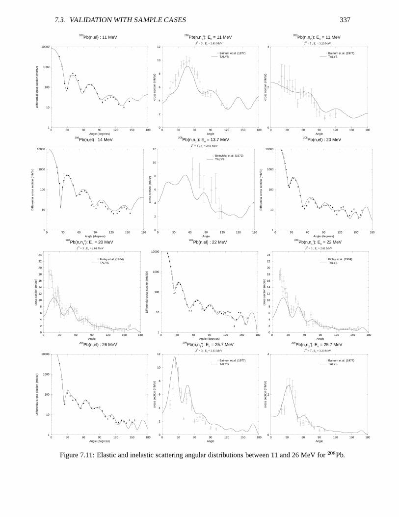
7.3. VALIDATION WITH SAMPLE CASES 337
0 30 60 90 120 150 180Angle (degrees)
1
10
100
1000
10000
Diff
eren
tial c
ross
sec
tion
(mb/
Sr)
208Pb(n,el) : 11 MeV
0 30 60 90 120 150 180Angle
0
2
4
6
8
10
12
cros
s se
ctio
n (m
b/sr
)
208Pb(n,n1’): En = 11 MeV
JΠ = 3
−, Ex = 2.61 MeV
Bainum et al. (1977)TALYS
0 30 60 90 120 150 180Angle
0
2
4
cros
s se
ctio
n (m
b/sr
)
208Pb(n,n2’): En = 11 MeV
JΠ = 5
−, Ex = 3.20 MeV
Bainum et al. (1977)TALYS
0 30 60 90 120 150 180Angle (degrees)
1
10
100
1000
10000
Diff
eren
tial c
ross
sec
tion
(mb/
Sr)
208Pb(n,el) : 14 MeV
0 30 60 90 120 150 180Angle
0
2
4
6
8
10
12cr
oss
sect
ion
(mb/
sr)
208Pb(n,n1’): En = 13.7 MeV
JΠ = 3
−, Ex = 2.61 MeV
Belovickij et al. (1972)TALYS
0 30 60 90 120 150 180Angle (degrees)
1
10
100
1000
10000
Diff
eren
tial c
ross
sec
tion
(mb/
Sr)
208Pb(n,el) : 20 MeV
0 30 60 90 120 150 180Angle
0
2
4
6
8
10
12
14
16
18
20
22
24
cros
s se
ctio
n (m
b/sr
)
208Pb(n,n1’): En = 20 MeV
JΠ = 3
−, Ex = 2.61 MeV
Finlay et al. (1984)TALYS
0 30 60 90 120 150 180Angle (degrees)
1
10
100
1000
10000
Diff
eren
tial c
ross
sec
tion
(mb/
Sr)
208Pb(n,el) : 22 MeV
0 30 60 90 120 150 180Angle
0
2
4
6
8
10
12
14
16
18
20
22
24
cros
s se
ctio
n (m
b/sr
)
208Pb(n,n1’): En = 22 MeV
JΠ = 3
−, Ex = 2.61 MeV
Finlay et al. (1984)TALYS
0 30 60 90 120 150 180Angle (degrees)
1
10
100
1000
10000
Diff
eren
tial c
ross
sec
tion
(mb/
Sr)
208Pb(n,el) : 26 MeV
0 30 60 90 120 150 180Angle
0
2
4
6
8
10
12
cros
s se
ctio
n (m
b/sr
)
208Pb(n,n1’): En = 25.7 MeV
JΠ = 3
−, Ex = 2.61 MeV
Bainum et al. (1977)TALYS
0 30 60 90 120 150 180Angle
0
2
4
cros
s se
ctio
n (m
b/sr
)
208Pb(n,n2’): En = 25.7 MeV
JΠ = 5
−, Ex = 3.20 MeV
Bainum et al. (1977)TALYS
Figure 7.11: Elastic and inelastic scattering angular distributions between 11 and 26 MeV for208Pb.
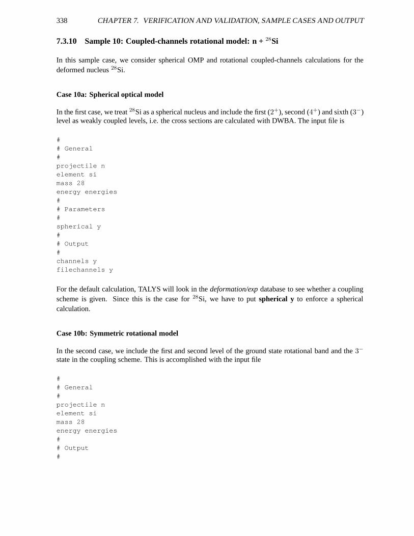
338 CHAPTER 7. VERIFICATION AND VALIDATION, SAMPLE CASES AND OUTPUT
7.3.10 Sample 10: Coupled-channels rotational model: n +28Si
In this sample case, we consider spherical OMP and rotational coupled-channels calculations for thedeformed nucleus28Si.
Case 10a: Spherical optical model
In the first case, we treat28Si as a spherical nucleus and include the first (2+), second (4+) and sixth (3−)level as weakly coupled levels, i.e. the cross sections are calculated with DWBA. The input file is
## General#projectile nelement simass 28energy energies## Parameters#spherical y## Output#channels yfilechannels y
For the default calculation, TALYS will look in thedeformation/expdatabase to see whether a couplingscheme is given. Since this is the case for28Si, we have to putspherical y to enforce a sphericalcalculation.
Case 10b: Symmetric rotational model
In the second case, we include the first and second level of theground state rotational band and the3−
state in the coupling scheme. This is accomplished with the input file
## General#projectile nelement simass 28energy energies## Output#
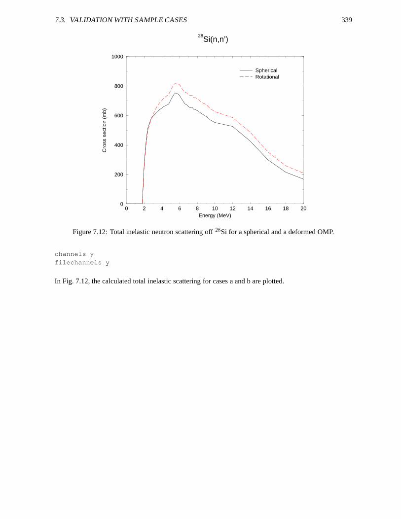
7.3. VALIDATION WITH SAMPLE CASES 339
0 2 4 6 8 10 12 14 16 18 20Energy (MeV)
0
200
400
600
800
1000
Cro
ss s
ectio
n (m
b)
28Si(n,n’)
SphericalRotational
Figure 7.12: Total inelastic neutron scattering off28Si for a spherical and a deformed OMP.
channels yfilechannels y
In Fig. 7.12, the calculated total inelastic scattering forcases a and b are plotted.
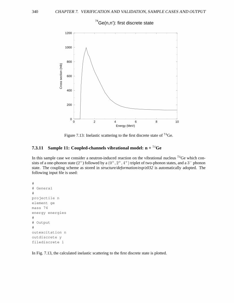
340 CHAPTER 7. VERIFICATION AND VALIDATION, SAMPLE CASES AND OUTPUT
0 2 4 6 8 10Energy (MeV)
0
200
400
600
800
1000
1200
Cro
ss s
ectio
n (m
b)
74Ge(n,n’): first discrete state
Figure 7.13: Inelastic scattering to the first discrete state of 74Ge.
7.3.11 Sample 11: Coupled-channels vibrational model: n +74Ge
In this sample case we consider a neutron-induced reaction on the vibrational nucleus74Ge which con-sists of a one-phonon state (2+) followed by a(0+, 2+, 4+) triplet of two-phonon states, and a3− phononstate. The coupling scheme as stored instructure/deformation/exp/z032is automatically adopted. Thefollowing input file is used:
## General#projectile nelement gemass 74energy energies## Output#outexcitation noutdiscrete yfilediscrete 1
In Fig. 7.13, the calculated inelastic scattering to the first discrete state is plotted.
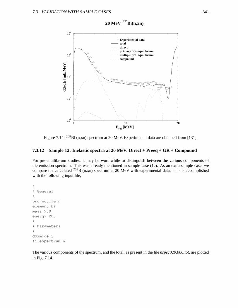
7.3. VALIDATION WITH SAMPLE CASES 341
0 10 20Eout [MeV]
100
101
102
103
104
dσ/d
E [m
b/M
eV]
20 MeV 209
Bi(n,xn)
Experimental datatotaldirectprimary pre−equilibriummultiple pre−equilibriumcompound
Figure 7.14:209Bi (n,xn) spectrum at 20 MeV. Experimental data are obtainedfrom [131].
7.3.12 Sample 12: Inelastic spectra at 20 MeV: Direct + Preeq+ GR + Compound
For pre-equilibrium studies, it may be worthwhile to distinguish between the various components ofthe emission spectrum. This was already mentioned in samplecase (1c). As an extra sample case, wecompare the calculated209Bi(n,xn) spectrum at 20 MeV with experimental data. This is accomplishedwith the following input file,
## General#projectile nelement bimass 209energy 20.## Parameters#ddxmode 2filespectrum n
The various components of the spectrum, and the total, as present in the filenspec020.000.tot, are plottedin Fig. 7.14.
342 CHAPTER 7. VERIFICATION AND VALIDATION, SAMPLE CASES AND OUTPUT
7.3.13 Sample 13: Gamma-ray intensities:208Pb(n, nγ) and 208Pb(n, 2nγ)
This feature could simply have been included in the sample case on excitation functions for208Pb, but inorder not to overburden the description of that sample case we include it here. With the input file
## General#projectile nelement pbmass 208energy energies## Parameters#isomer 1.e-4maxZ 0gnorm 0.35Rgamma 2.2egr 82 209 12.0 E1 1optmodfileN 82 pb.omp## Output#channels yfilechannels yfileresidual youtgamdis y
all discrete gamma lines are printed and stored in separate files. To avoid the production of too many datafiles, we have putmaxZ 0 so that only the gamma-ray production files for Pb-chain are created. Also, weinclude a special OMP with the filepb.ompand we setisomer 1.e-4to allow for gamma decay of somerather short-lived levels. Experimental data exists for the208Pb(n, n′γ) cross section for level 1 to level 0and the208Pb(n, 2n′γ) cross section for level 2 to level 0 and for level 1 to level 0. These data have beenplotted together with the results of the calculated filesgam082208L01L00.tot, gam082207L02L00.totandgam082207L01L00.tot, in Fig. 7.15.
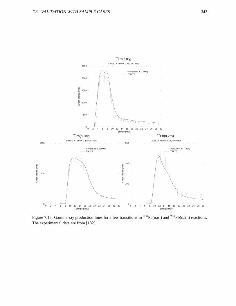
7.3. VALIDATION WITH SAMPLE CASES 343
0 2 4 6 8 10 12 14 16 18 20 22 24 26 28 30Energy (MeV)
0
500
1000
1500
2000
2500
Cro
ss s
ectio
n (m
b)
208Pb(n,n’γ)
Level 1 −> Level 0: Eγ=2.61 MeV
Vonach et al. (1994)TALYS
0 2 4 6 8 10 12 14 16 18 20 22 24 26 28 30Energy (MeV)
0
500
1000
Cro
ss s
ectio
n (m
b)
208Pb(n,2nγ)
Level 1 −> Level 0: Eγ=0.57 MeV
Vonach et al. (1994)TALYS
0 2 4 6 8 10 12 14 16 18 20 22 24 26 28 30Energy (MeV)
0
100
200
300
Cro
ss s
ectio
n (m
b)
208Pb(n,2nγ)
Level 2 −> Level 0: Eγ=0.89 MeV
Vonach et al. (1994)TALYS
Figure 7.15: Gamma-ray production lines for a few transitions in208Pb(n,n’) and208Pb(n,2n) reactions.The experimental data are from [132].
344 CHAPTER 7. VERIFICATION AND VALIDATION, SAMPLE CASES AND OUTPUT
7.3.14 Sample 14: Fission yields for238U
In this sample case we compute fission fragment/product mass/isotope yields. The fission fragment massyield curve is determined for neutrons on238U at incident energies of 1.6 and 5.5 MeV (these incidentenergies are given in the fileenergies). The following input file is used:
projectile nelement Umass 238energy energiespartable ybins 40channels yfilechannels yautorot ybest yecissave ymassdis yffevaporation y
The long list of adjustable parameters, not visible here butautomatically taken fromtalys/structure/best/U238/z092a238n.bestthrough thebest y keyword, is mainly needed to give a decent (though not yet perfect) description ofthe total fission cross section. For completeness, we show the results for238U we obtained for incidentenergies of 1, 1.6, 3.5, 5.5, 7.5 and 10 MeV. The TALYS resultsfor the pre-neutron emission mass yieldscan be found inyield001.600.fisandyield005.500.fisand are given in the upper plot of Fig. 7.16. Thetwo other plots show a comparison of the normalized yields with experimental data [122].
Since we have added the keywordffevaporation yto the input, we have also calculated the fissionproduct isotope yields. Fig. 7.17 contains the result for the production of the fission products115Cdand140Ba. The left plot shows the cumulative yield (obtained afteradding the calculated independentyields of all beta-decay precursors). The normalized cumulative yields are compared to experimentaldata [123, 124] in the other two plots.
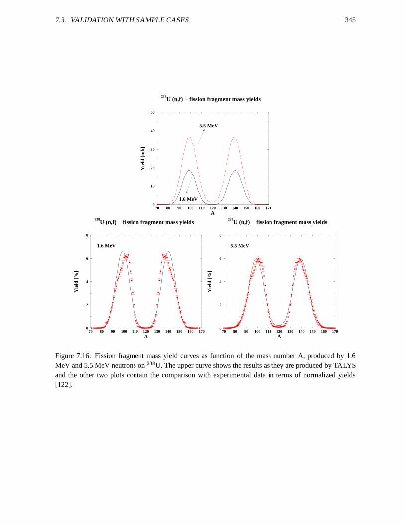
7.3. VALIDATION WITH SAMPLE CASES 345
70 80 90 100 110 120 130 140 150 160 170A
0
10
20
30
40
50
Yie
ld [m
b]
238U (n,f) − fission fragment mass yields
5.5 MeV
1.6 MeV
70 80 90 100 110 120 130 140 150 160 170A
0
2
4
6
8
Yie
ld [%
]
238U (n,f) − fission fragment mass yields
1.6 MeV
70 80 90 100 110 120 130 140 150 160 170A
0
2
4
6
8
Yie
ld [%
]
238U (n,f) − fission fragment mass yields
5.5 MeV
Figure 7.16: Fission fragment mass yield curves as functionof the mass number A, produced by 1.6MeV and 5.5 MeV neutrons on238U. The upper curve shows the results as they are produced by TALYSand the other two plots contain the comparison with experimental data in terms of normalized yields[122].
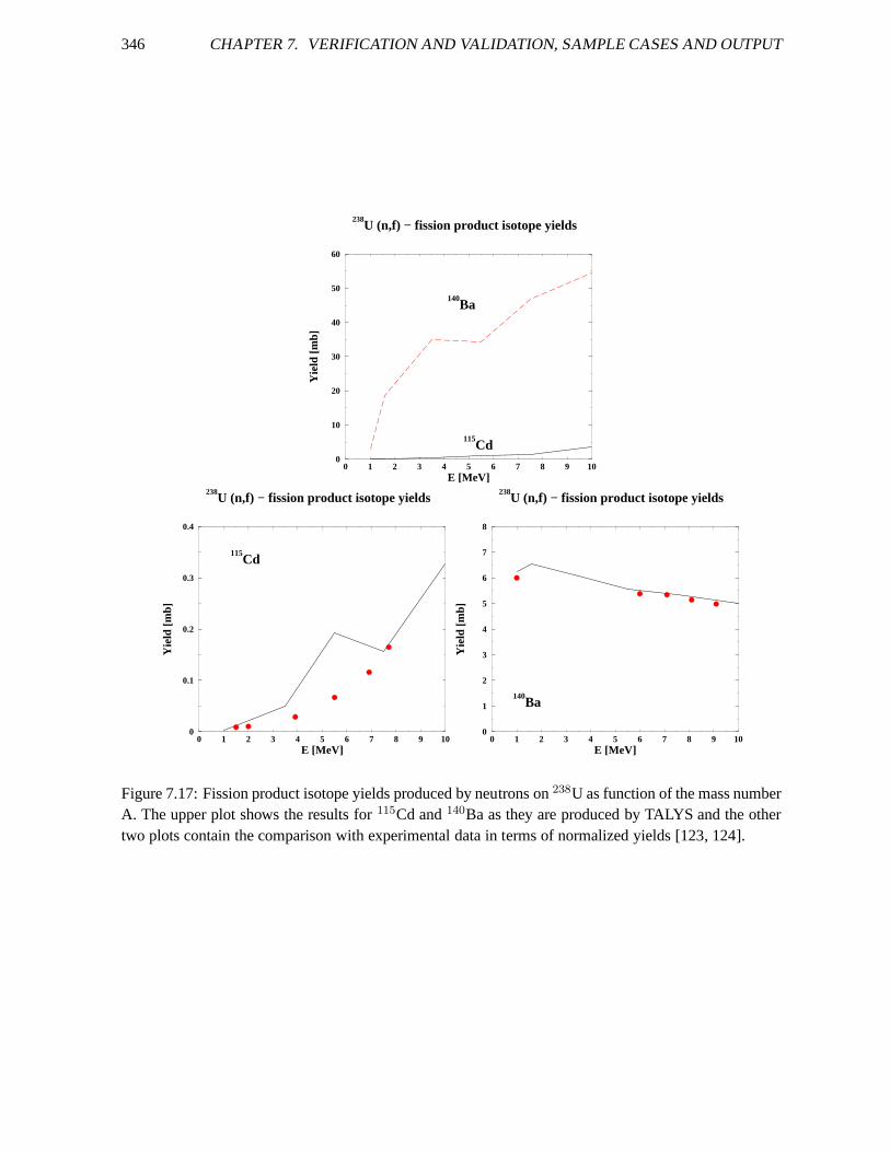
346 CHAPTER 7. VERIFICATION AND VALIDATION, SAMPLE CASES AND OUTPUT
0 1 2 3 4 5 6 7 8 9 10E [MeV]
0
10
20
30
40
50
60
Yie
ld [m
b]
238U (n,f) − fission product isotope yields
140Ba
115Cd
0 1 2 3 4 5 6 7 8 9 10E [MeV]
0
0.1
0.2
0.3
0.4
Yie
ld [m
b]
238U (n,f) − fission product isotope yields
115Cd
0 1 2 3 4 5 6 7 8 9 10E [MeV]
0
1
2
3
4
5
6
7
8
Yie
ld [m
b]
238U (n,f) − fission product isotope yields
140Ba
Figure 7.17: Fission product isotope yields produced by neutrons on238U as function of the mass numberA. The upper plot shows the results for115Cd and140Ba as they are produced by TALYS and the othertwo plots contain the comparison with experimental data in terms of normalized yields [123, 124].
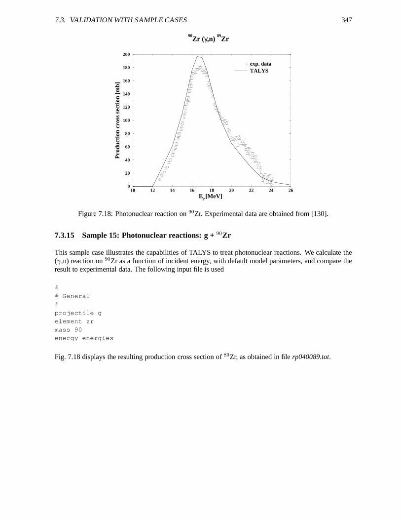
7.3. VALIDATION WITH SAMPLE CASES 347
10 12 14 16 18 20 22 24 26Eγ [MeV]
0
20
40
60
80
100
120
140
160
180
200
Pro
duct
ion
cros
s se
ctio
n [m
b]
90Zr ( γ,n)
89Zr
exp. dataTALYS
Figure 7.18: Photonuclear reaction on90Zr. Experimental data are obtained from [130].
7.3.15 Sample 15: Photonuclear reactions: g +90Zr
This sample case illustrates the capabilities of TALYS to treat photonuclear reactions. We calculate the(γ,n) reaction on90Zr as a function of incident energy, with default model parameters, and compare theresult to experimental data. The following input file is used
## General#projectile gelement zrmass 90energy energies
Fig. 7.18 displays the resulting production cross section of 89Zr, as obtained in filerp040089.tot.
348 CHAPTER 7. VERIFICATION AND VALIDATION, SAMPLE CASES AND OUTPUT
7.3.16 Sample 16: Different optical models : n +120Sn
To demonstrate the variety of optical models that we have added recently to TALYS, we include a samplecase in which 4 OMP’s for neutrons on120Sn are compared. The results are given in Fig. 7.19 for thetotal cross section and in Fig.7.20 for the total inelastic cross section.
Case 16a: Koning-Delaroche local potential
The input file is
## General#projectile nelement snmass 120energy energies
This is the default calculation: TALYS will find a local OMP inthe structure database and will use it.
Case 16b: Koning-Delaroche global potential
The input file is
## General#projectile nelement snmass 120energy energies## Parameters#localomp n
Case 16c: Koning-Delaroche local dispersive potential
The input file is
## General#projectile nelement sn
7.3. VALIDATION WITH SAMPLE CASES 349
mass 120energy energies## Parameters#dispersion y
Case 16d: Bauge-Delaroche JLM potential
The input file is
## General#projectile nelement snmass 120energy energies## Parameters#jlmomp y
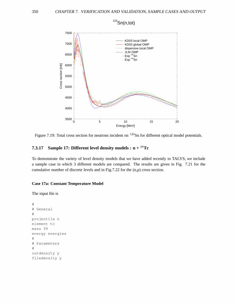
350 CHAPTER 7. VERIFICATION AND VALIDATION, SAMPLE CASES AND OUTPUT
0 5 10 15 20Energy [MeV]
3500
4000
4500
5000
5500
6000
6500
7000
7500
Cro
ss s
ectio
n [m
b]
120Sn(n,tot)
KD03 local OMPKD03 global OMPdispersive local OMPJLM OMPExp
natSn
Exp nat
Sn
Figure 7.19: Total cross section for neutrons incident on120Sn for different optical model potentials.
7.3.17 Sample 17: Different level density models : n +99Tc
To demonstrate the variety of level density models that we have added recently to TALYS, we includea sample case in which 3 different models are compared. The results are given in Fig. 7.21 for thecumulative number of discrete levels and in Fig.7.22 for the(n,p) cross section.
Case 17a: Constant Temperature Model
The input file is
## General#projectile nelement tcmass 99energy energies## Parameters#outdensity yfiledensity y
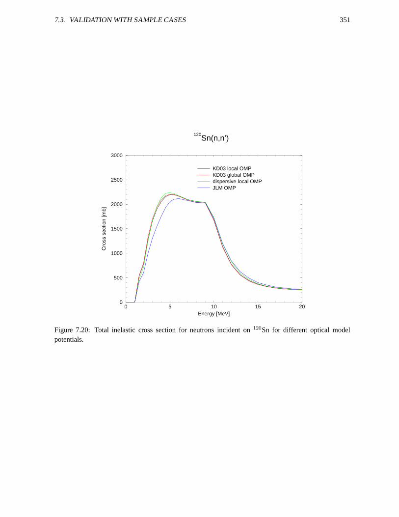
7.3. VALIDATION WITH SAMPLE CASES 351
0 5 10 15 20Energy [MeV]
0
500
1000
1500
2000
2500
3000
Cro
ss s
ectio
n [m
b]
120Sn(n,n’)
KD03 local OMPKD03 global OMPdispersive local OMPJLM OMP
Figure 7.20: Total inelastic cross section for neutrons incident on 120Sn for different optical modelpotentials.
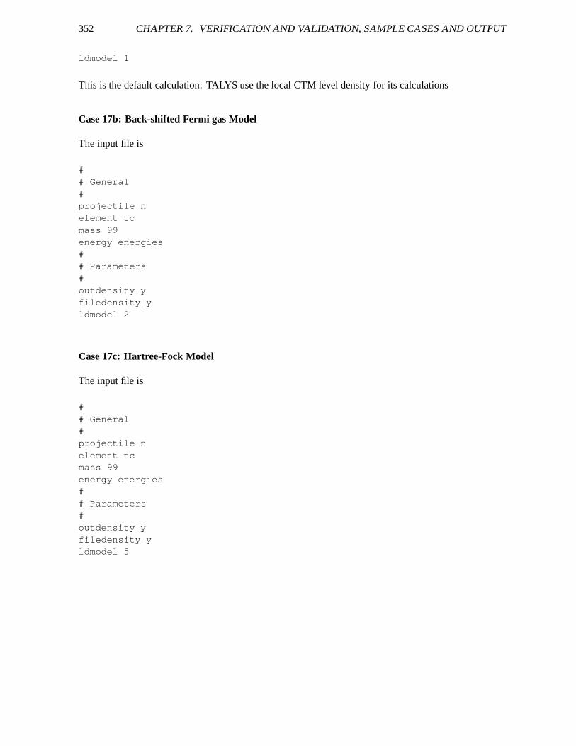
352 CHAPTER 7. VERIFICATION AND VALIDATION, SAMPLE CASES AND OUTPUT
ldmodel 1
This is the default calculation: TALYS use the local CTM level density for its calculations
Case 17b: Back-shifted Fermi gas Model
The input file is
## General#projectile nelement tcmass 99energy energies## Parameters#outdensity yfiledensity yldmodel 2
Case 17c: Hartree-Fock Model
The input file is
## General#projectile nelement tcmass 99energy energies## Parameters#outdensity yfiledensity yldmodel 5
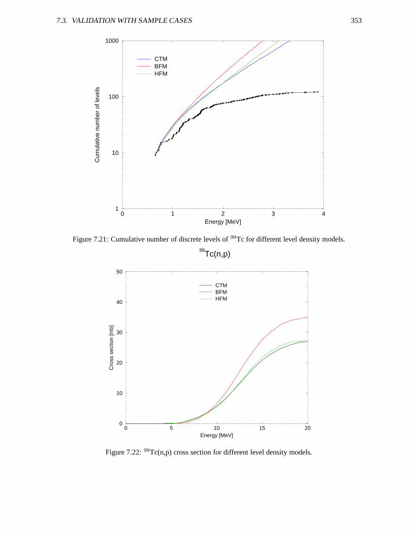
7.3. VALIDATION WITH SAMPLE CASES 353
0 1 2 3 4Energy [MeV]
1
10
100
1000
Cum
ulat
ive
num
ber
of le
vels
CTMBFMHFM
Figure 7.21: Cumulative number of discrete levels of99Tc for different level density models.
0 5 10 15 20Energy [MeV]
0
10
20
30
40
50
Cro
ss s
ectio
n [m
b]
99Tc(n,p)
CTMBFMHFM
Figure 7.22:99Tc(n,p) cross section for different level density models.
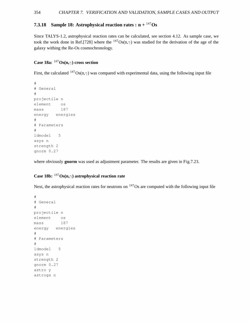
354 CHAPTER 7. VERIFICATION AND VALIDATION, SAMPLE CASES AND OUTPUT
7.3.18 Sample 18: Astrophysical reaction rates : n +187Os
Since TALYS-1.2, astrophysical reaction rates can be calculated, see section 4.12. As sample case, wetook the work done in Ref.[728] where the187Os(n,γ) was studied for the derivation of the age of thegalaxy withing the Re-Os cosmochronology.
Case 18a:187Os(n,γ) cross section
First, the calculated187Os(n,γ) was compared with experimental data, using the following input file
## General#projectile nelement osmass 187energy energies## Parameters#ldmodel 5asys nstrength 2gnorm 0.27
where obviouslygnorm was used as adjustment parameter. The results are given in Fig.7.23.
Case 18b:187Os(n,γ) astrophysical reaction rate
Next, the astrophysical reaction rates for neutrons on187Os are computed with the following input file
## General#projectile nelement osmass 187energy energies## Parameters#ldmodel 5asys nstrength 2gnorm 0.27astro yastrogs n
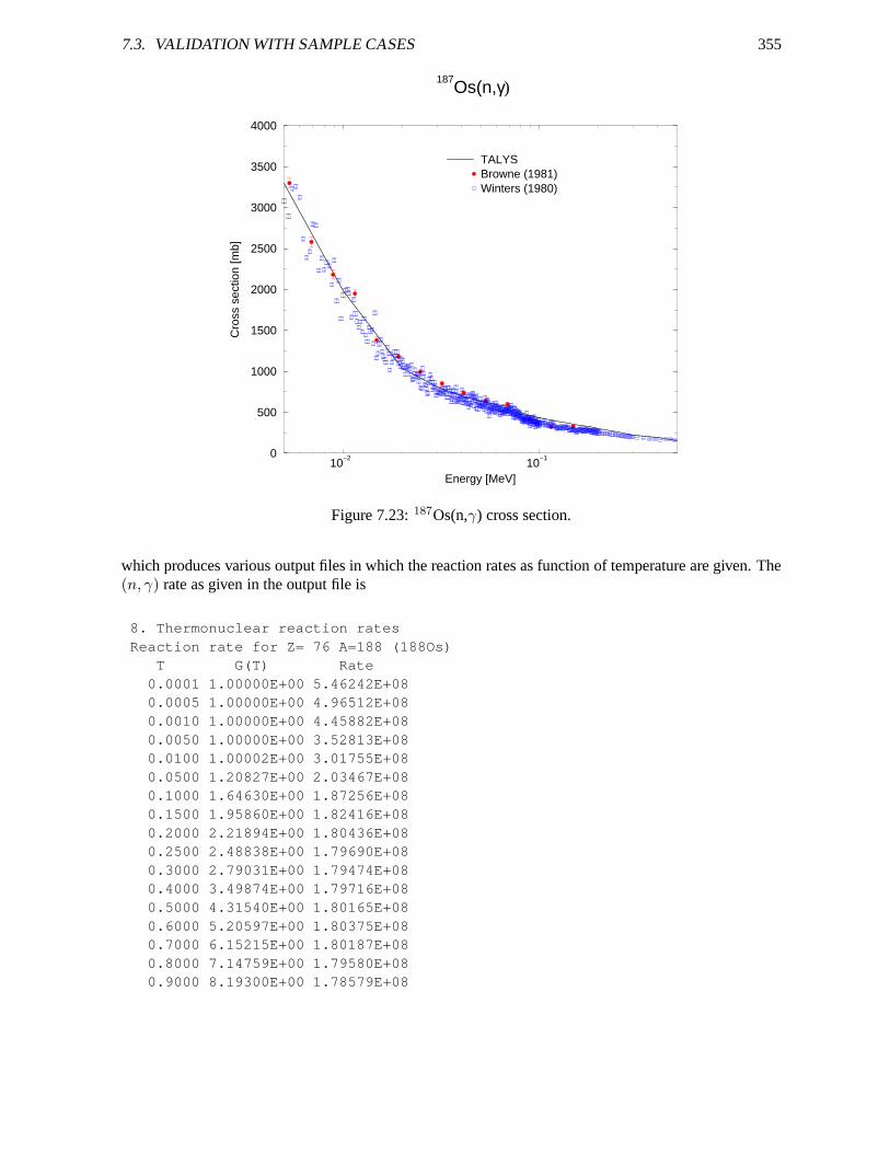
7.3. VALIDATION WITH SAMPLE CASES 355
10−2
10−1
Energy [MeV]
0
500
1000
1500
2000
2500
3000
3500
4000
Cro
ss s
ectio
n [m
b]
187Os(n,γ)
TALYSBrowne (1981)Winters (1980)
Figure 7.23:187Os(n,γ) cross section.
which produces various output files in which the reaction rates as function of temperature are given. The(n, γ) rate as given in the output file is
8. Thermonuclear reaction ratesReaction rate for Z= 76 A=188 (188Os)
T G(T) Rate0.0001 1.00000E+00 5.46242E+080.0005 1.00000E+00 4.96512E+080.0010 1.00000E+00 4.45882E+080.0050 1.00000E+00 3.52813E+080.0100 1.00002E+00 3.01755E+080.0500 1.20827E+00 2.03467E+080.1000 1.64630E+00 1.87256E+080.1500 1.95860E+00 1.82416E+080.2000 2.21894E+00 1.80436E+080.2500 2.48838E+00 1.79690E+080.3000 2.79031E+00 1.79474E+080.4000 3.49874E+00 1.79716E+080.5000 4.31540E+00 1.80165E+080.6000 5.20597E+00 1.80375E+080.7000 6.15215E+00 1.80187E+080.8000 7.14759E+00 1.79580E+080.9000 8.19300E+00 1.78579E+08

356 CHAPTER 7. VERIFICATION AND VALIDATION, SAMPLE CASES AND OUTPUT
1.0000 9.29313E+00 1.77221E+08.....................................
The same numbers can be found in the separate fileastrorate.g. In astrorate.totthe rates for all reactionscan be found.
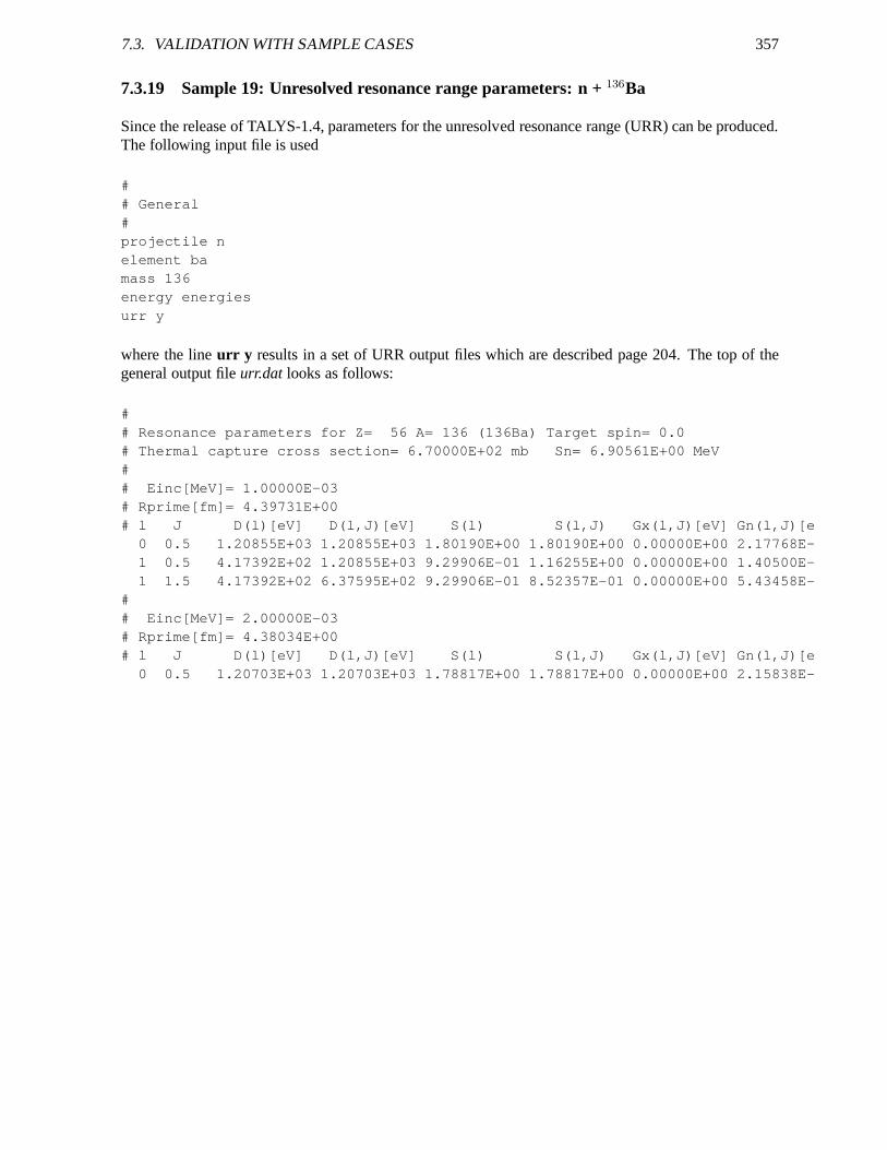
7.3. VALIDATION WITH SAMPLE CASES 357
7.3.19 Sample 19: Unresolved resonance range parameters: n+ 136Ba
Since the release of TALYS-1.4, parameters for the unresolved resonance range (URR) can be produced.The following input file is used
## General#projectile nelement bamass 136energy energiesurr y
where the lineurr y results in a set of URR output files which are described page 204. The top of thegeneral output fileurr.dat looks as follows:
## Resonance parameters for Z= 56 A= 136 (136Ba) Target spin= 0 .0# Thermal capture cross section= 6.70000E+02 mb Sn= 6.90561 E+00 MeV## Einc[MeV]= 1.00000E-03# Rprime[fm]= 4.39731E+00# l J D(l)[eV] D(l,J)[eV] S(l) S(l,J) Gx(l,J)[eV] Gn(l,J)[e
0 0.5 1.20855E+03 1.20855E+03 1.80190E+00 1.80190E+00 0.0 0000E+00 2.17768E-1 0.5 4.17392E+02 1.20855E+03 9.29906E-01 1.16255E+00 0.0 0000E+00 1.40500E-1 1.5 4.17392E+02 6.37595E+02 9.29906E-01 8.52357E-01 0.0 0000E+00 5.43458E-
## Einc[MeV]= 2.00000E-03# Rprime[fm]= 4.38034E+00# l J D(l)[eV] D(l,J)[eV] S(l) S(l,J) Gx(l,J)[eV] Gn(l,J)[e
0 0.5 1.20703E+03 1.20703E+03 1.78817E+00 1.78817E+00 0.0 0000E+00 2.15838E-
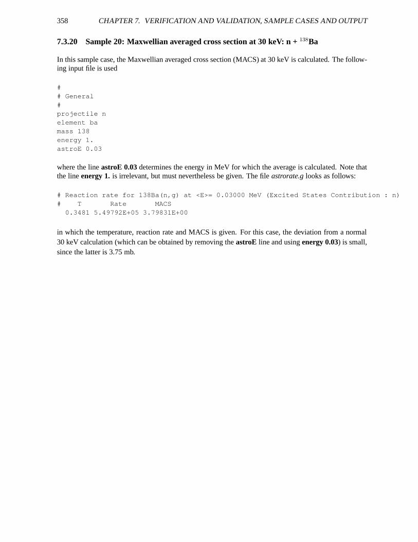
358 CHAPTER 7. VERIFICATION AND VALIDATION, SAMPLE CASES AND OUTPUT
7.3.20 Sample 20: Maxwellian averaged cross section at 30 keV: n + 138Ba
In this sample case, the Maxwellian averaged cross section (MACS) at 30 keV is calculated. The follow-ing input file is used
## General#projectile nelement bamass 138energy 1.astroE 0.03
where the lineastroE 0.03determines the energy in MeV for which the average is calculated. Note thatthe lineenergy 1.is irrelevant, but must nevertheless be given. The fileastrorate.glooks as follows:
# Reaction rate for 138Ba(n,g) at <E>= 0.03000 MeV (Excited S tates Contribution : n)# T Rate MACS
0.3481 5.49792E+05 3.79831E+00
in which the temperature, reaction rate and MACS is given. For this case, the deviation from a normal30 keV calculation (which can be obtained by removing theastroE line and usingenergy 0.03) is small,since the latter is 3.75 mb.
7.3. VALIDATION WITH SAMPLE CASES 359
7.3.21 Sample 21: Medical isotope production with p +100Mo
In this sample case, the activity of all the produced isotopes from the reaction p +100Mo are given, for a150µA proton accelerator, as a function of time. The following input file is used
## General#projectile pelement Momass 100energy 8. 30. 0.5## Spherical OMP#spherical y## Medical isotope production#production yIbeam 0.15Ebeam 24.Eback 10.
Note the use of theenergy keyword, available since TALYS-1.6: Cross sections are calculated for in-cident energies between 8 and 30 MeV with 0.5 MeV energy steps. The keywordproduction y meansthat activities of all radioactive products as a function ofbombarding and/or decay time will be producedin tables. The incident energy of the particle beam is 24 MeV,and the required thickness of the target(which is given in the output) is such that at the back of the target the energy is 10 MeV. Other keywordsrelevant for isotope production, such asTcool, see page 248,Tirrad , see page 248,rho, see page 247,area, see page 246,radiounit , see page 247,yieldunit , see page 247, have their default values in thissample case.
We like to point out an efficient option for medical isotope calculations. Suppose one is interestedin varying several accelerator options, such as e.g.Ebeam. Once the first calculation, like the samplecase above, has been done, one may rerun that case and add the extra line reaction n to the input file.Then, TALYS will not redo the nuclear reaction calculations, but use the variousrpZZZAAA.tot, etc.cross section output files which are already available in thework directory. Obviously,Ebeam andEback must always fall inside the energy grid for which the cross sections are calculated, in this casebetween 8 and 30 MeV.
The tail of the standard output files contains some general parameters:
Summary of isotope production
Maximal irradiation time : 0 years 1 days 0 hours 0 minutes 0 se condsCooling time : 0 years 1 days 0 hours 0 minutes 0 secondsEnergy range : 24.000 --> 10.000 MeV
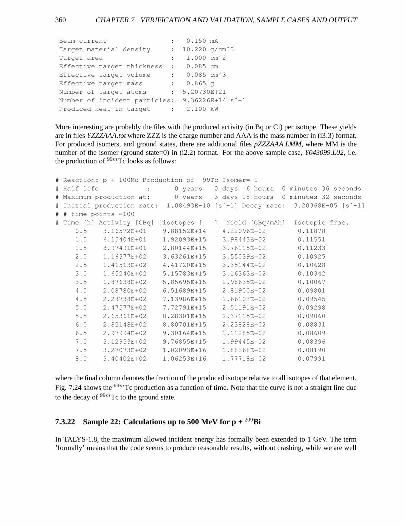
360 CHAPTER 7. VERIFICATION AND VALIDATION, SAMPLE CASES AND OUTPUT
Beam current : 0.150 mATarget material density : 10.220 g/cmˆ3Target area : 1.000 cmˆ2Effective target thickness : 0.085 cmEffective target volume : 0.085 cmˆ3Effective target mass : 0.865 gNumber of target atoms : 5.20730E+21Number of incident particles: 9.36226E+14 sˆ-1Produced heat in target : 2.100 kW
More interesting are probably the files with the produced activity (in Bq or Ci) per isotope. These yieldsare in filesYZZZAAA.totwhere ZZZ is the charge number and AAA is the mass number in (i3.3) format.For produced isomers, and ground states, there are additional files pZZZAAA.LMM, where MM is thenumber of the isomer (ground state=0) in (i2.2) format. For the above sample case,Y043099.L02, i.e.the production of99mTc looks as follows:
# Reaction: p + 100Mo Production of 99Tc Isomer= 1# Half life : 0 years 0 days 6 hours 0 minutes 36 seconds# Maximum production at: 0 years 3 days 18 hours 0 minutes 32 se conds# Initial production rate: 1.08493E-10 [sˆ-1] Decay rate: 3 .20368E-05 [sˆ-1]# # time points =100# Time [h] Activity [GBq] #isotopes [ ] Yield [GBq/mAh] Isoto pic frac.
0.5 3.16572E+01 9.88152E+14 4.22096E+02 0.118781.0 6.15404E+01 1.92093E+15 3.98443E+02 0.115511.5 8.97491E+01 2.80144E+15 3.76115E+02 0.112332.0 1.16377E+02 3.63261E+15 3.55039E+02 0.109252.5 1.41513E+02 4.41720E+15 3.35144E+02 0.106283.0 1.65240E+02 5.15783E+15 3.16363E+02 0.103423.5 1.87638E+02 5.85695E+15 2.98635E+02 0.100674.0 2.08780E+02 6.51689E+15 2.81900E+02 0.098014.5 2.28738E+02 7.13986E+15 2.66103E+02 0.095455.0 2.47577E+02 7.72791E+15 2.51191E+02 0.092985.5 2.65361E+02 8.28301E+15 2.37115E+02 0.090606.0 2.82148E+02 8.80701E+15 2.23828E+02 0.088316.5 2.97994E+02 9.30164E+15 2.11285E+02 0.086097.0 3.12953E+02 9.76855E+15 1.99445E+02 0.083967.5 3.27073E+02 1.02093E+16 1.88268E+02 0.081908.0 3.40402E+02 1.06253E+16 1.77718E+02 0.07991
where the final column denotes the fraction of the produced isotope relative to all isotopes of that element.Fig. 7.24 shows the99mTc production as a function of time. Note that the curve is nota straight line dueto the decay of99mTc to the ground state.
7.3.22 Sample 22: Calculations up to 500 MeV for p +209Bi
In TALYS-1.8, the maximum allowed incident energy has formally been extended to 1 GeV. The term’formally’ means that the code seems to produce reasonable results, without crashing, while we are well
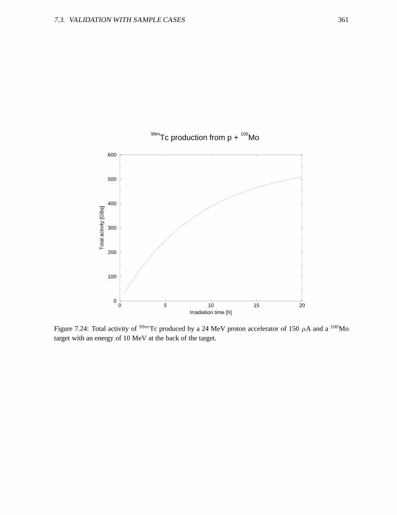
7.3. VALIDATION WITH SAMPLE CASES 361
0 5 10 15 20Irradiation time [h]
0
100
200
300
400
500
600
Tot
al a
ctiv
ity [G
Bq]
99mTc production from p +
100Mo
Figure 7.24: Total activity of99mTc produced by a 24 MeV proton accelerator of 150µA and a100Motarget with an energy of 10 MeV at the back of the target.
362 CHAPTER 7. VERIFICATION AND VALIDATION, SAMPLE CASES AND OUTPUT
aware that the physics beyond about 200 MeV is different fromthat at lower energies. The question is atwhich energy the “low-energy” models will start to fail. To investigate this, the extension to 1 GeV hasbeen made. In this sample case we perform calculations for p +209Bi at 5 different energies,
## General#projectile pelement bimass 209energy 100. 500. 100.bins 60
Here we use the option to give equidistant incident energiesfrom 100 to 500 MeV with steps of 100MeV. All results can be found in the usual files, e.g. the residual production cross sections of204Pb arein rp082204.tot, which look as follows
# p + 209Bi: Production of 204Pb - Total# Q-value =-4.42737E+00 mass= 203.973043# E-threshold= 4.44871E+00# # energies = 5# E xs1.000E+02 2.81964E+012.000E+02 3.70364E+013.000E+02 4.09552E+014.000E+02 3.84491E+015.000E+02 3.62129E+01
Obviously, the user may extend this case up to 1 GeV and with a finer incident energy grid.
7.3.23 Sample 23: Neutron multiplicities and fission yieldsfor n + 242Pu
TALYS-1.8 contains a partial implementation of the GEF codeby Karl-Heinz Schmidt and Beatriz Ju-rado. Part of GEF has been translated by Vasily Simutkin and Michail Onegin into a Fortran subroutine.In this sample case, the prompt neutron multiplicity as a function of mass,ν(A), number of neutrons,P (ν), and the total average,ν, are calculated, as well as the pre- and post-neutron fissionyields as afunction ofN andA. The following input file is used
## General#projectile nelement Pumass 242energy n0-20.grid## Parameters and models
7.3. VALIDATION WITH SAMPLE CASES 363
#maxrot 2fymodel 2best y## Output#channels yfilechannels yecissave yinccalc yeciscalc ymassdis y# In a second run, you may set# eciscalc n# inccalc n# for time-efficient variations of this input file
Note the comment given at the end of the input file. Note also that a hardwired energy grid is usedthroughn0-20.grid. The prompt average neutron multiplicityν is given in the output filenubar.tot. Fig.7.25 shows a comparison with experimental data and some of the world nuclear data libraries. Fig. 7.26presents the distribution ofν(A) as a function of fission product mass, for an incident energy of 1 MeV.This is given in output filenuA001.000.fis. Fig. 7.27 presents the distribution ofν as a function ofnumber of neutrons, for an incident energy of 1 MeV. This is given in output filePnu001.000.fis.
7.3.24 Sample 24: Local parameter adjustment for n +93Nb
## General#projectile nelement nbmass 93energy 0.2 5. 0.2outomp y## Local parameter adjustment#rvadjust 1.02 1. 3. 2. 1.10avadjust 1.02 1. 3. 2. 0.95
######### OPTICAL MODEL PARAMETERS ##########
neutron on 93Nb
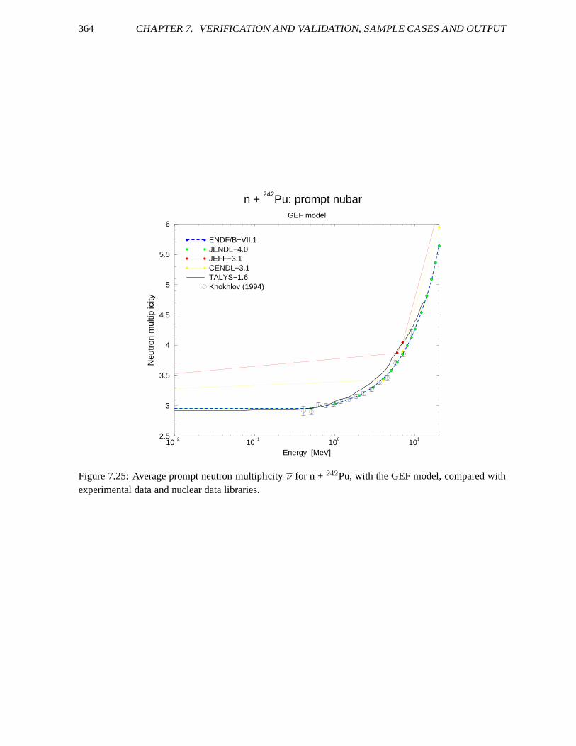
364 CHAPTER 7. VERIFICATION AND VALIDATION, SAMPLE CASES AND OUTPUT
10−2
10−1
100
101
Energy [MeV]
2.5
3
3.5
4
4.5
5
5.5
6
Neu
tron
mul
tiplic
ity
n + 242
Pu: prompt nubarGEF model
ENDF/B−VII.1JENDL−4.0JEFF−3.1CENDL−3.1TALYS−1.6Khokhlov (1994)
Figure 7.25: Average prompt neutron multiplicityν for n + 242Pu, with the GEF model, compared withexperimental data and nuclear data libraries.
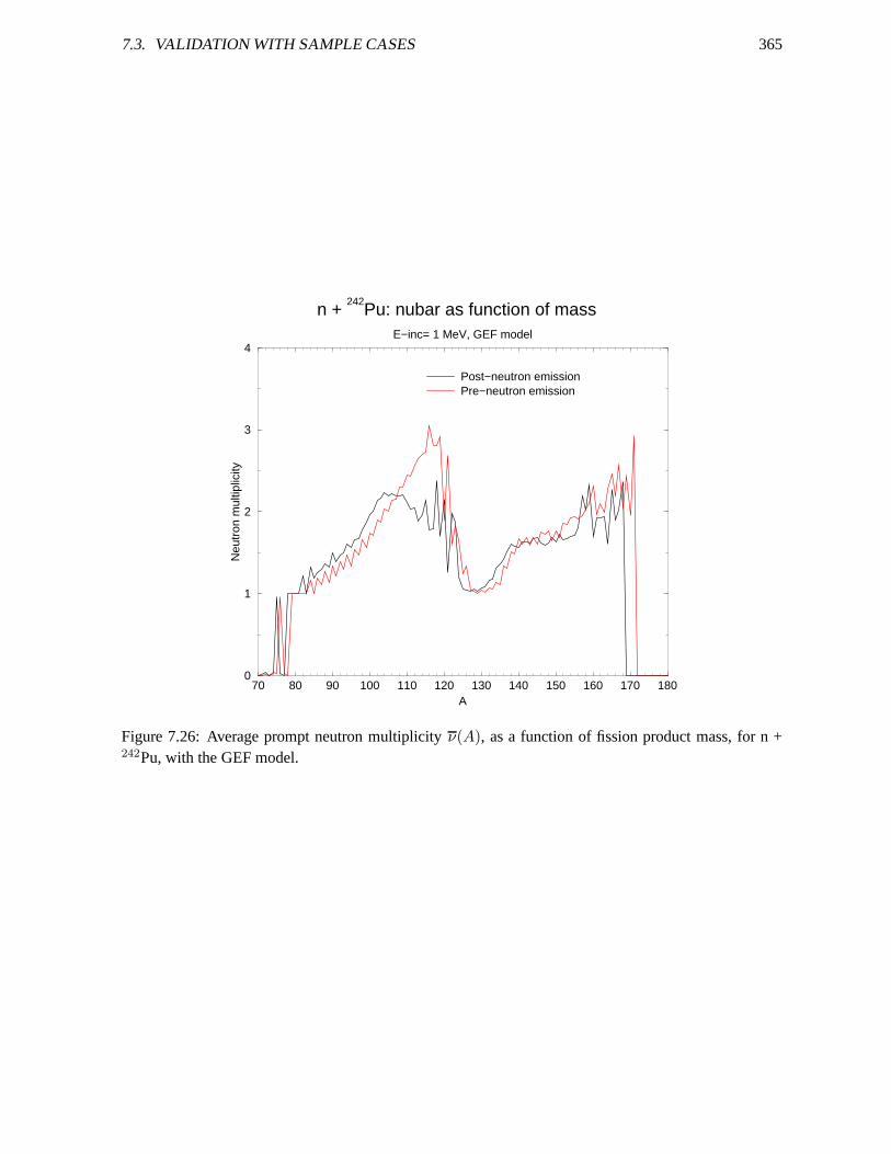
7.3. VALIDATION WITH SAMPLE CASES 365
70 80 90 100 110 120 130 140 150 160 170 180A
0
1
2
3
4
Neu
tron
mul
tiplic
ity
n + 242
Pu: nubar as function of massE−inc= 1 MeV, GEF model
Post−neutron emissionPre−neutron emission
Figure 7.26: Average prompt neutron multiplicityν(A), as a function of fission product mass, for n +242Pu, with the GEF model.
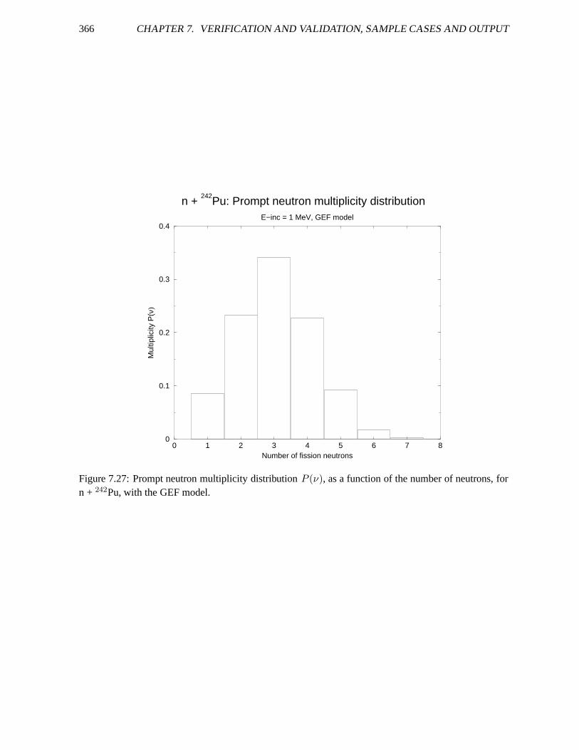
366 CHAPTER 7. VERIFICATION AND VALIDATION, SAMPLE CASES AND OUTPUT
0 1 2 3 4 5 6 7 8Number of fission neutrons
0
0.1
0.2
0.3
0.4
Mul
tiplic
ity P
(ν)
n + 242
Pu: Prompt neutron multiplicity distributionE−inc = 1 MeV, GEF model
Figure 7.27: Prompt neutron multiplicity distributionP (ν), as a function of the number of neutrons, forn + 242Pu, with the GEF model.
7.3. VALIDATION WITH SAMPLE CASES 367
Energy V rv av W rw aw Vd rvd avd Wd rwd
0.001 51.02 1.239 0.676 0.14 1.239 0.676 0.00 1.274 0.534 3.3 2 1.2740.002 51.02 1.239 0.676 0.14 1.239 0.676 0.00 1.274 0.534 3.3 2 1.274
.....................0.910 50.69 1.239 0.676 0.17 1.239 0.676 0.00 1.274 0.534 3.8 0 1.2741.011 50.66 1.239 0.676 0.18 1.239 0.676 0.00 1.274 0.534 3.8 5 1.2741.112 50.62 1.240 0.676 0.18 1.239 0.676 0.00 1.274 0.534 3.9 0 1.2741.213 50.58 1.244 0.675 0.18 1.239 0.676 0.00 1.274 0.534 3.9 5 1.2741.314 50.55 1.257 0.671 0.19 1.239 0.676 0.00 1.274 0.534 4.0 0 1.2741.415 50.51 1.282 0.665 0.19 1.239 0.676 0.00 1.274 0.534 4.0 5 1.2741.516 50.47 1.309 0.657 0.20 1.239 0.676 0.00 1.274 0.534 4.1 0 1.2741.617 50.44 1.331 0.651 0.20 1.239 0.676 0.00 1.274 0.534 4.1 5 1.2741.718 50.40 1.346 0.647 0.20 1.239 0.676 0.00 1.274 0.534 4.2 0 1.2741.820 50.37 1.355 0.645 0.21 1.239 0.676 0.00 1.274 0.534 4.2 4 1.2741.921 50.33 1.360 0.643 0.21 1.239 0.676 0.00 1.274 0.534 4.2 9 1.2742.022 50.29 1.363 0.643 0.22 1.239 0.676 0.00 1.274 0.534 4.3 4 1.2742.224 50.22 1.352 0.646 0.22 1.239 0.676 0.00 1.274 0.534 4.4 3 1.2742.426 50.15 1.323 0.653 0.23 1.239 0.676 0.00 1.274 0.534 4.5 2 1.2742.628 50.08 1.270 0.668 0.24 1.239 0.676 0.00 1.274 0.534 4.6 1 1.2742.830 50.00 1.241 0.676 0.25 1.239 0.676 0.00 1.274 0.534 4.7 0 1.2743.033 49.93 1.239 0.676 0.26 1.239 0.676 0.00 1.274 0.534 4.7 8 1.2743.235 49.86 1.239 0.676 0.27 1.239 0.676 0.00 1.274 0.534 4.8 6 1.2743.437 49.79 1.239 0.676 0.28 1.239 0.676 0.00 1.274 0.534 4.9 5 1.274
.....................
Note that outside 1 and 3 MeV both rv and av have their constantvalues while in between these energiesthe parameters vary according to the prescription given in Section 6.2.12.
7.3.25 Sample 25: Direct neutron capture for n +89Y
For this sample case we use the input file
## General#projectile nelement ymass 89energy n0-5.grid## Parameters#gnorm 0.35racap y
The contribution of the direct capture process can be found in the last column oftotal.tot.
368 CHAPTER 7. VERIFICATION AND VALIDATION, SAMPLE CASES AND OUTPUT
7.3.26 Sample 26: Different alpha-particle optical model potentials: alpha + 165Ho
To demonstrate the variety of (spherical) optical model potentials for alpha-particles available in TALYS,we include a sample case in which 4 OMPs for alpha-particles on 165Ho are compared. The results aregiven in Fig. 7.28 for the (α,n) reaction cross sections within the incident-energy range of most recentmeasured data [24] below the Coulomb barrier.
Case 26a: Watanabe folding approach with Koning-Delarochenucleon potentials
The input file is
## General#projectile aelement Homass 165energy energies## Output#outomp y
where the file energies consists of energies between 7 and 15.5 MeV with 0.5 MeV energy steps, corre-sponding to the energy range of the measured data. This is thedefault calculation. Fig. 7.28 displays theresulting (α,n) reaction cross sections for the target nucleus 165Ho, asobtained in the file rp069168.tot.
Case 26b: McFadden-Satchler [21] potential
The input file, using the alphaomp keyword value of 2, is
## General#projectile aelement Homass 165energy energies## Model#alphaomp 2## Output#outomp y
7.3. VALIDATION WITH SAMPLE CASES 369
Case 26c: Demetriou, Grama and Goriely [22] double folding dispersive potential
The input file, using the alphaomp keyword value of 5, is
## General#projectile aelement Homass 165energy energies## Model#alphaomp 5## Output#outomp y
Case 26d: Avrigeanu et al. [25] potential
The input file, using the alphaomp keyword additional value of 6, is
## General#projectile aelement Homass 165energy energies## Model#alphaomp 6## Output#outomp y
where the file energies consists in addition of energies up to33 MeV corresponding to all energy rangeswhich are considered in Table II of Ref. [25].
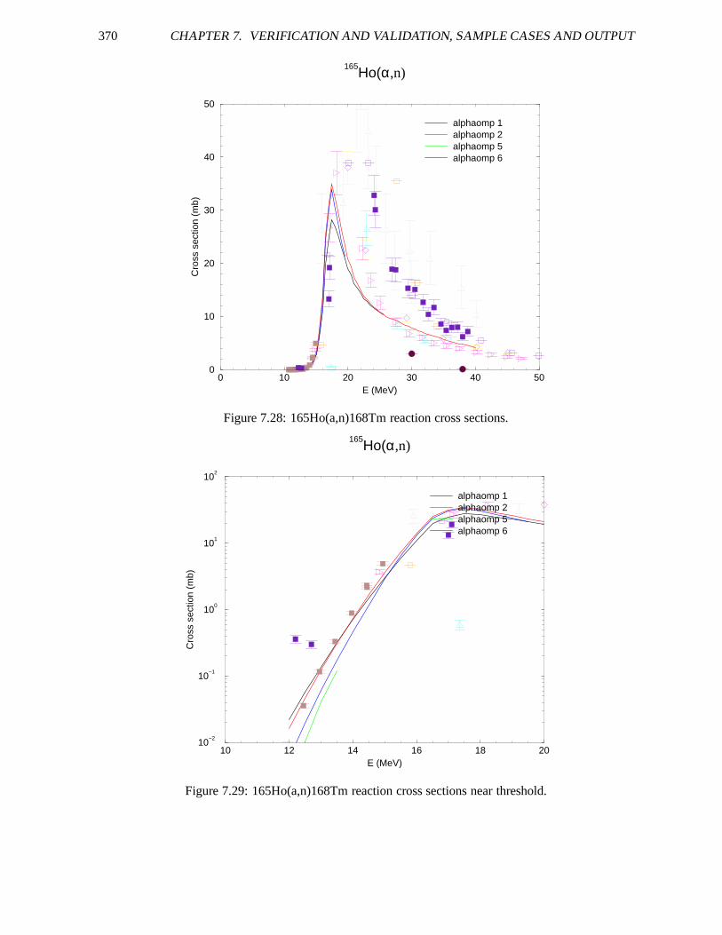
370 CHAPTER 7. VERIFICATION AND VALIDATION, SAMPLE CASES AND OUTPUT
0 10 20 30 40 50E (MeV)
0
10
20
30
40
50
Cro
ss s
ectio
n (m
b)
165Ho(α,n)
alphaomp 1alphaomp 2alphaomp 5alphaomp 6
Figure 7.28: 165Ho(a,n)168Tm reaction cross sections.
10 12 14 16 18 20E (MeV)
10−2
10−1
100
101
102
Cro
ss s
ectio
n (m
b)
165Ho(α,n)
alphaomp 1alphaomp 2alphaomp 5alphaomp 6
Figure 7.29: 165Ho(a,n)168Tm reaction cross sections nearthreshold.
7.3. VALIDATION WITH SAMPLE CASES 371
7.3.27 Sample 27: Low energy resonance data for n +107Ag
TALYS can read in resonance parameters, from various possible sources, and call the RECENT code ofRed Cullen’s PREPRO package, in TALYS included as a subroutine. Low energy pointwise resonancecross sections will then be added to channels like total, elastic, fission and capture.
Case 27a: Resonance input file: Standard
The input file is
## General#projectile nelement Ymass 89energy n0-2.grid## Model#resonance y## Output#channels yfilechannels y
wheren0-2.grid is the built-in TALYS energy grid for neutrons between 0 and 2MeV.
Case 27b: Resonance input file: Temperature broadening
The input file is
## General#projectile nelement Ymass 89energy n0-2.grid## Model#resonance yTres 1200.#
372 CHAPTER 7. VERIFICATION AND VALIDATION, SAMPLE CASES AND OUTPUT
# Output#channels yfilechannels y
Case 27c: Resonance input file: Group structure
The input file is
## General#projectile nelement Ymass 89energy n0-2.grid## Model#resonance ygroup y## Output#channels yfilechannels y
The results are depicted in Fig. 7.30. Note the discontinuity between the end of the resonance range andthe statistical model energy range of TALYS.
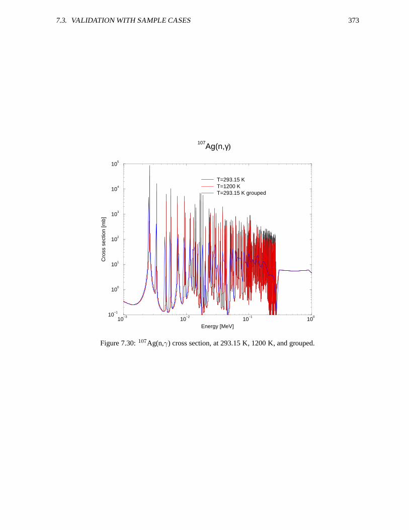
7.3. VALIDATION WITH SAMPLE CASES 373
10−3
10−2
10−1
100
Energy [MeV]
10−1
100
101
102
103
104
105
Cro
ss s
ectio
n [m
b]
107Ag(n,γ)
T=293.15 KT=1200 KT=293.15 K grouped
Figure 7.30:107Ag(n,γ) cross section, at 293.15 K, 1200 K, and grouped.

374 CHAPTER 7. VERIFICATION AND VALIDATION, SAMPLE CASES AND OUTPUT
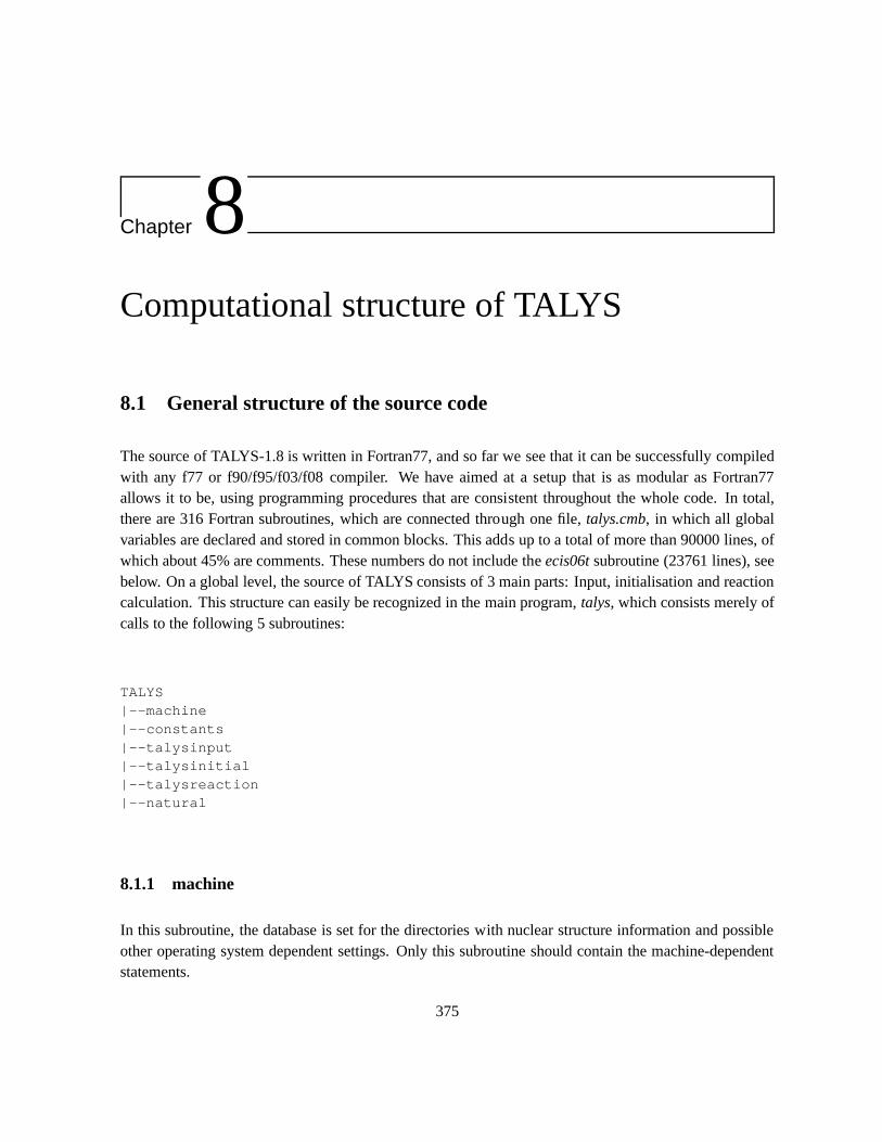
Chapter 8Computational structure of TALYS
8.1 General structure of the source code
The source of TALYS-1.8 is written in Fortran77, and so far wesee that it can be successfully compiledwith any f77 or f90/f95/f03/f08 compiler. We have aimed at a setup that is as modular as Fortran77allows it to be, using programming procedures that are consistent throughout the whole code. In total,there are 316 Fortran subroutines, which are connected through one file,talys.cmb, in which all globalvariables are declared and stored in common blocks. This adds up to a total of more than 90000 lines, ofwhich about 45% are comments. These numbers do not include theecis06tsubroutine (23761 lines), seebelow. On a global level, the source of TALYS consists of 3 main parts: Input, initialisation and reactioncalculation. This structure can easily be recognized in themain program,talys, which consists merely ofcalls to the following 5 subroutines:
TALYS|--machine|--constants|--talysinput|--talysinitial|--talysreaction|--natural
8.1.1 machine
In this subroutine, the database is set for the directories with nuclear structure information and possibleother operating system dependent settings. Only this subroutine should contain the machine-dependentstatements.
375
376 CHAPTER 8. COMPUTATIONAL STRUCTURE OF TALYS
8.1.2 constants
In this subroutine the fundamental constants are defined. First, in the block data moduleconstants0the nuclear symbols and the fundamental properties of particles are defined. Also, the magic numbers,character strings for the two possible parity values and a few fundamental constants are initialized. Fromthese constants, other constants that appear in various reaction formulae are directly defined in subroutineconstants. Examples are2π/~, ~c, 1/π2
~2c2, 1/π2
~3c2 andamu/π2
~3c2. In the initialisation, they are
directly defined in units of MeV and mb. Also, a few other constants are set.
8.1.3 talysinput
Subroutine for the user input of keywords and their defaults.
8.1.4 talysinitial
Subroutine for the initialisation of nuclear structure andother basic parameters.
8.1.5 talysreaction
Subroutine with reaction models.
8.1.6 natural
For calculations of reactions on natural elements a fifth subroutine may be called, namely a subroutineto handle natural elements as target. In this subroutine, another loop overtalysinput, talysinitial andtalysreactionis performed, for each isotope of the element.
8.1.7 ecis06t
Another integral part of TALYS that should explicitly be mentioned is Raynal’s multi-disciplinary reac-tion code ECIS-06, which we have included as a subroutine. Itis called several times by TALYS for thecalculation of basic reaction cross sections, angular distributions and transmission coefficients, for eitherspherical or deformed nuclei. To enable the communication between ECIS-06 and the rest of TALYS, afew extra lines were added to the original ECIS code. In the sourceecis06t.four modifications, not morethan 30 lines, can be recognized by the extensionak000000in columns 73-80.
We will now describe the main tasks of the three main subroutines mentioned above. We will startwith the calling sequence of the subroutines, followed by anexplanation of each subroutine. A subroutinewill only be explained the first time it appears in the callingtree. Moreover, if a subtree of subroutineshas already been described before in the text, we put a “>” behind the name of the subroutine, indicatingit can be found in the text above.
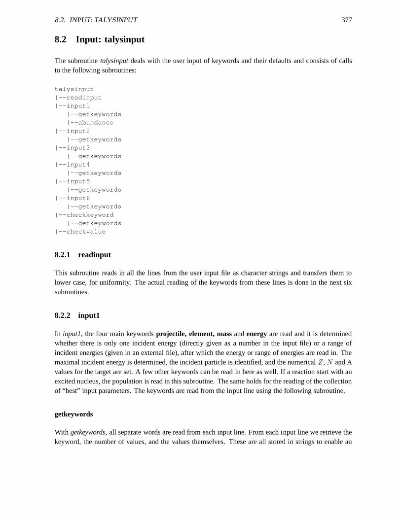
8.2. INPUT: TALYSINPUT 377
8.2 Input: talysinput
The subroutinetalysinputdeals with the user input of keywords and their defaults and consists of callsto the following subroutines:
talysinput|--readinput|--input1
|--getkeywords|--abundance
|--input2|--getkeywords
|--input3|--getkeywords
|--input4|--getkeywords
|--input5|--getkeywords
|--input6|--getkeywords
|--checkkeyword|--getkeywords
|--checkvalue
8.2.1 readinput
This subroutine reads in all the lines from the user input fileas character strings and transfers them tolower case, for uniformity. The actual reading of the keywords from these lines is done in the next sixsubroutines.
8.2.2 input1
In input1, the four main keywordsprojectile, element, massandenergyare read and it is determinedwhether there is only one incident energy (directly given asa number in the input file) or a range ofincident energies (given in an external file), after which the energy or range of energies are read in. Themaximal incident energy is determined, the incident particle is identified, and the numericalZ, N and Avalues for the target are set. A few other keywords can be readin here as well. If a reaction start with anexcited nucleus, the population is read in this subroutine.The same holds for the reading of the collectionof “best” input parameters. The keywords are read from the input line using the following subroutine,
getkeywords
With getkeywords, all separate words are read from each input line. From each input line we retrieve thekeyword, the number of values, and the values themselves. These are all stored in strings to enable an
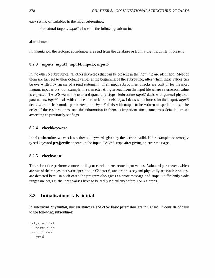
378 CHAPTER 8. COMPUTATIONAL STRUCTURE OF TALYS
easy setting of variables in the input subroutines.
For natural targets,input1also calls the following subroutine,
abundance
In abundance, the isotopic abundances are read from the database or from auser input file, if present.
8.2.3 input2, input3, input4, input5, input6
In the other 5 subroutines, all other keywords that can be present in the input file are identified. Most ofthem are first set to their default values at the beginning of the subroutine, after which these values canbe overwritten by means of a read statement. In all input subroutines, checks are built in for the mostflagrant input errors. For example, if a character string is read from the input file where a numerical valueis expected, TALYS warns the user and gracefully stops. Subroutine input2deals with general physicalparameters,input3deals with choices for nuclear models,input4deals with choices for the output,input5deals with nuclear model parameters, andinput6 deals with output to be written to specific files. Theorder of these subroutines, and the information in them, is important since sometimes defaults are setaccording to previously set flags.
8.2.4 checkkeyword
In this subroutine, we check whether all keywords given by the user are valid. If for example the wronglytyped keywordprojjectile appears in the input, TALYS stops after giving an error message.
8.2.5 checkvalue
This subroutine performs a more intelligent check on erroneous input values. Values of parameters whichare out of the ranges that were specified in Chapter 6, and are thus beyond physically reasonable values,are detected here. In such cases the program also gives an error message and stops. Sufficiently wideranges are set, i.e. the input values have to be really ridiculous before TALYS stops.
8.3 Initialisation: talysinitial
In subroutinetalysinitial, nuclear structure and other basic parameters are initialised. It consists of callsto the following subroutines:
talysinitial|--particles|--nuclides|--grid
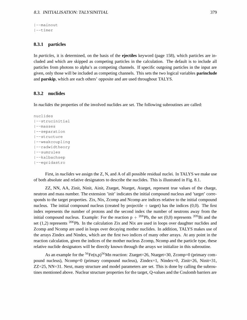
8.3. INITIALISATION: TALYSINITIAL 379
|--mainout|--timer
8.3.1 particles
In particles, it is determined, on the basis of theejectileskeyword (page 158), which particles are in-cluded and which are skipped as competing particles in the calculation. The default is to include allparticles from photons to alpha’s as competing channels. Ifspecific outgoing particles in the input aregiven, only those will be included as competing channels. This sets the two logical variablesparincludeandparskip, which are each others’ opposite and are used throughout TALYS.
8.3.2 nuclides
In nuclidesthe properties of the involved nuclides are set. The following subroutines are called:
nuclides|--strucinitial|--masses|--separation|--structure|--weakcoupling|--radwidtheory|--sumrules|--kalbachsep|--egridastro
First, innuclideswe assign the Z, N, and A of all possible residual nuclei. In TALYS we make useof both absolute and relative designators to describe the nuclides. This is illustrated in Fig. 8.1.
ZZ, NN, AA, Zinit, Ninit, Ainit, Ztarget, Ntarget, Atarget,represent true values of the charge,neutron and mass number. The extension ’init’ indicates theinitial compound nucleus and ’target’ corre-sponds to the target properties. Zix, Nix, Zcomp and Ncomp are indices relative to the initial compoundnucleus. The initial compound nucleus (created by projectile + target) has the indices (0,0). The firstindex represents the number of protons and the second index the number of neutrons away from theinitial compound nucleus. Example: For the reaction p+ 208Pb, the set (0,0) represents209Bi and theset (1,2) represents206Pb. In the calculation Zix and Nix are used in loops over daughter nuclides andZcomp and Ncomp are used in loops over decaying mother nuclides. In addition, TALYS makes use ofthe arrays Zindex and Nindex, which are the first two indices of many other arrays. At any point in thereaction calculation, given the indices of the mother nucleus Zcomp, Ncomp and the particle type, theserelative nuclide designators will be directly known through the arrays we initialize in this subroutine.
As an example for the56Fe(n,p)56Mn reaction: Ztarget=26, Ntarget=30, Zcomp=0 (primary com-pound nucleus), Ncomp=0 (primary compound nucleus), Zindex=1, Nindex=0, Zinit=26, Ninit=31,ZZ=25, NN=31. Next, many structure and model parameters areset. This is done by calling the subrou-tines mentioned above. Nuclear structure properties for the target, Q-values and the Coulomb barriers are
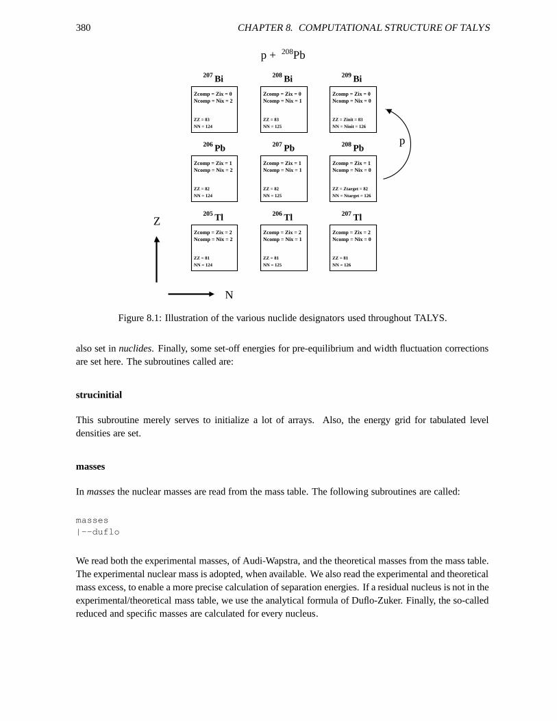
380 CHAPTER 8. COMPUTATIONAL STRUCTURE OF TALYS
Zcomp = Zix = 0Ncomp = Nix = 0
Zcomp = Zix = 0 Zcomp = Zix = 0
Ncomp = Nix = 0
NN = Ntarget = 126
ZZ = Ztarget = 82
ZZ = Zinit = 83
NN = Ninit = 126
ZZ = 83
NN = 125
ZZ = 83
NN = 124
ZZ = 82
NN = 124
ZZ = 82
NN = 125
ZZ = 81
NN = 124
ZZ = 81
NN = 125
ZZ = 81
NN = 126
Ncomp = Nix = 0Zcomp = Zix = 1Zcomp = Zix = 1Zcomp = Zix = 1
Zcomp = Zix = 2 Zcomp = Zix = 2 Zcomp = Zix = 2
Ncomp = Nix = 1
Ncomp = Nix = 1
Ncomp = Nix = 1
Ncomp = Nix = 2
Ncomp = Nix = 2
Ncomp = Nix = 2
Pb208p +
p
Z
N
205Tl Tl206 207Tl
Pb208Pb207Pb206
207Bi 208Bi 209Bi
Figure 8.1: Illustration of the various nuclide designators used throughout TALYS.
also set innuclides. Finally, some set-off energies for pre-equilibrium and width fluctuation correctionsare set here. The subroutines called are:
strucinitial
This subroutine merely serves to initialize a lot of arrays.Also, the energy grid for tabulated leveldensities are set.
masses
In massesthe nuclear masses are read from the mass table. The following subroutines are called:
masses|--duflo
We read both the experimental masses, of Audi-Wapstra, and the theoretical masses from the mass table.The experimental nuclear mass is adopted, when available. We also read the experimental and theoreticalmass excess, to enable a more precise calculation of separation energies. If a residual nucleus is not in theexperimental/theoretical mass table, we use the analytical formula of Duflo-Zuker. Finally, the so-calledreduced and specific masses are calculated for every nucleus.
8.3. INITIALISATION: TALYSINITIAL 381
duflo
Subroutine with the analytical mass formula of Duflo-Zuker.
separation
In separation, the separation energies for all light particles on all involved nuclides are set. For consis-tency, separation energies are always calculated using twonuclear masses of the same type, i.e. bothexperimental or both theoretical. Hence if nucleus A is in the experimental part of the table but nucleusB is not, for both nuclides the theoretical masses are used.
structure
This is a very important subroutine. Instructure, for each nuclide that can be reached in the reactionchain the nuclear structure properties are read in from the nuclear structure and model database. If thenuclear parameters are not available in tabular form they are determined using models or systematics.TALYS is written such that a call tostructureonly occurs when a new nuclide is encountered in thereaction chain. First, it is called for the binary reaction.Later on, inmultiple, the call tostructure isrepeated for nuclides that can be reached in multiple emission. The full calling tree is as follows:
structure|--levels|--gammadecay|--deformpar|--resonancepar|--gammapar|--omppar|--radialtable|--fissionpar|--densitypar|--densitytable|--densitymatch|--phdensitytable|--thermalxs|--partable
levels
In levels, the discrete level information is read. First, for any nuclide, we assign a 0+ ground state toeven-even and odd-odd nuclei and a 1/2+ ground state to odd nuclei. Of course, if there is information inthe discrete level file, this will be overwritten by the full discrete level info. The amount of informationthat is read in is different for the first several levels and higher lying levels. For the discrete levelsthat explicitly appear in the multiple Hauser-Feshbach decay (typically the first 20 levels), we need allinformation, i.e. the energy, spin, parity, lifetime and branching ratio’s. We also read extra levels which
382 CHAPTER 8. COMPUTATIONAL STRUCTURE OF TALYS
are used only for the level density matching problem or for direct reactions (deformation parameters) inthe continuum. The branching ratios and lifetimes are not read for these higher levels. Inlevels, it is alsodetermined whether the target nucleus is in an excited state, in which case the level properties are readin.
gammadecay
For ENDF-6 data files, specific information on gamma-ray branching ratios, namely the cumulated fluxoriginating from a starting level, needs to be handled. Thisis performed ingammadecay.
deformpar
In deformpar, the deformation parameters or deformation lengths are read, together with the associatedcoupling scheme for the case of coupled-channels calculations. In the case of vibrational nuclides, simplesystematical formulae are used for the first few excited states if no experimental information is available.Spherical (S), vibrational (V) or rotational (R) coupled-channels calculations are automated. Finally, thedeformation parameter for rotational enhancement of fission barrier level densities is read in from thenuclear structure database.
resonancepar
The experimental values from the resonance parameter file,D0, Γγ , andS0 are read here. A simple sys-tematics forΓγ derived by Kopecky (2002), is provided in the block data module gamdata for nuclidesnot present in the table.
gammapar
In gammapar, the default giant dipole resonance parameters for gamma-ray strength functions are readfrom the database. Also the default values for M1, E1, E2 etc., are set using systematics if no value ispresent in the database [163]. Also, Goriely’s microscopicgamma ray strength functions can be read inthis subroutine.
omppar
The optical model parameters for nucleons are read from the database. If there are no specific parametersfor a nuclide, they are determined by a global optical model for neutrons and protons. Also possible user-supplied input files with optical model parameters are read here.
8.3. INITIALISATION: TALYSINITIAL 383
radialtable
The radial matter densities for protons and neutrons are read from the database, to perform semi-microscopic OMP calculations. Also possible user-supplied input files with radial matter densities areread here.
fissionpar
In fissionpar, the fission barrier parameters are read, using the following subroutines:
fissionpar|--barsierk
|--plegendre|--rldm|--wkb|--rotband|--rotclass2
Several databases with fission barrier parameters can be read. There are also calls to two subroutines,barsierk and rldm, which provide systematical predictions for fission barrier parameters from Sierk’smodel and the rotating liquid drop model, respectively. As usual, it is also possible to overrule theseparameters with choices from the user input. Iffismodel 1, also the head band states and possible class IIstates are read in this subroutine. Iffismodel 5, the WKB approximation as implemented inwkb.fis used.Finally, rotational bands are built on transition and classII states. Note that next to the chosen fissionmodel (fismodel), there is always an alternative fission model (fismodelalt) which comes into play iffission parameters for the first choice model are not available.
barsierk
Using the rotating finite range model, the l-dependent fission barrier heights are estimated with A.J.Sierk’s method. This subroutine returns the fission barrierheight in MeV. It is based on calculationsusing yukawa-plus-exponential double folded nuclear energy, exact Couloumb diffuseness corrections,and diffuse-matter moments of inertia [103]. The implementation is analogous to the subroutine ”asierk”written by A.J. Sierk (LANL, 1984). This subroutine makes use of the block data modulefisdata.
plegendre
This function calculates the Legendre polynomial.
rldm
Using the rotating liquid drop model [104], the fission barrier heights are estimated. This subroutinereturns the fission barrier height in MeV and is based on the subroutine FISROT incorporated in ALICE-
384 CHAPTER 8. COMPUTATIONAL STRUCTURE OF TALYS
91 [3]. This subroutine makes use of the block data modulefisdata.
wkb
This subroutines computes fission transmission coefficients according to the WKB approximation. Thesubroutine itself calls various other subroutines and functions.
rotband
Here, the rotational bands are built from the head band transition states, for fission calculations.
rotclass2
Here, the rotational bands are built from the class II states. For this, the maximum energy of class IIstates is first determined.
densitypar
In densitypar, parameters for the level density are set, or read from the database. The following subrou-tines are called:
densitypar|--mliquid1|--mliquid2
TheNL andNU of the discrete level region where the level density should match are read or set. Nextthe spin cut-off parameter for the discrete energy region isdetermined. All parameters of the Ignatyukformula are determined, either from systematics or from mutual relations, for the level density modelunder consideration. Pairing energies and, for the generalized superfluid model, critical functions that donot depend on energy, are set. There are many input possibilities for the energy-dependent level densityparameter of the Ignatyuk formula. The required parametersare alev, alimit, gammald and deltaW. TheIgnatyuk formula implies that these parameters can notall be given at the same time in the input file, or ina table. All possibilities are handled in this subroutine. Also, the single-particle state density parametersare set.
mliquid1
Function to calculate the Myers-Swiatecki liquid drop massfor spherical nuclei.
mliquid2
Function to calculate the Goriely liquid drop mass for spherical nuclei.
8.3. INITIALISATION: TALYSINITIAL 385
densitytable
This subroutine reads in microscopic tabulated level densities.
phdensitytable
This subroutine reads in microscopic tabulated particle-hole level densities.
densitymatch
The following subroutines are called:
densitymatch|--ignatyuk|--colenhance|--fermi|--matching|--pol1|--dtheory
In densitymatch, the matching levels for the temperature and Fermi gas leveldensities are determined,and the level density matching problem is solved for both ground-state level densities and level densitieson fission barriers. The matching problem is solved by calling matching.
ignatyuk
The level density parameter as function of excitation energy is calculated here.
colenhance
In colenhance, the collective (vibrational and rotational) enhancementfor fission level densities is cal-culated. Here, a distinction is made between (a)colenhance n: collective effects for the ground stateare included implicitly in the intrinsic level density, andcollective effects on the barrier are determinedrelative to the ground state, and (b)colenhance y: both ground state and barrier collective effects areincluded explicitly. The calling tree is:
colenhance|--ignatyuk
fermi
In fermi, the Fermi gas level density is calculated. The calling treeis:
386 CHAPTER 8. COMPUTATIONAL STRUCTURE OF TALYS
fermi|--spincut
spincut
In spincut, the spin cut-off parameter is calculated. Above the matching energy, this is done by an energy-dependent systematical formula. Below the matching energy, the value for the spin cut-off parameter isinterpolated from the value at the continuum energy and the value from the discrete energy region. Forthe generalized superfluid model, the spin cut-off parameter is related to its value at the critical energy.
matching
In matching, the matching problem of Eq. (4.271) is solved. First, we determine the possible region ofthe roots of the equation, then we determine the number of solutions and finally we choose the solutionfor our problem. The calling tree is:
matching|--ignatyuk|--zbrak|--rtbis|--match
|--pol1
zbrak
This subroutine finds the region in which the matching equation has a root (“bracketing” a function).
rtbis
This function finds the roots of a function.
match
This function represents Eq. (4.271).
pol1
Subroutine for interpolation of first order.
8.3. INITIALISATION: TALYSINITIAL 387
dtheory
Subroutine to calculate the theoretical average resonancespacing from the level density. The followingsubroutines are called:
dtheory|--levels|--density
density
This is the function for the level density. It is calculated as a function of the excitation energy, spin,parity, fission barrier and model identifier. On the basis ofldmodel, the level density model is chosen.The following subroutines are called:
density|--ignatyuk|--densitytot|--spindis|--locate
densitytot
This is the function for the total level density. It is calculated as a function of the excitation energy,fission barrier and model identifier. On the basis ofldmodel, the level density model is chosen. Thefollowing subroutines are called:
densitytot|--ignatyuk|--colenhance >|--gilcam
|--fermi >|--bsfgmodel
|--fermi >|--spincut >
|--superfluid|--fermi >|--spincut >
|--locate
spindis
In spindis, the Wigner spin distribution is calculated. The calling tree is:
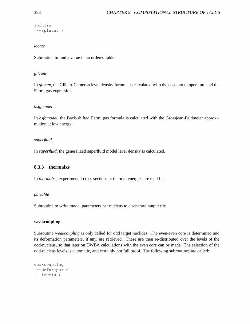
388 CHAPTER 8. COMPUTATIONAL STRUCTURE OF TALYS
spindis|--spincut >
locate
Subroutine to find a value in an ordered table.
gilcam
In gilcam, the Gilbert-Cameron level density formula is calculated with the constant temperature and theFermi gas expression.
bsfgmodel
In bsfgmodel, the Back-shifted Fermi gas formula is calculated with the Grossjean-Feldmeier approxi-mation at low energy.
superfluid
In superfluid, the generalized superfluid model level density is calculated.
8.3.3 thermalxs
In thermalxs, experimental cross sections at thermal energies are read in.
partable
Subroutine to write model parameters per nucleus to a separate output file.
weakcoupling
Subroutineweakcouplingis only called for odd target nuclides. The even-even core isdetermined andits deformation parameters, if any, are retrieved. These are then re-distributed over the levels of theodd-nucleus, so that later on DWBA calculations with the even core can be made. The selection of theodd-nucleus levels is automatic, and certainly not full proof. The following subroutines are called:
weakcoupling|--deformpar >|--levels >
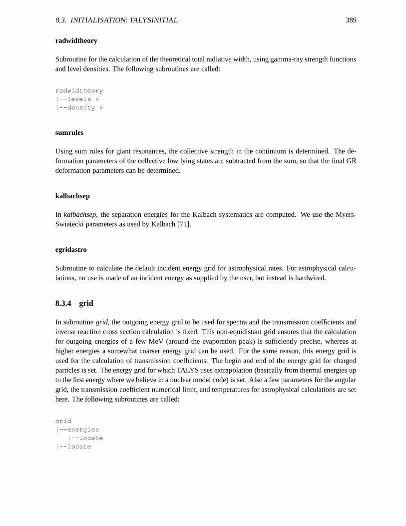
8.3. INITIALISATION: TALYSINITIAL 389
radwidtheory
Subroutine for the calculation of the theoretical total radiative width, using gamma-ray strength functionsand level densities. The following subroutines are called:
radwidtheory|--levels >|--density >
sumrules
Using sum rules for giant resonances, the collective strength in the continuum is determined. The de-formation parameters of the collective low lying states aresubtracted from the sum, so that the final GRdeformation parameters can be determined.
kalbachsep
In kalbachsep, the separation energies for the Kalbach systematics are computed. We use the Myers-Swiatecki parameters as used by Kalbach [71].
egridastro
Subroutine to calculate the default incident energy grid for astrophysical rates. For astrophysical calcu-lations, no use is made of an incident energy as supplied by the user, but instead is hardwired.
8.3.4 grid
In subroutinegrid, the outgoing energy grid to be used for spectra and the transmission coefficients andinverse reaction cross section calculation is fixed. This non-equidistant grid ensures that the calculationfor outgoing energies of a few MeV (around the evaporation peak) is sufficiently precise, whereas athigher energies a somewhat coarser energy grid can be used. For the same reason, this energy grid isused for the calculation of transmission coefficients. The begin and end of the energy grid for chargedparticles is set. The energy grid for which TALYS uses extrapolation (basically from thermal energies upto the first energy where we believe in a nuclear model code) isset. Also a few parameters for the angulargrid, the transmission coefficient numerical limit, and temperatures for astrophysical calculations are sethere. The following subroutines are called:
grid|--energies
|--locate|--locate
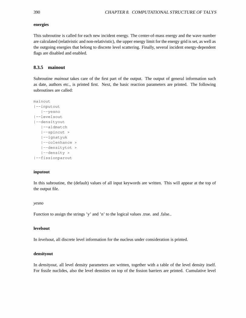
390 CHAPTER 8. COMPUTATIONAL STRUCTURE OF TALYS
energies
This subroutine is called for each new incident energy. The center-of-mass energy and the wave numberare calculated (relativistic and non-relativistic), the upper energy limit for the energy grid is set, as well asthe outgoing energies that belong to discrete level scattering. Finally, several incident energy-dependentflags are disabled and enabled.
8.3.5 mainout
Subroutinemainouttakes care of the first part of the output. The output of general information suchas date, authors etc., is printed first. Next, the basic reaction parameters are printed. The followingsubroutines are called:
mainout|--inputout
|--yesno|--levelsout|--densityout
|--aldmatch|--spincut >|--ignatyuk|--colenhance >|--densitytot >|--density >
|--fissionparout
inputout
In this subroutine, the (default) values of all input keywords are written. This will appear at the top ofthe output file.
yesno
Function to assign the strings ’y’ and ’n’ to the logical values .true. and .false..
levelsout
In levelsout, all discrete level information for the nucleus under consideration is printed.
densityout
In densityout, all level density parameters are written, together with a table of the level density itself.For fissile nuclides, also the level densities on top of the fission barriers are printed. Cumulative level
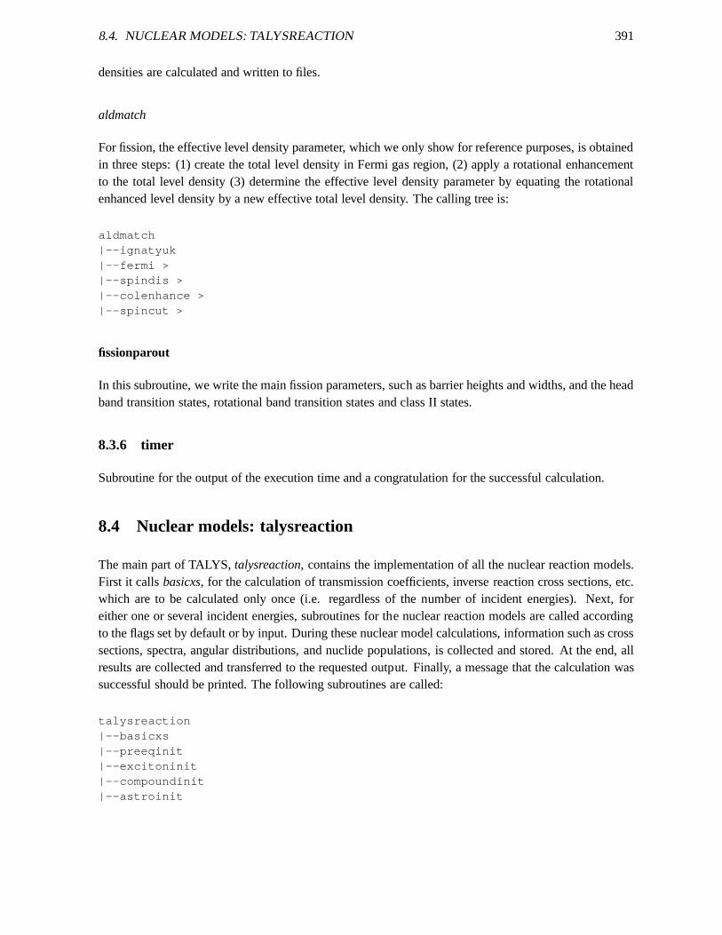
8.4. NUCLEAR MODELS: TALYSREACTION 391
densities are calculated and written to files.
aldmatch
For fission, the effective level density parameter, which weonly show for reference purposes, is obtainedin three steps: (1) create the total level density in Fermi gas region, (2) apply a rotational enhancementto the total level density (3) determine the effective leveldensity parameter by equating the rotationalenhanced level density by a new effective total level density. The calling tree is:
aldmatch|--ignatyuk|--fermi >|--spindis >|--colenhance >|--spincut >
fissionparout
In this subroutine, we write the main fission parameters, such as barrier heights and widths, and the headband transition states, rotational band transition statesand class II states.
8.3.6 timer
Subroutine for the output of the execution time and a congratulation for the successful calculation.
8.4 Nuclear models: talysreaction
The main part of TALYS,talysreaction, contains the implementation of all the nuclear reaction models.First it callsbasicxs, for the calculation of transmission coefficients, inversereaction cross sections, etc.which are to be calculated only once (i.e. regardless of the number of incident energies). Next, foreither one or several incident energies, subroutines for the nuclear reaction models are called accordingto the flags set by default or by input. During these nuclear model calculations, information such as crosssections, spectra, angular distributions, and nuclide populations, is collected and stored. At the end, allresults are collected and transferred to the requested output. Finally, a message that the calculation wassuccessful should be printed. The following subroutines are called:
talysreaction|--basicxs|--preeqinit|--excitoninit|--compoundinit|--astroinit
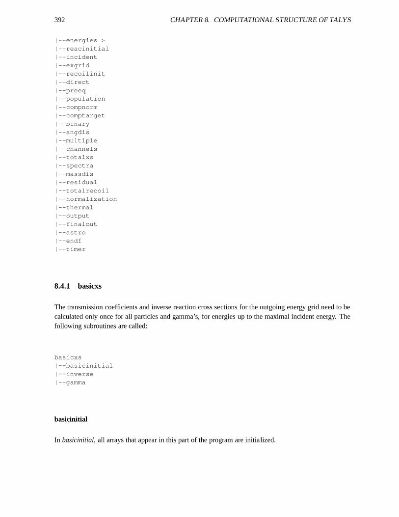
392 CHAPTER 8. COMPUTATIONAL STRUCTURE OF TALYS
|--energies >|--reacinitial|--incident|--exgrid|--recoilinit|--direct|--preeq|--population|--compnorm|--comptarget|--binary|--angdis|--multiple|--channels|--totalxs|--spectra|--massdis|--residual|--totalrecoil|--normalization|--thermal|--output|--finalout|--astro|--endf|--timer
8.4.1 basicxs
The transmission coefficients and inverse reaction cross sections for the outgoing energy grid need to becalculated only once for all particles and gamma’s, for energies up to the maximal incident energy. Thefollowing subroutines are called:
basicxs|--basicinitial|--inverse|--gamma
basicinitial
In basicinitial, all arrays that appear in this part of the program are initialized.
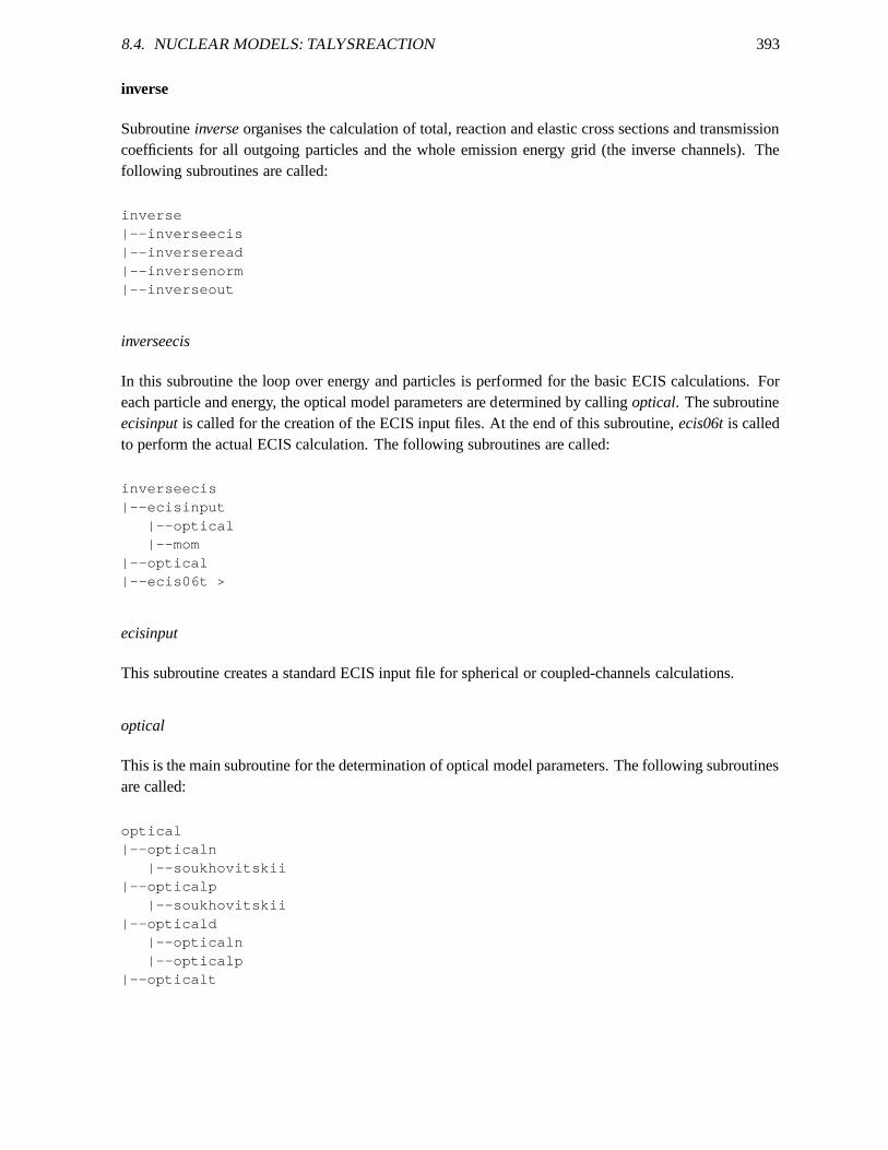
8.4. NUCLEAR MODELS: TALYSREACTION 393
inverse
Subroutineinverseorganises the calculation of total, reaction and elastic cross sections and transmissioncoefficients for all outgoing particles and the whole emission energy grid (the inverse channels). Thefollowing subroutines are called:
inverse|--inverseecis|--inverseread|--inversenorm|--inverseout
inverseecis
In this subroutine the loop over energy and particles is performed for the basic ECIS calculations. Foreach particle and energy, the optical model parameters are determined by callingoptical. The subroutineecisinputis called for the creation of the ECIS input files. At the end ofthis subroutine,ecis06tis calledto perform the actual ECIS calculation. The following subroutines are called:
inverseecis|--ecisinput
|--optical|--mom
|--optical|--ecis06t >
ecisinput
This subroutine creates a standard ECIS input file for spherical or coupled-channels calculations.
optical
This is the main subroutine for the determination of opticalmodel parameters. The following subroutinesare called:
optical|--opticaln
|--soukhovitskii|--opticalp
|--soukhovitskii|--opticald
|--opticaln|--opticalp
|--opticalt
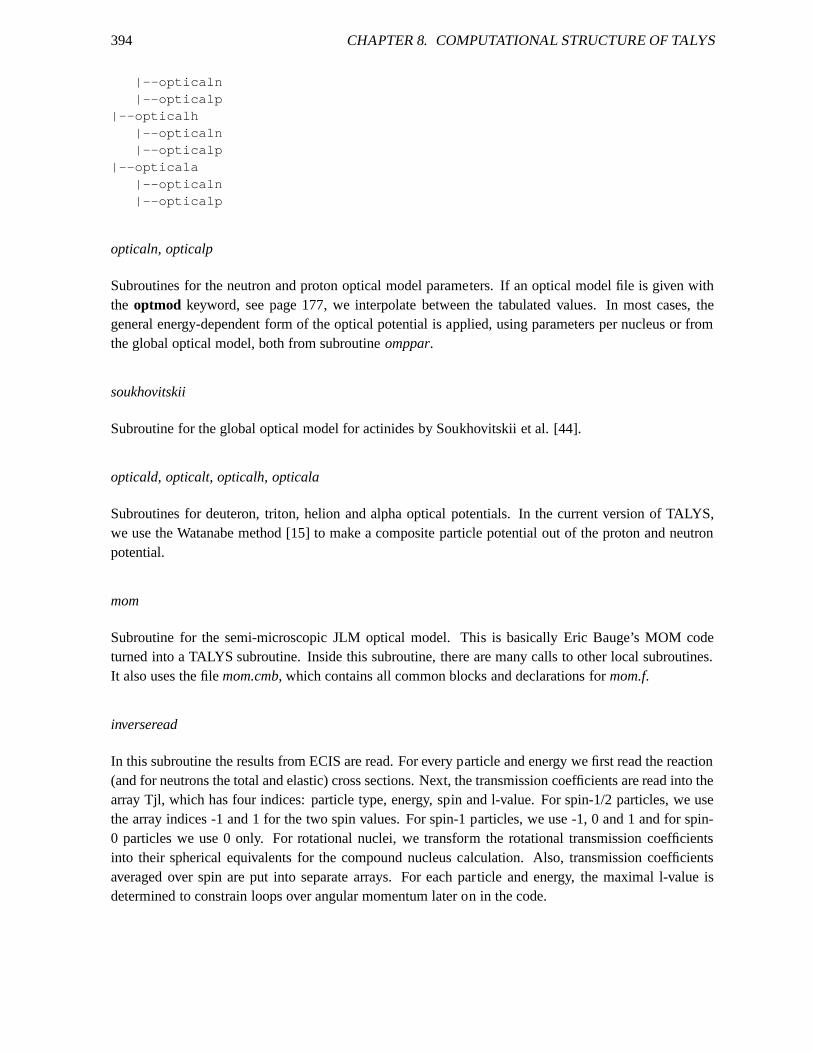
394 CHAPTER 8. COMPUTATIONAL STRUCTURE OF TALYS
|--opticaln|--opticalp
|--opticalh|--opticaln|--opticalp
|--opticala|--opticaln|--opticalp
opticaln, opticalp
Subroutines for the neutron and proton optical model parameters. If an optical model file is given withthe optmod keyword, see page 177, we interpolate between the tabulatedvalues. In most cases, thegeneral energy-dependent form of the optical potential is applied, using parameters per nucleus or fromthe global optical model, both from subroutineomppar.
soukhovitskii
Subroutine for the global optical model for actinides by Soukhovitskii et al. [44].
opticald, opticalt, opticalh, opticala
Subroutines for deuteron, triton, helion and alpha opticalpotentials. In the current version of TALYS,we use the Watanabe method [15] to make a composite particle potential out of the proton and neutronpotential.
mom
Subroutine for the semi-microscopic JLM optical model. This is basically Eric Bauge’s MOM codeturned into a TALYS subroutine. Inside this subroutine, there are many calls to other local subroutines.It also uses the filemom.cmb, which contains all common blocks and declarations formom.f.
inverseread
In this subroutine the results from ECIS are read. For every particle and energy we first read the reaction(and for neutrons the total and elastic) cross sections. Next, the transmission coefficients are read into thearray Tjl, which has four indices: particle type, energy, spin and l-value. For spin-1/2 particles, we usethe array indices -1 and 1 for the two spin values. For spin-1 particles, we use -1, 0 and 1 and for spin-0 particles we use 0 only. For rotational nuclei, we transform the rotational transmission coefficientsinto their spherical equivalents for the compound nucleus calculation. Also, transmission coefficientsaveraged over spin are put into separate arrays. For each particle and energy, the maximal l-value isdetermined to constrain loops over angular momentum later on in the code.
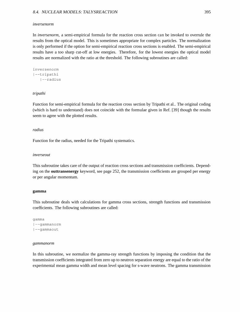
8.4. NUCLEAR MODELS: TALYSREACTION 395
inversenorm
In inversenorm, a semi-empirical formula for the reaction cross section can be invoked to overrule theresults from the optical model. This is sometimes appropriate for complex particles. The normalizationis only performed if the option for semi-empirical reactioncross sections is enabled. The semi-empiricalresults have a too sharp cut-off at low energies. Therefore,for the lowest energies the optical modelresults are normalized with the ratio at the threshold. The following subroutines are called:
inversenorm|--tripathi
|--radius
tripathi
Function for semi-empirical formula for the reaction crosssection by Tripathi et al.. The original coding(which is hard to understand) does not coincide with the formulae given in Ref. [39] though the resultsseem to agree with the plotted results.
radius
Function for the radius, needed for the Tripathi systematics.
inverseout
This subroutine takes care of the output of reaction cross sections and transmission coefficients. Depend-ing on theouttransenergykeyword, see page 252, the transmission coefficients are grouped per energyor per angular momentum.
gamma
This subroutine deals with calculations for gamma cross sections, strength functions and transmissioncoefficients. The following subroutines are called:
gamma|--gammanorm|--gammaout
gammanorm
In this subroutine, we normalize the gamma-ray strength functions by imposing the condition that thetransmission coefficients integrated from zero up to neutron separation energy are equal to the ratio of theexperimental mean gamma width and mean level spacing for s-wave neutrons. The gamma transmission
396 CHAPTER 8. COMPUTATIONAL STRUCTURE OF TALYS
coefficients are generated through calls to the strength function fstrength. The gamma-ray cross sectionsare also normalized. The following subroutines are called:
gammanorm|--density >|--fstrength|--gammaxs
|--fstrength
fstrength
In fstrength, the gamma-ray strength functions according to Kopecky-Uhl or Brink-Axel are calculated,or are interpolated from Goriely’s HFB or HFBCS tables.
gammaxs
In gammaxs, the photo-absorption cross sections are calculated. Theyconsist of a GDR part and a quasi-deuteron part.
gammaout
In gammaout, the gamma-ray strength functions, transmission coefficients and cross sections are writtento output. The following subroutines are called:
gammaout|--fstrength
8.4.2 preeqinit
General quantities needed for pre-equilibrium calculations are set, such as factorials, spin distributionfunctions and Pauli correction factors. The following subroutines are called:
preeqinit|--bonetti
|--mom >|--optical >
bonetti
In this subroutine, the average imaginary volume potentialfor the internal transition rates is calculated.
8.4. NUCLEAR MODELS: TALYSREACTION 397
8.4.3 excitoninit
Quantities needed for exciton model calculations are set, such as preformation factors, factors for theemission rates and charge conserving Q-factors.
8.4.4 compoundinit
Quantities needed for compound nucleus model calculationsare set, such as factors for width fluctuationand angular distribution calculations. The following subroutines are called:
compoundinit|--gaulag|--gauleg
8.4.5 astroinit
Quantities needed for astrophysical reaction calculations are initialized.
gaulag
This subroutine is for Gauss-Laguerre integration.
gauleg
This subroutine is for Gauss-Legendre integration.
8.4.6 reacinitial
In reacinitial, all arrays that appear in the nuclear reaction model part ofthe program are initialized.
8.4.7 incident
Subroutineincidenthandles the calculation of total, reaction, elastic cross section, transmission coeffi-cients and elastic angular distribution for the incident energy. Also, some main parameters for the currentincident energy are set. The following subroutines are called:
incident|--yesno|--incidentecis
|--optical >|--mom >
398 CHAPTER 8. COMPUTATIONAL STRUCTURE OF TALYS
|--ecisinput >|--incidentread|--incidentnorm
|--tripathi >|--incidentgamma
|--fstrength|--gammaxs >
|--radwidtheory >|--gammanorm >|--spr|--incidentout
incidentecis
In this subroutine the basic ECIS calculation for the incident particle and energy is performed for eithera spherical or a deformed nucleus. The optical model parameters are determined by callingoptical. Thesubroutineecisinput is called for the creation of the ECIS input files. At the end ofthis subroutine,ecis06tis called to perform the actual ECIS calculation.
incidentread
In this subroutine the results from ECIS are read for the incident particle and energy. We first read thereaction (and for neutrons the total and elastic) cross section. Next, the transmission coefficients are readinto the array Tjlinc, which has has four indices: particle type, energy, spin and l-value. For spin-1/2particles, we use the indices -1 and 1 for the two spin values.For spin-1 particles, we use -1, 0 and 1and for spin-0 particles we use 0 only. For rotational nuclei, we transform the rotational transmissioncoefficients into their spherical equivalents for the compound nucleus calculation. Also, transmission co-efficients averaged over spin are put into separate arrays. The maximal l-value is determined to constrainloops over angular momentum later on in the code. The direct reaction Legendre coefficients and an-gular distribution are also read in. For coupled-channels calculations, we also read the discrete inelasticangular distributions and cross sections.
incidentnorm
In incidentnorm, the transmission coefficients can be normalized with values obtained from semi-empiricalsystematics for the reaction cross section, if required.
incidentgamma
Here, the transmission coefficients for the incident gamma channel, in the case of photo-nuclear reac-tions, are generated.
8.4. NUCLEAR MODELS: TALYSREACTION 399
spr
In spr, the S, P and R resonance parameters for low incident neutronenergies are calculated and, ifrequested, written to file.
incidentout
In this subroutine the basic cross sections, transmission coefficients and possible resonance parametersfor the incident channel are written to output.
8.4.8 exgrid
In exgrid, the possible routes to all reachable residual nuclei are followed, to determine the maximumpossible excitation energy for each nucleus, given the incident energy. From this, the excitation energygrid for each residual nucleus is determined. The first NL values of the excitation energy grid Ex cor-respond to the discrete level excitation energies of the residual nucleus. The NL+1th value correspondsto the first continuum energy bin. The continuum part of the nuclides are then divided into energy bins.The Q-values for the residual nuclides are also determined.Finally, the calculation of level densities inTALYS can be done outside many loops of various quantum numbers performed in other subroutines.Therefore, inexgridwe store the level density as function of residual nucleus, excitation energy, spin andparity. The following subroutines are called:
exgrid|--density >|--spincut >
8.4.9 recoilinit
In this subroutine the basic recoil information is initialized. Various arrays are initialized and the maxi-mum recoil energies for all residual nuclides are determined. Recoil energy and angular bins are deter-mined.
8.4.10 direct
Subroutinedirect takes care of the calculation of direct cross sections to discrete states that have notalready been covered as coupled-channels for the incident channel, such as DWBA and giant resonancecross sections. The following subroutines are called:
direct|--directecis
|--ecisinput >|--directread
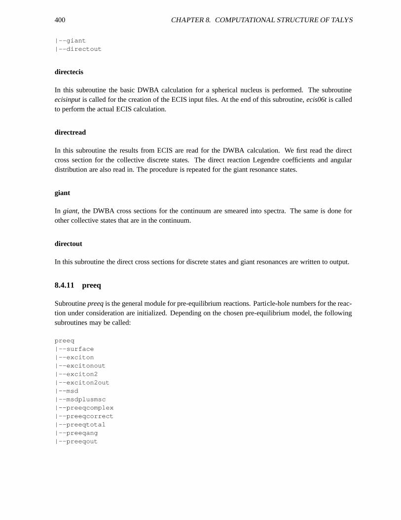
400 CHAPTER 8. COMPUTATIONAL STRUCTURE OF TALYS
|--giant|--directout
directecis
In this subroutine the basic DWBA calculation for a spherical nucleus is performed. The subroutineecisinputis called for the creation of the ECIS input files. At the end ofthis subroutine,ecis06tis calledto perform the actual ECIS calculation.
directread
In this subroutine the results from ECIS are read for the DWBAcalculation. We first read the directcross section for the collective discrete states. The direct reaction Legendre coefficients and angulardistribution are also read in. The procedure is repeated forthe giant resonance states.
giant
In giant, the DWBA cross sections for the continuum are smeared into spectra. The same is done forother collective states that are in the continuum.
directout
In this subroutine the direct cross sections for discrete states and giant resonances are written to output.
8.4.11 preeq
Subroutinepreeqis the general module for pre-equilibrium reactions. Particle-hole numbers for the reac-tion under consideration are initialized. Depending on thechosen pre-equilibrium model, the followingsubroutines may be called:
preeq|--surface|--exciton|--excitonout|--exciton2|--exciton2out|--msd|--msdplusmsc|--preeqcomplex|--preeqcorrect|--preeqtotal|--preeqang|--preeqout
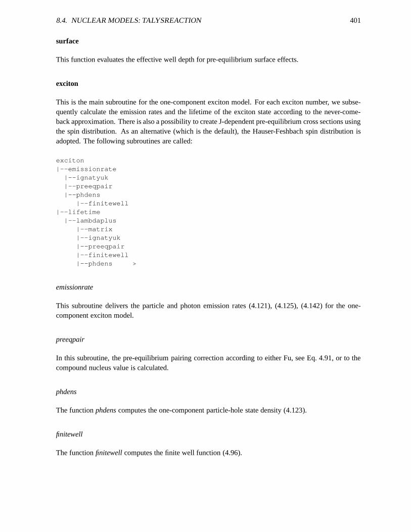
8.4. NUCLEAR MODELS: TALYSREACTION 401
surface
This function evaluates the effective well depth for pre-equilibrium surface effects.
exciton
This is the main subroutine for the one-component exciton model. For each exciton number, we subse-quently calculate the emission rates and the lifetime of theexciton state according to the never-come-back approximation. There is also a possibility to create J-dependent pre-equilibrium cross sections usingthe spin distribution. As an alternative (which is the default), the Hauser-Feshbach spin distribution isadopted. The following subroutines are called:
exciton|--emissionrate
|--ignatyuk|--preeqpair|--phdens
|--finitewell|--lifetime
|--lambdaplus|--matrix|--ignatyuk|--preeqpair|--finitewell|--phdens >
emissionrate
This subroutine delivers the particle and photon emission rates (4.121), (4.125), (4.142) for the one-component exciton model.
preeqpair
In this subroutine, the pre-equilibrium pairing correction according to either Fu, see Eq. 4.91, or to thecompound nucleus value is calculated.
phdens
The functionphdenscomputes the one-component particle-hole state density (4.123).
finitewell
The functionfinitewellcomputes the finite well function (4.96).
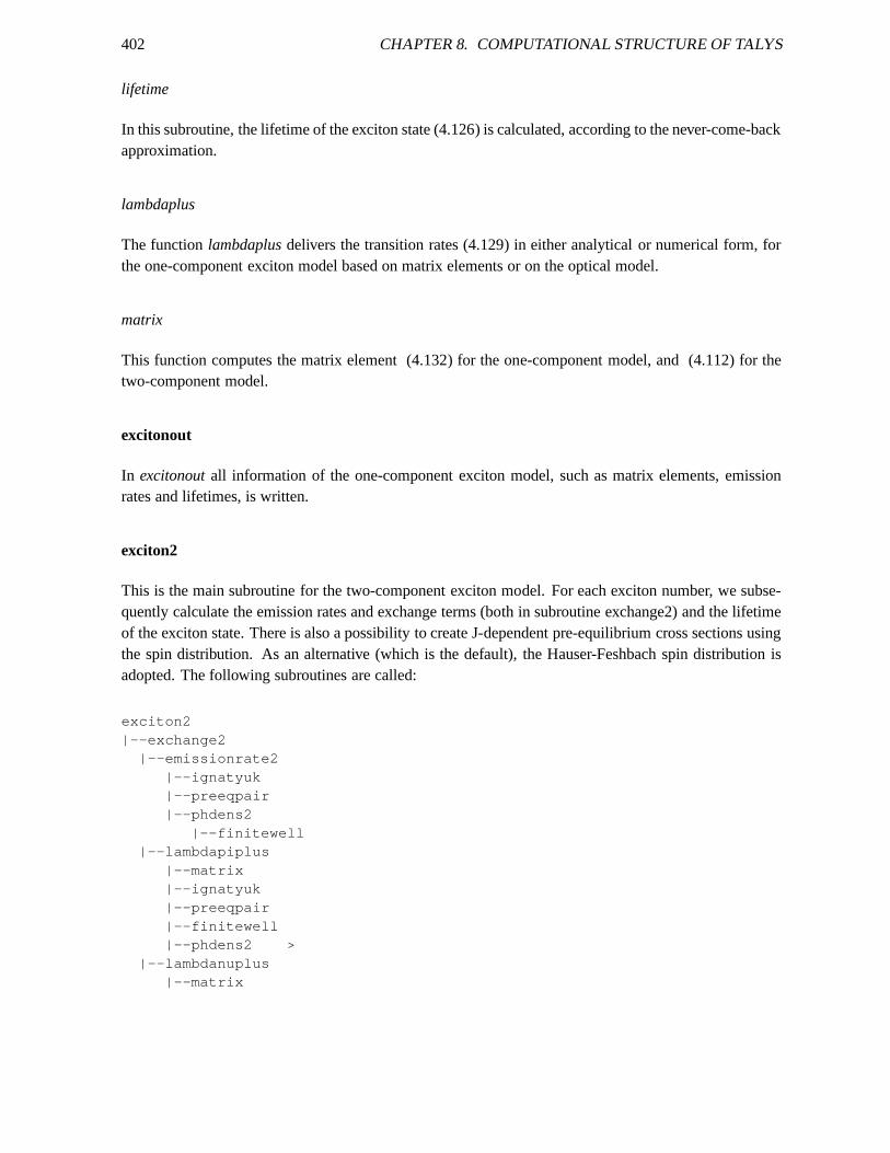
402 CHAPTER 8. COMPUTATIONAL STRUCTURE OF TALYS
lifetime
In this subroutine, the lifetime of the exciton state (4.126) is calculated, according to the never-come-backapproximation.
lambdaplus
The functionlambdaplusdelivers the transition rates (4.129) in either analyticalor numerical form, forthe one-component exciton model based on matrix elements oron the optical model.
matrix
This function computes the matrix element (4.132) for the one-component model, and (4.112) for thetwo-component model.
excitonout
In excitonoutall information of the one-component exciton model, such asmatrix elements, emissionrates and lifetimes, is written.
exciton2
This is the main subroutine for the two-component exciton model. For each exciton number, we subse-quently calculate the emission rates and exchange terms (both in subroutine exchange2) and the lifetimeof the exciton state. There is also a possibility to create J-dependent pre-equilibrium cross sections usingthe spin distribution. As an alternative (which is the default), the Hauser-Feshbach spin distribution isadopted. The following subroutines are called:
exciton2|--exchange2
|--emissionrate2|--ignatyuk|--preeqpair|--phdens2
|--finitewell|--lambdapiplus
|--matrix|--ignatyuk|--preeqpair|--finitewell|--phdens2 >
|--lambdanuplus|--matrix
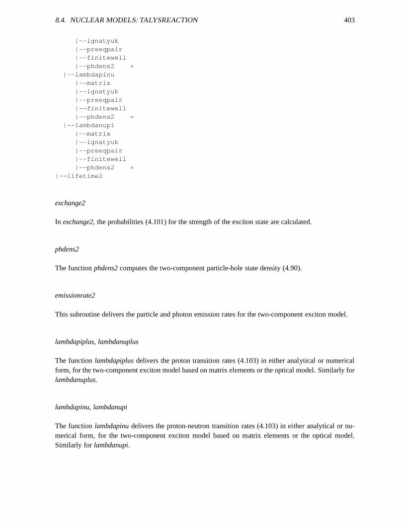
8.4. NUCLEAR MODELS: TALYSREACTION 403
|--ignatyuk|--preeqpair|--finitewell|--phdens2 >
|--lambdapinu|--matrix|--ignatyuk|--preeqpair|--finitewell|--phdens2 >
|--lambdanupi|--matrix|--ignatyuk|--preeqpair|--finitewell|--phdens2 >
|--lifetime2
exchange2
In exchange2, the probabilities (4.101) for the strength of the exciton state are calculated.
phdens2
The functionphdens2computes the two-component particle-hole state density (4.90).
emissionrate2
This subroutine delivers the particle and photon emission rates for the two-component exciton model.
lambdapiplus, lambdanuplus
The functionlambdapiplusdelivers the proton transition rates (4.103) in either analytical or numericalform, for the two-component exciton model based on matrix elements or the optical model. Similarly forlambdanuplus.
lambdapinu, lambdanupi
The functionlambdapinudelivers the proton-neutron transition rates (4.103) in either analytical or nu-merical form, for the two-component exciton model based on matrix elements or the optical model.Similarly for lambdanupi.

404 CHAPTER 8. COMPUTATIONAL STRUCTURE OF TALYS
lifetime2
In this subroutine, the lifetime of the exciton state through the quantity of Eq. (4.100) is calculated.
exciton2out
In exciton2outall information of the two-component exciton model, such asmatrix elements, emissionrates and lifetimes, is written.
msd
This subroutine calculates pre-equilibrium cross sections according to the macroscopic multi-step direct(MSD) model. The MSD model is implemented for neutrons and protons only. The following subrou-tines are called:
msd|--msdinit
|--interangle|--dwbaecis
|--ecisdwbamac|--optical >
|--dwbaread|--dwbaout|--dwbaint|--onecontinuumA
|--ignatyuk|--omega
|--phdens >|--onestepA
|--ignatyuk|--omega >|--locate|--pol2
|--msdcalc|--onestepB
|--cmsd|--onecontinuumB| |--cmsd|--multistepA|--multistepB| |--locate| |--pol2
|--msdtotal|--msdout
8.4. NUCLEAR MODELS: TALYSREACTION 405
msdinit
This subroutine initializes various arrays for the multi-step direct calculation, such as the MSD energygrid and the intermediate angles through a call tointerangle.
interangle
Subroutineinterangleproduces the intermediate angles for MSD model, by the addition theorem. Formulti-step reactions, this is necessary to transform the ingoing angle of the second step and link it withthe outgoing angle of the first step.
dwbaecis
This subroutine takes care of all the ECIS calculations thatneed to be performed for the various steps ofthe multi-step reaction. Subsequently, DWBA calculationsare performed for the first exchange one-stepreaction, the inelastic one-step reaction and the second exchange one-step reaction. For this, varioussubroutines are called.
dwbaecis
Subroutineecisdwbamaccreates the ECIS input file for a macroscopic DWBA calculation. Potentialsfor the incident, transition and outgoing channel are calculated.
dwbaread
In this subroutine the results from ECIS are read. For every energy and spin we read the total DWBAcross section and the angle-differential DWBA cross section.
dwbaread
This subroutine takes care of the output of the DWBA cross sections.
dwbaint
In dwbaint, the DWBA cross sections are interpolated on the appropriate energy grid.
onecontinuumA
In onecontinuumA, the continuum one-step cross sections to be used in multi-step calculations are cal-culated by multiplying the DWBA cross sections by particle-hole state densities.

406 CHAPTER 8. COMPUTATIONAL STRUCTURE OF TALYS
omega
This is a function of the particle-hole state density per angular momentum.
onestepA
In onestepA, the unnormalized one-step direct cross sections for the outgoing energy grid are calculated(these will be normalized in subroutine onestepB).
pol2
Subroutine for interpolation of second order.
msdcalc
This is the general subroutine for the final MSD calculations.
onestepB
In onestepB, the one-step direct cross sections are calculated using a final normalization.
onecontinuumB
In onecontinuumB, the final one-step direct cross sections for use in the multi-step calculations are com-puted using the final normalization.
multistepA
In multistepA, the multi-step direct cross sections (second and higher steps) are calculated using a finalnormalization.
multistepB
In multistepB, the multi-step direct cross sections are interpolated on the final outgoing energy grid.
msdtotal
In msdtotal, the total multi-step direct cross sections are calculated.
8.4. NUCLEAR MODELS: TALYSREACTION 407
msdout
In msdout, the multi-step direct cross sections are written to output.
msdplusmsc
In this subroutine, the MSD cross sections are put in the general pre-equilibrium cross sections.
preeqcomplex
Subroutinepreeqcomplexhandles pre-equilibrium complex particle emission. The implemented complexparticle emission model is described in Section 4.4.4. Notethat several purely empirical fixes to themodel were needed to prevent divergence of certain cross section estimates. The subroutine consistsof two main parts: One for stripping/pickup and one for alphaknock-out reactions. The followingsubroutines are called:
preeqcomplex|--phdens2 >
preeqcorrect
This subroutine handles the correction of pre-equilibriumcross sections for direct discrete cross sections.If the cross sections for discrete states havenot been calculated by a direct reaction model, we collapsethe continuum pre-equilibrium cross sections in the high-energy region on the associated discrete states.After this, the pre-equilibrium cross sections in the discrete energy region are set to zero. The followingsubroutines are called:
preeqcorrect|--locate
preeqtotal
In preeqtotal, the total pre-equilibrium cross sections are calculated.The pre-equilibrium spectra andspectra per exciton number are summed to total pre-equilibrium cross sections. Special care is takenfor the continuum bin with the highest outgoing energy, i.e.the one that overlaps with the energy cor-responding to the last discrete state. In line with unitarity, the summed direct + pre-equilibrium crosssection may not exceed the reaction cross section. In these cases, we normalize the results. Also, thediscrete pre-equilibrium contribution is added to the discrete state cross sections.
408 CHAPTER 8. COMPUTATIONAL STRUCTURE OF TALYS
preeqang
In preeqang, the pre-equilibrium angular distribution is calculated.Also here, there is a correction ofthe pre-equilibrium cross sections for direct discrete angular distributions. If the angular distributionsfor discrete states havenot been calculated by a direct reaction model, we collapse the continuum pre-equilibrium angular distributions in the high energy region on the associated discrete states. For theexciton model, the pre-equilibrium angular distributionsare generated with the Kalbach systematics.The following subroutines are called:
preeqang|--kalbach
kalbach
This is the function for the Kalbach systematics [71].
preeqout
In preeqout, the output of pre-equilibrium cross sections is handled. The following subroutines arecalled:
preeqout|--ignatyuk|--phdens >|--phdens2 >
8.4.12 population
In population, the pre-equilibrium spectra are processed into population bins. The pre-equilibrium crosssections have been calculated on the emission energy grid. They are interpolated on the excitation energygrids of the level populations (both for the total and the spin/parity-dependent cases) to enable furtherdecay of the residual nuclides. also, the pre-equilibrium population cross section are normalized. Due tointerpolation, the part of the continuum population that comes from pre-equilibrium is not exactly equalto the total pre-equilibrium cross section. The normalization is done over the whole excitation energyrange. The following subroutines are called:
population|--locate|--pol1
8.4. NUCLEAR MODELS: TALYSREACTION 409
8.4.13 compnorm
There is a small difference between the reaction cross section as calculated by ECIS and the sum overtransmission coefficients. We therefore normalize the level population accordingly in this subroutine.The compound nucleus formation cross section xsflux and the associated normalization factors are cre-ated.
8.4.14 comptarget
In comptarget, the compound reaction for the initial compound nucleus is calculated. First, the leveldensities and transmission coefficients are prepared before the nested loops over all quantum numbersare performed. Next the following nested loops are performed:
• compound nucleus parity
• total angular momentumJ of compound nucleus
• j of incident channel
• l of incident channel
• outgoing particles and gammas
• outgoing excitation energies
• residual parity
• residual spin
• j of outgoing channel
• l of outgoing channel
There are two possible types of calculation for the initial compound nucleus. If either width fluctuationcorrections or compound nucleus angular distributions arewanted, we need to sum explicitly over allpossible quantum numbers before we calculate the width fluctuation or angular factor. If not, the sumoverj andl of the transmission coefficients can be lumped into one factor, which decreases the calcula-tion time. In the latter case, the partial decay widths enumhf are calculated in subroutinecompprepare.
In order to get do-loops running over integer values, certain quantum numbers are multiplied by2, which can be seen from a 2 present in the corresponding variable names. For each loop, the begin andend point is determined from the triangular rule.
For everyJ andP (parity), first the denominator (total width) denomhf for the Hauser-Feshbachformula is constructed in subroutine compprepare. Also width fluctuation variables that only dependon J and P and not on the other angular momentum quantum numbers are calculated in subroutinewidthprepare. For the width fluctuation calculation, all transmission coefficients need to be placed in
410 CHAPTER 8. COMPUTATIONAL STRUCTURE OF TALYS
one sequential array. Therefore, a counter tnum needs to be followed to keep track of the proper indexfor the transmission coefficients.
Inside the nested loops listed above, compound nucleus calculations for photons, particles andfission are performed. In the middle of all loops, we determine the index for the width fluctuation calcu-lation and call the subroutine that calculates the correction factor. Also, compound angular distributions,i.e. the Legendre coefficients, for discrete states are calculated.
The following subroutines are called:
comptarget|--densprepare|--tfission|--compprepare|--widthprepare|--widthfluc|--clebsch|--racah|--tfissionout|--raynalcomp
densprepare
In densprepare, we prepare the energy grid, level density and transmissioncoefficient information forthe compound nucleus and its residual nuclides. For varioustypes of decay (continuum to discrete,continuum to continuum, etc.) we determine the energetically allowed transitions. These are then takeninto account for the determination of integrated level densities. To get the transmission coefficients onthe excitation energy grid from those on the emission energygrid, we use interpolation of the secondorder. Finally, the fission level densities are calculated.
The following subroutines are called:
densprepare|--fstrength|--locate|--pol2|--density >
tfission
In this subroutine, the fission transmission coefficients are calculated. The fission transmission coeffi-cients decrease very rapidly with excitation energy. Therefore, we calculate them at the end points and atthe middle of each excitation energy bin. With this information, we can do logarithmic integration. Callsto subroutinet1barrier are done for 1, 2 and 3 barriers. Also transmission coefficients corrected for thepresence of class II states are calculated.
The following subroutines are called:
8.4. NUCLEAR MODELS: TALYSREACTION 411
tfission|--t1barrier
|--thill
t1barrier
Subroutinet1barrier handles the fission transmission coefficient for one barrier. Both discrete states andthe continuum are taken into account.
thill
Function for the Hill-Wheeler formula.
compprepare
In compprepare, information for the initial compound nucleus is prepared.The transmission coefficientsare put in arrays for possible width fluctuation calculations. Also the total width denomhf appearingin the denominator of the compound nucleus formula is created. Note that the complete subroutine isperformed inside the loop over compound nucleus spinJ and parityP in subroutine comptarget.
widthprepare
In this subroutine, the preparation of width fluctuation calculations is done. All width fluctuation vari-ables that only depend onJ and P and not on the other angular momentum quantum numbers arecalculated. The following subroutines are called:
widthprepare|--molprepare|--hrtwprepare|--goeprepare
|--prodm|--prodp
molprepare
This subroutine takes care of the preparation of the Moldauer width fluctuation correction (informationonly dependent onJ andP ).
hrtwprepare
This subroutine takes care of the preparation of the HRTW width fluctuation correction (informationonly dependent onJ andP ).
412 CHAPTER 8. COMPUTATIONAL STRUCTURE OF TALYS
goeprepare
This subroutine takes care of the preparation of the GOE triple integral width fluctuation correction(information only dependent onJ andP ).
prodm, prodp
Functions to calculate a product for the GOE calculation.
widthfluc
General subroutine for width fluctuation corrections. The following subroutines are called:
widthfluc|--moldauer|--hrtw|--goe
|--func1
moldauer
Subroutine for the Moldauer width fluctuation correction.
hrtw
Subroutine for the HRTW width fluctuation correction.
goe
Subroutine for the GOE width fluctuation correction.
clebsch
Function for the calculation of Clebsch-Gordan coefficients.
racah
Function for the calculation of Racah coefficients.
8.4. NUCLEAR MODELS: TALYSREACTION 413
tfissionout
Subroutinetfissionouttakes care of the output of fission transmission coefficients.
raynalcomp
Using subroutineraynalcomp, a compound nucleus run by ECIS can be performed, in additionto thecalculation by TALYS. The results as calculated by ECIS willhowever not be used for TALYS but arejust for comparison. The following subroutines are called:
raynalcomp|--eciscompound
|--optical >
eciscompound
In eciscompound, an ECIS input file for a compound nucleus calculation is prepared.
8.4.15 binary
In binary, the binary reaction cross section are accumulated. The direct and pre-equilibrium cross sec-tions are processed into population arrays. Binary feedingchannels, necessary for exclusive cross sec-tions, are determined. Also the population after binary emission is printed. The following subroutinesare called:
binary|--ignatyuk|--spindis >|--binaryspectra
|--binemission|--locate|--pol1
|--binaryrecoil
binaryspectra
Subroutine to interpolate decay, from one bin to another, onthe emission spectrum. The binary andcompound emission spectra are constructed.
binemission
In binemission, the decay from the primary compound nucleus to residual nuclei is converted from theexcitation energy grid to emission energies. Due to interpolation errors, there is always a small difference
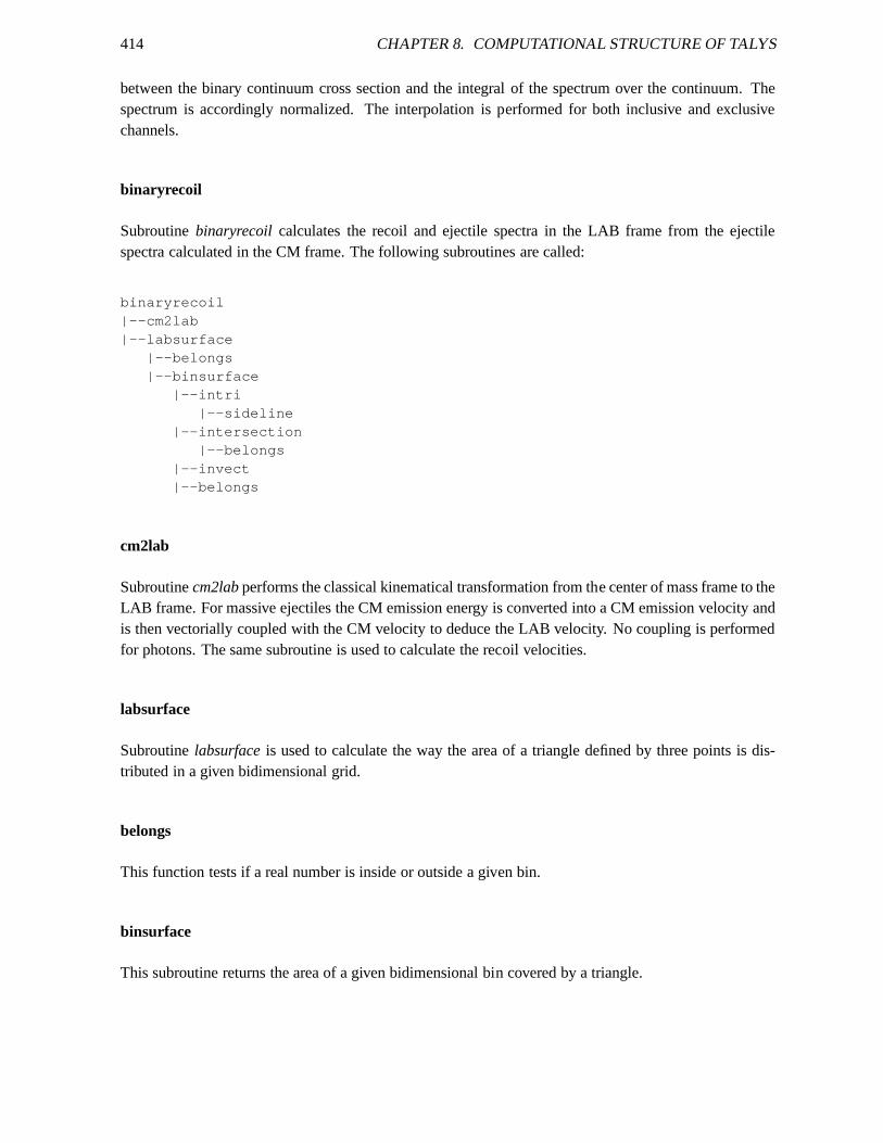
414 CHAPTER 8. COMPUTATIONAL STRUCTURE OF TALYS
between the binary continuum cross section and the integralof the spectrum over the continuum. Thespectrum is accordingly normalized. The interpolation is performed for both inclusive and exclusivechannels.
binaryrecoil
Subroutinebinaryrecoil calculates the recoil and ejectile spectra in the LAB frame from the ejectilespectra calculated in the CM frame. The following subroutines are called:
binaryrecoil|--cm2lab|--labsurface
|--belongs|--binsurface
|--intri|--sideline
|--intersection|--belongs
|--invect|--belongs
cm2lab
Subroutinecm2labperforms the classical kinematical transformation from the center of mass frame to theLAB frame. For massive ejectiles the CM emission energy is converted into a CM emission velocity andis then vectorially coupled with the CM velocity to deduce the LAB velocity. No coupling is performedfor photons. The same subroutine is used to calculate the recoil velocities.
labsurface
Subroutinelabsurfaceis used to calculate the way the area of a triangle defined by three points is dis-tributed in a given bidimensional grid.
belongs
This function tests if a real number is inside or outside a given bin.
binsurface
This subroutine returns the area of a given bidimensional bin covered by a triangle.
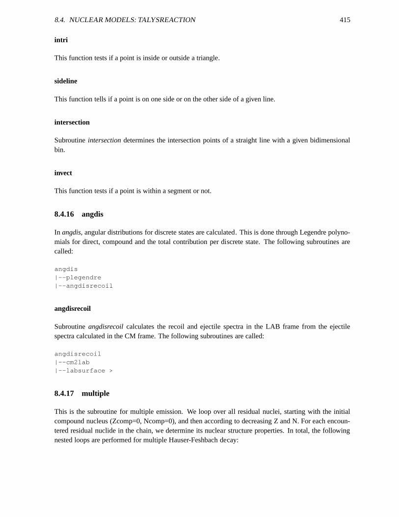
8.4. NUCLEAR MODELS: TALYSREACTION 415
intri
This function tests if a point is inside or outside a triangle.
sideline
This function tells if a point is on one side or on the other side of a given line.
intersection
Subroutineintersectiondetermines the intersection points of a straight line with agiven bidimensionalbin.
invect
This function tests if a point is within a segment or not.
8.4.16 angdis
In angdis, angular distributions for discrete states are calculated. This is done through Legendre polyno-mials for direct, compound and the total contribution per discrete state. The following subroutines arecalled:
angdis|--plegendre|--angdisrecoil
angdisrecoil
Subroutineangdisrecoilcalculates the recoil and ejectile spectra in the LAB frame from the ejectilespectra calculated in the CM frame. The following subroutines are called:
angdisrecoil|--cm2lab|--labsurface >
8.4.17 multiple
This is the subroutine for multiple emission. We loop over all residual nuclei, starting with the initialcompound nucleus (Zcomp=0, Ncomp=0), and then according todecreasing Z and N. For each encoun-tered residual nuclide in the chain, we determine its nuclear structure properties. In total, the followingnested loops are performed for multiple Hauser-Feshbach decay:
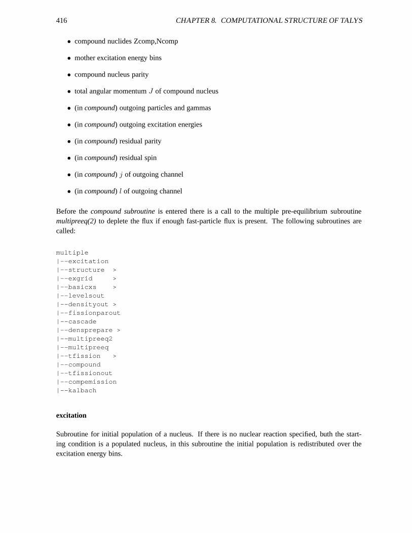
416 CHAPTER 8. COMPUTATIONAL STRUCTURE OF TALYS
• compound nuclides Zcomp,Ncomp
• mother excitation energy bins
• compound nucleus parity
• total angular momentumJ of compound nucleus
• (in compound) outgoing particles and gammas
• (in compound) outgoing excitation energies
• (in compound) residual parity
• (in compound) residual spin
• (in compound) j of outgoing channel
• (in compound) l of outgoing channel
Before thecompound subroutineis entered there is a call to the multiple pre-equilibrium subroutinemultipreeq(2)to deplete the flux if enough fast-particle flux is present. The following subroutines arecalled:
multiple|--excitation|--structure >|--exgrid >|--basicxs >|--levelsout|--densityout >|--fissionparout|--cascade|--densprepare >|--multipreeq2|--multipreeq|--tfission >|--compound|--tfissionout|--compemission|--kalbach
excitation
Subroutine for initial population of a nucleus. If there is no nuclear reaction specified, buth the start-ing condition is a populated nucleus, in this subroutine theinitial population is redistributed over theexcitation energy bins.
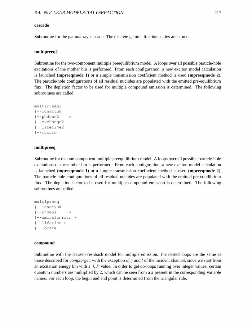
8.4. NUCLEAR MODELS: TALYSREACTION 417
cascade
Subroutine for the gamma-ray cascade. The discrete gamma line intensities are stored.
multipreeq2
Subroutine for the two-component multiple preequilibriummodel. A loops over all possible particle-holeexcitations of the mother bin is performed. From each configuration, a new exciton model calculationis launched (mpreeqmode 1) or a simple transmission coefficient method is used (mpreeqmode 2).The particle-hole configurations of all residual nuclides are populated with the emitted pre-equilibriumflux. The depletion factor to be used for multiple compound emission is determined. The followingsubroutines are called:
multipreeq2|--ignatyuk|--phdens2 >|--exchange2|--lifetime2|--locate
multipreeq
Subroutine for the one-component multiple preequilibriummodel. A loops over all possible particle-holeexcitations of the mother bin is performed. From each configuration, a new exciton model calculationis launched (mpreeqmode 1) or a simple transmission coefficient method is used (mpreeqmode 2).The particle-hole configurations of all residual nuclides are populated with the emitted pre-equilibriumflux. The depletion factor to be used for multiple compound emission is determined. The followingsubroutines are called:
multipreeq|--ignatyuk|--phdens >|--emissionrate >|--lifetime >|--locate
compound
Subroutine with the Hauser-Feshbach model for multiple emission. the nested loops are the same asthose described forcomptarget, with the exception ofj andl of the incident channel, since we start froman excitation energy bin with aJ, P value. In order to get do-loops running over integer values,certainquantum numbers are multiplied by 2, which can be seen from a 2present in the corresponding variablenames. For each loop, the begin and end point is determined from the triangular rule.
418 CHAPTER 8. COMPUTATIONAL STRUCTURE OF TALYS
For everyJ andP (parity), first the denominator (total width) denomhf for the Hauser-Feshbachformula is constructed. Inside the nested loops, compound nucleus calculations for photons, particlesand fission are performed.
compemission
In compemission, the compound nucleus emission spectra are determined fromthe multiple Hauser-Feshbach decay scheme. The decay from compound to residual nuclei is converted from the excitationenergy grid to emission energies. The spectrum is obtained by spreading the decay over the mother binand, in the case of continuum-continuum transitions, the residual bin. For each mother excitation energybin, we determine the highest possible excitation energy bin for the residual nuclei. As reference, wetake the top of the mother bin. The maximal residual excitation energy is obtained by subtracting theseparation energy from this. Various types of decay are possible:
• Decay from continuum to continuum. For most residual continuum bins, no special care needs tobe taken and the emission energy that characterizes the transition is simply the average betweenthe highest energetic transition that is possible and the lowest.
• Decay from continuum to discrete. The lowest possible mother excitation bin can not entirely de-cay to the discrete state. For the residual discrete state, it is checked whether the mother excitationbin is such a boundary case. This is done by adding the particle separation energy to the excitationenergy of the residual discrete state.
When the decay type has been identified, the decay from the population is distributed over the emissionenergy bins. All possible end point problems are taken into account. The following subroutines arecalled:
compemission|--locate|--comprecoil
comprecoil
If recoil y, the recoil and/or light particle spectra in the LAB frame are calculated incomprecoil. Thefollowing subroutines are called:
comprecoil|--kalbach|--cm2lab|--labsurface >
8.4. NUCLEAR MODELS: TALYSREACTION 419
8.4.18 channels
In channels, the exclusive reaction cross sections and spectra as outlined in Section 3.2.2 are calculated.A loop over all residual nuclides is performed and it is determined whether the residual nucleus underconsideration can be reached by a certain particle combination. The associated gamma-ray productionand isomeric exclusive cross sections are also computed. Finally, numerical checks with the total crosssections are performed. The following subroutines are called:
channels|--specemission
|--locate
specemission
In specemission, the exclusive emission spectra are computed. The procedure is analogous to that ofcompemission.
8.4.19 totalxs
In this subroutine, a few total cross sections are cumulated, such as the continuum exclusive cross section,the total particle production cross section and the total fission cross section.
8.4.20 spectra
In spectra, smoothed discrete cross sections are added to the emissionspectra. A more precise energygrid at the high-energy tail is created to account for the structure of discrete states. This is done for bothangle-integrated and double-differential spectra. The following subroutines are called:
spectra|--locate
8.4.21 massdis
In massdisthe fission fragment and product yields are calculated. A loop over all fissioning systems isperformed. Some of the excitation energy bins are lumped into larger energy bins to save computationtime. The fission yields per fissioning system are weighted with the fission cross section and added toform the total yield. The following subroutines are called:
massdis|--brosafy
|--spline|--ignatyuk
420 CHAPTER 8. COMPUTATIONAL STRUCTURE OF TALYS
|--trans|--funcfismode
|--ignatyuk|--splint|--density >
|--trapzd|--funcfismode
|--splint|--neck
|--bdef|--fcoul|--fsurf
|--ignatyuk|--fmin|--rpoint
|--vr2|--vr1|--vr2|--vr3|--rtbis|--evap
|--bdef|--sform|--rhodi|--fidi
|--vr1|--vr2|--vr3
brosafy
In this subroutine the fission fragment and product mass yields are determined per fissioning system. Therelative contribution of each fission mode is calculated. Subsequently, the fission yields per fission modeare calculated and summed with the fission mode weight.
spline
This subroutine performs a spline fit to the fission mode barrier parameters and the deformation param-eters used in the subroutineneck.
trans
This subroutine calculates the fission transmission coefficient per fission mode to determine the relativecontribution of each fission mode.

8.4. NUCLEAR MODELS: TALYSREACTION 421
funcfismode
This function corresponds to the expression of the fission transmission coefficient.
splint
This subroutine uses the spline fit obtained in the subroutine splineto interpolate.
neck
In this subroutine the actual fission fragment and product mass yield per fission mode is computed basedon the Random-neck Rupture model.
bdef
This subroutine computes the binding energy of a deformed nucleus with an eccentricity by the dropletmodel without shell corrections.
fcoul
This function contains the form factor for the Coulomb self energy.
fsurf
This function contains the form factor for the surface energy.
fmin
This subroutine searches the minimal value of a function.
rpoint
This subroutine is used to calculate the rupture pointzriss for a given nucleon number hidden in theleft-hand side of the dinuclear complex.
vr1
This function gives the volume of the projectile-like section.
422 CHAPTER 8. COMPUTATIONAL STRUCTURE OF TALYS
vr2
This function gives the volume of the neck.
vr3
This function gives the volume of the target-like section.
evap
This function is used to determine the number of evaporated neutrons for a given fission fragment.
sform
This function determines the form factor for the coulomb interaction energy between two spheroids.
rhodi
This function computes the shape of the dinuclear system.
fidi
This function determines the exact shape of the dinuclear complex.
8.4.22 residual
In residual, the residual production cross sections, both total and isomeric, are stored in arrays.
8.4.23 totalrecoil
In this subroutine, the total recoil results are assembled.
8.4.24 normalization
In this subroutine, cross sections can be normalized to experimental or evaluated data.
8.4.25 thermal
In thermal, the cross sections down to thermal energies are estimated.For non-threshold channels,the cross sections are extrapolated down to 1.e-5 eV. Capture values at thermal energies are used. For
8.4. NUCLEAR MODELS: TALYSREACTION 423
energies up to 1 eV, the 1/sqrt(E) law is used. Between 1 eV andthe first energy at which TALYSperforms the statistical model calculation, we use logarithmic interpolation. The following subroutinesare called:
thermal|--pol1
8.4.26 output
Subroutineoutputhandles the output of all cross sections, spectra, angular distributions, etc. per incidentenergy. The following subroutines are called:
output|--totalout|--binaryout|--productionout|--residualout|--fissionout|--discreteout|--channelsout|--spectraout|--recoilout|--angleout|--ddxout
|--locate|--gamdisout
totalout
Subroutine for the output of total cross sections, such as total, non-elastic, pre-equilibrium, direct, etc.
binaryout
Subroutine for the output of the binary cross sections.
productionout
Subroutine for the output of particle production cross sections and total fission cross section.
residualout
Subroutine for the output of residual production cross sections.

424 CHAPTER 8. COMPUTATIONAL STRUCTURE OF TALYS
fissionout
Subroutine for the output of fission cross sections per fissioning nuclide.
discreteout
Subroutine for the output of cross sections for discrete states for inelastic and other non-elastic channels.
channelsout
Subroutine for the output of exclusive channel cross sections and spectra, including ground state andisomer production and fission.
spectraout
Subroutine for the output of angle-integrated particle spectra.
recoilout
Subroutine for the output of recoil information.
angleout
Subroutine for the output of angular distributions for elastic scattering, inelastic scattering to discretestates and non-elastic scattering to other discrete states.
ddxout
Subroutine for the output of double-differential cross sections.
gamdisout
Subroutine for the output of discrete gamma-ray production.
8.4.27 finalout
In finalout, all results are printed as a function of incident energy, i.e. all excitation functions. Thisinformation appears in the main output file and/or in separate output files per reaction channel. Also,general nuclear model parameters are written to the parameter file.
8.4. NUCLEAR MODELS: TALYSREACTION 425
8.4.28 astro
Subroutine for astrophysical reaction rates. The following subroutines are called:
|--stellarrate|--partfunc
|--astroout
stellarrate
Subroutine for the calculation of the reaction rate for a Maxwell-Boltzmann distribution.
partfunc
Partition function for astrophysical calculations.
astroout
Subroutine for the output of astrophysical reaction rates.
8.4.29 endf
Subroutine for the output of cross sections and informationfor the production of an ENDF-6 file. Thefollowing subroutines are called:
endf|--endfinfo|--endfenergies|--endfecis
|--optical >|--ecisinput >
|--endfread|--tripathi >
endfinfo
Subroutine for writing the general information (i.e. the main reaction parameters) needed to create anENDF-6 file.
426 CHAPTER 8. COMPUTATIONAL STRUCTURE OF TALYS
endfenergies
Subroutine to create the energy grid for cross sections for an ENDF-6 file. This grid ensures that thetotal, elastic and reaction cross section are calculated ona sufficiently precise energy grid. Thresholdsfor all partial cross sections are also added to this grid.
endfecis
In this subroutine the loop over the energy grid created inendfenergiesis done to perform basic ECIScalculations. The optical model parameters are determinedby callingoptical. The subroutineecisinputis called for the creation of the ECIS input files. At the end ofthis subroutine,ecis06tis called to performthe actual ECIS calculation.
endfread
In this subroutine the results from ECIS are read. For every incident energy we read the reaction (andfor neutrons the total and elastic) cross sections. These are then written to a separate file for ENDF-6formatting.
8.5 Programming techniques
In general, we aim to apply a fixed set of programming rules consistently throughout the whole code.Here are some of the rules we apply to enforce readability androbustness:
- We use descriptive variable names as much as possible.
- Every variable in a subroutine, apart from dummy variablesappearing in e.g. a do loop, is ex-plained once in the comment section. In addition, we aim to give as much explanation as possiblefor the used algorithms.
- We useimplicit none as the first line oftalys.cmband all stand-alone subroutines and functions.This means that every variable must be declared, which is a powerful recipe against typing errors.
- We program directly “from the physics”, as much as possible, i.e. we use array indices whichcorrespond one-to-one to the indices of the physical formulae from articles and books.
- Cosmetical features:
- Different tasks within a subroutine are clearly separated. A block, which contains one sub-task, is separated by asterisks, e.g.cc *************************** Constants ************** ****************c
8.6. CHANGING THE ARRAY DIMENSIONS 427
The last asterisk is always in column 72. In the first block, the labels are numbered 10, 20,30, etc. In the second block, the labels are numbered 110, 120, 130, etc.
- We indent two blanks in do loops and if statements.
- In the file talys.cmb, we systematically store variables of type logical, character, integer, real anddouble precision in separate common blocks. The order of appearance of variables intalys.cmbfollows that of the subroutines.
- Every subroutine has the same heading structure: We give the author, date and task of the sub-routine. Next, the filetalys.cmbis included, followed by the inclusion of declarations for possiblelocal variables.
- We use nuclear model parameterisations that are as generalas possible within the programmednuclear reaction mechanisms, to enable easy implementation of future refinements. For example,level densities will never be hardwired “on the spot”, but will be called by a functiondensity. Animprovement, or alternative choice, of a level density model will then have a consistent impactthroughout the whole code.
- If there are exceptions to the procedures outlined above, it is probably since a few subroutineshave been adopted from other sources, such as the collectionof old style subroutines for the fissionyields model.
As a general rule, although we aim to program as clever as possible, we always prefer readability overspeed and memory economy. Some nuclear physicists are more expensive than computers, or at leastshould be.
8.6 Changing the array dimensions
As explained in the previous sections, almost all arrays aredefined in the common block filetalys.cmb.At the top of talys.cmb, the parameters are set for the dimensions of the various arrays. Their namesall start withnum. Most of these parameters should be left untouched, becausethey determine basicquantities of a nuclear model calculation. Some of them can however be changed. They can be reduced,for the case that the working memory of your computer is too small, or be increased, in cases whereyou want to perform more extensive or precise calculations than we thought were necessary. However,in normal cases you only need to change the keyword values in the input file and not the parameters intalys.cmb. In the standard version of TALYS, the latter already have reasonable values. Nevertheless, thefollowing parameters can be changed and will have a significant effect:
• memorypar: general multiplication factor for dimensions of several arrays. Use a small value fora small computer. Normally, changing this parameter does not require any further changes of theparameters that follow below.
• numbins: the maximum number of continuum excitation energy bins in the decay chains. Obvi-ously, this could be increased to allow for more precision.
428 CHAPTER 8. COMPUTATIONAL STRUCTURE OF TALYS
• numZchan, numNchanandnumchantot: the depth to which exclusive reaction channels are fol-lowed can be set by these parameters. However, as mentioned in Section 3.2.2, exclusive channelsthat go beyond 4 outgoing particles are rarely of interest (only for certain activation codes thatwork at high energies). Also, since the exclusive reaction calculation involves some large arrays,one may easily run into memory problems by choosing too largevalues. If one works on e.g. a 64Mb machine it may be helpful, or even necessary, to choose smaller values if one is not interestedin exclusive calculations at all. Table 8.1 displays the values that are theoretically possible. In thistable, we use
(8.1) numchantot =
numchannel∑
m=0
(
m + 5
m
)
which is the total number of channels for 6 different outgoing particles (neutrons up to alphaparticles) if we gonumchannelsparticles deep. In practice, less are needed since many channelsnever open up and this is what we have assumed by setting the value fornumchantot in talys.cmb.
• numZ andnumN: The maximum number of proton and neutron units, respectively, away fromthe initial compound nucleus that can be reached after multiple emission. If you want to try yourluck with TALYS at very high incident energies, these parameters may need to be increased.
• numlev: The maximum number of included discrete levels.
• numang: The maximum number of outgoing angles for discrete states.
• numangcont: The maximum number of outgoing angles for the continuum.
Obviously, after increasing these values you still need to set the associated keywords in the input file touse the increased limits, although some of them, e.g.maxZ, are always by default set to their maximumvalue. You could increase a parameter and simultaneously reduce another one that is of no relevance tothe particular problem under study, to remain within the available memory of your computer. Of course,you should always completely re-compile TALYS after changing anything intalys.cmb.
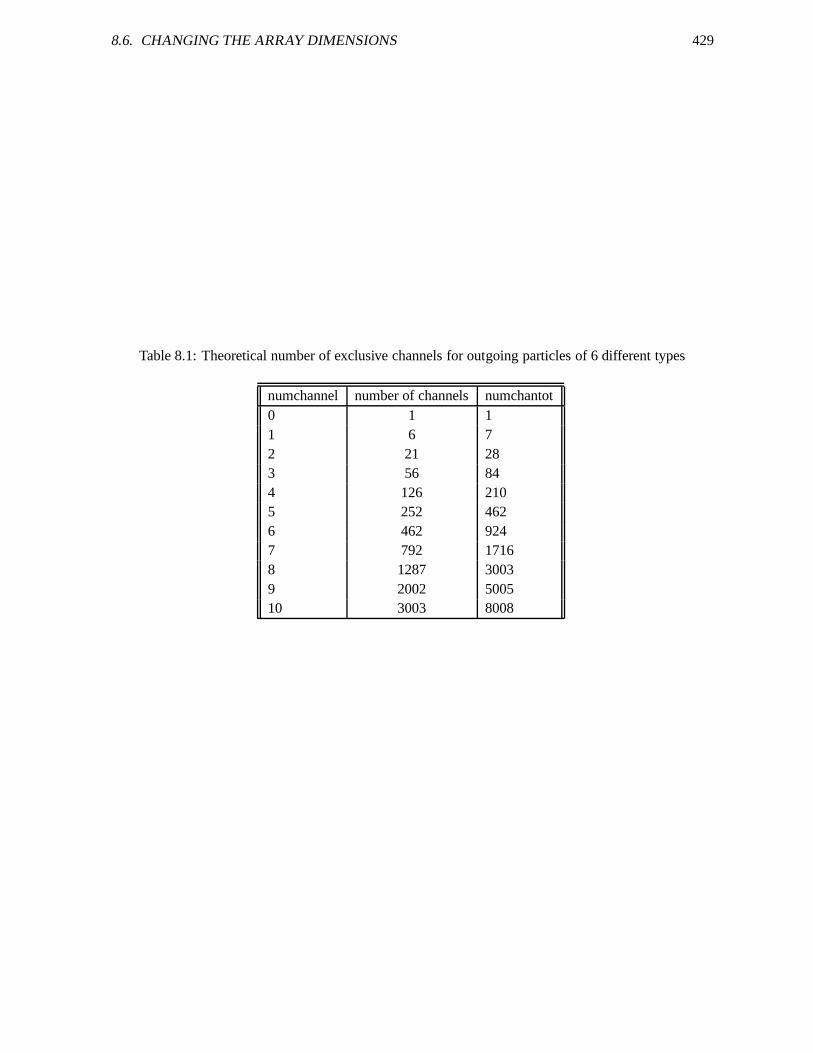
8.6. CHANGING THE ARRAY DIMENSIONS 429
Table 8.1: Theoretical number of exclusive channels for outgoing particles of 6 different types
numchannel number of channels numchantot0 1 11 6 72 21 283 56 844 126 2105 252 4626 462 9247 792 17168 1287 30039 2002 500510 3003 8008

430 CHAPTER 8. COMPUTATIONAL STRUCTURE OF TALYS
Chapter 9Outlook and conclusions
This manual describes TALYS-1.8, a nuclear reaction code developed at NRG Petten and CEA Bruyeres-le-Chatel. After several years of development, and application in various areas, by many users [133]-[748], we decided that after the previous (TALYS-0.64, TALYS-0.72) beta releases, the first officialVersion 1.0 of the code could be released at the end of 2007. After the release of TALYS-1.2 in december2009, TALYS-1.4 in december 2011, TALYS-1.6 in december 2013, TALYS-1.8 is the fourth update ofthat release.
We note that various extensions are possible for the physicsincluded in TALYS, and some willbe mentioned below. Obviously, we can not guarantee that these will be included in a future release (ifany). This depends on the required effort, future careers ofthe authors, your willingness to share yourextensions with us, our willingness to implement them, and in the case of significant extensions, financialinput from research programs that require nuclear data.
In general, the nuclear structure database can still be extended with more tables based on micro-scopic nuclear structure calculations. Through a trivial change in the TALYS code, the impact of theseingredients on reaction calculations can immediately be tested.
The default local and global spherical and deformed opticalmodels that are used in TALYS arequite powerful. However, it would be good to extend the optical model database with more cases. Aconnection with the RIPL OMP database is then the most obvious. Another extension is needed forlight nuclides(A < 24). Also, TALYS is already being used with microscopic OMPs, but only with thespherical JLM method. An extension to deformed JLM has been made available by Eric Bauge, but isnot yet implemented. A few direct reaction items, such as theprediction of the Isobaric Analogue State,are also yet to be completed.
One type of observable still missing is the fission neutron spectrum. For this, both phenomeno-logical and more physical approaches (in the latter, one would perform a loop over all excited fissionfragments) are possible. Also, models for simulating the number of prompt and delayed neutrons couldbe included. In general, the fission parameter database for TALYS still needs to be settled, althoughsignificant progress has been made recently. This will probably be added in the next version of the code,
431
432 CHAPTER 9. OUTLOOK AND CONCLUSIONS
when the entire GEF module will become available. A general analysis of all actinides simultaneouslyshould result in a stable, ready-to-use fission database. Itis clear that the theoretical fission modelsthemselves are also not yet mature, even though microscopicfission paths are now included.
Concerning continuum reactions, there exists a microscopic multi-step direct code, MINGUS, forquantum-mechanical pre-equilibrium calculations(MSD/MSC) [81], which still needs to be merged withTALYS.
Coupling with high-energy intranuclear cascade (INC) codes is possible, now that TALYS is ableto take a pre-defined population distribution as the starting point. The INC code would take care ofenergies above e.g. 200 MeV, while TALYS takes over below that cut-off energy. The well-validated pre-equilibrium and Hauser-Feshbach approach at lower energies may then lead to more precise simulateddata (including isomer production), even for reactions in the GeV
As for computational possibilities, the current day computer power enables to use nuclear modelcodes in ways that were previously thought impossible. Activities that have already proven to be possibleare the generation of nuclear-model based covariances withMonte Carlo methods, automatic multi-parameter fitting of all partial cross sections to the existing experimental data, and dripline-to-driplinegeneration of all cross sections over the entire energy and projectile range, see e.g. the TENDL link onour website. The applications range from basic science (e.g. astrophysics) to the production of nucleardata libraries for existing and future nuclear technologies.
We are considering a complete upgrade of TALYS to Fortran90/95. For the moment, however, wehave restricted ourselves to adding as much modules to TALYSas possible, using Fortran77, withoutletting that project interfere with the use of other programming languages. Once we feel TALYS hasreached a certain level, in terms of included physics and options, that calls for a global upgrade to a moremodern language, we will certainly do so and we will apply such an update to the whole codeat once.At the moment, all authors of TALYS master at least Fortran77, which is a strong argument in favor ofthe present approach. However, TALYS-1.8 may have been the last version for which we insist on fullFortran77 compatibility. A huge extra effort would be needed to make our methods fully quality assured,even though we know that we are already deviating, in a positive sense, from those currently practised incomputational nuclear science.
There are two important satellite codes for TALYS, written at NRG, that have appeared in theliterature: TASMAN [491], for determining nuclear model based covariances and automatic optimizationto experimental data, and TEFAL [463], for translating the results of TALYS into ENDF-6 data libraries.However, this is proprietary software, and it is not yet foreseen that this software becomes generallyavailable. The current plan is to include both in a new Fortran90/95/03/08 version of TALYS, whichwould be called TALYS-2.0.
The development of TALYS has always followed the “first completeness, then quality” principle.This merely means that, in our quest for completeness, we tried to divide our effort equally among allnuclear reaction types. We think that, with the exception ofa few issues the code is indeedcompleteinterms of predicted quantities. We now hope that TALYS also qualifies for “completeness and quality”.Nevertheless, it is certain that future theoretical enhancements as suggested above are needed to bringour computed results even closer to measurements.
Bibliography
First, the references for this manual are listed .
Next, all publications in which TALYS has been used are listed, from new to old, for the followingcategories:
General publications and code releasesDevelopment of nuclear reaction mechanismsAnalysis of measurements below 20 MeVAnalysis of measurements above 20 MeVEvaluated nuclear data librariesUncertainties, covariances and Monte CarloGlobal testing and cross section tablesFusionHigh energy codes and applicationsMedical applicationsAstrophysicsOther applications
References used for this manual
[1] S. Goriely and J.-P. Delaroche, “The isovector imaginary neutron potential: A key ingredient forthe r-process nucleosynthesis”, Phys. Lett. B653 (2007) 178183.
[2] P.G. Young, E.D. Arthur, and M.B. Chadwick, inWorkshop on Computation and Analysis of Nu-clear Data Relevant to Nuclear Energy and Safety, edited by M.K. Mehta and J.J. Schmidt, Feb. 10- March 13 1992, Trieste, Italy, (1993), p. 622.
[3] M. Blann, inWorkshop on Computation and Analysis of Nuclear Data Relevant to Nuclear Energyand Safety, edited by M.K. Mehta and J.J. Schmidt, Feb. 10 - March 13 1992, Trieste, Italy, (1993),p. 622.
433
434 BIBLIOGRAPHY
[4] M. Uhl and B. Strohmaier,Computer code for particle induced activation cross sections and relatedquantities, IRK report No. 76/01, Vienna (1976).
[5] M. Herman, inWorkshop on Nuclear Reaction Data and Nuclear Reactors: Physics, Design andSafety, edited by N. Paver, M. Herman and A. Gandini, March 13 - April14 2000, Trieste Italy,(2001), p. 137.
[6] J. Raynal,Notes on ECIS94, CEA Saclay Report No. CEA-N-2772, (1994).
[7] A.M. Baldin, Kinematics of Nuclear Reactions, Oxford University Press, (1961).
[8] M.J. Lopez Jimenez, B. Morillon and P. Romain, Ann. Nucl.Energy 32, 195 (2005).
[9] B. Morillon, H. Duarte and P. Romain, ”New BRC Neutron Evaluations of Actinides with theTALYS code : Modelization and First Validation Tests” in: A.Chatillon, H. Faust, G. Fioni, D.Goutte, H. Goutte [Eds], Proceedings of the 4th International Workshop on Nuclear Fission andFission-Product Spectroscopy, Cadarache, France, May 13-16, AIP Conference Proceedings, p.79(2009).
[10] M.B. Chadwick, P.G. Young, S. Chiba, S.C. Frankle, G.M.Hale, G. Hughes, A.J. Koning, R.C.Little, R.E. Macfarlane, R.E. Prael, and L.S. Waters, Nucl.Sci. Eng.131(1999), 293.
[11] M.B. Chadwick, P.G. Young, R.E. Macfarlane, and A.J. Koning, “High Energy Nuclear Data Li-braries for Accelerator-Driven Technologies: Calculational Method for Heavy Recoils”,SecondInternational Conference on Accelerator-Driven Transmutation Technologies and Applications,Kalmar, Sweden, June 3-7 1996, 483.
[12] A.J. Koning, “Extension of TALYS to 1 GeV”, Proceedingsof ND-2013, New York (2014).
[13] S. Typel, O. Riedl, H.H. Wolter, NUC. PHYS. A709, 299 (2002).
[14] S. Chibaet al., in SPEC. MEET. ON THE NUCLEON NUCLEUS OPTICAL MODEL UP TO200 MEV,BRUYERES-LE-CHATEL (1996).
[15] S. Watanabe, Nucl. Phys.8, 484 (1958).
[16] D.G. Madland, inProceedings of a Specialists’ Meeting on preequilibrium nuclear reactions, Sem-mering, Austria, February 10-12 (1988), p. 103.
[17] W.W. Daehnick, J.D. Childs, Z. Vrcelj, Phys. Rev C21, 2253 (1980).
[18] J. Bojowald et al, Phys. Rev. C38, 1153 (1988).
[19] Y. Han, Y. Shi and Q. Shen, Phys. Rev. C74, 044615 (2006).
[20] Haixia An and Chonghai Cai, Phys. Rev. C73, 054605 (2006).
[21] L. McFadden, G.R. Satchler, Nucl. Phys. 84 (1966) 177.
[22] P. Demetriou, C. Grama and S. Goriely, Nucl. Phys. A707,253 (2002).
BIBLIOGRAPHY 435
[23] D.E. Cullen, PREPRO 2015 - 2015 ENDF-6 Pre-processing codes, Technical report IAEA-NDS-39(Rev.14), IAEA (2010).
[24] J. Glorius et al., Phys. Rev.C 89, 065808 (2014).
[25] V. Avrigeanu et al. Phys. Rev. C 90, 044612 (2014).
[26] Nolte et al., Phys. Rev. C 36, 1312 (1987).
[27] V. Avrigeanu et al. Phys. Rev. C49, 2136 (1994).
[28] E. Bauge, J.P. Delaroche, M. Girod, Phys. Rev. C63, 024607 (2001).
[29] F. Marechal, T. Suomijarvi, Y.Blumenfeld, A. Azhari, E. Bauge, D. Bazin, J.A. Brown, P.D. Cottle,J.P. Delaroche, M. Fauerbach, M. Girod, T. Glassmacher, S.E. Hirzebruch, J.K. Jewel, J.H. Kelley,K.W. Kemper, P.F. Mantica, D.J. Morissey, L.A. Riley, J.A. Scarpaci, H. Sheit, M. Steiner, Phys.Rev C60, 034615 (1999).
[30] H. Sheit, F. Marechal, T. Glassmacher, E. Bauge, Y.Blumenfeld, J.P. Delaroche, M. Girod, R.W.Ibbotson, K.W. Kemper, J. Libert, B. Pritychenko, T. Suomijarvi, Phys. Rev. C63014604 (2000).
[31] E. Khan, T. Suomijarvi, Y.Blumenfeld, Nguyen Van Giai, N. Alamanos, F. Auger, E. Bauge, D.Beaumel, J.P. Delaroche, P. Delbourgo-Salvador, A. Drouart, S. Fortier, N. Frascaria, A. Gilibert,M. Girod, C. Jouanne, K.W. Kemper, A. Lagoyannis, V. Lapoux,A. Lepine-Szily, I. Lhenry, J.Libert, F. Marechal, J.M. Maison, A. Mussumara, S. Ottini-Hustache, P. Piattelli, S. Pita, E.C.Pollaco, P. Roussel-Chomaz, D. Santonocito, J.E. Sauvestre, J.A. Scarpacci, T. Zerguerras, Nucl.PhysA 694, 103 (2001).
[32] E. Bauge, J.P. Delaroche, M. Girod, G. Haouat, J. Lachkar, Y. Patin, J. Sigaud, J. Chardine, Phys.Rev. C61, 034306 (2000).
[33] J.P. Jeukenne, A. Lejeune, and C. Mahaux, Phys. Rep.25C, 83 (1976).
[34] J.P. Jeukenne, A. Lejeune, and C. Mahaux, Phys. Rev. C10, 1391 (1974).
[35] J.P. Jeukenne, A. Lejeune, and C. Mahaux, Phys. Rev. C15, 10 (1977).
[36] J.P. Jeukenne, A. Lejeune, and C. Mahaux, Phys. Rev. C16, 80 (1977).
[37] E.Bauge, J.P. Delaroche, M. Girod, Phys. Rev. C58 1118 (1998).
[38] R.R. Scheerbaum, Nucl. Phys.A257, 77 (1976).
[39] R.K. Tripathi, F.A. Cucinotta and J.W. Wilson, NASA technical paper 3621, January 1997.
[40] T. Tamura, Rev. Mod. Phys.37, 679 (1965).
[41] J.P. Delaroche, in Proceedings of the International Symposium onNuclear Data EvaluationMethodology, ed. C.L. Dunford, October 12-16 1992, Brookhaven, USA, p. 347.
[42] N. Olsson, E. Ramstrom, and B. Trostell, Nucl. Phys.A513, 205 (1990).
436 BIBLIOGRAPHY
[43] B.V. Carlsson, inWorkshop on Nuclear Reaction Data and Nuclear Reactors: Physics, Design andSafety, edited by N. Paver, M. Herman and A. Gandini, March 13 - April14 2000, Trieste Italy,(2001), p. 61.
[44] E. Sh Soukhovitskii, S. Chiba, J.-Y. Lee, O. Iwamoto andT. Fukahori, J. Phys. G: Nucl. Part. Phys.30, 905 (2004).
[45] P.P. Guss, R.C. Byrd, C.R. Howell, R.S. Pedroni, G. Tungate, R.L. Walter, and J.P. Delaroche, Phys.Rev. C39, 405 (1989).
[46] G.R. Satchler,Direct Nuclear Reactions, Oxford University Press, New York, 1983.
[47] P.E. Hodgson,Nuclear Reactions and Nuclear Structure, Clarendon Press, Oxford, 1971.
[48] A. van der Woude, inElectric and Magnetic Giant Resonances in Nuclei, edited by J. Speth (WorldScientific, Singapore, 1991), p. 99-232.
[49] C. Kalbach, Phys. Rev. C62, 44608 (2000).
[50] D.M. Brink, Nucl. Phys.4, 215 (1957); P. Axel, Phys. Rev.126, 671 (1962).
[51] J. Kopecky and M. Uhl, Phys. Rev. C41, 1941 (1990).
[52] J. Kopecky, M. Uhl and R.E. Chrien,, Phys. Rev. C47, 312 (1993).
[53] D.G. Gardner, inNeutron Radiative Capture, OECD/NEA Series on Neutron Physics and NuclearData in Science and Technology, eds. A. Michaudon et al., p. 62 (1984).
[54] J. Kopecky, private communication.
[55] M.B. Chadwick, P. Oblozinsky, P.E. Hodgson, and G. Reffo, Phys. Rev. C44, 814 (1991); Hand-book onphotonuclear data for applications: Cross sections and spectra, IAEA-TECDOC-1178(2000).
[56] H. Gruppelaar, P. Nagel, and P.E. Hodgson, Riv. Nuovo Cimento9, No. 7, 1 (1986).
[57] E. Gadioli and P.E. Hodgson,Pre-equilibrium nuclear reactions, Oxford Univ. Press (1992).
[58] C. Kalbach, Phys. Rev. C33, 818 (1986).
[59] C.K. Cline and M. Blann, Nucl. Phys.A172, 225 (1971).
[60] J. Dobes and E. Betak, Zeit. Phys.A310, 329 (1983).
[61] E. Betak and J. Dobes, Zeit. Phys.A279, 319 (1976).
[62] C.Y. Fu, Nucl. Sci. Eng.86, 344 (1984).
[63] C. Kalbach, Phys. Rev. C32, 1157 (1985).
[64] C. Kalbach-Cline, Nucl. Phys.A210, 590 (1973).
BIBLIOGRAPHY 437
[65] F. C. Williams, Nucl. Phys.A166, 231 (1971).
[66] J.M. Akkermans and H. Gruppelaar, Phys. Lett.157B, 95 (1985).
[67] H. Gruppelaar,IAEA Advisory Group Meeting on Basic and Applied Problems onNuclear LevelDensities(Brookhaven National Laboratory report, 1983), p. 143.
[68] C. Kalbach, Phys. Rev. C71, 034606 (2005).
[69] C. Kalbach, private communication (2007).
[70] A.J. Koning and J.M. Akkermans, Ann. Phys.208, 216 (1991).
[71] C. Kalbach, Phys. Rev. C37, 2350 (1988).
[72] W.D. Myers and W.J. Swiatecki, Nucl. Phys.81, 1 (1966).
[73] H.M. Hofmann, J. Richert, J.W. Tepel and H.A. Weidenmuller, Ann. Phys. (N.Y.)90, 403 (1975).
[74] J.W. Tepel, H.M. Hofmann and H.A. Weidenmuller, Phys.Lett. 49B, 1 (1974).
[75] H.M. Hofmann, T. Mertelmeier, M. Herman and J.W. Tepel,Zeit. Phys.A297, 153 (1980).
[76] P.A. Moldauer, Phys. Rev. C14, 764 (1976).
[77] P.A. Moldauer, Nucl. Phys.A344, 185 (1980).
[78] J.J.M. Verbaarschot, H.A. Weidenmuller and M.R. Zirnbauer, Phys. Rep.129, 367 (1985).
[79] H. Gruppelaar and G. Reffo, Nucl. Sci. Eng.62, 756 (1977).
[80] M.B. Chadwick, P.G. Young, D.C. George and Y. Watanabe,Phys. Rev. C50, 996 (1994).
[81] A.J. Koning and M.B. Chadwick, Phys. Rev. C56, 970 (1997).
[82] T. Ericson, Adv. Phys.9, 425 (1960).
[83] A. Gilbert and A.G.W. Cameron, Can. J. Phys.43, 1446 (1965).
[84] W. Dilg, W. Schantl, H. Vonach, and M. Uhl, Nucl. Phys.A217, 269 (1973).
[85] H. Baba, Nucl. Phys.A159, 625 (1970).
[86] A.V. Ignatyuk, G.N. Smirenkin and A.S. Tishin, Sov. J. Nucl. Phys.21, no. 3, 255 (1975).
[87] G. Audi and A.H. Wapstra, Nucl. Phys.A729, 129 (2003).
[88] A. Mengoni and Y. Nakajima, J. Nucl. Sci. Techn.31, 151 (1994).
[89] S. Goriely, Nucl. Phys.A605, 28 (1996).
[90] S. Hilaire, PhD thesis, unpublished (1997).
438 BIBLIOGRAPHY
[91] S.F. Mughabghab and C. Dunford, Phys. Rev. Lett.81, 4083 (1998).
[92] A.S. Iljinov, M.V. Mebel, N. Bianchi, E. De Sanctis, C. Guaraldo, V. Lucherini, V. Muccifora, E.Polli, A.R. Reolon, and P. Rossi, Nucl. Phys.A543, 517 (1992).
[93] M.K. Grossjean and H. Feldmeier, Nucl. Phys.A444, 113 (1985).
[94] O.T. Grudzevich, A.V. Ignatyuk, V.I. Plyaskin, A.V. Zelenetsky, in Proc. Nuclear Data for Scienceand Technology (Mito, JAERI), p 187 (1988)
[95] A.R. Junghans, M. de Jong, H.-G. Clerc, A.V. Ignatyuk, G.A. Kudyaev, and K.-H. Schmidt, Nucl.Phys.A629, 635 (1998).
[96] G. Hansen and A.S. Jensen, Nucl. Phys.A406, 236 (1983).
[97] P. Demetriou and S. Goriely, Nucl. Phys.A695, 95 (2001).
[98] S. Goriely, F. Tondeur, J.M. Pearson, Atom. Data Nucl. Data Tables77, 311 (2001).
[99] S.F. Mughabghab, Atlas of Neutron Resonances, 5th edition, Elsevier Publisher, 2006.
[100] E.V. Gaı, A.V. Ignatyuk, N.S. Rabotnov, G.N. Smirenkin, 1969.Physics and Chemistry of Fission,I.A.E.A., Vienna, p.337.
[101] A.V. Ignatyuk, K.K. Istekov, and G.N. Smirenkin, Sov.J. Nucl. Phys.29, no. 4, 450 (1979).
[102] A.V. Ignatyuk, J.L. Weil, S. Raman, and S. Kahane, Phys. Rev.C47, 1504 (1993).
[103] A. J. Sierk, Phys. Rev. C33, 2039 (1986).
[104] S. Cohen, F. Plasil, and W. J. Swiatecki,Ann. of Phys.82, 557 (1974).
[105] M. Sin, R. Capote and A. Ventura, Phys. Rev. C74, 014608 (2006).
[106] A. Mamdouh, J.M. Pearson, M. Rayet and F. Tondeur, Nucl. Phys.A679, 337 (2001).
[107] A. D’Arrigo et al., Journ. Phys. G20, 365 (1994).
[108] U. Brosa, S. Großmann and Muller, Phys. Rep.197, 167 (1990).
[109] M.C. Duijvestijn, A.J. Koning, and F.-J. Hambsch, Phys. Rev. C64, 014607 (2001).
[110] W.D. Myers and W.S. Swiatecki, Ark. Fysik36, 593 (1967).
[111] B.D. Wilkins, E.P. Steinberg, and R. R. Chasman, Phys.Rev. C14, 1832 (1976).
[112] J. Kopecky, M.G. Delfini, H.A.J. van der Kamp and D. Nierop: Revisions and extensions ofneutron capture cross-sections in the European ActivationFile EAF-3, ECN-C–92-051, July 1992.
[113] S. Lemaire, P. Talou, T. Kawano, M.B. Chadwick, and D.G. Madland, Phys. Rev.C72, 024601(2005).
BIBLIOGRAPHY 439
[114] J.A. Holmes, S.E. Woosley, W.A. Fowler, B.A. Zimmerman, At. Data Nucl. Data Tables18, 306(1976).
[115] K.-H. Schmidt and B. Jurado, Phys. Rev. C 82 (2011) 014607.
[116] H. Bateman, Proc. Cambridge Phil. Soc. 15, 423 (1910).
[117] W. Rubinson, J. Chem. Phys. 17, 542 (1949.
[118] W. R. Leo, “Techniques for Nuclear and Particle Physics Experiments”, Springer Verlag, Berlin,1994.
[119] S. Goriely and J.M. Pearson, Phys. Rev. Lett. 102, 152503 (2009).
[120] P. Moller, J.R. Nix, W.D. Myers and W.J. Swiatecki, Atomic Data Nucl. Data Tab.59, 185 (1995).
[121] J. Duflo and A. Zuker, unpublished.
[122] F. Vives, F. -J. Hambsch, H. Bax, and S. Oberstedt,Nucl. Phys.A662, 63 (2000).
[123] S. Nagg, K.F. Flynn, J.E. Gindler, J.W. Meadows, and L.E. Glendening, Phys. Rev. C17, 163(1978).
[124] T.C. Chapman, G.A. Anzelon, G.C. Spitale, and D.R. Nethaway Phys. Rev. C17, 1089 (1978).
[125] T.C. Chapman, G.A. Anzelon, G.C. Spitale, and D.R. Nethaway Phys. Rev. C17, 1089 (1978).
[126] S. Goriely, Phys. Lett. B436, 10 (1998).
[127] A.A. Cowley, A. van Kent, J.J. Lawrie, S.V. Fortsch, D.M. Whittal, J.V. Pilcher, F.D. Smit, W.A.Richter, R. Lindsay, I.J. van Heerden, R. Bonetti, and P.E. Hodgson, Phys. Rev. C43, 678 (1991).
[128] W. Scobel, M. Trabandt, M. Blann, B. A. Pohl, B. A. Remington, R. C. Byrd, C. C. Foster, R.Bonetti, C. Chiesa, and S. M. Grimes, Phys. Rev. C41, 2010 (1990).
[129] R. Michel, R. Bodemann, H. Busemann, R. Daunke, M. Gloris, H.-J. Lange, B. Klug, A. Krins,I. Leya, M. Luepke, S. Neumann, H. Reinhardt, M. Schnatz-Buettgen, U. Herpers, TH. Schiekel,F. Sudbrock, B. Holmqvist, H. Conde, P. Malmborg, M. Suter, B. Dittrich-Hannen, P.-W. Kubik,H.-A. Sinal, D. Filges, Nucl. Inst. Meth.B129, 153 (1997).
[130] B.L. Berman,J.T. Caldwell,R.R. Harvey,M.A. Kelly, R.L. Bramblett,S.C. Fultz, Phys. Rev.162,1098 (1967).
[131] A. Marcinkowski, J. Rapaport, R. Finlay, X. Aslanoglou, and D. Kielan, Nucl. Phys.A530, 75(1991).
[132] H. Vonach, A. Pavlik, M.B. Chadwick, R.C. Haight, R.O.Nelson, S.A. Wender, and P.G. Young,Phys. Rev. C50, 1952 (1994).
440 BIBLIOGRAPHY
All references to TALYS
General publications and code releases
[133] A.J. Koning, S. Hilaire and M.C. Duijvestijn, “TALYS-1.0”, Proceedings of the InternationalConference on Nuclear Data for Science and Technology - ND2007, May 22 - 27, 2007, Nice,France, editors O.Bersillon, F.Gunsing, E.Bauge, R.Jacqmin, and S.Leray, EDP Sciences, p. 211-214 (2008).
[134] S. Hilaire, S. Goriely, A.J. Koning, and E. Bauge, “Towards universal predictions with the Talyscode”, Proceedings of 2nd International Conference on Frontiers in Nuclear Structure, Astrophysicsand Reactions Aghios Nikolaos, Crete, Greece, September 10-14, (2007).
[135] A.J. Koning, S. Hilaire and M.C. Duijvestijn, “Predicting nuclear reactions with TALYS”,Pro-ceedings of the Workshop on Neutron Measurements, Evaluations and Applications - 2, October20-23, 2004 Bucharest, Romania (2006), ed. A. Plompen,htpp://www.irmm.jrc.be/html/publications/technicalreports/index.htm
[136] A.J. Koning, “Current status and future of nuclear model-based data evaluation”, inPerspectiveson Nuclear Data for the Next Decade, CEA-DIF Bruyeres-le-Chatel, France, September 26-282005, p. 1-7, NEA report (2006).
[137] A.J. Koning, S. Hilaire and M.C. Duijvestijn, “TALYS:Comprehensive nuclear reaction model-ing”, Proceedings of the International Conference on Nuclear Data for Science and Technology -ND2004, AIP vol. 769, eds. R.C. Haight, M.B. Chadwick, T. Kawano, and P. Talou, Sep. 26 - Oct.1, 2004, Santa Fe, USA, p. 1154 (2005).
Development of nuclear reaction mechanisms
[138] S. Hilaire, M. Girod, S. Goriely and A.J. Koning, “Temperature dependent combinatorial leveldensities with the D1M Gogny force”, to be published (2013).
[139] Yi Xu and Stephane Goriely, “Systematic study of direct neutron capture”, Phys. Rev. C86, 045801(2012).
[140] E. Bauge et al, “Coherent investigation of nuclear data at CEA DAM: Theoretical models, exper-iments and evaluated data”, Eur. Phys. Journ. A48, 113 (2012).
[141] K. Gul, “A theoretical study of the excitation functions for the 197Au(d,2n), 197Au(d,4n) reac-tions and isomeric cross section ratios up to 40 MeV deuteronenergy”, Nucl. Instr. Meth. B280,131 (2012).
[142] G. Boutoux et al., “Study of the surrogate-reaction method applied to neutron-induced capturecross sections”, Phys. Lett. B712, 319 (2012).
BIBLIOGRAPHY 441
[143] Y.S. Perkasa, A. Waris R. Kurniadi, Z. Suud, “Implementation of new fission barrier model inTALYS code”, Appl. Mech. and Mat. 110-116, 2475 (2012).
[144] Y.S. Perkasa, A. Waris, R. Kurniadi and Z. Su’ud, “Calculation of fission yield using fission barrierfrom optimal shapes of liquid drop model”, 3rd Int COnf. on advances in Nucl. Sci. and Eng. 2011:ICANSE 2011, AIP Conf. Proc. 1448, 297 (2012).
[145] S. Goriely, S. Hilaire, A.J. Koning and R. Capote, “Towards improved evaluation of neutron-induced cross section on actinides”, Phys. Rev. C83, 034601(2011).
[146] G. Boutoux et al., “Neutron-induced Capture Cross Sections via the Surrogate Reaction Method”,Proceedings of the International Conference on Nuclear Data for Science and Technology, April26-30, 2010, Jeju, Korea, Journ. Kor. Phys. Soc. 59, no. 23, 1924 (2011).
[147] J.J. Jeremiah, B.M.A. Jyrwa, “Poschl Teller model forthe total cross secrions of neutron scatteringfrom 232Th”, Indian Journal of Pure and Applied Physics 50 (2012).
[148] A. Avdeenkov, S. Goriely, S. Kamerdzhiev, and S. Krewald, “Self-consistent calculations of thestrength function and radiative neutron capture cross section for stable and unstable tin isotopes”,Phys. Rev. C83, 064316 (2011). “Impact of the Phonon Coupling on the Dipole Strength and Ra-diative Neutron Capture”, Proceedings of the International Conference on Nuclear Data for Scienceand Technology, April 26-30, 2010, Jeju, Korea, Journ. Kor.Phys. Soc. 59, no. 23, 967 (2011).
[149] S. Hilaire, M. Girod, S. Goriely and A.J. Koning, Temperature dependent combinatorial leveldensities with the D1M Gogny force”, submitted to Phys Rev C (2012).
[150] S. Goriely, S. Hilaire, A.J. Koning and M. Girod, “Nuclear ingredients for cross section calculationof exotic nuclei”, Conference on Nuclear Physics in Astrophysics V, Eilat, April 3-8 (2011).
[151] K. Gul, “A theoretical study of excitation functions of isomers and isomeric cross section ratios inalpha induced reactions on 107,109Ag”, Nucl. Instr. Meth. B269, 764 (2011).
[152] J.J. Jeremiah, D. Surchiang and B.M. Jyrwa, “Excitation functions and isotopic effects in (n,p)reactions for stable iron isotopes from reaction thresholdto 20 MeV”, Ann. Nuc. En. 43, 208(2012).
[153] S. Goriely, S. Hilaire, A.J. Koning, and R. Capote, “Towards improved evaluation of neutron-induced fission cross section”, Proceedings of the International Conference on Nuclear Data forScience and Technology, April 26-30, 2010, Jeju, Korea, Journ. Kor. Phys. Soc. 59, no. 23, 979(2011).
[154] S. Hilaire, A.J. Koning and S. Goriely, “Microscopic cross sections: an utopia?”, Proceedings ofthe EFNUDAT Workshop on Measurements and Models of Nuclear Reactions , May 25-27, 2010,Paris, France, Europ. Phys. Journ 8, 02004 (2010).
[155] S. Hilaire, A.J. Koning and S. Goriely, “Towards many body theory based nuclear data evalua-tions”, Proceedings of the International Conference on Nuclear Data for Science and Technology,April 26-30, 2010, Jeju, Korea, Journ. Kor. Phys. Soc. 59, no. 23, 767 (2011).
442 BIBLIOGRAPHY
[156] S. Hilaire , S. Goriely, M. Girod, A.J. Koning, R. Capote and M. Sin, “Combinatorial level densi-ties for practical applications”, CNR*09 - Second International Workshop on Compound NuclearReactions and Related Topics, eds. L. Bonneau, N. Dubray, F.Gunsing, B. Jurado, 05 - 08 October2009, Bordeaux, France, European Physical Journal, vol. 2,04005 (2010).
[157] M. Sabri and M. Haddad, “Calculation of fission productyields for some nuclei with TALYScode”, CNR*09 - Second International Workshop on Compound Nuclear Reactions and RelatedTopics, eds. L. Bonneau, N. Dubray, F. Gunsing, B. Jurado, 05- 08 October 2009, Bordeaux,France, European Physical Journal, vol. 2, 14003 (2010).
[158] A. C. Larsen and S. Goriely, “Impact of a low-energy enhancement in the g-ray strength functionon the neutron-capture cross section” Phys. Rev. C82, 014318 (2010).
[159] A.C. Larsen, U. Agvaanluvsan, L.A. Bernstein, A. Brger, R. Chankova, S. Goriely, M. Guttorm-sen, T. Lonnroth, G.E. Mitchell, H.T. Nyhus, S. Siem, N.U.H.Syed, H.K. Toft and A. Voinov,“Soft structure of gamma-ray strength functions studied with the Oslo method”, CNR*09 - SecondInternational Workshop on Compound Nuclear Reactions and Related Topics, eds. L. Bonneau,N. Dubray, F. Gunsing, B. Jurado, 05 - 08 October 2009, Bordeaux, France, European PhysicalJournal, vol. 2, 03001 (2010).
[160] T. Kawano, P. Talou, M.B. Chadwick, T. Watanabe, “Monte Carlo simulation for particle andgamma-ray emissions in statistical Hauser-Feshbach model”, Journ. Nucl. Sc. Techn. 47(5) 462(2010).
[161] T. Watanabe, T. Kawano, M.B. Chadwick, R.O. Nelson, S.Hilaire, E. Bauge, P. Dossantos-Usarralde, “Calculation of prompt fission product average cross sections for neutron-induced fissionof 235U and 239Pu”, Journ. Nucl. Sci. Techn., 47(5), 470 (2010).
[162] M. Aiche, G. Boutoux, B. Jurado. G. Barreau, L. Matthieu, D. Dassie, B. Haas, V. Meot, O. Roig,L. Gaudefroy, J. Taieb, N. Pillet, T. Faul, O. Serot, E. Baugeand F. Gunsing, “Neutron-inducedcapture cross sections of short-lived actinides with the surrogate reaction method”, EPJ Web ofconferences 2, 06002 (2010).
[163] R. Capote, M. Herman, P. Oblozinsky, P.G. Young, S. Goriely, T. Belgya, A.V. Ignatyuk, A.J.Koning, S. Hilaire, V. Plujko, M. Avrigeanu, O. Bersillon, M.B. Chadwick, T. Fukahori, S. Kailas,J. Kopecky, V.M. Maslov, G. Reffo, M. Sin, E. Soukhovitskii,P. Talou, H. Yinlu, and G. Zhigang,“RIPL - Reference Input Parameter Library for calculation of nuclear reactions and nuclear dataevaluation”, Nucl. Data Sheets 110, 3107 (2009).
[164] S. Goriely, S. Hilaire, A.J. Koning, M. Sin and R. Capote, “Towards prediction of fission crosssection on the basis of microscopic nuclear inputs”, Phys. Rev. C79, 024612 (2009).
[165] S. P. Weppner, R. B. Penney, G. W. Diffendale, and G. Vittorini, “Isospin dependent globalnucleon-nucleus optical model at intermediate energies”,Phys. Rev. C80, 034608 (2009).
[166] S. Perez-Martin, S. Hilaire, and E. Bauge, “A methodology to compute fission prompt neutronmultiplicity by statistical decay of fragments”, Proceedings of the 4th International Workshop on
BIBLIOGRAPHY 443
nuclear fission and fission-product spectroscopy, Oct 15 (2009), AIP Conf. Proc. 1175, issue 1, 103(2009).
[167] S Goriely and S Hilaire, and N. Chamel, “Nuclear inputsfor nucleosynthesis applications”, TheThirteenth International Symposium on Capture Gamma-Ray Spectroscopy and Related Topics,Aug. 25-29 2008, Cologne, Germany, (eds. A. Blazhev, J. Jolie, N. Warr, A. Zilges, AIP Conferenceproceedings Vol. 1090, New York) (2009).
[168] A.J. Koning, S. Hilaire and S. Goriely, “Global and local level density models”, Nucl Phys. A810,13-76 (2008).
[169] S. Goriely, S. Hilaire and A.J. Koning, “Improved microscopic nuclear level densities within theHFB plus combinatorial method”, Phys. Rev. C 78, 064307 (2008).
[170] S. Hilaire , S. Goriely and A.J. Koning, “Drip line to drip line microscopic nuclear level densities”,Kernz-08 - International Conference on Interfacing Structure and Reactions at the Centre of theAtom, Dec. 1-5 2008, Queenstown, New Zealand, to be published (2009).
[171] S. Hilaire , S. Goriely, A.J. Koning, M. Sin and R. Capote, “Towards prediction of fission crosssection on the basis of microscopic nuclear inputs”, Kernz-08 - International Conference on In-terfacing Structure and Reactions at the Centre of the Atom,Dec. 1-5 2008, Queenstown, NewZealand, to be published (2009).
[172] S. Hilaire , E. Bauge, A.J. Koning, and S. Goriely, “Towards microscopic predictions of crosssections with TALYS”, Kernz-08 - International Conferenceon Interfacing Structure and Reactionsat the Centre of the Atom, Dec. 1-5 2008, Queenstown, New Zealand, to be published (2009).
[173] S. Goriely , S. Hilaire , A.J. Koning , M. Sin and R. Capote, “Towards predictions of neutron-induced fission cross section”, The Thirteenth International Symposium on Capture Gamma-RaySpectroscopy and Related Topics, Aug. 25-29 2008, Cologne,Germany, (eds. A. Blazhev, J. Jolie,N. Warr, A. Zilges, AIP Conference proceedings Vol. 1090, New York) (2009).
[174] M. Sin, R. Capote, S. Goriely, S. Hilaire and A.J. Koning, “Neutron-induced fission cross sec-tion on actinides using microscopic fission energy surfaces”, Proceedings of the InternationalConference on Nuclear Data for Science and Technology, April 22-27, 2007, Nice, France, edi-tors O.Bersillon, F.Gunsing, E.Bauge, R.Jacqmin, and S.Leray, EDP Sciences, 2008, p. 313-316.(2008).
[175] S. Hilaire, S. Goriely and A.J. Koning, “Global microscopic nuclear level densities within the HFBplus combinatorial method for practical applications”, Proceedings of the International Conferenceon Nuclear Data for Science and Technology, April 22-27, 2007, Nice, France, editors O.Bersillon,F.Gunsing, E.Bauge, R.Jacqmin, and S.Leray, EDP Sciences,2008, p. 199-202. (2008).
[176] E. Betal, A. Likar and T. Vidmar, “Radiative nucleon capture-a dual approach” Proceedings of theInternational Conference on Nuclear Data for Science and Technology, April 22-27, 2007, Nice,France, editors O.Bersillon, F.Gunsing, E.Bauge, R.Jacqmin, and S.Leray, EDP Sciences, (2008).
444 BIBLIOGRAPHY
[177] M. Avrigeanu, R.A. Forrest, A.J. Koning, F.L. Roman, V. Avrigeanu, “On the role of activation andparticle-emission data for reaction model validation”, Proceedings of the International Conferenceon Nuclear Data for Science and Technology, April 22-27, 2007, Nice, France, editors O.Bersillon,F.Gunsing, E.Bauge, R.Jacqmin, and S.Leray, EDP Sciences,2008, p. 223-226. (2008).
[178] S. Perez-Martin, S. Hilaire, and E. Bauge, “Fission prompt neutron and gamma multiplicit bystatistical decay of fragments”, Seminar on fission: Corsenk Priory Belgium, 18-21 Sep 2007, p.147 (2007).
[179] M.C. Duijvestijn and A.J. Koning, “Exciton model calculations up to 200 MeV: the optical modelpoints the way”,Proceedings of the International Conference on Nuclear Data for Science andTechnology - ND2004, AIP vol. 769, eds. R.C. Haight, M.B. Chadwick, T. Kawano, and P. Talou,Sep. 26 - Oct. 1, 2004, Santa Fe, USA, p. 1150 (2005).
[180] M.C. Duijvestijn and A.J. Koning, “Fission yield predictions with TALYS”, Proceedings of theInternational Conference on Nuclear Data for Science and Technology - ND2004, AIP vol. 769,eds. R.C. Haight, M.B. Chadwick, T. Kawano, and P. Talou, Sep. 26 - Oct. 1, 2004, Santa Fe, USA,p. 1225 (2005).
[181] A.J. Koning and M.C. Duijvestijn, “A global pre-equilibrium analysis from 7 to 200 MeV basedon the optical model potential”, Nucl. Phys.A744, 15 (2004).
[182] A.J. Koning and J.P. Delaroche,“Local and global nucleon optical models from 1 keV to 200MeV”, Nucl. Phys.A713, 231 (2003).
[183] S. Hilaire, Ch. Lagrange, and A.J. Koning, “Comparisons between various width fluctuation cor-rection factors for compound nucleus reactions”, Ann. Phys. 306, 209 (2003).
Analysis of measurements below 20 MeV
[184] H. C. Pandey, B. Pandey, H.M. Agrawal, “Pre-equilibrium effects on (n,p) reactions of Gd and Dyisotopes from threshold to 20 MeV”, Ann. Nucl. En. 64, 8 (2014).
[185] D. Suchiang, J. J. Jeremiah, B.M. Jyrwa, L. Khongiang,“Excitation functions of the90,91,92,94,96Zr(n,p) reactions from reaction thresholdto 20 MeV”, Ann. Nuc. En., 65, March2014, 97 (2014).
[186] M. Kerveno, J.C. Thiry, A. Bacquias, C. Borcea, P. Dessagne, J.C. Drohe, S. Goriely, S. Hilaire,E. Jericha, H. Karam, A. Negret, A. Pavlik, A.J.M. Plompen, P. Romain, C. Rouki, G. Rudolf, andM. Stanoiu, “Measurement of 235U(n,n’g) and 235U(n,2ng) reaction cross sections”, Phys. Rev.C87, 024609 (2013).
[187] J.J. Jeremiah, D. Suchiang, B.M. Jyrwa, “Excitation functions of (n,2n) reactions for stable leadisotopes from reaction threshold to 20 MeV”, Ann. Nuc. En. 56, 44 (2013).
[188] Y. Zhang, L. Zhao, X. Kong, R. Liu and J. Li, “Cross-sections for (n,2n) and (n,p) reactions onneodymium isotopes and 160Gd(n,a)157Sm at neutron energy between 13.5 and 14.7 MeV”, Ann.Nuc. En. 53, 99 (2013).
BIBLIOGRAPHY 445
[189] h. Aytekin and B. Ridvan, “Pre-equilibrium and equilibrium calculations of (n, p) reactions on32S, 64Zn, 67Zn, 89Y, 90Zr and 153Eu targets used for production of 32P, 64Cu, 67Cu, 89Sr, 90Yand 153Sm therapeutic radionuclides”, Ann. Nuc. En. 53, 439(2013)
[190] C. Bhatia, S. W. Finch, M. E. Gooden, and W. Tornow, “40Ar(n,p)40Cl reaction cross sectionbetween 9 and 15 MeV”, Phys. Rev. C86, 041602 (2012).
[191] J.J. Jeremiah, D. Suchiang, B.M. Jyrwa, “Excitation functions of (n,2n) reactions for stable ironisotopes from reaction threshold to 20 MeV”, Ann. Nuc. En. 43, 208 (2012).
[192] C. Plaisir, F. Hannachi, F. Gobet, M. Tarisien, M. M. Aleonard, V. Meot, G. Gosselin, P. Morel,B. Morillon, “Measurement of the 85Rb(g,n)84mRb cross-section in the energy range 10-19 MeVwith bremsstrahlung photons”, Eur. Phys. Journ. A48, 68 (2012).
[193] M. Serris et al, “Experimental and theoretical study of the (n,2n) reaction on Hf-174,176 isotopes”,Phys. Rev. C86, 034602 (2012).
[194] I. Vishnevskii, V. Zheltonozhkskii, A. Savrasov, “Investigating Np237 and Am241 photofission”,Bull. Rus. Acad. Sci. 76, 8, 901 (2012).
[195] P.K. Saran, M. Nandy, P.K. Sarkar, S.L. Goyal, ”Production of long-lived 26Al and 24Na fromneutron interaction in Al target”, Indian Journ. Pure and Applied Physics 50 (7), 509 (2012).
[196] A. Plompen, P. Archier, A. Bacquias, C. Borcea, D. Deleanu, C. De Saint-Jean, P. Dessagne, E.Gasser, S. Hilaire, M. Kerveno, A. Koning, L. Leal, A. Negret, G. Noguere, P. Romain, C. Rouki1,G. Rudolf, J.C. Thiry, C. Vaglio-Gaudard, “Neutron inelastic scattering, recent experiments andtheir interpretation”, Proceedings of the 13th International Conference on nuclear reaction mecha-nisms, Varenna (Italy), June 11 - 15, (2012).
[197] A. Bacquias, C. Borcea, Ph. Dessagne, E. Gasser, S. Goriely, S. Hilaire, M. Kerveno, J.C. Drohe,A.J. Koning, N. Nankov, A.L. Negret, A. Plompen, P. Romain, C. Rouki, G. Rudolf, M. Stanoiu,J.C. Thiry, ”Study of (n,xng) reactions on 235,238U”, Proceedings of the 13th International Con-ference on nuclear reaction mechanisms, Varenna (Italy), June 11 - 15, (2012).
[198] S.P. Simakov, V.G. Pronyaev, R. Capote, R.O. Nelson “48Ti(n,ng) gamma production reactionas a candidate for a reference cross section”, Proceedings of the 13th International Conference onnuclear reaction mechanisms, Varenna (Italy), June 11 - 15,(2012).
[199] B.S. Ishkhanov, S. Yu. Troschiev and V.A. Chetvertkova, “Yields of photonuclear reactions on Snisotopes at an energy of 19.1 MeV”, Bull. Russ. Ac. Sci.: Physics 76, 481 (2012).
[200] M. Beard, S. Frauendorf, B. Kaempfer, R. Schwengner and M. Wiescher, “Photonuclear andradiative-capture reaction rates for nuclear astrophysics and transmutation: 92-100Mo, 88Sr, 90Zrand 139La”, Phys. Rev. C85, 065808 (2012).
[201] C. Oprea, A. Oprea and A. Mihul, “Cross section evaluation in the photodisintegration pf 152Smisotope”, Physics Procedia 31, 178 (2012).
446 BIBLIOGRAPHY
[202] R. Crasta et al., “Measurement of 232Th(n,g) and 232Th(n,2n) reaction cross-sections at neutronenergies of 8.04 and 11.90 MeV”, Ann. Nuc. En. 47, 160 (2012).
[203] I.A. Reyhancan, “Measurements and model calculations of isomeric cross sections for (n,alpha)reaction on Ce140 isotope around 14 MeV neutrons”, Ann. Nuc.En. 47, 81 (2012).
[204] P.M. Prajapati et al., “Measurement of the neutron capture cross sections of 232Th at 5.9 MeVand 15.5 MeV”, Eur. Phys. Journ A48, 35 (2012).
[205] B. S. Shivashankar, H. Naik, S. V. Suryanarayana, P. M.Prajapati, V. K. Mulik, K. C. Ja-gadeesan, S. V. Thakare, A. Goswami, S. Ganesan, “Measurement of reaction cross-sections for64Ni(n,g)65Ni at En = 0.025 eV and 58Ni(n,p) 58Co at En = 3.7 MeV ” Journal of Radioanalyticaland Nuclear Chemistry, (2012).
[206] B. Lalremruata, N. Otuka, G. J. Tambave, V. K. Mulik, B.J. Patil, S. D. Dhole, A. Saxena, S.Ganesan, and V. N. Bhoraskar, “Systematic study of (n,p) reaction cross sections from the reactionthreshold to 20 MeV”, Phys. Rev. C 85, 024624 (2012).
[207] N. Dzysiuk, A. Kadenko, I. Kadenko G. Primenko, “Measurement and systematic study of (n,x)cross sections for Dy, Er and Yb isotopes at 14.7 MeV neutron energy”, Phys. Rev. C86, 034609(2012).
[208] M. Avrigeanu, V. Avrigeanu and A.J. Koning, “Investigation of deuteron breakup and deuteron-induced fission on actinide nuclei at low incident energies”, Phys. Rev. C85, 034603 (2012).
[209] H. Naik, et al.,“Mass distribution in the 50-, 60-, and70-MeV bremsstrahlung-induced fission ofTh232”, Phys. Rev. C85, 024623 (2012).
[210] H. Naik, A. Goswami, G. N. Kim, M. W. Lee, K. S. Kim, S. V. Suryanarayana, E. A. Kim, S.G. Shin, and M.-H. Cho, “Mass-yield distributions of fissionproducts from photofission of 232Thinduced by 45- and 80-MeV bremsstrahlung”, Phys. Rev. C86, 054607 (2012).
[211] M. Avrigeanu, V. Avrigeanu and F.L. Roman, “Deuteron-induced reaction mechanisms at low en-ergies”, Proceedings of CNR*11 : Third International Workshop on Compound Nuclear Reactionsand Related Topics, Prague, 2011, EPJ Web of Conferences 21,07003 (2012).
[212] M. Avrigeanu, V. Avrigeanu and F.L. Roman, “On neutron-induced reaction mechanisms atmedium energies”, Proceedings of CNR*11 : Third International Workshop on Compound Nu-clear Reactions and Related Topics, Prague, 2011, EPJ Web ofConferences 21, 07004 (2012).
[213] V.M. Mazur, Z.M. Bigan, D.M. Symochko, and T.V. Poltorzhytska, “Cross-sections of isomericstate excitation of the 119Te and 121Te nuclei in (g,n) reactions in an energy range of 9-20 MeV”,Phys. Part and Nuclei Letters 9, 248 (2012).
[214] M. Avrigeanu, V. Avrigeanu and F.L. Roman, “On neutron-induced reaction mechanisms atmedium energies”, Proceedings of CNR*11 : Third International Workshop on Compound Nu-clear Reactions and Related Topics, Prague, 2011, EPJ Web ofConferences 21, 07004 (2012).
BIBLIOGRAPHY 447
[215] M. Avrigeanu, V. Avrigeanu, M. Diakaki and R. Vlastou,“Isomeric cross sections of fast-neutron-induced reactions on 197Au”, Phys. Rev. C85, 044618 (2012).
[216] C. Gustavsson, J. Blomgren, C. Hellesen, A. Oehrn, S. Pomp and the SCANDAL collaboration,“Inelastic neutron scattering from carbon, iron, yttrium and lead”, Proceedings of CNR*11 : ThirdInternational Workshop on Compound Nuclear Reactions and Related Topics, Prague, 2011, EPJWeb of Conferences 21, 03004 (2012).
[217] J.R. Tompkins, C.W. Arnold, H.J. Karwowski, G.C. Rich, L.G. Sobotka and C.R. Howell, “Mea-surement of the 48Ca(g,n) reaction”, Phys. Rev. C84, 044331(2011)
[218] N.K. Skobelev, V. Kroha, A.A. Kulko, Yu.E. Penionzhkevich, R. Kalpakchieva, “Excitation func-tions of the isotopes 44Sc, 46Sc and 47Sc in the reactions 45Sc + d and 45Sc + 6He”, Proceedingsof NPAE, Kyiv 2010 (2011).
[219] H. K. Toft, A. C. Larsen, A. Brger, M. Guttormsen, A. Grgen, H. T. Nyhus, T. Renstrm, S. Siem,G. M. Tveten, and A. Voinov, “Evolution of the pygmy dipole resonance in Sn isotopes”, Phys.Rev. C 83, 044320 (2011).
[220] V.K. Mulik, B.S. Shivashankar, P.M. Prajapati, S.V. Suryanarayana, H. Naik, K.C.Jagadeesan,S.V.Thakare, S.C. Sharma, P.V. Bhagwat, A.Goswami, S.Ganesan, S.D. Dhole and V.N. Bhora,“Measurements of 56Fe(n,p)56 Mn reaction cross-section atneutron energy of 15.5 MeV”, Pro-ceedings of the DAE Symp. on Nucl. Phys. 56 (2011).
[221] S.V. Surayanarayana, H. Naik, V. K. Mulik, P. M. Prajapati, B. S. Sivashankar, K. C .Jagadeesan,S.V.Thakare, D. Raj, S.C. Sharma, P.V. Bhagwat, S. D. Dhole,S. Ganesan and V.N. Bhoras, “Mea-surement of the neutron capture cross-section of 238U usingthe neutron activation technique”,Proceedings of the DAE Symp. on Nucl. Phys. 56 (2011).
[222] B. Pandey, H.M. Agrawal, “Excitation Functions of neutron induced reactions on Ytterbium iso-topes”, Proceedings of the DAE Symp. on Nucl. Phys. 56 (2011).
[223] P.K. Saran, M. Nandy, P.K. Sarkar, S.L. Goyal, “Excitation functions for the production of radio-isotopes 62Cu and 63Ni from 63Cu” Proceedings of the DAE Symp. on Nucl. Phys. 56 (2011).
[224] P. Mohr, “Total reaction cross sections from 141Pr(a,a)141Pr elastic scattering and a-induced re-action cross sections at low energies”, Phys. Rev. C84, 055803 (2011).
[225] V.A. Zheltonozhsky and A.N. Savrasov, “Investigating the excitation of 8- isomers in the odd-oddnuclei of 116-120Sb in the (p,n) reaction”, Bull. Russ. Ac. Sci.: Physics 75(9), 1274 (2011).
[226] V. Semkova, R. Jaime Tornin, N. Janeva, N. Koyumdjieva, A. Moens, A.J. Plompen and K. Volev,“Neutron-induced Activation Cross Sections on Hafnium Isotopes from the Threshold to 20 MeV”,Proceedings of the International Conference on Nuclear Data for Science and Technology, April26-30, 2010, Jeju, Korea, Journ. Kor. Phys. Soc. 59, no. 23, 1737 (2011).
[227] A. Negret, C. Borcea and A.J. Plompen, “Cross Sectionsfor Neutron Inelastic Scattering on 28Si”,Proceedings of the International Conference on Nuclear Data for Science and Technology, April26-30, 2010, Jeju, Korea, Journ. Kor. Phys. Soc. 59, no. 23, 1765 (2011).
448 BIBLIOGRAPHY
[228] M. Hagiwara, T. Sanami, Y. Iwamoto, N. Matsuda, Y. Sakamoto, Y. Nakane, H. Nakashima, K.Masumoto and Y. Uwamino, “Spectrum Measurement of Neutronsand Gamma-rays from ThickH2 18O Target Bombarded with 18 MeV Protons” Proceedings of the International Conference onNuclear Data for Science and Technology, April 26-30, 2010,Jeju, Korea, Journ. Kor. Phys. Soc.59, no. 23, 2035 (2011).
[229] N.-C. Shu, Y.-J. Chen, T.-J. Liu, Z.-J. Sun, X.-Z. Wu, T.-S. Fan, J. Qian and R.-R. Xu, “Semi-empirical Study on the Yield Energy-dependence of the 235U+n Fission”, Proceedings of the Inter-national Conference on Nuclear Data for Science and Technology, April 26-30, 2010, Jeju, Korea,Journ. Kor. Phys. Soc. 59, no. 23, 1353 (2011).
[230] Y. Gledenov, G. Zhang, P. Koehler, M. Sedysheva, J. Zhang, H. Wu, J. Liu, J. Cheng, G.Khuukhenkhuu and P. Szalanski, “Investigation of (n,) Reaction for Rare-earth Elements in theMeV Neutron Energy Region”, Proceedings of the International Conference on Nuclear Data forScience and Technology, April 26-30, 2010, Jeju, Korea, Journ. Kor. Phys. Soc. 59, no. 23, 1693(2011).
[231] H. Benhabiles Mezhoud, J. Kiener, J. P. Thibaud, V. Tatischeff, I. Deloncle, A. Coc, J. Duprat,C. Hamadache, A. Lefebvre Schuhl, J. C. Dalouzy, F. de Grancey, F. de Oliveira, F. Dayras, N. deSereville, M. G. Pellegriti, L. Lamia and S. Ouichaoui “Measurements of nuclear gamma-ray lineemission in interactions of protons and alpha particles with N, O, Ne, and Si”, Phys. Rev. C83,024603 (2011).
[232] R. Crasta, H. Naik, S.V. Suryanarayana, Ganesh Sanjeev, P.M. Prajapati, M. Kumar, T.N.Nathaniel, V.T. Nimje, K.C. Mittal, “Measurement of photoneutron cross section of 93Nb at endpoint brehmsstrahlung energy of 10 MeV”, Proceedings of theDEA symposium on Nuclear physics56, 1022 (2011).
[233] R. Crasta, H. Naik, S.V. Suryanarayana, P.M. Prajapati, K.C. Jagadisan, S.V. Thakare, S. Ganesh,V.T. Nimje, K.C. Mittal, A. Goswami, “Photo-neutron cross section of 100Mo”, Journ. Radioan.nucl. chem. 290(2), 367 (2011).
[234] H. Naik, V.T. Nimje, D. Raj, S.V. Suryanarayana, A. Goswami, Sarbjit Singh, S.N. Acharya,K.C. Mittal, S. Ganesan, P. Chandrachoodan, V.K. Manchanda, V. Venugopal, S. Banarjee, “Massdistribution in the Bremsstrahlung-induced fission of 232Th, 238U and 240Pu”, Nucl. Phys. A853,1 (2011).
[235] A. Tsinganis, M. Diakaki, M. Kokkoris, A. Lagoyannis,E. Mara, C.T. Papadopoulos and R. Vlas-tou, “Isomeric cross section of the 197Au(n,2n) reaction”,Phys. Rev. C83, 024609 (2011).
[236] N. N. Kalmykov, O. P. Shustova, A. V. Uryson, “Spectra and Mass Composition of Ultrahigh-Energy Cosmic Rays from Point Sources”, Journ. Cosm. Astr. Part. Phys. 2012, 035 (2012).
[237] O.P. Shustova, N.N. Kalmykov and A.V. Uryson, “Influence of background radiation on the com-position of ultrahigh energy cosmic rays in propagating from their source to an earth based facility”,Bull. Russ. Ac. Sci: physics 75 (3), 313 (2011).
BIBLIOGRAPHY 449
[238] R. Raut, A.S. Crowell, B. Fallin, C.R. Howell, C. Huibregtse, J.H. Kelley, T. Kawano, E. Kwan,G. Rusev, A.P. Tonchev, W. Tornow, D.J. Vieira and J.B. Wilhelmy, “Cross section measurementsof neutron-induced reactions on GaAs using monoenergetic beams from 7.5 to 15 MeV”, Phys.Rev. C83,044621 (2011).
[239] H. Naik, P.M. Prajapati, S.V. Suryanarayana, et al, “Measurement of the neutron capture crosssection of 232Th using the neutron activation technique”, Europ. Phys. Journ A47, no 4, 51 (2011).
[240] B.S. Ishkhanov, V.N. Orlin and S. Yu. Troschiev, “Photodisintegration of tantalum”, Phys. AtomicNuclei 75, 253 (2012).
[241] B.S. Ishkhanov and S. Yu. Troschiev, “Simulation of photodisintegration of heavy nuclei”,Moscow Univ. Phys. Bull. 66 (3), 219 (2011).
[242] B.S. Ishkhanov, V.N. Orlin and S. Yu. Troschiev, “Photonuclear reactions on mercury isotopes inthe region of the giant-dipole-resonance energy”, Phys. At. Nuclei 74, 706 (2011).
[243] S. R. Elliott, V. E. Guiseppe, B. H. LaRoque, R. A. Johnson, and S. G. Mashnik, “Fast-neutronactivation of long-lived isotopes in enriched Ge”, Phys. Rev. C 82, 054610 (2010).
[244] J.C. Thiry , C. Borcea, P. Dessagne, J.C. Drohe, E. Jericha, H. Karam, M. Kerveno, A.J. Koning,A. Negret, A. Pavlik, A. Plompen, P. Romain, C. Rouki, G. Rudolf, and M. Stanoiu, “Measurementof (n,xng) reactions of interest for the new nuclear reactors”, Proceedings of the International Con-ference on Nuclear Data for Science and Technology, April 26-30, 2010, Jeju, Korea, Journ. Kor.Phys. Soc. 59, no. 23, 1880 (2011).
[245] Maelle Kerveno, Catalin Borcea, Philippe Dessagne, Jean Claude Drohe, Erwin Jericha, HabibKaram, Arjan J. Koning, Alexandru Negret, Andreas Pavlik, Arjan J. M. Plompen, Chariklia Rouki,Gerard Rudolf, Mihai Stanoiu, Jean Claude Thiry, “Measurement of (n,xn) reactions of interest forthe new nuclear reactors”, Proceedings of the NEMEA-6 Workshop on Neutron Measurements,Evaluations and Applications: Exploring the frontiers of nuclear data and measurements, theiruncertainties and covariances , October 25-28, 2010 Krakow, Poland (2011), p. 93 (2010), alsoNEA Nuclear Science NEA/NSC/DOC(2011) 4.
[246] J. C. Thiry, C. Borcea, P. Dessagne, J.C. Drohe, E. Jericha, H. Karam, M. Kerveno, A.J. Koning,A. Negret, A. Pavlik, A.J.M. Plompen, C. Rouki, G. Rudolf, M.Stanoiu, “Measurement of (n,xng)reactions at high precision”, Proceedings of the NEMEA-6 Workshop on Neutron Measurements,Evaluations and Applications: Exploring the frontiers of nuclear data and measurements, theiruncertainties and covariances , October 25-28, 2010 Krakow, Poland, p. 121 (2010), also NEANuclear Science NEA/NSC/DOC(2011) 4.
[247] N. Dzysiuk, I. Kadenko, A.J. Koning, “Cross sections for (d-t) neutron interaction with germaniumisotopes”, Nuc. Phys. A858, 1 (2011).
[248] N. Dzysiuk, I. Kadenko, A.J. Koning, R. Yermolenko, “Cross sections for fast neutron interactionwith Lu, Tb and Ta isotopes”, Phys. Rev. C81, 014610 (2010).
450 BIBLIOGRAPHY
[249] V.M. Bondar, O.M. Gorbachenko, I.M. Kadenko, B.Y. Leshchenko, Y.M. Onishchuk, V. Plujko,“Spectra of gamma rays in (n,xn) reactions on ferrum and bismuth nuclei” Nucl. Phys. At. En.11(3), 246 (2010).
[250] C. Sage, V. Semkova, O. Bouland, P. Dessagne, A. Fernandez, F. Gunsing, C. Naestren, G. Nogure,H. Ottmar, A. J. M. Plompen, P. Romain, G. Rudolf, J. Somers, and F. Wastin, “High resolutionmeasurements of the 241Am(n,2n) reaction cross section”, Phys. Rev. C81, 064604 (2010).
[251] V.M. Mazur, Z.M. Bigan, D.M. Symochko, “Population ofmetastable states in Rb isotopes in thephotoneutron reactions”, Journ. Phys. G 37, 035101 (2010).
[252] G. Noguere, “Neutron average cross sections of 237Np”, Phys. Rev. C81, 044607 (2010).
[253] V.S. Bokhinuk, Z.M. Bigan, O.M. Parlag, I.V. Sokoluk,D.M., Symochko, T.J. Marynets, “Excita-tion of 117in 1/2-isomeric state in (g,p) reactions”, Journal of Physical Studies, 14(1) (2010).
[254] J. Luo, C. Li, Z. Liu, X. Wang, R. Liu, L.Jiang, “Measurement of neutron-induced activation crosssections of lanthanum at 14.8 MeV”, Journ. Radioan. Nucl. Chem. 283(2), 421 (2010).
[255] Y.M. Gledenov, G. Zhang, G. Khuukhenkhuu, M.V. Sedysheva, P.J. Szalanski, P.E., Koehler, et al,“Cross-section measurement and analysis for the Sm149(n,a)Nd146 reaction at 6.0 MeV”, Phys.Rev. C82, 014601 (2010).
[256] V.A. Zheltonozhskii and A.N. Savrasov, “Investigation of the near-threshold (g,n) reaction on the116Cd and 121Sb nuclei”, Bull. Russ Ac. Sciences: physics 74, 829 (2010).
[257] G. Zhang, H. Wu, J. Zhang, J. Liu, J. Chen, Y.M. Gledenov, M.V. Sedysheva, G. Khuukhenkhuuand P.J. Szalansky, “Cross-section measurement for the 67Zn(n,a)64Ni reaction at 6.0 MeV”, Eu-ropean Physical Journal A, 43(1), 1 (2010).
[258] M. Erhard, A. R. Junghans, C. Nair, R. Schwengner, R. Beyer, J. Klug, K. Kosev, A. Wagner,and E. Grosse, “Experimental study of the electric dipole strength in the even Mo nuclei and itsdeformation dependence”, Phys. Rev. C81, 034319 (2010).
[259] C. Koumeir, F. Haddad, V. Metivier, N. Servagent and N.Michel, “A new facility for high energyPIXE at the ARRONAX facility”, Proceedings of the European Conference on X-ray spectrometry,June 20-25 2010, Figueira da Foz, Coimbra, (2010).
[260] I.M. Vyshnevskyi, O.I. Davidoskaya, V.O. Zheltonozhsky, A.M. Savrasov, P.M. Trifonov, V.M.Mazur, D.M. Symochko, “Investigation of isomeric yields ratio in (g,n)-reaction in nucleus of121Sb”, Nuclear = Physics and Atomic Energy 10(4), 352-356 (2009).
[261] A. Makinaga, R. Schwengner, G. Rusev, F. Donau, S. Frauendorf, D. Bemmerer, R. Beyer, P.Crespo, M. Erhard, A. R. Junghans, J. Klug, K. Kosev, C. Nair,K. D. Schilling, and A. Wagner,“Dipole strength in 139La below the neutron-separation energy”, Phys. Rev. C 82, 024314 (2010).
[262] V. Semkova, E. Bauge, A.J.M. Plompen, D.L. Smith, “Neutron activation cross sections for zirco-nium isotopes”, Nucl. Phys. A832, 149 (2010).
BIBLIOGRAPHY 451
[263] N.R. Dzysiuk, I.M. Kadenko, V.K. Maidanyuk, G.I. Primenko, R.V. Yermolenko, “The cross sec-tions for (n,x) nuclear reactions on terbium and lutetium isotopes”, Nuclear Physics and AtomicEnergy, 9(2), 34-38 (2008).
[264] A. Hutcheson, C. Angell, J.A. Becker, A.S. Crowell, D.Dashdorj, B. Fallin, N. Fotiades, C.R.Howell, H.J. Karwowski, T. Kawano, J.H. Kelley, E. Kwan, R.A. Macri, R.O. Nelson, R.S. Pedroni,A.P. Tonchev, W. Tornow, “Cross sections for238U(n,n’γ) and238U(n,2nγ) reactions at incidentneutron energies between 5 and 14 MeV, Phys. Rev. C80, 014603(2009).
[265] Zheng Na, Zhong Chunlai, Ma Liyong, Li Xiangqing, ChenJinxiang, Fan Tieshuan, “The de-pendence of cumulative 238U(n,f) fission yield on incident-neutron energy”, Nucl. Sci and Techn.20(5) (2009).
[266] O.A. Bezshyyko, A.N. Dovbnya, L.O. Golinka-Bezshyyko, I.M. Kadenko, I.S. Kulakov, V.A.Kushnir, V.V. Mitrochenko, S.N. Olejnik, G.E. Tuller, A.N.Vodin, “Isomer ratios of photonuclearreaction products of silver and indium isotopes for Bremsstrahlung energies above 35 MeV”, Prob-lems of atomic science and technology N5, series: nuclear physics investigations 52, 23 (2009).
[267] F.M.D. Attar, S.D. Dhole, S. Kailas and V.N. Bhoraskar, “Cross sections for the formation ofisomeric pair75Gem,g through (n,2n), (n,p) and (n,α) reactions measured over 13.73 to 14.77 MeVand calculated from near threshold to 20 MeV neutron energies”, Nucl. Phys. A828, 253 (2009).
[268] Yu. M. Gledenov, M.V. Sedysheva, V.A. Stolupin, G. Zhang, J. Zhang, J. Liu, J. Chen,G. Khuukhenkhuu, P.E. Koehler, P.J. Szalanski, “Cross sections of the 143Nd(n,α)140Ce and147Sm(n,α)144Nd reactions in the MeV neutron region”, Phys. Rev. C80, 044602 (2009).
[269] P. Reimer, A.J. Koning, A.J.M. Plompen, S.M. Qaim, andS. Sudar, “Neutron induced reactioncross sections for the radioactive target nucleus 99Tc”, Nuc. Phys. A815, 1-17 (2009).
[270] B. Lalremruata, S.D. Dhole, S. Ganesan, V.N. Bhoraskar, “Double differential cross-sections of(n,α) reactions in aluminium and nickel at 14.77 MeV neutrons”, Nucl. Phys. A821, 23 (2009).
[271] B. Lalremruata, S. Ganesan, V.N. Bhoraskar, S.D. Dhole, “Excitation functions and isotopic ef-fects in (n, p) reactions for stable nickel isotopes from”, Ann. Nuc. En. 36, 458 (2009).
[272] B. Lalremruata, S. D. Dhole, S. Ganesan, and V. N. Bhoraskar, “Excitation function of the93Nb(n,2n)92Nbm reaction from threshold to 24 MeV ”, Phys. Rev. C80, 014608 (2009).
[273] O.A. Bezshyyko, A.N. Vonin, L.O. Golinka-Bezshyyko,A.N. Dovbnya, I.M. Kadenko, O.A. Ko-valenko, A. Kushnir, A.I. Levon, V.V. Mitrochenko, S.N. Olejnik, G.E. Tuller, “Isomer ratios ofphotonuclear reaction products for indium isotopes in the energy region above 33 MeV”, Nucl.Phys. and At. Energy 10(2), 32 (2009).
[274] I.N. Vishnevsky, V.A. Zheltonozhsky, A.N. Savrasov,N.V. Strilchuk, “Isomeric yield ratio in nu-clei 190Ir and150,152Eu”, Phys. Rev. C79, 014615 (2009).
[275] A.V. Avdeenkov, S. Goriely and S.P. Kamerdzhiev, “Impact of the phonon coupling of the radiativeneutron capture”, Phys. At. Nucl. 73, no 7, 1119 (2010).
452 BIBLIOGRAPHY
[276] G. Rusev, R. Schwengner, R. Beyer, M. Erhard, E. Grosse, A. R. Junghans, K. Kosev, C. Nair,K. D. Schilling, A. Wagner, F. Dnau, and S. Frauendorf, “Enhanced electric dipole strength belowparticle-threshold as a consequence of nuclear deformation”, Phys. Rev. C79, 061302 (2009).
[277] V. Semkova, P. Reimer, T. Altzitzoglou, A.J. Koning, A.J.M. Plompen, S.M. Qaim, C. Quetel,D.L. Smith, S. Sudar, “Neutron activation cross sections onlead isotopes” , Phys. Rev. C80, 024610(2009).
[278] R. Kurniadi, Y.S. Perkasa, K. Basar, A. Waris, “Fission cross section calculation using TALYSbased on two different level density models”, 2nd International conference on advances in nuclearscience and engineering 2009-ICANSE, AIP Conf Proc. 1244, 300 (2010).
[279] Y.S. Perkasa, R. Kurniadi, K. Basar, A. Waris, “Fission cross section and fission yield calculationof Am-241(n,f), Th-232(n,f) and U-235(N,F) using TALYS”, Proceedings of the 2nd Int Conf. onadvances in nuclear science and engineering - ICANSE 2009 (2010).
[280] Y.S. Perkasa, R. Kurniadi, A. Waris, “Application of TALYS code for calculation of fission crosssection and fission yield of several heavy nuclides”, Indonesian Journ. Phys. 20(3) (2009).
[281] F.M.D. Attar, R. Mandal, S.D. Dhole, A. Saxena, Ashokkumar, S. Ganesan, S. Kailas, V.N. Bho-raskar, “Cross-sections for formation of 89Zrm through 90Zr(n,2n)89Zrm reaction over neutronenergy range 13.73 MeV to 14.77 MeV”, Nucl. Phys. A802, 1 (2008).
[282] V.E. Guiseppe, M. Devlin, S.R. Elliott, N. Fotiades, A. Hime, D.-M. Mei, R.O. Nelson, and D.V.Perepelitsa, “Neutron inelastic scattering and reactionsin natural Pb as a background in neutrinolessdouble-beta decay experiments”, Phys. Rev. C79, 054604 (2008).
[283] J. Hasper, S. Muller, D. Savran, L. Schnorrenberger, K. Sonnabend, A. Zilges, “Investigation ofphotoneutron reactions close to and above the neutron emission threshold in the rare earth region”,Phys. Rev. C77, 015803 (2008).
[284] M. Avrigeanu, H. Leeb, W. von Oertzen, F.L. Roman, and V. Avrigeanu, “Low energy deuteronelastic scattering on light and medium nuclei”, International Conference on Nuclear Data for Sci-ence and Technology, April 22-27, 2007, Nice, France, editors O.Bersillon, F.Gunsing, E.Bauge,R.Jacqmin, and S.Leray, EDP Sciences, (2008).
[285] L.C. Mihailescu, C. Borcea, P. Baumann, Ph. Dessagne,E. Jericha, H. Karam, M. Kerveno, A.J.Koning, N. Leveque, A. Pavlik, A.J.M. Plompen, C. Quetel, G.Rudolf, I. Tresl, “Measurement of(n,xnγ) cross sections for Pb208 from threshold up to 20 MeV”, Nucl.Phys. A811, 1 (2008).
[286] V.A. Zheltonozhsky, V.M. Mazur, Z.M. Bigan, D.M. Symochko, “Investigation of isomeric ratiosin (g,n) reactions of rubidium isotopes in giant dipole resonance energy region”, Nuclear Physicsand Atomic Energy, 9(2), 13-17 (2008).
[287] L.C. Mihailescu, C. Borcea, A.J. Koning, A. Pavlik, A.J.M. Plompen, “High resolution measure-ment of neutron inelastic scattering and (n,2n) cross sections for 209Bi”, Nucl. Phys. A799, no. 1,p. 1-29 (2008).
BIBLIOGRAPHY 453
[288] V. Semkova, A. Moens, A. Plompen, R.J. Tornin, “Measurement of neutron-induced reaction crosssections on Ni, Zr, Ta and W isotopes with activation technique”, 1st Workshop on AcceleratorRadiation induced activation”, Oct. 13 2008, PSI Switzerland, aria.web.psi.ch (2008).
[289] N.-C. Shu, T.-J. Liu, H.-W. Yu and Y.-J. Chen, “Systematics study of the Zp model for the U235 +n fission” Proceedings of the International Conference on Nuclear Data for Science and Technology,April 22-27, 2007, Nice, France, editors O.Bersillon, F.Gunsing, E.Bauge, R.Jacqmin, and S.Leray,EDP Sciences, 2008, p. 347 (2008).
[290] V. Semkova, R.J. Tornin, A.J. Koning, A. Moens, A. Plompen, “New cross section measurementsfor neutron-induced reactions on Cr, Ni, Cu, Ta and W isotopes obtained with the activation tech-nique”, Proceedings of the International Conference on Nuclear Data for Science and Technology,April 22-27, 2007, Nice, France, editors O.Bersillon, F.Gunsing, E.Bauge, R.Jacqmin, and S.Leray,EDP Sciences, p. 559-562 (2008).
[291] L.C. Mihailescu, P. Baumann, C. Borcea, P. Dessagne, E. Jericha, M. Kerveno, S. Lukic, A.J.Koning, A. Pavlik, A.J.M. Plompen, G. Rudolf, “High resolution neutron (n,xn) cross sectionmeasurements for 206,207,208Pb and 209Bi from threshold upto 20 MeV”, Proceedings of theInternational Conference on Nuclear Data for Science and Technology, April 22-27, 2007, Nice,France, editors O.Bersillon, F.Gunsing, E.Bauge, R.Jacqmin, and S.Leray, EDP Sciences, p. 567-570 (2008).
[292] V. Semkova and A.J. Plompen, “Neutron-induced dosimetry reaction cross-section measurementsfrom the threshold up to 20 MeV”, Rad. prot. Dos. 126, 126 (2007).
[293] L.C. Mihailescu, C. Borcea, A.J.M. Plompen, and A.J. Koning, “High resolution measurement ofneutron inelastic scattering and (n,2n) cross-sections for 52Cr” Nucl. Phys A786, p. 1-23 (2007).
[294] R. Schwengner, G. Rusev, N. Benouaret, R. Beyer, M. Erhard, E. Grosse, A. R. Junghans, J. Klug,K. Kosev, L. Kostov, C. Nair, N. Nankov, K. D. Schilling, and A. Wagner, “Dipole response of 88Srup to the neutron-separation energy”, Phys. Rev. C 76, 034321 (2007).
[295] O.A. Bezshyyko, L.O. Golinka-Bezshyyko, I.M. Kadenko, A.O. Lymanets, “Analysis of charac-teristics of the photonuclear reactions with charged particles in output channel using EMPIRE IIand TALYS”, Problems of At. Science and techn. Nuclear physics investigations 48, p. 18 (2007).
[296] V. Avrigeanu, S.V. Chuvaev, R. Eichin, A.A. Filatenkov, R.A. Forrest, H. Freiesleben, M. Her-man, A.J. Koning and K. Seidel, “Pre-equilibrium reactionson the stable tungsten isotopes at lowenergy”, Nucl. Phys. A765, p. 1 (2006).
[297] M. Erhard, C. Nair, R. Beyer, E. Grosse, A.R. Junghans,J. Klug, K. Kosev, N. Nankov, G. Rusev,K.D. Schilling, R. Schwengner, and A. Wagner, “Electromagnetic, excitations in nuclei: from pho-ton scattering to photodisintegration”, Internation symposium on Nuclear Astrophysics - Nuclei inthe Cosmos IX, Cern (2006).
[298] X. Ledoux, I. Lantuejoul, N. Arnal, J.M. Laborie, J.P.Lochard, P. Pras, C. Varignon, “An improvedexperimental set-up for (n,xn) reaction studies”, Proceedings of the International Workshop on Fastneutron detectors, Univ. Cape Town, South-Africa, April 3-6, 2006, Proceedings of Science (2006).
454 BIBLIOGRAPHY
[299] M. Erhard, A.R. Junghans, R. Beyer, E. Grosse, J, Klug,K. Kosev, C. Nair, N. Nankov, G. Ru-sev, K.D. Schilling, R. Schwengner, A. Wagner, “Photodissociation of p-process nuclei studied byBremsstrahlung induced activation”, Eur. Phys. J. A27 135-140 (2006).
[300] P. Baumann, C. Borcea, E. Jericha, S. Jokic, M. Kerveno, S. Lukic, L. C. Mihailescu, A. Pavlik,A.J.M. Plompen, and G. Rudolf “207Pb(n,2ngamma)206Pb Cross-Section Measurements by In-Beam Gamma-Ray Spectroscopy”, Proceedings of Capture gamma-ray spectroscopy and relatedtopics: 12th International Symposium, AIP Conf. Proc. 819,p. 561 (2006).
[301] V. Avrigeanu, R. Eichin, R.A. Forrest, H. Freiesleben, M. Herman, A.J. Koning, and K. Seidel,“Sensitivity Of Activation Cross Sections Of Tungsten To Nuclear Reaction Mechanisms”,Pro-ceedings of the International Conference on Nuclear Data for Science and Technology - ND2004,AIP vol. 769, eds. R.C. Haight, M.B. Chadwick, T. Kawano, andP. Talou, Sep. 26 - Oct. 1, 2004,Santa Fe, USA, p. 1501 (2005).
[302] V. Semkova, A.J.M. Plompen, D.L. Smith, “Measurementof 58Ni(n,t)59Fe and63Cu(n,alpha)60Co reaction cross sections from 14 to 20 MeV”, Proceedings of the Inter-national Conference on Nuclear Data for Science and Technology - ND2004, AIP vol. 769, eds.R.C. Haight, M.B. Chadwick, T. Kawano, and P. Talou, Sep. 26 -Oct. 1, 2004, Santa Fe, USA, p.1501 (2005).
[303] V. Semkova, A.J.M. Plompen, D.L. Smith, “Light charged-particle production activation crosssections of Zr isotopes from 14 to 20 MeV”,Proceedings of the International Conference on Nu-clear Data for Science and Technology - ND2004, AIP vol. 769, eds. R.C. Haight, M.B. Chadwick,T. Kawano, and P. Talou, Sep. 26 - Oct. 1, 2004, Santa Fe, USA, p. 1501 (2005).
[304] A. Plompen,“Cross section measurements in the fast neutron energy range”, Proceedings of the In-ternational Workshop on “Nuclear data Needs for GenerationIV Nuclear energy systems, Antwer-pen, April 5-7, 2005, ed. P. Rullhusen, World Scientific p. 208 (2006).
[305] A. Plompen, “Gamma production cross sections for inelastic scattering and (n,2n) reactions”, inPerspectives on Nuclear Data for the Next Decade, CEA-DIF Bruyeres-le-Chatel, France, Septem-ber 26-28 2005 (2006).
[306] K.Y. Hara, H. Harada, F. Kitatani, S. Goko, S. Hohara, T. Kaihori, A. Makinaga, H. Utsunomiya,H. Toyokawa, K. Yamada and Y. Watanabe, “Photonuclear reaction cross section of 152Sm”, Pro-ceedings of NEMEA-3 Workshop on Neutron Measurements, Evaluations and Applications, 25-28October 2006. Borovets, Bulgaria, EUR 22794 EN (2006).
[307] S. Goko, H. Utsonomiya, A. Makinaga, T. Kaihori, S. Hohara, H. Akimune, T. Yamagata, S.Goriely, A.J. Koning, S. Hilaire, H. Toyokawa, Y.-W. Lui, “Photodisintegration of 181Ta leadingto the isomeric state 180mTa”¡/a¿, Proceedings of the International Symposium on Nuclear Astro-physics - Nuclei in the Cosmos - IX. 25-30 June 2006, CERN., p.253.1 (2006).
[308] V. Semkova, V. Avrigeanu, A.J. Koning, A.J.M. Plompen, D.L. Smith, and S. Sudar,“A systematicinvestigation of reaction cross sections and isomer ratiosup to 20 MeV on Ni-isotopes and59Co
BIBLIOGRAPHY 455
by measurements with the activation technique and new modelstudies of the underlying reactionmechanisms”, Nucl. Phys.A730, 255 (2004).
[309] P. Reimer, V. Avrigeanu, S.V. Chuvaev, A.A. Filatenkov, T. Glodariu, A.J. Koning, A.J.M. Plom-pen, S.M. Qaim, D.L. Smith, and H. Weigmann, “Reaction mechanisms of fast neutrons on stableMo isotopes below 21 MeV”, Phys. Rev. C71, 044617 (2003).
[310] V. Semkova, V. Avrigeanu, A.J.M. Plompen, P. Reimer, D.L. Smith, S. Sudar, A. Koning, R.Forrest,“Neutron activation cross sections for safety of nuclear reactors”, European CommissionJRC report, EUR Report 20820 EN, ISBN 92-894-6095-4 (2003).
Analysis of measurements above 20 MeV
[311] F. Ditroi, F. Tarkanyi, S. Takacs, A. Hermanne, H. Yamazaki, A. Mohammadi and A.V. Ignatyuk,“Investigation of activation cross-section data of protoninduced reactions on natural rhenium”, tobe published (2013).
[312] F. Ditroi, F. Tarkanyi, S. Takacs, A. Hermanne, H. Yamazaki, A. Mohammadi, “Activation cross-sections of longer lived products of proton induced nuclearreactions on manganese up to 70 MeV”,to be published (2013).
[313] F. Ditroi, F. Tarkanyi, S. Takacs, A. Hermanne, H. Yamazaki, A. Mohammadi, “Activation cross-sections of longer lived products of proton induced nuclearreactions on cobalt up to 70 MeV”, tobe published (2013).
[314] F. Tarkanyi, F. Ditroi, S. Takacs, A. Hermanne, H. Yamazaki, M. Baba, A. Mohammadi, A.V.Ignatyuk, “Activation cross-sections of longer lived products of deuteron induced nuclear reactionson ytterbium up to 40 MeV”, to be published (2013).
[315] F. Tarkanyi, A. Hermanne, S. Takacs, A.V. Ignatyuk, “Investigation of production routes for161Ho Auger-electron emitting radiolanthanide, a candidate for therapy”, to be published (2013).
[316] F. Tarkanyi, F. Ditroi, A. Hermanne, S. Takacs, R. Adam-Rebeles, N. Walravens, O. Cichelli andA.V. Ignatyuk, “Investigation of activation cross-sections of proton induced nuclear reactions onnat-Tl up to 42 MeV: Review, new data and evaluation”, Appl. Rad. Isot. 74, 109 (2013).
[317] S.A. Kandil and M. Al-Abyad, “Cross section measurements and theoretical calculations of protoninduced nuclear reactions on natural tellurium”, Radiochimica Acta 101, 67 (2013).
[318] A. Kulko, N. K. Skobelev, V. Kroha, Yu. E. Penionzhkevich, J. Mrazek, V. Burjan, Z. Hons, E.Simeckova, S. Piskor and A. Kugler, et al., “Excitation functions for deuterium-induced reactionson 194Pt near the coulomb barrier”, Physics of Particles andNuclei Letters Volume 9, Numbers6-7 (2012), 502-507 (2012).
[319] I. Rovni, M. Szieberth, and S. Feher, “Secondary charged particle activation method for measuringthe tritium production rate in the breeding blankets of a fusion reactor”, Nucl. Instr. Meth A690, 85(2012).
456 BIBLIOGRAPHY
[320] A. Kaplan, “Investigation of Neutron-Production Cross Sections of the Structural Fusion Material181Ta for (a,xn) Reactions up to 150 MeV Energy”, Journ. Fus.En. (2012).
[321] A. Aydin, I. H. Sarpun, A. Kaplan and E. Tel, “Calculations of Double Differential DeuteronEmission Cross Sections at 62 MeV Proton Induced Reactions”, Journ. Fus. En. (2012).
[322] R. Adam Rebeles, P. Van den Winkel, A. Hermanne, F. Tarkanyi, S. Takacs, “Experimental exci-tation functions of deuteron induced reactions of natural thallium up to 50 MeV”, Nucl. Instr. Meth.B288, 94 (2012).
[323] A.A. Cowley, “Pre-equilibrium emission of alpha-particles with energies down to the region ofthose from compound nucleus decay”, Proceedings of CNR*11 :Third International Workshopon Compound Nuclear Reactions and Related Topics, Prague, 2011, EPJ Web of Conferences 21,9002 (2012).
[324] S. Pomp et al., “A Medley with over ten years of (mostly)light-ion production measurements atthe Svedberg Laboratory” Proceedings of the EFNUDAT Workshop on Measurements and Modelsof Nuclear Reactions , May 25-27, 2010, Paris, France, Europ. Phys. Journ 8, 07013 (2012).
[325] Y.S. Perkasa, A. Waris, R. Kurniadi and Z. Su’ud, “Prediction of nat-Pb and 209Bi neutron in-duced fission cross section using TALYS for energy up to 200 MeV”, 3rd international conferenceon advances in nuclear science and engineering 2011, Bali Indonesia (2011).
[326] M.A. Norsworthy, “Active interrogation source basedon deuteron reactions”, Nuclear ScienceSymposium and medical imaging conference, 1362 (2011).
[327] Megan E. Bennett, Dmitriy A. Mayorov, Kyle D. Chapkin,Marisa C. Alfonso, Tyler A. Werke,Charles M. Folden III, “Measurement of the natLu(p,x)175Hfexcitation function”, Nucl. Instr.Meth. B276, 62 (2012).
[328] O. Svoboda, J. Vrzalova, A. Krasa, A. Kugler, M. Majerle, V. Wagner, “Three years of crosssection measurements of (n,xn) threshold reactions at TSL Uppsala and NPI Rez”, Proceedings ofthe EFNUDAT Workshop on Measurements and Models of Nuclear Reactions , May 25-27, 2010,Paris, France, Europ. Phys. Journ 8, 07003 (2012).
[329] S. MacMullin, M. Boswell, M. Devlin, S. R. Elliott, N. Fotiades, V. E. Guiseppe, R. Henning, T.Kawano, B. H. LaRoque, R. O. Nelson, J. M. O’Donnell, “Neutron-induced gamma-ray productioncross sections for the first excited-state transitions in Ne-20 and Ne-22”, to be published (2012).
[330] S. MacMullin, M. Boswell, M. Devlin, S. R. Elliott, N. Fotiades, V. E. Guiseppe, R. Henning, B.LaRoque, R. O. Nelson, J. M. O’Donnell, “Partial gamma-ray cross sections for (n,xng) reactionsin natural argon from 1-30 MeV”, Phys. Rev. C85, 064614 (2012).
[331] J. Vrzalova, O. Svoboda, A. Kugler, M. Suchopar and V. Wagner, “Cross-section measurementsof neutron threshold reactions in various materials”, Physics Procedia 126 (2012).
[332] J. Vrzalova, O. Svoboda, A. Kugler, M. Suchopar and V. Wagner, “Measurements of cross-sectionsof (n,xn) threshold reactions in various materials”, Proceedings of CNR*11 : Third International
BIBLIOGRAPHY 457
Workshop on Compound Nuclear Reactions and Related Topics,Prague, 2011, EPJ Web of Con-ferences 21, 10007 (2012).
[333] M. Al-Abyad, F. Tarkanyi, F. Ditroi and S. Takacs, “Excitation function of 3He induced nuclearreactions on nat-Pt up to 26 MeV”, Appl. Rad. Isot. 72, 73 (2013).
[334] M. Al-Abyad, A.S. Abdel-Hamid, F. Tarkanyi, F. Ditroi, S. Takacs, U. Seddik and I.I. Bashter”,“Cross-section measurements and nuclear model calculation for proton induced nuclear reaction onzirconium”, Appl. Rad. Isot. 7, 257 (2012).
[335] F. Ditroi, F. Tarkanyi, S. Takacs, A. Hermanne, A.V. Ignatyuk, M. Baba “Activation cross sectionsof deuteron induced reactions on natural palladium”, Nucl.Instr. Meth. B270, 61 (2012).
[336] E. Simeckova et al., “65Cu(d,p) excitation function at deuteron energies up to 20 MeV”, Proceed-ings of the EFNUDAT Workshop on Measurements and Models of Nuclear Reactions , May 25-27,2010, Paris, France, Europ. Phys. Journ 8, 07002 (2012).
[337] F. Ditri, F. Trknyi, S. Takcs, R. Dczi, A. Hermanne, A.V. Ignatyuk, “Study of excitation functionof deuteron induced reactions on natKr up to 20 MeV ”, Appl. Rad. Iso., Vol. 70 (4), 574 (2012).
[338] F. Ditroi, A. Hermanne, F. Tarkanyi, S. Takacs, A.V. Ignatyuk, “Investigation of the a-particleinduced nuclear reactions on natural molybdenum”, Nucl. Instr. Meth. B285, 125 (2012).
[339] R. Bevilacqua, S. Pomp, et al, “Study of pre-equilibrium emission of light complex particles fromFe and Bi induced by intermediate energy neutrons”, Journ. Phys. Conf. Ser. 312, 082013 (2011).
[340] I.C. Sagrado Garcia et al, “Neutron production in neutron-induced reactions at 96 MeV on 56Feand 208Pb”, Phys. Rev. C84, 044619 (2011).
[341] M. Bielewicz, S. Kilim, E. Strugalska-Gola, M. Szuta and A. Wojciechowski, “Yttrium as a NewThreshold Detector for Fast Neutron Energy Spectrum (¿10 MeV) Measurement”, Proceedings ofthe International Conference on Nuclear Data for Science and Technology, April 26-30, 2010, Jeju,Korea, Journ. Kor. Phys. Soc. 59, no. 23, 2014 (2011).
[342] M.S. Uddin, S. Sudr and S.M. Qaim, “Formation of the isomeric pair 194Irm,g in interactions ofalpha particles with 192Os”, Phys. Rev. C84, 024605 (2011).
[343] I. Leya and R. Michel, “Cross sections for neutron-induced reactions up to 1.6 GeV for targetelements relevant for cosmochemical, geochemical and technological applications”, Nucl. Instr.Meth. B269, 2487 (2011).
[344] M. Hayashi et al, “Measurement of light-ion production at the new Uppsala facility”, Proceedingsof the International Conference on Nuclear Data for Scienceand Technology, April 22-27, 2007,Nice, France, editors O.Bersillon, F.Gunsing, E.Bauge, R.Jacqmin, and S.Leray, EDP Sciences(2008).
[345] I.C. Sagrado Garcia et al, “(n,xn) measurements at 96 MeV”, Proceedings of the InternationalConference on Nuclear Data for Science and Technology, April 22-27, 2007, Nice, France, editorsO.Bersillon, F.Gunsing, E.Bauge, R.Jacqmin, and S.Leray,EDP Sciences (2008).
458 BIBLIOGRAPHY
[346] A.A. Alharbi, J. Alzahrani and A. Azzam, “Activation cross section measurements of some protoninduced reactions on Ni, Co and Mo for proton activation analysis (PAA) purposes”, RadiochimActa 99 (12), 763 (2011).
[347] M. Al-Abyad, I. Spahn, B. Scholten, S. Spellerberg, M.N. Comsan, S.M. Qaim and H.H. Coenen,“Cross Section Measurements of Proton Induced Reactions on55Mn and Comparison of Experi-mental Results with Different Nuclear Model Calculations”, Proceedings of the International Con-ference on Nuclear Data for Science and Technology, April 26-30, 2010, Jeju, Korea, Journ. Kor.Phys. Soc. 59, no. 23, 1888 (2011).
[348] I.V. Ryzhov et al., “Measurement of Fragment Mass Yields in Neutron-induced Fission of 232Thand 238U at 33, 45 and 60 MeV”, Proceedings of the International Conference on Nuclear Data forScience and Technology, April 26-30, 2010, Jeju, Korea, Journ. Kor. Phys. Soc. 59, no. 23, 1864(2011).
[349] M.U. Khandaker, K. Kim, M.W. Lee, K.S. Kim and G.N. Kim,“Excitation Functions for the27Al(p,x)22,24Na Nuclear Reactions up to 40 MeV”, Proceedings of the International Conferenceon Nuclear Data for Science and Technology, April 26-30, 2010, Jeju, Korea, Journ. Kor. Phys.Soc. 59, no. 23, 1821 (2011).
[350] S. Kunieda, S. Hirayama, T. Fukahori and Y. Watanabe, “Applicability of Pre-equilibrium Co-alescence Model to Evaluation of Alpha-particle Production Cross Sections”, Proceedings of theInternational Conference on Nuclear Data for Science and Technology, April 26-30, 2010, Jeju,Korea, Journ. Kor. Phys. Soc. 59, no. 23, 911 (2011).
[351] M. Avrigeanu and V. Avrigeanu, “Analysis of Deuteron Breakup and Induced Activation onMedium Nuclei”, Proceedings of the International Conference on Nuclear Data for Science andTechnology, April 26-30, 2010, Jeju, Korea, Journ. Kor. Phys. Soc. 59, no. 23, 903 (2011).
[352] U. Tippawan et al., “Light-ion Production in 175 MeV Neutron-induced Reactions on Oxygen”,Proceedings of the International Conference on Nuclear Data for Science and Technology, April26-30, 2010, Jeju, Korea, Journ. Kor. Phys. Soc. 59, no. 23, 1979 (2011).
[353] Md. Shakilur Rahman, Manwoo Lee, Kyung-Sook Kim, Guinyun Kim, Eunae Kim, Moo-HyunCho, Valery Shvetshov, Pham Duc Khue, Nguyen Van Do, “Measurement of isomeric-yield ratiosof 109m,gPd and 115m,gCd with 50-, 60-, and 70-MeV bremsstrahlung”, Nucl. Instr. Meth. B276,44 (2012).
[354] M.S. Rahman, K.S. Kim, M.W. Lee, G.N. Kim, V.D. Nguyen,P.D. Khue, M.H. Cho and W.Namkung, “Measurements of Isomeric Yield Ratios of 44m,gScand 85m,gY with IntermediateEnergy Bremsstrahlung”, Proceedings of the InternationalConference on Nuclear Data for Scienceand Technology, April 26-30, 2010, Jeju, Korea, Journ. Kor.Phys. Soc. 59, no. 23, 1749 (2011).
[355] R. Bevilacqua, “New neutron data measurements at 175 MeV for Accelerator Driven Systems”,Proceedings of International Congress on Advances in Nuclear Power Plants (ICAPP 2011), 2828(2011).
BIBLIOGRAPHY 459
[356] R. Bevilacqua et al., “Light-Ion Production in the Interaction of 175 MeV Neutrons with Iron andBismuth”, Proceedings of the International Conference on Nuclear Data for Science and Technol-ogy, April 26-30, 2010, Jeju, Korea, Journ. Kor. Phys. Soc. 59, no. 23, 1701 (2011).
[357] T. Kajimoto, N. Shigyo, K. Ishibashi, D. Moriguchi, Y.Nakamura, H. Arakawa, S. Kunieda,T. Watanabe and R.C. Haight, “Measurements of Neutron-induced Neutron-production Double-differential Cross Sections from 50 to 150 MeV”, Proceedings of the International Conference onNuclear Data for Science and Technology, April 26-30, 2010,Jeju, Korea, Journ. Kor. Phys. Soc.59, no. 23, 1721 (2011).
[358] V. Avrigeanu and M. Avrigeanu, “Key Issues for Consistent Description of Neutron-induced Re-actions on Cr Isotopes”, Proceedings of the International Conference on Nuclear Data for Scienceand Technology, April 26-30, 2010, Jeju, Korea, Journ. Kor.Phys. Soc. 59, no. 23, 891 (2011).
[359] O. Svoboda, J. Vrzalov, A. Krsa, A. Kugler, M. Majerle and V. Wagner, “Cross-Section Mea-surements of (n,xn) Threshold Reactions in Au, Bi, I, In and Ta”, Proceedings of the InternationalConference on Nuclear Data for Science and Technology, April 26-30, 2010, Jeju, Korea, Journ.Kor. Phys. Soc. 59, no. 23, 1709 (2011).
[360] E. Simeckova, P. Bem, M. Honusek, M. Stefanik, U. Fischer, S.P. Simakov, R.A. Forrest, A.J.Koning, J.-C. Sublet, M. Avrigeanu, F.L. Roman, and V. Avrigeanu, “Low and medium energydeuteron-induced reactions on 63,65Cu nuclei”, Phys. Rev.C84, 014605 (2011).
[361] E. Simeckova, P. Bem, M. Honusek, L. Zavorka, U. Fischer, S.P. Simakov, R.A. Forrest, M.Avrigeanu, V. Avrigeanu and F.L. Roman, “On Low and Medium Energy Deuteron-induced Reac-tions on 63,65Cu”, Proceedings of the International Conference on Nuclear Data for Science andTechnology, April 26-30, 2010, Jeju, Korea, Journ. Kor. Phys. Soc. 59, no. 23, 1928 (2011).
[362] A.V. Voinov, S.M. Grimes. C.R. Brune, A. Burger, A. Gorgen, M. Guttormsen, A.C. Larsen, T.N.Massey, S. Siem, C. Kalbach, “Equilibrium and pre-equilibrium processes in the 55Mn(6Li,xp) and57Fe(a,xp) reactions”, Phys. Rev. C83, 054605 (2011).
[363] A. Pichard, J. Mrazek, M. Assie, M. Hass, G. Lhersonneau, F. de Oliveira de Santos, M.-G.Saint-Laurent and E. Simeckova, “A new cross section measurement of reactions induced by 3He-particles on a carbon target”, Europ. Phys. Journ. A - Hadrons and Nuclei 47(6), 72 (2011).
[364] F. Tarkanyi, F. Ditroi, S. Takacs, A. Hermanne, M. Baba, A.V. Ignatyuk, “Investigation of activa-tion cross sections od deuteron induced reactions on vanadium up to 40 MeV”, Nucl. Instr. Meth.B269, 1792 (2011).
[365] F. Tarkanyi, F. Ditroi, A. Hermanne, S. Takacs, B. Kiraly, M. Baba, A.V. Ignatyuk, “Experimentalstudy of the excitation functions of deuteron induced reactions on natSn up to 40 MeV”, Nucl. Instr.Meth. B269(4), 405 (2011).
[366] F. Tarkanyi, F. Ditroi, A. Hermanne, S. Takacs, B. Kiraly, H. Yamazaki and A.V. Ignatyuk, “Ac-tivation cross sections of deuteron induced reactions on gold up to 40 MeV”, Nucl. Instr. Meth.B269, 1389 (2011).
460 BIBLIOGRAPHY
[367] H. Naik, P. M. Prajapati, S. V. Suryanarayana, P. N. Pathak, D. R. Prabhu, V. Chavan, D. Raj, P.C. Kalsi, A. Goswami and S. Ganesan, et al, “233Pa(2nth,f ) cross-section determination using afission track technique” Europ. Phys. Journ. A 47, (8), 100 (2011).
[368] H. Naik, S. Singh, A. Goswami, V. K. Manchanda, G. Kim, K.S. Kim, M.W. Lee, M.S. Rah-man, D. Raj, S. Ganesan, S. Suryanarayana, M.H. Cho and W. Namkung, “Measurement of photo-neutron cross-sections in 208Pb and 209Bi with 50-70 MeV Bremsstrahlung”, Nucl. Instr. Meth.B269, 1417 (2011).
[369] K.S. Kim et al, “Measurement of isomeric yield ratios for 93Nb(g,4n)89m,gNb and nat-Mo(g,xn1p)95m,gNb reactions with 50, 60 and 70 MeV Bremsstrahlung, Journ. Radioanal. andNucl. Chem. 287, vol 3, 869 (2011).
[370] A.A. Kulko et al, “Excitation functions for 44Sc, 46Scand 47Sc radionuclides produced in theinteraction of 45Sc with deuterons and 6He”, Bull. Russ. Ac.Sci. 75, 4, 538 (2011).
[371] M.U. Khandaker, K. Kim, M. Lee, K.S. Kim, G. Kim, N. Otuka, “Investigations of89Y(p,x)86,88,89gZr, 86m+g,87g,87m,88gY, 85gSr, and 84gRb nuclear processes up to 42 MeV”,Nucl. Instr. Meth. B271, 72 (2011).
[372] M.U. Khandaker, K. Kim, M. Lee, K.S. Kim, G. Kim, “Excitation functions of (p,x) reactions onnatural nickel up to 40MeV”, Nucl. Inst. Methods B269, 1140 (2011).
[373] A. Oehrn , C. Gustavsson, M. Blann, V. Blideanu, J. Blomgren, S. Chiba, H. Duarte, F. Haddad, C.Kalbach, J. Klug, A. Koning, C. Le Brun, C. Lebrun, F.R. Lecolley, X. Ledoux, N. Marie-Noury,P. Mermod, L. Nilsson, M. Osterlund, S. Pomp, A. Prokofiev, U.Tippawan, and Y. Watanabe,“Measurements of inelastic neutron scattering at 96 MeV from carbon, iron, yttrium and lead”,Proceedings of the International Conference on Nuclear Data for Science and Technology, April26-30, 2010, Jeju, Korea, Journ. Kor. Phys. Soc. 59, no. 23, 1817 (2011).
[374] O. Svoboda, J. Vrzalova, A. Krasa, A. Kugler, M. Majerle, V. Wagner, “Cross-section measure-ments of (n,xn) threshold reactions in Au, Bi, I, In and Ta”, Proceedings of the International Confer-ence on Nuclear Data for Science and Technology, April 26-30, 2010, Jeju, Korea, to be published(2011)
[375] U. Tippawan, S. Pomp, J. Blomgren, S. Dangtip, C. Gustavsson, J. Klug, P. Nadel-Turonski, M.Osterlund, L. Nilsson, N. Olsson, O. Jonsson, A.V. Prokofiev, V. Corcalciuc, A.J. Koning, and Y.Watanabe, “Double-Differential Cross Sections and Kerma Coefficients for Light-Charged ParticlesProduced by 96 MeV Neutrons on Carbon”, Radiation Measurements 45, 1134-1138 (2010).
[376] F. Ditroi, F. Tarkanyi, S. Takacs, A. Hermanne, M. Baba, and A.V. Ignatyuk, “Investigationdeuteron-induced reactions on cobalt”, Nucl. Instr. Meth.B268, 2571 (2010).
[377] P. Demetriou, Th. Keutgen, R. Prieels, and Y. El Masri,“Fission properties of actinide nuclei fromproton-induced fission at 26.5 and 62.9 MeV incident proton energies”, Phys. Rev. C82, 054606(2010).
BIBLIOGRAPHY 461
[378] R. Bevilacqua, S. Pomp, V.D. Simutkin, U. Tippawan, P.Andersson, J. Blomgren et al, “Neutroninduced light-ion production from iron and bismuth at 175 MeV”, Rad. Meas., 45, 1145 (2010).
[379] F. Simonelli, K. Abbas, P. Chau Huu-Tai, U. Holzwarth,I. Cydzik, “Measurement of excitationfunctions for production of cerium radioisotopes by deuteron induced reactions on natural ceriumfor nanobioscience applications”, Rad. chim. Acta, 98(4),187 (2010).
[380] M. Al-Abyad, I. Spahn, S.M. Qaim, “Experimental studies and nuclear model calculations onproton induced reactions on manganese up to 45MeV with reference to production of 55Fe, 54Mnand 51Cr”, Appl. Rad. Isot. 68(12), 2393 (2010).
[381] M. Avrigeanu and V. Avrigeanu, “Deuteron breakup effects on activation cross sections at low andmedium energies”, Journ. Phys. Conference series 205 012014 (2010).
[382] M.U. Khandaker, K. Kim, G. Kim, N. Otuka, “Cyclotron Production of the 105, 106mAg, 100,101Pd, 100, 101m, 105Rh Radionuclides by natPd (p, x) Nuclear Processes, Nucl. Instr. Meth.B268 (14) 2303 (2010).
[383] U. Tippawan, S. Pomp, J. Blomgren, S. Dangtip, C. Gustavsson, J. Klug, L. Nilsson, M. Osterlund,N. Olsson, A.V. Prokofiev, P.-U. Renberg, P. Nadel-Turonski, V. Corcalciuc, Y. Watanabe and A.J.Koning, “Light-ion production in the interaction of 96 MeV neutrons with carbon”, Phys. Rev. C79,064611 (2009).
[384] H. Naik, S. Singh, A. V. R. Reddy, V. K. Manchanda, S. Ganesan, D. Raj, Md. Shakilur Rahman,K. S. Kim, M. W. Lee and G. Kim, et al, “Measurement of photo-fission yields and photo-neutroncross-sections in 209Bi with 50 and 65 MeV Bremsstrahlung”,Eur. Phys. J. A41, 323 (2009).
[385] F. Ditroi, A. Hermanne, E. Corniani, S. Takakcs, F. Tarkanyi, J. Csikai, Yu. N. Shubin, “Investiga-tion of proton induced reactions on niobium at low and mediumenergies”, Nucl. Instr. Meth. B267,3364 (2009).
[386] A. Hermanne, L. Daraban, F. Tarkanyi, S. Takacs, F. Ditroi, A. Ignatyuk, R. Adam Rebeles, M.Baba, “Excitation functions for some W, Ta and Hf radionuclides obtained by deuteron irradiationof 181Ta up to 40 MeV”, Nucl. Instr. Meth. B267, 3293 (2009).
[387] M.U. Khandaker, K. Kim, M.W. Lee, K.S. Kim, G.N. Kim and, “Investigations of the nat-Ti (p,x)43, 44m, 44g, 46, 47, 48Sc,48V nuclear processes up to 40MeV”, Appl. Rad. Isot. 67, 1348 (2009).
[388] M.U. Khandaker, K. Kim, M.W. Lee, K.S. Kim, G.N. Kim and, “Experimental determination ofproton-induced cross-sections on natural zirconium”, Appl. Rad. Isot. 67, 1341 (2009).
[389] M.U. Khandaker, K. Kim, K.S. Kim, M. Lee, Y.S. Lee, G. Kim, and, “Excitation functions of theproton-induced nuclear reactions on nat-Sn up to 40MeV”, Nucl. Inst. Methods B267, 23 (2009).
[390] M.S. Rahman, K.-S. Kim, M. Lee, G.N. Kim, Y. Oh, H.-S. Lee, M.-H. Cho, I.S. Ko, W. Namkung,N. van Do, P.D. Khue, K.T. Thanh and T.-I. Ro, “Measurement ofisomeric yield ratios for90Zr(g,n)89m,gZr, natZr(g,xn1p)86m,gY, and 89Y(g,xn)87m,g,86m,gY reactions with 50-, 60-,and 70-MeV Bremsstrahlung”, Nucl. Instr. Meth. B267(21-22), 3511 (2009).
462 BIBLIOGRAPHY
[391] I. Leya, J.C. David, S. Leray, R. Wieler and R. Michel, “Production of noble gas isotopes byproton-induced reactions on bismuth”, Nucl. Instr. Meth. B266, 1030 (2008).
[392] M.U. Khandaker, K. Kim, M.W. Lee, K.S. Kim, G.N. Kim and, “Production cross-sections forthe residual radionuclides from the nat-Cd (p, x) nuclear processes”, Nucl. Inst. Meth. B266, 4877(2008).
[393] M.U. Khandaker, K. Kim, K.S. Kim, M. Lee, G. Kim, Y.S. Cho and, “Production cross-sections ofresidual radionuclides from proton-induced reactions on nat-Ag up to 40 MeV”, Nucl. Inst. Meth.B266, 5101 (2008).
[394] M.U. Khandaker, M.S. Uddin, K. Kim, M.W. Lee, K.S. Kim,Y.S. Lee, G.N. Kim, Y.S. Cho, Y.O.Lee, “Excitation functions of proton induced nuclear reactions on natW up to 40 MeV”, Nucl. Instr.Meth. B266, 1021 (2008).
[395] G. Kim, M.U. Khandaker, K. Kim, M. Lee, K.S. Kim, Y.S. Lee, S. Uddin, “Measurement ofexcitation functions for proton induced nuclear reactionson natW”, Nuclear Science Symposium2008, Honolulu (2008).
[396] K. Ammon, I. Leya, B. Lavielle, E. Gilabert, J.-C. David, U. Herpers, R. Michel, “Cross sectionsfor the production of helium, neon and argon isotopes by proton-induced reactions on iron andnickel”, Nucl. Instr. Meth. B266, 2 (2008).
[397] S. Isaev, R. Prieels, Th. Keutgen, J. van Mol, P. Demetriou, “Proton-induced fission on actinidenuclei at energies 27 and 63 MeV”, Nucl. Phys. A809, 1 (2008).
[398] S. Pomp, V. Blideanu, J. Blomgren, P. Eudes and A. Guertin, “Neutron-induced light-ion produc-tion from Fe, Pb and U at 96 MeV”, Rad. Prot. Dosim. 126, 123 (2007).
[399] M. Avrigeanu, S.V. Chuvaev, A.A. Filatenkov, R.A. Forrest, M. Herman, A.J. Koning, A.J.M.Plompen, F.L. Roman, V. Avrigeanu, “Fast neutron induced preequilibrium reactions on 55Mn and63,65Cu at energies up to 40 MeV”, Nucl. Phys. A806, p. 15-39 (2008).
[400] M.S. Uddin, M. Baba, M. Hagiwara, F. Tarkanyi, F. Ditroi, “Experimental determination ofdeuteron-induced activation cross sections of yttrium”, Radioch. Acta. 95, no. 4, 187 (2007).
[401] U. Tippawan, S. Pomp, J. Blomgren, S. Dangtip, C. Johansson, J. Klug, P. Mermod, L. Nilsson,A. Ohrn, M. Osterlund, N. Olsson, A.V. Prokofiev, P. Nadel-Turonski, V. Corcalciuc, A.J. Kon-ing, and Y. Watanabe, “Light charged particle production in96 MeV neutron-induced reactionson carbon and oxygen”, Radiation Protection Dosimetry, vol126 no. 1-4, p. 35-39, 2007; doi:10.1093/rpd/ncm008, Proceedings of the Tenth Symposium onNeutron Dosimetry, Uppsala, June12-16 2006. (2007).
[402] M Avrigeanu and FL Roman, “On the need of microscopic models for evaluation of deuteronactivation data”, Proceedings of NEMEA-3 Workshop on Neutron Measurements, Evaluations andApplications, 25-28 October 2006. Borovets, Bulgaria, EUR22794 EN (2006).
BIBLIOGRAPHY 463
[403] P. Mermod, J. Blomgren, C. Johansson, A. Ohrn, M. Osterlund, S. Pomp, B. Bergenwall, J. Klug,L. Nilsson, N. Olsson, U. Tippawan, P. Nadel-Turonski, O. Jonsson, A. Prokofiev, P.-U. Renberg,Y. Maeda, H. Sakai, A. Tamii, K. Amos, R. Crespo, and A. Moro, “95 MeV neutron scattering onhydrogen, deuterium, carbon, and oxygen”, Phys. Rev. C74, 054002 (2006).
[404] U. Tippawan, S. Pomp, A. Atac, B. Bergenwall, J. Blomgren, S. Dangtip, A. Hildebrand, C.Johansson, J. Klug, P. Mermod, L. Nilsson, M. Osterlund, N. Olsson, A.V. Prokofiev, P. Nadel-Turonski, V. Corcalciuc, and A.J. Koning, “Light-ion production in the interaction of 96 MeVneutrons with oxygen”, Phys. Rev. C73, 034611 (2006).
[405] Y. El Masri, Ch. Dufauquez, V. Roberfroid, J. Cabrera,Th. Keutgen, J. Van Mol, P. Demetriou,D. Bertrand and R. Charity, “Microscopic studies of light charged particle and neutron productionin natSi using proton and alpha beams of energies between 20 and 65 MeV”, Journ. Phys. Conf.series 41, 248 (2006).
[406] Ch. Dufauquez, Y. El Masri, V. Roberfroid, J. Cabrera,Th. Keutgen, J. Van Mol, P. Demetriou, R.Charity, “Light charged particle and neutron production inproton- and particle-induced reactionson natSi at energies between 20 and 65 MeV”, Nucl. Phys. A773,24 (2006).
[407] M.S. Uddin, M. Baba, M. Hagiwara, F. Tarkanyi and F. Ditroi, “Experimental studies of thedeuteron-induced activation cross-sections on nat-Ag”, Appl. Rad. Isot. 64, no. 9, 1013 (2006).
[408] P. Demetriou, Ch. Dufauquez, E. El Masri, and A.J. koning, “Light charged-particle productionfrom proton and alpha-induced reactions onnatSi at energies from 20 to 65 MeV: A theoreticalanalysis”, Phys Rev C72, 034607 (2005).
[409] Udomrat Tippawan, Stephan Pomp, Ayse Atac, Bel Bergenwall, Jan Blomgren, Somsak Dangtip,Angelica Hildebrand, Cecilia Johansson, Joakim Klug, Philippe Mermod, Leif Nilsson, MichaelOsterlund, Klas Elmgren, Nils Olsson, Olle Jonsson, Alexander Prokofiev, P.-U. Renberg, PawelNadel-Turonski, Valentin Corcalciuc, Yukinobu Watanabe,Arjan Koning, “Light-ion productionin the interaction of 96 MeV neutrons with silicon”Proceedings of the International Conferenceon Nuclear Data for Science and Technology - ND2004, AIP vol. 769, eds. R.C. Haight, M.B.Chadwick, T. Kawano, and P. Talou, Sep. 26 - Oct. 1, 2004, Santa Fe, USA, p. 1592 (2005).
[410] R. Michel, M. Gloris, J. Protoschill, M.A.M. Uosif, M.Weug, U. Herpers, J. Kuhnhenn, P.-W.Kubik, D. Schumann, H.-A. Synal, R. Weinreich, I. Leya, J.C.David, S. Leray, M. Duijvestijn, A.Koning, A. Kelic, K.H. Schmidt, and J. Cugnon, “From The HINDAS Project: Excitation FunctionsFor Residual Nuclide Production By Proton-Induced Reactions”, Proceedings of the InternationalConference on Nuclear Data for Science and Technology - ND2004, AIP vol. 769, eds. R.C. Haight,M.B. Chadwick, T. Kawano, and P. Talou, Sep. 26 - Oct. 1, 2004,Santa Fe, USA, p. 1551 (2005).
[411] R. Michel, W. Glasser, U. Herpers, H. Schuhmacher, H.J. Brede, V. Dangendorf, R. Nolte, P.Malmborg, A.V. Prokofiev, A.N. Smirnov, I. Rishkov, D. Kollar, J.P. Meulders, M. Duijvestijn, andA. Koning, “Residual Nuclide Production From Iron, Lead, And Uranium By Neutron-InducedReactions Up To 180 MeV”,Proceedings of the International Conference on Nuclear Data forScience and Technology - ND2004, AIP vol. 769, eds. R.C. Haight, M.B. Chadwick, T. Kawano,and P. Talou, Sep. 26 - Oct. 1, 2004, Santa Fe, USA, p. 861 (2005).
464 BIBLIOGRAPHY
[412] M.A.M. Uosif, R. Michel, U. Herpers, P.-W. Kubik, M. Duijvestijn, and A. Koning, “ResidualNuclide Production By Proton-Induced Reactions On UraniumFor Energies Between 20 MeVAnd 70 MeV”, Proceedings of the International Conference on Nuclear Data for Science andTechnology - ND2004, AIP vol. 769, eds. R.C. Haight, M.B. Chadwick, T. Kawano, and P. Talou,Sep. 26 - Oct. 1, 2004, Santa Fe, USA, p. 1547 (2005).
[413] Vilen P. Eismont, Nikolay P. Filatov, Andrey N. Smirnov, Gennady A. Tutin, Jan Blomgren, HenriConde, Nils Olsson, Marieke C. Duijvestijn, and Arjan J. Koning, “On Nuclear Structure Effects inthe Nucleon-Induced Fission Cross Sections of Nuclei Near 208Pb at Intermediate Energies”,Pro-ceedings of the International Conference on Nuclear Data for Science and Technology - ND2004,AIP vol. 769, eds. R.C. Haight, M.B. Chadwick, T. Kawano, andP. Talou, Sep. 26 - Oct. 1, 2004,Santa Fe, USA, p. 629 (2005).
[414] Vilen P. Eismont, Nikolay P. Filatov, Sergey N. Kirillov, Andrey N. Smirnov, Jan Blomgren, HenriConde, Nils Olsson, Marieke C. Duijvestijn, and Arjan J. Koning, “Angular Anisotropy of Inter-mediate Energy Nucleon-Induced Fission of Pb Isotopes and Bi”, Proceedings of the InternationalConference on Nuclear Data for Science and Technology - ND2004, AIP vol. 769, eds. R.C. Haight,M.B. Chadwick, T. Kawano, and P. Talou, Sep. 26 - Oct. 1, 2004,Santa Fe, USA, p. 633 (2005).
[415] Andrey N. Smirnov, Vilen P. Eismont, Nikolay P. Filatov, Sergey N. Kirillov, Jan Blomgren, HenriConde, Nils Olsson, Marieke C. Duijvestijn, and Arjan J. Koning, “Correlation of Intermediate En-ergy Proton- and Neutron-Induced Fission Cross Section in the Lead-Bismuth Region”,Proceed-ings of the International Conference on Nuclear Data for Science and Technology - ND2004, AIPvol. 769, eds. R.C. Haight, M.B. Chadwick, T. Kawano, and P. Talou, Sep. 26 - Oct. 1, 2004, SantaFe, USA, p. 637 (2005).
[416] Oleg I. Batenkov, Vilen P. Eismont, Mikhail I. Majorov, Andrey N. Smirnov, Kjell Aleklett, WalterLoveland, Jan Blomgren, Henri Conde, Marieke C. Duijvestijn, and Arjan J. Koning, “Comparisonof Experimental and Calculated Mass Distributions of Fission Fragments in Proton-Induced Fissionof 232Th, 235U, 238U and 237Np in the Intermediate Energy Region”, Proceedings of the Interna-tional Conference on Nuclear Data for Science and Technology - ND2004, AIP vol. 769, eds. R.C.Haight, M.B. Chadwick, T. Kawano, and P. Talou, Sep. 26 - Oct.1, 2004, Santa Fe, USA, p. 625(2005).
[417] C. Dufauquez, Y. El Masri, V. Roberfroid, J. Cabrera, Th. Keutgen, J. van Mol, V. Demetriou, andA.J. Koning, “Light charged and neutral particles emissionin proton and alpha induced reactionsonnatSi between 20 and 65 MeV,Proceedings of the International Conference on Nuclear Data forScience and Technology - ND2004, AIP vol. 769, eds. R.C. Haight, M.B. Chadwick, T. Kawano,and P. Talou, Sep. 26 - Oct. 1, 2004, Santa Fe, USA, p. 941 (2005).
[418] U. Tippawan, S. Pomp, A. Atac, B. Bergenwall, J. Blomgren, S. Dangtip, A. Hildebrand, C.Johansson, J. Klug, P. Mermod, L. Nilsson, M. Osterlund, N. Olsson, K. Elmgren, O. Jonsson, A.V.Prokofiev, P.-U. Renberg, P. Nadel-Turonski, V. Corcalciuc, Y. Watanabe, and A.J. Koning, “Light-ion production in the interaction of 96 MeV neutrons with silicon”, Phys. Rev. C69, 064609 (2004).

BIBLIOGRAPHY 465
[419] I. Slypen, N. Nica, A.J. Koning, E. Raeymackers, S. Benck, J.P. Meulders, and V. Corcalciuc,“Light charged particle emission induced by fast neutrons with energies between 25 and 65 MeVon Iron”, Journ. Phys.G30, 45 (2004).
[420] M. Kerveno, P. Baumann, A. Nachab, G. Rudolf, A. Pavlik, E. Jericha, S. Jokic, S. Lukic, L.Mihailescu, A. Plompen, R. Nolte, M. Reginatto, J.P. Meulders, J. Jeknic, S. Hilaire, A.J. Koning,and the n-TOF collaboration, “Measurements of (n,xn) crosssections for hybrid systems”, Pro-ceedings of the 8th Information Exchange Meeting on Actinide and Fission Product Partitioningand Transmutation, Las Vegas, USA Nov 9-11 2004 (2005).
[421] A. Guertin, N. Marie, S. Auduc, V. Blideanu, Th. Delbar, P. Eudes, Y. Foucher, F. Haddad, T.Kirchner, Ch. Le Brun, C. Lebrun, F. R. Lecolley, J. F. Lecolley, X. Ledoux, F. Lefebvres, T. Lefort,M. Louvel, A. Ninane, Y. Patin, Ph. Pras, G. Riviere and C. Varignon, “Neutron and light-charged-particle productions in proton-induced reactions on 208Pbat 62.9 MeV”, Eur. Phys. J. A23, 49-60(2005).
[422] E. Raeymackers, S. Benck, N. Nica, I. Slypen, J.P. Meulders, V. Corcalciuc and A.J. Koning,“Light charged particle emission in fast neutron (25-65 MeV) induced reactions on209Bi nuclei”,Nucl. Phys.A726, 175 (2003).
[423] E. Raeymackers, S. Benck, I. Slypen, J.P. Meulders, N.Nica, V. Corcalciuc and A. Koning, “Lightcharged particle production in the interaction of fast neutrons (25-65 MeV) with Uranium nuclei”,Phys. Rev. C68, 24604 (2003)
[424] M. Pandurovic, S. Lukic, P. Baumann, S. Hilaire, J. Jeknic, E. Jericha, S. Jokic, M. Kerveno,C. Mihailescu, A. Pavlik, A. Plompen, and G. Rudolf, “Measurement of (n, xn’gamma) ReactionCross-Sections on Natural Lead Using in-Beam Gamma-Ray Spectroscopy”, Nucl. Techn. Rad.Prot.18, no. 1, 22 (2003).
[425] A.J. Koning,“HINDAS: Experiments, models and data libraries below 200 MeV”, Proceedings ofthe International Workshop on Nuclear Data for the Transmutation of Nuclear Waste, eds. A. Kelicand K.-H. Schmidt, GSI Darmstadt, Sep 1-5 2003. http://www-wnt.gsi.de/tramu/ (2004).
[426] R. Michel, W. Glasser, M. Gloris, S. Neumann, J. Protoschill, M.A.M. Uosif, M. Weug, U. Her-pers, J. Kuhnhenn, F. Sudbrock, P. Malmborg, P.-W. Kubik, J.C. David, S. Leray, M. Duijvestijn,A.J. Koning, A. Kelic, K.H. Schmidt, H. Schuhmacher, H.J. Brede, V. Dangendorf, R. Nolte, A.N.Smirnov, I. Rishkov, A.V. Prokofiev, D. Kollar, J.P. Meulders, “Production of residual nuclidesby neutron- and proton-induced reactions”, Proceedings ofthe International Workshop on NuclearData for the Transmutation of Nuclear Waste, eds. A. Kelic and K.-H. Schmidt, GSI Darmstadt,Sep 1-5 2003. http://www-wnt.gsi.de/tramu/, ISBN 3-00-012276-1s. (2004).
[427] A.J. Koning, H. Beijers, J. Benlliure, O. Bersillon, J. Blomgren, J. Cugnon, M. Duijvestijn, P.Eudes, D. Filges, F. Haddad, S. Hilaire, C. Lebrun, F.-R. Lecolley, S. Leray, J.-P. Meulders, R.Michel, R. Neef, R. Nolte, N. Olsson, R. Ostendorf, E. Ramstroem, K.-H. Schmidt, H. Schuh-macher, I. Slypen, H.-A. Synal, R. Weinreich, “HINDAS: A European nuclear data program for
466 BIBLIOGRAPHY
accelerator-driven systems”, Proceedings of the International Conference on Nuclear Data for Sci-ence and Technology, Oct. 7-12, 2001, Tsukuba, Ibaraki, Japan, ed. K. Shibata, Journ. Sci. Techn.,Suppl. 2 p. 1161 (2002).
[428] J.P. Meulders, E. Raeymackers, I. Slypen, S. Benck, N.Nica, V. Corcalciuc and A.J. Kon-ing, “Neutron-induced Light-charged particle production(En=25-65 MeV) on elements of ADS-interest, AccApp’03, Accelerator Applications in a Nuclear Renaissance, San Diego, USA, June1-5 2003 (2003).
[429] M. Kerveno, F. Haddad, Ph. Eudes, T. Kirchner, C. Lebrun, I. Slypen, J.P. Meulders, C. Le Brun,F.R. Lecolley, J.F. Lecolley, F. Lefebvres, S. Hilaire andA.J. Koning, ”Hydrogen isotope double-differential production cross sections induced by 62.7 MeVneutrons on a lead target”, Phys. Rev.C 66, 014601 (2002).
Evaluated nuclear data libraries
[430] D. Rochman, A.J. Koning, J. Kopecky, J.-C. Sublet, P. Ribon and M. Moxon, “From averageparameters to statistical resolved resonances”, Ann. Nuc.En. 51, 60 (2013).
[431] A.J. Koning and D. Rochman, “Modern nuclear data evaluation with the TALYS code system”,Nucl. Data Sheets 113 (12), 2841 (2012).
[432] J.-C. Sublet, J. Eastwood, G. Morgan, A. Koning and D. Rochman, “EASY-II(12): modern mod-elling of n, d, p, g, a activation and transmutation processes”, Proceedings of the 12th IntewrnationaloOnference on Radiation Shielding, Sep 2-7 2012, Nara, Japan, Progress in Nuclear Science andTechnology (2013).
[433] D. Rochman and A.J. Koning, “TENDL-2011: TALYS-basedEvaluated Nuclear Data Library”,PHYSOR2012 Advances in Reactor Physics, Knoxville Tenessee, USA, April 15-20 (2012).
[434] D. Rochman and A.J. Koning, “Evaluating and adjusting239Pu, 56Fe, 28Si and 95Mo nucleardata with a Monte Carlo technique”, PHYSOR2012 Advances in Reactor Physics, KnoxvilleTenessee, USA, April 15-20 (2012).
[435] D. Rochman and A.J. Koning, “Evaluation and adjustment of the neutron-induced reactions of63,65Cu”, Nucl. Sci. Eng. 170 (3), 265 (2012).
[436] P.M. Prajapati, “Measurement of neutron-induced reaction cross sections in zirconium isotopes atthermal, 2.45 MeV and 9.85 MeV energies”, Nucl. Sci. Eng. 171(1), 78 (2012).
[437] Y. Tur et al, “Analysis of integral experiment on erbia-loaded thermal spectrum cores using Ky-oto University Critical Assembly by MCNP code with various cross section libraries”, Journ. Sci.Techn. 49, 10, 1028 (2012).
[438] M. Kostal et al., “The effect of biological shielding on fast neutron and photon transport in theVVER-1000 mock-up model placed in the LR-0 reactor”, Appl. Rad. Isot. 75, 37 (2013).
BIBLIOGRAPHY 467
[439] M. Kostal et al., “Neutron and photon transport in Fe with the employment of TENDL2009,CENDL3.1, JENDL4 and JENDL4 evolution from JENDL3.3 in caseof Fe”, NUcl. Eng. Des. 249,275 (2012).
[440] M.B. Chadwick, M. Herman, P. Oblo?insk, M.E. Dunn, Y. Danon, A.C. Kahler, D.L. Smith, B.Pritychenko, G. Arbanas, R. Arcilla, R. Brewer, D.A. Brown,R. Capote, A.D. Carlson, Y.S. Cho,H. Derrien, K. Guber, G.M. Hale, S. Hoblit, S. Holloway, et al., “ENDF/B-VII.1 Nuclear Data forScience and Technology: Cross Sections, Covariances, Fission Product Yields and Decay Data”,Nucl. Data Sheets 112 (12), 2887 (2011).
[441] L.W. Packer, J.-C. Sublet, J. Kopecky and R.A. Forrest, “Recent Progress in Neutron-, Proton-and Deuteron-induced Reaction Nuclear Data for EAF-2010 and the European Activation System”,Proceedings of the International Conference on Nuclear Data for Science and Technology, April26-30, 2010, Jeju, Korea, Journ. Kor. Phys. Soc. 59, no. 23, 1100 (2011).
[442] G. Noguere, P. Archier, B. Habert, C.D. Jean, D. Bernard and J. Tommasi, “Fission Product CrossSection Evaluations using Integral Experiments”, Proceedings of the International Conference onNuclear Data for Science and Technology, April 26-30, 2010,Jeju, Korea, Journ. Kor. Phys. Soc.59, no. 23, 1343 (2011).
[443] U. Fischer, P. Batistoni, E. Dupont, R.A. Forrest, H. Henriksson, J. Izquierdo and J.-C. Sublet,“The European Effort on the Evaluation and Validation of Nuclear Data for Fusion TechnologyApplications”, Proceedings of the International Conference on Nuclear Data for Science and Tech-nology, April 26-30, 2010, Jeju, Korea, Journ. Kor. Phys. Soc. 59, no. 23, 1369 (2011).
[444] P. Pereslavtsev, A. Konobeyev, L. Leal and U. Fischer,“Evaluation of 50Cr, 52Cr, 53Cr, 54CrNeutron Cross Section Data for Energies up to 200 MeV”, Proceedings of the International Con-ference on Nuclear Data for Science and Technology, April 26-30, 2010, Jeju, Korea, Journ. Kor.Phys. Soc. 59, no. 23, 931 (2011).
[445] H.I. Kim, M. Mun, D.H. Kim and Y.-O. Lee, “Nuclear Data Evaluations for Silicon IsotopesInduced by Proton, Deuteron and Alpha”, Proceedings of the International Conference on NuclearData for Science and Technology, April 26-30, 2010, Jeju, Korea, Journ. Kor. Phys. Soc. 59, no.23, 1023 (2011).
[446] D. Brown et al., “Overview of the 2009 Release of the Evaluated Nuclear Data Library(ENDL2009)”, Proceedings of the International Conferenceon Nuclear Data for Science and Tech-nology, April 26-30, 2010, Jeju, Korea, Journ. Kor. Phys. Soc. 59, no. 23, 1084 (2011).
[447] D. Rochman and A.J. Koning, “How to randomly evaluate nuclear data: a new method applied toPu-239”, Nucl. Sci. Eng. 169(1), 68 (2011).
[448] D. Rochman, A.J. Koning, D.F. da Cruz, P. Archier, J. Tommasi, “On the evaluation of 23Naneutron-induced reactions and validations”, Nucl. Instr.Meth. A612, 374 (2010).
[449] A.J. Koning and D. Rochman, “Modern nuclear data evaluation: Straight from nuclear physicsto applications”, Proceedings of the International Conference on Nuclear Data for Science andTechnology, April 26-30, 2010, Jeju, Korea, Journ. Kor. Phys. Soc. 59, no. 23, 773 (2011).
468 BIBLIOGRAPHY
[450] D.A. Brown, B. Beck, M.-A. Descalle, R. Hoffman, E. Ormand, P. Navratil, N. Summers, I.Thompson, R. Vogt, W. Younes, R. Barnowski, “Overview of therelease of the 2009 evaluatednuclear data library (ENDL2009)” LLNL report LLNL-PROC-430652 (2010).
[451] Y-S. Cho, Y.-O. Lee, G. Kim, “A new approach for cross section evaluations in the high energyregion”, Nucl. Instr. Meth B267, 1882 (2009).
[452] D. Brown, M.-A. Descalle, R. Hoffman, K. Kelley, P. Navratil, J. Pruet, N. Summers, I. Thompson,“Release of the 2008 evaluated nuclear data library (ENDL2008)” LLNL report UCRL-TR-413190(2009).
[453] H.I. Kim and Y.O. Lee, “Nuclear data evaluation for proton-induced reaction on Aluminum withTALYS”, Journ. Korean Phys. Soc. 52(3), 837 (2008).
[454] D. Rochman and A.J. Koning, “Pb and Bi neutron data libraries with full covariance evaluationand improved integral tests”, Nucl. Instr. Meth. A589, p. 85-108 (2008).
[455] E. Dupont, I. Raskinyte, A.J. Koning and D. Ridikas, “Photonuclear data evaluations of actinidesup to 130 MeV”, Proceedings of the International Conferenceon Nuclear Data for Science andTechnology, April 22-27, 2007, Nice, France, editors O.Bersillon, F.Gunsing, E.Bauge, R.Jacqmin,and S.Leray, EDP Sciences, p. 685-688 (2008).
[456] A.J. Koning and M.C. Duijvestijn, “New nuclear data evaluations for Ca and Sc isotopes” Journ.Nucl. Sci. Techn. 44, no.6, p. 823-837 (2007).
[457] A.J. Koning, M.C. Duijvestijn, S.C. van der Marck, R. Klein Meulekamp, and A. Hogenbirk,“New nuclear data libraries for Pb and Bi and their impact on ADS design”, Nucl. Sci. Eng. 156, p.357-390 (2007).
[458] D. Brown, N. Summers, I. Thompson, W. Younes, “Proposed 237U evaluation for the next ENDLrelease”, LLNL report UCRL-TR-237309 (2007).
[459] P. Romain, B. Morillon, and A.J. Koning, “Neutron actinides evaluations with the TALYS code”,Proceedings of the Workshop on Neutron Measurements, Evaluations and Applications - 2, October25-28, 2006 Borovets, Bulgaria 2006, EUR 22794 EN, p. 113-116 (2007).
[460] M.C. Duijvestijn and A.J. Koning, “New intermediate-energy nuclear data libraries for Fe”, Ann.Nuc. En. 33, 1196 (2006).
[461] A.J. Koning and M.C. Duijvestijn, “New nuclear data evaluations for Ge isotopes” Nucl. Instr.Meth. B248, 197 (2006).
[462] G. Noguere, O. Bouland, A. Courcelle, E. Dupont, O. Serot, J.C. Sublet,“Nuclear data evaluationfor Generation-IV”, Proceedings of the International Workshop on “Nuclear data Needs for Gener-ation IV Nuclear energy systems, Antwerpen, April 5-7, 2005, ed. P. Rullhusen, World Scientific,p. 253 (2006).
BIBLIOGRAPHY 469
[463] A.J. Koning, M.C. Duijvestijn, S.C. van der Marck, R. Klein Meulekamp, and A. Hogenbirk,“New nuclear data evaluations for Ca, Sc, Fe, Ge, Pb, and Bi isotopes”Proceedings of the Interna-tional Conference on Nuclear Data for Science and Technology - ND2004, AIP vol. 769, eds. R.C.Haight, M.B. Chadwick, T. Kawano, and P. Talou, Sep. 26 - Oct.1, 2004, Santa Fe, USA, p. 422(2005).
[464] E. Dupont, E. Bauge, S. Hilaire, A. Koning, and J.-C. Sublet, “Neutron Data Evaluation andValidation of Rhodium-103”,Proceedings of the International Conference on Nuclear Data forScience and Technology - ND2004, AIP vol. 769, eds. R.C. Haight, M.B. Chadwick, T. Kawano,and P. Talou, Sep. 26 - Oct. 1, 2004, Santa Fe, USA, p. 95 (2005).
Uncertainties, covariances and Monte Carlo
[465] H. Sjostrand, E. Alhassan, J. Duan, C. Gustavsson, S. Pomp, D. Rochman, A¿ Koning, M. Oster-lund, “Total Monte Carlo evaluation of the European lead-cooled train reactor”, proceedings of theWonder workshop (2012).
[466] D.F. da Cruz, D. Rochman, and A.J. Koning, “Uncertainty analysis on reactivity and dischargedinventory due to U235,238, Pu239,240,241 and fission products nuclear data uncertainties - appli-cation to a pressurized water reactor fuel assembly”, to be published (2012).
[467] D.F. da Cruz, D. Rochman and A.J. Koning, “Uncertaintyanalysis on reactivity and dischargedinventory for a pressurized water reactor fuel assembly dueto 235,238U nuclear data uncertainties”,Proceedings of ICAPP’12, Chicago USA, June 24-28, 2012.
[468] D. Rochman, A.J. Koning and D. da Cruz, “Propagation of235,236,238U and 239Pu nuclear datauncertainties for a typical PWR fuel element”, to be published (2012).
[469] P. Dossantos-Uzarralde, H.-P. Jacquet, G. Dejonghe,I. Kodeli, “Methodology investigations onuncertainties propagation in nuclear data evaluation”, Nucl. Eng. Design 246, 49 (2011).
[470] D. Neudecker, S. Gundacker, T. Srdinko, V. Wildpaner and H. Leeb, “Comparison of CovarianceMatrices Obtained by Different Methods”, Proceedings of the International Conference on NuclearData for Science and Technology, April 26-30, 2010, Jeju, Korea, Journ. Kor. Phys. Soc. 59, no.23, 1272 (2011).
[471] D. Neudecker, St. Gundacker, H. Leeb, T. Srdinko, and V. Wildpaner, “Prior of structural materi-als”, Proceedings of 2nd workshop on neutron cross section covariances, Wien 2011, EPJ Web ofConferences 27, 00003 (2012).
[472] V. Wildpaner, D. Neudecker, T. Srdinko, and H. Leeb, “Status of GENEUS”, Proceedings of 2ndworkshop on neutron cross section covariances, Wien 2011, EPJ Web of Conferences 27, 00003(2012).
[473] H. Leeb, S. Gundacker, D. Neudecker, T. Srdinko and V. Wildpaner, “The GENEUS Project -Development of an Evaluation Tool”, Proceedings of the International Conference on Nuclear Datafor Science and Technology, April 26-30, 2010, Jeju, Korea,Journ. Kor. Phys. Soc. 59, no. 23, 959(2011).
470 BIBLIOGRAPHY
[474] H. Leeb, S. Gundacker, D. Neudecker, T. Srdinko and V. Wildpaner, “Bayesian Based Uncer-tainties of Neutron-induced Reaction Cross Sections of Mn-55”, Proceedings of the InternationalConference on Nuclear Data for Science and Technology, April 26-30, 2010, Jeju, Korea, Journ.Kor. Phys. Soc. 59, no. 23, 1230 (2011).
[475] A.Y. Konobeyev, U. Fischer and P.E. Pereslavtsev, “Computational Approach for Evaluation ofNuclear Data Including Covariance Information”, Proceedings of the International Conference onNuclear Data for Science and Technology, April 26-30, 2010,Jeju, Korea, Journ. Kor. Phys. Soc.59, no. 23, 923 (2011).
[476] E. Bauge and P. Dossantos-Uzarralde, “Evaluation of the Covariance Matrix of 239Pu NeutronicCross Sections in the Continuum Using the Backward-forwardMonte-Carlo Method”, Proceedingsof the International Conference on Nuclear Data for Scienceand Technology, April 26-30, 2010,Jeju, Korea, Journ. Kor. Phys. Soc. 59, no. 23, 1218 (2011).
[477] T. Sugawara, M. Sarotto, A. Stankovskiy, G. Van den Eynde, “Nuclear data sensitivity/uncertaintyanalysis for XT-ADS”, Ann. Nucl. En. 38(5) 1098 (2011).
[478] D. Rochman, A.J. Koning, S.C. van der Marck, A. Hogenbirk and C.M. Sciolla, “Nuclear datauncertainty propagation: perturbation vs. Monte Carlo”, Ann. Nuc. En. 38(5), 942 (2011).
[479] D. Rochman, A.J. Koning, D.F. da Cruz, “Uncertaintiesfor the Kalimer Sodium Fast Reactor:void coefficient, keff, Beff, burn-up and radiotoxicity”, Jap. Journ. Sci. Techn. 48 (8) 1193 (2011).
[480] D. Rochman, A.J. Koning, S.C. van der Marck, A. Hogenbirk, and D. van Veen, “Propagation ofnuclear data uncertainty: Exact or with covariances”, Proceedings of the EFNUDAT Workshop onMeasurements and Models of Nuclear Reactions , May 25-27, 2010, Paris, France, Europ. Phys.Journ 8, 04003 (2010).
[481] D. Rochman, A.J. Koning, S.C. van der Marck, A. Hogenbirk, and D. van Veen, “Nuclear datauncertainty propagation: Total Monte Carlo vs. covariances”, Proceedings of the International Con-ference on Nuclear Data for Science and Technology, April 26-30, 2010, Jeju, Korea, Journ. Kor.Phys. Soc. 59, no. 23, 1236 (2011).
[482] D. Rochman, A.J. Koning, D.F. da Cruz, “Nuclear data uncertainty propagation for a Sodium FastReactor”, Proceedings of the International Conference on Nuclear Data for Science and Technol-ogy, April 26-30, 2010, Jeju, Korea, Journ. Kor. Phys. Soc. 59, no. 23, 1195 (2011).
[483] G. Noguere, P. Blaise, O. Litaize, D. Bernard, J.-M. Ruggieri, “Group-average covariance matricesfor the hafnium isotopes of interest for light water reactorapplications”, Ann. Nucl. En. 36, 1059(2009).
[484] D. Rochman, A.J. Koning and S.C. van der Marck, “Uncertainties for criticality-safety bench-marks and keff distributions”, Ann. Nuc. En. 36, 810 (2009).
[485] A.J. Koning and D. Rochman, “Towards sustainable nuclear energy: Putting nuclear physics towork”, Ann. Nuc. En. 35, p. 2024-2030 (2008).
BIBLIOGRAPHY 471
[486] A.J. Koning, “New working methods for nuclear data evaluation: how to make a nuclear data li-brary?”, Proceedings of the International Conference on Nuclear Data for Science and Technology,April 22-27, 2007, Nice, France, editors O.Bersillon, F.Gunsing, E.Bauge, R.Jacqmin, and S.Leray,EDP Sciences, p. 679-684 (2008).
[487] E. Bauge, S. Hilaire and P. Dossantos-Uzarralde, “Evaluation of the covariance matrix of neutroniccross sections with the Backward-Forward Monte Carlo method”, Proceedings of the InternationalConference on Nuclear Data for Science and Technology, April 22-27, 2007, Nice, France, editorsO.Bersillon, F.Gunsing, E.Bauge, R.Jacqmin, and S.Leray,EDP Sciences, (2008).
[488] M. Salvatores et al, “Uncertainty and target accuracyassessment for innovative systems usingrecent covariance data evaluations”, WPEC Subgroup-26, NEA report, OECD ISBN 978-92-64-99053-1, www.nea.fr (2008).
[489] H. Leeb, D. Neudecker, Th. Srdinko, “Consistent procedure for nuclear data evaluation based onmodeling”, Nucl. Data Sheets 109, 2762 (2008).
[490] M.B. Chadwick, T. Kawano, P. Talou, E. Bauge and S. Hilaire, “Yttrium ENDF/B-VII Datafrom Theory and LANSCE/GEANIE Measurements and Covariances Estimated using, Nucl. DataSheets 108, 2742 (2007).
[491] A.J. Koning,“Generating covariance data with nuclear models”, Proceedings of the InternationalWorkshop on “Nuclear data Needs for Generation IV Nuclear energy systems, Antwerpen, April5-7, 2005, ed. P. Rullhusen, World Scientific, p. 153 (2006).
Global testing and cross section tables
[492] E. Dupont, A.J. Koning and N. Otsuka, “Exploratory data analysis of the EXFOR database”,Proceedings of the International Conference on Nuclear Data for Science and Technology, April26-30, 2010, Jeju, Korea, Journ. Kor. Phys. Soc. 59, no. 23, 1333 (2011).
[493] A. Yu. Konobeyev, U. Fischer, A.J. Koning, H. Leeb, S. Leray and Y. Yariv, “What can we expectfrom the use of nuclear models implemented in MCNPX at projectile energies below 150 MeV?Detailed comparison with experimental data”, Proceedingsof the International Conference on Nu-clear Data for Science and Technology, April 26-30, 2010, Jeju, Korea, Journ. Kor. Phys. Soc. 59,no. 23, 927 (2011).
[494] A. Yu. Konobeyev, U. Fischer, A.J. Koning, P.E. Pereslavtsev, and M. Blann, “Implementation ofthe geometry dependent hybrid model in TALYS”, Proceedingsof the International Conference onNuclear Data for Science and Technology, April 26-30, 2010,Jeju, Korea, Journ. Kor. Phys. Soc.59, no. 23, 935 (2011).
[495] Y.A. Korovin, A.A. Natalenko, A.Y. Stankovskiy, S.G.Mashnik, A.Y. Konobeyev, “High energyactivation data library (HEAD-2009)”, Nucl. Instr. Meth. A624(1), 20 (2010).
[496] A. Konobeyev, C.H.M. Broeders, U. Fischer, L. Mercatali, I. Schmuck and S.P. Simakov,“Theproton activation data file PADF-2007”, Proceedings of the International Conference on Nuclear
472 BIBLIOGRAPHY
Data for Science and Technology, April 22-27, 2007, Nice, France, editors O.Bersillon, F.Gunsing,E.Bauge, R.Jacqmin, and S.Leray, EDP Sciences, p. 709 (2008).
[497] L. Mercatali, A.Y. Konobeyev, and C.H.M. Broeders, “On the uncertainty in the nuclear modelcalculation of neutron and proton induced reaction cross sections”, International Conference onNuclear Data for Science and Technology, April 22-27, 2007,Nice, France, editors O.Bersillon,F.Gunsing, E.Bauge, R.Jacqmin, and S.Leray, EDP Sciences,(2008).
[498] C.H.M. Broeders, U. Fischer, A.Y. Konobeyev, L. Mercatali, “Proton Activation Data File toStudy Activation and Transmutation of Materials Irradiated with ”, Journ. Nucl. Sc. Techn. 44, 933(2007).
[499] Yury A. Korovin, Alexander Yu. Konobeyev, Gennady B. Pilnov, Alexey Yu. Stankovskiy,“Neutron- and proton-induced evaluated transport libraryup to 150 MeV”, Nucl. Instr. Meth. 562,721 (2006).
[500] C.H.M. Broeders, A.Yu. Konobeyev, L. Mercatali, “Investigation of nuclear model predictions forproton-induced reaction cross sections up to 150 MeV”, Kerntechnik 72, no 5/6, 274 (2007).
[501] C.H.M. Broeders, A.Yu. Konobeyev, L. Mercatali, “Global comparison of TALYS and ALICEcode calculations and evaluated data from ENDF/B, JENDL, FENDL and JEFF files with mea-sured neutron induced reaction cross-sections at energiesabove 0.1 MeV” Journ. Nucl. Radiochem.Sciences, 7(1), S.N1-N4 (2006).
Fusion
[502] W. Guanbo et al., “Thermal-to-fusion neutron convertor and Monte Carlo coupled simulation ofdeuteron/triton transport and secondary products generation”, submitted to Nucl. Instr. Meth. B(2012).
[503] T.S. Reshid, “Calculation of excitation function of some structural fusion material for (n,p) reac-tions up to 25 MeV”, Journ. Fusion Energy 10.1007 (2012).
[504] A. Kaplan, “Investigation of neutron-production cross sections of the structural fusion material181Ta for (a,xn) reactions up to 150 MeV Energy” Journ. Fusion Energy (2012).
[505] Daniel Lopez, Javier Sanz, Francisco Ogando, “Radioactive waste assessment for theIFMIF/EVEDA facility ”, Fus. Eng. Design, to be published (2012).
[506] B. Jansky, Z. Turzik, E. Novak, M. Svadlenkova, M. Barta, L.A. Trykov and A.I. Blokhin, “Neu-tron and Gamma Spectra Measurement and Calculations Using Different Data Libraries on NickelBenchmark Assembly”, Proceedings of the International Conference on Nuclear Data for Scienceand Technology, April 26-30, 2010, Jeju, Korea, Journ. Kor.Phys. Soc. 59, no. 23, 1154 (2011).
[507] U. Fischer, A. Klix, J. Li, P. Pereslavstev, S.P. Simakov, R. Forrest, F. Wasastjerna, “State-of-the-art of Computational Tools and Data for IFMIF Neutronics andActivation Analyses”, Journ. Nucl.Mat. 417, 1311 (2011).
BIBLIOGRAPHY 473
[508] V. Blideanu, M. Garca, P. Joyer, D. Lopez, A. Mayoral, F. Ogando, F. Ortz, J. Sanz, P. Sauvan,“Deuteron Cross Section Evaluation for Safety and Radioprotection Calculations of Ifmif/EvedaAccelerator Prototype”, Journ. Nucl. Mat. 417, 1271 (2011).
[509] A. Mayoral, J. Sanz, P. Sauvan, D. Lopez, M. Garcia and F. Ogando, “Relevance of d-D inter-actions on neutron and tritium production in IFMIF-EVEDA accelerator prototype”, Journ. Nucl.Mat. 417, 1288 (2011).
[510] M. Hagiwara, T. Itoga, M. Baba, S. Uddin, M. Sugimoto, “Experimental Studies on Deuteron-induced Activation Reactions in IFMIF Accelerator Structural Elements”, Journ. Nucl. Mat. 417,1267 (2011).
[511] D. Rochman, A.J. Koning and S.C. van der Marck, “Exact nuclear data uncertainty propagationfor fusion design”, Fusion Engineering and Design 85, 669-682 (2010).
[512] D. Rochman, A.J. Koning, S.C. van der Marck, “Exact nuclear data uncertainty propagation forfusion design”, Proceedings of the International Conference on Nuclear Data for Science and Tech-nology, April 26-30, 2010, Jeju, Korea, Journ. Kor. Phys. Soc. 59, no. 23, 1386 (2011).
[513] P. Sauvan, A. Mayoral, J. Sanz, A.J. Koning, F. Ogando,M. Garcia, D. Lopez, A. Ibarra, “Com-putational tools and nuclear data for radioprotection studies in low energy light ions accelerators”,Proceedings of the International Conference on Nuclear Data for Science and Technology, April26-30, 2010, Jeju, Korea, Journ. Kor. Phys. Soc. 59, no. 23, 1195 (2011).
[514] P. Sauvan, J. Sanz, F. Ogando, “New capabilities for Monte Carlo simulation of deuteron transportand secondary products generation”, Nucl. Instr. Meth. A614, 323 (2010).
[515] P. Bem, E. Simeckova, M. Honusek, U. Fischer, S. P. Simakov, R. A. Forrest, M. Avrigeanu, A.C. Obreja, F. L. Roman, and V. Avrigeanu, “Low and medium energy deuteron-induced reactionson 27Al”, Phys. Rev. C79, 044610 (2009).
[516] J.C. Sublet, R.A. Forrest, J. Kopecky, “The EAF-2007 neutron, deuteron, and proton activationlibraries”, Nuclear Technology, 168(2), 279-283 (2009).
[517] J. Sanz, M. Garcia, F. Ogando, A. Mayoral, P. Sauvan, B.Branas, “First IFMIF/EVEDA radiopro-tection studies for the preliminary design of the accelerator beam dump”, Proceedings of the ANStopical meeting on the technology of fusion energy no. 18, San Francisco, 28-09-2008, Fus. Sci.Techn. vol 56, 273 (2009).
[518] R.A. Forrest, J. Kopecky and A.J. Koning, “Detailed analysis of (n,p) and (n,a) cross sectionsin the EAF-2007 and TALYS-generated libraries”, Fusion Engineering and Design 83, p. 634-643(2008).
[519] K. Ochiai, M. Nakao, N. Kubota, S. Sato,, M. Yamaguchi,N. Ishioka, T. Nishitani, and C. Konno,“Deuteron induced activation cross section measurement for IFMIF”, Proceedings of the Interna-tional Conference on Nuclear Data for Science and Technology, April 22-27, 2007, Nice, France,editors O.Bersillon, F.Gunsing, E.Bauge, R.Jacqmin, and S.Leray, EDP Sciences (2008).
474 BIBLIOGRAPHY
[520] R.A. Forrest, J. Kopecky and A.J. Koning, “Revisions and improvements of neutron capture crosssections for EAF-2009 and validation of TALYS calculations”, UKAEA report UKAEA FUS 546(2008).
[521] R.A. Forrest and J. Kopecky, “EASY-2007: a new generation of activation modelling includingneutron-, proton- and deuteron-induced reactions”, Proceedings of the International Conference onNuclear Data for Science and Technology, April 22-27, 2007,Nice, France, editors O.Bersillon,F.Gunsing, E.Bauge, R.Jacqmin, and S.Leray, EDP Sciences (2008).
[522] R.A. Forrest and J. Kopecky, “Statistical analysis ofcross sections - A new tool for data valida-tion”, Fus. Eng. Des. 82, 73 (2007).
[523] R.A. Forrest, “Deuteron-induced activation data in EAF for IFMIF calculations”, Fus. Eng. Design82, 2478 (2007).
[524] R.A. Forrest and M.J. Loughlin, “Neutron and deuteronactivation calculations for IFMIF”, Journ.Nucl. Mat. 367-370, 1568 (2007).
[525] R.A. Forrest, J. Kopecky and J.-Ch. Sublet, “The European Activation File: EAF-2007 neutron-induced cross section library”, EASY documentation seriesUKAEA report FUS 535 (2007).
[526] R.A. Forrest, “The European Activation File: EAF-2007 deuteron- and proton-induced cross sec-tion libraries”, EASY documentation series UKAEA report FUS 536 (2007).
[527] T. Itoga, M. Hagiwara, T. Oishi, S. Kamada, M. Baba, “Measurement of 40 MeV Deuteron In-duced Reaction on Fe and Ta for Neutron Emission Spectrum andActivation Cross Section”, JAEASymposium on Nuclear Data, 124 (2006).
[528] R.A. Forrest, “Data requirements for neutron activation: Part 1: Cross sections” Fus. Eng. Des.81, issue 18, 2143 (2006).
[529] R.A. Forrest and J. Kopecky, “EASY-2005: Validation and new tools for data checking”, Fus.Eng. Des. 82, 2471 (2007).
[530] R.A. Forrest, “Extending the energy range of materials activation modeling” Journ. Nucl. Mat.329, 1633 (2004).
[531] R.A. Forrest, J. Kopecky and J.-Ch. Sublet, “The European Activation File: EAF-2005 crosssection library”, Euratom UKAEA Fusion, EASY documentation series, UKAEA report FUS 515(2005).
[532] R.A. Forrest, J. Kopecky and J.-Ch. Sublet, “The European Activation File: EAF-2003 crosssection library”, Euratom UKAEA Fusion, EASY documentation series, UKAEA report FUS 486(2002).
High energy codes and applications
[533] C.J. Diez, O. Cabellos, D. Rochman, A.J. Koning, J.S. Martinez, “Monte Carlo uncertainty prop-agation approaches in ADS burn-up calculations”, Ann. Nuc.En. 54, 27 (2013).
BIBLIOGRAPHY 475
[534] M. Nandy and C. Lahiri, “Radioactivity generation in Pb target by protons - A comparative studyfrom MeV to GeV”, Indian, Journ. of Pure and Appl. Phys. 50, 761 (2012).
[535] V. Wagner, O. Svoboda, J. Vrzalova, M. Suchopar, B. Geier, A. Kugler and M. Honusek, “Mea-surement of Neutrons in Different Pb/U Setups Irradiated byRelativistic Protons and Deuterons bymeans of Activation Samples”, Journ. Phys. 366, 012047 (2012).
[536] M. Ghergherehchi et al., “Dosimetry and microdosimetry of 10-220 MeV proton beams withCR-39 and their verifications by calculation of reaction cross sections using ALICE, TALYS andGEANT4 codes”, Radiation measurements 47, 410 (2012).
[537] K.S. Babu, Y.O. Lee, S. Mukherjee, “Analysis of charged particle induced reactions for beammonitor applications” Nucl. Instr. Meth. B283, 46 (2012).
[538] E. Mendoza, “A new physics model for the charged particle transport with GEANT4”, NuclearScience Symposium and medical imaging conference, 2242 (2011).
[539] C. Bhatia and V. Kumar, “Status, evaluation and role of(n,xn) reaction cross sections in ADS ma-terials” Proceedings of the International Conference on Mathematics and Computational MethodsM and C 2011, Rio de Janeiro, May 8-12 (2011).
[540] N. Shigyo et al., “Measurement of Deuteron Induced Thick Target Neutron Yields at 9 MeV”,Proceedings of the International Conference on Nuclear Data for Science and Technology, April26-30, 2010, Jeju, Korea, Journ. Kor. Phys. Soc. 59, no. 23, 1725 (2011).
[541] A. Yu. Konobeyev, U. Fischer, L. Zanini, “Analysis of nuclide production in the MEGAPIE tar-get”, Nucl. Instr. Meth. A605, 224 (2009).
[542] C. Bhatia and V. Kumar, “Impact of spallation neutronson criticality” Proceedings of the Interna-tional Symposium on Nuclear Physics (2009).
[543] A.Y. Stankovskiy and A.Y. Konobeyev, “CASCADEX - A combination of intranuclear cas-cade model from CASCADE/INPE with the HauserFeshbach evaporation/fission calculations fromTALYS”, Nucl. Inst. Meth. A594, 420 (2008).
[544] Young-Sik Cho, Cheol-Woo Lee, Young-Ouk Lee, “Evaluation of proton cross-sections for radia-tion sources in the proton accelerator”, Nucl. Instr. Meth.A579, 468 (2007).
[545] E.J. Buis, H. Beijers, S. Brandenburg, A.J.J. Bos, “Measurement and simulation of proton inducedactivation of LaBr3: Ce”, Nucl. Inst. Meth. A578, 239 (2007).
[546] E.J. Buis, F. Quarati, S. Brandenburg, A.J.J. Bos and,“Proton induced activation of LaBr3: Ceand LaCl3: Ce”, Nucl. Inst. Meth. A580, 902 (2007).
Medical applications
[547] T. Kakavand, M. Aref, S. Rajabifar and R. Razavi, “Cyclotron production of 94mTc via 94Mo (p,n) 94mTc reaction”, Indian Journ. Pure and Appl. Phys. 51 (2013).
476 BIBLIOGRAPHY
[548] M.K. Bakht, M. Sadeghi, S.J. Ahmadi, S.S. Sadjadi, C. Tenreiro, “Preparation of radioactivepraseodymium oxide as a multifunctional agent in nuclear medicine: expanding the horizons ofcancer therapy using nanosized neodymium oxide”, Nucl. Med. Comm. 34, 5 (2013).
[549] A. Hermanne, R. Adam-Rebeles, F. Tarkanyi, S. Takacs,M.P. Takacs, A.V. Ignatyuk, M.S. Uddin,“Excitation functions of deuteron induced reactions on nat-Os up to 50 MeV: Experiments andcomparison with theoretical codes”, Nucl. Instr. Meth. B297, 75 (2013).
[550] A. Hermanne, S. Takacs, R. Adam-Rebeles, F. Tarkanyi,M.P. Takacs, “New measurements andevaluation of database for deuteron induced reactions on Niup to 50 MeV”, Nucl. Instr. Meth.B299, 8 (2013).
[551] S. Takcs, M.P. Takcs, A. Hermanne, F. Trknyi, R. Adam Rebeles, “Cross sections of proton-induced reactions on natSb”, Nucl. Instr. Meth. B297, 44 (2013).
[552] Z. Riazi, H. Afarideh and R. Sadighi-Bonabi, “Influence of ridge filter material on the beamefficiency and secondary neutron production in a proton therapy system”, Zeit. Med. Physik, 22,231 (2012).
[553] L. M. Oranj, T. Kakavand, M. Sadeghi and M.A. Rovias, “Monte Carlo FLUKA code simulationfor study of 68Ga production by direct proton-induced reaction” Nucl. Instr. Meth. A677, 22 (2012).
[554] E. Seravalli et al., “Monte Carlo calculations of positron emitter yields in proton radiotherapy”,Phys. Med. Biol. 57, 1659 (2012).
[555] Abdulrahman Alfuraih, Khalid Alzimami, Andy K. Ma andAli Alghamdi, “Optimization of 89Zrproduction using Monte Carlo simulations”, Journal of Radioanalytical and Nuclear Chemistry2012, DOI: 10.1007/s10967-012-2074-6 (2012).
[556] S.M. Qaim, S. Sudar, B. Scholten, A.J. Koning and H.H. Coenen, “Evaluation of excitation func-tions of 100Mo(p,d+pn)99Mo and 100Mo(p,2n)99mTc reactions : Estimation of long-lived Tc-impurity and its implication on the specific activity of cyclotron-produced 99mTc”, to be publishedin Appl. Rad. Isot. (2012).
[557] B. Braunn, A. Boudard, J.C. david, S. Leray and A.J. Koning, “A new nuclear database for protontherapy application”, submitted to Phys. Med. Biol. (2012).
[558] J.M. Verburg, H.A. Shih and J. Seco, “Simulation of prompt gamma-ray emission during protonradiotherapy”, Physics in Medicien and Biology 57 (17), 5459 (2012).
[559] M.U. Khandaker, K. Kim and G. Kim, “Production parameters of the therapeutic 105Rh radionu-clide using medium energy cyclotron”, Pramana Journal of physics 79, 2, 243 (2012).
[560] N. Zandi, M. Sadeghi, H. Afarideh, M. Yarmohamadi, “Radiochemical studies relevant to cy-clotron production of the therapeutic radionuclide Tm167”, Radiochim. Acta, to be published(2012).
[561] N. Zandi, M. Sadeghi, H. Afarideh, “Evaluation of the cyclotron production of 165Er by differentreactions”, Journ. Radioan. nucl. chem. (2012).
BIBLIOGRAPHY 477
[562] Mahdi Sadeghi, Nadia Zandi and Hossein Afarideh, “Targetry and specification of 167Tm pro-duction parameters by different reactions”, Journ. Radioan. Nuclear Chem. 291, 3, 731-738 (2012).
[563] A. Alfuraih, K. Alzimami, A.K. Ma, A. Alghamdi, “Optimization of 89Zr production using MonteCarlo simulations”, Journ. Radioan. Nucl. Chem. (2012).
[564] M. Taghilo, T. Kakavand, S. Rajabifar and P. Sarabadani, “Cyclotron production of 89Zr: A potentradionuclide for positron emission tomography”, Int. Journ. Phys. Sci. 7, 1321 (2012).
[565] Mahdi Sadeghi, Mahdi Bakhtiari, M.K. Bakht, M. Anjomrouz and L. Mokhtari, “Overview ofmercury radionuclides and nuclear model calculations of 195Hg(m,g) and 197Hg(m,g) to evaluateexperimental cross section data”, Phys. Rev. C85, 034605 (2012).
[566] Mahdi Sadeghi, Nadia Zandi, Mahdi Bakhtiari, “Nuclear model calculation for cyclotron produc-tion of Cu61 as a PET imaging”, Journ. Radioan. Nucl. Chem. 292, 777 (2012).
[567] Mayeen Uddin Khandaker, H. Haba, J. Kanaya, N. Otuka, “Excitation functions of (d,x) nuclearreactions on natural titanium up to 24 MeV”, Nucl. Instr. Meth. B296, 14 (2012).
[568] Mayeen Uddin Khandaker, Kwangsoo Kim, Guinyun Kim, “Production cross sections of short-lived silver radionuclides from natPd(p,xn) nuclear processes”, Nucl. Instr. Meth. B274, 148 (2012).
[569] Mayeen Uddin Khandaker, Kwangsoo Kim, Man-Woo Lee, Kyung-Sook Kim, Guinyun Kim,Naohiko Otuka, “Investigations of 89Y(p,x)86,88,89gZr, 86m+g,87g,87m,88gY, 85gSr, and 84gRbnuclear processes up to 42 MeV”, Nucl. Instr. Meth. B271, 72 (2012).
[570] Mahdi Sadeghi, Milad Enferadi, Mahdi Bakhtiari, “Accelerator production of the positron emitterzirconium-89”, Ann. Nuc. En. 41, 97 (2012).
[571] A. Mihailescu, N. Verga, M.A. Popovici, L. Strasses, D. Filipescu, G. Cata-Danil, “Residual ra-dioactivity induced by protons and 12C ions in biomedical materials”, Rom. Rep. Phys. 63 (2), 729(2011).
[572] S. Takcs, M.P. Takcs, A. Hermanne, F. Trknyi, R. Adam Rebeles, “Cross sections of deuteron-induced reactions on natSb up to 50 MeV”, Nucl. Instr. Meth. B278, 93 (2012).
[573] A. Hermanne, F. Trknyi, S. Takcs, R. Adam-Rebeles, A. Ignatyuk, “Activation cross sections fordeuteron induced reactions on Si up to 50 MeV”, Nuc. Instr. Meth. B285, 43 (2012).
[574] A. Hermanne, S. Takacs, F. Tarkanyi, R. Adam-Rebeles,A. Ignatyuk, “Excitation function for 7Beproduction in carbon by deuteron irradiations up to 50 MeV”,Appl. Rad. Iso. 70 (6), 911 (2012).
[575] F. Tarkanyi, F. Ditroi, A. Hermanne, S. Takacs, A.V. Ignatyuk, “Investigation of activation cross-sections of proton induced nuclear reactions on natMo up to 40 MeV: New data and evaluation”Nucl. Instr. Meth. B280, (1), 45 (2012).
[576] F. Tarkanyi, F. Ditroi, S. Takacs, A. Hermanne, and A.V. Ignatyuk, “Excitation functions ofdeuteron induced reactions on nat-Xe: new data up to 20 MeV”,submitted to Appl. Rad. Iso.(2012).
478 BIBLIOGRAPHY
[577] F. Tarkanyi, A. Hermanne, S. Takacs, F. Ditroi, I. Spahn and A.V. Ignatyuk, “Activation cross-sections of proton induced reactions on thulium in the 20-45MeV energy range”, Appl. Rad. Isot.70, 309 (2012)
[578] F. Trknyi, F. Ditri, S. Takcs, B. Kirly, A. Hermanne, M.Sonck, M. Baba, A.V. Ignatyuk, “Inves-tigation of activation cross-sections of deuteron inducednuclear reactions on natural Mo up to 50MeV”, Nucl. Instr. Meth. B274, 1 (2012).
[579] M. Maiti, “New measurement of cross sections of evaporation residues from the natPr + 12Creaction: A comparative study on the production of 149Tb”, Phys. Rev. C84 (4) 044615 (2011).
[580] M. Sadeghi and M. Enferadi, “Production and radiochemical separation of no-carrier added 88Yby liquid-liquid extraction”, Radiochemistry 53(5), 539 (2011).
[581] Z. Alipoor, Z. Gholamzadeh, M. Sadeghi, M. Aref, “Dataevaluation acquired TALYS-1.0 code toproduce 111In from various accelerator-based reactions”,Int. J. Modern Pys. E20 (5) 1307 (2011).
[582] M.N. Aslam, S. Sudar, M. Hussain, A.A. Malik and S.M. Qaim, “Evaluation of excitation func-tions of proton, 3He and alpha-particle induced reactions for production of the medically interestingpositron-emitter bromine-76”, Appl. Rad. Isot. 69, 1490 (2011).
[583] M. Hussain, S. Sudar, M.N. Aslam, R. Ahmad, H.A. Shah, A.A. Malik and S.M. Qaim, “Evalua-tions of Charged Particle Data for Production of the Therapeutic Radionuclides 103Pd, 186Re and67Cu, Proceedings of the International Conference on Nuclear Data for Science and Technology,April 26-30, 2010, Jeju, Korea, Journ. Kor. Phys. Soc. 59, no. 23, 1987 (2011).
[584] F. Ditri, S. Takcs, F. Trknyi, M. Baba and R.W. Smith, “Investigation of Proton and DeuteronInduced Reactions on Cobalt”, Proceedings of the International Conference on Nuclear Data forScience and Technology, April 26-30, 2010, Jeju, Korea, Journ. Kor. Phys. Soc. 59, no. 23, 1697(2011).
[585] F. Ditroi, F. Tarkanyi, S. Takacs, A. Hermanne, H. Yamazaki, M. Baba, A. Mohammadi and A. V.Ignatyuk, “ Study of activation cross sections of deuteron induced reactions on rhodium up to 40MeV”, Nucl. Instr. Meth. B269 (18), 1963 (2011).
[586] F. Ditroi, F. Tarkanyi, S. Takacs, A. Hermanne, H. Yamazaki, M. Baba, A. Mohammadi and A. V.Ignatyuk, “Activation cross sections of deuteron induced nuclear reactions on manganese up to 40MeV”, Nucl. Instr. Meth. B269 (17) 1878 (2011).
[587] M. Enferadi, M. Sadeghi and H. Nadi, “72As, a powerful positron emitter for immunoimagingand receptor mapping: Study of the cyclotron production”, Radiochemistry 53 (4), 407 (2011).
[588] P. Saidi, M. Sadeghi, M. Enferadi and G. Aslani, “Investigation of palladium-103 production andIR07-103Pd brachytherapy seed preparation”, Ann. Nuc. En.38, 2168 (2011).
[589] D. Wittwer, R. Dressler, R. Eichler, H.W. Gaeggeler, D. Piguet, A. Serov, A. Tuerler and A.Vogele, “The thermal release of scandium from titanium metal - a simple way to produce pure 44Scfor PET application”, Radiochim. Acta 99 (3), 193 (2011).
BIBLIOGRAPHY 479
[590] S. Takacs, F. Tarkanyi, A Hermanne, R. Adam Rebeles, “Activation cross sections of deuteroninduced nuclear reactions on natural hafnium”, Nucl. Instr. Meth. B269 (23), 2824 (2011).
[591] M.S. Uddin, A. Hermanne, S. Sudr, M.N. Aslam, B. Scholten, H.H. Coenen, S.M. Qaim, “Exci-tation functions of alpha-particle induced reactions on enriched 123Sb and natSb for production of124I”, Appl. Rad. Isot. 69(4), 699 (2011).
[592] F. Tarkanyi, A. Hermanne, S. Takacs, M. Sonck, Z. Szuacutecs, B. Kiraly, et al, “Investigation ofalternative production routes of 99mTc: Deuteron induced reactions on 100Mo”, Appl. Rad. Isot.,69(1), 18-25 (2011).
[593] M.N. Aslam, S. Sudar, M. Hussain, A.A. Malik, S.M. Qaim, “Evaluation of excitation functions of3He- and a-particle induced reactions on antimony isotopeswith special relevance to the productionof iodine-124”, Appl. Rad. Isot., 69(1), 94-104 (2011).
[594] F. Tarkanyi, A. Hermanne, B. Kiraly, S. Takacs, F. Ditroi, M. Baba, et al., “Investigation of ac-tivation cross sections of deuteron induced reactions on indium up to 40 MeV for production of a113Sn/113mIn generator”, Appl. Rad. Isot. 69(1), 26-36 (2011).
[595] A. Hermanne, R. Adam Rebeles, F. Tarkanyi, S. Takacs, M. Takacs, J. Csikai and A.V. Ignatyuk,“Cross sections of deuteron induced reactions on 45Sc up to 50 MeV: Experiments and comparisonwith theoretical codes”, Nucl. Instr. Meth. B270, 106 (2012).
[596] A. Hermanne, R. Adam Rebeles, F. Tarkanyi, S. Takacs, M. Takacs and A.V. Ignatyuk, “Crosssections of deuteron induced reactions on nat-Cr up to 50 MeV: Experiments and comparison withtheoretical codes”, Nucl. Instr. Meth. B269 (21) 2563 (2011).
[597] A. Hermanne, F. Tarkanyi, S. Takacs, R. Adam Rebeles, S. Spellerberg and R. Schweikert, “Lim-itation of the long lived 121Te contaminant in production of123I trough the 124Xe (p, x) route”,Appl. Rad. Isot. 69(2), 358 (2011).
[598] T. Kakavand and M. Sadeghi, “Determination of 89Zr production parameters via different reac-tions using ALICE and TALYS codes”, Kerntechnik 76, 362 (2011).
[599] A. Hermanne, R. Adam Rebeles, F. Tarkanyi, S. Takacs, B. Kiraly, A.V. Ignatyuk, “Cross sectionsfor production of longer lived 170,168,167Tm in 16 MeV proton irradiation of natEr”, Nucl. Instr.Meth. B269(7), 695 (2011).
[600] M. Sadeghi and M. Enferadi, “Nuclear model calculations on the production of 119Sb via variousnuclear reactions”, Ann. Nucl. En. 38(4), 825 (2011).
[601] M.K. Bakht, M. Sadeghi and C. Tenreiro, “A novel technique for simultaneous diagnosis andradioprotection by radioactive cerium oxide nanoparticles: study of cyclotron production of137mCe”, Journ. Radioan. Nucl. Chem. 292, 53-59 (2012).
[602] M. Sadeghi, M.K. Bakht and L. Mokhtari, “Practicalityof the cyclotron production of radiolan-thanide 142Pr: a potential for therapeutic applications and biodistribution studies”, Journ. Ra-dioanal. Nucl. Chem. 288, no 3 937 (2011).
480 BIBLIOGRAPHY
[603] M. Sadeghi, M. Enferadi, M. Aboudzadeh and P. Sarabadani, “Production of 122Sb for the studyof environmental pollution” Journ. Radioanal. Nucl. Chem.287, no 2 585 (2011).
[604] M. Enferadi, M. Sadeghin and H. Nadi, “45Ti, a candidate for positron emission tomography:Study of the cyclotron production”, Radiochemistry 53 (4),411 (2011).
[605] TAGHILO M. ; KAKAVAND T. ; SADEGHI M “Determination of 89Zr production parametersvia different reactions using ALICE and TALYS codes”, Kerntechnik 76, 362 (2011).
[606] M. Enferadi, M. Sadeghi, “122Sb - a potential radiotracer: Evaluation of cyclotron production vianovel routes”, Nucl. Techn. Rad. Prot. 26, issue 1, 58 (2011).
[607] M. Enferadi, M. Sadeghi, “Nuclear data for the cyclotron production of 117Sb and 90Nb”, ChinesePhysics C35(3), 248 (2011).
[608] H.E. Hassan and S.M. Qaim, “A critical survey of experimental cross section data, comparisonwith nuclear model calculations and estimation of production yields of 77Br and 77Kr in no-carrier-added form via various nuclear processes”, Nucl. Instr. Meth. B269, 1121 (2011).
[609] M. Sadeghi, Z. Alipoor, A. Majdabadi, “Nuclear model calculation on charged particle inducedreaction on Rb and Kr targets and targetry for 82Sr production”, Journ. Radioanal. Nucl. Chem.288, no 3 745 (2011).
[610] M.S. Uddin, B. Scholten, A. Hermanne, S. Sudar, H. Coenen, and S.M. Qaim, “Radiochemicaldetermination of cross sections of a-particle induced reactions on 192Os for the production of thetherapeutic radionuclide 193mPt”, Appl. Rad. Isot. 68(10), 2001 (2010).
[611] S.M. Qaim, K. kettern, Y.N. Shubin, S. Sudar, “Excitation functions of nuclear reactions leadingto the soft-radiation emitting radionuclides 45Ca, 49V and204TI in beam collimator materials usedin proton therapy”,Rad. chim. Acta 98, 447 (2010).
[612] M.N. Aslam, S. Sudar, M. Hussain, A.A. Malik, H.A. Shah, ans S.M. Qaim, “Evaluation of excita-tion functions of proton and deuteron induced reactions on enriched tellurium isotopes with specialrelevance to the production of iodine-124”, Appl. Rad. Isot. 68, 1760 (2010).
[613] M. Sadeghi, A. Ghanbarzadeh, M. Enferadi, “Nuclear data for cyclotron production of114mIn/114In and 140Nd/140Pr used in gamma camera monitoring, RIT, ERT and PET”, Kern-technik 75(6), 363 (2010).
[614] P.S. Bidokhti, M. Sadeghi, B. Fateh, M. Matloobi, G. Aslani, “Nuclear data measurement of 186Reproduction via various reactions”, Nucl. Eng. Techn. 42(5), 600 (2010).
[615] M. Sadeghi, M. Enferadi, H. Nadi, “Study of the cyclotron production of 172Lu: An excellentradiotracer”, Journ. Radioan. Nucl. Chem. 286(1), 259 (2010).
[616] M. Sadeghi, M. Enferadi, H. Nadi, C. Tenreiro, “A novelmethod for the cyclotron productionno-carrier-added 93mMo for nuclear medicine”, Journ. Radioan. Nucl. Chem., 286(1), 141 (2010).
BIBLIOGRAPHY 481
[617] M. Hussain, S. Sudar, M.N. Aslam, A.A. Malik, R. Ahmad,S.M. Qaim, “Evaluation of chargedparticle induced reaction cross section data for production of the important therapeutic radionuclide186Re”, Rad. chim. Acta, 98(7), 385 (2010).
[618] S. Takacs, F. Tarkanyi and A Hermanne, “Activation cross sections of deuteron induced nuclearreactions on hafnium”, Nucl. Instr. Meth. B268 (22), 3443 (2010).
[619] F. Tarkanyi, A. Hermanne, S. Takacs, F. Ditroi, B. Kiraly, H. Yamazaki, M. Baba, A. Mohammadi,A.V. Ignatyuk, “New measurements and evaluation of excitation functions for (p,xn), (p,pxn) and(p,2pxn) reactions on 133Cs up to 70 MeV proton energy”, Appl. Rad. Isot. 68, 47 (2010).
[620] S. Mahdi et al, “Data evaluation of Yb-169-producing reactions by charged particles”, Nucl. Sci.Techn. 21, 110 (2010).
[621] A. Hermanne, R. Adam Rebeles, F. Tarkanyi, S. Takacs, I. Spahn, and A.V. Ignatyuk, “High yieldproduction of the medical radioisotope 167Tm by the 167Er(d,2n) reaction”, Appl. Rad. Isot. 69,475 (2010).
[622] F. Tarkanyi, A. Hermanne, S. Takacs, B. Kiraly, I. Spahn, A.V. Ignatyuk, “Experimental study ofthe excitation functions of proton induced nuclear reactions on 167Er for production of medicallyrelevant 167Tm” Appl. Rad. Isot. 68, 250 (2010).
[623] F. Tarkanyi. F. Ditroi, B. Kiraly, S. Takacs, H. Yamazaki, M. Baba, A. Mohammadi and A.V.Ignatyuk, “Study of activation cross sections of proton induced reactions on barium: Production of131Ba–¿ 131Cs” Appl. Rad. Isot. 68(10) 1869 (2010).
[624] M. Sadeghi, T. Kakavand, and Z. Alipoor, “85Sr Production via Proton Induced on Various TargetsUsing Talys 1.0 Code”, Mod. Phys. Lett. A 25, 1541 (2010).
[625] M. Sadeghi, S. Seyyedi, Z. Gholamzadeh, “Comparison of nuclear data of 64Cu production usingan accelerator by TALYS-1.0 code”, Nucl. Techn. Rad. Prot. 62 (2010).
[626] T. Kakavand and M. Taghilo, “Calculations of excitation functions to produce 88Y via variousnuclear reactions by ALICE/91 and TALYS-1.0 codes”, 18th Internation conference on nuclearengineering vol 3, May 17-21 2010 Xian, p. 285 (2010).
[627] S.M. Qaim, K. Hilgers, S. Sudar, H.H. Coenen, “Excitation function of the 192Os(3He,4n)-reaction for production of 191Pt”, Appl. Rad. Isot. 67, 1074(2009).
[628] M. Aslam, S. Sudar, M. Hussain, A. A. Malik, H. A. Shah and Syed M. Qaim, “Charged particleinduced reaction cross section data for production of the emerging medically important positronemitter 64Cu: A comprehensive evaluation”, Radio. Chim. Acta 97, 667 (2009).
[629] M. Hussain, S. Sudar, M.N. Aslam, H.A. Shah, R. Ahmad, A.A. Malik, S.M. Qaim, “A compre-hensive evaluation of charged-particle data for production of the therapeutic radionuclide103Pd”,Appl. Rad. Iso. 67, 1842 (2009).
482 BIBLIOGRAPHY
[630] F. Tarkanyi, A. Hermanne, S. Takacs, F. Ditroi, H. Yamazaki, M. Baba, A. Mohammadi, andA.V. Ignatyuk, “Activation cross sections of proton induced nuclear reactions on ytterbium up to 70MeV”, Nucl. Instr. Meth. B267, 2789 (2009).
[631] F. Tarkanyi, A. Hermanne, S. Takacs, R.A. Rebeles, P. van den Winkel, B. Kiraly, F. Ditroi, A.V.Ignatyuk, “Cross section measurements of the131Xe(p,n) reaction for production of the therapeuticnuclides131Cs”, Appl. Rad. Iso. 67, 1751 (2009).
[632] M. Sadeghi, T. Kakavand, L. Mokhtari and Z. Gholamzadeh, “Determination of 68Ga productionparameters by different reactions using ALICE and TALYS codes, Pramana Journ. of Phys. 72,no.2, 335 (2009).
[633] M. Sadeghi, M. Aboudzadeh, A. Zali and M. Mirzaii, “Radiochemical studies relevant to 86Yproduction via 86Sr (p, n) 86Y for PET imaging”, App. Rad. Isot. 67, no. 1, 7 (2009).
[634] M. Maiti and S. Lahiri, “Theoretical approach to explore the production routes of astatine radionu-clides”, Phys. Rev. C79, 0247611 (2009).
[635] E. Betak, E. Rurarz, S. Mikolajewski, and J. Wojtkowska, “A new method of pure 111In produc-tion by proton-induced nuclear reactions with enriched 112Sn”, Nukleonika 52, 17 (2007).
[636] A.J. Koning and M.C. Duijvestijn, “Nuclear theory forhigh-energy nuclear reactions of biomed-ical relevance”, Radiation Protection Dosimetry 2007; doi: 10.1093/rpd/ncm008, Proceedings ofthe Tenth Symposium on Neutron Dosimetry, Uppsala, June 12-16 2006 (2007)
Astrophysics
[637] R. Trappitsch nad I. Leya, “Cosmogenic production rates and recoil loss effects in micrometeoritesand interplanetary dust particles”, Meteoritics and planetary science, to be published (2013).
[638] A. Palumbo, W.P. Tan, J. Gorres, M. Wiescher, N. Ozkan,R. T. Guray, and C. Yalcin, “Measure-ment of 120Te(a,n) cross sections relevant to the astrophysical p process”, Phys. Rev. C85, 028801(2012).
[639] D. Robertson, J. Grres, P. Collon, M. Wiescher and H.-W. Becker, “New measurement of theastrophysically important 40Ca(a,g)44Ti reaction”, Phys. Rev. C85, 045810 (2012).
[640] Ruo-Yu Liu and Xiang-Yu Wang, “Energy spectrum and chemical composition of ultra-high en-ergy cosmic rays from semi-relativistic hypernovae”, Astroph. Journ 746, 40 (2012).
[641] C. Lahiri and G. Gangopadhyay, “Low-energy proton reactions of astrophysical interest in theA=90-100 region”, Phys. Rev. C86, 047601 (2012).
[642] S. Mukerji et al., “Measurement of 232Th(n,g) and 232Th(n,2n) cross-sections at neutron energiesof 13.5, 15.5 and 17.28 MeV using neutron activation techniques”, Physics and astronomy 79, 249(2012).
[643] I. Daoutidis and S. Goriely, “Large-scale continuum random-phase approximation predictions ofdipole strength for astrophysical applications”, Phys. Rev. C86, 034328 (2012).
BIBLIOGRAPHY 483
[644] T. Kondo, H. Utsunomiya, S. Goriely, I. Daoutidis, C. Iwamoto, H. Akimune, A. Okamoto, T.Yamagata, M. Kamata, O. Itoh, H. Toyokawa, Y.-W. Lui, H. Harada, F. Kitakani, S. Hilaire, andA.J. Koning, “Total and partial photoneutron cross sections for Pb isotopes”, submitted to Phys.Rev. C (2012).
[645] L.I. Miroshnichecnko and W.Q Gan, “Particle acceleration and gamma rays in solar flares: Recentobservations and new modeling”, Advances in Space Research50, 6, 736 (2012).
[646] W. Chen and W.Q. Gan, “The effect of Compton scatteringof gamma-ray spectra of the 2005january 20 flare”, Research in Astron. Astrop. 12, 10, 1439 (2012).
[647] W. Chen and W.Q. Gan, “The Calculation of Solar Gamma-Rays by TALYS”, Chinese Astronomyand Astrophysics 36, 49 (2012).
[648] E. Kafexhiu, F. Aharonian, G.S. Vila, “Nuclear reactions in hot astrophysical plasmas withT >
1010 K” Intern. journ. Mod. Phys. D21, 1250009 (2012).
[649] L. Csige, M. Csatlos, T. Faestermann, J. Gulyas, D. Habs, R. Hertenberger, M. Hunyadi, A. Krasz-nahorkay, H.J. Maier, P.G. Thirolf, H.F. Wirth, “Transmission resonance spectroscopy in the thirdminimum of 232Pa”, Phys. Rev. C85, 054306 (2012).
[650] S. Goriely, A. Bauswein, and H.T. Janka, “R-process nucleosynthesis during the decompressionof neutron star crust material”, Journ. Phys. Conf. Series 337, 012039 (2012).
[651] L. Csige, M. Csatlos, T. Faestermann, J. Gulyas, D. Habs, R. Hertenberger, M. Hunyadi, A. Krasz-nahorkay, H.J. Maier, P.G. Thirolf, H.F. Wirth, “High resolution spectroscopy in the third minimumof 232Pa”, Acta Polonica 42 (2012).
[652] O. Lebeda, V. Lozza, P. Schrock, J. Stursa, K. Zuber, “Excitation functions of proton-inducedreactions on natural Nd in the 10-30 MeV energy range, and production of radionuclides relevantfor double-beta decay”, Phys. Rev. C85, 014602 (2012).
[653] R. Raut, W. Tornow, A.P. Tonchev, G. Rusev, J.H. Kelley, A.C. Crowell, M.W. Ahmed, S.C. Stave,C. Illiadis, M. Lugaro, J. Buntain, R. Schwengner, A. Banu, “Photodisintegration studies at HIgS:Addressing the few and the many”, to be published (2012).
[654] Gy. Gyurky, P. Mohr, Zs. Fulop, Z. Halasz, G. G. Kiss, T.Szucs, and E. Somorjai “Relationbetween total cross sections from elastic scattering and a-induced reactions: The example of 64Zn”,Phys. Rev. C86, 041601 (2012).
[655] Gy. Gyurky, J. Farkas, Z. Halasz, Zs. Fulop, E. Somorjai, P. Mohr, A. Wallner, “Experimentalstudy of a-induced reactions on 64Zn for the astrophysical g-process”, Journ. Phys. Conf. Ser. 337,012009 (2012).
[656] R. Raut, A Banu, C Iliadis, J H Kelley, G Rusev, R Schwengner, A P Tonchev and W Tornow,“Cross-Section Measurements of the 86Kr(g, n) Reaction to Probe the s-Process Branching at 85Kr”, J. Phys.: Conf. Ser. 337 012048 (2012).
484 BIBLIOGRAPHY
[657] A. Coc, S. Goriely, Y. XU, M. Saimpert, E. Vangioni, “Standard big-bang nucleosynthesis up toCNO with an improved extended nuclear network”, Astrophys Journ. Suppl. 744, 158 (2012).
[658] A. Coc, “Variation of fundamental constants and the triple-alpha reaction in Population III starsand BBN”, J. Phys.: Conf. Ser. 337 012037 (2012).
[659] A. Coc, S. Goriely, M. Saimpert, E. Vangioni, and Yi Xu “Nuclear uncertaintiesin CNO production by Big Bang nucleosynthesis” AIP Conf. Proc. 1484, pp. 354-359; doi:http://dx.doi.org/10.1063/1.4763419, ORIGIN OF MATTER AND EVOLUTION OFGALAXIES 2011, November 2011, Wako, Japan (2012)
[660] Li Zhihong et al.,“Study of the primordial Lithium abundance”, Sci. Chin. G54, s67 (2011).
[661] A. Arcones and G. Martnez-Pinedo, “Dynamical r-process studies within the neutrino-driven windscenario and its sensitivity to the nuclear physics input”,Phys. Rev. C 83, 045809 (2011).
[662] A. C. Larsen, S. Goriely, et al, “Gamma-ray strength functions and their relation to astrophysics”,AIP Conf Proc 1377, 239 (2011), Frontiers in nuclear structure, astrophysics and reactions: FI-NUSTAR 3.
[663] G.F. Herzog, M.W. Caffee, T. Faestermann, R. Hertenberger, G. Korschinek, I. Leya, R..Reedy, J.M. Sisterson, “Cross sections from 5 to 35 MeV for the reactions natMg(3He,x)26Al,27Al(3He,x)26Al, natCa(3He,x)41Ca and natCa(3He,x)36Cl: implications for early irradiation inthe solar system”, Meteoritics and planetary science 46(10), 1427 (2011).
[664] F. Kitatani, H. Harada, S. Goko, H. Utsunomiya, H. Akimune, H. Toyokawa, K. Yamada, “Mea-surement of 76Se and 78Se(g,n) cross sections”, Journ. Nucl. Sci. Techn. 48(7) 1017 (2011).
[665] G. Gyurky, J. Farkas, Z. Halasz, Z. Fulop, E. Somorjai,T. Szucs, P. Mohr and A. Wallner, “Ex-perimental study of alpha-induced reactions on 64Zn for theastrophysical g-process’, submitted toJourn Phys. (2011).
[666] W. Chen and W.Q. Gan, “The calculation of solar gamma rays by TALYS”, Chinese Astron.Astrop. 36, 49 (2012).
[667] A. Sauerwein, H.W. Becker, H. Dombrowski, M. Elvers, J. Endres, U. Giesen, J. Hasper, A.Hennig, L. Nettderdon, T. Rauscher, D. Rogalla, K.O. Zell and A. Zilges, “Determination of141Pr(a,n)144Pm cross section at energies of relevance forthe astrophysical p process using thegg coincidence method”, Phys. Rev. C84, 045808 (2011).
[668] S. Goriely, N. Chamel, H.T. Janka and J.M. Pearson, “The decompression of the outer neutronstar crust and r-process nucleosynthesis”, Astron. Astrop. 531, A78 (2011).
[669] S. Goriely, N. Chamel and J.M. Pearson, “HFB Mass Models for Nucleosynthesis Applications”,Proceedings of the International Conference on Nuclear Data for Science and Technology, April26-30, 2010, Jeju, Korea, Journ. Kor. Phys. Soc. 59, no. 23, 2100 (2011).
BIBLIOGRAPHY 485
[670] F. Kaeppeler, A. Mengoni, M. Mosconi, K. Fujii, M. Heil, C. Domingo-Pardo and the nTOF Col-laboration, “Neutron Studies for Dating the Universe”, Proceedings of the International Conferenceon Nuclear Data for Science and Technology, April 26-30, 2010, Jeju, Korea, Journ. Kor. Phys. Soc.59, no. 23, 2094 (2011).
[671] H. Utsunomiya, S. Goriely, H. Akimune, H. Harada, F. Kitatani, S. Goko, H. Toyokawa, K.Yamada and Y.-W. Lui, “The gSF Method - Determination of Radiative Neutron Capture CrossSections for Unstable Nuclei”, Proceedings of the International Conference on Nuclear Data forScience and Technology, April 26-30, 2010, Jeju, Korea, Journ. Kor. Phys. Soc. 59, no. 23, 1713(2011).
[672] H. Utsunomiya, S. Goriely, M. Kamata, H. Akimune, T. Kondo, O. Itoh, C. Iwamoto, T. Yamagata,H. Toyokawa, Y.-W. Lui, H. Harada, F. Kitatani, S. Goko, S. Hilaire, and A.J. Koning, “Photoneu-tron cross sections for 118-124Sn and the gamma-ray strength function method”, Phys. Rev. C84,055805 (2011).
[673] M. Ahlers and J. Salvado, “Cosmogenic gamma-rays and the composites of cosmic rays”, submit-ted to High energy astroph. phenomena (2011).
[674] S. Goriely, A. Bauswein, and H.T. Janka, “R-process nucleosynthesis in dynamically ejected mat-ter of neutron star mergers”, Astrop. Journ. Lett. 738 L32 (2011).
[675] J. Glorius, M. Knorzer, S. Muller, N. Pietralla, A. Sauerwein, K. Sonnabend, C. Walzlein and M.Wiescher, “p-process nucleosynthesis: Activation experiments”, Progr. Part. Nucl Phys. 66(2), 379(2011).
[676] B. Oginni, C. Iliadis, A. Champagne, “Theoretical evaluation of the reaction rates for26Al(n,p)26Mg and 26Al(n,a)23Na”, Phys. Rev. C83, 025802 (2011).
[677] H. Utsunomiya, S. Goriely, H. Akimune, H. Harada, F. Kitatani, S. Goko, H. Toyokawa, K. Ya-mada, T. Kondo, O. Itoh, M. Kamata, T. Yamagata, Y.-W. Lui, I.Daouitidis, D.P. Arteaga, S.Hilaire, and A.J. Koning, “Gamma-ray strength function method and its application to 107Pd”,Phys. Rev. C82, 064610 (2010).
[678] H. Utsunomiya, H. Akimune, H. Harada, F. Kitatani, S. Goko, H. Toyokawa, S. Goriely, Y.-W.Lui, S. Hilaire, A. Koning, K. Yamada, T. Yamagata, T. Kondo,C. Iwamoto and A. Okamoto,“Study of neutron capture cross sections for 93Zr and 107Pd with the gamma-ray strength functionmethod”, 2011 Annual Meeting of Atomic Energy Society of Japan, Fukui (Japan), (2011).
[679] H. Utsunomiya, S. Goriely, H. Akimune, T. Yamagata, H.Toyokawa, H. Harada, F. Kitatani, Y.-W.Lui, I. Daoutidis, D.P. Arteaga, S. Hilaire, and A.J. Koning, “Gamma-ray strength function methodand applications”, 2011 Oslo Workshop.
[680] I. Leya, “Cosmogenic effects on 7Li/6Li, 10B/11B, and182W/184W in CAIs from carbonaceouschondrites”, Geoch. Cosmoch. Acta 75(6), 1507 (2011).
486 BIBLIOGRAPHY
[681] R.J. Murphy, B. Kozlovsky, and G.H. Share, “Nuclear cross sections for gamma-ray deexcita-tion line production by secondary neutrons in the earth’s atmosphere”, Journ. Geophys. Res. 116,A03308 (2011).
[682] E. Kafexhiu, G.S. Vila, F. Aharonian, “Excitation anddestruction of nuclei in hot astrophysicalplasmas around black holes”, 11th symposium on nuclei in thecosmos, NIC XI, July 19-23, 2010,Heidelberg, Germany, Proceedings of Science (2010).
[683] S. Cebrian, H. Gomez, G. Luzon, J. Morales, A. Tomas, J.A. Villar, “Cosmogenic activation ingermanium and copper for rare event searches”, Astroparticle Physics 33, 316 (2010).
[684] G.H. Share, R.J. Murphy, A.J. Tylka, B. Kozlovsky, J.M. Ryan, C. Gwon, “Physics of Solar Neu-tron Production: Questionable Detection of Neutrons from the 2007 December 31 Flare”, Journ.Geoph. Res. 116, A03102 (2011).
[685] H. Utsunomiya, S. Goriely, H. Akimune, H. Harada, F. Kitatani, S. Goko, H. Toyokawa, K. Ya-mada, T. Kondo, O. Itoh, M. Kamata, T. Yamagata, Y.-W. Lui, S.Hilaire, and A.J. Koning, “Pho-toneutron cross sections for 96Zr: a systematic study of photoneutron and radiative neutron capturecross section for zirconium isotopes”, Phys. Rev. C81, 035801 (2010).
[686] Z.-B. Yin, D.-M. Mei, S.R. Elliott, “Studies on cosmogenic production as a background for rarephysics processes”, Nucl. Phys. A834, 823c (2010).
[687] S. Hilaire, S. Goriely, A.J. Koning, M. Girod, “Nuclear ingredients for cross section calculation ofexotic nuclei”, 3rd international conference on ”Frontiers In NUclear STructure, Astrophysics andReactions” (FINUSTAR 3), August 23-27 2010, Rhodos (2011).
[688] H. Utsunomiya, S. Goriely, H. Akimune, T. Yamagata, T.Kondo, C. Iwamoto, A. Okamoto, H.Harada, F. Kitatani, S. Goko, H. Toyokawa, K. Yamada, Y.-W. Lui, S. Hilaire, and A.J. Koning,“The gamma-ray Strength Function Method”, 3rd international conference on ”Frontiers In NU-clear STructure, Astrophysics and Reactions” (FINUSTAR 3), August 23-27 2010, Rhodos (2011).
[689] H. Utsunomiya, S. Goriely, H. Akimune, T. Yamagata, T.Kondo, C. Iwamoto, M. Kamata, O.Itoh, H. Harada, F. Kitatani, S. Goko, H. Toyokawa, K. Yamada, Y.-W. Lui, S. Hilaire, and A.J.Koning, “Application of the SF Method to Palladium”, 3rd international conference on ”FrontiersIn NUclear STructure, Astrophysics and Reactions” (FINUSTAR 3), August 23-27 2010, Rhodos(2011).
[690] J. Hasper, M. B. Bussing, M. Elvers, J. Endres and A. Zilges, “In-beam experiments on (p,g) and(a,g) reactions for the astrophysical p process”, J. Phys. Conf. Ser. 202 01 2005 (2010).
[691] A. Matic, A. M. van den Berg, M. N. Harakeh, H. J. Woertche, G. P. A. Berg, M. Couder, J.Goerres, P. LeBlanc, S. OBrien, M. Wiescher, K. Fujita, K. Hatanaka, Y. Sakemi, Y. Shimizu, Y.Tameshige, A. Tamii, M. Yosoi, T. Adachi, Y. Fujita, Y. Shimbara, H. Fujita, T. Wakasa, B. A.Brown and H. Schatz “High-precision (p,t) reaction to determine 25Al(p,g)26Si reaction rates”,Phys. Rev. C 82, 025807 (2010).
BIBLIOGRAPHY 487
[692] M. Mosconi, M. Heil, F. Kaeppeler, R. Plag, and A. Mengoni, “Neutron physics of the Re/Osclock. II. The (n,n) cross section of 187Os at 30 keV neutron energy”, Phys. Rev. C82, 015803(2010).
[693] K. Fujii et al. (The nTOF Collaboration) “Neutron physics of the Re/Os clock. III. Resonanceanalyses and stellar (n,g) cross sections of 186,187,188Os”, Phys. Rev. C82, 015804 (2010).
[694] D.-M. Mei, C. Zhang, K. Thomas, F. Gray, “Early resultson radioactive background characteriza-tion for Sanford Laboratory and DUSEL experiments”, Astroparticle Physics 34, 33 (2010).
[695] G. Gangopadhyay, “Low-energy (p,g) reactions in Ni and Cu nuclei using a microscopic opticalmodel”, Phys. Rev. C 82, 027603 (2010)
[696] M. Wiescher and T. Rauscher, “Nuclear reactions”, Lect. Notes Phys. 812, 461 (2011).
[697] I.V. Panov and I.Y. Korneev, T Rauscher, G. Martinez-Pinedo, A. Kelic-Heil, N.T. Zinner, F.-K.Thieleman, “Neutron-induced astrophysical reaction rates for translead nuclei”, Astronomy andAstrophysics 513 id.A61 (2010).
[698] M. Ahlers and A.M. Taylor, “Analytic Solutions of Ultra-High Energy Cosmic Ray Nuclei Revis-ited”, Phys. Rev. D 82, 123005 (2010).
[699] C. Nair, A.R. Junghans, M. Erhard, D. Bemmerer, R. Beyer, E. Grosse, K. Kosev, M. Marta, G.Rusev, K.D. Schilling, R. Schwengner, and A. Wagner, “Dipole strength in 144Sm studied via (g,n),(g,p) and (g,a) reactions”, Phys. Rev. C81, 055806 (2010).
[700] D.-M. Mei, Z.-B. Yin, J. Spaans, M. Koppang, A. Hime, C.Keller, and V. M. Gehman, “Predictionof underground argon content for dark matter experiments”,Phys. Rev. C81, 055802 (2010).
[701] K. Ammon, J. Masarik and I. Leya, “New model calculations for the production rates of cosmo-genic nuclides in iron meteorites”, Meteorics and Planetary Science 44(4), 485 (2010).
[702] H. Utsunomiya, S. Goriely, M. Kamata, T. Kondo, O. Itoh, H. Akimune, T. Yamagata, H.Toyokawa, Y.-W. Lui, S. Hilaire, and A.J. Koning, “Gamma-ray strength function for 116,117Snwith pygmy dipole resonance balanced in the photoneutron and neutron capture channels”, Phys.Rev. C80, 055806 (2009).
[703] I. Leya, M. Schonbachler, U. Krahenbuhl, and A.N. Halliday, “New Titanium isotopes data forAllende and Efremovka CAIs”, Astroph. Journ. 702(2), 1118 (2009).
[704] A. Makinaga, H. Utsunomiya, S. Goriely, T. Kaihori, S.Goko, H. Akimune, T. Yamagata, H.Toyokawa, T. Matsumoto, H. Harano, H. Harada, F. Kitatani, Y.K. Hara, S. Hohara, Y.-W. Lui,“Photodisintegration80Se: Implications for the s-process branching at79Se”, Phys. Rev. C79,025801 (2009).
[705] R.T. Guray, N. Ozkan, C. Yalcin, A. Palumbo, R. deBoer,J. Gorres, P.J. Leblanc, S. O’Brien, E.Strandberg, W.P. Tan, M. Wiescher, Zs. Fulop, E. Somorjai, H.Y. Lee, J.P. Greene, “Measurementsof proton-induced reaction cross sections on120Te for the astrophysical p process”, Phys. Rev. C80,035804 (2009).
488 BIBLIOGRAPHY
[706] I. Dillmann, C. Domingo-Pardo, M. Heil, F. Kppeler, A.Wallner, O. Forstner, R. Golser, W.Kutschera, A. Priller, P. Steier, A. Mengoni, R. Gallino, M.Paul, and C. Vockenhuber, “Determi-nation of the stellar (n,g) cross section of 40Ca with accelerator mass spectrometry”, Phys. Rev. C79, 065805 (2009).
[707] D.L. Cook, E. Berger, T. Faestermann, G.F. Herzog, K. Knie, G. Korschinek, M. Poutivtsev, G.Rugel, and F. Serefiddin, “60Fe, 10Be and 26Al in lunar cores 12025/8 and 60006/7: Search for anearby supernovae”, 40th Lunar and Planetary Science Conference (2009).
[708] R.J. Murphy, B. Kozlovsky, J. Kiener and G.H. Share, “Nuclear gamma-ray de-excitation linesand continuum from accelerated-particle interactions in solar flare”, Astroph. Journ. Suppl Series183, 142 (2009).
[709] I. Leya, J. Masarik, “Cosmogenic nuclides in stony meteorites revisited”, Meteoritics and plane-tary science 44(7), 1061 (2009).
[710] M. Mei, Z.B. Yin and S.R. Elliott, “Cosmogenic Production as a Background in Searching forRare Physics Processes”, Astroparticle Phys. 31, 417 (2009).
[711] M.-C. Liu and K.D. McKeegan, “On an irradiation originfor magnesium isotope anomalies inmeteoritic hibonite”, Astroph. Journ. 697, L145 (2009).
[712] K.H. Kampert, J.K. Kulbartz, N. Nierstenhoefer, M. Risse, and G. SIgl, “Propagation of ultra-highenergy nuclei with CRPopa”, proceedings of the 31st ICRC, Lodz (2009).
[713] C. Fitoussi, J. Duprat, V. Tatischeff, J. Kiener, F. Naulin, G. Raisbeck, M. Assuncao, C. Bourgeois,M. Chabot, A. Coc, C. Engrand, M. Gounelle, F. Hammache, A. Lefebvre, M.-G. Porquet, J.-A.Scarpaci, N. De Sereville, J.-P. Thibaud, and F. Yiou, “Measurement of the 24Mg(3He,p)26Al crosssection: Implication for 26Al production in the early solarsystem”, Phys. Rev. C78, 044613 (2008).
[714] S.I. Fujimoto, R. Matsuba and K. Arai, “Lithium production on a low mass secondary in a blackhole soft X-ray transient”, Astro. Journ. Lett. 673, L51 (2008).
[715] K. Sonnabend, S. Muller, N. Pietralla, D. Savran, and S. Krewald, “Self-consistent calculationsof the strength function and radiative neutron capture cross section for stable and unstable tin iso-topes”, Phys. Rev. C83, 064316 (2011). L. Schnorrenberger,J. Hasper, A. Zilges, “Experimentson photon-induced reactions for p-processes nucleosynthesis”, 10th symposium on Nuclei in thecosmos, july 2008, Mackinac Island, USA (2008).
[716] S. Goriely, S. Hilaire and A.J. Koning, “Improved predictions of nuclear reaction rates with theTALYS reaction code for astrophysical applications”, Astronomy and Astrophysics Journal 487,767-774 (2008).
[717] H. Utsunomiya, S. Goriely, T. Kondo, T. Kaihori, A. Makinaga, S. Goko, H. Akimune, T. Ya-magata, H. Toyokawa, T. Matsumoto, H. Harano, S. Hohara, Y.-W. Lui, S. Hilaire, S. Peru, andA.J. Koning, “M1 strength for zirconium nuclei in the photoneutron channel”, Phys. Rev. Lett. 100,162502 (2008).
BIBLIOGRAPHY 489
[718] C. Nair, A.R. Junghans, M. Erhard, D. Bemmerer and R. Beyer, “Photodisintegration studies onp-nuclei: the case of Mo and Sm isotopes”, Journ. Phys. G35, 014036 (2008).
[719] A. Spyrou, A. Lagoyannis, P. Demetriou, S. Harissopulos, “Cross section measurements of (p,γ)reactions on Pd isotopes relevant to the p process”, Phys. Rev. C77, 065801 (2008).
[720] D.M. Mei, C. Zhang, A. Hime, M. Ito and, “Evaluation of (alpha, n) Induced Neutrons as aBackground for Dark Matter Experiments”, Nucl. Instrum. Meth. A606, 651 (2008).
[721] J. Duprat and V. Tatischeff, “On non-thermal nucleosynthesis of Short-Lived Radionuclei in theearly solar system”, New Astronomy Reviews 52, 463 (2008).
[722] S. Goriely , S. Hilaire and A.J. Koning, “Improved predictions of reaction rates for astrophysicsapplications with the TALYS reaction code”, Kernz-08 - International Conference on InterfacingStructure and Reactions at the Centre of the Atom, Dec. 1-5 2008, Queenstown, New Zealand, tobe published (2009).
[723] S. Goriely , S. Hilaire and A.J. Koning, “Improved reaction rates for astrophysics applicationswith the TALYS reaction code”, The Thirteenth International Symposium on Capture Gamma-RaySpectroscopy and Related Topics, Aug. 25-29 2008, Cologne,Germany, to be published (2009).
[724] H. Utsunomiya, S. Goriely, T. Kondo, M. Kamata, O. Itoh, H. Toyokawa, T. Matsumoto, S. Hilaireand A.J. Koning, “Low-lying strength in Sn photoneutron reactions”, The Thirteenth InternationalSymposium on Capture Gamma-Ray Spectroscopy and Related Topics, Aug. 25-29 2008, Cologne,Germany, to be published (2009).
[725] H. Utsunomiya, H. Akimune, T. Yamagata, T. Kondo, M. Kamata, O. Itoh, H. Toyokawa, K. Ya-mada, T. Matsumoto, H. Harada, F. Kitatani, S. Goko, S. Goriely, S. Hilaire, A.J. Koning, “PhotonProbe in Nuclear Astrophysics”, 6th Japan-Italy symposiumon Heavy Ion Physics (11-15th Nov.2008), Tokai, Japan (2009).
[726] J. Kiener, A. Belhout, V. Tatischeff, and H. Benhabiles-Mezhoud, “Nuclear reaction studies for so-lar flares”, Proceedings of the DAE Symposium on Nuclear Physics, Vol. 53, Roorkee, India, 22-26December, 2008 editors R. K. Choudhury, Alok Saxena, B. J. Roy, Indian Institute of Technology,Roorkee, Uttarakhand, (2008).
[727] J. Duprat and V. Tatischeff, “Energetic Constraints on In Situ Production of Short-Lived Radionu-clei in the Early Solar System”, Astro. Journ. Letters 671, L69 (2007).
[728] M. Segawa, T. Masaki, Y.Nagai, Y.Temma, T.Shima, K. Mishima, M.Igashira, S. Goriely, A.Koning, and S. Hilaire, “Neutron capture cross sections of186Os,187Os, and189Os for the Re-Oschronology”, Phys. Rev. C 76, 022802 (2007)
[729] S. Goriely, S. Hilaire and A.J. Koning, “Improved predictions of nuclear reaction rates for astro-physics applications with the TALYS reaction code”, Proceedings of the International Conferenceon Nuclear Data for Science and Technology, April 22-27, 2007, Nice, France, editors O.Bersillon,F.Gunsing, E.Bauge, R.Jacqmin, and S.Leray, EDP Sciences,p. 1329-1332 (2008).
490 BIBLIOGRAPHY
[730] A. Belhout, J. Kiener, A. Coc, J. Duprat, C. Engrand, C.Fitoussi, M. Gounelle, A. Lefebvre-Schuhl, N. de Srville, V. Tatischeff, J.-P. Thibaud, M. Chabot, F. Hammache, and H. Benhabiles-Mezhoud, “γ-ray production by proton and -particle induced reactions on 12C, 16O, 24Mg, andFe”, Phys. Rev. C 76, 034607 (2007).
[731] S. Goriely, “Nucleosynthesis by accelerated particles to account for the surface composition ofHD 101065”, Astronomy and Astrophysics 466, 619 (2007).
[732] E. Khan,“Astrophysical roles for giant resonances inexotic nuclei”, Nucl. Phys. A788, 121 (2007).
[733] C. Vockenhuber, I. Dillmann, M. Heil, F. Kaeppeler, N.Winckler, W. Kutschera, A. Wallner,M. Bichler, S. Dababneh, S. Bisterzo, and R. Gallino, “Stellar (n,γ) cross sections of 174Hf andradioactive 182Hf”, Phys. Rev. C75, 015804 (2007).
[734] H. Utsunomiya, S. Goriely, A.J. Koning, S. Hilaire, S.Goko, A. Makinaga, T. Kaihori, T. Kondo,T. Yamagata, H. Akimune, H. Toyokawa, T. Matsumoto, H. Harano and Y.-W. Lui, “Enhanced pho-toneutron cross sections for zirconium isotopes near threshold: evidence for extra M1 strength?”,Proceedings of 2nd International Conference on Frontiers in Nuclear Structure, Astrophysics andReactions Aghios Nikolaos, Crete, Greece, September 10-14, 2007 (2008).
[735] S. Goko, H. Utsunomiya, S. Goriely, A. Makinaga, T. Kaihori, S. Hohara, H. Akimune, T. Yama-gata, Y.-W. Lui, H. Toyokawa, A.J. Koning, and S. Hilaire, “Partial photoneutron cross sections forthe isomeric state Ta-180m”, Phys. Rev. Lett. 96, 192501 (2006).
[736] V. Tatischeff, B. Kozlovsky, J. Kiener, R. J. Murphy, “Delayed X and GammaRay Line Emissionfrom Solar Flare Radioactivity”, Astro. Journ. Supp. Series, 165:606-617 (2006).
[737] E. Khan, S. Goriely, D. Allard, E. Parizot, T. Suomijarvi, A.J. Koning, S. Hilaire, and M.C.Duijvestijn,“Impact of the giant dipole resonance on the photodisintegration of ultrahigh energycosmic rays”, Astroparticle physics Volume 23, Issue 2, 191(2005).
Other applications
[738] R. Luis, J. G. Marques, T. Stora, P. Vaz and L. Zanini, “Optimization studies of the CERN-ISOLDE neutron converter and fission target system”. European Physical Journal A - Hadrons andNuclei Volume 48, Number 6 (2012), 90, DOI: 10.1140/epja/i2012-12090-9 (2012).
[739] A. Stankovskyi and G. van den Eynde, “Advanced method for calculations of burn-up, activa-tion of structural materials, and spallation products accumulation in accelerator-driven systems”,Science and technology of nuclear installations 2012, 545103 (2012).
[740] A. Milocco et al, “Monte Carlo simulation of the experimental pulse height spectra produced indiamond detectors by quasi-mono-energetic neutrons”, Nucl. Instr. Meth. A to be published (2013).
[741] T Y Hirsh, D Berkovits, M Hass, P Jardin, A Pichard, M L Rappaport, Y Shachar and I Silverman,“Towards an intense radioactive 8Li beam at SARAF Phase I”, Nuclear Physics in Astrophysics V,Eilat 2011, Journal of Physics Conference Series 337 012010(2012).
BIBLIOGRAPHY 491
[742] E. Aprile et al. (XENON100 Collaboration), “Study of the electromagnetic background in theXENON100 experiment”, Phys. Rev. D 83, 082001 (2011).
[743] M.M. Guenther, K. Sonnabend, E. Brambrink, K. Vogt, V.Bagnoud, K. Harres and M. Roth,“A novel nuclear pyrometry for the characterization of high-energy Bremsstrahlung and electronsproduced in relativistic laser-plasma interactions’ Physics of plasmas 18, 083102 (2011).
[744] P.J. Griffin and C.D. Peters, “Use of Model-based Covariance Estimates in Dosimetry Applica-tions”, Proceedings of the International Conference on Nuclear Data for Science and Technology,April 26-30, 2010, Jeju, Korea, Journ. Kor. Phys. Soc. 59, no. 23, 1248 (2011).
[745] E.P. Hartouni, “An assessment of nuclear isomers as anenergy storage medium”, LLNL reportLLNL-PROC-409454 (2009).
[746] J. Blomgren and A.J. Koning, “Neutron physics research for the development of accelerator-drivensystems”, in Nuclear reactors: Research, technology and safety, ed. Nova science, ISBN 978-1-60692-508-9 (2009).
[747] J. Blomgren, S. Pomp, J.-C. Bourselier, M. Oesterlund, A. Prokofiev, A.J. Koning, “Mono-energyneutron testing of single event effects”, Proceedings of the International Conference on NuclearData for Science and Technology, April 22-27, 2007, Nice, France, editors O.Bersillon, F.Gunsing,E.Bauge, R.Jacqmin, and S.Leray, EDP Sciences, p. 1287-1290 (2008).
[748] S.C. van der Marck, A.J. Koning, D. Rochman, “Photoproduction data for heating calculations”,in International Conference on the physics of reactors, Physor 2008 (2008).
[749] T. Zagar, J. Galy, J. Magill and M. Kellett, “Laser-generated nanosecond pulsed neutron sources:scaling from VULCAN to table-top”, New journ phys. 7, 253 (2005).

492 BIBLIOGRAPHY
Appendix ALog file of changes since the release ofTALYS-1.0
Development of TALYS since release of TALYS-1.0
- December 21, 2007
********** Release of TALYS-1.0 **********
- January 11, 2008
Repaired little bug for angular distributions in isomeric r eactions in
angleout.f, discovered by Neil Summers, LLNL
- January 17 2008
Added protection for average radiative width in resonancep ar.f
gamgam is never larger than 10.
Only required for extreme cases.
- January 22 2008
Suggestion from Stephane Goriely:
Added HFB deformations, consistent with the HFB masses
Added keyword deformmodel to choose between Moeller deform ations
(deformmodel 1) and HFB deformations (deformmodel 2)
- March 4 2008
493
494 APPENDIX A. LOG FILE OF CHANGES SINCE THE RELEASE OF TALYS-1.0
Suggestion by Emmeric Dupont: small format change for writi ng D0
in partable.f
- March 4 2008
Advice of Stephane Goriely:
Removed unphysical behavior of pre-equilibrium gamma emis sion for
extremely neutron rich nuclides. Changed emissionrate.f, emissionrate2.f
and preeqtotal.f
- March 4 2008
Added very small preequilibrium contribution to inelastic cross
section, in preeqcorrect.f, to prevent discontinuous inel astic
cross sections.
- March 11 2008
Emmeric Dupont spotted a small omission in partable.f for
the second GDR Lorentzian. Solved.
- March 13 2008
Removed an error for Kopecky-Uhl gamma-ray strength functi ons
They are now computed at every incident energy since the mode l
is incident energy dependent.
- March 29 2008
Introduced keywords aadjust, gnadjust, gpadjust, gamgama djust
(all default 1.)
to make relative changes to level density and other paramete rs.
This avoid looking up the default values of a, etc. and changi ng
them.
- April 8 2008
Stephane Hilaire found an important initialization proble m for the
case ’projectile 0’; the maximum l-value was zero instead of gamma. This
is repaired in densprepare.f
- April 18 2008
495
Changed a few 0 energies in the file hbstates.eo by energy 0.0 1 as
given in Maslov’s report. This was pointed out by Emmeric Dup ont.
- May 5 2008
Error with ’segment’ variable in spectra.f. Found by Ian Tho mpson.
- May 19 2008
Added extra if statement for calculation of radiative width s
in nuclides.f. Test case 9 crashed for Vittorio Zecca.
- May 24, 2008
Corrected gamma-ray branching ratios with electron conver sion, following
advice of Olivier Bersillon and Arjan Plompen.
Default is now ’electronconv y’.
Also the branching ratios in the levels database have change d.
- June 20 2008
Pascal Romain found a problem with indexing optical model fi les,
for cases where more than 1 external potential per particle i s given.
Therefore, the array index for omplines has been enlarged to 3 dimensions.
- June 30 2008
Small normalization problem solved for pre-equilibrium. T he
pre-equilibrium cross section could be slightly negative, and this is
repaired in preeq.f, preeqtot.f and binary.f. Found by Step hane Hilaire.
-July 29 2008
Solved a bug found by Arnd Junghans. Small change in basicini tial.f where lmax
is set to gamma for gamma’s. This caused problems for calcula tions with
ompall y.
- August 1 2008
Added the possibility to use microscopic particle-hole con figurations, as
generated from Stephane Hilaire’s HFB software. A director y
structure/density/ph has been added in the nuclear structu re database, which
contains 2-component particle-hole state densities for ma ny configurations per
nuclide. A new keyword has been introduced, phmodel, where p hmodel 1 is used
for the (default) analytical densities and phmodel 2 is used for the
496 APPENDIX A. LOG FILE OF CHANGES SINCE THE RELEASE OF TALYS-1.0
tabulated densities. Various subroutines were generalize d to accommodate
the choice between these different types of ph-densities. A subroutine
phdensitytable.f was added to read in the values from the str ucture database.
Inside phdens.f and phdens2.f there is now a choice for the mo del.
- August 4 2008
Added a keyword endfecis, similar to inccalc and eciscalc, s uch that
calculations for a more precise ENDF-6 energy grid can be kep t from a
previous run.
- August 14 2008
Added a keyword omponly, so that Talys runs can be done in whic h
ONLY an optical model calculation is done, i.e. Talys simply acts as
a driver for ECIS.
- August 20 2008
Stephane Goriely sent a table with ground state and spins pre dicted by
HFB calculations. This has now been added to the nuclear stru cture database.
If the ground state spin and/or parity is not know experiment ally, we now
take it from the HFB table instead of a simple 0+ (even) or 0.5+ (odd)
assignment.
- August 20 2008
A keyword jlmmode has been added to enable different normali zations for
the imaginary potential, as explained in
‘‘The isovector imaginary neutron potential:
A key ingredient for the r-process nucleosynthesis’’,
S. Goriely, , J.-P. Delaroche, Physics Letters B 653 (2007) 1 78183
Obviously, this keyword only works if ’jlmomp y’.
- August 20 2008
On advice of Stephane Goriely, the possibility to include Py gmy
resonance parameters for gamma-ray strength functions was included.
Three new keywords ’epr’, ’gpr’ and ’tpr’ were defined.
- September 6 2008
Repaired small error with nbins in input2.f
497
- September 11 2008
Added correction factor for gamma-ray strength function to take into account
isospin -forbidden transitions, and the associated fiso ke yword.
Also included strength function model 5 for Goriely’s hybri d strength model.
Added a keyword micro to do a completely microscopic calcula tion, i.e.
without any phenomenological models or adjustment
- September 21 2008
Added a keyword ’best’ to adopt a set of adjusted best paramet ers for a
particular reaction. Such parameter sets can be stored in th e
structure/best directory.
- October 17 2008
Added the flexibility to use user-defined thermal capture, (n,p),
and (n,alpha) cross sections. Also created a new subroutine thermalxs.f
to handle these values there.
- November 1 2008
Changed the default for multiple preequilibrium reactions , i.e. mpreeqmode 2
is now the default. This means that the transmission coeffic ient method of
Chadwick is used instead of multiple exciton model. This may increase the speed
of TALYS at higher energies by several factors.
- November 17 2008
Corrected small database reading bug for strength=5 in gamm apar.f.
Discovered by Stephane Goriely.
Stephane Goriely discovers a Lab/CM bug in his stellarrate s ubroutine which
may be non-negligible for light nuclides. Corrected versio n adopted.
- December 1 2008
Solved a problem encountered by Arjan Plompen for JLM based e xciton model
transitions in bonetti.f (fluctuating behaviour at low out going energies).
For negative energies, the JLM results are normalized to the
phenomenological imaginary potential. This only applies i f ’preeqmode 3’
and ’jlmomp y’.
498 APPENDIX A. LOG FILE OF CHANGES SINCE THE RELEASE OF TALYS-1.0
- December 2 2008
External optical model input files can now also be made adjus table
through the rvadjust, etc. keywords. Changed opticaln.f,. ..opticala.f
for this.
- December 16 2008
Implemented several corrections and options by Pascal Roma in for
fission calculations:
- Increased maximum possible number of rotational levels to 20 in
checkvalue.f
- Possibility to read in head band and class2 states for 3 barr iers
in fissionpar.f
- Increased maximum number of incident energies to 500 in tal ys.cmb
- Increased maximum number of rotational states to 700 in tal ys.cmb
- Updated the subroutine tfission.f with improved equation s for the
treatment of class-II states.
- Re-introduced the keyword colldamp. If ’colldamp y’ fissi on calculations
according to the method of Pascal Romain of CEA Bruyeres-le- Chatel are
performed. This means different options for the spin cutoff parameter
and the collective enhancement. Also different defaults fo r some level
density parameters are used.
- January 13 2009
TALYS can now produce a table with average resonance paramet ers,
for the description of the Unresolved Resonance Range (URR) .
A keyword ’urr’ has been added. If ’urr y’, a file called urr.d at
will be produced, which for each incident energy contains th e
relevant neutron and gamma strength functions S, mean level
spacings D(J,l) and decay widths Gn(J,l) and Gg(J,l).
To enable this, the subroutines radwidtheory.f and spr.f ar e
now called for every incident neutron energy.
- February 9 2009
Amir A Bahadori found a problem for emission spectra in a natu ral
element calculation. The emission energy grids for the vari ous isotopes
were out of sync. I revised the subroutine natural.f to solve this.
- February 20 2009
499
Added the possibility to normalize certain reaction channe ls in TALYS
directly to experimental or evaluated data. A new subroutin e
normalization.f was written and the keyword ’rescuefile’ w as added.
With a "rescue file" normalization factors can be given on an incident
energy grid, after which the cross sections are normalized. The
difference is then corrected for in the elastic cross sectio n.
Use with care.
- March 20 2009
Change default of including class 2 states. The default is no w class2 y.
- March 20 2009
Corrected little error in densityout.f. The name of the nucl eus was
written incorrectly to the ld * files
- April 1 2009
Change the default for deformed OMP calculations: If the inc ident particle
is a neutron or a proton, only for that particle (as projectil e and
ejectile) a deformed OMP is adopted. The default for the othe r particle
is set to false. As usual this can all be overwritten with the
’rotational’ keyword.
- April 6 2009
Ian Thompson found unphysical oscillatory behavior for Al2 6(n,n’)
excitation functions. The vause of this lies in a too large
pre-equilibrium alpha contribution. Therefore, I changed some
C/A terms in preeqcomplex.f into C/(max(A,40)).
- April 9 2009
Added isotopic specification for natural targets, for reco il output
files on advice of Reto Trappitsch. Changed recoilout.f and natural.f.
- April 14 2009
For very short-lived target nuclei the definition of ’isome r’ is
overwritten with the lifetime of the target level.
This means that if e.g. the lifetime of the target nucleus is 1 ms,

500 APPENDIX A. LOG FILE OF CHANGES SINCE THE RELEASE OF TALYS-1.0
then all other levels with a lifetime longer than 1 ms will be t reated
as "isomer". This overwrites the isomer default or value giv en in
the input. Change made in levels.f.
- April 16 2009
Changed maximum value of eninclow in grid.f to prevent array overflow.
Only relevant for very exotic nuclei.
- April 23 2009
Updated preeqcomplex.f after discussions with Connie Kalb ach on complex
particle pre-equilibrium emission. Changed lab energy int o CM energy at
a few formula’s
- April 23 2009
Made a correction in recoilinit.f. For reactions with very l arge
Q-values, e.g. Li-7(d,n) the recoil energy grid was not well defined.
Problem encountered by Markus Lauscher.
- April 29 2009
Added the latest mass and deformation tables from Stephane G oriely,
as published in Phys Rev Lett 102, 152503 (2009).
- April 29 2009
Included default normalization factors for microscopic fi ssion
calculations as published in Goriely et al Phys Rev C79, 0246 12 (2009).
- April 29 2009
Introduced logarithmic interpolation for tabulated level densities,
instead of linear. Changed densitot.f and phdens.f, phdens 2.f.
- May 5 2009
Updated preeqcomplex.f after discussions with Connie Kalb ach: included
pairing correction
- May 5 2009

501
Generalized nuclear mass, deformation and discrete level t ables.
Nuclear masses are now read from different subdirectories i nstead of
from one file. This will allow easier addition of alternativ e mass models
in the future.
Also the number of theoretical deformation parameter datab ases is extended.
For both masses and deformation parameters, HFB calculatio ns based on the
Gogny D1M force are now also an option.
For discrete levels, HFB based ground state spins and pariti es are
added to the discrete level database for nuclides for which n o
experimental information exists.
The nuclear structure database, masses.f deformation.f an d levels.f
were changed for this.
- May 10 2009
Further changes to the masses, deformation, and ground stat e property tables.
I removed the ’deformmodel’ keyword again (introduced afte r the release of
TALYS-1.0, so no problems with angry users). It is obvious th at theoretical
deformation parameters should be taken from the same model a s that of the
masses. The structure/deformation directory is also clean ed. It now only
consists of the subdirectory exp/ where the coupling scheme s for
coupled channels (and possibly deformation parameters) ar e given. The
theoretical deformation parameters are now found in the mas s tables.
However, they can be overruled by other values in the deforma tion/exp files.
In most cases however, only the coupling scheme and vibratio nal deformation
parameters (from Raman and Kibedi) remain.
For all (or at least most) stable nuclides above Z=30 and acti nides a
coupling scheme is provided in deformation/exp. This will s oon be finalized
for all nuclides, enabling default coupled-channel calcul ations.
I also changed the numbering of the massmodels.
0: Duflo-Zuker (analytical formula for the masses, no defor mation and
ground state spins, instead, take these from ’massmodel 2’
1: Moller
2: HFB-17 (Skyrme force): this is the default when exp data is not available
3: HFBD1M (Gogny force)
- May 11 2009
The keywords "addelastic" and "adddiscrete", to fold in dir ect peaks in
secondary spectra, for easy comparison with experiment, ha ve been made
energy dependent, similar to that of e.g. the "preequilibri um" keyword.
Possibilities are now e.g.
502 APPENDIX A. LOG FILE OF CHANGES SINCE THE RELEASE OF TALYS-1.0
addelastic y
addelastic n
addelastic 25.
and similarly for adddiscrete.
- May 18 2009
After one year, I ran the monkey code again, and included all n ew
keywords for testing. This means running Talys with random i nput files
with bout 300 keywords, and the requirement that it does not c rash, run out
of array boundaries etc. A few minor problems were solved in s everal
subroutines.
- May 19 2009
Introduced new keyword strengthM1, to vary between M1 stren gth functions.
The default is strengthM1 = 2 (RIPL-2 prescription) while a v alue
of 1 corresponds to the older prescription of RIPL-1.
- May 22 2009
Adopted the Duflo-Zuker formula from 1996 (from the RIPL-2 w ebsite)
and replaced the older version. This is only used for masses o utside
the masstables.
- May 22 2009
Adopted the suggestion of David Perticone to use the longest -lived
nuclide as default for natural element calculations for ele ments
without stable isotopes. In other words ’element Tc’ in comb ination with
’mass 0’ will no longer give an error message but instead A=98 will
be adopted.
- May 22 2009
Added the isotope number to double-differential spectra in the case
of natural targets. David Perticone discovered that this wa s missing.
- June 9 2009
Added the possibility to give ’nbins 0’ in the input. In this c ase,
TALYS tries to adopt a clever number of bins, depending on the incident

503
energy, rather than a constant number of bins (the default).
- June 9 2009
Since all theoretical deformations are now in the mass direc tory,
there is only one set of data left in the structure/deformati on/,
the subdirectory exp/ is therefore removed, and the
structure/deformation/ directory now merely contains the coupling schemes.
Added many coupling schemes in this directory
- June 9 2009
Removed an input inconsistency for D0. Both in the input and f rom the
structure database they are now read in keV.
- August 5 2009
Improved some of the ECIS flags for low incident energies for
deformed nuclides, according to suggestions of Pascal Roma in.
Also introduced the keyword ’soswitch’ to set the energy whe re
deformed spin-orbit calculations and sequential iteratio ns begin.
Introduced the keyword ’coulomb’ to (de-)activate Coulomb excitation
calculations by ECIS
Reprogrammed the energy dependence of fstrength.f (again! ), after
discussion with Pascal Romain and Roberto Capote.
- August 24 2009
Solved a problem with angular distributions for reactions o n isomeric
states. Incorrect levels were read in (in other words, elast ic and
inelastic angular distributions were mixed.)
- October 28 2009
Included new thermal cross section database of Mughabghab i n structure
database. This will change the low energy extension down to t hermal
energies.
- December 1 2009
Added new keywords rvadjustF, avadjustF, to enable energy- dependent
504 APPENDIX A. LOG FILE OF CHANGES SINCE THE RELEASE OF TALYS-1.0
geometry parameters for the optical model. This is useful fo r local
optimization of the optical model. We can now slightly devia te from
constant values, in a smooth manner, and for a restricted ene rgy
range given by the user.
- December 11 2009
Added a keyword bestpath to allow a different directory to st ore input
files with best TALYS input parameters
- December 17 2009
Smoothened microscopical particle-hole states read from t able.
Appendix BLog file of changes since the release ofTALYS-1.2
Development of TALYS since release of TALYS-1.2
- December 23, 2009
********** Release of TALYS-1.2 **********
- January 6, 2010
Changed some of the defaults for ’micro y’ (fully microscopi c option).
Among others, the phmodel is kept to 1. Also ’strength 4’ if ’m icro y’.
- January 8, 2010
Tiny correction by Stephane Goriely
in levels.f, line 153
if (massmodel.ne.2) then
has been changed into
if (massmodel.le.1) then
since in the case of D1M (massmodel=3), a spin and parity is al so assigned.
- January 21, 2010
Solved a problem with Elow (eninclow in the source code) foun d by Dimitri
Rochman: If the highest incident energy is smaller that Elow , Elow is set
to zero (otherwise there would be no output of cross sections ).
505
506 APPENDIX B. LOG FILE OF CHANGES SINCE THE RELEASE OF TALYS-1.2
- February 1, 2010
Corrected an indexing problem for exclusive channels in cha nnels.f
For exotic nuclei sometimes the exclusive channel does not o pen up
at the right moment, so the idnum index is incorrect. This cau sed
a wrong extrapolation at thermal energies for Th-150(n,n’)
Added a small output extension for the branching ratios of
residual products
- February 24 2010
Added a correction for the indexing of exclusive channels
(see also Feb 1). In the case of using ’rescue’ files the captu re
channel may appear to be closed while the (n,gf) channel, whi ch is
not normalized, remains open. Variables chanopen, in chann els.f,
and chanexist, in strucinitial.f, are now reinitialized to true
for the capture channel.
Nikolaj Filatov found a few small bugs, or potential problem s, in the Brosa
subroutines. for fission yield calculations. These have no w been corrected
- March 2 2010
Solved a precision problem in molprepare.f for width fluctu ation
calculations Very small numbers were multiplied with very l arge numbers,
leading to NaN’s in some cases.
The thermal (n,a) cross section in the thermal database was a factor a
million too high. This is corrected.
- March 7 2010
Erich Ormand found a Bug in Fu’s pairing correction, importa nt if
pairmodel 1 (the default is pairmodel 2). The formula contai ns a factor
(U/delta) ** 0.68 and not (U/delta ** 0.68) as coded. Formula corrected.
- March 11 2010
Solved an old problem, first mentioned by Arjan Plompen and n ow also by
Alexander Konobeyev: Different compilers produce differe nt answers for
the gamma spectrum at low energies. This was visible in sampl e case 6.

507
Solved this by a small correction in specemission.f and comp emission.f.
After advice of Yan Shengquan, I added a print of the compound nucleus
formation cross section per spin and parity value. This will only be
done if flagcheck y.
- March 12 2010
On the advice of Stephane Hilaire, S(Zcomp,Ncomp,1) was cha nged into
S(Zcomp,Ncomp,k0) in the Kopecky-Uhl generalized Lorentz ian part
of fstrength.f
- March 26 2010
Separated subroutine preeqcomplex into subroutines strip ping, knockout
and breakup.
- March 28 2010
Implemented Kalbach’s new model for break-up reactions, do cumented
in a FENDL-3 report (March 2010). For this, the Cbreak keywor d was
introduced, similar to Cknock and Cstrip. The new model is in
subroutine breakup.
- March 30 2010
After a problem discovered by Mihai Horoi, and on the advice o f
Stephane Goriely, the limits to take transmission coeffici ents and
cross sections (popeps, etc.) into account are lowered for
astrophysical calculations.
- April 9 2010
Repaired a problem found by Tak Pui Lou. If ’compound n’, as in
sample case 9, no subroutine or function calculating gamma r ay
strength functions should be called. This was ensured by cha nging
an if statement near the end of incident.f
- April 14 2010
Erich Ormand found a bug for the exciton model emission rates for
the use of pairmodel=1 (Fu’s pairing correction). The excit on number
of the residual system should be taken in preeqpair, when app ropriate.

508 APPENDIX B. LOG FILE OF CHANGES SINCE THE RELEASE OF TALYS-1.2
Changed emissionrate.f and emissionrate2.f for this.
- May 20 2010
Added the recoil flag to the endf.inf file, for ENDF evaluati ons
- June 25 2010
Ronald Murphy discovered an error for angular distribution s to
discrete states for reactions other than inelastic scatter ing.
This problem occurs for low incident energies of complex par ticles
such as alpha’s. Subroutine angdis.f was corrected for this .
- June 28 2010
Ronald Murphy discovered another error for continuum angul ar
distributions. An if statement was removed from spectra.f
- September 2 2010
Generalized input of characters: filenames and other strin gs can
now also be given in uppercase
- December 7 2010
An input file of Mahdi Bakhtiari and Mahdi Sadeghi led me to a p roblem on
interpolation of (input) tabulated OMP parameters with the
optmod keyword. Solved in subroutine omppar.f.
Also, they spotted an error in the manual on the outexcitatio n
keyword that I corrected, and it TALYS now stops if a microsco pic
level density model (ldmodel 4,5) is used in combination wit h
colenhance y (which only works for phenomenological models ).
- December 27 2010
On the advice of Stephane Goriely, I wiped a problem with the J LM
OMP under the carpet: for very neutron-rich nuclides the JLM potential
by Bauge and Delaroche may produce negative reaction cross s ections.
Instead of stopping the TALYS calculation directly, we now s et
the reaction cross section to zero. Changed incidentread.f and
directread.f for this.
- December 29 2010
509
Adopted Stephane Goriely’s double folding alpha potential .
A new subroutine foldalpha.f was added, and now alphaomp run s from 1
to 5. The default for the alpha OMP remains unchanged.
- January 3 2011
Extended the flexibility for using level densities. It is no w possible,
in one and the same calculation, to use different level densi ty models
for different nuclides. If the input file contains e.g.
ldmodel 5
ldmodel 24 52 1
ldmodel 24 53 2
then ldmodel 5 will be used for all nuclides, with the excepti on of
Cr-52 and Cr-53 for which ldmodel 1 and 2, respectively, will be used.
The level density model thus becomes an adjustable paramete r of integer
type.
- January 5 2011
Changed the meaning of the keyword adddiscrete. For (n,p).. .(n,alpha)
reactions discrete state cross sections are now always adde d to the energy
spectrum of the cumulative (n,xp)...(n,xa) spectra.
- January 10 2011
Changed a small cross section limit in preeqcorrect.f to all ow
calculation of very small alpha-induced cross sections of
astrophysical interest
- February 3 2011
Solved an error in the extrapolation of partial (n,p) cross s ections
to thermal values.
- February 22 2011
Solved a consistency error in the GSM in densitypar.f,
found by Heedong Choi. After determination of the critical
level density parameters, the global l.d. alimit should not be
redefined.
- April 13 2011
510 APPENDIX B. LOG FILE OF CHANGES SINCE THE RELEASE OF TALYS-1.2
Changed the lower input boundary for the Pygmy resonance wid th to
0.1 MeV, due to a problem found by Samantha Hammond.
- May 10 2011
Added 4 global deuteron OMP’s, since the default model comin g from
standard Watanabe folding does not perform well. A keyword ’ deuteronomp’
has been made to make a choice between the models:
deuteronomp 1 --> Watanabe potential
deuteronomp 2 --> Daehnick potential
deuteronomp 3 --> Bojowald potential
deuteronomp 4 --> Han potential
deuteronomp 5 --> Haixia An potential
- May 11 2011
Added flexibility in the OMP adjustment factors. If necessa ry, all
geometrical parameters can now be independently varied (e. g. we no longer
necessarily have rw=rv, etc.)
- May 11 2011
Adopted new egridastro.f subroutine from Stephane Goriely for a finer
energy grid in astrophysical calculations
- June 27 2011
On the advice of Kevin Kelley, I allowed the combination ’eci ssave y’
and ’eciscalc n’. TALYS now checks whether transmission coe fficients are
available from a previous run. If not, it will create them.
- June 30 2011
Corrected the treatment of the URR: there was an error in the r ules
for possible angular momentum combinations in urr.f, disco vered by
Paul Koehler. I also included the calculation of the average gamma
width for the URR in the correct place, as suggested by Gilles Noguere.
All URR related actions in TALYS can now be found by searching for
the variable flagurr.
- July 1 2011
511
Included the possibility to calculate the effective cross s ection
for integral activation measurements, by folding the excit ation
functions by an experimental flux. In talys/structure/flu x, we have
stored more than 40 spectra, coming from the EASY package, wh ich
have been used in past activation benchmarks. Such benchmar k activities
should eventually be performed using (processed) nuclear d ata libraries,
especially for reactions containing a low energy resonance range, but it
is helpful to get an idea of the performance directly with TAL YS as well.
A new keyword ’integral’ has been introduced for this.
- September 19 2011
Adopted Gilles Noguere’s subroutines for the calculation o f
unresolved resonance parameters. The urr keyword now acts l ike the
widthfluc keyword: it can be y, n or a value between 0 and 20 MeV
for the on-set of the URR calculations. For more flexibility ,
also the keyword lurr (maximal l-value for URR calculations )
and urrnjoy (to normalize capture and fission widths accord ing
to the NJOY URR method). The URR subroutines are urr.f, urrou t.f,
csunr2.f, unfac.f, gnrl.f and strengthfunc.f
- September 19 2011
In addition to making ldmodel nuclide-dependent, the same w as done
for the colenhance keyword, i.e. for every nuclide in the
chain the collective enhancement for the level density can b e turned
on and off.
- November 17 2011
Added the possibility to print the direct, pre-equilibrium and compound
components of each cross section in the output files. This ca n be
enabled with a new keyword: components
- December 22 2011
Added the possibility to calculate Maxwellian averaged cro ss sections (MACS).
This was already implicitly available for the calculation o f astrophysical
reaction rates, but now with the keywords ’astroE’ and ’astr oT’ the MACS
can be calculated at a user-specified energy, e.g. 30 keV, or temperature.

512 APPENDIX B. LOG FILE OF CHANGES SINCE THE RELEASE OF TALYS-1.2
Appendix CLog file of changes since the release ofTALYS-1.4
Development of TALYS since release of TALYS-1.4
- December 28, 2011
********** Release of TALYS-1.4 **********
- December 30, 2011
Introduced non-equidistant binning for the excitation ene rgy grid.
The excitation energies can now be given on a logarithmic gri d,
and this has also become the default. It allows to use less exc itation
energy bins while not losing precision. The old situation, o f TALYS-1.4
and before, can be invoked with the new ’equidistant’ keywor d, but
from now on the default will be ’equidistant n’.
Especially for cross sections above 100 MeV the improvement is
significant: smoothness and more reliable absolute values .
TALYS can now technically be used up to 600 MeV, though I did
not validate that with experimental data yet.
- January 2, 2012
Added the extra MT numbers 152-200, introduced in the ENDF-6 format
in 2010, in the normalization subroutine.
- January 9, 2012
513
514 APPENDIX C. LOG FILE OF CHANGES SINCE THE RELEASE OF TALYS-1.4
Multiplied the normalization factor for stripping reactio ns for
helions with a factor of 5 to better fit (n,h) data.
- January 16, 2012
Added the statement "Positive parity" to the level density o utput
file in case of parity-dependent level densities, on the adv ice
of Goran Arbanas.
- January 17, 2012
Solved a problem reported by Patric Granholm.
At energies far below the Coulomb Barrier, some excitation f unctions
showed discontinuities. This was due to a too strict choice o f
pre-equilibrium spin distributions in subroutine binary. f.
A popepsA constant is now added.
- January 17, 2012
Turned a few TALYS-errors into warnings (TALYS no longer sto ps) in
integral.f. Also changed the naming of the associated data i nto
talys/structure/integral in which experimental data and f luxes
can be found.
- January 21, 2012
Patric Granholm’s problem of jan 17 motivated me to extend th e
’preeqspin’ keyword. There are now 3 possibilities:
preeqspin 1 (equivalent to the old ’preeqspin n’): the pre-e q spin
distribution is made equal to the relative spin-dependent p opulation
after compound nucleus emission
preeqspin 2: the spin distribution from total level densiti es is adopted
preeqspin 3 (equivalent to the old ’preeqspin y’): the pre-e q spin
distribution is based on particle-holr state densities
The input is backward compatible, i.e.
preeqspin y is transformed into preeqspin 3
preeqspin n is transformed into preeqspin 1
Total number of possibilities: preeqspin can be equal to y,n ,1,2,3
- February 1, 2012
Added more adjustment flexibility. With the tljadjust keyw ord the
transmission coefficients for the outgoing channel can be c hanged in a

515
certain energy range.
- February 3, 2012
Added more adjustment flexibility. With the ’branch’ keywo rd the
branching ratio for any discrete level in the database can ea sily be
overwritten in the user input. This may be necessary to adjus t isomeric
cross sections.
- February 13, 2012
Corrected a bug found by Yuki Watanabe: for charged-particl e elastic
and inelastic scattering the compound components are not wr itten to
output. Corrected angdis.f for this.
- February 13, 2012
Fixed a problem with the calculation of D0 for the case of inci dent
photons, (used for level density studies) found by Stephane Goriely.
I changed dtheory.f for this.
- February 14, 2012
Removed a bug in rldm.f, introduced just before the release o f
TALYS-1.4: A min() function was introduced to prevent an arr ay running
out of bounds. However, this gives huge fission cross sectio ns for
neutrons on subactinides (or any other case where the RLDM is needed),
as discovered by Stephane Goriely.
- February 16, 2012
On the advice of Stephane Goriely, I made a change in fissionp ar.f: if
no fission barriers are found in the tables with phenomenolo gical
values, first the tables of Mamdouh (fismodel 2) are scanned for
values, before an analytical model is used.
- February 20, 2012
After a question by Yuki Watanabe, I decided to introduce the
’cpang’ keyword, to enable the calculation of discrete leve l
compound nucleus angular distributions for incident charg ed particles
- February 25, 2012

516 APPENDIX C. LOG FILE OF CHANGES SINCE THE RELEASE OF TALYS-1.4
Changed the order of reading lines from files of the best/ dir ectory
such that the "best" parameters are now also used for natural targets.
- March 6, 2012
Added radiative capture model for direct and semi-direct ca pture cross
section. For this the ’racap’ keyword was made. By default, ’ racap n’.
- March 11, 2012
Added new microscopic level densities, this time generated from
temperature-dependent HFB calculations and the Gogny D1M n ucleon force.
This option is now ’ldmodel 6’
- March 27, 2012
Automatically increased the number of included discrete le vels for a
highly excited isomer.
- March 27, 2012
To increase fitting flexibility I added the keywords egradj ust,
ggradjust, sgradjust, epradjust, gpradjust, spradjust, E 0adjust,
Exmatchadjust, Tadjust, fisbaradjust and fishwadjust, al l with a
default value of 1.
- March 27, 2012
About 70 keywords can now have energy-dependent values. Aft er the
keyword and its value are given in the input, an energy range c an
be specified over which the corresponding model parameter i s altered.
- March 29, 2012
Incident energies can now be given in any order, not necessar ily in
ascending order. They will be sorted first. Also double ener gy points
will be removed. TALYS will thus no longer stop when this is pr ovided.
- April 11 2012
Solved an output bug found by Mahdi Baktiari. At energies far below
the Coulomb barrier the direct elastic angular distributio n for charged

517
particles is not copied into the total column.
- April 21 2012
Changed nexout into nexout2 in do loop around line 70 in spece mission.f
That error has been there for several years.
- April 26 2012
Generalized a few energy grids, so that TALYS can be used up to 600 MeV.
- May 7 2012
Vivian Demetriou found a problem in the alpha folding potent ial
which I corrected.
- August 12 2012
Added keyword ’production’ for (medical) isotope producti on.
Added decay data subroutine.
- August 15 2012
Extended nucleon OMP to 1 GeV. For this the keywords Vinf, Ejo in,
w3adjust and w4adjust give some extra flexibility. TALYS ca n now
technically be used up to 1 GeV.
- August 28 2012
Added all other routines for medical isotope production. Wi th
the ’production’ keyword, excitation functions are automa tically
transferred into isotope production rates in MBq. Various
extra keywords are included for flexibility.
- September 11 2012
Corrected an error for particle multiplicities found by Ped ro Arce.
The yields should be defined relative to the nonelastic cros s section
and not to the reaction cross section. This makes a differenc e at
low energies and will change charged-particle nuclear data libraries,
which use this information.
- September 15 2012

518 APPENDIX C. LOG FILE OF CHANGES SINCE THE RELEASE OF TALYS-1.4
Added possibility to locally adjust the OMP parameters for o utgoing
channels only, with the keyword ’incadjust’. If ’incadjust n’ then OMP
adjustments are not performed for the incident channel. Thi s gives more
fitting flexibility. Physical argument is that the magnitu de of the
approximation to regard inverse channels as occurring from the ground
state, it unknown. (temperature dependent OMP). The defaul t is however
still ’incadjust y’.
- September 15 2012
Arnd Junghans discovered a reading error in the RIPL file for S0.
Some of the values do not have a decimal point, resulting in a f actor
of 100 difference for some nuclides. Fortunately S0 is not us ed,
apart from reference, but the error is now corrected anyway. At his
advice, I also removed the printing of the neutron strength f unction
at the wrong place (it was in the middle of the gamma data).
- October 6 2012
Introduced a keyword Liso to enforce the isomeric number of t he target
(by default it is determined from the discrete level databas e).
- October 15 2012
Added a keyword fisfeed to output the fission per excitation energy bin.
This allows to couple TALYS with a fission yields code, like G EF.
To enable this, a few outlets in multiple.f had to be made.
- December 10 2012
Changed a statement in the output about level densities. The ’total’
column is given per parity. (issue discovered by Paul Koehle r).
- December 21 2012
Revised the direct radiative capture model together with St ephane
Goriely. Three new keywords were introduced:
ldmodelracap, sfexp and sfth.
- December 21 2012
The resulting intermediate code version is called TALYS-1. 50
519
- March 19 2013
Complemented RIPL discrete level database with levels calc ulated from
microscopic densities. A new keyword ’disctable’ was intro duced to
include or exclude such additions. The default is now ’disct able 1’,
i.e. RIPL discrete levels file + levels added up to level numb er 100
if missing from RIPL.
- April 27 2013
Changed ’ecis06’ into ’ecis’ for filenames etc., to make
the filenames independent of the version of ECIS.
- May 18 2013
Increased boundaries for keyword massexcess from 0.500 to 0 .600 a.m.u.
- May 20 2013
Put an if statement around loop 150 in comptarget.f to solve a n NaN
problem found by Satoshi Chiba for astrophysical calculati ons.
- May 21 2013
Enforced that the non-elastic cross section is non-negativ e by
putting a max around xsnonel in binary.f
- May 21 2013
Changed an .lt. into an .le. in tripathi.f which solves a stra nge ifort
compilation problem.
- May 27 2013
Problem found by Mahdi Bakhtiari for elastic scattering ang ular
distributions for natural targets. For charged particles t hese
were not summed to the natural value. Corrected natural.f
- June 4 2013
Wrote more parameters to parameters.dat file
520 APPENDIX C. LOG FILE OF CHANGES SINCE THE RELEASE OF TALYS-1.4
- June 24 2013
Corrected two problems found by Peter Mohr: if cpang y then th e
charged-particle compound elastic angular distribution s hould
be anisotropic (though symmetric). Corrected angdis.f for this.
Also, for incident charged particles, direct discrete
contributions are not taken into account if a coupling schem e
is given. The default for the ’spherical’ keyword is changed for this.
- June 30 2013
Added call for GEF subroutine, created by Vasily Simutkin an d
Michail Onegin, to massdis.f to use the Schmidt-Jurado mode l for
fission observables. Introduced the fymodel keyword to cho ose FY
model fymodel 1= Brosa, fymodel 2 = GEF.
fymodel 1 is now also the default.
- August 18 2013
As requested by Paul Koehler, added the average alpha and pro ton widths
in the output of the URR subroutines.
- August 22 2013
Disabled the renormalization of the URR by the NJOY method, a s a
default at least, to avoid unstable results for the competit ive width.
- September 24 2013
Added radiounit and yieldunit keywords to specify units for medical
isotope production
- October 11 2013
Repaired an error in optical model adjustment, discovered b y Vlad and
Marilena Avrigeanu, the Coulomb radius was not adjusted wit h rcadjust.
- December 1 2013
Added new version of GEF subroutine, created by Vasily Simut kin and
Michail Onegin, called geftalys.f. Fission yields, P(nu), nubar, and nu
as function of Z and A are added to the output. Introduced two e xtra
keywords: outfy, to give detailed output of the GEF calculat ion,

521
and gefran, for the number of random events to be fed to GEF.

522 APPENDIX C. LOG FILE OF CHANGES SINCE THE RELEASE OF TALYS-1.4
Appendix DLog file of changes since the release ofTALYS-1.6
Development of TALYS since release of TALYS-1.6
- December 23, 2013
********** Release of TALYS-1.6 **********
- January 10, 2014
Stephane Goriely found an error in densitytable.f where for ldmodel=6
no parity-dependence was included. This is corrected.
- January 23, 2014
Introduced extra adjustment to pairing shift with keyword P shiftadjust.
This works for the Backshifted Fermi Gas model and avoids loo king up
the actual value for Pshift for adjustment.
- January 26, 2014
Extended the range of gamgamadjust. Lower limit is now 0.01.
- February 10, 2014
Fixed a problem for FY calculation spotted after calculatin g a test case for
Charlotte Duchemin.
523

524 APPENDIX D. LOG FILE OF CHANGES SINCE THE RELEASE OF TALYS-1.6
An extra check is done in massdis.f to speed up the FY calculat ions considerably.
Charlotte also noted that not al FP files are present. A corre ction in
massdisout.f was made. In addition, total FP cross sections per A
(cumulative cross section) are now given.
- February 13, 2014
Re-introduced the possibility to fit average radiative wid th for masses below A=40.
This is now performed if the gamgamadjust keyword is explici tly given in the input.
- February 21, 2014
Added low energy resonance cross sections to the output. For this, the
keyword ’resonance’ was introduced. If resonance y, TALYS w ill read in
resonance parameters, from various possible sources, and c all the
RECENT code of Red Cullen’s PREPRO package, which is include d as a
subroutine. Low energy pointwise
resonance cross sections will be added to channels like tota l,
elastic, fission and capture.
Choices for various libraries can be made with the reslib key word,
which can be equal to default, endfb7.1, jeff3.1, jendl4.0
- March 10, 2014
Extended the resonance option with the SIGMA1 code, for reso nance broadening,
and GROUPIE, for groupwise cross sections, of the PREPRO pac kage.
Introduced the new keywords ’Tres’ and ’group’ for this. Giv ing e.g.
Tres 100.
group y
will produce groupwise cross sections at 100 Kelvin Doppler broadening.
- April 1, 2014
Sort of solved an indexing problem for exclusive channels, f ound after a
crash (indeed!) of TALYS with an input case of Arjen van Vliet .
When maxchannel is high, e.g. 8, so many channels are open tha t an indexing
problem occurs. The ultimate correction has not been found b ut a small
change in channels.f, when we jump out of the loop if the index reaches
numchantot-10, seems to do the trick.
- April 1, 2014
Solved a problem discovered by Ismail Sarpun. The GSM model w as insensitive
525
to variations of the level density parameter a in the input. T his is because
the GSM model contains a critical level density parameter a_ crit that is solved
by iteration. Now ’a’ from the input is set equal to alimit.
- May 29, 2014
Solved a problem for medical isotope production found by Wil l Webster.
TALYS was not protected against using a very fine incident en ergy.
This has now been solved and up to 2000 incident energies can b e used.
Also some indices for the radioactive decay chain were wrong ly assigned,
which is solved now.
- June 21, 2014
Added the absorption cross section to the output. This was mi ssing so far.
The absorpion cross section is the sum of all partial cross se ctions that
do not have the initial particle (usually a neutron) in the ex it channel.
While it is not needed for any application, EXFOR contains so me data sets
that can be compared with this.
- July 7, 2014
Added a keyword bestend to insert a structure/best file at th e end of
the input file instead of at the beginning. This gives more fl exibility
for overruling parameter values.
- July 14, 2014
Replaced HFB masses by HFB24.
- July 14, 2014
Replaced microscopic ph-densities by latest version from S tephane Hilaire.
- July 14, 2014
Added strength 6,7,8 models for gamma-ray strength functio ns.
Added a new keyword E1file to read in user-defined gamma-ray strength functions.
- July 29, 2014
Added keyword Estop to stop calculation if incident energy g ets above Estop
(while not changing the file with incident energies which ma y go beyond Estop).
526 APPENDIX D. LOG FILE OF CHANGES SINCE THE RELEASE OF TALYS-1.6
- August 6, 2014
Changed acceptable range for aadjust, gnadjust and gpadjus t into 0.1 - 10.
Also extended a few other ranges to accommodate random varia tions for TASMAN.
- August 8, 2014
Continue calculation if number of built rotational or class 2 states exceeds
numrot (currently 700). Instead of an error message we simpl y stop building
more states.
- August 18, 2014
Solved a problem for medical isotope production found by Ism ail Sarpun.
The wrong lifetime is read from the decay data file for the gro und state if
a nuclide has more than 1 isomer. Solved this in decaydata.f.
- August 27, 2014
Extended the range of elements up to Z=124, with nuclear symb ols Rg(111),
Cn(112), Fl(114) and Lv(116), B3(113), B5(115), B7-9(117- 119), C0-4(120-124)
- August 28, 2014
Unified the output in separate files a bit more. Everything i s now in 1p,e12.5
format. This makes processing by TEFAL and TASMAN easier.
- September 8, 2014
Added the stand-alone Fortran version of the GEF code as a sub routine to
enable, in principle, the evaporation of fission fragments by TALYS. For this,
TALYS "loops over itself", i.e. it is restarted internally f or every excited
fission fragment. The option for this is fymodel 3.
- October 8, 2014
Added extra security in compound.f to prevent division by ze ro in the case
of fission. A rare NaN by TALYS was found for 160 MeV helions on Bi-203.
- October 22, 2014
Re-indexed the excitation energies in case of an incident po pulation grid.

527
This was corrected before but not written down. Olivier Dela une pointed
me to that error of TALYS-1.6. Created a new keyword popMeV. I f popMeV y,
the population grid is given as a spectrum per MeV (like befor e).
If popMeV n (the default), the table represents pure histogr ams.
- November 25, 2014
Added alpha global OMP by Avrigeanu et al and Nolte et al.
The range for alphaomp has now been extended to 8.
- December 21, 2014
Added keyword bestbranch to enable the adoption of adjusted branching ratios
from the structure/levels/branch/ directory, for better d escription of
isomeric cross sections and gamma-ray cross sections.
- April 13 2015
Corrected an error in the manual, the default GSF is Kopecky- Uhl for incident
neutrons only, otherwise it is Brink-Axel. Found by David Wa lz.
- May 1 2015
Started implementing breakup model by Marilena Avrigeanu. There is now
a keyword breakupmode which can have the values 1 (Kalbach) o r 2 (Avrigeanu).
The implementation is not yet complete.
- May 7 2015
On the advice of Stefan Buller, I added a keyword outbinspect ra, which
prints the emission spectra per compound nucleus bin. Obvio usly, the
default is outbinspectra n, since it generates a lot of outpu t.
- September 6 2015
Solved a problem for astrophysical reaction rates, found by Stylianos Nikas.
The non-equidistant binning of excitation energies was not properly coded
in partfunc.f leading to wrong astrophysical reaction rate s, especially
for high temperatures.
- September 24 2015
Defined deltaEx(0) to be half the energy of the first discret e level.

528 APPENDIX D. LOG FILE OF CHANGES SINCE THE RELEASE OF TALYS-1.6
It used to be zero.
- October 3 2015
Added keyword ffspin to enable a choice between spin depende nt excitation
functions for excited fission fragments as emerging from GE F, or
assignment of spin distributions by TALYS
Added keyword skipCN to skip the decay of a compound nucleus a ltogether.
- October 10 2015
Generalized GSM for fission according to suggestions of Mic hael Onegin.
Various level density parameters for the GSM now have an extr a fission
barrier index.
Appendix EDerivation of the isotope productionequations
For the target nuclide we have
(E.1)dNT (t)
dt= −RT NT (t).
This is easily integrated to give
(E.2) NT (t) = NT (0) e−RT t.
For every parent nuclide we have
(E.3)dNp(t)
dt= RT→pNT (t) − λpNp(t).
Multiplying both sides witheλpt gives
(E.4) eλpt dNp(t)
dt= eλpt [RT→pNT (t) − λpNp(t)] ,
or,
(E.5) eλpt dNp(t)
dt+ eλptλpNp(t) = eλptRT→pNT (t),
or,
(E.6)d[eλptNp(t)]
dt= eλptRT→pNT (t).
Integrating this, after insertion of Eq. (E.2), gives
eλptNp(t) = NT (0)RT→p
∫
dte(λp−RT )t
=NT (0)RT→p
λp − RTe(λp−RT )t + C,(E.7)
529
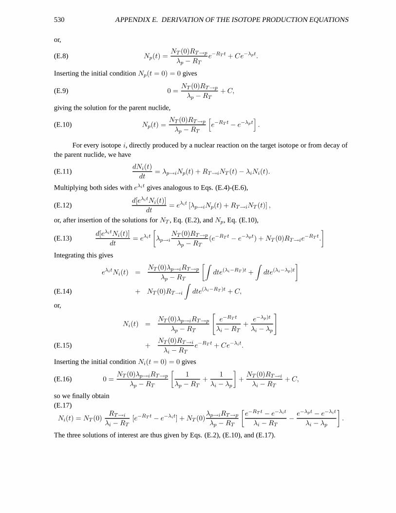
530 APPENDIX E. DERIVATION OF THE ISOTOPE PRODUCTION EQUATIONS
or,
(E.8) Np(t) =NT (0)RT→p
λp − RTe−RT t + Ce−λpt.
Inserting the initial conditionNp(t = 0) = 0 gives
(E.9) 0 =NT (0)RT→p
λp − RT+ C,
giving the solution for the parent nuclide,
(E.10) Np(t) =NT (0)RT→p
λp − RT
[
e−RT t − e−λpt]
.
For every isotopei, directly produced by a nuclear reaction on the target isotope or from decay ofthe parent nuclide, we have
(E.11)dNi(t)
dt= λp→iNp(t) + RT→iNT (t) − λiNi(t).
Multiplying both sides witheλit gives analogous to Eqs. (E.4)-(E.6),
(E.12)d[eλitNi(t)]
dt= eλit [λp→iNp(t) + RT→iNT (t)] ,
or, after insertion of the solutions forNT , Eq. (E.2), andNp, Eq. (E.10),
(E.13)d[eλitNi(t)]
dt= eλit
[
λp→iNT (0)RT→p
λp − RT(e−RT t − e−λpt) + NT (0)RT→ie
−RT t.
]
Integrating this gives
eλitNi(t) =NT (0)λp→iRT→p
λp − RT
[∫
dte(λi−RT )t +
∫
dte(λi−λp)t
]
+ NT (0)RT→i
∫
dte(λi−RT )t + C,(E.14)
or,
Ni(t) =NT (0)λp→iRT→p
λp − RT
[
e−RT t
λi − RT+
e−λp)t
λi − λp
]
+NT (0)RT→i
λi − RTe−RT t + Ce−λit.(E.15)
Inserting the initial conditionNi(t = 0) = 0 gives
(E.16) 0 =NT (0)λp→iRT→p
λp − RT
[
1
λp − RT+
1
λi − λp
]
+NT (0)RT→i
λi − RT+ C,
so we finally obtain(E.17)
Ni(t) = NT (0)RT→i
λi − RT[e−RT t − e−λit] + NT (0)
λp→iRT→p
λp − RT
[
e−RT t − e−λit
λi − RT− e−λpt − e−λit
λi − λp
]
.
The three solutions of interest are thus given by Eqs. (E.2),(E.10), and (E.17).

Appendix FTERMS AND CONDITIONS FORCOPYING, DISTRIBUTION ANDMODIFICATION
1. This License applies to any program or other work which contains a notice placed by the copyrightholder saying it may be distributed under the terms of this General Public License. The ”Program”,below, refers to any such program or work, and a ”work based onthe Program” means either theProgram or any derivative work under copyright law: that is to say, a work containing the Programor a portion of it, either verbatim or with modifications and/or translated into another language.(Hereinafter, translation is included without limitationin the term ”modification”.) Each licenseeis addressed as ”you”.
Activities other than copying, distribution and modification are not covered by this License; theyare outside its scope. The act of running the Program is not restricted, and the output from theProgram is covered only if its contents constitute a work based on the Program (independent ofhaving been made by running the Program). Whether that is true depends on what the Programdoes.
2. You may copy and distribute verbatim copies of the Program’s source code as you receive it, in anymedium, provided that you conspicuously and appropriatelypublish on each copy an appropriatecopyright notice and disclaimer of warranty; keep intact all the notices that refer to this Licenseand to the absence of any warranty; and give any other recipients of the Program a copy of thisLicense along with the Program.
You may charge a fee for the physical act of transferring a copy, and you may at your option offerwarranty protection in exchange for a fee.
3. You may modify your copy or copies of the Program or any portion of it, thus forming a workbased on the Program, and copy and distribute such modifications or work under the terms ofSection 1 above, provided that you also meet all of these conditions:
531

532APPENDIX F. TERMS AND CONDITIONS FOR COPYING, DISTRIBUTIONAND MODIFICATION
a) You must cause the modified files to carry prominent noticesstating that you changed thefiles and the date of any change.
b) You must cause any work that you distribute or publish, that in whole or in part contains oris derived from the Program or any part thereof, to be licensed as a whole at no charge to allthird parties under the terms of this License.
c) If the modified program normally reads commands interactively when run, you must causeit, when started running for such interactive use in the mostordinary way, to print or displayan announcement including an appropriate copyright noticeand a notice that there is no war-ranty (or else, saying that you provide a warranty) and that users may redistribute the programunder these conditions, and telling the user how to view a copy of this License. (Exception:if the Program itself is interactive but does not normally print such an announcement, yourwork based on the Program is not required to print an announcement.)
These requirements apply to the modified work as a whole. If identifiable sections of that work arenot derived from the Program, and can be reasonably considered independent and separate worksin themselves, then this License, and its terms, do not applyto those sections when you distributethem as separate works. But when you distribute the same sections as part of a whole which isa work based on the Program, the distribution of the whole must be on the terms of this License,whose permissions for other licensees extend to the entire whole, and thus to each and every partregardless of who wrote it.
Thus, it is not the intent of this section to claim rights or contest your rights to work written entirelyby you; rather, the intent is to exercise the right to controlthe distribution of derivative or collectiveworks based on the Program.
In addition, mere aggregation of another work not based on the Program with the Program (or witha work based on the Program) on a volume of a storage or distribution medium does not bring theother work under the scope of this License.
4. You may copy and distribute the Program (or a work based on it, under Section 2) in object codeor executable form under the terms of Sections 1 and 2 above provided that you also do one of thefollowing:
a) Accompany it with the complete corresponding machine-readable source code, which mustbe distributed under the terms of Sections 1 and 2 above on a medium customarily used forsoftware interchange; or,
b) Accompany it with a written offer, valid for at least threeyears, to give any third party, fora charge no more than your cost of physically performing source distribution, a completemachine-readable copy of the corresponding source code, tobe distributed under the termsof Sections 1 and 2 above on a medium customarily used for software interchange; or,
c) Accompany it with the information you received as to the offer to distribute correspondingsource code. (This alternative is allowed only for noncommercial distribution and only if youreceived the program in object code or executable form with such an offer, in accord withSubsection b above.)
533
The source code for a work means the preferred form of the workfor making modifications toit. For an executable work, complete source code means all the source code for all modules itcontains, plus any associated interface definition files, plus the scripts used to control compilationand installation of the executable. However, as a special exception, the source code distributedneed not include anything that is normally distributed (in either source or binary form) with themajor components (compiler, kernel, and so on) of the operating system on which the executableruns, unless that component itself accompanies the executable.
If distribution of executable or object code is made by offering access to copy from a designatedplace, then offering equivalent access to copy the source code from the same place counts asdistribution of the source code, even though third parties are not compelled to copy the sourcealong with the object code.
5. You may not copy, modify, sublicense, or distribute the Program except as expressly providedunder this License. Any attempt otherwise to copy, modify, sublicense or distribute the Program isvoid, and will automatically terminate your rights under this License. However, parties who havereceived copies, or rights, from you under this License willnot have their licenses terminated solong as such parties remain in full compliance.
6. You are not required to accept this License, since you havenot signed it. However, nothing elsegrants you permission to modify or distribute the Program orits derivative works. These actionsare prohibited by law if you do not accept this License. Therefore, by modifying or distributingthe Program (or any work based on the Program), you indicate your acceptance of this License todo so, and all its terms and conditions for copying, distributing or modifying the Program or worksbased on it.
7. Each time you redistribute the Program (or any work based on the Program), the recipient auto-matically receives a license from the original licensor to copy, distribute or modify the Programsubject to these terms and conditions. You may not impose anyfurther restrictions on the recip-ients’ exercise of the rights granted herein. You are not responsible for enforcing compliance bythird parties to this License.
8. If, as a consequence of a court judgment or allegation of patent infringement or for any otherreason (not limited to patent issues), conditions are imposed on you (whether by court order,agreement or otherwise) that contradict the conditions of this License, they do not excuse youfrom the conditions of this License. If you cannot distribute so as to satisfy simultaneously yourobligations under this License and any other pertinent obligations, then as a consequence you maynot distribute the Program at all. For example, if a patent license would not permit royalty-freeredistribution of the Program by all those who receive copies directly or indirectly through you,then the only way you could satisfy both it and this License would be to refrain entirely fromdistribution of the Program.
If any portion of this section is held invalid or unenforceable under any particular circumstance,the balance of the section is intended to apply and the section as a whole is intended to apply inother circumstances.

534APPENDIX F. TERMS AND CONDITIONS FOR COPYING, DISTRIBUTIONAND MODIFICATION
It is not the purpose of this section to induce you to infringeany patents or other property rightclaims or to contest validity of any such claims; this section has the sole purpose of protecting theintegrity of the free software distribution system, which is implemented by public license practices.Many people have made generous contributions to the wide range of software distributed throughthat system in reliance on consistent application of that system; it is up to the author/donor todecide if he or she is willing to distribute software throughany other system and a licensee cannotimpose that choice.
This section is intended to make thoroughly clear what is believed to be a consequence of the restof this License.
9. If the distribution and/or use of the Program is restricted in certain countries either by patentsor by copyrighted interfaces, the original copyright holder who places the Program under thisLicense may add an explicit geographical distribution limitation excluding those countries, so thatdistribution is permitted only in or among countries not thus excluded. In such case, this Licenseincorporates the limitation as if written in the body of thisLicense.
10. The Free Software Foundation may publish revised and/ornew versions of the General PublicLicense from time to time. Such new versions will be similar in spirit to the present version, butmay differ in detail to address new problems or concerns.
Each version is given a distinguishing version number. If the Program specifies a version numberof this License which applies to it and ”any later version”, you have the option of following theterms and conditions either of that version or of any later version published by the Free SoftwareFoundation. If the Program does not specify a version numberof this License, you may chooseany version ever published by the Free Software Foundation.
11. If you wish to incorporate parts of the Program into otherfree programs whose distribution con-ditions are different, write to the author to ask for permission. For software which is copyrightedby the Free Software Foundation, write to the Free Software Foundation; we sometimes make ex-ceptions for this. Our decision will be guided by the two goals of preserving the free status of allderivatives of our free software and of promoting the sharing and reuse of software generally.
*NO WARRANTY*
12. BECAUSE THE PROGRAM IS LICENSED FREE OF CHARGE, THERE IS NO WARRANTYFOR THE PROGRAM, TO THE EXTENT PERMITTED BY APPLICABLE LAW. EXCEPTWHEN OTHERWISE STATED IN WRITING THE COPYRIGHT HOLDERS AND/OR OTHERPARTIES PROVIDE THE PROGRAM ”AS IS” WITHOUT WARRANTY OF ANY KIND, EI-THER EXPRESSED OR IMPLIED, INCLUDING, BUT NOT LIMITED TO, THE IMPLIEDWARRANTIES OF MERCHANTABILITY AND FITNESS FOR A PARTICULARPURPOSE.THE ENTIRE RISK AS TO THE QUALITY AND PERFORMANCE OF THE PROGRAM ISWITH YOU. SHOULD THE PROGRAM PROVE DEFECTIVE, YOU ASSUME THECOST OFALL NECESSARY SERVICING, REPAIR OR CORRECTION.
13. IN NO EVENT UNLESS REQUIRED BY APPLICABLE LAW OR AGREED TOIN WRIT-ING WILL ANY COPYRIGHT HOLDER, OR ANY OTHER PARTY WHO MAY MODIFY

535
AND/OR REDISTRIBUTE THE PROGRAM AS PERMITTED ABOVE, BE LIABLE TO YOUFOR DAMAGES, INCLUDING ANY GENERAL, SPECIAL, INCIDENTAL ORCONSEQUEN-TIAL DAMAGES ARISING OUT OF THE USE OR INABILITY TO USE THE PROGRAM(INCLUDING BUT NOT LIMITED TO LOSS OF DATA OR DATA BEING RENDERED INAC-CURATE OR LOSSES SUSTAINED BY YOU OR THIRD PARTIES OR A FAILURE OF THEPROGRAM TO OPERATE WITH ANY OTHER PROGRAMS), EVEN IF SUCH HOLDER OROTHER PARTY HAS BEEN ADVISED OF THE POSSIBILITY OF SUCH DAMAGES.