UPTEC F 19064

Examensarbete 30 hpMaj 2020

Estimating fission fragment angular momentum using TALYS

Dany Gabro

Teknisk- naturvetenskaplig fakultet UTH-enheten Besöksadress: Ångströmlaboratoriet Lägerhyddsvägen 1 Hus 4, Plan 0 Postadress: Box 536 751 21 Uppsala Telefon: 018 – 471 30 03 Telefax: 018 – 471 30 00 Hemsida: http://www.teknat.uu.se/student

Abstract

Estimating fission fragment angular momentum usingTALYS

Dany Gabro

The Division of Applied nuclear physics at Uppsala university, is regularly performing high-precision measurements on isomeric fission yield ratios (IYR). Its aim is to explore the physics behind nuclear fission, in particular how angular momentum is generated. The department has developed a method to obtain the root mean square (rms) values of the primary fission fragment angular momentum distribution (Jrms). However, several assumptions are made in the model; thus this project aims to assess the sensitivity of the model parameters. In particular, the focus is on assessing the mean and width of the excitation energy distribution, as well as the correlation between the excitation energy and the angular momentum. The task is to implement a method that builds upon the previous model. The method that was implemented is based on random sampling, which randomises values of the parameters in a specific range depending on the type of distribution.Three types of distributions (Normal, Rayleigh and Poisson) of the excitation energy were tested, and it seemed to have little effect on the system. The fact that the distributions are symmetric or antisymmetric seemed to have negligible impact. The nucleus that was studied was 134I after the fission process with parent nucleus 235U in the thermal energy range. The IYR was plotted against four parameters: Jrms, a proportionality constant (A) between the energy and angular momentum, the intrinsic energy (Eint) and the spread of the energy (E).Their mean values and spread was acquired from a fission simulations software called GEF. Using these as inputs to another software TALYS, one can acquire the isomeric yield ratios (IYR) for the nucleus with different neutron channels. Jrms has the most impact, and had a clear interval which gave a IYR value close to experiments. The three other parameters showed no clear correlation which results in the conclusion: the IYR says very little about the fragments excitation energy but quite a lot about its angular momentum in the case of 134I with the assumptions made.

Tryckt av: Institutionen för fysik och astronomi, Tillämpad kärnfysik på Uppsalauniversitet

ISSN: 1401-5757, UPTEC F19064Examinator: Tomas NybergÄmnesgranskare: Henrik SjöstrandHandledare: Ali Al-Adili, Andreas Solders

Sammanfattning Institutionen för fysik och astronomi, tillämpad kärnfysik på Uppsala universitet, utför regelbundet hög precisionsmätningar av så kallade isomera utbyteskvoter eller isomeric fission yield ratios (IYR) som det heter på engelska. De har som mål att utforska och förstå fysiken bakom fission, i synnerhet det totala rörelsemängdsmomentet. En grupp på avdelningen har utvecklat en metod för att uppskatta det kvadratiska medelvärdet för det primära fissionsfragmentets rörelsemängdsmoment. Metoden har dock många antaganden. Därför har detta projekt som mål att uppskatta hur känsligt resultatet är för modellparametrarna. I synnerhet medelvärdet och bredden på excitationsenergifördelningen, men även korrelationen mellan excitationsenergin och rörelsemängdsmomentet. Uppgiften är att implementera en metod som bygger på den tidigare modellen, och förbättra osäkerheterna i beräkningarna. Metoden som implementerades var en Total Monte Carlo metod, vilket slumpmässigt väljer ut värden i ett specifikt intervall beroende på vilken sorts distribution som används.

Tre typer av distributioner (Normal, Rayleigh och Poisson) för excitationsenergin testades, och det ser ut som att valet av distribution har liten påverkan på resultatet. Faktumet att distributionerna är symmetriska eller antisymmetriska verkar inte ha en större påverkan på resultatet.

Kärnan som studerades var 134I efter att 235U hade fissionerats i det termiska energiintervallet på 0 MeV. IYR plottades mot fyra parametrar: Jrms, en proportionalitetskonstant (A) mellan energin och rörelsemängdsmomentet, den inneboende energin och bredden på energin Parametrarnas medelvärde)(Eint ).(σE och deras gränser kom från ett program som simulerar fissionsprocessen kallat GEF. Med hjälp av dessa som input till ett annat simulerings program kallat TALYS kan man få fram IYR för kärnan. Jrms var den parametern med störst påverkan på systemet och hade ett tydligt intervall, där IYR-värdet var nära experimenten. De tre andra parametrarna visade ingen tydlig korrelation vilket leder till slutsatsen: IYR säger väldigt lite om fragmentets excitationsenergi men mycket om dess rörelsemängdsmoment i fallet för 134I med de antaganden som gjorts.

1

Introduction 4

Background 4 Objective 5

Theory 5 Fission process 5 Fission fragment 6 GEF and TALYS 11

Method 13

Results 15 GEF 16 TALYS 21

Normal distribution of the input parameters 21 Uniform distribution of the input parameters 23

Discussion 25

Conclusion 26

References 27

Appendix 28 Normal distribution of the parameters 28 Uniform distribution of the parameters 31

2

1. Introduction a. Background Nuclear fission is a process in physics that is studied and researched by scientists all around the world. The process starts by colliding a particle (usually a neutron or proton) with a heavy nucleus. The energy from the particle is added to the nucleus which makes it excited and unstable. The unstable nucleus splits up into two smaller fragments. The fragments are highly excited and unstable. To reduce the fragments excess energy they will evaporate neutrons and gamma particles, resulting in higher stability. These emitted neutrons are referred to as fission neutrons or prompt neutrons. After the emission the fragment can end up in two possible states, the ground state or the isomeric state. The isomeric state is a meta-stable state. Not every nucleus can end up in the isomeric state however. Fission is used in a variety of fields, most notably in nuclear power plants. The fission process is a reaction that creates a large amount of energy which can be transformed into electricity. This is a way to provide our society with electricity and thus understanding the fission process is important. The more we understand it, the higher the efficiency and advantageous is the process of harnessing the energy for our society. The population of meta-stable states in exotic fission products is strongly correlated with the nuclear angular momentum of the initial fragments. The Division of Applied nuclear physics at Uppsala university, are regularly performing high-precision measurements on isomeric fission yield ratios (IYR) at the IGISOL (Ion Guide Isotope Separation On-Line) facility in Jyväskylä, Finland [1]. Their aim is to explore the physics behind fission, in particular how angular momentum is generated. An important step in the determination of the fragments total angular momentum is the nuclear de-excitation modeling. This is performed with the TALYS reaction code using the statistical evaporation of particles and γ-rays [2]. The various variables used in the model govern the calculated probability of meta-stable state population. By varying the initial angular momentum distribution P(J), one can alter the calculated IYR, and the results can be compared with experimentally deduced IYRs. A method has been developed to obtain root mean square (rms) values of the primary fission fragment angular momentum distribution [3]. The method has been benchmarked and compared with other fission codes. However, several assumptions are made e.g., the model assumed no correlation between energy and angular momentum. Therefore, a more accurate analysis is required to quantify the model parameter uncertainties.

3

b. Objective This project aims to assess the sensitivity of the fission parameters, i.e, which parameters affect the IYR most and what is the best estimated value for these parameters. This is done by implementing a Monte Carlo method which randomly samples the input parameters. In particular, the mean and width of the excitation energy distribution, as well as the correlation between the excitation energy and the angular momentum, are studied. The task is to implement a method and script that will be used on the TALYS calculations, to improve the uncertainty quantification of the performed calculations.

2. Theory a. Fission process

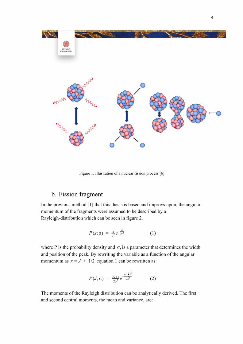
Fission is a process where a heavy nucleus receives an energy boost when capturing a neutron, proton, or gamma particle. This increase of energy causes the nucleus to reach an excited state, which leads to a split of the nucleus into two smaller nuclei. Each fragment has an excitation energy and an angularE* momentum .J The resulting fission fragments are still in an excited state. Depending on how excited the fragments are, the process can continue through the release of additional neutrons. Gamma particles will always be released whether or not additional neutrons are released. The nuclei before and after it has released additional neutrons are called, fission fragments and fission products respectively. By emitting gamma particles after the neutron emission the excited nucleus will decrease its excitation energy and two possibilities can occur: either the nucleus ends up in the stable ground state, or it gets trapped in an isomeric state [4]. The ground state and the isomeric state have the same number of nucleons in its nucleus; what sets them apart is the energy excitation levels. Isomers are excited and have hence higher energy with respect to the ground state which, by definition is not excited. The lifetimes of the isomers can be between milliseconds all the way up to minutes [5]. The entire fission process can be seen in the illustration in figure 1.

4

Figure 1: Illustration of a nuclear fission process [6]

b. Fission fragment In the previous method [1] that this thesis is based and improvs upon, the angular momentum of the fragments were assumed to be described by a Rayleigh-distribution which can be seen in figure 2.

(x; ) eP σ = xσ2

− x22σ2 (1)

where P is the probability density and is a parameter that determines the width,σ and position of the peak. By rewriting the variable as a function of the angular momentum as equation 1 can be rewritten as: 1/2x = J +

(J ; ) eP σ = 2σ2

2J+1 −2σ2

(J+ )21 2

(2)

The moments of the Rayleigh distribution can be analytically derived. The first and second central moments, the mean and variance, are:

5

(x) E = σ√ 2π (3)

(x) (2 )V = σ2 − 2π (4)

From this the Root-Mean-Square of the Rayleigh distribution can beE(x ))( 2 derived:

) (x ) (x) (x) (2 ) σ(xrms2 = E 2 = E 2 + V = σ2

2π + σ2 − 2

π = 2 2 (5)

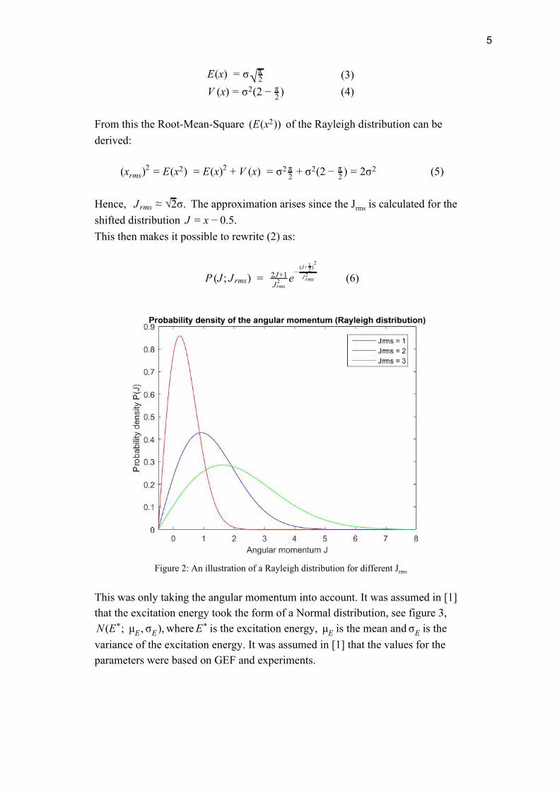
Hence, The approximation arises since the Jrms is calculated for theσ.J rms ≈ √2 shifted distribution .5.J = x − 0 This then makes it possible to rewrite (2) as:

(J ; ) eP J rms = J2

rms

2J+1 −J2

rms

(J+ )21 2

(6)

Figure 2: An illustration of a Rayleigh distribution for different Jrms

This was only taking the angular momentum into account. It was assumed in [1] that the excitation energy took the form of a Normal distribution, see figure 3,

where is the excitation energy, is the mean and is the(E ; μ , ),N * E σE E* μE σE variance of the excitation energy. It was assumed in [1] that the values for the parameters were based on GEF and experiments.

6

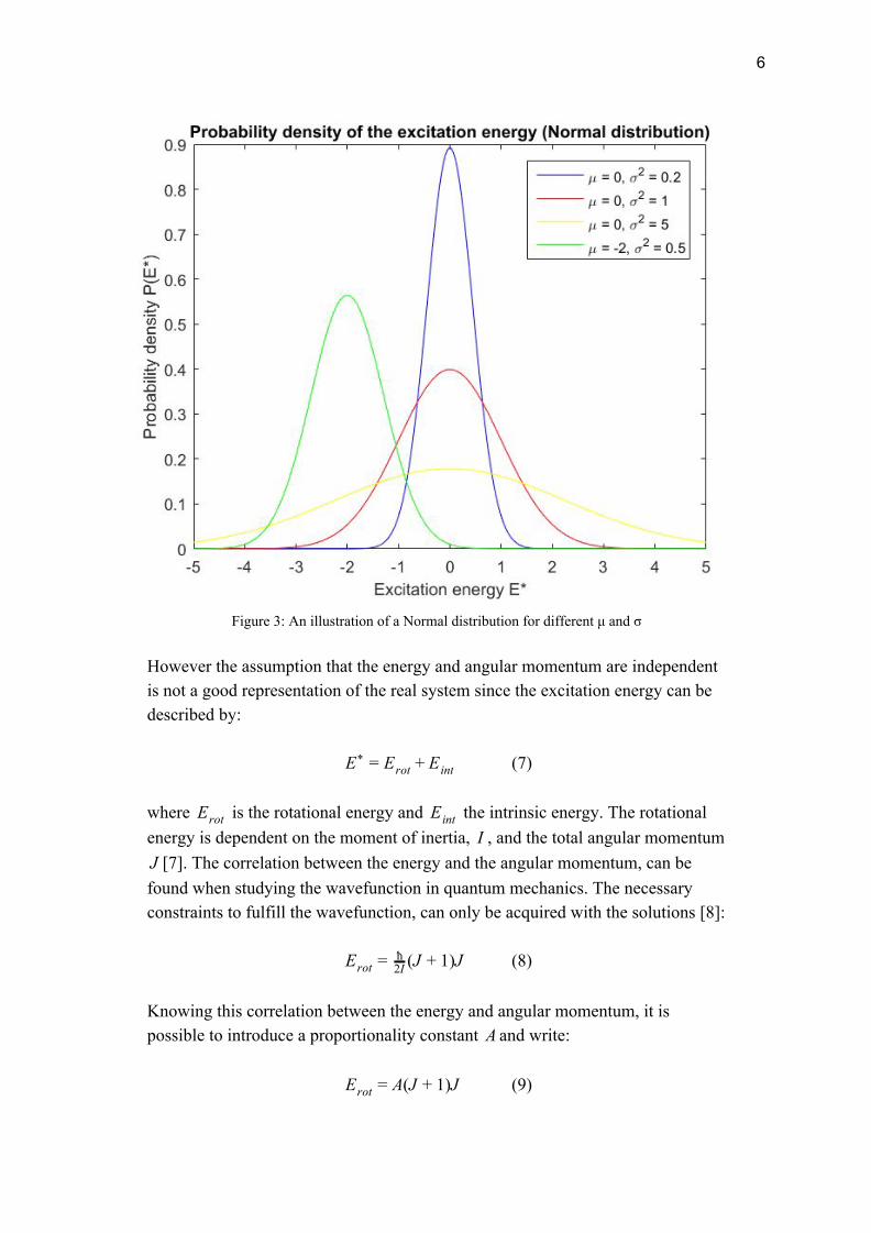
Figure 3: An illustration of a Normal distribution for different μ and σ

However the assumption that the energy and angular momentum are independent is not a good representation of the real system since the excitation energy can be described by:

E* = Erot + Eint (7) where is the rotational energy and the intrinsic energy. The rotationalErot Eint energy is dependent on the moment of inertia, , and the total angular momentumI

[7]. The correlation between the energy and the angular momentum, can beJ found when studying the wavefunction in quantum mechanics. The necessary constraints to fulfill the wavefunction, can only be acquired with the solutions [8]:

(J )JErot = ħ2I + 1 (8)

Knowing this correlation between the energy and angular momentum, it is possible to introduce a proportionality constant and write:A

(J )JErot = A + 1 (9)

7

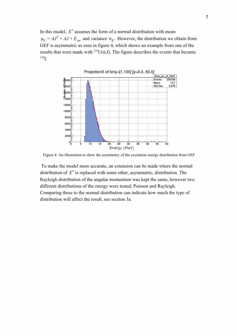
In this model, assumes the form of a normal distribution with meanE* and variance However, the distribution we obtain fromJ JμE = A 2 + A + Eint .σE

GEF is asymmetric as seen in figure 4, which shows an example from one of the results that were made with 235U(n,f). The figure describes the events that became 134I.

Figure 4: An illustration to show the asymmetry of the excitation energy distribution from GEF

To make the model more accurate, an extension can be made where the normal distribution of is replaced with some other, asymmetric, distribution. TheE* Rayleigh distribution of the angular momentum was kept the same, however two different distributions of the energy were tested; Poisson and Rayleigh. Comparing these to the normal distribution can indicate how much the type of distribution will affect the result, see section 3a.

8

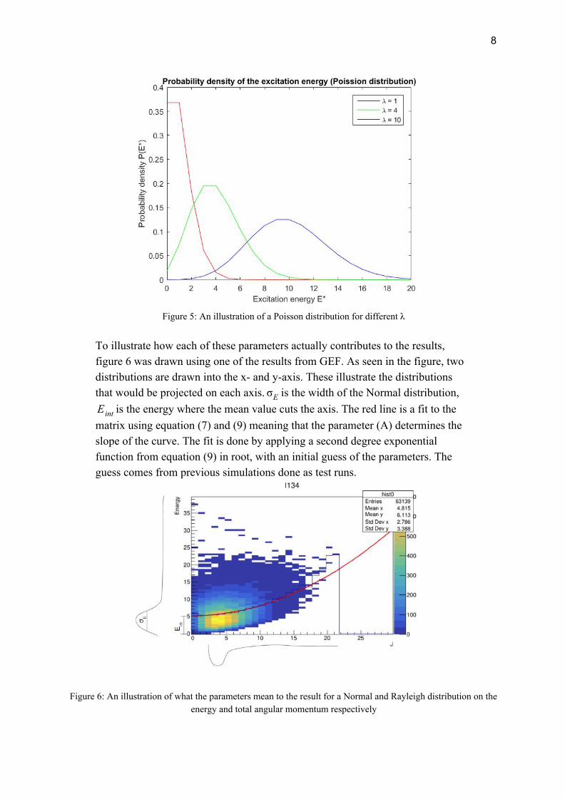
Figure 5: An illustration of a Poisson distribution for different λ

To illustrate how each of these parameters actually contributes to the results, figure 6 was drawn using one of the results from GEF. As seen in the figure, two distributions are drawn into the x- and y-axis. These illustrate the distributions that would be projected on each axis. is the width of the Normal distribution,σE

is the energy where the mean value cuts the axis. The red line is a fit to theEint matrix using equation (7) and (9) meaning that the parameter (A) determines the slope of the curve. The fit is done by applying a second degree exponential function from equation (9) in root, with an initial guess of the parameters. The guess comes from previous simulations done as test runs.

Figure 6: An illustration of what the parameters mean to the result for a Normal and Rayleigh distribution on the energy and total angular momentum respectively

9

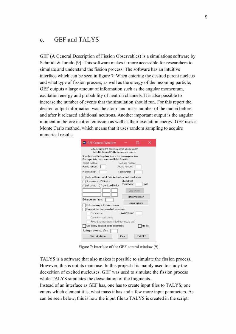
c. GEF and TALYS GEF (A General Description of Fission Observables) is a simulations software by Schmidt & Jurado [9]. This software makes it more accessible for researchers to simulate and understand the fission process. The software has an intuitive interface which can be seen in figure 7. When entering the desired parent nucleus and what type of fission process, as well as the energy of the incoming particle, GEF outputs a large amount of information such as the angular momentum, excitation energy and probability of neutron channels. It is also possible to increase the number of events that the simulation should run. For this report the desired output information was the atom- and mass number of the nuclei before and after it released additional neutrons. Another important output is the angular momentum before neutron emission as well as their excitation energy. GEF uses a Monte Carlo method, which means that it uses random sampling to acquire numerical results.

Figure 7: Interface of the GEF control window [9]

TALYS is a software that also makes it possible to simulate the fission process. However, this is not its main use. In this project it is mainly used to study the deexcition of excited nucleuses. GEF was used to simulate the fission process while TALYS simulates the deexcitation of the fragments. Instead of an interface as GEF has, one has to create input files to TALYS; one enters which element it is, what mass it has and a few more input parameters. As can be seen below, this is how the input file to TALYS is created in the script:

10

"element $ZZZ" > tmp_input "mass $AAA" >> tmp_input "projectile 0" >> tmp_input "energy $file" >> tmp_input

"best y" >> tmp_input "channels y" >> tmp_input

"preequilibrium y" >> tmp_input "outpreequilibrium y" >> tmp_input

"outinverse y" >> tmp_input "outtransenergy y" >> tmp_input

"outgamma y" >> tmp_input First the element is chosen as well as its mass number in the form of input parameters “element” and “mass”. “projectile 0” means that the the system starts with a group of excited nucleuses instead of having a reaction. “energy $file” is a file that consists of a matrix of excitation energy and angular momentum. “best” stores the best input parameters per nuclide. “channels” takes the cross section of all exclusive reactions into account. “preequilibrium” as the name implies enables the pre-equilibrium for any incident energy. “outpreequilibrium” keeps the parameters of the pre-equilibrium output and its cross sections. “outinverse” keeps the output of the particle transmission coefficients as well as the inverse reaction cross section. “outtransenergy” sorts the output of the transmission coefficient per energy or momentum depending on what you want. “outgamma” keeps the output for the gamma particles which include the strength functions, transmission coefficient and reaction cross sections. After the TALYS program is run, it outputs a large output file with information, however, the important datum that is considered in this project, is the isomeric yield ratio.

11

3. Method and results In this section a method to compare modelled fission using TALYS, GEF and sampling of model parameters with experimental data is further explained. The order of the project and the results can be split up into five sections:

1. Determine if the IYR is dependent on which type of probability distribution the excitation energy is, see section 3a.

2. A simulation with GEF is performed to determine the distribution between the different neutron channels, see section 3b.

3. Using the simulation from GEF to determine the mean and variance of the input parameters for TALYS, see section 3c.

4. The TALYS simulation is performed using the input parameters from GEF, see section 3d.

5. The experimental results were then compared to the calculated values from TALYS, see section 3e.

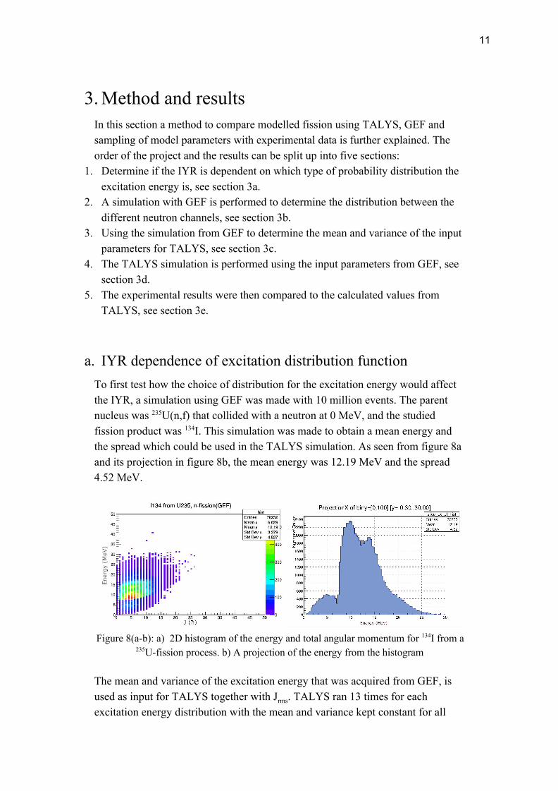
a. IYR dependence of excitation distribution function To first test how the choice of distribution for the excitation energy would affect the IYR, a simulation using GEF was made with 10 million events. The parent nucleus was 235U(n,f) that collided with a neutron at 0 MeV, and the studied fission product was 134I. This simulation was made to obtain a mean energy and the spread which could be used in the TALYS simulation. As seen from figure 8a and its projection in figure 8b, the mean energy was 12.19 MeV and the spread 4.52 MeV.

Figure 8(a-b): a) 2D histogram of the energy and total angular momentum for 134I from a

235U-fission process. b) A projection of the energy from the histogram

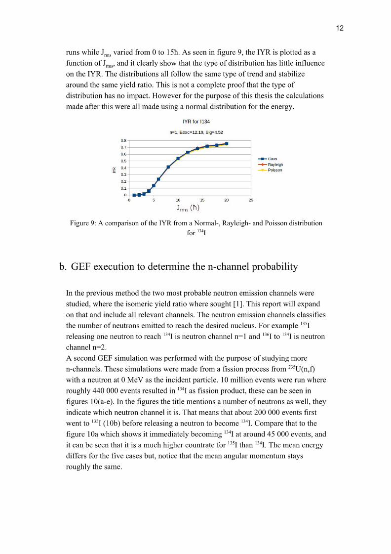
The mean and variance of the excitation energy that was acquired from GEF, is used as input for TALYS together with Jrms. TALYS ran 13 times for each excitation energy distribution with the mean and variance kept constant for all

12

runs while Jrms varied from 0 to 15ħ. As seen in figure 9, the IYR is plotted as a function of Jrms, and it clearly show that the type of distribution has little influence on the IYR. The distributions all follow the same type of trend and stabilize around the same yield ratio. This is not a complete proof that the type of distribution has no impact. However for the purpose of this thesis the calculations made after this were all made using a normal distribution for the energy.

Figure 9: A comparison of the IYR from a Normal-, Rayleigh- and Poisson distribution

for 134I

b. GEF execution to determine the n-channel probability

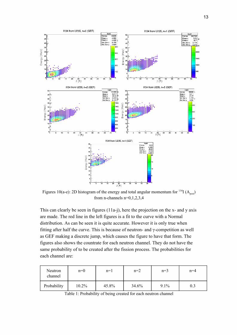
In the previous method the two most probable neutron emission channels were studied, where the isomeric yield ratio where sought [1]. This report will expand on that and include all relevant channels. The neutron emission channels classifies the number of neutrons emitted to reach the desired nucleus. For example 135I releasing one neutron to reach 134I is neutron channel n=1 and 136I to 134I is neutron channel n=2. A second GEF simulation was performed with the purpose of studying more n-channels. These simulations were made from a fission process from 235U(n,f) with a neutron at 0 MeV as the incident particle. 10 million events were run where roughly 440 000 events resulted in 134I as fission product, these can be seen in figures 10(a-e). In the figures the title mentions a number of neutrons as well, they indicate which neutron channel it is. That means that about 200 000 events first went to 135I (10b) before releasing a neutron to become 134I. Compare that to the figure 10a which shows it immediately becoming 134I at around 45 000 events, and it can be seen that it is a much higher countrate for 135I than 134I. The mean energy differs for the five cases but, notice that the mean angular momentum stays roughly the same.

13

Figures 10(a-e): 2D histogram of the energy and total angular momentum for 134I (Apost)

from n-channels n=0,1,2,3,4

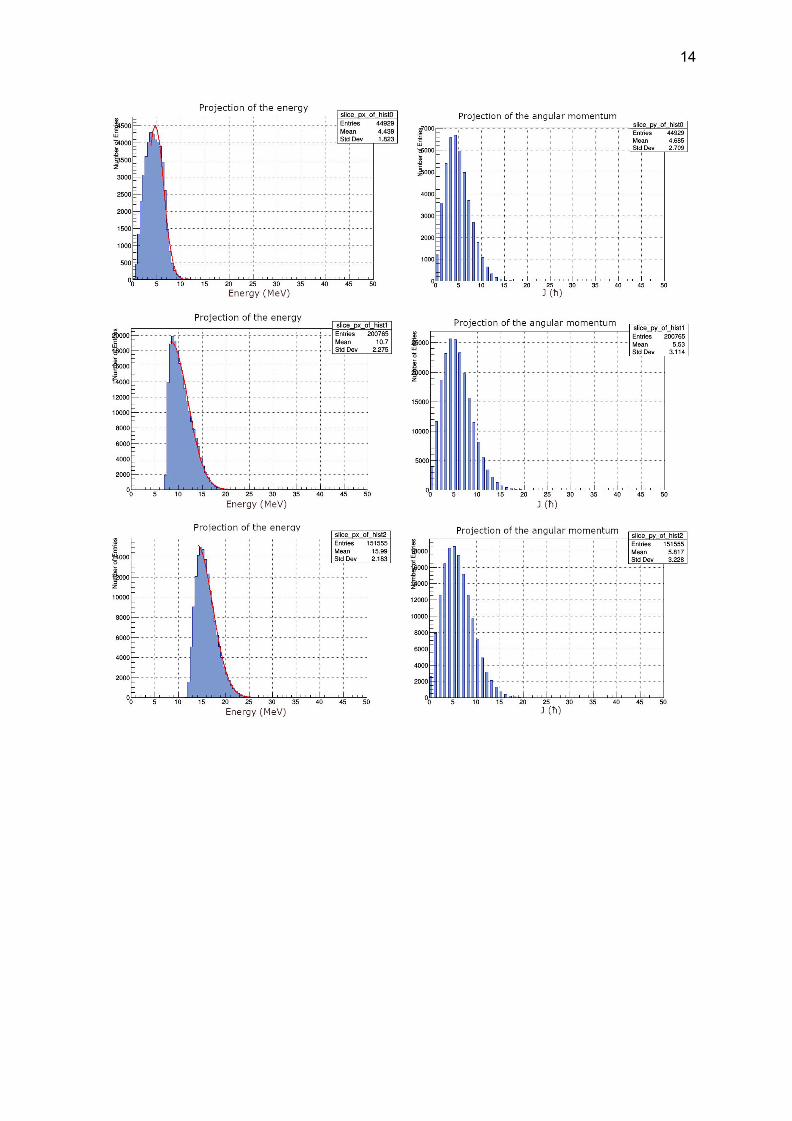
This can clearly be seen in figures (11a-j), here the projection on the x- and y axis are made. The red line in the left figures is a fit to the curve with a Normal distribution. As can be seen it is quite accurate. However it is only true when fitting after half the curve. This is because of neutron- and γ-competition as well as GEF making a discrete jump, which causes the figure to have that form. The figures also shows the countrate for each neutron channel. They do not have the same probability of to be created after the fission process. The probabilities for each channel are:

Neutron channel

n=0 n=1 n=2 n=3 n=4

Probability 10.2% 45.8% 34.6% 9.1% 0.3

Table 1: Probability of being created for each neutron channel

14

15

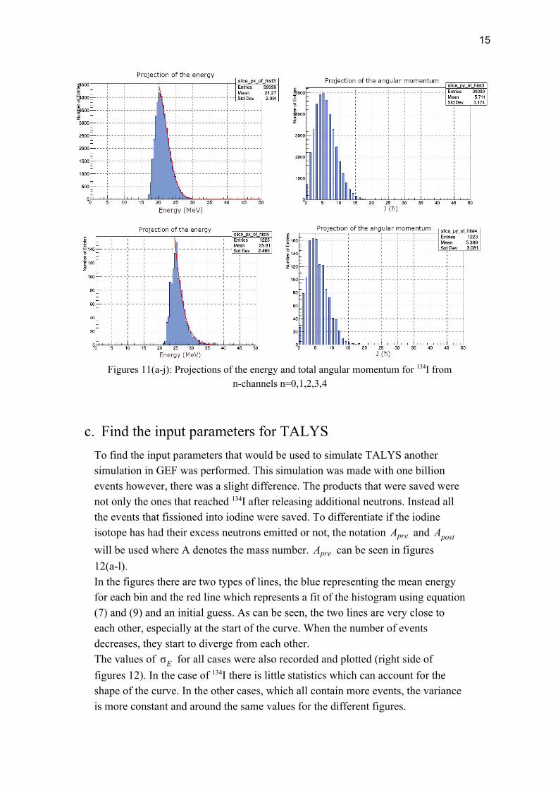
Figures 11(a-j): Projections of the energy and total angular momentum for 134I from

n-channels n=0,1,2,3,4

c. Find the input parameters for TALYS To find the input parameters that would be used to simulate TALYS another simulation in GEF was performed. This simulation was made with one billion events however, there was a slight difference. The products that were saved were not only the ones that reached 134I after releasing additional neutrons. Instead all the events that fissioned into iodine were saved. To differentiate if the iodine isotope has had their excess neutrons emitted or not, the notation and Apre Apost will be used where A denotes the mass number. can be seen in figuresApre 12(a-l). In the figures there are two types of lines, the blue representing the mean energy for each bin and the red line which represents a fit of the histogram using equation (7) and (9) and an initial guess. As can be seen, the two lines are very close to each other, especially at the start of the curve. When the number of events decreases, they start to diverge from each other. The values of for all cases were also recorded and plotted (right side ofσE figures 12). In the case of 134I there is little statistics which can account for the shape of the curve. In the other cases, which all contain more events, the variance is more constant and around the same values for the different figures.

16

17

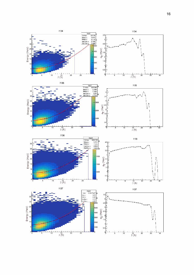
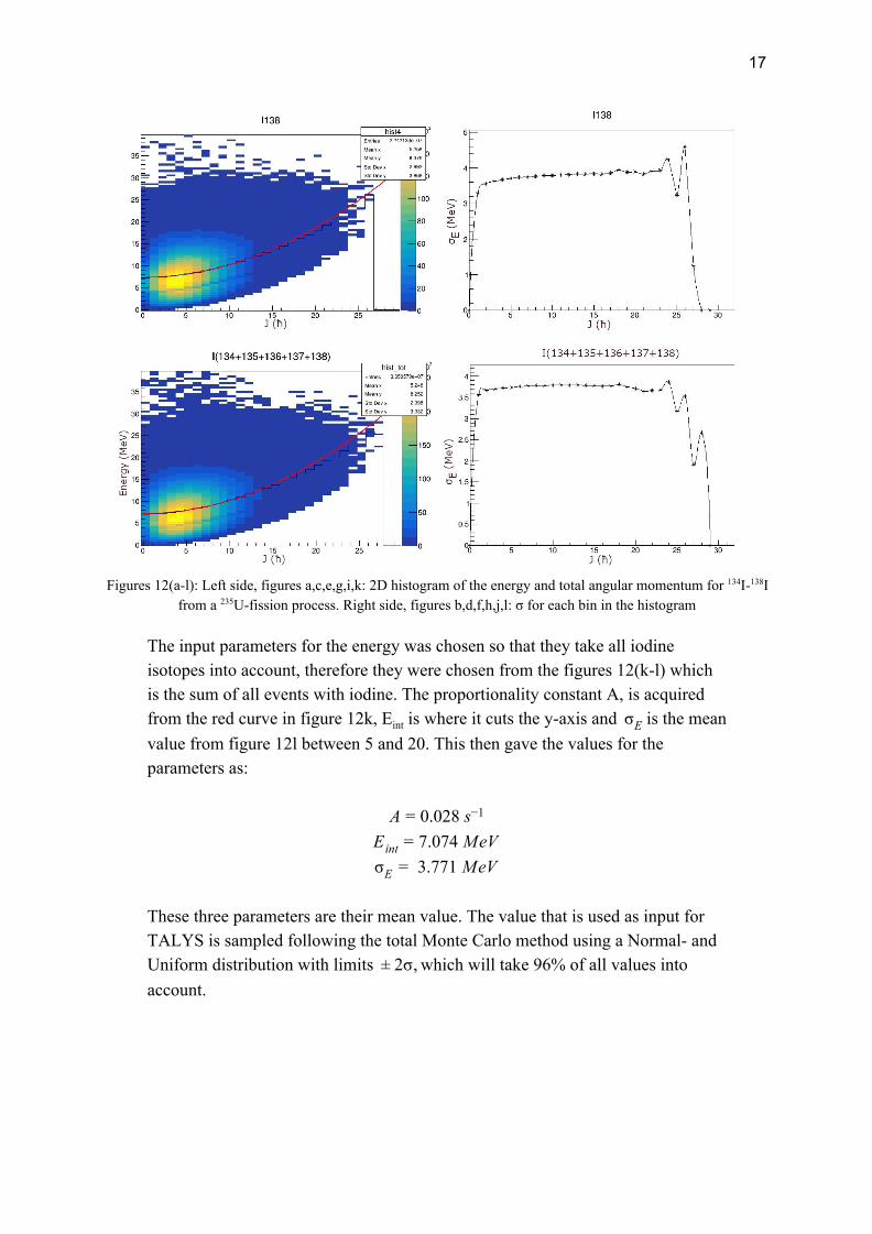
Figures 12(a-l): Left side, figures a,c,e,g,i,k: 2D histogram of the energy and total angular momentum for 134I-138I

from a 235U-fission process. Right side, figures b,d,f,h,j,l: σ for each bin in the histogram

The input parameters for the energy was chosen so that they take all iodine isotopes into account, therefore they were chosen from the figures 12(k-l) which is the sum of all events with iodine. The proportionality constant A, is acquired from the red curve in figure 12k, Eint is where it cuts the y-axis and is the meanσE value from figure 12l between 5 and 20. This then gave the values for the parameters as:

.028 sA = 0 −1

.074 MeVEint = 7 3.771 MeVσE =

These three parameters are their mean value. The value that is used as input for TALYS is sampled following the total Monte Carlo method using a Normal- and Uniform distribution with limits which will take 96% of all values intoσ,± 2 account.

18

d. Random rampling as input for TALYS

After the simulations in GEF are performed and the parameters are acquired, they can be used as input values for TALYS. They are sampled randomly around their mean value. The algorithm for the random sampling can be split up into 6 steps: 1. A value of is sampled from a Uniform distribution from 0 to 30ħ.J rms 2. A value of is sampled from a Normal distribution with mean ( ) andEint μint variance ( ) chosen based on GEF simulations.σint 3. A value of is sampled from a Normal distribution with mean ( ) andA μA variance ( ) chosen based on GEF simulations.σA 4. A value of is sampled from a Normal distribution with mean ( ) andσE μσE

variance ( ) chosen based on GEF simulations.σσE

5. The obtained parameters are used to construct the input matrix vs JE* for TALYS. 6. TALYS is run for all relevant precursors nuclei ( ) with the, , , , ..n = 0 1 2 3 . same input matrix. 7. Combining the results from the different precursors. 8. Repeat from 1 for x number of times. 9. The results are binned. 10. The results are compared to experimental results.

The algorithm was also tested with using a uniform distribution in step 2,3 and 4, with values between around the mean value of each parameter that wasσ± 2 acquired form GEF. An output from step 6, i.e., for each set of parameters, one IYR for each neutron emission channel is produced. By calculating the weighted mean of these, using the probabilities of each neutron emission channel, see table 1, from GEF as weights, it is possible to get one combined value of the IYR for each set of parameters. The obtained calculated values are binned and compared to the experimental values from IGISOL by calculating the -squared value of the meanχ of each bin:

χ2 = σ2(C−E)2

(10)

where C is the calculated value and E is the experimental value. A weight w, based on the likelihood of each bin is calculated using equation (11) [10]:

19

w = 1N ∑

N

ie− 2

χi2

(11)

A high weight w represent that the calculation is in good agreement with the experiment. A difference to [10] is that in this thesis the average weight of each bin is calculated. This is done in order to reduce the dependence of the sampling distribution.

20

e. Comparing the calculated results with experimental data This section is divided into two parts. The first part is the simulations when the parameters were sampled using a normal distribution, and the second part are sampled uniformly.

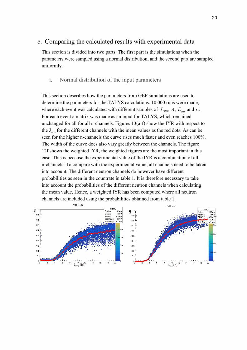
i. Normal distribution of the input parameters This section describes how the parameters from GEF simulations are used to determine the parameters for the TALYS calculations. 10 000 runs were made, where each event was calculated with different samples of and , A, EJ rms int .σ For each event a matrix was made as an input for TALYS, which remained unchanged for all for all n-channels. Figures 13(a-f) show the IYR with respect to the Jrms for the different channels with the mean values as the red dots. As can be seen for the higher n-channels the curve rises much faster and even reaches 100%. The width of the curve does also vary greatly between the channels. The figure 12f shows the weighted IYR, the weighted figures are the most important in this case. This is because the experimental value of the IYR is a combination of all n-channels. To compare with the experimental value, all channels need to be taken into account. The different neutron channels do however have different probabilities as seen in the countrate in table 1. It is therefore necessary to take into account the probabilities of the different neutron channels when calculating the mean value. Hence, a weighted IYR has been computed where all neutron channels are included using the probabilities obtained from table 1.

21

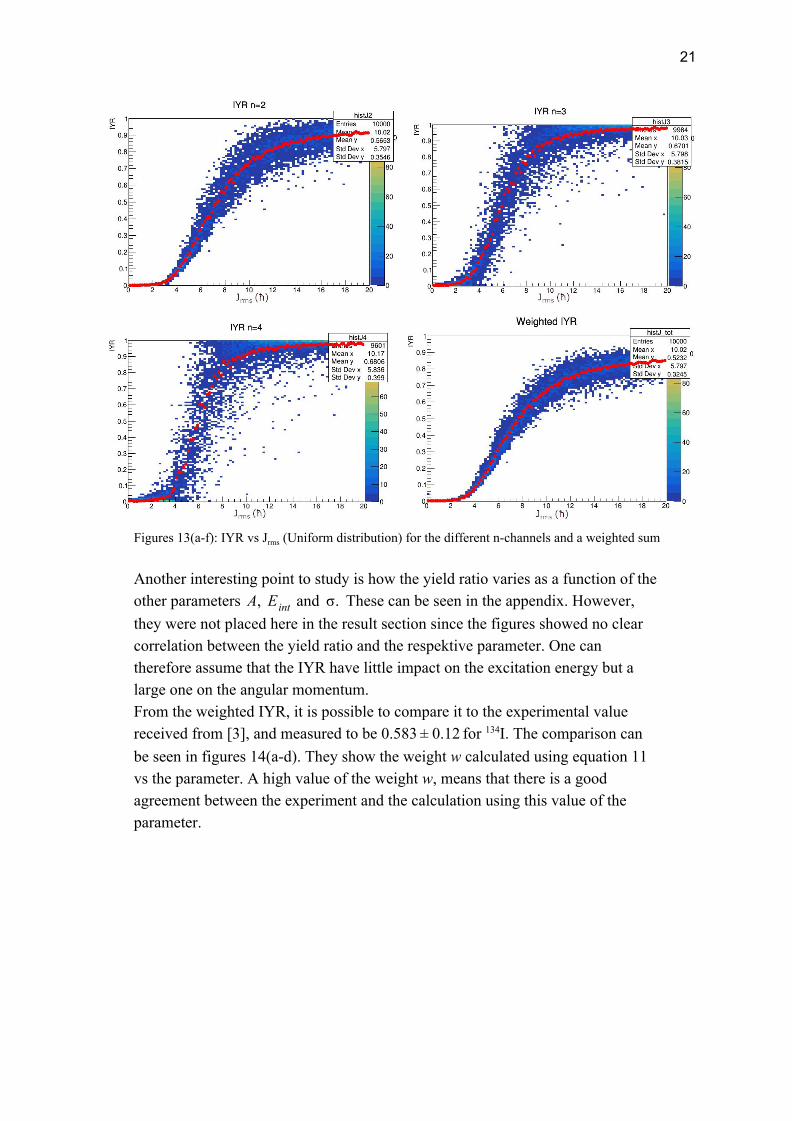
Figures 13(a-f): IYR vs Jrms (Uniform distribution) for the different n-channels and a weighted sum

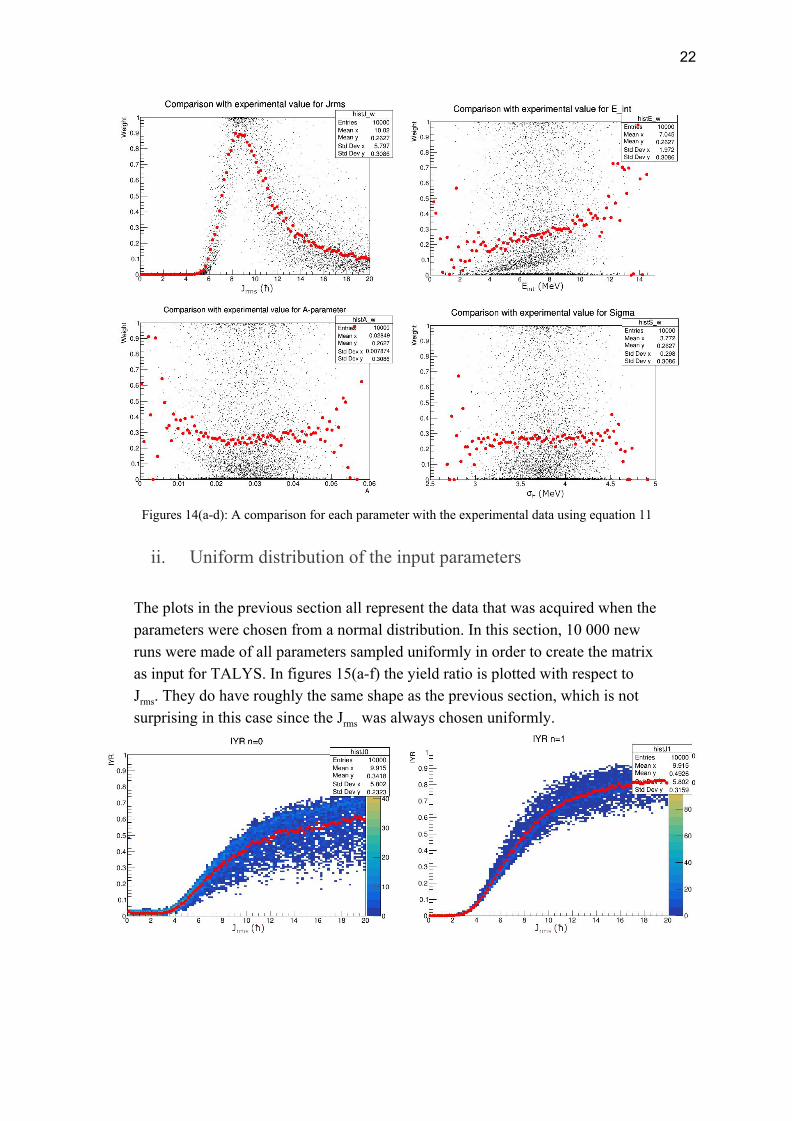
Another interesting point to study is how the yield ratio varies as a function of the other parameters and These can be seen in the appendix. However,, EA int .σ they were not placed here in the result section since the figures showed no clear correlation between the yield ratio and the respektive parameter. One can therefore assume that the IYR have little impact on the excitation energy but a large one on the angular momentum. From the weighted IYR, it is possible to compare it to the experimental value received from [3], and measured to be 0.583 for 134I. The comparison can.12± 0 be seen in figures 14(a-d). They show the weight w calculated using equation 11 vs the parameter. A high value of the weight w, means that there is a good agreement between the experiment and the calculation using this value of the parameter.

22

Figures 14(a-d): A comparison for each parameter with the experimental data using equation 11

ii. Uniform distribution of the input parameters

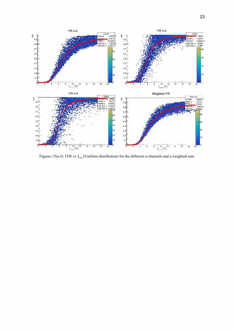
The plots in the previous section all represent the data that was acquired when the parameters were chosen from a normal distribution. In this section, 10 000 new runs were made of all parameters sampled uniformly in order to create the matrix as input for TALYS. In figures 15(a-f) the yield ratio is plotted with respect to Jrms. They do have roughly the same shape as the previous section, which is not surprising in this case since the Jrms was always chosen uniformly.

23

Figures 15(a-f): IYR vs Jrms (Uniform distribution) for the different n-channels and a weighted sum

24

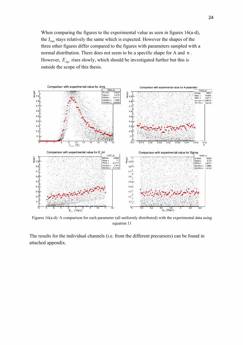
When comparing the figures to the experimental value as seen in figures 16(a-d), the Jrms stays relatively the same which is expected. However the shapes of the three other figures differ compared to the figures with parameters sampled with a normal distribution. There does not seem to be a specific shape for A and .σ However, rises slowly, which should be investigated further but this isEint outside the scope of this thesis.

Figures 16(a-d): A comparison for each parameter (all uniformly distributed) with the experimental data using

equation 11

The results for the individual channels (i.e. from the different precursors) can be found in attached appendix.

25

4. Discussion

The yield ratio for each parameters has been simulated and plotted in the previous section. As seen for the IYR vs the Jrms figures 13(a-f), they all roughly follow the same shape. For the low n-channels it rises slower than for higher, and in fact they never reaches 100%. Something that is worth mentioning is that, for n-channels 4, and even more rarely 3, sometimes never produced the nuclei 134I. Meaning that the nucleus never gave out a their respective number of neutrons to reach that, the nucleuses were stable enough at 135I. This means that there are not the same number of events for all the plots. This has been accounted for in the weighted plots, by increasing the chances for n=0,1,2 channels in these rare cases. The comparison between the simulated and experimental data figure 14a and 16a, clearly shows that the “best” values for the Jrms should be around nine. For σ and A parameter no clear trend is observed.

The figures 14b and 16c where the IYR is plotted with respect to the intrinsic energy, the weight increase when the intrinsic energy increases. It seems that the parameter with the strongest effect on the system is Jrms, followed by the Eint The other parameters do not seem to have that big of an impact on the system, meaning that for future studies the main parameter to study are the Jrms and Eint.

5. Conclusion

This thesis set out to assess the sensitivity of the fission model parameters, with respect to the IYR and what is the best estimated value for these parameters. The method used Jrms; the mean excitation energy and its spread; as well as a proportionality constant as input. By varying these parameters the isomeric yield ratio of the fragments can be changed and compared to experimental isomeric yield ratios.

When comparing the yield ratio to the Jrms a clear trend can be seen, where it quickly rises until it flattens out. This is the case for all neutron channels but they do rise faster for the higher channels. When comparing the result to the experimental data, there is a clear best estimated value. This value can be found around 9ħ.

The three other parameters do however vary the isomeric yield ratio quite a bit. For the proportionality constant and the spread in energy, no clear trends are found. For Eint seems to have better agreement with the experimental data when

26

Eint increases. However, to make a definitive conclusion higher energies have to be considered and tested.

In conclusion, the IYR is very sensitive to a fragments angular momentum but only weakly sensitive to the excitation energy. This cannot for certain be said for all nucleuses, however it seems to be valid for the nucleus 134I with the assumptions made in this study.

27

References [1] V. Rakopoulos et al., PHYSICAL REVIEW C 99, 014617 (2019). [2] A.J. Koning and D. Rochman, "Modern Nuclear Data Evaluation With The TALYS Code System", Nuclear Data Sheets 113 (2012) 2841. [ONLINE] Available at: https://tendl.web.psi.ch/tendl_2019/reference.html. [Accessed September 2019] [3] A. Al-Adili, et al., Eur. Phys. J. A (2019) 55: 61 [4] V. Rakopoulos (2018) “Isomeric yield ratio measurements with JYFLTRAP”, Uppsala University [5] H.D. Young, R.A. Freedman, “University physics with modern physics” 12th edition (2007) [6] Private communication A. Göök, Kungliga Tekniska Högskolan [7] C. Qi “Theoretical nuclear physics” KTH - Rotational Modeling https://www.kth.se/social/upload/5176d9b0f276543c2c2bd4db/CH5.pdf [Accessed 12 December] [8] R. Nave “Energy Calculation for Rigid Rotor Molecules” [ONLINE] Available at: http://hyperphysics.phy-astr.gsu.edu/hbase/molecule/rotqm.html [Accessed Mars 2020] [9] K.H. Schmidt, B. Jurado, Ch. Amouroux, JEFF-Report 24, Data Bank, Nuclear-Energy Agency, OECD, 2014 [ONLINE] Available at: http://www.khs-erzhausen.de/GEF.html. [Accessed September 2019]. [10] P. Helgesson et al., “Combining Total Monte Carlo and Unified Monte Carlo: Bayesian nuclear data uncertainty quantification from auto-generated experimental covariances,” Progress in Nuclear Energy, vol. 96, pp. 76–96, Apr. 2017, doi: 10.1016/j.pnucene.2016.11.006. [11] V. Rakopoulos et al. ”Measurements of isomeric yield ratios of fission products from protoninduced fission on natU and 232Th via direct ion counting. ND 2016 : International Conference on Nuclear Data for Science and Technology (pp. 04054). [12] A. Al-Adili et al. “Isomer yields in nuclear fission” (2019)

28

Appendix

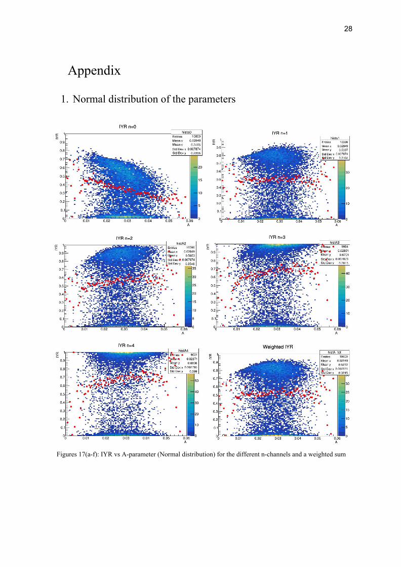
1. Normal distribution of the parameters

Figures 17(a-f): IYR vs A-parameter (Normal distribution) for the different n-channels and a weighted sum

29

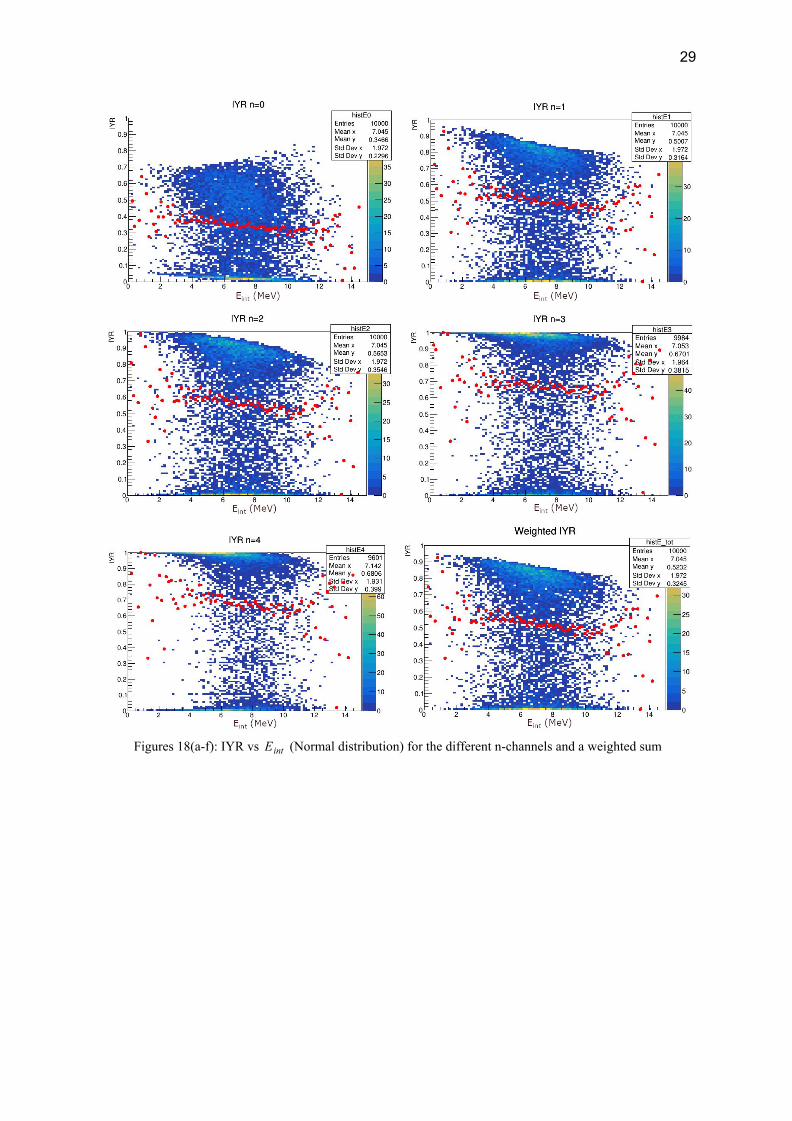
Figures 18(a-f): IYR vs (Normal distribution) for the different n-channels and a weighted sum Eint

30

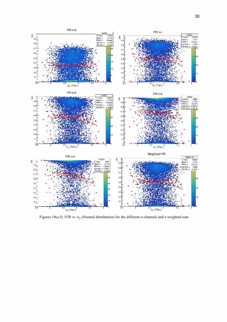
Figures 19(a-f): IYR vs (Normal distribution) for the different n-channels and a weighted sum σE

31

2. Uniform distribution of the parameters

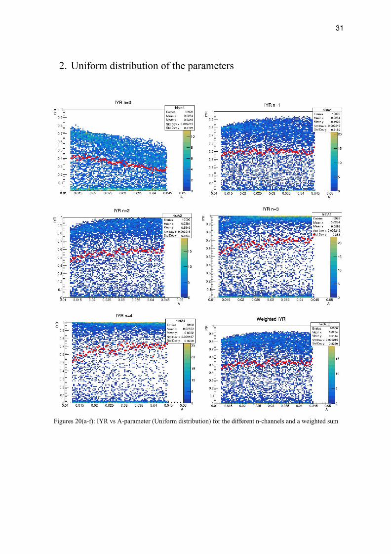
Figures 20(a-f): IYR vs A-parameter (Uniform distribution) for the different n-channels and a weighted sum

32

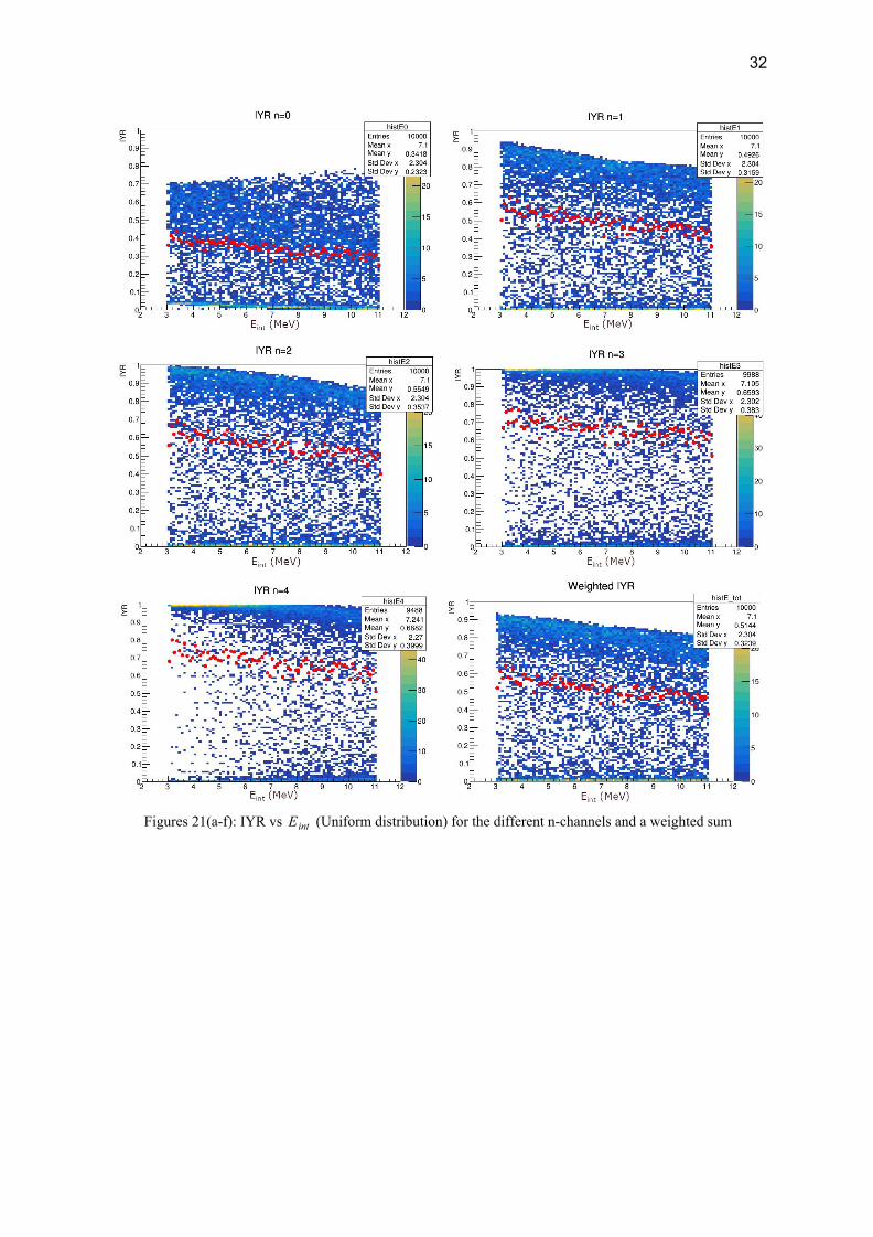
Figures 21(a-f): IYR vs (Uniform distribution) for the different n-channels and a weighted sum Eint

33

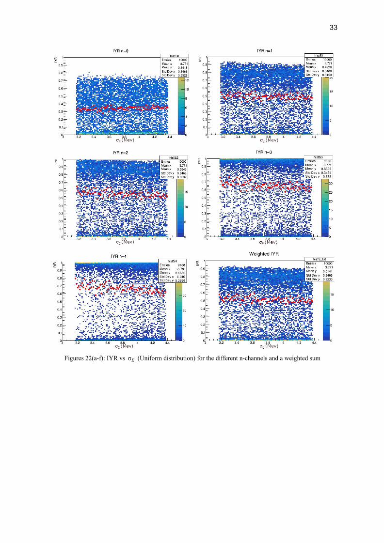
Figures 22(a-f): IYR vs (Uniform distribution) for the different n-channels and a weighted sum σE