Embed Size (px)
DESCRIPTION
vv
Citation preview
Preface
And having an equally venerable age theory or Processing Systems
Signals can be easily ascertained by studying its history the identification
Systems emerged and developed around with Automatica Therefore it
naturally become a fundamental subject of this area along with
disciplines mentioned above which is related When referring to
concepts such as process System regulator state or signal (first 4 being
Specific Automatic Control) discussion is based on the concept of model (mathematical)
Mathematical modeling entities on a suitable implementation means
Automatic calculation is a first and important objective of Automatic Control Default
mathematical modeling calls for construction of an assembly
consistent and rigorous ways entity considered to be identified with
the most appropriate mathematical model best adapted to the characteristics
its core In this type of problem has occurred and to
developed (and modeling) Identification Systems as interdisciplinary science
This book aims to describe the theoretical and practical aspects of modeling and
System Identification As a work of applied mathematics in technical (ie
in Automatic) which addresses the reader must have a knowledge base
located at least the first two years of training in a faculty of electrical profile
However the book was conceived in the spirit of the phrase self-contained ie
Presentation of gradual starting from the simplest terms by the complicated
without making numerous references to references nested and often difficult
available Whenever it was necessary the reader is reminded concepts
it needs to understand the arguments developed in chapters work
Of the four constituent chapters aims to introduce the first
discipline specific terminology is peppered with historical notes Identification
Systems is a discipline developed in a referential format of 3
major coordinates mathematical model associated entity to be identified
signal that it can be stimulated to provide data on behavior
its evolution and its intrinsic or the method that is determined model
especially math They constitute the nucleus of the 3 main chapters of the book
Each chapter concludes with a collection of exercises to be solved whose
purpose is to facilitate understanding
It is possible that some readers find too mathematized presentation especially
the end of the last chapter although the book contains numerous references to practical
discipline For those who prefer more practical purpose methods or
the algorithm rather than rigorous argumentation for construction and
their accuracy there is a paper alternative [SMS04]
Once learned the fundamentals of modeling and System Identification is expected
It can provide a basis for understanding other disciplines Automation
For example two of the subjects that has Systems Modelling and Identification
Setting a direct impact are automatic and automatic management of processes
We hope that the study material in the book to be as interesting and useful numbers
more readers
Chapter 1
Overview
The first chapter of this book is an opening
introduction to the terminology and problematic areas
Identification Systems (IS) Starting from the concepts of process
and system is specified fundamendală problem while being
highlighted the three coordinates that define the IS models
Mathematical they operate in practice the input signals
they stimulate the processes and methods of providing data
which is expected parameters selected models
11 The subject
Identification Systems (IS) is a discipline whose object of study is
process modeling dynamic systems using experimental data acquired
During their operation In this context modeling and construction means
determining a mathematical model associated entity usually progressive with a
momentum The entity is seen as a black box about whose structure
Internal no details A model is a mathematical relationship abstract
accurately describe certain characteristics and or dynamic operation of a
entities Mathematical models in the IS (also called identification models) are
used in a systemic manner More specifically the identification model reflects a relationship
of entry that stimulates a particular entity (called process or system) and
output encoding appropriate reaction to that entity Mathematical models
which operates in the IS are mainly based on the concepts of equation
Differential (for continuous-time systems development) and equation with differences
(for discrete-time systems development) However the models based on other
concepts are also used but more for the purpose of qualitative descriptions
behavior of the process to be identified Building models
Identification is based on experimental data provided by the black box (see
Figure 1)
The need to identify entities with unknown internal structure appears
numerous applications among which we mention only a few simulation in order
highlighting key characteristics and or behavior in various situations
forms recognition signal processing prediction forecast diagnosis of
defective design of automated systems management or control etc
There are two categories of identification techniques analytical and experimental In
Analytical identification aims to determine the physical parameters of a process
used for this purpose physicochemical laws at its base (ie the balance equations
mass energy equation of dynamic equilibrium etc) Experimental identification is
objective determination of general parameters without physical meaning but capable
describes the process behavior around a specific operating point
Compared with mathematical models obtained by writing equations balance
Results of expression laws of physics experimental models show identification
following characteristics
bull have a generality and validity limited to certain classes of processes signals
stimulus and even operating only at certain points of the same process
bull they have a physical interpretation difficult to give because in most cases
parameters have clear physical meanings parameters are rather used as
tools to facilitate description of the operation pocesului
bull Their determination is often made using algorithmic what they
gives efficiency and simplicity
In this book the discussion will focus on modeling and identification issues
Experimental trials A (short) refers to the identification of physical parameters
less complex processes can be found in [SMS04]
12 Historical Notes
IS Field was outlined in particular with the publications of KJ Aringstroumlm and
P Eykhoff in the 70s and 80s [AsEy71] [EyP74] [EyP81] In parallel there may be mentioned
important contributions to the development of research and outlining some directions
through his publications RL Kashyap and AR Rao [KaRa76] RK Mehra and D G Lainiois
[MeLa76] GC Goodwin and RL Payne [GoPa77] or T Soumlderstroumlm [SoT84]
Applications Identification and parameter estimation techniques (involving and modeling
mathematics) were not slow to appear They are described in a number of conferences
IFAC dedicated to IS and parameter estimation techniques such as those from Prague
(1967 1970) The Hague (1973) Tbilisi (1976) Darmstadt (1979) Washington DC (1982)
Numerous papers and overview synthesis were published especially
Automatic journals published by IFAC committee [IFAC80] [IFAC82] But one of the
more complete characterization of the domain was published in [SoSt89] - probably the
most cited reference in a decade They followed [LjGl94] and [LjL99] - two references
oriented identification algorithms
In Romania during the most prolific in terms of publications in the field of IS (years
70 -80) Does not go unnoticed Thus it can be said that the Romanian school
Identifications were initiated mainly through the works of C Penescu M and P Stoica Tertişco
[PITC71] [TeSt80] [TeSt85] [TSP87] An extremely practical vision related to IS (in
Automatic control systems context) was published by ID Landau
[LaID93] (in French) a book that was translated into Romanian [LaID97] A
Another paper dealing with practical aspects of the IS range is [SMS04]
Undoubtedly this brief history may not include vast panoply contributions
which led to diversification and enrichment IS domain Today the IS continues
in particular through the development of applications requiring openness to interdisciplinary approaches
The fast algorithms and techniques for identifying unconventional started
to appear since the early 90s through interaction with other fields
research especially with Signal Processing (PS) Artificial Intelligence (AI) and
Evolutionary Programming (EP)
13 Coordinates IS domain
Studying IS domain lies in the very concept of modeling
math Numerous applications Automation and or Computer Science
uses mathematical models In many cases the processes studied are so
complex that it is not possible to characterize them by describing phenomena
Physical underlying their behavior ie using the principles and laws of physics
expressed by balance equations Often it equations obtained in this way contain a
large number of unknown parameters In such cases the user is bound
circumstances to seek to identify models and experimental techniques
The specific work of IS is structured around three fundamental concepts
the mathematical model of the stimulus signal and the method of identification We refer on
In summary as to each of them They are described in detail in
The following three chapters of the book
Mathematical models are nonparametric and parametric The models
nonparametric are mainly used to obtain descriptions priori (preliminary)
more qualitative the process to be identified In this case the data
acquired are regarded as statistical data on the evolution dynamics of the process
Relatively simple statistical methods (generally based on technical (self-) correlation) are
applied to the data to obtain models both time domain and frequency as well
These models are described through charts or tables but without resorting to
Parameter concept They are useful in analyzing the process from different perspectives In
basically 4 types of analyzes can be performed transient analysis analysis
frequency analysis based on auto-correlation and spectral analysis
Parametric models most used applications in class ARMAX
(Auto-regressive moving average with exogenous control) As described in
Chapter 2 general class ARMAX model shows that the signal output
obtained as a result of the superposition of a useful signal obtained by filtering the signal
input and a signal obtained by filtering white noise parasite Particular cases
the most used applications are used ARX AR MA and ARMA The first model is
Typical applications optimal numerical control (or automatic control) while
last 3 are used particularly for modeling and predicting time series (less
specifically their stochastic component) A series of time (or a time stochastic process
discreet) is seen as an embodiment of a process driven by white noise
The choice of stimulus signals is based on a general principle if the
complex is integrated into a larger system - that works in closed loop -
The stimulus signal is then used during operation if the process can
function in open loop then a more accurate mathematical model is obtained by
stimulation of a persistent signal The concept of persistence is crucial
IS and will be described in detail in Chapter 3
The input signal is ideal white noise which has infinite persistence From
Unfortunately this signal can not be generated artificially More specifically the signals
artifacts (ie artificially produced) can not persist indefinitely order There are
artifacts signals with finite order of persistence approximate white noise in
auto-covariance purposes (and possibly the probability distribution) These
call pseudo-random binary signals (SPAB) or simply signed
Pseudo-Random (SPA) They are periodic as the algorithms used for
their generation using finite representational accuracy of the numerical values on a
Automatic calculation means Interestingly though their persistence is proportional order
period Moreover as the period increases they are closer to white noise
ie their values are becoming more correlated
Using SPAB or SPA IS is very frequent whenever the
identified open loop can be stimulated The models obtained using these
signals have high precision and are very versatile and can be used for a wide
range of operating points the stimulus signal and or configuration of the system
Finally identification methods aim to determine the parameters
naive model suggests either direct relationship computing or iterative procedures
However lack not only parameter values but their numbers
It entails adopting a strategy where the structural complexity iterative
model is gradually increased to the extent that its accuracy is not
significantly improved Specifically starting with the simplest model ie
parsimonios1 For each model given structure determine its parameters and
evaluate the error to the process (using a predefined criterion) If error
decreases significantly re-iterative process that is increase the number of
parameters then reassess them and error to the process Otherwise the process
iterative stalled and retain top model determined This model must be
finally validated using specific tests For example a model is valid if the error
between measured and simulated data has the characteristics of a Gaussian white noise
Determination of the unknown parameters of a mathematical model can be achieved in
mainly using methods drawn from optimization theory and or estimate Theory
(Statistics) A quick but discarded objects on these methods would put the
show their advantages and disadvantages Thus the methods of optimization algorithms provide
iterative (implemented) parameter estimation but estimates can not be
characterized statistically They provide the point of convergence
optimal but does not guarantee consistency in terms of statistical estimate (In this
context a consistent estimate of a parameter that tends to value
true that parameter as the number of data acquired from the process
tends to infinity whatever the data set used) From the other perspective Theory
Estimates consistency parameters can be tested but actual methods
neimplementabilitate assessment suffers generally rather a
theoretical support for other methods In addition these methods are based on assumptions
often restrictive in order to ensure consistency Fortunately the two theories
intersect The methods for identifying the most interesting and useful are the results
the combination of optimizing estimate They are implemented (possibly iterative) and
allow statistical characterization of the estimated parameters The prototype method you constiuie
Least squares (LSM) which will be presented in detail in Chapter 4
LSM is a kind of mother method which arose many
Other methods of identification adaptations inspired by the type of model used (Method
Instrumental Variables for ARX models Prediction Error Minimization Method
ARMAX models predictions Optimal Method for AR models etc) Although
However the IS is not limited to the family of methods generated by LSM
There are for example methods for the estimation of states in the Kalman filter or the method of
Robust identification The overwhelming majority of these methods are described in
[SoSt89] most of which are described in this volume
IS methodology but can not be a panacea but has its limits More
it should be used with caution and science The most important practical problems
appear in the identification process are listed below
bull Selection of sizes and can be measured There are situations where
sizes of paramount importance for the identification process can not be
measured directly inaccessible For example if it is desired
determining a model of the vibrations of a bearing integrated in a system
A mechanical fault detection its view it is very possible that sensors
vibration (accelerometers) can not be placed directly on the housing
bearing Their location to other locations may result in the combination and or
measuring the signal interfering with the vibration signals produced by other
mechanical system components so the possible mathematical models
inadequate To solve this difficult problem the user has
to formulate an alternative identification problem to extract information
studied the process of measured data in the context in which it is
Place this if known interactions between different subsystems
the global system Returning to the example of the bearing a method of extraction
desired vibration sensors is the use of directional orientation
bearing and use a method to mitigate interference (Such
The method has been patented in the US for example [CaDL96]) The cost of such
But solutions can be high so that the user will be restricted means
financial capabilities
bull Primary data acquisition and processing Trials identified
characterized by datasets acquired for the report semnalzgomot
(SNR - Signal-to-noise ratio) is reasonably high values Other
words the noise should not dominate useful data The more SNR is lower
so the model associated with risk be imprecise process and the process is more
less identifiable Increased SNR (signal dominance that is useful to the
Noise) can be achieved to some extent by processing
The primary data It consists mainly of a technical mitigation
noise (denoising) based filtering The user is faced here
Inadequate data distortion problem by choosing a filter or method
noise mitigation Unfortunately between useful and spurious data is not
can draw a clear line so that whatever method
Primary processing used some useful data likely to be eliminated while
What part of spurious data likely to be interpreted as useful data For
emphasizing the difference between useful data and parasitic methods are needed
Sophisticated processing undesirably complicating algorithm
Identification Consequently the user must carefully design the experiment
data acquisition so SNR equals big enough
bull Selecting a suitable mathematical model This can be a difficult problem
especially when the user is faced with a process having a strong
nonlinear behavior Identifying common models are linear One way
course is to address non-linearities in the selection of nonlinear models with
provided that non-linearities can be characterized in terms
mathematically Another approach would be based on the adaptation and implementation of a
Neural networks (The theory of neural networks [DuHa96] [TaI97] is
LSM is all that optimization technique during training network) Third
strategy closer to the IS is to use linear models
but with time-varying parameters that systematically adapts itself according
The acquired data Finally the process can be non-linear behavior
multi-shaped and the technique used Thus an appropriate model is chosen
a stored pre-defined depending on the current operating point
bull variability of processes over time This feature simply result in
that the true values of the parameters vary over time Thus it requires
use of mathematical models with time-varying parameters (as in the case
nonlinearities) The main problem now arises is related to
consistency estimates This time the parameter estimates should not
only tend statistically (ie with increasing horizon extent) to
their true values but to pursue precisely the time evolution
large enough The two requirements are obviously opposite so that
the main objective of the method of identification used (which can only be
Iterative) is to provide a good compromise between tracking ability
estimates and precision Another compromise to be made is that between
adaptability and robustness mathematical model as dynamic system It is
well-known that excessive lead to loss of robustness adaptability
systems (ie their ability to reject certain performance
containing shocks and disturbances to remain stable) In turn robustness
Excessive lead to poor tracking performance (ie adaptability)
Although brief presentation of this section of the discussion focused on
IS domain should be noted however that some of the techniques of identification may be
employed and to signal processing Especially if the process
I can not study highlights the input signals information about its evolution
is encoded in the output data set which is a time series Series models
frames are commonly used in spectral estimation [OpSc85] [OpWi85] [PrMa96]
prediction [TeSt85] [StD9603] [SMS04] or adaptive filtering [HaS86] - standard applications
PS rather than IS But between IS and PS can not draw a clear line
dividing at their intersection While undergoing some modern and effective methods and techniques
goals that serve both areas
14 Determinism and nondeterminism
The black box that we want to build a mathematical model must be
the ability to provide data and can potentially be stimulated for it In
Automation such entities operate with the input signals and provides
Output signals are generally referred systems (dynamic) A dynamical system
It is described by a set of differential equations (continuous-time) or the difference (in
discrete time) as
Also in the equations (1) I denoted by x any derivatives x1048581 (t) (continuous time
tisinR) or x [n + 1] (discrete time normalized nisinR) By convention brackets
Round indicates continuous time and the right - discrete time All sizes listed
in the equation (1) depends on time Figure 2 illustrates the usual representation of a system
dynamic Observe group separate from the internal quantities outside the system
Although most entities that can be represented using dynamic systems
are inherently nonlinear linear models are often preferred linear correspondent
a system of type (1) may be expressed as
where AisinN times n times m BisinN CisinRp times n times n DisinRq EisinRn times l times r FisinRp GisinRq times m
HisinRp times m matrix coefficients are constant or variable over time
The systems described by equations (2) is the subject of Theory
Linear Systems (TSL) [IoV85] where stability properties observability
controllability and robustness are extensively analyzed Within TSL faults v and w
play a secondary role being used primarily in the capacity of a system to study them
rejection offset or retain intrinsic stability whatever their nature Of
Therefore mathematical models of the TS (L) have a deterministic character despite
the presence of disturbances In other words at any point in time the quantities that describe
unique mathematical model values determined by that point of time whether
known or not
In reality however faults have a deterministic character and should be considered
as random variables (stochastic) are characterized by certain distributions
probability This means that at a certain time values
disturbances are not uniquely determined but varies in a certain range (range)
each having a certain probability of occurrence Therefore other
sizes that are trouble-deterministic inherit their character
becoming stochastic The study deterministic systems is affected by disturbances
conducted within the IS (though not the only area concerned about this
problematic) from a perspective different from that of TS (L) determining the parameters and
their characteristics In the case of linear systems (2) the parameters are coefficients
matrix H
To emphasize the distinction between behavior systems
deterministic and non-deterministic behavior we take the example of a
I continuous linear system of order whose ideal transfer function is
isinR where K is the gain and Tgt 0 is the time constant which is
system parameters In the absence of disturbances the two parameters can be easily determined
about graphics using step response of the system (ie the step response
unit) as shown in Figure 3 Thus the amplification of the asymptote is given by
horizontal and the time constant is found assesses the tangent at abscissa
origin of the graph intersects the horizontal asymptote
above is found rarely The curve may look more like Figure 4 Such
variation is called and development (system) Moreover repeating the experiment
system stimulation with the exact same type input stage and measurement unit
output can drive each time to a different deployment of previous achievements
as shown in Figure 5 This behavior is due to deterministic disturbances which
corrupt system output It can be seen from Figure 5 it is virtually impossible
determined pair of parameters that characterize the system operation more
namely (K T) using the same technique in the case of deterministic system
The set of all achievements system is called deterministic process
(stochastic) Given the nature of the data deterministically output image
Figure 5 should be complemented with information about the probability distribution of
perturbations that have produced this effect Often preliminary knowledge
the probability distribution associated with a stochastic process is however very difficult if
not impossible Fortunately a large class of stochastic processes are or may be
considered normally distributed ie with probability density
where y is the average and σ2 is the variance of the random variable y (t) This density
by Carl Gauss was introduced (1777-1855) its shape illustrated in Figure 6 the
like a bell (Gauss bell) with the opening of the σ measured
For having the probability distribution (4) further writes yisinN (y σ2)
(ie y belongs to the class of normal distributed processes mean and variance σ2 y)
In Class N (y σ2) falls often probability distribution processes
Unknown based on the Central Limit Theorem (TLC) of Statistică2
Distribution normal Gaussian will often adopted developments in this
book but applied systems discrete processes In this case definition (4) changes
only the argument temporal (t) will be replaced with (NTS) or more simply with
[n] where Ts is sampling period (default unit) Note that the argument
The main probability distribution is not time but the values of the random variable
that the output y in the example chosen
Obviously because p is a probability distribution check identity
int (()) () = 1
+ infin
-infin
p y t dy t foralltisinR (5)
what comes to property cert probability that the value of y to
It is included in R (ie the interval (-infin + infin)) is uniform at any time
(Area under the bell of Gauss is always uniform)
Another interesting property is as follows the probability that the value of y to
be included in the range (y - 3σ y + 3σ) (appointed ad hoc and 3σ interval) is at
less than 95 at any time
()
3
3
() () 095
y
y
dy t y t
+ Σ
- Σ
int p ge foralltisinR (6)
The area under the bell of Gauss is almost above the range 3σ
equal to the entire area This implies that the values of y will belong close
3σ safe range It is noted that this range is controlled by the values of σ
called standard deviation The range looks and how precisely is determined y located
The higher the standard deviation is higher much weaker y is located on the real axis
(Gauss bell is dilated) and therefore less precise Deviations
standard (or variant) small lead to high accuracy (Gauss bell being
tablet) Basically it is essential Gauss bell located above 3σ range
Finally a third interesting property which can be demonstrated as follows
(Y (t)) y (t) dy (t) y
+ infin
-infin
int p = foralltisinR (7)
indicating that the statistical mean value of y is even y at any time
time Of course media y may depend in turn time even if this
addiction does not appear explicitly in the definition (4)
Property (7) induces that t is most likely value or value
the expected y This means that a finite sequence of experiments
measurement of y y value at a certain time has the highest frequency
great appearance
In the case of systems processes discrete equations (5) (6) and (7) during continuous
It should be replaced with discrete time (normalized) But they show the same properties
We conclude this section by stressing again that the distinction between
System concepts deterministic (that is operating in the TS (L)) and the
deterministic or stochastic process system (that is operating within IS) Often
dynamic system is considered an idealization process data provider being
also it is used as generator of the data if necessary
Starting with the next section the discussion will focus on identifying patterns
having an input and an output (SISO - Single Input Single Output) Other types of
models (SIMO - Single Input Multiple Output MISO - Multiple Input Single Output
MIMO - Multiple Input Multiple Output) are not practical subject of this book
15 The general issues in IS
The main objective of the experiment IS is that starting from a process
P stochastic structure and behavior unknown to build and
determine a mathematical model M which matches well the process in a sense
defined Generally adequate trial model is tested using criteria
a priori defined The criteria can fall into 3 main categories
a empirical criteria (quasi-statistical)
b criteria optimization
c estimation criteria
Empirical criteria based on some elementary statistics and are
often used to describe non-parametric models These models are used to
The qualitative description of the often rough imprecise process In
next chapter will describe some identification techniques (called analysis) using
nonparametric empirical models and criteria on which to evaluate accuracy
thereof
More interesting however are appropriate criteria for parametric models In this
case the mathematical model is described by a number of unknown parameters
to be determined Note that not only parameter values are not known but
their number In the IS the unknown parameters are packed in a vector denoted by θ
size (still unknown) nθ (As in the TS the IS working with vectors
column) adopted fundamental assumption in this case is
H The process works like a mathematical model with real parameters
unknown values deterministic (possibly time-varying) whose
vector is denoted by θ and has nθ size
In this context there are two formulations of the fundamental problem identification
adequacy criterion used by nature the formulation of Optimization Theory
(TO) and the formulation of the Estimation Theory (Statistics) (TE)
151 The problem from the perspective IS TOO
Within TOO problem identification is a formulation that relies on image
in Figure 7
Thus both the P (θ ) and the M (θ) are stimulated with the same input
u which is the collection of data measured in a 1 N [] = U = As horizon
It is normally finished for example of length N isinN The process provides output data
measured in N y n 1 [] = Y = The mathematical model provides simulated data
n N yn 1 [] = θ YM M which depend on the parameters determined from the data vector
measured For the same set of measured data U Y one can obtain a collection of
vectors of unknown parameters (both as a value and as dimensions) and therefore sets
simulated data It was noted by ε [n θ] error between the measured data
Simulated (ie the process and model) at the current time
[n θ] y [n] y [n θ]
def
M ε = - forallnisin1 N (8)
All errors (8) is used to define the criteria for adequacy V (θ) which
It must be optimized to determine the unknown parameters Choosing
adequate mathematical model often involves an iterative process following which
set of possible models is reduced to a finite collection The model is then appropriate
especially in this set taking into account not only appropriate but also other considerations
implementabilitatea related to it This is the meaning of the arrow returned
the casings of the model in Figure 7
Efficiency and complexity of the optimization depends sensitive to the manner in
which was defined criterion of adequacy Note that adequate criterion value
evaluated for a particular model identification is often interpreted as a
an indicator of the accuracy of the model Next specified two criteria of adequacy
frequently used applications
V (θ) ε [ θ] (robust criterion) (9)
Σ =
=
N
n
f
n
1
V (θ) ε 2 [ θ] (quadratic criterion) (10)
Both criteria evaluates the total error between process and model but using applications
different The first criterion (the robust (9)) looks more natural because it sums
the absolute values of all errors The second criterion (the quadratic (10)) is both more
easy to use optimization as function module used in the first criterion
It is differentiable everywhere Optimization is performed within IS using primarily
gradient techniques (some of which are described in Chapter 4) Other methods
Optimization can also be used (for example AI-based techniques or
PE) Turning to criteria (9) and (10) appropriate parameter vector of measured data
Note N θ is obtained by minimizing nonlinear Troubleshooter
Argmin ()
n
N isin sube θ
=
θ
θ θ
And R
V (11)
where S sube stability Rnθ is the model matematic3 and argmin
means the argument that minimizes (specified criterion function) Naturally
want the resulting model different as little of the data provider ie
leading to a minimal total error Typically applications to accurately determine the
the optimum point is not possible but there are techniques for approximating it with
precisely controlled (as are the techniques of gradient) These techniques are based on
iterative whose main quality characteristics are complexity
convergence and speed of convergence Of these the optimum convergence is
Foremost
The optimization problem (11) is solved for a finite size
vector parameters (ie nθisin1 Nθ) in order to provide finite collection
vectors which will subsequently choose suitable parameter vector It should be noted that it
Suitable parameters are always the most precise meaning of criterion V as
will see later
You can define other criteria than those listed above (for some
it is necessary to solve a problem of maximization and minimization not) The
The resulting data will be suitable but only for the purposes of general mathematical criterion
used It is unlikely that a suitable model by a certain criterion to continue
after changing the criteria to be suitable
152 The problem IS the light of TE
Theory estimate (TE) consists of a set of techniques for determining
unknown parameters using statistical concepts As the data provided by
are of stochastic process it is transferred and parameters which
They are called in this context and parameters estimated The method for producing
estimates of unknown parameters is called estimator The quality of a
estimator is given by the following main characteristics complexity consistency
(or statistical convergence) and efficiency (or convergence speed) Of these
features (described in the next chapter) consistency is of prime importance
Problem identification is in this context suggested forms of image
Figure 8
Figure 8 Identification parameters using criteria TE
This image and that of Figure 7 are very similar Consequently
There are many similarities between the two formulations of the problem of identification We
briefly only differences between them
So this time the output measured and simulated using
to build adequate criterion P (θ) called auto-covariance matrix
the estimation error As the name P (θ) is a matrix of order nθisin1 Nθ
It is defined using statistical average operator E (presented in chapter
next)
() () () T
def
P θ = E θ - θ θ - θ (12)
The definition (12) the difference θ - θ is the error of estimation parameters and bull T is
transposition operator It also notes the use of the external
two vectors (VVT) One can easily see that this criterion directly addresses
true parameters (which are unknown) so apparently it is impossible
rated However it can be shown (as in Chapter 4) that for certain
estimated matrix P (θ) can be estimated despite vector
True parameter is unknown
Identification problem in this case is reduced to a nonlinear problem
minimization
Argmin ()
n
N isin sube θ
=
θ
P θ θ
And R
(13)
where the minimization is performed in the positive sense of ownership defining matrices
More specifically a square matrix P1 is less than or equal to a matrix P2
having the same size if the matrix P2 - P1 is positive semi-defined
2 1 0 P - P ge Minimization condition is not only natural but also required
Consistency property It can show the consistency that the property is
equivalent to the following condition
lim () N rarr infin N
P θ = 0 (14)
The problem (13) can turn equivalently or can relax by
formulating a problem of maximizing the probability of a particular estimate
parameter vector (as described in Chapter 4) However problems
Optimization of the TE are more difficult than those of the TO
To conclude this section will be highlighted advantages and
disadvantages of each type of translation solutions solve the problem identification
the two theories The TO-based solutions have the advantage of being produced
using relatively easy to implement algorithms on an automatic means of calculation but
the disadvantage that can not be characterized statistically In the TE
solutions provides the opportunity to evaluate a number of statistical properties but methods
Their often used to obtain a theoretical without leading to
Implemented algorithms However the IS aflicircndu is somewhat at the intersection of
two theories provide general problem solving methods that combine
advantages of each of them as can be noted in Chapter 4
16 Identification experiment
In general terms the issue raised in the previous section can be solved
(for models identification parameters) by organizing an experiment
Identification This section is devoted to description of the manner in which it can be
designed an experiment to identify and ends with an example (finding
heaters)
161 Diagram of an identification experiment
The experiment identifier means a series of sequential operations or
parallel is made according to the organizational chart in Figure 9 We will describe briefly
In continuation
A Initial data
Designing an experiment identification process begins by stating
Provider of data to be identified The efficiency and success of the experiment
depend on how much sensitive information is a priori known about
process This information should contain the following minimum
1048581 type of process strong non-linear non-linear almost linear linear Most
Nonlinear processes are nonlinear and strong but linearized around
rated operating points Therefore practically it should be laid
operating points around which it is desired to build a model
linear mathematical If I know the equations of continuous operation while
(by the application of physicochemical laws) they may be discretized
to obtain information on identifying the model structure would
You are chosen Otherwise they will be (eventually) take several experiments
Successive identification of a suitable model for the construction and valid
1048581 type of variation slow (over 5s) medium (between 1s and 5s) fast (sub 1s)
This information refers to the amount of stabilizing the output when
step process is stimulated with a certain amplitude accepted
(not leading to instability) and is useful in determining the period
sampling (Ts) to be chosen for the purchase of digital data
1048581 intrinsic dead time of the process While its value detection
and conversion to continuous (even imprecise) discrete-time (as a number
throughout the sampling period) lead to a simplification model
Identification choice In the absence of this information the mathematical model can
work with a number of parameters parasites which increase the complexity
thereof
In practice the determination of the dead time can be effected by stimulating the
preliminary stage of the process with a certain amplitude which does not
leading to instability
1048581 process variability while Many processes behave as
systems with time-varying parameters If the parameters vary slowly over time
it can be considered that they are constant provided that at certain intervals
time associated mathematical model to be reassessed If however the parameters
varies rapidly over time then the model must be adapted to the dynamics des
process The information on the temporal variability of the process is useful in the
choice of appropriate identification method non-recursive (off-line)
or recursive (on-line)
1048581 classes stimulus signals accepted by the process It is very possible
as though to obtain a more accurate model to be necessary to stimulate
process a certain type of signals which would lead to instability
In this case the mathematical model could be determined using only
signals of classes admitted by process (occurring in exploitation
The usual) The result however suffer from lack of generality Instability
processes is typically produced shocks with high amplitudes
entries Even if they can not determine the class of the stimulus signal
accepted the use of sufficiently small amplitude signals can
lead to general mathematical models and precise enough
Classes 1048581 interference posed to the process This information is
helpful in selecting a suitable model of noise that can affect
the measurements of the process output Without it experiment
Identification can be repeated several times until the establishment of a model
Noise appropriate
1048581 purpose of performing identification (simulation control command
numerical prediction generation of data etc) This information is useful in
choosing a mathematical model for the use of appropriate accuracy
For example disturbances affecting the output of the process model will be
namely where the model for predictive overall than if
its use in a numerical control application
B Organization econometric experiment
Econometrics is experimental measurement technique The result of the experiment
is a series econometric (generally finished) the data representing the point of
Physical size measured numerically The accuracy of this representation
It depends on the mathematical model constructed from the data measured Thats why
econometric experiment organization must be done carefully
In general the organization of an econometric experiment to identify
a process involves the following main stages which
Choose solution sampling method for quantifying signal stimulus
needed sensors and their locations
Choosing 1048581 sampling solution rests on the one hand the information
preliminary process and on the other hand the financial resources
available
The sampling period which is the core of the sample solution is
You may choose starting from the type of process variation Trials will slow
be sampled using sampling periods greater than the fast
A more precise information in choosing the sampling period (although
connected with the type of process variation but difficult to determine)
the process is bandwidth Common processes are vast
majority finite band filters This means according to his theorems
Joseph Fourier [StD9602a] [StD9602b] the output signal spectrum
is essentially located in a finite bandwidth pulse for example [0 Ωc]
where Ωcgt 0 is called pulsatile tăiere4
As is known the spectrum of a signal is determined by evaluation
Amplitude Fourier Transform (FT) of that signal In this section
Specific mathematical notation is shown TF definition signals
discrete A similar definition can be formulated for continuous signals
ie continuous time [OpSc85] [PrMa96]
Basically as suggested by Figure 10 the input signals spectrum
pulsation located beyond cutting the high frequencies are strongly
attenuated It also says that the process is insensitive to these signals
Sampling can be selected using sampling theoremss
Kotelnikov and Shannon Nyquist [StD9602a] These results led to the
the following rule-Nyquist sampling Shannon
bull minimum sampling frequency (or the critical frequency of
Nyquist) (FNYQ) is twice the cutoff frequency (Fc)
1 2 c
NYQ s c
s
F F F
T
Ω
= ge = =
π
(15)
Under Nyquist frequency signal obtained by sampling meshed
the continuous distortion due mainly contains aliasing
high frequencies (aliasing) a phenomenon described for example in [OpSc85] and
[StD9602a] This implies that the process acquired data can
not reflect its actual behavior they are disturbed by noise
High-frequency sampling the more important by frequency
the sample is lower than the critical one
A very intuitive image sampling rule is given by
T meshing a sine period Three possible situations can be made
in evidence
a if Tsgt T 2 resulting discrete signal may be periodically period
at least 2TSgt T and non-routine (as the T Ts
or not a rational number)
b if Ts = T 2 the resulting discrete signal constant (non-scheduled)
c where Ts ltt 2 resulting periodic discrete signal and period
proportional ⎣T Ts ⎦sdotTs non-routine (as the T Ts
or not a rational number)
How in practice can not be obtained sampling periods with values
irrational virtually sampled sinewave is correct only if
is followed by Shannon-Nyquist (ie when c above)
So according to this rule sampling how time frequency
Sampling is lower higher much better rendering discrete signal
on the continuity that comes (in the sense of avoiding aliasing
ie minimal distortion of the original spectrum) One limitation however there
and it is time the cost of sampling solution chosen which may increase
lot for performances
Mark
bull The current technology allows operation with sampling frequencies of the order of several
MHz without excessive costs which increase with performance yet but linear The range
tens and hundreds of MHz up to hundreds of GHz the cost increases exponentially with value
sampling frequency But there is a theoretical upper limit The electron can
provide only a limited switching speed due to its inert mass (911sdot10-31 kg) Although
small it can not be neglected at high speed switching The ratio of
Plancks constant and the electron energy (6626sdot10-34 [J1048581s]) is the frequency of its own
oscillation - the order of 124 times 1011 GHz According to the principles of quantum limit [WiE71] report
energy and natural frequency of oscillation must be higher Plancks constant
This automatically implies the existence of a maximum sampling frequency which if
using electric field is situated below the threshold of 106 GHz The range
ultra-high frequencies a solution is foreseen is the use of photons rather than
electronically having masses of about 1010 times smaller than the electron
Considering the product of higher energy and a constant sampling frequency
sampling threshold photons moving around 1016 GHz
To avoid aliasing in practice the procedure of
Figure 11 above Thus before the actual sampling signal
It is filtered with a continual analog of low-pass (LPF) band
range It requires a certain cutoff frequency Fc depending on the type
The variation of process data provider (lower cutoff frequency
processes slow and fast processes bigger) Frequency
the sample is then chosen to be equal to twice the cutoff frequency
thus fixed Fs = 2FC On the one hand analog pre-filtering can result
the loss of high-frequency useful information On the other hand
treble attenuation positive effects of removing disturbances
all high frequency that could corrupt the measured data
Although aliasing was avoided by pre-filtration technique
analog data distortions are inevitably produced with
quantifying their operation By quantifying means the representation
numeric values using a finite number of bits each bit being awarded to
Δ a certain quantum of the ranges covered by the data set
Quantification can be uniform (most common) or irregular (if
that require greater precision in certain sub-ranges
Range) The effect on measured data quantification is widely
analyzed [PrMa96] or [JaNo84]
For example if the value range is [-5 + 7] and we want data representation
12-bit then quantification requires use of quantum uniform
Δ = 12 (211 -1) cong 00059 (taking into account the sign bit and that
the number of quanta is 211 -1) This means that the value is null
assigned to the entire range (-Δ 2 + Δ 2) and that the values are null
approximated to the nearest whole multiple of Δ Of course this
introduce errors that are much less important is how quantum Δ
smaller Quanta small built on the increasing number of bits
representation and therefore data storage capacity Nowadays
data storage capacity has increased significantly and is no longer
Practical problems in the 80s and 90s that However the quantification of not
It can be done using any number of bits Limiting the number of
bit quantization sampler is because all that is required to
record every bit numeric value at a time at most equal to a
sampling period Choosing an appropriate method for quantifying
(generally uniform) and the number of bits to represent the data
Numeric is therefore restricted the sample solution adopted
A uniform 12-bit quantization is often considered a very good
compromise Higher accuracies are obtained 16-bit but beyond
this number may force solution chosen quantification choosing
Unduly small sampling periods accompanied by a significant increase in the
costs
Note that the data transfer means operating automatic calculation
depictions 32 64 or 128 bits (ie more precise than those
adopted for quantification) does not increase accuracy On the contrary
calculation errors in the further processing of data are primarily
quantum of representation influenced by data values rather than accuracy
Once the word car (which would lead to much lower quanta)
Choosing 1048581 stimulus signals conform to the following principle
Overall
a If there is preliminary information about classes signals
process stimulus accepted by either selecting signal to beach
the richest frequencies or if it can not otherwise choose
signal used in the actual operation of the process
b If the information about allowable process entries are missing
then put it signals how much stimulation
Persistent
The concept of persistence will be presented in detail in Chapter 3 He refers
the ability of a stimulus signal to drive the calculation of
of the sequence desired number of weight values for a linear system or
equivalent to boost system (process) on a desired number of frequencies
Mathematical models obtained by the stimulation signals
Persistent are versatile and have a higher degree of generality than
the signal obtained with the low persistence
Effective stimulus process can be done either directly with signal
selected input (if the process is discrete) or more commonly through
a converted many analog (CNA) when the process evolves over time
continuously It is the instruments dual ADC Numeric
(CAN) responsible for sampling CNA performs interpolation
discrete sequences according to certain rules The most commonly used
order interpolation are at 0 and the order 1 Interpolatorul order 0
(Zero Order Holder - ZOH) Discontinued produce a signal in scale through
maintaining the sample at a constant value for a period of
sampling Interpolatorul of order 1 (First Order Holder - FOH) produce
a continuous signal but derived discontinuous (in general) using a
linear regulator (each a line is drawn between any two samples
adjacent) By interpolation the original input signal is more or
less distorted depending on the rule used FOH is more accurate
than ZOH but more difficult physically That is why ZOH is preferred
the majority of applications with sufficiently small sampling period
(fast processes or environments) Instead FOH should be preferred in case
slow processes (for medium and slow) to avoid shocks of
changing the rare stimulus signal values
1048581 sensors 5 by means of which one can collect process data should be elected
Depending on the nature of the physical quantity measured Their performance however
limited financial resources available
In general to not introduce significant distortions in the data sensors
must have characteristics that influence how much less the size of the
is measured How much linear conversion law as lower weight speed
The larger switching etc Linearity measured size conversion
size (usually electricity) sampled throughout the perception
Sensor is a primary requirement but whose satisfaction can
incur high costs Therefore often it is accepted choice of
Linear sensors with local characteristics around values specified a
expensive sensor can thus be replaced by a less expensive sensor network with
local linear features around different operating points The problem
a main sensor networks is the elimination of interference
of the signals measured by it Generally this problem
solves both by suitable location of the sensors (solution requires
but a fairly good knowledge of the process and location
its components) and through initial data processing methods
collected The location of the sensors is a difficult problem in general
In many applications the quantities to be measured are difficult to access or
the topological point of view the hostility of the environment in which it is to be
place the sensors For example when measuring the vibrations produced by
mechanical fault diagnosis view it is possible that just in
neighborhood defective part can not be placed accelerometers
that the measurements are performed In this case it is necessary
their location in an area as close as possible to the location of the component
damaged so that interference with the vibration induced by other components
mechanical (some of them also affected by possible defects) to
have amplitudes as small as possible Another example is the application of control
automatic chemical industry where often sensors must be placed in
corrosive environments which in time affect their performance
The more choice and placement problem is better solved sensors with
so the data collected is less affected by disturbances and models
mathematical results are more accurate Sensors with modest features
and or placed in locations affected by interference leading to sensitive
the need for primary data processing algorithms complexity
high and less accurate mathematical models
C Primary data acquisition and processing
After econometric experiment parameters have been set following
initiation to collect data which is called operation
data acquisition Note that the industry offers numerous solutions to collect
data from one process integrated form of direct acquisition boards
connected to an automatic means of calculation They differ in performance and
related costs
In principle a data acquisition board containing both analog filters as well as filters
digital They are used both in the choice of sampling rate and
solution quantization storage processing and the primary
thereof Schematic diagram of Figure 11 should continue with a block
digital filtering (ie using a digital filter) whose main objective is
to eliminate gross errors of measurement data and possibly alleviate
interference The design of these filters is by techniques described by
eg [PrMa96] Usually designing or LPF (most often) or type filters
Bandpass (FTB) or filters of high pass (FTS) depending on the application and
The purpose of identification
If interference affected data is generally required
primary processing more elaborate This involves using methods
complex than simple filtration methods aimed at extracting
Useful information of data acquired The problem of separation of the useful data
parasite is generally difficult to solve data having lower SNR More
regardless of the SNR no method of parasite data can not
ensure perfect extraction of useful information Always a part of
useful information is lost (when considered parasitic) while a part of
parasitic information is interpreted as useful Useful information can be encoded
the spectrum signals included in any frequency band Eg
voice intonation is encoded in the medium and high frequency spectrum
Speech while having significantly less power than the spectral
Lead voice formants A filter whose purpose is to remove
High frequency noise can alleviate parasite sensitive information about
intonation leaving unincorporated voice signal as would have been generated
artificially using a specialized system for voice synthesis
The result is the acquisition of datasets measured in N a 1 [] = U = and
N N y n 1 [] = Y = (in the case of off-line identification) or rows of the measured data
entry and exit (in the case of identification on-line) Note that entry can be
generated directly in numerical form or can be measured by the same method
as output
D Choosing class of models and model identification
Along with organizing and conducting econometric experiment acquisition
Data models can be specified class identification that works
(using preliminary information available) Class is most used in IS
ARMAX which has been mentioned in section 13 which will be described in
Chapter 2 It however is not the only set of patterns that may be
used as can be seen also in Chapter 2
Choosing a particular model type specified class is made taking
account several desirable characteristics It is good that the model be
bull sufficiently precise equations approached by the application of laws
describing physicochemical process operation (if these equations
They are available)
bull parsimonios with minimal complexity of the involved algorithms
methods needed to determine to
The two properties are obviously opposed It is well known that if
It wants greater precision of a mathematical model the complexity
it should be increased A compromise is always possible however In the IS
Parsimoniei resort to principle according to which is sacrificed accuracy
implementabilităţii model for his or method of identification
Chosen model type M (θ) is then used both in choosing the method of
identification as well as the determination of its parameters
The choice of method for identifying E
The mathematical model often determines the method for determining the parameters
Its as method by its complexity can force another election
mathematical model easier to determine For example for applications
NC highly used ARX model This is not because
ARX model would be the best in these applications but because it can be
2 simplest determined readily implemented (or LSM method
Instrumental Variables (MVI)) The models that respond better this
Applications are either the type Error Output (Output Error - OE) or the type
Filtered inputs Filtered disturbances (Filtered Input Filtered Noise - FIFN) more
Specifically than OE model However the methods by which one can determine parameters
these models ie Prediction Error Minimization Method (MMEP) (form
the LSM generalized) or Error Minimization Method Output (MMEI) are
much higher complexity than conventional LSM or MVI Some of
Identifying these models and methods are described in Chapters 2 and 4
F Determining the optimal models and model appropriate
The main loop identification experiment consists of
determining the actual parameters of the model chosen for the different indicators
nθ structural note in the chart of Figure 9 m (for ease) a
maximum structural index (Nθ = M) stop the process The models
They are optimal in the sense defined adequacy criteria chosen Each model
The determined optimal M (θm) and is assessed and precision using all criteria
appropriate Thus identifying models of the same type but different
structures can be compared with each other from the point of view of accuracy in
choosing the appropriate order
Choosing an appropriate model of the M available not performed
only based on its accuracy but also resorted to a series of tests
Suitably the most used are described in Chapter 4 These tests help
users to take a decision on the optimal structure that should have
adequate mathematical model Thus for example can be drawn chart
quadratic optimization criterion V (θm) as shown in Figure 12 The graph was
interpolated to provide a clearer picture It notes that while models
maximum structural index led to the highest precision (ie the value
Criterion less suitable) starting at a certain structural indicators
improve the accuracy of models no longer significant The principle
parsimoniei (mentioned earlier) it is unnecessary to operate with models
complex if they can not ensure a noticeably higher accuracy than models
simpler
The appropriate optimal model will have a structural indicator given the entry into
precision landing of the chart (denoted mo) and not its maximum From
Therefore it is appropriate that the pattern denoted by M (θo) was elected
using test criterion flattening accuracy This test is but one component
subjective which can be mitigated through other such criteria selection
optimal structural index
G test validity
For a model of proper identification data acquired to be adopted
it is necessary that he be tested for validity Only an appropriate model
It will be returned valid identification at the end of the experiment Validation is
testing the operation of the process model as compared to when the
starting a new session stimulating both entities with the same input
For the model to be valid the error between process and model must check
some properties will generally be determined by the method of identification used in
during the experiment The usual validation tests are described in detail in
Chapter 4
For example if the appropriate model has been determined using LSM
trial and error of the model defined by (8) must have characteristics
a normally distributed white noise (Gaussian) for the model to be validated
For this reason test validation test is called bleaching
If the model fails the test validation identification experiment
It should be resumed from its main stages Attempting be reviewing
econometric experiment (perhaps the data are too affected by disturbances)
be reconsidering class models and or type of model or a change
Method of identification
Note that it is extremely important that validation is performed in another set
different than the one used to determine the parameters of the model Therefore
practice the dataset acquired is always divided into two sub-sets
disjoint one for identification and one for validation
The following example illustrates the manner in which it conducted an experiment
having as an objective the identification of a mathematical model used in the construction of a loop
auto
One of the main features of a heating system such as that illustrated in
Figure 13 is to keep a constant temperature at the exit of the ventilation air in
Despite air temperatures absorbed This is achieved with a system of
temperature compensation based on a simple control loop If the heater is
placed in an environment having different temperatures of the air streams they can
they disrupt normal operation Therefore we assume desired
air heater in the open loop identification following the mathematical model obtained to be
used in the design of the controller to ensure disturbance rejection and maintaining
the temperature around a desired value
We will go through all the main stages of the experiment on identification related
building mathematical model desired
1 Informaţiipreliminare
Heating is an electro-mechanical system whose operation equations based
the laws of dynamics electricity and thermodynamics lead to the conclusion that the order
Maximum model identifier 2 The scheme is its functional principle
plotted in Figure 14
The cold air is ventilated by an electrical resistance powered by
means a power amplifier This may vary the voltage and or
intensity electric current going through Size Control
power amplifier is entering the system System output is
provided by the temperature sensor placed in the hot air stream produced by
resistance Both entry and exit as measurable
Basically the circuit from input to output of the process there are four components
power amplifier the electrical resistance hot air flow sensor
temperature The process is nonlinear but linearized around each of temperatures
Beach permissible that can provide electrical resistance (having power
The maximum) Also the process can be considered as having an average type of
variation because the settling time of a fixed temperature is about 2s
The process dead time is about 01s Its parameters can be considered
They are constants (Their variations become noticeable when the heater has a
given the high wear resistance aging electrical and or
power amplifier due to damaging the temperature sensor
its exposure to high temperatures etc) Heating can be controlled with a range
range of input signals including high persistence Their amplitude
however it will be limited by the capacity of the power amplifier
The disturbance comes from the cold air flow which can be both temperature as well as
Variable flow The variable temperature due to the environment in which it is
Located heater (that is an external noise) while variations in flux
rather they may be due to defects in the electric motor acting
fan (internal noise they produce) No distinction will be made between the two
types of disturbances and shall be deemed heater is affected by one
global6 noise Order the disturbance model is unknown but it can go
from simple designs to intricate as usual
The objective (or purpose) is to provide identification of a mathematical model needed
designing an automatic regulator that ensures both a good rejection
interference as well as maintaining the temperature of the hot air flow around an
specified The temperature is fixed manually via amplifier
power which is equipped with a thermostat An automatic adjustment scheme in which
compensator is designed based on the model identification can be seen in
Figure 15 The design of patterns starting from the numerical controllers Identification
It is described in detail in many works among which we mention only [LaID93]
[LaID97] [GePo97] or [DTFP04]
Process and data acquisition 2Stimularea
Based on preliminary information it is sufficient to select a frequency
tens of Hz sampling at most Covering may be fixed
Fs = 100 Hz ie Ts = 10ms This leads to an analog filter having
Fs = 50Hz cutoff frequency (frequency as forced convection air heaters power source)
and a normalized dead time nk = 10 It is yet to give pre-filtering
Digital because SNR is large enough Data collection can be done
be a general purpose acquisition board or a dedicated acquisition system a
Such a system is expensive but provides more flexibility in handling and
Primary data processing
The image in Figure 16 shows the portable system LMS Belgian acquisition
Roadrunner [LMS99] which has a micro-computer integrated (functionally
Windows operating system)
Among other things it provides pre filter data simultaneous data acquisition
at least 2 channels (4 channels features and can be expanded to 16 channels) a wide range
Sampling frequency (between 1 Hz and 100 kHz) compatibility with a large
number of sensors the possibility to trace spectra and even spectrogram (ie
Spectra variables over time) etc
To stimulate forced convection air heater choosing a high persistence signal generated
by means of an algorithm implemented on a computer One such signal is
the pseudo-random (binary) known under the abbreviation SPA (B) Some algorithms
generating SPA (B) are shown in Chapter 3 (As I already said
models obtained using high persistence signals are more specific
versatile than those obtained with low persistence signals) signal
Stimulus is interpolated using a CNA based ZOH for simplicity
Data acquisition horizon is fixed at N = 210 = 1024 Powers of 2
Signals favoring spectra evaluation using an algorithm type
Fast Fourier Transform (Fast Fourier Transform - FFT) [OpSc85] [PrMa96]
Data acquired (identification and validation) are quantized 12-bit and will
Computer representation in the form of floating-point numbers 32-bit
3Alegereaclaseidemodeleşiamodeluluispecific
Initially trying to determine the mathematical model of useful data It will return
subsequently adding a model of the disturbance Class of standard models
IS is ARMAX General equations describing ARMAX are presented in class
Chapter 2 For clarity we reproduce in this context
General Equation of class ARMAX [na nb nc nk] (a difference equation) is
as follows
A (Q 1) y [n] B (q -1) [not] C (Q 1) e [n]
AR X MA
- = - + - 10485811048581104858110485811048581 10485811048581104858110485811048581 10485811048581104858110485811048581 forallnisinN (16)
where
bull u is the input signal or stimulus
bull y is the output signal or system response
bull e is ideal stochastic called white noise signal in statistical terms
White noise is the prototype total neautocorelate signals ie
2
0 E e [n] e [m] = λ δ [n - m] foralln misinZ (17)
where E is the statistical average operator 0 δ is the impulse unit
centered in origin (Kroneckers symbol) and λ2 is the variance of noise
unknown
bull Q-1 is a step delay operator (sampling) defined by
(q-1 f) [n] = f [n-1] forallnisinZ for any string of data f (scalar or vector)
bull A B C are finite polynomial⎢ ⎢ ⎢ ⎢⎣⎡= + + +
= +
= + + +
- - -
- - - -
- - -
nc
nc
nb nk
nb
NA
NA
C q c q c q
B q b q b q q
A q q q
1048581
1048581
1048581
1
1
1
1 1
1
1
1
1
1
() 1
() ()
() 1
(18)
for which the coefficients ii na 1 isin ii nb b 1 isin ii nc c 1 isin (model parameters)
Grades na nb nc (structural indices of the model) (and sometimes nk - delay
intrinsic model) are unknown variables
Having a clear identification the usual pattern they operate
application control CNC is ARX [na nb] Using the information
preliminary order of this model is approximately equal to 2 This implies
that the appropriate model to be found among the ARX models [22 nk]
ARX [23 nk] ARX [32 nk] and ARX [33 nk]
4Alegereametodeideidentificare
Determination ARX model can be made using two methods LSM and MVI
(as revised version of LSM) Of these MVI is well adapted
model and will be taken further
5Determinareamodeluluiadecvat
After running the experiment for identifying the main loop you can choose
ARX appropriate type model [2310]
(1) [] (1) [] s [n]
X
B q u n
AR
A Q Y n = - +
10485811048581104858110485811048581 10485811048581104858110485811048581 forallnisinN (19)
with⎢ ⎢⎣⎡= +
= +
- - - -
- - -
() ()
() 1
2
3
1
1 2
1 October
2
2
1
1
1
B b b q b q q q
A q q q
(20)
(intrinsic delay is already known and equal to 10 times of sampling)
Another suitable model possible but parsimonios is ARX [2210] Comparing
the two models it appears that the model parameter b3 (19) - (20) has a
much smaller than the absolute value of the absolute values of the other two parameters
polynomial B It follows that the term 2
3
b q may be neglected This leads to
reducing model size by one Note that this model parameters
parsimonios are identical to those that have more complex model such
that neglect of 2
3
bq- require reassessment of remaining in the competition parameters
6Validareamodeluluiadecvat
Especially suitable model (ARX [2210]) fails the validation test than the one
satisfactory probably because of interference pattern which is not
accurate Therefore identification should be resumed with a model experiment
mathematical model that includes a complex of disturbances
7Reconsiderareamodeluluimatematicşiametodeideidentificare
To work this time with more general models such ARMAX [22 nc 10]
The identification method is also changed from MVI in the extended version of the MMEP
MVI Maximum structural index of the MA is set to Nc = 10
8Redeterminareamodeluluiadecvat
This time the optimal model 10 produced by the main loop
Experimental identification model is suitable or ARMAX [22110] or
Again it appears that the absolute value of the model coefficient c2 second
It is negligible compared with the absolute value of the coefficient C1 Thats why
The model is preferred parsimonios ARMAX [22110] It should be noted once again that
model parameters are different from the corresponding models
ARX [2210] and ARMAX [22210]
9Validareanouluimodeladecvat
Assay validation is passed to the new model described by polynomials
the following⎢ ⎢ ⎢ ⎢⎣⎡= +
= +
= +
- -
- - -
- - -
1
1
1
1
1 2
1 October
2
2
1
1
1
() 1
() ()
() 1
C q c q
B b b q q q
A q q q
(21)
The model is sufficiently precise to play details of transitional arrangements
characterized heater Its step response but can be approximated
that of a system of order 1 (ie having only one pole) If the model (16) amp (21)
is too complex for automatic adjustment application then you can choose one
simple models of ARX [1210] or ARMAX [12110] slaughtering
the accuracy and validity area
1048581
The objective of this chapter was to briefly present the main coordinates of
IS domain Subsequent chapters will provide more details on these
although approaches will remain at the basic level introductory
17 Exercises proposed
Exercise 11 (mini-project)
To emphasize the distinction between behavior systems
deterministic and non-deterministic behavior take the example of a
second order linear continuous system and show how it can be determined about graphics
its parameters Write a program with which to generate MATLAB
various embodiments of the system particularly in the case where the output is corrupted by a
perturbation amplitude Gaussian additive chosen by the user (To
generate interference I can use MATLAB routines rand or randn To simulate
operation of a discrete linear dynamic system transfer function rational
MATLAB can be used for routine filter) What can be said about identifiable
system perturbation amplitude chose
Exercise 12
Demonstrate the properties (5) (6) and (7) of Gaussian distribution (4) using
Poissons identity
2 e t dt
-infin
-
-infin
int = π
exercise 13
Using Gaussian distribution (4) demonstrate the following property
(Y (t)) (y (t) y) 2DY (t) 2
+ infin
-infin
int p - = σ foralltisinR
Exercise 14 (mini-project)
Write a program in MATLAB by which to regularly check sampling
Nyquist-Shannons where meshing a continuous sinusoid period
time Show graphs illustrating the operation of sampling accuracy It is
thus possible to obtain a sampled signal using a non-routine
Automatic calculation means If not show why If so build signal
non-routine and display graph or a long enough time horizon
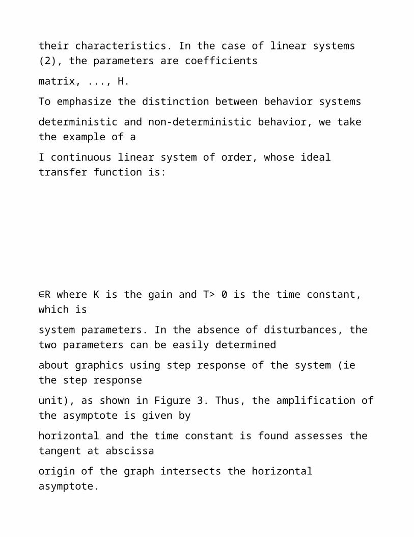
def
M ε = - forallnisin1 N (8)
All errors (8) is used to define the criteria for adequacy V (θ) which
It must be optimized to determine the unknown parameters Choosing
adequate mathematical model often involves an iterative process following which
set of possible models is reduced to a finite collection The model is then appropriate
especially in this set taking into account not only appropriate but also other considerations
implementabilitatea related to it This is the meaning of the arrow returned
the casings of the model in Figure 7
Efficiency and complexity of the optimization depends sensitive to the manner in
which was defined criterion of adequacy Note that adequate criterion value
evaluated for a particular model identification is often interpreted as a
an indicator of the accuracy of the model Next specified two criteria of adequacy
frequently used applications
V (θ) ε [ θ] (robust criterion) (9)
Σ =
=
N
n
f
n
1
V (θ) ε 2 [ θ] (quadratic criterion) (10)
Both criteria evaluates the total error between process and model but using applications
different The first criterion (the robust (9)) looks more natural because it sums
the absolute values of all errors The second criterion (the quadratic (10)) is both more
easy to use optimization as function module used in the first criterion
It is differentiable everywhere Optimization is performed within IS using primarily
gradient techniques (some of which are described in Chapter 4) Other methods
Optimization can also be used (for example AI-based techniques or
PE) Turning to criteria (9) and (10) appropriate parameter vector of measured data
Note N θ is obtained by minimizing nonlinear Troubleshooter
Argmin ()
n
N isin sube θ
=
θ
θ θ
And R
V (11)
where S sube stability Rnθ is the model matematic3 and argmin
means the argument that minimizes (specified criterion function) Naturally
want the resulting model different as little of the data provider ie
leading to a minimal total error Typically applications to accurately determine the
the optimum point is not possible but there are techniques for approximating it with
precisely controlled (as are the techniques of gradient) These techniques are based on
iterative whose main quality characteristics are complexity
convergence and speed of convergence Of these the optimum convergence is
Foremost
The optimization problem (11) is solved for a finite size
vector parameters (ie nθisin1 Nθ) in order to provide finite collection
vectors which will subsequently choose suitable parameter vector It should be noted that it
Suitable parameters are always the most precise meaning of criterion V as
will see later
You can define other criteria than those listed above (for some
it is necessary to solve a problem of maximization and minimization not) The
The resulting data will be suitable but only for the purposes of general mathematical criterion
used It is unlikely that a suitable model by a certain criterion to continue
after changing the criteria to be suitable
152 The problem IS the light of TE
Theory estimate (TE) consists of a set of techniques for determining
unknown parameters using statistical concepts As the data provided by
are of stochastic process it is transferred and parameters which
They are called in this context and parameters estimated The method for producing
estimates of unknown parameters is called estimator The quality of a
estimator is given by the following main characteristics complexity consistency
(or statistical convergence) and efficiency (or convergence speed) Of these
features (described in the next chapter) consistency is of prime importance
Problem identification is in this context suggested forms of image
Figure 8
Figure 8 Identification parameters using criteria TE
This image and that of Figure 7 are very similar Consequently
There are many similarities between the two formulations of the problem of identification We
briefly only differences between them
So this time the output measured and simulated using
to build adequate criterion P (θ) called auto-covariance matrix
the estimation error As the name P (θ) is a matrix of order nθisin1 Nθ
It is defined using statistical average operator E (presented in chapter
next)
() () () T
def
P θ = E θ - θ θ - θ (12)
The definition (12) the difference θ - θ is the error of estimation parameters and bull T is
transposition operator It also notes the use of the external
two vectors (VVT) One can easily see that this criterion directly addresses
true parameters (which are unknown) so apparently it is impossible
rated However it can be shown (as in Chapter 4) that for certain
estimated matrix P (θ) can be estimated despite vector
True parameter is unknown
Identification problem in this case is reduced to a nonlinear problem
minimization
Argmin ()
n
N isin sube θ
=
θ
P θ θ
And R
(13)
where the minimization is performed in the positive sense of ownership defining matrices
More specifically a square matrix P1 is less than or equal to a matrix P2
having the same size if the matrix P2 - P1 is positive semi-defined
2 1 0 P - P ge Minimization condition is not only natural but also required
Consistency property It can show the consistency that the property is
equivalent to the following condition
lim () N rarr infin N
P θ = 0 (14)
The problem (13) can turn equivalently or can relax by
formulating a problem of maximizing the probability of a particular estimate
parameter vector (as described in Chapter 4) However problems
Optimization of the TE are more difficult than those of the TO
To conclude this section will be highlighted advantages and
disadvantages of each type of translation solutions solve the problem identification
the two theories The TO-based solutions have the advantage of being produced
using relatively easy to implement algorithms on an automatic means of calculation but
the disadvantage that can not be characterized statistically In the TE
solutions provides the opportunity to evaluate a number of statistical properties but methods
Their often used to obtain a theoretical without leading to
Implemented algorithms However the IS aflicircndu is somewhat at the intersection of
two theories provide general problem solving methods that combine
advantages of each of them as can be noted in Chapter 4
16 Identification experiment
In general terms the issue raised in the previous section can be solved
(for models identification parameters) by organizing an experiment
Identification This section is devoted to description of the manner in which it can be
designed an experiment to identify and ends with an example (finding
heaters)
161 Diagram of an identification experiment
The experiment identifier means a series of sequential operations or
parallel is made according to the organizational chart in Figure 9 We will describe briefly
In continuation
A Initial data
Designing an experiment identification process begins by stating
Provider of data to be identified The efficiency and success of the experiment
depend on how much sensitive information is a priori known about
process This information should contain the following minimum
1048581 type of process strong non-linear non-linear almost linear linear Most
Nonlinear processes are nonlinear and strong but linearized around
rated operating points Therefore practically it should be laid
operating points around which it is desired to build a model
linear mathematical If I know the equations of continuous operation while
(by the application of physicochemical laws) they may be discretized
to obtain information on identifying the model structure would
You are chosen Otherwise they will be (eventually) take several experiments
Successive identification of a suitable model for the construction and valid
1048581 type of variation slow (over 5s) medium (between 1s and 5s) fast (sub 1s)
This information refers to the amount of stabilizing the output when
step process is stimulated with a certain amplitude accepted
(not leading to instability) and is useful in determining the period
sampling (Ts) to be chosen for the purchase of digital data
1048581 intrinsic dead time of the process While its value detection
and conversion to continuous (even imprecise) discrete-time (as a number
throughout the sampling period) lead to a simplification model
Identification choice In the absence of this information the mathematical model can
work with a number of parameters parasites which increase the complexity
thereof
In practice the determination of the dead time can be effected by stimulating the
preliminary stage of the process with a certain amplitude which does not
leading to instability
1048581 process variability while Many processes behave as
systems with time-varying parameters If the parameters vary slowly over time
it can be considered that they are constant provided that at certain intervals
time associated mathematical model to be reassessed If however the parameters
varies rapidly over time then the model must be adapted to the dynamics des
process The information on the temporal variability of the process is useful in the
choice of appropriate identification method non-recursive (off-line)
or recursive (on-line)
1048581 classes stimulus signals accepted by the process It is very possible
as though to obtain a more accurate model to be necessary to stimulate
process a certain type of signals which would lead to instability
In this case the mathematical model could be determined using only
signals of classes admitted by process (occurring in exploitation
The usual) The result however suffer from lack of generality Instability
processes is typically produced shocks with high amplitudes
entries Even if they can not determine the class of the stimulus signal
accepted the use of sufficiently small amplitude signals can
lead to general mathematical models and precise enough
Classes 1048581 interference posed to the process This information is
helpful in selecting a suitable model of noise that can affect
the measurements of the process output Without it experiment
Identification can be repeated several times until the establishment of a model
Noise appropriate
1048581 purpose of performing identification (simulation control command
numerical prediction generation of data etc) This information is useful in
choosing a mathematical model for the use of appropriate accuracy
For example disturbances affecting the output of the process model will be
namely where the model for predictive overall than if
its use in a numerical control application
B Organization econometric experiment
Econometrics is experimental measurement technique The result of the experiment
is a series econometric (generally finished) the data representing the point of
Physical size measured numerically The accuracy of this representation
It depends on the mathematical model constructed from the data measured Thats why
econometric experiment organization must be done carefully
In general the organization of an econometric experiment to identify
a process involves the following main stages which
Choose solution sampling method for quantifying signal stimulus
needed sensors and their locations
Choosing 1048581 sampling solution rests on the one hand the information
preliminary process and on the other hand the financial resources
available
The sampling period which is the core of the sample solution is
You may choose starting from the type of process variation Trials will slow
be sampled using sampling periods greater than the fast
A more precise information in choosing the sampling period (although
connected with the type of process variation but difficult to determine)
the process is bandwidth Common processes are vast
majority finite band filters This means according to his theorems
Joseph Fourier [StD9602a] [StD9602b] the output signal spectrum
is essentially located in a finite bandwidth pulse for example [0 Ωc]
where Ωcgt 0 is called pulsatile tăiere4
As is known the spectrum of a signal is determined by evaluation
Amplitude Fourier Transform (FT) of that signal In this section
Specific mathematical notation is shown TF definition signals
discrete A similar definition can be formulated for continuous signals
ie continuous time [OpSc85] [PrMa96]
Basically as suggested by Figure 10 the input signals spectrum
pulsation located beyond cutting the high frequencies are strongly
attenuated It also says that the process is insensitive to these signals
Sampling can be selected using sampling theoremss
Kotelnikov and Shannon Nyquist [StD9602a] These results led to the
the following rule-Nyquist sampling Shannon
bull minimum sampling frequency (or the critical frequency of
Nyquist) (FNYQ) is twice the cutoff frequency (Fc)
1 2 c
NYQ s c
s
F F F
T
Ω
= ge = =
π
(15)
Under Nyquist frequency signal obtained by sampling meshed
the continuous distortion due mainly contains aliasing
high frequencies (aliasing) a phenomenon described for example in [OpSc85] and
[StD9602a] This implies that the process acquired data can
not reflect its actual behavior they are disturbed by noise
High-frequency sampling the more important by frequency
the sample is lower than the critical one
A very intuitive image sampling rule is given by
T meshing a sine period Three possible situations can be made
in evidence
a if Tsgt T 2 resulting discrete signal may be periodically period
at least 2TSgt T and non-routine (as the T Ts
or not a rational number)
b if Ts = T 2 the resulting discrete signal constant (non-scheduled)
c where Ts ltt 2 resulting periodic discrete signal and period
proportional ⎣T Ts ⎦sdotTs non-routine (as the T Ts
or not a rational number)
How in practice can not be obtained sampling periods with values
irrational virtually sampled sinewave is correct only if
is followed by Shannon-Nyquist (ie when c above)
So according to this rule sampling how time frequency
Sampling is lower higher much better rendering discrete signal
on the continuity that comes (in the sense of avoiding aliasing
ie minimal distortion of the original spectrum) One limitation however there
and it is time the cost of sampling solution chosen which may increase
lot for performances
Mark
bull The current technology allows operation with sampling frequencies of the order of several
MHz without excessive costs which increase with performance yet but linear The range
tens and hundreds of MHz up to hundreds of GHz the cost increases exponentially with value
sampling frequency But there is a theoretical upper limit The electron can
provide only a limited switching speed due to its inert mass (911sdot10-31 kg) Although
small it can not be neglected at high speed switching The ratio of
Plancks constant and the electron energy (6626sdot10-34 [J1048581s]) is the frequency of its own
oscillation - the order of 124 times 1011 GHz According to the principles of quantum limit [WiE71] report
energy and natural frequency of oscillation must be higher Plancks constant
This automatically implies the existence of a maximum sampling frequency which if
using electric field is situated below the threshold of 106 GHz The range
ultra-high frequencies a solution is foreseen is the use of photons rather than
electronically having masses of about 1010 times smaller than the electron
Considering the product of higher energy and a constant sampling frequency
sampling threshold photons moving around 1016 GHz
To avoid aliasing in practice the procedure of
Figure 11 above Thus before the actual sampling signal
It is filtered with a continual analog of low-pass (LPF) band
range It requires a certain cutoff frequency Fc depending on the type
The variation of process data provider (lower cutoff frequency
processes slow and fast processes bigger) Frequency
the sample is then chosen to be equal to twice the cutoff frequency
thus fixed Fs = 2FC On the one hand analog pre-filtering can result
the loss of high-frequency useful information On the other hand
treble attenuation positive effects of removing disturbances
all high frequency that could corrupt the measured data
Although aliasing was avoided by pre-filtration technique
analog data distortions are inevitably produced with
quantifying their operation By quantifying means the representation
numeric values using a finite number of bits each bit being awarded to
Δ a certain quantum of the ranges covered by the data set
Quantification can be uniform (most common) or irregular (if
that require greater precision in certain sub-ranges
Range) The effect on measured data quantification is widely
analyzed [PrMa96] or [JaNo84]
For example if the value range is [-5 + 7] and we want data representation
12-bit then quantification requires use of quantum uniform
Δ = 12 (211 -1) cong 00059 (taking into account the sign bit and that
the number of quanta is 211 -1) This means that the value is null
assigned to the entire range (-Δ 2 + Δ 2) and that the values are null
approximated to the nearest whole multiple of Δ Of course this
introduce errors that are much less important is how quantum Δ
smaller Quanta small built on the increasing number of bits
representation and therefore data storage capacity Nowadays
data storage capacity has increased significantly and is no longer
Practical problems in the 80s and 90s that However the quantification of not
It can be done using any number of bits Limiting the number of
bit quantization sampler is because all that is required to
record every bit numeric value at a time at most equal to a
sampling period Choosing an appropriate method for quantifying
(generally uniform) and the number of bits to represent the data
Numeric is therefore restricted the sample solution adopted
A uniform 12-bit quantization is often considered a very good
compromise Higher accuracies are obtained 16-bit but beyond
this number may force solution chosen quantification choosing
Unduly small sampling periods accompanied by a significant increase in the
costs
Note that the data transfer means operating automatic calculation
depictions 32 64 or 128 bits (ie more precise than those
adopted for quantification) does not increase accuracy On the contrary
calculation errors in the further processing of data are primarily
quantum of representation influenced by data values rather than accuracy
Once the word car (which would lead to much lower quanta)
Choosing 1048581 stimulus signals conform to the following principle
Overall
a If there is preliminary information about classes signals
process stimulus accepted by either selecting signal to beach
the richest frequencies or if it can not otherwise choose
signal used in the actual operation of the process
b If the information about allowable process entries are missing
then put it signals how much stimulation
Persistent
The concept of persistence will be presented in detail in Chapter 3 He refers
the ability of a stimulus signal to drive the calculation of
of the sequence desired number of weight values for a linear system or
equivalent to boost system (process) on a desired number of frequencies
Mathematical models obtained by the stimulation signals
Persistent are versatile and have a higher degree of generality than
the signal obtained with the low persistence
Effective stimulus process can be done either directly with signal
selected input (if the process is discrete) or more commonly through
a converted many analog (CNA) when the process evolves over time
continuously It is the instruments dual ADC Numeric
(CAN) responsible for sampling CNA performs interpolation
discrete sequences according to certain rules The most commonly used
order interpolation are at 0 and the order 1 Interpolatorul order 0
(Zero Order Holder - ZOH) Discontinued produce a signal in scale through
maintaining the sample at a constant value for a period of
sampling Interpolatorul of order 1 (First Order Holder - FOH) produce
a continuous signal but derived discontinuous (in general) using a
linear regulator (each a line is drawn between any two samples
adjacent) By interpolation the original input signal is more or
less distorted depending on the rule used FOH is more accurate
than ZOH but more difficult physically That is why ZOH is preferred
the majority of applications with sufficiently small sampling period
(fast processes or environments) Instead FOH should be preferred in case
slow processes (for medium and slow) to avoid shocks of
changing the rare stimulus signal values
1048581 sensors 5 by means of which one can collect process data should be elected
Depending on the nature of the physical quantity measured Their performance however
limited financial resources available
In general to not introduce significant distortions in the data sensors
must have characteristics that influence how much less the size of the
is measured How much linear conversion law as lower weight speed
The larger switching etc Linearity measured size conversion
size (usually electricity) sampled throughout the perception
Sensor is a primary requirement but whose satisfaction can
incur high costs Therefore often it is accepted choice of
Linear sensors with local characteristics around values specified a
expensive sensor can thus be replaced by a less expensive sensor network with
local linear features around different operating points The problem
a main sensor networks is the elimination of interference
of the signals measured by it Generally this problem
solves both by suitable location of the sensors (solution requires
but a fairly good knowledge of the process and location
its components) and through initial data processing methods
collected The location of the sensors is a difficult problem in general
In many applications the quantities to be measured are difficult to access or
the topological point of view the hostility of the environment in which it is to be
place the sensors For example when measuring the vibrations produced by
mechanical fault diagnosis view it is possible that just in
neighborhood defective part can not be placed accelerometers
that the measurements are performed In this case it is necessary
their location in an area as close as possible to the location of the component
damaged so that interference with the vibration induced by other components
mechanical (some of them also affected by possible defects) to
have amplitudes as small as possible Another example is the application of control
automatic chemical industry where often sensors must be placed in
corrosive environments which in time affect their performance
The more choice and placement problem is better solved sensors with
so the data collected is less affected by disturbances and models
mathematical results are more accurate Sensors with modest features
and or placed in locations affected by interference leading to sensitive
the need for primary data processing algorithms complexity
high and less accurate mathematical models
C Primary data acquisition and processing
After econometric experiment parameters have been set following
initiation to collect data which is called operation
data acquisition Note that the industry offers numerous solutions to collect
data from one process integrated form of direct acquisition boards
connected to an automatic means of calculation They differ in performance and
related costs
In principle a data acquisition board containing both analog filters as well as filters
digital They are used both in the choice of sampling rate and
solution quantization storage processing and the primary
thereof Schematic diagram of Figure 11 should continue with a block
digital filtering (ie using a digital filter) whose main objective is
to eliminate gross errors of measurement data and possibly alleviate
interference The design of these filters is by techniques described by
eg [PrMa96] Usually designing or LPF (most often) or type filters
Bandpass (FTB) or filters of high pass (FTS) depending on the application and
The purpose of identification
If interference affected data is generally required
primary processing more elaborate This involves using methods
complex than simple filtration methods aimed at extracting
Useful information of data acquired The problem of separation of the useful data
parasite is generally difficult to solve data having lower SNR More
regardless of the SNR no method of parasite data can not
ensure perfect extraction of useful information Always a part of
useful information is lost (when considered parasitic) while a part of
parasitic information is interpreted as useful Useful information can be encoded
the spectrum signals included in any frequency band Eg
voice intonation is encoded in the medium and high frequency spectrum
Speech while having significantly less power than the spectral
Lead voice formants A filter whose purpose is to remove
High frequency noise can alleviate parasite sensitive information about
intonation leaving unincorporated voice signal as would have been generated
artificially using a specialized system for voice synthesis
The result is the acquisition of datasets measured in N a 1 [] = U = and
N N y n 1 [] = Y = (in the case of off-line identification) or rows of the measured data
entry and exit (in the case of identification on-line) Note that entry can be
generated directly in numerical form or can be measured by the same method
as output
D Choosing class of models and model identification
Along with organizing and conducting econometric experiment acquisition
Data models can be specified class identification that works
(using preliminary information available) Class is most used in IS
ARMAX which has been mentioned in section 13 which will be described in
Chapter 2 It however is not the only set of patterns that may be
used as can be seen also in Chapter 2
Choosing a particular model type specified class is made taking
account several desirable characteristics It is good that the model be
bull sufficiently precise equations approached by the application of laws
describing physicochemical process operation (if these equations
They are available)
bull parsimonios with minimal complexity of the involved algorithms
methods needed to determine to
The two properties are obviously opposed It is well known that if
It wants greater precision of a mathematical model the complexity
it should be increased A compromise is always possible however In the IS
Parsimoniei resort to principle according to which is sacrificed accuracy
implementabilităţii model for his or method of identification
Chosen model type M (θ) is then used both in choosing the method of
identification as well as the determination of its parameters
The choice of method for identifying E
The mathematical model often determines the method for determining the parameters
Its as method by its complexity can force another election
mathematical model easier to determine For example for applications
NC highly used ARX model This is not because
ARX model would be the best in these applications but because it can be
2 simplest determined readily implemented (or LSM method
Instrumental Variables (MVI)) The models that respond better this
Applications are either the type Error Output (Output Error - OE) or the type
Filtered inputs Filtered disturbances (Filtered Input Filtered Noise - FIFN) more
Specifically than OE model However the methods by which one can determine parameters
these models ie Prediction Error Minimization Method (MMEP) (form
the LSM generalized) or Error Minimization Method Output (MMEI) are
much higher complexity than conventional LSM or MVI Some of
Identifying these models and methods are described in Chapters 2 and 4
F Determining the optimal models and model appropriate
The main loop identification experiment consists of
determining the actual parameters of the model chosen for the different indicators
nθ structural note in the chart of Figure 9 m (for ease) a
maximum structural index (Nθ = M) stop the process The models
They are optimal in the sense defined adequacy criteria chosen Each model
The determined optimal M (θm) and is assessed and precision using all criteria
appropriate Thus identifying models of the same type but different
structures can be compared with each other from the point of view of accuracy in
choosing the appropriate order
Choosing an appropriate model of the M available not performed
only based on its accuracy but also resorted to a series of tests
Suitably the most used are described in Chapter 4 These tests help
users to take a decision on the optimal structure that should have
adequate mathematical model Thus for example can be drawn chart
quadratic optimization criterion V (θm) as shown in Figure 12 The graph was
interpolated to provide a clearer picture It notes that while models
maximum structural index led to the highest precision (ie the value
Criterion less suitable) starting at a certain structural indicators
improve the accuracy of models no longer significant The principle
parsimoniei (mentioned earlier) it is unnecessary to operate with models
complex if they can not ensure a noticeably higher accuracy than models
simpler
The appropriate optimal model will have a structural indicator given the entry into
precision landing of the chart (denoted mo) and not its maximum From
Therefore it is appropriate that the pattern denoted by M (θo) was elected
using test criterion flattening accuracy This test is but one component
subjective which can be mitigated through other such criteria selection
optimal structural index
G test validity
For a model of proper identification data acquired to be adopted
it is necessary that he be tested for validity Only an appropriate model
It will be returned valid identification at the end of the experiment Validation is
testing the operation of the process model as compared to when the
starting a new session stimulating both entities with the same input
For the model to be valid the error between process and model must check
some properties will generally be determined by the method of identification used in
during the experiment The usual validation tests are described in detail in
Chapter 4
For example if the appropriate model has been determined using LSM
trial and error of the model defined by (8) must have characteristics
a normally distributed white noise (Gaussian) for the model to be validated
For this reason test validation test is called bleaching
If the model fails the test validation identification experiment
It should be resumed from its main stages Attempting be reviewing
econometric experiment (perhaps the data are too affected by disturbances)
be reconsidering class models and or type of model or a change
Method of identification
Note that it is extremely important that validation is performed in another set
different than the one used to determine the parameters of the model Therefore
practice the dataset acquired is always divided into two sub-sets
disjoint one for identification and one for validation
The following example illustrates the manner in which it conducted an experiment
having as an objective the identification of a mathematical model used in the construction of a loop
auto
One of the main features of a heating system such as that illustrated in
Figure 13 is to keep a constant temperature at the exit of the ventilation air in
Despite air temperatures absorbed This is achieved with a system of
temperature compensation based on a simple control loop If the heater is
placed in an environment having different temperatures of the air streams they can
they disrupt normal operation Therefore we assume desired
air heater in the open loop identification following the mathematical model obtained to be
used in the design of the controller to ensure disturbance rejection and maintaining
the temperature around a desired value
We will go through all the main stages of the experiment on identification related
building mathematical model desired
1 Informaţiipreliminare
Heating is an electro-mechanical system whose operation equations based
the laws of dynamics electricity and thermodynamics lead to the conclusion that the order
Maximum model identifier 2 The scheme is its functional principle
plotted in Figure 14
The cold air is ventilated by an electrical resistance powered by
means a power amplifier This may vary the voltage and or
intensity electric current going through Size Control
power amplifier is entering the system System output is
provided by the temperature sensor placed in the hot air stream produced by
resistance Both entry and exit as measurable
Basically the circuit from input to output of the process there are four components
power amplifier the electrical resistance hot air flow sensor
temperature The process is nonlinear but linearized around each of temperatures
Beach permissible that can provide electrical resistance (having power
The maximum) Also the process can be considered as having an average type of
variation because the settling time of a fixed temperature is about 2s
The process dead time is about 01s Its parameters can be considered
They are constants (Their variations become noticeable when the heater has a
given the high wear resistance aging electrical and or
power amplifier due to damaging the temperature sensor
its exposure to high temperatures etc) Heating can be controlled with a range
range of input signals including high persistence Their amplitude
however it will be limited by the capacity of the power amplifier
The disturbance comes from the cold air flow which can be both temperature as well as
Variable flow The variable temperature due to the environment in which it is
Located heater (that is an external noise) while variations in flux
rather they may be due to defects in the electric motor acting
fan (internal noise they produce) No distinction will be made between the two
types of disturbances and shall be deemed heater is affected by one
global6 noise Order the disturbance model is unknown but it can go
from simple designs to intricate as usual
The objective (or purpose) is to provide identification of a mathematical model needed
designing an automatic regulator that ensures both a good rejection
interference as well as maintaining the temperature of the hot air flow around an
specified The temperature is fixed manually via amplifier
power which is equipped with a thermostat An automatic adjustment scheme in which
compensator is designed based on the model identification can be seen in
Figure 15 The design of patterns starting from the numerical controllers Identification
It is described in detail in many works among which we mention only [LaID93]
[LaID97] [GePo97] or [DTFP04]
Process and data acquisition 2Stimularea
Based on preliminary information it is sufficient to select a frequency
tens of Hz sampling at most Covering may be fixed
Fs = 100 Hz ie Ts = 10ms This leads to an analog filter having
Fs = 50Hz cutoff frequency (frequency as forced convection air heaters power source)
and a normalized dead time nk = 10 It is yet to give pre-filtering
Digital because SNR is large enough Data collection can be done
be a general purpose acquisition board or a dedicated acquisition system a
Such a system is expensive but provides more flexibility in handling and
Primary data processing
The image in Figure 16 shows the portable system LMS Belgian acquisition
Roadrunner [LMS99] which has a micro-computer integrated (functionally
Windows operating system)
Among other things it provides pre filter data simultaneous data acquisition
at least 2 channels (4 channels features and can be expanded to 16 channels) a wide range
Sampling frequency (between 1 Hz and 100 kHz) compatibility with a large
number of sensors the possibility to trace spectra and even spectrogram (ie
Spectra variables over time) etc
To stimulate forced convection air heater choosing a high persistence signal generated
by means of an algorithm implemented on a computer One such signal is
the pseudo-random (binary) known under the abbreviation SPA (B) Some algorithms
generating SPA (B) are shown in Chapter 3 (As I already said
models obtained using high persistence signals are more specific
versatile than those obtained with low persistence signals) signal
Stimulus is interpolated using a CNA based ZOH for simplicity
Data acquisition horizon is fixed at N = 210 = 1024 Powers of 2
Signals favoring spectra evaluation using an algorithm type
Fast Fourier Transform (Fast Fourier Transform - FFT) [OpSc85] [PrMa96]
Data acquired (identification and validation) are quantized 12-bit and will
Computer representation in the form of floating-point numbers 32-bit
3Alegereaclaseidemodeleşiamodeluluispecific
Initially trying to determine the mathematical model of useful data It will return
subsequently adding a model of the disturbance Class of standard models
IS is ARMAX General equations describing ARMAX are presented in class
Chapter 2 For clarity we reproduce in this context
General Equation of class ARMAX [na nb nc nk] (a difference equation) is
as follows
A (Q 1) y [n] B (q -1) [not] C (Q 1) e [n]
AR X MA
- = - + - 10485811048581104858110485811048581 10485811048581104858110485811048581 10485811048581104858110485811048581 forallnisinN (16)
where
bull u is the input signal or stimulus
bull y is the output signal or system response
bull e is ideal stochastic called white noise signal in statistical terms
White noise is the prototype total neautocorelate signals ie
2
0 E e [n] e [m] = λ δ [n - m] foralln misinZ (17)
where E is the statistical average operator 0 δ is the impulse unit
centered in origin (Kroneckers symbol) and λ2 is the variance of noise
unknown
bull Q-1 is a step delay operator (sampling) defined by
(q-1 f) [n] = f [n-1] forallnisinZ for any string of data f (scalar or vector)
bull A B C are finite polynomial⎢ ⎢ ⎢ ⎢⎣⎡= + + +
= +
= + + +
- - -
- - - -
- - -
nc
nc
nb nk
nb
NA
NA
C q c q c q
B q b q b q q
A q q q
1048581
1048581
1048581
1
1
1
1 1
1
1
1
1
1
() 1
() ()
() 1
(18)
for which the coefficients ii na 1 isin ii nb b 1 isin ii nc c 1 isin (model parameters)
Grades na nb nc (structural indices of the model) (and sometimes nk - delay
intrinsic model) are unknown variables
Having a clear identification the usual pattern they operate
application control CNC is ARX [na nb] Using the information
preliminary order of this model is approximately equal to 2 This implies
that the appropriate model to be found among the ARX models [22 nk]
ARX [23 nk] ARX [32 nk] and ARX [33 nk]
4Alegereametodeideidentificare
Determination ARX model can be made using two methods LSM and MVI
(as revised version of LSM) Of these MVI is well adapted
model and will be taken further
5Determinareamodeluluiadecvat
After running the experiment for identifying the main loop you can choose
ARX appropriate type model [2310]
(1) [] (1) [] s [n]
X
B q u n
AR
A Q Y n = - +
10485811048581104858110485811048581 10485811048581104858110485811048581 forallnisinN (19)
with⎢ ⎢⎣⎡= +
= +
- - - -
- - -
() ()
() 1
2
3
1
1 2
1 October
2
2
1
1
1
B b b q b q q q
A q q q
(20)
(intrinsic delay is already known and equal to 10 times of sampling)
Another suitable model possible but parsimonios is ARX [2210] Comparing
the two models it appears that the model parameter b3 (19) - (20) has a
much smaller than the absolute value of the absolute values of the other two parameters
polynomial B It follows that the term 2
3
b q may be neglected This leads to
reducing model size by one Note that this model parameters
parsimonios are identical to those that have more complex model such
that neglect of 2
3
bq- require reassessment of remaining in the competition parameters
6Validareamodeluluiadecvat
Especially suitable model (ARX [2210]) fails the validation test than the one
satisfactory probably because of interference pattern which is not
accurate Therefore identification should be resumed with a model experiment
mathematical model that includes a complex of disturbances
7Reconsiderareamodeluluimatematicşiametodeideidentificare
To work this time with more general models such ARMAX [22 nc 10]
The identification method is also changed from MVI in the extended version of the MMEP
MVI Maximum structural index of the MA is set to Nc = 10
8Redeterminareamodeluluiadecvat
This time the optimal model 10 produced by the main loop
Experimental identification model is suitable or ARMAX [22110] or
Again it appears that the absolute value of the model coefficient c2 second
It is negligible compared with the absolute value of the coefficient C1 Thats why
The model is preferred parsimonios ARMAX [22110] It should be noted once again that
model parameters are different from the corresponding models
ARX [2210] and ARMAX [22210]
9Validareanouluimodeladecvat
Assay validation is passed to the new model described by polynomials
the following⎢ ⎢ ⎢ ⎢⎣⎡= +
= +
= +
- -
- - -
- - -
1
1
1
1
1 2
1 October
2
2
1
1
1
() 1
() ()
() 1
C q c q
B b b q q q
A q q q
(21)
The model is sufficiently precise to play details of transitional arrangements
characterized heater Its step response but can be approximated
that of a system of order 1 (ie having only one pole) If the model (16) amp (21)
is too complex for automatic adjustment application then you can choose one
simple models of ARX [1210] or ARMAX [12110] slaughtering
the accuracy and validity area
1048581
The objective of this chapter was to briefly present the main coordinates of
IS domain Subsequent chapters will provide more details on these
although approaches will remain at the basic level introductory
17 Exercises proposed
Exercise 11 (mini-project)
To emphasize the distinction between behavior systems
deterministic and non-deterministic behavior take the example of a
second order linear continuous system and show how it can be determined about graphics
its parameters Write a program with which to generate MATLAB
various embodiments of the system particularly in the case where the output is corrupted by a
perturbation amplitude Gaussian additive chosen by the user (To
generate interference I can use MATLAB routines rand or randn To simulate
operation of a discrete linear dynamic system transfer function rational
MATLAB can be used for routine filter) What can be said about identifiable
system perturbation amplitude chose
Exercise 12
Demonstrate the properties (5) (6) and (7) of Gaussian distribution (4) using
Poissons identity
2 e t dt
-infin
-
-infin
int = π
exercise 13
Using Gaussian distribution (4) demonstrate the following property
(Y (t)) (y (t) y) 2DY (t) 2
+ infin
-infin
int p - = σ foralltisinR
Exercise 14 (mini-project)
Write a program in MATLAB by which to regularly check sampling
Nyquist-Shannons where meshing a continuous sinusoid period
time Show graphs illustrating the operation of sampling accuracy It is
thus possible to obtain a sampled signal using a non-routine
Automatic calculation means If not show why If so build signal
non-routine and display graph or a long enough time horizon
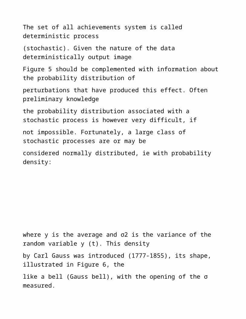
=
θ
θ θ
And R
V (11)
where S sube stability Rnθ is the model matematic3 and argmin
means the argument that minimizes (specified criterion function) Naturally
want the resulting model different as little of the data provider ie
leading to a minimal total error Typically applications to accurately determine the
the optimum point is not possible but there are techniques for approximating it with
precisely controlled (as are the techniques of gradient) These techniques are based on
iterative whose main quality characteristics are complexity
convergence and speed of convergence Of these the optimum convergence is
Foremost
The optimization problem (11) is solved for a finite size
vector parameters (ie nθisin1 Nθ) in order to provide finite collection
vectors which will subsequently choose suitable parameter vector It should be noted that it
Suitable parameters are always the most precise meaning of criterion V as
will see later
You can define other criteria than those listed above (for some
it is necessary to solve a problem of maximization and minimization not) The
The resulting data will be suitable but only for the purposes of general mathematical criterion
used It is unlikely that a suitable model by a certain criterion to continue
after changing the criteria to be suitable
152 The problem IS the light of TE
Theory estimate (TE) consists of a set of techniques for determining
unknown parameters using statistical concepts As the data provided by
are of stochastic process it is transferred and parameters which
They are called in this context and parameters estimated The method for producing
estimates of unknown parameters is called estimator The quality of a
estimator is given by the following main characteristics complexity consistency
(or statistical convergence) and efficiency (or convergence speed) Of these
features (described in the next chapter) consistency is of prime importance
Problem identification is in this context suggested forms of image
Figure 8
Figure 8 Identification parameters using criteria TE
This image and that of Figure 7 are very similar Consequently
There are many similarities between the two formulations of the problem of identification We
briefly only differences between them
So this time the output measured and simulated using
to build adequate criterion P (θ) called auto-covariance matrix
the estimation error As the name P (θ) is a matrix of order nθisin1 Nθ
It is defined using statistical average operator E (presented in chapter
next)
() () () T
def
P θ = E θ - θ θ - θ (12)
The definition (12) the difference θ - θ is the error of estimation parameters and bull T is
transposition operator It also notes the use of the external
two vectors (VVT) One can easily see that this criterion directly addresses
true parameters (which are unknown) so apparently it is impossible
rated However it can be shown (as in Chapter 4) that for certain
estimated matrix P (θ) can be estimated despite vector
True parameter is unknown
Identification problem in this case is reduced to a nonlinear problem
minimization
Argmin ()
n
N isin sube θ
=
θ
P θ θ
And R
(13)
where the minimization is performed in the positive sense of ownership defining matrices
More specifically a square matrix P1 is less than or equal to a matrix P2
having the same size if the matrix P2 - P1 is positive semi-defined
2 1 0 P - P ge Minimization condition is not only natural but also required
Consistency property It can show the consistency that the property is
equivalent to the following condition
lim () N rarr infin N
P θ = 0 (14)
The problem (13) can turn equivalently or can relax by
formulating a problem of maximizing the probability of a particular estimate
parameter vector (as described in Chapter 4) However problems
Optimization of the TE are more difficult than those of the TO
To conclude this section will be highlighted advantages and
disadvantages of each type of translation solutions solve the problem identification
the two theories The TO-based solutions have the advantage of being produced
using relatively easy to implement algorithms on an automatic means of calculation but
the disadvantage that can not be characterized statistically In the TE
solutions provides the opportunity to evaluate a number of statistical properties but methods
Their often used to obtain a theoretical without leading to
Implemented algorithms However the IS aflicircndu is somewhat at the intersection of
two theories provide general problem solving methods that combine
advantages of each of them as can be noted in Chapter 4
16 Identification experiment
In general terms the issue raised in the previous section can be solved
(for models identification parameters) by organizing an experiment
Identification This section is devoted to description of the manner in which it can be
designed an experiment to identify and ends with an example (finding
heaters)
161 Diagram of an identification experiment
The experiment identifier means a series of sequential operations or
parallel is made according to the organizational chart in Figure 9 We will describe briefly
In continuation
A Initial data
Designing an experiment identification process begins by stating
Provider of data to be identified The efficiency and success of the experiment
depend on how much sensitive information is a priori known about
process This information should contain the following minimum
1048581 type of process strong non-linear non-linear almost linear linear Most
Nonlinear processes are nonlinear and strong but linearized around
rated operating points Therefore practically it should be laid
operating points around which it is desired to build a model
linear mathematical If I know the equations of continuous operation while
(by the application of physicochemical laws) they may be discretized
to obtain information on identifying the model structure would
You are chosen Otherwise they will be (eventually) take several experiments
Successive identification of a suitable model for the construction and valid
1048581 type of variation slow (over 5s) medium (between 1s and 5s) fast (sub 1s)
This information refers to the amount of stabilizing the output when
step process is stimulated with a certain amplitude accepted
(not leading to instability) and is useful in determining the period
sampling (Ts) to be chosen for the purchase of digital data
1048581 intrinsic dead time of the process While its value detection
and conversion to continuous (even imprecise) discrete-time (as a number
throughout the sampling period) lead to a simplification model
Identification choice In the absence of this information the mathematical model can
work with a number of parameters parasites which increase the complexity
thereof
In practice the determination of the dead time can be effected by stimulating the
preliminary stage of the process with a certain amplitude which does not
leading to instability
1048581 process variability while Many processes behave as
systems with time-varying parameters If the parameters vary slowly over time
it can be considered that they are constant provided that at certain intervals
time associated mathematical model to be reassessed If however the parameters
varies rapidly over time then the model must be adapted to the dynamics des
process The information on the temporal variability of the process is useful in the
choice of appropriate identification method non-recursive (off-line)
or recursive (on-line)
1048581 classes stimulus signals accepted by the process It is very possible
as though to obtain a more accurate model to be necessary to stimulate
process a certain type of signals which would lead to instability
In this case the mathematical model could be determined using only
signals of classes admitted by process (occurring in exploitation
The usual) The result however suffer from lack of generality Instability
processes is typically produced shocks with high amplitudes
entries Even if they can not determine the class of the stimulus signal
accepted the use of sufficiently small amplitude signals can
lead to general mathematical models and precise enough
Classes 1048581 interference posed to the process This information is
helpful in selecting a suitable model of noise that can affect
the measurements of the process output Without it experiment
Identification can be repeated several times until the establishment of a model
Noise appropriate
1048581 purpose of performing identification (simulation control command
numerical prediction generation of data etc) This information is useful in
choosing a mathematical model for the use of appropriate accuracy
For example disturbances affecting the output of the process model will be
namely where the model for predictive overall than if
its use in a numerical control application
B Organization econometric experiment
Econometrics is experimental measurement technique The result of the experiment
is a series econometric (generally finished) the data representing the point of
Physical size measured numerically The accuracy of this representation
It depends on the mathematical model constructed from the data measured Thats why
econometric experiment organization must be done carefully
In general the organization of an econometric experiment to identify
a process involves the following main stages which
Choose solution sampling method for quantifying signal stimulus
needed sensors and their locations
Choosing 1048581 sampling solution rests on the one hand the information
preliminary process and on the other hand the financial resources
available
The sampling period which is the core of the sample solution is
You may choose starting from the type of process variation Trials will slow
be sampled using sampling periods greater than the fast
A more precise information in choosing the sampling period (although
connected with the type of process variation but difficult to determine)
the process is bandwidth Common processes are vast
majority finite band filters This means according to his theorems
Joseph Fourier [StD9602a] [StD9602b] the output signal spectrum
is essentially located in a finite bandwidth pulse for example [0 Ωc]
where Ωcgt 0 is called pulsatile tăiere4
As is known the spectrum of a signal is determined by evaluation
Amplitude Fourier Transform (FT) of that signal In this section
Specific mathematical notation is shown TF definition signals
discrete A similar definition can be formulated for continuous signals
ie continuous time [OpSc85] [PrMa96]
Basically as suggested by Figure 10 the input signals spectrum
pulsation located beyond cutting the high frequencies are strongly
attenuated It also says that the process is insensitive to these signals
Sampling can be selected using sampling theoremss
Kotelnikov and Shannon Nyquist [StD9602a] These results led to the
the following rule-Nyquist sampling Shannon
bull minimum sampling frequency (or the critical frequency of
Nyquist) (FNYQ) is twice the cutoff frequency (Fc)
1 2 c
NYQ s c
s
F F F
T
Ω
= ge = =
π
(15)
Under Nyquist frequency signal obtained by sampling meshed
the continuous distortion due mainly contains aliasing
high frequencies (aliasing) a phenomenon described for example in [OpSc85] and
[StD9602a] This implies that the process acquired data can
not reflect its actual behavior they are disturbed by noise
High-frequency sampling the more important by frequency
the sample is lower than the critical one
A very intuitive image sampling rule is given by
T meshing a sine period Three possible situations can be made
in evidence
a if Tsgt T 2 resulting discrete signal may be periodically period
at least 2TSgt T and non-routine (as the T Ts
or not a rational number)
b if Ts = T 2 the resulting discrete signal constant (non-scheduled)
c where Ts ltt 2 resulting periodic discrete signal and period
proportional ⎣T Ts ⎦sdotTs non-routine (as the T Ts
or not a rational number)
How in practice can not be obtained sampling periods with values
irrational virtually sampled sinewave is correct only if
is followed by Shannon-Nyquist (ie when c above)
So according to this rule sampling how time frequency
Sampling is lower higher much better rendering discrete signal
on the continuity that comes (in the sense of avoiding aliasing
ie minimal distortion of the original spectrum) One limitation however there
and it is time the cost of sampling solution chosen which may increase
lot for performances
Mark
bull The current technology allows operation with sampling frequencies of the order of several
MHz without excessive costs which increase with performance yet but linear The range
tens and hundreds of MHz up to hundreds of GHz the cost increases exponentially with value
sampling frequency But there is a theoretical upper limit The electron can
provide only a limited switching speed due to its inert mass (911sdot10-31 kg) Although
small it can not be neglected at high speed switching The ratio of
Plancks constant and the electron energy (6626sdot10-34 [J1048581s]) is the frequency of its own
oscillation - the order of 124 times 1011 GHz According to the principles of quantum limit [WiE71] report
energy and natural frequency of oscillation must be higher Plancks constant
This automatically implies the existence of a maximum sampling frequency which if
using electric field is situated below the threshold of 106 GHz The range
ultra-high frequencies a solution is foreseen is the use of photons rather than
electronically having masses of about 1010 times smaller than the electron
Considering the product of higher energy and a constant sampling frequency
sampling threshold photons moving around 1016 GHz
To avoid aliasing in practice the procedure of
Figure 11 above Thus before the actual sampling signal
It is filtered with a continual analog of low-pass (LPF) band
range It requires a certain cutoff frequency Fc depending on the type
The variation of process data provider (lower cutoff frequency
processes slow and fast processes bigger) Frequency
the sample is then chosen to be equal to twice the cutoff frequency
thus fixed Fs = 2FC On the one hand analog pre-filtering can result
the loss of high-frequency useful information On the other hand
treble attenuation positive effects of removing disturbances
all high frequency that could corrupt the measured data
Although aliasing was avoided by pre-filtration technique
analog data distortions are inevitably produced with
quantifying their operation By quantifying means the representation
numeric values using a finite number of bits each bit being awarded to
Δ a certain quantum of the ranges covered by the data set
Quantification can be uniform (most common) or irregular (if
that require greater precision in certain sub-ranges
Range) The effect on measured data quantification is widely
analyzed [PrMa96] or [JaNo84]
For example if the value range is [-5 + 7] and we want data representation
12-bit then quantification requires use of quantum uniform
Δ = 12 (211 -1) cong 00059 (taking into account the sign bit and that
the number of quanta is 211 -1) This means that the value is null
assigned to the entire range (-Δ 2 + Δ 2) and that the values are null
approximated to the nearest whole multiple of Δ Of course this
introduce errors that are much less important is how quantum Δ
smaller Quanta small built on the increasing number of bits
representation and therefore data storage capacity Nowadays
data storage capacity has increased significantly and is no longer
Practical problems in the 80s and 90s that However the quantification of not
It can be done using any number of bits Limiting the number of
bit quantization sampler is because all that is required to
record every bit numeric value at a time at most equal to a
sampling period Choosing an appropriate method for quantifying
(generally uniform) and the number of bits to represent the data
Numeric is therefore restricted the sample solution adopted
A uniform 12-bit quantization is often considered a very good
compromise Higher accuracies are obtained 16-bit but beyond
this number may force solution chosen quantification choosing
Unduly small sampling periods accompanied by a significant increase in the
costs
Note that the data transfer means operating automatic calculation
depictions 32 64 or 128 bits (ie more precise than those
adopted for quantification) does not increase accuracy On the contrary
calculation errors in the further processing of data are primarily
quantum of representation influenced by data values rather than accuracy
Once the word car (which would lead to much lower quanta)
Choosing 1048581 stimulus signals conform to the following principle
Overall
a If there is preliminary information about classes signals
process stimulus accepted by either selecting signal to beach
the richest frequencies or if it can not otherwise choose
signal used in the actual operation of the process
b If the information about allowable process entries are missing
then put it signals how much stimulation
Persistent
The concept of persistence will be presented in detail in Chapter 3 He refers
the ability of a stimulus signal to drive the calculation of
of the sequence desired number of weight values for a linear system or
equivalent to boost system (process) on a desired number of frequencies
Mathematical models obtained by the stimulation signals
Persistent are versatile and have a higher degree of generality than
the signal obtained with the low persistence
Effective stimulus process can be done either directly with signal
selected input (if the process is discrete) or more commonly through
a converted many analog (CNA) when the process evolves over time
continuously It is the instruments dual ADC Numeric
(CAN) responsible for sampling CNA performs interpolation
discrete sequences according to certain rules The most commonly used
order interpolation are at 0 and the order 1 Interpolatorul order 0
(Zero Order Holder - ZOH) Discontinued produce a signal in scale through
maintaining the sample at a constant value for a period of
sampling Interpolatorul of order 1 (First Order Holder - FOH) produce
a continuous signal but derived discontinuous (in general) using a
linear regulator (each a line is drawn between any two samples
adjacent) By interpolation the original input signal is more or
less distorted depending on the rule used FOH is more accurate
than ZOH but more difficult physically That is why ZOH is preferred
the majority of applications with sufficiently small sampling period
(fast processes or environments) Instead FOH should be preferred in case
slow processes (for medium and slow) to avoid shocks of
changing the rare stimulus signal values
1048581 sensors 5 by means of which one can collect process data should be elected
Depending on the nature of the physical quantity measured Their performance however
limited financial resources available
In general to not introduce significant distortions in the data sensors
must have characteristics that influence how much less the size of the
is measured How much linear conversion law as lower weight speed
The larger switching etc Linearity measured size conversion
size (usually electricity) sampled throughout the perception
Sensor is a primary requirement but whose satisfaction can
incur high costs Therefore often it is accepted choice of
Linear sensors with local characteristics around values specified a
expensive sensor can thus be replaced by a less expensive sensor network with
local linear features around different operating points The problem
a main sensor networks is the elimination of interference
of the signals measured by it Generally this problem
solves both by suitable location of the sensors (solution requires
but a fairly good knowledge of the process and location
its components) and through initial data processing methods
collected The location of the sensors is a difficult problem in general
In many applications the quantities to be measured are difficult to access or
the topological point of view the hostility of the environment in which it is to be
place the sensors For example when measuring the vibrations produced by
mechanical fault diagnosis view it is possible that just in
neighborhood defective part can not be placed accelerometers
that the measurements are performed In this case it is necessary
their location in an area as close as possible to the location of the component
damaged so that interference with the vibration induced by other components
mechanical (some of them also affected by possible defects) to
have amplitudes as small as possible Another example is the application of control
automatic chemical industry where often sensors must be placed in
corrosive environments which in time affect their performance
The more choice and placement problem is better solved sensors with
so the data collected is less affected by disturbances and models
mathematical results are more accurate Sensors with modest features
and or placed in locations affected by interference leading to sensitive
the need for primary data processing algorithms complexity
high and less accurate mathematical models
C Primary data acquisition and processing
After econometric experiment parameters have been set following
initiation to collect data which is called operation
data acquisition Note that the industry offers numerous solutions to collect
data from one process integrated form of direct acquisition boards
connected to an automatic means of calculation They differ in performance and
related costs
In principle a data acquisition board containing both analog filters as well as filters
digital They are used both in the choice of sampling rate and
solution quantization storage processing and the primary
thereof Schematic diagram of Figure 11 should continue with a block
digital filtering (ie using a digital filter) whose main objective is
to eliminate gross errors of measurement data and possibly alleviate
interference The design of these filters is by techniques described by
eg [PrMa96] Usually designing or LPF (most often) or type filters
Bandpass (FTB) or filters of high pass (FTS) depending on the application and
The purpose of identification
If interference affected data is generally required
primary processing more elaborate This involves using methods
complex than simple filtration methods aimed at extracting
Useful information of data acquired The problem of separation of the useful data
parasite is generally difficult to solve data having lower SNR More
regardless of the SNR no method of parasite data can not
ensure perfect extraction of useful information Always a part of
useful information is lost (when considered parasitic) while a part of
parasitic information is interpreted as useful Useful information can be encoded
the spectrum signals included in any frequency band Eg
voice intonation is encoded in the medium and high frequency spectrum
Speech while having significantly less power than the spectral
Lead voice formants A filter whose purpose is to remove
High frequency noise can alleviate parasite sensitive information about
intonation leaving unincorporated voice signal as would have been generated
artificially using a specialized system for voice synthesis
The result is the acquisition of datasets measured in N a 1 [] = U = and
N N y n 1 [] = Y = (in the case of off-line identification) or rows of the measured data
entry and exit (in the case of identification on-line) Note that entry can be
generated directly in numerical form or can be measured by the same method
as output
D Choosing class of models and model identification
Along with organizing and conducting econometric experiment acquisition
Data models can be specified class identification that works
(using preliminary information available) Class is most used in IS
ARMAX which has been mentioned in section 13 which will be described in
Chapter 2 It however is not the only set of patterns that may be
used as can be seen also in Chapter 2
Choosing a particular model type specified class is made taking
account several desirable characteristics It is good that the model be
bull sufficiently precise equations approached by the application of laws
describing physicochemical process operation (if these equations
They are available)
bull parsimonios with minimal complexity of the involved algorithms
methods needed to determine to
The two properties are obviously opposed It is well known that if
It wants greater precision of a mathematical model the complexity
it should be increased A compromise is always possible however In the IS
Parsimoniei resort to principle according to which is sacrificed accuracy
implementabilităţii model for his or method of identification
Chosen model type M (θ) is then used both in choosing the method of
identification as well as the determination of its parameters
The choice of method for identifying E
The mathematical model often determines the method for determining the parameters
Its as method by its complexity can force another election
mathematical model easier to determine For example for applications
NC highly used ARX model This is not because
ARX model would be the best in these applications but because it can be
2 simplest determined readily implemented (or LSM method
Instrumental Variables (MVI)) The models that respond better this
Applications are either the type Error Output (Output Error - OE) or the type
Filtered inputs Filtered disturbances (Filtered Input Filtered Noise - FIFN) more
Specifically than OE model However the methods by which one can determine parameters
these models ie Prediction Error Minimization Method (MMEP) (form
the LSM generalized) or Error Minimization Method Output (MMEI) are
much higher complexity than conventional LSM or MVI Some of
Identifying these models and methods are described in Chapters 2 and 4
F Determining the optimal models and model appropriate
The main loop identification experiment consists of
determining the actual parameters of the model chosen for the different indicators
nθ structural note in the chart of Figure 9 m (for ease) a
maximum structural index (Nθ = M) stop the process The models
They are optimal in the sense defined adequacy criteria chosen Each model
The determined optimal M (θm) and is assessed and precision using all criteria
appropriate Thus identifying models of the same type but different
structures can be compared with each other from the point of view of accuracy in
choosing the appropriate order
Choosing an appropriate model of the M available not performed
only based on its accuracy but also resorted to a series of tests
Suitably the most used are described in Chapter 4 These tests help
users to take a decision on the optimal structure that should have
adequate mathematical model Thus for example can be drawn chart
quadratic optimization criterion V (θm) as shown in Figure 12 The graph was
interpolated to provide a clearer picture It notes that while models
maximum structural index led to the highest precision (ie the value
Criterion less suitable) starting at a certain structural indicators
improve the accuracy of models no longer significant The principle
parsimoniei (mentioned earlier) it is unnecessary to operate with models
complex if they can not ensure a noticeably higher accuracy than models
simpler
The appropriate optimal model will have a structural indicator given the entry into
precision landing of the chart (denoted mo) and not its maximum From
Therefore it is appropriate that the pattern denoted by M (θo) was elected
using test criterion flattening accuracy This test is but one component
subjective which can be mitigated through other such criteria selection
optimal structural index
G test validity
For a model of proper identification data acquired to be adopted
it is necessary that he be tested for validity Only an appropriate model
It will be returned valid identification at the end of the experiment Validation is
testing the operation of the process model as compared to when the
starting a new session stimulating both entities with the same input
For the model to be valid the error between process and model must check
some properties will generally be determined by the method of identification used in
during the experiment The usual validation tests are described in detail in
Chapter 4
For example if the appropriate model has been determined using LSM
trial and error of the model defined by (8) must have characteristics
a normally distributed white noise (Gaussian) for the model to be validated
For this reason test validation test is called bleaching
If the model fails the test validation identification experiment
It should be resumed from its main stages Attempting be reviewing
econometric experiment (perhaps the data are too affected by disturbances)
be reconsidering class models and or type of model or a change
Method of identification
Note that it is extremely important that validation is performed in another set
different than the one used to determine the parameters of the model Therefore
practice the dataset acquired is always divided into two sub-sets
disjoint one for identification and one for validation
The following example illustrates the manner in which it conducted an experiment
having as an objective the identification of a mathematical model used in the construction of a loop
auto
One of the main features of a heating system such as that illustrated in
Figure 13 is to keep a constant temperature at the exit of the ventilation air in
Despite air temperatures absorbed This is achieved with a system of
temperature compensation based on a simple control loop If the heater is
placed in an environment having different temperatures of the air streams they can
they disrupt normal operation Therefore we assume desired
air heater in the open loop identification following the mathematical model obtained to be
used in the design of the controller to ensure disturbance rejection and maintaining
the temperature around a desired value
We will go through all the main stages of the experiment on identification related
building mathematical model desired
1 Informaţiipreliminare
Heating is an electro-mechanical system whose operation equations based
the laws of dynamics electricity and thermodynamics lead to the conclusion that the order
Maximum model identifier 2 The scheme is its functional principle
plotted in Figure 14
The cold air is ventilated by an electrical resistance powered by
means a power amplifier This may vary the voltage and or
intensity electric current going through Size Control
power amplifier is entering the system System output is
provided by the temperature sensor placed in the hot air stream produced by
resistance Both entry and exit as measurable
Basically the circuit from input to output of the process there are four components
power amplifier the electrical resistance hot air flow sensor
temperature The process is nonlinear but linearized around each of temperatures
Beach permissible that can provide electrical resistance (having power
The maximum) Also the process can be considered as having an average type of
variation because the settling time of a fixed temperature is about 2s
The process dead time is about 01s Its parameters can be considered
They are constants (Their variations become noticeable when the heater has a
given the high wear resistance aging electrical and or
power amplifier due to damaging the temperature sensor
its exposure to high temperatures etc) Heating can be controlled with a range
range of input signals including high persistence Their amplitude
however it will be limited by the capacity of the power amplifier
The disturbance comes from the cold air flow which can be both temperature as well as
Variable flow The variable temperature due to the environment in which it is
Located heater (that is an external noise) while variations in flux
rather they may be due to defects in the electric motor acting
fan (internal noise they produce) No distinction will be made between the two
types of disturbances and shall be deemed heater is affected by one
global6 noise Order the disturbance model is unknown but it can go
from simple designs to intricate as usual
The objective (or purpose) is to provide identification of a mathematical model needed
designing an automatic regulator that ensures both a good rejection
interference as well as maintaining the temperature of the hot air flow around an
specified The temperature is fixed manually via amplifier
power which is equipped with a thermostat An automatic adjustment scheme in which
compensator is designed based on the model identification can be seen in
Figure 15 The design of patterns starting from the numerical controllers Identification
It is described in detail in many works among which we mention only [LaID93]
[LaID97] [GePo97] or [DTFP04]
Process and data acquisition 2Stimularea
Based on preliminary information it is sufficient to select a frequency
tens of Hz sampling at most Covering may be fixed
Fs = 100 Hz ie Ts = 10ms This leads to an analog filter having
Fs = 50Hz cutoff frequency (frequency as forced convection air heaters power source)
and a normalized dead time nk = 10 It is yet to give pre-filtering
Digital because SNR is large enough Data collection can be done
be a general purpose acquisition board or a dedicated acquisition system a
Such a system is expensive but provides more flexibility in handling and
Primary data processing
The image in Figure 16 shows the portable system LMS Belgian acquisition
Roadrunner [LMS99] which has a micro-computer integrated (functionally
Windows operating system)
Among other things it provides pre filter data simultaneous data acquisition
at least 2 channels (4 channels features and can be expanded to 16 channels) a wide range
Sampling frequency (between 1 Hz and 100 kHz) compatibility with a large
number of sensors the possibility to trace spectra and even spectrogram (ie
Spectra variables over time) etc
To stimulate forced convection air heater choosing a high persistence signal generated
by means of an algorithm implemented on a computer One such signal is
the pseudo-random (binary) known under the abbreviation SPA (B) Some algorithms
generating SPA (B) are shown in Chapter 3 (As I already said
models obtained using high persistence signals are more specific
versatile than those obtained with low persistence signals) signal
Stimulus is interpolated using a CNA based ZOH for simplicity
Data acquisition horizon is fixed at N = 210 = 1024 Powers of 2
Signals favoring spectra evaluation using an algorithm type
Fast Fourier Transform (Fast Fourier Transform - FFT) [OpSc85] [PrMa96]
Data acquired (identification and validation) are quantized 12-bit and will
Computer representation in the form of floating-point numbers 32-bit
3Alegereaclaseidemodeleşiamodeluluispecific
Initially trying to determine the mathematical model of useful data It will return
subsequently adding a model of the disturbance Class of standard models
IS is ARMAX General equations describing ARMAX are presented in class
Chapter 2 For clarity we reproduce in this context
General Equation of class ARMAX [na nb nc nk] (a difference equation) is
as follows
A (Q 1) y [n] B (q -1) [not] C (Q 1) e [n]
AR X MA
- = - + - 10485811048581104858110485811048581 10485811048581104858110485811048581 10485811048581104858110485811048581 forallnisinN (16)
where
bull u is the input signal or stimulus
bull y is the output signal or system response
bull e is ideal stochastic called white noise signal in statistical terms
White noise is the prototype total neautocorelate signals ie
2
0 E e [n] e [m] = λ δ [n - m] foralln misinZ (17)
where E is the statistical average operator 0 δ is the impulse unit
centered in origin (Kroneckers symbol) and λ2 is the variance of noise
unknown
bull Q-1 is a step delay operator (sampling) defined by
(q-1 f) [n] = f [n-1] forallnisinZ for any string of data f (scalar or vector)
bull A B C are finite polynomial⎢ ⎢ ⎢ ⎢⎣⎡= + + +
= +
= + + +
- - -
- - - -
- - -
nc
nc
nb nk
nb
NA
NA
C q c q c q
B q b q b q q
A q q q
1048581
1048581
1048581
1
1
1
1 1
1
1
1
1
1
() 1
() ()
() 1
(18)
for which the coefficients ii na 1 isin ii nb b 1 isin ii nc c 1 isin (model parameters)
Grades na nb nc (structural indices of the model) (and sometimes nk - delay
intrinsic model) are unknown variables
Having a clear identification the usual pattern they operate
application control CNC is ARX [na nb] Using the information
preliminary order of this model is approximately equal to 2 This implies
that the appropriate model to be found among the ARX models [22 nk]
ARX [23 nk] ARX [32 nk] and ARX [33 nk]
4Alegereametodeideidentificare
Determination ARX model can be made using two methods LSM and MVI
(as revised version of LSM) Of these MVI is well adapted
model and will be taken further
5Determinareamodeluluiadecvat
After running the experiment for identifying the main loop you can choose
ARX appropriate type model [2310]
(1) [] (1) [] s [n]
X
B q u n
AR
A Q Y n = - +
10485811048581104858110485811048581 10485811048581104858110485811048581 forallnisinN (19)
with⎢ ⎢⎣⎡= +
= +
- - - -
- - -
() ()
() 1
2
3
1
1 2
1 October
2
2
1
1
1
B b b q b q q q
A q q q
(20)
(intrinsic delay is already known and equal to 10 times of sampling)
Another suitable model possible but parsimonios is ARX [2210] Comparing
the two models it appears that the model parameter b3 (19) - (20) has a
much smaller than the absolute value of the absolute values of the other two parameters
polynomial B It follows that the term 2
3
b q may be neglected This leads to
reducing model size by one Note that this model parameters
parsimonios are identical to those that have more complex model such
that neglect of 2
3
bq- require reassessment of remaining in the competition parameters
6Validareamodeluluiadecvat
Especially suitable model (ARX [2210]) fails the validation test than the one
satisfactory probably because of interference pattern which is not
accurate Therefore identification should be resumed with a model experiment
mathematical model that includes a complex of disturbances
7Reconsiderareamodeluluimatematicşiametodeideidentificare
To work this time with more general models such ARMAX [22 nc 10]
The identification method is also changed from MVI in the extended version of the MMEP
MVI Maximum structural index of the MA is set to Nc = 10
8Redeterminareamodeluluiadecvat
This time the optimal model 10 produced by the main loop
Experimental identification model is suitable or ARMAX [22110] or
Again it appears that the absolute value of the model coefficient c2 second
It is negligible compared with the absolute value of the coefficient C1 Thats why
The model is preferred parsimonios ARMAX [22110] It should be noted once again that
model parameters are different from the corresponding models
ARX [2210] and ARMAX [22210]
9Validareanouluimodeladecvat
Assay validation is passed to the new model described by polynomials
the following⎢ ⎢ ⎢ ⎢⎣⎡= +
= +
= +
- -
- - -
- - -
1
1
1
1
1 2
1 October
2
2
1
1
1
() 1
() ()
() 1
C q c q
B b b q q q
A q q q
(21)
The model is sufficiently precise to play details of transitional arrangements
characterized heater Its step response but can be approximated
that of a system of order 1 (ie having only one pole) If the model (16) amp (21)
is too complex for automatic adjustment application then you can choose one
simple models of ARX [1210] or ARMAX [12110] slaughtering
the accuracy and validity area
1048581
The objective of this chapter was to briefly present the main coordinates of
IS domain Subsequent chapters will provide more details on these
although approaches will remain at the basic level introductory
17 Exercises proposed
Exercise 11 (mini-project)
To emphasize the distinction between behavior systems
deterministic and non-deterministic behavior take the example of a
second order linear continuous system and show how it can be determined about graphics
its parameters Write a program with which to generate MATLAB
various embodiments of the system particularly in the case where the output is corrupted by a
perturbation amplitude Gaussian additive chosen by the user (To
generate interference I can use MATLAB routines rand or randn To simulate
operation of a discrete linear dynamic system transfer function rational
MATLAB can be used for routine filter) What can be said about identifiable
system perturbation amplitude chose
Exercise 12
Demonstrate the properties (5) (6) and (7) of Gaussian distribution (4) using
Poissons identity
2 e t dt
-infin
-
-infin
int = π
exercise 13
Using Gaussian distribution (4) demonstrate the following property
(Y (t)) (y (t) y) 2DY (t) 2
+ infin
-infin
int p - = σ foralltisinR
Exercise 14 (mini-project)
Write a program in MATLAB by which to regularly check sampling
Nyquist-Shannons where meshing a continuous sinusoid period
time Show graphs illustrating the operation of sampling accuracy It is
thus possible to obtain a sampled signal using a non-routine
Automatic calculation means If not show why If so build signal
non-routine and display graph or a long enough time horizon
- - -
() ()
() 1
2
3
1
1 2
1 October
2
2
1
1
1
B b b q b q q q
A q q q
(20)
(intrinsic delay is already known and equal to 10 times of sampling)
Another suitable model possible but parsimonios is ARX [2210] Comparing
the two models it appears that the model parameter b3 (19) - (20) has a
much smaller than the absolute value of the absolute values of the other two parameters
polynomial B It follows that the term 2
3
b q may be neglected This leads to
reducing model size by one Note that this model parameters
parsimonios are identical to those that have more complex model such
that neglect of 2
3
bq- require reassessment of remaining in the competition parameters
6Validareamodeluluiadecvat
Especially suitable model (ARX [2210]) fails the validation test than the one
satisfactory probably because of interference pattern which is not
accurate Therefore identification should be resumed with a model experiment
mathematical model that includes a complex of disturbances
7Reconsiderareamodeluluimatematicşiametodeideidentificare
To work this time with more general models such ARMAX [22 nc 10]
The identification method is also changed from MVI in the extended version of the MMEP
MVI Maximum structural index of the MA is set to Nc = 10
8Redeterminareamodeluluiadecvat
This time the optimal model 10 produced by the main loop
Experimental identification model is suitable or ARMAX [22110] or
Again it appears that the absolute value of the model coefficient c2 second
It is negligible compared with the absolute value of the coefficient C1 Thats why
The model is preferred parsimonios ARMAX [22110] It should be noted once again that
model parameters are different from the corresponding models
ARX [2210] and ARMAX [22210]
9Validareanouluimodeladecvat
Assay validation is passed to the new model described by polynomials
the following⎢ ⎢ ⎢ ⎢⎣⎡= +
= +
= +
- -
- - -
- - -
1
1
1
1
1 2
1 October
2
2
1
1
1
() 1
() ()
() 1
C q c q
B b b q q q
A q q q
(21)
The model is sufficiently precise to play details of transitional arrangements
characterized heater Its step response but can be approximated
that of a system of order 1 (ie having only one pole) If the model (16) amp (21)
is too complex for automatic adjustment application then you can choose one
simple models of ARX [1210] or ARMAX [12110] slaughtering
the accuracy and validity area
1048581
The objective of this chapter was to briefly present the main coordinates of
IS domain Subsequent chapters will provide more details on these
although approaches will remain at the basic level introductory
17 Exercises proposed
Exercise 11 (mini-project)
To emphasize the distinction between behavior systems
deterministic and non-deterministic behavior take the example of a
second order linear continuous system and show how it can be determined about graphics
its parameters Write a program with which to generate MATLAB
various embodiments of the system particularly in the case where the output is corrupted by a
perturbation amplitude Gaussian additive chosen by the user (To
generate interference I can use MATLAB routines rand or randn To simulate
operation of a discrete linear dynamic system transfer function rational
MATLAB can be used for routine filter) What can be said about identifiable
system perturbation amplitude chose
Exercise 12
Demonstrate the properties (5) (6) and (7) of Gaussian distribution (4) using
Poissons identity
2 e t dt
-infin
-
-infin
int = π
exercise 13
Using Gaussian distribution (4) demonstrate the following property
(Y (t)) (y (t) y) 2DY (t) 2
+ infin
-infin
int p - = σ foralltisinR
Exercise 14 (mini-project)
Write a program in MATLAB by which to regularly check sampling
Nyquist-Shannons where meshing a continuous sinusoid period
time Show graphs illustrating the operation of sampling accuracy It is
thus possible to obtain a sampled signal using a non-routine
Automatic calculation means If not show why If so build signal
non-routine and display graph or a long enough time horizon


![carmen don.ppt [Read-Only] · CH1:1. CH1:2. CH1:3. CH1:4 DREDGING UFGS SECTION 02325. CH1:5 HOW IT STARTED Corps Spec Steering Committee: Need Suggested Queried Districts Districts:](https://img.pdfslide.us/doc/110x75/5f13e2ca0b294765f40b232e/carmen-donppt-read-only-ch11-ch12-ch13-ch14-dredging-ufgs-section-02325.jpg)