Embed Size (px)
Citation preview

T-Stress Solutions of Cracks Emanating from Circular Holes
by
Jackie Yu, B.Eng.
A thesis submitted to
The Faculty of Graduate Studies and Research
in partial fulfilment of
the degree requirements of
Master of Applied Science
Ottawa-Carleton Institute for
Mechanical and Aerospace Engineering
Department of Mechanical and Aerospace Engineering
Carleton University
Ottawa, Ontario, Canada
April, 2006
Copyright ©
2006 - Jackie Yu
Reproduced with permission of the copyright owner. Further reproduction prohibited without permission.

Library and Archives Canada
Bibliotheque et Archives Canada
Published Heritage Branch
395 Wellington Street Ottawa ON K1A 0N4 Canada
Your file Votre reference ISBN: 978-0-494-16470-9 Our file Notre reference ISBN: 978-0-494-16470-9
Direction du Patrimoine de I'edition
395, rue Wellington Ottawa ON K1A 0N4 Canada
NOTICE:The author has granted a nonexclusive license allowing Library and Archives Canada to reproduce, publish, archive, preserve, conserve, communicate to the public by telecommunication or on the Internet, loan, distribute and sell theses worldwide, for commercial or noncommercial purposes, in microform, paper, electronic and/or any other formats.
AVIS:L'auteur a accorde une licence non exclusive permettant a la Bibliotheque et Archives Canada de reproduire, publier, archiver, sauvegarder, conserver, transmettre au public par telecommunication ou par I'lnternet, preter, distribuer et vendre des theses partout dans le monde, a des fins commerciales ou autres, sur support microforme, papier, electronique et/ou autres formats.
The author retains copyright ownership and moral rights in this thesis. Neither the thesis nor substantial extracts from it may be printed or otherwise reproduced without the author's permission.
L'auteur conserve la propriete du droit d'auteur et des droits moraux qui protege cette these.Ni la these ni des extraits substantiels de celle-ci ne doivent etre imprimes ou autrement reproduits sans son autorisation.
In compliance with the Canadian Privacy Act some supporting forms may have been removed from this thesis.
While these forms may be included in the document page count, their removal does not represent any loss of content from the thesis.
Conformement a la loi canadienne sur la protection de la vie privee, quelques formulaires secondaires ont ete enleves de cette these.
Bien que ces formulaires aient inclus dans la pagination, il n'y aura aucun contenu manquant.
i * i
CanadaReproduced with permission of the copyright owner. Further reproduction prohibited without permission.

ABSTRACT
Geometries with circular holes under loads are commonly found in engineering practice,
e.g. rivet and bolt holes in aircraft structures, and they are often the site of crack
initiation. In this thesis, the elastic 7-stress and stress intensity factor solutions for
geometries with cracks emanating from the edge of circular hole(s) are obtained. The 7-
stress, in conjunction with the stress intensity factor, provides a more accurate
characterization of the stress field in the vicinity of a crack. Such a two-parameter
approach is increasingly being employed in fracture assessments of cracked components.
The two-dimensional boundary element method (BEM) is employed for the
determination of the parameters. The BEM procedure is first validated with available 7-
stress and stress intensity factor solutions in the literature. Some mesh design guidelines
for using the BEM program are established from this analysis. In the present study, a
wide range of cracked geometries involving plates with single and multiple holes are
analyzed. The 7-stress and stress intensity factor solutions for single hole geometries are
first presented. The influence of adjacent holes on a central hole when cracks have
formed is then discussed. It is shown that the size and distance between these adjacent
holes have a significant effect on the 7-stress and stress intensity factor, particularly for
relatively small cracks. The determination of 7-stress and stress intensity factors using
the weight function method is also carried out for these geometries. It is demonstrated
that this technique can be used to provide a quick and accurate means of obtaining 7-
stress and stress intensity factor solutions for cracked geometries with circular hole(s)
when under complex loading conditions.
Reproduced with permission of the copyright owner. Further reproduction prohibited without permission.
ACKNOWLEDGEMENTS
I would like to acknowledge my supervisors, Dr. Choon Lai Tan and Dr. Xin Wang, for
their tremendous patience and guidance, and for their continuous injection of confidence.
Thanks are also due to Jian Li and Pranav Dhoj Shah for their expert and admirable
assistance. I would also like express my appreciation to Nancy Powell, Marlene Groves
and Christie Egbert at the office of the Department of Mechanical and Aerospace
Engineering for their wonderful help with cumbersome, yet unavoidable, administrative-
related issues.
I would like to thank my parents for their nurturing and exceptional support, both
emotionally as well as financially. I would also express my appreciation to Jen Tran for
her tireless understanding and never-ending encouragement. Finally, I would like to give
a shout out to my colleagues at Carleton University, including Travis “The Tizzle”
Mikjaniec, Phillipe “Philbert” Genereux, Andrew Furlong, Marc-Andre Muller, and
Patrick Boisvert.
iv
Reproduced with permission of the copyright owner. Further reproduction prohibited without permission.

TABLE OF CONTENTS
ABSTRACT............................................................................................................................iii
ACKNOWLEDGEMENTS..................................................................................................iv
TABLE OF CONTENTS..................................................................................................v
LIST OF TABLES................................................................................................................. ix
LIST OF FIGURES.............................................................................................................xiii
NOMENCLATURE.............................................................................................................. xx
CHAPTER 1 INTRODUCTION..................................................................................... 1
CHAPTER 2 TWO-PARAMETER LINEAR ELASTIC FRACTURE
MECHANICS APPROACH AND THEIR NUMERICAL
EVALUATION.......................................................................................... 5
2.0 Introduction.............................................................................................................. 5
2.1 Linear Elastic Fracture Mechanics (LEFM)...........................................................6
2.2 T-Stress and Two-Parameter LEFM....................................................................... 7
2.3 Weight Functions.....................................................................................................9
2.3.1 Weight Functions for Stress Intensity Factors.............................................. 10
2.3.2 Weight Functions for T-Stress........................................................................11
2.4 The Boundary Element Method for T-Stress Determination............................. 13
2.4.1 Review of the BEM ........................................................................................ 14
2.4.2 Contour Integral for Calculating T-Stress Using BEM.................................. 17
Reproduced with permission of the copyright owner. Further reproduction prohibited without permission.

2.4.3 Self-Regularized Boundary Element Method.............................................. 22
2.5 Summary..................................................................................................................25
CHAPTER 3 BEM VALIDATION AND TEST PROBLEMS................................ 31
3.0 Introduction............................................................................................................. 31
3.1 Numerical Modelling and Mesh Design Guidelines............................................32
3.1.1 Relative Quarter-Point Crack-Tip Element Size (l/a) and Relative
Contour Radii (r/a) ........................................................................................33
3.2 Test Cases for BEM Validation..............................................................................34
3.2.1 Circular Disk with Internal Crack (Problem A)...........................................34
3.2.2 Circular Disk with Single Edge-Crack (Problem B)................................... 35
3.2.3 Single Edge-Cracked Plate (Problem C)....................................................... 35
3.2.4 U-Notch Cracked Plate (Problem D )............................................................ 36
3.2.5 Infinite Plate with Double-Cracks Emanating from the Edge of a
Circular Hole (Problem E )............................................................................ 36
3.3 Conclusions............................................................................................................37
CHAPTER 4 ELASTIC T-STRESS AND STRESS INTENSITY FACTOR
SOLUTIONS FOR CRACKS EMANATING FROM
CIRCULAR HOLES IN A RECTANGULAR PLATE....................60
4.0 Introduction............................................................................................................60
4.1 T-Stress and Stress Intensity Factor from Crack(s) Emanating from a
Circular Hole..........................................................................................................61
4.1.1 Finite Plate with Double-Cracks Emanating from the Edge of a Circular
Hole under Remote Tension (Problem F).................................................... 61
4.1.2 Finite Plate with Double-Cracks Emanating from the Edge of a Circular
Hole under Remote Bending (Problem G)................................................... 63
Reproduced with permission of the copyright owner. Further reproduction prohibited without permission.

4.1.3 Infinite Plate with a Single Crack Emanating from the Edge of a Circular
Hole under Remote Tension (Problem H )................................................... 64
4.1.4 Finite Plate with a Single Crack Emanating from the Edge of a Circular
Hole under Remote Tension (Problem I)..................................................... 65
4.1.5 Finite Plate with a Single Crack Emanating from the Edge of a Circular
Hole under Remote Bending (Problem J).................................................... 66
4.2 Influence of Adjacent Holes on T-Stress and Stress Intensity Factor............... 67
4.2.1 Infinite Plate with Double-Cracks Emanating from a Periodic Array of
Holes under Remote Tension (Problem K).................................................. 68
4.2.2 Infinite Plate with a Single Crack Emanating from a Periodic Array of
Holes under Remote Tension (Problem L ).................................................. 69
4.2.3 Infinite Plate with Double-Cracks Emanating from the Edge of a
Circular Hole Influence by Adjacent Holes under Remote Tension
(Problem M)....................................................................................................70
4.3 Summary................................................................................................................ 72
CHAPTER 5 WEIGHT FUNCTION METHOD FOR DETERMINING
FRACTURE PARAMETERS..........................................................123
5.0 Introduction.......................................................................................................... 123
5.1 Formulation of the Weight Function Method.................................................... 124
5.1.1 Weight Function for Stress Intensity Factor.............................................. 124
5.1.2 Weight Function for T-Stress.......................................................................126
5.2 Verification Problems.......................................................................................... 127
5.2.1 Infinite Plate with Double-Cracks Emanating from the Edge of a
Circular Hole under Remote Tension (Problem E)....................................128
5.2.2 Finite Plate with Double-Cracks Emanating from the Edge of a Circular
Hole under Remote Tension (Problem F).................................................. 130
5.2.3 Finite Plate with a Single Crack Emanating from the Edge of a Circular
Hole under Remote Tension (Problem I)....................................................132
Reproduced with permission of the copyright owner. Further reproduction prohibited without permission.

5.3 Summary...............................................................................................................133
CHAPTER 6 CONCLUSIONS....................................................................................148
REFERENCES ...................................................................................................................151
Reproduced with permission of the copyright owner. Further reproduction prohibited without permission.

LIST OF TABLES
Table 3.1: List of problems analyzed in Chapter 3
Table 3.2: Comparison of normalized stress intensity factor and 7-stress solutions obtained by BEM and by Fett (2002) for Problem A; a/R = 0.2
Table 3.3: Comparison of normalized stress intensity factor and 7-stress solutions obtained by BEM and by Fett (2002) for Problem B; a/R = 0.4
Table 3.4: Comparison of normalized stress intensity factor and 7-stress solutions obtained by BEM and by Fett (2002) for Problem C; a/W= 0.6
Table 3.5: Comparison of normalized stress intensity factor and 7-stress solutions between BEM and Fett (2002) for different relative crack lengths (a/R) for Problem A
Table 3.6: Comparison of normalized stress intensity factor and 7-stress solutions between BEM and Fett (2002) for different relative crack lengths (a/R) for Problem B
Table 3.7: Comparison of normalized stress intensity factor and 7-stress solutions between BEM and Fett (2002) for different relative crack lengths (a/W) for Problem C
Table 3.8: Comparison of normalized 7-stress between BEM and Lewis (2005) for different relative crack lengths (a/R) for Problem D
Table 3.9: Comparison of normalized stress intensity factor and 7-stress between BEM and those from literature for different relative crack lengths (a/R) for Problem E
Table 4.1: List of problems analyzed in Chapter 4
Table 4.2: Variation of normalized stress intensity factors and 7-stress with relative crack lengths for Problem F; RJW= 0.25
Table 4.3: Variation of normalized stress intensity factors and 7-stress with relative crack lengths for Problem F; RJW- 0.50
Table 4.4: Effect of height-to-width ratio (H/W) on stress intensity factor and 7- stress for Problem F; R/W = 0.25
ix
Reproduced with permission of the copyright owner. Further reproduction prohibited without permission.
39
40
40
41
41
42
42
43
43
74
75
75
76

Table 4.5: Effect of height-to-width ratio (H/W) on stress intensity factor and T- stress for Problem F; R /W — 0.50
Table 4.6: Variation of normalized stress intensity factors and T-stress with relative crack lengths for Problem G; RJW= 0.25
Table 4.7: Variation of normalized stress intensity factors and T-stress with relative crack lengths for Problem G; R/W= 0.50
Table 4.8: Variations of normalized stress intensity factors and T-stress with relative crack lengths for Problem H
Table 4.9: Variation of normalized stress intensity factors and T-stress with relative crack lengths for Problem I; R/W= 0.25
Table 4.10: Variation of normalized stress intensity factors and T-stress with relative crack lengths for Problem I; R /W - 0.50
Table 4.11: Comparison of normalized stress intensity factors and T-stress between single crack and double-cracks emanating from a circular hole in a finite plate under remote tension; R/W= 0.25
Table 4.12: Comparison of normalized stress intensity factors and T-stress between single crack and double-cracks emanating from a circular hole in a finite plate under remote tension; R/W= 0.50
Table 4.13: Comparison of normalized stress intensity factors and T-stress between single crack and double-cracks emanating from a circular hole in a finite plate under remote bending; R/W = 0.25
Table 4.14: Comparison of normalized stress intensity factors and T-stress between single crack and double-cracks emanating from a circular hole in a finite plate under remote bending; R/W =0.50
Table 4.15: Variation of normalized stress intensity factors and T-stress with relative crack lengths for Problem K; RJW= 0.25
Table 4.16: Variation of normalized stress intensity factors and T-stress with relative crack lengths for Problem K; RJW= 0.50
Table 4.17: Variation of normalized stress intensity factors and T-stress with relative crack lengths for Problem L; R/W = 0.25
Table 4.18: Variation of normalized stress intensity factors and T-stress with relative crack lengths for Problem L; R/W = 0.50
76
77
77
78
78
79
79
80
80
81
81
82
82
83
Reproduced with permission of the copyright owner. Further reproduction prohibited without permission.

Table 4.19: Variation of normalized stress intensity factors and 7-stress withrelative crack lengths and radius ratios a = R2/R 1 for Problem M; d* = d/Ri = 2.5 83
Table 4.20: Variation of normalized stress intensity factors and 7-stress withrelative crack lengths and radius ratios a = R2/R 1 for Problem M; d* = d/Ri = 4.0 84
Table 4.21: Variation of normalized stress intensity factors and 7-stress withrelative crack lengths and radius ratios a = R2/R 1 for Problem M; d* = d/Ri = 5.0 84
Table 4.22: Variation of normalized stress intensity factors and 7-stress withrelative crack lengths and radius ratios a = R2/R 1 for Problem M; d* = d/Rj = 10.0 85
Table 5.1: Variation of normalized stress intensity factor and 7-stress with relativecrack lengths for Problem E under uniform and linear crack face loading 134
Table 5.2: Coefficients for normalized stress intensity factor Y under uniform andlinear crack face loading for Problem E 134
Table 5.3: Coefficients for normalized 7-stress V under uniform and linear crackface loading for Problem E 134
Table 5.4: Comparison of stress intensity factor and 7-stress solutions betweensolutions obtained using the weight function method and those available in literature for Problem E 135
Table 5.5: Variation of normalized stress intensity factor and 7-stress with relativecrack lengths for Problem F under uniform and linear crack face loading 135
Table 5.6: Coefficients for normalized stress intensity factor Y under uniform andlinear crack face loading for Problem F 136
Table 5.7: Coefficients for normalized 7-stress V under uniform and linear crackface loading for Problem F 136
Table 5.8: Normalized stress distribution obtained using BEM for Problem F 137
Table 5.9: Comparison of stress intensity factor and 7-stress solutions betweensolutions obtained using the weight function method and those obtained by BEM for Problem F 138
xi
Reproduced with permission of the copyright owner. Further reproduction prohibited without permission.

Table 5.10: Variation of normalized stress intensity factor and T-stress with relativecrack lengths for Problem I under uniform and linear crack face loading 138
Table 5.11: Coefficients for normalized stress intensity factor Y under uniform andlinear crack face loading for Problem I 139
Table 5.12: Coefficients for normalized T-stress V under uniform and linear crackface loading for Problem I 139
Table 5.13: Comparison of stress intensity factor and T-stress solutions betweensolutions obtained using the weight function method and those obtained by BEM for Problem I 139
xii
Reproduced with permission of the copyright owner. Further reproduction prohibited without permission.
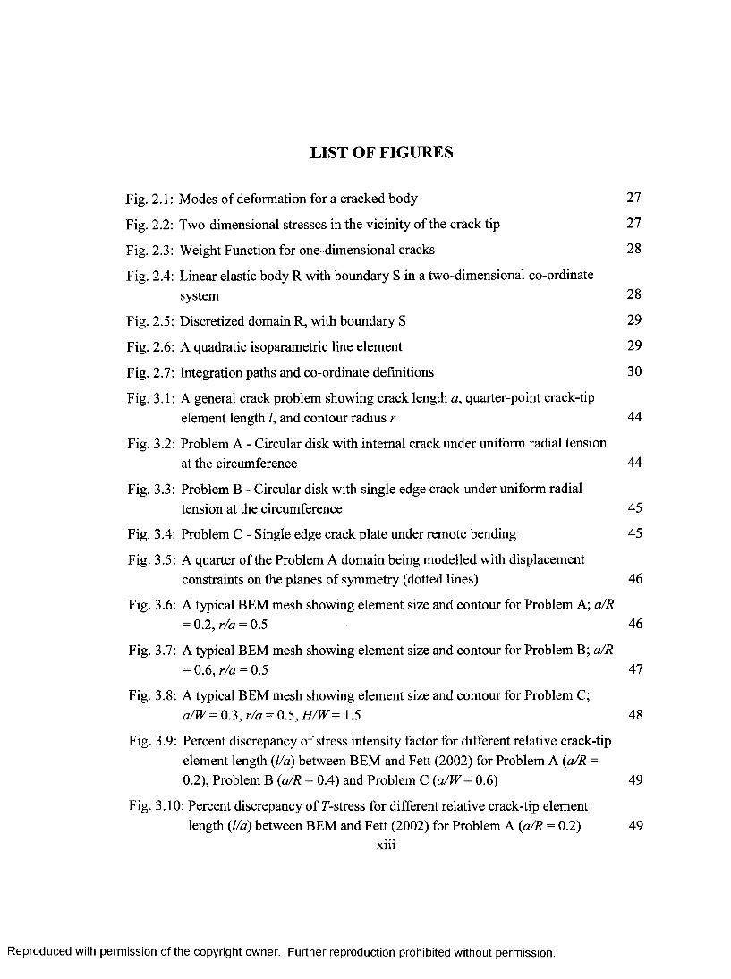
LIST OF FIGURES
Fig. 2.1: Modes of deformation for a cracked body 27
Fig. 2.2: Two-dimensional stresses in the vicinity of the crack tip 27
Fig. 2.3: Weight Function for one-dimensional cracks 28
Fig. 2.4: Linear elastic body R with boundary S in a two-dimensional co-ordinatesystem 28
Fig. 2.5: Discretized domain R, with boundary S 29
Fig. 2.6: A quadratic isoparametric line element 29
Fig. 2.7: Integration paths and co-ordinate definitions 30
Fig. 3.1: A general crack problem showing crack length a, quarter-point crack-tipelement length /, and contour radius r 44
Fig. 3.2: Problem A - Circular disk with internal crack under uniform radial tensionat the circumference 44
Fig. 3.3: Problem B - Circular disk with single edge crack under uniform radialtension at the circumference 45
Fig. 3.4: Problem C - Single edge crack plate under remote bending 45
Fig. 3.5: A quarter of the Problem A domain being modelled with displacementconstraints on the planes of symmetry (dotted lines) 46
Fig. 3.6: A typical BEM mesh showing element size and contour for Problem A; a/R= 0.2, r/a = 0.5 46
Fig. 3.7: A typical BEM mesh showing element size and contour for Problem B; a/R= 0.6, r/a = 0.5 47
Fig. 3.8: A typical BEM mesh showing element size and contour for Problem C;a/W= 0.3, r/a = 0.5, H/W= 1.5 48
Fig. 3.9: Percent discrepancy of stress intensity factor for different relative crack-tip element length (l/a) between BEM and Fett (2002) for Problem A (a/R =0.2), Problem B (a/R = 0.4) and Problem C (a/W = 0.6) 49
Fig. 3.10: Percent discrepancy of T-stress for different relative crack-tip elementlength (1/a) between BEM and Fett (2002) for Problem A (a/R = 0.2) 49
xiii
Reproduced with permission of the copyright owner. Further reproduction prohibited without permission.

Fig. 3.11: Percent discrepancy of T-stress for different relative crack-tip elementlength (l/a) between BEM and Fett (2002) for Problem B (a/R = 0.4) 50
Fig. 3.12: Percent discrepancy of T-stress for different relative crack-tip elementlength (1/a) between BEM and Fett (2002) for Problem C (a/W= 0.6) 50
Fig. 3.13: Variation of normalized T-stress with relative crack lengths for Problem A 51
Fig. 3.14: Variation of normalized stress intensity factors with relative crack lengthsfor Problem A 51
Fig. 3.15: The numerical model of one half of the Problem B geometry withdisplacement constraints on the plane of symmetry (dotted line) 52
Fig. 3.16: Variation of normalized T-stress with relative crack lengths for Problem B 52
Fig. 3.17: Variation of normalized stress intensity factors with relative crack lengthsfor Problem B 53
Fig. 3.18: Variation of normalized T-stress with relative crack lengths for Problem C 53
Fig. 3.19: Variation of normalized stress intensity factors with relative crack lengthsfor Problem C 54
Fig. 3.20: Problem D - U-notch cracked plate under remote tension 54
Fig. 3.21: A typical BEM mesh showing element size and contour integral forProblem D; L/W= 0.3, H/W= 3.0, R/W= 0.025, a/R = 1.0, r/a = 0.5 55
Fig. 3.22: A typical FEM mesh used by Lewis (2005) for the U-notch geometry 56
Fig. 3.23: Variation of normalized T-stress with relative crack lengths for Problem D 57
Fig. 3.24: Problem E - Double-cracks emanating from a circular hole in an infiniteplate under remote tension 57
Fig. 3.25: A typical BEM mesh showing element size and contour integral forProblem E; a/R = 2.0, r/a - 0.5 58
Fig. 3.26: Variation of normalized T-stress with relative crack lengths for Problem E 59
Fig. 3.27: Variation of normalized stress intensity factors with relative crack lengthsfor Problem E 59
Fig. 4.1: Problem F - Finite plate with double-cracks emanating from the edge of acircular hole under remote tension 86
Fig. 4.2: A quarter of the Problem F domain being modelled with displacementconstraints on the planes of symmetry (dotted lines) 86
xiv
Reproduced with permission of the copyright owner. Further reproduction prohibited without permission.

Fig. 4.3: A typical BEM mesh showing element size and contour integral for Problem F; R/W= 0.25, a/R = 2.0, H/W= 2.0, r/(a-R) = 0.5
Fig. 4.4: Variations of normalized T-stress with relative crack length a/R for Problem F
Fig. 4.5: Variations of normalized stress intensity factors with relative crack length a/R for Problem F
Fig. 4.6: Effect of height-to-width ratio (H/W) on T-stress for Problem F; R/W= 0.25
Fig. 4.7: Effect of height-to-width ratio (H/W) on stress intensity factor for Problem F; R/W= 0.25
Fig. 4.8: Effect of height-to-width ratio (H/W) on T-stress for Problem F; R/W= 0.50
Fig. 4.9: Effect of height-to-width ratio (H/W) on stress intensity factor for Problem F; R/W= 0.50
Fig. 4.10: Problem G - Finite plate with double-cracks emanating from the edge of a circular hole under remote bending
Fig. 4.11: A half of the Problem G domain being modelled with displacementconstraints on the planes of symmetry (dotted lines) and a nodal constraint at the lower right comer
Fig. 4.12: A typical BEM mesh showing element size and contour integral forProblem G; R/W= 0.25, a/R = 2.0, H/W= 2.0, r/(a-R) = 0.5
Fig. 4.13: Comparison of normalized T-stress between remote bending and remote tension on double-cracks emanating from a circular hole in a finite plate
Fig. 4.14: Comparison of normalized stress intensity factor between remote bending and remote tension on double-cracks emanating from a circular hole in a finite plate
Fig. 4.15: Problem H - Infinite plate with a single crack emanating from the edge of a circular hole under remote tension
Fig. 4.16: A typical BEM mesh showing element size and contour integral for Problem H; a/R = 2.0, r/(a-R) = 0.5
Fig. 4.17: Comparison of normalized T-stress between a single and double-crack configuration in an infinite plate under remote tension
Fig. 4.18: Comparison of normalized stress intensity factor between a single and double-crack configuration in an infinite plate under remote tension
xv
87
88
88
89
89
90
90
91
91
92
93
93
94
95
96
96
Reproduced with permission of the copyright owner. Further reproduction prohibited without permission.
Fig. 4.19: Problem I - Finite plate with a single crack emanating from the edge of acircular hole under remote tension 97
Fig. 4.20: A typical BEM mesh showing element size and contour integral forProblem I; R/W= 0.25, a/R = 2.0, H/W= 2.0, r/(a-R) = 0.5 98
Fig. 4.21: Variations of normalized E-stress with relative crack lengths for Problem I 99
Fig. 4.22: Variations of normalized stress intensity factor with relative crack lengthsfor Problem I 99
Fig. 4.23: Comparison of normalized E-stress between single crack and doublecracks emanating from a circular hole in a finite plate under remote tension 100
Fig. 4.24: Comparison of normalized stress intensity factor between single crack and double-cracks emanating from a circular hole in a finite plate under remote tension 100
Fig. 4.25: Problem J - Finite plate with a single crack emanating from the edge of acircular hole under remote bending 101
Fig. 4.26: A typical BEM mesh showing element size and contour integral forProblem J; R/W= 0.25, a/R = 2.0, H/W= 2.0, r/(a-R) = 0.5 102
Fig. 4.27: Comparison of normalized E-stress between single crack and doublecracks emanating from a circular hole in a finite plate under remote bending 103
Fig. 4.28: Comparison of normalized stress intensity factor between single crack and double-cracks emanating from a circular hole in a finite plate under remote bending 103
Fig. 4.29: Problem K - Infinite plate with double-cracks emanating from a periodicarray of holes under remote tension 104
Fig. 4.30: A section of the Problem K domain being modelled with displacementconstraints on the planes of symmetry (dotted lines) 105
Fig. 4.31: A typical BEM mesh showing element size and contour integral forProblem K; R/W= 0.25, a/R = 2.0, H/W= 2.0, r/(a-R) = 0.5 106
Fig. 4.32: Comparison of normalized E-stress between double-cracks in a finite andan infinite plate under remote tension 107
xvi
Reproduced with permission of the copyright owner. Further reproduction prohibited without permission.

Fig. 4.33: Comparison of normalized stress intensity factor between double-cracks in a finite and an infinite plate under remote tension
Fig. 4.34: Problem L - Infinite plate with a single crack emanating from a periodic array of holes under remote tension
Fig. 4.35: A section of the Problem L domain being modelled with displacement constraints on the planes of symmetry (dotted lines)
Fig. 4.36: A typical BEM mesh showing element size and contour integral for Problem L; R/W= 0.25, a/R = 2.0, H/W= 2.0, r/(a-R) = 0.5
Fig. 4.37: Comparison of normalized T-stress between a single crack in a finite and an infinite plate under remote tension
Fig. 4.38: Comparison of normalized stress intensity factor between a single crack in a finite and an infinite plate under remote tension
Fig. 4.39: Comparison of normalized T-stress between single and double-crack configuration in an infinite array of holes under remote tension
Fig. 4.40: Comparison of normalized stress intensity factor between a single and double-crack configuration in an infinite array of holes under remote tension
Fig. 4.41: Problem M: Infinite plate with double-cracks emanating from the edge of a circular hole influence by adjacent holes under remote tension
Fig. 4.42: A quarter of the Problem M domain being modelled with displacement constraints on the planes of symmetry (dotted lines)
Fig. 4.43: A typical BEM mesh showing element size and contour integral for Problem M; a/Ri = 2.0, a = R2/Ri = 0.5, d* = d/Rj = 4, r/(a-Rj) = 0.5
Fig. 4.44: Variations of normalized T-stress with relative crack lengths for different relative hole distance d * = d/Ri for Problem M; a = R2/R1 = 0.25
Fig. 4.45: Variations of normalized stress intensity factor with relative crack lengths for different relative hole distance d* = d/Ri for Problem M; a = R2/R1 - 0.25
Fig. 4.46: Variations of normalized T-stress with relative crack lengths for different relative hole distance d* = d/Rj for Problem M; a = R2/R 1 - 0.50
xvii
Reproduced with permission of the copyright owner. Further reproduction prohibited without permission.

Fig. 4.47: Variations of normalized stress intensity factor with relative crack lengths for different relative hole distance d* = d/R] for Problem M; a = R2/R1 =0.50 116
Fig. 4.48: Variations of normalized T-stress with relative crack lengths for differentrelative hole distance d* = d/Rj for Problem M; a = R2/Rj= 0.75 117
Fig. 4.49: Variations of normalized stress intensity factor with relative crack lengths for different relative hole distance d* = d/Ri for Problem M; a = R2/R1 —0.75 117
Fig. 4.50: Variations of normalized T-stress with relative crack lengths for differentrelative hole distance d* = d/Rj for Problem M; a = R2/R1 = 1.0 118
Fig. 4.51: Variations of normalized stress intensity factor with relative crack lengths for different relative hole distance d* = d/Ri for Problem M; a = R2/R1 =1.0 118
Fig. 4.52: Variations of normalized T-stress with relative crack lengths for differentradius ratios a = R2/R1 for Problem M; d* = d/Rj = 2.5 119
Fig. 4.53: Variations of normalized stress intensity factor with relative crack lengthsfor different radius ratios a = R2/R 1 for Problem M; d* = d/Ri - 2.5 119
Fig. 4.54: Variations of normalized T-stress with relative crack lengths for differentradius ratios a = R2/R1 for Problem M; d* = d/R] - 4.0 120
Fig. 4.55: Variations of normalized stress intensity factor with relative crack lengthsfor different radius ratios a = R2/R 1 for Problem M; d* = d/Ri = 4.0 120
Fig. 4.56: Variations of normalized T-stress with relative crack lengths for differentradius ratios a = R2/R / for Problem M; d* = d/R/ = 5.0 121
Fig. 4.57: Variations of normalized stress intensity factor with relative crack lengthsfor different radius ratios a = R2/R 1 for Problem M; d * = d/Rj = 5.0 121
Fig. 4.58: Variations of normalized T-stress with relative crack lengths for differentradius ratios a = R2/R1 for Problem M; d* = d/Rj = 10.0 122
Fig. 4.59: Variations of normalized stress intensity factor with relative crack lengthsfor different radius ratios a = R2/R1 for Problem M; d* = d/Rj = 10.0 122
A
Fig. 5.1: Crack face loading cr(x') of n order on an arbitrary geometry involving acircular hole; x'= x - R , a'= a - R 140
xviii
Reproduced with permission of the copyright owner. Further reproduction prohibited without permission.

Fig. 5.2: Variations of normalized stress intensity factor with relative crack lengthsfor Problem E under uniform and linear crack face loading 141
Fig. 5.3: Variations of normalized T-stress with relative crack lengths for Problem Eunder uniform and linear crack face loading 141
Fig. 5.4: Variation of normalized stress intensity factors with relative crack lengthsfor Problem E 142
Fig. 5.5: Variation of normalized T-stress with relative crack lengths for Problem E 142
Fig. 5.6: Variations of normalized stress intensity factor with relative crack lengthsfor Problem F under uniform and linear crack face loading 143
Fig. 5.7: Variations of normalized T-stress with relative crack lengths for Problem Funder uniform and linear crack face loading 143
Fig. 5.8: Normalized uncracked stress distribution in the y-direction on theperspective crack face due to remote tension for Problem F 144
Fig. 5.9: Variation of normalized stress intensity factors with relative crack lengthsfor Problem F 145
Fig. 5.10: Variation of normalized T-stress with relative crack lengths for Problem F 145
Fig. 5.11: Variations of normalized stress intensity factor with relative crack lengthsfor Problem I under uniform and linear crack face loading 146
Fig. 5.12: Variations of normalized T-stress with relative crack lengths for Problem Iunder uniform and linear crack face loading 146
Fig. 5.13: Variation of normalized stress intensity factors with relative crack lengthsfor Problem I 147
Fig. 5.14: Variation of normalized T-stress with relative crack lengths for Problem I 147
xix
Reproduced with permission of the copyright owner. Further reproduction prohibited without permission.

NOMENCLATURE
a crack length
Ai coefficients of least-squares fit for normalized T-stress
BIE boundary integral equation
BEM the boundary element method
Bi coefficients of least-squares fit for normalized stress intensity factor
d hole distance between adjacent holes and the central hole
Di, D2 weight function parameters for T-stress
E Young’s modulus
H plate height; general elastic modulus
\J(£)\ Jacobian of transformation
K stress intensity factor
Kj mode I (opening) stress intensity factor
Kic mode I fracture toughness
Kr reference stress intensity factor
/ crack-tip element size
L notch depth
LEFM linear elastic fracture mechanics
m(x,a) weight function for stress intensity factor
M number of boundary elements
xx
Reproduced with permission of the copyright owner. Further reproduction prohibited without permission.

Mj, M2, M3 weight function parameters for stress intensity factor
n power index for stress distribution
rij unit outward normal
N number of nodes
N°} shape functions
P load or source point in BEM analysis
pd(b,c) cth node of the bth element
Q field point; second parameter for elastic-plastic LEFM analysis
r contour radius; distance between load and field point; r co-ordinate
R circular hole radius; an arbitrary isotropic linear body; notch radius
S boundary of a domain; far field stress
U tractions
t(x,a) weight function for T-stress
T T-stress
Tjt traction fundamental solutions
Ui displacements
Uji displacement fundamental solutions
Vo, V, normalized T-stress for uniform and linear crack face loading
w plate width
WF weight function
Xi Cartesian coordinates
Xi body force per unit volume
xxi
Reproduced with permission of the copyright owner. Further reproduction prohibited without permission.

Y0, Y, normalized stress intensity factor for uniform and linear crack face loading
a radius ratio
P biaxiality ratio
<% Kronecker delta
oo nominal stress
stress tensor
a (x ) crack face stress distribution
e angular coordinate
V Poisson’s ratio
£ natural coordinate for isoparametric element
r integral contour
Q BEM domain
shear modulus
xxii
Reproduced with permission of the copyright owner. Further reproduction prohibited without permission.

CHAPTER 1 INTRODUCTION
Failure of components of mechanical systems or structures which are under stress can
result in catastrophic consequences. The evaluation and prediction of failure of such
components has therefore been widely studied. The stress intensity factor (K), which
stems from the first term in the Williams (1957) series expansion for the stress field in the
vicinity of the crack-tip, has long been developed as the sole characterizing parameter for
linear elastic fracture mechanics (LEFM) analysis. Failure was assumed to occur as the
geometry and loading condition dependent stress intensity factor reaches the fracture
toughness of the material. Much emphasis has been invested in the determination of K
solutions for numerous geometries and loading conditions, and a voluminous amount of
these solutions are available in the literature today, e.g. Murakami (2003). Over the
years, however, questions have been raised concerning this so-called single parameter
LEFM approach to fracture assessment particularly under “low constraint” conditions in
the vicinity of the crack-tip. Experimentally-obtained fracture toughness of materials are
usually obtained under “high constraint” crack-tip conditions, such as the standard
compact tension or three-point bending tests. When using these material properties for
design against fracture, it has been frequently observed over the years that the stress
intensity factor approach often leads to overly-conservative estimates of the failure loads
1
Reproduced with permission of the copyright owner. Further reproduction prohibited without permission.

2
and hence the design. Larsson and Carlsson (1973) proposed to include the second, non
singular, term in the Williams (1957) series expansion to provide a better characterization
of the stress field in the vicinity of the crack. This term is often referred to as the elastic
T-stress, or simply the T-stress in fracture mechanics analysis.
Significant amounts of research have been performed on the implications of the
elastic T-stress in LEFM analysis, such as on fracture toughness, crack growth rate and
crack instability. The importance of the sign and magnitude of the T-stress was
investigated by, for example, Leevers et al. (1976), Cotterall and Rice (1980), and Bilby
et al. (1986). Positive T-stress was found to increase crack-tip constraint, thus increasing
the possibility of brittle fracture, while negative T-stress reduces crack-tip constraint and
promotes plasticity development. It has been discovered that positive T-stress leads to
out-of-plane crack growth, while stable in-plane crack growth was demonstrated with
negative T-stress levels at the crack-tip. These findings have led quite recently to the T-
stress being included as a second parameter in fracture assessment in design codes (see
e.g. Ainsworth et al. (2002)).
T-stress solutions for different loading conditions and geometries have been
presented by a number of authors; see e.g. Fett (2002), Li (2004). Surprisingly, however,
only a limited amount of solutions have been performed for geometries involving stress
concentrations, even though they are commonly found in practical engineering situations,
e.g. notches and rivet holes. Recent examples of work with this focus include those by
Lewis (2005), who investigated the effects of T-stress on a U-notch cracked plate, and by
Broberg (2003), who obtained T-stress solutions for an infinite plate with double-cracks
Reproduced with permission of the copyright owner. Further reproduction prohibited without permission.

3
emanating from the edge of a circular hole. The primary aim of the present study is to
extend the work by Broberg (2003) by investigating finite plates with a single hole and
plates with multiple holes under a range of loading conditions. For completeness, the
stress intensity factor solutions will also be obtained and compared with those from the
literature where possible.
In practical applications, components undergo complex stress fields, e.g. residual
stresses, thermal stresses, stress concentrations. The weight function (WF) method,
which is essentially a Green’s function method, was developed to provide an efficient
technique to analyze for stress intensity factor solutions. Wang (2002) extended this
method to obtain T-stress solutions for these complex stress distributions. Although there
are ample demonstration of this WF approach for the determination of K and T-stress
solutions for a variety of geometries, its applicability to plates with circular holes has yet
to be proven. Thus, this analytical method will also be investigated in the present study.
The boundary element method (BEM), also know as the boundary integral
equation (BIE) method, will be the numerical stress tool used throughout this thesis. It
offers significant advantages over other numerical methods, such as the finite element
method (FEM). As the name implies, only the boundary of the domain needs to be
discretized, thus reducing mesh complexity and data preparation time.
The organization of this thesis will be as follows. In the next chapter, the
fundamentals of linear elastic fracture mechanics (LEFM), the weight function (WF)
method, and the boundary element method (BEM) will be briefly reviewed. The
procedures for the contour integral method for obtaining T-stress solutions and the self
Reproduced with permission of the copyright owner. Further reproduction prohibited without permission.

4
regularizing feature for BEM analysis will be discussed. The confidence of the BEM as
the numerical technique for analysis will be validated in Chapter 3, where stress intensity
factor and T-stress solutions are compared with those available in the literature.
Numerical modelling procedures and mesh design guidelines will be described. Chapter
4 presents the results of the investigation on T-stress for problems of plates with cracks
emanating from a single or multiple circular holes. Several of these problems will be
reanalyzed using the weight function method in Chapter 5, to verify its validity.
Conclusions from the work of this thesis will be summarized in Chapter 6.
Reproduced with permission of the copyright owner. Further reproduction prohibited without permission.

CHAPTER 2 TWO-PARAMETER LINEAR ELASTIC FRACTURE MECHANICS APPROACH AND THEIR NUMERICAL EVALUATION
2.0 Introduction
In this chapter, the fundamentals of linear elastic fracture mechanics will be reviewed.
The significance of T-stress and its recent developments will then be discussed. Due to
complex loading conditions in practical environments, such as the presence of thermal
and residual stresses, the weight function method will be introduced to obtain solutions
for non-uniform stress distributions. In the last part of the chapter, the boundary element
method (BEM) is discussed; it is the computational tool employed for all numerical
analysis. The mutual or M-contour integral for T-stress evaluation in conjunction with
BEM is described. To this end, self-regularized BEM will also be examined, as it allows
further refinement of the modelling strategy and accuracy of the computed solution.
5
Reproduced with permission of the copyright owner. Further reproduction prohibited without permission.
6
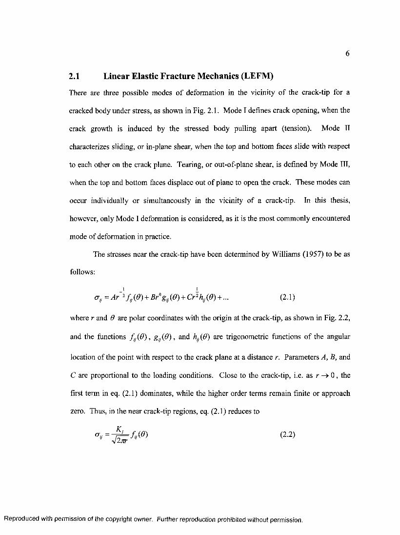
2.1 Linear Elastic Fracture Mechanics (LEFM)
There are three possible modes of deformation in the vicinity of the crack-tip for a
cracked body under stress, as shown in Fig. 2.1. Mode I defines crack opening, when the
crack growth is induced by the stressed body pulling apart (tension). Mode II
characterizes sliding, or in-plane shear, when the top and bottom faces slide with respect
to each other on the crack plane. Tearing, or out-of-plane shear, is defined by Mode III,
when the top and bottom faces displace out of plane to open the crack. These modes can
occur individually or simultaneously in the vicinity of a crack-tip. In this thesis,
however, only Mode I deformation is considered, as it is the most commonly encountered
mode of deformation in practice.
The stresses near the crack-tip have been determined by Williams (1957) to be as
follows:
where r and 6 are polar coordinates with the origin at the crack-tip, as shown in Fig. 2.2,
and the functions (6 ) , and hy{6 ) are trigonometric functions of the angular
location of the point with respect to the crack plane at a distance r. Parameters A, B, and
C are proportional to the loading conditions. Close to the crack-tip, i.e. as r -> 0 , the
first term in eq. (2.1) dominates, while the higher order terms remain finite or approach
zero. Thus, in the near crack-tip regions, eq. (2.1) reduces to
(2 .1)
(2 .2)
Reproduced with permission of the copyright owner. Further reproduction prohibited without permission.
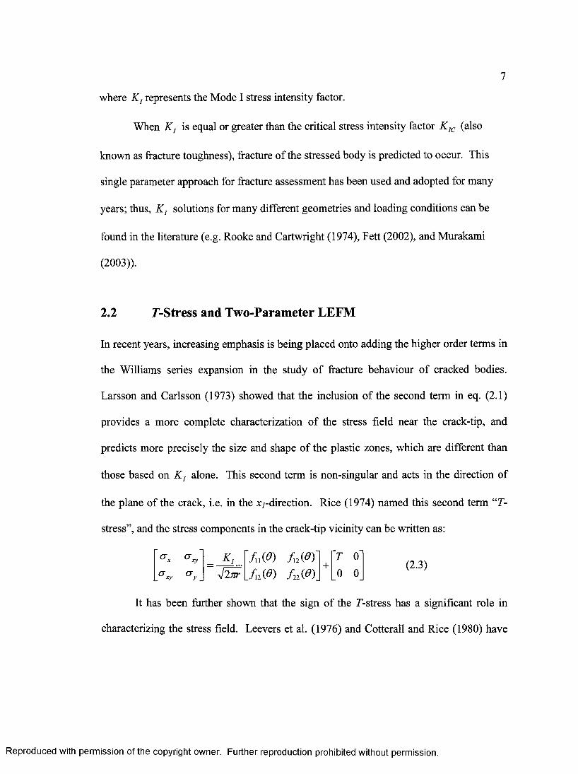
where K, represents the Mode I stress intensity factor.
When K[ is equal or greater than the critical stress intensity factor K IC (also
known as fracture toughness), fracture of the stressed body is predicted to occur. This
single parameter approach for fracture assessment has been used and adopted for many
years; thus, K, solutions for many different geometries and loading conditions can be
found in the literature (e.g. Rooke and Cartwright (1974), Fett (2002), and Murakami
(2003)).
2.2 T-Stress and Two-Parameter LEFM
In recent years, increasing emphasis is being placed onto adding the higher order terms in
the Williams series expansion in the study of fracture behaviour of cracked bodies.
Larsson and Carlsson (1973) showed that the inclusion of the second term in eq. (2.1)
provides a more complete characterization of the stress field near the crack-tip, and
predicts more precisely the size and shape of the plastic zones, which are different than
those based on K , alone. This second term is non-singular and acts in the direction of
the plane of the crack, i.e. in the x/-direction. Rice (1974) named this second term ‘T-
stress”, and the stress components in the crack-tip vicinity can be written as:
(2.3)
It has been further shown that the sign of the T-stress has a significant role in
characterizing the stress field. Leevers et al. (1976) and Cotterall and Rice (1980) have
^ xy_ K i 7 n (0 ) fn iP )
_a xy a y . Jn (P ) f 22(d)
"r o'+ 0 0
Reproduced with permission of the copyright owner. Further reproduction prohibited without permission.

8
shown that positive T-stress increases constraint on the crack-tip, which discourages
plastic deformation and yielding. As a result, the fracture trajectory would diverge from
the direction of the initial crack from the increase in crack-tip triaxiality. In contrast,
negative T-stress reduces crack-tip constraint by reducing the mean stress, thus promoting
plasticity development. This results in a more stable crack growth along the plane of the
initial crack. Leevers and Radon (1982) developed a dimensionless parameter called the
biaxiality ratio, /?, to normalize the effect of T-stress with respect to the stress intensity
factor, where
It was found by Leevers and Radon (1982) that negative biaxiality ratio influences stable
crack growth in the direction of the crack plane, while high positive /? will result in
directional instability of the crack. For elastic materials, the K-T two-parameter approach
provides an accurate representation of the stress field. Betegon and Hancock (1991) and
Du and Hancock (1991) have adopted the T-stress as the second parameter to the J-
integral to account for elastic-plastic behaviour in the material. The J-integral proposed
by Rice (1968) is a function of the strain energy density and the vector components of
displacement and traction, and it is path independent. Later study by O’Dowd and Shih
(1991) and Wang (1993) found that in order to accommodate plasticity from small-scale
yielding to fully yielded conditions, the J-Q two-parameter approach is more suitable,
where Q is related to T-stress and the material yield stress crY by (O’Dowd and Shih
(1991))
Reproduced with permission of the copyright owner. Further reproduction prohibited without permission.

9
Q = — (2.5)<7r
Since the work of Larsson and Carlsson (1973), a relatively huge volume of
papers have been published on F-stress for a variety of geometries. For example, Fett
(2002) has obtained one-dimensional crack F-stress solutions for many different
geometries. Wang (2002) has evaluated F-stress solutions for semi-elliptical surface
cracks in finite plates. The effect of a circular hole in an infinite plate on F-stress was
studied by Broberg (2004). Li et al. (2005) obtained F-stress solutions for cracks in a
thick-walled cylinder due to internal pressure. Crack stability related to F-stress has also
been studied. Melin (2002) has discovered that the directional stability of the crack
depends on not only J and F-stress, but also the material properties as well as geometric
parameters. Tong (2002) found that fatigue crack growth behaviour can be described
more in detail using F-stress, since conventional LEFM failed to explain the irregularity
in crack growth caused by temperature elevation.
2.3 Weight Functions
F-stress solutions can be obtained through numerical analysis for many different
geometries and loading conditions. In many practical situations, however, components
undergo loading conditions with high degree of complexity. A stress field due to stress
concentrations, thermal stresses and residual stresses is often more complex than those
for which solutions are readily available. The weight function method provides a means
of obtaining stress intensity factors and F-stresses in a relatively simple procedure for the
Reproduced with permission of the copyright owner. Further reproduction prohibited without permission.

10
same geometry without the need for more complex repeated analysis once the weight
functions have been determined.
2.3.1 Weight Functions for Stress Intensity Factors
Using the method of superposition, Bueckner (1970) first established that for a cracked
body, as shown in Fig. 2.3(a), under stress loading S, the stress intensity factor is
equivalent to the summation of the same cracked body under crack face loading cr(x)
(Fig. 2.3(b)) and the same uncracked body under the applied load S (Fig. 2.3(c)). The
stress distribution <x(x) is that on the prospective crack plane in the uncracked body
under the load S. Since the stress intensity factor for the uncracked body is zero, i.e.
uncracked = 0, the stress intensity factor for the entire system is only a function of a x, i.e.
K = -Kcrack pressure- The calculation for the stress intensity factor for a specific geometry
under any applied load can then be transformed to the same geometry under the
corresponding crack face pressure. By integrating the product of the weight function
m(x, a) and the crack face pressure cr(x), as shown,
the stress intensity factor can be obtained. The advantage of this method is that the
weight function m(x,a) depends only on the geometry of the body. For a specific
geometry, the stress intensity factor for any <r(x) can be determined using eq. (2.6) once
the weight function has been derived.
a
(2.6)0
Reproduced with permission of the copyright owner. Further reproduction prohibited without permission.

11
The weight function m(x,a) is a generalization of Green’s function, where the
system responds to an impulse, as shown in Fig. 2.3(d). Rice (1972) simplified the
expression for the weight function to:
H du (x, a)m(x,a) = —------- ------
K, da
where H =for plane stress for plane strain
(2.7)
(2 .8)[ £ / ( l - v ) 2
In eq. (2.8), E is the Young’s modulus and v is the Poisson’s ratio. The corresponding
crack opening displacement field is denoted as ur (jc, a) . Since it is difficult to obtain,
numerical approximations for ur(x,a) have been developed. Shen and Glinka (1991)
found that the following four-term weight function approximation could be applied to
several one-dimensional edge- and through-cracks:
m(x, a) 1 - A/ r x^ 21 - - + M 2 1----- + m 3 1 —
V a j I a) I a )yJ27r(a - x)
where Mj, M2, and M3 are geometric constants for a specific cracked body.
(2.9)
2.3.2 Weight Functions for T-Stress
The weight function for T-stress can be developed in a similar manner as for stress
intensity factors described above. Consider the cracked body under applied load system
S, as shown in Fig. 2.3(a). The stress field of this cracked body can be divided into two
parts: the uncracked body of the same geometry under the original applied load S (Fig.
2.3(c)), resulting in the stress field <t(jc) on the prospective crack plane, and the cracked
Reproduced with permission of the copyright owner. Further reproduction prohibited without permission.

12
body subjected to crack face loading corresponding to cr(x), as shown in Fig. 2.3(b),
similar to that seen before for the stress intensity factor. Hence, the problem as described
by Fig. 2.3(a) can now be represented by superposition as follows:
T = T +T (2 101crackpresmre uncracked ' ’ '
Recall that the regular stress field (Fig. 2.3(c)) has no singularity at the crack-tip,
thus, the corresponding stress intensity factor is zero. The same cannot be said for the T-
stress, as Wang (2002) has shown that:
^ uncracked ^ y ^c ra c k tip ̂ 0
The T-stress under the crack face pressure <x(x) can be determined by integrating the
product of the T-stress weight function, t(x,a), and er(x), as shown:
a
Tcrackpressure = ’ K * , d ) d x (2 . 12)0
The T-stress weight function depends only on the crack geometry, and is
independent of loading conditions, similar to the Kj weight function. The weight function
is essentially Green’s function, a pair of unit loads on the crack face, for T-stress (Fig.
2.3(d)). Therefore, substituting eq. (2.11) and eq. (2.12) into eq. (2.10), the T-stress for
the stressed crack body under load S (Fig. 2.3(a)) is found to be:
a
T = J o - ( x ) • t(x,a)dx + (ax - <Jy)cracktip (2.13)o
For any arbitrary loading condition, eq. (2.13) provides a very efficient way to
obtain the elastic T-stress. For a specific geometry, once t(x,a) is found, and
Reproduced with permission of the copyright owner. Further reproduction prohibited without permission.
13
[<jx - 0 ’y)cracktip is determined by stress analysis of the uncracked body, the corresponding
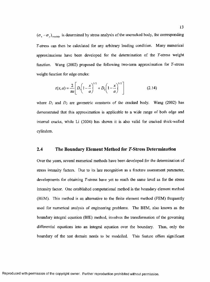
f-stress can then be calculated for any arbitrary loading condition. Many numerical
approximations have been developed for the determination of the f-stress weight
function. Wang (2002) proposed the following two-term approximation for f-stress
weight function for edge cracks:
2t( x, a) =
m Af Yv/2 1 - -
v a j+ D-
f v \ 3/2
1 - -
V a )(2.14)
where D; and D2 are geometric constants of the cracked body. Wang (2002) has
demonstrated that this approximation is applicable to a wide range of both edge and
internal cracks, while Li (2004) has shown it is also valid for cracked thick-walled
cylinders.
2.4 The Boundary Element Method for f-Stress Determination
Over the years, several numerical methods have been developed for the determination of
stress intensity factors. Due to its late recognition as a fracture assessment parameter,
developments for obtaining f-stress have yet to reach the same level as for the stress
intensity factor. One established computational method is the boundary element method
(BEM). This method is an alternative to the finite element method (FEM) frequently
used for numerical analysis of engineering problems. The BEM, also known as the
boundary integral equation (BIE) method, involves the transformation of the governing
differential equations into an integral equation over the boundary. Thus, only the
boundary of the test domain needs to be modelled. This feature offers significant
Reproduced with permission of the copyright owner. Further reproduction prohibited without permission.

14
advantages over the FEM in efforts taken in mesh designs and data preparation, as well as
analysis time. Due to its efficiency and high accuracy for problems with high gradients
in the solution variables, such as crack problems, the BEM has become a popular tool for
elastic fracture mechanics analysis. Recent work performed by, e.g. Ortiz and Cisilino
(2005), demonstrated that BEM can be employed to analyze bimaterial interface cracks in
three-dimensions for mixed modes stress intensity factors as well.
F-stress determination using BEM has also been studied in recent years. Sladek et
al. (1997) has developed contour integral formulae, in conjunction with BEM, to evaluate
the F-stress for two-dimensional geometries. This work was subsequently extended to
analyze F-stress in dynamic loading conditions (Sladek et al. (1999)) and three-
dimensional cracked cases (Sladek and Sladek (2000)). Also, Tan and Wang (2003) had
derived a simple formula employing the use of quarter-point quadratic isoparametric
elements for obtaining F-stress solutions of cracked body using BEM. The contour
integral method described by Sladek et al. (1997) will be further discussed later in this
section, as it will serve as the analysis tool for this thesis.
2.4.1 Review of the BEM
The analytical formulation of BEM starts from the differential equations for equilibrium.
By the use of the fundamental solution to the governing differential equations and a
reciprocal theorem, they are transformed into integral equations. For brevity, the indicial
notation will be used hereafter, in which subscript indices (1,2,3) will replace the
Cartesian co-ordinate direction of (x,y,z).
Reproduced with permission of the copyright owner. Further reproduction prohibited without permission.

15
In the present work, only two-dimensional isotropic, linear elastostatic problems
are considered. Consider an isotropic linear body, R, with boundary S as shown in Fig.
2.4. Beginning with the Navier’s equation of equilibrium, and applying Betti-Rayleigh’s
reciprocal work theorem and fundamental solutions, they are transformed into integral
equations over the surface of the solution domain. Following the usual limiting process,
and in the absence of body forces, the boundary integral equation for elastostatics is (Tan
(1987)):
C,i ( / > , ( / ■ ) + [u,(Q)T1,(P,Q)dS(Q)= [ t.m u„(.P ,Q )dS(Q ) (2.15)
where Un (P, Q) and 77 (P, Q) are the Kelvin’s fundamental solutions for displacements
and tractions to Navier’s equation, respectively. More specifically, Ujj (P, Q) and
Tj, (P, Q) are the displacement and traction, respectively, in the x,-direction at Q(x) due to
the application of a unit concentrated load in the xy-direction at P(x). In eq. (2.15),
ut(P,Q) and (P,Q) denote the unknown displacements and tractions, respectively, and
CjXP) = lim [ Tfi{PtQ)dS{Q) (2.16)J E—>0 JSe J
where Cfi{P) depends on the local geometry of the surface at point P, and s£ is the
boundary of the small region of exclusion around P.
Equation (2.15) is an integral equation that relates the boundary tractions to the
boundary displacements. It is generally too difficult to solve this equation analytically;
hence, a numerical technique must be used. To this end, the boundary S is represented by
a sequence of M line elements, as shown in Fig. 2.5. As presented by Tan (1987), the
Reproduced with permission of the copyright owner. Further reproduction prohibited without permission.

16
quadratic isoparametric element (Fig. 2.6) is used here to describe the variation of
element geometry and functions. It is defined by three equally spaced nodes with
intrinsic co-ordinates £ = -1, <f = 0, and £ = 1, respectively. The corresponding shape
functions are described as follows:
N ° \ 0 = Q - f f
= + (2.17)
where the superscripts on the shape function N {,](^) represents the local nodes of the
element. Expressing in terms of shape functions and nodal values, the geometric
parameters, displacements and tractions can be written as:
x ^ ) = N \ 4 )xcj
uJig) = N '{ f iu ' j
tJ(£) = N c(Z )fj c = 1,3 (2.18)
Substituting eq. (2.18) into eq. (2.15), the discretized form of the boundary integral
equation is:
M 3
C„(P‘)«,(/-) + Y Y lu,(P1<M) f Tf (P° ,Q )N ‘ (<?)|y(fl|dS6=1 c=l
M 3
= f )|j(^)|rfS (2.19)6=1 c=1
Pa = l,N
where M= number of elements in the domain
N= number of nodes in the domain = 2M
Pdfb’c) = c th node of the bth element
Reproduced with permission of the copyright owner. Further reproduction prohibited without permission.

17
b = 1,M
c= 1,3
\J{£,)\ - Jacobian of transformation
Equation (2.19) represents a total of AM linear algebraic equations for the unknown
displacements and tractions at the boundary nodes of the discretized domain. The
unknown displacements and tractions on the boundary S can now be solved using
standard matrix manipulations.
2.4.2 Contour Integral for Calculating T-Stress Using BEM
The contour integral described by Rice (1968) was introduced to overcome the
difficulties in determining strain concentrations when analyzing notched and cracked
geometries. Since then, this contour integral technique has been widely used to solve a
variety of problems. The evaluation of elastic T-stress using the contour integral was
introduced by Sladek et al. (1997). It is based on Betti-Rayleigh’s reciprocal work
theorem and an auxiliary field, and it is particularly suitable for implementation with the
BEM. These authors derived a path independent contour integral around the crack-tip,
termed the mutual or M-integral, which is directly related to the T-stress. The contour
integral is along a closed path sufficiently far from the crack-tip. This in turn obviates
the need to compute the stress field near the vicinity of the crack, where the crack-tip
stress singularity can cause large numerical errors. The required field variables along the
integration path are obtained from the BEM analysis.
Reproduced with permission of the copyright owner. Further reproduction prohibited without permission.

18
The following briefly describes the key steps in the derivation of the M-contour
integral and its relationship with the T-stress. Consider a cracked isotropic, elastic
domain R with boundary S, as shown in Fig. 2.7. Inside this domain, consider a closed
integration path comprised of ro, 7c+, and / c ’. Using Gauss’ divergence theorem,
Hooke’s law and strain-displacement relations, the Betti-Rayleigh’s reciprocal theorem
for two sets of equilibrium states of the sub-domain can be expressed as:
= \ ( X l'ui - X iUi')-dQ. (2.20)
where X i and X ' are body forces in two load states, respectively; and rij is the unit
outward normal of the contour F of integration in sub-domain Q. A small circular region
bounded by r e near the crack-tip has to be excluded due to the existence of the
singularity. This region is small and will reduce to zero in the limiting process. The
contour of integration r = F0 + Fc + Fc~ - jT£ is a closed path in the counterclockwise
direction.
Without the loss of generality, assume that in eq. (2.20), the primed and unprimed
states correspond to an auxiliary and the unknown fields, respectively. Assume an
auxiliary field where cr.. '= 0 on crack faces and body forces X ' - 0. Equation (2.20)
can be rewritten as:
[ K ' V j - a lUl'n j ) -d r = - t r ^ ' n ^ - d T
- ( < « > / - CTfu'nj-y dr (2.21)
- lim f X u ' dQ.
Reproduced with permission of the copyright owner. Further reproduction prohibited without permission.

19
where and rij are unit outward normal on the upper and lower crack face,
respectively, and n* = -n ~. Also, assume that c r + = cr.” for small equilibrium stress
loads. Using the relationship between traction and stress, i.e. tt = a ijn] , eq. (2.21) can be
transformed into:
This equation can be used to derive integral formulas for evaluating various
fracture parameters by choosing different auxiliary fields. Bueckner (1989) employed
singular auxiliary fields to obtain integral equations for stress intensity factor Kj.
However, to obtain the non-vanishing contribution to elastic T-stress, a special auxiliary
field has to be determined. It must also eliminate the singular integrand contribution in
the process. It was proposed by Sladek et al. (1997) to use an auxiliary field that is one
order higher than the one utilized by Kfouri (1986). The auxiliary displacements and
tractions are obtained by differentiating Kfouri’s field, with respect to xj, and they are
proportional to Hr and \lr2, respectively. This auxiliary field is represented by:
(2.22)
ux'(r,6 ) = — — (1 - v2) • (cos 9 ---- — sin2 9 cos 6 )nEr l - v
u2 '(r,9) = — (1 + v) • (1 - 2v - cos29) ■ ( - sin9) 2nEr
crn '(r,9) = cos2 9- (cos2 9 - 3 sin2 9)7 ir
Reproduced with permission of the copyright owner. Further reproduction prohibited without permission.

20
cr12'(r,6 ) = - ^ s i n 2 6 ■ (3cos2 6 - sin2 9) (2.23)m
where / is a static point force applied at the crack-tip in the crack propagating direction
(Fig. 2.7).
The unknown asymptotic displacements and tractions can be separated into two parts:
ui = uf + UJ (2.24)
+ < (2.25)
The terms with the superscript “5” represent those of the singular stress field, cr? is
equivalent to eq. (2.2), while uf is given as:
( 2 ' 2 6 )
where n is the shear modulus, and v is Poisson’s ratio.
The terms with superscript “7”’ are given as follows:
<rT9 = T -SaSfl (2.27)
UJ =-—\ s n( } - v 1 )cos6 - 8 nv(\ + v)sm.6 \ (2.28)E
Substituting the above auxiliary field solution and the non-singular term of the Williams
series expansion into the left-hand-side of eq.(2.22), gives
ton f (f; u j - 1, \ ' ) ■ d r = 1 ^ 1 T ■ f (2.29)£->0 F.
Reproduced with permission of the copyright owner. Further reproduction prohibited without permission.

21
Performing the same task again, but this time with uf and erf , the left-hand-side of
eq.(2.22) disappears, i.e.
lim f ( t fu f - t f u .') • dT = 0 (2.30)£->0 -T,.
By substituting eq. (2.29) and eq. (2.30) into eq. (2.22), the f-stress term, without any
body forces, can finally be determined:
7 = i ■dc - 7?f^T 1 • (2'3/ ( I ~ V ) 0 / ( l - V ) ' T c
Equation (2.31) can be further simplified as the second term in the equation, for Mode I
loading, is always zero. Hence, the f-stress solution now becomes
T = , , . E 2, f ft'K, - • dT (2.32)/ ( l - v )
By substituting eq. (2.22) into eq. (2.32), a more explicit f-stress solution can be
obtained:
f = Fij(d)ui —tj-•Tn r/r Jv E
■dT (2.33)/ ( l - v 2) *h> nr1
where f . (0) contains trigonometric functions of the angular location. This explicit f-
stress expression can now be solved numerically using, for example, a Gaussian
quadrature scheme. The nodal displacements and tractions along the integration path, ut
and tt , can be computed from the BEM analysis.
Reproduced with permission of the copyright owner. Further reproduction prohibited without permission.

22
2.4.3 Self-Regularized Boundary Element Method
As aforementioned, £/,.,.(/?, 0 and 77 (p, Q) are the displacement and traction
fundamental solutions to Navier’s equation, respectively. They are explicitly expressed
as:
u„ (p,Q) = , , ‘ ' [(3 - 4v XSt + r„ r,t )] (2.34)16^(1 - v ) p r
Tj,(p ,Q) = ~2v)S, + 3r„ r , , )]- (1 - 2 ) | (2.35)
where r here is the distance between the source and the field point. Differentiating eq.
(2.15) with respect to the co-ordinates at p, and using Hooke’s Law, the Somigliana’s
identity for stresses can be obtained:
<re(p)= l l , (8 )O v (p,Q)ds(Q)= f M 0)S*O >.G )*(0) (2.36)
where the kernels Dkij(p ,Q ) and Skij(p, Q), containing derivatives of Ujt(p,Q) and
Tjt(p, 0 , can be written in the following forms:
Dkij(p,Q) = gn ^ _ vy 2 [ 0 - 2v \ S kir,j + ^ / „ +Sgr,k ) + 3r„ r ,, r,k] (2.37)
SkiJ(p,Q) = A - t 3— KI - 2v)diJr,k+v(Skir,J+Skjr ,l )4^(1 - v)r3 ( dn
~ 5r>i r>j rn 1 + 3 v in f ' j r,k- n jr,i r,k ) (2.38)+ (1 - 2v)(3«,r„. r,j +njSikSJk )
- (1 - 4v)nkSjj}
As evident in the order of r that is present in the denominator of these equations,
Uji(p,Q) is weakly singular, Tp (p,Q) and Dkij(p,Q) are strongly singular, and
Reproduced with permission of the copyright owner. Further reproduction prohibited without permission.

23
Skij(p,Q ) is hypersingular. This may contribute to numerical errors when evaluating
displacements and stresses at interior points near the boundaries since the integrands in
the BIE become nearly singular. These integrals are difficult to evaluate by standard
quadrature procedures as errors will increase when the interior point approaches the
domain boundary, i.e. as r —> 0. This is sometimes referred to as the boundary layer
effect in the BEM community. To overcome this problem, an obvious strategy is to
increase the number of boundary elements, by reducing their lengths, in the vicinity of
the interior points. This approach is, however, cumbersome as the mesh near the interior
points needs to be extremely refined.
An alternate scheme to overcome the near-singularity problem is to “regularize”
the integrals, either locally on certain segments on the boundary (e.g. Huang and Cruse
(1994)) or globally (e.g. Cruse and Richardson (1996, 1999)), so that the integration can
be carried out normally using standard quadrature techniques. In this thesis, the self
regularized forms from Cruse and Richardson (1996, 1999), will be adopted along with
contour integral formulas to derive accurate T-stress solutions.
Cruse and Richardson (1996) proposed a self-regularized displacement BIE
(DBIE). This can be derived from the Somigliana displacement identity by subtracting a
simple solution that corresponds to rigid body motion, as shown below:
u,(p) - u,(P) = - f Q)dS(Q)* (2.39)
+ [ t , ( .Q )V M Q )d S (Q )
Reproduced with permission of the copyright owner. Further reproduction prohibited without permission.

24
where p is the source point (internal point) and P is the regularizing point at the
boundary usually taken to be close to p. Both of the integrals in this equation are regular
at every internal point. This suggests that the boundary layer effect is eliminated and no
special attention is required for internal points close to boundary nodes.
For stress, Cruse and Richardson (1996) also derived a self-regularized BIE
(SBIE) from the Somigliana stress identity. This can be obtained by subtracting and
adding back the first and second terms of the Taylor series expansion to the original form
of the SBIE. The procedure is equivalent to subtracting and adding back a simple
solution corresponding to a state of constant stress in the body that is equal to the
boundary stress at a surface point P, and can be expressed as
a , (P) ~ (P) = - f K ( 0 - ( 8 ) k (P> « )* (2.40)
+ 1[<1(0 ) - '» i ( 0 K ( a 0 V 'S ( 0
where uk (Q) and tLk (Q) represent the linear state of displacements and tractions
associated with the boundary stress at P, and are given by
»t(0 ) = «„(P) + (2-41)
'i ( 0 ) = CT*.(f K ( 0 ) (2-42)
The coefficient uk m (P) is the displacement gradients at the regularizing point P. xm (Q)
and xm(P) are the Cartesian co-ordinates of the field point and regularizing point,
respectively; and crkm (P) represents the stress components at P. Following the
procedures described by Cruse and Richardson (1999), a system of equations relating
Reproduced with permission of the copyright owner. Further reproduction prohibited without permission.

25
local traction and displacement tangential derivatives with the displacement gradients can
be obtained:
/i«CN.
2̂< > =
u , f
2M 1-V)l - 2 v 2 //v
n,2 f iv
l - 2 v - j ( € ) n 2
0
m 2 Mn 2 ------- nil - 2 v2 ju ( \-v )
m l - 2 v0 J(Z)n i 0
m n 2 0 m n y
* 1,1
u2,1
* 1,2
* 2,2
(2.43)
where J(£) is the Jacobian of transformation. Finally, by inverting the above matrix, the
displacement gradients at the regularizing point can be obtained in terms of local
tractions and displacements
(2.44);=i
where Aklr(^ p) and Bklr{%p) are the mapping functions. Using this regularized
technique, the solutions from BEM analysis have been shown to be highly accurate
(Cruse and Richardson (1999)) even for interior points very close to the domain
boundary.
2.5 Summary
The theory of linear elastic fracture mechanics (LEFM) has been reviewed. The T-stress
(non-singular) term in the Williams (1957) series expansion has been shown to be a
significant factor in describing more accurately the stress field in the vicinity of a crack.
Due to the complexity of loading conditions in practical applications, the weight function
method was also reviewed to provide a convenient method for solving these types of
Reproduced with permission of the copyright owner. Further reproduction prohibited without permission.

26
problems. The review of the boundary element method (BEM) was carried out as it
would serve as the numerical tool for all analysis. Finally, T-stress determination using
the mutual contour integral method, in conjunction with self-regularizing BEM to
minimize errors in evaluating the contours, was discussed.
Reproduced with permission of the copyright owner. Further reproduction prohibited without permission.

27
Mode I-OPENING Mode II - SLIDING Mode III - TEARING
Fig. 2.1: Modes of deformation for a cracked body
G-ack
Fig. 2.2: Two-dimensional stresses in the vicinity of the crack tip
Reproduced with permission of the copyright owner. Further reproduction prohibited without permission.

Fig. 2.3: Weight Function for one-dimensional cracks
y
Fig. 2.4: Linear elastic body R with boundary S' in a two-dimensional co-ordinate system
Reproduced with permission of the copyright owner. Further reproduction prohibited without permission.

BourKtey Nods*
Boumtoy Etament
Fig. 2.5: Discretized domain R, with boundary S
S = +i
= o
S = - i
Fig. 2.6: A quadratic isoparametric line element
Reproduced with permission of the copyright owner. Further reproduction prohibited without permission.

30
o
o
Fig. 2.7: Integration paths and co-ordinate definitions
Reproduced with permission of the copyright owner. Further reproduction prohibited without permission.

CHAPTER 3 BEM VALIDATION AND TEST PROBLEMS
3.0 Introduction
In this chapter, the effectiveness and accuracy of the boundary element method (BEM)
for determining stress intensity factor, Ki, and T-stress is verified. The BEM computer
program used for all analysis was a variation of the one for two-dimensional stress
analysis using the quadratic isoparametric numerical formulation; it was developed by
Prof. C.L. Tan at Carleton University. Numerical modelling procedure will first be
discussed, and proper crack-tip element size and contour radii for testing crack problems
are established to ascertain accurate results, when using the computer program. Different
test geometries, as listed in Table 3.1, will be analyzed using the BEM and comparisons
are then made with corresponding solutions in the literature.
31
Reproduced with permission of the copyright owner. Further reproduction prohibited without permission.

32
3.1 Numerical Modelling and Mesh Design Guidelines
BEM fracture mechanics analysis entails the use of the well-known quarter-point crack
tip element and the contour integral method, as shown in Fig. 3.1. Li (2004) has shown
that relative crack-tip element (l/a) and relative contour radius sizes (r/a) can have some
effect on the accuracy of computed BEM results. For self-regularizing BEM, it is
necessary to again establish these parameters that provide comparable results to those
available in literature before carrying out any analysis. Three different geometries were
tested: a circular disk with internal crack under uniform radial tension at the
circumference (Problem A), as shown in Fig. 3.2; a circular disk with single edge-crack
under uniform radial tension at the circumference (Problem B), as shown in Fig. 3.3, and
a single edge-crack plate under remote bending (Problem C), as shown in Fig. 3.4. The
relative crack sizes considered in these problems was arbitrarily chosen to be a/R = 0.2
and 0.4 for Problems A and B, respectively, and a/W = 0.6 for Problem C. Numerical
results for these problems are available in the literature, such as the ones obtained from
Fett (2002) using the method of boundary collocation.
The numerical modelling of each of these test cases can take advantage of
symmetry, hence only a fraction of the geometry needs to be analyzed. For example,
only a quarter of the Problem A domain needs to be modelled (Fig. 3.5). The vertical
plane of symmetry is constrained in the xi-direction, while free to displace in the X2-
direction. The horizontal plane (uncracked portion) is constrained in the X2-direction,
while being able to displace freely in the xi-direction. Also due to the symmetry of the
Reproduced with permission of the copyright owner. Further reproduction prohibited without permission.

33
problem, only a semi-circular contour is needed for the T-stress determination, as shown
in Fig. 3.6. Two-dimensional standard quadratic isoparametric elements were used
except for the crack-tip elements, with the sizes gradually being enlarged away from the
crack-tip. Figure 3.6 shows the BEM mesh employed for Problem A, with the contour
integral path used in the interior of the numerical domain. Plane strain condition was
assumed. The integration of the contour can be performed numerically using Gaussian
quadrature scheme. The contour was represented by 12 discretized circular elements, and
10th order Gaussian quadrature was used for numerical integration. The corresponding
BEM meshes used for Problems B and C are shown in Figures 3.7 and 3.8, respectively.
3.1.1 Relative Quarter-Point Crack-Tip Element Size (l/a) and Relative
Contour Radii (r/a)
The relative quarter-point crack-tip element lengths l/a = 0.05, 0.10, 0.15, and 0.20 and
relative contour radii r/a - 0.4, 0.5, and 0.6 were tested. The results for the normalized
stress intensity factor ( K, / cr^fm ) and T-stress (T/d) are shown in Tables 3.2 - 3.4.
Generally, excellent agreement with less than 2% discrepancy between the BEM results
and that obtained by Fett (2002) was achieved for all three test problems considered,
suggesting that the solutions obtained by the self-regularizing BEM were fairly
insensitive to the crack-tip element size or contour radii. As shown in Fig. 3.9, the l/a =
0.10 case exhibited the least amount of discrepancy, for all geometries. Thus, this
relative crack-tip element length will be adopted for all of the BEM analysis in this thesis.
The T-stress results for the three different geometries are shown in Fig. 3 .10-3 .12 . All
Reproduced with permission of the copyright owner. Further reproduction prohibited without permission.

34
of the r/a ratios tested provided equally accurate results, and although it is not necessary
to use all three ratios to verify the results, they are nevertheless considered for all the
analysis carried out in this thesis as a check on the numerical solutions of the T-stress
obtained.
3.2 Test Cases for BEM Validation
Having established appropriate relative crack-tip element lengths and contour paths for
three arbitrarily chosen test problems above, a more comprehensive test involving a
wider range of crack sizes for those three geometries was carried out. In addition, two
other problems with a crack or cracks emanating from stress concentrations were also
treated. They were a U-notch cracked plate (Problem D) and an infinite plate with two
cracks emanating from the edge of a circular hole (Problem E).
3.2.1 Circular Disk with Internal Crack (Problem A)
Two-dimensional BEM analysis was performed for the circular disk with internal crack
under uniform radial tension at the circumference, as shown in Fig. 3.2. As previously
mentioned, the numerical modelling of this geometry can be reduced to one quarter of its
original geometry, by virtue of symmetry. Relative crack size of a/R = 0.1 - 0.6 were
analyzed and the results are presented in Table 3.5 and Fig. 3.13 and 3.14. The BEM
results show very good agreement indeed with those by Fett (2002), using the method of
boundary collocation, for both the normalized stress intensity factor and the T-stress.
Reproduced with permission of the copyright owner. Further reproduction prohibited without permission.
35
3.2.2 Circular Disk with Single Edge-Crack (Problem B)
The circular disk with single edge-crack under uniform normal traction at the
circumference case as shown in Fig. 3.3, was analyzed with two-dimensional BEM.
Again, symmetry can be employed to reduce the size of the solution domain. However,
since this domain is only symmetric about the xy-axis, one half of the physical problem
was modelled (Fig. 3.15), with the plane of symmetry constrained in the X2-direction. It
is also shown in Fig. 3.15 that due to the lack of constraint in the xy-direction, a boundary
nodal constraint is applied at the lower right comer to preclude rigid body motion.
Relative crack size of a/R = 0.1 - 0.6 were analyzed, and the results are shown in Table
3.6 and Fig. 3.16 and 3.17. The obtained results from BEM are again compared to those
by Fett (2002), with discrepancies of generally less than 2%.
3.2.3 Single Edge-Cracked Plate (Problem C)
Two-dimensional BEM analysis was performed on the single edge-cracked plate under
remote bending (Fig. 3.4). Again, similar to Problem B, only half of the domain was
numerically modelled by virtue of symmetry. Relative crack size of a/W= 0.1 - 0.6 were
treated for a height-to-width ratio (H/W) of 1.5. The results are listed in Table 3.7, and
shown graphically in Fig. 3.18 and 3.19. Generally very good agreement was again
achieved compared to the values from Fett (2002), for both the normalized stress
intensity factor, K{ / <j4na , and T-stress, T/a.
Reproduced with permission of the copyright owner. Further reproduction prohibited without permission.

36
3.2.4 U-Notch Cracked Plate (Problem D)
The U-notch cracked plate under remote tension problem (Fig. 3.20) was solved
numerically in BEM for the normalized T-stress. Lewis (2005) has recently obtained T-
stress solutions for this geometry using the finite element method (FEM). It therefore
provides another comparison check of the effectiveness of BEM. The plate geometry is
defined by the height 2H, width W, notch depth L, notch radius R, and crack length a, as
shown in Fig. 3.20. A typical BEM mesh for this problem is shown in Fig. 3.21, while a
typical FEM mesh used by Lewis (2005) is shown in Fig 3.22. It is evident that the FEM
modelling scheme involves the use of substantially more elements than the BEM. The
modelling complexity for FEM, especially around the crack-tip, can also be seen when
comparing Fig. 3.21 and 3.22. Relative crack lengths of a/R - 0.1, 0.2, 0.3, 0.5, and 1.0
were analyzed for the case of L/W = 0.3, H/W = 3.0, R/W - 0.025. The normalized T-
stresses evaluated using BEM are shown in Table 3.8 and in Fig. 3.23. It can be seen that
the two sets of numerical results are in excellent agreement, which further provides
confidence in the self-regularizing BEM for its efficiency and accuracy.
3.2.5 Infinite Plate with Double-Cracks Emanating from the Edge of a Circular
Hole (Problem E)
T-stress solutions for double-cracks emanating from a circular hole in an infinite plate, as
shown in Fig. 3.24, are available from the recent paper by Broberg (2004). Unlike the
previous four cases, this test case involves an infinite plate. Numerical representation of
such problems can be achieved by treating a relatively large plate. It is usually sufficient
Reproduced with permission of the copyright owner. Further reproduction prohibited without permission.

37
to model the size of the domain boundary to be 20 times the length of the crack, i.e. (a-
R)/W = 0.05 and (a-R)/H = 0.05, where W and H represent the width and height of the
numerical domain, respectively. Symmetry can again be taken advantage of for this
infinite plate case, thus only one quarter of the domain needs to be analyzed with the
appropriate boundary conditions as in Problem A. The BEM mesh used for analysis for
this problem is shown in Fig. 3.25.
Relative crack sizes of a/R = 1.1 - 10.0 were considered. The results from the
two-dimensional BEM analysis are shown in Table 3.9, and graphically in Fig. 3.26 and
3.27. The normalized 7-stresses (77b) obtained from the BEM analysis show very good
agreement with those from Broberg (2004); the discrepancies were less than 2%.
Comparison was also drawn for the normalized stress intensity factor, K { / a ^ jn (a -R ) ,
between the calculated BEM results and those from Bowie (1965); the discrepancy was
less than 1.4%. Thus, it is established here that the BEM is an excellent tool for solving
this type of geometry for Kj and 7-stress.
3.3 Conclusions
The two-dimensional self-regularized boundary element method (BEM) was employed to
analyze the stress intensity factor and 7-stress solutions for five different test problems.
Relative crack-tip element size (l/a) was found to have a small effect on Kj, but not on T.
It was shown that the contour integral method generates accurate solutions for 7-stress
for different contour radii (r/a). It was established that relative crack-tip element size l/a
of 0.1 and contour radius r/a of 0.5 would generate accurate results using the BEM. It
Reproduced with permission of the copyright owner. Further reproduction prohibited without permission.

38
has been established from this part of the study that the BEM gave numerical results of Kj
and T-stress which were in excellent agreement with those established in the literature,
with discrepancies which were generally less than 2% for the problems considered.
Reproduced with permission of the copyright owner. Further reproduction prohibited without permission.

39
Table 3.1: List of problems analyzed in Chapter 3
Problem Definition Figure #
A Circular Disk with Internal Crack Under Uniform Radial Tension 3.2
B Circular Disk with Single Edge-Crack Under Uniform Radial Tension 3.3
C Single Edge-Cracked Plate Under Remote Bending 3.4
D U-Notch Cracked Plate Under Remote Tension 3.20
EInfinite Plate with Double-Cracks Emanating from the Edge of a Circular Hole Under Remote Tension
3.24
Reproduced with permission of the copyright owner. Further reproduction prohibited without permission.
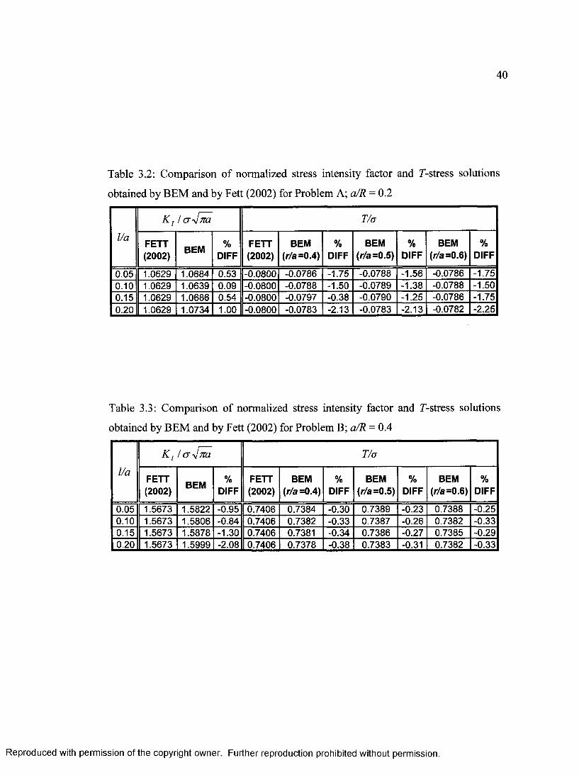
40
Table 3.2: Comparison of normalized stress intensity factor and T-stress solutions
obtained by BEM and by Fett (2002) for Problem A; a/R = 0.2
l/a
K j / <T*$na T/a
FETT(2002) BEM %
DIFFFETT(2002)
BEM (r/a =0.4)
%DIFF
BEM (r/a =0.5)
%DIFF
BEM (r/a =0.6)
%DIFF
0.05 1.0629 1.0684 0.53 -0.0800 -0.0786 -1.75 -0.0788 -1.56 -0.0786 -1.750.10 1.0629 1.0639 0.09 -0.0800 -0.0788 -1.50 -0.0789 -1.38 -0.0788 -1.500.15 1.0629 1.0686 0.54 -0.0800 -0.0797 -0.38 -0.0790 -1.25 -0.0786 -1.750.20 1.0629 1.0734 1.00 -0.0800 -0.0783 -2.13 -0.0783 -2.13 -0.0782 -2.25
Table 3.3: Comparison of normalized stress intensity factor and J ’-stress solutions
obtained by BEM and by Fett (2002) for Problem B; a/R = 0.4
l/a
K j / crV^n T/a
FETT(2002) BEM %
DIFFFETT(2002)
BEM (r/a =0.4)
%DIFF
BEM (r/a =0.5)
%DIFF
BEM(r/a =0.6)
%DIFF
0.05 1.5673 1.5822 -0.95 0.7406 0.7384 -0.30 0.7389 -0.23 0.7388 -0.250.10 1.5673 1.5806 -0.84 0.7406 0.7382 -0.33 0.7387 -0.26 0.7382 -0.330.15 1.5673 1.5878 -1.30 0.7406 0.7381 -0.34 0.7386 -0.27 0.7385 -0.290.20 1.5673 1.5999 -2.08 0.7406 0.7378 -0.38 0.7383 -0.31 0.7382 -0.33
Reproduced with permission of the copyright owner. Further reproduction prohibited without permission.

41
Table 3.4: Comparison of normalized stress intensity factor and T-stress solutions
obtained by BEM and by Fett (2002) for Problem C; a /W - 0.6
l/aK j / G-Jna T/a
FETT(2002)
BEM %DIFF
FETT(2002)
BEM (r/a =0.4)
%DIFF
BEM (r/a =0.5)
%DIFF
BEM(r/a =0.6)
%DIFF
0.05 1.9140 1.9134 0.03 0.8313 0.8321 0.10 0.8324 0.14 0.8324 0.140.10 1.9140 1.9138 0.01 0.8313 0.8319 0.08 0.8323 0.13 0.8319 0.080.15 1.9140 1.9174 -0.18 0.8313 0.8317 0.05 0.8320 0.09 0.8321 0.100.20 1.9140 1.8856 1.48 0.8313 0.8322 0.11 0.8323 0.13 0.8325 0.15
Table 3.5: Comparison of normalized stress intensity factor
and T-stress solutions between BEM and Fett (2002) for
different relative crack lengths (a/R) for Problem A
a/R l/aK j/cr^fm T/a
FETT(2002)
BEM %DIFF
FETT(2002)
BEM %DIFF
0.100 0.100 1.0167 1.0326 1.56 -0.0216 -0.0201 -7.010.200 0.100 1.0629 1.0639 -0.09 -0.0806 -0.0789 -2.060.300 0.100 1.1368 1.1502 -1.19 -0.1712 -0.1714 0.100.400 0.100 1.2415 1.2590 -1.42 -0.2937 -0.2974 1.270.500 0.100 1.3844 1.4080 -1.70 -0.4569 -0.4610 0.910.600 0.100 1.5785 1.6005 -1.39 -0.6868 -0.6656 -3.09
Reproduced with permission of the copyright owner. Further reproduction prohibited without permission.
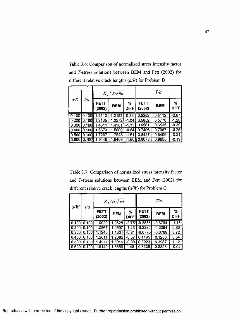
42
Table 3.6: Comparison of normalized stress intensity factor
and T-stress solutions between BEM and Fett (2002) for
different relative crack lengths (a/R) for Problem B
a/R l/aK j / <r^[m T/a
FETT(2002)
BEM %DIFF
FETT(2002) BEM
%DIFF
0.100 0.100 1.2112 1.2152 0.33 0.5252 0.5112 -2.670.200 0.100 1.3135 1.3272 -1.04 0.5852 0.5778 -1.260.300 0.100 1.4311 1.4501 -1.33 0.6561 0.6535 -0.390.400 0.100 1.5673 1.5806 -0.84 0.7406 0.7387 -0.260.500 0.100 1.7267 1.7545 -1.61 0.8427 0.8409 -0.210.600 0.100 1.9149 1.9466 -1.66 0.9673 0.9655 -0.19
Table 3.7: Comparison of normalized stress intensity factor
and T-stress solutions between BEM and Fett (2002) for
different relative crack lengths (a/W) for Problem C
a/W l/aK j / cr-fm T/a
FETT(2002) BEM %
DIFFFETT(2002)
BEM %DIFF
0.100 0.100 1.0929 1.0628 -2.75 -0.3838 -0.3794 -1.150.200 0.100 1.0567 1.0697 -1.23 -0.2380 -0.2394 0.600.300 0.100 1.1240 1.1331 -0.81 -0.0770 -0.0799 3.720.400 0.100 1.2611 1.2682 -0.57 0.1195 0.1203 0.640.500 0.100 1.4971 1.5016 -0.30 0.3923 0.3967 1.120.600 0.100 1.9140 1.8856 1.48 0.8325 0.8323 -0.02
Reproduced with permission of the copyright owner. Further reproduction prohibited without permission.
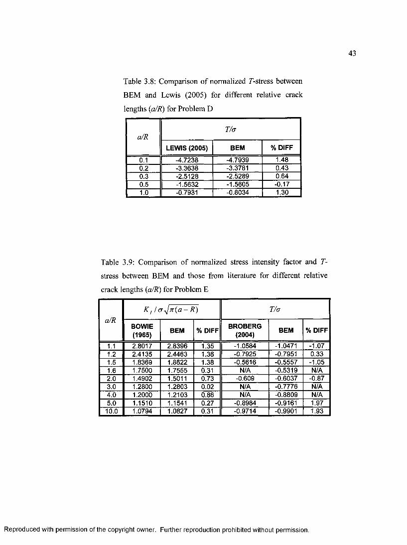
43
Table 3.8: Comparison of normalized T-stress between
BEM and Lewis (2005) for different relative crack
lengths (a/R) for Problem D
a/RT/a
LEWIS (2005) BEM % DIFF
0.1 -4.7238 -4.7939 1.480.2 -3.3638 -3.3781 0.430.3 -2.5128 -2.5289 0.640.5 -1.5632 -1.5605 -0.171.0 -0.7931 -0.8034 1.30
Table 3.9: Comparison of normalized stress intensity factor and T-
stress between BEM and those from literature for different relative
crack lengths (a/R) for Problem E
a/RK j ! < j^jn(a- R) T/a
BOWIE(1965) BEM % DIFF BROBERG
(2004) BEM % DIFF
1.1 2.8017 2.8396 1.35 -1.0584 -1.0471 -1.071.2 2.4135 2.4463 1.36 -0.7925 -0.7951 0.331.5 1.8369 1.8622 1.38 -0.5616 -0.5557 -1.051.6 1.7500 1.7555 0.31 N/A -0.5319 N/A2.0 1.4902 1.5011 0.73 -0.609 -0.6037 -0.873.0 1.2800 1.2803 0.02 N/A -0.7776 N/A4.0 1.2000 1.2103 0.86 N/A -0.8809 N/A5.0 1.1510 1.1541 0.27 -0.8984 -0.9161 1.9710.0 1.0794 1.0827 0.31 -0.9714 -0.9901 1.93
Reproduced with permission of the copyright owner. Further reproduction prohibited without permission.

44
-Q-
Fig. 3.1: A general crack problem showing crack length a, quarter-point crack-tip
element length /, and contour radius r
Fig. 3.2: Problem A - Circular disk with internal crack under uniform radial tension at the
circumference
Reproduced with permission of the copyright owner. Further reproduction prohibited without permission.
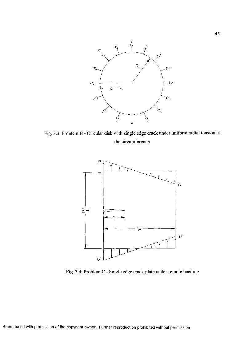
45
Fig. 3.3: Problem B - Circular disk with single edge crack under uniform radial tension at
the circumference
O
2 H
o
o
o
Fig. 3.4: Problem C - Single edge crack plate under remote bending
Reproduced with permission of the copyright owner. Further reproduction prohibited without permission.

46
X2
Xi
Fig. 3.5: A quarter of the Problem A domain being modelled with displacement
constraints on the planes of symmetry (dotted lines)
BoundaryNodes
ContourIntegralPath
Fig. 3.6: A typical BEM mesh showing element size and contour for Problem A; a/R =
0.2, r/a = 0.5
Reproduced with permission of the copyright owner. Further reproduction prohibited without permission.

47
BoundaryNodes
ContourIntegralPath
Fig. 3.7: A typical BEM mesh showing element size and contour for Problem B; a/R =
0.6, r/a = 0.5
Reproduced with permission of the copyright owner. Further reproduction prohibited without permission.
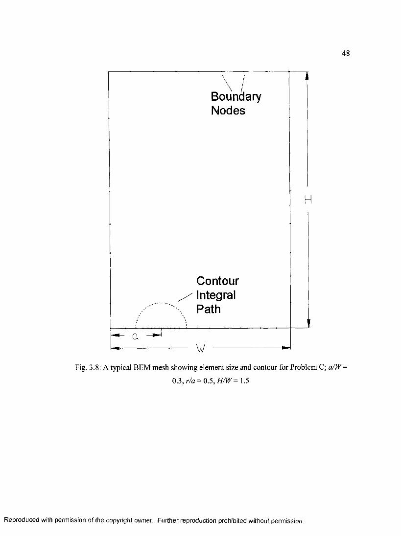
BoundaryNodes
H
ContourIntegralPath
a „ r
w
Fig. 3.8: A typical BEM mesh showing element size and contour for Problem C; a/W
0.3, r/a = 0.5, H/W= 1.5
Reproduced with permission of the copyright owner. Further reproduction prohibited without permission.

49
Problem A: a/R = 0.2 Problem B: a/R = 0.4 —a — Problem C: a/W * 0.6
2.0
& 0.0
-2.0
-3.00.250.200.150.100.050.00
Relative Crack-Tip Element Length (l/a)
Fig. 3.9: Percent discrepancy of stress intensity factor for different relative crack-tip
element length (l/a) between BEM and Fett (2002) for Problem A (a/R = 0.2), Problem B
(a/R = 0.4) and Problem C (a/W= 0.6)
—»— l/a = 0.05 - » - l / a = 0.10 - * - l / a = 0.15 I/a = 0.20 |
0.00
-0.50
- 1.00
•1.50
-2.00
-2.500.60 0.650.40 0.45 0.50 0.550.35
Relative Contour Radius (r/a)
Fig. 3.10: Percent discrepancy of J-stress for different relative crack-tip element length
(l/a) between BEM and Fett (2002) for Problem A (a/R = 0.2)
Reproduced with permission of the copyright owner. Further reproduction prohibited without permission.

50
I/a = 0.15 I/a = 0.20I/a = 0.05 I/a = 0.10
-0.20
-0.25
-0.35
-0.400.650.55 0.600.50 i
Relative Contour Radius (r/a)0.450.35 0.40
Fig. 3.11: Percent discrepancy of T-stress for different relative crack-tip element length
(l/a) between BEM and Fett (2002) for Problem B (a/R = 0.4)
i/a = 0.15 I/a = 0.20
0.20
0.15
0.10
0.05
0.000.35 0.40 0.50 i
Relative Contour Radius (r/a)0.55 0.60 0.650.45
Fig. 3.12: Percent discrepancy of T-stress for different relative crack-tip element length
(l/a) between BEM and Fett (2002) for Problem C (a/W =0.6)
Reproduced with permission of the copyright owner. Further reproduction prohibited without permission.

51
□ Fett (2002) BEM
0.2
0.0
-0.2
-0.4
- 0.6
- 0.80.70.3 0.4
Relative Crack Length (a/R)0.5 0.60.20.0
Fig. 3.13: Variation of normalized 7-stress with relative crack lengths for Problem A
□ Fett (2002) BEM
2.0
- o rC3-c r
0.5
0.00.2 0.3
Relative Crack Length (a/R)
0.70.0 0.4 0.5
Fig. 3.14: Variation of normalized stress intensity factors with relative crack lengths for
Problem A
Reproduced with permission of the copyright owner. Further reproduction prohibited without permission.

52
Xi
Fig. 3.15: The numerical model of one half of the Problem B geometry with displacement
constraints on the plane of symmetry (dotted line)
G Fett (2002) BEM
0.7
0.5
0.40.6 0.70.0 0.1 0.2 0.3
Relative Crack Length {a/R)0.4 0.5
Fig. 3.16: Variation of normalized 7-stress with relative crack lengths for Problem B
Reproduced with permission of the copyright owner. Further reproduction prohibited without permission.

53
□ Fett (2002) BEM2.5
2.0
• c r
■nr3-
1.0
0.5
0.00.6 0.70.3
Relative Crack Length (a/R)0.4 0.50.20.0
Fig. 3.17: Variation of normalized stress intensity factors with relative crack lengths for
Problem B
□ Fett (2002) BEM
1.00
0.75
2 hi
0.25
0.00
-0.25
-0.500.70.0 0.1 0.3 0.4
Relative Crack Length (a/W)0.50.2
Fig. 3.18: Variation of normalized T-stress with relative crack lengths for Problem C
Reproduced with permission of the copyright owner. Further reproduction prohibited without permission.

54
□ Fett (2002) | BEM
2.5
2.0
Q---
2H
0.5
0.00.70.50.3
Relative Crack Length (a/W)0.40.1 0.20.0
Fig. 3.19: Variation of normalized stress intensity factors with relative crack lengths for
Problem C
G
I
-L a
- W -
2H
Ia
Fig. 3.20: Problem D - U-notch cracked plate under remote tension
Reproduced with permission of the copyright owner. Further reproduction prohibited without permission.

55
BoundaryNodes
7 LL
ContourIntegralPath
a
Fig. 3.21: A typical BEM mesh showing element size and contour integral for Problem
D; L/W= 0.3, HZW= 3.0, R/W= 0.025, a/R = 1.0, r/a = 0.5
Reproduced with permission of the copyright owner. Further reproduction prohibited without permission.

56
CDB; i JJE&QOS/S&jeufer* 6 .4 -1 Vs* S u l tX 46:46:59 S«**6£a Jfc«Mlard T4fc« 2 DOS
slop ; St#p~lSaeim a** 1: $t«tp t lx * * 4*603
ODB: job. cdb AEACUS/St«wi*x4 6.4-1 Thu 21 24:45:5$ Xfttttra Staador* f l a t 2005
SncxxaMSK. 1 : S ? « p T ia * * 1 .6 0 0
Fig. 3.22: A typical FEM mesh used by Lewis (2005) for the U-notch geometry
Reproduced with permission of the copyright owner. Further reproduction prohibited without permission.
5250

57
0.00
BEM
□ LEWIS (2005)- 1.00
S -2 00
2 -3.002H
-4.00
-5.000.4 0.6
Relative Crack Length (a/R)0.0 0.2
Fig. 3.23: Variation of normalized F-stress with relative crack lengths for Problem D
O
O
Fig. 3.24: Problem E - Double-cracks emanating from a circular hole in an infinite plate
under remote tension
Reproduced with permission of the copyright owner. Further reproduction prohibited without permission.

58
BoundaryNodes
ContourIntegralPath
ContourIntegralPath
Fig. 3.25: A typical BEM mesh showing element size and contour integral for Problem E;
a/R = 2.0, r/a = 0.5
Reproduced with permission of the copyright owner. Further reproduction prohibited without permission.

59
-0.5
-0.7
-0.8
BEM
□ BROBERG (2004)
4.53.5
Relative Crack Length (a/R)
2.51.5
Fig. 3.26: Variation of normalized F-stress with relative crack lengths for Problem E
3.0
2.5 BEM
□ BOWIE (1956)
2.0
4.52.5 3.5
Relative Crack Length (a/R)
Fig. 3.27: Variation of normalized stress intensity factors with relative crack lengths for
Problem E
Reproduced with permission of the copyright owner. Further reproduction prohibited without permission.

CHAPTER 4 ELASTIC T-STRESS AND STRESS INTENSITYFACTOR SOLUTIONS FOR CRACKS EMANATING FROM CIRCULAR HOLES IN A RECTANGULAR PLATE
4.0 Introduction
This chapter examines the effect of geometry and loading conditions on elastic 7-stress
and stress intensity factors for cracks emanating from the edge of a circular hole in a
rectangular plate. In Chapter 3, the effects of such cracks in an infinite plate were
studied. The evaluation of similar types of geometry will be further investigated. First,
the influence of a crack or cracks emanating from a single circular hole will be analyzed.
The 7-stress and stress intensity factor solutions will then be compared to those obtained
for geometries involving multiple circular holes. Table 4.1 lists the problems analyzed in
this chapter.
60
Reproduced with permission of the copyright owner. Further reproduction prohibited without permission.
61
4.1 T-Stress and Stress Intensity Factor from Crack(s) Emanating
from a Circular Hole
T-stress and stress intensity factor of a crack or cracks emanating from a single circular
hole will be evaluated in this section. First, double-cracks in a finite plate under remote
tension and bending will be discussed. Single-crack configuration for an infinite plate
under remote tension will be studied. The analysis of this crack configuration is then
extended to finite plate under remote tension and bending.
4.1.1 Finite Plate with Double-Cracks Emanating from the Edge of a Circular
Hole under Remote Tension (Problem F)
Two-dimensional BEM was employed to analyze the effects on T-stress and stress
intensity factor of double-cracks emanating from a circular hole in a finite plate under
remote tension. The geometry of the problem is defined by the plate width 2 W, plate
height 2H, and hole radius R, as shown in Fig. 4.1. Similar to Problem E in the previous
chapter, the domain needed to be analyzed can be reduced to a quarter of its physical
domain, due to symmetry, as shown in Fig. 4.2. Figure 4.3 shows the BEM mesh used
for analysis. The stress intensity factor and T-stress solutions for the relative hole radius
R/W of 0.25 and 0.50 and relative height-to-width ratio (H/W) of 2 was analyzed.
Relative crack lengths a/R of 1.1, 1.2, 1.6, 2, 2.4, 2.8, 3.2 were analyzed for the R/W =
0.25 case, and a/R of 1.1-1.6 for the R/W= 0.50 case.
Reproduced with permission of the copyright owner. Further reproduction prohibited without permission.

62
Tables 4.2 and 4.3 show the results for the normalized T-stress T/a and stress
intensity factor K , I a ^ 7i{ a -K ) for R/W = 0.25 and R/W = 0.50, respectively. The
normalized stress intensity factor solutions obtained are compared to those by Newman
(1971); generally very good agreement of less than 2% discrepancy was achieved
between the two sets of results for both R/W cases. The results were also shown
graphically in Fig. 4.4 and 4.5 for T/a and K ; / cr^7t(a - R ) , respectively. It can be seen
in Fig. 4.4 that the normalized T-stress results for all cases are negative, thus indicating
low constraint conditions. Higher T-stress gradient was noticed as R/W increases,
illustrating the significant influence of the finite boundary. The presence of the circular
hole was also noticed from the dramatic incline for small cracks, and decline for larger
cracks. With small cracks, the stress distribution in the vicinity of the hole is
significantly altered due to the presence of the hole. As the crack becomes longer, there
is less influence from the circular hole, which explains the declining trend in the larger
cracks region. Furthermore, it is evident that a finite boundary causes the T-stress to
continually decrease, while the infinite boundary case shows an asymptotic trend that
levels off for increasing crack lengths.
The effect of changing the height-to-width ratio H/W was also studied. The
height-to-width ratio of 2.5 and 3 were tested as well. The normalized stress intensity
factor and 7-stress solutions are listed in Tables 4.4 and 4.5, and shown graphically in
Fig. 4.6 - 4.9. It is evident that all stress intensity factor and T-stress values remained
almost constant for the three height-to-width ratios. This suggests that any testing of this
type of geometry need not exceed a height-to-width ratio of 2.
Reproduced with permission of the copyright owner. Further reproduction prohibited without permission.

63
4.1.2 Finite Plate with Double-Cracks Emanating from the Edge of a Circular
Hole under Remote Bending (Problem G)
The geometry of double-cracks emanating from a circular hole under remote bending
problem is identical to that of Problem F, with only a change in the loading conditions, as
shown in Fig. 4.10. The numerical analysis can be reduced to half of its physical domain,
as shown in Fig. 4.11. A nodal constraint in the xy-direction is again required to preclude
rigid body motion. Figure 4.12 shows typical BEM mesh used for analysis. Note that
two different contours are required to evaluate the two crack-tips, although the primary
focus will be the results from the tension side of the plate under the bending load. For
comparison with the tension problem, relative crack lengths a/R of 1.1, 1.2, 1.6, 2, 2.4,
2.8, 3.2 for the relative hole radius R/W= 0.25 case, and a/R of 1.1-1.6 for the R/W= 0.50
case were again analyzed.
The normalized stress intensity factor and T-stress solutions are presented in
Tables 4.6 and 4.7 for R/W= 0.25 and 0.50, respectively. Figures 4.13 and 4.14 compare
the remote bending and remote tension solutions for T-stress and Kj, respectively. It is
evident that the bending load has resulted in smaller magnitude than the tension case for
both the normalized Ki and T-stress, due to the compression portion of the applied load.
The variation of the bending solution with a/R is also noticed to be more gradual,
especially for small cracks where more rapid changes in Ki and T-stress are present for
the remote tension problem. As before, all normalized T-stress solutions obtained are
negative in magnitude.
Reproduced with permission of the copyright owner. Further reproduction prohibited without permission.

64
4.1.3 Infinite Plate with a Single Crack Emanating from the Edge of a Circular
Hole under Remote Tension (Problem H)
The problem with a single crack emanating from a circular hole in an infinite plate (Fig.
4.15) was analyzed using two-dimensional BEM. The numerical domain of this problem
can be reduced to half of its physical domain, due to symmetry. Figure 4.16 shows a
typical BEM mesh for this problem; as before in Problem E, the boundaries of the
numerical domain is set at 20 times the crack length. The boundary conditions of this
problem are applied in the same manner as for Problem C, with the plane of symmetry
constrained in the ^-direction, and a nodal constraint in the x/-direction to preclude rigid
body motion. Relative crack lengths a/R of 1.1 - 4.0 were analyzed.
The normalized stress intensity factor, K, / (T^7i(a - K) , and T-stress, T/a,
solutions are listed in Table 4.8 and illustrated in Fig. 4.17 and 4.18. Very good
agreement of generally less than 3% discrepancy was achieved for Kj between the results
obtained from BEM and those by Newman (1971). It is shown in Fig. 4.17 that the
normalized T-stress has the same trends as the double-crack case (Problem E) and is
negative in magnitude. Lower constraint at the crack-tip is therefore implied from the T-
stress obtained. It is observed that the J-stress for the single crack case peaks at a higher
value and has a steeper decline than the corresponding double-crack case. Since the T-
stress solutions for both the single and double crack problems are similar, it is evident
that, for rough approximation, evaluation of T-stress is only necessary to be performed
once.
Reproduced with permission of the copyright owner. Further reproduction prohibited without permission.
65
4.1.4 Finite Plate with a Single Crack Emanating from the Edge of a Circular
Hole under Remote Tension (Problem I)
For the finite plate with a single crack emanating from a circular hole problem, as shown
in Fig. 4.19, symmetry can again be used for BEM analysis, and only half of the domain
needs to be modelled. Figure 4.20 shows the typical BEM mesh used for this geometry.
The boundary conditions used for this problem are identical to those applied for Problem
H. Relative crack lengths a/R of 1.1, 1.2, 1.6, 2, 2.4, 2.8, 3.2 were analyzed for the
relative hole radius R/W = 0.25 case, and a/R of 1.1-1.6 for the R/W = 0.50 case (these
ratios are identical to Problem F for comparison purposes).
Tables 4.9 and 4.10 show the normalized stress intensity factor K { / a ^ n { a - R )
and T’-stress T/a solutions for the two different hole radii cases. Figures 4.21 and 4.22
compare the normalized T-stress and stress intensity factor results, respectively, with the
infinite plate case (Problem H). It can be seen that the normalized T-stress solutions
exhibit a peak value, then declines as a/R is increased for all R/W cases. The case with
the largest circular hole, i.e. R/W = 0.50, exhibits a significantly more severe variation
than the other two. As for Kj, it is evident that the infinite plate problem has the lowest
magnitude, while the presence of the finite boundary increased the crack-tip stress
intensity factor for the other two cases.
From the results obtained from BEM analysis, it was found that the normalized
stress intensity factor and T-stress trends were similar for both finite plate problems with
single and double-cracks. Tables 4.11 and 4.12 compare the two sets of data, and Fig.
4.23 and 4.24 illustrate them graphically. It is evident that the difference between the
Reproduced with permission of the copyright owner. Further reproduction prohibited without permission.

66
single and double-crack cases increases significantly as a/R increases for the normalized
stress intensity factor for both R/W ratios. This was expected as the asymmetry of the
single crack problem reduces the nominal net-section stress at the plane of the crack,
resulting in a much lower stress intensity factor. The cause for the increase in difference
between the two crack configurations as a/R increases stems from the fact that the
geometry becomes increasingly asymmetric, which enlarges the reduction in the
magnitude of the nominal net-section stress. The asymmetry aspect also holds true for
the normalized T-stress, as the difference between single and double-crack increases with
a/R. It should be noted that the percentage difference for Kj is higher than that for 77a,
especially for large a/R ratios, which implies that the stress intensity factor is much more
sensitive to geometric asymmetry than the 7’-stress. Figure 4.23 more clearly illustrates
this fact as the single and double crack configuration values remain close to each other,
and diverges slightly as a/R is increased. The implication here is that for small crack
lengths, analysis for T'-stress is only necessary on either the single or double-crack
geometry, with the results being fairly accurate for both configurations. Again, similar to
previous geometries tested, the normalized T’-stress solutions are negative in magnitude.
4.1.5 Finite Plate with a Single Crack Emanating from the Edge of a Circular
Hole under Remote Bending (Problem J)
This problem has the exact geometry of Problem G, only with a single crack instead of
two, as shown in Fig. 4.25. BEM analysis was performed by modelling half of the
physical domain, as shown in Fig. 4.26, with the boundary conditions similar to that of
Reproduced with permission of the copyright owner. Further reproduction prohibited without permission.
67
Problem H. The same relative crack lengths a/R of 1.1, 1.2, 1.6, 2, 2.4, 2.8, 3.2 were
analyzed for the relative hole radius R/W = 0.25 case, and a/R of 1.1-1.6 for the R/W =
0.50 case.
The solutions for normalized stress intensity factor and T-stress are presented in
Tables 4.13 and 4.14, and are compared to those of the double-crack case. Figures 4.27
and 4.28 graphically illustrate the T-stress and stress intensity factor results, respectively.
It is evident that both the Kj and T-stress solutions for the single crack case followed the
same trend as the double-crack case. The stress intensity factor solutions can be observed
to diverge between the two crack configurations for longer crack lengths (up to 14.5%
difference). On the other hand, the T-stress solutions showed that it is less sensitive to
the crack configuration, even for longer cracks. As shown in Table 4.13, a difference of
only 4.7% exists between the single and double-crack problem for the longest crack
analyzed, i.e. a/R = 3.2.
4.2 Influence of Adjacent Holes on J-Stress and Stress Intensity
Factor
T-stress and stress intensity factor solutions will be presented for geometries that have
multiple holes in this section. The solutions obtained will also be compared to those of
the single-hole geometry. The geometries considered include: double and single crack
emanating from a periodic array of holes in an infinite plate under remote tension, and the
influence of adjacent holes not in the plane of the crack on double-cracks emanating from
a circular hole in an infinite plate under remote tension.
Reproduced with permission of the copyright owner. Further reproduction prohibited without permission.

68
4.2.1 Infinite Plate with Double-Cracks Emanating from a Periodic Array of
Holes under Remote Tension (Problem K)
The problem of periodic array of holes with double-cracks (Fig. 4.29) is essentially an
infinite array of the Problem F geometry. A section of the physical domain was modelled
with the same boundary conditions as Problem F, with the addition of an ^/-direction
constraint on the extra plane of symmetry, as shown in Fig. 4.30. Figure 4.31 shows a
typical BEM mesh for the problem at hand. Relative height-to-width ratio H/W of 2 was
used as the domain geometry, since it was established in Section 4.1.1 that greater H/W
values yielded the same results. The relative crack lengths a/R and hole radius R/W
considered are identical to those of Problem F, namely, a/R of 1.1, 1.2, 1.6, 2, 2.4, 2.8,
3.2 for the R/W= 0.25 case, and a/R of 1.1-1.6 for the R/W= 0.50 case.
The numerical results for the stress intensity factor and 7-stress are listed in
Tables 4.15 and 4.16. Compared to the corresponding solutions for the finite plate
problem (Problem F) in Fig. 4.32 and 4.33, it can be seen that Kj is significantly reduced
for the infinite array case, especially for the R/W - 0.50 case. The normalized 7-stress
solutions decreased very gradually for increasing a/R values (when the uncracked portion
of the plate become small), in contrast to the declining behaviour in 7-stress for the finite
plate case. As explained in Section 4.1.1, the 7-stress declines for the finite plate as the
effect from the presence of the hole is reduced when the crack grows longer. This effect
is negated as an infinite array creates extra constraint between the holes, which explains
the large deviation between the two sets of data.
Reproduced with permission of the copyright owner. Further reproduction prohibited without permission.

69
4.2.2 Infinite Plate with a Single Crack Emanating from a Periodic Array of
Holes under Remote Tension (Problem L)
The geometry of Problem L is composed of an infinite array of the Problem I geometry,
as shown in Fig. 4.34. The numerical modelling of this geometry is only necessary on a
small section of physical domain, as shown in Fig. 4.35. The height-to-width ratio H /W
is again taken to be 2 for convenience. Figure 4.35 also shows the boundary conditions
of the BEM mesh, where the two vertical boundaries are constrained in the x/-direction to
represent the infinite array. A typical BEM mesh for this problem is shown in Fig. 4.36.
The normalized solutions for stress intensity factor and T-stress are given in
Tables 4.17 and 4.18. Figures 4.37 and 4.38 compare these results to those of the finite
plate problem (Problem H). It is evident that the trends follow those described in Section
4.2.1, where the stress intensity factor is substantially reduced and the T-stress declines at
a gradual pace for increasing crack lengths. The numerically determined results are also
compared against the infinite array with double-crack case (Problem K), as shown in Fig.
4.39 and 4.40. It can be seen that the Kr solutions of the two crack configurations
diverged substantially as a/R increased, while the T-stress solutions exhibited only small
changes. For both R/W cases the T-stress solutions begin to diverge only when a/R > 1.5,
suggesting that for small relative crack lengths, the T-stress for one crack configuration is
also accurate for the other.
Reproduced with permission of the copyright owner. Further reproduction prohibited without permission.

70
4.2.3 Infinite Plate with Double-Cracks Emanating from the Edge of a Circular
Hole Influence by Adjacent Holes under Remote Tension (Problem M)
The effects of adjacent holes not in the plane of the crack on double-cracks emanating
from a circular hole are studied in this section. The geometry of the problem is shown in
Fig. 4.41, with hole radius Ri, adjacent hole radius R2, hole-distance d, and crack length
a. Only a quarter of the physical domain needs to be modelled, by virtue of symmetry.
Figure 4.42 shows the boundary conditions applied and Fig. 4.43 shows a typical BEM
mesh used for analysis. Relative crack lengths a/Rj of 1.1, 1.2, 1.4, 1.6, 2, 3, 4, and 10
was analyzed for relative hole-distance d* of 2.5, 4, 5, 10 and radius ratio a of 0 - 1.0,
where d* = d/Rj and a = R2/R1.
The BEM results for normalized stress intensity factor K f / <r^7c (a - i?j) and T-
stress T/a are shown in Tables 4.19 - 4.22. The results are also shown graphically for the
different radius ratios a in Fig. 4.44 - 4.51. It can be seen that for a = 0.25, only very
small deviations for both T-stress and Ki solutions exist from the case with no adjacent
holes (R.2 = 0), for all d* ratios. This is especially true for a/Ri < 3, as the numerical
values of both T-stress and K[ for all d* ratios are, for all practical purposes, identical.
For larger a values, it is evident that the relative hole-distance d* contributes significantly
for both T-stress and Ki. The effects can be easily noticed in Fig. 4.50 for T-stress and
Fig. 4.51 for Kj, where the solutions for a = 1.0 are significantly affected. The
normalized stress intensity factor decreased significantly as d* decreased, illustrating the
effects as the adjacent holes move closer to the central-hole. The normalized T-stress
Reproduced with permission of the copyright owner. Further reproduction prohibited without permission.

71
solutions showed that as d* was reduced, the peak of the curve also decreased, while
exhibiting a more gradual trend.
To understand the effects of the radius ratio a, the 7-stress and Kj were again
plotted for a specific d* value, as shown in Fig. 4.52 - 4.59. It is clear that the effect for
increasing the size of the adjacent holes is similar to that of decreasing the distance
between the holes. It is evident that for very short cracks, i.e. a/Ri < 1.4, enlarging the
adjacent holes results in corresponding decreases in magnitude in Kj from the a = 0 case.
Figures 4.52 and 4.53 best illustrate this behaviour due to the close proximity of the
adjacent holes. It is indicated that the magnitude of the 7-stress is also reduced, but
remains negative. For cracks in the range of 1.4 < a/Ri < 4, it is evident that the
introduction for adjacent holes decreased both the 7-stress and K/. The implication of
this is that by having adjacent holes near a circular hole with small double-cracks, the
crack-tip constraint can be substantially reduced, if this is permitted.
It can be observed that for longer crack lengths, such as when a/Rj > 4, the effects
of the adjacent holes are minimal as the solution for all a values converged. This implies
that for large cracks, the presence of adjacent holes is not very significant for 7-stress and
K, analysis. Furthermore, it can be seen that for adjacent holes located far from the
central-hole (Fig. 4.58 and 4.59), the deviations between the different a values are small.
This suggests that for relative hole-distance d* > 10, the problem can be simplified to that
of the infinite plate problem with only one circular hole (Problem E).
Reproduced with permission of the copyright owner. Further reproduction prohibited without permission.

72
4.3 Summary
Elastic 7-stress and stress intensity factor solutions for cracked plates involving circular
holes were determined in this chapter. For all geometries and loading conditions, it was
observed that for cracks emanating from circular holes, the 7-stress first becomes less
negative over relatively small increases in crack length. Beyond a certain relative crack
length, the decrease in constraint (i.e. 7-stress become more negative in magnitude)
begins to occur. Of significance to note is that for all the geometries and loading
conditions analyzed, the 7-stress obtained is negative in value. Low crack-tip constraint
is therefore indicated, implying that the stress field characterized solely by the stress
intensity factor may b e overly conservative. From the present work, the following
observations can also be made:
• The presence of a finite boundary further accentuates the rate of change of the above
described behaviour, as expected.
• The stress intensity factors obtained for remote bending loads were determined to be
significantly less than those for remote tension loads.
• Comparisons between single and double crack configurations indicated that the 7-
stress solutions only diverged beyond a relatively large crack size for remote tension
loaded problems.
• The problem with an infinite array of holes indicated that the 7-stress declines more
gradually for increasing crack lengths, as compared to the steeper declining behaviour
for the single-hole problem.
Reproduced with permission of the copyright owner. Further reproduction prohibited without permission.

73
• The influence of adjacent holes not in the plane of the crack in an infinite plate was
also studied. Both the adjacent hole-radius and the distance between holes were
shown to have an effect on both the 7-stress and stress intensity factor. Increasing the
adjacent hole-radius significantly reduces the stress intensity factor, while generating
gentler gradients in the 7-stress behaviour. By locating the adjacent holes closer to
the central-hole, the maximum value of the 7-stress decreases and the stress intensity
factor is also reduced. Moreover, the introduction of adjacent holes far from the
centrally-cracked hole has little effect on both the 7-stress and the stress intensity
factor.
Reproduced with permission of the copyright owner. Further reproduction prohibited without permission.

74
Table 4.1: List of problems analyzed in Chapter 4
Problem Definition Figure #
F Finite Plate with Double-Cracks Emanating from the Edge of a Circular Hole Under Remote Tension
4.1
G Finite Plate with Double-Cracks Emanating from the Edge of a Circular Hole Under Remote Bending
4.10
H Infinite Plate with a Single Crack Emanating from the Edge of a Circular Hole Under Remote Tension
4.15
1 Finite Plate with a Single Crack Emanating from the Edge of a Circular Hole Under Remote Tension
4.19
J Finite Plate with a Single Crack Emanating from the Edge of a Circular Hole Under Remote Bending
4.25
K Infinite Plate with Double-Cracks Emanating from a Periodic Array of Holes Under Remote Tension
4.29
L Infinite Plate with a Single Crack Emanating from a Periodic Array of Holes Under Remote Tension
4.34
M Infinite Plate with Double-Cracks Emanating from the Edge of a Circular Hole Influence by Adjacent Holes Under Remote Tension
4.41
Reproduced with permission of the copyright owner. Further reproduction prohibited without permission.
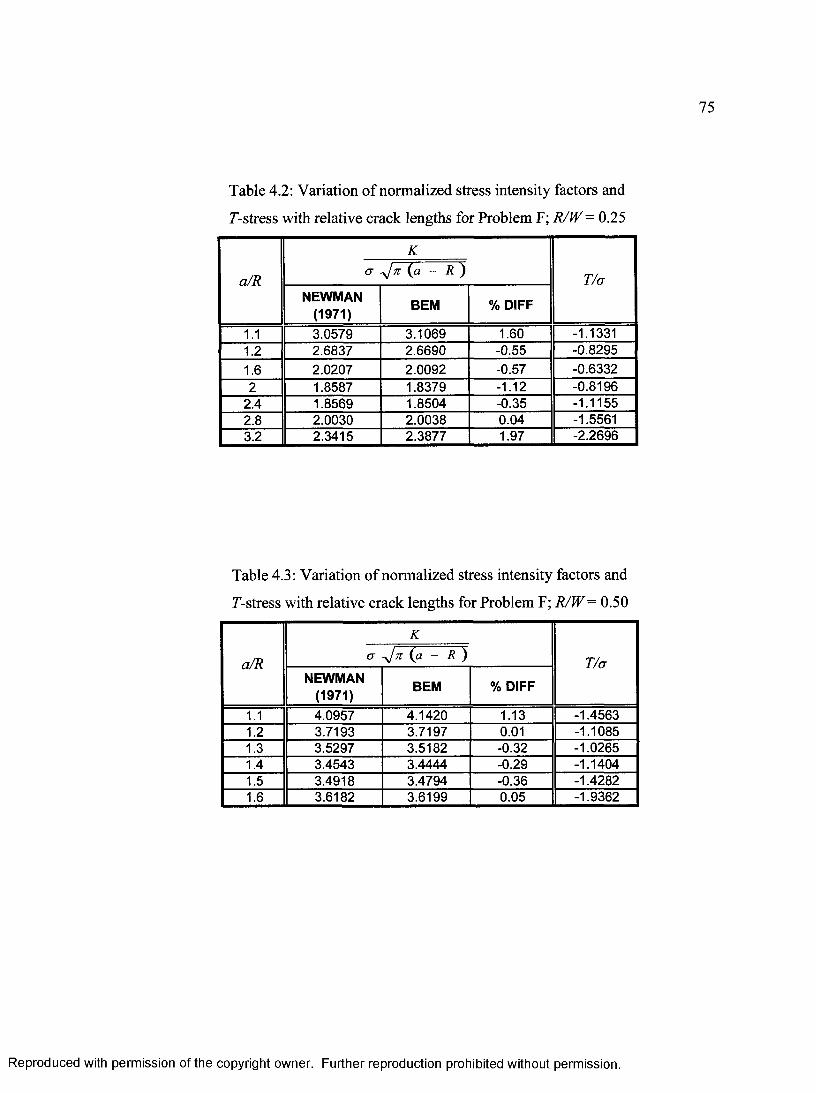
75
Table 4.2: Variation of normalized stress intensity factors and
T-stress with relative crack lengths for Problem F; R/W = 0.25
a/Ra
Kyjx (a - R )
T/aNEWMAN
(1971)BEM % DIFF
1.1 3.0579 3.1069 1.60 -1.13311.2 2.6837 2.6690 -0.55 -0.82951.6 2.0207 2.0092 -0.57 -0.63322 1.8587 1.8379 -1.12 -0.8196
2.4 1.8569 1.8504 -0.35 -1.11552.8 2.0030 2.0038 0.04 -1.55613.2 2.3415 2.3877 1.97 -2.2696
Table 4.3: Variation of normalized stress intensity factors and
T-stress with relative crack lengths for Problem F; R/W = 0.50
a/R aK
Ajn (a - R ) T/aNEWMAN
(1971)BEM % DIFF
1.1 4.0957 4.1420 1.13 -1.45631.2 3.7193 3.7197 0.01 -1.10851.3 3.5297 3.5182 -0.32 -1.02651.4 3.4543 3.4444 -0.29 -1.14041.5 3.4918 3.4794 -0.36 -1.42821.6 3.6182 3.6199 0.05 -1.9362
Reproduced with permission of the copyright owner. Further reproduction prohibited without permission.

76
Table 4.4: Effect of height-to-width ratio (H/W) on stress intensity factor and T-
stress for Problem F; R/W= 0.25
a/RK
T/au -Jn (a - R )
H/W = 2.0 H/W = 2.5 H/W = 3.0 H/W = 2.0 H/W = 2.5 H/W = 3.01.1 3.1069 3.1025 3.1002 -1.1331 -1.1329 -1.13261.2 2.6690 2.6648 2.6643 -0.8359 -0.8351 -0.83511.6 2.0092 2.0053 2.0052 -0.6359 -0.6357 -0.63592.0 1.8379 1.8342 1.8342 -0.8345 -0.8347 -0.83522.4 1.8504 1.8472 1.8472 -1.1397 -1.1406 -1.14172.8 2.0038 1.9888 1.9893 -1.5832 -1.5923 -1.59583.2 2.3877 2.3167 2.3165 -2.3658 -2.4279 -2.4273
Table 4.5: Effect of height-to-width ratio (H/W) on stress intensity factor and T-
stress for Problem F; R/W = 0.50
a/RK
T/aa ^Jn(a - R )
H/W = 2.0 H/W = 2.5 H/W = 3.0 H/W = 2.0 H/W = 2.5 H/W = 3.01.1 4.1420 4.1205 4.1194 -1.4563 -1.4532 -1.45291.2 3.7197 3.7006 3.6995 -1.1085 -1.1069 -1.10681.3 3.5182 3.5009 3.5000 -1.0265 -1.0295 -1.02961.4 3.4444 3.4287 3.4278 -1.1404 -1.1483 -1.14861.5 3.4794 3.4659 3.4652 -1.4282 -1.4443 -1.44461.6 3.6199 3.6065 3.6058 -1.9362 -1.9484 -1.9488
Reproduced with permission of the copyright owner. Further reproduction prohibited without permission.

77
Table 4.6: Variation of normalized stress intensity
factors and T-stress with relative crack lengths for
Problem G; R/W= 0.25
a/RK
T/a<T^x{a - R)
1.1 0.5026 -0.21331.2 0.4307 -0.18351.6 0.3678 -0.28952.0 0.3867 -0.43842.4 0.4366 -0.59582.8 0.5143 -0.78923.2 0.6432 -1.0964
Table 4.7: Variation of normalized stress intensity
factors and T-stress with relative crack lengths for
Problem G; R/W= 0.50
a/RK
T/ai
S'b
1.1 1.0622 -0.42911.2 0.9644 -0.40451.3 0.9187 -0.46021.4 0.9074 -0.56881.5 0.9278 -0.72471.6 0.9816 -0.9414
Reproduced with permission of the copyright owner. Further reproduction prohibited without permission.

78
Table 4.8: Variations of normalized stress intensity factors and
T-stress with relative crack lengths for Problem H
a/Ro
K
- r ) T/aNEWMAN
(1971)BEM % DIFF
1.1 2.7900 2.8707 2.89 -1.05731.2 2.3528 2.4160 2.69 -0.75871.4 1.8779 1.9201 2.25 -0.55021.6 1.6357 1.6372 0.09 -0.53031.8 1.4758 1.4584 -1.18 -0.56642.0 1.3667 1.3362 -2.23 -0.61642.2 1.2811 1.2495 -2.47 -0.66642.4 1.2175 1.1837 -2.77 -0.71172.6 1.1611 1.1339 -2.34 -0.75142.8 1.1141 1.0942 -1.79 -0.78574.0 0.9430 0.9666 2.50 -0.9152
Table 4.9: Variation of normalized stress
intensity factors and T-stress with relative
crack lengths for Problem I; RJW = 0.25
a/RK
T/a<7 (a - R )
1.1 3.0719 -1.12981.2 2.6082 -0.81261.6 1.8077 -0.61262.0 1.5300 -0.79502.4 1.4350 -1.04322.8 1.4505 -1.37763.2 1.5928 -1.9479
Reproduced with permission of the copyright owner. Further reproduction prohibited without permission.
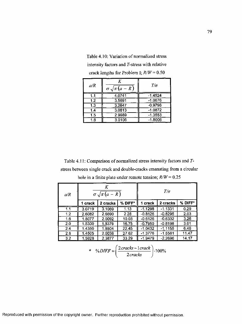
79
Table 4.10: Variation of normalized stress
intensity factors and T-stress with relative
crack lengths for Problem I; RJW— 0.50
a/RK
T/a(T-yJn:{a - R )
1.1 4.0741 -1.45241.2 3.5691 -1.06761.3 3.2647 -0.97981.4 3.0813 -1.08721.5 2.9989 -1.35531.6 3.0106 -1.8006
Table 4.11: Comparison of normalized stress intensity factors and T-
stress between single crack and double-cracks emanating from a circular
hole in a finite plate under remote tension; R/W= 0.25
a/R
KT/aIfc:
Sb
1 crack 2 cracks % DIFF* 1 crack 2 cracks % DIFF*1.1 3.0719 3.1069 1.13 -1.1298 -1.1331 0.291.2 2.6082 2.6690 2.28 -0.8126 -0.8295 2.031.6 1.8077 2.0092 10.03 -0.6126 -0.6332 3.262.0 1.5300 1.8379 16.75 -0.7950 -0.8196 3.012.4 1.4350 1.8504 22.45 -1.0432 -1.1155 6.482.8 1.4505 2.0038 27.62 -1.3776 -1.5561 11.473.2 1.5928 2.3877 33.29 -1.9479 -2.2696 14.17
* %DIFF =f 2 cracks -1 crack ̂
2 cracks• 100%
Reproduced with permission of the copyright owner. Further reproduction prohibited without permission.

80
Table 4.12: Comparison of normalized stress intensity factors and T-
stress between single crack and double-cracks emanating from a circular
hole in a finite plate under remote tension; R/W= 0.50
a/R
Kc ra n ia - R )
T/a
1 crack 2 cracks % DIFF* 1 crack 2 cracks % DIFF*
1.1 4.0741 4.1420 1.64 -1.4524 -1.4563 0.271.2 3.5691 3.7197 4.05 -1.0676 -1.1085 3.691.3 3.2647 3.5182 7.21 -0.9798 -1.0265 4.551.4 3.0813 3.4444 10.54 -1.0872 -1.1404 4.671.5 2.9989 3.4794 13.81 -1.3553 -1.4282 5.101.6 3.0106 3.6199 16.83 -1.8006 -1.9362 7.00
* Vo DIFF =r 2 cracks -1 crack ̂
2 cracks• 100%
Table 4.13: Comparison of normalized stress intensity factors and T-stress
between single crack and double-cracks emanating from a circular hole in
a finite plate under remote bending; R/W= 0.25
a/R
KT/aa -^7t (a - R )
1 crack 2 cracks % DIFF* 1 crack 2 cracks % DIFF*
1.1 0.5055 0.5026 -0.57 -0.2141 -0.2133 -0.351.2 0.4398 0.4307 -2.12 -0.1860 -0.1835 -1.361.6 0.3980 0.3678 -8.24 -0.2930 -0.2895 -1.212.0 0.4325 0.3867 -11.82 -0.4443 -0.4384 -1.352.4 0.4964 0.4366 -13.71 -0.6093 -0.5958 -2.272.8 0.5889 0.5143 -14.52 -0.8167 -0.7892 -3.483.2 0.7346 0.6432 -14.22 -1.1474 -1.0964 -4.65
* %DIFF = r 2 cracks -1 crack ̂2 cracks
• 100%
Reproduced with permission of the copyright owner. Further reproduction prohibited without permission.
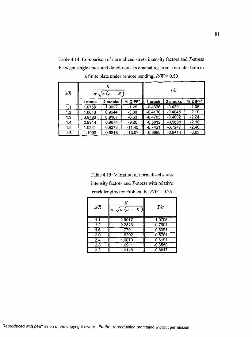
81
Table 4.14: Comparison of normalized stress intensity factors and T-stress
between single crack and double-cracks emanating from a circular hole in
a finite plate under remote bending; RJW - 0.50
a/RK
T/a<j {a - Z? )
1 crack 2 cracks % DIFF* 1 crack 2 cracks % DIFF*1.1 1.0756 1.0622 -1.26 -0.4336 -0.4291 -1.051.2 1.0010 0.9644 -3.80 -0.4130 -0.4045 -2.101.3 0.9796 0.9187 -6.63 -0.4705 -0.4602 -2.241.4 0.9914 0.9074 -9.26 -0.5812 -0.5688 -2.181.5 1.0341 0.9278 -11.45 -0.7421 -0.7247 -2.401.6 1.1099 0.9816 -13.07 -0.9699 -0.9414 -3.03
Table 4.15: Variation of normalized stress
intensity factors and T-stress with relative
crack lengths for Problem K; RJW - 0.25
a/RK
T/aa s jn (a - R )
1.1 2.9017 -1.07081.2 2.2813 -0.78911.6 1.7701 -0.53912.0 1.6202 -0.57042.4 1.6079 -0.61912.8 1.6911 -0.65503.2 1.9118 -0.6817
Reproduced with permission of the copyright owner. Further reproduction prohibited without permission.

82
Table 4.16: Variation of normalized stress
intensity factors and T-stress with relative
crack lengths for Problem K; RJW = 0.50
a/RK
T/aa -yjn (a - R )
1.1 2.9989 -1.16701.2 2.6980 -0.92531.3 2.5386 -0.78751.4 2.4696 -0.70841.5 2.4822 -0.66211.6 2.5760 -0.6331
Table 4.17: Variation of normalized stress
intensity factors and T-stress with relative
crack lengths for Problem L; R/W= 0.25
a/RK
T/aa -yj7t (a - R )
1.1 2.8724 -1.07061.2 2.2414 -0.77031.6 1.6261 -0.53202.0 1.3926 -0.59182.4 1.2918 -0.66852.8 1.2633 -0.73313.2 1.3042 -0.7909
Reproduced with permission of the copyright owner. Further reproduction prohibited without permission.

83
Table 4.18: Variation of normalized stress
intensity factors and 7-stress with relative
crack lengths for Problem L; R/W= 0.50
a/RK
T/al
>b
1.1 2.9680 -1.16471.2 2.6286 -0.89571.3 2.4138 -0.74961.4 2.2767 -0.66671.5 2.2044 -0.61801.6 2.1897 -0.5900
Table 4.19: Variation of normalized stress intensity factors and 7-stress with relative
crack lengths and radius ratios a = R2/R1 for Problem M; d* = d/Rj = 2.5
a/R ;K, / a^n(a - Rx) T/a
a=0 a=0.25 a=0.50 a=0.75 CF1.0 a=0 a=0.25 a=0.50 a=0.75 a=1.0
1.1 2.8396 2.8362 2.7081 2.4700 2.0694 -1.0471 -1.0512 -1.0051 -0.9204 -0.7788
1.2 2.4463 2.4229 2.3168 2.1258 1.8258 -0.7951 -0.7635 -0.7389 -0.6945 -0.6204
1.4 N/A 1.9840 1.9160 1.7882 1.5749 N/A -0.5678 -0.5759 -0.5866 -0.5878
1.6 1.7555 1.7352 1.6811 1.5963 1.4634 -0.5319 -0.5369 -0.5562 -0.5851 -0.6177
2.0 1.5011 1.4892 1.4718 1.4249 1.3605 -0.6037 -0.6018 -0.6251 -0.6621 -0.7066
3.0 1.2803 1.2955 1.2941 1.2905 1.2844 -0.7776 -0.7859 -0.7942 -0.8078 -0.8241
4.0 1.2103 1.2357 1.2372 1.2400 1.2453 -0.8809 -0.8905 -0.8902 -0.8890 -0.8835
10.0 1.0827 1.1129 1.1137 1.1157 1.1181 -0.9901 -1.0067 -1.0010 -0.9904 -0.9722
Reproduced with permission of the copyright owner. Further reproduction prohibited without permission.
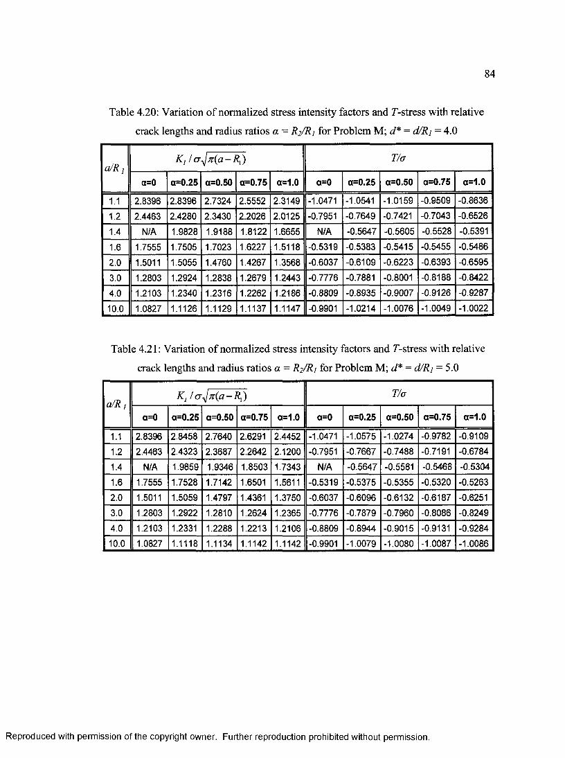
84
Table 4.20: Variation of normalized stress intensity factors and T-stress with relative
crack lengths and radius ratios a - R2/R 1 for Problem M; d* = d/R] = 4.0
a/R 1Kj / cr^j7r(a- R{) T/a
a=0 a=0.25 a=0.50 a=0.75 a=1.0 cfO a=0.25 a=0.50 a=0.75 a=1.0
1.1 2.8396 2.8396 2.7324 2.5552 2.3149 -1.0471 -1.0541 -1.0159 -0.9509 -0.8636
1.2 2.4463 2.4280 2.3430 2.2026 2.0125 -0.7951 -0.7649 -0.7421 -0.7043 -0.6526
1.4 N/A 1.9828 1.9188 1.8122 1.6655 N/A -0.5647 -0.5605 -0.5528 -0.5391
1.6 1.7555 1.7505 1.7023 1.6227 1.5118 -0.5319 -0.5383 -0.5415 -0.5455 -0.5486
2.0 1.5011 1.5055 1.4760 1.4267 1.3568 -0.6037 -0.6109 -0.6223 -0.6393 -0.6595
3.0 1.2803 1.2924 1.2838 1.2679 1.2443 -0.7776 -0.7881 -0.8001 -0.8188 -0.8422
4.0 1.2103 1.2340 1.2316 1.2262 1.2186 -0.8809 -0.8935 -0.9007 -0.9126 -0.9287
10.0 1.0827 1.1126 1.1129 1.1137 1.1147 -0.9901 -1.0214 -1.0076 -1.0049 -1.0022
Table 4.21: Variation of normalized stress intensity factors and T-stress with relative
crack lengths and radius ratios a = R2/R1 for Problem M; d* = d/Rj = 5.0
a/R 1K j! <j^7t(a-Rx) T/a
a=0 a=0.25 a=0.50 a=0.75 a=1.0 a=0 a=0.25 a=0.50 a=0.75 a=1.0
1.1 2.8396 2.8458 2.7640 2.6291 2.4452 -1.0471 -1.0575 -1.0274 -0.9782 -0.9109
1.2 2.4463 2.4323 2.3687 2.2642 2.1200 -0.7951 -0.7667 -0.7488 -0.7191 -0.6784
1.4 N/A 1.9859 1.9346 1.8503 1.7343 N/A -0.5647 -0.5581 -0.5468 -0.5304
1.6 1.7555 1.7528 1.7142 1.6501 1.5611 -0.5319 -0.5375 -0.5355 -0.5320 -0.5263
2.0 1.5011 1.5059 1.4797 1.4361 1.3750 -0.6037 -0.6096 -0.6132 -0.6187 -0.6251
3.0 1.2803 1.2922 1.2810 1.2624 1.2365 -0.7776 -0.7879 -0.7960 -0.8086 -0.8249
4.0 1.2103 1.2331 1.2288 1.2213 1.2106 -0.8809 -0.8944 -0.9015 -0.9131 -0.9284
10.0 1.0827 1.1118 1.1134 1.1142 1.1142 -0.9901 -1.0079 -1.0080 -1.0087 -1.0086
Reproduced with permission of the copyright owner. Further reproduction prohibited without permission.

85
Table 4.22: Variation of normalized stress intensity factors and T-stress with relative
crack lengths and radius ratios a = R2/R1 for Problem M; d* = d/Ri = 10.0
a/R ]K j! a^7t{a-R x) T/a
a=0 a=0.25 a=0.50 a=0.75 CF1.0 a=0 a=0.25 a=0.50 a=0.75 a=1.0
1.1 2.8396 2.8508 2.8229 2.7655 2.7104 -1.0471 -1.0577 -1.0479 -1.0421 -1.0117
1.2 2.4463 2.4352 2.4147 2.3690 2.3284 -0.7951 -0.7655 -0.7597 -0.7582 -0.7379
1.4 N/A 1.9827 1.9644 1.9285 1.8898 N/A -0.5615 -0.5572 -0.5561 -0.5422
1.6 1.7555 1.7466 1.7325 1.7025 1.6747 -0.5319 -0.5307 -0.5274 -0.5289 -0.5171
2.0 1.5011 1.4918 1.4807 1.4572 1.4324 -0.6037 -0.5959 -0.5928 -0.5963 -0.5796
3.0 1.2803 1.2686 1.2611 1.2464 1.2308 -0.7776 -0.7700 -0.7678 -0.7735 -0.7628
4.0 1.2103 1.1942 1.1889 1.1791 1.1677 -0.8809 -0.8672 -0.8665 -0.8727 -0.8667
10.0 1.0827 1.0805 1.0801 1.0809 1.0790 -0.9901 -0.9822 -0.9834 -0.9867 -0.9882
Reproduced with permission of the copyright owner. Further reproduction prohibited without permission.

86
O
Fig. 4.1: Problem F - Finite plate with double-cracks emanating from the edge of a
circular hole under remote tension
G
X i
Fig. 4.2: A quarter of the Problem F domain being modelled with displacement
constraints on the planes of symmetry (dotted lines)
Reproduced with permission of the copyright owner. Further reproduction prohibited without permission.

87
BoundaryNodes
Contour Integral Path
Fig. 4.3: A typical BEM mesh showing element size and contour integral for Problem F;
R/W= 0.25, a/R = 2.0, H/W= 2.0, r/(a-R) = 0.5
Reproduced with permission of the copyright owner. Further reproduction prohibited without permission.

88
0.0
-0.5 -
- 1.0
-1.58H
- o * Infinite Plate R/W=0.25 RM/=0.50
'd W '
-2.53.5 4.03.02.0 2.5 :
Relative Crack Length (a/R)
Fig. 4.4: Variations of normalized F-stress with relative crack length a/R for Problem F
4.5
4.0
3.5 2H
3.0 ■ 2 V -- e - infinite Plate R/W=0,25 R/W-0.50
2.0
' *o
4.02.0 2.5 :Relative Crack Length (a/R)
3.0 3.51.0
Fig. 4.5: Variations of normalized stress intensity factors with relative crack length a/R
for Problem F
Reproduced with permission of the copyright owner. Further reproduction prohibited without permission.

89
0.0
-0.5
£ - 1.0 -
f- -1.5
Eo -2 .0
-2.5
2.5Height-to-Width Ratio (H/W)
-a/R = 1.1 -a /R = 1.2 -a /R = 1.6 -a /R =2.0 -a /R = 2.4 -a /R = 2.8 -a /R = 3.2
Fig. 4.6: Effect of height-to-width ratio (H/W) on F-stress for Problem F; RJW= 0.25
1.5 •
-♦ -a /R = 1.1- • - a /R 1.2-*~ a/R = 1.6-* -a /R = 2.0-* -a /R 2.4- • - a /R = 2.8—+ -a/R = 3.2
2.5Height-to-Width Ratio (H/W)
Fig. 4.7: Effect of height-to-width ratio (H/W) on stress intensity factor for Problem F;
R/W= 0.25
Reproduced with permission of the copyright owner. Further reproduction prohibited without permission.

90
-0.50
- 1.00
a/R = 1.1
a/R = 1.2
a/R = 1.3-1.50
a/R = 1.5
- • - a / R = 1.1
- 2.00
-2.502.5
Height-to-Width Ratio (H/W)
Fig. 4.8: Effect o f height-to-width ratio (H/W) on E-stress for Problem F; RJW— 0.50
4.5
4.0 •a/R = 1.1
a/R = 1.2
•a/R = 1.3
•a/R = 1.4
a/R = 1.5
a/R = 1.<3.5
3.02.5
Height-to-Width Ratio (H/W)
Fig. 4.9: Effect o f height-to-width ratio (H/W) on stress intensity factor for Problem F;
R/W= 0.50
Reproduced with permission of the copyright owner. Further reproduction prohibited without permission.

91
2H
2 V
Fig. 4.10: Problem G - Finite plate with double-cracks emanating from the edge of a
circular hole under remote bending
X2
( S i A— G — ^ ^ — Q —
Fig. 4.11: A half of the Problem G domain being modelled with displacement constraints
on the planes of symmetry (dotted lines) and a nodal constraint at the lower right comer
Reproduced with permission of the copyright owner. Further reproduction prohibited without permission.

92
2V
BoundaryNodes
Contour Integral Path
Fig. 4.12: A typical BEM mesh showing element size and contour integral for Problem
G; R/W= 0.25, a/R = 2.0, H/W= 2.0, r/(a-R) = 0.5
Reproduced with permission of the copyright owner. Further reproduction prohibited without permission.

93
0.0 R/W=0.25 (Bending) -R/W=0.50 (Bending)
RM/=0.25 (Tension) -R/W=0.50 (Tension)
-0.5
- 1.0
-1.5
-2.0
-2.53.53.02.0 2.5
Relative Crack Length (a/R)
Fig. 4.13: Comparison of normalized T-stress between remote bending and remote
tension on double-cracks emanating from a circular hole in a finite plate
4.5
4.0
3.52H
3.0
2.5
2.0
- - R/W=0.25 (Bending) --------R/W=0.50 (Bending)
R/W=0.50 (Tension)— -R /W =0.25 (Tension)
0.5
0.03.53.02.0
Relative Crack Length (a/R)2.5
Fig. 4.14: Comparison of normalized stress intensity factor between remote bending and
remote tension on double-cracks emanating from a circular hole in a finite plate
Reproduced with permission of the copyright owner. Further reproduction prohibited without permission.

94
a
aFig. 4.15: Problem H - Infinite plate with a single crack emanating from the edge of a
circular hole under remote tension
Reproduced with permission of the copyright owner. Further reproduction prohibited without permission.

95
BoundaryNodes
ContourIntegralWath
ContourIntegral
R Path
-Q-
Fig. 4.16: A typical BEM mesh showing element size and contour integral for Problem
H; a/R = 2.0, r/(a-R) = 0.5
Reproduced with permission of the copyright owner. Further reproduction prohibited without permission.

96
•0.4
■0.5
- O . f
-0.7
- 1 CRACK
& 2 CRACKS
4.03.0 3.52.0 2.5Relative Crack Length (a/R)
Fig. 4.17: Comparison of normalized 7-stress between a single and double-crack
configuration in an infinite plate under remote tension
3.0
2.5
2.0
T~n
- 1 CRACK
2 CRACKS
4.02.0 3.52.5Relative Crack Length (a/R)
3.0
Fig. 4.18: Comparison of normalized stress intensity factor between a single and double
crack configuration in an infinite plate under remote tension
Reproduced with permission of the copyright owner. Further reproduction prohibited without permission.

97
ii 11
a
I I I I
2 H
f f f f f I fa
Fig. 4.19: Problem I - Finite plate with a single crack emanating from the edge of a
circular hole under remote tension
Reproduced with permission of the copyright owner. Further reproduction prohibited without permission.

98
2W
BoundaryNodes
Contour Integral Path
o OGO
Fig. 4.20: A typical BEM mesh showing element size and contour integral for Problem I;
R/W= 0.25, a/R = 2.0, H/W= 2.0, r/(a-R) = 0.5
Reproduced with permission of the copyright owner. Further reproduction prohibited without permission.

99
0.0
-0.5
- 1.0
2H- 2.0 - a - infinite Plate
R/W=0.25
R/W=0.50
-2.53.5 4.02.0 2.5 2
Relative Crack Length (a/R)3.0
Fig. 4.21: Variations of normalized F-stress with relative crack lengths for Problem I
5.0
4.0
2H
3.0 -2W-
2.0
■ s - Infinite Plate
R/W=0.25 R/W=0.50
0.04.02.0 2.5
Relative Crack Length (a/R)
3.0 3.5
Fig. 4.22: Variations of normalized stress intensity factor with relative crack lengths for
Problem I
Reproduced with permission of the copyright owner. Further reproduction prohibited without permission.

100
0.0
-0.5 -
- 1.0
-1.5
-2.0
R/W=0.25 (1 crack) --------R/W=0.50 (1 crack)
R/W=0.25 (2 cracks)--------R/W=0.50 {2 cracks)
-2.53.53.02.52.0
Relative Crack Length (a/R)
Fig. 4.23: Comparison of normalized T-stress between single crack and double-cracks
emanating from a circular hole in a finite plate under remote tension
5.0
4.0
3.0
- - R/W=0.25 (1 crack) --------R/W=0.50 (1 crack)
- - R/W -0.25 (2 cracks) R/W=0.50 (2 cracks)
0.03.52.5 3.02.0
Relative Crack Length (a/R)
Fig. 4.24: Comparison of normalized stress intensity factor between single crack and
double-cracks emanating from a circular hole in a finite plate under remote tension
Reproduced with permission of the copyright owner. Further reproduction prohibited without permission.

101
2 H
2 W
- a
- a
Fig. 4.25: Problem J - Finite plate with a single crack emanating from the edge of a
circular hole under remote bending
Reproduced with permission of the copyright owner. Further reproduction prohibited without permission.

102
2W
BoundaryNodes
Contour Integral Path
Fig. 4.26: A typical BEM mesh showing element size and contour integral for Problem J;
RJW= 0.25, a/R = 2.0, H/W= 2.0, r/(a-R) = 0.5
Reproduced with permission of the copyright owner. Further reproduction prohibited without permission.

103
0.0
-0.2
-0.4
-1.0
■ - R/W = 0.25 (1 c r a c k ) --------R/W = 0.50 (1 crack)
- - - R/W = 0.25 {2 c r a c k s ) R/W = 0.50 (2 cracks)-1.2
-1.43.53.02.0
Relative Crack Length (a/R)2.5
Fig. 4.27: Comparison of normalized F-stress between single crack and double-cracks
emanating from a circular hole in a finite plate under remote bending
2W
0.6
■ - - R/W = 0.25 (1 c r a c k ) --------R/W = 0.50 (1 crack)
R/W = 0.25 (2 c ra c k s ) --------R/W = 0.50 (2 cracks)
0.22.0
Relative Crack Length (a/R)3.0 3.51.0 2.5
Fig. 4.28: Comparison of normalized stress intensity factor between single crack and
double-cracks emanating from a circular hole in a finite plate under remote bending
Reproduced with permission of the copyright owner. Further reproduction prohibited without permission.

104
— L Ma
tTT
j [_ ♦ i t t t t H i
R
-2W-
1 T T T T To
Fig. 4.29: Problem K - Infinite plate with double-cracks emanating from a periodic array
of holes under remote tension
Reproduced with permission of the copyright owner. Further reproduction prohibited without permission.

105
a
x2
X i
Fig. 4.30: A section of the Problem K domain being modelled with displacement
constraints on the planes of symmetry (dotted lines)
Reproduced with permission of the copyright owner. Further reproduction prohibited without permission.

106
BoundaryNodes
Contour Integral Path
Fig. 4.31: A typical BEM mesh showing element size and contour integral for Problem
K; R/W= 0.25, a/R = 2.0, H/W= 2.0, r/(a-R) = 0.5
Reproduced with permission of the copyright owner. Further reproduction prohibited without permission.

107
0.0 R/W = 0.50 (Finite Plate)
R/W = 0.50 (Infinite Array)
R/W = 0.25 (Finite Plate)
R/W = 0.25 (Infinite Array)
-0.5
-1.0
-1.5
-2.0
TTTTnrTTTTTT
-2.53.53.02.52.0
Relative Crack Length (a/R)
Fig. 4.32: Comparison of normalized F-stress between double-cracks in a finite and an
infinite plate under remote tension
5.0
R/W = 0.50 (Finite Plate)
R/W = 0.50 (Infinite Array)
- - R/W = 0.25 (Finite Plate)
- - R/W = 0.25 (Infinite Array)
4.0 I JJJLLL I I I UJ-LU
3.0
2.0 2.5Relative Crack Length (a/R)
3.0 3.5
Fig. 4.33: Comparison of normalized stress intensity factor between double-cracks in a
finite and an infinite plate under remote tension
Reproduced with permission of the copyright owner. Further reproduction prohibited without permission.

108
O
I t U J ̂ I 1J J J —LLU
R
O f
-2W-
p p x ^ ,'~ ~ n t t t t ^ } n j ( v
o
Fig. 4.34: Problem L - Infinite plate with a single crack emanating from a periodic array
of holes under remote tension
a
X2
Xi
Fig. 4.35: A section of the Problem L domain being modelled with displacement
constraints on the planes of symmetry (dotted lines)
Reproduced with permission of the copyright owner. Further reproduction prohibited without permission.

109
2 W
BoundaryNodes
Contour Integral Path
Fig. 4.36: A typical BEM mesh showing element size and contour integral for Problem L;
R/W= 0.25, a/R = 2.0, H/W= 2.0, r/(a-R) = 0.5
Reproduced with permission of the copyright owner. Further reproduction prohibited without permission.

110
0.0- - R/W=0.25 (Infinite Array)
- -R /W =0.25 (Finite Plate)
R/W=0.50 (Infinite Array)
R/W=0.50 (Finite Plate)
-0.5 — *
-1.0
-1.5
-2.0
TTTn-rrrTTTTT
-2.53.53.02.0
Relative Crack Length (a/R)
2.5
Fig. 4.37: Comparison of normalized T-stress between a single crack in a finite and an
infinite plate under remote tension
4.5
R/W=0.25 (Infinite Array) --------R/W=0.50 (Infinite Array)
R/W=0.25 (Finite Plate) --------R/W=0.50 (Finite Plate)4.0
3.5
3.0
2.5 j ! £V 1I^TTTrrrrTTTTJTrrrTJTJ-
2.0
" — ■*-. _
2.5 3.0 3.52.0Relative Crack Length (a/R)
Fig. 4.38: Comparison of normalized stress intensity factor between a single crack in a
finite and an infinite plate under remote tension
Reproduced with permission of the copyright owner. Further reproduction prohibited without permission.
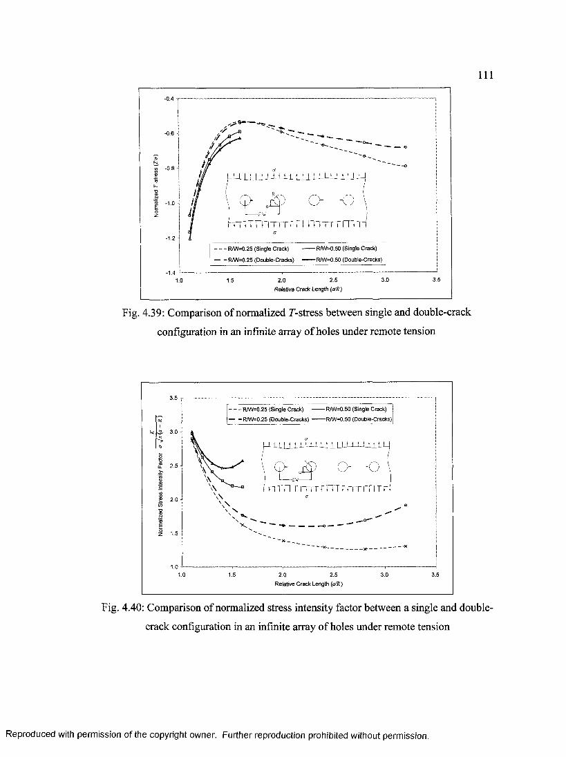
I l l
-0.4
- - -o
L 2W J ITTmTrrrTTTTTrrrrmTri
-1.2
- - R/W=0.25 (Single Crack) --------R/W*0.50 (Single Crack)
R/W=0.50 (Double-Cracks) R/W=0.25 (Double-Cracks)
3.53.02.52.0Relative Crack Length (a/R)
Fig. 4.39: Comparison of normalized 7-stress between single and double-crack
configuration in an infinite array of holes under remote tension
3.5
R/W=0.25 (Single Crack) --------R/W=0.50 (Single Crack)
— -R/W =0.25 (Double-Cracks) — R/W=0.50 (Double-Cracks)
3.0
2.5
2.0
3.0 3.52.0Relative Crack Length (a/R)
2.5
Fig. 4.40: Comparison of normalized stress intensity factor between a single and double
crack configuration in an infinite array of holes under remote tension
Reproduced with permission of the copyright owner. Further reproduction prohibited without permission.

112
O
il I I I
M i l lo
Fig. 4.41: Problem M: Infinite plate with double-cracks emanating from the edge of a
circular hole influence by adjacent holes under remote tension
Reproduced with permission of the copyright owner. Further reproduction prohibited without permission.

113
a
■** Xi
Fig. 4.42: A quarter of the Problem M domain being modelled with displacement
constraints on the planes of symmetry (dotted lines)
Reproduced with permission of the copyright owner. Further reproduction prohibited without permission.

114
BoundaryNodes
ContourrategralPfcth
ContourIntegralPath
Fig. 4.43: A typical BEM mesh showing element size and contour integral for Problem
M; a/Rj = 2.0, a = R2/Rj = 0.5, d* = d/R, = 4, r/(a-Rj) = 0.5
Reproduced with permission of the copyright owner. Further reproduction prohibited without permission.

115
-0.5
-1.0
10.08.07.04.0 5.0 6.0
Relative Crack Length (a/R,3.02.0
Fig. 4.44: Variations of normalized F-stress with relative crack lengths for different
relative hole distance d* = d/Ri for Problem M; a = R2/R 1 - 0.25
3.0
2.5
2.0
1.09.0 10.03.0 4.0 5.0 6.0
Relative Crack Length (a/R,)
7.02.0
Fig. 4.45: Variations of normalized stress intensity factor with relative crack lengths for
different relative hole distance d* = d/R; for Problem M; a = R2/Rj = 0.25
Reproduced with permission of the copyright owner. Further reproduction prohibited without permission.

116
-0.5
-0.1
-0.7
-0.1
-1.0
9.0 10.07.03.0 4.0 5.0 6.0
Relative Crack Length (a/R,)1.0 2.0
Fig. 4.46: Variations of normalized T-stress with relative crack lengths for different
relative hole distance d* = d/Rj for Problem M; a ~ R2/R 1 = 0.50
3.0
2.5
2.0 -
10.05.0 6.0Relative Crack Length (a/R,)
7.02.0 3.0 4.0
Fig. 4.47: Variations of normalized stress intensity factor with relative crack lengths for
different relative hole distance d* = d/Ri for Problem M; a = R2/R1 = 0.50
Reproduced with permission of the copyright owner. Further reproduction prohibited without permission.

117
-0.5
-0.7
-0.8
-1.0
10.07.0 8.04.0 5.0 6.0
Relative Crack Length (a/R,)
2.0 3.0
Fig. 4.48: Variations of normalized T-stress with relative crack lengths for different
relative hole distance d* = d/Ri for Problem M; a = R2/R 1 - 0.75
3.0
7.0 10.02.0 3.0 4.0 5.0 6.0 i
Relative Crack Length (a/R,)
8.0
Fig. 4.49: Variations of normalized stress intensity factor with relative crack lengths for
different relative hole distance d* = d/Ri for Problem M; a = R2/R1 = 0.75
Reproduced with permission of the copyright owner. Further reproduction prohibited without permission.

118
-0.5
-0.7
- 0.1
-0.9
- 1.0
10.09.07.0 8.04.0 5.0 6.0Relative Crack Length (a/R,)
3.02.0
Fig. 4.50: Variations of normalized F-stress with relative crack lengths for different
relative hole distance d* = d/Rj for Problem M; a = R2/R 1 =1.0
3.0
2.5
2.0
8.0 10.02.0 3.0 4.0 5.0 6.0Relative Crack Length (a/R,)
7.0
Fig. 4.51: Variations of normalized stress intensity factor with relative crack lengths for
different relative hole distance d* = d/Rj for Problem M; a = R2/R1 = 1.0
Reproduced with permission of the copyright owner. Further reproduction prohibited without permission.

119
-LLL-0.50
a=0
■0=0.25
a=0.50
■a=0.75
•a=1.0
-0.60
-0.70
-0.80
-0.90
- 1.00
- 1.10
Relative Crack Length {a/R,)
Fig. 4.52: Variations of normalized 7-stress with relative crack lengths for different
radius ratios a = R2/R 1 for Problem M; d* = d/Ri = 2.5
3.00
2.50
2.00
1.50
1.00
Relative Crack Length (a/R,)
Fig. 4.53: Variations o f normalized stress intensity factor with relative crack lengths for
different radius ratios a = R2/R1 for Problem M; d* = d/R] - 2.5
Reproduced with permission of the copyright owner. Further reproduction prohibited without permission.

120
-0.40
-0.50
-0.60
-0.70
-0.80
-0.90
- 1.00
- 1.10
Relative Crack Length (a/R,)
Fig. 4.54: Variations of normalized T-stress with relative crack lengths for different
radius ratios a = R2/R 1 for Problem M; d* = d/Ri = 4.0
3.00
2.50
2.00
1.50
1.00
Relative Crack Length (a/R,)
Fig. 4.55: Variations of normalized stress intensity factor with relative crack lengths for
different radius ratios a = R2/R1 for Problem M; d* = d/Ri = 4.0
Reproduced with permission of the copyright owner. Further reproduction prohibited without permission.

121
-0.40
-0.50
-0.60
-0.70
-0.80
- 1.00
- 1.10
Relative Crack Length (a/R,)
Fig. 4.56: Variations of normalized T-stress with relative crack lengths for different
radius ratios a = R2/R1 for Problem M; d* = d/R, = 5.0
3.00
2.50
a=0.50
0 = 1.02.00
1.50
1.00
Relative Crack Length (a/R,)
Fig. 4.57: Variations of normalized stress intensity factor with relative crack lengths for
different radius ratios a = R2/R1 for Problem M; d* = d/R; = 5.0
Reproduced with permission of the copyright owner. Further reproduction prohibited without permission.

122
-0.40
-0.50a=0
-0.60
-0.70
-0.80
-0.90
- 1.00
- 1.10
Relative Crack Length (a/R,)
Fig. 4.58: Variations of normalized 7-stress with relative crack lengths for different
radius ratios a = R2/R 1 for Problem M; d* = d/Rj = 10.0
3.00
a=02.50
a=0.75
2.00 -
1.50
1.00
Relative Crack Length {a/R,)
Fig. 4.59: Variations of normalized stress intensity factor with relative crack lengths for
different radius ratios a = R2/R1 for Problem M; d* = d/Ri = 10.0
Reproduced with permission of the copyright owner. Further reproduction prohibited without permission.

CHAPTER 5 WEIGHT FUNCTION METHOD FORDETERMINING FRACTURE PARAMETERS
5.0 Introduction
In this chapter, the accuracy and effectiveness of the weight function method for
obtaining T-stress and stress intensity factor solutions for cracked plates with circular
holes are established. The weight function (WF) method provides a means to obtain
these fracture parameters under complex stress fields. The formulation and determination
of the weight functions for stress intensity factor and T-stress will first be discussed.
Three problems will be analyzed using WF and the solutions will be compared to those
available in literature or to those obtained directly from BEM, as presented in the
previous chapters.
123
Reproduced with permission of the copyright owner. Further reproduction prohibited without permission.

124
5.1 Formulation of the Weight Function Method
This section studies the weight function (WF) method as it relates to problems involving
plates with circular holes. As previously mentioned in Chapter 2, the weight functions
for stress intensity factor and F-stress involves the use of geometric constants. It is
therefore necessary to develop the procedure in which they can be derived.
5.1.1 Weight Function for Stress Intensity Factor
The formulation of the WF method involves the absolute length of the crack, which does
not include the radius of the hole. Thus, for convenience, the position ahead of the
circular hole in the x-direction and the crack length are denoted with prime superscript
(Fig. 5.1), i.e.
x'= x - R a '- a - R
Equation (2.9) now becomes
2
(5.1)
-y/27t{a'-x')1 + M, 1 - -
a+ M, r x* 1- -
v a\+ M, 1
a'(5.2)
where Mi, M2 , and M3 are geometric constants for a specific cracked body. Two
reference stress states, as shown in Fig. 5.1, in the form of
o-(x') = <70/ v.y 1- - .
V fl'J(5.3)
Reproduced with permission of the copyright owner. Further reproduction prohibited without permission.

125
where n denotes the order of the crack face loading condition and <j0 is the nominal
stress, are used to solve for these geometric constants. A third condition proposed by
Shen and Glinka (1991), which states that the derivative of the WF at x ’ = 0 is zero,
provides the necessary means to solve for all three constants. The two reference stress
states used are uniform and linear crack face loading. For uniform crack face loading (n
= 0), i.e. cr(x') = cr0,
K ir = a 0 J m '-Y 0 (5.4)
and for linear crack face loading (n — 1), i.e. cr(x') = cr0f x'^
1 - -
V a'j
(5.5)
where 70 and Yx are the boundary correction factors for uniform and linear crack face
loading, respectively. Figure 5.1 shows the application of the crack face loading. The
boundary correction factors are determined using BEM analysis for the each of the crack
length tested, and approximated by simple polynomials using least-squares fit, in the
following form:
Y = B0 +Bl + B- + B-, + b a\ R j
+ B<kR j
(5.6)
Using the null derivative of WF at x ’ = 0 and the two reference stress states, the
geometric parameters can be shown to be:
Reproduced with permission of the copyright owner. Further reproduction prohibited without permission.

126
Mj = 71^2
5
3 0 3649
M, =■ - ^ ( 2 4 ^ - 1 2 I ’0)+ 7 (5.7)
M3 =-5^V 2[271- 7 0] -16
The weight function for stress intensity factor m(x',a') can now be obtained using eq.
(5.2).
5.1.2 Weight Function for T-Stress
Similar to the stress intensity factor, the T-stress weight function also requires
modification to account for the absolute crack length. Equation (2.14) now becomes
m Af r 'V /2 1- -
v a'j+ D.
f r . \ 3/2 1- -
. a’J(5.8)
where Di and D2 are geometric constants of the cracked body. Two reference stress
states are necessary to determine these parameters. Uniform and linear crack face
loading are applied once again. For uniform crack face loading (n = 0), i.e. <r(x') = cr0,
A = < v*o (5.9)
and for linear crack face loading ( n - 1), i.e. cr(x’) = cr{r x
1 - -
v a'j
(5.10)
where V0 and Vx are the normalized T-stress for uniform and linear crack face loading,
respectively. The normalized T-stress solution is determined using BEM analysis for the
Reproduced with permission of the copyright owner. Further reproduction prohibited without permission.

127
each of the crack length tested, and approximated by simple polynomials using least-
squares fit, in the following form:
V — An + A, + An\ R ) ^
+ An' a ^kR ;
+ A,\ R j
+ Ac\ R j
(5.11)
Using these reference stress states, the geometric constants can now be derived, as
follows:
lo
D2 = ^ ( 3 5 F , - 2 i r 0)(5.12)
The T-stress weight function t(x',a') can therefore be obtained with eq. (5.8).
5.2 Verification Problems
Verification of the weight function (WF) method is performed on three different
problems. The results obtained from WF for stress intensity factor and T-stress will be
compared to those obtained from direct BEM analysis or those from the literature. The
three verification problems are (a) an infinite plate with double-cracks at the edge of a
hole (Problem E), (b) a finite plate with double-cracks at the edge of a hole (Problem F),
and (c) a finite plate with a single crack at the edge of a hole (Problem I).
Reproduced with permission of the copyright owner. Further reproduction prohibited without permission.

128
5.2.1 Infinite Plate with Double-Cracks Emanating from the Edge of a Circular
Hole under Remote Tension (Problem E)
The infinite plate with double-cracks emanating from a circular hole problem was
analyzed using the WF method. The BEM was again employed to determine stress
intensity factor and 7-stress solutions due to crack face loading. The geometry was
described previously in Chapter 3, and graphically shown in Fig. 3.24. The numerical
modelling of this problem is identical to that described in Chapter 3, except for the
loading condition. The remote boundary is now a free boundary while the crack face is
subjected to either uniform or linear variation of loading. Since the interest here is to
validate the accuracy of the WF method, only some sample relative crack lengths from
those considered in Chapter 3 were analyzed.
The normalized stress intensity factor and 7-stress solutions for different relative
crack lengths are listed in Table 5.1, and graphically illustrated in Fig. 5.2 and 5.3. Note
that due to the formulation of the WF method, both Ki and 7-stress solutions are plotted
against (a-R)/R, instead of a/R as previously performed. The polynomial fitted
approximations of less than 1% error are also shown in Fig 5.2 and 5.3, with the values of
the coefficients B and A given in Tables 5.2 and 5.3, respectively. By substituting the
polynomial approximations of V and Y into eq. (5.12) and (5.7), respectively, the WF
parameters for 7-stress and stress intensity factor can be obtained.
The stress intensity factor solution is determined by integrating the product of the
uncracked stress distribution er(x') and the weight function m (x',a') over the crack
length, according to eq. (2.6). This stress distribution cr(x') is the uncracked stress
Reproduced with permission of the copyright owner. Further reproduction prohibited without permission.
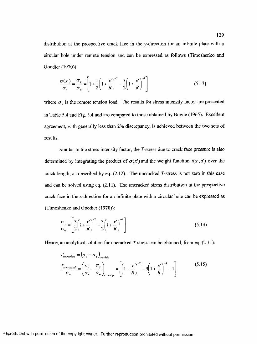
129
distribution at the prospective crack face in the ^-direction for an infinite plate with a
circular hole under remote tension and can be expressed as follows (Timoshenko and
Goodier (1970)):
where crn is the remote tension load. The results for stress intensity factor are presented
in Table 5.4 and Fig. 5.4 and are compared to those obtained by Bowie (1965). Excellent
agreement, with generally less than 2% discrepancy, is achieved between the two sets of
results.
Similar to the stress intensity factor, the T-stress due to crack face pressure is also
determined by integrating the product of cr(x') and the weight function t(x',a') over the
crack length, as described by eq. (2.12). The uncracked T-stress is not zero in this case
and can be solved using eq. (2.11). The uncracked stress distribution at the prospective
crack face in the x-direction for an infinite plate with a circular hole can be expressed as
(Timoshenko and Goodier (1970)):
Hence, an analytical solution for uncracked T-stress can be obtained, from eq. (2.11):
(5.13)
(5.14)
T„uncracked y ’cracktipy ’cracktip
T„uncracked(5.15)
<y,n
Reproduced with permission of the copyright owner. Further reproduction prohibited without permission.

130
The T-stress solutions can now be obtained by the addition of Tuncracked and Tcrackpresuure,
using eq. (2.10). The normalized T-stress solutions are compared to those obtained by
Broberg (2004), as shown in Table 5.4 and Fig. 5.5, and very good agreement can be
observed.
5.2.2 Finite Plate with Double-Cracks Emanating from the Edge of a Circular
Hole under Remote Tension (Problem F)
The finite plate with two symmetric cracks at the edge of a circular hole, as shown in Fig.
4.1, was analyzed using the WF method. Two-dimensional BEM was used to obtain the
reference normalized stress intensity factor Y and T-stress V. The same BEM mesh as
described in Chapter 4 was used, but with crack face loading conditions. Relative hole
radius R/W =0 .25 and a height-to-width ratio H/W = 2 with the same corresponding
crack lengths were tested.
The obtained results for uniform and linear crack face loading are shown in Table
5.5, and in Fig. 5.6 and 5.7. Both the boundary correction factor Y and normalized T-
stress V were approximated using polynomial fits with less than 2% error, with the values
of the coefficients of B and A given in Tables 5.6 and 5.7. The WF geometric constants
for stress intensity factor and T-stress can then be determined, as previously described.
No analytical expressions are available in literature for the uncracked stress distribution
on the prospective crack face cr(x') . Thus, the BEM was used to obtain this stress
distribution for the uncracked finite plate. The results for the stresses normalized with
respect to crn, in the x- and y-direction are given in Table 5.8. The stress a y is also
Reproduced with permission of the copyright owner. Further reproduction prohibited without permission.

131
shown graphically in Fig. 5.8, and is approximated using 6th order polynomial least-
squares fit of less than 2% error from the computed values. The approximated
polynomial of this stress is:
cr(x ') a ycr
= 3.245 - 7.2875 • — + 13.486 R
f . . . X 4
( rU 2A -14.729- A
U j JU
+ 9.1404'R
-2.9511 + 0.3828
(5.16)
The stress intensity factor solutions at the various crack lengths are determined by
again integrating the product of cr(x’) and the weight function m(x’, a') over the crack
length. Table 5.9 and Fig. 5.9 compares the WF and BEM obtained solutions. It can be
seen that good agreement is attained, with the discrepancies all within 3 percent.
Using the results for a x in Table 5.8, the “uncracked” 7-stress can be calculated
at the corresponding crack-tip locations, as listed. The crack face pressure induced 7-
stress is determined by integrating the product of the BEM obtained uncracked stress
distribution and the weight function t(x’,a ') . The normalized 7-stress for the entire
system, at various crack lengths, can then be determined by the addition of Tuncracked and
crackpresuure . Very good agreement is again observed when comparing the results obtained
by the WF method and those directly by the BEM, as shown in Table 5.9 and Fig. 5.10.
Reproduced with permission of the copyright owner. Further reproduction prohibited without permission.

132
5.2.3 Finite Plate with a Single Crack Emanating from the Edge of a Circular
Hole under Remote Tension (Problem I)
Verification of the weight function method was also performed on the finite plate with a
single crack at the edge of a circular hole problem (Fig. 4.19). The normalized stress
intensity factor and 7-stress for the two reference stress states were once again
determined using two-dimensional BEM.
The results for normalized stress intensity factor and 7-stress for relative hole
radius R/W of 0.25 for the two crack face loading conditions are shown in Table 5.10.
Polynomial fits of less than 2% error of the boundary correction factor Y and normalized
7-stress V are shown in Fig. 5.11 and 5.12, with the values of the coefficients of B and A
given in Tables 5.11 and 5.12. The WF parameters for stress intensity factor and 7-stress
can therefore be obtained using these expressions. The uncracked stress distribution on
the prospective crack face in both x- and y-directions is identical to that of Problem F
(since identical uncracked geometry).
The computed results of stress intensity factor using the WF method are tabulated
in Table 5.13 (and graphically shown in Fig. 5.13) and compared to those obtained
directly using BEM. Discrepancy of less than 3% can be seen between the solutions
obtained by the two methods. Also shown in the table are the 7-stress values calculated
using the WF method and those obtained directly from BEM. Figure 5.14 shows the 7-
stress results graphically. The discrepancies between these 7-stress results are less than 4
percent.
Reproduced with permission of the copyright owner. Further reproduction prohibited without permission.

133
5.3 Summary
Weight functions for determining stress intensity factor and T-stress have been obtained
for three test problems here. They demonstrate the applicability of the WF method for
the plate problems with cracks at a circular hole. Very good agreement was achieved
between the present solutions and those previously established.
Reproduced with permission of the copyright owner. Further reproduction prohibited without permission.
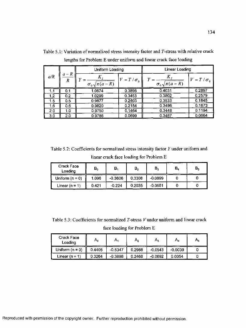
134
Table 5.1: Variation of normalized stress intensity factor and T-stress with relative crack
lengths for Problem E under uniform and linear crack face loading
a/R a - RR
Uniform Loading Linear Loading
Y V = T / a o Y K i V = T / a 0c r ^ n { a - R ) cr0 j x ( a - R )
1 . 1 0 . 1 1.0674 0.3898 0.4031 0.28971 . 2 0 . 2 1.0299 0.3453 0.3802 0.25791.5 0.5 0.9877 0.2403 0.3533 0.18451 . 6 0 . 6 0.9820 0.2154 0.3496 0.16732 . 0 1 . 0 0.9750 0.1464 0.3448 0.11943.0 2 . 0 0.9786 0.0699 0.3467 0.0664
Table 5.2: Coefficients for normalized stress intensity factor Y under uniform and
linear crack face loading for Problem E
Crack Face Loading B0 Bi b2 b 3 b 4 b 5
Uniform (n = 0) 1.096 -0.3606 0.3308 -0.0899 0 0
Linear (n = 1) 0.421 -0.224 0.2035 -0.0551 0 0
Table 5.3: Coefficients for normalized T-stress V under uniform and linear crack
face loading for Problem E
Crack Face Loading Ao At a 2 a 3 A4 A5
Uniform (n = 0) 0.4405 -0.5347 0.2988 -0.0543 -0.0039 0
Linear (n = 1) 0.3264 -0.3898 0.2466 -0.0692 0.0054 0
Reproduced with permission of the copyright owner. Further reproduction prohibited without permission.

135
Table 5.4: Comparison of stress intensity factor and T-stress solutions between solutions
obtained using the weight function method and those available in literature for Problem E
a/RK , / a -yjn (a - R ) T/o
BOWIE (1965) WEIGHTFUNCTIONS % DIFF
BROBERG(2004)
WEIGHTFUNCTIONS
% DIFF
1.1 2.8017 2.7600 -1.49 -1.0584 -1.0659 0.711.2 2.4135 2.3885 -1.04 -0.7925 -0.8205 3.531.5 1.8369 1.8763 2.15 -0.5616 -0.5646 0.531.6 1.7500 1.7753 1.44 N/A -0.5594 N/A2.0 1.4902 1.5047 0.98 -0.6090 -0.6168 1.283.0 1.2800 1.2679 -0.95 N/A -0.7833 N/A
Table 5.5: Variation of normalized stress intensity factor and T-stress with relative crack
lengths for Problem F under uniform and linear crack face loading
a/R a - RR
Uniform Loading Linear Loading
y _ K l V = T / a o Y K i V - T /<t qa r ^ 7 i{ a -R ) a 0^ ( a - R )1.1 0.100 1.0676 0.4066 0.4018 0.29641.2 0.200 1.0445 0.3555 0.3892 0.25481.6 0.600 1.0443 0.2129 0.3868 0.15332.0 1.000 1.1018 0.0881 0.4207 0.07272.4 1.400 1.2026 -0.0747 0.4794 -0.02772.8 1.800 1.3653 -0.3453 0.5733 -0.18713.2 2.200 1.6758 -0.8553 0.7493 -0.4754
Reproduced with permission of the copyright owner. Further reproduction prohibited without permission.
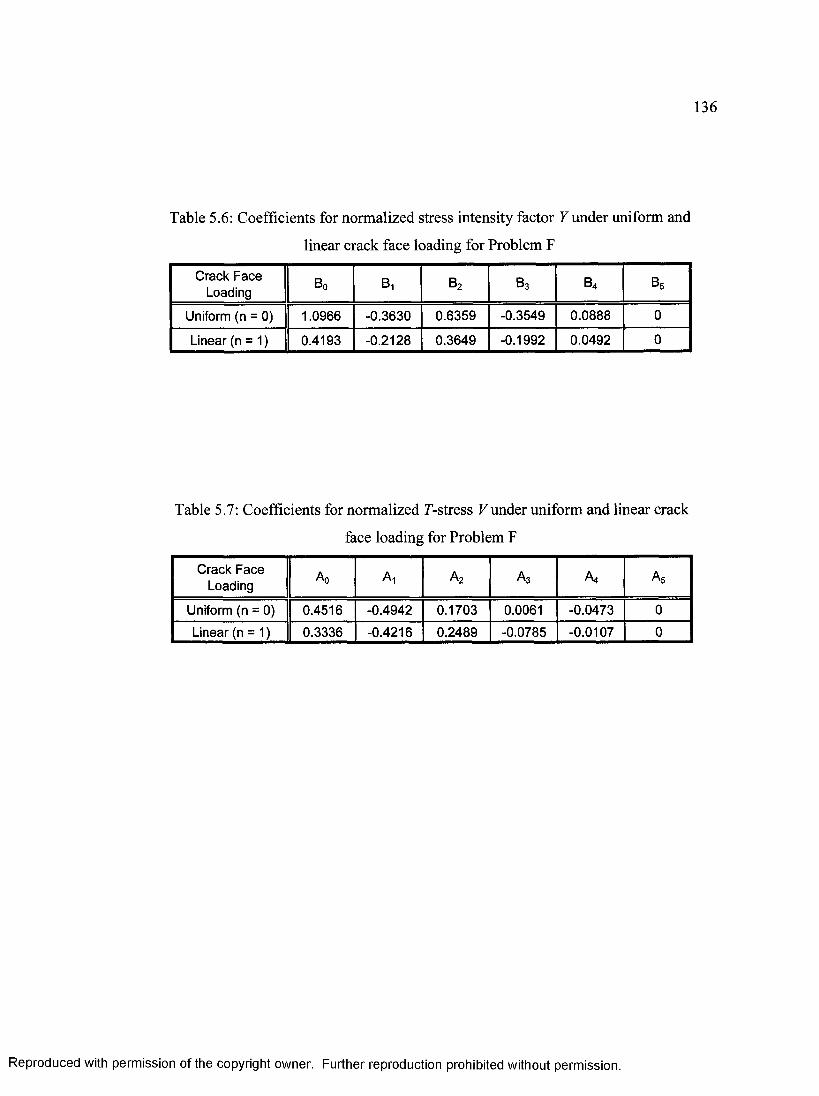
136
Table 5.6: Coefficients for normalized stress intensity factor Y under uniform and
linear crack face loading for Problem F
Crack Face Loading B0 Bi b2 b3 b4 b5
Uniform (n = 0) 1.0966 -0.3630 0.6359 -0.3549 0.0888 0
Linear (n = 1) 0.4193 -0.2128 0.3649 -0.1992 0.0492 0
Table 5.7: Coefficients for normalized T-stress V under uniform and linear crack
face loading for Problem F
Crack Face Loading A d Ai a 2 a 3 A< As
Uniform (n = 0) 0.4516 -0.4942 0.1703 0.0061 -0.0473 0
Linear (n = 1) 0.3336 -0.4216 0.2489 -0.0785 -0.0107 0
Reproduced with permission of the copyright owner. Further reproduction prohibited without permission.
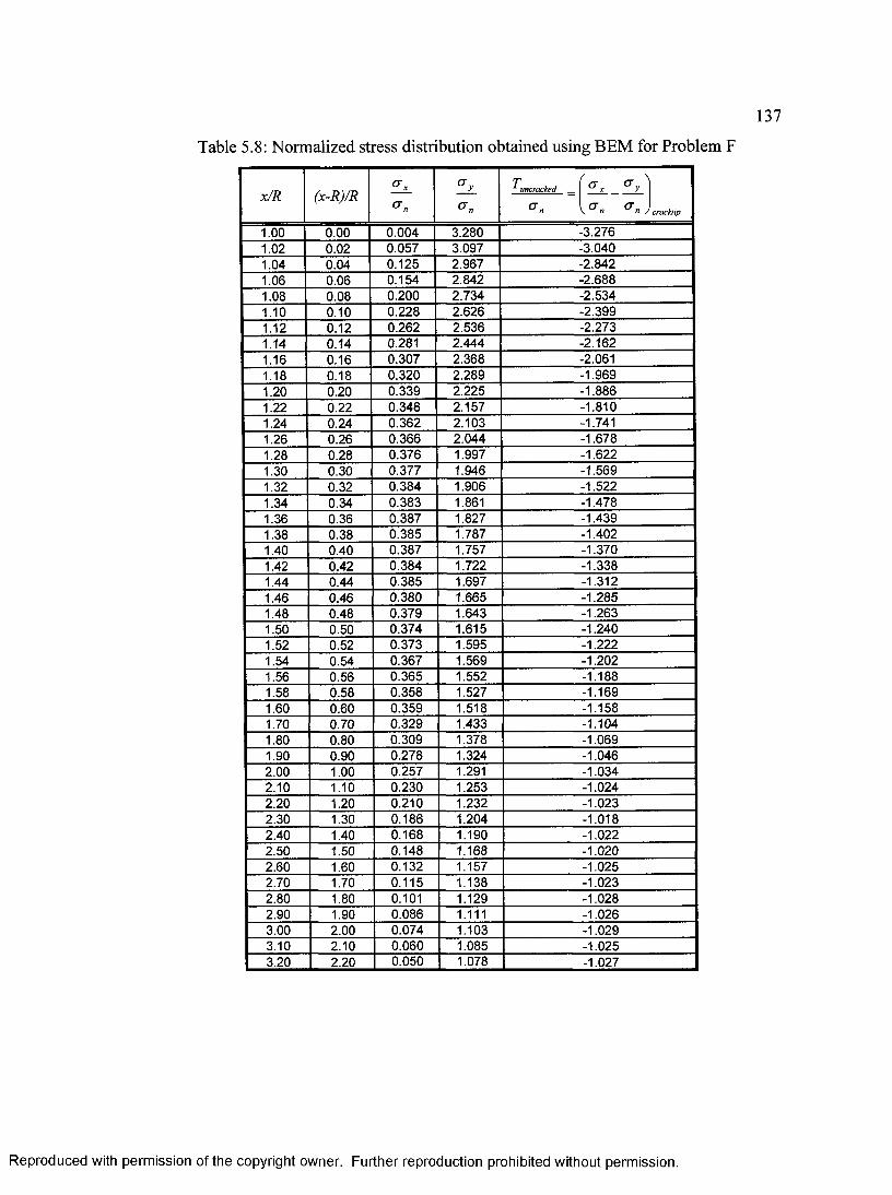
137
Table 5.8: Normalized stress distribution obtained using BEM for Problem F
x/R (x-R)/R°n O'*
T ( rr \uncracked _ >
^ n V ^ n ^ n ) cracktip1.00 0.00 0.004 3.280 -3.2761.02 0.02 0.057 3.097 -3.0401.04 0.04 0.125 2.967 -2.8421.06 0.06 0.154 2.842 -2.6881.08 0.08 0.200 2.734 -2.5341.10 0.10 0.228 2.626 -2.3991.12 0.12 0.262 2.536 -2.2731.14 0.14 0.281 2.444 -2.1621.16 0.16 0.307 2.368 -2.0611.18 0.18 0.320 2.289 -1.9691.20 0.20 0.339 2.225 -1.8861.22 0.22 0.348 2.157 -1.8101.24 0.24 0.362 2.103 -1.7411.26 0.26 0.366 2.044 -1.6781.28 0.28 0.376 1.997 -1.6221.30 0.30 0.377 1.946 -1.5691.32 0.32 0.384 1.906 -1.5221.34 0.34 0.383 1.861 -1.4781.36 0.36 0.387 1.827 -1.4391.38 0.38 0.385 1.787 -1.4021.40 0.40 0.387 1.757 -1.3701.42 0.42 0.384 1.722 -1.3381.44 0.44 0.385 1.697 -1.3121.46 0.46 0.380 1.665 -1.2851.48 0.48 0.379 1.643 -1.2631.50 0.50 0.374 1.615 -1.2401.52 0.52 0.373 1.595 -1.2221.54 0.54 0.367 1.569 -1.2021.56 0.56 0.365 1.552 -1.1881.58 0.58 0.358 1.527 -1.1691.60 0.60 0.359 1.518 -1.1581.70 0.70 0.329 1.433 -1.1041.80 0.80 0.309 1.378 -1.0691.90 0.90 0.278 1.324 -1.0462.00 1.00 0.257 1.291 -1.0342.10 1.10 0.230 1.253 -1.0242.20 1.20 0.210 1.232 -1.0232.30 1.30 0.186 1.204 -1.0182.40 1.40 0.168 1.190 -1.0222.50 1.50 0.148 1.168 -1.0202.60 1.60 0.132 1.157 -1.0252.70 1.70 0.115 1.138 -1.0232.80 1.80 0.101 1.129 -1.0282.90 1.90 0.086 1.111 -1.0263.00 2.00 0.074 1.103 -1.0293.10 2.10 0.060 1.085 -1.0253.20 2.20 0.050 1.078 -1.027
Reproduced with permission of the copyright owner. Further reproduction prohibited without permission.

138
Table 5.9: Comparison of stress intensity factor and 7-stress solutions between solutions
obtained using the weight function method and those obtained by BEM for Problem F
a/RK j / <j - Jx ( a - R) 7/(7
BEMWEIGHT
FUNCTIONS% DIFF BEM
WEIGHTFUNCTIONS
% DIFF
1.1 3.1069 3.0141 -2.99 -1.1331 -1.1622 2.571.2 2.6690 2.6894 0.76 -0.8295 -0.8446 1.831.6 2.0092 2.0257 0.82 -0.6332 -0.6415 1.302.0 1.8379 1.8202 -0.96 -0.8196 -0.8249 0.642.4 1.8504 1.8327 -0.96 -1.1155 -1.1072 -0.742.8 2.0038 2.0227 0.94 -1.5561 -1.5807 1.583.2 2.3877 2.3682 -0.82 -2.2696 -2.3135 1.93
Table 5.10: Variation of normalized stress intensity factor and 7-stress with relative crack
lengths for Problem I under uniform and linear crack face loading
a/R a - RR
Uniform Loading Linear Loading
r _ K, V = T / a o y K, V = T / cr0a 0^ 7 r (a - R) a 0^ j n ( a - R )
1.1 0.100 1.0593 0.4088 0.3945 0.29021.2 0.200 1.0161 0.3667 0.3659 0.25581.6 0.600 0.9538 0.2234 0.3267 0.15972.0 1.000 0.9467 0.1068 0.3204 0.08432.4 1.400 0.9726 -0.0247 0.3333 0.00372.8 1.800 1.0407 -0.2246 0.3680 -0.11023.2 2.200 1.1889 -0.6243 0.4423 -0.3206
Reproduced with permission of the copyright owner. Further reproduction prohibited without permission.

139
Table 5.11: Coefficients for normalized stress intensity factor Y under uniform
and linear crack face loading for Problem I
Crack Face Loading B0 Bi b 2 b 3 b 4 b5
Uniform (n = 0) 1.1015 -0.5092 0.5853 -0.2959 0.0651 0
Linear (n = 1) 0.4208 -0.3220 0.3651 -0.1814 0.0382 0
Table 5.12: Coefficients for normalized T-stress V under uniform and linear crack
face loading for Problem I
Crack Face Loading Ao Ai a 2 a 3 A4 A5
Uniform (n = 0) 0.4478 -0.4016 -0.0097 0.1353 -0.0675 0
Linear (n = 1) 0.3211 -0.3373 0.1177 0.0032 -0.0215 0
Table 5.13: Comparison of stress intensity factor and T-stress solutions between
solutions obtained using the weight function method and those obtained by BEM for
Problem I
a/RK j I a s in (a - R ) T/tr
BEMWEIGHT
FUNCTIONS% DIFF BEM
WEIGHTFUNCTIONS
% DIFF
1 . 1 3.0719 2.9810 -2.96 -1.1298 -1.1524 2 . 0 0
1 . 2 2.6082 2.5742 -1.31 -0.8126 -0.8477 4.321 . 6 1.8077 1.7967 -0.60 -0.6126 -0.6267 2.312 . 0 1.5300 1.5192 -0.70 -0.7950 -0.7790 -2 . 0 1
2.4 1.4350 1.4246 -0.73 -1.0432 -1.0188 -2.342 . 8 1.4505 1.4641 0.94 -1.3776 -1.3769 -0.053.2 1.5928 1.5976 0.30 -1.9479 -1.9205 -1.41
Reproduced with permission of the copyright owner. Further reproduction prohibited without permission.

140
1 ------
Fig. 5.1: Crack face loading cr(x') of nth order on an arbitrary geometry involving a
circular hole; x ’- x - R , a ' - a ~ R
Reproduced with permission of the copyright owner. Further reproduction prohibited without permission.

141
1.20
1.00
0.80
Uniform Loading
Linear Loading
0.40
0.202.00.50.0
a-RRelative Crack Length
Fig. 5.2: Variations of normalized stress intensity factor with relative crack lengths for
Problem E under uniform and linear crack face loading
0.50
0.40
Uniform Loading
Linear Loading0.30
0.20
0.10
0.002.00.0 0.5
a-RRelative Crack Length
Fig. 5.3: Variations of normalized F-stress with relative crack lengths for Problem E
under uniform and linear crack face loading
Reproduced with permission of the copyright owner. Further reproduction prohibited without permission.

142
3.00
2.80— Weight Function Method
» BOWIE (1965)2.60
> 2.40b
ooCOLL
2.20
s ' 2.00coc
(A£wT3N 1.60CD
oz 1.40
1.203.02.51.5 2.01.0
Relative Crack Length (a/R)
Fig. 5.4: Variation of normalized stress intensity factors with relative crack lengths for
Problem E
-0.50
— Weight Function Method
■ Broberg (2003)-0.60
-0.70
-0.80 -
-0.90
- 1.00
- 1.103.02.0
Relative Crack Length (a/R)
2.5
Fig. 5.5: Variation of normalized F-stress with relative crack lengths for Problem E
Reproduced with permission of the copyright owner. Further reproduction prohibited without permission.

143
2.00
Uniform Loading
Linear Loading
1.20
0.40
0.002.42.00.0 0.4
Relative Crack Length ^
Fig. 5.6: Variations of normalized stress intensity factor with relative crack lengths for
Problem F under uniform and linear crack face loading
0.50
Uniform Loading
Linear Loading
0.25
0.00
-0.25
-0.50
-0.75 -
- 1.000.4 0.8 2.0 2.40.0
Relative Crack Length - —
Fig. 5.7: Variations of normalized F-stress with relative crack lengths for Problem F
under uniform and linear crack face loading
Reproduced with permission of the copyright owner. Further reproduction prohibited without permission.

144
3.5
2.5
2.0
0.5
0.02.52.00.50.0
Position A head of th e Circular Hole (x-R)/R
Fig. 5.8: Normalized uncracked stress distribution in the ̂ -direction on the perspective
crack face due to remote tension for Problem F
Reproduced with permission of the copyright owner. Further reproduction prohibited without permission.

145
3.20
3.00
2.80
2.60 - 2H
2.40
-2 V-2.20
2.00
1.80a BEM
— Weight Function Method
1.403.02.52.0
Relative Crack Length (a/R)
Fig. 5.9: Variation of normalized stress intensity factors with relative crack lengths for
Problem F
-0.50
• BEM
— Weight Function Method
- 1.00
-1.50
2H
-2.00
*2 W'
-2.502.5 3.02.0
Relative Crack Length (a/R)
Fig. 5.10: Variation of normalized F-stress with relative crack lengths for Problem F
Reproduced with permission of the copyright owner. Further reproduction prohibited without permission.

146
1.60
— Uniform Loading
- - Linear Loading, S 1.20
0.80
0.40
0.002.42.00.0 0.4
Relative Crack L eng th ------
Fig. 5.11: Variations of normalized stress intensity factor with relative crack lengths for
Problem I under uniform and linear crack face loading
0.50
— Uniform Loading
— Linear Loading0.25 -
0.00
-0.25
-0.50
-0.752.0 2.40.0 0.4 0.8
Relative Crack Length — —
Fig. 5.12: Variations of normalized F-stress with relative crack lengths for Problem I
under uniform and linear crack face loading
Reproduced with permission of the copyright owner. Further reproduction prohibited without permission.

147
3.20
2.80
2.40 2H
2.00
1.60
a BEM
— Weight Function Method
1.203.02.0
Relative Crack Length (a/R)
2.5
Fig. 5.13: Variation of normalized stress intensity factors with relative crack lengths for
Problem I
-0.50
a BEM
— Weight Function Method
- 1.00
-1.50
2H
-2.00
-2.502.0
Relative Crack Length (a/R)
2.5 3.0
Fig. 5.14: Variation of normalized F-stress with relative crack lengths for Problem I
Reproduced with permission of the copyright owner. Further reproduction prohibited without permission.

CHAPTER 6 CONCLUSIONS
The scope of this thesis was to determine a measure of crack-tip constraint of plates with
circular holes. To this end, the stress intensity factor (K) and T-stress solutions for these
geometries were obtained. The geometries analyzed include plates with a single circular
hole under remote tension and bending, and plates with multiple holes under remote
tension. The boundary element method (BEM), in conjunction with the mutual or M-
contour integral, was used to determine the K and T-stress solutions numerically.
The principles of linear elastic fracture mechanics (LEFM) and the significance of
T-stress as a second parameter for LEFM analysis have been briefly described in Chapter
2. The formulation of the weight function (WF) method and the BEM for obtaining K
and T-stress solutions were discussed. To overcome cumbersome meshing procedures
around the crack-tip, self-regularized BEM, as described in Chapter 2, was employed.
The validation of the BEM as the numerical tool for this thesis was discussed in
Chapter 3. Several problems with published values of stress intensity factor and T-stress,
including those with stress concentrations, were evaluated using the BEM. Comparisons
of the solutions with those from the literature demonstrated the accuracy of the BEM, as
well as efficiency against other numerical techniques. From the BEM-obtained solutions,
some general modelling guidelines were established.
148
Reproduced with permission of the copyright owner. Further reproduction prohibited without permission.

149
The stress intensity factor and T-stress solutions obtained from BEM for plates
with circular hole(s) were presented in Chapter 4. Some general trends were observed for
all of the analyzed geometries. First, the T-stresses obtained from BEM were all negative
in value, which indicate low constraint conditions. Second, the negative T-stresses
become increasingly less negative for increasing crack length, then declines rapidly
beyond a certain crack length. Plates with a single circular hole were first evaluated. The
presence of a finite boundary around a circular hole was found to increase the rate-of-
change of the “uptrend-downtrend” behaviour of the T-stress as the crack size becomes
larger, when compared to the corresponding crack lengths of the infinite plate case. Also,
the difference in value for T-stress between single and double-crack configuration was
found to be significant only for relatively large crack lengths. Bending loads on the finite
plates were also studied. A significant reduction from the values obtained for the tension
case for the stress intensity factors was observed.
The effects of adding adjacent holes were also examined. For the infinite array of
holes problems, it was found that the declining behaviour of the T-stress, as described
above, was much more gradual. The addition of adjacent holes not in the plane of the
crack was also investigated for the infinite plate problem. Increasing the size of the
adjacent holes reduced the magnitude of the stress intensity factors and generated gentler
gradients in the T-stress behaviour. Also, by reducing the distance between the holes,
both stress intensity factors and T-stress decreased in value, resulting in even lower
crack-tip constraint.
Reproduced with permission of the copyright owner. Further reproduction prohibited without permission.

150
The weight function method has been shown to be an efficient technique in
determining K and T-stress solutions for complex stress distributions for cracked-
geometries. Several test problems were reanalyzed using this method, as described in
Chapter 5. Very good agreement was achieved between the solutions obtained directly
from BEM and those obtained using the WF method, hence validating its effectiveness
for plates with crack(s) emanating from circular holes.
Reproduced with permission of the copyright owner. Further reproduction prohibited without permission.

REFERENCES
Ainsworth, R.A., Bannister, A.C. and Zerbst U., (2002). “An Overview of the European Flaw Assessment Procedure SINTAP and Its Validation". International Journal o f Pressure Vessels and Piping. 77, pp. 869-876.
Betegon, C. and Hancock, J.W., (1991). “Two-Parameter Characterization of Elastic- Plastic Crack Tip Field”. ASME Journal o f Applied Mechanics. 58, pp. 104-110.
Bettinson, A.D., O’Dowd, N.P., Nikbin, K. and Webster, G.A.,(2000). “Two-parameter Characterisation of Crack Tip Fields under Creep Conditions”. In: Murakami S, Ohno N, editor, 5th IUTAM symposium on creep in structures; Nagoya, Japan, 3 -7 April 2000, Boston, Kluwer Academic Publisher, pp. 95-104.
Bilby, B.A., Cardew, G.E., Goldthorpe, M.R. and Howard, I.C., (1986). “A Finite Element Investigation of the Effect of Specimen Geometry on the Fields of Stress and Strains at the Tips of Stationary Cracks”. Size Effects in Fracture, pp. 37-46. Mechanical Engineering Publications Limited, London.
Broberg, K.B., (2004). “A Note on 7-stress Determination Using Dislocation Arrays”. International Journal o f Fracture. 131, pp. 1-14.
Bueckner, H.F., (1970). “A Novel Principle of the Computation of Stress Intensity Factors”. Zeitschriftfur Angewandte Mathematik und Mechanik. 50, pp. 129-146.
Cotterell, B. and Rice, J.R. (1980). “Slightly Curved or Kinked Cracks”. International Journal o f Fracture. 16, pp. 155-169.
Cruse, T. and Richardson, J.D., (1996). “Non-Singular Somigliana Stress Identities in Elasticity”. International Journal for Numerical Methods in Engineering. 39, pp. 3273- 3304.
Du, Z.Z. and Hancock, J.W., (1991). “The Effect of Non-Singular Stresses on Crack Tip Constraint”. Journal o f the Mechanics and Physics o f Solids. 39, pp. 555-567.
151
Reproduced with permission of the copyright owner. Further reproduction prohibited without permission.

152
Fett, T., (1997). “A Green’s Function for T-Stress in an Edge Cracked Rectangular Plate”. Engineering Fracture Mechanics. 57. pp. 365-373.
Fett, T., (2002). T-Stress Solutions and Stress Intensity Factors for 1-D Cracks. VDI Verlag, Dusseldorf.
Huang, Q. and Cruse, T.A., (1994). “On the Non-Singular Traction-BIE in Elasticity”. International Journal for Numerical Methods in Engineering. 37, pp. 2041-2072.
Kfouri, A.P., (1986). “Some Evaluations of the Elastic T-Term Using Eshelby’s Method”. International Journal o f Fracture. 30, pp. 301-315.
Larsson, S.G. and Carlsson, A.J. (1973). “Influence of Non-Singular Stress Terms and Specimen Geometry on Small-Scale Yielding at Crack Tips in Elastic-Plastic Materials”. Journal o f the Mechanics and Physics o f Solids. 21, pp. 263-277.
Leevers, P.S., Radon, J.C. and Culver, L.E., (1976). “Fracture Trajectories in a Biaxial Plate”. Journal o f the Mechanics and Physics o f Solids. 24, pp. 381-395.
Leevers, P.S. and Radon, J.C., (1982). “Inherent Stress Biaxiality in Various Fracture Specimen Geometries”. International Journal o f Fracture. 19, pp. 311-325.
Lewis, T., (2005). T-Stress Solutions fo r Cracks at Notches and in Cylinders. M.A.Sc. Thesis, Carleton University, Ottawa, ON.
Li, J., (2004). The Evaluation o f T-Stress Using Boundary Element Method. M.A.Sc. Thesis, Carleton University, Ottawa, ON.
Li, J., Tan, C.L. and Wang, X., (2005). “Weight Functions for T-Stress for Edge Cracks in Thick-Walled Cylinders”. ASME Journal o f Pressure Vessel Technology. 127, pp. 457- 463.
Murakami, Y., (2003). Stress Intensity Factors Handbook. Pergamon Press, Elmsford, New York.
Reproduced with permission of the copyright owner. Further reproduction prohibited without permission.

153
Nakamura, T. and Parks, D.M., (1992). “Determination of Elastic T-Stress Along Three- Dimensional Crack Fronts Using an Interaction Integral”. International Journal o f Solids and Structures. 29, pp. 1597-1611.
O’Dowd, N.P. and Shih, C.F., (1991). “Family of Crack Tip Fields Characterized by A Triaxiality Parameter-I. Structure of Fields”. Journal o f the Mechanics and Physics o f Solids. 24, pp. 989-1015.
Ortiz, J.E. and Cisilino, A.P., (2005). “Boundary Element Method for 7-Integral and Stress Intensity Factor Computations in Three-Dimensional Interface Cracks”. International Journal o f Fracture. 133, pp. 197-222.
Rice, J.R., (1968). “A Path Independent Integral and the Approximate Analysis of Strain Concentration by Notches and Cracks”. Journal o f Applied Mechanics. 35, pp. 379-386.
Rice, J.R., (1972). “Some Remarks on Elastic Crack Tip Field”. International Journal o f Solids and Structures. 8, pp. 751-758.
Rice, J.R., (1974). “Limitations to Small-Scale Yielding Approximation for Crack Tip Plasticity”. Journal o f the Mechanics and Physics o f Solids. 22, pp. 17-26.
Richardson, J.D. and Cruse, T., (1999). “Weakly Singular Stress-BEM for 2D Elastostatics”. International Journal for Numerical Methods in Engineering. 45, pp. 13- 35.
Rooke, D.P. and Cartwright, D.J., (1976). Compendium o f Stress Intensity Factors. Hillington Press, Uxbridge, Middx.
Shen, G. and Glinka, G., (1991). “Determination of Weight Functions from Reference Stress Intensity Factors”. Theoretical and Applied Fracture Mechanics. 12, pp. 237-245.
Sladek, J., Sladek, V. and Fedelinski, P., (1997). “Contour Integrals for Mixed-Mode Crack Analysis: Effect of Nonsingular Terms”. Theoretical and Applied Fracture Mechanics. 27, pp. 115-127.
Reproduced with permission of the copyright owner. Further reproduction prohibited without permission.

154
Sladek, J., Sladek, V. and Fedelinski, P., (1999). “Computation of the Second Fracture Parameter in Elastodynamics by the Boundary Element Method”. Advances in Engineering Software. 30, pp. 725-734.
Sladek, J., Sladek, V., (2000). “Evaluation of Elastic E-stress in Three-Dimensional Crack Problems Using an Integral Formula”. International Journal o f Fracture. 101, pp. 47-52.
Tan, C.L. (1987), The Boundary Element Method: A Short Course, Carleton University, Ottawa, Ontario.
Tan, C.L. and Wang, X., (2003). “The Use of Quarter-Point Crack-Tip Elements for E- Stress Determination in Boundary Element Method Analysis”. Engineering Fracture Mechanics. 70. pp. 2247-2252.
Timoshenko and S.P.Goodier, J.N., (1970). The Theory o f Elasticity, McGraw Hill, New York, USA.
Wang, X., (2002). “Determination of Weight Functions for Elastic E-Stress from Reference E-Stress solutions”. Fatigue and Fracture o f Engineering Materials and Structures. 25. pp. 965-973.
Wang, X., (2002). “Elastic E-stress for Cracks in Test Specimens Subjected to Non- Uniform Stress Distributions”. Engineering Fracture Mechanics. 69. pp. 1339-1352.
Wang, X., (2002). “Elastic E-Stress Solutions for Semi-Elliptical Surface Cracks in Finite Thickness Plates”. Engineering Fracture Mechanics. 70. pp. 731-756.
Wang, Y.Y., (1993). “On the Two-Parameter Characterization of Elastic-Plastic Crack Front Fields in Surface Cracked Plates”. In: Hackett E.M., Schwalbe K.H., Dodds R.H. Editors. Constraint Effects in Fracture. ASTM STP1171. American Society for Testing and Materials, Philadelphia.
Williams, M.L., (1957). “On the Stress Distribution at the Base of A Stationary Crack”. ASME Journal o f Applied Mechanics. 24, pp. 109-114.
Reproduced with permission of the copyright owner. Further reproduction prohibited without permission.