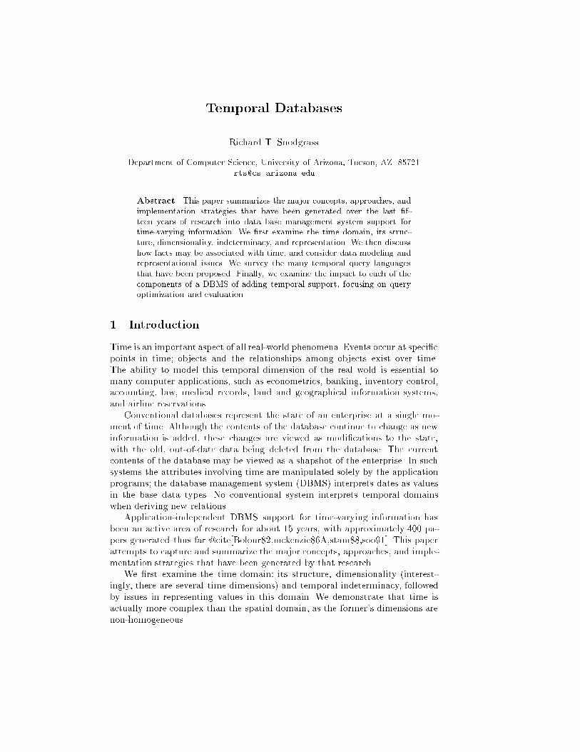
Temporal DatabasesRichard T. SnodgrassDepartment of Computer Science, University of Arizona, Tucson, AZ 85721rts@cs.arizona.eduAbstract. This paper summarizes the major concepts, approaches, andimplementation strategies that have been generated over the last �f-teen years of research into data base management system support fortime-varying information. We �rst examine the time domain, its struc-ture, dimensionality, indeterminacy, and representation. We then discusshow facts may be associated with time, and consider data modeling andrepresentational issues. We survey the many temporal query languagesthat have been proposed. Finally, we examine the impact to each of thecomponents of a DBMS of adding temporal support, focusing on queryoptimization and evaluation.1 IntroductionTime is an important aspect of all real-world phenomena. Events occur at speci�cpoints in time; objects and the relationships among objects exist over time.The ability to model this temporal dimension of the real wold is essential tomany computer applications, such as econometrics, banking, inventory control,accounting, law, medical records, land and geographical information systems,and airline reservations.Conventional databases represent the state of an enterprise at a single mo-ment of time. Although the contents of the database continue to change as newinformation is added, these changes are viewed as modi�cations to the state,with the old, out-of-date data being deleted from the database. The currentcontents of the database may be viewed as a shapshot of the enterprise. In suchsystems the attributes involving time are manipulated solely by the applicationprograms; the database management system (DBMS) interprets dates as valuesin the base data types. No conventional system interprets temporal domainswhen deriving new relations.Application-independent DBMS support for time-varying information hasbeen an active area of research for about 15 years, with approximately 400 pa-pers generated thus far @cite[Bolour82,mckenzie86A,stam88,soo91]. This paperattempts to capture and summarize the major concepts, approaches, and imple-mentation strategies that have been generated by that research.We �rst examine the time domain: its structure, dimensionality (interest-ingly, there are several time dimensions) and temporal indeterminacy, followedby issues in representing values in this domain. We demonstrate that time isactually more complex than the spatial domain, as the former's dimensions arenon-homogeneous.

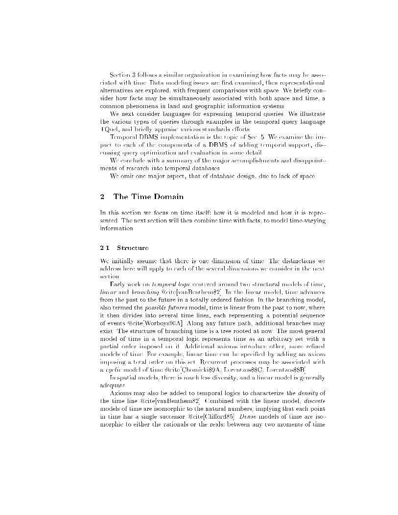
Section 3 follows a similar organization in examining how facts may be asso-ciated with time. Data modeling issues are �rst examined, then representationalalternatives are explored, with frequent comparisons with space. We brie y con-sider how facts may be simultaneously associated with both space and time, acommon phenomena in land and geographic information systems.We next consider languages for expressing temporal queries. We illustratethe various types of queries through examples in the temporal query languageTQuel, and brie y appraise various standards e�orts.Temporal DBMS implementation is the topic of Sec. 5. We examine the im-pact to each of the components of a DBMS of adding temporal support, dis-cussing query optimization and evaluation in some detail.We conclude with a summary of the major accomplishments and disappoint-ments of research into temporal databases.We omit one major aspect, that of database design, due to lack of space.2 The Time DomainIn this section we focus on time itself: how it is modeled and how it is repre-sented. The next section will then combine time with facts, to model time-varyinginformation.2.1 StructureWe initially assume that there is one dimension of time. The distinctions weaddress here will apply to each of the several dimensions we consider in the nextsection.Early work on temporal logic centered around two structural models of time,linear and branching @cite[vanBenthem82]. In the linear model, time advancesfrom the past to the future in a totally ordered fashion. In the branching model,also termed the possible futures model, time is linear from the past to now, whereit then divides into several time lines, each representing a potential sequenceof events @cite[Worboys90A]. Along any future path, additional branches mayexist. The structure of branching time is a tree rooted at now. The most generalmodel of time in a temporal logic represents time as an arbitrary set with apartial order imposed on it. Additional axioms introduce other, more re�nedmodels of time. For example, linear time can be speci�ed by adding an axiomimposing a total order on this set. Recurrent processes may be associated witha cyclic model of time @cite[Chomicki89A, Lorentzos88C, Lorentzos88B].In spatial models, there is much less diversity, and a linear model is generallyadequate.Axioms may also be added to temporal logics to characterize the density ofthe time line @cite[vanBenthem82]. Combined with the linear model, discretemodels of time are isomorphic to the natural numbers, implying that each pointin time has a single successor @cite[Cli�ord85]. Dense models of time are iso-morphic to either the rationals or the reals: between any two moments of time

another moment exists. Continuous models of time are isomorphic to the reals,i.e., they are both dense and unlike the rationals, contain no \gaps."In the continuous model, each real number corresponds to a \point" in time;in the discrete model, each natural number corresponds to a nondecomposableunit of time with an arbitrary duration. Such a nondecomposable unit of timeis refered to as a chronon @cite[Ariav86A,Cli�ord87B] (other, perhaps less desir-able, terms include \time quantum"@cite[Anderson82], \moment"@cite[Allen85B],\instant" @cite[Gadia86A] and \time unit" @cite[Navathe87,Tansel86E]). A chrononis the smallest duration of time that can be represented in this model. It is nota point, but a line segment on the time line.Although time itself is generally perceived to be continuous, most proposalsfor adding a temporal dimension to the relational data model are based on thediscrete time model. Several practical arguments are given in the literature forthis preference for the discrete model over the continuous model. First, measuresof time are inherently imprecise @cite[ANDERSON82, CLIFFORD85]. Clock-ing instruments invariably report the occurrence of events in terms of chronons,not time \points." Hence, events, even so-called \instantaneous" events, can atbest be measured as having occurred during a chronon. Secondly, most naturallanguage references to time are compatible with the discrete time model. Forexample, when we say that an event occurred at 4:30 p.m., we usually don'tmean that the event occurred at the \point" in time associated with 4:30 p.m.,but at some time in the chronon (perhaps minute) associated with 4:30 p.m.@cite[ANDERSON82, CLIFFORD87B, Dyreson92D]. Thirdly, the concepts ofchronon and interval allow us to naturally model events that are not instanta-neous, but have duration @cite[ANDERSON82]. Finally, any implementation ofa data model with a temporal dimension will of necessity have to have somediscrete encoding for time (Sec. 2.4).Space may similarly be regarded as discrete, dense, or continuous. Note that,in all three of these alternatives, two separate space-�lling objects cannot belocated in the same point in space and time: they can be located in the sameplace at di�erent times, or at the same time in di�erent places.Axioms can also be placed on the boundedness of time. Time can be boundedorthogonally in the past and in the future. The same applies to models of space.Models of time may include the concept of distance (most temporal logicsdo not do so, however). Both time and space are metrics, in that they havea distance function satisfying four properties: (1) the distance is nonnegative,(2) the distance between any two non-identical elements is non-zero, (3) thedistance from time � to time � is identical to the distance from � to �, and (4)the distance from � to is equal to or greater than the distance from � to �plus the distance from � to (the triangle inequality).With distance and boundedness, restrictions on range can be applied. Thescienti�c cosmology of the \Big Bang" posits that time begins with the Big Bang,14�4 billion years ago. There is much debate on when it will end, depending onwhether the universe is open or closed (Hawking provides a readable introductionto this controversy @cite[Hawking88]). If the universe is closed then time will

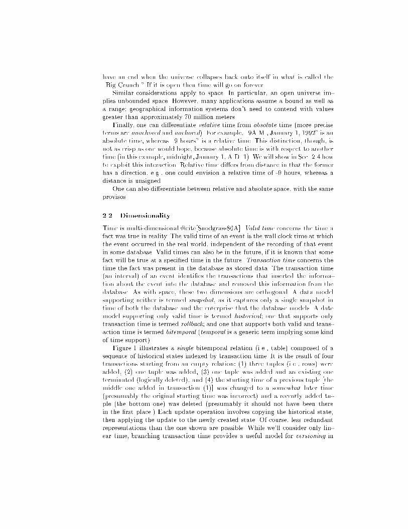
have an end when the universe collapses back onto itself in what is called the\Big Crunch." If it is open then time will go on forever.Similar considerations apply to space. In particular, an open universe im-plies unbounded space. However, many applications assume a bound as well asa range; geographical information systems don't need to contend with valuesgreater than approximately 70 million meters.Finally, one can di�erentiate relative time from absolute time (more preciseterms are unachored and anchored). For example, \9A.M., January 1, 1992" is anabsolute time, whereas \9 hours" is a relative time. This distinction, though, isnot as crisp as one would hope, because absolute time is with respect to anothertime (in this example, midnight, January 1, A.D. 1). We will show in Sec. 2.4 howto exploit this interaction. Relative time di�ers from distance in that the formerhas a direction, e.g., one could envision a relative time of -9 hours, whereas adistance is unsigned.One can also di�erentiate between relative and absolute space, with the sameprovisos.2.2 DimensionalityTime is multi-dimensional @cite[Snodgrass86A]. Valid time concerns the time afact was true in reality. The valid time of an event is the wall clock time at whichthe event occurred in the real world, independent of the recording of that eventin some database. Valid times can also be in the future, if it is known that somefact will be true at a speci�ed time in the future. Transaction time concerns thetime the fact was present in the database as stored data. The transaction time(an interval) of an event identi�es the transactions that inserted the informa-tion about the event into the database and removed this information from thedatabase. As with space, these two dimensions are orthogonal. A data modelsupporting neither is termed snapshot, as it captures only a single snapshot intime of both the database and the enterprise that the database models. A datemodel supporting only valid time is termed historical; one that supports onlytransaction time is termed rollback; and one that supports both valid and trans-action time is termed bitemporal (temporal is a generic term implying some kindof time support).Figure 1 illustrates a single bitemporal relation (i.e., table) composed of asequence of historical states indexed by transaction time. It is the result of fourtransactions starting from an empty relation: (1) three tuples (i.e., rows) wereadded, (2) one tuple was added, (3) one tuple was added and an existing oneterminated (logically deleted), and (4) the starting time of a previous tuple [themiddle one added in transaction (1)] was changed to a somewhat later time(presumably the original starting time was incorrect) and a recently added tu-ple (the bottom one) was deleted (presumably it should not have been therein the �rst place.) Each update operation involves copying the historical state,then applying the update to the newly created state. Of course, less redundantrepresentations than the one shown are possible. While we'll consider only lin-ear time, branching transaction time provides a useful model for versioning in

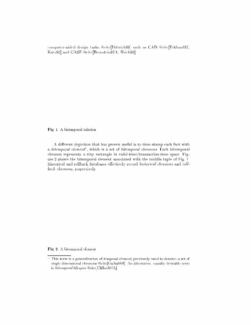
computer-aided design tasks @cite[Dittrich88] such as CAD @cite[Ecklund87,Katz86] and CASE @cite[Bernstein87A, Hsieh89].Fig. 1. A bitemporal relationA di�erent depiction that has proven useful is to time-stamp each fact witha bitemporal element1, which is a set of bitemporal chronons. Each bitemporalchronon represents a tiny rectangle in valid-time/transaction-time space. Fig-ure 2 shows the bitemporal element associated with the middle tuple of Fig. 1.Historical and rollback databases e�ectively record historical chronons and roll-back chronons, respectively.Fig. 2. A bitemporal element1 This term is a generalization of temporal element, previously used to denotes a set ofsingle dimensional chronons @cite[Gadia88B]. An alternative, equally desirable termis bitemporal lifespan @cite[Cli�ord87A].

While valid time may be bounded or unbounded (as we saw, cosmologistsfeel that it is at least bounded in the past), transaction time is bounded on bothends. Speci�cally, transaction time starts when the database is created (beforewhich time, nothing was stored), and doesn't extend past now (no facts areknown to have been stored in the future). Changes to the database state arerequired to be stamped with the current transaction time. Hence, rollback andbitemporal relations are append-only, making them prime candidates for storageon write-once optical disks. As the database state evolves, transaction times growmonotonically. In contrast, successive transactions may mention widely varyingvalid times. For instance, the fourth transaction in Fig. 1 added information tothe database that was transaction time-stamped with time 4, while changing avalid time of one of the tuples to 2.The three dimensions in space are truly orthogonal and homogeneous, the oneexception being the special treatment sometimes accorded elevation. In contrast,the two time dimensions are not homogeneous; transaction time has a di�erentsemantics than valid time. Valid and transaction time are orthogonal, thoughthere are generally some application dependent correlations between the twotimes. As a simple example, consider the situation where a fact is recorded assoon as it becomes valid in reality. In such a specialized bitemporal database,termed degenerate @cite[Jensen92], valid and transaction time are identical. Asanother example, if a cloud cover measurement is recorded at most two days afterit was valid in reality, and if it takes at least six hours from the measurement timeto record the measurement, then such a relation is delayed strongly retroactivelybounded with bounds six hours and two days.Multiple transaction times may also be stored in the same relation, termedtemporal generalization @cite[Jensen92]. These times may also be related to eachother, or to the valid time, in various specialized ways. For example, a particularvalue for the re ectivity of a cloud over a point on the Earth may be recordedby an Earth Sensing Satellite at a particular time. Here, the valid time andtransaction time are correlated, and the satellite's database may be considered tobe a degenerate bitemporal database. Later, this data is sent to a ground stationand stored; the transaction time of the stored data will be di�erent from the validtime; this database may be classi�ed as a bounded retroactive database. Laterstill, the data from several ground stations are merged into a central database,storing the original valid time, the transaction time of the recording into thecentral database, and the inherited transaction time when the data was storedin the ground station database. All three times may be needed, for instance, ifdata massaging was done with algorithms that were being improved over time.Such multiple transaction time dimensions do not have a spatial analogue.2.3 IndeterminacyInformation that is historically indeterminate can be characterized as \don'tknow exactly when" information. This kind of information is prevalent; it arisesin various situations, including the following.

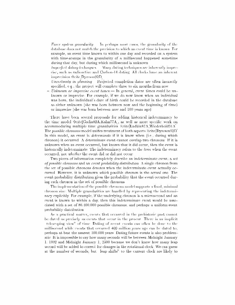
{ Finer system granularity | In perhaps most cases, the granularity of thedatabase does not match the precision to which an event time is known. Forexample, an event time known to within one day and recorded on a systemwith time-stamps in the granularity of a millisecond happened sometimeduring that day, but during which millisecond is unknown.{ Imperfect dating techniques |Many dating techniques are inherently impre-cise, such as radioactive and Carbon-14 dating. All clocks have an inherentimprecision @cite[Dyreson92D].{ Uncertainty in planning { Projected completion dates are often inexactlyspeci�ed, e.g., the project will complete three to six months from now.{ Unknown or imprecise event times | In general, event times could be un-known or imprecise. For example, if we do now know when an individualwas born, the individual's date of birth could be recorded in the databaseas either unknown (she was born between now and the beginning of time)or imprecise (she was born between now and 100 years ago).There have been several proposals for adding historical indeterminacy tothe time model @cite[Gadia92A,Kahn77A], as well as more speci�c work onaccommodating multiple time granularities @cite[Ladkin87A,Wiederhold91A].The possible chrononsmodel uni�es treatment of both aspects @cite[Dyreson92D].In this model, an event is determinate if it is know when (i.e., during whichchronon) it occurred. A determinate event cannot overlap two chronons. If it isunknown when an event occurred, but known that it did occur, then the event ishistorically indeterminate. The indeterminacy refers to the time when the eventoccurred, not whether the event did or did not occur.Two pieces of information completely describe an indeterminate event: a setof possible chronons and an event probability distribution. A single chronon fromthe set of possible chronons denotes when the indeterminate event actually oc-curred. However, it is unknown which possible chronon is the actual one. Theevent probability distribution gives the probability that the event occurred dur-ing each chronon in the set of possible chronons.The implementation of the possible chronons model supports a �xed, minimalchronon size. Multiple granularities are handled by representing the indetermi-nacy explicitly. For example, if the underlying chronon is a microsecond and anevent is known to within a day, then this indeterminate event would be asso-ciated with a set of 86,400,000 possible chronons, and perhaps a uniform eventprobability distribution.As a practical matter, events that occurred in the prehistoric past cannotbe dated as precisely as events that occur in the present. There is an implicit\telescoping view" of time. Dating of recent events can often be done to themillisecond while events that occurred 400 million years ago can be dated to,perhaps at best the nearest 100,000 years. Dating future events is also problem-atic. It is impossible to say how many seconds will be between Midnight January1, 1992 and Midnight January 1, 2300 because we don't know how many leapsecond will be added to correct for changes in the rotational clock. We can guessat the number of seconds, but \leap shifts" to the current clock are likely to

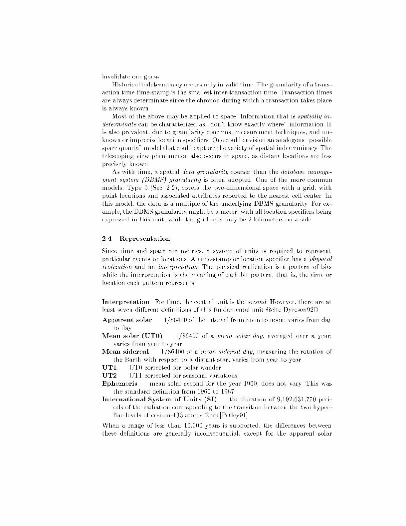
invalidate our guess.Historical indeterminacy occurs only in valid time. The granularity of a trans-action time time-stamp is the smallest inter-transaction time. Transaction timesare always determinate since the chronon during which a transaction takes placeis always known.Most of the above may be applied to space. Information that is spatially in-determinate can be characterized as \don't know exactly where" information. Itis also prevalent, due to granularity concerns, measurement techniques, and un-known or imprecise location speci�ers. One could envision an analogous \possiblespace quanta" model that could capture the variety of spatial indeterminacy. Thetelescoping view phenomenon also occurs in space, as distant locations are lessprecisely known.As with time, a spatial data granularity coarser than the database manage-ment system (DBMS) granularity is often adopted. One of the more commonmodels, Type 0 (Sec. 2.2), covers the two-dimensional space with a grid, withpoint locations and associated attributes reported to the nearest cell center. Inthis model, the data is a multiple of the underlying DBMS granularity. For ex-ample, the DBMS granularity might be a meter, with all location speci�ers beingexpressed in this unit, while the grid cells may be 2 kilometers on a side.2.4 RepresentationSince time and space are metrics, a system of units is required to representparticular events or locations. A time-stamp or location speci�er has a physicalrealization and an interpretation. The physical realization is a pattern of bitswhile the interpretation is the meaning of each bit pattern, that is, the time orlocation each pattern represents.Interpretation. For time, the central unit is the second. However, there are atleast seven di�erent de�nitions of this fundamental unit @cite[Dyreson92D].Apparent solar | 1=86400 of the interval from noon to noon; varies from dayto day.Mean solar (UT0) | 1=86400 of a mean solar day, averaged over a year;varies from year to year.Mean sidereal | 1=86400 of a mean sidereal day, measuring the rotation ofthe Earth with respect to a distant star; varies from year to year.UT1 | UT0 corrected for polar wander.UT2 | UT1 corrected for seasonal variations.Ephemeris | mean solar second for the year 1900; does not vary. This wasthe standard de�nition from 1960 to 1967.International System of Units (SI) | the duration of 9,192,631,770 peri-ods of the radiation corresponding to the transition between the two hyper-�ne levels of cesium-133 atoms @cite[Petley91].When a range of less than 10,000 years is supported, the di�erences betweenthese de�nitions are generally inconsequential, except for the apparent solar

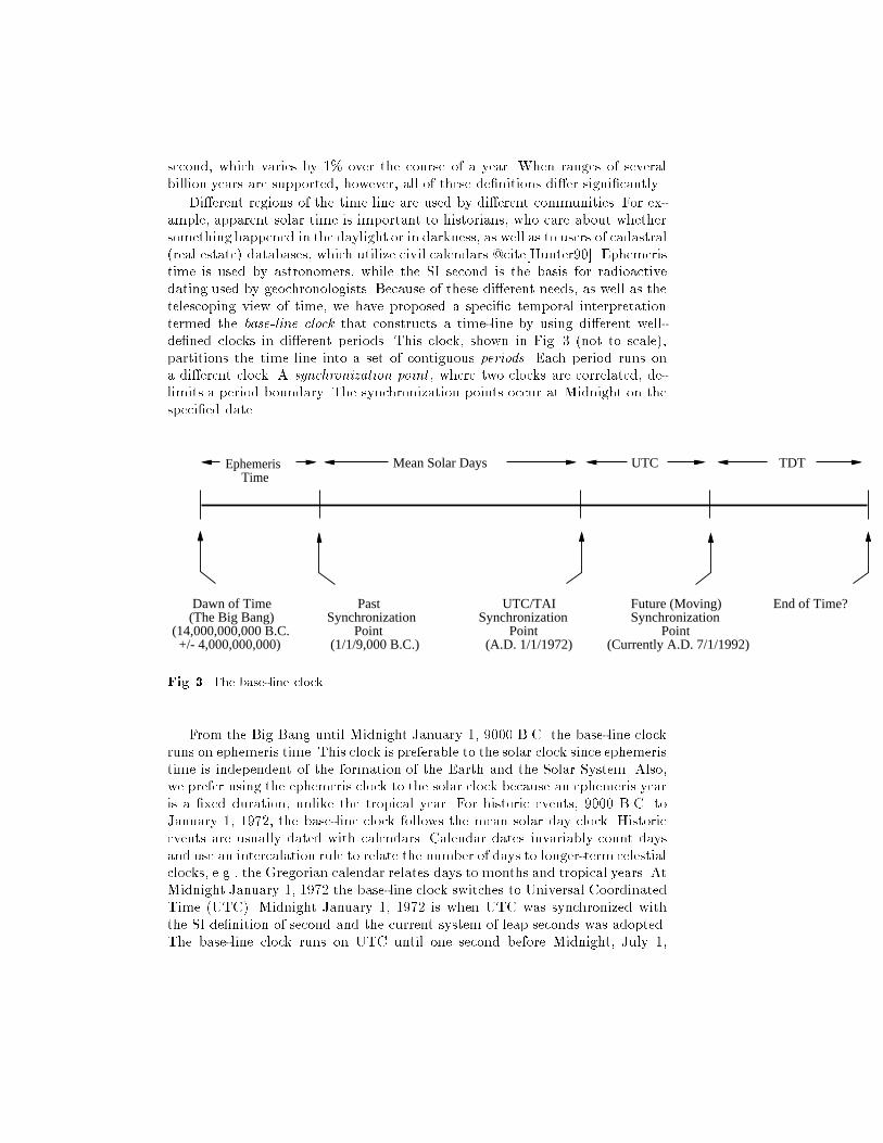
second, which varies by 1% over the course of a year. When ranges of severalbillion years are supported, however, all of these de�nitions di�er signi�cantly.Di�erent regions of the time line are used by di�erent communities. For ex-ample, apparent solar time is important to historians, who care about whethersomething happened in the daylight or in darkness, as well as to users of cadastral(real estate) databases, which utilize civil calendars @cite[Hunter90]. Ephemeristime is used by astronomers, while the SI second is the basis for radioactivedating used by geochronologists. Because of these di�erent needs, as well as thetelescoping view of time, we have proposed a speci�c temporal interpretationtermed the base-line clock that constructs a time-line by using di�erent well-de�ned clocks in di�erent periods. This clock, shown in Fig. 3 (not to scale),partitions the time line into a set of contiguous periods. Each period runs ona di�erent clock. A synchronization point , where two clocks are correlated, de-limits a period boundary. The synchronization points occur at Midnight on thespeci�ed date. Dawn of Time (The Big Bang)(14,000,000,000 B.C. +/- 4,000,000,000)

Past Synchronization Point (1/1/9,000 B.C.)

UTC/TAI Synchronization Point (A.D. 1/1/1972)

Future (Moving) Synchronization Point(Currently A.D. 7/1/1992)

End of Time?

Ephemeris Time

Mean Solar Days UTC TDT

Fig. 3. The base-line clockFrom the Big Bang until Midnight January 1, 9000 B.C. the base-line clockruns on ephemeris time. This clock is preferable to the solar clock since ephemeristime is independent of the formation of the Earth and the Solar System. Also,we prefer using the ephemeris clock to the solar clock because an ephemeris yearis a �xed duration, unlike the tropical year. For historic events, 9000 B.C. toJanuary 1, 1972, the base-line clock follows the mean solar day clock. Historicevents are usually dated with calendars. Calendar dates invariably count daysand use an intercalation rule to relate the number of days to longer-term celestialclocks, e.g., the Gregorian calendar relates days to months and tropical years. AtMidnight January 1, 1972 the base-line clock switches to Universal CoordinatedTime (UTC). Midnight January 1, 1972 is when UTC was synchronized withthe SI de�nition of second and the current system of leap seconds was adopted.The base-line clock runs on UTC until one second before Midnight, July 1,

1992. This is the next time at which a leap second may be added (a leap secondwill be added on this date according to the latest International Earth RotationService bulletin @cite[USNO92]). After Midnight July 1, 1992, until the \BigCrunch" or the end of our base-line clock, the base-line clock follows TerrestrialDynamic Time (TDT), an \idealized atomic time" @cite[Guinot88] based on theSI second, since both UTC and mean solar time are unknown and unpredictable.The situation is much simpler for space. Here, the (SI) meter is the com-monly accepted unit, with a single accepted de�nition, the length of the pathtraveled by light in vacuum during a time interval of 1/299,792,458 of a second@cite[Petley91]. Distance is de�ned in terms of time, rather than the other wayaround, because time can be measured more accurately (1 part in 1010 over longintervals and 1 part in 1015 for between a minute and a day @cite[Quinn91,Ramsey91C]).The base-line clock and its representation are independent of any calendar.We used Gregorian calendar dates in the above discussion only to provide aninformal indication of when the synchronization points occurred. Many calendarsystems are in use today; example calendars include academic (years consists ofsemesters), common �scal (�nancial year beginning at the New Year), federal�scal (�nancial year beginning the �rst of October) and time card (8 hour daysand 5 day weeks, year-round). The usage of a calendar depends on the cultural,legal, and even business orientation of the user @cite[Soo92]. A DBMS attempt-ing to support time values must be capable of supporting all the multiple notionsof time that are of interest to the user population.Space also has multiple notions, though with less variability. The metric,U.S., and nautical unit systems are the most prevalent. Both time and spacehave precisely de�ned underlying semantics that may be mapped to multipledisplay formats. The spatial base-line is less complex than that for time; itconsists of a single measure, the meter.Physical Realization. The base-line clock de�nes the meaning of each time-stamp bit pattern in the physical realization of a time-stamp. The chronons ofthe base-line clock are the chronons in its constituent clocks. We assume thateach chronon is one second in the underlying constituent clock. A chronon maybe denoted by an integer, corresponding to a single (DBMS) granularity, or itmay be denoted by a sequence of integers, corresponding to a nested granularity.For example, if we assume a granularity of a second relative to Midnight, January1, 1980, then in a single granularity the integer 164,281,022 denotes 9:37:02AMMarch 15, 1985. If we assume a nested granularity of hyear, month, day, hour,minute, secondi, then the sequence h6,3,15,9,37,2i denotes that same time.Various time-stamps are in use in commercial database management sys-tems and operating systems; a summary is provided in Table 1. This table com-pares formats from operating systems (speci�cally Unix, MSDOS, and the Mac-Intosh operating systems), the database systems DB2 @cite[Date90B], SQL2@cite[Date89A,Melton90], and several proposed formats to be discussed shortly.The SQL2 datetime time-stamp appears twice in the comparison, once with itsoptional fractional second precision �eld set to microseconds, and once without

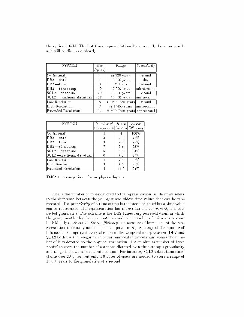
the optional �eld. The last three representations have recently been proposed,and will be discussed shortly.SYSTEM Size Range Granularity(bytes)OS (several) 4 � 136 years secondDB2 |date 4 10,000 years dayDB2 |time 3 24 hours secondDB2 |timestamp 10 10,000 years microsecondSQL2 |datetime 20 10,000 years secondSQL2 |fractional datetime 27 10,000 years microsecondLow Resolution 8 � 36 billion years secondHigh Resolution 8 � 17400 years microsecondExtended Resolution 12 � 36 billion years nanosecondSYSTEM Number of Bytes SpaceComponents Needed E�ciencyOS (several) 1 4 100%DB2 |date 3 2.9 71%DB2 |time 3 2.2 72%DB2 |timestamp 7 7.3 73%SQL2 |datetime 5 4.8 24%SQL2 |fractional datetime 6 7.3 27%Low Resolution 1 7.6 95%High Resolution 3 7.5 93%Extended Resolution 4 11.3 94%Table 1. A comparison of some physical layoutsSize is the number of bytes devoted to the representation, while range refersto the di�erence between the youngest and oldest time values that can be rep-resented. The granularity of a time-stamp is the precision to which a time valuecan be represented. If a representation has more than one component, it is of anested granularity. The extreme is the DB2 timestamp representation, in whichthe year, month, day, hour, minute, second, and number of microseconds areindividually represented. Space e�ciency is a measure of how much of the rep-resentation is actually needed. It is computed as a percentage of the number ofbits needed to represent every chronon in the temporal interpretation (DB2 andSQL2 both use the Gregorian calendar temporal interpretation) versus the num-ber of bits devoted to the physical realization. The minimum number of bytesneeded to store the number of chronons dictated by a time-stamp's granularityand range is shown as a separate column. For instance, SQL2's datetime time-stamp uses 20 bytes, but only 4.8 bytes of space are needed to store a range of10,000 years to the granularity of a second.

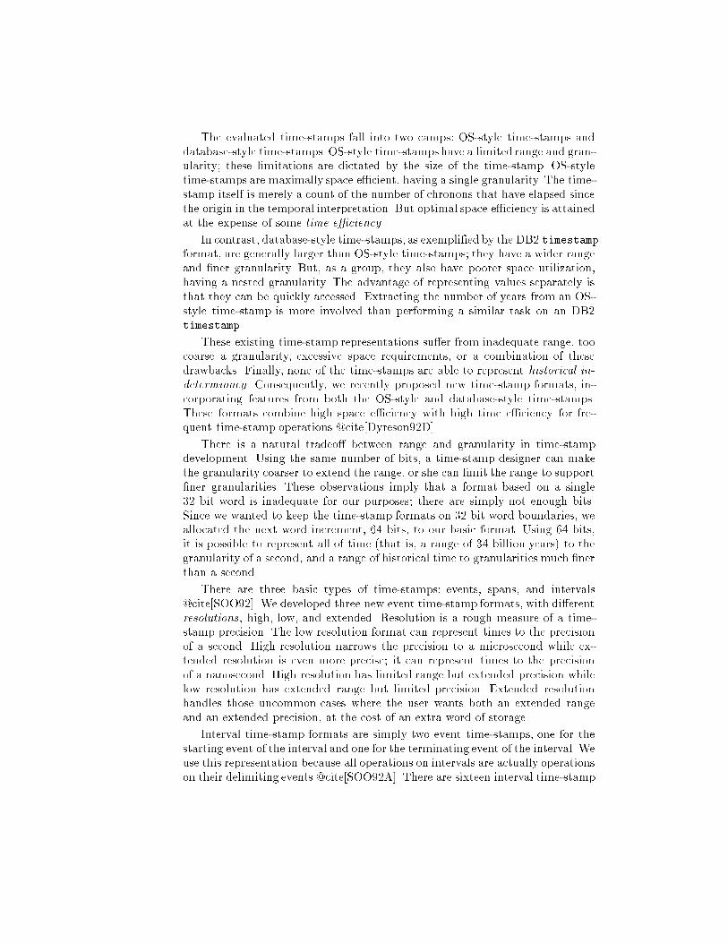
The evaluated time-stamps fall into two camps: OS-style time-stamps anddatabase-style time-stamps.OS-style time-stamps have a limited range and gran-ularity; these limitations are dictated by the size of the time-stamp. OS-styletime-stamps are maximally space e�cient, having a single granularity. The time-stamp itself is merely a count of the number of chronons that have elapsed sincethe origin in the temporal interpretation. But optimal space e�ciency is attainedat the expense of some time e�ciency .In contrast, database-style time-stamps, as exempli�ed by the DB2 timestampformat, are generally larger than OS-style time-stamps; they have a wider rangeand �ner granularity. But, as a group, they also have poorer space utilization,having a nested granularity. The advantage of representing values separately isthat they can be quickly accessed. Extracting the number of years from an OS-style time-stamp is more involved than performing a similar task on an DB2timestamp.These existing time-stamp representations su�er from inadequate range, toocoarse a granularity, excessive space requirements, or a combination of thesedrawbacks. Finally, none of the time-stamps are able to represent historical in-determinacy . Consequently, we recently proposed new time-stamp formats, in-corporating features from both the OS-style and database-style time-stamps.These formats combine high space e�ciency with high time e�ciency for fre-quent time-stamp operations @cite[Dyreson92D].There is a natural tradeo� between range and granularity in time-stampdevelopment. Using the same number of bits, a time-stamp designer can makethe granularity coarser to extend the range, or she can limit the range to support�ner granularities. These observations imply that a format based on a single32 bit word is inadequate for our purposes; there are simply not enough bits.Since we wanted to keep the time-stamp formats on 32 bit word boundaries, weallocated the next word increment, 64 bits, to our basic format. Using 64 bits,it is possible to represent all of time (that is, a range of 34 billion years) to thegranularity of a second, and a range of historical time to granularities much �nerthan a second.There are three basic types of time-stamps: events, spans, and intervals@cite[SOO92]. We developed three new event time-stamp formats, with di�erentresolutions, high, low, and extended. Resolution is a rough measure of a time-stamp precision. The low resolution format can represent times to the precisionof a second. High resolution narrows the precision to a microsecond while ex-tended resolution is even more precise; it can represent times to the precisionof a nanosecond. High resolution has limited range but extended precision whilelow resolution has extended range but limited precision. Extended resolutionhandles those uncommon cases where the user wants both an extended rangeand an extended precision, at the cost of an extra word of storage.Interval time-stamp formats are simply two event time-stamps, one for thestarting event of the interval and one for the terminating event of the interval. Weuse this representation because all operations on intervals are actually operationson their delimiting events @cite[SOO92A]. There are sixteen interval time-stamp

formats in toto. The type �elds in the delimiting event time-stamps distinguisheach format.Spans are relative times. There are two kinds of spans, �xed and variable@cite[SOO92]. A �xed span is a count of chronons. It represents a �xed duration(in terms of chronons) on the base-line clock between two time values. The�xed span formats use exactly the same layouts as the standard event formats,with a di�erent interpretation. The chronon count in the span representationis independent of the origin, instead of being interpreted as a count from theorigin. The sign bit indicates whether the span is positive or negative ratherthan indicating the direction from the origin.A variable span's duration is dependent on an associated event. A commonvariable span is a month. The duration represented by a month depends onwhether that month is associated with an event in June (30 days) or in July(31 days), or even in February (28 or 29 days). Variable spans use a specializedformat requiring 64 bits.To represent indeterminate events, we added nine formats, three of eachresolution. There are three analogous formats for low resolution, and three forextended resolution. The most common, for high resolution with a uniform dis-tribution, requires only 64 bits.As we have seen in other areas, the considerations for space are similar, yetconsiderably simpler. A spatial representation of 32 bits (per dimension) for arange required to map the Earth results in a granularity of one decimeter, andof one centimeter for the third dimension (the atmosphere, the oceans, and theEarth's interior) or for restricted areas such as the United States or Europe.Moving up to 64 bits makes spatial indeterminacy representations feasible, andreduces the granularity to a nanometer, which should be adequate for quite awhile.3 Associating Facts with TimeThe previous section explored models and representations for the time domain.We now turn to associating time with facts.3.1 Underlying Data ModelTime has been added to many data models: the entity-relationshipmodel @cite[DeAntonellis79,Klopprogge81],semantic data models @cite[Hammer81,Urban86], knowledge-based data models@cite[Dayal86A], deductive databases @cite[Chomicki88,Chomicki89A,Chomicki90,Kabanza90],and object-oriented models @cite[Dayal92,Manola86A,Narasimhalu88,Rose91,Sciore91,Sciore91A,Wuu92].However, by far the majority of work in temporal databases is based on the re-lational model. For this reason, we will assume this data model in subsequentdiscussion.

3.2 Attribute VariabilityThere are several basic ways in which an attribute associated with an objectcan interact with time and space. A time-invariant attribute @cite[Navathe89]does not change over time. Some temporal data models require that the keyof a relation be time-invariant; some others identify the object(s) participat-ing in the relation with a time-invariant surrogate, a system-generated, uniqueidenti�er of an item that can be referenced and compared for equality, but notdisplayed to the user @cite[Hall76]. Secondly, the value of an attribute may bedrawn from a temporal domain. An example is date stamping, where cadastralparcel records in a land information system contain �elds that note the datesof registration of deeds, transfers of titles, and other pertinent historical in-formation @cite[Vrana89]. Such temporal domains are termed user-de�ned time@cite[Snodgrass86A]; other than being able to be read in, displayed, and perhapscompared, no special semantics is associated with such domains. Interestingly,most such attributes are time-invariant. For example, the transfer date for aparticular title transfer is valid over all time.An analogous sitation exists for space. There are space-invariant attributesas well as attributes that are drawn from spatial domains, an example beingan attribute recording the square feet of a residence, which is a relative spatialmeasure in two dimensions.Time- and space-varying attributes are more interesting. There are �ve basiccases to consider.{ The value of an attribute associated with a space-invariant object may varyover time, termed attribute temporality @cite[Vrana89]. An example is per-centage of cloud cover over the Earth, which has a single value at each pointin time, but varies over time. The value is uniquely speci�ed by the temporalcoordinate(s) (either valid time, or a combination of valid and transactiontime).{ The value of an attribute associated with a region in space may be timeinvariant. An example is elevation: the value varies spatially but not tempo-rally (assuming historical time; certainly the elevation varies over geologictime!). The value is unique given spatial coordinates.{ The value of an attribute associated with a region in space may vary overtime. An example is the percentage of cloud cover over each 10-kilometersquare grid element. Here, the object is identi�ed spatially, and each objectis associated with a time-varying sequence of values. Both the temporal andthe spatial coordinates are required to uniquely identify a value.{ The boundary lines identifying a cadastral object, e.g., a particular landpacket, may vary over time, termed temporal topology @cite[Vrana89]. Theorientation and interaction of spatial objects change over time; such objectscould nevertheless have time-invariant attributes, such as initial purchaseprice. The temporal and spatial coordinates are required to uniquely identifya value, but this identi�cation is indirect, via the topology.{ The �nal case is the most complex: the value of an attribute, which variesover time, is associated with a cartographic feature that also varies over time

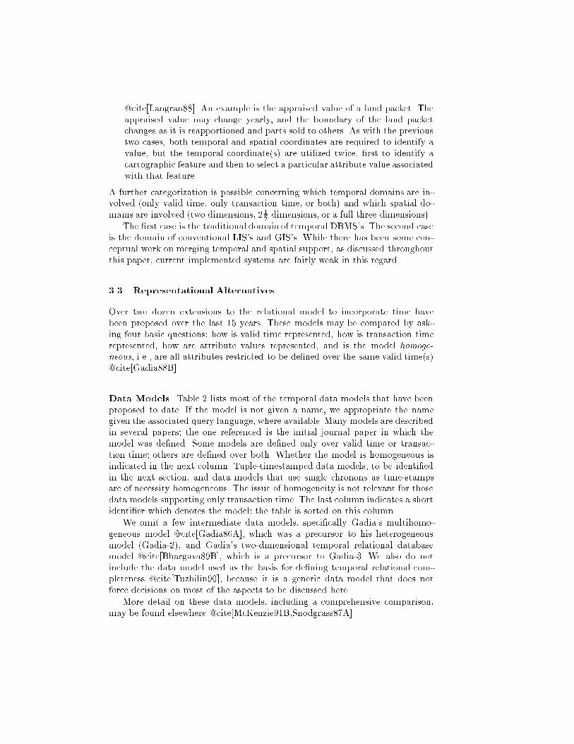
@cite[Langran88]. An example is the appraised value of a land packet. Theappraised value may change yearly, and the boundary of the land packetchanges as it is reapportioned and parts sold to others. As with the previoustwo cases, both temporal and spatial coordinates are required to identify avalue, but the temporal coordinate(s) are utilized twice, �rst to identify acartographic feature and then to select a particular attribute value associatedwith that feature.A further categorization is possible concerning which temporal domains are in-volved (only valid time, only transaction time, or both) and which spatial do-mains are involved (two dimensions, 212 dimensions, or a full three dimensions).The �rst case is the traditional domain of temporal DBMS's. The second caseis the domain of conventional LIS's and GIS's. While there has been some con-ceptual work on merging temporal and spatial support, as discussed throughoutthis paper, current implemented systems are fairly weak in this regard.3.3 Representational AlternativesOver two dozen extensions to the relational model to incorporate time havebeen proposed over the last 15 years. These models may be compared by ask-ing four basic questions: how is valid time represented, how is transaction timerepresented, how are attribute values represented, and is the model homoge-neous, i.e., are all attributes restricted to be de�ned over the same valid time(s)@cite[Gadia88B].Data Models. Table 2 lists most of the temporal data models that have beenproposed to date. If the model is not given a name, we appropriate the namegiven the associated query language, where available.Many models are describedin several papers; the one referenced is the initial journal paper in which themodel was de�ned. Some models are de�ned only over valid time or transac-tion time; others are de�ned over both. Whether the model is homogeneous isindicated in the next column. Tuple-timestamped data models, to be identi�edin the next section, and data models that use single chronons as time-stampsare of necessity homogeneous. The issue of homogeneity is not relevant for thosedata models supporting only transaction time. The last column indicates a shortidenti�er which denotes the model; the table is sorted on this column.We omit a few intermediate data models, speci�cally Gadia's multihomo-geneous model @cite[Gadia86A], which was a precursor to his heterogeneousmodel (Gadia-2), and Gadia's two-dimensional temporal relational databasemodel @cite[Bhargava89B], which is a precursor to Gadia-3. We also do notinclude the data model used as the basis for de�ning temporal relational com-pleteness @cite[Tuzhilin90], because it is a generic data model that does notforce decisions on most of the aspects to be discussed here.More detail on these data models, including a comprehensive comparison,may be found elsewhere @cite[McKenzie91B,Snodgrass87A].

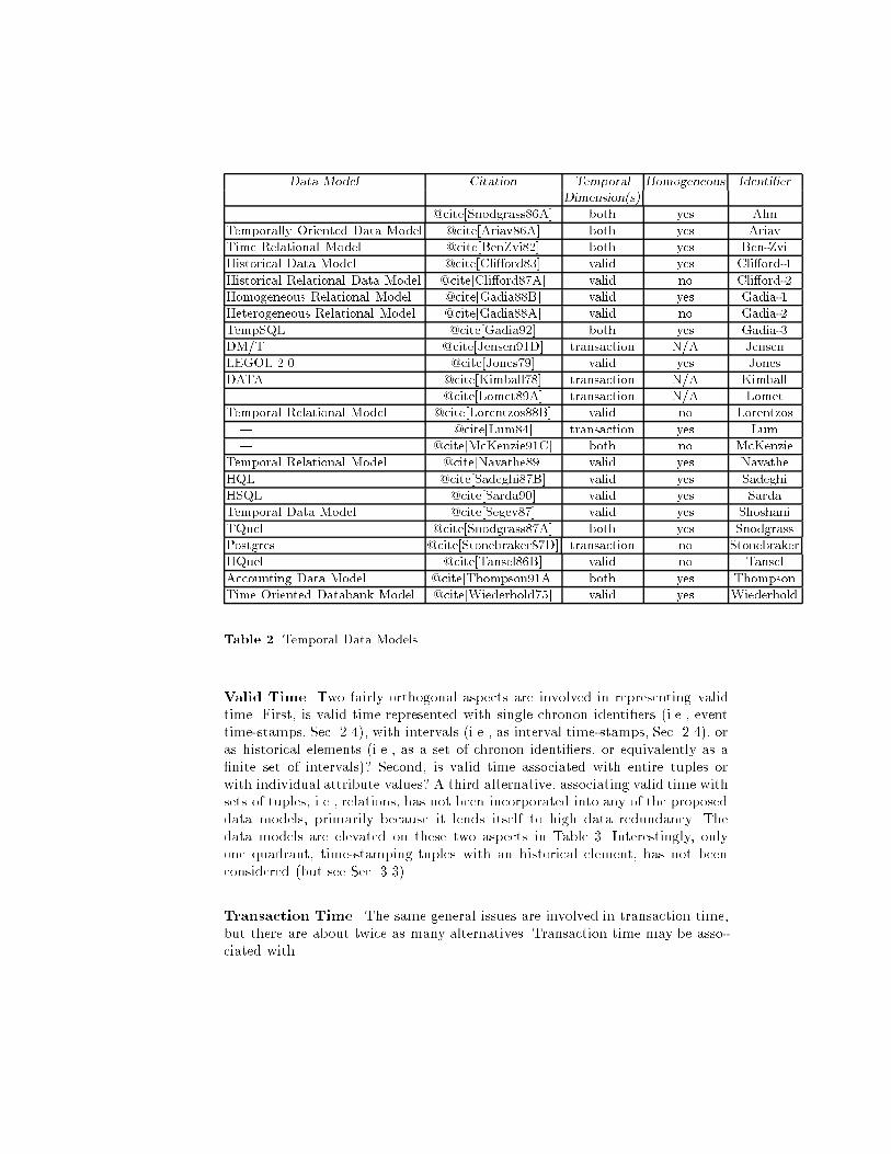
Data Model Citation Temporal Homogeneous Identi�erDimension(s)| @cite[Snodgrass86A] both yes AhnTemporally Oriented Data Model @cite[Ariav86A] both yes AriavTime Relational Model @cite[BenZvi82] both yes Ben-ZviHistorical Data Model @cite[Cli�ord83] valid yes Cli�ord-1Historical Relational Data Model @cite[Cli�ord87A] valid no Cli�ord-2Homogeneous Relational Model @cite[Gadia88B] valid yes Gadia-1Heterogeneous Relational Model @cite[Gadia88A] valid no Gadia-2TempSQL @cite[Gadia92] both yes Gadia-3DM/T @cite[Jensen91D] transaction N/A JensenLEGOL 2.0 @cite[Jones79] valid yes JonesDATA @cite[Kimball78] transaction N/A Kimball| @cite[Lomet89A] transaction N/A LometTemporal Relational Model @cite[Lorentzos88B] valid no Lorentzos| @cite[Lum84] transaction yes Lum| @cite[McKenzie91C] both no McKenzieTemporal Relational Model @cite[Navathe89] valid yes NavatheHQL @cite[Sadeghi87B] valid yes SadeghiHSQL @cite[Sarda90] valid yes SardaTemporal Data Model @cite[Segev87] valid yes ShoshaniTQuel @cite[Snodgrass87A] both yes SnodgrassPostgres @cite[Stonebraker87D] transaction no StonebrakerHQuel @cite[Tansel86B] valid no TanselAccounting Data Model @cite[Thompson91A] both yes ThompsonTime Oriented Databank Model @cite[Wiederhold75] valid yes WiederholdTable 2. Temporal Data ModelsValid Time. Two fairly orthogonal aspects are involved in representing validtime. First, is valid time represented with single chronon identi�ers (i.e., eventtime-stamps, Sec. 2.4), with intervals (i.e., as interval time-stamps, Sec. 2.4), oras historical elements (i.e., as a set of chronon identi�ers, or equivalently as a�nite set of intervals)? Second, is valid time associated with entire tuples orwith individual attribute values? A third alternative, associating valid time withsets of tuples, i.e., relations, has not been incorporated into any of the proposeddata models, primarily because it lends itself to high data redundancy. Thedata models are elevated on these two aspects in Table 3. Interestingly, onlyone quadrant, time-stamping tuples with an historical element, has not beenconsidered (but see Sec. 3.3)Transaction Time. The same general issues are involved in transaction time,but there are about twice as many alternatives. Transaction time may be asso-ciated with

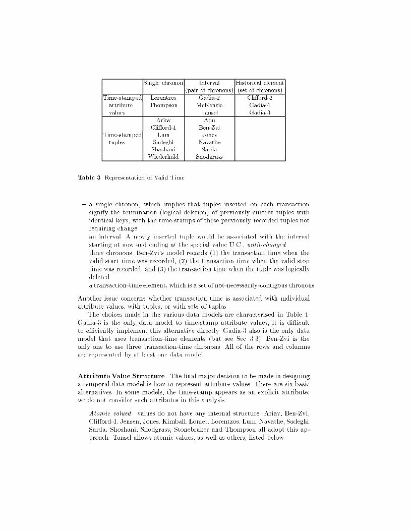
Single chronon Interval Historical element(pair of chronons) (set of chronons)Time-stamped Lorentzos Gadia-2 Cli�ord-2attribute Thompson McKenzie Gadia-1values Tansel Gadia-3Ariav AhnCli�ord-1 Ben-ZviTime-stamped Lum Jonestuples Sadeghi NavatheShoshani SardaWiederhold SnodgrassTable 3. Representation of Valid Time{ a single chronon, which implies that tuples inserted on each transactionsignify the termination (logical deletion) of previously current tuples withidentical keys, with the time-stamps of these previously recorded tuples notrequiring change.{ an interval. A newly inserted tuple would be associated with the intervalstarting at now and ending at the special value U.C., until-changed.{ three chronons. Ben-Zvi's model records (1) the transaction time when thevalid start time was recorded, (2) the transaction time when the valid stoptime was recorded, and (3) the transaction time when the tuple was logicallydeleted.{ a transaction-time element, which is a set of not-necessarily-contigous chronons.Another issue concerns whether transaction time is associated with individualattribute values, with tuples, or with sets of tuples.The choices made in the various data models are characterized in Table 4.Gadia-3 is the only data model to time-stamp attribute values; it is di�cultto e�ciently implement this alternative directly. Gadia-3 also is the only datamodel that uses transaction-time elements (but see Sec. 3.3). Ben-Zvi is theonly one to use three transaction-time chronons. All of the rows and columnsare represented by at least one data model.Attribute Value Structure. The �nal major decision to be made in designinga temporal data model is how to represent attribute values. There are six basicalternatives. In some models, the time-stamp appears as an explicit attribute;we do not consider such attributes in this analysis.{ Atomic valued|values do not have any internal structure. Ariav, Ben-Zvi,Cli�ord-1, Jensen, Jones, Kimball, Lomet, Lorentzos, Lum, Navathe, Sadeghi,Sarda, Shoshani, Snodgrass, Stonebraker and Thompson all adopt this ap-proach. Tansel allows atomic values, as well as others, listed below.

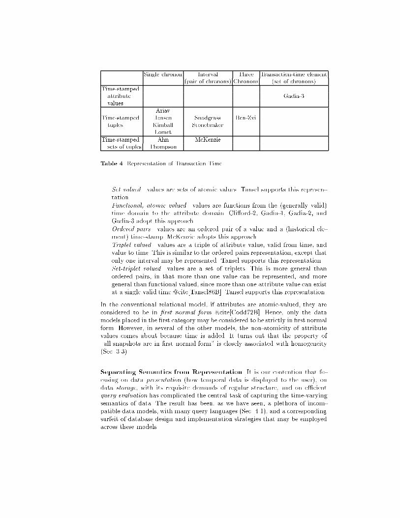
Single chronon Interval Three Transaction-time element(pair of chronons) Chronons (set of chronons)Time-stampedattribute Gadia-3values AriavTime-stamped Jensen Snodgrass Ben-Zvituples Kimball StonebrakerLometTime-stamped Ahn McKenziesets of tuples ThompsonTable 4. Representation of Transaction Time{ Set valued|values are sets of atomic values. Tansel supports this represen-tation.{ Functional, atomic valued|values are functions from the (generally valid)time domain to the attribute domain. Cli�ord-2, Gadia-1, Gadia-2, andGadia-3 adopt this approach.{ Ordered pairs|values are an ordered pair of a value and a (historical ele-ment) time-stamp. McKenzie adopts this approach.{ Triplet valued|values are a triple of attribute value, valid from time, andvalue to time. This is similar to the ordered pairs representation, except thatonly one interval may be represented. Tansel supports this representation.{ Set-triplet valued|values are a set of triplets. This is more general thanordered pairs, in that more than one value can be represented, and moregeneral than functional valued, since more than one attribute value can existat a single valid time @cite[Tansel86B]. Tansel supports this representation.In the conventional relational model, if attributes are atomic-valued, they areconsidered to be in �rst normal form @cite[Codd72B]. Hence, only the datamodels placed in the �rst category may be considered to be strictly in �rst normalform. However, in several of the other models, the non-atomicity of attributevalues comes about because time is added. It turns out that the property of\all snapshots are in �rst normal form" is closely associated with homogeneity(Sec. 3.3).Separating Semantics from Representation. It is our contention that fo-cusing on data presentation (how temporal data is displayed to the user), ondata storage, with its requisite demands of regular structure, and on e�cientquery evaluation has complicated the central task of capturing the time-varyingsemantics of data. The result has been, as we have seen, a plethora of incom-patible data models, with many query languages (Sec. 4.1), and a correspondingsurfeit of database design and implementation strategies that may be employedacross these models.

We advocate instead a very simple conceptual temporal data model thatcaptures the essential semantics of time-varying relations, but has no illusionsof being suitable for presentation, storage, or query evaluation. Existing datamodel(s) may be used for these latter tasks. This conceptual model time-stampstuples with bitemporal elements, sets of bitemporal chronons, which are rectan-gles in the two-dimensional space spanned by valid time and transaction time(see Fig. 2). Because no two tuples with mutually identical explicit attributevalues (termed value-equivalent tuples) are allowed in a bitemporal relation in-stance, the full time history of a fact is contained in a single tuple.In Table 3, the conceptual temporal data model occupies the un�lled entrycorresponding to time-stamping tuples with historical elements, and occupiesthe entry in Table 4 corresponding to time-stamping tuples with transaction-time elements. An important property of the conceptual model, shared with theconventional relational model but not held by the representational models, isthat relation instances are semantically unique; distinct instances model di�erentrealities and thus have distinct semantics.It is possible to demonstrate equivalence mappings between the conceptualmodel and several representational models @cite[Jensen92A]. Mappings havealready been demonstrated for three data models: Gadia-3 (attribute time-stamping), Jensen (tuple time-stamping with a single transaction chronon), andSnodgrass (tuple time-stamping, with interval valid and transaction times). Thisequivalence is based on snapshot equivalence, which says that two relation in-stances are equivalent if all their snapshots, taken at all times (valid and transac-tion), are identical. Snapshot equivalence provides a natural means of comparingrather disparate representations. An extension to the conventional relational al-gebraic operators may be de�ned in the conceptual data model, and can bemapped to analogous operators in the representational models. Finally, we feelthat the conceptual data model is the appropriate location for database designand query optimization.In essence, we advocate moving the distinction between the various existingtemporal data models from a semantic basis to a physical, performance-relevantbasis, utilizing the proposed conceptual data model to capture the time-varyingsemantics. Data presentation, storage representation, and time-varying seman-tics should be considered in isolation, utilizing di�erent data models. Semantics,speci�cally as determined by logical database design, should be expressed in theconceptual model. Multiple presentation formats should be available, as di�erentapplications require di�erent ways of viewing the data. The storage and process-ing of bitemporal relations should be done in a data model that emphasizese�ciency.4 QueryingA data model consists of a set of objects with some structure, a set of constraintson those objects, and a set of operations on those objects @cite[Tsichritzis82]. Inthe two previous sectins we have investigated in detail the structure of and con-

straints on the objects of temporal relational databases, the temporal relation.In this section, we complete the picture by discussing the operations, speci�callytemporal query languages.Many temporal query languages have been proposed. In fact, it seems oblig-atory for each researcher to de�ne their own data model and query language (wereturn to this issue at the end of this section). We �rst summarize the twenty-odd query languages that have been proposed thus far. We then brie y discussthe various activities that should be supported by a temporal query language,using a speci�c language in the examples. Finally, we touch on work being donein the standards arena that is attempting to bring highly needed order to thisconfusing collection of languages.We do not consider the related topic of temporal reasoning (also termed infer-encing or rule-based search) @cite[Chomicki90,Kahn77A,Karlsson86A,Lee85,Sheng84,Sripada88]that uses arti�cial intelligence techniques to performmore sophisticated analysesof temporal relationships, generally with much lower query processing e�ciency.4.1 Language ProposalsTable 5 lists the major temporal query language proposals to date. While manyof these languages each have several associated papers, we have indicated themost comprehensive or most readily available reference. The underlying datamodel is a reference to Table 2. The next column lists the conventional querylanguage the temporal proposal is based on, from the following.SQL Structured Query Language @cite[Date89B], a tuple calculus-based lan-guage; the lingua franca of conventional relational databases.Quel The tuple calculus based query language @cite[Held75] originally de�nedfor the Ingres relational DBMS @cite[Stonebraker76A].QBE Query-by-Example @cite[Zloof75], a domain calculus based query lan-guage.ILs An intensional logic formulated in the context of computational linguistics@cite[Montague73].relational algebra A procedural language with relations as objects @cite[Codd72].DEAL An extension of the relational algebra incorporating functions, recursion,and deduction @cite[Deen85].Most of the query languages have a formal de�nition. Some of the calculus-basedquery languages have an associated algebra that provides a means of evaluatingqueries.More comprehensive comparisonsmay be found elsewhere @cite[McKenzie91B,Snodgrass87A].4.2 Types of Temporal QueriesWe now examine the types of temporal queries that each of the above-listed querylanguages support to varying degrees. We'll use TQuel @cite[Snodgrass93A] inthe examples, as it is the most completely de�ned temporal language @cite[Snodgrass87A].

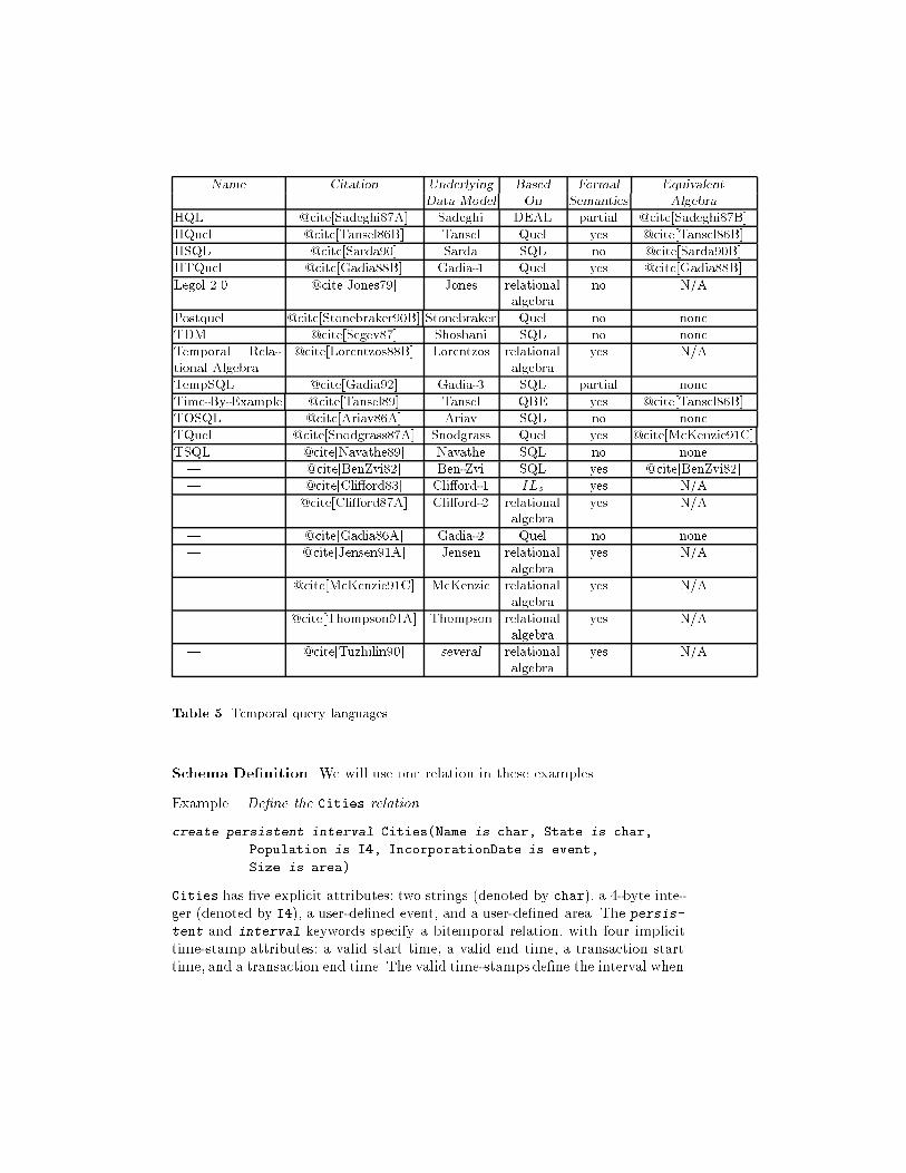
Name Citation Underlying Based Formal EquivalentData Model On Semantics AlgebraHQL @cite[Sadeghi87A] Sadeghi DEAL partial @cite[Sadeghi87B]HQuel @cite[Tansel86B] Tansel Quel yes @cite[Tansel86B]HSQL @cite[Sarda90] Sarda SQL no @cite[Sarda90B]HTQuel @cite[Gadia88B] Gadia-1 Quel yes @cite[Gadia88B]Legol 2.0 @cite[Jones79] Jones relationalalgebra no N/APostquel @cite[Stonebraker90B] Stonebraker Quel no noneTDM @cite[Segev87] Shoshani SQL no noneTemporal Rela-tional Algebra @cite[Lorentzos88B] Lorentzos relationalalgebra yes N/ATempSQL @cite[Gadia92] Gadia-3 SQL partial noneTime-By-Example @cite[Tansel89] Tansel QBE yes @cite[Tansel86B]TOSQL @cite[Ariav86A] Ariav SQL no noneTQuel @cite[Snodgrass87A] Snodgrass Quel yes @cite[McKenzie91C]TSQL @cite[Navathe89] Navathe SQL no none| @cite[BenZvi82] Ben-Zvi SQL yes @cite[BenZvi82]| @cite[Cli�ord83] Cli�ord-1 ILs yes N/A| @cite[Cli�ord87A] Cli�ord-2 relationalalgebra yes N/A| @cite[Gadia86A] Gadia-2 Quel no none| @cite[Jensen91A] Jensen relationalalgebra yes N/A| @cite[McKenzie91C] McKenzie relationalalgebra yes N/A| @cite[Thompson91A] Thompson relationalalgebra yes N/A| @cite[Tuzhilin90] several relationalalgebra yes N/ATable 5. Temporal query languagesSchema De�nition. We will use one relation in these examples.Example. De�ne the Cities relation.create persistent interval Cities(Name is char, State is char,Population is I4, IncorporationDate is event,Size is area)Cities has �ve explicit attributes: two strings (denoted by char), a 4-byte inte-ger (denoted by I4), a user-de�ned event, and a user-de�ned area. The persis-tent and interval keywords specify a bitemporal relation, with four implicittime-stamp attributes: a valid start time, a valid end time, a transaction starttime, and a transaction end time. The valid time-stamps de�ne the interval when

the attribute values were true in reality, and the transaction time-stamps specifythe interval when the information was current in the database. 2Quel Retrieval Statements. Since TQuel is a strict superset of Quel, all Quelqueries are also TQuel queries @cite[Snodgrass87A]. Here we give one such query,as a review of Quel.The query uses a range statement to specify the tuple variable C, which willremain active for use in subsequent queries.Example. What is the current population of the cities in Arizona?range of C is Citiesretrieve (C.Name, C.Population)where C.State = "Arizona"The target list speci�es which attributes of the qualifying tuples are to be retainedin the result, and the where clause speci�es which underlying tuples from theunderlying relation(s) qualify to participate in the query. Because the defaultshave been de�ned appropriately, each TQuel query yields the same result as itsQuel counterpart. 2Rollback (Transaction-time Slice). The as of clause rolls back a trans-action-time relation (consisting of a sequence of snapshot relation states) or abitemporal relation (consisting of a sequence of valid-time relation states) to thestate that was current at the speci�ed transaction time. It can be considered tobe a transaction time analogue of the where clause, restricting the underlyingtuples that participate in the query.Example. What was the population of Arizona's cities as best known in 1980?retrieve (C.Name, C.Population)where C.State = "Arizona"as of begin of |January 1, 1980|This query uses an event temporal constant, delimited with vertical bars, \|� � �|".TQuel supports multiple calendars and calendric systems @cite[Soo92, Soo92A,Soo92C]. In this case, the default is the Gregorian calendar with English monthnames. 2Valid-time Selection. The when clause is the valid-time analogue of the whereclause: it speci�es a predicate on the event or interval time-stamps of the under-lying tuples that must be satis�ed for those tuples to participate in the remainderof the processing of the query.Example. What was the population of the cities in Arizona in 1980 (as bestknown right now)?retrieve (C.Name, C.Population)

where C.State = "Arizona"when C overlap |January 1, 1980|as of presentA careful examination of the prose statement of this and the previous queryillustrates the fundamental di�erence between valid time and transaction time.The as of clause selects a particular transaction time, and thus rolls back therelation to its state stored at the speci�ed time. Corrections stored after that timewill not be incorporated into the retrieved result. The particular when statementgiven here selects the facts valid in reality at the speci�ed time. All correctionsstored up to the time the query was issued are incorporated into the result. Inthis case, all corrections made after 1980 to the census of 1980 will be includedin the resulting relation. 2Example. What was the population of the cities in Arizona in 1980, as bestknown at that time?retrieve (C.Name, C.Population)where C.State = "Arizona"when C overlap |January 1, 1980|as of |January 1, 1980|The result of this query, executed any time after January 1, 1980, will be identicalto the result of the �rst query speci�ed, \What is the current population of thecities in Arizona?", executed exactly on midnight of that date. 2Valid Time Projection. The valid clause serves the same purpose as thetarget list; it speci�es some aspect of the derived tuples, in this case, the validtime of the derived tuple.Example. For what date is the most recent information on Arizona's citiesvalid? retrieve (C.All)valid at begin of Cwhere C.State = "Arizona"This query extracts relevant events from an interval relation. 2Aggregates. As TQuel is a superset of Quel, all Quel aggregates are still avail-able @cite[Snodgrass92A].Example. What is the current population of Arizona?retrieve (sum(C.Population where C.State = "Arizona"))Note that this query only counts city residents. 2This query applied to a bitemporal relation yields the same result as itsconventional analogues, that is, a single value. With just a little more work, wecan extract its time-varying behavior.

Example. How has the population of Arizona ucuated over time?retrieve (sum(C.Population where C.State = "Arizona"))when true 2New, temporally-oriented aggregates are also available in TQuel. One of themost useful computes the interval when the argument was rising in value. Thisaggregate may be used wherever an interval expression is expected.Example. For each growing city, when did it start growing?retrieve (C.Name)valid at begin of rising(C.Population by C.Namewhere C.State = "Arizona") 2Historical Indeterminacy. Indeterminacy aspects can hold for individual tu-ples, or for all the tuples in a relation.Example. The information in the Cities relation is known only to within thirtydays. modify cities to indeterminate span = %30 days%%30 days% is a span, an unanchored length of time @cite[Soo92C]. Spans canbe created by taking the di�erence of two events; spans can also be added to anevent to obtain a new event. 2Example. What cities in Arizona de�nitely had a population over 500,000 atthe beginning of 1980?retrieve (C.Name)where C.State = "Arizona" and C.Population > 500000when C overlap |January 1, 1980|The default is to only retrieve tuples that fully satisfy the predicate. This isconsistent with the Quel semantics. 2Historical indeterminacy enters queries at two places, specifying the credibil-ity of the underlying information to be utilized in the query, and specifying theplausibility of temporal relationships expressed in the when and valid clauses.We'll only illustrate plausibility here.Example. What cities in Arizona had a population over 500,000 probably at thebeginning of 1980?retrieve (C.Name)where C.State = "Arizona" and C.Population > 500000when C overlap |January 1, 1980| probablyHere, \probably" is syntactic sugar for \with plausibility 70". 2

Schema Evolution. Often the database schema needs to be modi�ed to ac-commodate a changing set of applications. The modify statement has severalvariants, allowing any previous decision to be later changed or undone. Schemaevolution involves transaction time, as it concerns how the data is stored in thedatabase @cite[McKenzie90A]. As an example, changing the type of a relationfrom a bitemporal relation to an historical relation will cause future intermedi-ate states to not be recorded; states stored when the relation was a temporalrelation will still be available.Example. The Cities relation should no longer record all errors.modify Stocks to not persistent 24.3 StandardsSupport for time in conventional data base systems (e.g., @cite[ENFORM83,ORACLE87]) is entirely at the level of user-de�ned time (i.e., attribute valuesdrawn from a temporal domain). These implementations are limited in scopeand are, in general, unsystematic in their design @cite[DATE88, DATE90B].The standards bodies (e.g., ANSI) are somewhat behind the curve, in that SQLincludes no time support. Date and time support very similar to that in DB2 iscurrently being proposed for SQL2 @cite[MELTON90]. SQL2 corrects some ofthe inconsistencies in the time support provided by DB2 but inherits its basicdesign limitations @cite[Soo92C].An e�ort is currently underway within the research community to consolidateapproaches to temporal data models and calculus-based query languages, toachieve a consensus extension to SQL and an associated data model upon whichfuture research can be based. This extension is termed the Temporal StructuredQuery Language, or TSQL (not to be confused with an existing language proposalof the same name).5 System ArchitectureThe three previous sections in concert sketched the boundaries of a temporaldata model, by examining the temporal domain, how facts may be associatedwith time, and how temporal information may be queried. We now turn tothe implementation of the temporal data model, as encapsulated in a temporalDBMS.Adding temporal support to a DBMS impacts virtually all of its compo-nents. Figure 4 provides a simpli�ed architecture for a conventional DBMS. Thedatabase administrator (DBA) and her sta� design the database, producing aphysical schema speci�ed in a data de�nition language (DDL), which is processedby the DDL Compiler and stored, generally as system relations, in the SystemCatalog. Users prepare queries, either ad hoc or embedded in procedural code,which is submitted to the Query Processor. The query is �rst lexically and syn-tactically analyzed, using information from the system catalog, then optimized

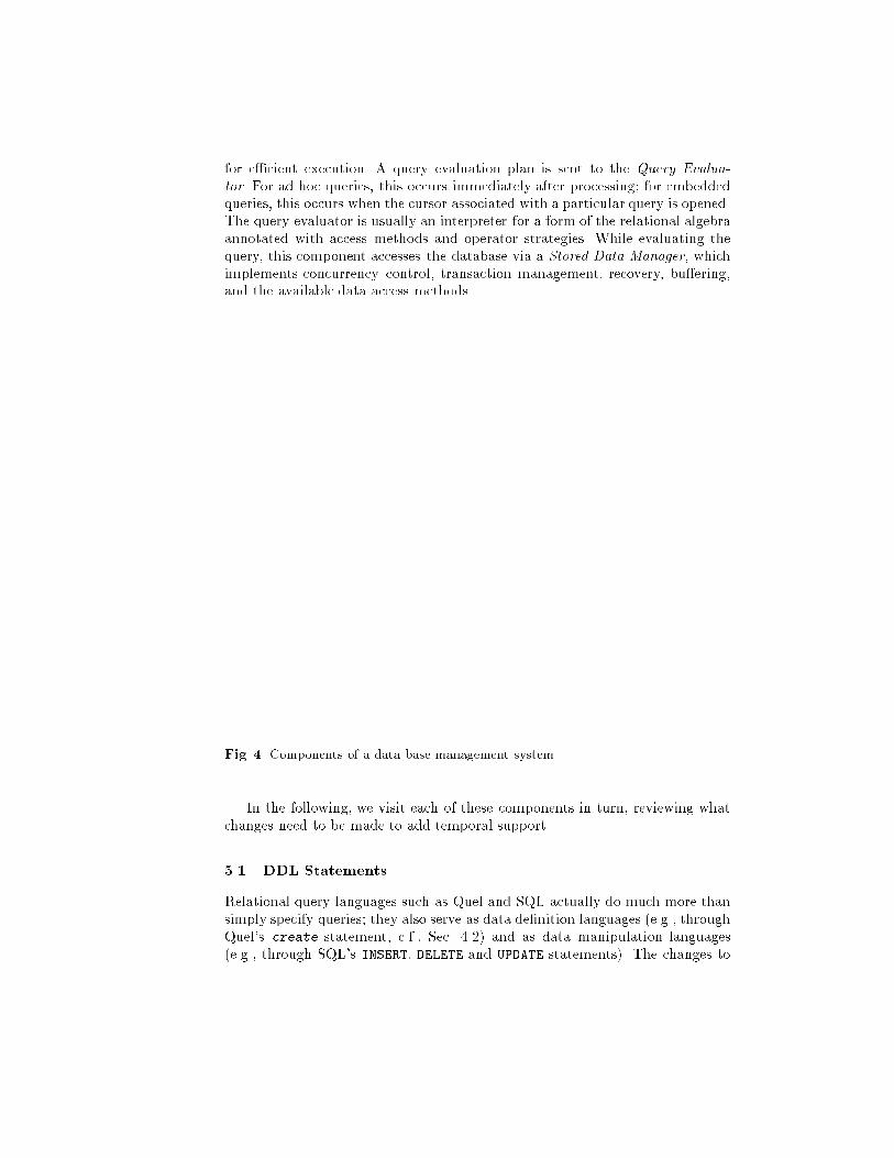
for e�cient execution. A query evaluation plan is sent to the Query Evalua-tor. For ad hoc queries, this occurs immediately after processing; for embeddedqueries, this occurs when the cursor associated with a particular query is opened.The query evaluator is usually an interpreter for a form of the relational algebraannotated with access methods and operator strategies. While evaluating thequery, this component accesses the database via a Stored Data Manager, whichimplements concurrency control, transaction management, recovery, bu�ering,and the available data access methods.

Fig. 4. Components of a data base management systemIn the following, we visit each of these components in turn, reviewing whatchanges need to be made to add temporal support.5.1 DDL StatementsRelational query languages such as Quel and SQL actually do much more thansimply specify queries; they also serve as data de�nition languages (e.g., throughQuel's create statement, c.f., Sec. 4.2) and as data manipulation languages(e.g., through SQL's INSERT, DELETE and UPDATE statements). The changes to

support time involve adding temporal domains, such as event, interval, and span@cite[Soo92C] and adding constructs to specify support for transaction and validtime, such as the TQuel keywords persistent and interval.5.2 System CatalogThe big change here is that the system catalog must consist of transaction-timerelations. Schema evolution concerns only the recording of the data, and hencedoes not involve valid time. The attributes and their domains, the indexes, eventhe names of the relations all vary over transaction time.5.3 Query ProcessingThere are two aspects here, one easily extended (language analysis) and one forwhich adding temporal support is much more complex (query optimization).Language analysis needs to consider multiple calendars, which extend thelanguage with calendar-speci�c functions. An example is monthof, which onlymakes sense in calendars for which there are months. The changes to languageprocessing, primarily involving modi�cations to semantic analysis (name resolu-tion and type checking), have been worked out in some detail @cite[Soo92A].Optimization of temporal queries is substantially more involved than that forconventional queries, for several reasons. First, optimization of temporal queriesis more critical, and thus easier to justify expending e�ort on, than conventionaloptimization. The relations that temporal queries are de�ned over are larger,and are growing monotonically, with the result that unoptimized queries takelonger and longer to execute. This justi�es trying harder to optimize the queries,and spending more execution time to perform the optimization.Second, the predicates used in temporal queries are harder to optimize @cite[Leung90,Leung91A].In traditional database applications, predicates are usually equality predicates(hence the prevalence of equi-joins and natural joins); if a less-than join is in-volved, it is rarely in combination with other less-than predicates. On the otherhand, in temporal queries, less-than joins appear more frequently, as a conjunc-tion of several inequality predicates. As an example, the TQuel overlap operatoris translated into two less-than predicates on the underlying time-stamps. Opti-mization techniques in conventional databases focus on equality predicates, andoften implement inequality joins as cartesian products, with their associatedine�ciency.And third, there is greater opportunity for query optimization when timeis present @cite[Leung91A]. Time advances in one direction: the time domainis continuous expanding, and the most recent time point is the largest value inthe domain. This implies that a natural clustering or sort order will manifestitself, which can be exploited during query optimization and evaluation. Theintegrity constraint beginof (t) < endof (t) holds for every time-interval tuple t.Also, for many relations it is the case that the intervals associated with a keyare contiguous in time, with one interval starting exactly when the previousinterval ended. An example is salary data, where the intervals associated with

the salaries for each employee are contiguous. Semantic query optimization canexploit these integrity constraints, as well as additional ones that can be inferred@cite[Shenoy89].In this section, we �rst examine local query optimization, of a single query,then consider global query optimization, of several queries simultaneously. Bothinvolve the generation of a query evaluation plan, which consists of an algebraicexpression annotated with access methods.Local Query Optimization. A single query can be optimizing by replacingthe algebraic expression with an equivalent one that is more e�cient, by changingan access method associated with a particular operator, or by adopting a partic-ular implementation of an operator. The �rst alternative requires a de�nition ofequivalence, in the form of a set of tautologies. Tautologies have been identi�edfor the conventional relational algebra @cite[Enderton77,Smith75B,Ullman88B],as well as for many of the algebras listed in Table 5. Some of these temporal al-gebras support the standard tautologies, enabling existing query optimizers tobe used.To determine which access method is best for each algebraic operator, meta-data, that is, statistics on the stored temporal data, and cost models, that is,predictors of the execution cost for each operator implementation/access methodcombination, are needed. Temporal data requires additional meta-data, such aslifespan of a relation (the time interval over which the relation is de�ned), thelifespans of the tuples, the surrogate and tuple arrival distributions, the distri-butions of the time-varying attributes, regularity and granularity of temporaldata, and the frequency of null values, which are sometimes introduced whenattributes within a tuple aren't synchronized @cite[Gunadhi89A]. Such statisti-cal data may be updated by random sampling or by a scan through the entirerelation.There has been some work in developing cost models for temporal opera-tors. An extensive analytical model has been developed and validated for TQuelqueries @cite[Ahn88B,Ahn89], and selectivity estimates on the size of the resultsof various temporal joins have been derived @cite[Gunadhi89D,Gunadhi89A].Global Query Optimization. In global query optimization, a collection ofqueries is simultaneously optimized, the goal being to produce a single queryevaluation plan that is more e�cient than the collection of individual plans@cite[Satoh85A,Sellis86A]. A state transition network appears to be the best wayto organize this complex task @cite[Jensen92G].Materialized views@cite[Blakeley86B,Blakeley90,Roussopoulos82,Roussopoulos91]are expected to play an important role in achieving high performance in theface of temporal databases of monotonically increasing size. For an algebrato utilize this approach, incremental forms of the operators are required (c.f.,@cite[McKenzie88,Jensen91D]).

5.4 Query EvaluationAchieving adequate e�ciency in query evaluation is very important. We �rst ex-amine operations on time-stamps, some of which are critical to high performance.We then review a study that showed that a straightforward implementationwould not result in reasonable performance. Since joins are the most expensive,yet very common, operations, they have been the focus of a signi�cant amountof research. Finally, we will examine the many temporal indexes that have beenproposed.Domain Operations. In Sec. 2 we outlined the domain of time-stamps. Queryevaluation performs input, comparison, arithmetic, and output operations onvalues of this domain. Ordered by contribution to execution e�ciency, they arecomparison (which is often in the \inner loop" of join processing), arithmetic(which is most often performed during creation of the resulting tuple), output(which is only done when transferring results to the screen or to paper, a muchslower process than execution or even disk I/O), and �nally input (which is doneexactly once per value). However, the SQL2 format, with its �ve components (seeTable 1) is optimized for the relatively infrequent operations of (Gregorian) in-put and output, and is rather slow at comparison and addition. The proposedformats instead optimize comparison at the expense of input and output. Fora sequence of operations that inputs two relations and computes and outputsthe overlap (favoring input and output more than expected), the high resolu-tion format is more e�cient, with only 50 tuples, than the SQL2 format, eventhough the high resolution format has much greater range and smaller granular-ity @cite[Dyreson92C].Performing these operations e�ciently in the presence of historical inde-terminacy is more challenging. For the default range credibility and orderingplausibility, and for comparing events whose sets of possible chronons do notoverlap, there is little overhead even when historical indeterminacy is supported@cite[Dyreson92D]. The average worse case for comparison, over all plausibil-ities, when the sets of possible chronons overlap sign�cantly, is less than 100microseconds on a Sun-4, or about the time to transfer a 100-byte tuple fromdisk.A Straightforward Implementation. The importance of e�cient query op-timization and evaluation for temporal databases was underscored by an initialstudy that analyzed the performance of a brute-force approach to adding timesupport to a conventional DBMS. In this study, the university Ingres DBMSwas extended in a minimal fashion to support TQuel querying @cite[Ahn86B].The results were very discouraging for those who might have been consideringsuch an approach. Sequential scans, as well as access methods such as hashingand ISAM, su�ered from rapid performance degradation due to ever-growingover ow chains. Because adding time creates multiple tuple versions with thesame key, reorganization does not help to shorten over ow chains. The objective

of work in temporal query evaluation then is to avoid looking at all of the data,because the alternative implies that queries will continue to slow down as thedatabase accumulates facts.There were four basic responses to this challenge. The �rst was a proposal toseparate the historical data, which grew monotonically, from the current data,whose size was fairly stable and whose accesses were more frequent @cite[Lum84].This separation, termed temporal partitioning, was shown to signi�cantly im-prove performance of some queries @cite[Ahn88B], and was later generalized toallowmultiple cached states, which further improves performance @cite[Jensen92G].Second, new query optimization strategies were proposed (Sec. 5.3). Third, newjoin algorithms, to be discussed next, were proposed. And �nally, new temporalindexes, also to be discussed, were proposed.Joins. Three kinds of temporal joins have been studied: binary joins, multiwayjoins, and joins executed on multiprocessors.A wide variety of binary joins have been considered, including time-join, time-equijoin (TE-join) @cite[Cli�ord87A], event-join,TE-outerjoin@cite[Gunadhi91],contain-join, contain-semijoin, intersect-join@cite[Leung91A], and contain-semijoin@cite[Leung92]. The various algorithms proposed for these joins have generallybeen extensions to nested loop or merge joins that exploit sort orders or localworkspace.Leung argues that a checkpoint index (Sec. 5.4) is useful when stream pro-cessing is employed to evaluate both two-way and multi-way joins @cite[Leung92].Finally, Leung has explored in depth partitioning strategies and temporalquery processing on multiprocessors @cite[Leung91].Temporal Indexes. Conventional indexes have long been proposed to reducethe need to scan an entire relation to access a subset of its tuples. Indices areeven more important in temporal relations that grow monotonically in size. Intable 6 we summarize the temporal index structures that have been proposed todate. Most of the indexes are based on B+-Trees @cite[Comer79], which indexon values of a single key; the remainder are based on R-Trees @cite[Guttman84],which index on ranges (intervals) of multiple keys. There has been considerablediscussion concerning the applicability of point-based schemes for indexing in-terval data. Some argue that structures that explicitly accommodate intervals,such as R-Trees and their variants, are preferable; others argue that mappingintervals to their endpoints is e�cient for spatial search @cite[Lomet91].If the structure requires that exactly one record with each key value existat any time, or if the data records themselves are stored in the index, thenit is designated a primary storage structure; otherwise, it can be used eitheras a primary storage structure or as a secondary index. The checkpoint index isassociated with a particular indexing condition, making it suitable for use duringthe processing of queries consistent with that condition.A majority of the indexes are tailored to transaction time, exploiting theappend-only nature of such information. Most utilize as a key the valid-time or

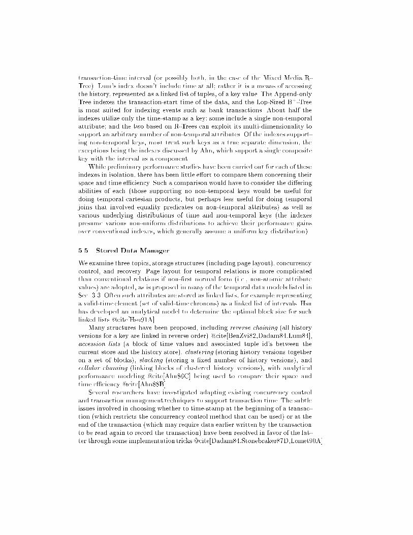
transaction-time interval (or possibly both, in the case of the Mixed Media R-Tree). Lum's index doesn't include time at all; rather it is a means of accessingthe history, represented as a linked list of tuples, of a key value. The Append-onlyTree indexes the transaction-start time of the data, and the Lop-Sized B+-Treeis most suited for indexing events such as bank transactions. About half theindexes utilize only the time-stamp as a key; some include a single non-temporalattribute; and the two based on R-Trees can exploit its multi-dimensionality tosupport an arbitrary number of non-temporal attributes. Of the indexes support-ing non-temporal keys, most treat such keys as a true separate dimension, theexceptions being the indexes discussed by Ahn, which support a single compositekey with the interval as a component.While preliminary performance studies have been carried out for each of theseindexes in isolation, there has been little e�ort to compare them concerning theirspace and time e�ciency. Such a comparison would have to consider the di�eringabilities of each (those supporting no non-temporal keys would be useful fordoing temporal cartesian products, but perhaps less useful for doing temporaljoins that involved equality predicates on non-temporal attributes) as well asvarious underlying distributions of time and non-temporal keys (the indexespresume various non-uniform distributions to achieve their performance gainsover conventional indexes, which generally assume a uniform key distribution).5.5 Stored Data ManagerWe examine three topics, storage structures (including page layout), concurrencycontrol, and recovery. Page layout for temporal relations is more complicatedthan conventional relations if non-�rst normal form (i.e., non-atomic attributevalues) are adopted, as is proposed in many of the temporal data models listed inSec. 3.3. Often such attributes are stored as linked lists, for example representinga valid-time element (set of valid-time chronons) as a linked list of intervals. Hsuhas developed an analytical model to determine the optimal block size for suchlinked lists @cite[Hsu91A].Many structures have been proposed, including reverse chaining (all historyversions for a key are linked in reverse order) @cite[BenZvi82,Dadam84,Lum84],accession lists (a block of time values and associated tuple id's between thecurrent store and the history store), clustering (storing history versions togetheron a set of blocks), stacking (storing a �xed number of history versions), andcellular chaining (linking blocks of clustered history versions), with analyticalperformance modeling @cite[Ahn86C] being used to compare their space andtime e�ciency @cite[Ahn88B].Several researchers have investigated adapting existing concurrency controland transaction management techniques to support transaction time. The subtleissues involved in choosing whether to time-stamp at the beginning of a transac-tion (which restricts the concurrency control method that can be used) or at theend of the transaction (which may require data earlier written by the transactionto be read again to record the transaction) have been resolved in favor of the lat-ter through some implementation tricks @cite[Dadam84,Stonebraker87D,Lomet90A].

Non-Name Citation Based On Primary/ Temporal Temporal TemporalSecondary Dimension(s) Key(s) Key(s)Append-only @cite[Gunadhi91A] B+-Tree primary transaction event 0TreeCheckpoint @cite[Leung92] B+-Tree secondary transaction event 0IndexLop-Sided @cite[Kolovson90B] B+-Tree both transaction event 0B+-TreeMonotonic @cite[Elmasri92] Time Index both transaction interval 0B+-Tree| @cite[Lum84] B+-Tree or primary transaction none 1HashingTime-Split @cite[Lomet90] B+-Tree primary transaction interval 1B-TreeMixed Media @cite[Kolovson89] R-Tree both transaction, interval, k ranges,R-Tree trans+valid pairs of k � 1intervalsTime Index @cite[Elmasri90] B+-Tree both both interval 0Two-level Combined @cite[Elmasri91] B+-Tree both both interval 1Attribute/Time +Time IndexIndex| @cite[Ahn88B] B+-Tree, various various interval 1HashingSR-Tree @cite[Kolovson90] Segment Index both both interval, k ranges,+ R-Tree pairs of k � 1intervalsTable 6. Temporal IndexesThe Postgres system is an impressive prototype DBMS that supports transac-tion time@cite[Stonebraker90B]. Time-stamping in a distributed setting has alsobeen considered @cite[Lomet90A]. Integrating temporal indexes with concur-rency control to increase the available concurrency has been studied @cite[Lomet91B].Finally, since a transaction-time database contains all past versions of thedatabase, it can be used to recover from media failures that cause a portion orall of the current version to be lost @cite[Lomet91].6 ConclusionWe conclude with a list of accomplishments, a list of disappointments, and apointer to future work.There have been many signi�cant accomplishments over the past �fteen yearsof temporal database research.

{ The semantics of the time domain, including its structure, dimensionality,and indeterminacy, is well-understood.{ Representational issues of time-stamps have recently been resolved.{ Operations on time-stamps are now well-understood, and e�cient implemen-tations exist.{ A great amount of research has been expended on temporal data models,addressing this extraordinarily complex and subtle design problem.{ Many temporal query languages have been proposed. The numerous types oftemporal queries are fairly well-understood. Half of the proposed temporalquery languages have a strong formal basis.{ Temporal joins are well-understood, and a multitude of implementationsexist.{ Approximately a dozen temporal index structures have been proposed.{ The interaction between transaction time support and concurrency controland transaction management has been studied to some depth.{ Several prototype temporal DBMS implementations have been developed.There have also been some disappointments.{ The user-de�ned time support in the SQL2 standard is poorly designed.The representation speci�ed in that standard su�ers from inadequate range,excessive space requirements, and ine�cient operations.{ There has been almost no work done in comparing the two dozen temporaldata models, to identify common features and de�ne a consensus data modelupon which future research and commercialization may be based. It is ourfeeling that expecting a data model to simultaneously express time-varyingsemantics while optimizing data presentation, data storage, and query evalu-ation is unrealistic. We advocate a two-tiered data model, with a conceptualdata model expressing the semantics, and with several representational datamodels serving these other objectives.{ There is also a need to consolidate approaches to temporal query languages,identify the best features of each of the proposed languages, and incorporatethese features into a consensus query language that could serve as the basisfor future research into query optimization and evaluation. Also, more workis needed on adding time to so-called fourth generation languages that arerevolutionizing user interfaces for commercially available DBMS's.{ It has been demonstrated that a straightforward implementation of a tem-poral DBMS will exhibit poor performance.{ More empirical studies are needed to compare join algorithms, and to pos-sibly suggest even more e�cient variants.{ While there are a host of individual approaches to isolated portions of aDBMS, no coherent architecture has arisen. While the analysis given in Sec. 5may be viewed as a starting point, much more work is needed to integratethese approaches into a cohesive structure.{ There has been little e�ort to compare the relative performance of temporalindexes, making selection in speci�c situations di�cult or impossible.

{ Temporal database design is still in its infancy, hindered by the plethora oftemporal data models.{ There are as yet no prominent commercial temporal DBMS's, despite theobvious need in the marketplace.Obviously these disappointments should be addressed. In addition, future workis also needed on adding time to the newer data models that are gaining recogni-tion, including object-oriented data models and deductive data models. Finally,there is a great need for integration of spatial and temporal data models, querylanguages, and implementation techniques.7 AcknowledgementsThis work was supported in part by NSF grant ISI-8902707. James Cli�ord washelpful in understanding structural aspects of models of time. Curtis Dyreson,Christian S. Jensen, Nick Kline and Michael Soo provided useful comments ona previous draft.8 Bibliography@bib

Table of Contents1 Introduction : : : : : : : : : : : : : : : : : : : : : : : : : : : : : : : : : : : 12 The Time Domain : : : : : : : : : : : : : : : : : : : : : : : : : : : : : : : 22.1 Structure : : : : : : : : : : : : : : : : : : : : : : : : : : : : : : : : : : : 22.2 Dimensionality : : : : : : : : : : : : : : : : : : : : : : : : : : : : : : : : 42.3 Indeterminacy : : : : : : : : : : : : : : : : : : : : : : : : : : : : : : : : 62.4 Representation : : : : : : : : : : : : : : : : : : : : : : : : : : : : : : : : 8Interpretation. : : : : : : : : : : : : : : : : : : : : : : : : : : : : : : : : 8Physical Realization. : : : : : : : : : : : : : : : : : : : : : : : : : : : : : 103 Associating Facts with Time : : : : : : : : : : : : : : : : : : : : : : : : : 133.1 Underlying Data Model : : : : : : : : : : : : : : : : : : : : : : : : : : : 133.2 Attribute Variability : : : : : : : : : : : : : : : : : : : : : : : : : : : : : 143.3 Representational Alternatives : : : : : : : : : : : : : : : : : : : : : : : : 15Data Models. : : : : : : : : : : : : : : : : : : : : : : : : : : : : : : : : : 15Valid Time. : : : : : : : : : : : : : : : : : : : : : : : : : : : : : : : : : : 16Transaction Time. : : : : : : : : : : : : : : : : : : : : : : : : : : : : : : 16Attribute Value Structure. : : : : : : : : : : : : : : : : : : : : : : : : : 17Separating Semantics from Representation. : : : : : : : : : : : : : : : : 184 Querying : : : : : : : : : : : : : : : : : : : : : : : : : : : : : : : : : : : : : 194.1 Language Proposals : : : : : : : : : : : : : : : : : : : : : : : : : : : : : 204.2 Types of Temporal Queries : : : : : : : : : : : : : : : : : : : : : : : : : 20Schema De�nition. : : : : : : : : : : : : : : : : : : : : : : : : : : : : : : 21

Quel Retrieval Statements. : : : : : : : : : : : : : : : : : : : : : : : : : 22Rollback (Transaction-time Slice). : : : : : : : : : : : : : : : : : : : : : 22Valid-time Selection. : : : : : : : : : : : : : : : : : : : : : : : : : : : : : 22Valid Time Projection. : : : : : : : : : : : : : : : : : : : : : : : : : : : 23Aggregates. : : : : : : : : : : : : : : : : : : : : : : : : : : : : : : : : : : 23Historical Indeterminacy. : : : : : : : : : : : : : : : : : : : : : : : : : : 24Schema Evolution. : : : : : : : : : : : : : : : : : : : : : : : : : : : : : : 254.3 Standards : : : : : : : : : : : : : : : : : : : : : : : : : : : : : : : : : : : 255 System Architecture : : : : : : : : : : : : : : : : : : : : : : : : : : : : : : 255.1 DDL Statements : : : : : : : : : : : : : : : : : : : : : : : : : : : : : : : 265.2 System Catalog : : : : : : : : : : : : : : : : : : : : : : : : : : : : : : : : 275.3 Query Processing : : : : : : : : : : : : : : : : : : : : : : : : : : : : : : : 27Local Query Optimization. : : : : : : : : : : : : : : : : : : : : : : : : : 28Global Query Optimization. : : : : : : : : : : : : : : : : : : : : : : : : : 285.4 Query Evaluation : : : : : : : : : : : : : : : : : : : : : : : : : : : : : : 29Domain Operations. : : : : : : : : : : : : : : : : : : : : : : : : : : : : : 29A Straightforward Implementation. : : : : : : : : : : : : : : : : : : : : 29Joins. : : : : : : : : : : : : : : : : : : : : : : : : : : : : : : : : : : : : : 30Temporal Indexes. : : : : : : : : : : : : : : : : : : : : : : : : : : : : : : 305.5 Stored Data Manager : : : : : : : : : : : : : : : : : : : : : : : : : : : : 316 Conclusion : : : : : : : : : : : : : : : : : : : : : : : : : : : : : : : : : : : : 327 Acknowledgements : : : : : : : : : : : : : : : : : : : : : : : : : : : : : : : 34

8 Bibliography : : : : : : : : : : : : : : : : : : : : : : : : : : : : : : : : : : : 34

This article was processed using the LaTEX macro package with LLNCS style