Embed Size (px)
Citation preview
APPROVED:
Angela K. Wilson, Major Professor Weston T. Borden, Committee Member Thomas R. Cundari, Committee Member Martin Schwartz, Committee Member Michael G. Richmond, Chair of the Chemistry
Department Michael Monticino, Interim Dean of the Robert
B. Toulouse School of Graduate Studies
SYSTEMATIC APPROACHES TO PREDICTIVE COMPUTATIONAL CHEMISTRY
USING THE CORRELATION CONSISTENT BASIS SETS
Brian P. Prascher, B.S.
Dissertation Prepared for the Degree of
DOCTOR OF PHILOSOPHY
UNIVERSITY OF NORTH TEXAS
May 2009
Prascher, Brian P., Systematic Approaches to Predictive Computational
Chemistry using the Correlation Consistent Basis Sets
The development of the correlation consistent basis sets, cc-pVnZ (where n = D,
T, Q, etc.) have allowed for the systematic elucidation of the intrinsic accuracy of ab
initio quantum chemical methods. In density functional theory (DFT), where the cc-pVnZ
basis sets are not necessarily optimal in their current form, the elucidation of the
intrinsic accuracy of DFT methods cannot always be accomplished. This dissertation
outlines investigations into the basis set requirements for DFT and how the intrinsic
accuracy of DFT methods may be determined with a prescription involving recontraction
of the cc-pVnZ basis sets for specific density functionals. Next, the development and
benchmarks of a set of cc-pVnZ basis sets designed for the s-block atoms lithium,
beryllium, sodium, and magnesium are presented. Computed atomic and molecular
properties agree well with reliable experimental data, demonstrating the accuracy of
these new s-block basis sets. In addition to the development of cc-pVnZ basis sets, the
development of a new, efficient formulism of the correlation consistent Composite
Approach (ccCA) using the resolution of the identity (RI) approximation is employed.
The new formulism, denoted ‘RI-ccCA,’ has marked efficiency in terms of computational
time and storage, compared with the ccCA formulism, without the introduction of
significant error. Finally, this dissertation reports three separate investigations of the
properties of FOOF-like, germanium arsenide, and silicon hydride/halide molecules
using high accuracy ab initio methods and the cc-pVnZ basis sets.
. Doctor of Philosophy (Physical
Chemistry), May 2009, 275 pp., 49 tables, 28 illustrations, references, 307 titles.

ii
Copyright 2009
by
Brian P. Prascher

iii
ACKNOWLEDGEMENTS
I would like to acknowledge Jesus Christ as my source of strength in all things. (“I have
strength for all things in Christ who empowers me,” Philippians 4:13) Further, the love, support,
and encouragement of my wife and best friend, Laura; my beautiful daughters, Emma and
Charlotte; my Mom and Dad; and Lew and Diane, has been paramount for me during my
graduate career.
I wish to thank my colleagues during my time in the Wilson Group (in order of
appearance): Xuelin Wang, Scott Yockel, James Seals, Ray Bell, Ben Mintz, Pankaj Sinha, John
Determan, Nathan DeYonker, Sammer Tekarli, Gavin Williams, Brent Wilson, Gbenga Oyedepo,
Kameron Jorgensen, and Marie Majkut, for constantly challenging me with questions about
computational chemistry and, in so doing, kept my knowledge of the subject up to par. In
particular, I want to thank and acknowledge Brent Wilson and Gavin Williams for their
contributions to projects discussed in this dissertation. Many thanks and acknowledgements
also go to the numerous undergraduates that served in the Wilson Group, particularly Rebecca
Lucente‐Schultz, Arjun Kavi, and Jeremy Lai for their contributions to work presented herein.
I also want to thank the professors of the Chemistry Department, who challenged and
molded me into the academic that I am today. Finally, I would like to give a heart‐felt thanks to
Angela Wilson, my academic mother and mentor, whose open‐door, yet hands‐off approach
gave me room to spread my wings.
iv
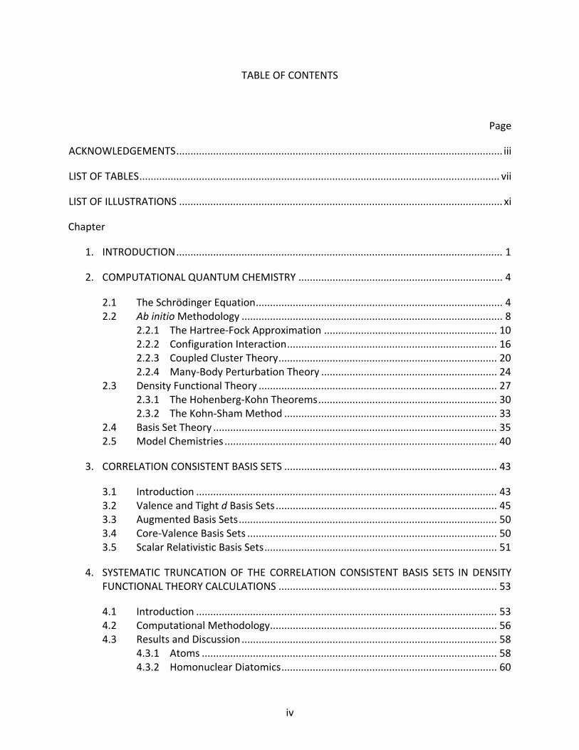
TABLE OF CONTENTS
Page
ACKNOWLEDGEMENTS ................................................................................................................... iii
LIST OF TABLES ............................................................................................................................... vii
LIST OF ILLUSTRATIONS .................................................................................................................. xi
Chapter
1. INTRODUCTION ................................................................................................................... 1
2. COMPUTATIONAL QUANTUM CHEMISTRY ........................................................................ 4
2.1 The Schrödinger Equation ....................................................................................... 4 2.2 Ab initio Methodology ............................................................................................ 8
2.2.1 The Hartree‐Fock Approximation ............................................................. 10 2.2.2 Configuration Interaction .......................................................................... 16 2.2.3 Coupled Cluster Theory ............................................................................. 20 2.2.4 Many‐Body Perturbation Theory .............................................................. 24
2.3 Density Functional Theory .................................................................................... 27 2.3.1 The Hohenberg‐Kohn Theorems ............................................................... 30 2.3.2 The Kohn‐Sham Method ........................................................................... 33
2.4 Basis Set Theory .................................................................................................... 35 2.5 Model Chemistries ................................................................................................ 40
3. CORRELATION CONSISTENT BASIS SETS ........................................................................... 43
3.1 Introduction .......................................................................................................... 43 3.2 Valence and Tight d Basis Sets .............................................................................. 45 3.3 Augmented Basis Sets ........................................................................................... 50 3.4 Core‐Valence Basis Sets ........................................................................................ 50 3.5 Scalar Relativistic Basis Sets .................................................................................. 51
4. SYSTEMATIC TRUNCATION OF THE CORRELATION CONSISTENT BASIS SETS IN DENSITY FUNCTIONAL THEORY CALCULATIONS ............................................................................. 53
4.1 Introduction .......................................................................................................... 53 4.2 Computational Methodology ................................................................................ 56 4.3 Results and Discussion .......................................................................................... 58
4.3.1 Atoms ........................................................................................................ 58 4.3.2 Homonuclear Diatomics ............................................................................ 60
v
4.3.3 CH4, SiH4, NH3, PH3, H2O, and H2S ............................................................. 63 4.3.4 Computational Time Savings ..................................................................... 65
4.4 Conclusions ........................................................................................................... 66
5. SYSTEMATIC RECONTRACTION OF THE CORRELATION CONSISTENT BASIS SETS FOR DENSITY FUNCTIONAL THEORY CALCULATIONS ............................................................... 82
5.1 Introduction .......................................................................................................... 82 5.2 Computational Methodology ................................................................................ 85 5.3 Results and Discussion .......................................................................................... 87
5.3.1 Atoms ........................................................................................................ 87 5.3.2 Molecules .................................................................................................. 89 5.3.3 Kohn‐Sham Limits ...................................................................................... 92 5.3.4 Basis Set Superposition Error .................................................................... 94 5.3.5 Diffuse Functions ....................................................................................... 95
5.4 Conclusions ........................................................................................................... 96
6. THE DEVELOPMENT OF S‐BLOCK CORRELATION CONSISTENT BASIS SETS .................... 116
6.1 Introduction ........................................................................................................ 116 6.2 Computational Methodology .............................................................................. 118 6.3 Basis Set Construction ........................................................................................ 120
6.3.1 Tight d Functions for Inner Valence Correlation ..................................... 120 6.3.2 Core‐Valence Functions for Sub‐Valence Correlation ............................ 121 6.3.3 Recontracted Basis Sets for Scalar Relativistic Computations ................ 123
6.4 Benchmark Computations .................................................................................. 125 6.4.1 Ionization Potentials and Electron Affinities ........................................... 125 6.4.2 Optimized Geometries and Vibrational Frequencies .............................. 128 6.4.3 Thermochemistry .................................................................................... 129
6.5 Conclusions ......................................................................................................... 130
7. THE RESOLUTION OF THE IDENTITY APPROXIMATION APPLIED TO THE CORRELATION CONSISTENT COMPOSITE APPROACH ............................................................................ 137
7.1 Introduction ........................................................................................................ 137 7.2 Computational Methodology .............................................................................. 142 7.3 Results and Discussion ........................................................................................ 144
7.3.1 RI‐ccCA Implementation ......................................................................... 144 7.3.2 Auxiliary Basis Sets for RI‐ccCA ............................................................... 145 7.3.3 Energetic Properties ................................................................................ 146 7.3.4 Computational Cost................................................................................. 147
7.4 Conclusions ......................................................................................................... 152
8. A SYSTEMATIC INVESTIGATION OF DIHALOGEN‐μ‐DICHALCOGENIDES ......................... 168
vi
8.1 Introduction ........................................................................................................ 168 8.2 Computational Methodology .............................................................................. 171 8.3 Results and Discussion ........................................................................................ 173
8.3.1 Stability of X2A2 Compounds ................................................................... 173 8.3.2 XAAX Structures ...................................................................................... 174 8.3.3 Vibrational Frequency Analyses .............................................................. 176 8.3.4 Anomeric Effects ..................................................................................... 177
8.4 Conclusions ......................................................................................................... 180
9. A SYSTEMATIC INVESTIGATION OF GERMANIUM ARSENIDES ....................................... 188
9.1 Introduction ........................................................................................................ 188 9.2 Computational Methodology .............................................................................. 190 9.3 Results and Discussion ........................................................................................ 192
9.3.1 Optimized Structures .............................................................................. 192 9.3.2 Classical Barriers to Isomerization .......................................................... 195 9.3.3 Thermochemistry and Relative Stabilities .............................................. 197
9.4 Conclusions ......................................................................................................... 199
10. A SYSTEMATIC INVESTIGATION OF SILICON HYDRIDES AND HALIDES ........................... 218
10.1 Introduction ........................................................................................................ 218 10.2 Computational Methodology .............................................................................. 220 10.3 Optimized Structures .......................................................................................... 221
10.3.1 SiH, SiF, and SiCl ...................................................................................... 221 10.3.2 SiH2, SiF2, SiCl2, SiHF, and SiHCl ............................................................... 222 10.3.3 SiH3, SiF3, SiCl3, SiH2F, SiH2Cl, SiHF2, and SiHCl2 ...................................... 223 10.3.4 SiH4, SiF4, SiCl4, SiH3F, SiH3Cl, SiH2F2, SiH2Cl2, SiHF3, and SiHCl3 .............. 224
10.4 Thermochemistry ................................................................................................ 226 10.4.2 Atomization Energies and Enthalpies of Formation ............................... 227 10.4.3 Dissociation Reaction Enthalpies ............................................................ 233
10.5 Conclusions ......................................................................................................... 234
11. CONCLUDING REMARKS ................................................................................................. 257
REFERENCES ................................................................................................................................ 259
vii
LIST OF TABLES
Table 3.1 The composition of the correlation consistent basis sets for the first three rows of the main group. ................................................................................................ 45
Table 4.1 Total energies (Eh) of the carbon and oxygen atoms computed with full and truncated basis sets; energy differences are listed in mEh. .................................. 69
Table 4.2 Ionization potentials (eV) of the carbon and oxygen atoms computed with full and truncated basis sets; relative differences are listed below the full basis set values. ................................................................................................................... 71
Table 4.3 Electron affinities (eV) of the carbon and oxygen atoms computed with full, truncated, and augmented truncated basis sets (aug); relative differences are listed below the full basis set values. ................................................................... 72
Table 4.4 Total energies (Eh) of the C2 and O2 molecules computed with full and truncated basis sets; energy differences are listed in mEh. ................................................... 74
Table 4.5 BLYP vertical ionization potentials (eV), electron affinities (eV), atomization energies (kcal/mol), and optimized bond lengths (Å) of the C2 and O2 molecules computed with full and truncated basis sets; electron affinities include diffuse functions and relative energy differences are listed below the full basis set values. ................................................................................................................... 76
Table 4.6 B3LYP atomization energies (kcal/mol) and optimized bond lengths (Å) for CH4 and SiH4 (both
1A1); relative differences are listed below the full basis set values................................................................................................................................ 78
Table 4.7 B3LYP optimized geometries (Å and degrees) for NH3 and PH3 (both 1A1); relative
differences are listed below the full basis set values. .......................................... 79
Table 4.8 B3LYP optimized geometries (Å and degrees) for H2O and H2S (both 1A1); relative
differences are listed below the full basis set values. .......................................... 80
Table 4.9 Percent CPU time and average time saved computing B3LYP single‐point energies with truncated basis sets, relative to the full basis sets. ....................... 81
Table 5.1 A comparison of the BLYP and B3LYP total energies (Eh) of the first row atoms (including hydrogen) computed with the original and recontracted cc‐pVnZ basis sets; relative differences to the original basis sets are shown in mEh under [rc].............................................................................................................................. 101
viii
Table 5.2 A comparison of the BLYP and B3LYP ionization potentials and electron affinities (eV) of the first row atoms (including hydrogen) computed with the original and recontracted cc‐pVnZ basis sets; relative differences to the original basis sets are shown under [rc]. ................................................................................................ 102
Table 5.3 A comparison of the BLYP and B3LYP total energies (Eh), ionization potentials, and electron affinities (eV) of the first row dimers (including hydrogen) computed with the original and recontracted cc‐pVnZ basis sets; relative differences to the original basis sets are shown in mEh (total energies) and eV under [rc]. ........................................................................................................... 103
Table 5.4 The BLYP and B3LYP optimized geometries (Å and degrees) of several first row molecules computed with the original and recontracted basis sets; relative differences to the original basis set are shown under [rc]. ................................ 105
Table 5.5 The BLYP and B3LYP atomization energies (kcal/mol) of several first row molecules computed with the original and recontracted basis sets; relative differences to the original basis set are shown under [rc]. ................................ 107
Table 5.6 Two‐ and three‐point extrapolated BLYP and B3LYP Kohn‐Sham limits of atomization energies (kcal/mol) computed with the original and recontracted basis sets. Non‐monotonic behavior is denoted by ‘‐‐‐’. .................................... 110
Table 5.7 The BLYP and B3LYP atomization energies (kcal/mol) and their extrapolated Kohn‐Sham limits of four molecules corrected for basis set superposition error (BSSE). ................................................................................................................. 113
Table 5.8 A comparison of BLYP and B3LYP atomization energies (kcal/mol) and their extrapolated Kohn‐Sham values using the aug‐cc‐pVnZ, aug‐cc‐pVnZ[rc], and aug‐cc‐pVnZ[rc] basis sets corrected for basis set superposition error (BSSE). ........ 114
Table 6.1 The composition of the correlation consistent basis sets for s‐block atoms. .... 119
Table 6.2 CCSD(T) ionization potentials and electron affinities of Li, Be, Na, and Mg; the tight d correlation consistent basis sets for Na and Mg have been used. ......... 131
Table 6.3 CCSD(T) optimized geometries (Re, Å) of some s‐block molecules computed with various families of correlation consistent basis sets. ......................................... 132
Table 6.4 CCSD(T) harmonic vibrational frequencies (Å) of some s‐block molecules computed with various families of correlation consistent basis sets................. 134
Table 6.5 CCSD(T) standard state enthalpies of formation at 298.15 K (kcal/mol) for some s‐block molecules computed with various families of correlation consistent basis sets; tight d functions have been used for the Na and Mg atoms. .................... 135
ix
Table 7.1 Differences between ccCA and RI‐ccCA total energies (mEh), relative CPU times, and relative disk space using different combinations of RI‐SCF and RI‐MP2 auxiliary basis sets.a ............................................................................................ 154
Table 7.2 Total energies (Eh) computed with ccCA, RI‐ccCA, and RI‐ccCA+L; differences (mEh) are relative to the ccCA energies. ............................................................. 155
Table 7.3 Enthalpies of formation (ΔHf°) at 298 K (kcal/mol) computed with ccCA, RI‐ccCA, and RI‐ccCA+L. ..................................................................................................... 159
Table 7.4 CPU times and disk space usage of RI‐ccCA and RI‐ccCA+L relative to ccCA...... 164
Table 8.1 Stabilities (kcal/mol) of the different isomers of X2A2 molecules relative to the gauche isomer, XAAX, computed with B3LYP and CCSD(T). ............................... 182
Table 8.2 B3LYP and CCSD(T) optimized geometries (Å and degrees) of the fluorine species using various correlation consistent basis sets. ................................................. 183
Table 8.3 B3LYP and CCSD(T) optimized geometries (Å and degrees) of the chlorine species using various correlation consistent basis sets. ................................................. 184
Table 8.4 B3LYP and CCSD(T) optimized geometries (Å and degrees) of the bromine species using various correlation consistent basis sets. ................................................. 185
Table 8.5 B3LYP and CCSD(T) harmonic vibrational frequencies (cm‐1) computed with the aug‐cc‐pVTZ basis set. ......................................................................................... 186
Table 8.6 A comparison of CCSD(T) harmonic and anharmonic vibrational frequencies (cm‐1) of FSSF computed with the cc‐pVDZ basis set. ......................................... 187
Table 9.1 Non‐relativistic and spin‐orbit (SO) total energies (Eh) of some main group atoms computed at the MCSCF/cc‐pVTZ level of theory; SO corrections are given in kcal/mol. ............................................................................................................. 202
Table 9.2 A comparison of the CCSD(T) optimized geometries (Å and degrees) for the L‐GeAs and GeAs‐L isomers; previously reported geometries are included for comparison. ........................................................................................................ 203
Table 9.3 A comparison of the B3LYP optimized geometries (Å and degrees) for the L‐GeAs and GeAs‐L isomers; previously reported geometries are included for comparison. ........................................................................................................ 205
Table 9.4 CCSD(T) and B3LYP classical reaction barriers (kcal/mol) for the forward (f) and reverse (r) reactions; previously reported reaction barriers are included for comparison. ........................................................................................................ 207
x
Table 9.5 Non‐relativistic (NR), Cowan‐Griffin (CG), and Douglas‐Kroll (DK) enthalpies of formation at 298 K (kcal/mol) of the L‐GeAs isomers computed with CCSD(T) and B3LYP; spin‐orbit effects have been included in the relativistic enthalpies. ...... 209
Table 9.6 Non‐relativistic (NR), Cowan‐Griffin (CG), and Douglas‐Kroll (DK) enthalpies of formation at 298 K (kcal/mol) of the GeAs‐L isomers computed with CCSD(T) and B3LYP; spin‐orbit effects have been included in the relativistic enthalpies. ...... 212
Table 9.7 CCSD(T) and B3LYP enthalpies of isomerization (kcal/mol) from L‐GeAs to GeAs‐L at 298 K. Various basis set levels and CBS limits are represented as well as non‐relativistic (NR) and relativistic energies using the Cowan‐Griffin (CG) and Douglas‐Kroll (DK) approach. .............................................................................. 215
Table 10.1 CCSD(T) optimized geometries (Å) of SiH, SiF, and SiCl. ..................................... 239
Table 10.2 CCSD(T) optimized geometries (Å and degrees) of SiH2, SiF2, SiCl2, SiHF, and SiHCl.............................................................................................................................. 240
Table 10.3 CCSD(T) optimized geometries (Å and degrees) of SiH3, SiF3, SiCl3, SiH2F, SiH2Cl, SiHF2, and SiHCl2. ................................................................................................ 242
Table 10.4 CCSD(T) optimized geometries (Å and degrees) of SiH4, SiF4, SiCl4, SiHF3, SiH3F, SiHCl3, SiH3Cl, SiH2F2, and SiH2Cl2. ....................................................................... 244
Table 10.5 CCSD(T) and ccCA atomization energies (kcal/mol) and extrapolated energies; atomic spin‐orbit corrections have been applied to the CCSD(T) results. ......... 246
Table 10.6 CCSD(T) and ccCA enthalpies of formation at 298 K (kcal/mol) and extrapolated energies; atomic spin‐orbit corrections have been applied to the CCSD(T) results.............................................................................................................................. 249
Table 10.7 CCSD(T) and ccCA enthalpies of dissociation at 298.15 K (kcal/mol) of the silicon hydrides, computed with the aug‐cc‐pV(n+d)Z basis sets; the mean absolute deviation (MAD) is relative to the experimental values. .................................... 252
Table 10.8 CCSD(T) and ccCA enthalpies of dissociation at 298.15 K (kcal/mol) of the silicon fluorides, computed with the aug‐cc‐pV(n+d)Z basis sets; the mean absolute deviation (MAD) is relative to the experimental values. .................................... 253
Table 10.9 CCSD(T) and ccCA enthalpies of dissociation at 298.15 K (kcal/mol) of the silicon chlorides, computed with the aug‐cc‐pV(n+d)Z basis sets; the mean absolute deviation (MAD) is relative to the experimental values. .................................... 255
xi
LIST OF ILLUSTRATIONS
Figure 2.1 Representations of restricted closed‐shell (I), restricted open‐shell (II), and unrestricted (III) wavefunctions. .......................................................................... 14
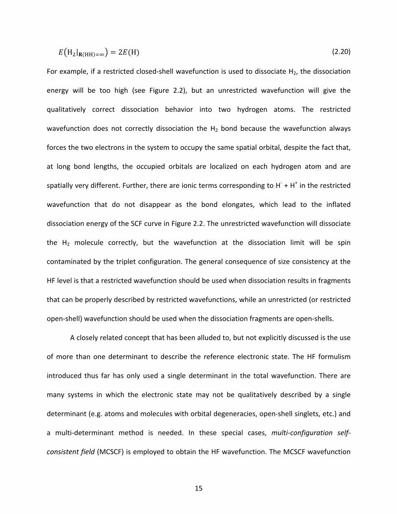
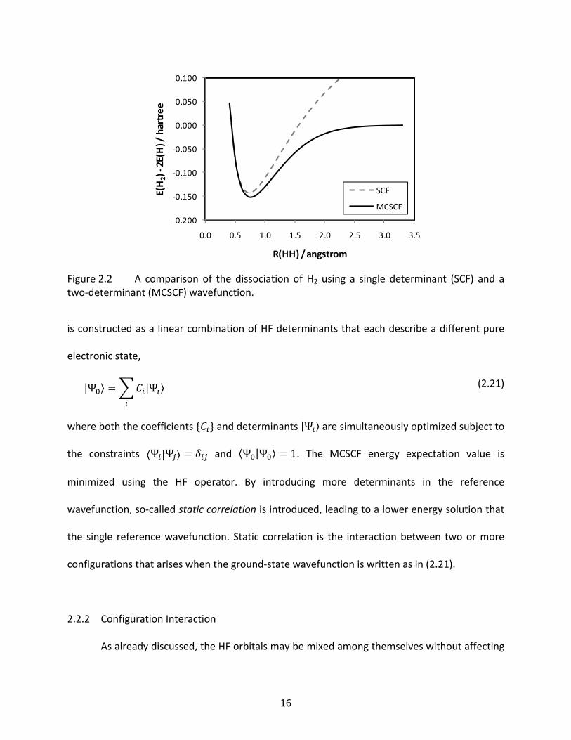
Figure 2.2 A comparison of the dissociation of H2 using a single determinant (SCF) and a two‐determinant (MCSCF) wavefunction. ............................................................ 16
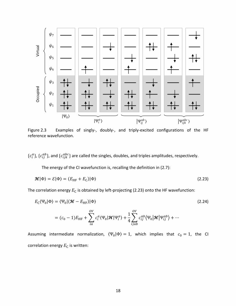
Figure 2.3 Examples of singly‐, doubly‐, and triply‐excited configurations of the HF reference wavefunction. ....................................................................................... 18
Figure 2.4 Plots comparing the behavior of a single STO to a single GTO (left) and that of a single STO with a linear combination (LC) of three GTOs (right). The units are arbitrary. ............................................................................................................... 38
Figure 2.5 A conceptual view of basis set size versus level of sophistication in correlated ab initio methods. The number of determinants with respect to excitation level (n), number of electrons (N), and basis set size (K) is given by the formula on the lower axis. ............................................................................................................. 41
Figure 4.1 BLYP ionization potentials of the oxygen atom computed with truncated basis sets (hash marks) and plotted against the full basis set values. The inset shows more detail at the quadruple‐ζ level. Points denoted ‘l > 3’ are the truncated basis sets with only s, p, d, and f basis functions. ................................................. 61
Figure 4.2 BLYP ionization potentials of the O2 molecule (3Σg) computed with truncated basis sets (hash marks) and plotted against the full basis set values. Points denoted ‘l > 3’ are the truncated basis sets with only s, p, d, and f basis functions................................................................................................................................ 62
Figure 4.3 Comparisons of CPU time savings (closed circles), ionization potentials (triangles), electron affinities (upside‐down triangles), atomization energies (open squares), and total energies (closed squares) between the full and truncated cc‐pV5Z basis set using B3LYP. Truncation levels: ‘0’ is the full basis, ‘1’ is cc‐pV5Z(‐1h ; 1g), ‘2’ is cc‐pV5Z(‐1h1g ; 1g1f), etc. .......................................... 68
Figure 5.1 The BLYP potential energy curve of O2 (3Σg) computed with the original and
recontracted correlation consistent basis sets. .................................................... 91
Figure 5.2 A comparison of the BLYP atomization energies computed with the original and recontracted correlation consistent basis sets. .................................................... 92
xii
Figure 5.3 A comparison of BLYP atomization energies computed with the original and recontracted correlation consistent basis sets, and the recontracted basis sets with basis set superposition error (BSSE) removed. ............................................ 99
Figure 5.4 A comparison of BLYP atomization energies computed with the pc‐n, aug‐cc‐pVnZ, and aug‐cc‐pVnZ[rc] basis sets with basis set superposition error (BSSE) removed. .................................................................................................. 100
Figure 6.1 The incremental CISD correlation energy lowering of the Mg atom due to each polarization function. .......................................................................................... 121
Figure 6.2 Comparisons of the Na atom valence (cc‐pVnZ) exponents with the core‐valence (cc‐pCVnZ) and weighted core‐valence (cc‐pwCVnZ) exponents; the exponents are grouped by angular momentum. .................................................................. 122
Figure 6.3 The spacing of the d exponents in the cc‐pVnZ basis sets compared with those in the cc‐pV(n+d)Z basis sets. ................................................................................. 123
Figure 6.4 CCSD(T) valence correlation energies recovered by the cc‐pVnZ (V/V), cc‐pCVnZ (V/CV), and cc‐pwCVnZ (V/wCV) basis sets. ....................................................... 124
Figure 6.5 CCSD(T) core‐valence plus valence correlation energies recovered by the cc‐pVnZ (CV/V), cc‐pCVnZ (CV/CV), and cc‐pwCVnZ (CV/wCV); the 1s orbitals of Na and Mg were kept frozen in each calculation. ........................................................... 126
Figure 6.6 Comparisons of the scalar relativistic corrections to the atomic Hartree‐Fock energy using the original contractions (diamonds) and the Douglas‐Kroll contractions (squares) with increasing basis set size. ........................................ 127
Figure 7.1 CPU times of RI‐ccCA (top) and RI‐ccCA+L (bottom) versus ccCA; each data point represents a molecule in the test set. ................................................................ 148
Figure 7.2 Disk space usage of RI‐ccCA (top) and RI‐ccCA+L (bottom) versus ccCA; each data point represents a molecule in the test set. ....................................................... 150
Figure 7.3 Correlation between molecular size and average CPU time and disk space saved using RI‐ccCA and RI‐ccCA+L, relative to ccCA. ................................................... 151
Figure 8.1 The orbital representation of anomeric delocalization in XAAX systems: the lone pair on a bridging A atom delocalizes into the adjacent σ*(AX) orbital. ............ 170
Figure 8.2 The lowest unoccupied CISD natural orbitals of FSSF: both contour plots are F‐S σ* orbitals (14A, left; 13B, right). The perspective is down the z‐axis (iso‐contour value: 0.095). ...................................................................................................... 178
xiii
Figure 8.3 The molecules FSSF (left), ClSSCl (center), and BrSSBr (right), and the lone pair orbitals responsible for anomeric delocalization. The prespective is down the z‐axis (iso‐contour values: 0.06, 0.03, and 0.03, respectively). ............................. 179
Figure 9.1 A schematic of the forward (f) and reverse (r) reaction coordinates of L migration from the germanium atom to the arsenic atom. ................................................ 195
Figure 9.2 A side‐by‐side comparison of non‐relativistic and Douglas‐Kroll (DK) relativistic CCSD(T) and B3LYP relative energies from mixed Gaussian/exponential extrapolations. .................................................................................................... 201
Figure 10.1 Plots comparing the CCSD(T) optimized geometries of SiH, SiF, and SiCl using four different families of correlation consistent basis sets. ....................................... 237
Figure 10.2 Plots comparing the CCSD(T) enthalpies of formation at 298 K of the silicon fluorides using four families of correlation consistent basis sets. ..................... 238
1
CHAPTER 1
INTRODUCTION
The practice of chemistry, in one form or another, has been around for millennia, but
only in the past two centuries has the practice of chemistry evolved from archaic alchemy to a
pure and applied science. Modern chemistry is able to probe the structure, microscopic
properties, and reactions of atoms and molecules through systematic laboratory methods that
include synthetic techniques, such as directly reacting a substance with another substance in a
controlled environment; instrumental techniques, including the myriad of spectroscopic
techniques; and, more recently, computational techniques. With the advent of quantum
mechanics in the early 20th century, the way in which chemical properties traditionally are
elucidated changed dramatically. Schrödinger’s wave mechanics, simultaneously introduced
alongside Heisenberg’s matrix mechanics, offered ways of calculating both static and dynamic
properties of quantized systems. Following the construction of the first electronic computer,
chemists and physicists began to submit atomic and molecular properties for calculation using
Schrödinger’s and Dirac’s mathematics. The amount of information acquired about chemical
properties during the early years of quantum mechanics was not substantial, limited primarily
by the computational expense of both the underlying mathematics and the physical
computational resources (i.e. storage, time, and software).
The general organization of this dissertation is such that systematically approaching a
problem with computational chemistry is covered in detail, from the selection of a

2
computational model (Chapter 2) and basis sets (Chapter 3); the development of systematic
basis sets for density functional theory (Chapters 4 and 5) and ab initio methods (Chapter 6); to
the application and benchmarking of these basis sets (Chapters 7‐10).
First, a basic working knowledge of the mathematics behind computational chemistry,
specifically ab initio methods and density functional methods, is presented in some detail in
Chapter 2. From there, Chapter 3 discusses a special class of basis sets, called the correlation
consistent basis sets, which are the focal point of this dissertation as every subsequent chapter
employs them.
In Chapters 4 and 5, work is described that has been done to gain a greater
understanding of the basis set requirements in density functional theory calculations. By
examining the effects of systematically truncating and recontracting the existing correlation
consistent basis sets, a set of compact, fine‐tuned basis sets is presented that provides accurate
results relative to the original correlation consistent basis sets at a reduced computational cost.
Further, the recontracted basis sets, augmented with diffuse functions and a correction for
basis set superposition error, restore the smooth, monotonic behavior inherent to the
correlation consistent basis sets in Kohn‐Sham calculations. Chapter 6 discusses the
development and benchmarks of new correlation consistent basis sets for the s‐block atoms
lithium, beryllium, sodium, and magnesium. As discussed in the chapter, these atoms present a
unique challenge in the development of accurate basis sets due to their electronic structure.
Chapter 7 describes the implementation of the resolution of the identity approximation
into the correlation consistent composite approach. Specifically, this chapter presents the
implementation and discusses the need for specialized correlation consistent basis sets
3
optimized for the resolution of the identity. The chapter is concluded by demonstrating the
incredible efficiency of resolution of the identity methods, which are the key to accessing larger
and larger electronic systems on current computational hardware.
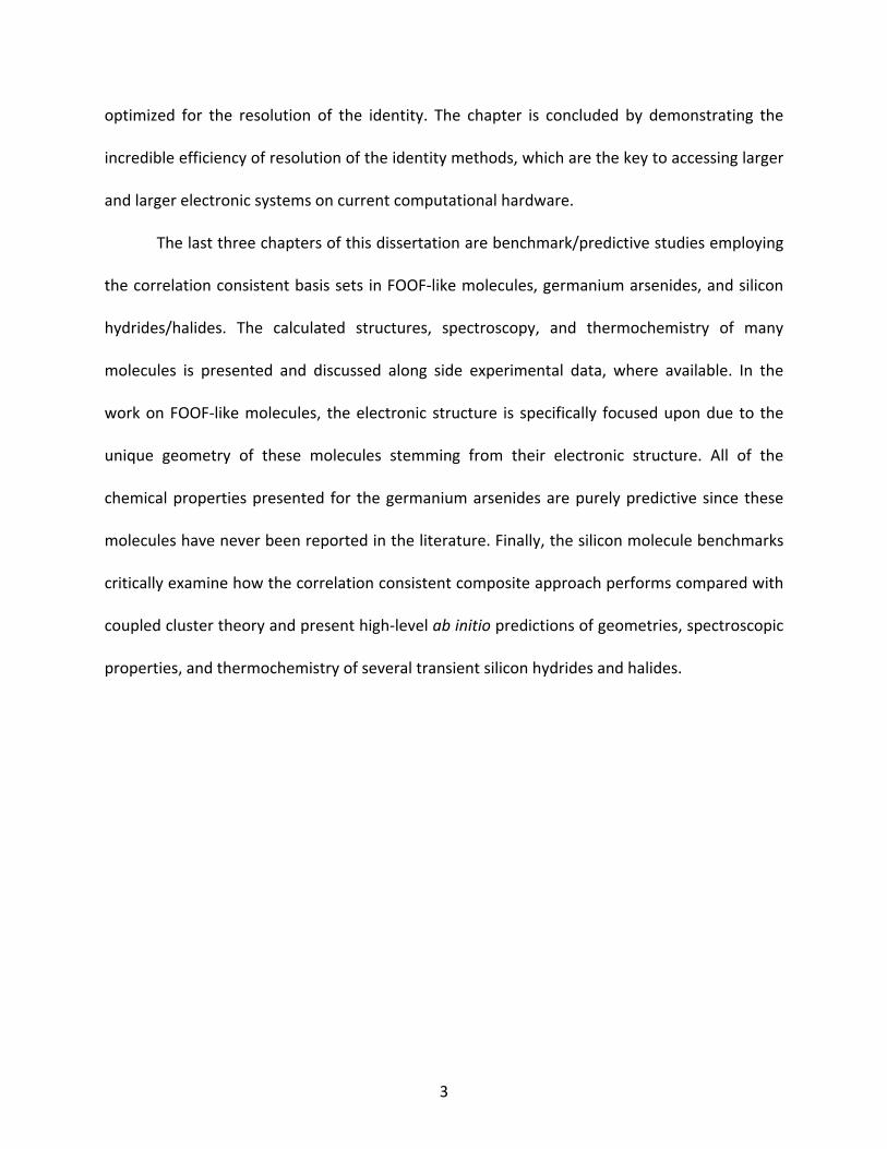
The last three chapters of this dissertation are benchmark/predictive studies employing
the correlation consistent basis sets in FOOF‐like molecules, germanium arsenides, and silicon
hydrides/halides. The calculated structures, spectroscopy, and thermochemistry of many
molecules is presented and discussed along side experimental data, where available. In the
work on FOOF‐like molecules, the electronic structure is specifically focused upon due to the
unique geometry of these molecules stemming from their electronic structure. All of the
chemical properties presented for the germanium arsenides are purely predictive since these
molecules have never been reported in the literature. Finally, the silicon molecule benchmarks
critically examine how the correlation consistent composite approach performs compared with
coupled cluster theory and present high‐level ab initio predictions of geometries, spectroscopic
properties, and thermochemistry of several transient silicon hydrides and halides.
4
CHAPTER 2
COMPUTATIONAL QUANTUM CHEMISTRY
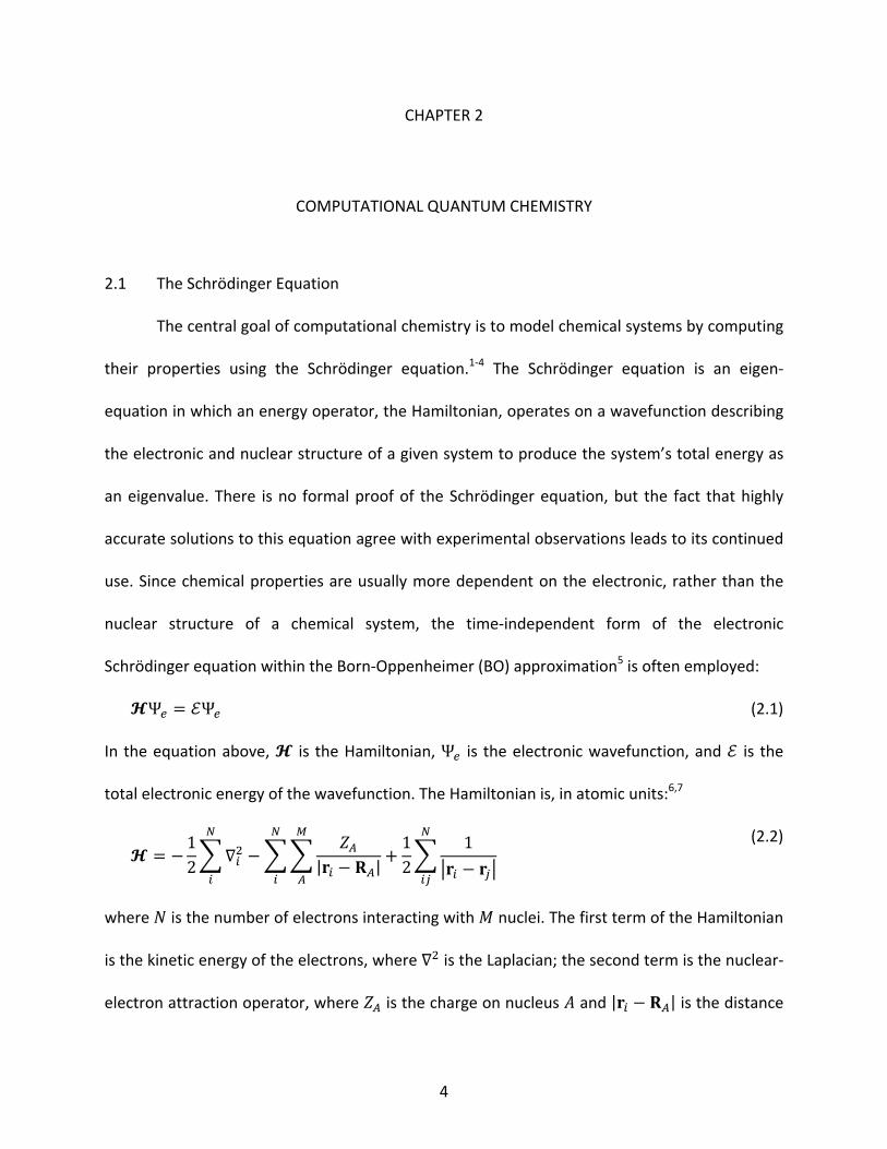
2.1 The Schrödinger Equation
The central goal of computational chemistry is to model chemical systems by computing
their properties using the Schrödinger equation.1‐4 The Schrödinger equation is an eigen‐
equation in which an energy operator, the Hamiltonian, operates on a wavefunction describing
the electronic and nuclear structure of a given system to produce the system’s total energy as
an eigenvalue. There is no formal proof of the Schrödinger equation, but the fact that highly
accurate solutions to this equation agree with experimental observations leads to its continued
use. Since chemical properties are usually more dependent on the electronic, rather than the
nuclear structure of a chemical system, the time‐independent form of the electronic
Schrödinger equation within the Born‐Oppenheimer (BO) approximation5 is often employed:
Ψ Ψ (2.1)
In the equation above, is the Hamiltonian, Ψ is the electronic wavefunction, and is the
total electronic energy of the wavefunction. The Hamiltonian is, in atomic units:6,7
12 | |
12
1
(2.2)
where is the number of electrons interacting with nuclei. The first term of the Hamiltonian
is the kinetic energy of the electrons, where is the Laplacian; the second term is the nuclear‐
electron attraction operator, where is the charge on nucleus and | | is the distance
5
between electron and nucleus ; and the third term is the electron‐electron repulsion, where
is the distance between two electrons. The Hamiltonian is more compactly written as
, where is the kinetic term, is the nuclear‐electron term, and is
the electron‐electron term. Once the nuclear‐electron potential (plus any external potential)
has been specified, the Hamiltonian is uniquely defined for a given electronic system.
The time‐independent wavefunction Ψ is a mathematical function of the electron
positions within a field of fixed nuclei. All information regarding the static discrete energy states
of the electrons is contained within this wavefunction and is extracted using the energy
operators of the Hamiltonian.6,7 In general, the wavefunction is complex‐valued and has no
direct physical interpretation, but, the squared modulus of the wavefunction, |Ψ | , is the
electron density (discussed later), which is observable by experiment using x‐ray photoelectron
spectroscopy. Considering this, the wavefunction itself may be interpreted from a statistical
point of view as a position function of the electrons. Despite the statistical interpretation, the
wavefunction may not be used to find the exact position of the electrons – a consequence of
the Heisenberg uncertainty principle.8
The wavefunction must have various mathematical properties so that it remains
physically viable (i.e. spans a Hilbert space): 1) it must be single‐valued at all points in space, 2)
it must be continuous at all points in space, 3) it must be zero‐valued at the boundaries (usually
taken to be infinity), 4) its derivatives at the boundaries must also be zero‐valued, and 5) the
wavefunction must be square integrable.6 Further, the electronic wavefunction must be anti‐
symmetric (change sign) with respect to the interchange of two electron coordinates.6,7 That is
to say, the wavefunction must obey the Pauli exclusion principle,9,10
6
Ψ , , … , , , … , Ψ , , … , , , … , (2.3)
One method of writing an N‐electron wavefunction with the necessary anti‐symmetry, |Ψ , is
the Slater determinant:7,11
|Ψ1√ !
1√ !
1!
(2.4)
where the columns represent electron orbitals and the rows represent electrons. The factor
1 √ !⁄ is a normalization constant, 1 is the parity of the th term, and is the
permutation operator, which interchanges the orbital indices. The term in brackets is a product
wavefunction called the Hartree product.12‐14 From linear algebra, it is known that the
properties of a determinant are such that the interchange of two rows (electrons in this case)
leads to a change of sign in the value of the determinant.15 Thus, the necessary anti‐symmetry
is taken care of naturally using a determinant as the wavefunction. The form of the individual
electron orbitals may be any mathematical function that obeys the five conditions previously
discussed, and are usually taken from Gaussian‐type basis sets (discussed later).
A subtle point worth making here is that the non‐relativistic Hamiltonian does not
intrinsically account for the spin of the electrons. This phenomenon is accounted for a
posteriori by using generalized electron coordinates of the form , where contains
the spatial components and the spin component. The generalized coordinates used in (2.4)
lead to spin orbitals, which may be separated into their spatial and spin components as:
|
|
(2.5)
The spin functions | and | are orthonormal, | . When the Hamiltonian (more
7
specifically, the operator) is applied to the determinant wavefunction, the anti‐symmetry,
along with the orthogonal nature of the spin orbitals produces an exchange interaction. This
interaction (also called exchange correlation or same spin correlation) only occurs between
electrons of the same spin, has no classical analog, and lowers the classical Coulomb repulsion
energy a wavefunction without anti‐symmetry (i.e. a Hartree product). Spin anti‐symmetry is
one of the underlying phenomenon responsible for Hund’s rules.16,17
The Hamiltonian operator contains two 2‐particle interaction terms: the term and
the term. The nuclear positions are fixed in the BO approximation, reducing to a 1‐
electron problem. However, remains a 2‐electron term. It is well‐known that there is no
closed form solution to the interacting 3‐particle (or higher) problem, and thus no closed form
solution to the electronic Schrödinger equation for more than one electron. This is the central
problem of computational quantum chemistry.6,7
To overcome the intractable problem of finding wavefunctions that satisfy the many‐
electron Schrödinger equation, approximate wavefunctions may be constructed using
variational calculus. Once constructed, the energy of an approximate wavefunction may be
computed as the expectation value of the Hamiltonian,
Ψ | |Ψ d d Ψ ,… , Ψ ,… , (2.6)
where the wavefunction is assumed to be normalized, Ψ |Ψ 1. To obtain the best
approximation to the exact solution of the Schrödinger equation, an approximate wavefunction
is constructed with variational parameters that may be adjusted until the expectation value of
the energy is minimized. Once minimized, the wavefunction is the best solution (in a variational
sense) to the Schrödinger equation. The question then arises as to how the variational
8
parameters are chosen and how the initial wavefunction is constructed. The answer to this
question leads to the many approximate methods of constructing many‐electron wavefunctions
and basis set theory. There are two categories of computational methods that will be focused
on in this dissertation: ab initio methods and density functional theory. Basis set theory is
discussed later in this chapter.
2.2 Ab initio Methodology
Ab initio, or “from the beginning,” methods are so‐called because only fundamental
physical laws and constants (e.g. Coulomb’s law, the elementary charge, the masses of
subatomic particles, Planck’s constant, the speed of light, etc.) are employed in them, and thus,
no bias from experimental data.6,18,19 Ab initio methods first construct an approximate
wavefunction as a reference, then use that reference in more rigorous methods to approximate
the exact solution to the Schrödinger equation.
The first ab initio approximation to the solution of the Schrödinger equation is the
Hartree‐Fock approximation,12‐14,20,21 which recasts the many‐electron Hamiltonian as a sum of
one‐electron operators and an average electron‐electron repulsion potential. This procedure
typically accounts for greater than 99% of the exact energy obtained with the Schrödinger
equation. However, as a result of this approximation, the Hartree‐Fock method recovers all but
the opposite spin correlation energy (hereafter referred to as just correlation energy), which is
physically interpreted as the instantaneous changes in the motions of electrons due to
repulsions by other electrons. The correlation energy is defined as the difference between the
exact ( ) and Hartree‐Fock ( HF) energies:7,22
9
C HF (2.7)
Although a small fraction of the total energy, the correlation energy is responsible for the
quantitative and, in many cases, qualitative description of chemical properties. Computing the
correlation energy is computationally demanding, and in order to obtain all of the correlation
energy for an electronic system, every electron must be correlated or allowed to interact with
every other electron simultaneously in the wavefunction. In practice, this corresponds to a full
configuration interaction (FCI)7,23‐25 treatment of the system, which is only possible to employ,
using current computing technology, on systems of a few electrons (i.e. ten or less). The task of
approximating a FCI treatment is the so‐called N‐electron problem,18 and correlated ab initio
methods are distinguished from one another in how they recover the correlation energy from a
HF reference wavefunction.7,19,22
Correlated ab initio methods become more computationally demanding as the number
of electrons increases, and so, there are two approximations that are often employed to reduce
the computational demand: 1) the frozen core approximation and 2) truncation of the
correlation space. The frozen core approximation assumes that chemical properties are
dominated by valence electron effects, and, thus, only valence electrons need to be correlated.
The remaining core electrons are left frozen, that is, uncorrelated. Truncation of the correlation
space involves only correlating a certain number of electrons simultaneously. For example, it is
well known that the largest contributor to correlation energy is the electron pair energy,
followed by the single electron correlation energy. Thus, some correlated ab initio methods are
able to recover a significant amount of the total correlation energy by only correlating up to
two electrons simultaneously.19
10
2.2.1 The Hartree‐Fock Approximation
Since the Schrödinger equation may not be solved exactly as an eigenvalue equation for
a many‐electron system, the Hartree‐Fock (HF) method is invoked as a first approximation to
the exact many‐electron wavefunction. Starting from a trial one‐electron orbitals, the HF
method seeks to find an optimal set of one‐electron orbitals that minimize the energy
expectation value of the determinant.7 In molecular HF calculations, each one‐electron orbital
is approximated as a linear combination of fixed one‐electron functions . This is the
so‐called linear combination of atomic orbitals (LCAO) theory,7,18 in which the molecular orbitals
(MOs) forming are taken to be a weighted sum of fixed atomic orbitals (AOs):
(2.8)
The coefficients may be varied so that the energy expectation value reaches a minimum,
leading to the variational nature of the HF method. In this way, the HF wavefunction is known
to be the best possible wavefunction constructed from the set of AOs when the total energy
has been minimized. The energy produced by the HF procedure will always be an upper bound
to the exact ground state energy.
The actual HF approximation replaces the exact electron‐electron repulsion operator
with an average effective potential (called the HF potential) by fixing an electron’s coordinates
and computing its interaction with the other 1 electrons. To arrive at this potential,
consider the electronic Hamiltonian recast in terms of a one‐electron core‐Hamiltonian
operator and the term, taking :
11
12 | |
12
(2.9)
According to Slater’s rules,7,26 the electron‐electron repulsion operator connects all pairs of
electrons in a Slater determinant such that:
12 Ψ Ψ
12
(2.10)
where the following shorthand has been introduced:
1 (2.11)
The permutation operator interchanges the orbital indices of electrons and , a
consequence of the anti‐symmetry of the Slater determinant. The first integral that results is
the classical Coulomb repulsion integral, denoted , while the second integral is the afore‐
mentioned exchange interaction between two electrons, denoted , and only arises when
electrons and have the same spin. Now, we define two operators that correspond to the
values of and :
d
d
(2.12)
Note that these new operators are one‐electron operators, and each represents a piece of the
average electron‐electron interaction experienced by electron in the field of electron . By
summing over all the occupied MOs, we obtain the HF potential for a single electron:
12
HF (2.13)
Next, a Fock operator for a single electron21 is defined and a new one‐electron Hamiltonian is
written in terms of these Fock operators:
HF
(2.14)
The operator is often referred to as the HF, or zeroth‐order,22 Hamiltonian. Thus, the HF
approximation is to turn the complicated, many‐electron Schrödinger equation into a one‐
electron problem. As a consequence of replacing the exact electron‐electron repulsion with the
average HF potential, the correlation of the electrons is lost.
The HF approximation leads to a new set of Schrödinger‐like equations called the HF
equations. The Fock operator operates on a given orbital to produce an eigenvalue – the
orbital energy within the averaged‐out electron‐electron repulsion:
| |
(2.15)
The HF orbitals are constrained to be orthogonal, and the orbital energy is
| | (2.16)
According to Koopmans’ theorem,27 this orbital energy may be interpreted as the ionization
potential of the corresponding orbital. However, Koopmans’ theorem neglects both the
correlated motions of electrons and orbital relaxation upon ionization.7
To solve the HF equations, (2.8) is inserted into (2.15):7,22,28
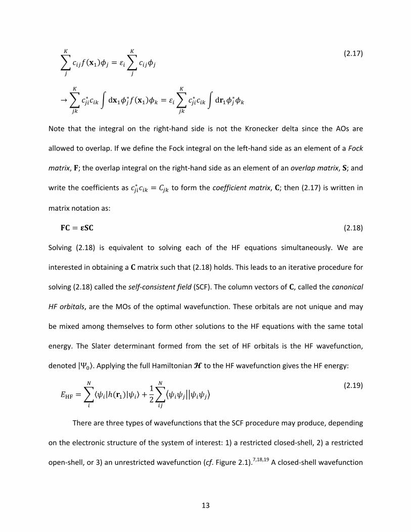
13
d d
(2.17)
Note that the integral on the right‐hand side is not the Kronecker delta since the AOs are
allowed to overlap. If we define the Fock integral on the left‐hand side as an element of a Fock
matrix, ; the overlap integral on the right‐hand side as an element of an overlap matrix, ; and
write the coefficients as to form the coefficient matrix, ; then (2.17) is written in
matrix notation as:
(2.18)
Solving (2.18) is equivalent to solving each of the HF equations simultaneously. We are
interested in obtaining a matrix such that (2.18) holds. This leads to an iterative procedure for
solving (2.18) called the self‐consistent field (SCF). The column vectors of , called the canonical
HF orbitals, are the MOs of the optimal wavefunction. These orbitals are not unique and may
be mixed among themselves to form other solutions to the HF equations with the same total
energy. The Slater determinant formed from the set of HF orbitals is the HF wavefunction,
denoted |Ψ . Applying the full Hamiltonian to the HF wavefunction gives the HF energy:
HF | |12
(2.19)
There are three types of wavefunctions that the SCF procedure may produce, depending
on the electronic structure of the system of interest: 1) a restricted closed‐shell, 2) a restricted
open‐shell, or 3) an unrestricted wavefunction (cf. Figure 2.1).7,18,19 A closed‐shell wavefunction
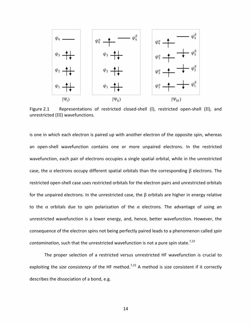
14
is one in which each electron is paired up with another electron of the opposite spin, whereas
an open‐shell wavefunction contains one or more unpaired electrons. In the restricted
wavefunction, each pair of electrons occupies a single spatial orbital, while in the unrestricted
case, the α electrons occupy different spatial orbitals than the corresponding β electrons. The
restricted open‐shell case uses restricted orbitals for the electron pairs and unrestricted orbitals
for the unpaired electrons. In the unrestricted case, the β orbitals are higher in energy relative
to the α orbitals due to spin polarization of the α electrons. The advantage of using an
unrestricted wavefunction is a lower energy, and, hence, better wavefunction. However, the
consequence of the electron spins not being perfectly paired leads to a phenomenon called spin
contamination, such that the unrestricted wavefunction is not a pure spin state.7,22
The proper selection of a restricted versus unrestricted HF wavefunction is crucial to
exploiting the size consistency of the HF method.7,22 A method is size consistent if it correctly
describes the dissociation of a bond, e.g.
Figure 2.1 Representations of restricted closed‐shell (I), restricted open‐shell (II), andunrestricted (III) wavefunctions.
3
2
1
4
2
1
3
4α 4
β
1α 1
β
2α 2
β
3α 3
β
4α
4β
|ΨI |ΨII |ΨIII
15
H | HH 2 H (2.20)
For example, if a restricted closed‐shell wavefunction is used to dissociate H2, the dissociation
energy will be too high (see Figure 2.2), but an unrestricted wavefunction will give the
qualitatively correct dissociation behavior into two hydrogen atoms. The restricted
wavefunction does not correctly dissociation the H2 bond because the wavefunction always
forces the two electrons in the system to occupy the same spatial orbital, despite the fact that,
at long bond lengths, the occupied orbitals are localized on each hydrogen atom and are
spatially very different. Further, there are ionic terms corresponding to H‐ + H+ in the restricted
wavefunction that do not disappear as the bond elongates, which lead to the inflated
dissociation energy of the SCF curve in Figure 2.2. The unrestricted wavefunction will dissociate
the H2 molecule correctly, but the wavefunction at the dissociation limit will be spin
contaminated by the triplet configuration. The general consequence of size consistency at the
HF level is that a restricted wavefunction should be used when dissociation results in fragments
that can be properly described by restricted wavefunctions, while an unrestricted (or restricted
open‐shell) wavefunction should be used when the dissociation fragments are open‐shells.
A closely related concept that has been alluded to, but not explicitly discussed is the use
of more than one determinant to describe the reference electronic state. The HF formulism
introduced thus far has only used a single determinant in the total wavefunction. There are
many systems in which the electronic state may not be qualitatively described by a single
determinant (e.g. atoms and molecules with orbital degeneracies, open‐shell singlets, etc.) and
a multi‐determinant method is needed. In these special cases, multi‐configuration self‐
consistent field (MCSCF) is employed to obtain the HF wavefunction. The MCSCF wavefunction
16
is constructed as a linear combination of HF determinants that each describe a different pure
electronic state,
|Ψ |Ψ (2.21)
where both the coefficients and determinants |Ψ are simultaneously optimized subject to
the constraints Ψ |Ψ and Ψ |Ψ 1. The MCSCF energy expectation value is
minimized using the HF operator. By introducing more determinants in the reference
wavefunction, so‐called static correlation is introduced, leading to a lower energy solution that
the single reference wavefunction. Static correlation is the interaction between two or more
configurations that arises when the ground‐state wavefunction is written as in (2.21).
2.2.2 Configuration Interaction
As already discussed, the HF orbitals may be mixed among themselves without affecting
Figure 2.2 A comparison of the dissociation of H2 using a single determinant (SCF) and atwo‐determinant (MCSCF) wavefunction.
‐0.200
‐0.150
‐0.100
‐0.050
0.000
0.050
0.100
0.0 0.5 1.0 1.5 2.0 2.5 3.0 3.5
E(H2) ‐2E(H) / hartree
R(HH) / angstrom
SCF
MCSCF
17
a change in the total energy.7,22 Thus, it can be said that the occupied HF orbitals form an
orbital basis for the single determinant ground state wavefunction. However, the entire
collection of HF orbitals, occupied and virtual (unoccupied), form an orbital basis for the fully‐
interacting ground state wavefunction. Another way to look at it is to consider the entire set of
HF orbitals, arranged from lowest to highest orbital energy. By the aufbau principle, the HF
ground state will have the electrons filling up the lowest energy orbitals. But, this is only one
possible configuration of the electrons. In fact, there are possible configurations (where
is the number of one‐electron basis functions and is the number of electrons). These other
configurations (Slater determinants) form a basis for the exact N‐electron wavefunction.
Determining how these configurations interact with each other leads to the method of
configuration interaction (CI).7,19,22‐25
The fully‐interacting wavefunction may be written as a linear combination of excited
Slater determinants formed from the HF orbitals:
|Φ |Ψ |Ψ14 Ψ
136 Ψ
(2.22)
Here, |Ψ represents the HF reference wavefunction, while |Ψ , Ψ , and Ψ represent
connected singly‐, doubly‐, and triply‐excited determinants formed from the HF reference,
respectively (the term connected will be discussed in subsection 2.2.3). A few examples of these
types of excited determinants are shown in Figure 2.3. The set … is the occupied ( )
orbitals and … are the virtual ( ) orbitals. The script notation “|Ψ ” denotes the th
occupied orbital is excited to the th virtual orbital, etc., and the factors 1/4 and 1/36 ensure
that no excited configuration enters the overall wavefunction more than once. Finally, the sets
18
, , and are called the singles, doubles, and triples amplitudes, respectively.
The energy of the CI wavefunction is, recalling the definition in (2.7):
|Φ |Φ HF C |Φ (2.23)
The correlation energy C is obtained by left‐projecting (2.23) onto the HF wavefunction:
C Ψ |Φ Ψ | HF |Φ
C Ψ |Φ 1 HF Ψ | |Ψ14 Ψ Ψ
(2.24)
Assuming intermediate normalization, Ψ |Φ 1, which implies that 1, the CI
correlation energy C is written:
Figure 2.3 Examples of singly‐, doubly‐, and triply‐excited configurations of the HFreference wavefunction.
|Ψ0
3
2
1
4
5
6
7 Occup
ied
Virtual
|Ψ Ψ Ψ
19
C Ψ | |Ψ14 Ψ Ψ
136 Ψ Ψ
(2.25)
As a consequence of Brillouin’s theorem,7,22 which states that the HF wavefunction does not mix
with its singly‐excited determinants, the first summation in (2.25) equals zero. Also, according
to Slater’s rules,26 the Hamiltonian does not connect determinants that vary by more than two
permutations of the electrons. Thus, the triply‐excited, and higher, determinants drop out of
the expansion in (2.25) leaving:
C14 Ψ Ψ
(2.26)
Now, all that must be obtained to find the correlation energy of the fully‐interacting
wavefunction is the set of doubles amplitudes. Equation (2.26) demonstrates why two‐electron
correlation is the predominate contributor to the total correlation energy.
In practice, obtaining the doubles amplitudes is non‐trivial since they are coupled to not
only the other doubles amplitudes, but also to the reference, singles, triples, and quadruples
amplitudes. This means that in order to compute the correlation energy, all of the singly‐,
doubly‐, triply‐, and quadruply‐excited determinants must be formed from the HF reference.
Even more complication arises since the reference, singles, triples, etc. amplitudes are also
coupled to other excited determinants. As an example, if (2.24) is left‐projected by an arbitrary
singly‐excited determinant Ψ , the result would be:
C Ψ HF Ψ14
Ψ Ψ136
Ψ Ψ (2.27)
Note that, even though (2.27) is an expression for the amplitude , the presence of the other
20
singles amplitudes in this equation precludes that a method of obtaining each of the sets of
amplitudes simultaneously is needed. This leads to the construction of the FCI matrix, which, in
general, is very large and requires computing expectation values over all possible combinations
of configurations.7,19,22 For this reason, the FCI method is computationally demanding and can
only be performed on systems with a few electrons.
Instead of constructing the entire FCI matrix, the frozen core and truncated
wavefunction approximations discussed earlier may be employed. If the correlated
wavefunction of (2.22) is truncated after, say, the doubly‐excited determinants, then the size of
the CI matrix is reduced to a much more tractable form, called CI singles and doubles (CISD).
There are two major problems in truncated CI theory. One of these problems is the lack of size
consistency, despite the correct choice of a restricted or unrestricted HF reference. Truncated
CI wavefunctions do not have multiplicative separability, and, thus, not all excitations necessary
to properly describe bond dissociation are included when two fragments are pulled apart. The
other problem with truncated CI theory is the lack of size extensivity.29 A correlated method is
size extensive if the correlation energy recovered scales properly with the number of electrons.
Further, size extensivity ensures that the same amount of correlation energy is recovered
everywhere on the potential energy surface of an electronic system. The lack of size extensivity
in truncated CI methods stems from the fact that disconnected excitations (discussed in the
following section) do not enter the correlated wavefunction.
2.2.3 Coupled Cluster Theory
Instead of constructing all or some of the possible excited determinants from the HF
21
reference wavefunction, it is possible to recover correlation energy by writing the correlated
wavefunction in terms of cluster functions.30 A cluster function is a term added to the HF
wavefunction that correlates electrons. For example, consider a reference wavefunction
describing a system containing three electrons,
|Ψ1√3!
(2.28)
A cluster function that correlates electrons in orbitals and may be constructed as follows:
,12
(2.29)
Here, … and have the same meaning as in subsection 2.2.2, and is a doubles cluster
amplitude. If this cluster function is added to the orbital product , resembling a
sort of CI expansion, and replaced in the reference wavefunction as follows, a correlated
wavefunction results:
|Φ ,
|Φ |Ψ12
|
(2.30)
The correlated wavefunction in (2.30) includes only pair correlation stemming from electrons
occupying the orbitals and . If cluster functions correlating all possible orbital
combinations (not just pairs) were included in the reference wavefunction, then the FCI
wavefunction would result.30 This process is called the coupled cluster (CC) method.31‐36 It can
be shown that the CC wavefunction may be written in an exponential ansatz:
22
|ΦCC |Ψ1!
|Ψ (2.31)
Note that the Taylor series expansion of has been included for later discussion. The cluster
operator is composed of single ( ), double ( ), etc., up through N‐
tuple ( ) cluster functions, each defined by how they operate on the reference wavefunction:
|Ψ |Ψ
|Ψ14 Ψ
|Ψ1! …
… Ψ ……
……
(2.32)
If the cluster operator were applied directly to the reference wavefunction, the FCI
wavefunction (2.22) would result. However, the principle difference between CI and CC
theories is the exponential ansatz of (2.31), which gives multiplicative separability to the CC
wavefunction.29,37
Truncated CC methods are defined by restricting the cluster operator . For example,
the singles and doubles coupled cluster (CCSD) wavefunction is determined by setting
and inserting into the exponential ansatz (2.31):
|ΦCCSD1!
|Ψ
|ΦCCSD 112
16
|Ψ .
(2.33)
Consider the system composed of three electrons in (2.28); the highest possible excitation is a
23
triple excitation, thus, only cluster operators and products of cluster operators that correspond
to, at most, a triple excitation will be included in the CCSD wavefunction.30,38 In this case, (2.33)
then reduces to
|ΦCCSD 112 2
16
|Ψ
|ΦCCSD |ΦCISD12 2
16
|Ψ .
(2.34)
It is clear from this equation that the CCSD wavefunction includes more configurations than the
CISD wavefunction, and hence, includes more correlation than the CISD wavefunction. In fact,
not only do single and double excitations enter the CCSD wavefunction, but triple excitations
enter through the disconnected excitation terms and . Overall, the exponential ansatz
allows for disconnected excitations to enter truncated CC wavefunctions, which are the reason
that CC methods are both size consistent and size extensive.30
Despite the recovery of more correlation in the wavefunction compared with truncated
CI methods, the most popular implementations of CC are not variational.30 Although, it is
possible evaluate the truncated CC energy in a manner similar to that of truncated CI. Many
conventional CC methods exploit simplifications that arise from using a similarity transformed
Hamiltonian, . This transformed Hamiltonian comes from the bra‐representation of
(2.31), whereby the inverse exponential arises as the adjoint of . Due to Slater’s rules,26
naturally truncates at quadruple excitations making it more computationally efficient
than computing the full CC matrix (analogous to the FCI matrix) introduced in subsection 2.2.2.
As a consequence of employing the transformed Hamiltonian, both the variational and
hermitian nature of the CC equations are lost, but the resultant energy eigenvalues of
24
are, typically, very close to those of , which is motivation for the continued use of this
implementation of CC theory.30
2.2.4 Many‐Body Perturbation Theory
The correlated methods discussed up to this point have used different configurations
formed from the HF orbitals as a basis for constructing correlated wavefunctions. However,
another method of obtaining correlation energy is many‐body perturbation theory
(MBPT).7,19,22,34 Perturbation methods add corrections (perturbations) to the Hamiltonian and
wavefunction, which, in turn, give rise to a perturbed total energy:
|Φ |Ψ |Ψ |Ψ
(2.35)
Here, |Ψ and are the th‐order wavefunction and energy, respectively, of the th
eigenstate of the given system. Inserting these perturbed quantities into the Schrödinger
equation and collecting in orders of yields the th‐order perturbed Schrödinger equation:
|Ψ |Ψ |Ψ (2.36)
Next, MBPT, like the CI and CC methods, assumes that the eigenstates of the zeroth‐order
wavefunction form a basis for the th‐order wavefunction such that
|Ψ |Ψ (2.37)
If the eigenstates of the zeroth‐order wavefunction are orthonormal, Ψ Ψ , then
25
to find the th‐order energy, left‐project (2.36) by the zeroth‐order eigenstate to obtain
Ψ Ψ (2.38)
Now, it appears that the th‐order energy may be calculated from the 1 ‐order
wavefunction, but Wigner has shown that the th‐order wavefunction may be used to obtain up
to the energy up to order 2 1 .22,39 To obtain a given order wavefunction, we need to
calculate the set of coefficients , which are obtained by inserting (2.37) into (2.36), left‐
projecting by an arbitrary eigenstate of the zeroth‐order wavefunction, and using algebra to
clean up the resulting equation. Because this dissertation will only discuss MBPT results up
through second‐order, the derivation of the necessary quantities for obtaining the second‐
order energy is now presented.
According to Wigner’s theorem, the first‐order wavefunction is all that is necessary for
obtaining the second‐order energy. Thus, inserting (2.37) into (2.36), where 1, and left‐
projecting by Ψ yields
Ψ Ψ Ψ Ψ Ψ Ψ Ψ Ψ (2.39)
With some algebra and recalling the orthogonality of the eigenstates of the zeroth‐order
wavefunction, the coefficient for the th component of the first‐order wavefunction is
Ψ Ψ
(2.40)
Inserting (2.40) into (2.37), then into (2.38) gives the second‐order energy as
Ψ Ψ Ψ Ψ
(2.41)
Now, consider the form of the perturbation operator . If the operator is the HF
26
operator (2.14) then the perturbation is defined using (2.9), (2.14), and (2.35):
12
(2.42)
The zeroth‐order wavefunction is taken to be the HF wavefunction, and the different
eigenstates are the excited configurations of the HF wavefunction. This form of MBPT is known
as Møller‐Plesset perturbation theory (MPn, where n denotes the order of perturbation).7,19,22,40
Using (2.36), the zeroth‐order ground state energy is just the sum of the HF orbital energies,
Ψ Ψ | | (2.43)
The first‐order correction to the energy is found using (2.10) and (2.38):
Ψ Ψ12
(2.44)
Note that the total energy to first order is the HF energy (2.19), MPHF. This
very important result demonstrates that the HF wavefunction is stable to first order, which is
proof that mixing the HF orbitals among themselves will not lower the total energy. As a result,
eigenstates outside the HF ground state must be considered to compute the second‐order
energy. Further, note that the first‐order energy correction effectively removes the double‐
counting of the electron‐electron interactions inherent to the zeroth‐order energy. In the
energy expression of (2.41), the eigenstates that correspond to |Ψ must be doubly‐excited
configurations of the HF wavefunction since 1) the HF wavefunction is stable to first‐order and
2) the singles do not mix with the HF ground state by Brillouin’s theorem. Thus, using script
notation defined earlier, the second‐order energy is
27
14
Ψ Ψ
(2.45)
Here, and are the orbital energies of the and occupied orbitals connected by to the
virtual orbitals and , whose energies are and defined by (2.15). Again it is shown that
the predominate contributor to the correlation energy is the double excitations (specifically the
pair correlation) since it is the leading correction to the HF energy.
Perturbative methods, in general, are not variational, and, thus, the energies obtained
are not upper bounds to the exact energy.22 However, MP2 recovers a significant fraction of the
total correlation energy at a lower computational cost than both CISD and CCSD. Further, MPn
is both size consistent and size extensive, making it a more desirable method than CISD. The
size consistency of MPn, like CI and CC methods, hinges on the proper selection of the
underlying HF wavefunction. If the zeroth‐order wavefunction is sufficient for describing the
electronic state, then the MPn energies will be size consistent. In homolytic bond cleavage or
dissociation of a molecule into open‐shell fragments, MPn, as discussed so far, will lose size
consistency since the underlying reference wavefunction is not size consistent.
2.3 Density Functional Theory
Instead of deriving electronic properties from a wavefunction, it is possible to derive
electronic properties from an electron density. The concept of using an electron density in place
of the wavefunction to solve the Schrödinger equation was explored by Thomas, Fermi, and
Dirac from 1927‐1930 using a simplified quantum model called the homogeneous electron
gas.41‐43 It was not until 1964, however, that the formal proof of principle was introduced by
28
Hohenberg and Kohn,44 the landmark theorems of whom have become the basis for a modern
quantum model called density functional theory (DFT).45‐48 There are several fundamental
differences between ab initio methodology and DFT. For one, the wavefunction cannot simply
be replaced by the electron density in the Schrödinger equation and be expected to produce
meaningful information. This is because the Hamiltonian is specified using the positions of the
electrons, the information of which is not explicitly available in the electron density. Thus, the
whole of DFT is dependent upon designing density functionals, which are operators analogous
to and that act on densities instead of wavefunctions to extract the energy of the
electronic system. Before discussing density functionals in detail, it is pertinent to define the
concept of an electron density and discuss its properties. In the sections that follow, the
fundamental theorems comprising atomic and molecular DFT are discussed.
As already discussed, the wavefunction is a function describing the spatial and spin
coordinates of the electrons in an electronic system. The distribution function or density of
electrons is generally defined by
; Ψ ,… , Ψ ,… , (2.46)
where the primed and unprimed electron coordinates represent two independent sets.45,49 If
the primed and unprimed sets are equal, then is just the squared modulus of the
wavefunction, and the integration of (2.46) over all coordinates is unity (assuming
normalization). Equation (2.46) is defined as the reduced density function (RDF) of order N. The
two independent sets are interpreted as coordinates for an element of the reduced density
matrix (RDM) of order N.50 Other important RDFs are the first‐ and second‐order RDFs, defined
respectively as
29
; d d Ψ , … , Ψ , … ,
;1
2 d d Ψ , , … , Ψ , , … ,
(2.47)
When and , both RDFs of (2.47) represent diagonal elements of their
respective RDMs (corresponding to physical observables) such that
; d d |Ψ |
;1
2 d d |Ψ | , ,/
(2.48)
where is a spin orbital, and , is a spin geminal, or two‐electron function. Both
the set of spin orbitals and spin geminals form orthonormal sets. The product of ; and
a coordinate element is statistically equivalent to the probability of finding any electron within
the coordinate element. If all possible electron coordinates are integrated over, then the result
for is the number of electrons, while the result for is the number of unique electron pairs:
d ; d
d d ; d d , ,/
12
(2.49)
Using algebra and the results of (2.49), a relationship between and may be established:
;21 d ;
(2.50)
Equation (2.50) is an important property that stems from a more general observation that first‐
order RDFs may be used to construct higher order RDMs.49,50
30
The diagonal first‐ and second‐order RDFs can be further simplified to their respective
spatial densities, denoted , by integrating out the spin component:45,48
d ; d d d |Ψ |
, d d ;1
2 d d d d |Ψ |
(2.51)
This assumes that the electron spin has been included a posteriori as in (2.5). A similar process
may be used to obtain the spin densities and , by integrating out the spatial
components. If the orbitals are defined by the LCAO theory (2.8), then may be
written in terms of AOs as
(2.52)
where is an element of the charge density matrix.7 The electron label is spurious since the
anti‐symmetric nature of the wavefunction does not allow individual electrons to be
distinguished from one another, and will be dispensed with in the following sections. Equation
(2.52) is the fundamental quantity that will be focused on in the Hohenberg‐Kohn and Kohn‐
Sham theorems below.
2.3.1 The Hohenberg‐Kohn Theorems
Much of the following derivations follow directly from the original paper of Hohenberg
and Kohn.51 Recall that the Hamiltonian (2.2) for a given electronic system is uniquely defined
for a given nuclear‐electron potential , and thus, so are the wavefunction Ψ and energy .
The extension that uniquely defines the density and that , in turn, uniquely
31
defines is the first Hohenberg‐Kohn (HK) theorem. To prove this, first consider two
systems with different potentials: and . Now, assume that the potentials and
produce the same density. Since the Hamiltonians and
are uniquely defined, it follows that Ψ Ψ. The respective energies are
Ψ| |Ψ Ψ Ψ Ψ Ψ
Ψ Ψ Ψ Ψ Ψ Ψ
(2.53)
The integrals on the right‐hand side of the above equations may be further simplified to:
Ψ Ψ d
Ψ Ψ d
(2.54)
where the spatial density is used instead of the total density since the potential only depends
on the spatial coordinates. Inserting (2.54) into (2.53) and adding the resulting equations
together gives a contradiction, , disproving that two different potentials can lead
to the same density. It is said that is a unique functional of , where a functional is a
mathematical function that maps one function to another, and is written as . The
implication of the first HK theorem is that given any density, the exact nuclear‐electron
potential can be deduced.
The second HK theorem demonstrates a variational approach to minimizing the total
energy with respect to the electron density. Written as a density functional, the energy is
Ψ| |Ψ Ψ| |Ψ Ψ| |Ψ
d
(2.55)
where Ψ| |Ψ is a universal energy functional (universal in the sense that it
32
may be applied to any number of electrons in any potential) describing the kinetic and Coulomb
energies. The total density is used in the expression since the term contains the
exchange interaction. If the number of particles in the wavefunction remains constant (i.e.
equation (2.51) is enforced), then Ψ may be varied to minimize the energy. If a trial
wavefunction Ψ is based on a different potential than the ground state wavefunction Ψ, then
d d (2.56)
in which is the density of Ψ and is the density of Ψ. This equation demonstrates that
the energy of an electron density may be minimized by varying the density arbitrarily with
respect to a given potential.
For convenience, the classical Coulomb repulsion is separated from the universal
functional since it may be directly evaluated with one‐electron densities:
12 d d | |
(2.57)
Here, is another universal functional of the density that contains information on the
kinetic, exchange, and correlation energies. The universal energy formula of Hohenberg and
Kohn is written as follows, without any recourse as to the form of .
d 12 | |
(2.58)
Given a trial density and the exact form of , the HK theorems demonstrate that the
exact, non‐relativistic energy of an electronic system may be obtained by variationally
minimizing the energy with respect to the density. In practice, a density must have certain
properties, namely it must be N‐representable and V‐representable.45,46 For an electron density
to be N‐representable, there must be some anti‐symmetric wavefunction that corresponds to
33
it; while to be V‐representable, the density must be N‐representable and correspond to a
unique potential (via the first HK theorem). Parr and Yang give a proof that one‐electron
densities are automatically N‐representable if they can be decomposed as in (2.48) with
occupation numbers between 0 and 1 (that is, the density obeys the Pauli principle).45 By
extension, two‐electron densities are also N‐representable by (2.50) if the one‐electron density
is N‐representable. The conditions for a density to be V‐representable are not known, and, as a
result, the variational nature of the second HK theorem is not strictly enforceable.45
2.3.2 The Kohn‐Sham Method
Following the seminal paper of Hohenberg and Kohn, Kohn and Sham formulated the HK
theorems into a self‐consistent procedure – entirely analogous to the HF‐SCF procedure – with
respect to one‐electron densities.52 The first step in the Kohn‐Sham (KS) procedure is to recast
the universal functional in terms of directly calculable quantities; writing it as a sum of
the remaining energy terms,
KS XC (2.59)
where KS is the KS kinetic energy functional and XC is an exchange‐correlation (XC)
functional. The kinetic energy functional KS is chosen to be that of the non‐interacting electron
model, similar to the HF approximation:
KS12 d
12 d
(2.60)
Because a non‐interacting model is assumed, the kinetic energy of KS is deficient such that,
KS Δ (2.61)
34
in which is the (unknown) exact kinetic energy functional and the residual Δ 0. The use of
KS removes sole dependency of the model on the density and introduces orbitals called the KS
orbitals. It is worth noting that (2.60) is not the only form that the kinetic energy functional may
take. As Kohn and Sham and others have discussed, the use of orbitals in this manner helps to
properly describe the shell structures of atoms.
Using equations (2.59), (2.60), and (2.58), a KS equation can be written using the density
functionals of each energy contribution as
12
12 d | |
XC (2.62)
where is the KS orbital energy and the fourth term in the parentheses is the exchange‐
correlation potential for a single electron. Solving the KS equations becomes an iterative
procedure since the KS energy is a functional of the density:
KS KS 12 | | XC
(2.63)
For the KS energy functional to be exact, the form of the XC functional must include not only
exchange and correlation effects, but also the kinetic energy residual:45,46
XC X C Δ (2.64)
The energy expression of (2.64) is the attention of most modern DFT research. The exchange
term X has a form that is known exactly (from the HF approximation), however, the form of
the correlation functional C is not known. In practice, the exact HF exchange is only used in a
class of density functionals called hybrid functionals, and even then, generally no more than
50% of the exact exchange is implemented. Another class of density functionals called pure
functionals do not use HF exchange at all. When approximate exchange functionals are used in
35
place of the exact HF exchange, self‐interaction occurs, and must be corrected.45,46 Self‐
interaction is the spurious interaction of an electron with itself that occurs when the Coulomb
and exchange energies do not exactly cancel as they would, cf. (2.13), if the exact HF exchange
were employed.
In using any class of density functionals to evaluate the KS equations, the KS orbitals do
not retain any physical meaning, only a mathematical convenience for expressing the electron
density.45,48 As a result, Koopmans’ theorem does not strictly apply. Further, the variational
nature of the second HK theorem is lost since the exact energy functional is not known,
nor are the conditions for V‐representability. Despite these facts, the KS procedure does
provide a much faster method of including (approximate) correlation effects in atoms,
molecules, and extended systems without the computational cost associated with correlated ab
initio methods.
2.4 Basis Set Theory
Broadly speaking, a basis set is a collection of fixed elementary functions, called basis
functions, the linear combination of which will describe any function in a given function space.15
A basis set is called complete if it spans all space for any function, and orthogonal if the basis
functions are linearly independent. In computational quantum chemistry, a basis set is a set of
fixed elementary functions that are used to construct the electronic wavefunction.6,7,18,19,22 As
already discussed, the basis set must have the five characteristics of a physically viable
wavefunction.
It is known that the exact radial solution to the Schrödinger equation for the hydrogen
36
atom takes the form of a combination of Laguerre and Legendre polynomials in spherical
coordinates.6 In quantum chemistry, these functions are called Slater‐type orbitals (STOs):6
Ψ , , , (2.65)
Here, is an integer called the principle quantum number and is the exponential parameter
that may assume any positive value and determines the radial extent of the wavefunction. The
angular dependence, and hence, the orbital and magnetic quantum numbers (the integers and
, respectively) of the exact solution enters through the spherical harmonic . The values of
determine the shape of the orbital ( 0 is an s‐type function, 1 is a p‐type function, 2
is a d‐type function, etc.), while the value of takes values as – , and determines the
spatial orientation of the orbital. The number of radial nodes in a wavefunction is 1 and
the number of angular nodes is . Since the many‐electron Schrödinger equation has no closed
form solution, it is assumed that a wavefunction describing two or more electrons may be
written as a linear combination of these one‐electron, or hydrogen‐like STO solutions since the
Laguerre and Legendre polynomials form a complete set. This assumption is entirely analogous
to the expansion of an electric potential in terms of Legendre polynomials in classical
electrodynamics.53,54 A many‐electron wavefunction expanded in a basis set of STOs is quite
accurate, having the correct short‐range and long‐range behavior about the nucleus.22
Variational methods employing STO basis sets produce ground state energies that quickly
converge as the number of STOs increases. However, the 2‐electron integrals that arise due to
the use of STOs in solving the many‐electron Schrödinger equation are non‐trivial in molecular
computations and must be solved using numerical techniques.55 While many efficient numerical
techniques exist for computing integrals, the computational demand dramatically increases
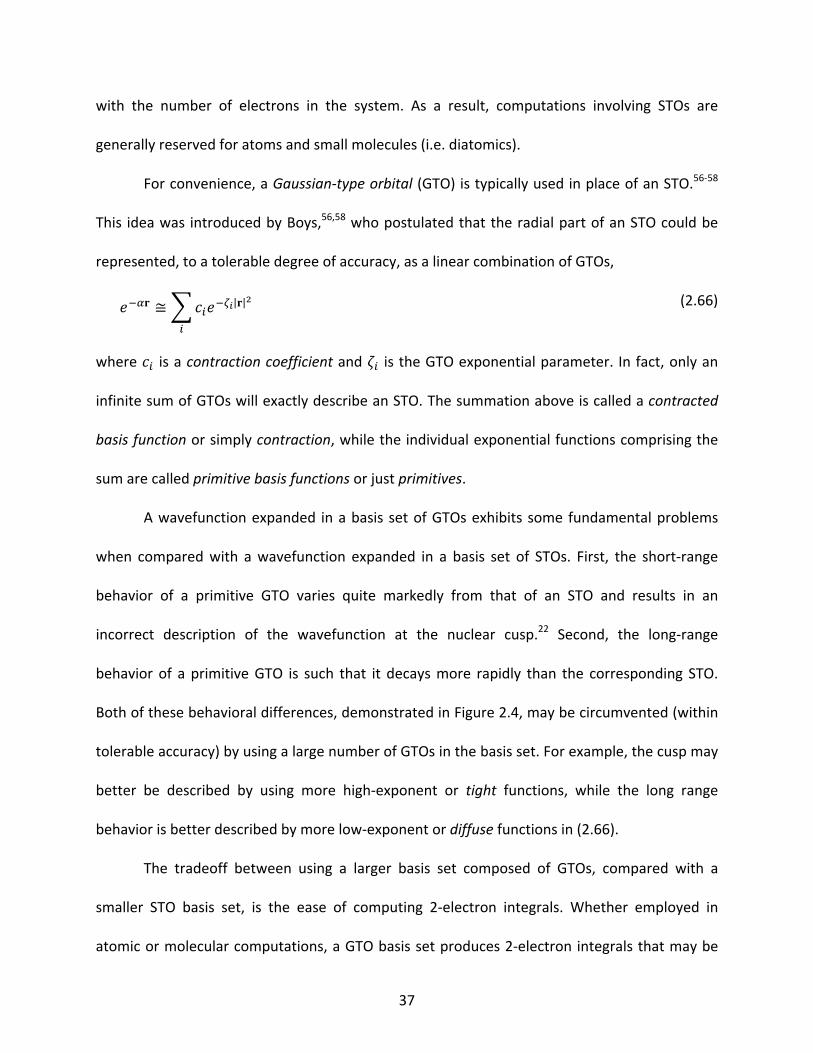
37
with the number of electrons in the system. As a result, computations involving STOs are
generally reserved for atoms and small molecules (i.e. diatomics).
For convenience, a Gaussian‐type orbital (GTO) is typically used in place of an STO.56‐58
This idea was introduced by Boys,56,58 who postulated that the radial part of an STO could be
represented, to a tolerable degree of accuracy, as a linear combination of GTOs,
| | (2.66)
where is a contraction coefficient and is the GTO exponential parameter. In fact, only an
infinite sum of GTOs will exactly describe an STO. The summation above is called a contracted
basis function or simply contraction, while the individual exponential functions comprising the
sum are called primitive basis functions or just primitives.
A wavefunction expanded in a basis set of GTOs exhibits some fundamental problems
when compared with a wavefunction expanded in a basis set of STOs. First, the short‐range
behavior of a primitive GTO varies quite markedly from that of an STO and results in an
incorrect description of the wavefunction at the nuclear cusp.22 Second, the long‐range
behavior of a primitive GTO is such that it decays more rapidly than the corresponding STO.
Both of these behavioral differences, demonstrated in Figure 2.4, may be circumvented (within
tolerable accuracy) by using a large number of GTOs in the basis set. For example, the cusp may
better be described by using more high‐exponent or tight functions, while the long range
behavior is better described by more low‐exponent or diffuse functions in (2.66).
The tradeoff between using a larger basis set composed of GTOs, compared with a
smaller STO basis set, is the ease of computing 2‐electron integrals. Whether employed in
atomic or molecular computations, a GTO basis set produces 2‐electron integrals that may be
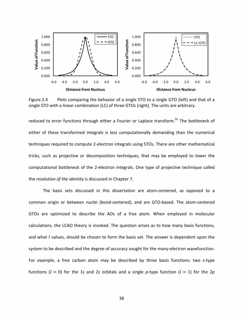
38
reduced to error functions through either a Fourier or Laplace transform.55 The bottleneck of
either of these transformed integrals is less computationally demanding than the numerical
techniques required to compute 2‐electron integrals using STOs. There are other mathematical
tricks, such as projective or decomposition techniques, that may be employed to lower the
computational bottleneck of the 2‐electron integrals. One type of projective technique called
the resolution of the identity is discussed in Chapter 7.
The basis sets discussed in this dissertation are atom‐centered, as opposed to a
common origin or between nuclei (bond‐centered), and are GTO‐based. The atom‐centered
GTOs are optimized to describe the AOs of a free atom. When employed in molecular
calculations, the LCAO theory is invoked. The question arises as to how many basis functions,
and what values, should be chosen to form the basis set. The answer is dependent upon the
system to be described and the degree of accuracy sought for the many‐electron wavefunction.
For example, a free carbon atom may be described by three basis functions: two s‐type
functions ( 0) for the 1s and 2s orbitals and a single p‐type function ( 1) for the 2p
Figure 2.4 Plots comparing the behavior of a single STO to a single GTO (left) and that of asingle STO with a linear combination (LC) of three GTOs (right). The units are arbitrary.
0.000
0.200
0.400
0.600
0.800
1.000
‐6.0 ‐4.0 ‐2.0 0.0 2.0 4.0 6.0
Value
of Fun
ction
Distance from Nucleus
STOGTO
0.000
0.200
0.400
0.600
0.800
1.000
‐6.0 ‐4.0 ‐2.0 0.0 2.0 4.0 6.0
Value
of Fun
ction
Distance from Nucleus
STO
LC‐GTO
39
orbital. This is an example of a minimal basis set, where there are just enough functions to
cover the occupied AOs of each atom. Each occupied orbital is described by a contracted
function rather than a single GTO due to the deficiencies of GTOs described earlier. The
problem with employing a minimal basis set is two‐fold: 1) the basis set is not flexible enough
to describe the many possible chemical environments an atom might be in and 2) employing a
minimal basis set in correlated ab initio methods does not recover much correlation energy.7
The electronic structure of a free atom is much different than the same atom in a
molecule, and the electronic structure from atom to atom varies markedly as well. Thus, it is
imperative to have a basis set that will be flexible enough, that is, have basis functions
describing the proper orbital space, from one chemical environment to another. Consider a π
bond between two carbon atoms, formed by the overlap of their 2p orbitals. If d‐type functions
are added to the carbon basis sets, then some of the d orbitals will mix with the p orbitals by
symmetry and cause the overlap forming the π bond to increase; a sort of p‐d hybridization
occurs, lowering the bond energy.18 These additional d‐type basis functions are called
polarization functions because they polarize (distort) the 2p orbitals. It is typical of basis sets to
include at least some polarization functions since these functions aid in the qualitative and
quantitative description of chemical bonds. Polarization functions also become important in
systematically recovering correlation energy (discussed in Chapter 3). An investigation reported
by Schwartz on two‐electron systems demonstrated that the MP2 correlation energy is
proportional to the highest orbital quantum number in the basis set.59 This observation lends
credence to the use of polarization functions with ‐values well beyond the minimal basis set.
40
2.5 Model Chemistries
The discussion thus far has covered different types of computational methods that
construct approximate many‐electron wavefunctions (or densities) and basis sets that can be
used to expand such wavefunctions. A dichotomy arises as to which computational method
should be selected for a particular chemical system and which basis set will provide the most
accurate expansion of the wavefunction. Ideally, one would like to pair the FCI method with a
basis set that spans all possible AO space. This would give the exact solution to the non‐
relativistic Schrödinger equation within the BO approximation. However, a basis set that spans
all possible AO space requires an infinite linear combination of GTOs, making the approach
intractable. Instead, a compromise must be made as to how many and what type of basis
functions need to be employed to properly describe the electronic structure. Further, a
compromise as to which computational method is appropriate and applicable to the system of
interest must be made. Hehre et al. coined the term model chemistry, or level of theory to
describe the coupling of a computational method and a given basis set.18 This concept is
graphically represented in Figure 2.5.
Since doubles correlation is the dominant fraction of the total correlation energy,
compared with other excitation levels, ab initio methods such as CISD, CCSD, and MP2 are
generally sufficient and tractable for systems up to 25 non‐hydrogen atoms and a modest‐sized
basis set (the inclusion of singles in addition to doubles does not appreciably increase the
computational cost). In some electronic systems, triple and quadruple excitations make
appreciable contributions to the total correlation energy. To recover triples and some
quadruples, one may use the CCSDT method (note that CISDT is not usually employed since it is
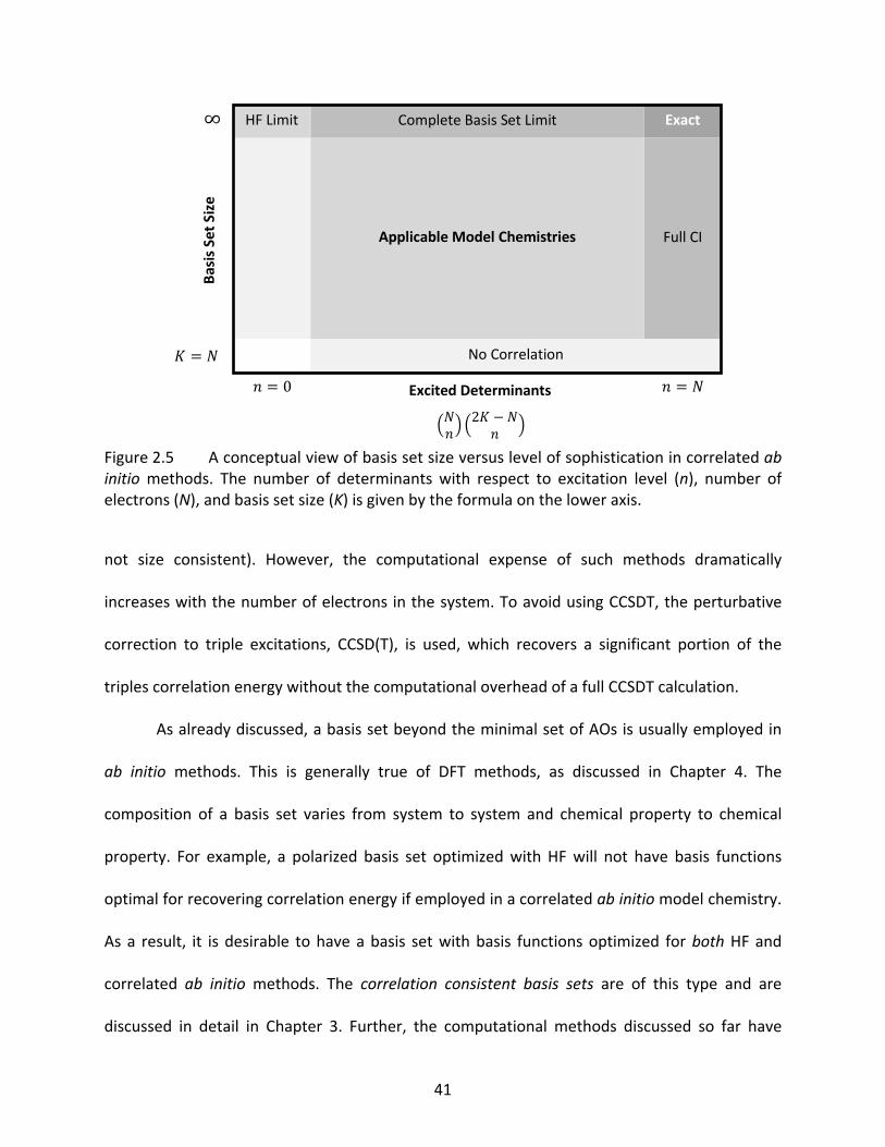
41
not size consistent). However, the computational expense of such methods dramatically
increases with the number of electrons in the system. To avoid using CCSDT, the perturbative
correction to triple excitations, CCSD(T), is used, which recovers a significant portion of the
triples correlation energy without the computational overhead of a full CCSDT calculation.
As already discussed, a basis set beyond the minimal set of AOs is usually employed in
ab initio methods. This is generally true of DFT methods, as discussed in Chapter 4. The
composition of a basis set varies from system to system and chemical property to chemical
property. For example, a polarized basis set optimized with HF will not have basis functions
optimal for recovering correlation energy if employed in a correlated ab initio model chemistry.
As a result, it is desirable to have a basis set with basis functions optimized for both HF and
correlated ab initio methods. The correlation consistent basis sets are of this type and are
discussed in detail in Chapter 3. Further, the computational methods discussed so far have
Figure 2.5 A conceptual view of basis set size versus level of sophistication in correlated abinitio methods. The number of determinants with respect to excitation level (n), number ofelectrons (N), and basis set size (K) is given by the formula on the lower axis.
Exact
Full CI
Complete Basis Set Limit
No Correlation
Applicable Model Chemistries
HF Limit
2
∞
0
Basis Set S
ize
Excited Determinants
42
been non‐relativistic, and if relativistic effects are to be included, a basis set optimized with a
non‐relativistic method will not recover all possible relativistic effects. It is pertinent that the
basis set employed in relativistic computations have core AOs optimized for the relativistic
Hamiltonian employed since the major fraction of relativistic effects come from these orbitals.
Relativistic basis sets are discussed in detail in Chapters 3 and 6.
Finally, there is a special class of model chemistries called composite methods in which
individually energy components of the total energy of a system are computed by different
levels of theory and specialized basis sets in an effort to achieve an approximation to a higher
(or intractable) level of theory.18,19 Often time, for example, only the valence correlation energy
is computed, but the correlation between core and valence electrons (called core‐valence
correlation) is important for accurately computing thermochemical properties. Further, most
computational methods are non‐relativistic, but atoms from the second row of the main group,
and heavier, have significant relativistic effects. To include these two energy components, a
composite method may compute the core‐valence energy and relativistic corrections at a low
level of theory like MP2 using specialized basis sets. These individual energy components are
then added to a previously computed reference energy that was computed at a higher level of
theory. There are several composite methods in popular use including the Gaussian‐n (Gn),60‐62
complete basis set (CBS‐n),63‐69 high accuracy extrapolated ab initio thermochemistry (HEAT),70
Weizmann‐n (Wn),71,72 and correlation consistent Composite Approach (ccCA)73‐80 methods.
Chapter 7 discusses the ccCA formulism in detail, including how the method recovers core‐
valence and relativistic effects.
43
CHAPTER 3
CORRELATION CONSISTENT BASIS SETS
3.1 Introduction
Having established the basics of basis set theory in computational quantum chemistry in
the previous chapter, a specific class of basis sets called the correlation consistent polarized
valence basis sets (cc‐pVnZ, where n = D, T, Q, etc.)81‐109 are discussed at length in this chapter.
The correlation consistent basis sets were introduced by Dunning as a means to systematically
recover correlation energy in correlated ab initio computations. The novel approach of
designing basis sets to help recover correlation energy was first studied by Ahlrichs et al.110‐112
and by Almlöf and Taylor.113,114 Dunning’s approach was similar to that of Almlöf and Taylor in
which 1) high angular momentum functions (d, f, g, etc.) are employed beyond the minimal
basis set and 2) basis functions are grouped according to their contribution to the total
correlation energy. Further, the optimized atomic orbitals (AOs) in the basis set are taken to be
the natural orbitals from correlated ab initio wavefunctions. The natural orbitals (NOs) are
obtained by diagonalizing the correlated density matrix,7,22,50 and have the intrinsic property of
forming a basis in which the correlated wavefunction converges most rapidly (as opposed to,
say, the molecular orbital basis). The primary difference between the basis sets developed by
Almlöf and Taylor and those of Dunning is the smaller sets of functions used by Dunning. In fact,
Dunning’s basis sets recover more than 99% of the correlation energy obtained by the basis
sets of Almlöf and Taylor, yet contain less basis functions.
44
The correlation consistent basis sets for the main group atoms were constructed using
Gaussian‐type orbital (GTO) basis sets developed by van Duijneveldt.115 The AOs represented in
each basis set were taken from non‐relativistic multi‐configuration self‐consistent field (MCSCF)
calculations, yielding a set of AOs that adequately describe the valence orbital degeneracy
inherent to most atoms. Each AO is represented by a general contraction of GTOs,114,116,117 in
which all symmetry‐equivalent basis functions are grouped in the contraction. From this point
on, this minimal set of AOs will be called the Hartree‐Fock (HF) basis set.
Within each family of correlation consistent basis sets, there is a hierarchy called the
ζ‐level, where the quality and size of the basis set increases with the ζ‐level. More than that, the
ζ‐level tells how many valence basis functions are used per atom. For example, a double‐ζ basis
set contains two functions per valence orbital; a triple‐ζ basis set contains three functions; etc.
The underlying principle of the ζ‐level is that more functions in the valence space give more
flexibility to the basis set. The core orbitals are always described by a single contracted GTO at
each ζ‐level. Because only the valence orbitals are described by multiple functions, the
correlation consistent basis sets are often referred to as split‐valence basis sets. Table 3.1 lists
the composition of the correlation consistent basis sets for main group atoms (including H and
He) according to each ζ‐level. Note that the primitive, or uncontracted, basis functions are
denoted by parentheses, while the contracted functions are denoted by brackets. The notation
“3s 2p 1d” indicates that three s‐type functions, two p‐type functions, and one d‐type function
comprise the basis set, and are not to be confused with the principle and orbital quantum
numbers. The following sections describe the process by which the correlation consistent basis
sets were developed by Dunning and coworkers, including basis sets for valence‐only
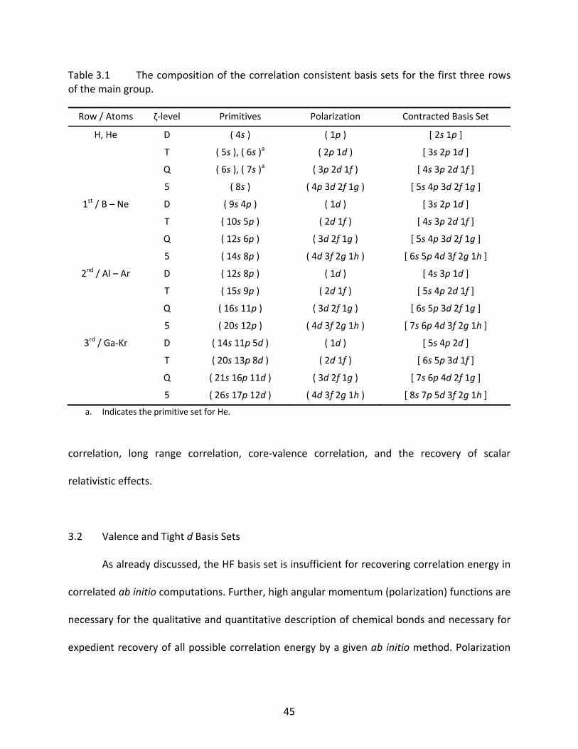
45
correlation, long range correlation, core‐valence correlation, and the recovery of scalar
relativistic effects.
3.2 Valence and Tight d Basis Sets
As already discussed, the HF basis set is insufficient for recovering correlation energy in
correlated ab initio computations. Further, high angular momentum (polarization) functions are
necessary for the qualitative and quantitative description of chemical bonds and necessary for
expedient recovery of all possible correlation energy by a given ab initio method. Polarization
Table 3.1 The composition of the correlation consistent basis sets for the first three rows of the main group.
Row / Atoms ζ‐level Primitives Polarization Contracted Basis Set
H, He D ( 4s ) ( 1p ) [ 2s 1p ]
T ( 5s ), ( 6s )a ( 2p 1d ) [ 3s 2p 1d ]
Q ( 6s ), ( 7s )a ( 3p 2d 1f ) [ 4s 3p 2d 1f ]
5 ( 8s ) ( 4p 3d 2f 1g ) [ 5s 4p 3d 2f 1g ]
1st / B – Ne D ( 9s 4p ) ( 1d ) [ 3s 2p 1d ]
T ( 10s 5p ) ( 2d 1f ) [ 4s 3p 2d 1f ]
Q ( 12s 6p ) ( 3d 2f 1g ) [ 5s 4p 3d 2f 1g ]
5 ( 14s 8p ) ( 4d 3f 2g 1h ) [ 6s 5p 4d 3f 2g 1h ]
2nd / Al – Ar D ( 12s 8p ) ( 1d ) [ 4s 3p 1d ]
T ( 15s 9p ) ( 2d 1f ) [ 5s 4p 2d 1f ]
Q ( 16s 11p ) ( 3d 2f 1g ) [ 6s 5p 3d 2f 1g ]
5 ( 20s 12p ) ( 4d 3f 2g 1h ) [ 7s 6p 4d 3f 2g 1h ]
3rd / Ga‐Kr D ( 14s 11p 5d ) ( 1d ) [ 5s 4p 2d ]
T ( 20s 13p 8d ) ( 2d 1f ) [ 6s 5p 3d 1f ]
Q ( 21s 16p 11d ) ( 3d 2f 1g ) [ 7s 6p 4d 2f 1g ]
5 ( 26s 17p 12d ) ( 4d 3f 2g 1h ) [ 8s 7p 5d 3f 2g 1h ]
a. Indicates the primitive set for He.
46
functions optimized using HF will aid in the non‐correlated description of chemical bonds,
however, HF polarization functions are far from optimal as virtual orbitals in correlated
methods. Therefore, the polarization functions of the correlation consistent basis sets were
optimized as an even‐tempered expansion using singles and doubles configuration interaction
(CISD). An even‐tempered expansion of basis functions is a method of determining the
exponential parameters using a geometric series:116,118
, 1,2, … (3.1)
The parameters and are unique for each group of basis functions with the same value
and are varied so as to minimize the correlation energy. The advantages of using (3.1) instead
of explicit optimization of each polarization function are 1) there are only two parameters to
optimize for the entire group of functions and 2) the polarization functions are evenly
distributed in log‐space, providing even coverage of the orbital space.22
The high angular functions were optimized using (3.1) in groups according to their
values, and were added to the HF basis set of each atom, as suggested by Schwartz,59 until the
correlation energy did not change appreciably. By adding functions this way, the correlation
space for each particular value is saturated. Dunning noted that certain functions within each
group contributed similar amounts of correlation energy. Specifically, it was noted that the
first d function contributed most to the correlation energy; while the second d and first f
functions contributed similar amounts to the correlation energy; the third d, second f, and first
g functions contributed similar amounts to the correlation energy; etc. From this, Dunning
suggested that high angular functions should be added to the HF basis sets in a correlation
consistent manner, that is, in shells as ( 1d ), ( 2d 1f ), ( 3d 2f 1g ), etc. In this way, the
47
correlation energy is systematically recovered with each additional shell of high angular
functions. Further tests were performed by explicitly optimizing the high angular functions
within each group, but no appreciable change was noted in the correlation energy, so the
even‐tempered scheme was kept. Even‐tempered optimizations of s and p functions in addition
to the HF basis sets were also performed with respect to the correlation energy. Dunning found
that uncontracting the outermost s and p functions had the same effect of lowering the
correlation energy as explicit optimization. The split valence nature of the correlation
consistent basis sets stems from the number of s and p functions that are uncontracted: a
single s and p function are uncontracted at the double‐ζ level, two s and p functions are
uncontracted at the triple‐ζ level, etc. (cf. Table 3.1)
After being introduced, studies by Bauschlicher and Partridge119 and Martin et al.120‐122
employing the cc‐pVnZ basis sets showed that including an additional tight d function
significantly improved the computed atomization energies of molecules containing second row
atoms. While the most dramatic improvements were shown for energetics of sulfur species,
Bauschlicher and Partridge also showed that the atomization energies of SiH3 and SiH4 were
affected by 1.1 and 1.6 kcal/mol, respectively, when a tight d function was employed in the
triple‐ζ basis set. The role of an additional tight d function in second row atoms was
commented on by Woon and Dunning in their original paper, however, the need for such a
function did not become evident until the properties of a wider variety of molecular species
than were in the original benchmarking papers were studied.123 As a result, Dunning, Peterson,
and Wilson modified the sets, developing the tight d correlation consistent basis sets,
cc‐pV(n+d)Z,124 and in numerous studies, have demonstrated the importance of the augmented
48
tight d basis sets in coupled cluster and density functional theory studies.101,125‐128
The correlation consistent build‐up of high angular functions with increasing ζ‐level
leads to smooth, monotonic behavior of total energies. As the basis set becomes saturated at
high ζ‐levels, more and more of the AO space is covered by the basis functions, resulting in a
nearly complete basis set. Once the basis set reaches completeness, any remaining error
between a computed chemical property and a reliable experimental measurement is due solely
to the computational method. As the ζ‐level increases, the total energy computed with the
cc‐pVnZ basis sets asymptotically approaches the complete basis set (CBS) limit.93 The exact
mathematical form of the monotonic behavior is not known, but resembles an exponential‐type
decay. To this end, several empirical extrapolation techniques have been developed to
approximate the CBS limit.85,95,129‐132 Two popular extrapolation schemes are below:
CBS (3.2)
CBS (3.3)
Equation (3.2) is a standard exponential fit due to Feller,132 while (3.3) is a mixed
Gaussian/exponential fit due to Woon, Dunning, and Peterson.85,95 In each equation, and
are fitting parameters, is the chemical property (i.e. energy) computed at the th ζ‐level
( 2 for double‐ζ, 3 for triple‐ζ, etc.), and CBS is the estimated CBS limit. Both equations
are analytic for three points, but are numerical for any more. Taking to be the lowest ζ‐level in
a series of three points, the analytic forms of the parameters in (3.2) are
49
CBS 2
2
ln
(3.4)
while those in (3.3) are
CBS
(3.5)
Another extrapolation formula in common use is that of Halkier et al.,133 a two‐point scheme
based on the convergence of correlation energies in atoms:
CBS11
(3.6)
in which takes on the same meaning as in (3.2) and (3.3). The virtue of using (3.6) over (3.2)
or (3.3) is that it only requires two points to estimate the CBS limit. However, it is not possible
to estimate higher ζ‐levels with (3.6) as it is with (3.2) and (3.3). Further, using one of the
exponential‐type extrapolation formulas will sometimes provide a better approximation to the
true CBS limit since more points are used in the fit.
50
3.3 Augmented Basis Sets
In order to quantitatively describe chemistry stemming from long‐range phenomena
such as van der Waals interactions, Rydberg states, multipole moments, polarizabilities,
hydrogen bonding, and the binding of excess electrons, diffuse functions must be employed in
the basis set. Dunning and coworkers have developed augmented correlation consistent basis
sets (aug‐cc‐pVnZ) describing such chemical phenomena.86,88,91,93,95,99,100
The diffuse functions added at each ζ‐level are comprised of a single function of each
value present. For example, to the double‐ζ basis set is added a set of ( 1s 1p 1d ) functions, to
the triple‐ζ basis set is added a set of ( 1s 1p 1d 1f ) functions, etc. The diffuse s and p functions
were optimized on top of the HF basis set in MCSCF calculations of the atomic anions, while the
high angular functions were optimized with CISD on top of the polarization functions already
present.
3.4 Core‐Valence Basis Sets
Valence‐only, or valence‐valence (VV) correlation is generally accepted to be adequate
for accurately computing most chemical properties since the qualitative and quantative
description of many chemical properties relies on changes in the valence electronic structure.
As already discussed, the cc‐pVnZ and aug‐cc‐pVnZ basis sets recover this correlation
systematically with increasing ζ‐level. Also well‐known is that in order to achieve ±1.0 kcal/mol
accuracy, or better, in thermodynamic properties, core‐valence (CV) correlation must also be
included.93,134 The cc‐pVnZ and aug‐cc‐pVnZ basis sets are not optimal for the recovery of CV
correlation and were reoptimized specifically for the recovery of CV correlation by Woon,
51
Peterson, and Dunning.81,98
There are two types of CV correlation consistent basis sets, the original CV basis sets
(cc‐pCVnZ)98 and the weighted core‐valence (wCV) correlation consistent basis sets
(cc‐pwCVnZ).81 The principle difference between the CV and wCV basis sets is that the former
are designed to recover more core‐core (CC) correlation energy, while the wCV basis sets are
intentionally biased towards CV (almost no CC) correlation energy. The optimization of the
core‐correlation (tight) functions proceeded by adding H/He‐like basis sets for correlating the
1s electrons to the first row, main group atoms. Woon and Dunning found that adding groups
of tight functions as ( 1s 1p ) to the double‐ζ basis set, ( 2s 2p 1d ) to the triple‐ζ basis set, etc.
resulted in smooth, monotonic behavior of the CC, CV, and VV energies, as opposed to the
erratic behavior of these energies when the valence‐only cc‐pVnZ basis sets were used. The
following formula was used to optimize the core‐correlating functions:
Δ CISD CC CV VV CISD CC CISD CV CISD VV (3.7)
The weight, , in the above equation is taken to be 1.00 in the cc‐pCVnZ basis sets, and to be
0.01 in the cc‐pwCVnZ basis sets from an in‐depth study of CC and CV effects of first and second
row molecules by Peterson and Dunning.81 It has been noted by Peterson81,93 that both the
cc‐pCVnZ and cc‐pwCVnZ basis sets converge on similar CBS limits, although the cc‐pwCVnZ
basis sets tend to produce lower energies in valence‐only calculations because of the more
diffuse nature of the weighted core‐correlation functions.
3.5 Scalar Relativistic Basis Sets
As discussed in section 2.4, basis sets optimized with non‐relativistic methods are not
52
optimal for use in relativistic calculations. The correlation consistent basis sets discussed so far
were all developed using non‐relativistic formulisms of HF and CISD. One of the most common
relativistic models is the spin‐free Douglas‐Kroll (DK) Hamiltonian,135‐137 which approximates the
full, four‐component Dirac equation138,139 by a transformation of the electron orbitals. The
resulting orbitals are then used in a subsequent HF or correlated ab initio calculation to include
scalar relativistic effects such as the mass‐velocity and Darwin corrections, the two largest
contributors to the relativistic energy.137,140,141 These corrections are termed scalar relativistic
since they do not include inner products containing spin components (i.e. spin‐orbit coupling,
spin‐spin coupling, etc.) The largest effect of scalar relativity occurs in the core orbitals, which
contract inward toward the nucleus due to their increased kinetic energy. Because the core
orbitals of the cc‐pVnZ basis sets are represented by a single contracted GTO, there is no
flexibility in the core to change under the DK transformation, resulting in a loss of accuracy
within the relativistic model. Thus, the core contractions must be reoptimized. Instead of
recontracting only the core orbitals, all of the contractions are typically reoptimized to account
for variations in the valence orbitals due to fluctuations in the core.
The first to report on correlation consistent basis sets optimized for scalar relativistic
computations, denoted cc‐pVnZ‐DK, were de Jong et al.142 Their scheme for recontracting the
cc‐pVnZ basis sets is as follows: 1) remove the polarization functions (d, f, g, and h) from the
cc‐pVnZ basis sets, and uncontract the s and p basis set; 2) run a HF calculation using the
uncontracted sp basis set and the DK Hamiltonian; and 3) the optimized s and p contraction
coefficients are then determined by a population analysis. A similar scheme is used in Chapter
6, in which DK‐optimized basis sets for the s‐block atoms are reported.
53
CHAPTER 4
SYSTEMATIC TRUNCATION OF THE CORRELATION CONSISTENT BASIS SETS IN DENSITY
FUNCTIONAL THEORY CALCULATIONS†
4.1 Introduction
The plethora of density functionals available46 has brought about a tremendous
challenge in applying density functional theory (DFT)44,45,52 to the study of chemical systems,
namely, the choice of a density functional that is suitable for the problem of interest.
Unfortunately, no simple means currently exists to aid in density functional selection, barring
whether or not a density functional was specifically developed for a particular problem, and
reliance upon benchmark studies, when available, is essential. However, it is of great interest to
have a simple, efficient means to gauge the intrinsic error of a density functional. To accomplish
this, a first step is to develop a greater understanding of the behavior of density functionals
with respect to the basis set.
As shown in Chapter 3, the correlation consistent basis sets exhibit smooth, monotonic
convergence in energetic properties with increasing basis set size, and that the complete basis
set (CBS) limit may be numerically approximated through the use of various extrapolation
schemes. Unfortunately, it is not clear whether or not such an approach is possible for DFT
calculations since the correlation consistent basis sets were developed specifically for ab initio
† This entire chapter is adapted from B.P. Prascher, B.R. Wilson, and A.K. Wilson, “Behavior of Density Functionals with Respect to Basis Set. VI. Truncation of the Correlation Consistent Basis Sets.” J. Chem. Phys. 2007, 127, 124110, with permission from the American Institute of Physics.
54
methods.
Energetic and structural properties are generally known to converge more quickly with
respect to increasing basis set size for DFT than for ab initio methods.125,126,143‐156 In fact, it is
commonly assumed that small changes in energetic properties beyond the triple‐ζ basis set
level typically occur, but recent work has demonstrated that significant changes in energetic
properties sometime do occur beyond the triple‐ζ level.148,149 Further, recent work has shown
non‐monotonic behavior of energetic properties can occur with respect to increasing basis set
size in DFT calculations.125,126,152‐158 This observation has been made using a number of
molecules and density functionals, with no obvious trends appearing as to when the non‐
monotonic behavior does or does not occur. When monotonic behavior does occur, then it has
been shown that various extrapolation formulas can be used to estimate the CBS limit, or in the
case of density functional theory, the Kohn‐Sham (KS) limit.144,145,154‐156 However, with non‐
monotonic behavior, such an approach is not reliable. To date, no single solution to the non‐
monotonic problem has evolved; rather, a number of possible solutions have emerged.
Provided a reasonable grid size is utilized for the numerical calculation of the DFT energy, grid
selection does not seem to impact the basis set convergence.156 Other factors that influence
convergence include basis set superposition error152 and basis set contraction,156 which, when
combined, have been shown to lead to monotonic convergence (discussed in the next
chapter).148 It is important to note that systematic convergence to the KS limit should not
necessarily be expected from the correlation consistent basis sets as they were explicitly
developed for ab initio methods. However, Jensen has developed a series of polarization
consistent basis sets (pc‐n, where n = 1‐4) explicitly for DFT,143‐145 and non‐monotonic behavior
55
using various density functionals is still observed for these basis sets.155
Ab initio methods rely directly on the inclusion of many excited determinants,
constructed from high angular momentum functions, while density functionals do not. High
angular momentum functions in DFT computations have the same effect as in Hartree‐Fock
(HF), that is, to polarize the electron density. As a result, DFT computations are less basis set
dependent than ab initio computations, and DFT computations, with systematic increases in
basis set size, tend to converge quickly. Rapid convergence towards the KS limit is desirable, but
the high angular momentum functions included in many basis sets may not have a significant
effect on a computed property. Thus, these functions create unnecessary overhead in terms of
computational expense and, as shown in this chapter, may be removed without the
introduction of significant error.
Earlier work has utilized truncated or auxiliary basis sets as a means to reduce
computational cost in DFT calculations. For example, the resolution of the identity Coulomb
approximation (RI‐J) has been studied by Skylaris et al.159 and by Head‐Gordon et al.150 In the
RI‐J approximation, an auxiliary basis set is used to compute the Coulomb integrals, which can
reduce the computational cost without introducing errors of more than a few millihartrees in
the total energy.159
Head‐Gordon et al. have also investigated a dual basis approach, first proposed by Van
Alsenoy and Vahtras et al.160,161 in which a truncated form of a basis set, such as cc‐pVTZ
without f functions or the inner d functions, is used to construct an initial approximation to the
full cc‐pVTZ basis density. Subsequent parameterization is included to help account for the
difference in densities between the full cc‐pVTZ basis set and the truncated basis set.151 Earlier
56
work by Jensen examined truncation of core basis functions from double‐ and triple‐ζ polarized
basis sets (DZP and TZP, respectively) as well as the pc‐n basis sets.147 The conclusions from his
investigation indicate that basis sets truncated of certain core functions lead to results similar
to those obtained when the full basis sets are employed. However, truncation of core functions
is not suitable for the accurate determination of KS limits due to the incomplete coverage of
the exponent space.
The present investigation examines the truncation of valence basis functions from the
correlation consistent basis sets without parameterization, and does not suffer from reduced
coverage of the necessary exponent space since neither the s or p functions are removed from
the HF basis set. By analyzing the change in computed properties as basis functions are
systematically truncated, the necessity of high angular momentum functions becomes clear, as
was demonstrated in a similar study by Mintz et al. in which truncated correlation consistent
basis sets were studied in ab initio methods.162,163 Understanding how high angular momentum
functions impact not only computed properties, but also basis set convergence, will aid in
designing basis sets for DFT computations.
4.2 Computational Methodology
Two popular density functionals have been included in this study, including pure and
hybrid density functionals. The pure density functional is the gradient‐corrected Becke (B)164
exchange functional, coupled with the Lee‐Yang‐Parr (LYP)165 gradient‐corrected correlation
functional, BLYP. For the hybrid DFT computations, the Becke three‐parameter scheme (B3)166
is employed with the LYP correlation functional, utilizing the third parameterization of the
57
Vosko, Wilk, and Nusair local correlation functional (VWN‐3).167
The correlation consistent basis sets, cc‐pVnZ,94‐101 through quintuple‐ζ quality have
been employed. Systematic truncation of these basis sets follows that of the scheme published
by Mintz et al. for the hydrogen atom,162,163 but is extended to include non‐hydrogen atoms.
The truncation scheme involves removing the highest ‐value basis function first, then the most
diffuse function from the 1 shell, then the second‐most diffuse function from the 1
shell, etc. The truncation continues through the polarization functions, but does not include the
contracted s and p functions. The notation used is as follows: the full triple‐ζ basis is denoted as
usual: cc‐pVTZ; the first truncation of this basis is denoted cc‐pVTZ(–1f); the second truncation
is denoted cc‐pVTZ(–1f 1d); and the third truncation is denoted cc‐pVTZ(–1f 2d) which reflects
the removal of one f function and the two most diffuse d functions (for cc‐pVTZ, this means
removal of all of the d functions). It is implied that the first truncation of a specific ‐shell is the
most diffuse (i.e. lowest exponent).
In atomic computations it is common practice to perform a symmetry‐averaging of
degenerate electronic states since this leads to a more physically‐sound wavefunction. If the
resulting wavefunction is spherically symmetric ( 0), then basis functions of angular
momentum not present in the filled, state‐averaged orbitals can be separated from the total
wavefunction without consequence to the total energy. This phenomenon has been
investigated in great detail by Bauschlicher and Taylor.168 This chapter strictly employs single
reference wavefunctions in all computations. Atomic symmetry breaking of the type used here
has been discussed in rigorous detail elsewhere, and is often necessary to correctly compute
electronic properties.46,169 As atom‐centered basis sets are typically used in molecular
58
computations, where atoms are not spherically‐symmetric, broken symmetry in atomic
computations is an appropriate means to effectively gauge basis set truncation effects.
Vertical ionization potentials and electron affinities have been determined using
experimental geometries for the neutral molecules taken from the National Institute of
Standards and Technology (NIST) Webbook.170‐172 The geometry was fixed so that the impact of
removing high angular momentum functions could be gauged without a geometry optimization
affecting the energy. Optimized geometries and their atomization energies are reported after
gauging the impact of truncation. The use of diffuse functions in the basis set has been
restricted to only the s and p functions here, which are taken from the augmented
(aug‐cc‐pVnZ) basis sets, and have been employed in computations of electron affinities.173
Atoms of the first and second rows, their dimers, and the molecules CH4, SiH4, NH3, PH3, H2O,
and H2S have been investigated. All DFT computations of this study have been performed using
the Gaussian software suite of programs.174 The default pruned grid (75,302)175 has been used
in all computations, and total energies in all computations are converged to 10‐8 Eh, or better.
4.3 Results and Discussion
4.3.1 Atoms
Total energies for the first row atoms carbon and oxygen are given in Table 4.1. Ideally,
the energy difference between a truncated basis and the full basis set should not be more than
1.0 mEh (approximately 1.0 kcal/mol) since this is the typical accuracy sought for computed
energetics when compared with experiment. As shown in the table, truncation effects in BLYP
59
computations are similar to those in B3LYP computations. The largest difference between BLYP
and B3LYP as a result of truncation occurs for carbon and is 0.110 mEh at the cc‐pVTZ(‐1f 2d)
level. Comparing carbon to oxygen, the effect of truncation on the total energy of oxygen is
almost twice that of carbon. For example, at the cc‐pV5Z(‐1h 2g 3f 4d) level for carbon, the
change in the BLYP energy with respect to the full basis set is 1.190 mEh, while for the oxygen
atom the change is 2.266 mEh. The greatest difference between the truncated and full basis
sets occurs for the fully truncated quintuple‐ζ basis set, cc‐pV5Z(‐1h 2g 3f 4d), for all atoms
investigated. Generally, the fully truncated cc‐pV5Z value for the total energy is comparable to
the full cc‐pVQZ basis set value for atoms with non‐spherical wavefunctions.
Computed ionization potentials and electron affinities of carbon and oxygen are shown
in Table 4.2 and Table 4.3, respectively. It is immediately obvious that electron affinities are not
as affected by truncation as ionization potentials (note that the electron affinities have been
computed using the s and p diffuse functions from the aug‐cc‐pVnZ basis sets). In the oxygen
atom, significant changes (i.e. more than 0.04 eV, or 1.0 kcal/mol) in the computed ionization
potential do not occur until f functions are completely removed. The carbon atom ionization
potentials show little change relative to the full basis, even with complete truncation of all high
angular momentum functions. Electron affinities, on the other hand, do not change until d
functions are truncated, and even then, the differences between the full and truncated basis
sets are less than 0.04 eV. There is little dependence on the density functional used since
truncation effects appear at the same level for B3LYP and BLYP. For example, the ionization
potential of oxygen begins to be affected by truncation at the cc‐pVTZ(‐1f), cc‐pVQZ(‐1g 1f), and
cc‐pV5Z(‐1h 2g 1f) levels in both BLYP and B3LYP. A similar trend results for electron affinities.
60
Figure 4.1 is a plot of the full basis set versus truncated basis set ionization potential of oxygen
determined with BLYP. Because basis functions of 3 do not significantly affect the
computed ionization potentials of atoms, a plot of each basis set containing only s, p, d, and f
functions is included for comparison in Figure 4.1. The 3 values coincide well with the full
basis set values. The inset in the figure demonstrates the effect of different truncation levels at
the cc‐pVQZ level on computed ionization potentials. Based on these observations for first row
atomic properties, a basis set for use in DFT computations need only contain up through f
functions to achieve full cc‐pVnZ basis set results for total energies, ionization potentials, and
electron affinities within 1.0 kcal/mol for atoms.
4.3.2 Homonuclear Diatomics
The BLYP and B3LYP total energies for the first row diatomics C2 and O2 are shown in
Table 4.4. In general, truncation affects the diatomic total energies by almost an order of
magnitude more than in atoms. This is expected, since the high angular momentum functions
are necessary for a better description of bonding and anti‐bonding orbitals, specifically d and f
functions which polarize p functions in σ‐ and π‐type bonds. This is readily seen for each
diatomic investigated, where truncation of f functions from the cc‐pV5Z basis set typically
causes the difference in total energy relative to the full basis to increase on the order of mEh,
and the truncation of d functions increases on the order of tens of mEh. Table 4.5 lists
computed ionization potentials, electron affinities, and optimized bond lengths for the first row
dimers with BLYP. The ionization potentials remain unaffected by truncation until d functions
have been truncated, but the electron affinities are affected with truncation of the f functions.
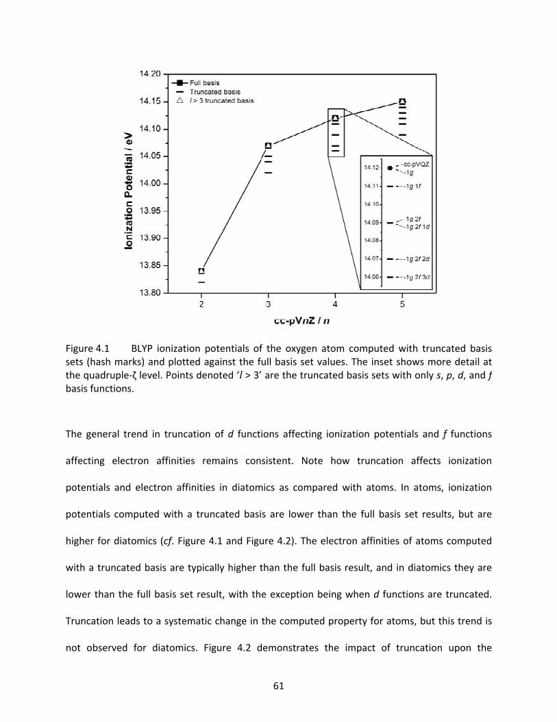
61
The general trend in truncation of d functions affecting ionization potentials and f functions
affecting electron affinities remains consistent. Note how truncation affects ionization
potentials and electron affinities in diatomics as compared with atoms. In atoms, ionization
potentials computed with a truncated basis are lower than the full basis set results, but are
higher for diatomics (cf. Figure 4.1 and Figure 4.2). The electron affinities of atoms computed
with a truncated basis are typically higher than the full basis result, and in diatomics they are
lower than the full basis set result, with the exception being when d functions are truncated.
Truncation leads to a systematic change in the computed property for atoms, but this trend is
not observed for diatomics. Figure 4.2 demonstrates the impact of truncation upon the
Figure 4.1 BLYP ionization potentials of the oxygen atom computed with truncated basissets (hash marks) and plotted against the full basis set values. The inset shows more detail atthe quadruple‐ζ level. Points denoted ‘l > 3’ are the truncated basis sets with only s, p, d, and fbasis functions.
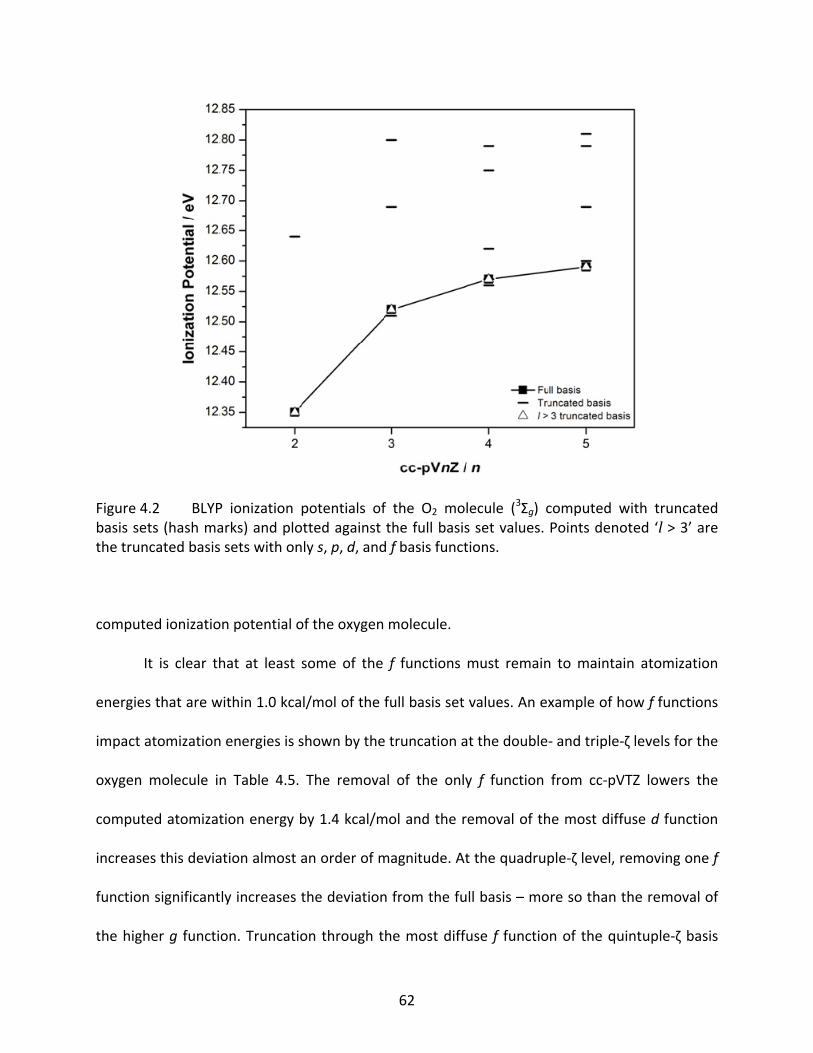
62
computed ionization potential of the oxygen molecule.
It is clear that at least some of the f functions must remain to maintain atomization
energies that are within 1.0 kcal/mol of the full basis set values. An example of how f functions
impact atomization energies is shown by the truncation at the double‐ and triple‐ζ levels for the
oxygen molecule in Table 4.5. The removal of the only f function from cc‐pVTZ lowers the
computed atomization energy by 1.4 kcal/mol and the removal of the most diffuse d function
increases this deviation almost an order of magnitude. At the quadruple‐ζ level, removing one f
function significantly increases the deviation from the full basis – more so than the removal of
the higher g function. Truncation through the most diffuse f function of the quintuple‐ζ basis
Figure 4.2 BLYP ionization potentials of the O2 molecule (3Σg) computed with truncatedbasis sets (hash marks) and plotted against the full basis set values. Points denoted ‘l > 3’ arethe truncated basis sets with only s, p, d, and f basis functions.
63
does not significantly alter the computed atomization energy, but removing the second f
function does. It is clear that the f shell must be retained in the homonuclear diatomics to
minimize the deviation of the truncated basis atomization energy from that of the full basis.
Optimized bond lengths follow a trend similar to that of molecular electron affinities in
that they depend heavily on the d functions in the basis set. Target accuracy for truncated basis
set bond lengths is 0.01 Å relative to the bond length determined using the full basis set. The
removal of the d function from the double‐ζ basis set in a BLYP computation of the oxygen
molecule affect the optimized bond length by 0.060 Å. At the triple‐ζ level, truncation of the
most diffuse d function significantly affects the bond length and removal of the entire d shell
causes the bond length to deviate by 0.064 Å from the full basis set result. The most diffuse d
function of the quadruple‐ and quintuple‐ζ basis sets does not significantly affect the bond
length upon truncation, but removal of any of the other d functions from these bases
significantly impacts the computed value. These deviations in truncated basis set bond lengths
for BLYP are also typical in B3LYP computations.
4.3.3 CH4, SiH4, NH3, PH3, H2O, and H2S
Table 4.6, Table 4.7, and Table 4.8 provide B3LYP optimized geometries for CH4, NH3,
H2O, SiH4, PH3, and H2S. The truncation notation used in these tables has two terms. The first
represents the truncation of the non‐hydrogen basis set, and the second represents the
truncation of the hydrogen basis set. For example, at the triple‐ζ level, ‘‐1f 2d ; 1d 2p’ denotes
truncation of one f and two d functions from the non‐hydrogen basis and one d and two p
functions from the hydrogen atom basis set. Both truncations are performed simultaneously.
64
Included in the tables for CH4 and SiH4 are atomization energies. Table 4.6 shows that the
atomization energies in heteronuclear molecules are sensitive to the basis set truncation,
varying more than 1.0 kcal/mol when truncation of d functions from the non‐hydrogen basis
(including p functions from the hydrogen basis) occurs. Compared with the atomization
energies for homonuclear diatomics, the atomization energies for larger heteronuclear
molecules is less sensitive to basis set truncation overall. In fact, the atomization energy of the
oxygen molecule suffers almost a 30.0 kcal/mol deviation from the full basis set result when
truncation of all of the high angular momentum functions from each basis set is done. For
methane, full truncation of the basis sets only results in a 10.0 kcal/mol deviation from the full
basis set atomization energy. The atomization energy for silane is comparable to that of oxygen
in that the largest angular momentum functions required are f functions in the non‐hydrogen
basis set to maintain energies within 1.0 kcal/mol of those of the full basis set. Therefore, f
functions remain necessary in the non‐hydrogen basis set for computed atomization energies.
In molecules composed of first row atoms, the computed bond lengths do not vary by
more than 0.01 Å when the d and p shells are truncated from the non‐hydrogen and hydrogen
basis sets, respectively. In contrast, molecules which include a second row atom do depend on
the d and p shells from the non‐hydrogen and hydrogen basis sets, respectively, to avoid
deviating by more than 0.01 Å from the full basis set bond length. This is not surprising
considering that the second row atoms are known to form bonds with more 3p character than
3s, and the 3p orbitals are polarized by d functions present in the basis set. Further, angles of
second row systems are not as dependent on the d and p functions of the non‐hydrogen and
hydrogen basis sets, respectively. This is the direct result of more p character in the bonding
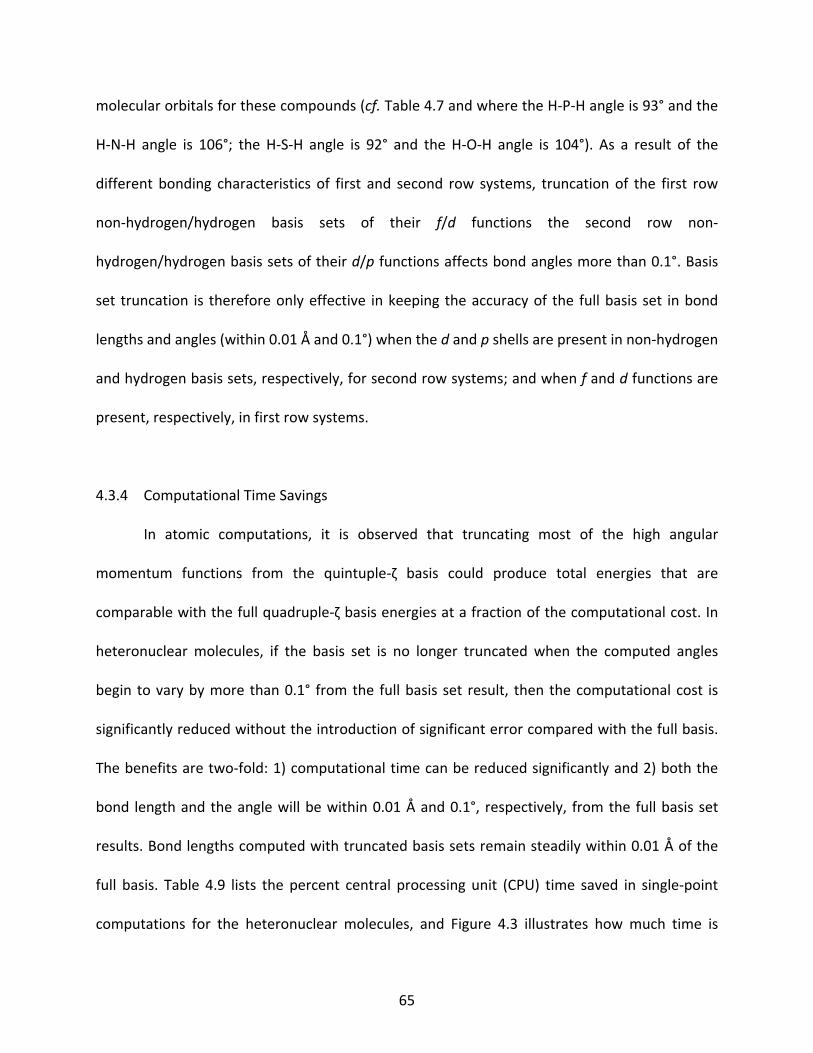
65
molecular orbitals for these compounds (cf. Table 4.7 and where the H‐P‐H angle is 93° and the
H‐N‐H angle is 106°; the H‐S‐H angle is 92° and the H‐O‐H angle is 104°). As a result of the
different bonding characteristics of first and second row systems, truncation of the first row
non‐hydrogen/hydrogen basis sets of their f/d functions the second row non‐
hydrogen/hydrogen basis sets of their d/p functions affects bond angles more than 0.1°. Basis
set truncation is therefore only effective in keeping the accuracy of the full basis set in bond
lengths and angles (within 0.01 Å and 0.1°) when the d and p shells are present in non‐hydrogen
and hydrogen basis sets, respectively, for second row systems; and when f and d functions are
present, respectively, in first row systems.
4.3.4 Computational Time Savings
In atomic computations, it is observed that truncating most of the high angular
momentum functions from the quintuple‐ζ basis could produce total energies that are
comparable with the full quadruple‐ζ basis energies at a fraction of the computational cost. In
heteronuclear molecules, if the basis set is no longer truncated when the computed angles
begin to vary by more than 0.1° from the full basis set result, then the computational cost is
significantly reduced without the introduction of significant error compared with the full basis.
The benefits are two‐fold: 1) computational time can be reduced significantly and 2) both the
bond length and the angle will be within 0.01 Å and 0.1°, respectively, from the full basis set
results. Bond lengths computed with truncated basis sets remain steadily within 0.01 Å of the
full basis. Table 4.9 lists the percent central processing unit (CPU) time saved in single‐point
computations for the heteronuclear molecules, and Figure 4.3 illustrates how much time is
66
saved with respect to energetic properties at various truncation levels of the cc‐pV5Z basis set.
The percent CPU time saved over the full basis computation escalates quickly as high angular
momentum functions are removed, reaching more than 50% when the highest angular
momentum functions are removed from the cc‐pVQZ and cc‐pV5Z basis sets. CPU time savings
are greater than 80% at the cc‐pV5Z level when the two highest angular momentum shells are
removed from both the non‐hydrogen and the hydrogen basis. Since truncation impacts
molecular ionization potentials, electron affinities, and atomization energies when truncating
the f functions, by only removing the higher angular momentum functions, the percent time
saved in computing these properties can be as large as 90% without deviating more than 1.0
kcal/mol (0.04 eV) from the full basis set results. Further, in bond lengths (without considering
angles) where the d shell is important for the non‐hydrogen basis, truncating the higher angular
momentum shells saves over 95% of the computational time without deviating from the full
basis set bond length by more than 0.01 Å.
4.4 Conclusions
Truncation of the correlation consistent basis sets in DFT is an excellent way to save
computational time and resources when computing various energetic properties without the
introduction of significant error. In the atoms and molecules studied, truncation of high angular
functions such as g and h functions affects ionization potentials and election affinities by less
than 0.01 eV, and affects atomization energies by less than 1.0 kcal/mol. Typical CPU time
savings upon truncation of only g and h functions from non‐hydrogen and hydrogen basis sets
are on the order of 60‐70%.
67
Unlike ab initio studies of cc‐pVnZ basis set truncation,162,163 DFT allows for the
truncation of not only the hydrogen basis but also the non‐hydrogen atom basis set.
Simultaneous truncation of both the hydrogen f and g functions and non‐hydrogen atom g and
h functions from the cc‐pV5Z basis set impacts optimized geometries by less than 0.01 Å in
bond lengths and 0.1° in angles as compared with the full basis geometry. In all molecules
investigated here, the removal of f functions from the non‐hydrogen basis with simultaneous
removal of d functions from the hydrogen basis does not affect bond lengths by more than
0.01 Å and affects angles by no more than 0.47°. The geometries of molecules composed of first
row atoms are not affected as greatly as those composed of second row atoms.
With truncation of all but the s, p, d, and f functions from the correlation consistent
basis sets, full basis set values for total energies, atomization energies, ionization potentials,
electron affinities (using s and p diffuse functions), and geometries are accessible (within
1.0 kcal/mol in energetics and 0.01 Å/0.1° in bond lengths/angles) with a large reduction in CPU
computational overhead on the order of 70‐90%. The trends of truncation versus property hold
for both functionals investigated here. When the correlation consistent basis sets of double‐
through quintuple‐ζ quality are employed in DFT computations, much computational overhead
can be alleviated by truncating the basis sets of all but the s, p, d, and f functions without the
introduction of significant error in energetics or geometries compared with the full basis sets.
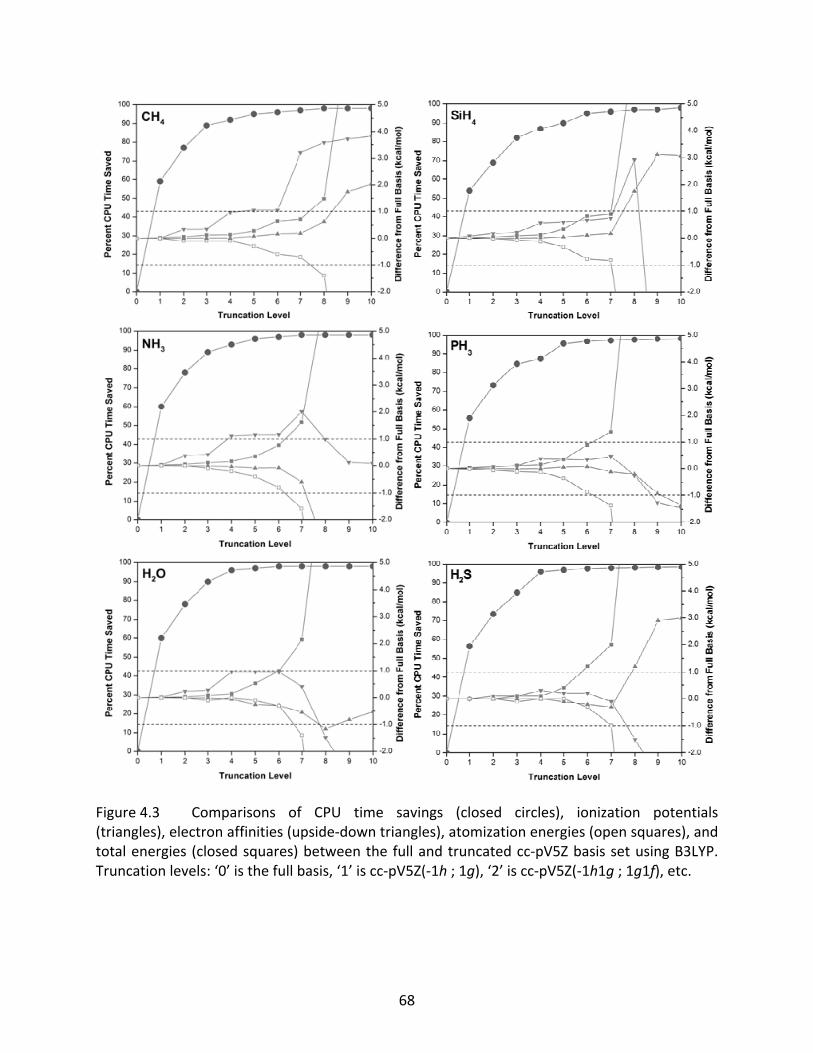
68
Figure 4.3 Comparisons of CPU time savings (closed circles), ionization potentials(triangles), electron affinities (upside‐down triangles), atomization energies (open squares), andtotal energies (closed squares) between the full and truncated cc‐pV5Z basis set using B3LYP.Truncation levels: ‘0’ is the full basis, ‘1’ is cc‐pV5Z(‐1h ; 1g), ‘2’ is cc‐pV5Z(‐1h1g ; 1g1f), etc.
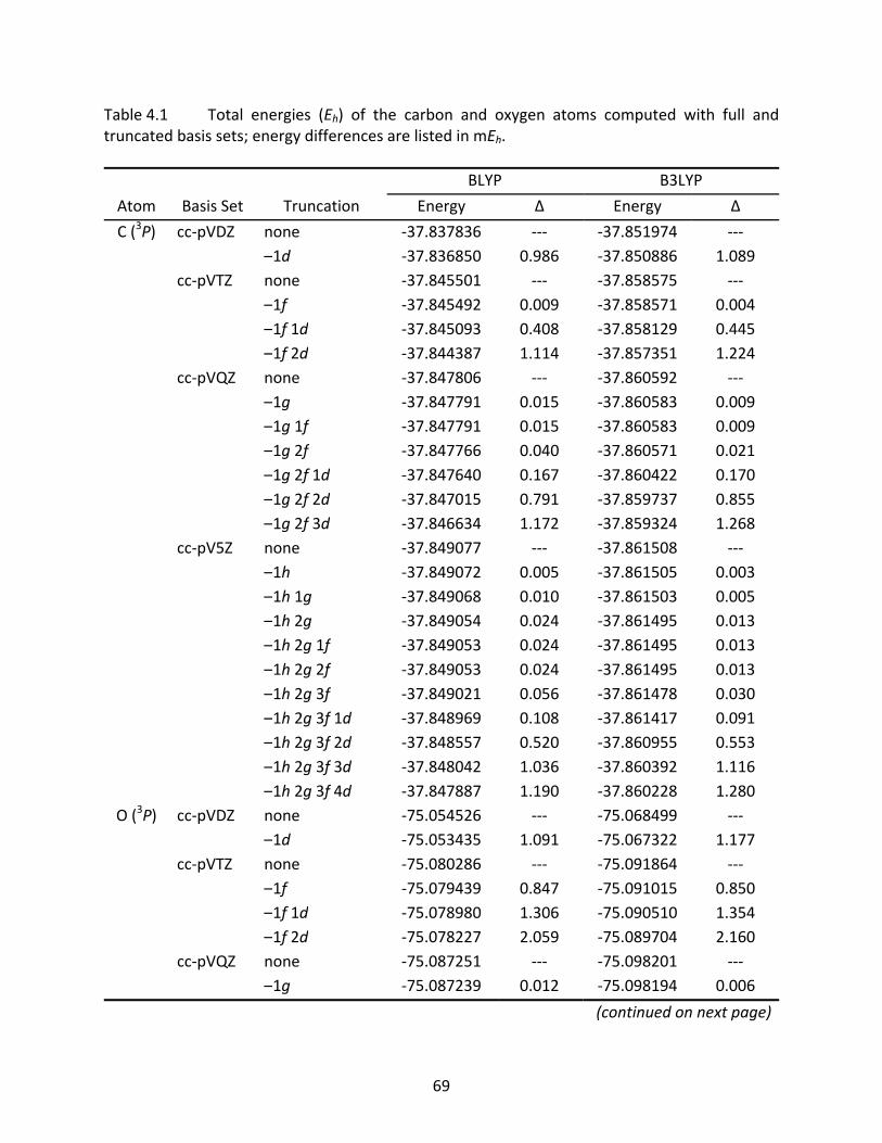
69
Table 4.1 Total energies (Eh) of the carbon and oxygen atoms computed with full and truncated basis sets; energy differences are listed in mEh.
BLYP B3LYP
Atom Basis Set Truncation Energy Δ Energy Δ
C (3P) cc‐pVDZ none ‐37.837836 ‐‐‐ ‐37.851974 ‐‐‐ –1d ‐37.836850 0.986 ‐37.850886 1.089 cc‐pVTZ none ‐37.845501 ‐‐‐ ‐37.858575 ‐‐‐ –1f ‐37.845492 0.009 ‐37.858571 0.004 –1f 1d ‐37.845093 0.408 ‐37.858129 0.445 –1f 2d ‐37.844387 1.114 ‐37.857351 1.224 cc‐pVQZ none ‐37.847806 ‐‐‐ ‐37.860592 ‐‐‐ –1g ‐37.847791 0.015 ‐37.860583 0.009 –1g 1f ‐37.847791 0.015 ‐37.860583 0.009 –1g 2f ‐37.847766 0.040 ‐37.860571 0.021 –1g 2f 1d ‐37.847640 0.167 ‐37.860422 0.170 –1g 2f 2d ‐37.847015 0.791 ‐37.859737 0.855 –1g 2f 3d ‐37.846634 1.172 ‐37.859324 1.268 cc‐pV5Z none ‐37.849077 ‐‐‐ ‐37.861508 ‐‐‐ –1h ‐37.849072 0.005 ‐37.861505 0.003 –1h 1g ‐37.849068 0.010 ‐37.861503 0.005 –1h 2g ‐37.849054 0.024 ‐37.861495 0.013 –1h 2g 1f ‐37.849053 0.024 ‐37.861495 0.013 –1h 2g 2f ‐37.849053 0.024 ‐37.861495 0.013 –1h 2g 3f ‐37.849021 0.056 ‐37.861478 0.030 –1h 2g 3f 1d ‐37.848969 0.108 ‐37.861417 0.091 –1h 2g 3f 2d ‐37.848557 0.520 ‐37.860955 0.553 –1h 2g 3f 3d ‐37.848042 1.036 ‐37.860392 1.116 –1h 2g 3f 4d ‐37.847887 1.190 ‐37.860228 1.280
O (3P) cc‐pVDZ none ‐75.054526 ‐‐‐ ‐75.068499 ‐‐‐ –1d ‐75.053435 1.091 ‐75.067322 1.177 cc‐pVTZ none ‐75.080286 ‐‐‐ ‐75.091864 ‐‐‐ –1f ‐75.079439 0.847 ‐75.091015 0.850 –1f 1d ‐75.078980 1.306 ‐75.090510 1.354 –1f 2d ‐75.078227 2.059 ‐75.089704 2.160 cc‐pVQZ none ‐75.087251 ‐‐‐ ‐75.098201 ‐‐‐ –1g ‐75.087239 0.012 ‐75.098194 0.006
(continued on next page)
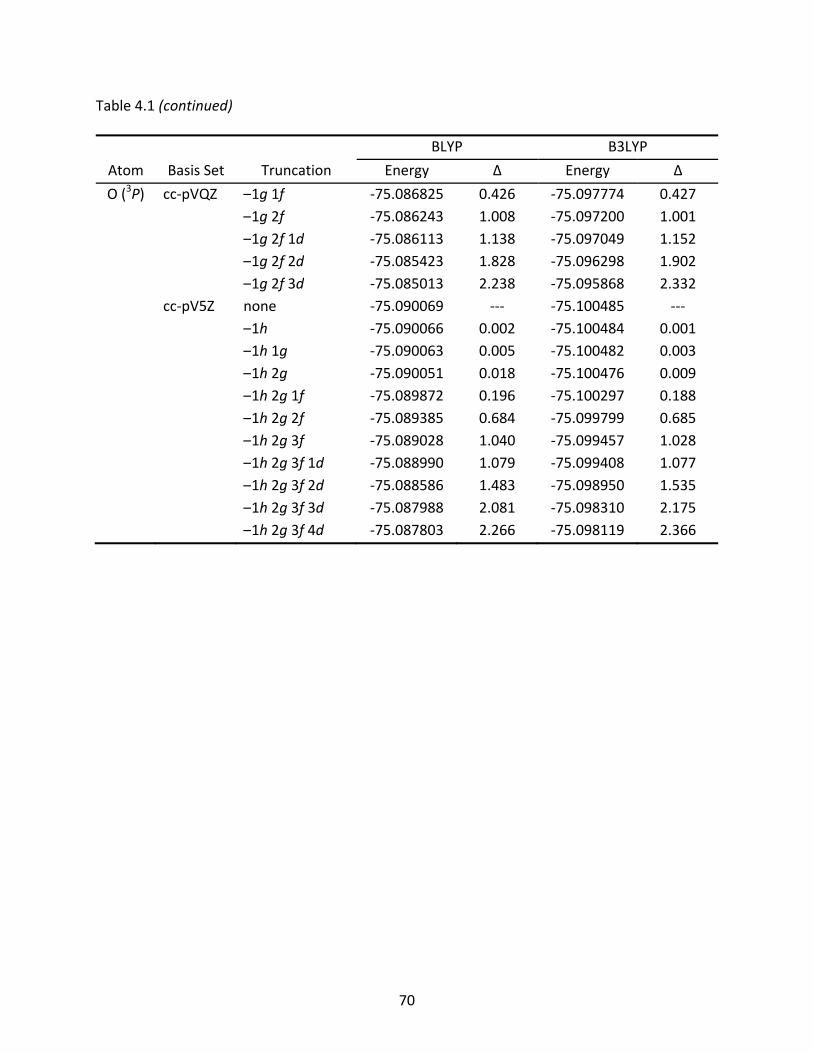
70
Table 4.1 (continued)
BLYP B3LYP
Atom Basis Set Truncation Energy Δ Energy Δ
O (3P) cc‐pVQZ –1g 1f ‐75.086825 0.426 ‐75.097774 0.427 –1g 2f ‐75.086243 1.008 ‐75.097200 1.001 –1g 2f 1d ‐75.086113 1.138 ‐75.097049 1.152 –1g 2f 2d ‐75.085423 1.828 ‐75.096298 1.902 –1g 2f 3d ‐75.085013 2.238 ‐75.095868 2.332 cc‐pV5Z none ‐75.090069 ‐‐‐ ‐75.100485 ‐‐‐ –1h ‐75.090066 0.002 ‐75.100484 0.001 –1h 1g ‐75.090063 0.005 ‐75.100482 0.003 –1h 2g ‐75.090051 0.018 ‐75.100476 0.009 –1h 2g 1f ‐75.089872 0.196 ‐75.100297 0.188 –1h 2g 2f ‐75.089385 0.684 ‐75.099799 0.685 –1h 2g 3f ‐75.089028 1.040 ‐75.099457 1.028 –1h 2g 3f 1d ‐75.088990 1.079 ‐75.099408 1.077 –1h 2g 3f 2d ‐75.088586 1.483 ‐75.098950 1.535 –1h 2g 3f 3d ‐75.087988 2.081 ‐75.098310 2.175 –1h 2g 3f 4d ‐75.087803 2.266 ‐75.098119 2.366
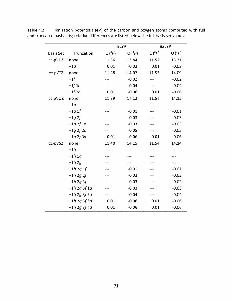
71
Table 4.2 Ionization potentials (eV) of the carbon and oxygen atoms computed with full and truncated basis sets; relative differences are listed below the full basis set values.
BLYP B3LYP
Basis Set Truncation C (3P) O (3P) C (3P) O (3P)
cc‐pVDZ none 11.36 13.84 11.52 13.31 –1d 0.01 ‐0.03 0.01 ‐0.03
cc‐pVTZ none 11.38 14.07 11.53 14.09 –1f ‐‐‐ ‐0.02 ‐‐‐ ‐0.02 –1f 1d ‐‐‐ ‐0.04 ‐‐‐ ‐0.04 –1f 2d 0.01 ‐0.06 0.01 ‐0.06
cc‐pVQZ none 11.39 14.12 11.54 14.12 –1g ‐‐‐ ‐‐‐ ‐‐‐ ‐‐‐ –1g 1f ‐‐‐ ‐0.01 ‐‐‐ ‐0.01 –1g 2f ‐‐‐ ‐0.03 ‐‐‐ ‐0.03 –1g 2f 1d ‐‐‐ ‐0.03 ‐‐‐ ‐0.03 –1g 2f 2d ‐‐‐ ‐0.05 ‐‐‐ ‐0.05 –1g 2f 3d 0.01 ‐0.06 0.01 ‐0.06
cc‐pV5Z none 11.40 14.15 11.54 14.14 –1h ‐‐‐ ‐‐‐ ‐‐‐ ‐‐‐ –1h 1g ‐‐‐ ‐‐‐ ‐‐‐ ‐‐‐ –1h 2g ‐‐‐ ‐‐‐ ‐‐‐ ‐‐‐ –1h 2g 1f ‐‐‐ ‐0.01 ‐‐‐ ‐0.01 –1h 2g 2f ‐‐‐ ‐0.02 ‐‐‐ ‐0.02 –1h 2g 3f ‐‐‐ ‐0.03 ‐‐‐ ‐0.03 –1h 2g 3f 1d ‐‐‐ ‐0.03 ‐‐‐ ‐0.03 –1h 2g 3f 2d ‐‐‐ ‐0.04 ‐‐‐ ‐0.04 –1h 2g 3f 3d 0.01 ‐0.06 0.01 ‐0.06 –1h 2g 3f 4d 0.01 ‐0.06 0.01 ‐0.06
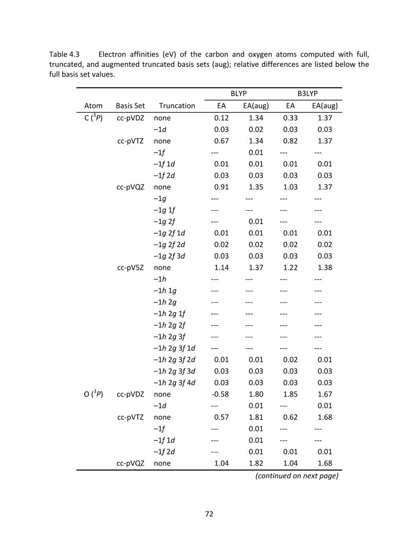
72
Table 4.3 Electron affinities (eV) of the carbon and oxygen atoms computed with full, truncated, and augmented truncated basis sets (aug); relative differences are listed below the full basis set values.
BLYP B3LYP
Atom Basis Set Truncation EA EA(aug) EA EA(aug)
C (3P) cc‐pVDZ none 0.12 1.34 0.33 1.37 –1d 0.03 0.02 0.03 0.03 cc‐pVTZ none 0.67 1.34 0.82 1.37 –1f ‐‐‐ 0.01 ‐‐‐ ‐‐‐ –1f 1d 0.01 0.01 0.01 0.01 –1f 2d 0.03 0.03 0.03 0.03 cc‐pVQZ none 0.91 1.35 1.03 1.37 –1g ‐‐‐ ‐‐‐ ‐‐‐ ‐‐‐ –1g 1f ‐‐‐ ‐‐‐ ‐‐‐ ‐‐‐ –1g 2f ‐‐‐ 0.01 ‐‐‐ ‐‐‐ –1g 2f 1d 0.01 0.01 0.01 0.01 –1g 2f 2d 0.02 0.02 0.02 0.02 –1g 2f 3d 0.03 0.03 0.03 0.03 cc‐pV5Z none 1.14 1.37 1.22 1.38 –1h ‐‐‐ ‐‐‐ ‐‐‐ ‐‐‐ –1h 1g ‐‐‐ ‐‐‐ ‐‐‐ ‐‐‐ –1h 2g ‐‐‐ ‐‐‐ ‐‐‐ ‐‐‐ –1h 2g 1f ‐‐‐ ‐‐‐ ‐‐‐ ‐‐‐ –1h 2g 2f ‐‐‐ ‐‐‐ ‐‐‐ ‐‐‐ –1h 2g 3f ‐‐‐ ‐‐‐ ‐‐‐ ‐‐‐ –1h 2g 3f 1d ‐‐‐ ‐‐‐ ‐‐‐ ‐‐‐ –1h 2g 3f 2d 0.01 0.01 0.02 0.01 –1h 2g 3f 3d 0.03 0.03 0.03 0.03 –1h 2g 3f 4d 0.03 0.03 0.03 0.03
O (3P) cc‐pVDZ none ‐0.58 1.80 1.85 1.67 –1d ‐‐‐ 0.01 ‐‐‐ 0.01 cc‐pVTZ none 0.57 1.81 0.62 1.68 –1f ‐‐‐ 0.01 ‐‐‐ ‐‐‐ –1f 1d ‐‐‐ 0.01 ‐‐‐ ‐‐‐ –1f 2d ‐‐‐ 0.01 0.01 0.01 cc‐pVQZ none 1.04 1.82 1.04 1.68
(continued on next page)
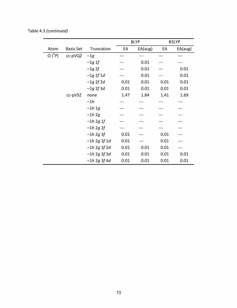
73
Table 4.3 (continued)
BLYP B3LYP
Atom Basis Set Truncation EA EA(aug) EA EA(aug)
O (3P) cc‐pVQZ –1g ‐‐‐ ‐‐‐ ‐‐‐ ‐‐‐ –1g 1f ‐‐‐ 0.01 ‐‐‐ ‐‐‐ –1g 2f ‐‐‐ 0.01 ‐‐‐ 0.01 –1g 2f 1d ‐‐‐ 0.01 ‐‐‐ 0.01 –1g 2f 2d 0.01 0.01 0.01 0.01 –1g 2f 3d 0.01 0.01 0.01 0.01 cc‐pV5Z none 1.47 1.84 1.41 1.69 –1h ‐‐‐ ‐‐‐ ‐‐‐ ‐‐‐ –1h 1g ‐‐‐ ‐‐‐ ‐‐‐ ‐‐‐ –1h 2g ‐‐‐ ‐‐‐ ‐‐‐ ‐‐‐ –1h 2g 1f ‐‐‐ ‐‐‐ ‐‐‐ ‐‐‐ –1h 2g 2f ‐‐‐ ‐‐‐ ‐‐‐ ‐‐‐ –1h 2g 3f 0.01 ‐‐‐ 0.01 ‐‐‐ –1h 2g 3f 1d 0.01 ‐‐‐ 0.01 ‐‐‐ –1h 2g 3f 2d 0.01 0.01 0.01 ‐‐‐ –1h 2g 3f 3d 0.01 0.01 0.01 0.01 –1h 2g 3f 4d 0.01 0.01 0.01 0.01
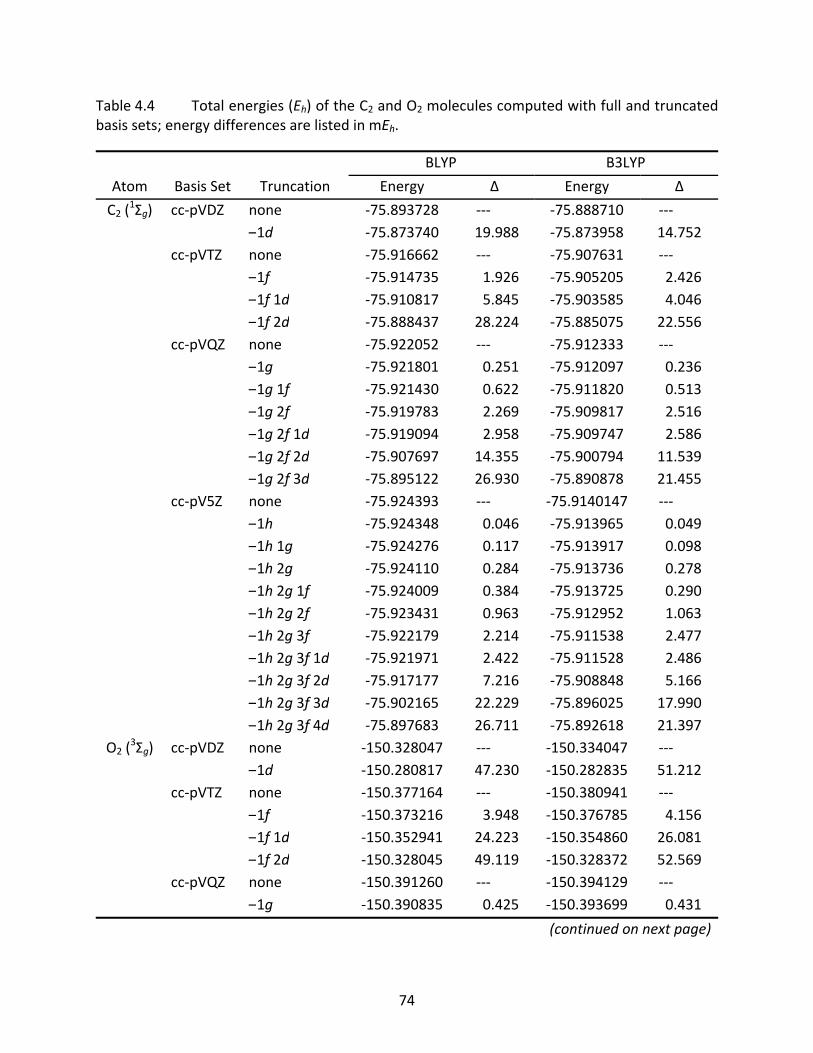
74
Table 4.4 Total energies (Eh) of the C2 and O2 molecules computed with full and truncated basis sets; energy differences are listed in mEh.
BLYP B3LYP
Atom Basis Set Truncation Energy Δ Energy Δ
C2 (1Σg) cc‐pVDZ none ‐75.893728 ‐‐‐ ‐75.888710 ‐‐‐ –1d ‐75.873740 19.988 ‐75.873958 14.752 cc‐pVTZ none ‐75.916662 ‐‐‐ ‐75.907631 ‐‐‐ –1f ‐75.914735 1.926 ‐75.905205 2.426 –1f 1d ‐75.910817 5.845 ‐75.903585 4.046 –1f 2d ‐75.888437 28.224 ‐75.885075 22.556 cc‐pVQZ none ‐75.922052 ‐‐‐ ‐75.912333 ‐‐‐ –1g ‐75.921801 0.251 ‐75.912097 0.236 –1g 1f ‐75.921430 0.622 ‐75.911820 0.513 –1g 2f ‐75.919783 2.269 ‐75.909817 2.516 –1g 2f 1d ‐75.919094 2.958 ‐75.909747 2.586 –1g 2f 2d ‐75.907697 14.355 ‐75.900794 11.539 –1g 2f 3d ‐75.895122 26.930 ‐75.890878 21.455 cc‐pV5Z none ‐75.924393 ‐‐‐ ‐75.9140147 ‐‐‐ –1h ‐75.924348 0.046 ‐75.913965 0.049 –1h 1g ‐75.924276 0.117 ‐75.913917 0.098 –1h 2g ‐75.924110 0.284 ‐75.913736 0.278 –1h 2g 1f ‐75.924009 0.384 ‐75.913725 0.290 –1h 2g 2f ‐75.923431 0.963 ‐75.912952 1.063 –1h 2g 3f ‐75.922179 2.214 ‐75.911538 2.477 –1h 2g 3f 1d ‐75.921971 2.422 ‐75.911528 2.486 –1h 2g 3f 2d ‐75.917177 7.216 ‐75.908848 5.166 –1h 2g 3f 3d ‐75.902165 22.229 ‐75.896025 17.990 –1h 2g 3f 4d ‐75.897683 26.711 ‐75.892618 21.397
O2 (3Σg) cc‐pVDZ none ‐150.328047 ‐‐‐ ‐150.334047 ‐‐‐ –1d ‐150.280817 47.230 ‐150.282835 51.212 cc‐pVTZ none ‐150.377164 ‐‐‐ ‐150.380941 ‐‐‐ –1f ‐150.373216 3.948 ‐150.376785 4.156 –1f 1d ‐150.352941 24.223 ‐150.354860 26.081 –1f 2d ‐150.328045 49.119 ‐150.328372 52.569 cc‐pVQZ none ‐150.391260 ‐‐‐ ‐150.394129 ‐‐‐ –1g ‐150.390835 0.425 ‐150.393699 0.431
(continued on next page)
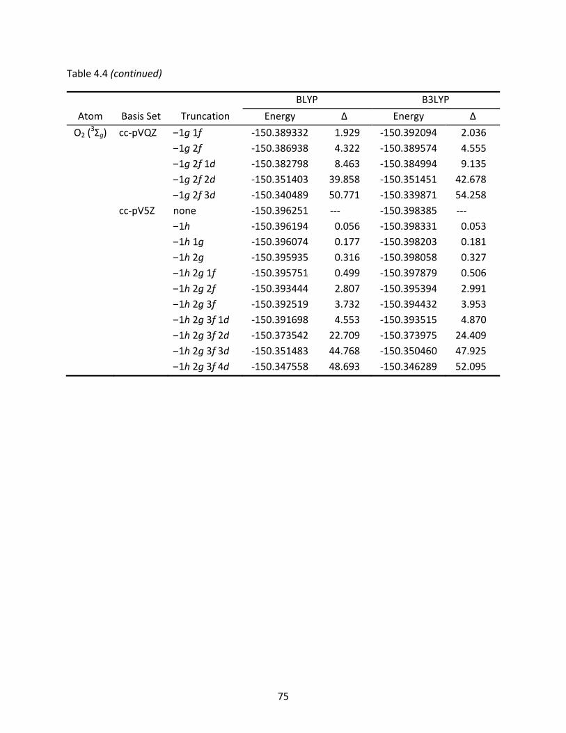
75
Table 4.4 (continued)
BLYP B3LYP
Atom Basis Set Truncation Energy Δ Energy Δ
O2 (3Σg) cc‐pVQZ –1g 1f ‐150.389332 1.929 ‐150.392094 2.036 –1g 2f ‐150.386938 4.322 ‐150.389574 4.555 –1g 2f 1d ‐150.382798 8.463 ‐150.384994 9.135 –1g 2f 2d ‐150.351403 39.858 ‐150.351451 42.678 –1g 2f 3d ‐150.340489 50.771 ‐150.339871 54.258 cc‐pV5Z none ‐150.396251 ‐‐‐ ‐150.398385 ‐‐‐ –1h ‐150.396194 0.056 ‐150.398331 0.053 –1h 1g ‐150.396074 0.177 ‐150.398203 0.181 –1h 2g ‐150.395935 0.316 ‐150.398058 0.327 –1h 2g 1f ‐150.395751 0.499 ‐150.397879 0.506 –1h 2g 2f ‐150.393444 2.807 ‐150.395394 2.991 –1h 2g 3f ‐150.392519 3.732 ‐150.394432 3.953 –1h 2g 3f 1d ‐150.391698 4.553 ‐150.393515 4.870 –1h 2g 3f 2d ‐150.373542 22.709 ‐150.373975 24.409 –1h 2g 3f 3d ‐150.351483 44.768 ‐150.350460 47.925 –1h 2g 3f 4d ‐150.347558 48.693 ‐150.346289 52.095
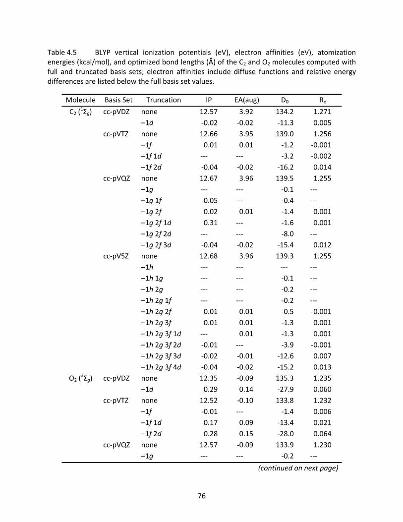
76
Table 4.5 BLYP vertical ionization potentials (eV), electron affinities (eV), atomization energies (kcal/mol), and optimized bond lengths (Å) of the C2 and O2 molecules computed with full and truncated basis sets; electron affinities include diffuse functions and relative energy differences are listed below the full basis set values.
Molecule Basis Set Truncation IP EA(aug) D0 ReC2 (
1Σg) cc‐pVDZ none 12.57 3.92 134.2 1.271 –1d ‐0.02 ‐0.02 ‐11.3 0.005 cc‐pVTZ none 12.66 3.95 139.0 1.256 –1f 0.01 0.01 ‐1.2 ‐0.001 –1f 1d ‐‐‐ ‐‐‐ ‐3.2 ‐0.002 –1f 2d ‐0.04 ‐0.02 ‐16.2 0.014 cc‐pVQZ none 12.67 3.96 139.5 1.255 –1g ‐‐‐ ‐‐‐ ‐0.1 ‐‐‐ –1g 1f 0.05 ‐‐‐ ‐0.4 ‐‐‐ –1g 2f 0.02 0.01 ‐1.4 0.001 –1g 2f 1d 0.31 ‐‐‐ ‐1.6 0.001 –1g 2f 2d ‐‐‐ ‐‐‐ ‐8.0 ‐‐‐ –1g 2f 3d ‐0.04 ‐0.02 ‐15.4 0.012 cc‐pV5Z none 12.68 3.96 139.3 1.255 –1h ‐‐‐ ‐‐‐ ‐‐‐ ‐‐‐ –1h 1g ‐‐‐ ‐‐‐ ‐0.1 ‐‐‐ –1h 2g ‐‐‐ ‐‐‐ ‐0.2 ‐‐‐ –1h 2g 1f ‐‐‐ ‐‐‐ ‐0.2 ‐‐‐ –1h 2g 2f 0.01 0.01 ‐0.5 ‐0.001 –1h 2g 3f 0.01 0.01 ‐1.3 0.001 –1h 2g 3f 1d ‐‐‐ 0.01 ‐1.3 0.001 –1h 2g 3f 2d ‐0.01 ‐‐‐ ‐3.9 ‐0.001 –1h 2g 3f 3d ‐0.02 ‐0.01 ‐12.6 0.007 –1h 2g 3f 4d ‐0.04 ‐0.02 ‐15.2 0.013
O2 (3Σg) cc‐pVDZ none 12.35 ‐0.09 135.3 1.235 –1d 0.29 0.14 ‐27.9 0.060 cc‐pVTZ none 12.52 ‐0.10 133.8 1.232 –1f ‐0.01 ‐‐‐ ‐1.4 0.006 –1f 1d 0.17 0.09 ‐13.4 0.021 –1f 2d 0.28 0.15 ‐28.0 0.064 cc‐pVQZ none 12.57 ‐0.09 133.9 1.230 –1g ‐‐‐ ‐‐‐ ‐0.2 ‐‐‐
(continued on next page)
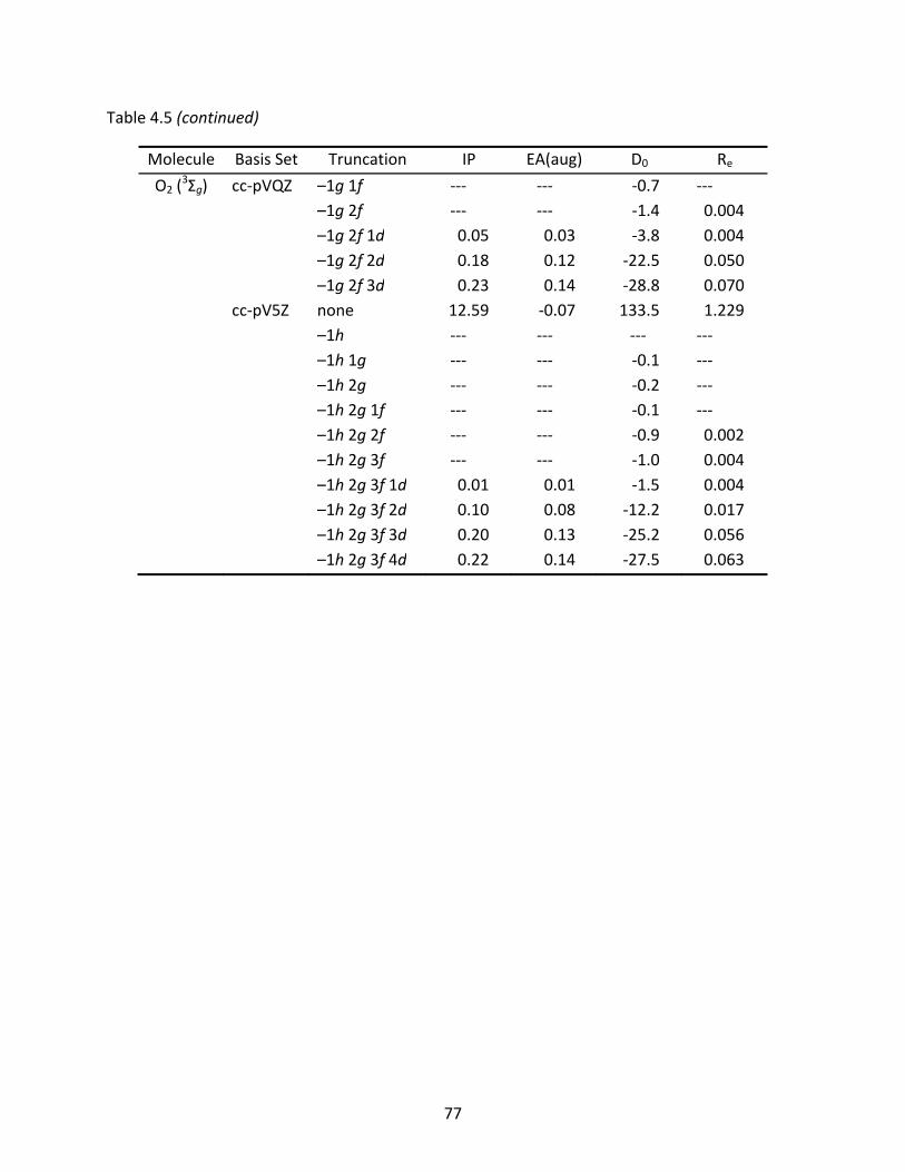
77
Table 4.5 (continued)
Molecule Basis Set Truncation IP EA(aug) D0 ReO2 (
3Σg) cc‐pVQZ –1g 1f ‐‐‐ ‐‐‐ ‐0.7 ‐‐‐ –1g 2f ‐‐‐ ‐‐‐ ‐1.4 0.004 –1g 2f 1d 0.05 0.03 ‐3.8 0.004 –1g 2f 2d 0.18 0.12 ‐22.5 0.050 –1g 2f 3d 0.23 0.14 ‐28.8 0.070 cc‐pV5Z none 12.59 ‐0.07 133.5 1.229 –1h ‐‐‐ ‐‐‐ ‐‐‐ ‐‐‐ –1h 1g ‐‐‐ ‐‐‐ ‐0.1 ‐‐‐ –1h 2g ‐‐‐ ‐‐‐ ‐0.2 ‐‐‐ –1h 2g 1f ‐‐‐ ‐‐‐ ‐0.1 ‐‐‐ –1h 2g 2f ‐‐‐ ‐‐‐ ‐0.9 0.002 –1h 2g 3f ‐‐‐ ‐‐‐ ‐1.0 0.004 –1h 2g 3f 1d 0.01 0.01 ‐1.5 0.004 –1h 2g 3f 2d 0.10 0.08 ‐12.2 0.017 –1h 2g 3f 3d 0.20 0.13 ‐25.2 0.056 –1h 2g 3f 4d 0.22 0.14 ‐27.5 0.063
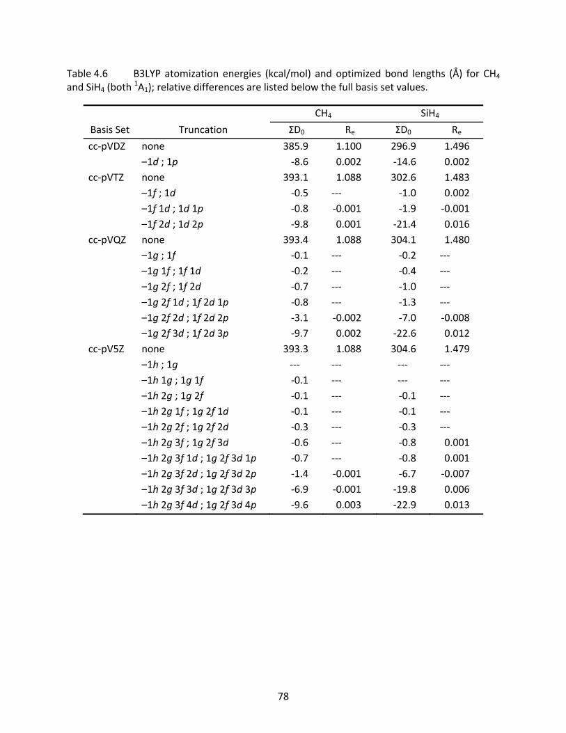
78
Table 4.6 B3LYP atomization energies (kcal/mol) and optimized bond lengths (Å) for CH4 and SiH4 (both
1A1); relative differences are listed below the full basis set values.
CH4 SiH4
Basis Set Truncation ΣD0 Re ΣD0 Recc‐pVDZ none 385.9 1.100 296.9 1.496 –1d ; 1p ‐8.6 0.002 ‐14.6 0.002cc‐pVTZ none 393.1 1.088 302.6 1.483 –1f ; 1d ‐0.5 ‐‐‐ ‐1.0 0.002 –1f 1d ; 1d 1p ‐0.8 ‐0.001 ‐1.9 ‐0.001 –1f 2d ; 1d 2p ‐9.8 0.001 ‐21.4 0.016cc‐pVQZ none 393.4 1.088 304.1 1.480 –1g ; 1f ‐0.1 ‐‐‐ ‐0.2 ‐‐‐ –1g 1f ; 1f 1d ‐0.2 ‐‐‐ ‐0.4 ‐‐‐ –1g 2f ; 1f 2d ‐0.7 ‐‐‐ ‐1.0 ‐‐‐ –1g 2f 1d ; 1f 2d 1p ‐0.8 ‐‐‐ ‐1.3 ‐‐‐ –1g 2f 2d ; 1f 2d 2p ‐3.1 ‐0.002 ‐7.0 ‐0.008 –1g 2f 3d ; 1f 2d 3p ‐9.7 0.002 ‐22.6 0.012cc‐pV5Z none 393.3 1.088 304.6 1.479 –1h ; 1g ‐‐‐ ‐‐‐ ‐‐‐ ‐‐‐ –1h 1g ; 1g 1f ‐0.1 ‐‐‐ ‐‐‐ ‐‐‐ –1h 2g ; 1g 2f ‐0.1 ‐‐‐ ‐0.1 ‐‐‐ –1h 2g 1f ; 1g 2f 1d ‐0.1 ‐‐‐ ‐0.1 ‐‐‐ –1h 2g 2f ; 1g 2f 2d ‐0.3 ‐‐‐ ‐0.3 ‐‐‐ –1h 2g 3f ; 1g 2f 3d ‐0.6 ‐‐‐ ‐0.8 0.001 –1h 2g 3f 1d ; 1g 2f 3d 1p ‐0.7 ‐‐‐ ‐0.8 0.001 –1h 2g 3f 2d ; 1g 2f 3d 2p ‐1.4 ‐0.001 ‐6.7 ‐0.007 –1h 2g 3f 3d ; 1g 2f 3d 3p ‐6.9 ‐0.001 ‐19.8 0.006 –1h 2g 3f 4d ; 1g 2f 3d 4p ‐9.6 0.003 ‐22.9 0.013
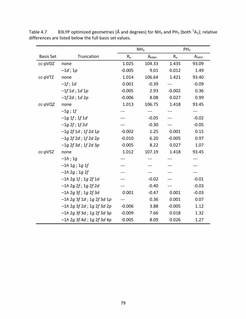
79
Table 4.7 B3LYP optimized geometries (Å and degrees) for NH3 and PH3 (both 1A1); relative
differences are listed below the full basis set values.
NH3 PH3
Basis Set Truncation Re AHNH Re AHPH
cc‐pVDZ none 1.025 104.33 1.435 93.09 –1d ; 1p ‐0.005 9.01 0.012 1.49cc‐pVTZ none 1.014 106.64 1.421 93.40 –1f ; 1d 0.001 ‐0.39 ‐‐‐ ‐0.09 –1f 1d ; 1d 1p ‐0.005 2.93 ‐0.002 0.36 –1f 2d ; 1d 2p ‐0.006 8.08 0.027 0.99cc‐pVQZ none 1.013 106.75 1.418 93.45 –1g ; 1f ‐‐‐ ‐‐‐ ‐‐‐ ‐‐‐ –1g 1f ; 1f 1d ‐‐‐ ‐0.05 ‐‐‐ ‐0.02 –1g 2f ; 1f 2d ‐‐‐ ‐0.30 ‐‐‐ ‐0.05 –1g 2f 1d ; 1f 2d 1p ‐0.002 1.25 0.001 0.15 –1g 2f 2d ; 1f 2d 2p ‐0.010 6.20 ‐0.005 0.97 –1g 2f 3d ; 1f 2d 3p ‐0.005 8.22 0.027 1.07cc‐pV5Z none 1.012 107.19 1.418 93.45 –1h ; 1g ‐‐‐ ‐‐‐ ‐‐‐ ‐‐‐ –1h 1g ; 1g 1f ‐‐‐ ‐‐‐ ‐‐‐ ‐‐‐ –1h 2g ; 1g 2f ‐‐‐ ‐‐‐ ‐‐‐ ‐‐‐ –1h 2g 1f ; 1g 2f 1d ‐‐‐ ‐0.02 ‐‐‐ ‐0.01 –1h 2g 2f ; 1g 2f 2d ‐‐‐ ‐0.40 ‐‐‐ ‐0.03 –1h 2g 3f ; 1g 2f 3d 0.001 ‐0.47 0.001 ‐0.03 –1h 2g 3f 1d ; 1g 2f 3d 1p ‐‐‐ 0.36 0.001 0.07 –1h 2g 3f 2d ; 1g 2f 3d 2p ‐0.006 3.88 ‐0.005 1.12 –1h 2g 3f 3d ; 1g 2f 3d 3p ‐0.009 7.66 0.018 1.32 –1h 2g 3f 4d ; 1g 2f 3d 4p ‐0.005 8.09 0.026 1.27
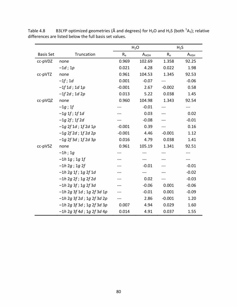
80
Table 4.8 B3LYP optimized geometries (Å and degrees) for H2O and H2S (both 1A1); relative
differences are listed below the full basis set values.
H2O H2S
Basis Set Truncation Re AHOH Re AHSH
cc‐pVDZ none 0.969 102.69 1.358 92.25 –1d ; 1p 0.021 4.28 0.022 1.98cc‐pVTZ none 0.961 104.53 1.345 92.53 –1f ; 1d 0.001 ‐0.07 ‐‐‐ ‐0.06 –1f 1d ; 1d 1p ‐0.001 2.67 ‐0.002 0.58 –1f 2d ; 1d 2p 0.013 5.22 0.038 1.45cc‐pVQZ none 0.960 104.98 1.343 92.54 –1g ; 1f ‐‐‐ ‐0.01 ‐‐‐ ‐‐‐ –1g 1f ; 1f 1d ‐‐‐ 0.03 ‐‐‐ 0.02 –1g 2f ; 1f 2d ‐‐‐ ‐0.08 ‐‐‐ ‐0.01 –1g 2f 1d ; 1f 2d 1p ‐0.001 0.39 ‐‐‐ 0.16 –1g 2f 2d ; 1f 2d 2p ‐0.001 4.46 ‐0.001 1.12 –1g 2f 3d ; 1f 2d 3p 0.016 4.79 0.038 1.41cc‐pV5Z none 0.961 105.19 1.341 92.51 –1h ; 1g ‐‐‐ ‐‐‐ ‐‐‐ ‐‐‐ –1h 1g ; 1g 1f ‐‐‐ ‐‐‐ ‐‐‐ ‐‐‐ –1h 2g ; 1g 2f ‐‐‐ ‐0.01 ‐‐‐ ‐0.01 –1h 2g 1f ; 1g 2f 1d ‐‐‐ ‐‐‐ ‐‐‐ ‐0.02 –1h 2g 2f ; 1g 2f 2d ‐‐‐ 0.02 ‐‐‐ ‐0.03 –1h 2g 3f ; 1g 2f 3d ‐‐‐ ‐0.06 0.001 ‐0.06 –1h 2g 3f 1d ; 1g 2f 3d 1p ‐‐‐ ‐0.01 0.001 ‐0.09 –1h 2g 3f 2d ; 1g 2f 3d 2p ‐‐‐ 2.86 ‐0.001 1.20 –1h 2g 3f 3d ; 1g 2f 3d 3p 0.007 4.94 0.029 1.60 –1h 2g 3f 4d ; 1g 2f 3d 4p 0.014 4.91 0.037 1.55
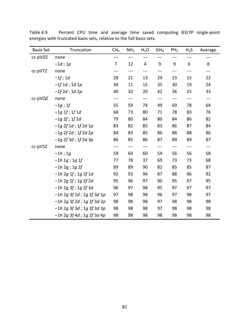
81
Table 4.9 Percent CPU time and average time saved computing B3LYP single‐point energies with truncated basis sets, relative to the full basis sets.
Basis Set Truncation CH4 NH3 H2O SiH4 PH3 H2S Average
cc‐pVDZ none ‐‐‐ ‐‐‐ ‐‐‐ ‐‐‐ ‐‐‐ ‐‐‐ ‐‐‐ –1d ; 1p 7 12 4 9 9 6 8cc‐pVTZ none ‐‐‐ ‐‐‐ ‐‐‐ ‐‐‐ ‐‐‐ ‐‐‐ ‐‐‐ –1f ; 1d 28 21 13 29 23 15 22 –1f 1d ; 1d 1p 34 11 15 35 30 19 24 –1f 2d ; 1d 2p 40 32 20 42 36 25 33cc‐pVQZ none ‐‐‐ ‐‐‐ ‐‐‐ ‐‐‐ ‐‐‐ ‐‐‐ ‐‐‐ –1g ; 1f 55 59 74 49 69 78 64 –1g 1f ; 1f 1d 68 73 80 71 78 83 76 –1g 2f ; 1f 2d 79 80 84 80 84 86 82 –1g 2f 1d ; 1f 2d 1p 83 82 85 83 86 87 84 –1g 2f 2d ; 1f 2d 2p 84 83 85 86 88 88 86 –1g 2f 3d ; 1f 2d 3p 86 85 86 87 89 89 87cc‐pV5Z none ‐‐‐ ‐‐‐ ‐‐‐ ‐‐‐ ‐‐‐ ‐‐‐ ‐‐‐ –1h ; 1g 59 60 60 54 56 56 58 –1h 1g ; 1g 1f 77 78 37 69 73 73 68 –1h 2g ; 1g 2f 89 89 90 82 85 85 87 –1h 2g 1f ; 1g 2f 1d 92 93 96 87 88 96 92 –1h 2g 2f ; 1g 2f 2d 95 96 97 90 95 97 95 –1h 2g 3f ; 1g 2f 3d 96 97 98 95 97 97 97 –1h 2g 3f 1d ; 1g 2f 3d 1p 97 98 98 96 97 98 97 –1h 2g 3f 2d ; 1g 2f 3d 2p 98 98 98 97 98 98 98 –1h 2g 3f 3d ; 1g 2f 3d 3p 98 98 98 97 98 98 98 –1h 2g 3f 4d ; 1g 2f 3d 4p 98 98 98 98 98 98 98
82
CHAPTER 5
SYSTEMATIC RECONTRACTION OF THE CORRELATION CONSISTENT BASIS SETS FOR DENSITY
FUNCTIONAL THEORY CALCULATIONS†
5.1 Introduction
With correlated ab initio approaches, such as coupled cluster theory with single, double,
and perturbative triple excitations, CCSD(T),35,38 a high level of accuracy in properties such as
energetics can be achieved (e.g., atomization energies within 1.0 kcal/mol from reliable
experiment) when paired with a large basis set. However, CCSD(T) becomes so costly in terms
of computational time, memory, and disk space that this method is generally restricted to
molecules composed of no more than 10‐15 non‐hydrogen atoms with a modest‐sized basis
set. A practical alternative is density functional theory (DFT),44,45,52 which includes correlation
energy without the additional computational overhead of correlated ab initio methods.
One of the challenges in using DFT is determining the best and most appropriate
functional for a problem of interest. There are hundreds of density functionals available, each
designed for different tasks or with respect to a test set of atoms and molecules. Because of the
increasing number of density functionals available and the popularity of DFT, a quick and
efficient means to determine the intrinsic error of a density functional is needed.
The use of systematically constructed basis sets has proven to be a valuable tool in
† This entire chapter is adapted from B.P Prascher and A.K. Wilson, “The Behaviour of Density Functionals with Respect to Basis Set. V. Recontraction of Correlation Consistent Basis Sets.” Mol. Phys. 2007, 105(19‐22), 2899, with permission from Taylor & Francis.
83
determining the successes and failures of ab initio methods.122,133,176 For example, the
monotonic convergence towards the complete basis set (CBS) limit exhibited by a number of
molecular properties computed with the correlation consistent basis sets in Hartree‐Fock (HF),
DFT, and electron correlation methods, as the basis set size increases, allows for the systematic
elucidation of the intrinsic error of ab initio methods. Unlike numerical methods for
determining the HF CBS limit, which tend to be computationally expensive for systems larger
than two atoms, accurate approximations of the CBS limit by extrapolating a series of
properties computed with the correlation consistent basis sets can be done at the HF level for
molecules of many atoms.
Recently, a set of polarization consistent basis sets (pc‐n, where n = 1‐4) specifically
optimized for DFT were developed.143‐145,147 Wang and Wilson showed that using the pc‐n basis
sets in DFT calculations do not necessarily result in an improvement in the accuracy of
properties computed using the correlation consistent basis sets.155,156 For example, Wang and
Wilson showed that the performance of the correlation consistent basis sets is similar to that of
the pc‐n basis sets within 0.10 kcal/mol in computed energetics for a test set of 17 first row,
main group molecules.155 Yet, the correlation consistent basis sets have fewer basis functions
than the comparable polarization consistent basis set beyond the double‐ζ level.
The impact of employing segmented contraction versus general contraction schemes in
DFT has been investigated by Jensen.147 A segmented contraction does not include all the basis
functions of a given symmetry type in a basis set, whereas a general contraction does.19 Jensen
concluded that core functions are typically not important for either valence orbital descriptions
or for energetic properties computed with DFT that are largely impacted by the valence space
84
such as ionization potentials and atomization energies. This means that if a segmented
contraction scheme is used, high exponent basis functions need not be included in the
contracted valence functions; or, anaglogously, if a general contraction scheme is used, the
core functions do not need large contraction coefficients in the valence basis functions. In a
subsequent paper, Jensen discussed how the contraction of a basis set (independent of the
type of contraction scheme used) in DFT computations tends to impact computed properties
more than the choice of primitive functions.146 The overall conclusion of his papers was that so‐
called core‐pruned basis sets should be sufficient for valence energetic properties in DFT
computations, and that optimization of the contraction coefficients rather than the primitive
basis functions leads to a greater impact on the energetic properties. As a result of their
construction, the contracted valence basis functions in the correlation consistent basis sets
have small weights on the core functions, making them a type of core‐pruned basis sets.
Another important effect to examine when studying atomization energies is basis set
superposition error (BSSE).152,177‐179 In the linear combination of atomic orbitals (LCAO)
approximation, the interaction between two subunits is described by the overlap of their
respective basis sets. In the overlap region, there is a better description of the orbital space
than within the individual subunits. This leads to interaction energies that are too high,
compared with a more even description of the orbital space. To account for this effect, the ex
post facto Boys‐Bernardi correction is typically employed:178
AB AB A B (5.1)
where AB represents the dissociation energy of the system composed of subunits A and B
(or atomization energy of a molecule). The terms A and B are total energies of the
85
respective subunits computed in the presence of the basis sets of both subunits. Applying (5.1)
is a way of accounting for the over‐described regions of space by the overlapping basis sets; in
effect, smoothing out the basis set description so that the entire molecule is evenly described
by the basis set. As the basis set increases in size (i.e. becomes more complete) the BSSE
decreases. For example, the BSSE for the CO2 atomization energy in BLYP computations was
7.11 kcal/mol at the cc‐pVDZ level, 2.25 kcal/mol at the cc‐pVTZ level, and 1.36 kcal/mol at the
quadruple‐ζ level.152 It has also been reported that correcting for BSSE in computations with the
cc‐pVnZ basis sets can lead to monotonic behavior in computed atomization energies.156
Based on the observations of Jensen regarding basis set contractions in DFT, the success
of recontracting the correlation consistent basis sets for the recovery of scalar relativistic
effects (discussed in Chapter 3), and in continuing with the theme of Chapter 4 in determining
the basis sets requirements for DFT, this chapter reports on reoptimization of the contractions
of the correlation consistent basis sets specifically for DFT computations. The effect on the
convergent behavior of various energetic properties including atomization energies, vertical
ionization potentials, and vertical electron affinities is examined in addition to its impact on
optimized geometries. Further, the effects of incorporating diffuse functions in the basis sets
and the removal of BSSE are examined.
5.2 Computational Methodology
As in Chapter 4, the Becke 1988 gradient‐corrected exchange functional (B)164 has been
coupled with the Lee‐Yang‐Parr correlation functional (LYP)165 in pure DFT computations, and
the Becke three‐parameter exchange scheme (B3)166 has been coupled with the LYP functional
86
in hybrid DFT computations. In the latter case, the third parameterization of the Vosko‐Wilk‐
Nusair local correlation functional (VWN‐3)167 is used.
The correlation consistent basis sets, cc‐pVnZ, were employed from double‐ to
quintuple‐ζ quality (n = D, T, Q, and 5). Recontraction of the s and p functions in these basis sets
was performed in a similar manner to that described in Chapter 3: 1) all high angular
momentum functions were removed from the basis set; 2) the s and p functions were
uncontracted; 3) computations of atomic energies with BLYP and B3LYP were performed; and
4) the atomic orbital (AO) coefficients from Kohn‐Sham (KS) orbital analyses were then taken as
the new contraction coefficients. After replacing the high angular momentum functions (d, f,
etc.) from the original cc‐pVnZ basis sets, the new basis sets are denoted cc‐pVnZ[rc], where rc
stands for recontracted. Diffuse functions have also been added to these recontracted basis
sets to form augmented basis sets; the diffuse functions are unaltered from the original
aug‐cc‐pVnZ basis sets.
Recontraction of the correlation consistent basis sets was performed with the Molpro
software package180 using a variable grid size to achieve better than mEh convergence in the
total atomic energy. The Gaussian 03 software suite174 was then employed with the default grid
(75,302) to perform the BLYP and B3LYP computations with the recontracted basis sets. All
computations were performed using the spin‐unrestricted formalism, and the impact of BSSE
has been examined. Two extrapolation schemes including the Halkier et al. two‐point (3.6)133
and Feller three‐point exponential approach (3.2)132 were employed in estimating KS limits.
87
5.3 Results and Discussion
For oxygen and fluorine, there are two sets of contraction coefficients possible for the
2p manifold: the singly‐occupied p eigenstate or the doubly‐occupied p eigenstate. For
example, the oxygen p manifold has the electronic configuration , which leads to two
possibilities for contraction coefficients since and are degenerate. The properties
computed in this investigation used contracted coefficients from the doubly‐occupied
eigenstates since they produce lower atomic energies.
Several energetic properties were computed and examined using the recontracted
correlation consistent basis sets including vertical ionization potentials, electron affinities
(vertical attachment energies). The effect of adding diffuse functions to the recontracted basis
sets has been examined with respect to electron affinities and atomization energies.
Recontracted basis sets that include the diffuse functions of the original aug‐cc‐pVnZ basis
sets95,99,100 were used.
Molecules from the test set of Wang et al.152,154‐156 have been included in this study,
specifically H2, N2, F2, HF, CO, CO2, O3, H2O, and CH3OH. In addition, several molecules have
been added to augment the set, including O2, Ne2, CH, NH, OH, CH2 (singlet and triplet states),
NH3, CH4, (H2O)2, and (HF)2.
5.3.1 Atoms
Table 5.1 displays the changes in total energies of hydrogen and the first row atoms B‐
Ne using the recontracted basis sets compared with the original basis sets. The change in
energy is greatest at the double‐ and triple‐ζ levels and tends to increase as the atom size
88
increases. The energy changes are smaller for B3LYP than for BLYP, with the largest changes
occurring at the double‐ζ level for both methods. For example, the total energy for the carbon
atom is 3.160 mEh lower with the recontracted basis sets as compared with the total energy
arising from original basis set using BLYP, but is only 2.015 mEh lower using B3LYP. The
differences in energy grow to 7.285 and 4.626 mEh for BLYP and B3LYP, respectively, for the
neon atom.
Table 5.1 also helps to gauge the importance of specific density functional optimizations
of the contraction. The B3LYP recontraction of the basis sets, denoted cc‐pVnZ[B3LYP], was
utilized to compute BLYP energies, and the BLYP recontraction, denoted cc‐pVnZ[BLYP], was
used to calculate B3LYP energies. Overall, when the same functional is used for both the
recontraction and the calculation of the total energy, lower energies are obtained. The
exceptions occur for the B3LYP/cc‐pVDZ[BLYP] calculations for oxygen and fluorine, where the
total energies are lower than those obtained using the B3LYP recontraction by ‐0.030 and
‐0.178 mEh, respectively. The largest differences in total energies for the B3LYP and BLYP
recontraction schemes are observed for the BLYP calculations, with differences of 0.475 and
0.707 mEh, for oxygen and fluorine, respectively.
The ionization potentials and electron affinities of the first row atoms B‐Ne and H using
the double‐ and triple‐ζ basis sets are given in Table 5.2. Overall, comparing the cc‐pVnZ basis
sets to the recontracted sets shows very little difference in ionization potentials for each atom.
The largest differences occur at the double‐ζ level. For oxygen and fluorine, the impact of
recontraction increases the ionization potential by 0.06 and 0.07 eV, respectively, using BLYP.
These increases are above the threshold of chemical accuracy (0.04 eV). Using B3LYP, the
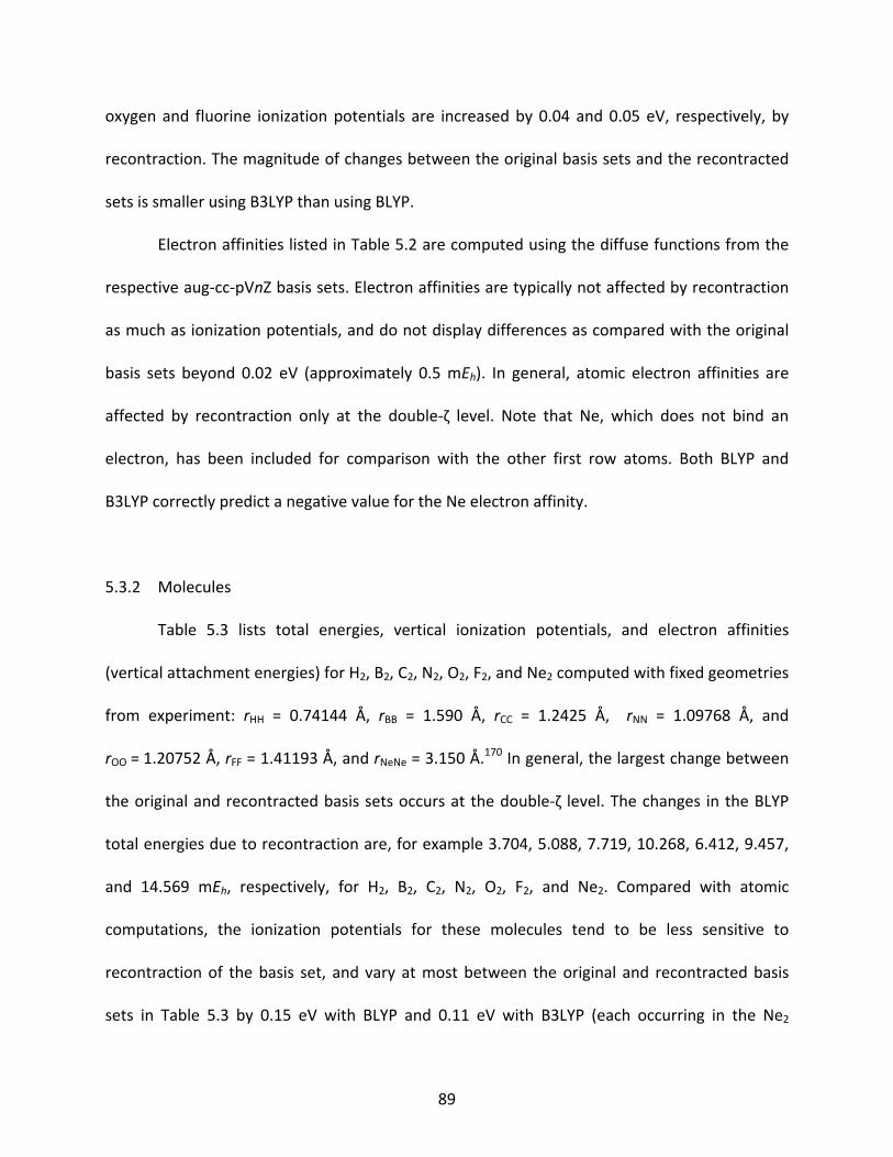
89
oxygen and fluorine ionization potentials are increased by 0.04 and 0.05 eV, respectively, by
recontraction. The magnitude of changes between the original basis sets and the recontracted
sets is smaller using B3LYP than using BLYP.
Electron affinities listed in Table 5.2 are computed using the diffuse functions from the
respective aug‐cc‐pVnZ basis sets. Electron affinities are typically not affected by recontraction
as much as ionization potentials, and do not display differences as compared with the original
basis sets beyond 0.02 eV (approximately 0.5 mEh). In general, atomic electron affinities are
affected by recontraction only at the double‐ζ level. Note that Ne, which does not bind an
electron, has been included for comparison with the other first row atoms. Both BLYP and
B3LYP correctly predict a negative value for the Ne electron affinity.
5.3.2 Molecules
Table 5.3 lists total energies, vertical ionization potentials, and electron affinities
(vertical attachment energies) for H2, B2, C2, N2, O2, F2, and Ne2 computed with fixed geometries
from experiment: rHH = 0.74144 Å, rBB = 1.590 Å, rCC = 1.2425 Å, rNN = 1.09768 Å, and
rOO = 1.20752 Å, rFF = 1.41193 Å, and rNeNe = 3.150 Å.170 In general, the largest change between
the original and recontracted basis sets occurs at the double‐ζ level. The changes in the BLYP
total energies due to recontraction are, for example 3.704, 5.088, 7.719, 10.268, 6.412, 9.457,
and 14.569 mEh, respectively, for H2, B2, C2, N2, O2, F2, and Ne2. Compared with atomic
computations, the ionization potentials for these molecules tend to be less sensitive to
recontraction of the basis set, and vary at most between the original and recontracted basis
sets in Table 5.3 by 0.15 eV with BLYP and 0.11 eV with B3LYP (each occurring in the Ne2
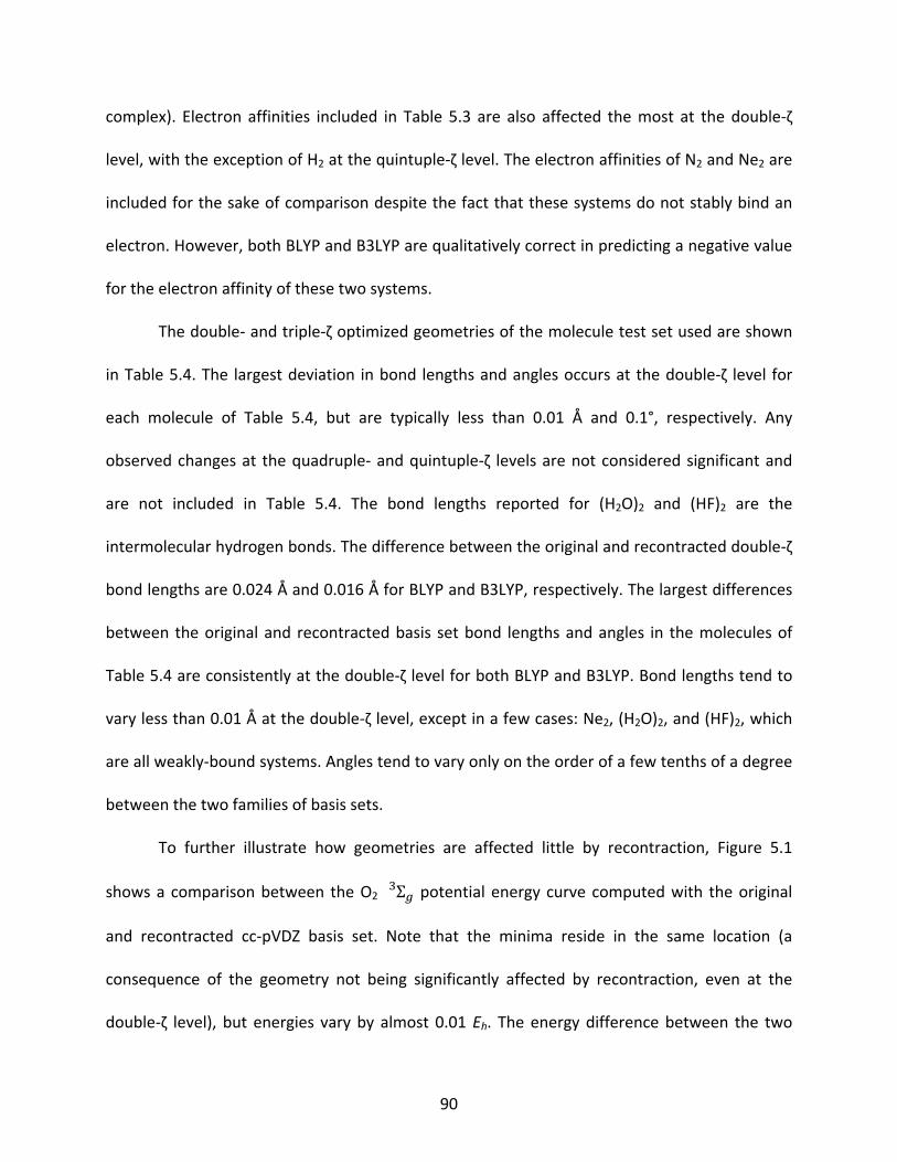
90
complex). Electron affinities included in Table 5.3 are also affected the most at the double‐ζ
level, with the exception of H2 at the quintuple‐ζ level. The electron affinities of N2 and Ne2 are
included for the sake of comparison despite the fact that these systems do not stably bind an
electron. However, both BLYP and B3LYP are qualitatively correct in predicting a negative value
for the electron affinity of these two systems.
The double‐ and triple‐ζ optimized geometries of the molecule test set used are shown
in Table 5.4. The largest deviation in bond lengths and angles occurs at the double‐ζ level for
each molecule of Table 5.4, but are typically less than 0.01 Å and 0.1°, respectively. Any
observed changes at the quadruple‐ and quintuple‐ζ levels are not considered significant and
are not included in Table 5.4. The bond lengths reported for (H2O)2 and (HF)2 are the
intermolecular hydrogen bonds. The difference between the original and recontracted double‐ζ
bond lengths are 0.024 Å and 0.016 Å for BLYP and B3LYP, respectively. The largest differences
between the original and recontracted basis set bond lengths and angles in the molecules of
Table 5.4 are consistently at the double‐ζ level for both BLYP and B3LYP. Bond lengths tend to
vary less than 0.01 Å at the double‐ζ level, except in a few cases: Ne2, (H2O)2, and (HF)2, which
are all weakly‐bound systems. Angles tend to vary only on the order of a few tenths of a degree
between the two families of basis sets.
To further illustrate how geometries are affected little by recontraction, Figure 5.1
shows a comparison between the O2 Σ potential energy curve computed with the original
and recontracted cc‐pVDZ basis set. Note that the minima reside in the same location (a
consequence of the geometry not being significantly affected by recontraction, even at the
double‐ζ level), but energies vary by almost 0.01 Eh. The energy difference between the two
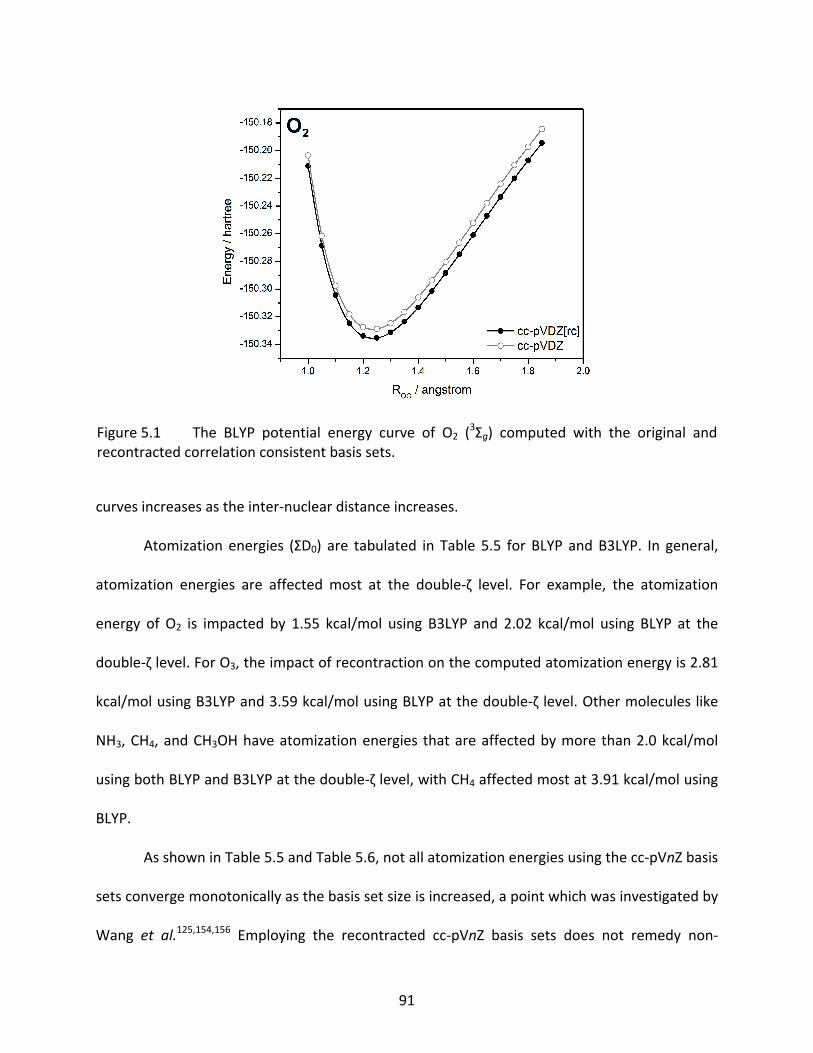
91
curves increases as the inter‐nuclear distance increases.
Atomization energies (ΣD0) are tabulated in Table 5.5 for BLYP and B3LYP. In general,
atomization energies are affected most at the double‐ζ level. For example, the atomization
energy of O2 is impacted by 1.55 kcal/mol using B3LYP and 2.02 kcal/mol using BLYP at the
double‐ζ level. For O3, the impact of recontraction on the computed atomization energy is 2.81
kcal/mol using B3LYP and 3.59 kcal/mol using BLYP at the double‐ζ level. Other molecules like
NH3, CH4, and CH3OH have atomization energies that are affected by more than 2.0 kcal/mol
using both BLYP and B3LYP at the double‐ζ level, with CH4 affected most at 3.91 kcal/mol using
BLYP.
As shown in Table 5.5 and Table 5.6, not all atomization energies using the cc‐pVnZ basis
sets converge monotonically as the basis set size is increased, a point which was investigated by
Wang et al.125,154,156 Employing the recontracted cc‐pVnZ basis sets does not remedy non‐
Figure 5.1 The BLYP potential energy curve of O2 (
3Σg) computed with the original andrecontracted correlation consistent basis sets.
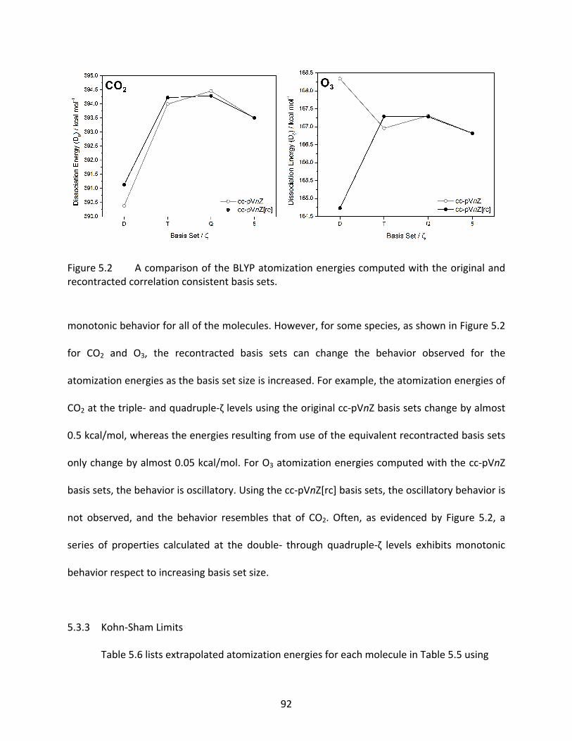
92
monotonic behavior for all of the molecules. However, for some species, as shown in Figure 5.2
for CO2 and O3, the recontracted basis sets can change the behavior observed for the
atomization energies as the basis set size is increased. For example, the atomization energies of
CO2 at the triple‐ and quadruple‐ζ levels using the original cc‐pVnZ basis sets change by almost
0.5 kcal/mol, whereas the energies resulting from use of the equivalent recontracted basis sets
only change by almost 0.05 kcal/mol. For O3 atomization energies computed with the cc‐pVnZ
basis sets, the behavior is oscillatory. Using the cc‐pVnZ[rc] basis sets, the oscillatory behavior is
not observed, and the behavior resembles that of CO2. Often, as evidenced by Figure 5.2, a
series of properties calculated at the double‐ through quadruple‐ζ levels exhibits monotonic
behavior respect to increasing basis set size.
5.3.3 Kohn‐Sham Limits
Table 5.6 lists extrapolated atomization energies for each molecule in Table 5.5 using
Figure 5.2 A comparison of the BLYP atomization energies computed with the original andrecontracted correlation consistent basis sets.
93
the two‐ and three‐point approaches described earlier. In the two‐point scheme, the first
extrapolation is performed using double‐ and triple‐ζ points, (DT), while the second
extrapolation uses the triple‐ and quadruple‐ζ points, (TQ). In the three‐point scheme, the
first extrapolation uses double‐ through quadruple‐ζ points, (DTQ), and the second uses
triple‐ through quintuple‐ζ points, (TQ5).
In general, KS limits should not be calculated for each extrapolation approach for all of
the molecules in Table 5.6 because of the non‐monotonic convergence of the atomization
energies with respect to increasing basis set size. Out of the 20 molecules represented, the
atomization energies of H2, N2, O2, F2, CO, CO2, O3, CH4, and (H2O)2 cannot be extrapolated
using all four extrapolation techniques employed. Typically, if non‐monotonic behavior is
observed in BLYP, then it is also observed in B3LYP. The obvious exceptions to this trend in
Table 5.6 are N2, O2, F2, and O3. The N2 molecule is unique in that its B3LYP atomization
energies can be extrapolated with all four extrapolation approaches, but those of BLYP cannot
be extrapolated with all four schemes. The F2 molecule is even more peculiar since only the
BLYP atomization energies employing the original cc‐pVnZ basis sets can be extrapolated.
Recontraction affects the computed F2 atomization energy ies such that the extrapolations of
the BLYP values are not possible beyond (DT). Further, all B3LYP computations on the F2
atomization energy cannot be extrapolated due to non‐monotonic behavior beyond the (DT)
scheme.
The largest difference between the original and recontracted KS limit extrapolations
occurs for the (DT) scheme for most molecules studied. For O3, CH4, and NH3, the differences
are 1.99, 1.57 and 1.26 kcal/mol for BLYP and 1.54, 1.16, and 1.02 kcal/mol for B3LYP,
94
respectively. This is expected since the largest impact on energetics due to recontraction occurs
at the double‐ζ level. The largest molecule of this study, CH3OH, varies in (DT) extrapolations
of its computed atomization energy by 0.91 kcal/mol and 0.71 kcal/mol at the BLYP and B3LYP
levels, respectively. In BLYP computations on Ne2, only the double‐ζ level atomization energy is
affected by recontraction (cf. Table 5.5). Therefore, the Ne2 molecule experiences the smallest
difference between the cc‐pVnZ and cc‐pVnZ[rc] basis set extrapolated energies, with
differences ranging from 0.01 to 0.33 kcal/mol in magnitude.
5.3.4 Basis Set Superposition Error
As discussed, BSSE can be corrected using the Boys‐Bernardi counterpoise correction.
Table 5.7 and Figure 5.3 demonstrate how counterpoise corrections can be important in
restoring monotonic behavior expected with the correlation consistent basis sets using BLYP.
Recall from Table 5.6 that BLYP atomization energies of N2, F2, and O3 computed with cc‐pVnZ
or cc‐pVnZ[rc] were not extrapolated due to non‐monotonic behavior except with the (DT)
scheme. Correcting each ζ‐level for BSSE improves the behavior so that it is monotonic for N2
with both the original and recontracted basis sets (cf. Table 5.7). For F2, employing the
counterpoise correction does not alleviate the non‐monotonic behavior in the recontracted
basis set computations; it also does not affect any convergent behavior of the original basis set
computations. The O3 computed atomization energies, when corrected for BSSE, become
monotonic only in the original basis set computations. Unfortunately, including a counterpoise
correction in CO computations with BLYP does not result in monotonic behavior. Non‐
monotonic behavior, even after a counterpoise correction has been applied, is not surprising in
95
light of the work of Wang et al.,152,156 who also found that some first row molecules did not
display monotonic behavior after accounting for BSSE (e.g. CO).
Accounting for BSSE using the counterpoise correction lowers the atomization energy at
the double‐ and triple‐ζ levels for each of the five systems in Figure 5.3. For F2, the difference
between the BLYP/cc‐pVDZ[rc] energy and the cc‐pVDZ[rc] energy including a counterpoise
correction is almost 4.5 kcal/mol, while in CO and O3 the difference is almost 2.5 kcal/mol. At
the triple‐ζ level, F2 has an energy difference of almost 2.0 kcal/mol when counterpoise‐
corrected; and at the quadruple‐ζ level, the difference is almost 1.0 kcal/mol. The N2 molecule
displays the smallest difference between the cc‐pVnZ[rc] atomization energies and their
respective counterpoise‐corrected values.
5.3.5 Diffuse Functions
The impact of including diffuse functions in BLYP and B3LYP computations employing
the cc‐pVnZ basis sets has been investigated by Wang.156 Eight molecules that do not display
monotonic behavior with either the original or recontracted cc‐pVnZ basis sets have been
reexamined after the addition of diffuse functions to the recontracted basis sets. The BLYP‐ and
B3LYP‐computed atomization energies of H2, N2, O2, F2, CO, CO2, O3, and CH4 using the
aug‐cc‐pVnZ[rc] basis sets with and without a counterpoise correction for BSSE are included in
Table 5.8 and are compared with aug‐cc‐pVnZ results.
It is evident that the inclusion of diffuse functions improves the convergence of
atomization energies as compared with the original cc‐pVnZ basis sets (cf. Table 5.6), which is in
accord with the conclusions of Wang.156 However, including diffuse functions for each of the
96
eight molecules of Table 5.8 does not completely alleviate non‐monotonic behavior as the basis
set size increases. Specifically, O2, F2, and O3 with BLYP and B3LYP do not display monotonic
behavior, nor does CH4 with BLYP when the aug‐cc‐pVnZ basis sets are utilized. For each of
these systems with the exception of F2, the convergence problem in both BLYP and B3LYP is
eliminated by using the aug‐cc‐pVnZ[rc] basis sets. Further employing a counterpoise correction
to the F2 molecule alleviates non‐monotonic behavior. It is now clear that simply employing
diffuse functions does not correct non‐monotonic behavior for any of the first row systems
studied. Rather, recontraction, in addition, to diffuse functions and a correction for BSSE is
needed to achieve monotonic behavior with the correlation consistent basis sets.
Figure 5.4 shows the atomization energies of H2, N2, F2, CO, CO2, and O3 computed with
the augmented and recontracted basis sets (a counterpoise correction is added to the latter)
compared with the pc‐n basis sets. The pc‐n data is from Wang,156 which does not include O2 or
CH4. Examining the plots, it is evident that the three different basis set families converge on
similar KS limits. The molecule F2 stands out in that it is the system in which the pc‐n basis sets
display erratic behavior, while the correlation consistent basis sets result in monotonic
convergence with respect to increasing basis set size.
5.4 Conclusions
Fine‐tuning the cc‐pVnZ basis sets for DFT through optimization of the contraction
coefficients for BLYP and B3LYP has lead to a revised family of cc‐pVnZ basis sets, which are
referred to as cc‐pVnZ[rc] basis sets. For atomic energies, the most significant impact of
recontraction occurs at the double‐ζ level and, overall, is on the order of several mEh for each
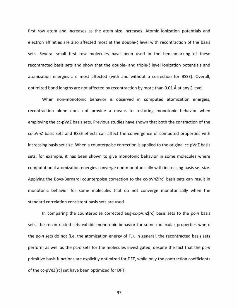
97
first row atom and increases as the atom size increases. Atomic ionization potentials and
electron affinities are also affected most at the double‐ζ level with recontraction of the basis
sets. Several small first row molecules have been used in the benchmarking of these
recontracted basis sets and show that the double‐ and triple‐ζ level ionization potentials and
atomization energies are most affected (with and without a correction for BSSE). Overall,
optimized bond lengths are not affected by recontraction by more than 0.01 Å at any ζ‐level.
When non‐monotonic behavior is observed in computed atomization energies,
recontraction alone does not provide a means to restoring monotonic behavior when
employing the cc‐pVnZ basis sets. Previous studies have shown that both the contraction of the
cc‐pVnZ basis sets and BSSE effects can affect the convergence of computed properties with
increasing basis set size. When a counterpoise correction is applied to the original cc‐pVnZ basis
sets, for example, it has been shown to give monotonic behavior in some molecules where
computational atomization energies converge non‐monotonically with increasing basis set size.
Applying the Boys‐Bernardi counterpoise correction to the cc‐pVnZ[rc] basis sets can result in
monotonic behavior for some molecules that do not converge monotonically when the
standard correlation consistent basis sets are used.
In comparing the counterpoise corrected aug‐cc‐pVnZ[rc] basis sets to the pc‐n basis
sets, the recontracted sets exhibit monotonic behavior for some molecular properties where
the pc‐n sets do not (i.e. the atomization energy of F2). In general, the recontracted basis sets
perform as well as the pc‐n sets for the molecules investigated, despite the fact that the pc‐n
primitive basis functions are explicitly optimized for DFT, while only the contraction coefficients
of the cc‐pVnZ[rc] set have been optimized for DFT.

98
Employing the Boys‐Bernardi counterpoise correction with these recontracted basis sets
can correct non‐monotonic behavior in energetic properties at the double‐, triple‐, and
quadruple‐ζ levels. When a counterpoise correction on the cc‐pVnZ[rc] basis sets does not
alleviate non‐monotonic behavior, the addition of diffuse functions acts to correct non‐
convergent behavior in most systems of this study. However, it is necessary to also include the
Boys‐Bernardi scheme with the aug‐cc‐pVnZ[rc] basis sets in the case of F2 to achieve
monotonic behavior with BLYP and B3LYP atomization energies. Thus, all three corrections:
recontracting the basis sets, adding diffuse functions, and including the counterpoise correction
can alleviate non‐monotonic behavior in the molecules of this study. Further, it is
recommended that the cc‐pVnZ[rc] basis sets be used in BLYP and B3LYP computations due to
their smaller size as compared with the pc‐n basis sets.
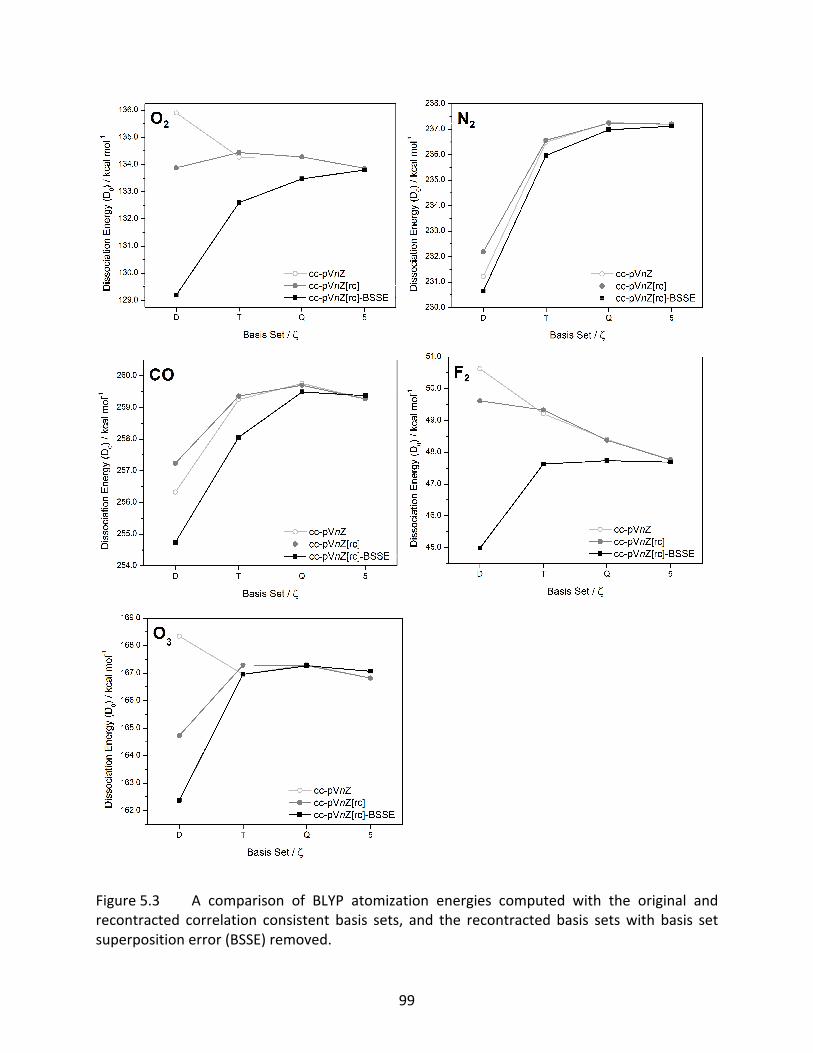
99
Figure 5.3 A comparison of BLYP atomization energies computed with the original and recontracted correlation consistent basis sets, and the recontracted basis sets with basis set superposition error (BSSE) removed.
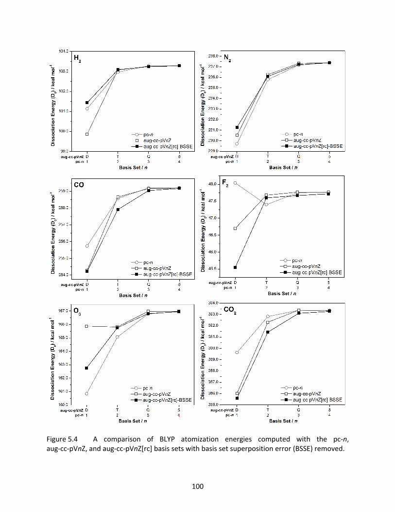
100
Figure 5.4 A comparison of BLYP atomization energies computed with the pc‐n, aug‐cc‐pVnZ, and aug‐cc‐pVnZ[rc] basis sets with basis set superposition error (BSSE) removed.
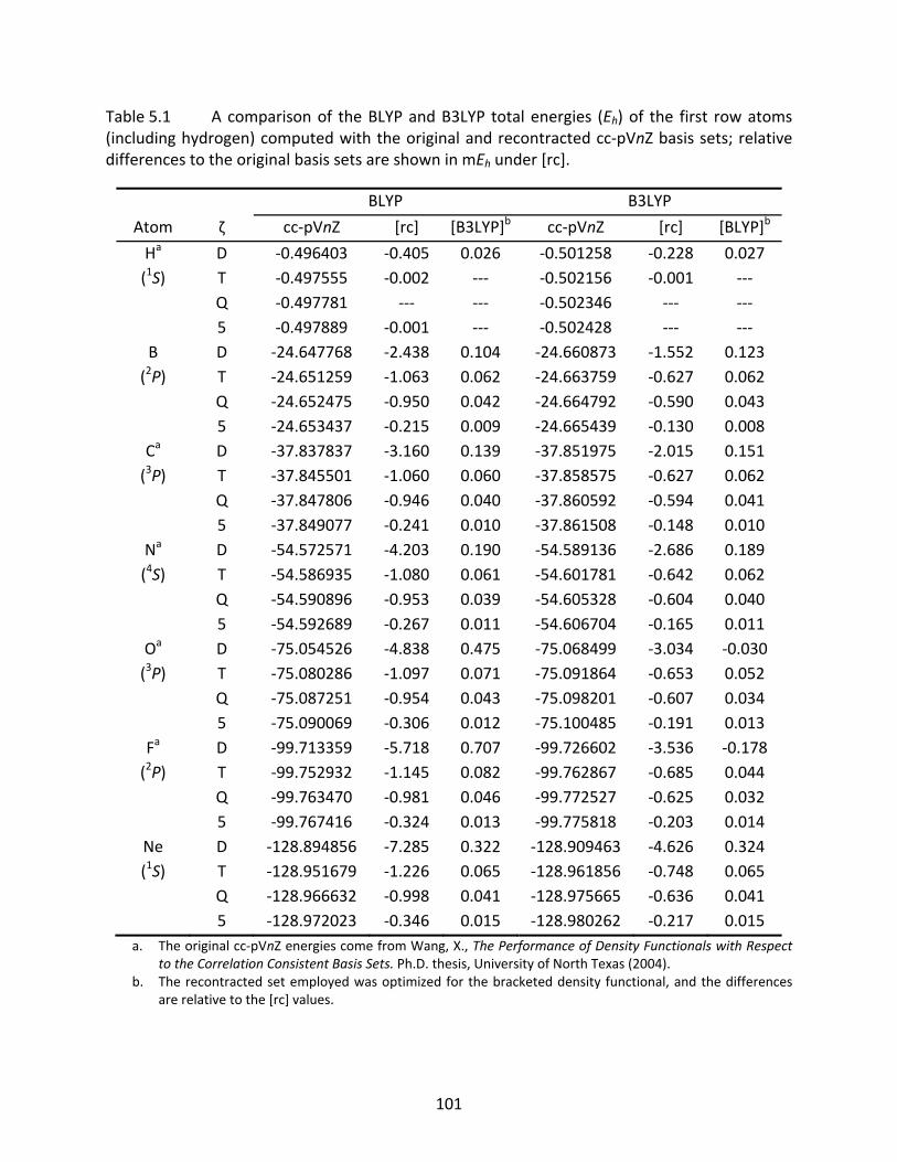
101
Table 5.1 A comparison of the BLYP and B3LYP total energies (Eh) of the first row atoms (including hydrogen) computed with the original and recontracted cc‐pVnZ basis sets; relative differences to the original basis sets are shown in mEh under [rc].
BLYP B3LYP
Atom ζ cc‐pVnZ [rc] [B3LYP]b cc‐pVnZ [rc] [BLYP]b
Ha D ‐0.496403 ‐0.405 0.026 ‐0.501258 ‐0.228 0.027(1S) T ‐0.497555 ‐0.002 ‐‐‐ ‐0.502156 ‐0.001 ‐‐‐ Q ‐0.497781 ‐‐‐ ‐‐‐ ‐0.502346 ‐‐‐ ‐‐‐ 5 ‐0.497889 ‐0.001 ‐‐‐ ‐0.502428 ‐‐‐ ‐‐‐B D ‐24.647768 ‐2.438 0.104 ‐24.660873 ‐1.552 0.123(2P) T ‐24.651259 ‐1.063 0.062 ‐24.663759 ‐0.627 0.062 Q ‐24.652475 ‐0.950 0.042 ‐24.664792 ‐0.590 0.043 5 ‐24.653437 ‐0.215 0.009 ‐24.665439 ‐0.130 0.008Ca D ‐37.837837 ‐3.160 0.139 ‐37.851975 ‐2.015 0.151(3P) T ‐37.845501 ‐1.060 0.060 ‐37.858575 ‐0.627 0.062 Q ‐37.847806 ‐0.946 0.040 ‐37.860592 ‐0.594 0.041 5 ‐37.849077 ‐0.241 0.010 ‐37.861508 ‐0.148 0.010Na D ‐54.572571 ‐4.203 0.190 ‐54.589136 ‐2.686 0.189(4S) T ‐54.586935 ‐1.080 0.061 ‐54.601781 ‐0.642 0.062 Q ‐54.590896 ‐0.953 0.039 ‐54.605328 ‐0.604 0.040 5 ‐54.592689 ‐0.267 0.011 ‐54.606704 ‐0.165 0.011Oa D ‐75.054526 ‐4.838 0.475 ‐75.068499 ‐3.034 ‐0.030(3P) T ‐75.080286 ‐1.097 0.071 ‐75.091864 ‐0.653 0.052 Q ‐75.087251 ‐0.954 0.043 ‐75.098201 ‐0.607 0.034 5 ‐75.090069 ‐0.306 0.012 ‐75.100485 ‐0.191 0.013Fa D ‐99.713359 ‐5.718 0.707 ‐99.726602 ‐3.536 ‐0.178(2P) T ‐99.752932 ‐1.145 0.082 ‐99.762867 ‐0.685 0.044 Q ‐99.763470 ‐0.981 0.046 ‐99.772527 ‐0.625 0.032 5 ‐99.767416 ‐0.324 0.013 ‐99.775818 ‐0.203 0.014
Ne D ‐128.894856 ‐7.285 0.322 ‐128.909463 ‐4.626 0.324(1S) T ‐128.951679 ‐1.226 0.065 ‐128.961856 ‐0.748 0.065 Q ‐128.966632 ‐0.998 0.041 ‐128.975665 ‐0.636 0.041 5 ‐128.972023 ‐0.346 0.015 ‐128.980262 ‐0.217 0.015
a. The original cc‐pVnZ energies come from Wang, X., The Performance of Density Functionals with Respect to the Correlation Consistent Basis Sets. Ph.D. thesis, University of North Texas (2004).
b. The recontracted set employed was optimized for the bracketed density functional, and the differences are relative to the [rc] values.
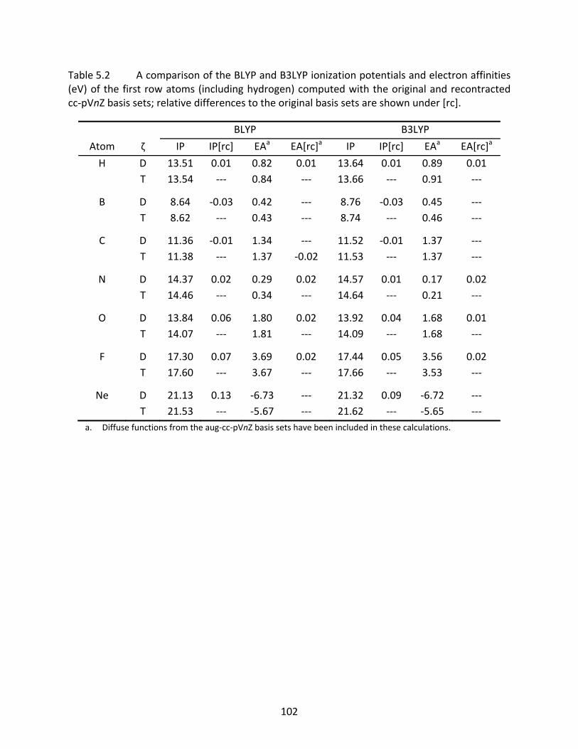
102
Table 5.2 A comparison of the BLYP and B3LYP ionization potentials and electron affinities (eV) of the first row atoms (including hydrogen) computed with the original and recontracted cc‐pVnZ basis sets; relative differences to the original basis sets are shown under [rc].
BLYP B3LYP
Atom ζ IP IP[rc] EAa EA[rc]a IP IP[rc] EAa EA[rc]a
H D 13.51 0.01 0.82 0.01 13.64 0.01 0.89 0.01 T 13.54 ‐‐‐ 0.84 ‐‐‐ 13.66 ‐‐‐ 0.91 ‐‐‐
B D 8.64 ‐0.03 0.42 ‐‐‐ 8.76 ‐0.03 0.45 ‐‐‐ T 8.62 ‐‐‐ 0.43 ‐‐‐ 8.74 ‐‐‐ 0.46 ‐‐‐
C D 11.36 ‐0.01 1.34 ‐‐‐ 11.52 ‐0.01 1.37 ‐‐‐ T 11.38 ‐‐‐ 1.37 ‐0.02 11.53 ‐‐‐ 1.37 ‐‐‐
N D 14.37 0.02 0.29 0.02 14.57 0.01 0.17 0.02 T 14.46 ‐‐‐ 0.34 ‐‐‐ 14.64 ‐‐‐ 0.21 ‐‐‐
O D 13.84 0.06 1.80 0.02 13.92 0.04 1.68 0.01 T 14.07 ‐‐‐ 1.81 ‐‐‐ 14.09 ‐‐‐ 1.68 ‐‐‐
F D 17.30 0.07 3.69 0.02 17.44 0.05 3.56 0.02 T 17.60 ‐‐‐ 3.67 ‐‐‐ 17.66 ‐‐‐ 3.53 ‐‐‐
Ne D 21.13 0.13 ‐6.73 ‐‐‐ 21.32 0.09 ‐6.72 ‐‐‐ T 21.53 ‐‐‐ ‐5.67 ‐‐‐ 21.62 ‐‐‐ ‐5.65 ‐‐‐
a. Diffuse functions from the aug‐cc‐pVnZ basis sets have been included in these calculations.
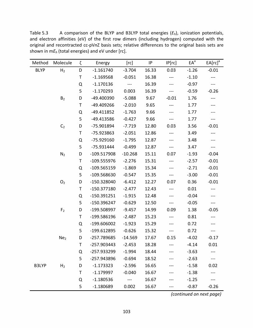
103
Table 5.3 A comparison of the BLYP and B3LYP total energies (Eh), ionization potentials, and electron affinities (eV) of the first row dimers (including hydrogen) computed with the original and recontracted cc‐pVnZ basis sets; relative differences to the original basis sets are shown in mEh (total energies) and eV under [rc].
Method Molecule ζ Energy [rc] IP IP[rc] EAa EA[rc]a
BLYP H2 D ‐1.161740 ‐3.704 16.33 0.03 ‐1.26 ‐0.01 T ‐1.169568 ‐0.051 16.38 ‐‐‐ ‐1.10 ‐‐‐ Q ‐1.170136 ‐‐‐ 16.39 ‐‐‐ ‐0.97 ‐‐‐ 5 ‐1.170293 0.003 16.39 ‐‐‐ ‐0.59 ‐0.26 B2 D ‐49.400390 ‐5.088 9.67 ‐0.01 1.76 ‐‐‐ T ‐49.409266 ‐2.010 9.65 ‐‐‐ 1.77 ‐‐‐ Q ‐49.411852 ‐1.763 9.66 ‐‐‐ 1.77 ‐‐‐ 5 ‐49.413586 ‐0.427 9.66 ‐‐‐ 1.77 ‐‐‐ C2 D ‐75.901894 ‐7.719 12.80 0.03 3.56 ‐0.01 T ‐75.923863 ‐2.051 12.86 ‐‐‐ 3.49 ‐‐‐ Q ‐75.929160 ‐1.795 12.87 ‐‐‐ 3.48 ‐‐‐ 5 ‐75.931444 ‐0.499 12.87 ‐‐‐ 3.47 ‐‐‐ N2 D ‐109.517908 ‐10.268 15.11 0.07 ‐1.93 ‐0.04 T ‐109.555976 ‐2.276 15.31 ‐‐‐ ‐2.57 ‐0.01 Q ‐109.565159 ‐1.869 15.34 ‐‐‐ ‐2.71 ‐0.01 5 ‐109.568630 ‐0.547 15.35 ‐‐‐ ‐3.00 ‐0.01 O2 D ‐150.328040 ‐6.412 12.27 0.07 0.36 ‐0.01 T ‐150.377180 ‐2.477 12.43 ‐‐‐ 0.01 ‐‐‐ Q ‐150.391251 ‐1.915 12.48 ‐‐‐ ‐0.04 ‐‐‐ 5 ‐150.396247 ‐0.629 12.50 ‐‐‐ ‐0.05 ‐‐‐ F2 D ‐199.508997 ‐9.457 14.99 0.09 1.38 ‐0.05 T ‐199.586196 ‐2.487 15.23 ‐‐‐ 0.81 ‐‐‐ Q ‐199.606002 ‐1.923 15.29 ‐‐‐ 0.72 ‐‐‐ 5 ‐199.612895 ‐0.626 15.32 ‐‐‐ 0.72 ‐‐‐ Ne2 D ‐257.789685 ‐14.569 17.67 0.15 ‐4.02 ‐0.17 T ‐257.903443 ‐2.453 18.28 ‐‐‐ ‐4.14 0.01 Q ‐257.933299 ‐1.994 18.44 ‐‐‐ ‐3.63 ‐‐‐ 5 ‐257.943896 ‐0.694 18.52 ‐‐‐ ‐2.63 ‐‐‐
B3LYP H2 D ‐1.173323 ‐2.596 16.65 ‐‐‐ ‐1.58 0.02 T ‐1.179997 ‐0.040 16.67 ‐‐‐ ‐1.38 ‐‐‐ Q ‐1.180536 ‐‐‐ 16.67 ‐‐‐ ‐1.25 ‐‐‐ 5 ‐1.180689 0.002 16.67 ‐‐‐ ‐0.87 ‐0.26
(continued on next page)
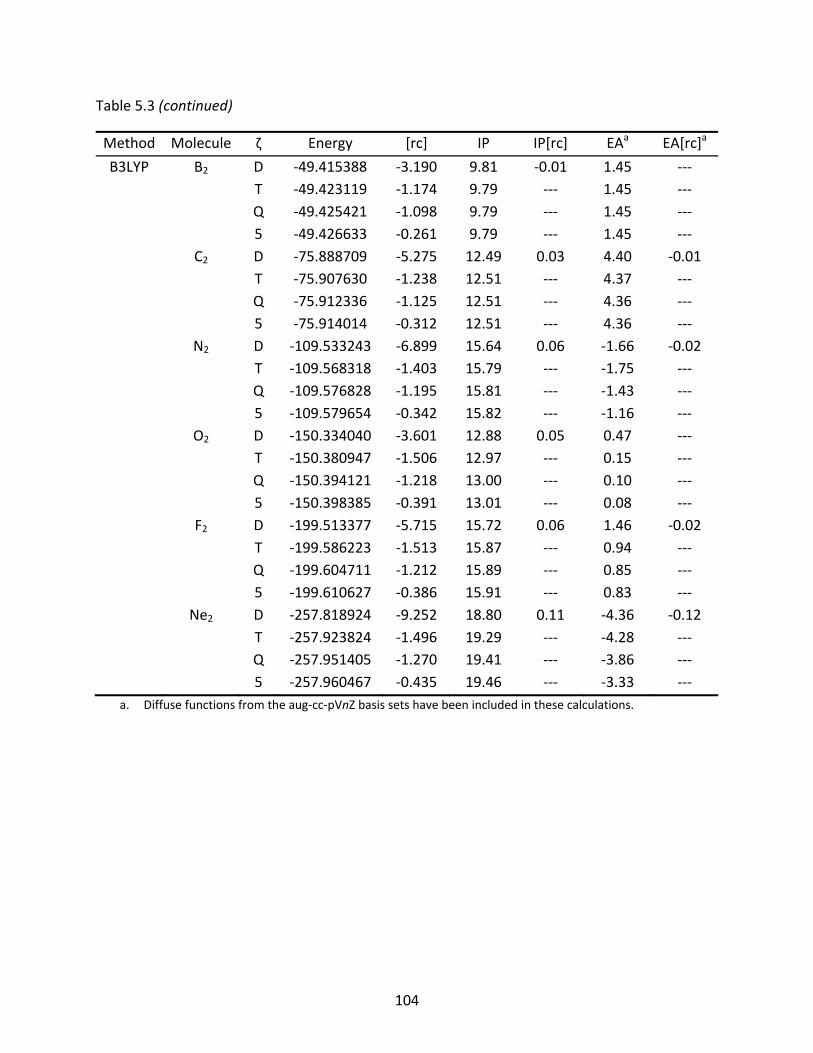
104
Table 5.3 (continued)
Method Molecule ζ Energy [rc] IP IP[rc] EAa EA[rc]a
B3LYP B2 D ‐49.415388 ‐3.190 9.81 ‐0.01 1.45 ‐‐‐ T ‐49.423119 ‐1.174 9.79 ‐‐‐ 1.45 ‐‐‐ Q ‐49.425421 ‐1.098 9.79 ‐‐‐ 1.45 ‐‐‐ 5 ‐49.426633 ‐0.261 9.79 ‐‐‐ 1.45 ‐‐‐ C2 D ‐75.888709 ‐5.275 12.49 0.03 4.40 ‐0.01 T ‐75.907630 ‐1.238 12.51 ‐‐‐ 4.37 ‐‐‐ Q ‐75.912336 ‐1.125 12.51 ‐‐‐ 4.36 ‐‐‐ 5 ‐75.914014 ‐0.312 12.51 ‐‐‐ 4.36 ‐‐‐ N2 D ‐109.533243 ‐6.899 15.64 0.06 ‐1.66 ‐0.02 T ‐109.568318 ‐1.403 15.79 ‐‐‐ ‐1.75 ‐‐‐ Q ‐109.576828 ‐1.195 15.81 ‐‐‐ ‐1.43 ‐‐‐ 5 ‐109.579654 ‐0.342 15.82 ‐‐‐ ‐1.16 ‐‐‐ O2 D ‐150.334040 ‐3.601 12.88 0.05 0.47 ‐‐‐ T ‐150.380947 ‐1.506 12.97 ‐‐‐ 0.15 ‐‐‐ Q ‐150.394121 ‐1.218 13.00 ‐‐‐ 0.10 ‐‐‐ 5 ‐150.398385 ‐0.391 13.01 ‐‐‐ 0.08 ‐‐‐ F2 D ‐199.513377 ‐5.715 15.72 0.06 1.46 ‐0.02 T ‐199.586223 ‐1.513 15.87 ‐‐‐ 0.94 ‐‐‐ Q ‐199.604711 ‐1.212 15.89 ‐‐‐ 0.85 ‐‐‐ 5 ‐199.610627 ‐0.386 15.91 ‐‐‐ 0.83 ‐‐‐ Ne2 D ‐257.818924 ‐9.252 18.80 0.11 ‐4.36 ‐0.12 T ‐257.923824 ‐1.496 19.29 ‐‐‐ ‐4.28 ‐‐‐ Q ‐257.951405 ‐1.270 19.41 ‐‐‐ ‐3.86 ‐‐‐ 5 ‐257.960467 ‐0.435 19.46 ‐‐‐ ‐3.33 ‐‐‐
a. Diffuse functions from the aug‐cc‐pVnZ basis sets have been included in these calculations.
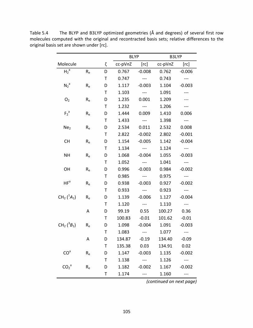
105
Table 5.4 The BLYP and B3LYP optimized geometries (Å and degrees) of several first row molecules computed with the original and recontracted basis sets; relative differences to the original basis set are shown under [rc].
BLYP B3LYP
Molecule ζ cc‐pVnZ [rc] cc‐pVnZ [rc]
H2a Re D 0.767 ‐0.008 0.762 ‐0.006 T 0.747 ‐‐‐ 0.743 ‐‐‐
N2a Re D 1.117 ‐0.003 1.104 ‐0.003 T 1.103 ‐‐‐ 1.091 ‐‐‐ O2 Re D 1.235 0.001 1.209 ‐‐‐ T 1.232 ‐‐‐ 1.206 ‐‐‐
F2a Re D 1.444 0.009 1.410 0.006 T 1.433 ‐‐‐ 1.398 ‐‐‐
Ne2 Re D 2.534 0.011 2.532 0.008 T 2.822 ‐0.002 2.802 ‐0.001
CH Re D 1.154 ‐0.005 1.142 ‐0.004 T 1.134 ‐‐‐ 1.124 ‐‐‐
NH Re D 1.068 ‐0.004 1.055 ‐0.003 T 1.052 ‐‐‐ 1.041 ‐‐‐
OH Re D 0.996 ‐0.003 0.984 ‐0.002 T 0.985 ‐‐‐ 0.975 ‐‐‐
HFa Re D 0.938 ‐0.003 0.927 ‐0.002 T 0.933 ‐‐‐ 0.923 ‐‐‐
CH2 (1A1) Re D 1.139 ‐0.006 1.127 ‐0.004 T 1.120 ‐‐‐ 1.110 ‐‐‐ A D 99.19 0.55 100.27 0.36 T 100.83 ‐0.01 101.62 ‐0.01
CH2 (3B1) Re D 1.098 ‐0.004 1.091 ‐0.003 T 1.083 ‐‐‐ 1.077 ‐‐‐ A D 134.87 ‐0.19 134.40 ‐0.09 T 135.38 0.03 134.91 0.02
COa Re D 1.147 ‐0.003 1.135 ‐0.002 T 1.138 ‐‐‐ 1.126 ‐‐‐
CO2a Re D 1.182 ‐0.002 1.167 ‐0.002
T 1.174 ‐‐‐ 1.160 ‐‐‐
(continued on next page)
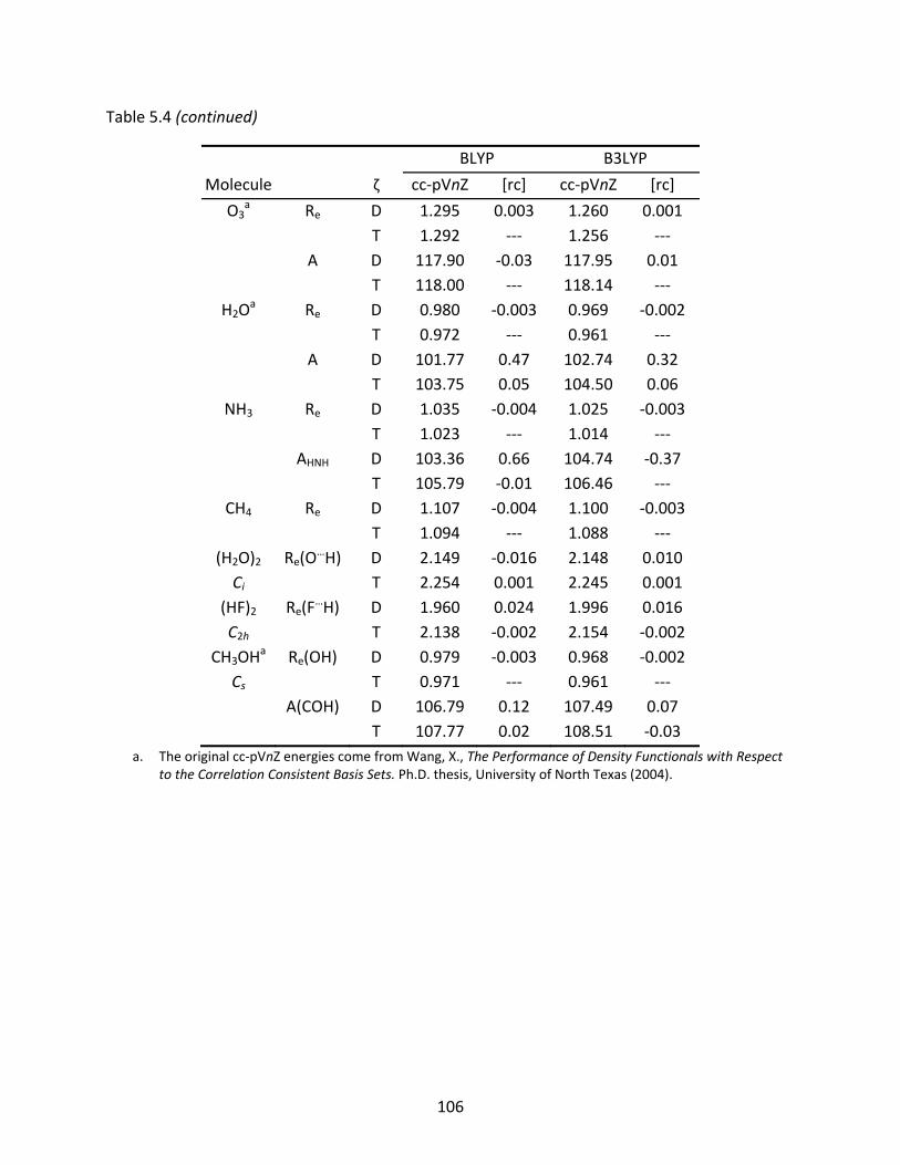
106
Table 5.4 (continued)
BLYP B3LYP
Molecule ζ cc‐pVnZ [rc] cc‐pVnZ [rc]
O3a Re D 1.295 0.003 1.260 0.001 T 1.292 ‐‐‐ 1.256 ‐‐‐ A D 117.90 ‐0.03 117.95 0.01 T 118.00 ‐‐‐ 118.14 ‐‐‐
H2Oa Re D 0.980 ‐0.003 0.969 ‐0.002
T 0.972 ‐‐‐ 0.961 ‐‐‐ A D 101.77 0.47 102.74 0.32 T 103.75 0.05 104.50 0.06
NH3 Re D 1.035 ‐0.004 1.025 ‐0.003 T 1.023 ‐‐‐ 1.014 ‐‐‐ AHNH D 103.36 0.66 104.74 ‐0.37 T 105.79 ‐0.01 106.46 ‐‐‐
CH4 Re D 1.107 ‐0.004 1.100 ‐0.003 T 1.094 ‐‐‐ 1.088 ‐‐‐
(H2O)2 Re(O…H) D 2.149 ‐0.016 2.148 0.010
Ci T 2.254 0.001 2.245 0.001 (HF)2 Re(F
…H) D 1.960 0.024 1.996 0.016 C2h T 2.138 ‐0.002 2.154 ‐0.002
CH3OHa Re(OH) D 0.979 ‐0.003 0.968 ‐0.002
Cs T 0.971 ‐‐‐ 0.961 ‐‐‐ A(COH) D 106.79 0.12 107.49 0.07 T 107.77 0.02 108.51 ‐0.03
a. The original cc‐pVnZ energies come from Wang, X., The Performance of Density Functionals with Respect to the Correlation Consistent Basis Sets. Ph.D. thesis, University of North Texas (2004).
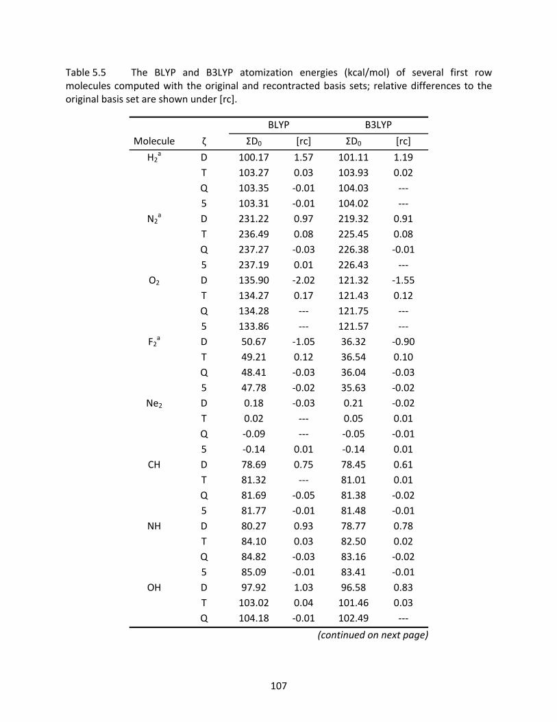
107
Table 5.5 The BLYP and B3LYP atomization energies (kcal/mol) of several first row molecules computed with the original and recontracted basis sets; relative differences to the original basis set are shown under [rc].
BLYP B3LYP
Molecule ζ ΣD0 [rc] ΣD0 [rc]
H2a D 100.17 1.57 101.11 1.19 T 103.27 0.03 103.93 0.02 Q 103.35 ‐0.01 104.03 ‐‐‐ 5 103.31 ‐0.01 104.02 ‐‐‐
N2a D 231.22 0.97 219.32 0.91 T 236.49 0.08 225.45 0.08 Q 237.27 ‐0.03 226.38 ‐0.01 5 237.19 0.01 226.43 ‐‐‐ O2 D 135.90 ‐2.02 121.32 ‐1.55 T 134.27 0.17 121.43 0.12 Q 134.28 ‐‐‐ 121.75 ‐‐‐ 5 133.86 ‐‐‐ 121.57 ‐‐‐
F2a D 50.67 ‐1.05 36.32 ‐0.90 T 49.21 0.12 36.54 0.10 Q 48.41 ‐0.03 36.04 ‐0.03 5 47.78 ‐0.02 35.63 ‐0.02
Ne2 D 0.18 ‐0.03 0.21 ‐0.02 T 0.02 ‐‐‐ 0.05 0.01 Q ‐0.09 ‐‐‐ ‐0.05 ‐0.01 5 ‐0.14 0.01 ‐0.14 0.01
CH D 78.69 0.75 78.45 0.61 T 81.32 ‐‐‐ 81.01 0.01 Q 81.69 ‐0.05 81.38 ‐0.02 5 81.77 ‐0.01 81.48 ‐0.01
NH D 80.27 0.93 78.77 0.78 T 84.10 0.03 82.50 0.02 Q 84.82 ‐0.03 83.16 ‐0.02 5 85.09 ‐0.01 83.41 ‐0.01
OH D 97.92 1.03 96.58 0.83 T 103.02 0.04 101.46 0.03 Q 104.18 ‐0.01 102.49 ‐‐‐
(continued on next page)
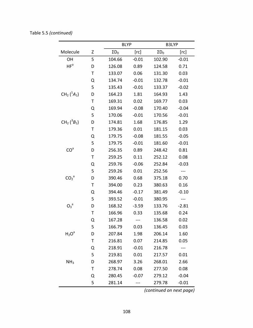
108
Table 5.5 (continued)
BLYP B3LYP
Molecule Ζ ΣD0 [rc] ΣD0 [rc]
OH 5 104.66 ‐0.01 102.90 ‐0.01 HFa D 126.08 0.89 124.58 0.71 T 133.07 0.06 131.30 0.03 Q 134.74 ‐0.01 132.78 ‐0.01 5 135.43 ‐0.01 133.37 ‐0.02
CH2 (1A1) D 164.23 1.81 164.93 1.43 T 169.31 0.02 169.77 0.03 Q 169.94 ‐0.08 170.40 ‐0.04 5 170.06 ‐0.01 170.56 ‐0.01
CH2 (3B1) D 174.81 1.68 176.85 1.29 T 179.36 0.01 181.15 0.03 Q 179.75 ‐0.08 181.55 ‐0.05 5 179.75 ‐0.01 181.60 ‐0.01
COa D 256.35 0.89 248.42 0.81 T 259.25 0.11 252.12 0.08 Q 259.76 ‐0.06 252.84 ‐0.03 5 259.26 0.01 252.56 ‐‐‐
CO2a D 390.46 0.68 375.18 0.70
T 394.00 0.23 380.63 0.16 Q 394.46 ‐0.17 381.49 ‐0.10 5 393.52 ‐0.01 380.95 ‐‐‐
O3a D 168.32 ‐3.59 133.76 ‐2.81 T 166.96 0.33 135.68 0.24 Q 167.28 ‐‐‐ 136.58 0.02 5 166.79 0.03 136.45 0.03
H2Oa D 207.84 1.98 206.14 1.60
T 216.81 0.07 214.85 0.05 Q 218.91 ‐0.01 216.78 ‐‐‐ 5 219.81 0.01 217.57 0.01
NH3 D 268.97 3.26 268.01 2.66 T 278.74 0.08 277.50 0.08 Q 280.45 ‐0.07 279.12 ‐0.04 5 281.14 ‐‐‐ 279.78 ‐0.01
(continued on next page)
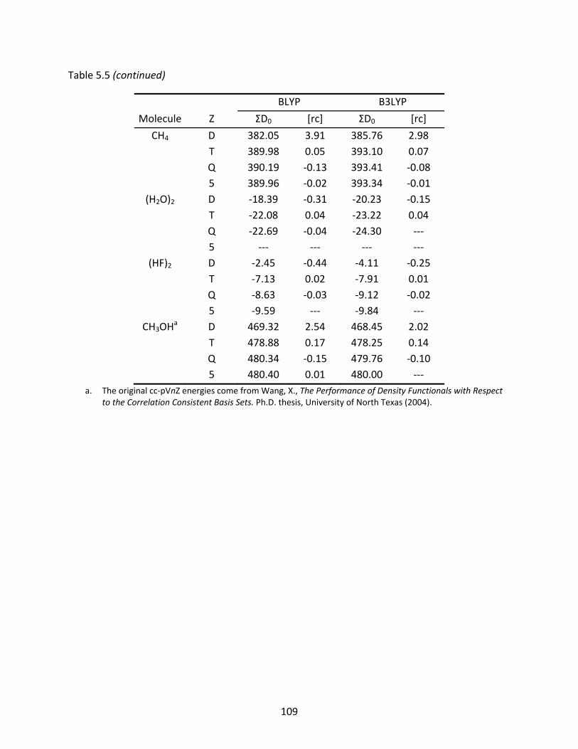
109
Table 5.5 (continued)
BLYP B3LYP
Molecule Ζ ΣD0 [rc] ΣD0 [rc]
CH4 D 382.05 3.91 385.76 2.98 T 389.98 0.05 393.10 0.07 Q 390.19 ‐0.13 393.41 ‐0.08 5 389.96 ‐0.02 393.34 ‐0.01
(H2O)2 D ‐18.39 ‐0.31 ‐20.23 ‐0.15 T ‐22.08 0.04 ‐23.22 0.04 Q ‐22.69 ‐0.04 ‐24.30 ‐‐‐ 5 ‐‐‐ ‐‐‐ ‐‐‐ ‐‐‐
(HF)2 D ‐2.45 ‐0.44 ‐4.11 ‐0.25 T ‐7.13 0.02 ‐7.91 0.01 Q ‐8.63 ‐0.03 ‐9.12 ‐0.02 5 ‐9.59 ‐‐‐ ‐9.84 ‐‐‐
CH3OHa D 469.32 2.54 468.45 2.02
T 478.88 0.17 478.25 0.14 Q 480.34 ‐0.15 479.76 ‐0.10 5 480.40 0.01 480.00 ‐‐‐
a. The original cc‐pVnZ energies come from Wang, X., The Performance of Density Functionals with Respect to the Correlation Consistent Basis Sets. Ph.D. thesis, University of North Texas (2004).
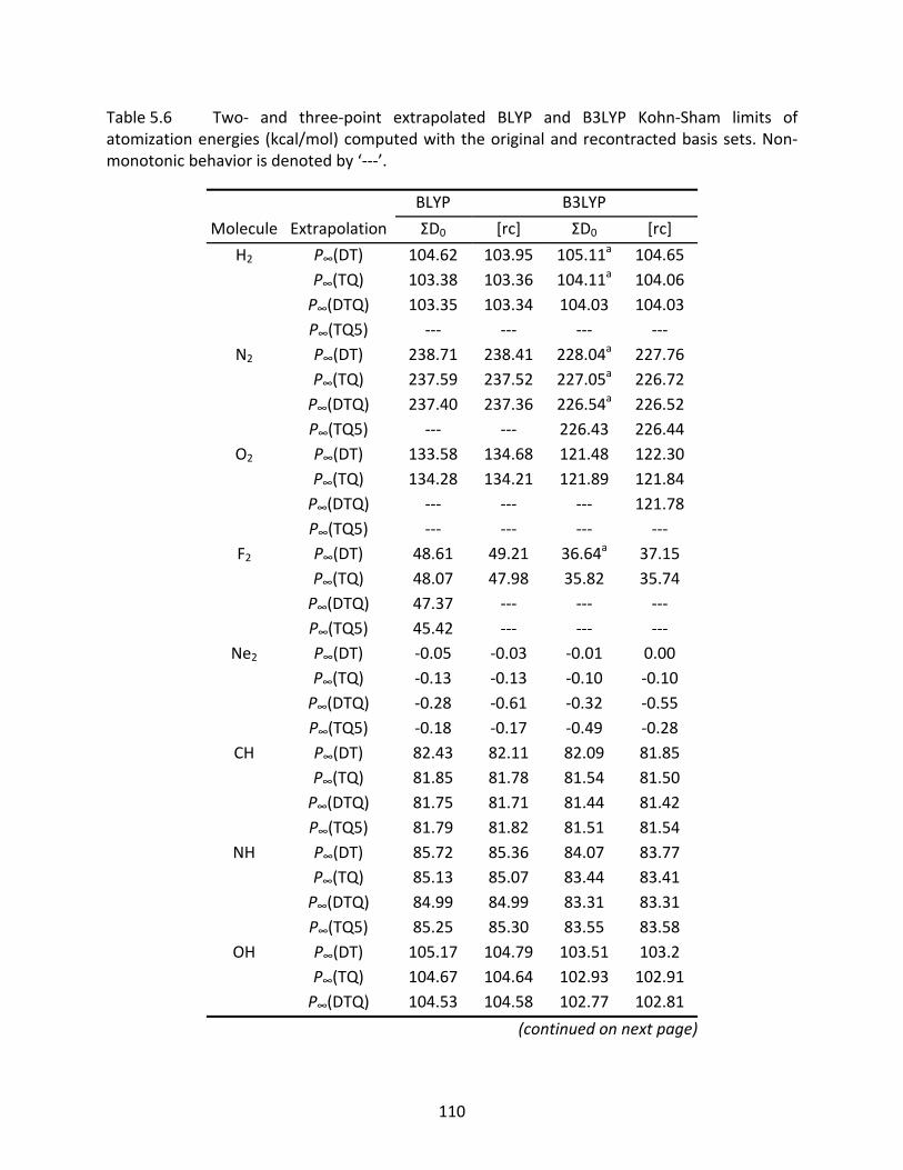
110
Table 5.6 Two‐ and three‐point extrapolated BLYP and B3LYP Kohn‐Sham limits of atomization energies (kcal/mol) computed with the original and recontracted basis sets. Non‐monotonic behavior is denoted by ‘‐‐‐’.
BLYP B3LYP
Molecule Extrapolation ΣD0 [rc] ΣD0 [rc]
H2 P∞(DT) 104.62 103.95 105.11a 104.65 P∞(TQ) 103.38 103.36 104.11a 104.06 P∞(DTQ) 103.35 103.34 104.03 104.03 P∞(TQ5) ‐‐‐ ‐‐‐ ‐‐‐ ‐‐‐ N2 P∞(DT) 238.71 238.41 228.04a 227.76 P∞(TQ) 237.59 237.52 227.05a 226.72 P∞(DTQ) 237.40 237.36 226.54a 226.52 P∞(TQ5) ‐‐‐ ‐‐‐ 226.43 226.44 O2 P∞(DT) 133.58 134.68 121.48 122.30 P∞(TQ) 134.28 134.21 121.89 121.84 P∞(DTQ) ‐‐‐ ‐‐‐ ‐‐‐ 121.78 P∞(TQ5) ‐‐‐ ‐‐‐ ‐‐‐ ‐‐‐ F2 P∞(DT) 48.61 49.21 36.64a 37.15 P∞(TQ) 48.07 47.98 35.82 35.74 P∞(DTQ) 47.37 ‐‐‐ ‐‐‐ ‐‐‐ P∞(TQ5) 45.42 ‐‐‐ ‐‐‐ ‐‐‐
Ne2 P∞(DT) ‐0.05 ‐0.03 ‐0.01 0.00 P∞(TQ) ‐0.13 ‐0.13 ‐0.10 ‐0.10 P∞(DTQ) ‐0.28 ‐0.61 ‐0.32 ‐0.55 P∞(TQ5) ‐0.18 ‐0.17 ‐0.49 ‐0.28
CH P∞(DT) 82.43 82.11 82.09 81.85 P∞(TQ) 81.85 81.78 81.54 81.50 P∞(DTQ) 81.75 81.71 81.44 81.42 P∞(TQ5) 81.79 81.82 81.51 81.54
NH P∞(DT) 85.72 85.36 84.07 83.77 P∞(TQ) 85.13 85.07 83.44 83.41 P∞(DTQ) 84.99 84.99 83.31 83.31 P∞(TQ5) 85.25 85.30 83.55 83.58
OH P∞(DT) 105.17 104.79 103.51 103.2 P∞(TQ) 104.67 104.64 102.93 102.91 P∞(DTQ) 104.53 104.58 102.77 102.81
(continued on next page)
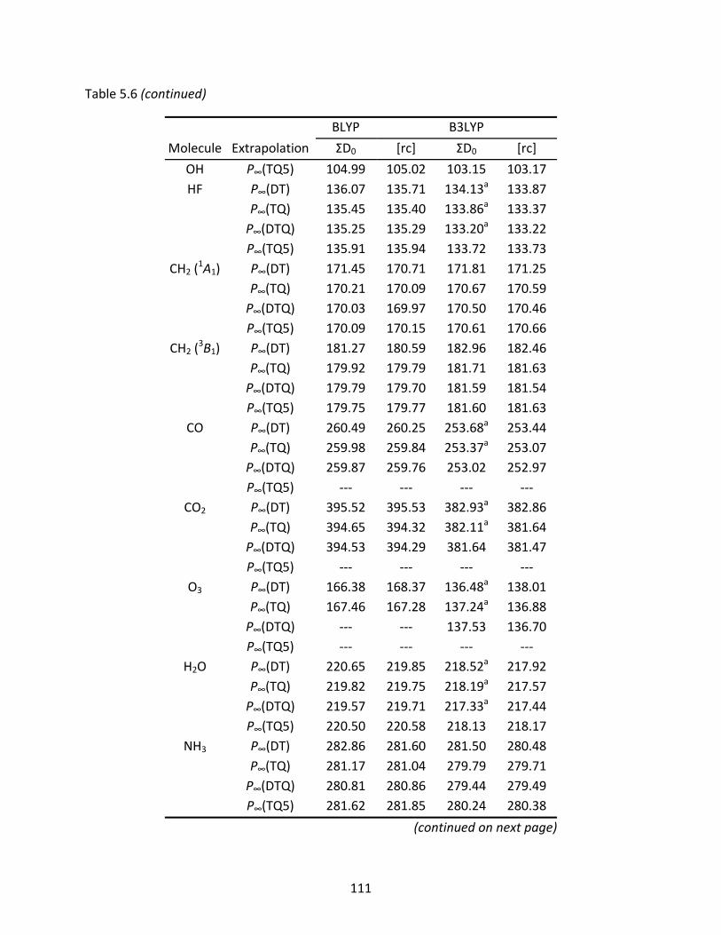
111
Table 5.6 (continued)
BLYP B3LYP
Molecule Extrapolation ΣD0 [rc] ΣD0 [rc]
OH P∞(TQ5) 104.99 105.02 103.15 103.17 HF P∞(DT) 136.07 135.71 134.13a 133.87 P∞(TQ) 135.45 135.40 133.86a 133.37 P∞(DTQ) 135.25 135.29 133.20a 133.22 P∞(TQ5) 135.91 135.94 133.72 133.73
CH2 (1A1) P∞(DT) 171.45 170.71 171.81 171.25 P∞(TQ) 170.21 170.09 170.67 170.59 P∞(DTQ) 170.03 169.97 170.50 170.46 P∞(TQ5) 170.09 170.15 170.61 170.66
CH2 (3B1) P∞(DT) 181.27 180.59 182.96 182.46
P∞(TQ) 179.92 179.79 181.71 181.63 P∞(DTQ) 179.79 179.70 181.59 181.54 P∞(TQ5) 179.75 179.77 181.60 181.63
CO P∞(DT) 260.49 260.25 253.68a 253.44 P∞(TQ) 259.98 259.84 253.37a 253.07 P∞(DTQ) 259.87 259.76 253.02 252.97 P∞(TQ5) ‐‐‐ ‐‐‐ ‐‐‐ ‐‐‐
CO2 P∞(DT) 395.52 395.53 382.93a 382.86 P∞(TQ) 394.65 394.32 382.11a 381.64 P∞(DTQ) 394.53 394.29 381.64 381.47 P∞(TQ5) ‐‐‐ ‐‐‐ ‐‐‐ ‐‐‐ O3 P∞(DT) 166.38 168.37 136.48a 138.01 P∞(TQ) 167.46 167.28 137.24a 136.88 P∞(DTQ) ‐‐‐ ‐‐‐ 137.53 136.70 P∞(TQ5) ‐‐‐ ‐‐‐ ‐‐‐ ‐‐‐
H2O P∞(DT) 220.65 219.85 218.52a 217.92 P∞(TQ) 219.82 219.75 218.19a 217.57 P∞(DTQ) 219.57 219.71 217.33a 217.44 P∞(TQ5) 220.50 220.58 218.13 218.17
NH3 P∞(DT) 282.86 281.60 281.50 280.48 P∞(TQ) 281.17 281.04 279.79 279.71 P∞(DTQ) 280.81 280.86 279.44 279.49 P∞(TQ5) 281.62 281.85 280.24 280.38
(continued on next page)
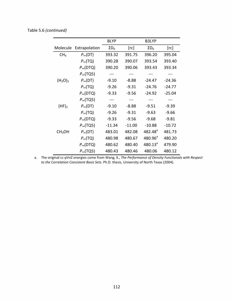
112
Table 5.6 (continued)
BLYP B3LYP
Molecule Extrapolation ΣD0 [rc] ΣD0 [rc]
CH4 P∞(DT) 393.32 391.75 396.20 395.04 P∞(TQ) 390.28 390.07 393.54 393.40 P∞(DTQ) 390.20 390.06 393.43 393.34 P∞(TQ5) ‐‐‐ ‐‐‐ ‐‐‐ ‐‐‐
(H2O)2 P∞(DT) ‐9.10 ‐8.88 ‐24.47 ‐24.36 P∞(TQ) ‐9.26 ‐9.31 ‐24.76 ‐24.77 P∞(DTQ) ‐9.33 ‐9.56 ‐24.92 ‐25.04 P∞(TQ5) ‐‐‐ ‐‐‐ ‐‐‐ ‐‐‐
(HF)2 P∞(DT) ‐9.10 ‐8.88 ‐9.51 ‐9.39 P∞(TQ) ‐9.26 ‐9.31 ‐9.63 ‐9.66 P∞(DTQ) ‐9.33 ‐9.56 ‐9.68 ‐9.81 P∞(TQ5) ‐11.34 ‐11.00 ‐10.88 ‐10.72
CH3OH P∞(DT) 483.01 482.08 482.48a 481.73 P∞(TQ) 480.98 480.67 480.96a 480.20 P∞(DTQ) 480.62 480.40 480.13a 479.90 P∞(TQ5) 480.43 480.46 480.06 480.12
a. The original cc‐pVnZ energies come from Wang, X., The Performance of Density Functionals with Respect to the Correlation Consistent Basis Sets. Ph.D. thesis, University of North Texas (2004).
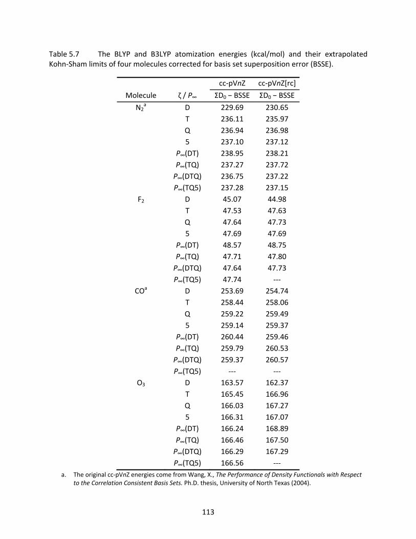
113
Table 5.7 The BLYP and B3LYP atomization energies (kcal/mol) and their extrapolated Kohn‐Sham limits of four molecules corrected for basis set superposition error (BSSE).
cc‐pVnZ cc‐pVnZ[rc]
Molecule ζ / P∞ ΣD0 − BSSE ΣD0 − BSSE
N2a D 229.69 230.65 T 236.11 235.97 Q 236.94 236.98 5 237.10 237.12 P∞(DT) 238.95 238.21 P∞(TQ) 237.27 237.72 P∞(DTQ) 236.75 237.22 P∞(TQ5) 237.28 237.15F2 D 45.07 44.98 T 47.53 47.63 Q 47.64 47.73 5 47.69 47.69 P∞(DT) 48.57 48.75 P∞(TQ) 47.71 47.80 P∞(DTQ) 47.64 47.73 P∞(TQ5) 47.74 ‐‐‐
COa D 253.69 254.74 T 258.44 258.06 Q 259.22 259.49 5 259.14 259.37 P∞(DT) 260.44 259.46 P∞(TQ) 259.79 260.53 P∞(DTQ) 259.37 260.57 P∞(TQ5) ‐‐‐ ‐‐‐O3 D 163.57 162.37 T 165.45 166.96 Q 166.03 167.27 5 166.31 167.07 P∞(DT) 166.24 168.89 P∞(TQ) 166.46 167.50 P∞(DTQ) 166.29 167.29 P∞(TQ5) 166.56 ‐‐‐
a. The original cc‐pVnZ energies come from Wang, X., The Performance of Density Functionals with Respect to the Correlation Consistent Basis Sets. Ph.D. thesis, University of North Texas (2004).
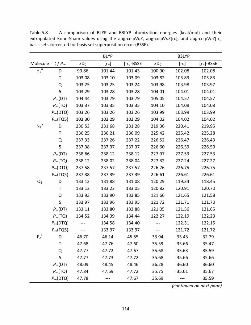
114
Table 5.8 A comparison of BLYP and B3LYP atomization energies (kcal/mol) and their extrapolated Kohn‐Sham values using the aug‐cc‐pVnZ, aug‐cc‐pVnZ[rc], and aug‐cc‐pVnZ[rc] basis sets corrected for basis set superposition error (BSSE).
BLYP B3LYP
Molecule ζ / P∞ ΣD0 [rc] [rc]‐BSSE ΣD0 [rc] [rc]‐BSSE
H2a D 99.86 101.44 101.43 100.90 102.08 102.08 T 103.08 103.10 103.09 103.82 103.83 103.83 Q 103.25 103.25 103.24 103.98 103.98 103.97 5 103.29 103.28 103.28 104.01 104.01 104.01 P∞(DT) 104.44 103.79 103.79 105.05 104.57 104.57 P∞(TQ) 103.37 103.35 103.35 104.10 104.08 104.08 P∞(DTQ) 103.26 103.26 103.26 103.99 103.99 103.99 P∞(TQ5) 103.30 103.29 103.29 104.02 104.02 104.02
N2a D 230.53 231.68 231.28 219.36 220.41 219.95 T 236.25 236.21 236.09 225.42 225.42 225.28 Q 237.33 237.26 237.22 226.52 226.47 226.43 5 237.38 237.37 237.37 226.60 226.59 226.59 P∞(DT) 238.66 238.12 238.12 227.97 227.53 227.53 P∞(TQ) 238.12 238.02 238.04 227.32 227.24 227.27 P∞(DTQ) 237.58 237.57 237.57 226.76 226.75 226.75 P∞(TQ5) 237.38 237.39 237.39 226.61 226.61 226.61O2 D 133.13 131.88 131.08 120.29 119.34 118.45 T 133.12 133.23 133.05 120.82 120.91 120.70 Q 133.93 133.90 133.85 121.66 121.65 121.58 5 133.97 133.96 133.95 121.72 121.71 121.70 P∞(DT) 133.11 133.80 133.88 121.05 121.56 121.65 P∞(TQ) 134.52 134.39 134.44 122.27 122.19 122.23 P∞(DTQ) ‐‐‐ 134.58 134.40 ‐‐‐ 122.31 122.15 P∞(TQ5) ‐‐‐ 133.97 133.97 ‐‐‐ 121.72 121.72
F2a D 46.70 46.14 45.55 33.94 33.43 32.79 T 47.68 47.76 47.60 35.59 35.66 35.47 Q 47.77 47.72 47.67 35.68 35.63 35.59 5 47.77 47.73 47.72 35.68 35.66 35.66 P∞(DT) 48.09 48.45 48.46 36.28 36.60 36.60 P∞(TQ) 47.84 47.69 47.72 35.75 35.61 35.67 P∞(DTQ) 47.78 ‐‐‐ 47.67 35.69 ‐‐‐ 35.59
(continued on next page)
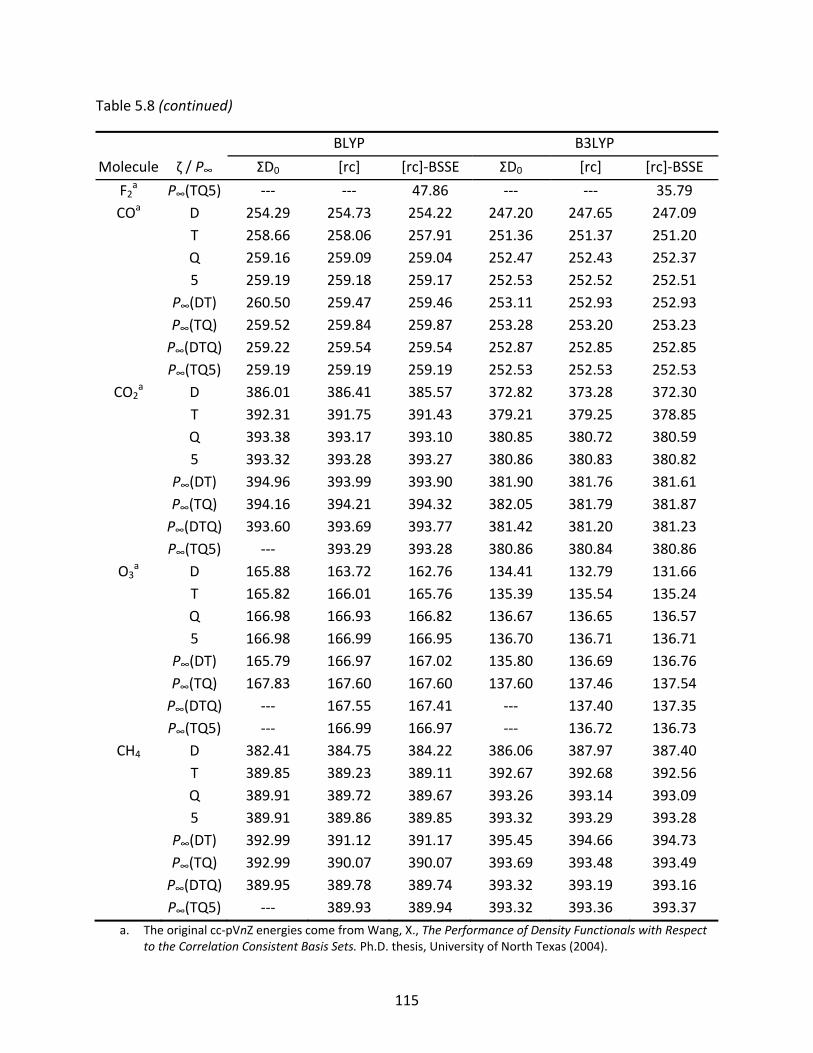
115
Table 5.8 (continued)
BLYP B3LYP
Molecule ζ / P∞ ΣD0 [rc] [rc]‐BSSE ΣD0 [rc] [rc]‐BSSE
F2a P∞(TQ5) ‐‐‐ ‐‐‐ 47.86 ‐‐‐ ‐‐‐ 35.79
COa D 254.29 254.73 254.22 247.20 247.65 247.09 T 258.66 258.06 257.91 251.36 251.37 251.20 Q 259.16 259.09 259.04 252.47 252.43 252.37 5 259.19 259.18 259.17 252.53 252.52 252.51 P∞(DT) 260.50 259.47 259.46 253.11 252.93 252.93 P∞(TQ) 259.52 259.84 259.87 253.28 253.20 253.23 P∞(DTQ) 259.22 259.54 259.54 252.87 252.85 252.85 P∞(TQ5) 259.19 259.19 259.19 252.53 252.53 252.53
CO2a D 386.01 386.41 385.57 372.82 373.28 372.30
T 392.31 391.75 391.43 379.21 379.25 378.85 Q 393.38 393.17 393.10 380.85 380.72 380.59 5 393.32 393.28 393.27 380.86 380.83 380.82 P∞(DT) 394.96 393.99 393.90 381.90 381.76 381.61 P∞(TQ) 394.16 394.21 394.32 382.05 381.79 381.87 P∞(DTQ) 393.60 393.69 393.77 381.42 381.20 381.23 P∞(TQ5) ‐‐‐ 393.29 393.28 380.86 380.84 380.86
O3a D 165.88 163.72 162.76 134.41 132.79 131.66 T 165.82 166.01 165.76 135.39 135.54 135.24 Q 166.98 166.93 166.82 136.67 136.65 136.57 5 166.98 166.99 166.95 136.70 136.71 136.71 P∞(DT) 165.79 166.97 167.02 135.80 136.69 136.76 P∞(TQ) 167.83 167.60 167.60 137.60 137.46 137.54 P∞(DTQ) ‐‐‐ 167.55 167.41 ‐‐‐ 137.40 137.35 P∞(TQ5) ‐‐‐ 166.99 166.97 ‐‐‐ 136.72 136.73
CH4 D 382.41 384.75 384.22 386.06 387.97 387.40 T 389.85 389.23 389.11 392.67 392.68 392.56 Q 389.91 389.72 389.67 393.26 393.14 393.09 5 389.91 389.86 389.85 393.32 393.29 393.28 P∞(DT) 392.99 391.12 391.17 395.45 394.66 394.73 P∞(TQ) 392.99 390.07 390.07 393.69 393.48 393.49 P∞(DTQ) 389.95 389.78 389.74 393.32 393.19 393.16 P∞(TQ5) ‐‐‐ 389.93 389.94 393.32 393.36 393.37
a. The original cc‐pVnZ energies come from Wang, X., The Performance of Density Functionals with Respect to the Correlation Consistent Basis Sets. Ph.D. thesis, University of North Texas (2004).
116
CHAPTER 6
THE DEVELOPMENT OF S‐BLOCK CORRELATION CONSISTENT BASIS SETS†
6.1 Introduction
In correlated ab initio methodology, achieving the exact solution to the non‐relativistic
Schrödinger equation requires two criteria: 1) a complete N‐electron treatment and 2) a
complete (infinite) basis set.7,18 The former can be achieved through a full configuration
interaction (FCI) treatment, which is rarely applicable to any but the smallest of electronic
systems (i.e. less than ten electrons). Even in small systems where FCI can be applied, the use of
modest‐sized basis sets is a limiting factor in achieving the exact solution of the Schrödinger
equation since FCI scales factorially in basis set size. Further, the use of an infinite basis set is
computationally infeasible. In a practical sense, the N‐electron treatment and basis set must be
chosen considering both the desired level of accuracy and the computational feasibility.
As already discussed in Chapter 2, the use of an infinite basis set is desirable but
infeasible, and the best method of approximating the exact solution to the Schrödinger
equation would be to select as large a basis set as possible. However, this quickly limits both
the system size and the N‐electron treatment that can be employed. The correlation consistent,
polarized valance basis sets (cc‐pVnZ)81‐109 were specifically designed so that ab initio methods
recover correlation energy more quickly than other basis sets (e.g. basis sets developed with
Hartree‐Fock). Further, the correlation consistent basis sets offer a way to circumvent the
† Work reported in this chapter was performed in collaboration with Kirk A. Peterson, David E. Woon, and Thom H. Dunning, Jr.
117
infeasibility of infinite basis sets by systematically approaching the complete basis set (CBS)
limit as the ζ‐level, or cardinal number, increases.
Correlation consistent basis sets have been developed for much of the main group,
including all‐electron basis sets for the first three rows and pseudopotential basis sets for the
fourth and fifth rows.81‐109 Further, correlation consistent basis sets have been developed for
the 3d and 4d transition metals, while development of basis sets for the heavier transition
metals continues. There are several families of correlation consistent basis sets beyond the
standard valence sets, including the tight d basis sets for inner valence correlation in second
row, main group atoms [cc‐pV(n+d)Z];101 the augmented basis sets for long range interactions
[aug‐cc‐pVnZ];95,99,100 the core‐valence basis sets for sub‐valence correlation energy [cc‐pCVnZ
and cc‐pwCVnZ];81,98,103 and the Douglas‐Kroll (DK) basis sets for accurate recovery of scalar
relativistic energy [cc‐pVnZ‐DK].142 Finally, there has been recent development of correlation
consistent basis sets for resolution of the identity (RI) and explicitly correlated methods.104,181
Correlation consistent basis sets for Li, Be, Na, and Mg93 have been available for some
time via the extensible Basis Set Exchange.182,183 However, only unpublished basis sets through
quadruple‐ζ quality have ever been available. Further, no tight d basis sets are available through
the Basis Set Exchange for the Na and Mg atoms. The goal of this chapter is to present the
correlation consistent basis sets for Li, Be, Na, and Mg, while at the same time revisiting the
construction of their polarization functions (d, f, g, and h) using the robust Broyden‐Fletcher‐
Goldfarb‐Shanno (BFGS)184 numerical optimization technique. The preexisting Hartree‐Fock (HF)
sp basis sets are left intact, and sp sets for the quintuple‐ζ level are presented. The new basis
sets formed from the BFGS‐optimized polarization functions have already found a niche in
118
benchmarking the correlation consistent Composite Approach (ccCA)73‐77 and studying the ab
initio potential energy surfaces of BeOH and MgOH.185,186 The first half of this chapter discusses
the details of building the different families of correlation consistent basis sets for s‐block
atoms, while the second half focuses on various benchmark calculations of atomic and
molecular properties utilizing these new basis sets. In particular, double‐ through quintuple‐ζ
basis sets are presented for standard valence, tight d valence (for Na and Mg only), diffuse,
core‐valence, and DK scalar relativistic computations.
6.2 Computational Methodology
The construction of correlation consistent basis sets follows that of previous work. First,
a set of HF atomic orbitals are developed, then shells of correlation consistent polarization
functions are developed. The development of the HF basis sets for Li, Be, Na, and Mg differs
from that of the main group atoms in that there are no filled valence p orbitals. However, the
inclusion of optimized p orbitals in the valence space is paramount to accurately describing the
bonding environments of these atoms in molecules. The valence p functions were optimized
using the excited states of the atoms ( for Li, Na and for Be, Mg) in multi‐configuration
self‐consistent field (MCSCF) calculations. The HF basis set was then contracted using the
general contraction scheme (see Chapter 3). The distinguishing characteristic of the Li, Be, Na,
and Mg basis sets, compared with those of the main group atoms, is the contracted valence p
function is unoccupied in the ground state. The number and type of primitive and contracted
basis functions used for Li, Be, Na, and Mg are listed in Table 6.1.
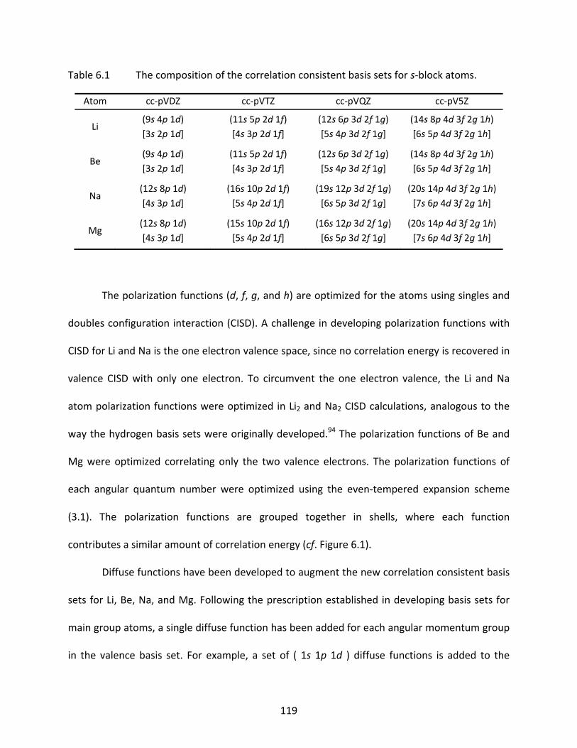
119
The polarization functions (d, f, g, and h) are optimized for the atoms using singles and
doubles configuration interaction (CISD). A challenge in developing polarization functions with
CISD for Li and Na is the one electron valence space, since no correlation energy is recovered in
valence CISD with only one electron. To circumvent the one electron valence, the Li and Na
atom polarization functions were optimized in Li2 and Na2 CISD calculations, analogous to the
way the hydrogen basis sets were originally developed.94 The polarization functions of Be and
Mg were optimized correlating only the two valence electrons. The polarization functions of
each angular quantum number were optimized using the even‐tempered expansion scheme
(3.1). The polarization functions are grouped together in shells, where each function
contributes a similar amount of correlation energy (cf. Figure 6.1).
Diffuse functions have been developed to augment the new correlation consistent basis
sets for Li, Be, Na, and Mg. Following the prescription established in developing basis sets for
main group atoms, a single diffuse function has been added for each angular momentum group
in the valence basis set. For example, a set of ( 1s 1p 1d ) diffuse functions is added to the
Table 6.1 The composition of the correlation consistent basis sets for s‐block atoms.
Atom cc‐pVDZ cc‐pVTZ cc‐pVQZ cc‐pV5Z
Li (9s 4p 1d) [3s 2p 1d]
(11s 5p 2d 1f) [4s 3p 2d 1f]
(12s 6p 3d 2f 1g) [5s 4p 3d 2f 1g]
(14s 8p 4d 3f 2g 1h) [6s 5p 4d 3f 2g 1h]
Be (9s 4p 1d) [3s 2p 1d]
(11s 5p 2d 1f) [4s 3p 2d 1f]
(12s 6p 3d 2f 1g) [5s 4p 3d 2f 1g]
(14s 8p 4d 3f 2g 1h) [6s 5p 4d 3f 2g 1h]
Na (12s 8p 1d) [4s 3p 1d]
(16s 10p 2d 1f) [5s 4p 2d 1f]
(19s 12p 3d 2f 1g) [6s 5p 3d 2f 1g]
(20s 14p 4d 3f 2g 1h) [7s 6p 4d 3f 2g 1h]
Mg (12s 8p 1d) [4s 3p 1d]
(15s 10p 2d 1f) [5s 4p 2d 1f]
(16s 12p 3d 2f 1g) [6s 5p 3d 2f 1g]
(20s 14p 4d 3f 2g 1h) [7s 6p 4d 3f 2g 1h]
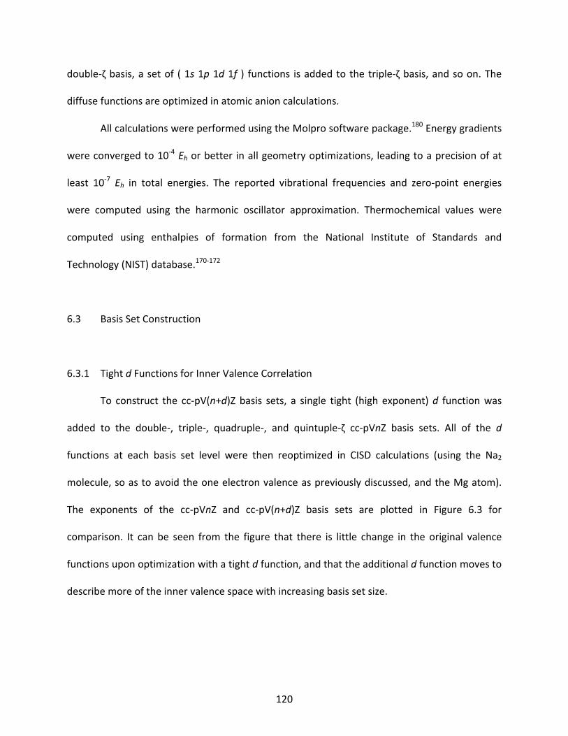
120
double‐ζ basis, a set of ( 1s 1p 1d 1f ) functions is added to the triple‐ζ basis, and so on. The
diffuse functions are optimized in atomic anion calculations.
All calculations were performed using the Molpro software package.180 Energy gradients
were converged to 10‐4 Eh or better in all geometry optimizations, leading to a precision of at
least 10‐7 Eh in total energies. The reported vibrational frequencies and zero‐point energies
were computed using the harmonic oscillator approximation. Thermochemical values were
computed using enthalpies of formation from the National Institute of Standards and
Technology (NIST) database.170‐172
6.3 Basis Set Construction
6.3.1 Tight d Functions for Inner Valence Correlation
To construct the cc‐pV(n+d)Z basis sets, a single tight (high exponent) d function was
added to the double‐, triple‐, quadruple‐, and quintuple‐ζ cc‐pVnZ basis sets. All of the d
functions at each basis set level were then reoptimized in CISD calculations (using the Na2
molecule, so as to avoid the one electron valence as previously discussed, and the Mg atom).
The exponents of the cc‐pVnZ and cc‐pV(n+d)Z basis sets are plotted in Figure 6.3 for
comparison. It can be seen from the figure that there is little change in the original valence
functions upon optimization with a tight d function, and that the additional d function moves to
describe more of the inner valence space with increasing basis set size.
121
6.3.2 Core‐Valence Functions for Sub‐Valence Correlation
The importance of valence correlation energy cannot be over emphasized in the
accurate calculation of atomic and molecular properties. Moreover, the importance of core‐
valence (CV) correlation energy (the energy of interaction between valence and sub‐valence
electrons) is also to be emphasized, especially when accuracy below 1.0 kcal/mol in atomic and
molecular properties (i.e thermochemistry) is required. For that reason, CV basis sets for Li, Be,
Na, and Mg that monotonically approach the CBS limit are introduced.
The CV basis sets are optimized in an analogous manner as those for main group atoms
using atomic CISD calculations using (3.7). For the Li and Be atoms, all of the electrons are
correlated, but the 1s orbitals of Na and Mg are constrained to be doubly‐occupied (frozen) in
each correlated calculation. Following the core‐valence prescription previously discussed in
Chapter 3, shells of tight functions are added to the cc‐pVnZ basis sets of Li and Be as follows:
Figure 6.1 The incremental CISD correlation energy lowering of the Mg atom due to eachpolarization function.
0.01
0.1
1
10
100
0 1 2 3 4 5
|ΔE c
orr| (m
illihartree)
Number of Functions
Mg
3d4f5g6h
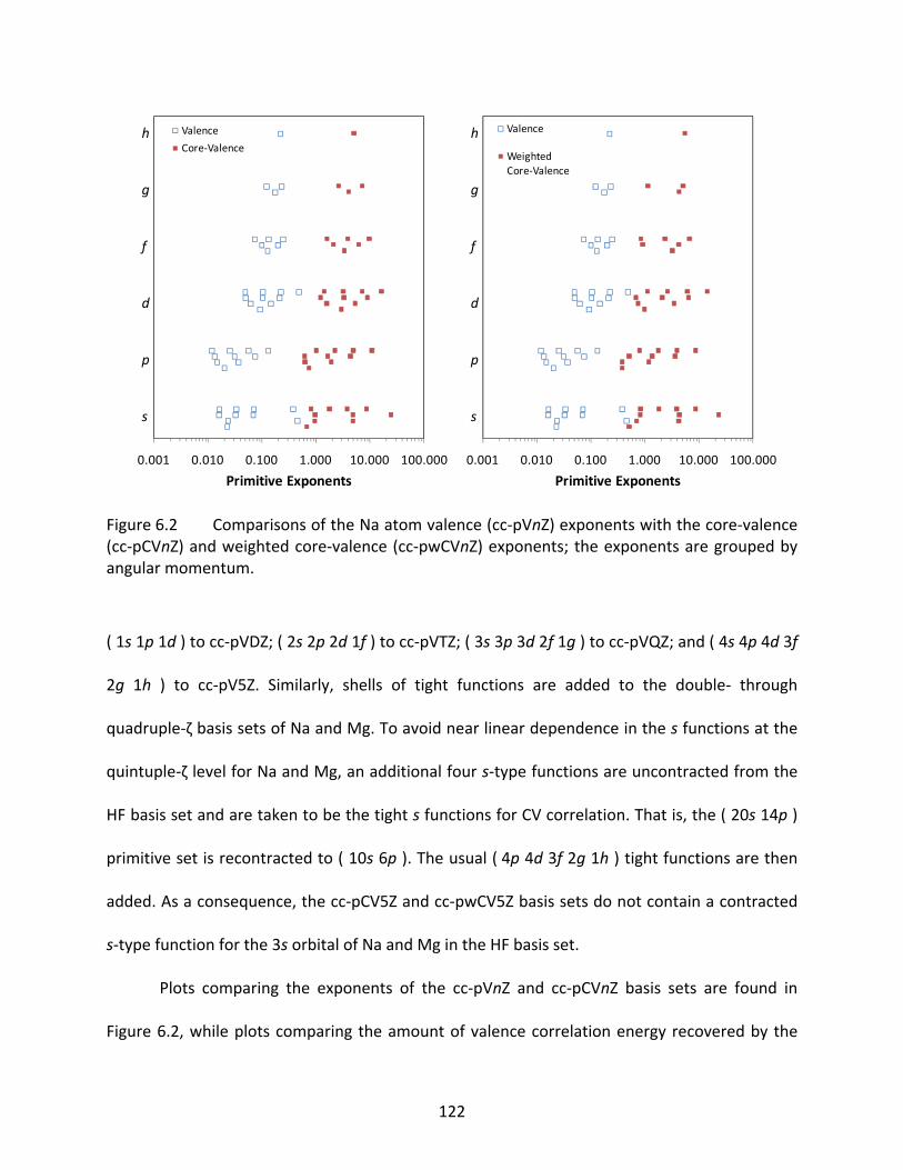
122
( 1s 1p 1d ) to cc‐pVDZ; ( 2s 2p 2d 1f ) to cc‐pVTZ; ( 3s 3p 3d 2f 1g ) to cc‐pVQZ; and ( 4s 4p 4d 3f
2g 1h ) to cc‐pV5Z. Similarly, shells of tight functions are added to the double‐ through
quadruple‐ζ basis sets of Na and Mg. To avoid near linear dependence in the s functions at the
quintuple‐ζ level for Na and Mg, an additional four s‐type functions are uncontracted from the
HF basis set and are taken to be the tight s functions for CV correlation. That is, the ( 20s 14p )
primitive set is recontracted to ( 10s 6p ). The usual ( 4p 4d 3f 2g 1h ) tight functions are then
added. As a consequence, the cc‐pCV5Z and cc‐pwCV5Z basis sets do not contain a contracted
s‐type function for the 3s orbital of Na and Mg in the HF basis set.
Plots comparing the exponents of the cc‐pVnZ and cc‐pCVnZ basis sets are found in
Figure 6.2, while plots comparing the amount of valence correlation energy recovered by the
Figure 6.2 Comparisons of the Na atom valence (cc‐pVnZ) exponents with the core‐valence(cc‐pCVnZ) and weighted core‐valence (cc‐pwCVnZ) exponents; the exponents are grouped byangular momentum.
0.001 0.010 0.100 1.000 10.000 100.000
Primitive Exponents
Valence
Core‐Valence
s
h
g
d
p
f
0.001 0.010 0.100 1.000 10.000 100.000
Primitive Exponents
Valence
Weighted Core‐Valence
s
h
g
d
p
f
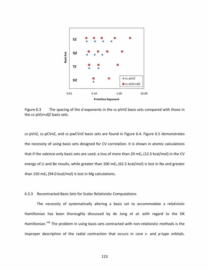
123
cc‐pVnZ, cc‐pCVnZ, and cc‐pwCVnZ basis sets are found in Figure 6.4. Figure 6.5 demonstrates
the necessity of using basis sets designed for CV correlation. It is shown in atomic calculations
that if the valence‐only basis sets are used, a loss of more than 20 mEh (12.5 kcal/mol) in the CV
energy of Li and Be results, while greater than 100 mEh (62.5 kcal/mol) is lost in Na and greater
than 150 mEh (94.0 kcal/mol) is lost in Mg calculations.
6.3.3 Recontracted Basis Sets for Scalar Relativistic Computations
The necessity of systematically altering a basis set to accommodate a relativistic
Hamiltonian has been thoroughly discussed by de Jong et al. with regard to the DK
Hamiltonian.142 The problem in using basis sets contracted with non‐relativistic methods is the
improper description of the radial contraction that occurs in core s‐ and p‐type orbitals.
Figure 6.3 The spacing of the d exponents in the cc‐pVnZ basis sets compared with those inthe cc‐pV(n+d)Z basis sets.
0.01 0.10 1.00 10.00
Basis S
et
Primitive Exponent
cc‐pVnZ
cc‐pV(n+d)ZDZ
5Z
QZ
TZ
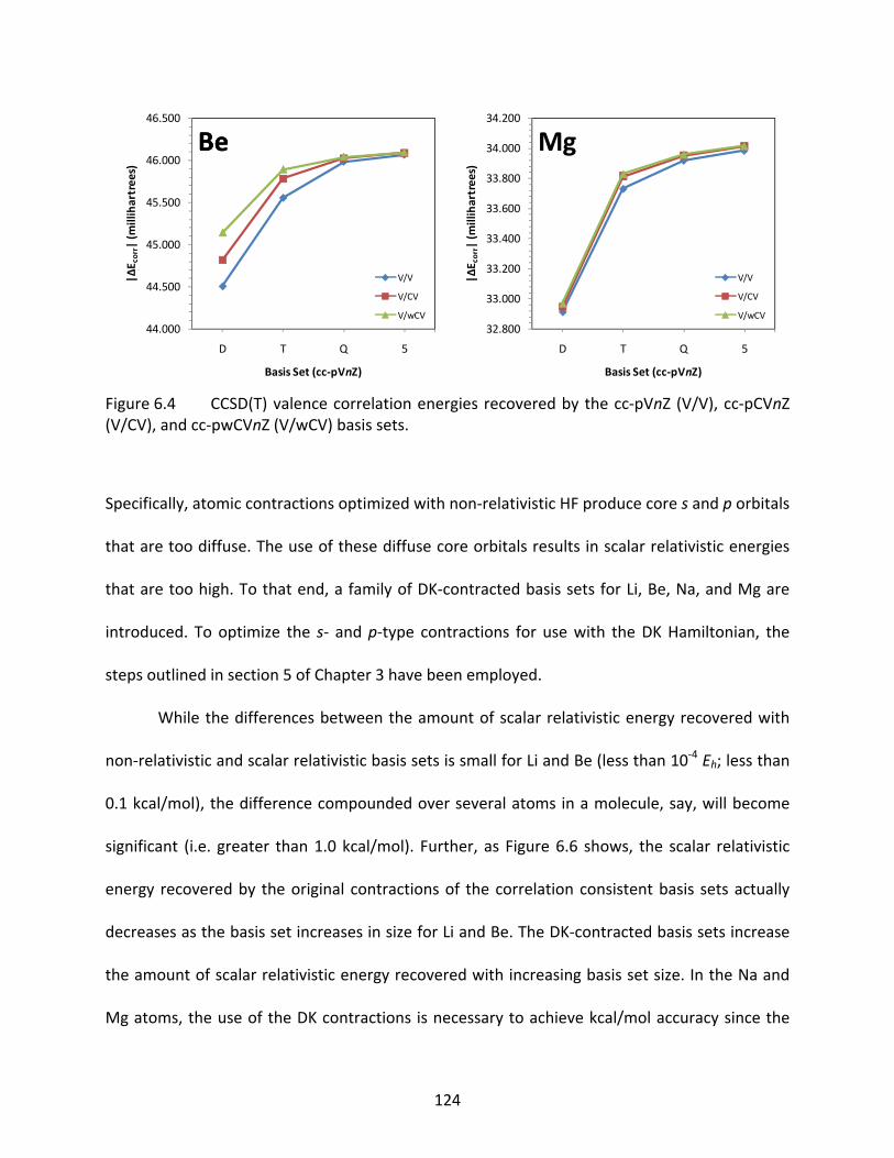
124
Specifically, atomic contractions optimized with non‐relativistic HF produce core s and p orbitals
that are too diffuse. The use of these diffuse core orbitals results in scalar relativistic energies
that are too high. To that end, a family of DK‐contracted basis sets for Li, Be, Na, and Mg are
introduced. To optimize the s‐ and p‐type contractions for use with the DK Hamiltonian, the
steps outlined in section 5 of Chapter 3 have been employed.
While the differences between the amount of scalar relativistic energy recovered with
non‐relativistic and scalar relativistic basis sets is small for Li and Be (less than 10‐4 Eh; less than
0.1 kcal/mol), the difference compounded over several atoms in a molecule, say, will become
significant (i.e. greater than 1.0 kcal/mol). Further, as Figure 6.6 shows, the scalar relativistic
energy recovered by the original contractions of the correlation consistent basis sets actually
decreases as the basis set increases in size for Li and Be. The DK‐contracted basis sets increase
the amount of scalar relativistic energy recovered with increasing basis set size. In the Na and
Mg atoms, the use of the DK contractions is necessary to achieve kcal/mol accuracy since the
Figure 6.4 CCSD(T) valence correlation energies recovered by the cc‐pVnZ (V/V), cc‐pCVnZ(V/CV), and cc‐pwCVnZ (V/wCV) basis sets.
44.000
44.500
45.000
45.500
46.000
46.500
D T Q 5
|ΔE c
orr| (m
illihartrees)
Basis Set (cc‐pVnZ)
V/V
V/CV
V/wCV
BeBe
32.800
33.000
33.200
33.400
33.600
33.800
34.000
34.200
D T Q 5
|ΔE c
orr| (m
illihartrees)
Basis Set (cc‐pVnZ)
V/V
V/CV
V/wCV
Mg
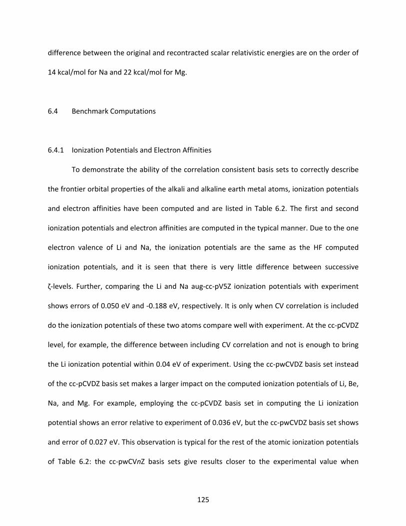
125
difference between the original and recontracted scalar relativistic energies are on the order of
14 kcal/mol for Na and 22 kcal/mol for Mg.
6.4 Benchmark Computations
6.4.1 Ionization Potentials and Electron Affinities
To demonstrate the ability of the correlation consistent basis sets to correctly describe
the frontier orbital properties of the alkali and alkaline earth metal atoms, ionization potentials
and electron affinities have been computed and are listed in Table 6.2. The first and second
ionization potentials and electron affinities are computed in the typical manner. Due to the one
electron valence of Li and Na, the ionization potentials are the same as the HF computed
ionization potentials, and it is seen that there is very little difference between successive
ζ‐levels. Further, comparing the Li and Na aug‐cc‐pV5Z ionization potentials with experiment
shows errors of 0.050 eV and ‐0.188 eV, respectively. It is only when CV correlation is included
do the ionization potentials of these two atoms compare well with experiment. At the cc‐pCVDZ
level, for example, the difference between including CV correlation and not is enough to bring
the Li ionization potential within 0.04 eV of experiment. Using the cc‐pwCVDZ basis set instead
of the cc‐pCVDZ basis set makes a larger impact on the computed ionization potentials of Li, Be,
Na, and Mg. For example, employing the cc‐pCVDZ basis set in computing the Li ionization
potential shows an error relative to experiment of 0.036 eV, but the cc‐pwCVDZ basis set shows
and error of 0.027 eV. This observation is typical for the rest of the atomic ionization potentials
of Table 6.2: the cc‐pwCVnZ basis sets give results closer to the experimental value when
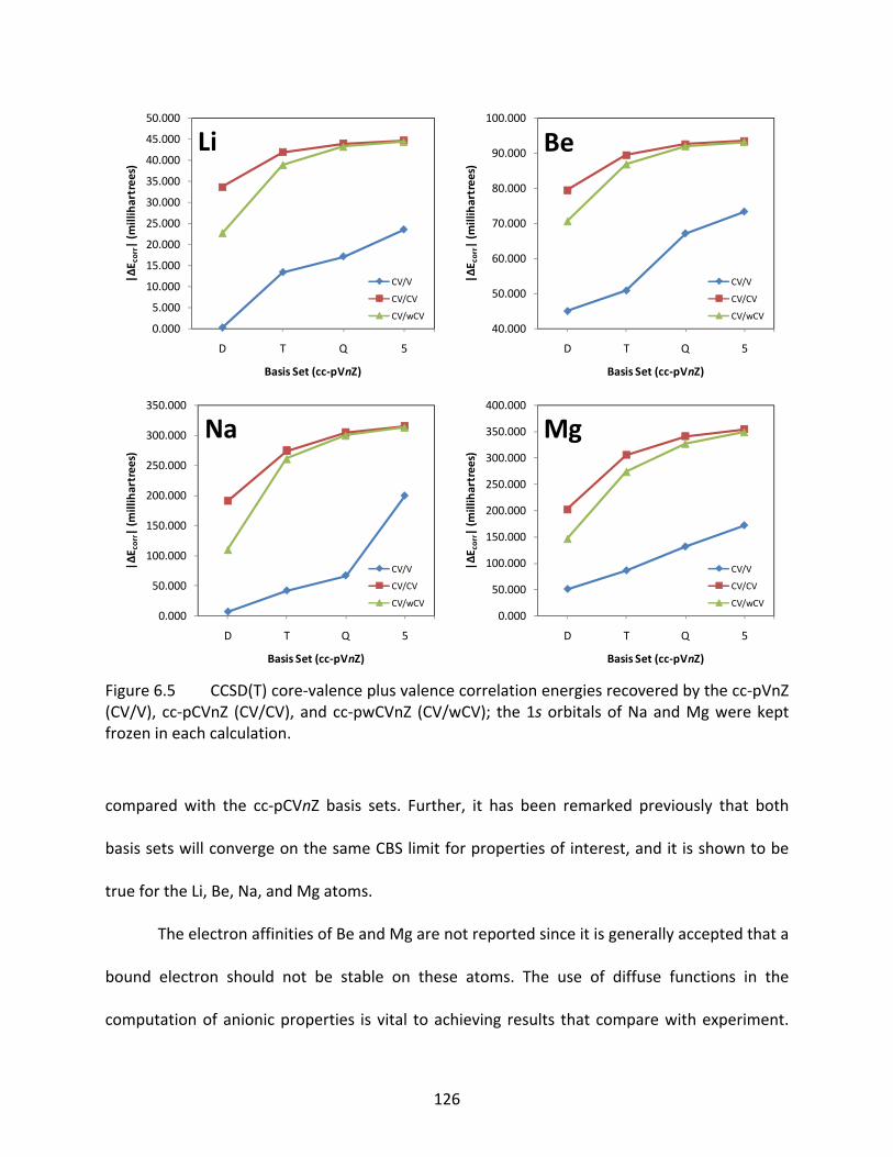
126
compared with the cc‐pCVnZ basis sets. Further, it has been remarked previously that both
basis sets will converge on the same CBS limit for properties of interest, and it is shown to be
true for the Li, Be, Na, and Mg atoms.
The electron affinities of Be and Mg are not reported since it is generally accepted that a
bound electron should not be stable on these atoms. The use of diffuse functions in the
computation of anionic properties is vital to achieving results that compare with experiment.
Figure 6.5 CCSD(T) core‐valence plus valence correlation energies recovered by the cc‐pVnZ(CV/V), cc‐pCVnZ (CV/CV), and cc‐pwCVnZ (CV/wCV); the 1s orbitals of Na and Mg were keptfrozen in each calculation.
0.000
5.000
10.000
15.000
20.000
25.000
30.000
35.000
40.000
45.000
50.000
D T Q 5
|ΔE c
orr| (m
illihartrees)
Basis Set (cc‐pVnZ)
CV/V
CV/CV
CV/wCV
Li
40.000
50.000
60.000
70.000
80.000
90.000
100.000
D T Q 5
|ΔE c
orr| (m
illihartrees)
Basis Set (cc‐pVnZ)
CV/V
CV/CV
CV/wCV
Be
0.000
50.000
100.000
150.000
200.000
250.000
300.000
350.000
D T Q 5
|ΔE c
orr| (m
illihartrees)
Basis Set (cc‐pVnZ)
CV/V
CV/CV
CV/wCV
Na
0.000
50.000
100.000
150.000
200.000
250.000
300.000
350.000
400.000
D T Q 5
|ΔE c
orr| (m
illihartrees)
Basis Set (cc‐pVnZ)
CV/V
CV/CV
CV/wCV
Mg
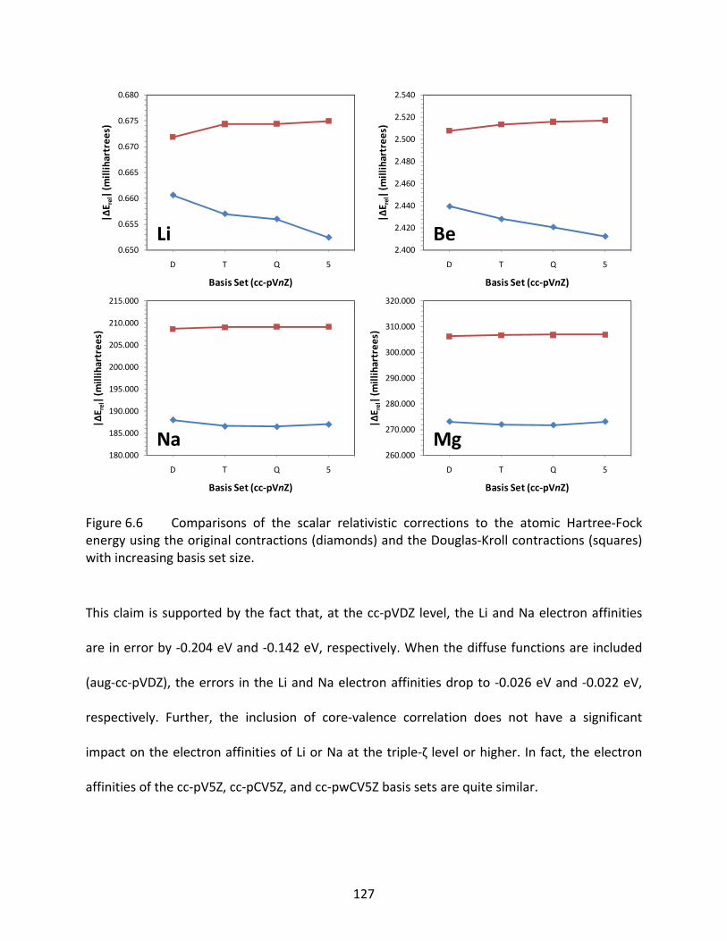
127
This claim is supported by the fact that, at the cc‐pVDZ level, the Li and Na electron affinities
are in error by ‐0.204 eV and ‐0.142 eV, respectively. When the diffuse functions are included
(aug‐cc‐pVDZ), the errors in the Li and Na electron affinities drop to ‐0.026 eV and ‐0.022 eV,
respectively. Further, the inclusion of core‐valence correlation does not have a significant
impact on the electron affinities of Li or Na at the triple‐ζ level or higher. In fact, the electron
affinities of the cc‐pV5Z, cc‐pCV5Z, and cc‐pwCV5Z basis sets are quite similar.
Figure 6.6 Comparisons of the scalar relativistic corrections to the atomic Hartree‐Fockenergy using the original contractions (diamonds) and the Douglas‐Kroll contractions (squares)with increasing basis set size.
0.650
0.655
0.660
0.665
0.670
0.675
0.680
D T Q 5
|ΔE r
el| (m
illihartree
s)
Basis Set (cc‐pVnZ)
Li2.400
2.420
2.440
2.460
2.480
2.500
2.520
2.540
D T Q 5
|ΔE r
el| (m
illihartree
s)
Basis Set (cc‐pVnZ)
Be
180.000
185.000
190.000
195.000
200.000
205.000
210.000
215.000
D T Q 5
|ΔE r
el| (m
illihartree
s)
Basis Set (cc‐pVnZ)
Na260.000
270.000
280.000
290.000
300.000
310.000
320.000
D T Q 5
|ΔE r
el| (m
illihartree
s)
Basis Set (cc‐pVnZ)
Mg
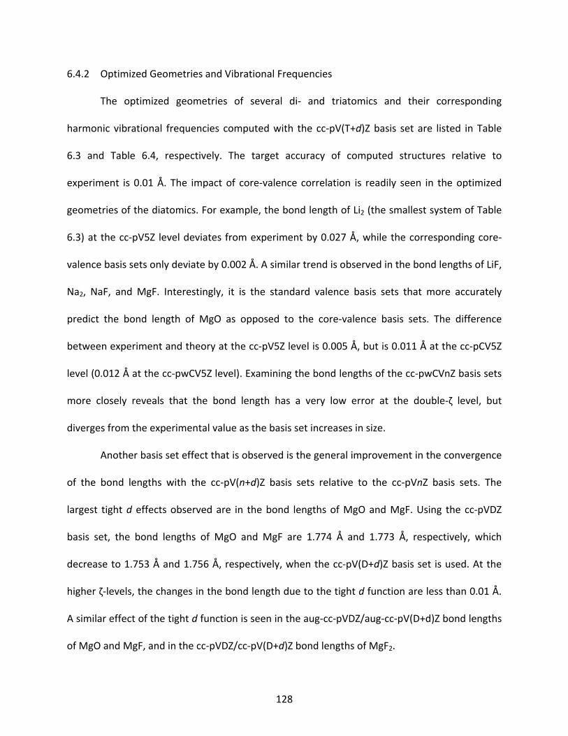
128
6.4.2 Optimized Geometries and Vibrational Frequencies
The optimized geometries of several di‐ and triatomics and their corresponding
harmonic vibrational frequencies computed with the cc‐pV(T+d)Z basis set are listed in Table
6.3 and Table 6.4, respectively. The target accuracy of computed structures relative to
experiment is 0.01 Å. The impact of core‐valence correlation is readily seen in the optimized
geometries of the diatomics. For example, the bond length of Li2 (the smallest system of Table
6.3) at the cc‐pV5Z level deviates from experiment by 0.027 Å, while the corresponding core‐
valence basis sets only deviate by 0.002 Å. A similar trend is observed in the bond lengths of LiF,
Na2, NaF, and MgF. Interestingly, it is the standard valence basis sets that more accurately
predict the bond length of MgO as opposed to the core‐valence basis sets. The difference
between experiment and theory at the cc‐pV5Z level is 0.005 Å, but is 0.011 Å at the cc‐pCV5Z
level (0.012 Å at the cc‐pwCV5Z level). Examining the bond lengths of the cc‐pwCVnZ basis sets
more closely reveals that the bond length has a very low error at the double‐ζ level, but
diverges from the experimental value as the basis set increases in size.
Another basis set effect that is observed is the general improvement in the convergence
of the bond lengths with the cc‐pV(n+d)Z basis sets relative to the cc‐pVnZ basis sets. The
largest tight d effects observed are in the bond lengths of MgO and MgF. Using the cc‐pVDZ
basis set, the bond lengths of MgO and MgF are 1.774 Å and 1.773 Å, respectively, which
decrease to 1.753 Å and 1.756 Å, respectively, when the cc‐pV(D+d)Z basis set is used. At the
higher ζ‐levels, the changes in the bond length due to the tight d function are less than 0.01 Å.
A similar effect of the tight d function is seen in the aug‐cc‐pVDZ/aug‐cc‐pV(D+d)Z bond lengths
of MgO and MgF, and in the cc‐pVDZ/cc‐pV(D+d)Z bond lengths of MgF2.
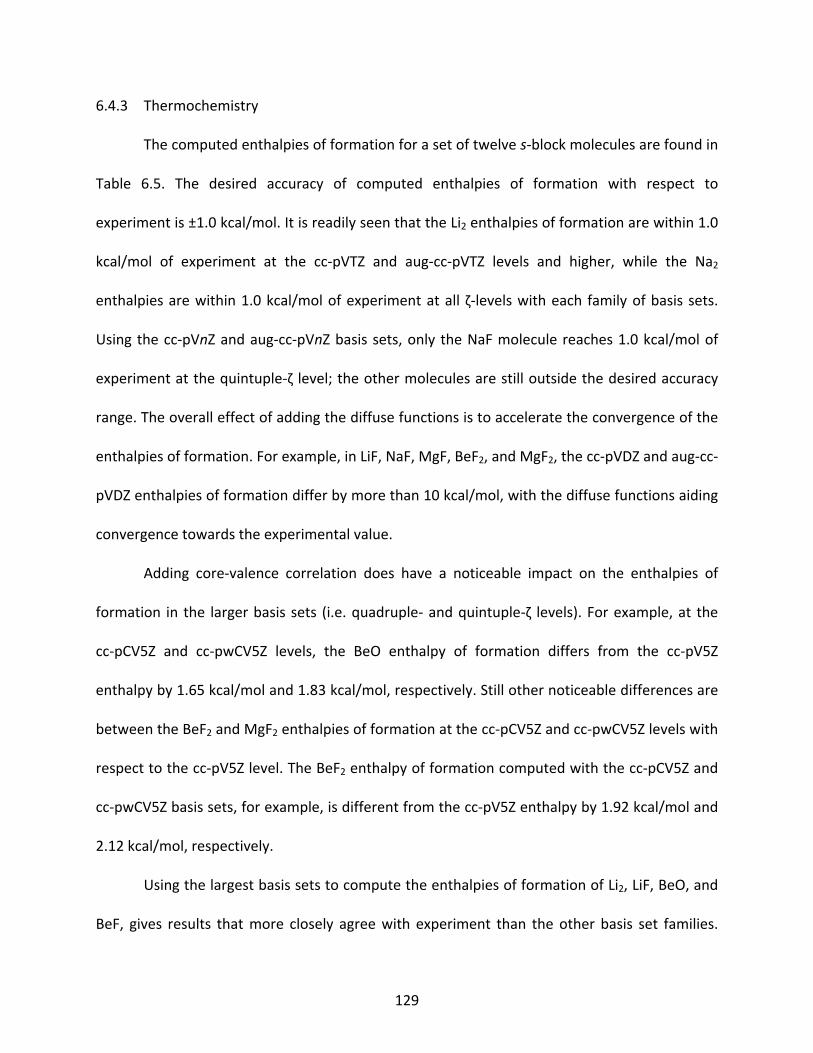
129
6.4.3 Thermochemistry
The computed enthalpies of formation for a set of twelve s‐block molecules are found in
Table 6.5. The desired accuracy of computed enthalpies of formation with respect to
experiment is ±1.0 kcal/mol. It is readily seen that the Li2 enthalpies of formation are within 1.0
kcal/mol of experiment at the cc‐pVTZ and aug‐cc‐pVTZ levels and higher, while the Na2
enthalpies are within 1.0 kcal/mol of experiment at all ζ‐levels with each family of basis sets.
Using the cc‐pVnZ and aug‐cc‐pVnZ basis sets, only the NaF molecule reaches 1.0 kcal/mol of
experiment at the quintuple‐ζ level; the other molecules are still outside the desired accuracy
range. The overall effect of adding the diffuse functions is to accelerate the convergence of the
enthalpies of formation. For example, in LiF, NaF, MgF, BeF2, and MgF2, the cc‐pVDZ and aug‐cc‐
pVDZ enthalpies of formation differ by more than 10 kcal/mol, with the diffuse functions aiding
convergence towards the experimental value.
Adding core‐valence correlation does have a noticeable impact on the enthalpies of
formation in the larger basis sets (i.e. quadruple‐ and quintuple‐ζ levels). For example, at the
cc‐pCV5Z and cc‐pwCV5Z levels, the BeO enthalpy of formation differs from the cc‐pV5Z
enthalpy by 1.65 kcal/mol and 1.83 kcal/mol, respectively. Still other noticeable differences are
between the BeF2 and MgF2 enthalpies of formation at the cc‐pCV5Z and cc‐pwCV5Z levels with
respect to the cc‐pV5Z level. The BeF2 enthalpy of formation computed with the cc‐pCV5Z and
cc‐pwCV5Z basis sets, for example, is different from the cc‐pV5Z enthalpy by 1.92 kcal/mol and
2.12 kcal/mol, respectively.
Using the largest basis sets to compute the enthalpies of formation of Li2, LiF, BeO, and
BeF, gives results that more closely agree with experiment than the other basis set families.
130
However, the enthalpies of formation of NaF and MgF2 computed with the cc‐pCVnZ and
cc‐pwCVnZ basis sets are slightly better (relative to experiment) than those computed with the
aug‐cc‐pCVnZ and aug‐cc‐pwCVnZ basis sets.
6.5 Conclusions
The unpublished basis sets for Li, Be, Na, and Mg have been reexamined using robust
numerical optimization techniques, and new official correlation consistent basis sets for these
four atoms are presented. Specifically, new cc‐pVnZ and aug‐cc‐pVnZ basis sets of double‐,
triple‐, quadruple‐, and quintuple‐ζ quality have been developed and benchmarked. In addition,
a set of tight d basis sets, cc‐pV(n+d)Z, have been developed for Na and Mg in correlated
valence calculations.
For subvalence correlation, new core‐valence and weighted core‐valence (cc‐pCVnZ and
cc‐pwCVnZ) basis sets have been developed. Benchmark calculations of atomic CV correlation
energies demonstrate the necessity of including core‐valence functions when subvalence
correlation is needed (i.e. for high accuracy thermochemistry). Benchmarks of molecular
properties also demonstrate the necessity of CV correlation, especially in Li and Na, whose one
electron valence is not a large enough valence space for correlated molecular calculations when
0.01 Å and 1.0 kcal/mol accuracy is desired.
Finally, the HF sp basis sets have been recontracted for scalar relativistic DK calculations,
resulting in cc‐pVnZ‐DK basis sets that consistently recover more scalar relativistic energy than
the original HF contractions at each basis set level.
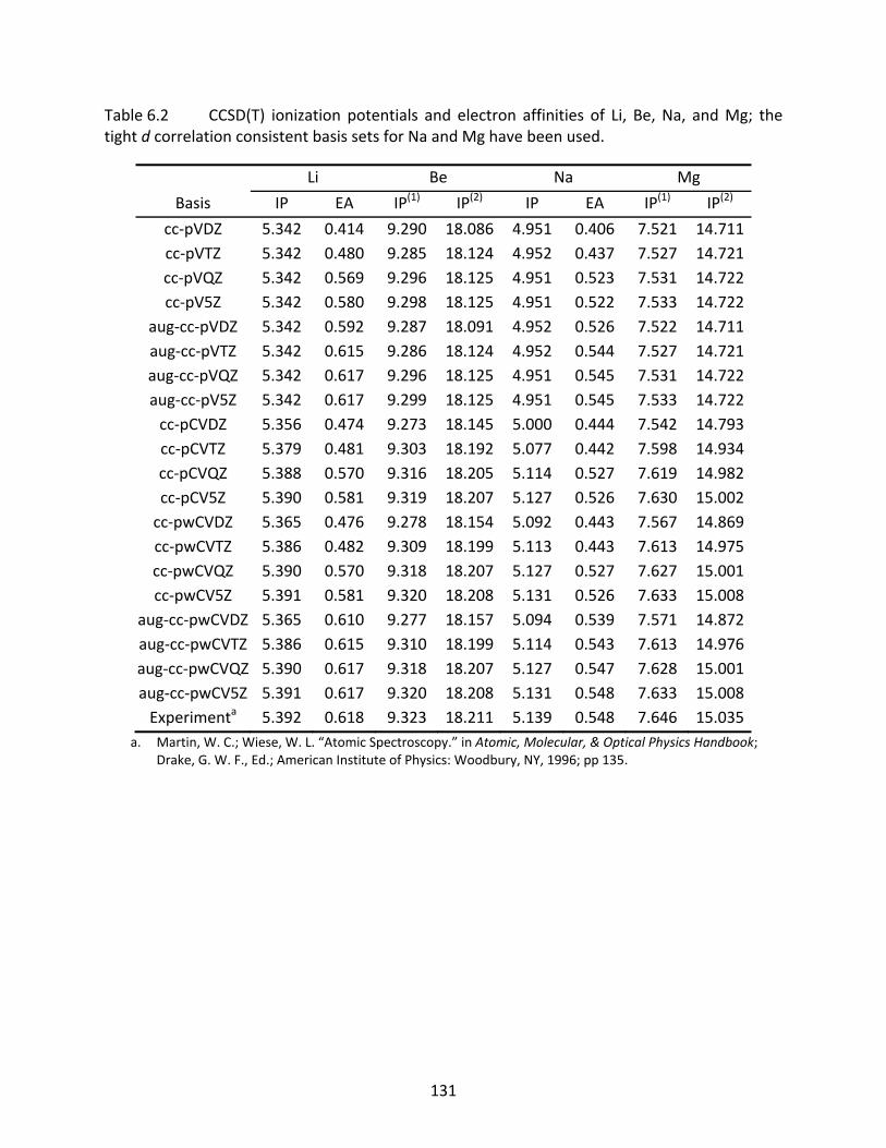
131
Table 6.2 CCSD(T) ionization potentials and electron affinities of Li, Be, Na, and Mg; the tight d correlation consistent basis sets for Na and Mg have been used.
Li Be Na Mg
Basis IP EA IP(1) IP(2) IP EA IP(1) IP(2)
cc‐pVDZ 5.342 0.414 9.290 18.086 4.951 0.406 7.521 14.711cc‐pVTZ 5.342 0.480 9.285 18.124 4.952 0.437 7.527 14.721cc‐pVQZ 5.342 0.569 9.296 18.125 4.951 0.523 7.531 14.722cc‐pV5Z 5.342 0.580 9.298 18.125 4.951 0.522 7.533 14.722
aug‐cc‐pVDZ 5.342 0.592 9.287 18.091 4.952 0.526 7.522 14.711aug‐cc‐pVTZ 5.342 0.615 9.286 18.124 4.952 0.544 7.527 14.721aug‐cc‐pVQZ 5.342 0.617 9.296 18.125 4.951 0.545 7.531 14.722aug‐cc‐pV5Z 5.342 0.617 9.299 18.125 4.951 0.545 7.533 14.722cc‐pCVDZ 5.356 0.474 9.273 18.145 5.000 0.444 7.542 14.793cc‐pCVTZ 5.379 0.481 9.303 18.192 5.077 0.442 7.598 14.934cc‐pCVQZ 5.388 0.570 9.316 18.205 5.114 0.527 7.619 14.982cc‐pCV5Z 5.390 0.581 9.319 18.207 5.127 0.526 7.630 15.002cc‐pwCVDZ 5.365 0.476 9.278 18.154 5.092 0.443 7.567 14.869cc‐pwCVTZ 5.386 0.482 9.309 18.199 5.113 0.443 7.613 14.975cc‐pwCVQZ 5.390 0.570 9.318 18.207 5.127 0.527 7.627 15.001cc‐pwCV5Z 5.391 0.581 9.320 18.208 5.131 0.526 7.633 15.008
aug‐cc‐pwCVDZ 5.365 0.610 9.277 18.157 5.094 0.539 7.571 14.872aug‐cc‐pwCVTZ 5.386 0.615 9.310 18.199 5.114 0.543 7.613 14.976aug‐cc‐pwCVQZ 5.390 0.617 9.318 18.207 5.127 0.547 7.628 15.001aug‐cc‐pwCV5Z 5.391 0.617 9.320 18.208 5.131 0.548 7.633 15.008Experimenta 5.392 0.618 9.323 18.211 5.139 0.548 7.646 15.035
a. Martin, W. C.; Wiese, W. L. “Atomic Spectroscopy.” in Atomic, Molecular, & Optical Physics Handbook; Drake, G. W. F., Ed.; American Institute of Physics: Woodbury, NY, 1996; pp 135.
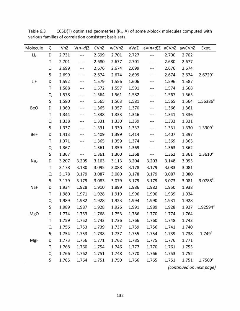
132
Table 6.3 CCSD(T) optimized geometries (Re, Å) of some s‐block molecules computed with various families of correlation consistent basis sets.
Molecule ζ VnZ V(n+d)Z CVnZ wCVnZ aVnZ aV(n+d)Z aCVnZ awCVnZ Expt.
Li2 D 2.731 ‐‐‐ 2.699 2.701 2.727 ‐‐‐ 2.700 2.702 T 2.701 ‐‐‐ 2.680 2.677 2.701 ‐‐‐ 2.680 2.677 Q 2.699 ‐‐‐ 2.676 2.674 2.699 ‐‐‐ 2.676 2.674 5 2.699 ‐‐‐ 2.674 2.674 2.699 ‐‐‐ 2.674 2.674 2.6729a
LiF D 1.592 ‐‐‐ 1.579 1.556 1.606 ‐‐‐ 1.596 1.587 T 1.588 ‐‐‐ 1.572 1.557 1.591 ‐‐‐ 1.574 1.568 Q 1.578 ‐‐‐ 1.564 1.561 1.582 ‐‐‐ 1.567 1.565 5 1.580 ‐‐‐ 1.565 1.563 1.581 ‐‐‐ 1.565 1.564 1.56386a
BeO D 1.369 ‐‐‐ 1.365 1.357 1.370 ‐‐‐ 1.366 1.361 T 1.344 ‐‐‐ 1.338 1.333 1.346 ‐‐‐ 1.341 1.336 Q 1.338 ‐‐‐ 1.331 1.330 1.339 ‐‐‐ 1.333 1.331 5 1.337 ‐‐‐ 1.331 1.330 1.337 ‐‐‐ 1.331 1.330 1.3309a
BeF D 1.413 ‐‐‐ 1.409 1.399 1.414 ‐‐‐ 1.407 1.397 T 1.371 ‐‐‐ 1.365 1.359 1.374 ‐‐‐ 1.369 1.365 Q 1.367 ‐‐‐ 1.361 1.359 1.369 ‐‐‐ 1.363 1.362 5 1.367 ‐‐‐ 1.361 1.360 1.368 ‐‐‐ 1.362 1.361 1.3610a
Na2 D 3.207 3.205 3.163 3.113 3.204 3.203 3.148 3.095 T 3.178 3.180 3.095 3.088 3.178 3.179 3.083 3.081 Q 3.178 3.179 3.087 3.080 3.178 3.179 3.087 3.080 5 3.179 3.179 3.083 3.079 3.179 3.179 3.073 3.081 3.0788a
NaF D 1.934 1.928 1.910 1.899 1.986 1.982 1.950 1.938 T 1.980 1.971 1.928 1.919 1.996 1.990 1.939 1.934 Q 1.989 1.982 1.928 1.923 1.994 1.990 1.931 1.928 5 1.989 1.987 1.928 1.926 1.991 1.989 1.928 1.927 1.92594a
MgO D 1.774 1.753 1.768 1.753 1.786 1.770 1.774 1.764 T 1.759 1.752 1.743 1.736 1.766 1.760 1.748 1.743 Q 1.756 1.753 1.739 1.737 1.759 1.756 1.741 1.740 5 1.754 1.753 1.738 1.737 1.755 1.754 1.739 1.738 1.749a
MgF D 1.773 1.756 1.771 1.762 1.785 1.775 1.776 1.771 T 1.768 1.760 1.754 1.746 1.777 1.770 1.761 1.755 Q 1.766 1.762 1.751 1.748 1.770 1.766 1.753 1.752 5 1.765 1.764 1.751 1.750 1.766 1.765 1.751 1.751 1.7500a
(continued on next page)
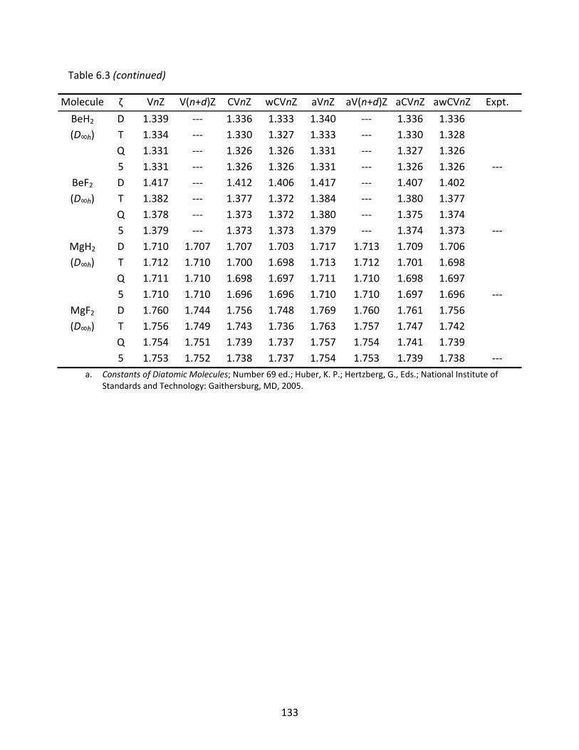
133
Table 6.3 (continued)
Molecule ζ VnZ V(n+d)Z CVnZ wCVnZ aVnZ aV(n+d)Z aCVnZ awCVnZ Expt.
BeH2 D 1.339 ‐‐‐ 1.336 1.333 1.340 ‐‐‐ 1.336 1.336 (D∞h) T 1.334 ‐‐‐ 1.330 1.327 1.333 ‐‐‐ 1.330 1.328
Q 1.331 ‐‐‐ 1.326 1.326 1.331 ‐‐‐ 1.327 1.326 5 1.331 ‐‐‐ 1.326 1.326 1.331 ‐‐‐ 1.326 1.326 ‐‐‐
BeF2 D 1.417 ‐‐‐ 1.412 1.406 1.417 ‐‐‐ 1.407 1.402 (D∞h) T 1.382 ‐‐‐ 1.377 1.372 1.384 ‐‐‐ 1.380 1.377
Q 1.378 ‐‐‐ 1.373 1.372 1.380 ‐‐‐ 1.375 1.374 5 1.379 ‐‐‐ 1.373 1.373 1.379 ‐‐‐ 1.374 1.373 ‐‐‐
MgH2 D 1.710 1.707 1.707 1.703 1.717 1.713 1.709 1.706 (D∞h) T 1.712 1.710 1.700 1.698 1.713 1.712 1.701 1.698
Q 1.711 1.710 1.698 1.697 1.711 1.710 1.698 1.697 5 1.710 1.710 1.696 1.696 1.710 1.710 1.697 1.696 ‐‐‐
MgF2 D 1.760 1.744 1.756 1.748 1.769 1.760 1.761 1.756 (D∞h) T 1.756 1.749 1.743 1.736 1.763 1.757 1.747 1.742
Q 1.754 1.751 1.739 1.737 1.757 1.754 1.741 1.739 5 1.753 1.752 1.738 1.737 1.754 1.753 1.739 1.738 ‐‐‐a. Constants of Diatomic Molecules; Number 69 ed.; Huber, K. P.; Hertzberg, G., Eds.; National Institute of
Standards and Technology: Gaithersburg, MD, 2005.
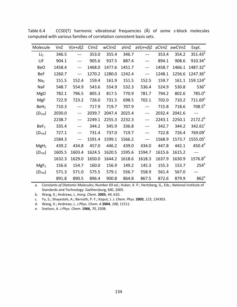
134
Table 6.4 CCSD(T) harmonic vibrational frequencies (Å) of some s‐block molecules computed with various families of correlation consistent basis sets.
Molecule VnZ V(n+d)Z CVnZ wCVnZ aVnZ aV(n+d)Z aCVnZ awCVnZ Expt.
Li2 346.5 ‐‐‐ 353.0 355.4 346.7 ‐‐‐ 353.4 354.2 351.43a
LiF 904.1 ‐‐‐ 905.6 937.5 887.4 ‐‐‐ 894.1 908.6 910.34a
BeO 1458.4 ‐‐‐ 1468.0 1477.6 1451.7 ‐‐‐ 1458.7 1466.1 1487.32a
BeF 1260.7 ‐‐‐ 1270.2 1280.0 1242.4 ‐‐‐ 1248.1 1256.6 1247.36a
Na2 151.5 152.4 159.4 161.9 151.5 152.5 159.7 161.1 159.124a
NaF 548.7 554.9 543.6 554.9 532.3 536.4 524.9 530.8 536a
MgO 782.1 796.5 805.3 817.5 770.9 781.7 794.2 802.6 785.0a
MgF 722.9 723.2 726.0 731.5 698.5 702.1 702.0 710.2 711.69a
BeH2 710.3 ‐‐‐ 717.9 719.7 707.9 ‐‐‐ 715.8 718.6 708.5b
(D∞h) 2030.0 ‐‐‐ 2039.7 2047.4 2025.4 ‐‐‐ 2032.4 2041.6 ‐‐‐ 2238.7 ‐‐‐ 2249.1 2255.3 2232.3 ‐‐‐ 2243.1 2250.1 2172.2b
BeF2 335.4 ‐‐‐ 344.2 345.9 336.8 ‐‐‐ 342.7 344.2 342.61c
(D∞h) 727.1 ‐‐‐ 731.4 737.0 719.7 ‐‐‐ 722.8 726.4 769.09c
1584.3 ‐‐‐ 1591.4 1599.1 1566.2 ‐‐‐ 1568.9 1573.7 1555.05c
MgH2 439.2 434.8 457.0 446.2 439.0 434.0 447.8 442.1 450.4d
(D∞h) 1605.5 1603.4 1624.5 1620.5 1595.6 1594.7 1615.6 1615.2 ‐‐‐ 1632.3 1629.0 1650.0 1644.2 1618.6 1618.3 1637.9 1630.9 1576.8d
MgF2 156.6 154.7 160.0 156.9 149.2 145.3 155.3 153.7 254e
(D∞h) 571.3 571.0 575.5 579.1 556.7 558.9 561.4 567.0 ‐‐‐ 891.8 890.5 896.4 900.8 864.8 867.5 872.6 879.9 862e
a. Constants of Diatomic Molecules; Number 69 ed.; Huber, K. P.; Hertzberg, G., Eds.; National Institute of Standards and Technology: Gaithersburg, MD, 2005.
b. Wang, X.; Andrews, L. Inorg. Chem. 2005, 44, 610. c. Yu, S.; Shayesteh, A.; Bernath, P. F.; Koput, J. J. Chem. Phys. 2005, 123, 134303. d. Wang, X.; Andrews, L. J.Phys. Chem. A 2004, 108, 11511. e. Snelson, A. J.Phys. Chem. 1966, 70, 3208.
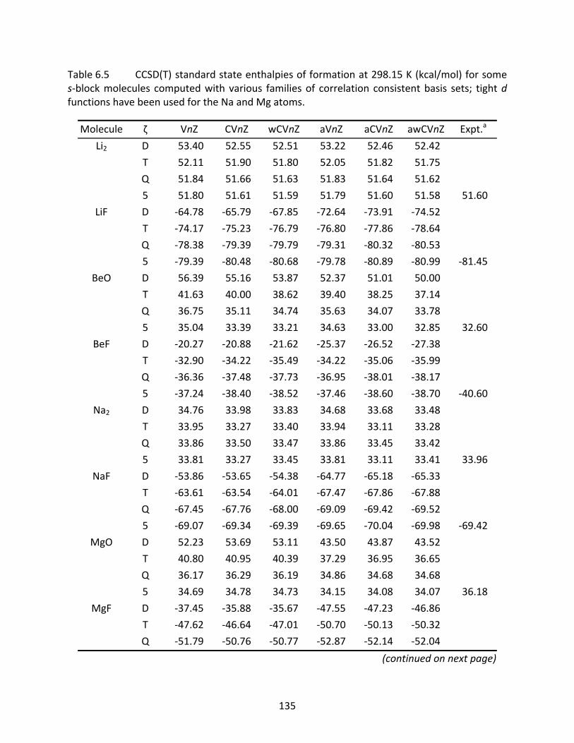
135
Table 6.5 CCSD(T) standard state enthalpies of formation at 298.15 K (kcal/mol) for some s‐block molecules computed with various families of correlation consistent basis sets; tight d functions have been used for the Na and Mg atoms.
Molecule ζ VnZ CVnZ wCVnZ aVnZ aCVnZ awCVnZ Expt.a
Li2 D 53.40 52.55 52.51 53.22 52.46 52.42
T 52.11 51.90 51.80 52.05 51.82 51.75
Q 51.84 51.66 51.63 51.83 51.64 51.62
5 51.80 51.61 51.59 51.79 51.60 51.58 51.60
LiF D ‐64.78 ‐65.79 ‐67.85 ‐72.64 ‐73.91 ‐74.52
T ‐74.17 ‐75.23 ‐76.79 ‐76.80 ‐77.86 ‐78.64
Q ‐78.38 ‐79.39 ‐79.79 ‐79.31 ‐80.32 ‐80.53
5 ‐79.39 ‐80.48 ‐80.68 ‐79.78 ‐80.89 ‐80.99 ‐81.45
BeO D 56.39 55.16 53.87 52.37 51.01 50.00
T 41.63 40.00 38.62 39.40 38.25 37.14
Q 36.75 35.11 34.74 35.63 34.07 33.78
5 35.04 33.39 33.21 34.63 33.00 32.85 32.60
BeF D ‐20.27 ‐20.88 ‐21.62 ‐25.37 ‐26.52 ‐27.38
T ‐32.90 ‐34.22 ‐35.49 ‐34.22 ‐35.06 ‐35.99
Q ‐36.36 ‐37.48 ‐37.73 ‐36.95 ‐38.01 ‐38.17
5 ‐37.24 ‐38.40 ‐38.52 ‐37.46 ‐38.60 ‐38.70 ‐40.60
Na2 D 34.76 33.98 33.83 34.68 33.68 33.48
T 33.95 33.27 33.40 33.94 33.11 33.28
Q 33.86 33.50 33.47 33.86 33.45 33.42
5 33.81 33.27 33.45 33.81 33.11 33.41 33.96
NaF D ‐53.86 ‐53.65 ‐54.38 ‐64.77 ‐65.18 ‐65.33
T ‐63.61 ‐63.54 ‐64.01 ‐67.47 ‐67.86 ‐67.88
Q ‐67.45 ‐67.76 ‐68.00 ‐69.09 ‐69.42 ‐69.52
5 ‐69.07 ‐69.34 ‐69.39 ‐69.65 ‐70.04 ‐69.98 ‐69.42
MgO D 52.23 53.69 53.11 43.50 43.87 43.52
T 40.80 40.95 40.39 37.29 36.95 36.65
Q 36.17 36.29 36.19 34.86 34.68 34.68
5 34.69 34.78 34.73 34.15 34.08 34.07 36.18
MgF D ‐37.45 ‐35.88 ‐35.67 ‐47.55 ‐47.23 ‐46.86
T ‐47.62 ‐46.64 ‐47.01 ‐50.70 ‐50.13 ‐50.32
Q ‐51.79 ‐50.76 ‐50.77 ‐52.87 ‐52.14 ‐52.04
(continued on next page)
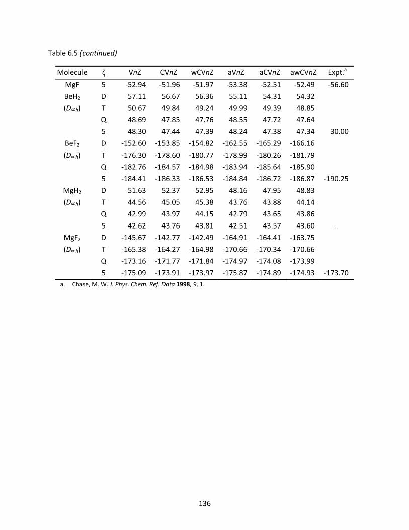
136
Table 6.5 (continued)
Molecule ζ VnZ CVnZ wCVnZ aVnZ aCVnZ awCVnZ Expt.a
MgF 5 ‐52.94 ‐51.96 ‐51.97 ‐53.38 ‐52.51 ‐52.49 ‐56.60
BeH2 D 57.11 56.67 56.36 55.11 54.31 54.32
(D∞h) T 50.67 49.84 49.24 49.99 49.39 48.85
Q 48.69 47.85 47.76 48.55 47.72 47.64
5 48.30 47.44 47.39 48.24 47.38 47.34 30.00
BeF2 D ‐152.60 ‐153.85 ‐154.82 ‐162.55 ‐165.29 ‐166.16
(D∞h) T ‐176.30 ‐178.60 ‐180.77 ‐178.99 ‐180.26 ‐181.79
Q ‐182.76 ‐184.57 ‐184.98 ‐183.94 ‐185.64 ‐185.90
5 ‐184.41 ‐186.33 ‐186.53 ‐184.84 ‐186.72 ‐186.87 ‐190.25
MgH2 D 51.63 52.37 52.95 48.16 47.95 48.83
(D∞h) T 44.56 45.05 45.38 43.76 43.88 44.14
Q 42.99 43.97 44.15 42.79 43.65 43.86
5 42.62 43.76 43.81 42.51 43.57 43.60 ‐‐‐
MgF2 D ‐145.67 ‐142.77 ‐142.49 ‐164.91 ‐164.41 ‐163.75
(D∞h) T ‐165.38 ‐164.27 ‐164.98 ‐170.66 ‐170.34 ‐170.66
Q ‐173.16 ‐171.77 ‐171.84 ‐174.97 ‐174.08 ‐173.99
5 ‐175.09 ‐173.91 ‐173.97 ‐175.87 ‐174.89 ‐174.93 ‐173.70a. Chase, M. W. J. Phys. Chem. Ref. Data 1998, 9, 1.
137
CHAPTER 7
THE RESOLUTION OF THE IDENTITY APPROXIMATION APPLIED TO THE CORRELATION
CONSISTENT COMPOSITE APPROACH†
7.1 Introduction
In correlated ab initio methods, the number of four‐index two‐electron Coulomb
integrals (2.11) increases dramatically as the number of electrons increases.7,19,22,55 The
computation and storage of these integrals is the bottleneck in applying correlated methods,
and so it is highly desirable to have efficient ways of computing and storing them. Typically,
integral screening techniques187 are employed to avoid computing very small (i.e 10‐14 Eh)
integrals, which helps reduce the number of four‐index integrals stored. To deal efficiently with
the other integrals, a novel approach is to employ a projective technique.
The resolution of the identity (RI) is a well‐known projective technique from vector
algebra.188 Consider a ket vector | expanded in a complete, orthonormal basis :
| | (7.1)
By projecting | onto an arbitrary basis vector in , the component of | along that vector is
resolved:
| | (7.2)
Insertion of (7.2) into (7.1) yields the following result:
† Work reported in this chapter was performed in collaboration with Jeremy D. Lai, and has been submitted for publication in the Journal of Chemical Physics.
138
| | | | | | (7.3)
where the summation in parentheses apparently takes the form of an algebraic ‘1’:
| | (7.4)
The object in (7.4) has several names in the literature including identity operator, completeness
relation, and unit dyadic, the latter of which is used throughout this chapter. The summation
terms are projection operators instead of scalar products, since the ket is written before the
bra. When (7.4) operates on a ket vector, the result is the same ket represented in whatever
basis set comprises the unit dyadic, provided that basis is complete. This is why this
mathematical construct is called the resolution of the identity, because it resolves a vector in
one basis to another. For example, a unit dyadic in the basis may be constructed as
| | (7.5)
then, since | | , the vector | may be resolved in the new basis using (7.1):
| | | | | |
| | |
(7.6)
The components of | in are now defined in terms of its components in and the overlap
between the two basis sets | .
More generally, if the domain of the bra vector in (7.4) is different from the domain in
the ket, then the resulting operator is the Dirac delta function:7
139
| | (7.7)
Instead of resolving vectors from one basis to another, the Dirac delta function resolves a
function in one domain into another as follows:
d (7.8)
As a sidebar, the definition of the Dirac delta function in (7.7) is entirely analogous to the
definition of the first‐order reduced density function in (2.47). The Dirac delta function is
related to the following Fourier integral, where is the momentum vector:
d , (7.9)
which is why RI methods are sometimes referred to as pseudospectral methods in the
literature.189 Finally, it is readily seen from (7.9) that the inverse Fourier transform of the Dirac
delta function, and, by extension the unit dyadic, is unity.
Boys and Shavitt first introduced the idea of reducing the computational cost of four‐
index integrals using the RI technique,190 while Löwdin discussed the use of RI in terms of
describing quantum phenomena.191 Since then, the RI approximation has been employed in
density functional theory (DFT),161,192 Hartree‐Fock self‐consistent field (HF‐SCF),160 second‐
order Møller‐Plesset perturbation theory (MP2),160,193 and coupled cluster theory.194 For a
review of the RI approximation in computational chemistry, see Kendall and Früchtl.190
Following the derivations of Vahtras et al. with regards to various RI approximations,160
any four‐index integral can be approximated as a linear combination of three‐ or two‐index
integrals by insertion of the unit dyadic. Vahtras et al. showed that describing charge
distributions with the RI approximation leads to three different formulas for approximating
140
four‐index Coulomb integrals:160
| | 1 | (7.10)
| | 1 1 (7.11)
| | 1 (7.12)
in which the basis sets denoted by , , , are called auxiliary basis sets. The bracketed terms
on the right‐hand side are three‐center overlap integrals, the terms are two‐center overlap
integrals (in matrix form) between two auxiliary basis sets, and the terms are two‐center,
two‐electron Coulomb integrals (also in matrix form). Equations (7.10) and (7.11) are called the
S and SVS approximations, respectively, in which the individual charge distributions are
projected onto an auxiliary basis set. Note that the auxiliary basis set for the bra vector is not
necessarily the same used for the ket vector in the S and SVS approximations, which is why the
additional overlap integrals enter the equations. Equation (7.12) is called the V approximation,
in which the Coulomb operator is projected onto an auxiliary basis set. The V approximation
more closely approximates the exact four‐index integral in practice, and, consequently, is the
most common RI approximation in use for approximating the four‐index integrals in SCF, DFT,
and MP2 calculations.
In more recent implementations of RI methods, a single auxiliary basis is used instead of
multiple auxiliary basis sets as indicated by the equations above. When a single auxiliary basis
set is used in the V approximation, the number of four‐index integrals is reduced from to
approximately , where is the number of orbital basis functions and is the number
of auxiliary basis functions. So long as does not exceed , there will be an effective
141
reduction in the number, and hence, the computational scaling of four‐index integrals. This is
the primary motivation behind employing the RI approximation in correlated ab initio methods,
where the number of four‐index integrals over excited determinants becomes very large. In DFT
methods, the RI approximation takes on a slightly different role, namely, that of projecting the
exchange‐correlation functional, which may not have a trivial integral form, onto an auxiliary
basis set in which integrals over the exchange‐correlation functional become more tractable. In
practice, a different auxiliary basis set is used for each computational method, each having
been optimized specifically for that method’s ansatz. For example, a density‐fit or Coulomb‐fit
auxiliary basis set might be used for all or some of the HF‐SCF integrals, while a different
auxiliary basis set is used for correlated integrals that arise in an MP2 calculation employing
those HF orbitals.
An additional means to reduce the computational expense of ab initio methods is via
composite methods (discussed in Chapter 2). These approaches approximate a high‐level
correlated ab initio/large basis set calculation with a series of lower‐level/small basis set
calculations. Examples of composite methods include the Gaussian‐n methods (Gn),60‐62
Weizmann‐n methods (Wn),71,72 the high‐accuracy extrapolated ab initio thermochemistry
(HEAT) method,70 complete basis set (CBS‐n) methods,63‐69 and the recently developed
correlation consistent Composite Approach (ccCA).73‐80 In general, each composite method
listed varies in the target accuracy with respect to reliable experimental data and in
formulation. The ccCA method makes use of the well‐known monotonic behavior of the
correlation consistent basis sets, cc‐pVnZ,94‐101 with respect to increasing basis set size for
energetic properties (e.g., thermochemical properties, atomization energies), and considers
142
additional effects such as high‐order correlation effects, core‐valence effects, and scalar
relativistic effects. Further, ccCA has been applied to over 700 main group molecules, resulting
in an overall mean absolute deviation (MAD) of approximately 1 kcal/mol from reliable
experiment.73‐80 The use of composite methodology may be able to approximate high‐level
computational methods with a lower computational expense, however, further modifications
to the handling of four‐index integrals can be introduced to further reduce the computational
scaling.
In this Chapter, the RI approximation is applied to the ccCA method and the resulting
formulism (RI‐ccCA) is discussed. The accuracy of properties computed with RI‐ccCA is
compared with those computed with the original formulation of ccCA. Further, relative timings
and storage requirements are presented for RI‐ccCA and are compared with the original ccCA
formulation.
7.2 Computational Methodology
The set of molecules examined is a subset of the G2/97 test set61 containing 102 closed
shell systems, including both first and second row, main group atoms. All calculations were
performed with the Molpro 2006.1 software package180 without employing symmetry and using
the default semi‐direct algorithm. Energy gradients and hessians were converged to at least
0.1 mEh in the geometry optimizations and frequency calculations. Following the formulation
for the ccCA method,73‐80 the geometry optimization of each molecule is performed using
Becke’s 3‐parameter exchange scheme coupled with the Lee‐Yang‐Parr correlation functional,
B3LYP,165,166 and the cc‐pVTZ basis set. Harmonic frequencies are then computed at the same
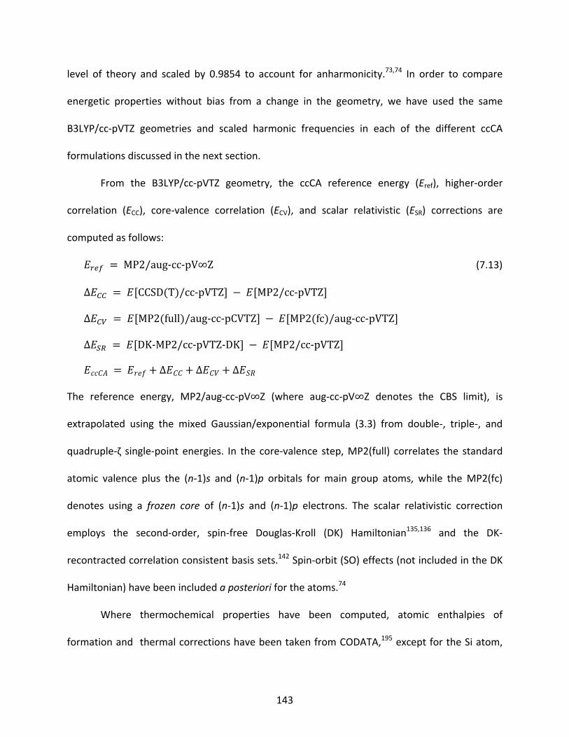
143
level of theory and scaled by 0.9854 to account for anharmonicity.73,74 In order to compare
energetic properties without bias from a change in the geometry, we have used the same
B3LYP/cc‐pVTZ geometries and scaled harmonic frequencies in each of the different ccCA
formulations discussed in the next section.
From the B3LYP/cc‐pVTZ geometry, the ccCA reference energy (Eref), higher‐order
correlation (ECC), core‐valence correlation (ECV), and scalar relativistic (ESR) corrections are
computed as follows:
MP2/aug‐cc‐pV∞Z
∆ CCSD T /cc‐pVTZ MP2/cc‐pVTZ
∆ MP2 full /aug‐cc‐pCVTZ MP2 fc /aug‐cc‐pVTZ
∆ DK‐MP2/cc‐pVTZ‐DK MP2/cc‐pVTZ
∆ ∆ ∆
(7.13)
The reference energy, MP2/aug‐cc‐pV∞Z (where aug‐cc‐pV∞Z denotes the CBS limit), is
extrapolated using the mixed Gaussian/exponential formula (3.3) from double‐, triple‐, and
quadruple‐ζ single‐point energies. In the core‐valence step, MP2(full) correlates the standard
atomic valence plus the (n‐1)s and (n‐1)p orbitals for main group atoms, while the MP2(fc)
denotes using a frozen core of (n‐1)s and (n‐1)p electrons. The scalar relativistic correction
employs the second‐order, spin‐free Douglas‐Kroll (DK) Hamiltonian135,136 and the DK‐
recontracted correlation consistent basis sets.142 Spin‐orbit (SO) effects (not included in the DK
Hamiltonian) have been included a posteriori for the atoms.74
Where thermochemical properties have been computed, atomic enthalpies of
formation and thermal corrections have been taken from CODATA,195 except for the Si atom,
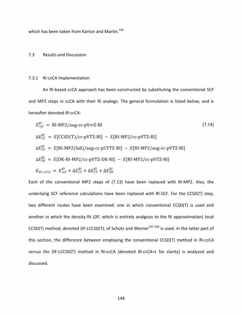
144
which has been taken from Karton and Martin.196
7.3 Results and Discussion
7.3.1 RI‐ccCA Implementation
An RI‐based ccCA approach has been constructed by substituting the conventional SCF
and MP2 steps in ccCA with their RI analogs. The general formulation is listed below, and is
hereafter denoted RI‐ccCA:
RI‐MP2/aug‐cc‐pV∞Z‐RI
Δ CCSD T /cc‐pVTZ‐RI RI‐MP2/cc‐pVTZ‐RI
Δ RI‐MP2 full /aug‐cc‐pCVTZ‐RI RI‐MP2/aug‐cc‐pVTZ‐RI
Δ DK‐RI‐MP2/cc‐pVTZ‐DK‐RI RI‐MP2/cc‐pVTZ‐RI
‐ Δ Δ Δ
(7.14)
Each of the conventional MP2 steps of (7.13) have been replaced with RI‐MP2. Also, the
underlying SCF reference calculations have been replaced with RI‐SCF. For the CCSD(T) step,
two different routes have been examined: one in which conventional CCSD(T) is used and
another in which the density‐fit (DF, which is entirely analgous to the RI approximation) local
CCSD(T) method, denoted DF‐LCCSD(T), of Schütz and Werner197‐199 is used. In the latter part of
this section, the difference between employing the conventional CCSD(T) method in RI‐ccCA
versus the DF‐LCCSD(T) method in RI‐ccCA (denoted RI‐ccCA+L for clarity) is analyzed and
discussed.
145
7.3.2 Auxiliary Basis Sets for RI‐ccCA
To determine the optimal auxiliary basis sets to be used in the RI‐SCF and RI‐MP2
calculations, a comparison has been made between RI‐ccCA, which utilizes conventional
CCSD(T), and ccCA employing several different auxiliary basis sets. Utilimately, the auxiliary
basis sets should be chosen so that the convergent nature of the correlation consistent basis
sets remains intact, and so that the RI‐ccCA energies are as close to the ccCA energies as
possible.
In the RI‐SCF steps, the use of completely unconctracted cc‐pVnZ basis sets one ζ‐level
higher than the orbital basis set, denoted cc‐pV(n+1)Z(unc), and the basis sets of Weigend,
denoted ‘JKFIT,’200 have been studied. (It is common practice when using RI methods to assume
that an uncontracted basis set that is larger than the orbital basis set is an adequate auxiliary
basis set; i.e. if a cc‐pVTZ orbital basis set is used, then the uncontracted cc‐pVQZ basis set is
assumed to be adequate as an auxiliary basis set.) The JKFIT basis sets are studied here because
they have been reported to reproduce conventional SCF atomic energies within 120 μEh at any
ζ‐level through quadruple‐ζ.200 Further, the use of the cc‐pV(n+1)Z(unc) and the cc‐pVnZ‐RI
basis sets of Weigend et al.181 have been studied as potential auxiliary basis sets in the RI‐MP2
steps of RI‐ccCA. The latter auxiliary sets were optimized specifically for use with the correlation
consistent basis sets, which is why they were selected, and have been reported to reproduce
conventional MP2 correlation energies withing 101 μEh per atom in molecules containing first
and second row atoms.181
The results of the test calculations described above for H2P+, Cl‐, CH3
‐, NH2‐, OH‐, SiH3
‐,
PH2‐, SH‐, CN‐, NH4
+, H3O+, C2H3
+, SiH5+, PH4
+, H3S+, and H2Cl
+ are listed in Table 7.1 according to
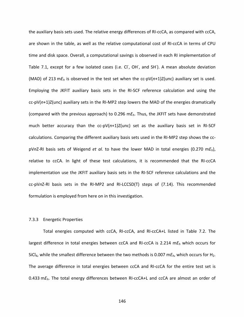
146
the auxiliary basis sets used. The relative energy differences of RI‐ccCA, as compared with ccCA,
are shown in the table, as well as the relative computational cost of RI‐ccCA in terms of CPU
time and disk space. Overall, a computational savings is observed in each RI implementation of
Table 7.1, except for a few isolated cases (i.e. Cl‐, OH‐, and SH‐). A mean absolute deviation
(MAD) of 213 mEh is observed in the test set when the cc‐pV(n+1)Z(unc) auxiliary set is used.
Employing the JKFIT auxiliary basis sets in the RI‐SCF reference calculation and using the
cc‐pV(n+1)Z(unc) auxiliary sets in the RI‐MP2 step lowers the MAD of the energies dramatically
(compared with the previous approach) to 0.296 mEh. Thus, the JKFIT sets have demonstrated
much better accuracy than the cc‐pV(n+1)Z(unc) set as the auxiliary basis set in RI‐SCF
calculations. Comparing the different auxiliary basis sets used in the RI‐MP2 step shows the cc‐
pVnZ‐RI basis sets of Weigend et al. to have the lower MAD in total energies (0.270 mEh),
relative to ccCA. In light of these test calculations, it is recommended that the RI‐ccCA
implementation use the JKFIT auxiliary basis sets in the RI‐SCF reference calculations and the
cc‐pVnZ‐RI basis sets in the RI‐MP2 and RI‐LCCSD(T) steps of (7.14). This recommended
formulation is employed from here on in this investigation.
7.3.3 Energetic Properties
Total energies computed with ccCA, RI‐ccCA, and RI‐ccCA+L listed in Table 7.2. The
largest difference in total energies between ccCA and RI‐ccCA is 2.214 mEh which occurs for
SiCl4, while the smallest difference between the two methods is 0.007 mEh, which occurs for H2.
The average difference in total energies between ccCA and RI‐ccCA for the entire test set is
0.433 mEh. The total energy differences between RI‐ccCA+L and ccCA are almost an order of
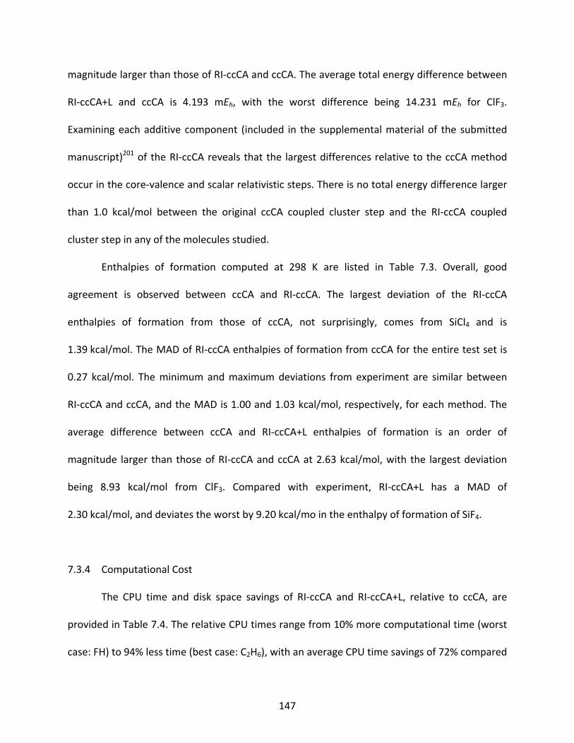
147
magnitude larger than those of RI‐ccCA and ccCA. The average total energy difference between
RI‐ccCA+L and ccCA is 4.193 mEh, with the worst difference being 14.231 mEh for ClF3.
Examining each additive component (included in the supplemental material of the submitted
manuscript)201 of the RI‐ccCA reveals that the largest differences relative to the ccCA method
occur in the core‐valence and scalar relativistic steps. There is no total energy difference larger
than 1.0 kcal/mol between the original ccCA coupled cluster step and the RI‐ccCA coupled
cluster step in any of the molecules studied.
Enthalpies of formation computed at 298 K are listed in Table 7.3. Overall, good
agreement is observed between ccCA and RI‐ccCA. The largest deviation of the RI‐ccCA
enthalpies of formation from those of ccCA, not surprisingly, comes from SiCl4 and is
1.39 kcal/mol. The MAD of RI‐ccCA enthalpies of formation from ccCA for the entire test set is
0.27 kcal/mol. The minimum and maximum deviations from experiment are similar between
RI‐ccCA and ccCA, and the MAD is 1.00 and 1.03 kcal/mol, respectively, for each method. The
average difference between ccCA and RI‐ccCA+L enthalpies of formation is an order of
magnitude larger than those of RI‐ccCA and ccCA at 2.63 kcal/mol, with the largest deviation
being 8.93 kcal/mol from ClF3. Compared with experiment, RI‐ccCA+L has a MAD of
2.30 kcal/mol, and deviates the worst by 9.20 kcal/mo in the enthalpy of formation of SiF4.
7.3.4 Computational Cost
The CPU time and disk space savings of RI‐ccCA and RI‐ccCA+L, relative to ccCA, are
provided in Table 7.4. The relative CPU times range from 10% more computational time (worst
case: FH) to 94% less time (best case: C2H6), with an average CPU time savings of 72% compared
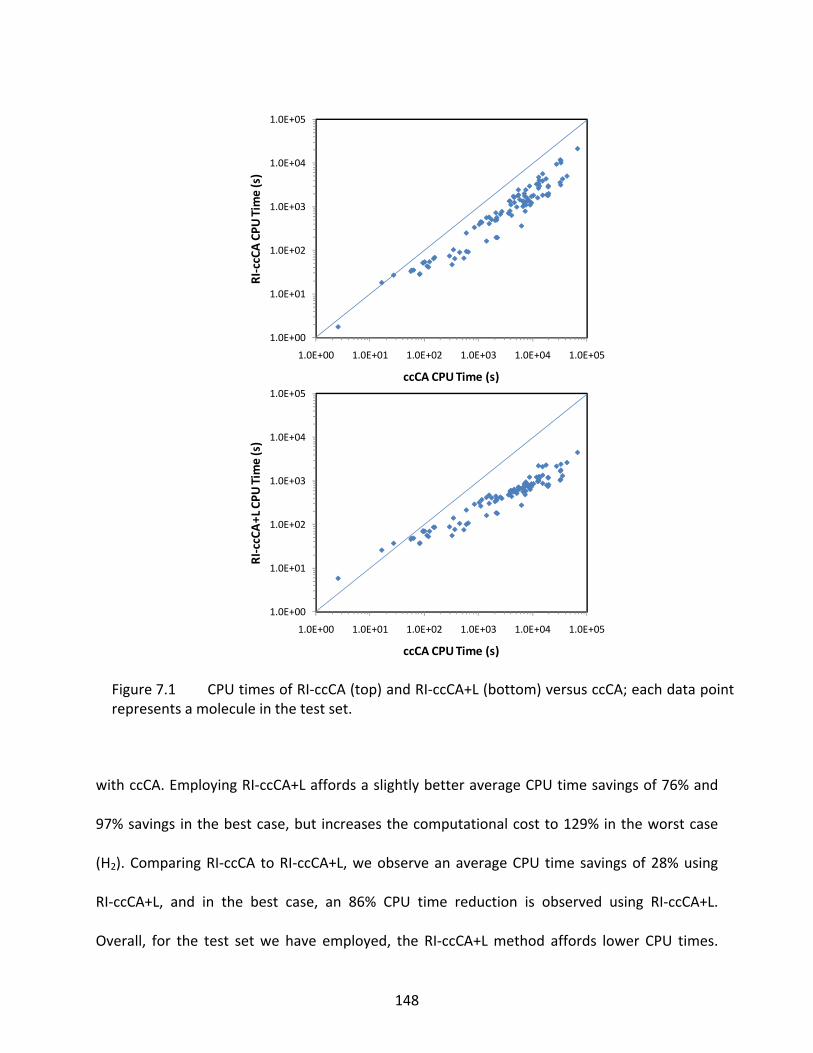
148
with ccCA. Employing RI‐ccCA+L affords a slightly better average CPU time savings of 76% and
97% savings in the best case, but increases the computational cost to 129% in the worst case
(H2). Comparing RI‐ccCA to RI‐ccCA+L, we observe an average CPU time savings of 28% using
RI‐ccCA+L, and in the best case, an 86% CPU time reduction is observed using RI‐ccCA+L.
Overall, for the test set we have employed, the RI‐ccCA+L method affords lower CPU times.
Figure 7.1 CPU times of RI‐ccCA (top) and RI‐ccCA+L (bottom) versus ccCA; each data pointrepresents a molecule in the test set.
1.0E+00
1.0E+01
1.0E+02
1.0E+03
1.0E+04
1.0E+05
1.0E+00 1.0E+01 1.0E+02 1.0E+03 1.0E+04 1.0E+05
RI‐ccCA CPU
Tim
e (s)
ccCA CPU Time (s)
1.0E+00
1.0E+01
1.0E+02
1.0E+03
1.0E+04
1.0E+05
1.0E+00 1.0E+01 1.0E+02 1.0E+03 1.0E+04 1.0E+05
RI‐ccCA+L CPU
Tim
e (s)
ccCA CPU Time (s)
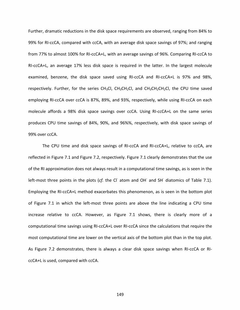
149
Further, dramatic reductions in the disk space requirements are observed, ranging from 84% to
99% for RI‐ccCA, compared with ccCA, with an average disk space savings of 97%; and ranging
from 77% to almost 100% for RI‐ccCA+L, with an average savings of 96%. Comparing RI‐ccCA to
RI‐ccCA+L, an average 17% less disk space is required in the latter. In the largest molecule
examined, benzene, the disk space saved using RI‐ccCA and RI‐ccCA+L is 97% and 98%,
respectively. Further, for the series CH3Cl, CH3CH2Cl, and CH3CH2CH2Cl, the CPU time saved
employing RI‐ccCA over ccCA is 87%, 89%, and 93%, respectively, while using RI‐ccCA on each
molecule affords a 98% disk space savings over ccCA. Using RI‐ccCA+L on the same series
produces CPU time savings of 84%, 90%, and 96%%, respectively, with disk space savings of
99% over ccCA.
The CPU time and disk space savings of RI‐ccCA and RI‐ccCA+L, relative to ccCA, are
reflected in Figure 7.1 and Figure 7.2, respectively. Figure 7.1 clearly demonstrates that the use
of the RI approximation does not always result in a computational time savings, as is seen in the
left‐most three points in the plots (cf. the Cl‐ atom and OH‐ and SH‐ diatomics of Table 7.1).
Employing the RI‐ccCA+L method exacerbates this phenomenon, as is seen in the bottom plot
of Figure 7.1 in which the left‐most three points are above the line indicating a CPU time
increase relative to ccCA. However, as Figure 7.1 shows, there is clearly more of a
computational time savings using RI‐ccCA+L over RI‐ccCA since the calculations that require the
most computational time are lower on the vertical axis of the bottom plot than in the top plot.
As Figure 7.2 demonstrates, there is always a clear disk space savings when RI‐ccCA or RI‐
ccCA+L is used, compared with ccCA.
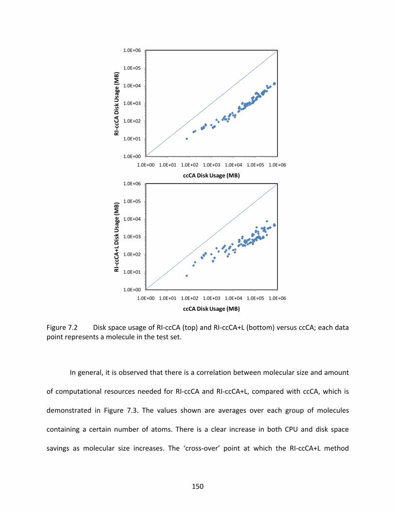
150
In general, it is observed that there is a correlation between molecular size and amount
of computational resources needed for RI‐ccCA and RI‐ccCA+L, compared with ccCA, which is
demonstrated in Figure 7.3. The values shown are averages over each group of molecules
containing a certain number of atoms. There is a clear increase in both CPU and disk space
savings as molecular size increases. The ‘cross‐over’ point at which the RI‐ccCA+L method
Figure 7.2 Disk space usage of RI‐ccCA (top) and RI‐ccCA+L (bottom) versus ccCA; each datapoint represents a molecule in the test set.
1.0E+00
1.0E+01
1.0E+02
1.0E+03
1.0E+04
1.0E+05
1.0E+06
1.0E+00 1.0E+01 1.0E+02 1.0E+03 1.0E+04 1.0E+05 1.0E+06
RI‐ccCA Disk Usage
(MB)
ccCA Disk Usage (MB)
1.0E+00
1.0E+01
1.0E+02
1.0E+03
1.0E+04
1.0E+05
1.0E+06
1.0E+00 1.0E+01 1.0E+02 1.0E+03 1.0E+04 1.0E+05 1.0E+06
RI‐ccCA
+L Disk Usage
(MB)
ccCA Disk Usage (MB)
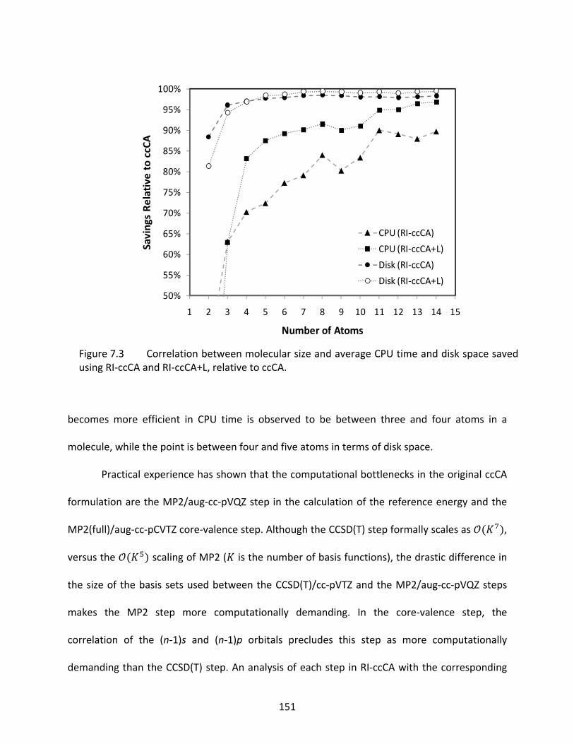
151
becomes more efficient in CPU time is observed to be between three and four atoms in a
molecule, while the point is between four and five atoms in terms of disk space.
Practical experience has shown that the computational bottlenecks in the original ccCA
formulation are the MP2/aug‐cc‐pVQZ step in the calculation of the reference energy and the
MP2(full)/aug‐cc‐pCVTZ core‐valence step. Although the CCSD(T) step formally scales as ,
versus the scaling of MP2 ( is the number of basis functions), the drastic difference in
the size of the basis sets used between the CCSD(T)/cc‐pVTZ and the MP2/aug‐cc‐pVQZ steps
makes the MP2 step more computationally demanding. In the core‐valence step, the
correlation of the (n‐1)s and (n‐1)p orbitals precludes this step as more computationally
demanding than the CCSD(T) step. An analysis of each step in RI‐ccCA with the corresponding
Figure 7.3 Correlation between molecular size and average CPU time and disk space savedusing RI‐ccCA and RI‐ccCA+L, relative to ccCA.
50%
55%
60%
65%
70%
75%
80%
85%
90%
95%
100%
1 2 3 4 5 6 7 8 9 10 11 12 13 14 15
Savings Relative to ccCA
Number of Atoms
CPU (RI‐ccCA)
CPU (RI‐ccCA+L)
Disk (RI‐ccCA)
Disk (RI‐ccCA+L)
152
step in the original ccCA implementation shows that every molecule of this study has a
significant CPU time reduction in the MP2/aug‐cc‐pVQZ step – the average CPU reduction being
91%. Further, 95 of the 102 molecules of this study have a significant CPU time reduction in the
MP2(full)/aug‐cc‐pCVTZ step as well, with an average CPU time reduction of 77%. Thus, both
bottlenecks of the original ccCA implementation are greatly reduced when the RI
approximation is invoked.
7.4 Conclusions
A new formulation of the ccCA method employing the RI approximation in the MP2
steps has been developed and benchmarked for total energies, atomization energies, and
enthalpies of formation for a test set containing 102 molecules containing first and second row,
main group atoms. This new formulation of ccCA, denoted RI‐ccCA, reproduces total energies
within 0.433 mEh, on average, compared to the original implementation of ccCA. Further, the
average error in enthalpies of formation introduced by the RI approximation in ccCA is
0.27 kcal/mol. There are dramatic CPU time and disk space reductions afforded by using
RI‐ccCA over ccCA, both of which correlate with molecular size. The average CPU time reduction
by RI‐ccCA over ccCA for our test set is 72%, while the average disk space reduction is 97%. If
the conventional CCSD(T) step of ccCA is replaced with DF‐LCCSD(T), then the computational
cost of RI‐ccCA may be further reduced when larger molecules are to be investigated. It has
been shown here that employing RI‐ccCA+L in molecules composed of four, or more, atoms
affords a greater computational savings in terms of CPU time and disk space than with RI‐ccCA:
the average CPU time reduction for RI‐ccCA+L being 76% with a disk space reduction of 96%,
153
relative to ccCA. However, employing RI‐ccCA+L results in an average deviation from the ccCA
total energies of 4.193 mEh and 2.63 kcal/mol in enthalpies of formation.
In summary, the RI‐ccCA method is recommended as a means to significantly reducing
the computational cost of ccCA calculations, thus accessing much larger molecules in correlated
ab initio computations. The original ccCA method is limited severely by bottlenecks in the
MP2/aug‐cc‐pVQZ reference energy step and MP2(full)/aug‐cc‐pCVTZ core‐valence energy step;
RI‐ccCA has demonstrated that these bottlenecks can successfully be overcome without the
introduction of significant error. When even larger molecules (i.e. 14, or more, atoms) are to be
studied, RI‐ccCA+L affords greater computational cost reduction, but at a significant (i.e.
>1.0 kcal/mol) cost in accuracy relative to ccCA.
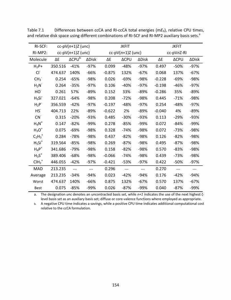
154
Table 7.1 Differences between ccCA and RI‐ccCA total energies (mEh), relative CPU times, and relative disk space using different combinations of RI‐SCF and RI‐MP2 auxiliary basis sets.a
RI‐SCF: cc‐pV(n+1)Z (unc) JKFIT JKFIT RI‐MP2: cc‐pV(n+1)Z (unc) cc‐pV(n+1)Z (unc) cc‐pVnZ‐RI
Molecule ΔE ΔCPUb ΔDisk ΔE ΔCPU ΔDisk ΔE ΔCPU ΔDisk
H2P+ 350.516 ‐41% ‐97% 0.099 ‐48% ‐97% 0.497 ‐50% ‐97%Cl‐ 474.637 140% ‐66% ‐0.875 132% ‐67% 0.068 137% ‐67%CH3
‐ 0.254 ‐65% ‐98% 0.026 ‐69% ‐98% ‐0.228 ‐69% ‐98%H2N
‐ 0.264 ‐35% ‐97% 0.106 ‐40% ‐97% ‐0.198 ‐46% ‐97%HO‐ 0.261 57% ‐89% 0.152 33% ‐89% ‐0.286 35% ‐89%H3Si
‐ 327.021 ‐64% ‐98% 0.208 ‐72% ‐98% 0.445 ‐71% ‐98%H2P
‐ 356.559 ‐42% ‐97% ‐0.197 ‐48% ‐97% 0.254 ‐48% ‐97%HS‐ 404.713 22% ‐89% ‐0.622 2% ‐89% ‐0.040 4% ‐89%CN‐ 0.315 ‐20% ‐93% 0.485 ‐30% ‐93% 0.113 ‐29% ‐93%H4N
+ 0.147 ‐82% ‐99% 0.278 ‐85% ‐99% 0.072 ‐84% ‐99%H3O
+ 0.075 ‐69% ‐98% 0.328 ‐74% ‐98% 0.072 ‐73% ‐98%C2H3
+ 0.284 ‐78% ‐98% 0.437 ‐82% ‐98% 0.126 ‐82% ‐98%H5Si
+ 319.564 ‐85% ‐98% 0.269 ‐87% ‐98% 0.495 ‐87% ‐98%H4P
+ 341.686 ‐79% ‐98% 0.158 ‐82% ‐98% 0.570 ‐83% ‐98%H3S
+ 389.406 ‐68% ‐98% ‐0.066 ‐74% ‐98% 0.439 ‐73% ‐98%ClH2
+ 446.055 ‐42% ‐97% ‐0.421 ‐53% ‐97% 0.422 ‐50% ‐97%
MAD 213.235 ‐‐‐ ‐‐‐ 0.296 ‐‐‐ ‐‐‐ 0.270 ‐‐‐ ‐‐‐ Average 213.235 ‐34% ‐94% 0.023 ‐42% ‐94% 0.176 ‐42% ‐94%Worst 474.637 140% ‐66% 0.875 132% ‐67% 0.570 137% ‐67%Best 0.075 ‐85% ‐99% 0.026 ‐87% ‐99% 0.040 ‐87% ‐99%a. The designation unc denotes an uncontracted basis set, while n+1 indicates the use of the next highest ζ‐
level basis set as an auxiliary basis set; diffuse or core‐valence functions where employed as appropriate. b. A negative CPU time indicates a savings, while a positive CPU time indicates additional computational cost
relative to the ccCA formulation.
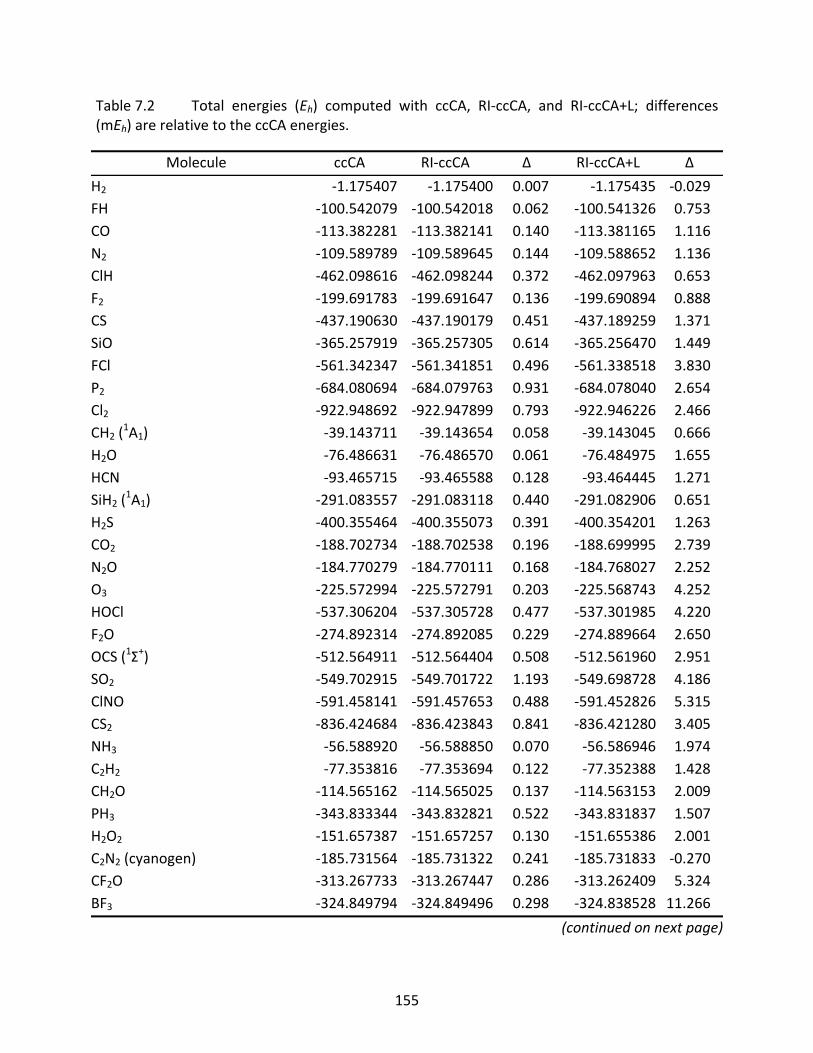
155
Table 7.2 Total energies (Eh) computed with ccCA, RI‐ccCA, and RI‐ccCA+L; differences (mEh) are relative to the ccCA energies.
Molecule ccCA RI‐ccCA Δ RI‐ccCA+L Δ
H2 ‐1.175407 ‐1.175400 0.007 ‐1.175435 ‐0.029FH ‐100.542079 ‐100.542018 0.062 ‐100.541326 0.753CO ‐113.382281 ‐113.382141 0.140 ‐113.381165 1.116N2 ‐109.589789 ‐109.589645 0.144 ‐109.588652 1.136ClH ‐462.098616 ‐462.098244 0.372 ‐462.097963 0.653F2 ‐199.691783 ‐199.691647 0.136 ‐199.690894 0.888CS ‐437.190630 ‐437.190179 0.451 ‐437.189259 1.371SiO ‐365.257919 ‐365.257305 0.614 ‐365.256470 1.449FCl ‐561.342347 ‐561.341851 0.496 ‐561.338518 3.830P2 ‐684.080694 ‐684.079763 0.931 ‐684.078040 2.654Cl2 ‐922.948692 ‐922.947899 0.793 ‐922.946226 2.466CH2 (
1A1) ‐39.143711 ‐39.143654 0.058 ‐39.143045 0.666H2O ‐76.486631 ‐76.486570 0.061 ‐76.484975 1.655HCN ‐93.465715 ‐93.465588 0.128 ‐93.464445 1.271SiH2 (
1A1) ‐291.083557 ‐291.083118 0.440 ‐291.082906 0.651H2S ‐400.355464 ‐400.355073 0.391 ‐400.354201 1.263CO2 ‐188.702734 ‐188.702538 0.196 ‐188.699995 2.739N2O ‐184.770279 ‐184.770111 0.168 ‐184.768027 2.252O3 ‐225.572994 ‐225.572791 0.203 ‐225.568743 4.252HOCl ‐537.306204 ‐537.305728 0.477 ‐537.301985 4.220F2O ‐274.892314 ‐274.892085 0.229 ‐274.889664 2.650OCS (1Σ+) ‐512.564911 ‐512.564404 0.508 ‐512.561960 2.951SO2 ‐549.702915 ‐549.701722 1.193 ‐549.698728 4.186ClNO ‐591.458141 ‐591.457653 0.488 ‐591.452826 5.315CS2 ‐836.424684 ‐836.423843 0.841 ‐836.421280 3.405NH3 ‐56.588920 ‐56.588850 0.070 ‐56.586946 1.974C2H2 ‐77.353816 ‐77.353694 0.122 ‐77.352388 1.428CH2O ‐114.565162 ‐114.565025 0.137 ‐114.563153 2.009PH3 ‐343.833344 ‐343.832821 0.522 ‐343.831837 1.507H2O2 ‐151.657387 ‐151.657257 0.130 ‐151.655386 2.001C2N2 (cyanogen) ‐185.731564 ‐185.731322 0.241 ‐185.731833 ‐0.270CF2O ‐313.267733 ‐313.267447 0.286 ‐313.262409 5.324BF3 ‐324.849794 ‐324.849496 0.298 ‐324.838528 11.266
(continued on next page)
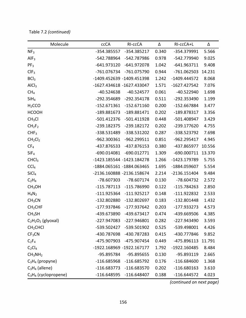
156
Table 7.2 (continued)
Molecule ccCA RI‐ccCA Δ RI‐ccCA+L Δ
NF3 ‐354.385557 ‐354.385217 0.340 ‐354.379991 5.566AlF3 ‐542.788964 ‐542.787986 0.978 ‐542.779940 9.025PF3 ‐641.973120 ‐641.972078 1.042 ‐641.963711 9.408ClF3 ‐761.076734 ‐761.075790 0.944 ‐761.062503 14.231BCl3 ‐1409.452639 ‐1409.451398 1.242 ‐1409.444572 8.068AlCl3 ‐1627.434618 ‐1627.433047 1.571 ‐1627.427542 7.076CH4 ‐40.524638 ‐40.524577 0.061 ‐40.522940 1.698SiH4 ‐292.354689 ‐292.354178 0.511 ‐292.353490 1.199H2CCO ‐152.671361 ‐152.671160 0.200 ‐152.667884 3.477HCOOH ‐189.881673 ‐189.881471 0.202 ‐189.878317 3.356CH3Cl ‐501.412376 ‐501.411928 0.448 ‐501.408947 3.429CH2F2 ‐239.182375 ‐239.182172 0.202 ‐239.177620 4.755CHF3 ‐338.531489 ‐338.531202 0.287 ‐338.523792 7.698CH2Cl2 ‐962.300361 ‐962.299511 0.851 ‐962.295417 4.945CF4 ‐437.876533 ‐437.876153 0.380 ‐437.865977 10.556SiF4 ‐690.014081 ‐690.012771 1.309 ‐690.000711 13.370CHCl3 ‐1423.185544 ‐1423.184278 1.266 ‐1423.179789 5.755CCl4 ‐1884.065161 ‐1884.063465 1.695 ‐1884.059607 5.554SiCl4 ‐2136.160888 ‐2136.158674 2.214 ‐2136.151404 9.484C2H4 ‐78.607303 ‐78.607174 0.130 ‐78.604732 2.572CH3OH ‐115.787113 ‐115.786990 0.122 ‐115.784263 2.850H4N2 ‐111.925364 ‐111.925217 0.148 ‐111.922832 2.533CH3CN ‐132.802880 ‐132.802697 0.183 ‐132.801448 1.432CH2CHF ‐177.937846 ‐177.937642 0.203 ‐177.933273 4.573CH3SH ‐439.673890 ‐439.673417 0.474 ‐439.669506 4.385C2H2O2 (glyoxal) ‐227.947083 ‐227.946801 0.282 ‐227.943490 3.593CH2CHCl ‐539.502427 ‐539.501902 0.525 ‐539.498001 4.426CF3CN ‐430.787698 ‐430.787283 0.415 ‐430.777846 9.852C2F4 ‐475.907903 ‐475.907454 0.449 ‐475.896113 11.791C2Cl4 ‐1922.168969 ‐1922.167177 1.792 ‐1922.160485 8.484CH3NH2 ‐95.895784 ‐95.895655 0.130 ‐95.893119 2.665C3H4 (propyne) ‐116.685968 ‐116.685792 0.176 ‐116.684600 1.368C3H4 (allene) ‐116.683773 ‐116.683570 0.202 ‐116.680163 3.610C3H4 (cyclopropene) ‐116.648595 ‐116.648407 0.188 ‐116.644572 4.023
(continued on next page)
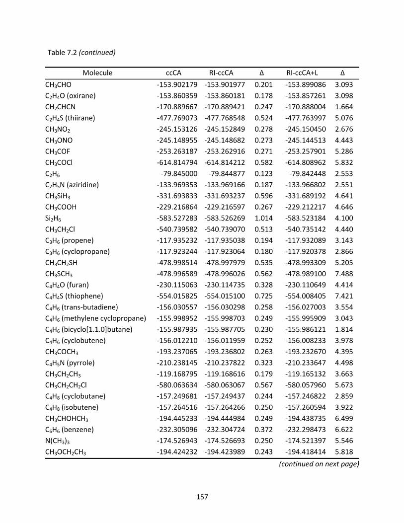
157
Table 7.2 (continued)
Molecule ccCA RI‐ccCA Δ RI‐ccCA+L Δ
CH3CHO ‐153.902179 ‐153.901977 0.201 ‐153.899086 3.093C2H4O (oxirane) ‐153.860359 ‐153.860181 0.178 ‐153.857261 3.098CH2CHCN ‐170.889667 ‐170.889421 0.247 ‐170.888004 1.664C2H4S (thiirane) ‐477.769073 ‐477.768548 0.524 ‐477.763997 5.076CH3NO2 ‐245.153126 ‐245.152849 0.278 ‐245.150450 2.676CH3ONO ‐245.148955 ‐245.148682 0.273 ‐245.144513 4.443CH3COF ‐253.263187 ‐253.262916 0.271 ‐253.257901 5.286CH3COCl ‐614.814794 ‐614.814212 0.582 ‐614.808962 5.832C2H6 ‐79.845000 ‐79.844877 0.123 ‐79.842448 2.553C2H5N (aziridine) ‐133.969353 ‐133.969166 0.187 ‐133.966802 2.551CH3SiH3 ‐331.693833 ‐331.693237 0.596 ‐331.689192 4.641CH3COOH ‐229.216864 ‐229.216597 0.267 ‐229.212217 4.646Si2H6 ‐583.527283 ‐583.526269 1.014 ‐583.523184 4.100CH3CH2Cl ‐540.739582 ‐540.739070 0.513 ‐540.735142 4.440C3H6 (propene) ‐117.935232 ‐117.935038 0.194 ‐117.932089 3.143C3H6 (cyclopropane) ‐117.923244 ‐117.923064 0.180 ‐117.920378 2.866CH3CH2SH ‐478.998514 ‐478.997979 0.535 ‐478.993309 5.205CH3SCH3 ‐478.996589 ‐478.996026 0.562 ‐478.989100 7.488C4H4O (furan) ‐230.115063 ‐230.114735 0.328 ‐230.110649 4.414C4H4S (thiophene) ‐554.015825 ‐554.015100 0.725 ‐554.008405 7.421C4H6 (trans‐butadiene) ‐156.030557 ‐156.030298 0.258 ‐156.027003 3.554C4H6 (methylene cyclopropane) ‐155.998952 ‐155.998703 0.249 ‐155.995909 3.043C4H6 (bicyclo[1.1.0]butane) ‐155.987935 ‐155.987705 0.230 ‐155.986121 1.814C4H6 (cyclobutene) ‐156.012210 ‐156.011959 0.252 ‐156.008233 3.978CH3COCH3 ‐193.237065 ‐193.236802 0.263 ‐193.232670 4.395C4H5N (pyrrole) ‐210.238145 ‐210.237822 0.323 ‐210.233647 4.498CH3CH2CH3 ‐119.168795 ‐119.168616 0.179 ‐119.165132 3.663CH3CH2CH2Cl ‐580.063634 ‐580.063067 0.567 ‐580.057960 5.673C4H8 (cyclobutane) ‐157.249681 ‐157.249437 0.244 ‐157.246822 2.859C4H8 (isobutene) ‐157.264516 ‐157.264266 0.250 ‐157.260594 3.922CH3CHOHCH3 ‐194.445233 ‐194.444984 0.249 ‐194.438735 6.499C6H6 (benzene) ‐232.305096 ‐232.304724 0.372 ‐232.298473 6.622N(CH3)3 ‐174.526943 ‐174.526693 0.250 ‐174.521397 5.546CH3OCH2CH3 ‐194.424232 ‐194.423989 0.243 ‐194.418414 5.818
(continued on next page)
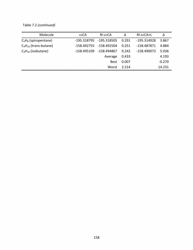
158
Table 7.2 (continued)
Molecule ccCA RI‐ccCA Δ RI‐ccCA+L Δ
C5H8 (spiropentane) ‐195.318795 ‐195.318505 0.291 ‐195.314928 3.867C4H10 (trans‐butane) ‐158.492755 ‐158.492504 0.251 ‐158.487871 4.884C4H10 (isobutane) ‐158.495109 ‐158.494867 0.242 ‐158.490073 5.036
Average 0.433 4.193Best 0.007 ‐0.270
Worst 2.214 14.231
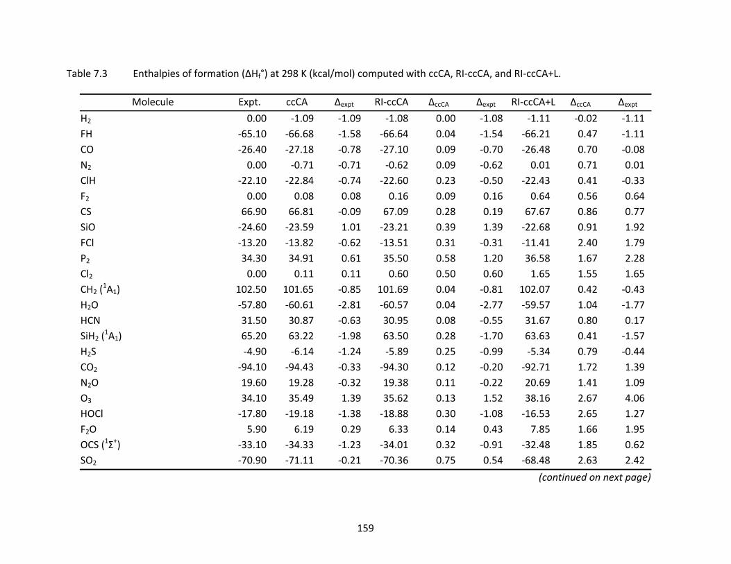
159
Table 7.3 Enthalpies of formation (ΔHf°) at 298 K (kcal/mol) computed with ccCA, RI‐ccCA, and RI‐ccCA+L.
Molecule Expt. ccCA Δexpt RI‐ccCA ΔccCA Δexpt RI‐ccCA+L ΔccCA Δexpt
H2 0.00 ‐1.09 ‐1.09 ‐1.08 0.00 ‐1.08 ‐1.11 ‐0.02 ‐1.11FH ‐65.10 ‐66.68 ‐1.58 ‐66.64 0.04 ‐1.54 ‐66.21 0.47 ‐1.11CO ‐26.40 ‐27.18 ‐0.78 ‐27.10 0.09 ‐0.70 ‐26.48 0.70 ‐0.08N2 0.00 ‐0.71 ‐0.71 ‐0.62 0.09 ‐0.62 0.01 0.71 0.01ClH ‐22.10 ‐22.84 ‐0.74 ‐22.60 0.23 ‐0.50 ‐22.43 0.41 ‐0.33F2 0.00 0.08 0.08 0.16 0.09 0.16 0.64 0.56 0.64CS 66.90 66.81 ‐0.09 67.09 0.28 0.19 67.67 0.86 0.77SiO ‐24.60 ‐23.59 1.01 ‐23.21 0.39 1.39 ‐22.68 0.91 1.92FCl ‐13.20 ‐13.82 ‐0.62 ‐13.51 0.31 ‐0.31 ‐11.41 2.40 1.79P2 34.30 34.91 0.61 35.50 0.58 1.20 36.58 1.67 2.28Cl2 0.00 0.11 0.11 0.60 0.50 0.60 1.65 1.55 1.65CH2 (
1A1) 102.50 101.65 ‐0.85 101.69 0.04 ‐0.81 102.07 0.42 ‐0.43H2O ‐57.80 ‐60.61 ‐2.81 ‐60.57 0.04 ‐2.77 ‐59.57 1.04 ‐1.77HCN 31.50 30.87 ‐0.63 30.95 0.08 ‐0.55 31.67 0.80 0.17SiH2 (
1A1) 65.20 63.22 ‐1.98 63.50 0.28 ‐1.70 63.63 0.41 ‐1.57H2S ‐4.90 ‐6.14 ‐1.24 ‐5.89 0.25 ‐0.99 ‐5.34 0.79 ‐0.44CO2 ‐94.10 ‐94.43 ‐0.33 ‐94.30 0.12 ‐0.20 ‐92.71 1.72 1.39N2O 19.60 19.28 ‐0.32 19.38 0.11 ‐0.22 20.69 1.41 1.09O3 34.10 35.49 1.39 35.62 0.13 1.52 38.16 2.67 4.06HOCl ‐17.80 ‐19.18 ‐1.38 ‐18.88 0.30 ‐1.08 ‐16.53 2.65 1.27F2O 5.90 6.19 0.29 6.33 0.14 0.43 7.85 1.66 1.95OCS (1Σ+) ‐33.10 ‐34.33 ‐1.23 ‐34.01 0.32 ‐0.91 ‐32.48 1.85 0.62SO2 ‐70.90 ‐71.11 ‐0.21 ‐70.36 0.75 0.54 ‐68.48 2.63 2.42
(continued on next page)
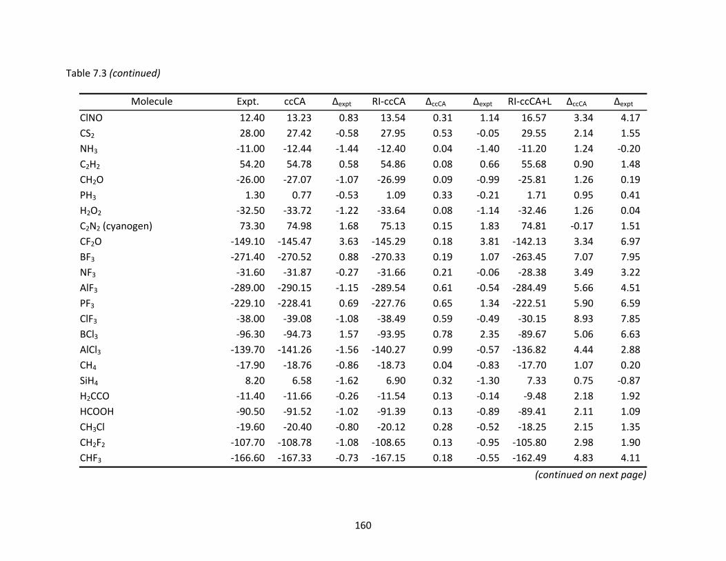
160
Table 7.3 (continued)
Molecule Expt. ccCA Δexpt RI‐ccCA ΔccCA Δexpt RI‐ccCA+L ΔccCA Δexpt
ClNO 12.40 13.23 0.83 13.54 0.31 1.14 16.57 3.34 4.17CS2 28.00 27.42 ‐0.58 27.95 0.53 ‐0.05 29.55 2.14 1.55NH3 ‐11.00 ‐12.44 ‐1.44 ‐12.40 0.04 ‐1.40 ‐11.20 1.24 ‐0.20C2H2 54.20 54.78 0.58 54.86 0.08 0.66 55.68 0.90 1.48CH2O ‐26.00 ‐27.07 ‐1.07 ‐26.99 0.09 ‐0.99 ‐25.81 1.26 0.19PH3 1.30 0.77 ‐0.53 1.09 0.33 ‐0.21 1.71 0.95 0.41H2O2 ‐32.50 ‐33.72 ‐1.22 ‐33.64 0.08 ‐1.14 ‐32.46 1.26 0.04C2N2 (cyanogen) 73.30 74.98 1.68 75.13 0.15 1.83 74.81 ‐0.17 1.51CF2O ‐149.10 ‐145.47 3.63 ‐145.29 0.18 3.81 ‐142.13 3.34 6.97BF3 ‐271.40 ‐270.52 0.88 ‐270.33 0.19 1.07 ‐263.45 7.07 7.95NF3 ‐31.60 ‐31.87 ‐0.27 ‐31.66 0.21 ‐0.06 ‐28.38 3.49 3.22AlF3 ‐289.00 ‐290.15 ‐1.15 ‐289.54 0.61 ‐0.54 ‐284.49 5.66 4.51PF3 ‐229.10 ‐228.41 0.69 ‐227.76 0.65 1.34 ‐222.51 5.90 6.59ClF3 ‐38.00 ‐39.08 ‐1.08 ‐38.49 0.59 ‐0.49 ‐30.15 8.93 7.85BCl3 ‐96.30 ‐94.73 1.57 ‐93.95 0.78 2.35 ‐89.67 5.06 6.63AlCl3 ‐139.70 ‐141.26 ‐1.56 ‐140.27 0.99 ‐0.57 ‐136.82 4.44 2.88CH4 ‐17.90 ‐18.76 ‐0.86 ‐18.73 0.04 ‐0.83 ‐17.70 1.07 0.20SiH4 8.20 6.58 ‐1.62 6.90 0.32 ‐1.30 7.33 0.75 ‐0.87H2CCO ‐11.40 ‐11.66 ‐0.26 ‐11.54 0.13 ‐0.14 ‐9.48 2.18 1.92HCOOH ‐90.50 ‐91.52 ‐1.02 ‐91.39 0.13 ‐0.89 ‐89.41 2.11 1.09CH3Cl ‐19.60 ‐20.40 ‐0.80 ‐20.12 0.28 ‐0.52 ‐18.25 2.15 1.35CH2F2 ‐107.70 ‐108.78 ‐1.08 ‐108.65 0.13 ‐0.95 ‐105.80 2.98 1.90CHF3 ‐166.60 ‐167.33 ‐0.73 ‐167.15 0.18 ‐0.55 ‐162.49 4.83 4.11
(continued on next page)
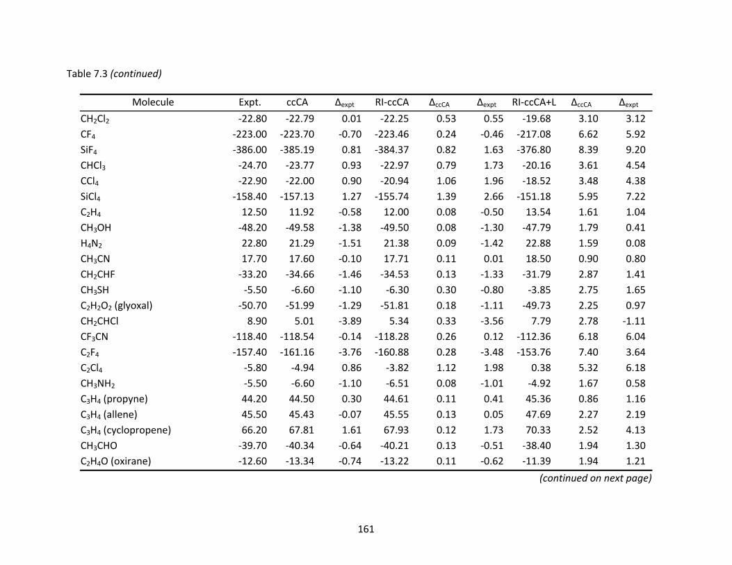
161
Table 7.3 (continued)
Molecule Expt. ccCA Δexpt RI‐ccCA ΔccCA Δexpt RI‐ccCA+L ΔccCA Δexpt
CH2Cl2 ‐22.80 ‐22.79 0.01 ‐22.25 0.53 0.55 ‐19.68 3.10 3.12CF4 ‐223.00 ‐223.70 ‐0.70 ‐223.46 0.24 ‐0.46 ‐217.08 6.62 5.92SiF4 ‐386.00 ‐385.19 0.81 ‐384.37 0.82 1.63 ‐376.80 8.39 9.20CHCl3 ‐24.70 ‐23.77 0.93 ‐22.97 0.79 1.73 ‐20.16 3.61 4.54CCl4 ‐22.90 ‐22.00 0.90 ‐20.94 1.06 1.96 ‐18.52 3.48 4.38SiCl4 ‐158.40 ‐157.13 1.27 ‐155.74 1.39 2.66 ‐151.18 5.95 7.22C2H4 12.50 11.92 ‐0.58 12.00 0.08 ‐0.50 13.54 1.61 1.04CH3OH ‐48.20 ‐49.58 ‐1.38 ‐49.50 0.08 ‐1.30 ‐47.79 1.79 0.41H4N2 22.80 21.29 ‐1.51 21.38 0.09 ‐1.42 22.88 1.59 0.08CH3CN 17.70 17.60 ‐0.10 17.71 0.11 0.01 18.50 0.90 0.80CH2CHF ‐33.20 ‐34.66 ‐1.46 ‐34.53 0.13 ‐1.33 ‐31.79 2.87 1.41CH3SH ‐5.50 ‐6.60 ‐1.10 ‐6.30 0.30 ‐0.80 ‐3.85 2.75 1.65C2H2O2 (glyoxal) ‐50.70 ‐51.99 ‐1.29 ‐51.81 0.18 ‐1.11 ‐49.73 2.25 0.97CH2CHCl 8.90 5.01 ‐3.89 5.34 0.33 ‐3.56 7.79 2.78 ‐1.11CF3CN ‐118.40 ‐118.54 ‐0.14 ‐118.28 0.26 0.12 ‐112.36 6.18 6.04C2F4 ‐157.40 ‐161.16 ‐3.76 ‐160.88 0.28 ‐3.48 ‐153.76 7.40 3.64C2Cl4 ‐5.80 ‐4.94 0.86 ‐3.82 1.12 1.98 0.38 5.32 6.18CH3NH2 ‐5.50 ‐6.60 ‐1.10 ‐6.51 0.08 ‐1.01 ‐4.92 1.67 0.58C3H4 (propyne) 44.20 44.50 0.30 44.61 0.11 0.41 45.36 0.86 1.16C3H4 (allene) 45.50 45.43 ‐0.07 45.55 0.13 0.05 47.69 2.27 2.19C3H4 (cyclopropene) 66.20 67.81 1.61 67.93 0.12 1.73 70.33 2.52 4.13CH3CHO ‐39.70 ‐40.34 ‐0.64 ‐40.21 0.13 ‐0.51 ‐38.40 1.94 1.30C2H4O (oxirane) ‐12.60 ‐13.34 ‐0.74 ‐13.22 0.11 ‐0.62 ‐11.39 1.94 1.21
(continued on next page)
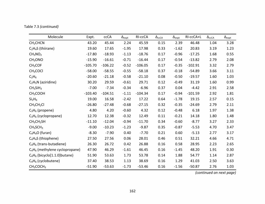
162
Table 7.3 (continued)
Molecule Expt. ccCA Δexpt RI‐ccCA ΔccCA Δexpt RI‐ccCA+L ΔccCA Δexpt
CH2CHCN 43.20 45.44 2.24 45.59 0.15 2.39 46.48 1.04 3.28C2H4S (thiirane) 19.60 17.65 ‐1.95 17.98 0.33 ‐1.62 20.83 3.19 1.23CH3NO2 ‐17.80 ‐18.93 ‐1.13 ‐18.76 0.17 ‐0.96 ‐17.25 1.68 0.55CH3ONO ‐15.90 ‐16.61 ‐0.71 ‐16.44 0.17 ‐0.54 ‐13.82 2.79 2.08CH3COF ‐105.70 ‐106.22 ‐0.52 ‐106.05 0.17 ‐0.35 ‐102.91 3.32 2.79CH3COCl ‐58.00 ‐58.55 ‐0.55 ‐58.18 0.37 ‐0.18 ‐54.89 3.66 3.11C2H6 ‐20.60 ‐21.18 ‐0.58 ‐21.10 0.08 ‐0.50 ‐19.57 1.60 1.03C2H5N (aziridine) 30.20 29.59 ‐0.61 29.71 0.12 ‐0.49 31.19 1.60 0.99CH3SiH3 ‐7.00 ‐7.34 ‐0.34 ‐6.96 0.37 0.04 ‐4.42 2.91 2.58CH3COOH ‐103.40 ‐104.51 ‐1.11 ‐104.34 0.17 ‐0.94 ‐101.59 2.92 1.81Si2H6 19.00 16.58 ‐2.42 17.22 0.64 ‐1.78 19.15 2.57 0.15CH3CH2Cl ‐26.80 ‐27.48 ‐0.68 ‐27.15 0.32 ‐0.35 ‐24.69 2.79 2.11C3H6 (propene) 4.80 4.20 ‐0.60 4.32 0.12 ‐0.48 6.18 1.97 1.38C3H6 (cyclopropane) 12.70 12.38 ‐0.32 12.49 0.11 ‐0.21 14.18 1.80 1.48CH3CH2SH ‐11.10 ‐12.04 ‐0.94 ‐11.70 0.34 ‐0.60 ‐8.77 3.27 2.33CH3SCH3 ‐9.00 ‐10.23 ‐1.23 ‐9.87 0.35 ‐0.87 ‐5.53 4.70 3.47C4H4O (furan) ‐8.30 ‐7.90 0.40 ‐7.70 0.21 0.60 ‐5.13 2.77 3.17C4H4S (thiophene) 27.50 27.56 0.06 28.01 0.46 0.51 32.21 4.66 4.71C4H6 (trans‐butadiene) 26.30 26.72 0.42 26.88 0.16 0.58 28.95 2.23 2.65C4H6 (methylene cyclopropane) 47.90 46.29 ‐1.61 46.45 0.16 ‐1.45 48.20 1.91 0.30C4H6 (bicyclo[1.1.0]butane) 51.90 53.63 1.73 53.78 0.14 1.88 54.77 1.14 2.87C4H6 (cyclobutene) 37.40 38.53 1.13 38.69 0.16 1.29 41.03 2.50 3.63CH3COCH3 ‐51.90 ‐53.63 ‐1.73 ‐53.46 0.16 ‐1.56 ‐50.87 2.76 1.03
(continued on next page)
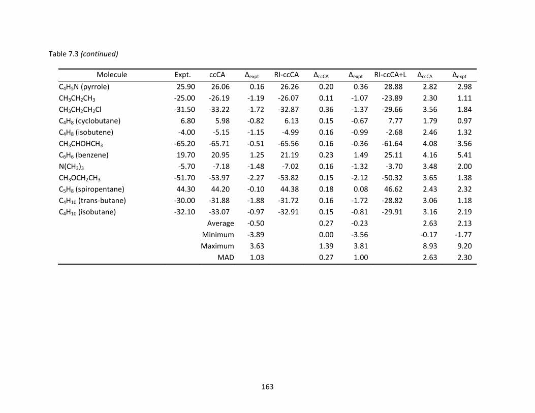
163
Table 7.3 (continued)
Molecule Expt. ccCA Δexpt RI‐ccCA ΔccCA Δexpt RI‐ccCA+L ΔccCA Δexpt
C4H5N (pyrrole) 25.90 26.06 0.16 26.26 0.20 0.36 28.88 2.82 2.98CH3CH2CH3 ‐25.00 ‐26.19 ‐1.19 ‐26.07 0.11 ‐1.07 ‐23.89 2.30 1.11CH3CH2CH2Cl ‐31.50 ‐33.22 ‐1.72 ‐32.87 0.36 ‐1.37 ‐29.66 3.56 1.84C4H8 (cyclobutane) 6.80 5.98 ‐0.82 6.13 0.15 ‐0.67 7.77 1.79 0.97C4H8 (isobutene) ‐4.00 ‐5.15 ‐1.15 ‐4.99 0.16 ‐0.99 ‐2.68 2.46 1.32CH3CHOHCH3 ‐65.20 ‐65.71 ‐0.51 ‐65.56 0.16 ‐0.36 ‐61.64 4.08 3.56C6H6 (benzene) 19.70 20.95 1.25 21.19 0.23 1.49 25.11 4.16 5.41N(CH3)3 ‐5.70 ‐7.18 ‐1.48 ‐7.02 0.16 ‐1.32 ‐3.70 3.48 2.00CH3OCH2CH3 ‐51.70 ‐53.97 ‐2.27 ‐53.82 0.15 ‐2.12 ‐50.32 3.65 1.38C5H8 (spiropentane) 44.30 44.20 ‐0.10 44.38 0.18 0.08 46.62 2.43 2.32C4H10 (trans‐butane) ‐30.00 ‐31.88 ‐1.88 ‐31.72 0.16 ‐1.72 ‐28.82 3.06 1.18C4H10 (isobutane) ‐32.10 ‐33.07 ‐0.97 ‐32.91 0.15 ‐0.81 ‐29.91 3.16 2.19
Average ‐0.50 0.27 ‐0.23 2.63 2.13Minimum ‐3.89 0.00 ‐3.56 ‐0.17 ‐1.77Maximum 3.63 1.39 3.81 8.93 9.20
MAD 1.03 0.27 1.00 2.63 2.30
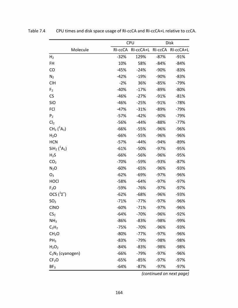
164
Table 7.4 CPU times and disk space usage of RI‐ccCA and RI‐ccCA+L relative to ccCA.
CPU Disk
Molecule RI‐ccCA RI‐ccCA+L RI‐ccCA RI‐ccCA+L
H2 ‐32% 129% ‐87% ‐91% FH 10% 58% ‐84% ‐84% CO ‐45% ‐24% ‐90% ‐83% N2 ‐42% ‐19% ‐90% ‐83% ClH ‐2% 36% ‐85% ‐79% F2 ‐40% ‐17% ‐89% ‐80% CS ‐46% ‐27% ‐91% ‐81% SiO ‐46% ‐25% ‐91% ‐78% FCl ‐47% ‐31% ‐89% ‐79% P2 ‐57% ‐42% ‐90% ‐79% Cl2 ‐56% ‐44% ‐88% ‐77% CH2 (
1A1) ‐66% ‐55% ‐96% ‐96% H2O ‐66% ‐55% ‐96% ‐96% HCN ‐57% ‐44% ‐94% ‐89% SiH2 (
1A1) ‐61% ‐50% ‐97% ‐95% H2S ‐66% ‐56% ‐96% ‐95% CO2 ‐70% ‐59% ‐93% ‐87% N2O ‐60% ‐65% ‐96% ‐93% O3 ‐62% ‐69% ‐97% ‐96% HOCl ‐58% ‐64% ‐97% ‐97% F2O ‐59% ‐76% ‐97% ‐97% OCS (1Σ+) ‐62% ‐68% ‐96% ‐93% SO2 ‐71% ‐77% ‐97% ‐96% ClNO ‐60% ‐71% ‐97% ‐96% CS2 ‐64% ‐70% ‐96% ‐92% NH3 ‐86% ‐83% ‐98% ‐99% C2H2 ‐75% ‐70% ‐96% ‐93% CH2O ‐80% ‐77% ‐97% ‐96% PH3 ‐83% ‐79% ‐98% ‐98% H2O2 ‐84% ‐83% ‐98% ‐98% C2N2 (cyanogen) ‐66% ‐79% ‐97% ‐96% CF2O ‐65% ‐85% ‐97% ‐97% BF3 ‐64% ‐87% ‐97% ‐97%
(continued on next page)
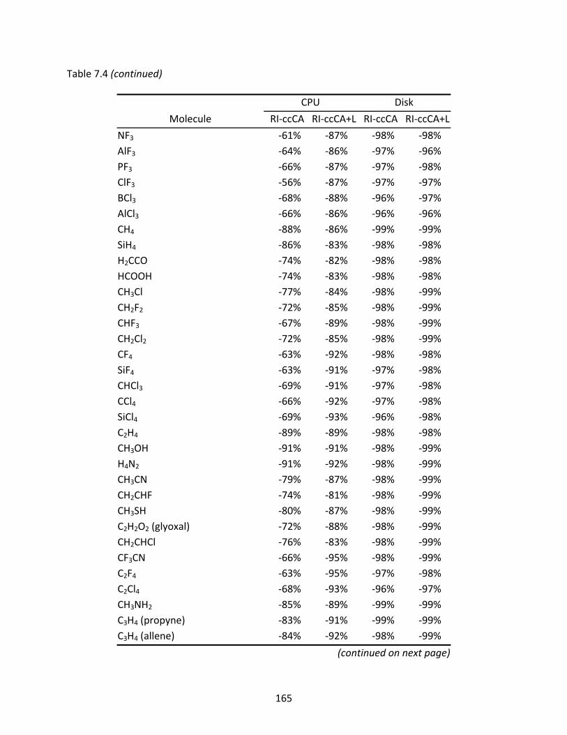
165
Table 7.4 (continued)
CPU Disk
Molecule RI‐ccCA RI‐ccCA+L RI‐ccCA RI‐ccCA+L
NF3 ‐61% ‐87% ‐98% ‐98% AlF3 ‐64% ‐86% ‐97% ‐96% PF3 ‐66% ‐87% ‐97% ‐98% ClF3 ‐56% ‐87% ‐97% ‐97% BCl3 ‐68% ‐88% ‐96% ‐97% AlCl3 ‐66% ‐86% ‐96% ‐96% CH4 ‐88% ‐86% ‐99% ‐99% SiH4 ‐86% ‐83% ‐98% ‐98% H2CCO ‐74% ‐82% ‐98% ‐98% HCOOH ‐74% ‐83% ‐98% ‐98% CH3Cl ‐77% ‐84% ‐98% ‐99% CH2F2 ‐72% ‐85% ‐98% ‐99% CHF3 ‐67% ‐89% ‐98% ‐99% CH2Cl2 ‐72% ‐85% ‐98% ‐99% CF4 ‐63% ‐92% ‐98% ‐98% SiF4 ‐63% ‐91% ‐97% ‐98% CHCl3 ‐69% ‐91% ‐97% ‐98% CCl4 ‐66% ‐92% ‐97% ‐98% SiCl4 ‐69% ‐93% ‐96% ‐98% C2H4 ‐89% ‐89% ‐98% ‐98% CH3OH ‐91% ‐91% ‐98% ‐99% H4N2 ‐91% ‐92% ‐98% ‐99% CH3CN ‐79% ‐87% ‐98% ‐99% CH2CHF ‐74% ‐81% ‐98% ‐99% CH3SH ‐80% ‐87% ‐98% ‐99% C2H2O2 (glyoxal) ‐72% ‐88% ‐98% ‐99% CH2CHCl ‐76% ‐83% ‐98% ‐99% CF3CN ‐66% ‐95% ‐98% ‐99% C2F4 ‐63% ‐95% ‐97% ‐98% C2Cl4 ‐68% ‐93% ‐96% ‐97% CH3NH2 ‐85% ‐89% ‐99% ‐99% C3H4 (propyne) ‐83% ‐91% ‐99% ‐99% C3H4 (allene) ‐84% ‐92% ‐98% ‐99%
(continued on next page)
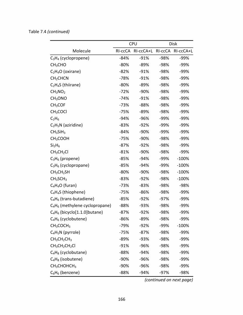
166
Table 7.4 (continued)
CPU Disk
Molecule RI‐ccCA RI‐ccCA+L RI‐ccCA RI‐ccCA+L
C3H4 (cyclopropene) ‐84% ‐91% ‐98% ‐99% CH3CHO ‐80% ‐89% ‐98% ‐99% C2H4O (oxirane) ‐82% ‐91% ‐98% ‐99% CH2CHCN ‐78% ‐91% ‐98% ‐99% C2H4S (thiirane) ‐80% ‐89% ‐98% ‐99% CH3NO2 ‐72% ‐90% ‐98% ‐99% CH3ONO ‐74% ‐91% ‐98% ‐99% CH3COF ‐73% ‐88% ‐98% ‐99% CH3COCl ‐75% ‐89% ‐98% ‐99% C2H6 ‐94% ‐96% ‐99% ‐99% C2H5N (aziridine) ‐83% ‐92% ‐99% ‐99% CH3SiH3 ‐84% ‐90% ‐99% ‐99% CH3COOH ‐75% ‐90% ‐98% ‐99% Si2H6 ‐87% ‐92% ‐98% ‐99% CH3CH2Cl ‐81% ‐90% ‐98% ‐99% C3H6 (propene) ‐85% ‐94% ‐99% ‐100% C3H6 (cyclopropane) ‐85% ‐94% ‐99% ‐100% CH3CH2SH ‐80% ‐90% ‐98% ‐100% CH3SCH3 ‐83% ‐92% ‐98% ‐100% C4H4O (furan) ‐73% ‐83% ‐98% ‐98% C4H4S (thiophene) ‐75% ‐86% ‐98% ‐99% C4H6 (trans‐butadiene) ‐85% ‐92% ‐97% ‐99% C4H6 (methylene cyclopropane) ‐88% ‐93% ‐98% ‐99% C4H6 (bicyclo[1.1.0]butane) ‐87% ‐92% ‐98% ‐99% C4H6 (cyclobutene) ‐86% ‐89% ‐98% ‐99% CH3COCH3 ‐79% ‐92% ‐99% ‐100% C4H5N (pyrrole) ‐75% ‐87% ‐98% ‐99% CH3CH2CH3 ‐89% ‐93% ‐98% ‐99% CH3CH2CH2Cl ‐91% ‐96% ‐98% ‐99% C4H8 (cyclobutane) ‐88% ‐94% ‐98% ‐99% C4H8 (isobutene) ‐90% ‐96% ‐98% ‐99% CH3CHOHCH3 ‐90% ‐96% ‐98% ‐99% C6H6 (benzene) ‐88% ‐94% ‐97% ‐98%
(continued on next page)
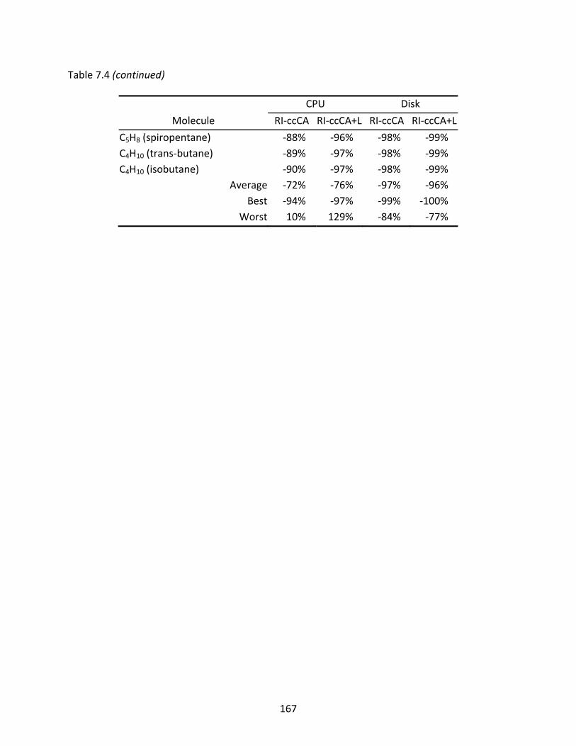
167
Table 7.4 (continued)
CPU Disk
Molecule RI‐ccCA RI‐ccCA+L RI‐ccCA RI‐ccCA+L
C5H8 (spiropentane) ‐88% ‐96% ‐98% ‐99% C4H10 (trans‐butane) ‐89% ‐97% ‐98% ‐99% C4H10 (isobutane) ‐90% ‐97% ‐98% ‐99%
Average ‐72% ‐76% ‐97% ‐96% Best ‐94% ‐97% ‐99% ‐100%
Worst 10% 129% ‐84% ‐77%
168
CHAPTER 8
A SYSTEMATIC INVESTIGATION OF DIHALOGEN‐μ‐DICHALCOGENIDES†
8.1 Introduction
Mixed halogen‐chalcogen species, in particular the fluorine‐ and oxygen‐containing class
of compounds, have drawn much attention in the literature over the past seven decades both
for their applications and unique bonding. Molecules containing a fluorine‐oxygen bond, such
as FOOF, have many applications, such as a near‐room‐temperature fluorinating agent for
various actinides and xenon.202‐205 Sometimes referred to as oxyfluorides, these compounds
have also been reported to be of use in various rocket fuels.206 They are also speculated to
participate in various reactions of atmospheric importance, such as the depletion of ozone by a
photolysis mechanism that produces FO radicals.207,208 The sulfur analog of FOOF, FSSF, has also
been implicated in the depletion of ozone.209 Other halogenated persulfides, ClSSCl, BrSSBr,
ClSeSeCl, and BrSeSeBr, are used extensively as plasma etchants in manufacturing various
microelectronic devices.210‐213 Disulfide and diselenide bonds are particularly important in
biological systems, specifically cystine‐rich proteins in the case of disulfides. Molecules with
disulfide bridges are studied to gain insight into the relationship between the strength of the
S‐S bond with respect to varying the terminal substituents. An understanding of this
relationship can provide insight into the structure‐activity relationship of proteins, especially in
† This entire chapter is adapted from B.P. Prascher and A.K. Wilson, “A Computational Study of Dihalogen‐μ‐dichalcogenides: XAAX (X = F, Cl, Br; A = S, Se),” J. Mo. Struct. THEOCHEM, 2007, 814(1‐3), 1, with permission from Elsevier.
169
proteins where a disulfide bond is involved in the chemistry of the active site or if the disulfide
bond stabilizes the tertiary structure of the protein.214‐218
While the applications of FOOF and a few of its sulfur analogs are known in the
literature, there has been disagreement between computational and experimental geometries.
In the earliest microwave spectroscopy experiment reported by Jackson219 on FOOF, a short O‐
O bond length resembling that of O2 and a long F‐O bond relative to FO were observed.
Subsequent reports in the literature fail to reproduce Jackson’s geometry, instead reporting a
peroxide‐like (longer) O‐O bond and shorter F‐O bonds. A careful electron diffraction study
undertaken by Hedberg and coworkers220 verified the structure Jackson had observed, and
noted that a better understanding of the structure of FOOF is crucial to elucidating the
mechanism by which its fluorinating abilities arise.
The structure of FOOF has F‐O bond lengths of 1.575 Å,219,220 longer than that of FO at
1.354 Å.221 FOOF also has an O‐O bond length of 1.216 Å,219,220 resembling the oxygen molecule,
1.208 Å,222,223 and not a typical peroxide (1.44 – 1.46 Å).224 From microwave spectroscopy, it is
known that FSSF also has a short A‐A bond and long A‐X bonds.225‐228 Another structural
anomaly of XSSX species is the increase in the S‐S bond length when the halogen size is
increased,229 a trend which is observed in XOOX species also.222,230
The structural anomalies of FOOF have been addressed in much detail elsewhere207 as
the result of overlap between an oxygen lone pair orbital and the adjacent unoccupied F‐O σ*
orbital – a phenomenon called anomeric delocalization (see Figure 8.1). This phenomenon is
not unique to the FOOF molecule, but also exists in molecules such as α‐fluoroethers231 and
other molecules where highly electronegative atoms are in close proximity to one another.
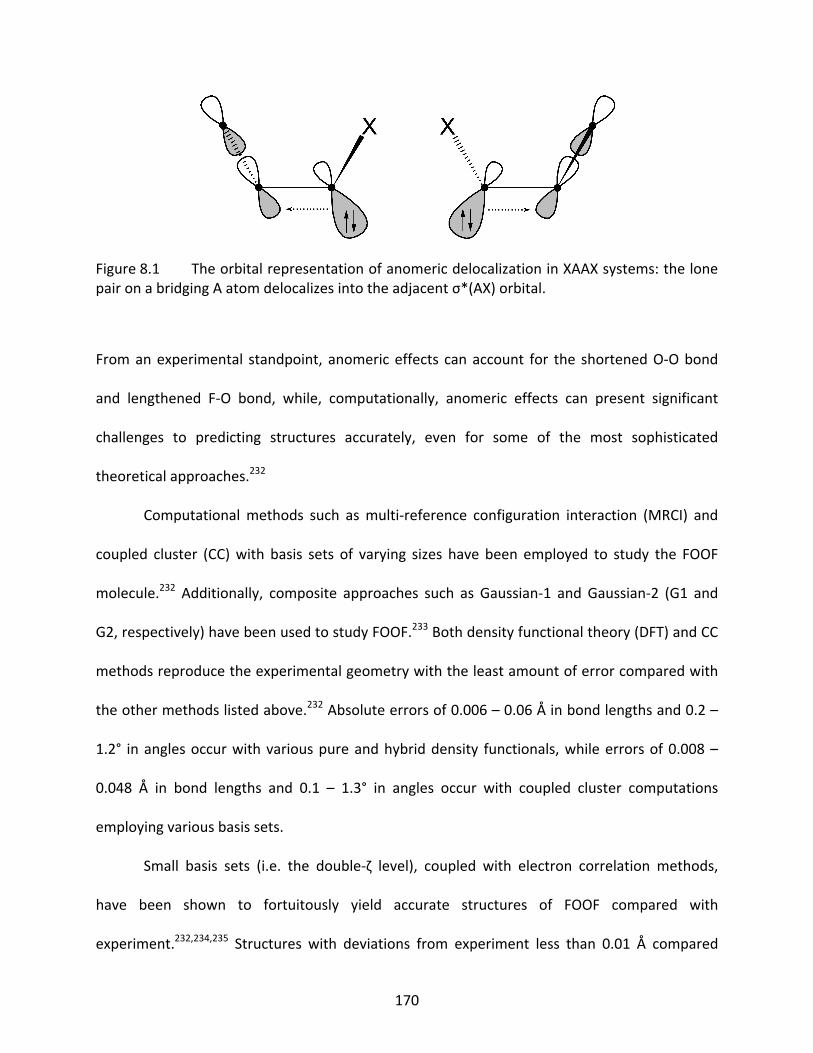
170
From an experimental standpoint, anomeric effects can account for the shortened O‐O bond
and lengthened F‐O bond, while, computationally, anomeric effects can present significant
challenges to predicting structures accurately, even for some of the most sophisticated
theoretical approaches.232
Computational methods such as multi‐reference configuration interaction (MRCI) and
coupled cluster (CC) with basis sets of varying sizes have been employed to study the FOOF
molecule.232 Additionally, composite approaches such as Gaussian‐1 and Gaussian‐2 (G1 and
G2, respectively) have been used to study FOOF.233 Both density functional theory (DFT) and CC
methods reproduce the experimental geometry with the least amount of error compared with
the other methods listed above.232 Absolute errors of 0.006 – 0.06 Å in bond lengths and 0.2 –
1.2° in angles occur with various pure and hybrid density functionals, while errors of 0.008 –
0.048 Å in bond lengths and 0.1 – 1.3° in angles occur with coupled cluster computations
employing various basis sets.
Small basis sets (i.e. the double‐ζ level), coupled with electron correlation methods,
have been shown to fortuitously yield accurate structures of FOOF compared with
experiment.232,234,235 Structures with deviations from experiment less than 0.01 Å compared
Figure 8.1 The orbital representation of anomeric delocalization in XAAX systems: the lonepair on a bridging A atom delocalizes into the adjacent σ*(AX) orbital.
171
have been computed in the past by adding non‐optimized polarization235 and diffuse
functions236 to a double‐ζ basis set. An improvement in the accuracy of the O‐O bond length is
typically observed with a loss of accuracy in the O‐F bond length using this approach.
Computational studies with smaller, more rigid basis sets, such as that of Scuseria237 where the
polarization functions of the oxygen and fluorine basis sets were constrained to have equal
exponents, tend to give results closer to experiment. This work, and others,232,235 do not
condone the use of such nonstandard approaches to predictive quantum chemistry since the
method cannot be readily applied to study other molecular systems. Instead, one would like to
apply a standard and systematic approach to studying similar systems.
In this chapter, the heavier analogs of the FOOF molecule with the structure XAAX (X =
F, Cl, Br and A = S, Se) are investigated. When this investigation was published, no systematic ab
initio or DFT study on the structure, frequencies, and anomeric effects had been performed on
the sulfur and selenium XAAX analogs of FOOF, nor had CC computations on the relative
stabilities of the XAAX conformation compared with other A2X2 isomers been reported.
8.2 Computational Methodology
Both hybrid DFT and CC methods have been utilized for this work. DFT is particularly
attractive because of its formal scaling (where is the number of basis functions). The
DFT method employed is Becke’s three‐parameter exchange scheme (B3)166 coupled with the
Lee‐Yang‐Parr (LYP) correlation functional.165 The third parameterization of Vosko, Wilk, and
Nusair correlation functional (VWN‐3) has been used. The coupled cluster method including
singles, doubles, and non‐iterative, perturbative triples is also employed, CCSD(T).31,38
172
A series of natural orbital (NO) analyses using singles and doubles configuration
interaction (CISD) has been performed. The CISD NOs provide insight into the amount of multi‐
reference character of the system and the most important orbitals involved in computing the
dynamic correlation energy. The NOs reported here also demonstrate how well correlated
methods, specifically truncated ab initio methods, describe XAAX systems with respect to
anomeric delocalization.
The correlation consistent, polarized valence basis sets, cc‐pVnZ (where n = D, T, and
Q)94‐101 have been employed in this study. In computations involving second row atoms, the
tight d correlation consistent basis sets, cc‐pV(n+d)Z,101 were employed. Additionally, the
augmented correlation consistent basis sets, aug‐cc‐pVnZ and aug‐cc‐pV(n+d)Z,95,99,100 were
used for describing long‐range effects, specifically lone pair interactions.
This investigation is concerned with the chemistry of disulfide and diselenide
compounds, following the results of experimental work regarding the stability of the
conformations of X2A2 compounds.215,216,225,238‐241 Structures have been fully optimized at each
level of theory and basis set, utilizing symmetry where present. The B3LYP calculations were
performed using the Gaussian 03 software suite,174 while the Molpro software package180 was
used for CCSD(T) and CISD computations. Harmonic vibrational frequencies were computed
analytically with B3LYP and numerically with CCSD(T) at the aug‐cc‐pVTZ level. Computed
anharmonic frequencies are included for comparison.242
173
8.3 Results and Discussion
8.3.1 Stability of X2A2 Compounds
Following the reported stabilities of several conformations of FOOF by Kraka et al.,232
computations have been performed at the aug‐cc‐pVTZ level to compare the stabilities of the
linear, cis, trans, and X2AA conformations of the heavier analogs with their gauche forms. The
computed relative stabilities (in kcal/mol) are tabulated in Table 8.1 for both B3LYP and
CCSD(T). It is found that all the conformations are significantly less stable than the gauche form.
For F2S2, the B3LYP value shows FSSF to be more stable than F2SS, but CCSD(T) does not. This
apparent contradiction to what is known experimentally regarding FSSF being more stable than
F2SS215,216,225 has been investigated further through a series of computations using the
augmented double‐ through quadruple‐ζ basis sets with both methods. As the basis set size
increases, B3LYP predicts that FSSF is the more stable compound. The CCSD(T) computations
with increasing basis set size show F2SS as the more stable conformation . However, when a
thermal correction (for 298 K) is applied to the CCSD(T) electronic energy, FSSF is shown to be
more stable than the F2SS conformation by 0.04 kcal/mol.
Other isomers of the XAAX‐type molecules have been investigated previously,
specifically the XAXA and AXXA isomers of iodine oxides.243,244 We have briefly examined these
two isomeric forms here using second‐order Møller‐Plesset perturbation theory (MP2) and the
aug‐cc‐pVTZ basis set. MP2 has been used since CCSD(T) computations without symmetry can
become time intensive, and MP2 will recover a significant percent of the CCSD(T) correlation
energy. Further, test computations on the cis, trans, and linear forms have shown MP2 relative
174
stabilities to be comparable to CCSD(T) stability energies. For most XAAX compounds of this
study, the corresponding XAXA compound is found to dissociate into two XA fragments as
doublet electronic states. Only in the case of FSFS does the molecule dissociate into FSF ( ) +
S ( ). Similarly, the AXXA compounds display no bound minima as tetraatomic molecules, but
dissociate into two XA fragments, each with a doublet electron configuration.
8.3.2 XAAX Structures
Optimized geometries are listed in Table 8.2, Table 8.3, and Table 8.4 for the fluorine,
chlorine, and bromine species, respectively. For the fluorine compounds, relative to experiment
both B3LYP and CCSD(T) result in the least error at the aug‐cc‐pVQZ level as compared with the
other basis sets – the errors being 0.013 Å and 0.011 Å, respectively. The CCSD(T) S‐F bond
length is in good agreement with experiment, with a difference of only 0.01 Å at the triple‐ζ
level. CCSD(T) only slightly outperforms B3LYP for the bond lengths and angles. B3LYP dihedral
angles tend to converge to the experimental value while CCSD(T) dihedrals converge away from
experiment. In FSeSeF, the optimized Se‐Se bond length converges away from the experimental
value for both methods and their smallest errors relative to experiment are 0.023 Å for B3LYP
and 0.014 Å for CCSD(T) at the cc‐pVDZ level. Just as in the case of FSSF, the Se‐F bonds with
CCSD(T) are within chemical accuracy by the triple‐ζ basis set. The dihedral in FSeSeF is closest
to the experimental value for both methods when the smallest basis set is employed. The
differences between the computed angles and the experimental angle range from 5.06° – 5.33°
for B3LYP and from 4.19° – 4.55° for CCSD(T), where an experimental value of 100° has been
reported by Haas.245 In either the case of B3LYP or CCSD(T), adding diffuse functions does not
175
significantly affect the bond lengths, but does affect the angles and dihedral angles. The
inclusion of the tight d function in FSSF is important, especially at the double‐ and triple‐ζ levels
where the bond length can be affected by up to 0.016 Å and 0.010 Å, respectively.
For the chlorine species, ClSSCl, the optimized S‐S and S‐Cl bond lengths in ClSSCl move
towards experiment as the basis set size is increased for both CCSD(T) and B3LYP. The results
are within 0.01 Å with CCSD(T) at the cc‐pV(Q+d)Z level. Angles are closer to experiment with
CCSD(T) than with B3LYP at the largest basis set level. Dihedrals show a similar trend as that of
the angles. The tight d basis set is again noted to improve upon the description of bond lengths
and angles as compared with the standard correlation consistent basis sets for both B3LYP and
CCSD(T), which suggests that core polarization can be important in DFT.126,246 For example, with
B3LYP, the error in the bond lengths is lowered by 0.019 Å – 0.036 Å at the double‐ζ level when
a tight d function is added to the valence and augmented basis sets. For ClSeSeCl, the B3LYP
computations using the quadruple‐ζ basis sets (original and tight d) converge to similar values
for the Se‐Cl bond length. It is observed that the addition of the tight d function will not
significantly affect bond lengths in DFT computations since this method is typically not very
basis set dependent. CCSD(T) is more basis set dependent, and we observe that the addition of
a tight d function also has little effect on the computed bond lengths of ClSeSeCl.
Optimized bond lengths for S‐S and S‐Br in BrSSBr are within 0.01 Å of experiment when
computed with the CCSD(T) method, however, the basis set level at which the errors are lowest
varies. Table 8.4 shows that for cc‐pVQZ and aug‐cc‐pVQZ, the CCSD(T) deviation from
experiment in the S‐S bond is 0.005 Å and 0.006 Å, respectively. The valence and augmented
tight d sets deviate by 0.003 Å and 0.005 Å, respectively, at the triple‐ζ level. Computed B3LYP
176
S‐S bond lengths and bond angles converge away from the experimental values when the basis
set size is increased. Additionally, the tight d function helps to accelerate this convergence
away from the experimental values. The opposite trend is observed in the S‐Br bond length
with B3LYP: the larger basis sets yield the more accurate geometries. In BrSeSeBr, as seen in
ClSeSeCl, there is no effect of adding diffuse functions since the valence and augmented sets
converge on the same values at the quadruple‐ζ level. The B3LYP computations show a
deviation of 0.023 Å in the Se‐Se bond and 0.143 Å in the Se‐Br bond relative to experiment at
the quadruple‐ζ level of both families of basis sets, while CCSD(T) shows deviations of
approximately 0.014 Å and 0.111 Å in the Se‐Se bond and Se‐Br bond, respectively. The addition
of diffuse functions does not significantly affect these results, which is not surprising since the
cc‐pVQZ basis set already contains functions that are rather diffuse.
8.3.3 Vibrational Frequency Analyses
Computed harmonic infrared (IR) vibrational frequencies at the aug‐cc‐pVTZ level for the
six molecules in this investigation are presented in Table 8.5. The assignments of computed
normal modes concur with experimental assignments. There is an artifact in the S‐Br
asymmetric stretch in which the computed frequencies deviate from the experimental
frequencies of Frenzel et al.241 by 39.6 cm‐1 and 67.3 cm‐1 for B3LYP and CCSD(T), respectively.
The magnitude of the deviation between theory and experiment in this particular case not
consistent with computed results of the other normal modes for this compound and the results
of two other experimental determinations of the spectrum of BrSSBr have been included for
comparison. An explanation of the discrepancy between later experiments and that of Frenzel
177
et al. is offered by Forneris et al.239 as due to liquid Br2 dissolved in the BrSSBr sample from
which the spectrum was taken. The dissolved Br2 impurity has the effect of dampening the
observed S‐Br asymmetric stretch frequency considerably.
To compare our computations with experimental IR spectra, computations of the
anharmonic corrections to the normal modes of FSSF have been performed at the
CCSD(T)/cc‐pVDZ level242 and documented in Table 8.6. The largest difference between the
harmonic and anharmonic frequencies in FSSF occurs in the S‐S stretching mode and has a
magnitude of 11.5 cm‐1. The correction for anharmonicity to the zero‐point energy is computed
to be 0.017 kcal/mol. From these anharmonic computations and the low deviation of the
computed harmonic frequencies from the experimental values, it is postulated that the
anharmonic corrections for the other dihalo‐μ‐dichalcogenides investigated here will be
negligible. As a result, the computed harmonic frequencies, as well as geometries, may be
compared to the experimental values without the introduction of significant error.
8.3.4 Anomeric Effects
The two lowest unoccupied NOs for FSSF are displayed in Figure 8.2. These orbitals
represent F‐S σ* orbitals with equal occupation numbers of 0.063. This indicates that the
heaviest contributors to the dynamic correlation energy are excited configurations involving
these σ* orbitals. This observation is in accord with the conclusion reported by Kraka et al. that
the unique geometry of FOOF is a result of anomeric delocalization.232 These F‐S σ* orbitals are
formally unoccupied in the ground state, but symmetry allows for overlap between them and
adjacent lone pairs. The result is a destabilization of the F‐S bond and a stabilization of the S‐S
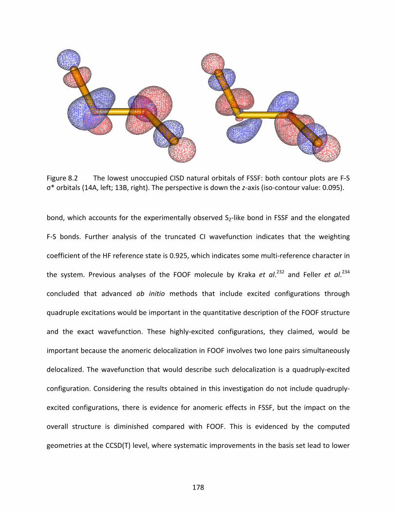
178
bond, which accounts for the experimentally observed S2‐like bond in FSSF and the elongated
F‐S bonds. Further analysis of the truncated CI wavefunction indicates that the weighting
coefficient of the HF reference state is 0.925, which indicates some multi‐reference character in
the system. Previous analyses of the FOOF molecule by Kraka et al.232 and Feller et al.234
concluded that advanced ab initio methods that include excited configurations through
quadruple excitations would be important in the quantitative description of the FOOF structure
and the exact wavefunction. These highly‐excited configurations, they claimed, would be
important because the anomeric delocalization in FOOF involves two lone pairs simultaneously
delocalized. The wavefunction that would describe such delocalization is a quadruply‐excited
configuration. Considering the results obtained in this investigation do not include quadruply‐
excited configurations, there is evidence for anomeric effects in FSSF, but the impact on the
overall structure is diminished compared with FOOF. This is evidenced by the computed
geometries at the CCSD(T) level, where systematic improvements in the basis set lead to lower
Figure 8.2 The lowest unoccupied CISD natural orbitals of FSSF: both contour plots are F‐Sσ* orbitals (14A, left; 13B, right). The perspective is down the z‐axis (iso‐contour value: 0.095).
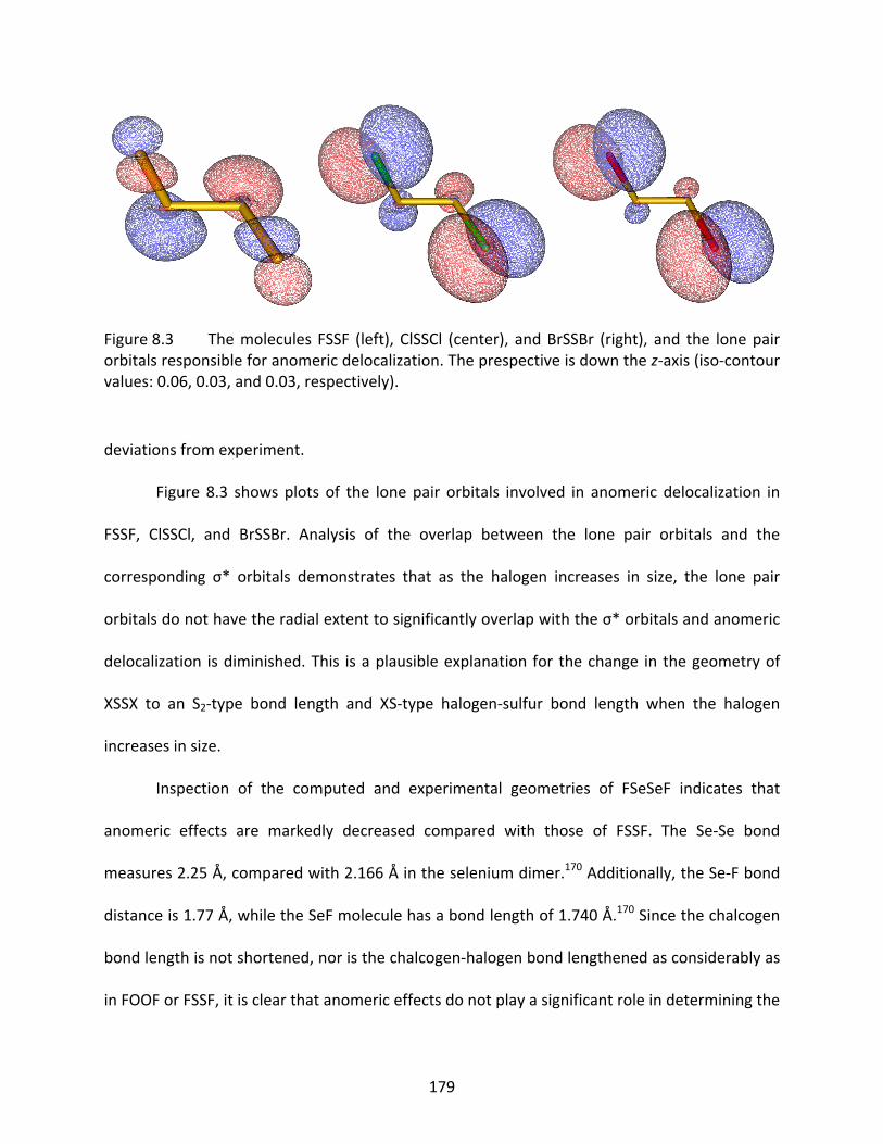
179
deviations from experiment.
Figure 8.3 shows plots of the lone pair orbitals involved in anomeric delocalization in
FSSF, ClSSCl, and BrSSBr. Analysis of the overlap between the lone pair orbitals and the
corresponding σ* orbitals demonstrates that as the halogen increases in size, the lone pair
orbitals do not have the radial extent to significantly overlap with the σ* orbitals and anomeric
delocalization is diminished. This is a plausible explanation for the change in the geometry of
XSSX to an S2‐type bond length and XS‐type halogen‐sulfur bond length when the halogen
increases in size.
Inspection of the computed and experimental geometries of FSeSeF indicates that
anomeric effects are markedly decreased compared with those of FSSF. The Se‐Se bond
measures 2.25 Å, compared with 2.166 Å in the selenium dimer.170 Additionally, the Se‐F bond
distance is 1.77 Å, while the SeF molecule has a bond length of 1.740 Å.170 Since the chalcogen
bond length is not shortened, nor is the chalcogen‐halogen bond lengthened as considerably as
in FOOF or FSSF, it is clear that anomeric effects do not play a significant role in determining the
Figure 8.3 The molecules FSSF (left), ClSSCl (center), and BrSSBr (right), and the lone pairorbitals responsible for anomeric delocalization. The prespective is down the z‐axis (iso‐contourvalues: 0.06, 0.03, and 0.03, respectively).
180
structure of the selenium compounds in this investigation.
The unique structure of these compounds is due to the presence of anomeric
delocalization, and this delocalization is directly related to the radial extent of the lone pair
orbitals. The other factor in determining the impact of anomeric effects in these species is
symmetry. In computations performed at the CCSD(T)/aug‐cc‐pV(T+d)Z level on trans‐FSSF
(C2h), the S‐S bond extends from 1.908 Å to 2.126 Å, and the S‐F bond recedes from 1.641 Å to
1.626 Å. The lone pairs cannot overlap with the F‐S σ* orbitals in this conformation, thus
leaving the structure with a typical disulfide bond length and a S‐F bond length resembling that
of diatomic SF. This is not new to the literature, as it has been reported by Samdal et al.229 for a
variety of dihalo‐μ‐dichalcogenides computed at the HF/6‐31G* level. The present investigation
reports for the first time correlated computations demonstrating that anomeric effects
diminish as the dihedral angle changes. Kraka et al.232 also performed similar computations with
B3LYP and reported that trans‐FOOF has a peroxide‐like structure with O‐F bond lengths similar
to that of molecular FO.
8.4 Conclusions
For the sulfur systems in this investigation, geometries accurate to 0.011 Å are possible
with CCSD(T) and 0.013 Å with B3LYP when the correlation consistent basis sets of quadruple‐ζ
quality are employed. The largest deviations, relative to experimental values occur for the
geometries of FSSF. The geometries of the selenium compounds optimized with CCSD(T)
deviate by no more than 0.111 Å in bond lengths, while B3LYP geometries deviate by as much
as 0.143 Å in bond lengths relative to experiment when computed with the cc‐pVQZ basis set.
181
Bond angles deviate up to 5.07° in CCSD(T)/cc‐pVQZ computations with respect to experiment,
however, overall CCSD(T) angles result in less deviation from experimental values as compared
with B3LYP.
The use of the cc‐pV(n+d)Z basis sets improves the computed geometries at the double‐
and triple‐ζ basis set levels for the CCSD(T) geometries, and, as expected, only slightly improves
B3LYP‐optimized geometries. The inclusion of diffuse functions in the basis has little impact on
the geometry of the species investigated here. For the computed harmonic vibrational
frequencies, the maximum deviation from experimental values is almost 67 cm‐1, which is
attributed to damping from Br2 impurities in one of the experimental studies referenced on
BrSSBr. Other compounds have computed frequencies that deviate no more than 25 cm‐1.
Computed anharmonic effects of the FSSF molecule revealed that their impact on bond lengths
and harmonic frequencies is negligible.
Anomeric effects have been investigated by others as the source of the unique
geometry of the FOOF molecule. The current investigation shows that the impact of anomeric
delocalization on FSSF is decreased as compared with the impact on FOOF, and that it has
almost no impact on the structure of FSeSeF. Upon increasing the halogen size to chlorine and
bromine, the radial extent of the lone pair orbitals is not sufficient for significant overlap with
the appropriate σ* orbitals, and thus anomeric effects on the geometric structure are almost
nonexistent. When FSSF is rotated into the trans conformation, anomeric delocalization cannot
occur due to broken symmetry. The natural consequence of this is an increase in S‐S bond
length and a decrease in the S‐F bond length.
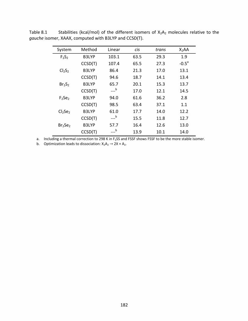
182
Table 8.1 Stabilities (kcal/mol) of the different isomers of X2A2 molecules relative to the gauche isomer, XAAX, computed with B3LYP and CCSD(T).
System Method Linear cis trans X2AA
F2S2 B3LYP 103.1 63.5 29.3 1.9 CCSD(T) 107.4 65.5 27.3 ‐0.5a
Cl2S2 B3LYP 86.4 21.3 17.0 13.1 CCSD(T) 94.6 18.7 14.1 13.4
Br2S2 B3LYP 65.7 20.1 15.3 13.7 CCSD(T) ‐‐‐b 17.0 12.1 14.5
F2Se2 B3LYP 94.0 61.6 36.2 2.8 CCSD(T) 98.5 63.4 37.1 1.1
Cl2Se2 B3LYP 61.0 17.7 14.0 12.2 CCSD(T) ‐‐‐b 15.5 11.8 12.7
Br2Se2 B3LYP 57.7 16.4 12.6 13.0 CCSD(T) ‐‐‐b 13.9 10.1 14.0
a. Including a thermal correction to 298 K in F2SS and FSSF shows FSSF to be the more stable isomer. b. Optimization leads to dissociation: X2A2 2X + A2.
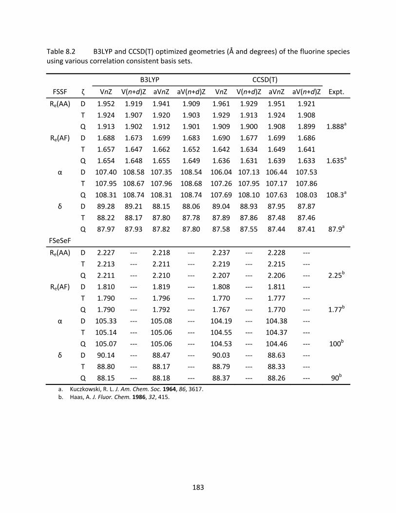
183
Table 8.2 B3LYP and CCSD(T) optimized geometries (Å and degrees) of the fluorine species using various correlation consistent basis sets.
B3LYP CCSD(T)
FSSF ζ VnZ V(n+d)Z aVnZ aV(n+d)Z VnZ V(n+d)Z aVnZ aV(n+d)Z Expt.
Re(AA) D 1.952 1.919 1.941 1.909 1.961 1.929 1.951 1.921
T 1.924 1.907 1.920 1.903 1.929 1.913 1.924 1.908
Q 1.913 1.902 1.912 1.901 1.909 1.900 1.908 1.899 1.888a
Re(AF) D 1.688 1.673 1.699 1.683 1.690 1.677 1.699 1.686
T 1.657 1.647 1.662 1.652 1.642 1.634 1.649 1.641
Q 1.654 1.648 1.655 1.649 1.636 1.631 1.639 1.633 1.635a
α D 107.40 108.58 107.35 108.54 106.04 107.13 106.44 107.53
T 107.95 108.67 107.96 108.68 107.26 107.95 107.17 107.86
Q 108.31 108.74 108.31 108.74 107.69 108.10 107.63 108.03 108.3a
δ D 89.28 89.21 88.15 88.06 89.04 88.93 87.95 87.87
T 88.22 88.17 87.80 87.78 87.89 87.86 87.48 87.46
Q 87.97 87.93 87.82 87.80 87.58 87.55 87.44 87.41 87.9a
FSeSeF
Re(AA) D 2.227 ‐‐‐ 2.218 ‐‐‐ 2.237 ‐‐‐ 2.228 ‐‐‐
T 2.213 ‐‐‐ 2.211 ‐‐‐ 2.219 ‐‐‐ 2.215 ‐‐‐
Q 2.211 ‐‐‐ 2.210 ‐‐‐ 2.207 ‐‐‐ 2.206 ‐‐‐ 2.25b
Re(AF) D 1.810 ‐‐‐ 1.819 ‐‐‐ 1.808 ‐‐‐ 1.811 ‐‐‐
T 1.790 ‐‐‐ 1.796 ‐‐‐ 1.770 ‐‐‐ 1.777 ‐‐‐
Q 1.790 ‐‐‐ 1.792 ‐‐‐ 1.767 ‐‐‐ 1.770 ‐‐‐ 1.77b
α D 105.33 ‐‐‐ 105.08 ‐‐‐ 104.19 ‐‐‐ 104.38 ‐‐‐
T 105.14 ‐‐‐ 105.06 ‐‐‐ 104.55 ‐‐‐ 104.37 ‐‐‐
Q 105.07 ‐‐‐ 105.06 ‐‐‐ 104.53 ‐‐‐ 104.46 ‐‐‐ 100b
δ D 90.14 ‐‐‐ 88.47 ‐‐‐ 90.03 ‐‐‐ 88.63 ‐‐‐
T 88.80 ‐‐‐ 88.17 ‐‐‐ 88.79 ‐‐‐ 88.33 ‐‐‐
Q 88.15 ‐‐‐ 88.18 ‐‐‐ 88.37 ‐‐‐ 88.26 ‐‐‐ 90b
a. Kuczkowski, R. L. J. Am. Chem. Soc. 1964, 86, 3617. b. Haas, A. J. Fluor. Chem. 1986, 32, 415.
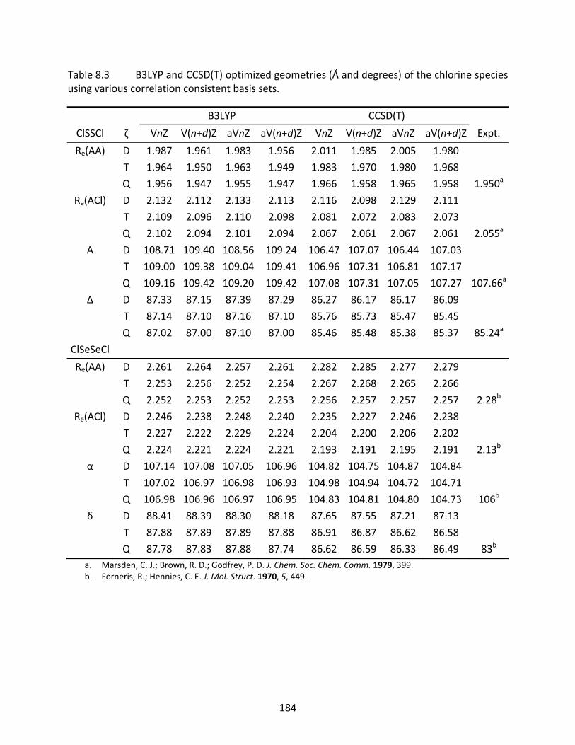
184
Table 8.3 B3LYP and CCSD(T) optimized geometries (Å and degrees) of the chlorine species using various correlation consistent basis sets.
B3LYP CCSD(T)
ClSSCl ζ VnZ V(n+d)Z aVnZ aV(n+d)Z VnZ V(n+d)Z aVnZ aV(n+d)Z Expt.
Re(AA) D 1.987 1.961 1.983 1.956 2.011 1.985 2.005 1.980
T 1.964 1.950 1.963 1.949 1.983 1.970 1.980 1.968
Q 1.956 1.947 1.955 1.947 1.966 1.958 1.965 1.958 1.950a
Re(ACl) D 2.132 2.112 2.133 2.113 2.116 2.098 2.129 2.111
T 2.109 2.096 2.110 2.098 2.081 2.072 2.083 2.073
Q 2.102 2.094 2.101 2.094 2.067 2.061 2.067 2.061 2.055a
Α D 108.71 109.40 108.56 109.24 106.47 107.07 106.44 107.03
T 109.00 109.38 109.04 109.41 106.96 107.31 106.81 107.17
Q 109.16 109.42 109.20 109.42 107.08 107.31 107.05 107.27 107.66a
Δ D 87.33 87.15 87.39 87.29 86.27 86.17 86.17 86.09
T 87.14 87.10 87.16 87.10 85.76 85.73 85.47 85.45
Q 87.02 87.00 87.10 87.00 85.46 85.48 85.38 85.37 85.24a
ClSeSeCl
Re(AA) D 2.261 2.264 2.257 2.261 2.282 2.285 2.277 2.279
T 2.253 2.256 2.252 2.254 2.267 2.268 2.265 2.266
Q 2.252 2.253 2.252 2.253 2.256 2.257 2.257 2.257 2.28b
Re(ACl) D 2.246 2.238 2.248 2.240 2.235 2.227 2.246 2.238
T 2.227 2.222 2.229 2.224 2.204 2.200 2.206 2.202
Q 2.224 2.221 2.224 2.221 2.193 2.191 2.195 2.191 2.13b
α D 107.14 107.08 107.05 106.96 104.82 104.75 104.87 104.84
T 107.02 106.97 106.98 106.93 104.98 104.94 104.72 104.71
Q 106.98 106.96 106.97 106.95 104.83 104.81 104.80 104.73 106b
δ D 88.41 88.39 88.30 88.18 87.65 87.55 87.21 87.13
T 87.88 87.89 87.89 87.88 86.91 86.87 86.62 86.58
Q 87.78 87.83 87.88 87.74 86.62 86.59 86.33 86.49 83b
a. Marsden, C. J.; Brown, R. D.; Godfrey, P. D. J. Chem. Soc. Chem. Comm. 1979, 399. b. Forneris, R.; Hennies, C. E. J. Mol. Struct. 1970, 5, 449.

185
Table 8.4 B3LYP and CCSD(T) optimized geometries (Å and degrees) of the bromine species using various correlation consistent basis sets.
B3LYP CCSD(T)
BrSSBr ζ VnZ V(n+d)Z aVnZ aV(n+d)Z VnZ V(n+d)Z aVnZ aV(n+d)Z Expt.
Re(AA) D 1.992 1.961 1.988 1.957 2.017 1.987 2.014 1.984
T 1.969 1.952 1.968 1.952 1.991 1.977 1.990 1.975
Q 1.960 1.950 1.960 1.950 1.975 1.966 1.974 1.965 1.980a
Re(ABr) D 2.293 2.288 2.294 2.290 2.282 2.276 2.291 2.286
T 2.273 2.270 2.274 2.270 2.244 2.241 2.245 2.242
Q 2.269 2.267 2.269 2.267 2.231 2.229 2.231 2.230 2.24a
α D 109.35 110.01 109.18 109.90 106.83 107.44 106.69 107.33
T 109.56 109.98 109.64 109.98 107.16 107.50 107.04 107.38
Q 109.77 110.01 109.77 110.01 107.21 107.44 107.17 107.41 105a
δ D 87.29 87.37 87.33 87.61 85.59 85.68 85.53 85.65
T 86.99 87.06 86.98 87.06 85.06 85.11 84.62 84.70
Q 86.99 87.01 86.99 87.01 84.70 84.76 84.51 84.55 83.5a
BrSeSeBr
Re(AA) D 2.267 ‐‐‐ 2.263 ‐‐‐ 2.290 ‐‐‐ 2.286 ‐‐‐
T 2.259 ‐‐‐ 2.258 ‐‐‐ 2.276 ‐‐‐ 2.275 ‐‐‐
Q 2.257 ‐‐‐ 2.257 ‐‐‐ 2.266 ‐‐‐ 2.266 ‐‐‐ 2.28b
Re(ABr) D 2.401 ‐‐‐ 2.405 ‐‐‐ 2.393 ‐‐‐ 2.404 ‐‐‐
T 2.386 ‐‐‐ 2.387 ‐‐‐ 2.363 ‐‐‐ 2.364 ‐‐‐
Q 2.383 ‐‐‐ 2.383 ‐‐‐ 2.351 ‐‐‐ 2.351 ‐‐‐ 2.24b
α D 107.85 ‐‐‐ 107.76 ‐‐‐ 105.12 ‐‐‐ 105.03 ‐‐‐
T 107.72 ‐‐‐ 107.73 ‐‐‐ 105.21 ‐‐‐ 104.94 ‐‐‐
Q 107.69 ‐‐‐ 107.71 ‐‐‐ 104.92 ‐‐‐ 104.94 ‐‐‐ 106b
δ D 88.28 ‐‐‐ 88.15 ‐‐‐ 86.86 ‐‐‐ 86.50 ‐‐‐
T 87.88 ‐‐‐ 87.84 ‐‐‐ 86.10 ‐‐‐ 86.73 ‐‐‐
Q 87.80 ‐‐‐ 87.68 ‐‐‐ 85.58 ‐‐‐ 85.56 ‐‐‐ 83b
a. Hirota, E. Bull. Chem. Soc. Jpn. 1958, 31, 130. b. Forneris, R.; Hennies, C. E. J. Mol. Struct. 1970, 5, 449.
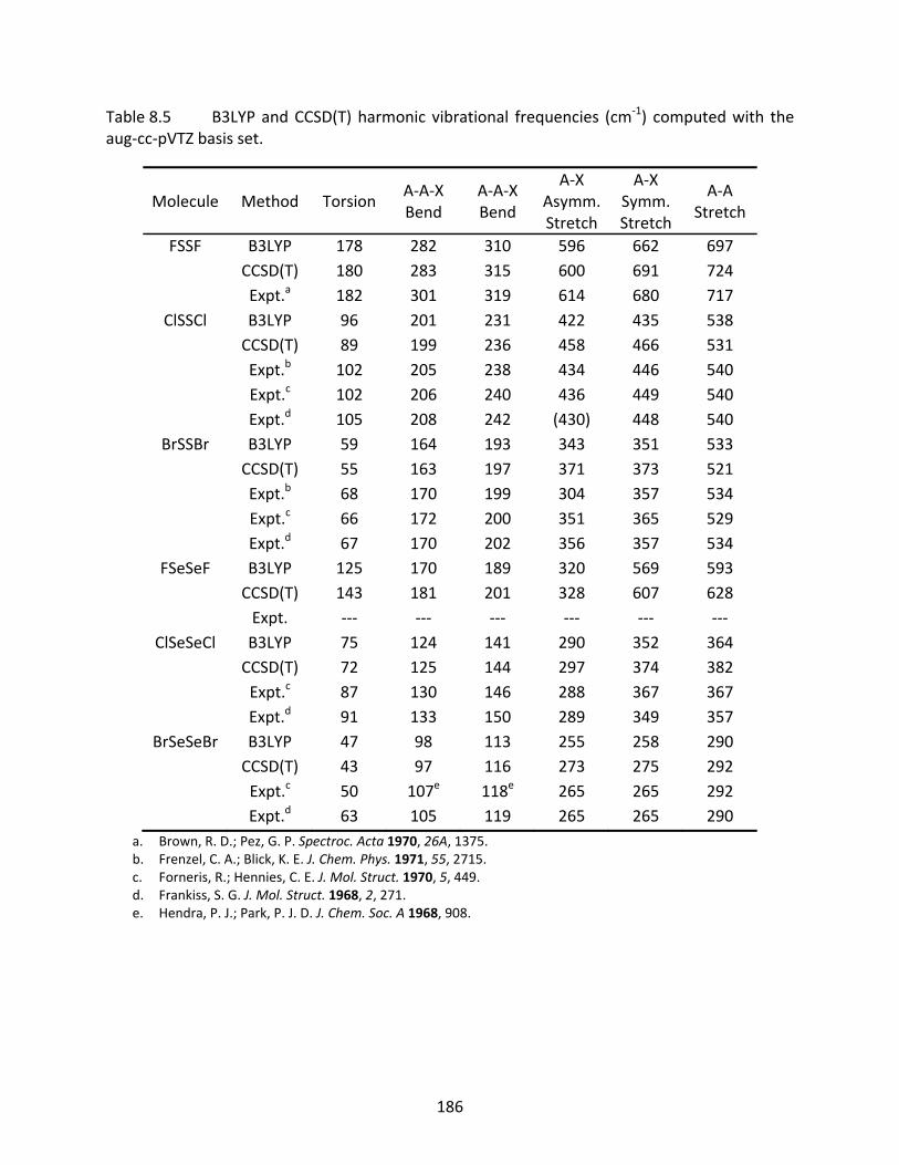
186
Table 8.5 B3LYP and CCSD(T) harmonic vibrational frequencies (cm‐1) computed with the aug‐cc‐pVTZ basis set.
Molecule Method Torsion A‐A‐X Bend
A‐A‐X Bend
A‐X Asymm. Stretch
A‐X Symm. Stretch
A‐A Stretch
FSSF B3LYP 178 282 310 596 662 697 CCSD(T) 180 283 315 600 691 724 Expt.a 182 301 319 614 680 717
ClSSCl B3LYP 96 201 231 422 435 538 CCSD(T) 89 199 236 458 466 531 Expt.b 102 205 238 434 446 540 Expt.c 102 206 240 436 449 540 Expt.d 105 208 242 (430) 448 540
BrSSBr B3LYP 59 164 193 343 351 533 CCSD(T) 55 163 197 371 373 521 Expt.b 68 170 199 304 357 534 Expt.c 66 172 200 351 365 529 Expt.d 67 170 202 356 357 534
FSeSeF B3LYP 125 170 189 320 569 593 CCSD(T) 143 181 201 328 607 628 Expt. ‐‐‐ ‐‐‐ ‐‐‐ ‐‐‐ ‐‐‐ ‐‐‐
ClSeSeCl B3LYP 75 124 141 290 352 364 CCSD(T) 72 125 144 297 374 382 Expt.c 87 130 146 288 367 367 Expt.d 91 133 150 289 349 357
BrSeSeBr B3LYP 47 98 113 255 258 290 CCSD(T) 43 97 116 273 275 292 Expt.c 50 107e 118e 265 265 292 Expt.d 63 105 119 265 265 290
a. Brown, R. D.; Pez, G. P. Spectroc. Acta 1970, 26A, 1375. b. Frenzel, C. A.; Blick, K. E. J. Chem. Phys. 1971, 55, 2715. c. Forneris, R.; Hennies, C. E. J. Mol. Struct. 1970, 5, 449. d. Frankiss, S. G. J. Mol. Struct. 1968, 2, 271. e. Hendra, P. J.; Park, P. J. D. J. Chem. Soc. A 1968, 908.
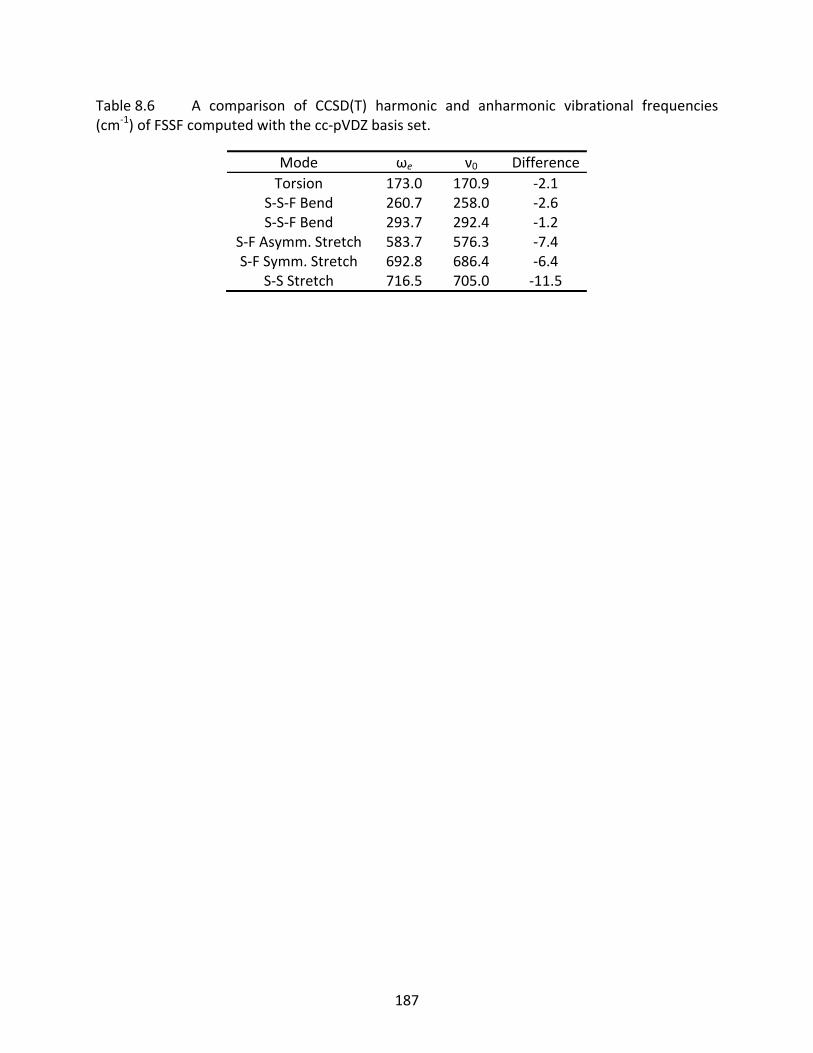
187
Table 8.6 A comparison of CCSD(T) harmonic and anharmonic vibrational frequencies (cm‐1) of FSSF computed with the cc‐pVDZ basis set.
Mode ωe ν0 Difference Torsion 173.0 170.9 ‐2.1
S‐S‐F Bend 260.7 258.0 ‐2.6 S‐S‐F Bend 293.7 292.4 ‐1.2
S‐F Asymm. Stretch 583.7 576.3 ‐7.4 S‐F Symm. Stretch 692.8 686.4 ‐6.4
S‐S Stretch 716.5 705.0 ‐11.5
188
CHAPTER 9
A SYSTEMATIC INVESTIGATION OF GERMANIUM ARSENIDES†
9.1 Introduction
Compounds containing heavy group 14 and 15 elements, especially compounds with
multiple bonds, have received considerable attention over the past three decades by both
experimentalists and theoreticians.247‐263 The surge in interest in these compounds came after
the synthesis of several non‐transient multiply‐bonded phosphorus and silicon systems in 1981,
and these species have been the subject of several reviews.250,252,260‐263 Before that time, it was
believed that multiple bonds between heavy main group elements would likely not exist due to
the so‐called double‐bond rule, which stated that elements such as silicon and phosphorus
would exhibit weak π bonds formed by their p orbitals.259,264 Subsequent attempts to synthesize
these types of compounds failed since the molecules would oligomerize in solution. The
oligomerization was found to be reduced by incorporating large, bulky substituents on the
heavy main group atoms.250,260 Since that time, several compounds that have multiply‐bonded
group 14 and 15 elements with low coordination numbers (i.e. P2, Si2, SiC, PC, etc.) have been
reported. However, compounds that are not found in earlier reviews are those with germanium
multiply‐bonded to an arsenic atom – so called arsagermenes and arsagermynes (germanium
doubly‐ and triply‐bonded to arsenic, respectively). While it is purported that these types of
systems should exist, and could be synthesized via similar mechanisms as analogous silicon
† This entire chapter is adapted from B.P. Prascher, A.M. Kavi, B. Mintz, S.M. Yockel, and A.K. Wilson, “Theoretical Investigation of the Germanium Arsenides,” Chem. Phys., 2008, 353(1‐3), 209, with permission from Elsevier.
189
phosphide systems, no such studies have been reported.
Germanium arsenides are important in various research fields. Although gallium
arsenides are routinely encountered in solid state research, germanium arsenide materials such
as GeAsS glasses and MGeAs2 (M = Zn, Cd) are of interest for their nonlinear optical properties
and electrical properties. Germanium arsenide materials have been studied both by
experimentalists and by theoreticians for their applications in solar cells and as ternary
semiconductors.247,248 Another example of an exotic germanium arsenide is the material
(Ge38As8)8+ ∙ 8 I‐, which has been characterized by x‐ray and neutron diffraction, and is a known
N‐type semiconductor.253
The only previous computational investigation of the germanium arsenide molecules
considered in the present study was performed by Lai et al.258 They utilized both correlated ab
initio methodology and density functional theory (DFT) with the 6‐311++G(d,p) and
6‐311++G(3df,3pd) basis sets (triple‐ζ quality basis sets with diffuse and polarization functions)
to describe the structures, bonding characteristics, and relative stabilities of L‐GeAs and GeAs‐L
molecules. They computed that the most stable L‐GeAs molecule of their test set should be
H2N‐GeAs, while the most stable GeAs‐L molecule should be GeAs‐AlH2. Further, Lai et al.
predicted with DFT that, for L = F, OH, and CH3, the GeAs‐L isomer should be more stable than
L‐GeAs, while their ab initio predictions showed the opposite (i.e. the L‐GeAs isomer is more
stable for these L groups). This apparent discrepancy between DFT and correlated ab initio
methodology has prompted this systematic re‐investigation of Lai’s molecules.
One of the differences between the present investigation and that of Lai et al.258 is the
use of the correlation consistent basis sets, cc‐pVnZ.94‐101 The systematic construction of the
190
correlation consistent basis sets leads to monotonic convergence towards the complete basis
set (CBS) limit of many energetic properties as the basis set size increases93 – a property not
inherent to the basis sets used by Lai et al.265
The present investigation reexamines the GeAs‐L and L‐GeAs molecules studied by Lai et
al.258 (where L = H, Li, Na, BeH, MgH, BH2, AlH2, CH3, SiH3, NH2, PH2, OH, SH, F, and Cl; and has
been extended to include Br) Reported are transition state energies, enthalpies of formation at
298 K, and enthalpies of isomerization at 298 K. Typically, the threshold for chemical accuracy
of main group molecules is considered to be 1.0 kcal/mol. To achieve this threshold of chemical
accuracy for third row, main group systems, it has been shown that scalar relativistic and spin‐
orbit effects must be included.62,266‐271 Since this is a predictive investigation into the properties
of third row, main group molecules yet to be characterized by experiment, relativistic effects
cannot be ignored.
9.2 Computational Methodology
Coupled cluster with single, double, and non‐iterative, perturbative triple excitations,
CCSD(T), is used.31,38 In addition, the hybrid three‐parameter exchange functional of Becke
(B3)166 coupled with the Lee‐Yang‐Parr (LYP)165 correlation functional, B3LYP, has been
employed. In all B3LYP computations, the third parameterization of the Vosko‐Wilk‐Nusair local
correlation functional (VWN‐3) is invoked.167
The correlation consistent basis sets94‐101 of double‐ through quadruple‐ζ quality have
been employed. For germanium arsenides that contain an alkali or alkaline earth metal, new
cc‐pVnZ basis sets discussed in Chapter 6 have been used; while for atoms in the second row of
191
the periodic table (Na, Mg, and Al‐Ar), the tight d correlation consistent basis sets,
cc‐pV(n+d)Z101 have been employed. To compute CBS limits, the exponential (3.2) and mixed
Gaussian/exponential (3.3) extrapolation schemes have been employed.85,95,132
The geometries of the L‐GeAs and GeAs‐L systems were fully optimized using both
B3LYP and CCSD(T) at each basis set level. Zero‐point energies were computed from cc‐pVTZ
harmonic vibrational frequencies using each method. Classical barriers were computed from
transition state structures with exactly one imaginary frequency along the isomerization
pathway. Enthalpies of formation and enthalpies of isomerization were determined using the
equations of Ockterski272 from atomic enthalpies of formation at 100 kPa and 298 K.195,273 All
B3LYP computations were performed using the Gaussian 03 software suite,174 while CCSD(T)
computations were performed using the Molpro software package.180
Scalar relativistic corrections for both the CCSD(T) and B3YLP energetics were
determined using both the Cowan‐Griffin (CG)274 and the second‐order, spin‐free Douglas‐Kroll
(DK) Hamiltonians.135‐137 The DK approach is variational, while the CG (perturbative) approach is
not.141,275 Relativistic corrections were computed using the B3LYP/cc‐pVTZ geometry at each
basis set level, since scalar relativistic effects are not very sensitive to changes in the
geometry.276 Spin‐orbit (SO) coupling of the L‐GeAs and GeAs‐L molecules is neglected because
they are closed shell molecules. First‐order SO corrections (see Table 9.1) are included a
posteriori in the atomic energies since the spin‐free implementations of the CG and DK
Hamiltonians do not include it intrinsically. These SO corrections were computed using multi‐
configuration self‐consistent field (MCSCF) wavefunctions and the Breit‐Pauli spin‐orbit
Hamiltonian180,277 implemented in the Molpro software package.
192
9.3 Results and Discussion
9.3.1 Optimized Structures
The bonding characteristics of L‐GeAs and GeAs‐L systems have been discussed in some
detail by Lai et al.258 The structures of L‐GeAs systems are linear, or very close to linear, and
exhibit a triple bond between the germanium and arsenic atoms not unlike a cyanide group.
However, the GeAs‐L systems exhibit a strongly bent structure as opposed to the linear
structure of an isocyanide molecule. Instead, there is a double bond between the germanium
and arsenic atoms, with a lone pair on the arsenic atom, resembling an extremely bent imine‐
type structure. The decrease in bond order in migrating the L group from the germanium to the
arsenic atom is reinforced by the increase in the Ge‐As bond length. For example (cf. Table 9.2
and Table 9.3), in the optimized structures of the L‐GeAs molecules of this study, the Ge‐As
bond length falls in the range of 2.134 – 2.187 Å for CCSD(T) and 2.106 – 2.149 Å for B3LYP.
Further evidence to support a triple bond between germanium and arsenic in the L‐GeAs
molecules is that the bond lengths resemble that of the arsenic dimer, which has a formal triple
bond and bond length of 2.103 Å.170 The Ge‐As bond length in the optimized structures of the
GeAs‐L molecules falls in the range of 2.222 – 2.389 Å for CCSD(T) and 2.205 – 2.370 Å for
B3LYP, resembling that of the GeAs diatomic at 2.283 Å.270 The Ge‐As‐L angle remains rather
small, even when L groups that are highly electropositive or highly electronegative are used,
making the bonding characteristics of germanium arsenides unique among main group
molecules.
In Table 9.2 and Table 9.3 the CCSD(T)‐ and B3LYP‐optimized geometries for the
193
different L groups of this study are listed. The results of Lai et al.258, which are included for
comparison in the tables, were computed using CCSD(T)/6‐311G++(3df,3pd)//
B3LYP/6‐311G++(d,p). Overall, for the L‐GeAs molecules optimized with CCSD(T), the L‐Ge and
Ge‐As bond lengths differ up to 0.057 Å and 0.049 Å, respectively, when compared with the
results of Lai et al. The same bond lengths differ up to 0.024 Å and 0.006 Å, respectively, when
optimized with B3LYP. The largest differences between the bond lengths of Lai et al. and this
study are in the CCSD(T) geometries of Li‐GeAs, Na‐GeAs, HBe‐GeAs, and HMg‐GeAs. The small
difference between the B3LYP results and those previously published reaffirms the fact that
B3LYP bond lengths for these species are not very basis set dependent. The average difference
between results reported here and those of Lai et al. are 0.017 Å and 0.007 Å for the L‐Ge bond
length and 0.029 Å and 0.004 Å for the Ge‐As bond length, for CCSD(T) and B3LYP, respectively.
In the GeAs‐L molecules, the variations between previously published bond lengths and
those of this study are more dramatic. The CCSD(T)‐optimized As‐L and Ge‐As bond lengths
differ the most from previous work258 up to 0.216 Å and 0.147 Å, respectively. However, the
B3LYP As‐L and Ge‐As bond lengths show less dramatic differences with respective variations
up to 0.108 Å and 0.162 Å. The largest differences between both the CCSD(T) and B3LYP bond
lengths and those of Lai et al.258 arise in the GeAs‐AlH2 molecule. Also, the increased variation
in bond lengths between the B3LYP results and those previously published indicate that B3LYP
is more sensitive to the choice of basis set for GeAs‐L systems, compared with the L‐GeAs
systems.
Bond angles are affected more than bond lengths in both the L‐GeAs and GeAs‐L
systems, however, the qualitative structure remains the same as previously reported – the
194
L‐GeAs systems are linear in X‐Ge‐As (within 5.0°), where X is the non‐hydrogen atom of the L
group, and GeAs‐L systems are severely bent in the Ge‐As‐X angle. In both the CCSD(T)‐ and
B3LYP‐optimized structures of the L‐GeAs molecules, the differences in the bond angles are in
the range 0.0 – 5.0°, compared with Lai et al.,258 but the differences in the bond angles of the
GeAs‐L molecules are in the range of 0.0 – 26.4°. The largest differences between the computed
bond angles and those of Lai et al. occur in the GeAs‐OH molecule with CCSD(T), and in the
GeAs‐AlH2 molecule with both CCSD(T) and B3LYP. Upon closer examination, the B3LYP/
6‐311++G(d,p) structures of the HO‐GeAs and GeAs‐OH isomers that Lai et al. reported were
reproduced, and it was found that explicit optimization with CCSD(T)/cc‐pVnZ, as performed in
this investigation, is responsible for the large variation in the bond angle.
Comparing the CCSD(T) to the B3LYP optimized geometries, the largest differences
between the two methods are: in the Ge‐F bond length (0.056 Å at the cc‐pVQZ level); in the
As‐OH bond length (0.186 Å at the cc‐pVTZ level); and in the Ge‐As bond length of the L‐GeAs
isomers, the largest differences between the two methods are 0.054 Å (L‐GeAs isomers) in
HBe‐GeAs at the cc‐pVTZ and cc‐pVQZ levels and 0.083 Å (GeAs‐L isomers) in GeAs‐Br at the
cc‐pVQZ level. Further, the X‐Ge‐As and Ge‐As‐X bond angles vary between the two methods up
to 3.7° and 38.1°, respectively. In general, CCSD(T) and B3LYP agree on the linearity of the
L‐GeAs molecules, however, the ranges of the bond lengths and angles of the GeAs‐L molecules
are significantly different between the two methods. The average differences in the geometries
of CCSD(T) compared with B3LYP are 0.014 Å in the Ge‐L bond, 0.031 Å in the Ge‐As bond of the
L‐GeAs isomers, 0.034 Å in the As‐L bond, 0.023 Å in the Ge‐As bond of the GeAs‐L isomers,
0.28° in the L‐Ge‐As angle, and 5.23° in the Ge‐As‐L angle.
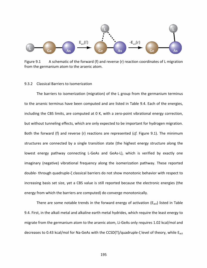
195
9.3.2 Classical Barriers to Isomerization
The barriers to isomerization (migration) of the L group from the germanium terminus
to the arsenic terminus have been computed and are listed in Table 9.4. Each of the energies,
including the CBS limits, are computed at 0 K, with a zero‐point vibrational energy correction,
but without tunneling effects, which are only expected to be important for hydrogen migration.
Both the forward (f) and reverse (r) reactions are represented (cf. Figure 9.1). The minimum
structures are connected by a single transition state (the highest energy structure along the
lowest energy pathway connecting L‐GeAs and GeAs‐L), which is verified by exactly one
imaginary (negative) vibrational frequency along the isomerization pathway. These reported
double‐ through quadruple‐ζ classical barriers do not show monotonic behavior with respect to
increasing basis set size, yet a CBS value is still reported because the electronic energies (the
energy from which the barriers are computed) do converge monotonically.
There are some notable trends in the forward energy of activation (Eact) listed in Table
9.4. First, in the alkali metal and alkaline earth metal hydrides, which require the least energy to
migrate from the germanium atom to the arsenic atom, Li‐GeAs only requires 1.02 kcal/mol and
decreases to 0.43 kcal/mol for Na‐GeAs with the CCSD(T)/quadruple‐ζ level of theory, while Eact
Figure 9.1 A schematic of the forward (f) and reverse (r) reaction coordinates of L migrationfrom the germanium atom to the arsenic atom.
196
for HBe‐GeAs is 3.57 kcal/mol and decreases to 1.44 kcal/mol in HMg‐GeAs. A similar trend
holds for both computational methods at the quadruple‐ζ level, and in each of the other L
groups in the forward reaction: the larger the non‐hydrogen atom in the L substituent within
the periodic table group, the lower the Eact. For example, in the main group species, H3C‐GeAs
has an Eact = 24.20 kcal/mol versus H3Si‐GeAs with an Eact = 6.00 kcal/mol. The halogens, which
also follow the preceding trend, vary by less than 1.0 kcal/mol between one another in the
forward Eact. For example, the L = F, Cl, and Br values for Eact are 15.15, 14.96, and
14.68 kcal/mol, respectively for CCSD(T), and are 12.25, 11.93, and 11.23 kcal/mol, respectively
for B3LYP. Further, the forward value of Eact increases as the size of the non‐hydrogen atom
increases across the period, peaking at L = NH2 and PH2 in each period.
The same trend of increasing Eact values down a periodic group is also observed in the
reverse migration of the L = Li, Na, BeH, and MgH molecules, but is reversed for substituents of
the main group. For example, for GeAs‐BH2, the reverse Eact value is 15.63 kcal/mol and
increases to 18.38 kcal/mol when AlH2 is substituted for BH2 at the CCSD(T)/quadruple‐ζ level of
theory; the Eact is 21.48 kcal/mol for GeAs‐CH3 and increases to 22.61 kcal/mol for GeAs‐SiH3;
etc. The halogens do not have as similar Eact values in the reverse migration, where for L = F, Cl,
and Br the energies are 12.12, 18.39, and 18.34 kcal/mol at the CCSD(T)/quadruple‐ζ level.
Similar trends occur with B3LYP at the quadruple‐ζ basis set level, except that the reverse Eact
value is 19.32 kcal/mol for GeAs‐BH2 and decreases to 16.06 kcal/mol for AlH2.
The computed CCSD(T) and B3LYP Eact values differ significantly (>1.0 kcal/mol) from one
another for several of the molecules studied here. The variations in the activation energies
between CCSD(T) and B3LYP are tabulated in a supplemental table accompanying this
197
manuscript. Overall, the mean absolute difference is 2.42 kcal/mol for the forward Eact and
2.12 kcal/mol for the reverse Eact at the quadruple‐ζ basis set level between the two
computational methods. The absolute differences range from 0.07 kcal/mol in the forward Eact
for L = Li to as large as 9.31 kcal/mol in the reverse Eact for L = OH. The large variation in the
L = OH barrier is likely attributed to the large angle difference computed with our methodology
(see previous section for discussion). These variations between CCSD(T) and B3LYP indicate the
sensitivity of the barrier heights to the choice of method since the same basis sets are used
with each method.
9.3.3 Thermochemistry and Relative Stabilities
The enthalpies of formation reported here show how much energy is required to form
the molecule from the gas phase atoms. Table 9.5 and Table 9.6 include the CCSD(T)‐ and
B3LYP‐computed enthalpies of formation at 298 K for L‐GeAs and GeAs‐L, respectively, while
Table 9.7 lists the enthalpies of isomerization at 298 K. Included in the supplemental tables of
this article are the atomization energies of the CCSD(T) and B3LYP‐optimized structures of this
investigation.
The computed SO corrections in Table 9.1 agree with those referenced by Kedziora et
al.255 It is obvious from Table 9.5 and Table 9.6 that the impact of including scalar relativistic
and SO effects is significant (>1.0 kcal/mol). Consider the CG and the DK relativistic corrections
together for the entire test set. In all systems, except for L = Br, the relativistic contribution to
the enthalpies of formation of the L‐GeAs systems can be as large as 6.93 kcal/mol, while the
contribution is as large as 5.48 kcal/mol for the GeAs‐L systems. In the bromine systems, the
198
relativistic contributions are 9.20 kcal/mol for Br‐GeAs and 7.60 kcal/mol for GeAs‐Br, and are
the highest in the test set due to the presence of three third row, main group atoms. Overall,
the CG and DK corrections are similar for each molecule. The largest difference between the
two relativistic corrections is approximately 3 kcal/mol for the L = SiH3 molecules at the cc‐pVDZ
level.
Table 9.7 lists the enthalpies of isomerization at 298 K in the migration of the L group
from the germanium terminus to the arsenic terminus. The advantage of computing the
enthalpies of isomerization instead of simply computing the difference in classical barrier
heights as an indication of relative stability is that the former takes into account thermal effects
in the synthesis of the respective isomers. It is observed, from the non‐relativistic CCSD(T)
enthalpies in Table 9.7 (cf. Figure 9.2), that the GeAs‐L isomer is more stable than the L‐GeAs
isomer for each L group except L = NH2, OH, and F. The same is true of the non‐relativistic
B3LYP isomerization enthalpies for L = NH2 and F. Both L = CH3 and F have little appreciable
difference in the non‐relativistic B3LYP energy difference between the two isomers. For L = F,
non‐relativistic CCSD(T) with larger basis sets shows L‐GeAs to be the more stable isomer, but
including either the CG or DK corrections shows the GeAs‐L isomer to be more stable. The same
is true of the B3LYP non‐relativistic versus relativistic stabilities. The relative stabilities of the
isomers computed here using non‐relativistic B3LYP are in agreement with those of Lai et al.,
except in the case of L = F. Further, the CCSD(T) results show GeAs‐CH3 to be the more stable
isomer, and the GeAs‐OH isomer of this study is computed to be almost 10 kcal/mol more
stable than previously reported.
The choice of basis set can significantly affect the computed enthalpy of formation and
199
enthalpy of isomerization (cf. Table 9.5, Table 9.6, and Table 9.7). For example, increasing the
basis set from cc‐pVDZ to cc‐pVTZ lowers the enthalpy of formation of the L‐GeAs systems an
average of 20.00 kcal/mol, while increasing from cc‐pVTZ to cc‐pVQZ further lowers the
enthalpy of formation an average of 7.19 kcal/mol.
9.4 Conclusions
This investigation has reported energy‐minimized structures, classical barriers heights,
enthalpies of formation, and enthalpies of isomerization computed with both CCSD(T) and
B3LYP. In terms of optimized geometries, it is observed that both CCSD(T) and B3LYP agree
qualitatively for all of the molecules under investigation, but do not always agree quantitatively
(within 0.01 Å for bond lengths, and 1.0° in bond angles). The most notable differences
between the two computational methods stem from the GeAs‐L systems. Comparing structures
computed here with those of Lai et al., it is observed that the largest differences in the L‐GeAs
molecules occur when L = Li, Na, BeH, and MgH, while the largest differences in the GeAs‐L
molecules occur when L = AlH2.
In the computation of classical barrier heights, it is observed in the forward migration
reaction that the heavier the L substituent within a column of the periodic table, the lower the
energy of activation. Also, as the non‐hydrogen atom in the L substituent increases across the
periodic table, the forward activation energy increases, peaking at L = NH2 and PH2, then
decreasing. In the reverse migration reaction, the same trends hold for group 1 and 2
substituents, but the main group substituents follow an opposite trend of increasing the
activation energy upon reverse migration. The only exception to these periodic trends
200
encountered is in the B3LYP/quadruple‐ζ reverse energies of activation of L = BH2 and AlH2.
Predicted enthalpies of formation and isomerization agree within approximately
3 kcal/mol between CCSD(T) and B3LYP at the cc‐pVQZ level, and the present investigation
demonstrates that the inclusion of relativistic effects is vital to achieving kcal/mol chemical
accuracy. This is especially true for the newly reported enthalpies of formation and
isomerization of GeAsBr molecules, where the relativistic contributions are between 6.53 and
9.44 kcal/mol. The enthalpies of formation and isomerization should be useful as a reference
for experiment. We predict that the H2N‐GeAs and HO‐GeAs molecules should be the more
stable respective isomer at 298 K, while the other substituents of this investigation (except for
L = F) should be more stable in the GeAs‐L form. The F‐GeAs and GeAs‐F isomers have similar
extrapolated energies when relativistic CCSD(T) energies are considered. The large computed
barrier to isomerization (approximately 15 kcal/mol) indicates that both fluorine isomers should
coexist at 298 K, but isomerization should be slow.
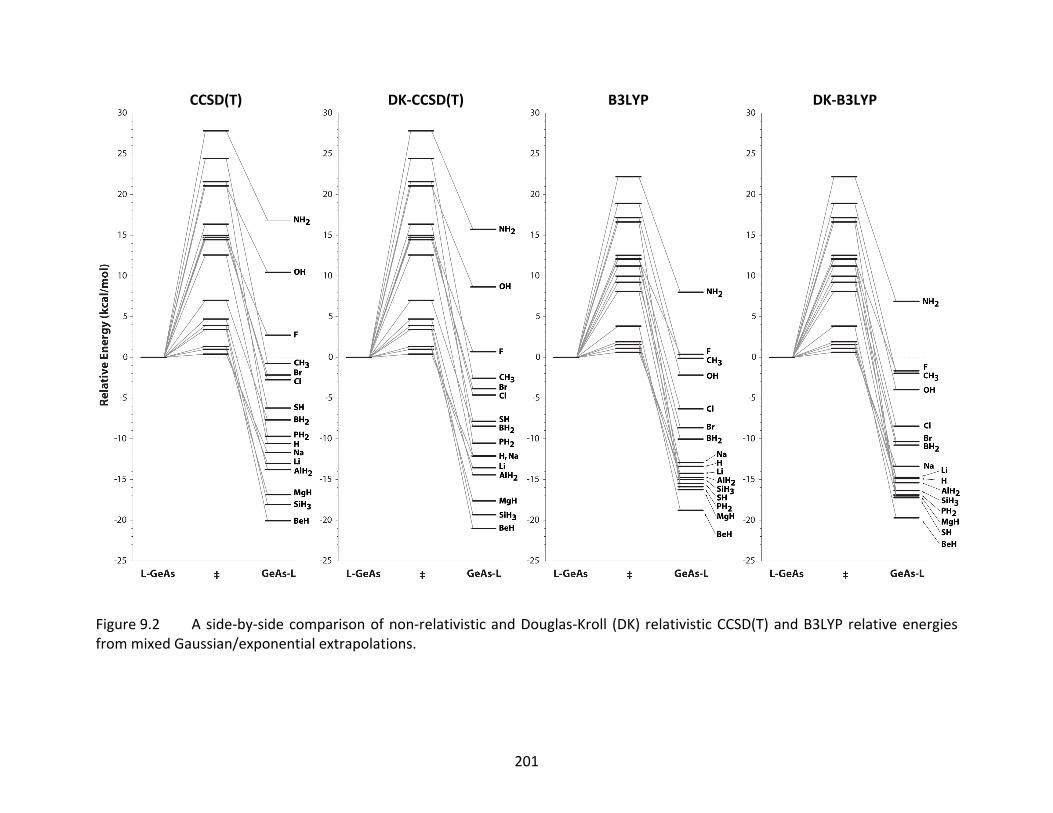
201
Figure 9.2 A side‐by‐side comparison of non‐relativistic and Douglas‐Kroll (DK) relativistic CCSD(T) and B3LYP relative energies from mixed Gaussian/exponential extrapolations.
CCSD(T) DK‐CCSD(T) B3LYP DK‐B3LYP
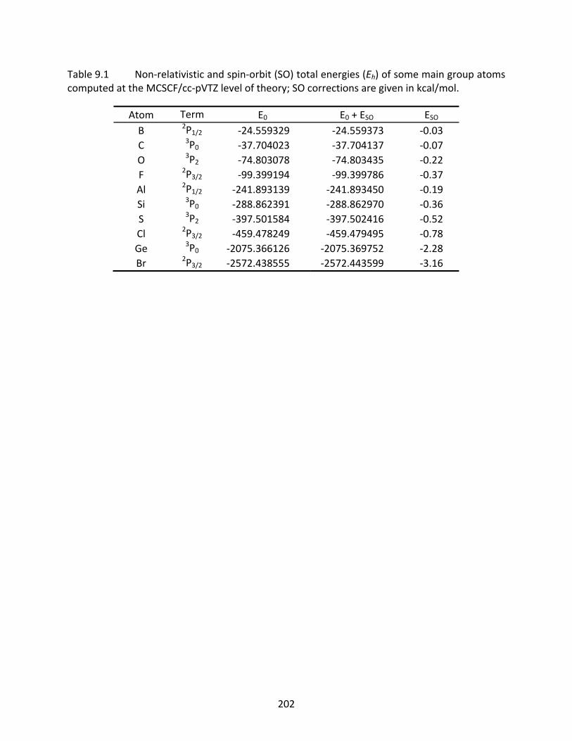
202
Table 9.1 Non‐relativistic and spin‐orbit (SO) total energies (Eh) of some main group atoms computed at the MCSCF/cc‐pVTZ level of theory; SO corrections are given in kcal/mol.
Atom Term E0 E0 + ESO ESO B 2P1/2 ‐24.559329 ‐24.559373 ‐0.03 C 3P0 ‐37.704023 ‐37.704137 ‐0.07 O 3P2 ‐74.803078 ‐74.803435 ‐0.22 F 2P3/2 ‐99.399194 ‐99.399786 ‐0.37 Al 2P1/2 ‐241.893139 ‐241.893450 ‐0.19 Si 3P0 ‐288.862391 ‐288.862970 ‐0.36 S 3P2 ‐397.501584 ‐397.502416 ‐0.52 Cl 2P3/2 ‐459.478249 ‐459.479495 ‐0.78 Ge 3P0 ‐2075.366126 ‐2075.369752 ‐2.28 Br 2P3/2 ‐2572.438555 ‐2572.443599 ‐3.16
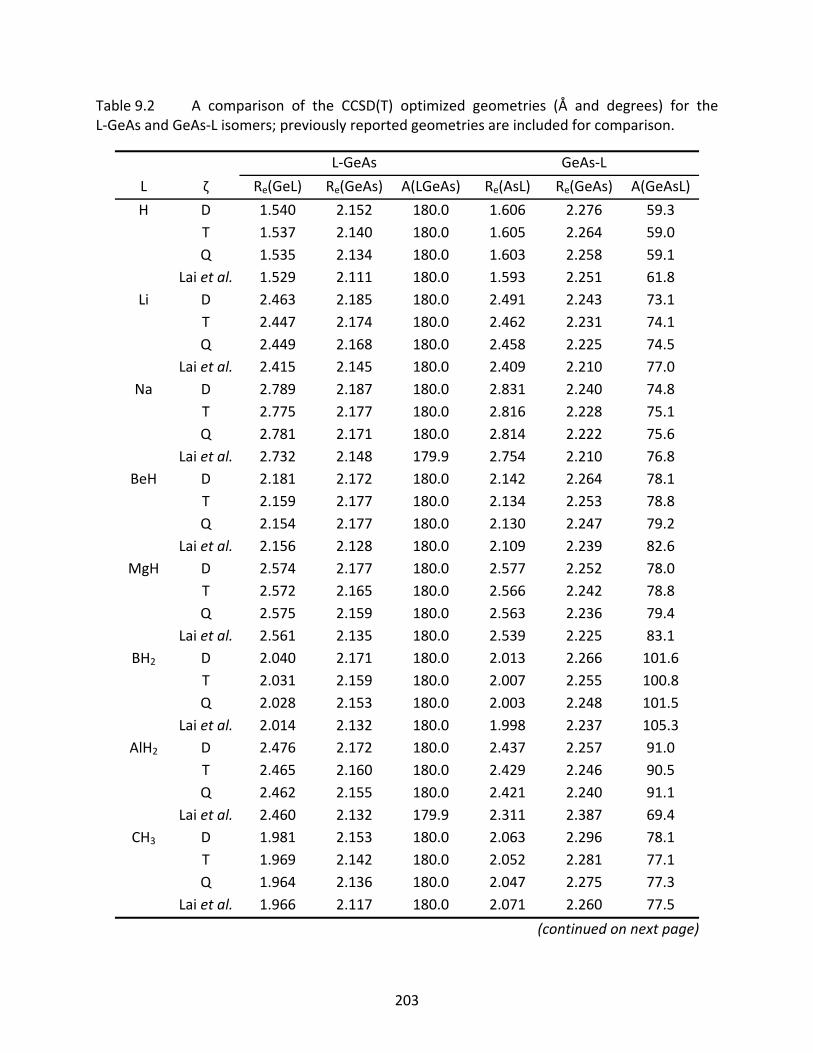
203
Table 9.2 A comparison of the CCSD(T) optimized geometries (Å and degrees) for the L‐GeAs and GeAs‐L isomers; previously reported geometries are included for comparison.
L‐GeAs GeAs‐L
L ζ Re(GeL) Re(GeAs) A(LGeAs) Re(AsL) Re(GeAs) A(GeAsL)
H D 1.540 2.152 180.0 1.606 2.276 59.3 T 1.537 2.140 180.0 1.605 2.264 59.0 Q 1.535 2.134 180.0 1.603 2.258 59.1 Lai et al. 1.529 2.111 180.0 1.593 2.251 61.8Li D 2.463 2.185 180.0 2.491 2.243 73.1 T 2.447 2.174 180.0 2.462 2.231 74.1 Q 2.449 2.168 180.0 2.458 2.225 74.5 Lai et al. 2.415 2.145 180.0 2.409 2.210 77.0
Na D 2.789 2.187 180.0 2.831 2.240 74.8 T 2.775 2.177 180.0 2.816 2.228 75.1 Q 2.781 2.171 180.0 2.814 2.222 75.6 Lai et al. 2.732 2.148 179.9 2.754 2.210 76.8
BeH D 2.181 2.172 180.0 2.142 2.264 78.1 T 2.159 2.177 180.0 2.134 2.253 78.8 Q 2.154 2.177 180.0 2.130 2.247 79.2 Lai et al. 2.156 2.128 180.0 2.109 2.239 82.6
MgH D 2.574 2.177 180.0 2.577 2.252 78.0 T 2.572 2.165 180.0 2.566 2.242 78.8 Q 2.575 2.159 180.0 2.563 2.236 79.4 Lai et al. 2.561 2.135 180.0 2.539 2.225 83.1
BH2 D 2.040 2.171 180.0 2.013 2.266 101.6 T 2.031 2.159 180.0 2.007 2.255 100.8 Q 2.028 2.153 180.0 2.003 2.248 101.5 Lai et al. 2.014 2.132 180.0 1.998 2.237 105.3
AlH2 D 2.476 2.172 180.0 2.437 2.257 91.0 T 2.465 2.160 180.0 2.429 2.246 90.5 Q 2.462 2.155 180.0 2.421 2.240 91.1 Lai et al. 2.460 2.132 179.9 2.311 2.387 69.4
CH3 D 1.981 2.153 180.0 2.063 2.296 78.1 T 1.969 2.142 180.0 2.052 2.281 77.1 Q 1.964 2.136 180.0 2.047 2.275 77.3 Lai et al. 1.966 2.117 180.0 2.071 2.260 77.5
(continued on next page)
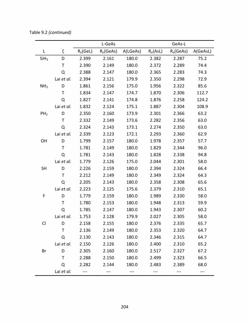
204
Table 9.2 (continued)
L‐GeAs GeAs‐L
L ζ Re(GeL) Re(GeAs) A(LGeAs) Re(AsL) Re(GeAs) A(GeAsL)
SiH3 D 2.399 2.161 180.0 2.382 2.287 75.2 T 2.390 2.149 180.0 2.372 2.289 74.4 Q 2.388 2.147 180.0 2.365 2.283 74.3 Lai et al. 2.394 2.121 179.9 2.350 2.298 72.9
NH2 D 1.861 2.156 175.0 1.956 2.322 85.6 T 1.834 2.147 174.7 1.870 2.306 112.7 Q 1.827 2.141 174.8 1.876 2.258 124.2 Lai et al. 1.832 2.124 175.1 1.887 2.304 108.9
PH2 D 2.350 2.160 173.9 2.301 2.366 63.2 T 2.332 2.149 173.6 2.282 2.356 63.0 Q 2.324 2.143 173.1 2.274 2.350 63.0 Lai et al. 2.339 2.123 172.1 2.293 2.360 62.9
OH D 1.799 2.157 180.0 1.978 2.357 57.7 T 1.781 2.149 180.0 1.829 2.344 96.0 Q 1.781 2.143 180.0 1.828 2.338 94.8 Lai et al. 1.779 2.126 175.0 2.044 2.301 58.0
SH D 2.226 2.159 180.0 2.394 2.324 66.4 T 2.212 2.149 180.0 2.349 2.324 64.3 Q 2.205 2.143 180.0 2.358 2.308 65.6 Lai et al. 2.223 2.125 175.6 2.379 2.310 65.1F D 1.779 2.159 180.0 1.989 2.330 58.0 T 1.780 2.153 180.0 1.948 2.313 59.9 Q 1.785 2.147 180.0 1.943 2.307 60.2 Lai et al. 1.753 2.128 179.9 2.027 2.305 58.0Cl D 2.158 2.155 180.0 2.376 2.335 65.7 T 2.136 2.149 180.0 2.353 2.320 64.7 Q 2.130 2.143 180.0 2.346 2.315 64.7 Lai et al. 2.150 2.126 180.0 2.400 2.310 65.2Br D 2.305 2.160 180.0 2.517 2.327 67.2 T 2.288 2.150 180.0 2.499 2.323 66.5 Q 2.282 2.144 180.0 2.483 2.389 68.0 Lai et al. ‐‐‐ ‐‐‐ ‐‐‐ ‐‐‐ ‐‐‐ ‐‐‐
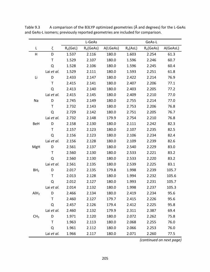
205
Table 9.3 A comparison of the B3LYP optimized geometries (Å and degrees) for the L‐GeAs and GeAs‐L isomers; previously reported geometries are included for comparison.
L‐GeAs GeAs‐L
L ζ Re(GeL) Re(GeAs) A(LGeAs) Re(AsL) Re(GeAs) A(GeAsL)
H D 1.537 2.116 180.0 1.603 2.254 61.3 T 1.529 2.107 180.0 1.596 2.246 60.7 Q 1.528 2.106 180.0 1.596 2.245 60.4 Lai et al. 1.529 2.111 180.0 1.593 2.251 61.8Li D 2.433 2.147 180.0 2.422 2.214 76.9 T 2.415 2.141 180.0 2.407 2.206 77.1 Q 2.413 2.140 180.0 2.403 2.205 77.2 Lai et al. 2.415 2.145 180.0 2.409 2.210 77.0
Na D 2.745 2.149 180.0 2.755 2.214 77.0 T 2.732 2.143 180.0 2.753 2.206 76.8 Q 2.729 2.142 180.0 2.751 2.205 76.7 Lai et al. 2.732 2.148 179.9 2.754 2.210 76.8
BeH D 2.158 2.130 180.0 2.111 2.242 82.3 T 2.157 2.123 180.0 2.107 2.235 82.5 Q 2.156 2.123 180.0 2.106 2.234 82.4 Lai et al. 2.156 2.128 180.0 2.109 2.239 82.6
MgH D 2.561 2.137 180.0 2.540 2.229 83.0 T 2.560 2.130 180.0 2.533 2.221 83.2 Q 2.560 2.130 180.0 2.533 2.220 83.2 Lai et al. 2.561 2.135 180.0 2.539 2.225 83.1
BH2 D 2.017 2.135 179.8 1.998 2.239 105.7 T 2.013 2.128 180.0 1.994 2.232 105.6 Q 2.012 2.127 180.0 1.993 2.231 105.7 Lai et al. 2.014 2.132 180.0 1.998 2.237 105.3
AlH2 D 2.466 2.134 180.0 2.419 2.234 95.6 T 2.460 2.127 179.7 2.415 2.226 95.6 Q 2.457 2.126 179.4 2.412 2.225 95.8 Lai et al. 2.460 2.132 179.9 2.311 2.387 69.4
CH3 D 1.971 2.120 180.0 2.072 2.262 75.8 T 1.963 2.113 180.0 2.068 2.255 76.0 Q 1.961 2.112 180.0 2.066 2.253 76.0 Lai et al. 1.966 2.117 180.0 2.071 2.260 77.5
(continued on next page)
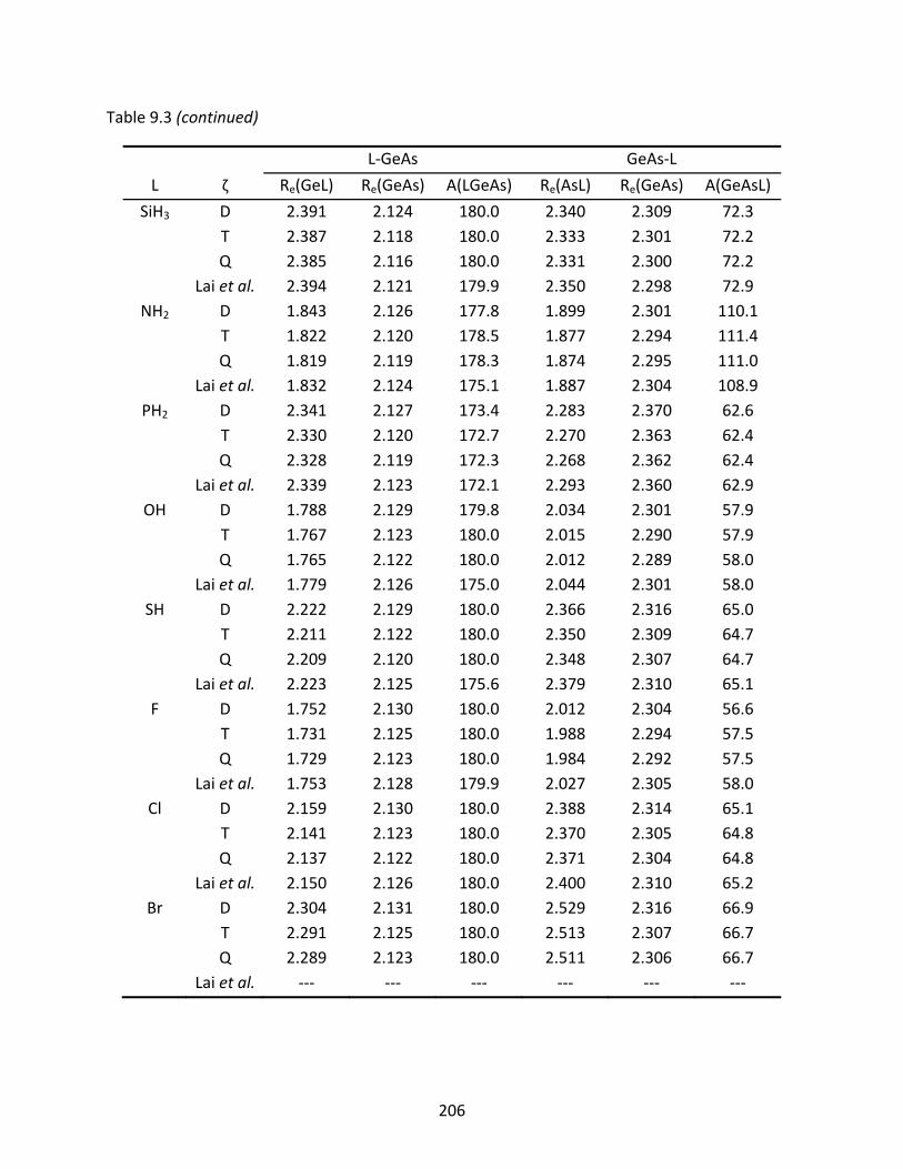
206
Table 9.3 (continued)
L‐GeAs GeAs‐L
L ζ Re(GeL) Re(GeAs) A(LGeAs) Re(AsL) Re(GeAs) A(GeAsL)
SiH3 D 2.391 2.124 180.0 2.340 2.309 72.3 T 2.387 2.118 180.0 2.333 2.301 72.2 Q 2.385 2.116 180.0 2.331 2.300 72.2 Lai et al. 2.394 2.121 179.9 2.350 2.298 72.9
NH2 D 1.843 2.126 177.8 1.899 2.301 110.1 T 1.822 2.120 178.5 1.877 2.294 111.4 Q 1.819 2.119 178.3 1.874 2.295 111.0 Lai et al. 1.832 2.124 175.1 1.887 2.304 108.9
PH2 D 2.341 2.127 173.4 2.283 2.370 62.6 T 2.330 2.120 172.7 2.270 2.363 62.4 Q 2.328 2.119 172.3 2.268 2.362 62.4 Lai et al. 2.339 2.123 172.1 2.293 2.360 62.9
OH D 1.788 2.129 179.8 2.034 2.301 57.9 T 1.767 2.123 180.0 2.015 2.290 57.9 Q 1.765 2.122 180.0 2.012 2.289 58.0 Lai et al. 1.779 2.126 175.0 2.044 2.301 58.0
SH D 2.222 2.129 180.0 2.366 2.316 65.0 T 2.211 2.122 180.0 2.350 2.309 64.7 Q 2.209 2.120 180.0 2.348 2.307 64.7 Lai et al. 2.223 2.125 175.6 2.379 2.310 65.1F D 1.752 2.130 180.0 2.012 2.304 56.6 T 1.731 2.125 180.0 1.988 2.294 57.5 Q 1.729 2.123 180.0 1.984 2.292 57.5 Lai et al. 1.753 2.128 179.9 2.027 2.305 58.0Cl D 2.159 2.130 180.0 2.388 2.314 65.1 T 2.141 2.123 180.0 2.370 2.305 64.8 Q 2.137 2.122 180.0 2.371 2.304 64.8 Lai et al. 2.150 2.126 180.0 2.400 2.310 65.2Br D 2.304 2.131 180.0 2.529 2.316 66.9 T 2.291 2.125 180.0 2.513 2.307 66.7 Q 2.289 2.123 180.0 2.511 2.306 66.7 Lai et al. ‐‐‐ ‐‐‐ ‐‐‐ ‐‐‐ ‐‐‐ ‐‐‐
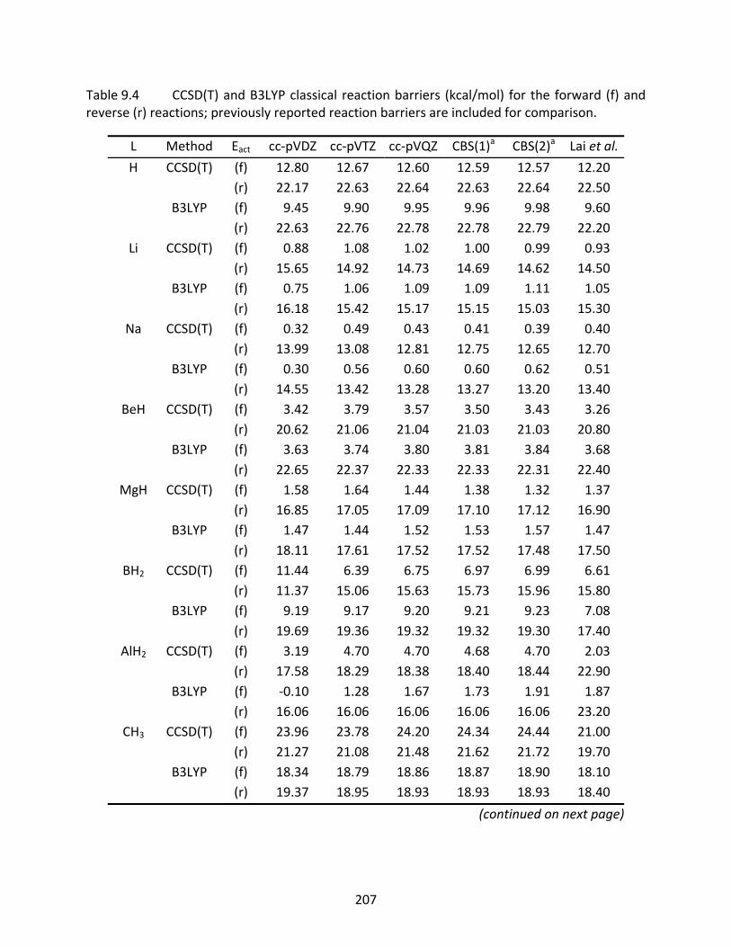
207
Table 9.4 CCSD(T) and B3LYP classical reaction barriers (kcal/mol) for the forward (f) and reverse (r) reactions; previously reported reaction barriers are included for comparison.
L Method Eact cc‐pVDZ cc‐pVTZ cc‐pVQZ CBS(1)a CBS(2)a Lai et al.
H CCSD(T) (f) 12.80 12.67 12.60 12.59 12.57 12.20 (r) 22.17 22.63 22.64 22.63 22.64 22.50 B3LYP (f) 9.45 9.90 9.95 9.96 9.98 9.60 (r) 22.63 22.76 22.78 22.78 22.79 22.20Li CCSD(T) (f) 0.88 1.08 1.02 1.00 0.99 0.93 (r) 15.65 14.92 14.73 14.69 14.62 14.50 B3LYP (f) 0.75 1.06 1.09 1.09 1.11 1.05 (r) 16.18 15.42 15.17 15.15 15.03 15.30
Na CCSD(T) (f) 0.32 0.49 0.43 0.41 0.39 0.40 (r) 13.99 13.08 12.81 12.75 12.65 12.70 B3LYP (f) 0.30 0.56 0.60 0.60 0.62 0.51 (r) 14.55 13.42 13.28 13.27 13.20 13.40
BeH CCSD(T) (f) 3.42 3.79 3.57 3.50 3.43 3.26 (r) 20.62 21.06 21.04 21.03 21.03 20.80 B3LYP (f) 3.63 3.74 3.80 3.81 3.84 3.68 (r) 22.65 22.37 22.33 22.33 22.31 22.40
MgH CCSD(T) (f) 1.58 1.64 1.44 1.38 1.32 1.37 (r) 16.85 17.05 17.09 17.10 17.12 16.90 B3LYP (f) 1.47 1.44 1.52 1.53 1.57 1.47 (r) 18.11 17.61 17.52 17.52 17.48 17.50
BH2 CCSD(T) (f) 11.44 6.39 6.75 6.97 6.99 6.61 (r) 11.37 15.06 15.63 15.73 15.96 15.80 B3LYP (f) 9.19 9.17 9.20 9.21 9.23 7.08 (r) 19.69 19.36 19.32 19.32 19.30 17.40
AlH2 CCSD(T) (f) 3.19 4.70 4.70 4.68 4.70 2.03 (r) 17.58 18.29 18.38 18.40 18.44 22.90 B3LYP (f) ‐0.10 1.28 1.67 1.73 1.91 1.87 (r) 16.06 16.06 16.06 16.06 16.06 23.20
CH3 CCSD(T) (f) 23.96 23.78 24.20 24.34 24.44 21.00 (r) 21.27 21.08 21.48 21.62 21.72 19.70 B3LYP (f) 18.34 18.79 18.86 18.87 18.90 18.10 (r) 19.37 18.95 18.93 18.93 18.93 18.40
(continued on next page)
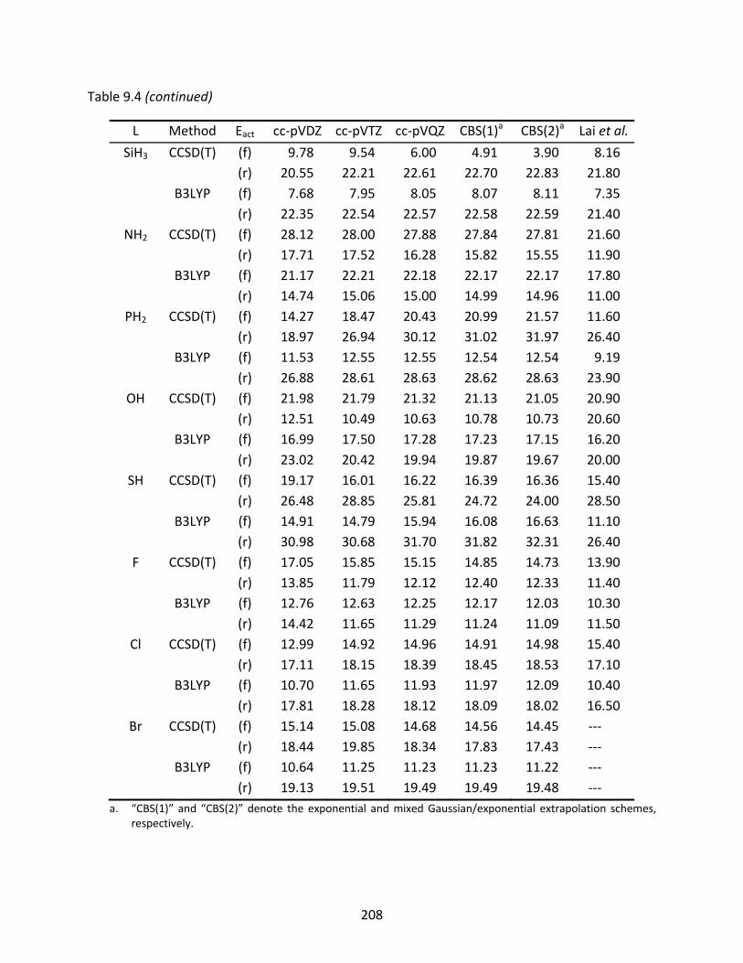
208
Table 9.4 (continued)
L Method Eact cc‐pVDZ cc‐pVTZ cc‐pVQZ CBS(1)a CBS(2)a Lai et al.
SiH3 CCSD(T) (f) 9.78 9.54 6.00 4.91 3.90 8.16 (r) 20.55 22.21 22.61 22.70 22.83 21.80 B3LYP (f) 7.68 7.95 8.05 8.07 8.11 7.35 (r) 22.35 22.54 22.57 22.58 22.59 21.40
NH2 CCSD(T) (f) 28.12 28.00 27.88 27.84 27.81 21.60 (r) 17.71 17.52 16.28 15.82 15.55 11.90 B3LYP (f) 21.17 22.21 22.18 22.17 22.17 17.80 (r) 14.74 15.06 15.00 14.99 14.96 11.00
PH2 CCSD(T) (f) 14.27 18.47 20.43 20.99 21.57 11.60 (r) 18.97 26.94 30.12 31.02 31.97 26.40 B3LYP (f) 11.53 12.55 12.55 12.54 12.54 9.19 (r) 26.88 28.61 28.63 28.62 28.63 23.90
OH CCSD(T) (f) 21.98 21.79 21.32 21.13 21.05 20.90 (r) 12.51 10.49 10.63 10.78 10.73 20.60 B3LYP (f) 16.99 17.50 17.28 17.23 17.15 16.20 (r) 23.02 20.42 19.94 19.87 19.67 20.00
SH CCSD(T) (f) 19.17 16.01 16.22 16.39 16.36 15.40 (r) 26.48 28.85 25.81 24.72 24.00 28.50 B3LYP (f) 14.91 14.79 15.94 16.08 16.63 11.10 (r) 30.98 30.68 31.70 31.82 32.31 26.40F CCSD(T) (f) 17.05 15.85 15.15 14.85 14.73 13.90 (r) 13.85 11.79 12.12 12.40 12.33 11.40 B3LYP (f) 12.76 12.63 12.25 12.17 12.03 10.30 (r) 14.42 11.65 11.29 11.24 11.09 11.50Cl CCSD(T) (f) 12.99 14.92 14.96 14.91 14.98 15.40 (r) 17.11 18.15 18.39 18.45 18.53 17.10 B3LYP (f) 10.70 11.65 11.93 11.97 12.09 10.40 (r) 17.81 18.28 18.12 18.09 18.02 16.50Br CCSD(T) (f) 15.14 15.08 14.68 14.56 14.45 ‐‐‐ (r) 18.44 19.85 18.34 17.83 17.43 ‐‐‐ B3LYP (f) 10.64 11.25 11.23 11.23 11.22 ‐‐‐ (r) 19.13 19.51 19.49 19.49 19.48 ‐‐‐
a. “CBS(1)” and “CBS(2)” denote the exponential and mixed Gaussian/exponential extrapolation schemes, respectively.
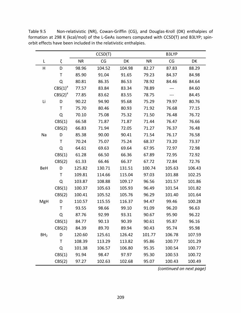
209
Table 9.5 Non‐relativistic (NR), Cowan‐Griffin (CG), and Douglas‐Kroll (DK) enthalpies of formation at 298 K (kcal/mol) of the L‐GeAs isomers computed with CCSD(T) and B3LYP; spin‐orbit effects have been included in the relativistic enthalpies.
CCSD(T) B3LYP
L ζ NR CG DK NR CG DK
H D 98.96 104.52 104.98 82.27 87.83 88.29 T 85.90 91.04 91.65 79.23 84.37 84.98 Q 80.81 86.35 86.53 78.92 84.46 84.64 CBS(1)a 77.57 83.84 83.34 78.89 ‐‐‐ 84.60 CBS(2)a 77.85 83.62 83.55 78.75 ‐‐‐ 84.45Li D 90.22 94.90 95.68 75.29 79.97 80.76 T 75.70 80.46 80.93 71.92 76.68 77.15 Q 70.10 75.08 75.32 71.50 76.48 76.72 CBS(1) 66.58 71.87 71.87 71.44 76.47 76.66 CBS(2) 66.83 71.94 72.05 71.27 76.37 76.48
Na D 85.38 90.00 90.41 71.54 76.17 76.58 T 70.24 75.07 75.24 68.37 73.20 73.37 Q 64.61 69.63 69.64 67.95 72.97 72.98 CBS(1) 61.28 66.50 66.36 67.89 72.95 72.92 CBS(2) 61.33 66.46 66.37 67.72 72.84 72.76
BeH D 125.82 130.71 131.51 100.74 105.63 106.43 T 109.81 114.66 115.04 97.03 101.88 102.25 Q 103.87 108.88 109.17 96.56 101.57 101.86 CBS(1) 100.37 105.63 105.93 96.49 101.54 101.82 CBS(2) 100.41 105.52 105.76 96.29 101.40 101.64
MgH D 110.57 115.55 116.37 94.47 99.46 100.28 T 93.55 98.66 99.10 91.09 96.20 96.63 Q 87.76 92.99 93.31 90.67 95.90 96.22 CBS(1) 84.77 90.13 90.39 90.61 95.87 96.16 CBS(2) 84.39 89.70 89.94 90.43 95.74 95.98
BH2 D 120.60 125.61 126.42 101.77 106.78 107.59 T 108.39 113.29 113.82 95.86 100.77 101.29 Q 101.38 106.57 106.80 95.35 100.54 100.77 CBS(1) 91.94 98.47 97.97 95.30 100.53 100.72 CBS(2) 97.27 102.63 102.68 95.07 100.43 100.49
(continued on next page)
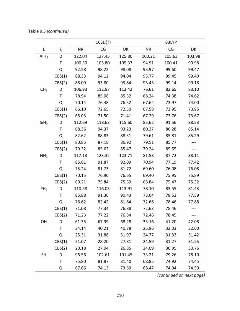
210
Table 9.5 (continued)
CCSD(T) B3LYP
L ζ NR CG DK NR CG DK
AlH2 D 122.04 127.45 125.80 100.21 105.63 103.98 T 100.30 105.80 105.37 94.91 100.41 99.98 Q 92.58 98.22 98.08 93.97 99.60 99.47 CBS(1) 88.33 94.12 94.04 93.77 99.45 99.40 CBS(2) 88.09 93.80 93.84 93.43 99.14 99.18
CH3 D 106.93 112.97 113.42 76.61 82.65 83.10 T 78.94 85.08 85.32 68.24 74.38 74.62 Q 70.14 76.48 76.52 67.62 73.97 74.00 CBS(1) 66.10 72.65 72.50 67.58 73.95 73.95 CBS(2) 65.03 71.50 71.41 67.29 73.76 73.67
SiH3 D 112.69 118.63 115.60 85.62 91.56 88.53 T 88.36 94.37 93.23 80.27 86.28 85.14 Q 82.62 88.83 88.31 79.61 85.81 85.29 CBS(1) 80.85 87.18 86.92 79.51 85.77 ‐‐‐ CBS(2) 79.32 85.63 85.47 79.24 85.55 ‐‐‐
NH2 D 117.13 123.32 123.71 81.53 87.72 88.11 T 85.61 91.87 92.09 70.94 77.19 77.42 Q 75.24 81.73 81.72 69.60 76.08 76.08 CBS(1) 70.15 76.90 76.65 69.40 75.95 75.89 CBS(2) 69.21 75.84 75.69 68.84 75.47 75.32
PH2 D 110.58 116.03 113.91 78.10 83.55 81.43 T 85.88 91.36 90.43 73.04 78.52 77.59 Q 76.62 82.42 81.84 72.66 78.46 77.88 CBS(1) 71.08 77.34 76.88 72.63 78.46 ‐‐‐ CBS(2) 71.23 77.22 76.84 72.46 78.45 ‐‐‐
OH D 61.35 67.39 68.28 35.16 41.20 42.08 T 34.14 40.21 40.78 25.96 32.03 32.60 Q 25.31 31.88 31.97 24.77 31.33 31.42 CBS(1) 21.07 28.20 27.81 24.59 31.27 31.25 CBS(2) 20.18 27.04 26.85 24.09 30.95 30.76
SH D 96.56 102.61 101.45 73.21 79.26 78.10 T 75.80 81.87 81.40 68.85 74.92 74.45 Q 67.66 74.13 73.69 68.47 74.94 74.50
(continued on next page)
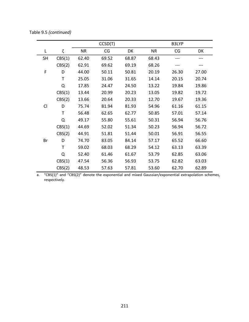
211
Table 9.5 (continued)
CCSD(T) B3LYP
L ζ NR CG DK NR CG DK
SH CBS(1) 62.40 69.52 68.87 68.43 ‐‐‐ ‐‐‐ CBS(2) 62.91 69.62 69.19 68.26 ‐‐‐ ‐‐‐F D 44.00 50.11 50.81 20.19 26.30 27.00 T 25.05 31.06 31.65 14.14 20.15 20.74 Q 17.85 24.47 24.50 13.22 19.84 19.86 CBS(1) 13.44 20.99 20.23 13.05 19.82 19.72 CBS(2) 13.66 20.64 20.33 12.70 19.67 19.36Cl D 75.74 81.94 81.93 54.96 61.16 61.15 T 56.48 62.65 62.77 50.85 57.01 57.14 Q 49.17 55.80 55.61 50.31 56.94 56.76 CBS(1) 44.69 52.02 51.34 50.23 56.94 56.72 CBS(2) 44.91 51.81 51.44 50.01 56.91 56.55Br D 74.70 83.05 84.14 57.17 65.52 66.60 T 59.02 68.03 68.29 54.12 63.13 63.39 Q 52.40 61.46 61.67 53.79 62.85 63.06 CBS(1) 47.54 56.36 56.93 53.75 62.82 63.03 CBS(2) 48.53 57.63 57.81 53.60 62.70 62.89
a. “CBS(1)” and “CBS(2)” denote the exponential and mixed Gaussian/exponential extrapolation schemes, respectively.
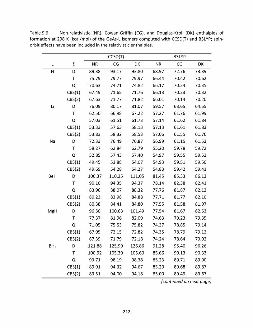
212
Table 9.6 Non‐relativistic (NR), Cowan‐Griffin (CG), and Douglas‐Kroll (DK) enthalpies of formation at 298 K (kcal/mol) of the GeAs‐L isomers computed with CCSD(T) and B3LYP; spin‐orbit effects have been included in the relativistic enthalpies.
CCSD(T) B3LYP
L ζ NR CG DK NR CG DK
H D 89.38 93.17 93.80 68.97 72.76 73.39 T 75.79 79.77 79.97 66.44 70.42 70.62 Q 70.63 74.71 74.82 66.17 70.24 70.35 CBS(1) 67.49 71.65 71.76 66.13 70.23 70.32 CBS(2) 67.63 71.77 71.82 66.01 70.14 70.20Li D 76.09 80.17 81.07 59.57 63.65 64.55 T 62.50 66.98 67.22 57.27 61.76 61.99 Q 57.03 61.51 61.73 57.14 61.62 61.84 CBS(1) 53.33 57.63 58.13 57.13 61.61 61.83 CBS(2) 53.83 58.32 58.53 57.06 61.55 61.76
Na D 72.33 76.49 76.87 56.99 61.15 61.53 T 58.27 62.84 62.79 55.20 59.78 59.72 Q 52.85 57.43 57.40 54.97 59.55 59.52 CBS(1) 49.45 53.88 54.07 54.93 59.51 59.50 CBS(2) 49.69 54.28 54.27 54.83 59.42 59.41
BeH D 106.37 110.25 111.05 81.45 85.33 86.13 T 90.10 94.35 94.37 78.14 82.38 82.41 Q 83.96 88.07 88.32 77.76 81.87 82.12 CBS(1) 80.23 83.98 84.88 77.71 81.77 82.10 CBS(2) 80.38 84.41 84.80 77.55 81.58 81.97
MgH D 96.50 100.63 101.49 77.54 81.67 82.53 T 77.37 81.96 82.09 74.63 79.23 79.35 Q 71.05 75.53 75.82 74.37 78.85 79.14 CBS(1) 67.95 72.15 72.82 74.35 78.79 79.12 CBS(2) 67.39 71.79 72.18 74.24 78.64 79.02
BH2 D 121.88 125.99 126.86 91.28 95.40 96.26 T 100.92 105.39 105.60 85.66 90.13 90.33 Q 93.71 98.19 98.38 85.23 89.71 89.90 CBS(1) 89.91 94.32 94.67 85.20 89.68 89.87 CBS(2) 89.51 94.00 94.18 85.00 89.49 89.67
(continued on next page)
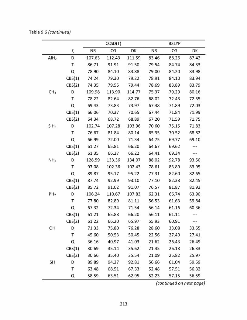
213
Table 9.6 (continued)
CCSD(T) B3LYP
L ζ NR CG DK NR CG DK
AlH2 D 107.63 112.43 111.59 83.46 88.26 87.42 T 86.71 91.91 91.50 79.54 84.74 84.33 Q 78.90 84.10 83.88 79.00 84.20 83.98 CBS(1) 74.24 79.30 79.22 78.91 84.10 83.94 CBS(2) 74.35 79.55 79.44 78.69 83.89 83.79
CH3 D 109.98 113.90 114.77 75.37 79.29 80.16 T 78.22 82.64 82.76 68.02 72.43 72.55 Q 69.43 73.83 73.97 67.48 71.89 72.03 CBS(1) 66.06 70.37 70.65 67.44 71.84 71.99 CBS(2) 64.34 68.72 68.89 67.20 71.59 71.75
SiH3 D 102.74 107.28 103.96 70.60 75.15 71.83 T 76.67 81.84 80.14 65.35 70.52 68.82 Q 66.99 72.00 71.34 64.75 69.77 69.10 CBS(1) 61.27 65.81 66.20 64.67 69.62 ‐‐‐ CBS(2) 61.35 66.27 66.22 64.41 69.34 ‐‐‐
NH2 D 128.59 133.36 134.07 88.02 92.78 93.50 T 97.08 102.36 102.43 78.61 83.89 83.95 Q 89.87 95.17 95.22 77.31 82.60 82.65 CBS(1) 87.74 92.99 93.10 77.10 82.38 82.45 CBS(2) 85.72 91.02 91.07 76.57 81.87 81.92
PH2 D 106.24 110.67 107.83 62.31 66.74 63.90 T 77.80 82.89 81.11 56.53 61.63 59.84 Q 67.32 72.34 71.54 56.14 61.16 60.36 CBS(1) 61.21 65.88 66.20 56.11 61.11 ‐‐‐ CBS(2) 61.22 66.20 65.97 55.93 60.91 ‐‐‐
OH D 71.33 75.80 76.28 28.60 33.08 33.55 T 45.60 50.53 50.45 22.56 27.49 27.41 Q 36.16 40.97 41.03 21.62 26.43 26.49 CBS(1) 30.69 35.14 35.62 21.45 26.18 26.33 CBS(2) 30.66 35.40 35.54 21.09 25.82 25.97
SH D 89.89 94.27 92.81 56.66 61.04 59.59 T 63.48 68.51 67.33 52.48 57.51 56.32 Q 58.59 63.51 62.95 52.23 57.15 56.59
(continued on next page)
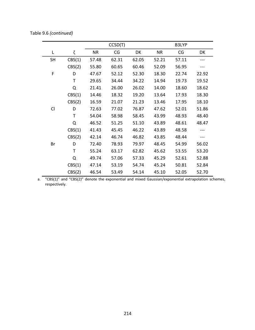
214
Table 9.6 (continued)
CCSD(T) B3LYP
L ζ NR CG DK NR CG DK
SH CBS(1) 57.48 62.31 62.05 52.21 57.11 ‐‐‐ CBS(2) 55.80 60.65 60.46 52.09 56.95 ‐‐‐ F D 47.67 52.12 52.30 18.30 22.74 22.92 T 29.65 34.44 34.22 14.94 19.73 19.52 Q 21.41 26.00 26.02 14.00 18.60 18.62 CBS(1) 14.46 18.32 19.20 13.64 17.93 18.30 CBS(2) 16.59 21.07 21.23 13.46 17.95 18.10Cl D 72.63 77.02 76.87 47.62 52.01 51.86 T 54.04 58.98 58.45 43.99 48.93 48.40 Q 46.52 51.25 51.10 43.89 48.61 48.47 CBS(1) 41.43 45.45 46.22 43.89 48.58 ‐‐‐ CBS(2) 42.14 46.74 46.82 43.85 48.44 ‐‐‐ Br D 72.40 78.93 79.97 48.45 54.99 56.02 T 55.24 63.17 62.82 45.62 53.55 53.20 Q 49.74 57.06 57.33 45.29 52.61 52.88 CBS(1) 47.14 53.19 54.74 45.24 50.81 52.84 CBS(2) 46.54 53.49 54.14 45.10 52.05 52.70
a. “CBS(1)” and “CBS(2)” denote the exponential and mixed Gaussian/exponential extrapolation schemes, respectively.
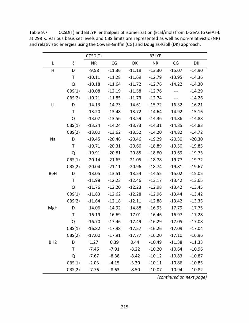
215
Table 9.7 CCSD(T) and B3LYP enthalpies of isomerization (kcal/mol) from L‐GeAs to GeAs‐L at 298 K. Various basis set levels and CBS limits are represented as well as non‐relativistic (NR) and relativistic energies using the Cowan‐Griffin (CG) and Douglas‐Kroll (DK) approach.
CCSD(T) B3LYP
L ζ NR CG DK NR CG DK
H D ‐9.58 ‐11.36 ‐11.18 ‐13.30 ‐15.07 ‐14.90 T ‐10.11 ‐11.28 ‐11.69 ‐12.79 ‐13.95 ‐14.36 Q ‐10.18 ‐11.64 ‐11.72 ‐12.76 ‐14.22 ‐14.30 CBS(1) ‐10.08 ‐12.19 ‐11.58 ‐12.76 ‐‐‐ ‐14.29 CBS(2) ‐10.21 ‐11.85 ‐11.73 ‐12.74 ‐‐‐ ‐14.26Li D ‐14.13 ‐14.73 ‐14.61 ‐15.72 ‐16.32 ‐16.21 T ‐13.20 ‐13.48 ‐13.72 ‐14.64 ‐14.92 ‐15.16 Q ‐13.07 ‐13.56 ‐13.59 ‐14.36 ‐14.86 ‐14.88 CBS(1) ‐13.24 ‐14.24 ‐13.73 ‐14.31 ‐14.85 ‐14.83 CBS(2) ‐13.00 ‐13.62 ‐13.52 ‐14.20 ‐14.82 ‐14.72
Na D ‐19.45 ‐20.46 ‐20.46 ‐19.29 ‐20.30 ‐20.30 T ‐19.71 ‐20.31 ‐20.66 ‐18.89 ‐19.50 ‐19.85 Q ‐19.91 ‐20.81 ‐20.85 ‐18.80 ‐19.69 ‐19.73 CBS(1) ‐20.14 ‐21.65 ‐21.05 ‐18.78 ‐19.77 ‐19.72 CBS(2) ‐20.04 ‐21.11 ‐20.96 ‐18.74 ‐19.81 ‐19.67
BeH D ‐13.05 ‐13.51 ‐13.54 ‐14.55 ‐15.02 ‐15.05 T ‐11.98 ‐12.23 ‐12.46 ‐13.17 ‐13.42 ‐13.65 Q ‐11.76 ‐12.20 ‐12.23 ‐12.98 ‐13.42 ‐13.45 CBS(1) ‐11.83 ‐12.62 ‐12.28 ‐12.96 ‐13.44 ‐13.42 CBS(2) ‐11.64 ‐12.18 ‐12.11 ‐12.88 ‐13.42 ‐13.35
MgH D ‐14.06 ‐14.92 ‐14.88 ‐16.93 ‐17.79 ‐17.75 T ‐16.19 ‐16.69 ‐17.01 ‐16.46 ‐16.97 ‐17.28 Q ‐16.70 ‐17.46 ‐17.49 ‐16.29 ‐17.05 ‐17.08 CBS(1) ‐16.82 ‐17.98 ‐17.57 ‐16.26 ‐17.09 ‐17.04 CBS(2) ‐17.00 ‐17.91 ‐17.77 ‐16.20 ‐17.10 ‐16.96
BH2 D 1.27 0.39 0.44 ‐10.49 ‐11.38 ‐11.33 T ‐7.46 ‐7.91 ‐8.22 ‐10.20 ‐10.64 ‐10.96 Q ‐7.67 ‐8.38 ‐8.42 ‐10.12 ‐10.83 ‐10.87 CBS(1) ‐2.03 ‐4.15 ‐3.30 ‐10.11 ‐10.86 ‐10.85 CBS(2) ‐7.76 ‐8.63 ‐8.50 ‐10.07 ‐10.94 ‐10.82
(continued on next page)
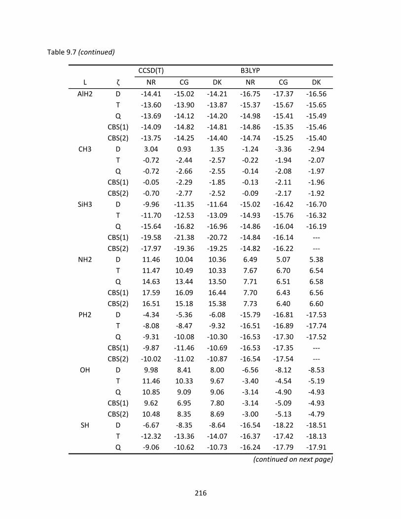
216
Table 9.7 (continued)
CCSD(T) B3LYP
L ζ NR CG DK NR CG DK
AlH2 D ‐14.41 ‐15.02 ‐14.21 ‐16.75 ‐17.37 ‐16.56 T ‐13.60 ‐13.90 ‐13.87 ‐15.37 ‐15.67 ‐15.65 Q ‐13.69 ‐14.12 ‐14.20 ‐14.98 ‐15.41 ‐15.49 CBS(1) ‐14.09 ‐14.82 ‐14.81 ‐14.86 ‐15.35 ‐15.46 CBS(2) ‐13.75 ‐14.25 ‐14.40 ‐14.74 ‐15.25 ‐15.40
CH3 D 3.04 0.93 1.35 ‐1.24 ‐3.36 ‐2.94 T ‐0.72 ‐2.44 ‐2.57 ‐0.22 ‐1.94 ‐2.07 Q ‐0.72 ‐2.66 ‐2.55 ‐0.14 ‐2.08 ‐1.97 CBS(1) ‐0.05 ‐2.29 ‐1.85 ‐0.13 ‐2.11 ‐1.96 CBS(2) ‐0.70 ‐2.77 ‐2.52 ‐0.09 ‐2.17 ‐1.92
SiH3 D ‐9.96 ‐11.35 ‐11.64 ‐15.02 ‐16.42 ‐16.70 T ‐11.70 ‐12.53 ‐13.09 ‐14.93 ‐15.76 ‐16.32 Q ‐15.64 ‐16.82 ‐16.96 ‐14.86 ‐16.04 ‐16.19 CBS(1) ‐19.58 ‐21.38 ‐20.72 ‐14.84 ‐16.14 ‐‐‐ CBS(2) ‐17.97 ‐19.36 ‐19.25 ‐14.82 ‐16.22 ‐‐‐
NH2 D 11.46 10.04 10.36 6.49 5.07 5.38 T 11.47 10.49 10.33 7.67 6.70 6.54 Q 14.63 13.44 13.50 7.71 6.51 6.58 CBS(1) 17.59 16.09 16.44 7.70 6.43 6.56 CBS(2) 16.51 15.18 15.38 7.73 6.40 6.60
PH2 D ‐4.34 ‐5.36 ‐6.08 ‐15.79 ‐16.81 ‐17.53 T ‐8.08 ‐8.47 ‐9.32 ‐16.51 ‐16.89 ‐17.74 Q ‐9.31 ‐10.08 ‐10.30 ‐16.53 ‐17.30 ‐17.52 CBS(1) ‐9.87 ‐11.46 ‐10.69 ‐16.53 ‐17.35 ‐‐‐ CBS(2) ‐10.02 ‐11.02 ‐10.87 ‐16.54 ‐17.54 ‐‐‐
OH D 9.98 8.41 8.00 ‐6.56 ‐8.12 ‐8.53 T 11.46 10.33 9.67 ‐3.40 ‐4.54 ‐5.19 Q 10.85 9.09 9.06 ‐3.14 ‐4.90 ‐4.93 CBS(1) 9.62 6.95 7.80 ‐3.14 ‐5.09 ‐4.93 CBS(2) 10.48 8.35 8.69 ‐3.00 ‐5.13 ‐4.79
SH D ‐6.67 ‐8.35 ‐8.64 ‐16.54 ‐18.22 ‐18.51 T ‐12.32 ‐13.36 ‐14.07 ‐16.37 ‐17.42 ‐18.13 Q ‐9.06 ‐10.62 ‐10.73 ‐16.24 ‐17.79 ‐17.91
(continued on next page)
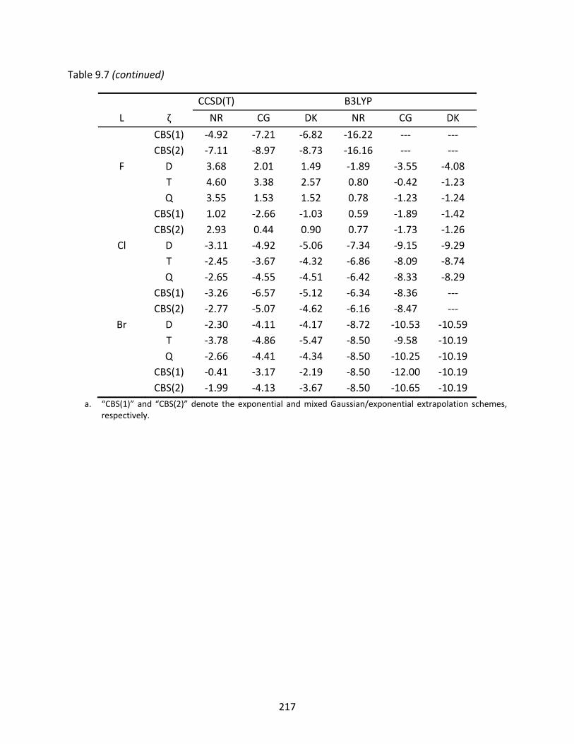
217
Table 9.7 (continued)
CCSD(T) B3LYP
L ζ NR CG DK NR CG DK
CBS(1) ‐4.92 ‐7.21 ‐6.82 ‐16.22 ‐‐‐ ‐‐‐ CBS(2) ‐7.11 ‐8.97 ‐8.73 ‐16.16 ‐‐‐ ‐‐‐ F D 3.68 2.01 1.49 ‐1.89 ‐3.55 ‐4.08 T 4.60 3.38 2.57 0.80 ‐0.42 ‐1.23 Q 3.55 1.53 1.52 0.78 ‐1.23 ‐1.24 CBS(1) 1.02 ‐2.66 ‐1.03 0.59 ‐1.89 ‐1.42 CBS(2) 2.93 0.44 0.90 0.77 ‐1.73 ‐1.26Cl D ‐3.11 ‐4.92 ‐5.06 ‐7.34 ‐9.15 ‐9.29 T ‐2.45 ‐3.67 ‐4.32 ‐6.86 ‐8.09 ‐8.74 Q ‐2.65 ‐4.55 ‐4.51 ‐6.42 ‐8.33 ‐8.29 CBS(1) ‐3.26 ‐6.57 ‐5.12 ‐6.34 ‐8.36 ‐‐‐ CBS(2) ‐2.77 ‐5.07 ‐4.62 ‐6.16 ‐8.47 ‐‐‐ Br D ‐2.30 ‐4.11 ‐4.17 ‐8.72 ‐10.53 ‐10.59 T ‐3.78 ‐4.86 ‐5.47 ‐8.50 ‐9.58 ‐10.19 Q ‐2.66 ‐4.41 ‐4.34 ‐8.50 ‐10.25 ‐10.19 CBS(1) ‐0.41 ‐3.17 ‐2.19 ‐8.50 ‐12.00 ‐10.19 CBS(2) ‐1.99 ‐4.13 ‐3.67 ‐8.50 ‐10.65 ‐10.19
a. “CBS(1)” and “CBS(2)” denote the exponential and mixed Gaussian/exponential extrapolation schemes, respectively.
218
CHAPTER 10
A SYSTEMATIC INVESTIGATION OF SILICON HYDRIDES AND HALIDES†
10.1 Introduction
Silicon‐containing species are of vital importance in many industries, with the vast
majority of applications in the semiconductor industry. Specifically, crystalline silicon provides
the foundation for both micro‐ and macro‐electronic devices from computer processors to
light‐emitting devices and solar cells.278 Halogenated silanes, such as SiF4 and SiCl4, are found in
the etching of metal surfaces such as copper.279,280 Further, plasmas of silicon are used in
chemical vapor deposition (CVD) and chemical etching of crystalline silicon and silicon oxide
surfaces.281 In the CVD process, for example, electric discharge decomposes silanes into
transient species that react readily with the surface. Many small reactive compounds produced
in such plasmas have been characterized by experiment,282 yet other compounds believed to be
produced in the same plasmas have not, or cannot at present, be characterized due to their
transient nature and short lifetimes. This affords an excellent opportunity for theoretical
computations to model these transient intermediates and predict their properties.
Hydrides, fluorides, and chlorides of silicon have been the topic of both experimental
and theoretical studies. The primary focus of many of these studies has been upon the accurate
determination of thermodynamic properties, including atomization energies and enthalpies of
formation, enabling a better understanding of industrial processes. Numerous experimental
† Work reported in this chapter was performed in collaboration with Rebecca M. Lucente‐Schultz, and has been submitted for publication in Chemical Physics.
219
thermodynamic studies have been reviewed in a paper by Walsh.283 A review of the theoretical
treatments of silicon hydrides has been presented by Allen and Schaefer,282 while numerous
fluorine and chlorine silicon species were investigated by Ignacio and Schlegel284,285 and Ho et
al.286,287 Silicon hydrides, fluorides, and chlorides have been studied using methods that range
from Hartree‐Fock (HF)60 and density functional theory (DFT)288 to coupled cluster (CC)
theory,289‐292 in combination with basis sets ranging from 3‐21G (27 basis functions per silicon
atom) to aug‐cc‐pV6Z (227 basis functions per silicon atom).293 Further, Martin et al. and Begue
et al. have investigated silane and difluorosilane, respectively, using ab initio anharmonic force
fields.121,294 Despite the different theoretical approaches that have been used to study silicon
hydrides and halides, no extensive CC study has been reported utilizing the augmented tight d
correlation consistent basis sets for many (SiH4 is an exception)121,294 of the silicon‐containing
molecules of this study (SiH, SiF, SiCl, SiH2, SiF2, SiCl2, SiHF, SiHCl, SiH3, SiF3, SiCl3, SiH2F, SiH2Cl,
SiHF2, SiHCl2, SiF4, SiCl4, SiH3F, SiH3Cl, SiH2F2, SiH2Cl2, SiHF3, SiHCl3), nor has a comparison of
coupled cluster with single, double, and non‐iterative triple excitations, CCSD(T),31,38 and the
recently development correlation consistent Composite Approach (ccCA)73‐80 been reported.
The ccCA method has been shown to be successful in computing ionization potentials,
electron affinities, and enthalpies of formation for the Gaussian‐3 1999 (G3/99) test set with
small mean absolute deviations (MAD) relative to experiment.74,75 Compared with the
Gaussian‐n (Gn) methods, ccCA performs well without the need for an empirical high‐level
correction. Further, ccCA is more efficient than CCSD(T) since the bottleneck in ccCA is a
second‐order perturbation single point computation with a quadruple‐ζ basis set, which scales
, while CCSD(T) scales as , where is the number of basis functions. Despite the
220
fact that ccCA does contain a CCSD(T) step, it is coupled with a small basis set, which does not
make it more computationally demanding than the bottleneck perturbation step. The
demonstrated success and efficiency of ccCA has motivated employing it as a computational
method this investigation to further benchmark it against coupled cluster theory in the study of
silicon‐containing molecules (the bulk of which were not included in previous benchmark
papers with ccCA).73‐80
10.2 Computational Methodology
The standard and augmented correlation consistent, polarized valence basis sets
(cc‐pVnZ and aug‐cc‐pVnZ, where n = D, T, Q, and 5)94‐101 have been used, as well as the tight d
correlation consistent basis sets, cc‐pV(n+d)Z and aug‐cc‐pV(n+d)Z.101 The mixed
Gaussian/exponential extrapolation scheme (3.3) has been employed herein to approximate
the complete basis set (CBS) limit.85,93,95 In the following discussions, the term ‘CBS(DTQ)’
denotes an extrapolation using the double‐, triple‐, and quadruple‐ζ points, ‘CBS(TQ5)’ denotes
an extrapolation using the triple‐, quadruple‐, and quintuple‐ζ points, and ‘CBS(DTQ5)’ denotes
an extrapolation using each ζ point. All 4‐point extrapolations have been fit using a least‐
squares procedure with a residual less than 10‐5 hartree, while the 3‐point extrapolations utilize
the analytical equation (3.5) for the CBS limit.
The CCSD(T) method31,38 has been employed along side the ccCA method.73‐80 Using a
fixed geometry optimized with the Becke three‐parameter exchange scheme (B3) and the Lee‐
Yang‐Parr (LYP) correlation functional, B3LYP, the ccCA method uses perturbation and CCSD(T)
theories in combination with the cc‐pVnZ basis sets to account for higher order correlation,
221
core‐valence (CV) correlation, and scalar relativistic corrections from second‐order Douglas‐
Kroll (DK) theory135‐137 as additive corrections (see Chapter 7 for a detailed discussion). These
corrections are then applied to an extrapolated, second‐order perturbation theory reference
energy. The ccCA method also includes atomic spin‐orbit (SO) coupling corrections. The target
accuracy of ccCA is the DK‐CCSD(T)/aug‐cc‐pCV(∞+d)Z level of theory for energetic properties.
In computations on open‐shell molecules, the restricted open‐shell CCSD(T) formulism was
used, while the unrestricted formalism was used in the ccCA computations.
All CCSD(T) computations were performed using the Molpro software package,180 while
ccCA computations utilized the Gaussian 03 software package.174 Gradients were converged to
at least 10‐4 Eh, while harmonic frequencies were computed at the cc‐pVTZ level.
Thermochemical properties were computed using atomic enthalpies of formation taken from
the JANAF or CODATA tables,195,273 except the enthalpy of formation of the silicon atom, which
was taken from Karton and Martin196 (see discussion in section 10.4). Atomic SO corrections (cf.
Table 9.1) were applied to the computed thermodynamic properties.
10.3 Optimized Structures
10.3.1 SiH, SiF, and SiCl
The CCSD(T)‐optimized structures of SiH, SiF, and SiCl are listed in Table 10.1. The JANAF
tables report a bond length for SiH (Re = 1.5201 Å) from theoretical (HF) studies,170,273 and many
subsequent experimental and theoretical investigations reference the JANAF value. However,
an extensive rovibrational investigation on the 28SiH radical isotopomer has been done by
222
Betrencourt et al.,295 and this value (Re = 1.51966 Å) has been included in Table 10.1. Similarly,
bond lengths from high resolution spectroscopic studies of SiF (Re = 1.60099 Å) and SiCl (Re =
2.05706 Å) have been used for comparison instead of the JANAF values.296,297 In comparison
with experiment, the SiH CCSD(T) bond lengths fall within 0.01 Å when using a triple‐ζ or higher
level basis set. The tight d function affects the double‐ζ bond length by shorting the bond from
1.540 Å to 1.533 Å with the standard basis sets and 1.543 Å to 1.535 Å in the augmented basis
sets, making the tight d basis sets closer to the experimental value of 1.51996 Å.
The tight d basis sets converge faster in the bond length than the standard basis sets (cf.
Figure 10.1). For example, the cc‐pV(T+d)Z basis set gives a bond length of SiF (1.611 Å) similar
to that arising from the cc‐pVQZ basis set (1.611 Å), while the cc‐pV(Q+d)Z basis set gives a
bond length (1.608 Å) similar to that of the cc‐pV5Z basis set (1.607 Å). Similar effects are
observed in the CCSD(T)‐computed bond lengths of SiCl. Overall, using the tight d basis sets
result in bond lengths at the (n+1) standard basis set level.
10.3.2 SiH2, SiF2, SiCl2, SiHF, and SiHCl
Table 10.2 lists the optimized geometries of the triatomic species. The desired 0.01 Å
accuracy is achieved at the quadruple‐ζ level with the standard and augmented basis sets for
SiH2, but is achieved at the triple‐ζ level with the tight d basis sets. Further, the SiF2 bond
lengths agree with experiment at the quadruple‐ζ level with all the basis set families employed.
Optimized bond angles of SiH2 agree with experiment within 0.5° at all basis set levels, while
that of SiF2 agrees within 0.5° at the triple‐ζ level and higher. Compared with the experimental
geometry reported in JANAF for SiCl2 (Re = 2.03 Å, A = 105° ± 3), the optimized geometries have
223
discrepancies of >0.04 Å and >3.5° at the quintuple‐ζ level. The underlying assumption in
JANAF, however, is that the bond lengths and bond angle of SiCl2 are the same as for Si‐Cl and
Cl‐Si‐Cl in SiH2Cl2. Fujitake and Hirota have reported the microwave spectrum of SiCl2,298 which
gives a structure (in Table 10.2 for comparison) much closer to the CCSD(T)‐optimized structure.
In SiHF and SiHCl, the Si‐H bond length is already within 0.01 Å at the triple‐ζ level, using
the standard and augmented basis sets, and is within this same accuracy at the double‐ζ level
using the tight d basis sets. Indeed, the Si‐F bond length converges toward the experimental
value with each family of basis set, however, 0.01 Å is not achieved until the quadruple‐ζ level.
The exception is for the cc‐pV(n+d)Z bond lengths, where the triple‐ζ level Si‐F bond length is
1.611 Å, compared with experiment (1.603 Å). The Si‐Cl bond of SiHCl, in constrast to the Si‐F
bond of SiHF does not reach 0.01 Å of experiment until the quintuple‐ζ level of the standard
and augmented basis sets and quadruple‐ζ level in the tight d basis sets.
10.3.3 SiH3, SiF3, SiCl3, SiH2F, SiH2Cl, SiHF2, and SiHCl2
Qualitative bond angles from electron paramagnetic resonance (EPR) studies of the SiH3
and SiF3 radicals have been reported,299,300 but no geometric parameters are well known for the
other tri‐substituted silicon radicals in this investigation. Microwave studies have reported
structures for SiH3 and SiF3,301,302 though they used a fixed F‐Si‐F bond angle in computing the
Si‐F bond length (reported in Table 10.3). One qualitative aspect that theory corroborates is the
pyramidal structure of the SiH3 radical, as compared with that of the isoelectronic CH3 radical,
which is planar.
Although very little structural information is available for these molecules from
224
experiment, trends in the computed structures from the mono‐, di‐, and tetra‐substituted
molecules lead to the following observations. One obvious trend is the decrease in the Si‐H
bond length in the procession from SiH to SiH4. For example, the bond length in SiH is 1.522 Å at
the largest basis set level and decreases to 1.517 Å in SiH2, then to 1.479 Å in SiH3 and SiH4.
Comparing the optimized structure of the SiH3 radical to that of gaseous silyl acetylene
(HCC‐SiH3) [Rz(SiH) = 1.4794 Å] determined by Brookman et al.,303 quantitative agreement for
the Si‐H bond length is observed. The Si‐F bonds show a decrease from 1.607 Å in SiF to 1.596 Å
in SiF2, then to 1.576 Å in SiF3, and finally to 1.563 Å in SiF4. Note the significant change in bond
length from SiF3 to SiF4, as compared with SiH3 to SiH4. A similar trend is observed in the
procession from SiCl2 to SiCl4 (the SiCl bond length is actually shorter than in SiCl2).
The Si‐H bond lengths are approximately 1.480 Å in the SiH2F, SiHF2, SiH2Cl, and SiHCl2
molecules. However, both the Si‐F and Si‐Cl bonds contract in going from SiH2X to SiHX2. This is
shown in Table 10.3: the Si‐F bond length is 1.600 Å at the largest basis set level of SiH2F and
contracts to 1.587 Å in SiHF2. Similarly, the Si‐Cl bond length is 2.054 Å in SiH2Cl and contracts
to 2.045 Å in SiHCl2. Finally, the H‐Si‐X and H‐Si‐H bond angles remain relatively constant in
each of the mixed hydride/halogen species, but the X‐Si‐X bond angles of SiHF2 and SiHCl2 are
markedly different. The F‐Si‐F angle, for example, is 107.15° at the largest basis set level and
expands to 109.99° for Cl‐Si‐Cl.
10.3.4 SiH4, SiF4, SiCl4, SiH3F, SiH3Cl, SiH2F2, SiH2Cl2, SiHF3, and SiHCl3
All of the optimized geometries of the tetra‐substituted silicon species examined are
listed in Table 10.4, and only basis sets through quadruple‐ζ have been used to optimize the
225
geometries. Considering the tetrahedral species, CCSD(T)‐optimized bond lengths of SiH4, SiF4,
and SiCl4 are within 0.005, 0.008, and 0.005 Å of experiment, respectively, at the quadruple‐ζ
level. The tight d effect is again pronounced by accelerating the convergence of the bond
lengths of each tetrahedral species.
The Si‐H bonds of SiHF3 and SiH3F agree with experiment at the quadruple‐ζ level for all
basis sets, including the tight d sets, while those of SiHCl3 and SiH3Cl agree with experiment by
the triple‐ζ level. The Si‐F bond length of SiHF3 is within 0.01 Å of experiment at the quadruple‐ζ
level using the tight d basis sets, but differs from experiment by 0.011 Å and 0.012 Å with the
standard and augmented basis sets, respectively, at the quadruple‐ζ level. In contrast, the Si‐F
bond length of SiH3F is well within 0.01 Å of experiment at triple‐ζ level for all basis set families
except the aug‐cc‐pVnZ sets. The Si‐Cl bond of SiHCl3, although approaching the experimental
value (Re = 2.020 Å) as the basis increases in size, differs from experiment by 0.009 Å and
0.010 Å at the cc‐pV(Q+d)Z and aug‐cc‐pV(Q+d)Z levels, respectively, but differs from
experiment by 0.013 Å and 0.014 Å at the cc‐pVQZ and aug‐cc‐pVQZ levels, respectively. A
similar observation is made for the Si‐Cl bond in SiH3Cl with differences, relative to experiment
(Re = 2.0506 Å), of 0.010 Å, 0.006 Å, 0.011 Å, and 0.007 Å at the cc‐pVQZ, cc‐pV(Q+d)Z, aug‐cc‐
pVQZ, and aug‐cc‐pV(Q+d)Z basis set levels, respectively. This shows that the inclusion of the
tight d function is vital to achieving 0.01 Å accuracy, relative to experiment. The bond angles of
SiHF3, SiH3F, SiHCl3, and SiH3Cl are within 0.5° of experiment at the double‐ζ level of each basis
set family.
226
10.4 Thermochemistry
The enthalpy of formation of the silicon atom reported by JANAF and CODATA has been
heavily criticized due to its large error bars (106.60 ± 1.91 kcal/mol).195,273 Ochterski et al.304
computed the enthalpy of formation of the silicon atom with lower error bars by using reliable
experimental enthalpies of formation of SiH4 and Si2H6 following the method of Grev and
Schaefer.290 Their recommended 0 K enthalpy of formation for silicon is 108.1 ± 0.5 kcal/mol.
Karton and Martin196 have recently reinvestigated the enthalpy of formation of the silicon atom
using the Weizmann‐4 (W4) composite approach. Karton and Martin’s reinvestigation of the
silicon enthalpy of formation did not rely on semi‐empirical corrections;305 their reported value
of the 0 K enthalpy of formation for silicon is 107.15 ± 0.20 kcal/mol, which is the value used in
this investigation.
Several atomization energies of Table 10.5 were calculated from the 0 K enthalpies of
formation taken from JANAF or CODATA. The experimental atomization energies (Σ ) for each
molecule have been calculated using the following equation:272,306
Σ Δ ,° Δ ,
° molecule (10.1)
In the formula, is the number of atoms of a particular type; the values for Δ ,° and
Δ ,° molecule are the experimental 0 K enthalpies of formation for the th atom and
molecule, respectively. Enthalpies that do not appear in JANAF or CODATA are taken from other
sources listed in Table 10.5.
There are six molecules for which neither an experimental atomization energy nor an
enthalpy of formation could be found: SiHF, SiHCl, SiH2F, SiH2Cl, SiHF2, and SiHCl2. The
227
enthalpies of formation of these molecules have been calculated from DK‐CCSD(T)/CBS(DTQ)
total energies (including atomic SO corrections) using the aug‐cc‐pCVnZ‐DK basis sets81,142 and
experimental infrared (IR) frequencies, where available, using statistical thermodynamics. The
thermal contributions of translational, rotational, and vibrational energy have been calculated
from the following equations from McQuarrie and Simon:306
(10.2)
Θ2
Θ /
1 / , where Θ (10.3)
It is assumed that there is no appreciable degeneracy in the electronic wavefunction, and the
thermal correction to the electronic energy is, therefore, negligible. The translational and
rotational thermal contributions, and , respectively, are taken as 3/2 each. The
vibrational frequencies of the molecules ( ) are taken directly from experimental infrared (IR)
frequencies. The first term in the summation of (10.3) is the zero‐point energy (ZPE) and the
second term is the thermal correction to the vibrational energy (Boltzmann correction); the
number 3 6 ( is the number of atoms) is the number of vibrational degrees of
freedom. The atomization energies computed in this manner are considerd in this study to be
the best estimate of the true value in the absence of a reliable experimental value.
10.4.2 Atomization Energies and Enthalpies of Formation
Computed atomization energies at 0 K are listed in Table 10.5 and enthalpies of
formation at 298.15 K are listed in Table 10.6. Experimental data are presented for comparison
with the atomization energy and the enthalpy of formation for each molecule. If the
228
atomization energy was not found to be directly available from experiment, it was calculated
from the experimental enthalpy of formation from equation (10.1). Conversely, if the enthalpy
of formation was not found to be available from experiment, then it was calculated from the
experimental atomization energy using equation (10.1).
The IR spectra for SiHF and SiHCl from JANAF were used to derive the respective
experimental atomization energies, but no spectral data for the SiH2F, SiH2Cl, SiHF2, and SiHCl2
molecules could be found, so harmonic frequencies from CCSD(T)/aug‐cc‐pV(T+d)Z
computations were employed. The atomization energies and enthalpies of formation for these
six molecules are listed in Table 10.5 and Table 10.6, respectively. It should be noted that
Ignacio and Schlegel have reported enthalpies of formation for SiHF (‐41 ± 5 kcal/mol), SiH2F
(‐49 ± 5 kcal/mol), and SiHF2 (‐144 ± 5 kcal/mol) using a linear interpolation scheme reported in
the JANAF tables.273,284 The DK‐CCSD(T)/CBS(DTQ) enthalpies reported here are within the error
bars of these three fluorine species.
The impact of employing atomization energies from sources other than the JANAF
tables can be quite significant. For example, in SiCl, when the JANAF‐derived atomization
energy (88.84 kcal/mol) is compared to the CCSD(T)/CBS(DTQ5) value, the difference is
12.02 kcal/mol for the aug‐cc‐pV(n+d)Z basis sets. Using a very recent value reported by
Hildenbrand et al.307 (98.68 kcal/mol), there is much better agreement between theory and
experiment, with the error reduced to 2.18 kcal/mol. Other similar cases of JANAF‐derived
atomization energies differing significantly from theory exist as well (e.g. SiF2, SiF3, and SiCl3),
and using the experimental data reported by various other sources (listed in Table 10.5) shows
much better agreement between theory and experiment. These large sources of error can be
229
attributed to the averaging of different experimental enthalpies of formation reported in the
JANAF tables.273
For each of the silicon fluorides represented, it is seen in Figure 10.2 that employing the
tight d function also accelerates the convergence of the enthalpy of formation, although
employing the diffuse functions more rapidly accelerates the convergence, especially at the
double‐ζ level, relative to the cc‐pVnZ results. More generally, the diffuse functions accelerate
convergence of the enthalpies of formation of all molecules of this investigation. However, the
cc‐pV(n+d)Z basis sets produce enthalpies of formation comparable to the aug‐cc‐pVnZ basis
sets in many of the silicon molecules at the computational cost of a single d function (five
angular functions) versus a shell of multiple diffuse functions.
The data in Table 10.5 and Table 10.6 demonstrates that large basis sets are needed to
converge the CCSD(T) energies to the kcal/mol accuracy regime, particularly for the larger
silicon molecules. The difference between the cc‐pVDZ and cc‐pVTZ energies is 64.97 kcal/mol
for SiF4, which decreases to 19.06 kcal/mol between cc‐pVTZ and cc‐pVQZ, and then to 6.85
kcal/mol between the cc‐pVQZ and cc‐pV5Z energies. Further, basis set effects are seen in SiF in
which the molecule is predicted to be enthalpically unstable at the double‐ζ level (cf. Figure
10.2), with the exception of the aug‐cc‐pV(n+d)Z basis sets, but instability is not observed for
basis sets of at least triple‐ζ quality.
Comparing the CBS limits of Table 10.5 and Table 10.6, it becomes evident that
extrapolating different data points can lead to significantly different limits. Differences greater
than 1.0 kcal/mol between the extrapolated CBS limits of Table 10.5 and experiment are found,
for example, with SiF2, SiCl2, SiCl3, SiH2F, SiHF2, SiHCl2, SiH4, SiF4, SiCl4, SiHF3, SiH2F2, SiH3F,
230
SiHCl3, and SiH2Cl2. Large differences between the extrapolated CBS limits, like for SiF4,
complicate the comparison with experiment, but examining the CBS(DTQ5) extrapolation can
be illuminating. For example, the difference between the SiF4 cc‐pV(n+d)Z CBS(DTQ) and
CBS(TQ5) atomization energies is 3.21 kcal/mol, while the CBS(DTQ5) is almost half‐way
between the CBS(DTQ) and CBS(TQ5) atomization energies. It is commonly assumed that a
CBS(TQ5) extrapolation is close to the actual CBS limit for the system since the difference
between the quintuple‐ζ point and the actual CBS limit is usually small. However, using the
double‐ζ point can provide an anchor point that changes the curvature of the CBS fitting
function, as is shown in Table 10.5 for the SiF4 atomization energy, causing significant
differences between the CBS limits. In CBS(DTQ5) extrapolations, like that of SiF4, the quintuple‐
ζ point is not as close to the basis set limit as predicted by the CBS(TQ5) extrapolation.
Comparing the SiF4 cc‐pV(n+d)Z CBS(DTQ5) limit with experiment shows a difference of 2.97
kcal/mol, while the CBS(DTQ) and CBS(TQ5) limits show differences of 4.51 and 1.30 kcal/mol,
respectively. Note that the CBS(TQ5) extrapolation, in this case, is closer to experiment than the
other extrapolations.
The MAD of the enthalpies of formation from experiment, excluding those of SiHF,
SiHCl, SiH2F, SiHF2, SiH2Cl, and SiHCl2 since there are no direct experimental enthalpies to
compare with, are, at the CCSD(T)/CBS(TQ5) level vs. the CCSD(T)/CBS(DTQ5) level: 2.25 vs. 2.07
kcal/mol (cc‐pVnZ); 1.98 vs. 2.17 kcal/mol (cc‐pV(n+d)Z); 2.35 vs. 2.24 kcal/mol (aug‐cc‐pVnZ);
and 2.13 vs. 2.34 kcal/mol (aug‐cc‐pV(n+d)Z). These MADs indicate that the CBS(TQ5)
extrapolation slightly outperforms the CBS(DTQ5) extrapolation in the tight d basis sets, but not
in the standard and augmented basis sets. The largest errors between CCSD(T)/CBS(DTQ5) and
231
experimental enthalpies of formation are in SiCl3 and SiCl4.
It should be noted that a direct comparison of ccCA results to CCSD(T) should not be
made since ccCA contains additive corrections for both CV and scalar relativistic effects. The
CCSD(T)/CBS(DTQ) extrapolations reported here were done as a reference point for comparison
with ccCA, since ccCA uses a CBS(DTQ) reference energy. The CCSD(T)/CBS(DTQ) enthalpy of
formation MAD is 2.03 kcal/mol [cc‐pVnZ], 2.53 kcal/mol [cc‐pV(n+d)Z], 2.25 kcal/mol [aug‐cc‐
pVnZ], and 2.68 kcal/mol [aug‐cc‐pV(n+d)Z]. The ccCA MAD from experiment is 2.62 kcal/mol.
Further, the average deviation from experiment for ccCA is 1.98 ± 2.99 kcal/mol, while the
CCSD(T)/CBS(DTQ) average deviation is ‐2.05 ± 2.37 kcal/mol using the aug‐cc‐pV(n+d)Z basis
sets.
In every molecule of this study, CCSD(T)/CBS(DTQ) extrapolations of the enthalpy of
formation are too low relative to experiment, and ccCA tends to be too high, but slightly closer
to experiment. This observation stems from the CCSD(T)/CBS(DTQ) atomization energies being
too high, while those of ccCA are too low. Assuming that all basis set error has been removed
by the extrapolated CCSD(T) energies, then the enthalpies of formation are too low due to the
lack of higher‐order correlation, CV correlation, and DK scalar relativistic effects. Computations
were performed explicitly including CV and DK scalar relativistic effects in the CCSD(T)
enthalpies of formation for a subset of silicon molecules. Overall, including CV and DK scalar
relativistic components in the CCSD(T) treatment does not appreciably improve the enthalpies
since these corrections tend to increase computed atomization energies.
Removing the CV and DK scalar relativistic corrections from ccCA approximates the
CCSD(T)/aug‐cc‐pV(∞+d)Z level of theory. When these two corrections are removed, the MAD
232
of the ccCA enthalpies of formation reduces to 1.95 kcal/mol, compared to the CCSD(T) MAD of
2.68 kcal/mol. This is because the additive corrections tend to overcorrect the ccCA atomization
energies and the remaining difference between ccCA and CCSD(T) is fortuitously due to the
additive correction approximation. Although the MAD from experiment is lowered when the CV
and DK scalar relativistic corrections are removed, they are necessary for accurately describing
the enthalpies of formation of SiH, SiF, SiH2, SiCl2, SiH4, and SiHF3. For example, removing these
corrections from the SiH4 enthalpy of formation raises the difference between ccCA and
experiment from 0.88 kcal/mol to 2.81 kcal/mol; and that of SiHF3 from 0.85 kcal/mol to 1.88
kcal/mol.
Further, comparison of CCSD(T)/aug‐cc‐pV(n+d)Z and ccCA to experiment shows that
neither method is within the experimental error bars for the enthalpies of formation of SiF,
SiH2, SiCl2, SiF3, SiCl3, SiH4, SiF4, SiCl4, and SiHCl3 (cf. Table 10.6, excluding the SiHF, SiHCl, SiH2F,
SiHF2, SiH2Cl, and SiHCl2 molecules due to the bias introduced from their experimental
enthalpies of formation being derived from CCSD(T) energies). For the SiH and SiCl molecules,
ccCA is within the experimental error bars, but the CCSD(T) extrapolations are not; for the SiF2
and SiH3 molecules, CCSD(T) is within the experimental errors bars, but ccCA is not. The latter
two enthalpies of formation computed by ccCA differ from experiment by 1.57 kcal/mol for SiF2
and differ by 1.88 kcal/mol for SiH3.
Comparing this investigation with other high accuracy studies, Martin et al. examined
the atomization energy and enthalpy of formation of SiH4 (experiment: Σ = 303.19 kcal/mol;
Δ ,° = 10.5 ± 0.5 kcal/mol) using CCSD(T) and an ab initio quartic force field. Their study of SiH4
was motivated by the purported problems with the experimental values.121 They included inner
233
valence, scalar relativistic, and SO corrections leading to 303.80 kcal/mol for the computed
atomization energy and 9.90 kcal/mol for the enthalpy of formation at 0 K. The aug‐cc‐pV(n+d)Z
CCSD(T)/CBS(DTQ) computations of this study include inner valence effects and atomic SO
corrections, giving an atomization energy of 305.68 kcal/mol and a 0 K enthalpy of formation of
8.01 kcal/mol (see supplemental material). The ccCA values for the atomization energy and 0 K
enthalpy of formation are, respectively, 304.05 and 9.62 kcal/mol. Thus, ccCA more closely
predicts the atomization energy and enthalpy of formation of SiH4 computed with an
anharmonic force field and the values from experiment than CCSD(T) at a comparable basis set
size.
10.4.3 Dissociation Reaction Enthalpies
Table 10.7, Table 10.8, and Table 10.9 repsectively show reaction enthalpies at 298 K for
the hydrogen‐, fluorine‐, and chlorine‐based silicon molecules of this study. In addition to the
JANAF enthalpies of formation of hydrogen, fluorine, and chlorine (recall that silicon comes
from Karton and Martin)196, the computed enthalpies of formation for HF [CCSD(T)/CBS(DTQ):
‐66.89 kcal/mol; CCSD(T)/CBS(TQ5): ‐66.35 kcal/mol; CCSD(T)/CBS(DTQ5): ‐65.82 kcal/mol;
ccCA: ‐65.99 kcal/mol] and HCl [CCSD(T)/CBS(DTQ): ‐24.66 kcal/mol; CCSD(T)/CBS(TQ5):
‐24.57 kcal/mol; CCSD(T)/CBS(DTQ5): ‐22.88 kcal/mol; ccCA: ‐22.14 kcal/mol] have been used
along with the JANAF values of ‐65.14 kcal/mol and ‐22.06 kcal/mol for HF and HCl,
respectively.
The enthalpies of Table 10.7 show CCSD(T) to perform slightly better than ccCA in
silicon‐hydrogen reactions. The average difference of the CCSD(T)/CBS(DTQ) reaction enthalpies
234
relative to experiment is 0.46 ± 1.31 kcal/mol, while that of ccCA is ‐0.67 ± 1.76 kcal/mol. In the
silicon‐fluorine and ‐chlorine reactions, the reactions involving SiHF, SiHCl, SiH2F, SiHF2, SiH2Cl,
and SiHCl2 enthalpies have been excluded as in the previous section so as to compare theory
directly with experimental enthalpies. In the fluorine reactions of Table 10.8, the
CCSD(T)/CBS(DTQ) and ccCA results compare with average differences relative to experiment of
0.37 ± 2.45 kcal/mol and ‐2.05 ± 2.31 kcal/mol, respectively. In Table 10.9, the
CCSD(T)/CBS(DTQ) and ccCA results compare with average differences relative to experiment of
0.21 ± 2.97 kcal/mol and ‐2.31 ± 3.61 kcal/mol, respectively. Since the SiCl3 enthalpy of
formation had the largest difference relative to experiment using both CCSD(T) and ccCA, the
recomputed MADs excluding reactions involving SiCl3 are also listed in Table 10.9 for
comparison. There is a drastic decrease, as expected, in the MADs as a result of excluding the
SiCl3 reactions, and comparing the average differences relative to experiment of
CCSD(T)/CBS(DTQ) with those of ccCA gives 0.23 ± 1.85 kcal/mol (MAD = 1.40 kcal/mol) and
‐2.18 ± 1.91 kcal/mol (MAD = 2.23 kcal/mol), respectively. Removing the SiCl3 outlier reveals
that ccCA, on average, more accurately predicts reaction enthalpies in the silicon‐chlorine
reactions of Table 9 than CCSD(T)/CBS(TQ5).
10.5 Conclusions
This investigation has presented CCSD(T)‐optimized geometries for 24 silicon hydrides
and halides, employing the cc‐pVnZ and aug‐cc‐pVnZ basis sets and their tight d analogs
cc‐pV(n+d)Z and aug‐cc‐pV(n+d)Z. Overall, agreement within 0.01 Å in bond lengths and within
0.5° in bond angles of experiment is achieved for the geometries reported as the basis set
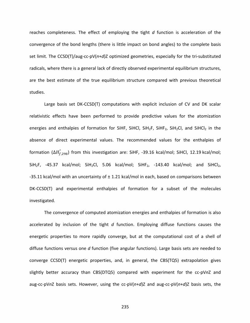
235
reaches completeness. The effect of employing the tight d function is acceleration of the
convergence of the bond lengths (there is little impact on bond angles) to the complete basis
set limit. The CCSD(T)/aug‐cc‐pV(n+d)Z optimized geometries, especially for the tri‐substituted
radicals, where there is a general lack of directly observed experimental equilibrium structures,
are the best estimate of the true equilibrium structure compared with previous theoretical
studies.
Large basis set DK‐CCSD(T) computations with explicit inclusion of CV and DK scalar
relativistic effects have been performed to provide predictive values for the atomization
energies and enthalpies of formation for SiHF, SiHCl, SiH2F, SiHF2, SiH2Cl, and SiHCl2 in the
absence of direct experimental values. The recommended values for the enthalpies of
formation (Δ ,° ) from this investigation are: SiHF, ‐39.16 kcal/mol; SiHCl, 12.19 kcal/mol;
SiH2F, ‐45.37 kcal/mol; SiH2Cl, 5.06 kcal/mol; SiHF2, ‐143.40 kcal/mol; and SiHCl2,
‐35.11 kcal/mol with an uncertainty of ± 1.21 kcal/mol in each, based on comparisons between
DK‐CCSD(T) and experimental enthalpies of formation for a subset of the molecules
investigated.
The convergence of computed atomization energies and enthalpies of formation is also
accelerated by inclusion of the tight d function. Employing diffuse functions causes the
energetic properties to more rapidly converge, but at the computational cost of a shell of
diffuse functions versus one d function (five angular functions). Large basis sets are needed to
converge CCSD(T) energetic properties, and, in general, the CBS(TQ5) extrapolation gives
slightly better accuracy than CBS(DTQ5) compared with experiment for the cc‐pVnZ and
aug‐cc‐pVnZ basis sets. However, using the cc‐pV(n+d)Z and aug‐cc‐pV(n+d)Z basis sets, the

236
CBS(DTQ5) extrapolation performs slightly better than the CBS(TQ5) extrapolation. Comparing
ccCA to CCSD(T) shows that ccCA gives, on average, atomization energies and enthalpies of
formation that are closer to experiment than CCSD(T)/CBS(DTQ) and DK‐CCSD(T).
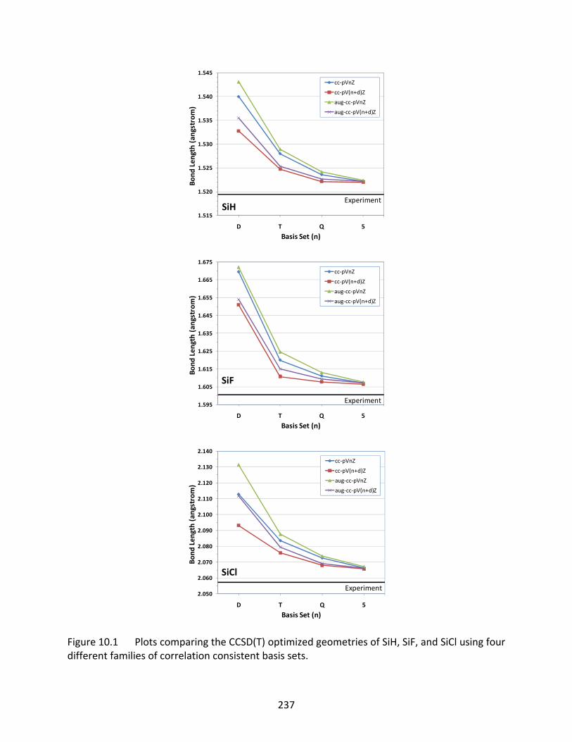
237
Figure 10.1 Plots comparing the CCSD(T) optimized geometries of SiH, SiF, and SiCl using four different families of correlation consistent basis sets.
1.515
1.520
1.525
1.530
1.535
1.540
1.545
D T Q 5
cc‐pVnZ
cc‐pV(n+d)Z
aug‐cc‐pVnZ
aug‐cc‐pV(n+d)Z
Experiment
Basis Set (n)
Bond
Length (an
gstrom
)
SiH
1.595
1.605
1.615
1.625
1.635
1.645
1.655
1.665
1.675
D T Q 5
cc‐pVnZ
cc‐pV(n+d)Z
aug‐cc‐pVnZ
aug‐cc‐pV(n+d)Z
Experiment
Basis Set (n)
Bond
Length (an
gstrom
)
SiF
2.050
2.060
2.070
2.080
2.090
2.100
2.110
2.120
2.130
2.140
D T Q 5
cc‐pVnZ
cc‐pV(n+d)Z
aug‐cc‐pVnZ
aug‐cc‐pV(n+d)Z
Experiment
Basis Set (n)
Bond
Length (an
gstrom
)
SiCl
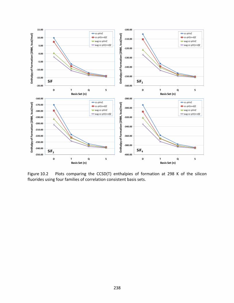
238
Figure 10.2 Plots comparing the CCSD(T) enthalpies of formation at 298 K of the silicon fluorides using four families of correlation consistent basis sets.
‐20.00
‐15.00
‐10.00
‐5.00
0.00
5.00
10.00
15.00
D T Q 5
cc‐pVnZ
cc‐pV(n+d)Z
aug‐cc‐pVnZ
aug‐cc‐pV(n+d)Z
Basis Set (n)
Enthalpy
of Formation (298K, kcal/mol)
SiF‐160.00
‐150.00
‐140.00
‐130.00
‐120.00
‐110.00
‐100.00
D T Q 5
cc‐pVnZ
cc‐pV(n+d)Z
aug‐cc‐pVnZ
aug‐cc‐pV(n+d)Z
Basis Set (n)
Enthalpy
of Formation (298K, kcal/mol)
SiF2
‐250.00
‐240.00
‐230.00
‐220.00
‐210.00
‐200.00
‐190.00
‐180.00
‐170.00
‐160.00
D T Q 5
cc‐pVnZ
cc‐pV(n+d)Z
aug‐cc‐pVnZ
aug‐cc‐pV(n+d)Z
Basis Set (n)
Enthalpy
of Formation (298K, kcal/mol)
SiF3‐400.00
‐380.00
‐360.00
‐340.00
‐320.00
‐300.00
‐280.00
D T Q 5
cc‐pVnZ
cc‐pV(n+d)Z
aug‐cc‐pVnZ
aug‐cc‐pV(n+d)Z
Basis Set (n)
Enthalpy
of Formation (298K, kcal/mol)
SiF4
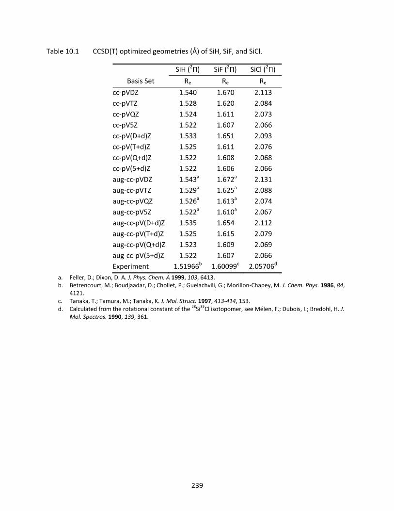
239
Table 10.1 CCSD(T) optimized geometries (Å) of SiH, SiF, and SiCl.
SiH (2Π) SiF (2Π) SiCl (2Π)
Basis Set Re Re Recc‐pVDZ 1.540 1.670 2.113cc‐pVTZ 1.528 1.620 2.084cc‐pVQZ 1.524 1.611 2.073cc‐pV5Z 1.522 1.607 2.066cc‐pV(D+d)Z 1.533 1.651 2.093cc‐pV(T+d)Z 1.525 1.611 2.076cc‐pV(Q+d)Z 1.522 1.608 2.068cc‐pV(5+d)Z 1.522 1.606 2.066aug‐cc‐pVDZ 1.543a 1.672a 2.131aug‐cc‐pVTZ 1.529a 1.625a 2.088aug‐cc‐pVQZ 1.526a 1.613a 2.074aug‐cc‐pV5Z 1.522a 1.610a 2.067aug‐cc‐pV(D+d)Z 1.535 1.654 2.112aug‐cc‐pV(T+d)Z 1.525 1.615 2.079aug‐cc‐pV(Q+d)Z 1.523 1.609 2.069aug‐cc‐pV(5+d)Z 1.522 1.607 2.066Experiment 1.51966b 1.60099c 2.05706d
a. Feller, D.; Dixon, D. A. J. Phys. Chem. A 1999, 103, 6413. b. Betrencourt, M.; Boudjaadar, D.; Chollet, P.; Guelachvili, G.; Morillon‐Chapey, M. J. Chem. Phys. 1986, 84,
4121. c. Tanaka, T.; Tamura, M.; Tanaka, K. J. Mol. Struct. 1997, 413‐414, 153. d. Calculated from the rotational constant of the 28Si35Cl isotopomer, see Mélen, F.; Dubois, I.; Bredohl, H. J.
Mol. Spectros. 1990, 139, 361.
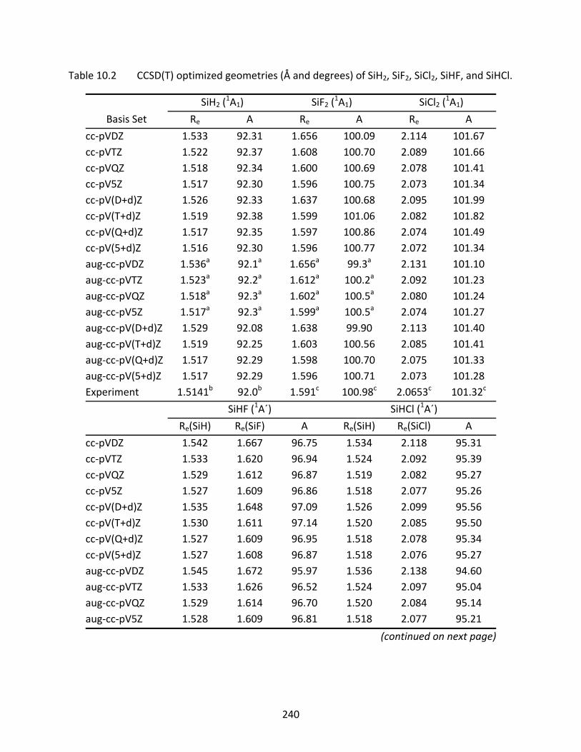
240
Table 10.2 CCSD(T) optimized geometries (Å and degrees) of SiH2, SiF2, SiCl2, SiHF, and SiHCl.
SiH2 (1A1) SiF2 (
1A1) SiCl2 (1A1)
Basis Set Re A Re A Re A
cc‐pVDZ 1.533 92.31 1.656 100.09 2.114 101.67cc‐pVTZ 1.522 92.37 1.608 100.70 2.089 101.66cc‐pVQZ 1.518 92.34 1.600 100.69 2.078 101.41cc‐pV5Z 1.517 92.30 1.596 100.75 2.073 101.34cc‐pV(D+d)Z 1.526 92.33 1.637 100.68 2.095 101.99cc‐pV(T+d)Z 1.519 92.38 1.599 101.06 2.082 101.82cc‐pV(Q+d)Z 1.517 92.35 1.597 100.86 2.074 101.49cc‐pV(5+d)Z 1.516 92.30 1.596 100.77 2.072 101.34aug‐cc‐pVDZ 1.536a 92.1a 1.656a 99.3a 2.131 101.10aug‐cc‐pVTZ 1.523a 92.2a 1.612a 100.2a 2.092 101.23aug‐cc‐pVQZ 1.518a 92.3a 1.602a 100.5a 2.080 101.24aug‐cc‐pV5Z 1.517a 92.3a 1.599a 100.5a 2.074 101.27aug‐cc‐pV(D+d)Z 1.529 92.08 1.638 99.90 2.113 101.40aug‐cc‐pV(T+d)Z 1.519 92.25 1.603 100.56 2.085 101.41aug‐cc‐pV(Q+d)Z 1.517 92.29 1.598 100.70 2.075 101.33aug‐cc‐pV(5+d)Z 1.517 92.29 1.596 100.71 2.073 101.28Experiment 1.5141b 92.0b 1.591c 100.98c 2.0653c 101.32c
SiHF (1A´) SiHCl (1A´)
Re(SiH) Re(SiF) A Re(SiH) Re(SiCl) A
cc‐pVDZ 1.542 1.667 96.75 1.534 2.118 95.31cc‐pVTZ 1.533 1.620 96.94 1.524 2.092 95.39cc‐pVQZ 1.529 1.612 96.87 1.519 2.082 95.27cc‐pV5Z 1.527 1.609 96.86 1.518 2.077 95.26cc‐pV(D+d)Z 1.535 1.648 97.09 1.526 2.099 95.56cc‐pV(T+d)Z 1.530 1.611 97.14 1.520 2.085 95.50cc‐pV(Q+d)Z 1.527 1.609 96.95 1.518 2.078 95.34cc‐pV(5+d)Z 1.527 1.608 96.87 1.518 2.076 95.27aug‐cc‐pVDZ 1.545 1.672 95.97 1.536 2.138 94.60aug‐cc‐pVTZ 1.533 1.626 96.52 1.524 2.097 95.04aug‐cc‐pVQZ 1.529 1.614 96.70 1.520 2.084 95.14aug‐cc‐pV5Z 1.528 1.609 96.81 1.518 2.077 95.21
(continued on next page)
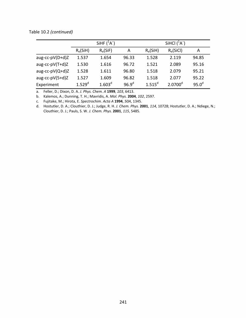
241
Table 10.2 (continued)
SiHF (1A´) SiHCl (1A´)
Re(SiH) Re(SiF) A Re(SiH) Re(SiCl) A
aug‐cc‐pV(D+d)Z 1.537 1.654 96.33 1.528 2.119 94.85aug‐cc‐pV(T+d)Z 1.530 1.616 96.72 1.521 2.089 95.16aug‐cc‐pV(Q+d)Z 1.528 1.611 96.80 1.518 2.079 95.21aug‐cc‐pV(5+d)Z 1.527 1.609 96.82 1.518 2.077 95.22Experiment 1.529d 1.603d 96.9d 1.515d 2.0700d 95.0d
a. Feller, D.; Dixon, D. A. J. Phys. Chem. A 1999, 103, 6413. b. Kalemos, A.; Dunning, T. H.; Mavridis, A. Mol. Phys. 2004, 102, 2597. c. Fujitake, M.; Hirota, E. Spectrochim. Acta A 1994, 50A, 1345. d. Hostutler, D. A.; Clouthier, D. J.; Judge, R. H. J. Chem. Phys. 2001, 114, 10728; Hostutler, D. A.; Ndiege, N.;
Clouthier, D. J.; Pauls, S. W. J. Chem. Phys. 2001, 115, 5485.
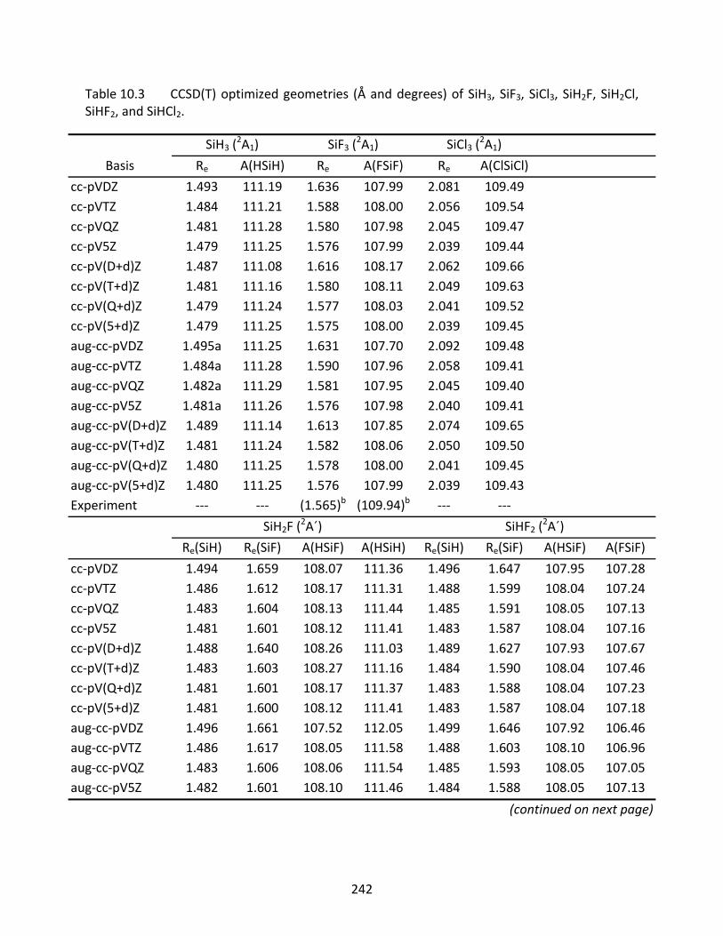
242
Table 10.3 CCSD(T) optimized geometries (Å and degrees) of SiH3, SiF3, SiCl3, SiH2F, SiH2Cl, SiHF2, and SiHCl2.
SiH3 (2A1) SiF3 (
2A1) SiCl3 (2A1)
Basis Re A(HSiH) Re A(FSiF) Re A(ClSiCl)
cc‐pVDZ 1.493 111.19 1.636 107.99 2.081 109.49 cc‐pVTZ 1.484 111.21 1.588 108.00 2.056 109.54 cc‐pVQZ 1.481 111.28 1.580 107.98 2.045 109.47 cc‐pV5Z 1.479 111.25 1.576 107.99 2.039 109.44 cc‐pV(D+d)Z 1.487 111.08 1.616 108.17 2.062 109.66 cc‐pV(T+d)Z 1.481 111.16 1.580 108.11 2.049 109.63 cc‐pV(Q+d)Z 1.479 111.24 1.577 108.03 2.041 109.52 cc‐pV(5+d)Z 1.479 111.25 1.575 108.00 2.039 109.45 aug‐cc‐pVDZ 1.495a 111.25 1.631 107.70 2.092 109.48 aug‐cc‐pVTZ 1.484a 111.28 1.590 107.96 2.058 109.41 aug‐cc‐pVQZ 1.482a 111.29 1.581 107.95 2.045 109.40 aug‐cc‐pV5Z 1.481a 111.26 1.576 107.98 2.040 109.41 aug‐cc‐pV(D+d)Z 1.489 111.14 1.613 107.85 2.074 109.65 aug‐cc‐pV(T+d)Z 1.481 111.24 1.582 108.06 2.050 109.50 aug‐cc‐pV(Q+d)Z 1.480 111.25 1.578 108.00 2.041 109.45 aug‐cc‐pV(5+d)Z 1.480 111.25 1.576 107.99 2.039 109.43 Experiment ‐‐‐ ‐‐‐ (1.565)b (109.94)b ‐‐‐ ‐‐‐
SiH2F (2A´) SiHF2 (
2A´)
Re(SiH) Re(SiF) A(HSiF) A(HSiH) Re(SiH) Re(SiF) A(HSiF) A(FSiF)
cc‐pVDZ 1.494 1.659 108.07 111.36 1.496 1.647 107.95 107.28cc‐pVTZ 1.486 1.612 108.17 111.31 1.488 1.599 108.04 107.24cc‐pVQZ 1.483 1.604 108.13 111.44 1.485 1.591 108.05 107.13cc‐pV5Z 1.481 1.601 108.12 111.41 1.483 1.587 108.04 107.16cc‐pV(D+d)Z 1.488 1.640 108.26 111.03 1.489 1.627 107.93 107.67cc‐pV(T+d)Z 1.483 1.603 108.27 111.16 1.484 1.590 108.04 107.46cc‐pV(Q+d)Z 1.481 1.601 108.17 111.37 1.483 1.588 108.04 107.23cc‐pV(5+d)Z 1.481 1.600 108.12 111.41 1.483 1.587 108.04 107.18aug‐cc‐pVDZ 1.496 1.661 107.52 112.05 1.499 1.646 107.92 106.46aug‐cc‐pVTZ 1.486 1.617 108.05 111.58 1.488 1.603 108.10 106.96aug‐cc‐pVQZ 1.483 1.606 108.06 111.54 1.485 1.593 108.05 107.05aug‐cc‐pV5Z 1.482 1.601 108.10 111.46 1.484 1.588 108.05 107.13
(continued on next page)
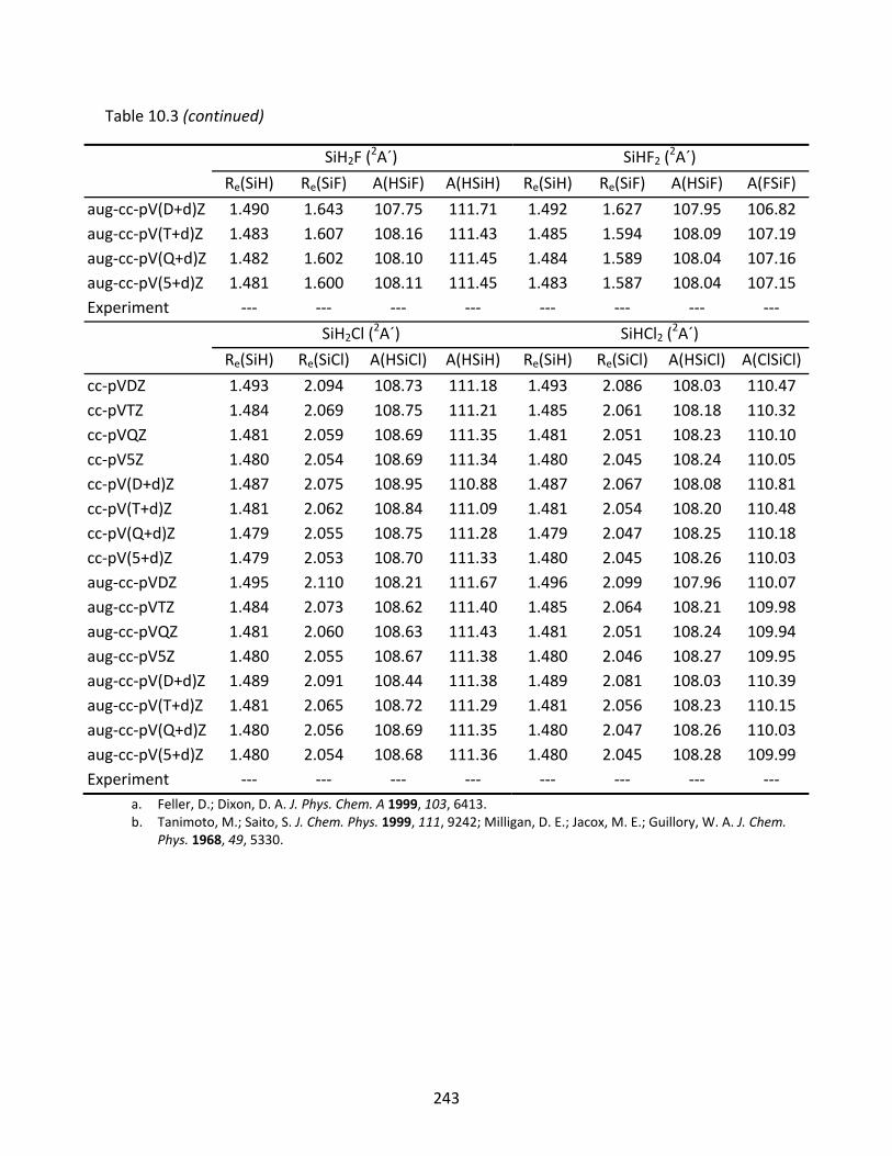
243
Table 10.3 (continued)
SiH2F (2A´) SiHF2 (
2A´)
Re(SiH) Re(SiF) A(HSiF) A(HSiH) Re(SiH) Re(SiF) A(HSiF) A(FSiF)
aug‐cc‐pV(D+d)Z 1.490 1.643 107.75 111.71 1.492 1.627 107.95 106.82aug‐cc‐pV(T+d)Z 1.483 1.607 108.16 111.43 1.485 1.594 108.09 107.19aug‐cc‐pV(Q+d)Z 1.482 1.602 108.10 111.45 1.484 1.589 108.04 107.16aug‐cc‐pV(5+d)Z 1.481 1.600 108.11 111.45 1.483 1.587 108.04 107.15Experiment ‐‐‐ ‐‐‐ ‐‐‐ ‐‐‐ ‐‐‐ ‐‐‐ ‐‐‐ ‐‐‐
SiH2Cl (2A´) SiHCl2 (
2A´)
Re(SiH) Re(SiCl) A(HSiCl) A(HSiH) Re(SiH) Re(SiCl) A(HSiCl) A(ClSiCl)
cc‐pVDZ 1.493 2.094 108.73 111.18 1.493 2.086 108.03 110.47cc‐pVTZ 1.484 2.069 108.75 111.21 1.485 2.061 108.18 110.32cc‐pVQZ 1.481 2.059 108.69 111.35 1.481 2.051 108.23 110.10cc‐pV5Z 1.480 2.054 108.69 111.34 1.480 2.045 108.24 110.05cc‐pV(D+d)Z 1.487 2.075 108.95 110.88 1.487 2.067 108.08 110.81cc‐pV(T+d)Z 1.481 2.062 108.84 111.09 1.481 2.054 108.20 110.48cc‐pV(Q+d)Z 1.479 2.055 108.75 111.28 1.479 2.047 108.25 110.18cc‐pV(5+d)Z 1.479 2.053 108.70 111.33 1.480 2.045 108.26 110.03aug‐cc‐pVDZ 1.495 2.110 108.21 111.67 1.496 2.099 107.96 110.07aug‐cc‐pVTZ 1.484 2.073 108.62 111.40 1.485 2.064 108.21 109.98aug‐cc‐pVQZ 1.481 2.060 108.63 111.43 1.481 2.051 108.24 109.94aug‐cc‐pV5Z 1.480 2.055 108.67 111.38 1.480 2.046 108.27 109.95aug‐cc‐pV(D+d)Z 1.489 2.091 108.44 111.38 1.489 2.081 108.03 110.39aug‐cc‐pV(T+d)Z 1.481 2.065 108.72 111.29 1.481 2.056 108.23 110.15aug‐cc‐pV(Q+d)Z 1.480 2.056 108.69 111.35 1.480 2.047 108.26 110.03aug‐cc‐pV(5+d)Z 1.480 2.054 108.68 111.36 1.480 2.045 108.28 109.99Experiment ‐‐‐ ‐‐‐ ‐‐‐ ‐‐‐ ‐‐‐ ‐‐‐ ‐‐‐ ‐‐‐
a. Feller, D.; Dixon, D. A. J. Phys. Chem. A 1999, 103, 6413. b. Tanimoto, M.; Saito, S. J. Chem. Phys. 1999, 111, 9242; Milligan, D. E.; Jacox, M. E.; Guillory, W. A. J. Chem.
Phys. 1968, 49, 5330.
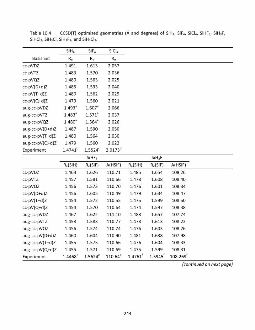
244
Table 10.4 CCSD(T) optimized geometries (Å and degrees) of SiH4, SiF4, SiCl4, SiHF3, SiH3F, SiHCl3, SiH3Cl, SiH2F2, and SiH2Cl2.
SiH4 SiF4 SiCl4
Basis Set Re Re Re
cc‐pVDZ 1.491 1.613 2.057 cc‐pVTZ 1.483 1.570 2.036 cc‐pVQZ 1.480 1.563 2.025 cc‐pV(D+d)Z 1.485 1.593 2.040 cc‐pV(T+d)Z 1.480 1.562 2.029 cc‐pV(Q+d)Z 1.479 1.560 2.021 aug‐cc‐pVDZ 1.493a 1.607a 2.066 aug‐cc‐pVTZ 1.483a 1.571a 2.037 aug‐cc‐pVQZ 1.480a 1.564a 2.026 aug‐cc‐pV(D+d)Z 1.487 1.590 2.050 aug‐cc‐pV(T+d)Z 1.480 1.564 2.030 aug‐cc‐pV(Q+d)Z 1.479 1.560 2.022 Experiment 1.4741b 1.5524c 2.0173d
SiHF3 SiH3F
Re(SiH) Re(SiF) A(HSiF) Re(SiH) Re(SiF) A(HSiF)
cc‐pVDZ 1.463 1.626 110.71 1.485 1.654 108.26 cc‐pVTZ 1.457 1.581 110.66 1.478 1.608 108.40 cc‐pVQZ 1.456 1.573 110.70 1.476 1.601 108.34 cc‐pV(D+d)Z 1.456 1.605 110.49 1.479 1.634 108.47 cc‐pV(T+d)Z 1.454 1.572 110.55 1.475 1.599 108.50 cc‐pV(Q+d)Z 1.454 1.570 110.64 1.474 1.597 108.38 aug‐cc‐pVDZ 1.467 1.622 111.10 1.488 1.657 107.74 aug‐cc‐pVTZ 1.458 1.583 110.77 1.478 1.613 108.22 aug‐cc‐pVQZ 1.456 1.574 110.74 1.476 1.603 108.26 aug‐cc‐pV(D+d)Z 1.460 1.604 110.90 1.481 1.638 107.98 aug‐cc‐pV(T+d)Z 1.455 1.575 110.66 1.476 1.604 108.33 aug‐cc‐pV(Q+d)Z 1.455 1.571 110.69 1.475 1.599 108.31 Experiment 1.4468e 1.5624e 110.64e 1.4761f 1.5945f 108.269f
(continued on next page)
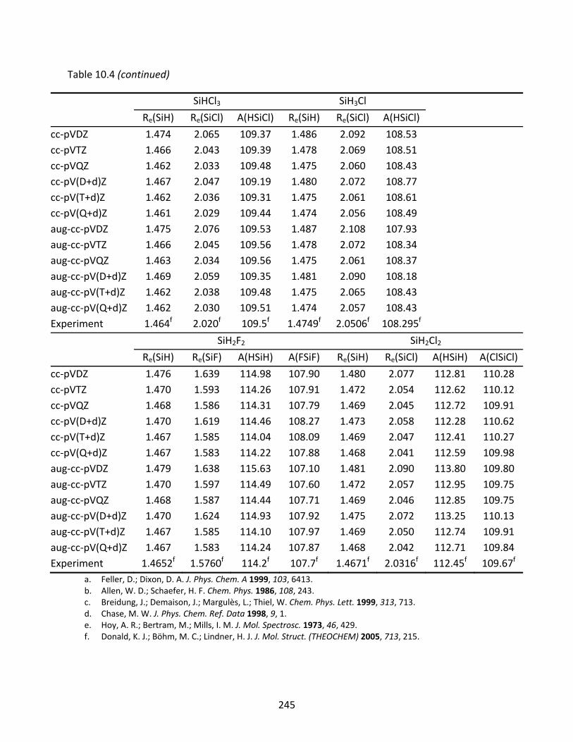
245
Table 10.4 (continued)
SiHCl3 SiH3Cl
Re(SiH) Re(SiCl) A(HSiCl) Re(SiH) Re(SiCl) A(HSiCl)
cc‐pVDZ 1.474 2.065 109.37 1.486 2.092 108.53 cc‐pVTZ 1.466 2.043 109.39 1.478 2.069 108.51 cc‐pVQZ 1.462 2.033 109.48 1.475 2.060 108.43 cc‐pV(D+d)Z 1.467 2.047 109.19 1.480 2.072 108.77 cc‐pV(T+d)Z 1.462 2.036 109.31 1.475 2.061 108.61 cc‐pV(Q+d)Z 1.461 2.029 109.44 1.474 2.056 108.49 aug‐cc‐pVDZ 1.475 2.076 109.53 1.487 2.108 107.93 aug‐cc‐pVTZ 1.466 2.045 109.56 1.478 2.072 108.34 aug‐cc‐pVQZ 1.463 2.034 109.56 1.475 2.061 108.37 aug‐cc‐pV(D+d)Z 1.469 2.059 109.35 1.481 2.090 108.18 aug‐cc‐pV(T+d)Z 1.462 2.038 109.48 1.475 2.065 108.43 aug‐cc‐pV(Q+d)Z 1.462 2.030 109.51 1.474 2.057 108.43 Experiment 1.464f 2.020f 109.5f 1.4749f 2.0506f 108.295f
SiH2F2 SiH2Cl2
Re(SiH) Re(SiF) A(HSiH) A(FSiF) Re(SiH) Re(SiCl) A(HSiH) A(ClSiCl)
cc‐pVDZ 1.476 1.639 114.98 107.90 1.480 2.077 112.81 110.28cc‐pVTZ 1.470 1.593 114.26 107.91 1.472 2.054 112.62 110.12cc‐pVQZ 1.468 1.586 114.31 107.79 1.469 2.045 112.72 109.91cc‐pV(D+d)Z 1.470 1.619 114.46 108.27 1.473 2.058 112.28 110.62cc‐pV(T+d)Z 1.467 1.585 114.04 108.09 1.469 2.047 112.41 110.27cc‐pV(Q+d)Z 1.467 1.583 114.22 107.88 1.468 2.041 112.59 109.98aug‐cc‐pVDZ 1.479 1.638 115.63 107.10 1.481 2.090 113.80 109.80aug‐cc‐pVTZ 1.470 1.597 114.49 107.60 1.472 2.057 112.95 109.75aug‐cc‐pVQZ 1.468 1.587 114.44 107.71 1.469 2.046 112.85 109.75aug‐cc‐pV(D+d)Z 1.470 1.624 114.93 107.92 1.475 2.072 113.25 110.13aug‐cc‐pV(T+d)Z 1.467 1.585 114.10 107.97 1.469 2.050 112.74 109.91aug‐cc‐pV(Q+d)Z 1.467 1.583 114.24 107.87 1.468 2.042 112.71 109.84Experiment 1.4652f 1.5760f 114.2f 107.7f 1.4671f 2.0316f 112.45f 109.67f
a. Feller, D.; Dixon, D. A. J. Phys. Chem. A 1999, 103, 6413. b. Allen, W. D.; Schaefer, H. F. Chem. Phys. 1986, 108, 243. c. Breidung, J.; Demaison, J.; Margulès, L.; Thiel, W. Chem. Phys. Lett. 1999, 313, 713. d. Chase, M. W. J. Phys. Chem. Ref. Data 1998, 9, 1. e. Hoy, A. R.; Bertram, M.; Mills, I. M. J. Mol. Spectrosc. 1973, 46, 429. f. Donald, K. J.; Böhm, M. C.; Lindner, H. J. J. Mol. Struct. (THEOCHEM) 2005, 713, 215.
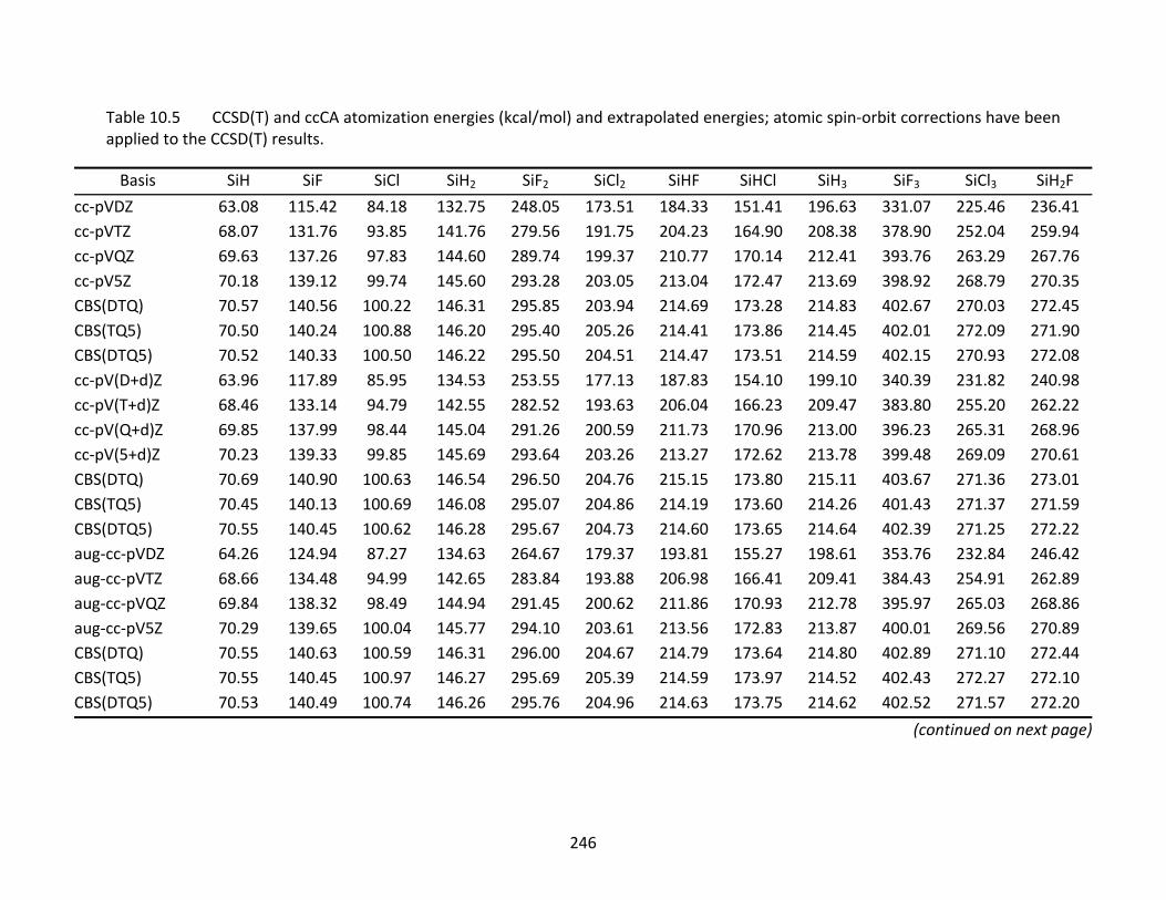
246
Table 10.5 CCSD(T) and ccCA atomization energies (kcal/mol) and extrapolated energies; atomic spin‐orbit corrections have been applied to the CCSD(T) results.
Basis SiH SiF SiCl SiH2 SiF2 SiCl2 SiHF SiHCl SiH3 SiF3 SiCl3 SiH2F
cc‐pVDZ 63.08 115.42 84.18 132.75 248.05 173.51 184.33 151.41 196.63 331.07 225.46 236.41cc‐pVTZ 68.07 131.76 93.85 141.76 279.56 191.75 204.23 164.90 208.38 378.90 252.04 259.94cc‐pVQZ 69.63 137.26 97.83 144.60 289.74 199.37 210.77 170.14 212.41 393.76 263.29 267.76cc‐pV5Z 70.18 139.12 99.74 145.60 293.28 203.05 213.04 172.47 213.69 398.92 268.79 270.35CBS(DTQ) 70.57 140.56 100.22 146.31 295.85 203.94 214.69 173.28 214.83 402.67 270.03 272.45CBS(TQ5) 70.50 140.24 100.88 146.20 295.40 205.26 214.41 173.86 214.45 402.01 272.09 271.90CBS(DTQ5) 70.52 140.33 100.50 146.22 295.50 204.51 214.47 173.51 214.59 402.15 270.93 272.08cc‐pV(D+d)Z 63.96 117.89 85.95 134.53 253.55 177.13 187.83 154.10 199.10 340.39 231.82 240.98cc‐pV(T+d)Z 68.46 133.14 94.79 142.55 282.52 193.63 206.04 166.23 209.47 383.80 255.20 262.22cc‐pV(Q+d)Z 69.85 137.99 98.44 145.04 291.26 200.59 211.73 170.96 213.00 396.23 265.31 268.96cc‐pV(5+d)Z 70.23 139.33 99.85 145.69 293.64 203.26 213.27 172.62 213.78 399.48 269.09 270.61CBS(DTQ) 70.69 140.90 100.63 146.54 296.50 204.76 215.15 173.80 215.11 403.67 271.36 273.01CBS(TQ5) 70.45 140.13 100.69 146.08 295.07 204.86 214.19 173.60 214.26 401.43 271.37 271.59CBS(DTQ5) 70.55 140.45 100.62 146.28 295.67 204.73 214.60 173.65 214.64 402.39 271.25 272.22aug‐cc‐pVDZ 64.26 124.94 87.27 134.63 264.67 179.37 193.81 155.27 198.61 353.76 232.84 246.42aug‐cc‐pVTZ 68.66 134.48 94.99 142.65 283.84 193.88 206.98 166.41 209.41 384.43 254.91 262.89aug‐cc‐pVQZ 69.84 138.32 98.49 144.94 291.45 200.62 211.86 170.93 212.78 395.97 265.03 268.86aug‐cc‐pV5Z 70.29 139.65 100.04 145.77 294.10 203.61 213.56 172.83 213.87 400.01 269.56 270.89CBS(DTQ) 70.55 140.63 100.59 146.31 296.00 204.67 214.79 173.64 214.80 402.89 271.10 272.44CBS(TQ5) 70.55 140.45 100.97 146.27 295.69 205.39 214.59 173.97 214.52 402.43 272.27 272.10CBS(DTQ5) 70.53 140.49 100.74 146.26 295.76 204.96 214.63 173.75 214.62 402.52 271.57 272.20
(continued on next page)
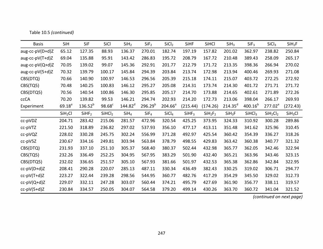
247
Table 10.5 (continued)
Basis SiH SiF SiCl SiH2 SiF2 SiCl2 SiHF SiHCl SiH3 SiF3 SiCl3 SiH2F
aug‐cc‐pV(D+d)Z 65.12 127.35 88.93 136.37 270.01 182.74 197.19 157.82 201.02 362.97 238.82 250.84aug‐cc‐pV(T+d)Z 69.04 135.88 95.91 143.42 286.83 195.72 208.79 167.72 210.48 389.43 258.09 265.17aug‐cc‐pV(Q+d)Z 70.05 139.02 99.07 145.36 292.91 201.77 212.79 171.72 213.35 398.36 266.94 270.02aug‐cc‐pV(5+d)Z 70.32 139.79 100.17 145.84 294.39 203.84 213.74 172.98 213.94 400.46 269.93 271.08CBS(DTQ) 70.66 140.90 100.97 146.53 296.56 205.39 215.18 174.11 215.07 403.72 272.25 272.92CBS(TQ5) 70.48 140.25 100.83 146.12 295.27 205.08 214.31 173.74 214.30 401.72 271.71 271.72CBS(DTQ5) 70.56 140.54 100.86 146.30 295.85 205.17 214.70 173.88 214.65 402.61 271.89 272.26ccCA 70.20 139.82 99.53 146.21 294.74 202.93 214.20 172.73 213.06 398.04 266.17 269.93Experiment 69.18a 136.52b 98.68c 144.82d 296.29b 204.66a (215.44) (174.26) 214.35d 400.16b 277.02e (272.43)
SiH2Cl SiHF2 SiHCl2 SiH4 SiF4 SiCl4 SiHF3 SiH2F2 SiH3F SiHCl3 SiH2Cl2 SiH3Cl
cc‐pVDZ 204.71 283.42 215.06 281.57 472.96 320.54 425.25 373.95 324.33 310.92 300.28 289.86cc‐pVTZ 221.50 318.89 236.82 297.02 537.93 356.10 477.17 413.11 351.48 341.62 325.96 310.45cc‐pVQZ 228.02 330.28 245.75 302.24 556.99 371.28 492.97 425.54 360.42 354.39 336.27 318.26cc‐pV5Z 230.67 334.16 249.81 303.94 563.84 378.79 498.55 429.83 363.42 360.38 340.77 321.32CBS(DTQ) 231.93 337.10 251.10 305.37 568.40 380.37 502.44 432.98 365.77 362.05 342.46 322.94CBS(TQ5) 232.26 336.49 252.25 304.95 567.95 383.29 501.90 432.40 365.21 363.96 343.46 323.15CBS(DTQ5) 232.02 336.65 251.57 305.10 567.93 381.66 501.97 432.53 365.38 362.86 342.84 322.95cc‐pV(D+d)Z 208.41 290.28 220.07 285.13 487.11 330.34 436.49 382.43 330.25 319.02 306.71 294.77cc‐pV(T+d)Z 223.27 322.44 239.28 298.56 544.95 360.77 482.76 417.29 354.29 345.50 329.02 312.73cc‐pV(Q+d)Z 229.07 332.11 247.28 303.07 560.44 374.21 495.79 427.69 361.90 356.77 338.11 319.57cc‐pV(5+d)Z 230.84 334.57 250.05 304.07 564.58 379.20 499.14 430.26 363.70 360.72 341.04 321.52
(continued on next page)
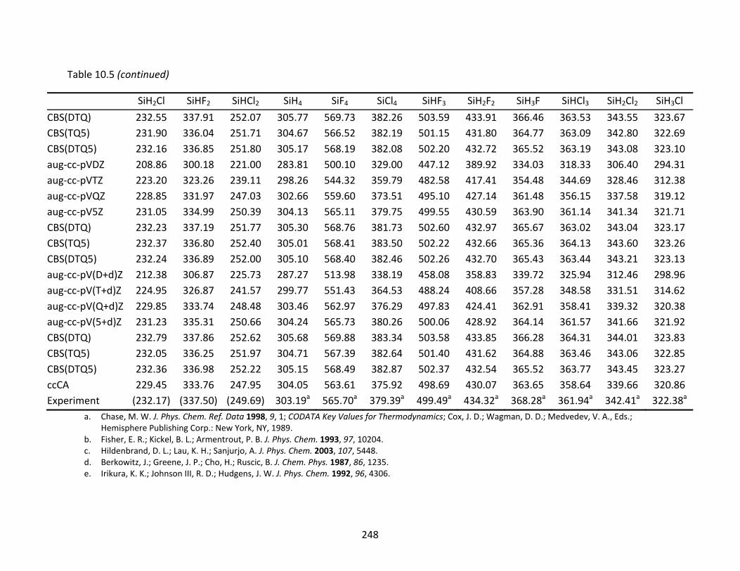
248
Table 10.5 (continued)
SiH2Cl SiHF2 SiHCl2 SiH4 SiF4 SiCl4 SiHF3 SiH2F2 SiH3F SiHCl3 SiH2Cl2 SiH3Cl
CBS(DTQ) 232.55 337.91 252.07 305.77 569.73 382.26 503.59 433.91 366.46 363.53 343.55 323.67CBS(TQ5) 231.90 336.04 251.71 304.67 566.52 382.19 501.15 431.80 364.77 363.09 342.80 322.69CBS(DTQ5) 232.16 336.85 251.80 305.17 568.19 382.08 502.20 432.72 365.52 363.19 343.08 323.10aug‐cc‐pVDZ 208.86 300.18 221.00 283.81 500.10 329.00 447.12 389.92 334.03 318.33 306.40 294.31aug‐cc‐pVTZ 223.20 323.26 239.11 298.26 544.32 359.79 482.58 417.41 354.48 344.69 328.46 312.38aug‐cc‐pVQZ 228.85 331.97 247.03 302.66 559.60 373.51 495.10 427.14 361.48 356.15 337.58 319.12aug‐cc‐pV5Z 231.05 334.99 250.39 304.13 565.11 379.75 499.55 430.59 363.90 361.14 341.34 321.71CBS(DTQ) 232.23 337.19 251.77 305.30 568.76 381.73 502.60 432.97 365.67 363.02 343.04 323.17CBS(TQ5) 232.37 336.80 252.40 305.01 568.41 383.50 502.22 432.66 365.36 364.13 343.60 323.26CBS(DTQ5) 232.24 336.89 252.00 305.10 568.40 382.46 502.26 432.70 365.43 363.44 343.21 323.13aug‐cc‐pV(D+d)Z 212.38 306.87 225.73 287.27 513.98 338.19 458.08 358.83 339.72 325.94 312.46 298.96aug‐cc‐pV(T+d)Z 224.95 326.87 241.57 299.77 551.43 364.53 488.24 408.66 357.28 348.58 331.51 314.62aug‐cc‐pV(Q+d)Z 229.85 333.74 248.48 303.46 562.97 376.29 497.83 424.41 362.91 358.41 339.32 320.38aug‐cc‐pV(5+d)Z 231.23 335.31 250.66 304.24 565.73 380.26 500.06 428.92 364.14 361.57 341.66 321.92CBS(DTQ) 232.79 337.86 252.62 305.68 569.88 383.34 503.58 433.85 366.28 364.31 344.01 323.83CBS(TQ5) 232.05 336.25 251.97 304.71 567.39 382.64 501.40 431.62 364.88 363.46 343.06 322.85CBS(DTQ5) 232.36 336.98 252.22 305.15 568.49 382.87 502.37 432.54 365.52 363.77 343.45 323.27ccCA 229.45 333.76 247.95 304.05 563.61 375.92 498.69 430.07 363.65 358.64 339.66 320.86Experiment (232.17) (337.50) (249.69) 303.19a 565.70a 379.39a 499.49a 434.32a 368.28a 361.94a 342.41a 322.38a
a. Chase, M. W. J. Phys. Chem. Ref. Data 1998, 9, 1; CODATA Key Values for Thermodynamics; Cox, J. D.; Wagman, D. D.; Medvedev, V. A., Eds.; Hemisphere Publishing Corp.: New York, NY, 1989.
b. Fisher, E. R.; Kickel, B. L.; Armentrout, P. B. J. Phys. Chem. 1993, 97, 10204. c. Hildenbrand, D. L.; Lau, K. H.; Sanjurjo, A. J. Phys. Chem. 2003, 107, 5448. d. Berkowitz, J.; Greene, J. P.; Cho, H.; Ruscic, B. J. Chem. Phys. 1987, 86, 1235. e. Irikura, K. K.; Johnson III, R. D.; Hudgens, J. W. J. Phys. Chem. 1992, 96, 4306.
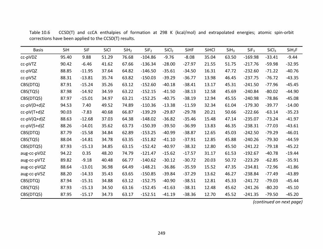
249
Table 10.6 CCSD(T) and ccCA enthalpies of formation at 298 K (kcal/mol) and extrapolated energies; atomic spin‐orbit corrections have been applied to the CCSD(T) results.
Basis SiH SiF SiCl SiH2 SiF2 SiCl2 SiHF SiHCl SiH3 SiF3 SiCl3 SiH2F
cc‐pVDZ 95.40 9.88 51.29 76.68 ‐104.86 ‐9.76 ‐8.08 35.04 63.50 ‐169.98 ‐33.41 ‐9.44cc‐pVTZ 90.42 ‐6.46 41.62 67.66 ‐136.34 ‐28.00 ‐27.97 21.55 51.75 ‐217.76 ‐59.98 ‐32.95cc‐pVQZ 88.85 ‐11.95 37.64 64.82 ‐146.50 ‐35.61 ‐34.50 16.31 47.72 ‐232.60 ‐71.22 ‐40.76cc‐pV5Z 88.31 ‐13.81 35.74 63.82 ‐150.03 ‐39.29 ‐36.77 13.98 46.45 ‐237.75 ‐76.72 ‐43.35CBS(DTQ) 87.91 ‐15.24 35.26 63.12 ‐152.60 ‐40.18 ‐38.41 13.17 45.31 ‐241.50 ‐77.96 ‐45.45CBS(TQ5) 87.98 ‐14.92 34.59 63.22 ‐152.15 ‐41.50 ‐38.13 12.58 45.69 ‐240.84 ‐80.02 ‐44.90CBS(DTQ5) 87.97 ‐15.01 34.97 63.21 ‐152.25 ‐40.75 ‐38.19 12.94 45.55 ‐240.98 ‐78.86 ‐45.08cc‐pV(D+d)Z 94.53 7.40 49.52 74.89 ‐110.36 ‐13.38 ‐11.59 32.34 61.04 ‐179.30 ‐39.77 ‐14.00cc‐pV(T+d)Z 90.03 ‐7.83 40.68 66.87 ‐139.29 ‐29.87 ‐29.78 20.21 50.66 ‐222.66 ‐63.14 ‐35.23cc‐pV(Q+d)Z 88.63 ‐12.68 37.03 64.38 ‐148.02 ‐36.82 ‐35.46 15.48 47.14 ‐235.07 ‐73.24 ‐41.97cc‐pV(5+d)Z 88.26 ‐14.01 35.62 63.73 ‐150.39 ‐39.50 ‐36.99 13.83 46.35 ‐238.31 ‐77.03 ‐43.61CBS(DTQ) 87.79 ‐15.58 34.84 62.89 ‐153.25 ‐40.99 ‐38.87 12.65 45.03 ‐242.50 ‐79.29 ‐46.01CBS(TQ5) 88.04 ‐14.81 34.78 63.35 ‐151.82 ‐41.10 ‐37.91 12.85 45.88 ‐240.26 ‐79.30 ‐44.59CBS(DTQ5) 87.93 ‐15.13 34.85 63.15 ‐152.42 ‐40.97 ‐38.32 12.80 45.50 ‐241.22 ‐79.18 ‐45.22aug‐cc‐pVDZ 94.22 0.35 48.20 74.79 ‐121.47 ‐15.62 ‐17.57 31.17 61.53 ‐192.67 ‐40.78 ‐19.44aug‐cc‐pVTZ 89.82 ‐9.18 40.48 66.77 ‐140.62 ‐30.12 ‐30.72 20.03 50.72 ‐223.29 ‐62.85 ‐35.91aug‐cc‐pVQZ 88.64 ‐13.01 36.98 64.49 ‐148.21 ‐36.86 ‐35.59 15.52 47.35 ‐234.81 ‐72.96 ‐41.86aug‐cc‐pV5Z 88.20 ‐14.33 35.43 63.65 ‐150.85 ‐39.84 ‐37.29 13.62 46.27 ‐238.84 ‐77.49 ‐43.89CBS(DTQ) 87.94 ‐15.31 34.88 63.12 ‐152.75 ‐40.90 ‐38.51 12.81 45.33 ‐241.72 ‐79.03 ‐45.44CBS(TQ5) 87.93 ‐15.13 34.50 63.16 ‐152.45 ‐41.63 ‐38.31 12.48 45.62 ‐241.26 ‐80.20 ‐45.10CBS(DTQ5) 87.95 ‐15.17 34.73 63.17 ‐152.51 ‐41.19 ‐38.36 12.70 45.52 ‐241.35 ‐79.50 ‐45.20
(continued on next page)
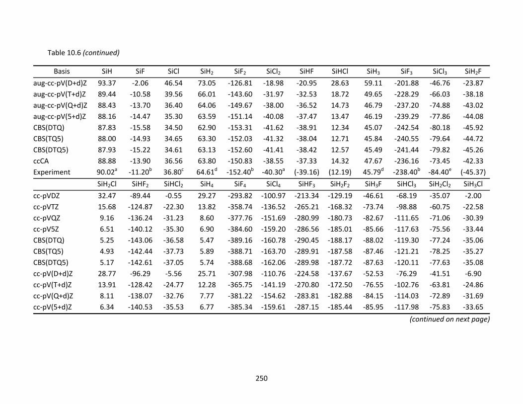
250
Table 10.6 (continued)
Basis SiH SiF SiCl SiH2 SiF2 SiCl2 SiHF SiHCl SiH3 SiF3 SiCl3 SiH2F
aug‐cc‐pV(D+d)Z 93.37 ‐2.06 46.54 73.05 ‐126.81 ‐18.98 ‐20.95 28.63 59.11 ‐201.88 ‐46.76 ‐23.87aug‐cc‐pV(T+d)Z 89.44 ‐10.58 39.56 66.01 ‐143.60 ‐31.97 ‐32.53 18.72 49.65 ‐228.29 ‐66.03 ‐38.18aug‐cc‐pV(Q+d)Z 88.43 ‐13.70 36.40 64.06 ‐149.67 ‐38.00 ‐36.52 14.73 46.79 ‐237.20 ‐74.88 ‐43.02aug‐cc‐pV(5+d)Z 88.16 ‐14.47 35.30 63.59 ‐151.14 ‐40.08 ‐37.47 13.47 46.19 ‐239.29 ‐77.86 ‐44.08CBS(DTQ) 87.83 ‐15.58 34.50 62.90 ‐153.31 ‐41.62 ‐38.91 12.34 45.07 ‐242.54 ‐80.18 ‐45.92CBS(TQ5) 88.00 ‐14.93 34.65 63.30 ‐152.03 ‐41.32 ‐38.04 12.71 45.84 ‐240.55 ‐79.64 ‐44.72CBS(DTQ5) 87.93 ‐15.22 34.61 63.13 ‐152.60 ‐41.41 ‐38.42 12.57 45.49 ‐241.44 ‐79.82 ‐45.26ccCA 88.88 ‐13.90 36.56 63.80 ‐150.83 ‐38.55 ‐37.33 14.32 47.67 ‐236.16 ‐73.45 ‐42.33Experiment 90.02a ‐11.20b 36.80c 64.61d ‐152.40b ‐40.30a (‐39.16) (12.19) 45.79d ‐238.40b ‐84.40e (‐45.37)
SiH2Cl SiHF2 SiHCl2 SiH4 SiF4 SiCl4 SiHF3 SiH2F2 SiH3F SiHCl3 SiH2Cl2 SiH3Cl
cc‐pVDZ 32.47 ‐89.44 ‐0.55 29.27 ‐293.82 ‐100.97 ‐213.34 ‐129.19 ‐46.61 ‐68.19 ‐35.07 ‐2.00cc‐pVTZ 15.68 ‐124.87 ‐22.30 13.82 ‐358.74 ‐136.52 ‐265.21 ‐168.32 ‐73.74 ‐98.88 ‐60.75 ‐22.58cc‐pVQZ 9.16 ‐136.24 ‐31.23 8.60 ‐377.76 ‐151.69 ‐280.99 ‐180.73 ‐82.67 ‐111.65 ‐71.06 ‐30.39cc‐pV5Z 6.51 ‐140.12 ‐35.30 6.90 ‐384.60 ‐159.20 ‐286.56 ‐185.01 ‐85.66 ‐117.63 ‐75.56 ‐33.44CBS(DTQ) 5.25 ‐143.06 ‐36.58 5.47 ‐389.16 ‐160.78 ‐290.45 ‐188.17 ‐88.02 ‐119.30 ‐77.24 ‐35.06CBS(TQ5) 4.93 ‐142.44 ‐37.73 5.89 ‐388.71 ‐163.70 ‐289.91 ‐187.58 ‐87.46 ‐121.21 ‐78.25 ‐35.27CBS(DTQ5) 5.17 ‐142.61 ‐37.05 5.74 ‐388.68 ‐162.06 ‐289.98 ‐187.72 ‐87.63 ‐120.11 ‐77.63 ‐35.08cc‐pV(D+d)Z 28.77 ‐96.29 ‐5.56 25.71 ‐307.98 ‐110.76 ‐224.58 ‐137.67 ‐52.53 ‐76.29 ‐41.51 ‐6.90cc‐pV(T+d)Z 13.91 ‐128.42 ‐24.77 12.28 ‐365.75 ‐141.19 ‐270.80 ‐172.50 ‐76.55 ‐102.76 ‐63.81 ‐24.86cc‐pV(Q+d)Z 8.11 ‐138.07 ‐32.76 7.77 ‐381.22 ‐154.62 ‐283.81 ‐182.88 ‐84.15 ‐114.03 ‐72.89 ‐31.69cc‐pV(5+d)Z 6.34 ‐140.53 ‐35.53 6.77 ‐385.34 ‐159.61 ‐287.15 ‐185.44 ‐85.95 ‐117.98 ‐75.83 ‐33.65
(continued on next page)
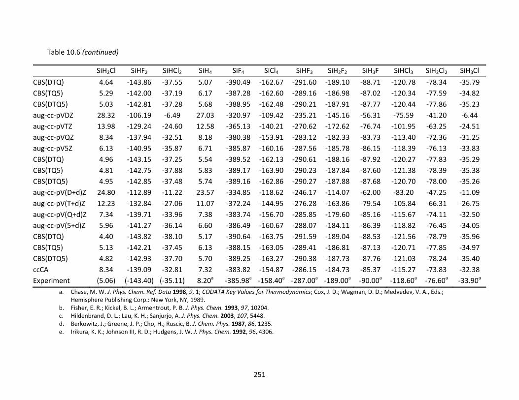
251
Table 10.6 (continued)
SiH2Cl SiHF2 SiHCl2 SiH4 SiF4 SiCl4 SiHF3 SiH2F2 SiH3F SiHCl3 SiH2Cl2 SiH3Cl
CBS(DTQ) 4.64 ‐143.86 ‐37.55 5.07 ‐390.49 ‐162.67 ‐291.60 ‐189.10 ‐88.71 ‐120.78 ‐78.34 ‐35.79CBS(TQ5) 5.29 ‐142.00 ‐37.19 6.17 ‐387.28 ‐162.60 ‐289.16 ‐186.98 ‐87.02 ‐120.34 ‐77.59 ‐34.82CBS(DTQ5) 5.03 ‐142.81 ‐37.28 5.68 ‐388.95 ‐162.48 ‐290.21 ‐187.91 ‐87.77 ‐120.44 ‐77.86 ‐35.23aug‐cc‐pVDZ 28.32 ‐106.19 ‐6.49 27.03 ‐320.97 ‐109.42 ‐235.21 ‐145.16 ‐56.31 ‐75.59 ‐41.20 ‐6.44aug‐cc‐pVTZ 13.98 ‐129.24 ‐24.60 12.58 ‐365.13 ‐140.21 ‐270.62 ‐172.62 ‐76.74 ‐101.95 ‐63.25 ‐24.51aug‐cc‐pVQZ 8.34 ‐137.94 ‐32.51 8.18 ‐380.38 ‐153.91 ‐283.12 ‐182.33 ‐83.73 ‐113.40 ‐72.36 ‐31.25aug‐cc‐pV5Z 6.13 ‐140.95 ‐35.87 6.71 ‐385.87 ‐160.16 ‐287.56 ‐185.78 ‐86.15 ‐118.39 ‐76.13 ‐33.83CBS(DTQ) 4.96 ‐143.15 ‐37.25 5.54 ‐389.52 ‐162.13 ‐290.61 ‐188.16 ‐87.92 ‐120.27 ‐77.83 ‐35.29CBS(TQ5) 4.81 ‐142.75 ‐37.88 5.83 ‐389.17 ‐163.90 ‐290.23 ‐187.84 ‐87.60 ‐121.38 ‐78.39 ‐35.38CBS(DTQ5) 4.95 ‐142.85 ‐37.48 5.74 ‐389.16 ‐162.86 ‐290.27 ‐187.88 ‐87.68 ‐120.70 ‐78.00 ‐35.26aug‐cc‐pV(D+d)Z 24.80 ‐112.89 ‐11.22 23.57 ‐334.85 ‐118.62 ‐246.17 ‐114.07 ‐62.00 ‐83.20 ‐47.25 ‐11.09aug‐cc‐pV(T+d)Z 12.23 ‐132.84 ‐27.06 11.07 ‐372.24 ‐144.95 ‐276.28 ‐163.86 ‐79.54 ‐105.84 ‐66.31 ‐26.75aug‐cc‐pV(Q+d)Z 7.34 ‐139.71 ‐33.96 7.38 ‐383.74 ‐156.70 ‐285.85 ‐179.60 ‐85.16 ‐115.67 ‐74.11 ‐32.50aug‐cc‐pV(5+d)Z 5.96 ‐141.27 ‐36.14 6.60 ‐386.49 ‐160.67 ‐288.07 ‐184.11 ‐86.39 ‐118.82 ‐76.45 ‐34.05CBS(DTQ) 4.40 ‐143.82 ‐38.10 5.17 ‐390.64 ‐163.75 ‐291.59 ‐189.04 ‐88.53 ‐121.56 ‐78.79 ‐35.96CBS(TQ5) 5.13 ‐142.21 ‐37.45 6.13 ‐388.15 ‐163.05 ‐289.41 ‐186.81 ‐87.13 ‐120.71 ‐77.85 ‐34.97CBS(DTQ5) 4.82 ‐142.93 ‐37.70 5.70 ‐389.25 ‐163.27 ‐290.38 ‐187.73 ‐87.76 ‐121.03 ‐78.24 ‐35.40ccCA 8.34 ‐139.09 ‐32.81 7.32 ‐383.82 ‐154.87 ‐286.15 ‐184.73 ‐85.37 ‐115.27 ‐73.83 ‐32.38Experiment (5.06) (‐143.40) (‐35.11) 8.20a ‐385.98a ‐158.40a ‐287.00a ‐189.00a ‐90.00a ‐118.60a ‐76.60a ‐33.90a
a. Chase, M. W. J. Phys. Chem. Ref. Data 1998, 9, 1; CODATA Key Values for Thermodynamics; Cox, J. D.; Wagman, D. D.; Medvedev, V. A., Eds.; Hemisphere Publishing Corp.: New York, NY, 1989.
b. Fisher, E. R.; Kickel, B. L.; Armentrout, P. B. J. Phys. Chem. 1993, 97, 10204. c. Hildenbrand, D. L.; Lau, K. H.; Sanjurjo, A. J. Phys. Chem. 2003, 107, 5448. d. Berkowitz, J.; Greene, J. P.; Cho, H.; Ruscic, B. J. Chem. Phys. 1987, 86, 1235. e. Irikura, K. K.; Johnson III, R. D.; Hudgens, J. W. J. Phys. Chem. 1992, 96, 4306.
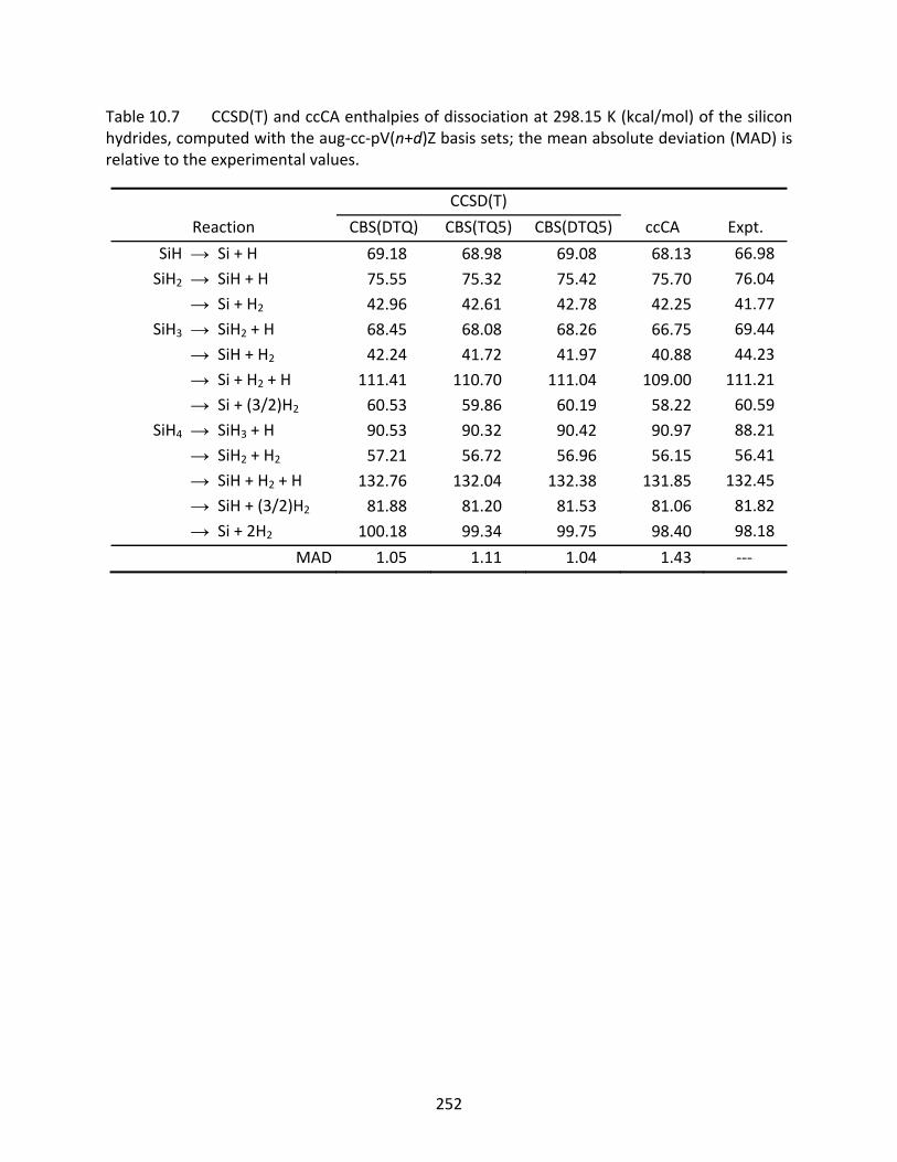
252
Table 10.7 CCSD(T) and ccCA enthalpies of dissociation at 298.15 K (kcal/mol) of the silicon hydrides, computed with the aug‐cc‐pV(n+d)Z basis sets; the mean absolute deviation (MAD) is relative to the experimental values.
CCSD(T)
Reaction CBS(DTQ) CBS(TQ5) CBS(DTQ5) ccCA Expt.
SiH → Si + H 69.18 68.98 69.08 68.13 66.98
SiH2 → SiH + H 75.55 75.32 75.42 75.70 76.04
→ Si + H2 42.96 42.61 42.78 42.25 41.77
SiH3 → SiH2 + H 68.45 68.08 68.26 66.75 69.44
→ SiH + H2 42.24 41.72 41.97 40.88 44.23
→ Si + H2 + H 111.41 110.70 111.04 109.00 111.21
→ Si + (3/2)H2 60.53 59.86 60.19 58.22 60.59
SiH4 → SiH3 + H 90.53 90.32 90.42 90.97 88.21
→ SiH2 + H2 57.21 56.72 56.96 56.15 56.41
→ SiH + H2 + H 132.76 132.04 132.38 131.85 132.45
→ SiH + (3/2)H2 81.88 81.20 81.53 81.06 81.82
→ Si + 2H2 100.18 99.34 99.75 98.40 98.18
MAD 1.05 1.11 1.04 1.43 ‐‐‐
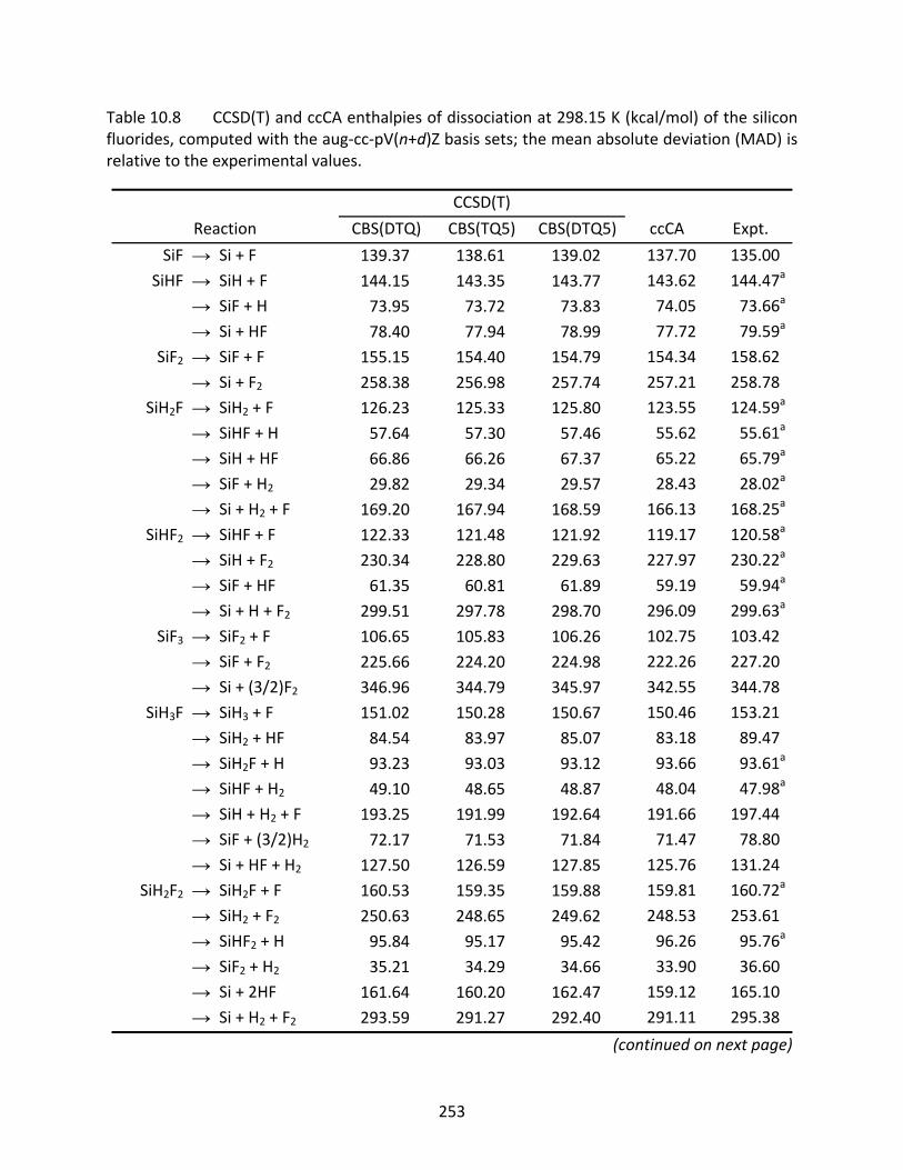
253
Table 10.8 CCSD(T) and ccCA enthalpies of dissociation at 298.15 K (kcal/mol) of the silicon fluorides, computed with the aug‐cc‐pV(n+d)Z basis sets; the mean absolute deviation (MAD) is relative to the experimental values.
CCSD(T)
Reaction CBS(DTQ) CBS(TQ5) CBS(DTQ5) ccCA Expt.
SiF → Si + F 139.37 138.61 139.02 137.70 135.00
SiHF → SiH + F 144.15 143.35 143.77 143.62 144.47a
→ SiF + H 73.95 73.72 73.83 74.05 73.66a
→ Si + HF 78.40 77.94 78.99 77.72 79.59a
SiF2 → SiF + F 155.15 154.40 154.79 154.34 158.62
→ Si + F2 258.38 256.98 257.74 257.21 258.78 SiH2F → SiH2 + F 126.23 125.33 125.80 123.55 124.59a
→ SiHF + H 57.64 57.30 57.46 55.62 55.61a
→ SiH + HF 66.86 66.26 67.37 65.22 65.79a
→ SiF + H2 29.82 29.34 29.57 28.43 28.02a
→ Si + H2 + F 169.20 167.94 168.59 166.13 168.25a
SiHF2 → SiHF + F 122.33 121.48 121.92 119.17 120.58a
→ SiH + F2 230.34 228.80 229.63 227.97 230.22a
→ SiF + HF 61.35 60.81 61.89 59.19 59.94a
→ Si + H + F2 299.51 297.78 298.70 296.09 299.63a
SiF3 → SiF2 + F 106.65 105.83 106.26 102.75 103.42
→ SiF + F2 225.66 224.20 224.98 222.26 227.20
→ Si + (3/2)F2 346.96 344.79 345.97 342.55 344.78
SiH3F → SiH3 + F 151.02 150.28 150.67 150.46 153.21
→ SiH2 + HF 84.54 83.97 85.07 83.18 89.47
→ SiH2F + H 93.23 93.03 93.12 93.66 93.61a
→ SiHF + H2 49.10 48.65 48.87 48.04 47.98a
→ SiH + H2 + F 193.25 191.99 192.64 191.66 197.44
→ SiF + (3/2)H2 72.17 71.53 71.84 71.47 78.80
→ Si + HF + H2 127.50 126.59 127.85 125.76 131.24 SiH2F2 → SiH2F + F 160.53 159.35 159.88 159.81 160.72a
→ SiH2 + F2 250.63 248.65 249.62 248.53 253.61
→ SiHF2 + H 95.84 95.17 95.42 96.26 95.76a
→ SiF2 + H2 35.21 34.29 34.66 33.90 36.60
→ Si + 2HF 161.64 160.20 162.47 159.12 165.10
→ Si + H2 + F2 293.59 291.27 292.40 291.11 295.38
(continued on next page)
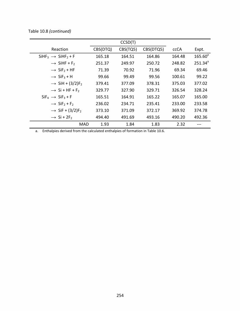
254
Table 10.8 (continued)
CCSD(T)
Reaction CBS(DTQ) CBS(TQ5) CBS(DTQ5) ccCA Expt.
SiHF3 → SiHF2 + F 165.18 164.51 164.86 164.48 165.60a
→ SiHF + F2 251.37 249.97 250.72 248.82 251.34a
→ SiF2 + HF 71.39 70.92 71.96 69.34 69.46
→ SiF3 + H 99.66 99.49 99.56 100.61 99.22
→ SiH + (3/2)F2 379.41 377.09 378.31 375.03 377.02
→ Si + HF + F2 329.77 327.90 329.71 326.54 328.24
SiF4 → SiF3 + F 165.51 164.91 165.22 165.07 165.00
→ SiF2 + F2 236.02 234.71 235.41 233.00 233.58
→ SiF + (3/2)F2 373.10 371.09 372.17 369.92 374.78
→ Si + 2F2 494.40 491.69 493.16 490.20 492.36
MAD 1.93 1.84 1.83 2.32 ‐‐‐a. Enthalpies derived from the calculated enthalpies of formation in Table 10.6.
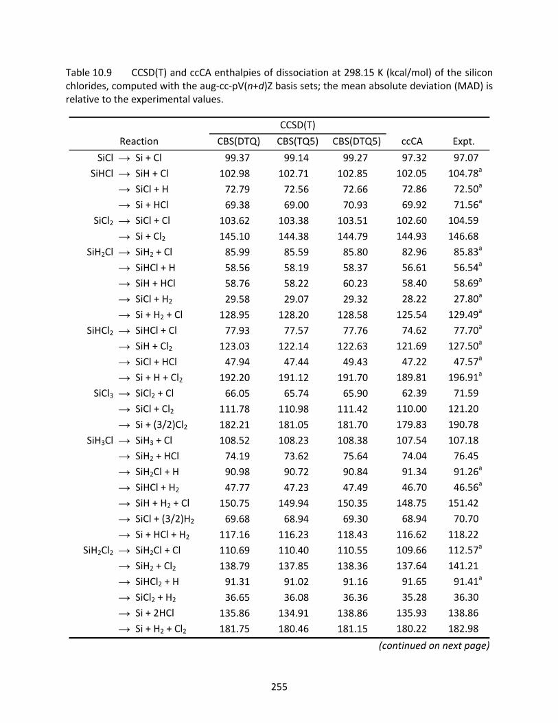
255
Table 10.9 CCSD(T) and ccCA enthalpies of dissociation at 298.15 K (kcal/mol) of the silicon chlorides, computed with the aug‐cc‐pV(n+d)Z basis sets; the mean absolute deviation (MAD) is relative to the experimental values.
CCSD(T)
Reaction CBS(DTQ) CBS(TQ5) CBS(DTQ5) ccCA Expt.
SiCl → Si + Cl 99.37 99.14 99.27 97.32 97.07
SiHCl → SiH + Cl 102.98 102.71 102.85 102.05 104.78a
→ SiCl + H 72.79 72.56 72.66 72.86 72.50a
→ Si + HCl 69.38 69.00 70.93 69.92 71.56a SiCl2 → SiCl + Cl 103.62 103.38 103.51 102.60 104.59
→ Si + Cl2 145.10 144.38 144.79 144.93 146.68 SiH2Cl → SiH2 + Cl 85.99 85.59 85.80 82.96 85.83a
→ SiHCl + H 58.56 58.19 58.37 56.61 56.54a
→ SiH + HCl 58.76 58.22 60.23 58.40 58.69a
→ SiCl + H2 29.58 29.07 29.32 28.22 27.80a
→ Si + H2 + Cl 128.95 128.20 128.58 125.54 129.49a
SiHCl2 → SiHCl + Cl 77.93 77.57 77.76 74.62 77.70a
→ SiH + Cl2 123.03 122.14 122.63 121.69 127.50a
→ SiCl + HCl 47.94 47.44 49.43 47.22 47.57a
→ Si + H + Cl2 192.20 191.12 191.70 189.81 196.91a
SiCl3 → SiCl2 + Cl 66.05 65.74 65.90 62.39 71.59
→ SiCl + Cl2 111.78 110.98 111.42 110.00 121.20
→ Si + (3/2)Cl2 182.21 181.05 181.70 179.83 190.78
SiH3Cl → SiH3 + Cl 108.52 108.23 108.38 107.54 107.18
→ SiH2 + HCl 74.19 73.62 75.64 74.04 76.45
→ SiH2Cl + H 90.98 90.72 90.84 91.34 91.26a
→ SiHCl + H2 47.77 47.23 47.49 46.70 46.56a
→ SiH + H2 + Cl 150.75 149.94 150.35 148.75 151.42
→ SiCl + (3/2)H2 69.68 68.94 69.30 68.94 70.70
→ Si + HCl + H2 117.16 116.23 118.43 116.62 118.22 SiH2Cl2 → SiH2Cl + Cl 110.69 110.40 110.55 109.66 112.57a
→ SiH2 + Cl2 138.79 137.85 138.36 137.64 141.21
→ SiHCl2 + H 91.31 91.02 91.16 91.65 91.41a
→ SiCl2 + H2 36.65 36.08 36.36 35.28 36.30
→ Si + 2HCl 135.86 134.91 138.86 135.93 138.86
→ Si + H2 + Cl2 181.75 180.46 181.15 180.22 182.98
(continued on next page)
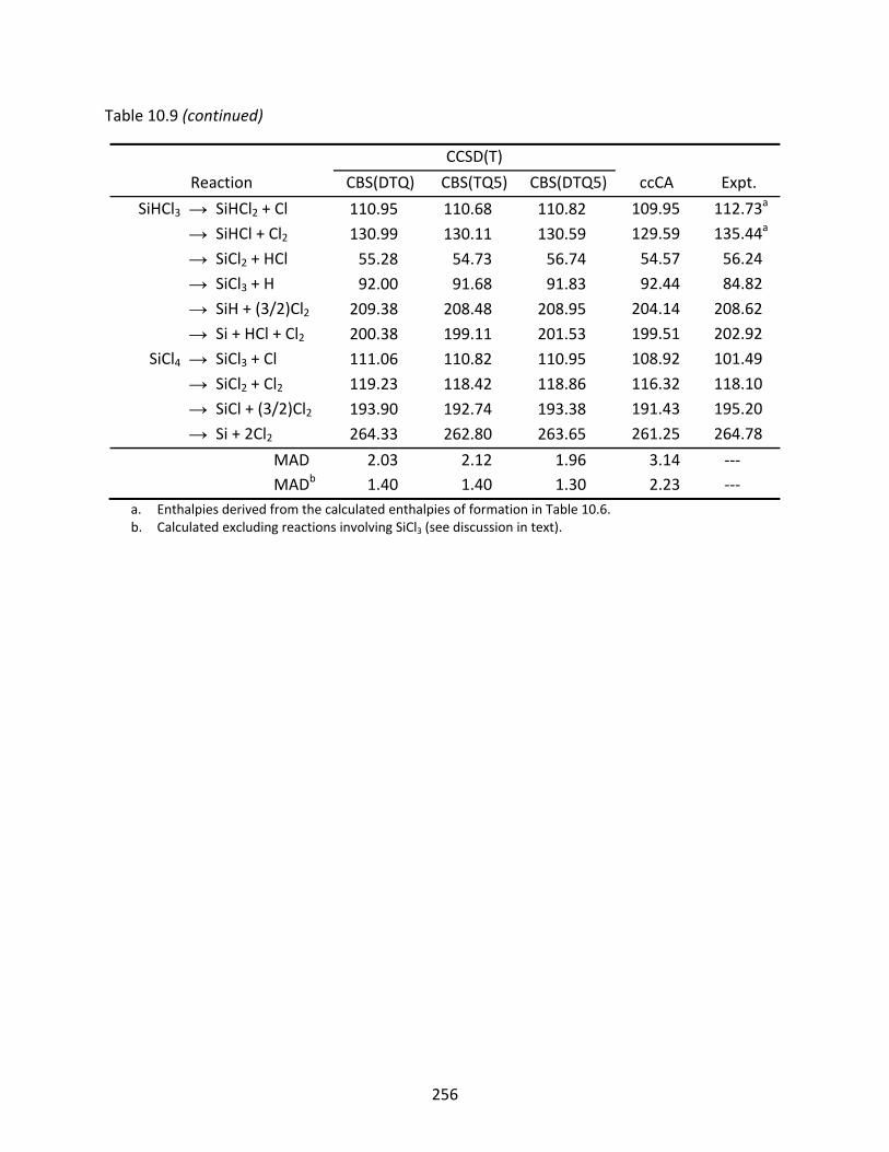
256
Table 10.9 (continued)
CCSD(T)
Reaction CBS(DTQ) CBS(TQ5) CBS(DTQ5) ccCA Expt.
SiHCl3 → SiHCl2 + Cl 110.95 110.68 110.82 109.95 112.73a
→ SiHCl + Cl2 130.99 130.11 130.59 129.59 135.44a
→ SiCl2 + HCl 55.28 54.73 56.74 54.57 56.24
→ SiCl3 + H 92.00 91.68 91.83 92.44 84.82
→ SiH + (3/2)Cl2 209.38 208.48 208.95 204.14 208.62
→ Si + HCl + Cl2 200.38 199.11 201.53 199.51 202.92
SiCl4 → SiCl3 + Cl 111.06 110.82 110.95 108.92 101.49
→ SiCl2 + Cl2 119.23 118.42 118.86 116.32 118.10
→ SiCl + (3/2)Cl2 193.90 192.74 193.38 191.43 195.20
→ Si + 2Cl2 264.33 262.80 263.65 261.25 264.78
MAD 2.03 2.12 1.96 3.14 ‐‐‐MADb 1.40 1.40 1.30 2.23 ‐‐‐
a. Enthalpies derived from the calculated enthalpies of formation in Table 10.6. b. Calculated excluding reactions involving SiCl3 (see discussion in text).
257
CHAPTER 11
CONCLUDING REMARKS
This dissertation has covered several aspects of both predictive and comparative
computational quantum chemistry employing the correlation consistent basis sets. As shown in
this work, the systematic contruction of the correlation consistent basis sets may be employed
not only in ab initio calculations, but also in density functional theory (DFT) calculations to
evaluate the complete basis set (CBS) limit, and hence, the intrinsic accuracy of a given
computational method.
In DFT computations, the correlation consistent basis sets in their original form are not
optimal, efficient, nor entirely adequate for elucidating Kohn‐Sham (KS) limits. This dissertation
has discussed both the basis set requirements and the effects of recontracting (fine‐tuning) the
correlation consistent basis sets for DFT. Specifically, it has been shown that truncating the
correlation consistent basis sets of all but s, p, d, and f functions does not result in deviations
greater than a kcal/mol in computed atomic and molecular properties (relative to the full basis
set), making the correlation consistent basis sets more efficient in DFT computations. Further,
recontraction of the Hartree‐Fock (HF) minimal basis set for a specific density functional (e.g
BLYP and B3LYP) along with the inclusion of diffuse functions and a correction for basis set
superposition error (BSSE) has been shown to give smooth, monotonic convergence towards
the KS limit for main group atoms and molecules.
Regarding the development of correlation consistent basis sets for ab initio
258
methodologies, new basis sets for the s‐block atoms lithium, beryllium, sodium, and
magnesium have been reported and discussed. In particular, the standard valence, core‐
valence, augmented, and Douglas‐Kroll (DK) scalar relativistic correlation consistent basis sets
were benchmarked and discussed, and shown to give kcal/mol accuracy in many atomic and
molecular properties while exhibiting smooth, monotonic convergence towards the CBS limit.
Next, the resolution of the identity (RI) approximation was applied to the recently
developed correlation consistent Composite Approach (ccCA), a composite ab initio method
that exploits the convergent behavior of the correlation consistent basis sets. The newly
formulated RI‐ccCA method has been benchmarked against the original ccCA formulation, and
shown to give accuracy better 1.5 kcal/mol in molecular atomization energies. More novel than
the application of the RI approximation to ccCA is the dramatic difference in the computational
cost of RI‐ccCA compared with ccCA, namely, the reduction in computing time by almost an
order of magnitude and the reduction in disk space by almost two orders of magnitude.
Finally, three separate benchmark studies of heavy FOOF‐like molecules, germanium
arsenides, and silicon hydrides/halides utilizing the correlation consistent basis sets were
presented. Computed geometries, spectroscopic properties, and thermochemical properties
were discussed with respect to experimental observations. The convergent behavior of the
correlation consistent basis sets was exploited in the latter two chapters to compute CBS limits
of bond lengths, atomization energies, and enthalpies of formation, thus presenting highly
reliable predictions of experimental observations yet to be made.
259
REFERENCES
(1) Schrödinger, E. Ann. Phys. 1926, 385, 437. (2) Schrödinger, E. Ann. Phys. 1926, 384, 489. (3) Schrödinger, E. Ann. Phys. 1926, 384, 361. (4) Schrödinger, E. Phys. Rev. 1926, 28, 1049. (5) Born, M.; Oppenheimer, J. R. Ann. Phys. 1927, 389, 457. (6) Levine, I. N. Quantum Chemistry, 5 ed.; Prentice Hall, 2000. (7) Szabo, A.; Ostlund, N. S. Modern Quantum Chemistry: Introduction to Advanced
Electronic Structure Theory; McGraw‐Hill, Inc.: New York, NY, 1989. (8) Heisenberg, W. Z. Phys. 1927, 43, 172. (9) Pauli, W. Z. Phys. 1925, 31, 765. (10) Pauli, W. "Exclusion principle and quantum mechanics." (Nobel Prize Lecture) Geneva,
Switzerland, 1945. (11) Slater, J. C. Phys. Rev. 1929, 34, 1293. (12) Hartree, D. R. Proc. Camb. Phil. Soc. 1928, 24, 89. (13) Hartree, D. R. Proc. Camb. Phil. Soc. 1928, 24, 111. (14) Hartree, D. R. Proc. Camb. Phil. Soc. 1928, 24, 426. (15) Lay, D. C. Linear Algebra and its Applications, 2 ed.; Addison Wesley Longman, Inc.:
Reading, MA, 2000. (16) Hund, F. Z. Phys. 1925, 33, 345. (17) Hund, F. Z. Phys. 1925, 34, 296. (18) Hehre, W. J.; Radom, L.; Schleyer, P. v. R.; Pople, J. A. Ab Initio Molecular Orbital Theory;
John Wiley & Sons, Inc.: New York, NY, 1986.
260
(19) Jensen, F. Introduction to Computational Chemistry; John Wiley & Sons Ltd.: Chichester, West Sussex, 1999.
(20) Hartree, D. R.; Hartree, W.; Swirles, B. Phil. Trans. Roy. Soc. (London) 1939, A238, 229. (21) Fock, V. Z. Phys. A 1930, 61, 126. (22) Helgaker, T.; Jørgensen, P.; Olsen, J. Molecular Electronic‐Structure Theory; John Wiley &
Sons Ltd.: Chichester, West Sussex, 2000. (23) Hylleraas, E. A. Z. Phys. 1928, 48, 469. (24) Hylleraas, E. A. Z. Phys. 1929, 54, 347. (25) Hylleraas, E. A. Z. Phys. 1930, 65, 209. (26) Slater, J. C. Phys. Rev. 1930, 36, 57. (27) Koopmans, T. A. Physica 1933, 1, 104. (28) Roothaan, C. C. J. Rev. Mod. Phys. 1951, 23, 69. (29) Nooijen, M.; Shamasundar, K. R.; Mukherjee, D. Mol. Phys. 2005, 103, 2277. (30) Crawford, T. D.; Schaefer III, H. F. "An Introduction to Coupled Cluster Theory for
Computational Chemists." In Reviews in Computational Chemistry; Boyd, D. B., Lipkowitz, K. B., Eds.; Wiley‐VCH: New York, NY, 2000; Vol. 14; pp 33.
(31) Bartlett, R. J. Journal of Physical Chemistry 1989, 93, 1697. (32) Paldus, J. "Coupled Cluster Theory." In Methods in Computational Molecular Physics;
Wilson, S., Diercksen, H. F., Eds.; Plenum Press: New York, NY, 1992. (33) Paldus, J.; Li, X. "A Critical Assessment of Coupled Cluster Method in Quantum
Chemistry." In Advances in Chemical Physics; Prigogine, I., Rice, S., Eds.; John Wiley and Sons, Inc., 1999; Vol. 110; pp 1.
(34) Bartlett, R. J. Ann. Rev. Phys. Chem. 1981, 32, 359. (35) Bartlett, R. J. "Coupled‐Cluster Theory: An Overview of Recent Developments." In
Modern Electronic Structure Theory, Part II; Yarkony, D. R., Ed.; World Scientific: Singapore, 1995.
261
(36) Bartlett, R. J.; Stanton, J. F. "Applications of Post‐Hartree‐Fock Methods: A Tutorial." In Reviews in Computational Chemistry; Lipkowitz, K. B., Boyd, D. B., Eds.; VCH Publishers, Inc.: New York, NY, 1994; Vol. 5.
(37) Lee, T. J.; Rendell, A. P.; Taylor, P. R. J. Phys. Chem. 1990, 94, 5463. (38) Raghavachari, K.; Trucks, G. W.; Pople, J. A.; Head‐Gordon, M. Chem. Phys. Lett. 1989,
157, 479. (39) Kvasnička, V.; Laurinc, V.; Biskupič, S. Mol. Phys. 1980, 39, 143 (40) Møller, C.; Plesset, M. S. Phys. Rev. 1934, 46, 618. (41) Dirac, P. A. M. Proc. Camb. Phil. Soc. 1930, 26, 376. (42) Fermi, E. Z. Phys. 1928, 48, 73. (43) Thomas, L. H. Proc. Camb. Phil. Soc. 1927, 23, 542. (44) Hohenberg, P.; Kohn, W. Phys. Rev. 1964, 136, B864. (45) Parr, R. G.; Yang, W. Density‐Functional Theory of Atoms and Molecules; Oxford
University Press, Inc.: New York, NY, 1989. (46) Koch, W.; Holthausen, M. C. A Chemist's Guide to Density Functional Theory, 2 ed.;
Wiley‐VCH Verlag GmbH: Weinheim, Germany, 2002. (47) A Primer in Density Functional Theory; Fiolhais, C.; Nogueira, F.; Marques, M., Eds.;
Springer‐Verlag: Berlin, 2003. (48) Density Functional Theory: A Bridge Between Chemistry and Physics; Geerlings, P.; De
Proft, F.; Langenaeker, W., Eds.; VUB University Press: Brussels, 1999. (49) Many‐Electron Densities and Reduced Density Matrices; Cioslowski, J., Ed.; Kluwer
Academic/Plenum Publishers: New York, NY, 2000. (50) Löwdin, P.‐O. Phys. Rev. 1955, 97, 1474. (51) Hohenberg, P.; Kohn, W. Physical Review 1964, 136, B864. (52) Kohn, W.; Sham, L. J. Phys. Rev. 1965, 140, A1133. (53) Jackson, J. D. Classical Electrodynamics, 3 ed.; John Wiley & Sons, Inc.: New York, NY,
1998.
262
(54) Griffiths, D. J. Introduction to Electrodynamics, 3 ed.; Prentice Hall: Upper Saddle River,
NJ, 1999. (55) Cook, D. B. Handbook of Computational Quantum Chemistry; Dover Publications, Inc.:
Mineola, NY, 2005. (56) Boys, S. F. Proc. Roy. Soc. (London) 1950, A200, 542. (57) Taketa, H.; Huzinaga, S.; O‐Ohata, K. J. Phys. Soc. Jpn. 1966, 21, 2313. (58) Boys, S. F. Proc. Roy. Soc. (London) 1950, A201, 125. (59) Schwartz, C. Phys. Rev. 1962, 126, 1015. (60) Curtiss, L. A.; Pople, J. A. Chem. Phys. Lett. 1988, 144, 38. (61) Curtiss, L. A.; Raghavachari, K.; Trucks, G. W.; Pople, J. A. J. Chem. Phys. 1991, 94, 7221. (62) Curtiss, L. A.; Redfern, P. C.; Rassolov, V. A.; Kedziora, G. S.; Pople, J. A. J. Chem. Phys.
2001, 114, 9287. (63) Montgomery Jr., J. A.; Frisch, M. J.; Ochterski, J. W.; Petersson, G. A. J. Chem. Phys. 1999,
110, 2822. (64) Montgomery Jr., J. A.; Frisch, M. J.; Ochterski, J. W.; Petersson, G. A. J. Chem. Phys. 2000,
112, 6532. (65) Montgomery Jr., J. A.; Ochterski, J. W.; Petersson, G. A. J. Chem. Phys. 1994, 101, 5900. (66) Ochterski, J. W.; Petersson, G. A.; Montgomery Jr., J. A. J. Chem. Phys. 1996, 104, 2598. (67) Petersson, G. A.; Al‐Laham, M. A. J. Chem. Phys. 1991, 94, 6081. (68) Petersson, G. A.; Bennett, A.; Tensfeldt, T. G.; Al‐Laham, M. A.; Shirley, W. A.; Mantzaris,
J. J. Chem. Phys. 1988, 89, 2193. (69) Petersson, G. A.; Tensfeldt, T. G.; Montgomery Jr., J. A. J. Chem. Phys. 1991, 94, 6091. (70) Harding, M. E.; Vazquez, J.; Ruscic, B.; Wilson, A. K.; Gauss, J.; Stanton, J. F. J. Chem.
Phys. 2008, 128, 114111. (71) Boese, A. D.; Oren, M.; Atasoylu, O.; Martin, J. M. L.; Kállay, M.; Gauss, J. J. Chem. Phys.
2004, 120, 4129.
263
(72) Martin, J. M. L.; De Oliveira, G. J. Chem. Phys. 1999, 111, 1843. (73) DeYonker, N. J.; Cundari, T. R.; Wilson, A. K. J. Chem. Phys. 2006, 124, 114104. (74) DeYonker, N. J.; Grimes, T.; Yockel, S. M.; Dinescu, A.; Mintz, B. J.; Cundari, T. R.; Wilson,
A. K. J. Chem. Phys. 2006, 125, 104111. (75) DeYonker, N. J.; Ho, D. S.; Wilson, A. K.; Cundari, T. R. J. Phys. Chem. A 2007, 111, 10776. (76) DeYonker, N. J.; Mintz, B. J.; Cundari, T. R.; Wilson, A. K. J. Chem. Theor. Comput. 2008,
4, 328. (77) DeYonker, N. J.; Peterson, K. A.; Steyl, G.; Wilson, A. K.; Cundari, T. R. J. Phys. Chem. A
2007, 111, 11269. (78) Grimes, T. V.; Cundari, T. R.; DeYonker, N. J.; Wilson, A. K. J. Chem. Phys. 2007, 127,
154117. (79) Williams, T. G.; Wilson, A. K. J. Sulf. Chem. 2008, 29, 353. (80) Ho, D. S.; DeYonker, N. J.; Wilson, A. K.; Cundari, T. R. J. Phys. Chem. A 2007, 110, 9767. (81) Peterson, K. A.; Dunning Jr., T. H. J. Chem. Phys. 2002, 117, 10548. (82) Woon, D. E.; Dunning Jr., T. H. J. Chem. Phys. 1993, 99, 1914. (83) Peterson, K. A.; Kendall, R. A.; Dunning Jr., T. H. J. Chem. Phys. 1993, 99, 1930. (84) Peterson, K. A.; Kendall, R. A.; Dunning Jr., T. H. J. Chem. Phys. 1993, 99, 9790. (85) Peterson, K. A.; Woon, D. E.; Dunning Jr., T. H. J. Chem. Phys. 1994, 100, 7410. (86) Woon, D. E.; Peterson, K. A.; Dunning Jr., T. H. J. Chem. Phys. 1998, 109, 2233. (87) Woon, D. E.; Dunning Jr., T. H. J. Chem. Phys. 1994, 101, 8877. (88) Peterson, K. A.; Dunning Jr., T. H. J. Chem. Phys. 1995, 102, 2032. (89) Peterson, K. A.; Dunning Jr., T. H. J. Chem. Phys. 1997, 106, 4119. (90) Wilson, A. K.; Dunning Jr., T. H. J. Chem. Phys. 1997, 106, 8718. (91) van Mourik, T.; Wilson, A. K.; Dunning Jr., T. H. Mol. Phys. 1999, 96, 529.
264
(92) Peterson, K. A.; Figgen, D.; Dolg, M.; Stoll, H. J. Chem. Phys. 2007, 126, 124101. (93) Peterson, K. A. Ann. Rep. Comp. Chem. 2007, 3, 195. (94) Dunning Jr., T. H. J. Chem. Phys. 1989, 90, 1007. (95) Woon, D. E.; Dunning Jr., T. H. J. Chem. Phys. 1992, 98, 1358. (96) Woon, D. E.; Dunning Jr., T. H. J. Chem. Phys. 1994, 100, 2975. (97) Wilson, A. K.; Woon, D. E.; Peterson, K. A.; Dunning Jr., T. H. J. Chem. Phys. 1999, 110,
7667. (98) Woon, D. E.; Dunning Jr., T. H. J. Chem. Phys. 1995, 103, 4572. (99) Wilson, A. K.; van Mourik, T.; Dunning Jr., T. H. J. Mol. Struct. (THEOCHEM) 1996, 388,
339. (100) van Mourik, T.; Dunning Jr., T. H. Int. J. Quant. Chem. 1999, 76, 205. (101) Dunning Jr., T. H.; Peterson, K. A.; Wilson, A. K. J. Chem. Phys. 2001, 114, 9244. (102) Prascher, B. P.; Wilson, A. K.; Dunning Jr., T. H.; Woon, D. E.; Peterson, K. A. (in
preparation). (103) Yockel, S. M. The evaluation, development, and application of the correlation consistent
basis sets. Ph.D. Thesis, University of North Texas, USA, 2006. (104) Peterson, K. A.; Adler, T. B.; Werner, H.‐J. J. Chem. Phys. 2008, 128, 084102. (105) Balabanov, N. B.; Peterson, K. A. J. Chem. Phys. 2005, 123, 064107. (106) Peterson, K. A.; Puzzarini, C. Theoret. Chem. Acc. 2005, 114, 283. (107) Peterson, K. A. J. Chem. Phys. 2003, 119, 11099. (108) Peterson, K. A.; Figgen, D.; Goll, E.; Stoll, H.; Dolg, M. J. Chem. Phys. 2003, 119, 11113. (109) Balabanov, N. B.; Peterson, K. A. J. Phys. Chem. A 2003, 107, 7465. (110) Jankowski, K.; Becherer, R.; Scharf, P.; Schiffer, H.; Ahlrichs, R. J. Chem. Phys. 1985, 82,
1413.
265
(111) Ahlrichs, R.; Scharf, P.; Jankowski, K. Chem. Phys. 1985, 98, 381. (112) Becherer, R.; Ahlrichs, R. Chem. Phys. 1985, 99, 389. (113) Almlöf, J.; Taylor, P. R. J. Chem. Phys. 1987, 86, 4070. (114) Almlöf, J.; Taylor, P. R. J. Chem. Phys. 1990, 92, 551. (115) van Duijneveldt, F. B. IBM Research Report 1971, RJ 945. (116) Raffenetti, R. C. J. Chem. Phys. 1973, 58, 4452. (117) Almlöf, J.; Taylor, P. R. J. Chem. Phys. 1987, 86, 4070. (118) Ruedenberg, K.; Raffenetti, R. C.; Bardo, R. D. “Energy, Structure, and Reactivity.”;
Proceedings from the 1972 Boulder Seminar Research Conference on Theoretical Chemistry, Boulder, Colorado.
(119) Bauschlicher, C. W.; Partridge, H. Chem. Phys. Lett. 1995, 240, 533. (120) Martin, J. M. L. J. Chem. Phys. 1998, 108, 2791. (121) Martin, J. M. L.; Baldridge, K. K.; Lee, T. J. Mol. Phys. 1999, 97, 945. (122) Martin, J. M. L.; Uzan, O. Chem. Phys. Lett. 1998, 282, 16. (123) Woon, D. E.; Dunning, T. H. J. Chem. Phys. 1992, 98, 1358. (124) Dunning, T. H.; Peterson, K. A.; Wilson, A. K. J. Chem. Phys. 2001, 114, 9244. (125) Wang, N. X.; Wilson, A. K. J. Phys. Chem. A 2003, 107, 6720. (126) Wang, N. X.; Wilson, A. K. J. Phys. Chem. A 2005, 109, 7187. (127) Wilson, A. K.; Dunning Jr., T. H. J. Chem. Phys. 2003, 119, 11712. (128) Wilson, A. K.; Dunning Jr., T. H. J. Phys. Chem. A 2004, 108, 3129. (129) Heckert, M.; Kállay, M.; Tew, D. P.; Klopper, W.; Gauss, J. J. Chem. Phys. 2006, 125,
044108. (130) Bakowies, D. J. Chem. Phys. 2007, 127, 084105. (131) Varandas, A. J. C. J. Chem. Phys. 2000, 113, 8880.
266
(132) Feller, D. J. Chem. Phys. 1992, 96, 6104. (133) Halkier, A.; Helgaker, T.; Jorgensen, P.; Klopper, W.; Koch, H.; Olsen, J.; Wilson, A. K.
Chem. Phys. Lett. 1998, 286, 243. (134) Taylor, P. R. Lecture Notes on Quantum Chemistry; Roos, B. O., Ed.; Springer‐Verlag:
Berlin, Germany, 1992; pp 406. (135) Douglas, M.; Kroll, N. M. Ann. Phys. 1974, 82, 89. (136) Hess, B. A. Phys. Rev. A 1986, 33, 3742. (137) Relativistic Effects in Heavy‐Element Chemistry and Physics; Hess, B. A., Ed.; John Wiley
and Sons, Ltd.: Chichester, West Sussex, England, 2003. (138) Dirac, P. A. M. Proc. Roy. Soc. (London) 1928, 117, 610. (139) Dirac, P. A. M. Proc. Roy. Soc. (London) 1930, 126, 360. (140) Balasubramanian, K. Relativistic Effects in Chemistry; John Wiley and Sons, Inc.: New
York, NY, 1997. (141) Dyall, K. G.; Fægri, K. Introduction to Relativistic Quantum Chemistry; Oxford University
Press: New York, NY, 2007. (142) de Jong, W. A.; Harrison, R. J.; Dixon, D. A. J. Chem. Phys. 2001, 114, 48. (143) Jensen, F. J. Chem. Phys. 2001, 115, 9113. (144) Jensen, F. J. Chem. Phys. 2002, 116, 7372. (145) Jensen, F. J. Chem. Phys. 2003, 118, 2459. (146) Jensen, F. Chem. Phys. Lett. 2005, 402, 510. (147) Jensen, F. J. Chem. Phys. 2005, 122, 74111. (148) Prascher, B. P.; Wilson, A. K. Mol. Phys. 2007, 105, 2899. (149) Prascher, B. P.; Wilson, B. R.; Wilson, A. K. J. Chem. Phys. 2007, 127, 124110. (150) Sodt, A.; Subotnik, J. E.; Head‐Gordon, M. J. Chem. Phys. 2006, 125, 194109.
267
(151) Steele, R. P.; Shao, Y.; DiStasio, R. A.; Head‐Gordon, M. J. Phys. Chem. A. 2006, 110, 13915.
(152) Wang, N. X.; Venkatesh, K.; Wilson, A. K. J. Phys. Chem. A. 2006, 110, 779. (153) Wang, N. X.; Wilson, A. K. (unpublished results). (154) Wang, N. X.; Wilson, A. K. J. Chem. Phys. 2004, 121, 7632. (155) Wang, N. X.; Wilson, A. K. Mol. Phys. 2005, 103, 345. (156) Wang, X. The performance of density functionals with respect to the correlation
consistent basis sets. Ph.D. Disstertation, University of North Texas, 2005. (157) Sekusak, S.; Frenking, G. J. Mol. Struct. (THEOCHEM) 2001, 541, 17. (158) Raymond, K. S.; Wheeler, R. A. J. Comput. Chem. 1999, 20, 207. (159) Skylaris, C.‐K.; Gagliardi, L.; Handy, N. C.; Ioannou, A. G.; Spencer, S.; Willetts, A. J. Mol.
Struct. (THEOCHEM) 2000, 501‐502, 229. (160) Vahtras, O.; Almlöf, J. E.; Feyereisen, M. W. Chem. Phys. Lett. 1993, 213, 514. (161) Van Alsenoy, C. J. Comp. Chem. 1988, 9, 620. (162) Mintz, B. J.; Lennox, K. P.; Wilson, A. K. J. Chem. Phys. 2004, 121, 5629. (163) Mintz, B. J.; Wilson, A. K. J. Chem. Phys. 2005, 122, 134106. (164) Becke, A. D. Phys. Rev. A. 1988, 38, 3098. (165) Lee, C.; Yang, W.; Parr, R. G. Phys. Rev. B 1987, 37, 785. (166) Becke, A. D. J. Chem. Phys. 1993, 98, 5648. (167) Vosko, S. H.; Wilk, L.; Nusair, M. Can. J. Phys. 1980, 58, 1200. (168) Bauschlicher, C. W.; Taylor, P. R. Theor. Chim. Acta 1988, 74, 63. (169) Dunlap, B. I. "Symmetry and degeneracy in Xa and density functional theory." In Ab
Initio Methods in Quantum Chemistry, Part II; Lawley, K. P., Ed.; John Wiley and Sons: Chicester, 1987.
268
(170) Constants of Diatomic Molecules; Number 69 ed.; Huber, K. P.; Hertzberg, G., Eds.; National Institute of Standards and Technology: Gaithersburg, MD, 2005.
(171) Lias, S. G. "Ionization Energy Evaluation." In NIST Chemistry WebBook, NIST Standard
Reference Database Number 69; Linstrom, P. J., Mallard, W. G., Eds.; National Institute of Standards and Technology: Gaithersburg, MD, 2005.
(172) Lias, S. G.; Bartmess, J. E.; Liebman, J. F.; Holmes, J. L.; Levin, R. D.; Mallard, W. G. "Ion
Energetics Data." In NIST Chemistry WebBook, NIST Standard Reference Database Number 69; Linstrom, P. J., Mallard, W. G., Eds.; National Institute of Standards and Technology: Gaithersburg, MD, 2005.
(173) Yamanaka, S.; Nakata, K.; Ukai, T.; Takada, T.; Yamaguchi, K. Int. J. Quant. Chem. 2006,
106, 3312. (174) Frisch, M. J.; Trucks, G. W.; Schlegel, H. B.; Scuseria, G. E.; Robb, M. A.; Cheeseman, J. R.;
Montgomery, J., J. A.; Vreven, T.; Kudin, K. N.; Burant, J. C.; Millam, J. M.; Iyengar, S. S.; Tomasi, J.; Barone, V.; Mennucci, B.; Cossi, M.; Scalmani, G.; Rega, N.; Petersson, G. A.; Nakatsuji, H.; Hada, M.; Ehara, M.; Toyota, K.; Fukuda, R.; Hasegawa, J.; Ishida, M.; Nakajima, T.; Honda, Y.; Kitao, O.; Nakai, H.; Klene, M.; Li, X.; Knox, J. E.; Hratchian, H. P.; Cross, J. B.; Bakken, V.; Adamo, C.; Jaramillo, J.; Gomperts, R.; Stratmann, R. E.; Yazyev, O.; Austin, A. J.; Cammi, R.; Pomelli, C.; Ochterski, J. W.; Ayala, P. Y.; Morokuma, K.; Voth, G. A.; Salvador, P.; Dannenberg, J. J.; Zakrzewski, V. G.; Dapprich, S.; Daniels, A. D.; Strain, M. C.; Farkas, O.; Malick, D. K.; Rabuck, A. D.; Raghavachari, K.; Foresman, J. B.; Ortiz, J. V.; Cui, Q.; Baboul, A. G.; Clifford, S.; Cioslowski, J.; Stefanov, B. B.; Liu, G.; Liashenko, A.; Piskorz, P.; Komaromi, I.; Martin, R. L.; Fox, D. J.; Keith, T.; Al‐Laham, M. A.; Peng, C. Y.; Nanayakkara, A.; Challacombe, M.; Gill, P. M. W.; Johnson, B.; Chen, W.; Wong, M. W.; Gonzalez, C.; Pople, J. A. Gaussian 03; version B.05, C.02, and D.01; Gaussian, Inc.: Wallingford, CT, 2004.
(175) Krack, M.; Köster, A. M. J. Chem. Phys. 1998, 108, 3226. (176) Martin, J. M. L. J. Chem. Phys. 1998, 108, 2791. (177) van Duijneveldt, F. B.; van Duijneveldt‐van de Rijdt, J. G. C. M.; van Lenthe, J. H. Chem.
Rev. 1994, 94, 1873. (178) Boys, S. F.; Bernardi, F. Mol. Phys. 1970, 19, 553. (179) van Mourik, T.; Wilson, A. K.; Peterson, K. A.; Woon, D. E.; Dunning Jr., T. H. Adv. Quant.
Chem. 1999, 31, 105. (180) Amos, R. D.; Bernhardsson, A.; Berning, A.; Celani, P.; Cooper, D. L.; Deegan, M. J. O.;
Dobbyn, A. J.; Eckert, F.; Hampel, C.; Hetzer, G.; Knowles, P. J.; Korona, T.; Lindh, R.;
269
Lloyd, A. W.; McNicholas, S. J.; Manby, F. R.; Meyer, W.; Mura, M. E.; Nicklass, A.; Palmieri, P.; Pitzer, R.; Rauhut, G.; Schütz, M.; Schumann, U.; Stoll, H.; Stone, A. J.; Tarroni, R.; Thorsteinsson, T.; Werner, H.‐J. MOLPRO, a package of ab initio programs designed by H.‐J. Werner and P. J. Knowles; version version 2002.6.
(181) Weigend, F.; Köhn, A.; Hättig, C. J. Chem. Phys. 2002, 116, 3175. (182) Feller, D. J. Comp. Chem. 1996, 17, 1571. (183) Schuchardt, K. L.; Didier, B. T.; Elsethagen, T.; Sun, L.; Gurumoorthi, V.; Chase, J.; Li, J.;
Windus, T. L. J. Chem. Inform. Mod. 2007, 47, 1045. (184) Press, W. H.; Flannery, B. P.; Teukolsky, S. A.; Vetterling, W. T. Numerical Recipes in
FORTRAN 77: The Art of Scientific Computing., 2 ed.; Cambridge University Press, 1992. (185) Koput, J.; Peterson, K. A. J. Phys. Chem. A 2003, 107, 3981. (186) Koput, J.; Carter, S.; Peterson, K. A.; Theodorakopoulos, G. J. Chem. Phys. 2002, 117,
1529. (187) Ruud, K.; Jonsson, D.; Norman, P.; Agren, H.; Saue, T.; Jensen, H. J. A.; Dahle, P.;
Helgaker, T. J. Chem. Phys. 1998, 108, 7973. (188) Schwartz, C. Ann. Phys. 1967, 42, 367. (189) Martinez, T. J.; Carter, E. A. "Pseudospectral Methods Applied to the Electron
Correlation Problem." In Modern Electronic Structure Theory; Yarkony, D. R., Ed.; World Scientific: River Edge, New Jersey, 1995; Vol. 2.
(190) Kendall, R. A.; Früchtl, H. A. Theor. Chem. Acc. 1997, 97, 158. (191) Löwdin, P.‐O. Rev. Mod. Phys. 1967, 39, 259. (192) Baerends, E. J.; Ellis, D. E.; Ros, R. Chem. Phys. 1973, 2, 41. (193) Feyereisen, M. W.; Fitzgerald, G.; Komornicki, A. Chem. Phys. Lett. 1993, 208, 359. (194) Rendell, A. P.; Lee, T. J. J. Chem. Phys. 1994, 101, 400. (195) CODATA Key Values for Thermodynamics; Cox, J. D.; Wagman, D. D.; Medvedev, V. A.,
Eds.; Hemisphere Publishing Corp.: New York, NY, 1989. (196) Karton, A.; Martin, J. M. L. J. Phys. Chem. A 2007, 111, 5936.
270
(197) Schütz, M. J. Chem. Phys. 2000, 113, 9986. (198) Schütz, M.; Werner, H.‐J. Chem. Phys. Lett. 2000, 318, 370. (199) Schütz, M.; Werner, H.‐J. J. Chem. Phys. 2001, 114, 661. (200) Weigend, F. Phys. Chem. Chem. Phys. 2006, 8, 1057. (201) Prascher, B. P.; Lai, J. D.; Wilson, A. K. J. Chem. Phys., (submitted). (202) Asprey, L. B.; Kinkead, S. A.; Eller, P. G. Nuc. Tech. 1986, 73, 69. (203) Erilov, P. E.; Titov, V. V.; Serik, V. F.; Sokolov, V. B. Atomic Energy 2002, 92, 57. (204) Morrow, S. I.; Young, A. R. Inorg. Chem. 1965, 4, 759. (205) Streng, A. G. Chem. Rev. 1963, 63, 607. (206) Dickinson, L. A.; Amster, A. B.; Capener, E. L. J. Spacecr. Rocket. 1968, 5, 1329. (207) Bridgeman, A. J.; Rothery, J. J. Chem. Soc. Dalt. Trans. 1999, 4077. (208) Francisco, J. S.; Maricq, M. M. Acc. Chem. Res. 1996, 29, 391. (209) Grabowski, J. J.; Zhang, L. J. Amer. Chem. Soc. 1989, 111, 1193. (210) Kadomura, S. (Sony Corp. Japan) Plasma etching in manufacture of semiconductor
device. In Sony Corp., Japanese Kokai Tokkyo Koho, Japan; JP‐08069995: Japan, 1996. (211) Nagayama, T. (Sony Corp. Japan) Plasma etching of organic antirelfective flim. In Sony
Corp., Japanese Kokai Tokkyo Koho, Japan; JP‐10312993: Japan, 1998. (212) Nagayama, T. (Sony Corp. Japan) Plasma etching of organic antireflective flim in
manufacture of semiconductor device. In Sony Corp., Japanese Kokai Tokkyo Koho, Japan; JP‐10312992: Japan, 1998.
(213) Yokoyama, S. (Sharp Corp., Japan) Manufacture of dielectric thin film device. In Sharp
Corp., Japanese Kokai Tokkyo Koho, Japan; JP‐11354505: Japan, 1999. (214) Bachrach, S. M.; Demoin, D. W.; Luk, M.; Miller Jr., J. V. J. Phys. Chem. A 2004, 108,
4040. (215) Cao, X.; Qian, X.; Qiao, C.; Wang, D. Chemical Physics Letters 1999, 299, 322.
271
(216) Cao, X.; Qiao, C.; Wang, D. Chem. Phys. Lett. 1998, 290, 405. (217) Kurney, G. W.; Turnbull, K. Chem. Rev. 1982, 82, 333. (218) Meyer, M. J. Mol. Struct. 1992, 273, 99. (219) Jackson, R. H. J. Chem. Soc. 1962, 4585. (220) Hedberg, L.; Hedberg, K.; Eller, P. G.; Ryan, R. R. Inorg. Chem. 1988, 27, 232. (221) Hammer, P. D.; Sinha, A.; Burkholder, J. B.; Howard, C. J. J. Mol. Spectrosc. 1988, 129,
199. (222) Freedman, P. A.; Jones, W. J. J. Chem. Soc. Farad. Trans. 2 1975, 71, 286. (223) Gouedard, G.; Lehmann, J. C. J. Phys. B 1976, 9, 2113. (224) Christen, D.; Mack, H.‐G.; Oberhammer, H. Tetrahedron 1988, 44, 7363. (225) Kuczkowski, R. L. Journal of the American Chemical Society 1963, 85, 3047. (226) Kuczkowski, R. L. J. Amer. Chem. Soc. 1964, 86, 3617. (227) Kuczkowski, R. L.; Wilson, E. B. J. Amer. Chem. Soc. 1963, 85, 2028. (228) Marsden, C. J.; Oberhammer, H.; Lösking, O.; Willner, H. J. Mol. Struct. 1989, 193, 233. (229) Samdal, S.; Mastryukov, V. S.; Boggs, J. E. J. Mol. Struct. (THEOCHEM) 1994, 309, 21. (230) Birk, M.; Friedl, R. R.; Cohen, E. A.; Pickett, H. M. J. Chem. Phys. 1989, 91, 6588. (231) Borden, W. T. Chem. Comm. 1998, 1919. (232) Kraka, E.; He, Y.; Cremer, D. J. Phys. Chem. 2001, 105, 3269. (233) Jursic, B. S. J. Mol. Struct. (THEOCHEM) 1999, 459, 23. (234) Feller, D.; Dixon, D. J. Phys. Chem. A 2003, 107, 9641. (235) Lucchese, R. R.; Schaefer III, H. F.; Rodwell, W. R.; Radom, L. J. Chem. Phys. 1978, 68,
2507. (236) Mack, H.‐G.; Oberhammer, H. Chem. Phys. Lett. 1988, 145, 121.
272
(237) Scuseria, G. E. J. Chem. Phys. 1991, 94, 442. (238) Colton, R. J.; Rabalais, J. W. J. Elec. Spectrosc. Rel. Phenom. 1974, 3, 345. (239) Forneris, R.; Hennies, C. E. J. Mol. Struct. 1970, 5, 449. (240) Frankiss, S. G. J. Mol. Struct. 1968, 2, 271. (241) Frenzel, C. A.; Blick, K. E. J. Chem. Phys. 1971, 55, 2715. (242) DeYonker, N., (personal communication). (243) Marshall, P.; Misra, A. J. Phys. Chem. A 1998, 102, 9056. (244) Papayannis, D. K.; Melissas, V. S.; Kosmas, A. M. Chem. Phys. Lett. 2001, 349, 299. (245) Haas, A. J. Flourin. Chem. 1986, 32, 415. (246) Denis, P. A. J. Chem. Theor. Comput. 2005, 1, 900. (247) Aitken, B. G.; Youngman, R. E.; Ponader, C. W. J. Noncrystal. Sol. 2001, 284, 34. (248) Asokamani, R.; Rita, R. Phys. Stat. Sol. 2001, 226, 375. (249) Bachelet, G. B.; Christensen, N. E. Phys. Rev. B 1985, 31, 879. (250) Barrau, J.; Escudié, J.; Satgé, J. Chem. Rev. 1990, 90, 283. (251) Basch, H. Inorg. Chim. Acta 1996, 252, 265. (252) Brook, A. G.; Baines, K. M. Adv. Organomet. Chem. 1986, 25, 1. (253) Chu, T. L.; Chu, S. S.; Ray, L. J. Appl. Phys. 1982, 53, 7102. (254) Curtiss, L. A.; Redfern, P. C.; Rassolov, V. A.; Kedziora, G. S.; Pople, J. A. J. Chem. Phys.
2001, 114, 9287. (255) Kedziora, G. S.; Pople, J. A.; Rassolov, V. A.; Ratner, M. A.; Redfern, P. C.; Curtiss, L. A. J.
Chem. Phys. 1999, 110, 7123. (256) Kedziora, G. S.; Pople, J. A.; Ratner, M. A.; Redfern, P. C.; Curtiss, L. A. J. Chem. Phys.
2001, 115, 718. (257) Koizumi, H.; Dávalos, J. Z.; Baer, T. Chem. Phys. 2006, 324, 385.
273
(258) Lai, C.‐H.; Su, M.‐D.; Chu, S.‐Y. Polyhedron 2002, 21, 579. (259) Pitzer, K. S. J. Am. Chem. Soc. 1948, 70, 2140. (260) Power, P. P. Chem. Rev. 1999, 99, 3463. (261) Raabe, G.; Michl, J. Chem. Rev. 1985, 85, 419. (262) West, R. Science 1984, 225, 1109. (263) Wiberg, J. J. Organomet. Chem. 1984, 273, 141. (264) Mulliken, R. S. J. Am. Chem. Soc. 1950, 72, 4493. (265) Del Bene, J. E.; Aue, D. H.; Shavitt, I. J. Am. Chem. Soc. 1992, 114, 1631. (266) Bachelet, G. B.; Christensen, N. E. Phys. Rev. B 1985, 31, 879. (267) Kedziora, G. S.; Pople, J. A.; Rassolov, V. A.; Ratner, M. A.; Redfern, P. C.; Curtiss, L. A. J.
Chem. Phys. 1999, 110, 7123. (268) Kedziora, G. S.; Pople, J. A.; Ratner, M. A.; Redfern, P. C.; Curtiss, L. A. J. Chem. Phys.
2001, 115, 718. (269) Koizumi, H.; Dávalos, J. Z.; Baer, T. Chem. Phys. 2006, 324, 385. (270) Kalcher, J. Phys. Chem. Chem. Phys. 2002, 4, 3311. (271) Yockel, S. M.; Mintz, B. J.; Wilson, A. K. J. Chem. Phys. 2004, 121, 60. (272) Ochterski, J. W. Thermochemistry in Gaussian; Gaussian, Inc.: Wallingford, CT., 2000. (273) Chase, M. W. J. Phys. Chem. Ref. Data 1998, 9, 1. (274) Cowan, R. D.; Griffin, D. C. J. Opt. Soc. Amer. 1976, 66, 1010. (275) Barysz, M.; Flocke, N.; Karwowski, J. Acta Physica Polonica A 2001, 99, 631. (276) de Jong, W. A.; Harrison, R. J.; Dixon, D. A. J. Chem. Phys. 2001, 114, 48. (277) Berning, A.; Schweizer, M.; Werner, H.‐J.; Knowles, P. J.; Palmieri, P. Mol. Phys. 2000, 98,
1823.
274
(278) Rohatgi, A. “Fundamental Research and Development for Improved Crystalline Silicon Solar Cells,” National Renewable Energy Laboratory, U.S. Department of Energy, 2007.
(279) Pelletier, J. J. Phys. D Appl. Phys. 1987, 20, 858. (280) Park, S. C.; Stansfield, R. A.; Clary, D. C. J. Phys. D Appl. Phys. 1987, 20, 880. (281) Jasinski, J. M.; Meyerson, B. S.; Scott, B. A. Ann. Rev. Phys. Chem. 1987, 38, 109. (282) Allen, W. D.; Schaefer, H. F. Chem. Phys. 1986, 108, 243. (283) Walsh, R. J. Chem. Soc., Faraday Trans. 1983, 79, 2233. (284) Ignacio, E. W.; Schlegel, H. B. J. Chem. Phys. 1990, 92, 5404. (285) Ignacio, E. W.; Schlegel, H. B. J. Phys. Chem. 1992, 96, 5830. (286) Ho, P.; Coltrin, M. E.; Binkley, J. S.; Melius, C. F. J. Phys. Chem. 1985, 89, 4647. (287) Ho, P.; Melius, C. F. J. Phys. Chem. 1990, 94, 5120. (288) Gutsev, G. L. J. Phys. Chem. 1994, 98, 1570. (289) Bauschlicher, C. W.; Partridge, H. Chem. Phys. Lett. 1997, 276, 47. (290) Grev, R. S.; Schaefer, H. F. J. Chem. Phys. 1992, 97, 8389. (291) Ricca, A.; Bauschlicher, C. W. J. Phys. Chem. A 1998, 102, 876. (292) Ricca, A.; Bauschlicher, C. W. Chem. Phys. Lett. 1998, 287, 239. (293) Feller, D.; Dixon, D. A. J. Phys. Chem. A 1999, 103, 6413. (294) Begue, D.; Carbonniere, P.; Barone, V.; Pouchan, C. Chem. Phys. Lett. 2005, 415, 25. (295) Betrencourt, M.; Boudjaadar, D.; Chollet, P.; Guelachvili, G.; Morillon‐Chapey, M. J.
Chem. Phys. 1986, 84, 4121. (296) Mélen, F.; Dubois, I.; Bredohl, H. J. Mol. Spectrosc. 1990, 139, 361. (297) Tanaka, T.; Tamura, M.; Tanaka, K. J. Mol. Struct. 1997, 413‐414, 153. (298) Fujitake, M.; Hirota, E. Spectrochim. Acta A 1994, 50A, 1345.
275
(299) Adrian, F. J.; Cochran, E. L.; Bowers, V. A. Advan. Chem. Ser. 1962, 36, 50. (300) Merritt, M. V.; Fessensen, R. W. J. Chem. Phys. 1972, 56, 2353. (301) Yamada, C.; Hirota, E. Phys. Rev. Lett. 1986, 56, 923. (302) Tanimoto, M.; Saito, S. J. Chem. Phys. 1999, 111, 9242. (303) Brookman, C. A.; Cradock, S.; Rankin, D. W. H.; Robertson, N.; Vefghi, P. J. Mol. Struct.
1990, 216, 191. (304) Ochterski, J. W.; Petersson, G. A.; Wiberg, K. B. J. Am. Chem. Soc. 1995, 117, 11299. (305) Karton, A.; Rabinovich, E.; Martin, J. M. L.; Ruscic, B. J. Chem. Phys. 2006, 125, 144108. (306) McQuarrie, D. A.; Simon, J. D. Molecular Thermodynamics; University Science Books:
Sausalito, CA, 1999. (307) Hildenbrand, D. L.; Lau, K. H.; Sanjurjo, A. J. Phys. Chem. 2003, 107, 5448.