Synchronization of symmetric chaotic systems

Synchronization of symmetric chaotic systems

J. M. Gonza´lez-MirandaDepartamento de Fı´sica Fundamental, Universidad de Barcelona, Avenida Diagonal 647, 08028 Barcelona, Spain

~Received 10 January 1995; revised manuscript received 17 January 1996!

This paper contains a study of the synchronization by homogeneous nonlinear driving of systems that aresymmetric in phase space. The main consequence of this symmetry is the ability of the response to synchronizein more than just one way to the driving systems. These different forms of synchronization are to be understoodas generalized synchronization states in which the motions of drive and response are in complete correlation,but the phase space distance between them does not converge to zero. In this case the synchronizationphenomenon becomes enriched because there is multistability. As a consequence, there appear multiple basinsof attraction and special responses to external noise. It is shown, by means of a computer simulation of variousnonlinear systems, that:~i! the decay to the generalized synchronization states is exponential,~ii ! the basins ofattraction are symmetric, usually complicated, frequently fractal, and robust under the changes in the param-eters, and~iii ! the effect of external noise is to weaken the synchronization, and in some cases to producejumps between the various synchronization states available.@S1063-651X~96!04806-4#

PACS number~s!: 05.45.1b, 47.52.1j, 84.30.2r

I. INTRODUCTION

It has been reported by Pecora and Carroll@1,2# that twoidentical chaotic systems, characterized by exponential di-vergence of trajectories in phase space, may be synchro-nized. By synchronization they meant that the distance be-tween the state points of both systems in phase space willconverge to zero as time increases. This is achieved by driv-ing one of the systems, the response, with a convenient cha-otic signal generated by the other system, the drive. Thepossibility of realizing such synchronization has been suc-cessfully tested by computer simulations@1–3# and experi-ments on electronic circuits@4,5#. This phenomenon isknown as synchronization by homogeneous nonlinear driv-ing. Besides its theoretical importance as a different phenom-enon, there have been arguments on its possible practicalinterest in fields such as communications@6–9#, control@10,11#, and neural science@1,2,12#.

Recent work in this field has drawn attention to the exist-ence of meaningful generalizations of the idea of synchroni-zation @13,14#. In these generalizations, the variables of theresponse evolve in correlation with the variables of the drive,although they do not take the same values. Amritkar andGupte@13# characterize this generalization by means of con-venient correlation dimensions that quantitatively measurethe correlations between drive and response. Rulkovet al.@14# generalize the idea of synchronization equating vari-ables from the response with a function of the variables ofthe drive.

In this article I will report on a particular type of nonlin-ear dynamical systems that exhibit synchronization behav-iors of a generalized type together with the usual~Pecora andCarroll! synchronization. These nonlinear systems are de-scribed by equations that hold symmetries such that a re-sponse may synchronize in more than just one way to thedrive. The synchronization behavior achieved is determinedby the initial conditions of drive and response. In this casesynchronization is to be understood in a generalized sense, asa state in which there is some generalized distance that goes

to zero as time increases. This must be a nontrivial functionof the phase space positions of drive and response. Thensynchronization of chaotic systems by homogeneous nonlin-ear driving becomes a phenomenon richer than initiallythought. In this article, I will develop these ideas for autono-mous nonlinear systems and present a computer simulationstudy of various mathematical models whose equations ex-hibit symmetries of that type.

The contents of the article are arranged as follows. In Sec.II, I will present a general discussion on system symmetry,the appearance of multiple synchronization states, and itsconsequences. Moreover, I will present three particular clari-fying examples. In Sec. III, I will present and discuss a nu-merical study of the model systems proposed in the preced-ing section as examples. In particular, I will pay attention tothe chaotic behavior, the synchronization behavior, the ba-sins of attraction to the several synchronization states avail-able, and the effect of external noise on the synchronization.Finally, in Sec. IV, I will discuss and summarize the mainresults presented in the paper.

II. THEORETICAL CONSIDERATIONS

A. Theory

Let us begin with a brief review of some backgroundconcepts. The drive system is a homogeneous nonlinear au-tonomous n-dimensional system with variablesu5(u1 ,...,un), evolving under the equationsu5 f (u) withf5„f 1(u),...,f n(u)…, which can be divided in two sub-systemsn5(u1 ,...,um) andw5(um11,...,un), governed bythe equationsn5g(n,w) with g5„f 1(u),...,f m(u)…, andw5h(n,w) with h5„f m11(u),...,f n(u)…, respectively. Theresponse system is a copy ofw, w85(um118 ,...,un8), whichevolves underw85h(n,w8), so that it is run by its ownvariables w85(um118 ,...,un8) plus the variablesn5(u1 ,...,um) of the drive, which are called the drive sig-nal. Pecora and Carroll define synchronization as the situa-tion in which the distance in phase space between the sub-

PHYSICAL REVIEW E JUNE 1996VOLUME 53, NUMBER 6

531063-651X/96/53~6!/5656~14!/$10.00 5656 © 1996 The American Physical Society

systemsw andw8 Dw(t)5w8(t)2w(t) converges to zeroas time increases. The evolution ofDw(t), in the limit ofinfinitesimal Dw, obeys the variational equation@1#:d(Dw)/dt5Dwh(n,w)Dw, whereDwh(n,w) is the Jaco-bian of thew subsystem. The Lyapunov exponents resultingfrom this equation are called conditional Lyapunov expo-nents and measure the average rate of divergence ofw8 fromw for smallDw(t) @2#. The necessary and sufficient condi-tion for synchronization is that the conditional Lyapunov ex-ponents must be all negative@1,2#. In addition, Badola,Tambe, and Kulkarni@3#, have reported that negativity ofconditional Lyapunov exponents is only a guarantee of syn-chronization for a subset of initial conditions, so that only inthese cases synchronization occurs. In particular, they re-ported computer simulation results of coupled lattice mapswith negative conditional Lyapunov exponents, for whichnot all sets of initial conditions gave rise to synchronization.

My point in this paper is that the idea of synchronizationcan be enriched in a meaningful and interesting way. Thishappens when there is a transformation of coordinatesT:w→w* , such that the evolution equations forn andw areinvariant under this change, so thatn5g(n,w* ) andw*5h(n,w* ) hold. In this case, if there is a set of initialconditions for whichw8 synchronizes withw in the sensethat the distancew82w→0, then it must also happen thatw8*2w→0 for another set of initial conditions, obtainedfrom the first by means of the above transformation of coor-dinates. However, the variablesw* andw can be obtainedone from each other by means of some function relatingthemw*5T(w). Then, it follows that—for this second setof initial conditions—there is a generalized distanceD(w8,w)[T(w8)2w that goes to zero as time increases. Ina broader sense this means thatw8 is synchronized withw ina form different than the usual (w82w→0). So we have twodifferent ways for the response to evolve in synchrony withthe drive; that is, two different synchronization states avail-able. Which of them is to be achieved in a particular casewill depend on the initial conditions of drive and response inthat case. It is important to note that the existence of thissecond synchronization state of the response follows fromthe symmetry of the system plus the existence of the usualsynchronization state for a particular set of initial conditions.That is, besides symmetry one needs negative conditionalLyapunov exponents to ensure the usual synchronizationstate to exist@1#, at least for a subset of initial conditions@3#.

This opens up a scenario in which, for attractors whichare invariant unders nontrivial symmetry transformations$w1*5T1(w),w2*5T2(w),...,ws*5Ts(w)%, one may havedrive systems and signals for which there is a set ofs11different synchronization states available,aP$0,1,2,...,s%,each with its own distanceDa(w,w8)5Ta(w8)2w thatgoes to zero for properly chosen initial conditions of driveand response. Here,a50 stands for the usual synchroniza-tion state (T0(w)5w). The synchronization states discussedhere can be seen as particular cases of the idea of generalizedsynchronization as introduced by Rulkovet al. @14#, whounderstand synchronization as equality of the variables ofone of the subsystems to a function of the other subsystem.In the present case, the functionTa(w) plays this role, be-causeDa→0 meansw5Ta(w8) for time large enough.

According to Badola, Tambe, and Kulkarni@3#, whenonly the usual Pecora and Carroll synchronization state isavailable, the 2n–m dimensional space of initial conditions(u0 ,w08), is divided into two sets of initial conditions: onethat leads to synchronization and another that does not. In thepresent case, the situation becomes even more interestingbecause the space of initial conditions is to be divided in asmany subsets, or basins of attraction, as synchronizationstates available; to which, eventually, one must add possibleinitial conditions that do not drop down to synchronizationstates. From the above discussion it follows that such divi-sion in basins of attraction must exhibit symmetries reminis-cent of those of the attractor. In particular, the regions ofnonsynchronization initial conditions must be invariant un-der the coordinate transformationsTa of the equations of thedrive; whereas, such kinds of transformations, must convertthe different regions of generalized synchronization behaviorinto each other.

An important related issue is the effect of external pertur-bations, such as external noise in the synchronizing signal,on the synchronization phenomenon. In the present case, ifthe perturbations are not too large, one can expect their effectto be of one or both of the following types:~i! a weakeningof the synchronization, in which none of theDa converges tozero, but one of them remains small, so that its time averageis a well defined small constant, and~ii ! a jumping behavior,in which the response switches between the different syn-chronization ~or nonsynchronization! states available. Theparticular effect observed and its intensity will depend on thesystem considered and on the strength and properties of theperturbation.

The weakening of the synchronization is mainly due tothe competition between the tendency of the subsystems tosynchronize, given by the conditional Lyapunov exponents,and the tendency of the noise to put them apart. Thereforeone can expect different models to respond in the samequalitative manner. This behavior may be described bymeans of a set of probability densities for the distancePa(D) each of them defined for one of the generalized dis-tances involved. These probability densities are defined suchthat Pa(D)dD is the probability of finding the drive andresponse at a generalized distanceDa betweenD andD1dD. In a weakly synchronization state, the generalizeddistance between drive and response will fluctuate in such away that, for the value ofa for which there is weak synchro-nization, the corresponding probability densityPa(D) willbe peaked around a value of maximum expectationD whichwill be small and must increase with increasing noisestrength. For the distances corresponding to values ofa forwhich there is no synchronization at all, the correspondingdistribution function should exhibit a broad maximumaround values of the same magnitude than the attractor size.The value ofD represents a compromise between the ten-dency of the distance to exponentially decay to zero~givenby the conditional Lyapunov exponents!, and the size anddistribution of the external fluctuations that act to separatethe response from the drive. As for the generalized distancesthat do not synchronize, they will take values correspondingto distances between different parts of the attractor; and, thisis why, they should fluctuate around values of the same orderof magnitude of the attractor size.

53 5657SYNCHRONIZATION OF SYMMETRIC CHAOTIC SYSTEMS

Otherwise, the jumping behavior between synchronizationstates is very likely to be a consequence of the particulargeometry of the attractors involved. A jump will occur whena fluctuation is large enough to send the system from onesynchronization state to another. For a given distribution offluctuations the probability of such an event will depend onhow separated, in the response attractor, are the couples ofstate pointsw8 andw8* which are related by a symmetrytransformation (w8* )5Ta(w8). This is something given bythe shape of the attractor. For example, attractors with thetopology of a single loop~the type shown by the Ro¨sslerattractor@15#! are expected to be more robust against jumpsthan attractors with the topology of two tangent loops~thetype of the Lorenz model@16#!. This is because in this sec-ond case it is very likely that a fluctuation throws a systemevolving in one loop to the other when it is moving in theneighborhood of the point of contact between the loops. Thissituations is, however much less likely in the case of thesingle loop because the distance betweenw8 andw8* will beof the same order of magnitude that the attractor size. I shallremark at this point that I do not mean that the Ro¨ssler andLorenz models are going to exhibit the behavior previouslydescribed. I am just using the overall image of two very wellknown dynamical systems to illustrate a general idea. Ex-amples of systems that exhibit the behavior studied in thispaper are presented in the next subsection.

B. Examples

Consider, for example, a drive with variablesu5(x,y,z)such that the equationu5 f (u) has inversion symmetry inthe x-y plane; that is, it is invariant under the change(x,y,z)→(2x,2y,z). Let us takez as the driving signal and(x,y) as the response. If for some initial condition of thedrive and the initial condition of the response (x08 ,y08) ithappens that D0[ux82xu1uy82yu→0, then D1[ux81xu1uy81yu→0 must occur for the same initial con-dition of the drive and the initial condition of the response(2x08 ,2y08). So we will have two different synchronizationstates, each available from the proper set of initial condi-tions. A couple of particular examples of models holding thistype of symmetry, to which I will dedicate particular atten-tion in the numerical part of this paper, are given by thesystems of first order differential equations

x52ax1bz sin~y!,

y52y1~z2g!x,

z512xy, ~1!

beinga, b, andg parameters of the model, and

x5y1A sin~Vy!,

y52y2~z2R!x,

z5x22z, ~2!

with A, V, andR parameters of the model. These equationsare invariant under the change (x,y,z)→(2x,2y,z). Then,if the drive u5(x,y,z) is decomposed inn5(z) andw5(x,y), they have available two possible synchronizationstates, which correspond to the above distancesD0 andD1.

As a second illustrative example consider the case of sys-tems with variables (x,y,z) that are invariant under rotationsof thex-y plane around thez axis. In this case one will haveas many synchronization states as the order of the rotationalsymmetry groupCm . A case of easy study isC4; that is,invariance under rotations under angles that are integer mul-tiples ofp/2 radians. In this case we will have invariance ofthe evolution equations under the identity, plus the followingthree different coordinate transformations:T1 :(x,y,z)→(2x,2y,z), T2 :(x,y,z) →(y,2x,z), and, T3 :(x,y,z)→(2y,x,z). Therefore, given an initial condition of thedrive, if D0[ux82xu1uy82yu→0 for some initial conditionof the response (x08 ,y08), then it must occur thatD1[ux81xu1uy81yu→0 for (2x08 ,2y08), D2

[uy82xu1ux81yu→0 for (y08 ,2x08), and D3

[uy81xu1ux82yu→0 for (2y08 ,x08). Then we will havefour different synchronization states available from theproper sets of initial conditions. An example of an attractorthat exhibitsC4 symmetry, and which will be studied belowin this paper, is given by the following three dimensionalflux:

x5e~x,y!@2ax1bz sin~y!#1d~x,y!@2x1~g2z!y#,

y5e~x,y!@2y1~z2g!x#1d~x,y!@2ay2bz sin~x!#,

z5e~x,y!@12xy#1d~x,y!@11xy#, ~3!

being e(x,y)5@11tanh(2sxy)#/2, d(x,y)5@12tanh(2sxy)#/2, anda, b, g, ands are parameters of themodel.

I must note that the equations presented above are formathematical models, with no immediate physical interpre-tation or applied motivation, that are proposed just for thesake of illustration. In fact, Eqs.~1! and~3! are modificationsof the equations for a magneto-mechanical model proposedby Rikitake to study the time reversal of earth’s magneticfield @17#, and Eqs.~2! are a mathematical model introduced

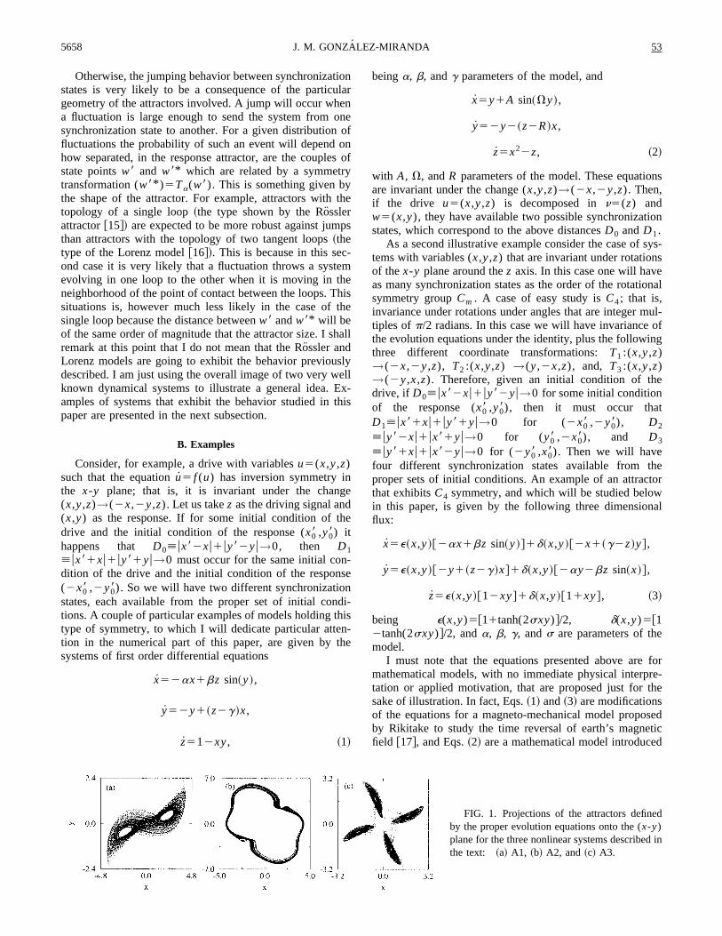
FIG. 1. Projections of the attractors definedby the proper evolution equations onto the (x-y)plane for the three nonlinear systems described inthe text: ~a! A1, ~b! A2, and~c! A3.

5658 53J. M. GONZALEZ-MIRANDA

here only as an illustrative example. However, when dealingwith models with direct physical motivation, the variablesx,y, and z will be physical quantities whose values define aparticular state of the system. In particular, they may be ve-locities, electrical currents, temperature gradients, or otherphysical quantities, so that a change of sign or numericalvalues would mean significant changes in the correspondingexperimental situations. Accordingly, the occurrence ofDaÞ0→0 instead ofD0→0 would imply different physicalsituations, and so it follows that what I am describing heremay manifest itself as a phenomenon with physical meaning.

III. NUMERICAL EXPERIMENTS

A. Chaotic attractors

To illustrate the theoretical points raised above I will nowpresent and discuss some numerical results for the math-ematical models used above as examples. These have beenobtained working in double precision, and integrating theevolution equations by means of a fourth order Runge-Kuttaalgorithm. Most of the numerical results in this section cor-respond to the following cases:~A1! Equation~1!, at theparameter valuesa51.5, b52.0, andg53.75, and an inte-gration time step of 0.03,~A2! Equation~2!, at parametervaluesA53.2,V51.4, andR55.2, and an integration step of0.01, ~A3! Equation~3! at parameter valuesa52.0,b52.0,g53.0, ands516.0, and an integration step of 0.03. Thesecases will be designated throughout this paper with the cor-responding abbreviation An,nP$1,2,3%.

In the first place, to ensure that at the above parametervalues the systems considered are chaotic, I have performeda series of standard tests@18,19#. The results of some of themare displayed in Figs. 1–3. In Fig. 1 there appear plots of theattractors which tend to fill up a section of the phase space,as corresponds to chaotic evolutions. Besides, this figureshows how the attractors exhibit the symmetry of the corre-sponding evolution equations. In particular, one can appreci-

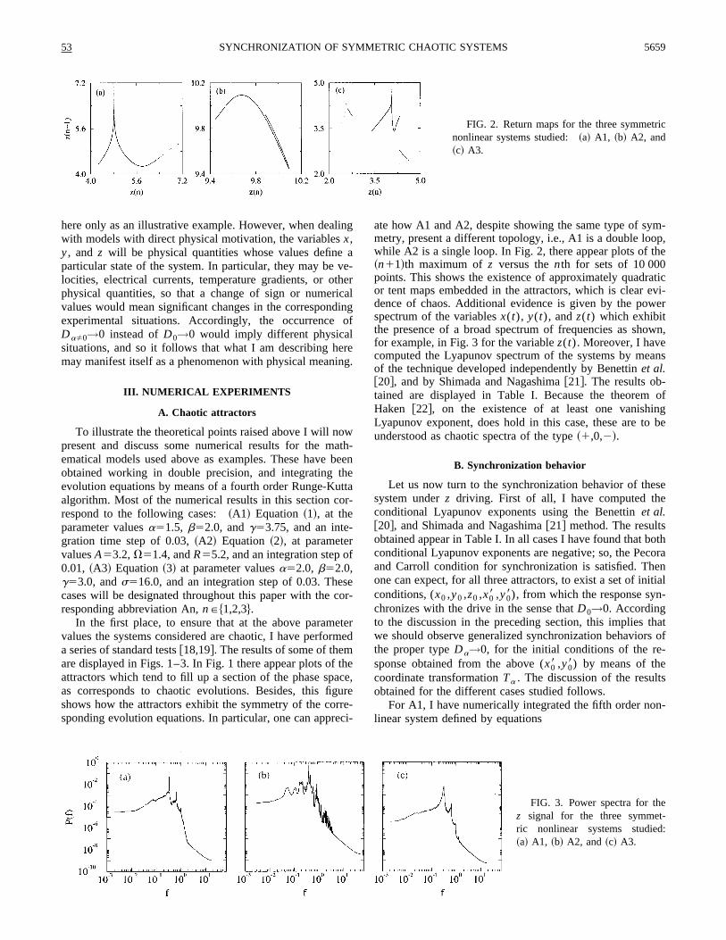
ate how A1 and A2, despite showing the same type of sym-metry, present a different topology, i.e., A1 is a double loop,while A2 is a single loop. In Fig. 2, there appear plots of the~n11!th maximum ofz versus thenth for sets of 10 000points. This shows the existence of approximately quadraticor tent maps embedded in the attractors, which is clear evi-dence of chaos. Additional evidence is given by the powerspectrum of the variablesx(t), y(t), andz(t) which exhibitthe presence of a broad spectrum of frequencies as shown,for example, in Fig. 3 for the variablez(t). Moreover, I havecomputed the Lyapunov spectrum of the systems by meansof the technique developed independently by Benettinet al.@20#, and by Shimada and Nagashima@21#. The results ob-tained are displayed in Table I. Because the theorem ofHaken @22#, on the existence of at least one vanishingLyapunov exponent, does hold in this case, these are to beunderstood as chaotic spectra of the type~1,0,2!.

B. Synchronization behavior

Let us now turn to the synchronization behavior of thesesystem underz driving. First of all, I have computed theconditional Lyapunov exponents using the Benettinet al.@20#, and Shimada and Nagashima@21# method. The resultsobtained appear in Table I. In all cases I have found that bothconditional Lyapunov exponents are negative; so, the Pecoraand Carroll condition for synchronization is satisfied. Thenone can expect, for all three attractors, to exist a set of initialconditions, (x0 ,y0 ,z0 ,x08 ,y08), from which the response syn-chronizes with the drive in the sense thatD0→0. Accordingto the discussion in the preceding section, this implies thatwe should observe generalized synchronization behaviors ofthe proper typeDa→0, for the initial conditions of the re-sponse obtained from the above (x08 ,y08) by means of thecoordinate transformationTa . The discussion of the resultsobtained for the different cases studied follows.

For A1, I have numerically integrated the fifth order non-linear system defined by equations

FIG. 2. Return maps for the three symmetricnonlinear systems studied:~a! A1, ~b! A2, and~c! A3.

FIG. 3. Power spectra for thez signal for the three symmet-ric nonlinear systems studied:~a! A1, ~b! A2, and~c! A3.


x852ax81bz sin~y8!,

y852y81~z2g!x8, ~4!

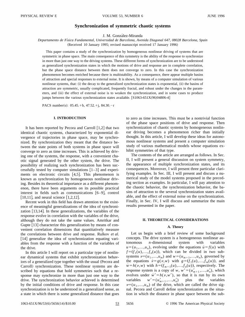
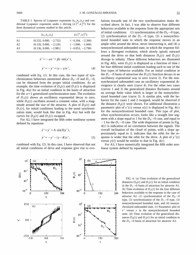
combined with Eq.~1!. In this case, the two types of syn-chronization behaviors mentioned aboveD0→0 andD1→0,can be obtained from the proper initial conditions. As anexample, the time evolution ofD0(t) andD1(t) is displayedin Fig. 4~a! for an initial condition in the basin of attractionfor thea51 generalized synchronization state. The evolutionof D1(t) shows an oscillatory exponential decay to zero,while D0(t) oscillates around a constant value, with a mag-nitude around the size of the attractor. A plot ofD0(t) andD1(t), for initial conditions leading to the usual synchroni-zation state, would look like that in Fig. 4~a! but with thecurves forD0(t) andD1(t) swapped.

For A2, I have integrated the fifth order nonlinear systemdefined by equations

x85y81A sin~Vy8!,

y852y82~z2R!x8, ~5!

combined with Eq.~2!. In this case, I have observed that notall initial conditions of drive and response give rise to evo-

lutions towards one of the two synchronization states de-scribed above. In fact, I was able to observe four differentbehaviors available to the response from the appropriate setsof initial conditions: ~1! synchronization of theD0→0 type,~2! synchronization of theD1→0 type, ~3! a nonsynchro-nized bounded state in which the response moves in anample orbit around the drive, never intersecting it, and~4! anonsynchronized unbounded state, in which the response fol-lows a divergent evolution, which slowly spirals outwardaround the drive so that both distancesD0(t) and D1(t)diverge to infinity. These different behaviors are illustratedin Fig. 4~b!, wereD1(t) is displayed as a function of timetfor four different initial conditions leading each to one of thefour types of behavior available. For an initial condition intheD1→0 basin of attraction theD1(t) function decays in anoscillatory exponential way to zero~curve 2!. For the non-synchronized unbounded case an oscillatory exponential di-vergence is clearly seen~curve 4!. For the other two cases~curves 1 and 3! the generalized distance fluctuates aroundan average finite value which is larger in the nonsynchro-nized bounded case~curve 3!. A similar plot, with the be-havior for the cases 1 and 2 swapped, would be observed ifthe distanceD0(t) were shown. For additional illustration aparametric plot ofx8(t) versusx(t) is displayed in Fig. 4~c!for the nonsynchronized bounded case. This type of plot,when synchronization occurs, looks like a straight line seg-ment with a slope equal to 1 for theD0→0 case, and equal to21 for theD1→0 case. The wide dispersion of points in Fig.4~c! is indication of no correlation between the signals. Theoverall inclination of the cloud of points, with a slope ap-proximately equal to 3, indicates that the orbit for the re-sponse is wider that the orbit for the drive. A plot ofy8(t)versusy(t) would be similar to that in Fig. 4~c!.

For A3, I have numerically integrated the fifth order non-linear system defined by equations

TABLE I. Spectra of Lyapunov exponents~l1,l2,l3! and con-ditional Lyapunov exponents underz driving (l 1

(z) ,l 2(z)) for the

three dynamical systems studied in this article.

~l1,l2,l3! (l 1(z) ,l 2

(z))

A1 ~0.232, 0.000,22.732! ~20.104,22.396!A2 ~0.126, 0.000,22.126! ~21.000,21.000!A3 ~0.136, 0.000,22.981! ~20.053,22.790!

FIG. 4. ~a! Time evolution of the generalizeddistancesD0(t) andD1(t) for an initial conditionin theD1→0 basin of attraction for attractor A1.~b! Time evolution ofD1(t) for the four differentbehaviors available to the response in the case ofattractor A2: ~1! synchronization of theD0→0type, ~2! synchronization of theD1→0 type, ~3!nonsynchronized bounded state, and~4! nonsyn-chronized unbounded state.~c! Parametric plot ofx8 versus x in the nonsynchronized boundedstate.~d! Time evolution of the generalized dis-tancesD0(t) andD3(t) for an initial condition intheD3→0 basin of attraction for attractor A3.


x85e~x8,y8!@2ax81bz sin~y8!#1d~x8,y8!

3@2x81~g2z!y8#,

y85e~x8,y8!@2y81~z2g!x8#1d~x8,y8!

3@2ay82bz sin~x8!#, ~6!

combined with Eq.~3!. As in the previous cases, I have beenable to observe all the synchronization states given byDa(t),with aP$0,1,2,3% for initial conditions chosen conveniently~see Sec. II B!. As an example, a plot ofD3(t) displaying thecharacteristic exponential decay to zero appears in Fig. 4~d!,for an initial condition in theD3→0 basin of attraction.Moreover, in this plot there appearsD0(t), for the sameinitial condition, which fluctuates around a finite value@thesame behavior will be observed ifD1(t) or D2(t) wereshown#. The corresponding plots for the other three caseswould exhibit a similar look. I must note that besides thesefour synchronization behaviors available, there is the possi-bility of no synchronization between drive and response forinitial conditions of the response close to~0,0!. In this casethe response evolves towards a fixed point located at theorigin of coordinates.

The plots forDa(t) in Fig. 4 illustrate the possibility ofthe synchronization states of types different than the usual,

described in Sec. II, to exist. It is worth noting that Pecoraand Carroll also reported this type of oscillatory exponentialdecay in their study of synchronization of systems with justthe usual synchronization state available@1,2#. The observa-tion of systems with negative conditional Lyapunov expo-nents for which some initial conditions synchronize whileothers do not, gives additional illustration to the finding ofBadola, Tambe, and Kulkarni@3# that negativity of condi-tional Lyapunov exponents is not a guarantee of synchroni-zation for all initial conditions.

C. Basins of attraction

The study of the basins of attraction in the present case isquite difficult, because we are faced with a five dimensionalspace of initial conditions. To have some insight on theshape of the basins of attraction to the different types ofbehaviors available to the response, I have proceeded as fol-lows. I chose some point in the attractor as initial conditionfor the drive, (x0 ,y0 ,z0), and a grid ofN3N initial points inthe (x8,y8) subspace for the response. Then, I ran the equa-tions for drive and response to see the time evolution ofDafor each point in the grid. A plot was prepared in which eachpoint of the grid is colored according to the synchronizationstate achieved, so that one can have an image of the basins of

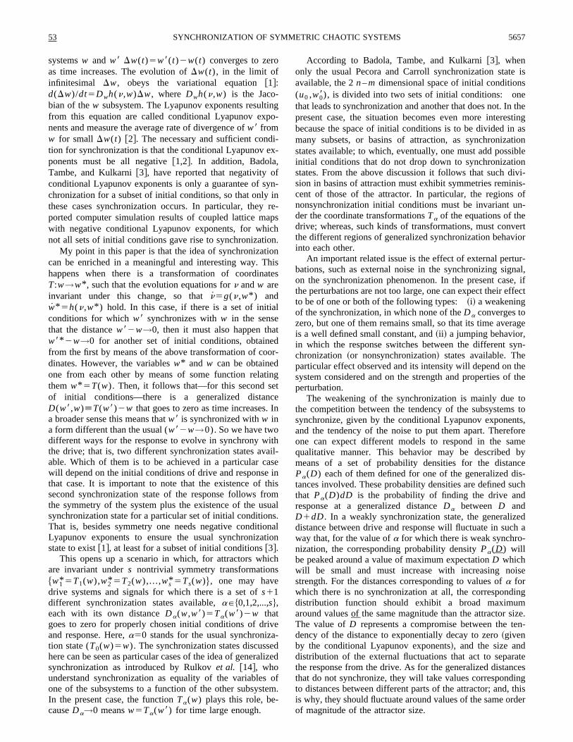
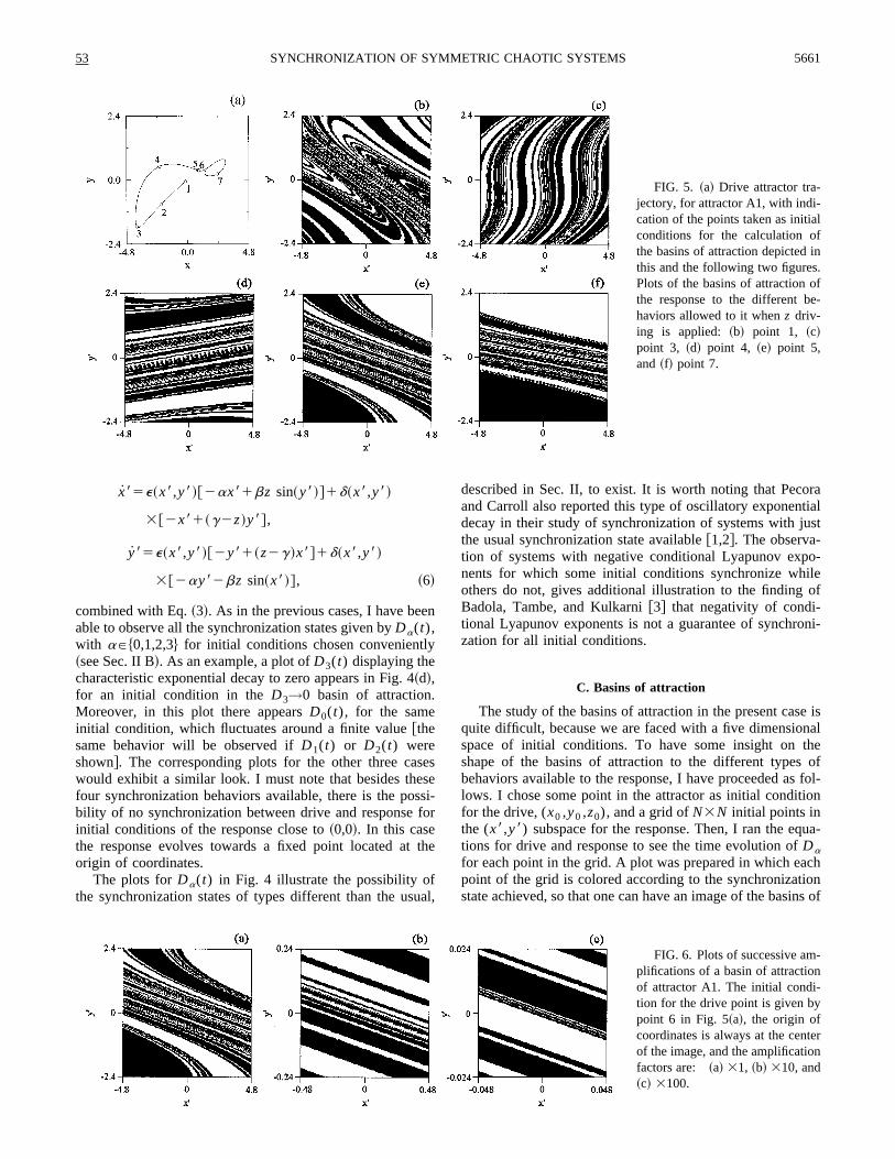
FIG. 5. ~a! Drive attractor tra-jectory, for attractor A1, with indi-cation of the points taken as initialconditions for the calculation ofthe basins of attraction depicted inthis and the following two figures.Plots of the basins of attraction ofthe response to the different be-haviors allowed to it whenz driv-ing is applied: ~b! point 1, ~c!point 3, ~d! point 4, ~e! point 5,and ~f! point 7.

FIG. 6. Plots of successive am-plifications of a basin of attractionof attractor A1. The initial condi-tion for the drive point is given bypoint 6 in Fig. 5~a!, the origin ofcoordinates is always at the centerof the image, and the amplificationfactors are: ~a! 31, ~b! 310, and~c! 3100.


attraction for the particular initial condition of the drive(x0 ,y0 ,z0). In almost all the cases that follow, these picturesare centered at the origin of coordinates and show a region ofphase space a bit larger than the one spanned by the attractor.In the case when the pictures represent regions not centeredat the origin or with dimensions different than those of thedrive attractor this is explicitly stated. In this study, I havepaid particular attention to the evolution of the basins withthe values of (x0 ,y0 ,z0) ~always chosen as a point in thestable drive attractor!, to the nature of the basin boundaries,and to the effect of the changes in the parameters of thesystem on the basin pictures. In this last case I have studiedattractors with parameters different than those indicated atthe beginning of this section, chosen so that the system isstill chaotic, and the conditional Lyapunov exponents con-tinue to be negative. In this case, the values of the driveinitial conditions (x0 ,y0 ,z0) cannot be exactly the same forall choices of parameters because they are to be points of thestable attractor which is a set of points that changes when theparameters change. However they have been carefully cho-sen to ensure that the points used for every choice of param-eters are very close among them.

Representative examples of such basins in the case of A1are displayed in Figs. 5, 6, and 7. There, grids of 1613161initial conditions for the response are displayed with thepoints in the grid colored white ifD1→0 and black ifD0→0.Except when explicitly indicated, the regions studied has asize of 9.634.8; which corresponds to the region of phasespace shown in Fig. 5~a!. All initial conditions give rise toone of the two synchronization states available, with the onlyexception of the origin of coordinates, which is an unstablefixed point. Moreover, from these pictures it is clear that ifD0→0 for (x08 ,y08), then D1→0 for (2x08 ,2y08), as ex-pected. The basin shapes vary with the initial condition ofthe drive. This variation is illustrated in Fig. 5, where fivebasin pictures are shown with an indication of the drive pointtrajectory to which they belong. Additional pictures can beseen in Fig. 6~a! and Fig. 7~a!. The shape of the basinsevolves smoothly along the drive trajectory@compare Fig.5~e! with Fig. 6~a!# but experiences noticeable changes whenthe point in the drive attractor are far away. In general, theshapes of the basins are complicated and the two types ofsynchronization behaviors available appear entangled. Thenature of these basins seems to be fractal as more detail isseen with amplification; as illustrated in Fig. 6, where suc-cessive amplifications by a power of ten of the central regionof one of them are displayed. Moreover, as illustrated in Fig.7, the overall shape of the basin pictures appears robust un-der changes in the parameters of the attractor; although, the

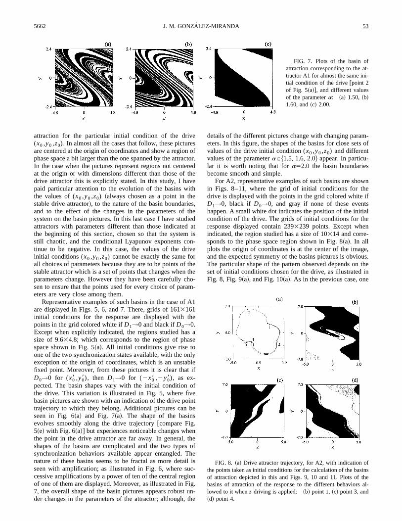
details of the different pictures change with changing param-eters. In this figure, the shapes of the basins for close sets ofvalues of the drive initial condition (x0 ,y0 ,z0) and differentvalues of the parameteraP$1.5, 1.6, 2.0% appear. In particu-lar it is worth noting that fora52.0 the basin boundariesbecome smooth and simple.

For A2, representative examples of such basins are shownin Figs. 8–11, where the grid of initial conditions for thedrive is displayed with the points in the grid colored white ifD1→0, black if D0→0, and gray if none of these eventshappen. A small white dot indicates the position of the initialcondition of the drive. The grids of initial conditions for theresponse displayed contain 2393239 points. Except whenindicated, the region studied has a size of 10314 and corre-sponds to the phase space region shown in Fig. 8~a!. In allplots the origin of coordinates is at the center of the image,and the expected symmetry of the basins pictures is obvious.The particular shape of the pattern observed depends on theset of initial conditions chosen for the drive, as illustrated inFig. 8, Fig. 9~a!, and Fig. 10~a!. As in the previous case, one

FIG. 7. Plots of the basin ofattraction corresponding to the at-tractor A1 for almost the same ini-tial condition of the drive@point 2of Fig. 5~a!#, and different valuesof the parametera: ~a! 1.50, ~b!1.60, and~c! 2.00.

FIG. 8. ~a! Drive attractor trajectory, for A2, with indication ofthe points taken as initial conditions for the calculation of the basinsof attraction depicted in this and Figs. 9, 10 and 11. Plots of thebasins of attraction of the response to the different behaviors al-lowed to it whenz driving is applied: ~b! point 1,~c! point 3, and~d! point 4.


obtains an evolution of the basin pictures with the change onthe drive initial condition (x0 ,y0 ,z0). However the overallappearance of the basins is quite different than those of A1.The more significant difference is that, despite the variety ofbehaviors available, the different basins of attraction arewide and clearly separated. Moreover, the values of the ini-tial conditions of the response coincident with those of thedrive always appear far from the basin boundaries. Thesebasin boundaries, however, still seem to be fractal as illus-trated in Fig. 9 by means of successive amplification, by afactor ten, of the central region of one of them. The basinshapes appear robust under the changes in parameter values,as shown in Fig. 10, where basin pictures are displayed forclose drive initial conditions corresponding to different val-ues of the parameterRP$5.20, 5.15, 4.80%, showing the sameoverall shape but changes in the details. A particularity ofthis system is the existence of other states available to theresponse besides to the two synchronized ones. To showmore clearly the presence of these states, in Fig. 11, there aredisplayed basin pictures for the same drive initial conditionsas those in Fig. 8, but displaying a region of 1003140 ~i.e.,10 times larger!. The light gray region indicates the initialconditions that gives rise to bounded nonsynchronized states,and the medium gray regions~far from where the attractorevolves! the initial condition from which the distances di-verge.

Results for the basins of attraction of A3, are displayed inFigs. 12–15. As for A1, the grids of points are 1613161.Different shades of gray are used in this case with the fol-lowing code: black forD0→0, white forD1→0, light grayfor D2→0, dark gray forD3→0, and medium gray for theinitial conditions from which the response drops towards thefixed point at the origin. Moreover, a white dot indicates theposition of the initial condition of the drive. The region stud-ied, except when indicated, has a size of 6.436.4 and corre-sponds to the square shown in Fig. 12~a!. The symmetriesassociated to theC4 symmetry of the attractor are clearlyseen through these pictures, except in Figs. 13~b! and 13~c!that are not centered at the origin of coordinates. The evolu-tion of the basins with the initial conditions, which is smoothas in the previous cases, is illustrated in Fig. 12, and Figs.13~a! and 14~a!. Despite having its own shape, these basinsresemble those of A2 in that there are wide regions for eachof the behaviors available in which there is no mixing amongthe different behaviors available. This is so despite the basinboundaries seeming to be fractal as illustrated in Fig. 13 bysuccessive amplifications by a power of ten of the centralregion of one of them. The changes with the parameters ofthe system resemble those of the two previous cases in thatthe overall shape of the basins does not change, while thedetails of the boundaries are somewhat modified. This isshown in Fig. 14 where there appear results for the parameter

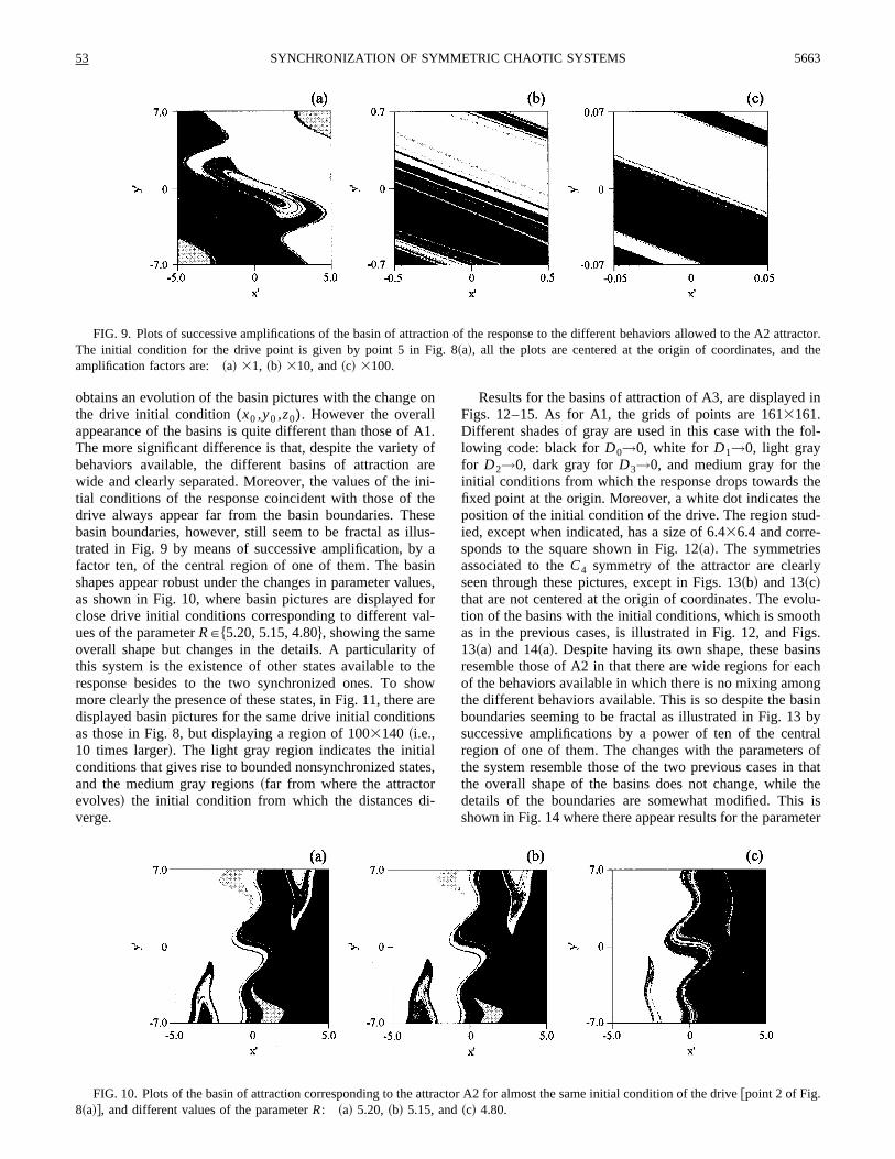
FIG. 9. Plots of successive amplifications of the basin of attraction of the response to the different behaviors allowed to the A2 attractor.The initial condition for the drive point is given by point 5 in Fig. 8~a!, all the plots are centered at the origin of coordinates, and theamplification factors are: ~a! 31, ~b! 310, and~c! 3100.

FIG. 10. Plots of the basin of attraction corresponding to the attractor A2 for almost the same initial condition of the drive@point 2 of Fig.8~a!#, and different values of the parameterR: ~a! 5.20, ~b! 5.15, and~c! 4.80.


s taking values in$16.0, 14.0, 12.0%. An interesting observa-tion, for this attractor, is that, although almost all the time thenumerical values corresponding to the initial condition of theattractor are well inside theD0→0 basin of attraction, forsome special points they become very close to the bound-aries. This situations is illustrated in Fig. 15, where thereappear the boundaries for two close points near a region inwhich the attractor bifurcates between two different loops. Itdeserves to be noted how different the basins are, despitepoints 1 and 2 being quite close. This reflects the fact thatpoint 1 is in a trajectory inside a loop, while point 2 is in atrajectory corresponding to a jump between loops.

The results in Figs. 5 to 15 illustrate the practical possi-bility of synchronization in a way different than usual whenwe deal with symmetric systems. Moreover, they tell us thateach particular nonlinear system will display a set of peculiarpatterns that are a specific property of that system. Thismeans that the shapes of the basin boundaries are expected tobe as diverse as the dynamical systems themselves are. How-ever, some regularities are present:~i! the basins displaysymmetries reminiscent of those of the dynamical system towhich they belong,~ii ! they change smoothly with the varia-tion of (x0 ,y0 ,z0) along the drive trajectory, and~iii ! theyappear to be robust under small changes of the parameters ofthe system, despite that a change in parameters implieschanges in the attractor properties~expected to be small! aswell as in the values of the initial conditions of the drive.Large changes in the parameters can alter in a significantextent the basin boundaries. Moreover, the boundary basinsseem to be fractal, although this is not expected to be thegeneral rule as some of the plots indicate@see Fig. 7~c! andFig. 14~c!#.

D. Effect of external noise

To test the effect of external noise on the synchronizationin the models studied here, I have studied how synchroniza-tion is affected by a white noise in the driving signal. To dothis I have integrated, together with the equations for thedrive, the corresponding equations for the response adding arandom Gaussian variableh with a standard deviations, tothe drive signalz. In the calculations performed, I have cho-sen initial conditions well inside one of the basins of attrac-tion to one of the synchronization states involved. Then, Iran the equations of motion for 108 time steps, for values of

s between 10 and 1.031025 for A1, 10 and 5.031024 forA2, and 10 and 1.031028 for A3. The objective is to getsome insight on the shape and behavior of the probabilitydensitiesPa(D) and the rate of jumps between synchroniza-tion states. To achieve this, I have computed, in that timewindow: ~i! the histograms for the number of occurrencesDNa(D) of a generalized distanceDa betweenD andD1DD, and~ii ! the number of jumps between synchroniza-tion states along the runNJ . To do this last calculation, Iconsider the system to be weakly synchronized when one oftheDa is less 3s, while all the others are much greater thanthat quantity. A jump happens when the particular value ofafor which Da is small, the others being large, changes.This choice is justified by what follows. Moreover,I will note that, in this subsection, the histogramsDNa(D)are presented under the form for the functionsf a(D)

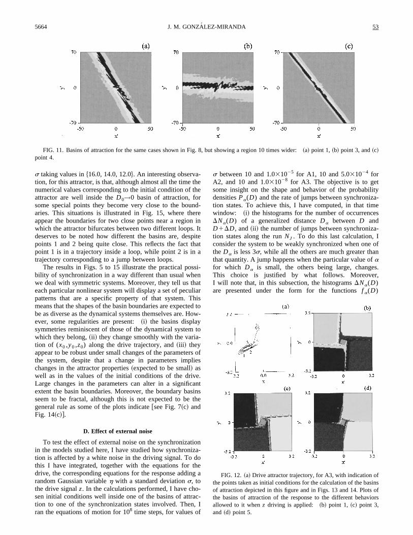
FIG. 11. Basins of attraction for the same cases shown in Fig. 8, but showing a region 10 times wider:~a! point 1, ~b! point 3, and~c!point 4.

FIG. 12. ~a! Drive attractor trajectory, for A3, with indication ofthe points taken as initial conditions for the calculation of the basinsof attraction depicted in this figure and in Figs. 13 and 14. Plots ofthe basins of attraction of the response to the different behaviorsallowed to it whenz driving is applied: ~b! point 1, ~c! point 3,and ~d! point 5.


5DNa(D)/NObs, beingNObs the number of observations ofD in the above time window, for a givenDD. In each casethe value ofDD has been chosen according to the range ofdefinition of the functionf a(D), to ensure that their shapesare well resolved. The results obtained are independent of theparticular choice ofa for the basin of attraction of the initialcondition.

For A1 I have integrated, together with the above Eqs.~1!for the drive, the following equations for the response:

x852ax81b~z1h!sin~y8!,

y852y81@~z1h!2g#x8, ~7!

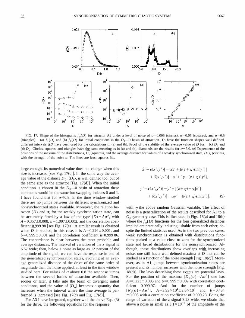
with h the above random Gaussian variable. The shape of thehistogramsf a(D) for D0(t) and D1(t) exhibits the samebehavior, no matter in which basin of attraction the initialcondition was set. This is illustrated by means of the resultsfor f 0(D) and f 1(D), at a particular value ofs, shown forthe smallD region in Fig. 16~a! and for the largeD region inFig. 16~b!. Both distribution functions show the same ap-pearance and are practically put on top of each other despitethe statistics implying only a finite number of observations.This is an indication of repeated changes between synchro-nization states. That is, what we see in these figures, for eachf a(D), is the combination of the distribution functions fortwo different synchronization states: the case when the re-

sponse is in theDa→0 state@Fig. 16~a!# with the case whenthe response is in theDa8Þa→0 state@Fig. 16~b!#. In thesmallDa region these functions present a well defined maxi-mum close to zero, which signals a state of weak synchroni-zation, in which the distance between both systems fluctuatesaround the distance corresponding to this maximum. ThelargeDa regions correspond to the time when the system isin the other synchronization state so that the distance fluctu-ates around values that are of the same order of magnitude asthe attractor size. It is important to notice that the distributionfunctions for these two states have an overlapping region, asseen in Fig. 16~b!, in accordance with the idea that the sys-tem can easily jump between synchronization states. How-ever, one has a well defined maximum for the times whengeneralized synchronization occurs, so that it is possible tocompute the dependence of the value of the position of themaximaD, with s. The results, that appear in Fig. 16~c!, canbe accurately fitted by a potential law of the typeDa(s)5Asb, beingA50.41960.015,b50.99960.005, andthe correlation coefficient 0.999 94. The dependence of thenumber of jumps between synchronization statesNJ with theamplitude of the noises is displayed in Fig. 16~d!. Thefunction NJ~s! can be approximated by a law of the typeNJ(s)5Asb with A51.10310661.73105 and b51.03960.021, being the correlation coefficient 0.999 83. As theinterval of the variation of thez signal is 6.37 wide, we seethat above a noise as small as 1.631026 of the amplitude of

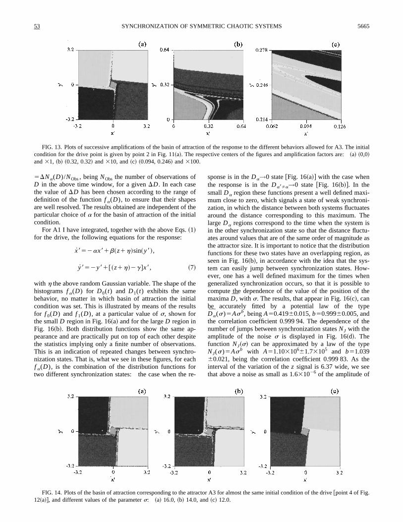
FIG. 13. Plots of successive amplifications of the basin of attraction of the response to the different behaviors allowed for A3. The initialcondition for the drive point is given by point 2 in Fig. 11~a!. The respective centers of the figures and amplification factors are:~a! ~0,0!and31, ~b! ~0.32, 0.32! and310, and~c! ~0.094, 0.246! and3100.

FIG. 14. Plots of the basin of attraction corresponding to the attractor A3 for almost the same initial condition of the drive@point 4 of Fig.12~a!#, and different values of the parameters: ~a! 16.0, ~b! 14.0, and~c! 12.0.


this signal we still see jumps between synchronization states~at this level of noise only nine jumps were observed in thetime window studied!. Anyway, the extrapolation ofDa~s!andNJ~s! to s50 indicates that, when no noise is present,the system stays in only one of the synchronization statesavailable. The effects of adding noise is to weaken the syn-chronization and to introduce a rate of jumps between syn-chronization states. These effects become more and moreintense as the level of noise is increased until synchroniza-tion is completely lost.


x85y81A sin~Vy8!,

y852y82@~z1h!2R#x8, ~8!

with h the above random Gaussian variable. One must notethat these equations also describe the behavior of the system

under a fluctuatingR parameter for the response, which in aphysical situation would stand for a response system in con-tact with a fluctuating environment. In the following discus-sion I will assume the noisy drive signal picture, however thetranslation to the fluctuatingR case is straightforward. Fig-ures 17~a! and 17~b! show, respectively, the shape of thedistribution functionsf 1(D) and f 0(D) for three differentvalues ofs. The initial condition for this particular picturewas in theD1→0 basin of attraction. Those plots indicatethat both distances fluctuate inside intervals that are wellseparated; i.e., negligible overlap betweenf a(D) functionsat different synchronization states. Forf 1(D), this interval isnarrow and close to zero, while forf 0(D) it is wide and farfrom zero. Moreover, the values forf 1(D) can be scaled in asingle curve when the distance is divided by the strength ofthe noise. For values ofs below 0.8, the average value of thedistance for the weakly synchronized state^D1& is small andwell defined. I have verified that for a size of the sample

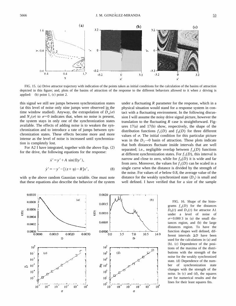
FIG. 15. ~a! Drive attractor trajectory with indication of the points taken as initial conditions for the calculation of the basins of attractiondepicted in this figure; and, plots of the basins of attraction of the response to the different behaviors allowed to it whenz driving isapplied: ~b! point 1, ~c! point 2.

FIG. 16. Shape of the histo-grams f a(D) for the distancesD0(t) andD1(t) for attractor A1under a level of noise ofs50.000 3 in ~a! the small dis-tances region, and~b! the largedistances region. To have thefunction shapes well defined, dif-ferent intervals DD have beenused for the calculations in~a! and~b!. ~c! Dependence of the posi-tions of the maxima of the distri-butions with the strength of thenoise for the weakly synchronizedstate.~d! Dependence of the num-ber of synchronization statechanges with the strength of thenoise. In ~c! and ~d!, the squaresare for numerical results and thelines for their least squares fits.


large enough, its numerical value does not change when thissize is increased@see Fig. 17~c!#. In the same way the aver-age value of the distanceD0, ^D0&, is well defined too, but ofthe same size as the attractor@Fig. 17~d!#. When the initialcondition is chosen in theD0→0 basin of attraction thesecomments would be the same but swapping indexes 0 and 1.I have found that fors<0.8, in the time window studiedthere are no jumps between the different synchronized andnonsynchronized states available. Moreover, the relation be-tween^D& ands, for the weakly synchronization state, canbe accurately fitted by a law of the type^D&5Asb, withA50.35760.008,b51.00760.002, and the correlation coef-ficient 0.999 98@see Fig. 17~e!#. A similar result is obtainedwhen D is studied; in this case, it isA50.22660.001, andb50.99960.001 and the correlation coefficient is 0.999 86.The concordance is clear between the most probable andaverage distances. The interval of variation of thez signal is6.57 wide; then, below a noise as large as 12 percent of theamplitude of the signal, we can have the response in one ofthe generalized synchronization states, evolving at an aver-age generalized distance of the drive of the same order ofmagnitude than the noise applied, at least in the time windowstudied here. For values ofs above 0.8 the response jumpsbetween the several basins of attraction available. Then,sooner or later, it falls into the basin of divergent initialconditions, and the value ofDa& becomes a quantity thatincreases when the interval where the time average is per-formed is increased@see Fig. 17~c! and Fig. 17~d!#.


x85e~x8,y8!@2ax81b~z1h!sin~y8!#

1d~x8,y8!$2x81@g2~z1h!#y8%,

y85e~x8,y8!$2y81@~z1h!2g#x8%

1d~x8,y8!@2ay82b~z1h!sin~x8!#, ~9!

with h the above random Gaussian variable. The effect ofnoise is a generalization of the results described for A1 to aC4 symmetry case. This is illustrated in Figs. 18~a! and 18~b!where thef a(D) functions for the four generalized distancesimplied are practically indistinguishable from each other, de-spite the limited statistics used. As in the two previous cases,weak synchronization is obtained with distributions func-tions peaked at a value close to zero for the synchronizedstate and broad distributions for the nonsynchronized. Al-though, these distributions show overlaps with increasingnoise, one still has a well defined maxima atD that can bestudied as a function of the noise strength@Fig. 18~c!#. More-over, as in A1, jumps between synchronization states arepresent and its number increases with the noise [email protected]~d!#. The laws describing these events are potential laws.For the position of the maxima [Da(s)5Asb] one hasA50.22360.005 andb50.99960.002 with correlation coef-ficient 0.999 97. And for the number of jumps[NJ(s)5Asb], A53.93310462.63103 and b50.45460.005 with a correlation coefficient of 0.999 23. Being therange of variation of thez signal 3.23 wide, we obtain thatabove a noise as small as 3.131029 of the amplitude of the

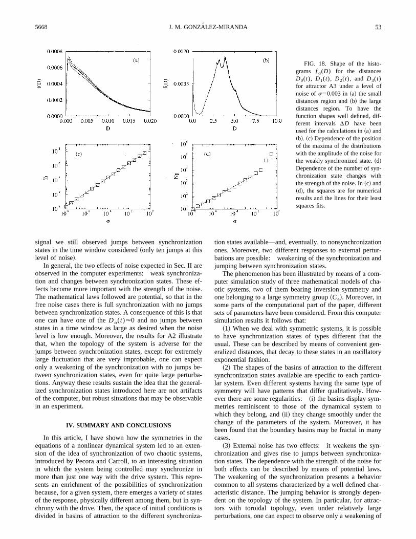
FIG. 17. Shape of the histogramsf a(D) for attractor A2 under a level of noise ofs50.005 ~circles!, s50.05 ~squares!, ands50.5~triangles!: ~a! f 1(D) and ~b! f 0(D) for initial conditions in theD1→0 basin of attraction. To have the function shapes well defined,different intervalsDD have been used for the calculations in~a! and~b!. Proof of the stability of the average value ofD for: ~c! D1 and~d! D0. Circles, squares, and triangles have the same meaning as in~a! and~b!, diamonds are the results fors55.0. ~e! Dependence of thepositions of the maxima of the distributions,D, ~squares!, and the average distance for values of a weakly synchronized state,^D&, ~circles!,with the strength of the noises. The lines are least squares fits.


signal we still observed jumps between synchronizationstates in the time window considered~only ten jumps at thislevel of noise!.

In general, the two effects of noise expected in Sec. II areobserved in the computer experiments: weak synchroniza-tion and changes between synchronization states. These ef-fects become more important with the strength of the noise.The mathematical laws followed are potential, so that in thefree noise cases there is full synchronization with no jumpsbetween synchronization states. A consequence of this is thatone can have one of theDa(t)'0 and no jumps betweenstates in a time window as large as desired when the noiselevel is low enough. Moreover, the results for A2 illustratethat, when the topology of the system is adverse for thejumps between synchronization states, except for extremelylarge fluctuation that are very improbable, one can expectonly a weakening of the synchronization with no jumps be-tween synchronization states, even for quite large perturba-tions. Anyway these results sustain the idea that the general-ized synchronization states introduced here are not artifactsof the computer, but robust situations that may be observablein an experiment.

IV. SUMMARY AND CONCLUSIONS

In this article, I have shown how the symmetries in theequations of a nonlinear dynamical system led to an exten-sion of the idea of synchronization of two chaotic systems,introduced by Pecora and Carroll, to an interesting situationin which the system being controlled may synchronize inmore than just one way with the drive system. This repre-sents an enrichment of the possibilities of synchronizationbecause, for a given system, there emerges a variety of statesof the response, physically different among them, but in syn-chrony with the drive. Then, the space of initial conditions isdivided in basins of attraction to the different synchroniza-

tion states available—and, eventually, to nonsynchronizationones. Moreover, two different responses to external pertur-bations are possible: weakening of the synchronization andjumping between synchronization states.

The phenomenon has been illustrated by means of a com-puter simulation study of three mathematical models of cha-otic systems, two of them bearing inversion symmetry andone belonging to a large symmetry group~C4!. Moreover, insome parts of the computational part of the paper, differentsets of parameters have been considered. From this computersimulation results it follows that:

~1! When we deal with symmetric systems, it is possibleto have synchronization states of types different that theusual. These can be described by means of convenient gen-eralized distances, that decay to these states in an oscillatoryexponential fashion.

~2! The shapes of the basins of attraction to the differentsynchronization states available are specific to each particu-lar system. Even different systems having the same type ofsymmetry will have patterns that differ qualitatively. How-ever there are some regularities:~i! the basins display sym-metries reminiscent to those of the dynamical system towhich they belong, and~ii ! they change smoothly under thechange of the parameters of the system. Moreover, it hasbeen found that the boundary basins may be fractal in manycases.

~3! External noise has two effects: it weakens the syn-chronization and gives rise to jumps between synchroniza-tion states. The dependence with the strength of the noise forboth effects can be described by means of potential laws.The weakening of the synchronization presents a behaviorcommon to all systems characterized by a well defined char-acteristic distance. The jumping behavior is strongly depen-dent on the topology of the system. In particular, for attrac-tors with toroidal topology, even under relatively largeperturbations, one can expect to observe only a weakening of

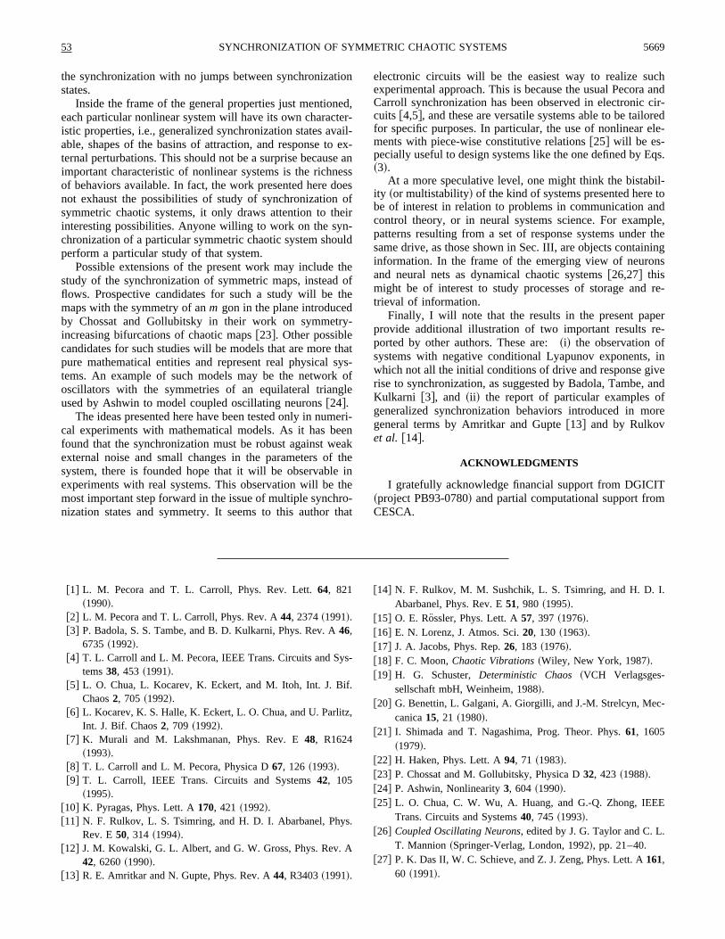
FIG. 18. Shape of the histo-grams f a(D) for the distancesD0(t), D1(t), D2(t), and D3(t)for attractor A3 under a level ofnoise ofs50.003 in~a! the smalldistances region and~b! the largedistances region. To have thefunction shapes well defined, dif-ferent intervals DD have beenused for the calculations in~a! and~b!. ~c! Dependence of the positionof the maxima of the distributionswith the amplitude of the noise forthe weakly synchronized state.~d!Dependence of the number of syn-chronization state changes withthe strength of the noise. In~c! and~d!, the squares are for numericalresults and the lines for their leastsquares fits.


the synchronization with no jumps between synchronizationstates.

Inside the frame of the general properties just mentioned,each particular nonlinear system will have its own character-istic properties, i.e., generalized synchronization states avail-able, shapes of the basins of attraction, and response to ex-ternal perturbations. This should not be a surprise because animportant characteristic of nonlinear systems is the richnessof behaviors available. In fact, the work presented here doesnot exhaust the possibilities of study of synchronization ofsymmetric chaotic systems, it only draws attention to theirinteresting possibilities. Anyone willing to work on the syn-chronization of a particular symmetric chaotic system shouldperform a particular study of that system.

Possible extensions of the present work may include thestudy of the synchronization of symmetric maps, instead offlows. Prospective candidates for such a study will be themaps with the symmetry of anm gon in the plane introducedby Chossat and Gollubitsky in their work on symmetry-increasing bifurcations of chaotic maps@23#. Other possiblecandidates for such studies will be models that are more thatpure mathematical entities and represent real physical sys-tems. An example of such models may be the network ofoscillators with the symmetries of an equilateral triangleused by Ashwin to model coupled oscillating neurons@24#.

The ideas presented here have been tested only in numeri-cal experiments with mathematical models. As it has beenfound that the synchronization must be robust against weakexternal noise and small changes in the parameters of thesystem, there is founded hope that it will be observable inexperiments with real systems. This observation will be themost important step forward in the issue of multiple synchro-nization states and symmetry. It seems to this author that

electronic circuits will be the easiest way to realize suchexperimental approach. This is because the usual Pecora andCarroll synchronization has been observed in electronic cir-cuits @4,5#, and these are versatile systems able to be tailoredfor specific purposes. In particular, the use of nonlinear ele-ments with piece-wise constitutive relations@25# will be es-pecially useful to design systems like the one defined by Eqs.~3!.

At a more speculative level, one might think the bistabil-ity ~or multistability! of the kind of systems presented here tobe of interest in relation to problems in communication andcontrol theory, or in neural systems science. For example,patterns resulting from a set of response systems under thesame drive, as those shown in Sec. III, are objects containinginformation. In the frame of the emerging view of neuronsand neural nets as dynamical chaotic systems@26,27# thismight be of interest to study processes of storage and re-trieval of information.

Finally, I will note that the results in the present paperprovide additional illustration of two important results re-ported by other authors. These are:~i! the observation ofsystems with negative conditional Lyapunov exponents, inwhich not all the initial conditions of drive and response giverise to synchronization, as suggested by Badola, Tambe, andKulkarni @3#, and ~ii ! the report of particular examples ofgeneralized synchronization behaviors introduced in moregeneral terms by Amritkar and Gupte@13# and by Rulkovet al. @14#.

ACKNOWLEDGMENTS

I gratefully acknowledge financial support from DGICIT~project PB93-0780! and partial computational support fromCESCA.

@1# L. M. Pecora and T. L. Carroll, Phys. Rev. Lett.64, 821~1990!.

@2# L. M. Pecora and T. L. Carroll, Phys. Rev. A44, 2374~1991!.@3# P. Badola, S. S. Tambe, and B. D. Kulkarni, Phys. Rev. A46,

6735 ~1992!.@4# T. L. Carroll and L. M. Pecora, IEEE Trans. Circuits and Sys-

tems38, 453 ~1991!.@5# L. O. Chua, L. Kocarev, K. Eckert, and M. Itoh, Int. J. Bif.

Chaos2, 705 ~1992!.@6# L. Kocarev, K. S. Halle, K. Eckert, L. O. Chua, and U. Parlitz,

Int. J. Bif. Chaos2, 709 ~1992!.@7# K. Murali and M. Lakshmanan, Phys. Rev. E48, R1624

~1993!.@8# T. L. Carroll and L. M. Pecora, Physica D67, 126 ~1993!.@9# T. L. Carroll, IEEE Trans. Circuits and Systems42, 105

~1995!.@10# K. Pyragas, Phys. Lett. A170, 421 ~1992!.@11# N. F. Rulkov, L. S. Tsimring, and H. D. I. Abarbanel, Phys.

Rev. E50, 314 ~1994!.@12# J. M. Kowalski, G. L. Albert, and G. W. Gross, Phys. Rev. A

42, 6260~1990!.@13# R. E. Amritkar and N. Gupte, Phys. Rev. A44, R3403~1991!.

@14# N. F. Rulkov, M. M. Sushchik, L. S. Tsimring, and H. D. I.Abarbanel, Phys. Rev. E51, 980 ~1995!.

@15# O. E. Rossler, Phys. Lett. A57, 397 ~1976!.@16# E. N. Lorenz, J. Atmos. Sci.20, 130 ~1963!.@17# J. A. Jacobs, Phys. Rep.26, 183 ~1976!.@18# F. C. Moon,Chaotic Vibrations~Wiley, New York, 1987!.@19# H. G. Schuster,Deterministic Chaos~VCH Verlagsges-

sellschaft mbH, Weinheim, 1988!.@20# G. Benettin, L. Galgani, A. Giorgilli, and J.-M. Strelcyn, Mec-

canica15, 21 ~1980!.@21# I. Shimada and T. Nagashima, Prog. Theor. Phys.61, 1605

~1979!.@22# H. Haken, Phys. Lett. A94, 71 ~1983!.@23# P. Chossat and M. Gollubitsky, Physica D32, 423 ~1988!.@24# P. Ashwin, Nonlinearity3, 604 ~1990!.@25# L. O. Chua, C. W. Wu, A. Huang, and G.-Q. Zhong, IEEE

Trans. Circuits and Systems40, 745 ~1993!.@26# Coupled Oscillating Neurons, edited by J. G. Taylor and C. L.

T. Mannion~Springer-Verlag, London, 1992!, pp. 21–40.@27# P. K. Das II, W. C. Schieve, and Z. J. Zeng, Phys. Lett. A161,

60 ~1991!.


Documents

Synchronization of symmetric chaotic systems