Embed Size (px)
Citation preview

A P PEN D I X: S Y M B 0 L S USE D
SYMBOLS USED IN CHAPTER 2
c
e
K
n
p
q(
Q
t
individual's available capabilities, supplied in job j.
working conditions, job j
labor cost
environmental quality of a firm (job)
return to time share A, activity i
short run production function
learning curve parameter
investment outlay
labor input index, job j
number of operations, learning curve
number of workers, job j
output price
production function
output
job requirements, job j
experience
wage, job j
learning curve parameter
elasticity of x to Y

300 CAPABILITIES, ALLOCATION AND EARNINGS
share of worker time devoted to activity i
Langrangean multiplier
SYMBOLS USED IN CHAPTER 3 (IF NEW OR DIFFERENT)
a o initial capability level
e education type
g(r) constraint function for job choice
h( ) ,h() constraint functions for job choice (upper bounds and lower bounds)
s
u(
u
5,A
p
rate of return to s years of schooling
upper and lower bounds on available jobs, capability j.
length of schooling
utility function
utility
shadow prices (Kuhn-Tucker multipliers)
marginal rate of substitution, job requirement to wage
individual discount rate

APPENDIX: SYMBOLS USED 301
SYMBOLS USED IN CHAPTER 4 (IF NEW OR DIFFERENT)
y
~i
~ij
~i
personal characteristics individual i
output individual i, activity j
earnings
job characteristics, job j
relative dispersion (available to required) capability i
unobserved tastes, individual i
index for individual i to select job j (0,1)
coefficient of variation, required capability i
share of time devoted to activity i (section 4.4)
coefficients earnings function (section 4.3)
mean of distribution of capability j (i=a: available, i=r: required)
unobserved skills, individual i
profit from hiring worker i
standard deviation of distribution capability j (i=a:available, i=r: required)
index for individual i to want job j
coefficients utility function
of

NOTES
1 INTRODUCTION
1 This section draws on Hartog(198la, Chapter 7), where
much more detail can be found, as well as additional
references.
2 For a critical evaluation of the DOT-measurements, see
Ann Miller, et al (1980).
3 The discussion draws heavily from Peterson and Bownas
(1982) .
4 It is interesting to note in passing, that psychol
ogical research has identified a limited number of
stable types of preferences. To quote from Peterson and
Bownas (1982, p.83):"Evidence collected by many
investigators ... indicates that vocational preferences
are highly stable (after age 21) for individuals over
long periods of time (up to 25-30 years). They are
also reasonably effective predictors of future occupa
tional classification for persons- -especially within
broad occupational families as opposed to highly
specific occupations". Perhaps not surprisingly, they

304 CAPABILITIES, ALLOCATION AND EARNINGS
have poor predictive value for performance within
occupations.
5 Hunter and Schmidt (1982) give some empirical evidence
that the dispersion of the dollar value of performance
across individuals differs among occupations.
6 A concept often used is skill. It may refer to specific
job skills and then reflects proficiency in performing
a particular activity, e.g., typing. The distinction
between unskilled, semi-skilled and skilled workers
can be based on required training time for proficiency
in a particular job, ranging from at most a few days
for unskilled to a few years for skilled work. Skills
are activity-specific, but they can be measured
uniformly along the time-scale. The concept of skill
will not be used here. See also the discussion in
Rumberger (1983).
7 Note that this suggests an optimal allocation of
individuals to jobs (assigning the top ten percent of
the labor force to jobs requiring that level), but
since these scales are defined separately for each
type of ability, this can never be real ized (unless
the correlation between the abilities is perfect).
NOTES 305
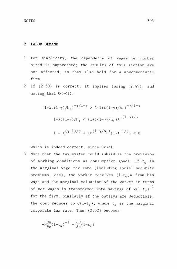
2 LABOR DEMAND
1 For simplicity, the dependence of wages on number
hired is suppressed; the results of this section are
not affected, as they also hold for a monopsonistic
firm.
2 If (2.50) is correct, it implies (using (2.49), and
noting that O<~<l):
[l+At(l-~)/hl }-~/l-~ > A(l+t(l-~)/hl }-~/l-~
l+H(l-~) /hl < {l+t (l-~) /hl } A -(l-~) h
which is indeed correct, since O<A<l.
3 Note that the tax system could subsidize the provision
of working conditions as consumption goods. If tw is
the marginal wage tax rate (including social security
premiums, etc), the worker receives (l-tw)w from his
wage and the marginal valuation of the worker in terms
of net wages is transformed into savings of w(l-tw)-l
for the firm. Similarly if the outlays are deductible,
the cost reduces to e(l-tc)' where tc is the marginal
corporate tax rate. Then (2.52) becomes
aC(l_t ) ae c

306
With wage
under the
CAPABILITIES, ALLOCATION AND EARNINGS
savings increasing and cost decreasing,
usual conditions this means an increased
consumption of working conditions. In fact, firms have
an incentive to stimulate working conditions over
raising wages, as it is a cheaper way of increasing
worker utility.
4 In a newspaper ad, a firm selling air conditioning
systems refers to research claiming that every addi
tional degree Celsius above 20° reduces labor produc-
tivity by 4%. NRC, May 5, 1987, p.16.
3 SCHOOLING AND SUPPLY
1 The result applies that for a function
N J: f (z) dz,
aN/ax
2 Just to illustrate the tremendous size of the choice
set: Kodde and Theunissen (1984), in an analysis of
educational careers in the Netherlands, note that
after secondary education, individuals can choose
among at least 130 types of education in higher
education (p.118).

NOTES 307
3 It is assumed that there is only one intersection that
also satisfies the second-order condition for an
earnings maximum.
4 The decomposition of (3.21) into two separate condi
tions only makes sense if one takes the scale of
measurement of capability levels as a useful reference.
Test scores should neither be standardized for age nor
for education. Note that the scaling problem does not
apply to (3.19).
5 It will be assumed that for each individual both
educations yield a sufficient rate of return.
6 The analogy of the present model to that of Rosen is
quite close and the results obtained above for the
case of individuals ranked by aOA/aOB are very similar
to his results of assigning different workers to
identical tasks (section III).
7 See Varian (1978), p.259. It is assumed that 'con
straint qualification' holds for the binding con
straints.
8 Varian (1978), p.268.
9 In particular for lengthy education, it is better to
measure the increases relative to some reference
education, to make the evaluation with first-order
derivatives more adequate: it would not be apt to
measure these derivatives at zero-years of education.
10 This result is found from setting OJ=O in the general
school effect equation
(aw/aae-ojahj/aae-I~magm/aae) ,
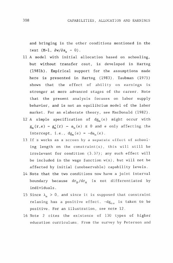
308 CAPABILITIES, ALLOCATION AND EARNINGS
and bringing in the other conditions mentioned in the
text (M=l, aw/aae = 0).
11 A model with initial allocation based on schooling,
but without transfer cost, is developed in Hartog
(198lb). Empirical support for the assumptions made
here is presented in Hartog (1983). Taubman (1975)
shows that the effect of ability on earnings is
stronger at more advanced stages of the career. Note
that the present analysis focuses on labor supply
behavior, and is not an equilibrium model of the labor
market. For an elaborate theory, see MacDonald (1982).
12
13
A simple specification of dgm (e) might occur with
~ (r, e) = &;.(r) - am (e) :s 0 and e only affecting the
intercept, i. e. , dgm (e) = -dam (e) .
If s works as a screen by a separate effect of school-
ing length on the constraint(s), this will still be
irrelevant for condition (3.37); any such effect will
be included in the wage function w(s), but will not be
affected by initial (unobservable) capability levels.
14 Note that the two conditions now have a joint interval
boundary because drB/drA is not differentiated by
individuals.
15 Since Am > 0, and since it is supposed that constraint
relaxing has a positive effect, -dgme is taken to be
positive. For an illustration, see note 12.
16 Note 2 cites the existence of 130 types of higher
education curriculums. From the survey by Peterson and

NOTES 309
Bownas(1982), one may conclude that the relevant number
of capability types is far less.
17 In case of utility maximization, the discussion should
be cast in terms of the distribution of welfare rather
than of earnings.
18 In secondary school, students choose Latin and Greek
significantly more often if in elementary school they
scored high at language; they choose sciences sig
nificantly more often if in elementary school they
scored high at mathematics. Similar results hold on
type of secondary school chosen.
4 EQUILIBRIUM AND OPTIMUM
1 Lucas(1977) specifies only Zj and refers to McFadden's
axiom on the Independence of the Irrelevant Alterna
tive. This seems an unnecessary strong condition to
impose, and is not copied here.
2 For continuity, Tinbergen's symbols have been replaced
by those of the present book. Details on deriving the
solution are given in Tinbergen(1956); some generaliza
tion and error correction is available in Van Batenburg
and Tinbergen (1984).
3 Both available degrees a 1 and az and demanded degrees
r 1 and r z are assumed to be independently distributed.
The solution is obtained by calculating first an
individual's optimum supply of attributes given his

310 CAPABILITIES, ALLOCATION AND EARNINGS
available levels and the utility and wage function.
The transformation of ' available' levels into ' sup
plied' levels then transforms an 'available' distribu
tion into a 'supplied' distribution, i.e., transforms
the moments of the bivariate normal 'available'
distribution, into moments of a normal 'supplied'
distribution. These moments are then equated to those
of the required distribution, which allows to solve
for the parameters Ai j .
4 The results reported here, in Tables 4.1, 4.2, A4.l
and A4.2 were calculated by Peimin Zhang whose work as
a research assistant was financed by the Department of
Economics of Queen's University in Canada.
5 A generalization of Tinbergen's theory to an arbitrary
number of attributes while maintaining the basic
structure has been given by Epple(1987); see also
Epple(l984) .
6 Such a result is already contained in Roy(1951) .
7 Note that with increasing returns to time share (as
discussed in Chapter 2), the output frontier for a
given worker (say, of capability r3 in the terminology
of section 2.3.2) would be convex to the origin:
I
9 I
". ~
1\ I~

NOTES 311
If a represents the output for one man devoting a time
share a to producing ql and (1-a) to qz' then qlO >
ql(a)/a and qzo > qz(l-a)/(l-a), where qi (x) means qi
produced at time share x. Clearly specialization is
now advantageous. This can even be reinforced if
workers specializing in ql or qz can be chosen at
optimal capability level r 1 and r z .
8 In equilibrium marginal rates of substitution for the
activity outputs should be equal among consumers A and
B, since they face the same price ratio.
9 This statement depends on the crossing of individual
output frontiers; see below in main text.
10 See e.g., Layard & Walters (1978, p89). For related
literature on
Dreze(1976) ,
(1979) .
the problem, see Dreze and Hagen(1975),
Duncan and Stafford(1980), Weddepohl
11 Atkinson and Stiglitz(1980), Lecture 17.
12 The thesis would seem to appear quite generally to any
bargaining when represented members differ in preferen
ces.
13 Benarot, Kamens and Meyer (1989). The analysis is
still very preliminary and appears to hide more varia
tion than the authors conclude to (cf the final table
in their paper).

312 CAPABILITIES, ALLOCATION AND EARNINGS
5 IMPLICATIONS FOR EMPIRICAL WORK
1 The same result occurs with any other selec tion rule
and correlated errors between the selection function
and the earnings function.
2 Since marital status of males was not known, this was
predicted from a random drawing of a number between 0
and 1, assigning the individual to 'married' if the
number is not above p, with p the known proportion of
married males in the relevant age group. The procedure
was suggested and implemented by Gerard Pfann.
3 Work by John Ham (1982) indicates that estimation
from midpoints may produce only very mild bias.
APPENDIX 5.1.
1 A detailed account of the data collection is given
(in Dutch) in Hartog & Pfann (1985).
2 It was K. Molenaar who discovered that the 1952
questionnaires were still available in a university
archive in Nijmegen.
3 Some schools had school years beginning in April
rather than in September. For these schools, half the
pupils of half the schools were included in the sample;
this yielded 369 answers (among a total of 5823).
4 The probability of non-response for a standard male
(all dummies at zero, IQ = 100, scholastic achievement

NOTES 313
score = 7) in the probit-only model is the area under
the standard normal distribution up to z .279-
(.005) 100 + (.032)7 = + .052. The other calculations
are similar.
6 ALLOCATION
1 The program was written by Geert Ridder at the Univer
siteit van Amsterdam (GRMAX).
2 Note that
where the subscript n refers to the n- th explanatory
variable in the vector Xi .
3 To avoid complicated statements, the expresssion
'relative to the effect on the probability of obtaining
the highest job level', is usually suppressed.
4 Cases of misreporting (i. e., the first year of a new
school is before the last year of a preceding school)
were eliminated.
5 Measuring education in years, the coefficients are
estimated on 2000 observations and predictions are
made for 245 cases. The specifications with education
dummies and childhood variables use 1300 observations
to estimate and 110 to predict.

314 CAPABILITIES, ALLOCATION AND EARNINGS
6 In view of the high computer cos t and limits on the
number of explanatory variables, various alternative
specifications have been tried in turn to allow some
selection of variables.
7 Checks have indicated that the effect of experience is
quite independent of that of years educated.
8 The effect of family background through schooling has
been ignored.
9 Since job level is measured at an ordinal scale,
comparison of expected job levels, strictly speaking,
is an arbitrary standard. However, Table 6.8 indicates
that only at two job levels (4 and 7) the upward
effect of education is not substantially smaller for
the group with the higher actual education. This
points in the same direction.
10 The comparison is made between two predicted job
levels, and not with observed job level as reference.
Otherwise, the resul t would be confounded wi th the
prediction error from the model. The predicted job
level is not necessarily equal to the observed job
level; this explains why downward shifts may occur at
the lowest observed level and upward shifts at the
highest observed level.
11 See Maddala (1983, p. 46) for an exposition of the
model.
12 These conditions are spelled out in Madda1a (1983,
p.48). The computer routine used was GRMAX (See note 1)

NOTES 315
13 Extensive work on the effect of market situation on
allocation is reported in Teu1ings (1990).

316 CAPABILITIES, ALLOCATION AND EARNINGS
7 EARNINGS
1 The estimates are only consistent if the error term in
the price equation is uncorrelated both with the
errors in the supplier's valuation function and those
in the demanders' valuation function, see section 5.4.
2 They are available in: Hartog, Van Ophem and Pfann
(1985), Hartog (1986a,b)
3 Lang and Dickens (1988) argue that such a test as
applied here has limited value. Adding job characteris
tics after allowing for worker characteristics would
also produce significant coefficients if only worker
characteristics were relevant, because of correlation
between unobserved worker characteristics and observed
job characteristics (such correlation follows from the
hedonic model, see section 4.2). At the least, this
calls for datasets that contain as many worker charac
teristics as possible. It also calls for structural
models specifying the relations between worker and job
characteristics.
4 This derivation of the multinomial logit model is due
to McFadden; see Maddala (1983).
5 Using the theory of hedonic prices, the predicted sign
is ambiguous. The offered wage-hours relation may be
parabolic, due to fixed cost at low hours and declining
marginal productivity at high hours. Moffitt (1984),
in the context of a labor supply model simultaneously
estimates an hours and a wage equation and finds a

NOTES 317
quadratic wage relation with negative slope for weekly
hours above 34.
6 If three outlyers are removed from the observations at
job level 7, the intercept increases to 11.38 (1.62),
the effect of test score is reduced to .825 (2.02) and
the coefficient of >. increases to -18.50 (1.90). At
job level 5 IQ and>. are highly collinear. If >. is
deleted, the intercept is reduced to 19.54 (5.12), the
coefficient of IQ is reduced to -.044 (1.34) and of
test score to .629 (1.86). If IQ is deleted, the
coefficient of >. becomes - .349 (1.41), with other
coeffcients not much affected.
7 The routine was provided by Centrum voor Wiskunde en
Informatica (C.W.I.), Universiteit van Amsterdam.
8 The earnings coefficients are the coefficients on
dummies for each education job level combination
(with some job levels combined, as indicated) in a
regression equation that also includes age, age
squared, experience with present employer, sex, and an
intercept, all highly significant.
9 The dataset is known as the NPAO-Mobility survey. The
original sample consists of 2677 observations. Earnings
are reported as after - tax earnings in Dutch guilders
per period, turned into hourly earnings by dividing by
reported usual hours of work. Education is recorded
according to the Standard Classification of Education
(used by the Dutch National Statistical Office, CBS),
classifying schools in 5 levels that work out to

318 CAPABILITIES, ALLOCATION AND EARNINGS
durations in multiples of 3 years (from 6 to 18). The
number of observations used for the regressions in
Table 7.14 is 540 for total, 394 for males and 140 for
females.
10 The following translation of schooling levels into
years is made: some grade school =4,
school =8, some high school =10, finish
=12, some college =14, finish college
college =17.5.
8 APPLICATIONS, CONCLUSIONS, EXTENSIONS
1 See section 6.2.5.
2 See section 8.3.
3 See section 7.4.2.
finish grade
high school
=16, beyond
4 Such cost would occur for transition from one alloca
tion to another. It is not sure what would happen if
there were a transition to a different system of
allocating individuals to jobs and job levels.

NAME INDEX
Atkinson, A.B. 311 Bartik, T.J. 149 Becker, G.S. 3 Benarot, A. 311 Bierens, H.J. 230 Bownas, D.A. 6,303,309 Brasse, P. 280 Braverman, H. 19,20,142 Brown, B.W. 86 Brown, J.N. 149 Conen, G.J.M. 145 Davies, J.B. 89,135 Dickens, W.T. 316 Dreze, J.H. 311 Dronkers, J. 144 Duncan, G.J. 263, 311 Edwards, R.C. 238 Epple, D. 149,151,242,310 Hagen, K.P. 311 Ham, J. 312 Hanushek, E.A. 48,49 Hartog,J. 1,4,5,34,47,105,133,135,
195,230,236,267,278,283, 303,308,312,316
Hay, J.W. 233,273,275 Heckman, J.J. 147 Hirschman, A.O. 130

320 CAPABILITIES, ALLOCATION AND EARNINGS
Hoffman, S.D. 263 Holmlund, B. 40 Huijgen, F. 145 Hunter, T.E. 295,304 Jovanic, B. 296 Kamens, D. 311 Kodde, D.A. 89,306 Lancaster, K. 135 Lang, K. 316 Lau, L.J. 48 Layard, P.R.G. 311 Levin, H.M. 48,249 Lindsay, C.M. 135 Lucas, R.E.B. 91,92,309 Lutz, B. 144 MacDonald, G.M.T. 89,119,133,308 Maddala, G.S. 146,181,233,270,314 Mangione, T. 154 Markusen, T.R. 119 Marshall, A. 19 McCormick, E.J. 4 McKelvey, R.D. 212,252 Meyer, J. 311 Miller, A. 303 Miller, R.A. 296 Moffitt, R. 316 Molenaar, K. 312 Oosterbeek, H. 265 Peterson, N.G. 6,303,308 Pfann, G.J. 237,283,312,316 Quinn, R. 154 Ridder, G. 283 Riesewijk, B. 145 Ritzen, J.M.M. 132 Rosen, S. 68,87,89,99,119,148,151 Rosen, H.S. 149 Roy, A.D. 310 Rumberger, R.W. 145,304 Saks, D.H. 86 sattinger, M.A. 118 Schmidt, F.L. 295,304 Seashore, S. 154 Sedlacek, G. 147 Sengenberger, W. 144 Sicherman, N. 268

NAME INDEX
Sikking, E. 280 smith, A. 18 Spence, A.M. 79 Stafford, F.P. 311 staines, G. 154 stiglitz, J.E. 311 Taubman, P. 308 Terza, J.V. 233 Teulings, C. 315 Theunissen, M.A.M. 89,306 Thurow, L.C. 226,264 Tinbergen, J. 91,98,105,259,309 Tsang, M.C. 249 Van Batenburg, P. 105,309 Van Hoof, J.J. 144 Van Ophem, J.C. 237,316 Varian, H. 307 vriend, N.J. 277 Walters, A.A. 311 Watson, C. 89 Weddepohl, C. 311 Weiss, A. 36 Willis, R.J. 87,89 Zanders, H.L.G. 153 zavoina, W. 212,252
321

SUBJECT INDEX
ability index 113 achievement test score 48 aptitudes 98 Babbage's Principle 19,30 bid function 96 cognitive abilities 6 comparative advantage 61,107 compensating differential 97 constraint lifting 73 corporate tax 305 curriculum (educational) 55,132 diploma (school) 90 discount rate 56 earnings distribution 88 economies of scale 133 education length 55 educational production function 48 efficiency units 121 effort 83 envelope-property 94,136 Envelope Theorem 73 equity 254 excess demand 210 excess supply 210 Gumbel distribution 270 hiring standards 44 hours (of work) 123

CAPABILITIES, ALLOCATION AND EARNINGS 323
Information 133 integration 22 intelligence 6 IQ 165 job complexity 4,8 job design 122 job difficulty 108 job enrichment 36 job matching 295 job requirements 5,7,41 labor market segment 26,226 labor union 131 learning curve 34 leisure 123 Lindahl solution 128 minorities (ethnic) 277 mismatch 254 multiple job holding 124 non-cognitive abilities 48 non-response 164 overeducation 223 overqualification 211 overutilization 98 Pareto-efficiency 240 personality variables 6 polarization 20,28,31 product differentiation 135 psychomotor abilities 6 public goods 126 quality of work 18 returns to education (rate of) 56 safety regulations 130 scholastic achievement 167 scholastic test score (deciles) 202 screening 49 selectivity bias 146 self-selection 146 separatibility 106 skill bumping 142 social efficiency 240 sorting: vertical 57,201
horizontal 58 specialization 22,109 sUbstitution: quality - quantity 16

324
tax rate: wage tax 305 corporate tax 305
Taylor system 36 Tiebout hypothesis 128 time share sensitivity 23 trickling down 104,142 undereducation 223 underqualification 211 underutilization 98 vocational preference 6 worker alienation 18 working conditions 124
SUBJECT INDEX