SURF BEAT FORCING AND DISSIPATION

By

Stephen M. Henderson

SUBMITTED IN PARTIAL FULFILLMENT OF THE

REQUIREMENTS FOR THE DEGREE OF

DOCTOR OF PHILOSOPHY

AT

DALHOUSIE UNIVERSITY

HALIFAX, NOVA SCOTIA

APRIL 2002

c Copyright by Stephen M. Henderson, 2002

DALHOUSIE UNIVERSITY

DEPARTMENT OF

OCEANOGRAPHY

The undersigned hereby certify that they have read and recommend

to the Faculty of Graduate Studies for acceptance a thesis entitled

“Surf beat forcing and dissipation” by Stephen M. Henderson in partial

fulfillment of the requirements for the degree of Doctor of Philosophy.

Dated: April 2002

External Examiner:Thomas H.C. Herbers

Research Supervisor:Anthony J. Bowen

Examing Committee:Barry Ruddick

Keith Thompson

Alex Hay

Paul Hill

Bruce Smith

ii

DALHOUSIE UNIVERSITY

Date: April 2002

Author: Stephen M. Henderson

Title: Surf beat forcing and dissipation

Department: Oceanography

Degree: Ph.D. Convocation: May Year: 2002

Permission is herewith granted to Dalhousie University to circulate and tohave copied for non-commercial purposes, at its discretion, the above title upon therequest of individuals or institutions.

Signature of Author

THE AUTHOR RESERVES OTHER PUBLICATION RIGHTS, AND NEITHERTHE THESIS NOR EXTENSIVE EXTRACTS FROM IT MAY BE PRINTED OROTHERWISE REPRODUCED WITHOUT THE AUTHOR’S WRITTEN PERMISSION.

THE AUTHOR ATTESTS THAT PERMISSION HAS BEEN OBTAINEDFOR THE USE OF ANY COPYRIGHTED MATERIAL APPEARING IN THISTHESIS (OTHER THAN BRIEF EXCERPTS REQUIRING ONLY PROPERACKNOWLEDGEMENT IN SCHOLARLY WRITING) AND THAT ALL SUCHUSE IS CLEARLY ACKNOWLEDGED.

iii

Contents

Abstract vii

List of symbols viii

Acknowledgements xiii

1 Introduction 1

1.1 What is surf beat? . . . . . . . . . . . . . . . . . . . . . . . . . . . . . . . 1

1.2 Edge waves, surf beat resonance, and dissipation . . . . . . . . . . . . . . 3

1.3 Surf beat propagation and energy transport . . . . . . . . . . . . . . . . . . 6

1.4 Thesis outline . . . . . . . . . . . . . . . . . . . . . . . . . . . . . . . . . 7

2 The surf beat energy balance 8

2.1 Introduction . . . . . . . . . . . . . . . . . . . . . . . . . . . . . . . . . . 8

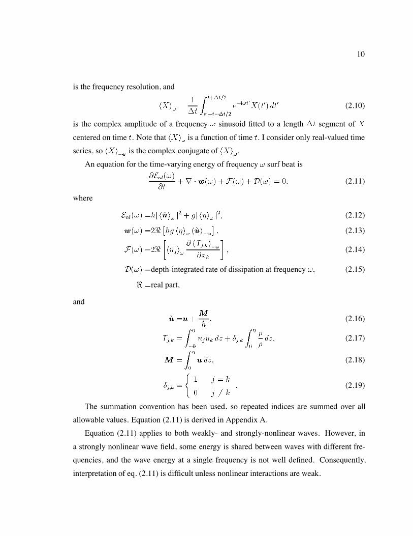
2.2 Energy equation . . . . . . . . . . . . . . . . . . . . . . . . . . . . . . . . 9

2.2.1 Energy balance in differential form . . . . . . . . . . . . . . . . . 9

2.2.2 Energy balance in integral form . . . . . . . . . . . . . . . . . . . 14

2.3 Field site and instrumentation . . . . . . . . . . . . . . . . . . . . . . . . . 16

2.4 Results . . . . . . . . . . . . . . . . . . . . . . . . . . . . . . . . . . . . . 16

2.5 Discussion and conclusions . . . . . . . . . . . . . . . . . . . . . . . . . . 28

3 The cross-shore structure of surf beat 31

3.1 Introduction . . . . . . . . . . . . . . . . . . . . . . . . . . . . . . . . . . 31

iv

3.2 Field site and instrumentation . . . . . . . . . . . . . . . . . . . . . . . . . 31

3.3 Spatially-coherent surf beat . . . . . . . . . . . . . . . . . . . . . . . . . . 32

3.3.1 Methods . . . . . . . . . . . . . . . . . . . . . . . . . . . . . . . 32

3.3.2 Results and discussion . . . . . . . . . . . . . . . . . . . . . . . . 34

3.4 Energy transport . . . . . . . . . . . . . . . . . . . . . . . . . . . . . . . . 40

3.5 Summary . . . . . . . . . . . . . . . . . . . . . . . . . . . . . . . . . . . 46

4 Simulations of dissipative surf beat 47

4.1 Introduction . . . . . . . . . . . . . . . . . . . . . . . . . . . . . . . . . . 47

4.2 Model derivation . . . . . . . . . . . . . . . . . . . . . . . . . . . . . . . 48

4.2.1 Governing equations . . . . . . . . . . . . . . . . . . . . . . . . . 48

4.2.2 Forcing . . . . . . . . . . . . . . . . . . . . . . . . . . . . . . . . 50

4.2.3 Solution . . . . . . . . . . . . . . . . . . . . . . . . . . . . . . . . 52

4.3 Model results . . . . . . . . . . . . . . . . . . . . . . . . . . . . . . . . . 56

4.3.1 Edge waves . . . . . . . . . . . . . . . . . . . . . . . . . . . . . . 56

4.3.2 Evanescent waves . . . . . . . . . . . . . . . . . . . . . . . . . . . 66

4.3.3 Dissipative decoupling . . . . . . . . . . . . . . . . . . . . . . . . 69

4.3.4 Realistic forcing and dissipation . . . . . . . . . . . . . . . . . . . 81

4.4 Comment on normal modes . . . . . . . . . . . . . . . . . . . . . . . . . . 87

4.5 Discussion and conclusions . . . . . . . . . . . . . . . . . . . . . . . . . . 87

5 Conclusions 91

5.1 Summary . . . . . . . . . . . . . . . . . . . . . . . . . . . . . . . . . . . 91

5.2 Possible future research . . . . . . . . . . . . . . . . . . . . . . . . . . . . 92

A Derivation of a nonlinear frequency-domain energy equation 95

A.1 Mass and momentum conservation . . . . . . . . . . . . . . . . . . . . . . 95

A.2 Fourier identity . . . . . . . . . . . . . . . . . . . . . . . . . . . . . . . . 98

A.3 Energy equation . . . . . . . . . . . . . . . . . . . . . . . . . . . . . . . . 98

B Nonlinear coupling and higher order spectra 100

v

C Cross-shore profiles of surf beat energy density and energy flux 104

D Homogeneous solutions of the dissipative shallow water wave problem 115

E Solution for forced, dissipative waves on beach with varying slope and friction

coefficient 118

F Normal modes 121

F.1 Introduction . . . . . . . . . . . . . . . . . . . . . . . . . . . . . . . . . . 121

F.2 Method . . . . . . . . . . . . . . . . . . . . . . . . . . . . . . . . . . . . 121

F.3 Resonance . . . . . . . . . . . . . . . . . . . . . . . . . . . . . . . . . . . 123

F.4 Propagation . . . . . . . . . . . . . . . . . . . . . . . . . . . . . . . . . . 124

F.5 Evanescent waves . . . . . . . . . . . . . . . . . . . . . . . . . . . . . . . 125

F.6 Dissipative decoupling . . . . . . . . . . . . . . . . . . . . . . . . . . . . 127

F.7 Summary . . . . . . . . . . . . . . . . . . . . . . . . . . . . . . . . . . . 129

vi

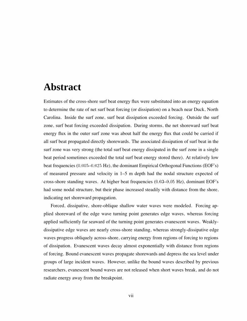
AbstractEstimates of the cross-shore surf beat energy flux were substituted into an energy equation

to determine the rate of net surf beat forcing (or dissipation) on a beach near Duck, North

Carolina. Inside the surf zone, surf beat dissipation exceeded forcing. Outside the surf

zone, surf beat forcing exceeded dissipation. During storms, the net shoreward surf beat

energy flux in the outer surf zone was about half the energy flux that could be carried if

all surf beat propagated directly shorewards. The associated dissipation of surf beat in the

surf zone was very strong (the total surf beat energy dissipated in the surf zone in a single

beat period sometimes exceeded the total surf beat energy stored there). At relatively low

beat frequencies (– Hz), the dominant Empirical Orthogonal Functions (EOF’s)

of measured pressure and velocity in 1–5 m depth had the nodal structure expected of

cross-shore standing waves. At higher beat frequencies (– Hz), dominant EOF’s

had some nodal structure, but their phase increased steadily with distance from the shore,

indicating net shoreward propagation.

Forced, dissipative, shore-oblique shallow water waves were modeled. Forcing ap-

plied shoreward of the edge wave turning point generates edge waves, whereas forcing

applied sufficiently far seaward of the turning point generates evanescent waves. Weakly-

dissipative edge waves are nearly cross-shore standing, whereas strongly-dissipative edge

waves progress obliquely across-shore, carrying energy from regions of forcing to regions

of dissipation. Evanescent waves decay almost exponentially with distance from regions

of forcing. Bound evanescent waves propagate shorewards and depress the sea level under

groups of large incident waves. However, unlike the bound waves described by previous

researchers, evanescent bound waves are not released when short waves break, and do not

radiate energy away from the breakpoint.

vii

List of symbols

hXi complex amplitude of time series X at frequency

hXi complex amplitude of windowed time series X at frequency

X complex amplitude of X at frequency and

longshore wavenumber k

X sample mean of X

an amplitude of mode n edge wave (m)

cf bottom drag coefficient

Cg group velocity (ms)

D depth-integrated dissipation of frequency motion (ms)

EX expected value of X

E

Z

zh

j huzi j dz gj hi j

depth-integrated linear

energy density of frequency wave (ms)

Enl hj hui j gj hi j

(ms)

Esb

Z Hz

c HzEc depth-integrated linear energy

density of surf beat (ms)

fe wave dissipation factor

viii

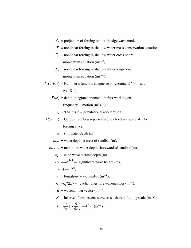
fn projection of forcing onto n’th edge wave mode

F nonlinear forcing in shallow water mass conservation equation

Fx nonlinear forcing in shallow water cross-shore

momentum equation (ms)

Fy nonlinear forcing in shallow water longshore

momentum equation (ms)

Fa b c Kummer’s function (Laguerre polynomial if b and

a Z)

F depth-integrated momentum flux working on

frequency motion (ms)

g 9.81 ms = gravitational acceleration

Gx xf Green’s function representing sea level response at x to

forcing at xf

h still water depth (m)

hbar water depth at crest of sandbar (m)

htrough maximum water depth shoreward of sandbar (m)

hT edge wave turning depth (m)

Hs w

significant wave height (m)

i

k longshore wavenumber (m)

kc k cyclic longshore wavenumber (m)

k wavenumber vector (m)

K inverse of evanescent wave cross-shore e-folding scale (m)

L

x

x

x

kx (m)

ix

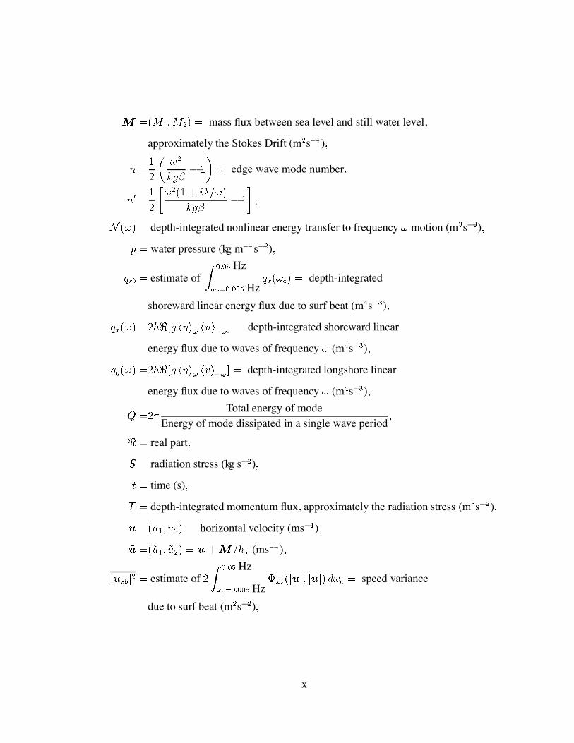
M MM mass flux between sea level and still water level,

approximately the Stokes Drift (ms)

n

kg

edge wave mode number

n

i

kg

N depth-integrated nonlinear energy transfer to frequency motion (ms)

p water pressure (kg ms)

qsb estimate ofZ Hz

c Hzqxc depth-integrated

shoreward linear energy flux due to surf beat (ms)

qx hg hi hui depth-integrated shoreward linear

energy flux due to waves of frequency (ms)

qy hg hi hvi depth-integrated longshore linear

energy flux due to waves of frequency (ms)

Q Total energy of mode

Energy of mode dissipated in a single wave period

real part

S radiation stress (kg s)

t time (s)

T depth-integrated momentum flux, approximately the radiation stress (ms)

u u u horizontal velocity (ms)

u u u uMh (ms)

jusbj estimate of Z Hz

c Hzcjuj juj dc speed variance

due to surf beat (ms)

x

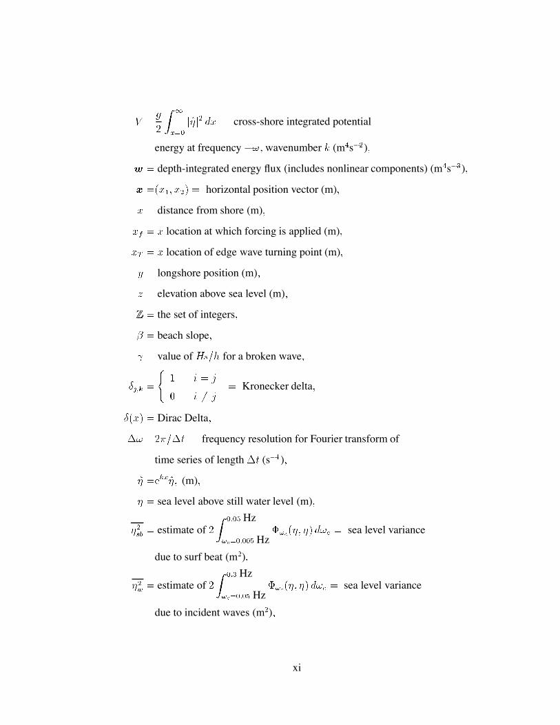
V g

Z

x

jj dx cross-shore integrated potential

energy at frequency , wavenumber k (ms)

w depth-integrated energy flux (includes nonlinear components) (ms)

x x x horizontal position vector (m)

x distance from shore (m)

xf x location at which forcing is applied (m)

xT x location of edge wave turning point (m)

y longshore position (m)

z elevation above sea level (m)

Z the set of integers

beach slope

value of Hsh for a broken wave

jk

i j

i j Kronecker delta

x Dirac Delta

t frequency resolution for Fourier transform of

time series of length t (s)

ekx (m)

sea level above still water level (m)

sb estimate of Z Hz

c Hzc dc sea level variance

due to surf beat (m)

w estimate of Z Hz

c Hzc dc sea level variance

due to incident waves (m)

xi

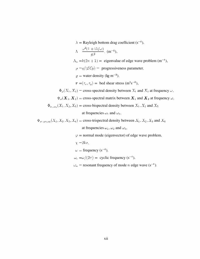
Rayleigh bottom drag coefficient (s)

i

g (m)

n kn eigenvalue of edge wave problem (m)

qECg progressiveness parameter

water density (kg m)

x y bed shear stress (ms)

XX cross-spectral density between X and X at frequency

XX cross-spectral matrix between X and X at frequency

XXX cross-bispectral density between X, X and X

at frequencies and

XXXX cross-trispectral density between X, X, X and X

at frequencies , and

normal mode (eigenvector) of edge wave problem

kx

frequency (s)

c cyclic frequency (s)

n resonant frequency of mode n edge wave (s)

xii

Acknowledgements

First, I’d like to thank my supervisor, Dr. Tony Bowen. Tony has been insightful, patient,

generous, and a pleasure to work with — an excellent supervisor.

Bob Guza and Steve Elgar provided the data for Chapter 3 of this thesis, and have made

many helpful suggestions. Steve Elgar helped me write the paper on which Chapter 3 is

based.

Thanks to my committee (Keith Thompson, Barry Ruddick, Alex Hay, Bruce Smith,

Paul Hill) for their helpful comments.

Many thanks to all those who helped collect the Sandyduck data on which Chapter

2 is based, and who’ve also helped me enjoy my time at Dalhousie: Alex Hay, Carolyn

Smyth, Todd Mudge, Anna Crawford, Dave Hazen, Wes Paul, Phil MacAulay, Dianne

Foster, Walter Judge, and Xingping Zou. Thanks also to the staff at the Field Research

Facility at Duck, who helped collect data used in both Chapters 2 & 3.

My research was funded by the Izaak Walton Killam Foundation, the Andrew Mellon

Foundation, and the Natural Sciences and Engineering Research Council of Canada.

Thanks to Christine Pequignet, Karin Bryan and Conrad Pilditch for making me so

welcome when I arrived at Dalhousie. I’ve enjoyed chatting with my work-mates Armani

Ngusaru and Keith Borg, and paddling with Mark Richard and Brian May. Finally, thanks

to Mum, Dad, and Alison for their support.

xiii

Chapter 1

Introduction

1.1 What is surf beat?

Strong winds blowing over the deep ocean generate large waves with periods between about

5 and 15 seconds. When these waves approach a beach, they grow taller and eventually

break. The energy of the incoming waves is then transfered to turbulence in spectacular

fashion. Often the resulting loss of wave energy is almost total, and only a small remnant

of each incident wave finally reaches the shore.

Hidden among the broken waves near the shore are lower frequency (0.005–0.05 Hz)

waves called ‘infragravity waves’ or ‘surf beat’. These waves are not eye-catching, because

they have long periods and change the sea level only slowly. However, unlike breaking

incident waves, surf beat actually gets bigger as the shore is approached. At the shore, surf

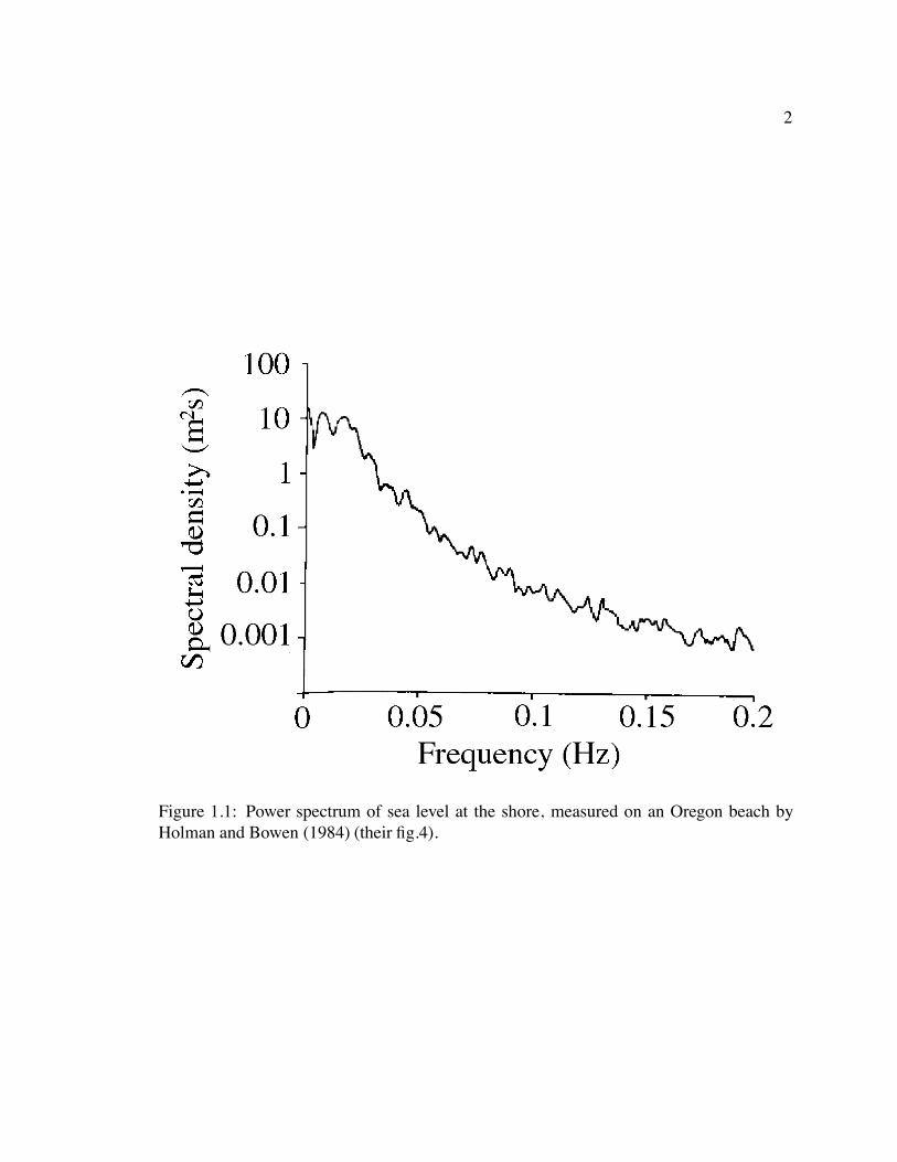
beat often is bigger than breaking incident waves. Figure 1.1 shows a power spectrum of

the sea level at the shore, measured on an Oregon beach by Holman and Bowen (1984). On

this occasion surf beat accounted for 99.9% of sea level variance at the shore.

During storms, surf beat can change the sea level at the shore by more than a meter.

Consequently, surf beat contributes to coastal flooding. Surf beat might also transport

sand, and thereby erode or build a beach (Bowen and Inman, 1971; Guza and Inman, 1975;

Short, 1975; Bowen, 1981; Holman and Bowen, 1982; Bauer and Greenwood, 1990; Howd

et al., 1992; O’Hare and Huntley, 1994; Bryan and Bowen, 1996; Vittori et al., 1999).

1

2

Figure 1.1: Power spectrum of sea level at the shore, measured on an Oregon beach byHolman and Bowen (1984) (their fig.4).

3

Furthermore, surf beat might control the location of the dangerous, seaward flowing ‘rip

currents’ that are common near the shore (Bowen, 1969a, 1969b; Holman and Bowen,

1984; Symonds and Rangasinghe, 2001).

The dynamics of surf beat are not well understood. Published comparisons between

surf beat models and field observations are rather qualitative, and sometimes reveal ma-

jor discrepancies between predicted and observed behaviour (Ruessink, 1998b; Lippmann

et al., 1998, 2001). In this thesis, I present my Ph.D. research into surf beat dynamics. I

will emphasise the surprisingly strong effects of dissipation on surf beat behaviour.

1.2 Edge waves, surf beat resonance, and dissipation

This section describes the two types of freely-propagating surf beat that exist on natural

beaches. I also discuss surf beat resonance, and note the importance of damping in limiting

the height of resonant waves.

Surface waves propagate more slowly in shallow water than in deep water. Con-

sequently, shore-oblique waves refract towards the shore. Certain seaward-propagating

waves, called edge waves, are turned back towards the shore by refraction. They then prop-

agate shorewards until they reach the beach, reflect, and propagate back out to sea. Ideally,

the cycle of refraction and reflection continues indefinitely, so that edge wave energy is for-

ever trapped near the shore (Eckart, 1951; Ursell, 1952). The interference pattern produced

by incoming and outgoing freely-propagating edge waves moves along the coast at a speed

determined by the wave frequency1.

Not all waves are trapped near the shore. Surface waves that can propagate freely to

and from the deep ocean are called leaky waves. Near the beach, leaky waves propagate

almost directly shorewards or seawards, with wave crests almost parallel to the shore. Con-

sequently, leaky waves have very long longshore wavelengths. For example, all 40 s leaky

waves have longshore wavelengths greater than about 2.5 km. Edge waves propagate at

greater angles to the shore, and have shorter longshore wavelengths.

1In fact a finite set of longshore speeds is possible at each frequency, with each speed corresponding to asingle edge wave mode (Appendix F).

4

Surf beat is generated by nonlinear interactions with higher frequency waves. Just as

turbulent eddies exert a Reynolds stress, and particles of an ideal gas in random thermal

motion exert a pressure, water waves exert a stress called the ‘radiation stress’. Spatial gra-

dients of the radiation stress force water from regions where waves are big to regions where

waves are small (this is not the whole story — the radiation stress tensor is anisotropic, and

dissipative waves can force non-divergent, rotational flows). On natural beaches the wave

height changes slowly through time, and the resulting slow changes in the radiation stress

force surf beat (the mass transported by the incident waves might also play a role — see

Chapter 4). Nonlinear forcing is usually thought of as a source of surf beat energy, but

nonlinear forcing could also oppose low frequency motions, and thereby damp surf beat

(Schaffer, 1993; Van Dongeren et al., 1996). However, surf beat energy must somehow

be maintained in the presence of frictional dissipation, so the net, cross-shore integrated,

effect of nonlinear interactions is probably to add energy to surf beat.

The longshore structure of surf beat forcing can be viewed as a random superposition

of many Fourier components, each with its own frequency and longshore phase speed.

Those components of the total forcing that have the frequency and longshore phase speed

of a freely-propagating edge wave generate resonant edge waves. Since edge waves can

not radiate energy to deep water, resonant edge waves on a longshore-uniform beach grow

until some damping mechanism limits their amplitude. In contrast, when leaky waves are

forced, they radiate their energy into the deep ocean, and do not resonate2.

Surf beat damping is not understood. Several researchers have suggested mechanisms

that could damp surf beat, including bottom friction (Guza and Davis, 1974; Lippmann

et al., 1997), wave breaking (Bowen, 1977; Schaffer, 1993; Van Dongeren et al., 1996)

and propagation of nonlinearly-forced higher frequency waves to deeper water (Guza and

Bowen, 1976a; Mathew and Akylas, 1990). The energy of edge waves propagating over an

irregular seabed might also be scattered to leaky waves, and then radiated to the deep ocean

(Chen and Guza, 1999). These theories have not been tested against field observations

2At least, leaky waves do not resonate with quadratic nonlinear forcing, because they are orthogonal tosuch forcing in deep water. They do resonate with higher order nonlinear forcing, but this forcing seems tobe too weak to generate the large beat-frequency waves observed inside the surf zone

5

and, because wave breaking is not fully understood, it is not known which of the possible

dissipation mechanisms is most important.

If dissipation was very weak, then resonant edge waves would grow to be very large,

and eventually dominate over non-resonant waves. However, if dissipation was strong then

the effects of forcing could not accumulate over many wave periods, so resonance would be

suppressed. The degree to which a resonant edge wave mode dominates over non-resonant

modes is determined in part by the parameter

Q Total energy of mode

Energy of mode dissipated in a single wave period (1.1)

(Green, 1955). Note that Q is approximately the time scale for wave dissipation divided by

the wave period, so a low Q indicates rapid dissipation, whereas a high Q indicates slow

dissipation. Only if Q can the effects of forcing accumulate over many wave periods,

generating a strong resonant response.

Field observations indicate that much surf beat energy is carried by waves which have

the frequencies and longshore wavelengths of resonant edge waves (Munk et al., 1964;

Huntley et al., 1981; Oltman-Shay and Guza, 1987). Similar evidence indicates that reso-

nant edge waves can be trapped over offshore sand bars, at both infragravity and incident

frequencies (Schonfeldt, 1995; Bryan and Bowen, 1996; Bryan et al., 1998). These obser-

vations provide compelling evidence that edge waves do indeed resonate, and that the Q of

infragravity edge waves is often greater than one. However, it is not clear just how large

Q is. Indeed, several theories that neglect resonance entirely have successfully predicted

aspects of surf beat behaviour that resonant edge wave theories do not predict.

Longuet-Higgins and Stewart (1962) and Hasselmann et al. (1963) showed that groups

of waves propagating over a flat seabed nonlinearly force low frequency ‘bound waves’,

which propagate with the wave groups. The models of Longuet-Higgins and Stewart (1962)

and Hasselmann et al. (1963) assume a flat seabed, and therefore do not simulate refractive

trapping and edge wave resonance (although they could be extended to do so (Herbers

et al., 1995a)). Nevertheless, the average phase between surf beat and short-wave energy

departs only slightly from the 180 degrees predicted by these models. Furthermore, up to

half of the surf beat variance observed near the shore is coherent with co-located nonlinear

6

forcing (Huntley and Kim, 1984; Guza et al., 1984; Elgar and Guza, 1985a; Middleton

et al., 1987; Masselink, 1995; Ruessink, 1998a, 1998b). Strongly-resonant edge waves

accumulate energy over many wave periods, so only a small proportion of their energy is

forced locally. The strong coherence between surf beat and co-located nonlinear forcing

lead Huntley and Kim (1984) and Middleton et al. (1987) to conclude that the surf beat

energy they observed was distributed fairly evenly between locally-forced bound waves,

and remotely-forced ‘free’ waves. Further offshore ( 8 m water depth) only a small

proportion of low frequency energy can be explained by local nonlinear forcing, although

this proportion does increase during storms (Okihiro et al., 1992; Elgar et al., 1992; Herbers

et al., 1994, 1995b). Munk et al. (1964) found that strongly resonant (high Q) edge waves

dominated the infragravity energy they observed in m water depth on the Californian

Continental Shelf.

1.3 Surf beat propagation and energy transport

Propagating surface gravity waves carry an energy flux. If the group velocity of the prop-

agating waves is much greater than the mean water velocity, as is usually the case in the

field, then this energy flux is carried in the direction of wave propagation. A steady surface

wave field carries energy from regions of net forcing to regions of net dissipation, so wave

propagation is linked closely with wave forcing and dissipation.

In the absence of forcing and dissipation, both edge and leaky waves are cross-shore

standing, and carry no cross-shore energy flux. If Q is sufficiently high, edge waves are

cross-shore standing (Chapter 4). Leaky waves can propagate across-shore, even when Q

is very high (Schaffer, 1993; Van Dongeren et al., 1996).

Sea and swell are mostly dissipated by breaking before they reach the shore. Conse-

quently, sea and swell waves are reflected only very weakly from the shore, and propagate

shorewards. In contrast, surf beat can be strongly reflected from the shore to form a cross-

shore standing pattern. Holman (1981), Holland et al. (1995), and others presented field

evidence for the existence of cross-shore standing waves at beat frequencies in water depths

7

less than 4 m. However, they did not show that these cross-shore standing waves dominated

over progressive waves. Elgar et al. (1994) and Herbers et al. (1995a) presented field evi-

dence of significant net cross-shore surf beat propagation in 13 m water depth.

1.4 Thesis outline

If dissipation is very weak, then cross-shore standing, resonant edge waves dominate surf

beat. Edge wave resonance has been observed in the field, but the rate of surf beat dissipa-

tion, and the strength of edge wave resonance, are not known. Furthermore, observations

of strong correlations between surf beat and local nonlinear forcing suggest that surf beat

might not always be dominated by strongly-resonant edge waves.

This thesis aims to determine some of the major effects of dissipation on surf beat.

Surf beat dissipation is linked closely with surf beat forcing, and some observations of

surf beat forcing will also be presented. In Chapter 2, I use measurements of water pres-

sure and velocity to estimate the rate of net surf beat dissipation (or forcing) on a natural

beach. When incident waves were small, net dissipation was weak. When incident waves

were large, net dissipation in the surf zone was very strong. Chapter 3 presents observa-

tions of the cross-shore structure of surf beat. Surf beat propagated shorewards into the

surf zone when incident waves were large. The observed shoreward surf beat propagation

constitutes a leading-order departure from the predictions of weakly-dissipative edge wave

models. Chapter 4 presents a dissipative surf beat model which predicts shoreward prop-

agation, in qualitative agreement with observations. Recently, model simulations lead to

the recognition of a type of shoreward-propagating wave that I had previously neglected —

the ‘evanescent bound wave’. Evanescent waves are introduced in Chapter 4.2.3. I do not

know yet whether evanescent waves play an important role in the field.

Chapter 2

The surf beat energy balance

2.1 Introduction

This chapter presents observations of the approximate strength of surf beat forcing and

dissipation. Section 2.2 presents a simple energy balance equation for surf beat. This en-

ergy balance equation can be combined with measurements of water pressure, velocity, and

depth to yield spatially-averaged rates of net surf beat forcing (or dissipation). This method

provides estimates of the difference between surf beat forcing and dissipation, but does not

allow us to evaluate forcing and dissipation separately. I will use the method developed in

Section 2.2 to analyse data collected from a beach near Duck, North Carolina. Section 2.3

describes the field site and instrumentation. Results are presented in Section 2.4. Net surf

beat forcing (or dissipation) was strong when incident waves were large and weak when

incident waves were small. Forcing exceeded dissipation outside the surf zone and dissi-

pation exceeded forcing inside the surf zone. During storms, a shoreward surf beat energy

flux maintained surf beat energy inside the surf zone. I discuss the implications of these re-

sults and present conclusions in Section 2.5. Related results were presented by Henderson

and Bowen (2002).

8

9

2.2 Energy equation

Schaffer (1993) derived an energy balance equation for surf beat by assuming that beat

frequencies are much lower than incident-wave frequencies. Section 2.2.1 shows that a

slightly modified form of Schaffer’s energy equation applies even when beat frequencies

are not much lower than incident wave frequencies. This result is useful because beat

frequencies often are not much lower than incident-wave frequencies (surf beat frequencies

are as high as Hz and the peak frequency of incident waves is often only Hz).

Section 2.2.2 presents a simpler energy equation for a statistically steady wave field on a

long, straight beach. The following definitions will be needed throughout this chapter:

t time (2.1)

xj j’th horizontal coordinate (j or ) (2.2)

u horizontal water velocity (2.3)

uj j’th component of u (2.4)

h still water depth (2.5)

sea surface elevation (above still water level) (2.6)

g gravitational acceleration (2.7)

When analysing field data I will estimate h as the mean measured water depth, implicitly

assuming that the mean depth approximately equals the still depth, which it does.

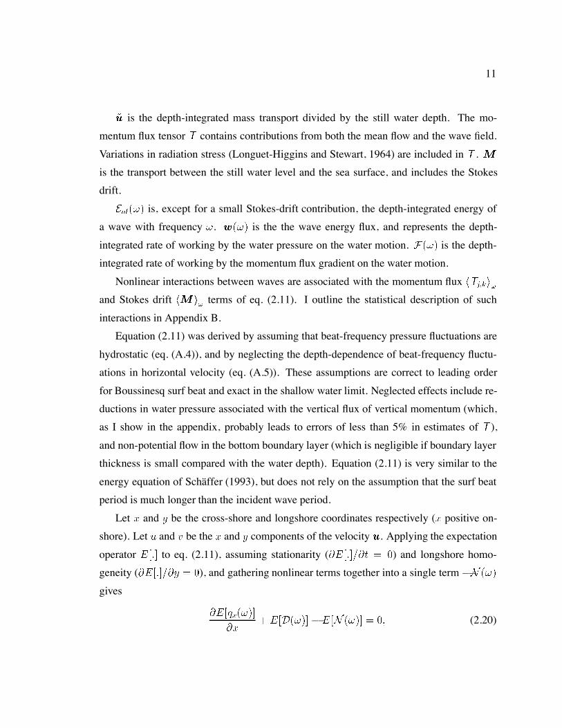
2.2.1 Energy balance in differential form

For any variable X , let hXi be the time-varying complex amplitude of a frequency

Fourier component of X , so

Xt X

j

eijt hXij (2.8)

where

t (2.9)

10

is the frequency resolution, and

hXi

t

Z tt

ttt

eit

Xt dt (2.10)

is the complex amplitude of a frequency sinusoid fitted to a length t segment of X

centered on time t. Note that hXi is a function of time t. I consider only real-valued time

series, so hXi is the complex conjugate of hXi.

An equation for the time-varying energy of frequency surf beat is

Enl

tr w F D (2.11)

where

Enl hj hui j gj hi j

(2.12)

w hg hi hui

(2.13)

F

huji

hTjkixk

(2.14)

D depth-integrated rate of dissipation at frequency (2.15)

real part

and

u uM

h (2.16)

Tjk

Z

h

ujuk dz jk

Z

p

dz (2.17)

M

Z

u dz (2.18)

jk

j k

j k (2.19)

The summation convention has been used, so repeated indices are summed over all

allowable values. Equation (2.11) is derived in Appendix A.

Equation (2.11) applies to both weakly- and strongly-nonlinear waves. However, in

a strongly nonlinear wave field, some energy is shared between waves with different fre-

quencies, and the wave energy at a single frequency is not well defined. Consequently,

interpretation of eq. (2.11) is difficult unless nonlinear interactions are weak.

11

u is the depth-integrated mass transport divided by the still water depth. The mo-

mentum flux tensor T contains contributions from both the mean flow and the wave field.

Variations in radiation stress (Longuet-Higgins and Stewart, 1964) are included in T . M

is the transport between the still water level and the sea surface, and includes the Stokes

drift.

Enl is, except for a small Stokes-drift contribution, the depth-integrated energy of

a wave with frequency . w is the the wave energy flux, and represents the depth-

integrated rate of working by the water pressure on the water motion. F is the depth-

integrated rate of working by the momentum flux gradient on the water motion.

Nonlinear interactions between waves are associated with the momentum flux hTjkiand Stokes drift hM i terms of eq. (2.11). I outline the statistical description of such

interactions in Appendix B.

Equation (2.11) was derived by assuming that beat-frequency pressure fluctuations are

hydrostatic (eq. (A.4)), and by neglecting the depth-dependence of beat-frequency fluctu-

ations in horizontal velocity (eq. (A.5)). These assumptions are correct to leading order

for Boussinesq surf beat and exact in the shallow water limit. Neglected effects include re-

ductions in water pressure associated with the vertical flux of vertical momentum (which,

as I show in the appendix, probably leads to errors of less than 5% in estimates of T ),

and non-potential flow in the bottom boundary layer (which is negligible if boundary layer

thickness is small compared with the water depth). Equation (2.11) is very similar to the

energy equation of Schaffer (1993), but does not rely on the assumption that the surf beat

period is much longer than the incident wave period.

Let x and y be the cross-shore and longshore coordinates respectively (x positive on-

shore). Let u and v be the x and y components of the velocity u. Applying the expectation

operator E to eq. (2.11), assuming stationarity (Et ) and longshore homo-

geneity (Ey ), and gathering nonlinear terms together into a single term N

gives

Eqx

x EDEN (2.20)

12

where

qx hg hi hui

(2.21)

and

N

g hi hMxi

x huji

hTjkixk

(2.22)

In a spatially homogeneous wave field, the first term on the right-hand side of eq. (2.22)

vanishes, and the second term represents a nonlinear transfer of energy between waves of

different frequencies. In this case, nonlinear energy transfers do not change the total energy

at any single location. However, in an inhomogeneous wave field, both of the terms on the

right hand side of eq. (2.22) can change the total energy at any single location (this is true

regardless of the strength of nonlinearity). Near the surf zone, the water depth changes

greatly in a single surf beat wave length, and the surf beat wave field is inhomogeneous.

Consequently, the nonlinear termN probably represents more than just a localised transfer

of energy between frequencies, and might change the total energy at any given location.

From eq. (2.21), for a sufficiently long time series, the mean energy flux per unit fre-

quency is

qx Eqx gh u (2.23)

where

u lim

Ehi hui (2.24)

is the density of the cross-spectrum between u and at frequency ( is the frequency

resolution defined by eq. (2.9)). Similarly, let

D D (2.25)

and

N N (2.26)

13

Eldeberky and Battjes (1996), Elgar et al. (1997), Chen and Guza (1997) and Herbers

et al. (2000) applied eq. (2.20) to simulate breaking waves, but they assumed shoreward

propagation (although Herbers et al. (2000) allowed for small departures from this assump-

tion), so to leading order

qx ECg (2.27)

where

E

Z

zh

j huzi j dz gj hi j

(2.28)

is the linear wave energy density, z elevation above sea level, and Cg group ve-

locity. The assumption of shoreward propagation is probably a good approximation for the

incident wave frequencies to which eq. (2.27) has primarily been applied, but its applica-

tion to surf beat is not justified. Reflection of surf beat from the shore, broad directional

spread, and refractive trapping of edge waves ensure that eq. (2.27) does not apply to surf

beat. In contrast, eq. (2.21) allows for reflection and directional spread and is free from

these problems.

Large arrays of instruments can be used to estimate directional spectra of infragrav-

ity waves. This approach allows for reflection, and therefore can be used to estimate net

infragravity energy fluxes. Usually, a spatially-homogeneous wave field is assumed (Her-

bers et al., 1994, 1995b, 1995a; Elgar et al., 1994). This assumption is not valid very near

the shore, where the depth varies rapidly, and the nodal structure of cross-shore standing

waves is pronounced. Sheremet et al. (2001) showed that the assumption of homogeneity

can be relaxed if the infragravity wave field is assumed to be composed of a limited set of

uncorrelated modes with phase velocities near gh. A very large array is required to

resolve the wave field (Sheremet et al. (2001) used an array of 35 instrumented frames),

whereas application of eq. (2.23) requires measurements from only one location. Further-

more, eq. (2.23) has the advantage that no assumptions regarding the horizontal structure

of the wave field are required. However, the method of Sheremet et al. (2001) has the

advantage that the directional properties of the infragravity wave field are resolved. The

14

results obtained by Sheremet et al. (2001) are fascinating, and will be discussed further in

Chapter 4.

2.2.2 Energy balance in integral form

Integrating eq. (2.20) from xa to xb and applying eq. (2.23) gives

qxjxb qxjxa

Z b

xa

ED EN dx (2.29)

Equation (2.29) is an energy balance for statistically steady and longshore-homogeneous

waves in the cross-shore region a x b (we are free to chose a and b). The first

two terms represent respectively the energy flux carried out of, and into, this region by

propagating surf beat. The integral of D represents the total dissipation between a and b.

The integral of N represents the nonlinear addition of energy to surf beat (it is through

this term that groups of incident waves force surf beat). Therefore, eq. (2.29) shows that

the net surf beat energy flux out of a cross-shore region equals the excess of forcing over

dissipation within the region.

Given measurements of water pressure, water velocity, and mean water depth at two

points xa and xb in the cross-shore, the net surf beat energy flux out of the region be-

tween a and b can be calculated using eq. (2.23). Equation (2.29) can then be solved for the

excess of dissipation over forcing (negative if forcing exceeds dissipation) between a and

b. Alternatively, we can choose b to be the shoreline, across which there is no flux of surf

beat energy. Then the shoreward energy flux at xa equals the excess of dissipation over

forcing onshore of a. Unfortunately, it is difficult to separate the forcing and dissipation

terms of eq. (2.29), but the difference between forcing and dissipation still provides useful

information.

Equation (2.29) applies at every surf beat frequency, but for simplicity I will integrate

eq. (2.29) over all surf beat frequencies to obtain a total surf beat energy balance.

15

0 100 200 300 400 500

−2

0

2

4

6

8

1

2 3 4

Tidalrange

13 Aug.

16 Sep.

23 Oct.

Dep

th (

m b

elow

MSL

)

Cross−shore distance (m)

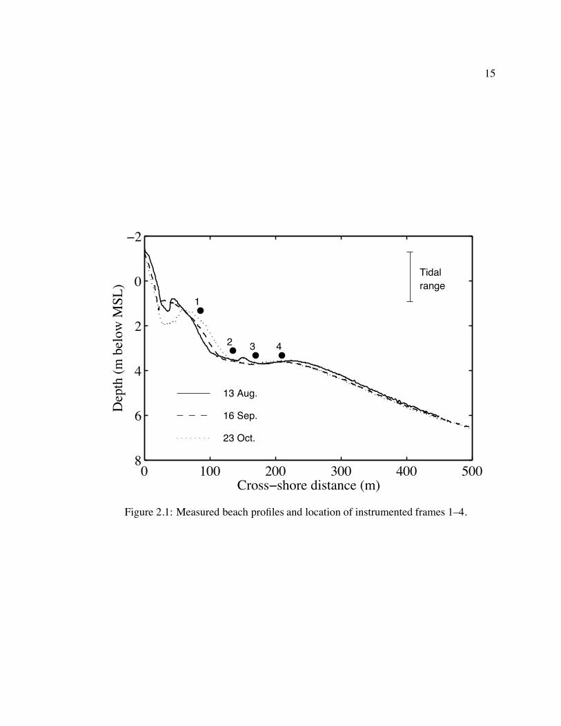
Figure 2.1: Measured beach profiles and location of instrumented frames 1–4.

16

2.3 Field site and instrumentation

This chapter presents analysis of data collected on an ocean beach near Duck, North Car-

olina by the Dalhousie nearshore research group during the Sandyduck beach experiment

of 1997. Figure 2.1 shows the cross-shore array of four instrumented frames from which

the data were collected, together with measured beach profiles. Water pressures and veloc-

ities were measured at Hz at every frame. During the Sandyduck experiment, the U.S.

Army Corps of Engineers regularly measured sea bed elevation profiles using the Coastal

Research Amphibious Buggy (Lee and Birkemeier, 1993). Sea bed elevations beneath the

instrumented frames were also measured continuously using sonar altimeters.

2.4 Results

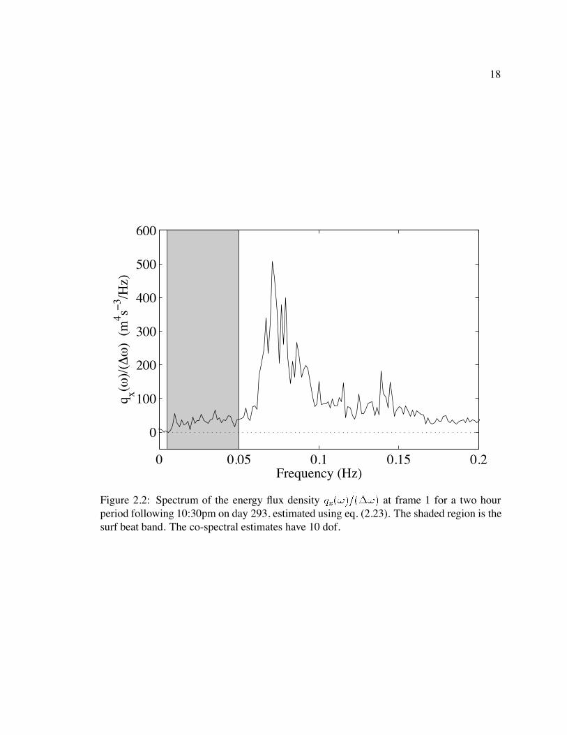
Cross-periodograms between water pressure and velocity were calculated from quadratically-

detrended half-hour time series. Spectra of the wave energy flux were estimated by aver-

aging these cross-periodograms and applying eq.’s (2.23) & (A.4). Figure 2.2 shows a

spectrum of the shoreward energy flux measured over two hours during a storm on day

293. The shaded region of fig. 2.2 is the surf beat band (– Hz). For every half-

hour of the experiment, I estimated the total surf beat energy flux qsb by integrating raw

cross-periodograms between pressure and velocity over the entire surf beat band and mul-

tiplying by the water depth h. Other statistics, such as significant wave height and the

beat-frequency sea level variance, were also calculated every half hour. I estimated sea

surface elevations from water pressure measurements using linear wave theory. The signif-

icant wave height was calculated as w

, where the overbar denotes a sample mean, and

w is the estimated sea level variance due to waves with frequencies greater than Hz.

Equation (2.29) neglects the longshore gradient of the longshore energy flux. The ratio

of the longshore flux gradient to the cross-shore flux gradient is

R

qyyqxx

qyqx Lx

Ly

(2.30)

17

where

qy longshore component of surf beat energy flux

Lx cross-shore length scale over which qx varies

Ly longshore length scale over which qy varies

Since the beach at Duck is long and straight, I assume LxLy . When incident waves

were large, the observed longshore surf beat energy flux was usually an order of magnitude

smaller than the cross-shore surf beat energy flux. When incident waves were small, the

longshore and cross-shore energy fluxes were of the same magnitude. Therefore, when

incident waves were large R , so the longshore-uniform approximation made in the

derivation of eq. (2.20) was reasonable. I can not be sure how accurate the longshore-

uniform approximation was when incident waves were small.

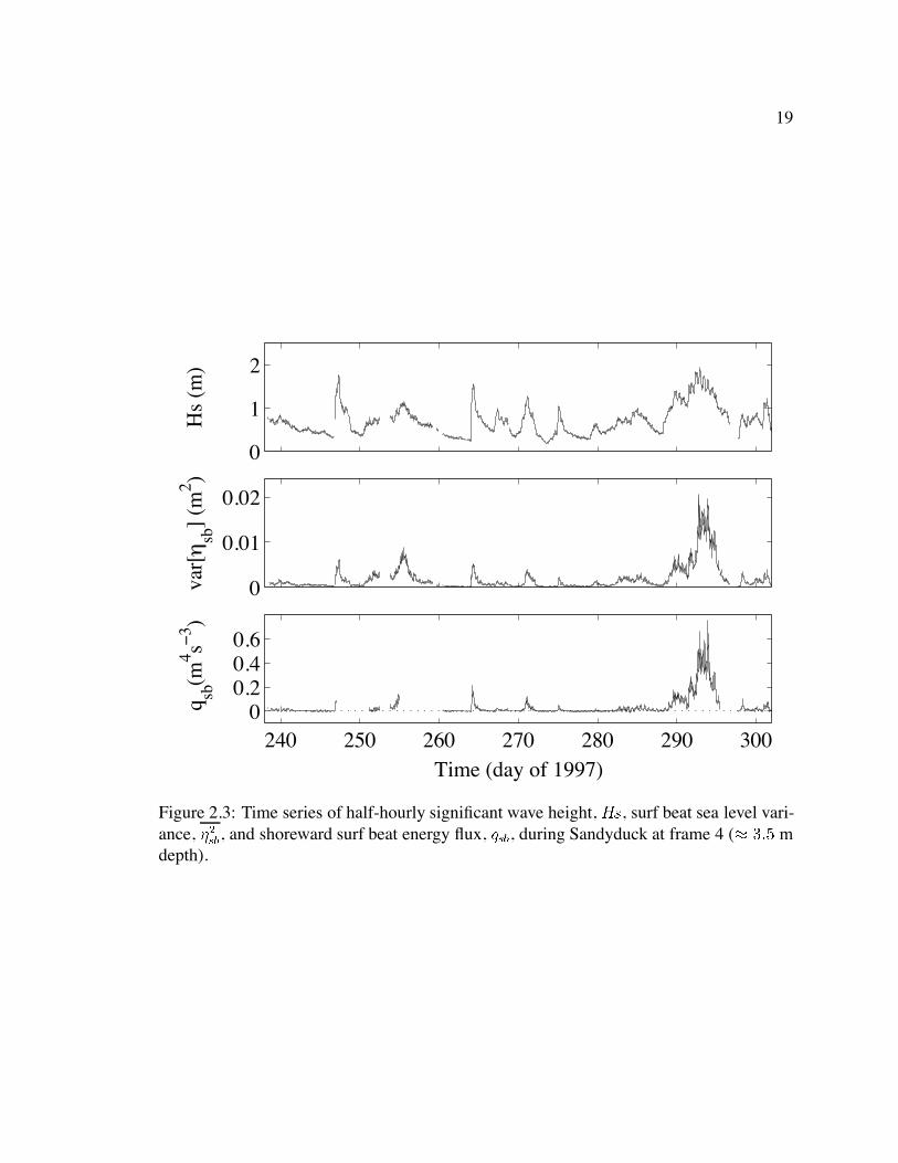
Figure 2.3 shows the time series of significant wave height, surf beat sea level variance,

and shoreward surf beat energy flux, measured at frame 4. Similar results were obtained

from the other three frames. Surf beat energy increased with increasing significant wave

height, consistent with the findings of Tucker (1950), Holman (1981), Guza and Thorn-

ton (1985), and others. The surf beat energy flux was directed onshore in 86% of cases,

suggesting that the nearshore zone ( m depth) was usually a region of net surf beat

dissipation during the Sandyduck experiment (eq. (2.29)). Shoreward energy fluxes were

most pronounced when incident waves were large — when the significant wave height was

greater than m the surf beat energy flux was always directed onshore. The observed

shoreward energy flux does not imply that surf beat forcing was weak near the shore, but it

does imply that dissipation was usually stronger than forcing.

During the Sandyduck experiment, incident wave (– Hz) energy fluxes ranged

from ms to ms, and were always directed onshore.

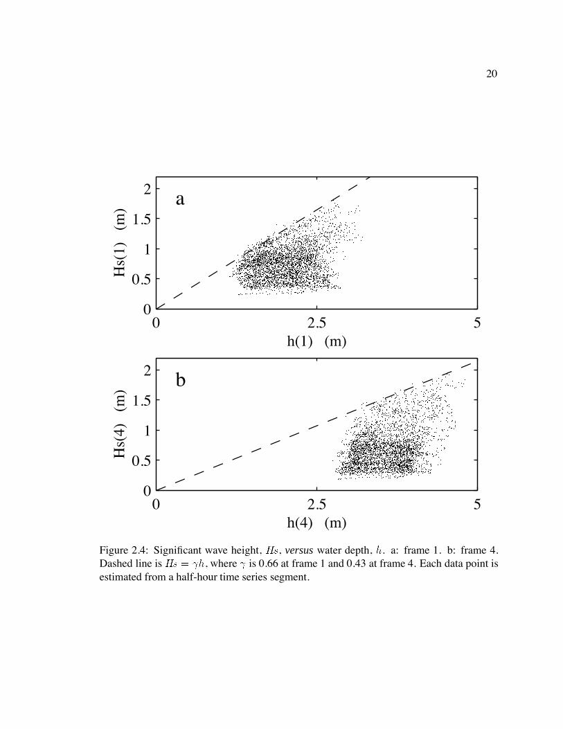
Figure 2.4 shows the significant wave height Hs as a function of water depth at frames

1 and 4. Wave heights were limited by breaking, as described by the relation

Hs h (2.31)

18

0 0.05 0.1 0.15 0.2

0

100

200

300

400

500

600

Frequency (Hz)

q x(ω)/

(∆ω

) (

m4 s−

3 /Hz)

Figure 2.2: Spectrum of the energy flux density qx at frame 1 for a two hourperiod following 10:30pm on day 293, estimated using eq. (2.23). The shaded region is thesurf beat band. The co-spectral estimates have 10 dof.

19

0

1

2

Hs

(m)

0

0.01

0.02

var[η

sb]

(m2 )

240 250 260 270 280 290 3000

0.20.40.6

q sb (m

4 s−3 )

Time (day of 1997)

Figure 2.3: Time series of half-hourly significant wave height, Hs, surf beat sea level vari-ance, sb, and shoreward surf beat energy flux, qsb, during Sandyduck at frame 4 ( mdepth).

20

0 2.5 50

0.5

1

1.5

2

h(1) (m)

Hs(

1)

(m)

a

0 2.5 50

0.5

1

1.5

2

h(4) (m)

Hs(

4)

(m) b

Figure 2.4: Significant wave height, Hs, versus water depth, h. a: frame 1. b: frame 4.Dashed line is Hs h, where is 0.66 at frame 1 and 0.43 at frame 4. Each data point isestimated from a half-hour time series segment.

21

where the breaker-ratio (chosen to fit the data) equals at frame 1 and at frame

4. Sallenger and Holman (1985) and Raubenheimer et al. (1996) discuss the application of

eq. (2.31) to the surf zone at Duck. In order to determine approximately whether frame 1

was inside or outside the saturated surf zone, I define the shoaled significant wave height

Hs h hHs (2.32)

where Hs and h are the significant wave height and water depth at frame 4, and

h is the local water depth. Hs is the wave height that would be observed given linear,

non-dissipative shoaling of shore-normal shallow water waves. Roughly, frame 1 is inside

(outside) the saturated surf zone when Hsh is greater than (less than) at frame 1. At

frame 4, Hs Hs.

The shoreward surf beat energy flux shown in fig. 2.3 implies some shoreward propa-

gation of surf beat. Let

qsb

Esbgh (2.33)

where Esb is the total linear surf beat energy density. is the ratio between the actual surf

beat energy flux, calculated from eq. (2.23), and the surf beat energy flux expected for a

purely shore-normal, shoreward-propagating wave, calculated from eq. (2.27). If all surf

beat propagates directly shorewards , if all surf beat propagates directly seawards

, and if all surf beat is standing in the cross-shore . Directional spreading of

waves (away from shore-normal) reduces the magnitude of . I estimated the total surf beat

energy density as twice the potential energy density, or

Esb g sb (2.34)

where sb is the estimated sea surface elevation variance due to surf beat. The use of

eq. (2.34) introduced errors into Esb estimates, but allowed separation of surf beat (grav-

ity wave) energy from the shear wave energy that often contributes a large proportion of

the total low frequency kinetic energy (Lippmann et al., 1999). Figure 2.5 shows the ob-

served dependence of on the non-dimensional shoaled wave height Hsh. When the

22

0.05 0.1 0.2 0.4 0.7 1 1.4−1

−0.5

0

0.5

1a

Hs(1)′/h(1)

ρ(1)

0.05 0.1 0.2 0.4 0.7 1 1.4−1

−0.5

0

0.5

1b

Hs(4)′/h(4)

ρ(4)

Figure 2.5: Onshore-progressiveness of surf beat, qsbEsb Cg, versus shoaled signif-icant wave height (eq. (2.32)) divided by water depth, Hsh. a: frame 1. b: frame 4. Thevertical dashed lines indicate Hsh . Each data point is estimated from a half-hourtime series segment.

23

non-dimensional wave height was small, and surf beat was approximately standing

in the cross-shore. When the non-dimensional wave height was large, and there was

a significant shoreward-propagating component of surf beat.

The observed net surf beat dissipation is consistent with a standard bottom stress pa-

rameterisation. The dissipation of the energy of a frequency wave by bottom friction

is

D fejujj hui j (2.35)

where fe is a dimensionless energy dissipation factor. Values of fe observed in the field for

incident-frequency waves are usually in the range – (Sleath, 1984).

Let x y be the bed shear stress divided by the water density. Feddersen et al.

(1998) showed that the drag force (divided by the water density) retarding the mean long-

shore current, v, at Duck is

y cf jujv

where the bottom drag coefficient, cf , is roughly outside the surf zone and

inside the surf zone. Applying the same parameterisation to surf beat

h i cf juj hui

D h i hui cf jujj hui j (2.36)

Equation (2.36) differs from eq. (2.35) only in the magnitude of the non-dimensional coef-

ficient — dissipation factors for waves are one or two orders of magnitude larger than drag

coefficients for the mean current (Nielsen, 1992).

From eq.’s (2.35) & (2.36), the total dissipation of surf beat energy by bottom drag

scales with

jujjujsb (2.37)

where jujsb is the contribution to velocity variance from surf beat frequencies. To separate

gravity wave dissipation from shear wave dissipation, I re-write eq. (2.37) in terms of the

24

sea surface elevation variance. For gravity waves in shallow water (Lippmann et al., 1999)

juj gh

D fegh

sb (2.38)

From eq.’s (2.29) and (2.38)

qsbjxa

Z shore

xa

fegh

sb ENsbdx (2.39)

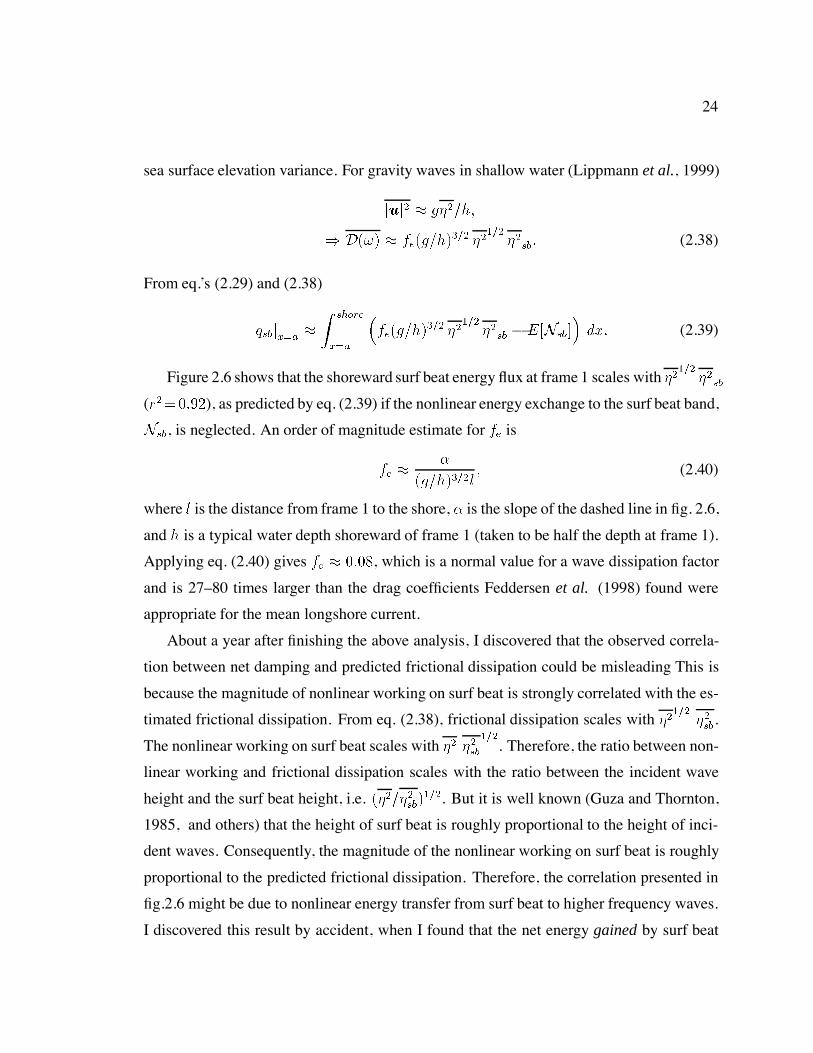
Figure 2.6 shows that the shoreward surf beat energy flux at frame 1 scales with

sb

(r), as predicted by eq. (2.39) if the nonlinear energy exchange to the surf beat band,

Nsb, is neglected. An order of magnitude estimate for fe is

fe

ghl (2.40)

where l is the distance from frame 1 to the shore, is the slope of the dashed line in fig. 2.6,

and h is a typical water depth shoreward of frame 1 (taken to be half the depth at frame 1).

Applying eq. (2.40) gives fe , which is a normal value for a wave dissipation factor

and is 27–80 times larger than the drag coefficients Feddersen et al. (1998) found were

appropriate for the mean longshore current.

About a year after finishing the above analysis, I discovered that the observed correla-

tion between net damping and predicted frictional dissipation could be misleading This is

because the magnitude of nonlinear working on surf beat is strongly correlated with the es-

timated frictional dissipation. From eq. (2.38), frictional dissipation scales with

sb.

The nonlinear working on surf beat scales with sb

. Therefore, the ratio between non-

linear working and frictional dissipation scales with the ratio between the incident wave

height and the surf beat height, i.e. sb. But it is well known (Guza and Thornton,

1985, and others) that the height of surf beat is roughly proportional to the height of inci-

dent waves. Consequently, the magnitude of the nonlinear working on surf beat is roughly

proportional to the predicted frictional dissipation. Therefore, the correlation presented in

fig.2.6 might be due to nonlinear energy transfer from surf beat to higher frequency waves.

I discovered this result by accident, when I found that the net energy gained by surf beat

25

0 0.002 0.004 0.006 0.008 0.01 0.012

0

0.2

0.4

0.6

0.8

1

var[η]1/2var[η]sb

(m3)

q x (m

4 s−3 )

Figure 2.6: Onshore surf beat energy flux, qsb, versus sb at frame 1. Dashed line is

qsb sb, with chosen to give least-squares fit. Each data point is estimated from

a half-hour time series segment.

26

outside the surf zone was strongly correlated with estimated frictional dissipation. Both

bottom friction and nonlinear damping might account for the observed dissipation, but we

can not determine which was most important from correlations of the sort shown in fig. 2.6.

Section 1.2 introduced Q as a measure of the strength of surf beat dissipation. Since I

can measure only spatially-averaged net forcing or dissipation, I can not measure Q values

for individual surf beat modes. Instead, I define the net forcing strength

Net surf beat energy generated in one beat period

Total surf beat energy (2.41)

R b

xa ENsb EDsb dx

R b

xaEsb dx

From eq. (2.29)

qsbjxb qsbjxa

HzR b

xaEsb dx

(2.42)

where Hz has been chosen as a typical surf beat frequency. Since this ‘typical’ beat

frequency was chosen somewhat arbitrarily, only the sign and order of magnitude of are

significant. Where possible I estimated the integral in eq. (2.42) using the trapezoidal rule.

To estimate the integral between frame 1 and the shore, I multiplied the energy density at

frame 1 by the distance to the shore. The energy density Esb was estimated using eq. (2.34).

is positive (negative) if total forcing exceeds total dissipation (dissipation exceeds

forcing) between x a and x b. If jj is order one, then the surf beat energy forced (or

dissipated) between xa and xb in a single beat period is of the same order as the total

amount of surf beat energy stored between xa and xb. If jj , then net forcing (or

dissipation) is weak, but this does not imply that actual forcing and dissipation are weak.

If strong forcing and strong dissipation happen to cancel, then . Therefore, large jj

values indicate strong forcing or dissipation, whereas small jj values are ambiguous.

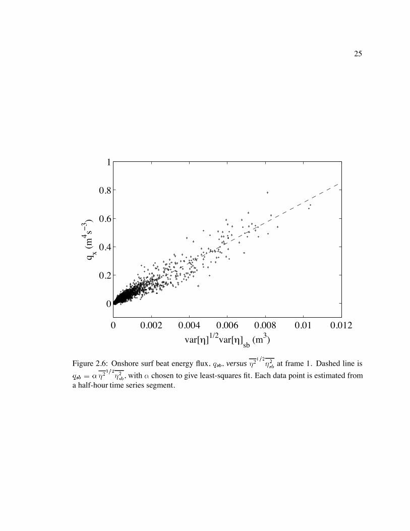
Figure 2.7a shows the estimated strength of net surf beat forcing, , for the region

between frames 1 and 4. Figure 2.7b shows for the region between frame 1 and the

shore. The vertical dashed lines indicate the non-dimensional wave height at which frame

1 is approximately on the edge of the saturated surf zone. When incident waves were small,

27

0.1 0.2 0.4 0.7 1 1.4−1

0

1

2Ω

Hs(1)′/h(1)

a

0.1 0.2 0.4 0.7 1 1.4−3

−2

−1

0

1

Ω

Hs(1)′/h(1)

b

Figure 2.7: Estimated net forcing strength, , defined by eq. (2.41) versus shoaled signif-icant wave height (eq. (2.32)) divided by water depth, Hsh, at frame 1. a: Net forcingstrength between frames 1 and 4. b: Net forcing strength onshore of frame 1. The verticaldashed lines indicate Hsh . Each data point is estimated from a half-hour timeseries segment.

28

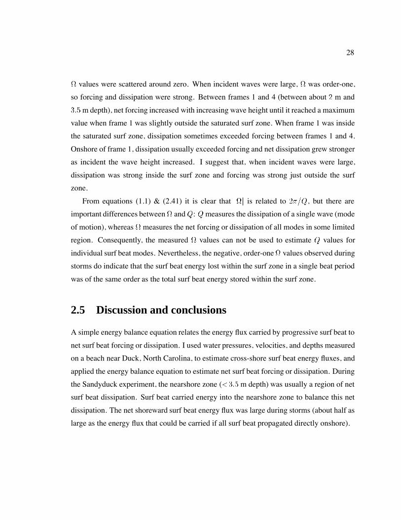
values were scattered around zero. When incident waves were large, was order-one,

so forcing and dissipation were strong. Between frames 1 and 4 (between about m and

m depth), net forcing increased with increasing wave height until it reached a maximum

value when frame 1 was slightly outside the saturated surf zone. When frame 1 was inside

the saturated surf zone, dissipation sometimes exceeded forcing between frames 1 and 4.

Onshore of frame 1, dissipation usually exceeded forcing and net dissipation grew stronger

as incident the wave height increased. I suggest that, when incident waves were large,

dissipation was strong inside the surf zone and forcing was strong just outside the surf

zone.

From equations (1.1) & (2.41) it is clear that jj is related to Q, but there are

important differences between andQ: Qmeasures the dissipation of a single wave (mode

of motion), whereas measures the net forcing or dissipation of all modes in some limited

region. Consequently, the measured values can not be used to estimate Q values for

individual surf beat modes. Nevertheless, the negative, order-one values observed during

storms do indicate that the surf beat energy lost within the surf zone in a single beat period

was of the same order as the total surf beat energy stored within the surf zone.

2.5 Discussion and conclusions

A simple energy balance equation relates the energy flux carried by progressive surf beat to

net surf beat forcing or dissipation. I used water pressures, velocities, and depths measured

on a beach near Duck, North Carolina, to estimate cross-shore surf beat energy fluxes, and

applied the energy balance equation to estimate net surf beat forcing or dissipation. During

the Sandyduck experiment, the nearshore zone ( m depth) was usually a region of net

surf beat dissipation. Surf beat carried energy into the nearshore zone to balance this net

dissipation. The net shoreward surf beat energy flux was large during storms (about half as

large as the energy flux that could be carried if all surf beat propagated directly onshore).

29

The strong shoreward energy fluxes reported here are consistent with the incomplete re-

flection of surf beat observed in the the surf zone by Nelson and Gonsalves (1992), Rauben-

heimer et al. (1995), Saulter et al. (1997), Henderson et al. (2001), and Sheremet et al.

(2001).

Most existing surf beat models do not predict strong shoreward propagation because

they do not simulate strong surf-zone dissipation. Unforced, undamped surf beat mod-

els (Eckart, 1951; Ursell, 1952; Kenyon, 1970; Holman and Bowen, 1979, 1982; Howd

et al., 1992; Bryan and Bowen, 1996) predict that surf beat is cross-shore standing. Non-

dissipative and weakly-dissipative models that allow for the possibility of edge wave res-

onance (Gallagher, 1971; Bowen and Guza, 1978; Schaffer, 1994; Lippmann et al., 1997)

also predict that surf beat is cross-shore standing. The breakpoint-forcing model of Sy-

monds et al. (1982) predicts cross-shore standing waves onshore of the breakpoint, and

seaward propagating waves offshore of the breakpoint. The models of Schaffer (1993)

and Van Dongeren et al. (1996) predict that nonlinear forcing due to intermittent wave

breaking opposes incident bound-wave motions, leading to net nonlinear damping of surf

beat at the breakpoint, and shoreward propagation just outside the breakpoint. However,

these last three models exclude the possibility of edge wave resonance through the arbitrary

assumption that forcing is entirely shore-normal.

During the Sandyduck experiment, dissipation was strongest well inside the saturated

surf zone, exactly where incident waves were limited by breaking and surf beat made an

important contribution to the total flow field. Models of surf beat dynamics should incor-

porate rapid surf-zone dissipation.

A standard bottom dissipation parameterisation predicted the observed net surf beat

dissipation well. The wave dissipation factor for surf beat was O, within the range

of dissipation factors usually observed for higher frequency incident waves. However, the

magnitude of nonlinear working on surf beat was correlated with the predicted frictional

dissipation, so the correlation between net dissipation and predicted frictional damping

might not indicate a causal relationship.

The region between m and m depth was a region of net surf beat forcing, except

30

when incident waves were very large and the saturated surf zone extended beyond m

depth. I suggest that surf beat forcing usually exceeded dissipation outside the surf zone,

whereas dissipation exceeded forcing inside the surf zone. This is consistent with the cross-

shore structure of surf beat forcing predicted by Longuet-Higgins and Stewart (1962) and

Symonds et al. (1982), and with the suggestion of Guza and Bowen (1976b) and others

that surf beat dissipation might be most rapid inside the surf zone.

Surf beat forcing and dissipation were very strong during storms. When incident waves

were large, the surf beat energy dissipated within the surf zone during a single beat period

was of the same order as the total surf beat energy stored within the surf zone. The surf

beat energy forced in a single beat period near the edge of the surf zone was also of the

same order as the total surf beat energy stored near the edge of the surf zone.

Chapter 3

The cross-shore structure of surf beat

3.1 Introduction

In Chapter 2, long time series of water pressure and velocity, measured at just four loca-

tions on a natural beach, were used to show that surf beat is dissipated rapidly in the surf

zone. This chapter presents further observations from a different field experiment. Only a

few short time series are analysed, but a very dense cross-shore array of 15 instrumented

frames allows better resolution of the cross-shore structure of surf beat. The field site and

instrumentation are described in Section 3.2. Section 3.3 shows that spatially-coherent surf

beat was partly cross-shore standing, and partly cross-shore (usually shoreward) progres-

sive. Section 3.4 presents estimates of the cross-shore energy flux carried by progressive

surf beat. Results are summarised in Section 3.5. Related results were presented by Hen-

derson et al. (2001).

3.2 Field site and instrumentation

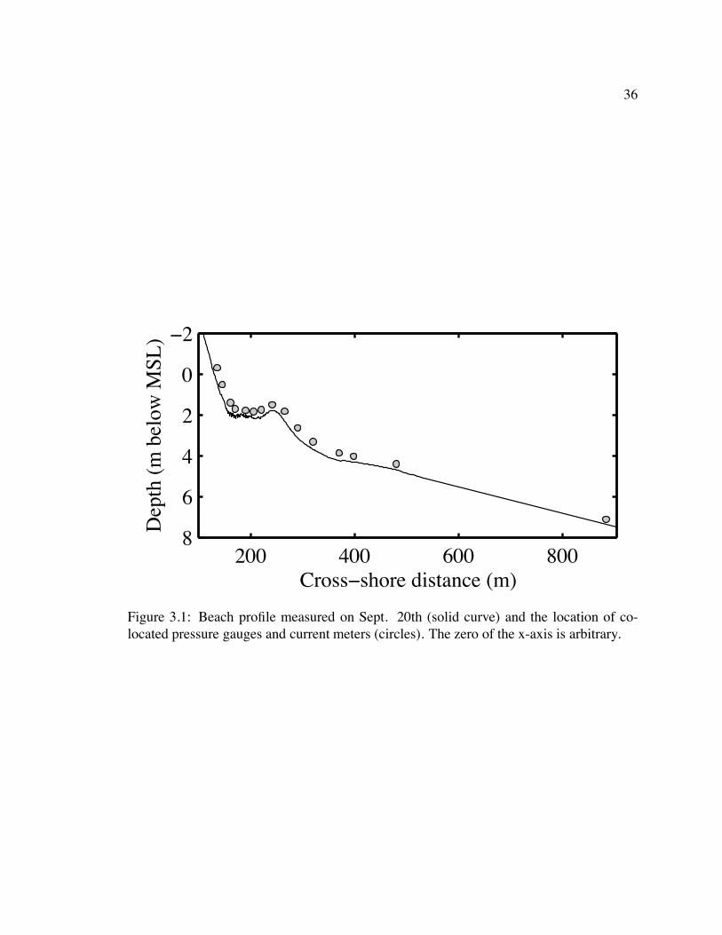
Data were collected on an ocean beach near Duck, North Carolina, during the Duck94

experiment at the U.S. Army Field Research Facility (Gallagher et al., 1998; Elgar et al.,

1997). Near-bottom water pressure and horizontal velocity were measured (at Hz) at 16

locations along a cross-shore transect extending from the shore to about 8 m water depth

31

32

(fig.3.1). Seabed elevations were determined with surveys from an amphibious vehicle

(Lee and Birkemeier, 1993) and sonar altimeters (Gallagher et al., 1996) co-located with

the pressure and current sensors.

3.3 Spatially-coherent surf beat

3.3.1 Methods

At each instrument location, 3-hr time series of bottom pressure were broken into ninety

50% overlapping segments, with

pjkt j’th time series of bottom pressure (in m water) at location k

Each time series segment was Hanning windowed and Fourier transformed. Let

hpjki

Fourier component of windowed pjk at frequency

pj

BBBBB

hpji

hpji

...

hpji

CCCCCA

so that the vectorpj

represents the cross-shore structure of pressure fluctuations at

frequency . Pressure fluctuations measured at the most offshore location (7.5 m depth,

fig.3.1) were not included inpj.

A cross-spectral matrix was estimated at every frequency ,

pp pj

pTj

where the overbar denotes an average over all realizations (i.e. all values of j), and T

denotes a transpose. At each frequency, the eigenvectors of pp are the frequency-

domain Empirical Orthogonal Functions (EOF’s), or principal components, of the pressure

fluctuations. There are as many EOF’s as there are elements ofpj

, but here only the

33

dominant EOF is considered (i.e. the eigenvector of pp associated with the largest

eigenvalue). Johnson and Wichern (1982) show that the dominant EOF is the vector

that minimises the mean square error jjj inpj aj j

where the amplitudes aj are chosen to obtain the best fit. In this sense, the dominant

EOF is the single cross-shore structure that best fits the observed cross-shore structure of

pressure fluctuations at frequency . In the cases presented the dominant EOF accounted

for between 45% and 70% of the variance summed over all instruments.

If is a dominant EOF, then so is for any constant . The EOF’s are nor-

malised so that the component representing the pressure fluctuation closest to the shore

equals 1 m.

The combined pressure and cross-shore velocity EOF’s also were estimated as the dom-

inant eigenvectors of the cross-spectral matrix

hji

Tj

where

hji

BBBBBBBBBBBBBBBB

g hpji

g hpji

...

g hpji

h huji

h huji

...

h huji

CCCCCCCCCCCCCCCCA

hujki

Fourier component of windowed ujk at frequency

ujkt j’th time series of shoreward water velocity at frame k

g gravitational acceleration

h water depth

34

At every frequency a dominant EOF of was estimated from . This single dominant

EOF represented the cross-shore structure of both pressure and velocity.

Note the energy-based weighting of hpi and hui . For linear shallow water waves,

jg hpi j potential energy density at frequency , (3.1)

jh hui j kinetic energy density at frequency . (3.2)

Finally, the pressure components of the dominant EOF of were divided by g

and the velocity components were divided by h to convert back to units of pressure (m)

and velocity (ms).

3.3.2 Results and discussion

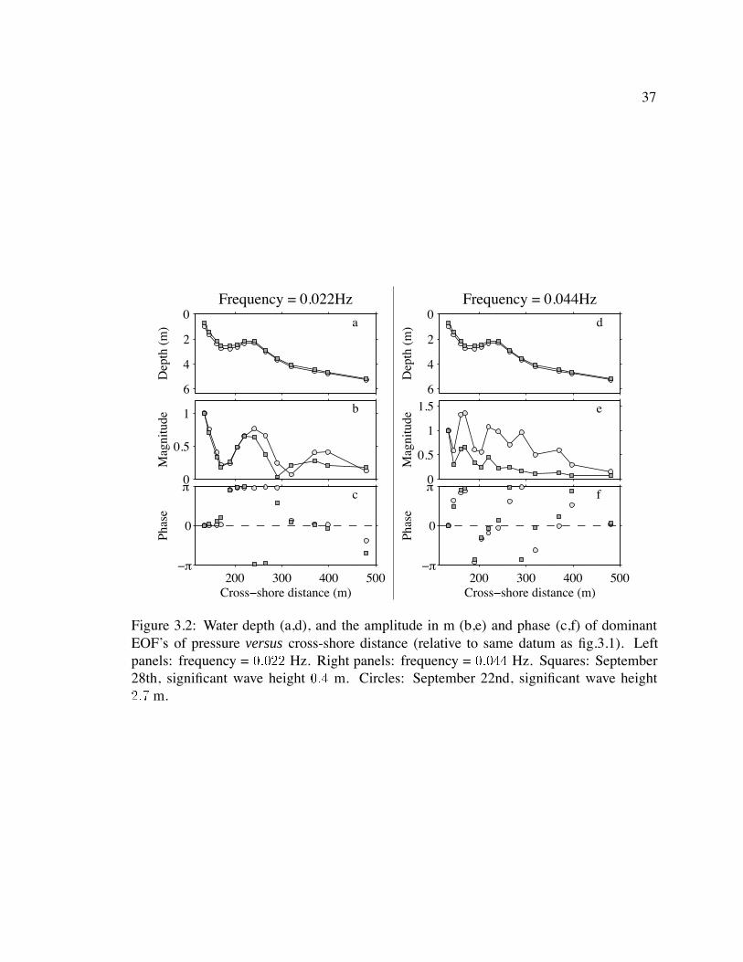
Figure 3.2a–c shows the dominant EOF’s of low frequency ( Hz) pressure fluctuations

for two different 3 hr pressure time series. Both EOF’s have clear amplitude maxima (at

the shore and x m) and minima (at x and x m), with a phase jump of

at each minimum, consistent with the presence of a cross-shore standing wave. Here.

unlike in Chapter 2, x is positive seawards. Monotonic changes of phase with distance

from the shore, which would indicate the presence of a cross-shore progressive wave, were

not observed.

The EOF’s shown in fig.3.2a–c are typical of those observed at frequencies less than

about Hz. However at surf beat frequencies above about Hz, the EOF’s had

a different cross-shore structure, as shown in fig. 3.2d–f ( Hz). Although the

higher-frequency EOF had some nodal structure (fig.3.2e), the phase jumps obvious in the

low frequency case have been replaced by a monotonic increase in phase with distance

from the shore (fig.3.2f), indicating the presence of some shoreward-progressive surf beat.

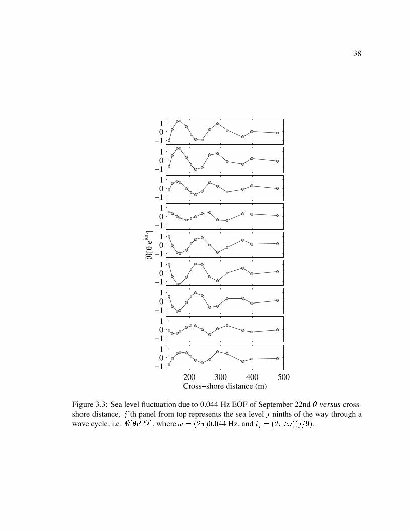
The sea level fluctuation associated with a given EOF is proportional to eit. Figure

3.3 presents a sequence of ‘snapshots’ of eit through the wave cycle for the 0.044 Hz

EOF of September 22nd (fig. 3.2d–f).

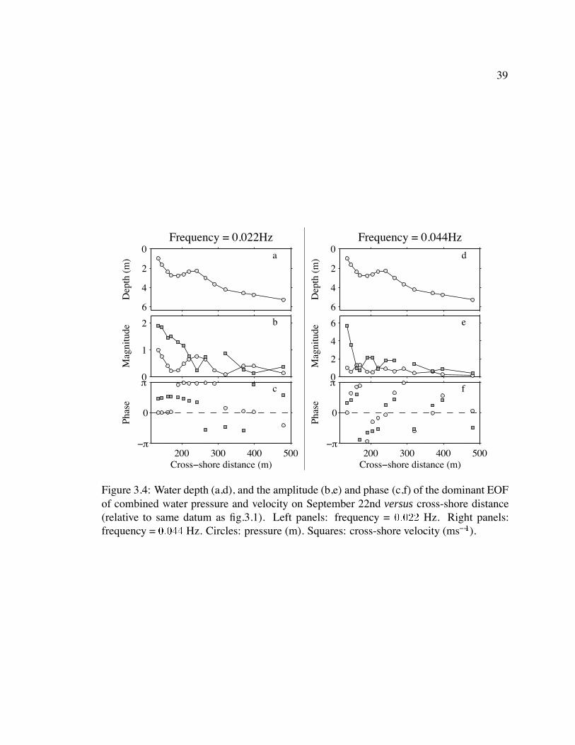
Figure 3.4a–c shows a dominant EOF of combined pressure and velocity fluctuations

35

at Hz. Note that in fig.3.4b,c a single 28-element EOF, with 14 pressure com-

ponents and 14 velocity components, is plotted as two curves, with one curve represent-

ing the cross-shore structure of pressure EOF components and the other representing the

cross-shore structure of velocity EOF components. Also note that, although the absolute

magnitude of the EOF is arbitrary, the relative magnitudes of the pressure and velocity

components are not arbitrary. For example, if the EOF plotted in fig.3.4a–c had gener-

ated a pressure fluctuation of 1 m at the most onshore instrument location, the associated

co-located velocity fluctuation would have been about 2 ms (fig.3.4b).

The pressure component of the dominant EOF of combined pressure and velocity fluc-

tuations (circles, fig.3.4b,c) is similar to the EOF of pressure fluctuations alone (circles,

fig.3.2b,c). Contributions to both pressure and velocity fluctuations show nodes, antinodes,

and phase jumps. Offshore of x m the nodes of pressure fluctuations coincided

with the antinodes of velocity fluctuations, and vice-versa. Onshore of x m pres-

sures were about out of phase with co-located velocities. All of of these features are

predicted by cross-shore standing wave theories.

The dominant EOF of combined water pressure and velocity fluctuations at Hz

displays a mixture of progressive and standing wave behaviours (fig.3.4d–f). Some nodal

structure is present, but there is a monotonic increase in phase with distance from the shore,

indicating net shoreward propagation. With the exception of the most offshore location,

the magnitude of the phase between pressure and velocity was between the phase of

standing waves and the zero phase of shoreward progressive waves.

Since the dominant EOF does not account for all of the observed variance, the results of

the section are not conclusive. Nevertheless, it is encouraging that the cross-shore structure

of surf beat revealed by EOF analysis is consistent with the observations of shoreward

energy fluxes reported in Chapter 2, and in Section 3.4.

36

200 400 600 800

−2

0

2

4

6

8

Dep

th (

m b

elow

MSL

)

Cross−shore distance (m)

Figure 3.1: Beach profile measured on Sept. 20th (solid curve) and the location of co-located pressure gauges and current meters (circles). The zero of the x-axis is arbitrary.

37

0

2

4

6

Dep

th (

m) a

Frequency = 0.022Hz

0

0.5

1

Mag

nitu

de

b

200 300 400 500

Cross−shore distance (m)

Phas

e

−π

0

πc

0

2

4

6D

epth

(m

) d

Frequency = 0.044Hz

0

0.5

1

1.5M

agni

tude

e

200 300 400 500

Cross−shore distance (m)

Phas

e

−π

0

πf

Figure 3.2: Water depth (a,d), and the amplitude in m (b,e) and phase (c,f) of dominantEOF’s of pressure versus cross-shore distance (relative to same datum as fig.3.1). Leftpanels: frequency = Hz. Right panels: frequency = Hz. Squares: September28th, significant wave height m. Circles: September 22nd, significant wave height m.

38

−101

−101

−101

−101

−101

ℜ[θ

eiω

t ]

−101

−101

−101

200 300 400 500−1

01

Cross−shore distance (m)

Figure 3.3: Sea level fluctuation due to 0.044 Hz EOF of September 22nd versus cross-shore distance. j’th panel from top represents the sea level j ninths of the way through awave cycle, i.e. eitj , where Hz, and tj j.

39

0

2

4

6

Dep

th (

m) a

Frequency = 0.022Hz

0

1

2

Mag

nitu

de

b

200 300 400 500

Cross−shore distance (m)

Phas

e

−π

0

πc

0

2

4

6D

epth

(m

) d

Frequency = 0.044Hz

0

2

4

6M

agni

tude

e

200 300 400 500

Cross−shore distance (m)

Phas

e

−π

0

πf

Figure 3.4: Water depth (a,d), and the amplitude (b,e) and phase (c,f) of the dominant EOFof combined water pressure and velocity on September 22nd versus cross-shore distance(relative to same datum as fig.3.1). Left panels: frequency = Hz. Right panels:frequency = Hz. Circles: pressure (m). Squares: cross-shore velocity (ms).

40

3.4 Energy transport

This Section presents observations of wave energy density and energy flux. I consider

three frequency bands: Low frequency surf beat (0.005–0.025 Hz), high frequency surf

beat (0.025–0.05 Hz), and sea/ swell (0.05–0.3 Hz). Since sea and swell are not always

in shallow water, it is necessary to allow for depth-dependence of the water pressure and

velocity fields. I assumed that the depth-dependence of the pressure and velocity is given

by linear theory (Mei, 1983). The energy flux was then estimated as the depth-integrated

product of pressure and velocity (depth dependence was allowed for, but had very little

effect, at infragravity frequencies). I neglected vertical variations in pressure and veloc-

ity associated with wave breaking. Consequently, the estimates of incident wave energy

density and flux presented in this section might not be accurate inside the surf zone. In

contrast, estimates of surf beat energy densities and fluxes are probably not affected greatly

by vertical structure (Section 2.2.1 and Appendix A.1).

About 1000 three-hour time series were collected during the Duck94 experiment. Most

were clearly non-stationary, and were excluded from the data set presented here. The re-

maining data set was reduced to just 13 three-hour time series by removing occasions when

longshore currents were greater than 0.25 ms, and occasions when the longshore surf beat

energy flux was greater than half the cross-shore energy flux. The exclusion of cases where

longshore currents were significant ensured that shear waves contributed little to the ob-

served low frequency motions. Cases where the longshore surf beat energy flux was strong

were removed to minimise the effects of longshore non-uniformity on the surf beat energy

balance. This section presents results from three typical three-hour times series. Results

from the remaining 10 time series are presented in Appendix C.

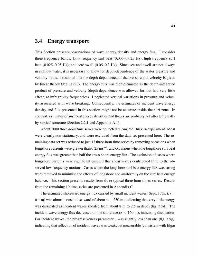
The estimated shoreward energy flux carried by small incident waves (Sept. 17th, Hs

m) was almost constant seaward of about x 250 m, indicating that very little energy

was dissipated as incident waves shoaled from about 8 m to 2.5 m depth (fig. 3.5d). The

incident wave energy flux decreased on the shoreface (x 160 m), indicating dissipation.

For incident waves, the progressiveness parameter was slightly less than one (fig. 3.5g),

indicating that reflection of incident waves was weak, but measurable (consistent with Elgar

41

et al. (1997)).

Seaward of x 300 m, the surf beat energy fluxes and values were almost constant

and near zero, indicating that surf beat was nearly cross-shore standing (fig. 3.5e,f,g). Be-

tween x 200 m and x 300 m, the estimated shoreward surf beat energy flux increased,

indicating that surf beat energy was generated in this region. Shoreward of x 200 m, the

energy flux carried by high frequency surf beat increased slightly, whereas the energy flux

carried by low frequency surf beat seemed to decrease just shoreward of x 200 m, before

again increasing shoreward of x 170 m. Shoreward of about x 250 m, was slightly

greater than zero, indicating that surf beat was nearly cross-shore standing, but there was

some weak net shoreward propagation.

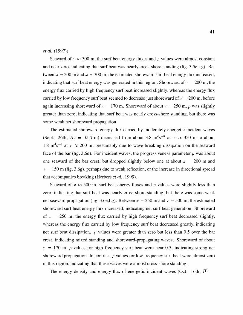
The estimated shoreward energy flux carried by moderately energetic incident waves

(Sept. 26th, Hs m) decreased from about 3.8 ms at x 350 m to about

1.8 ms at x 200 m, presumably due to wave-breaking dissipation on the seaward

face of the bar (fig. 3.6d). For incident waves, the progressiveness parameter was about

one seaward of the bar crest, but dropped slightly below one at about x 200 m and

x 150 m (fig. 3.6g), perhaps due to weak reflection, or the increase in directional spread

that accompanies breaking (Herbers et al., 1999).

Seaward of x 500 m, surf beat energy fluxes and values were slightly less than

zero, indicating that surf beat was nearly cross-shore standing, but there was some weak

net seaward propagation (fig. 3.6e,f,g). Between x 250 m and x 500 m, the estimated

shoreward surf beat energy flux increased, indicating net surf beat generation. Shoreward

of x 250 m, the energy flux carried by high frequency surf beat decreased slightly,

whereas the energy flux carried by low frequency surf beat decreased greatly, indicating

net surf beat dissipation. values were greater than zero but less than 0.5 over the bar

crest, indicating mixed standing and shoreward-propagating waves. Shoreward of about

x 170 m, values for high frequency surf beat were near 0.5, indicating strong net

shoreward propagation. In contrast, values for low frequency surf beat were almost zero

in this region, indicating that these waves were almost cross-shore standing.

The energy density and energy flux of energetic incident waves (Oct. 16th, Hs

42

0

5

Dep

th (

m)

a

0

0.05

0.1

P.E

. (m

3 s−2 )

b>0.05Hz

0

5

x 10−3

P.E

. (m

3 s−2 )

c

0.025−0.05Hz0.005−0.025Hz

0

0.5

q (m

4 s−3 ) d

−5

0

5

x 10−3

e

q (m

4 s−3 )

100 200 300 400 500 600 700 800 900−1

0

1

ρ

Cross−shore distance (m)

g

0

5

Dep

th (

m)

a

0

0.05

0.1

P.E

. (m

3 s−2 )

b>0.05Hz

0

5

x 10−3

P.E

. (m

3 s−2 )

c

0.025−0.05Hz0.005−0.025Hz

0

0.5

q (m

4 s−3 ) d

−202

x 10−3

f

q (m

4 s−3 )

100 200 300 400 500 600 700 800 900−1

0

1

ρ

Cross−shore distance (m)

g

Figure 3.5: Water depth (a), potential energy density PE (b: swell. c: surf beat), shore-ward energy flux q (d: swell. e: high frequency surf beat. f: low frequency surf beat), andprogressiveness parameter (g) versus cross-shore distance. Values estimated from 3 hrtime series on September 17th, Hs m. Squares: Swell ( Hz). Triangles: Highfrequency surf beat (– Hz). Circles: Low frequency surf beat (– Hz).

43

0

5

Dep

th (

m)

a

0

0.2

P.E

. (m

3 s−2 )

b>0.05Hz

0

0.01

0.02

P.E

. (m

3 s−2 )

c

0.025−0.05Hz0.005−0.025Hz

0

2

4

q (m

4 s−3 ) d

−0.020

0.02 e

q (m

4 s−3 )

100 200 300 400 500 600 700 800 900−1

0

1

ρ

Cross−shore distance (m)

g

0

5

Dep

th (

m)

a

0

0.2

P.E

. (m

3 s−2 )

b>0.05Hz

0

0.01

0.02

P.E

. (m

3 s−2 )

c

0.025−0.05Hz0.005−0.025Hz

0

2

4

q (m

4 s−3 ) d

−0.02

0

0.02 f

q (m

4 s−3 )

100 200 300 400 500 600 700 800 900−1

0

1

ρ

Cross−shore distance (m)

g

Figure 3.6: Water depth (a), potential energy density PE (b: swell. c: surf beat), shore-ward energy flux q (d: swell. e: high frequency surf beat. f: low frequency surf beat), andprogressiveness parameter (g) versus cross-shore distance. Values estimated from 3 hrtime series on September 26th,Hs m. Squares: Swell ( Hz). Triangles: Highfrequency surf beat (– Hz). Circles: Low frequency surf beat (– Hz).

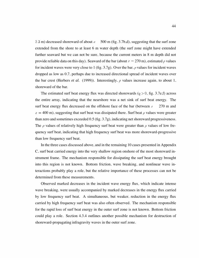
44

m) decreased shoreward of about x 500 m (fig. 3.7b,d), suggesting that the surf zone

extended from the shore to at least 6 m water depth (the surf zone might have extended

further seaward but we can not be sure, because the current meters in 8 m depth did not

provide reliable data on this day). Seaward of the bar (about x 270 m), estimated values

for incident waves were very close to 1 (fig. 3.7g). Over the bar, values for incident waves

dropped as low as 0.7, perhaps due to increased directional spread of incident waves over

the bar crest (Herbers et al. (1999)). Interestingly, values increase again, to about 1,

shoreward of the bar.

The estimated surf beat energy flux was directed shorewards (q , fig. 3.7e,f) across

the entire array, indicating that the nearshore was a net sink of surf beat energy. The

surf beat energy flux decreased on the offshore face of the bar (between x 270 m and

x 400 m), suggesting that surf beat was dissipated there. Surf beat values were greater

than zero and sometimes exceeded 0.5 (fig. 3.7g), indicating net shoreward progressiveness.

The values of relatively high frequency surf beat were greater than values of low fre-

quency surf beat, indicating that high frequency surf beat was more shoreward-progressive

than low frequency surf beat.

In the three cases discussed above, and in the remaining 10 cases presented in Appendix

C, surf beat carried energy into the very shallow region onshore of the most shoreward in-

strument frame. The mechanism responsible for dissipating the surf beat energy brought

into this region is not known. Bottom friction, wave breaking, and nonlinear wave in-

teractions probably play a role, but the relative importance of these processes can not be

determined from these measurements.

Observed marked decreases in the incident wave energy flux, which indicate intense

wave breaking, were usually accompanied by marked decreases in the energy flux carried

by low frequency surf beat. A simultaneous, but weaker, reduction in the energy flux

carried by high frequency surf beat was also often observed. The mechanism responsible

for the rapid loss of surf beat energy in the outer surf zone is not known. Bottom friction

could play a role. Section 4.3.4 outlines another possible mechanism for destruction of

shoreward-propagating infragravity waves in the outer surf zone.

45

0

5

Dep

th (

m)

a

0

1

2P.

E. (

m3 s−

2 )

b>0.05Hz

0

0.05

P.E

. (m

3 s−2 )

c

0.025−0.05Hz0.005−0.025Hz

0

10

20

q (m

4 s−3 ) d

−0.2

0

0.2 e

q (m

4 s−3 )

100 200 300 400 500 600 700 800 900−1

0

1

ρ

Cross−shore distance (m)

g

0

5

Dep

th (

m)

a

0

1

2P.

E. (

m3 s−

2 )

b>0.05Hz

0

0.05

P.E

. (m

3 s−2 )

c

0.025−0.05Hz0.005−0.025Hz

0

10

20

q (m

4 s−3 ) d

−0.1

0

0.1 f

q (m

4 s−3 )

100 200 300 400 500 600 700 800 900−1

0

1

ρ

Cross−shore distance (m)

g

Figure 3.7: Water depth (a), potential energy density PE (b: swell. c: surf beat), shore-ward energy flux q (d: swell. e: high frequency surf beat. f: low frequency surf beat), andprogressiveness parameter (g) versus cross-shore distance. Values estimated from 3 hrtime series on October 16th, Hs m. Squares: Swell ( Hz). Triangles: Highfrequency surf beat (– Hz). Circles: Low frequency surf beat (– Hz).

46

3.5 Summary

Frequency-domain EOF’s based on observations of near-bottom pressure and velocity along

a cross-shore transect between the shore and 8 m water depth on a barred beach were used

to identify the dominant spatially coherent components of surf beat. The dominant EOF’s

at relatively low beat frequencies (– Hz) were consistent with standing wave the-

ories. In contrast, the dominant EOF’s at relatively high beat frequencies (– Hz)

displayed a mixture of progressive and standing wave behaviours. The net shoreward en-

ergy flux carried by propagating surf beat was sometimes as large as half the energy flux

that could have been carried if all surf beat propagated directly shorewards, consistent with

partially progressive waves.

Surf beat carried energy towards the shore, where it was lost in water less than about

m deep. The cross-shore surf beat energy flux also converged in the outer surf zone,

suggesting strong surf beat dissipation there. The mechanism responsible for dissipating

surf beat is not known, but bottom friction, wave breaking, and nonlinear wave interactions

might play a role. The loss of infragravity energy in the outer surf zone is discussed further

in Chapter 4.

Chapter 4

Simulations of dissipative surf beat

4.1 Introduction

So far, this thesis has been devoted to presenting field evidence of strong shoreward surf

beat propagation, and an associated rapid loss of surf beat energy in the surf zone. Af-

ter finishing the analysis on which Chapter 2 is based, I visited Alex Sheremet and Bob

Guza at the Scripps Institution of Oceanography. I discovered that they had (independently

and simultaneously) also found strong shoreward surf beat propagation. They discovered

that they could not adequately fit pressure and velocity fluctuations measured by an ex-

tensive array of 35 instrumented frames with just a set of cross-shore standing waves —

energetic shoreward-progressive waves were required (Sheremet et al., 2001). They also

found that most shoreward-progressive waves propagated at an oblique angle to the shore.

Consequently, shoreward-propagating waves had the short longshore wavelengths that are

characteristic of edge waves.

Previously-published edge wave models assume that dissipation is weak, and therefore

predict that surf beat is cross-shore standing (Sections 1.3 and 2.5). Leaky wave models

do predict cross-shore propagation, regardless of the strength of dissipation (Sections 1.3

and 2.5), but the shore-oblique propagation observed by Alex Sheremet and co-workers

strongly suggests that the observed shoreward-propagating waves were not predominantly

leaky waves.

47

48

This chapter presents a model of infragravity waves that includes dissipation at lead-

ing order. The model is introduced in Section 4.2. The model simulates only shore-oblique

shallow water waves, and therefore can not simulate leaky waves. I discuss the possible im-

portance of leaky waves in Sections 4.2, 4.3, & 4.5. Section 4.3 presents model results. As

expected, dissipation introduces cross-shore propagating edge waves, which carry energy

from regions of forcing to regions of dissipation. Perhaps more surprisingly, shore-oblique

shallow water waves can be strongly modified by dissipation, even when dissipation is weak

and Q . In certain cases, including some high Q cases, evanescent waves can dominate

over edge waves. Realistic forcing generates group-bound evanescent waves, which appear

very similar to the group-bound waves described by Longuet-Higgins and Stewart (1962)

and Hasselmann et al. (1963). However, group-bound evanescent waves are not released

when wave groups are destroyed by breaking. Instead, incoming evanescent waves simply

disappear when the reach the vicinity of the breakpoint. Weak dissipation (Q ) can

also have a leading-order effect by decoupling bar- and shore-trapped edge waves. In Sec-

tion 4.5 I summarise the effects of dissipation on simulated shore-oblique shallow water

waves, and note several model predictions that could be tested using field data. Related

results were presented by Henderson and Bowen (2001).

4.2 Model derivation

4.2.1 Governing equations

In this Section we derive a set of equations that governs the dynamics of forced, dissipative,

shore-oblique shallow water waves.

Let

t time,

x distance from shore,

y longshore position,

49

u x component of Eulerian water velocity,

v y component of Eulerian water velocity,

Mx x component of Stokes drift,

My y component of Stokes drift,

u uMxh

v v Myh

h still water depth,

sea surface displacement,

g gravitational acceleration.

Here, x is positive seawards, in contrast to Chapter 2. The definition of MxMy as the

Stokes drift conflicts with the definition of M used in Chapter 2 because the mean water

depth differs from the still water depth. This error is small compared with other errors

inherent in the model presented in this Chapter, and will be ignored. I have included the

Stokes drift in the depth-averaged transport velocity u v (c.f. Longuet-Higgins and Stew-

art (1962) and p.62 of Phillips (1977)).

The forced, dissipative shallow water equations are

u

t g

x u Fx (4.1)

v

t g

y v Fy (4.2)

thu

xhv

y (4.3)

where is a damping coefficient (here assumed constant). I have assumed that friction acts

on the Eulerian flow, but not on the Stokes drift.

Let

h x (4.4)

50

where is a constant beach slope.

I have assumed unrealistically simple forms for h and , but Appendix E shows how

realistic conditions can be modeled by simply patching together solutions of eq.’s (4.1)–

(4.4).

Assume solutions of the form xeikyt, and similarly for u v Fx FyMx and

My . Since we are interested in steady, longshore-homogeneous waves, I assume and k

are real. The Fourier components defined here are a function of the longshore wavenumber

k, and are denoted with a hat (), whereas the Fourier components of Chapters 2 and 3 were

evaluated at a point, were not associated with a particular wavenumber, and were denoted

by angle brackets(h i). Solving eq.’s (4.1)–(4.4) for gives

x

x

x

g

i

kx

F (4.5)

where the dimensionless forcing is

F

g

x

x Fx Mx

ik

x Fy My

(4.6)

If and F then eq. (4.5) reduces to the free edge wave equation (Mei, 1983,

p.155).

Boundary conditions are

limx

x

x (4.7)

and

is bounded as x (4.8)

Equations (4.5), (4.7) & (4.8) govern forced, dissipative, shore-oblique shallow water

waves.

4.2.2 Forcing

The special case where F x is a Dirac delta-function (denoted by ) will play an important

role in the remainder of this Chapter. I refer to such forcing as ‘point forcing’, because it is

51

applied at a single cross-shore location, but recall that forcing is assumed to be sinusoidal

alongshore.

Many different fields of applied force F Fx Fy can produce the same forcing F

in the sea level equation (eq. 4.5). By choosing appropriate potentials P and P, we can

decompose the total force field into divergent and non-divergent parts:

F

hrP r Pz (4.9)

where z is a vertical unit vector. Only the divergent part of the forcing (rP) appears in the

sea level equation (eq. 4.5). Similarly, only the divergent part of the Stokes Drift appears in

the sea level equation. However, non-divergent components of the applied force and Stokes

Drift do appear the momentum equations.

Most results presented in this Chapter concern sea level fluctuations, not water velocity

fluctuations. Consequently, we seldom need to specify the non-divergent forcing. However,

non-divergent forcing will become important when we discuss the energy flux carried by

edge waves. When discussing energy fluxes, I will avoid ambiguity by partitioning F as

follows:

F F F (4.10)

F

x

x Fx i Mx

g

(4.11)

F ik

x Fy My

g

x

i Mx

g

(4.12)

If F x xF , then F is associated with point forcing (at xF ) in the longshore mo-

mentum and mass conservation equations (eq. 4.2 & 4.3), whereas F is associated with

distributed forcing (seaward of xF ) in the cross-shore momentum equation (eq. 4.1).

If surf beat is forced by the radiation stress, S , then

Fx

h

Sxxx

Sxyy

(4.13)

Fy

h

Syyy

Sxyx

(4.14)

52

and

F

g

Sxxx

ikSxyx

kSyy

g

Mx

x ik My

(4.15)

where water density.

4.2.3 Solution

Two linearly-independent homogeneous solutions of eq. (4.5), fA and fB , are derived in

Appendix D. fB satisfies the shoreline boundary condition (eq. (4.7)), but not the seaward

boundary condition (eq. (4.8)), whereas fA satisfies the seaward boundary condition but

not the shoreline boundary condition. Since no linear combination of fA and fB satisfies

both boundary conditions, no steady homogeneous solution of eq.’s (4.5), (4.7) & (4.8)

exists. This is not surprising, since no steady unforced wave field can exist in the presence

of dissipation.

fA and fB can be used to construct forced solutions to eq.’s (4.5), (4.7) & (4.8). The

dimensionless Green’s function

Gx xF

BfBkx x xF

AfAkx x xF (4.16)

where A and B are chosen to satisfy

limxxF

Gx xF limxxF

Gx xF (4.17)

and

limxxF

Gx xF

x lim

xxF

Gx xF

x

xF (4.18)

is the response at x to point forcing F x xF , where is the Dirac delta func-

tion. Therefore, fA represents the wave field seaward of the point of forcing, whereas fB

represents the wave field shoreward of the point of forcing.

The particular solution of eq.’s (4.5), (4.7) & (4.8) for arbitrary F x is (Arfken and

Weber, 2001, p.618)

x

ZxF

Gx xF F xF dxF (4.19)

53

Therefore, the response to forcing at one cross-shore location is described by a Green’s

function, and the response to distributed forcing given by an integral of Green’s func-

tions. The behaviour of the Green’s functions is described in Sections 4.3.1–4.3.3, and

the response to distributed forcing (by groups of incident breaking waves) is discussed in

Section 4.3.4.

Appendix E shows how forced, dissipative shallow water waves can be simulated for

complex profiles of water depth and dissipation strength by patching together the planar

beach solutions discussed in this Section.

fA and fB are functions of the non-dimensional cross-shore distance

kx (4.20)

the dissipation strength , and the mode number

n

kg

(4.21)

Eckart (1951) showed that, in the absence of forcing and dissipation, edge waves exist on a

planar beach only for integer values of the mode number n. In contrast, forced waves have

the wavenumber and frequency of the applied forcing, and exist for non-integer values of

n. I refer to n as the mode number, even when n takes non-integer values.

Figure 4.1 summarises the behaviour of fA for n between -0.5 and 4.5. A vertical

section through each plot gives the cross-shore structure of the wave field for a particular

value of n. Figure 4.1a,b shows weakly-dissipative waves, and fig. 4.1c,d shows strongly-

dissipative waves. Since fA is a homogeneous solution, its amplitude is arbitrary. In

fig.4.1a,c, fA has been renormalised so that the mean square value of fA shoreward of

the edge wave turning point (where gh k, dashed line in fig. 4.1) equals one.

Recall that fA represents the wave field seaward of regions of forcing. Waves propagating

seawards, away from regions of forcing, are reflected from the turning point. Outside the

turning point the magnitude of fA decays almost exponentially. Waves reflected from the

turning point interfere with outgoing waves, setting up a cross-shore standing pattern, with

nodes and antinodes (light and dark bands in fig. 4.1a), and 180 degree phase jumps at the

nodes (fig. 4.1b). The cross-shore standing structure, clear in the weakly-dissipative case

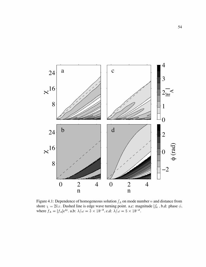
54

0 2 4

8

16

24

n

χ

b

8

16

24

χ

a

−2

0

2

φ (r

ad)

0 2 4n

d

0

1

2

3

4

|f A|

c

Figure 4.1: Dependence of homogeneous solution fA on mode number n and distance fromshore kx. Dashed line is edge wave turning point. a,c: magnitude jfaj, b,d: phase ,where fA jfAjei. a,b: , c,d: .

55

(fig. 4.1a,b), is modified by dissipation, as shown most clearly in the strongly-dissipative

case (fig. 4.1c,d). Since energy is dissipated as waves propagate to the turning point and

back, the nodal structure is incomplete (weakly-developed light and dark bands in fig. 4.1c)

and net seaward propagation results (except for wraps, the phase increases smoothly

with distance from shore in fig. 4.1d).

Figure 4.2 summarises the behaviour of fB. Inside the edge wave turning point, waves

propagate shorewards, away from regions of forcing, and reflect from the shore, setting

up a standing wave structure (fig. 4.2a,b). Dissipation leads to net shoreward propagation

(fig. 4.2d), and weakened nodal structure (fig. 4.2c). For non-integer mode numbers, fB

grows almost exponentially with distance seaward of the turning point. For near-integer

mode numbers, the exponential growth of fB begins far seaward of the turning point. Note

that all magnitudes greater than 4 are represented by black shading in fig. 4.2a,c. Conse-

quently, the region of exponential growth seaward of the turning point, where magnitudes

often greatly exceed 4, is black in fig. 4.2a,c.

For integer mode numbers, both fA and fB converge to the classical non-dissipative

solution of Eckart (1951) as tends to zero. However, this convergence is non-uniform.

For finite , there is always a neighborhood of x in which fA differs greatly from the

non-dissipative solution. Similarly, for finite , fB differs greatly from the non-dissipative

solution for sufficiently large x.

All shore-oblique shallow water waves have a turning point at n . Near the

turning point, waves propagate almost parallel to the shore. However, when n becomes

large, the turning point moves far offshore, and near the shore the wave field becomes

almost shore-normal. When n and x is fixed, fB tends towards the dissipative shore-

normal homogeneous solution

x J

ix

g

(4.22)

where J is the zero-order Bessel function (Magnus et al., 1966, 2nd identity, Section

6.7.1). However, at the turning point,

kh n (4.23)

56

For sufficiently large n, kh is order-one at the turning point, and the shallow water approx-

imation fails. If is small, this problem can be overcome by matching the shallow water

solution to a fully-dispersive WKB solution. If n , the resulting waves are leaky

waves. I have assumed that shallow water theory holds at leading order, which is true at the

turning point only when n . Consequently, leaky waves are excluded from my

analysis. I discuss the possible importance of leaky waves in Sections 4.3.2 & 4.3.4.

4.3 Model results

The functions fA and fB shown in fig.’s 4.1 & 4.2, together with conditions (4.17) & (4.18),

determine the wave field generated by point forcing. The wave field generated by dis-

tributed forcing is an integral of responses to point forcing (eq. (4.19)). Consequently,

much of the qualitative behaviour of forced, dissipative shallow water waves can be deter-

mined by inspection of fig.’s 4.1 & 4.2. This Section contains examples of forced, dissipa-

tive shallow water waves, which illustrate physical phenomena such as refractive trapping,

resonance, evanescence, and dissipative decoupling.

4.3.1 Edge waves

Figure 4.3 shows Green’s functions for dissipative waves of 40 s period, forced shoreward

of the edge wave turning point (at x 140 m), on a planar beach of slope 0.02. The

cross-shore structure of the weakly-dissipated mode 2 wave (fig. 4.3a,b) is very similar to

the cross-shore structure of a free mode 2 edge wave (Mei, 1983, p.156). The cross-shore

structure of the weakly-dissipated mode 2.5 wave (fig. 4.3c,d) depends strongly on the

location of the forcing, and differs from the structure of free waves. I refer to both mode

2 and mode 2.5 waves as ‘edge waves’, because both are trapped close to the shore (near

the edge of the ocean) by refraction. Figure 4.3e–h shows strongly-dissipated mode 2 and

2.5 waves. The wave field is now a mixture of cross-shore standing waves and cross-shore

progressive waves. The waves are still trapped near the shore by refraction, and therefore

can still be called ‘edge waves’. Since edge waves also propagate alongshore (with speed

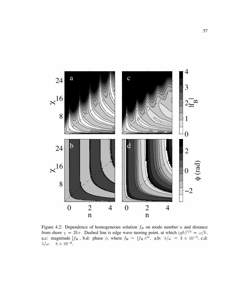
57

0 2 4

8

16

24

n

χ

b

8

16

24

χ

a

−2

0

2

φ (r

ad)

0 2 4n

d

0

1

2

3

4

|f B|

c

Figure 4.2: Dependence of homogeneous solution fB on mode number n and distancefrom shore kx. Dashed line is edge wave turning point, at which gh k.a,c: magnitude jfBj, b,d: phase , where fB jfBjei. a,b: , c,d: .

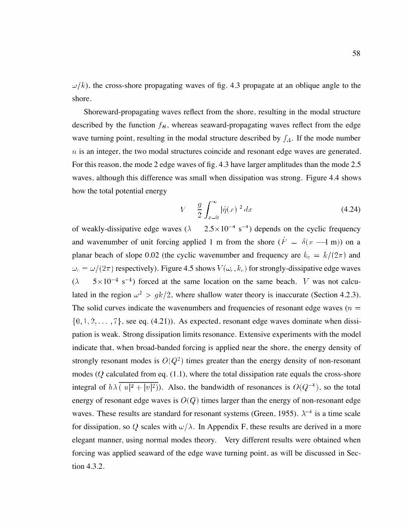
58

k), the cross-shore propagating waves of fig. 4.3 propagate at an oblique angle to the

shore.

Shoreward-propagating waves reflect from the shore, resulting in the modal structure

described by the function fB , whereas seaward-propagating waves reflect from the edge

wave turning point, resulting in the modal structure described by fA. If the mode number

n is an integer, the two modal structures coincide and resonant edge waves are generated.

For this reason, the mode 2 edge waves of fig. 4.3 have larger amplitudes than the mode 2.5

waves, although this difference was small when dissipation was strong. Figure 4.4 shows

how the total potential energy

V g

Z

x

jxj dx (4.24)

of weakly-dissipative edge waves ( 2.510 s) depends on the cyclic frequency

and wavenumber of unit forcing applied 1 m from the shore ( F x 1 m) on a

planar beach of slope 0.02 (the cyclic wavenumber and frequency are kc k and

c respectively). Figure 4.5 shows V c kc for strongly-dissipative edge waves

( 510 s) forced at the same location on the same beach. V was not calcu-

lated in the region gk, where shallow water theory is inaccurate (Section 4.2.3).

The solid curves indicate the wavenumbers and frequencies of resonant edge waves (n

f g, see eq. (4.21)). As expected, resonant edge waves dominate when dissi-

pation is weak. Strong dissipation limits resonance. Extensive experiments with the model

indicate that, when broad-banded forcing is applied near the shore, the energy density of

strongly resonant modes is OQ times greater than the energy density of non-resonant

modes (Q calculated from eq. (1.1), where the total dissipation rate equals the cross-shore

integral of h juj jvj). Also, the bandwidth of resonances is OQ, so the total

energy of resonant edge waves is OQ times larger than the energy of non-resonant edge

waves. These results are standard for resonant systems (Green, 1955). is a time scale

for dissipation, so Q scales with . In Appendix F, these results are derived in a more

elegant manner, using normal modes theory. Very different results were obtained when

forcing was applied seaward of the edge wave turning point, as will be discussed in Sec-

tion 4.3.2.

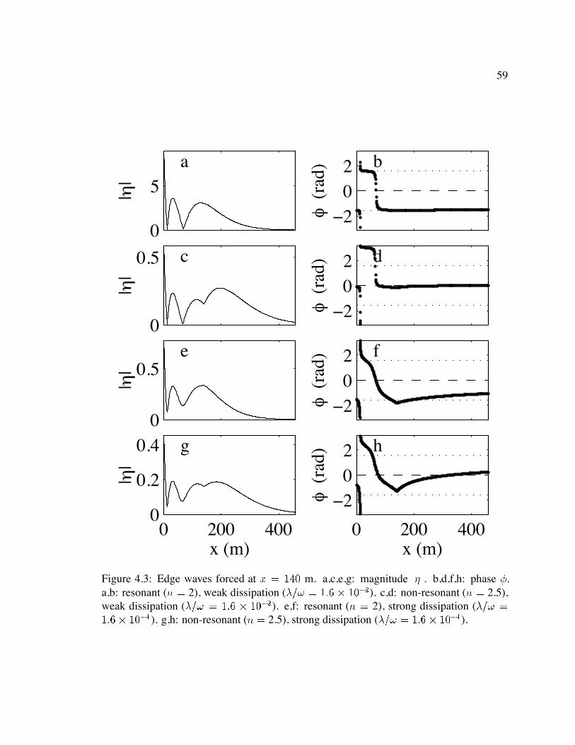
59

0

5

|η

| a

−202

φ (

rad)

b

0

0.5

|η

| c

−202

φ (

rad)

d

0

0.5

|η

| e

−202

φ (

rad)

f

0 200 4000

0.2

0.4

x (m)

|η

| g

0 200 400

−202

x (m)

φ (

rad)

h

Figure 4.3: Edge waves forced at x m. a,c,e,g: magnitude jj. b,d,f,h: phase .a,b: resonant (n 2), weak dissipation ( ). c,d: non-resonant (n 2.5),weak dissipation ( ). e,f: resonant (n 2), strong dissipation ( ). g,h: non-resonant (n 2.5), strong dissipation ( ).

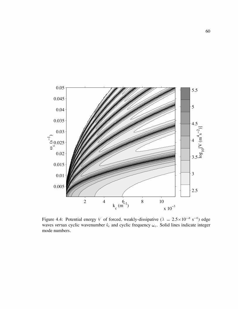
60

2.5

3

3.5

4

4.5

5

5.5

log 10

[V (

m4 s−

2 )]2 4 6 8 10

x 10−3

0.005

0.01

0.015

0.02

0.025

0.03

0.035

0.04

0.045

0.05

kc (m−1)

ωc (

s−1 )

Figure 4.4: Potential energy V of forced, weakly-dissipative ( 2.510 s) edgewaves versus cyclic wavenumber kc and cyclic frequency c. Solid lines indicate integermode numbers.

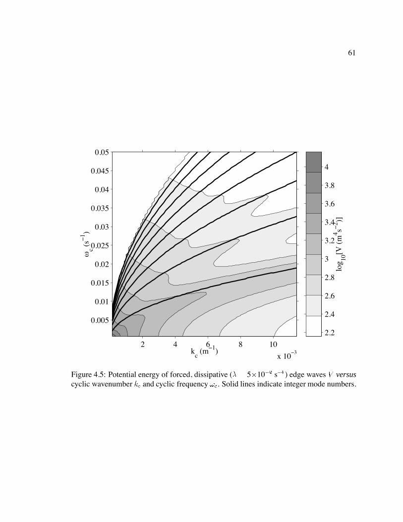
61

2.2

2.4

2.6

2.8

3

3.2

3.4

3.6

3.8

4

log 10

[V (

m4 s−

2 )]2 4 6 8 10

x 10−3

0.005

0.01

0.015

0.02

0.025

0.03

0.035

0.04

0.045

0.05

kc (m−1)

ωc (

s−1 )

Figure 4.5: Potential energy of forced, dissipative ( 510 s) edge waves V versuscyclic wavenumber kc and cyclic frequency c. Solid lines indicate integer mode numbers.

62

Propagating shallow water waves carry an energy flux, equal to the mean depth-integrated

product of water pressure and velocity (Section 2.2). The divergence of the energy flux

equals the rate of net generation of surf beat energy (negative if dissipation exceeds gener-

ation) (Section 2.2).

As was discussed in Section 4.2.2, the sea level fluctuates in response to the forcing

F F F (eq.’s (4.5), (4.10), (4.11), and (4.12)), whereas the cross-shore velocity is

unaffected by F (eq.’s (4.1) & (4.12)). Consequently, the cross-shore energy flux depends

not only on F , but also on the manner in which F is partitioned into F and F. Fig-

ure 4.6a,c,e,g shows the shoreward energy flux carried by the edge waves of fig. 4.3 when

F F (so F ). Infragravity energy is generated at the point of forcing (where the

divergence of the energy flux is singular and positive), and carried to surrounding regions

of dissipation (where the energy flux converges). Figure 4.6b,d,f,h shows the cross-shore

energy flux carried by the edge waves of fig. 4.3 when F F (so F ). Shoreward

of xF , the motion is unforced and the shoreward energy flux is the same as it was whenF F. Seaward of xF , hFx Mxt is non-zero, and the energy flux usually diverges,

indicating that the work done by the forcing usually exceeds dissipation. However, in some

parts of the region x xF , dissipation exceeds forcing and the energy flux converges.

In the field, the non-dimensional energy flux (eq. (2.33)) is as large as 0.5 during

storms, indicating strong shoreward propagation. Figure 4.7 shows the non-dimensional

energy flux for the edge waves presented in fig. 4.3. Shoreward of the turning point, both

resonant and non-resonant weakly-dissipative edge waves are almost cross-shore standing,

so (fig. 4.7a–d). In contrast, strongly-dissipative edge waves propagate across-shore

(fig. 4.3e–h), and have jj values as large as 0.5. Outside the turning point, departs from

zero in the weakly-dissipative, resonant case shown in fig. 4.7b, although the associated

energy flux is very small (fig. 4.6b). Cross-shore energy transport outside the turning point

is discussed in the next section.

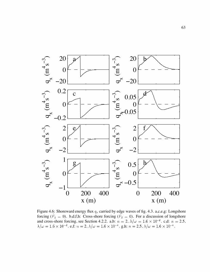
63

−20

0

20

q x (m

4 s−3 ) a

−20

0

20

q x (m

4 s−3 ) b

−0.2

0

0.2

q x (m

4 s−3 ) c

−0.050

0.05

q x (m

4 s−3 ) d

−2

0

2

q x (m

4 s−3 ) e

−2

0

2

q x (m

4 s−3 ) f

0 200 400−1

0

1

x (m)

q x (m

4 s−3 ) g

0 200 400

−0.50

0.5

x (m)

q x (m

4 s−3 ) h

Figure 4.6: Shoreward energy flux qx carried by edge waves of fig. 4.3. a,c,e,g: Longshoreforcing ( F ). b,d,f,h: Cross-shore forcing ( F ). For a discussion of longshoreand cross-shore forcing, see Section 4.2.2. a,b: n 2, . c,d: n 2.5, . e,f: n 2, . g,h: n 2.5, .

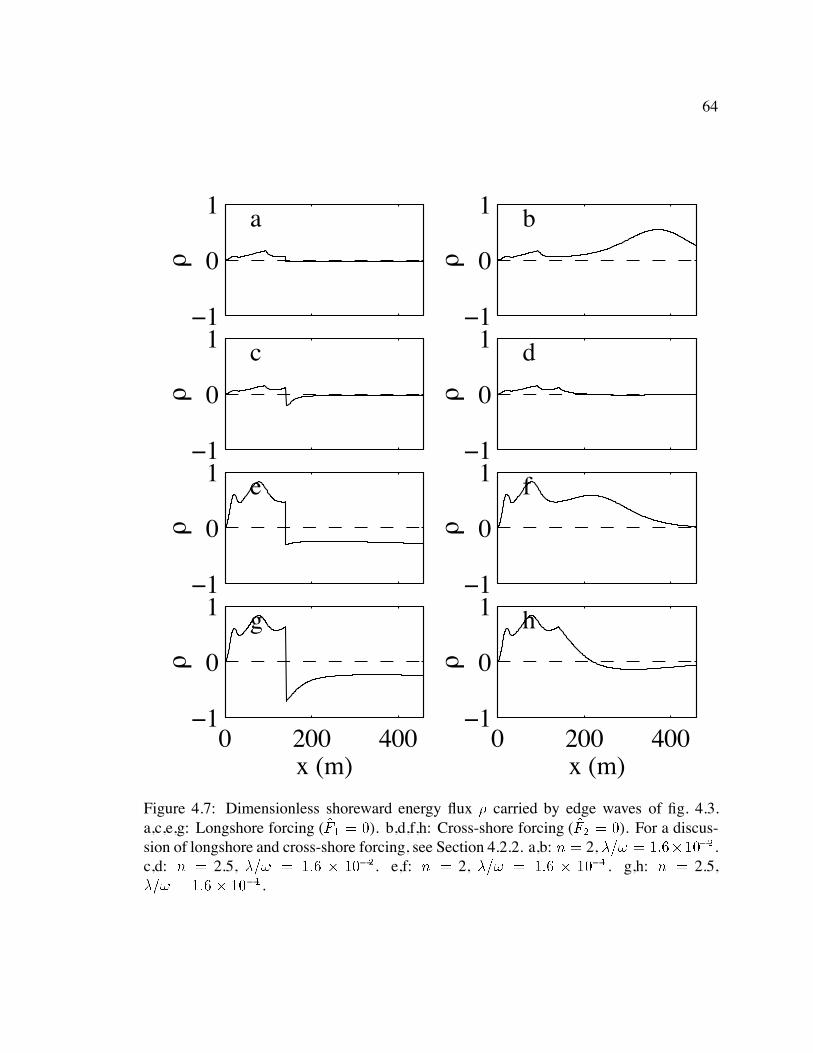
64

−1

0

1

ρ

a

−1

0

1

ρ

b

−1

0

1

ρ

c

−1

0

1

ρ

d

−1

0

1

ρ

e

−1

0

1

ρ

f

0 200 400−1

0

1

x (m)

ρ

g

0 200 400−1

0

1

x (m)

ρ

h

Figure 4.7: Dimensionless shoreward energy flux carried by edge waves of fig. 4.3.a,c,e,g: Longshore forcing ( F ). b,d,f,h: Cross-shore forcing ( F ). For a discus-sion of longshore and cross-shore forcing, see Section 4.2.2. a,b: n 2, .c,d: n 2.5, . e,f: n 2, . g,h: n 2.5, .

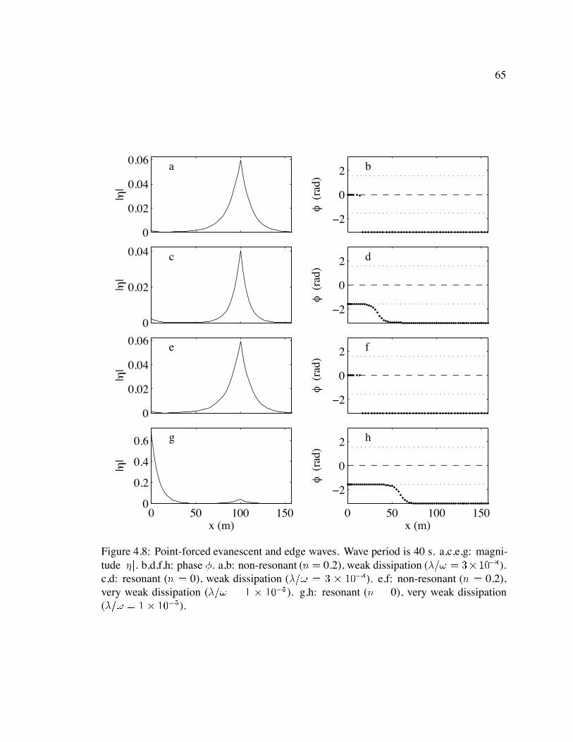
65

0

0.02

0.04

0.06

|η

|

a

−2

0

2

φ (

rad)

b

0

0.02

0.04

|η

|

c

−2

0

2

φ (

rad)

d

0

0.02

0.04

0.06

|η

|

e

−2

0

2

φ (

rad)

f

0 50 100 1500

0.2

0.4

0.6

x (m)

|η

|

g

0 50 100 150

−2

0

2

x (m)

φ (

rad)

h

Figure 4.8: Point-forced evanescent and edge waves. Wave period is 40 s. a,c,e,g: magni-tude jj. b,d,f,h: phase . a,b: non-resonant (n 0.2), weak dissipation ( ).c,d: resonant (n 0), weak dissipation ( ). e,f: non-resonant (n 0.2),very weak dissipation ( ). g,h: resonant (n 0), very weak dissipation( ).

66

4.3.2 Evanescent waves

Forcing applied shoreward of the edge wave turning point generates edge waves (Sec-

tion 4.3.1). Figure 4.8 shows that very different behaviour can result when forcing is ap-

plied seaward of the turning point (xF 100 m, xT 8 m). Only when forcing was reso-

nant, and dissipation was extremely weak, were energetic edge waves excited (fig. 4.8g,h).

Otherwise, only localised waves were generated (fig. 4.8a–f). These localised waves were

‘evanescent’, that is, they did not propagate freely, but decayed approximately exponen-

tially with cross-shore distance away from the point of forcing.

A simple model explains the behaviour shown in fig. 4.8. From eq. (1.1), the edge wave

energy dissipated in a single period is

D gaedgexT

Q (4.25)

where gaedgexT is the total energy of the edge wave, and aedge is a typical edge wave

amplitude.

Forcing is applied only outside the turning point, so the energy flux carried to the turn-

ing point by evanescent waves must balance the edge wave dissipation D. I will derive

an approximate expression for the energy flux carried to the turning point by evanescent

waves, and then calculate the relative amplitudes of edge and evanescent waves by equating

this energy flux with edge wave dissipation. The energy flux carried by evanescent waves is

mathematically analogous to the probability flux carried by quantum-mechanical particles

tunneling through a potential barrier (Ohanian, 1990, Section 3). Consequently, the evanes-

cent wave energy flux can be estimated using standard methods of quantum mechanics. A

crude approximation of the cross-shore structure of evanescent waves is

aeieKxxT ae

ieKxxF (4.26)

where a and a are approximately the evanescent wave amplitudes at xT and xF respec-

tively, and are real constants, and K . The cross-shore e-folding distance for

evanescent waves is (Longuet-Higgins, 1967, p.788)

K k gh (4.27)

67

Equation (4.27) is simplified by assuming h xT xF , which is the water depth

half way between the point of forcing and the turning point. From eq.’s (2.21), (4.1), (4.26)

& (4.27), the amount of energy carried to the turning point by evanescent waves in a single

period is

qx

Khg

eKLaa sin (4.28)

where L xF xT . When KL is large, evanescent waves decay greatly between the point

of forcing and the turning point, and therefore can carry very little energy to the turning

point.

Equating edge wave forcing and dissipation, noting that hxT , a aedge, a

aev (where aev is the evanescent wave amplitude at xF ), leads to

aedgeaev

O

K

k

sin

n

QeKL

(4.29)

(eq. (4.29) has been simplified using eq. (4.21)). The ratio between edge and evanescent

wave amplitudes depends on their relative phase . For resonant edge waves,

, so sin (eg. fig. 4.8d,h). In contrast, can be close to

or 0 (so sin can be much less than one) if edge waves are non-resonant (eg.

fig. 4.8b,f). Figure 4.9 shows that eq. (4.29), with sin , predicted the ratio

between evanescent and resonant edge wave amplitudes to within a factor of 2, except when

edge waves were much larger than evanescent waves (aedgeaev ) and KL is small

(KL ). For KL , forcing is very close to the turning point, and eq. (4.29) fails.

Non-resonant edge waves are much smaller than evanescent waves when KL is large. If

forcing is broad-banded, then the bandwidth of the spectral peaks associated with resonant

edge waves is OQ (Section 4.3.1), so the ratio between total edge and evanescent wave

energy scales with QeKLn kK. When KL is large, evanescent waves can

dominate over edge waves, even if Q .

According to shallow water theory, all shore-oblique waves have a turning point, sea-

ward of which waves are evanescent. In reality, waves have a turning point if and only

if gk. If gk, waves are leaky and are nowhere evanescent. Therefore, when

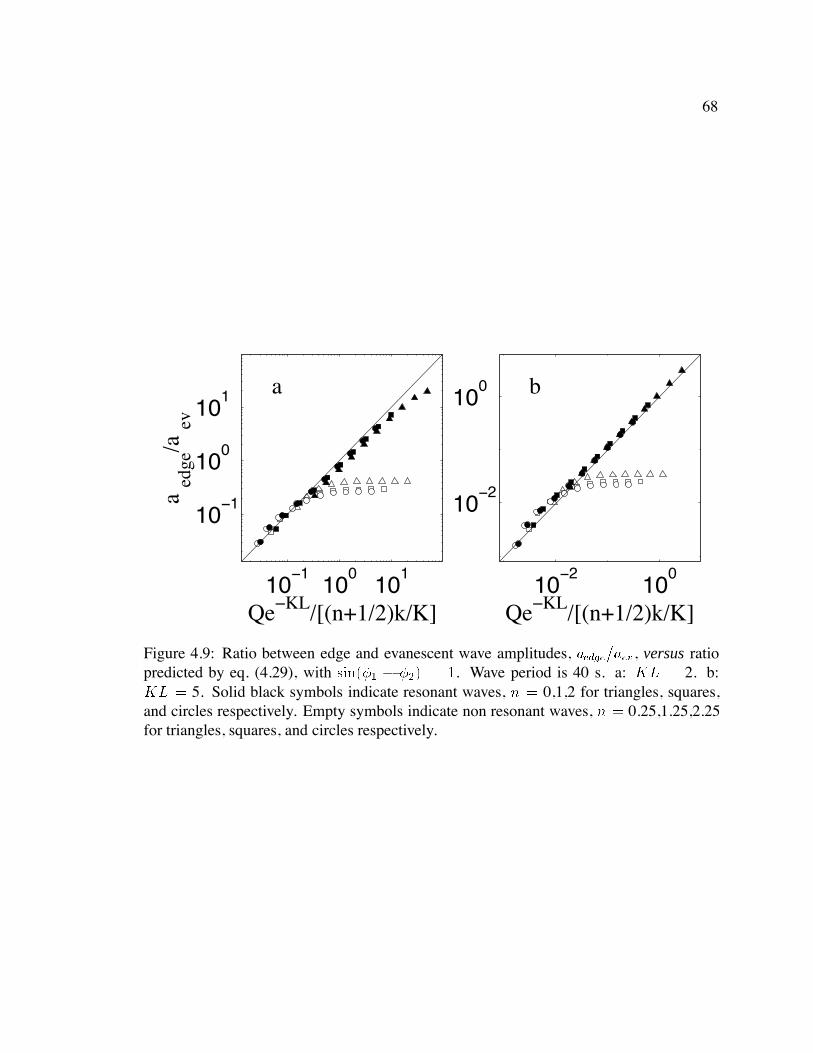
68

10−1

100

101

10−1

100

101 a

Qe−KL/[(n+1/2)k/K]

aed

ge/a

ev

10−2

100

10−2

100 b

Qe−KL/[(n+1/2)k/K]

Figure 4.9: Ratio between edge and evanescent wave amplitudes, aedgeaev , versus ratiopredicted by eq. (4.29), with sin . Wave period is 40 s. a: KL 2. b:KL 5. Solid black symbols indicate resonant waves, n 0,1,2 for triangles, squares,and circles respectively. Empty symbols indicate non resonant waves, n 0.25,1.25,2.25for triangles, squares, and circles respectively.

69

gk, forcing sufficiently far offshore produces only a localised evanescent response,

whereas when gk, energy can always be radiated far from the point of forcing.

4.3.3 Dissipative decoupling

Schonfeldt (1995), Bryan and Bowen (1996), and Bryan et al. (1998) showed that refrac-

tion can trap edge waves over sandbars. When waves are trapped over sandbars, evanescent

waves exist between the sandbar and the beach. Evanescent waves transport very little en-

ergy over cross-shore distances large compared with k gh (Section 4.3.2).

Consequently, the region of evanescent waves shoreward of the sandbar is a barrier to en-

ergy transport which can effectively decouple dissipative bar- and shore-trapped waves.

If forcing is applied only over the sandbar, and a region of evanescent waves exists

between the sandbar and the shore, then an argument similar to the one used to derive

eq. (4.29) leads to

ashoreabar

O

K

k

sins b

n

QeKL

(4.30)

where ashore and abar are the amplitudes of shore- and bar-trapped waves respectively, L

is the width of the region of evanescent waves in the trough, b and s are the respective

phases of bar- and shore-trapped waves at their turning points, and n is the mode number of

the shore-trapped wave. K is the e-folding distance for evanescent waves in the trough,

which I crudely approximate by k ghT htrough, where hT is the turning

depth, and htrough is the maximum water depth in the trough. As in Section 4.3.2, sinb

s is about one (zero) if shore-trapped waves are (are not) resonant.

If forcing is applied at the shoreface, then abarashore approximately equals the negative

of the right-hand side of eq. (4.30) (the term n is modified, but on realistic beaches the

order of magnitude of abarashore remains unchanged). If QeKLn kK ,

then forcing over the bar does not generate significant shore-trapped waves, and forcing

over the shoreface does not generate significant bar-trapped waves. In this case, bar- and

shore-trapped waves have negligible influence on one-another, and we say that they are

‘dissipatively decoupled’. If the trough is wide and deep, then even high Q waves can be

70

decoupled.

An example of a barred beach is shown in fig. 4.10. I solve eq.’s (4.1), (4.2) & (4.3) for

the beach shown in fig. 4.10 by patching together planar beach solutions, as described in

Appendix E.

Figure 4.11 shows how the total potential energy of weakly-dissipative waves V

(eq. (4.24)) depends on the wavenumber and frequency of unit forcing applied 0.3 m from

the shore ( F x 0.3 m). V is presented for both infragravity and incident frequen-

cies, because field observations show that bar-trapped waves can be important at incident

frequencies (Bryan et al., 1998). Shoreward of the trough, the barred beach of fig. 4.10 has

a slope of 0.045, so resonant waves trapped shoreward of the trough will have wavenum-

bers and frequencies close to the wavenumbers and frequencies of resonant edge waves

on a planar beach of slope 0.045. The solid curves of fig. 4.11 mark these planar-beach

resonance curves (n f g, see eq. (4.21)).

If the edge wave turning depth (hT ) is greater than the maximum water depth in the

trough (htrough), then oscillatory edge waves exist over the entire region from the shore to

the bar, and evanescent waves exist only seaward of the bar (Bryan and Bowen, 1996). I

will call the region of wavenumber-frequency space where hT htrough ‘Region 1’. The

dash-dotted line in fig. 4.11 marks hT htrough, so Region 1 lies above and to the left of

this line.

When hbar hT htrough, oscillatory waves exist over both the shoreface and the bar,

and evanescent waves exist both in the trough and seaward of the bar. I will call the region

of wavenumber-frequency space where hbar hT htrough Region 2. The dashed line

in fig. 4.11 marks hT hbar, so Region 2 lies between the dashed and dash-dotted lines.

Trapping and amplification of edge waves over the bar occurs only in Region 2. Resonance

curves for bar-trapped waves are lines in Region 2 lying almost parallel to hT hbar

(Bryan and Bowen, 1996).

If hT hbar, then oscillatory waves exist only on the shoreface, whereas evanescent

waves exist over the trough, the bar, and seaward of the bar. The region of wavenumber-

frequency space where hT hbar, which I call Region 3, lies below and to the right of the

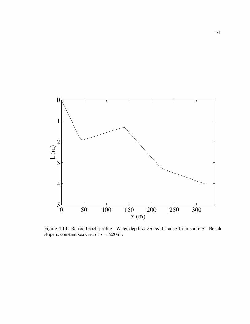
71

0 50 100 150 200 250 300

0

1

2

3

4

5

x (m)

h (m

)

Figure 4.10: Barred beach profile. Water depth h versus distance from shore x. Beachslope is constant seaward of x 220 m.

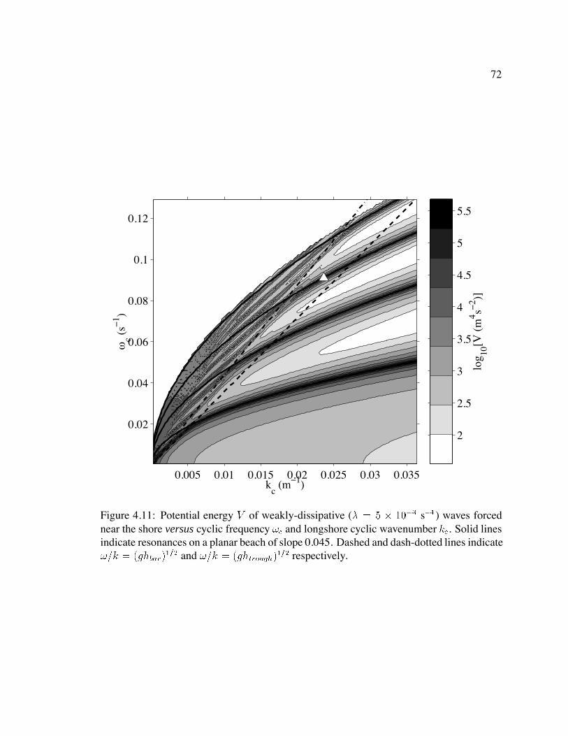
72

2

2.5

3

3.5

4

4.5

5

5.5

log 10

[V (

m4 s−

2 )]0.005 0.01 0.015 0.02 0.025 0.03 0.035

0.02

0.04

0.06

0.08

0.1

0.12

kc (m−1)

ωc (

s−1 )

Figure 4.11: Potential energy V of weakly-dissipative ( s) waves forcednear the shore versus cyclic frequency c and longshore cyclic wavenumber kc. Solid linesindicate resonances on a planar beach of slope 0.045. Dashed and dash-dotted lines indicatek ghbar and k ghtrough respectively.

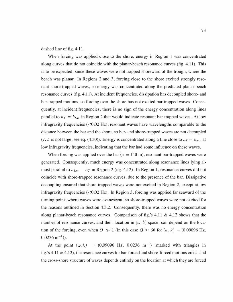
73

dashed line of fig. 4.11.

When forcing was applied close to the shore, energy in Region 1 was concentrated

along curves that do not coincide with the planar-beach resonance curves (fig. 4.11). This

is to be expected, since these waves were not trapped shoreward of the trough, where the

beach was planar. In Regions 2 and 3, forcing close to the shore excited strongly reso-

nant shore-trapped waves, so energy was concentrated along the predicted planar-beach

resonance curves (fig. 4.11). At incident frequencies, dissipation has decoupled shore- and

bar-trapped motions, so forcing over the shore has not excited bar-trapped waves. Conse-

quently, at incident frequencies, there is no sign of the energy concentration along lines

parallel to hT hbar in Region 2 that would indicate resonant bar-trapped waves. At low

infragravity frequencies (0.02 Hz), resonant waves have wavelengths comparable to the

distance between the bar and the shore, so bar- and shore-trapped waves are not decoupled

(KL is not large, see eq. (4.30)). Energy is concentrated along a line close to hT hbar at

low infragravity frequencies, indicating that the bar had some influence on these waves.

When forcing was applied over the bar (x m), resonant bar-trapped waves were

generated. Consequently, much energy was concentrated along resonance lines lying al-

most parallel to hbar hT in Region 2 (fig. 4.12). In Region 1, resonance curves did not

coincide with shore-trapped resonance curves, due to the presence of the bar. Dissipative

decoupling ensured that shore-trapped waves were not excited in Region 2, except at low

infragravity frequencies (0.02 Hz). In Region 3, forcing was applied far seaward of the

turning point, where waves were evanescent, so shore-trapped waves were not excited for

the reasons outlined in Section 4.3.2. Consequently, there was no energy concentration

along planar-beach resonance curves. Comparison of fig.’s 4.11 & 4.12 shows that the

number of resonance curves, and their location in k space, can depend on the loca-

tion of the forcing, even when Q (in this case Q for k (0.09096 Hz,

0.0236 m)).

At the point k (0.09096 Hz, 0.0236 m) (marked with triangles in

fig.’s 4.11 & 4.12), the resonance curves for bar-forced and shore-forced motions cross, and

the cross-shore structure of waves depends entirely on the location at which they are forced

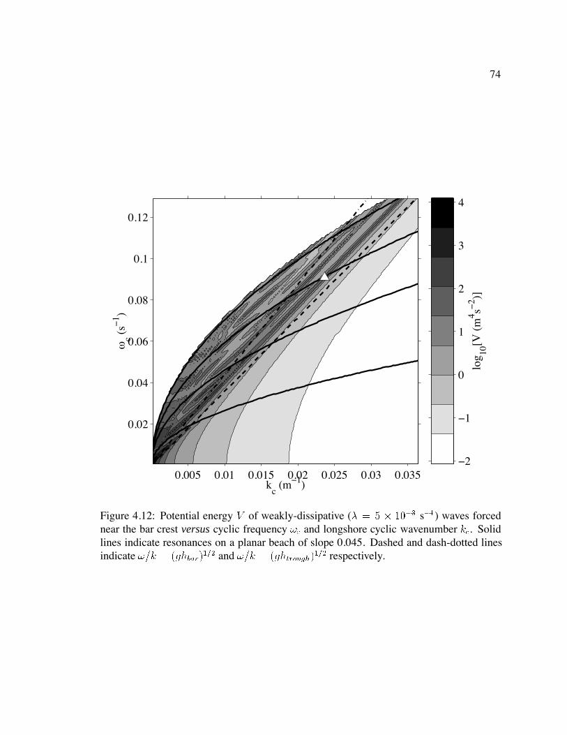
74

−2

−1

0

1

2

3

4

log 10

[V (

m4 s−

2 )]0.005 0.01 0.015 0.02 0.025 0.03 0.035

0.02

0.04

0.06

0.08

0.1

0.12

kc (m−1)

ωc (

s−1 )

Figure 4.12: Potential energy V of weakly-dissipative ( s) waves forcednear the bar crest versus cyclic frequency c and longshore cyclic wavenumber kc. Solidlines indicate resonances on a planar beach of slope 0.045. Dashed and dash-dotted linesindicate k ghbar and k ghtrough respectively.

75

0

20

|η

| a

−202

φ (

rad)

b

0 100 2000

0.5

x (m)

|η

| c

0 100 200

−202

x (m)

φ (

rad)

d

Figure 4.13: Weakly-dissipative ( s) waves of cyclic frequency 0.09096 Hzand cyclic wavenumber 0.0236 m. a,c: magnitude jj. b,d: phase . a,b: Forced nearshore. c,d: Forced near bar crest.

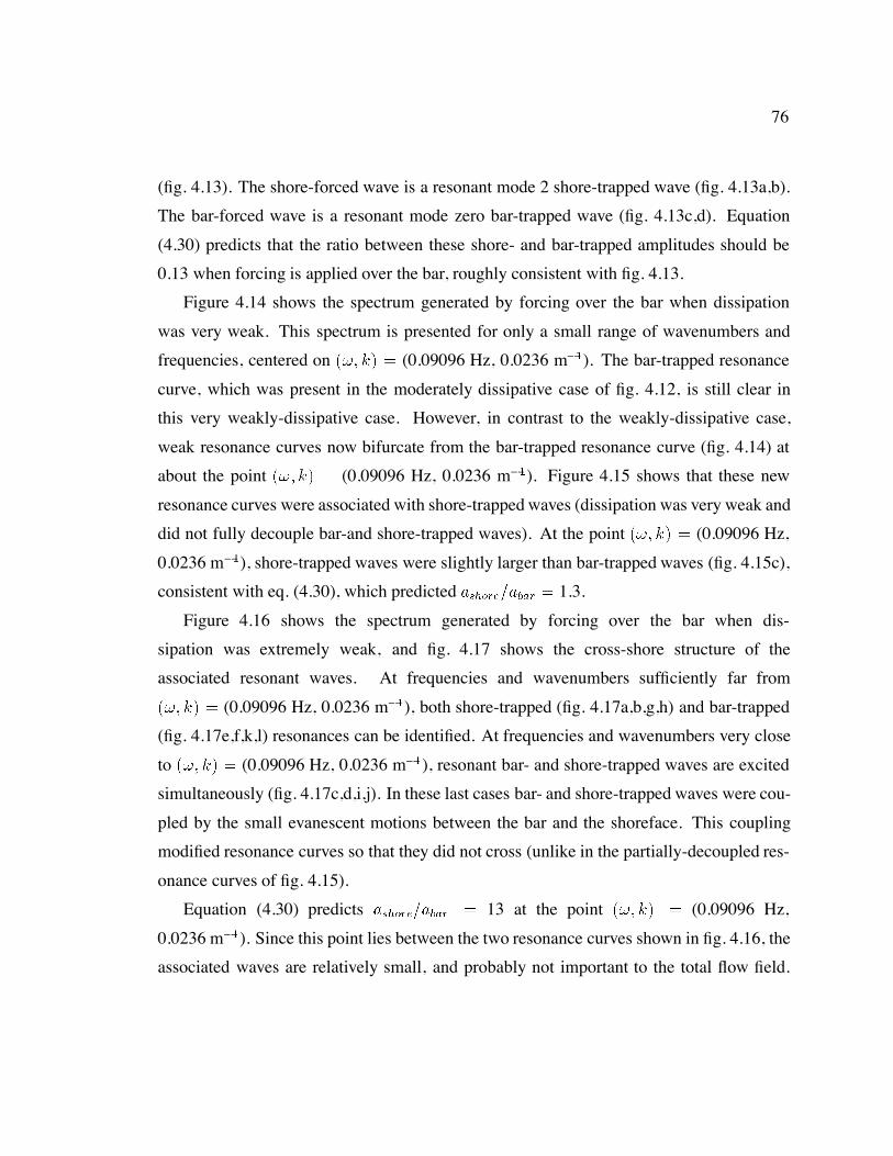
76

(fig. 4.13). The shore-forced wave is a resonant mode 2 shore-trapped wave (fig. 4.13a,b).

The bar-forced wave is a resonant mode zero bar-trapped wave (fig. 4.13c,d). Equation

(4.30) predicts that the ratio between these shore- and bar-trapped amplitudes should be

0.13 when forcing is applied over the bar, roughly consistent with fig. 4.13.

Figure 4.14 shows the spectrum generated by forcing over the bar when dissipation

was very weak. This spectrum is presented for only a small range of wavenumbers and

frequencies, centered on k (0.09096 Hz, 0.0236 m). The bar-trapped resonance

curve, which was present in the moderately dissipative case of fig. 4.12, is still clear in

this very weakly-dissipative case. However, in contrast to the weakly-dissipative case,

weak resonance curves now bifurcate from the bar-trapped resonance curve (fig. 4.14) at

about the point k (0.09096 Hz, 0.0236 m). Figure 4.15 shows that these new

resonance curves were associated with shore-trapped waves (dissipation was very weak and

did not fully decouple bar-and shore-trapped waves). At the point k (0.09096 Hz,

0.0236 m), shore-trapped waves were slightly larger than bar-trapped waves (fig. 4.15c),

consistent with eq. (4.30), which predicted ashoreabar 1.3.

Figure 4.16 shows the spectrum generated by forcing over the bar when dis-

sipation was extremely weak, and fig. 4.17 shows the cross-shore structure of the

associated resonant waves. At frequencies and wavenumbers sufficiently far from

k (0.09096 Hz, 0.0236 m), both shore-trapped (fig. 4.17a,b,g,h) and bar-trapped

(fig. 4.17e,f,k,l) resonances can be identified. At frequencies and wavenumbers very close

to k (0.09096 Hz, 0.0236 m), resonant bar- and shore-trapped waves are excited

simultaneously (fig. 4.17c,d,i,j). In these last cases bar- and shore-trapped waves were cou-

pled by the small evanescent motions between the bar and the shoreface. This coupling

modified resonance curves so that they did not cross (unlike in the partially-decoupled res-

onance curves of fig. 4.15).

Equation (4.30) predicts ashoreabar 13 at the point k (0.09096 Hz,

0.0236 m). Since this point lies between the two resonance curves shown in fig. 4.16, the

associated waves are relatively small, and probably not important to the total flow field.

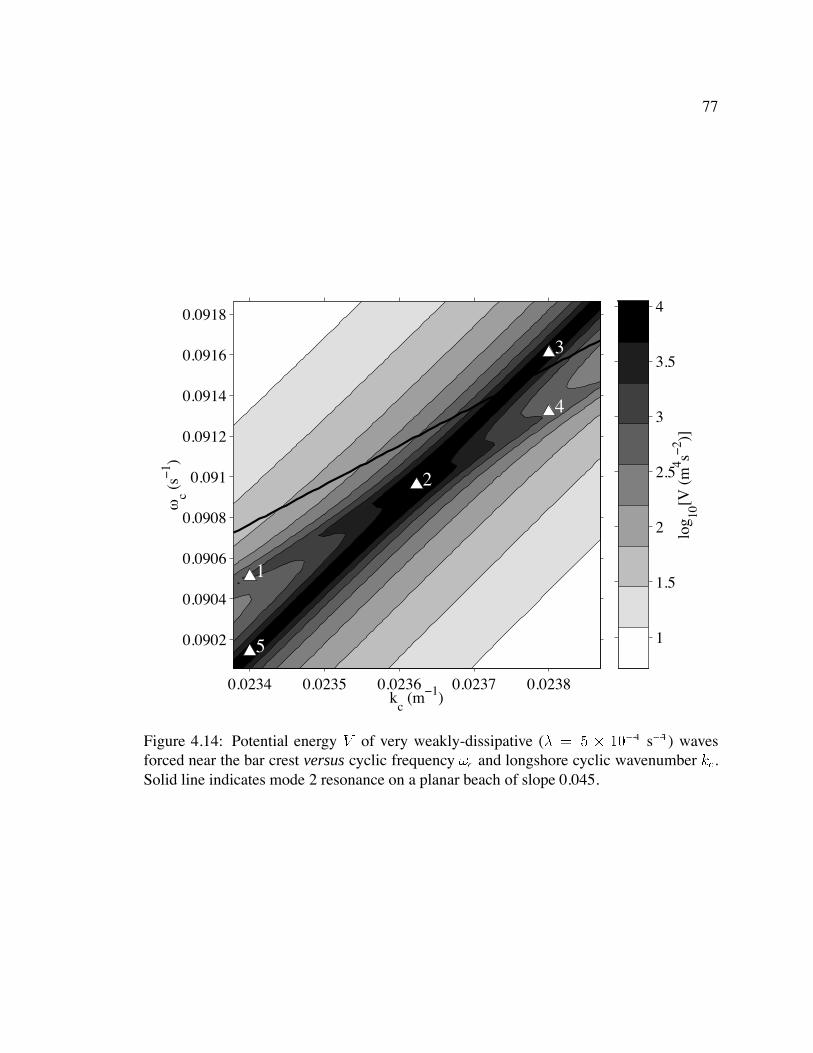
77

1

1.5

2

2.5

3

3.5

4

log 10

[V (

m4 s−

2 )]0.0234 0.0235 0.0236 0.0237 0.0238

0.0902

0.0904

0.0906

0.0908

0.091

0.0912

0.0914

0.0916

0.0918

kc (m−1)

ωc (

s−1 )

1

2

3

4

5

Figure 4.14: Potential energy V of very weakly-dissipative ( s) wavesforced near the bar crest versus cyclic frequency c and longshore cyclic wavenumber kc.Solid line indicates mode 2 resonance on a planar beach of slope 0.045.

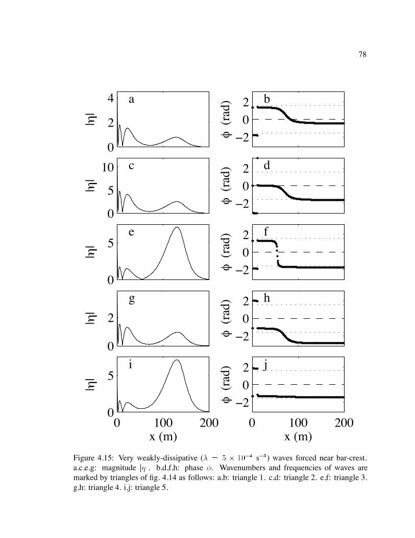
78

0

2

4

|η|

a

−202

φ (

rad)

b

0

5

10

|η

| c

−202

φ (

rad)

d

0

5

|η

| e

−202

φ (

rad)

f

0

2

|η

| g

−202

φ (

rad)

h

0 100 2000

5

x (m)

|η

| i

0 100 200

−202

x (m)

φ (

rad)

j

Figure 4.15: Very weakly-dissipative ( s) waves forced near bar-crest.a,c,e,g: magnitude jj. b,d,f,h: phase . Wavenumbers and frequencies of waves aremarked by triangles of fig. 4.14 as follows: a,b: triangle 1. c,d: triangle 2. e,f: triangle 3.g,h: triangle 4. i,j: triangle 5.

79

1

1.5

2

2.5

3

3.5

4

4.5

5

5.5

6

log 10

[V (

m4 s−

2 )]0.0234 0.0235 0.0236 0.0237 0.0238

0.0902

0.0904

0.0906

0.0908

0.091

0.0912

0.0914

0.0916

0.0918

kc (m−1)

ωc (

s−1 )

1

2

3

4

5

6

Figure 4.16: Potential energy V of extremely weakly-dissipative ( s) wavesforced near the bar crest versus cyclic frequency c and longshore cyclic wavenumber kc.Solid line indicates mode 2 resonance on a planar beach of slope 0.045.

80

0

10

20

|η|

a

−202

φ (

rad)

b

0

50

100

|η

| c

−202

φ (

rad)

d

0

20

|η

| e

−202

φ (

rad)

f

0

5

10

|η

| g

−202

φ (

rad)

h

0

50

100

|η

| i

−202

φ (

rad)

j

0 100 2000

20

40

x (m)

|η

| k

0 100 200

−202

x (m)

φ (

rad)

l

Figure 4.17: Extremely weakly-dissipative ( s) waves forced near bar-crest.a,c,e,g,i,k: magnitude jj. b,d,f,h,j,l: phase . Wavenumbers and frequencies of waves aremarked by triangles of fig. 4.14 as follows: a,b: triangle 1. c,d: triangle 2. e,f: triangle 3.g,h: triangle 4. i,j: triangle 5. k,l: triangle 6.

81

Nevertheless, shore-trapped waves were indeed an order of magnitude larger than bar-

trapped waves at k (0.09096 Hz, 0.0236 m). Generally, whenever eq. (4.30)

predicts that the indirectly-forced wave is much larger than the directly-forced wave, the

time scale for dissipation is much longer than the time scale for energy exchange between

bar- and shore-trapped waves, and separated resonance curves similar to the ones shown in

fig. 4.16 are expected.

For the beach considered above, coupling between bar- and shore-trapped waves was

so weak (Qwas for the waves of fig.’s 4.16 & 4.17) that they would almost certainly

have been decoupled in the field. If the bar had been closer to the shore, or the trough had

been shallower, or the wave frequency had been lower, then decoupling would not have

been so certain (eq. (4.30)).

Mode coupling, of which coupling between shore- and bar-trapped waves is an exam-

ple, occurs in many branches of physics. Coupling between free, non-dissipative modes has

received a great deal of attention (eg. Eckart (1961) considered coupling between internal

waves on two separate pycnoclines, Parrish and Niiler (1971) considered coupling between

surface and internal waves over the shelf break, Louisell (1960) considered coupled electri-

cal circuits, and Flynn and Littlejohn (1994) considered coupling in quantum mechanics).

Coupling between dissipative modes has received much less attention, although Garrett

(1969) pointed out that dissipation might decouple free modes in the atmosphere (we have

considered forced modes), and Grimshaw and Allen (1982) examined the effects of dissi-

pation on coupled unforced modes in a slowly-varying medium.

4.3.4 Realistic forcing and dissipation

So far, I have presented only point-forced waves, and have assumed that the dissipation

factor is constant. This Section presents simulations of wave fields generated by more

realistic, distributed forcing in the presence of spatially-varying dissipation. These simula-

tions are of waves on the barred beach shown in fig. 4.10.

82

A standard bottom friction parameterisation (Section 2.4) suggests

Cjujh (4.31)

where juj is a typical water speed, and C is a constant, here assumed to be . To

simulate dissipation when incident waves were small (large), I assume juj 0.3 ms

(juj 1 ms). Equation (4.31) fails at the shore, since tends to infinity as the depth

tends to zero. Miles (1990) showed that, in the absence of capillary forces, eq. (4.31)

incorrectly predicts total absorption (zero reflection) of linear waves at the shore. To avoid

this problem, I arbitrarily set all values of shoreward of h m equal to Cjuj/(0.5 m).

I divided the region seaward of h m into a series of segments, each 10 m wide, and

calculated one value of for each segment using the local mean depth and eq. (4.31).

Forcing is due to wave groups with frequency and wavenumber k, which are pro-

duced by interference between two sinusoidal wave trains with frequencies s and s ,

and longshore wavenumbers ks and ks k. Spectral forcing could be represented by sim-

ply summing over all such wave groups, but this Section presents simulations for only

two infragravity frequencies (0.017 Hz and 0.037 Hz) and a single longshore infragravity

wavenumber (0.005 m). Only the case s s, ks k is considered. The

complex amplitudes as and as of the two wave trains are calculated by assuming linear,

non-dissipative, WKB shoaling of shoreward-propagating waves over a longshore-uniform

beach (giving eq.(2) of Guza and Bowen (1976b), with r , for each velocity potential).

The assumptions of zero reflection and zero dissipation are inconsistent. Consequently,

the complex amplitude of group-frequency energy fluctuations (aG gasas) tends to

infinity as groups approach the shore. During storms, breaking dissipates wave energy,

and destroys wave groups as they approach the shore (Symonds et al., 1982; List, 1991).

Breaking is simulated by assuming

aGx tanhx xb

aG x (4.32)

where aGx is the amplitude of group-frequency energy fluctuations in the presence of

breaking. The constants xb and determine respectively the location of the outer edge of

the surf zone, and the width of the region over which wave groups are destroyed. When

83

incident waves are very small they do not break, but we can not set aG aG at the

shore, since this would give infinite forcing. To simulate small non-breaking waves, we set

aG aG in water depths greater than 30 cm, and simply ignore forcing in water depths

less than 30 cm. The amplitude aG was substituted into energy-based formulas for the

Stokes drift and radiation stress (Whitham, 1962), and the nonlinear forcing F was then

calculated from eq. (4.15).

The above method for calculating the cross-shore structure of surf beat forcing relies

on many dubious assumptions. Linear shoaling neglects nonlinear triad interactions, which

transfer energy to harmonics of the primary incident frequencies (Freilich and Guza, 1984;

Elgar and Guza, 1985a, 1985b). The longshore wavenumber of linear waves is conserved

during shoaling over a longshore-uniform beach, but in the field the longshore wavenumber

of breaking waves is not conserved, for reasons that are not understood (Herbers et al.,

1999). In the absence of field-tested models for the destruction of wave groups by breaking,

I arbitrarily assumed that wave group destruction could be represented by the simple tanh

window of eq. (4.32). I have ignored forcing by unbroken incident waves in very shallow

water, as well as reflection of unbroken waves from the shore. Due these shortcomings,

only the gross features of the model predictions are significant.

When incident waves are very small, groups propagate into very shallow water, and

even those edge waves that are trapped very close to the shore are excited. Figure 4.18

shows that very low frequency (0.017 Hz) groups of small unbroken incident waves gen-

erated a strongly-resonant, cross-shore standing, mode zero edge wave. Figure 4.19 shows

that higher frequency (0.037 Hz) groups of unbroken waves generated a strongly-resonant,

cross-shore standing, mode five edge wave.

When incident waves are large, breaking destroys wave groups far offshore, and those

edge waves that are trapped very close to the shore not excited. Figure 4.20 shows that,

when incident waves broke far offshore, very low frequency (0.017 Hz) groups did not ex-

cite an energetic edge wave, even though forcing resonated with a mode zero edge wave (cf.

fig. 4.18). Instead, only evanescent waves were generated. These evanescent waves propa-

gated shorewards with the short-wave groups, and the associated sea level fluctuations were

84

0

0.05

|E| (

m3 s−

2 )

a

−202

φE (

rad)

b

0 5000

0.1

x (m)

|η

| (m

) c

0 500

−202

x (m)

φη (

rad) d

Figure 4.18: Low frequency (0.017 Hz) groups of non-breaking incident waves (a,b), andassociated infragravity waves (c,d). a,c: Magnitude. b,c: Phase.

85

0

0.05

|E| (

m3 s−

2 )

a

−202

φE (

rad)

b

0 5000

0.5

x (m)

|η

| (m

) c

0 500

−202

x (m)

φη (

rad) d

Figure 4.19: High frequency (0.037 Hz) groups of non-breaking incident waves (a,b), andassociated infragravity waves (c,d). a,c: Magnitude. b,c: Phase.

86

180 degrees out of phase with co-located fluctuations in short-wave energy. In this regard,

these waves were similar to the bound waves described by Longuet-Higgins and Stewart

(1962), so we call them ‘evanescent bound waves’. However, evanescent waves do not

propagate freely across-shore (Section 4.3.2). Instead, the shoreward propagation evident

in fig. 4.20d was entirely due to the shoreward propagation of the short-wave groups. This

is most obvious at about x 400 m, where short-wave groups were destroyed by breaking.

Whereas Longuet-Higgins and Stewart (1962) suggested that bound waves are released

when short waves break, the simulated evanescent bound waves simply disappeared.

Evanescent bound waves propagate shorewards, and carry a shoreward energy flux. As-

sociated with the loss of evanescent bound wave energy at the breakpoint is a loss of the

shoreward energy flux carried by evanescent waves. Section 3.4 showed that marked reduc-

tions in the shoreward energy flux carried by low frequency surf beat often accompanied

wave breaking in the field. The observed loss of surf beat energy at the breakpoint might

have been due to the presence of evanescent bound waves. However, marked reductions in

the energy flux carried by relatively high frequency surf beat were not usually observed,

and further field observations will be required to determine the importance of evanescent

bound waves.

Infragravity energy was lost near the breakpoint, as shown in fig. 4.20c, because the

breakpoint was outside the turning point and bound waves were evanescent. Figure 4.21

shows the response to higher frequency (0.037 Hz) forcing, which resonates with a much

higher mode number (n 5) edge wave. Now the turning point is seaward of the break-

point, and energetic edge waves propagate shorewards, radiating energy away from the

breakpoint. Outside the edge wave turning point, shoreward-propagating evanescent bound

waves can still be seen.

Forcing with a frequency greater than gk generates leaky waves. These leaky

waves have no turning point, and always radiate energy away from the breakpoint. The

bound wave model of Longuet-Higgins and Stewart (1962) assumes that waves are uni-

directional (k ). Consequently, the bound waves simulated by Longuet-Higgins and

Stewart are not evanescent, and always radiate energy away from the breakpoint. The

87

model of Hasselmann et al. (1963) does simulate evanescent bound waves, but forcing is

assumed to be homogeneous, so evanescence has no striking effect.

4.4 Comment on normal modes

I have used Green’s functions to solve the dissipative edge wave problem. I could also

have used normal modes, by extending previous analysis (eg. Bowen and Guza (1978),

Lippmann et al. (1997)) to allow for strong dissipation. Normal modes have the advantage

that they provide very simple expressions for the amplitude and cross-shore structure of

high Q edge waves. I discuss the representation of forced, dissipative edge waves by nor-

mal modes in Appendix F. I chose not to base this chapter on normal mode theories for two

reasons. Firstly, the use of normal modes complicates the discussion of cross-shore propa-

gation, evanescence and dissipative decoupling, all of which are associated with coherence

between normal modes (Appendix F). Secondly, I do not know how to calculate normal

modes for complex profiles of water depth and dissipation strength without resorting to

numerical methods.

4.5 Discussion and conclusions

Field observations show that much infragravity energy exists in the form of shoreward-

propagating waves (Chapters 2 and 3). This chapter has shown that shoreward propagation

can be simulated using a dissipative shallow water model. This dissipative model predicts

several additional phenomena that might be important to surf beat dynamics, such as non-

resonant edge waves, evanescent bound waves, and dissipative decoupling. However, given

the current lack of understanding of both incident wave breaking and infragravity wave

dissipation, field observations will be required to test whether these phenomena are in fact

important on natural beaches.

Strongly-dissipative edge waves propagate obliquely across-shore, carrying energy

from regions of forcing to regions of dissipation. If forcing is weaker than dissipation

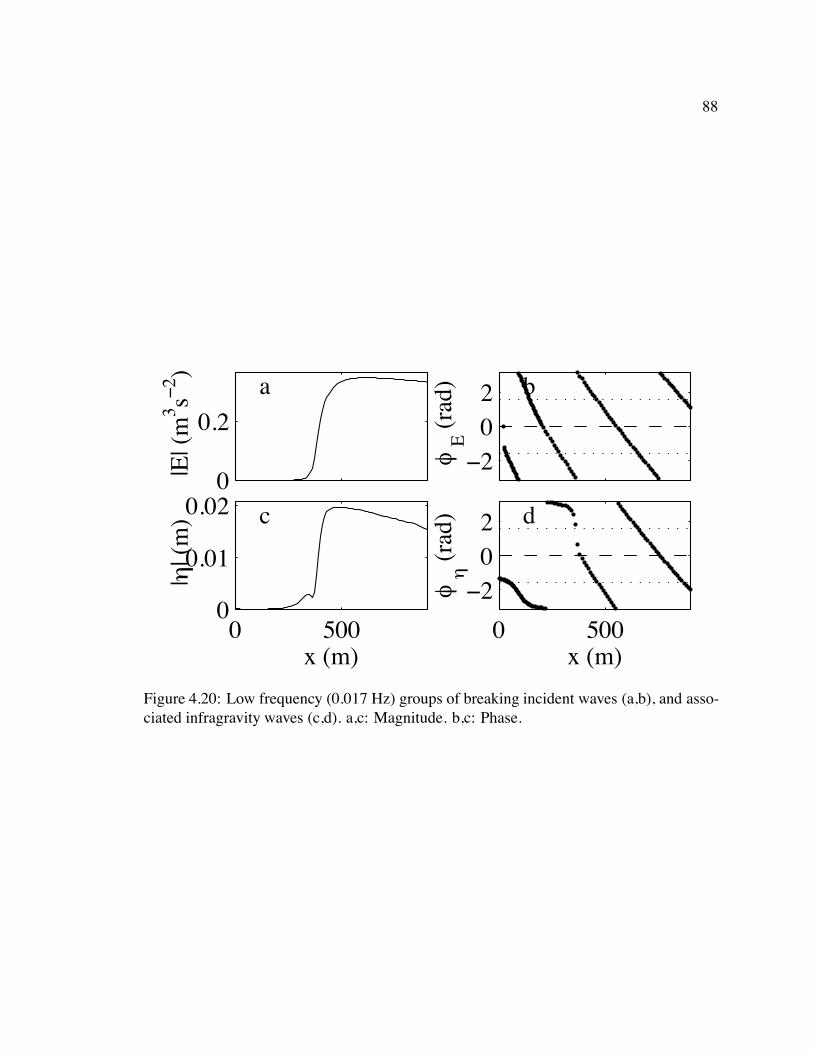
88

0

0.2

|E| (

m3 s−

2 )

a

−202

φE (

rad)

b

0 5000

0.01

0.02

x (m)

|η

| (m

) c

0 500

−202

x (m)

φη (

rad) d

Figure 4.20: Low frequency (0.017 Hz) groups of breaking incident waves (a,b), and asso-ciated infragravity waves (c,d). a,c: Magnitude. b,c: Phase.

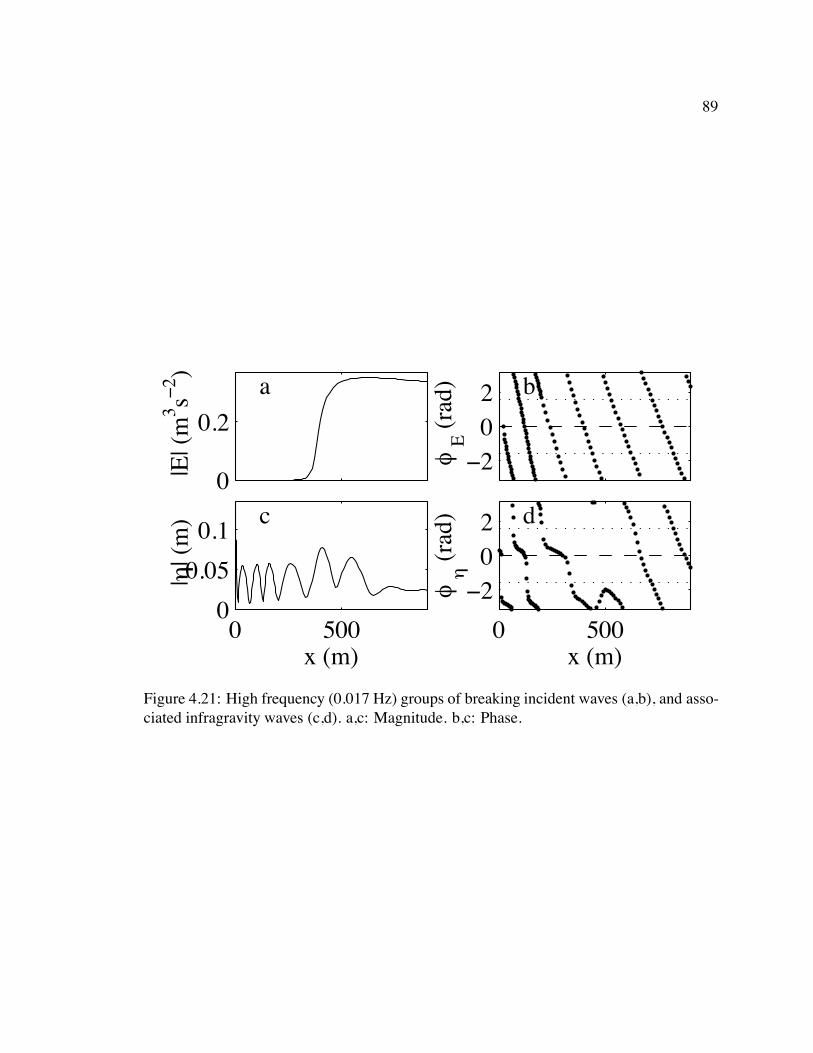
89

0

0.2

|E| (

m3 s−

2 )

a

−202

φE (

rad)

b

0 5000

0.05

0.1

x (m)

|η

| (m

) c

0 500

−202

x (m)

φη (

rad) d

Figure 4.21: High frequency (0.017 Hz) groups of breaking incident waves (a,b), and asso-ciated infragravity waves (c,d). a,c: Magnitude. b,c: Phase.

90

inside the surf zone, then edge waves propagate shorewards into the surf zone. Outside

the edge wave turning point, wave groups generate evanescent bound waves, which propa-

gate shorewards with the wave groups. I suggest that the shoreward-propagating surf beat

observed near the surf zone on natural beaches might be comprised of dissipative edge

waves or evanescent bound waves. In contrast to the bound waves of Longuet-Higgins and

Stewart (1962), whose energy radiates freely away from the breakpoint, evanescent bound

waves simply disappear near the breakpoint. Therefore, field evidence for the existence

of evanescent bound waves might include a major reduction in the shoreward energy flux

near the edge of the surf zone. Field observations of such a reduction in the shoreward en-

ergy flux were presented in Section 3.4, although further evidence will be required before

solid conclusions can be drawn. Field evidence for the existence of shoreward-propagating

edge waves might include observations of shoreward-propagating waves with edge-wave

frequencies and longshore wavenumbers inside the edge wave turning point.

Dissipation can decouple bar- and shore-trapped waves. Consequently, forcing over the

sandbar can generate bar-trapped waves without generating shore-trapped waves. Simi-

larly, forcing over the shoreface can generate shore-trapped waves without generating bar-

trapped waves.

Chapter 5

Conclusions

5.1 Summary

This thesis has investigated the effects of forcing and dissipation on surf beat behaviour.

Field observations have shown that, when incident waves are large, rapid damping of infra-

gravity waves in the surf zone leads to net shoreward infragravity wave propagation. When

incident waves are small, net infragravity wave damping is relatively weak, and infragravity

waves are almost cross-shore standing.

A model of dissipative, shore-oblique shallow water waves suggests that the ob-

served shoreward-propagating infragravity waves could be either dissipative edge waves

or evanescent bound waves. When dissipation is very weak, forcing close to the shore

generates cross-shore standing edge waves. Stronger dissipation introduces edge waves

that progress obliquely across-shore, carrying energy from regions of forcing to regions of

dissipation. Evanescent waves, which decay almost exponentially away from regions of

forcing, dominate over resonant edge waves when forcing is applied sufficiently far outside

the edge wave turning point. Group-bound evanescent waves propagate shorewards with

short-wave groups and remain about 180 degrees out of phase with co-located short-wave

energy but, unlike the group-bound waves described by previous researchers, they simply

disappear when short waves break. In the field, marked reductions in the shoreward en-

ergy flux carried by low frequency surf beat often accompanied wave breaking, suggesting

91

92

that evanescent bound waves were present. However, this result is not conclusive, and

shoreward energy fluxes associated with relatively high frequency surf beat did not usually

decrease greatly in the outer surf zone. Leaky waves can also propagate shorewards, but

observations of oblique shoreward propagation reported by Sheremet et al. (2001) seem to

rule out leaky waves as the main source of shoreward-propagating infragravity energy.

Model results suggest that dissipation might decouple bar- and shore-trapped waves.

Decoupling is strongest when the trough between the shore and the bar is wide and deep.

5.2 Possible future research

I have not identified the mechanism responsible for the strong surf beat damping ob-

served during storms. Possible mechanisms include bottom friction, breaking, and non-

linear damping. Three-dimensional flow structure could also lead to shear-dispersive mix-

ing (Svendsen and Putrevu, 1994; Van Dongeren et al., 1998). Longuet-Higgins (1967)

showed that the time scale for dissipation in a wave bottom boundary layer with constant

eddy viscosity is Ohh wave periods, where h is the water depth and h is the boundary

layer thickness. I expect that a similar result holds when the eddy viscosity is not constant.

If so, then measurements of the thickness of the surf beat bottom boundary layer might be

used to determine whether bottom friction is responsible for much of the observed surf beat

energy loss. The importance of nonlinear damping could be estimated by direct evaluation

of the nonlinear terms in the energy equation (2.11), using measured water pressures and

velocities and the nonlinear spectral techniques described in Appendix B. Estimation of the

roller contributions to wave momentum (eq. (2.18)) and momentum flux (eq. (2.17)) would

be difficult. Dense arrays of instruments would be required to resolve spatial gradients of

the momentum flux.

Observations from longshore arrays of current meters or pressure gauges could be used

to distinguish between edge and evanescent waves. The proportion of energy carried by

93

evanescent waves could be determined from such data using the ‘direct estimator’ of El-

gar et al. (1994) (evanescent waves have wavenumbers greater than gh). Band-

integrated cross-spectra could be estimated using a generalisation of the direct estimator,

so that shoreward energy fluxes carried by evanescent waves might also be calculated. To

measure evanescent bound waves, longshore arrays should be located near the outer edge

of surf zone. Evanescent waves are most likely to be found when the height and direc-

tional spread of incident waves are both large. The loss of evanescent wave energy in the

outer surf zone is associated with rapid nonlinear surf beat damping in the outer surf zone.

Therefore, if evanescent waves are energetic, then direct evaluation of the nonlinear terms

in the energy equation, as outlined in the previous paragraph, should show strong nonlinear

damping in the outer surf zone.

Predictions of dissipative decoupling of bar- and shore-trapped waves might be tested

by comparing waves observed near the shore with waves observed over a well-developed

bar. Observations of coherence and relative energy levels might be particularly useful.

However, interpretation of coherence between bar- and shore-trapped waves would require

care, because forcing over the bar might be coherent with forcing near the shore.

Observed surf beat energy levels do not decay seawards at the rate predicted by free

wave theories (Ruessink, 1998b; Lippmann et al., 1998, 2001). Chapter 4 showed that

forcing and dissipation modify the cross-shore structure of surf beat. It would be interesting

to see whether the cross-shore variation in surf beat energy levels can be predicted by a

simple dissipative model.

Thorough calibration and testing of a dissipative surf beat model would be valuable.

Such calibration might improve our understanding of surf beat dissipation. Furthermore,

calibration of a dissipative model would be an important step towards the ultimate goal

of predicting the infragravity wave field from the incident wave field. Existing models

of shoaling incident waves seriously underpredict the directional spread of incident waves,

and therefore the longshore wavenumbers at which surf beat is forced. The longshore struc-

ture of surf beat forcing is important, since it determines whether leaky, edge, or evanescent

94

waves are forced. Therefore, accurate simulation of surf beat will require either direct eval-

uation of nonlinear forcing from field data, or improved models of incident waves.

Appendix A

Derivation of a nonlinear

frequency-domain energy equation

A.1 Mass and momentum conservation

An exact, depth-integrated momentum equation for waves in water of constant density and

arbitrary depth is (eq. 3.6.7 of Phillips (1977))

t

Z

h

uj dz

xk

Z

h

ujuk dz

xj

Z

h

p

dz

p

h

xj (A.1)

Z

h

ujt

dz

Z

h

p

xjdz

Tjk

xkMj

t (A.2)

where T and M are defined by eq.’s (2.17) & (2.18), p water pressure, and water

density.

Equation (A.2) can be rewritten using the Fourier components defined by eq.’s (2.8)

& (2.10): Z

h

ujt

dz

Z

h

hpixj

dz hTjkixk

Mj

t

(A.3)

I approximate the motion at frequency by assuming

hpi g hi (A.4)

huji is independent of z. (A.5)

95

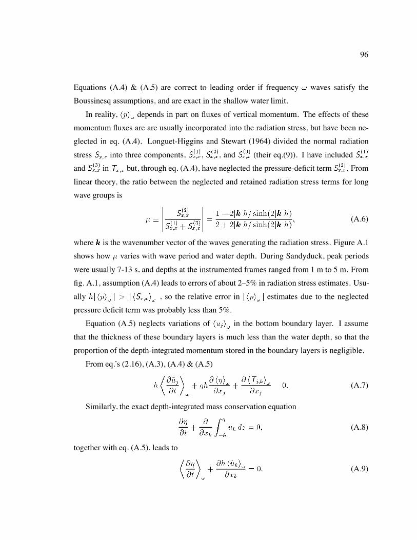
96

Equations (A.4) & (A.5) are correct to leading order if frequency waves satisfy the

Boussinesq assumptions, and are exact in the shallow water limit.

In reality, hpi depends in part on fluxes of vertical momentum. The effects of these

momentum fluxes are are usually incorporated into the radiation stress, but have been ne-

glected in eq. (A.4). Longuet-Higgins and Stewart (1964) divided the normal radiation

stress Sxx into three components, Sxx, S xx, and S

xx (their eq.(9)). I have included S

xx

and S xx in Txx but, through eq. (A.4), have neglected the pressure-deficit term S

xx. From

linear theory, the ratio between the neglected and retained radiation stress terms for long

wave groups is

Sxx

Sxx S

xx

jkjh sinhjkjh

jkjh sinhjkjh (A.6)

where k is the wavenumber vector of the waves generating the radiation stress. Figure A.1

shows how varies with wave period and water depth. During Sandyduck, peak periods

were usually 7-13 s, and depths at the instrumented frames ranged from 1 m to 5 m. From

fig. A.1, assumption (A.4) leads to errors of about 2–5% in radiation stress estimates. Usu-

ally hj hpi j j hSxxi j, so the relative error in j hpi j estimates due to the neglected

pressure deficit term was probably less than 5%.

Equation (A.5) neglects variations of huji in the bottom boundary layer. I assume

that the thickness of these boundary layers is much less than the water depth, so that the

proportion of the depth-integrated momentum stored in the boundary layers is negligible.

From eq.’s (2.16), (A.3), (A.4) & (A.5)

h

ujt

gh hixj

hTjkixj

(A.7)

Similarly, the exact depth-integrated mass conservation equation

t

xk

Z

h

uk dz (A.8)

together with eq. (A.5), leads to

t

h hukixk

(A.9)

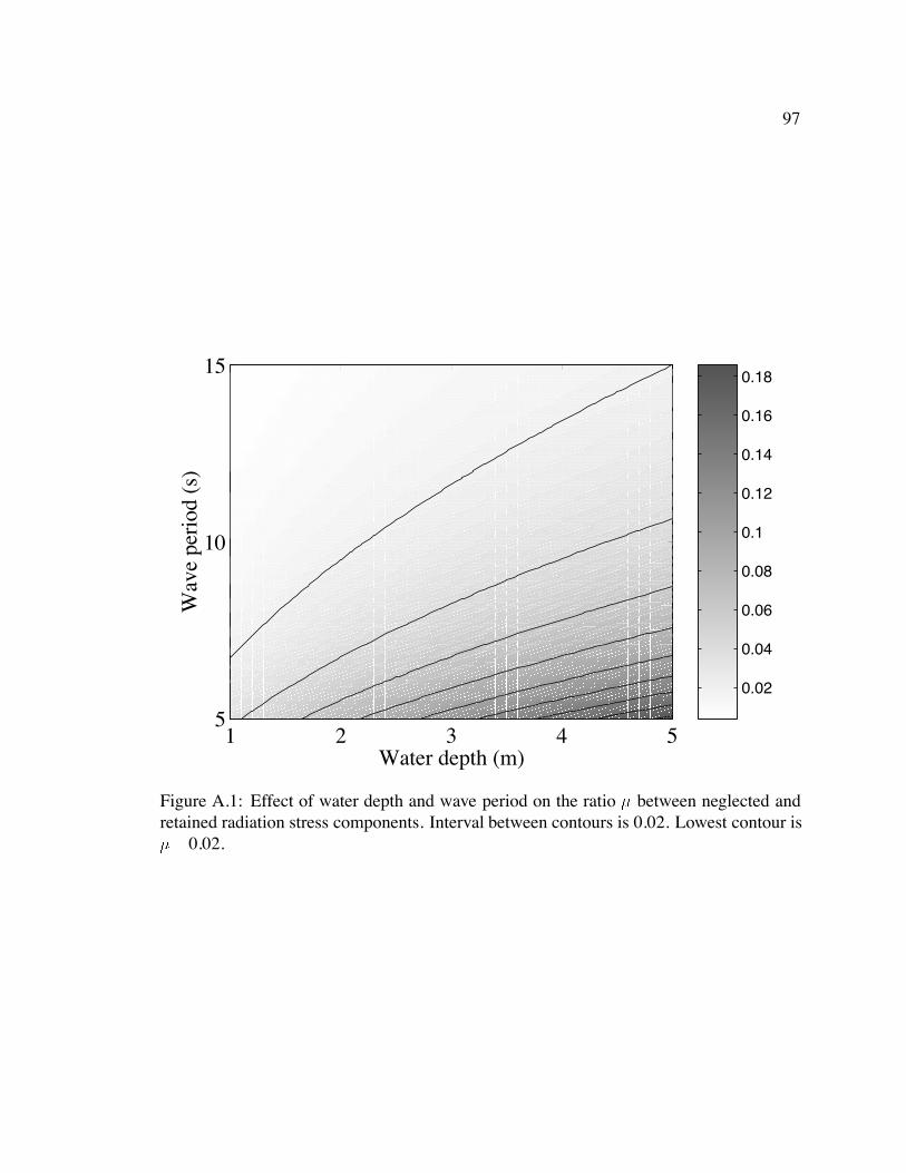
97

0.02

0.04

0.06

0.08

0.1

0.12

0.14

0.16

0.18

1 2 3 4 55

10

15

Water depth (m)

Wav

e pe

riod

(s)

Figure A.1: Effect of water depth and wave period on the ratio between neglected andretained radiation stress components. Interval between contours is 0.02. Lowest contour is 0.02.

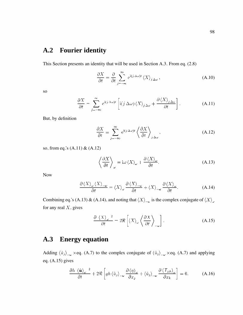
98

A.2 Fourier identity

This Section presents an identity that will be used in Section A.3. From eq. (2.8)

X

t

t

Xj

eijt hXij (A.10)

so

X

t

Xj

eijt

ij hXij

hXij

t

(A.11)

But, by definition

X

t

Xj

eijt

X

t

j

(A.12)

so, from eq.’s (A.11) & (A.12)

X

t

i hXi hXit

(A.13)

Now

hXi hXit

hXi hXi

t hXi

hXit

(A.14)

Combining eq.’s (A.13) & (A.14), and noting that hXi is the complex conjugate of hXifor any real X , gives

j hXi j

t

hXi

X

t

(A.15)

A.3 Energy equation

Adding huji eq. (A.7) to the complex conjugate of huji eq. (A.7) and applying

eq. (A.15) gives

hj hui j

t

gh huji

hixj

huji hTjkixk

(A.16)

99

But

gh huji hixj

gh huji hi

xj g hi

h hujixj

(A.17)

so from eq.’s (A.9), (A.17) & (A.15)

gh huji

hixj

hg hi huji

xj

gj hi j

t (A.18)

Substituting eq. (A.18) into eq. (A.16) gives

Enlt

wj

xj F (A.19)

where Enl, wj , and F are defined by eq.’s (2.12)–(2.14).

Finally, adding to eq. (A.19) a term D to represent the effects of dissipation gives

eq. (2.11).

Appendix B

Nonlinear coupling and higher order

spectra

Let X, X, X, and X be continuous stationary time series (most results of this section

also hold for regularly sampled discrete time series). Let the time series length t in

eq.’s (2.8) & (2.10) tend to infinity, so is replaced by the infinitesimal d, and the

series of eq. (2.8) is replaced by the Fourier-Stieltjes integral

Xn

Z

eithXni (B.1)

For non-zero frequencies, the cross-spectral density XX, the bispectral density

XXX, and the trispectral density XXXX are defined by

(Priestley, 1988)

EhXi hXi d

XX

otherwise (B.2)

EhXi hXi hXi d

XXX

otherwise

(B.3)

100

101

and

EhXi hXi hXi hXid

XXXX

XXXX

XXXX

XXXX

otherwise

(B.4)

The Stokes Drift M and the radiation stress S both involve products of pairs of un-

knowns. Consequently, we are interested in the frequency-domain representation of such

products. Let XnXm be the time series obtained by multiplying Xn by Xm. The Fourier

coefficients of XnXm are

hXnXmi

Z

hXnihXmi (B.5)

The energy equation (2.11) involves products such as huji hSjki xk and r

g hiM, so the mean values of such products represent mean energy exchanges and

are given by cross-spectra of the form

XXX EhXihXXid (B.6)

From eq.’s(B.5)&(B.6)

XXX

Z

E

hXihXihXi

d d

d (B.7)

XXX

Z

XXX d (B.8)

(see also Yeh and Van Atta (1973) and Tugnait (1994)). Consequently, mean energy ex-

changes can be represented either as cross-spectra involving nonlinear products, such as

uj Sjkxk, or as integrals of the bispectrum. Cross-spectra are easier to understand

102

and estimate, whereas bispectra can be used to determine exactly which triads are respon-

sible for the energy exchange. Herbers and Burton (1997) and Herbers et al. (2000) used

integrals of the bispectrum to represent energy exchanges between shoaling and breaking

Boussinesq waves.

From eq. (B.6) and the preceding discussion, we see that there can be a mean nonlinear

energy exchange to a wave of frequency only if the wave is coherent with nonlinear

forcing. The coherence between a response X and a nonlinear forcing term X is

XX

XX

XXX X

(B.9)

Coherence with nonlinear forcing is usually estimated only within a single time series, so

I have chosen the forcing to be X (rather than XX, which would be more general) to

simplify the algebra which follows. Huntley and Kim (1984) used jj to estimate the

proportion of surf beat energy that was ‘forced’ (as opposed to ‘free’). More recently, Her-

bers and Guza (1992), Herbers et al. (1994), and Ruessink (1998a) have estimated the

proportion of energy that is forced as using the parameter

XX

RXXX dh

XXRXXXX d

i (B.10)

If the trispectrum is large, then jj has no simple interpretation. I will conclude

this appendix by showing that if the trispectrum is sufficiently small. From

eq.’s (B.8) & (B.10)

XX

XX h

XXRXXXX d

i (B.11)

It remains to show that the denominator of eq. (B.11) equals the denominator of eq. (B.9).

For non-zero , the cross spectrum between XX and XX is

XXXX EhXXihXXid (B.12)

From eq.’s(B.5)&(B.12),

XXXX

Z

Z

E

hXihXihXihXi

d d d

d d (B.13)

103

so, from eq.’s (B.4) & (B.13)

XXXX Z

XX XX XXXX d

Z

Z

XXXX d d (B.14)

Therefore, if and the trispectral density is zero, then (from eq. (B.14))

X X

Z

XXXX d (B.15)

Substituting eq. (B.15) into eq. (B.11) leads to eq. (B.9).

Appendix C

Cross-shore profiles of surf beat energy

density and energy flux

Section 3.4 presented typical cross-shore profiles of surf beat energy density and energy

flux measured during the Duck94 experiment. Here the remainder of the profiles that sat-

isfied the conditions outlined in Section 3.4 are presented in order of increasing incident

wave height.

104

105

0

5

Dep

th (

m)

a

0

0.05

0.1

P.E

. (m

3 s−2 )

b>0.05Hz

0

5

x 10−3

P.E

. (m

3 s−2 )

c

0.025−0.05Hz0.005−0.025Hz

0

0.5

q (m

4 s−3 ) d

−5

0

5

x 10−3

e

q (m

4 s−3 )

100 200 300 400 500 600 700 800 900−1

0

1

ρ

Cross−shore distance (m)

g

0

5

Dep

th (

m)

a

0

0.05

0.1

P.E

. (m

3 s−2 )

b>0.05Hz

0

5

x 10−3

P.E

. (m

3 s−2 )

c

0.025−0.05Hz0.005−0.025Hz

0

0.5

q (m

4 s−3 ) d

−5

0

5x 10

−3

f

q (m

4 s−3 )

100 200 300 400 500 600 700 800 900−1

0

1

ρ

Cross−shore distance (m)

g

Figure C.1: Water depth (a), potential energy density PE (b: swell. c: surf beat), shore-ward energy flux q (d: swell. e: high frequency surf beat. f: low frequency surf beat), andprogressiveness parameter (g) versus cross-shore distance. Values estimated from 3 hrtime series on September 28th,Hs m. Squares: Swell ( Hz). Triangles: Highfrequency surf beat (– Hz). Circles: Low frequency surf beat (– Hz).

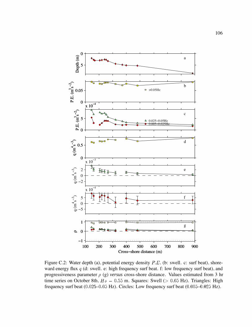
106

0

5

Dep

th (

m)

a

0

0.05

P.E

. (m

3 s−2 )

b>0.05Hz

0

5

x 10−4

P.E

. (m

3 s−2 )

c

0.025−0.05Hz0.005−0.025Hz

0

0.5

q (m

4 s−3 ) d

−202

x 10−3

e

q (m

4 s−3 )

100 200 300 400 500 600 700 800 900−1

0

1

ρ

Cross−shore distance (m)

g

0

5

Dep

th (

m)

a

0

0.05

P.E

. (m

3 s−2 )

b>0.05Hz

0

5

x 10−4

P.E

. (m

3 s−2 )

c

0.025−0.05Hz0.005−0.025Hz

0

0.5

q (m

4 s−3 ) d

−505

x 10−4

f

q (m

4 s−3 )

100 200 300 400 500 600 700 800 900−1

0

1

ρ

Cross−shore distance (m)

g

Figure C.2: Water depth (a), potential energy density PE (b: swell. c: surf beat), shore-ward energy flux q (d: swell. e: high frequency surf beat. f: low frequency surf beat), andprogressiveness parameter (g) versus cross-shore distance. Values estimated from 3 hrtime series on October 8th, Hs m. Squares: Swell ( Hz). Triangles: Highfrequency surf beat (– Hz). Circles: Low frequency surf beat (– Hz).

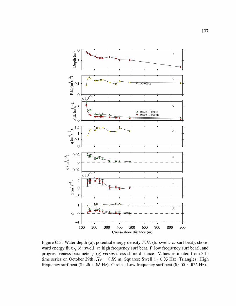
107

0

5

Dep

th (

m)

a

0

0.1

P.E

. (m

3 s−2 )

b>0.05Hz

0

5

x 10−3

P.E

. (m

3 s−2 )

c

0.025−0.05Hz0.005−0.025Hz

0

0.5

1

1.5

q (m

4 s−3 ) d

−0.02

0

0.02 e

q (m

4 s−3 )

100 200 300 400 500 600 700 800 900−1

0

1

ρ

Cross−shore distance (m)

g

0

5

Dep

th (

m)

a

0

0.1

P.E

. (m

3 s−2 )

b>0.05Hz

0

5

x 10−3

P.E

. (m

3 s−2 )

c

0.025−0.05Hz0.005−0.025Hz

0

0.5

1

1.5

q (m

4 s−3 ) d

−5

0

5x 10

−3

f

q (m

4 s−3 )

100 200 300 400 500 600 700 800 900−1

0

1

ρ

Cross−shore distance (m)

g

Figure C.3: Water depth (a), potential energy density PE (b: swell. c: surf beat), shore-ward energy flux q (d: swell. e: high frequency surf beat. f: low frequency surf beat), andprogressiveness parameter (g) versus cross-shore distance. Values estimated from 3 hrtime series on October 29th, Hs m. Squares: Swell ( Hz). Triangles: Highfrequency surf beat (– Hz). Circles: Low frequency surf beat (– Hz).

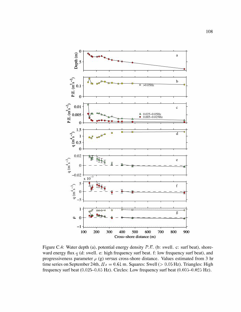
108

0

5

Dep

th (

m)

a

0

0.1

P.E

. (m

3 s−2 )

b>0.05Hz

0

0.005

0.01

P.E

. (m

3 s−2 )

c

0.025−0.05Hz0.005−0.025Hz

0

0.5

1

1.5

q (m

4 s−3 ) d

−0.02

0

0.02e

q (m

4 s−3 )

100 200 300 400 500 600 700 800 900−1

0

1

ρ

Cross−shore distance (m)

g

0

5

Dep

th (

m)

a

0

0.1

P.E

. (m

3 s−2 )

b>0.05Hz

0

0.005

0.01

P.E

. (m

3 s−2 )

c

0.025−0.05Hz0.005−0.025Hz

0

0.5

1

1.5

q (m

4 s−3 ) d

−5

0

5x 10

−3

f

q (m

4 s−3 )

100 200 300 400 500 600 700 800 900−1

0

1

ρ

Cross−shore distance (m)

g

Figure C.4: Water depth (a), potential energy density PE (b: swell. c: surf beat), shore-ward energy flux q (d: swell. e: high frequency surf beat. f: low frequency surf beat), andprogressiveness parameter (g) versus cross-shore distance. Values estimated from 3 hrtime series on September 24th,Hs m. Squares: Swell ( Hz). Triangles: Highfrequency surf beat (– Hz). Circles: Low frequency surf beat (– Hz).

109

0

5

Dep

th (

m)

a

0

0.1

0.2P.

E. (

m3 s−

2 )

b>0.05Hz

0

0.005

0.01

P.E

. (m

3 s−2 )

c

0.025−0.05Hz0.005−0.025Hz

0

1

2

q (m

4 s−3 ) d

−0.02

0

0.02e

q (m

4 s−3 )

100 200 300 400 500 600 700 800 900−1

0

1

ρ

Cross−shore distance (m)

g

0

5

Dep

th (

m)

a

0

0.1

0.2P.

E. (

m3 s−

2 )

b>0.05Hz

0

0.005

0.01

P.E

. (m

3 s−2 )

c

0.025−0.05Hz0.005−0.025Hz

0

1

2

q (m

4 s−3 ) d

−0.01

0

0.01 f

q (m

4 s−3 )

100 200 300 400 500 600 700 800 900−1

0

1

ρ

Cross−shore distance (m)

g

Figure C.5: Water depth (a), potential energy density PE (b: swell. c: surf beat), shore-ward energy flux q (d: swell. e: high frequency surf beat. f: low frequency surf beat),and progressiveness parameter (g) versus cross-shore distance. Values estimated from 3hr time series on September 27th (10 pm), Hs m. Squares: Swell ( Hz).Triangles: High frequency surf beat (– Hz). Circles: Low frequency surf beat(– Hz).

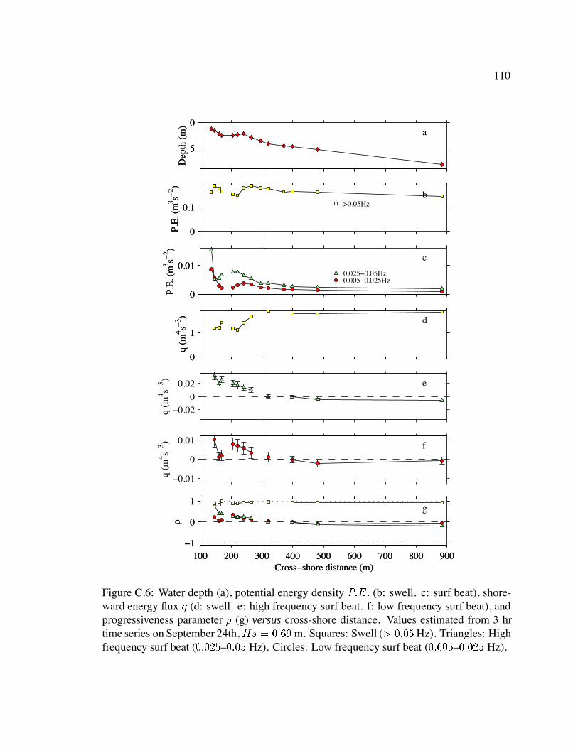
110

0

5

Dep

th (

m)

a

0

0.1

P.E

. (m

3 s−2 )

b>0.05Hz

0

0.01

P.E

. (m

3 s−2 )

c

0.025−0.05Hz0.005−0.025Hz

0

1

q (m

4 s−3 ) d

−0.020

0.02 e

q (m

4 s−3 )

100 200 300 400 500 600 700 800 900−1

0

1

ρ

Cross−shore distance (m)

g

0

5

Dep

th (

m)

a

0

0.1

P.E

. (m

3 s−2 )

b>0.05Hz

0

0.01

P.E

. (m

3 s−2 )

c

0.025−0.05Hz0.005−0.025Hz

0

1

q (m

4 s−3 ) d

−0.01

0

0.01 f

q (m

4 s−3 )

100 200 300 400 500 600 700 800 900−1

0

1

ρ

Cross−shore distance (m)

g

Figure C.6: Water depth (a), potential energy density PE (b: swell. c: surf beat), shore-ward energy flux q (d: swell. e: high frequency surf beat. f: low frequency surf beat), andprogressiveness parameter (g) versus cross-shore distance. Values estimated from 3 hrtime series on September 24th,Hs m. Squares: Swell ( Hz). Triangles: Highfrequency surf beat (– Hz). Circles: Low frequency surf beat (– Hz).

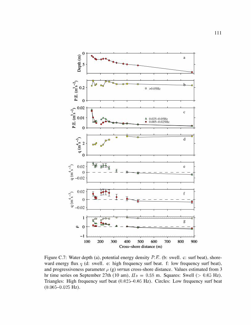
111

0

5

Dep

th (

m)

a

0

0.2

P.E

. (m

3 s−2 )

b>0.05Hz

0

0.01

0.02

P.E

. (m

3 s−2 )

c

0.025−0.05Hz0.005−0.025Hz

0

2

q (m

4 s−3 ) d

−0.020

0.02 e

q (m

4 s−3 )

100 200 300 400 500 600 700 800 900−1

0

1

ρ

Cross−shore distance (m)

g

0

5

Dep

th (

m)

a

0

0.2

P.E

. (m

3 s−2 )

b>0.05Hz

0

0.01

0.02

P.E

. (m

3 s−2 )

c

0.025−0.05Hz0.005−0.025Hz

0

2

q (m

4 s−3 ) d

−0.02

0

0.02 f

q (m

4 s−3 )

100 200 300 400 500 600 700 800 900−1

0

1

ρ

Cross−shore distance (m)

g

Figure C.7: Water depth (a), potential energy density PE (b: swell. c: surf beat), shore-ward energy flux q (d: swell. e: high frequency surf beat. f: low frequency surf beat),and progressiveness parameter (g) versus cross-shore distance. Values estimated from 3hr time series on September 27th (10 am), Hs m. Squares: Swell ( Hz).Triangles: High frequency surf beat (– Hz). Circles: Low frequency surf beat(– Hz).

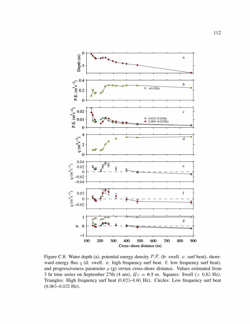
112

0

5

Dep

th (

m)

a

0

0.2

0.4P.

E. (

m3 s−

2 )

b>0.05Hz

0

0.01

0.02

P.E

. (m

3 s−2 )

c

0.025−0.05Hz0.005−0.025Hz

0

2

4

q (m

4 s−3 ) d

−0.04−0.02

00.020.04

e

q (m

4 s−3 )

100 200 300 400 500 600 700 800 900−1

0

1

ρ

Cross−shore distance (m)

g

0

5

Dep

th (

m)

a

0

0.2

0.4P.

E. (

m3 s−

2 )

b>0.05Hz

0

0.01

0.02

P.E

. (m

3 s−2 )

c

0.025−0.05Hz0.005−0.025Hz

0

2

4

q (m

4 s−3 ) d

−0.020

0.02 f

q (m

4 s−3 )

100 200 300 400 500 600 700 800 900−1

0

1

ρ

Cross−shore distance (m)

g

Figure C.8: Water depth (a), potential energy density PE (b: swell. c: surf beat), shore-ward energy flux q (d: swell. e: high frequency surf beat. f: low frequency surf beat),and progressiveness parameter (g) versus cross-shore distance. Values estimated from3 hr time series on September 27th (4 am), Hs m. Squares: Swell ( Hz).Triangles: High frequency surf beat (– Hz). Circles: Low frequency surf beat(– Hz).

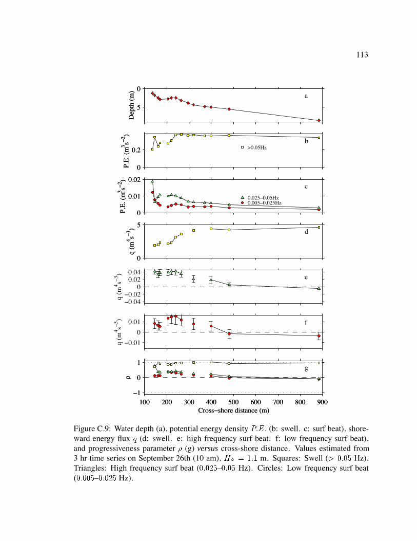
113

0

5

Dep

th (

m)

a

0

0.2

P.E

. (m

3 s−2 )

b>0.05Hz

0

0.01

0.02

P.E

. (m

3 s−2 )

c

0.025−0.05Hz0.005−0.025Hz

0

5

q (m

4 s−3 ) d

−0.04−0.02

00.020.04

e

q (m

4 s−3 )

100 200 300 400 500 600 700 800 900−1

0

1

ρ

Cross−shore distance (m)

g

0

5

Dep

th (

m)

a

0

0.2

P.E

. (m

3 s−2 )

b>0.05Hz

0

0.01

0.02

P.E

. (m

3 s−2 )

c

0.025−0.05Hz0.005−0.025Hz

0

5

q (m

4 s−3 ) d

−0.01

0

0.01 f

q (m

4 s−3 )

100 200 300 400 500 600 700 800 900−1

0

1

ρ

Cross−shore distance (m)

g

Figure C.9: Water depth (a), potential energy density PE (b: swell. c: surf beat), shore-ward energy flux q (d: swell. e: high frequency surf beat. f: low frequency surf beat),and progressiveness parameter (g) versus cross-shore distance. Values estimated from3 hr time series on September 26th (10 am), Hs m. Squares: Swell ( Hz).Triangles: High frequency surf beat (– Hz). Circles: Low frequency surf beat(– Hz).

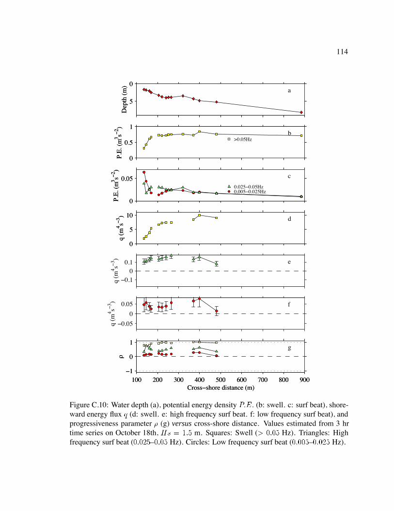
114

0

5

Dep

th (

m)

a

0

0.5

1P.

E. (

m3 s−

2 )

b>0.05Hz

0

0.05

P.E

. (m

3 s−2 )

c

0.025−0.05Hz0.005−0.025Hz

0

5

10

q (m

4 s−3 ) d

−0.10

0.1 e

q (m

4 s−3 )

100 200 300 400 500 600 700 800 900−1

0

1

ρ

Cross−shore distance (m)

g

0

5

Dep

th (

m)

a

0

0.5

1P.

E. (

m3 s−

2 )

b>0.05Hz

0

0.05

P.E

. (m

3 s−2 )

c

0.025−0.05Hz0.005−0.025Hz

0

5

10

q (m

4 s−3 ) d

−0.05

0

0.05 f

q (m

4 s−3 )

100 200 300 400 500 600 700 800 900−1

0

1

ρ

Cross−shore distance (m)

g

Figure C.10: Water depth (a), potential energy density PE (b: swell. c: surf beat), shore-ward energy flux q (d: swell. e: high frequency surf beat. f: low frequency surf beat), andprogressiveness parameter (g) versus cross-shore distance. Values estimated from 3 hrtime series on October 18th, Hs m. Squares: Swell ( Hz). Triangles: Highfrequency surf beat (– Hz). Circles: Low frequency surf beat (– Hz).

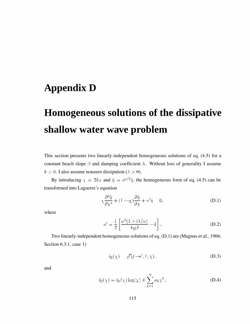
Appendix D

Homogeneous solutions of the dissipative

shallow water wave problem

This section presents two linearly-independent homogeneous solutions of eq. (4.5) for a

constant beach slope and damping coefficient . Without loss of generality I assume

k . I also assume nonzero dissipation ( ).

By introducing kx and e, the homogeneous form of eq. (4.5) can be

transformed into Laguerre’s equation

n (D.1)

where

n

i

kg

(D.2)

Two linearly-independent homogeneous solutions of eq. (D.1) are (Magnus et al., 1966,

Section 6.3.1, case 1)

Fn (D.3)

and

log Xk

akk (D.4)

115

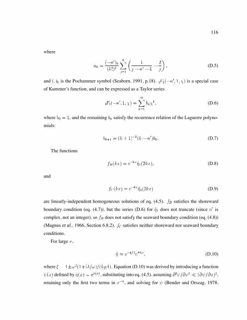
116

where

ak nkk

kXj

j n

j

(D.5)

and k is the Pochammer symbol (Seaborn, 1991, p.18). Fn is a special case

of Kummer’s function, and can be expressed as a Taylor series

Fn

Xk

bkk (D.6)

where b , and the remaining bk satisfy the recurrence relation of the Laguerre polyno-

mials:

bk k k nbk (D.7)

The functions

fBkx ekxkx (D.8)

and

fCkx ekxkx (D.9)

are linearly-independent homogeneous solutions of eq. (4.5). fB satisfies the shoreward

boundary condition (eq. (4.7)), but the series (D.6) for does not truncate (since n is

complex, not an integer), so fB does not satisfy the seaward boundary condition (eq. (4.8))

(Magnus et al., 1966, Section 6.8.2). fC satisfies neither shoreward nor seaward boundary

conditions.

For large x,

xekx (D.10)

where ikg. Equation (D.10) was derived by introducing a function

x defined by x ex, substituting into eq. (4.5), assuming x x,

retaining only the first two terms in x, and solving for (Bender and Orszag, 1978,

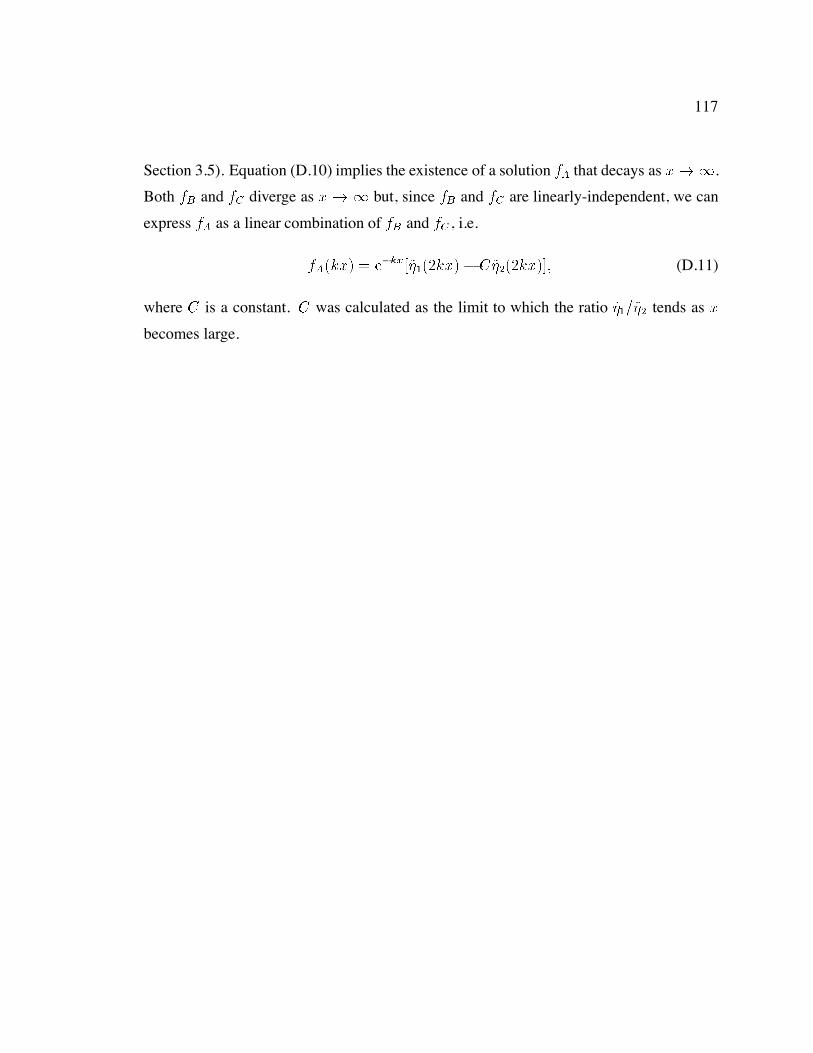
117

Section 3.5). Equation (D.10) implies the existence of a solution fA that decays as x.

Both fB and fC diverge as x but, since fB and fC are linearly-independent, we can

express fA as a linear combination of fB and fC , i.e.

fAkx ekxkx Ckx (D.11)

where C is a constant. C was calculated as the limit to which the ratio tends as x

becomes large.

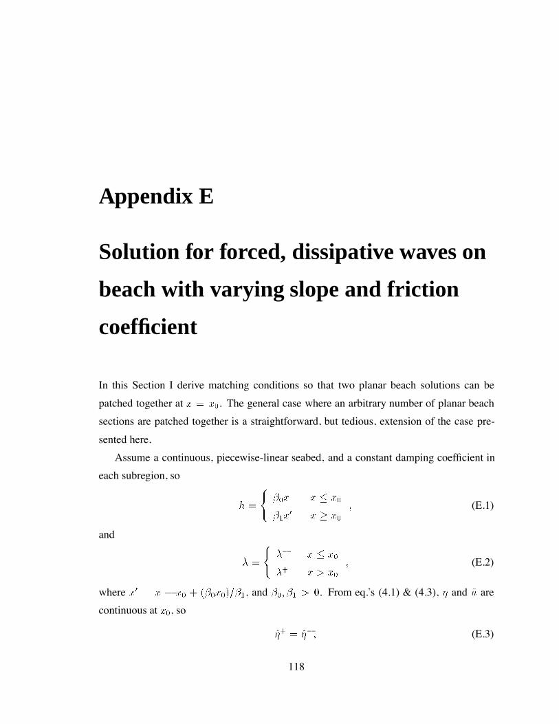
Appendix E

Solution for forced, dissipative waves on

beach with varying slope and friction

coefficient

In this Section I derive matching conditions so that two planar beach solutions can be

patched together at x x. The general case where an arbitrary number of planar beach

sections are patched together is a straightforward, but tedious, extension of the case pre-

sented here.

Assume a continuous, piecewise-linear seabed, and a constant damping coefficient in

each subregion, so

h

x x x

x x x

(E.1)

and

x x

x x (E.2)

where x x x x, and . From eq.’s (4.1) & (4.3), and u are

continuous at x, so

(E.3)

118

119

and

Fx g x M

x h

i

Fx g x M

x h

i (E.4)

x

ix

i

g

Fx M

x h

i

Fx M

x h

i

(E.5)

where

limxx

x (E.6)

and

limxx

x (E.7)

and similarly for x, F and Mx.

The inhomogeneous matching condition (eq. (E.5)) complicates matters. The most

straightforward expression for the solution is

x

ZxF

xF x

Gx xF F xF dxF Gx x (E.8)

where ZxF

xF x

(E.9)

is the integral over all values of xF except x. Gx xF satisfies eq.’s (4.17), (4.18), and

the homogeneous matching conditions

(E.10)

and

x

i

x

i (E.11)

120

The function G is added to satisfy the inhomogeneous matching conditions, and is defined

by

Gx x

BfBn

x x x

AfAn x x x (E.12)

where A and B are chosen to satisfy eq.’s (E.3) & (E.5). n and n are the values of n

for each subregion, determined from eq. (D.2). Here the dependence of fA and fB on n is

made explicit to emphasise the dependence of n on cross-shore location.

The point-forced solutions presented in Section 4.3.3 were obtained by assuming that

Fx Mxh , so G . The solutions presented in Section 4.3.4 allowed for non-zero

values of G.

Appendix F

Normal modes

F.1 Introduction

Forced, dissipative shallow water waves on a planar beach can be viewed as a superposition

of normal modes (Section F.2). Normal modes are eigensolutions to the unforced, or ‘free

wave’ problem. When Q is high, and a significant proportion of the forcing projects onto

resonant modes, the cross-shore structure of forced waves is similar to the the structure

of free waves, and normal modes provide a very efficient description of the wave field

(Section F.3). However, when Q is low, or forcing is nearly orthogonal to the resonant

modes, forced waves differ greatly from free waves, and normal modes do not simplify

the physical description of the problem. In fact, as I show in Sections F.4–F.6, the use of

normal modes greatly complicates the discussion of cross-shore propagation, evanescence,

and dissipative decoupling.

F.2 Method

The homogeneous form of eq. (4.5) is

L (F.1)

121

122

where

L

x

x

x

kx (F.2)

and

g

i

(F.3)

Dissipation has been incorporated into eq. (F.3). The operator L is unchanged by the intro-

duction of dissipation1, so the eigenvalues n and eigenfunctions n are the same as in the

non-dissipative case, namely

n kn (F.4)

where n Z,

nx ekx Fn kx (F.5)

and Fn kx is defined by eq.’s (D.6) & (D.7). The eigenfunctions are orthogonal,

so Z

x

nxmxk dx nm (F.6)

From eq.’s (F.3) & (F.4), is complex if k is real. Therefore, all longshore-homogeneous

free waves decay due to the presence of dissipation. Next, I show that the eigenfunctions

n can be used to determine the steady-state response to forcing.

The forced edge wave problem is

L F (F.7)

Assume that forcing is steady and longshore-homogeneous. Now and k are real, so

must be complex (note that the set fng is the set of eigenvalues, but is no longer an

eigenvalue). We express and F as sums of normal modes, i.e.

Xn

ann (F.8)

1However, if varied with x, then we would have to incorporate dissipation into L. The problem couldthen be solved using dissipative normal modes (Garrett and Greenberg, 1977).

123

and

F

Xn

fnn (F.9)

where

fn

Z

x

F xnxk dx (F.10)

Equation (F.7) now becomes

Xn

anLn Xn

ann Xn

fnn (F.11)

Xn

an nn Xn

fnn (F.12)

Introducing n gn, multiplying by km, and integrating over x from zero to

infinity gives

Xn

i n

gan

Z

x

nmk dx

Xn

fn

Z

x

nmk dx (F.13)

From eq.’s (F.6) & (F.13)

am gfm

iQ m

(F.14)

where

Q (F.15)

The particular solution of the dissipative edge wave problem is given by eq.’s (F.5), (F.8),

(F.14), & (F.15).

F.3 Resonance

The parameter Q defined by equation (F.15) is equivalent to the Q defined by eq. (1.1),

and determines the strength of edge wave resonance. When Q is large, the gain function

124

jamfmj has a resonant peak centered on the frequency m Q, whose height is

OQ, and whose half-power width is mQ (eq. (F.14)).

Equation (F.14) is identical to the equation for the response of a dissipative simple

harmonic oscillator to sinusoidal forcing. The use of normal modes has lead to an elegant

solution, one which emphasises the role of Q in determining the strength of edge wave

resonance. The normal modes approach was previously used by Gallagher (1971), Bowen

(1977), Bowen and Guza (1978), & Lippmann et al. (1997) (these authors assumed weak

dissipation).

F.4 Propagation

In Section F.2 I showed that forced, dissipative edge waves can be expressed as a sum of

normal modes. Each mode has the same cross-shore structure as a non-dissipative, free

edge wave, and is cross-shore standing. Yet the sum of the normal modes represents a

dissipative edge wave, which propagates across-shore (Section 4.3.1). Figures F.1 & F.2

show how the forced, dissipative edge wave presented in fig. 4.3e,f is approximated by the

first four normal modes. The n mode resonates and has a large amplitude (fig. F.1c).

Other normal modes do not resonate, and have smaller amplitudes. Non-resonant modes

are almost 90 degrees out of phase with the resonant mode, so the sum of the first four

modes forms a cross-shore progressive pattern (fig.F.2). This pattern is similar, but not

identical, to the full Green’s function solution shown in fig.4.3e,f. As more modes are

added, the normal mode solution converges to the Green’s function (when plotted, the sum

of the first 30 normal modes is almost indistinguishable from the Green’s function).

From the discussion above, we see that propagating waves can be represented as a sum

of cross-shore standing normal modes. These normal modes are coherent (their amplitudes

co-vary), so their sum represents a cross-shore shape different from the shape of any one

normal mode. The situation would be simpler if propagation was described by individual

normal modes, rather than by a set of coherent modes. Individual dissipative normal modes,

which are obtained by including dissipation in the operator L rather than in the eigenvalue

125

of eq. (F.1), can propagate (Webster, 1985). Such propagation redistributes the energy

of each mode to regions where dissipation is particularly strong. However, the direction

of forced wave propagation (as opposed to normal mode propagation) is not determined

solely by the intensity of dissipation. Since waves propagate from regions of net forcing

to regions of net dissipation (Section 4.2.3), the distribution of forcing plays a vital role

in determining the direction of net cross-shore propagation. Dissipative waves propagate

seawards offshore of regions of forcing, and shorewards onshore of regions of forcing.

Normal modes, whether dissipative or non-dissipative, are solutions to the homogeneous

problem — they are calculated without any reference to the spatial distribution of forcing.

Consequently, individual normal modes can not represent propagation away from regions

of forcing. When a forced wave field is represented using normal modes, a set of coherent

modes is required to represent propagation away from regions of forcing.

F.5 Evanescent waves

Consider the case where resonant forcing of frequency and wavenumber k is applied far

outside the turning point. Most of the variance of the resonant mode is confined inside

the turning point. Consequently, the forcing is almost orthogonal to the resonant normal

mode, and the projection of forcing onto the resonant mode (fn) is very small (eq. (F.10)).

If Q is not very large, then the small forcing fn can not excite a large response. However,

if Q is sufficiently large, then the denominator of eq. (F.14) becomes very small, and a

large resonant edge wave is generated. Since the resonant normal mode decays as approx-

imately eKx outside the turning point, the amplitude of the resonant response scales with

QeKL, in agreement with eq. (4.29) (L is the distance from the turning point to the point

of forcing).

Figure F.3 shows several approximations to the point-forced evanescent wave of

fig. 4.8e,f obtained using finite sums of normal modes. Many coherent normal modes

are required to represent evanescent waves, because the cross-shore structure of evanescent

waves differs greatly from the cross-shore structure of each individual normal mode. The

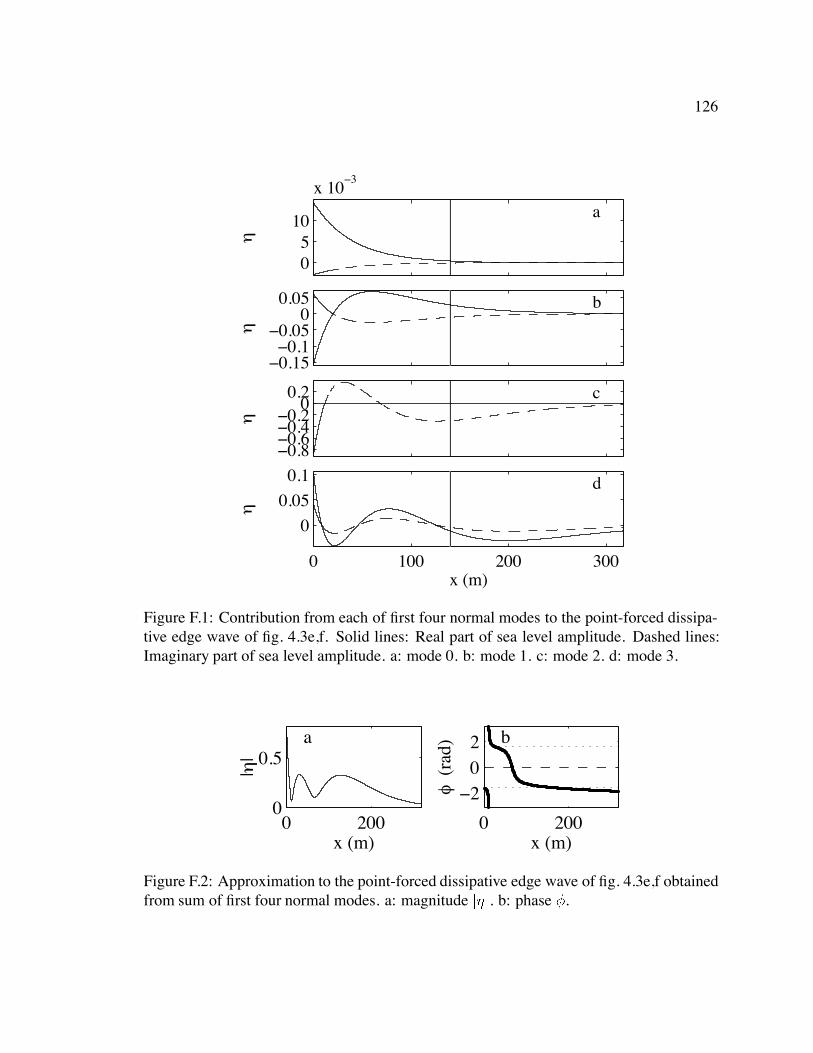
126

05

10

x 10−3

η

a

−0.15−0.1−0.05

00.05

η

b

−0.8−0.6−0.4−0.2

00.2

η

c

0 100 200 300

0

0.05

0.1

η

x (m)

d

Figure F.1: Contribution from each of first four normal modes to the point-forced dissipa-tive edge wave of fig. 4.3e,f. Solid lines: Real part of sea level amplitude. Dashed lines:Imaginary part of sea level amplitude. a: mode 0. b: mode 1. c: mode 2. d: mode 3.

0 2000

0.5

x (m)

|η

| a

0 200

−202

x (m)

φ (

rad)

b

Figure F.2: Approximation to the point-forced dissipative edge wave of fig. 4.3e,f obtainedfrom sum of first four normal modes. a: magnitude jj. b: phase .

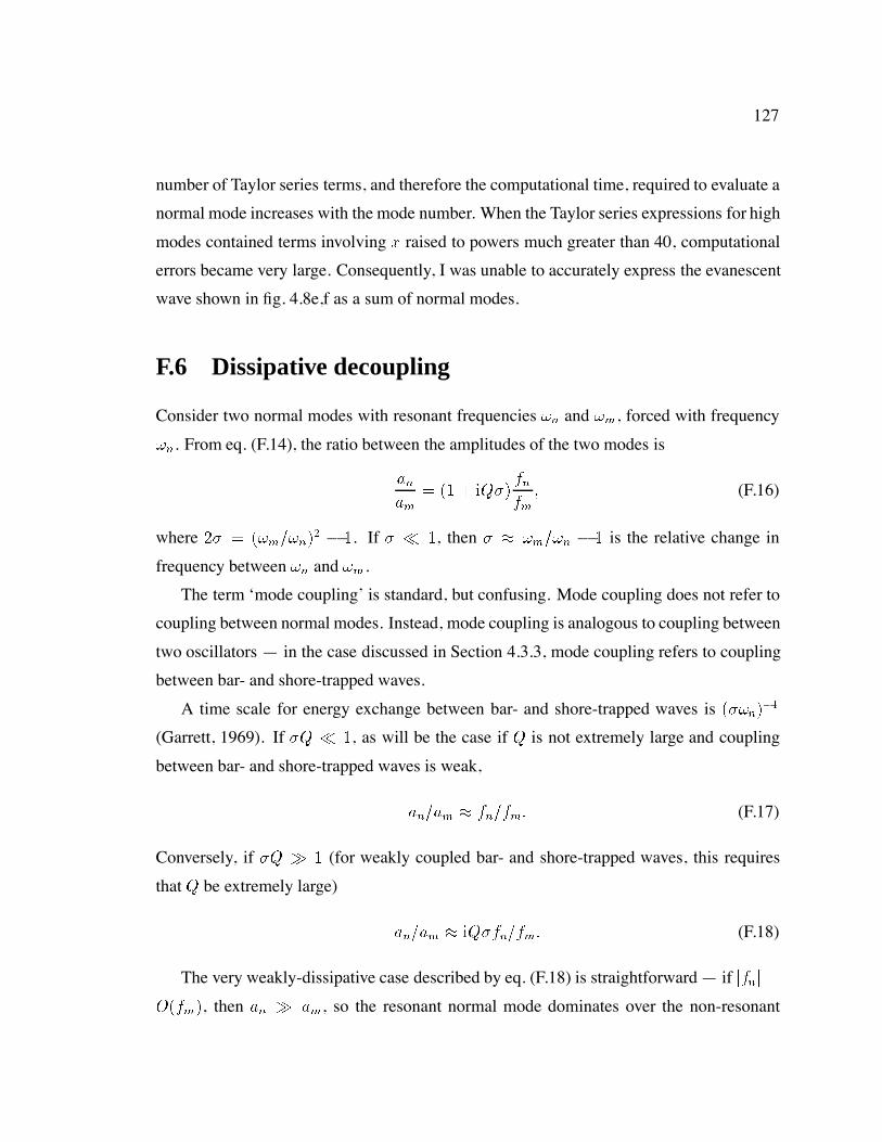
127

number of Taylor series terms, and therefore the computational time, required to evaluate a

normal mode increases with the mode number. When the Taylor series expressions for high

modes contained terms involving x raised to powers much greater than 40, computational

errors became very large. Consequently, I was unable to accurately express the evanescent

wave shown in fig. 4.8e,f as a sum of normal modes.

F.6 Dissipative decoupling

Consider two normal modes with resonant frequencies n and m, forced with frequency

n. From eq. (F.14), the ratio between the amplitudes of the two modes is

anam

iQfnfm

(F.16)

where mn . If , then mn is the relative change in

frequency between n and m.

The term ‘mode coupling’ is standard, but confusing. Mode coupling does not refer to

coupling between normal modes. Instead, mode coupling is analogous to coupling between

two oscillators — in the case discussed in Section 4.3.3, mode coupling refers to coupling

between bar- and shore-trapped waves.

A time scale for energy exchange between bar- and shore-trapped waves is n

(Garrett, 1969). If Q , as will be the case if Q is not extremely large and coupling

between bar- and shore-trapped waves is weak,

anam fnfm (F.17)

Conversely, if Q (for weakly coupled bar- and shore-trapped waves, this requires

that Q be extremely large)

anam iQfnfm (F.18)

The very weakly-dissipative case described by eq. (F.18) is straightforward — if jfnj

Ofm, then an am, so the resonant normal mode dominates over the non-resonant

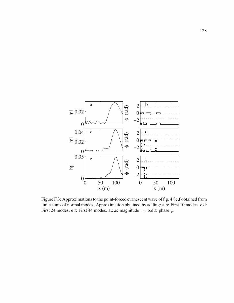
128

0

0.02

|η

| a

−202

φ (

rad)

b

0

0.02

0.04

|η

| c

−202

φ (

rad)

d

0 50 1000

0.05

x (m)

|η

| e

0 50 100

−202

x (m)

φ (

rad)

f

Figure F.3: Approximations to the point-forced evanescent wave of fig. 4.8e,f obtained fromfinite sums of normal modes. Approximation obtained by adding: a,b: First 10 modes. c,d:First 24 modes. e,f: First 44 modes. a,c,e: magnitude jj. b,d,f: phase .

129

normal mode. Examples of resonant normal modes are shown in fig 4.17c,d,i,j. Note that a

single resonant normal mode was made up of coupled bar- and shore-trapped waves.

To understand the more dissipative case described by eq. (F.17), consider the normal

modes shown in fig. 4.17c,d,i,j. If we call these modes n and m, then from fig. 4.17

n

m over bar

m over shoreface (F.19)

If forcing is confined to the bar, then fn fm (eq.’s (F.10) & (F.19)), so an am

(eq. (F.17)) and

ann over bar

over shoreface (F.20)

The two normal modes reinforce one another over the bar and cancel over the shoreface.

By adding two normal modes, each with energy over both the bar and the shoreface, we

get only a bar-trapped wave. If forcing is applied over the shoreface, then fn fm, so

an am, the normal modes reinforce over the shoreface and cancel over the bar, and we

get only shore-trapped waves. In this manner, dissipative decoupling is represented as a

sum of two coherent normal modes.

F.7 Summary

This thesis investigates the modification of surf beat by dissipation and forcing. Dissipation

and forcing modify surf beat by introducing waves that propagate from regions of forcing

to regions of dissipation, by decoupling bar- and shore-trapped waves, and by allowing

evanescent waves to be seen at leading order. These processes ensure that the cross-shore

structure of dissipative infragravity waves depends on the cross-shore structure of the ap-

plied forcing. In contrast, the cross-shore structure of normal modes is independent of the

applied forcing. Therefore, when normal modes are used, we must represent a wave whose

structure depends on the forcing, using modes whose structure is independent of the forc-

ing. We can not solve this problem using any one normal mode. We can achieve the desired

130

result using an infinite sum of normal modes, but such an approach leads to a complicated

discussion of straightforward physics.

Bibliography

Arfken, G. B. and Weber, H. J., 2001: , Mathematical methods for physicists. Academic

Press, San Diego, 5 edition.

Bauer, B. O. and Greenwood, B., 1990: Modification of a linear bar-trough system by a

standing edge wave. Marine Geology, 92, 177–204.

Bender, C. M. and Orszag, S. A., 1978: , Advanced mathematical methods for scientists

and engineers. McGraw-Hill, New York.

Bowen, A., 1969a: Rip currents 1. Theoretical discussion. Journal of Geophysical Re-

search, 74, 5467–5490.

Bowen, A., 1969b: Rip currents 2. laboratory and field observations. Journal of Geophys-

ical Research, 74, 5479–5490.

Bowen, A., 1977: Wave-wave interactions near the shore. Lecture notes in Physics, 64,

102–113.

Bowen, A., 1981: Simple models of nearshore sedimentation; beach profiles and longshore

bars. The Coastline of Canada, 80-10, 1–11.

Bowen, A. and Guza, R., 1978: Edge waves and surf beat. Journal of Geophysical Re-

search, 83, 1913–1920.

Bowen, A. J. and Inman, D. L., 1971: Edge waves and crescentic bars. Journal of Geo-

physical Research, 76, 8662–8671.

131

132

Bryan, K. and Bowen, A., 1996: Edge wave trapping and amplification on barred beaches.

Journal of Geophysical Research, 101, 6543–6552.

Bryan, K., Howd, P., and Bowen, A., 1998: Field observations of bar-trapped edge waves.

Journal of Geophysical Research, 103, 1285–1305.

Chen, Y. and Guza, R., 1997: Modeling spectra of breaking surface waves in shallow water.

Journal of Geophysical Research, 102, 25035–25046.

Chen, Y. and Guza, R., 1999: Resonant scattering of edge waves on longshore periodic

topography: Finite beach slope. Journal of Fluid Mechanics, 387, 255–269.

Eckart, C., 1951: . Surface waves in water of variable depth. Wave Rep. 100, Scripps

Institution of Oceanography, La Jolla, California.

Eckart, C., 1961: Internal waves in the ocean. Physics of Fluids, 4, 791–799.

Eldeberky, Y. and Battjes, J., 1996: Spectral modeling of wave breaking: Applications of

Boussinesq equations. Journal of Geophysical Research, 101, 1253–1264.

Elgar, S. and Guza, R., 1985a: Observations of bispectra of shoaling surface gravity waves.

Journal of Fluid Mechanics, 161, 425–448.

Elgar, S. and Guza, R., 1985b: Shoaling gravity waves: comparisons between field obser-

vations, linear theory, and a nonlinear model. Journal of Fluid Mechanics, 158, 47–70.

Elgar, S., Herbers, T., Okihiro, M., Oltman-Shay, J., and Guza, R., 1992: Observations of

infragravity waves. Journal of Geophysical Research, 97, 15573–15577.

Elgar, S., Herbers, T., and Guza, R., 1994: Reflection of ocean surface gravity waves from

a natural beach. Journal of Physical Oceanography, 24, 1503–1511.

Elgar, S., Guza, R., Raubenheimer, B., Herbers, T., and Gallagher, E. L., 1997: Spectral

evolution of shoaling and breaking waves on a barred beach. Journal of Geophysical

Research, 102, 15797–15805.

133

Feddersen, F., Guza, R., Elgar, S., and Herbers, T., 1998: Alongshore momentum balances

in the nearshore. Journal of Geophysical Research, 103, 15667–15676.

Flynn, W. G. and Littlejohn, R. G., 1994: Normal forms for linear mode conversion and

Landau-Zerner transitions in one dimension. Annals of Physics, 234, 334–403.

Freilich, M. and Guza, R., 1984: Nonlinear effects on shoaling surface gravity waves.

Philosophical transactions of the Royal Society of London, 311, 1–41.

Gallagher, B., 1971: Generation of surf beat by non-linear wave interactions. Journal of

Fluid Mechanics, 49, 1–20.

Gallagher, E. L., Elgar, S., and Guza, R., 1998: Observations of sand bar evolution on a

natural beach. Journal of Geophysical Research, 103, 3203–3215.

Gallagher, E., Boyd, W., Elgar, S., Guza, R., and Woodward, B., 1996: Performance of a

sonar altimeter in the nearshore. Marine Geology, 133, 241–248.

Garrett, C., 1969: Atmospheric edge waves. Quarterly Journal of the Royal Meteorological

Society, 95, 731–753.

Garrett, C. and Greenberg, D., 1977: Predicting changes in tidal regime: The open bound-

ary problem. Journal of Physical Oceanography, 7, 171–181.

Green, E. I., 1955: The story of Q. American Scientist, 43, 584–594.

Grimshaw, R. and Allen, J., 1982: The effect of dissipation on linearly coupled, slowly

varying oscillators. Studies in Applied Mathematics, 67, 169–198.

Guza, R. and Bowen, A., 1976a: Finite amplitude edge waves. Journal of Marine Research,

34, 269–293.

Guza, R. and Bowen, A., 1976b: . Resonant interactions for waves breaking on a beach. In

Proceedings of the 15th International Conference on Coastal Engineering, pages 560–

579. ASCE.

134

Guza, R. and Davis, R., 1974: Excitation of edge waves by waves incident on a beach.

Journal of Geophysical Research, 79, 1285–1291.

Guza, R. and Inman, D. L., 1975: Edge waves and beach cusps. Journal of Geophysical

Research, 80, 2997–3012.

Guza, R. and Thornton, E., 1985: Observations of surf beat. Journal of Geophysical

Research, 90, 3161–3172.

Guza, R., Thornton, E., and Holman, R., 1984: . Swash on steep and shallow beaches. In

Proceedings of the 19th International Conference on Coastal Engineering, pages 708–

723. ASCE.

Hasselmann, K., Munk, W., and MacDonald, G., 1963: . Bispectra of ocean waves. In

M.Rosenblatt, editor, Proceedings of the symposium on time series analysis, SIAM series

in applied maths, pages 125–139. Wiley.

Henderson, S. M. and Bowen, A., 2001: . The dynamics of dissipative edge waves. In

Coastal Dynamics 2001, pages 263–271. ASCE.

Henderson, S. M. and Bowen, A., 2002: Observations of surf beat forcing and dissipation.

Journal of Geophysical Research, page in press.

Henderson, S. M., Elgar, S., and Bowen, A., 2001: . Observations of surf beat propa-

gation and energetics. In Proceedings of the 27th International Conference on Coastal

Engineering, pages 1412–1421. ASCE.

Herbers, T. and Burton, M., 1997: Nonlinear shoaling of directionally spread waves on a

beach. Journal of Geophysical Research, 102, 21101–21114.

Herbers, T. and Guza, R., 1992: Wind-wave nonlinearity observed at the sea floor. part 2:

Wavenumbers and third order statistics. Journal of Physical Oceanography, 22, 489–

504.

135

Herbers, T., Elgar, S., and Guza, R., 1994: Infragravity-frequency (0.005–0.05Hz) motions

on the shelf. Part 1: Forced waves. Journal of Physical Oceanography, 24, 917–927.

Herbers, T., Elgar, S., and Guza, R., 1995a: Generation and propagation of infragravity

waves. Journal of Geophysical Research, 100, 24863–24872.

Herbers, T., Elgar, S., Guza, R., and O’Reilly, W., 1995b: Infragravity-frequency (0.005–

0.05Hz) motions on the shelf. Part 2: Free waves. Journal of Physical Oceanography,

25, 1063–1079.

Herbers, T., Elgar, S., and Guza, R., 1999: Directional spreading of waves in the nearshore.

Journal of Geophysical Research, 104, 7683–7693.

Herbers, T., Russnogle, N., and Elgar, S., 2000: Spectral energy balance of breaking waves

within the surf zone. Journal of Physical Oceanography, 30, 2723–2737.

Holland, K., Raubenheimer, B., Guza, R., and Holman, R., 1995: Runup kinematics on a

natural beach. Journal of Geophysical Research, 100, 4985–4993.

Holman, R., 1981: Infragravity energy in the surf zone. Journal of Geophysical Research,

86, 6442–6450.

Holman, R. and Bowen, A., 1979: Edge waves on complex beach profiles. Journal of

Geophysical Research, 84, 6339–6346.

Holman, R. and Bowen, A., 1982: Bars, bumps and holes: Models for the generation of

complex beach topography. Journal of Geophysical Research, 87, 457–468.

Holman, R. and Bowen, A., 1984: Longshore structure of infragravity wave motions.

Journal of Geophysical Research, 89, 6446–6452.

Howd, P. A., Bowen, A., and Holman, R. A., 1992: Edge waves in the presence of strong

longshore currents. Journal of Geophysical Research, 97, 11357–11371.

Huntley, D., Guza, R., and Thornton, E., 1981: Field observations of surf beat. 1. Progres-

sive edge waves. Journal of Geophysical Research, 86, 6451–6466.

136

Huntley, D. A. and Kim, C. S., 1984: . Is surf beat forced or free? In Proceedings of the

19th International Conference on Coastal Engineering, pages 871–885. ASCE.

Johnson, R. A. and Wichern, D. W., 1982: , Applied multivariate statistical analysis.

Prentice-Hall, Englewood Cliffs, NJ 07632, 3rd edition.

Kenyon, K., 1970: A note on conservative edge wave interactions. Deep-Sea Research,

17, 197–201.

Lee, G. and Birkemeier, W., 1993: . Beach and nearshore survey data: 1985–1991, CERC

field research facility. In Technical Report CERC-93-3. U.S. Army Corps of Engineers,

Waterways Exp. Stn, Vicksburg, Miss.

Lippmann, T., Holman, R., and Bowen, A., 1997: Generation of edge waves in shallow

water. Journal of Geophysical Research, 102, 8663–8679.

Lippmann, T., Herbers, T., and Thornton, E., 1999: Gravity and shear wave contributions to

nearshore infragravity wave motions. Journal of Physical Oceanography, 29, 231–239.

Lippmann, T., Herbers, T., and Thornton, E., 1998: . Cross-shore variability of infragravity

wave pressure and velocities on a barred beach. In Coastal Dynamics ’97, pages 1023–

1032. ASCE.

Lippmann, T., Herbers, T., and Thornton, E., 2001: . Observations of infragravity waves

in the nearshore. In H. Hanson and M. Larson, editors, Coastal Dynamics ’01, pages

55–61. ASCE.

List, J. H., 1991: Wave groupiness variations in the nearshore. Coastal Engineering, 15,

475–496.

Longuet-Higgins, M., 1967: On trapping of wave energy round islands. Journal of Fluid

Mechanics, 29, 781–821.

Longuet-Higgins, M. and Stewart, R., 1962: Radiation stress and mass transport in gravity

waves, with application to ‘surf beats’. Journal of Fluid Mechanics, 13, 481–504.

137

Longuet-Higgins, M. and Stewart, R., 1964: Radiation stresses in water waves: a physical

discussion, with applications. Deep-Sea Research, 11, 529–562.

Louisell, W. H., 1960: , Coupled mode and parametric electronics. Wiley, New York.

Magnus, W., Oberhettinger, F., and Soni, R. P., 1966: , Formulas and theorems for the

special functions of mathematical physics. Springer-Verlag, New York, 3 edition.

Masselink, G., 1995: Group bound long waves as a source of infragravity energy in the

surf zone. Continental Shelf Research, 15, 1525–1547.

Mathew, J. and Akylas, T., 1990: On the radiation damping of finite amplitude edge waves.

Proceedings of the Royal Society of London, Series A, 431, 419–431.

Mei, C. C., 1983: , The applied dynamics of ocean surface waves. Wiley, New York.

Middleton, J. H., Cahill, M. L., and Hsieh, W. W., 1987: Edge waves on the Sydney coast.

Journal of Geophysical Research, 92, 9487–9493.

Miles, J., 1990: Wave reflection from a gently sloping beach. Journal of Fluid Mechanics,

214, 59–66.

Munk, W., Snodgrass, F., and Gilbert, F., 1964: Long waves on the continental shelf:

an experiment to separate leaky and trapped waves. Journal of Fluid Mechanics, 20,

529–554.

Nelson, R. and Gonsalves, J., 1992: Surf zone transformation of wave height to water

depth ratios. Coastal Engineering, 17, 49–70.

Nielsen, P., 1992: , Coastal bottom boundary layers and sediment transport. World Scien-

tific, River Edge, N.J., U.S.A.

Ohanian, H. C., 1990: , Principles of quantum mechanics. Prentice Hall, New Jersey.

O’Hare, T. and Huntley, D., 1994: Bar formation due to wave groups and associated long

waves. Marine Geology, 116, 313–325.

138

Okihiro, M., Guza, R., and Seymour, R., 1992: Bound infragravity waves. Journal of

Geophysical Research, 97, 11453–11469.

Oltman-Shay, J. and Guza, R., 1987: Infragravity edge wave observations on two Califor-

nia beaches. Journal of Physical Oceanography, 17, 644–663.

Parrish, D. F. and Niiler, P. P., 1971: Topographic generation of long internal waves in a

channel. Geophysical Fluid Dynamics, 2, 1–15.

Phillips, O., 1977: , The dynamics of the upper ocean. Cambridge University Press, Cam-

bridge, England, 2 edition.

Priestley, M., 1988: , Non-linear and non-stationary time series analysis. Academic Press,

24/28 Oval Road, London NW1 7DX, England.

Raubenheimer, B., Guza, R., Elgar, S., and Kobayashi, N., 1995: Swash on a gently sloping

beach. Journal of Geophysical Research, 100, 8751–8760.

Raubenheimer, B., Guza, R., and Elgar, S., 1996: Wave transformation across the inner

surf zone. Journal of Geophysical Research, 101, 25589–25597.

Ruessink, B., 1998a: Bound and free infragravity waves in the nearshore zone under

breaking and nonbreaking conditions. Journal of Geophysical Research, 103, 12795–

12805.

Ruessink, B., 1998b: The temporal and spatial variability of infragravity energy in a barred

nearshore zone. Continental Shelf Research, 18, 585–605.

Sallenger, A. H. and Holman, R. A., 1985: Wave energy saturation on a natural beach of

variable slope. Journal of Geophysical Research, 90, 11939–11944.

Saulter, A. N., O’Hare, T. J., and Russell, P. E., 1997: . Analysis of infragravity wave-

driven sediment transport on macrotidal beaches. In Coastal Dynamics, pages 1033–

1042. ASCE.

139

Schaffer, H., 1993: Infragravity waves induced by short-wave groups. Journal of Fluid

Mechanics, 247, 551–588.

Schaffer, H., 1994: Edge waves forced by short-wave groups. Journal of Fluid Mechanics,

259, 125–148.

Schonfeldt, H.-J., 1995: On the modification of edge waves by longshore currents. Conti-

nental Shelf Research, 15, 1213–1220.

Seaborn, J. B., 1991: , Hypergeometric functions and their applications. Number 8 in Texts

in Applied Mathematics. Springer-Verlag, New York.

Sheremet, A., Guza, R., Elgar, S., and Herbers, T., 2001: . Estimating infragravity wave

properties from pressure-current meter array observations. In Proceedings of the 27th

International Conference on Coastal Engineering, pages 1476–1489. ASCE.

Short, A. D., 1975: Multiple offshore bars and standing waves. Journal of Geophysical

Research, 80, 3838–3840.

Sleath, J., 1984: , Sea bed mechanics. Wiley, New York.

Svendsen, I. A. and Putrevu, U., 1994: Nearshore mixing and dispersion. Proceedings of

the Royal Society of London, Series A, 445, 561–576.

Symonds, G., Huntley, D., and Bowen, A., 1982: Two-dimensional surf beat: Long wave

generation by a time-varying breakpoint. Journal of Geophysical Research, 87, 492–498.

Symonds, G. and Rangasinghe, R., 2001: . On the formation of rip currents on a plane

beach. In Proceedings of the 27th International Conference on Coastal Engineering,

pages 468–481. ASCE.

Tucker, M., 1950: Surf beats: Sea waves of 1 to 5 min. period. Proceedings of the Royal

Society of London, Series A, 202, 565–573.

Tugnait, J. K., 1994: Detection on non-gaussian signals using integrated polyspectrum.

IEEE transactions on signal processing, 42, 3137–3149.

140

Ursell, F., 1952: Edge waves on a sloping beach. Proceedings of the Royal Society, Series

A, 214, 79–97.

Van Dongeren, A., Svendsen, I., and Sancho, F., 1996: . Generation of infragravity waves.

In Proceedings of the 25th International Conference on Coastal Engineering, pages

1335–1348. ASCE.

Van Dongeren, A., Svendsen, I., and Putrevu, U., 1998: . Quasi 3-d effects in infragravity

waves. In Proceedings of the 26th International Conference on Coastal Engineering,

pages 1323–1336. ASCE.

Vittori, G., De Swart, H., and Blondeaux, P., 1999: Crescentic bedforms in the nearshore

region. Journal of Fluid Mechanics, 381, 271–303.

Webster, I., 1985: Frictional continental shelf waves and the circulation response of a

continental shelf to wind forcing. Journal of Physical Oceanography, 15, 855–864.

Whitham, G., 1962: Mass, momentum and energy flux in water waves. Journal of Fluid

Mechanics, 12, 135–147.

Yeh, T. and Van Atta, C., 1973: Spectral transfer of scalar and velocity fields in heated grid

turbulence. Journal of Fluid Mechanics, 58, 233–261.