A Wiener-Laguerre Model of VIV Forces Given Recent ...downloads.hindawi.com/journals/mpe/2011/414702.pdf · A Wiener-Laguerre Model of VIV Forces Given Recent Cylinder Velocities

Hindawi Publishing CorporationMathematical Problems in EngineeringVolume 2011, Article ID 414702, 43 pagesdoi:10.1155/2011/414702

Research ArticleA Wiener-Laguerre Model of VIV Forces GivenRecent Cylinder Velocities

Philippe Maincon

Centre for Ships and Ocean Structures, Marine Technology Centre, N7491 Trondheim, Norway

Correspondence should be addressed to Philippe Maincon, [email protected]

Received 25 October 2010; Revised 28 March 2011; Accepted 10 April 2011

Academic Editor: Yuri Vladimirovich Mikhlin

Copyright q 2011 Philippe Maincon. This is an open access article distributed under the CreativeCommons Attribution License, which permits unrestricted use, distribution, and reproduction inany medium, provided the original work is properly cited.

Slender structures immersed in a cross flow can experience vibrations induced by vortex shedding(VIV), which cause fatigue damage and other problems. VIV models that are used in structuraldesign today tend to assume harmonic oscillations in some way or other. A time domain modelwould allow to capture the chaotic nature of VIV and to model interactions with other loads andnonlinearities. Such a model was developed in the present work: for each cross section, recentvelocity history is compressed using Laguerre polynomials. The compressed information is usedto enter an interpolation function to predict the instantaneous force, allowing to step the dynamicanalysis. An offshore riser was modeled in this way: some analyses provided an unusually finelevel of realism, while in other analyses, the riser fell into an unphysical pattern of vibration. It isconcluded that the concept is promising, yet that more work is needed to understand orbit stabilityand related issues, in order to produce an engineering tool.

1. Introduction

1.1. Relevance

Vortex-induced vibration (VIV) is a vibration of a flexible structure that occurs when afluid flowing around the structure sheds vortices at near-regular intervals, locked with thestructure’s own vibration. VIV is a major concern in the offshore oil industry in particular,where marine currents can cause slender structures like pipelines, risers, umbilicals, andcables to vibrate, inducing fatigue damage. While design tools are available, they are stillimprovable. Today, VIV is still actively studied.

A brief classification of existing VIV models is presented in the following. Theclassification is biased in the sense that it aims at comparing existing models with the modelproposed here. More comprehensive overviews of existing models can be found in [1, 2].

2 Mathematical Problems in Engineering

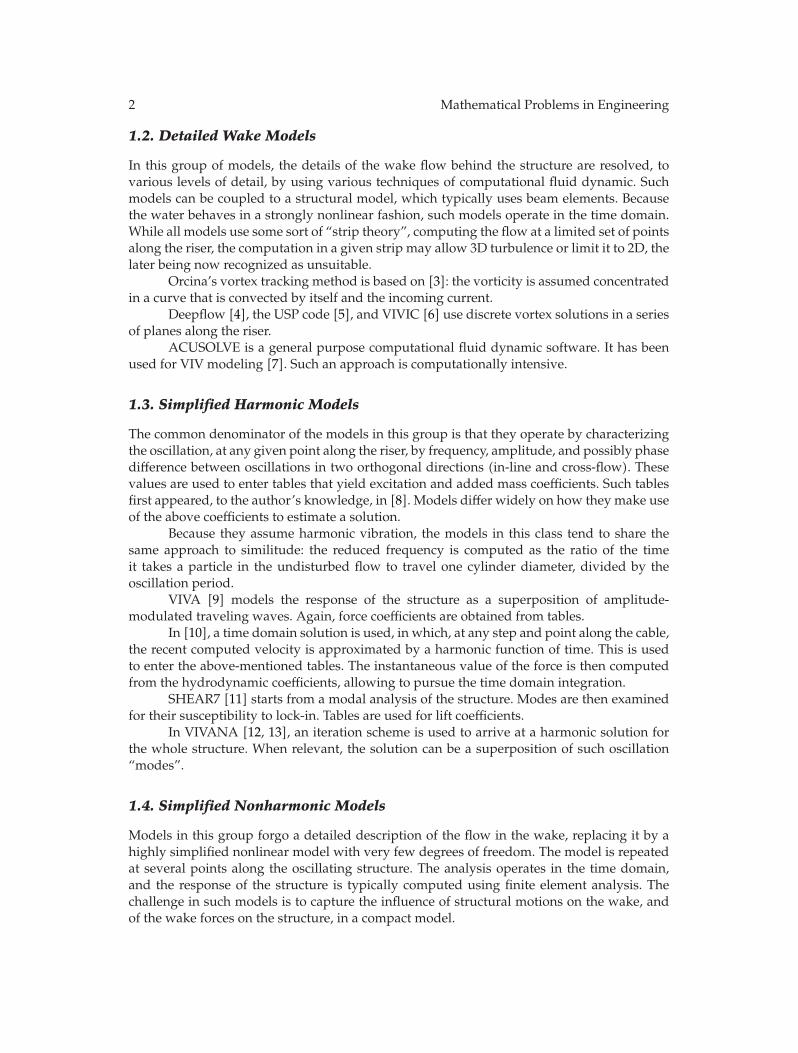
1.2. Detailed Wake Models

In this group of models, the details of the wake flow behind the structure are resolved, tovarious levels of detail, by using various techniques of computational fluid dynamic. Suchmodels can be coupled to a structural model, which typically uses beam elements. Becausethe water behaves in a strongly nonlinear fashion, such models operate in the time domain.While all models use some sort of “strip theory”, computing the flow at a limited set of pointsalong the riser, the computation in a given strip may allow 3D turbulence or limit it to 2D, thelater being now recognized as unsuitable.

Orcina’s vortex tracking method is based on [3]: the vorticity is assumed concentratedin a curve that is convected by itself and the incoming current.

Deepflow [4], the USP code [5], and VIVIC [6] use discrete vortex solutions in a seriesof planes along the riser.

ACUSOLVE is a general purpose computational fluid dynamic software. It has beenused for VIV modeling [7]. Such an approach is computationally intensive.

1.3. Simplified Harmonic Models

The common denominator of the models in this group is that they operate by characterizingthe oscillation, at any given point along the riser, by frequency, amplitude, and possibly phasedifference between oscillations in two orthogonal directions (in-line and cross-flow). Thesevalues are used to enter tables that yield excitation and added mass coefficients. Such tablesfirst appeared, to the author’s knowledge, in [8]. Models differ widely on how they make useof the above coefficients to estimate a solution.

Because they assume harmonic vibration, the models in this class tend to share thesame approach to similitude: the reduced frequency is computed as the ratio of the timeit takes a particle in the undisturbed flow to travel one cylinder diameter, divided by theoscillation period.

VIVA [9] models the response of the structure as a superposition of amplitude-modulated traveling waves. Again, force coefficients are obtained from tables.

In [10], a time domain solution is used, in which, at any step and point along the cable,the recent computed velocity is approximated by a harmonic function of time. This is usedto enter the above-mentioned tables. The instantaneous value of the force is then computedfrom the hydrodynamic coefficients, allowing to pursue the time domain integration.

SHEAR7 [11] starts from a modal analysis of the structure. Modes are then examinedfor their susceptibility to lock-in. Tables are used for lift coefficients.

In VIVANA [12, 13], an iteration scheme is used to arrive at a harmonic solution forthe whole structure. When relevant, the solution can be a superposition of such oscillation“modes”.

1.4. Simplified Nonharmonic Models

Models in this group forgo a detailed description of the flow in the wake, replacing it by ahighly simplified nonlinear model with very few degrees of freedom. The model is repeatedat several points along the oscillating structure. The analysis operates in the time domain,and the response of the structure is typically computed using finite element analysis. Thechallenge in such models is to capture the influence of structural motions on the wake, andof the wake forces on the structure, in a compact model.

Mathematical Problems in Engineering 3

Several models make use of simple nonlinear oscillators to represent the self-excitingand self-limiting nature of VIV response: A single degree of freedom van der Pol oscillatorhas been used in several models [14–17]. Orcina also uses a wake oscillator with few degreesof freedom [18].

1.5. Discussion

The drawback of detailed wake models is that for the relevant Reynolds numbers, theyare computationally very demanding. Hence they do not really offer a practical optionin structural design and design verification, where extensive computations are needed toadequately sample the statistics of currents and other operating conditions that the structureis likely to encounter.

Despite the fact that they currently provide the most used tools in VIV design,simplified harmonic models have several drawbacks. Most of them do not operate in thetime domain, which makes it difficult to account for structural nonlinearities. The modelscharacterize the oscillation of a cross section by amplitude and frequency, which is notadequate to describe more general types of motions.

Time domain models based on nonlinear oscillators have been proved to be able toreproduce some aspects of VIV behavior, but so far seem limited in their ability to capture thedetails of the response in a range of current conditions.

A good time domain, nonharmonic, simplified model, if it existed, would open newpossibilities, compared to harmonic models:

(1) study of VIV on nonlinear structures, for example, studying the damping effect ofseafloor interaction in a steel riser or using a hysteretic cross section model for VIVon flexible pipes,

(2) accounting for VIV caused by unsteady water flows, in particular by waves orvessel motions,

(3) accounting for the increase in drag at wave frequency due to VIV,

(4) accounting for the superposition of wave-frequency and VIV-frequency stresses infatigue analysis,

(5) accounting for the asymmetry of oscillation patterns in the vicinity of, for example,a seafloor.

1.6. Objective

The objective of thework reported here is to demonstrate the viability of a local, deterministic,time-domain force model for VIV on slender bodies with cylindrical cross sections.

The model is to treat in-line and cross flow vibrations jointly.It is to characterize the recent history of velocity of the cross section relative to the

surrounding fluid without making a harmonic assumption. The characterization is to be usedto enter a “table”, necessarily more complex than those used under harmonic assumption, topredict the instantaneous value of the hydrodynamic force. The model is to handle externalsteady or unsteady water currents.

Like many other models discussed above, this force model is to be used at each Gausspoint of the dynamic finite element (FE)model of a slender structure. The model is to be usedwithin a time domain analysis (e.g., Newmark-β time integration with Newton-Raphsoniteration).


Hence the FE model resembles that commonly used in a slender structure analysis,with degrees of freedom for the structure, and none for the surrounding fluid. In other words,the proposed model takes the place usually held in software by the Morison model for waveinduced loads.

2. Model Outline

2.1. Postulate

The present work hinges on the following postulate. The force exerted by the surrounding fluidon a section of the slender structure is completely determined by the recent histories at that sectionof the velocities of the structure and of the undisturbed fluid. Several points in this sentence areworthy of discussion.

The “force” includes the components usually distributed into added mass, excitationforces, drag, lift, and so forth.

That the force “at a section of the slender structure” is determined by the history “atthat section” implies a “strip theory” in which it is excluded that motions of the structureat a point A cause disturbances in the fluid that affect the force at point B away from A.In other words, it is assumed that there is no significant transmission of information in theaxial direction within the water (as opposed to within the slender structure). This wouldbe proved wrong if it turned out that unstable phenomena, like boundary layer shedding,although transmitting little energy along the structure, transmit information that steers howlocal hydrodynamic energy is channeled at a given point along the structure.

That the force should be “completely determined” implies that the behavior of thestructure is deterministic. This does not contradict the observation of hysteretic response ofshort cylindersmounted on elastic support. Uniqueness of forces for a given position does notimply uniqueness of static equilibrium. Neither does “completely determined” contradict theobservation of irregular and unpredictable responses to VIV: nonlinear dynamic systems canhave a chaotic behavior. Still, complete determinism is provably wrong, since a short verticalcylinder dragged at uniform speed through water will experience oscillating lift forces. Atany given moment, there is nothing in the history of (constant) velocity that allows to predictwhether the lift is left or right. So the present work is based on the bet that ignoring such“bifurcations” still leaves us with a useful model.

“Recent” can be defined as anything between the present time and a few times tw,where the value of tw still is an object of debate. tw is likely to be case dependent. The currentwill transport (convect) away vortices so that they quickly loose significance. The time twshould then be of the order of D/U where D is the cross section diameter and U the currentvelocity. In contrast, if the cylinder is oscillating in still water, it will be traveling in its ownwake, and tw should be related to the rate of diffusion and/or viscous dissipation of vortices,which is likely to result in much higher values of tw. Tests on periodic forced motion of shortcylinders sometimes show a slow drift of the forces (over as many as ten periods). In contrast,force decay tests for a cylinder stopped after oscillations at zero mean velocity, point towardsa fraction of a period. In the present work, the idea is to choose an upper bound for tw, afteradequate scaling (cf. Section 3.2).

The “velocity histories” are what count. Accelerations would not do because forexample, zero acceleration can correspond to different speeds and hence different forces. Onthe other hand, the force on a cylinder will not be affected by a uniform translation of itswhole trajectory, so a history of positions contains irrelevant information.


In the remainder of this text, the word “trajectory” will be given a very specificmeaning. The trajectory is defined as the recent history of the velocity vector of the cylinder relativeto the undisturbed surrounding fluid.

2.2. Restrictions

In the present phase of research, the following restrictions are introduced, in order to achievesome simplification of the task. The outer cross section of the slender structure is assumedperfectly circular and smooth. The surrounding fluid is assumed to be infinite, excluding thepresence of sea floor, free surface, or neighboring risers. Only fluid flows perpendicular to thecylinder at any point are considered.

2.3. Input and Output

As stated earlier, the VIV model being developed here replaces the Morison model for wave-induced loads. The VIV model is called at each step and iteration, and at each Gauss point ornode of each element.

The model is to receive as input:

(1) the diameter of the cylinder, the viscosity, and density of the surrounding fluid,

(2) the instantaneous velocity of the cross section relative to the undisturbed fluid,

(3) the instantaneous velocity and acceleration of the local undisturbed fluid, in aGalilean reference system.

The model uses velocity information stored from previous steps. On this basis, the modelproduces as output:

(1) the vector of hydrodynamic forces per unit length, acting on the cylinder,

(2) the matrix containing the derivative of the above with respect to instantaneousvalues of the cylinder’s behavior.

Gauss integration is then used to compute a consistent load vector and partial derivativematrices (damping, stiffness, and mass) for each element. Note that these element matricesare likely to vary significantly over each VIV oscillation “period”—in contrast to added massor damping matrices, deemed to be constant over a long time in semiempirical VIV models.The connection of the force model to the finite element analysis is discussed in Section 7.

2.4. Algorithmic Steps

Only the local VIV model is described here, not the whole FE analysis.

(1) The relative velocity of the cylinder relative to water (thereafter: “velocity”) iscomputed.

(2) The velocity is scaled (Reynolds scaling) to that the cylinder diameter is the unit ofdistance (Section 3.2).

(3) The trajectory (again: the recent histories of both x and y components of velocity)is compressed into a small number of “Laguerre coefficients”. This compressionis such that it provides detailed information over the recent past and increasinglycoarse information for the more distant past (Section 4).

(4) The Laguerre coefficients are used to enter an interpolation function (a feed-forward neural network with some specifically tailored properties) which returns


x and y components of hydrodynamic force (Section 5). The fitting of theinterpolation function is discussed in Section 8.1.

(5) The force is scaled back to the relevant diameter (Section 3.2).

(6) The Froude-Krylov forces, which depend on the acceleration of the undisturbedflow, are added (Section 3.1)

The identification of nonlinear systems using a bank of orthogonal filters (including Laguerrefilter) to generate multiple signals from a single one, and then using the multiple signals toenter a nonlinear, memory-less function, was introduced by Wiener [19] (Wiener-Laguerrefiltering). In the present work, a base of Laguerre polynomials is used, in contrast to Laguerrefunctions introduced by Wiener. While Wiener apparently did not use neural networks asnonlinear functions (but e.g., Hermite polynomials), neural networks in Wiener models havebeen studied for some time [20–22]. In the present work, Laguerre filtering is presentedwithout making use of the vocabulary of cybernetics. In particular, the z-transform is notintroduced here.

3. Exploiting Similitudes

3.1. Froude-Krylov Forces

This section gives the justification for point 6 of Section 2.4. If the undisturbed fluid in whichthe cylinder is plunged is accelerating (because of surface waves, e.g.,), then it is natural tointroduce two reference systems: G is a Galilean reference system, for example, fixed relativeto the sea floor and A is an accelerated reference system, locally following the undisturbedflow. Transforming the equations of equilibrium fromG (in whichwe carry out FEM analysis)to A (for which we have experimental data, in water that is not accelerated) requires theaddition of inertia forces.

The inertial forces create a uniform pressure gradient that was not present in thelaboratory test. The effect of a pressure gradient on a submerged body is variously referred toas “Archimedes forces” when the pressure gradient results from the acceleration of gravity,or as “Froude-Krylov forces” when the pressure gradient is due to fluid acceleration in forexample, surface waves. As familiar, the integral of the pressure over the wet surface istransformed into a volume integral [23].

It is assumed that this pressure gradient does not affect the turbulent flow, so that thepressure gradient can simply be added to the pressures resulting from turbulence. This seemsreasonable enough for incompressible flows, and indeedwhen it comes to Archimedes forces,the submerged weight of a cylinder is routinely subtracted to laboratory measurements andthe relevant correction added again in FEM analysis—even though the Archimedes forces inthe laboratory do not necessarily scale with those in the analysis. To the author’s knowledge,there is no experimental indication that a horizontal and vertical cylinder, all other conditionsbeing equal, experience different forces.

To conclude, the hydrodynamic force acting on the cylinder at a given instant is thesum of two terms:

(1) a force that is a function of only the cylinder diameter and the recent history of thevelocity of the cylinder relative to the undisturbed, steady water flow,

(2) Froude-Krylov forces.

All computations in Sections 4 and 5 deal only with the first of the above two terms.


3.2. Scaling

This section details how points 2 and 5 of Section 2.4 are implemented. In order to reduce theamount of experimental data necessary to create the interpolation function used in point 4,one must take advantage of scale similarities. To that effect, all data used to either train orquery the database is scaled. Correspondingly, all forces returned by the database are scaledback. The present model uses a scaling that is quite different from the scaling typical used bysimplified harmonic models (Section 1.3): reduced amplitudes and frequencies are not used.Instead velocities histories are scaled in a manner familiar from the Reynolds number.

VIV forces are assumed to be uniquely defined by fluid density ρ, kinematic viscosityν, cylinder diameter D, and the motion history. Hence, in order to create a database that is tobe entered with scaled velocities, we wish all experimental data to be scaled to fixed referencevalues ρo, νo, and Do. The choice of ρo, νo, and Do is arbitrary, and in this work, all are set tothe value 1.

By expressing the units of these quantities, one gets three equations on λm, λs, andλkg , which are the scaling factors for the basic units of distance, time, and mass. Solving thesystem yields

λm =1D,

λs =ν

D2,

λkg =1

ρD3.

(3.1)

Once the scaling of basic units is known, the scaling of any derived quantities, for example,velocities, accelerations, and forces per unit length can be expressed:

λms−1 =D

ν, (3.2)

λms−2 =D3

ν2, (3.3)

λNm−1 =D

ρν2. (3.4)

The choice Do = 1 [m] hence implies that scaled displacements can be considered to have “1diameter” as unit. Similarly, the choices Do = 1 [m] and νo = 1 [m2/s] together imply thatscaled velocities are expressed as Reynolds numbers since the scaled velocity is calculated asDv/νwhere v is the velocity. The Reynolds number is usually computed using some velocitythat is characteristic of the system under study. In VIV science, the undisturbed velocity of thecurrent is used. By contrast, in this work, instantaneous local values of the relative velocityvector are multiplied by D/ν. The scaled velocities thus obtained are a generalization of thetraditional use of Reynolds number: considering an immobile cylinder in a current, the normof its scaled relative velocity vector is equal to the traditional Reynolds number. To preventconfusion of the present usage of Reynolds number with the more particular classical one,


yet emphasize the relation between both, the expression “ilr-Reynolds” (for “instant, local,relative Reynolds”) will be used in this document.

Since scaling is applied consistently to all derived quantities, all nondimensionalnumbers based on combinations of distance, time and mass (including Reynolds and Froudenumbers) are conserved. However, any dimensional quantity with units different from thoseof ρ, ν, and D is scaled to values that depend of ρ, ν, and D. In particular, (3.3) shows thatall accelerations, including the acceleration of gravity g, are scaled with a factor proportionaltoD3/ν2. So while the scaling used here may conserve Froude’s number, it does not allow tobuild a database of forces related to surface wave effects, because the database does not referto a uniform value go.

4. Characterization of Trajectory

4.1. Foreword

This section details how point 3 in Section 2.4 is to be implemented. The objective is, for anygiven point in time, to distill a “summary” of the recent history of the velocity of the cylinderrelative to the surrounding fluid (trajectory). Note that the history of each component of thevelocity vector is treated separately in this section and that the procedure is applied to thescaled trajectory.

The trajectory is approximated as a linear combination of some adequate family offunctions, and the coefficients in this linear combination are the summary. The family offunctions that is used here is the series of Laguerre polynomials (Section 4.2). It is shownin Section 4.3 that if the “Laguerre coefficients” of the linear combination are obtained byintegrating the product of the trajectory by adequate “Laguerre analysis functions”, then thedifference between the approximating linear combination and the real trajectory is small inthe recent past and larger in the further past. This justifies the choice of Laguerre polynomials:they allow to summarize the trajectory in a way that represents recent velocities veryprecisely, and older velocities in a coarser manner. It is assumed that this corresponds tothe information needed to obtain a good estimate of the hydrodynamic force.

Computing the integral of the product of Laguerre analysis functions and trajectorytakes time. Luckily, one can show (Section 4.5) that the Laguerre coefficients are the solutionof a differential equation driven by the instant value of the velocity. To obtain results thatare independent of step size, this differential equation must be carefully discretised in time(Section 4.6) when summarizing experimental data.

4.2. Definitions

The Laguerre polynomial (Figure 1, top) of degree i − 1 can be defined by its Rodriguesformula [24]

Li(x) ≡ ex

i!di

dxi

(xie−x

). (4.1)

Laguerre polynomials verify the orthonormality property

∫∞

0Li(x)Lj(x)e−xdx = δij . (4.2)


−5 −4.5 −4 −3.5 −3 −2.5 −2 −1.5 −1 −0.5 0

−5 −4.5 −4 −3.5 −3 −2.5 −2 −1.5 −1 −0.5 0

−5 −4.5 −4 −3.5 −3 −2.5 −2 −1.5 −1 −0.5 0

−0.50

0.51

−20

2Laguerre polynomials (synthesis) (nlgr = 10)

0

0.5

1Weight function

Time (s)

Laguerre analysis functions, times to decay/dt

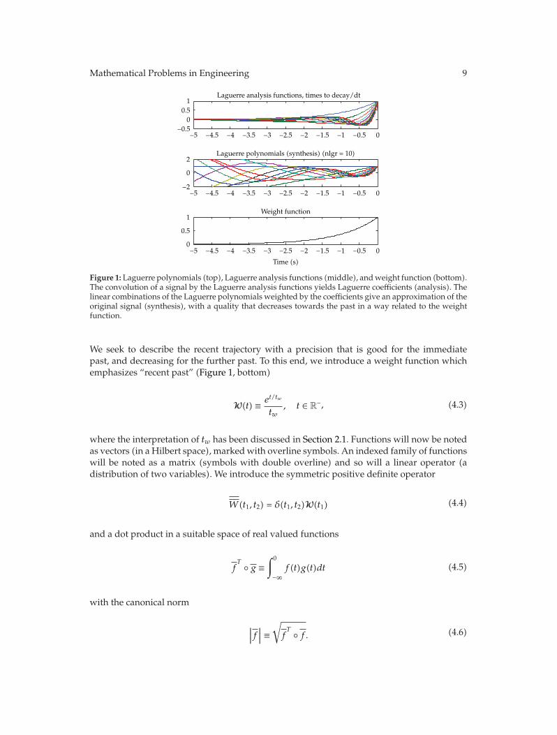
Figure 1: Laguerre polynomials (top), Laguerre analysis functions (middle), andweight function (bottom).The convolution of a signal by the Laguerre analysis functions yields Laguerre coefficients (analysis). Thelinear combinations of the Laguerre polynomials weighted by the coefficients give an approximation of theoriginal signal (synthesis), with a quality that decreases towards the past in a way related to the weightfunction.

We seek to describe the recent trajectory with a precision that is good for the immediatepast, and decreasing for the further past. To this end, we introduce a weight function whichemphasizes “recent past” (Figure 1, bottom)

W(t) ≡ et/tw

tw, t ∈ R

−, (4.3)

where the interpretation of tw has been discussed in Section 2.1. Functions will now be notedas vectors (in a Hilbert space), markedwith overline symbols. An indexed family of functionswill be noted as a matrix (symbols with double overline) and so will a linear operator (adistribution of two variables). We introduce the symmetric positive definite operator

W(t1, t2) = δ(t1, t2)W(t1) (4.4)

and a dot product in a suitable space of real valued functions

fT ◦ g ≡

∫0

−∞f(t)g(t)dt (4.5)

with the canonical norm

∣∣∣f∣∣∣ ≡

√fT ◦ f. (4.6)


Further we introduce the base

L(t, i) ≡ Li

(− t

tw

), t ∈ R

−, i ∈ {1, . . . , n}. (4.7)

Equation (4.2) can be rewritten in matrix notation as

I = LT

◦W ◦ L, (4.8)

where I is the n × n identity matrix. It is useful to introduce the weighted norm or w-norm

∣∣∣f∣∣∣w≡√fT ◦W ◦ f. (4.9)

Note that sinceW(t) is of dimension [1/s], |f |w is of the same dimension as f . So when takingf as a scaled velocity, |f |w is an ilr-Reynolds number.

4.3. Analysis and Synthesis

For a history v(t) of either the x or y component of the velocity, we seek the vector of

“Laguerre coefficients” τ with which to combine the columns L, that minimize the weightederror J defined as

J =12

∣∣∣∣v − L · τ∣∣∣∣2

w

=12

(v − L · τ

)T

◦W ◦(v − L · τ

).

(4.10)

A notation borrowed from physics is used here: the dot in the above equations symbolizes asum, as would appear in a matrix-vector product or the scalar product of two vectors. In thisnotation, the sum acts on the last index of the left argument and the first index of the rightargument. Vector transpositions are hence without effect, but have been added in the text forreaders that prefer matrix notations.

To this effect, we require that the derivative be zero:

∂J

∂τ= L

T

◦W ◦ L · τ − LT

◦W ◦ v, (4.11)


which implies

τ =(LT

◦W ◦ L)−1

· LT

◦W ◦ v (4.12)

= LT

◦W ◦ v, (4.13)

τ = DT

◦ v (4.14)

with

D ≡ W ◦ L. (4.15)

The “Laguerre analysis functions” D (Figure 1, middle) are by definition equal to

D(t, i) = Di

(−ttw

)

= Li

(−ttw

)et/tw

tw.

(4.16)

The Laguerre analysis functionsDmust not be confusedwith the Laguerre functions (note thefactor 2 in (4.18)). Incidentally, Wiener-Laguerre models use Laguerre filters whose impulseresponse is Laguerre functions (not analysis function), so the present approach is slightlydifferent from the classical Wiener-Laguerre model. A justification for the present choice willappear in Section 6.1.

4.4. Convergence

Laguerre functions, which can be defined as

F(t, i) ≡ Fi

(−ttw

)(4.17)

≡ Li

(−ttw

)et/(2tw)√

tw(4.18)

or in matrix notation as

F =

√W ◦ L, (4.19)


have been extensively studied. Series of Laguerre functions are known to converge almosteverywhere (under some conditions of continuity) [25]. In matrix notation, this result can bestated as

limn→∞

∣∣∣∣F · FT

◦ f − f

∣∣∣∣ = 0. (4.20)

This can be used to obtain a result on the convergence of series of Laguerre polynomials. Weintroduce the change of variables

f =

√W ◦ g (4.21)

so that

∣∣∣∣F · FT

◦ f − f

∣∣∣∣ =∣∣∣∣∣F ·D

T

◦ g −√W ◦ g

∣∣∣∣∣

=

∣∣∣∣∣

√W ◦

(L ·D

T

◦ g − g

)∣∣∣∣∣

=∣∣∣∣L ·D

T

◦ g − g

∣∣∣∣w

.

(4.22)

We hence have convergence in terms of the quality of approximation that we are seeking,with emphasis on the recent past. Further, on any finite (or “compact”) interval, convergencein thew-norm is equivalent to convergence almost everywhere. So under some conditions of

continuity on g, the series of Laguerre polynomials obtained using D as analysis functionsconverges almost everywhere towards g in any finite interval.

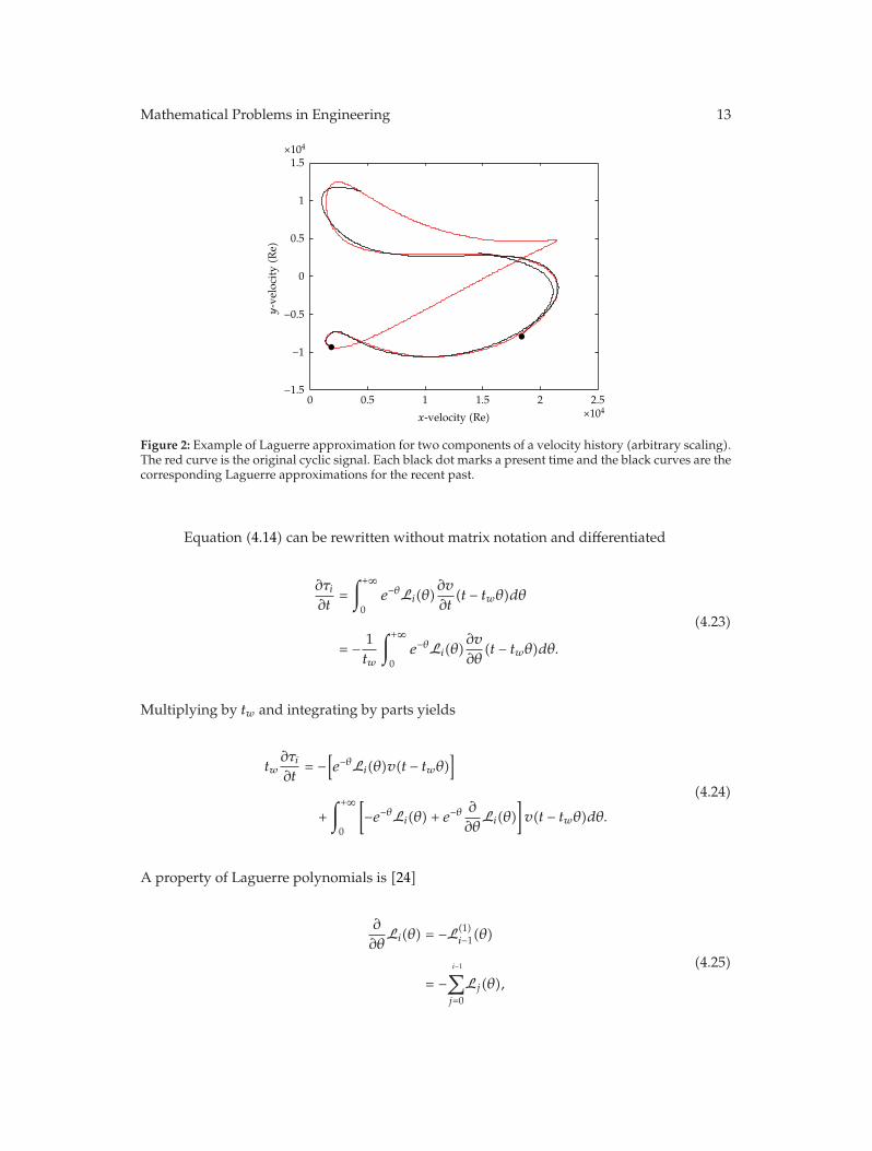
Figure 2 illustrates how Laguerre coefficients indeed provide a “summary” of thetrajectory

4.5. Differential Equation for Laguerre Coefficients

In the finite element analysis, we need to update the Laguerre coefficients at each iterationof each time step, for every Gauss point of every node of the system. The explicit calculationof (4.14) for every update is hence a CPU-time critical operation, taking in the order of n ×N floating point operations (flops), where n is the number of Laguerre polynomial usedand N the number of time steps that the analysis functions take to decay to a negligiblevalue. Further, for each Gauss point, 2N velocity values need to be stored, a severe memoryrequirement.

In the present section and the next, it is shown how the computation of (4.14) can becarried out by a recursive operation requiring no other storage than that of the Laguerrecoefficients and the last velocity values, and taking in the order of n × n flops, which isadvantageous because n � N. In this section, it is shown that τ verifies a differential equationdriven by the history v of the velocity component. In Section 4.6, this differential equation issolved time-step by time-step in a recursive update.


0 0.5 1 1.5 2 2.5×104

×104

−1.5

−1

−0.5

0

0.5

1

1.5

x-velocity (Re)

y-velocity(R

e)

Figure 2: Example of Laguerre approximation for two components of a velocity history (arbitrary scaling).The red curve is the original cyclic signal. Each black dot marks a present time and the black curves are thecorresponding Laguerre approximations for the recent past.

Equation (4.14) can be rewritten without matrix notation and differentiated

∂τi∂t

=∫+∞

0e−θLi(θ)

∂v

∂t(t − twθ)dθ

= − 1tw

∫+∞

0e−θLi(θ)

∂v

∂θ(t − twθ)dθ.

(4.23)

Multiplying by tw and integrating by parts yields

tw∂τi∂t

= −[e−θLi(θ)v(t − twθ)

]

+∫+∞

0

[−e−θLi(θ) + e−θ

∂

∂θLi(θ)

]v(t − twθ)dθ.

(4.24)

A property of Laguerre polynomials is [24]

∂

∂θLi(θ) = −L(1)

i−1(θ)

= −i−1∑j=0

Lj(θ),(4.25)


where L(1)i (θ) is a generalized Laguerre polynomial. Hence we can write

tw∂τi∂t

= Li(0)v(t) − τi −∫+∞

0e−θ

i−1∑j=1

Lj(θ)v(t − twθ)dθ

= v(t) − τi −i−1∑j=1

τj

= v(t) −i∑

j=1

τj .

(4.26)

which is of the form

∂τ

∂t(t) = μ · τ(t) + n v(t) (4.27)

with

μij =

⎧⎨⎩− 1tw

j ≤ i

0 j > i,

ni =1tw

.

(4.28)

Equation (4.27) shows that at any time t, the rate of the Laguerre coefficients is fully definedby the Laguerre coefficients and the velocity signal.

4.6. Recursive Filter

The discrete integration of (4.27) must be done carefully, for two reasons. Firstly, it isimportant to obtain Laguerre coefficients that are independent of the sampling rate used (aslong as the sampling rate is “adequate”). This is because the experimental data on whichthe VIV model is based may come from experiments which, after scaling, may have differentsampling rates. Further, the numerical analysis in which the VIV model is used may use yetanother time step. The choice of time step or sampling ratemust not affect the way a trajectoryis characterized by Laguerre coefficient.

The second reason for care in discrete integration is that we wish to be able to create

synthesized signals L·τ of good quality. Synthesized signals are neither used in the numericalprocess of creating a force interpolation function (Section 5) or in the FEM use of the VIVmodel. However, visualization is essential to the process of research, both for fault diagnosisand quality control, and to communicate an understanding of the method.

This discrete integration is only used in the analysis of experimental data, to providean input to the training of the “rotatron” (Section 5.6). In dynamic analysis, the integration of(4.27) is done by means of the Newmark-β method, as detailed in Section 7.


Assume that velocity is sampled at regular intervals

vj = v(t0 + jdt

). (4.29)

We seek the values of the Laguerre coefficients at the same intervals

τj = τ(t0 + jdt

). (4.30)

The vector τj (the list of the coefficients for all Laguerre polynomials, taken at step j) mustnot be confused with scalar τi (the coefficient for the Laguerre polynomial of degree i). Wechoose t0 such that t0 + jdt = 0, and we approximate v by a function that is linear over theinterval [0, dt]. Equation (4.27) becomes

∂τ

∂t(t) = μ · τ(t) + α + βt (4.31)

with

α = nv(0),

β = nv(dt) − v(0)

dt.

(4.32)

This new differential equation can be solved exactly: we seek a solution of the form

τ(t) = exp(μt)· a + bt + c (4.33)

over the interval. Here exp(μt) stands for a matrix exponential. Replacing this expression into(4.31), noting that

∂

∂texp

(μt)= μ · exp

(μt),

exp(0)

= I,

(4.34)

and identifying the constant and linear terms and enforcing the initial value leads to

b = −μ−1 · β,

c = −μ−2 · β − μ−1 · α,

a = τ(0) + μ−2 · β + μ

−1 · α.

(4.35)


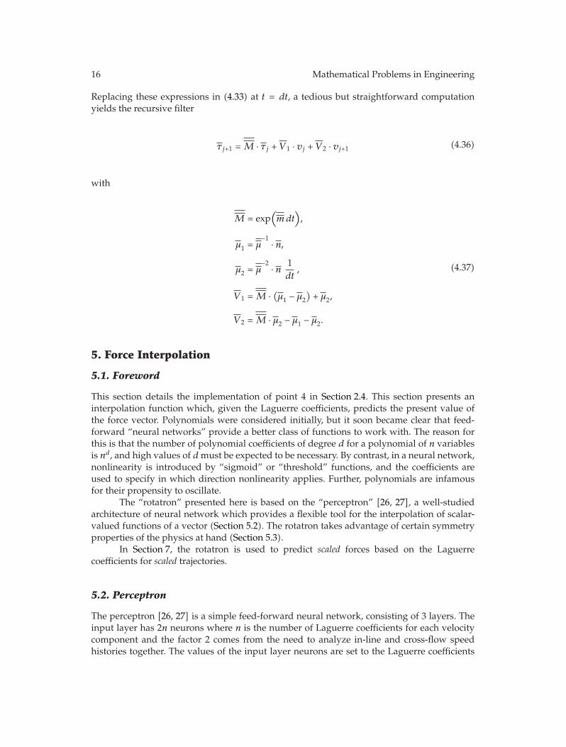
Replacing these expressions in (4.33) at t = dt, a tedious but straightforward computationyields the recursive filter

τj+1 = M · τj + V 1 · vj + V 2 · vj+1 (4.36)

with

M = exp(mdt

),

μ1 = μ−1 · n,

μ2 = μ−2 · n 1

dt,

V 1 = M · (μ1 − μ2

)+ μ2,

V 2 = M · μ2 − μ1 − μ2.

(4.37)

5. Force Interpolation

5.1. Foreword

This section details the implementation of point 4 in Section 2.4. This section presents aninterpolation function which, given the Laguerre coefficients, predicts the present value ofthe force vector. Polynomials were considered initially, but it soon became clear that feed-forward “neural networks” provide a better class of functions to work with. The reason forthis is that the number of polynomial coefficients of degree d for a polynomial of n variablesis nd, and high values of dmust be expected to be necessary. By contrast, in a neural network,nonlinearity is introduced by “sigmoid” or “threshold” functions, and the coefficients areused to specify in which direction nonlinearity applies. Further, polynomials are infamousfor their propensity to oscillate.

The “rotatron” presented here is based on the “perceptron” [26, 27], a well-studiedarchitecture of neural network which provides a flexible tool for the interpolation of scalar-valued functions of a vector (Section 5.2). The rotatron takes advantage of certain symmetryproperties of the physics at hand (Section 5.3).

In Section 7, the rotatron is used to predict scaled forces based on the Laguerrecoefficients for scaled trajectories.

5.2. Perceptron

The perceptron [26, 27] is a simple feed-forward neural network, consisting of 3 layers. Theinput layer has 2n neurons where n is the number of Laguerre coefficients for each velocitycomponent and the factor 2 comes from the need to analyze in-line and cross-flow speedhistories together. The values of the input layer neurons are set to the Laguerre coefficients


for both velocity components. The second layer has nhid neurons, whose values are an affinefunction of the values of the first layer, passed through a sigmoid function like

σ(x) = 1 − 2e2x + 1

. (5.1)

Finally, the third layer gives the output of the perceptron, and its values are an affine functionof the values of the second layer. This can be summarized as

fi = Mij · σ(Njkl · τkl + Vj

)+Ui. (5.2)

Mij , Njkl, Ui and Vj are the “weights” or interpolation coefficients, that must be adjustedto fit the perceptron to interpolate some given data. τkl are Laguerre coefficients and fi arepredicted force components. i is the index of force direction (x versus y), j the index of neuronin the hidden layer, k the index of velocity direction, and l the index of Laguerre coefficient.

Each output of the perceptron can be seen as a function, which is a sum of sigmoidsteps in directions defined by Njkl.

5.3. Symmetries

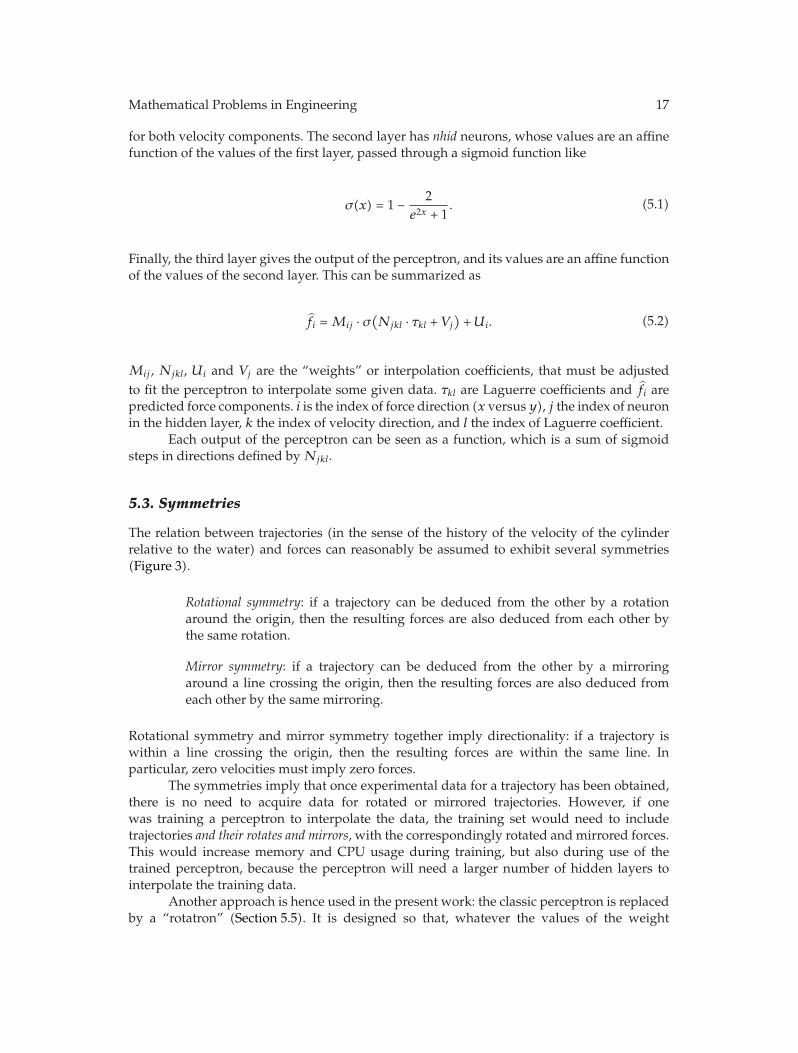
The relation between trajectories (in the sense of the history of the velocity of the cylinderrelative to the water) and forces can reasonably be assumed to exhibit several symmetries(Figure 3).

Rotational symmetry: if a trajectory can be deduced from the other by a rotationaround the origin, then the resulting forces are also deduced from each other bythe same rotation.

Mirror symmetry: if a trajectory can be deduced from the other by a mirroringaround a line crossing the origin, then the resulting forces are also deduced fromeach other by the same mirroring.

Rotational symmetry and mirror symmetry together imply directionality: if a trajectory iswithin a line crossing the origin, then the resulting forces are within the same line. Inparticular, zero velocities must imply zero forces.

The symmetries imply that once experimental data for a trajectory has been obtained,there is no need to acquire data for rotated or mirrored trajectories. However, if onewas training a perceptron to interpolate the data, the training set would need to includetrajectories and their rotates and mirrors, with the correspondingly rotated and mirrored forces.This would increase memory and CPU usage during training, but also during use of thetrained perceptron, because the perceptron will need a larger number of hidden layers tointerpolate the training data.

Another approach is hence used in the present work: the classic perceptron is replacedby a “rotatron” (Section 5.5). It is designed so that, whatever the values of the weight


−1 −0.5 0 0.5 1 1.5 2 2.5 3×104

−5000

0

5000

10000

15000

20000

x-velocity (Re)

y-velocity(R

e)

Figure 3: For circular cross sections, it is assumed that if two trajectories that can be deduced from eachother by rotation or mirroring; then the corresponding forces are deduced from each other by the sameoperation.

coefficient, a rotation or mirroring of the input trajectory results in the same rotation ormirroring of the output force vector.

5.4. Index Notations

In the present work, index notations inspired from tensor analysis are used. However, thepresent setting differs from tensor analysis in at least three ways.

Firstly, we assume that we are only operating in Euclidean spaces (and not inmore general Riemannian manifolds) so that orthogonal bases can be used. This makes itunnecessary to distinguish between co- and contravariant bases and coordinates. Hence, onlylowered indexes appear in the present work. Incidentally, it was here assumed that the stateof the model is a point in a vector space, which is not true when finite rotations are presentand Riemannian geometry should be introduced instead.

Secondly, in tensor notations, each index spans the dimension of the manifold. In anexpression like σij = Cijklεkl, the indexes range from 1 to 3. Following Einstein’s convention,indexes k and l are summed over, and the relation is valid for any combination of i and j.The fact that the equation is valid at each point within a solid is implicit in the notation.In the present work, we prepare for the manipulations of arrays in a computer, involvingoperations that are repeated, for example, for various locations along a riser. If indexes x, yand zwere introduced to note the position to which the various tensors refer, one would tendto write σijxyz = Cijklxyz εklxyz, which violates Einstein’s convention, because no summation(or rather: no integral) is implied over the positions.

Thirdly, we introduce nonlinear functions. These functions can combine the values ofthe coordinates for some indexes (these will be noted in brackets) and operate in parallel onthe coordinates for other indexes (not brackets). For example, by definition of the notation

|y[j]k| is equal to√y21k + y2

2k, all values of j are present in one evaluation of the square root,and the square root is evaluated for each value of k.


V

V

D

DM

M

U

fIL

fCF

σIL

σCF

VIL

VCF

yIL

yCF

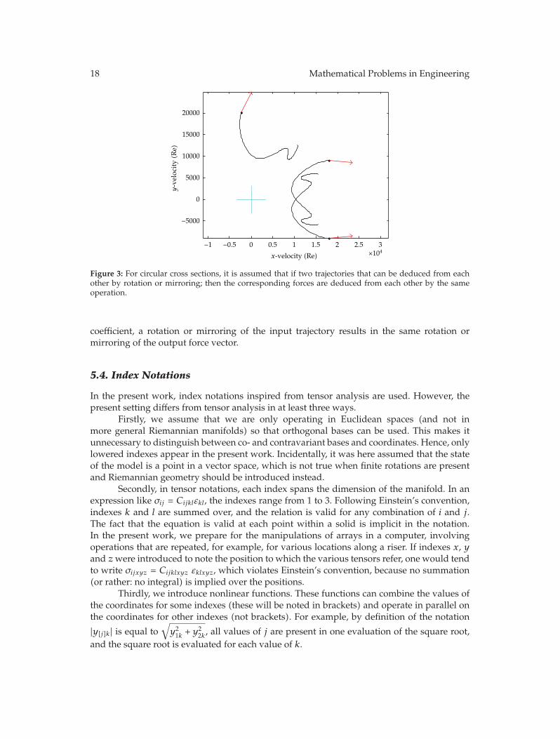
Figure 4: Laguerre analysis and rotatron transform velocity histories into a hydrodynamic force. ThematrixD is the discrete form of the Laguerre analysis functions, which appear in (4.14). The dots symbolizea matrix-matrix product.

Appendix A gives a detailed description of the conventions used.

5.5. Rotatron

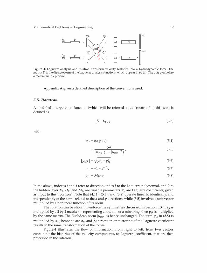
A modified interpolation function (which will be referred to as “rotatron” in this text) isdefined as

fi = Vkσik (5.3)

with

σik = σi

(y[j]k

)(5.4)

=yik∣∣y[j]k

∣∣(1 + ∣∣y[j]k∣∣αk

) , (5.5)

∣∣y[j]k∣∣ =

√y21k + y2

2k, (5.6)

αk = −1 − e−Uk , (5.7)

yjk = Mklτjl. (5.8)

In the above, indexes i and j refer to direction, index l to the Laguerre polynomial, and k tothe hidden layer. Vk, Uk, and Mkl are tunable parameters. τjl are Laguerre coefficients, givenas input to the “rotatron”. Note that (4.14), (5.3), and (5.8) operate linearly, identically, andindependently of the terms related to the x and y directions, while (5.5) involves a unit vectormultiplied by a nonlinear function of its norm.

The rotatron can be shown to enforce the symmetries discussed in Section 5.3: if τjl ismultiplied by a 2 by 2 matrix sjj ′ representing a rotation or a mirroring, then yjk is multipliedby the same matrix. The Euclidean norm |y[j]k| is hence unchanged. The term yik in (5.5) ismultiplied by sij ′ , hence so are σik and fi: a rotation or mirroring of the Laguerre coefficientresults in the same transformation of the forces.

Figure 4 illustrates the flow of information, from right to left, from two vectorscontaining the histories of the velocity components, to Laguerre coefficient, that are thenprocessed in the rotatron.


0 0.5 1 1.5 2 2.5 30

0.1

0.2

0.3

0.4

0.5

0.6

0.7

0.8

0.9

1

x

σ(x)

Figure 5: Log-logistic sigmoid functions.

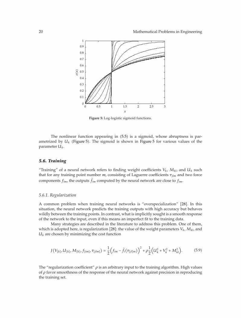
The nonlinear function appearing in (5.5) is a sigmoid, whose abruptness is par-ametrized by Uk (Figure 5). The sigmoid is shown in Figure 5 for various values of theparameter Uk.

5.6. Training

“Training” of a neural network refers to finding weight coefficients Vk, Mkl, and Uk suchthat for any training point number m, consisting of Laguerre coefficients τjlm and two forcecomponents fim, the outputs fim computed by the neural network are close to fim.

5.6.1. Regularization

A common problem when training neural networks is “overspecialization” [28]. In thissituation, the neural network predicts the training outputs with high accuracy but behaveswildly between the training points. In contrast, what is implicitly sought is a smooth responseof the network to the input, even if this means an imperfect fit to the training data.

Many strategies are described in the literature to address this problem. One of them,which is adopted here, is regularization [28]: the value of the weight parameters Vk,Mkl, andUk are chosen by minimizing the cost function

J(V[k], U[k],M[k], f[im], τ[jlm]

)=

12

(fim − fi

(τ[jl]m

))2+ ρ

12

(U2

k + V 2k +M2

kl

). (5.9)

The “regularization coefficient” ρ is an arbitrary input to the training algorithm. High valuesof ρ favor smoothness of the response of the neural network against precision in reproducingthe training set.


Arguments of symmetry by permutation of the numbering of the first index of yjk

in (5.6) show that the cost function has multiple minima. Further, there are probably localminima higher than the lowest maxima.

5.6.2. Conjugate Gradient Optimization

J is a function of a large number of weight coefficients, and hence it is not practical to computethe Hessian of J , because the Hessian is a full matrix. It also proves to be very costly to evencompute an approximation to it as done in the Levenberg-Marquardt algorithm [29, 30]. Onthe other hand, the Nelder-Mead “downhill simplex” algorithm [31], which uses only thevalues of J , proved very slow in this case. Hence a search method is chosen, that determinesthe search direction from the gradient of J [32]. This is a conjugate gradient method, in whichthe step length is found by deriving the gradient in the direction of the search. In this method,the positive definiteness of the (implicit)Hessian is forced by adding a scaled identity matrixto it, a technique known as “trust region”.

The conjugate gradient method proved far more efficient than the Levenberg-Marquardt and Nelder-Mead methods for the present task.

The weight coefficients are set to random values at the start of the conjugate gradientiterations.

6. Metric

6.1. Euclidean Metric and Distance

In order to describe the available data, it is useful to define a distance between trajectories.This will allow to determine to what extend the set of available data “fills” the set of allpossible trajectories, or to detect zones of transition from one hydrodynamic behavior tothe other. Finally, this will help detecting contradictions in the available data, arising froma variety of sources, including hidden experimental variables, measurement uncertainties, orinadequate modeling in inverse methods and not least, the natural variability of VIV forces.

The x and y components of a trajectory are described by a pair of functions:

f ≡(fx, fy

). (6.1)

We can define a scalar product between trajectories, that captures any recent differences:

fT � g ≡ f

T

x ◦W ◦ gx + fT

y ◦W ◦ gy

=∫0

−∞

et/tw

tw

(fx(t)gx(t) + fy(t)gy(t)

)dt.

(6.2)

By replacing fx, fy, gx, and gy by their expression in terms of Laguerre polynomials andtheir respective Laguerre coefficients τfx, τfy, τgx, and τgy, one finds that

fT � g = τTfx · τgx + τTfy · τgy

= τTf · τg(6.3)


0 2 4 6 8 10 12 14 16 18

−10000

−8000

−6000

−4000

−2000

0

2000

4000

x-velocity (Re)

y- velo city( R

e )

×103

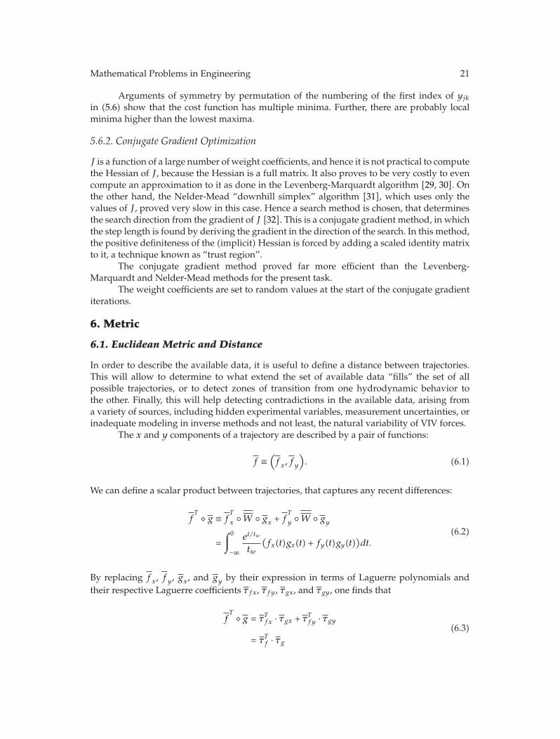
Figure 6: A set of neighboring trajectories according to (6.6). Typical distance between trajectories: 103 [ilrRe].

with

τf ≡[τfx

τfy

], τg ≡

[τgx

τgy

]. (6.4)

The distance is defined from the scalar product in the usual manner:

∣∣∣f − g∣∣∣ ≡

√(f − g

)T �(f − g

), (6.5)

=∣∣τf − τg

∣∣. (6.6)

In other words, neighboring vectors of Laguerre coefficients describe trajectories that aresimilar in the recent past. This is illustrated by taking random samples of Laguerrecoefficients around a given value obtained from data analysis and plotting the synthesizedtrajectories (Figure 6). Given that trajectories are compared using an integral weighted withan exponential (4.2). This important property can be seen as the justification of the choice ofthe Laguerre coefficients to “summarize” trajectories.

6.2. Rotatron Distance

The above does not account for rotational and mirror symmetries. We seek a distance forwhich the distance of a trajectory to its transforms by rotation or mirroring is zero. Anotherdistance is hence introduced:

d(f, g

)≡ min

(minR∈R

∣∣∣f − R(g)∣∣∣,min

S∈S

∣∣∣f − S(g)∣∣∣), (6.7)


0 0.5 1 1.5 2 2.5×104

×104

−1

−0.5

0

0.5

1

Vx (Re)

Vy(R

e)

Typical distance 11496 (Re)

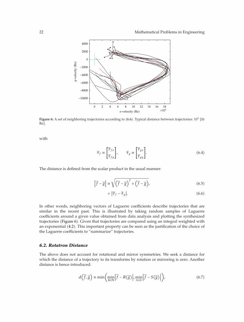
Figure 7: A trajectory and its neighbors in terms of rotatron distance. Smooth curve: Laguerreapproximation of trajectory, stippled arrow: true force, smooth arrow: predicted force. Black is for thetrajectory used to enter the model to find the force. Green and red are used for the three closest points inthe database, respectively, before and after rotation or mirroring.

where R is the set of all rotations of the trajectories around the origin and S the set of allmirroring of trajectories around a line passing by the origin. Note that no norm or scalarproduct associated to the distance d is presented here (The vector-space of trajectories,divided by the group of rotations and mirrorings, is not a vector space).

Because fx is related to τfx by the same linear relation that relates fy to τfy, linear

combinations of fx and fy (including rotation and mirroring) are related to the same linear

combinations of τfx and τfy. By expressing the distance |f − R(g)| as a function of the angleα of the rotation R, and then differentiating it with respect to α, it can be shown that the valueof α that minimizes |f − R(g)| is

α = arctan(τfx · τgy − τfy · τgx, τfy · τgy + τfx · τgx

), (6.8)

where arctan(y, x) ∈ ] − π,π] is the angle of a vector [x, y]T with the x-axis. Similarly, it canbe shown that the mirroring that minimizes |f −S(g)| is the composition of a rotation of angle

β = arctan(τfx · τgy + τfy · τgx, τfy · τgy − τfx · τgx

)(6.9)

by a swap of the sign of the x-coordinates. Equations (6.8) and (6.9) allow to compute (6.7).Figure 7 shows a trajectory and the trajectories within a small database that have the

smallest distance to it, measured using d.


6.3. Existence of Functional Relation

6.3.1. Introduction

From experiments, one can obtain databases of velocity histories, and the correspondinghydrodynamic forces. The velocity histories can be “summarized” into Laguerre coefficients.An open question at this stage is whether there is actually a functional relationship betweenthe Laguerre coefficients and the forces, that the rotatron could be used to approximate. Forexample, if the decay time tw was chosen too small, then the same velocity in the recentpast (represented by the Laguerre coefficient)will result in different forces, depending on thevelocity in the more remote past. In that case, there is no functional relation. The functionalrelation could also be lost if too few Laguerre coefficients are used, or if the force in theexperiments is affected by incoming turbulence. In the absence of a functional relation,attempting to train the rotatron will not give useful results, in the same way as no curvedrawn through a cloud of points on a piece of paper will provide a useful model.

The approach in this section hinges on two ideas. Firstly, the higher the dimension ofa spaceis, the faster the volume of a ball increases with its radius. Hence, the statistic of thedistances between points in a cloud of data can be used to define a dimension (Section 6.3.4).For example, a set of points on a piece of paper will be shown to follow a curve if the numberof neighbors increases linearly with the radius. Secondly, if Laguerre coefficients τ predictforces f , then the dimension of the cloud of experimental τ values must be the same as thedimension of the cloud of [τ, f] points (Section 6.3.3).

6.3.2. Minkowski-Bouligand Dimension

Considering a relatively uniform cloud of points, the number m of points in a ball isproportional to the radius r of the sphere to the power of p, where p is the dimension ofthe space in which the cloud is defined. For example, using 2 × 10 Laguerre coefficients todescribe both components of a trajectory, the number of points in the ball would bem ∝ r20.

Conversely, one can define the Minkowski-Bouligand dimension (often referred to asthe fractal dimension [33]) p of a set (in particular, of a “database” of Laguerre coefficients)by counting the numberm(r) of pairs of points in a set, which have a distance smaller than r:

p(r) ≡ ∂ logm(r)∂ log r

. (6.10)

In practice, one should either smooth m(r) or compute the derivative by finite differencesover a large enough interval. Note that the fractal dimension p is a function of the scale r.

6.3.3. Functional Relation

Imagine that we have a series of data-points (x, y, z), and we are investigating whether z canbe predicted using x and y. Let us imagine that the fractal dimension of the set of (x, y) pairsis 2 (the set of (x, y) fills the plane). If the fractal dimension of the set of (x, y, z) is equal to2, then the set of (x, y, z) is within a surface, and z can be predicted using x and y. If thefractal dimension of the set of (x, y, z) is equal to 3, the data forms a cloud, and x and y are


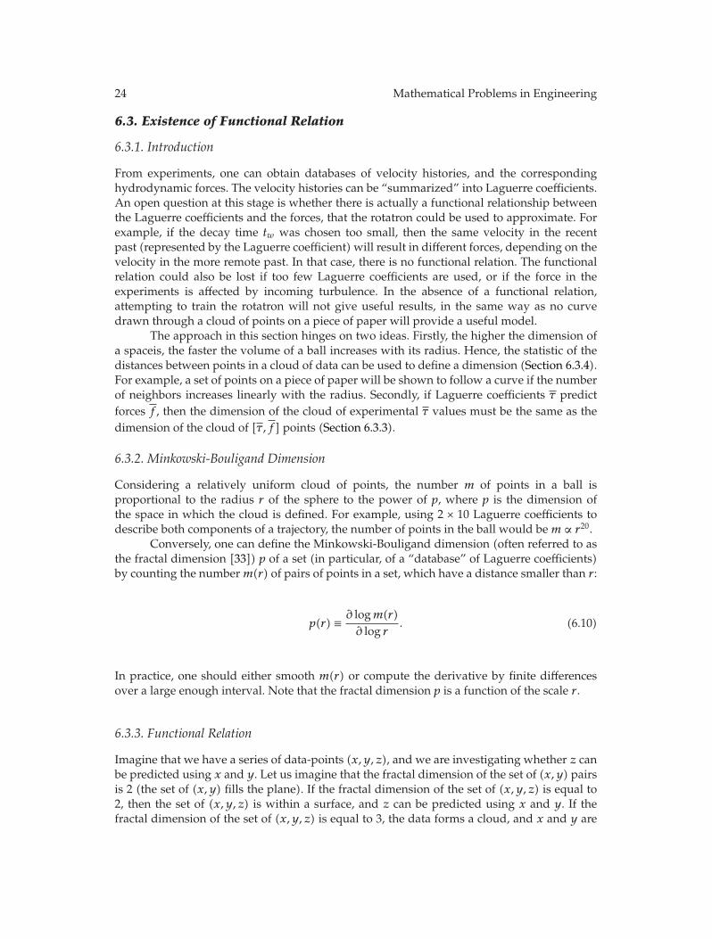
102 103 104 10510−6

10−5

10−4

10−3

10−2

10−1

100

Velocity (ilr-Re)

Cum

ulativeprob

ability

τ distanceτf distance

Figure 8: Statistics of the distance between vectors of Laguerre coefficients (“τ distance”, black) and vectorsof Laguerre coefficients and forces (“τ-f distance”, red). the four red curves, from left to right correspondto an added random noise to the force with standard deviation 0, 1 × 107, 2 × 107, and 10 × 107 [N/m].

not sufficient to predict z, therefore other hidden variables must be at play. These conceptsare now applied to the study of the experimental database.

6.3.4. Minkowski-Bouligand Dimension

Figure 8 shows the cumulative distribution of the distances between trajectories (“τ-distance”, black curve) computed using (6.7). p is seen to depend on the scale: from afar(r > 2 × 104 [ilr Re]), the slope of the curve is zero, hence the dimension is zero: all the dataare lumped into a point. Zooming into the data set (r = 3 × 103 [ilr Re]), one can discern acloud of dimension 4.76. At r = 1.5 × 103 [ilr-Re], the slope decreases to about p = 2, and it isbelieved that this is the dimension of the data set for a given point along the riser. At a smallscale (r < 1× 103 [ilr Re]), the dimension increases again, possibly due to noise in the data. orweaknesses in the Laguerre approximation.

The red curves in Figure 8 are computed by adding the sum of squares of thedifferences between force components (suitably scaled) to the squares of the distancesbetween trajectories, and then extracting the square root (“τf-distance”). The four red curves,from left to right, are drawn using the original force data, to which Gaussian noise of standarddeviation 0, 107, 108, and 109 [N/m], respectively, has been added (The standard deviationof the original force is about 2 × 108 [N/m]). The first curve is close to the black one, whichis strongly suggestive that indeed, there is a functional relation. The two first red curves areindistinguishable, which seems to indicate that we cannot expect to achieve a 10% precisionin force predictions. Themarked difference with curves 3 and 4 shows, however, that we haveassets in hand to predict the force. Similar curves have been produced with added noise ofstandard deviations 1 × 107, 2 × 107 and 10 × 107, [N/m], and already at 2 × 107 [N/m] thecurve is distinct from the one based on the original data.


6.3.5. Discussion

The present study suggests that there is indeed a functional relation to be seen in the dataset used here. The Laguerre coefficients can be used to predict the forces, with a precisionof about 107 [N/m]. The conclusion must be treated carefully, however. The dimensionalanalysis provides a necessary condition, not a sufficient one: it does not exclude, for example,that there exists a neighborhood of points τ in which two distinct values of f appear.

7. Dynamic Analysis

7.1. Foreword

Once it is possible to predict hydrodynamic forces on a cross section for a given velocityhistory, the next development is to include the force thus predicted in a dynamic time domainsimulation. Because the VIV forces introduce severe nonlinearities, a naive connection (wherethe forces are just added to the right-hand side of the system)might lead to slow convergenceor to divergence of the Newton-Raphson iterations used at each time step. To obtain a properformulation, it is necessary to jointly treat the system of differential equations composedof the state equations of the structure and the differential equations (4.27) followed by theLaguerre coefficient. However, in doing so, for each displacement degree of freedom, nLaguerre coefficients are added, and it is crucial for efficiency to eliminate them before solvinga large linear system of equations.

To this effect, in this section, the following sequence of transformations is applied tothe differential equations.

(1) The differential equations are first set in incremental form (Section 7.3).

(2) Time discretisation by the Newmark-β method is introduced (Section 7.4).

(3) The Laguerre coefficients are condensed out of the system of equations(Section 7.5).

(4) Finite element interpolation is introduced (space discretisation), using Gaussquadrature (Section 7.6).

This particular sequence leads to a VIV model that is implemented at the Gauss pointlevel and can easily be introduced in a general purpose FEM software with standard,displacement-based beam, or cable elements. Another sequence, 1, 4, 2, 3, can be used toobtain either a hybrid element, or alternatively, a mixed element which would require aspecialized solver for optimal efficiency. These alternatives are more difficult to integrate intoexisting software working with displacement-based elements and are not discussed here.

7.2. Differential Equations

The dynamic differential equation of a 3D beam subjected to VIV loads can be formalized as

rdi(x[bj], x[bj], x[bj], t

)= λ−1

Nm−1 fd(τ[pb]i

)+ Edi, (7.1)


where Newton’s “dot” notation for a time derivative stands for a derivation with respect tounscaled time t, as opposed to scaled time t∗, and with [23, 34]

Edi = CLρν(wdi − xdi) + CQ12ρDi|wdi − xdi|(wdi − xdi)

+ CMπ

4ρD2

i (wdi − xdi) +π

4ρD2

i wdi.

(7.2)

The four terms in the above Morison’s equation are the linear drag, the quadratic drag, thesum of diffraction and added mass forces, and the Froude-Krylov forces. The fourth termintroduces the correction discussed in Section 3.1.

If CL, CQ, or CM are set to values different from zero, then it is necessary to subtractthe corresponding values from the forces fdi used to train the rotatron. Experience shows thatusing CM = 1, CQ = 1, and CL = 0 contributes to the stability of the dynamic analysis.

Equation (4.27)must be scaled to keep only derivatives with respect to unscaled time,for the application of Newmark-β (Section 7.4)

∂τlbi∂t∗

= μlpτpbi + nlλ−1ms(xbi − wbi) (7.3)

so that

λ−1s τlbi = μlpτpbi + nlλms−1(xbi − wbi). (7.4)

The indexes d and b span pairs of directions, orthogonal to the cylinder. Indexes i and jstand for positions along the cylinder and span a continuous set of values (coordinates alongthe cylinder). Indexes l and p refer to the Laguerre coefficients of various degrees. Forcesfdi = fd(τ[pb]i) at location i only depend on the Laguerre coefficients τpbi for the same location.At that location, the force component in direction d depends on the Laguerre coefficientsof all degrees b for both directions p. ρ is the fluid density and wdi is the acceleration ofthe undisturbed fluid. π/4ρD2

i wdi stands for the Froude-Krylov forces. Diffraction forces arepresent in the laboratory tests and hence accounted for by fd.

7.3. Incremental Form

The incremental form of (7.1) and (7.4) is

rdi + kdibjdxbj + cdibjdxbj +mdibjdxbj = λ−1Nm−1 fdi + hdipbjdτpbj + Edi, (7.5)

λ−1s (τlbi + dτlbi) = μlp

(τpbi + dτpbi

)+ nlλms−1(xbi + dxbi − wdi) (7.6)


with

kdibj =∂rdi∂xbj

,

cdibj =∂rdi∂xbj

+ CQρDiδij[∣∣w[p]i − x[p]i

∣∣δbd+(wdi − xdi)(wbi − xbi)∣∣w[p]i − x[p]i

∣∣−1]+CLρνδijδbd,

mdibj =∂rdi∂xbj

+ CMπ

4ρDiδijδbd,

hdipbj = λ−1Nm−1

∂fdi∂τpb

δij .

(7.7)

The expression for ∂fdi/∂τpb is presented in Appendix B.

7.4. Time Discretisation

Newmark-β is a method geared towards second order differential equations. Equation (7.6),however, is only of the first order. The reason for using Newmark-β here is that the presentVIV model is to be integrated into the model of a larger structure, and the differential systemfor that structure is of the second order. Preparing a first order equation for a second ordersolver opens two options: we can treat (7.6) as being of the second order in τlbi, but with thecoefficient of τlbi being zero. Alternatively, we can introduce the antiderivative Tlbi of τlbi, andtreat (7.6) as being of the second order in Tlbi, but with the coefficient of Tlbi being zero. Thelatter option was chosen, based on the weak justification that this treats τlbi and xbj both asfirst derivatives, which seems natural considering (4.14).

Applying Newmark-β to (7.5) and (7.6) in this way yields

∀d, i,[kdibj +

γ

βdtcdibj +

1βdt2

mdibj

]dxbj −

γ

βdthdipbjdTpbj

= λ−1Nm−1 fdi + Edi − rdi + cdibjb

xbj +mdibja

xbj − hdipbjb

τpbj ,

− γ

βdtnlλms−1dxbi +

[1

βdt2λ−1s δlp −

γ

βdtμlp

]dTpbi

= nlλms−1(xbi − wbi) + μlpτpbi − λ−1s τlbi − nlλms−1bxbi − μlpb

τpbi + aτ

lbi

(7.8)

with

axbj =

1βdt

xbj +12β

xbj ,

bxbj =γ

βxbj +

(γ

2β− 1

)dt xbj ,

aτpbj =

1βdt

τpbj +12β

τpbj ,

bτpbj =γ

βτpbj +

(γ

2β− 1

)dt τpbj .

(7.9)


For refinement iterations, axbj , b

xbj , a

τpbj , and bτpbj are set to zero. Typically, γ = 1/2, β = 1/4.

The step dt refers to unscaled time.As usual in the Newmark-βmethod, the increments for the time derivatives are found

from the increment as

dxbj =γ

βdtdxbj − bxbj , (7.10)

dxbj =1

βdt2dxbj − ax

bj , (7.11)

dτpbj =γ

βdtdTpbj − bτpbj , (7.12)

dτpbj =1

βdt2dTpbj − aτ

pbj . (7.13)

7.5. Condensation

The time discrete equations can be rewritten in a compact form:

s1dibjdxbj − s2dipbjdTpbj = s3di,

s4l dxbi + s5lpdTpbi = s6lbi

(7.14)

with

s1dibj = kdibj +γ

βdtcdibj +

1βdt2

mdibj , (7.15)

s2dipbj =γ

βdthdipbj , (7.16)

s3di = λ−1Nm−1 fdi + Edi − rdi + cdibjb

xbj +mdibja

xbj − hdipbjb

τpbj , (7.17)

s4l = − γ

βdtnlλms−1 , (7.18)

s5lp =1

βdt2λ−1s δlp −

γ

βdtμlp, (7.19)

s6lbi = nlλms−1(xbi − wbi) + μlpτpbi − λ−1s τlbi − nlλms−1bxbi − μlpb

τpbi + λ−1s aτ

lbi. (7.20)

One can then condense dTpbi out of the above system of equations:

dTpbj =(s5)−1

pl

(s6lbj − s4l dxbj

), (7.21)

[s1dibj + s2dipbj

(s5)−1

pls4l

]dxbj = s3di + s2dipbj

(s5)−1

pls6lbj . (7.22)


Equation (7.22) is forced into “Newmark form” as

[k∗dibj + kdibj +

γ

βdtcdibj +

1βdt2

mdibj

]dxbj = f∗

di − rdi + cdibjbxbj +mdibja

xbj (7.23)

with

k∗dibj = s2dipbj

(s5)−1

pls4l ,

f∗di = λ−1

Nm−1 fdi + Edi − hdipbjbτpbj + s2dipbj

(s5)−1

pls6lbj

(7.24)

k∗dibj

and f∗di

both depend on dt, β, and γ : the symbol k∗dibj

was chosen to indicate that thematrix is handled by the Newmark-β solver in the same way as a stiffness. However, thisterm cannot be interpreted physically as a stiffness.

7.6. Spacial Discretisation

The consistent discretisation by Galerkin finite elements of (7.23) leads to

K∗nm = Ndink

∗dibjNbjm,

F∗n = Ndinf

∗di.

(7.25)

K∗nm and F∗

n are typically computed by Gauss quadrature. Note that no space derivative ispresent in k∗

dibj , so no partial integration or Gauss quadrature with curvature shape functionappears. One can hence simplify the expression of the element matrix to

K∗nm = Ndink

∗dibNbim (7.26)

which means “same quadrature as for a mass matrix”.

7.7. Implementation

In nonlinear FEM code, incremental matrices and vectors are computed by Gauss quadrature.The Gauss quadrature involves shape functions, tensors that are local, continuous versionsof the stiffness, damping and mass matrices, and the force imbalance vector. For example,for the drag damping of a beam element, the tensor relates a vector whose componentsare increments in velocities in three directions, to another vector whose components areincrements in forces per unit length in three directions.

Within an iteration, the linear solver provides incremental nodal positions, velocitiesand accelerations for the model. These are disassembled and provided to the elements. The


Table 1: Reynolds number in NDP tests.

Test name Reynolds number CurrentTN2030 13500 uniformTN2340 0–16200 shearTN2370 0–24300 shear

elements compute positions, velocities, and accelerations (and more) in a corotated referencesystem at Gauss points. The resulting values are handed to the VIV-Gauss point procedure.

The axial velocities are discarded. The procedure scales the provided values using (3.2)and (3.3).

Having stored the previous approximation of the scaled position, the proceduredetermines the position increment dxbj , and then uses (7.21) to obtain the Laguerre coefficientincrement dTpbj . From there, (7.12) and (7.13) are used to compute dτpbj and dτpbj . The valuesof Tpbj , τpbj , and τpbj are updated from previously stored values. τpbj is then used to evaluatefdi and its derivative with respect to τpbj . These are scaled back, and Froude-Krylov forces areadded, leading to k∗

dibjand f∗

di.

The above matrix and vector are padded with zeros to indicate zero force in the axialdirection and zero torque.

The condensation of a larger system of time-discretised equations introduces someinelegant features compared to standard dynamic FEM: the VIV-Gauss point must beprovided with β, γ , and dt and a flag showing whether a call is made at a step or withina refinement iteration.

Note that when the VIV model is integrated in the dynamic FEM computation, in theway detailed in this section, the recursive Laguerre filter presented in Section 4.6 is not used.In this work, the filter was used only to process velocities time series and product Laguerrecoefficients for the training of the rotatron model. The filter provides a very efficient way toprocess whole time series.

8. Results

8.1. Training

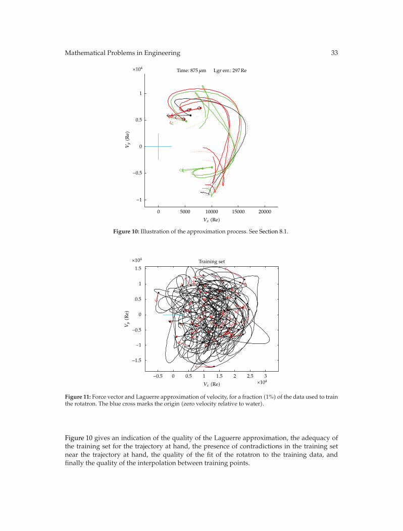
The Norwegian Deepwater Program was a research effort in which reduced scale testswere carried out on long, flexible riser models, subject to uniform or sheared current [35].The displacement histories thus acquired at 19 points along the riser model were laterprescribed on short stiff cylinders, and the hydrodynamic forces acting on the cylindersdirectly measured [36, 37]. Some data from [36, 37] is used in this work. It consists of thedisplacements at 19 points along the NDP riser model, for 3 current profiles (Table 1), so atotal of 57 short cylinder test runs. For each of the 57 runs, 100 instants are randomly selected,yielding a training set of the rotatron with 5700 “points”. Each “point” consists of two sets ofn = 30 Laguerre coefficients and the two components of the corresponding force (Figure 11).

The rotatron was trained using n = 30 Laguerre polynomials, 200 neurons in thehidden layer, and 50 to 1000 iterations of the conjugate gradient optimization algorithm.Other settings have been studied. No precision improvement was obtained from increasingthe number of neurons or from increasing the number of iterations. This may suggest that theoptimization algorithm converges on a local minima. If that is the case, improvement would


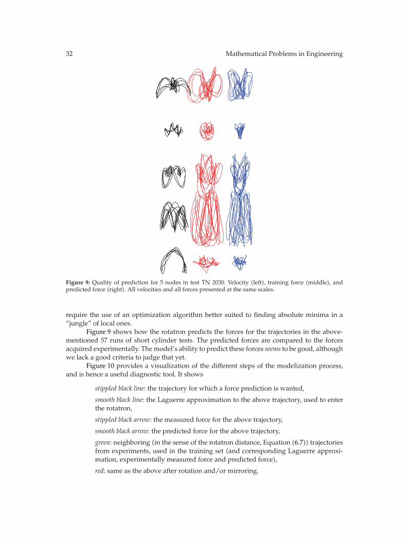
Figure 9: Quality of prediction for 5 nodes in test TN 2030. Velocity (left), training force (middle), andpredicted force (right). All velocities and all forces presented at the same scales.

require the use of an optimization algorithm better suited to finding absolute minima in a“jungle” of local ones.

Figure 9 shows how the rotatron predicts the forces for the trajectories in the above-mentioned 57 runs of short cylinder tests. The predicted forces are compared to the forcesacquired experimentally. Themodel’s ability to predict these forces seems to be good, althoughwe lack a good criteria to judge that yet.

Figure 10 provides a visualization of the different steps of the modelization process,and is hence a useful diagnostic tool. It shows

stippled black line: the trajectory for which a force prediction is wanted,

smooth black line: the Laguerre approximation to the above trajectory, used to enterthe rotatron,

stippled black arrow: the measured force for the above trajectory,

smooth black arrow: the predicted force for the above trajectory,

green: neighboring (in the sense of the rotatron distance, Equation (6.7)) trajectoriesfrom experiments, used in the training set (and corresponding Laguerre approxi-mation, experimentally measured force and predicted force),

red: same as the above after rotation and/or mirroring.


0 5000 10000 15000 20000

−1

−0.5

0

0.5

1

×104

Vx (Re)

Vy(R

e)

Time: 875μm Lgr err.: 297Re

Figure 10: Illustration of the approximation process. See Section 8.1.

−0.5 0 0.5 1 1.5 2 2.5 3

×104

−1.5

−1

−0.5

0

0.5

1

1.5

×104

Training set

Vx (Re)

Vy(R

e)

Figure 11: Force vector and Laguerre approximation of velocity, for a fraction (1%) of the data used to trainthe rotatron. The blue cross marks the origin (zero velocity relative to water).

Figure 10 gives an indication of the quality of the Laguerre approximation, the adequacy ofthe training set for the trajectory at hand, the presence of contradictions in the training setnear the trajectory at hand, the quality of the fit of the rotatron to the training data, andfinally the quality of the interpolation between training points.


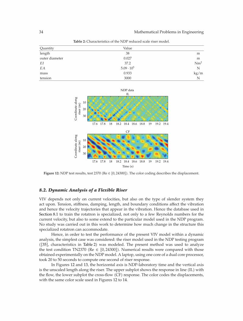
Table 2: Characteristics of the NDP reduced scale riser model.

Quantity Valuelength 38 mouter diameter 0.027 mEI 37.2 Nm2

EA 5.09 · 105 Nmass 0.933 kg/mtension 3000 N

IL

17.6 17.8 18 18.2 18.4 18.6 18.8 19 19.2 19.4

17.6 17.8 18 18.2 18.4 18.6 18.8 19 19.2 19.4

10

20

30

10

20

30

NDP data

Time (s)

Coo

rdinatealon

griser(m

)Coo

rdinatealon

griser(m

)

CF

Figure 12: NDP test results, test 2370 (Re ∈ [0, 24300]). The color coding describes the displacement.

8.2. Dynamic Analysis of a Flexible Riser

VIV depends not only on current velocities, but also on the type of slender system theyact upon. Tension, stiffness, damping, length, and boundary conditions affect the vibrationand hence the velocity trajectories that appear in the vibration. Hence the database used inSection 8.1 to train the rotatron is specialized, not only to a few Reynolds numbers for thecurrent velocity, but also to some extend to the particular model used in the NDP program.No study was carried out in this work to determine how much change in the structure thisspecialized rotatron can accommodate.

Hence, in order to test the performance of the present VIV model within a dynamicanalysis, the simplest case was considered: the riser model used in the NDP testing program([35], characteristics in Table 2) was modeled. The present method was used to analyzethe test condition TN2370 (Re ∈ [0, 24300]). Numerical results were compared with thoseobtained experimentally on the NDPmodel. A laptop, using one core of a dual core processor,took 20 to 50 seconds to compute one second of riser response.

In Figures 12 and 13, the horizontal axis is NDP-laboratory time and the vertical axisis the unscaled length along the riser. The upper subplot shows the response in line (IL)withthe flow, the lower subplot the cross-flow (CF) response. The color codes the displacements,with the same color scale used in Figures 12 to 14.


0.4 0.6 0.8 1 1.2 1.4 1.6 1.8 2 2.2

0.4 0.6 0.8 1 1.2 1.4 1.6 1.8 2 2.2

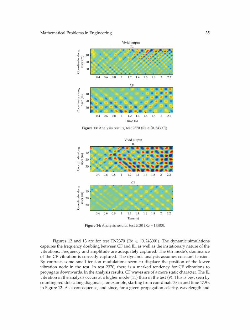
Vivid outputIL

10

20

30

10

20

30

Time (s)

Coo

rdinatealon

griser(m

)Coo

rdinatealon

griser(m

)CF

Figure 13: Analysis results, test 2370 (Re ∈ [0, 24300]).

IL

0.4 0.6 0.8 1 1.2 1.4 1.6 1.8 2 2.2

10

20

30

0.4 0.6 0.8 1 1.2 1.4 1.6 1.8 2 2.2

10

20

30

Vivid output

Time (s)

CF

Coo

rdinatealon

griser(m

)Coo

rdinatealon

griser(m

)

Figure 14: Analysis results, test 2030 (Re = 13500).

Figures 12 and 13 are for test TN2370 (Re ∈ [0, 24300]). The dynamic simulationscaptures the frequency doubling between CF and IL, as well as the instationary nature of thevibrations. Frequency and amplitude are adequately captured. The 6th mode’s dominanceof the CF vibration is correctly captured. The dynamic analysis assumes constant tension.By contrast, some small tension modulations seem to displace the position of the lowervibration node in the test. In test 2370, there is a marked tendency for CF vibrations topropagate downwards. In the analysis results, CF waves are of a more static character. The ILvibration in the analysis occurs at a higher mode (11) than in the test (9). This is best seen bycounting red dots along diagonals, for example, starting from coordinate 38m and time 17.9 sin Figure 12. As a consequence, and since, for a given propagation celerity, wavelength and


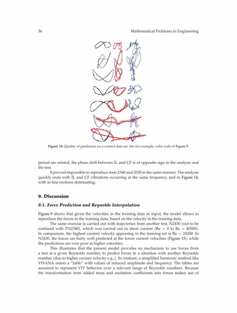
Figure 15: Quality of prediction on a control data set. See for example, color code of Figure 9.

period are related, the phase drift between IL and CF is of opposite sign in the analysis andthe test.

It proved impossible to reproduce tests 2340 and 2030 in the samemanner. The analysisquickly ends with IL and CF vibrations occurring at the same frequency, and in Figure 14,with in-line motions dominating.

9. Discussion

9.1. Force Prediction and Reynolds Interpolation

Figure 9 shows that given the velocities in the training data as input, the model allows toreproduce the forces in the training data, based on the velocity in the training data.

The same exercise is carried out with trajectories from another test, N2430 (not to beconfused with TN2340), which was carried out in shear current (Re = 0 to Re = 40500).In comparison, the highest current velocity appearing in the training set is Re = 24300. InN2430, the forces are fairly well predicted at the lower current velocities (Figure 15), whilethe predictions are very poor at higher velocities.

This illustrates that the present model provides no mechanism to use forces froma test at a given Reynolds number, to predict forces in a situation with another Reynoldsnumber (due to higher current velocity e.g.,). In contrast, a simplified harmonic method likeVIVANA enters a “table” with values of reduced amplitude and frequency. The tables areassumed to represent VIV behavior over a relevant range of Reynolds numbers. Becausethe transformation from added mass and excitation coefficients into forces makes use of


the current speed (which is proportional to the Reynolds number), this effectively providesVIVANA with a mechanism for interpolation over Reynolds number. The present model,on the other hand, uses a compressed form (Laguerre coefficient) of recent velocity history,scaled to Reynolds-like numbers. The scaling and data compression scheme used in thepresent model does not separate the classical Reynolds number as a separate variable.Instead, it is embedded in the compressed data as the average of the recent scaled in linevelocity already provided to the rotatron.

It remains an open question whether one should at all try to add such a Reynoldsinterpolation scheme in models of the present type. In a range of Reynolds number values inwhich the wake flow remains similar, it is reasonable to assume that viscous forces increaselinearly with velocity and inertial forces increase quadratically. For harmonic motions, thecomponent of the force in phase with acceleration can be attributed to an inertial force, andthe component in phase with velocity, to a viscous force. For more general motions, “phase”becomes a problematic concept, making it difficult to separate the force into viscous andinertial components that one can scale each according to their own law.

9.2. Dynamic Analysis

The comparison of Figures 12 and 13 is encouraging: when simulating exactly the systemfrom which trajectories were acquired experimentally in the first place, the simulation comesstrikingly close to the experimental results. It is understood that a simulation is good if itcaptures the statistical properties of the real response. With VIV being chaotic, there is nohope to reproduce exactly any given realization of the response.

Figure 14 shows the result of a simulation of a case which is also directly representedin the training data. The simulation fails, in the sense that IL and CF vibrations are simulatedto occur at the same frequency. Two explanations are proposed.

The quality of the force prediction by the rotatron, illustrated in Figure 9, was declared“satisfactory”, but this constitutes only an observation that the fitting procedure is operating.On what criteria should one judge that the fit is adequate? When training was carried out,the average norm of the difference between the training force and the predicted force wasfound to be about 30% of the average norm. For a control group composed of data pointsfrom the same experimental database, but not used in training the perceptron, the same ratiowas about 40%. These numbers are high and can be reduced to some extend by increasingthe number of hidden layers and of training iterations, but this was not found to yieldbetter simulations. Further specializing the perceptron (by training it with data from test2030) did not lead to successful simulations. One study which might help to understandthe observations would be to find the corrective forces that need to be added to the forcespredicted by the model, to force the simulation to track the motions observed during test2030. This can be achieved using dynamic inverse FEM analysis [38–40].

Even if the above corrective forces were strictly zero, so that the model was accuratelypredicting forces for the riser motion from test 2030, this would not be sufficient to ensurethat the simulation adequately mimics test 2030. A given trajectory could still have verydifferent stability properties in the physical system and in the simulation. It could be that inthe physical system, the trajectories follow the “bottom of a valley” while themodel renders itas the “crest of a mountain”. Ameasure of stability for this is the Lyapunov exponent [41, 42].Procedures exist to compute Lyapunov exponents from experimental data, and this shouldbe compared to Lyapunov exponents for the simulation.


9.3. Influence of tw

One issue that was explored was the adequacy of tw: the rotatron was trained with tw =5 · 10−5. This corresponds roughly to 1/4 of a cross-flow oscillation period in reduced scalefor test 2370, and to a smaller fraction for other tests at lower current velocity. It could beargued that this fraction becoming too small could be the cause of the failure of analyses atlower velocities (Figure 14). The rotatron was hence trained again using a suitably increasedvalue of tw. This was done twice, once with the full training set and increasing the numberof Laguerre polynomials to n = 60, and once with only the experimental data from lowercurrents and an unchanged number of polynomials (n = 30). Neither rotatrons allowed toperform a successful simulation for the lower current velocities.

9.4. Tension

In Figure 12, one can observe modulations of the positions of the vibration nodes (inparticular on the cross-flow graph). One possible explanation for this would be that in thephysical system, the tension is modulated by the vibration. This effect, if present, is notcaptured by the numerical model, which assumes constant tension. The method presentedhere is designed for use in a nonlinear analysis. However, in this research, time was saved byusing a simpler linear structural model.

10. Conclusions

A model for the prediction of VIV forces given the history of velocity of a cylindrical crosssection relative to the undisturbed fluid has been developed. The model is closely relatedto Wiener-Laguerre filters: the recent history of velocity is represented by the coefficients of aLaguerre polynomial series. These coefficients are then used to enter a memory-less nonlinearinterpolation function, in this case, a custom made neural network in which some relevantsymmetry properties were “hard-wired”. The neural network was trained by using forcesand displacements obtained in irregular forced motion tests on a short cylinder.

The proposedmodel operates in the time domain, making it well suited for integrationinto fully nonlinear analyses with unsteady currents. It further deals with in-line and cross-flow vibrations as one inseparable issue, which is arguably a necessity to improve on existingVIV models.

The model could provide a “good” reproduction of the forces in the training test, aswell as a “good” prediction of forces for “comparable” trajectories. Where the model wasqueried with trajectories very different from those present in the training data, the modelgave very poor results—as should be expected. Due to the limited amount of experimentaldata available, the present model remains quite specialized to a limited number of situations.What remains unknown at this stage is the size of the training set, and of the neural networkmodel, necessary to create a model with some ambition of generality.

In some dynamic analyses of laboratory tests (NDP TN2030 and TN2430) with a longflexible riser, the numerical solution fell into an unphysical mode of vibration with the samefrequency for in-line and cross flow vibration. On the other hand, for another case (TN2470),some unusually fine details were captured by the numerical model. From this, it is concludedthat the concept has merit and deserves to be pursued.

At the same time, the present paper leaves several important questions unanswered.


The proposed method assumes that hydrodynamic forces can be predicted by therecent history of velocity of the pipe relative to the surrounding fluid. Fractal dimensionalanalysis in Section 6.3.4 suggests that this is, to some extent, the case. On the other hand,experimental evidence clearly shows that if a cylinder is forced twice to follow the sametrajectory, the histories of hydrodynamic forces will not be exactly the same. Will adding arandom force process to the output of the model be of any value in reproducing the dynamicsbehavior of a pipeline? If so, how should such a random process be studied and modeled?

What is the information content of the relation between velocities and forces? As thesize of the experimental database is increased, will data points confirm each other and beinterpolated with a relatively simple model (a rotatron with few tunable parameters), or willa landscape of ever increasing complexity appear, defeating the present approach?

The rotatron was found to be able to predict forces “reasonably” well, yet, whenincluded in a dynamic model, the ability to reproduce the dynamics of the system waslimited. Can the measure of force agreement, used in training the rotatron be improved?Would it be useful, as suggested to the author by Dr. Halvor Lie to emphasize a goodprediction of the power of the force? More generally, how does one ensure that anapproximate model reasonably reproduces the statistics of the response of the originalnonlinear dynamics system?

Appendices

A. Conventions for Indexed Notations

The following conventions for indexed notations are used in this text.

(1) By default, where an index appears more than once in a combination of productsand/or divisions, a summation over the index is implied. If that index has acontinuous range, then the “sum” is an integration over the range. Points 2, 3, and4 specify exceptions to this rule.

(2) Point 1 notwithstanding, if an equation is preceded by the symbol ∀, followed by alist of indexes, then the listed indexes are not summed over.

(3) Point 1 notwithstanding, if within an equation, there is a combination of productsand/or divisions within which an index appears only once, then no sum over thatindex is carried out in the whole equation. (In any situation other than a simpleterm in the left-hand side, readability should be improved by using the symbol ∀.)

(4) Point 1 notwithstanding, if an index appears within an input to a function, and theoutput of the function is multiplied or divided by one or several terms that havethe same index, then no sum within the input to the function is carried out on thatindex.

(5) If an index of an argument to a function is within brackets, then the whole rangeof index values is used as input to one function evaluation. For example, σi(y[j]k)refers to the evaluation at multiple locations (k) of a vector-valued (i) function of avector (j).

(6) When the output of the function is shorthanded without explicitly writing its input,then the indexes of the input that are not within brackets are added to the indexesof the function. For example, σi(y[j]k) can be shorthanded σik.


(7) Derivatives of a function are noted with only the bracketed indexes of the inputappearing under the fraction: ∂σi/∂yj . To refer to the value of that derivative forinput k, one writes ∂σik/∂yj .

B. Rotatron Gradients

The derivative of the force predicted by the rotatron, with respect to the Laguerre coefficientsis needed in Section 7. With references to (5.3) to (5.8) that describe the rotatron, we can write

∂fin∂τjl

=∂fin∂σk

∂σikn

∂yj

∂yjkn

∂τl

= Vk∂σikn

∂yjMkl

(B.1)

with

∂σikn

∂yj= − 1

∣∣y[j]kn∣∣3(∣∣y[j]kn

∣∣αk + 1)2

×[αkyiknyjkn

∣∣y[j]kn∣∣αk + (−1)δij y¬ikny¬jkn

(∣∣y[j]kn∣∣αk + 1

)].

(B.2)

Here index i ranges over two values (for two directions orthogonal to the cylinder), and ¬i isthe other direction than i.

The gradients of the rotatron with respect to its coefficients are also needed in order tocompute the gradient of the target function with respect to the parameters Vk,Uk, andMkl:

∂fin∂Vl

= σiln,

∂fin∂Mkl

=∂fin∂σk

∂σikn

∂yj

∂yjkn

∂Mkl

= Vk∂σikn

∂yjτjln,

∂fin∂Ul

= Vk∂σikn

∂Ul

(B.3)

with

∂σikn

∂Ul= −δkl

e−Ulyikn

∣∣y[j]kn∣∣αk−1 log

∣∣y[j]kn∣∣

(∣∣y[j]kn∣∣αk + 1

)2 . (B.4)


C. Inverse of s5

The inverse of s5 (Equation (7.19)), where s5 is of the form

s5ij = αTij + βδij (C.1)

with

Tij =

⎧⎨⎩1 j ≤ i

0 j > i,(C.2)

can be verified to be lower triangular banded, with terms on diagonal i equal to

Q1 =1

α + β,

Qi = − αβi−2(α + β

)i , i ∈ {2 . . . n}.(C.3)

Acknowledgments

The author is indebted to Ida Aglen, Celeste Barnardo, Trygve Kristiansen, Carl MartinLarsen, Halvor Lie, Elizabeth Passano, Thomas Sauder, Wu Jie, Yin Decao and an anonymousreviewer for inspiring discussions on the subject of VIV, that either led to or helped thepresent research and writing. Thanks are extended to CeSOS (Centre of Excellence for Shipsand Offshore Structures) at NTNU (Norwegian University of Science and Technology) and toMARINTEK for sponsoring this research. Very special thanks to Professor Carl Martin Larsenof CeSOS who, faced with a barrage of dubious ideas from the author, responded by makingthis research possible.

References

[1] J. R. Chaplin, P. W. Bearman, Y. Cheng et al., “Blind predictions of laboratory measurements of vortexinduced vibrations of a tension riser,” Journal of Fluids and Structures, vol. 21, no. 1, pp. 25–40, 2005.

[2] H. Lie, D. Spencer, S. Huang et al., “The specialist committee on vortex induced vibrations, final reportand recommendations to the 25th ITTC,” in Proceedings of the 25th International Towing Tank Conference,pp. 641–668, 2008.

[3] T. Sarpkaya and R. L. Schoaff, “Inviscid model of two-dimensional vortex shedding by a circularcylinder,” AIAA Journal, vol. 17, no. 11, pp. 1193–1200, 1979.

[4] S. Etienne, Contribution a la modelisation de l’ecoulement de fluide visqueux autour de faisceaux de cylindrescirculaires, Ph.D. thesis, Universite de la Mediterranee, Aix-Marseille, France, 1999.

[5] C. T. Yamamoto, J. R. Meneghini, F. Saltara, R. A. Fregonesi, and J. A. Ferrari, “Numerical simulationsof vortex-induced vibration on flexible cylinders,” Journal of Fluids and Structures, vol. 19, no. 4, pp.467–489, 2004.

[6] R. H. J. Willden and J. M. R. Graham, “Multi-modal vortex-induced vibrations of a vertical riser pipesubject to a uniform current profile,” European Journal of Mechanics B, vol. 23, no. 1, pp. 209–218, 2004.

[7] Y. Constantinides, O. H. Oakley, and S. Holmes, “Analysis of turbulent flows and VIV of truss sparrisers,” in Proceedings of the 25th International Conference on Offshore Mechanics and Arctic Engineering(OMAE ’06), June 2006.


[8] R. Gopalkrishnan,Vortex induced forces on oscillatingbluff cylinders, Ph.D. thesis, MIT, Cambridge,Mass,USA, 1993.

[9] M. S. Triantafyllou, M. A. Grosenbaugh, and R. Gopalkrishnan, “Vortex induced vibrations in asheared flow: a new predictive model,” Tech. Rep., ONR, 1994.

[10] H. Lie, “A time domain model for simulation of vortex induced vibrations on a cable,” in Flow InducedVibration, Bearman, Ed., pp. 455–466, Balkema, 1995.

[11] J. K. Vandiver, “SHEAR7 program user manual,” Tech. Rep., MIT, 1999.[12] C. M. Larsen, K. Vikestad, R. Yttervik, and E. Passano, “VIVANA—theory manual,” Tech. Rep.,

MARINTEK, 2000.[13] C. M. Larsen, K. Vikestad, R. Yttervik, and E. Passano, “Empirical model for analysis of vortex

induced vibrations—theoretical background and case studies,” in Proceedings of the 20th InternationalConference on Ocean, Offshore and Arctic Engineering, 2001.

[14] M. L. Facchinetti, E. de Langre, and F. Biolley, “Coupling of structure and wake oscillators in vortex-induced vibrations,” Journal of Fluids and Structures, vol. 19, no. 2, pp. 123–140, 2004.

[15] L. Mathelin and E. de Langre, “Vortex-induced vibrations and waves under shear flow with a wakeoscillator model,” European Journal of Mechanics B, vol. 24, no. 4, pp. 478–490, 2005.

[16] R. Violette, E. de Langre, and J. Szydlowski, “Computation of vortex-induced vibrations of longstructures using a wake oscillator model: comparison with DNS and experiments,” Computers andStructures, vol. 85, no. 11–14, pp. 1134–1141, 2007.

[17] R. Violette, Modele lineaire des vibrations induites par vortex de structures elancees, Ph.D. thesis, EcolePolytechnique, 2009.

[18] M. Falco, F. Fossati, and F. Resta, “On the vortexinduced vibration of submarine cables: designoptimizationof wrapped cables for controlling vibrations,” in Proceedings of the 3rd InternationalSymposiumon Cable Dynamics, Trondheim, Norway, 1999.

[19] N. Wiener, Nonlinear Problems in Random Theory, Technology Press Research Monographs, TheTechnology Press of The Massachusetts Institute of Technology, New York, NY, USA, 1958.

[20] Z. Fejzo and H. Lev-Ari, “Adaptive non-linear Wiener-Laguerre lattice models,” in Proceedings of theInternational Conference on Acoustics, Speech and Signal processing, pp. 977–980, 1995.

[21] P. Saha, S. H. Krishnan, V. S. R. Rao, and S. C. Patwardhan, “Modeling and predictive control ofMIMO nonlinear systems using Wiener-Laguerre models,” Chemical Engineering Communications, vol.191, no. 8, pp. 1083–1119, 2004.

[22] T. O. Silva, “Laguerre filters—an introduction,” Reista do DETUA, vol. 1, no. 3, pp. 237–248, 1995.[23] O. M. Faltinsen, Sea Loads on Ships and Offshores Tructures, Cambridge University Press, Cambridge,

UK, 1990.[24] M. Abramowitz and I. A. Stegun, Handbook of Mathematical Functions with Formulas, Graphs, and

Mathematical Tables, Dover, GPO, New York, NY, USA, 9th, 10th edition, 1964.[25] B. Muckenhoupt, “Mean convergence of Hermite and Laguerre series. I, II,” Transactions of the

American Mathematical Society, vol. 147, pp. 433–460, 1970.[26] F. Rosenblatt, “The perceptron: a probabilistic model for information storage and organization in the

brain,” Psychological Review, vol. 65, no. 6, pp. 386–408, 1958.[27] B. Muller and J. Reinhardt, Neural Networks: A Systematic Introduction, Physics of Neural Networks,

Springer, Berlin, Germany, 1990.[28] J. Sjoberg and L. Ljung, “Overtraining, regularization, and searching for minimum in neural

networks,” in Proceedings of the IFAC Symposium on Adaptive Systems in Control and Signal Processing,pp. 669–674, 1992.

[29] K. Levenberg, “A method for the solution of certain non-linear problems in least squares,” Quarterlyof Applied Mathematics, vol. 2, pp. 164–168, 1944.

[30] D. W. Marquardt, “An algorithm for least-squares estimation of nonlinear parameters,” SIAM Journalon Applied Mathematics, vol. 11, pp. 431–441, 1963.

[31] J. A. Nelder and R. Mead, “A simplex method forfunction minimization,” Computer Journal, vol. 7,pp. 308–313, 1965.

[32] M. F. Møller, “A scaled conjugate gradient algorithm for fast supervised learning,” Neural Networks,vol. 6, no. 4, pp. 525–533, 1993.

[33] B. Mandelbrot, “How long is the coast of Britain? Statistical self-similarity and fractional dimension,”Science, vol. 156, no. 3775, pp. 636–638, 1967.

[34] J. R. Morison, M. P. O’Brien, J. W. Johnson, and S. A. Schaaf, “The force exerted by surface waves onpiles,” Petroleum Transactions, vol. 189, pp. 149–154, 1950.


[35] H. Braaten and H. Lie, “NDP riser high mode VIVtests—main report,” Tech. Rep. MT51 F05-072,MARINTEK, 2005.

[36] D. Yin and C. M. Larsen, “On determination of VIV coefficients under shear flow condition,” Journalof Offshore Mechanics and Arctic Engineering, vol. 6, pp. 547–556, 2010.

[37] D. Yin and C. M. Larsen, “Experimental and numerical analysis of forced motion of a circularcylinder,” in Proceedings of the 30th International Conferenceon Ocean, Offshore and Arctic Engineering,2011.

[38] P. Maincon, “Inverse finite element methods – part I: estimating loads and structural response frommeasurements,” in Proceedings of the Structural Engineering, Mechanics and Computation Conference, A.Zingoni, Ed., 2004.

[39] P. Maincon, “Inverse finite element methods – part II: dynamic and non-linear problems,” inProceedings of the Structural Engineering, Mechanics and Computation Conference, A. Zingoni, Ed., 2004.

[40] P. Maincon, C. Barnardo, and C. M. Larsen, “VIV force estimation using inverse FEM,” in Proceedingsof 27th International Conference on Offshore Mechanics and Arctic Engineering, 2008.

[41] A. Lyapunov, General problem of the stability ofmotion, Ph.D. thesis, Moscow University, 1892.[42] E. Ott, Chaos in Dynamical Systems, Cambridge University Press, Cambridge, UK, 2nd edition, 2002.

Submit your manuscripts athttp://www.hindawi.com

Hindawi Publishing Corporationhttp://www.hindawi.com Volume 2014

MathematicsJournal of


Mathematical Problems in Engineering

Hindawi Publishing Corporationhttp://www.hindawi.com

Differential EquationsInternational Journal of

Volume 2014

Applied MathematicsJournal of


Probability and StatisticsHindawi Publishing Corporationhttp://www.hindawi.com Volume 2014

Journal of


Mathematical PhysicsAdvances in

Complex AnalysisJournal of


OptimizationJournal of


CombinatoricsHindawi Publishing Corporationhttp://www.hindawi.com Volume 2014

International Journal of


Operations ResearchAdvances in

Journal of


Function Spaces

Abstract and Applied AnalysisHindawi Publishing Corporationhttp://www.hindawi.com Volume 2014

International Journal of Mathematics and Mathematical Sciences


The Scientific World JournalHindawi Publishing Corporation http://www.hindawi.com Volume 2014


Algebra

Discrete Dynamics in Nature and Society



Decision SciencesAdvances in

Discrete MathematicsJournal of

Hindawi Publishing Corporationhttp://www.hindawi.com

Volume 2014 Hindawi Publishing Corporationhttp://www.hindawi.com Volume 2014

Stochastic AnalysisInternational Journal of

Documents

A Wiener-Laguerre Model of VIV Forces Given Recent ...downloads.hindawi.com/journals/mpe/2011/414702.pdf · A Wiener-Laguerre Model of VIV Forces Given Recent Cylinder Velocities