Support Vector Machine for Structural Abnormality Detection

A Thesis Presented by:

David Michael Vines-Cavanaugh

to

The Department of Civil and Environmental Engineering

in partial fulfillment of the requirements

for the degree of

Master of Science

in

Civil Engineering

in the field of

Structures

Northeastern University Boston, Massachusetts

January, 2011

NORTHEASTERN UNIVERSITY

Graduate School of Engineering

Thesis Title: Support Vector Machine for Structural Abnormality Detection Author: David M. Vines-Cavanaugh Department: Department of Civil and Environmental Engineering Approved for Thesis Requirement of the Master of Science Degree ______________________________________________________ __________________ Thesis Advisor Date ______________________________________________________ __________________ Thesis Reader Date ______________________________________________________ __________________ Thesis Reader Date ______________________________________________________ __________________ Department Chair Date Graduate School Notified of Acceptance: ______________________________________________________ __________________ Director of the Graduate School Date

i

ACKNOWLEDGEMENTS

I would like to thank my advisor, Professor Ming Wang, for overseeing my progress and for providing inspiration when research obstacles were encountered. He also provided connections to valuable resources such as a highly talented multidisciplinary research group and vibration data from the Zhanjiang Bay Bridge's health monitoring system. I would also like to thank Yinghong (Henry) Cao ,Ph. D, for his technical insight and behind the scenes efforts. It's hard to imagine the success of this project without his availability, patience, and willingness to answer questions and help solve problems. Lastly, I would like to thank the National Science Foundation (NSF) and Northeastern University for the funding and training I received through the IGERT fellowship for intelligent diagnostics of aging civil infrastructure (NSF grant number DGE - 0654176). My thanks also goes out to some of the students and faculty associated with this program, Professor Sara Wadia-Fascetti, Professor Dionisio Bernal, Kimberly Belli, Matt Maddalo, Christopher Wright, and Dave Abramo, who helped make my time at Northeastern University both enjoyable and productive.

ii

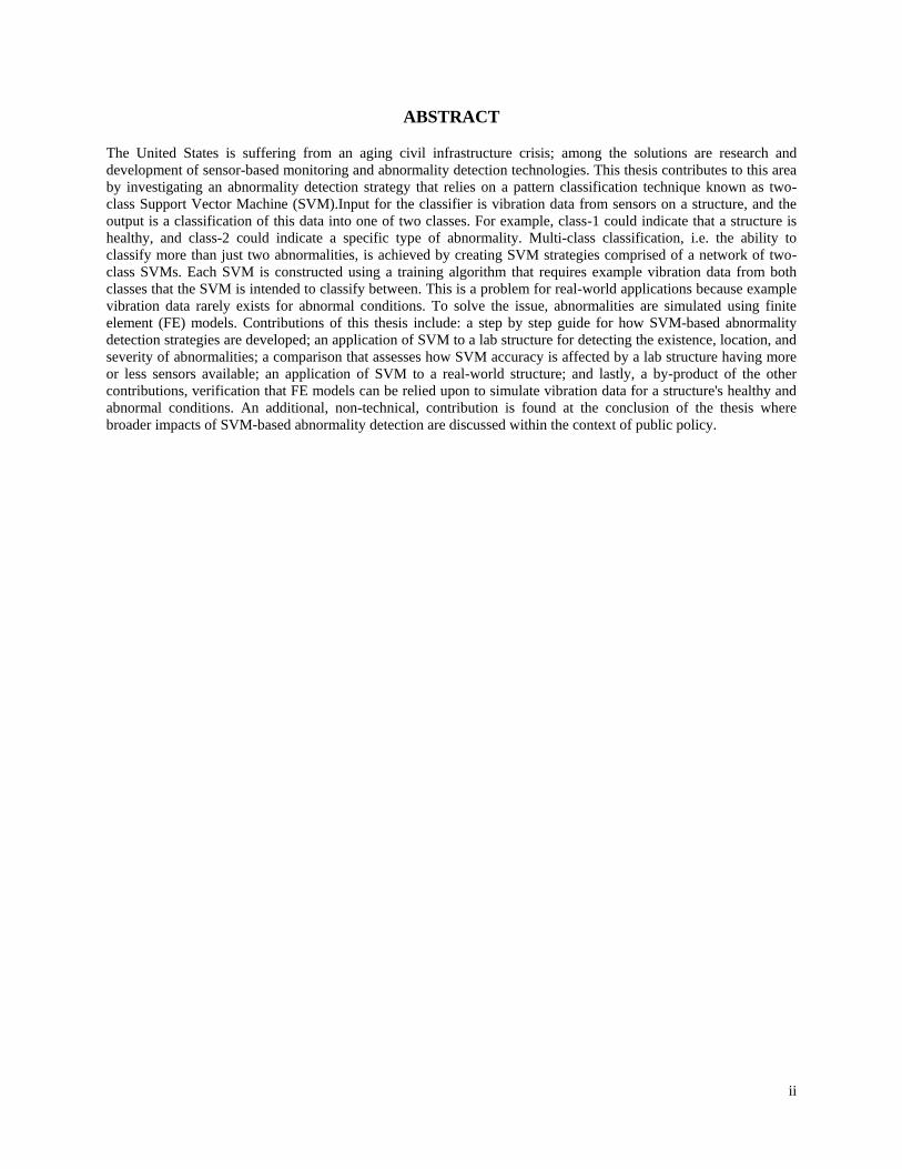
ABSTRACT

The United States is suffering from an aging civil infrastructure crisis; among the solutions are research and development of sensor-based monitoring and abnormality detection technologies. This thesis contributes to this area by investigating an abnormality detection strategy that relies on a pattern classification technique known as two-class Support Vector Machine (SVM).Input for the classifier is vibration data from sensors on a structure, and the output is a classification of this data into one of two classes. For example, class-1 could indicate that a structure is healthy, and class-2 could indicate a specific type of abnormality. Multi-class classification, i.e. the ability to classify more than just two abnormalities, is achieved by creating SVM strategies comprised of a network of two-class SVMs. Each SVM is constructed using a training algorithm that requires example vibration data from both classes that the SVM is intended to classify between. This is a problem for real-world applications because example vibration data rarely exists for abnormal conditions. To solve the issue, abnormalities are simulated using finite element (FE) models. Contributions of this thesis include: a step by step guide for how SVM-based abnormality detection strategies are developed; an application of SVM to a lab structure for detecting the existence, location, and severity of abnormalities; a comparison that assesses how SVM accuracy is affected by a lab structure having more or less sensors available; an application of SVM to a real-world structure; and lastly, a by-product of the other contributions, verification that FE models can be relied upon to simulate vibration data for a structure's healthy and abnormal conditions. An additional, non-technical, contribution is found at the conclusion of the thesis where broader impacts of SVM-based abnormality detection are discussed within the context of public policy.

iii

TABLE OF CONTENTS

Acknowledgements ........................................................................................................................................................i Abstract ........................................................................................................................................................................ ii 1. Introduction ........................................................................................................................................................... 1 2. Literature Review ................................................................................................................................................. 4

2.1 NNs vS. SVM ................................................................................................................................................. 4 2.2 Two-Class Svm Vs. Other Forms of SVM ..................................................................................................... 6 2.3 State of the Art: Two-Class SVM For Structural Abnormality Detection ..................................................... 8

3. Two-Class Support Vector Machine ................................................................................................................... 10 3.1 Example: 2-DOF Tower ............................................................................................................................... 10 3.2 Overview: Training and Testing Processes .................................................................................................. 10 3.3 Training Process and Theory ........................................................................................................................ 11

3.3.1 Separating Hyperplane ........................................................................................................................... 13 3.3.2 Maximum Margin Separating Hyperplane ............................................................................................ 14 3.3.3 The Hard and Soft Margin ..................................................................................................................... 16 3.3.4 Nonlinear SVM and Kernel Functions................................................................................................... 16

3.4 Testing Process ............................................................................................................................................ 17 3.5 Computer Software: LIBSVM and MATLAB ............................................................................................. 19

4. The Adopted Approach for SVM-Based Structural Abnormality Detection ...................................................... 20 4.1 Training Datasets from FE models ............................................................................................................... 20 4.2 Unbiased Training Datasets ......................................................................................................................... 21 4.3 Multi-Class Classification with SVM Networks .......................................................................................... 21 4.4 Step-by-Step Guide For SVM-Based Structural Abnormality Detection ..................................................... 22

5. SVM-Based Abnormality Detection Applied to Lab Structure .......................................................................... 24 5.1 Define Structure ........................................................................................................................................... 24 5.2 Define Abnormalities ................................................................................................................................... 26 5.3 Define Sensor Setup and Data Processing.................................................................................................... 27 5.4 Define SVM Network .................................................................................................................................. 29 5.5 Create Training Datasets .............................................................................................................................. 30 5.6 Train SVM Network .................................................................................................................................... 32 5.7 Create Testing Datasets ................................................................................................................................ 32 5.8 Implement SVM Network ............................................................................................................................ 33 5.9 Enhanced SVM Strategies ............................................................................................................................ 34

5.9.1 Increased Number of Features ............................................................................................................... 34 5.9.2 Severity Detection ................................................................................................................................. 36

6. SVM-Based Abnormality Detection Applied to Real-World Structure .............................................................. 39 6.1 Define Structure ........................................................................................................................................... 39 6.2 Define Abnormalities ................................................................................................................................... 42 6.3 Define Sensor Setup and Data Processing.................................................................................................... 42

iv

6.4 Define SVM Network .................................................................................................................................. 43 6.5 Create Training Datasets .............................................................................................................................. 44 6.6 Train SVMS .................................................................................................................................................. 47 6.7 Create Testing Datasets ................................................................................................................................ 47 6.8 Implement SVM Network ............................................................................................................................ 47

7. Conclusions and Broader Impacts ....................................................................................................................... 49 7.1 Summary and Future Work .......................................................................................................................... 49 7.2 Broader Impacts ........................................................................................................................................... 49

7.2.1 Marketing SVM-Based Abnormality Detection to Policy Makers ........................................................ 50 7.2.2 Policy Changes ...................................................................................................................................... 52

8. References ........................................................................................................................................................... 54

v

LIST OF FIGURES

Figure 1. Advantage of SVM: Simple geometric interpretation .................................................................................... 4 Figure 2. Global solution to optimization problem ........................................................................................................ 5 Figure 3. 2-DOF tower ................................................................................................................................................ 10 Figure 4. SVM training process ................................................................................................................................... 10 Figure 5. SVM testing process ..................................................................................................................................... 10 Figure 6. Class-1 time histories ................................................................................................................................... 12 Figure 7. Class-1 pattern matrix .................................................................................................................................. 12 Figure 8. Class-1 training pair matrix .......................................................................................................................... 12 Figure 9. Full training dataset ...................................................................................................................................... 13 Figure 10. Training dataset plotted in the input space ................................................................................................. 13 Figure 11. Separating hyperplane ................................................................................................................................ 14 Figure 12. Maximum margin separating hyperplane ................................................................................................... 14 Figure 13. Testing dataset ............................................................................................................................................ 18 Figure 14. Example two-class SVM network .............................................................................................................. 21 Figure 15. Guide for creating SVM-based abnormality detection strategies ............................................................... 22 Figure 16. Two story frame dimensions ...................................................................................................................... 24 Figure 17. Fixed boundary condition at base and associated clamp, respectively ....................................................... 25 Figure 18. 100 lbf modal shaker from The Modal Shop, Inc. (model 2100E11) ......................................................... 26 Figure 19. Shaker applied to floor 1, floor 2, and close up of floor 2 application, respectively .................................. 26 Figure 20. Lab structure: Abnormalities of interest ..................................................................................................... 27 Figure 21. Uni-axial accelerometer from PCB Piezotronics (model 333B30) ............................................................ 28 Figure 22. Sensor setup-1 ............................................................................................................................................ 28 Figure 23. SVM Network for 2 story frame ................................................................................................................ 29 Figure 24. ANSYS model of 2-story frame ................................................................................................................. 30 Figure 25. Location of impact load for 2-story frame.................................................................................................. 31 Figure 26. Node setup-1 for 2-story frame .................................................................................................................. 31 Figure 27. Biased training dataset for SVM-1 ............................................................................................................. 31 Figure 28. Training dataset for SVM-1 ....................................................................................................................... 32 Figure 29. Training datasets for SVM-2,3, and 4, respectively ................................................................................... 32 Figure 30. Sensor setup-2 and node setup-2, respectively ........................................................................................... 35 Figure 31. Lab structure: Abnormalities 1 and 5, respectively .................................................................................... 37 Figure 32. Zhanjiang Bay Bridge ................................................................................................................................ 39 Figure 33. Bridge dimensions ...................................................................................................................................... 39 Figure 34. Cross section of span center (unit: mm) ..................................................................................................... 40 Figure 35. Cross section of tower (unit: mm) .............................................................................................................. 40 Figure 36. Modular expansion joint [29] ..................................................................................................................... 42 Figure 37. Bridge sensors used for abnormality detection ........................................................................................... 43 Figure 38. SVM Network for cable-stayed bridge ....................................................................................................... 43 Figure 39. FE model for cable-stayed bridge............................................................................................................... 44 Figure 40. Comparison of test truck loads and simulated FE model loads .................................................................. 45 Figure 41. Node locations for bridge model ................................................................................................................ 45 Figure 42. Abnormality simulation for bridge model .................................................................................................. 46 Figure 43. Location of impact excitations for bridge model ........................................................................................ 46 Figure 44. Small training dataset for SVM10 .............................................................................................................. 46 Figure 45. Large training dataset for SVM10 .............................................................................................................. 46

vi

LIST OF TABLES

Table 1. Accuracy comparison between SVM and NNs ............................................................................................... 5 Table 2. State of the art: One-class SVM for structural abnormality detection ............................................................. 7 Table 3. State of the art: SVR for structural abnormality detection ............................................................................... 7 Table 4. State of the art: Two-class SVM for structural abnormality detection ............................................................ 8 Table 5. Process for creating training datasets ............................................................................................................. 11 Table 6. Process for creating testing datasets .............................................................................................................. 18 Table 7. 2-Story frame: Basic properties ..................................................................................................................... 25 Table 8. Results: SVM applied to healthy testing datasets .......................................................................................... 33 Table 9. Results: SVM applied to abnormality-1 testing datasets ............................................................................... 33 Table 10. Results: SVM applied to abnormality-2 testing datasets ............................................................................. 33 Table 11. Results: SVM applied to abnormality-3 testing datasets ............................................................................. 34 Table 12. Results: SVM applied to abnormality-4 testing datasets ............................................................................. 34 Table 13. Results: 8-feature SVM applied to healthy testing datasets ......................................................................... 35 Table 14. Results: 8-feature SVM applied to abnormality-1 testing datasets .............................................................. 35 Table 15. Results: 8-feature SVM applied to abnormality-2 testing datasets .............................................................. 35 Table 16. Results: 8-feature SVM applied to abnormality-3 testing datasets .............................................................. 36 Table 17. Results: 8-feature SVM applied to abnormality-4 testing datasets .............................................................. 36 Table 18. Results: 4-feature SVM applied to all testing datasets ................................................................................ 36 Table 19. Results: 8-feature SVM applied to all testing datasets ................................................................................ 36 Table 20. Detecting abnormality severity: A1 testing datasets .................................................................................... 37 Table 21. Detecting abnormality severity: A5 testing datasets .................................................................................... 38 Table 22. Structural dimensions .................................................................................................................................. 41 Table 23. Element cross section properties.................................................................................................................. 41 Table 24. Available sensors (features) for the real-world structure ............................................................................. 43 Table 25. Modal comparison for cable-stayed bridge .................................................................................................. 44 Table 26. SVM20 applied to all 30 testing datasets ..................................................................................................... 47 Table 27. All SVMs applied to all testing datasets ...................................................................................................... 48

1

1. INTRODUCTION

Civil infrastructure is key to sustaining both the economy and day to day living. It is important that all associated structures have inspection processes that allow for effective monitoring, abnormality detection, and repair. Unfortunately, this has not been the case and the United States is currently in the midst of an aging civil infrastructure crisis. Evidence of this can be found in the infrastructure report card put out by The American Society of Civil Engineers, which gives the entire infrastructure system a ranking of D for the year 2009. Among the noted issues, the report classifies over 25% of the nation's bridges as either structurally deficient or functionally obsolete [1]. Health Monitoring Systems (HMSs) are likely to play a large role in restoring the confidence in our nation's infrastructure and preventing a similar crisis from happening in the future. These systems collect vibration data from sensor arrays placed on structures. Subsequently, an analysis technique is applied to this data to detect if abnormalities exist or if the structure is functioning within a region that engineers have defined to be healthy or safe. This type of technology offers several benefits: 1) constant monitoring of structures instead of periodic inspections; 2) monitoring results that are objective, rather than subjective which is an inherent characteristic of human inspections; 3) critical information is available from structures during and immediately following natural or man-made disasters; and 4) as the technology advances and becomes more economical, HMSs will be able to replace humans for many inspection tasks, saving time and money. These benefits have not gone unnoticed as HMSs have been gaining acceptance as useful aids in monitoring and detecting abnormalities on bridges since their inception in the 1930s [2]. They have been installed on modern long-span bridges [3] as well as older bridges experiencing symptoms of cracking, corrosion, and settlement [4, 5, 6]. Important concerns in designing a HMS are the type, number, and placement of sensors, as well as how all the data will be transmitted, processed, and stored. Another important concern, and the focus of this thesis, is the analysis technique that will be used to interpret this data and detect abnormalities, there are several accepted approaches. A common vibration-based approach is to detect abnormalities by comparing the modal responses of the structure to those from a finite element model. A more modern approach that is used in this thesis is to treat the detection task as a pattern recognition/classification problem. In this scenario raw measurements are extracted from a structure and then classified based on the pattern that a classifier associates them with. Two established approaches for pattern classification are Neural Networks (NNs) and Support Vector Machine (SVM). NNs are better known and have been used in more applications, however, a literature review has shown that SVM has some desirable characteristics over NNs. Namely, SVMs have a global and unique solution, and a simple geometric interpretation [7]. Of further importance, when both used for the same application, SVM has shown either comparable or superior results to NNs [ 8, 9, 13, 15]. For these reasons SVM is the chosen approach for this thesis. SVM exists in various forms: Support Vector Regression (SVR), one-class SVM, and two-class SVM. SVR and one-class SVM have a few key advantages. Namely, they can be less complicated to implement, and they are general enough to detect a wide variety of abnormalities, even those that are not anticipated by the user. Despite these advantages, these approaches are avoided for two main reasons. First, once these approaches detect an abnormality, a significant amount of work can be required to determine the location and severity. Second, these approaches assume the structure's current condition to be healthy, which means that any pre-existing and possibly significant abnormalities are overlooked.

2

Two-class SVM is the form of SVM used throughout this thesis. Input to this classifier is a pattern. In the context of this thesis, a pattern is a vector containing a single measurement from each vibration sensor of a structure's sensor array, all of these measurements, of course, have the same time stamp. The size of a pattern is directly dependent on the number of sensors a structure has, which are commonly referred to as features. Furthermore, although patterns are classified one at a time, for reasons of efficiency they are often grouped together in a matrix. This matrix is referred to as the testing dataset. The output from a two-class SVM is simply the classification of a pattern into one of two classes. For example, class-1 could indicate that a structure is healthy, and class-2 could indicate a specific type of abnormality. Multi-class classification, i.e. the ability to classify patterns into more than just two classes so that multiple abnormalities can be detected, is achieved by creating SVM strategies. These strategies are comprised of a network of two-class SVMs. Regarding the construction of individual SVMs, the "machine" in Support Vector Machine indicates an association with machine learning, a category of classifiers that are constructed using training algorithms in a training process. In the case of two-class SVM, the training algorithm requires example patterns from the structure for both classes that a SVM is intended to classify between. These patterns are often grouped into a matrix which is referred to as the training dataset. A challenge associated with obtaining these training datasets is that example patterns rarely exist for a structure's abnormal conditions. Two solutions are: 1) physically modify the structure at the risk of causing permanent damage or 2) simulate abnormal conditions using a model. Since the first option is unfeasible, example patterns and training datasets will be obtained using models, finite element (FE) models. Intuitively, the use of FE models adds a new level of complexity to this work. For instance, model complexity must be considered and choices must be made regarding element and shell types, as well as the fineness of meshing. These choices are made by taking, among other things, the complexity of the abnormalities that must be simulated into consideration. Once these decisions are made, it is necessary to consider how the model will be validated and updated to ensure that it agrees with the actual structure. A common approach for validating a model is to perform a modal comparison with the actual structure, static load tests can be used as well. Beyond these considerations, it is important to recall that the goal is to obtain vibration data from these models to use for training. It is necessary to provide some sort of excitation to the models so that this data can be obtained. Ideally, the excitation would be random loadings similar to the environmental and operational conditions experienced on a real-world structure. However, this type of approach is avoided because statistical information on these loadings is difficult to obtain and computationally intensive to simulate. The unique approach adopted for this thesis uses a structure-specific impact loading applied at a structure-specific location. The above is a summary of how this thesis approaches structural abnormality detection using two-class SVM. Other papers have investigated this area as well [8, 9, 17, 18, 19]. This thesis focuses on picking up where these papers left off, a summary of contributions is given below

• A step by step guide for how this thesis develops SVM-based abnormality detection strategies is defined, explained in detail, and implemented. This guide is intended to be applicable for real-world structures.

• A SVM strategy is developed and implemented on a lab structure to detect the existence, location, and severity of abnormalities. The lab structure is a two-story aluminum frame where abnormal conditions are created by removing bolts at locations where columns connect to floors. Previous research has focused on detecting only the existence and location of abnormalities, not severity.

3

• A comparison is made that assesses how SVM accuracy is affected by the number of features being used from a structure's sensor array. This comparison is done using the lab structure described in the previous bullet. Previous research has only considered this type of comparison for computer simulations.

• A SVM strategy is developed and implemented on a real-world structure for abnormality detection. The structure is an in-service cable-stayed bridge. SVM provides evidence that the horizontal movement of the main girder is being constrained by an abnormality at one of the bridge's expansion joints. Previous research has only considered SVM applications to computer simulations and lab structures.

• Evidence that in the absence of actual measurements, FE models can be relied upon to simulate vibration data that can be used for training SVMs.

In addition to these technical contributions, a non-technical contribution can be found in the last chapter of the thesis grouped in with the conclusions and suggested future work. This additional contribution is with regards to the broader impacts that SVM technology might have on public policy. Its purpose is to emphasize that the infrastructure crisis can't be solved by developments in technology alone, there are other factors, i.e. public policy, that need to be addressed. Current and past public policy issues that contributed to the infrastructure crisis are discussed, as well as how the technology discussed in this thesis can be marketed to policy makers, and changes that these policy makers could make that would allow SVM to help in resolving the crisis. The layout of this thesis is as follows: chapter 2 is a literature review that serves to establish the state of the art, as well as to provide insight as to why SVM is chosen over NNs, and why two-class SVM is chosen over the other forms of SVM; chapter 3 discusses two important processes associated with two-class SVM (training and testing processes), as well as the theory and available computer software; chapter 4 defines and explains a guide for developing SVM-based abnormality detection strategies; chapter 5 implements SVM on a two-story frame lab structure; chapter 6 implements SVM on an in-service cable-stayed bridge; and chapter 7 discusses major conclusions of the thesis, future work, and the broader impacts that SVM-based abnormality detection could have on public policy.

4

2. LITERATURE REVIEW

The goals of this chapter are to define why SVM is preferred over NNs, to explain why two-class SVM is chosen over other forms of SVM, and to establish the state of the art of two-class SVM for structural abnormality detection and how this thesis advances it. As indicated by the chapter title, these goals will be achieved by referencing previous research. 2.1 NNs VS. SVM

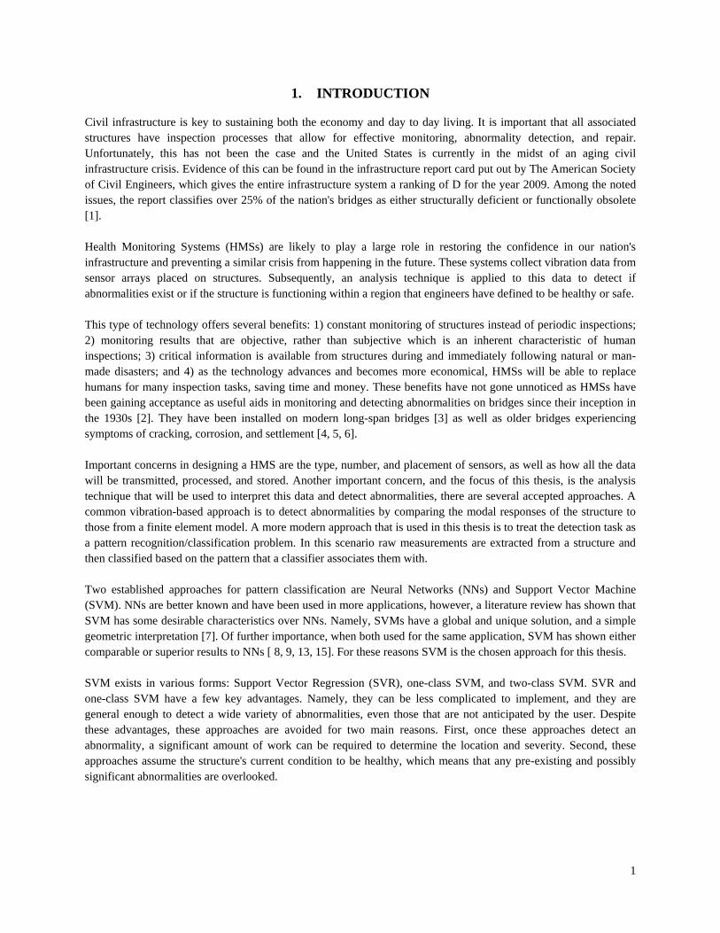
SVM has several advantages over NNs. References [7] and [17] point out many of these advantages, see below: Simple Geometric Interpretation: Two-class SVMs are constructed in a training process that requires example patterns from both classes that the SVM is intended to classify between. The idea behind this training process is simple to visualize, namely, a linear line (separating hyperplane) is found that separates class-1 training patterns from class-2 training patterns. An example is given in Fig. 1, each square represents a single class-1 training pattern and each triangle represents a single class-2 training pattern.

Figure 1. Advantage of SVM: Simple geometric interpretation

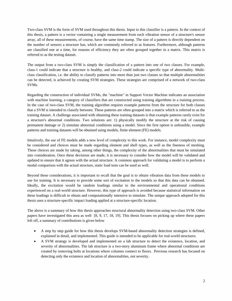
Once the linear separating boundary has been found, the training is complete and the SVM is ready to work. When previously unseen patterns arrive, i.e. a testing dataset, the SVM will classify them into class-1 or class-2 based on which side of the line they fall on [7]. It should be noted that fig. 1 is for patterns that have two features, and therefore the plot is 2D, if there were 3 features the plot would be 3D, for 4 features it would be 4D, and so on. Global Solution: An optimization problem is solved in the SVM training process. Parameters are found that will minimize classification errors when SVM is applied to previously unseen testing datasets. In other words, a global solution is found that provides optimal generalization. This is in contrast to the optimization problem solved for NNs, which can result in a local minimum solution. This type of solution allows NNs to perform well on training datasets, however, generalization to previously unseen testing datasets can be poor. This occurrence is often referred to as overfitting [7]. Fig. 2 illustrates this point below.

5

Figure 2. Global solution to optimization problem

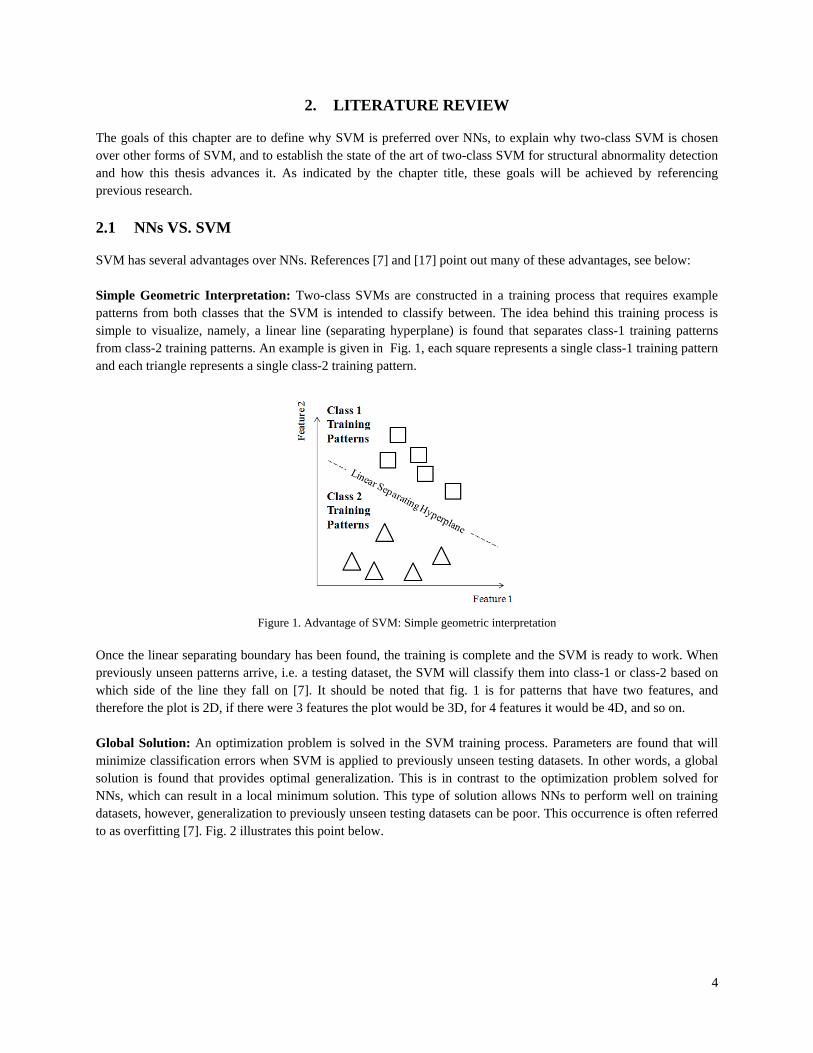
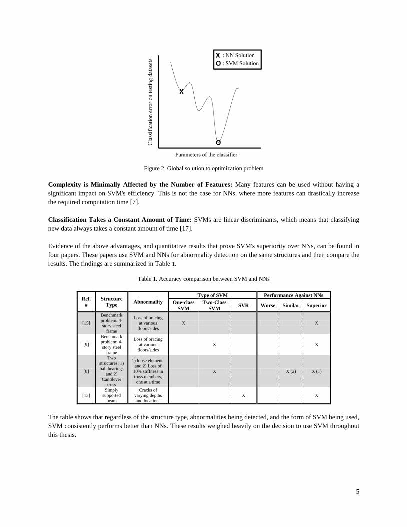
Complexity is Minimally Affected by the Number of Features: Many features can be used without having a significant impact on SVM's efficiency. This is not the case for NNs, where more features can drastically increase the required computation time [7]. Classification Takes a Constant Amount of Time: SVMs are linear discriminants, which means that classifying new data always takes a constant amount of time [17]. Evidence of the above advantages, and quantitative results that prove SVM's superiority over NNs, can be found in four papers. These papers use SVM and NNs for abnormality detection on the same structures and then compare the results. The findings are summarized in Table 1.

Table 1. Accuracy comparison between SVM and NNs

Ref. #

Structure Type Abnormality

Type of SVM Performance Against NNs One-class

SVM Two-Class

SVM SVR Worse Similar Superior

[15]

Benchmark problem: 4-story steel

frame

Loss of bracing at various

floors/sides X X

[9]

Benchmark problem: 4-story steel

frame

Loss of bracing at various

floors/sides X X

[8]

Two structures: 1) ball bearings

and 2) Cantilever

truss

1) loose elements and 2) Loss of

10% stiffness in truss members, one at a time

X X (2) X (1)

[13] Simply

supported beam

Cracks of varying depths and locations

X X

The table shows that regardless of the structure type, abnormalities being detected, and the form of SVM being used, SVM consistently performs better than NNs. These results weighed heavily on the decision to use SVM throughout this thesis.

6

2.2 TWO-CLASS SVM Vs. OTHER FORMS OF SVM

Brief descriptions of two-class SVM, one-class SVM, and SVR are given below: Two-Class SVM: As mentioned in the intro, the input for a trained two-class SVM is a testing dataset comprised of a number of individual patterns. The output is a classification of each pattern into one of two classes. Typically, each class represents a specific case, for example, class-1 could be a healthy 5-story frame, and class-2 could be the frame suffering from a 25% loss of stiffness at its 2nd story northeast column. One-Class SVM: This technique is similar to two-class SVM where testing data is fed to a trained SVM and the output from the SVM is a classification of the data into one of two classes. What distinguishes one-class SVM is that the user no longer has the ability to choose what conditions of the structure class-1 and class-2 will represent. Instead, class-1 must represent the structure's current and presumably healthy state, and class-2 must be extremely general and represent all abnormalities or combinations of abnormalities that could occur on the structure. Support Vector Regression (SVR): The input to SVR is vibration measurements from sensors on a structure, and the output, instead of being a classification into class-1 or class-2, is a prediction as to what the next measurement will be. The user then compares this prediction to the actual measured value. If the residual between measurement and prediction becomes too large then an abnormality is detected. Aside from each of these methods having different input/output relationships, there is another key difference that separates two-class SVM into a category of its own. Namely, to train a two-class SVM requires training data for both classes that it is intended to classify between, whereas one-class SVM and SVR only require data from the healthy structure. One-class SVM and SVR have several advantages that result from this difference, they are listed below:

• Preferable for Real-World Structural Abnormality Detection: These techniques do not require data for the structure in its abnormal conditions, which is often unavailable from real-world structures.

• Unlimited Detection Capabilities: There is potential to detect any abnormality that might occur on the structure. This is in contrast to two-class SVM, which can only detect abnormalities that are anticipated by the user.

• No FE Models Required: As training datasets are only needed from the healthy structure, there is no need for the user to be burdened with having to use complex FE models.

• Training and Testing Data Come From the Same Source: A source of error for two-class SVM is that for real-world applications the training and testing data must come from different sources, i.e. a FE model and the actual structure. This is a source of error because of the inherent errors associated with modeling; for example, it is impossible to model a structure's boundary conditions and abnormalities 100% accurately, and furthermore, there is error associated with the fact that the model is not subject to the same operational and environmental conditions as the real-world structure.

Evidence of these advantages can be seen in the success that one-class SVM and SVR have had in previous applications to structural abnormality detection. A summary of these papers is provided in Tables 2 and 3.

7

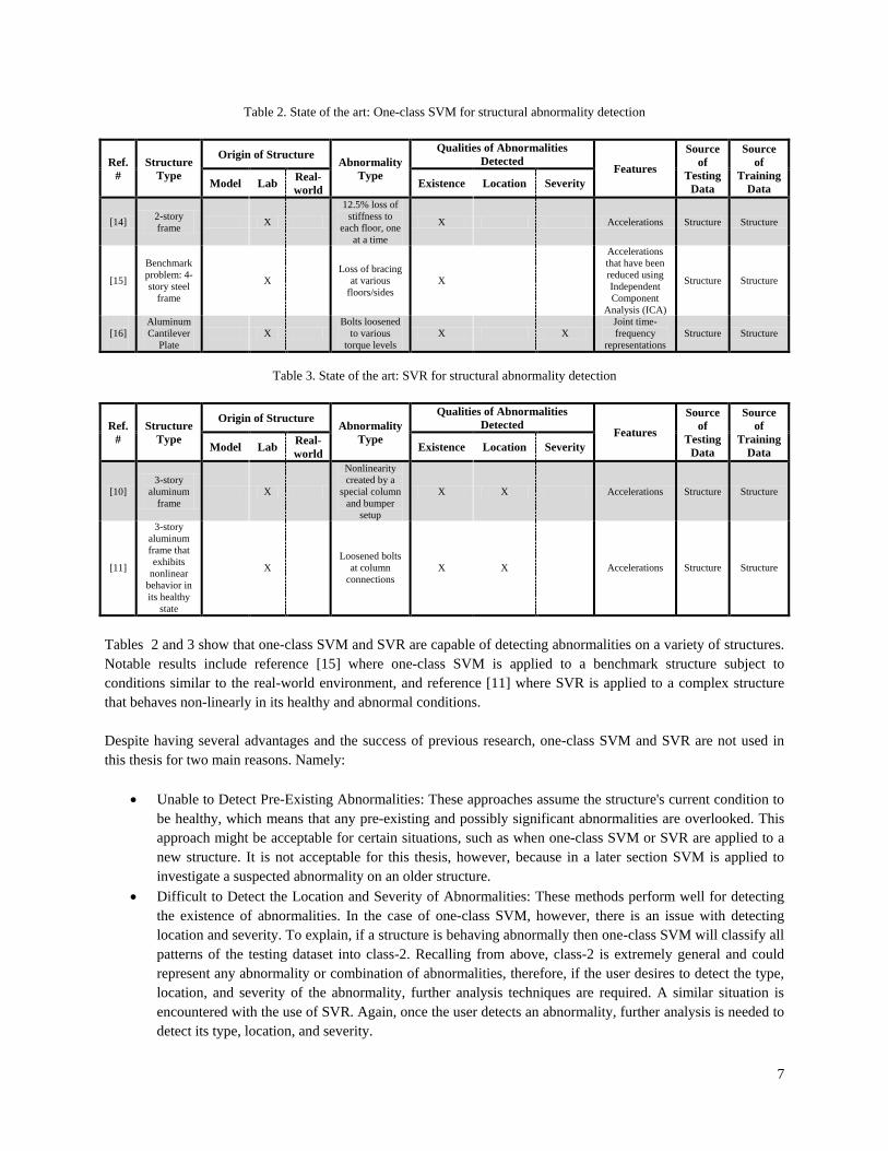
Table 2. State of the art: One-class SVM for structural abnormality detection

Ref. #

Structure Type

Origin of Structure Abnormality

Type

Qualities of Abnormalities Detected

Features

Source of

Testing Data

Source of

Training Data Model Lab Real-

world Existence Location Severity

[14] 2-story frame X

12.5% loss of stiffness to

each floor, one at a time

X Accelerations Structure Structure

[15]

Benchmark problem: 4-story steel

frame

X Loss of bracing

at various floors/sides

X

Accelerations that have been reduced using Independent Component

Analysis (ICA)

Structure Structure

[16]

Aluminum Cantilever

Plate X

Bolts loosened to various

torque levels X X

Joint time-frequency

representations Structure Structure

Table 3. State of the art: SVR for structural abnormality detection

Ref. #

Structure Type

Origin of Structure Abnormality

Type

Qualities of Abnormalities Detected

Features

Source of

Testing Data

Source of

Training Data Model Lab Real-

world Existence Location Severity

[10] 3-story

aluminum frame

X

Nonlinearity created by a

special column and bumper

setup

X X Accelerations Structure Structure

[11]

3-story aluminum frame that exhibits

nonlinear behavior in its healthy

state

X Loosened bolts

at column connections

X X Accelerations Structure Structure

Tables 2 and 3 show that one-class SVM and SVR are capable of detecting abnormalities on a variety of structures. Notable results include reference [15] where one-class SVM is applied to a benchmark structure subject to conditions similar to the real-world environment, and reference [11] where SVR is applied to a complex structure that behaves non-linearly in its healthy and abnormal conditions. Despite having several advantages and the success of previous research, one-class SVM and SVR are not used in this thesis for two main reasons. Namely:

• Unable to Detect Pre-Existing Abnormalities: These approaches assume the structure's current condition to be healthy, which means that any pre-existing and possibly significant abnormalities are overlooked. This approach might be acceptable for certain situations, such as when one-class SVM or SVR are applied to a new structure. It is not acceptable for this thesis, however, because in a later section SVM is applied to investigate a suspected abnormality on an older structure.

• Difficult to Detect the Location and Severity of Abnormalities: These methods perform well for detecting the existence of abnormalities. In the case of one-class SVM, however, there is an issue with detecting location and severity. To explain, if a structure is behaving abnormally then one-class SVM will classify all patterns of the testing dataset into class-2. Recalling from above, class-2 is extremely general and could represent any abnormality or combination of abnormalities, therefore, if the user desires to detect the type, location, and severity of the abnormality, further analysis techniques are required. A similar situation is encountered with the use of SVR. Again, once the user detects an abnormality, further analysis is needed to detect its type, location, and severity.

8

Evidence of the difficulty that one-class SVM has with detecting the location and severity of abnormalities can be seen in Table 2, as none of the papers detect location, and only one detects severity. In contrast to this, Table 3 shows that SVR is capable of detecting location. However, detecting the location required extra work. An additional step was needed that involved analyzing measurements from each sensor and comparing them to their corresponding SVR predictions. Based upon which sensors and corresponding SVR predictions yielded the largest residuals, the authors were able to predict a rough spatial location for the abnormality. 2.3 STATE OF THE ART: TWO-CLASS SVM FOR STRUCTURAL ABNORMALITY

DETECTION

Two-class SVM is the form of SVM used throughout this thesis. Among the papers investigated in this area, four were found to be particularly valuable. These papers are similar because each demonstrates SVM detecting various abnormalities with >90% accuracy. Characteristics that distinguish each paper's application are shown in Table 4.

Table 4. State of the art: Two-class SVM for structural abnormality detection

Ref. #

Structure Type

Origin of Structure Abnormality

Type

Qualities of Abnormalities Detected

Features Source of Testing

Data

Source of Training

Data Model Lab Real-world Existence Location Severity

[17] 9-span bridge X

Loss of 10-50% stiffness in piers, one at

a time

X X

1) Accelerations; and 2)

accelerations that have been

spatially and temporally

reduced

Model Model

[9]

Benchmark problem: 4-story steel

frame

X Loss of bracing

at various floors/sides

X

Accelerations that have been reduced using Independent

Component Analysis (ICA)

Structure Structure

[8] Cantilever truss X

Loss of 10% stiffness in

members, one at a time

X X

Displacement transmissibilities

formed from displacement

spectra

Model Model

[18]

3 and 4 story

bending structures

X

Loss of 66.67% story stiffness, one story at a time

X X Changes in

natural frequencies

Structure Model

The table establishes the state of the art. It can be seen that SVM detects the existence and location of abnormalities for both computer and laboratory structures. Of particular importance, are the applications to lab structures as these are more similar to the real-world, especially that of reference [9] where in-service building conditions were simulated. The table also shows that SVM is robust, namely: success is shown for various types of structures and abnormalities, even abnormalities that are very slight [8]; success is shown for a wide variety of features, which is important because different structures will have different features available; and lastly, success is shown for the case where features have been subjected to data reduction techniques, i.e. spatial and temporal reductions [17], and ICA [9].

These contributions are significant, but there is always room for advancement. For instance, the mentioned papers only detected abnormality existence and location, not severity. Also, only one of these papers [17] did a comparison to assess how SVM accuracy is affected by a structure having more or less features available, and this comparison was done only on a computer structure.

9

Another limitation is that none of the papers applied SVM to a real-world structure, and also, that the methods used in these papers, except [18], would not allow for it anyways. To explain, these methods obtained both training and testing datasets from the same source, however, for a real-world structure this data would need to come from separate sources. This requirement is rooted in the fact that the only way to obtain vibration data from an actual structure, for its various abnormalities, is to physically create the abnormalities on the structure, which is unfeasible. Therefore, a more realistic approach would have been for these papers to obtain training datasets from a model and testing datasets from the actual structure. This thesis intends to advance the state of the art. Accordingly, the limitations mentioned in the previous paragraphs are a main focus. Contributions of this thesis with respect to the state of the art are given below:

• A step by step guide to how this thesis develops SVM-based structural abnormality detection strategies is defined, explained in detail, and implemented. This guide is intended for real-world structures, and accordingly, obtains training and testing datasets from separate sources.

• SVM is implemented on a lab structure to detect the existence, location, and severity of abnormalities. • A comparison is made that assesses how SVM accuracy is affected by the number of features being used

from a lab structure's sensor array. • SVM is implemented on a real-world structure for structural abnormality detection.

10

3. TWO-CLASS SUPPORT VECTOR MACHINE

The purpose of this chapter is to explain two important processes associated with two-class SVM, namely, the training and testing processes. These processes will be explained in a detailed manner and theoretical concepts will be discussed. Also, a section is included at the end of the chapter to discuss important computer software that is used to carry out these processes. To help clarify the main points, a fabricated example structure is introduced in the first section and referenced throughout the entire chapter. 3.1 EXAMPLE: 2-DOF TOWER

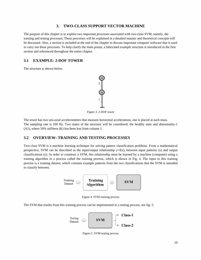
The structure is shown below.

Figure 3. 2-DOF tower

The tower has two uni-axial accelerometers that measure horizontal accelerations, one is placed at each mass. The sampling rate is 100 Hz. Two states of the structure will be considered, the healthy state and abnormality-1 (A1), where 50% stiffness (K) has been lost from column 1. 3.2 OVERVIEW: TRAINING AND TESTING PROCESSES

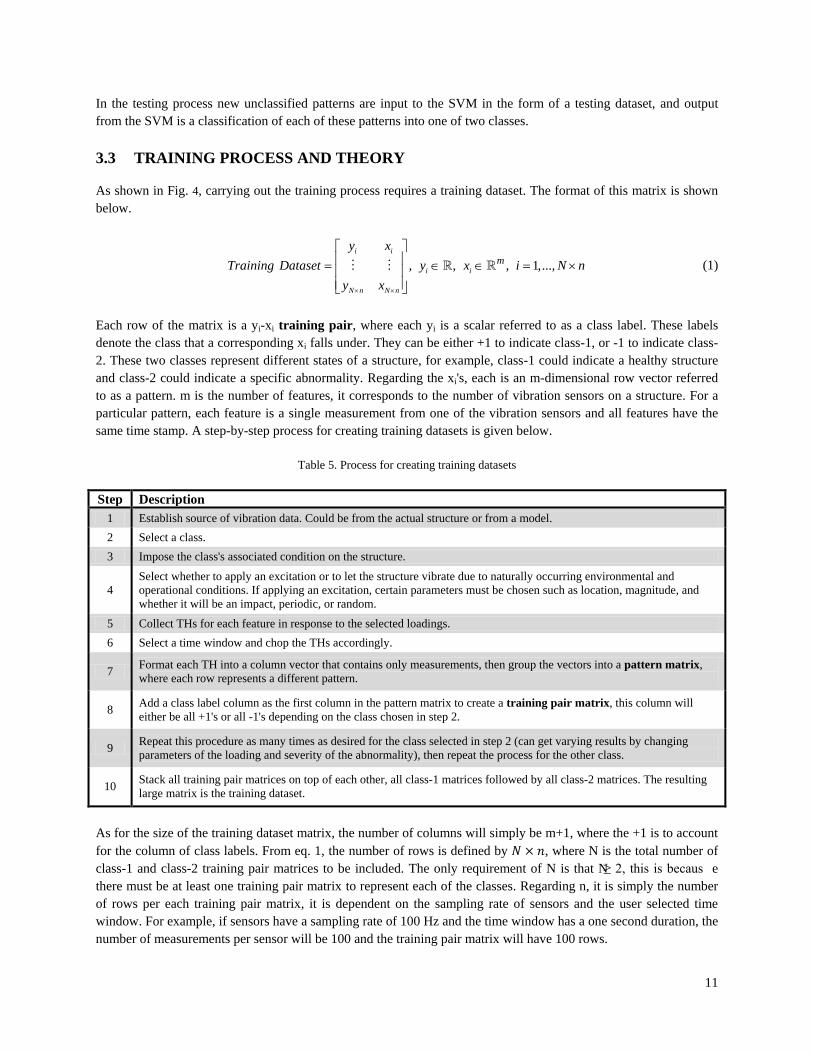
Two-class SVM is a machine learning technique for solving pattern classification problems. From a mathematical perspective, SVM can be described as the input/output relationship y=f(x), between input patterns (x) and output classifications (y). In order to construct a SVM, this relationship must be learned by a machine (computer) using a training algorithm in a process called the training process, which is shown in Fig. 4. The input to this training process is a training dataset, which contains example patterns from the two classifications that the SVM is intended to classify between.

Figure 4. SVM training process The SVM that results from this training process can be implemented in a testing process, see fig. 5.

Figure 5. SVM testing process

11

In the testing process new unclassified patterns are input to the SVM in the form of a testing dataset, and output from the SVM is a classification of each of these patterns into one of two classes. 3.3 TRAINING PROCESS AND THEORY

As shown in Fig. 4, carrying out the training process requires a training dataset. The format of this matrix is shown below.

, 1, ., , . .,i i

i i

N n N n

my x

Training Dataset y xy x

i N n

× ×

= ∈ ∈

= × (1)

Each row of the matrix is a yi-xi training pair, where each yi is a scalar referred to as a class label. These labels denote the class that a corresponding xi falls under. They can be either +1 to indicate class-1, or -1 to indicate class-2. These two classes represent different states of a structure, for example, class-1 could indicate a healthy structure and class-2 could indicate a specific abnormality. Regarding the xi's, each is an m-dimensional row vector referred to as a pattern. m is the number of features, it corresponds to the number of vibration sensors on a structure. For a particular pattern, each feature is a single measurement from one of the vibration sensors and all features have the same time stamp. A step-by-step process for creating training datasets is given below.

Table 5. Process for creating training datasets Step Description

1 Establish source of vibration data. Could be from the actual structure or from a model. 2 Select a class. 3 Impose the class's associated condition on the structure.

4 Select whether to apply an excitation or to let the structure vibrate due to naturally occurring environmental and operational conditions. If applying an excitation, certain parameters must be chosen such as location, magnitude, and whether it will be an impact, periodic, or random.

5 Collect THs for each feature in response to the selected loadings. 6 Select a time window and chop the THs accordingly.

7 Format each TH into a column vector that contains only measurements, then group the vectors into a pattern matrix, where each row represents a different pattern.

8 Add a class label column as the first column in the pattern matrix to create a training pair matrix, this column will either be all +1's or all -1's depending on the class chosen in step 2.

9 Repeat this procedure as many times as desired for the class selected in step 2 (can get varying results by changing parameters of the loading and severity of the abnormality), then repeat the process for the other class.

10 Stack all training pair matrices on top of each other, all class-1 matrices followed by all class-2 matrices. The resulting large matrix is the training dataset.

As for the size of the training dataset matrix, the number of columns will simply be m+1, where the +1 is to account for the column of class labels. From eq. 1, the number of rows is defined by 𝑁 × 𝑛, where N is the total number of class-1 and class-2 training pair matrices to be included. The only requirement of N is that N ≥ 2, this is becaus e there must be at least one training pair matrix to represent each of the classes. Regarding n, it is simply the number of rows per each training pair matrix, it is dependent on the sampling rate of sensors and the user selected time window. For example, if sensors have a sampling rate of 100 Hz and the time window has a one second duration, the number of measurements per sensor will be 100 and the training pair matrix will have 100 rows.

12

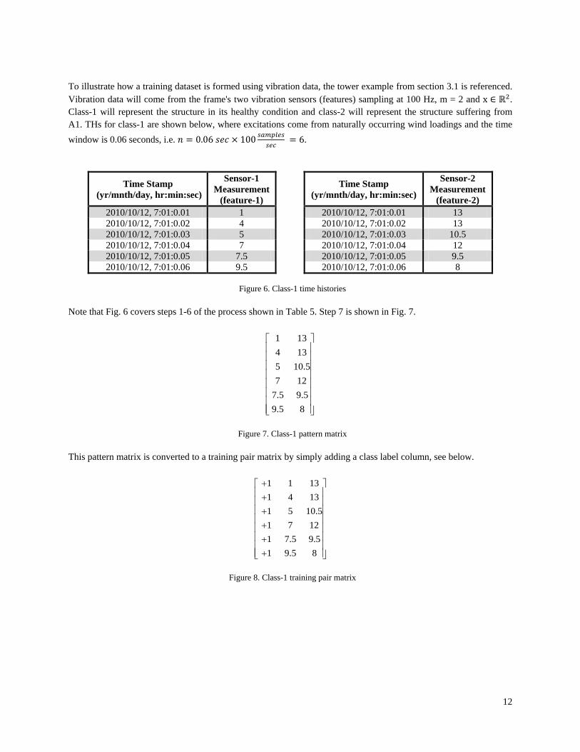
To illustrate how a training dataset is formed using vibration data, the tower example from section 3.1 is referenced. Vibration data will come from the frame's two vibration sensors (features) sampling at 100 Hz, m = 2 and x ∈ ℝ2. Class-1 will represent the structure in its healthy condition and class-2 will represent the structure suffering from A1. THs for class-1 are shown below, where excitations come from naturally occurring wind loadings and the time window is 0.06 seconds, i.e. 𝑛 = 0.06 𝑠𝑒𝑐 × 100 𝑠𝑎𝑚𝑝𝑙𝑒𝑠

𝑠𝑒𝑐 = 6.

Time Stamp (yr/mnth/day, hr:min:sec)

Sensor-1 Measurement

(feature-1)

Time Stamp (yr/mnth/day, hr:min:sec)

Sensor-2 Measurement

(feature-2) 2010/10/12, 7:01:0.01 1 2010/10/12, 7:01:0.01 13 2010/10/12, 7:01:0.02 4 2010/10/12, 7:01:0.02 13 2010/10/12, 7:01:0.03 5 2010/10/12, 7:01:0.03 10.5 2010/10/12, 7:01:0.04 7 2010/10/12, 7:01:0.04 12 2010/10/12, 7:01:0.05 7.5 2010/10/12, 7:01:0.05 9.5 2010/10/12, 7:01:0.06 9.5 2010/10/12, 7:01:0.06 8

Figure 6. Class-1 time histories

Note that Fig. 6 covers steps 1-6 of the process shown in Table 5. Step 7 is shown in Fig. 7.

1 134 135 10.57 12

7.5 9.59.5 8

Figure 7. Class-1 pattern matrix

This pattern matrix is converted to a training pair matrix by simply adding a class label column, see below.

1 1 131 4 131 5 10.51 7 121 7.5 9.51 9.5 8

+ + + +

+ +

Figure 8. Class-1 training pair matrix

13

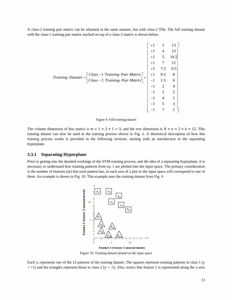
A class-2 training pair matrix can be obtained in the same manner, but with class-2 THs. The full training dataset with the class-1 training pair matrix stacked on top of a class-2 matrix is shown below.

1 1 131 4 131 5 10.51 7 121 7.5 9.5

1 1 9.5 82 1 1.5 6

1 2 41 2 21 4 11 5 31 7 1

Class Training Pair MatrixTraining Dataset

Class Training Pair Matrix

+ + + +

+

− + = = − − −

− − −

−

Figure 9. Full training dataset

The column dimension of this matrix is 𝑚 + 1 = 2 + 1 = 3, and the row dimension is 𝑁 × 𝑛 = 2 × 6 = 12. This training dataset can now be used in the training process shown in Fig. 4. A theoretical description of how this training process works is provided in the following sections, starting with an introduction to the separating hyperplane. 3.3.1 Separating Hyperplane Prior to getting into the detailed workings of the SVM training process, and the idea of a separating hyperplane, it is necessary to understand how training patterns from eq. 1 are plotted into the input space. The primary consideration is the number of features (m) that each pattern has, as each axis of a plot in the input space will correspond to one of them. An example is shown in Fig. 10. This example uses the training dataset from Fig. 9.

Figure 10. Training dataset plotted in the input space

Each xi represents one of the 12 patterns of the training dataset. The squares represent training patterns in class 1 (y = +1) and the triangles represent those in class 2 (y = -1). Also, notice that feature 1 is represented along the x-axis

14

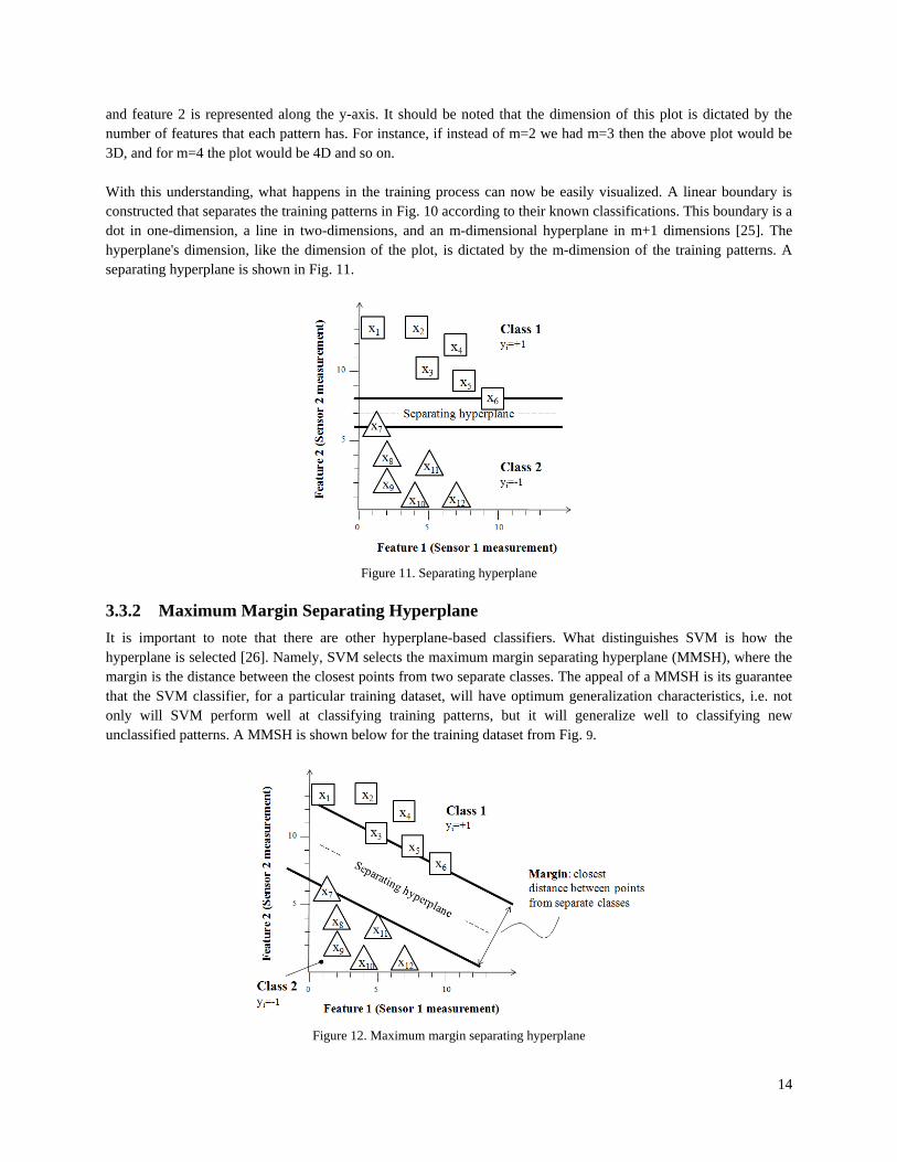
and feature 2 is represented along the y-axis. It should be noted that the dimension of this plot is dictated by the number of features that each pattern has. For instance, if instead of m=2 we had m=3 then the above plot would be 3D, and for m=4 the plot would be 4D and so on. With this understanding, what happens in the training process can now be easily visualized. A linear boundary is constructed that separates the training patterns in Fig. 10 according to their known classifications. This boundary is a dot in one-dimension, a line in two-dimensions, and an m-dimensional hyperplane in m+1 dimensions [25]. The hyperplane's dimension, like the dimension of the plot, is dictated by the m-dimension of the training patterns. A separating hyperplane is shown in Fig. 11.

Figure 11. Separating hyperplane

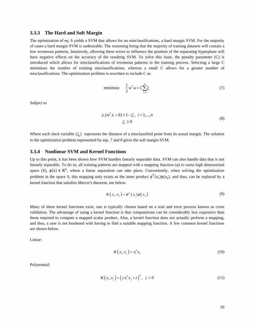
3.3.2 Maximum Margin Separating Hyperplane It is important to note that there are other hyperplane-based classifiers. What distinguishes SVM is how the hyperplane is selected [26]. Namely, SVM selects the maximum margin separating hyperplane (MMSH), where the margin is the distance between the closest points from two separate classes. The appeal of a MMSH is its guarantee that the SVM classifier, for a particular training dataset, will have optimum generalization characteristics, i.e. not only will SVM perform well at classifying training patterns, but it will generalize well to classifying new unclassified patterns. A MMSH is shown below for the training dataset from Fig. 9.

Figure 12. Maximum margin separating hyperplane

15

This figure can be compared to the hyperplane shown in Fig. 11, which was arbitrarily chosen and has a noticeably smaller margin. It can be seen that for the arbitrary hyperplane a small variation of points near the margin could result in misclassification, whereas for the MMSH a much larger variation would be needed. Also, the arbitrary hyperplane only accounts for separation in the y-direction, whereas the MMSH is more representative of the data because it accounts for separation in both x and y directions. Thus, the MMSH is a better separator than an arbitrary hyperplane with a smaller margin. Getting into the mathematical workings of SVM, the following expression for a separating hyperplane is introduced ( ) 0T

iw x b+ = (2) Where w is a vector of weighting parameters that weights the features of xi, and b is a scalar term referred to as a bias [24]. The separation between the two classes is defined below

1 1

2 1

Ti

Ti

x Class w x b

x Class w x b

⇒ + ≥

⇒ +∈ ≤ −

∈ (3)

Which can be expressed more generally as

( )( ) 1, 1, 2 .Ti iy w x b i n+ ≥ = … (4)

It can be shown that for the hyperplane defined by eqns. 2, 3, and 4, that the width of the margin is

2

2Mw

= (5)

Where ‖w‖2 is the 2-norm of w, which is equivalent to √wTw. Thus, to maximize the margin it is necessary to minimize √wTw, which is equivalent to minimizing wTw. The MMSH is found by solving the following optimization problem subject to the constraints of eq.4

1minimize 2

Tw w (6)

Note that (1/2) is included in the minimization term only for mathematical convenience.

16

3.3.3 The Hard and Soft Margin The optimization of eq. 6 yields a SVM that allows for no misclassifications, a hard margin SVM. For the majority of cases a hard margin SVM is undesirable. The reasoning being that the majority of training datasets will contain a few erroneous patterns. Intuitively, allowing these errors to influence the position of the separating hyperplane will have negative effects on the accuracy of the resulting SVM. To solve this issue, the penalty parameter (C) is introduced which allows for misclassifications of erroneous patterns in the training process. Selecting a large C minimizes the number of training misclassifications, whereas a small C allows for a greater number of misclassifications. The optimization problem is rewritten to include C as

minimize 1

12

nT

ii

w w C ξ=

+ ∑ (7)

Subject to

( ) 1 , 1,...

0,T

i i i

i

y w x b i nξξ

+ ≥ −≥

= (8)

Where each slack variable (ξi) represents the distance of a misclassified point from its actual margin. The solution to the optimization problem represented by eqs. 7 and 8 gives the soft margin SVM. 3.3.4 Nonlinear SVM and Kernel Functions Up to this point, it has been shown how SVM handles linearly separable data. SVM can also handle data that is not linearly separable. To do so, all training patterns are mapped with a mapping function (φ) to some high dimensional space (S), ϕ(x) ∈ ℝS, where a linear separation can take place. Conveniently, when solving the optimization problem in the space S, this mapping only exists as the inner product ϕT(xi)ϕ(xj), and thus, can be replaced by a kernel function that satisfies Mercer's theorem, see below. ( ) ( ) ( ), T

i j i jK x x x xφ φ= (9)

Many of these kernel functions exist, one is typically chosen based on a trial and error process known as cross validation. The advantage of using a kernel function is that computations can be considerably less expensive than those required to compute a mapped scalar product. Also, a kernel function does not actually perform a mapping, and thus, a user is not burdened with having to find a suitable mapping function. A few common kernel functions are shown below. Linear: ( ), T

i j i jK x x x x= (10)

Polynomial:

( ) ( ), , 0dT

i j i jK x x x x rγ γ= + > (11)

17

Sigmoid: ( ) tanh( )T

i j i jK x x x x rγ= + (12)

Radial Basis Function (RBF) :

2

i j( x x )i jK(x , x ) e , 0γ γ− −= > (13)

The RBF kernel nonlinearly maps patterns into a higher dimensional space. It is the most popular of these kernels and the only kernel used in this thesis because of the advantages listed below, mentioned in reference [28]:

• Fewer parameters to determine: This is evident in eqs. 10, 11, 12, and 13, where for the RBF kernel only 𝛾 has to be determined, whereas the Polynomial and Sigmoid Kernels require the user to determine both 𝛾 and 𝑟.

• Fewer numerical difficulties: It can be seen from eq. 13 that for the RBF kernel 0 ≤ 𝐾 ≤ 1, whereas for the Polynomial kernel in eq. 11 it can be seen that 𝐾 ≥ 0. Therefore, since the Polynomial kernel can be equal to infinity, or large values, it is subject to more numerical issues. Another example is that the RBF kernel will work regardless of the parameters chosen for it, whereas the Sigmoid kernel is not valid for certain parameters.

• General: In cases where patterns can be linearly separated, the RBF kernel can behave like the Linear kernel, and if patterns are not linearly separable it can handle this case as well, which is not possible using the Linear kernel. Also, the RBF kernel can behave like the Sigmoid kernel, which is advantageous because the RBF kernel has fewer numerical difficulties and requires fewer parameters to be found.

Regarding parameter selection for the RBF kernel, a common technique referred to as a grid search is used. Further explanation can be found in reference [28]. 3.4 TESTING PROCESS

Similar to the training process, the testing process in Fig. 5 requires an input matrix. This matrix is referred to as the testing dataset and is shown below.

, 1,., ..

TSTN

TST

i

n

mx

T i Nesting Data nset x

x ×

= ∈

= × (14)

Notice that the testing dataset has no class label column, and thus, that it is only comprised of pattern matrices, not training pair matrices. A step-by-step process for creating testing datasets is shown in Table 6.

18

Table 6. Process for creating testing datasets Step Description

1 Establish source of vibration data

2 Select whether to apply an excitation or to let the structure vibrate due to naturally occurring environmental and operational conditions. If applying an excitation, certain parameters must be chosen such as location, magnitude, and whether it will be an impact, periodic, or random.

3 Collect THs for each feature in response to the selected loadings. 4 Select a time window and chop the THs accordingly.

5 Format each TH into a column vector that contains only measurements, then group the vectors into a pattern matrix, where each row represents a different pattern.

6 Repeat this procedure as many times as desired, can get varying results by changing parameters of the loading or, if the loading is due to environmental and operational conditions, can collect THs from different times of day.

7 Stack all pattern matrices on top of each other. The resulting large matrix is a completed testing dataset of the form shown in eq. 14.

Notice that this process is simpler than that for creating training datasets, this is largely because there is no need to know the class labels, and therefore, it is unnecessary to impose any class related conditions on the structure. Regarding the size of the testing dataset, the number of columns is just m, and the number of rows is equal to 𝑁𝑇𝑆𝑇 × 𝑛, where NTST is the total number of pattern matrices being used, and n is the number of rows in each pattern matrix. It should be noted that for this thesis n for the testing dataset is equal to n for the training dataset. An example testing dataset is shown below for the example structure introduced in section 3.1. A single pattern matrix with a time window of 0.06 seconds was used to create it.

1 62 41 6.55 23 44.5 1.1

Testing Dataset

=

Figure 13. Testing dataset

Notice that there are no class labels. The matrix only has two columns, one corresponding to measurements from sensor-1 and the other corresponding to measurements from sensor-2.

19

3.5 COMPUTER SOFTWARE: LIBSVM AND MATLAB

To handle the SVM training and testing processes shown in figs. 4 and 5, and discussed above, this thesis uses LIBSVM -a suite of programs that handles various SVM related tasks. Its capabilities are shown below [27]:

• Different SVM formulations • Efficient multi-class classification • Cross validation for model selection • Grid search for kernel parameter selection • Probability estimates • Weighted SVM for unbalanced data • Both C++ and Java sources • GUI demonstrating SVM classification and regression • Python, R (also Splus), MATLAB, Perl, Ruby, Weka, Common LISP, CLISP, Haskell and LabVIEW

interfaces. C# .NET code is available. It's also included in some data mining environments: RapidMiner and PCP.

• Automatic model selection which can generate contour of cross validation accuracy • Simple interface where users can easily link it with their own programs

The suite of programs can be downloaded for free at http://www.csie.ntu.edu.tw/~cjlin/libsvm/. While LIBSVM handles the primary tasks of the SVM training and testing processes, it is not suitable for handling certain preliminary tasks. Accordingly, MATLAB is used to perform the following:

• Data formatting: Reads data from various formats (finite element programs, Excel, and data acquisition systems) and rearranges it into a common format.

• Data processing: Performs any necessary units conversions, as well as conversion to zero mean, scaling, normalizing, and filtering.

• Formation of Training or Testing Datasets: Formats data specifically for training or testing datasets according to eqs. 1 and 14. This includes the placement of class labels and ensuring that datasets are of the appropriate length.

An additional benefit of MATLAB is its capability to run other programs. This helps with efficiency, as rather than having to deal with the several programs and interfaces associated with LIBSVM, everything is run through MATLAB. Furthermore, controlling the programs with MATLAB allows important functions such as "for loops" and "if statements" to be used.

20

4. THE ADOPTED APPROACH FOR SVM-BASED STRUCTURAL ABNORMALITY DETECTION

Upon examining the previous chapter, and considering that abnormality detection problems are far more complicated than the 2-DOF tower example, it is realized that as SVM has been explained so far there are issues that might prevent it from being practical for structural abnormality detection on real-world structures. Three of these issues are: 1) Example patterns are typically unavailable for a real-world structure's abnormal conditions, this is a problem because training a two-class SVM requires example patterns for the two classes that the SVM is intended to classify between; 2) It is not always possible to obtain an even number of class-1 and class-2 training pair matrices for the training dataset, this causes the dataset to be biased and could lead to a biased SVM; and 3) two-class SVM can only classify data into one of two classes, which is a problem for cases where it is desired to classify several or more abnormalities. A primary goal of this chapter is to describe how this thesis solves these issues. Another goal is to organize these solutions, and ideas from the previous chapter, into a step by step guide that shows the approach used in this thesis for SVM-based structural abnormality detection. This guide is utilized in later chapters of the thesis to detect abnormalities on a lab structure and a real-world cable-stayed bridge. As mentioned in sections 1 and 2.3, this guide is a main contribution of the thesis. What distinguishes it from other works is its concern for real-world applicability. 4.1 TRAINING DATASETS FROM FE MODELS

It is important that training datasets are similar to the testing datasets that SVM will classify in the testing process. Therefore, the best way to obtain training datasets is by collecting patterns from the same sensors and structure used for testing datasets. This is unfeasible, however, for the case where two-class SVM is applied to a real-world structure. The reasoning is that training datasets for a two-class SVM must contain example patterns from each class that the SVM is intended to classify between. While there is often an abundance of data for the healthy condition, there is typically non for abnormal conditions. Two solutions are: 1) physically modify the structure at the risk of causing permanent damage or 2) simulate abnormal conditions using a model. Since the first option is unfeasible, example patterns and training datasets will be obtained using models, finite element (FE) models. Intuitively, the use of FE models adds a new level of complexity to this thesis. For instance, model complexity must be considered and choices must be made regarding element and shell types, as well as the fineness of meshing. These choices are made by taking, among other things, the complexity of the abnormalities that must be simulated into consideration. Once these decisions are made, it is necessary to consider how the model will be validated and updated to ensure that it agrees with the actual structure. A common approach for validating a model is to perform a modal comparison with the actual structure, static load tests can be used as well. Further complexity comes from the fact that dynamic data must be extracted from the model, and accordingly, that an appropriate excitation must be applied. Ideally, the excitation would be random loadings similar to the environmental and operational conditions experienced on a real-world structure. However, this type of approach is avoided because statistical information on these loadings is difficult to obtain and computationally intensive to simulate. The chosen approach instead focuses on using an impact loading. Characteristics of the impact are as follows: duration is determined by considering the frequency content of the structure; magnitude can be arbitrary as long as the response of the structure remains linear; and location is selected to be a point that is regularly excited on the actual structure.

21

Once these considerations have been made, a training dataset can be formed according to Table 5. It should be noted, however, that since a FE model has no sensors, the features will instead be nodal responses that correspond to the number, type, orientation, and sampling rate of sensors on the actual structure. 4.2 UNBIASED TRAINING DATASETS

The methodology for creating training datasets is discussed in section 3.3 and Table 5. An important issue, not mentioned in these sections, is how to handle a case where it is impossible to obtain an even number of class-1 and class-2 pattern matrices, which makes the training dataset biased and could lead to a biased SVM. One solution is to use the weighting function provided in the SVM software (LIBSVM, see section 0). This allows the user to increase the significance, or weight, of a class that is poorly represented in the training dataset. Another suggestion involves physically increasing the representation of the poorly represented class. This can be done by making copies of a pattern matrix and adding different Gaussian random vectors to each TH (recall that each column is a different TH). 4.3 MULTI-CLASS CLASSIFICATION WITH SVM NETWORKS

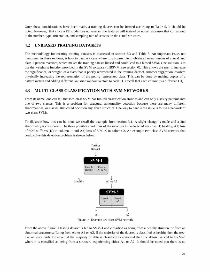
From its name, one can tell that two-class SVM has limited classification abilities and can only classify patterns into one of two classes. This is a problem for structural abnormality detection because there are many different abnormalities, or classes, that could occur on any given structure. One way to handle the issue is to use a network of two-class SVMs. To illustrate how this can be done we recall the example from section 3.1. A slight change is made and a 2nd abnormality is considered. The three possible conditions of the structure to be detected are now: H) healthy, A1) loss of 50% stiffness (K) in column 1, and A2) loss of 50% K in column 2. An example two-class SVM network that could solve this detection problem is shown below:

Figure 14. Example two-class SVM network

From the above figure, a testing dataset is fed to SVM-1 and classified as being from a healthy structure or from an abnormal structure suffering from either A1 or A2. If the majority of the dataset is classified as healthy then the tree-like network ends. However, if the majority of data is classified as abnormal then the dataset is sent to SVM-2, where it is classified as being from a structure experiencing either A1 or A2. It should be noted that there is no

22

specific routine used in this thesis to define an optimal network. Instead, these decisions are simply made by considering the structure and the abnormalities to be detected. 4.4 STEP-BY-STEP GUIDE FOR SVM-BASED STRUCTURAL ABNORMALITY

DETECTION

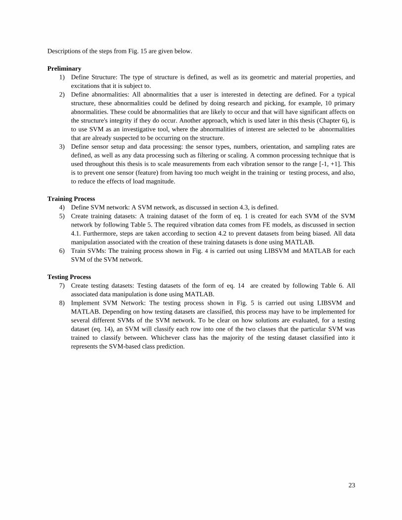
The purpose of this section is to provide the reader with the guide/checklist used later in this thesis to create SVM-based abnormality detection strategies for both a lab structure and an in-service cable-stayed bridge (Chapters 5 and 6). The guide highlights important considerations and gives the order in which they are made. An outline of the guide can be seen in Fig. 15.

Figure 15. Guide for creating SVM-based abnormality detection strategies

Before elaborating on each of these steps, it is important to note some important qualities that Fig. 15 is based on. First, the intent is to demonstrate the potential of SVM for structural abnormality detection, not to show a fully functioning real-time detection strategy. Therefore, real-time implementation is avoided. Second, the following items are assumed to be available: an existing structure to perform abnormality detection on; a modal analysis report for the structure; and access to computer programs that include MATLAB, LIBSVM, and a FE program such as ANSYS.

23

Descriptions of the steps from Fig. 15 are given below. Preliminary

1) Define Structure: The type of structure is defined, as well as its geometric and material properties, and excitations that it is subject to.

2) Define abnormalities: All abnormalities that a user is interested in detecting are defined. For a typical structure, these abnormalities could be defined by doing research and picking, for example, 10 primary abnormalities. These could be abnormalities that are likely to occur and that will have significant affects on the structure's integrity if they do occur. Another approach, which is used later in this thesis (Chapter 6), is to use SVM as an investigative tool, where the abnormalities of interest are selected to be abnormalities that are already suspected to be occurring on the structure.

3) Define sensor setup and data processing: the sensor types, numbers, orientation, and sampling rates are defined, as well as any data processing such as filtering or scaling. A common processing technique that is used throughout this thesis is to scale measurements from each vibration sensor to the range [-1, +1]. This is to prevent one sensor (feature) from having too much weight in the training or testing process, and also, to reduce the effects of load magnitude.

Training Process

4) Define SVM network: A SVM network, as discussed in section 4.3, is defined. 5) Create training datasets: A training dataset of the form of eq. 1 is created for each SVM of the SVM

network by following Table 5. The required vibration data comes from FE models, as discussed in section 4.1. Furthermore, steps are taken according to section 4.2 to prevent datasets from being biased. All data manipulation associated with the creation of these training datasets is done using MATLAB.

6) Train SVMs: The training process shown in Fig. 4 is carried out using LIBSVM and MATLAB for each SVM of the SVM network.

Testing Process

7) Create testing datasets: Testing datasets of the form of eq. 14 are created by following Table 6. All associated data manipulation is done using MATLAB.

8) Implement SVM Network: The testing process shown in Fig. 5 is carried out using LIBSVM and MATLAB. Depending on how testing datasets are classified, this process may have to be implemented for several different SVMs of the SVM network. To be clear on how solutions are evaluated, for a testing dataset (eq. 14), an SVM will classify each row into one of the two classes that the particular SVM was trained to classify between. Whichever class has the majority of the testing dataset classified into it represents the SVM-based class prediction.

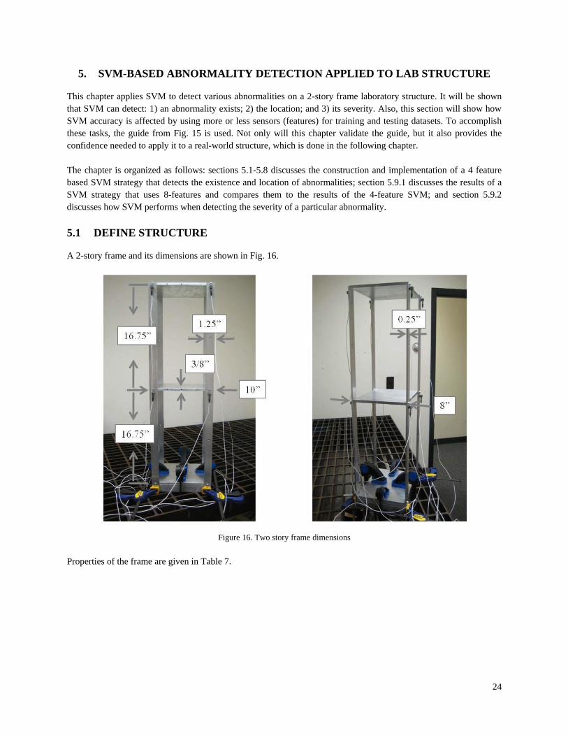
24

5. SVM-BASED ABNORMALITY DETECTION APPLIED TO LAB STRUCTURE

This chapter applies SVM to detect various abnormalities on a 2-story frame laboratory structure. It will be shown that SVM can detect: 1) an abnormality exists; 2) the location; and 3) its severity. Also, this section will show how SVM accuracy is affected by using more or less sensors (features) for training and testing datasets. To accomplish these tasks, the guide from Fig. 15 is used. Not only will this chapter validate the guide, but it also provides the confidence needed to apply it to a real-world structure, which is done in the following chapter. The chapter is organized as follows: sections 5.1-5.8 discusses the construction and implementation of a 4 feature based SVM strategy that detects the existence and location of abnormalities; section 5.9.1 discusses the results of a SVM strategy that uses 8-features and compares them to the results of the 4-feature SVM; and section 5.9.2 discusses how SVM performs when detecting the severity of a particular abnormality. 5.1 DEFINE STRUCTURE

A 2-story frame and its dimensions are shown in Fig. 16.

Figure 16. Two story frame dimensions Properties of the frame are given in Table 7.

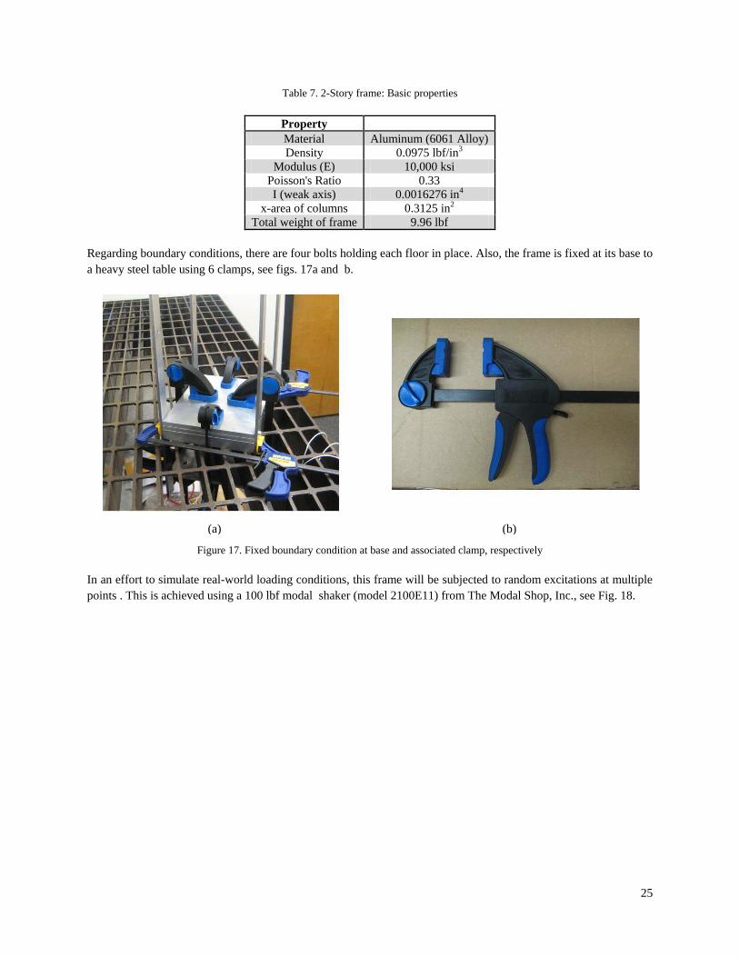
25

Table 7. 2-Story frame: Basic properties

Property Material Aluminum (6061 Alloy) Density 0.0975 lbf/in3

Modulus (E) 10,000 ksi Poisson's Ratio 0.33 I (weak axis) 0.0016276 in4

x-area of columns 0.3125 in2 Total weight of frame 9.96 lbf

Regarding boundary conditions, there are four bolts holding each floor in place. Also, the frame is fixed at its base to a heavy steel table using 6 clamps, see figs. 17a and b.

Figure 17. Fixed boundary condition at base and associated clamp, respectively

In an effort to simulate real-world loading conditions, this frame will be subjected to random excitations at multiple points . This is achieved using a 100 lbf modal shaker (model 2100E11) from The Modal Shop, Inc., see Fig. 18.

(a) (b)

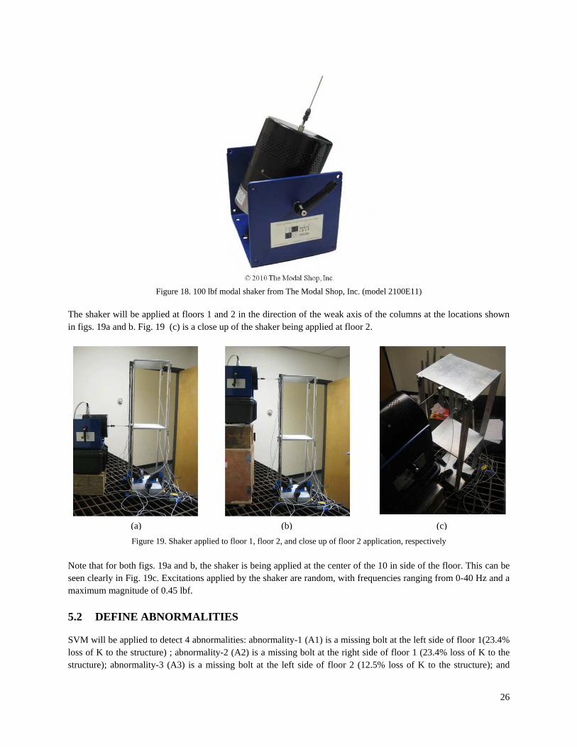
26

Figure 18. 100 lbf modal shaker from The Modal Shop, Inc. (model 2100E11)

The shaker will be applied at floors 1 and 2 in the direction of the weak axis of the columns at the locations shown in figs. 19a and b. Fig. 19 (c) is a close up of the shaker being applied at floor 2.

Figure 19. Shaker applied to floor 1, floor 2, and close up of floor 2 application, respectively

Note that for both figs. 19a and b, the shaker is being applied at the center of the 10 in side of the floor. This can be seen clearly in Fig. 19c. Excitations applied by the shaker are random, with frequencies ranging from 0-40 Hz and a maximum magnitude of 0.45 lbf. 5.2 DEFINE ABNORMALITIES

SVM will be applied to detect 4 abnormalities: abnormality-1 (A1) is a missing bolt at the left side of floor 1(23.4% loss of K to the structure) ; abnormality-2 (A2) is a missing bolt at the right side of floor 1 (23.4% loss of K to the structure); abnormality-3 (A3) is a missing bolt at the left side of floor 2 (12.5% loss of K to the structure); and

(a) (b) (c)

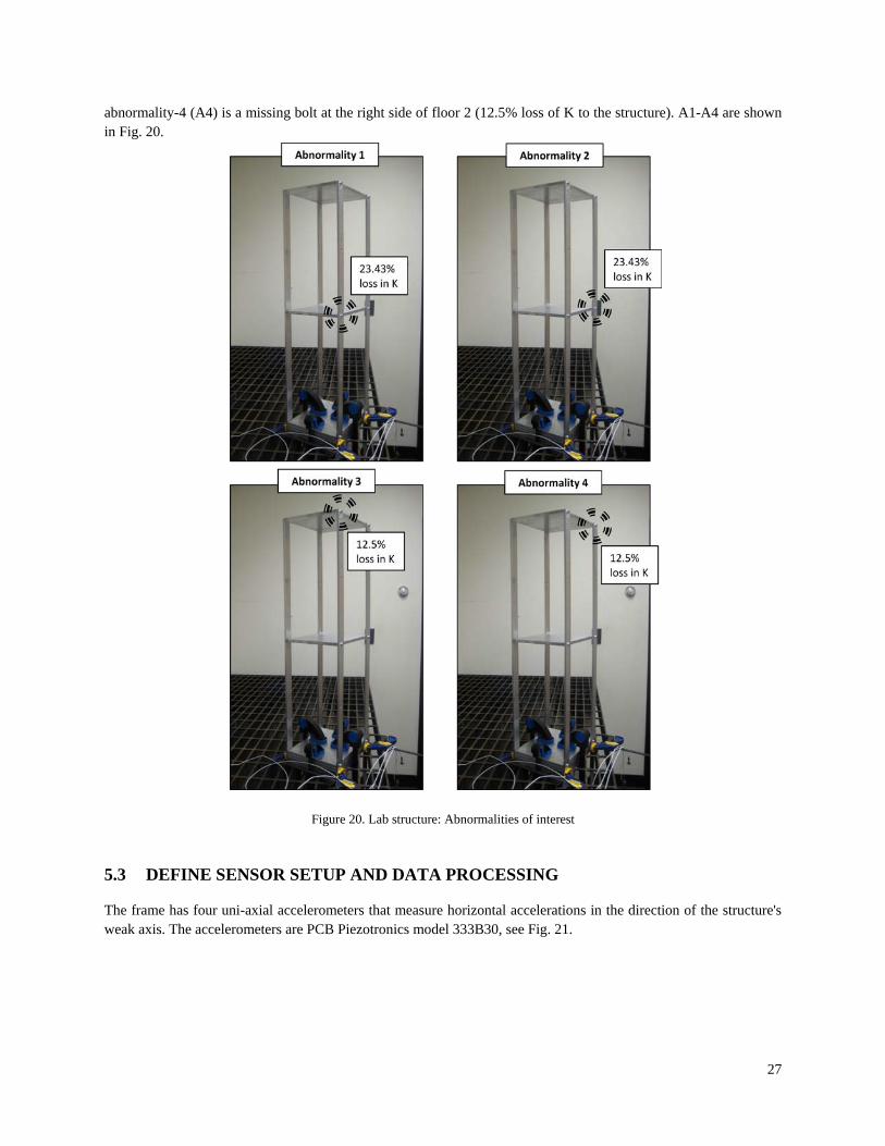
27

abnormality-4 (A4) is a missing bolt at the right side of floor 2 (12.5% loss of K to the structure). A1-A4 are shown in Fig. 20.

Figure 20. Lab structure: Abnormalities of interest

5.3 DEFINE SENSOR SETUP AND DATA PROCESSING

The frame has four uni-axial accelerometers that measure horizontal accelerations in the direction of the structure's weak axis. The accelerometers are PCB Piezotronics model 333B30, see Fig. 21.

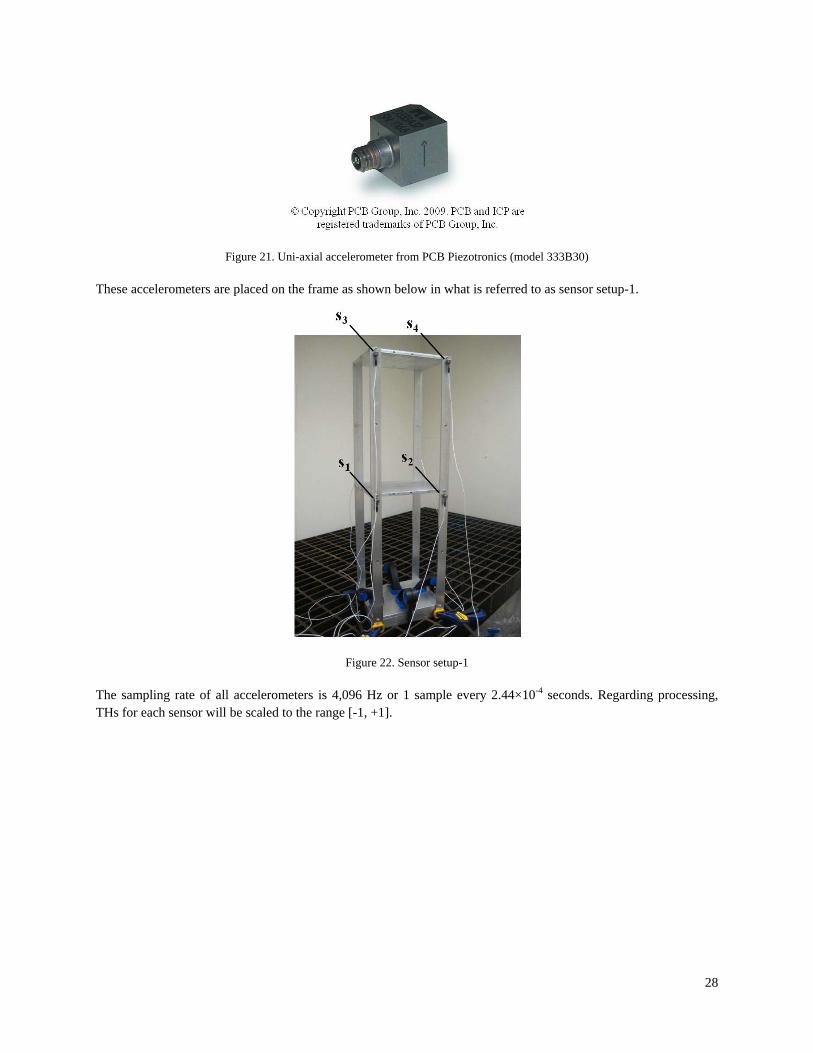
28

Figure 21. Uni-axial accelerometer from PCB Piezotronics (model 333B30)

These accelerometers are placed on the frame as shown below in what is referred to as sensor setup-1.

Figure 22. Sensor setup-1 The sampling rate of all accelerometers is 4,096 Hz or 1 sample every 2.44×10-4 seconds. Regarding processing, THs for each sensor will be scaled to the range [-1, +1].

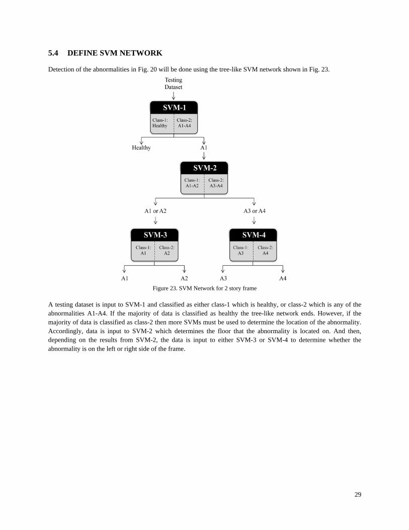
29

5.4 DEFINE SVM NETWORK

Detection of the abnormalities in Fig. 20 will be done using the tree-like SVM network shown in Fig. 23.

Figure 23. SVM Network for 2 story frame

A testing dataset is input to SVM-1 and classified as either class-1 which is healthy, or class-2 which is any of the abnormalities A1-A4. If the majority of data is classified as healthy the tree-like network ends. However, if the majority of data is classified as class-2 then more SVMs must be used to determine the location of the abnormality. Accordingly, data is input to SVM-2 which determines the floor that the abnormality is located on. And then, depending on the results from SVM-2, the data is input to either SVM-3 or SVM-4 to determine whether the abnormality is on the left or right side of the frame.

30

5.5 CREATE TRAINING DATASETS

Per the guide in Fig. 15, a training dataset of the form of eq. 1 is created for each SVM by following Table 5. THs for the pattern and training pair matrices are obtained using a FE model created in ANSYS, see below.

Figure 24. ANSYS model of 2-story frame

There are a total of 310 nodes. Beam elements are used for the columns and shell elements are used for the floors. The geometric and material properties are the same as those shown in Table 7. A modal analysis is performed to validate the model. The frequencies associated with the first two modes are calculated by ANSYS to be 12.52 Hz and 34.55 Hz. These are compared to a modal analysis performed on the actual frame which had frequencies of 10.66 Hz and 31.72 Hz. To make the model more accurate to the structure, the model's modulus (E) is updated to 8.5×106. The model now has frequencies of 11.54 Hz and 31.86 Hz which are closer to the frequencies of the actual structure. Table 5 is used to create training datasets. Important notes are given below for a few of the steps:

• Step 1: The source of vibration data is a FE model. THs are collected from node setup-1 shown in Fig. 26. The sampling rate and processing are the same as established for the actual structure in section 5.3, i.e. 4096 Hz and each TH is scaled to [-1, +1].

• Step 3: All abnormalities are simulated by removing boundary conditions at locations that correspond to where bolts are removed on the actual frame.

• Step 4: An impact loading will be applied. Characteristics of the loading are as follows: the duration will be 0.014 seconds, which ensures that the first two natural frequencies will be excited; the maximum magnitude will be 0.45 lbf; and the load will be applied at the first floor in the direction of the weak axis of the columns, see Fig. 25.

• Step 6: The time window for each TH is from 0.075 to 0.31 seconds after the impact load begins, which is a total duration of 0.235 seconds. Accordingly, with a sampling rate of 4096 Hz and a time window of 0.235 seconds, n of eq. 1 will be 𝑛 = 0.235 𝑠𝑒𝑐 × 4096 𝑠𝑎𝑚𝑝𝑙𝑒𝑠

𝑠𝑒𝑐= 963.

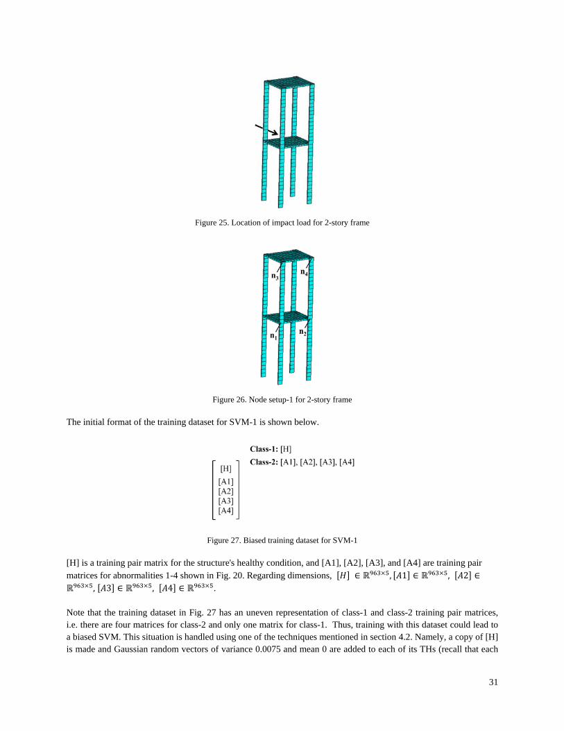
31

Figure 25. Location of impact load for 2-story frame

Figure 26. Node setup-1 for 2-story frame

The initial format of the training dataset for SVM-1 is shown below.

Figure 27. Biased training dataset for SVM-1 [H] is a training pair matrix for the structure's healthy condition, and [A1], [A2], [A3], and [A4] are training pair matrices for abnormalities 1-4 shown in Fig. 20. Regarding dimensions, [𝐻] ∈ ℝ963×5, [𝐴1] ∈ ℝ963×5, [𝐴2] ∈ℝ963×5, [𝐴3] ∈ ℝ963×5, [𝐴4] ∈ ℝ963×5. Note that the training dataset in Fig. 27 has an uneven representation of class-1 and class-2 training pair matrices, i.e. there are four matrices for class-2 and only one matrix for class-1. Thus, training with this dataset could lead to a biased SVM. This situation is handled using one of the techniques mentioned in section 4.2. Namely, a copy of [H] is made and Gaussian random vectors of variance 0.0075 and mean 0 are added to each of its THs (recall that each

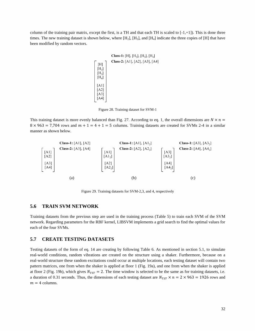
32

column of the training pair matrix, except the first, is a TH and that each TH is scaled to [-1,+1]). This is done three times. The new training dataset is shown below, where [H2], [H3], and [H4] indicate the three copies of [H] that have been modified by random vectors.

Figure 28. Training dataset for SVM-1

This training dataset is more evenly balanced than Fig. 27. According to eq. 1, the overall dimensions are 𝑁 × 𝑛 =8 × 963 = 7,704 rows and 𝑚 + 1 = 4 + 1 = 5 columns. Training datasets are created for SVMs 2-4 in a similar manner as shown below.

Figure 29. Training datasets for SVM-2,3, and 4, respectively

5.6 TRAIN SVM NETWORK

Training datasets from the previous step are used in the training process (Table 5) to train each SVM of the SVM network. Regarding parameters for the RBF kernel, LIBSVM implements a grid search to find the optimal values for each of the four SVMs. 5.7 CREATE TESTING DATASETS

Testing datasets of the form of eq. 14 are creating by following Table 6. As mentioned in section 5.1, to simulate real-world conditions, random vibrations are created on the structure using a shaker. Furthermore, because on a real-world structure these random excitations could occur at multiple locations, each testing dataset will contain two pattern matrices, one from when the shaker is applied at floor 1 (Fig. 19a), and one from when the shaker is applied at floor 2 (Fig. 19b), which gives 𝑁𝑇𝑆𝑇 = 2. The time window is selected to be the same as for training datasets, i.e. a duration of 0.31 seconds. Thus, the dimensions of each testing dataset are 𝑁𝑇𝑆𝑇 × 𝑛 = 2 × 963 = 1926 rows and 𝑚 = 4 columns.

(a) (b) (c)

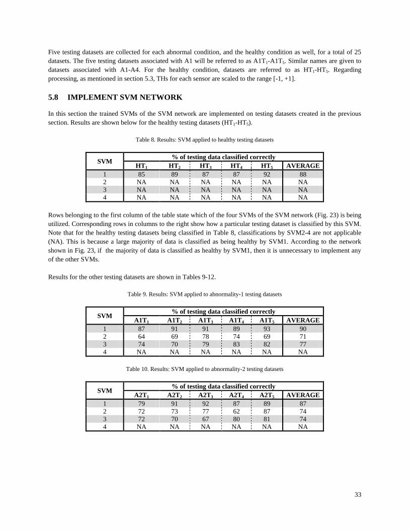
33

Five testing datasets are collected for each abnormal condition, and the healthy condition as well, for a total of 25 datasets. The five testing datasets associated with A1 will be referred to as A1T1-A1T5. Similar names are given to datasets associated with A1-A4. For the healthy condition, datasets are referred to as HT1-HT5. Regarding processing, as mentioned in section 5.3, THs for each sensor are scaled to the range [-1, +1]. 5.8 IMPLEMENT SVM NETWORK

In this section the trained SVMs of the SVM network are implemented on testing datasets created in the previous section. Results are shown below for the healthy testing datasets (HT1-HT5).

Table 8. Results: SVM applied to healthy testing datasets

SVM % of testing data classified correctly HT1 HT2 HT3 HT4 HT5 AVERAGE

1 85 89 87 87 92 88 2 NA NA NA NA NA NA 3 NA NA NA NA NA NA 4 NA NA NA NA NA NA

Rows belonging to the first column of the table state which of the four SVMs of the SVM network (Fig. 23) is being utilized. Corresponding rows in columns to the right show how a particular testing dataset is classified by this SVM. Note that for the healthy testing datasets being classified in Table 8, classifications by SVM2-4 are not applicable (NA). This is because a large majority of data is classified as being healthy by SVM1. According to the network shown in Fig. 23, if the majority of data is classified as healthy by SVM1, then it is unnecessary to implement any of the other SVMs. Results for the other testing datasets are shown in Tables 9-12.

Table 9. Results: SVM applied to abnormality-1 testing datasets

SVM % of testing data classified correctly A1T1 A1T2 A1T3 A1T4 A1T5 AVERAGE

1 87 91 91 89 93 90 2 64 69 78 74 69 71 3 74 70 79 83 82 77 4 NA NA NA NA NA NA

Table 10. Results: SVM applied to abnormality-2 testing datasets

SVM % of testing data classified correctly A2T1 A2T2 A2T3 A2T4 A2T5 AVERAGE

1 79 91 92 87 89 87 2 72 73 77 62 87 74 3 72 70 67 80 81 74 4 NA NA NA NA NA NA

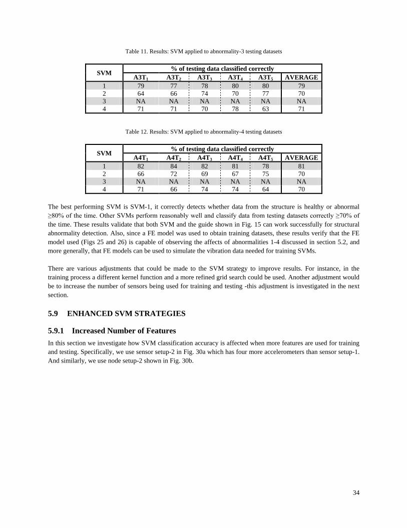
34

Table 11. Results: SVM applied to abnormality-3 testing datasets

SVM % of testing data classified correctly A3T1 A3T2 A3T3 A3T4 A3T5 AVERAGE

1 79 77 78 80 80 79 2 64 66 74 70 77 70 3 NA NA NA NA NA NA 4 71 71 70 78 63 71

Table 12. Results: SVM applied to abnormality-4 testing datasets

SVM % of testing data classified correctly A4T1 A4T2 A4T3 A4T4 A4T5 AVERAGE

1 82 84 82 81 78 81 2 66 72 69 67 75 70 3 NA NA NA NA NA NA 4 71 66 74 74 64 70

The best performing SVM is SVM-1, it correctly detects whether data from the structure is healthy or abnormal ≥80% of the time. Other SVMs perform reasonably well and classify data from testing datasets correctly ≥70% of the time. These results validate that both SVM and the guide shown in Fig. 15 can work successfully for structural abnormality detection. Also, since a FE model was used to obtain training datasets, these results verify that the FE model used (Figs 25 and 26) is capable of observing the affects of abnormalities 1-4 discussed in section 5.2, and more generally, that FE models can be used to simulate the vibration data needed for training SVMs. There are various adjustments that could be made to the SVM strategy to improve results. For instance, in the training process a different kernel function and a more refined grid search could be used. Another adjustment would be to increase the number of sensors being used for training and testing -this adjustment is investigated in the next section. 5.9 ENHANCED SVM STRATEGIES

5.9.1 Increased Number of Features In this section we investigate how SVM classification accuracy is affected when more features are used for training and testing. Specifically, we use sensor setup-2 in Fig. 30a which has four more accelerometers than sensor setup-1. And similarly, we use node setup-2 shown in Fig. 30b.

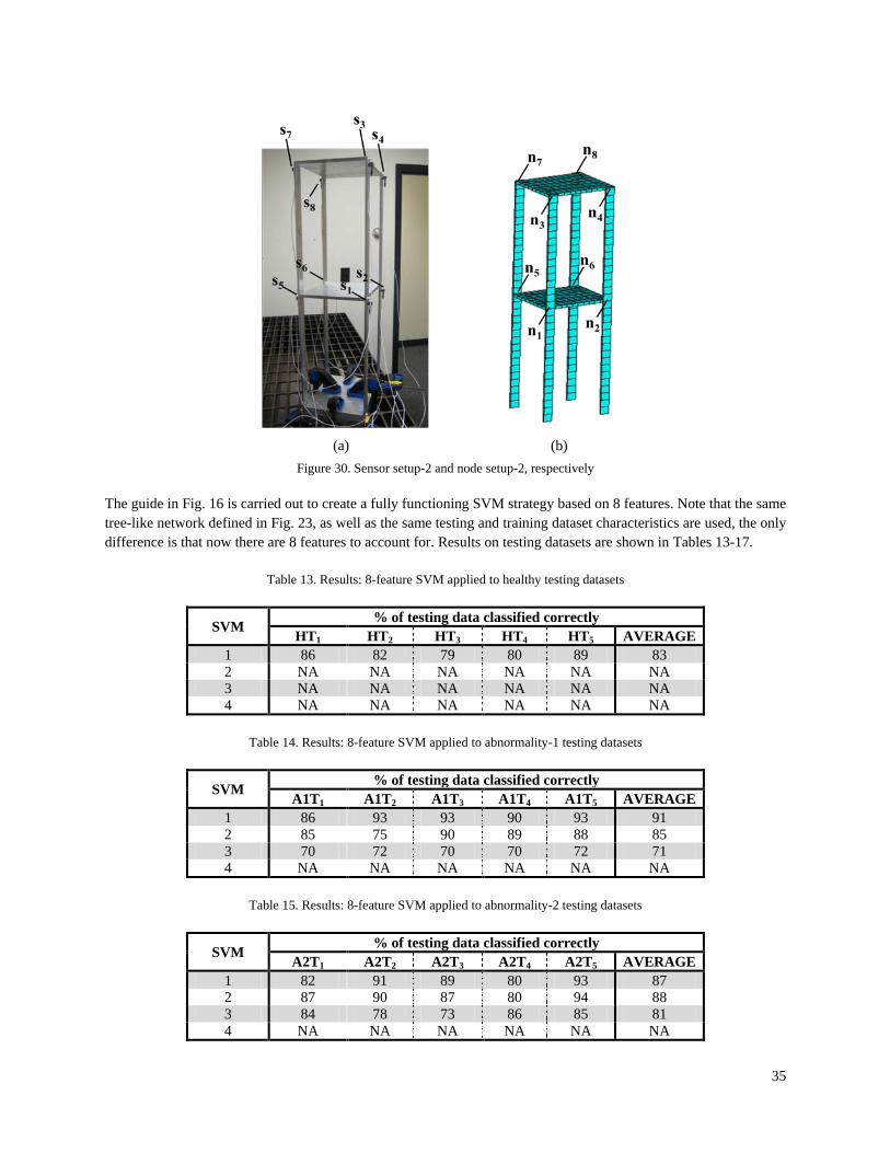
35

Figure 30. Sensor setup-2 and node setup-2, respectively The guide in Fig. 16 is carried out to create a fully functioning SVM strategy based on 8 features. Note that the same tree-like network defined in Fig. 23, as well as the same testing and training dataset characteristics are used, the only difference is that now there are 8 features to account for. Results on testing datasets are shown in Tables 13-17.

Table 13. Results: 8-feature SVM applied to healthy testing datasets

SVM % of testing data classified correctly HT1 HT2 HT3 HT4 HT5 AVERAGE

1 86 82 79 80 89 83 2 NA NA NA NA NA NA 3 NA NA NA NA NA NA 4 NA NA NA NA NA NA

Table 14. Results: 8-feature SVM applied to abnormality-1 testing datasets

SVM % of testing data classified correctly A1T1 A1T2 A1T3 A1T4 A1T5 AVERAGE

1 86 93 93 90 93 91 2 85 75 90 89 88 85 3 70 72 70 70 72 71 4 NA NA NA NA NA NA

Table 15. Results: 8-feature SVM applied to abnormality-2 testing datasets

SVM % of testing data classified correctly A2T1 A2T2 A2T3 A2T4 A2T5 AVERAGE

1 82 91 89 80 93 87 2 87 90 87 80 94 88 3 84 78 73 86 85 81 4 NA NA NA NA NA NA

(a) (b)

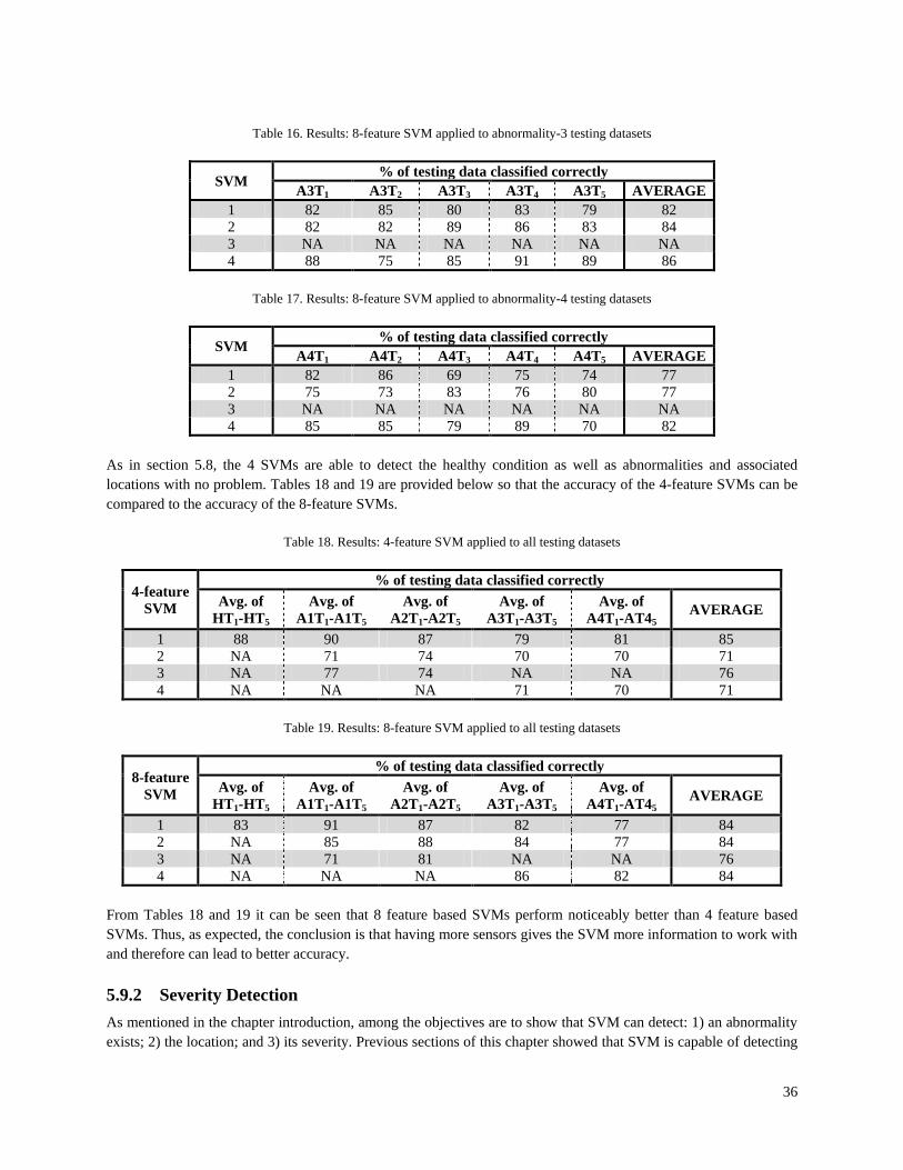
36

Table 16. Results: 8-feature SVM applied to abnormality-3 testing datasets

SVM % of testing data classified correctly A3T1 A3T2 A3T3 A3T4 A3T5 AVERAGE

1 82 85 80 83 79 82 2 82 82 89 86 83 84 3 NA NA NA NA NA NA 4 88 75 85 91 89 86

Table 17. Results: 8-feature SVM applied to abnormality-4 testing datasets

SVM % of testing data classified correctly A4T1 A4T2 A4T3 A4T4 A4T5 AVERAGE

1 82 86 69 75 74 77 2 75 73 83 76 80 77 3 NA NA NA NA NA NA 4 85 85 79 89 70 82

As in section 5.8, the 4 SVMs are able to detect the healthy condition as well as abnormalities and associated locations with no problem. Tables 18 and 19 are provided below so that the accuracy of the 4-feature SVMs can be compared to the accuracy of the 8-feature SVMs.

Table 18. Results: 4-feature SVM applied to all testing datasets

4-feature SVM

% of testing data classified correctly Avg. of

HT1-HT5 Avg. of

A1T1-A1T5 Avg. of

A2T1-A2T5 Avg. of

A3T1-A3T5 Avg. of

A4T1-AT45 AVERAGE

1 88 90 87 79 81 85 2 NA 71 74 70 70 71 3 NA 77 74 NA NA 76 4 NA NA NA 71 70 71

Table 19. Results: 8-feature SVM applied to all testing datasets

8-feature SVM

% of testing data classified correctly Avg. of

HT1-HT5 Avg. of

A1T1-A1T5 Avg. of

A2T1-A2T5 Avg. of

A3T1-A3T5 Avg. of

A4T1-AT45 AVERAGE

1 83 91 87 82 77 84 2 NA 85 88 84 77 84 3 NA 71 81 NA NA 76 4 NA NA NA 86 82 84

From Tables 18 and 19 it can be seen that 8 feature based SVMs perform noticeably better than 4 feature based SVMs. Thus, as expected, the conclusion is that having more sensors gives the SVM more information to work with and therefore can lead to better accuracy. 5.9.2 Severity Detection As mentioned in the chapter introduction, among the objectives are to show that SVM can detect: 1) an abnormality exists; 2) the location; and 3) its severity. Previous sections of this chapter showed that SVM is capable of detecting

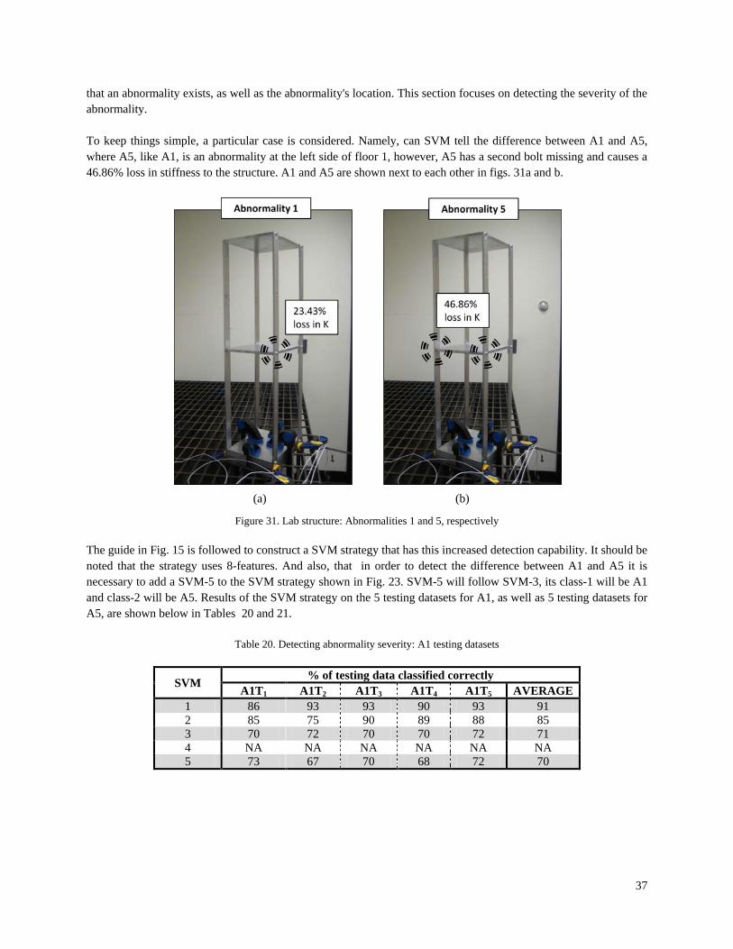
37

that an abnormality exists, as well as the abnormality's location. This section focuses on detecting the severity of the abnormality. To keep things simple, a particular case is considered. Namely, can SVM tell the difference between A1 and A5, where A5, like A1, is an abnormality at the left side of floor 1, however, A5 has a second bolt missing and causes a 46.86% loss in stiffness to the structure. A1 and A5 are shown next to each other in figs. 31a and b.

Figure 31. Lab structure: Abnormalities 1 and 5, respectively

The guide in Fig. 15 is followed to construct a SVM strategy that has this increased detection capability. It should be noted that the strategy uses 8-features. And also, that in order to detect the difference between A1 and A5 it is necessary to add a SVM-5 to the SVM strategy shown in Fig. 23. SVM-5 will follow SVM-3, its class-1 will be A1 and class-2 will be A5. Results of the SVM strategy on the 5 testing datasets for A1, as well as 5 testing datasets for A5, are shown below in Tables 20 and 21.

Table 20. Detecting abnormality severity: A1 testing datasets

SVM % of testing data classified correctly A1T1 A1T2 A1T3 A1T4 A1T5 AVERAGE

1 86 93 93 90 93 91 2 85 75 90 89 88 85 3 70 72 70 70 72 71 4 NA NA NA NA NA NA 5 73 67 70 68 72 70

(a) (b)

38

Table 21. Detecting abnormality severity: A5 testing datasets

SVM % of testing data classified correctly A5T1 A5T2 A5T3 A5T4 A5T5 AVERAGE

1 95 89 93 86 90 91 2 66 71 72 71 74 71 3 66 82 64 67 73 70 4 NA NA NA NA NA NA 5 73 73 72 70 72 72

Tables 20 and 21 show that SVM is capable of detecting abnormality severity.

39

6. SVM-BASED ABNORMALITY DETECTION APPLIED TO REAL-WORLD STRUCTURE

This chapter applies SVM for abnormality detection on an in-service cable-stayed bridge. Unlike the previous chapter where various abnormalities are detected, the goal here is to investigate a single abnormality. Namely, whether the east end expansion joint is constraining the longitudinal movement of the bridge's main girder, which is suspected due to the results of a finite element updating procedure [20]. The guide in Fig. 15 is used once again to create a SVM strategy and obtain results. The following sections correspond to the different steps of the guide. 6.1 DEFINE STRUCTURE

The Zhanjiang Bay Bridge was completed in December, 2006, and is located in an inner gulf of Zhanjiang city in south China. It is a cable-stayed bridge with a main span of 480m and total length of 3,981m. The bridge consists of five box girder spans; two reinforced concrete end spans and three steel interior spans. Additional steel is found in the parallel steel wires that compose the prefabricated stay cables. Aside from the mentioned girders and cables, all remaining bridge components are reinforced or pre-stressed concrete. The bridge is shown in Fig. 32, its dimensional and sectional properties are shown in figs. 33, 34, and 35, as well as in Tables 22 and 23.

Figure 32. Zhanjiang Bay Bridge

Figure 33. Bridge dimensions

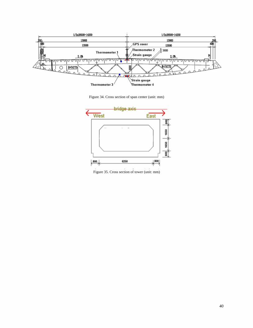
40

Figure 34. Cross section of span center (unit: mm)

Figure 35. Cross section of tower (unit: mm)

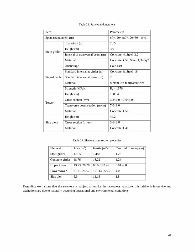
41

Table 22. Structural dimensions

Item Parameters

Span arrangement (m) 60+120+480+120+60 = 840

Main girder

Top width (m) 28.5

Height (m) 3.0

Interval of transversal beam (m) Concrete: 4, Steel: 3.2

Material Concrete: C50, Steel: Q345qC

Stayed cable

Anchorage Cold cast

Standard interval at girder (m) Concrete: 8, Steel: 16

Standard interval at tower (m) 2

Material Φ7mm Pre-fabricated wire

Strength (MPa) Ry = 1670

Tower

Height (m) 150.64

Cross section (m*) 3.2×6.0 ~ 7.0×8.0

Transverse beam section (m×m) 7.0×8.0

Material Concrete: C50

Side piers

Height (m) 49.2

Cross section (m×m) 3.6×3.8

Material Concrete: C40

Table 23. Element cross section properties

Element Area (m2) Inertia (m4) Centroid from top (m)

Steel girder 1.165 1.487 1.23

Concrete girder 18.76 18.22 1.24

Upper tower 13.73~20.20 65.0~142.26 3.01~4.0

Lower tower 21.31~25.67 171.14~224.79 4.0

Side pier 6.6 11.16 1.8

Regarding excitations that the structure is subject to, unlike the laboratory structure, this bridge is in-service and excitations are due to naturally occurring operational and environmental conditions.

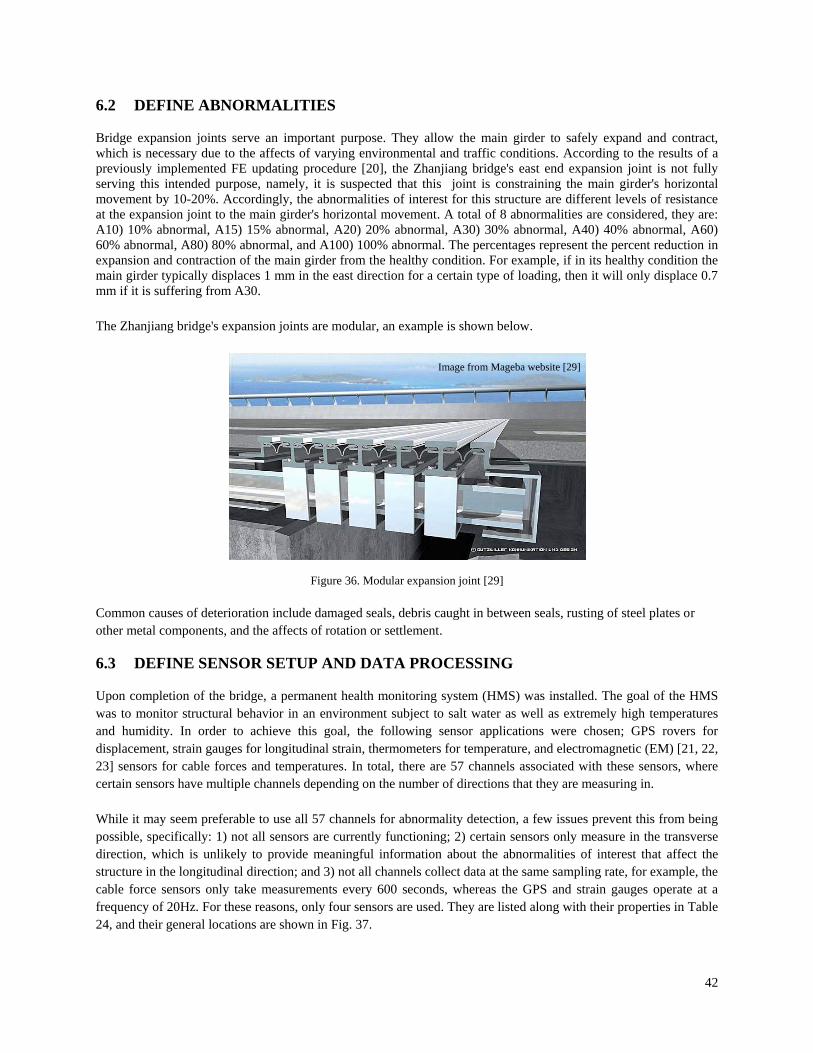
42

6.2 DEFINE ABNORMALITIES

Bridge expansion joints serve an important purpose. They allow the main girder to safely expand and contract, which is necessary due to the affects of varying environmental and traffic conditions. According to the results of a previously implemented FE updating procedure [20], the Zhanjiang bridge's east end expansion joint is not fully serving this intended purpose, namely, it is suspected that this joint is constraining the main girder's horizontal movement by 10-20%. Accordingly, the abnormalities of interest for this structure are different levels of resistance at the expansion joint to the main girder's horizontal movement. A total of 8 abnormalities are considered, they are: A10) 10% abnormal, A15) 15% abnormal, A20) 20% abnormal, A30) 30% abnormal, A40) 40% abnormal, A60) 60% abnormal, A80) 80% abnormal, and A100) 100% abnormal. The percentages represent the percent reduction in expansion and contraction of the main girder from the healthy condition. For example, if in its healthy condition the main girder typically displaces 1 mm in the east direction for a certain type of loading, then it will only displace 0.7 mm if it is suffering from A30.

The Zhanjiang bridge's expansion joints are modular, an example is shown below.

Figure 36. Modular expansion joint [29] Common causes of deterioration include damaged seals, debris caught in between seals, rusting of steel plates or other metal components, and the affects of rotation or settlement.

6.3 DEFINE SENSOR SETUP AND DATA PROCESSING

Upon completion of the bridge, a permanent health monitoring system (HMS) was installed. The goal of the HMS was to monitor structural behavior in an environment subject to salt water as well as extremely high temperatures and humidity. In order to achieve this goal, the following sensor applications were chosen; GPS rovers for displacement, strain gauges for longitudinal strain, thermometers for temperature, and electromagnetic (EM) [21, 22, 23] sensors for cable forces and temperatures. In total, there are 57 channels associated with these sensors, where certain sensors have multiple channels depending on the number of directions that they are measuring in. While it may seem preferable to use all 57 channels for abnormality detection, a few issues prevent this from being possible, specifically: 1) not all sensors are currently functioning; 2) certain sensors only measure in the transverse direction, which is unlikely to provide meaningful information about the abnormalities of interest that affect the structure in the longitudinal direction; and 3) not all channels collect data at the same sampling rate, for example, the cable force sensors only take measurements every 600 seconds, whereas the GPS and strain gauges operate at a frequency of 20Hz. For these reasons, only four sensors are used. They are listed along with their properties in Table 24, and their general locations are shown in Fig. 37.

Image from Mageba website [29]

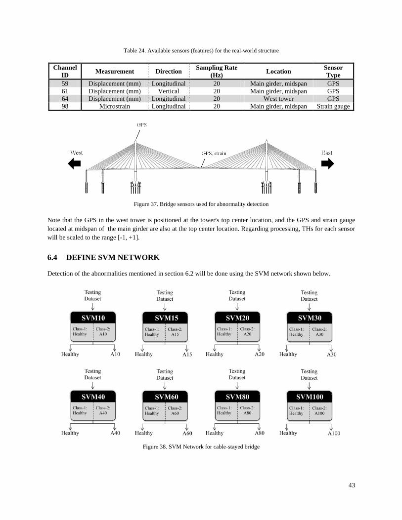
43

Table 24. Available sensors (features) for the real-world structure

Channel ID Measurement Direction Sampling Rate

(Hz) Location Sensor Type

59 Displacement (mm) Longitudinal 20 Main girder, midspan GPS 61 Displacement (mm) Vertical 20 Main girder, midspan GPS 64 Displacement (mm) Longitudinal 20 West tower GPS 98 Microstrain Longitudinal 20 Main girder, midspan Strain gauge

Figure 37. Bridge sensors used for abnormality detection

Note that the GPS in the west tower is positioned at the tower's top center location, and the GPS and strain gauge located at midspan of the main girder are also at the top center location. Regarding processing, THs for each sensor will be scaled to the range [-1, +1]. 6.4 DEFINE SVM NETWORK

Detection of the abnormalities mentioned in section 6.2 will be done using the SVM network shown below.

Figure 38. SVM Network for cable-stayed bridge

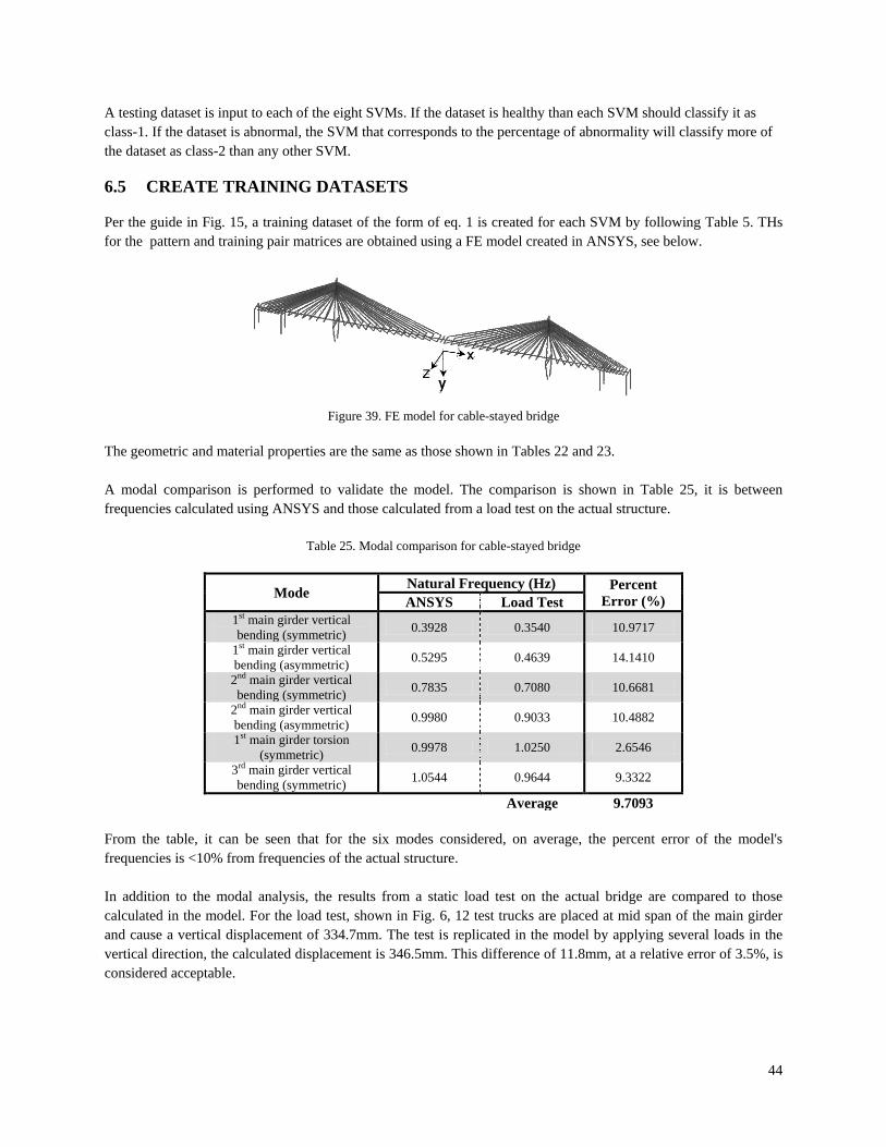
44

A testing dataset is input to each of the eight SVMs. If the dataset is healthy than each SVM should classify it as class-1. If the dataset is abnormal, the SVM that corresponds to the percentage of abnormality will classify more of the dataset as class-2 than any other SVM.

6.5 CREATE TRAINING DATASETS

Per the guide in Fig. 15, a training dataset of the form of eq. 1 is created for each SVM by following Table 5. THs for the pattern and training pair matrices are obtained using a FE model created in ANSYS, see below.

Figure 39. FE model for cable-stayed bridge

The geometric and material properties are the same as those shown in Tables 22 and 23. A modal comparison is performed to validate the model. The comparison is shown in Table 25, it is between frequencies calculated using ANSYS and those calculated from a load test on the actual structure.

Table 25. Modal comparison for cable-stayed bridge

Mode Natural Frequency (Hz) Percent Error (%) ANSYS Load Test

1st main girder vertical bending (symmetric) 0.3928 0.3540 10.9717

1st main girder vertical bending (asymmetric) 0.5295 0.4639 14.1410

2nd main girder vertical bending (symmetric) 0.7835 0.7080 10.6681

2nd main girder vertical bending (asymmetric) 0.9980 0.9033 10.4882

1st main girder torsion (symmetric) 0.9978 1.0250 2.6546

3rd main girder vertical bending (symmetric) 1.0544 0.9644 9.3322

Average 9.7093 From the table, it can be seen that for the six modes considered, on average, the percent error of the model's frequencies is <10% from frequencies of the actual structure. In addition to the modal analysis, the results from a static load test on the actual bridge are compared to those calculated in the model. For the load test, shown in Fig. 6, 12 test trucks are placed at mid span of the main girder and cause a vertical displacement of 334.7mm. The test is replicated in the model by applying several loads in the vertical direction, the calculated displacement is 346.5mm. This difference of 11.8mm, at a relative error of 3.5%, is considered acceptable.

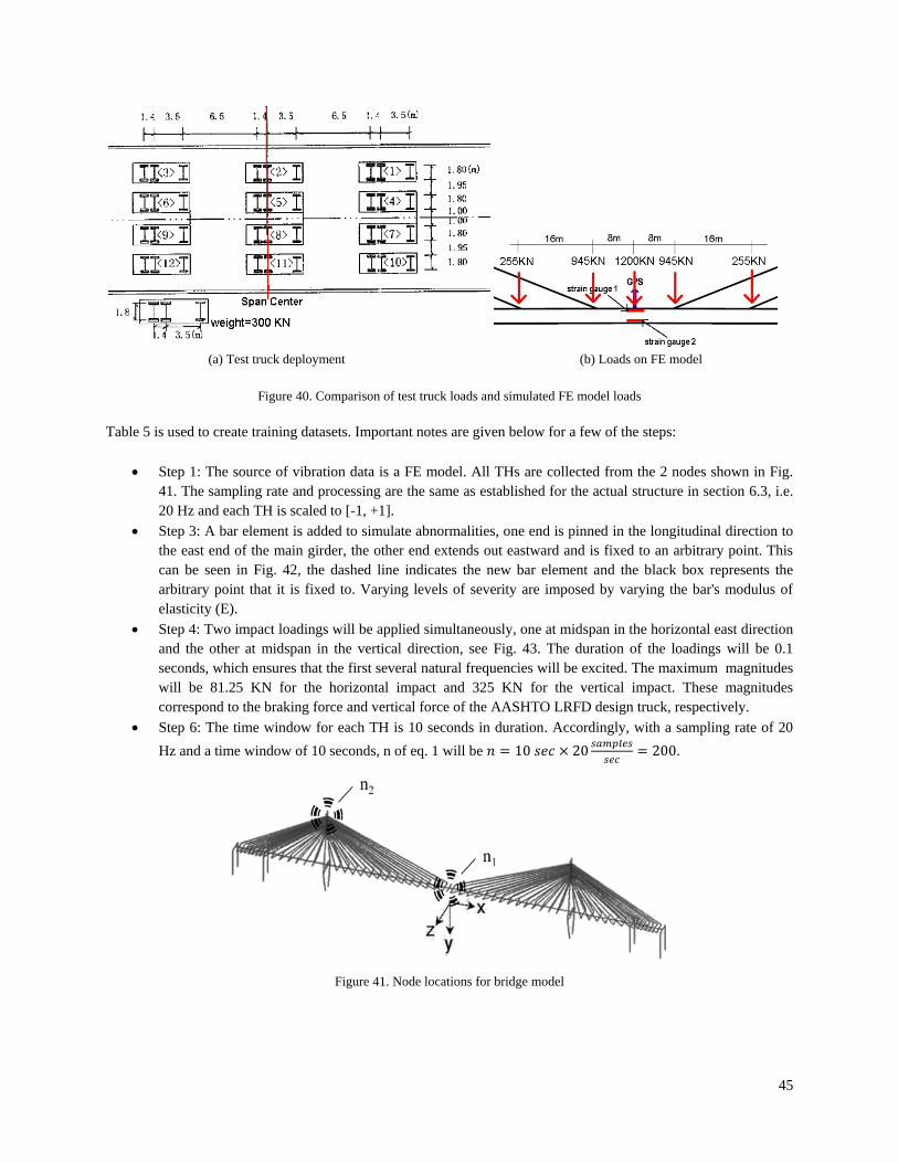
45

(a) Test truck deployment (b) Loads on FE model

Figure 40. Comparison of test truck loads and simulated FE model loads

Table 5 is used to create training datasets. Important notes are given below for a few of the steps:

• Step 1: The source of vibration data is a FE model. All THs are collected from the 2 nodes shown in Fig. 41. The sampling rate and processing are the same as established for the actual structure in section 6.3, i.e. 20 Hz and each TH is scaled to [-1, +1].

• Step 3: A bar element is added to simulate abnormalities, one end is pinned in the longitudinal direction to the east end of the main girder, the other end extends out eastward and is fixed to an arbitrary point. This can be seen in Fig. 42, the dashed line indicates the new bar element and the black box represents the arbitrary point that it is fixed to. Varying levels of severity are imposed by varying the bar's modulus of elasticity (E).

• Step 4: Two impact loadings will be applied simultaneously, one at midspan in the horizontal east direction and the other at midspan in the vertical direction, see Fig. 43. The duration of the loadings will be 0.1 seconds, which ensures that the first several natural frequencies will be excited. The maximum magnitudes will be 81.25 KN for the horizontal impact and 325 KN for the vertical impact. These magnitudes correspond to the braking force and vertical force of the AASHTO LRFD design truck, respectively.

• Step 6: The time window for each TH is 10 seconds in duration. Accordingly, with a sampling rate of 20 Hz and a time window of 10 seconds, n of eq. 1 will be 𝑛 = 10 𝑠𝑒𝑐 × 20 𝑠𝑎𝑚𝑝𝑙𝑒𝑠

𝑠𝑒𝑐= 200.

Figure 41. Node locations for bridge model

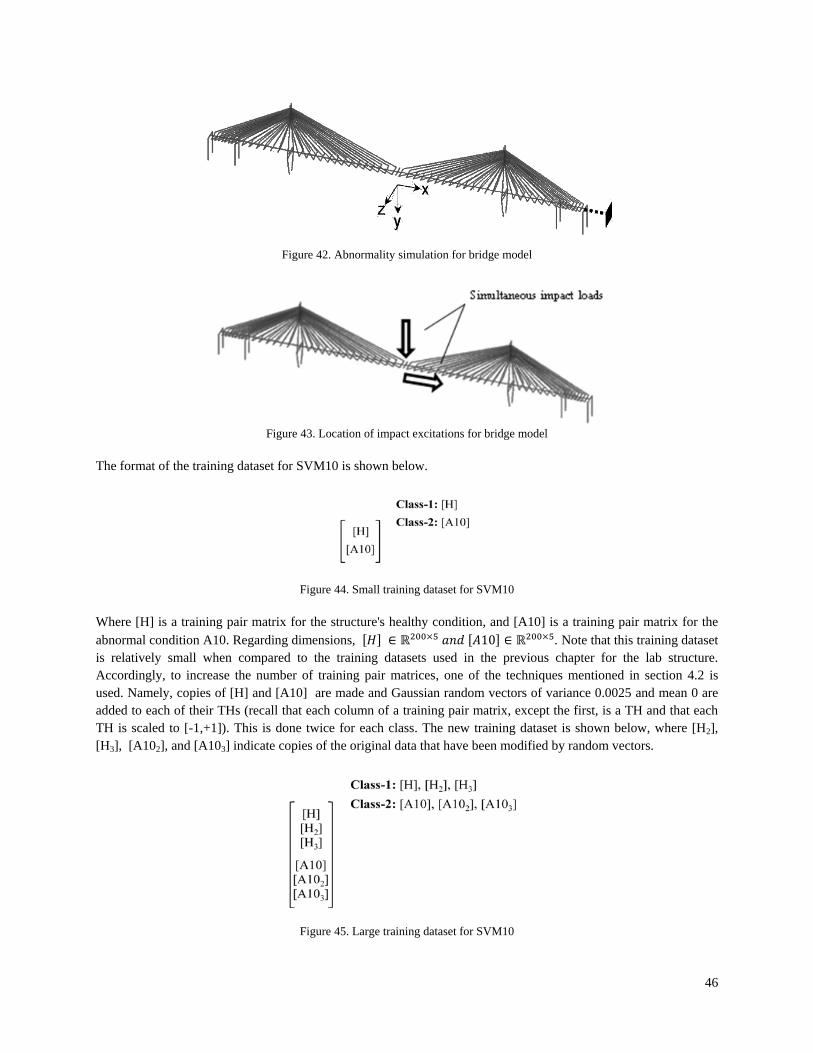
46

Figure 42. Abnormality simulation for bridge model

Figure 43. Location of impact excitations for bridge model

The format of the training dataset for SVM10 is shown below.

Figure 44. Small training dataset for SVM10 Where [H] is a training pair matrix for the structure's healthy condition, and [A10] is a training pair matrix for the abnormal condition A10. Regarding dimensions, [𝐻] ∈ ℝ200×5 𝑎𝑛𝑑 [𝐴10] ∈ ℝ200×5. Note that this training dataset is relatively small when compared to the training datasets used in the previous chapter for the lab structure. Accordingly, to increase the number of training pair matrices, one of the techniques mentioned in section 4.2 is used. Namely, copies of [H] and [A10] are made and Gaussian random vectors of variance 0.0025 and mean 0 are added to each of their THs (recall that each column of a training pair matrix, except the first, is a TH and that each TH is scaled to [-1,+1]). This is done twice for each class. The new training dataset is shown below, where [H2], [H3], [A102], and [A103] indicate copies of the original data that have been modified by random vectors.

Figure 45. Large training dataset for SVM10

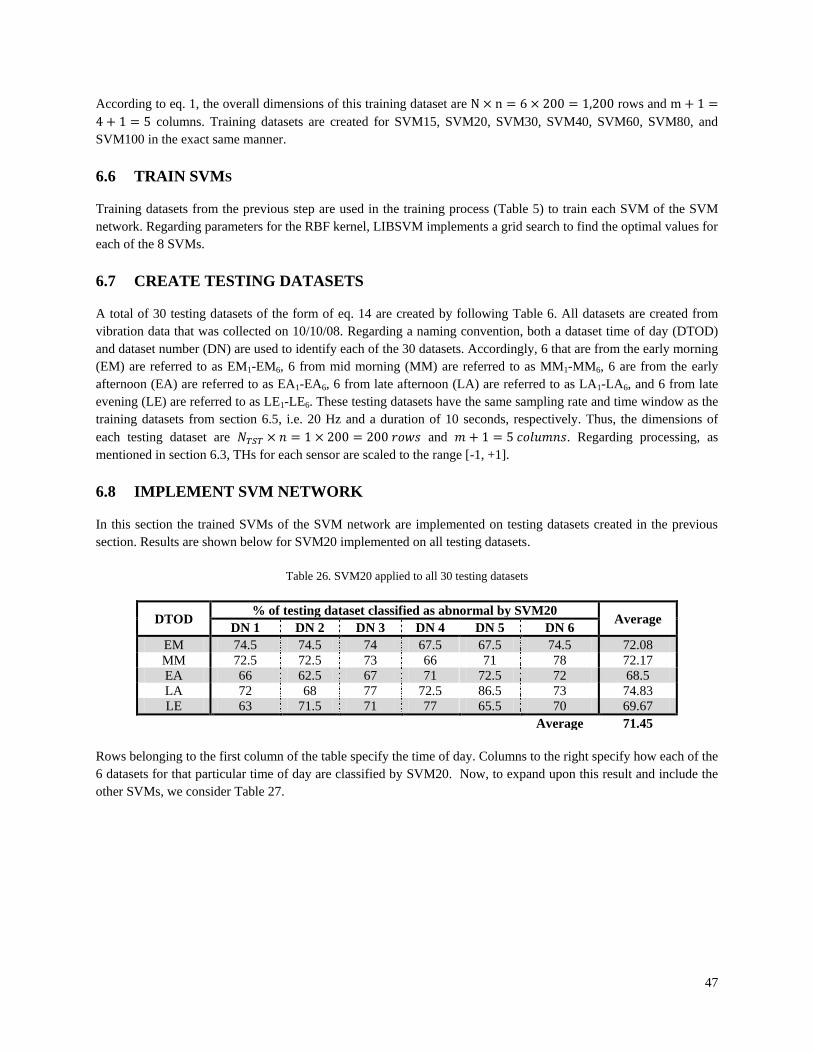
47

According to eq. 1, the overall dimensions of this training dataset are N × n = 6 × 200 = 1,200 rows and m + 1 =4 + 1 = 5 columns. Training datasets are created for SVM15, SVM20, SVM30, SVM40, SVM60, SVM80, and SVM100 in the exact same manner. 6.6 TRAIN SVMS

Training datasets from the previous step are used in the training process (Table 5) to train each SVM of the SVM network. Regarding parameters for the RBF kernel, LIBSVM implements a grid search to find the optimal values for each of the 8 SVMs. 6.7 CREATE TESTING DATASETS

A total of 30 testing datasets of the form of eq. 14 are created by following Table 6. All datasets are created from vibration data that was collected on 10/10/08. Regarding a naming convention, both a dataset time of day (DTOD) and dataset number (DN) are used to identify each of the 30 datasets. Accordingly, 6 that are from the early morning (EM) are referred to as EM1-EM6, 6 from mid morning (MM) are referred to as MM1-MM6, 6 are from the early afternoon (EA) are referred to as EA1-EA6, 6 from late afternoon (LA) are referred to as LA1-LA6, and 6 from late evening (LE) are referred to as LE1-LE6. These testing datasets have the same sampling rate and time window as the training datasets from section 6.5, i.e. 20 Hz and a duration of 10 seconds, respectively. Thus, the dimensions of each testing dataset are 𝑁𝑇𝑆𝑇 × 𝑛 = 1 × 200 = 200 𝑟𝑜𝑤𝑠 and 𝑚 + 1 = 5 𝑐𝑜𝑙𝑢𝑚𝑛𝑠. Regarding processing, as mentioned in section 6.3, THs for each sensor are scaled to the range [-1, +1]. 6.8 IMPLEMENT SVM NETWORK

In this section the trained SVMs of the SVM network are implemented on testing datasets created in the previous section. Results are shown below for SVM20 implemented on all testing datasets.

Table 26. SVM20 applied to all 30 testing datasets

DTOD % of testing dataset classified as abnormal by SVM20 Average DN 1 DN 2 DN 3 DN 4 DN 5 DN 6 EM 74.5 74.5 74 67.5 67.5 74.5 72.08 MM 72.5 72.5 73 66 71 78 72.17 EA 66 62.5 67 71 72.5 72 68.5 LA 72 68 77 72.5 86.5 73 74.83 LE 63 71.5 71 77 65.5 70 69.67

Average 71.45 Rows belonging to the first column of the table specify the time of day. Columns to the right specify how each of the 6 datasets for that particular time of day are classified by SVM20. Now, to expand upon this result and include the other SVMs, we consider Table 27.

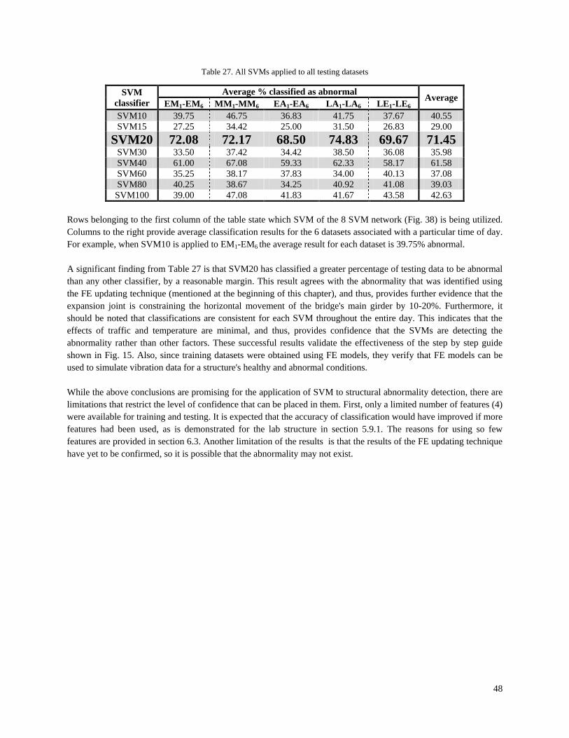
48

Table 27. All SVMs applied to all testing datasets

SVM classifier

Average % classified as abnormal Average EM1-EM6 MM1-MM6 EA1-EA6 LA1-LA6 LE1-LE6 SVM10 39.75 46.75 36.83 41.75 37.67 40.55 SVM15 27.25 34.42 25.00 31.50 26.83 29.00

SVM20 72.08 72.17 68.50 74.83 69.67 71.45 SVM30 33.50 37.42 34.42 38.50 36.08 35.98 SVM40 61.00 67.08 59.33 62.33 58.17 61.58 SVM60 35.25 38.17 37.83 34.00 40.13 37.08 SVM80 40.25 38.67 34.25 40.92 41.08 39.03 SVM100 39.00 47.08 41.83 41.67 43.58 42.63

Rows belonging to the first column of the table state which SVM of the 8 SVM network (Fig. 38) is being utilized. Columns to the right provide average classification results for the 6 datasets associated with a particular time of day. For example, when SVM10 is applied to EM1-EM6 the average result for each dataset is 39.75% abnormal. A significant finding from Table 27 is that SVM20 has classified a greater percentage of testing data to be abnormal than any other classifier, by a reasonable margin. This result agrees with the abnormality that was identified using the FE updating technique (mentioned at the beginning of this chapter), and thus, provides further evidence that the expansion joint is constraining the horizontal movement of the bridge's main girder by 10-20%. Furthermore, it should be noted that classifications are consistent for each SVM throughout the entire day. This indicates that the effects of traffic and temperature are minimal, and thus, provides confidence that the SVMs are detecting the abnormality rather than other factors. These successful results validate the effectiveness of the step by step guide shown in Fig. 15. Also, since training datasets were obtained using FE models, they verify that FE models can be used to simulate vibration data for a structure's healthy and abnormal conditions. While the above conclusions are promising for the application of SVM to structural abnormality detection, there are limitations that restrict the level of confidence that can be placed in them. First, only a limited number of features (4) were available for training and testing. It is expected that the accuracy of classification would have improved if more features had been used, as is demonstrated for the lab structure in section 5.9.1. The reasons for using so few features are provided in section 6.3. Another limitation of the results is that the results of the FE updating technique have yet to be confirmed, so it is possible that the abnormality may not exist.

49

7. CONCLUSIONS AND BROADER IMPACTS

7.1 SUMMARY AND FUTURE WORK

Chapter 1 mentions that the United States is in the midst of an aging civil infrastructure crisis. It then goes on to state that sensor-based health monitoring systems (HMSs) are likely to play a large role in restoring confidence and preventing a similar crisis from happening in the future. These systems collect vibration data from sensor arrays placed on structures. Subsequently, an analysis technique is applied to this data to detect and locate abnormalities. This thesis fits into the picture because it investigates one of these analysis techniques. Specifically, it investigates a pattern classification technique known as two-class Support Vector Machine (SVM). Other papers have investigated SVM for this application, their contributions and the state of the art are provided in chapter 2. The contributions that were made in this thesis are listed along with their corresponding chapters below:

• Chapter 4 introduced a step by step guide (Fig. 15) for how this thesis develops and implements SVM-based abnormality detection strategies. This guide is intended to be applicable for real-world structures.

• Chapter 5 successfully applied the guide in Fig. 15 to a 2-story frame lab structure to detect the existence, location, and severity of connection abnormalities.

• Chapter 5 assessed how SVM accuracy is affected by the number of features being used from a structure's sensor array.

• Chapter 6 applied the guide in Fig. 15 to a real-world structure. Evidence was found that the east end expansion joint of a cable-stayed bridge is constraining the horizontal movement of the main girder by 10-20%. This result agrees with the results of a previously implemented FE updating technique [20].

• Chapters 5 and 6 provided evidence that in the absence of actual measurements, FE models can be relied upon to simulate vibration data that can be used for training SVMs.

It should be noted that these contributions are not intended to present SVM-based abnormality detection as a finalized product, but instead to enhance previous research in the area. Accordingly, it is realized that significant future work is required before two-class SVM can be considered as a reliable means of structural abnormality detection. Among the suggestions for future work are to apply two-class SVM to structures that are more complex than the two story lab structure from chapter 5, and also, to detect abnormalities that are more subtle than the connection abnormalities shown in figs. 20 and 31. An additional suggestion would be to apply SVM to a lab structure subject to excitations that are more realistic than the single shaker shown in figs. 18 and 19, such as excitations from a shake table, wind tunnel, or the natural environment. One avenue for accomplishing this future work would be to apply two-class SVM to data for the benchmark structure used in references [9] and [15], and described in reference [30]. This 4-story frame structure is significantly larger and more complex than the structure used in this thesis, also, it is subjected to realistic loading conditions that include ambient vibrations from wind, traffic, and pedestrians. 7.2 BROADER IMPACTS

From the surface, it may appear as though the infrastructure crisis will resolve as soon as methods like the one discussed in this thesis are substantiated by rigorous experimentation and become accepted amongst the structural health monitoring community. This would be true if the infrastructure crisis were caused solely by issues with technology, which it was not. The current infrastructure crisis was largely the result of insufficient quality and frequency of inspection and maintenance, several contributing factors are listed below.

50

• Unclear responsibilities: According to a report put out by MSNBC in 2008 [32], when state officials were questioned as to why bridges in their state were overdue for inspection, they responded by saying that the bridges were the responsibility of local jurisdictions. This claim is untrue as federal regulations specify that while states can delegate inspection tasks to local jurisdictions, they are still responsible for making sure that the inspections are carried out.

• State delegation of inspection responsibilities to small jurisdictions: There are states, such as Hawaii, where all bridge inspection responsibilities are delegated to districts and counties [32]. If these communities happen to be small, finding personnel for inspection teams and training them can be an unrealistic task.

• Funding restrictions: Traditionally, federal funds for bridges were strictly for new construction or rehabilitation, they could not be used for inspection or maintenance [31].

• Delayed inspections: There is a provision within federal regulations that allows municipalities to delay bridge inspections from every two years to every four years. Included among the stipulations for this provision are that bridges must be relatively new, have low traffic, and not be fracture critical. However, these stipulations are not always followed. According to a report put out in 2008 [33], 1,630 ineligible bridges have been placed on delayed inspection schedules. An additional concern is the total number of bridges, not just the ineligible ones, that are on delayed inspection schedules, which is 30,000. This is a large number considering that experts recommend that no bridge should really go longer than 24 months without being inspected [33]. Ultimately, it seems as though the provision for delayed inspections, which was put into place so that inspections could be focused towards structures that needed them most, might have instead become a loophole that is exploited at the expense of public safety.

• Lack of enforcement: Federal officials are aware of many practices that violate federal regulations with regards to bridge inspections, however, no penalty has been assessed within the past 15 years [32].

A trend that is consistent for each of these factors is their association with public policy. Thus, since public policy played a major role in allowing the United States' civil infrastructure to deteriorate, it must also play a major role in the solution. This realization shapes the contents of this section, which will consider the broader impacts that SVM-based abnormality detection systems (SVMADSs) could have on public policy. The section will break this topic into two subsections: 1) how to market SVMADSs to policy makers and 2) policy changes that would allow SVMADSs to effectively play a role in resolving the infrastructure crisis.

7.2.1 Marketing SVM-Based Abnormality Detection to Policy Makers The product that we wish to market is a SVMADS that can be applied to new or existing structures. Regarding the system's capabilities, the number and types of abnormalities to be detected will be determined based on an in-depth analysis of the structure. This analysis will entail, for example, identifying abnormalities that will have the most significant impact on the structure's integrity, those that are most likely to occur, and those that occur in locations that are difficult to inspect (confined spaces, high elevations, etc...). Marketing points for this product are listed below.

• Continuous monitoring: Limited resources prevent inspection teams from inspecting sites more frequently. SVMADSs would be able to inspect the structure continuously.

• Validation of maintenance actions: In addition to detecting particular abnormalities, SVMADSs would be able to validate the success of associated maintenance work as well.

• Instant disaster response: Following a natural or man-made disaster it is desirable to be able to make immediate assessments regarding the condition of infrastructure, SVMADSs could be used for this purpose. For instance, in the event of an earthquake, authorities could use data from SVMADSs to save lives by dispatching rescue teams to structures that have been damaged most. Additionally, authorities would be able to prevent further catastrophe by using the data to make rapid decisions on which bridges are unsafe

51

and should be closed, and which should be left open such that fast and efficient rescue operations can be carried out.

• Objective inspections: A common critique of human inspections is that they are subjective in nature, i.e. different inspectors can inspect the same bridge and still manage to write drastically different reports. Since SVMADSs are computer based, this element of subjectivity is removed and inspections become objective.

• Enhanced lifetime management: Instead of having to wait two years, or more, for new inspection information, bridge management authorities could receive constant information for a network of structures. This continuous data inflow would allow management to update and optimize estimates for bridge lifespan, reliability, and the resources and scheduling needed for maintenance and rehab projects. This sort of updating could save significant time and money. An additional benefit is that improved management/planning could reduce the traffic congestion associated with maintenance and rehab projects. For example, if a situation arises where maintenance is required on multiple bridges, planning could be done to coordinate between the projects and minimize traffic effects.

• Elimination of time-based inspections: As technology advances it is not unrealistic to expect that in the future SVMADSs (or similar technology) could eliminate the need for time-based inspections. This means that the norm could shift towards performance-based inspections that occur only when abnormalities are signaled by an abnormality detection system. These types of inspections would occur much less frequently and would lead to a significant savings in time and money.

Each of these points affects the life of a bridge in one, or more, of three distinctive ways: 1) improves safety; 2) reduces costs; or 3) improves lifetime management/planning. These are desirable characteristics that policy makers will likely find appealing. However, in addition to these characteristics, there are also several challenges that need to be considered when implementing a SVMADS, see below.

• Initial costs: There will be initial, potentially significant, costs associated with the monitoring system design, as well as with the purchase and installation of associated equipment.

• Maintenance costs: Like the bridge itself, a monitoring system will deteriorate due to effects of operational and environmental conditions. Thus, it is necessary to account for some degree of required maintenance.

• Complexity of technology and associated training costs: Training may be required for those in charge of the monitoring and monitoring equipment, both for interpreting data and for maintaining the physical system.

• How to handle Type I errors: A type I error would occur if the monitoring system detected an abnormality when in fact the abnormality did not exist. Any actions taken based on this incorrect detection could result in a waste of time and money.

• How to handle Type II errors: A type II error would occur if the monitoring system detects no abnormality when in fact there is an abnormality. If no action is taken based on the monitoring system's incorrect assessment, and there are no inspection teams regularly inspecting the bridge, then failure and casualties could result.

As valuable as the benefits of SVM monitoring may be, the above challenges, if not handled properly, would be enough to discourage the public and policy makers from its use. Fortunately, there are ways of handling them. First, regarding all cost related challenges, sensor technology is constantly improving and the costs of sensors are dropping. An additional cost saving measure could be smart designs that incorporate features such as wireless sensors, these designs would reduce the complexity and maintenance requirements of monitoring systems. Regarding type I errors, to prevent a significant loss of time and money from sending inspection crews out to inspect false abnormalities, SVMADSs could be made to accept user input and their sensitivity could be reduced for

52

abnormalities that inspection crews have identified as false. Regarding type II errors, this issue can be handled if we state that SVMADSs are not intended to fully eliminate time-based inspections, but rather to supplement them with performance-based inspections. Thus, if an abnormality is missed by the SVMADS, an inspection team can detect it on their next regularly scheduled inspection. A thorough analysis would be needed to quantify whether the benefits of SVM outweigh its associated challenges. This type of analysis has not been performed, however, it is expected that due to the number of potential benefits, as well as the different options for minimizing the challenges, that the results of the analysis would turn up in support of SVMADSs. 7.2.2 Policy Changes The previous section might get policy makers interested in SVMADSs, but what happens once they are on board? What is necessary to allow the improved safety, reduced costs, and improved lifetime management associated with the technology to be experienced on civil infrastructure projects throughout the nation? The answer is policy changes. Policy changes that will not only allow us to reap the benefits of this new technology, but also those that will provide incentive for engineering and construction companies to use it. Five potential changes are listed below.

1. Reduced frequency of inspections: Provisions could be added to allow bridges outfitted with SVMADSs, especially newly constructed bridges, to operate under a hybrid time and performance-based inspection schedule. This provision would allow qualifying bridges to reduce the current frequency of their inspections, but to ensure safety, would require inspection teams to be dispatched whenever the monitoring system reported an abnormality, which could be in between scheduled inspection dates. If this is too drastic of a change, then an alternative might be to reduce inspection requirements for at least the areas of the structure outfitted with sensors. This would be especially helpful for complex structures that have regions that are hard for inspection teams to get to (confined spaces, high elevations, etc....). Obtaining access to these regions requires various machines and techniques such as cranes, snoopers, and trolleys, all of which cost money and can cause traffic congestion.

2. New regulations for delayed inspections: As mentioned in section 7.2, a condition that is not helping the current infrastructure crisis is the abuse of a provision within federal inspection regulations that allows bridges to have their inspections delayed from every two years to every four years. This provision could be improved by incorporating SVMADSs. Two possibilities are: 1) make SVMADSs a requirement for all bridges being considered for the provision, this would reduce the risk associated with delayed inspections; and more subtly 2) add SVMADSs as criteria to compensate for other criteria that might ordinarily prevent a bridge from receiving delayed inspections, such as a its age or designation as fracture critical.

3. Requirement of long term maintenance plans: If in addition to the design and construction costs that are normally considered for project bids, there was also consideration of a long term maintenance plan, we could see reduced lifetime costs and improved safety of structures. A way to encourage this would be to establish a requirement within the design code for a 100 year maintenance plan [31]. Technology like SVMADSs would be key elements of these maintenance plans as they would be essential for minimizing costs.

4. Increase funding for inspection and maintenance: Increasing the amount of funding that local jurisdictions can spend on maintenance and inspection will encourage the use of technologies such as SVMADSs (assuming that these types of technologies will be considered as inspection related).

5. Tax cuts/breaks to companies that use SVMADSs: Similar to the previous bullet, giving tax cuts/breaks to companies that use the technology will be key to encouraging its use.

These changes are not drastic, nor were they meant to be. These are changes that are thought to be within reach considering the technology investigated in this thesis and what could happen if it is substantiated by future rigorous

53

experimentation. With that said, these changes can still have significant impacts, for example, if legislation is made that allows the frequency of inspections to be reduced from every two years to every three years, then the amount of time and money spent on bridges throughout their lifetime could be reduced by as much as 1/3rd. All of this saved time and money could then be prioritized towards bridges that need them most, helping to get the United States' infrastructure back on track. Looking into the future, it is not unreasonable to expect that as technology and algorithms evolve, that the quantity and boldness of policy changes that can practically be suggested will increase. In other words, the policy changes suggested above are relatively tame compared to future suggestions like switching to entirely (or nearly entirely) performance-based inspections, or requiring that all bridges have some sort of abnormality detection system. These are the types of changes that could drastically aid with the infrastructure crisis and prevent another from occurring in the future. Accordingly, they are a great source of inspiration and motivation to researchers and funding sources to keep pushing forward in this direction.

54

8. REFERENCES

[1] American Society of Civil Engineers (ASCE), "Report Card for America's Infrastructure," http://www.infra -structurereportcard.org/ (2009)

[2] Carder D. S., "Observed vibrations of bridges," Bulletin, Seismological Society of America, vol. 27, 267-303 (1937).

[3] Ko, J. M. and Ni, Y. Q., "Technology developments in structural health monitoring of large-scale bridges," Engineering Structures, Vol. 27, 1715-1725 (2005).

[4] Olund, J. and DeWolf, J., "Passive structural health monitoring of Connecticut’s bridge infrastructure," Journal of Infrastructure Systems, 13(4), 330-339 (2007).

[5] Wang M. L., "Long term health monitoring of post-tensioning box girder bridges," International Journal of Smart Structures and Systems, 4(6), 711-726 (2008).

[6] Barr, P. J., Woodward, C. B., Najero, B., and Amin, Md. N., "Long-term structural health monitoring of the San Ysidro Bridge," Journal of Performance of Constructed Facilities, 20(1), 14-20 (.2006)

[7] Olson, D. L. and Delen, D., [Advanced Data Mining Techniques], Springer-Verlag, chapter 7, p111-123 (2008). [8] Worden, K., and Lane, A. J., "Damage identification using support vector machines," Smart Materials and

Structures 10(2001), 540-547. [9] Song, H., Zhong, L. and Han, B., "Structural damage detection by integrating independent component analysis

and support vector machine," International Journal of Science Systems 37(13), 961-967 (2006). [10] Bornn, L., Farrar, C. R., Park, G. and Farinholt, K., "Structural health monitoring with autoregressive support

vector machines," Journal of Vibration and Acoustics, vol. 131 (2009). [11] Bornn, L., Farrar, C. R., and Park, G., "Damage Detection in Initially Nonlinear Systems," International

Journal of Engineering Science, vol. 48, 909-920 (2010). [12] Zhang, J., Sato, T., "Experimental Verification of the Support Vector Regression Based Structural Identification

Method Using Shaking Table Test Data," Structural Control and Health Monitoring, vol. 15, 505-517 (2007). [13] Liu, L., Meng, G., "Crack Detection in Supported Beams Based on Neural Network and Support Vector

Machine," Proc. of Second International Symposium on Neural Networks Part III, Chongqing, China, 597-602 (2005).

[14] Tsou, C.H., Williams, J.R., "Vibration-Based Damage Detection Using Unsupervised Support Vector Machine," http://web.mit.edu/tsou/research.htm

[15] Lagaros, N. D., Tsompanakis, Y., [Intelligent Computational Paradigms in Earthquake Engineering], Idea Group Publishing, chapter 8, 158-187 (2007).

[16] Das, S., Srivastava, A. N. and Chattopadhyay, A., "Classification of Damage Signatures in Composite Plates using One-Class SVMs," Proc. IEEE Aerospace Conference 2007, Big Sky, MN, 1-19 (2007).

[17] Bulut, A., Singh, A. K., Shin, P., Fountain, T., Jasso, H., Yan, L. and Elgamal, A., "Real-time nondestructive structural health monitoring using support vector machines and wavelets," Proc. SPIE 5770, 180-189 (2005).

[18] Shimada, M., Mita, A., "Damage assessment of bending structures using support vector machine," Proc. SPIE 5765, 923-930 (2005).

[19] Mita, A., Hagiwara, H., "Damage diagnosis of a building structure using support vector machine and modal frequency patterns," Proc. SPIE 5057, 118-125 (2003).

[20] Cao, Y., Yim, J., Zhao, Y., and Wang, M. L. “Study of temperature induced displacement for cable stayed bridge using health monitoring system”, Proc. of the 7th International Workshop on Structural Health Monitoring, Stanford University, Stanford, CA, 1987-1994 (2009).

[21] Wang M. L., "Monitoring of cable forces using magneto-elastic sensors", Proc. 2nd U. S. -China Symposium workshop on Recent Developments and Future trends of computational mechanics in structural engineering, (1998).

[22] Wang, M. L., Sunitro, S. and Jarosevic, A., "Elasto-magnetic sensor utilization on steel cable stress measurement", FIB Congress, Osaka, Japan, 13-19 (2002).

55

[23] Wang, M. L., Zhao, Y, "Applications of magneto-elastic sensors to force measurement in large bridge cables", Structural Materials Technology: NDE/NDT for Highways and Bridges, 14-17 (2004).

[24] Huang, T. M., Kecman, V. and Kopriva, I., [Kernel based algorithms for mining huge data sets], Springer Berlin Heidelberg, New York, chapter 2 (2006).

[25] Morelli, R., "Using a support vector machine to analyze a DNA microarray," Tutorial available at http://2009.hfoss.org/images/c/c1/SVM_Tutorial.pdf (2007).

[26] Noble, W. S., "What is a support vector machine," Nature Biotechnology 24(12), 1565-1567 (2006). [27] Chih-Chung Chang and Chih-Jen Lin, LIBSVM : a library for support vector machines, 2001. Software

available at http://www.csie.ntu.edu.tw/~cjlin/libsvm [28] Hsu, C. W., Chang, C. C. and Lin, C. J., "A practical guide to support vector classification," Guide available at

http://www.csie.ntu.edu.tw/~cjlin/libsvm/ (2008). [29] Mageba, "TENSA®MODULAR Type LR," http://pdf.directindustry.com/pdf/mageba/prospekt-tensa-modular-

expansion-joint/Show/38983-47953.html [30] Dyke, S. J., Bernal, D., Beck, J. and Ventura, C., "Experimental Phase II of the Structural Health Monitoring

Benchmark Problem," Proc. 16th Engineering Mechanics Conference, University of Washington, Seattle, Washington, (2003)

[31] Messervey, T. B., "Integration of Structural Health Monitoring into the Design, Assessment, and Management of Civil Infrastructure," Unpublished PhD Thesis, University of Genoa, Italy, (2009)

[32] Dedman, B., "Late Inspections of Bridges Put Travelers at Risk," http://www.msnbc.msn.com/id/20998261/, (2008)

[33] Dedman, B., "Feds Let States Delay Inspections of Bad Bridges," http://www.msnbc.msn.com/id/22300234/, (2008)