Supplementary Materials for

Buying cures versus renting health: Financing health care with

consumer loans

Vahid Montazerhodjat, David M. Weinstock,* Andrew W. Lo*

*Corresponding author. E-mail: alo-admin@mit.edu (A.W.L.); dweinstock@partners.org (D.M.W.)

Published 24 February 2016, Sci. Transl. Med. 8, 327ps6 (2016)

DOI: 10.1126/scitranslmed.aad6913

The PDF file includes:

Portfolio theory: A simple example

Securitization

HCL portfolio assumptions

Credit enhancement techniques

HCL default assumptions

Post-treatment survival curve estimation

HCL fund performance results

Table S1. Model parameters

Table S2. Simulated performance results

Fig. S1. Risk, return, diversification, and securitization

Fig. S2. HCL default model

Fig. S3. Student-loan data

Fig. S4. Goodness-of-fit of default models

Fig. S5. Estimated post-treatment survival rates

Fig. S6. Sensitivity analysis of simulated performance

References (21–31)

www.sciencetranslationalmedicine.org/cgi/content/full/8/327/327ps6/DC1

Portfolio Theory: A Simple Example

Suppose a $40,000 loan is granted to a patient, and he/she is required to repay it by

making annual payments of $6,700 for 9 consecutive years following the loan origination,

referred to as the repayment period. Because during the repayment period, the borrower

might stop making payments—due to either default on the loan or death—there are

distinct scenarios for the stream of payments that can occur. For example, the lender might

receive one payment of $6,700 in the first year, and nothing afterwards. In another

scenario, the lender may receive all the payments over the repayment period as scheduled.

For simplicity, we assume that, in each year, the scheduled payment is either fully made or

missed, and if a payment is missed, all subsequent payments will be missed too. Any

investment that yields different streams of cash flows under different conditions is referred

to as a “risky” investment. The natural question to ask is: what is the value of this future

risky stream of payments from the lender’s perspective? Clearly, if the lender values this

investment below $40,000, the loan will not be made.

In financial economics, it is common to use the discounted cash flow valuation (net present

value) methodology to value multi-period risky investments, including the example

considered here (21, 22). This approach can be divided into two separate parts: First, the

net present value of the cash flow stream associated with each scenario is derived by

properly discounting future cash flows (net of costs) to the present (because $1 next year is

less valuable than $1 today). For example, the present value of the cash flow stream in the

case where the borrower stops their payments after making the first 𝑘 payments, denoted

by 𝑃𝑉𝑘, is given by:

𝑃𝑉𝑘 = ∑𝑋

(1 + 𝑅)𝑖

𝑘

𝑖=1

=𝑋

𝑅[1 − (

1

1 + 𝑅)

𝑘

] , 𝑘 = 0, 1, … , 𝑛, (1)

where 𝑋 = $6,700 and 𝑛 = 9 years, and 𝑅 > 0 represents the rate of return expected

(required) by the lender to justify bearing the risk of the investment, and is explained in

more detail below. The value of the investment, denoted by 𝑉, is then simply the

expectation of the present values over all possible scenarios:

𝑉 ≡ 𝐸[𝑃𝑉] = ∑ 𝑝𝑘𝑃𝑉𝑘

𝑛

𝑘=0

= ∑ 𝑝𝑘

𝑋

𝑅[1 − (

1

1 + 𝑅)

𝑘

]

𝑛

𝑘=0

, (2)

where 𝐸[⋅] is the expectations operator and 𝑝𝑘 represents the probability that only the first

𝑘 payments are made and the remaining payments are missed. We derive the final equation

by substituting the expression given in (1) for 𝑃𝑉𝑘.

Now, suppose that the combined probability of death and default for each year is denoted

by 𝑝0 = 5.0% , and defaults/deaths in different years are independent. Then, the

probabilities, 𝑝𝑘’s, in (2) can be derived as the following:

𝑝𝑘 = {𝑝0(1 − 𝑝0)𝑘, 𝑘 = 0, 1, … , 𝑛 − 1

(1 − 𝑝0)𝑘, 𝑘 = 𝑛

. (3)

Using the expressions for probabilities in (3), the value of the investment in (2) can be

calculated for different expected returns, as presented in Fig. S1a. In Fig. S1A, the expected

return for which the value is equal to the initial investment ($40,000) is 𝑅 = 3.69%.

As observed in Fig. S1A, the value of the lending, given by (2), decreases with the expected

return of the lender, 𝑅. The higher the expected return, 𝑅, the lower the value of the

investment, 𝑉, from the investor’s perspective ceteris paribus. The expected rate of return,

sometimes referred to as the cost of capital, of the lender represents the annual profit on

every dollar that the investor demands to gain, on average, from the initial investment. For

example, if 𝑅 = 10%, the lender requires 10 cents per year on every invested dollar. If the

investment meets this hurdle, i.e., if 𝑉 in (2) is larger than the initial investment ($40,000 in

our example), s/he makes the investment; otherwise, the investment is not profitable and

will not be made. Hence, in our example, the lender lends only if 𝑅 ≤ 3.69%.

Different classes of investors have different expectations and risk appetites. And, the larger

the investor’s risk appetite, the larger the return s/he demands on the investment. The

same holds true for investments: The higher the risk of an investment, the larger the

expected return it should offer to be viable. At one extreme, the most risk-averse investors

prefer safer investments such as bonds with low default risk, and as a result, they are

willing to accept lower expected returns (e.g., 𝑅 = 2% to 3%). For example, Treasury

bonds issued by the U.S. government are considered one of the safest investments in the

world and, consequently, they offer a rather small return (𝑅 = 1.51% for 5-year Treasury

Bills, updated September 2, 2015). At the other extreme, equity investors are willing to take

significant risk (larger potential downside and upside) if the potential upside and,

consequently, the expected return are large enough to justify the risk (e.g., high single-digit

or double digit returns, 𝑅 ≥ 12%).

The standard deviation of the cash flows that an investment generates can serve as a proxy

for its risk. The solid line and the blue bars in Fig. S1B demonstrate the expected value and

standard deviation of the payments, respectively, for a single loan during the repayment

period. To analyze the risk of the investment from another perspective, the blue staircase

curve in fig. S1C presents the cumulative probability distribution (CDF) of the normalized

present value of the stream of payments for a single loan, given by (1). The present value is

calculated using 𝑅 = 3.69%, and is normalized by the initial investment, i.e., $40,000. This

expected return is used because, as seen in fig. S1A, it makes the value of the investment,

which is the expectation of the present values, equal to the initial investment. However,

while the mean of the blue distribution in fig. S1C is 1, there is a significant likelihood of

receiving only a fraction of the initial investment. Visually, the blue curve has a wide spread

around the vertical line where the normalized present value is equal to 1.

Figs. S1B and S1C show that offering a single loan may be too risky for typical bond

investors. One solution to this conundrum is diversification. Consider making loans to 𝑁

borrowers rather than just one, i.e., investing in a portfolio of 𝑁 loans. The initial

investment required is 𝑁 times larger than for a single loan, but so is the expected cash

flow in each year. Hence, if normalized by 𝑁, the expectation of the cash flow is

independent of the size of the portfolio. However, assuming each borrower’s payments are

statistically independent of other borrowers’ payments, the standard deviation of future

cash flows does not increase linearly in 𝑁, but with the square root of 𝑁. Hence, if

normalized by 𝑁, the cash received in each year becomes increasingly more certain with

the number of loans in the portfolio. This is shown in fig. S1B, where each bar graph

demonstrates the standard deviation of the normalized cash flow for each portfolio size

over the repayment period. The expectation of the normalized cash flows, however, is

independent of the portfolio’s size. The risk reduction is also evident in fig. S1C, where the

distribution of the normalized present value becomes increasingly narrow as the portfolio

grows in size, while the mean of the distribution remains at 1.

In financial economics, diversification plays a significant role in risk reduction, and is the

centerpiece of portfolio theory (23). By reducing the risk of portfolio through

diversification, it is possible to make the portfolio more attractive to even the most risk-

averse investors. By appealing to these investors and considering the current low interest-

rate environment, we can facilitate greater funding for patients at lower cost. In the

following section, we explain how to use diversification to create a lower-risk investment

for investors with smaller risk appetite while, at the same time, creating attractive

investment opportunities for investors with higher risk appetite.

Securitization

As discussed in the previous section, there are different classes of investors, each with a

different set of risk-return preferences. Securitization is a commonly used financial

engineering method that allows us to benefit the most from the whole investor spectrum

by issuing different types of debt and equity (24, 25). Securitization effectively slices the

investment into sub-investments, each of which is tailored to a different risk-return profile

and is supported by a portion of the assets in the portfolio. By tailoring these sub-

investments to different investors’ preferences and expectations, securitization allows us

to tap into global capital markets to share risk among an enormous pool of investors. Debt

can reduce the overall cost of financing while equity and other credit enhancements protect

bond investors against capital loss.

For example, as seen in Fig. S1C, there is a 50% chance of having a present value less than

the initial investment, regardless of the size of the portfolio. Therefore, if the investors are

only willing to accept a 1% chance of a negative return (corresponding to a realization less

than 1), diversification by itself cannot help. However, if the initial investment were

provided by two different sets of investors, one that is more risk-tolerant than the other,

then it is indeed possible to satisfy both sets of investors. For example, suppose 80% of the

investment is provided by highly risk-averse investors that require less than a 1% chance

of experiencing any negative return, while the remaining 20% is provided by investors

seeking high returns and, therefore, willing to take high risk. Fig. S1C shows that this is

likely to be feasible for a sufficiently large portfolio size 𝑁. When 𝑁 = 10, the risk that the

investment falls below 80% of the initial capital is approximately 8%—unacceptably large

for the risk-averse investors—but for 𝑁 = 100, the likelihood of falling below 80% is much

lower than 1%, so the only question is whether the risk to the remaining 20% will be

acceptable to the more risk-tolerant investors. For sufficiently large 𝑁, the risk-tolerant

investors will also be satisfied with the risk-reward profile of the portfolio.

In summary, by using diversification and securitization, we can reduce the cost of financing

without becoming overly risk-averse; i.e., we can find a “sweet spot” in the risk-return

spectrum that most closely matches the characteristics of the investors who will finance

the portfolio.

HCL Portfolio Assumptions

Suppose a drug’s price is $84,000 and the insurance company pays only $44,000 for each

drug. In our proposed framework, the insurance company pays this portion of the price and

a “special purpose entity” (SPE) is set up to pay the remaining amount ($40,000 per drug)

on behalf of the patient so that s/he can access the drug immediately (fig. 1A in the main

text). The amount paid by the SPE is effectively a loan granted to the patient that has to be

repaid over a pre-specified period of time, referred to as the repayment period (nine years

in our main simulation). If we assume a 9.1% annual interest rate on the loan, the HCL

payments will be $6,700 per year for each borrower (fig. 1B in the main text). We assume

that each patient fulfills their payment obligations until they either die or default on their

loan. Under either condition, the payments will stop completely; i.e., the recovery rate on

loans with stopped payments is zero.

The SPE holds a portfolio of claims on the future HCL-payment streams (12,500 loans in

our simulations) to benefit from diversification as explained in the previous section. This is

similar to the securitization of home mortgages, student loans, auto loans, and credit card

receivables, to name just a few examples. The size of the fund managed by the SPE is $500

million ( 12,500 × $40,000 = $500 million ). The SPE is usually associated with an

independent entity, referred to as the fund’s general partner, to manage the portfolio;

however, for simplicity, we refer to both the manager and this SPE as the SPE. The SPE

raises the required $500 million by selling notes to both equity and bond investors. More

precisely, 80% of the fund, i.e., $400 million, is raised through the sale of senior bonds,

which are highly-rated bonds that have low default probabilities and small default losses.

These bonds have an annual coupon rate of 2.1% and pay the investors once a year (in the

U.S., bonds usually have semi-annual payments, however, for expositional simplicity, we

assume only annual payments). Of the remaining 20% of the fund, half (i.e., 10% or

equivalently, $50 million) is raised by selling subordinate (junior) notes that have less

protection against possible losses and offer a higher coupon rate in exchange for this

increased risk (e.g., 2.5% in our simulations). In addition to interest payments, both senior

and junior bonds repay their principal in nine equal annual installments starting in the first

year; i.e., they amortize in the first year. Equity investors invest in the remaining 10% of

the fund that amounts to a $50 million investment. There are not any scheduled payments

for these investors; however, they receive cash distributions in each year provided that the

fund has excess cash after making scheduled bond principal and interest payments and

saving $1 million in a cash reserve account to preserve the fund’s liquidity.

In the governing documents of the fund, the “cash flow waterfall” specifies the priority or

order in which different investors—senior bondholders, junior bondholders, and equity

investors—receive payments in both normal times and default events. The senior

bondholders have the highest priority, followed by junior bondholders, and the equity

investors have the lowest priority (fig. 1B in the main text). Therefore, equity investors are

the first to absorb any losses to the portfolio—due to loan defaults—then junior

bondholders; senior bond investors are last to experience any losses (losses propagate

through the capital structure of the fund from the bottom to the top in fig. 1B in the main

text). This provides senior bonds with a degree of protection because they constitute 80%

of the capital employed in the fund, hence, even if the portfolio experiences a loss, as long

as the loss is less than 20% of the fund’s capital, senior bondholders will not experience

any default or loss. This layering of the capital structure is usually referred to as

subordination, and is commonly used to protect the most senior bonds. In addition to the

subordination employed in the fund’s capital structure, we use extra credit enhancement

techniques such as interest coverage and overcollateralization tests to provide additional

protection to the bonds, especially the senior bonds. We explain these techniques in more

detail in the next section.

As the last layer of protection for bondholders, we assume a third-party guarantor for the

bonds issued by the SPE, promising to make scheduled interest and principal payments

were the SPE unable to do so. Having guarantees on the bonds helps protect bond investors

against extreme events, and consequently, the bonds’ coupon rates and therefore financing

costs can be reduced, decreasing the financial burden of the loans on patients (for a

detailed description of the relation between risk and expected return see Portfolio

Theory: A Simple Example).

Credit Enhancement Techniques

Interest Coverage Test. After making all the bond payments in each year, we calculate the

ratio of the expected cash, to be received in the next year from the loan repayments, to the

payments scheduled for the senior bonds in the next year. If this ratio is lower than 125%,

we divert cash flows to the senior bonds, and reduce their outstanding principal such that

this interest coverage ratio becomes lower than 125%, available cash permitting. After

having the interest coverage ratio for the senior tranche pass, we calculate a similar ratio

with the same numerator but a different denominator for the junior bonds. The

denominator this time is the sum of the bond payments scheduled for both senior and

junior notes. If this new ratio is less than 110%, we start paying the principal of the senior

bonds down until the ratio is back in line. If all the principal of the senior bonds is paid, and

the ratio is still higher than 110%, we pay down a portion of the junior bonds’ principal to

bring back the ratio to below 110%. After having both of these interest coverage tests pass,

we move on to the overcollateralization test explained next.

Overcollateralization Test. For this test, instead of comparing the expected cash flow to

be received by the portfolio with the scheduled payments to be made by the portfolio, we

compare the outstanding amount of the assets in the portfolio, i.e., the loans, to the

outstanding principals of the junior and senior tranches. Similar to the interest coverage

ratio, for each tranche, the denominator is the sum of the outstanding principals of that

tranche and all the tranches senior to it. The numerator is simply the outstanding amount

of the assets that the portfolio currently holds, i.e., the loans that have not stopped their

payments. We use the same thresholds for cash diversion to the two tranches.

HCL Default Assumptions

Considering that the debt-payment-to-income ratio, defined as the ratio of annual debt

payments to annual income, is a commonly used proxy for debt burden (26), we assume

that the borrower’s expected default probability increases with this ratio. In this section,

we design a statistical model for the relationship between a loan’s default probability and

the debt-payment-to-income ratio (DPI) attributed to that loan, and we then calibrate the

model parameters using federal student loan data as explained in the next section. Because

different borrowers have possibly different incomes, the dependence of the expected

default probability on the DPI creates a realistic heterogeneity among loan defaults in the

portfolio, which is crucial for any statistical modeling of a portfolio of loans. In addition, we

estimate the probability distribution of the annual household income for patients afflicted

with HCV using the Chronic Hepatitis Cohort Study (CHeCS) data on U.S. patients with

chronic HCV infection (27). Using the estimated income distribution, the annual loan

payments, and the relationship between expected probability of loan default and a

borrower’s DPI, we can then model the credit risk of the portfolio of HCLs in our proposed

framework.

Let us assume a simple statistical model for two borrowers’ default probabilities as

depicted in fig. S2. Suppose Alice and Bob are two borrowers, with two DPIs, defined as the

ratio of the annual loan payments ($6,700 in our simulations) to the borrower’s annual

income. These DPIs derive the leftmost blocks in fig. S2, where each borrower’s initial

expected default probability is uniquely determined by the input to the block, namely,

his/her DPI.

In each year, a common stochastic factor, representing all the relevant economic conditions

and borrowers’ financial circumstances, modulates both the initial expected default

probabilities to yield the borrowers’ final expected probabilities of default that are

correlated with each other. We assume that the magnitude of the modulating signal is

uniformly distributed over the interval [75%, 125%], and that the magnitude in one year is

independent of the magnitudes in other years. The induced default correlation is larger for

lower-income patients than the patients with a higher household income (e.g., 10% for two

patients with an annual household income of $40,000, and 5% for annual incomes of

$80,000), consistent with the assumption that the higher the debt burden—associated with

lower income—the more correlated are the loan defaults due to changes in the economy

and the borrower’s solvency. As in modern portfolio theory, correlation among loan

defaults limits the ability of diversification in reducing the risk of the portfolio since it

makes the defaults more likely to occur simultaneously rather than independently (23).

Finally, these default probabilities and correlations drive two separate beta random

variable generators (the rightmost blocks in fig. S2), yielding two correlated beta random

variables, each of which has a mean equal to its corresponding expected default probability

(the input to the block).

Our goal in this section is to estimate the dependence of each initial expected default

probability on its corresponding debt-payment-to-income ratio in the leftmost blocks in fig.

S2. We propose three different parametric models for this dependence, each of which is

characterized by two parameters, and we then use student-loan data to calibrate the

parameters of each model.

The baseline model, a generalization of the commonly used logistic model, is given by:

𝐸[PD] = (1 + exp(−𝛽𝛷−1(DPI) + 𝛼))−1, for 0 ≤ DPI ≤ 1, (4)

where 𝐸[PD] is the expected loan default probability, 𝛷−1 is the inverse of the CDF of the

standard normal random variable, and 𝛼 ≥ 0 and 𝛽 ≥ 0 are the model parameters.

The second model, referred to as the “pessimistic” model, is characterized by two

parameters 𝛼 ≥ 0 and 𝛽 > 0 as the following:

𝐸[PD] = exp (− (DPI−1−1

𝛽)

𝛼

) , for 0 ≤ DPI ≤ 1. (5)

Lastly, the third model, labeled the “optimistic” model, has two parameters 𝛼 ≥ 0 and 𝛽 >

0, and is given by:

𝐸[PD] = exp (− (1−DPI

𝛽)

𝛼

) , for 0 ≤ DPI ≤ 1. (6)

The pessimistic and optimistic models are two variations of the Weibull distribution, for

which the independent variable is DPI−1 − 1 and 1 − DPI, respectively.

We use the 3-year cohort default rates of federal student loans for the fiscal years 2009-

2011 made available by the U.S. Department of Education to estimate a probability

distribution for the annual default probability on those loans (for a detailed description of

the cohort default rates and their calculation, see

http://ifap.ed.gov/DefaultManagement/CDRGuideMaster.html). Since the reported default

rates correspond to a 3-year time window and our goal is to estimate the annual default

probabilities, we annualize the default rates using 𝑝1 = 1 − (1 − 𝑝3)1

3⁄ , where 𝑝1 and 𝑝3

denote the annual and 3-year default rates, respectively. The estimated distribution of the

annual default probabilities is displayed in Fig. S3A.

To estimate the distribution of family income for the student-loan borrowers, we then use

the family-income levels of the students who received subsidized and unsubsidized

Stafford loans in the year 2007–2008, reported by the National Association of Student

Financial Aid Administrators (NASFAA) (28) (the Stafford loans are a part of the Direct

Loan program, formerly known as the Federal Family Education Loan Program (FFELP)).

We fit a lognormal distribution to these empirical data to get a CDF for the family-income

distribution of the student-loan borrowers, and the result is presented in fig. S3B.

We use the reported numbers in (29) as a proxy for the DPI of student-loan borrowers for

different family-income categories along with the estimated income distribution in fig. S3B,

and each of the proposed models to calculate the probabilities of default for each income

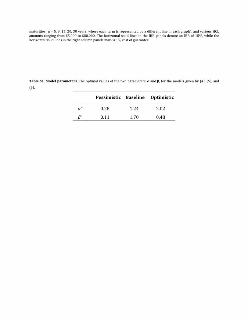
category and the overall population of student-loan borrowers. We then minimize the

distance of these estimated probabilities from the empirical probabilities to determine the

optimal values of 𝛼 and 𝛽 for each model. These optimal values for each scenario are

tabulated in table S1, and we present the resulting default probability distributions for each

model using these optimal parameter values in fig. S4.

Post-Treatment Survival Curve Estimation

In this section, we use the projected population numbers for the baby-boomer cohort in the

U.S., published by the U.S. Census Bureau (17), to derive a post-treatment survival curve for

the HCV patients in the U.S. We focus on this specific cohort because an estimated 75% of

the patients with HCV infection in the U.S. are baby-boomers. If the estimated population

size at year 𝑡 is given by 𝑁(𝑡), we define the survival curve of the population as 𝑆(𝑡) ≡

𝑁(𝑡)

𝑁(2015), for 𝑡 ≥ 2015. The population numbers, 𝑁(𝑡)’s, are reported over years with 5-year

increments, i.e., for 𝑡 = 2015, 2020, etc., and we interpolate the curve between every two

adjacent samples that are 5 years apart. By inspecting the given survival rates for the

selected years and their logarithms, we propose the following functional form:

�̂�(𝑡) = exp(−𝛬(𝑡)) , for 𝑡 ≥ 2015, (7)

where exp(⋅) is the exponential function, and the cumulative hazard function, 𝛬(𝑡), is given

by:

𝛬(𝑡 + 2015) = −1 + exp(𝑎𝑡2 + 𝑏𝑡) , for 𝑡 ≥ 0. (8)

To avoid over-fitting when estimating the survival curve for the first 9 years (the time

period required for our main simulation), we use the survival numbers for 𝑡 =

2015, 2020, 2025, 2030, and 2035; i.e., we consider the survival curve for 11 more years

than required for our simulations. We then determine the values of parameters 𝑎 and 𝑏 in

(8) such that they jointly minimize the error function, given by 𝐸(𝑎, 𝑏) = ∑ (𝑆(2015 +4𝑘=0

5𝑘) − �̂�(2015 + 5𝑘))2

. The minimizing values are 𝑎∗ = 5.0 × 10−4 and 𝑏∗ = 57.5 × 10−4,

and the estimated survival curve is presented in fig. S5.

To verify the accuracy of our estimated survival curve, we compare our estimate to the

result obtained by using the 3-parameter Burr Type XII distribution (30) instead of the

functional form given by (7) and (8). The Burr distribution is commonly used in survival

analyses and encompasses twelve different distributions, including the Weibull, logistic,

and log-logistic distributions, as its special cases (30, 31). The obtained results using this

distribution are depicted in fig. S5. The estimation error using the Burr distribution is

higher than the estimation error using our proposed model in (7) and (8), and the results of

the Burr distribution are a little more optimistic (i.e., yielding higher survival rates) over

the first 9 years. However, as seen in fig. S5, both estimates are fairly close to each other.

HCL Fund Performance Results

We use 10 million Monte Carlo simulation paths per each scenario of HCL default

probability, depicted in fig. 2A in the main text, to evaluate the performance of the HCL

fund, and several performance metrics for each scenario are reported in table S2. The

internal rate of return (IRR) is the discount rate that equates the initial equity investment

with the discounted value of all future payments to equity-holders, and is the standard

measure used by venture capitalists to gauge investment performance:

𝐼0 = ∑𝑐𝑘

(1 + IRR)𝑘

𝑛

𝑘=1

, (9)

where 𝐼0 represents the initial equity investment (𝐼0 = $50 million in our simulations), the

life of the fund is given by 𝑛 (in our simulations, 𝑛 = 9 years) and 𝑐𝑘 denotes the cash

received by equity investors in year 𝑘.

Table S2 shows a range of equity performance from the pessimistic scenario (expected

IRR = 9.4%) to the optimistic scenario (expected IRR = 15.8%), with the baseline case

falling in between (expected IRR = 12.5%). The IRR distributions in table S2 are consistent

with these patterns due to the trend in the probability of HCL defaults across these

scenarios (fig. 2A in the main text) and its impact on the equity performance. Overall, the

risk-reward profiles across all the scenarios are within an acceptable range to attract

potential equity investors.

For the performance of the HCL debt, we evaluate the probability of default (PD) and the

expected loss (EL) for both senior and junior debt tranches. Because of the guarantees on

the bonds, both debt tranches demonstrate the lowest possible PDs and ELs for all the

three scenarios, making the bonds attractive to prospective investors.

Finally, we calculate the cost of a guarantee (𝐺) to the guarantor of the bonds, and report

the probability that the guarantee is ever used to cover debt obligations during the fund’s

life, namely, Pr(𝐺 > 0), where Pr denotes probability. The cost of a guarantee (𝐺) is given

by

𝐺 = ∑𝑑𝑘

(1 + 𝑅𝑔)𝑘

𝑛

𝑘=1

, (10)

where 𝑑𝑘 is the amount drawn from the available guarantee in year 𝑘, and 𝑅𝑔 is the

assumed cost of capital for the guarantor (𝑅𝑔 = 2% in our simulations; for a description of

cost of capital, see Portfolio Theory: A Simple Example). The expected cost of guarantee

is simply the expected value of 𝐺 in (10).

In the pessimistic scenario, this probability is largest, standing only at 3.2%, while in the

baseline and optimistic scenarios it is only 0.1% and 0, respectively. Not surprisingly, the

pessimistic scenario has the highest expected cost of a guarantee because of the higher HCL

default probabilities in this case. However, the expected cost of a guarantee even in this

scenario is only $26.9K, a tiny fraction, 0.6 basis points (bps) of the face value of the bonds,

i.e., $450 million, where 1 bps = 0.01%. Moreover, the 98th and 99th percentiles of the cost

of guarantee distribution as well as the maximum cost of guarantee, listed in Table S2, are

clear testimonies to the negligible cost of a guarantee compared to the face value of the

bonds, i.e., $450 million, across all three scenarios.

We evaluate the performance of the proposed HCL fund for various HCL amounts in the

$5,000 to $80,000 range, different HCL maturities (n = 5, 9, 15, 20, and 30 years), and three

interest-rate scenarios. In the first scenario, we consider the market rates 𝑅𝑡 + 50bps for

yields on senior bonds and 𝑅𝑡 + 90bps for yields on junior bonds, where 𝑅𝑡 is the t-year

swap rate corresponding to the specific HCL term, i.e., 𝑡 =𝑛+1

2 years. The HCL interest rate

is 9.1% in this scenario. In the second and third interest-rate scenarios, we add 2.5% and

5.0%, respectively, to 𝑅𝑡 while maintaining the same 50bps and 90bps spreads for the

senior and junior bonds as in the first case. In these two cases, we assume that the interest-

rate increases are shifted entirely to HCL borrowers by assuming HCL interest rates of

11.6% and 14.1% in the second and third scenarios, respectively.

We calculate the IRR for equity investors, and the expected cost of the guarantee to the

guarantor of the bonds normalized by the face value of the bonds. The results are

presented in fig. S6, where the first, second, and third rows of figures correspond to the

first, second, and third interest-rate scenarios described above. The IRR results are

depicted in the left column, and the right column denotes the cost of guarantee

performance results.

The annual HCL payments that borrowers have to make increase with the interest rate,

hence the borrowers’ default rates increase as well. Therefore, we observe smaller IRRs

and higher expected guarantee costs, namely, poorer performance for the HCL fund, when

we move from the top row to the bottom row in fig. S6. The same trend can be seen when

the HCL amount (the amount of the co-pay) increases, namely, when we move from left to

right within a given graph, because an increase in the HCL amount raises the default rates,

which, in turn, adversely affects HCL fund performance.

The third trend involves changing the maturity of the HCLs. As we increase the maturity,

the annual HCL payments decrease, as do borrowers’ default rates in each single year. If we

denote the annual HCL default probability for a typical borrower by 𝑝1and 𝑝2, for 5-year

and 15-year HCLs, respectively, we have 𝑝1 > 𝑝2 because the debt burden is higher for a 5-

year HCL than a 15-year HCL, assuming all the other parameters are the same for these two

loans. Now, because the HCL fund makes cash distributions to its equity investors after

paying its debt obligations each year, and because the annual HCL default probabilities

decrease with the term of the HCLs, equity investors of a fund with longer term HCLs

receive larger cash returns earlier in the fund’s life. Hence, the return on equity increases

with HCL maturity.

The trend observed in the expected guarantee cost as a function of HCL maturity is less

straightforward. Because the debt issued by the HCL fund is repaid over a longer period of

time with an increase in HCL maturity, there are more opportunities, i.e., more “shots on

goal,” for a typical borrower to default over the fund’s life. For example, the extreme case is

when the term of the HCL is infinitely long, and regardless of how small the annual HCL

default probability is, as long as it is nonzero, the probability that a typical borrower

defaults over the fund’s life approaches 1. Therefore, increasing the maturity of HCLs is an

impediment to maintaining a small probability of default during the fund’s life. This, in

turn, implies that the probability that the guarantee on bonds is ever used, and hence, the

cost of guarantee, would increase with HCL maturity, given a fixed annual probability of

HCL default. On the other hand, we know that the annual HCL default probability does

decrease with maturity, which offsets the negative impact of maturity on the lifetime

default probability to some extent.

The interaction of these two conflicting forces yields the unique trend observed in the cost-

of-guarantee panels of fig. S6. As we start increasing the HCL term from 5 years to 9 years,

the cost of guarantee declines for any HCL interest rate and any HCL amount. The two

conflicting forces, described above, almost completely offset each other when the HCL term

is increased from 9 years to 15 years; therefore, the cost of guarantee stays almost intact.

Finally, when the term of the HCL is increased beyond 15 years to 20 years and 30 years,

the impact of multiple shots on goal becomes much stronger than the impact of reduction

in debt burden, and the expected guarantee cost steadily increases for any HCL amount and

interest rate.

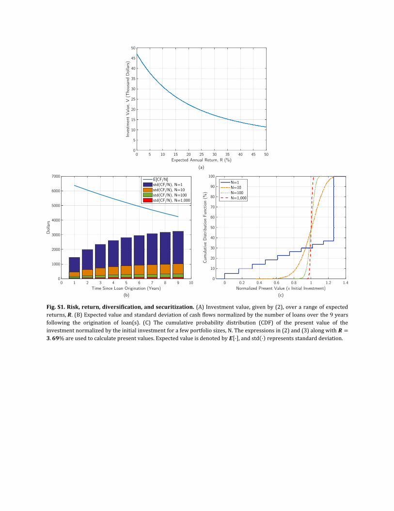
Fig. S1. Risk, return, diversification, and securitization. (A) Investment value, given by (2), over a range of expected

returns, 𝑹. (B) Expected value and standard deviation of cash flows normalized by the number of loans over the 9 years

following the origination of loan(s). (C) The cumulative probability distribution (CDF) of the present value of the

investment normalized by the initial investment for a few portfolio sizes, N. The expressions in (2) and (3) along with 𝑹 =

𝟑. 𝟔𝟗% are used to calculate present values. Expected value is denoted by 𝑬[⋅], and std(⋅) represents standard deviation.

Fig. S2. HCL default model. The statistical model used to generate loan default probabilities.

Fig. S3. Student-loan data. (A) The cumulative distribution of the annual probability of default for federal student loans, and (B) the estimated cumulative distribution of family-income for student loan borrowers along with the empirical numbers reported by the National Association of Student Financial Aid Administrators.

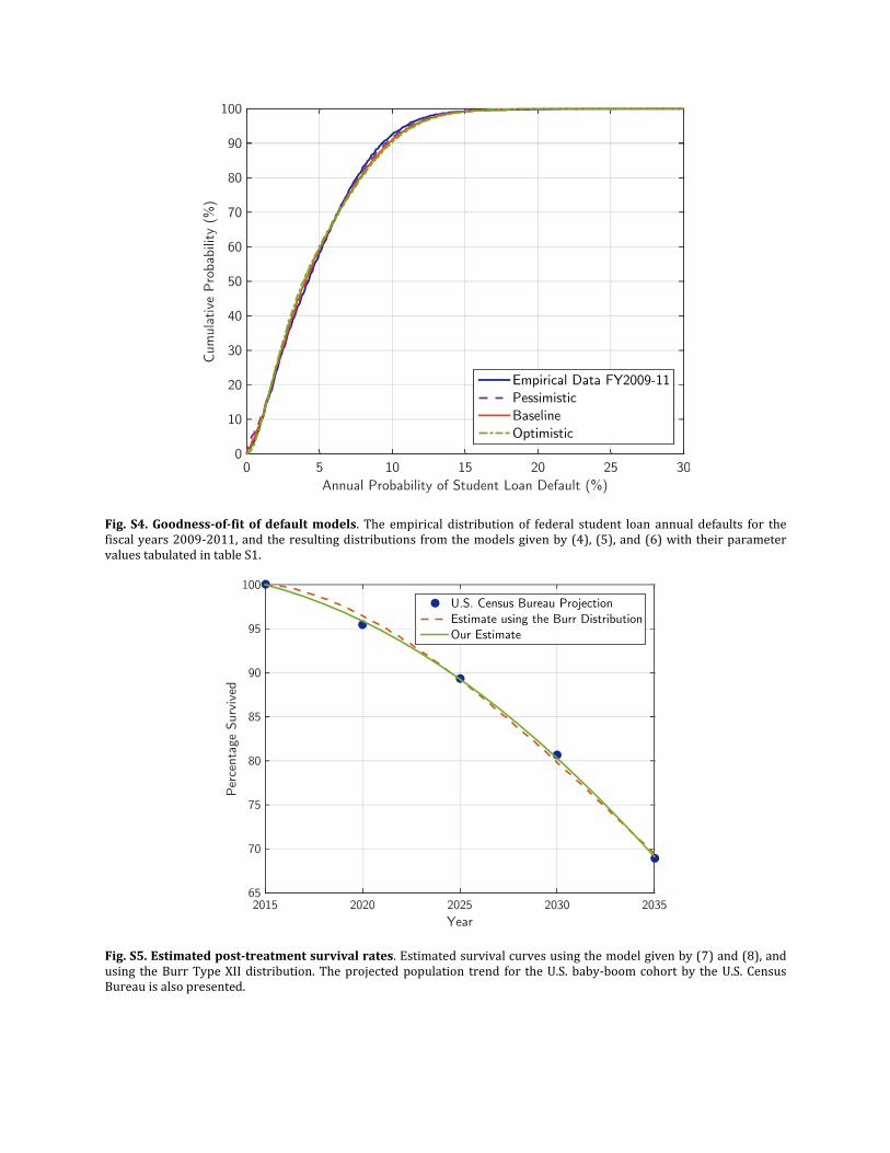
Fig. S4. Goodness-of-fit of default models. The empirical distribution of federal student loan annual defaults for the fiscal years 2009-2011, and the resulting distributions from the models given by (4), (5), and (6) with their parameter values tabulated in table S1.

Fig. S5. Estimated post-treatment survival rates. Estimated survival curves using the model given by (7) and (8), and using the Burr Type XII distribution. The projected population trend for the U.S. baby-boom cohort by the U.S. Census Bureau is also presented.

Fig. S6. Sensitivity analysis of simulated performance. Internal rate of return (IRR) for equity investors (left column) and expected cost of guarantee for the guarantor of bonds as a percentage of the face value of the bonds (right column) for the proposed HCL fund. We consider three interest-rate scenarios (the first row corresponds to current market rates, the second row corresponds to current market rates + 2.5%, and the last row assumes market rates + 5.0%), five HCL

maturities (n = 5, 9, 15, 20, 30 years, where each term is represented by a different line in each graph), and various HCL amounts ranging from $5,000 to $80,000. The horizontal solid lines in the IRR panels denote an IRR of 15%, while the horizontal solid lines in the right column panels mark a 1% cost of guarantee.

Table S1. Model parameters. The optimal values of the two parameters, 𝛂 and 𝛃, for the models given by (4), (5), and

(6).

Pessimistic Baseline Optimistic

𝛼∗ 0.28 1.24 2.02

𝛽∗ 0.11 1.70 0.48

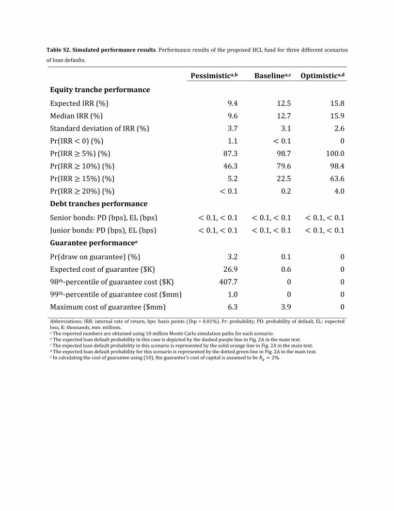
Table S2. Simulated performance results. Performance results of the proposed HCL fund for three different scenarios

of loan defaults.

Pessimistica,b Baselinea,c Optimistica,d

Equity tranche performance

Expected IRR (%) 9.4 12.5 15.8

Median IRR (%) 9.6 12.7 15.9

Standard deviation of IRR (%) 3.7 3.1 2.6

Pr(IRR < 0) (%) 1.1 < 0.1 0

Pr(IRR ≥ 5%) (%) 87.3 98.7 100.0

Pr(IRR ≥ 10%) (%) 46.3 79.6 98.4

Pr(IRR ≥ 15%) (%) 5.2 22.5 63.6

Pr(IRR ≥ 20%) (%) < 0.1 0.2 4.0

Debt tranches performance

Senior bonds: PD (bps), EL (bps) < 0.1, < 0.1 < 0.1, < 0.1 < 0.1, < 0.1

Junior bonds: PD (bps), EL (bps) < 0.1, < 0.1 < 0.1, < 0.1 < 0.1, < 0.1

Guarantee performancee

Pr(draw on guarantee) (%) 3.2 0.1 0

Expected cost of guarantee ($K) 26.9 0.6 0

98th-percentile of guarantee cost ($K) 407.7 0 0

99th-percentile of guarantee cost ($mm) 1.0 0 0

Maximum cost of guarantee ($mm) 6.3 3.9 0

Abbreviations: IRR: internal rate of return, bps: basis points (1bp = 0.01%). Pr: probability, PD: probability of default, EL: expected loss, K: thousands, mm: millions. a The reported numbers are obtained using 10 million Monte Carlo simulation paths for each scenario. b The expected loan default probability in this case is depicted by the dashed purple line in Fig. 2A in the main text. c The expected loan default probability in this scenario is represented by the solid orange line in Fig. 2A in the main text. d The expected loan default probability for this scenario is represented by the dotted green line in Fig. 2A in the main text. e In calculating the cost of guarantee using (10), the guarantor’s cost of capital is assumed to be 𝑅𝑔 = 2%.