Supplementary Material for: Efficient multiphoton generation in waveguide QED.(Dated: April 7, 2017)

2

In this Supplementary Material, we provide the full details of different protocols described within the main manuscript. For thesake of a better understanding, we make the Sections for each protocol self-contained, discussing for each of them the requiredatom-waveguide tools and the calculation of probabilities and fidelities. The outline of the Supplementary Material reads asfollows:

• In Section SM1 we give the common guidelines to understand the analysis of the different protocols.

• In Section SM2, we discuss the first protocol of the main manuscript which heralds the generation of m collective exci-tations using single photon detections within the waveguide. We discuss both the situation where we accumulate directlythe excitations into the same atomic level and where we store it in another hyperfine level and combine them a posteriori.

• In Section SM3, we discuss the second protocol of the main manuscript which accumulates excitations directly within thesame level using a two-step protocol. The protocol overcomes the trade-off between probability of success and fidelitiesof the first protocol but still requires an exponential number of operations.

• In Section SM4, we discuss the third protocol which shows how to overcome the exponential scaling of the number ofoperations of the second protocol by using additional auxiliary levels to store the excitations after each heralded transferwhile keeping the overall infidelity still low.

• Finally, in Section SM5 we discuss how to use beam splitter transformations and atomic detection to merge atomic exci-tations and reach high photon numbers.

SM1. GENERAL GUIDELINES TO ANALYZE THE PROTOCOLS.

In all the protocols the goal is the generation of m collective excitations in a collection of N atoms that we name the targetensemble. We denote such state as |Ψm〉. Moreover, our protocols rely on heralding the excitations one by one by measuringa given state in the auxiliary system that we denote by |Φher〉, which is either directly the photonic state within the waveguide(first protocol) or an auxiliary atomic state (i.e., the detector ensemble in the second and third protocols). Therefore, in order toanalyze the protocols we study two things:

• First, we analyze the scaling of the probability and the fidelity of heralding the addition of a single excitation. Thismeans that we start with a density matrix ρm(0) = |Ψm〉⊗ |Φ0〉〈Ψm|⊗〈Φ0|, where |Φ0〉 is the initial state of the auxiliarysystem. After a given evolution of the density matrix, denoted by Sρm(0), we calculate the probability of succeeding inthe heralding which reads

p = Tr [〈Φher|Sρm(0)|Φher〉] . (SM1)

However, the heralding is in general not perfect and we might have created states in the target ensemble other than thedesired one, i.e., |Ψm+1〉. This is quantified by the fidelity after heralding, which reads

Fm→m+1 =〈Ψm+1|〈Φher|Sρm(0)|Φher〉|Ψm+1〉

p(SM2)

The infidelity is defined as: Im→m+1 = 1−Fm→m+1.

• Once we have analyzed the previous general step, we consider the complete process to arrive from |Ψ0〉 → |Ψ1〉 → ·· · →|Ψm〉 and calculate the average number of repetitions, Rm, to arrive to |Ψm〉 and the average infidelity of the process Im.Both Rm and Im depend on the way we merge the excitations and changes with the different protocols, as we show below.

SM2. HERALDING MULTIPLE COLLECTIVE ATOMIC EXCITATIONS IN WAVEGUIDE QED SETUPS USING SINGLEPHOTON DETECTORS.

The protocol consists in heralding the transfer of a single collective atomic excitations m times through m photon detectionevents within the waveguide. We discuss two different approaches: i) one where we store the heralded single excitation in adifferent level s1 with methods that we revise in Section SM5; ii) or where we store the excitation directly into the same level.

The key step in both cases is to study how an additional single collective excitation can be added to an atomic ensemble whichalready contains m excitations in another level, s1, i.e.

|Φs1m 〉=

1√(Nm

) sym|s1〉⊗m|g〉⊗(N−m) . (SM3)

3

(a)

Target

...N atoms

z

Control fields (b)Detector

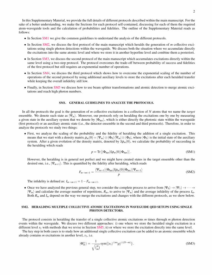
Figure SM1. (a) General setup for first protocol discussed in the main manuscript which consists of a collective ensemble where we preparesuperpositions and a single photon detector that we use to herald the excitations. (b) Internal level structure of emitters in which the transitione↔ s is coupled to a waveguide mode with rate Γ1d. The transition g↔ e is controlled through the Raman laser Ω. We also include thepossibility of having an extra auxiliary level s1 where excitations can be stored using microwave [or two-photon Raman] fields G.

A. Atom-waveguide resources

The tools/resources that we use are:

• N atoms trapped close to a one-dimensional waveguide as depicted in Fig. SM1 (a), with a level structure, as shown inFig. SM1(b), where one optical transition e↔ s is coupled to a waveguide mode with a rate Γ1d, and the other leg e→ g iscontrolled by a collective classical field Ωn = Ω. In one of the schemes that we explore, we also assume that we have anextra mode s1, where the excitations can be stored and which can be combined through microwave or two-photon Ramantransitions with Rabi frequency G.

• The atoms are placed at distances commensurate with the characteristic wavelength of the guided mode, λa, at the fre-quency of the transition e→ g, i.e. zn = nλa. With that assumption, it is easy to show that effective atom dynamics inducedby the interaction with the waveguide is solely driven by long-range dissipative couplings:

Lcoll [ρ] =Γ1d

2DSge [ρ] , (SM4)

where ρ is the reduced density matrix of the atomic system, DO[ρ] = (2OρO†−O†Oρ−ρO†O) is the dissipator associatedto a given jump operator O, and where we defined the collective spin operator of the target ensemble as Sαβ = ∑

Nn=1 σn

αβ,

with σnαβ

= |α〉n〈β |. Obviously, the excited state can also decay to other modes other than into the waveguide, whichleads to extra Lindblad terms which read:

L∗(ρ) = ∑n=1,...,N

(Γ∗

4Dσn

se [ρ]+Γ∗

4Dσn

ge [ρ]

), (SM5)

which lead to finite Purcell factor P1d =Γ1dΓ∗ .

• A single photon detector with overall efficiency η at the end of the waveguide to detect the emission of waveguide photons.

B. Protocol and calculation of probabilities.

The protocol works as follows: we apply a laser pulse during a short time T such that√

NΩT/2 = x 1. Then, the storedsuperposition |Φs1

m 〉 evolves into:

|Ψ0〉 ∝ |Φs1m 〉+ x

1√Nm

Seg|Φs1m 〉+

x2

2

√2

Nm(Nm−1)S2

eg|Φs1m 〉+O(x3) . (SM6)

Then, we let the system evolve only through the interaction with the waveguide and the bath of leaky photons. In orderto obtain the probabilities associated to different process, we use the expansion of the master equation [1] distinguishing theevolution of the effective non-hermitian Hamiltonian, i.e., S(t, t0)ρ = e−iHefftρeiH†

efft , and the one resulting from quantum jumpsevolution, i.e., Jρ , that is given in general by:

ρ(t) = S(t, t0)ρ(t0)+∞

∑n=1

∫ t

t0dtnS(t, tn)J(tn) . . .

∫ t2

t0dt1S(t1, t0)ρ(t0) . (SM7)

4

The non-hermitian evolution leads to:

|Ψ(t)〉 ∝ e−iHefft |Ψ0〉 ∝ |Φs1m 〉+ x

e−(Γ1d+Γ∗)t√

NmSeg |Φs1

m 〉+x2

2e−2(Γ1d+Γ∗)t

√2

Nm(Nm−1)S2

eg|Φs1m 〉+O(x3) , (SM8)

where we see that if we wait a time long enough, i.e., t (Γ∗)−1 the only population remaining in |Ψ(T )〉 → |Φs1m 〉. The

probability emitting a collective photon from Seg|Φs1m 〉 is given by:

pcoll =x2

1+ 1P1d

≈ x2(

1− 1P1d

), (SM9)

where in the last approximation we assumed to be in a regime with P1d 1, whereas the one of emitting an spontaneous emissionphoton from the same state:

p∗ =x2

P1d +1≈ x2

P1d. (SM10)

We herald with the detection of a waveguide photon with efficiency η , such that the final success probability of heralding is:

p = pcoll×η ≈ ηx2(

1− 1P1d

), (SM11)

In case of no detection it may have happened that our waveguide photon was emitted but not detected, that is, the atoms willindeed be in a superposition Ssg |Φs1

m 〉. So, before making a new attempt, we ensure to pump back any possible excitation in g tos minimizing the emission into leaky modes, which can be done as follows:

• First, apply a π pulse with a microwave field that flips all the excitations g→ s. This switches Ssg|Φs1m 〉 into Sgs|Ψs1

m 〉,where |Ψs1

m 〉 is the same as |Φs1m 〉 but with levels s and g interchanged.

• Then, we apply a fast Raman π-pulse with Ω NΓ1d such that Sgs|Ψs1m 〉 → Ses|Ψs1

m 〉 → |Ψs1m 〉. This incoherent transfer is

done through a collective photon, such that the probability of emitting a leaky photon is:

ppump,∗ ≈ (1−η)× pcoll×1

NmP1d≈ (1−η)

x2

NmP1d. (SM12)

• Finally, we reverse the microwave π-pulse such that g↔ s and therefore |Ψs1m 〉 → |Φs1

m 〉.

C. Fidelities of the protocol.

In order to calculate the errors (and fidelities) of the protocol we have to distinguish between the errors introduced aftersuccessfully heralding the excitations, and the error per trial that we introduce when we repeat the protocol after failure.

• Successful heralding: It can be shown that if we detect a single photon in the waveguide, this means that the initial densitymatrix ρm = |Ψm〉〈Ψm| transforms into:

ρm→1

NmSgsρmSsg +

2x2(1−ηd)

Nm(Nm−1)S2

gsρmS2sg , (SM13)

where the first term is the desired process, whereas the second corresponds to the probability of detecting only one ofthe two photons emitted from the doubly excited terms S2

es |Φs1m 〉. This introduces a large error as the state Sgs |Φs1

m 〉 isorthogonal to the state that we want to create, such that the error when heralding is:

εdouble = x2(1−η) . (SM14)

• Failed heralding: If we detect no photon, then, our state is projected to:

ρm→ (1− x2)ρm + pcoll(1−η)1

NmSgsρmSsg + p∗J∗ρm +O(x4) , (SM15)

5

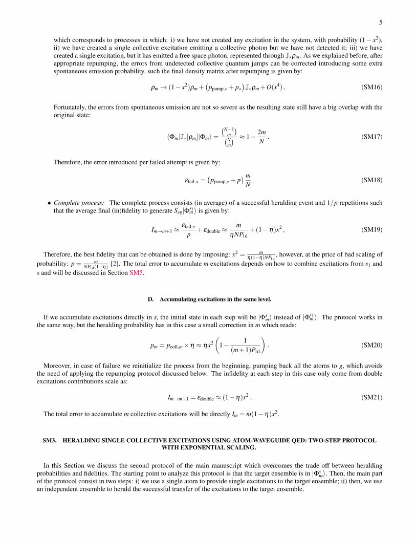
which corresponds to processes in which: i) we have not created any excitation in the system, with probability (1− x2),ii) we have created a single collective excitation emitting a collective photon but we have not detected it; iii) we havecreated a single excitation, but it has emitted a free space photon, represented through J∗ρm. As we explained before, afterappropriate repumping, the errors from undetected collective quantum jumps can be corrected introducing some extraspontaneous emission probability, such the final density matrix after repumping is given by:

ρm→ (1− x2)ρm +(

ppump,∗+ p∗)J∗ρm +O(x4) , (SM16)

Fortunately, the errors from spontaneous emission are not so severe as the resulting state still have a big overlap with theoriginal state:

〈Φm|J∗[ρm]|Φm〉=(N−1

m

)(Nm

) ≈ 1− 2mN

. (SM17)

Therefore, the error introduced per failed attempt is given by:

εfail,∗ =(

ppump,∗+ p) m

N(SM18)

• Complete process: The complete process consists (in average) of a successful heralding event and 1/p repetitions suchthat the average final (in)fidelity to generate Ssg|Φs1

m 〉 is given by:

Im→m+1 ≈εfail,∗

p+ εdouble ≈

mηNP1d

+(1−η)x2 , (SM19)

Therefore, the best fidelity that can be obtained is done by imposing: x2 = mη(1−η)NP1d

, however, at the price of bad scaling ofprobability: p = m

NP1d(1−η) [2]. The total error to accumulate m excitations depends on how to combine excitations from s1 ands and will be discussed in Section SM5.

D. Accumulating excitations in the same level.

If we accumulate excitations directly in s, the initial state in each step will be |Φsm〉 instead of |Φs1

m 〉. The protocol works inthe same way, but the heralding probability has in this case a small correction in m which reads:

pm = pcoll,m×η ≈ ηx2(

1− 1(m+1)P1d

). (SM20)

Moreover, in case of failure we reinitialize the process from the beginning, pumping back all the atoms to g, which avoidsthe need of applying the repumping protocol discussed below. The infidelity at each step in this case only come from doubleexcitations contributions scale as:

Im→m+1 = εdouble ≈ (1−η)x2 . (SM21)

The total error to accumulate m collective excitations will be directly Im = m(1−η)x2.

SM3. HERALDING SINGLE COLLECTIVE EXCITATIONS USING ATOM-WAVEGUIDE QED: TWO-STEP PROTOCOLWITH EXPONENTIAL SCALING.

In this Section we discuss the second protocol of the main manuscript which overcomes the trade-off between heraldingprobabilities and fidelities. The starting point to analyze this protocol is that the target ensemble is in |Φs

m〉. Then, the main partof the protocol consist in two steps: i) we use a single atom to provide single excitations to the target ensemble; ii) then, we usean independent ensemble to herald the successful transfer of the excitations to the target ensemble.

6

(a) (b)

Source Target

...

DetectorN atoms

z

Control fields

Nd atoms...

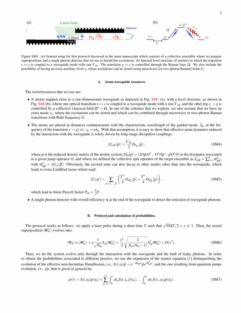
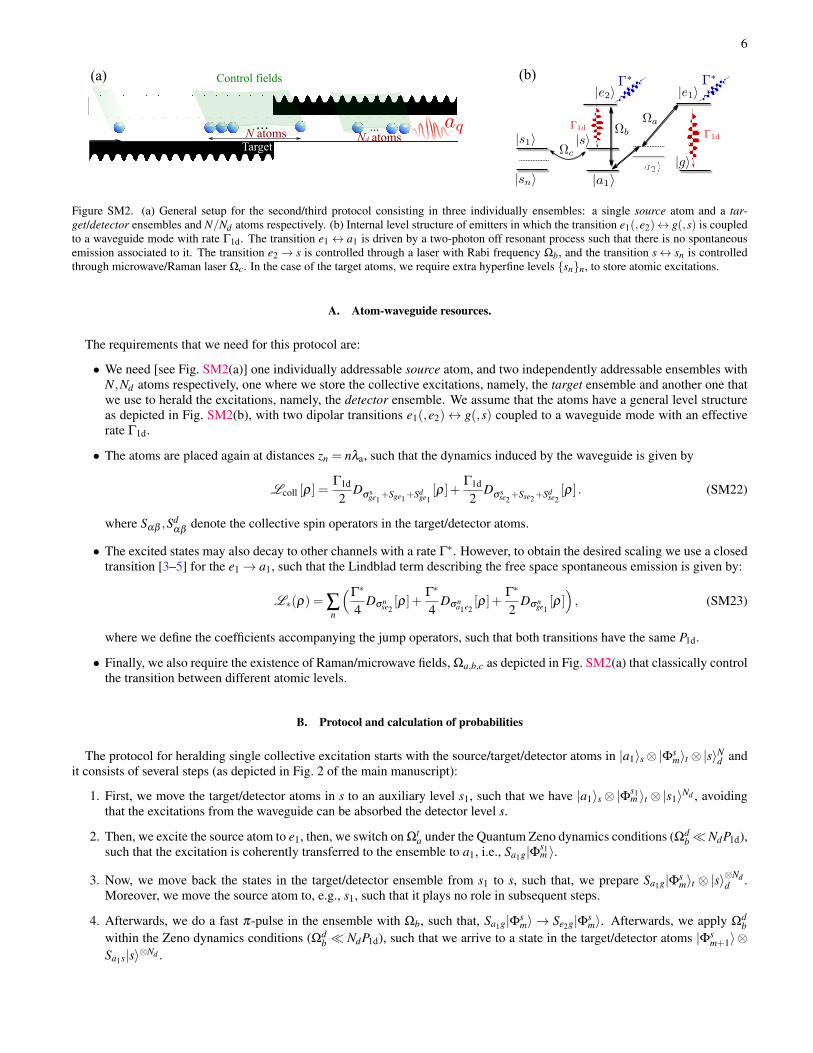
Figure SM2. (a) General setup for the second/third protocol consisting in three individually ensembles: a single source atom and a tar-get/detector ensembles and N/Nd atoms respectively. (b) Internal level structure of emitters in which the transition e1(,e2)↔ g(,s) is coupledto a waveguide mode with rate Γ1d. The transition e1↔ a1 is driven by a two-photon off resonant process such that there is no spontaneousemission associated to it. The transition e2→ s is controlled through a laser with Rabi frequency Ωb, and the transition s↔ sn is controlledthrough microwave/Raman laser Ωc. In the case of the target atoms, we require extra hyperfine levels snn, to store atomic excitations.

A. Atom-waveguide resources.

The requirements that we need for this protocol are:

• We need [see Fig. SM2(a)] one individually addressable source atom, and two independently addressable ensembles withN,Nd atoms respectively, one where we store the collective excitations, namely, the target ensemble and another one thatwe use to herald the excitations, namely, the detector ensemble. We assume that the atoms have a general level structureas depicted in Fig. SM2(b), with two dipolar transitions e1(,e2)↔ g(,s) coupled to a waveguide mode with an effectiverate Γ1d.

• The atoms are placed again at distances zn = nλa, such that the dynamics induced by the waveguide is given by

Lcoll [ρ] =Γ1d

2D

σ sge1

+Sge1+Sdge1

[ρ]+Γ1d

2D

σ sse2

+Sse2+Sdse2[ρ] . (SM22)

where Sαβ ,Sdαβ

denote the collective spin operators in the target/detector atoms.

• The excited states may also decay to other channels with a rate Γ∗. However, to obtain the desired scaling we use a closedtransition [3–5] for the e1→ a1, such that the Lindblad term describing the free space spontaneous emission is given by:

L∗(ρ) = ∑n

(Γ∗

4Dσn

se2[ρ]+

Γ∗

4Dσn

a1e2[ρ]+

Γ∗

2Dσn

ge1[ρ]), (SM23)

where we define the coefficients accompanying the jump operators, such that both transitions have the same P1d.

• Finally, we also require the existence of Raman/microwave fields, Ωa,b,c as depicted in Fig. SM2(a) that classically controlthe transition between different atomic levels.

B. Protocol and calculation of probabilities

The protocol for heralding single collective excitation starts with the source/target/detector atoms in |a1〉s⊗|Φsm〉t ⊗|s〉Nd and

it consists of several steps (as depicted in Fig. 2 of the main manuscript):

1. First, we move the target/detector atoms in s to an auxiliary level s1, such that we have |a1〉s⊗|Φs1m 〉t ⊗|s1〉Nd , avoiding

that the excitations from the waveguide can be absorbed the detector level s.

2. Then, we excite the source atom to e1, then, we switch on Ωta under the Quantum Zeno dynamics conditions (Ωd

bNdP1d),such that the excitation is coherently transferred to the ensemble to a1, i.e., Sa1g|Φs1

m 〉.

3. Now, we move back the states in the target/detector ensemble from s1 to s, such that, we prepare Sa1g|Φsm〉t ⊗ |s〉

⊗Ndd .

Moreover, we move the source atom to, e.g., s1, such that it plays no role in subsequent steps.

4. Afterwards, we do a fast π-pulse in the ensemble with Ωb, such that, Sa1g|Φsm〉 → Se2g|Φs

m〉. Afterwards, we apply Ωdb

within the Zeno dynamics conditions (Ωdb NdP1d), such that we arrive to a state in the target/detector atoms |Φs

m+1〉⊗Sa1s|s〉⊗Nd .

7

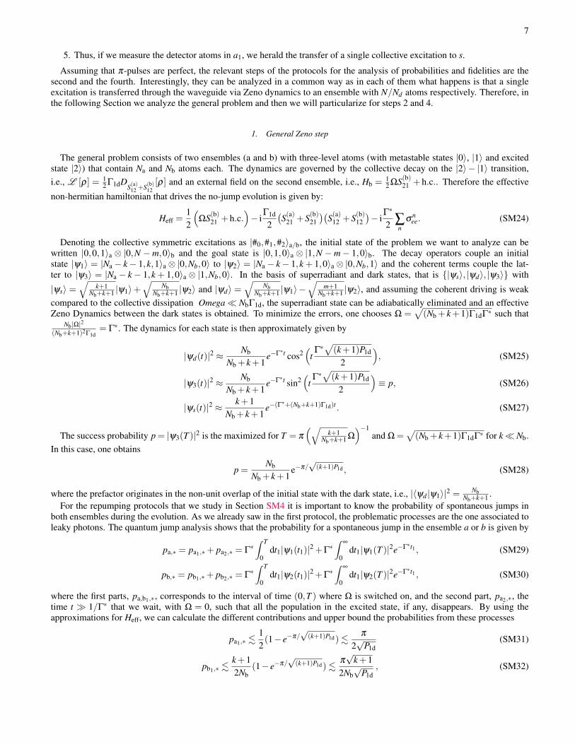
5. Thus, if we measure the detector atoms in a1, we herald the transfer of a single collective excitation to s.

Assuming that π-pulses are perfect, the relevant steps of the protocols for the analysis of probabilities and fidelities are thesecond and the fourth. Interestingly, they can be analyzed in a common way as in each of them what happens is that a singleexcitation is transferred through the waveguide via Zeno dynamics to an ensemble with N/Nd atoms respectively. Therefore, inthe following Section we analyze the general problem and then we will particularize for steps 2 and 4.

1. General Zeno step

The general problem consists of two ensembles (a and b) with three-level atoms (with metastable states |0〉, |1〉 and excitedstate |2〉) that contain Na and Nb atoms each. The dynamics are governed by the collective decay on the |2〉− |1〉 transition,i.e., L [ρ] = 1

2 Γ1dDS(a)12 +S(b)12

[ρ] and an external field on the second ensemble, i.e., Hb =12 ΩS(b)21 + h.c.. Therefore the effective

non-hermitian hamiltonian that drives the no-jump evolution is given by:

Heff =12

(ΩS(b)21 +h.c.

)− i

Γ1d

2(S(a)21 +S(b)21

)(S(a)12 +S(b)12

)− i

Γ∗

2 ∑n

σnee. (SM24)

Denoting the collective symmetric excitations as |#0,#1,#2〉a/b, the initial state of the problem we want to analyze can bewritten |0,0,1〉a ⊗ |0,N −m,0〉b and the goal state is |0,1,0〉a ⊗ |1,N −m− 1,0〉b. The decay operators couple an initialstate |ψ1〉 = |Na− k− 1,k,1〉a⊗ |0,Nb,0〉 to |ψ2〉 = |Na− k− 1,k + 1,0〉a⊗ |0,Nb,1〉 and the coherent terms couple the lat-ter to |ψ3〉 = |Na − k− 1,k + 1,0〉a ⊗ |1,Nb,0〉. In the basis of superradiant and dark states, that is |ψs〉, |ψd〉, |ψ3〉 with

|ψs〉 =√

k+1Nb+k+1 |ψ1〉+

√Nb

Nb+k+1 |ψ2〉 and |ψd〉 =√

NbNb+k+1 |ψ1〉−

√m+1

Nb+k+1 |ψ2〉, and assuming the coherent driving is weakcompared to the collective dissipation Omega NbΓ1d, the superradiant state can be adiabatically eliminated and an effectiveZeno Dynamics between the dark states is obtained. To minimize the errors, one chooses Ω =

√(Nb + k+1)Γ1dΓ∗ such that

Nb|Ω|2(Nb+k+1)2Γ1d

= Γ∗. The dynamics for each state is then approximately given by

|ψd(t)|2 ≈Nb

Nb + k+1e−Γ∗t cos2

(tΓ∗√(k+1)P1d

2

), (SM25)

|ψ3(t)|2 ≈Nb

Nb + k+1e−Γ∗t sin2

(tΓ∗√(k+1)P1d

2

)≡ p, (SM26)

|ψs(t)|2 ≈k+1

Nb + k+1e−(Γ

∗+(Nb+k+1)Γ1d)t . (SM27)

The success probability p = |ψ3(T )|2 is the maximized for T = π

(√k+1

Nb+k+1 Ω

)−1and Ω =

√(Nb + k+1)Γ1dΓ∗ for k Nb.

In this case, one obtains

p =Nb

Nb + k+1e−π/√

(k+1)P1d , (SM28)

where the prefactor originates in the non-unit overlap of the initial state with the dark state, i.e., |〈ψd |ψ1〉|2 = NbNb+k+1 .

For the repumping protocols that we study in Section SM4 it is important to know the probability of spontaneous jumps inboth ensembles during the evolution. As we already saw in the first protocol, the problematic processes are the one associated toleaky photons. The quantum jump analysis shows that the probability for a spontaneous jump in the ensemble a or b is given by

pa,∗ = pa1,∗+ pa2,∗ = Γ∗∫ T

0dt1|ψ1(t1)|2 +Γ

∗∫

∞

0dt1|ψ1(T )|2e−Γ∗t1 , (SM29)

pb,∗ = pb1,∗+ pb2,∗ = Γ∗∫ T

0dt1|ψ2(t1)|2 +Γ

∗∫

∞

0dt1|ψ2(T )|2e−Γ∗t1 , (SM30)

where the first parts, pa,b1,∗, corresponds to the interval of time (0,T ) where Ω is switched on, and the second part, pa2,∗, thetime t 1/Γ∗ that we wait, with Ω = 0, such that all the population in the excited state, if any, disappears. By using theapproximations for Heff, we can calculate the different contributions and upper bound the probabilities from these processes

pa1,∗ .12(1− e−π/

√(k+1)P1d).

π

2√

P1d(SM31)

pb1,∗ .k+12Nb

(1− e−π/√

(k+1)P1d).π√

k+12Nb√

P1d, (SM32)

8

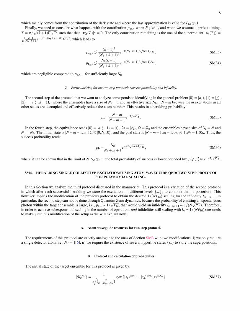
which mainly comes from the contribution of the dark state and where the last approximation is valid for P1d 1.Finally, we need to consider what happens with the contribution pa2,∗ when P1d 1, and when we assume a perfect timing,

T = π/√(k+1)Γ1dΓ∗ such that then |ψd(T )|2 = 0. The only contribution remaining is the one of the superradiant |ψs(T )〉 =√

k+1Nb+k+1 e−(Γ

∗+(Nb+k+1)Γ1d)T/2, which leads to

pa2,∗ .(k+1)2

(Nb + k+1)2 e−π(Nb+k+1)/√

(k+1)P1d , (SM33)

pb2,∗ .Nb(k+1)

(Nb + k+1)2 e−π(Nb+k+1)/√

(k+1)P1d , (SM34)

which are negligible compared to pa,b1,∗ for sufficiently large Nb.

2. Particularizing for the two step protocol: success probability and infidelity.

The second step of the protocol that we want to analyze corresponds to identifying in the general problem |0〉= |a1〉, |1〉= |g〉,|2〉= |e1〉, Ω = Ωa, where the ensembles have a size of Na = 1 and an effective size Nb = N−m because the m excitations in allother states are decoupled and effectively reduce the atom number. This results in a heralding probability:

pa =N−m

N−m+1e−π/

√P1d . (SM35)

In the fourth step, the equivalence reads |0〉= |a1〉, |1〉= |s〉, |2〉= |e2〉, Ω = Ωb and the ensembles have a size of Na = N andNb = Nd. The initial state is |N−m−1,m,1〉a⊗|0,Nd,0〉b and the goal state is |N−m−1,m+1,0〉a⊗|1,Nd−1,0〉b. Thus, thesuccess probability reads:

pb =Nd

Nd +m+1e−π/√

(m+1)P1d , (SM36)

where it can be shown that in the limit of N,Nd m, the total probability of success is lower bounded by: p & p2a ≈ e−2π/

√P1d .

SM4. HERALDING SINGLE COLLECTIVE EXCITATIONS USING ATOM-WAVEGUIDE QED: TWO-STEP PROTOCOLFOR POLYNOMIAL SCALING.

In this Section we analyze the third protocol discussed in the manuscript. This protocol is a variation of the second protocolin which after each successful heralding we store the excitations in different levels snn to combine them a posteriori. Thishowever implies the modification of the previous protocol to obtain the desired 1/(NP1d) scaling for the infidelity Im→m+1. Inparticular, the second step can not be done through Quantum Zeno dynamics, because the probability of emitting an spontaneousphoton within the target ensemble is large, i.e., pb,∗ ∝ 1/

√P1d, that would yield an infidelity Im→m+1 ∝ 1/(N

√P1d). Therefore,

in order to achieve subexponential scaling in the number of operations and infidelities still scaling with Im ∝ 1/(NP1d) one needsto make judicious modification of the setup as we will explain now.

A. Atom-waveguide resources for two-step protocol.

The requirements of this protocol are exactly analogue to the ones of Section SM3 with two modifications: i) we only requirea single detector atom, i.e., Nd = 1[6]; ii) we require the existence of several hyperfine states sn to store the superpositions.

B. Protocol and calculation of probabilities

The initial state of the target ensemble for this protocol is given by:

|Φsnm 〉= 1√( N

m1,m2,...,mn

) sym|s1〉⊗m1 . . . |sn〉⊗mn |g〉⊗Nm (SM37)

9

where( N

m1,m2,...,mn

)= N!

m1!...mN Nm)!is the number of states within the superposition, denoting Nm = N−m. The final goal state we

want to create is:

|Φgoal〉=1√Nm

Ssg|Φsnm 〉 . (SM38)

As we mention, the collective transfer of the excitation from the source to the target ensemble is analogous than the onediscussed in Section SM3. Thus, we focus only the second step which should be done different.

1. Step (b): heralding the transfer using fast π-pulses (no-jump evolution).

This second step of the protocol do not rely on quantum Zeno dynamics, and it will take place between the target and detectoratoms. The idea is to: i) first do a fast π pulse with Ωt

b Γ1d such that the possible excitation in Sa1g|Φsnm 〉 → Se2g|Φsn

m 〉;ii) let the system evolve only through the couplings induced by the waveguide; iii) do a π pulse in both the target and detectorensemble, i.e., Ωt

b,Ωdb Γ1d, such that any remaining excitation in the excited states e2 go back to a1. It is important to notice

that if no excitation has been transferred to a1 in step (a), nothing will happen in this step. Therefore, we consider our initialstate to be: |Ψ0,b〉= |Ψb,1〉= 1√

NmSe2g|Φsn

m 〉⊗ |s〉. The effective Hamiltonian in this case is then given by:

Hb,eff =−iΓ∗

2 ∑n

σne2e2− i

Γ1d

2(Se2s +σ

de2s)(

Sse2 +σdse2

). (SM39)

From here, it is simple to arrive to the solution of the dynamics: |Ψb(t)〉= e−iHb,efft |Ψ0,b〉= ∑ j β j(t)|Ψb, j〉, which read:

|β1(t)|2 =14

e−Γ∗t[1+ e−Γ1dt

]2(SM40)

|β2(t)|2 =14

e−Γ∗t[1− e−Γ1dt

]2≡ pb , (SM41)

Notice that pb will be the probability of having transferred the collective excitation to the target while changing the detectoratom state to a1, if we assume that the second π pulse is perfect. If we choose a time Tb = 1/Γ1d, then

|β1(Tb)|2 ≈(e+1)2

4e2

(1− 1

P1d

)= 0.46

(1− 1

P1d

), (SM42)

pb ≈(e−1)2

4e2

(1− 1

P1d

)≈ 0.1

(1− 1

P1d

), (SM43)

Interestingly, there is a sizeable probability of remaining in the initial state of this step. So instead of start from the beginningevery time that we fail, it is possible to repeat this step several times, which increases probability to pb ≈ 1/3.

2. Step b: heralding the transfer using fast π-pulses (quantum jump analysis).

The relevant quantum jumps in this step are Jbρ = Jb,∗ρ + Jb,collρ , with

Jb,∗ρ =Γ∗

2 ∑n

σnse2

ρσne2s +

Γ∗

2 ∑n

σna1e2

ρσne2a1

,

Jb,collρ = Γ1d(Sse2 +σ

dse2

)ρ(Se2s +σ

de2s). (SM44)

In this second step, we make a π-pulse with Ωtb, such that the initial state |Ψb,0〉= |Ψb,1〉= 1√

NmSe2g|Φsnn

m 〉. Then the system

is left free to evolve for a time Tb = 1Γ1d

, and switching the Ωtb,Ω

db such that no population remains in the excited state e2.

Therefore, the quantum jumps could only occur within a small time interval giving rise to

pb,∗ = Γ∗∫ Tb

0dt1|β1|2 ≈

0.67P1d

. (SM45)

In this regime, with P1d 1 and Tb = 1Γ1d

, it is also instructive to consider the probability of other quantum jumps. For

example, to calculate the probability that the excitation is transferred to Ssg|Φsnm 〉 but the state of the detector is unchanged, i.e.,

10

(a) 1st part (c) 3rd part(b) 2nd part

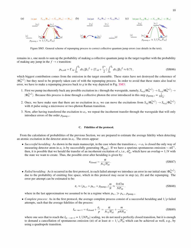
Figure SM3. General scheme of repumping process to correct collective quantum jump errors (see details in the text).

remains in s, one needs to sum up the probability of making a collective quantum jump in the target together with the probabilityof making any jump in the f → s transition:

pb,coll = Γ1d

∫ Tb

0dt1|β1|2 +(Γ1d +

Γ∗

2)∫ Tb

0dt1|β2|2 ≈ 0.71 , (SM46)

which biggest contribution comes from the emission in the target ensemble. These states have not destroyed the coherence of|Φsn

m 〉 but they need to be properly taken care of with the repumping process. In order to avoid that these states also lead toerror, we have to make a repumping process back to g in the way depicted in Fig. SM3:

1. First we pump incoherently back any possible excitation in c through the waveguide, namely, Sa1g|Φsnm 〉→ Se1g|Φsn

m 〉→|Φsn

m 〉. Because this process is done through a collective photon the error introduced in this step ppump,∗ ∝1

NP1d.

2. Once, we have make sure that there are no excitation in a1 we can move the excitations from Ssg|Φsnm 〉 → Sa1g|Φsn

m 〉with π pulse using a microwave or two-photon Raman transition.

3. Now, after having transferred the excitation to a1, we repeat the incoherent transfer through the waveguide that will onlyintroduce errors of the order ppump,∗.

C. Fidelities of the protocol.

From the calculation of probabilities of the previous Section, we are prepared to estimate the average fidelity when detectingan atomic excitation in the detector atom in a1. The errors appear:

• Successful heralding: As shown in the main manuscript, in the case where the transition e1→ a1 is closed the only way ofmeasuring detector atom in a1 is by successfully generating |Φgoal〉. If we have a spurious spontaneous emission ∼ αΓ∗,then, it is possible that we herald the transfer of an incoherent excitation of s, i.e., σn

sg, which have an overlap ∝ 1/N withthe state we want to create. Thus, the possible error after heralding is given by:

εclosed =α

N√

P1d. (SM47)

• Failed heralding: As it occurred in the first protocol, in each failed attempt we introduce an error in our initial state |Φsnm 〉

due to the probability of emitting free space, which in this protocol may occur in step (a), (b) and the repumping. Theerror per attempt can be estimated to be:

ε∗ ≈ (pa,∗+ pb,∗+ ppump,∗)mN≈ 0.67m

NP1d. (SM48)

where in the last approximation we assumed to be in a regime where pb,∗ pa,∗, ppump,∗.

• Complete process: As in the first protocol, the average complete process consist of a successful heralding and 1/p failedattempts, such that the average fidelities of the process:

Im→m+1 = εclosed +ε∗p=

α

N√

P1d+

mpNP1d

, (SM49)

where one sees that to reach the Im−>m+1 ∝ 1/(NP1d) scaling, we do not need a perfectly closed transition, but it is enoughto demand a cancellation of spontaneous emission (α) of at least α = 1/

√P1d which can be achieved as well, e.g., by

using a quadrupole transition.

11

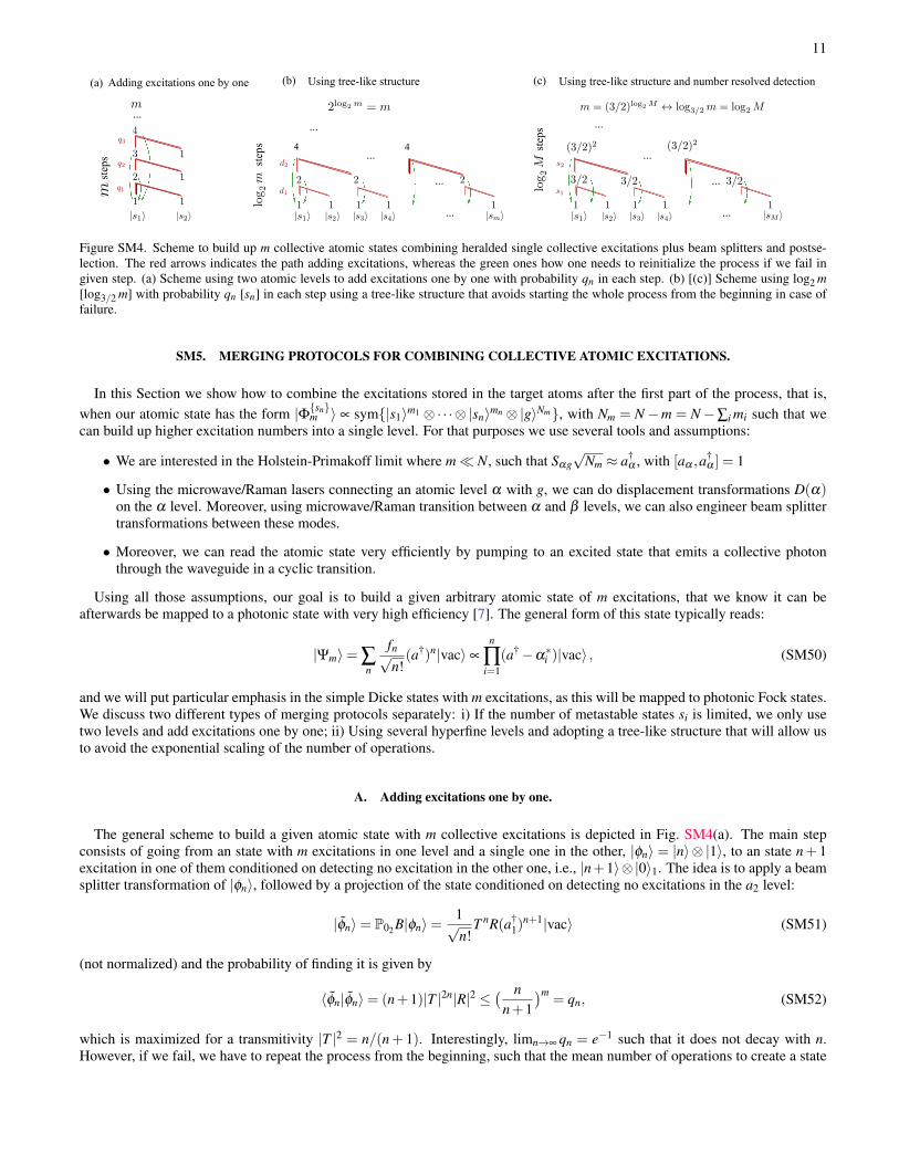
(a) Adding excitations one by one Using tree-like structure(b)

...

...

...4 4

Using tree-like structure and number resolved detection(c)

...

...

...

...

ste

ps ste

ps

......

ste

ps

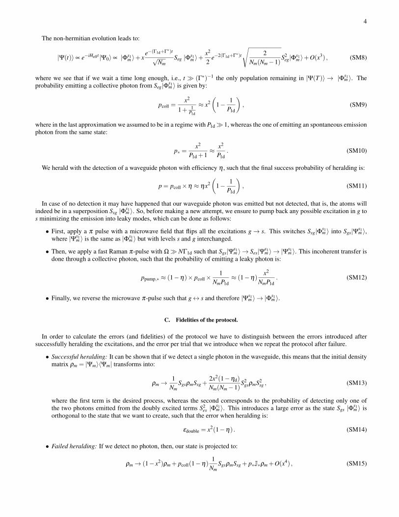
Figure SM4. Scheme to build up m collective atomic states combining heralded single collective excitations plus beam splitters and postse-lection. The red arrows indicates the path adding excitations, whereas the green ones how one needs to reinitialize the process if we fail ingiven step. (a) Scheme using two atomic levels to add excitations one by one with probability qn in each step. (b) [(c)] Scheme using log2 m[log3/2 m] with probability qn [sn] in each step using a tree-like structure that avoids starting the whole process from the beginning in case offailure.

SM5. MERGING PROTOCOLS FOR COMBINING COLLECTIVE ATOMIC EXCITATIONS.

In this Section we show how to combine the excitations stored in the target atoms after the first part of the process, that is,when our atomic state has the form |Φsn

m 〉 ∝ sym|s1〉m1 ⊗·· ·⊗ |sn〉mn ⊗|g〉Nm, with Nm = N−m = N−∑i mi such that wecan build up higher excitation numbers into a single level. For that purposes we use several tools and assumptions:

• We are interested in the Holstein-Primakoff limit where m N, such that Sαg√

Nm ≈ a†α , with [aα ,a

†α ] = 1

• Using the microwave/Raman lasers connecting an atomic level α with g, we can do displacement transformations D(α)on the α level. Moreover, using microwave/Raman transition between α and β levels, we can also engineer beam splittertransformations between these modes.

• Moreover, we can read the atomic state very efficiently by pumping to an excited state that emits a collective photonthrough the waveguide in a cyclic transition.

Using all those assumptions, our goal is to build a given arbitrary atomic state of m excitations, that we know it can beafterwards be mapped to a photonic state with very high efficiency [7]. The general form of this state typically reads:

|Ψm〉= ∑n

fn√n!(a†)n|vac〉 ∝

n

∏i=1

(a†−α∗i )|vac〉 , (SM50)

and we will put particular emphasis in the simple Dicke states with m excitations, as this will be mapped to photonic Fock states.We discuss two different types of merging protocols separately: i) If the number of metastable states si is limited, we only usetwo levels and add excitations one by one; ii) Using several hyperfine levels and adopting a tree-like structure that will allow usto avoid the exponential scaling of the number of operations.

A. Adding excitations one by one.

The general scheme to build a given atomic state with m collective excitations is depicted in Fig. SM4(a). The main stepconsists of going from an state with m excitations in one level and a single one in the other, |φn〉 = |n〉⊗ |1〉, to an state n+ 1excitation in one of them conditioned on detecting no excitation in the other one, i.e., |n+1〉⊗ |0〉1. The idea is to apply a beamsplitter transformation of |φn〉, followed by a projection of the state conditioned on detecting no excitations in the a2 level:

|φn〉= P02B|φn〉=1√n!

T nR(a†1)

n+1|vac〉 (SM51)

(not normalized) and the probability of finding it is given by

〈φn|φn〉= (n+1)|T |2n|R|2 ≤( n

n+1)m

= qn, (SM52)

which is maximized for a transmitivity |T |2 = n/(n+ 1). Interestingly, limn→∞ qn = e−1 such that it does not decay with n.However, if we fail, we have to repeat the process from the beginning, such that the mean number of operations to create a state

12

with m excitations can be obtained:

Rm =1+Rm−1

qm−1=

1qm−1

+1

qm−1qm−2+ · · ·+ 1

∏m−1n qn

. (SM53)

Taking into account that 2 = q1 > q2 > · · ·> qn > e−1 and q0 = p the probability to generate a single heralded excitation, themean number of states can be lower and upper bounded by:

2m−1

p< Rm <

mem

p, (SM54)

which increase exponentially to increase the number of excitations m. Moreover, it was shown in Ref. [8] that by combiningsingle photon addition with displacement transformation one can obtain any arbitrary superposition as in Eq. SM50, but alsowith an exponential number of operations.

B. Doubling the number of excitations post-selecting on no detection.

The key difference with respect to the previous protocol is that we are going to adopt a tree-like structures as depicted inFig. SM4(b), where we can reach the m excitations in log2 m steps and we do not have to repeat all of them if we fail. The firstbuilding block is to study the process that add up two states with |n〉 excitations to go to |n〉⊗|n〉 → |2n,0〉. It can be shown thatthe conditional outcome after a beam splitter and detecting no excitations in the second atomic level is given by:

|φ2n〉=1n!

T nRn(a†1)

2n|vac〉, (SM55)

which yields an (approximated) optimal probability for a 50−50 beam splitter transformation:

dn = 〈φ2n|φ2n〉=(2n)!

22n(n!)2 ≈ 1/√

πn , (SM56)

However, in spite of this decay, the use of of a tree-like structure is enough to circumvent the exponential scaling of addingexcitations one by one. The average number of operations to arrive to an state of m excitations can be calculated iteratively, i.e.,Rm = d−1

m/2, where the d−1m/2 terms represents the number of times we need to try in the step m/2 to succeed and the one with

2Rm/2 is the number of steps we need to repeat at the m-th step to get the the two branches of the tree. We lower and upperbound this number of operations to get m excitations by:

m2

4p< Rm <

m(log2 m)/2+1 log2 m2p

(SM57)

Thus, Rm is superpolynomial in m because the probability in each step, dm, decays with m. For completeness, let us mentionthat it is also possible to prove that one can also get arbitrary superpositions [9] using the tree-like structure of Fig. SM4(b).

C. Increasing the number of excitations with number resolved detection.

In this last Section, we show how by using atomic number resolved detection, we can overcome the superpolynomial scalingof the previous section. Instead of starting the process again when we detect some excitation in the a2, we can think of usingsome of these states that still have a non-negligible number of excitations in the a1 mode that we can use a posteriori. To furtherexplore this possibility, we generalize the operation of Eq. SM55 to see what is the resulting state after 50/50 beam splittertransformation when we want to sum up m and n excitations in the a1,2 modes when we detect the p excitations in the a2 mode:

fp(m,n) =1 〈m+n− p|φm+n−p〉=1 〈m+n− p|Pp2B(a†

1)m(a†

2)n

√m!√

n!|vac〉

=m

∑k=0

(−1)m−k

2(m+n)/2√

m!√

n!

(mk

)(n

m+n− k− p

)√p!√

(m+n− p)! . (SM58)

For the symmetric situation the expression of Eq. SM58 can be simplified as follows:

| f2n(m,m)|2 = (2m−2n)!(2n)!22m(m!)2

(mn

)2

≈ 1π

1√n(m−n)

. (SM59)

13

and f2n−1(m,m) ≡ 0 for n ∈ N, and where in the last approximation we assumed m,n 1 to use Stirling approximation. Byintegrating this expression it can be obtained that the probability of detecting an state p < m/2 lead to:

sp<m/2 =m/2

∑p=0| fp(m,m)|2 ≈

∫ m/4

0dn| f2n(m,m)|2 =

∫ m/4

0dn

1π

1√n(m−n)

= 1/3≡ s , (SM60)

which means that there is a probability s independent of m of going from |m〉1⊗|m〉2→ |2m− p > 3m/2〉1⊗|p〉2. In order tomake a worst case estimation, we assume that in each step we go only to |m〉1⊗|m〉2→ |3m/2〉1. This in principle can be donebecause if one obtains a higher excitation number it can be decreased by applying infinitesimal beam splitter transformationswith an empty mode as:

P02B(θ 1)|n〉1⊗|0〉2 ≈(

1− θ 2n2

)|n〉 ,

P02B(θ 1)|n〉1⊗|0〉2 ≈ iθ√

n|n−1〉1 ,(SM61)

which show that by switching θ 2n 1, we do not alter |n〉1, until we decrease one excitation. This can be applied several timesuntil we arrive to |3m/2〉. In this worst case scenario, starting again with M single excitations [see Fig. SM4(c)] we will arriveat least to m≥

( 32

)log2(M) [which lead log3/2 m = log2 M] in log2(M) steps, which means that with this protocol

Rm .log2(M)2log2 M−1

pslog2 M ≈m4.41 log3/2 m

2p, (SM62)

where we used logb x = loga xloga b . Thus, by using number resolved detection we turn the superpolynomial scaling into polynomial

which is big improvement if we want to scale our protocol for larger excitation numbers.

[1] Gardiner, G. W. & Zoller, P. Quantum Noise (Springer-Verlag, Berlin, 2000), 2nd edn.[2] All the expressions are valid obviously for detectors with 0 < η < 1.[3] van Enk, S. J., Cirac, J. I. & Zoller, P. Ideal quantum communication over noisy channels: A quantum optical implementation. Phys. Rev.

Lett. 78, 4293–4296 (1997).[4] Porras, D. & Cirac, J. Collective generation of quantum states of light by entangled atoms. Physical Review A 78, 053816 (2008).[5] Borregaard, J., Komar, P., Kessler, E. M., Sørensen, A. S. & Lukin, M. D. Heralded quantum gates with integrated error detection in

optical cavities. Phys. Rev. Lett. 114, 110502 (2015).[6] Actually the source atom can also play the role of the detector atom with appropriate modification of the protocol.[7] Gonzalez-Tudela, A., Paulisch, V., Chang, D. E., Kimble, H. J. & Cirac, J. I. Deterministic generation of arbitrary photonic states assisted

by dissipation. Phys. Rev. Lett. 115, 163603 (2015).[8] Dakna, M., Clausen, J., Knoll, L. & Welsch, D.-G. Generation of arbitrary quantum states of traveling fields. Phys. Rev. A 59, 1658–1661

(1999).[9] Fiurasek, J., Garcıa-Patron, R. & Cerf, N. J. Conditional generation of arbitrary single-mode quantum states of light by repeated photon

subtractions. Phys. Rev. A 72, 033822 (2005).