Assessing and benchmarking multiphoton microscopes for biologists …krummel.org/images/Publications/corbin-pub-2014-01.pdf · CHAPTER Assessing and benchmarking multiphoton microscopes

CHAPTER

Assessing andbenchmarking multiphotonmicroscopes for biologists

8Kaitlin Corbin*, Henry Pinkard*, Sebastian Peck*,1, Peter Beemiller{,

Matthew F. Krummel**Biological Imaging Development Center and Department of Pathology, University of California,

San Francisco, California, USA{Department of Pathology, University of California, San Francisco, California, USA

CHAPTER OUTLINE

Introduction: Practical Quantitative 2P Benchmarking ............................................... 136

8.1 Part I: Benchmarking Inputs..............................................................................136

8.1.1 Laser Power at the Sample .............................................................137

8.1.2 Photomultiplier Settings ................................................................138

8.1.2.1 Method 1—Fixed PMT Voltage ................................................139

8.1.2.2 Method 2—PMT Voltage Range...............................................140

8.1.3 Standard Samples .........................................................................140

8.1.3.1 A Standard Three-Dimensional Sample Set with Variable

Dispersive Properties...............................................................141

8.1.3.2 Standard Biological Samples....................................................143

8.1.4 Sample-Driven Parameters: How Fast/How Long...............................143

8.2 Part II: Benchmarking Outputs...........................................................................144

8.2.1 The Point Spread Function.............................................................144

8.2.2 SNR and Total Intensity .................................................................146

8.2.3 Maximal Depth of Acquisition.........................................................148

8.3 Troubleshooting/Optimizing...............................................................................150

8.4 A Recipe for Purchasing Decisions....................................................................150

Conclusion ............................................................................................................. 151

Acknowledgments ................................................................................................... 151

References ............................................................................................................. 151

1Present address: Nikon Instruments, Inc., 1300 Walt Whitman Road, Melville, New York, USA.

Methods in Cell Biology, Volume 123, ISSN 0091-679X, http://dx.doi.org/10.1016/B978-0-12-420138-5.00008-2

© 2014 Elsevier Inc. All rights reserved.135

http://dx.doi.org/10.1016/B978-0-12-420138-5.00008-2

AbstractMultiphoton microscopy has become staple tool for tracking cells within tissues and organs

due to superior depth of penetration, low excitation volumes, and reduced phototoxicity. Many

factors, ranging from laser pulse width to relay optics to detectors and electronics, contribute to

the overall ability of these microscopes to excite and detect fluorescence deep within tissues.

However, we have found that there are few standard ways already described in the literature to

distinguish between microscopes or to benchmark existing microscopes to measure the overall

quality and efficiency of these instruments. Here, we discuss some simple parameters and

methods that can either be used within a multiphoton facility or by a prospective purchaser

to benchmark performance. This can both assist in identifying decay in microscope perfor-

mance and in choosing features of a scope that are suited to experimental needs.

INTRODUCTION: PRACTICAL QUANTITATIVE2P BENCHMARKING

Benchmarking and comparison of multiphoton microscopes have traditionally had

little rhyme or reason. It is not uncommon for a biologist to make claims of depth

of penetration such as his or her microscope “is sensitive to 500 mm” as an attempted

method of comparison. However, such a metric clearly depends on many factors, not

the least of which is the nature of the sample. Specifically, intensity of the fluoro-

phore, intrinsic autofluorescence and particularly dispersion and scatter within a

tissue of interest all contribute extensively to such a metric. It is also possible to

illuminate a biological sample with sufficient power to make a single observation

at significant depth, but which effectively destroys the sample in the process. Multi-

photon illumination does produce photodamage, of course, only less than equivalent

single-photon illumination that would be required to illuminate a fluorophore when

dispersion and scatter are present.

We have found that the lack of routine quantitative measurements of key com-

ponents of microscope systems makes rational purchasing decisions difficult and

troubleshooting/maintenance uncertain. The former is important when one wishes

to independently assess the claims of commercial scopes. The latter is important

for keeping microscopes in optimal order and in evaluating the source of poor im-

aging quality from users of a given microscope. In this review, we discuss some of

the methods that we have come to use that allow us to keep track of the quality of

microscopes within a lab or shared facility. We have also used these methods for

purchasing decisions and we discuss both applications.

8.1 PART I: BENCHMARKING INPUTSBenchmarking a microscope is similar to conducting a controlled experiment; the

most important aspect is to keep key parameters constant. One crucial example is

laser power at the sample; every microscope can produce brighter images with lower

noise using higher laser power, but such power increase comes with a predictable and

136 CHAPTER 8 Assessing and benchmarking multiphoton microscopes

fairly routine increase in photodamage and photobleaching. Below, we introduce

three parameters that we keep constant when benchmarking or testing scopes. The

values of the parameters that we keep constant are similar but not identical to con-

ditions used in everyday biological experiments. For example, since the increase in

power per unit area within an illumination pixel in a scanning system is likely to pro-

duce fairly uniform increases across microscopes, we start by choosing a value for

this parameter and holding it constant across all measurements. Below, we define

three key parameters that are either maintained identically between benchmarking

sessions or that can be used routinely between microscopes to allow comparison.

8.1.1 LASER POWER AT THE SAMPLELaser power at the sample is a measure of photon flux to the sample and produces the

largest impact on sample viability of all the parameters we discuss here. It is there-

fore the most important parameter to keep constant when comparing instrument per-

formance. It also represents a quick check of laser excitation alignment. Decay in the

amount of excitation light reaching the sample may occur slowly on a day-to-day

basis, but over long periods of time will have a negative effect on the system’s overall

efficiency unless the system is routinely measured for misalignment or reduction of

the light reaching the sample. This measure can be a quick diagnosis for some of the

most common problems on a multiphoton microscope. The long path length in multi-

photon microscopes as the beam is routed on the bench top creates a number of op-

portunities for misalignment such as: temperature variations, accidental knocks of

beam steering mirrors, or malfunctions in the laser excitation pathway.

To obtain a baseline for the performance of the laser, a power meter is placed just

after the power modulator, in our case an electro-optical modulator (EOM), and the

maximum output wattage is recorded. Because the maximum wattage will vary

across the laser’s tunable range, this is done using several commonly used wave-

lengths about 100 nm apart as benchmarks. Using the same wavelengths and a

known amount of power after the EOM, it is expected that there will be a decrease

in the laser power reaching the sample due to the objective transmission capability,

overfilling the back aperture, and reflection or transmission efficiency of the primary

dichroic. In our system, we have observed this decay can be as high as 40% depend-

ing upon the wavelength. Such a decrease in the amount of light reaching the sample

without a corresponding drop in laser output at the EOM can be indicative of clipping

in the excitation path or dirty or misaligned optics. To measure the output then at the

objective for comparison, place the power meter below the objective (on an upright

microscope; above on an inverted stand) at approximately its specified working dis-

tance and record the wattage delivered at maximum output. For this purpose, we use

a Thor Labs brand power meter that integrates at 20 Hz. Whichever brand of power

meter selected, the device should be calibrated over time and used similarly for each

benchmark so as not to introduce this as an unknown variable in comparisons. It is

also important that the power meter chosen is able to handle the very high peak pow-

ers of titanium sapphire lasers. Note that some power meters will produce readings

1378.1 Part I: Benchmarking inputs

that vary slightly when used under a microscope objective so it is important to es-

tablish a routine. We have found that securing the detector to the microscope stage

and moving the stage incrementally allows us to find the optimal position fromwhich

we record the highest stable value.

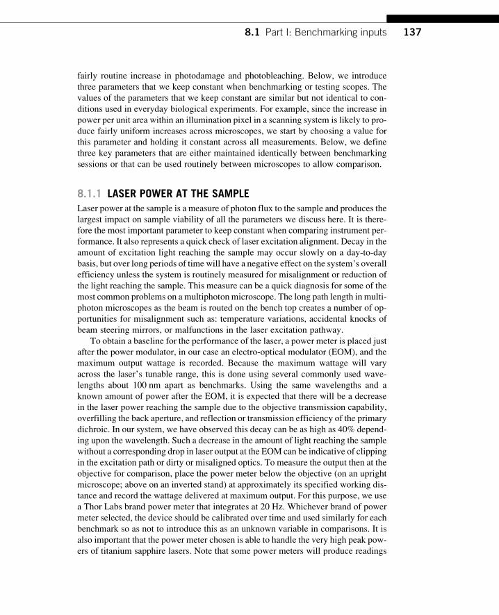
We note that it is important to consider the response of the modulator being used

to adjust laser power. Commonly used power modulators such as EOMs and acousto-

optic tunable filters often do not attenuate laser power linearly as voltage is applied,

resulting in a response curve similar to Fig. 8.1. While not essential for comparing

between microscopes, the generation of graphs such as Fig. 8.1 is helpful in selecting

appropriate settings for biological samples when the wattage applied can adversely

affect the life of the sample and fluorescence of interest. Set the modulator so that the

same laser power is delivered to the sample on each microscope during a continuous

scanning mode or when a single point is being continuously scanned. In our hands,

2 mW as measured at the objective is sufficient for the bead gel assay described be-

low and is a value that we routinely use. The lymph node, our standard biological

sample described, is routinely imaged using 12 mW for benchmarking.

8.1.2 PHOTOMULTIPLIER SETTINGSPhotomultiplier tubes (PMTs) are quite variable when implemented in a microscope

setting, even comparing those of identical manufacturer “minimum specification,”

and so benchmarking and standardizing for them can be one of the most difficult

aspects of this process. This is easier when comparing the performance of a micro-

scope over time, and we recommend choosing a single applied voltage for bench-

marking and keeping it constant. When comparing entire microscope rigs with

different makes or models of PMTs with different gain voltages or characteristics,

this can be a bit more difficult.

FIGURE 8.1

Change in laser power measured with corresponding EOM voltage change at the sample with

varied wavelength. Measured from Spectra Physics MaiTai XF-1 (710–920 nm).


To consider the problem is to consider signal and noise features in detectors gen-

erally. PMTs, like other detectors, contribute two distinct types of noise to the im-

ages they form. Dark noise can be observed when images are captured while no light

falls on the detectors. Dark noise generates low or zero intensity values for the vast

majority of pixels but yields stochastic, high intensity pixels that do not coincide in

position with the location of fluorescent objects. Frame averaging can be an excel-

lent method of removing this high intensity speckling since these bright pixels rarely

happen in the same place across multiple frames. Shot noise (Poisson noise;

Chapters 1 and 3), on the other hand, is signal dependent. As voltage is increased

in an effort to increase the signal intensity, noise also increases. The higher voltages

applied in this scenario also produce higher gains for signal so some excellent im-

ages can be produced under these conditions. There are many excellent reviews

(Yotter & Wilson, 2003), which are helpful in understanding the source and quan-

tification of noise.

Although we will discuss frame averaging later, we have observed in practice that

some users can mine very weak signals to detect and measure objects of interest (e.g.,

GFP-positive cells “identified” deep in tissue) when gains are used that produce

speckles of high intensity. Thus, although the average or standard deviation of the

noise may still be low, some pixels of very high intensity are found but can some-

times be accommodated. This is due to the higher gain in such a PMT giving rise to

higher overall signals for the true luminescent objects and the ability to “average” out

this noise at acquisition or remove single-pixel noise in postprocessing using a

Gaussian kernel. But if very small objects are ultimately to be best spatially resolved

it remains best to minimize this noise. Since frame averaging is essentially applied

identically across all microscopes and should also never vary in how it functions (it is

simply a mathematical average), for the purpose of this discussion, we will assume

that a user will always do benchmarking with the same frame averaging used. We

recommend single frame collection at the same frame rate in a resonant scanning

system is used if testing the samemicroscope over time, or when comparing between

scopes to determine efficiency of light detection/capture, identical criteria (notably

pixel dwell time) are applied.

There are, however, the practical issues of simply obtaining the best, unambiguous

detection of the objects of interest and of obtaining images that will yield quantitative

and revealing data about the response of the PMTs and their role in the system as a

whole. For this reason, we describe two approaches to benchmarking: the “fixed

PMT voltage” method is faster and easier to perform, and the “variable PMT bias

voltage” method which is more time consuming but yields a more complete character-

ization of the detectors, which can be useful for choosing parameters for imaging actual

tissues. In general, benchmarks via the first method will mirror those in the second.

8.1.2.1 Method 1—Fixed PMT voltageOften, end users raise PMT voltage to compensate for a poorly performing micro-

scope in an effort to obtain adequate signal, which results in noisy images. Although

having to apply high PMT voltage to detect signal may be indicative of PMT


insensitivity brought on by age or damage, the source of the problem may be found

elsewhere. To differentiate a loss of PMT sensitivity from a change in actual signal

generated or poor collection efficiency due to alignment, we have devised a

simple test.

For the purposes of the bead gel assay that we describe below, we choose a target

signal intensity for the most superficially detected beads that precludes pixel satura-

tion and adjust the PMT gain to achieve the desired value, keeping the laser power

constant. In an 8-bit system (intensity values 0–255), we typically set the PMT bias

voltage so that the target intensity is 240. Once this parameter has been set, we collect

Z-stacks of both the dispersive and nondispersive bead samples, at approximately the

Nyquist rate (Chapter 1) for the given system, that extend from most superficial

beads detected until signal can no longer be distinguished from noise. Our standard

data sets extend 500 mm in Z at approximately 500 and 250 nm pixel lateral resolu-

tion using a 20� or 25� water-dipping lens with a long working distance.

Using this method, the signal-to-noise ratio (SNR; Chapter 1) at a given sample

depth can be calculated, and changes in the instrument’s ability to detect objects deep

within a sample can be identified as discussed below. The large Z-stack collected

here will also be used to evaluate the point spread function (PSF; Chapters 1 and

10) of the instrument as another measure of performance.

8.1.2.2 Method 2—PMT voltage rangeThe second method of detector benchmarking, which more fully characterizes the

response of PMTs, allows more direct comparison and perhaps optimization of in-

dividual detectors. As with the previous method, the same laser power should be used

across all tests, but in this method, we will use a range of PMT voltages. Note that we

will be testing changes in SNR as a function of voltage change, it is therefore impor-

tant to avoid saturation (e.g., values >255 for 8-bit images). If the bead intensities

become saturated, there will be no gains in signal, while noise will continue to in-

crease, changing the response profile. Begin by collecting a small (�20 mm) repre-

sentative Z-stack at maximum PMT voltage, sampling at approximately the Nyquist

rate. Repeat the same Z-stack acquisition adjusting the PMT voltage by 10% through

the PMT’s entire range. Some users may choose to acquire the same series of images

using a standard biological sample as well due to greater heterogeneity in fluores-

cence, as it will alter the amount of shot noise produced and give a more accurate

picture of how the instrument behaves in experimental settings. In this case, it

may be acceptable to allow some saturation in bright areas as it allows dimmer, bi-

ologically relevant features to be detected.

8.1.3 STANDARD SAMPLESPerhaps, the most valuable part of benchmarking is the establishment of a standard

sample that can be used over time or at different physical sites. The key features are

reproducibility, and representative samples tailored to the types of challenges to


which multiphoton is best applied. To this end, while a standard 10-mm thick histol-

ogy slide, a pollen grain slide, or immobilized bead standards can provide some in-

sight, the best samples are thick specimens set into media that is dispersive to the

same extent as biological specimens. We recommend that one establish two such

samples. The first, which we have mentioned in passing above, is reproducible

fluorophore-impregnated beads distributed in dispersive nonfluorescent beads, all

embedded in a thick slab of hydrogel material. The fluorescent beads mimic fluor-

ophores that might be present in a biological tissue and the second set of beads mimic

the effects of biological tissues upon the mean-free path of light within tissues

(Theer, Hasan, & Denk, 2003). The sample described below may roughly mimic tis-

sue such as a lymph node. If the target tissue or organ for a study is vastly different,

a modified sample (e.g., fewer dispersive beads) may be made to better mimic its

properties. The second sample we will describe is a “standard biological sample,”

a tissue whose optical properties very faithfully represent samples to be used in final

experiments but critically whose fluorescent intensity can be maintained to very

close tolerances over time.

8.1.3.1 A standard three-dimensional sample set with variabledispersive propertiesWe recommend, in fact, that two formats of this sample should be made. A first

“nondispersive” sample will allow the comparison of the PSF of a multiphoton sys-

tem. Note that due to the lower numerical aperture (Chapter 2) typically used in mul-

tiphoton imaging, and due to the longer wavelength of light, this will typically be

inferior to collection in any of the other typical modalities. By collecting a

Z-stack of this sample, you will observe that, were tissues not complex (dispersive),

imaging depths would be limited only by the working distance of the objective lens.

The second variation of this sample, “dispersive,” will demonstrate the degree to

which the two-photon effect improves imaging at depths in complex tissues and,

in comparison to the first version, will demonstrate the degree to which dispersive

objects affect imaging deep within tissues.

8.1.3.1.1 Support protocol: Preparation of PSF beads in a dispersiveor nondispersive supportNondispersive gel:

1.5 ml Polyacrylamide (40%, 19:1 acrylamide:bis-acrylamide)

4.25 ml ddH20 (makes 10% polyacrylamide total)

10 ml Red beads (Invitrogen F13083 1.0 mM 1�1010/ml)

10 ml Green beads (Invitrogen F13081 1.0 mM 1�1010/ml)

250 ml APS (10% solution of powder (kept frozen))

5 ml TEMED to polymerize the gel


Dispersive gel:

1.5 ml Polyacrylamide (40%, 19:1 acrylamide:bis-acrylamide)

2.25 ml ddH20 (makes 10% polyacrylamide total)

10 ml Red beads (Invitrogen F13083 1.0 mM 1�1010/ml)

10 ml Green beads (Invitrogen F13081 1.0 mM 1�1010/ml)

2 ml Sulfate latex beads (Interfacial Dynamics/Invitrogen: 5 mm diameter. stock:6.1�108)

250 ml APS (10% solution of powder (kept frozen))

5 ml TEMED to polymerize the gel

Mix all ingredients except TEMED into a six-well dish or mold of choice. Then add

the TEMED and gently swirl. Allow to polymerize. Figure 8.2 shows samples ready

for use.

Note that other beads may be used but should have standardized emission spectra,

brightness, and shape. We have selected 1.0 mm beads, as they are small enough to

serve as an approximation of the PSF given the magnification and pixel calibration of

our systems, yet are large enough to evaluate SNR. Others may choose to prepare

separate samples or include smaller (0.1 mm) and larger beads (10 mm) to more crit-

ically evaluate these two parameters. Absolute knowledge of the refractive and dis-

persive properties is important for the sulfate latex beads or equivalent, but the most

important consideration for the purposes of your own benchmarking is that the QC of

these beads is consistent. Consider purchasing a lot and maintaining it in the fridge

over time.

Note also that the mean-free path for the dispersive sample described above is

�300 mm, calculated with a Mie scattering theorem. In our hands, this shows inten-

sity drop-offs with depths that are similar to mouse lymph nodes. The full calculation

FIGURE 8.2

Nondispersive (left) and dispersive (right) bead gels in 35-mm dishes ready for use.


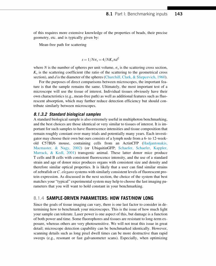
of this requires more extensive knowledge of the properties of beads, their precise

geometry, etc. and is typically given by:

Mean-free path for scattering

s¼ 1=Nss ¼ 4=NKspd2

where N is the number of spheres per unit volume, ss is the scattering cross section,

Ks is the scattering coefficient (the ratio of the scattering to the geometrical cross

section), and d is the diameter of the spheres (Churchill, Clark, & Sliepcevich, 1960).

For the purposes of direct comparisons between microscopes, the important fea-

ture is that the sample remains the same. Ultimately, the most important test of a

microscope will use the tissue of interest. Individual tissues obviously have their

own characteristics (e.g., mean-free path) as well as additional features such as fluo-

rescent absorption, which may further reduce detection efficiency but should con-

tribute similarly between microscopes.

8.1.3.2 Standard biological samplesA standard biological sample is also extremely useful in multiphoton benchmarking,

and the best choices are those identical or very similar to tissues of interest. It is im-

portant for such samples to have fluorescence intensities and tissue composition that

remain roughly constant over many trials and potentially many years. Each investi-

gator may choose their own but ours consists of a lymph node from a 6- to 12-week-

old C57Bl/6 mouse, containing cells from an ActinCFP (Hadjantonakis,

Macmaster, & Nagy, 2002) (or UbiquitinGFP; Schaefer, Schaefer, Kappler,

Marrack, & Kedl, 2001) transgenic animal. These latter donor mice produce

T cells and B cells with consistent fluorescence intensity, and the use of a standard

strain and age of donor mice produces organs with consistent size and density and

therefore similar optical properties. It is likely that a user can find similar strains

of zebrafish or C. elegans systems with similarly consistent levels of fluorescent pro-

tein expression. As discussed in the next section, the choice of the system that best

matches your “typical” experimental system may help to choose the last imaging pa-

rameters that you will want to hold constant in your benchmarking.

8.1.4 SAMPLE-DRIVEN PARAMETERS: HOW FAST/HOW LONGSince the goals of tissue imaging can vary, there is one last factor to consider in de-

termining how to benchmark your microscopes. This is the issue of how much light

your sample can tolerate. Laser power is one aspect of this, but damage is a function

of both power and time. Some fluorophores and tissues are resistant to long-term ex-

posure, whereas others are very photosensitive. We will not treat this issue in great

detail; microscope detection capability can be benchmarked identically. However,

scanning details such as long pixel dwell times can be more destructive than rapid

sweeps (e.g., resonant or fast galvanometer scans). Especially, when optimizing


imaging lengths, it may be useful to have prior knowledge of this feature when

choosing laser power and scanning parameters for benchmarking.

As an example, for the lymph node samples, our biological standard, we collect

timelapse sequences at 30-s intervals encompassing�100 mm of z-space at 5-mm in-

tervals. T cells (approximately 5 mm in diameter) will be assessed within the lymph

node. The goal of this collection is to assess both the detection depth but also, by

collecting a timelapse, to assess whether imaging conditions being tested are com-

patible with the biology; T cells are typically motile within lymph nodes, and it is a

good control that your standard benchmarking imaging conditions for this sample be

chosen to be in the range of biological compatibility.

8.2 PART II: BENCHMARKING OUTPUTSOnce a set of standard samples is identified and working parameters are established,

it remains to test the microscope for the quality of images that are produced. We

chose four parameters to measure routinely. First is the PSF, which allows one to

observe the transfer function of a microscope. In other words, for a small point source

of fluorescence in a sample, how well the microscope will transfer the intensity to an

ideally small region at the detector. Second are the intertwined parameters of total

intensity of an object (bead, cell) and the SNR of detection. Lastly, since detection

of fluorescence deep within a sample is a desirable feature in multiphoton micros-

copy, we describe the use of sensitivity as a function of depth as a measured

parameter.

8.2.1 THE POINT SPREAD FUNCTIONDegradation of the PSF is often the clearest indication of misalignment and optical

aberration in an imaging system that is performing at a suboptimal level (Chapter 7).

Figure 8.3A shows the severely aberrated intensity profile of a bead in nondispersive

media acquired while the primary dichroic was warped by an aberrant holder. Al-

though the central XY plane is comparable to that shown in Fig. 8.3B, a near ideal

PSF, it is clear in the XZ and YZ views that the light propagating axially from the

bead is asymmetric, distorting the shape of any detected object (Fig. 8.3C). The cross

shape of the PSF is characteristic of an astigmatism (Chapter 2) introduced by a

skewed optic or bowing of a mirror. The direction of laser propagation, if it is at

a slight angle rather than parallel to the objective as it enters the back aperture,

and position of the beam also have a direct impact on the shape of the PSF

(Fig. 8.3D). Aberrations may also result from an off-axis optic, for example, in a

damaged objective.

Spherical aberration is another prevalent source of degradation of the PSF in tis-

sues. Spherical aberration occurs when light rays that pass through the outside of the

optical axis are focused to a different Z position than light rays that pass through the

center of the optical axis (Chapter 2). For example, consider a simple curved lens that


is ground spherically, the rays that pass through the lens near the outside will be fo-

cused differently than the rays that pass through the center. This causes a large

spreading of the PSF in the Z axis, and decreases resolution and intensity consider-

ably. Modern optics are corrected for spherical aberration with a specific optical path

length, but in practice, this path length invariably changes when imaging through

large samples. This is why it is very important to use an objective that has an immer-

sion media matched to the sample, or use an objective that has a correction collar that

allows you to correct for any spherical aberration. Especially, when considering the

nonlinear dependence of multiphoton excitation, this can have a huge impact on the

brightness and quality of your image.

Using the Z-stack acquired of beads in nondispersive media, we select a repre-

sentative bead and calculate lateral and axial full-width half maximum (FWHM;

Chapter 7) based on the centroid intensity (Fig. 8.3E and F). Although this method

FIGURE 8.3

Acceptable and poor PSFs obtained during benchmarking. (A) Poor PSF suffering from

astigmatism. Central XY plane, XZ and YZ views. (B) Acceptable PSF central XY plane,

XZ and YZ views. (C) Maximum intensity Z-projections of a single bead (top A, bottom B).

(D) XZ view of PSF when the laser beam enters the objective at an angle. (E) FWHM resolution

of A. (F) FWHM resolution of B.

1458.2 Part II: Benchmarking outputs

may not be sensitive enough to be applied to other systems, particularly those

designed for high precision localization, it allows direct comparison between the per-

formance of instruments. Importantly, it provides a quick method of quantification

for gains made through incremental tweaks in alignment and optimization and al-

ways will affect the other two measurements we will make.

8.2.2 SNR AND TOTAL INTENSITYBecause SNR is a ratio, it is a dimensionless parameter that does not have units; it

provides an easy method of comparison of the quality of images. As a first measure of

system performance and sensitivity we use the large Z-stack acquired using the dis-

persive bead gel (method 1) to evaluate the SNR of the most superficial beads. We

use Imaris (Bitplane AG) spot detection to identify beads and calculate the average

signal intensity in a selected plane. This can also be done in ImageJ using the Track-

Mate plug-in or creating masks, which cover the bead area (for our systems �2�2

pixel spots).Whichever method is preferred, it should be used identically for all mea-

surements. There are several methods for calculating image noise (Paul,

Kalamatianos, Duessman, & Huber, 2008; Yotter &Wilson, 2003) all of which have

practical applications, but for our purposes in PMT detection where there can be high

shot noise, the standard deviation of pixel intensity in areas without beads is most

suitable. Two 140�140 pixel regions of interest (ROIs) in a single plane free of

beads were selected and used to calculate the standard deviation of the noise

(Fig. 8.4A). We consider that at a minimum standard, a scope should be able to de-

liver an SNR of no less than 10:1 for the fluorescent beads in dispersive media at

superficial depths or in a nondispersive sample. That is, with a target signal intensity

of 240, standard deviation of noise should be no greater than 24. In subsequent deeper

planes, the SNR can be expected to decrease with scattering and absorption until

beads can no longer be detected. SNR as a metric of maximal depth penetration will

be discussed below.

While the performance of the PMTs will affect the total intensity and maximal

depth of acquisition, any change in these metrics that can be traced back to other

elements such as alignment should be corrected prior to evaluating the response

of the detectors themselves.

The data set collected in method 2 can be used to generate the response profile of

a detector under standardized conditions. We select a representative plane from the

acquired Z-stack and repeat the same spot detection and noise calculation steps as

described for method 1 for images acquired using each PMT voltage. Both signal

(Fig. 8.4B) and noise (Fig. 8.4C and D) intensities increase as more voltage is

applied.

As evident visually in Fig. 8.4E, as higher voltage is applied, PMTs generate high

intensity noise at higher frequency. Because these high intensity pixels occur sto-

chastically, they are not biased toward particular pixels across frames and their effect

on noise standard deviation and maximum can be mitigated by frame averaging

(Fig. 8.4C and D). The cost of this noise reduction is a reduction in frame rate,


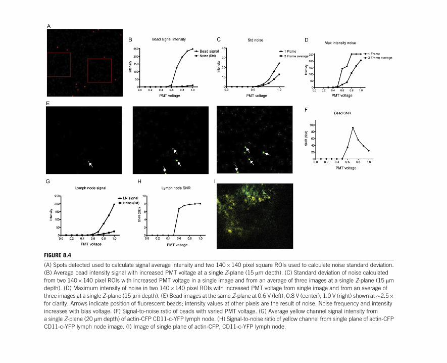
FIGURE 8.4

(A) Spots detected used to calculate signal average intensity and two 140�140 pixel square ROIs used to calculate noise standard deviation.

(B) Average bead intensity signal with increased PMT voltage at a single Z-plane (15 mm depth). (C) Standard deviation of noise calculated

from two 140�140 pixel ROIs with increased PMT voltage in a single image and from an average of three images at a single Z-plane (15 mmdepth). (D) Maximum intensity of noise in two 140�140 pixel ROIs with increased PMT voltage from single image and from an average of

three images at a single Z-plane (15 mm depth). (E) Bead images at the same Z-plane at 0.6 V (left), 0.8 V (center), 1.0 V (right) shown at�2.5�for clarity. Arrows indicate position of fluorescent beads; intensity values at other pixels are the result of noise. Noise frequency and intensity

increases with bias voltage. (F) Signal-to-noise ratio of beads with varied PMT voltage. (G) Average yellow channel signal intensity from

a single Z-plane (20 mm depth) of actin-CFP CD11-c-YFP lymph node. (H) Signal-to-noise ratio of yellow channel from single plane of actin-CFP

CD11-c-YFP lymph node image. (I) Image of single plane of actin-CFP, CD11-c-YFP lymph node.

for example, in Fig. 8.4 speed is reduced from 30 frames per second (video rate) to

10 frames per second. When acquisition speed and photodamage are not primary

concerns, averaging of an extremely noisy detector can generate images with

acceptable SNRs.

Ideally, as PMT voltage is increased, signal intensity will increase exponentially

while noise increases only linearly, improving the SNR. Typically, each detector has

a sample-dependent optimal setting for the signal gains beyond which increased volt-

age produces only marginal returns while continuing to produce noise. Figure 8.4F

shows the SNR curve for beads detected at varying voltages. Although the highest

SNR is achieved at 0.7 V, by visually inspecting the image, it is clear that several

beads that are present are not detected at this setting. Although a higher voltage results

in a decrease in SNR (to a level still well above our minimum detection threshold,

SNR>4), the gains in ability to identify objects of interest are more valuable. This

trade-off is made in biological samples in an effort to image dimmer, smaller features

of interest. We routinely perform the same benchmarking procedure using excised

lymph nodes containing actin-CFP as well as CD11c-YFP cells, in addition to bead

samples, as we have found the shot noise and signal gains generated are highly con-

text dependent (Fig. 8.4G and I). That is, the beads alone do not give a full picture of

how well the detector is truly doing when generating useful experimental images.

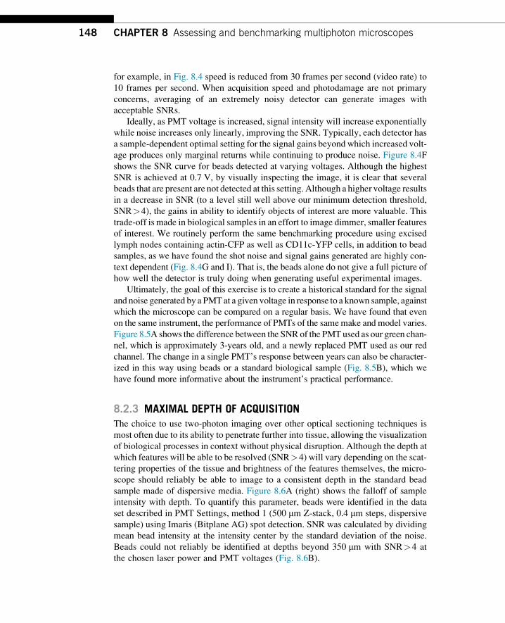
Ultimately, the goal of this exercise is to create a historical standard for the signal

and noise generated by a PMTat a given voltage in response to a known sample, against

which the microscope can be compared on a regular basis. We have found that even

on the same instrument, the performance of PMTs of the samemake and model varies.

Figure 8.5A shows the difference between the SNRof the PMTused as our green chan-

nel, which is approximately 3-years old, and a newly replaced PMT used as our red

channel. The change in a single PMT’s response between years can also be character-

ized in this way using beads or a standard biological sample (Fig. 8.5B), which we

have found more informative about the instrument’s practical performance.

8.2.3 MAXIMAL DEPTH OF ACQUISITIONThe choice to use two-photon imaging over other optical sectioning techniques is

most often due to its ability to penetrate further into tissue, allowing the visualization

of biological processes in context without physical disruption. Although the depth at

which features will be able to be resolved (SNR>4) will vary depending on the scat-

tering properties of the tissue and brightness of the features themselves, the micro-

scope should reliably be able to image to a consistent depth in the standard bead

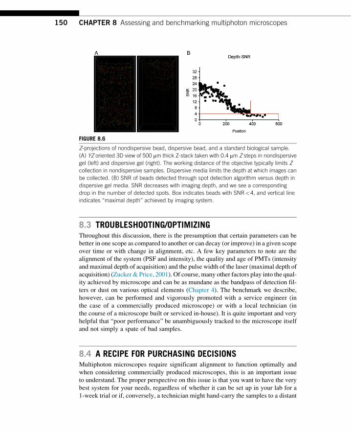
sample made of dispersive media. Figure 8.6A (right) shows the falloff of sample

intensity with depth. To quantify this parameter, beads were identified in the data

set described in PMT Settings, method 1 (500 mm Z-stack, 0.4 mm steps, dispersive

sample) using Imaris (Bitplane AG) spot detection. SNR was calculated by dividing

mean bead intensity at the intensity center by the standard deviation of the noise.

Beads could not reliably be identified at depths beyond 350 mm with SNR>4 at

the chosen laser power and PMT voltages (Fig. 8.6B).


Changes in depth of penetration between benchmarking experiments may be in-

dicative of several independent factors. As PMTs age, they may see increased noise

and decreased gains in signal, reducing overall sensitivity and making it more dif-

ficult to resolve features deep in the sample. Quantifying and diagnosing PMT

changes are discussed in the following section.

Temporal dispersion of the femtosecond laser pulses used in multiphoton systems

can decrease the effective power delivered to the focal plane, an affect that is wors-

ened with scattering deep in tissue. Such dispersion results from differential

wavelength-dependent refraction of excitation light caused by routing optics or

the optical properties of tissues. Some multiphoton lasers include hardware and soft-

ware packages that allow users to compensate for this dispersion by “chirping”

pulses (predispersing laser pulses in the opposite direction to compensate for disper-

sion introduced by the system).

Bead SNR

0.0 0.2 0.4 0.6 0.8 1.00

50

100

150

200

Red PMTGreen PMT

PMT voltage

SN

R (

Std

)

0.0 0.2 0.4 0.6 0.8 1.00

2

4

6

8

1020132012

Lymph node SNR

PMT voltage

SN

R (

Std

)

A

B

FIGURE 8.5

Comparison of SNR in beads and lymph nodes across years. (A) SNR from red and green

(solid and dashed in print version) beads generated under identical conditions between

two detectors on the same microscope. (B) SNR of images from the same detector of a

CD11c-YFP lymph node under identical conditions taken 1 year apart. Gains in SNR with

increased voltage are reduced between benchmarking experiments indicating decreased

sensitivity.

1498.2 Part II: Benchmarking outputs

8.3 TROUBLESHOOTING/OPTIMIZINGThroughout this discussion, there is the presumption that certain parameters can be

better in one scope as compared to another or can decay (or improve) in a given scope

over time or with change in alignment, etc. A few key parameters to note are the

alignment of the system (PSF and intensity), the quality and age of PMTs (intensity

and maximal depth of acquisition) and the pulse width of the laser (maximal depth of

acquisition) (Zucker & Price, 2001). Of course, many other factors play into the qual-

ity achieved by microscope and can be as mundane as the bandpass of detection fil-

ters or dust on various optical elements (Chapter 4). The benchmark we describe,

however, can be performed and vigorously promoted with a service engineer (in

the case of a commercially produced microscope) or with a local technician (in

the course of a microscope built or serviced in-house). It is quite important and very

helpful that “poor performance” be unambiguously tracked to the microscope itself

and not simply a spate of bad samples.

8.4 A RECIPE FOR PURCHASING DECISIONSMultiphoton microscopes require significant alignment to function optimally and

when considering commercially produced microscopes, this is an important issue

to understand. The proper perspective on this issue is that you want to have the very

best system for your needs, regardless of whether it can be set up in your lab for a

1-week trial or if, conversely, a technician might hand-carry the samples to a distant

FIGURE 8.6

Z-projections of nondispersive bead, dispersive bead, and a standard biological sample.

(A) YZ oriented 3D view of 500 mm thick Z-stack taken with 0.4 mm Z steps in nondispersive

gel (left) and dispersive gel (right). The working distance of the objective typically limits Z

collection in nondispersive samples. Dispersive media limits the depth at which images can

be collected. (B) SNR of beads detected through spot detection algorithm versus depth in

dispersive gel media. SNR decreases with imaging depth, and we see a corresponding

drop in the number of detected spots. Box indicates beads with SNR<4, and vertical line

indicates “maximal depth” achieved by imaging system.


site. We suggest the latter will be the best way to see the best instrument that a vendor

can offer. Based on our experiences, we recommend against having a vendor “demo”

microscope on-site since invariably the scope will not function optimally in a short

demonstration period, and even if it is functioning to its design optimum, you may

wonder if “it might have done better” given stable and optimal conditions. Such is

not a rational selection mechanism. A benchmark as used here can be best used dur-

ing instrument selection to choose ‘the best’ for your uses and then a second time

when a purchased instrument is installed to confirm that the instrument that is deliv-

ered operates to your required specification.

CONCLUSION

The process of benchmarking is important in the testing and acquisition of a system as

well as throughout its life span. It is important to define key collection parameters and

samples to use for benchmarking. A standard dispersive bead sample and a standard

biological sample represent key steps in establishing a protocol for obtaining andmain-

taining a microscope with optimal function for biological applications. Ultimately,

it helps to determine whether a biological experiment can or cannot be done, and

whether the biology or the microscope might be improved to facilitate an experiment.

ACKNOWLEDGMENTSThe authors thank the Krummel lab for helpful discussions. The authors declare no competing

financial interests.

REFERENCESChurchill, S. W., Clark, G. C., & Sliepcevich, C. M. (1960). Light-scattering by very dense

monodispersions of latex particles. Discussions of the Faraday Society, 30, 192–199.Hadjantonakis, A. K., Macmaster, S., & Nagy, A. (2002). Embryonic stem cells and mice

expressing different GFP variants for multiple non-invasive reporter usage within a single

animal. BMC Biotechnology, 2, 11.Paul, P., Kalamatianos, D., Duessman, H., & Huber, H. (2008). Automatic quality assessment

for fluorescence microscopy images. In 8th IEEE international conference on BioInfor-matics and BioEngineering, BIBE 2008, 8–10, 2008 (pp. 1–6), pp. 1–6.

Schaefer, B. C., Schaefer, M. L., Kappler, J. W., Marrack, P., & Kedl, R. M. (2001). Obser-

vation of antigen-dependent CD8+ T-cell/dendritic cell interactions in vivo. Cellular Im-munology, 214, 110–122.

Theer, P., Hasan, M. T., & Denk,W. (2003). Two-photon imaging to a depth of 1000 micron in

living brains by use of a Ti:Al2O3 regenerative amplifier. Optics Letters, 28, 1022–1024.Yotter, R. A., & Wilson, D. M. (2003). A review of photodetectors for sensing light-emitting

reporters in biological systems. IEEE Sensors Journal, 3, 288–303.Zucker, R. M., & Price, O. (2001). Evaluation of confocal microscopy system performance.

Cytometry, 44, 273–294.

151References

http://refhub.elsevier.com/B978-0-12-420138-5.00008-2/rf0005


















Documents

Assessing and benchmarking multiphoton microscopes for biologists …krummel.org/images/Publications/corbin-pub-2014-01.pdf · CHAPTER Assessing and benchmarking multiphoton microscopes