Supplemental Information: Geochemical evidence for cryptic sulfur

cycling linked to methane production in salt marsh sediments

J. V. Mills*, G. Antler, A. V. Turchyn

Department of Earth Sciences, University of Cambridge, Cambridge CB2 3EQ, UK.

* correspondence and requests for materials should be addressed to J.V.M.: jennifer.mills@berkeley.edu

Supplementary Methods

Incubation experiments

Experimental Setup:

Incubation experiments were run in 120mL glass vials, topped with crimp-sealed rubber stoppers (allautoclaved before the start of the experiment). Pond water collected from the sampling site was filtered(0.2µm syringe filters) and transferred into autoclaved vials (100mL). Half of the pond water was spiked to�18OH2O=190‰ using 98% 18O water. Lactate (1g/L) was added to two samples (18O-enriched water andregular pond water) at this stage. Vials were then bubbled with N

2

/CO2

(90%/10%) for one hour. Duringthis time, the sediment core was sampled for pore fluid and solid-phase geochemistry analysis (leaving ⇠8cmat the bottom of the core untouched for the incubation experiments). Following core sampling, the bottom8cm of sediment was extruded from the core liner into an N

2

-flushed bag that was quickly transferredto the anaerobic chamber. The bottom and sides of the core sediment were scraped off to remove anypotentially contaminated/oxidized sediments. The flushed pond water vials were also transferred into theanaerobic chamber. 5 or 10mL sediment aliquots were then collected from the core sediment using a 5mLcutoff syringe, and transferred into the pond water vials. After removal from the anaerobic chamber, theheadspace of the vials was flushed for 5 minutes in order to remove any H

2

, which is present in the chamberatmosphere.

The samples were then incubated at room temperature (16-20°C), in the dark, for a total of 162 days, afterwhich the sediment and water were depleted to the point where we worried about headspace contamination.

DTPA barite reprecipitation:

It has long been known a range of anions (and cations) can be present as impurities in precipitatedbarite (occluded in the barite through either coprecipitation, adsorption onto the solid surface, or simpletrapping of the mother solution) [1, 2]. This becomes a serious problem for �18OSO4 measurements whennon-sulfate oxyanions are occluded that are either present in high concentrations or have oxygen isotopiccompositions significantly different from the sulfate being measured. In order to remove these impurities,samples were cleaned using a barite reprecipitation technique presented by Bao, 2006 [2]. In this technique,the barite is dissolved in a diethylenetriaminepentaacetic acid (DTPA, a chelating agent) solution to removeany impurities trapped in the lattice before being reprecipitated by dropping the pH of the solution throughthe addition of concentrated HCl. After DTPA reprecipitation, all traces of contamination in the �18OSO4

signal were removed.

1

Lower Marsh

Upper Marsh

dune ridgeSampling SiteStonemeal C

reek

1000 ft

N

Norfolk Coast PathWells

Dep

th (c

m)

[Fe2+] (mM) δ34SSO4 (‰ VCDT) δ18OSO4

(‰ VSMOW) [SO4] (mM) [SO4]/[Cl] δ18OH2O (‰ VSMOW)

0

5

10

15

20

25

30

35

40

0 1 2 3 16 18 20 22 24 26 7 9 11 13 15 17 0 10 20 30 40 50 0.02 0.04 0.06 0.08 -2 -1 0 1

November Sampling March Sampling May Sampling

Seawater Ratio

100 ft

Warham Pond 1 (November, May samplings)

Warham Pond 2 (January Sampling)Warham Pond 3

(March Sampling)

A)

B)

Figure S1: Additional field sampling. A) Locations of ponds sampled at Warham salt marsh. B) Geochemicalprofiles of cores taken during November 2013 (green squares in manuscript Figure 2), March 2014, and May2014.

Supplementary Data

Additional field data: Spring and summer samplings

Iron-rich ponds from Warham salt marsh were also sampled during additional sampling campaigns inMarch and mid-May 2014 (Figure S1). While the pond pore fluid profiles from the core taken in Marchlargely match those from cores taken in November and January, the core taken in May exhibits signs of sulfatereduction in the uppermost 10cm of sediment. Both the sulfur and oxygen isotopes of sulfate are enrichedthrough this interval (�18OSO4 remains at 12-13‰, 3‰ enriched over seawater and �34SSO4 increases from21 to 23‰). The sulfate to chlorine ratio also dips below the seawater ratio in the upper 10cm of sediment,suggesting that sulfate is being consumed. Below this region of sulfate reduction, the May and Novemberpore fluid profiles exhibit largely similar behaviour - �34SSO4 remains constant with depth while �18OSO4

rises steeply in the bottom half of the core.We also performed sedimentary iron and sulfide extractions on the core from May, 2014. Acid-volatile

sulfide (AVS) and Chromium-reducible sulfide (CRS) were extracted from sediment samples preserved inZnAc (3mL, 20%) following a sequential extraction procedure modified from Alford et al., 2011 [3]. Highlyreactive Fe3+ oxide concentrations were measured using an ascorbic acid digestion following Sivan et al.,2011 [4]. We also performed x-ray fluorescence measurements on the core using a core scanner to obtainelemental abundances (data shown here normalized by titanium). We were only able to extract enoughsulfide for sulfur isotope analysis from the upper 10cm of core, where pore water data suggested active

2

Highly Reactive Iron (μmol/g dry sediment) Fe/Ti0 100 200 300 400 -34 -32 -30 -28 -26 0 10 20 30 0 1 2

Dep

th (c

m)

0

5

10

15

20

25

30

35

40

δ34Ssulfide (‰VCDT) S/Ti

AVSCRS

Sediment Extraction Core Scanner XRF Data

Figure S2: Solid-phase geochemistry from the Warham pond sampled in May, 2014 (pore fluid profilesshown in Figure S1). Far left: picture of core. Data (left to right): highly reactive iron concentration(mmol Fe / g dry sediment); �34SH2S (‰ VCDT) of acid-volatile sulfides (AVS, filled red diamonds) andchromium-reducible sulfides (CRS, empty red squares); and XRF core scanner data (normalized by Ti, 10kVsensitivity).

sulfate reduction (sulfate reduction was observed to occur in the uppermost, black, sediments during thissummer sampling – Figure S1). This finding is supported by the x-ray fluorescence data which shows a highabundance of solid-phase sulfur only in the upper 10cm.

Additional data from microcosm experiments:

Data for replicate samples of the incubation experiments presented in Figure 4 can be seen in FiguresS3-S5. Figure S3 compares lactate samples (to which 1g/L lactate was added) incubated in pond water and18O-enriched water. Identical geochemical behaviour is observed over the growth of the culture, althoughthe �18OSO4 data for the 18O-enriched sample cannot be considered due to potential contamination with18O-enriched impurities (the barite was not reprecipitated using DTPA due to insufficient material). Thisconfirms in duplicate that a marked acceleration of existing microbial activity occurs with the addition oflabile organic carbon.

Comparison of 10mL sediment sample replicates can be seen in Figure S4; Figure S5 compares 5mLsediment samples incubated in pond water and 18O-enriched water.

3

A)

0 20 40 60 80 100 120 140 160Time (days)

0.0

1.0

1.5

2.0

0.5

[Fe2+

] (m

M)

B)

C)

E)

δ34SS

O4 (‰

VCD

T)

15

25

30

35

20

40

0 20 40 60 80 100 120 140 160Time (days)

met

hane

0

4

2

6

8

10

12

14

16

18

[SO

4] (m

M)

[CH4 ] (ppm

v)

50

500

5000

0 20 40 60 80 100 120 140 160Time (days)

5

15

35

45

25

55

65

75

85

δ18O

SO4 (‰

VSM

OW

)

0 20 40 60 80 100 120 140 160Time (days)

δ18O

SO4 (‰

VSM

OW

)

δ34SSO4 (‰ VCDT)15 20 25 30 35 40

Incubation Experiment 1:

Lactate

Lactate, 18O-enriched water

D)

510

20

25

15

30

35

40

45

50

Figure S3: Samples incubated with lactate in pond water (green data shown in Figure 4) and in 18O-enrichedwater (blue data). Panels A-D show the evolution of A) ferrous iron concentration, B) sulfate and headspacemethane concentration, C) �34SSO4 , and D) �18OSO4 with time; panel E shows the �18OSO4 vs. �34SSO4

cross-plot. �18OSO4 data for the sample incubated in 18O-enriched water cannot be trusted due to potentialcontamination with 18O-enriched impurities - due to insufficient barite, these samples were not reprecipitatedusing DTPA. Despite this, general geochemical and isotope trends are consistent - iron reduction followed bysulfate reduction and then methanogenesis is observed in both the 18O-enriched and pond water samples.

4

A)

0 20 40 60 80 100 120 140 160Time (days)

0.0

1.0

1.5

2.0

0.5

[Fe2+

] (m

M)

B)

C) D)

E)

δ34SS

O4 (‰

VCD

T)

161718

2021222324

19

25

150 20 40 60 80 100 120 140 160

Time (days)

0

4

2

6

8

10

12

14

16

18

[SO

4] (m

M)

0 20 40 60 80 100 120 140 160Time (days)

5

10

15

20

25

30

35

δ18O

SO4 (‰

VSM

OW

)0 20 40 60 80 100 120 140 160

Time (days)

δ18O

SO4 (‰

VSM

OW

)

δ34SSO4 (‰ VCDT)10 15 20 25 30 35 40

5

10

15

20

25

30

35

Incubation Experiment 1:

10mL sediment

10mL sediment, 18O-enriched water

10mL sediment replicate

10mL sediment, 18O-enriched water replicate

Figure S4: Comparison of replicates for 10mL sediment samples. Replicates for the 10mL sample and the10mL-18O sample grown in 18O-enriched water (black and red data from Figure 4) are shown with dashedlines. Panels A-D show the evolution of A) ferrous iron concentration, B) sulfate concentration, C) �34SSO4 ,and D) �18OSO4 with time; panel E shows the �18OSO4 vs. �34SSO4 cross-plot. Both replicate samplesexperienced small air leaks during sampling on day 51, evidenced by a dip in ferrous iron concentrations.Subsequent data is thus potentially influenced by this O

2

exposure. Despite this, the duplicate experimentstrack each other remarkably well - with the exception of a slight offset in the magnitude of �18OSO4 increase,identical geochemical and isotopic trends are observed.

5

A)

0 20 40 60 80 100 120 140 160Time (days)

0.0

1.0

1.5

2.0

0.5

[Fe2+

] (m

M)

B)

C) D)

E)

δ34SS

O4 (‰

VCD

T)

161718

2021222324

19

25

150 20 40 60 80 100 120 140 160

Time (days)

0

4

2

6

8

10

12

14

16

18

[SO

4] (m

M)

0 20 40 60 80 100 120 140 160Time (days)

5

10

15

20

25

30

δ18O

SO4 (‰

VSM

OW

)0 20 40 60 80 100 120 140 160

Time (days)

δ18O

SO4 (‰

VSM

OW

)

δ34SSO4 (‰ VCDT)10 15 20 25 30 35 40

5

10

15

20

25

30

Incubation Experiment 1:

5mL, 18O-enriched water

5mL

Figure S5: 5mL sediment samples from incubation experiment 1 (5mL sample from Figure 4 shown in orange;5mL-spike sample incubated in 18O-enriched water shown in purple). Panels A-D show the evolution of A)ferrous iron concentration, B) sulfate concentration, C) �34SSO4 , and D) �18OSO4 with time; panel E showsthe �18OSO4 vs. �34SSO4 cross-plot. The two samples exhibit identical trends in ferrous iron concentration,sulfate concentration, and �34SSO4 , while an increase in �18OSO4 is observed only in the sample incubatedin 18O-enriched water.

6

Incubation Experiment 2: Independent Corroboration

A second set of incubation experiments were carried out using sediments from a pond cored at Warhamsalt marsh in March, 2014 in order to provide independent corroboration of the results from the initial setof incubation experiments. Results for a 10mL sediment sample incubated in pond water and a comparablesample incubated in 18O-enriched water (�18OH2O ⇠ 400‰) can be seen in Figure S6. Increases in theoxygen isotopes of sulfate (>15‰ shift in �18OSO4 over 100 days) are observed in the sediments incubatedin 18O-enriched water (light blue line, Figure S6) with no corresponding changes in �34SSO4 or sulfateconcentration. This provides independent corroboration of the finding of in-situ cryptic sulfur cycling inthese salt-marsh sediments.

0 20 40 60 80 100Time (days)

0

5

15

20

25

30

10

δ18O

SO4 (

‰ V

SMO

W)

A)

0 20 40 60 80 100Time (days)

0.0

0.2

0.3

0.4

0.1[Fe2+

] (m

M)

B)

C) D)

0 20 40 60 80 100Time (days)

17

19

23

25

27

29

21[SO

4] (m

M)

0 20 40 60 80 100Time (days)

15

17

21

23

25

19

δ34SS

O4 (

‰ V

CDT)

15 17 19 21 23 250

5

15

20

25

30

10

δ18O

SO4 (

‰ V

SMO

W)

δ34SSO4 (‰ VCDT)

E)

Incubation Experiment 2:

10mL, pond water

10mL, 18O-enriched water

Figure S6: Results from a second incubation experiment carried out in March 2014. Panels A-D show theevolution of A) ferrous iron concentration, B) sulfate concentration, C) �34SSO4 , and D) �18OSO4 ; Panel Eshows the �18OSO4 vs. �34SSO4 cross-plot for these experiments. Note that this set of incubation experimentswas grown in water with �18OH2O ⇠ 400‰ as opposed to �18OH2O ⇠ 200‰ in the first set of incubationexperiments; larger increases in �18OSO4 for the sample incubated in 18O-enriched water are thus observed,relative to that seen in the first incubation experiment.

7

Sulfate recycling rate model

Modelling sulfate recycling rate

‘Outside’ sulfate reservoirSO4

δ18OSO4

Isotopic Equilibration Process

δ18OH2O, εeq

Fin

δ18OSO4 + εk O isotopes in sulfate reset to some isotopeequilibrium with water

Fout

δ18OH2O + εeq

Sulfate Intake Rate

Unknown reduced sulfur species: sulfide, sulfite, or polysulfide?

Figure S7: Sulfate recycling rate model schematic.

To estimate the sulfate intake rate for the cryptic sulfur cycling observed, we constructed kinetic mass-balance models to track the evolution of the amount and oxygen isotopic composition of sulfate throughoutthe incubation experiment (Figure S7). The model is such that sulfate from the external sulfate reservoiris reduced to some lower valence state sulfur species, undergoes isotopic exchange with water, and is thenquantitatively reoxidized to sulfate. The branch point at which the reduced valence-state sulfur species isreoxidised to sulfate could be anywhere between sulfite and sulfide.

The mass of the sulfate reservoir (SO4) is a balance between the flux of sulfate in and out of the external(’outside’) sulfate reservoir (Figure S7):

dSO4

dt= Fout � Fin (1)

The associated change in the oxygen isotopic composition of the external sulfate reservoir��18OSO4(t)

�

can be represented as:

d�SO4 ⇤ �18OSO4(t)

�

dt= Fout

��18OSO4,out

�� Fin

��18OSO4,in

�(2)

= Fout

��18OH2O + ✏ex

�� Fin

��18OSO4(t) + ✏k

�(3)

= SO4d�18OSO4(t)

dt+ �18OSO4(t)

dSO4

dt(4)

(product rule)

Where �18OSO4,out is the oxygen isotopic composition of the sulfate returning to the outside reservoir(which has been reset to some isotopic equilibrium with water - �18OH2O+ ✏ex) and �18OSO4,in is the oxygenisotopic composition of the sulfate leaving the reservoir (which is simply the isotopic composition of thereservoir

��18OSO4(t)

�plus any kinetic isotope effect associated with uptake into the cell(s) - ✏k).

Assuming a steady-state sulfate concentration (given the negligible change in �34SSO4 and sulfate con-centration observed throughout the experiments) we have1:

dSO4

dt= Fout � Fin = 0 (5)

1It is important to note here that we are assuming there is no build up of a significant intracellular sulfate reservoir giventhat no changes in sulfate concentration are observed in the incubation experiments and no change in the sulfate to chlorineratio is observed in the pond sediments.

8

Parameter Value Reference�18OSO4,initial 10‰ measured

SO4 14mM measured�18OH2O 10mL sample: 180‰, 5mL sample: 185‰, non-18O enriched water: -3‰ measured

✏ex 25‰ 22-29‰* [5][6]✏k 0‰ [5]

*Apparent oxygen isotope equilibrium fractionations (which take into account the oxygen isotope exchange during both thereduction of sulfate to a reduced sulfur-species and subsequent re-oxidation) of ⇠ 22 � 29‰ are observed in the naturalenvironment.

Table S1: Parameters for sulfate intake rate calculation

d�SO4 ⇤ �18OSO4(t)

�

dt= SO4

d�18OSO4(t)

dt+ �18OSO4(t)

dSO4

dt(6)

= SO4d�18OSO4(t)

dt= Fout

��18OH2O + ✏ex

�� Fin

��18OSO4(t) + ✏k

�(7)

Isolating �18OSO4(t):

d�18OSO4(t)

dt=

Fout

��18OH2O + ✏ex

�� Fin

��18OSO4(t) + ✏k

�

SO4(8)

=�Fin

SO4

��18OSO4(t) + ✏k � �18OH2O � ✏ex

�(9)

Given that Fin = Fout (Equation 5).Solving for �18OSO4(t) we have:

d�18OSO4(t)

�18OSO4(t) + ✏k � �18OH2O � ✏ex=

�Fin

SO4dt (10)

and integrating:

ln��18OSO4(t) + ✏k � �18OH2O � ✏ex

�=

�Fin

SO4t+ C (11)

where C is a constant of integration, equal to ln��18OSO4,initial + ✏k � �18OH2O � ✏ex

�. Substituting,

ln��18OSO4(t) + ✏k � �18OH2O � ✏ex

�� ln

��18OSO4,initial + ✏k � �18OH2O � ✏ex

�=

�Fin

SO4t

ln

✓�18OSO4,initial + ✏k � �18OH2O � ✏ex�18OSO4(t) + ✏k � �18OH2O � ✏ex

◆=

Fin

SO4t (12)

The intake flux can thus be determined from the slope of ln⇣

�18OSO4,initial+✏k��18OH2O�✏ex�18OSO4 (t)+✏k��18OH2O�✏ex

⌘vs t (slope

= FinSO4

).Assuming a negligible kinetic isotope effect2, an oxygen equilibrium isotope effect of 25‰, and initial

parameters outlined in Table S1, this yields sulfate intake rates of 3 ⇤ 10�6 ± 1 ⇤ 10�6mol/cm3/yr and1.2⇤10�6±0.9⇤10�6mol/cm3/yr for the 10mL and 5mL incubation experiments, respectively3 (Figure S8).

2A negligible kinetic oxygen isotope fractionation was assumed given that no change in �18OSO4 was observed in theexperiments incubated in pond water (not 18O-enriched).

3The difference in the calculated sulfate intake rate using different equilibrium oxygen isotope fractionation factors, ✏ex=22‰vs. ✏ex=29‰ is 0.1*10-6 mol/cm3/yr. This difference in the calculated rates is two orders of magnitude lower than the ratesthemselves. Thus ✏ex=25‰ is used for the remainder of the calculations.

9

A) Linear regression, 10mL experiment B) Linear regression, 5mL experiment

0 20 40 60 80 100 120 140 160 2000.00

0.02

0.04

0.06

0.08

0.10

0.12ln

(Z)

0.00

0.02

0.04

0.06

0.08

0.10

0.12

ln(Z

)

Time (days)0 20 40 60 80 100 120 140 160 200

Time (days)

y=0.0005x-0.0104 y=0.0002x-0.0031

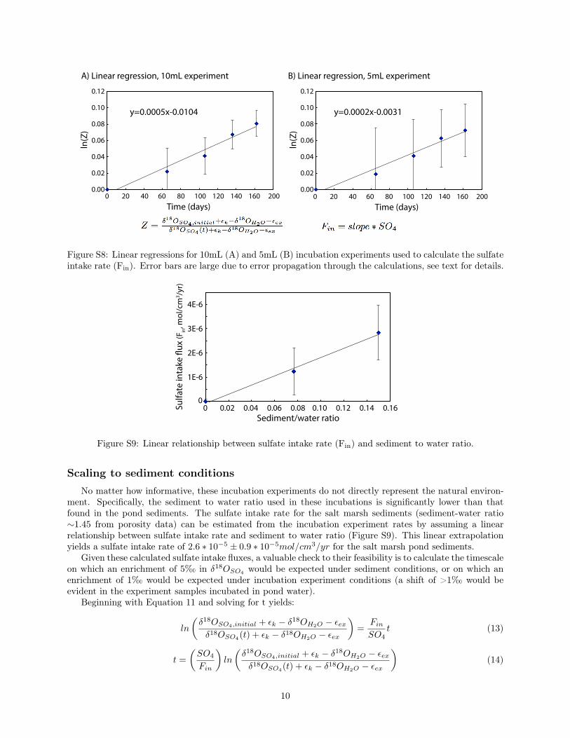
Figure S8: Linear regressions for 10mL (A) and 5mL (B) incubation experiments used to calculate the sulfateintake rate (F

in

). Error bars are large due to error propagation through the calculations, see text for details.

0 0.02 0.04 0.06 0.08 0.10 0.12 0.14 0.16Sediment/water ratio

0

1E-6

2E-6

3E-6

4E-6

Sulfa

te in

take

flux

(Fin

, mol

/cm

3 /yr)

Figure S9: Linear relationship between sulfate intake rate (Fin

) and sediment to water ratio.

Scaling to sediment conditions

No matter how informative, these incubation experiments do not directly represent the natural environ-ment. Specifically, the sediment to water ratio used in these incubations is significantly lower than thatfound in the pond sediments. The sulfate intake rate for the salt marsh sediments (sediment-water ratio⇠1.45 from porosity data) can be estimated from the incubation experiment rates by assuming a linearrelationship between sulfate intake rate and sediment to water ratio (Figure S9). This linear extrapolationyields a sulfate intake rate of 2.6 ⇤ 10�5 ± 0.9 ⇤ 10�5mol/cm3/yr for the salt marsh pond sediments.

Given these calculated sulfate intake fluxes, a valuable check to their feasibility is to calculate the timescaleon which an enrichment of 5‰ in �18OSO4 would be expected under sediment conditions, or on which anenrichment of 1‰ would be expected under incubation experiment conditions (a shift of >1‰ would beevident in the experiment samples incubated in pond water).

Beginning with Equation 11 and solving for t yields:

ln

✓�18OSO4,initial + ✏k � �18OH2O � ✏ex�18OSO4(t) + ✏k � �18OH2O � ✏ex

◆=

Fin

SO4t (13)

t =

✓SO4

Fin

◆ln

✓�18OSO4,initial + ✏k � �18OH2O � ✏ex�18OSO4(t) + ✏k � �18OH2O � ✏ex

◆(14)

10

Parameter Sediment conditions Incubation experiment conditions�18OSO4,initial 10‰ 10‰

SO4 28mM 14mM�18OH2O 0‰ -3‰

✏ex 25‰ 22-29‰✏k 0‰ 0‰

Fin

(mol/cm3/yr) 2.6 ⇤ 10�5 ± 0.9 ⇤ 10�5 2.6 ⇤ 10�5 ± 0.9 ⇤ 10�5 -2.6 ⇤ 10�5 ± 0.9 ⇤ 10�5 for ✏ex =22‰ and✏ex =29‰, respectively (10mL sample)

Table S2: Parameters for timescale of �18OSO4 enrichment calculations

For the parameters delineated in Table S1, under incubation experiment conditions with ✏ex=22‰, a 1‰shift in �18OSO4 would be expected after 208± 71 days; with ✏ex=29‰, a 1‰ shift would be expected afterjust 118± 42 days. Given that no significant shift in �18OSO4 is observed over the course of the experiment(162 days), this finding could suggest that the equilibrium isotope fractionation is on the smaller end ofthe range or that there is a non-negligible (positive) kinetic isotope effect not taken into account in thesecalculations. However, the error bars associated with the calculation are too large to make any definitivejudgments.

Under sediment conditions, a 5‰ shift in pore fluid �18OSO4 could be achieved after 160 ± 56 days(215 ± 76 days if a 38mM sulfate concentration is used to represent a hypersaline brine). This suggeststhat the �18OSO4 enrichments observed in the pore fluid profiles are possible even if the residence time ofsulfate in the system is short (<1 year). This is not to say that the sulfate in the pore fluids has simplybeen undergoing cryptic sulfur cycling for 160 days. The pore fluid �18OSO4 profile is at least in somepart controlled by delivery of sulfate from other sources in the salt marsh. It is thus difficult to estimate aresidence time for sulfate in the pore fluid system, and nearly impossible to determine a residence time ofsulfate in other locations within the salt marsh. This calculation simply confirms that a significant �18OSO4

enrichment can be achieved in a short period of time.

Comparison to other environments

The sulfate intake flux calculated for the cryptic sulfur cycling observed here can be compared to thatobserved during sulfate reduction in a range of natural environments using the dataset of �18OSO4 and�34SSO4 compiled and modelled by Antler et al., 2013 [6]. Here, it should be emphasized that the crypticsulfur cycling intake rate calculations used in the previous sections are derived from incubation experimentdata that has been extrapolated (significantly) to sediment conditions; this is not a direct comparison betweenrates measured in sediments, but it is informative nonetheless.

Antler and colleagues compiled a dataset of net sulfate reduction rates and the relative change of �18OSO4

vs. �34SSO4 (parameterized by the ’SALP’ (slope of the apparent linear phase) of the �18OSO4 vs. �34SSO4

cross-plot) from a range of environments with active sulfate reduction - from deep sea environments toestuaries. Given that the net sulfate reduction rate in the cryptic sulfur cycling observed here is zero, it ismore informative to compare rates of sulfate intake (i.e. flux of sulfate reduced to an intermediate valencestate sulfur species) across environments than sulfate reduction rates directly. Antler et al. utilize a reactivetransport model of bacterial sulfate reduction to parameterize a relationship between the SALP-1(inverseof the slope of the apparent linear phase) and X

3

- the ratio of the forward reduction flux of sulfate tosulfite (F

red

) and the backward oxidation flux of sulfite to sulfide (Box

) - see Figures S10 and S11. Here,we calculate X

3

for each of the natural system data points in the Antler et al., 2013 compilation, assumingopen-system conditions and a linear change between each of the data points calculated in the original model(Figure S11).

The sulfate intake flux can then be calculated directly from X3

and the net sulfate reduction rate (Fsulfide

in this model - Figure S10). X3

is simply the ratio of the backward oxidation to forward reduction fluxes ofsulfate to sulfite:

11

SO42-

(ex)

Bacterial Cell Membrane

SO4 incorporated, activated, and reduced

SO32- H2S

H2O

X3=Box

Fred

Fsulfide

Fred

Box

ε 18Oex

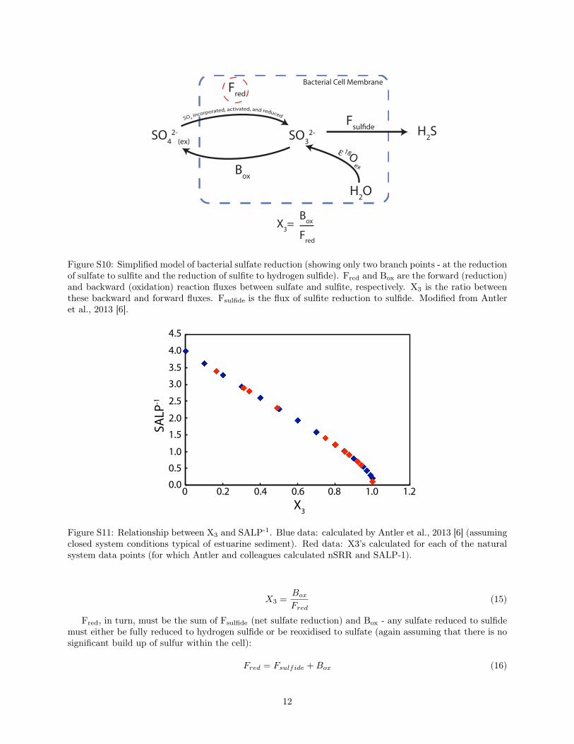
Figure S10: Simplified model of bacterial sulfate reduction (showing only two branch points - at the reductionof sulfate to sulfite and the reduction of sulfite to hydrogen sulfide). F

red

and Box

are the forward (reduction)and backward (oxidation) reaction fluxes between sulfate and sulfite, respectively. X

3

is the ratio betweenthese backward and forward fluxes. F

sulfide

is the flux of sulfite reduction to sulfide. Modified from Antleret al., 2013 [6].

0 0.2 0.4 0.6 0.8 1.0 1.2X3

SALP

-1

0.00.51.0

1.52.0

2.5

3.03.5

4.0

4.5

Figure S11: Relationship between X3

and SALP-1. Blue data: calculated by Antler et al., 2013 [6] (assumingclosed system conditions typical of estuarine sediment). Red data: X3’s calculated for each of the naturalsystem data points (for which Antler and colleagues calculated nSRR and SALP-1).

X3 =Box

Fred(15)

Fred

, in turn, must be the sum of Fsulfide

(net sulfate reduction) and Box

- any sulfate reduced to sulfidemust either be fully reduced to hydrogen sulfide or be reoxidised to sulfate (again assuming that there is nosignificant build up of sulfur within the cell):

Fred = Fsulfide +Box (16)

12

Fred = nSRR+Box (17)

Solving for Fred

:

X3 =Fred � nSRR

Fred(18)

Fred =nSRR

1�X3(19)

Compiled results can be found in Table S3 and Figure 5. The sulfate intake rate for the cryptic sulfurcycling in the Warham sediments is the same order of magnitude as sulfate intake rates seen in otherhigh-productivity environments like estuaries and the Amazon delta. However, while net sulfate reductionaccounts for more than half of the sulfate intake in most of these environments (with the exception of theAmazon delta, where sulfate reduction is only 20% of the total intake), at Warham there is no net removalof sulfate from the system.

Site Location SALP-1 nSRR(mol/cm3/yr)

X3

Sulfate intake rate(F

red

, mol/cm3/yr)Y1 Yarqon Stream estuary 2.3 3.0E-05 0.49 5.9E-05oil Gulf of Mexico 2.8 3.0E-05 0.34 4.6E-05

OST 2 Amazon delta 1.2 7.0E-06 0.80 3.5E-05Warham UK salt marsh (this study) 0 0.0E+00 1 2.6E-05

Y2 Yarqon Stream estuary 2.9 1.0E-05 0.31 1.5E-05red Gulf of Mexico 1.4 2.0E-06 0.75 7.9E-06BA1 Eastern Mediterranean 0.9 6.0E-08 0.88 4.8E-07HU Eastern Mediterranean 1 7.0E-08 0.85 4.7E-07

ODP 1123 SW Pacific 0.9 8.0E-12 0.88 6.4E-11ODP 1052 NW Atlantic 0.6 3.0E-12 0.94 5.0E-11ODP 807 NW Pacific 0.7 9.0E-13 0.92 1.1E-11

Table S3: Comparison of net sulfate reduction rates to sulfate intake rates in a range of environments. Datafrom Antler et al., 2013 [6] and the references contained within, other than the Warham salt marsh datapoint from this study (shown in bold).

13

Error Propagation

Error was propagated through the sulfate recycling rate calculations following the standard rules of errorpropagation described by Bevington and Robinson, 2002 [7].

For the function Z =�18OSO4,initial+✏k��18OH2O�✏ex

�18OSO4 (t)+✏k��18OH2O�✏exerror on �18OSO4(t) was calculated as (defining the

error to be �): �Z = Z ⇤⇣��18OSO4

(t)

�18OSO4 (t)

⌘. The error on ln(Z) was then calculated as: �ln(Z) =

�ZZ .

Linear regressions were calculated (taking the error in the dependent variable (�) into account) as:For the linear function: y(x) = a+ bx

a =1

�

✓X x2i

�2i

X yi�2i

�X xi

�2i

X xiyi�2i

◆

b =1

�

✓X 1

�2i

X xiyi�2i

�X xi

�2i

X yi�2i

◆

� =X 1

�2i

X x2i

�2i

�✓X xi

�2i

◆2

The error on the slope (�b) was calculated as:

�2b =

1

�

X 1

�2i

14

Supplemental References

[1] Nichols, M. L. & Smith, E. C. Coprecipitation with Barium Sulfate. The Journal of Physical Chemistry45, 411–421 (1941).

[2] Bao, H. Purifying barite for oxygen isotope measurement by dissolution and reprecipitation in a chelatingsolution. Analytical chemistry 78, 304–309 (2006).

[3] Alford, S. E., Alt, J. C. & Shanks III, W. C. Sulfur geochemistry and microbial sulfate reduction duringlow-temperature alteration of uplifted lower oceanic crust: insights from ODP Hole 735B. ChemicalGeology 286, 185–195 (2011).

[4] Sivan, O. et al. Geochemical evidence for iron-mediated anaerobic oxidation of methane. Limnology andOceanography 56, 1536–1544 (2011).

[5] Brunner, B., Bernasconi, S., Kleikemper, J. & Schroth, M. H. A model for oxygen and sulfur isotopefractionation in sulfate during bacterial sulfate reduction processes. Geochimica et Cosmochimica Acta69, 4773–4785 (2005).

[6] Antler, G., Turchyn, A. V., Rennie, V., Herut, B. & Sivan, O. Coupled sulfur and oxygen isotope insightinto bacterial sulfate reduction in the natural environment. Geochimica et Cosmochimica Acta 118,98–117 (2013).

[7] Bevington, P. R. & Robinson, D. K. Data reduction and error analysis for the physical sciences (McGraw-Hill New York, 2002), third edn.

15