Embed Size (px)
Citation preview
ARTICLE IN PRESS
0360-1323/$ - se
doi:10.1016/j.bu
�CorrespondE-mail addr
Building and Environment 41 (2006) 1339–1351
www.elsevier.com/locate/buildenv
Natural ventilation of multiple storey buildings: The use of stacksfor secondary ventilation
Stephen R Livermore�, Andrew W Woods
BP Institute for Multiphase flow, University of Cambridge, Cambridge CB3 0EZ, UK
Received 17 August 2004; received in revised form 19 April 2005; accepted 18 May 2005
Abstract
The natural ventilation of buildings may be enhanced by the use of stacks. As well as increasing the buoyancy pressure available
to drive a flow, the stacks may also be used to drive ventilation in floors where there is little heat load. This is achieved by connecting
the floor with a relatively low heat load to a floor with a higher heat load through a common stack. The warm air expelled from the
warmer space into the stack thereby drives a flow through the floor with no heat load. This principle of ventilation has been adopted
in the basement archive library of the new SSEES building at UCL. In this paper a series of laboratory experiments and supporting
quantitative models are used to investigate such secondary ventilation of a low level floor driven by a heat source in a higher level
floor. The magnitude of the secondary ventilation within the lower floor is shown to increase with the ratio of the size of the
openings on the lower to the upper floor and also the height of the stack. The results also indicate that the secondary ventilation
leads to a reduction in the magnitude of the ventilation through the upper floor, especially if the lower floor has a large inlet area.
r 2005 Elsevier Ltd. All rights reserved.
Keywords: Natural ventilation; Stacks; Secondary ventilation; Buoyancy
1. Introduction
There is increasing awareness of the high energyconsumption in buildings. Many buildings use mechan-ical air conditioning to regulate the internal environ-ment, but even with energy efficient designs, theytypically use around 230KWh=m2 of energy [1].However, in a number of buildings, alternative lowenergy systems use natural ventilation to significantlyreduce the energy consumption. Research has developeda good understanding of the basic principles of naturalventilation [2–4] within simple building structures. Oneof the key challenges now, is concerned with under-standing the subtleties of such flows within morecomplex multiple storey buildings.
A particular challenge associated with naturallyventilating large office spaces is the provision of
e front matter r 2005 Elsevier Ltd. All rights reserved.
ildenv.2005.05.037
ing author. Tel.: +441223 765711.
ess: [email protected] (S.R. Livermore).
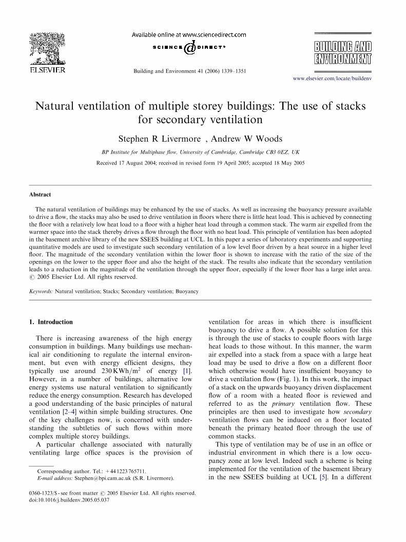
ventilation for areas in which there is insufficientbuoyancy to drive a flow. A possible solution for thisis through the use of stacks to couple floors with largeheat loads to those without. In this manner, the warmair expelled into a stack from a space with a large heatload may be used to drive a flow on a different floorwhich otherwise would have insufficient buoyancy todrive a ventilation flow (Fig. 1). In this work, the impactof a stack on the upwards buoyancy driven displacementflow of a room with a heated floor is reviewed andreferred to as the primary ventilation flow. Theseprinciples are then used to investigate how secondary
ventilation flows can be induced on a floor locatedbeneath the primary heated floor through the use ofcommon stacks.
This type of ventilation may be of use in an office orindustrial environment in which there is a low occu-pancy zone at low level. Indeed such a scheme is beingimplemented for the ventilation of the basement libraryin the new SSEES building at UCL [5]. In a different
ARTICLE IN PRESS
Fig. 1. Heat load on the upper floor driving the primary ventilation
flow. By coupling the two floors with a common stack, the warm
primary flow may be used to induce a secondary ventilation flow on
the lower floor.
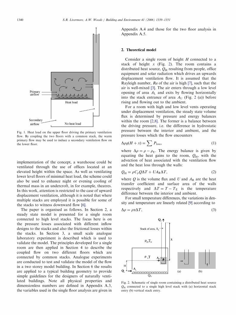
Fig. 2. Schematic of single room containing a distributed heat source
QH connected to a single high level stack with (a) horizontal stack
entry (b) vertical stack entry.
S.R. Livermore, A.W. Woods / Building and Environment 41 (2006) 1339–13511340
implementation of the concept, a warehouse could beventilated through the use of offices located at anelevated height within the space. As well as ventilatinglower level floors of minimal heat load, the scheme couldalso be used to enhance night or evening cooling ofthermal mass in an undercroft, in for example, theatres.In this work, attention is restricted to the case of upwarddisplacement ventilation, although it is noted that wheremultiple stacks are employed it is possible for some ofthe stacks to witness downward flow [6].
The paper is organised as follows. In Section 2, asteady state model is presented for a single roomconnected to high level stacks. The focus here is onthe pressure losses associated with different inflowdesigns to the stacks and also the frictional losses withinthe stacks. In Section 3, a small scale analoguelaboratory experiment is described which is used tovalidate the model. The principles developed for a singleroom are then applied in Section 4 to describe thecoupled flow on two different floors which areconnected by common stacks. Analogue experimentsare conducted to test and validate the model of the flowin a two storey model building. In Section 6 the resultsare applied to a typical building geometry to providesimple guidelines for the designers of naturally venti-lated buildings. Note all physical properties anddimensionless numbers are defined in Appendix A.3,the variables used in the single floor analysis are given in
Appendix A.4 and those for the two floor analysis inAppendix A.5.
2. Theoretical model
Consider a single room of height H connected to astack of height x (Fig. 2). The room contains adistributed heat source, QH resulting from people, officeequipment and solar radiation which drives an upwardsdisplacement ventilation flow. It is assumed that theRayleigh number, Ra of the air is high [7], such that theair is well-mixed [3]. The air enters through a low levelopening of area AL and exits by flowing horizontallyinto the stack entrance of area AU (Fig. 2 (a)) beforerising and flowing out to the ambient.
For a room with high and low level vents operatingunder displacement ventilation, the steady state volumeflux is determined by pressure and energy balanceswithin the room [2,8]. The former is a balance betweenthe driving pressure, i.e. the difference in hydrostaticpressure between the interior and ambient, and thepressure losses which the flow encounters
DrgðH þ xÞ ¼X
Ploss, (1)
where Dr ¼ r� rE. The energy balance is given byequating the heat gains to the room, QH, with theadvection of heat associated with the ventilation flowand the heat loss through the walls:
QH ¼ rCpQDT þUARDT , (2)
where Q is the volume flux and U and AR are the heattransfer coefficient and surface area of the wallsrespectively and DT ¼ T � TE is the temperaturedifference between the interior and ambient.
For small temperature differences, the variations in den-sity and temperature are linearly related [9] according to
Dr ¼ raDT , (3)
ARTICLE IN PRESS
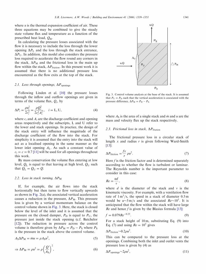
Fig. 3. Control volume analysis at the base of the stack. It is assumed
that PU ¼ PD such that the vertical acceleration is associated with the
pressure difference, DPM ¼ PD � PS.
S.R. Livermore, A.W. Woods / Building and Environment 41 (2006) 1339–1351 1341
where a is the thermal expansion coefficient of air. Thesethree equations may be combined to give the steadystate volume flux and temperature as a function of theprescribed heat load, QH.
In calculating the pressure losses associated with theflow it is necessary to include the loss through the loweropening DPL and the loss through the stack entrance,DPU. In addition, this model also considers the pressureloss required to accelerate the flow round any corners inthe stack, DPM and the frictional loss in the main upflow within the stack, DPfriction. In this present work it isassumed that there is no additional pressure lossencountered as the flow exits at the top of the stack.
2.1. Loss through openings, DPopenings
Following Linden et al. [10] the pressure lossesthrough the inflow and outflow openings are given interms of the volume flux, Qi, by
DPi ¼ru2
i
2c2i¼
rQ2i
2c2i A2i
; i ¼ L;U, (4)
where ci and Ai are the discharge coefficient and openingareas respectively and the subscripts, L and U refer tothe lower and stack openings. In practice, the design ofthe stack entry will influence the magnitude of thedischarge coefficient of the flow into the stack. Forsimplicity it is assumed that the entry into the stack willact as a localised opening in the same manner as thelower inlet opening AL. As such a constant value ofci ¼ c ¼ 0:7 [11] will be used for all openings throughoutthis work.
By mass conservation the volume flux entering at lowlevel, QL is equal to that leaving at high level, QU suchthat QL ¼ QU ¼ Q.
2.2. Loss in stack turning, DPM
If, for example, the air flows into the stackhorizontally but then turns to flow vertically upwardsas shown in Fig. 2(a), the associated vertical accelerationcauses a reduction in the pressure, DPM. This pressureloss is given by a vertical momentum balance on thecontrol volume shown in Fig. 3. Here, the stack is closedbelow the level of the inlet and it is assumed that thepressure on the closed damper, PD is equal to PU, thepressure just inside the stack opening (c.f. Batchelor[12]). The reduction in pressure across the controlvolume is therefore given by DPM ¼ PD � PS where PS
is the pressure in the stack above the control volume.
ASDPM ¼ _mu ¼ rASu2, (5)
) DPM ¼ ru2 ¼ rQ
AS
� �2
, (6)
where AS is the area of a single stack and _m and u are themass and velocity flux up the stack respectively.
2.3. Frictional loss in stack, DPfriction
The frictional pressure loss in a circular stack oflength x and radius r is given following Ward-Smith[13]:
DPfriction ¼fx
rru2. (7)
Here f is the friction factor and is determined separatelyaccording to whether the flow is turbulent or laminar.The Reynolds number is the important parameter toconsider in this case:
Re ¼ud
n, (8)
where d is the diameter of the stack and n is thekinematic viscosity. For example, with a ventilation flowrate of 1m3=s, the speed in a stack of diameter 0.5mwould be u�5m=s and the associated Re�105. It isanticipated that the flow within the stack will have largeRe and hence f is given by the Blasius formula [13]:
f ¼ 0:079Re�0:25. (9)
For a stack height of 10m, substituting Eq. (9) intoEq. (7) and using Re ¼ 105 gives
DPfriction�0:2ru2. (10)
This can be compared to the pressure loss at theopenings. Combining both the inlet and outlet vents thepressure loss is given by (4) as
DPopenings�2ru2, (11)
ARTICLE IN PRESSS.R. Livermore, A.W. Woods / Building and Environment 41 (2006) 1339–13511342
which is a factor of 10 greater than DPfriction. Thereforethe pressure loss resulting from friction within the stacksis only of secondary importance compared to thepressure losses at the openings and that due to themomentum change within the stack. Consequently it canbe omitted from the model.
2.3.1. Pressure and energy balances
By combining Eqs. (1), (4) and (6) the pressurebalance for the case of one stack is given by therelation
DrgðH þ xÞ ¼ rQ2 1
2c2A2L
þ1
2c2A2U
þ1
A2S
!, (12)
which can be rearranged into the form
Q ¼ A�Drr
gðH þ xÞ
� �1=2
. (13)
Here A� is the effective area given by
A� ¼
ffiffiffi2p
cALAUASffiffiffiffiffiffiffiffiffiffiffiffiffiffiffiffiffiffiffiffiffiffiffiffiffiffiffiffiffiffiffiffiffiffiffiffiffiffiffiffiffiffiffiffiffiffiffiffiffiffiffiffiffiffiffi2c2A2
LA2U þ A2
LA2S þ A2
UA2S
q . (14)
If it is assumed that the room is well insulated, the heatloss through the walls will be negligible compared withthe heat lost by advection through the openings. Thesteady state ventilation flow, Q is given in terms of aprescribed heat flux, QH as
Q ¼ A�2=3gaQHðH þ xÞ
rCp
� �1=3
. (15)
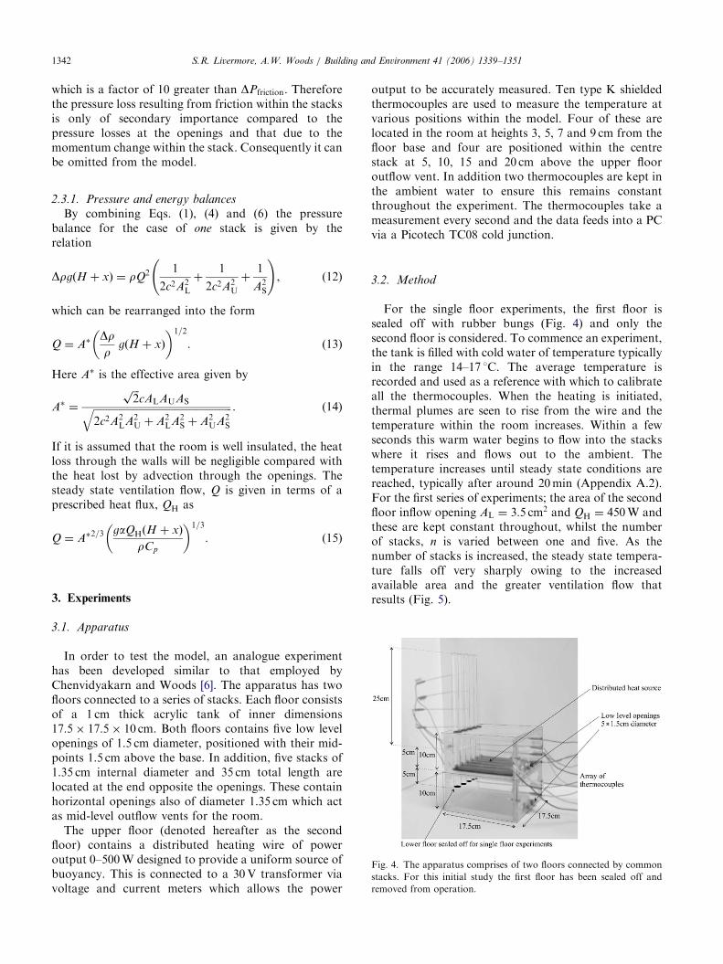
Fig. 4. The apparatus comprises of two floors connected by common
stacks. For this initial study the first floor has been sealed off and
removed from operation.
3. Experiments
3.1. Apparatus
In order to test the model, an analogue experimenthas been developed similar to that employed byChenvidyakarn and Woods [6]. The apparatus has twofloors connected to a series of stacks. Each floor consistsof a 1 cm thick acrylic tank of inner dimensions17:5� 17:5� 10 cm. Both floors contains five low levelopenings of 1.5 cm diameter, positioned with their mid-points 1.5 cm above the base. In addition, five stacks of1.35 cm internal diameter and 35 cm total length arelocated at the end opposite the openings. These containhorizontal openings also of diameter 1.35 cm which actas mid-level outflow vents for the room.
The upper floor (denoted hereafter as the secondfloor) contains a distributed heating wire of poweroutput 0–500W designed to provide a uniform source ofbuoyancy. This is connected to a 30V transformer viavoltage and current meters which allows the power
output to be accurately measured. Ten type K shieldedthermocouples are used to measure the temperature atvarious positions within the model. Four of these arelocated in the room at heights 3, 5, 7 and 9 cm from thefloor base and four are positioned within the centrestack at 5, 10, 15 and 20 cm above the upper flooroutflow vent. In addition two thermocouples are kept inthe ambient water to ensure this remains constantthroughout the experiment. The thermocouples take ameasurement every second and the data feeds into a PCvia a Picotech TC08 cold junction.
3.2. Method
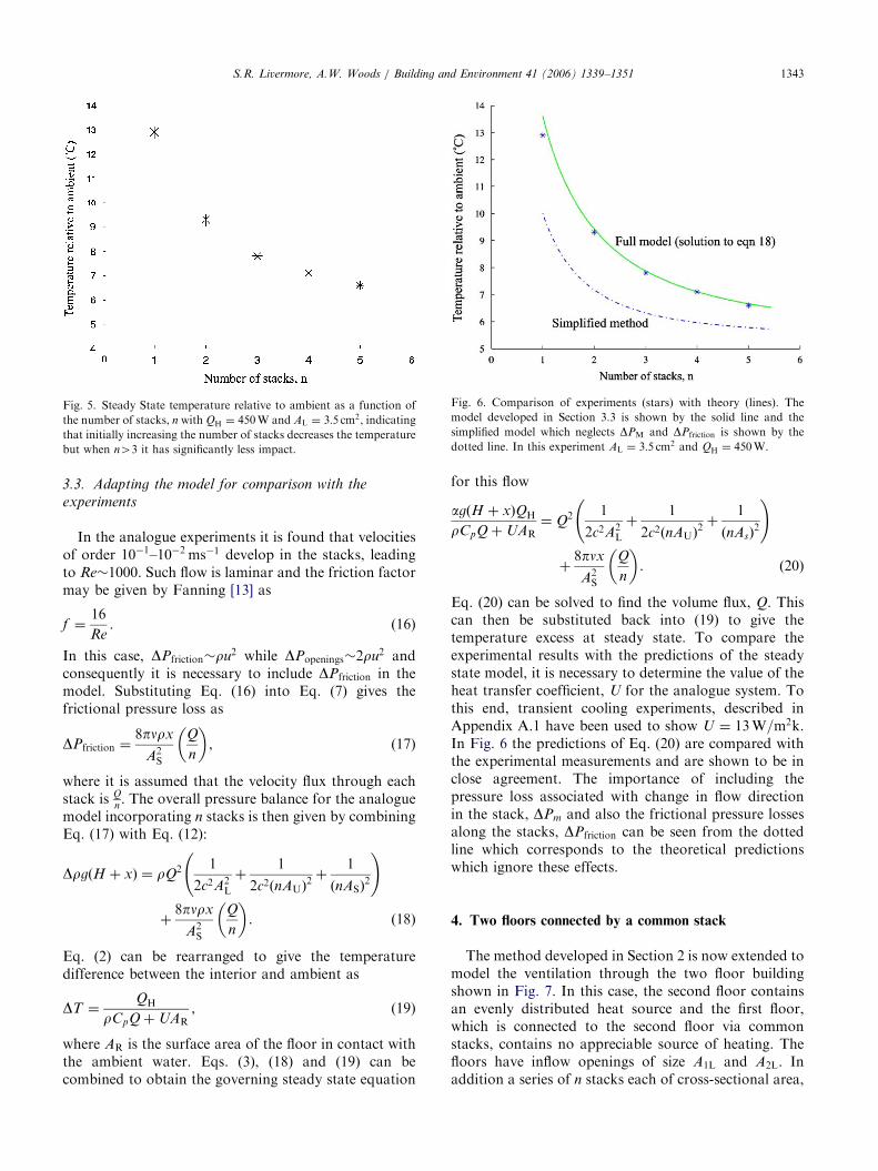
For the single floor experiments, the first floor issealed off with rubber bungs (Fig. 4) and only thesecond floor is considered. To commence an experiment,the tank is filled with cold water of temperature typicallyin the range 14–17 1C. The average temperature isrecorded and used as a reference with which to calibrateall the thermocouples. When the heating is initiated,thermal plumes are seen to rise from the wire and thetemperature within the room increases. Within a fewseconds this warm water begins to flow into the stackswhere it rises and flows out to the ambient. Thetemperature increases until steady state conditions arereached, typically after around 20min (Appendix A.2).For the first series of experiments; the area of the secondfloor inflow opening AL ¼ 3:5 cm2 and QH ¼ 450W andthese are kept constant throughout, whilst the numberof stacks, n is varied between one and five. As thenumber of stacks is increased, the steady state tempera-ture falls off very sharply owing to the increasedavailable area and the greater ventilation flow thatresults (Fig. 5).
ARTICLE IN PRESS
Fig. 5. Steady State temperature relative to ambient as a function of
the number of stacks, n with QH ¼ 450W and AL ¼ 3:5 cm2, indicating
that initially increasing the number of stacks decreases the temperature
but when n43 it has significantly less impact.
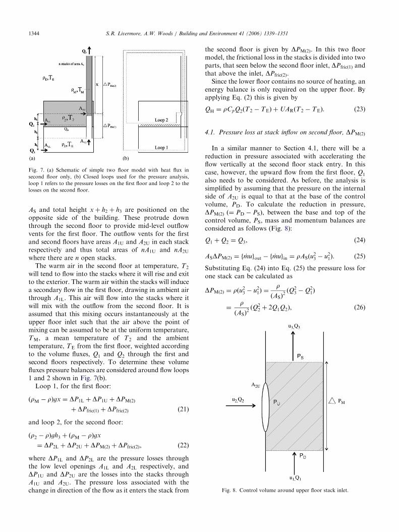
Fig. 6. Comparison of experiments (stars) with theory (lines). The
model developed in Section 3.3 is shown by the solid line and the
simplified model which neglects DPM and DPfriction is shown by the
dotted line. In this experiment AL ¼ 3:5 cm2 and QH ¼ 450W.
S.R. Livermore, A.W. Woods / Building and Environment 41 (2006) 1339–1351 1343
3.3. Adapting the model for comparison with the
experiments
In the analogue experiments it is found that velocitiesof order 10�1–10�2 ms�1 develop in the stacks, leadingto Re�1000. Such flow is laminar and the friction factormay be given by Fanning [13] as
f ¼16
Re. (16)
In this case, DPfriction�ru2 while DPopenings�2ru2 andconsequently it is necessary to include DPfriction in themodel. Substituting Eq. (16) into Eq. (7) gives thefrictional pressure loss as
DPfriction ¼8pnrx
A2S
Q
n
� �, (17)
where it is assumed that the velocity flux through eachstack is Q
n. The overall pressure balance for the analogue
model incorporating n stacks is then given by combiningEq. (17) with Eq. (12):
DrgðH þ xÞ ¼ rQ2 1
2c2A2L
þ1
2c2ðnAUÞ2þ
1
ðnASÞ2
!
þ8pnrx
A2S
Q
n
� �. ð18Þ
Eq. (2) can be rearranged to give the temperaturedifference between the interior and ambient as
DT ¼QH
rCpQþUAR, (19)
where AR is the surface area of the floor in contact withthe ambient water. Eqs. (3), (18) and (19) can becombined to obtain the governing steady state equation
for this flow
agðH þ xÞQH
rCpQþUAR¼ Q2 1
2c2A2L
þ1
2c2ðnAUÞ2þ
1
ðnAsÞ2
!
þ8pnx
A2S
Q
n
� �. ð20Þ
Eq. (20) can be solved to find the volume flux, Q. Thiscan then be substituted back into (19) to give thetemperature excess at steady state. To compare theexperimental results with the predictions of the steadystate model, it is necessary to determine the value of theheat transfer coefficient, U for the analogue system. Tothis end, transient cooling experiments, described inAppendix A.1 have been used to show U ¼ 13W=m2k.In Fig. 6 the predictions of Eq. (20) are compared withthe experimental measurements and are shown to be inclose agreement. The importance of including thepressure loss associated with change in flow directionin the stack, DPm and also the frictional pressure lossesalong the stacks, DPfriction can be seen from the dottedline which corresponds to the theoretical predictionswhich ignore these effects.
4. Two floors connected by a common stack
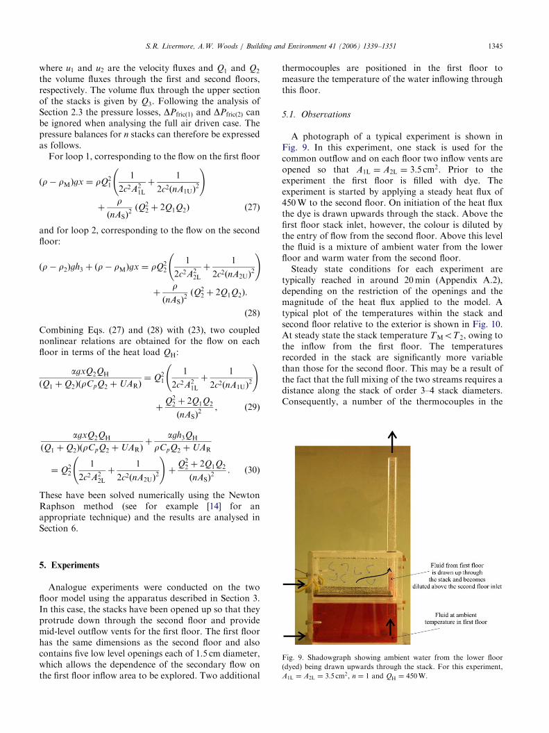
The method developed in Section 2 is now extended tomodel the ventilation through the two floor buildingshown in Fig. 7. In this case, the second floor containsan evenly distributed heat source and the first floor,which is connected to the second floor via commonstacks, contains no appreciable source of heating. Thefloors have inflow openings of size A1L and A2L. Inaddition a series of n stacks each of cross-sectional area,
ARTICLE IN PRESS
Fig. 7. (a) Schematic of simple two floor model with heat flux in
second floor only, (b) Closed loops used for the pressure analysis,
loop 1 refers to the pressure losses on the first floor and loop 2 to the
losses on the second floor.
Fig. 8. Control volume around upper floor stack inlet.
S.R. Livermore, A.W. Woods / Building and Environment 41 (2006) 1339–13511344
AS and total height xþ h2 þ h3 are positioned on theopposite side of the building. These protrude downthrough the second floor to provide mid-level outflowvents for the first floor. The outflow vents for the firstand second floors have areas A1U and A2U in each stackrespectively and thus total areas of nA1U and nA2U
where there are n open stacks.The warm air in the second floor at temperature, T2
will tend to flow into the stacks where it will rise and exitto the exterior. The warm air within the stacks will inducea secondary flow in the first floor, drawing in ambient airthrough A1L. This air will flow into the stacks where itwill mix with the outflow from the second floor. It isassumed that this mixing occurs instantaneously at theupper floor inlet such that the air above the point ofmixing can be assumed to be at the uniform temperature,TM, a mean temperature of T2 and the ambienttemperature, TE from the first floor, weighted accordingto the volume fluxes, Q1 and Q2 through the first andsecond floors respectively. To determine these volumefluxes pressure balances are considered around flow loops1 and 2 shown in Fig. 7(b).
Loop 1, for the first floor:
ðrM � rÞgx ¼ DP1L þ DP1U þ DPMð2Þ
þ DPfricð1Þ þ DPfricð2Þ ð21Þ
and loop 2, for the second floor:
ðr2 � rÞgh3 þ ðrM � rÞgx
¼ DP2L þ DP2U þ DPMð2Þ þ DPfricð2Þ, ð22Þ
where DP1L and DP2L are the pressure losses throughthe low level openings A1L and A2L respectively, andDP1U and DP2U are the losses into the stacks throughA1U and A2U. The pressure loss associated with thechange in direction of the flow as it enters the stack from
the second floor is given by DPMð2Þ. In this two floormodel, the frictional loss in the stacks is divided into twoparts, that seen below the second floor inlet, DPfricð1Þ andthat above the inlet, DPfricð2Þ.
Since the lower floor contains no source of heating, anenergy balance is only required on the upper floor. Byapplying Eq. (2) this is given by
QH ¼ rCpQ2ðT2 � TEÞ þUARðT2 � TEÞ. (23)
4.1. Pressure loss at stack inflow on second floor, DPMð2Þ
In a similar manner to Section 4.1, there will be areduction in pressure associated with accelerating theflow vertically at the second floor stack entry. In thiscase, however, the upward flow from the first floor, Q1
also needs to be considered. As before, the analysis issimplified by assuming that the pressure on the internalside of A2U is equal to that at the base of the controlvolume, PD. To calculate the reduction in pressure,DPMð2Þ ð¼ PD � PSÞ, between the base and top of thecontrol volume, PS, mass and momentum balances areconsidered as follows (Fig. 8):
Q1 þQ2 ¼ Q3, (24)
ASDPMð2Þ ¼ f _mugout � f _mugin ¼ rASðu23 � u2
1Þ. (25)
Substituting Eq. (24) into Eq. (25) the pressure loss forone stack can be calculated as
DPMð2Þ ¼ rðu23 � u2
1Þ ¼r
ðASÞ2ðQ2
3 �Q21Þ
¼r
ðASÞ2ðQ2
2 þ 2Q1Q2Þ, ð26Þ
ARTICLE IN PRESSS.R. Livermore, A.W. Woods / Building and Environment 41 (2006) 1339–1351 1345
where u1 and u2 are the velocity fluxes and Q1 and Q2
the volume fluxes through the first and second floors,respectively. The volume flux through the upper sectionof the stacks is given by Q3. Following the analysis ofSection 2.3 the pressure losses, DPfricð1Þ and DPfricð2Þ canbe ignored when analysing the full air driven case. Thepressure balances for n stacks can therefore be expressedas follows.
For loop 1, corresponding to the flow on the first floor
ðr� rMÞgx ¼ rQ21
1
2c2A21L
þ1
2c2ðnA1UÞ2
!
þr
ðnASÞ2ðQ2
2 þ 2Q1Q2Þ ð27Þ
and for loop 2, corresponding to the flow on the secondfloor:
ðr� r2Þgh3 þ ðr� rMÞgx ¼ rQ22
1
2c2A22L
þ1
2c2ðnA2UÞ2
!
þr
ðnASÞ2ðQ2
2 þ 2Q1Q2Þ.
ð28Þ
Combining Eqs. (27) and (28) with (23), two couplednonlinear relations are obtained for the flow on eachfloor in terms of the heat load QH:
agxQ2QH
ðQ1 þQ2ÞðrCpQ2 þUARÞ¼ Q2
1
1
2c2A21L
þ1
2c2ðnA1UÞ2
!
þQ2
2 þ 2Q1Q2
ðnASÞ2
, ð29Þ
agxQ2QH
ðQ1 þQ2ÞðrCpQ2 þUARÞþ
agh3QH
rCpQ2 þUAR
¼ Q22
1
2c2A22L
þ1
2c2ðnA2UÞ2
!þ
Q22 þ 2Q1Q2
ðnASÞ2
. ð30Þ
These have been solved numerically using the NewtonRaphson method (see for example [14] for anappropriate technique) and the results are analysed inSection 6.
Fig. 9. Shadowgraph showing ambient water from the lower floor
(dyed) being drawn upwards through the stack. For this experiment,
A1L ¼ A2L ¼ 3:5 cm2, n ¼ 1 and QH ¼ 450W.
5. Experiments
Analogue experiments were conducted on the twofloor model using the apparatus described in Section 3.In this case, the stacks have been opened up so that theyprotrude down through the second floor and providemid-level outflow vents for the first floor. The first floorhas the same dimensions as the second floor and alsocontains five low level openings each of 1.5 cm diameter,which allows the dependence of the secondary flow onthe first floor inflow area to be explored. Two additional
thermocouples are positioned in the first floor tomeasure the temperature of the water inflowing throughthis floor.
5.1. Observations
A photograph of a typical experiment is shown inFig. 9. In this experiment, one stack is used for thecommon outflow and on each floor two inflow vents areopened so that A1L ¼ A2L ¼ 3:5 cm2. Prior to theexperiment the first floor is filled with dye. Theexperiment is started by applying a steady heat flux of450W to the second floor. On initiation of the heat fluxthe dye is drawn upwards through the stack. Above thefirst floor stack inlet, however, the colour is diluted bythe entry of flow from the second floor. Above this levelthe fluid is a mixture of ambient water from the lowerfloor and warm water from the second floor.
Steady state conditions for each experiment aretypically reached in around 20min (Appendix A.2),depending on the restriction of the openings and themagnitude of the heat flux applied to the model. Atypical plot of the temperatures within the stack andsecond floor relative to the exterior is shown in Fig. 10.At steady state the stack temperature TMoT2, owing tothe inflow from the first floor. The temperaturesrecorded in the stack are significantly more variablethan those for the second floor. This may be a result ofthe fact that the full mixing of the two streams requires adistance along the stack of order 3–4 stack diameters.Consequently, a number of the thermocouples in the
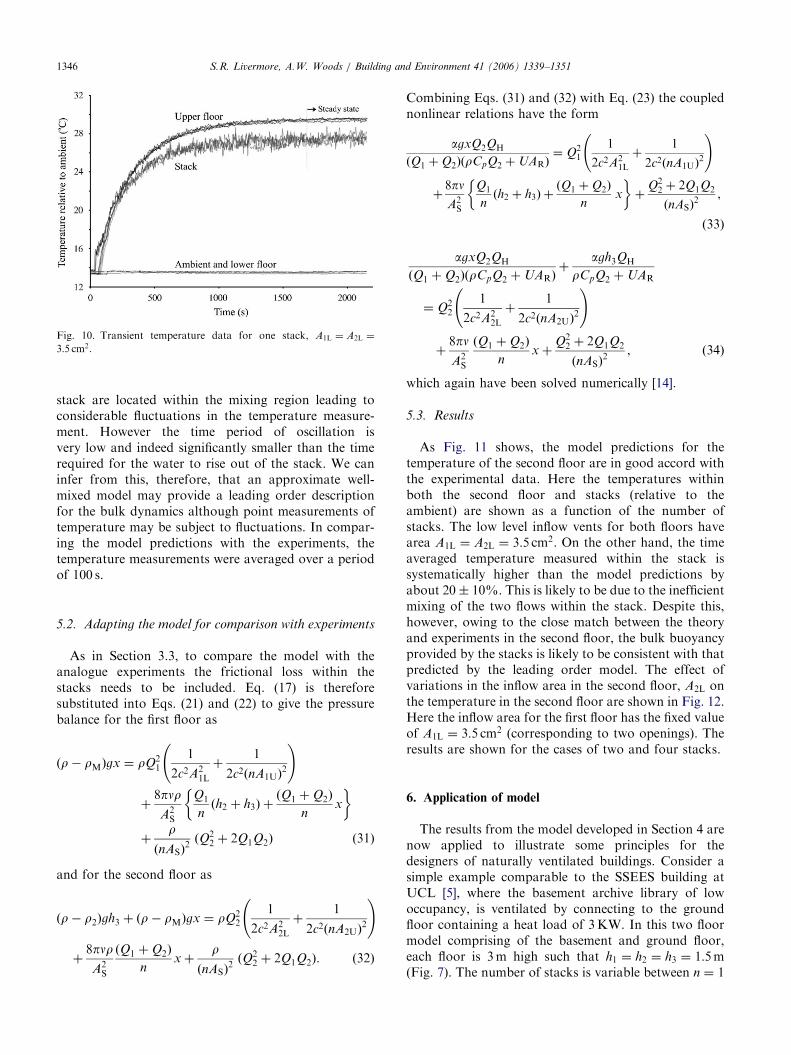
ARTICLE IN PRESS
Fig. 10. Transient temperature data for one stack, A1L ¼ A2L ¼
3:5 cm2.
S.R. Livermore, A.W. Woods / Building and Environment 41 (2006) 1339–13511346
stack are located within the mixing region leading toconsiderable fluctuations in the temperature measure-ment. However the time period of oscillation isvery low and indeed significantly smaller than the timerequired for the water to rise out of the stack. We caninfer from this, therefore, that an approximate well-mixed model may provide a leading order descriptionfor the bulk dynamics although point measurements oftemperature may be subject to fluctuations. In compar-ing the model predictions with the experiments, thetemperature measurements were averaged over a periodof 100 s.
5.2. Adapting the model for comparison with experiments
As in Section 3.3, to compare the model with theanalogue experiments the frictional loss within thestacks needs to be included. Eq. (17) is thereforesubstituted into Eqs. (21) and (22) to give the pressurebalance for the first floor as
ðr� rMÞgx ¼ rQ21
1
2c2A21L
þ1
2c2ðnA1UÞ2
!
þ8pnr
A2S
Q1
nðh2 þ h3Þ þ
ðQ1 þQ2Þ
nx
� �
þr
ðnASÞ2ðQ2
2 þ 2Q1Q2Þ ð31Þ
and for the second floor as
ðr� r2Þgh3 þ ðr� rMÞgx ¼ rQ22
1
2c2A22L
þ1
2c2ðnA2UÞ2
!
þ8pnr
A2S
ðQ1 þQ2Þ
nxþ
r
ðnASÞ2ðQ2
2 þ 2Q1Q2Þ. ð32Þ
Combining Eqs. (31) and (32) with Eq. (23) the couplednonlinear relations have the form
agxQ2QH
ðQ1 þQ2ÞðrCpQ2 þUARÞ¼ Q2
1
1
2c2A21L
þ1
2c2ðnA1UÞ2
!
þ8pn
A2S
Q1
nðh2 þ h3Þ þ
ðQ1 þQ2Þ
nx
� �þ
Q22 þ 2Q1Q2
ðnASÞ2
,
ð33Þ
agxQ2QH
ðQ1 þQ2ÞðrCpQ2 þUARÞþ
agh3QH
rCpQ2 þUAR
¼ Q22
1
2c2A22L
þ1
2c2ðnA2UÞ2
!
þ8pn
A2S
ðQ1 þQ2Þ
nxþ
Q22 þ 2Q1Q2
ðnASÞ2
, ð34Þ
which again have been solved numerically [14].
5.3. Results
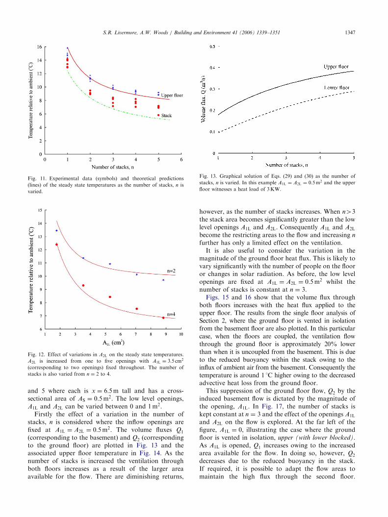
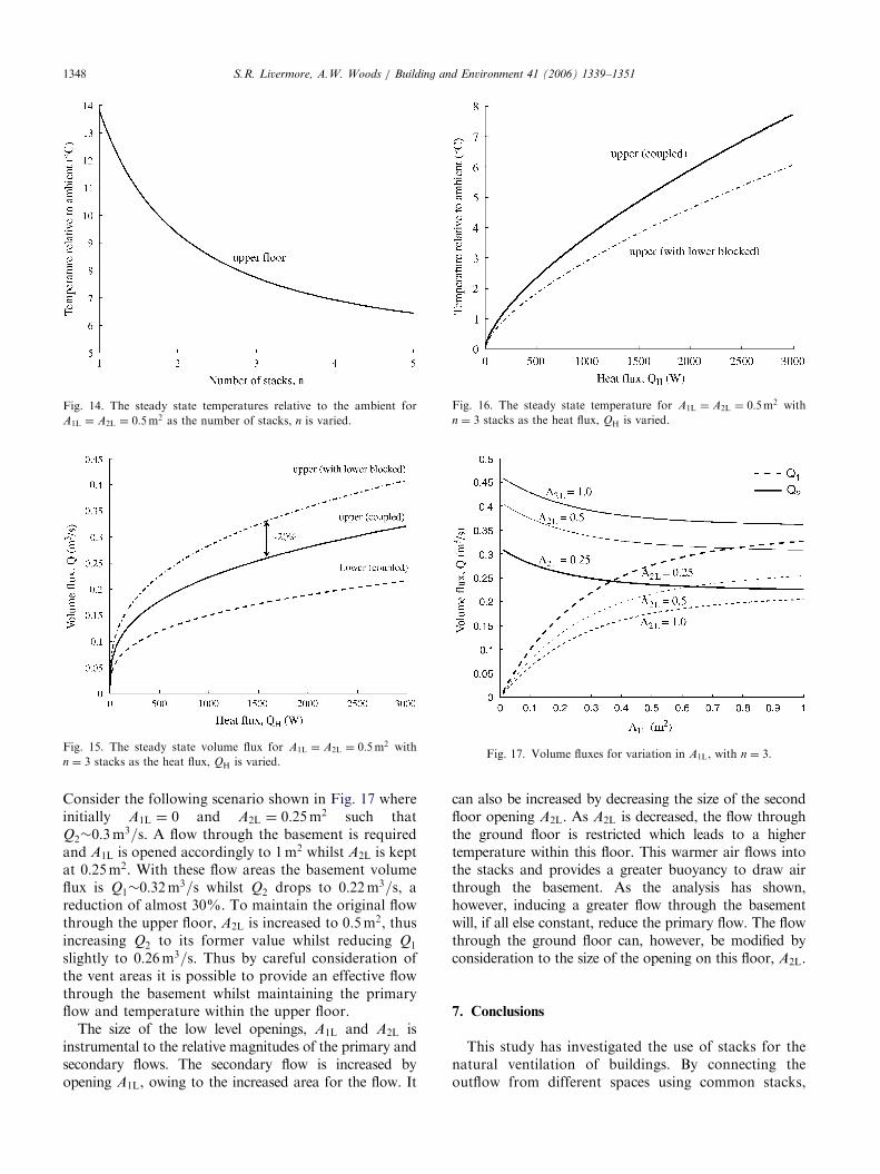
As Fig. 11 shows, the model predictions for thetemperature of the second floor are in good accord withthe experimental data. Here the temperatures withinboth the second floor and stacks (relative to theambient) are shown as a function of the number ofstacks. The low level inflow vents for both floors havearea A1L ¼ A2L ¼ 3:5 cm2. On the other hand, the timeaveraged temperature measured within the stack issystematically higher than the model predictions byabout 20� 10%. This is likely to be due to the inefficientmixing of the two flows within the stack. Despite this,however, owing to the close match between the theoryand experiments in the second floor, the bulk buoyancyprovided by the stacks is likely to be consistent with thatpredicted by the leading order model. The effect ofvariations in the inflow area in the second floor, A2L onthe temperature in the second floor are shown in Fig. 12.Here the inflow area for the first floor has the fixed valueof A1L ¼ 3:5 cm2 (corresponding to two openings). Theresults are shown for the cases of two and four stacks.
6. Application of model
The results from the model developed in Section 4 arenow applied to illustrate some principles for thedesigners of naturally ventilated buildings. Consider asimple example comparable to the SSEES building atUCL [5], where the basement archive library of lowoccupancy, is ventilated by connecting to the groundfloor containing a heat load of 3KW. In this two floormodel comprising of the basement and ground floor,each floor is 3m high such that h1 ¼ h2 ¼ h3 ¼ 1:5m(Fig. 7). The number of stacks is variable between n ¼ 1
ARTICLE IN PRESS
Fig. 12. Effect of variations in A2L on the steady state temperatures.
A2L is increased from one to five openings with A1L ¼ 3:5 cm2
(corresponding to two openings) fixed throughout. The number of
stacks is also varied from n ¼ 2 to 4.
Fig. 13. Graphical solution of Eqs. (29) and (30) as the number of
stacks, n is varied. In this example A1L ¼ A2L ¼ 0:5m2 and the upper
floor witnesses a heat load of 3KW.
Fig. 11. Experimental data (symbols) and theoretical predictions
(lines) of the steady state temperatures as the number of stacks, n is
varied.
S.R. Livermore, A.W. Woods / Building and Environment 41 (2006) 1339–1351 1347
and 5 where each is x ¼ 6:5m tall and has a cross-sectional area of AS ¼ 0:5m2. The low level openings,A1L and A2L can be varied between 0 and 1m2.
Firstly the effect of a variation in the number ofstacks, n is considered where the inflow openings arefixed at A1L ¼ A2L ¼ 0:5m2. The volume fluxes Q1
(corresponding to the basement) and Q2 (correspondingto the ground floor) are plotted in Fig. 13 and theassociated upper floor temperature in Fig. 14. As thenumber of stacks is increased the ventilation throughboth floors increases as a result of the larger areaavailable for the flow. There are diminishing returns,
however, as the number of stacks increases. When n43the stack area becomes significantly greater than the lowlevel openings A1L and A2L. Consequently A1L and A2L
become the restricting areas to the flow and increasing n
further has only a limited effect on the ventilation.It is also useful to consider the variation in the
magnitude of the ground floor heat flux. This is likely tovary significantly with the number of people on the flooror changes in solar radiation. As before, the low levelopenings are fixed at A1L ¼ A2L ¼ 0:5m2 whilst thenumber of stacks is constant at n ¼ 3.
Figs. 15 and 16 show that the volume flux throughboth floors increases with the heat flux applied to theupper floor. The results from the single floor analysis ofSection 2, where the ground floor is vented in isolationfrom the basement floor are also plotted. In this particularcase, when the floors are coupled, the ventilation flowthrough the ground floor is approximately 20% lowerthan when it is uncoupled from the basement. This is dueto the reduced buoyancy within the stack owing to theinflux of ambient air from the basement. Consequently thetemperature is around 1 1C higher owing to the decreasedadvective heat loss from the ground floor.
This suppression of the ground floor flow, Q2 by theinduced basement flow is dictated by the magnitude ofthe opening, A1L. In Fig. 17, the number of stacks iskept constant at n ¼ 3 and the effect of the openings A1L
and A2L on the flow is explored. At the far left of thefigure, A1L ¼ 0, illustrating the case where the groundfloor is vented in isolation, upper (with lower blocked).As A1L is opened, Q1 increases owing to the increasedarea available for the flow. In doing so, however, Q2
decreases due to the reduced buoyancy in the stack.If required, it is possible to adapt the flow areas tomaintain the high flux through the second floor.
ARTICLE IN PRESS
Fig. 14. The steady state temperatures relative to the ambient for
A1L ¼ A2L ¼ 0:5m2 as the number of stacks, n is varied.
Fig. 15. The steady state volume flux for A1L ¼ A2L ¼ 0:5m2 with
n ¼ 3 stacks as the heat flux, QH is varied.
Fig. 16. The steady state temperature for A1L ¼ A2L ¼ 0:5m2 with
n ¼ 3 stacks as the heat flux, QH is varied.
Fig. 17. Volume fluxes for variation in A1L, with n ¼ 3.
S.R. Livermore, A.W. Woods / Building and Environment 41 (2006) 1339–13511348
Consider the following scenario shown in Fig. 17 whereinitially A1L ¼ 0 and A2L ¼ 0:25m2 such thatQ2�0:3m
3=s. A flow through the basement is requiredand A1L is opened accordingly to 1m2 whilst A2L is keptat 0:25m2. With these flow areas the basement volumeflux is Q1�0:32m
3=s whilst Q2 drops to 0:22m3=s, areduction of almost 30%. To maintain the original flowthrough the upper floor, A2L is increased to 0:5m2, thusincreasing Q2 to its former value whilst reducing Q1
slightly to 0:26m3=s. Thus by careful consideration ofthe vent areas it is possible to provide an effective flowthrough the basement whilst maintaining the primaryflow and temperature within the upper floor.
The size of the low level openings, A1L and A2L isinstrumental to the relative magnitudes of the primary andsecondary flows. The secondary flow is increased byopening A1L, owing to the increased area for the flow. It
can also be increased by decreasing the size of the secondfloor opening A2L. As A2L is decreased, the flow throughthe ground floor is restricted which leads to a highertemperature within this floor. This warmer air flows intothe stacks and provides a greater buoyancy to draw airthrough the basement. As the analysis has shown,however, inducing a greater flow through the basementwill, if all else constant, reduce the primary flow. The flowthrough the ground floor can, however, be modified byconsideration to the size of the opening on this floor, A2L.
7. Conclusions
This study has investigated the use of stacks for thenatural ventilation of buildings. By connecting theoutflow from different spaces using common stacks,
ARTICLE IN PRESS
Fig. 18. Transient heat loss experiment, showing the temperature in
the upper floor, T , the theoretical prediction (Eq. (39)) and also the
ambient temperature TE.
S.R. Livermore, A.W. Woods / Building and Environment 41 (2006) 1339–1351 1349
buoyant air may be used to induce a secondary flow in aspace with insufficient heat load to drive a flow. A modelhas been derived to predict the ventilation within anunheated low level floor coupled with a higher levelheated floor. The model has been tested experimentallyand the results are in close agreement with thetheoretical predictions. The analysis has shown thatthe secondary ventilation increases with the ratio of thesize of the openings between the lower to the upper floorand also the area of the stacks. In driving this secondaryventilation, however, the primary ventilation will bereduced, in some cases by as much as 20% and thesteady state temperature increased by 1–1.5 1C. Thereduction of the primary ventilation can be minimised,however, by careful design of the low level opening A1L,ensuring that it is large enough to promote the sec-ondary flow but not to the extent that it adversely effectsthe primary flow. Alternatively, the primary flow may beenhanced by opening up the upper inlet vent, A2L.
Acknowledgements
This study was funded by the Cambridge-MITInstitute (CMI) and the BP institute for MultiphaseFlow. The authors thank Charlotte Gladstone forhelpful discussions.
Appendix A
A.1. Calculation of heat transfer coefficient
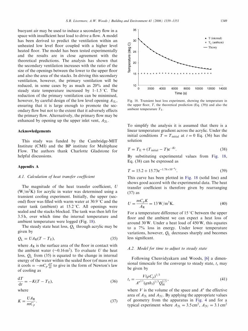
The magnitude of the heat transfer coefficient, U
ðW=m2KÞ for acrylic in water was determined using atransient cooling experiment. Initially, the upper (sec-ond) floor was filled with warm water at 30.9 1C and theouter tank (ambient) at 15.2 1C. All openings weresealed and the stacks blocked. The tank was then left for3.5 h, over which time the internal temperature andambient temperature were logged (Fig. 18).
The steady state heat loss, QL through acrylic may begiven by
QL ¼ UARðT � TEÞ, (35)
where AR is the surface area of the floor in contact withthe ambient water (�0:16m2). To evaluate U the heatloss, QL from (35) is equated to the change in internalenergy of the water within the sealed floor (of mass m) asit cools ¼ �mCp
dTdt
to give in the form of Newton’s lawof cooling as
dT
dt¼ �KðT � TEÞ, (36)
where
K ¼UAR
mCp
. (37)
To simplify the analysis it is assumed that there is alinear temperature gradient across the acrylic. Under theinitial conditions T ¼ T initial at t ¼ 0 Eq. (36) has thesolution
T ¼ TE þ ðT initial � TÞe�Kt. (38)
By substituting experimental values from Fig. 18,Eq. (38) can be expressed as
T ¼ 15:2þ 15:73e�1:78�10�4t. (39)
This curve has been plotted in Fig. 18 (solid line) andshows good accord with the experimental data. The heattransfer coefficient is therefore given by rearranging(37) as
U ¼mCpK
AR¼ 13W=m2K. (40)
For a temperature difference of 15 1C between the upperfloor and the ambient we can expect a heat loss ofaround 30W. Under a heat load of 450W, this equatesto a 7% loss in energy. Under lower temperaturevariations, however, QL decreases sharply and becomesless significant.
A.2. Model for time to adjust to steady state
Following Chenvidyakarn and Woods, [6] a dimen-sional timescale for the converge to steady state, ts maybe given by
ts ¼V ðrCpÞ
1=3
A�2=3ðgah3Þ
1=3Q1=3H
, (41)
where V is the volume of the space and A� the effectivearea of A2L and A2U. By applying the appropriate valuesof geometry from the apparatus in Fig. 4 and for atypical experiment where A2L ¼ 3:5 cm2, A2U ¼ 3:1 cm2
ARTICLE IN PRESS
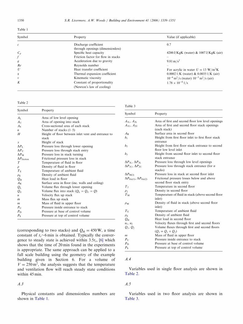
Table 1
Symbol Property Value (if applicable)
c Discharge coefficient 0.7
through openings (dimensionless)
Cp Specific heat capacity 4200 J/KgK (water) & 1007 J/KgK (air)
f Friction factor for flow in stacks –
g Acceleration due to gravity 9:81m=s2
Re Reynolds number –
U Heat transfer coefficient For acrylic in water U ¼ 13 W=m2K
a Thermal expansion coefficient 0.0002 1/K (water) & 0.0035 1/K (air)
n Kinematic viscosity 10�6 m2=s (water) 10�5 m2=s (air)K Constant of proportionality 1:78� 10�4 1=s
(Newton’s law of cooling)
Table 2
Symbol Property
AL Area of low level opening
AU Area of opening into stack
AS Cross-sectional area of each stack
n Number of stacks (1–5)
H Height of floor between inlet vent and entrance to
stack
x Height of stack
DPL Pressure loss through lower opening
DPU Pressure loss through stack entry
DPM Pressure loss in stack turning
DPfriction Frictional pressure loss in stack
T Temperature of fluid in floor
r Density of fluid in floor
TE Temperature of ambient fluid
rE Density of ambient fluid
QH Heat load in floor
AR Surface area in floor (inc. walls and ceiling)
QL Volume flux through lower opening
QU Volume flux into stack ðQL ¼ QU ¼ QÞ
u Velocity flux up stack
_m Mass flux up stack
m Mass of fluid in upper floor
PU Pressure inside entrance to stack
PD Pressure at base of control volume
PS Pressure at top of control volume
Table 3
Symbol Property
A1L, A2L Area of first and second floor low level openings
A1U, A2U Area of first and second floor stack openings
(each stack)
AR Surface area in second floor
h1 Height from first floor inlet to first floor stack
entrance
h2 Height from first floor stack entrance to second
floor low level inlet
h3 Height from second floor inlet to second floor
stack entrance
DP1L, DP2L Pressure loss through low level openings
DP1U, DP2U Pressure loss through stack entrance (for n
stacks)
DPMð2Þ Pressure loss in stack at second floor inlet
DPfricð1Þ, DPfricð2Þ Frictional pressure losses below and above
second floor stack entry
T2 Temperature in second floor
r2 Density in second floor
TM Temperature of fluid in stack (above second floor
inlet)
rM Density of fluid in stack (above second floor
inlet)
TE Temperature of ambient fluid
rE Density of ambient fluid
QH Heat load in second floor
u1, u2 Velocity fluxes through first and second floors
Q1, Q2 Volume fluxes through first and second floors
(Q3 ¼ Q1 þQ2)
m Mass of fluid in upper floor
PU Pressure inside entrance to stack
PD Pressure at base of control volume
PS Pressure at top of control volume
S.R. Livermore, A.W. Woods / Building and Environment 41 (2006) 1339–13511350
(corresponding to two stacks) and QH ¼ 450W, a timeconstant of ts�6min is obtained. Typically the conver-gence to steady state is achieved within 3:5ts, [6] whichshows that the time of 20min found in the experimentsis appropriate. The same approach can be applied to afull scale building using the geometry of the examplebuilding given in Section 6. For a volume ofV ¼ 250m2, the analysis suggests that the temperatureand ventilation flow will reach steady state conditionswithin 45min.
A.3
Physical constants and dimensionless numbers areshown in Table 1.
A.4
Variables used in single floor analysis are shown inTable 2.
A.5
Variables used in two floor analysis are shown inTable 3.
ARTICLE IN PRESSS.R. Livermore, A.W. Woods / Building and Environment 41 (2006) 1339–1351 1351
References
[1] Building Research Establishment, Selecting air conditioning
systems, Good Practice Guide, No. 71.
[2] Fitzgerald SD, Woods AW. Natural ventilation of a room with
vents at multiple levels. Building and Environment
2004;39:505–21.
[3] Gladstone C, Woods AW. On buoyancy-driven natural ventila-
tion of a room with a heated floor. J Fluid Mechanics
2001;441:293–314.
[4] Holford JM, Hunt GR. Fundamental atrium design for natural
ventilation. Building and Environment 2003;38:409–26.
[5] Short CA, Lomas KJ, Woods AW. Design strategy for low-
energy ventilation and cooling within an urban heat island.
Building Research Information 2004;32(3):187–206.
[6] Chenvidyakarn TB, Woods AW. Multiple steady states in stack
ventilation. Building and Environment 2005;40:399–410.
[7] Turner JS. Buoyancy effects in fluids. Cambridge: Cambridge
University Press; 1973.
[8] Li Y, Delsante A. Natural ventilation induced by combined wind
and thermal forces. Building and Environment 2001;36:59–71.
[9] Etheridge D, Sandberg M. Building ventilation, theory and
measurement. New York: Wiley; 1996.
[10] Linden PF, Lane-Serff GF, Smeed DA. Emptying filling boxes:
the fluid mechanics of natural ventilation. J Fluid Mechanics
1990;212:300–35.
[11] Douglas JF, Gasiorek JM, Swaffield JA. Fluid mechanics.
New York: Longman Scientific and Technical; 1986.
[12] Batchelor GK. An introduction to fluid mechanics. Cambridge:
Cambridge University Press; 1967.
[13] Ward-Smith AJ. Internal fluid flow, The fluid dynamics of flow in
pipes and ducts. Oxford: Clarendon Press; 1980.
[14] Press WH, Flannery BP, Teukolsky SA, Vetterling WT.
Numerical recipes. Cambridge: Cambridge University Press; 2002.