Embed Size (px)
Citation preview
Sum rules and semiclassical limits for the spectra of some elliptic PDEs and
pseudodifferential operators
Copyright 2010 by Evans M. Harrell II.
Evans Harrell Georgia Tech
www.math.gatech.edu/~harrell
Institut É. Cartan Univ. H. Poincaré Nancy 1
16 février, 2010
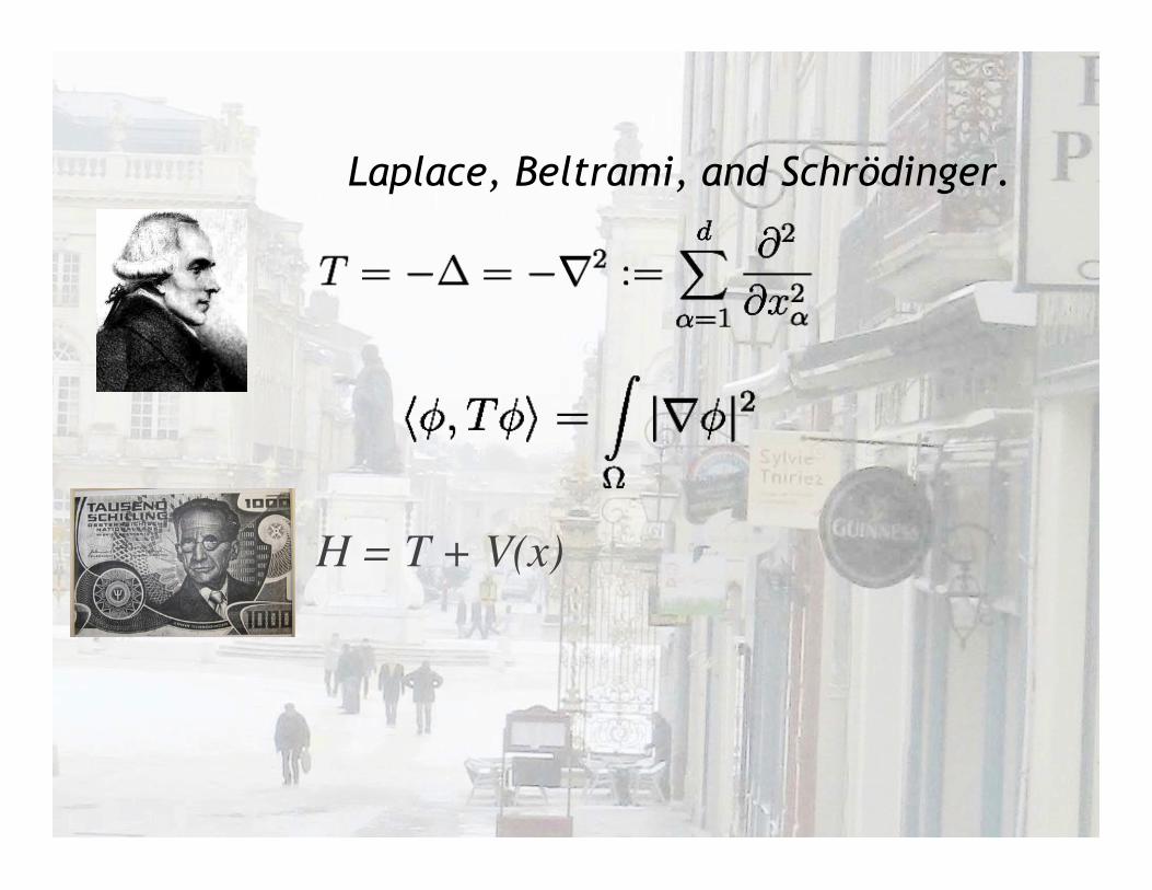
Laplace, Beltrami, and Schrödinger.
H = T + V(x)
Laplace, Beltrami, and Schrödinger.
H = T + V(x)
-
H φk = λk φk
What does “semiclassical”
mean?
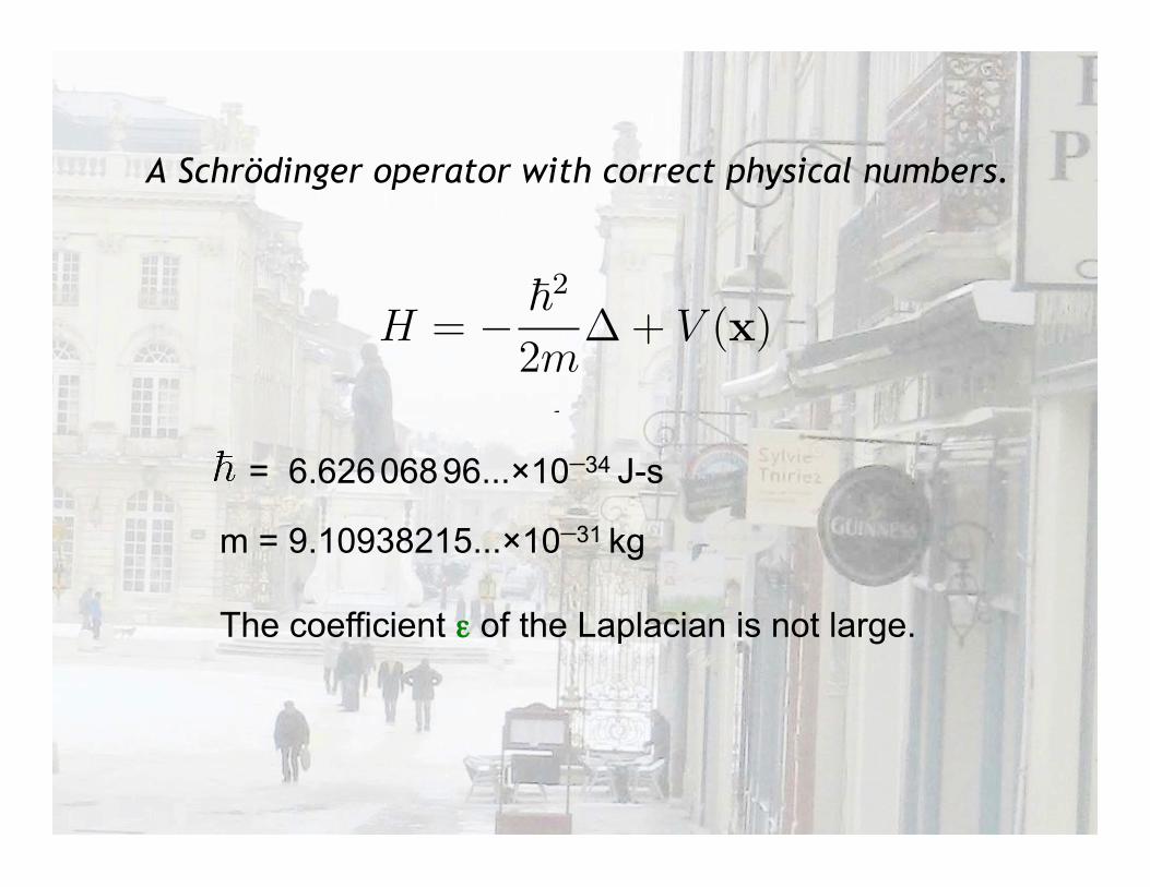
A Schrödinger operator with correct physical numbers.
H = ! !2
2m! + V (x)
k!
!=1
!k+1 ! !! "4
d
k!
!=1
(!k+1 ! !!)(!! + "!)
where
S := f convex, such thatf(z)
|z| #$
q(x) =1
4
"d!
j=1
#j
#2
! 1
2
d!
j=1
#2j
1 =4
d
!
!:"! !="j
|%$j,&$!'|2
!! ! !j
1
A Schrödinger operator with correct physical numbers.
H = ! !2
2m! + V (x)
k!
!=1
!k+1 ! !! "4
d
k!
!=1
(!k+1 ! !!)(!! + "!)
where
S := f convex, such thatf(z)
|z| #$
q(x) =1
4
"d!
j=1
#j
#2
! 1
2
d!
j=1
#2j
1 =4
d
!
!:"! !="j
|%$j,&$!'|2
!! ! !j
1
= 6.626 068 96...×10-34 J-s
m = 9.10938215...×10-31 kg
The coefficient ε of the Laplacian is not large.
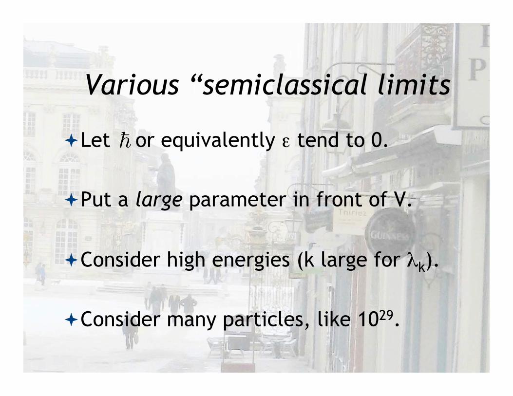
Various “semiclassical limits
Let or equivalently ε tend to 0.
Put a large parameter in front of V.
Consider high energies (k large for λk).
Consider many particles, like 1029.
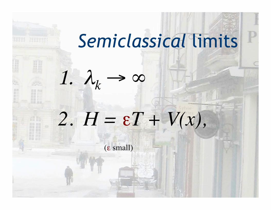
Semiclassical limits
1. λk → ∞
2. H = εT + V(x), (ε small)
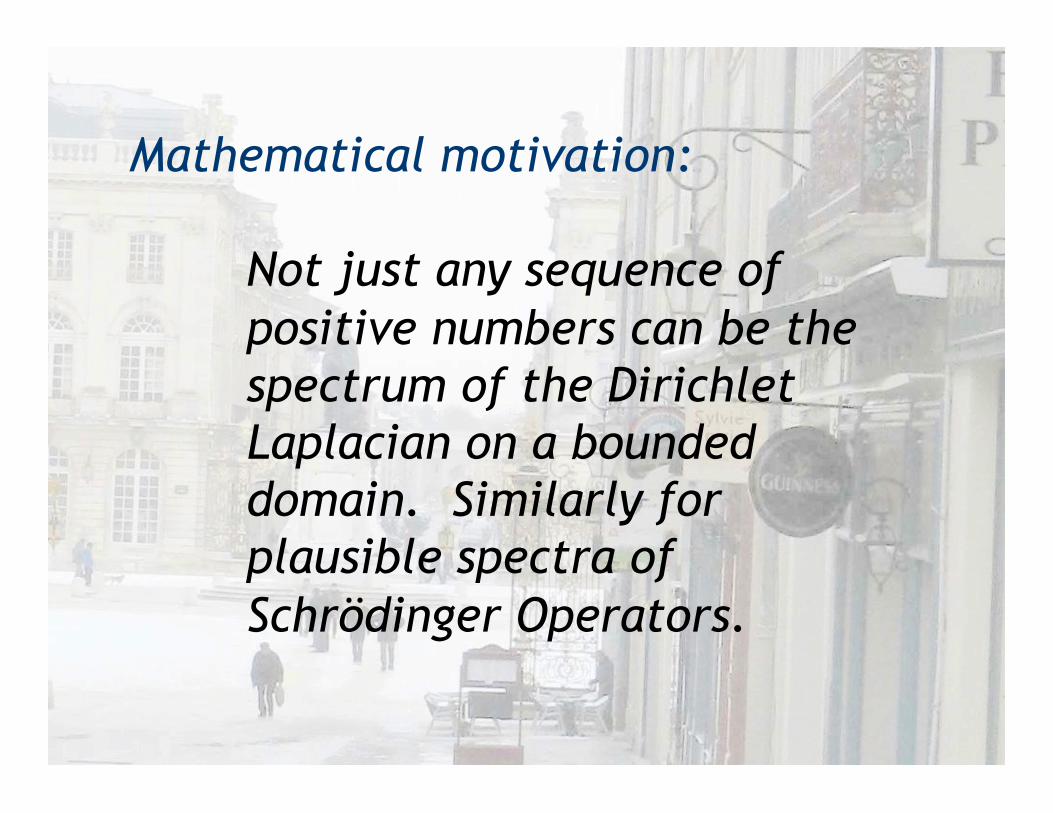
Mathematical motivation:
Not just any sequence of positive numbers can be the spectrum of the Dirichlet Laplacian on a bounded domain. Similarly for plausible spectra of Schrödinger Operators.
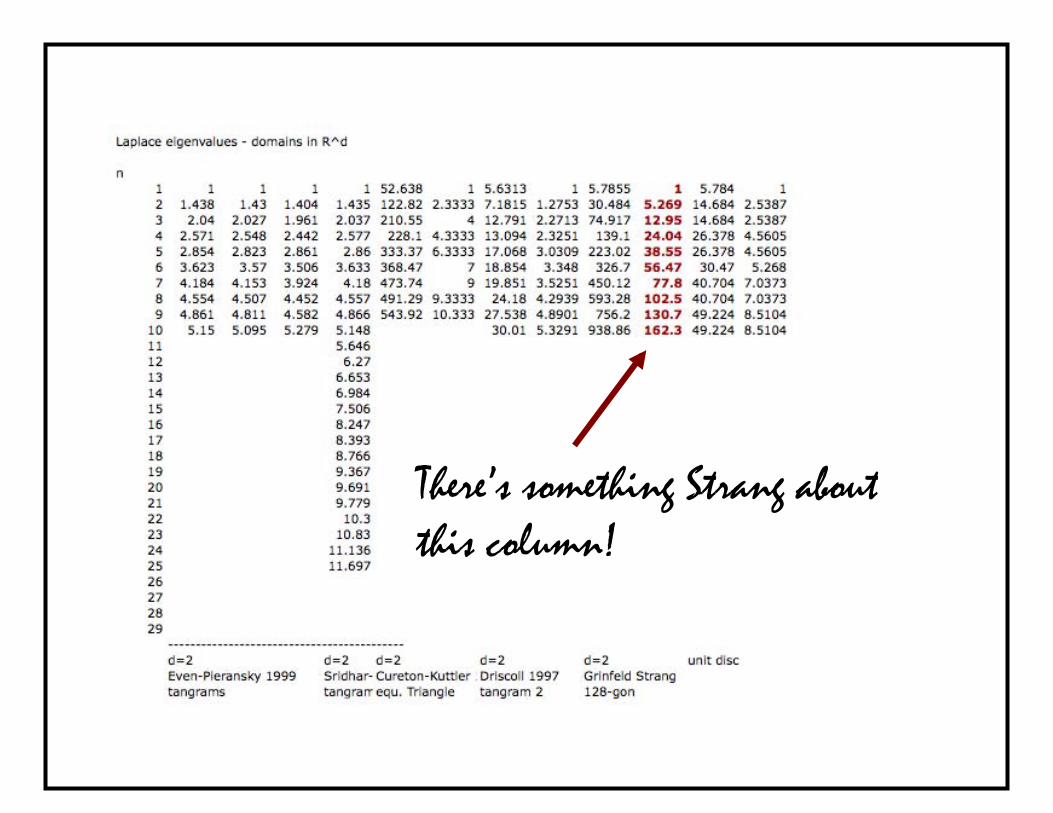
There’s something Strang about this column!
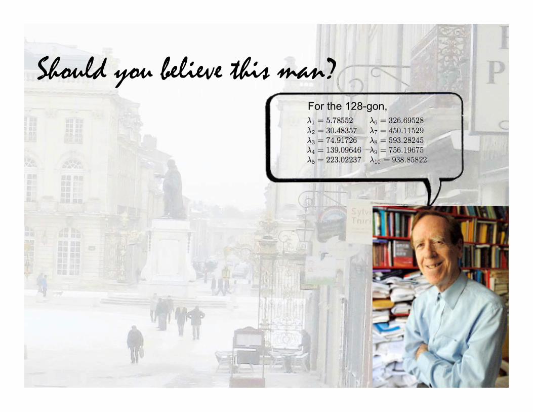
Should you believe this man? For the 128-gon,

Should you believe this man? For the 128-gon,

Should you believe this man? For the 128-gon,
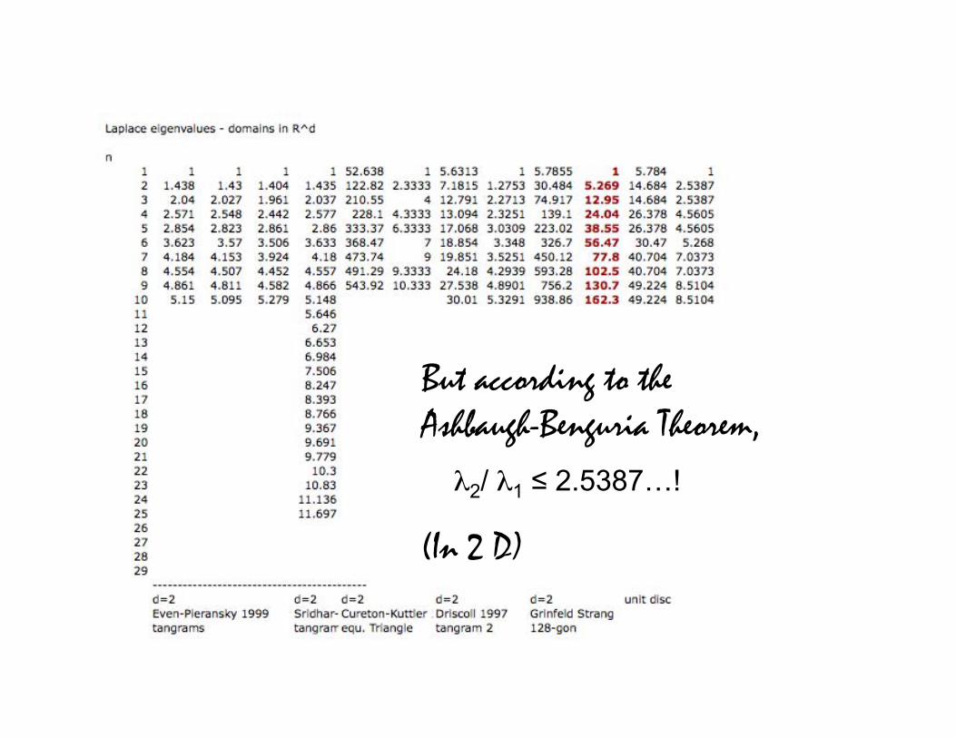
But according to the Ashbaugh-Benguria Theorem, λ2/ λ1 ≤ 2.5387…!
(In 2 D)
Aha!
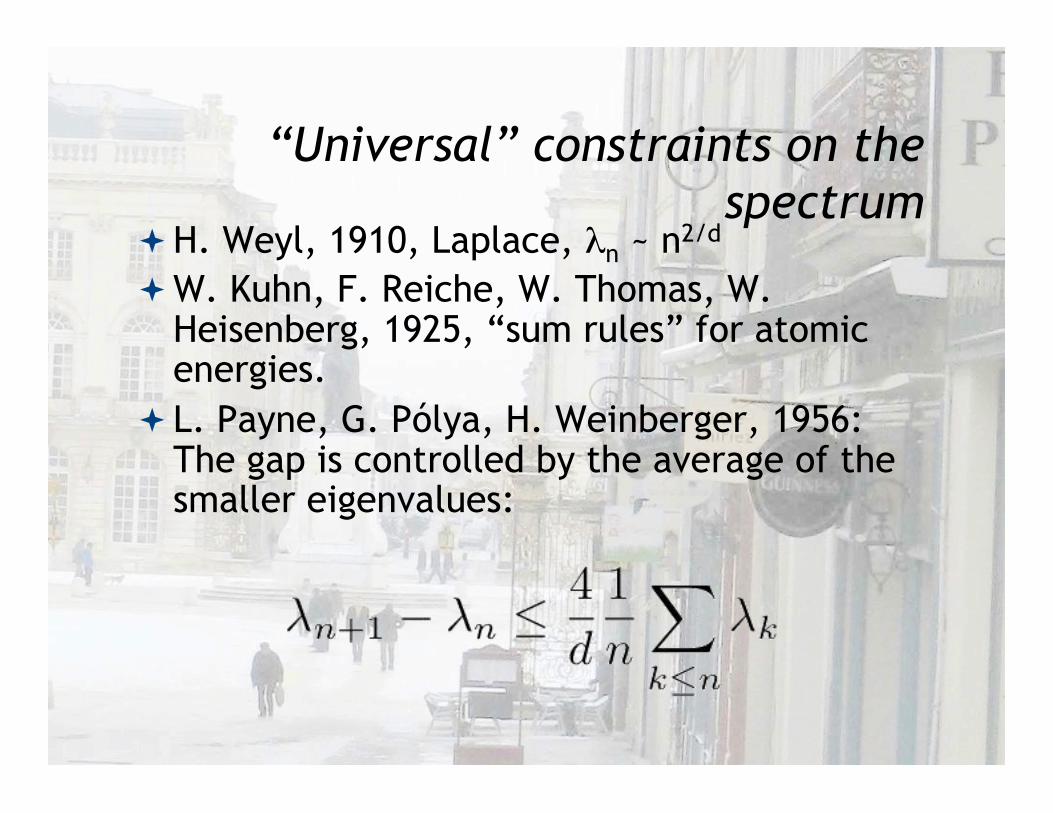
“Universal” constraints on the spectrum
H. Weyl, 1910, Laplace, λn ~ n2/d
“Universal” constraints on the spectrum
H. Weyl, 1910, Laplace, λn ~ n2/d W. Kuhn, F. Reiche, W. Thomas, W.
Heisenberg, 1925, “sum rules” for atomic energies.
“Universal” constraints on the spectrum
H. Weyl, 1910, Laplace, λn ~ n2/d W. Kuhn, F. Reiche, W. Thomas, W.
Heisenberg, 1925, “sum rules” for atomic energies.
L. Payne, G. Pólya, H. Weinberger, 1956: The gap is controlled by the average of the smaller eigenvalues:
Ashbaugh-Benguria 1991, isoperimetric conjecture of PPW proved.
H. Yang 1991, unpublished, formulae like PPW, respecting Weyl asymptotics for the first time.
Harrell 1993-present, commutator approach; with Michel, Stubbe, El Soufi and Ilias, Hermi, Yildirim.
Ashbaugh-Hermi, Levitin-Parnovsky, Cheng-Yang, Cheng-Chen, some others.
“Universal” constraints on the spectrum
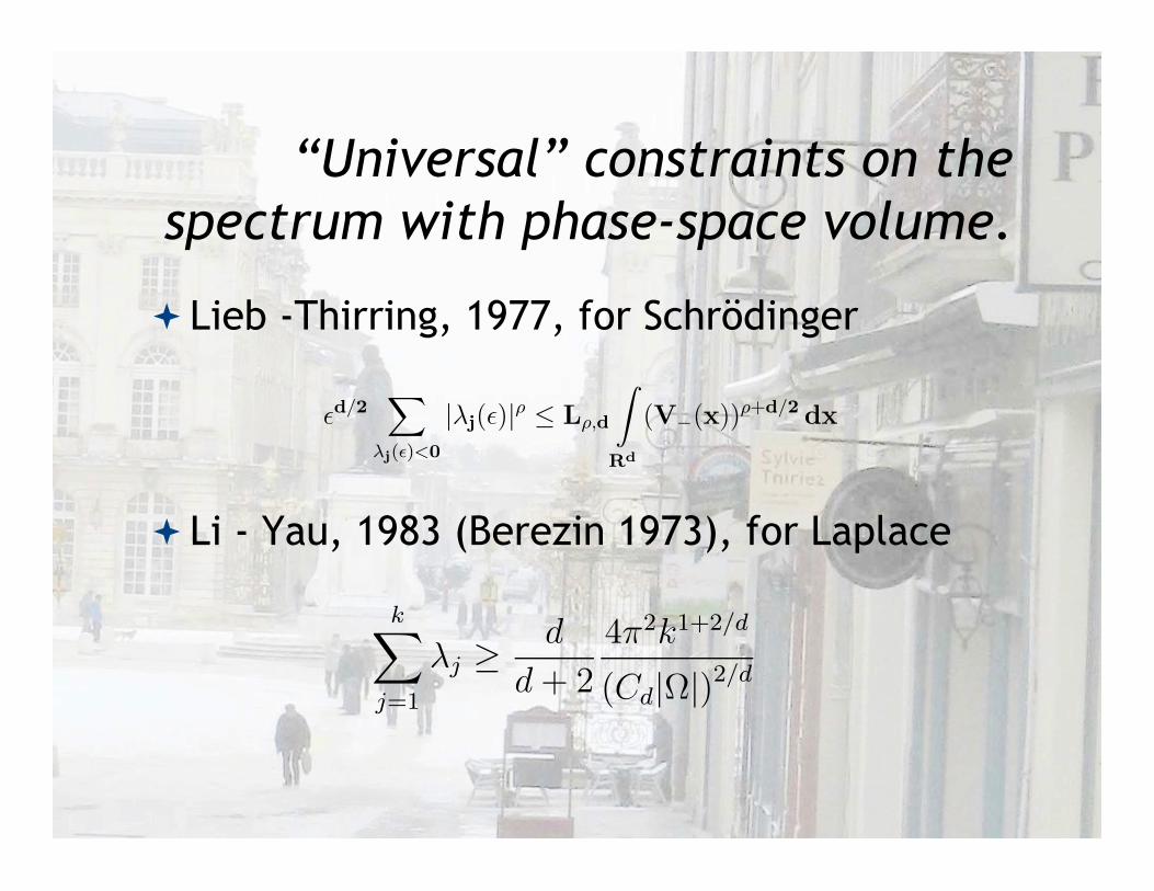
“Universal” constraints on the spectrum with phase-space volume.
Lieb -Thirring, 1977, for Schrödinger
Li - Yau, 1983 (Berezin 1973), for Laplace
ON RIESZ MEANS OF EIGENVALUES 5
with
uk(!) =1
(2")d
!
!
uk(x) eix·!dx.
Therefore, taking norms
"
k
|uk(!)|2 =
1
(2")d
!
!
|e!ix·!|2 dx =1
(2")d
!
!
dx =|!|
(2")d.
Incorporating this into (11) and Riesz iterating leads to (9) as desired. !
Remarks. The following are well-known facts provided here to o"er acomplete picture.
(i) The Li-Yau inequality
(11)k
"
j=1
#j !d
d + 2
4"2k1+2/d
(Cd|!|)2/d
valid for k ! 1 and its consequence (by virtue of the nondecreasingnature of the sequence of eigenvalues)
(12) #k !d
d + 2
4"2k2/d
(Cd|!|)2/d
are immediate corollaries. Indeed, (11) is what one obtains if sheapplied the Legendre transform to Berezin-Li-Yau (9) for $ = 1.The details are in [62] (see also [61], [49], [38]). In terms of thecounting function, Li-Yau reads
(13) N(z) "
#
d + 2
d
$d/2
Lcl0,d |!|zd/2.
(ii) Polya standing conjecture is the statement
(14) N(z) " Lcl0,d |!|zd/2.
In terms of eigenvalues, it is expressed as follows
(15) #k !4"2k2/d
(Cd|!|)2/d.
It was proved in this form [75] [76] [77] using methods reminiscentof those found in Courant-Hilbert [28], for tiling domains (see also[74] where motivations are o"ered).
(1) !d/2!
!j(")<0
|"j(!)|# ! L#,d
"
Rd
(V!(x))#+d/2 dx
Normalization:
f :=1"2#
"e!ikxf(x)dx.
Convolution theorem:
#fg =1"2#
f # g
Fact:
F1
1 + x2=
1
2e!|k|
Therefore, if f = g = 11+x2 , then
$f 2 =1
4"
2#
" infty
!"e!|$|!|k!$|d$.
For simplicity, suppose k > 0.
$f 2 =1
4"
2#
%" 0
!"+
" k
0
+
" "
k
&e!|$|!|k!$|d$.
=1
4"
2#
%" 0
!"e2$!kd$ +
" k
0
e!kd$ +
" "
k
e!2$+kd$
&
=1
4"
2#(k + 1)e!k.
Since F maps even functions to even functions, the final answer is
$f 2 =1
4"
2#(|k| + 1)e!|k|.
1
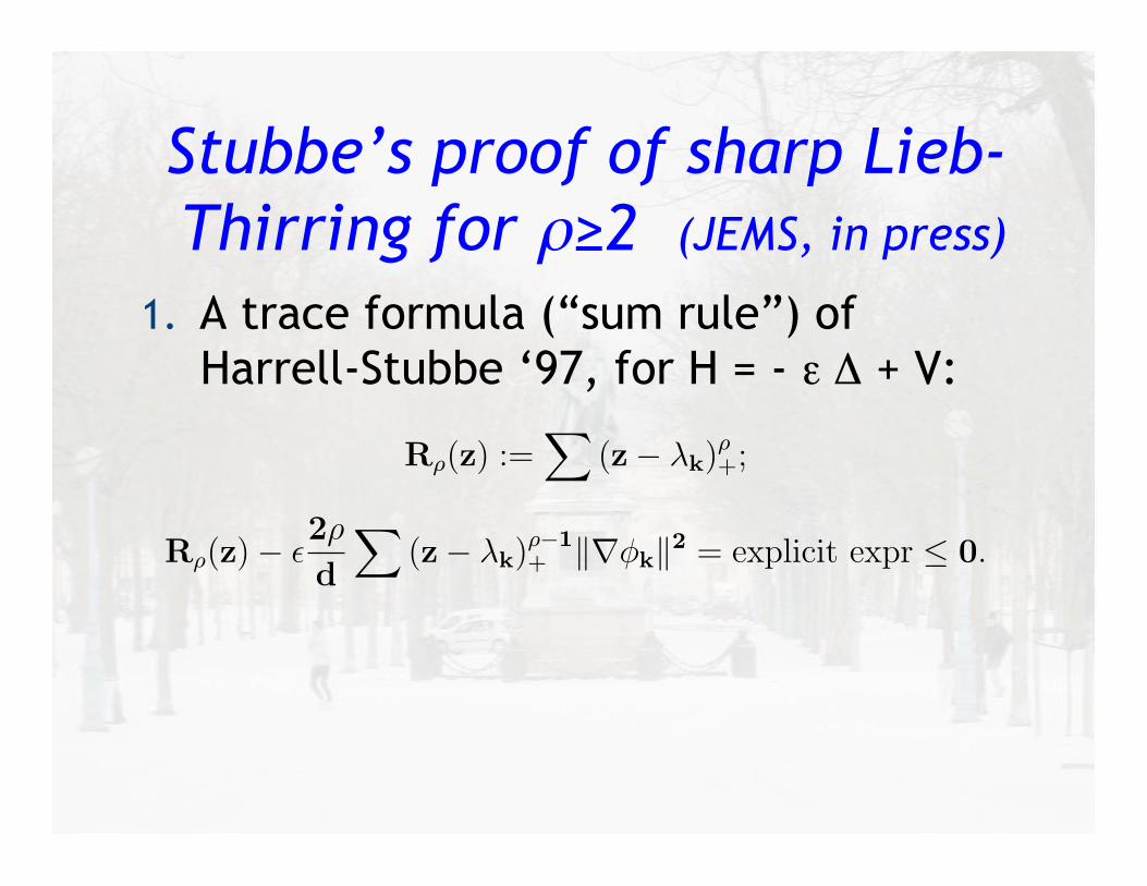
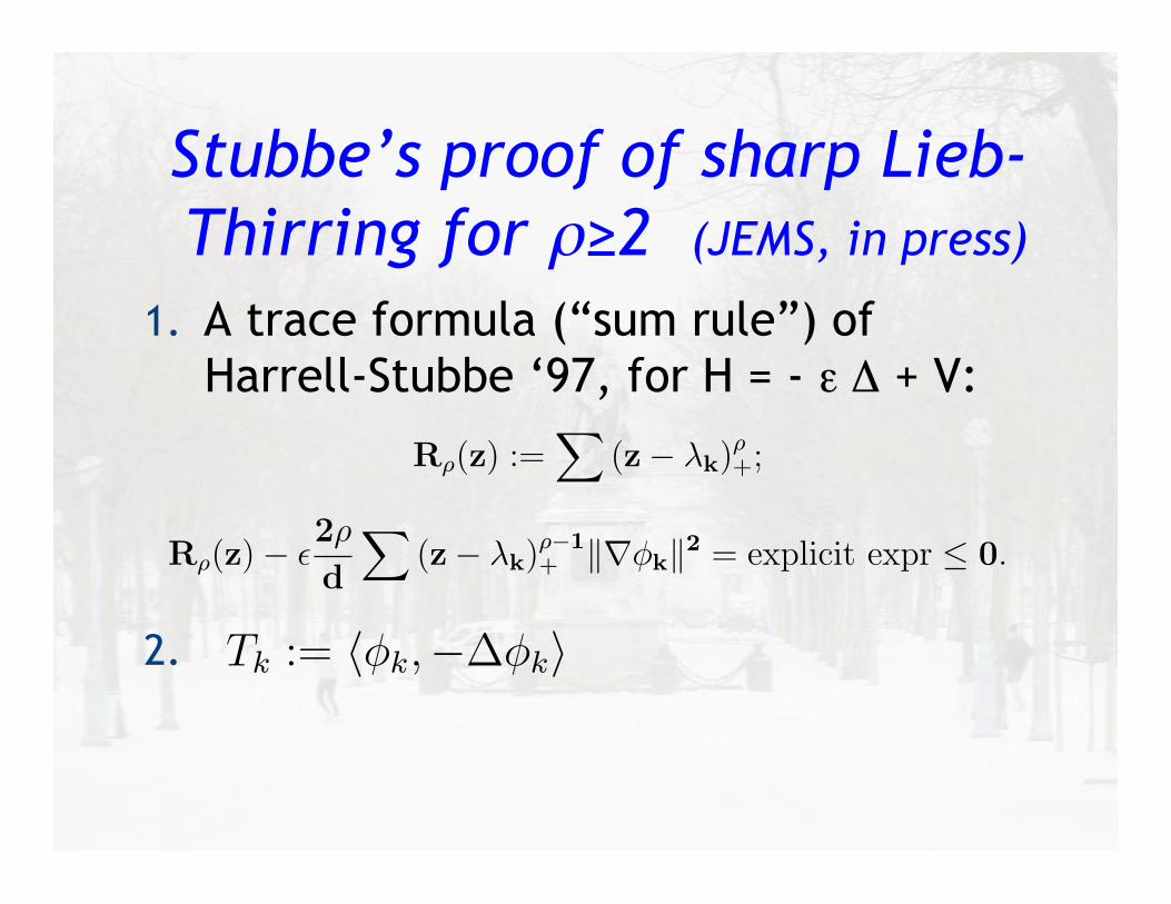
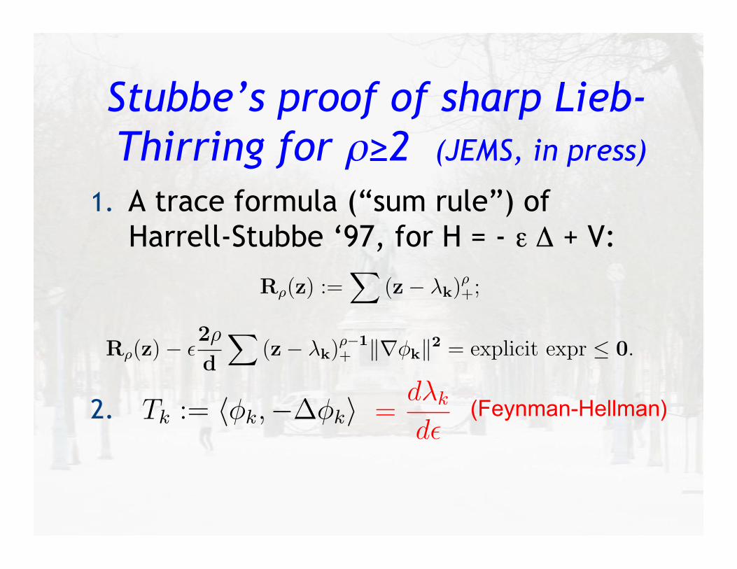
Stubbe’s proof of sharp Lieb-Thirring for ρ≥2 (JEMS, in press)
Stubbe’s proof of sharp Lieb-Thirring for ρ≥2 (JEMS, in press)
1. A trace formula (“sum rule”) of Harrell-Stubbe ‘97, for H = - ε Δ + V:
Rρ(z) :=∑
(z− λk)ρ+;
Rρ(z)− ε2ρ
d
∑(z− λk)
ρ−1+ ‖∇φk‖2 = explicit expr ≤ 0.
λk+1 ≤(
1 +2
d
)λk +
√Dk
Rσ(z) ≤ Lclσ,1
∫
!
(V(x)− z)σ+1/2− dx?
Rσ(z,α) ≤ α−d/2Lclσ,d
∫
M
(V (x)− z)σ+d/2− dx.
Tjk := |〈φk,∇φj〉|2 .∑
k
Tjk ≤ Tj :=⟨φj,−∇2φj
⟩.
Elementary gap formula:
〈φj, [H,G]φk〉 = (λj − λk) 〈φj, Gφk〉Since [H,G]φk = (H − λk)Gφk,
‖[H,G]φk‖2 =⟨Gφj, (H − λk)
2Gφk
⟩
and more generally
〈[H, G]φj, [H,G]φk〉 = 〈Gφj, (H − λj)(H − λk)Gφk〉 .Second commutator formula
〈φj, [G, [H, G]]φk〉 = 〈Gφj, (2H − λj − λk)Gφk〉 .In particular,
〈φj, [G, [H,G]]φj〉 = 2 〈Gφj, (H − λj)Gφk〉 .
H(g) = − d2
ds2+ gκ2
A =1
4π
∑
k
(|hk|2 − k2|hk|2
)=
p2
4π− stu!
1
1. A trace formula (“sum rule”) of Harrell-Stubbe ‘97, for H = - ε Δ + V:
2.
limα→0+
αd2
!
λj(α)<0
|λj(α)| = Lσ,d
"|V−(x)|σ+ d
2
R2(z) ≤ 4α
d
!(z − λk)+Tk,
For example, for V = 0,
Tk := 〈φk,−∆φk〉=dλk
dα
so td/2Z(t) is monotonically decreasing. Since it is known that
limt↓0
(4πt)d/2Z(t) = V ol(Ω),
we get a strengthening of an inequality of Kac,
Z(t) ≤ V ol(Ω)
(4πt)d/2.
Traditionally, we consider −∆+V (x) on all of Rd. If V (x) is in certain func-tion classes, the continuous spectrum consists of all real numbers, and theremay be some negative eigenvalues. How many and what good estimates arethere?
k!
$=1
λk+1 − λ$ ≤4
d
k!
$=1
(λk+1 − λ$)(λ$ + δ$)
where
S := f convex, such thatf(z)
|z| →∞
q(x) =1
4
#d!
j=1
κj
$2
− 1
2
d!
j=1
κ2j
1 =4
d
!
$:λ! $=λj
|〈φj,∇φ$〉|2
λ$ − λj
1
Stubbe’s proof of sharp Lieb-Thirring for ρ≥2 (JEMS, in press)
Rρ(z) :=∑
(z− λk)ρ+;
Rρ(z)− ε2ρ
d
∑(z− λk)
ρ−1+ ‖∇φk‖2 = explicit expr ≤ 0.
λk+1 ≤(
1 +2
d
)λk +
√Dk
Rσ(z) ≤ Lclσ,1
∫
!
(V(x)− z)σ+1/2− dx?
Rσ(z,α) ≤ α−d/2Lclσ,d
∫
M
(V (x)− z)σ+d/2− dx.
Tjk := |〈φk,∇φj〉|2 .∑
k
Tjk ≤ Tj :=⟨φj,−∇2φj
⟩.
Elementary gap formula:
〈φj, [H,G]φk〉 = (λj − λk) 〈φj, Gφk〉Since [H,G]φk = (H − λk)Gφk,
‖[H,G]φk‖2 =⟨Gφj, (H − λk)
2Gφk
⟩
and more generally
〈[H, G]φj, [H,G]φk〉 = 〈Gφj, (H − λj)(H − λk)Gφk〉 .Second commutator formula
〈φj, [G, [H, G]]φk〉 = 〈Gφj, (2H − λj − λk)Gφk〉 .In particular,
〈φj, [G, [H,G]]φj〉 = 2 〈Gφj, (H − λj)Gφk〉 .
H(g) = − d2
ds2+ gκ2
A =1
4π
∑
k
(|hk|2 − k2|hk|2
)=
p2
4π− stu!
1
1. A trace formula (“sum rule”) of Harrell-Stubbe ‘97, for H = - ε Δ + V:
2.
limα→0+
αd2
!
λj(α)<0
|λj(α)| = Lσ,d
"|V−(x)|σ+ d
2
R2(z) ≤ 4α
d
!(z − λk)+Tk,
For example, for V = 0,
Tk := 〈φk,−∆φk〉=dλk
dα
so td/2Z(t) is monotonically decreasing. Since it is known that
limt↓0
(4πt)d/2Z(t) = V ol(Ω),
we get a strengthening of an inequality of Kac,
Z(t) ≤ V ol(Ω)
(4πt)d/2.
Traditionally, we consider −∆+V (x) on all of Rd. If V (x) is in certain func-tion classes, the continuous spectrum consists of all real numbers, and theremay be some negative eigenvalues. How many and what good estimates arethere?
k!
$=1
λk+1 − λ$ ≤4
d
k!
$=1
(λk+1 − λ$)(λ$ + δ$)
where
S := f convex, such thatf(z)
|z| →∞
q(x) =1
4
#d!
j=1
κj
$2
− 1
2
d!
j=1
κ2j
1 =4
d
!
$:λ! $=λj
|〈φj,∇φ$〉|2
λ$ − λj
1
(Feynman-Hellman)
Stubbe’s proof of sharp Lieb-Thirring for ρ≥2 (JEMS, in press)
Rρ(z) :=∑
(z− λk)ρ+;
Rρ(z)− ε2ρ
d
∑(z− λk)
ρ−1+ ‖∇φk‖2 = explicit expr ≤ 0.
λk+1 ≤(
1 +2
d
)λk +
√Dk
Rσ(z) ≤ Lclσ,1
∫
!
(V(x)− z)σ+1/2− dx?
Rσ(z,α) ≤ α−d/2Lclσ,d
∫
M
(V (x)− z)σ+d/2− dx.
Tjk := |〈φk,∇φj〉|2 .∑
k
Tjk ≤ Tj :=⟨φj,−∇2φj
⟩.
Elementary gap formula:
〈φj, [H,G]φk〉 = (λj − λk) 〈φj, Gφk〉Since [H,G]φk = (H − λk)Gφk,
‖[H,G]φk‖2 =⟨Gφj, (H − λk)
2Gφk
⟩
and more generally
〈[H, G]φj, [H,G]φk〉 = 〈Gφj, (H − λj)(H − λk)Gφk〉 .Second commutator formula
〈φj, [G, [H, G]]φk〉 = 〈Gφj, (2H − λj − λk)Gφk〉 .In particular,
〈φj, [G, [H,G]]φj〉 = 2 〈Gφj, (H − λj)Gφk〉 .
H(g) = − d2
ds2+ gκ2
A =1
4π
∑
k
(|hk|2 − k2|hk|2
)=
p2
4π− stu!
1
=dλk
dε
Rρ(z)− ε2ρ
d
∑(z− λk)
ρ−1+ ‖∇φk‖2 = explicit expr ≤ 0.
λk+1 ≤(
1 +2
d
)λk +
√Dk
Rσ(z) ≤ Lclσ,1
∫
Γ
(V(x)− z)σ+1/2− dx?
Rσ(z,α) ≤ α−d/2Lclσ,d
∫
M
(V (x)− z)σ+d/2− dx.
Tjk := |〈φk,∇φj〉|2 .∑
k
Tjk ≤ Tj :=⟨φj,−∇2φj
⟩.
Elementary gap formula:
〈φj, [H,G]φk〉 = (λj − λk) 〈φj, Gφk〉Since [H,G]φk = (H − λk)Gφk,
‖[H,G]φk‖2 =⟨Gφj, (H − λk)
2Gφk
⟩
and more generally
〈[H, G]φj, [H,G]φk〉 = 〈Gφj, (H − λj)(H − λk)Gφk〉 .Second commutator formula
〈φj, [G, [H, G]]φk〉 = 〈Gφj, (2H − λj − λk)Gφk〉 .In particular,
〈φj, [G, [H,G]]φj〉 = 2 〈Gφj, (H − λj)Gφk〉 .
H(g) = − d2
ds2+ gκ2
A =1
4π
∑
k
(|hk|2 − k2|hk|2
)=
p2
4π− stuff
1
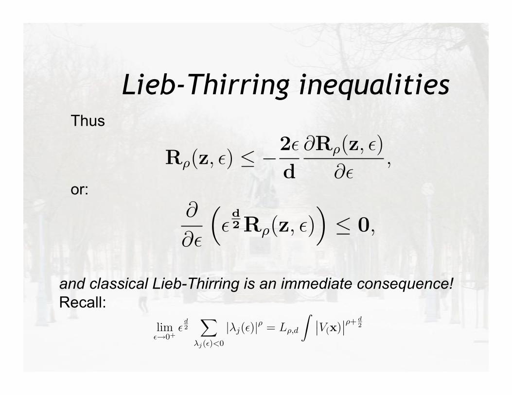
Lieb-Thirring inequalities Thus
and classical Lieb-Thirring is an immediate consequence! Recall:
or:
(1) !d/2!
!j(")<0
|"j(!)|# ! L#,d
"
Rd
(V!(x))#+d/2 dx
lim""0+
!d2
!
!j(")<0
|"j(!)|# = L#,d
" ##V(x)###+ d
2
Normalization:
f :=1"2#
"e!ikxf(x)dx.
Convolution theorem:
$fg =1"2#
f # g
Fact:
F1
1 + x2=
1
2e!|k|
Therefore, if f = g = 11+x2 , then
%f 2 =1
4"
2#
" infty
!#e!|$|!|k!$|d$.
For simplicity, suppose k > 0.
%f 2 =1
4"
2#
&" 0
!#+
" k
0
+
" #
k
'e!|$|!|k!$|d$.
=1
4"
2#
&" 0
!#e2$!kd$ +
" k
0
e!kd$ +
" #
k
e!2$+kd$
'
=1
4"
2#(k + 1)e!k.
Since F maps even functions to even functions, the final answer is
%f 2 =1
4"
2#(|k| + 1)e!|k|.
1
R!(z, ε) ≤ −ρε
d
∂R!(z, ρ)
∂ρ,
R!(z, ε) ≤ −2ε
d
∂R!(z, ε)
∂ε,
∂
∂ε
!ε
d2 R!(z, ε)
"≤ 0,
(1) εd/2#
"j(#)<0
|λj(ε)|! ≤ L!,d
$
Rd
(V!(x))!+d/2 dx
lim#"0+
εd2
#
"j(#)<0
|λj(ε)|! = L!,d
$ %%V(x)%%!+ d
2
Normalization:
〈φj, [G, [H,G]]φj〉 =#
k:"k #="j
(λk − λj)|Gkj|2
Convolution theorem:
&fg =1√2π
f ∗ g
Fact:
F1
1 + x2=
1
2e!|k|
Therefore, if f = g = 11+x2 , then
'f 2 =1
4√
2π
$ infty
!$e!|$|!|k!$|d'.
For simplicity, suppose k > 0.
'f 2 =1
4√
2π
($ 0
!$+
$ k
0
+
$ $
k
)e!|$|!|k!$|d'.
=1
4√
2π
($ 0
!$e2$!kd' +
$ k
0
e!kd' +
$ $
k
e!2$+kd'
)
=1
4√
2π(k + 1)e!k.
Since F maps even functions to even functions, the final answer is1
R!(z, !) ! ""!
d
#R!(z, ")
#",
R!(z, !) ! "2!
d
#R!(z, !)
#!,
#
#!
!!
d2 R!(z, !)
"! 0,
(1) !d/2#
"j(#)<0
|$j(!)|! ! L!,d
$
Rd
(V!(x))!+d/2 dx
lim#"0+
!d2
#
"j(#)<0
|$j(!)|! = L!,d
$ %%V(x)%%!+ d
2
Normalization:
#%j, [G, [H,G]]%j$ =#
k:"k #="j
($k " $j)|Gkj|2
Convolution theorem:
&fg =1%2&
f & g
Fact:
F1
1 + x2=
1
2e!|k|
Therefore, if f = g = 11+x2 , then
'f 2 =1
4%
2&
$ infty
!$e!|$|!|k!$|d'.
For simplicity, suppose k > 0.
'f 2 =1
4%
2&
($ 0
!$+
$ k
0
+
$ $
k
)e!|$|!|k!$|d'.
=1
4%
2&
($ 0
!$e2$!kd' +
$ k
0
e!kd' +
$ $
k
e!2$+kd'
)
=1
4%
2&(k + 1)e!k.
Since F maps even functions to even functions, the final answer is1
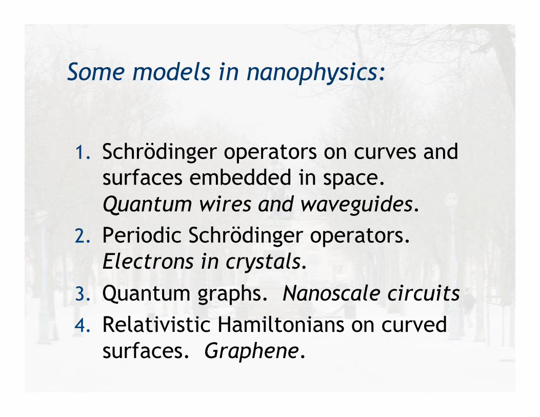
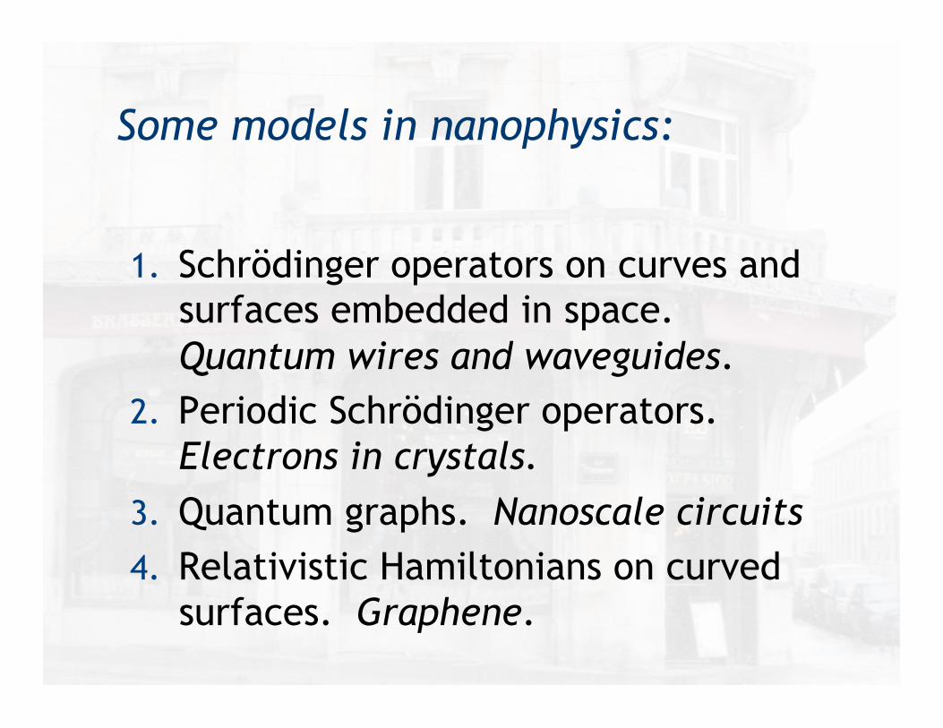
Some models in nanophysics:
1. Schrödinger operators on curves and surfaces embedded in space. Quantum wires and waveguides.
2. Periodic Schrödinger operators. Electrons in crystals.
3. Quantum graphs. Nanoscale circuits 4. Relativistic Hamiltonians on curved
surfaces. Graphene.
Are the spectra of these models controlled by “sum
rules,” like those known for Laplace/Schrödinger on
domains or all of Rd, or are there important differences?
Are the spectra of these models controlled by “sum rules”? If so, can we prove analogues of Lieb-Thirring,
Li-Yau, PPW, etc.?
Sum Rules
1. Used by Heisenberg in 1925 to explain regularities in atomic energy spectra
Sum Rules
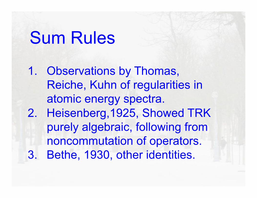
1. Observations by Thomas, Reiche, Kuhn of regularities in atomic energy spectra.
2. Heisenberg,1925, Showed TRK purely algebraic, following from noncommutation of operators.
3. Bethe, 1930, other identities.
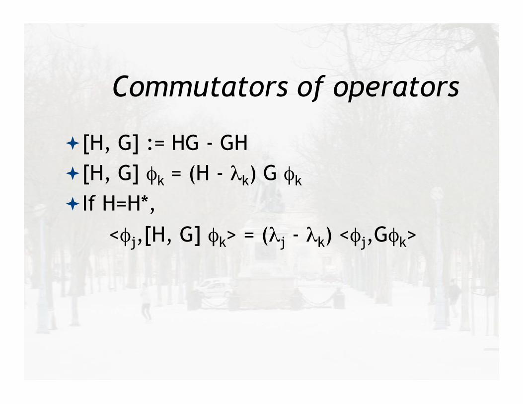
Commutators of operators
[H, G] := HG - GH [H, G] φk = (H - λk) G φk If H=H*, <φj,[H, G] φk> = (λj - λk) <φj,Gφk>
Commutators of operators
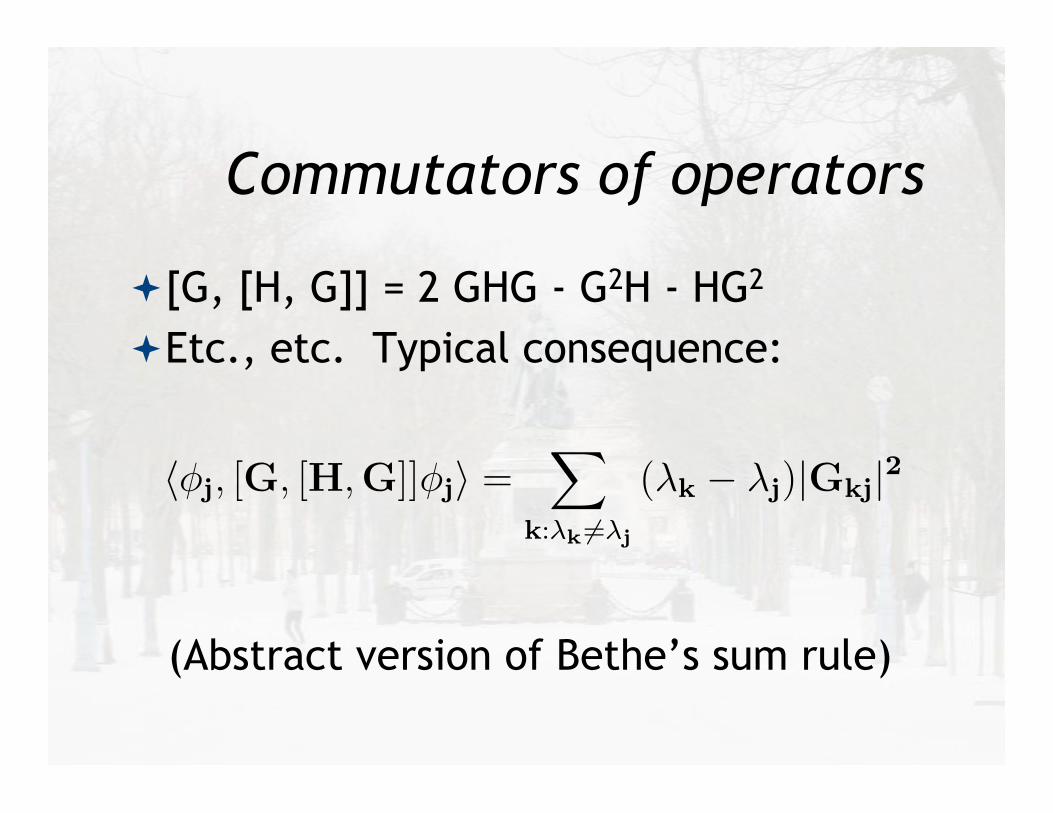
[G, [H, G]] = 2 GHG - G2H - HG2 Etc., etc. Typical consequence:
(Abstract version of Bethe’s sum rule)
(1) !d/2!
λj(ε)<0
|"j(!)|ρ ! Lρ,d
"
Rd
(V!(x))ρ+d/2 dx
limε"0+
!d2
!
λj(ε)<0
|"j(!)|ρ = Lρ,d
" ##V(x)##ρ+ d
2
Normalization:
"#j, [G, [H,G]]#j# =!
k:λk #=λj
("k $ "j)|Gkj|2
Convolution theorem:
$fg =1%2$
f & g
Fact:
F1
1 + x2=
1
2e!|k|
Therefore, if f = g = 11+x2 , then
%f 2 =1
4%
2$
" infty
!$e!|$|!|k!$|d%.
For simplicity, suppose k > 0.
%f 2 =1
4%
2$
&" 0
!$+
" k
0
+
" $
k
'e!|$|!|k!$|d%.
=1
4%
2$
&" 0
!$e2$!kd% +
" k
0
e!kd% +
" $
k
e!2$+kd%
'
=1
4%
2$(k + 1)e!k.
Since F maps even functions to even functions, the final answer is
%f 2 =1
4%
2$(|k| + 1)e!|k|.
1
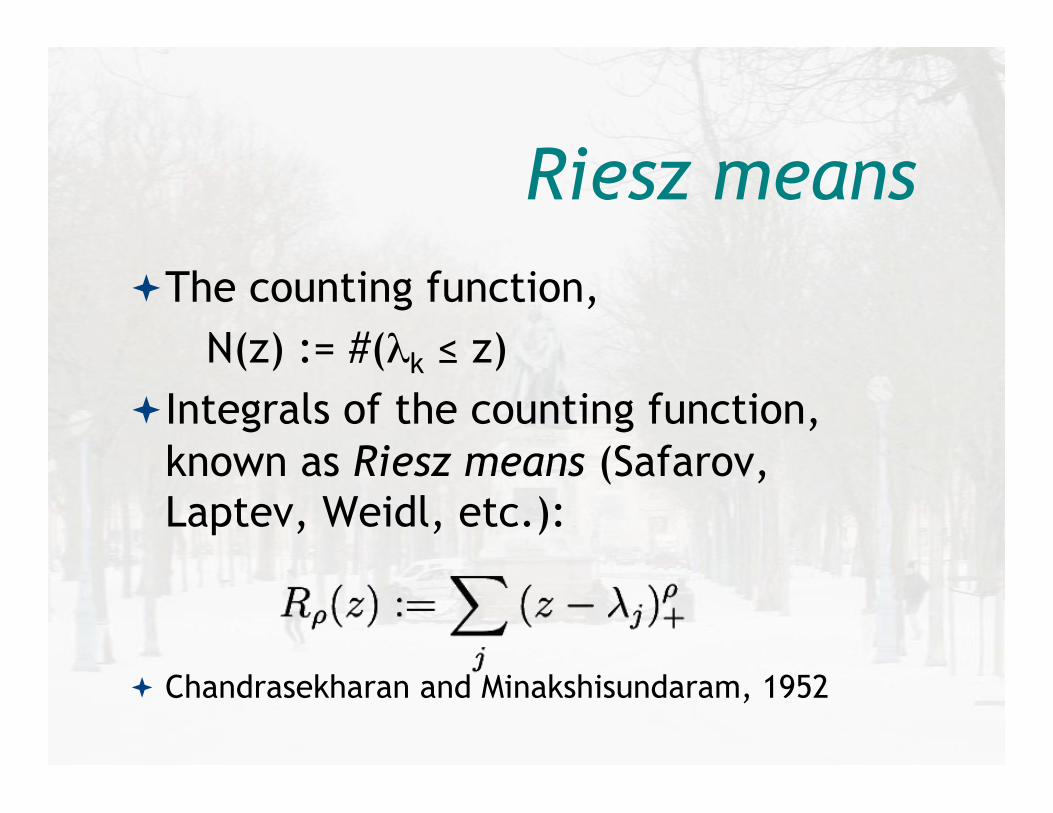
The counting function, N(z) := #(λk ≤ z) Integrals of the counting function,
known as Riesz means (Safarov, Laptev, Weidl, etc.):
Chandrasekharan and Minakshisundaram, 1952
Riesz means
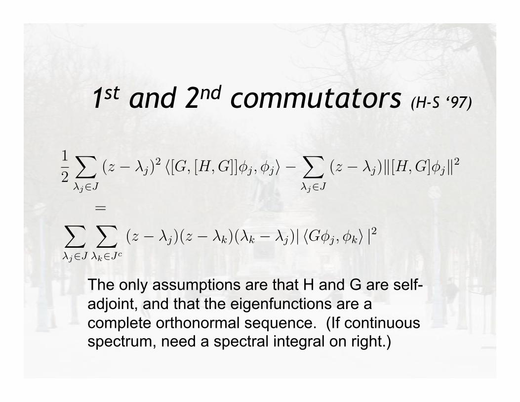
1st and 2nd commutators (H-S ‘97)
The only assumptions are that H and G are self-adjoint, and that the eigenfunctions are a complete orthonormal sequence. (If continuous spectrum, need a spectral integral on right.)
!k
!j
! 4 + d
2 + d
!k
j
"2/d
(1)
(2)d + 2
d!k !=
!k
j
" 2d!
d + 2
d!j +
#Dj
"
"R2(0, ") ! "2 4
d
$
k
(0" !k)Tk
Z(t) !!
2t
d
" $
j
exp("t!j)#$#j#2
1
2(z " !j) %[G, [H,G]]#j, #j& " #[H, G]#j#2(3)
=$
k
(z " !k)(!k " !j)| %G#j, #k& |2(4)
(5)
1
2
$
!j!J
(z " !j)2 %[G, [H, G]]#j, #j& "
$
!j!J
(z " !j)#[H,G]#j#2(6)
=(7)$
!j!J
$
!k!Jc
(z " !j)(z " !k)(!k " !j)| %G#j, #k& |2(8)
(9)
$(t) = e"iHt$(0)
"$2# + q(x) = "!! + q(x)
q(x) :=1
4
!%r
%
"2
" 1
2
%rr
%.
&n ' 0 with #&n# = 1, such that #(H " !)&n# ' 0.
F [f ] (k) = f(k) :=1
(2()d/2
%
Rd
e"ik·xf(x)dx
1
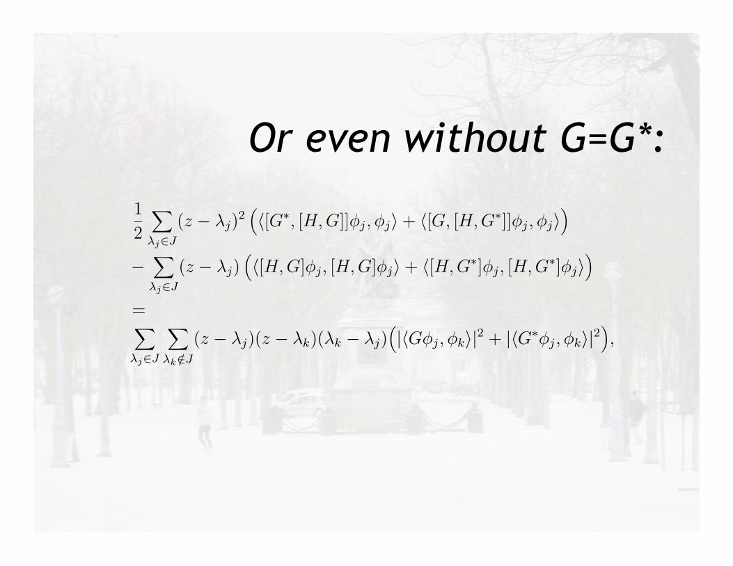
Or even without G=G*:
Proof of Theorem 2.1. We may write the first trace in Proposition 2.3 in termsof second commutators by applying the following algebraic identity, which isa direct computation:
G![H, G]+G[H,G!] =1
2[G!, [H,G]]+
1
2[G, [H,G!]]+
1
2[H,GG!+G!G]. (2.5)
When (2.5) is multiplied by P and the trace is taken, the last term vanishesand for the left side of (2.3) we obtain
tr!H2(G![H,G] + G[H,G!])P
"=
1
2tr
!H2([G!, [H,G]] + [G, [H,G!]])P
".
(2.6)
If the spectrum of H consists only of eigenvalues !j, with an orthonormal basisof eigenfunctions "j, the trace identity (2.6) and Corollary 2.3 imply
1
2
#
!j"J
(z ! !j)2
!"[G!, [H,G]]"j, "j#+ "[G, [H, G!]]"j, "j#
"
!#
!j"J
(z ! !j)!"[H,G]"j, [H,G]"j#+ "[H,G!]"j, [H,G!]"j#
"
=#
!j"J
#
!k /"J
(z ! !j)(z ! !k)(!k ! !j)!|"G"j, "k#|2 + |"G!"j, "k#|2
",
establishing (2.1). !
3 On the eigenvalues of periodic Schrodinger operators
In this section we suppose that H is of the form
H = !! + V (x) (3.1)
and is defined as a self-adjoint operator on L2("), where " $ Rd is a boundeddomain and the boundary conditions are such that the multiplication opera-tor G = exp(!iq · x) satisfies the domain-mapping conditions of Lemma 2.1.This situation arises in the Floquet decomposition of H when V (x) is a real,periodic, bounded measurable function [9,12,13] XXXAND OTHER POSSI-BLE REFS IN BIBLIOGRAPHYXXX, where " is a fundamental domain of
5
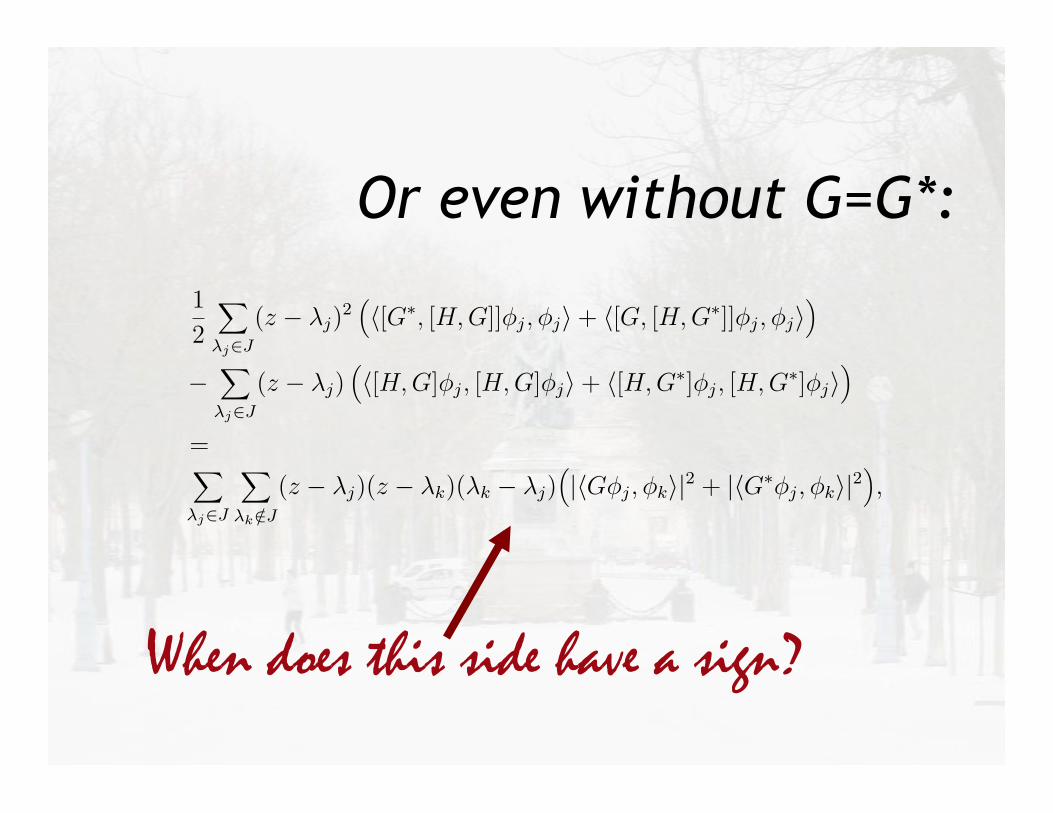
When does this side have a sign?
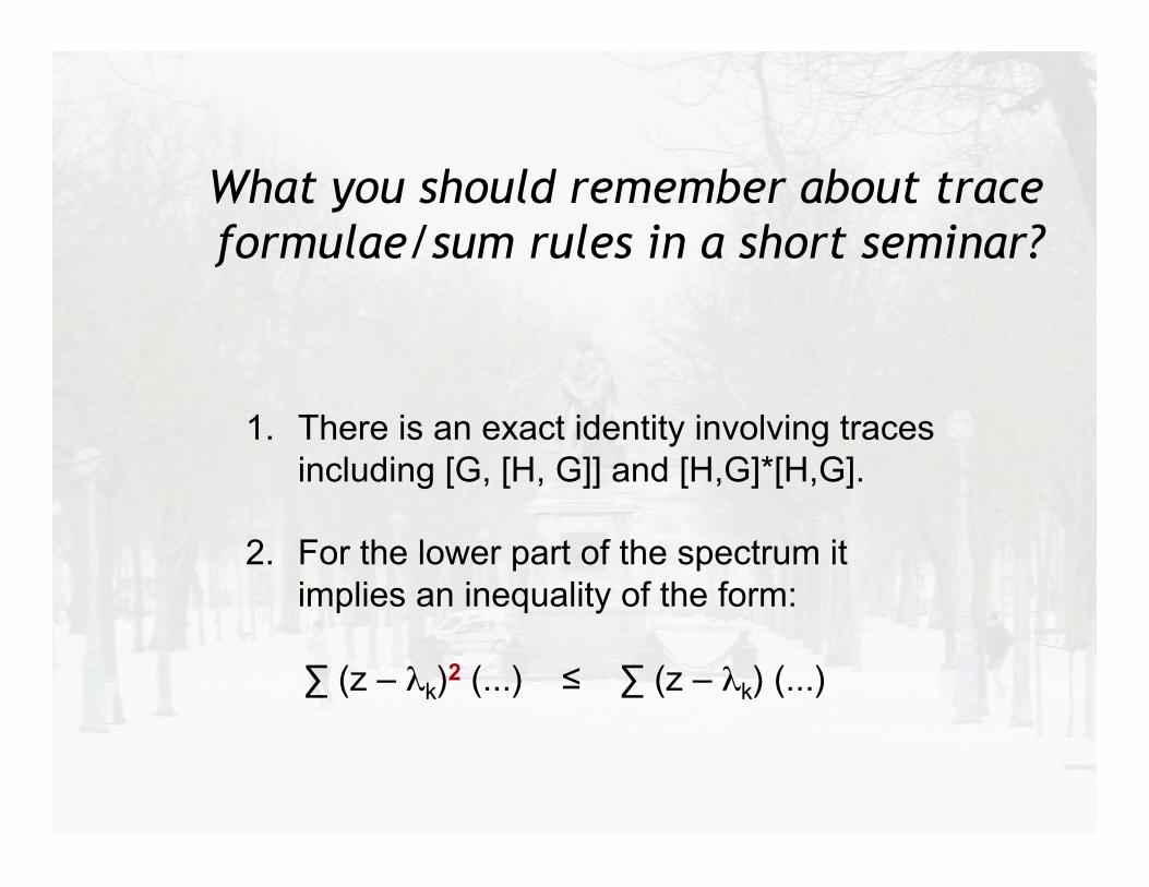
What you should remember about trace formulae/sum rules in a short seminar?
What you should remember about trace formulae/sum rules in a short seminar?
1. There is an exact identity involving traces including [G, [H, G]] and [H,G]*[H,G].
2. For the lower part of the spectrum it implies an inequality of the form:
∑ (z – λk)2 (...) ≤ ∑ (z – λk) (...)
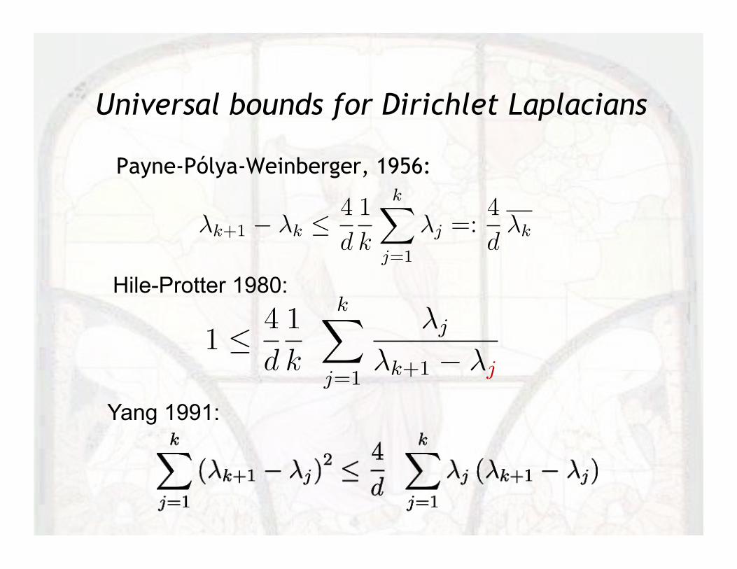
Universal bounds for Dirichlet Laplacians
Yang 1991:
1 ! 4
d
1
k
k!
j=1
!j
!k+1 " !j
#uj, [G, [H, G] , ] uj$ =!
k:!k !=!j
(!k " !j)|Gjk|2
1 =4
d
!
k:!k !=!j
| #uj,%uk$ |2
!k " !j
"
!
" #"Q
"x(x, y)" "P
"y(x, y)
$dxdy =
%
C
F(r) · dr
1
Hile-Protter 1980:
Payne-Pólya-Weinberger, 1956:
L [f ] (w) := supz
(w · z! f(z))
L : S " S,
where
S := f convex, such thatf(z)
|z| "#
!k+1 ! !k $4
d
1
k
k!
j=1
!j =:4
d!k
1
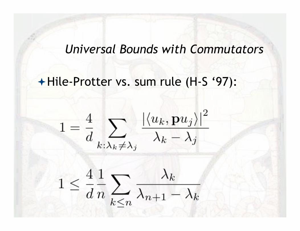
Universal Bounds with Commutators
Hile-Protter vs. sum rule (H-S ‘97):
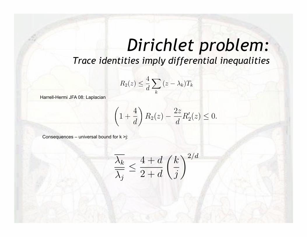
Dirichlet problem: Trace identities imply differential inequalities
Harrell-Hermi JFA 08: Laplacian
Consequences – universal bound for k >j:
!
!j!J
(z ! !j)2 "[G, [H,G]]"j, "j# ! 2(z ! !j) "[H,G]"j, [H,G]"j#(1)
= 2!
!j!J
!
!k!Jc
(z ! !j)(z ! !k)(!k ! !j)G2jk.
1 =4
d
!
k:!k "=!j
| ""j,$"k# |2
!k ! !j
R2(z) % 4
d
!
k
(z ! !k)Tk
"1 +
4
d
#R2(z) % 4
d
!
k
(z ! !kTk
Write the test function as
# =1&
$· (&$#)
and use the product rule in the form
%(t) = e#iHt%(0)
!$2$ + q(x) = !!! + q(x)
q(x) :=1
4
"$r
$
#2
! 1
2
$rr
$.
&n ' 0 with '&n' = 1, such that '(H ! !)&n' ( 0.
F [f ] (k) = f(k) :=1
(2()d/2
$
Rd
e#ik·xf(x)dx
H% = ! !2
2m$2%(x) + V (x)%(x)
F#1 [g] (x) = g(x) :=1
(2()d/2
$
Rd
e+ik·xg(k)dk
F%
)&
)x"
&(k) = k"&(k),
1
!k
!j
! 4 + d
2 + d
!k
j
"2/d
(1)
1 =4
d
#
k:!k !=!j
| ""j,#"k$ |2
!k % !j
#R2(0, #) ! #2 4
d
#
k
(0% !k)Tk
!1 +
4
d
"R2(z) ! 4
d
#
k
(z % !kTk
Write the test function as
$ =1&
%· (&%$)
and use the product rule in the form
&(t) = e"iHt&(0)
%#2# + q(x) = %!! + q(x)
q(x) :=1
4
!%r
%
"2
% 1
2
%rr
%.
'n ( 0 with ''n' = 1, such that '(H % !)'n' ( 0.
F [f ] (k) = f(k) :=1
(2))d/2
$
Rd
e"ik·xf(x)dx
H& = % !2
2m#2&(x) + V (x)&(x)
F"1 [g] (x) = g(x) :=1
(2))d/2
$
Rd
e+ik·xg(k)dk
F%
*'
*x"
&(k) = k"'(k),
F [%!']k = |k|2'(k),1

Statistics of spectra
A reverse Cauchy inequality:
The variance is dominated by the square of the mean.
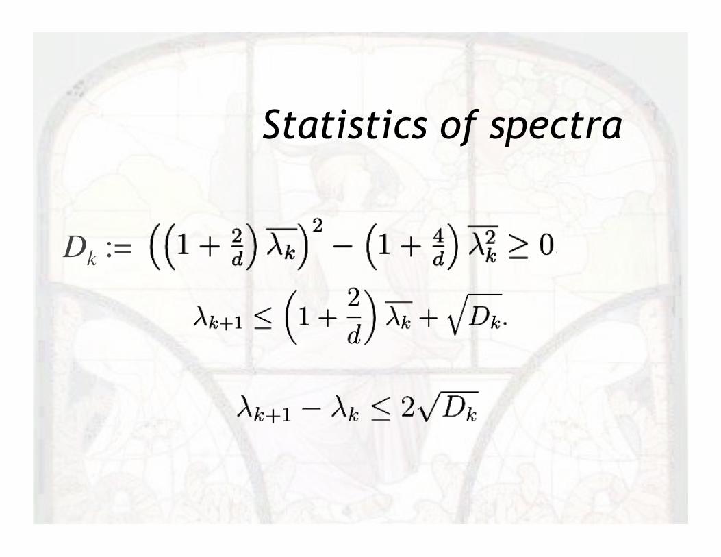
Statistics of spectra
Dk :=

How to get information about eigenvalues from information
on Riesz means?
How to get information about eigenvalues from information
on Riesz means? Riesz means are related to:
How to get information about eigenvalues from information
on Riesz means? Riesz means are related to
• sums of eigenvalues by Legendre transform
How to get information about eigenvalues from information
on Riesz means? Riesz means are related to
• sums of eigenvalues by Legendre transform
• partition functions by Laplace transform
Some models in nanophysics:
1. Schrödinger operators on curves and surfaces embedded in space. Quantum wires and waveguides.
2. Periodic Schrödinger operators. Electrons in crystals.
3. Quantum graphs. Nanoscale circuits 4. Relativistic Hamiltonians on curved
surfaces. Graphene.
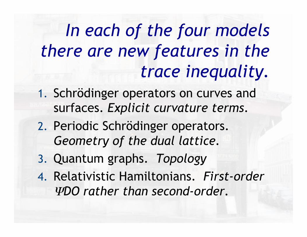
In each of the four models there are new features in the
trace inequality. 1. Schrödinger operators on curves and
surfaces. Explicit curvature terms. 2. Periodic Schrödinger operators.
Geometry of the dual lattice. 3. Quantum graphs. Topology 4. Relativistic Hamiltonians. First-order
ΨDO rather than second-order.
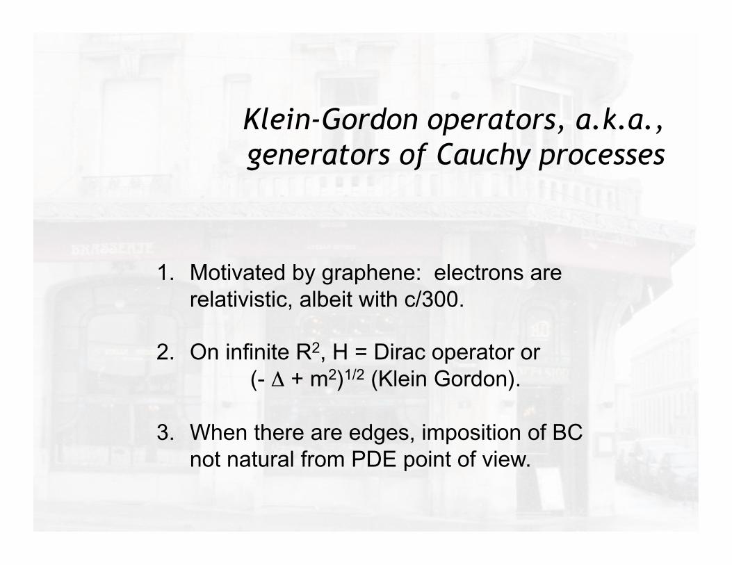
Klein-Gordon operators, a.k.a., generators of Cauchy processes
1. Motivated by graphene: electrons are relativistic, albeit with c/300.
2. On infinite R2, H = Dirac operator or (- Δ + m2)1/2 (Klein Gordon).
3. When there are edges, imposition of BC not natural from PDE point of view.
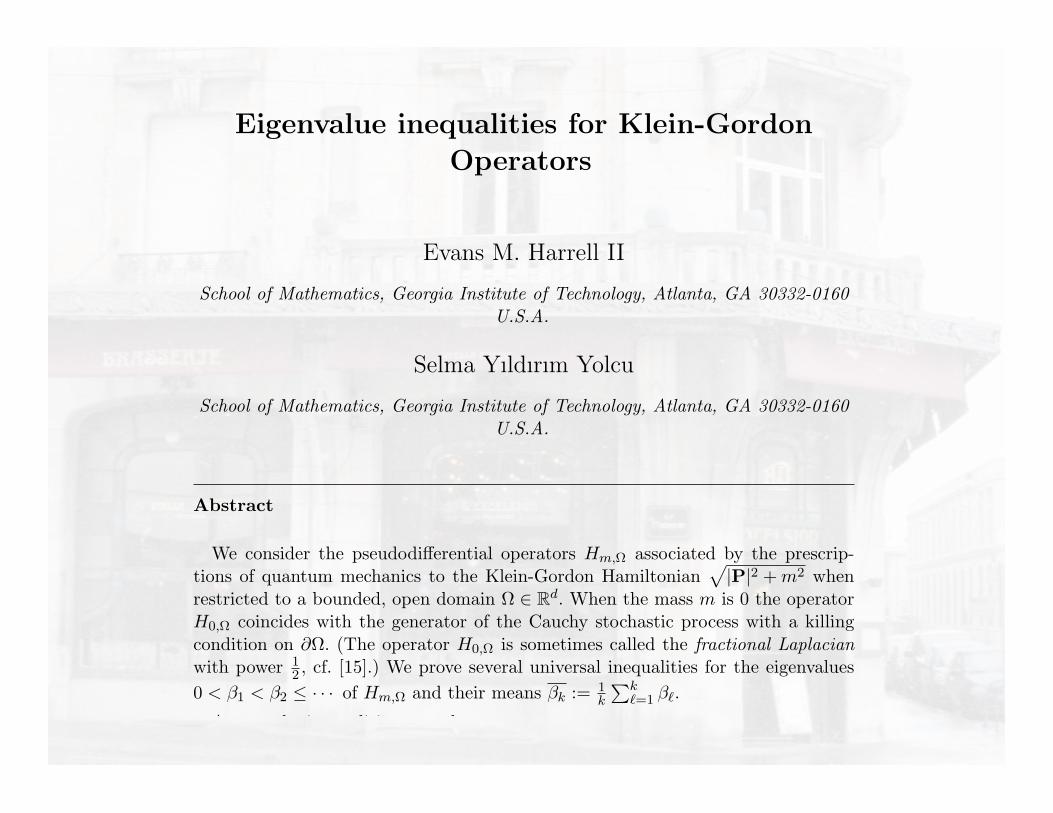
Eigenvalue inequalities for Klein-GordonOperators
Evans M. Harrell II
School of Mathematics, Georgia Institute of Technology, Atlanta, GA 30332-0160U.S.A.
Selma Yıldırım Yolcu
School of Mathematics, Georgia Institute of Technology, Atlanta, GA 30332-0160U.S.A.
Abstract
We consider the pseudodi!erential operators Hm,! associated by the prescrip-tions of quantum mechanics to the Klein-Gordon Hamiltonian
!|P|2 + m2 when
restricted to a bounded, open domain " ! Rd. When the mass m is 0 the operatorH0,! coincides with the generator of the Cauchy stochastic process with a killingcondition on !". (The operator H0,! is sometimes called the fractional Laplacianwith power 1
2 , cf. [15].) We prove several universal inequalities for the eigenvalues0 < "1 < "2 " · · · of Hm,! and their means "k := 1
k
"k!=1 "!.
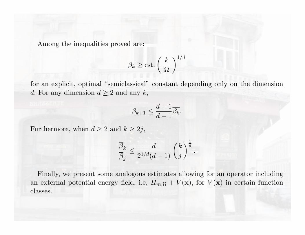
Among the inequalities proved are:
"k # cst.#
k
|"|
$1/d
for an explicit, optimal “semiclassical” constant depending only on the dimensiond. For any dimension d # 2 and any k,
"k+1 "d + 1d$ 1
"k.
Furthermore, when d # 2 and k # 2j,
"k
"j
" d
21/d(d$ 1)
#k
j
$ 1d
.
Finally, we present some analogous estimates allowing for an operator includingan external potential energy field, i.e, Hm,! + V (x), for V (x) in certain functionclasses.
Preprint submitted to Elsevier 2 December 2008
Laplacians [33,24,42]. Moreover, comparable universal bounds have been ob-tained with the same strategy for Schrodinger operators on Euclidean spaces[21], and both Laplacians and Schrodinger operators on embedded manifolds[29,43,20,32,10,11,14,16,17]. In many cases examples can be identified in whichthe inequalities are saturated.
The plan of attack is to use trace identities to derive universal spectral boundsand geometric spectral bounds for Hm,!. The generator of the Cauchy process,corresponding to the case m = 0, is often referred to as the fractional Laplacianand designated
!"!. The latter is, unfortunately, ambiguous notation, since
this operator is distinct from the operator!"!! as defined by the functional
calculus for the Dirichlet Laplacian "!!, except when " is all of Rd. Forthis reason we shall avoid the ambiguous notation when " is a proper subsetof Rd. (For the spectral theorem and the functional calculus, see, e.g., [34].)Whereas several universal eigenvalue bounds, mostly of unknown or indi#erentsharpness, have been obtained for higher-order partial di#erential operatorssuch as the bilaplacian (e.g., [27,20,12,38,41]), and for some first-order Diracoperators [9], universal bounds for pseudodi#erential operators appear not tohave been studied before.
In a final section we study interacting Klein-Gordon operators of the form
H = Hm,! + V (x), (1.2)
which is used in a semi-relativistic approximation to model the quantum dy-namics of a fast-moving spinless particle in an external field.
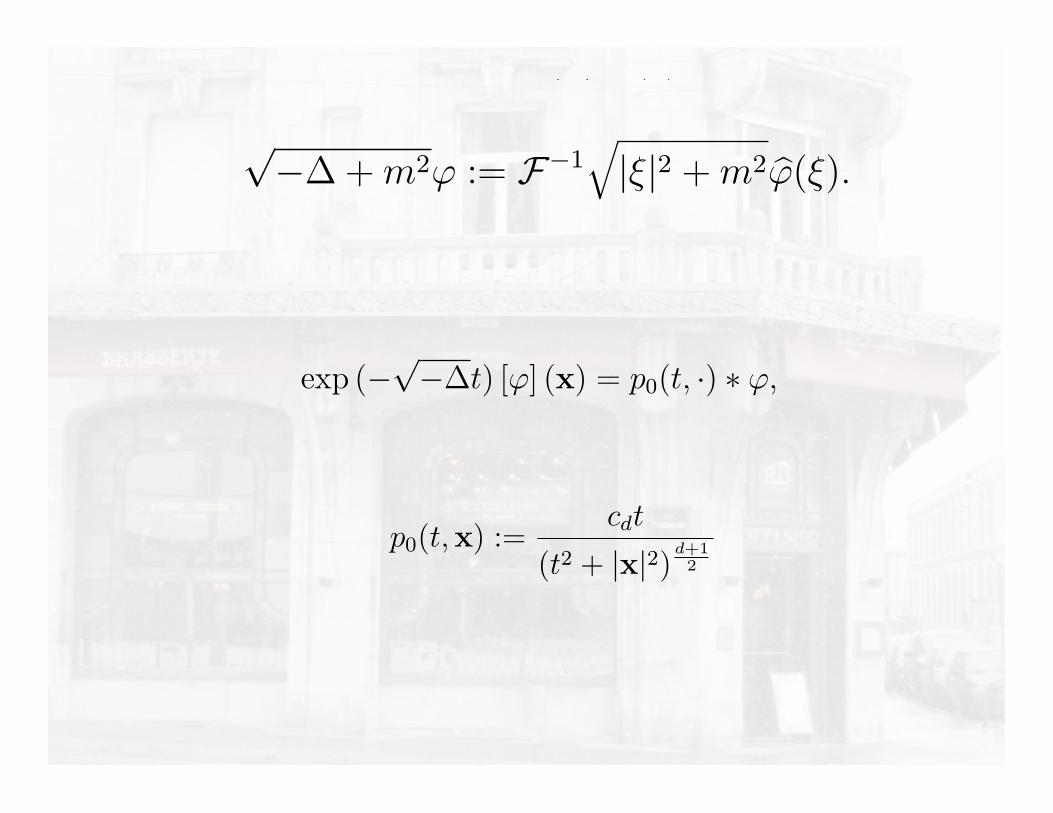
Klein-Gordon operators can be conveniently defined using the Fourier trans-form on the dense subspace of test functions C!c (Rd). With the normalization
!!(") = F [!] :=1
(2#)d/2
"
Rdexp ("i" · x)!(x)dx,
the Laplacian is given by "!! := F"1|"|2 !!("), and therefore
!"! + m2! := F"1
#|"|2 + m2 !!("). (1.3)
The semigroup generated on L2(Rd) is known explicitly, so that, for instancewith m = 0,
exp ("!"!t) [!] (x) = p0(t, ·) # !, (1.4)
3
Laplacians [33,24,42]. Moreover, comparable universal bounds have been ob-tained with the same strategy for Schrodinger operators on Euclidean spaces[21], and both Laplacians and Schrodinger operators on embedded manifolds[29,43,20,32,10,11,14,16,17]. In many cases examples can be identified in whichthe inequalities are saturated.
The plan of attack is to use trace identities to derive universal spectral boundsand geometric spectral bounds for Hm,!. The generator of the Cauchy process,corresponding to the case m = 0, is often referred to as the fractional Laplacianand designated
!"!. The latter is, unfortunately, ambiguous notation, since
this operator is distinct from the operator!"!! as defined by the functional
calculus for the Dirichlet Laplacian "!!, except when " is all of Rd. Forthis reason we shall avoid the ambiguous notation when " is a proper subsetof Rd. (For the spectral theorem and the functional calculus, see, e.g., [34].)Whereas several universal eigenvalue bounds, mostly of unknown or indi#erentsharpness, have been obtained for higher-order partial di#erential operatorssuch as the bilaplacian (e.g., [27,20,12,38,41]), and for some first-order Diracoperators [9], universal bounds for pseudodi#erential operators appear not tohave been studied before.
In a final section we study interacting Klein-Gordon operators of the form
H = Hm,! + V (x), (1.2)
which is used in a semi-relativistic approximation to model the quantum dy-namics of a fast-moving spinless particle in an external field.
Klein-Gordon operators can be conveniently defined using the Fourier trans-form on the dense subspace of test functions C!c (Rd). With the normalization
!!(") = F [!] :=1
(2#)d/2
"
Rdexp ("i" · x)!(x)dx,
the Laplacian is given by "!! := F"1|"|2 !!("), and therefore
!"! + m2! := F"1
#|"|2 + m2 !!("). (1.3)
The semigroup generated on L2(Rd) is known explicitly, so that, for instancewith m = 0,
exp ("!"!t) [!] (x) = p0(t, ·) # !, (1.4)
3where for t > 0 the transition density (= convolution kernel) is
p0(t,x) :=cdt
(t2 + |x|2) d+12
, (1.5)
with cd :=d!
(4!)d/2!(1 + d/2). (Cf. [4]. We note that cd is the same “semiclas-
sical” constant that appears in the Weyl estimate for the eigenvalues of theLaplacian. It is given in [4] and some other sources as !!
d+12 !
!d+12
", which
is equal to cd by an application of the duplication formula of the gammafunction.)
If " is a non-empty, bounded, open subset of Rd, then we define Hm,! asfollows. Consider the quadratic form on C"c (") given by
" !#
!""## + m2 "
(Here"## + m2 is calculated for Rd.) Since this quadratic form is positive
and defined on a dense subset of L2("), it extends to a unique minimal positiveoperator (the Friedrichs extension) on L2("), which we designate Hm,!. Thesemigroup e!tHm,! has an integral kernel pm,!(t,x,y), the form of which istypically not known explicitly, but is bounded by comparison with the operatore!t
#!"+m2
on L2(Rd), which is known explicitly ([31],p.183), and is boundedfor t > 0. Consequently, e!tHm,! is Hilbert-Schmidt and Hm,! has purelydiscrete spectrum.
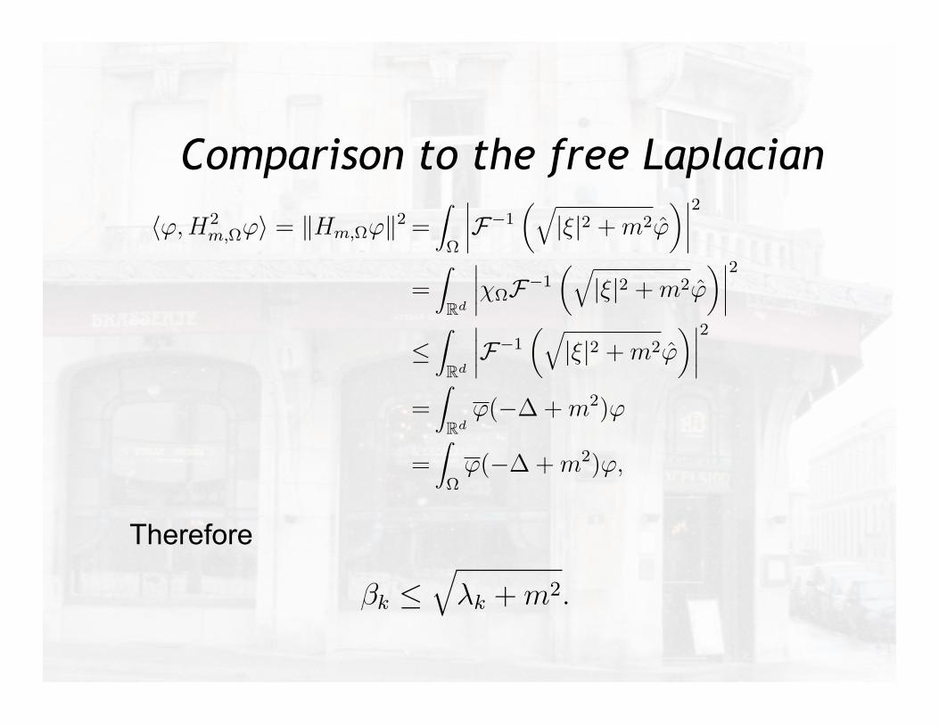
We remark that the Fourier transform can be more directly applied to Hm,!
than to the square root of the Dirichlet Laplacian according to the functionalcalculus, which dominates it in the following sense:
Suppose that " $ C"c (") % C"c (Rd). Then
&", H2m,!"' = (Hm,!"(2 =
#
!
$$$$F!1%&
|#|2 + m2"'$$$$
2
=#
Rd
$$$$$!F!1%&
|#|2 + m2"'$$$$
2
)#
Rd
$$$$F!1%&
|#|2 + m2"'$$$$
2
=#
Rd"(## + m2)"
=#
!"(## + m2)",
because supp(") $ " and ## is a local operator. Therefore, if %k denotes the
4
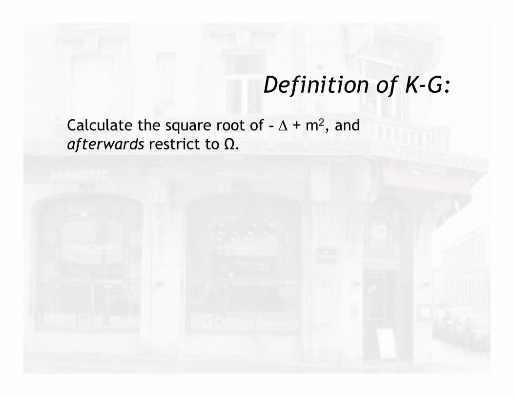
Definition of K-G:
Calculate the square root of - Δ + m2, and afterwards restrict to Ω.
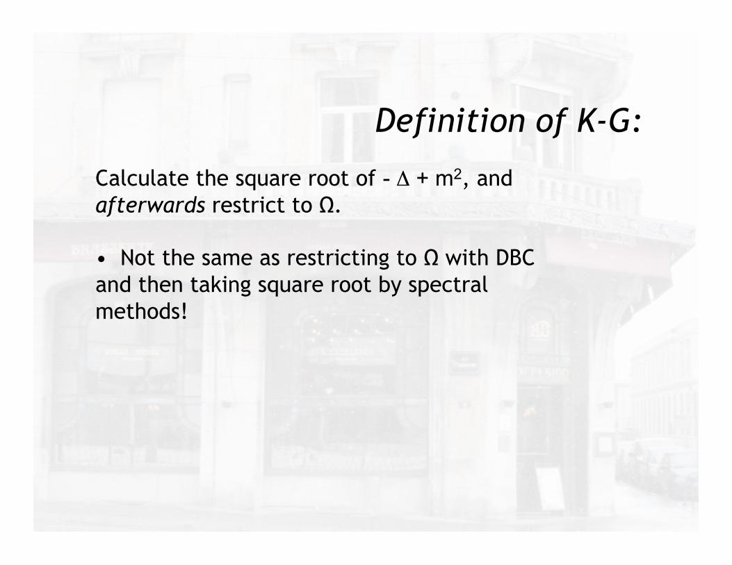
Definition of K-G:
Calculate the square root of - Δ + m2, and afterwards restrict to Ω.
• Not the same as restricting to Ω with DBC and then taking square root by spectral methods!
Comparison to the free Laplacian
where for t > 0 the transition density (= convolution kernel) is
p0(t,x) :=cdt
(t2 + |x|2) d+12
, (1.5)
with cd :=d!
(4!)d/2!(1 + d/2). (Cf. [4]. We note that cd is the same “semiclas-
sical” constant that appears in the Weyl estimate for the eigenvalues of theLaplacian. It is given in [4] and some other sources as !!
d+12 !
!d+12
", which
is equal to cd by an application of the duplication formula of the gammafunction.)
If " is a non-empty, bounded, open subset of Rd, then we define Hm,! asfollows. Consider the quadratic form on C"c (") given by
" !#
!""## + m2 "
(Here"## + m2 is calculated for Rd.) Since this quadratic form is positive
and defined on a dense subset of L2("), it extends to a unique minimal positiveoperator (the Friedrichs extension) on L2("), which we designate Hm,!. Thesemigroup e!tHm,! has an integral kernel pm,!(t,x,y), the form of which istypically not known explicitly, but is bounded by comparison with the operatore!t
#!"+m2
on L2(Rd), which is known explicitly ([31],p.183), and is boundedfor t > 0. Consequently, e!tHm,! is Hilbert-Schmidt and Hm,! has purelydiscrete spectrum.
We remark that the Fourier transform can be more directly applied to Hm,!
than to the square root of the Dirichlet Laplacian according to the functionalcalculus, which dominates it in the following sense:
Suppose that " $ C"c (") % C"c (Rd). Then
&", H2m,!"' = (Hm,!"(2 =
#
!
$$$$F!1%&
|#|2 + m2"'$$$$
2
=#
Rd
$$$$$!F!1%&
|#|2 + m2"'$$$$
2
)#
Rd
$$$$F!1%&
|#|2 + m2"'$$$$
2
=#
Rd"(## + m2)"
=#
!"(## + m2)",
because supp(") $ " and ## is a local operator. Therefore, if %k denotes the
4
Therefore
kth eigenvalue of Hm,!, and !k is the kth eigenvalue of !!,
"k "!
!k + m2. (1.6)
2 Trace formulae and inequalities for spectra of Hm,!
In [18] universal bounds for spectra of Laplacians were found as consequencesof di"erential inequalities for Riesz means defined on the sequence of eigenval-ues. The strategy here is the same, as adapted to the eigenvalues "j, j = 1, . . .of the first-order pseudodi"erential operator Hm,!. However, as the earlier ar-ticle made heavy use of the fact that the Laplacian is of second order and actslocally, neither of which circumstance applies here, the results we obtain hereand the details of the argument are quite di"erent.
An essential lemma is an adaptation of a result of [21,22].
Lemma 2.1 (Harrell-Stubbe) Let H be a self-adjoint operator on L2(#), # #Rd, with discrete spectrum "1 " "2 " · · · < inf #ess(H), interpreted as +$when #ess(H) is empty. Denoting the corresponding normalized eigenfunctionsuj, assume that for a Cartesian coordinate x!, the functions x!uj and x2
!uj
are in the domain of definition of H. Then for any z < inf #ess(H),
"
j:"j!z
(z ! "j)%uj, [x!, [H, x!]] uj& ! 2' [H, x!] uj'2 " 0, (2.1)
and
"
j:"j!z
(z ! "j)2%uj, [x!, [H, x!]] uj& ! 2(z ! "j)' [H, x!] uj'2 " 0. (2.2)
So that this article is self-contained, we provide a proof of the lemma underthe simplifying assumption that the spectrum is purely discrete.
Proof. Elementary calculations show that, subject to the domain assumptionsmade in the statement of the theorem,
[H, x!] uj = (H ! "j) x!uj,
and%uj, [x!, [H, x!]] uj& = 2%x!uj, (H ! "j) x!uj&.
These two identities can be combined and slightly rearranged to yield:
(z ! "j)%uj, [x!, [H, x!]] uj& ! 2' [H, x!] uj'2
5
Weyl asymptotic for HΩ,m
on w, we get
w = 2j
!(d! 1)z!(d + 1) !j
"d
. (2.26)
Thus the inequality is valid under the assumption that k > w " 2j.
3 Weyl asymptotics and semiclassical bounds for Hm,!
In this section we consider the eigenvalues !k of Hm,! as k # $. In view of
the elementary inequalities (1.1), and the fact that lim|!|"#
#|"|2 + m2
|"| = 1, it
su!ces to consider the case m = 0.
We begin with the analogue of the Weyl formula for the Laplacian, adaptingone of the standard proofs of the latter, which relies on an estimate of thepartition function Z(t) :=
$e$"jt for t > 0. Recall that the function Z(t)
can be written asZ(t) =
%e$"tdN(!), (3.1)
where N(!) :=$
"j%"
1 is the usual counting function. Another standard for-
mula for the partition function is
Z(t) =%
!p!(x,x, t)dx. (3.2)
If we accept that Hm,! is well approximated by%!"! in the “semiclassical
limit,” then the analogue for N(!) of the Weyl asymptotic formula for theLaplacian should be identical to the usual Weyl formula, with the identificationof !k with
%#k. This intuition is confirmed by the following:
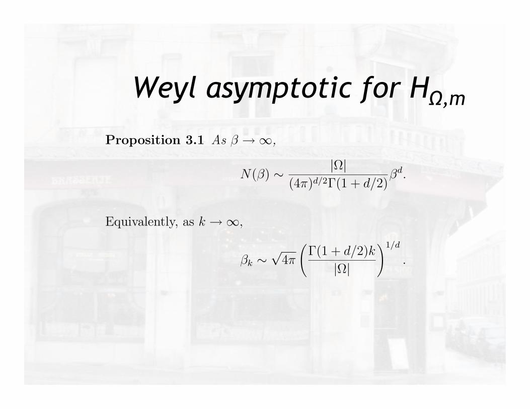
Proposition 3.1 As ! #$,
N(!) & |#|(4$)d/2$(1 + d/2)
!d. (3.3)
Equivalently, as k #$,
!k &%
4$
!$(1 + d/2)k
|#|
"1/d
. (3.4)
Moreover, the function U of (2.14) satisfies
U(z) & |#|2$d/2(d2 ! 1)$(1 + d/2)
zd+1.
11
Eigenvalue inequalities for Klein-GordonOperators
Evans M. Harrell II
School of Mathematics, Georgia Institute of Technology, Atlanta, GA 30332-0160U.S.A.
Selma Yıldırım Yolcu
School of Mathematics, Georgia Institute of Technology, Atlanta, GA 30332-0160U.S.A.
Abstract
We consider the pseudodi!erential operators Hm,! associated by the prescrip-tions of quantum mechanics to the Klein-Gordon Hamiltonian
!|P|2 + m2 when
restricted to a bounded, open domain " ! Rd. When the mass m is 0 the operatorH0,! coincides with the generator of the Cauchy stochastic process with a killingcondition on !". (The operator H0,! is sometimes called the fractional Laplacianwith power 1
2 , cf. [15].) We prove several universal inequalities for the eigenvalues0 < "1 < "2 " · · · of Hm,! and their means "k := 1
k
"k!=1 "!.
Among the inequalities proved are:
"k # cst.#
k
|"|
$1/d
for an explicit, optimal “semiclassical” constant depending only on the dimensiond. For any dimension d # 2 and any k,
"k+1 "d + 1d$ 1
"k.
Furthermore, when d # 2 and k # 2j,
"k
"j
" d
21/d(d$ 1)
#k
j
$ 1d
.
Finally, we present some analogous estimates allowing for an operator includingan external potential energy field, i.e, Hm,! + V (x), for V (x) in certain functionclasses.
Preprint submitted to Elsevier 2 December 2008
Calculate first and second commutators:
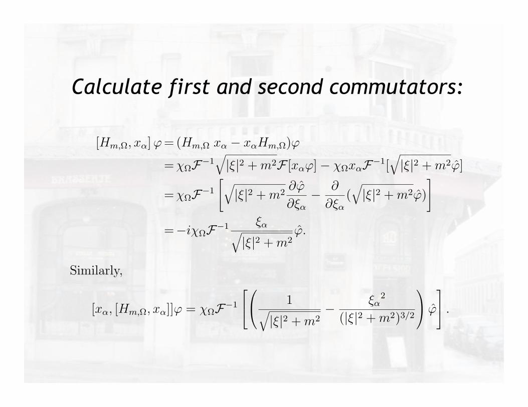
Proof of Theorem 2.1. We make the special choice H = Hm,! and calculatethe first and second commutators with the aid of the Fourier transform:
Writing Hm,! = !!F!1!|"|2 + m2F ,
[Hm,!, x!] # = (Hm,! x! ! x!Hm,!)#
= !!F!1!|"|2 + m2F [x!#]! !!x!F!1[
!|"|2 + m2#]
= !!F!1
"!|"|2 + m2
$#
$"!! $
$"!(!|"|2 + m2#)
#
=!i!!F!1 "!!|"|2 + m2
#. (2.9)
Similarly,
[x!, [Hm,!, x!]]# = !!F!1
$
%
&
' 1!|"|2 + m2
! "!2
(|"|2 + m2)3/2
(
) #
*
+ . (2.10)
Due to (2.9) and (2.10), there are simplifications when we sum over %:
d,
!=1
" [Hm,!, x!] #"2 #-
#,|"|2
|"|2 + m2#
.
# 1,
andd,
!=1
&
' 1!|"|2 + m2
! "!2
(|"|2 + m2)3/2
(
) =(d! 1)|"|2 + d m2
(|"|2 + m2)3/2
$ d! 1!|"|2 + m2
.
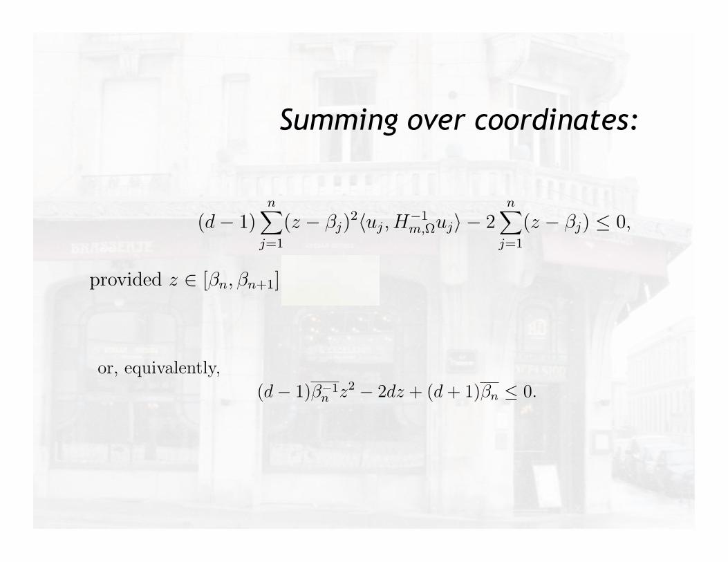
In consequence, (2.2) implies that
(d! 1)n,
j=1
(z ! &j)2%uj, H
!1m,!uj& ! 2
n,
j=1
(z ! &j) # 0, (2.11)
provided z ' [&n, &n+1]. Because
H!1m,!uj =
1
&juj,
and
(z ! &j) = !(z ! &j)(z ! &j ! z)
&j,
Eq. (2.11) can be rewritten as
(d + 1)n,
j=1
(z ! &j)2
&j! 2z
n,
j=1
(z ! &j)
&j# 0, (2.12)
8
Summing over coordinates:
Proof of Theorem 2.1. We make the special choice H = Hm,! and calculatethe first and second commutators with the aid of the Fourier transform:
Writing Hm,! = !!F!1!|"|2 + m2F ,
[Hm,!, x!] # = (Hm,! x! ! x!Hm,!)#
= !!F!1!|"|2 + m2F [x!#]! !!x!F!1[
!|"|2 + m2#]
= !!F!1
"!|"|2 + m2
$#
$"!! $
$"!(!|"|2 + m2#)
#
=!i!!F!1 "!!|"|2 + m2
#. (2.9)
Similarly,
[x!, [Hm,!, x!]]# = !!F!1
$
%
&
' 1!|"|2 + m2
! "!2
(|"|2 + m2)3/2
(
) #
*
+ . (2.10)
Due to (2.9) and (2.10), there are simplifications when we sum over %:
d,
!=1
" [Hm,!, x!] #"2 #-
#,|"|2
|"|2 + m2#
.
# 1,
andd,
!=1
&
' 1!|"|2 + m2
! "!2
(|"|2 + m2)3/2
(
) =(d! 1)|"|2 + d m2
(|"|2 + m2)3/2
$ d! 1!|"|2 + m2
.
In consequence, (2.2) implies that
(d! 1)n,
j=1
(z ! &j)2%uj, H
!1m,!uj& ! 2
n,
j=1
(z ! &j) # 0, (2.11)
provided z ' [&n, &n+1]. Because
H!1m,!uj =
1
&juj,
and
(z ! &j) = !(z ! &j)(z ! &j ! z)
&j,
Eq. (2.11) can be rewritten as
(d + 1)n,
j=1
(z ! &j)2
&j! 2z
n,
j=1
(z ! &j)
&j# 0, (2.12)
8
or, equivalently,(d! 1)!!1
n z2 ! 2dz + (d + 1)!n " 0. (2.13)
Setting z = !n+1, we see that !n+1 must be less than the larger root of (2.13),which is the conclusion of the theorem. !
For future purposes we note that this theorem extends with small modifica-tions to semirelativistic Hamiltonians of the form Hm,! + V (x). More specifi-cally, (2.11) is valid when uk and !k are the eigenfunctions and eigenvaluesof Hm,! + V (x).
We next apply similar reasoning to a function related to Riesz means. Witha+ := max(0, a), let
U(z) :=!
k
(z ! !k)2+
!k, (2.14)
where z is a real variable. Note that if z # [!j, !j+1], then
U(z)
j= !!1
j z2 ! 2z + !j. (2.15)
Theorem 2.3 The function z!(d+1)U(z) is nondecreasing in the variable z.Moreover, for d $ 2 and any j $ 1, the “Riesz mean” R1(z) :=
"k(z ! !k)+
satisfies
R1(z) $#
$ 2j(d! 1)d
(d + 1)d+1!jd
%
& zd+1 (2.16)
for all z $'
d + 1
d! 1
(
!j.
Proof. In notation that suppresses n, Eq. (2.12) can be written
(d + 1)!
k
(z ! !k)2+
!k! 2z
!
k
(z ! !k)+
!k" 0, (2.17)
which for the function U reads
(d + 1)U(z)! zU!(z) " 0,
or, equivalently,d
dz
)U(z)
zd+1
*
$ 0, (2.18)
proving the claim about U .
Eq. (2.11) tells us that
R1(z) $ d! 1
2U(z). (2.19)
9
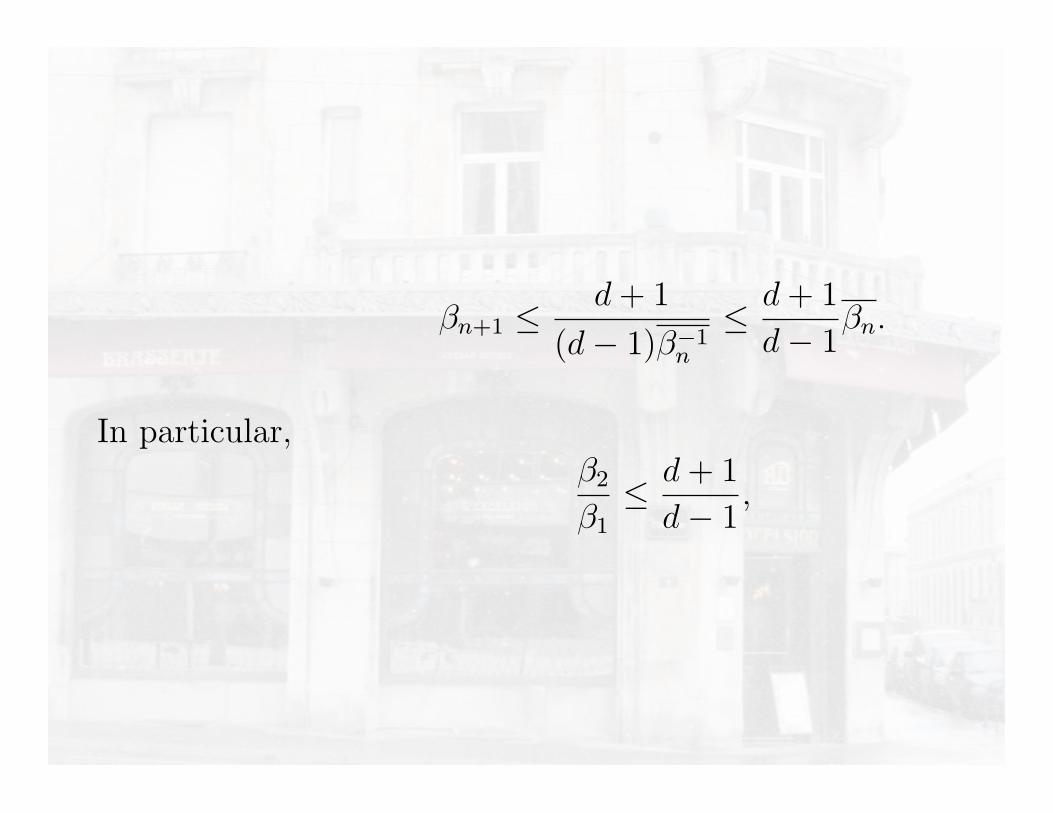
Before giving the proof we note two slightly weaker but more appealing vari-ants of (2.5) using the Cauchy-Schwarz inequality, 1 ! !n !!1
n , with the aidof which the universal bound (2.5) simplifies to
!n+1 !d + 1
(d" 1)!!1n
! d + 1
d" 1!n. (2.6)
In particular,!2
!1! d + 1
d" 1, (2.7)
regardless of any property of the domain other than compactness.
In this connection, recall that R. Banuelos and T. Kulczycki have proved in [5]that the fundamental gap of the Cauchy process is controlled by the inradiusin the case of a bounded convex domain ! of inradius Inr(!), viz., for m = 0,
!2 " !1 !#
"2 " (1/2)#
"1
Inr(!),
where "1 and "2 are the first and second eigenvalues for the Dirichlet Laplacianfor the unit ball, B1 in Rd. (Recall that the inradius Inr(!) of a region ! isdefined by
Inr(!) = supd(x) : x $ !,where d(x) = min|x" y| : y /$ ! [13].)
Since a ratio bound like (2.7) is algebraically equivalent to a gap bound, (2.7)provides an independent upper bound on the gap !2 " !1. Continuing to setm = 0, (1.6) and (2.7) in the form !2 " !1 ! 2
d!1!1 imply:
Corollary 2.2 If !"1 and ""1 denote the fundamental eigenvalues of H0,! and"", respectively, on the unit ball of Rd, then
!2 " !1 !!
2
d" 1
"!"1
Inr(!)!
!2
d" 1
" #""1
Inr(!). (2.8)
Proof of Corollary 2.2. Since H0,! is defined by closure from a core of functionsin C#
c , its fundamental eigenvalue satisfies the principle of domain monotonic-ity. That is, if !1 % !2, then !1(!1) ! !1(!2). In particular, if ! is a ball
of radius r, then !1(!) ! !"1r
, which is the fundamental eigenvalue of the unit
ball B1 by scaling. The first inequality follows from (2.7), and the second oneby (1.6) !
7
SinceU(z)
zd+1is nondecreasing, when z ! zj! ! !j,
U(z) !!
z
zj!
"d+1
U(zj!). (2.20)
From (2.15) with the Cauchy-Schwarz inequality we get
U(z)
j! 1
!j(z " !j)
2, (2.21)
so that with (2.19) and (2.20) we obtain
R1(z) ! (d" 1)j
2!j
!z
zj!
"d+1 #zj! " !j
$2. (2.22)
We now choose an optimized value of zj! to maximize the coe!cient of zd+1,
viz., zj! =d + 1
d" 1!j. Substituting this into (2.22), we get (2.16), as claimed. !
The Legendre transform of R1(z) is a straightforward calculation, to be foundexplicitly for example in [18,26]. The result for k " 1 < w < k is
R!1(w) = (w " [w])![w]+1 + [w]![w] , (2.23)
where [w] denotes the greatest integer # w. When w approaches an integervalue k from below, R!
1(k) = k!k.
With the Legendre transform of the right side of (2.16), we get
k!k #d !j
21/d j1/d(d" 1)k
d+1d . (2.24)
This leads us to the following upper bound for ratios of averages of eigenvaluesof Hm,!:
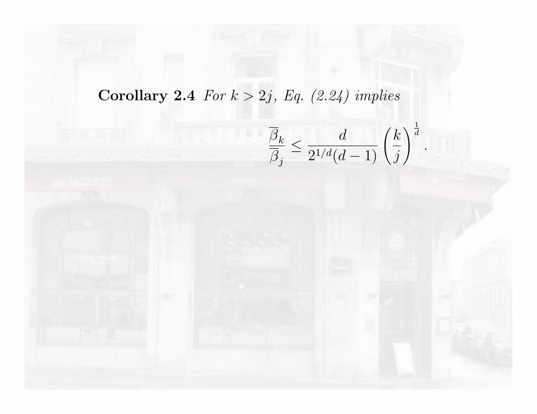
Corollary 2.4 For k > 2j, Eq. (2.24) implies
!k
!j
# d
21/d(d" 1)
!k
j
" 1d
. (2.25)
Remark 2.5 The reason for the restriction on k, j is that in Theorem 2.3, we
assumed that z !!
d + 1
d" 1
"
!j. Since the maximizing value of z! in the calcula-
tion of the Legendre transform of the right side of (2.16) depends monotonically
10
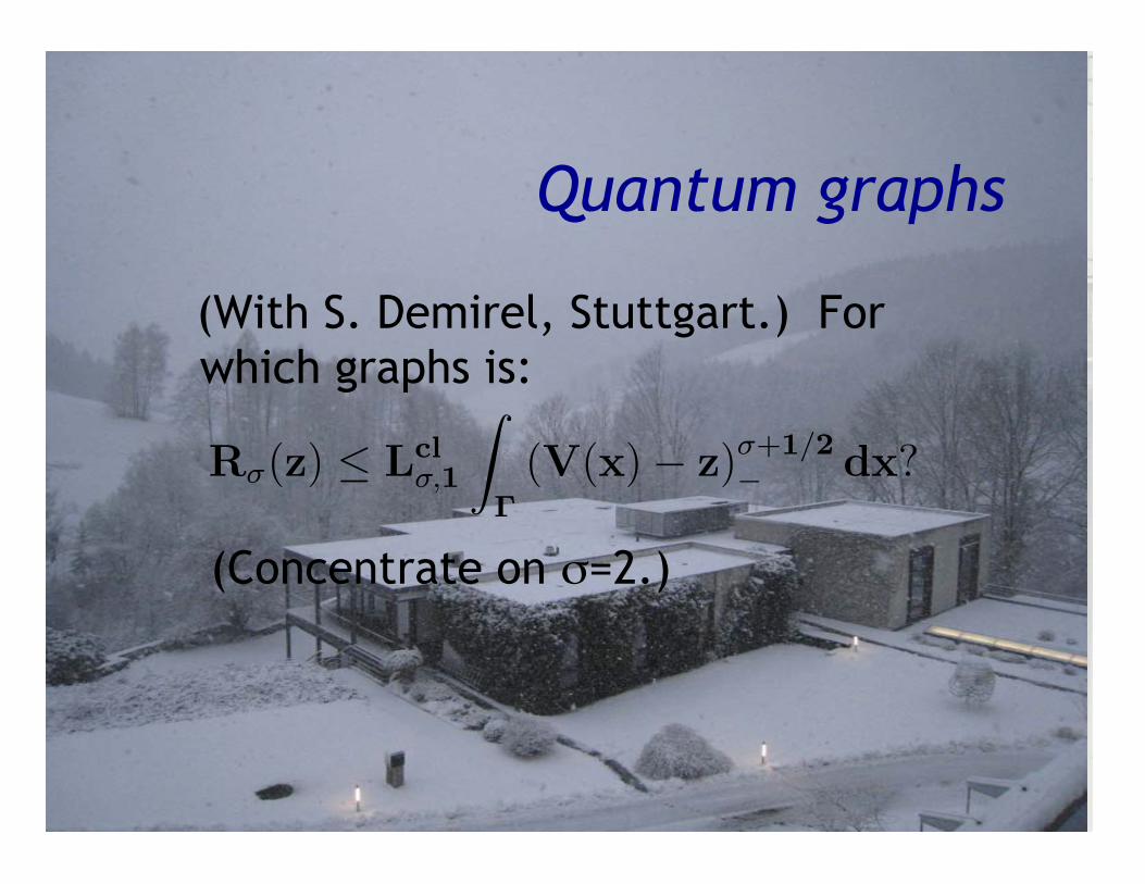
Quantum graphs
(With S. Demirel, Stuttgart.) For which graphs is:
(Concentrate on σ=2.)
R!(z) :=!
(z! !k)!+;
R!(z)! "2#
d
!(z! !k)
!!1+ "#$k"2 = explicit expr $ 0.
!k+1 $"
1 +2
d
#!k +
$Dk
R"(z) $ Lcl",1
%
!
(V(x)! z)"+1/2! dx?
R"(z,") $ "!d/2Lcl",d
%
M
(V (x)! z)"+d/2! dx.
Tjk := |%$k,#$j&|2 .!
k
Tjk $ Tj :=&$j,!#2$j
'.
Elementary gap formula:
%$j, [H,G]$k& = (!j ! !k) %$j, G$k&Since [H,G]$k = (H ! !k)G$k,
"[H,G]$k"2 =&G$j, (H ! !k)
2G$k
'
and more generally
%[H, G]$j, [H,G]$k& = %G$j, (H ! !j)(H ! !k)G$k& .Second commutator formula
%$j, [G, [H, G]]$k& = %G$j, (2H ! !j ! !k)G$k& .In particular,
%$j, [G, [H,G]]$j& = 2 %G$j, (H ! !j)G$k& .
H(g) = ! d2
ds2+ g%2
A =1
4&
!
k
(|hk|2 ! k2|hk|2
)=
p2
4&! stu!
1
ON SEMICLASSICAL AND UNIVERSAL INEQUALITIES FOR EIGENVALUESOF QUANTUM GRAPHS
SEMRA DEMIREL AND EVANS M. HARRELL II
Abstract. We study the spectra of quantum graphs with the method of trace identities (sum
rules), which are used to derive inequalities of Lieb-Thirring, Payne-Polya-Weinberger, and Yang
types, among others. We show that the sharp constants of these inequalities and even their forms
depend on the topology of the graph. Conditions are identified under which the sharp constants
are the same as for the classical inequalities; in particular, this is true in the case of trees. We also
provide some counterexamples where the classical form of the inequalities is false.
1. Introduction
This article is focused on inequalities for the means, moments, and ratios of eigenvalues of quantumgraphs. A quantum graph is a metric graph with one-dimensional Schrodinger operators acting on theedges and appropriate boundary conditions imposed at the vertices and at the finite external ends,if any. Here we shall define the Hamiltonian H on a quantum graph as the minimal (Friedrichs)self-adjoint extension of the quadratic form
! ! C!c "# E(!) :=
!
!|!"|2ds, (1.1)
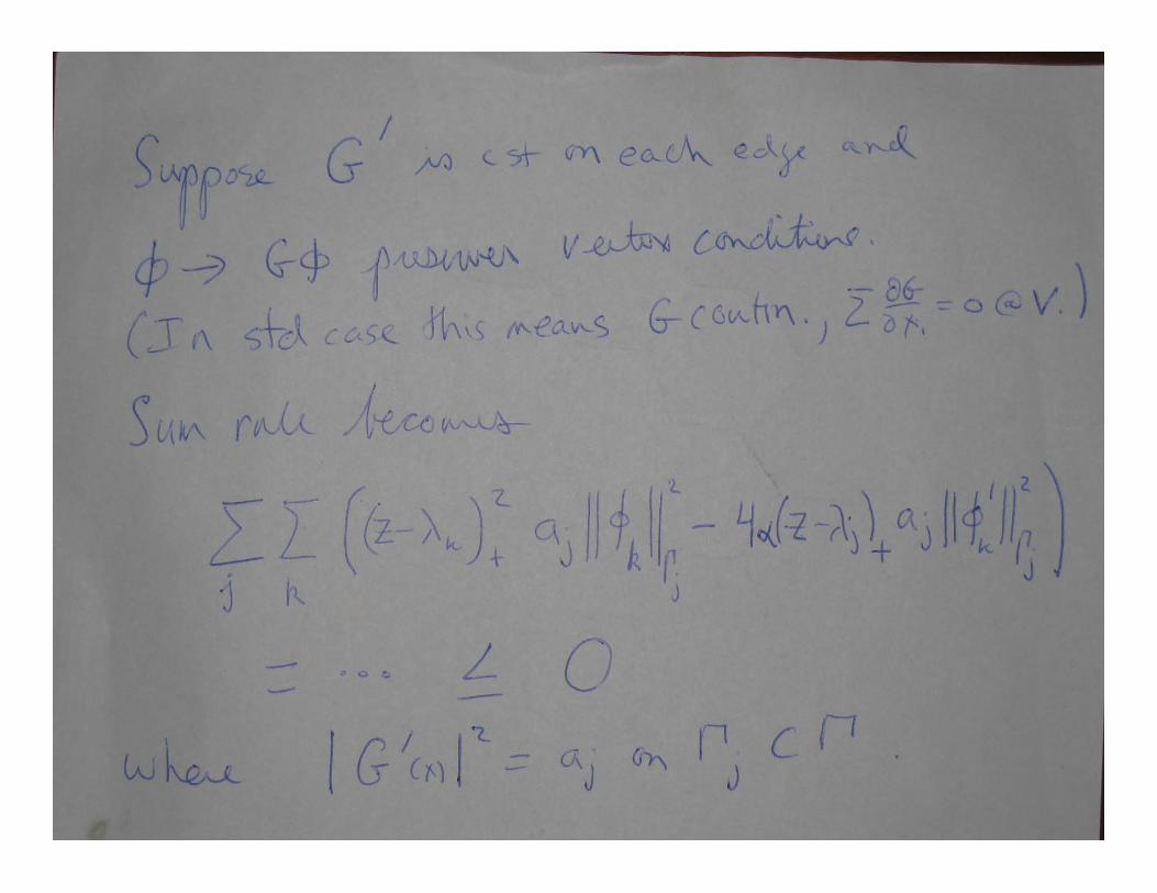
which leads to vanishing Dirichlet boundary conditions at the ends of exterior edges and to theconditions at each vertex vk that ! is continuous and moreover
"
j
"!
"xkj(0+) = 0, (1.2)
where the sum runs over all edges emanating from vk, and xkj designates the distance from vk alongthe j-th edge. (Edges connecting vk to itself are accounted twice.) In the literature these vertexconditions are usually known as Kirchho! or Neumann conditions. Other vertex conditions arepossible, and are amenable to our methods with some complications, but they will not be consideredin this article. For details about the definition of H we refer to [15].
Quantum mechanics on graphs has a long history in physics and physical chemistry [21, 24], butrecent progress in experimental solid state physics has renewed attention on them as idealized modelsfor thin domains. While the problem of quantum systems in high dimensions has to be solvednumerically, since quantum graphs are locally one dimensional their spectra can often be determinedexplicitly. A large literature on the subject has arisen, for which we refer to the bibliography givenin [3, 7].
The subject of inequalities for means, moments, and ratios of eigenvalues is rather well developedfor Laplacians on domains and for Schrodinger operators, and it is our aim to determine the extentto which analogous theorems apply to quantum graphs. For example, when there is a potentialenergy V (x) in appropriate function spaces, Lieb-Thirring inequalities provide an upper bound forthe moments of the negative eigenvalues Ej(#) of the Schrodinger operator H(#) = $#%2 +V (x) inL2(Rd), # > 0, of the form
#d/2"
Ej(!)<0
($Ej(#))" & L",d
!
Rd
(V#(x))"+d/2 dx (1.3)
1
Quantum graphs
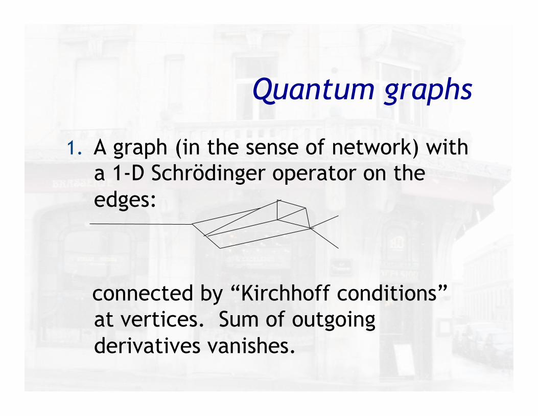
1. A graph (in the sense of network) with a 1-D Schrödinger operator on the edges:
connected by “Kirchhoff conditions” at vertices. Sum of outgoing derivatives vanishes.
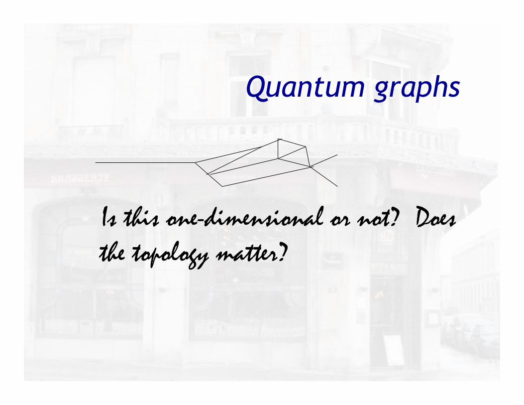
Quantum graphs
Is this one-dimensional or not? Does the topology matter?
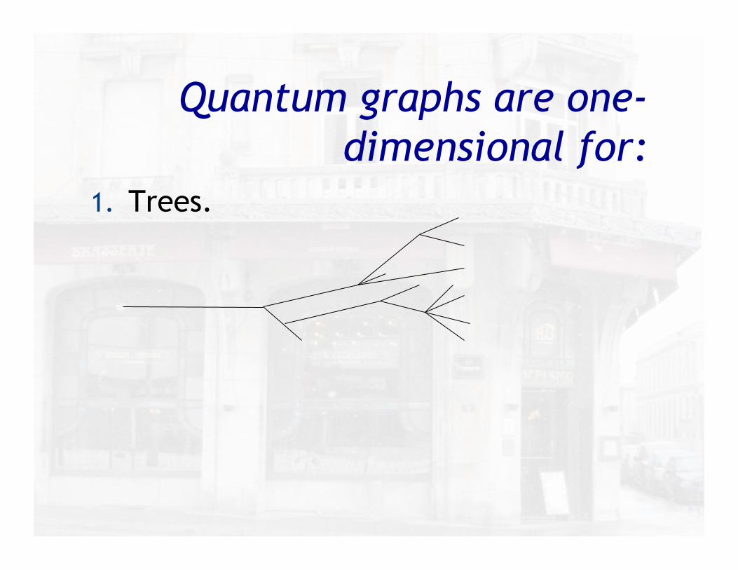
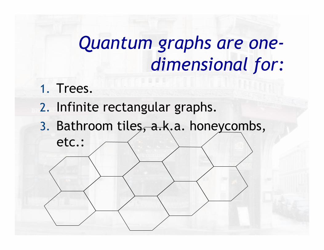
Quantum graphs are one-dimensional for:
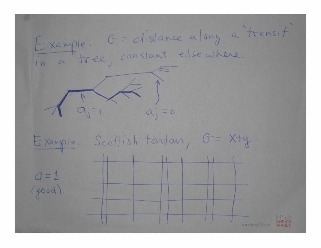
1. Trees.
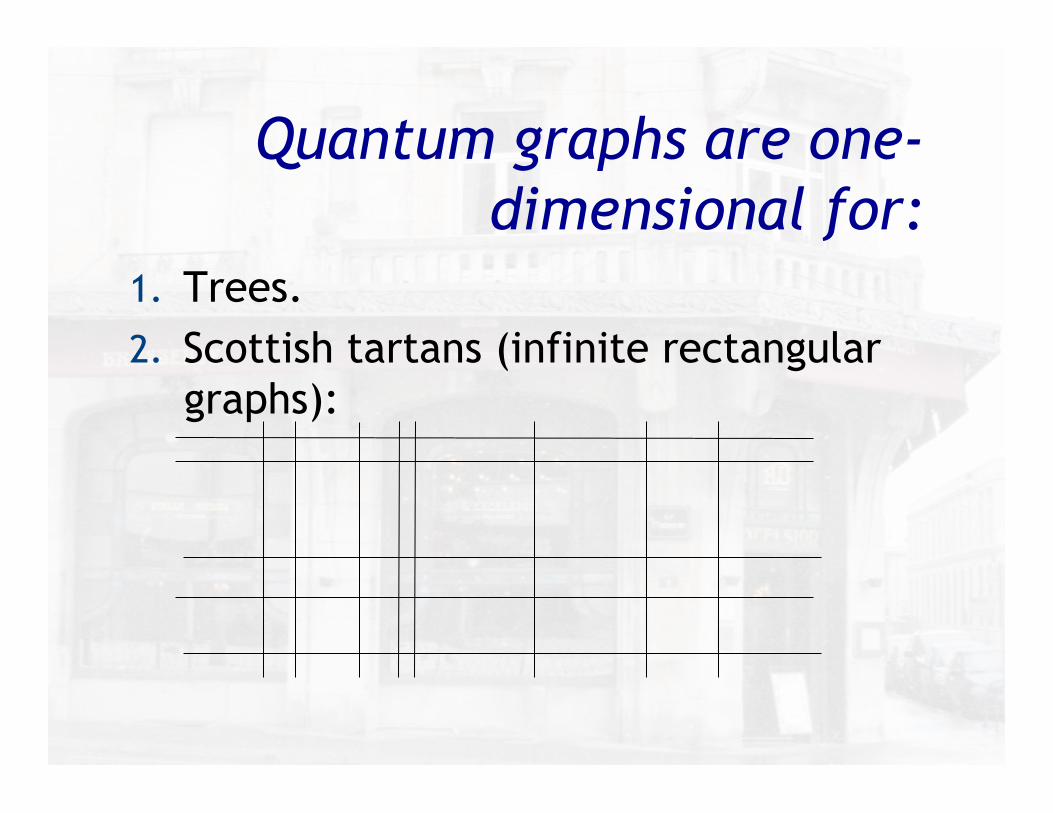
1. Trees. 2. Scottish tartans (infinite rectangular
graphs):
Quantum graphs are one-dimensional for:
Quantum graphs are one-dimensional for:
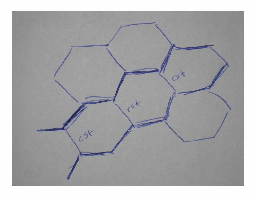
1. Trees. 2. Infinite rectangular graphs. 3. Bathroom tiles, a.k.a. honeycombs,
etc.:
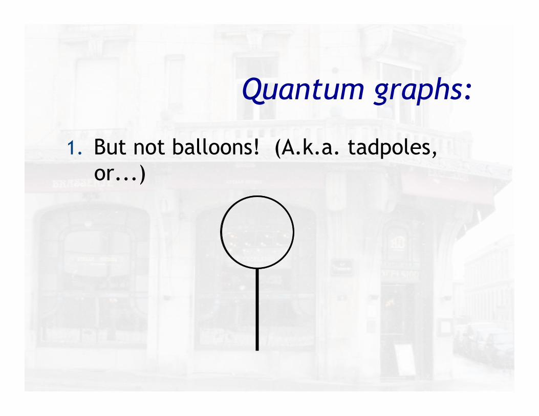
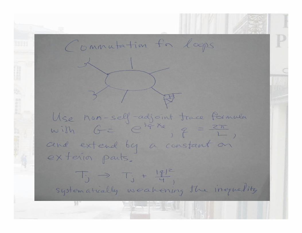
1. But not balloons! (A.k.a. tadpoles, or...)
Quantum graphs:
Quantum graphs
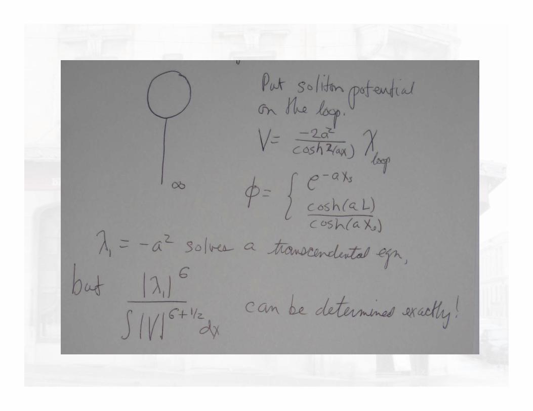
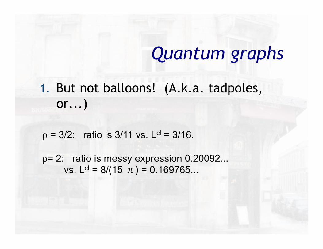
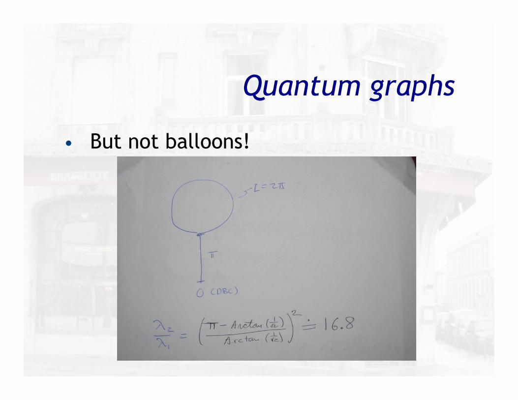
1. But not balloons! (A.k.a. tadpoles, or...)
ρ = 3/2: ratio is 3/11 vs. Lcl = 3/16.
ρ = 2: ratio is messy expression 0.20092... vs. Lcl = 8/(15 π) = 0.169765...
Quantum graphs
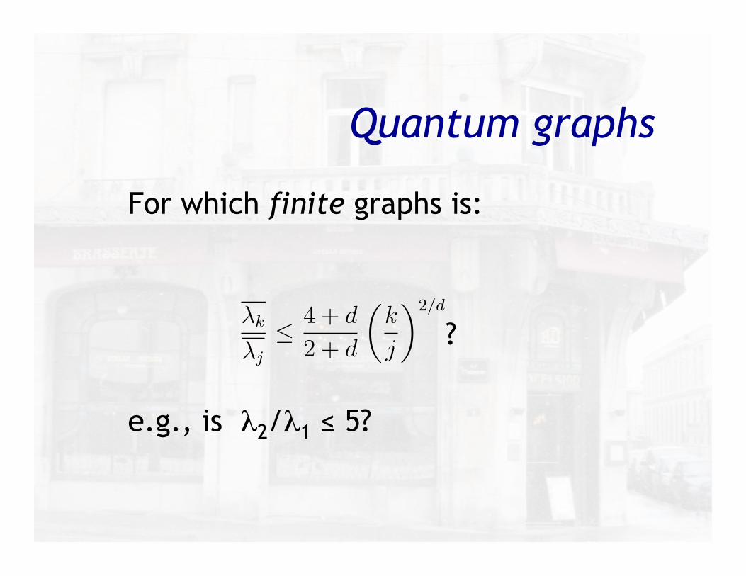
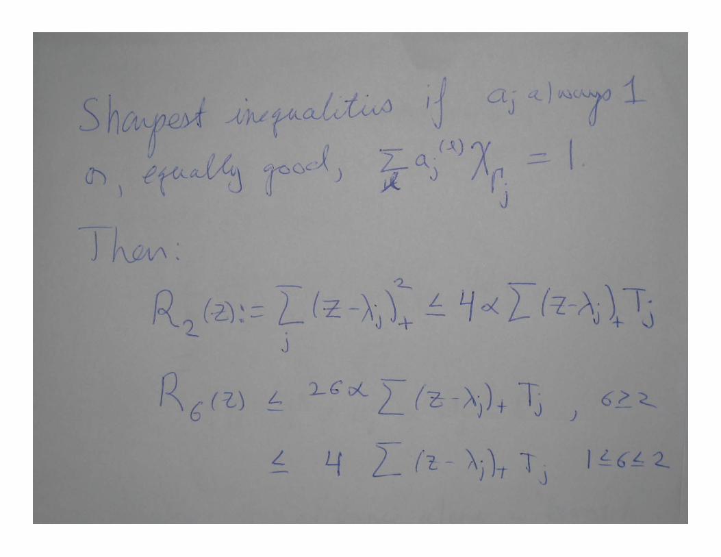
For which finite graphs is:
?
e.g., is λ2/λ1 ≤ 5?
!k
!j
! 4 + d
2 + d
!k
j
"2/d
(1)
1 =4
d
#
k:!k !=!j
| ""j,#"k$ |2
!k % !j
#R2(0, #) ! #2 4
d
#
k
(0% !k)Tk
!1 +
4
d
"R2(z) ! 4
d
#
k
(z % !kTk
Write the test function as
$ =1&
%· (&%$)
and use the product rule in the form
&(t) = e"iHt&(0)
%#2# + q(x) = %!! + q(x)
q(x) :=1
4
!%r
%
"2
% 1
2
%rr
%.
'n ( 0 with ''n' = 1, such that '(H % !)'n' ( 0.
F [f ] (k) = f(k) :=1
(2))d/2
$
Rd
e"ik·xf(x)dx
H& = % !2
2m#2&(x) + V (x)&(x)
F"1 [g] (x) = g(x) :=1
(2))d/2
$
Rd
e+ik·xg(k)dk
F%
*'
*x"
&(k) = k"'(k),
F [%!']k = |k|2'(k),1
Quantum graphs
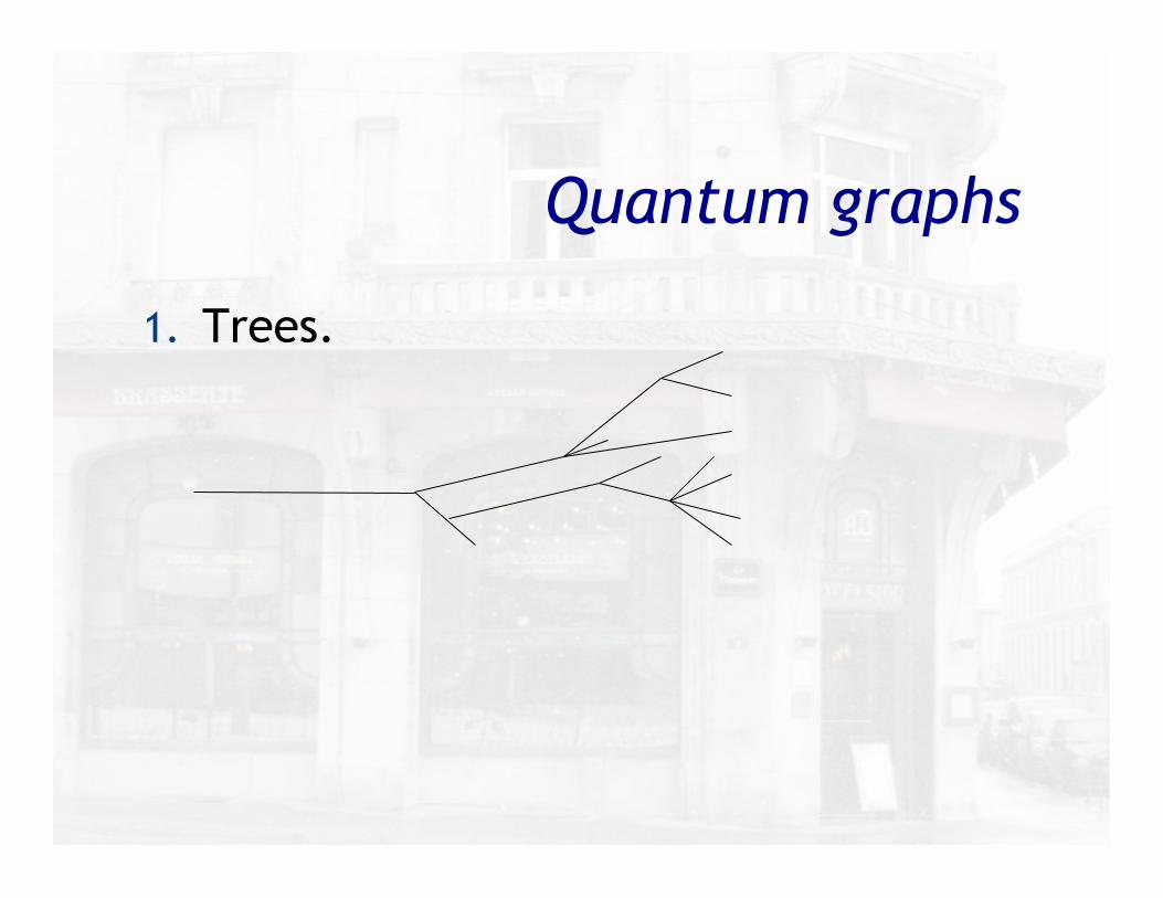
1. Trees.
Quantum graphs
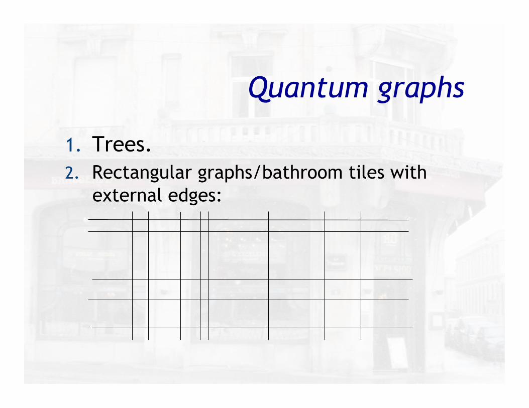
1. Trees. 2. Rectangular graphs/bathroom tiles with
external edges:
Quantum graphs
• But not balloons!
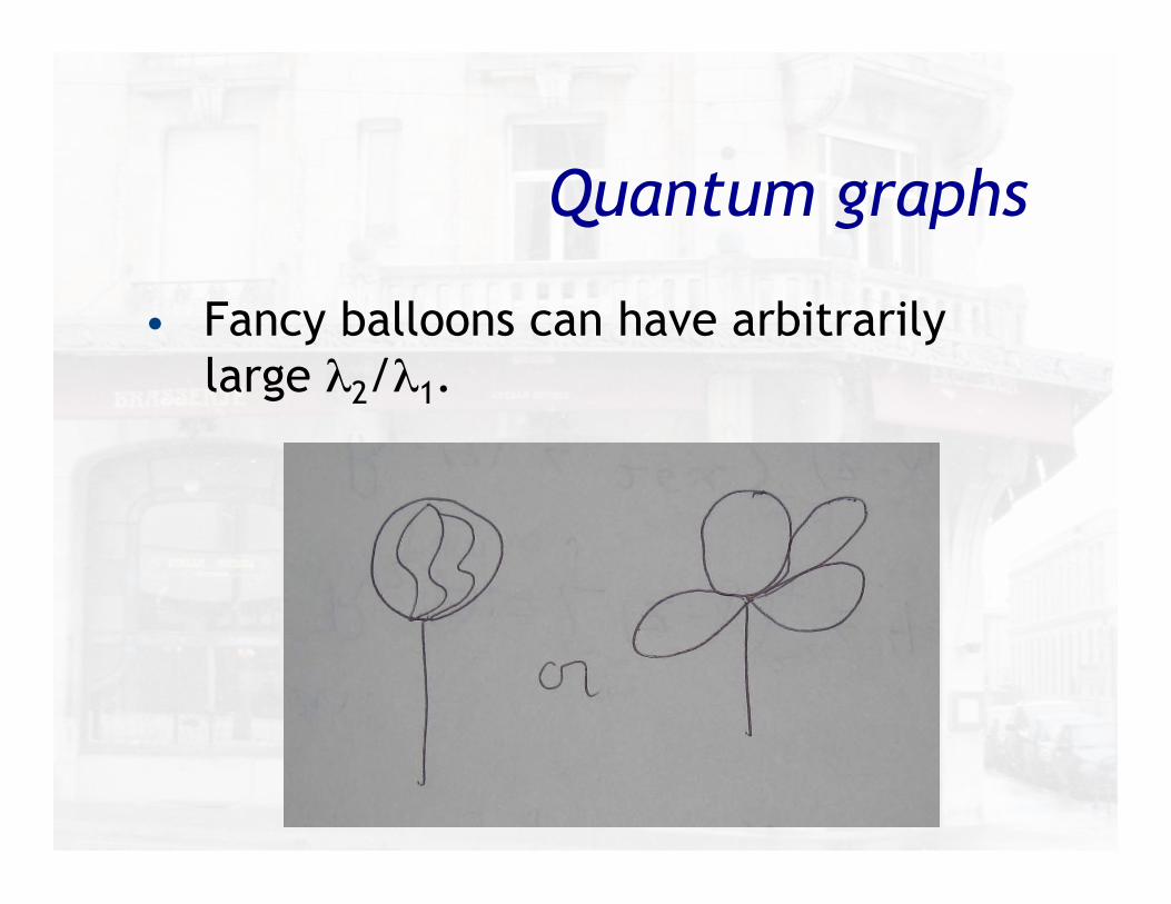
Quantum graphs
• Fancy balloons can have arbitrarily large λ2/λ1.
Why?
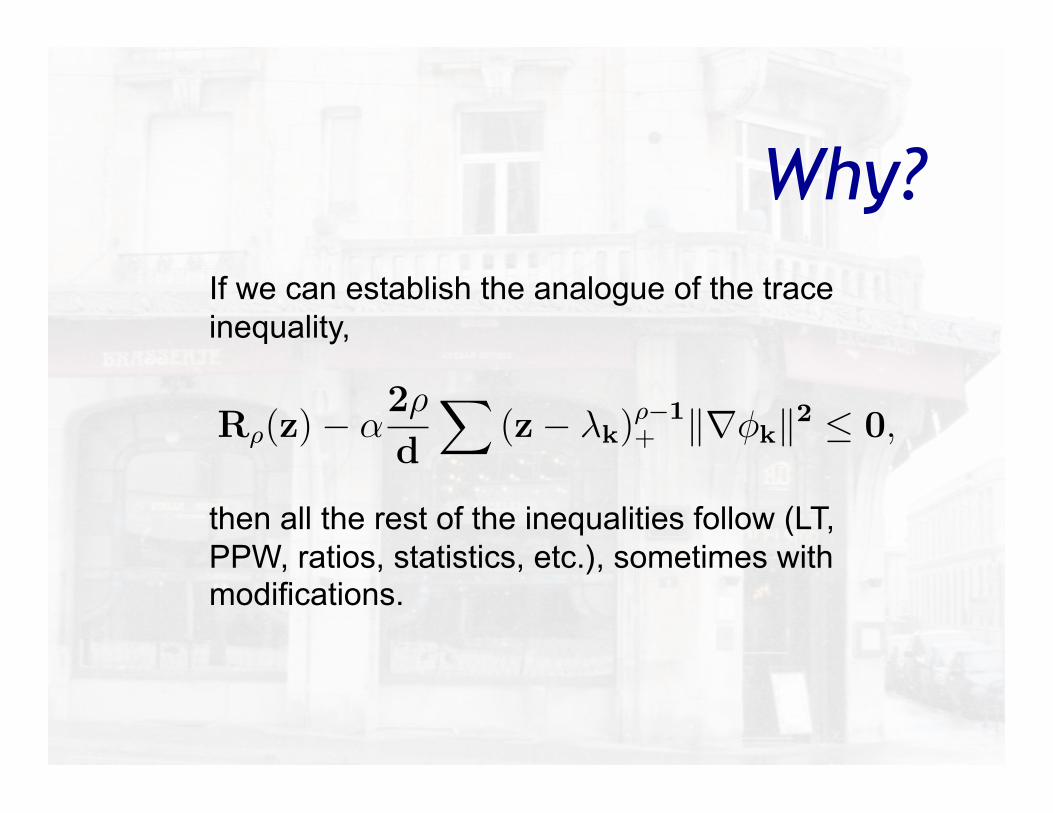
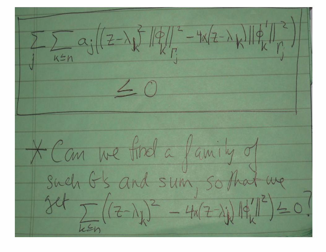
Why? If we can establish the analogue of the trace inequality,
then all the rest of the inequalities follow (LT, PPW, ratios, statistics, etc.), sometimes with modifications.
R!(z) :=!
(z! !k)!+;
R!(z)! "2#
d
!(z! !k)
!!1+ "#$k"2 $ 0,
!k+1 $"
1 +2
d
#!k +
$Dk
R"(z) $ Lcl",1
%
!
(V(x)! z)"+1/2! dx?
R"(z,") $ "!d/2Lcl",d
%
M
(V (x)! z)"+d/2! dx.
Tjk := |%$k,#$j&|2 .!
k
Tjk $ Tj :=&$j,!#2$j
'.
Elementary gap formula:
%$j, [H,G]$k& = (!j ! !k) %$j, G$k&Since [H,G]$k = (H ! !k)G$k,
"[H,G]$k"2 =&G$j, (H ! !k)
2G$k
'
and more generally
%[H, G]$j, [H,G]$k& = %G$j, (H ! !j)(H ! !k)G$k& .Second commutator formula
%$j, [G, [H, G]]$k& = %G$j, (2H ! !j ! !k)G$k& .In particular,
%$j, [G, [H,G]]$j& = 2 %G$j, (H ! !j)G$k& .
H(g) = ! d2
ds2+ g%2
A =1
4&
!
k
(|hk|2 ! k2|hk|2
)=
p2
4&! stu!
1
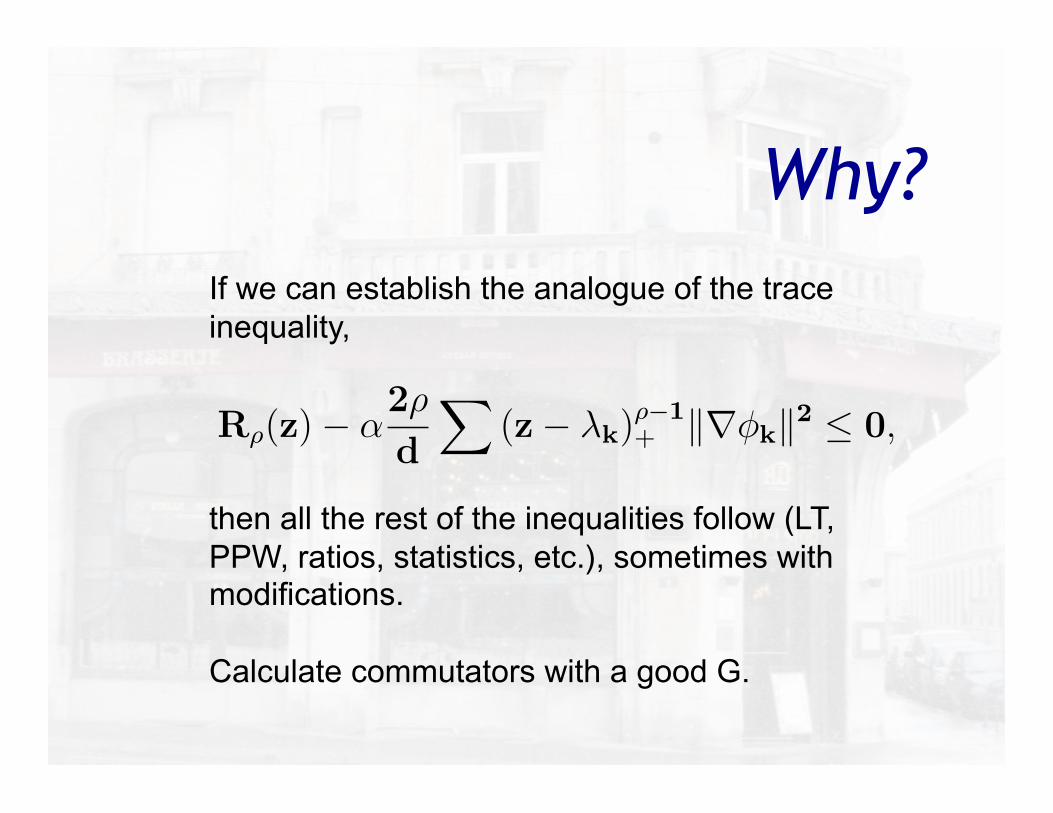
Why? If we can establish the analogue of the trace inequality,
then all the rest of the inequalities follow (LT, PPW, ratios, statistics, etc.), sometimes with modifications.
Calculate commutators with a good G.
R!(z) :=!
(z! !k)!+;
R!(z)! "2#
d
!(z! !k)
!!1+ "#$k"2 $ 0,
!k+1 $"
1 +2
d
#!k +
$Dk
R"(z) $ Lcl",1
%
!
(V(x)! z)"+1/2! dx?
R"(z,") $ "!d/2Lcl",d
%
M
(V (x)! z)"+d/2! dx.
Tjk := |%$k,#$j&|2 .!
k
Tjk $ Tj :=&$j,!#2$j
'.
Elementary gap formula:
%$j, [H,G]$k& = (!j ! !k) %$j, G$k&Since [H,G]$k = (H ! !k)G$k,
"[H,G]$k"2 =&G$j, (H ! !k)
2G$k
'
and more generally
%[H, G]$j, [H,G]$k& = %G$j, (H ! !j)(H ! !k)G$k& .Second commutator formula
%$j, [G, [H, G]]$k& = %G$j, (2H ! !j ! !k)G$k& .In particular,
%$j, [G, [H,G]]$j& = 2 %G$j, (H ! !j)G$k& .
H(g) = ! d2
ds2+ g%2
A =1
4&
!
k
(|hk|2 ! k2|hk|2
)=
p2
4&! stu!
1

THE END