Suboptimality of Asian Executive Options

Suboptimality of Asian ExecutiveOptions

by

Jit Seng Chen

A thesispresented to the University of Waterloo

in fulfillment of thethesis requirement for the degree of

Master of Quantitative Finance

Waterloo, Ontario, Canada, 2011

c© Jit Seng Chen 2011

I hereby declare that I am the sole author of this thesis. This is a true copy of the thesis,including any required final revisions, as accepted by my examiners.

I understand that my thesis may be made electronically available to the public.

ii

Abstract

This thesis applies the concept of cost efficiency to the design of executive compensation.In a classical Black-Scholes framework, we are able to express the cost efficient counterpartof the Asian Executive Option explicitly, and design a payoff that has the same distributionas the Asian Executive Indexed Option but comes at a cheaper price. The cost efficientcounterpart of the latter option is not analytically tractable, but we are able to simulateits price.

Furthermore, we extend the study of these two types of options in the presence ofstochastic interest rates modeled by a Vasicek process. We are able to derive new closed-form pricing formulas for these options. A framework for crafting the state price processis introduced. From here, an explicit expression for the state process is given and itsdistribution is derived.

Using the pricing formulas and the state price process, we are then able to simulatethe prices of the corresponding cost efficient counterparts in a stochastic interest rateenvironment.

We conclude with some avenues for future research.

iii

Acknowledgments

I express utmost gratitude to Professors Carole Bernard and Phelim Boyle for theirpatient, outstanding, and invaluable supervision. I wish to acknowledge Mary Flatt andProfessor Adam Kolkiewicz for their support of the Master of Quantitative Finance pro-gram, and Mary Lou Dufton for her coordination of Graduate Studies at the Departmentof Statistics and Actuarial Science. I also want to thank Professors Adam Kolkiewicz andKen Seng Tan for their reading of this thesis.

iv

Table of Contents

List of Tables ix

List of Figures x

1 Introduction 1

1.1 Indexing and Averaging . . . . . . . . . . . . . . . . . . . . . . . . . . . . 2

1.2 Cost Efficiency . . . . . . . . . . . . . . . . . . . . . . . . . . . . . . . . . 3

1.3 Main Results and Outline . . . . . . . . . . . . . . . . . . . . . . . . . . . 4

2 Asian Executive Compensation 7

2.1 Overview . . . . . . . . . . . . . . . . . . . . . . . . . . . . . . . . . . . . . 7

2.2 Framework . . . . . . . . . . . . . . . . . . . . . . . . . . . . . . . . . . . . 9

2.3 Asian Executive Option . . . . . . . . . . . . . . . . . . . . . . . . . . . . 10

2.4 Asian Executive Indexed Option . . . . . . . . . . . . . . . . . . . . . . . . 14

2.4.1 Construction of a Cheaper Payoff . . . . . . . . . . . . . . . . . . . 15

2.4.2 The True Cost Efficient Counterpart . . . . . . . . . . . . . . . . . 19

2.4.3 AT vs A?T vs AT . . . . . . . . . . . . . . . . . . . . . . . . . . . . . 25

3 Asian Options with Vasicek Interest Rates 30

3.1 Assets, Short Rate, and Bond Dynamics . . . . . . . . . . . . . . . . . . . 31

3.1.1 Dynamics Under the Risk Neutral Measure Q . . . . . . . . . . . . 31

v

3.1.2 Dynamics Under the T -Forward Measure QT . . . . . . . . . . . . . 33

3.2 Some Important Distributions . . . . . . . . . . . . . . . . . . . . . . . . . 34

3.3 Option Pricing Formulas . . . . . . . . . . . . . . . . . . . . . . . . . . . . 35

3.3.1 Geometric Asian Option (GAO) . . . . . . . . . . . . . . . . . . . . 35

3.3.2 Asian Exchange Option (AXO) . . . . . . . . . . . . . . . . . . . . 36

3.3.3 European Call Option (ECO) . . . . . . . . . . . . . . . . . . . . . 37

3.3.4 European Exchange Option (EXO) . . . . . . . . . . . . . . . . . . 38

3.4 Closed Form Expressions . . . . . . . . . . . . . . . . . . . . . . . . . . . . 40

3.4.1 Closed Form Expressions for the Terminal Values . . . . . . . . . . 41

3.4.2 Closed Form Expressions for the Geometric Averages . . . . . . . . 41

3.4.3 Closed Form Expressions for the Bond Price . . . . . . . . . . . . . 42

3.5 Deterministic Interest Rates . . . . . . . . . . . . . . . . . . . . . . . . . . 42

3.5.1 Setup . . . . . . . . . . . . . . . . . . . . . . . . . . . . . . . . . . 43

3.5.2 Deterministic Interest Rates Pricing Formulas . . . . . . . . . . . . 44

3.6 Monte Carlo Simulation . . . . . . . . . . . . . . . . . . . . . . . . . . . . 45

4 State Price Process with Vasicek Interest Rates 49

4.1 State Price Process . . . . . . . . . . . . . . . . . . . . . . . . . . . . . . . 50

4.1.1 Setup . . . . . . . . . . . . . . . . . . . . . . . . . . . . . . . . . . 50

4.1.2 An Explicit Expression for the State Price Process . . . . . . . . . . 52

4.2 State Price Process as a Function of Market Variables . . . . . . . . . . . . 53

4.3 Special Cases . . . . . . . . . . . . . . . . . . . . . . . . . . . . . . . . . . 55

4.3.1 Constant Instant Rates with One Risky Asset . . . . . . . . . . . . 55

4.3.2 Constant Instant Rates with Two Risky Assets . . . . . . . . . . . 56

4.3.3 Stochastic Interest Rates Only . . . . . . . . . . . . . . . . . . . . . 57

4.3.4 Stochastic Interest Rates with One Risky Asset . . . . . . . . . . . 58

4.3.5 Summary . . . . . . . . . . . . . . . . . . . . . . . . . . . . . . . . 59

vi

5 Asian Executive Compensation with Vasicek Interest Rates 62

5.1 Comparison with the Case of Constant Instant Rates . . . . . . . . . . . . 62

5.2 Setup . . . . . . . . . . . . . . . . . . . . . . . . . . . . . . . . . . . . . . . 63

5.3 Monte Carlo Simulation . . . . . . . . . . . . . . . . . . . . . . . . . . . . 64

6 Conclusion 71

APPENDICES 73

A Useful Identities 74

B Proofs 79

B.1 Proofs for Chapter 2 . . . . . . . . . . . . . . . . . . . . . . . . . . . . . . 79

B.1.1 Proof of Proposition 2.3.1 on page 11 . . . . . . . . . . . . . . . . . 79


B.1.3 Proof of Corollary 2.4.4 on page 16 . . . . . . . . . . . . . . . . . . 84


B.2.1 Proof of Lemma 3.1.1 on page 33 . . . . . . . . . . . . . . . . . . . 85



B.2.4 Proofs of Propositions 3.3.1 on page 35 and 3.3.7 on page 37 . . . . 97

B.2.5 Proofs of Propositions 3.3.4 on page 36 and 3.3.10 on page 38 . . . 97


B.2.7 Proof of Corollary 3.3.12 on page 39 . . . . . . . . . . . . . . . . . 98

B.2.8 Proofs of Propositions 3.5.1 to 3.5.3 on pages 44–45 . . . . . . . . . 98





vii

B.3.4 Proofs of Propositions 4.3.1 on page 55, 4.3.4 on page 56, 4.3.7 onpage 58, and 4.3.9 on page 58 . . . . . . . . . . . . . . . . . . . . . 104



C Glossary of Notation 109

C.1 Chapter 1 . . . . . . . . . . . . . . . . . . . . . . . . . . . . . . . . . . . . 109

C.2 Chapter 2 . . . . . . . . . . . . . . . . . . . . . . . . . . . . . . . . . . . . 109

C.3 Chapter 3 . . . . . . . . . . . . . . . . . . . . . . . . . . . . . . . . . . . . 110

C.4 Chapter 4 . . . . . . . . . . . . . . . . . . . . . . . . . . . . . . . . . . . . 112

C.5 Chapter 5 . . . . . . . . . . . . . . . . . . . . . . . . . . . . . . . . . . . . 113

References 115

viii

List of Tables

2.3.1 Base case parameters for sample GT and GT . . . . . . . . . . . . . . . . . . 12

2.3.2 Prices and efficiency loss of GT compared against GT across different pa-rameters. . . . . . . . . . . . . . . . . . . . . . . . . . . . . . . . . . . . . . 12

2.4.1 Base case parameters for sample AT , A?T and AT . . . . . . . . . . . . . . . 21

2.4.2 Prices and efficiency loss of AT and A?T and compared against AT acrossdifferent parameters. . . . . . . . . . . . . . . . . . . . . . . . . . . . . . . 22

3.6.1 Base case parameters for sample prices of the GAO on assets 1 and 2, andthe AXO. . . . . . . . . . . . . . . . . . . . . . . . . . . . . . . . . . . . . 46

3.6.2 Simulated prices of the GAO on assets 1 and 2. . . . . . . . . . . . . . . . 46

3.6.3 Simulated prices of the AXO on assets 1 and 2. . . . . . . . . . . . . . . . 47

3.6.4 Raw and control variate standard deviation of the prices of the GAO. . . . 48

3.6.5 Raw and control variate standard deviation of the prices of the AXO. . . . 48

4.3.1 Parameter values for the state price process. . . . . . . . . . . . . . . . . . 60

4.3.2 Parameter values for the state price process expressed in terms of the marketvariables. . . . . . . . . . . . . . . . . . . . . . . . . . . . . . . . . . . . . 61

5.3.1 Base case parameters for sample AEO and AEIO. . . . . . . . . . . . . . 65

5.3.2 Prices and efficiency loss of the AEO on assets 1 and 2. . . . . . . . . . . 65

5.3.3 Prices and efficiency loss of the AEIO. . . . . . . . . . . . . . . . . . . . . 66

ix

List of Figures

2.3.1 Sample prices for GT and GT across different cases . . . . . . . . . . . . . 13

2.3.2 Prices of GT and GT vs r . . . . . . . . . . . . . . . . . . . . . . . . . . . . 14

2.4.1 Prices of AT and A?T vs r . . . . . . . . . . . . . . . . . . . . . . . . . . . . 17

2.4.2 Prices of CT and C?T vs r . . . . . . . . . . . . . . . . . . . . . . . . . . . . 19

2.4.3 Sample prices for VT , V ?T and VT across different cases . . . . . . . . . . . . 24

2.4.4 Empirical CDF of AT , A? and AT . . . . . . . . . . . . . . . . . . . . . . . 25

2.4.5 Reshuffling of outcomes of AT to A?T . . . . . . . . . . . . . . . . . . . . . 26

2.4.6 Reshuffling of outcomes of AT to AT . . . . . . . . . . . . . . . . . . . . . 27

2.4.7 Outcomes of AT vs ξT . . . . . . . . . . . . . . . . . . . . . . . . . . . . . 28

2.4.8 Outcomes of A?T vs ξT . . . . . . . . . . . . . . . . . . . . . . . . . . . . . 28

2.4.9 Outcomes of AT vs ξT . . . . . . . . . . . . . . . . . . . . . . . . . . . . . 29

5.3.1 Sample prices for the AEO on asset 1 and its CEC across different cases. . 68

5.3.2 Sample prices for the AEO on asset 2 and its CEC across different cases. . 69

5.3.3 Sample prices for the AEIO and its CEC across different cases. . . . . . . 70

x

Chapter 1

Introduction

During the recent financial crisis in 2008, executives made millions of dollars in the formof stock options while bankrupting their respective firms. Executives at Bear Stearns andLehman Brothers made approximately $1 billion USD from exercising stock options andstock purchases [2]. Would they have engaged in such excessive risk taking had they notbeen granted stock options? Meanwhile, executive options that were granted when themarket bottomed out are now deep in the money due to the market’s rebound [52]. Areexecutives being compensated for their performance, or are they simply riding the wave ofrecovering market prices?

The main idea of granting executive options is to encourage executives to increaseshareholders value. Let us consider the toy example of an executive at Company X witha current stock price of $100. The executive is given the right, but not the obligation, topurchase 100 units of Company X shares 10 years from now at $1001. With this contract inplace, the executive has an incentive to work hard to increase the share price as it increasesthe payoff 10 years later.

If Company X stock price is greater than $100 10 years from now, the executive receivesa positive payoff; otherwise, the payoff is zero. If the stock price is greater (less) than $100,is it due to the executive’s effort, or good (bad) luck? If the executive is unscrupulous, heor she may be tempted to engage in all sorts of financial shenanigans in order to artificiallyincrease the stock price, cash out on the contract, and retire.

1This is essentially an at-the-money 10 year call option on Company X. It is a highly-simplified example;stock options that are issued in reality have many more bells and whistles. See [32] for some examples ofnon-traditional executive options.

1

The efficiency of traditional stock options was questioned by Hall and Murphy [25]where they argue that risk-averse and undiversified executives will actually value the op-tions lower than what they actually cost the firms to grant. The idea of executives dis-counting the cost granting these options is further investigated by [53]. Despite the lack ofconsensus on how beneficial stock options actually are [13], their use remains widespread[52]. They have been blamed for the misalignment of incentives and excessive risk taking2

as well as incentivizing executives to commit financial fraud [17]. Even though the use ofstock options has been named as one of the culprits of the recent crisis, Fahlenbrach andStulz [21] do not find any evidence of banks actually performing worse than their peersjust because they issued more stock options and bigger cash bonuses.

1.1 Indexing and Averaging

In an earlier paper, Johnson and Tian [31] designed an executive option with a strike pricethat is indexed to a benchmark. The main tenet underlying the use of indexing is that theexecutive should only be rewarded (penalized) for out-performance (under-performance),and not serendipity. This ties back to our toy example of the executive being rewarded forhis or her effort and not luck.

However, the use of indexing alone in executive options is “virtually non-existent” [25]and suboptimal according to Tian [53]. For that reason, the use of averaging is incorporatedby [53] and found to be more cost effective (discounted less from their market values by riskaverse executives) and incentive effective (stronger incentives to increase stock price) thantraditional stock options3. With averaging in place, the unscrupulous executive would haveto manipulate the entire stock price path instead of the price at just a particular pointin time. This is presumably much harder to achieve than actually doing a good job atincreasing shareholder value.

The conclusions drawn by [53] are based on analyses on the certainty equivalent valuefrom an expected utility model. The two classes of options proposed are the Asian Exec-utive Option (AEO), which takes the form of a continuous geometric average Asian calloption, and the Asian Executive Indexed Option (AEIO), which takes the form of contin-uous geometric average Asian exchange option. A more detailed overview of [53] is givenin Section 2.1 on page 7.

2“Heads, you become richer than Croesus; tails, you get no bonus, receive instead about four times thenational average salary, and may (or may not) have to look for a new job” [11]

3Interestingly enough, the use of averaging in executive compensation is also suggested by Ariely [1]from the perspective of human irrationality.

2

1.2 Cost Efficiency

The primary focus of this thesis is the application of cost efficiency as prescribed byBernard, Boyle and Vanduffel [4] to the design of the AEO and AEIO. In doing so, we areable to construct new payoffs that have the same distributions as the original payoffs, butcome at a cheaper price. At this point, we want to stress that while Tian’s study of theseoptions is primarily focused on their incentives, ours is focused on their costs instead.

Building on the work done by Dybvig [19][20], [4] devised an explicit representation ofa cost efficient strategy. The notion of cost efficiency will be defined below, but looselyspeaking, a strategy is said to be cost efficient if it is the cheapest possible way to achievea particular probability distribution.

Even though the use of copulas is not new in finance [16] nor actuarial science [41],their novel and brilliant insight is the coupling of the state price process with the payoffitself. This allows the use of techniques from the theory of copulas, including the Frechet-Hoeffding bounds to prove Theorem 1.2.4 on the following page and results from Tankov[51] to characterize cost efficient payoffs in the presence of state dependent preferences.

Using the same setup as [4], we will make the following assumptions:

1. We assume a Black-Scholes market. It is complete, frictionless and arbitrage free4.The risk free rate and volatility are assumed to be constant5.

2. Let (Ω,F ,P) be the corresponding probability space. Then, there exists a state-priceprocess ξt such that ξtSt is a martingale for all traded assets S in this market.

3. There are 2 risky assets in the market i.e. the stock (St) and index (It). Their pricedynamics are driven by 2-dimensional correlated Brownian motions.

4. Agents have preferences that depend only on the terminal distribution of wealth.

5. We assume that all agents agree on the pricing operator. Therefore, the choice of thestate price process is fixed.

We also recall the following definitions, and the main theorem that we will be usingfrom [4].

4Even Black [9] was fully aware of the deficiencies of the Black-Scholes model. However, in terms ofaccounting standards, it is still used for expensing executive options [47].

5We will later extend this to include stochastic interest rates modeled by a Vasicek process.

3

Definition 1.2.1. The cost6 of a strategy with terminal payoff XT is given by

c(XT ) = E[ξTXT ]

where the expectation is taken under the physical measure P.

Definition 1.2.2. A payoff is cost efficient (CE) if any other strategy that generates thesame distribution costs at least as much.

Definition 1.2.3. The distributional price of a cdf F is defined as

PD(F ) = minYT |YT∼F

c(YT )

where YT |YT ∼ F denotes the set of all payoffs that have the same distribution as F .The efficiency loss of a strategy with payoff XT at maturity T with cdf F is equal toc(XT )− PD(F ).

Theorem 1.2.4. Let ξT be continuous. Define

Y ?T = F−1

XT(1− FξT (ξT ))

as the cost efficient counterpart (CEC) of the payoff XT . Then, Y ?T is a CE payoff with

the same distribution as XT and is almost surely unique7.

1.3 Main Results and Outline

The rest of this thesis is organized as follows. In Chapter 2 on page 7 we study the AsianExecutive Option and Asian Executive Indexed Option that have been proposed by [53] inthe classical Black-Scholes framework. Using the concept of cost efficiency, we are able toconstruct a new cost efficient counterpart of the Asian Executive Option. We also designa new payoff that is cheaper than the Asian Executive Indexed Option which we call thePower Exchange Executive Option. The cost efficient counterpart of the Asian ExecutiveIndexed Option does not admit a closed form expression, but we are able to simulate itsprice and investigate the degree of efficiency loss through numerical techniques.

6Intuition: ξT represents the price of a particular state. When the sample space is discrete, the costcan be interpreted as the average of the outcome of each state weighted by its price.

7Intuition: The CEC is achieved by rearranging the outcomes of XT in each state in reverse order withξT while preserving the original distribution.

4

Starting from Chapter 3 on page 30 onwards, we will introduce stochastic interest ratesmodeled by a Vasicek process so that we can study the cost efficiency of the Asian ExecutiveOptions with this extra component. In order to do so, we require new pricing formulas forthe AEO and AEIO as well as an expression for the state price process in the presence ofstochastic interest rates.

The main results of Chapter 3 on page 30 is the derivation of new pricing formulas forthe Geometric Asian Option and the Asian Exchange Option when interest rates follow theVasicek process. As a verification of correctness, we also provide alternative derivationsfor the European Call Option and European Exchange Option that agree with existingresults.

The aim of Chapter 4 on page 49 is a new derivation of the state price process in amarket with two risky assets and stochastic interest rates modeled by the Vasicek process.We are able to derive an explicit formula for the state price process, find its distribution,as well as express it as a function of market variables. We also consider special cases withdifferent combinations of number of risky assets and stochastic/constant interest rates,and derive new expressions for their corresponding state price processes in terms of marketvariables. Whilst we do not utilize these special cases, they can be readily applied to thestudy of cost efficiency for different classes of options.

Chapter 5 on page 62 uses the results from the previous two chapters to investigatethe Asian Executive Option and Asian Executive Indexed Option in a stochastic interestrate environment. Their respective cost efficient counterparts do not admit closed-formexpressions, so we rely on numerical methods once again to study the degree of efficiencyloss.

To the best of our knowledge, the construction of the cost efficient counterpart for theAsian Executive Option and the design of the Power Exchange Executive Option are newresults. In the presence of Vasicek interest rates, the pricing formulas for the GeometricAsian Option and the Asian Exchange Option are our contributions. We also find newformulas for the various cases of the state price process and expressing them in terms ofthe market variables. The latter is valuable because in a particular state of the world,the state price process itself is not directly observable because it is not a traded assetper se. However, since we have an expression of the state price process in terms of themarket variables, we can first observe the market variables and then retrieve the state priceprocess.

Chapter 6 on page 71 ends the thesis with some conclusions and avenues for futureresearch.

Appendix A on page 74 contains some useful identities that are used in our proofs. All

5

proofs are provided in Appendix B on page 79, and we present a glossary of notations inAppendix C on page 109.

6

Chapter 2

Asian Executive Compensation

In this chapter, we will use the idea of cost-efficiency as spelled out by Bernard, Boyle andVanduffel [4] to study the Asian Executive Option (AEO) and Asian Executive IndexedOption (AEIO) as proposed by Tian [53]. Again, we want to reiterate that while Tian’sstudy of these options is primarily focused on their incentives, ours is focused on their costsinstead.

We begin this chapter with an overview of the AEO and AEIO as designed by [53]in Section 2.1. In Section 2.2 on page 9, the framework for our analysis is specified. InSection 2.3 on page 10, we are able to construct the cost efficient counterpart (CEC) forthe former option which turns out to be a power option. The latter does not admit anexplicit CEC, but we are able to design an option that has the same distribution with acheaper price in Section 2.4 on page 14. The simulation of the price of the true CEC isalso considered, along with some observations about these three options.

The main contributions of this chapter are given in Propositions 2.3.1 on page 11and 2.4.2 on page 16.

2.1 Overview

This section provides an overview of Tian’s work on the use of indexing and averaging inexecutive options. All of the definitions and results herein are due to [53].

Tian argues that the practice of granting stock options based on terminal stock prices is

7

suboptimal and firms should be using the average1 stock prices instead. This work buildson an earlier paper by Johnson and Tian [31] that discusses the use of indexing.

The use of averaging is found to be more cost effective and incentive effective than thetraditional stock options. This means that for a given cost of the option grant, risk-averseexecutives will have a higher subjective value of the Asian option than the European one.On the other hand, incentive effective means that the Asian option provides executiveswith stronger incentives to increase stock price than the European one.

Tian first assumes that the executive’s total wealth comprises of a fixed salary and stockoptions, and uses the certainty equivalent of the total wealth as a measure of the subjectivevalue of the option grant. The analysis done on this subjective value as a fraction of theactual cost of issuing the option indicates that the Asian option is more cost effective.

A modified version of the pay-performance measure [28] defined as the ratio of thepercentage change in the executive’s total wealth to the percentage change in stock priceis used to compare the incentive effectiveness of the Asian option. Loosely speaking, thisinvolves the partial derivative of the certainty equivalent with respect to the firm’s stockprice. Using this measure, Tian concludes that the Asian option is indeed more incentiveeffective as well.

Why is the Asian option more cost effective and incentive effective than the traditionalstock option? Firstly, the use of averaging reduces the volatility of the final payoff of theoption to the executive, which is more beneficial to risk-averse executives. Secondly, theuse of averaging makes it much harder for executives to manipulate the final payoff ofthe option. Instead of artificially increasing the stock price for a particular point in time,they would have to increase the entire stock price path. Thirdly, averaging also increasesthe probability of the option expiring in the money. This rectifies the problem of indexedoptions (indexing alone, without averaging) having lower probabilities of expiring in themoney than traditional stock options [25].

Remark 2.1.1. The use of the certainty equivalent in assessing an option from the ex-ecutive’s perspective was proposed by Lambert, Larcker and Verrecchia [36]. The extraconstraints imposed on executives (e.g. short selling constraints, restrictions on the salesof the underlying firm’s stock, non-transferability of the option itself, and etc.) invalidatethe dynamic-hedging arguments. Hence, the value of the option to an executive is notnecessarily its cost a la Black-Scholes.

1It is pointed out that the geometric average should be used instead of the arithmetic average since thearithmetic average will not penalize a spread that preserves the mean but increases the variance [43]. Weopt for the geometric average simply because it is analytically tractable.

8

2.2 Framework

In this section, we specify the notations as given in [53]. Firstly, we define the P-dynamicsfollowed by the stock and index as follow:

dStSt

= (µS − qS)dt+ σSdWSt

dItIt

= (µI − qI)dt+ σIdWIt (2.2.1)

dW St dW

It = ρdt

(µ and q are respectively the expected return and dividend rate, σ is the volatility and ρis the correlation. K as used below is understood to be the strike price.)We then define the geometric averages of the stock and the index as well as the benchmarks:

ST = e1T

∫ T0 ln(St)dt IT = e

1T

∫ T0 ln(It)dt

HT = K(IT/I0)β exp(ηT ) HT = K(IT/I0)β exp(ηT )(2.2.2)

whereη = (r − q?S)− β(r − q?I ) + 1

2σ2I β(1− β)

η = (r − qS)− β(r − qI) + 12σ2Iβ(1− β)

β = ρσSσI

β = ρσSσI

(2.2.3)

andq?S = 1

2

(r + qS +

σ2S

6

)q?I = 1

2

(r + qI +

σ2I

6

)qS = 1

2

(µS + qS +

σ2S

6

)qI = 1

2

(µI + qI +

σ2I

6

)σS = σS√

3σI = σI√

3

(2.2.4)

Remark 2.2.1. The · accent is used to denote the geometric average of a particular param-eter; omitting · refers to the terminal value. The relationship between the terminal andgeometric average parameters (e.g. between qS and qS) is due to the distribution of thegeometric averages of the stock and the index. See Kemna and Vorst [34] for more details.

Remark 2.2.2. HT as defined in (2.2.2) can be thought of as the price of an imaginaryasset that tracks the expected performance of the firm’s stock, given that the index hasno excess return. The idea is that the executive should only be rewarded for firm-specificperformance. It was first proposed by [31] and we recall their rationale here.

9

Firstly they define the excess return on the stock as

α = µS − r − β(µI − r) (2.2.5)

where β is given in (2.2.3) on the previous page. They point out that the motivation behindβ is not from the Capital Asset Pricing Model (though it looks identical), but from thefact that including β in (2.2.5) “produces an aggregate performance index (α) on whichan optimal sharing rule can be based”.

The benchmark is designed such that the executive is only rewarded for firm-specificperformance by conditioning the stock price on the index price assuming the latter has noexcess return. They calculate the following conditional expectation:

E(St|It, α = 0) = S0

(ItI0

)βeηt (2.2.6)

where η is given in (2.2.3) on the previous page. Based on (2.2.6), they then define HT asgiven in (2.2.2) on the previous page.

2.3 Asian Executive Option

With the above framework in place, we can now derive the CEC of the Asian ExecutiveOption. Its payoff at time T is defined as

GT = (ST −K)+ (2.3.1)

and the price of GT at time zero, E0, is simply the price of a continuous geometric Asianoption:

E0 = S0e− 1

2(r+qS+ 16σ2S)TN(d1)−Ke−rTN(d2)

where

d1 =ln(S0

K

)+ 1

2

(r − qS +

σ2S

6

)T

σS√T/3

d2 = d1 − σS√T/3

(2.3.2)

Proposition 2.3.1 on the following page extends the derivation of [4] and the price of apower option given by Macovschi and Quittard-Pinon [39] to the case of positive dividendyield.

10

Proposition 2.3.1. The cost efficient counterpart of the Asian Executive Option (2.3.1)on the previous page is given by

GT = d

(S

1/√

3T − K

d

)+

(2.3.3)

where d = S1−1/

√3

0 e

(12− 1√

3

)(µS−qS−

σ2S2

)T

. This is a power call option which is the simplecase of a polynomial option. Its price at time zero is given by

E0 = S0e

(1√3−1)r+(

12− 1√

3

)µS−

qS2−σ

2S

12

T

Φ(d1)−Ke−rTΦ(d2)

where

d1 =ln(S0

K

)+[(

12− 1√

3

)(µS − qS) + r−qS√

3+

σ2S

12

]T

σS

√T3

d2 = d1 − σS√T

3

(2.3.4)

Remark 2.3.2. Note that in this case, we are implicitly assuming that the only risky assetthat is traded in the market is the stock (ST ), which gives us a simple expression for thestate price process that only depends on one source of randomness. If we assume that theindex is also traded in the market, then the state price process, as well as the CEC, willtake a rather different form. In fact, the single-asset payoff GT will be suboptimal in amultidimensional Black-Scholes market [7].

Remark 2.3.3. When µS = r, it is clear that E0 = E0 from their respective pricing formulas.In fact, the price of GT is a decreasing function of the stock yield, and is only cheaper thanGT when the stock yield is greater than the risk free rate. We can see this by consideringthe first derivative of E0 with respect to the stock yield i.e. ∂

∂µSE0 ≤ 0 (and that E0 does

not depend on µS). Therefore, GT is less expensive GT if and only if µS > r. This comesalso from the fact that the CEC has a different form when µS < r, because in that case itis non-increasing with the underlying stock price (see [4]).

Figure 2.3.1 on page 13 plots some prices of GT and GT across different sets of pa-rameters to illustrate the efficiency loss (recall Definition 1.2.3 on page 4). Each pointcorresponds to the price for a particular parameter set. We consider the base case given inTable 2.3.1 on the following page, and perturb some of the input parameters as well. We

11

can see that the degree of efficiency loss is sensitive to all model parameters. The valuesthat are used to plot this figure are given in Table 2.3.2.

Option Interest StockT 1 r 6% S0 100K 100 σS 30%

µS 12%qS 2%

Table 2.3.1: Base case parameters for sample GT and GT .

ParametersGT GT

E0 E0 % Eff LossBase Case 6.9032 9.2567 34.09%K = 80 20.1972 23.8842 18.25%r = 4% 6.4431 8.2032 27.32%S0 = 120 20.9597 25.2216 20.33%µS = 8% 7.0668 9.2567 30.99%σS = 35% 7.8444 10.3265 31.64%qS = 1.5% 7.0352 9.4413 34.20%

Table 2.3.2: Prices and efficiency loss of GT compared against GT across different param-eters.

These are used to generate Figure 2.3.1 on the following page and the base caseparameters are given in Table 2.3.1.

We can see that across all cases, the price of GT is greater than GT in accordance withTheorem 1.2.4 on page 4. In the base case the efficiency loss of GT vs GT is 34.09% (9.2567vs 6.9032). The degree of efficiency loss is very much a function of the input parameters,with the highest loss of 34.20% (when we perturb qS to 1.5%) and the lowest loss of 18.25%(when we perturb K to 80).

12

6

8

10

12

14

16

18

20

22

24

26

Price

Base Case K = 80 S0 = 120 r = 4% µS = 8% σS = 35% qS = 1.5%

E0

E0

Figure 2.3.1: Sample prices for GT and GT across different cases

The values used to generate this plot are given in Table 2.3.2 on the previous page.

Note that since GT is a power call option, we have effectively removed the geometricaveraging component from the AEO. By removing this path-dependence, we have created apayoff that has the same distribution as the AEO but comes at a cheaper price. Althoughthe payoff only depends on the terminal stock price, we could argue that this value isdampened by the exponent of 1√

3(see (2.3.3) on page 11). This means that a wider swing

in the terminal stock price is required for the same dollar impact on the payoff of thepower call option as the AEO. Therefore, to a certain degree, the benefits of averaging i.e.reduction in volatility and difficulty in payoff manipulation (see Section 2.1 on page 7) arestill retained. In any case, the impact on executives’ incentives is an issue that deservesfurther research.

13

Figure 2.3.2 plots the prices of GT and GT vs the risk free rate, r. The parameters usedto generate the prices are the same base case parameters in Table 2.3.1 on page 12. Thevertical line corresponds to the expected stock return of µS = 12% in our base case. WhenµS > r, we can see that the price of GT is greater than the price of GT . When µS < r, theopposite is true, with equality holding when µS = r. This graph illustrates the observationthat we made in Remark 2.3.3 on page 11.

0 0.2 0.4 0.6 0.8 15

10

15

20

25

30

r

Price

µS = 12%

E0

E0

Figure 2.3.2: Prices of GT and GT vs r

The parameters used to generate this plot are given in Table 2.3.1 on page 12.

2.4 Asian Executive Indexed Option

The main contribution of Tian [53] is the design of the Asian Executive Indexed Option(AEIO) as a form of executive compensation. The analysis shows that the AEIO is moreeffective than traditional stock options and provide stronger incentives for the executive toincrease stock price. Its payoff at time T is given by

AT = (ST − HT )+ (2.4.1)

14

where ST is the average stock price and HT is the non-constant strike price that is linkedto the performance of the average benchmark index adjusted for the level of the systematicrisk β. The definitions of HT and β are the geometric average analogues of HT and β (seeRemark 2.2.2 on page 9).

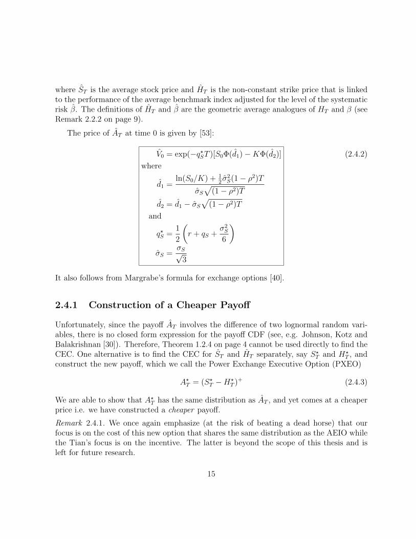
The price of AT at time 0 is given by [53]:

V0 = exp(−q?ST )[S0Φ(d1)−KΦ(d2)]

where

d1 =ln(S0/K) + 1

2σ2S(1− ρ2)T

σS√

(1− ρ2)T

d2 = d1 − σS√

(1− ρ2)T

and

q?S =1

2

(r + qS +

σ2S

6

)σS =

σS√3

(2.4.2)

It also follows from Margrabe’s formula for exchange options [40].

2.4.1 Construction of a Cheaper Payoff

Unfortunately, since the payoff AT involves the difference of two lognormal random vari-ables, there is no closed form expression for the payoff CDF (see, e.g. Johnson, Kotz andBalakrishnan [30]). Therefore, Theorem 1.2.4 on page 4 cannot be used directly to find theCEC. One alternative is to find the CEC for ST and HT separately, say S?T and H?

T , andconstruct the new payoff, which we call the Power Exchange Executive Option (PXEO)

A?T = (S?T −H?T )+ (2.4.3)

We are able to show that A?T has the same distribution as AT , and yet comes at a cheaperprice i.e. we have constructed a cheaper payoff.

Remark 2.4.1. We once again emphasize (at the risk of beating a dead horse) that ourfocus is on the cost of this new option that shares the same distribution as the AEIO whilethe Tian’s focus is on the incentive. The latter is beyond the scope of this thesis and isleft for future research.

15

Proposition 2.4.2 details the construction of such a payoff whereas Corollary 2.4.4 givesits price.

Proposition 2.4.2. Define respectively S?T and H?T as follow

S?T = dSS1/√

3T (2.4.4)

where dS = S1−1/

√3

0 e

(12− 1√

3

)(µS−qS−

σ2S2

)T

and

H?T = dHH

1/√

3T (2.4.5)

where dH = K1−1/√

3 exp(

12− 1√

3

)(µS − qS)T +

σ2ST

2

[ρ2(

1√3− 1

3

)− 1

6

]. Let

A?T = (S?T − A?T )+ = (dSS1/√

3T − dHH1/

√3

T )+ (2.4.6)

Then AT and A?T have the same distribution under the P measure.

Remark 2.4.3. Note that A?T ∈YT |YT ∼ FAT

(see Definition 1.2.3 on page 4) but it is

not the CEC of AT . This is because it is not a function of the state price process in the2-dimensional market constituted by the stock and the index (see [4] or [7]).

Corollary 2.4.4. The price of A?T at time 0 is given by

V ?0 = Υ?[S0Φ(d?1)−KΦ(d?2)]

where

d?1 =ln(S0

K

)+ 1

2ν2T

ν√T

d?2 = d?1 − ν√T

and

ν2 =1

3σ2S(1− ρ2)

Υ? = exp

[(1

2− 1√

3

)µS −

qS2

+

(1√3− 1

)r − σ2

S

12

]T

(2.4.7)

AT is strictly more expensive than A?T when µS > r.

16

0 0.2 0.4 0.6 0.8 12.6

2.8

3

3.2

3.4

3.6

3.8

4

4.2

4.4

4.6

r

Price

µS = 12%V0

V ⋆0

Figure 2.4.1: Prices of AT and A?T vs r


Figure 2.4.1 plots the prices of AT and A?T vs the risk free rate, r. The parametersused to generate the prices are the base case parameters in Table 2.4.1 on page 21. Thevertical line corresponds to the expected stock return of µS = 12% in our base case. WhenµS > r, we can see that the price of AT is greater than the price of A?T . When µS < r,the opposite is true, with equality holding when µS = r. We have seen this relationshipbetween the ordering of the option prices and the ordering of µS and r before when weconsidered GT and GT . In that case, the ordering is a result of GT being the CEC of GT

(see Remark 2.3.3 on page 11). However, in this case, even though V ?T is not the CEC of

VT , this relationship still holds and it illustrates Corollary 2.4.4 on the previous page.

Remark 2.4.5. Corollary 2.4.4 on the preceding page does not imply an arbitrage oppor-tunity. Even though AT ∼ A?T (i.e. AT and A?T have the same distribution) and V ?

0 < VT ,we do not have state-by-state dominance of A?T over AT . However, when initial costs aretaken into account, A?T does dominate AT in the first-order stochastic sense (see Levy [37])i.e. (AT − V0) ≺fsd (A?T −V ?

0 ). The proof of this fact is identical to the proof of Proposition5 in [4] and is omitted.

Remark 2.4.6. Unfortunately, the program applied to AT to construct A?T does not alwaysyield a cheaper payoff. For instance consider the option proposed by Kim [35]. Unlike [53],

17

only the index is averaged - the terminal payoff of the underlying asset is still used. Thispayoff is given by

CT = (ST − BT )+ (2.4.8)

where

BT = λS0(IT/I0)β exp(φT )

φ =1

2

[r − qS − β(r − qI)−

1

6(σ2

S − (3− 2β)βσ2I )]

(λ is an extra parameter introduced to make the design of the option grant more flexible.It is not to be confused with the market price of risk which will be defined and used inChapters 4 to 5 on pages 49–62.) Following the proof of Proposition 2.4.2 on page 16 andCorollary 2.4.4 on page 16, we can construct the new payoff as

C?T = (ST −B?

T )+ =(ST − dBB1/

√3

T

)+

(2.4.9)

where dB = (λS0)1−1/√

3 exp(

12− 1√

3

)(µS − qS)T +

σ2ST

2

[ρ2(

1√3− 1

3

)− 1

6

]with CT ∼

C?T .

Its price at time 0 is given by

P ?0 = ΥSΦ(d?1)−ΥBΦ(d?2)

where

ΥS = S0 exp(−qST )

ΥB = λS0 exp

[(1

2− 1√

3

)µS −

qS2

+

(1√3− 1

)r − σ2

S

12

]T

ν2 = σ2

S

[1 + ρ2

(1

3− 2√

3

)]d?1 =

− ln(λ) +[(

1√3− 1

2

)µS +

(1− 1√

3

)r − qS

2+

σ2S

12+ ν2

2

]T

ν√T

d?2 = d?1 − ν√T

(2.4.10)

When µS = r, we can check that CT and C?T have the same price at time zero. However,

when µS > r, the latter is actually more expensive by inspecting that ∂∂µS

P ?0 > 0. This

means that we have actually constructed a more expensive payoff and goes to show thatthe program that we applied to AT should only be used with care.

18

0 0.2 0.4 0.6 0.8 15

10

15

20

25

30

35

40

r

Price

µS = 12%

P0

P ⋆0

Figure 2.4.2: Prices of CT and C?T vs r


Figure 2.4.2 plots the prices of CT and C?T vs the risk free rate, r. The parameters used

to generate the prices are the base case parameters in Table 2.4.1 on page 21. The verticalline corresponds to the expected stock return of µS = 12% in our base case. When µS > r,we can see that the price of CT is less than the price of C?

T . When µS < r, the opposite istrue, with equality holding when µS = r.

2.4.2 The True Cost Efficient Counterpart

We have identified at least one payoff, A?T , with the same distribution as the Asian IndexedOption and comes at a cheaper price. The true CEC, which we denote by AT (and itsprice at time 0 by V0) can be estimated using numerical techniques. In order to do so, weneed an expression for the state price process for a 2-dimensional market constituted bythe stock and the index. To that effect, we follow the convention and results given by [7].

We define the (2× 2) matrix Σ as

Σ =[ σ2

S ρσSσIρσSσI σ2

I

]19

and the drift vector

µ−→ =[ µS − qSµI − qI

]The constant portfolio is defined as π−→(t) = π−→ =

[πS, πI

]Twhere the fractions of the

portfolio invested in the stock and index remain constant over time. The terminal valueof the security that is constructed using the constant mix π−→ is given by:

SπT = exp

(µ(π)− σ2(π)

2

)T + σ(π)W π

T

where W π

t is a standard Brownian motion defined by

W πt =

1√π−→T ·Σ · π−→

(πSσSW

St + πIσIW

It

)and

µ(π) = r + π−→T · ( µ−→− r · 1−→), σ2(π) = π−→

T ·Σ · π−→The market portfolio is given by

π−→∗ =

Σ−1 ·(µ−→− r · 1−→

)1−→T ·Σ−1 ·

(µ−→− r · 1−→

) (2.4.11)

Remark 2.4.7. The market portfolio given in (2.4.11) is the unique mean-variance efficientportfolio that is fully invested in risky assets (see Proposition 1 in [7]). For the closerelations between the market portfolio and the so-called growth optimal portfolio, see [18],[45] or [46].

Let θ∗ := θ(π∗) = µ(π∗)−rσ(π∗)

. Then, the state price process ξ∗(T ) is given by

ξ∗(T ) = exp

−rT − 1

2θ2∗T − θ∗W π∗

T

(2.4.12)

This means that ξ∗(T ) ∼ LN (M∗, θ2∗T ) where M∗ = −rT − 1

2θ2∗T . The true cost-efficient

payoff is given byAT = F−1

AT(1− Fξ∗(ξ∗(T ))) (2.4.13)

20

and its price at time 0 is given by

V0 = EP[ξ∗(T )AT ] = EP[ξ∗(T )F−1

AT(1− Fξ∗(ξ∗(T )))] (2.4.14)

Now that we have the state price process, it is straightforward to use Monte Carlo simu-lation to estimate the price of the CEC. This is done by making random draws from theknown distribution of ξ∗(T ) and evaluating the inverse CDF F−1

ATnumerically (both under

the P measure).

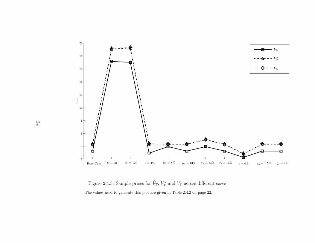
Figure 2.4.3 on page 24 plots some prices of AT , A?, AT across different sets of param-eters to illustrate the efficiency loss. Each point corresponds to the price for a particularparameter set. We consider the base case given in Table 2.4.1, and perturb some of theinput parameters as well. We can see that the degree of efficiency loss is sensitive to allmodel parameters. The values that are used to plot this figure are given in Table 2.4.1.

Option Interest Stock Index Correlation Monte CarloT 1 r 6% S0 100 I0 100 ρ 0.75 Paths 1,000,000K 100 σS 30% σI 20%

µS 12% µI 10%qS 2% qI 3%

Table 2.4.1: Base case parameters for sample AT , A?T and AT .

21

ParametersAT A?T AT

V0 St Dev V ?0 % Eff Loss V0 % Eff Loss

Base Case 3.2491 0.0075 4.3359 33.45% 4.3561 34.07%K = 80 17.2030 0.0122 19.0787 10.90% 19.1674 11.42%r = 4% 2.9594 0.0075 4.3727 47.76% 4.3998 48.68%S0 = 120 17.0242 0.0142 19.2661 13.17% 19.3557 13.70%µS = 8% 3.9538 0.0074 4.3493 10.00% 4.3561 10.17%µI = 13% 3.2561 0.0075 4.3359 33.16% 4.3561 33.78%σS = 35% 3.9730 0.0090 5.0439 26.95% 5.0673 27.54%σI = 15% 3.2579 0.0076 4.3359 33.09% 4.3561 33.71%qS = 1.5% 3.2632 0.0076 4.3467 33.20% 4.3670 33.82%qI = 2% 3.2598 0.0075 4.3359 33.01% 4.3561 33.63%ρ = 0.9 2.2739 0.0049 2.8582 25.70% 2.8715 26.28%

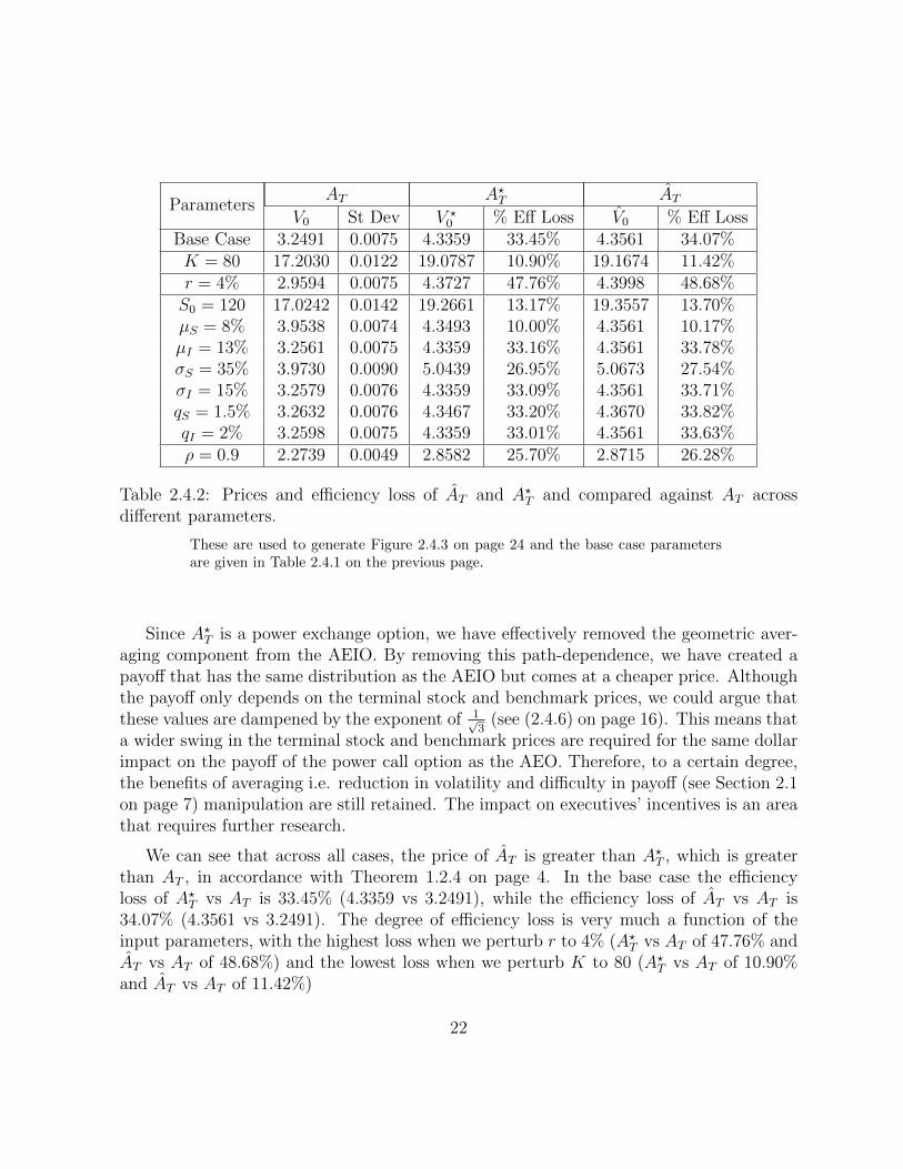
Table 2.4.2: Prices and efficiency loss of AT and A?T and compared against AT acrossdifferent parameters.

These are used to generate Figure 2.4.3 on page 24 and the base case parametersare given in Table 2.4.1 on the previous page.

Since A?T is a power exchange option, we have effectively removed the geometric aver-aging component from the AEIO. By removing this path-dependence, we have created apayoff that has the same distribution as the AEIO but comes at a cheaper price. Althoughthe payoff only depends on the terminal stock and benchmark prices, we could argue thatthese values are dampened by the exponent of 1√

3(see (2.4.6) on page 16). This means that

a wider swing in the terminal stock and benchmark prices are required for the same dollarimpact on the payoff of the power call option as the AEO. Therefore, to a certain degree,the benefits of averaging i.e. reduction in volatility and difficulty in payoff (see Section 2.1on page 7) manipulation are still retained. The impact on executives’ incentives is an areathat requires further research.

We can see that across all cases, the price of AT is greater than A?T , which is greaterthan AT , in accordance with Theorem 1.2.4 on page 4. In the base case the efficiencyloss of A?T vs AT is 33.45% (4.3359 vs 3.2491), while the efficiency loss of AT vs AT is34.07% (4.3561 vs 3.2491). The degree of efficiency loss is very much a function of theinput parameters, with the highest loss when we perturb r to 4% (A?T vs AT of 47.76% andAT vs AT of 48.68%) and the lowest loss when we perturb K to 80 (A?T vs AT of 10.90%and AT vs AT of 11.42%)

22

It is also interesting to note that the prices of A?T and AT are very close to each other,with the former still being cheaper than the latter in all cases. This highlights the fact thateven though our method of construction yields a cheaper payoff, it is still not the cheapestpayoff. For the latter, we still need to rely fully on Theorem 1.2.4 on page 4.

23

2

4

6

8

10

12

14

16

18

20

Price

Base Case K = 80 S0 = 120 r = 4% µS = 8% µI = 13% σS = 35% σI = 15% ρ = 0.9 qS = 1.5% qI = 2%

V0

V ⋆0

V0

Figure 2.4.3: Sample prices for VT , V ?T and VT across different cases

The values used to generate this plot are given in Table 2.4.2 on page 22.

24

2.4.3 AT vs A?T vs AT

Now that we have all three options in place: the Asian Executive Indexed Option (AT ),the Power Exchange Executive Option that we have constructed (A?T ), and the true costefficient counterpart (AT ), we can take a closer look at all three together.

0 10 20 30 40 50 60 70 80 900

0.1

0.2

0.3

0.4

0.5

0.6

0.7

0.8

0.9

1

Payoffs

Probabilitydistribution

Empirial CDFs of AT , A⋆T and AT

AT

A⋆T

AT

Figure 2.4.4: Empirical CDF of AT , A? and AT

The parameters used to generate this CDF are given in Table 2.4.1 on page 21.

Figure 2.4.3 shows the empirical CDFs of all three payoffs that have been generatedusing Monte Carlo simulation. As expected, these three distributions do coincide. Accord-ing to our assumption that the agent’s preference depend only on the terminal distributionof wealth (Assumption 4 on page 3), the executive would be indifferent between all threeoptions. However, the incentives that these three payoffs provide for the executive may bevery different.

From the firm’s perspective, the cost of issuing these three options are not the same, butthe executives are indifferent between all these. Hence, issuing any option other than the

25

CEC constitutes an efficiency loss. Table 2.4.2 on page 22 displays some sample prices andthe loss of efficiency in percentages for our options. In the cases that we have considered,the percentage efficiency loss ranges from a low of 10% to a high of 49%. Even though thedegree of efficiency loss varies with the parameters, there is a clear ordering of prices i.e.AT is the most expensive, followed by A?, with AT being the cheapest.

Intuitively speaking, the CEC is achieved by reshuffling the outcomes of AT in each statein reverse order with the state price process while still preserving the original distribution.When the state price process is continuous, Theorem 1.2.4 on page 4 provides the methodof doing so.

Figures 2.4.5 to 2.4.6 on pages 26–27 illustrate how the outcomes of AT are being reshuf-fled to A?T and AT respectively. In the former case, we can see a fairly linear relationshipbetween the outcomes of AT and A?T , with an empirical correlation is 0.8235. Even thoughthe reshuffling in Proposition 2.4.2 on page 16 is incomplete, we are still able to designa payoff that is cheaper, inherits the desired features of the AEIO, and has a terminalpayoff that is highly correlated with the original payoff. When the reshuffling is completein Figure 2.4.6 on the next page, we have the true CEC. The cheapest price is achieved atthe expense of the linear relationship (the empirical correlation drops to 0.3228).

0 10 20 30 40 50 60 700

10

20

30

40

50

60

70

80

AT

A⋆ T

Plot of AT vs A⋆T

Figure 2.4.5: Reshuffling of outcomes of AT to A?T

The parameters used to generate this graph are given in Table 2.4.1 on page 21.Their empirical correlation is 0.8235.

26

0 10 20 30 40 50 60 700

10

20

30

40

50

60

70

AT

AT

Plot of AT vs AT

Figure 2.4.6: Reshuffling of outcomes of AT to AT

The parameters used to generate this graph are given in Table 2.4.1 on page 21.Their empirical correlation is 0.3228.

Remark 2.4.8. If we modify Assumption 4 on page 3 so that agent preferences are statedependent, then the executive will no longer be indifferent between AT , A?T , and AT . Inthe presence of state dependent preferences, [4] also provides a construction of CEC byusing recent developments in the theory of copulas by Tankov [51].

We end this chapter with some graphs that illustrate the connection between outcomesof each of the payoff and the state price process. From Figures 2.4.7 on the next pageand 2.4.8 on the following page, we do not see any obvious relationship between ξT andAT , and ξT and A?T . However, in Figure 2.4.9 on page 29, where the payoff is cost-efficient,it becomes evident that AT is non-increasing with ξT . In fact, when ξT is continuous, thisturns out to be a necessary and sufficient condition for cost efficiency (see Proposition 2,[4]).

27

0.4 0.6 0.8 1 1.2 1.4 1.6 1.8 20

10

20

30

40

50

60

70

ξT

AT

Plot of AT vs ξT

Figure 2.4.7: Outcomes of AT vs ξT

The parameters used to generate this graph are given in Table 2.4.1 on page 21.

0.4 0.6 0.8 1 1.2 1.4 1.6 1.8 20

10

20

30

40

50

60

70

80

ξT

A⋆ T

Plot of A⋆T vs ξT

Figure 2.4.8: Outcomes of A?T vs ξT


28

0.4 0.6 0.8 1 1.2 1.4 1.6 1.8 20

10

20

30

40

50

60

70

ξT

AT

Plot of AT vs ξT

Figure 2.4.9: Outcomes of AT vs ξT


29

Chapter 3

Asian Options with Vasicek InterestRates

Thus far, we have assumed that interest rates are constant in our model. However, in real-ity, executive options have much longer maturities which make this assumption unrealistic.In fact, most of these options expire in ten years1 (see Murphy [44]). One reason for theissuance of long term options is that since the impact of the executive’s efforts on firmvalue typically take longer to surface (as compared to, say, salesmen or factory workers),it is more efficient to issue longer term contracts (see Fudenberg, Holmstrom and Milgrom[22]).

For this reason, we will incorporate stochastic interest rates modeled by a Vasicek[54] process in our study of cost efficiency. Even though the Vasicek model is far fromperfect (poor fitting of initial term structure, negative short rates, and etc.), its simplicityeventually leads to analytically tractable pricing formulas2. Another reason for using theVasicek model is that it is a simple enough model that incorporates reversion to a longterm mean. At the time of writing, we are in a low interest rates environment and theyare expected to rise over the long term3.

The first ingredient required for our study of cost efficiency in the presence of stochastic

1However, we have decided to use a maturity of T = 1 for most of our simulations. Any longermaturity would make the run time too restrictive, and introduces a large amount of time-stepping error.The conclusions that we have drawn are still valid despite this shorter maturity.

2This is presumably desirable for accounting purposes [47].3On July 20th 2011, the 30 day US Treasury rate is 0.01% while the 30 year rate is 4.25%. Data

retrieved from http://www.treasury.gov/resource-center/data-chart-center/interest-rates/

Pages/TextView.aspx?data=yield.

30

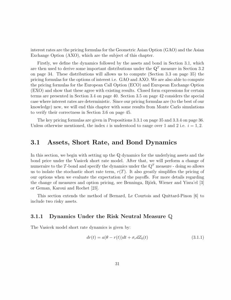
http://www.treasury.gov/resource-center/data-chart-center/interest-rates/Pages/TextView.aspx?data=yield

http://www.treasury.gov/resource-center/data-chart-center/interest-rates/Pages/TextView.aspx?data=yield

interest rates are the pricing formulas for the Geometric Asian Option (GAO) and the AsianExchange Option (AXO), which are the subject of this chapter.

Firstly, we define the dynamics followed by the assets and bond in Section 3.1, whichare then used to derive some important distributions under the QT measure in Section 3.2on page 34. These distributions will allows us to compute (Section 3.3 on page 35) thepricing formulas for the options of interest i.e. GAO and AXO. We are also able to computethe pricing formulas for the European Call Option (ECO) and European Exchange Option(EXO) and show that these agree with existing results. Closed form expressions for certainterms are presented in Section 3.4 on page 40. Section 3.5 on page 42 considers the specialcase where interest rates are deterministic. Since our pricing formulas are (to the best of ourknowledge) new, we will end this chapter with some results from Monte Carlo simulationsto verify their correctness in Section 3.6 on page 45.

The key pricing formulas are given in Propositions 3.3.1 on page 35 and 3.3.4 on page 36.Unless otherwise mentioned, the index i is understood to range over 1 and 2 i.e. i = 1, 2.

3.1 Assets, Short Rate, and Bond Dynamics

In this section, we begin with setting up the Q dynamics for the underlying assets and thebond price under the Vasicek short rate model. After that, we will perform a change ofnumeraire to the T -bond and specify the dynamics under the QT measure - doing so allowsus to isolate the stochastic short rate term, r(T ). It also greatly simplifies the pricing ofour options when we evaluate the expectation of the payoffs. For more details regardingthe change of measures and option pricing, see Benninga, Bjork, Wiener and Yisra’el [3]or Geman, Karoui and Rochet [23].

This section extends the method of Bernard, Le Courtois and Quittard-Pinon [6] toinclude two risky assets.

3.1.1 Dynamics Under the Risk Neutral Measure Q

The Vasicek model short rate dynamics is given by:

dr(t) = a(θ − r(t))dt+ σrdZ0(t) (3.1.1)

31

where a, θ, and σr are constants. We can interpret a as the rate of reversion to the longterm mean given by θ. This has the solution of:

r(t) = r(0)e−at + θ(1− e−at) + σr

∫ t

0

e−a(t−s)dZ0(s) (3.1.2)

It has an affine term structure which gives us:

P (t, T ) = A(t, T )e−B(t,T )r(t) (3.1.3)

B(t, T ) =1

a

1− e−a(T−t) (3.1.4)

A(t, T ) = exp

(θ − σ2

r

2a2

)(B(t, T )− T + t)− σ2

r

4aB2(t, T )

(3.1.5)

The bond price dynamics follows:

dP (t, T )

P (t, T )= r(t)dt− σP (t, T )dZ0(t) (3.1.6)

whereσP (t, T ) =

σra

[1− e−a(T−t)] (3.1.7)

By means of the Cholesky decomposition, we can express the dynamics for the underlyingassets and bond price using three independent Brownian motions:

dS1(t)

S1(t)= r(t)dt+ σ1C21dZ0(t) + σ1C22dZ1(t) (3.1.8)

dS2(t)

S2(t)= r(t)dt+ σ2C31dZ0(t) + σ2C32dZ1(t) + σ2C33dZ2(t) (3.1.9)

dP (t, T )

P (t, T )= r(t)dt− σP (t, T )dZ0(t) (3.1.10)

with the following diffusion terms:

C21 = ρ01 C22 =√

1− ρ201

C31 = ρ02 C32 = ρ12−ρ01ρ02√1−ρ201

C33 =√

1− ρ202 − (ρ12−ρ01ρ02)2

1−ρ201

(3.1.11)

32

3.1.2 Dynamics Under the T -Forward Measure QT

Now, we can change the numeraire to the T -bond. Under theQT measure, we want Si(t)P (t,T )

to

be martingales. A straightforward application of Ito’s Lemma to f(Si(t), P (t, T )) = Si(t)P (t,T )

and the use of Girsanov’s Theorem (see e.g. Karatzas and Shreve [33]) yields the followingQT dynamics:

dS1(t)

S1(t)= [r(t)− σ1σP (t, T )C21] dt+ σ1C21dZ

T0 (t) + σ1C22dZ

T1 (t) (3.1.12)

dS2(t)

S2(t)= [r(t)− σ2σP (t, T )C31] dt+ σ2C31dZ

T0 (t) + σ2C32dZ

T1 (t)

+ σ2C33dZT2 (t) (3.1.13)

dP (t, T )

P (t, T )=[r(t) + σ2

P (t, T )]dt− σP (t, T )dZT

0 (t) (3.1.14)

By Girsanov’s Theorem, the T -forward neutral measure QT is defined by its Radon-Nikodym derivative for u ≤ T

dQT

dQ

∣∣∣∣u

= exp

−∫ u

0

σP (s, T )dZ0(s)− 1

2

∫ u

0

σ2P (s, T )ds

Lemma 3.1.1 gives the expressions for the assets Si(t) that do not involve r(t).

Lemma 3.1.1.

S1(t) =S1(0)

P (0, t)exp

∫ t

0

[σ2P (u, t)− σ2

1

2− σP (u, T )(σ1C21 + σP (u, t))

]du

+

∫ t

0

[σ1C21 + σP (u, t)] dZT0 (u)

+

∫ t

0

σ1C22dZT1 (u)

(3.1.15)

S2(t) =S2(0)

P (0, t)exp

∫ t

0

[σ2P (u, t)− σ2

2

2− σP (u, T )(σ2C31 + σP (u, t))

]du

+

∫ t

0

[σ2C31 + σP (u, t)] dZT0 (u)

+

∫ t

0

σ2C32dZT1 (u)

33

+

∫ t

0

σ2C33dZT2 (u)

(3.1.16)

Remark 3.1.2. Henceforth, all calculations are done under the QT measure.

3.2 Some Important Distributions

Now we shift our focus to the distributions of the terminal values and geometric averagesof the underlying assets. The distributions of the terminal values are needed to computethe prices for the ECO and EXO, whereas the geometric averages are needed for the GAOand AXO. First, let us define the following quantities:

σi0(u, t) := σiC(i+1)i + σP (u, t) (3.2.1)

σij := σiC(i+1)(j+1) (3.2.2)

mi(u, t) :=σ2P (u, t)− σ2

i

2− σP (u, T )σi0(u, t) (3.2.3)

X1(t) :=

∫ t

0

m1(u, t)du+

∫ t

0

σ10(u, t)dZT0 (u) +

∫ t

0

σ11dZT1 (u) (3.2.4)

X2(t) :=

∫ t

0

m2(u, t)du+

∫ t

0

σ20(u, t)dZT0 (u) +

∫ t

0

σ21dZT1 (u) +

∫ t

0

σ22dZT2 (u) (3.2.5)

Xi(T ) :=1

T

∫ T

0

lnSi(t)dt (3.2.6)

Now we can recast the terminal values and geometric averages as follow:

Si(T ) =Si(0)

P (0, T )eXi(T ) (3.2.7)

Si(T ) = eXi(T ) (3.2.8)

From (3.2.4)–(3.2.6), it is clear that the terminal values and geometric averages are log-normally distributed. If we are able to identify the mean, variance, and covariance of thelog of Si(T ) and Si(T ), then we are done. These are done in Lemmas 3.2.1 to 3.2.2 onpages 34–35.

Lemma 3.2.1. S1(T ) and S2(T ) form a bivariate lognormal distribution where Si(T ) ∼LN (mi(T ), v2

i (T )) and their covariance is given by Cov[lnS1(T ), lnS2(T )] = v12(T ). Ex-plicit expressions for mi(T ), v2

i (T ), and v12(T ) are given in (3.4.1)–(3.4.3) on page 41.

34

Lemma 3.2.2. S1(T ) and S2(T ) form a bivariate lognormal distribution where Si(T ) ∼LN (mi(T ), v2

i (T )) and their covariance is given by Cov[ln S1(T ), ln S2(T )] = v12(T ). Ex-plicit expressions for mi(T ), v2

i (T ), and v12(T ) are given in (3.4.4)–(3.4.6) on page 42.

Remark 3.2.3. Note that we have deliberately left the terms in Lemmas 3.2.1 to 3.2.2on pages 34–35 unsimplified. This is because the evaluation of these integrals becomeincreasingly laborious, and necessitates the use of a computer algebra system (CAS). Theirexplicit forms are given in Section 3.4 on page 40 below.

Remark 3.2.4. Even though the statements of Lemmas 3.2.1 to 3.2.2 on pages 34–35 looksimple enough, their proofs are in fact rather involved. We have opted to include all thecomplete (repetitive) details in Appendex B.2 on page 85 for pedagogical reasons, but moreimportantly, as the pseudo code for evaluating the expressions in a CAS (see Remark 3.2.3).

3.3 Option Pricing Formulas

Now that we have the distributions for the terminal values and geometric averages (Lemmas3.2.1 to 3.2.2 on pages 34–35), the task of computing the pricing formulas becomes mucheasier (with the help of Lemmas A.1 on page 74 and A.3 on page 75). We present theseformulas in this section which take into account the stochastic interest rates given by theVasicek process in (3.1.1) on page 31.

The formulas for the Geometric Asian Option and Asian Exchange Option are newresults, whereas the ones for the European Call Option and European Exchange Optionagree with existing results. The former two will be used later for our study of cost efficiency;the latter two serve as corroboration that our alternative method of derivation is correct.

3.3.1 Geometric Asian Option (GAO)

Proposition 3.3.1. In the presence of stochastic interest rates given by the Vasicek processin (3.1.1) on page 31, the payoff of the Geometric Asian Option with strike K on theunderlying Si(T ) at time T is given by:

GAO = (Si(T )−K)+ =(e

1T

∫ T0 lnSi(t)dt −K

)+

(3.3.1)

35

Its price at time 0 is given by:

Price(GAO) = P (0, T )

[exp

mi(T ) +

1

2v2i (T )

Φ(f1(T ))−KΦ(f2(T ))

]where

f1(T ) =mi(T ) + v2

i (T )− lnK

vi(T )

f2(T ) = f1(T )− vi(T )

(3.3.2)

(mi(T ) and vi(T ) are given in (3.4.4)–(3.4.5) on page 42)

Remark 3.3.2. Recall that in the case of constant interest rates, the price of a GeometricAsian Option is of the following form:

Price(GAOConst) = e−rT[Si(0)erTΦ(f1)−KΦ(f2)

]where

f1 =ln Si(0)

K+(r − qi + σi

2

)T

σi√T

f2 = f1 − σi√T

(3.3.3)

We can see that (3.3.2) has the same functional form as (3.3.3), but with different inputparameters. The familiar relationship between f1 and f2 also holds for f1(T ) and f2(T ).

Remark 3.3.3. Zhang, Yuan and Wang [50] have in fact derived the price of the GAOunder the extended Vasicek model. However, their semi-closed form expression is highlycomplicated, not intuitive and left largely unsimplified. Their derivation relies on thebrute-force integration of the expectation term under the Q measure, as opposed to oursimpler approach of tackling the problem through the QT measure. However, it does seemthat the Hull-White model would naturally be the next extension for us to make.

3.3.2 Asian Exchange Option (AXO)

Proposition 3.3.4. In the presence of stochastic interest rates given by the Vasicek processin (3.1.1) on page 31, the payoff of the Asian Exchange Option on S1(T ) and S2(T ) attime T is given by:

AXO = (S1(T )− S2(T ))+ =(e

1T

∫ T0 lnS1(t)dt − e 1

T

∫ T0 lnS2(u)du

)+

(3.3.4)

36


Price(AXO) = P (0, T )

[exp

m1(T ) +

1

2v2

1(T )

Φ(g1(T ))

− exp

m2(T ) +

1

2v2

2(T )

Φ(g2(T ))

]where

g1(T ) =m1(T )− m2(T ) + v2

1(T )− v12(T )√v2

1(T )− 2v12(T ) + v22(T )

g2(T ) = g1(T )−√v2

1(T )− 2v12(T ) + v22(T )

(3.3.5)

(mi(T ), v2i (T ), and v12(T ) are given in (3.4.4)–(3.4.6) on page 42.)

Remark 3.3.5. Recall that in the case of constant interest rates, the price of an AsianExchange Option is of the following form:

Price(AXOConst) = e−rT[S1(0)erTΦ(g1)− S2(0)erTΦ(g2)

]where

g1 =ln S1(0)

S2(0)+ (σ2

1 + σ22 − 2σ1σ2ρ)T

2√(σ2

1 + σ22 − 2σ1σ2ρ)T

g2 = g1 −√

(σ21 + σ2

2 − 2σ1σ2ρ)T

(3.3.6)

Again, we can see that (3.3.5) has the same functional form as (3.3.6), and the samerelationship between the inputs into the normal cdf terms. It is also interesting to notethat the price of the option does not depend on the interest rate.

Remark 3.3.6. Our method generalizes Zhang’s [55] approach of computing the EXO underconstant interest rates to the AXO under stochastic interest rates.

3.3.3 European Call Option (ECO)

Proposition 3.3.7. In the presence of stochastic interest rates given by the Vasicek pro-cess in (3.1.1) on page 31, the payoff of the European Call Option with strike K on theunderlying Si(T ) at time T is given by:

ECO = (Si(T )−K)+ (3.3.7)

37

Its price at time 0 is given by:

Price(ECO) = P (0, T )

[exp

mi(T ) +

1

2v2i (T )

Φ(f1(T ))−KΦ(f2(T ))

]where

f1(T ) =mi(T ) + v2

i (T )− lnK

vi(T )

f2(T ) = f1(T )− vi(T )

(3.3.8)

(mi(T ) and v2i (T ) are given in (3.4.1)–(3.4.2) on page 41).

Remark 3.3.8. In fact, note that (3.3.8) is really just (3.3.2) on page 36, but with the meanand variance of the terminal values instead of the geometric averages.

Corollary 3.3.9. The price of the European Call Option given in (3.3.8) is equivalent tothe following given by Rabinovitch [48]:

Price(ECOR) = Si(0)Φ

(ln Si(0)

KP (0,T )+ 1

2v2i (0, T )

vi(0, T )

)

−KP (0, T )Φ

(ln Si(0)

KP (0,T )− 1

2v2i (0, T )

vi(0, T )

)where

v2i (0, T ) = V (0, T ) + σ2

i T + 2ρ0iσrσia

[T − 1

a(1− e−aT )

]V (0, T ) =

(σra

)2[T +

2

ae−aT − 1

2ae−2aT − 3

2a

]

(3.3.9)

3.3.4 European Exchange Option (EXO)

Proposition 3.3.10. In the presence of stochastic interest rates given by the Vasicek pro-cess in (3.1.1) on page 31, the payoff of the European Exchange Option on S1(T ) and S2(T )at time T is given by:

EXO = (S1(T )− S2(T ))+ (3.3.10)

38


Price(EXO) = P (0, T )

[exp

m1(T ) +

1

2v2

1(T )

Φ(g1(T ))

− exp

m2(T ) +

1

2v2

2(T )

Φ(g2(T ))

]where

g1(T ) =m1(T )−m2(T ) + v2

1(T )− v12(T )√v2

1(T )− 2v12(T ) + v22(T )

g2(T ) = g1(T )−√v2

1(T )− 2v12(T ) + v22(T )

(3.3.11)

(mi(T ), v2i (T ), and v12(T ), are given in (3.4.1)–(3.4.3) on page 41.)

Remark 3.3.11. Once again, note that (3.3.11) is really just (3.3.5) on page 37, but withthe mean, variance and covariance of the terminal values instead of the geometric averages.Moreover, even though the interest rates are assumed to be stochastic, the pricing formulahere does not involve the interest rate (much like Margrabe’s formula [40]).

Corollary 3.3.12. The price of the European Exchange Option given in (3.3.11) is equiv-alent to the following given by Bernard and Cui [5]:

Price(EXOBC) = S1(0)Φ(g1)− S2(0)Φ(g2)

where

g1 =ln S1(0)

S2(0)+ (σ2

1 + σ22 − 2σ1σ2ρ12)T

2√(σ2

1 + σ22 − 2σ1σ2ρ12)T

g2 = g1 −√

(σ21 + σ2

2 − 2σ1σ2ρ12)T

(3.3.12)

Remark 3.3.13. In Margrabe’s [40] original pricing of the EXO (with constant interestrates), the second asset is used as the numeraire instead of the T -bond. This methodsimplifies the problem as we can avoid performing a double integration. In fact, even wheninterest rates are stochastic, this method still works [5].

However in our case, since the payoffs involve geometric averages, we are unable touse the second asset as the numeraire. This is because the cancellations in the EXO thatsimplify the integration problem do not happen in the AXO. To see why this is the case,

39

we follow [5] and define the measure Q (this corresponds to using the second asset as thenumeraire) where its Radon-Nikodym derivative takes the following form for t ≤ T :

dQ

dQ

∣∣∣∣t

= exp

−1

2σ2

2t+ · · ·Z0(t) + · · ·Z1(t) + · · ·Z2(t)

Under Q, the dynamics for S1(t) and S2(t) would take the following form:

dS1(t)

S1(t)= r(t)dt+ · · · dZ0(t) + · · · dZ1(t)

dS2(t)

S2(t)= r(t)dt+ · · · dZ0(t) + · · · dZ1(t) + · · · dZ2(t)

Then,

S1(T ) = S1(0) exp

1

T

∫ T

0

[∫ t

0

r(s)ds+

∫ t

0

· · · dZ0(s) +

∫ t

0

· · · dZ1(s)

]dt

S2(T ) = S2(0) exp

1

T

∫ T

0

[∫ t

0

r(s)ds+

∫ t

0

· · · dZ0(s) +

∫ t

0

· · · dZ1(s) +

∫ t

0

· · · dZ2(s)

]dt

The price of the AXO is

Price(AXO) = EQ

[e−

∫ T0 r(s)ds

(S1(T )− S2(T )

)+]

= EQ

[e−

∫ T0 r(s)dsS2(T )

(S1(T )

S2(T )− 1

)+]

= EQ

[e−

∫ T0 r(s)dsS2(0) exp

1

T

∫ T

0

[∫ t

0

r(s)ds+ · · ·]dt

(S1(T )− S2(T )

)+]

In the case of a EXO, the integral of the short rate terms do cancel out, which lead toa simpler integration problem. However in our case, the integral in the first exponent,∫ T

0r(s)ds, does not cancel out with that in the second exponent,

∫ t0r(s)ds, and we are still

left with a complicated expectation term. Hence, using the second asset as the numeraireis not ideal for the problem at hand - we are better of with using the T -bond instead.

3.4 Closed Form Expressions

We are able to derive closed form Black-Scholes type formulas for the prices, but some ofthe key terms have been left unsimplified as they involve Riemann integrals that evaluate

40

to very long and complicated formulas. These expressions have been evaluated with thehelp of a CAS and are presented in this section.

3.4.1 Closed Form Expressions for the Terminal Values

Recall from Lemma 3.2.1 on page 34 that S1(T ) and S2(T ) form a bivariate lognormaldistribution where Si(T ) ∼ LN (mi(T ), v2

i (T )) and their covariance is given byCov[lnS1(T ), lnS2(T )] = v12(T ). The closed form expressions for the mean, variance andcovariance of the log of the terminal values are as follow:

mi(T )

= lnSi(0)

P (0, T )− σ2

i T

2+(σra

)2

1

aeaT

[1

4eaT− 1

]+

3

4a− T

2

+σrσiρ0i

a

1

a

[1− e−aT

]− T

(3.4.1)

v2i (T )

= σ2i T +

(σra

)2

2

aeaT

[1− 1

4eaT

]+ T − 3

2a

+

2σrσiρ0i

a

T − 1

a

[1− e−aT

](3.4.2)

v12(T )

= σ1σ2ρ12T +(σra

)2

2

aeaT

[1− 1

4eaT

]+ T − 3

2a

+σra

(σ1ρ01 + σ2ρ02)

T − 1

a

[1− e−aT

](3.4.3)

3.4.2 Closed Form Expressions for the Geometric Averages

Recall from Lemma 3.2.2 on page 35 that S1(T ) and S2(T ) form a bivariate lognormaldistribution where Si(T ) ∼ LN (mi(T ), v2

i (T )) and their covariance is given byCov[ln S1(T ), ln S2(T )] = v12(T ). The closed form expressions for the mean, variance and

41

covariance of the log of the geometric averages are as follow:

mi(T )

= lnSi(0) +T

2

θ − σ2

1

2

+θ − r0

a

1

aT

[1− e−aT

]− 1

+(σra

)2

1

aeaT

[1

aT− 1− 1

2aTeaT

]− T

2+

1

a

[1− 1

2aT

]+σrσiρ0i

a

1

a2T− T

2− 1

aeaT

[1

aT+ 1

](3.4.4)

v2i (T )

=σ2i T

3+(σra

)2T

3+

1

a

[1

aT− 1 +

1

2T 2a2

]− 2

a2TeaT

[1 +

1

4TaeaT

]+σrσiρ0i

a

2T

3+

1

a

[2

a2T 2− 1

]− 2

a2TeaT

[1

aT+ 1

](3.4.5)

v12(T )

=σ1σ2ρ12T

3+(σra

)2T

3+

1

a

[1

aT− 1 +

1

2T 2a2

]− 2

a2TeaT

[1 +

1

4TaeaT

]+σra

(σ1ρ01 + σ2ρ02)

T

3− 1

a2TeaT

[1

aT+ 1

]+

1

a

[1

a2T 2− 1

2

](3.4.6)

3.4.3 Closed Form Expressions for the Bond Price

The bond price term under the Vasicek model appears in the various option pricing for-mulas. We recall the following famous result for completeness (see, e.g. [15]):

P (0, T )

= exp

θ − r(0)

a

[1− e−aT

]− Tθ +

(σra

)2[T

2− 3

4a+

1

aeaT

(1− 1

4eaT

)](3.4.7)

3.5 Deterministic Interest Rates

Now that we have the pricing formulas for the various options under a Vasicek interest ratemodel (Section 3.3 on page 35), as well as the explicit expressions for the various input

42

parameters (Section 3.4 on page 40), we can consider the special case of zero interest ratevolatility (σr = 0) i.e. deterministic interest rates. The input parameters into the pricingformulas simplify considerably and we are able to express them in a more explicit fashion.

3.5.1 Setup

When σr = 0, the short rate dynamics becomes

dr(t) = a(θ − r(t))dt (3.5.1)

which has the solution ofr(t) = r(0)e−at + θ(1− e−at) (3.5.2)

The bond price becomes:

P (0, T ) = exp

θ − r(0)

a

[1− e−aT

]− Tθ

(3.5.3)

The mean, variance and covariance of the terminal values simplify to the following:

mi(T ) = lnSi(0)

P (0, T )− σ2

i T

2(3.5.4)

v2i (T ) = σ2

i T (3.5.5)

v12(T ) = σ1σ2ρ12T (3.5.6)

The mean, variance and covariance of the geometric averages simplify to the following:

mi(T ) = lnSi(0) +T

2

θ − σ2

i

2

+θ − r0

a

1

aT

[1− e−aT

]− 1

(3.5.7)

v2i (T ) =

σ2i T

3(3.5.8)

v12(T ) =σ1σ2ρ12T

3(3.5.9)

It is interesting to note that in the case of deterministic interest rates, the variance andcovariance for both the terminal values and geometric averages simplify to the familiarresults in the case of constant interest rates. However, the mean includes some extra terms.This is expected because the deterministic interest rates do not affect the randomness(volatility) of the assets per se - they only shift their price paths in a deterministic manner.

43

3.5.2 Deterministic Interest Rates Pricing Formulas

The following propositions detail the prices of the GAO, AXO and ECO when interestrates are deterministic. The price of the EXO is the same as Proposition 3.3.10 on page 38as we have seen that the interest rate does not enter the pricing formula.

Proposition 3.5.1. When the short rate dynamics is given by (3.5.1) on the precedingpage, the price of the GAO is given by:

Price(GAODeterministic)

= Si(0) exp

θ − r(0)

a

[1

aT− e−aT

(1

aT+ 1

)]− T

2

[θ +

σ2i

6

]× Φ(f1(T ))−K exp

θ − r(0)

a

[1− e−aT

]− Tθ

Φ(f2(T ))

where

f1(T ) =ln Si(0)

K+ T

2

[θ +

σ2i

6

]+ θ−r(0)

a

[1aT

(1− e−aT

)− 1]

σi√T/3

f2(T ) = f1(T )− σi√T/3

(3.5.10)

Proposition 3.5.2. When the short rate dynamics is given by (3.5.1) on the previouspage, the price of the AXO is given by:

Price(AXODeterministic)

= exp

θ − r(0)

a

[1

aT

(1− e−aT

)− e−aT

]− θT

2

×[S1(0) exp

−σ

21T

12

Φ (g1(T ))− S2(0) exp

−σ

22T

12

Φ (g2(T ))

]where

g1(T ) =ln S1(0)

S2(0)+ T

4

[σ21

3+ σ2

2

]− σ1σ2ρ12T

3√T3

(σ21 + σ2

2 − 2σ1σ2ρ12)

g2(T ) = g1(T )−√T

3(σ2

1 + σ22 − 2σ1σ2ρ12)

(3.5.11)

44

Proposition 3.5.3. When the short rate dynamics is given by (3.5.1) on page 43, theprice of the ECO is given by:

Price(ECODeterministic)

= Si(0)Φ(f1(T ))−K exp

θ − r(0)

a

(1− e−aT

)− θT

Φ(f2(T ))

where

f1(T ) =ln Si(0)

K+(σ2i

2+ θ)T − θ−r(0)

a

(1− e−aT

)σi√T

f2(T ) = f1(T )− σi√

(T )

(3.5.12)

3.6 Monte Carlo Simulation

We conclude this chapter with some Monte Carlo simulation to verify the correctness ofour pricing formulas given in Section 3.3 on page 35. A simple Euler scheme is used todiscretize the interest rates and stock price paths (see e.g., Glasserman [24]). Since wealready have the prices for the European Call Option and the European Exchange Option,we can use these two payoffs as control variates in an optimal fashion (see Boyle, Broadieand Glasserman [12]).

The simulation results for the Geometric Asian Option and Asian Exchange Optionare presented in Tables 3.6.2 to 3.6.3 on pages 46–47 respectively. We can see that acrossthe board, the pricing formulas agree very closely with the simulation results. In fact, allpercentage errors are less than 1% in absolute terms.

The standard deviation for these trials are given in Tables 3.6.4 to 3.6.5 on page 48.We can see that using the ECO and EXO as control variates reduce the standard deviationof our estimates significantly.

45

Option Vasicek Assets Correlation Monte CarloT 1 a 0.20 S1(0) 100 ρ01 0.25 Paths 100,000K 100 θ 0.35 S2(0) 120 ρ02 0.50 Time steps 100,000

r(0) 6% σ1 30% ρ12 0.75σr 20% σ2 40%

Table 3.6.1: Base case parameters for sample prices of the GAO on assets 1 and 2, and theAXO.

ParametersGAO on Asset 1 GAO on Asset 2

BS MC % Error BS MC % ErrorBase case 8.2394 8.2648 -0.3% 23.3099 23.3272 -0.07%T = 10 12.2563 12.2756 -0.16% 13.4416 13.5051 -0.47%K = 120 2.1669 2.1810 -0.65% 12.1107 12.0912 0.16%a = 0.4 8.5059 8.5122 -0.07% 23.5566 23.5221 0.15%θ = 0.15 8.0393 8.0355 0.05% 23.1622 23.1832 -0.09%

r(0) = 10% 8.9972 8.9705 0.30% 24.1711 24.1223 0.20%σr = 50% 8.6084 8.5712 0.43% 22.7620 22.7605 0.01%S2(0) = 100 8.2394 8.2404 -0.01% 10.0922 10.1097 -0.17%σ1 = 60% 13.1323 13.1661 -0.26% 23.3099 23.3252 -0.07%σ2 = 80% 8.2394 8.2307 0.11% 27.3507 27.3214 0.11%ρ01 = −0.15 7.9185 7.9282 -0.12% 23.3099 23.3533 -0.19%

ρ02 = −0.5, ρ12 = 0.6 8.2394 8.2431 -0.05% 23.6464 23.5934 0.22%ρ12 = −0.25 8.2394 8.2142 0.31% 23.3099 23.3341 -0.10%

Table 3.6.2: Simulated prices of the GAO on assets 1 and 2.

The base case parameters are given in Table 3.6.1.

46

ParametersAEO

BS MC % ErrorBase case 1.0274 1.0233 0.40%T = 10 10.1892 10.3010 -1.08%K = 120 1.0274 1.0289 -0.15%a = 0.4 1.0066 1.0123 -0.56%θ = 0.15 1.0402 1.0451 -0.47%

r(0) = 10% 1.0095 1.0060 0.35%σr = 50% 1.1318 1.1315 0.03%S2(0) = 100 6.2384 6.2011 0.60%σ1 = 60% 2.5576 2.5492 0.33%σ2 = 80% 8.6620 8.6637 -0.02%ρ01 = −0.15 1.0929 1.0832 0.90%

ρ02 = −0.5, ρ12 = 0.6 1.6374 1.6368 0.04%ρ12 = −0.25 6.1666 6.1641 0.04%

Table 3.6.3: Simulated prices of the AXO on assets 1 and 2.

The base case parameters are given in Table 3.6.1 on the preceding page.

47

ParametersGAO on Asset 1 GAO on Asset 2

R St Dev C St Dev % Diff R St Dev C St Dev % DiffBase case 0.0374 0.0205 82.5% 0.0736 0.0405 81.9%T = 10 0.0732 0.0688 6.4% 0.0793 0.0766 3.5%K = 120 0.0201 0.0126 59.3% 0.0587 0.0325 80.7%a = 0.4 0.0376 0.0206 82.7% 0.0735 0.0400 83.8%θ = 0.15 0.0371 0.0204 81.3% 0.0742 0.0406 82.6%

r(0) = 10% 0.0381 0.0207 83.7% 0.0732 0.0399 83.4%σr = 50% 0.0380 0.0211 79.5% 0.0726 0.0415 74.9%S2(0) = 100 0.0372 0.0203 82.8% 0.0489 0.0271 80.3%σ1 = 60% 0.0733 0.0432 69.8% 0.0739 0.0404 83.0%σ2 = 80% 0.0372 0.0206 80.5% 0.1331 0.0812 64.0%ρ01 = −0.15 0.0363 0.0210 72.8% 0.0736 0.0404 81.9%

ρ02 = −0.5, ρ12 = 0.6 0.0370 0.0204 81.7% 0.0752 0.0433 73.9%ρ12 = −0.25 0.0371 0.0205 81.3% 0.0735 0.0404 81.9%

Table 3.6.4: Raw and control variate standard deviation of the prices of the GAO.

ParametersAEO

R St Dev C St Dev % DiffBase case 0.0110 0.0079 39.8%T = 10 0.1149 0.1107 3.9%K = 120 0.0110 0.0078 41.7%a = 0.4 0.0108 0.0077 41.0%θ = 0.15 0.0111 0.0079 40.6%

r(0) = 10% 0.0107 0.0076 40.4%σr = 50% 0.0122 0.0089 37.4%S2(0) = 100 0.0266 0.0157 69.9%σ1 = 60% 0.0275 0.0187 46.8%σ2 = 80% 0.0407 0.0261 55.9%ρ01 = −0.15 0.0117 0.0084 40.1%

ρ02 = −0.5, ρ12 = 0.6 0.0142 0.0096 47.8%ρ12 = −0.25 0.0410 0.0256 60.4%

Table 3.6.5: Raw and control variate standard deviation of the prices of the AXO.

48

Chapter 4

State Price Process with VasicekInterest Rates

The second ingredient required for our study of cost efficiency with stochastic interestrates in the context of Asian Executive Compensation is an expression for the state priceprocess (see the definition of the cost efficient counterpart in Theorem 1.2.4 on page 4).More specifically, we require an explicit form for the state price process for a market withtwo risky assets and stochastic interest rates modeled by a Vasicek process. Even thoughthe literature abounds with option pricing methodologies under environments with muchstochasticity, not as much research has been done in the study of state price processes insuch frameworks.

Hurlimann [26] gives the state price process for risky assets and interest rates, butassumes that the interest rates and risky assets are driven by the same Brownian motions.Miltersen and Persson [42] provide a general framework for deriving the state price processand give concrete examples when the market has two sources of randomness. Howeverthis is insufficient as we need three sources of randomness in our case, and the extensionfrom two to three sources of randomness is non-trivial1. Jeanblanc, Yor and Chesney [27]provide a fairly general formulation of the state price process, but we want an explicitexpression in order to derive its distribution as well.

In Section 4.1 on the following page, we will derive an explicit expression for the stateprice process and its distribution, and recast it as a function of market variables in Sec-

1Boyle, Tan and Tian [14] write “Our colleague, Ken Vetzal pointed out that extensions of resultsfrom n = 2 to n = 3 are sometimes not very easy and cited Fermat’s Last Theorem as an illustration”.Fortunately, our problem is trivial compared to Fermat’s Last Theorem.

49

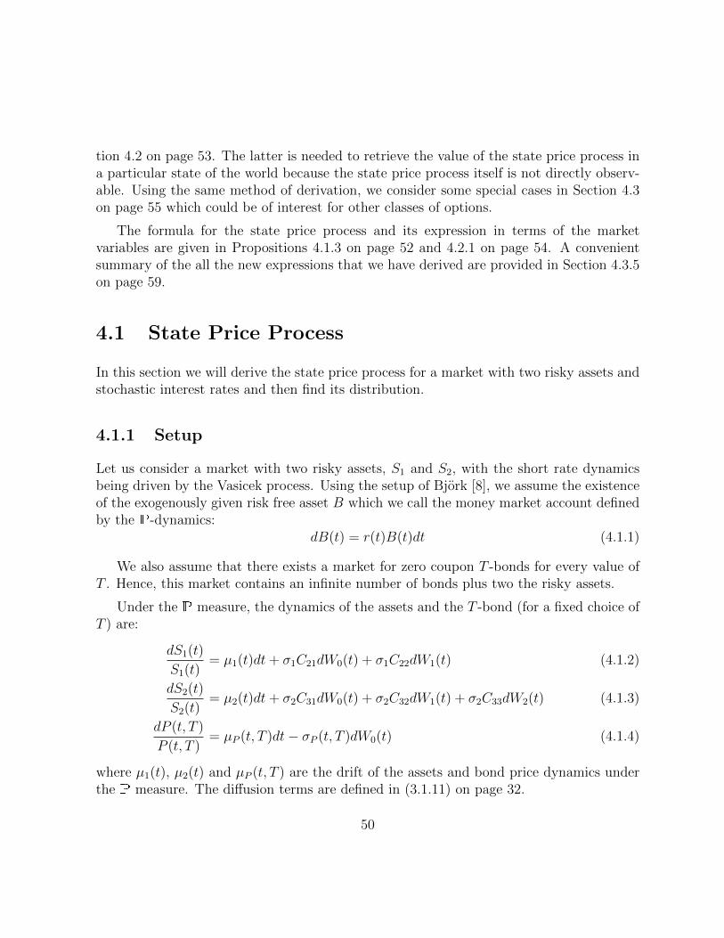
tion 4.2 on page 53. The latter is needed to retrieve the value of the state price process ina particular state of the world because the state price process itself is not directly observ-able. Using the same method of derivation, we consider some special cases in Section 4.3on page 55 which could be of interest for other classes of options.

The formula for the state price process and its expression in terms of the marketvariables are given in Propositions 4.1.3 on page 52 and 4.2.1 on page 54. A convenientsummary of the all the new expressions that we have derived are provided in Section 4.3.5on page 59.

4.1 State Price Process

In this section we will derive the state price process for a market with two risky assets andstochastic interest rates and then find its distribution.

4.1.1 Setup

Let us consider a market with two risky assets, S1 and S2, with the short rate dynamicsbeing driven by the Vasicek process. Using the setup of Bjork [8], we assume the existenceof the exogenously given risk free asset B which we call the money market account definedby the P-dynamics:

dB(t) = r(t)B(t)dt (4.1.1)

We also assume that there exists a market for zero coupon T -bonds for every value ofT . Hence, this market contains an infinite number of bonds plus two the risky assets.

Under the P measure, the dynamics of the assets and the T -bond (for a fixed choice ofT ) are:

dS1(t)

S1(t)= µ1(t)dt+ σ1C21dW0(t) + σ1C22dW1(t) (4.1.2)

dS2(t)

S2(t)= µ2(t)dt+ σ2C31dW0(t) + σ2C32dW1(t) + σ2C33dW2(t) (4.1.3)

dP (t, T )

P (t, T )= µP (t, T )dt− σP (t, T )dW0(t) (4.1.4)

where µ1(t), µ2(t) and µP (t, T ) are the drift of the assets and bond price dynamics underthe P measure. The diffusion terms are defined in (3.1.11) on page 32.

50

We assume that all risky assets traded in the market (i.e. the two risky assets and thebond) share the same market price of risk, λ, that is constant over time. The assumptionof the common market price of risk is reasonable, based on the Arbitrage Pricing Theory(see e.g., Ross [49]). The choice of a constant market price of risk (though it is fairlystraightforward to introduce time-dependence) is based on the common approach for theVasicek model [15]. With this in mind, we define the market price of risk as

λ =µ1(t)− r(t)

σ1

=µ2(t)− r(t)

σ2

=µP (t)− r(t)σP (t, T )

(4.1.5)

Combining (4.1.5) and (4.1.2)–(4.1.4) on the preceding page gives us:

dS1(t)

S1(t)= [r(t) + λσ1]dt+ σ1C21dW0(t) + σ1C22dW1(t) (4.1.6)

dS2(t)

S2(t)= [r(t) + λσ2]dt+ σ2C31dW0(t) + σ2C32dW1(t) + σ2C33dW2(t) (4.1.7)

dP (t, T )

P (t, T )= [r(t)− λσP (t, T )]dt− σP (t, T )dW0(t) (4.1.8)

A straightforward application of Ito’s Lemma to (4.1.6)–(4.1.8) gives us:

S1(t) = S1(0) exp

∫ t

0

r(s)ds+ σ1

(λ− σ1

2

)t

+

∫ t

0

σ1C21dW0(s) +

∫ t

0

σ1C22dW1(s)

(4.1.9)

S2(t) = S2(0) exp

∫ t

0

r(s)ds+ σ2

(λ− σ2

2

)t

+

∫ t

0

σ2C31dW0(s) +

∫ t

0

σ2C32dW1(s) +

∫ t

0

σ2C33dW2(s)

(4.1.10)

P (t, T ) = P (0, T ) exp

∫ t

0

r(s)ds− λ∫ t

0

σP (s, T )ds− 1

2

∫ t

0

σ2P (s, T )ds

−∫ t

0

σradW0(s) +

∫ t

0

σrae−a(T−s)dW0(s)

(4.1.11)

Under the P measure, the short rate has the following dynamics:

dr(t) = a

(θ +

λσra− r(t)

)dt+ σrdW0(t) (4.1.12)

51

This has the solution of

r(t) = r(0)e−at +

(θ +

λσra

)(1− e−at

)+ σr

∫ t

0

e−a(t−s)dW0(s) (4.1.13)

Remark 4.1.1. Compare the definition of (4.1.12)–(4.1.13) on pages 51–52 to (3.1.1)–(3.1.2)on pages 31–32. The dynamics are usually defined under the Q measure, and the Pdynamics are retrieved through the introduction of the market price of risk λ [15].

Remark 4.1.2. Note that we have expressed (4.1.11) on the preceding page in this mannerintentionally so that the time-dependent stochastic integrand term will cancel out with theone in (4.1.13). It will become apparent later that this makes it possible to express thestate price process as a function of market variables.

4.1.2 An Explicit Expression for the State Price Process

Using the setup given in Section 4.1.1 on page 50, Proposition 4.1.3 gives an explicitexpression of the state price process while Corollary 4.1.6 on the following page gives itsdistribution.

Proposition 4.1.3. Consider a market with two risky assets and stochastic interest ratesmodeled by the Vasicek process. The state price process is given by

ξS2(T ) = exp

−∫ T

0

r(s)ds− 1

2

(λ2 + α2

1 + α22

)T

−∫ T

0

λdW0(s)−∫ T

0

α1dW1(s)−∫ T

0

α2dW2(s)

where

A = ρ201 + ρ2

02 + ρ212 − 1− 2ρ01ρ02ρ12

α1 = λ

√1− ρ01

1 + ρ01

α2 = α1 ·1 + ρ01 − ρ02 − ρ12√

A

(4.1.14)

(4.1.15)

(4.1.16)

(4.1.17)

Remark 4.1.4. We have implicitly assumed that A > 0 in order for (4.1.17) to be welldefined. This is also required in order for the systems of equations (B.3.1.5) on page 99(proof of Proposition 4.1.3) and (B.3.3.5) on page 103 (proof of Proposition 4.2.1) to bewell defined.

52

Remark 4.1.5. To check the correctness of (4.1.14) on the preceding page, we can quicklycompute the differentials d(ξS2(t)S1(t)), d(ξS2(t)S2(t)), and d(ξS2(t)P (t, T )) using Ito’sLemma and verify that they have zero drift i.e. the quantities are martingales.

Corollary 4.1.6. Consider a market with two risky assets and stochastic interest ratesmodeled by the Vasicek process. Under the P measure, ξS2(T ) ∼ LN

(mξS2(T ), v2

ξS2(T )),

where

mξS2(T ) = −1

2(λ2 + α2

1 + α22)T

−(θ +

λσra

)T −

(r(0)− θ − λσr

a

)1− e−aT

a

v2ξS2

(T ) = (λ2 + α21 + α2

2)T +σra

(2λ+

σra

)(T − 1− e−aT

a

)− σ2

r

2a3(1− e−aT )2

(4.1.18)

(4.1.19)

4.2 State Price Process as a Function of Market Vari-

ables

In this section, we express the state price process as a function of market variables. Wewant this expression because in actuality, the state price process is not a traded asset andwe are unable to observe its value directly. If we have such a function, we are able toretrieve the value of the state price process through observable market variables and craftthe payoff of the true cost efficient counterpart (CEC).

The key challenge is to express the market variables in such a way that we are ableto match the stochastic integrals that arise in the state price process. We will start withmatching the stochastic integral terms in the state price process, followed by the integralof the short rate, and finally the constant terms. The program is as follow:

1. The stochastic integrands that appear in the state price process are all constants,so we are unable to match them by simply using the underlying assets and the T -bond since the stochastic integrand in the T -bond is a function of time. However, it

turns out that a combination of S1(T ), S2(T ) and P (0, T ) expr(T )a

will suffice (see

Remark 4.1.2 on the previous page and (B.3.3.1) on page 103).

53

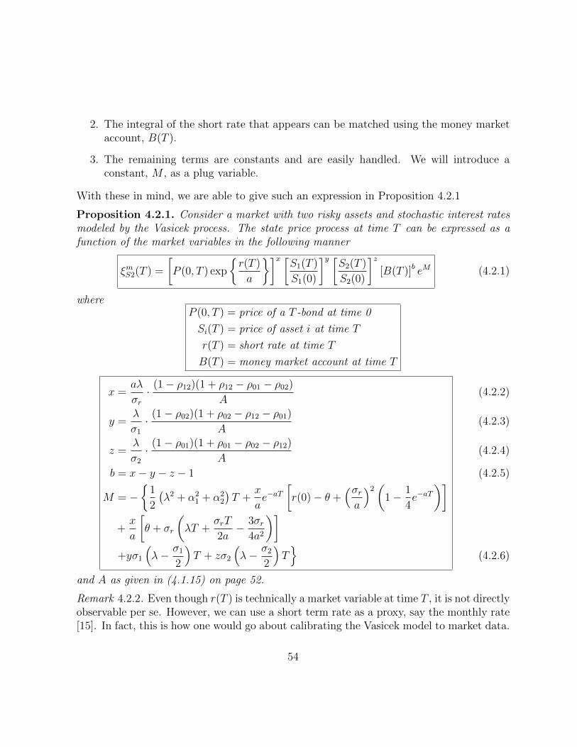
2. The integral of the short rate that appears can be matched using the money marketaccount, B(T ).

3. The remaining terms are constants and are easily handled. We will introduce aconstant, M , as a plug variable.

With these in mind, we are able to give such an expression in Proposition 4.2.1

Proposition 4.2.1. Consider a market with two risky assets and stochastic interest ratesmodeled by the Vasicek process. The state price process at time T can be expressed as afunction of the market variables in the following manner

ξmS2(T ) =

[P (0, T ) exp

r(T )

a

]x [S1(T )

S1(0)

]y [S2(T )

S2(0)

]z[B(T )]b eM (4.2.1)

whereP (0, T ) = price of a T -bond at time 0

Si(T ) = price of asset i at time T

r(T ) = short rate at time T

B(T ) = money market account at time T

x =aλ

σr· (1− ρ12)(1 + ρ12 − ρ01 − ρ02)

A

y =λ

σ1

· (1− ρ02)(1 + ρ02 − ρ12 − ρ01)

A

z =λ

σ2

· (1− ρ01)(1 + ρ01 − ρ02 − ρ12)

A

b = x− y − z − 1

M = −

1

2

(λ2 + α2

1 + α22

)T +

x

ae−aT

[r(0)− θ +

(σra

)2(

1− 1

4e−aT

)]+x

a

[θ + σr

(λT +

σrT

2a− 3σr

4a2

)]+yσ1

(λ− σ1

2

)T + zσ2

(λ− σ2

2

)T

(4.2.2)

(4.2.3)

(4.2.4)

(4.2.5)

(4.2.6)

and A as given in (4.1.15) on page 52.

Remark 4.2.2. Even though r(T ) is technically a market variable at time T , it is not directlyobservable per se. However, we can use a short term rate as a proxy, say the monthly rate[15]. In fact, this is how one would go about calibrating the Vasicek model to market data.

54

4.3 Special Cases

In this section, we will consider some special cases of the state price process as defined in(4.2.1) on the previous page by following the same program given in Section 4.2 on page 53.In fact, thus far, we have the following procedure that can be used to derive state priceprocesses for different combinations of stochastic/constant interest rates and number ofrisky assets:

1. Setup a system of equations similar to (B.3.1.5) on page 99 (proof of Proposition4.1.3) and solve for the unknowns to arrive at an expression for the state priceprocess similar to (4.1.14) on page 52. If a particular source of randomness is notpresent, set the corresponding unknown to zero.

2. Setup a system of equations similar to (B.3.3.5) on page 103 (proof of Proposition4.2.1) and solve for the unknowns to arrive at an expression for the state price processin terms of market variables, similar to (4.2.1) on the preceding page. If a particularsource of randomness is not present, set the corresponding unknown to zero.

As a verification of our procedure, we will see that in the case of constant interest rateswith one and two assets, our expressions of the state price process in terms of the marketvariables agree with existing results given by [4] and [7]. In fact, this must be the casebecause the market is complete when interest rates are constant i.e. the state price processis unique.

4.3.1 Constant Instant Rates with One Risky Asset

We begin with a market with just one risky asset, S1, and constant interest rate. This isthe classical Black-Scholes framework.

Proposition 4.3.1. Consider a market with one risky asset and constant interest rate.The state price process is given by

ξC1(T ) = exp

−rT − 1

2λ2T −

∫ T

0

λdW1(s)

(4.3.1)

In terms of the market variables, it can be expressed as

ξmC1(T ) =

[S1(T )

S1(0)

]yebrT beM (4.3.2)

55

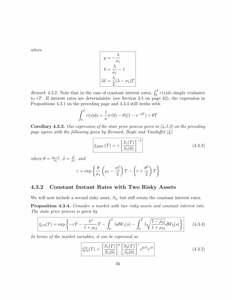
where

y = − λ

σ1

b =λ

σ1

− 1

M =λ

2(λ− σ1)T

Remark 4.3.2. Note that in the case of constant interest rates,∫ T

0r(s)ds simply evaluates

to rT . If interest rates are deterministic (see Section 3.5 on page 42), the expression inPropositions 4.3.1 on the preceding page and 4.3.4 still works with∫ T

0

r(s)ds =1

a(r(0)− θ)(1− e−aT ) + θT

Corollary 4.3.3. Our expression of the state price process given in (4.3.2) on the precedingpage agrees with the following given by Bernard, Boyle and Vanduffel [4]:

ξBBV (T ) = γ

[S1(T )

S1(0)

]−δ(4.3.3)

where θ = µ1−rσ1

, δ = θσ1

, and

γ = exp

θ

σ1

(µ1 −

σ21

2

)T −

(r +

θ2

2

)T

4.3.2 Constant Instant Rates with Two Risky Assets

We will now include a second risky asset, S2, but still retain the constant interest rates.

Proposition 4.3.4. Consider a market with two risky assets and constant interest rate.The state price process is given by

ξC2(T ) = exp

−rT − λ2

1 + ρ12

T −∫ T

0

λdW1(s)−∫ T

0

λ

√1− ρ12

1 + ρ12

dW2(s)

(4.3.4)


ξmC2(T ) =

[S1(T )

S1(0)

]y [S2(T )

S2(0)

]zebrT eM (4.3.5)

56

where

y = − λ

σ1(1 + ρ12)

z = − λ

σ2(1 + ρ12)

b =λ

1 + ρ12

(1

σ1

+1

σ2

)− 1

M =λ

1 + ρ12

[λ− σ1

2− σ2

2

]T

Corollary 4.3.5. Our expression of the state price process given in (4.3.5) on the previouspage agrees with the following given by Bernard, Maj and Vanduffel [7]:

ξBMV (T ) = γ

[Sπ(T )∗

S∗π(0)

]−δ(4.3.6)

where θ = µ(π∗)−rσ(π∗)

, δ = θ∗σ(π∗)

, and

γ = exp

θ∗

σ(π∗)

[µ(π∗)−

σ2(π∗)

2

]T −

(r +

θ2

2

)T

π−→∗ is the market portfolio and S∗π is the security that is constructed using the constant mix

π−→∗ as prescribed in Section 2.4.2 on page 19.

Remark 4.3.6. It appears that the formulation of the state price process given by [7] ismore succinct than ours. In fact, when the number of assets exceeds two, the marketportfolio formulation is more convenient to work with than our approach due to its use ofmatrix algebra; the expressions in our formulation will quickly become very complicated.However, it is not immediately clear how to extend their approach to incorporate stochasticinterest rates.

4.3.3 Stochastic Interest Rates Only

We now consider a market where the short rate is driven by a Vasicek process in (4.1.12) onpage 51 and the existence of the money market account B(t) defined in (4.1.1) on page 50.

57

Proposition 4.3.7. Consider a market stochastic interest rates modeled by a Vasicek pro-cess. The state price process is given by

ξS0(T ) = exp

−∫ T

0

r(s)ds− 1

2λ2T −

∫ T

0

λdW0(s)

(4.3.7)


ξmS0(T ) =

[P (0, T ) exp

r(T )

a

]x[B(T )]b eM (4.3.8)

where

x = −aλσr

b = −aλσr− 1

M = −λ2

2T +

λ

σr

e−aT

[r(0)− θ +

(σra

)2(

1− 1

4e−aT

)]+θ + σr

(λT +

σrT

2a− 3σr

4a2

)Remark 4.3.8. This state price process (4.3.7) could be used to investigate the cost efficiencyof a bond option.

4.3.4 Stochastic Interest Rates with One Risky Asset

Finally, we add one risky asset, S1, to the market described in Section 4.3.3 on the precedingpage.

Proposition 4.3.9. Consider a market with one risky asset and stochastic interest ratesmodeled by a Vasicek process The state price process is given by

ξS1(T ) = exp

−∫ T

0

r(s)ds− λ2

1 + ρ01

T −∫ T

0

λdW0(s)−∫ T

0

λ

√1− ρ01

1 + ρ01

dW1(s)

(4.3.9)

58


ξmS1(T ) =

[P (0, T ) exp

r(T )

a

]x [S1(T )

S1(0)

]y[B(T )]b eM (4.3.10)

where

x = −aλσr

(1

1 + ρ01

)y = − λ

σ1

(1

1 + ρ01

)b =

(λ

1 + ρ01

)(1

σ1

− a

σr

)− 1

M = − λ2

1 + ρ01

T +λ

σr(1 + ρ01)

e−aT

[r(0)− θ +

(σra

)2(

1− 1

4e−aT

)]+θ + σr

(λT +

σrT

2a− 3σr

4a2

)+

λ

1 + ρ01

(λ− σ1

2

)T

Remark 4.3.10. This state price process (4.3.9) on the previous page could be used toinvestigate the cost efficiency of any option written on a single asset in the presence ofstochastic interest rates.

4.3.5 Summary

In this section, we present a summary of all the cases considered in this chapter. Thegeneral form of the state price process is given by the following:

ξRi(T ) = exp

−∫ T

0

r(s)ds− 1

2

(α2

0 + α21 + α2

2

)T

−∫ T

0

α0dW0(s)−∫ T

0

α1dW1(s)−∫ T

0

α2dW2(s)

(4.3.11)

The R subscript refers to the randomness of the short rate (C for constant or S for stochas-tic) whereas the i subscript refers to the number of risky assets.

59

The following table specifies the values taken by the parameters for each of the followingcases.

Case Symbol Section α0 α1 α2

Const-1 ξC1(T ) 4.3.1 0 λ 0

Const-2 ξC2(T ) 4.3.2 0 λ λ√

1−ρ121+ρ12

Stoch-0 ξS0(T ) 4.3.3 λ 0 0

Stoch-1 ξS1(T ) 4.3.4 λ λ√

1−ρ011+ρ01

0

Stoch-2 ξS2(T ) 4.1.2 λ λ√

1−ρ011+ρ01

α1 · 1+ρ01−ρ02−ρ12√A

Table 4.3.1: Parameter values for the state price process.

Const-i and Stoch-i refer to the cases of constant and stochastic interest rates withi assets respectively. A is defined in (4.1.15) on page 52.

∫ T

0r(s)ds simplifies to

rT and 1a (r(0) − θ)(1 − e−aT ) + θT respectively in the constant and deterministic

interest rate cases.

60

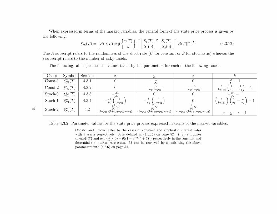
When expressed in terms of the market variables, the general form of the state price process is given bythe following:

ξmRi(T ) =

[P (0, T ) exp

r(T )

a

]x [S1(T )

S1(0)

]y [S2(T )

S2(0)

]z[B(T )]b eM (4.3.12)

The R subscript refers to the randomness of the short rate (C for constant or S for stochastic) whereas thei subscript refers to the number of risky assets.

The following table specifies the values taken by the parameters for each of the following cases.

Cases Symbol Section x y z b

Const-1 ξmC1(T ) 4.3.1 0 − λσ1

0 λσ1− 1

Const-2 ξmC2(T ) 4.3.2 0 − λσ1(1+ρ12)

− λσ2(1+ρ12)

λ1+ρ12

(1σ1

+ 1σ2

)− 1

Stoch-0 ξmS0(T ) 4.3.3 −aλσr

0 0 −aλσr− 1

Stoch-1 ξmS1(T ) 4.3.4 −aλσr

(1

1+ρ01

)− λσ1

(1

1+ρ01

)0

(λ

1+ρ01

)(1σ1− a

σr

)− 1

Stoch-2 ξmS2(T ) 4.2aλσr× λ

σ1× λ

σ2×

(1−ρ12)(1+ρ12−ρ01−ρ02)A

(1−ρ02)(1+ρ02−ρ12−ρ01)A

(1−ρ01)(1+ρ01−ρ02−ρ12)A

x− y − z − 1

Table 4.3.2: Parameter values for the state price process expressed in terms of the market variables.

Const-i and Stoch-i refer to the cases of constant and stochastic interest rateswith i assets respectively. A is defined in (4.1.15) on page 52. B(T ) simplifiesto exprT and exp

1a (r(0)− θ)(1− e−aT ) + θT

respectively in the constant and

deterministic interest rate cases. M can be retrieved by substituting the aboveparameters into (4.2.6) on page 54.

61

Chapter 5

Asian Executive Compensation withVasicek Interest Rates

We are now ready to return to our study of the cost efficiency of the Asian ExecutiveOption (AEO) and Asian Executive Indexed Option (AEIO), but with an added twist ofstochastic interest rates. We have derived the pricing formulas for the Geometric AsianOption (GAO) and Asian Exchange Option (AEO) in Chapter 3 on page 30, as well as therequired state price process in Chapter 4 on page 49.

Section 5.1 draws some comparisons with the case of constant interest rates whilstSection 5.2 on the following page provides some context for our study. This chapter endswith results from Monte Carlo simulation in Section 5.3 on page 64.

Unless otherwise mentioned, the index i is understood to range over 1 and 2 i.e. i = 1, 2.

5.1 Comparison with the Case of Constant Instant

Rates

Remark 5.1.1. In the case of constant interest rates, it is possible to construct explicitlythe CEC of the AEO as a power option (Proposition 2.3.1 on page 11). However in thepresence of stochastic interest rates, it seems like an explicit construction is no longeramenable to Theorem 1.2.4 on page 4, largely due to the extra path-dependence of theinterest rates.

62

Although we were unable to construct the CEC of the AEIO, we were still able toconstruct the Power Exchange Executive Option (PXEO) (Section 2.4.1 on page 15) thathas a cheaper price than the AEIO and yet inherits its desireable features. Once again,this no longer seems possible in the presence of stochastic interest rates. Therefore, weneed to resort to Monte Carlo simulation to estimate these CEC’s.

Remark 5.1.2. When interest rates are constant, the CEC is not path-dependent. Recallthat the CEC of the AEO, GT (Proposition 2.3.1 on page 11) is a power call option onthe terminal stock price ST , whereas the CEC of the AEIO is a function of the state priceprocess ξT which is also not path-dependent. Even the PXEO that we constructed is notpath-dependent. In fact, in the Black-Scholes model, path-dependent payoffs are not costefficient unless µS = r [4].

However, it is interesting to note that once we introduce stochastic interest rates, theCEC is necessarily path-dependent. The CEC is a function of the state price process, andwe have seen from Proposition 4.1.3 on page 52 that it is path-dependent.

5.2 Setup

Firstly, we have decided to exclude dividends in order to reduce the number of input param-eters. The various pricing formulas are complicated enough already (see Propositions 3.3.1on page 35 and 3.3.4 on page 36), even without the inclusion of dividends.

Recall from Chapter 2 on page 7 the following definitions of the payoff of the AEO((2.3.1) on page 10):

GT = (ST −K)+

and the AEIO ((2.4.1) on page 14):

AT = (ST − HT )+

(Recall also that HT is the non-constant strike price that is linked to the performance ofthe average benchmark index adjusted for the level of systematic risk β. See Remark 2.2.2on page 9 also.)

In order to distinguish between the constant and stochastic interest rates cases, we willlabel the latter in boldface1 and define their respective payoffs in a slightly different fashion

1AEO and AEIO for labels; G(T ) and A(T ) for payoffs; E0 and V0 for prices; G(T ) and A(T ) forCEC payoffs; E0 and V0 for CEC prices; ξ(T ) for the state price process.

63

as follow:

G(T ) = (Si(T )−K)+ (5.2.1)

A(T ) = (S1(T )− S2(T ))+ (5.2.2)

where K is the strike price, and S1(T ) and S2(T ) are defined in (4.1.9)–(4.1.10) on page 51respectively. Note that instead of using HT in (5.2.2), we have used S2(T ) as a proxy forthe benchmark instead. Once again, this is done mainly for simplicity - the key componentsof indexing and averaging of the AEIO are still preserved.

The prices at time 0 of AEO and AEIO, E0 and V0, can be calculated directly usingour formulas for the GAO (Proposition 3.3.1 on page 35) and the AEO (Proposition 3.3.4on page 36) respectively.

5.3 Monte Carlo Simulation

We can use the state price process given by Proposition 4.1.3 on page 52 and its distributionin Corollary 4.1.6 on page 53 to simulate the prices of the CEC. A simple Euler scheme isused to discretize the interest rates and stock price paths.

The CEC of the AEO and AEIO are given by

G(T ) = F−1

G(1− Fξ(ξ(T ))) (5.3.1)

A(T ) = F−1

A(1− Fξ(ξ(T ))) (5.3.2)

Their respective prices are:

E0 = EP[ξ(T )G(T )] (5.3.3)

V0 = EP[ξ(T )A(T )] (5.3.4)

(5.3.3)–(5.3.4) are estimated by making random draws from the known distribution of ξ(T )and evaluating the inverse CDF’s, F−1

Gand F−1

A, numerically under the P measure.

Remark 5.3.1. In the spirit of Section 4.1.1 on page 50, we will specify the value of themarket price of risk, λ, as an input parameter instead of the respective expected returns,µ.

Figures 5.3.1 to 5.3.3 on pages 68–70 plot some prices of the AEO and AEIO and theirrespective CEC’s across different sets of parameters to illustrate the degrees of efficiency

64

loss. Each point corresponds to the price for a particular parameter set. We consider thebase case given in Table 5.3.1, and perturb some of the input parameters as well. We cansee that the degree of efficiency loss is sensitive to all model parameters. The values thatare used to plot this figure are given in Table 5.3.2 to 5.3.3 on pages 65–66.

Option Vasicek Assets Correlation Monte CarloT 1 a 0.20 S1(0) 100 ρ01 0.25 Paths 1,000,000K 100 θ 0.35 S2(0) 120 ρ02 0.50

r(0) 6% σ1 30% ρ12 0.75σr 20% σ2 40%

λ 0.02

Table 5.3.1: Base case parameters for sample AEO and AEIO.

ParametersAEO on Asset 1 AEO on Asset 2

E0 E0 % Eff Loss St Dev E0 E0 % Eff Loss St DevBase case 8.24 7.62 8.1% 0.0140 23.31 22.28 4.6% 0.0285K = 120 2.17 1.97 10.1% 0.0078 12.11 11.47 5.6% 0.0230a = 0.4 8.51 7.91 7.5% 0.0142 23.56 22.62 4.1% 0.0287θ = 0.15 8.04 7.42 8.3% 0.0137 23.16 22.19 4.4% 0.0281

r(0) = 10% 9.00 8.41 7.0% 0.0149 24.17 23.19 4.2% 0.0294σr = 50% 8.61 7.63 12.9% 0.0172 22.76 21.11 7.8% 0.0338S1(0) = 140 40.40 39.06 3.4% 0.0271 23.31 22.32 4.4% 0.0283S2(0) = 100 8.24 7.62 8.1% 0.0140 10.09 9.50 6.2% 0.0190σ1 = 60% 13.13 11.84 11.0% 0.0271 23.31 22.26 4.7% 0.0284σ2 = 80% 8.24 7.73 6.6% 0.0141 27.35 25.84 5.8% 0.0524λ = 0.04 8.24 7.44 10.8% 0.0141 23.31 21.85 6.7% 0.0285

ρ01 = −0.15 7.92 7.08 11.9% 0.0127 23.31 22.50 3.6% 0.0286ρ02 = −0.5, ρ12 = 0.6 8.24 7.62 8.1% 0.0139 23.65 20.72 14.1% 0.0239

ρ12 = −0.25 8.24 7.68 7.2% 0.0140 23.31 22.45 3.8% 0.0285

Table 5.3.2: Prices and efficiency loss of the AEO on assets 1 and 2.

These are used to generate Figures 5.3.1 to 5.3.2 on pages 68–69 and the base caseparameters are given in Table 5.3.1.

65

ParametersAEIO

V0 V0 % Eff Loss St DevBase case 1.03 0.73 41.4% 0.0034K = 120 1.03 0.73 40.0% 0.0034a = 0.4 1.01 0.72 40.4% 0.0034θ = 0.15 1.04 0.72 44.7% 0.0033

r(0) = 10% 1.01 0.72 40.1% 0.0035σr = 50% 1.13 0.51 123.8% 0.0032S1(0) = 140 21.44 19.10 12.3% 0.0165S2(0) = 100 6.24 5.07 23.2% 0.0086σ1 = 60% 2.56 1.98 29.1% 0.0096σ2 = 80% 8.66 6.77 27.9% 0.0127λ = 0.04 1.03 0.70 47.0% 0.0034

ρ01 = −0.15 1.09 0.70 56.1% 0.0032ρ02 = −0.5, ρ12 = 0.6 1.64 1.56 5.0% 0.0060

ρ12 = −0.25 6.17 4.92 25.4% 0.0138

Table 5.3.3: Prices and efficiency loss of the AEIO.

These are used to generate Figure 5.3.3 on page 70 and the base case parametersare given in Table 5.3.1 on the previous page.

In the base case, the efficiency loss of the AEO on assets 1 and 2 are 5.9% and 2.6%respectively. For asset 1, the highest efficiency loss is 12.9% when we perturb σr to 50%,while the lowest is 3.4% when we perturb S1(0) to 140. For asset 2, the highest efficiencyloss is 14.1% when we perturb ρ02 and ρ12 to -0.5 and 0.6 respectively, and the lowestis 3.8% when we perturb ρ12 to -0.25. As expected, the efficiency loss is sensitive toall input parameters that pertain to the Vasicek interest rates (a, θ, r(0), and σr) i.e.the introduction of stochastic interest rates does have an impact on cost efficiency. Thesensitivity of the efficiency loss with respect to the Vasicek parameters is about the sameas the sensitivity with respect to the rest of parameters.

It is surprising that the degree of efficiency loss for the AEIO is much larger than theAEO across all cases, and it fluctuates wildly among the cases considered. For the casewhere σr = 50%, the efficiency loss is 123.8%! However, the large relative values could bean artifact of the small absolute values. The base case efficiency loss is 41.4%, and thelowest efficiency loss is at 5.0% when we perturb ρ02 and ρ12 to -0.5 and 0.6 respectively.It is noteworthy that unlike the AEO, the sensitivity of the efficiency loss with respect to

66

the Vasicek parameters seems to be larger than the sensitivity with respect to the rest ofthe parameters.

One thing that is certain is that the CEC’s of the AEO and AEIO are all cheaperthan their original payoffs, in agreement with Theorem 1.2.4 on page 4. However, we haveseen that the degree of efficiency loss is sensitive to the input parameters, as well as thetype of payoff itself. This connection is definitely an area ripe for future research.

67

0

5

10

15

20

25

30

35

40

45

Price

Base Case K = 120 a = 0.4 θ = 0.15 r(0) = 10% σr = 50% S1(0) = 140 S2(0) = 100 σ1 = 60% σ2 = 80% λ = 0.04ρ01 = −0.15

ρ02 = −0.5, ρ12 = 0.6

ρ12 = −0.25

AEO-1 BS Price

AEO-1 CEC Price

Figure 5.3.1: Sample prices for the AEO on asset 1 and its CEC across different cases.


68

8

10

12

14

16

18

20

22

24

26

28

Price

Base Case K = 120 a = 0.4 θ = 0.15 r(0) = 10% σr = 50% S1(0) = 140 S2(0) = 100 σ1 = 60% σ2 = 80% λ = 0.04ρ01 = −0.15

ρ02 = −0.5, ρ12 = 0.6

ρ12 = −0.25

AEO-2 BS Price

AEO-2 CEC Price

Figure 5.3.2: Sample prices for the AEO on asset 2 and its CEC across different cases.


69

0

5

10

15

20

25

Price

Base Case K = 120 a = 0.4 θ = 0.15 r(0) = 10% σr = 50% S1(0) = 140 S2(0) = 100 σ1 = 60% σ2 = 80%λ = 0.04ρ01 = −0.15

ρ02 = −0.5, ρ12 = 0.6

ρ12 = −0.25

AEIO BS Price

AEIO CEC Price

Figure 5.3.3: Sample prices for the AEIO and its CEC across different cases.


70

Chapter 6

Conclusion

In this thesis we apply the concept of cost efficiency as prescribed by Bernard, Boyle andVanduffel [4] to the Asian Executive Option and Asian Executive Indexed Option designedby Tian [53]. In doing so, we are able to find explicitly the cost efficient counterpart for theAsian Executive Option in the form of a power option, and design a payoff that is cheaperthan the Asian Executive Indexed Option in the form of the Power Exchange ExecutiveOption. The true cost efficient counterpart of the Asian Executive Indexed Option doesnot admit a closed form expression - but we are able to simulate its price using the stateprice process given by Bernard, Maj and Vanduffel [7] and study the degree of efficiencyloss.

Given that executive options generally have long maturities, we incorporate stochasticinterest rates modeled by a Vasicek process. In order to study the cost efficiency of theAsian Executive Option and Asian Executive Indexed Option, the key requirements are thepricing formulas for the Geometric Asian Option (GAO) and the Asian Exchange Option(AXO), as well as an expression for the state price process in the presence of stochasticinterest rates. We are able to meet both requirements and subsequently simulate theprices of the cost efficient counterpart for the Asian Executive Option and Asian ExecutiveIndexed Option.

To the best of our knowledge, all of our results and formulas are new.

Our research in this area is still nascent and here are some questions that remainunanswered:

1. The technique used to construct the Power Exchange Executive Option does not holdin general (Remark 2.4.6 on page 17). What are the conditions that guarantees thatour technique will construct a cheaper payoff?

71

2. How do the incentives of the Power Exchange Executive Option compare with thatof the Asian Executive Indexed Option (Remark 2.4.1 on page 15), and what is theincentive structure of its cost efficient counterpart?

3. How can we incorporate state-dependent preferences into the cost efficient counter-part (Remark 2.4.8 on page 27)?

4. Can we extend our pricing formulas to include more robust stochastic interest ratemodels (Remark 3.3.3 on page 36)?

5. Is there a way to incorporate stochastic interest rates into Bernard, Maj and Van-duffel’s [7] formulation of the state price process (Remark 4.3.6 on page 57)?

6. Are there any options that will admit closed form cost efficient counterparts undera stochastic interest rate environment (Remarks 4.3.8 on page 58 and 4.3.10 onpage 59)?

7. How can we incorporate Tian’s [53] benchmark (HT , (2.2.2) on page 9), into ourdesign of the AEO and AEIO (Section 5.2 on page 63)?

8. How do the pricing parameters for the Asian Executive Option and Asian ExecutiveIndexed Option impact the degree of efficiency loss (Section 5.3 on page 64)?

We hope that the contributions that we have made thus far will aid in tackling thequestions above.

72

APPENDICES

73

Appendix A

Useful Identities

In this appendix we will prove some identities that will be useful for deriving option pricingformulas.

Lemma A.1. Let X ∼ N (µ, σ2). Then

E[(eX −K)+] = eµ+σ2

2 Φ

(σ2 + µ− lnK

σ

)−KΦ

(µ− lnK

σ

)Proof. This is a standard result (see, e.g. [15]). Let X ∼ N (µ, σ2) and fX(x) be itscorresponding pdf. We are interested in evaluating E[(eX −K)+]. By definition, we have

E[(eX −K)+]

=

∫ ∞−∞

(ex −K)+fX(x)dx

=

∫ ∞lnK

(ex −K)fX(x)dx

=

∫ ∞lnK

exfX(x)dx−K∫ ∞

lnK

fX(x)dx

We consider each integral separately.∫ ∞lnK

exfX(x)dx

=

∫ ∞lnK

ex1√2πσ

e−12(x−µσ )

2

dx

74

= eµ+σ2

2

∫ ∞lnK−µ

σ

1√2πe−

12

(y−σ)2dy (Let y = x−µσ

)

= eµ+σ2

2

∫ ∞lnK−µ−σ2

σ

1√2πe−

12z2dz (Let z = y − σ)

= eµ+σ2

2 Prob

[Z ≥ lnK − µ− σ2

σ

]= eµ+σ2

2 Φ

(σ2 + µ− lnK

σ

)(A.1)∫ ∞

lnK

fX(x)dx = Prob

[Z ≥ lnK − µ

σ

]= Φ

(µ− lnK

σ

)(A.2)

Combining (A.1) and (A.2) we have:

E[(eX −K)+] = eµ+σ2

2 Φ

(σ2 + µ− lnK

σ

)−KΦ

(µ− lnK

σ

)

Lemma A.2. ∫ ∞−∞

φ(z)Φ(A+Bz)dz = Φ

(A√

1 +B2

)Proof. See the Proof of Proposition 1 in Li, Deng and Zhou [38].

Lemma A.3. Let X1 ∼ N (µ1, σ21), X2 ∼ N (µ2, σ

22), and Cov[X1, X2] = ρσ1σ2 = σ12. Then

E[(eX1 − eX2

)+]

= eµ1+ 12σ21Φ(d1)− eµ2+ 1

2σ22Φ(d2)

where d1 =µ1−µ2+σ2

1−σ12√σ21−2σ12+σ2

2

and d2 = d1 −√σ2

1 − 2σ12 + σ22

Proof. This proof is outlined briefly in [55], and the result is formulated differently. Weadapt it to our case, and fill in much of the details. Let f12(u, v), f1(u), f2(v), f1|2(u|v), andf2|1(v|u) denote the joint pdf, marginal pdfs, and conditional pdfs of X1 and X2. Then,we have

E[(eX1 − eX2

)+]

=

∫ ∞−∞

∫ ∞−∞

(eu − ev)+f12(u, v)dudv

75

=

∫ ∞−∞

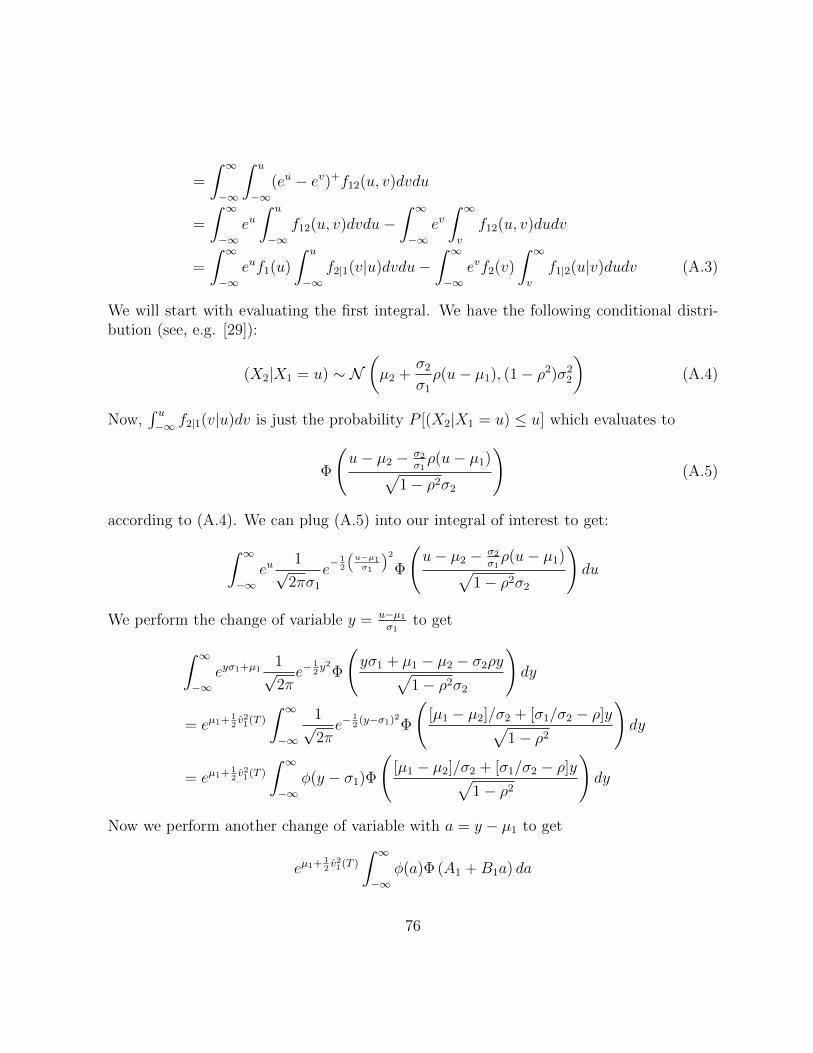
∫ u

−∞(eu − ev)+f12(u, v)dvdu

=

∫ ∞−∞

eu∫ u

−∞f12(u, v)dvdu−

∫ ∞−∞

ev∫ ∞v

f12(u, v)dudv

=

∫ ∞−∞

euf1(u)

∫ u

−∞f2|1(v|u)dvdu−

∫ ∞−∞

evf2(v)

∫ ∞v

f1|2(u|v)dudv (A.3)

We will start with evaluating the first integral. We have the following conditional distri-bution (see, e.g. [29]):

(X2|X1 = u) ∼ N(µ2 +

σ2

σ1

ρ(u− µ1), (1− ρ2)σ22

)(A.4)

Now,∫ u−∞ f2|1(v|u)dv is just the probability P [(X2|X1 = u) ≤ u] which evaluates to

Φ

(u− µ2 − σ2

σ1ρ(u− µ1)√

1− ρ2σ2

)(A.5)

according to (A.4). We can plug (A.5) into our integral of interest to get:∫ ∞−∞

eu1√

2πσ1

e− 1

2

(u−µ1σ1

)2Φ

(u− µ2 − σ2

σ1ρ(u− µ1)√

1− ρ2σ2

)du

We perform the change of variable y = u−µ1σ1

to get

∫ ∞−∞

eyσ1+µ11√2πe−

12y2Φ

(yσ1 + µ1 − µ2 − σ2ρy√

1− ρ2σ2

)dy

= eµ1+ 12v21(T )

∫ ∞−∞

1√2πe−

12

(y−σ1)2Φ

([µ1 − µ2]/σ2 + [σ1/σ2 − ρ]y√

1− ρ2

)dy

= eµ1+ 12v21(T )

∫ ∞−∞

φ(y − σ1)Φ

([µ1 − µ2]/σ2 + [σ1/σ2 − ρ]y√

1− ρ2

)dy

Now we perform another change of variable with a = y − µ1 to get

eµ1+ 12v21(T )

∫ ∞−∞

φ(a)Φ (A1 +B1a) da

76

where

A1 =[µ1 − µ2]/σ2 + [σ1/σ2 − ρ]σ1√

1− ρ2

B1 =[σ1/σ2 − ρ]√

1− ρ2

By Lemma A.2 on page 75, we can simplify our integral to the following

eµ1+ 12σ21Φ

(A1√

1 +B21

)

We will try to simplify A1√1+B2

1

. First, the numerator:

A1 =[µ1 − µ2]/σ2 + [σ1/σ2 − ρ]σ1√

1− ρ2=µ1 − µ2 + σ2

1 − σ12

σ2

√1− ρ2

(A.6)

Now, the denominator:

√1 +B2

1 =

√1 +

[σ1/σ2]2 − 2σ12/σ22 + [σ12/(σ1σ2)]2

1− ρ2

=

√[σ1/σ2]2 − 2σ12/σ2

2 + 1

1− ρ2(A.7)

Combining (A.6) and (A.7), we get

A1√1 +B2

1

=µ1 − µ2 + σ2

1 − v12(T )

σ2

√[σ1/σ2]2 − 2v12(T )/v2

2(T ) + 1

=µ1 − µ2 + σ2

1 − v12(T )√σ2

1 − 2v12(T ) + v22(T )

Finally, we have ∫ ∞−∞

euf1(u)

∫ u

−∞f2|1(v|u)dvdu = eµ1+ 1

2σ21Φ(d1) (A.8)

where

d1 =µ1 − µ2 + σ2

1 − σ12√σ2

1 − 2σ12 + σ22

(A.9)

77

The steps to derive the second integral are identical and are omitted. We eventually get∫ ∞−∞

euf1(u)

∫ u

−∞f2|1(v|u)dvdu = eµ1+ 1

2σ21Φ(d2) (A.10)

where

d2 =µ1 − µ2 − σ2

2 + σ12√σ2

1 − 2σ12 + σ22

= d1 −√σ2

1 + σ22 − 2ρσ1σ2 (A.11)

Substituting (A.8) on the previous page and (A.10) into (A.3) on page 76 (together with(A.9) on the preceding page and (A.11)) completes the proof of the identity.

78

Appendix B

Proofs

This appendix contains the proofs of various theorems and propositions.

B.1 Proofs for Chapter 2

B.1.1 Proof of Proposition 2.3.1 on page 11

Proof. From [34], we have

ST = S0 exp

1

2

(µS − qS −

σ2S

2

)T +

σS√3W ST

This gives the following cdf of ST under the physical measure P

P (ST ≤ s) = Φ

ln(sS0

)− 1

2

(µS − qS − σ2

S

2

)T

σS

√T3

Now, if we consider the cdf of the payoff, FGT , we get

FGT (x) = P (GT ≤ x) =

0 if x < 0

P (ST ≤ K + x) = Φ

ln(K+xS0

)− 1

2

(µS−qS−

σ2S2

)T

σS√

T3

if x ≥ 0

79

Let ν = Φ

ln(KS0

)− 1

2

(µS−qS−

σ2S2

)T

σS√

T3

, and consider y ∈ (0, 1). Then we have

F−1GT

(y) =

S0e

Φ−1(y)σS√

T3

+ 12

(µS−qS−

σ2S2

)T −K if y ≥ ν

0 if y < ν

Let ξT = exp−1

2θ2T − θW S

T − (r − qS)T

. Then, ln(ξT ) ∼ N (M, θ2T ), where M =−1

2θ2T − (r − qS)T and θ = µS−r

σS. So,

Fξ(x) = Φ

(ln(x)−Mθ√T

)⇒ 1− Fξ(ξT ) = Φ

(M − ln(ξT )

θ√T

)The cost efficient payoff that gives the same distribution as a continuous geometric Asianoption is given by GT = F−1

GT(1− Fξ(ξT )). After some algebra, this leads to the following:

GT =

(S0 exp

1

2

(µS − qS −

σ2S

2

)T + σS

√T

3

(M − ln(ξT )

θ√T

)−K

)+

Let b = θσ, a = exp

θσ

(µS − qS − σ2

S

2

)T −

(r − qS + θ2

2

)T

. Then, we can write ξT =

a(STS0

)−b. Using this, we can finally express

GT = d

(S

1/√

3T − K

d

)+

where

d = S1−1/

√3

0 e

(12− 1√

3

)(µS−qS−

σ2S2

)T

We can see that GT is a power call option, and we can calculate its price using risk neutralvaluation. The price of GT at time 0, E0 is given by

E0 = de−rTE

[(S

1/√

3T − K

d

)+]

It is easy to see that S1/√

3T = S

1/√

30 eYT where YT ∼ N

(1√3

(r − qS − σ2

S

2

)T,

σ2S

3T)

. Apply-

ing Lemma A.1 on page 74 gives us the desired result.

80


Proof. The program of this proof is as follows:

1. Construct the CEC of ST , S?T , in isolation of IT

2. Construct the CEC of HT , H?T , in isolation of ST

3. Demonstrate that AT ∼ A?T

Step 1

First, from [34], we have

ST = S0 exp

1

2

(µS − qS −

σ2S

2

)T +

σS√3W ST

Now, if we consider the CDF of the payoff ST , FST , we get

FST (s) =

0 if s < 0

P (ST ≤ s) = Φ

ln(sS0

)− 1

2

(µS−qS−

σ2S2

)T

σS√

T3

if s ≥ 0

We can invert this CDF to get

F−1

ST(y) =

S0e

Φ−1(y)σS√

T3

+ 12

(µS−qS−

σ2S2

)T

if 0 ≤ y ≤ 10 otherwise

Now let ξST = exp−1

2θ2ST − θSWT − (r − qS)T

. Then ln(ξST ) ∼ N(MS, θ

2ST ), where

MS = −12θ2ST − (r − qS)T and θS = µS−r

σS. Then we have

FξS(x) = Φ

(ln(x)−MS

θS√T

)⇒ 1− FξS(ξST ) = Φ

(MS − ln(ξST )

θS√T

)This gives us the following cost efficient payoff:

S?T = F−1

ST(1− FξS(ξST )) = S0 exp

1

2

(µS − qS −

σ2S

2

)T + σS

√T

3

(MS − ln(ξST )

θS√T

)

Let bS = θSσS

, aS = expθSσS

(µS − qS − σ2

S

2

)T −

(r − qS +

θ2S2

)T

. Then, we can write

ξST = aS

(STS0

)−bS. Using this, we have S?T = dSS

1/√

3T where dS = S

1−1/√

30 e

(12− 1√

3

)(µS−qS−

σ2S2

)T

81

Step 2

Firstly, let

η′ = (µS − qS)− β(µI − qI) +1

2σ2I β(1− β)

and it is easy (but tedious) to check that this is equivalent to η as defined in (2.2.3) onpage 9. Now we can rewrite HT as

HT = K(IT/I0)β exp(η′T )

From [34], we have

IT = I0 exp

(µI − qI −

σ2I

2

)T + σIW

IT

which leads us to (

ITI0

)β

= exp

βµIT − βqIT −

βσ2I

2T + ρσSW

IT

We also have

exp(η′T ) = exp

µST − qST − βµIT + βqIT +

βσ2I

2− 1

2ρ2σ2

ST

This gives us

HT = K exp

1

2

[µS − qS −

σ2S

3

(1

2+ ρ2

)]T +

ρσS√3W IT

Similarly, let

η′ = (µS − qS)− β(µI − qI) +1

2σ2Iβ(1− β)

and we can check that is equivalent to η as defined in (2.2.3) on page 9. Now rewrite HT

asHT = K(IT/I0)β exp(ηT )

Check that (ITI0

)β= exp

βµIT − βqIT −

βσ2I

2T + ρσSW

IT

82

and

exp(η′T ) = exp

µST − qST − βµIT + βqIT +

βσ2I

2− 1

2ρ2σ2

ST

This gives us

HT = K(IT/I0)β exp(η′T ) = K exp

(µS − qS −

1

2ρ2σ2

S

)T + ρσSW

IT

Now, if we consider the CDF of the payoff HT , FHT , we get

FHT (h) =

0 if h < 0

P (HT ≤ h) = Φ

ln( hK )−(µS−qS−

ρ2σ2S2

)T

ρσS√T

if h ≥ 0

We can invert this CDF to get

F−1

HT(y) =

Ke

Φ−1(y)ρσS√T+

(µS−qS−

ρ2σ2S2

)T

if 0 ≤ y ≤ 10 otherwise

Now, we have ξIT = exp−1

2θ2IT − θIW I

T − (r − qI)T

where θI = µI−rσI

. Therefore,

ln(ξIT ) ∼ N(MI , θ2IT ), where M = −1

2θ2IT − (r − qI)T . This leads us to

FξI (x) = Φ

(ln(x)−MI

θI√T

)⇒ 1− FξI (ξIT ) = Φ

(MI − ln(ξIT )

θI√T

)This gives us the following cost efficient payoff:

H?T = K exp

(µS − qS −

ρ2σ2S

2

)T + ρσS

(MI − ln(ξIT )

θI

)Let bI = θI

σI, aI = exp

θIσI

(µI − qI − σ2

I

2

)T −

(r − qI +

θ2I2

)T

. Then, we can write

ξIT = aI

(ITI0

)−bI. Define dH as follows:

dH = K1−1/√

3 exp

(1

2− 1√

3

)(µS − qS)T +

σ2ST

2

[ρ2

(1√3− 1

3

)− 1

6

]so that we can express the efficient payoff, H?

T as H?T = dHH

1/√

3T

83

Step 3

Note that AT and A?T have the same bivariate lognormal distribution since ST and HT

have the same distributions as S?T and H?T respectively. If we can show that they have the

same covariances, then we are done. We can check the equality of Cov[ln(ST ), ln(HT )

]and Cov

[ln(S?T ), ln(H?

T )]

as these two quantities are more tractable. In fact, we have

Cov[ln(ST ), ln(HT )

]= Cov [ln(S?T ), ln(H?

T )] =σ2Sρ

2

3T

B.1.3 Proof of Corollary 2.4.4 on page 16

Proof. A?T is a power exchange option and its price is given by Blenman and Clark [10] asfollows:

V ?0 = Υ

(dS,

1√3, qS, σS, S0, T

)Φ(d?1)−Υ

(dH ,

1√3, qS, ρσS, K, T

)Φ(d?2)

where

d?1 =

ln

(dSS

1/√

30

dHK1/√

3

)+[σ2S

2√

3

(1− 1√

3

)(ρ2 − 1) + 1

2ν2]T

ν√T

d?2 =

ln

(dSS

1/√

30

dHK1/√

3

)+[σ2S

2√

3

(1− 1√

3

)(ρ2 − 1)− 1

2ν2]T

ν√T

= d?1 − ν√T

and

ν2 =1

3σ2S(1− ρ2)

Υ

(dS,

1√3, qs, σS, S0, T

)= dSS

1/√

30 exp

[(

1√3− 1)r − 1√

3qS −

1√3

(1− 1√3

)σ2S

2

]T

Υ

(dH ,

1√3, qS, ρσS, K, T

)84

= dHK1/√

3 exp

[(

1√3− 1)r − 1√

3qS −

1√3

(1− 1√3

)ρ2σ2

S

2

]T

dS = S

1−1/√

30 exp

(1

2− 1√

3

)(µS − qS −

σ2S

2

)T

dH = K1−1/

√3 exp

(1

2− 1√

3

)(µS − qS)T +

σ2ST

2

[ρ2

(1√3− 1

3

)− 1

6

]This eventually simplifies to the desired result pricing formula. When µS = r it is easyto see that V0 and V ?

0 are equivalent. In fact, the price of A?T is a decreasing function ofµS, and is only cheaper than AT when µS > r. We can see this by considering the firstderivative of the power exchange option with respect to the stock yield i.e.

∂V ?0∂µS

< 0.


B.2.1 Proof of Lemma 3.1.1 on page 33

Proof. Consider a different bond price dynamics with S < T under QT

dP (t, S)

P (t, S)= [r(t) + σP (t, S)σP (t, T )] dt− σP (t, S)dZT

0 (t) (B.2.1.1)

Applying Ito’s Lemma to g(P (t, T ), P (t, S)) = ln P (t,T )P (t,S)

, and then replacing S with t, gives

us the following expression for the bond price P (t, T ) that does not involve r(t):

P (t, T ) =P (0, T )

P (0, t)exp

1

2

∫ t

0

[σP (u, T )− σP (u, t)]2 du

−∫ t

0

[σP (u, T )− σP (u, t)] dZT0 (u)

(B.2.1.2)

Apply Ito’s Lemma again to g(S1(t), P (t, T )) and g(S2(t), P (t, T )) to get:

S1(t)

P (t, T )=

S1(0)

P (0, T )exp

−1

2

∫ t

0

[σ2P (u, T ) + 2σ1σP (u, T )C21 + σ2

1

]du

+

∫ t

0

[σ1C21 + σP (u, T )] dZT0 (u)

+

∫ t

0

σ1C22dZT1 (u)

(B.2.1.3)

85

S2(t)

P (t, T )=

S2(0)

P (0, T )exp

−1

2

∫ t

0

[σ2P (u, T ) + 2σ2σP (u, T )C31 + σ2

2

]du

+

∫ t

0

[σ2C31 + σP (u, T )] dZT0 (u)

+

∫ t

0

σ2C32dZT1 (u)

+

∫ t

0

σ2C33dZT2 (u)

(B.2.1.4)

Finally, substitute (B.2.1.2) on the previous page into (B.2.1.3)–(B.2.1.4) on pages 85–86.


Proof. In view of the defintion of Si(T ) in (3.2.7) on page 34, we only need to computethe various quantities for Xi(T ) - the rest follows immediately. The mean and variance ofSi(T ) follow immediately from (3.2.4)–(3.2.5) on page 34 and the properties of the integralof a Brownian motion. By definition:

Cov[X1(T ), X2(T )] = E[X1(T )X2(T )]− E[X1(T )]E[X2(T )] (B.2.2.1)

Now, we are left with evaluating E[X1(T )X2(T )]. For simplicity let us define the followingterms:

Z10(a, b, c) =∫ baσ10(s, c)dZT

0 (s) Z11(a, b) =∫ baσ11dZ

T1 (s)

Z20(a, b, c) =∫ baσ20(s, c)dZT

0 (s) Z21(a, b) =∫ baσ21dZ

T1 (s)

Z22(a, b) =∫ baσ22dZ

T1 (s)

(B.2.2.2)

We can rewrite (3.2.4)–(3.2.5) on page 34 as:

X1(T ) = M1(0, T, T ) + Z10(0, T, T ) + Z11(0, T ) (B.2.2.3)

X2(T ) = M2(0, T, T ) + Z20(0, T, T ) + Z21(0, T ) + Z22(0, T ) (B.2.2.4)

Then, we have:

E[X1(T )X2(T )] = E[M1(0, T, T )X2(T )] + E[Z10(0, T, T )X2(T )]

+ E[Z11(0, T, T )X2(T )] (B.2.2.5)

86

Now we consider each term in (B.2.2.5) on the preceding page:

E[M1(0, T, T )X2(T )] = E[M1(0, T, T )M2(0, T, T )] +

:

0

E[M1(0, T, T )Z20(0, T, T )]︸︷︷︸§

+

:0

E[M1(0, T, T )Z21(0, T )]︸︷︷︸§

+

:0

E[M1(0, T, T )Z22(0, T )]︸︷︷︸§

E[Z10(0, T, T )X2(T )] =

:

0

E[Z10(0, T, T )M2(0, T, T )]︸︷︷︸§

+E[Z10(0, T, T )Z20(0, T, T )]

+

:0

E[Z10(0, T, T )Z21(0, T )]︸︷︷︸¶

+

:0

E[Z10(0, T, T )Z22(0, T )]︸︷︷︸¶

E[Z11(0, T )X2(T )] =

:0

E[Z11(0, T )M2(0, T, T )]︸︷︷︸§

+

:

0

E[Z11(0, T )Z20(0, T, T )]︸︷︷︸¶

+ E[Z11(0, T )Z21(0, T )] +

:0

E[Z11(0, T )Z22(0, T )]︸︷︷︸¶

§ : E[const ·∫· · · dZT ] = 0

¶ :∫· · · dZT

1 is independent of∫· · · dZT

2

By the properties of the Ito Integral, we have

E[Z10(0, T, T )Z20(0, T, T )] = E

[∫ T

0

σ10(s, T )dZT0 (s) ·

∫ T

0

σ20(s, T )dZT0 (s)

]=

∫ T

0

σ10(s, T )σ20(s, T )ds

E[Z11(0, T )Z21(0, T )] = E

[∫ T

0

σ11dZT1 (s) ·

∫ T

0

σ21dZT1 (s)

]=

∫ T

0

σ11σ21ds

= σ11σ21T

87

Combining all of the above, we finally get

E[X1(T )X2(T )] = M1(0, T, T )M2(0, T, T ) + σ11σ21T +

∫ T

0

σ10(s, T )σ20(s, T )ds (B.2.2.6)

Finally, we can plug (B.2.2.6) into (B.2.2.1) on page 86 to get the covariance. At thispoint, a computer algebra system is used to derive the explicit expressions that are givenin Section 3.4.1 on page 41.


Proof. In view of the defintion of Si(T ) in (3.2.8) on page 34 we only need to compute thevarious quantities for Xi(T ) - the rest follows immediately. The program for this proof isto calculate the following terms sequentially:

1. E[Xi(t)]

2. E[X2i (T )]

3. E[Xi(t)Xi(u)]

4.∫ T

0

∫ T0E[Xi(t)Xi(u)]dudt

5. V ar[Xi(T )]

6. E[X1(T )X2(T )]

7. E[X1(t)X2(u)]

8.∫ T

0

∫ T0E[X1(t)X2(u)]dudt

9. Cov[X1(T ), X2(T )]

After completing the above steps, we use a computer algebra system to arrive at the explicitexpressions given in Section 3.4.2 on page 41.

88

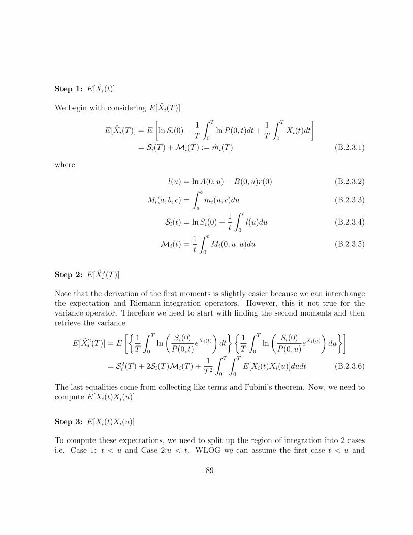
Step 1: E[Xi(t)]

We begin with considering E[Xi(T )]

E[Xi(T )] = E

[lnSi(0)− 1

T

∫ T

0

lnP (0, t)dt+1

T

∫ T

0

Xi(t)dt

]= Si(T ) +Mi(T ) := mi(T ) (B.2.3.1)

where

l(u) = lnA(0, u)−B(0, u)r(0) (B.2.3.2)

Mi(a, b, c) =

∫ b

a

mi(u, c)du (B.2.3.3)

Si(t) = lnSi(0)− 1

t

∫ t

0

l(u)du (B.2.3.4)

Mi(t) =1

t

∫ t

0

Mi(0, u, u)du (B.2.3.5)

Step 2: E[X2i (T )]

Note that the derivation of the first moments is slightly easier because we can interchangethe expectation and Riemann-integration operators. However, this it not true for thevariance operator. Therefore we need to start with finding the second moments and thenretrieve the variance.

E[X2i (T )] = E

[1

T

∫ T

0

ln

(Si(0)

P (0, t)eXi(t)

)dt

1

T

∫ T

0

ln

(Si(0)

P (0, u)eXi(u)

)du

]= S2

i (T ) + 2Si(T )Mi(T ) +1

T 2

∫ T

0

∫ T

0

E[Xi(t)Xi(u)]dudt (B.2.3.6)

The last equalities come from collecting like terms and Fubini’s theorem. Now, we need tocompute E[Xi(t)Xi(u)].

Step 3: E[Xi(t)Xi(u)]

To compute these expectations, we need to split up the region of integration into 2 casesi.e. Case 1: t < u and Case 2:u < t. WLOG we can assume the first case t < u and

89

retrieve the second case by symmetry. We have (recall (B.2.2.3)–(B.2.2.4) on page 86):

E[X1(t)X1(u)] = E[M1(0, t, t)X1(u)] + E[Z10(0, t, t)X1(u)]

+ E[Z11(0, t)X1(u)] (B.2.3.7)

E[X2(t)X2(u)] = E[M2(0, t, t)X2(u)] + E[Z20(0, t, t)X2(u)]

+ E[Z21(0, t)X2(u)] + E[Z22(0, t)X2(u)] (B.2.3.8)

We will start with considering each term in (B.2.3.7) separately:

E[M1(0, t, t)X1(u)] = E[M1(0, t, t)M1(0, u, u)] +

:0

E[M1(0, t, t)Z10(0, u, u)]︸︷︷︸

+

:0

E[M1(0, t, t)Z11(0, u)]︸︷︷︸

E[Z10(0, t, t)X1(u)] =

:0

E[Z10(0, t, t)M1(0, u, u)]︸︷︷︸

+E[Z10(0, t, t)Z10(0, t, u)]

+

:0

E[Z10(0, t, t)Z10(t, u, u)]︸︷︷︸♦

+

:0

E[Z10(0, t, t)Z11(0, u)]︸︷︷︸4

E[Z11(0, t)X1(u)] =

:0

E[Z11(0, t)M1(0, u, u)]︸︷︷︸

+

:0

E[Z11(0, t)Z10(0, u, u)]︸︷︷︸4

+ E[Z11(0, t)Z11(0, t)] +

:0

E[Z11(0, t)Z11(t, u)]︸︷︷︸♦

: E[const ·∫· · · dZT ] = 0

♦ :∫ t

0· · · dZT is independent of

∫ ut· · · dZT

4 :∫· · · dZT


2


E[Z10(0, t, t)Z10(0, t, u)] = E

[∫ t

0

σ10(s, t)dZT0 (s) ·

∫ t

0

σ10(s, u)dZT0 (s)

]90

=

∫ t

0

σ10(s, t)σ10(s, u)ds

:= x1(t, u)

E[Z11(0, t)Z11(0, t)] = E

[∫ t

0

σ11dZT1 (s) ·

∫ t

0

σ11dZT1 (s)

]=

∫ t

0

σ211ds

= σ211t


E[X1(t)X1(u)] = M1(0, t, t)M1(0, u, u) + σ211t+ x1(t, u) := E1(t, u) (B.2.3.9)

By symmetry, in Case 2: u < t, we get

E[X1(t)X1(u)] = M1(0, u, u)M1(0, t, t) + σ211u+ x1(u, t) := E1(u, t) (B.2.3.10)

Now we move on to each term in (B.2.3.8) on the previous page:

E[M2(0, t, t)X2(u)] = E[M2(0, t, t)M2(0, u, u)] +

:0

E[M2(0, t, t)Z20(0, u, u)]︸︷︷︸

+

:0

E[M2(0, t, t)Z21(0, u)]︸︷︷︸

+

:0

E[M2(0, t, t)Z22(0, u)]︸︷︷︸

E[Z20(0, t, t)X2(u)] =

:0

E[Z20(0, t, t)M2(0, u, u)]︸︷︷︸

+E[Z20(0, t, t)Z20(0, t, u)]

+

:0

E[Z20(0, t, t)Z20(t, u, u)]︸︷︷︸♣

+

:0

E[Z20(0, t, t)Z21(0, u)]︸︷︷︸♠

+

:0

E[Z20(0, t, t)Z22(0, u)]︸︷︷︸♠

E[Z21(0, t)X2(u)] =

:0

E[Z21(0, t)M2(0, u, u)]︸︷︷︸

+

:0

E[Z21(0, t)Z20(0, u, u)]︸︷︷︸♠

91

+ E[Z21(0, t)Z21(0, t)] +

:0

E[Z21(0, t)Z21(t, u)]︸︷︷︸♣

+

:0

E[Z21(0, t)Z22(0, u)]︸︷︷︸♠

E[Z22(0, t)X2(u)] =

:0

E[Z22(0, t)M2(0, u, u)]︸︷︷︸

+

:0

E[Z22(0, t)Z20(0, u, u)]︸︷︷︸♠

+

:0

E[Z22(0, t)Z21(0, u)]︸︷︷︸♠

+E[Z22(0, t)Z22(0, t)]

+

:0

E[Z22(0, t)Z22(t, u)]︸︷︷︸♣

: E[const ·∫· · · dZT ] = 0

♣ :∫ t


∫ ut· · · dZT

♠ :∫· · · dZT

1 ,∫· · · dZT

2 and∫· · · dZT

3 are independentBy the properties of the Ito Integral, we have

E[Z20(0, t, t)Z20(0, t, u)] = E

[∫ t

0

σ20(s, t)dZT0 (s) ·

∫ t

0

σ20(s, u)dZT0 (s)

]=

∫ t

0


:= x2(t, u)

E[Z21(0, t)Z21(0, t)] = E

[∫ t

0

σ21dZT1 (s) ·

∫ t

0

σ21dZT1 (s)

]=

∫ t

0

σ221ds

= σ211t

E[Z22(0, t)Z22(0, t)] = E

[∫ t

0

σ22dZT2 (s) ·

∫ t

0

σ22dZT2 (s)

]=

∫ t

0

σ222ds

92

= σ222t


E[X2(t)X2(u)] = M2(0, t, t)M2(0, u, u) + (σ221 + σ2

22)t+ x2(t, u) := E2(t, u) (B.2.3.11)

By symmetry, in Case 2: u < t, we get

E[X2(t)X2(u)] = M2(0, u, u)M2(0, t, t) + (σ221 + σ2

22)u+ x2(u, t) := E2(u, t) (B.2.3.12)

Step 4:∫ T

0

∫ T0E[Xi(t)Xi(u)]dudt

Now we are ready to evaluate these integrals. We split the region of integration into Case1:t < u and Case 2:u < t to get the following:∫ T

0

∫ T

0

E[Xi(t)Xi(u)]dudt =

∫ T

0

∫ u

0

Ei(t, u)dtdu︸︷︷︸Case 1

+

∫ T

0

∫ t

0

Ei(u, t)dudt︸︷︷︸Case 2

:= Ei(T ) (B.2.3.13)

Step 5: V ar[Xi(T )]

We can plug (B.2.3.13) into (B.2.3.6) on page 89 to get:

E[X2i (T )] = S2

i (T ) + 2Si(T )Mi(T ) +1

T 2Ei(T )

:= Mi(T ) (B.2.3.14)

Finally, this gives us the variance:

V ar[Xi(T )] = Mi(T )− m2i (T ) := v2

i (T ) (B.2.3.15)

Step 6: E[X1(T )X2(T )]

Note that (similar to the variance operator) we cannot interchange the covariance andRiemann-integration operators. So, we need to resort to the expectation operator thatappears in the definition of the covariance term. By definition we have:

Cov[X1(T ), X2(T )] = E[X1(T )X2(T )]− m1(T )m2(T ) (B.2.3.16)

93

Now we are left with E[X1(T )X2(T )].

E[X1(T )X2(T )] = E

[1

T

∫ T

0

ln

(S1(0)

P (0, t)eX1(t)

)dt

1

T

∫ T

0

ln

(S2(0)

P (0, u)eX2(u)

)du

]= S1(T )S2(T ) + S1(T )M2(T ) + S2(T )M1(T )

+1

T 2

∫ T

0

∫ T

0

E[X1(t)X2(u)]dudt (B.2.3.17)

The last equality comes from collecting like terms and Fubini’s theorem. We are left withevaluating E[X1(t)X2(u)].

Step 7: E[X1(t)X2(u)]

To compute these expectations, we use the same method presented in Step 3 on page 89.We will split the region of integration into 2 cases i.e. Case 1:t < u and Case 2:u < t. Notethat the nice symmetry that held for in Step 3 on page 89 does not hold completely inthis situation. We cannot blindly swap the orders of t and u in all terms - there are someterms that need to remain unchanged. We start with Case 1:t < u

E[X1(t)X2(u)] = E[M1(0, t, t)X2(u)] +E[Z10(0, t, t)X2(u)] +E[Z11(0, t)X2(u)] (B.2.3.18)

Now we consider each term in (B.2.3.18):

E[M1(0, t, t)X2(u)] = E[M1(0, t, t)M2(0, u, u)] +

:0

E[M1(0, t, t)Z20(0, u, u)]︸︷︷︸†

+

:0

E[M1(0, t, t)Z21(0, u)]︸︷︷︸†

+

:0

E[M1(0, t, t)Z22(0, u)]︸︷︷︸†

E[Z10(0, t, t)X2(u)] =

:0

E[Z10(0, t, t)M2(0, u, u)]︸︷︷︸†

+E[Z10(0, t, t)Z20(0, t, u)]

+

:0

E[Z10(0, t, t)Z20(t, u, u)]︸︷︷︸?

+

:0

E[Z10(0, t, t)Z21(0, u)]︸︷︷︸./

+

:0

E[Z10(0, t, t)Z22(0, u)]︸︷︷︸./

94

E[Z11(0, t)X2(u)] =

:0

E[Z11(0, t)M2(0, u, u)]︸︷︷︸†

+

:0

E[Z11(0, t)Z20(0, u, u)]︸︷︷︸./

+ E[Z11(0, t)Z21(0, t)] +

:0

E[Z11(0, t)Z21(t, u)]︸︷︷︸?

+

:0

E[Z11(0, t)Z22(0, u)]︸︷︷︸./

† : E[const ·∫· · · dZT ] = 0

? :∫ t


∫ ut· · · dZT

./:∫· · · dZT


2


E[Z10(0, t, t)Z20(0, t, u)] = E

[∫ t

0

σ10(s, t)dZT0 (s) ·

∫ t

0

σ20(s, u)dZT0 (s)

]=

∫ t

0


E[Z11(0, t)Z21(0, t)] = E

[∫ t

0

σ11dZT1 (s) ·

∫ t

0

σ21dZT1 (s)

]=

∫ t

0

σ11σ21ds

= σ11σ21t


E[X1(t)X2(u)] = M1(0, t, t)M2(0, u, u) + σ11σ21t

+

∫ t

0

σ10(s, t)σ20(s, u)ds := F (t, u) (B.2.3.19)

Repeating the above calculations for Case 2: u < t gives

E[X1(t)X2(u)] = M1(0, t, t)M2(0, u, u) + σ11σ21u

+

∫ u

0

σ10(s, t)σ20(s, u)ds := G(u, t) (B.2.3.20)

95

Sanity Check

What if we evaluated∫ T

0

∫ T0E[X1(u)X2(t)]dudt instead of

∫ T0

∫ T0E[X1(t)X2(u)]dudt for

Case 1: t < u and Case 2: u < t? We would certainly hope that this does not change ourfinal result, and that is the case. We have derived:∫ T

0

∫ T

0

E[X1(t)X2(u)]dudt

=

∫ T

0

∫ u

0

[M1(0, t, t)M2(0, u, u) + σ11σ21t+

∫ t

0


]dtdu

+

∫ T

0

∫ t

0

[M1(0, t, t)M2(0, u, u) + σ11σ21u+

∫ u

0


]dudt (B.2.3.21)

Repeating the calculations in Step 7 on page 94 would yield:∫ T

0

∫ T

0

E[X1(u)X2(t)]dudt

=

∫ T

0

∫ u

0

[M1(0, u, u)M2(0, t, t) + σ11σ21t+

∫ t

0

σ10(s, u)σ20(s, t)ds

]dtdu

+

∫ T

0

∫ u

0

[M1(0, u, u)M2(0, t, t) + σ11σ21u+

∫ u

0

σ10(s, u)σ20(s, t)ds

]dudt (B.2.3.22)

Then it is easy to see that (B.2.3.22) is the same as (B.2.3.21), but with the variables uand t swapped.

Step 8:∫ T

0

∫ T0E[X1(t)X2(u)]dudt

Now we are ready to evaluate these integrals. We split the region of integration into Case1:t < u and Case 2:u < t to get the following:∫ T

0

∫ T

0

E[X1(t)X2(u)]dudt =

∫ T

0

∫ u

0

F (t, u)dtdu︸︷︷︸Case 1

+

∫ T

0

∫ t

0

G(u, t)dudt︸︷︷︸Case 2

:= E12(T ) (B.2.3.23)

96

Step 9: Cov[X1(T ), X2(T )]

We can plug (B.2.3.23) on the preceding page into (B.2.3.17) on page 94 to get:

E[X1(T )X2(T )] = S1(T )S2(T ) + S1(T )M2(T )

+ S2(T )M1(T ) +1

T 2E12(T ) := M12(T ) (B.2.3.24)

Finally, we can plug (B.2.3.24) into (B.2.3.16) on page 93 to get:

Cov[X1(T ), X2(T )] = M12(T )− m1(T )m2(T ) := v12(T ) (B.2.3.25)

B.2.4 Proofs of Propositions 3.3.1 on page 35 and 3.3.7 on page 37

Proof. The prices of the GAO and ECO are given by

Price(GAO) = EQ

[e−

∫ T0 r(s)ds

(Si(T )−K

)+]

= P (0, T )EQT

[(Si(T )−K

)+]

(B.2.4.1)

Price(ECO) = EQ

[e−

∫ T0 r(s)ds (Si(T )−K)+

]= P (0, T )EQT

[(Si(T )−K)+] (B.2.4.2)

Apply Lemma A.1 on page 74 to (B.2.4.1)–(B.2.4.2) above (along with the distributions ofSi(T ) and Si(T ) given in Lemmas 3.2.1 to 3.2.2 on pages 34–35) to get (3.3.2) on page 36and (3.3.8) on page 38 respectively.

B.2.5 Proofs of Propositions 3.3.4 on page 36 and 3.3.10 onpage 38

Proof. The prices of the AXO and EXO are given by

Price(AXO) = EQ

[e−

∫ T0 r(s)ds

(S1(T )− S2(T )

)+]

= P (0, T )EQT

[(S1(T )− S2(T )

)+]

(B.2.5.1)

Price(EXO) = EQ

[e−

∫ T0 r(s)ds (S1(T )− S2(T ))+

]97

= P (0, T )EQT[(S1(T )− S2(T ))+] (B.2.5.2)

Apply Lemma A.3 on page 75 to (B.2.5.1)–(B.2.5.2) on pages 97–98 above (along with thedistributions of Si(T ) and Si(T ) given in Lemmas 3.2.1 to 3.2.2 on pages 34–35) to get(3.3.5) on page 37 and (3.3.11) on page 39 respectively.


Proof. It is easy (but tedious) to check that the following equalities hold:

1. mi(T ) + 12v2i (T ) = ln Si(0)

P (0,T )

2. mi(T ) + v2i (T )− lnK = ln Si(0)

KP (0,T )+ 1

2v2i (0, T )

3. v2i (T ) = v2

i (0, T )

The equivalence of (3.3.8)–(3.3.9) on page 38 follows from the above equalities.


Proof. Check the following equalities:

1. mi(T ) + 12v2i (T ) = ln Si(0)

P (0,T )

2. m1(T )−m2(T ) + v21(T )− v12(T ) = ln S1(0)

S2(0)+ (σ2

1 + σ22 − 2σ1σ2ρ12)T

2

3. v21(T )− 2v12(T ) + v2

2(T ) = (σ21 + σ2

2 − 2σ1σ2ρ12)T

The equivalence of (3.3.11)–(3.3.12) on page 39 follows from the above equalities.

B.2.8 Proofs of Propositions 3.5.1 to 3.5.3 on pages 44–45

Proof. Use the deterministic interest rate expressions for the mean, variance and covarianceof the terminal values ((3.5.4)–(3.5.6) on page 43) and geometric averages ((3.5.7)–(3.5.9)on page 43) in the pricing formulas given by Propositions 3.3.1 on page 35, 3.3.4 on page 36,and 3.3.7 on page 37.

98



Proof. In order to derive the state price process, we want to use the multidimensional Gir-sanov theorem to change the measure from P to Q. First, define the following independentBrownian motions:

dZ0(t) = dW0(t) + λdt dZ1(t) = dW1(t) + α1(t)dtdZ2(t) = dW2(t) + α2(t)dt

(B.3.1.1)

Substitute (B.3.1.1) into (4.1.6)–(4.1.8) on page 51 to get:

dS1(t)

S1(t)= [r(t) + λσ1]dt+ σ1C21[dZ0(t)− λdt] + σ1C22[dZ1(t)− α1(t)dt]

= [r(t) + λσ1(1− C21)− σ1C22α1(t)]dt+ σ1C21dZ0(t) + σ1C22dZ1(t) (B.3.1.2)

dS2(t)

S2(t)= [r(t) + λσ2]dt+ σ2C31[dZ0(t)− λdt] + σ2C32[dZ1(t)− α1(t)dt]

+ σ2C33[dZ2(t)− α2(t)dt]

= [r(t) + λσ2(1− C31)− σ2C32α1(t)− σ2C33α2(t)]dt

+ σ2C31dZ0(t) + σ2C32dZ1(t) + σ2C33dZ2(t) (B.3.1.3)

dP (t, T )

P (t, T )= r(t)dt− σP (t, T )dZ0(t) (B.3.1.4)

Now, under the Q measure, we want the drift terms in (B.3.1.2)–(B.3.1.4) to equal theshort rate r(t). This amounts to solving the following system of equations for α1(t) andα2(t):

λσ1(1− C21)− σ1C22α1(t) = 0

λσ2(1− C31)− σ2C32α1(t)− σ2C33α2(t) = 0 (B.3.1.5)

⇒

α1 = λ

√1− ρ01

1 + ρ01

α2 = α1 ·1 + ρ01 − ρ02 − ρ12√

A

(B.3.1.6)

(B.3.1.7)

whereA = ρ2

01 + ρ202 + ρ2

12 − 1− 2ρ01ρ02ρ12 (B.3.1.8)

99

(Note that since α1(t) and α2(t) do not depend on time t, the argument has been suppressedfor simplicity.)By Girsanov’s Theorem, the risk neutral measure Q is defined by its Radon-Nikodymderivative:

dP

dQ

∣∣∣∣u

= exp

−1

2

(λ2 + α2

1 + α22

)u−

∫ u

0

λdW0(s)−∫ u

0

α1dW1(s)−∫ u

0

α2dW2(s)

Finally, the state price process is given by:

ξS2(T ) = e−∫ T0 r(s)ds dP

dQ

∣∣∣∣T


Proof. From (4.1.13) on page 52 we can see that the integral of the short rate is normallydistributed. Then, from (4.1.14) on page 52 it is easy to see that ξ(T ) follows a lognormaldistribution. Now, define the following quantity

X(T ) = −∫ T

0

r(s)ds− 1

2

(λ2 + α2

1 + α22

)T

−∫ T

0

λdW0(s)−∫ T

0

α1dW1(s)−∫ T

0

α2dW2(s) (B.3.2.1)

so that we haveξS2(T ) = eX(T ) ∼ LN (E[X(T )], V ar[X(T )])

If we can identify E[X(T )] and V ar[X(T )], then we are done. [27] gives the following:∫ T

0

r(s)ds =1

a

[(aθ + λσr)T +

(r(0)− θ − λσr

a

)(1− e−aT

)−σre−aT

∫ T

0

easdW0(s) + σrW0(T )

](B.3.2.2)

E

[∫ T

0

r(s)ds

]=

(θ +

λσra

)T +

(r(0)− θ − λσr

a

)1− e−aT

a(B.3.2.3)

V ar

[∫ T

0

r(s)ds

]= − σ2

r

2a3

(1− e−aT

)2+(σra

)2(T − 1− e−aT

a

)(B.3.2.4)

100

(B.3.2.2) on the previous page follows from integrating both sides of (4.1.12) on page 51and substituting for (4.1.13) on page 52. It is easy to see that (B.3.2.3) on the precedingpage follows immediately from (B.3.2.2) on the previous page. As for (B.3.2.4) on thepreceding page, we can calculate it as follows:

V ar

[∫ T

0

r(s)ds

]=

1

a2V ar

[−σre−aT

∫ T

0

easdW0(s) + σrW0(T )

]=

1

a2

σ2re−2aTV ar

[∫ T

0

easdW0(s)

]+ σ2

rV ar [W0(T )]− 2σ2re−aTCov

[∫ T

0

easdW0(s),W0(T )

]=

1

a2

σ2re−2aT 1

2a

(e2aT − 1

)+ σ2

rT − 2σ2re−aTE

[∫ T

0

easdW0(s) ·∫ T

0

dW0(s)

]=

1

a2

σ2r

2a

(1− e−2aT

)+ σ2

rT − 2σ2re−aT

∫ T

0

easds

=

σ2r

2a3

(1− e−2aT

)+(σra

)2

T − 2σ2r

a3

(1− eaT

)= − σ2

r

2a3

(1− e−aT

)2+(σra

)2(T − 1− e−aT

a

)E[X(T )] is easily calculated as follows:

E[X(T )] = −1

2(λ2 + α2

1 + α22)T −

(θ +

λσra

)T −

(r(0)− θ − λσr

a

)1− e−aT

a

The variance term is more cumbersome:

V ar[X(T )] = V ar

[∫ T

0

r(s)ds

]+ V ar

[∫ T

0

λdW0(s)

]+ V ar

[∫ T

0

α1dW1(s)

]+ V ar

[∫ T

0

α2dW2(s)

]+ 2Cov

[−∫ T

0

r(s)ds,−∫ T

0

λdW0(s)

]= − σ2

r

2a3

(1− e−aT

)2+(σra

)2(T − 1− e−aT

a

)+ (λ2 + α2

1 + α22)T

+ 2Cov

[∫ T

0

r(s)ds,

∫ T

0

λdW0(s)

]We are left with the covariance term, which evaluates to:

Cov

[∫ T

0

r(s)ds,

∫ T

0

λdW0(s)

]101

= E

[∫ T

0

r(s)ds ·∫ T

0

λdW0(s)

]= E

[1

a

(aθ + λσr)T +

(r(0)− θ − λσr

a

)(1− e−aT

)·∫ T

0

λdW0(s)

]− σre

−aT

aE

[∫ T

0

easdW0(s) ·∫ T

0

λdW0(s)

]+σraE

[W0(T )

∫ T

0

λdW0(s)

]

The first expectation term is zero, whereas the next two evaluate to the following:

E

[∫ T

0

easdW0(s) ·∫ T

0

λdW0(s)

]=

∫ T

0

easλds =λ

a(eaT − 1)

E

[W0(T )

∫ T

0

λdW0(s)

]= λE[W0(T )(W0(T )−W0(0))] = λT

Finally, combining all of the above, we have:

V ar[X(T )] = (λ2 + α21 + α2

2)T +σra

(2λ+

σra

)(T − 1− e−aT

a

)− σ2

r

2a3(1− e−aT )2


Proof. We first express ξmS2(T ) as given by (4.2.1) on page 54:

ξmS2(T ) =

[P (0, T ) exp

r(T )

a

]x [S1(T )

S1(0)

]y [S2(T )

S2(0)

]z[B(T )]b eM

If we can solve for x, y, z, b, and M , then we are done. For completeness, we will expresseach term that appears in (4.2.1) on page 54 explicitly. Firstly, we have∫ T

0

σP (s, T )ds =

∫ T

0

σra

(1− e−a(T−s)) ds

=σra2

(e−aT + aT − 1

)∫ T

0

σ2P (s, T )ds =

∫ T

0

[σra

(1− e−a(T−s))]2

ds

102

=σ2r

2a3

(4e−aT − e−2aT + 2aT − 3

)(4.1.11) on page 51 and (4.1.13) on page 52 give:[

P (0, T ) exp

r(T )

a

]x= exp

xr(0)e−aT

a+x

a

(θ +

λσra

)(1− e−aT

)− x

∫ T

0

r(s)ds

+xλσra2

(aT + e−aT − 1

)+xσ2

r

4a3

(4e−aT − e−2aT + 2aT − 3

)+

∫ T

0

xσradW0(s)

(B.3.3.1)

(4.1.9) on page 51 gives:[S1(T )

S1(0)

]y= exp

y

∫ T

0

r(s)ds+ yσ1

(λ− σ1

2

)T

+y

∫ T

0

σ1C21dW0(s) + y

∫ T

0

σ1C22dW1(s)

(B.3.3.2)

(4.1.10) on page 51 gives:[S2(T )

S2(0)

]z= exp

z

∫ T

0

r(s)ds+ zσ2

(λ− σ2

2

)T + z

∫ T

0

σ2C31dW0(s)

+z

∫ T

0

σ2C32dW1(s) + z

∫ T

0

σ2C33dW2(s)

(B.3.3.3)

Finally, we have

B(T ) = exp

b

∫ T

0

r(s)ds

(B.3.3.4)

We will first start with matching the stochastic integral terms. If we compare (B.3.3.1)–(B.3.3.3) with (4.2.1) on page 54 we can see that we need to solve the following system ofequations:

xσra

+ yσ1C21 + zσ2C31 = −λyσ1C22 + zσ2C32 = −α1

zσ2C33 = −α2

(?)

(B.3.3.5)

103

⇒

x =aλ

σr· (1− ρ12)(1 + ρ12 − ρ01 − ρ02)

A

y =λ

σ1

· (1− ρ02)(1 + ρ02 − ρ12 − ρ01)

A

z =λ

σ2

· (1− ρ01)(1 + ρ01 − ρ02 − ρ12)

A

(B.3.3.6)

(B.3.3.7)

(B.3.3.8)

Note the curious fact in the numerators of (B.3.3.6)–(B.3.3.8) – we can see that the termsform a cyclic permutation i.e. ρ01 7→ ρ12 7→ ρ02 7→ ρ01. The integral of the short rate canbe matched by solving the following

(y + z − x+ b)

∫ T

0

r(s)ds = −∫ T

0

r(s)ds⇒ b = x− y − z − 1 (B.3.3.9)

Finally, we are left with matching the constant terms in the state price process. We wantto solve the following:

xr(0)e−aT

a+x

a

(θ +

λσra

)(1− e−aT

)+xλσra2

(aT + e−aT − 1

)+xσ2

r

4a3

(4e−aT − e−2aT + 2aT − 3

)+ yσ1

(λ− σ1

2

)T + zσ2

(λ− σ2

2

)T

+M

= −1

2

(λ2 + α2

1 + α22

)T

∴M = −

1

2

(λ2 + α2

1 + α22

)T +

x

ae−aT

[r(0)− θ +

(σra

)2(

1− 1

4e−aT

)]+x

a

[θ + σr

(λT +

σrT

2a− 3σr

4a2

)]+yσ1

(λ− σ1

2

)T + zσ2

(λ− σ2

2

)T

(B.3.3.10)

B.3.4 Proofs of Propositions 4.3.1 on page 55, 4.3.4 on page 56, 4.3.7on page 58, and 4.3.9 on page 58

Proof. Follow the program as prescribed in Section 4.3 on page 55. The details are verymuch in the spirit of the proofs of Propositions 4.1.3 on page 52 and 4.2.1 on page 54, andare omitted.

104


Proof. We have

ξBBV (T ) = γ

[S1(T )

S1(0)

]−δwhere

θ =µ1 − rσ1

= λ

δ =θ

σ1

=λ

σ1

= −y

and

γ = exp

θ

σ1

(µ1 −

σ21

2

)T −

(r +

θ2

2

)T

= exp

λ

σ1

(σ1λ+ r − σ2

1

2

)T −

(r +

λ2

2

)T

= exp

λ

2(λ− σ1)T

exp

(λ

σ1

− 1

)rT

= eM [B(T )]b

Note that we have adapated the definition of the market price of risk, λ, as given in (4.1.5)on page 51 to our case of constant interest rates. Therefore, it is easy to see that

ξBBV (T ) = γ

[S1(T )

S1(0)

]−δ=

[S1(T )

S1(0)

]y[B(T )]b eM = ξmC1(T )

(b and M are given in Proposition 4.3.1 on page 55)


Proof. For simplicity, we will omit the ∗ subscript/superscript notation and denote themarket portfolio by π−→ instead. See also Section 2.4.2 on page 19 for a more completedescription of the market portfolio.

We define the (2× 2) matrix Σ as

Σ =[ σ2

1 ρ12σ1σ2

ρ12σ1σ2 σ22

]105

and the drift vector

µ−→ =[ r + σ1λr + σ2λ

]by adapting the definition of the market price of risk as given in (4.1.5) on page 51 to ourcase of constant interest rates. The market portfolio is defined as

π−→ =Σ−1 ·

(µ−→− r · 1−→

)1−→T ·Σ−1 ·

(µ−→− r · 1−→

) =[ σ2

σ1+σ2σ1

σ1+σ2

]where the fractions of the portfolio invested in assets 1 and 2 remain constant over time.The drift and volatility of the price process of the security that is constructed using theconstant mix π−→ are given by:

µ(π) = r + π−→T · ( µ−→− r · 1−→) =

σ2r + 2λσ1σ2 + σ1r

σ1 + σ2

σ2(π) = π−→T ·Σ · π−→ =

2(ρ12 + 1)σ21σ

22

(σ1 + σ2)2

The terminal value of the security that is constructed using the constant mix π−→ is givenby:

Sπ(T )

Sπ(0)= exp

(µ(π)− σ2(π)

2

)T + π1σ1W1(T ) + π2σ2W2(T )

= exp

(π1µ1 + π2µ2 −

σ21π

21 + σ2

2π22 + 2ρ12π1π2σ1σ2

2

)T + πσ1W1(T ) + πσ2W2(T )

= exp

(π1µ1 −

π1σ21

2

)T + π1σ1W1(T )

exp

(π1σ

21

2− π2

1σ21

2

)T

× exp

(π2µ2 −

π2σ22

2

)T + π2σ2W2(T )

exp

(π2σ

22

2− π2

2σ22

2

)T

× exp −ρ12π1π2σ1σ2T

=

[S1(T )

S1(0)

]π1 [S2(T )

S2(0)

]π2exp

[π1σ

21

2(1− π1) +

π2σ22

2(1− π2)− ρ12π1π2σ1σ2

]T

[7] give the following expression of the state price process in terms of the market variables:

ξBMV (T ) = γ

[Sπ(T )

Sπ(0)

]−δ106

where

θ =µ(π)− rσ(π)

=

√2λ2

1 + ρ12

δ =θ

σ(π)=µ(π)− rσ2(π)

=(σ1 + σ2)λ

σ1σ2(1 + ρ12)

and

γ = exp

θ

σ(π)

[µ(π)− σ2(π)

2

]T −

(r +

θ2

2

)T

= exp

[(σ1 + σ2)λ

σ1σ2(1 + ρ12)

(σ2r + 2λσ1σ2 + σ1r

σ1 + σ2

− (1 + ρ12)σ21σ

22

(σ1 + σ2)2

)−(r +

λ2

1 + ρ12

)]T

= exp

(σ1r + σ2r + 2λσ1σ2)λ− (1+ρ12)σ2

1σ22λ

(σ1+σ2)2

σ1σ2(1 + ρ12)− r − λ2

1 + ρ12

T

= exp

[(λ

σ2(1 + ρ12)− λ

σ1(1 + ρ12)− 1

)r +

2λ2

1 + ρ12

− λσ1σ2

σ1 + σ2

− λ2

1 + ρ12

]T

= exp

[(λ

1 + ρ12

(1

σ1

+1

σ2

)− 1

)r + λ

(λ

1 + ρ12

− σ1σ2

σ1 + σ2

)]T

= exp brT exp

[λ

(λ

1 + ρ12

− σ1σ2

σ1 + σ2

)]T

Note that

−π1δ =σ2

σ1 + σ2

· (σ1 + σ2)λ

σ1σ2(1 + ρ12)= − λ

σ1(1 + ρ12)= y

−π2δ =σ1

σ1 + σ2

· (σ1 + σ2)λ

σ1σ2(1 + ρ12)= − λ

σ2(1 + ρ12)= z

Therefore, we have[Sπ(T )

Sπ(0)

]−δ=

[S1(T )

S1(0)

]y [S2(T )

S2(0)

]zexp

[yσ2

1

2(1− π1) +

zσ22

2(1− π2) +

ρ12(σ1 + σ2)λπ1π2

1 + ρ12

]T

Now, consider the last term in the RHS of the above equality

exp

[yσ2

1

2(1− π1) +

zσ22

2(1− π2) +

ρ12(σ1 + σ2)λπ1π2

1 + ρ12

]T

107

= exp

[− λσ1

2(1 + ρ12)

(1− σ2

σ1 + σ2

)− λσ2

2(1 + ρ12)

(1− σ1

σ1 + σ2

)+ρ12λ(σ1 + σ2) σ1σ2

(σ1+σ2)2

1 + ρ12

]T

= exp

[− λσ1

2(1 + ρ12)− λσ2

2(1 + ρ12)+

λσ1σ2

(1 + ρ12)(σ1 + σ2)+

λρ12σ1σ2

(1 + ρ12)(σ1 + σ2)

]T

= exp

[− λσ1

2(1 + ρ12)− λσ2

2(1 + ρ12)+λσ1σ2 + λρ12σ1σ2

(1 + ρ12)(σ1 + σ2)

]T

= exp

[− λσ1

2(1 + ρ12)− λσ2

2(1 + ρ12)+

λσ1σ2

σ1 + σ2

]T

Combining all of the above, we finally have

ξBMV (T )

= γ

[Sπ(T )

Sπ(0)

]−δ=

[S1(T )

S1(0)

]y [S2(T )

S2(0)

]zexp

[− λσ1

2(1 + ρ12)− λσ2

2(1 + ρ12)+

λσ1σ2

σ1 + σ2

]T

× exp brT exp

[λ

(λ

1 + ρ12

− σ1σ2

σ1 + σ2

)]T

=

[S1(T )

S1(0)

]y [S2(T )

S2(0)

]zexp

[− λσ1

2(1 + ρ12)− λσ2

2(1 + ρ12)+

λ2

1 + ρ12

]T

exp brT

=

[S1(T )

S1(0)

]y [S2(T )

S2(0)

]zexp

λ

1 + ρ12

[λ− σ1

2− σ2

2

]T

exp brT

=

[S1(T )

S1(0)

]y [S2(T )

S2(0)

]z[B(T )]b eM

= ξmC2(T )

108

Appendix C

Glossary of Notation

This appendix contains some important notation that is used in each chapter.

C.1 Chapter 1

1. ξt: State price process in a constant interest rate environment [Assumption 2 onpage 3]

2. CE: Cost efficient [Definition 1.2.2 on page 4]

3. CEC: Cost efficient counterpart of a particular payoff [Theorem 1.2.4 on page 4]

C.2 Chapter 2

All notation in this chapter refer to a constant interest rate environment.

1. ST : Terminal value of the stock at time T [(2.2.1) on page 9]

2. IT : Terminal value of the index at time T [(2.2.1) on page 9]

3. ST : Continuous geometric average of the stock at time T [(2.2.2) on page 9]

4. IT : Continuous geometric average of the index at time T [(2.2.2) on page 9]

5. HT : Terminal value of the benchmark at time T [(2.2.2) on page 9]

6. HT : Continuous geometric average of the benchmark at time T [(2.2.2) on page 9]

109

7. AEO: Asian Executive Option [Section 2.3 on page 10]

8. GT : Payoff of the AEO at time T [(2.3.1) on page 10]

9. E0: Price of the AEO at time 0 [(2.3.2) on page 10]

10. GT : Payoff of the CEC of the AEO at time T [(2.3.3) on page 11]

11. E0: Price of the CEC of the AEO at time 0 [(2.3.4) on page 11]

12. AEIO: Asian Executive Indexed Option [Section 2.4 on page 14]

13. AT : Payoff of the AEIO at time T [(2.4.1) on page 14]

14. V0: Price of the AEIO at time 0 [(2.4.2) on page 15]

15. PXEO: Power Exchange Executive Option [Section 2.4.1 on page 15]

16. A?T : Payoff of the PXEO at time T [(2.4.6) on page 16]

17. V ?0 : Price of the PXEO at time 0 [(2.4.7) on page 16]

18. AT : Payoff of the CEC of the AEIO at time T [(2.4.13) on page 20]

19. V0: Price of the CEC of the AEIO at time 0 [(2.4.14) on page 21]

C.3 Chapter 3

Unless otherwise mentioned, all notation in this chapter refer to a stochastic interest rateenvironment modeled by a Vasicek process. The index i is understood to range over 1 and2 i.e. i = 1, 2.

1. Z: Standard Brownian motion under the Q measure [Section 3.1.1 on page 31]

2. r(t): Short rate [(3.1.1) on page 31]

3. a: Constant rate of the short rate’s reversion to the long term mean [(3.1.1) onpage 31]

4. θ: Constant long term mean for the short rate [(3.1.1) on page 31]

5. σr: Constant short rate volatility [(3.1.1) on page 31]

6. P (t, T ): Price of a T -bond at time t [(3.1.3) on page 32]

7. σP (t, T ): Volatility of the T -bond price dynamics [(3.1.7) on page 32]

8. σi: Volatility of the price dynamics for asset i [(3.1.8)–(3.1.9) on page 32]

9. ρ01: Correlation between the short rate and asset 1 [(3.1.11) on page 32]

110

10. ρ02: Correlation between the short rate and asset 2 [(3.1.11) on page 32]

11. ρ12: Correlation between assets 1 and 2 [(3.1.11) on page 32]

12. Cij: Diffusion terms arising from the Cholesky decomposition [(3.1.11) on page 32]

13. ZT : Standard Brownian motion under the QT measure [Section 3.1.2 on page 33]

14. Si(T ): The terminal value of asset i at time T [(3.2.7) on page 34]

15. Si(T ): The continuous geometric average of asset i at time T [(3.2.8) on page 34]

16. GAO: Geometric Asian Option [(3.3.1) on page 35]

17. Price(GAO): Price of the GAO at time 0 [(3.3.2) on page 36]

18. GAOConst: Geometric Asian Option when interest rates are constant [Remark 3.3.2on page 36]

19. Price(GAOConst): Price of the GAOConst at time 0 [(3.3.3) on page 36]

20. AXO: Asian Exchange Option [(3.3.4) on page 36]

21. Price(AXO): Price of the Asian Exchange Option at time 0 [(3.3.5) on page 37]

22. AXOConst: Asian Exchange Option when interest rates are constant [Remark 3.3.5on page 37]

23. Price(AXOConst): Price of the AXOConst at time 0 [(3.3.6) on page 37]

24. ECO: European Call Option [(3.3.7) on page 37]

25. Price(ECO): Price of the ECO at time 0 [(3.3.8) on page 38]

26. EXO: European Exchange Option [(3.3.10) on page 38]

27. Price(EXO): Price of the EXO at time 0 [(3.3.11) on page 39]

28. mi(T ): Expected value of the terminal value of asset i at time T i.e. E[Si(T )] [(3.4.1)on page 41]

29. v2i (T ): Variance of the terminal value of asset i at time T i.e. V ar[Si(T )] [(3.4.2) on

page 41]

30. v12(T ): Covariance of the terminal values of assets 1 and 2 at time T i.e. Cov[S1(T ), S2(T )][(3.4.3) on page 41]

31. mi(T ): Expected value of the geometric average of asset i at time T i.e. E[Si(T )][(3.4.4) on page 42]

32. v2i (T ): Variance of the geometric average of asset i at time T i.e. V ar[Si(T )] [(3.4.5)

on page 42]

111

33. v12(T ): Covariance of the geometric averages of assets 1 and 2 at time T i.e. Cov[S1(T ), S2(T )][(3.4.6) on page 42]

C.4 Chapter 4

1. W : Standard Brownian motion under the P measure [Section 4.1.1 on page 50]

2. λ: Market price of risk [(4.1.5) on page 51]

3. ξS2(T ): State price process at time T in a market with two risky assets and stochasticinterest rates modeled by a Vasicek process [(4.1.14) on page 52]

4. mξ(T ): Expected value of the state price process at time T in a market with tworisky assets and stochastic interest rates modeled by a Vasicek process i.e. E[ξS2(T )][(4.1.18) on page 53]

5. v2ξ (T ): Variance of the state price process at time T in a market with two risky assets

and stochastic interest rates modeled by a Vasicek process i.e. V ar[ξS2(T )] [(4.1.19)on page 53]

6. ξmS2(T ): State price process at time T , expressed as a function of the market variables,in a market with two risky assets and stochastic interest rates modeled by a Vasicekprocess [(4.2.1) on page 54]

7. ξC1(T ): State price process at time T in a market with one risky asset and constantinterest rate [(4.3.1) on page 55]

8. ξBBV (T ): State price process given by Bernard, Boyle and Vanduffel [4] that isequivalent to ξC1(T ) [(4.3.3) on page 56]

9. ξmC1(T ): State price process at time T , expressed as a function of the market variables,in a market with one risky asset and constant interest rate [(4.3.2) on page 55]

10. ξC2(T ): State price process at time T in a market with two risky assets and constantinterest rate [(4.3.4) on page 56]

11. ξBMV (T ): State price process given by Bernard, Maj and Vanduffel [7] that is equiv-alent to ξC2(T ) [(4.3.6) on page 57]

112

12. ξmC2(T ): State price process at time T , expressed as a function of the market variables,in a market with two risky asset and constant interest rate [(4.3.5) on page 56]

13. ξS0(T ): State price process at time T in a market with stochastic interest ratesmodeled by a Vasicek process [(4.3.7) on page 58]

14. ξmS0(T ): State price process at time T , expressed as a function of the market variables,in a market with stochastic interest rates modeled by a Vasicek process [(4.3.8) onpage 58]

15. ξS1(T ): State price process at time T in a market with one risky asset and stochasticinterest rates modeled by a Vasicek process [(4.3.9) on page 58]

16. ξmS1(T ): State price process at time T , expressed as a function of the market variables,in a market with one risky asset and stochastic interest rates modeled by a Vasicekprocess [(4.3.10) on page 59]

C.5 Chapter 5

Unless otherwise mentioned, all notation in this chapter refer to a stochastic interest rateenvironment modeled by a Vasicek process. The index i is understood to range over 1 and2 i.e. i = 1, 2.

1. AEO: Asian Executive Option [Section 5.2 on page 63]

2. G(T ): Payoff of the AEO at time T [(5.2.1) on page 64]

3. E0: Price of the AEO at time 0 [Section 5.2 on page 63]

4. AEIO: Asian Executive Indexed Option [Section 5.2 on page 63]

5. A(T ): Payoff of the AEIO at time T [(5.2.2) on page 64]

6. V0: Price of the AEIO at time 0 [Section 5.2 on page 63]

7. ξ(T ): State price process at time T [Section 5.3 on page 64]

8. G(T ): Payoff of the CEC of the AEO at time T [(5.3.1) on page 64]

9. E0: Price of the CEC of the AEO at time 0 [(5.3.3) on page 64]

113

10. A(T ): Payoff of the CEC of the AEIO at time T [(5.3.2) on page 64]

11. V0: Price of the CEC of the AEIO at time 0 [(5.3.4) on page 64]

114

References

[1] D. Ariely. The Upside of Irrationality: The Unexpected Benefits of Defying Logic atWork and at Home. HarperCollins Publishers, 2011.

[2] L. A. Bebchuk, A. Cohen, and H. Spamann. The wages of failure: Executive compen-sation at bear stearns and lehman 2000-2008. Yale Journal on Regulation, 27:257–282,2010.

[3] S. Benninga, T. Bjork, Z. Wiener, and Makhon le-mehkar’asakim be Yisra’el. On theuse of numeraires in option pricing. Journal of Derivatives, 10(2):43–58, 2002.

[4] C. Bernard, P.P. Boyle, and S. Vanduffel. Explicit representation of cost-efficientstrategies. 2011. Working Paper, SSRN.

[5] C. Bernard and Z. Cui. A note on exchange options under stochastic interest rates.2010. Working Paper, SSRN.

[6] C. Bernard, O. Le Courtois, and F. Quittard-Pinon. Market value of life insurancecontracts under stochastic interest rates and default risk. Insurance: Mathematicsand Economics, 36(3):499–516, 2005.

[7] C. Bernard, M. Maj, and S. Vanduffel. Improving the design of financial products in amultidimensional black-scholes market. North American Actuarial Journal, 15(1):77–96, 2011.

[8] T. Bjork. Arbitrage Theory in Continuous Time. Oxford Finance Series. OxfordUniversity Press, 2009.

[9] F. Black. How to use the holes in black-scholes. Journal of Applied Corporate Finance,1(4):67–73, 1989.

115

[10] L.P. Blenman and S.P. Clark. Power exchange options. Finance Research Letters,2(2):97–106, 2005.

[11] S. Blinder. Crazy compensation and the crisis. Wall Street Journal, May 28, 2009.

[12] P. Boyle, M. Broadie, and P. Glasserman. Monte carlo methods for security pricing.Journal of Economic Dynamics and Control, 21(8-9):1267–1321, 1997.

[13] P. P. Boyle, R. Jha, S. Kennedy, and W. Tian. Stock and option proportions inexecutive compensation. Quarterly Journal of Finance, 1(1):169–203, 2011.

[14] P.P. Boyle, K.S. Tan, and W. Tian. Calibrating the black-derman-toy model: sometheoretical results. Applied Mathematical Finance, 8(1):27–48, 2001.

[15] D. Brigo and F. Mercurio. Interest Rate Models: Theory and Practice : With Smile,Inflation, and Credit. Springer Finance. Springer, 2006.

[16] U. Cherubini, E. Luciano, and W. Vecchiato. Copula methods in finance. Wileyfinance series. John Wiley & Sons, 2004.

[17] M. Chesney and R. Gibson. Stock options and managers incentives to cheat. Reviewof Derivatives Research, 11(1–2):41–59, 2008.

[18] M.M. Christensen. On the history of the growth optimal portfolio. Preprint, Universityof Southern Denmark, 389, 2005.

[19] P. Dybvig. Distributional analysis of portfolio choice. Journal of Business, 61(3):369–393, 1988.

[20] P. Dybvig. Inefficient dynamic portfolio strategies or how to throw away a milliondollars in the stock market. Review of Financial Studies, 1(1):67–88, 1988.

[21] R. R. Fahlenbrach and R. M. Stulz. Bank ceo incentives and the credit crisis. Journalof Financial Economics, 99(1):11–26, 2011.

[22] D. Fudenberg, B. Holmstrom, and P. Milgrom. Short-term contracts and long-termagency relationships. Journal of economic theory, 51(1):1–31, 1990.

[23] H. Geman, N. El Karoui, and J.C. Rochet. Changes of numeraire, changes of prob-ability measure and option pricing. Journal of Applied Probability, 32(2):443–458,1995.

116

[24] P. Glasserman. Monte Carlo Methods in Financial Engineering. Applications of math-ematics. Springer, 2004.

[25] B. J. Hall and K. J. Murphy. The trouble with stock options. Journal of EconomicPerspectives, 17(3):49–70, 2003.

[26] W. Hurlimann. An extension of the black-scholes and margrabe formulas to a multiplerisk economy. Applied Mathematics, 2:427–432, 2011.

[27] M. Jeanblanc, M. Yor, and M. Chesney. Mathematical Methods for Financial Markets.Springer Finance. Springer, 2009.

[28] M. C. Jensen and K. J. Murphy. Performance pay and top-management incentives.Journal of Political Economy, 98(2):225–264, 1990.

[29] N.L. Johnson and S. Kotz. Distributions in statistics: continuous multivariate distri-butions. Wiley series in probability and mathematical statistics: Applied probabilityand statistics. Wiley, 1972.

[30] N.L. Johnson, S. Kotz, and N. Balakrishnan. Continuous univariate distributions.Number v. 1 in Wiley series in probability and mathematical statistics: Applied prob-ability and statistics. Wiley & Sons, 1994.

[31] S.A. Johnson and Y.S. Tian. Indexed executive stock options. Journal of FinancialEconomics, 57(1):35–64, 2000.

[32] S.A. Johnson and Y.S. Tian. The value and incentive effects of nontraditional executivestock option plans. Journal of Financial Economics, 57(1):3–34, 2000.

[33] I. Karatzas and S.E. Shreve. Brownian Motion and Stochastic Calculus. Springer,1991.

[34] A.G.Z. Kemna and ACF Vorst. A pricing method for options based on average assetvalues. Journal of Banking & Finance, 14(1):113–129, 1990.

[35] H.S. Kim. An indexed executive stock option: Design, pricing and incentive effects.Available online at http://www.korfin.org/data/p_journal/2008-a18.pdf, 2008.

[36] R.A. Lambert, D.F. Larcker, and R.E. Verrecchia. Portfolio considerations in valuingexecutive compensation. Journal of Accounting Research, 29(1):129–149, 1991.

117

http://www.korfin.org/data/p_journal/2008-a18.pdf

[37] H. Levy. Stochastic dominance: investment decision making under uncertainty. Stud-ies in risk and uncertainty. Springer, 2006.

[38] M. Li, S. Deng, and J. Zhou. Closed-form approximations for spread option pricesand greeks. Journal of Derivatives, 15(3):58, 2008.

[39] S. Macovschi and F. Quittard-Pinon. On the pricing of power and other polynomialoptions. The Journal of Derivatives, 13(4):61–71, 2006.

[40] W. Margrabe. The value of an option to exchange one asset for another. The Journalof Finance, 33(1):177–186, 1978.

[41] A.J. McNeil, R. Frey, and P. Embrechts. Quantitative risk management: concepts,techniques and tools. Princeton series in finance. Princeton University Press, 2005.

[42] K.R. Miltersen and S.A. Persson. Pricing rate of return guarantees in a heath-jarrow-morton framework. Insurance: Mathematics and Economics, 25(3):307–325, 1999.

[43] D. W. Mitchell. 88.27 more on spreads and non-arithmetic means. The MathematicalGazette, 88(511):142–144, 2004.

[44] K.J. Murphy. Executive compensation. Handbook of labor economics, 3:2485–2563,1999.

[45] E. Platen. A benchmark approach to finance. Mathematical Finance, 16(1):131–151,2006.

[46] E. Platen and D. Heath. A benchmark approach to quantitative finance. Number v.13 in Springer finance. Springer, 2006.

[47] G. Poitras. Accounting standards for employee stock option disclosure. InternationalJournal of Business Governance and Ethics, 3(4):473–487, 2007.

[48] R. Rabinovitch. Pricing stock and bond options when the default-free rate is stochas-tic. Journal of Financial and Quantitative Analysis, 24(04):447–457, 1989.

[49] S. Ross. The arbitrage theory of capital asset pricing. Journal of Economic Theory,13(3):341–360, 1976.

[50] Z. Shuguang, Y. Shuiyong, and W. Lijun. Prices of asian options under stochasticinterest rates. Applied Mathematics-A Journal of Chinese Universities, 21(2):135–142, 2006.

118

[51] P. Tankov. Improved frechet bounds and model-free pricing of multi-asset options.Journal of Applied Probability, 48(2):389–403, 2011.

[52] S. Thurm. Options given during crisis spell large gains for ceos. Wall Street Journal,April 26, 2011.

[53] Y.S. Tian. Ironing out the wrinkles in executive compensation: Linking incentive payto average stock prices. Working Paper, 2011.

[54] O. Vasicek. An equilibrium characterization of the term structure. Journal of Finan-cial Economics, 5(2):177–188, 1977.

[55] P.G. Zhang. Exotic Options: A Guide to Second Generation Options. World Scientific,1998.

119

Documents

Suboptimality of Asian Executive Options