SU326 P30-13

NUMERICALCOMPUTATIONS FOR UNIVARIATHINEARMODELS

GENE H. GOLUB

GEORGE P. H. STYAN

STAN-CS-236-71SEPTEMBER 1971

COMPUTER SC-IENCE DEPARTMENTSchool of Humanities and Sciences

STANFORD UNIVERSITY

su326 ~30-13

Numerical Computations for Univariate Linear Models

bY

Gene H. Golub*

Stanford University

and

George P. H. Styan

McGill University

Issued simultaneously as a report of the

Department of Statistics

Princeton University

*Research supported by the Atomic Energy Commission undergrant No. A!I’(o~-3)326, PA.30, the National Science Foundationunder grant No. GP 25912, and the Office of Naval Researchunder grant No. ~ooolb67 -A-D151-0017.

Numerical Computations for Univariate Linear Models

bY

Gene H. Golub

Stanford University

and

George P. H. Styan

McGill University

Abstract

We consider the uual univariate linear model E(y) = Xy , V(y) = o?I .H HH H

In Part One of this paJ)er X has full column rank, Numerically stableH

and efficient computat!onal procedures are developed for the least squares

estimation of y and the error sum of squares. We employ an orthogonal

triangtilar decomposition of X using Householder transformations. A lower

bound for the condition number of X is immediately obtained from this

decomposition. Similar computational procedures are ,presented for the

usual P-test of the general linear hypothesis L*y = 0 ; Lty L- m isNN .-.a CI N N

also considered for m f 0 . Updating: techniques are given for adding to

or removing from Oh ,, a row, a set of rows or a column.WN

In Part Two, X has less than f'ull rank. Least squares estimates arec1

obtained using generalized inverses. The function L'y is estimableGIN

whenever it admits an unbiased estimator linear in y . We show how toH

computationally verify estimability of L'y and the equivalent testabilityH N

of L'y = 0 .GIN

Key Words

Linear Modek

Regression Analysis

Numerical Corr~putati~ns

Householder Transformations

Analysis of Variance

Matrix Analysis

Computer 4l~withms

ii

PAJxr ONE: UNIVARIATE LINEAR MODEL WITH FULL RANK

1. Least squares esthation and error sum of squares

We consider the univariate general linear model 1

(14 E(y) = X y ; V(y) = c21 I

where E(o) denotes m:tthematical expectation and V(O) the variance- j

covariance matrix. We take the design matrix X to be nxq of rank

q<n and-known; in part two we relax this assumption of full column

rank. The unknown vector y of q regression coefficients is estimated 1

by least squares from an observation y by minimizing the sum of squares _ “1

Prime denotes transposition; bold-face capital letters denote matrices

and bold lower-case letters vectors, with rows always appearing primed.

In the case where V(y) = c2A in (l.l), with A known and positive

definite, we may replace y by Fy and X by FX where F satisfiesc1 NH HN

FAF'=I. The matrix F is not unique but it is possible to find an FN&N M

which is lower triangular from the Cholesky decomposition of A (cf. e.g.,N

Healy, 1968).

It is well known Zhat the least squares estimate f satisfies theN

normal equations

(1*3) X’XT = X’yNCll c1 -

and is unique when X has full rank. The matrix XrX is greatlyH NN

1

cinfluenced by roundoff errors and is often ill-conditioned: by this

we mean that a relatively "small" change in X will induce a correspondingly

"large" change in (X?X)-l and in the solution 7 = (X'X)-?Xry to (1.3).NN GIN N N

For these reasons we prefer to work with X directly rather than XrX

[cf. e.g., Langley (1967), Wampler (1969, &'o)].

N&

It is possible to find an nxn orthogonal matrix P such that

-(1.4) 5 f) ; _p'X f) )

where R is upper triangular of order qxq . This orthogonal triangular

decomposition (CUD) may be made in various ways; a very stable numerical __

procedure (Golub, 1965) is to obtain P as the product of q Householder

transformations.

A square matrix of the form H = 1-2~~ , where u*u = 1, is definedN &N - N

to be a Householder transformation. Clearly H = H* andN

m' zz H'H = H2 = 1 , so that H is a symmetric and orthogonal matrix.cr& - c1 N

All but one of the characteristic roots of H are unity, the simpleN

root being -1 .

A vector x may be transformed by a Householder transformation to

a vector with each element zero except for the first, i.e.,

(1.5) Hx = r_el ;Nrc)

say, where e. is an-3

the j-th which is 1

transpose yields

(l-6) x'x = x'H'Hx- N c1 c1 CICI

r#o Y

nxl vector with each component

(j = 1,2,...,n) . Premultiplying

2 2=r,ezl=r .

2

0 except for

1.5) by its

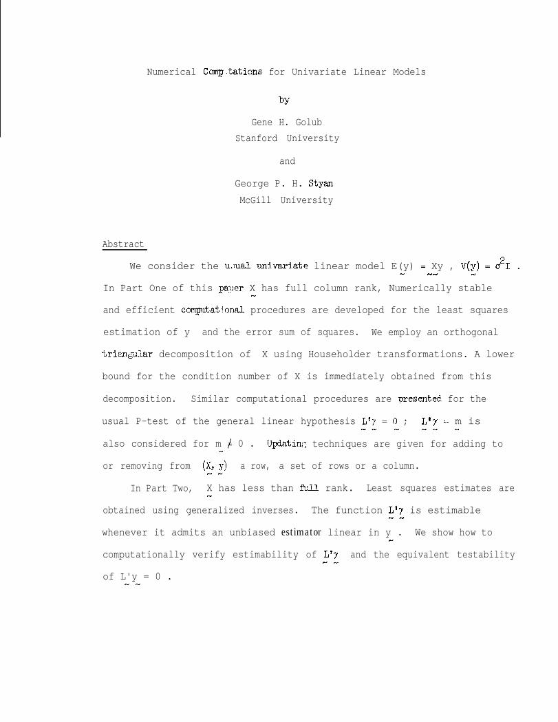
(107) x -%(u'x)u = x1,-NW

in

;

(1.5) gives

premuJ-tiplication by u' yjeJds -urx = ru1 , where u1 = ~2 , thera N -

f'iyi2, element in u . Substitution in (1.7) gives x+ 2~x4~~ = xl ,N

so that with x = {xi] ,

,. /?11, , f-:l >ast+.A cq_‘rpE; i.m wjl1 slwa]s be computed positive if the square root

I 1' (1.i;) is taken as

(J.11) s .z +(x'& .,.4 N

n ‘1Tience 2

cu” =1 (S2-XTj/(S2+ S\X,I) = l-(1X11/S) = 2(1-u:) . We note

i=2

that II need not be computed explicitly as Hx = x-2(u*x)u , for whichHN N - h)

we need only u and urx In the above form, it is necessary to compute- N

two square roots per Householder transformation; if, however, we write

H = I -u(u'u)-1

u' then only one square root need be calculated (Businger- IlHIU

and Golub, 1965;.

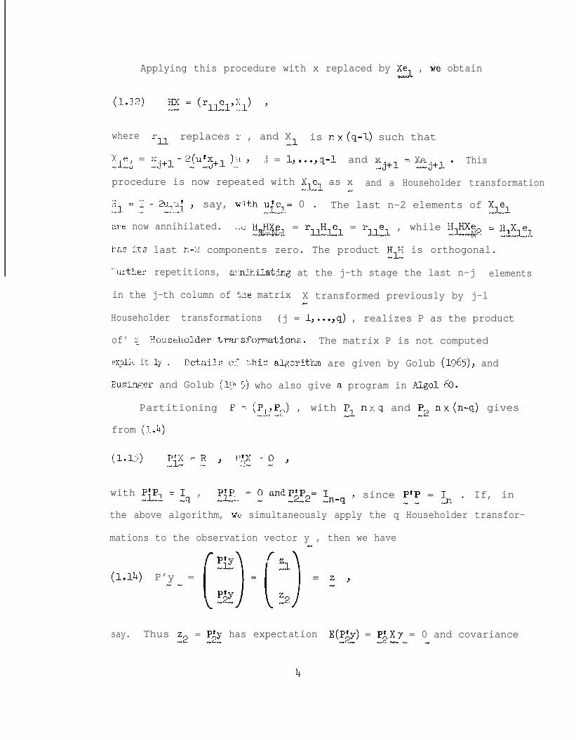
Applying this procedure with x replaced by XeL , tie obtainNN

where5.l replaces 1' , and X

-1is nx(q-1) such that

jCiei = x.-~+l- - -j+l rd '

2(u’x )lL j = l,...,q-1 and x - Xe This-J -j+l - --j+l '

procedure is now repeated with Xc1 as x and a Householder transformationIu

Ai:,1

z _I - 2UlU3; > say, w.!th u'e = 0 .,l,l

The last n-2 elements of 51_el

al+e now annihilated. *,G H,HXel = rllHLfiel = rllel , while H_pe2N-N- -N = H15:1

has its last n-Z components zero. The product HIJ is orthogonal.

3nrther repetitions, annihilating at the j-th stage the last n-j elements

in the j-th column of -?he matrix X transformed previously by j-lN

Householder transformations (j = l,...,q) , realizes P as the product

of' q Fouseholder transformations. The matrix P is not computed

FIxpli(, it ly . Detsils C-F this algcrithm are given by Golub (196$), and

&singer and Golub (I-9, 5) who also give a, program in ALLgo 60.

Partitioning P = (pl,PY) , with !l nxq and ,P2 nx(n-q) givesML

from (1.4)

with pzl = -Is , czcm = ,O and _P;E2= ,InBq f since P'P = ,II . If, in

the above algorithm, WC simultaneously apply the q Householder transfor-

mations to the observation vector y , then we have

1 =(1.14) P’y =N N

say. Thus z2 = _P;y has expectation E(l?;y) = p;Xy = 0 and covarianceHH CI

4

.matrix v(p;y) = dP:p, -I a5 . Hence :2 is an easily computed

-L--L -n-q

vector of uncorrelated regrossion residuals and may be used to test for

serial correlation (cf. e.g., Grossman cand Styan, 17'(O). It follows that

? n> f-.~!ch t,e~ on the led% -hand. :;-! de is idempotent and their cross-product

-i :: i) ; their sum 3 s i c‘m~d-t~~t+ with rank the sum of the ranks n-q and q.

for an3Jysis of the Liljrlar Itlxiel (cf. e.g., Draper and Smith, 1966).

FLY!.’ (jJ~-~~~~~’ ’ f ,

i’_’ _ ‘,(A i Q1.. j,l.,1 '3~ transformat i.:ms when the corresponding

I. - r, ;-, ) L’jrrcc p 7 p \h“:- =: ‘7: - ;r(x’Q -ht]y =I y-X? = r . However,I _ -.‘ *,' -L,. _.A -2 UNN Iv N N NU cu

it has been observed F; i;entl.c:man (1970) that computing r in this fashion

may be numerical@ unsi,able.

XC PASO find frr,l. (1.1~) that

(1.16) x’x =N N

Substitution in (1.3) yields R'R; = (R',O)P*y = _R*zl , so that solving4 NW N -cI-

(1.17) Ri; = tl--

gives T . This is eqedited by R being upper triangular.N

We note that RTR is a Choleslry factorization of XrX , for whichC1S-d N H

Healy (1968) has given a Fortran program.

The estimator p has covariance matrix V(y) = c2(XTX)-1 ; an

mN

unbiased estimate is Ge(xlx)-'/(n-q) which is easily camputed usingN r.#

(1.1.~') as (z;z,)fl(Rel) '/(n-q) . The generalized variance (cf. e.g.,- -

Anderson, 1958) is V.71-g I = c*'/IX'X( , where I* 1 denotes determinant.

In optimal design theo.*y a problem is to choose X so that IX'XI isc1 NN

maximized thus reducir' - Iv(j) 1 as much as possible. Again using (1.16)

we see that 1X*X1 = \I:'Rl = fir!. , as R is upper triangular. HenceN - - N i=l "-I ,-4

pm 1 is estimated b, [_"kZ,/ (n-q)]'/ I+ rfi .i=l

A measure of the Lll-conditioning of a matrix is its condition number

which we define as the ratio of the largest and smallest nonzero singular

vales 4' the matrix. The singular values of a (possibly rectangular)

matrix A are the positive square roots of the characteristic roots of

ATA or AA' . When t;le condition number far exceeds the rank we findP-) -

(cf. Wilkinson, 1967) -',hat the matrix is extremely ill-conditioned.

A lower bound for the condition number x(X) of the design matrix Xt-4

is the ratio of the la--<es-t and smallest (in absolute value) diagonal

elements of R . To see this we note first that X and P*X have theCI NN

same singular values, due ::o the orthogonality of P . As PX is merelyc1 H N

R bordered by zeroes, se;(x) = sg(R) , where sg(*) denotes singularw w

value. For any square matrix A of order nxn ,

(1.18) sgn(A) 5 Ichj(A) 1 5 sgl(A) ; 3 = l>***,nN

with ch(*) denoting characteristic root. The subscript j indicates

6

j-th largest. To prove (1.18) when A has real roots, let h = chj(A)w d

with Av = hv . Then-c1

(1919) sg;(A) = chl(A'A) =- N

max[xtArAx/xtx] 2 ytAtAv/vtv =x ------ c1 NCI N N

= hv'A'v/v'v = A2 .w--N-

Similarly sg;(A) 5 7~2 . Thus

max /ch(R) 1(1.20)

sqx) sgl(R) maxlr-jil☺q) = ,g$ = ,sgq(R) 2 -Ich(R) = iizqq l

c1) - - ,-a

Other properties of u(A) are given by Wilkinson (1967).

Why is the conditton number important and how can we use the

relationship (1,20)? Let 7 be the cowted approximation to 7 whichN

satisfies (1.3). Supptise that we wish to determine an upper bound for

the norm of the relati-;c error of 7 :

wllercb 11 a I\ indicates the Euclidean norm (ata) 112 . Define

(1.22) ‘E = y - xy ?NW

which we can compute q:-;tie accurately. Then

(1.23)

and hence

(1.24) -x*x( ; -7) = -xG ,

7

since X9 = 0 . Thus- c1

From (1.3), ilX'X?\\ = \I~~yl\ , so thatw HN u-

(1.26) Ilyy\l L \\ ? /(sg~(x) l

Combining (1.25) and (-~.26), we have

(1.27) IF-Wll~ll- -

Thus we see that the condition number may be used for determining an

upper bound for the relative error of 117 II . This upper bound is the

product of two factors; the first of which, W.*(X) , is independent of yrr) H

However, the lower bound provided by (1.20) would in some circumstances

give insight into the relative error. Hence, if

(l.:?q [may lrii 1 / nlin Irii 1 I* II XT; \I / 11 X’Y II- - N II

is large, then it is likely that the relative error in \\T \I is large.

The numerical efficiency of the above orthogonal triangular

decomposition is enhanced (cf. Golub, 1965) if the column selected for

each of the q Householder transformations maximizes the corresponding

sum of squares. That is, at the j-th stage (j = l,...,q) we transform

that column of the q-j+1 possibilities which maximizes the sum of

squares of its last n-j+1 components. The interchanges may be

summarized in a permutation matrix fl postmultiplying X . Thus (1.4)CI

becomes

8

R(1.29) x = P - IF ; PWT = - .

- 0

R

-o- ---(I

0

The vector z does not change and hence neither does Se . The solution

(1.17) changes however; substituting (1.29) into (1.3) now gives

m,Rflry = m,zl , so thatWN -- - NN H

(1.30) R(fl$) = ‘zl = Rf YCI--

is solved for 0 , and 7 = T@ . As these interchanges only rearrange

the rii we still find IX'X\ = firg . The lower bound for the conditionY .-.a i=l

number simplifies, however, as with these interchanges mulrii( = lrlll Y -

and min)riil = Jrqql so that u(X) 1 \ru/rqqI .

Given the nxn matrix

(1.31) A =

1 , -1 , -1 , . . . , -1

0 , 1 , -1 , . . . , -1. . . .. . . .. . . .

0 , 0 , 0 , l e* , 1m I Y

we see that maxlrii( -1 minlriil :- 1 , and so x(A) 21 , since f3 -1 E

when no column interchanges are made. However, if column interchanges

are performed then for‘ n = lo_ say, lrUl A 3.162, Ir,\ G .o03383

and n(A) 2 934.8. The actual value of U(A) = 1918.5 .& CI

The For-ban IV programs LLSQ and DLLSQ (double-precision) in the

Scientific Subroutine Package (SSP) of IBM (1968) solve the least squares

problem as described above. The SSP library is available at many IBM 360

computing centers. The SSP manual gives a write-up of the procedure and

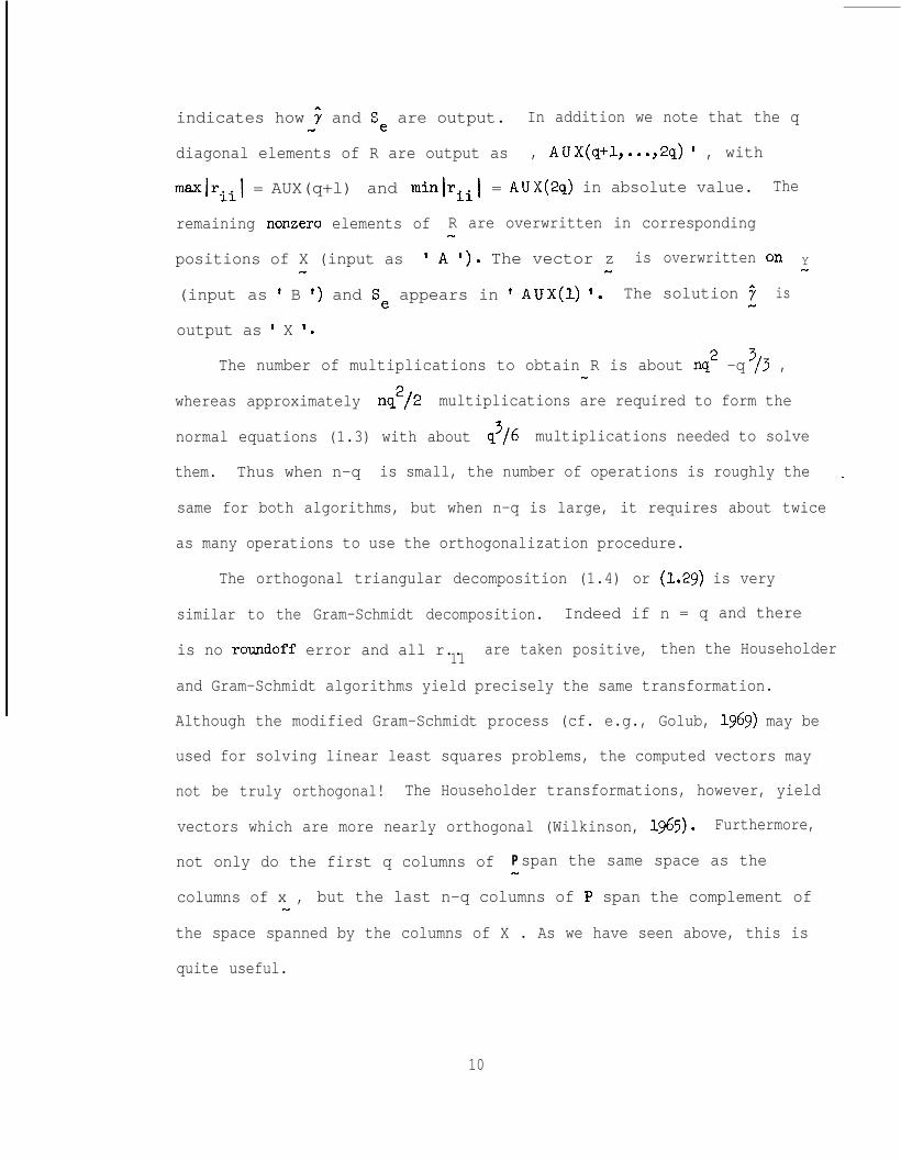
indicates how 7 and Se are output. In addition we note that the qc1)

diagonal elements of R are output as , AUX(q+l,...,2q) ' , with

maxIriiI = AUX(q+l) and min)r..) = AUX(2q) in absolute value.

remaining nonzero elements of R are overwritten in corresponding

positions of X (input as f A-'). The vector z is overwrittenCI

(input as t B ') and Se appears in ? AUX(1) '.- The solution 7CI

output as ' X *.

The

on YN

is

The number of multiplications to obtain R is about nq* -q /3 ,3m

whereas approximately nq2/2 multiplications are required to form the

normal equations (1.3) with about - q3/6 multiplications needed to solve

them. Thus when n-q is small, the number of operations is roughly the _

same for both algorithms, but when n-q is large, it requires about twice

as many operations to use the orthogonalization procedure.

The orthogonal triangular decomposition (1.4) or (1.29) is very

similar to the Gram-Schmidt decomposition. Indeed if n = q and there

is no roundoff error and all r.. are taken positive, then the Householder11

and Gram-Schmidt algorithms yield precisely the same transformation.

Although the modified Gram-Schmidt process (cf. e.g., Golub, 1969) may be

used for solving linear least squares problems, the computed vectors may

not be truly orthogonal! The Householder transformations, however, yield

vectors which are more nearly orthogonal (Wilkinson, 1965). Furthermore,

not only do the first q columns of P span the same space as theM

columns of x , but the last n-q columns of P span the complement ofH

the space spanned by the columns of X . As we have seen above, this is

quite useful.

10

2. Hypothesis testing and estimation under constraints '

Let us consider the general linear hypothesis

cm L'y = 0N H CI

for the linear model of Section 1. The contrast matrix L' is takenm

sxq offullrowrank s_<q. If we assume that y is normally

distributed then L*F is N(Lry,a2Lt(XrX)-?L) , with F = (X'X)%y .ma- -& CI HN Y MN m m

The numerator of the usual F-test for (2.1) is then well known to be

(2.2) ~'LIL'(x'x)-lL]-lL'~ = Sh ,m-m mm Y - Y

say, the "hypothesis sum of squares". Substituting (1.16) and (1.17)

into (2.2) gives

(2.3) sh = -’ -1 -1zi(R )'L[L'R (R )'L]

-1 -1- GIN m N

L'R zl .N m

We compute (R-l)*L = G , say, by solving R*G = L , with R* lowerN N m N II

triangular. We then obtain an orthogonal triangular decomposition of

as

G,-

say, where B is upper triangular s xs and the orthogonal matrix QCI

is the product of s Householder transformations. Then G*G = B'B ;CIti NN

partitioning Q = ($Q,) , where 'Ql is qx s and %2 qx (q-s) gives

G = CJ2 from y2.4). Substitution in (2.3) yieldsN

(2.5) Sh = ZiQlQi Z1- N u

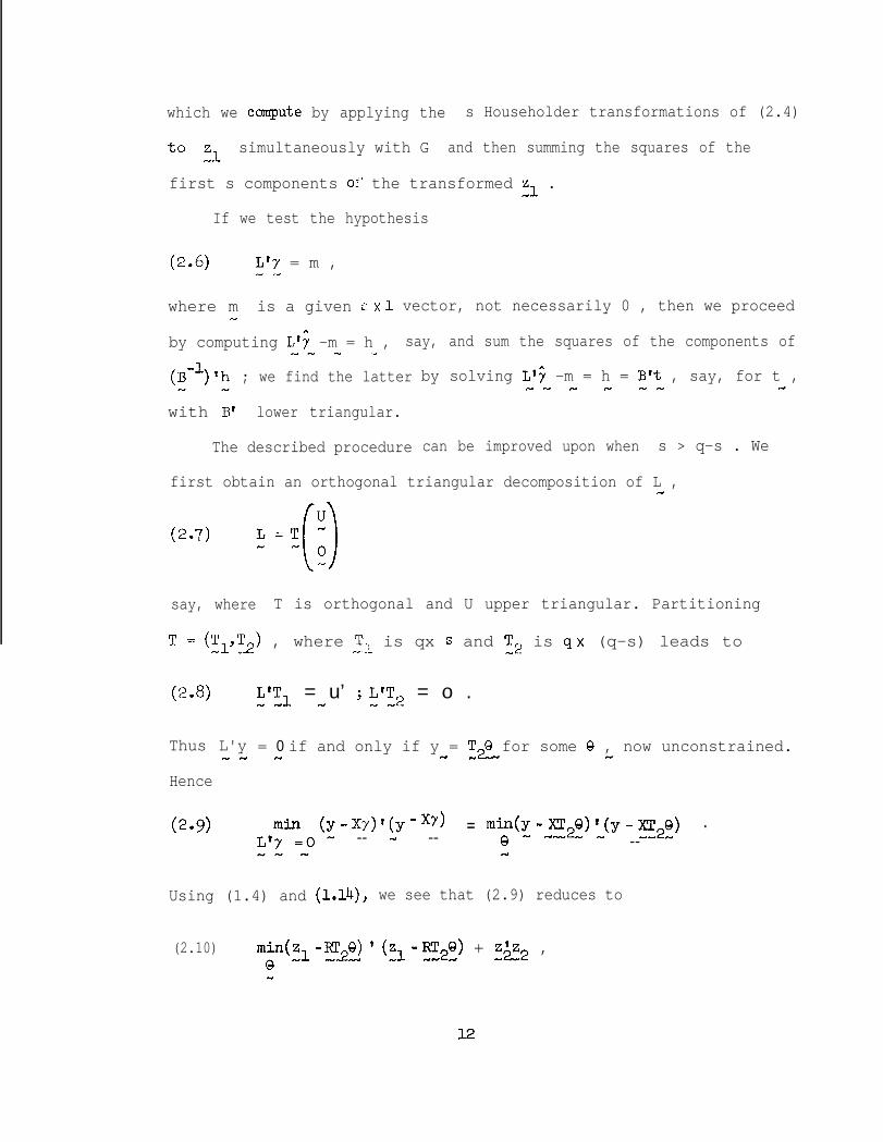
which we campute by applying the s Householder transformations of (2.4)

to :1simultaneously with G and then summing the squares of the

first s components of the transformed zl .

If we test the hypothesis

P4 L*y = m ,N m

where m is a given :: xl vector, not necessarily 0 , then we proceed-

by computing L'G -m = h , say, and sum the squares of the components ofmm - .?.I

(B-')'h ; we find the latter

with B* lower triangular.

The described procedure can be improved upon when s > q-s . We

by solving L*T -m = h = B*t , say, for t ,CIII N N c1cI m

first obtain an orthogonal triangular decomposition of L ,CI

(2.7)

say, where T is orthogonal and U upper triangular. Partitioning

T = &,T2) , where T., is qx s and !IJ2 is qx (q-s) leads tom m-

(2.8) :‘~,1 = u’ ; :‘T,* = o .N

Thus L'yN N

= 0 if and only if y = T2Q for some 0 , now unconstrained.CI c1 N CI

Hence

(2.9) mi3-1 (Y - XY) ’ (y - W) = min(y - Xr,0) t (y - XT2Q) .L'y =o - -- - -- Q - CIH - - -- -

Using (1.4) and (1.14), we see that (2.9) reduces to

(2.10) min(tlQ

- qa t <flMCI) N-RT,0) + $z2 ,

-cI CI Nm

I2

so that Sh equals thtl first term in (2.10) which is easily computed

as in Section 1 with lJ1 replacing y and RT2 replacing X . Sincemm

(cf. e,g., Good (1965); p. 89),

(2.12) wq(W L ::gq-s+lo L sgq+(xT;j) YNW mm WY

we have

P-13) ,,* mm mu(xT ) ,< wm) = u(x) '

Thus, by eliminating tie constraints, the linear least squares problem

may become better conditioned.

The

obtained

least squares estimate y* , say, of y subject to L*y = 0 is.-4 CI NCI N

from the solution 6 to (2.10) bym

(2.14)

If the constraints have nonnull righthand side m as in (2.9) thenN

the procedure is changed as follows. Evidently L*y = m holds if andMC1 M

only if y = CC2_e+~l(U-1)tm We obtain w by solvingN II

= T20 + T_1" , say.au N -

m = U'w , with Ut lower triangular.- N c1 II

Thus y is replaced by y-xTl~~CI M cum

and hence 3 by 54Tlw the resulting value of Sh is therefore

eu- CI

(2.15) min(zQ

,l-RT~-RT2Q)'(~l-RTlw-RT2@)e* NM N GIN d NW N

m

which we compute as in Section lwith zl -KT,w replacing y and IIQ2CICI u Md

replacing X l

II

13

The relevant F-te.;t for the hypotheses (2.1) or (2.6) is then

computed as

Sh sI(2.1(;) F = S-g-G? ,

wit'h the critical region formed by values of (2.16) exceeding the corres-

ponding tabulated value of F with s and n-q degrees

In some special, Jhough common, situations the above

simplify considerably.

of freedom.

computations

If we test a single contrast in y equal to 0 we obtain (2.1)m

with s = 1 . Let us write this as

(2.17) L’y=O .N d

A particular case might be testing a single regression coefficient equal

to 0 . Then (R -1)*L = K becomes (R-1)*1 = k , say, found by solvingry N N N CI

e = R*k as before. Then (2.3) becomesCI m CI

(2.18) (r';)2/k'k = sh ,CIH m #u

and we compute the denominator in (2.18) by summing squares of components

in k . The one-sided t-test forhl

(2.19) Py >o _GIN

has critical region large positive values of Pi/ [k*k S,/(n-q)] 112 .NN MN

Another special case occurs with s = q-l when Lry = 0 if' andWN 15)

only if

(2.20) 7 = 8t )N N

14

where 0 is now a scalar. The vector t is of'ten found tipon inspectionCI

(without transforming L ). For example in testing for homogeneity of0e

coefficients of y , we have t = e , the vector with each componentc c1

unity. Substituting t for 'IC2 in (2.10) yields

(2.21) (3 = ziRt/t'R'Rt >-- Nrr)dH

and

(2.22) Sh = zzl- (~~t)*/t'RrRt ,m m wed

with the denominators computed by summing squares of elements of Rt .mH

- -

15

3. Updating procedures

After a particular set of data has been analyzed it is often

pertinent to add to or remove from X and y a row (or set of rowsCI

or to add to or remove from X a column. This happens when new informa-I4

tion becomes available or when existing qerimental units have been

classified as extreme, or independent variables insignificant.

We begin by considering the addition of data from m , say, further

experimental units. Let XJn and & be the corresponding data of order

mxq and mxl respectively. Following (1.4) and (1.14) we may write

Applying q Householder transformations of order m+q to the first mtq

rows of (3.1) yields

(34 (r f) = El( i’ ;) .,

say, where R, is qxq upper triangular, zz is qxl and z: is#WA

mxl. Hence

(3 03)

where

(3.4)

-q

is an orthogonal matrix formed from 2q Householder transformations, and

has order m+n . The new residual sum of squares is $'zT + 2zz2 ,& c11

i e.,A_ . the previous sum of squares, !zzz2 , augmented by the sum of squaresN

*of the m components of z l these components themselves give m-1 '

additional uncorrelated residuals.

Next, suppose we wish to add a (q+l)--t n variable whose n values

constitute a vector x . We first compute P'x by applying in turn theN He

q Householder transformations determined by the stored vectors uIy

(cf. residual calculations in Section 1). We need then only one further

Householder transformation, H , say, of order n-q to annihilate theN

last n-q-l elements in P'x , i.e.,

(3.5)

I4Cm0 0

HCI

P'(X,x) =N CIrr,

R

= (:0 heJ

where P = (P P ) , as in $1, and h = x*P P*x , the sum of squares ofc1 ,I!,2 II 2L2-

the last n-q components of f*x .wk,

The procedure for removing an experimental unit is more complicated.

The method given previously by Golub and Saunders (1970),may under

certain circumstances prove unstable. We now give a new method which

should provide a more accurate solution.

17

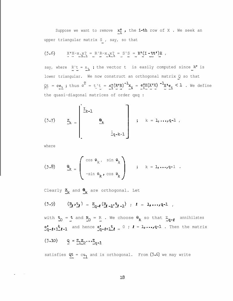
Suppose we want to remove cf ., the i-th row of X . We seek an

upper triangular matrix S , say, so thatd

(34 X*X-x.x? = R'R-x.x? = S'S = R'(I-tt')R ,N N -1-l c1 +..e -1-1 CI d N d NN H

say, where R't = x.-1

; the vector t is easily computed since R* isN N N

lower triangular. We now construct an orthogonal matrix Q so that

Qt = c_el ; thus c2 = t't = xf(RTR)-$ = ,ie--f- - N H -

e*X(XtX) -+('ei <-l . We definerrc1IN

the quasi-diagonal matrices of order qxq :

(3.7)

where

(34

Zk =

!!k =

.

:k-1

63,k

I-q-k-l

cos 0k' sin Qk

-sin 0k' cos 0k

I ; k = l,...,qq-1 ,

; k = l,...,q-1 .

Clearly Fk and tk are orthogonal. Let

(3*9) CQt,l = Z,-rcRJ-l,t_l-l) ; f = l,...,q-1 ,

with t,. = t and E. = R . We choose 0k so that Z annihilatesc1) N -q-I

t:&LclJ-1 and hence e* t

,q-i+l#J =0 ; I = l,...,q-1 . Then the matrix

satisfies Qt = ce,1 and is orthogonal. From (3.6) we may writeNN

18

(3.ll) S’S =NN

R1Qr(I-c2~~i)QR 9,-.a- H NCI

2which is positive definite if and only if c > 1 . It follows that

(3.x) F=W=

.

w21 9 w22 9 l *' w2,q-1 t w2q

0, w32 9 l w3,q-i ) w3q

. . . .

. . . .

e . . .

0, 0, . . .

�s,s-1 � ww.

is an upper Hessenberg matrix. Thus (3.11) becomes S'S = WtD2W , withN w MNr.0

which is real when c2<l. We compute S by applying orthogonalN

transformations to the upper Hessenberg matrix DW . LetHI1

(3.14)*

!k = ,zk Fk-1 ; k = 1, . . ..q-1 )

with So = DW and _zI: formed as !k in (3.7) but with 0: replacingGIN

'kand so chosen that- $

Iawihilates zLISkek = ~i+~Dwe~ and thus

- N m cI)cII

zi+lSkek = 0 . Then- N

(3.15) s = s =z* z** *

c1 -q-l -q-l -9-2l ** iz2 LZZIIE☺ .

This procedure requires about 9q2/2 multiplications and 2q-1 square 1I

roots.

19

The above algorithm can also be used for adding an observation but

about twice as many numerical operations are required as in the procedure

given by (3.3) and (3.4). We also note that the problem of deleting an

observation is numerically delicate. Since

(3.16) S'S = R'(I-tt')R ,NN N N -- N

it follows that

(3.17) x(S) ,< x(R)/ (1-t*t) 112 .c11 N H N

Thus if t*t is close to 1 , then x(S) could be quite large as theWN CI

right-hand side of (3.17) is attainable.

Finally suppose we wish to remove an independent variable or

column of x . If it is the last then no further calculations are

required; but suppose it is the first. Let

(3.18)

�I2 l *.

r22 l l *

.

.

.

0 . . .

= ( rlp1 Y n)

where fi is qx (q-l) and has one more row than an upper Hessenbergc1

matrix. We annihilate the elements just below the main diagonal of ]li ,N.lee., r22J l ..,rqq Y by applying orthogonal transformations of the type

(3.7) with

C-9) !k = ,zk 3-1 ; k = l,...,q-1 ,

20

and R = E l we choose Qk in Zk so that :hlRkBlek = rHlylrel-0 2 N

is annihilated; thus $+lRkek= 0 and R

&q-lis the new triangular

- N

matrix sought.

21

PART Two: UNIVARIA!FE LINEAR MODEL WITH LESS

THNTFULLRANK

4. Least squares estimation and error sum of squares

We consider now the univariate general linear model (1.1)'

(44 E(Y) =XY , V(Y) =a21 ,NN m rcI

with the design matrix X of rank r < q <n . We obtain the saxne normal

equations as (1.3)'

which are consistent; their solution, however, may not be unique. Consider

a solution to (4.2) which we may write

(4.3) 7 = (x'x)-X'y ,N NCI cIc1)

where (a)- denotes generalized inverse. We follow mingle and Rayner (1971)

and define a generalized inverse of a matrix A , mxn , as any matrix A-m w

satisfying

(4.4) AA-A = A .N- H d

h

Evidently A- has order nxm T Such a generalized inverse exists but ism

not unique in general; if, however, A- satisfies (4.4) andN

(4.5) A-AA- = A- ,- -he m

(4.7) (A-A)' = A-A ,NM Nm

22

then we write A- = A' , the pseudo-inverse of A . Whenwe only requireN N Y

that (4.4) is satisfied we will write A- = gl(A)N u-- a gl-inverse of A .

h)

Similarly when (4.4) and (4.5) are satisfied, A- = g12(A) ; (4.4)' (4.5)’

and (4.6): A- = g123(A) . The pseudo-inverse i' = g1234(A) . Theu

solution ;-0 '

say, to (4.3) which minimizes 7'7 equals X+y as isHU UN

shown, for example, by Peters and Wilkinson (1970). Our concern, however,

focuses more on estimable functions of y , rather than y per se so weu OI

will not discuss here computation of i. . We define an estimable function

of Y as a vector L'y which admits an unbiased estimator of the formN UU

K*y , where L* is s x q , say, and K* , sxn. The least squares- u CI u

estimate is then L*G = L*(X*X)-X*y so that K* = L*(X*X)-x' . We shallUC1 u UN UN u Y mu N

see (Section 5) that when L'y is estimable, L'(x'x)-X' is unique for -u NN N

all (X*X)' = gl(X*X) . Rather than form X*X ,UN mu UNfind a g,(X'X) and then

NU

postmultiply it by X* , we compute a gl23(X) directly, noting that GN H

is a e;@) if and only if it can be written as (A*A)-A' for some

@VA) --(A?*)- [Pringle and Rayner (1371)' p. g;]:

N

H u u N

We proceed as in Section 1 to orthogonally transform X by Householderu

transformations with column interchanges. If X has rank r then after rh)

Householder transformations we obtain, cf. (1.29),

w8)R

X- tw=p -- 0 i- -

R sIT’ ; p*xn’= - -

N UN

( 1Y

0 0N N

where R is upper triangular, rxr, S is rx (q-r) , and 71 is au u N

permutation matrix of order qxq . We now claim that

R-l 0(4.9) x* = ll -- -i- 1- P’ = g123(x) .

0 0” CI

I _- 23

‘1r

We have XX*UN clearly symmetric. Hence XX*%UN N

so that (4.9) is proved. The solution

"r = X*y to (4.2) afforded by (4.9) is often called a basic solution as it

contains at most q-r nonzero elements.

Thus (4.9) accomodates our purposes;

stronger g-inverse than is needed. As in

moreover we do not have a

Section 1 we partition

p = @p,> Y but now let Fl be nx r and l?2 nx(n-r) . From (4.8)U

it follows, cf. (1.13)' that

(4.10) :iXIl = (R'S)-u

(4.11) :;x = 0 .

Following (1.14) we now write

(4.12) p’y =CIU

202

Y

where2

is now rxl and z,2 (n-r) xl . Thus z2 is again a vector

of uncorrelated residuals; moreover

C4*13)-F2 P; +x(x*x)-x’ = 5; ,

N Y N Y u

as in (1.15)' with T2P,$ idempotent rank n-r and X(X*X)-X* symmetricUNN N

- idempotent rank r . By (4.11) their cross-product is 0 and so theirY

sum is idempotent rank (n-r)+r = n and hence zn as claimed. Thus

24

(4.14) :;z2 =- - UNu - Ny'(1 -x(x*x)-X')y

is the residual sum of squares, computed as the sum of squares of the

n-r components in z, .UL

The vector of (correlated) residuals r = y-XT = (I-X(X'X)-X*)y = E2P;yN - uu u u-u H CI u u

as in Section 1, and using (4.13) it follows that (4.14) equals r*r .N N

25

59 Estimating estimable functions and testing testable hypotheses

As mentioned in Section 4 we are not directly concerned with the

estimation per se of y . We define L*y to be an estimable functionuu

of Y whenever it admits an unbiased estimator which is linear in y ,

K'Y y say. Thusu u

(:>*l) ~'y = E(K'y) = K'X 1u N N u _ u-

AC in Section 3 we take L* to be s xq, but now relax the assumption of

full row rank taking r(L) = t 5 r . We obtain-2

directly from (5.2). Substituting (4.8) into (5.3) gives

(‘,I .‘I)

where we partition

(5*5) L’IT = (tiYL;) YH u H

1 - -= r(R) = r(X) :: :r ,

with L*-1

sxr,and L; sx(q-r) . The matrix L*fl is the contrastHU

matrix L* with its co3umns permuted according to the interchanges whichU

26

rearrange the columns of X to make the first r columns linearly

independent. Then L; are the corresponding r columns of L* or L*Tf l

N UN

we apply _v > r Museholder transformations of order s+r , whose

product is V* , say, s'> that

(5-6)

where5

is a permutation matrix, and T is upper triangular vxv .

If (5.b) is achieved at the r-th stage, i.e., v = r , then L*y isU N

estimable. If not, then L'y is not estimable.u u

An alternative procedure which is often easy to verify theoretically-

follows and is included for completeness.

TFLEOREN 5.1. The .f'unction L*y is estimable if and only if---wN N

L'(x'x)-x*x = L'CI ..a- YU(5.7)

for any- -

Proof.

implies

(x*x)' = gl(X'X) .u N UN

We show that (5.2) and (5.7) are equivalent. Clearly (5.7)

5.2) ; conversely

(5.8) L'(X'X)-X*X = K'X(X'X)-X*X = K'X = L' ,N NU NN.UNUU NIY CIY N

since X(X*X) -X*X = X [cf. Pringle and Rayner (ly'j9), p. 261.NNII rr)u N

Q.E.D.

We may use (5.7) to computationally verify estimability as follows.

Substituting (4.8) and (4.9) into (5.7)’ with X* = (X*X)-X* givesU UN cy

27

I R-'S(5.9) L'fi - - - 7-r' = L' .UN (- -100 - -

Substituting (5.5) into (5.9) yields

(5.m) LJR-1S = k$CI N

To verify (5.10)' therefore, we solve RW = S for W , say, which equalsNW N Y

R-'S , with R upper triangular.N N N

We then examine LJj -I$ and if close

enough to 0 conclude L*y estimable.N UU

For the remainder of this section we will assume L*y estimable.UN

From (4.3,

(5-W L’f = L'(x'x)-X'y = L'X"y ,UN u MN -II NUN

where XN* = (X*X)-X' = gU3(X) , cf. (4.9). Thus

NN N N

(5.12) -1~1 ,

using (kl2) and (5.5). We compute L*y , therefore, by solving Rw 2: zl

for w , say, which equals R-1 --

UN

z with R upper triangular. We thenu II -1' u

premultiply by ti which contains the r columns of L* correspondingN

to the r linearly independent columns of X which yielded R . We note

that Lry is uniquely determined by (5.U.) for any (X*X)-UN UN

= &(x*x) .NN

To see this, set L* = K*X from (5.2)' SO that L*(X'X)-X' = K*X(X*X)-X' =N UN u NN N NrYNN u

K'X(X'X)+X' = L'(x'x)+x' , since X(X*X)-X* is unique [cf. Pringle andeNN- M N NN Y mm- N

Rw=r (W7h P. 251.

28

We define the general linear hypothesis

(5.13) L'y = 0uw N

as testable whenever L*y is estimable. The numerator of the usual F-testu H

for testable (5.13) is then, cf. (2.2)'

(5.14) :'L[L'(x'x)-L]-L': = Sh 9u-u UN N NU

To see that (5.14) is invariant over choices of (X*X)- , notice thatUN

L'(x'x)-L = K'X(X'X)-X'K = K'X(X'X)+X'K = L'(X'X)+L from (5.2). Moreover,N NU u Ud *au

(5.14) is also-invariant over"cho;ces if ;L*;xSX)'L]- ; writingh) uu Y

X* = (x*x) -x* we find that (5.14) may be writtenY -- Y

(5*15) y'(x*)'L[L'x*(x*)'L]-L'x*y = Sh ,u u u-u #w N NNIY

using (5.7) and (5.11). Sh is uniquely defined since for any A ,N

A(A'A)-A' is unique [cf. Pringle and Rayner (1971)' p. 251.u-u N

To compute Sh we see from (4.9) and (5LL) that (5.15) may be written

(5.16) ‘h = ~i(R-l)'IJl[L_;R-l(R-l)' 21]-EiR-1El .H Y -

We obtain an orthogonal triangular decomposition of

(5.17) G = (Rol)'Ll = QU E; ,rr‘ -

say, where B is upper triangular t xt , with t = r(L) = r(kl) by (5.10).U N

. The orthogonal matrix Q is the product of t Householder transformations,Y

while the permutation matrix !2rearranges the columns of tl, rxs,

29

to make the first t linearly independent. Substituting (5.17) into

(5.16) yields

(5.18) Sh = 2iGGXZ-L 9NDI

where G* = g,,3(G) is given byc1) w

(5*19)

We partition Q = (!l,Q,) , where &l is rxt and !2 rx(r-t) .N

[ I f t=r, f21 z Q .] Then (5.18) reduces tod

(5.20) 'h = Zi?l!i?l 9-

as at (2.5). We compute (5.20) by applying the t Householder transfor-

mations of Q simultaneously with G and then summingIc)

in (5.17) to fld

the squares of the first t components of the transformed zl .

If we test the hypothesis

(5.21) L'y = mGIN

and L* is s xq with row rank t < s then m must satisfy the sameN

s-t restrictions that apply to the rows of L' , i.e., (5.21) must beM

consistent. Then the numerator sum of squares is uniquely given by

(5.22) +L-m')[L'(XTX)-L];(L$ -m) = Sh ;GIN #e h) him CI MY eu

following (5.15) and (5.16) we see that

(5*23) L'(X'X)-L = ";R-l(R-l)'tl = G'GN GIN CI m d Ya

30

for which we want a gl-inverse. We use

LEMMA 5.1. If A" = g,23(A) , then

A*(A*)' = g12(A'A) .& CI MN

Proof. From (4.4), (4.5) and (4.6) we have

(5.25) AA*A = -4 , A*AA* = A* , AA* = (A*)'A' .m- Y d & e-- N NY N eu

Hence A*(A*)'A*A = A*AA*A = A*A . Thus AIA[A*(A*)'A'A] = A' AA*A = A'ALI N HN M -nPy CIY YNII N HM & -0-w N H

and [A*(A*)'A~A]A*(A*)* = A*AA*(A*)' = A*(A*)' .N - NNN H N NY N N -

Q.E.D.

From Lemma 5 .l we obtain

(5.26) G*(G*)' = [L'(x'x)-Ll-N u #u -- @

= c2$( B-l) ‘K&

from (5J9L where we partition 22 = (z21,f122) , with c21 j sxt yN

identifying t linearly independent columns of tl , rx s l Hence

(5.27) 'h= ti- H(~'L-m')~2~01(B-1)f~~l(L'j -m) .- WN N

First L': -mNH Nis computed and rearranged to form llll(Lr$ -m) = h , say.NU - N

Then h = B*k is solved for k , where B* is lower triangular. FinallyN #uY Y Y

'h is found as the sum of squares of the components in

k = (B-')*h = (B-l)tT$l(LrT -m) .w

The relezt F-test-fir t"he hypotheses (5.13) or (5.21) is then

computed as

31

(5.28) F =qt

s,/oi

Y

cf. (2.19, with the critical region formed by values of (5.28) exceeding

the corresponding tabulated value of F with t and n-r degrees of

freedom.

The above procedures simplify slightly when the contrast matrix L' ,

sxq, has fullrank s <r =r(X) .- In that case (5.23) becomes non-cy

singular and the results of Lemma 5.1 are not needed. We use

LEMMA 5.2. When, L'y is estimable,NN -

(5*29) r [L*(X*X)-L] = r(L) ,,.d ..a- N CI

where d') denotes rank.

Proof. Using (5*7), r(L) = r[L'(X*X)-X'X] 5 r[L'(X'X)-Xf] =N

r[L*(X'X)-X'X((X*X)-)*L] =.r[L'(X'X;‘L] i r(L) .

Y NCI N

Q.E.D.

When Lr , s xq , has full row rank s 5 r the decomposition (5.17)N

becomes

(5.30)

say, where!!21

is now sx s and may equal IMS

(no column interchanges).

Formula (5.27) applies with essentially no change.*

We defer discussion of updating techniques for the less than full rank

case and extensions to multivariate models to a further paper. A computer$9*

program in Fortran IV for the IBM 360 is being developed for the procedures

discussed in this paper.

32

Acknowledgments

The work of the f5rs-b author was completed whilst a visitor at

Princeton University and IIMperial College. IEe thanks Professor

G. S. Watson and Professor D. R. Cox for the generous provision of

facilities. The second author thanks Vo Van Tinh and Laurel L. Ward

for helpf'ul discussions.

33

References

Anderson, T. W. (19fj8). An Introduction to Multivariate Statistical

Analysis. Wiley, New York.

Businger, Peter, and Golub, Gene H. (1965). Linear least squares solutions

by Householder transformations. Numer. Math., 7, 269-276.-

Draper, N. R.,and Smith, H. (1966). @lied Regression Analysis.

Wiley, New York.

Gentleman, M. (1970). Personal communication.

Golub, Gene H. (1965). Numerical methods for solving linear least squares

problems. Numer. Math., 7, 206-216.N

Golub, Gene H. (1969). Matrix decompositions and statistical calculations.

Statistical Computation (R. C. Milton and J. A. Nelder, eds.),

Academic Press, New York, 365-397.

Golub, Gene H., and Saunders, Michael (1970). Linear least squares and

quadratic programming. Integer and Nonlinear Programming

(J. Abadie, ed.), North-Holland, Amsterdam/American Elsevier,

New York, 229-256.

Good, Irving John (1965). The Estimation of Probabilities: An Essay on

Modern Bayesian Methods. Research Monograph No. 30, The M.I.T. Press,

Cambridge, Mass.

Grossman, Stanley I., and

regression residuals

Styan, George P. 1-E. (19'70). Uncorrelated

and singular values. Technical Report NO. 32,

Inst. Math. Stud. Sot. Sci., Stanford, 16 pp. (Optimality properties

of-Theil's BIUS residuals, J. Amer. Statist. Assoc., forthcoming.)

Healy, M. J. R. (1968). Triangular decomposition of a symmetric matrix.

Appl. Statist. (J. Roy. Statist. Sot. Ser. C), 5, 195-197.

I.B.M. (1968). System/360 Scientific Subroutine Package (36OA-C&03X)

Version III Programmer's Manual (Fourth Edition). IBM Manual

H20-0205-3, IBM, White Plains, N. Y.

34

Longley, James W. (1967). An appraisal of least squares programs for

the electronic computer from the point of view of the user.

J. Amer. Statist. Assoc., 3 819-841.

Peters, G., and Wilkinson, J. H. (1970). The least squares problem and

pseudo-inverses. The Camputer Journal, 2, 309-316.

Pringle, R. M., and Rayner, A. A. (1971). Generalized Inverse Matrices

with Applications to Statistics. Griffin, London.

Wampler, Roy H. (1969). An evaluation of linear least squares camputer

programs. J. Res. Nat. Bur. Standards Sect. B, 2, 59-90.

Wampler, Roy H. (1970). A report on the accuracy of scxne widely used

least squares cunputer progrtis. J. Amer. Statist. Assoc., 5,

549-565.

Wilkinson, J. H. (1965). Error analysis of transformations based onH

the use of matrices of the form I -2ww . Error in Digital

Computation: Volume 2 (Lo B. Rail, ea.), Wiley, New York, 77-101.

Wilkinson, J. H. (1967). The solution of ill-conditioned linear equations.

Mathematical Methods for Digital Computers: Volume 2 (A. Ralston

and H. S. Wilf, eds.), Wiley, New York, 65-93.

35