Embed Size (px)
Citation preview

Evnine-Vaughan Associates, Inc.
A multi-timescale statistical feedback model of volatility:
Stylized facts and
implications for option pricing
Lisa BorlandOctober, 2005

Acknowledgements:
Jeremy Evnine Roberto Osorio
Jean-Philippe BouchaudBenoit Pochart

Layout• Stylized facts of markets
- Why we need a new model
• The non-Gaussian model -Properties -Applications: Options and Credit
• The multi-time scale model-Capturing the stylized facts
• Work in progress and conclusions


Properties of Financial Time-Series
• Power Law distributions, persistent over very many timescales: minutes to weeks
Cumulative distribution power law tail -3Gopikrishnan,Plerou,Nunes Amaral,Meyer,Stanley (1999)

Properties of Financial Time-Series
• Power Law distributions, persistent• Slow decay to Gaussian, as • Volatility clustering and correlation• Volatility relaxation (Omori law)• Close-to log-normal distribution of volatility• Returns normally diffusive over time-scales• Leverage effect (Skew: Negative returns higher volatility)• Time-Reversal asymmetry
25.0−τ

o Empirical--- Gaussian
q=1.43 Tsallis Distribution


Consequences
• Risk control: under-estimate rare events
• Derivative markets: (options, credit)wrong model of underlying leads to wrong pricing, wrong hedging

Challenge
• A model that can reproduce the stylized facts• A model that can reproduce option prices, credit etc.• A model that captures the correct dynamical features
Desirable• Intuition• Parsimony• Analytic tractability

• Stochastic volatility (Heston 1993)
• Levy noise• GARCH • Multifractal models (Bacry,Delour,Muzy, 2001)
Popular models
Problems• Typically converge too quickly to Gaussian• Less parsimonious• Do not reproduce time reversal assymmetry

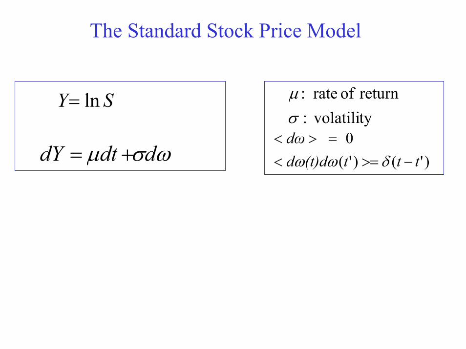
The Standard Stock Price Model
SY ln=
)'()'(0
ttt(t)dd dω
−>=<=><
δωω
ty volatili:returnofrate
σµ :
ωσµ ddtdY + =

The Standard Stock Price Model
)'()'(0
ttt(t) ω
−>=<=><
δωω
ty volatili:returnofrate
σµ :
Gaussian Distribution
Fokker-Planck Equation2
2
21
ωdPd
dtdP
=
)2
exp(21)(
2
ttP ω
πω −=
ωσµ ddtdY + =
SY ln=
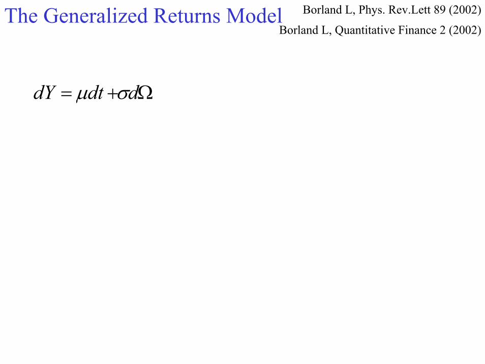
Ω+ = ddtdY σµ
The Generalized Returns Model Borland L, Phys. Rev.Lett 89 (2002)
Borland L, Quantitative Finance 2 (2002)

ωdPdq
21
)(−
Ω=Ω
Ω+ = ddtdY σµ
The Generalized Returns Model The Generalized Returns Model Borland L, Phys. Rev.Lett 89 (2002)
Borland L, Quantitative Finance 2 (2002)

The Generalized Returns Model The Generalized Returns Model Borland L, Phys. Rev.Lett 89 (2002)
Borland L, Quantitative Finance 2 (2002)
Tsallis Distribution
Nonlinear Fokker-Planck2
22
21
Ω=
−
dPd
dtdP q
qtqtZ
P −Ω−−= 11
2 ))()1(1()(
1 β
ωdPdq
21
)(−
Ω=Ω
Ω+ = ddtdY σµ

In other words:
State dependent deterministic model
ttttt dbqad ω21
2 ])1([ Ω−+=Ω
Work with
)(SΩ=Ω
as a computational tool allowing us to find the solution
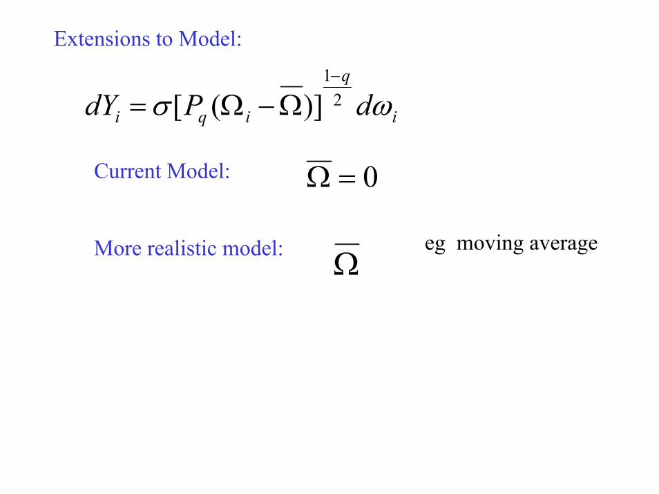
Extensions to Model:
i
q
iqi dPdY ωσ 21
)]([−
Ω−Ω=
0=ΩCurrent Model:
eg moving averageMore realistic model: Ω

Extensions to Model:
i
q
iqi dPdY ωσ 21
)]([−
Ω−Ω=
0=ΩCurrent Model:
eg moving averageMore realistic model: Ω
Or:
i
i
j
q
jiqi dPdY ωσ ∑−
=
−
ΩΩ=1
0
21
)]|([
(see later in this talk)


Not a perfect model of returns:
Well-defined starting price and time
Nevertheless:
Reproduces fat-tails and volatility clustering
Closed form option-pricing formulae
Success for options and credit (CDS) pricing

Example European CallQ
rT KTSec ]0,)(max[ −= −
Stock Price
⎭⎬⎫
⎩⎨⎧
Ω2
− + Ω= ∫ −2 T q
tT dtPrTSTS0
1)(exp)0()( σ

Example European CallQ
rT KTSec ]0,)(max[ −= −
Stock Price
⎭⎬⎫
⎩⎨⎧
Ω2
− + Ω= ∫ −2 T q
tT dtPrTSTS0
1)(exp)0()( σ
Integrate using generalized Feynman-Kac
2)(T
T Ω∝ γ

Example European CallQ
rT KTSec ]0,)(max[ −= −
Stock Price
⎭⎬⎫
⎩⎨⎧
Ω−−2
− + Ω=2
2)()1()(exp)0()(TT TgqTrTSTS γσ
21 dd T ≤Ω≤)( KTS >Payoff if

Example European CallQ
rT KTSec ]0,)(max[ −= −
∫ Τ− ΩΩ− =
2
1
)())((d
dTq
rT dPKTSec
σσ ,,)0( qrT
q KNeMS −−=
q = 1: P is Gaussian q >1 : P is fat tailed Tsallis dist.

q=1.5

K=50, T=0.4, sigma=0.3, r=.06
q=1.5q=1
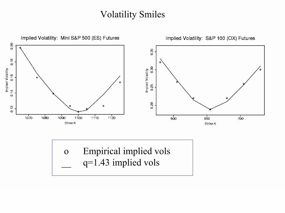
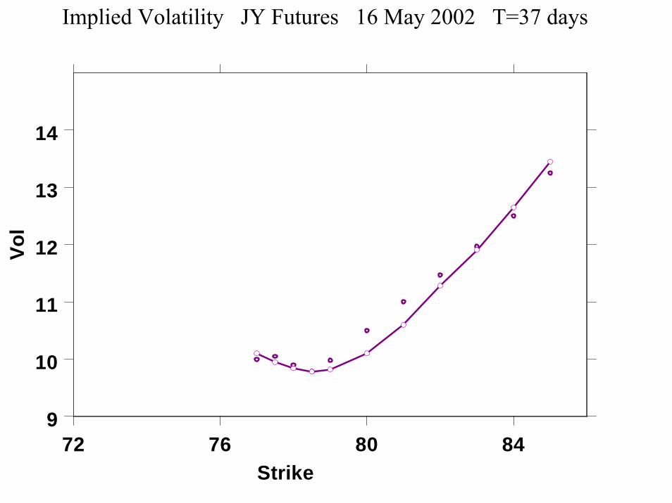
Volatility Smiles
o Empirical implied vols__ q=1.43 implied vols

72 76 80 84Strike
9
10
11
12
13
14
Vol
Implied Volatility JY Futures 16 May 2002 T=17 days
72 76 80 84Strike
9
10
11
12
13
14
Vol
Implied Volatility JY Futures 16 May 2002 T=37 days

72 76 80 84Strike
9
10
11
12
13
14
Vol
Implied Volatility JY Futures 16 May 2002 T=62 days

72 76 80 84Strike
9
10
11
12
13
14
Vol
Implied Volatility JY Futures 16 May 2002 T=82 days

72 76 80 84Strike
9
10
11
12
13
14
Vol
Implied Volatility JY Futures 16 May 2002 T=147 days

Example Currency Futures: (500 options)
1. 0.16
1.4 0.008
q Mean square relative pricing error
Benefits of a more parsimonious model:
1) Better pricing - arbitrage opportunities
2) Better hedging
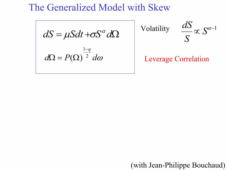
The Generalized Model with Skew
1−∝ αSSdS
Ω+ = dSSdtdS ασµ
ωdPdq
21
)(−
Ω=Ω
Volatility
Leverage Correlation
(with Jean-Philippe Bouchaud)

0 1 2 3 4
Time [Years]
-1.5
-1.0
-0.5
0.0
0.5
1.0
1.5
Ret
urn
[Hou
rly]
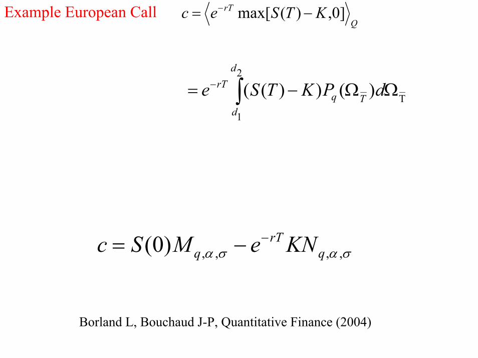
Example European CallQ
rT KTSec ]0,)(max[ −= −
∫ Τ− ΩΩ− =
2
1
)())((d
dTq
rT dPKTSe
σασα ,,,,)0( qrT
q KNeMSc −−=
Borland L, Bouchaud J-P, Quantitative Finance (2004)

5.0−=αq=1.5
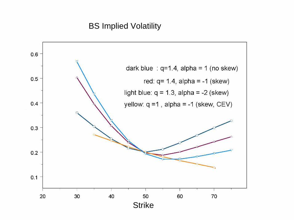
Strike
BS Implied Volatility

Strike K Strike K
T=.03
T=0.1
T=0.2
T=0.3
T=0.55
SP500 OX q=1.5, alpha = -1.
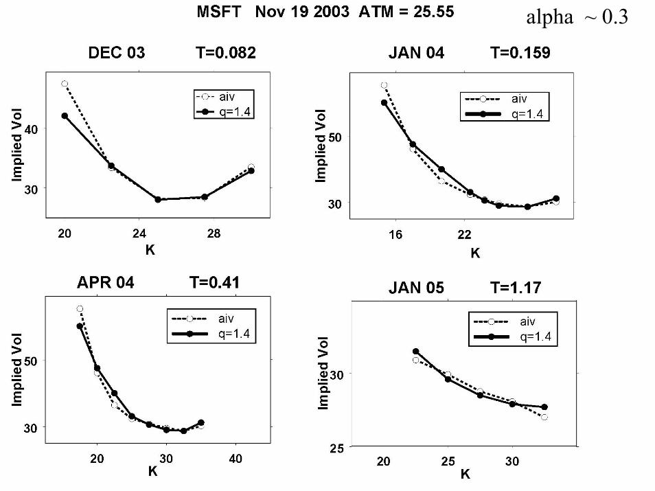
alpha ~ 0.3


4OCT30A 4OCT35A 4OCT40A 4OCT45A 4OCT50ASeries
0
5
10
15
cBid
Call Bid/Ask Theoretical value
TOL

4NOV35A 4NOV40A 4NOV45A 4NOV50AV12
0
2
4
6
8
10
12cB
id
Call Bid/Ask Theoretical value
TOL

0
5
10
15
20
cBid
4DEC25A 4DEC30A 4DEC35A 4DEC40A 4DEC45A 4DEC50A 4DEC50A 4DEC50AV56
Call Bid/Ask Theoretical value
TOL

5JAN10A 5JAN15A 5JAN20A 5JAN25A 5JAN30A 5JAN35A 5JAN40A 5JAN45A 5JAN50AV23
0
10
20
30
cBid
Call Bid/Ask Theoretical value
TOL

5MAR30A 5MAR35A 5MAR40A 5MAR45A 5MAR50AV34
0
5
10
15
cBid
Call Bid/Ask Theoretical value
TOL
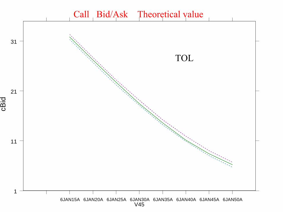
6JAN15A 6JAN20A 6JAN25A 6JAN30A 6JAN35A 6JAN40A 6JAN45A 6JAN50AV45
1
11
21
31
cBid
Call Bid/Ask Theoretical value
TOL

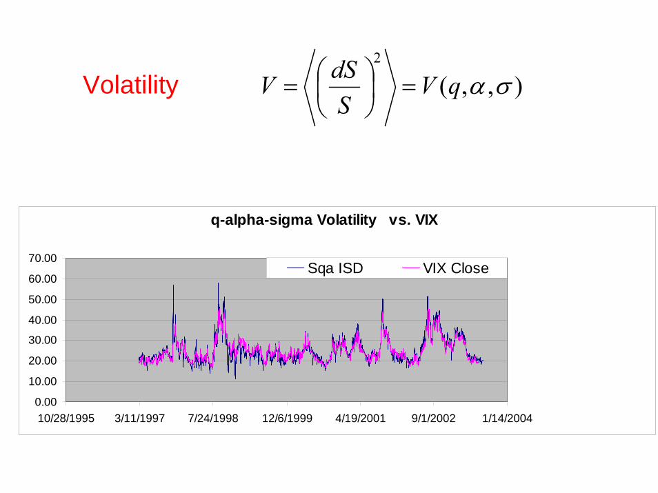
),,(2
σαqVS
dSV =⎟⎠⎞
⎜⎝⎛=Volatility
),,(2
σαqVS
dSV =⎟⎠⎞
⎜⎝⎛=Volatility
q-alpha-sigma Volatility vs. VIX
0.00
10.00
20.00
30.00
40.00
50.00
60.00
70.00
10/28/1995 3/11/1997 7/24/1998 12/6/1999 4/19/2001 9/1/2002 1/14/2004
Sqa ISD VIX Close

Options look good ….
What about pricing credit?
Borland L, Evnine J, Pochart B, cond-mat/0505359 (2005)
Chirayathumadom R, et al, Investment Practice Report Project, Stanford University (2004)

Merton Model (1974)
• Equity is a call option on underlying assets of firm
Assets = Debt + Equity
:DAT < Bond holders receive TA
Stock holders receive 0
:DAT > Stock holders receive DAT −
Bond holders receive D
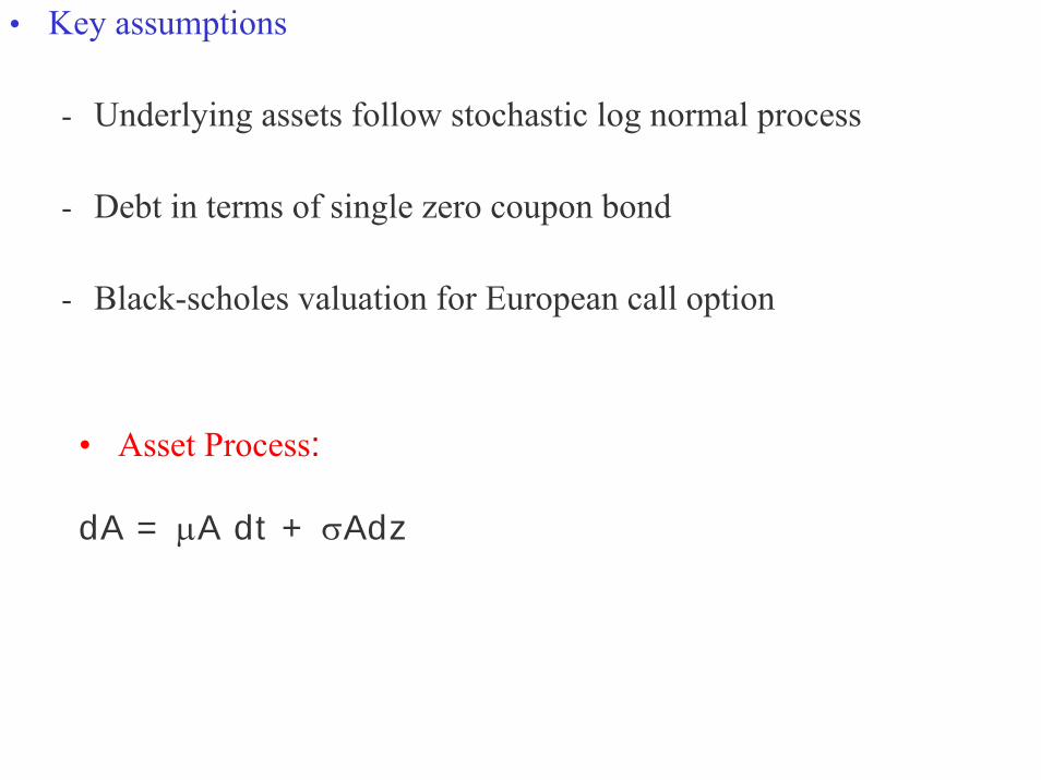
• Key assumptions
- Underlying assets follow stochastic log normal process
- Debt in terms of single zero coupon bond
- Black-scholes valuation for European call option
• Asset Process:
dA = µA dt + σAdz

• Key assumptions
- Underlying assets follow stochastic log normal process
- Debt in terms of single zero coupon bond
- Black-scholes valuation for European call option
• Asset Process:
dA = µA dt + σAdz
• Generalized Process:
dA= µA dt + σA Ωdα
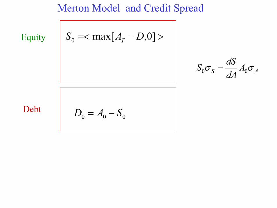
Merton Model and Credit Spread
>−=< ]0,max[ 0 DAS TEquity
000 SAD −=
AS AdAdSS σσ 00 =
Debt

Merton Model and Credit Spread
>−=< ]0,max[ 0 DAS TEquity
000 SAD −=
AS AdAdSS σσ 00 =
Debt0DDe yT =−
⎟⎠⎞
⎜⎝⎛−=− −rTDe
DT
ry 0log1Credit Spread y=risky yield

Merton Model and Credit Spread
>−=< ]0,max[ 0 DAS TEquity
000 SAD −=
AS AdAdSS σσ 00 =αα ,,00 q
rTq DNeMAS −−=
Debt0DDe yT =−
⎟⎠⎞
⎜⎝⎛−=− −rTDe
DT
ry 0log1Credit Spread y=risky yield

AnalysisSectors 1 through 7 are Aerospace, Communication, Construction, Energy, High tech equipment, Financial services and Retail
Q
00.20.40.60.8
11.21.41.6
aero
spac
e, a
uto
man
ufac
turin
g,ai
rline
s
Com
mun
icat
ion,
IT
elec
trica
l,co
nstru
ctio
nm
achi
nery
ener
gy
Equ
ipm
ents
(med
ical
and
elec
troni
c)
Fina
ncia
l ser
vice
s
reta
il, p
erso
nal
prod
ucts
, foo
dpr
oces
sing
Q values across Industry sectors
1
1.1
1.2
1.3
1.4
1.5
1.6
1
Companies
Q
q across industries q

0.4 0.6 0.8 1.0 1.2 1.4 1.6
d
0.12
0.17
0.22
0.27
0.32
0.37q=1, alpha=0q=1.2, alpha=1q=1.4, alpha=1q=1.4, alpha=0.5q=1.4, alpha=0
Standard model
“Reality”
Credit Implied volatility
D/A(0)

Results
- q mainly in range 1.2 – 1.5 and α = 0.3
- Extremely good model prediction

Summary
Non-Gaussian model well describes many features of:
Stock MarketsOption MarketsDebt and Credit Markets
Now :
Extending model of underlying

A multi-time scale non-Gaussian model of stock returns[Borland L., cond-mat/0412526 2004]
i
i
j
qjiqij dyyPw
Wdy ωσ ∑
−
−∞=
−=1
1)]|([
))()1(1(1 21jiij
ij
qq yyq
ZP −−−=− β
Motivation: Traders act on all different time horizons

A multi-time scale non-Gaussian model of stock returns[Borland L., cond-mat/0412526 2004]
i
i
j
qjiqij dyyPw
Wdy ωσ ∑
−
−∞=
−=1
1)]|([
))()1(1(1 21jiij
ij
qq yyq
ZP −−−=− β
Motivation: Traders act on all different time horizons
0jijw δ=Single-time model:
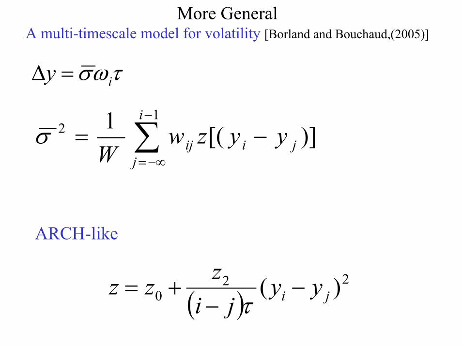
More GeneralA multi-timescale model for volatility [Borland and Bouchaud,(2005)]
τωσ iy =∆
)][(1 12
ji
i
jij yyzw
W−= ∑
−
−∞=
σ
ARCH-like
( )22
0 )( ji yyji
zzz −−
+=τ

A multi-timescale model for volatility [Borland and Bouchaud,(2005)]
τωσ iy =∆
)][(1 12
ji
i
jij yyzw
W−= ∑
−
−∞=
σ
ARCH-like
( )221
0 )()()( jiji yy
jizyy
jizzz −
−+−
−+=
ττ

A multi-timescale model for volatility [Borland and Bouchaud,(2005)]
kurtosis decay
)][(1 12
ji
i
jij yyzw
W−= ∑
−
−∞=
σ
τωσ iy =∆ aij jiw −−= )(
tailsskew
elementary timescale
( )221
0 )()()( jiji yy
jizyy
jizzz −
−+−
−+=
ττ
ARCH-like

1
0
z
z
g
τ
α
2zParameters: controls the tails
controls the memory
the elementary time scale
base volatility
skew

Calibration Universal
1
0
2
min7300/1
15.1
85.0
z
z
z
==
=
=
τ
α
controls the tails
controls the memory
the elementary time scale
base volatility
skew

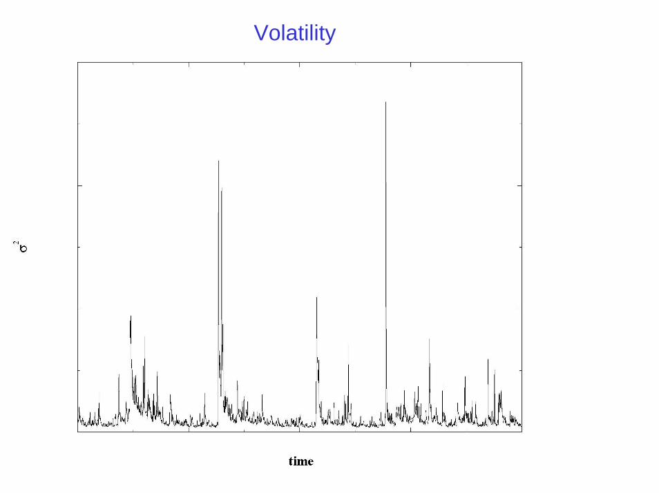
Volatility
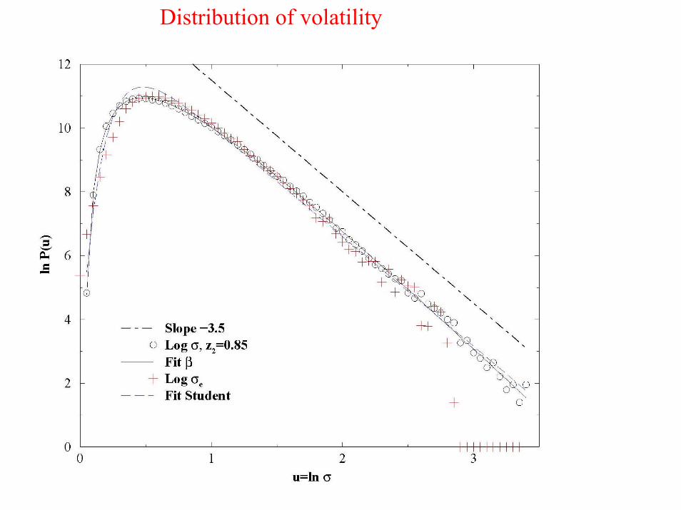
Distribution of volatility

Volatility-Volatility correlation variogram
α−2l
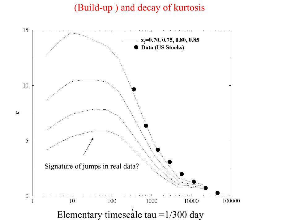
(Build-up ) and decay of kurtosis
Elementary timescale tau =1/300 day
Signature of jumps in real data?

Multifractal scaling
nlAxxlM nn
ilinζ=−= + ||)(

Evolution of 2σ conditioned on an initial volatility se22σVolatility relaxation
Matches results for SP500 [Sornette, Malevergne, Muzy, 2003)]
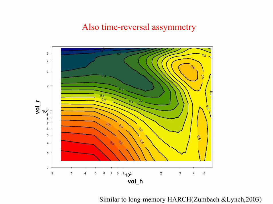
Also time-reversal assymmetry
Similar to long-memory HARCH(Zumbach &Lynch,2003)

∑∞
=+
−−=
11
2)(l
liii l
yyX α
Regression gives 9.02 ≈z

Analytic results Borland,Bouchaud 2005
• Volatility-volatility correlations: decay as
• Model well-defined with power-law tails for
• Volatility normally diffusive
α−2l
Numerical results• Tsallis distribution excellent description on all time-scales • Distribution of volatility• Multifractal scaling• Volatility relaxation• Time-reversal assymmetry• Tested premise of model on real data
tz
zy ∆−
=∆2
02
1)(
1,12 >< αz
Summary

Implications of model to market
• Soft-calibration (due to long relaxation)
• Model operating close to an instability
• Past price changes do influence future investor behavior
• Jumps (news) in addition to feedback effects
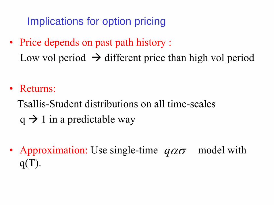
Implications for option pricing
• Price depends on past path history :Low vol period different price than high vol period
• Returns: Tsallis-Student distributions on all time-scalesq 1 in a predictable way
• Approximation: Use single-time model with q(T).
ασq

Conclusions
- Simple multi-time scale model
-Captures many statistical properties of real returns
-Closed form solution for single time case: options,credit
-Current and future work: General analytic solution

References:
Borland L, Phys. Rev.Lett 89 (2002)
Borland L, Quantitative Finance 2 (2002)
Borland L, Bouchaud J-P, Quantitative Finance(2004)
Chirayathumadom R, et al, Investment Practice Report Project, Stanford University (2004)
Borland L, cond-mat/04122526 (2004)
Borland L, Evnine J, Pochart B, cond-mat/0505359 (2005)
Borland L, Bouchaud J-P, Muzy J-F, Zumbach G, Wilmott Magazine, (March 2005)
Borland L, Bouchaud J-P,arXiv:physics/0507073 (2005)