HAL Id: hal-01353985https://hal-enac.archives-ouvertes.fr/hal-01353985

Submitted on 16 Aug 2016

HAL is a multi-disciplinary open accessarchive for the deposit and dissemination of sci-entific research documents, whether they are pub-lished or not. The documents may come fromteaching and research institutions in France orabroad, or from public or private research centers.

L’archive ouverte pluridisciplinaire HAL, estdestinée au dépôt et à la diffusion de documentsscientifiques de niveau recherche, publiés ou non,émanant des établissements d’enseignement et derecherche français ou étrangers, des laboratoirespublics ou privés.

Study on the cross-correlation of GNSS signals andtypical approximations

Myriam Foucras, Jérôme Leclère, Cyril Botteron, Olivier Julien, ChristopheMacabiau, P.-A. Farine, Bertrand Ekambi

To cite this version:Myriam Foucras, Jérôme Leclère, Cyril Botteron, Olivier Julien, Christophe Macabiau, et al.. Studyon the cross-correlation of GNSS signals and typical approximations. GPS Solutions, Springer Verlag,2016, �10.1007/s10291-016-0556-7�. �hal-01353985�

1

Study on the cross-correlation of GNSS signals and typical

approximations

Myriam Foucras · Jérôme Leclère · Cyril Botteron · Olivier Julien · Christophe

Macabiau · Pierre-André Farine · Bertrand Ekambi

Abstract In global navigation satellite system

(GNSS) receivers, the first signal processing stage

is the acquisition, which consists of detecting the

received GNSS signals and determining the

associated code delay and Doppler frequency by

means of correlations with a code and a carrier

replicas. These codes, as part of the GNSS signal,

were chosen to have very good correlation

properties without considering the effect of a

potential received Doppler frequency. In the

literature, it is often admitted that the maximum

GPS L1 C/A code cross-correlation is about

−24 dB. We show that this maximum can be as

high as −19.2 dB when considering a Doppler

frequency in a typical range of [−5, 5] kHz. We

also show the positive impact of the coherent

integration time on the cross-correlation, and that

even a satellite with Doppler outside the frequency

search space of a receiver impacts the cross-

correlation. In addition, the expression of the

correlation is often provided in the continuous

time domain while its implementation is typically

made in the discrete domain. It is then legitimate

to ask the validity of this approximation.

Therefore, the purpose of this research is twofold.

First, we discuss typical approximations and

evaluate their regions of validity. Second, we

provide characteristic values such as maximums

and quantiles of the auto and cross-correlation of

the GPS L1 C/A and Galileo E1 OS codes in

presence of Doppler, for frequency ranges up to 50

kHz, and for different integration times.

Keywords

Acquisition · Correlation · Cross ambiguity

function · Doppler · Galileo · GPS

Introduction

The first stage of a global navigation satellite

system (GNSS) receiver is acquisition, which

consists in determining the Doppler frequency and

the code delay of the received GNSS signals (Van

Diggelen 2009, pp 127-224). As shown in Fig. 1,

this is done by multiplying the received signal

with local replicas of the carrier and of the code

and integrating the result during a certain time,

called coherent integration time and denoted .

The output value then provides the degree of

similarity between the replicas and the received

signal. Since the receiver does not know a priori

the Doppler frequency and the code delay, the

different possibilities have to be tested. The output

of the acquisition, which is a two-dimensional

function of the code delay and Doppler frequency,

is called the cross ambiguity function, or CAF

(Ipatov 2005, pp. 7-76; Motella et al. 2010). An

illustration of a CAF is given in Fig. 1, with a GPS

L1 C/A signal where the incoming signal has a

Doppler frequency of 2600 Hz and a code delay of

766 chips. The evaluation of the CAF can be

performed sequentially by computing one point

after the other, or in parallel using methods based

on fast Fourier transforms (FFT) (Akopian 2005;

Foucras et al. 2012; Leclère et al. 2013).

incoming

signal

localcode

local carrier

Integration ǀ · ǀ

Fig. 1 Principle of the acquisition (top),

Illustration of the cross ambiguity function for a

GPS L1 C/A signal (bottom)

2

Quite often in the literature, approximate

models are used for the expression of the CAF.

However, the validity of such approximations has

not been completely justified. For example, the

model provided in Spilker (1996, pp. 57-120), and

Holmes (2007, pp. 349-472) considers that the

result of the codes correlation is independent from

the carrier Doppler frequency, which is actually

not the case. Indeed, the real auto and cross-

correlations of the GNSS codes can be affected by

a Doppler frequency. For example, Spilker (1996,

pp. 57-120) and Kaplan et al. (2005, pp. 113-152)

provide the probability that the cross-correlation

of C/A codes reaches a certain level, but only for

Doppler frequencies multiples of 1 kHz. However,

as shown later, these frequencies do not

necessarily correspond to the worst cases, because

they depend on the coherent integration time used.

Some papers already discussed the impact of the

cross-correlation with a Doppler on the carrier-to-

noise ratio or on the tracking discriminator error

(Raghavan et al. 1999,Van Dierendonck et al.

2002, Balaei and Akos 2011, Lestarquit and

Nouvel 2012, Margaria et al. 2012). Other papers

discussed the performance of several families of

GNSS codes, looking at the auto and cross-

correlations affected by the carrier Doppler and by

the data bit transitions (Soualle et al. 2005,

Wallner et al. 2007, Soualle 2009, Qaisar and

Dempster 2010). However, the impact of the

Doppler frequency is essentially studied only for

several frequency candidates or for a small

frequency range. Qaisar and Dempster (2007) also

presents some results regarding the impact of the

sampling frequency and of the Doppler on the

code correlation, but only for some specific

values.

Therefore, what is missing in the literature is a

more exhaustive study regarding the impact of the

Doppler frequency for an extensive set of values

and the coherent integration time used. Here, we

give the auto and cross-correlation results for

Doppler frequencies in different frequency ranges

corresponding to specific GNSS applications, and

the impact of the coherent integration time is also

discussed.

The first section presents the signals definitions

and the assumptions used. The second section

deals with the study of the usual approximations

on the CAF. The main objective is to provide the

associated region of validity of the

approximations. The results regarding the impact

of the Doppler frequency in the CAF are presented

in the third section, for the GPS L1 C/A and

Galileo E1 OS codes. This allows us to compare

the auto and cross-correlation properties for each

signal. Finally, conclusions are provided.

Signals definitions

The GPS L1 C/A signal transmitted by a satellite

can be defined as

(1)

where is the time, is the amplitude of the

signal, is the pseudo random noise (PRN) code,

is the data, and is the carrier frequency

used by the satellite (Navstar 2014). The GPS L1

C/A codes contain 1023 chips and are generated

with a chipping rate of 1.023 MHz, the code

length is thus 1 ms.

At the receiver antenna, the signal is the sum of

signals coming from satellites, where each

signal is the transmitted signal that has been

respectively attenuated, delayed and affected by

the Doppler effect. After the antenna, there is the

front-end where the signal is amplified, filtered,

down-converted to baseband or to an intermediate

frequency , and sampled at a frequency . At

the output of the front-end, considering a complex

sampling, the signal received can be defined as

∑

( ( ) )) (2)

where is the sampling period ( ), is

the delay of the code, is the Doppler

frequency, is the carrier phase, and is a white

Gaussian noise of zero mean coming from the

thermal noise. Note that this model does not take

into account some effects, such as the Doppler

effect on the code, since it can be neglected

regarding the small coherent integration times

considered later, or the impact of the oscillator on

the sampling frequency (Leclère 2014). Note also

that we consider a complex sampling because with

a real sampling there would be a term with the

sum of frequencies after the mixing with the local

carrier that would impact the correlation result

3

(Motella et al. 2010). Since we want to investigate

specifically the impact of the Doppler frequency

and of the coherent integration time, this double

frequency term is not wanted. However, the results

considering a real or complex sampling would be

relatively similar.

In the same way, considering the Galileo E1 OS

signal which has a data component and a data free

component called pilot, the signal after the front-

end can be written as

∑( (

)

( ( ) )) (3)

where is the secondary code on the pilot

component, and and denote the data and

pilot subcarriers due to CBOC modulation as

defined in European Union (2015). The Galileo E1

OS codes contain 4092 chips and are generated

with a chipping rate of 1.023 MHz, the codes

length is thus 4 ms.

In this study, it is assumed that the navigation

data and secondary code are constant during

the integration. See Wallner et al. (2007) and

Soualle (2009) for some results considering a bit

sign transition during the integration. Also, the

filtering and quantization performed by the front-

end are not taken into account. See Curran et al.

(2010) for more details about that topic. Finally,

the noise term is not considered since the focus of

this research is on the correlation properties.

Study of usual approximations

In this section, we perform a study on two typical

approximations, the first uses a continuous time

domain model although actual processing is

performed in discrete time domain, and the second

models the CAF assuming that the code and

Doppler are independent. For simplicity, we

develop the results for the GPS L1 C/A signal, i.e.

, since they can be easily extended to the

Galileo E1 OS signal and other GNSS signals.

Approximation continuous/discrete

In the literature, e.g. Kaplan et al. (2005, pp. 113-

152) and Holmes (2007, pp. 349-472), the output

of the CAF is often modeled by the following

continuous time version:

( ) (4)

|∫

|

| ∫

( ( ) ) |

where the superscript stands for continuous,

denotes the L1 C/A code number of the code

received, denotes the L1 C/A code number of the

code replica, is the local estimate of the code

delay, and is the local estimate of the carrier

frequency. This expression is an approximation of

what is really performed in a GNSS receiver since

the signals are actually discrete. Thus, the actual

output of the CAF is

( ) (5)

|∑

|

| ∑

( ( ) )|

where the superscript stands for discrete, and

is the number of samples during the coherent

integration time, i.e. . Remember that (5)

is still an approximation, since it does not take into

account the filtering of the front-end and the other

factors mentioned in the previous section.

Therefore, the question is “are the results

obtained with (4) close to those obtained with

(5) ?”, which is intuitively believed to be the case.

To check this, both equations have been evaluated

for all the GPS L1 C/A codes, with a step of 10 Hz

for over a range of 50 kHz and a step of 1 chip

for , and considering one sample per chip. The

details of how to compute exactly the integral of

(4) are given in the Appendix.

Fig. 2 shows the difference between ( )

and ( ) as function of the code delay and

Doppler frequency, and shows the distribution of

this difference. It can be seen that the higher the

Doppler frequency, the higher is the difference

4

between the two results, but this difference is

clearly negligible since the maximum difference is

0.0342 dB for a Doppler of 50 kHz. Therefore, we

can conclude that using (4) as approximation of

(5) is a valid hypothesis.

Fig. 2 Difference between the CAF in the discrete

and continuous cases, i.e. ( )

( ),

assuming receiving and generating L1 C/A code 1

Approximation on cross ambiguity function

In the literature, e.g. Holmes (2007, pp. 349-472),

the output of the CAF is often approximated as

( ) | ( )| (6)

where is the difference of code

delays, is the difference of carrier

frequencies, and is the cross-correlation

between the codes and , defined as

∫

(7)

If , is the autocorrelation of the code .

The approximation given by (6) is the result of the

following operation:

( ) (8)

|∫

∫ ( ( ) )

|

which is clearly not equal to (4). In Holmes (2007,

pp. 349-472), it is mentioned that in (6) has

been factored out of the integral as an

approximation assuming that is small compared

to the chip rate.

Fig. 3 Comparison of the CAF of L1 C/A code 1

computed using (4) and (6) when chip

(top), and Hz (bottom)

Therefore, the question is “when this

approximation is valid, i.e. when the results

obtained with (6) are equal or very close to those

obtained with (4) ?”. First, it can be easily checked

that if , i.e. , or if , i.e.

, equation (6) is identical to (4), i.e.

( )

( ) (9)

5

( )

( ) (10)

This is illustrated by Fig. 3with ms. As

a note, the CAF is symmetric with respect to

, but not to . Note that the model used

does not consider any filtering; in practice the

bandwidth is limited and the correlation peak is

rounded.

Fig. 4 Comparison of the CAF of L1 C/A code 1

computed using (4) and (6) when | | chip.

chip (top), chip (middle),

chip (bottom)

Fig. 5 Comparison of the CAF of L1 C/A code 1

computed using (4) and (6) when | | chip.

chips (top), chips (middle),

chips (bottom)

Then, as shown in Fig. 4, if | | chip, the

approximation is very close to the exact value

when kHz, i.e. for the main lobe of the

sinc. Outside the main lobe, the approximation

differs from the exact value. The higher | |, the

higher is the difference. However, when | |

chip, there are two cases as shown in Fig. 5 and

Fig. 6. If the code autocorrelation without Doppler

is very low, i.e. near −60 dB, a small error in the

Doppler such as dozens of hertz will imply few dB

of difference rapidly. However, if the code

autocorrelation without Doppler is not too low, i.e.

near −24 dB, the difference will be seen for a

higher error in the Doppler, from hundreds of

hertz, i.e. for frequencies within the main lobe.

Finally, regarding the cross-correlation between

two different codes, shown in Fig. 7, this case is

similar to the case of the autocorrelation with

| | chip shown in Fig. 5.

Fig. 6 Comparison of the CAF of L1 C/A code 1

computed using (4) and (6) when | | Hz.

Hz (top), Hz (middle),

Hz (bottom)

Fig. 7 Comparison of the CAF of L1 C/A code 1/

L1 C/A code 2 computed using (4) and (6).

chips (top), chips (middle),

chips (bottom)

6

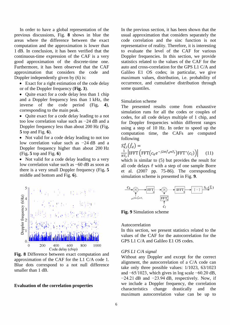
In order to have a global representation of the

previous discussions, Fig. 8 shows in blue the

areas where the difference between the exact

computation and the approximation is lower than

1 dB. In conclusion, it has been verified that the

continuous-time expression of the CAF is a very

good approximation of the discrete-time one.

Furthermore, it has been observed that the CAF

approximation that considers the code and

Doppler independently given by (6) is:

Exact for a right estimation of the code delay

or of the Doppler frequency (Fig. 3).

Quite exact for a code delay less than 1 chip

and a Doppler frequency less than 1 kHz, the

inverse of the code period (Fig. 4),

corresponding to the main peak.

Quite exact for a code delay leading to a not

too low correlation value such as −24 dB and a

Doppler frequency less than about 200 Hz (Fig.

5 top and Fig. 6).

Not valid for a code delay leading to not too

low correlation value such as −24 dB and a

Doppler frequency higher than about 200 Hz

(Fig. 5 top and Fig. 6)

Not valid for a code delay leading to a very

low correlation value such as −60 dB as soon as

there is a very small Doppler frequency (Fig. 5

middle and bottom and Fig. 6).

Fig. 8 Difference between exact computation and

approximation of the CAF for the L1 C/A code 1.

Blue dots correspond to a not null difference

smaller than 1 dB.

Evaluation of the correlation properties

In the previous section, it has been shown that the

usual approximation that considers separately the

code correlation and the sinc function is not

representative of reality. Therefore, it is interesting

to evaluate the level of the CAF for various

Doppler frequencies. In this section, we provide

statistics related to the values of the CAF for the

auto and cross-correlation for the GPS L1 C/A and

Galileo E1 OS codes; in particular, we give

maximum values, distribution, i.e. probability of

occurrence, and cumulative distribution through

some quantiles.

Simulation scheme

The presented results come from exhaustive

simulation runs for all the codes or couples of

codes, for all code delays multiple of 1 chip, and

for Doppler frequencies within different ranges

using a step of 10 Hz. In order to speed up the

computation time, the CAFs are computed

following

( )

| ( (

) )| (11)

which is similar to (5) but provides the result for

all code delays with a step of one sample Borre

et al. (2007 pp. 75-86). The corresponding

simulation scheme is presented in Fig. 9.

IFFTFFT

FFT*

cl

–j2π fd nTse

ck Sk,l ( fd )ǀ · ǀ

N

N N

Fig. 9 Simulation scheme

Autocorrelation

In this section, we present statistics related to the

values of the CAF for the autocorrelation for the

GPS L1 C/A and Galileo E1 OS codes.

GPS L1 C/A signal

Without any Doppler and except for the correct

alignment, the autocorrelation of a C/A code can

take only three possible values: 1/1023, 63/1023

and −65/1023, which gives in log scale −60.20 dB,

−24.21 dB and −23.94 dB, respectively. Now, if

we include a Doppler frequency, the correlation

characteristics change drastically and the

maximum autocorrelation value can be up to

7

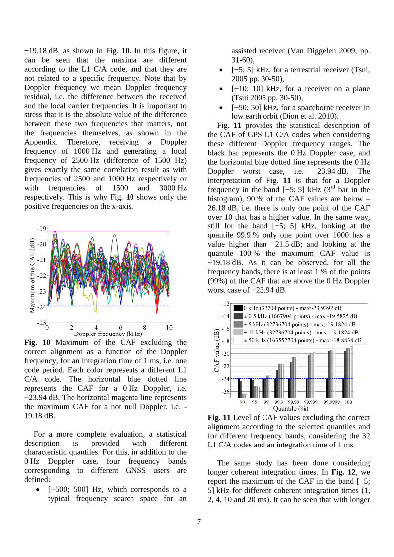
−19.18 dB, as shown in Fig. 10. In this figure, it

can be seen that the maxima are different

according to the L1 C/A code, and that they are

not related to a specific frequency. Note that by

Doppler frequency we mean Doppler frequency

residual, i.e. the difference between the received

and the local carrier frequencies. It is important to

stress that it is the absolute value of the difference

between these two frequencies that matters, not

the frequencies themselves, as shown in the

Appendix. Therefore, receiving a Doppler

frequency of 1000 Hz and generating a local

frequency of 2500 Hz (difference of 1500 Hz)

gives exactly the same correlation result as with

frequencies of 2500 and 1000 Hz respectively or

with frequencies of 1500 and 3000 Hz

respectively. This is why Fig. 10 shows only the

positive frequencies on the x-axis.

Fig. 10 Maximum of the CAF excluding the

correct alignment as a function of the Doppler

frequency, for an integration time of 1 ms, i.e. one

code period. Each color represents a different L1

C/A code. The horizontal blue dotted line

represents the CAF for a 0 Hz Doppler, i.e.

−23.94 dB. The horizontal magenta line represents

the maximum CAF for a not null Doppler, i.e. -

19.18 dB.

For a more complete evaluation, a statistical

description is provided with different

characteristic quantiles. For this, in addition to the

0 Hz Doppler case, four frequency bands

corresponding to different GNSS users are

defined:

[−500; 500] Hz, which corresponds to a

typical frequency search space for an

assisted receiver (Van Diggelen 2009, pp.

31-60),

[−5; 5] kHz, for a terrestrial receiver (Tsui,

2005 pp. 30-50),

[−10; 10] kHz, for a receiver on a plane

(Tsui 2005 pp. 30-50),

[−50; 50] kHz, for a spaceborne receiver in

low earth orbit (Dion et al. 2010).

Fig. 11 provides the statistical description of

the CAF of GPS L1 C/A codes when considering

these different Doppler frequency ranges. The

black bar represents the 0 Hz Doppler case, and

the horizontal blue dotted line represents the 0 Hz

Doppler worst case, i.e. −23.94 dB. The

interpretation of Fig. 11 is that for a Doppler

frequency in the band [−5; 5] kHz (3rd

bar in the

histogram), 90 % of the CAF values are below –

26.18 dB, i.e. there is only one point of the CAF

over 10 that has a higher value. In the same way,

still for the band [−5; 5] kHz, looking at the

quantile 99.9 % only one point over 1000 has a

value higher than −21.5 dB; and looking at the

quantile 100 % the maximum CAF value is

−19.18 dB. As it can be observed, for all the

frequency bands, there is at least 1 % of the points

(99%) of the CAF that are above the 0 Hz Doppler

worst case of −23.94 dB.

Fig. 11 Level of CAF values excluding the correct

alignment according to the selected quantiles and

for different frequency bands, considering the 32

L1 C/A codes and an integration time of 1 ms

The same study has been done considering

longer coherent integration times. In Fig. 12, we

report the maximum of the CAF in the band [−5;

5] kHz for different coherent integration times (1,

2, 4, 10 and 20 ms). It can be seen that with longer

8

integration times, the values on multiples of 1 kHz

are the same while the values on not multiples of

1 kHz decrease. Therefore, when the coherent

integration time is longer than the code period, the

CAF maximums are on multiples of 1 kHz.

Fig. 12 Maximum of the CAF excluding the

correct alignment of the GPS L1 C/A code 1 as a

function of the Doppler frequency, for integration

times of 1, 2, 4, 10 and 20 ms, respectively

This can be intuitively explained looking at the

spectrum of L1 C/A codes. Since the C/A codes

are periodic with a period of 1 ms, their spectrum

is discrete and the spectral lines are spaced by

1 kHz (Spilker 1996, pp. 57-120), as illustrated in

Fig. 13 (left) which zooms around 0 Hz, and

where the height of each line depends on the code.

The product of two L1 C/A codes is another L1

C/A code of the same period (Spilker 1996, pp.

57-120) therefore its spectrum is similar. A C/A

code with a carrier Doppler has a spectrum almost

similar to the one of a C/A code except that it is

shifted, as illustrated Fig. 13 (right). Therefore, the

product of a received C/A code with a carrier

Doppler by a local C/A code will have a spectrum

as shown in Fig. 13 (bottom). Such signal is then

integrated; the transfer function of the integration

is a sinc function as illustrated in Fig. 13 (bottom).

Therefore, considering first an integration time of

1 ms, if the incoming signal has no Doppler, we

have the spectrum shown in Fig. 14 (top left),

where it can be seen that only the line at 0 Hz is

kept after the integration. If the incoming signal

has a Doppler of 500 Hz, we have the spectrum

shown in Fig. 14 (middle left), and all the

spectrum lines will be attenuated but conserved. If

the incoming signal has a Doppler of 1000 Hz, we

have the spectrum shown inFig. 14 (bottom left),

and again only the line at 0 Hz is kept after the

integration.

Now, if we consider an integration time of

4 ms, the width of the sinc in the transfer function

will be four times smaller. If the incoming signal

has a Doppler that is a multiple of 1 kHz, see Fig.

14 (top and bottom right), only the line at 0 Hz is

kept after the integration, which gives exactly the

same result as with an integration of 1 ms. This

explains why the correlation value is the same for

Doppler that are multiple of 1 kHz whatever the

integration time is. But now, with a Doppler that is

a multiple of

, all the spectrum lines

will be cancelled as shown in Fig. 14 (middle

right). This explains the nulls that appear in Fig.

12 when the integration time is increased. Note

that these nulls can also be found analytically

using (17), given in the Appendix. Finally, for

other Doppler shifts all the spectrum lines will be

attenuated and conserved, but the attenuation is

much more compared to an integration time of

1 ms, which explains the lower CAF values.

f (kHz)1 20

1 20T T

f (kHz)

f (kHz)1 20

Fig. 13 Spectrum of a C/A code without carrier

Doppler (left), spectrum of a C/A code with a

carrier Doppler (right), transfer function of an

integration of duration ms (bottom)

9

1 20

1 20

1 20

1 20

1 20

1 20

Dopple

r

of

0 H

z

f (kHz)

f (kHz)

f (kHz)

f (kHz)

f (kHz)

f (kHz)

Dopple

r

of

0.5

kH

z

Dopple

r

of

1 k

Hz

Integration time of 1 ms Integration time of 4 ms

Fig. 14 Spectrum of a C/A code shifted by a

Doppler frequency of 0 Hz (top), 500 Hz (middle)

and 1 kHz (bottom), and transfer function using

1 ms of integration time (left) and using 4 ms of

integration time (right)

These observations are completed with the

distributions of the CAF presented in Fig. 15. For

example, with an integration time of 1 ms, 90 % of

the values are below −26.35 dB, as already shown

in Fig. 11, whereas with an integration time of

20 ms, 90 % of the values are below −44.56 dB

(more than 18 dB). In conclusion, the use of a

coherent integration time longer than the code

period is much better in terms of cross-correlation

protection.

Fig. 15 Cumulative distribution of the CAF

excluding the correct alignment of L1 C/A code 1,

for different coherent integration times, and a

search space of [–10; 10] kHz

Galileo E1 OS

The same study is now presented for the Galileo

E1 OS signal. In this case, only the first 3 Doppler

frequency ranges are considered. Indeed, because

of the higher number of codes and number of code

delays, to be exhaustive the quantiles should be

computed on several tens of billions of points for a

Doppler range of [−50; 50] kHz, which is not

possible due to Matlab memory limits (using

Matlab R2014a version).

Unlike GPS L1 C/A codes, for Galileo E1 OS

codes, when not considering Doppler frequency,

the number of possible autocorrelation or cross-

correlation values is not limited to 4 values.

However, thanks to their longer lengths, 4 ms

instead of 1 ms, the maximum autocorrelation

value excluding the correct alignment of Galileo

E1 codes is −25.39 dB without Doppler, which is

lower than the maximum of –23.94 dB with the

GPS L1 C/A codes. Nonetheless, with a Doppler

up to 10 kHz, the maximum can be up to

−23.45 dB.

Fig. 16 shows the values for some probabilities

of occurrence for the different frequency bands

and for the data and pilot codes. It can be observed

that the autocorrelation properties of the Galileo

E1 OS codes assigned to the data component are

equivalent to those of the codes assigned to the

pilot component in terms of distribution, and that

the autocorrelation without any Doppler has

indeed a multitude of different levels. It can also

be observed that there is a global improvement of

2 to 8 dB compared to the GPS L1 codes, thanks

to a code length that is four times longer.

10

Fig. 16 Level of CAF values excluding the correct

alignment according to the selected quantiles and

for different frequency bands, considering the 100

Galileo E1 OS codes and an integration time of

4 ms. Galileo E1 OS data codes (top), Galileo E1

OS pilot codes (bottom)

Obviously, in the case of the Galileo E1 OS

signals, and more generally for the modernized

GNSS signals, bit sign transitions can occur at

each spreading code period whereas for GPS L1

C/A signals, 19 spreading code periods are free of

bit transitions (Foucras 2015). In this study, it is

assumed that there is no bit sign transition.

The maximum of the CAF is shown in Fig. 17

for the band [−5; 5] kHz and different integration

times. It can be seen that the values on the

multiples of 250 Hz are the same whatever is the

integration time, which was expected given the

4 ms period of the primary codes.

Fig. 17 Maximum of the CAF excluding the

correct alignment of the Galileo E1 OS data code

1 as function of the Doppler frequency, for

integration times of 4, 8, 12, 16 and 20 ms,

respectively

Concluding this section on the autocorrelation,

we present Table 1, which allows us to compare

the autocorrelation values for the presented

quantiles. When comparing the GPS L1 C/A and

Galileo E1 OS code isolations, it can be observed

that Galileo E1 OS codes have better correlation

performance for an integration time equal to the

spreading code period, with an improvement

between 4 and 6 dB. Even if we compare both

code families with the same integration time of

4 ms, the maximum is at least 2 dB lower for

Galileo E1 OS codes. However, for a coherent

integration time of 20 ms, which corresponds to 20

L1 C/A code periods or 5 Galileo E1 OS code

periods, the lowest quantiles (90 % and 95 %) are

lower for GPS L1 C/A. But things are different for

the other quantiles (99 % and above) for which

Galileo E1 codes perform better by at least 3 dB.

This can be understood looking at Fig. 12 and Fig.

17, where we can see that there are more high

lobes with the Galileo E1 OS signal, but the local

maxima are still below the local maxima of the

GPS L1 C/A signal. Note that only the first 6

Galileo E1 OS data codes have been used due to

memory constraints. It is important to note that

these results do not take into account the square

sub-carrier modulation of BOC modulation.

11

Table 1 Levels of CAF values in dB according to

the distribution considering [–10; 10] kHz as range

for the Doppler frequency. For the integration time

of 20 ms, only the first 6 Galileo E1 OS data codes

have been used due to memory constraints.

(ms) 1

4

4

20

20

Signal

GP

S L

1

C/A

GP

S L

1

C/A

Gal

ileo

E1 O

S

GP

S L

1

C/A

Gal

ileo

E1 O

S

90 % −26.3 −30.3 −32.5 −44.6 −38.4

95 % −25.1 −27.1 −37.4 −37.7 −35.7

99 % −23.5 −24.2 −29.5 −29.0 −32.3

99.9 % −21.7 −22.7 −27.7 −24.7 −29.6

99.99 % −20.6 −21.1 −25.5 −21.3 −26.6

99.999 % −19.9 −21.1 −25.5 −21.3 −26.6

99.9999 % −19.4 −21.1 −24.7 −21.1 −25.7

Max −19.2 −21.1 −23.4 −21.1 −24.7

Cross-correlation

In this section, we present statistics related to the

values of the CAF for the cross-correlation for the

GPS L1 C/A and Galileo E1 OS codes. As it will

be shown, the results are relatively similar to those

of the autocorrelation.

GPS L1 C/A

In presence of Doppler, the cross-correlation is

similar to the autocorrelation, i.e. for an

integration time of 1 ms, the maximum cross-

correlation value can be up to −19.1 dB, as shown

in Fig. 18. The statistics for a Doppler range of

[−10; 10] kHz are provided in Table 2. For longer

integration times, a behavior similar to the one

shown in Fig. 12 will be observed, and the

maximum is obtained for a Doppler that is a

multiple of 1 kHz.

Van Diggelen (2009, p.219) states regarding

detection problem due to cross-correlations that

“both the code delay and the frequency offset of

the incorrect (strong) satellite would have to be in

the same search zone as the intended (weak)

satellite”. However, this statement is not correct,

because as demonstrated in the Appendix, what

matters is the difference between the received and

local frequencies For example, let us consider a

receiver with a frequency search space of

±500 Hz, which receives two GPS L1 C/A signals,

one weak with a Doppler of 300 Hz (PRN 1) and

one strong with a Doppler of 4100 Hz (PRN 2).

When the receiver will search PRN 1 and compute

the correlation with a local Doppler of 100 Hz,

there will be a high cross-correlation with the

incoming PRN 2 signal, because the difference

between its frequency and the local one is 4 kHz,

which is a multiple of 1 kHz.

Fig. 18 Distribution of the maximum of the cross-

correlation function per GPS L1 C/A codes couple

considering [−10; 10] kHz as range for the

Doppler frequency

Galileo E1 OS

For Galileo E1 OS signals, two kinds of cross-

correlation should be considered. The first one

deals with the correlation between the data and

pilot codes assigned to the same satellite.

Fig. 19 Level of CAF values according to the

selected quantiles and for different frequency

bands, considering the 50 Galileo E1 OS code

data/pilot couples of each satellite and an

integration time of 4 ms

Fig. 19 presents the statistical description of this

cross-correlation. With Doppler frequency in the

12

range [−10; 10] kHz, the worst isolation is

−23.62 dB.

The second Galileo cross-correlation

corresponds to the correlation between 2 codes

from two different satellites, Data and Data, Pilot

and Pilot, Data and Pilot. Table 2 allows us to

compare the maximum of each cross-correlation.

The best isolation is for a code couple assigned to

the same satellite. Indeed, they are chosen as

orthogonal as possible to not interfere for the

correlation of the local component with the

received Galileo E1 OS signal.

Table 2 Levels of CAF values in dB according to

the distribution considering [−10; 10] kHz as

range for the Doppler frequency. Blank elements

for Galileo E1 OS in the table were not computed

due to the high number of combinations.

GPS

L1 C/A

(1 ms)

Galileo E1 OS (4 ms)

Dat

a/P

ilot

Dat

a/D

ata

Pil

ot/

Pil

ot

Sam

e

sate

llit

e

90 % −26.2

95 % −24.9

99 % −23.5

99.9 % −21.6

99.99 % −20.5

99.999 % −19.8

99.9999 % −19.3

Max −19.1 −22.8 −22.6 −23.0 −23.6

Conclusion

We have presented various results regarding the

correlations of the GPS L1 C/A and Galileo E1 OS

codes. Some results are relatively well-known by

people working in the GNSS field but have been

clarified, while some of them are less known.

In a first part, we have studied the validity of

some approximations generally used. First, it was

shown that the discrete summations done in GNSS

receivers due to the sampling can be approximated

by a continuous integration, as intuitively

expected. The second point was about the classical

correlator output expression, which considers the

code and the Doppler frequency as independent.

The region of validity of this expression has been

clarified, and it is not only around the main peak

as it is often thought, but also for relatively low

Doppler frequencies, such as one or two hundreds

of hertz with the GPS L1 C/A signal, when the

theoretical code correlation is not extremely low,

e.g. near −24 dB.

In a second part, we have provided a statistical

description of the autocorrelation and cross-

correlation for GPS L1 C/A and Galileo E1 OS

codes, considering different carrier frequency

bands. For example, it has been shown that

Galileo E1 OS codes have a lower cross-

correlation than the GPS L1 C/A codes for any

Doppler frequency between −10 and 10 kHz

considering an integration time of one code

period, namely −23.44 dB against −19.18 dB.

When considering all potential Doppler

frequencies, comparing to no Doppler frequency

the isolation is degraded by a maximum of about

2 dB and 4.75 dB for Galileo E1 OS and GPS L1

C/A respectively. The same trends were shown for

the cross-correlation. For GPS L1 C/A, the

isolation is ensured to be at the minimum –

19.08 dB for any Doppler frequency between –10

and 10 kHz, which is 2 dB lower than the classical

value given in the literature which is only valid for

frequencies that are multiple of 1 kHz. For Galileo

E1 OS, the isolation between data and pilot codes

affected to the same satellite is −22.82 dB, which

is 2.34 dB higher than any couple of Galileo E1

OS codes. We have also highlighted the

significant impact of the coherent integration time,

and shown that having a coherent integration time

longer than the code period provides much better

correlation performance. We have also shown that

even the satellites which are outside the frequency

search space impact the correlation result, since

what matters is the difference between the

frequencies, and not the frequencies themselves.

This study could be extended in many ways.

First, other GNSS signals could be considered.

Then, it could be extended by considering

different sampling frequencies, since the sampling

13

frequency also changes the code correlation

properties. Finally, in the same way, the impact of

the code Doppler could be studied, especially with

signals having a chipping rate of 10.23 MHz or

having pilot channels which enable long coherent

integration.

Acknowledgments

The authors would like to thank Chris J. Hegarty,

Jack. K. Holmes, Francis Soualle and Phillip W.

Ward, for their valuable comments and advice.

Appendix: Computation of the continuous-time

CAF

This appendix shows how to compute numerically

the continuous-time expression given by (4). A

PRN code is a succession of chips of duration ,

whose value can be 1 or −1, that repeats each

chips; thus the duration of one code period is

. A PRN code is illustrated in Fig. 20,

and can be defined as

∑ ∑ [ ]

(12)

where indicates the PRN number, [ ] is the

PRN sequence, and is a

boxcar function with the unit step function.

Then, the product of a PRN code of chips

with another PRN code of chips shifted by

chips is another code. If is a multiple of the

chip duration , the resulting code is composed of

chips of duration , i.e. we can write

(13)

∑ ∑ [ ] (

)

where . If is not a multiple of

the chip duration , the resulting code would be

composed of chips, alternatively of duration

and .

Considering a delay that is a multiple of the

chip duration, for a coherent integration over a

time , i.e. there are code periods during

the integration, the cross ambiguity function is

given as

∫ ( )

(14)

∫

(

∫

∫

∫

)

(

∫

∫ ( )

∫ ( )

)

Since the code is periodic with a period ,

( ) (

). Therefore,

∫ ( )

(15)

(

∫

∫

∫

)

(

∫

∫

∫

)

(

)∫

(∑

)∫

∫

( )

( )∫

14

+1

–1

ci (t )

Tc

Tp = M Tc

t···

Fig. 20 Illustration of a PRN code

The remaining integral is the cross ambiguity

function for a coherent integration over one code

period, and is given as

∫

(16)

∫ ∑ ∑ [ ] (

)

∫ ∑ [ ]

∑ ∫ [ ]

∑ [ ] ∫

∑ [ ] [

]

∑ [ ]

∑ [ ]

∑

[ ]

( )

∑

[ ]

( ) ∑

[ ]

Therefore, the magnitude of the cross ambiguity

function is

|∫ ( )

| (17)

| ( )

( )| |∫

|

| ( )

( )| | ( )| |∑

[ ]

|

which can be computed numerically exactly. In

the same way, it is possible to numerically

compute the cross ambiguity function when the

delay between the codes is not a multiple of one

chip.

From (14) and (15), it can be seen that the

magnitude of the CAF does not depend on the

starting point of the integration. Therefore,

performing a non-coherent integration, i.e.

averaging the magnitude or the magnitude squared

of consecutive CAF results, will give the same

result as the magnitude of one CAF result.

Consequently, the distribution of the CAF

magnitude does not change with non-coherent

integrations.

References

Akopian D (2005) Fast FFT based GPS satellite

acquisition methods. IEE Proc - Radar

Sonar Navig 152:277. doi: 10.1049/ip-

rsn:20045096

Balaei AT, Akos D (2011) Cross Correlation

Impacts and Observations in GNSS

Receivers. Navig J Inst Navig 58:323 –

333.

Borre K, Akos DM, Bertelsen N, Rinder P, Jensen

SH (2007) A Software-Defined GPS and

Galileo Receiver, A Single-Frequency

Approach. Birhäuser

Curran JT, Borio D, Lachapelle G, Murphy CC

(2010) Reducing Front-End Bandwidth

May Improve Digital GNSS Receiver

Performance. IEEE Trans Signal Process

58:2399 – 2404.

Dion A, Boutillon E, Calmettes V, Liegeon E

(2010) A Flexible Implementation of a

Global Navigation Satellite System

(GNSS) Receiver for on-board Satellite

Navigation. In: Conference on Design and

Architectures for Signal and Image

Processing (DASIP), 2010. Edinburgh,

Scotland, pp 48 – 53

15

European Union (2015) European GNSS (Galileo)

Open Service Signal. In Space Interface

Control Document (OS SIS ICD) Issue 1.2.

Foucras M (2015) Performance Analysis of

Modernized GNSS Signal Acquisition.

Ph.D. thesis, Institut National

Polytechnique de Toulouse

Foucras M, Julien O, Macabiau C, Ekambi B

(2012) A Novel Computationally Efficient

Galileo E1 OS Acquisition Method for

GNSS Software Receiver. Proc. ION

GNSS 2012, Institute of Navigation.

Nashville, TN (USA), September, pp 365 –

383

Holmes JK (2007) Spread Spectrum Systems for

GNSS and Wireless Communications.

Artech House

Ipatov VP (2005) Spread Spectrum and CDMA:

Principles and Applications. Wiley

Kaplan ED, Hegarty CJ, Ward P (2005)

Understanding GPS: Principles and

Applications, 2nd edn. Artech House

Leclère J (2014) Resource-efficient Parallel

Acquisition Architectures for Modernized

GNSS Signals. Ph.D. thesis, École

Polytechnique Fédérale de Lausanne

(EPFL)

Leclère J, Botteron C, Farine P-A (2013)

Comparison Framework of FPGA-based

GNSS Signals Acquisition Architectures.

IEEE Trans Aerosp Electron Syst 49:1497

– 1518.

Lestarquit L, Nouvel O (2012) Determining and

measuring the true impact of C/A code

cross-correlation on tracking—Application

to SBAS georanging. In: Position Location

and Navigation Symposium (PLANS),

2012 IEEE/ION. Myrtle Beach, SC, USA,

pp 1134 – 1140

Margaria D, Motella B, Dovis F On the Impact of

Channel Cross-Correlations in High-

Sensitivity Receivers for Galileo E1 OS

and GPS L1C Signals, International

Journal of Navigation and Observation,

vol. 2012, Article ID 132078

Motella B, Lo Presti L (2010) The Math of

Ambiguity: What is the acquisition

ambiguity function and how is it expressed

mathematically? Inside GNSS 5:20 – 28.

Navstar (2014) GPS Space Segment/Navigation

User Interfaces (IS-GPS-200H).

Qaisar SU, Dempster AG (2010) Cross-correlation

performance assessment of global

positioning system (GPS) L1 and L2 civil

codes for signal acquisition. Radar Sonar

Navig IET 5:195 – 203.

Qaisar SU, Dempster AG (2007) An Analysis of

L1-C/A Cross Correlation & Acquisition

Effort in Weak Signal Environments. In:

Proceedings of International Global

Navigation Satellite Systems Society,

IGNSS Symposium. Sydney, Australia

Raghavan SH, Kumar R, Lazar S, et al (1999) The

CDMA Limits of C/A Codes in GPS

Applications - Analysis and Laboratory

Test Results. Proc. ION GPS 1999,

Institute of Navigation, Nashville, TN,

USA, September, pp 569 – 580.

Soualle F (2009) Correlation and Randomness

Properties of the Spreading Coding

Families for the current and Fututre

GNSSs. In: Fourth European Workshop on

GNSS Signals and Signal Processing.

Oberpfaffenhofen, Germany

Soualle F, Soellner M, Wallner S, et al (2005)

Spreading Code Selection Criteria for the

future GNSS Galileo. In: Proc. of the

European Navigation Conf. GNSS (2005).

Munich, Germany

Spilker JJ (1996) Gold Code Cross-Correlation

Properties. In: GPS Signal Structure and

Theoretical Performance. American

Institute of Aeronautics and Astronautics

Tsui JB-Y (2005) Fundamentals of Global

Positioning System Receivers: A Software

Approach, 2nd edn. Wiley Series in

Microwave and Optical Engineering

Van Dierendonck AJ, Erlandson RJ, McGraw GA,

Coker R (2002) Determination of C/A

Code Self-Interference Using Cross-

Correlation Simulations and Receiver

Bench Tests. Proc. ION GPS 2002,

Institute of Navigation, Portland, OR,

USA, September, pp 630 – 642

Van Diggelen FST (2009) A-GPS: Assisted GPS,

GNSS, and SBAS. Artech House

Wallner S, Avila-Rodriguez J-A, Hein GW,

Rushanan JJ (2007) Galileo E1 OS and

GPS L1C Pseudo Random Noise Codes -

16

Requirements, Generation, Optimization

and Comparison -. Proc. ION GNSS 2007,

Institute of Navigation, Fort Worth, TX,

USA, September, pp 1549 – 1563

Author Biographies

Myriam Foucras received her Masters of

Sciences degree in

Mathematical

engineering and

Fundamental

Mathematics from the

University of Toulouse

in 2009 and 2010. She

obtained her Ph.D.

degree in 2015 from

Ecole Nationale de

l’Aviation Civile

(ENAC) and funded by

ABBIA GNSS

Technologies, on the

performance analysis of

the modernized GNSS

signals. In the same

company, she continues

her work and focuses on

the performance of

Galileo.

Jérôme Leclère received

an engineering degree in

Electronics and Signal

Processing from

ENSEEIHT, Toulouse,

France, in 2008, and his

Ph.D. in the GNSS field

from EPFL, Switzerland,

in 2014. He is now with

the LASSENA, ÉTS,

Montréal, Canada. He

focuses his researches in

the reduction of the

complexity of the

acquisition of GNSS

signals, with application

to hardware receivers,

especially using FPGAs,

and on the GNSS/INS

integration.

Cyril Botteron is

lecturer and leading the

research and project

activities of the

Positioning, Navigation,

Timing, Sensing and

Communications sub-

group at EPFL. He

received his Ph.D. degree

in Electrical and

Computer Engineering

From the University of

Calgary in 2003. He is

the author or co-author

of 5 patent families and

over 100 publications in

major journals and

conferences in the fields

of UWB-based and

GNSS-based navigation

and sensing, ultra-low-

power RF

communications and

integrated circuits

design, and baseband

analog and digital signal

processing.

Olivier Julien is the

head of the Signal

Processing and

Navigation (SIGNAV)

research group of the

TELECOM laboratory of

ENAC, in Toulouse,

France. His research

interests are GNSS

receiver design, GNSS

multipath and

interference mitigation

and GNSS

interoperability. He

received his engineer

degree in digital

communications in 2001

from ENAC and his PhD

degree in 2005 from the

Departement of

Geomatics Engineering

17

of the University of

Calgary, Canada.

Christophe Macabiau graduated as an

electronics engineer

degree in 1992 from

ENAC in Toulouse,

France. Since 1994, he

has been working on the

application of satellite

navigation techniques to

civil aviation. He

received his PhD degree

in 1997 and has been in

charge of the TELECOM

laboratory of the ENAC

since 2011.

Pierre-André Farine is

professor in electronics

and signal processing at

EPFL, and is head of the

electronics and signal

processing laboratory.

He received the M.Sc.

and Ph.D. degrees in

Micro technology from

the University of

Neuchâtel, Switzerland,

in 1978 and 1984,

respectively. He is the

author or co-author of

more than 200

publications in

conference and journals

and more than 65 patents

families.

Bertrand Ekambi graduated by a Master in

Mathematical

Engineering from the

University of Toulouse

in 1999. Since 2000, he

is involved in the main

European GNSS

projects: EGNOS and

Galileo. He is the

founder manager of

ABBIA GNSS

Technologies, a French

SME working on Space

Industry, based in

Toulouse, France.