Embed Size (px)
Citation preview
Structural Optimization and Design
of a Strut-Braced Wing Aircraft
Amir H. Naghshineh-Pour
Thesis submitted to the Faculty of the
Virginia Polytechnic Institute and State University
in partial fulfillment of the requirements for the degree of
Master of Science
in
Aerospace Engineering
Rakesh K. Kapania, Chair
Joseph A. Schetz
William H. Mason
Eric R. Johnson
November 30, 1998
Blacksburg, Virginia
Keywords: Aircraft Design, Multidisciplinary Design Optimization,
Structural Optimization, Strut-Braced Wing, Wing Box
Copyright © 1998, Amir H. Naghshineh-Pour
ii
Structural Optimization and Design of a
Strut-Braced Wing Aircraft
Amir H. Naghshineh-Pour
(ABSTRACT)
A significant improvement can be achieved in the performance of transonic transport
aircraft using Multidisciplinary Design Optimization (MDO) by implementing truss-
braced wing concepts in combination with other advanced technologies and novel
design innovations. A considerable reduction in drag can be obtained by using a high
aspect ratio wing with thin airfoil sections and tip-mounted engines. However, such
wing structures could suffer from a significant weight penalty. Thus, the use of an
external strut or a truss bracing is promising for weight reduction.
Due to the unconventional nature of the proposed concept, commonly available wing
weight equations for transport aircraft will not be sufficiently accurate. Hence, a
bending material weight calculation procedure was developed to take into account the
influence of the strut upon the wing weight, and this was coupled to the Flight
Optimization System (FLOPS) for total wing weight estimation. The wing bending
material weight for single-strut configurations is estimated by modeling the wing
structure as an idealized double-plate model using a piecewise linear load method.
Two maneuver load conditions 2.5g and -1.0g × factor of safety of 1.5 and a 2.0g taxi
bump are considered as the critical load conditions to determine the wing bending
material weight. From preliminary analyses, the buckling of the strut under the –1.0g
load condition proved to be the critical structural challenge. To address this issue, an
innovative design strategy introduces a telescoping sleeve mechanism to allow the
strut to be inactive during negative g maneuvers and active during positive g
maneuvers. Also, more wing weight reduction is obtained by optimizing the strut
iii
force, a strut offset length, and the wing-strut junction location. The best
configuration shows a 9.2% savings in takeoff gross weight, an 18.2% savings in
wing weight and a 15.4% savings in fuel weight compared to a cantilever wing
counterpart.

iv
Acknowledgments
First and foremost, I would like to thank God for giving me the wisdom, strength,
faith, courage, right directions, and providing for all my needs.
I am greatly indebted to my advisor, Dr. Rakesh K. Kapania, whose enthusiastic
guidance, and vast knowledge enlightened me throughout this work. I would like to
acknowledge all the truss-braced wing team members, Dr. Bernard Grossman, Dr.
Joseph Schetz, Dr. William Mason, Dr. Rakesh Kapania, Dr. Raphael Haftka, Dr.
Frank Gern, Philippe-Andre Tetrault, Joel Grasmeyer, Erwin Sulaeman, Jay
Gundlach, and Andy Ko, for providing a unique environment of team work and
support which would be difficult to obtain otherwise. Also, my thanks are extended to
Dr. Dennis Bushnell, Chief Scientist at NASA Langley for providing the financial
support of this project and believing in us.
Regards are also due to Dr. Eric Johnson for his thoughtfulness and willingness to
serve on my thesis committee. My thanks to my other Virginia Tech professors for
contributing their technical expertise and assistance to my future.
I am also grateful to my friends at Virginia Tech especially Philippe, Bragi, Arash,
Mohamed, and Stina for their great friendship and support.
I would like to express my warmest appreciation to my parents Shahla and Bahman
Naghshineh-Pour whose encouragement, inspiration, life long support, and sacrifices
made my life easier and my accomplishment possible. And I would also like to thank
my brother for being my best friend throughout my life.
My thanks to my grandmother, relatives, and friends who are always in my mind and
will never forget.
v
Table of Contents
Acknowledgments .......................................................................................................iv
Table of Contents .........................................................................................................v
List of Figures........................................................................................................... viii
List of Tables ................................................................................................................x
Chapter 1 Introduction................................................................................................1
1.1 Motivation ............................................................................................................1
1.2 Multidisciplinary Design Optimization (MDO)...................................................2
1.3 Some Previous MDO Aircraft Design Applications ...........................................4
1.4 Previous Strut-Braced Wing Studies....................................................................4
1.5 Current Truss-Braced Wing Study.......................................................................6
1.6 Overview ..............................................................................................................8
Chapter 2 Strut-Braced Wing Configurations..........................................................9
2.1 Objective ..............................................................................................................9
2.2 Studied Design Procedures................................................................................10
2.3 Strut-Braced Wing Design Configurations ........................................................112.3.1 Strut Configuration Arrangement ...............................................................12
Chapter 3 Structural Formulation and Modeling ..................................................17
3.1 Problem Formulation.........................................................................................173.1.1 Derivation of Structural Equations Using the Direct IntegrationFormulation ..........................................................................................................203.1.2 Derivation of Structural Equations Using the Piecewise Formulation .......233.1.3 Moment of Inertia Distribution ...................................................................24
3.2 Taxi Bump Analysis............................................................................................273.2.1 Optimum Thickness Distribution for Wing Ground Strike DisplacementConstraint .............................................................................................................29
3.3 Landing Analysis................................................................................................32
vi
3.4 Bending Material Weight Optimization .............................................................343.4.1 Wing Bending Material Weight Calculation...............................................343.4.2 Strut Weight Calculation.............................................................................363.4.3 Wing Weight Estimation Scheme ...............................................................38
3.5 Validation...........................................................................................................39
Chapter 4 Optimization Problem .............................................................................40
4.1 Design Variables and Constraints .....................................................................40
4.2 MDO Code Connectivity....................................................................................43
Chapter 5 Results .......................................................................................................45
5.1 Material propeties..............................................................................................45
5.2 Critical Load Conditions ...................................................................................465.2.1 Landing Calculations ..................................................................................47
5.3 Strut-Braced Wing Optimum Configurations ....................................................48
5.4 Aerodynamic and Taxi bump Loads...................................................................50
5.5 Shear Force and Bending Moment Diagrams ...................................................53
5.6 Vertical Deflection Distributions .......................................................................56
5.7 Material Thickness Distributions.......................................................................58
5.8 Load Alleviation.................................................................................................60
5.9 Wing Weight Results and Comparison ..............................................................62
5.10 Wing weight and Takeoff Gross Weight Tradeoff Studies ...............................655.10.1 Variations of the Wing Weight and Takeoff Gross Weight Versus theStrut Force............................................................................................................655.10.2 Variations of the Wing Weight and Takeoff Gross Weight Versus theStrut Offset Length...............................................................................................675.10.3 Variations of the Wing Weight and Takeoff Gross Weight Versus Wing-Strut Intersection Location...................................................................................69
Chapter 6 A Preliminary Static Aeroelastic Analysis of the Strut-Braced Wing
Using the Finite Element Method .............................................................................73
6.1 MSC/NASTRAN..................................................................................................746.1.1 MSC/NASTRAN Aeroelastic Analysis Module.........................................746.1.2 MSC/NASTRAN Design Sensitivity and Optimization Module................75
6.2 MSC/NASTRAN Element Discriptions Used for Wing Modeling ......................756.2.1 CQUAD4 Shell Element .............................................................................756.2.2 CTRIA3 Shell Element ...............................................................................76
vii
6.2.3 CROD Truss Element .................................................................................77
6.3 Strut-Braced Wing Finite Element Arrangement...............................................77
6.4 Strut-Braced Wing Geometry Definitions ..........................................................80
6.5 Strut-Braced Wing Finite Element Model..........................................................81
6.6 Finite Element Model Validation.......................................................................82
6.7 Static Aeroelasticity Results...............................................................................85
Chapter 7 Concluding Remarks and Future Work................................................88
References ...................................................................................................................90
Appendix A FLOPS Wing Weight Equations .........................................................96
Appendix B Wing.f Code Description ......................................................................99
B.1 Wing.f Structure.................................................................................................99
B.2 Parameter set ..................................................................................................100
B.3 Other Important Parameters ...........................................................................102
B.4 *.in Input Files ................................................................................................103
B.5 *.fuel Input Files..............................................................................................104
B.6 *.loads Input Files...........................................................................................105
B.7 *.wing and *.dat Output Files .........................................................................105
B.8 Post-Processing...............................................................................................105
Vita ............................................................................................................................106
viii
List of Figures
Figure 2.1 Strut-braced wing design configurations (a) strut in tension with no offset(b) strut in compression with no offset (c) strut in tension with offset (d) strut incompression with offset. .........................................................................................12
Figure 2.2 Variation of the strut force versus the wing weight at different wing-strutintersection locations...............................................................................................13
Figure 2.3 Strut force versus strut length displacement...............................................14Figure 2.4 The clamped wing with a supporting telescoping sleeve strut (a) Strut
inactive in compression (b) Strut engages at a positive load factor. .......................15Figure 2.5 Strut offset member and applied loads. ......................................................16Figure 3.1 Strut-braced wing configuration with loading............................................18Figure 3.2 Local coordinates and load distribution......................................................19Figure 3.3 Piecewise representation of the aerodynamic loads. ..................................20Figure 3.4 Wing planform and geometry parameters. .................................................26Figure 3.5 Idealized wing box (double-plate model). ..................................................26Figure 3.6 Taxi loads. ..................................................................................................27Figure 3.7 Taxi weight analysis. ..................................................................................29Figure 3.8 Landing loads. ............................................................................................33Figure 3.9 Wing weight estimation scheme.................................................................38Figure 3.10 Wing weight validation. ...........................................................................39Figure 4.1 MDO code connectivity..............................................................................43Figure 5.1 Aerodynamic load distributions at the 2.5g and 1.0g load conditions (a) tip-
mounted engines (b) under-wing engines. ..............................................................51Figure 5.2 2.0g taxi bump loads (a) tip-mounted engines (b) under-wing engines. ....52Figure 5.3 Shear force distributions at the 2.5g and -1.0g maneuver and 2.0g taxi
bump load conditions (a) tip-mounted engines (b) under-wing engines.................54Figure 5.4 Bending moment distributions at the 2.5g and -1.0g maneuver and 2.0g
taxi bump load conditions (a) tip-mounted engines (b) under-wing engines..........55Figure 5.5 Vertical deflection distributions at the 2.5g and -1.0g maneuver and 2.0g
taxi bump load conditions (a) tip-mounted engines (b) under-wing engines..........57Figure 5.6 Material thickness distributions at the 2.5g and -1.0g maneuver and 2.0g
taxi bump load conditions (a) tip-mounted engines (b) under-wing engines..........59Figure 5.7 Wing weight comparison............................................................................64Figure 5.8 Takeoff gross weight comparison...............................................................65Figure 5.9 Total wing weight versus the strut force.....................................................66Figure 5.10 Takeoff gross weight versus the strut force..............................................67Figure 5.11 Total wing weight versus the strut offset length.......................................68Figure 5.12 Takeoff gross weight versus the strut offset length. .................................69Figure 5.13 Total wing weight versus the wing-strut intersection...............................71Figure 5.14 Takeoff weight versus the wing-strut intersection. ..................................72Figure 6.1 CQUAD4 element with coordinate systems...............................................76Figure 6.2 CTRIA3 element with coordinate systems. ................................................77Figure 6.3 CROD element. ..........................................................................................77Figure 6.4 Typical wing box cell used in strut-braced wing finite element modeling.79Figure 6.5 Wing spar and rib arrangement...................................................................79
ix
Figure 6.6 Finite element wing box. ............................................................................80Figure 6.7 MSC/NASTRAN strut-braced wing finite element model.........................82Figure 6.8 Finite element model validation (a) NASTRAN finite element result (b)
Piecewise load method result. .................................................................................84Figure 6.9 Rigid and flexible aerodynamic load distributions.....................................85Figure 6.10 Strut-braced wing displacements due to flexible aerodynamic load
distribution. .............................................................................................................87Figure B.1 Wing.f structure flowchart....................................................................... 100
x
List of Tables
Table 4.1 Strut-braced wing configuration variables...................................................41Table 4.2 Optimization constraints ..............................................................................42Table 4.3 Side constraints ............................................................................................42Table 5.1 Material Properties of an aluminum alloy....................................................46Table 5.2 Material properties of graphite-epoxy [45/-45/0/90/0/-45/45] ....................46Table 5.3 Cantilever and strut-braced wing optimum configurations .........................49Table 5.4 Optimum strut-braced wing configurations with active load alleviation.....61Table 5.5 Takeoff gross weight and wing weight breakdowns (lbs) ...........................63Table 6.1 Characteristics of the wing used for FE modeling.......................................80Table B.1 Wing.f parameter set ..................................................................................101Table B.2 Important wing.f internal parameters.........................................................102
1
Chapter 1 Introduction
1.1 Motivation
Strut-braced wing configurations have been used both in the early days of aviation
and today’s small airplanes. Adopting very thin airfoil sections needed external wing
structural support to sustain aerodynamic loads. However, those external structures
cost a significant penalty in drag. Gradually, it was understood that the external
bracing could be removed and lower drag could be achieved by replacing the wing-
bracing structure with a cantilever wing with an appropriate wing box and thickness
to chord ratios.
However, along with the idea of the cantilever wing configuration with its
aerodynamic advantages over the external bracing and wire wing configurations, the
concept of the truss-braced wing configuration also survived. This is due to the
tireless efforts of Werner Pfenninger at Northrop in the early 1950’s (Pfenninger,
1954) and his continuation of these efforts until the late 1980’s. In the summer of
1996 Dennis Bushnell, Chief Scientist at the NASA Langley Research Center,
challenged the Multidisciplinary Analysis and Design (MAD) Center of Virginia Tech
to evaluate the feasibility of a truss-braced wing for transonic commercial transport
aircraft. Using a strut or a truss offers the opportunity to increase the wing aspect ratio
and thus to decrease the induced drag significantly without a great wing weight
penalty relative to a cantilever wing. This makes it possible to achieve a long range
and meet large payload requirements. Also, a lower wing thickness becomes feasible
which reduces the transonic wave drag and hence results in a lower wing sweep. A
lower wing sweep and a high aspect ratio produce natural laminar flow due to low
Reynolds numbers. Consequently, a significant increase in the aircraft performance is
achieved (Joslin, 1998 and Grasmeyer et al., 1998).
2
1.2 Multidisciplinary Design Optimization (MDO)
Multidisciplinary design optimization (MDO) has become remarkably accessible in
aircraft preliminary design due to rapid advancements in computer technologies. For a
number of years, optimization tools using the sequential approach or the conventional
approach, have been employed in preliminary design of aircraft. However, because of
poor fidelity of analysis methods, it was rarely used by the industry (Kroo, 1997).
Today, improvements in optimization algorithms and modern computers have made it
possible to deal with preliminary design with hundreds of design variables from a
multidisciplinary point of view (Venkayya et al., 1996). Since in aircraft design
aerodynamics, structures, propulsion, stability and control are tightly coupled,
especially the somewhat adversarial relationship between the aerodynamics and
structures, i.e. thinner wings to achieve low drag and thicker wings to reduce wing
bending weight, it is advantageous to investigate the trade-off among these
disciplines. The MDO strategy allows simultaneous participation of all the disciplines
in the analyses and design rather than in a sequential fashion. Thus, the application of
MDO is promising for design of advanced vehicles in which the multidisciplinary
interactions are expected to play a dominant role. Although it has a long way to go
before maturity, MDO has provided a powerful tool to design these advanced
vehicles. This is especially true for unconventional aircraft design, since empirical
data and statistical methods are not available. The most recent applications of MDO
for the past few years are the High Speed Civil Transport (HSCT) (Giunta et al., 1997
and Korte et al., 1998), Unpiloted Air Vehicle (UAV) (Kroo, 1997), and Blended
Wing Body Concept (BWB) (Kroo, 1997), and an industrial application is the
development of the Boeing 777 (Kroo, 1997). Also, the work of Bennett et al. (1998)
can be mentioned in applications of multidisciplinary optimization in industry.
The aircraft design process can be divided into three steps: conceptual design,
preliminary design, and detailed design (Raymer, 1992). So far, the MDO
methodology has been applied successfully at the conceptual design stage and up to
some levels of preliminary design and detailed design stages. Usually in conceptual
design, statistical data or simple models are used for analyses, hence it is convenient
3
to apply MDO. The design problem is defined parametrically, and then optimization
is applied to all the disciplines simultaneously. Thus, the effects of each design
variable to all trends is taken into account. Several aircraft optimization design tools
such as Flight Optimization System (FLOPS) (McCullers) and Aircraft Synthesis
ACSYNT (Vanderplaats, 1976) have been developed for such a purpose.
After selection of a proper design concept, preliminary design employs more detailed
analyses with more accurate methods in each discipline such as the finite element
method (FEM) for structural analyses and computational fluid dynamics (CFD) for
aerodynamic analyses (Korte et al., 1998). Furthermore, aerodynamic and structural
behavior of aircraft are inherently very complex and nonlinear (Kroo, 1997).
Consequently, linking these methods together in the optimization process with several
design variables would require millions of analyses even for one optimization
iteration. That makes the process too expensive or impractical to maintain (Kroo et
al., 1994), although for a few cases such as the Aerospike Rocket Nozzle (Korte et al.,
1998) such advanced analysis approaches in an MDO context have been utilized.
Therefore, to bridge the gap between the simple and advanced methods,
approximation methods like response surfaces, design of experiments, and neural
networks are commonly employed to approximate detailed methods to build
aerodynamic and structural equations. The advantages of these models are to reduce
the number of analyses and to remove noise in the analysis methods. These equations
could be weight equations for structural design and lift and drag equations for
aerodynamic design. Three preliminary design examples using MDO are the
Aerospike Rocket Nozzle (Korte et al., 1998), the HSCT (Korte et al., 1998 and
Giunta et al., 1997), and design of a commercial transport (Kroo et al., 1994). All
show the advantages of MDO over conventional methods. Some commercial
structural optimization and CFD packages used at this stage are MSC/NASTRAN
(Patel, 1992), GENESIS (Thomas et al., 1991), USM3D (Parikh and Pirzadeh, 1991),
and the General Aerodynamic Simulation Program (GASP) (Aerosoft, 1996).
4
1.3 Some Previous MDO Aircraft Design Applications
The MDO approach has been implemented in several aircraft designs. Grossman et al.
(1986) investigated the interaction of aerodynamic and structural design of a
composite sailplane subject to aeroelastic, structural, and aerodynamic constraints to
increase the overall performance. They based their design on two different design
approaches, i.e. the conventional design or the sequential design and the
multidisciplinary design. They showed that the multidisciplinary design can yield
superior results than the sequential design. The Joined-Wing configurations were also
studied from the MDO point of view by Wolkovitch (1985), Hajela and Chen (1986),
Selberg and Cronin (1986), Kroo and Gallman (1990 and 1992), and Gallman et al.
(1993). Other references about Joined-Wing design can be found in the above articles.
They introduced a new concept which resulted in better structural and aerodynamic
performance compared with conventional cantilever wing configurations. Another
example is the application of MDO to a High Speed Civil Transport. The HSCT
configuration flies for a range of 5,500 nautical miles at a cruise Mach number of 2.4,
while carrying 251 passengers. A significant effort has been made at the
Multidisciplinary Analysis and Design (MAD) center of Virginia Tech to perform an
MDO of an HSCT. A few methods were developed for the better use of the MDO
approach for aircraft conceptual and preliminary design stages. More information
about this work can be obtained from Giunta et al. (1996 and 1997), Hutchison et al.
(1994), and Knill et al. (1998).
1.4 Previous Strut-Braced Wing Studies
Previously, a number of Strut-Braced Wing aircraft configurations have been
investigated. In continuing Pfenninger’s work, Kulfan and Vachal (1978) from the
Boeing Company performed preliminary design and evaluated the performance of a
large turbulent subsonic military airplane. Moreover, they compared the performance
and economics of a cantilever wing configuration with a strut-braced wing
configuration. The design mission of the transport has a range of 10,000 nautical
miles, payload of 350,000 lbs, and takeoff field length of 9,000 ft while the Mach
5
number was determined from tradeoff studies. Two load conditions, i.e. 2.5g
maneuver and 1.67 taxi bump were used to perform structural analyses. Their
optimization and sensitivity analyses showed that high aspect ratio wings with low
thickness to chord ratios would result in a significant fuel consumption reduction. For
their case the wing sweep was a less important parameter. Also, for the cantilever
configuration a ground strike problem arose during taxiing. This issue was resolved
by adding a strut to the wing structure. Moreover, their high fidelity analysis results
indicated that the strut-braced wing configuration requires less fuel (1.6%), lower
takeoff gross weight (1.8%), and lower empty weight (3%) than the cantilever wing
configuration. Furthermore, the cost comparisons showed that the operating costs of
the strut-braced wing configuration were also slightly less than those of the cantilever
wing configuration because of a lower takeoff gross weight. Also, Park (1978) from
the Boeing Company compared the block fuel consumption of a strutted wing versus
a cantilever wing. A mission profile with a range of two 500-statue-mile stages
including adequate reserve, a payload of 20,000 lbs, a cruise speed of 300 mi/hr at
25,000 ft, and takeoff and landing fields of 4,500 ft was considered. Even though he
concluded that the use of a strut saves wing structural weight, the significant increase
in the strut t/c to cope with its buckling at the -1.0g load condition increased the strut
drag and hence did not appear practical for this type of transport category aircraft due
to its higher fuel consumption compared to the cantilever case. Another study on
strut-braced wing configurations was conducted by Turriziani et al. (1980). They
addressed the fuel efficiency advantages of a strut-braced wing business jet
employing an aspect ratio of 25 over an equivalent conventional wing business jet
with the same payload range. They concluded that the strut-braced wing configuration
reduces the total aircraft weight, even though the wing and strut weight will increase
compared to the cantilever wing case. This is due to aerodynamic advantages of high
aspect ratio wings. Furthermore, the results showed a fuel weight savings of 20%.
6
1.5 Current Truss-Braced Wing Study
In June 1996, a research program was begun at the MAD center at Virginia Tech to
evaluate the benefits of the truss-braced wing configuration at the request of the
NASA Langley Research Center. A team consisting of five faculty members, Dr.
Bernard Grossman, Dr. William H. Mason, Dr. Rakesh K. Kapania, Dr. Joseph A.
Schetz, and Dr. Raphael T. Haftka (University of Florida), and three graduate
students, Philippe-Andre Tetrault (CFD and interference drag analyses), Joel M.
Grasmeyer (general aerodynamics, performance, stability and control, and
propulsion), and the author (structural analyses), began the work in earnest. Later in
April 1998, Lockheed Martin Aeronautical Systems (LMAS), with Virginia Tech as a
subcontractor, received a contract from the NASA Langley Research Center to further
investigate the truss-braced wing concept. At this stage, Erwin Sulaeman
(aeroelasticity), Dr. Frank Gern (structures and aeroelasticity), Jay Gundlach (MDO
and aerodynamics), and Andy Ko (MDO software engineering and aerodynamics)
joined the team.
The objective is to exploit truss-braced wing concepts in combination with advanced
technologies to improve the performance of transonic transport aircraft. The truss
topology introduces several opportunities. A high aspect ratio and decreased wing
thickness can be achieved without an increase in wing weight relative to a cantilever
wing. The increase in the aspect ration will result a decrease in the induced drag. The
reduction in thickness allows the wing sweep to be reduced without incurring a
transonic wave drag penalty. The reduced wing sweep allows a larger percentage of
the wing area to achieve natural laminar flow. Additionally, tip-mounted engines can
be used to reduce the induced drag. A Multidisciplinary Design Optimization (MDO)
approach is used to obtain the best technology integration in structural analyses,
aerodynamics, and controls of the truss-braced wing aircraft (Grasmeyer et al., 1998).
A Lockheed Martin Aeronautical Systems’ (LMAS) mission profile with a range of
7,500 nmi at Mach 0.85 with 325 passengers in a three-class configuration with an
additional 500 nmi of cruise for reserve fuel requirements is considered. So far, a
7
single-strut configuration has been used to represent the most basic truss
configuration.
Several different modules for aerodynamics, structures, and stability and control have
been built and integrated. The commercial optimization software, Design
Optimization Tools (DOT) (Vanderplaats Research & Development, Inc., 1995), is
utilized for optimization to minimize the maximum takeoff weight of the
configuration subject to defined constraints. The weight equations except for wing
bending material weight from NASA Langley’s Flight Optimization System (FLOPS)
(McCullers) are used to estimate the aircraft weight. First, an optimum cantilever
design is obtained from the baseline LMAS design for the advanced technology.
Then, strut-braced wing designs are obtained for the same technology and compared
with the optimum cantilever design to address the differences. Moreover, two design
configurations, i.e. tip-mounted and under-wing engines, are considered in this study.
Also, CFD analyses have been performed by Tetrault and Schetz at Virginia Tech to
design the strut-braced wing for minimum wing-strut interference drag in the
transonic flow regime. No detailed analysis in this category is available in the
literature. Only, the work of Hoerner (1965) can be mentioned for evaluating the
interference drag for various strut-wall intersections in subsonic flow. The
interference drag in transonic flow regimes is expected to be more significant than the
results obtained from Hoerner (1965) studies for subsonic flow regimes. Thus, for the
current work, an equation to estimate the wing-strut interference drag from the off-
line CFD analyses has been customized by Tetrault and Schetz for use in the MDO
code. For the strut-fuselage junction, an equation derived by Hoerner (1965) is used.
For more detailed studies general aerodynamics, performance, stability and control,
and propulsion refer to Grasmeyer (1997) and (1998).
The purpose of this thesis is a preliminary structural design and bending material
weight estimation for a strut-braced wing. First, the bending material weight
estimation using the piecewise linear load method is discussed and then an
8
introduction to detailed analysis and weight estimation using the finite element
method will be presented.
Two sets of results based on tip-mounted and under-wing engine configurations are
carried out. The results are tabulated, illustrated, and discussed.
The truss-braced wing has a high aspect ratio and is made of thin airfoil sections.
Preliminary studies showed that the wing may undergo large deformations at critical
maneuver load conditions. Thus, static aeroelastic effects should be considered in the
future to account for more realistic aerodynamic load distributions.
1.6 Overview
This work investigates the structural behavior and bending material weight estimation
of strut-braced wing configurations. The objective and different strut-braced
configuration arrangements are given in Chapter 2. In Chapter 3, structural
formulation and modeling, critical load conditions, the wing weight estimation
method, and model validation of the strut-braced wing are introduced and discussed in
detail. The optimization problem, the objective function, and the constraints are
presented in Chapter 4. Results, discussions, and comparisons on different strut-
braced wing configurations are tabulated, discussed, and illustrated in Chapter 5. In
Chapter 6, an introduction to static aeroelastic analysis using the finite element
method, strut-braced wing finite element modeling, and preliminary static aeroelastic
results are elaborated. And finally, concluding remarks and recommendations for the
future work are presented in Chapter 7. Wing weight equations in FLOPS and a code
description are given in Appendix A and Appendix B, respectively.
9
Chapter 2 Strut-Braced Wing Configurations
2.1 Objective
The objective of this study encompasses a multidisciplinary design optimization of a
strut-braced wing aircraft to minimize the maximum takeoff weight according to the
aforementioned mission profile. The aircraft wing is designed to operate at the 2.5g
and -1.0g × factor of safety of 1.5 maneuver load conditions and a 2.0g taxi bump
load condition. These symmetrical critical loads are adopted to determine the wing
bending material weight according to load factors per FAR 25.337(b) and (c) for
commercial transport aircraft (Lomax, 1996).
The weight equations from NASA Langley’s Flight Optimization System (FLOPS)
are used to estimate most of the structural weight and all of the non-structural weight
(McCullers). Because there is little wing weight data available for high aspect ratio
truss-braced wing commercial transports, and since FLOPS only uses an empirical
correction factor to account for strut-bracing, structural analyses and bending material
weight estimation were conducted to provide a proper means to the multidisciplinary
design of the truss-braced wing. The bracing factor in FLOPS was adopted from
available statistical data from strut-braced wing aircraft and cannot be used for the
current strut-braced wing analysis due to different structural design concepts.
Previous comparisons between FLOPS strut-braced wing bending material weight and
that of the strut-braced wing recent analysis showed a considerable difference. A
more detailed analysis using a piecewise linear load model has been adopted to
estimate the wing bending material weight and substituted for that value in FLOPS.
Replacing the bending material weight from FLOPS with other estimates has been
done in High Speed Civil Transport research at Virginia Tech for several years
(Dudley et al., 1995).
10
2.2 Studied Design Procedures
Two maneuver load conditions 2.5g and -1.0g × safety factor and a 2.0g taxi bump
load condition are used to determine the wing bending material weight (Lomax,
1996). Preliminary calculations showed that the landing load condition would not be
critical. Three different designs have been considered:
1. A design consisting of a cantilever wing with a supporting strut. The existence of
the strut causes the structure to be statically indeterminate.
2. A design consisting of a hinged support wing and a supporting strut.
3. A design consisting of a cantilever wing with a force-controlled supporting strut.
Coster and Haftka (1996) showed that for a truss-braced wing subjected to negative
maneuvers a significant weight penalty is required to prevent the strut from buckling
in the -1.0g load condition. They compared the buckling weights of strut-braced wing
configurations with those of truss-braced wing configurations to explore the effects of
buckling on different configurations. The results revealed that using a truss would
reduce the weight penalty approximately by 50%, but this is still too large. Hence, to
eliminate the weight penalty due to strut buckling a different design philosophy was
adopted.
The second design assumes a one-way hinge at the wing root. This means that the
wing configuration consists of a hinged support wing incorporating a resisting strut
for positive maneuvers and a cantilever wing with no strut for negative maneuvers
and the taxi bump load condition.
The third design assumes a clamped wing for all load conditions. The strut is assumed
to be inactive in compression during the -1.0g load condition. However, during
positive g maneuvers, the strut remains active. Since the wing is clamped to the
fuselage, it acts like a cantilever beam in negative load conditions and as a strut-
braced beam in positive load conditions. This could be done by a telescoping sleeve
mechanism on the strut. Moreover, the strut force is obtained by the global optimizer
to minimize the bending material weight at the 2.5g load condition. Other features
11
such as a slack distance and a strut offset have been added to the wing structure for
structural and aerodynamic reasons. This design approach results in a significant
reduction in the bending material weight compared to configurations 1 and 2. Thus, it
was chosen for further studies.
The bending material weight model idealizes the wing as a beam with properties
varying along the span. Because the strut force and the spanwise wing-strut
intersection position are design variables, the beam can be treated as a statically
determinate structure. This means that one can calculate the bending moment
distribution by simple quadrature and calculate the required panel thickness directly,
thus making the structural optimization very easy.
To put tension forces on the strut during the positive maneuvers, a high-wing
configuration is employed. In this way, the strut will be more beneficial to reduce
weight according to the adopted configuration. Moreover, a high wing will avoid
adverse transonic flow interference on the upper surface with a truss placed in the
supersonic flow region.
In the preliminary studies of a truss-braced wing, we direct our attention to only
single-strut-braced wing configurations which are a special case within the general
class of truss-braced wing configurations. The wing is assumed to be manufactured of
a high strength aluminum alloy. The effect of composite materials is studied by
multiplying the wing weight by a "technology factor". The wing box consists of upper
and lower skin panels. The wing is subjected to lift distribution loads obtained from
the aerodynamic analyses.
2.3 Strut-Braced Wing Design Configurations
Figure 2.1 shows some of the single-strut configurations. The strut-braced wing is a
clamped beam at the root with a supporting strut. A strut is employed to avoid wing
weight penalty due to the high aspect ratio and small thickness to chord ratios.
12
However, the supporting strut would be vulnerable to strut buckling at the -1.0g load
condition which would result in a very heavy strut. Although this phenomenon is
highly dependent on the wing-strut location and different strut configurations,
preliminary studies showed that a cantilever wing would be more efficient both
structurally and aerodynamically if the strut was designed to sustain the buckling. To
bridge this dilemma, an innovative design strategy was adopted.
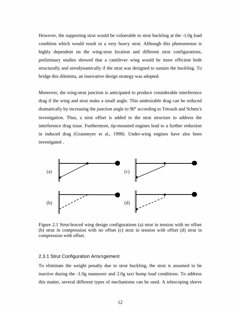
Moreover, the wing-strut junction is anticipated to produce considerable interference
drag if the wing and strut make a small angle. This undesirable drag can be reduced
dramatically by increasing the junction angle to 90° according to Tetrault and Schetz’s
investigation. Thus, a strut offset is added to the strut structure to address the
interference drag issue. Furthermore, tip-mounted engines lead to a further reduction
in induced drag (Grasmeyer et al., 1998). Under-wing engines have also been
investigated .
..(a)
(b)
..
..
(c)
(d)
Figure 2.1 Strut-braced wing design configurations (a) strut in tension with no offset(b) strut in compression with no offset (c) strut in tension with offset (d) strut incompression with offset.
2.3.1 Strut Configuration Arrangement
To eliminate the weight penalty due to strut buckling, the strut is assumed to be
inactive during the -1.0g maneuver and 2.0g taxi bump load conditions. To address
this matter, several different types of mechanisms can be used. A telescoping sleeve
13
mechanism was found suitable for the current design purposes. This strut arrangement
was suggested by Dr. R.T. Haftka. During positive g maneuvers, the strut is in
tension. Since the wing is clamped to the fuselage, it acts as a cantilever beam in the
negative load conditions and as a strut-braced beam in the positive load maneuvers.
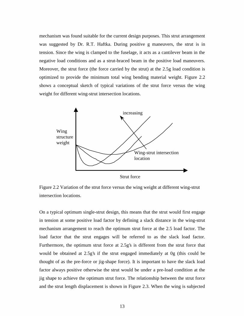
Moreover, the strut force (the force carried by the strut) at the 2.5g load condition is
optimized to provide the minimum total wing bending material weight. Figure 2.2
shows a conceptual sketch of typical variations of the strut force versus the wing
weight for different wing-strut intersection locations.
Wing-strut intersection location
Wingstructure weight
Strut force
increasing
Figure 2.2 Variation of the strut force versus the wing weight at different wing-strut
intersection locations.
On a typical optimum single-strut design, this means that the strut would first engage
in tension at some positive load factor by defining a slack distance in the wing-strut
mechanism arrangement to reach the optimum strut force at the 2.5 load factor. The
load factor that the strut engages will be referred to as the slack load factor.
Furthermore, the optimum strut force at 2.5g’s is different from the strut force that
would be obtained at 2.5g’s if the strut engaged immediately at 0g (this could be
thought of as the pre-force or jig-shape force). It is important to have the slack load
factor always positive otherwise the strut would be under a pre-load condition at the
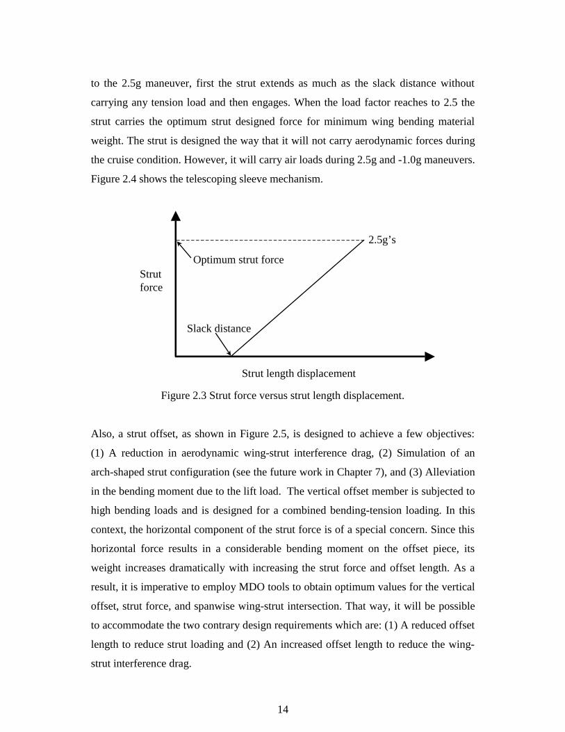
jig shape to achieve the optimum strut force. The relationship between the strut force
and the strut length displacement is shown in Figure 2.3. When the wing is subjected
14
to the 2.5g maneuver, first the strut extends as much as the slack distance without
carrying any tension load and then engages. When the load factor reaches to 2.5 the
strut carries the optimum strut designed force for minimum wing bending material
weight. The strut is designed the way that it will not carry aerodynamic forces during
the cruise condition. However, it will carry air loads during 2.5g and -1.0g maneuvers.
Figure 2.4 shows the telescoping sleeve mechanism.
Strut force
Strut length displacement
Slack distance
Optimum strut force
2.5g’s
Figure 2.3 Strut force versus strut length displacement.
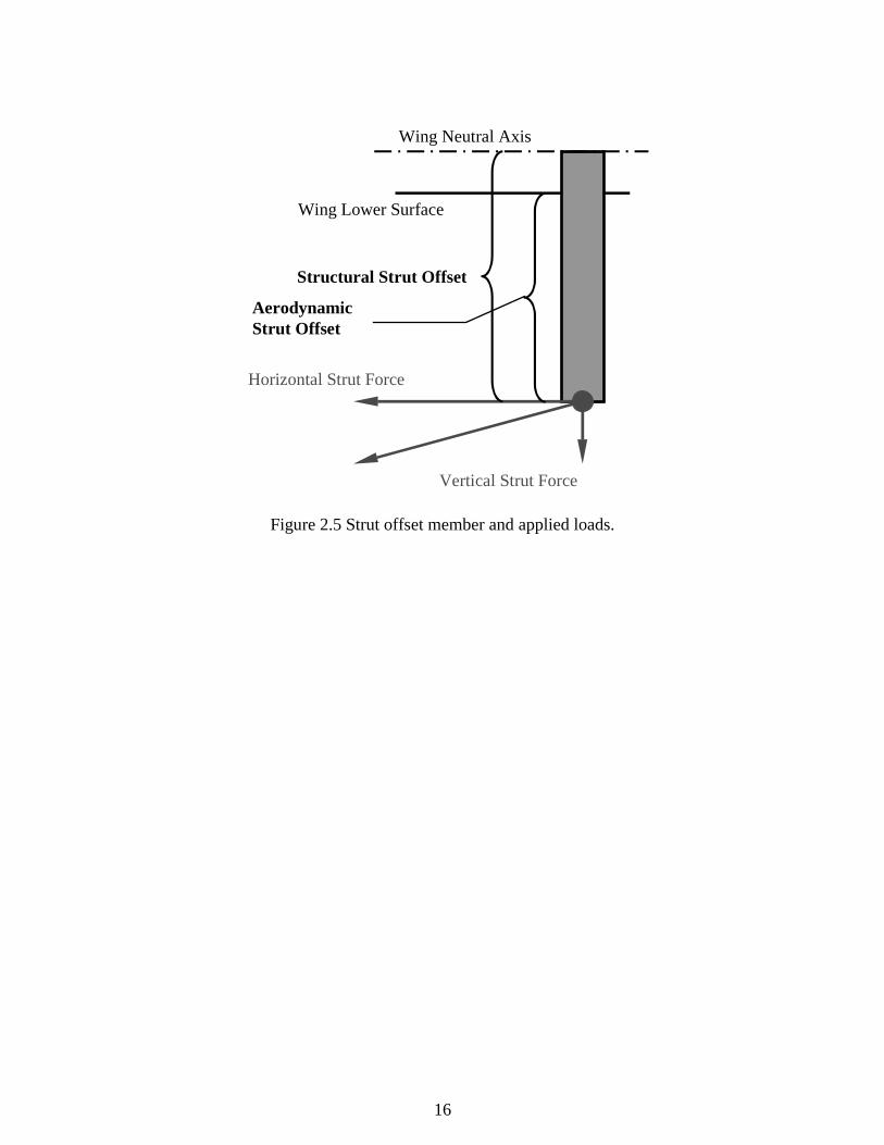
Also, a strut offset, as shown in Figure 2.5, is designed to achieve a few objectives:
(1) A reduction in aerodynamic wing-strut interference drag, (2) Simulation of an
arch-shaped strut configuration (see the future work in Chapter 7), and (3) Alleviation
in the bending moment due to the lift load. The vertical offset member is subjected to
high bending loads and is designed for a combined bending-tension loading. In this
context, the horizontal component of the strut force is of a special concern. Since this
horizontal force results in a considerable bending moment on the offset piece, its
weight increases dramatically with increasing the strut force and offset length. As a
result, it is imperative to employ MDO tools to obtain optimum values for the vertical
offset, strut force, and spanwise wing-strut intersection. That way, it will be possible
to accommodate the two contrary design requirements which are: (1) A reduced offset
length to reduce strut loading and (2) An increased offset length to reduce the wing-
strut interference drag.
15
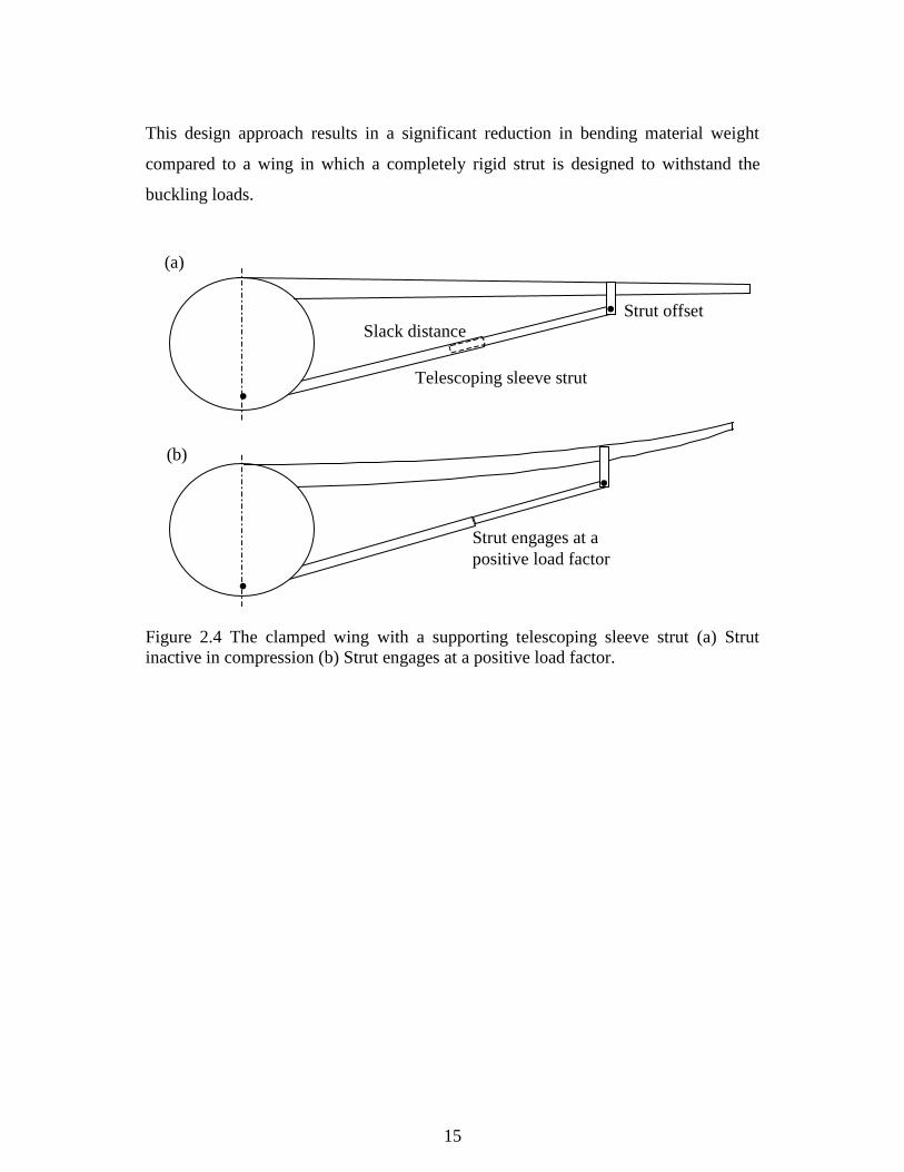
This design approach results in a significant reduction in bending material weight
compared to a wing in which a completely rigid strut is designed to withstand the
buckling loads.
.Strut engages at apositive load factor
.
.
Strut offset
Telescoping sleeve strut
.(a)
(b)
Slack distance
Figure 2.4 The clamped wing with a supporting telescoping sleeve strut (a) Strutinactive in compression (b) Strut engages at a positive load factor.
16
Wing Lower Surface
Wing Neutral Axis
Structural Strut Offset
Vertical Strut Force
Horizontal Strut Force
AerodynamicStrut Offset
Figure 2.5 Strut offset member and applied loads.
17
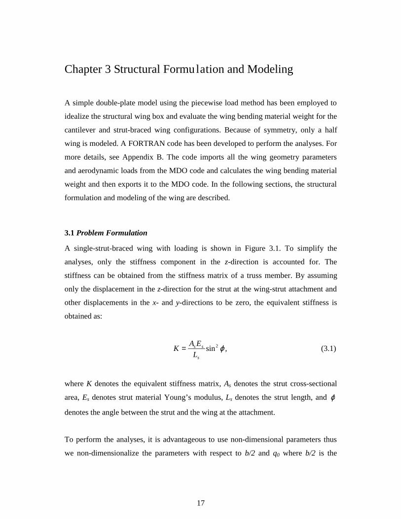
Chapter 3 Structural Formulation and Modeling
A simple double-plate model using the piecewise load method has been employed to
idealize the structural wing box and evaluate the wing bending material weight for the
cantilever and strut-braced wing configurations. Because of symmetry, only a half
wing is modeled. A FORTRAN code has been developed to perform the analyses. For
more details, see Appendix B. The code imports all the wing geometry parameters
and aerodynamic loads from the MDO code and calculates the wing bending material
weight and then exports it to the MDO code. In the following sections, the structural
formulation and modeling of the wing are described.
3.1 Problem Formulation
A single-strut-braced wing with loading is shown in Figure 3.1. To simplify the
analyses, only the stiffness component in the z-direction is accounted for. The
stiffness can be obtained from the stiffness matrix of a truss member. By assuming
only the displacement in the z-direction for the strut at the wing-strut attachment and
other displacements in the x- and y-directions to be zero, the equivalent stiffness is
obtained as:
,sin2 ϕs
ss
L
EAK = (3.1)
where K denotes the equivalent stiffness matrix, As denotes the strut cross-sectional
area, Es denotes strut material Young’s modulus, Ls denotes the strut length, and ϕ
denotes the angle between the strut and the wing at the attachment.
To perform the analyses, it is advantageous to use non-dimensional parameters thus
we non-dimensionalize the parameters with respect to b/2 and q0 where b/2 is the

18
wing half span in (ft) and q0 is the load at the wing root in (lbs/ft). Therefore, the
displacements, forces, and moments can be non-dimensionalized as follows:
LengthLength
b=
/ 2, Force
Force
q b=
0 2/, Moment
Moment
q b=
022( / )
, (3.2)
where Length and Length are general non-dimensional and dimensional
displacements, respectively, Force and Force are general non-dimensional and
dimensional forces, respectively, and Moment and Moment are general non-
dimensional and dimensional moments, respectively. All other parameters can be non-
dimensionalized accordingly.
.
Strut offset
Telescoping sleeve strut
.h
s
b/2
ϕ e
q0
y
z
Figure 3.1 Strut-braced wing configuration with loading.
19
Two methods based on the linear load method are employed for strut-braced wing
structural analyses. They are:
1. Direct integration method
2. Piecewise load method.
The direct integration method is used to develop the equations for the piecewise
method. To derive the equations for both cases
• The Euler-Bernoulli beam theory is used.
• Aerodynamic loads and wing geometry parameters are imported from the MDO
code.
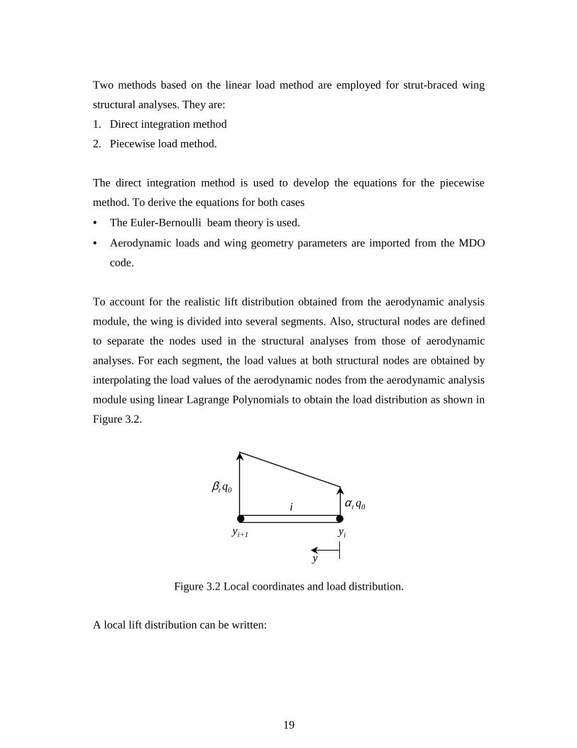
To account for the realistic lift distribution obtained from the aerodynamic analysis
module, the wing is divided into several segments. Also, structural nodes are defined
to separate the nodes used in the structural analyses from those of aerodynamic
analyses. For each segment, the load values at both structural nodes are obtained by
interpolating the load values of the aerodynamic nodes from the aerodynamic analysis
module using linear Lagrange Polynomials to obtain the load distribution as shown in
Figure 3.2.
.. αι q0
βι q0
yiyi+1
i
y
Figure 3.2 Local coordinates and load distribution.
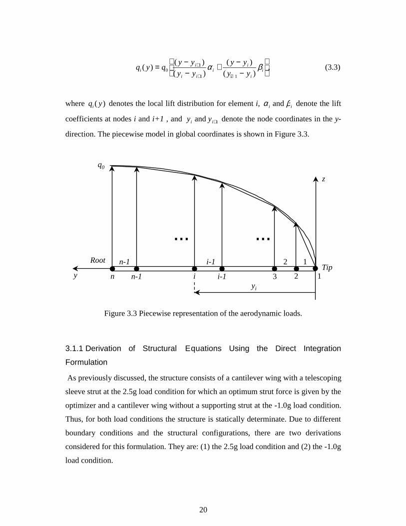
A local lift distribution can be written:
20
q y qy y
y y
y y
y yii
i ii
i
i ii( )
( )
( )
( )
( ),= −
−+ −
−
+
+ +0
1
1 1
α β (3.3)
where q yi ( ) denotes the local lift distribution for element i, α βi i and denote the lift
coefficients at nodes i and i+1 , and y yi i and +1 denote the node coordinates in the y-
direction. The piecewise model in global coordinates is shown in Figure 3.3.
Root
q0
Tip......123
i-1
i
12
i-1.n-1
n-1
yi
n
... ...
z
y
Figure 3.3 Piecewise representation of the aerodynamic loads.
3.1.1 Derivation of Structural Equations Using the Direct Integration
Formulation
As previously discussed, the structure consists of a cantilever wing with a telescoping
sleeve strut at the 2.5g load condition for which an optimum strut force is given by the
optimizer and a cantilever wing without a supporting strut at the -1.0g load condition.
Thus, for both load conditions the structure is statically determinate. Due to different
boundary conditions and the structural configurations, there are two derivations
considered for this formulation. They are: (1) the 2.5g load condition and (2) the -1.0g
load condition.
21
3.1.1.1 The 2.5g Load Condition
To derive the mechanics equation for the wing, first the unit step function is defined
as follows:
≥<
=0 if 1
0 if 0)(
y
yyu . (3.4)
The shear force and bending moment distributions can be obtained from the following
equations:
[ ] [ ] ,)()2/()2/()(0
dyyqsbyuFybyuWyVy
svee ∫−−−+−−= (3.5)
[ ] [ ][ ] [ ], )2/()2/()2/()(
)2/()2/()2/()()(
0sbyuLFybyuybWdyyyq
sbyusbFybyeuWyyVyM
offshe
y
ee
svee
−−+−−−+
−−−−+−−−−=
∫(3.6)
where )( yV indicates the shear force, svF indicates the strut force in the z-direction,
shF indicates the strut force in the y-direction, s indicates the wing-strut intersection
distance from the wing root, eW indicates the engine weight, ey indicates the engine
position from the root, offL indicates the strut offset length, and )( yM indicates the
bending moment.
The boundary conditions of the structure are defined
,0)2/( =bθ ,0)2/( =bw (3.7)
where )2/(bθ is the rotation of the wing at the wing root, and )2/(bw is deflection
of the wing at the wing root.
Using the governing differential equation of beams, the wing rotation is expressed as:
22
10 )(
)()( cdy
yEI
yMy
y+= ∫θ (3.8)
where )( yθ is the wing rotation and )( yEI is the flexural rigidity of the wing.
Integrating equation (3.8), the equation for wing deflections is obtained as:
,)()( 20 1 cycdyyywy
++= ∫ θ (3.9)
where )( yw is the deflection of the wing, and c c1 2 and are the coefficients to be
determined by the boundary conditions.
3.1.1.2 The -1.0g Load Condition
The boundary conditions at this load condition are:
,0)2/( and 0)2/( == bwbθ (3.10)
where )2/(bθ and )2/(bw denote the rotation and deflection of the wing at the root,
respectively.
The shear force and bending moment equations are obtained as:
[ ] ∫+−−−=y
ee dyyqybyuWyV0
,)()2/()( (3.11)
[ ][ ]. )2/()2/(
)()2/()()(0
eee
y
ee
ybyuybW
dyyyqybyeuWyyVyM
−−−
−+−−+−= ∫ (3.12)
The rotation and deflection equations can be readily derived from the beams
governing equation analogous to equations (3.8) and (3.9).
23
3.1.2 Derivation of Structural Equations Using the Piecewise Formulation
A piecewise formulation is used herein to account for the actual lift distributions.
Figure 3.3 depicts the piecewise model. The wing is divided into several segments
and for each segment the shear force, bending moment, and bending material weight
are evaluated. Two sets of formulations are also obtained for the two load cases, i.e.
2.5g’s and -1.0g.
3.1.2.1 The 2.5g Load Condition
The boundary conditions are identical to those of the direct integration method. Linear
interpolation is utilized to obtain the load distribution at the structural nodes from the
aerodynamic analysis. The shear force and bending moment for the ith element is
expressed as:
[ ] [ ]
∑∫ ∫−
=
+ −
−−−+−−=1
1
1
.)()(
)2/()2/()(i
i
y
y
y
y ii
eesvi
j
j i
dyyqdyyq
ybyuWsbyuFyV
(3.13)
[ ]
[ ][ ] [ ]. )2/( )2/()2/(
)()2/()2/(
)()()2/()(1
1
1
sbyuLFybyuybW
yyVsbyusbF
dyyqydyyyqybyeuWyM
offsheee
isv
i
y
y
i
j
y
y jeeii
j
j
−−+−−−+−−−−
+−−−−−= ∫∑∫−
=
+
(3.14)
3.1.2.2 The -1.0g Load Condition
The shear force and bending moment equations for the ith element are obtained as:
[ ] ∑∫ ∫−
=
+ ++−−−=1
1
1
)()()2/()(i
i
y
y
y
y iieei
j
j i
dyyqdyyqybyuWyV , (3.15)
[ ]
[ ]. )2/()2/()(
)()()2/()(1
1
1
eeei
i
y
y
i
j
y
y jeei
ybyuybWyyV
dyyqydyyyqybyeuWyMi
j
j
−−−−
−++−−= ∫∑∫−
=
+
(3.16)

24
It is essential to mention that the engine weight multiplied by the load factor is always
in the opposite direction of the maneuver loads. This phenomenon produces inertia
relief in the bending material weight of the wing.
3.1.2.3 Slope and Deflection Formulation
The slope and deflection equations for the ithelement are carried out as:
dyyEI
yMyy
i
i
y
yi
iiiii ∫ +−= ++
1
)(
)()()( 11θθ , (3.17)
))(( )(
)()()( 111
1
iiii
y
y
y
yi
iiiii yyydydy
yEI
yMyWyW
i
i i
−−
−= +++ ∫ ∫
+ θ . (3.18)
The integration constants were obtained from the boundary conditions.
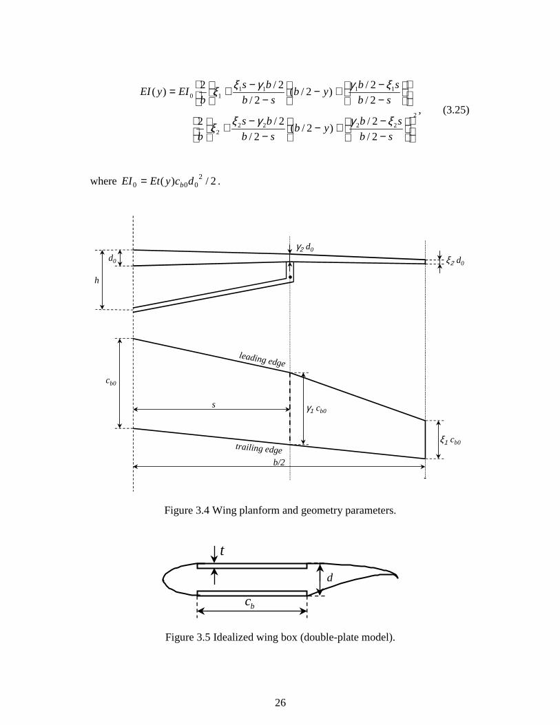
3.1.3 Moment of Inertia Distribution
In order to maintain generality, we assume that the EI distributions vary along the
wing. Figure 3.4 shows a linear variation of the chord along the wing. The wing
thickness is also assumed to vary linearly along the wing. Since the wing is built with
thin airfoils, an idealized wing box or a double-plate model was found suitable to
simulate the wing box airfoils as shown in Figure 3.5. This model is made of upper
and lower wing skin panels which are assumed to resist the bending moment. The
double-plate model offers the opportunity to extract the material thickness distribution
by a closed-form equation. The cross-sectional moment of inertia of the wing box can
be expressed as:
2
)()()()(
2 ydycytyI b= , (3.19)

25
where t(y) is the wing skin thickness, cb(y) is the wing box chord, and d(y) is the wing
airfoil thickness. All parameters are shown in Figure 3.4 and Figure 3.5.
The equations for cb(y) and d(y) are obtained using linear interpolation between the
wing root, break, and tip data as:
for 2/2/ bysb ≤≤− ,
+−−= 1)2/(
)1()( 1
0 ybs
cyc bb
γ, (3.20)
for sby −≤≤ 2/0 ,
−−+−
−−+=
sb
sbyb
sb
bs
bcyc bb 2/
2/)2/(
2/
2/2)( 1111
10
ξγγξξ , (3.21)
where 0bc is the wing box root chord, 1γ is the chord coefficient at the wing-strut
attachment, and ξ1 is the wing box tip chord coefficient, and
for 2/2/ bysb ≤≤− ,
+−−= 1)2/(
)1()( 2
0 ybs
dydγ
, (3.22)
and for sby −≤≤ 2/0 ,
−−+−
−−+=
sb
sbyb
sb
bs
bdyd
2/
2/)2/(
2/
2/2)( 2222
20
ξγγξξ , (3.23)
where 0d is the wing root thickness, 2γ is the thickness coefficient at the wing-strut
attachment, and ξ2 is the wing tip thickness coefficient.
Now using equation (3.19), the )( yEI distribution is obtained as:
for 2/2/ bysb ≤≤− ,
2
210 1)2/(
)1(1)2/(
)1()(
+−−
+−−= yb
syb
sEIyEI
γγ, (3.24)
and for sby −≤≤ 2/0 ,
26
2
22222
111110
2/
2/)2/(
2/
2/2
2/
2/)2/(
2/
2/2)(
−−+−
−−+
−−+−
−−+=
sb
sbyb
sb
bs
b
sb
sbyb
sb
bs
bEIyEI
ξγγξξ
ξγγξξ, (3.25)
where 2/)( 2000 dcyEtEI b= .
ξ2 d0
cb0
leading edge
trailing edge
γ1 cb0
ξ1 cb0
b/2
s
d0
γ2 d0
h .
Figure 3.4 Wing planform and geometry parameters.
t
cb
d
Figure 3.5 Idealized wing box (double-plate model).
27
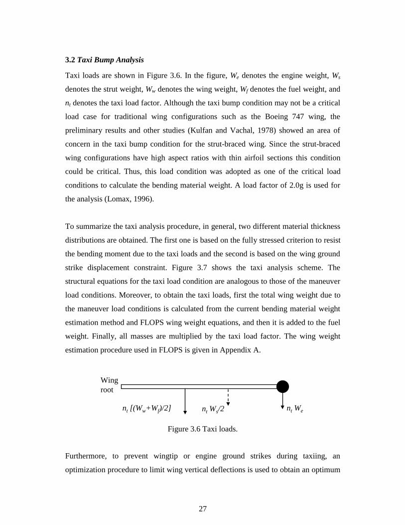
3.2 Taxi Bump Analysis
Taxi loads are shown in Figure 3.6. In the figure, We denotes the engine weight, Ws
denotes the strut weight, Ww denotes the wing weight, Wf denotes the fuel weight, and
nt denotes the taxi load factor. Although the taxi bump condition may not be a critical
load case for traditional wing configurations such as the Boeing 747 wing, the
preliminary results and other studies (Kulfan and Vachal, 1978) showed an area of
concern in the taxi bump condition for the strut-braced wing. Since the strut-braced
wing configurations have high aspect ratios with thin airfoil sections this condition
could be critical. Thus, this load condition was adopted as one of the critical load
conditions to calculate the bending material weight. A load factor of 2.0g is used for
the analysis (Lomax, 1996).
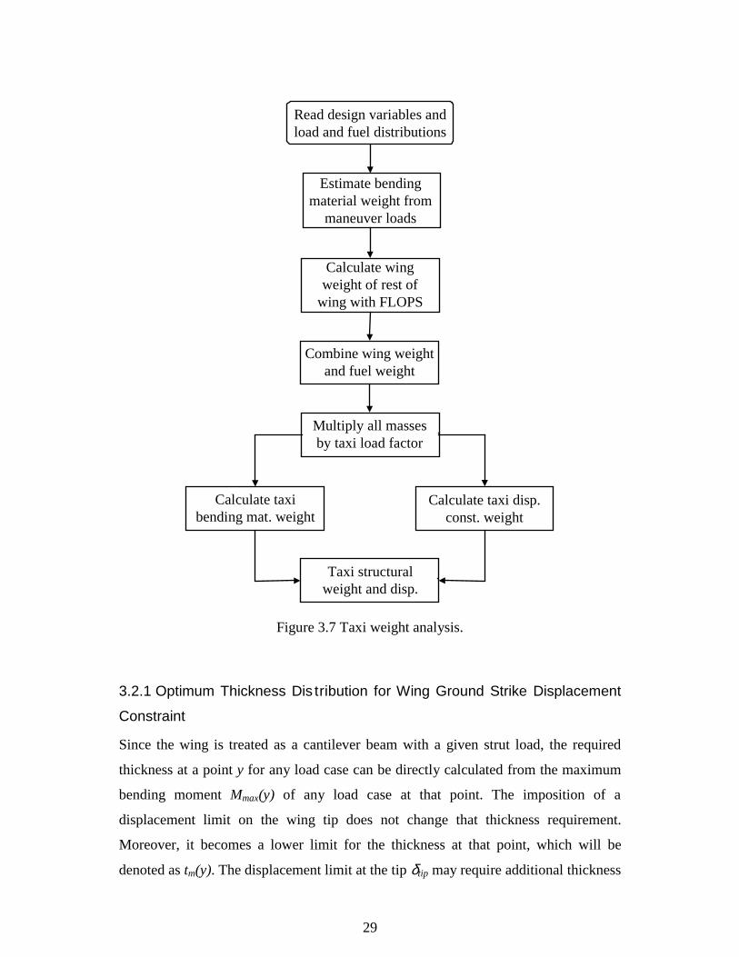
To summarize the taxi analysis procedure, in general, two different material thickness
distributions are obtained. The first one is based on the fully stressed criterion to resist
the bending moment due to the taxi loads and the second is based on the wing ground
strike displacement constraint. Figure 3.7 shows the taxi analysis scheme. The
structural equations for the taxi load condition are analogous to those of the maneuver
load conditions. Moreover, to obtain the taxi loads, first the total wing weight due to
the maneuver load conditions is calculated from the current bending material weight
estimation method and FLOPS wing weight equations, and then it is added to the fuel
weight. Finally, all masses are multiplied by the taxi load factor. The wing weight
estimation procedure used in FLOPS is given in Appendix A.
nt [(Ww+Wf)/2] nt Went Ws/2
Wingroot
Figure 3.6 Taxi loads.
Furthermore, to prevent wingtip or engine ground strikes during taxiing, an
optimization procedure to limit wing vertical deflections is used to obtain an optimum
28
wing material thickness distribution. Hence, a displacement limit based on the landing
gear length and the fuselage diameter is imposed to avoid such problems. This matter
will be discussed in the next section in more detail. The maximum vertical
displacement during taxiing is calculated for tip-mounted and under-wing engines
from the following equations. Obviously, for the tip mounted-engine configuration,
the wingtip should be checked for ground strikes while for the under-wing engine
configuration, most likely the engine mounting location would be the case to be
checked. Thus, for tip-mounted engines:
,2
nacellewingtiptip
d+= δδ (3.26)
and for under-wing engines:
,max nacellepylonenginewingengine dh ++= −− δδ (3.27)
where wingtipδ denotes the wingtip deflection, nacelled denotes the nacelle diameter,
enginewing −δ denotes the wing deflection at the engine location, and pylonh denotes the
pylon height.
29
Estimate bendingmaterial weight from
maneuver loads
Calculate wingweight of rest of
wing with FLOPS
Combine wing weightand fuel weight
Multiply all massesby taxi load factor
Read design variables andload and fuel distributions
Calculate taxibending mat. weight
Calculate taxi disp.const. weight
Taxi structuralweight and disp.
Figure 3.7 Taxi weight analysis.
3.2.1 Optimum Thickness Dis tribution for Wing Ground Strike Displacement
Constraint
Since the wing is treated as a cantilever beam with a given strut load, the required
thickness at a point y for any load case can be directly calculated from the maximum
bending moment Mmax(y) of any load case at that point. The imposition of a
displacement limit on the wing tip does not change that thickness requirement.
Moreover, it becomes a lower limit for the thickness at that point, which will be
denoted as tm(y). The displacement limit at the tip δtip may require additional thickness
30
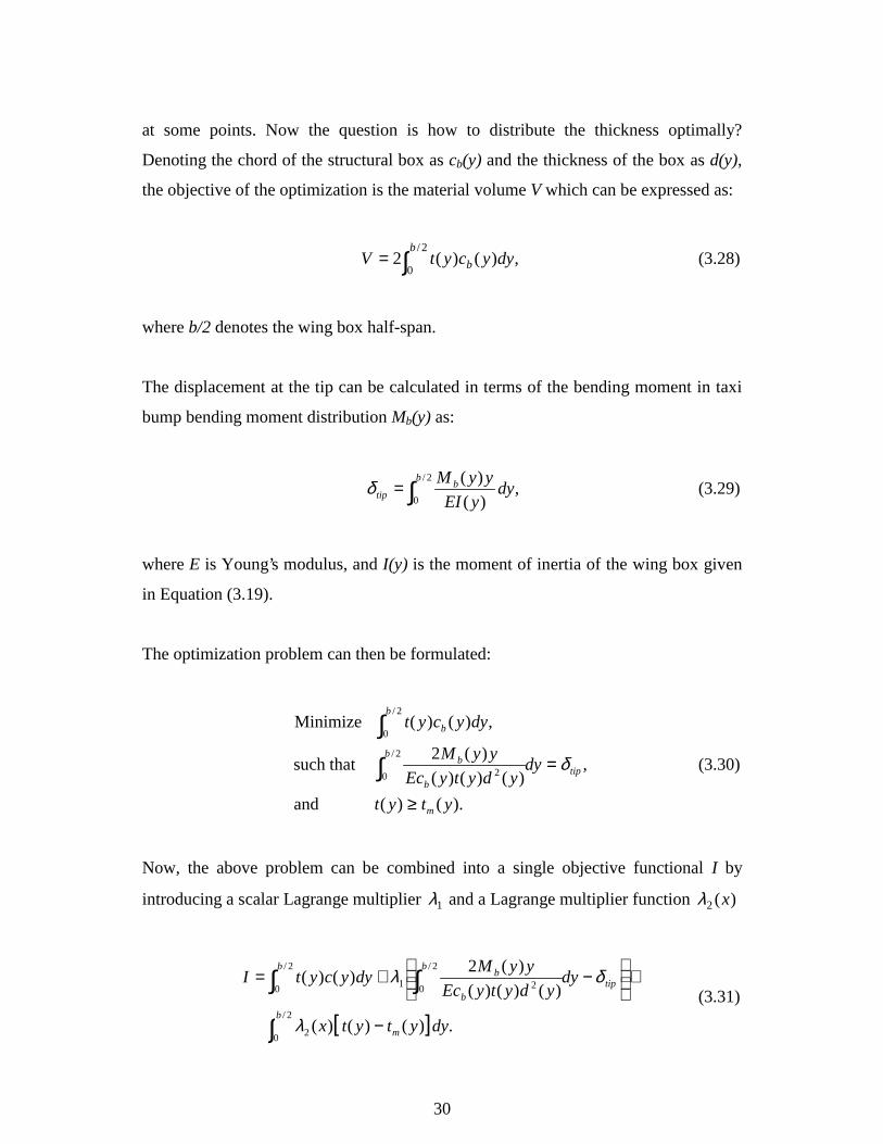
at some points. Now the question is how to distribute the thickness optimally?
Denoting the chord of the structural box as cb(y) and the thickness of the box as d(y),
the objective of the optimization is the material volume V which can be expressed as:
,)()(22/
0dyycytV
b
b∫= (3.28)
where b/2 denotes the wing box half-span.
The displacement at the tip can be calculated in terms of the bending moment in taxi
bump bending moment distribution Mb(y) as:
∫=2/
0,
)(
)(bb
tip dyyEI
yyMδ (3.29)
where E is Young’s modulus, and I(y) is the moment of inertia of the wing box given
in Equation (3.19).
The optimization problem can then be formulated:
).()( and
,)()()(
)(2 that such
,)()( Minimize
2/
0 2
2/
0
ytyt
dyydytyEc
yyM
dyycyt
m
tip
b
b
b
b
b
≥
=∫
∫δ (3.30)
Now, the above problem can be combined into a single objective functional I by
introducing a scalar Lagrange multiplier 1λ and a Lagrange multiplier function )(2 xλ
[ ] . )()( )(
)()()(
)(2)()(
2/
0 2
2/
0 21
2/
0
dyytytx
dyydytyEc
yyMdyycytI
b
m
tip
b
b
bb
∫
∫∫
−
+
−+=
λ
δλ(3.31)
31
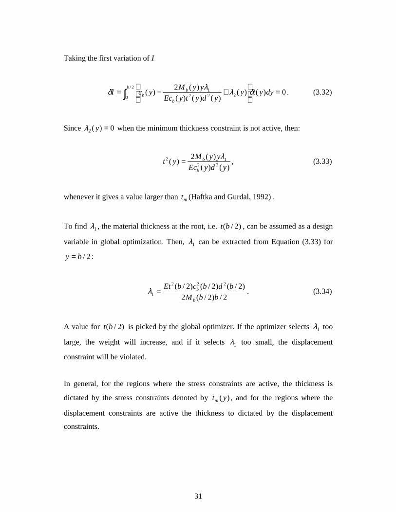
Taking the first variation of I
0)()()()()(
)(2)(
2/
0 2221 =
+−= ∫ dyyty
ydytyEc
yyMycI
b
b
bb δλλδ . (3.32)
Since 0)(2 =yλ when the minimum thickness constraint is not active, then:
)()(
)(2)(
2212
ydyEc
yyMyt
b
b λ= , (3.33)
whenever it gives a value larger than mt (Haftka and Gurdal, 1992) .
To find 1λ , the material thickness at the root, i.e. )2/(bt , can be assumed as a design
variable in global optimization. Then, 1λ can be extracted from Equation (3.33) for
2/by = :
2/)2/(2
)2/()2/()2/( 222
1 bbM
bdbcbEt
b
b=λ . (3.34)
A value for )2/(bt is picked by the global optimizer. If the optimizer selects 1λ too
large, the weight will increase, and if it selects 1λ too small, the displacement
constraint will be violated.
In general, for the regions where the stress constraints are active, the thickness is
dictated by the stress constraints denoted by )( ytm , and for the regions where the
displacement constraints are active the thickness to dictated by the displacement
constraints.
32
3.3 Landing Analysis
Landing loads could be critical because of the downward inertia loads as well as the
large concentrated loads applied to the wing due to the landing gear impact if the
landing gears are located on the wing. For the case of the strut-braced wing, the
landing gear is not located on the wing thus the landing gear loads do not directly
apply to the wing. This matter can be considered as a plus. Fuselage-mounted landing
gears are utilized for truss-braced wing configurations.
Inertia loads during landing can be found by multiplying the aircraft inertia factor by
the weights. The landing gear impact load factor can be obtained from the following
energy based equation (Niu, 1988):
( )
Ss
SttttS
LG X
XXW
L
W
XK
g
V
nη
η+
−+−
=1
22
22
, (3.35)
where W denotes the takeoff gross weight, SV denotes the sinking speed, tK denotes
the tire spring constant, tη denotes a factor to account for the fact that the tire
deflection is non-linear, tX denotes the tire deflection, L denotes the wing lift, SX
denotes the strut stroke, and sη denotes the strut efficiency (0.8 to 0.85). The sinking
speed for large transports is usually assumed 10 ft/sec and .WL =
The inertia factor on the aircraft is defined as:
,
+=W
Lnn LGL (3.36)
where L/W is the aircraft load factor during landing.
33
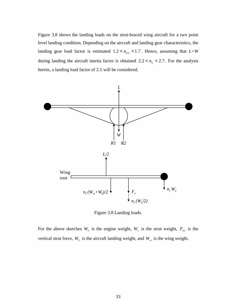
Figure 3.8 shows the landing loads on the strut-braced wing aircraft for a two point
level landing condition. Depending on the aircraft and landing gear characteristics, the
landing gear load factor is estimated 7.12.1 << LGn . Hence, assuming that L=W
during landing the aircraft inertia factor is obtained .7.22.2 << Ln For the analysis
herein, a landing load factor of 2.5 will be considered.
R1 R2
L
W
L/2
nl (Ww+Wf)/2nl We
nl (Ws/2)
Fs
Wingroot
Figure 3.8 Landing loads.
For the above sketches eW is the engine weight, sW is the strut weight, svF is the
vertical strut force, LW is the aircraft landing weight, and wW is the wing weight.
34
3.4 Bending Material Weight Optimization
3.4.1 Wing Bending Material Weight Calculation
Optimum weight is the key issue in designing an aircraft. A wing with a high aspect
ratio and small thickness to chord ratios has aerodynamic advantages compared to a
conventional cantilever wing aircraft. However, wings of that kind may encounter a
large weight penalty due to the increased material thickness to meet the yield
criterion. Thus, to reduce weight, using a strut or a truss to support the wing can be a
suitable solution since a strut or a truss can relieve the wing bending moment. As long
as the strut bears part of the loading, some of the wing bending moment distribution
diminishes and hence the required material weight decreases. Knowing the bending
moment distribution, the corresponding bending stress in the wing is calculated from
the following equation:
)(2
)()(max yI
ydyM=σ , (3.38)
where maxσ denotes the maximum stress and M(y) denotes the bending moment of
the wing.
If the wing is designed according to the fully-stressed criterion, one can substitute the
allowable stress into equation (3.38) for σmax . Furthermore, substituting equation
(3.19) into equation (3.38) for I(y), the wing skin thickness can be specified as:
allb ydyc
yMyt
σ)()(
)()( = , (3.39)
where σall indicates the allowable stress.
The bending material weight of the half-wing is expressed as:
35
dyycytWsb
bb ρ)()(22/
0∫= , (3.40)
where bs is the structural span. The structural span is obtained as:
bb
s =cos
,Λ
(3.41)
where Λ is the three quarter chord wing sweep angle (McCullers).
Then, assuming d(y) to be constant and substituting for t(y) into equation (3.40), the
bending material weight is formulated:
dyyMkWsb
wb ∫=2/
0)( , (3.42)
where k d all= 2ρ σ .
The non-dimensional form can be written:
3
0 2
=s
wbwb
bkq
WW , (3.43)
where wbW denotes the non-dimensional bending material weight. This equation
reveals the importance of the span in wing bending material weight.
Eventually, the non-dimensional bending material weight is obtained as:
ydyMWwb ∫=1
0)( . (3.44)
36
Equation (3.44) shows that the bending material weight is dependent directly on the
area under the bending moment diagram. Thus, to minimize the bending material
weight, the area under the bending moment diagram should be minimized.
If d varies along the wing in terms of y, the bending material weight will have the
form:
∫=1
0 )(
)(yd
yd
yMWwb , (3.45)
where d(y) is obtained from equations (3.22) and (3.23), k all= 2ρ σ , and
20 )2/(/ swbwb bkqWW = . Therefore, to have the bending material weight minimized,
the area under the integrand function in equation (3.45) should be minimized. This
functional as well as the strut weight is utilized as the objective function to minimize
the bending material weight of the wing.
3.4.2 Strut Weight Calculation
For all calculations the strut is considered as a truss member which is modeled as a
spring in the z-direction for simplicity. As shown before, the spring stiffness is
obtained from the stiffness matrix of a truss member. The effect of strut bending will
be considered in wing weight estimation by a simple assumption and will be
discussed later. The actual strut force can be calculated from its vertical component
as:
2
2
cos
Λ
+=s
svs
sh
h
FF , (3.46)
37
where sF is the actual strut force and sΛ is the strut sweep angle. The required cross-
sectional area of the strut, i.e. sA , is given as allss FA σ= . So that, the weight of the
strut capable of carrying tension loads is:
2
2
cos
Λ
+=s
ssst
shAW ρ , (3.47)
where sρ is the material density of the strut.
Substituting for sA and sF , we have:
svsall
sst F
sh
hW
Λ
+=2
2
cosσρ
. (3.48)
Since a real strut also carries bending loads, a factor of 1.5 was found reasonable to be
multiplied to the strut tension weight to account for the additional strut bending
weight. Consequently, the strut bending and tension weight will be:
sts WW 5.1= . (3.49)
Also, to take into account the extra compression weight due to the horizontal strut
force component in inboard wing, another additional weight equal to the strut tension
weight stW is added to the total bending material weight. Thus, a factor of 2.5 is
multiplied by the strut tension weight to account for both strut bending weight and
inboard compression weight. The total wing structure bending material weight is
expressed as:
( )stwbb WWW 5.22 += . (3.50)
38
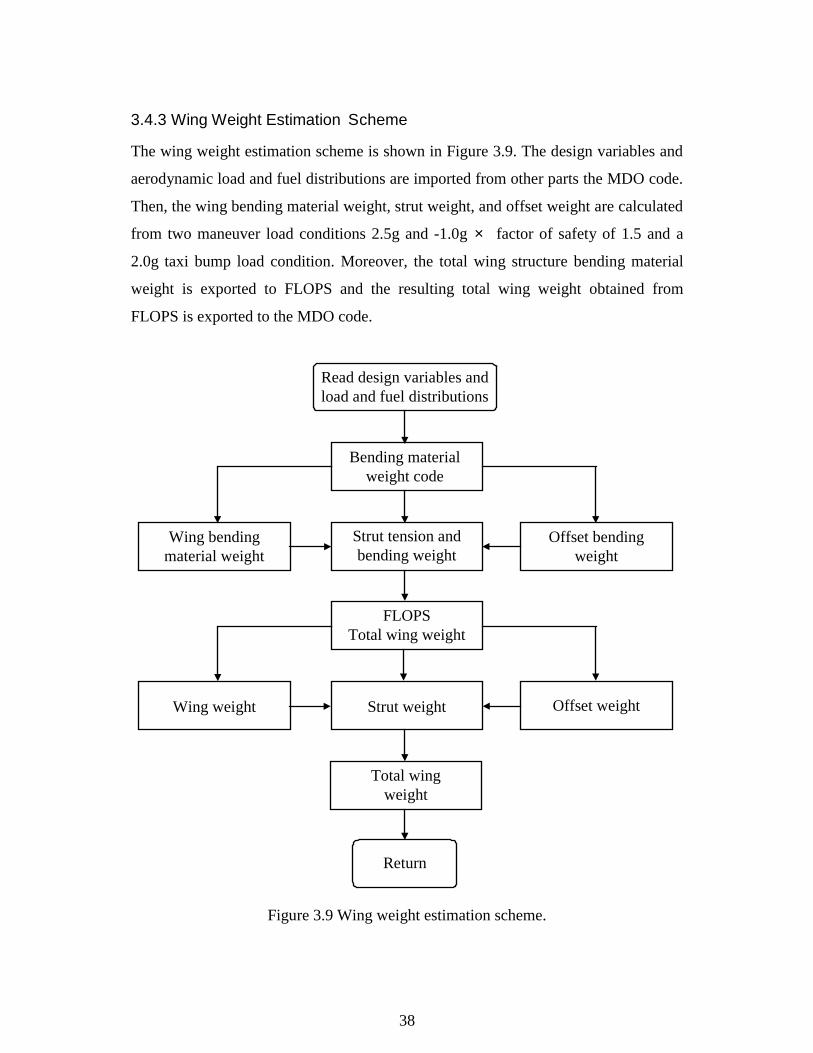
3.4.3 Wing Weight Estimation Scheme
The wing weight estimation scheme is shown in Figure 3.9. The design variables and
aerodynamic load and fuel distributions are imported from other parts the MDO code.
Then, the wing bending material weight, strut weight, and offset weight are calculated
from two maneuver load conditions 2.5g and -1.0g × factor of safety of 1.5 and a
2.0g taxi bump load condition. Moreover, the total wing structure bending material
weight is exported to FLOPS and the resulting total wing weight obtained from
FLOPS is exported to the MDO code.
Strut tension andbending weight
FLOPSTotal wing weight
Read design variables andload and fuel distributions
Bending materialweight code
Wing bendingmaterial weight
Offset bendingweight
Wing weight Offset weightStrut weight
Total wingweight
Return
Figure 3.9 Wing weight estimation scheme.
39
The above procedure has been coded and implemented in the MDO code for bending
material weight estimation.
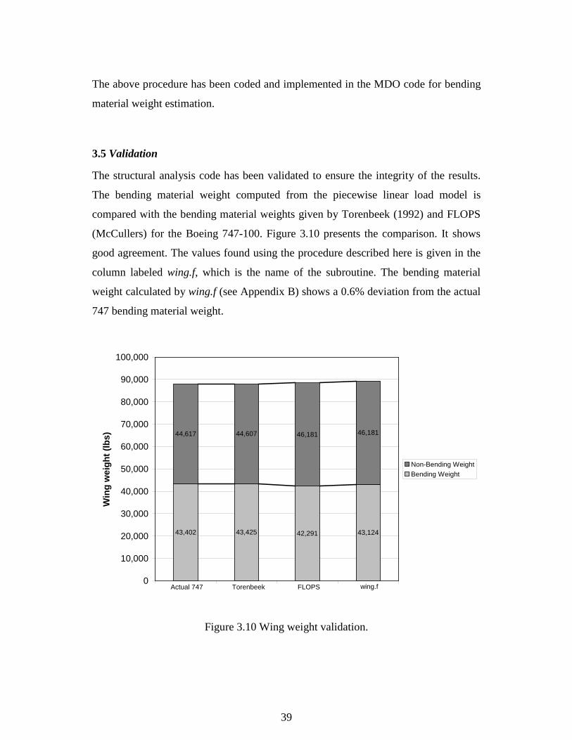
3.5 Validation
The structural analysis code has been validated to ensure the integrity of the results.
The bending material weight computed from the piecewise linear load model is
compared with the bending material weights given by Torenbeek (1992) and FLOPS
(McCullers) for the Boeing 747-100. Figure 3.10 presents the comparison. It shows
good agreement. The values found using the procedure described here is given in the
column labeled wing.f, which is the name of the subroutine. The bending material
weight calculated by wing.f (see Appendix B) shows a 0.6% deviation from the actual
747 bending material weight.
43,42543,402 42,291 43,124
46,18146,18144,60744,617
0
10,000
20,000
30,000
40,000
50,000
60,000
70,000
80,000
90,000
100,000
1 2 3 4
Win
g w
eig
ht
(lb
s)
Non-Bending WeightBending Weight
Actual 747 Torenbeek FLOPS wing.f
Figure 3.10 Wing weight validation.
40
Chapter 4 Optimization Problem
Multidisciplinary Design Optimization has been employed to optimize truss-braced
wing configurations to minimize the takeoff gross weight subject to realistic
constraints. The method of feasible directions in the Design Optimization Tools
(DOT) software package from Vanderplaats (1995) is used to perform optimizations.
A brief description of the optimization problem is presented herein. For more details
refer to Grasmeyer et al. (1998).
4.1 Design Variables and Constraints
In general, a single-strut-braced wing is parameterized by a total of 22 design
variables summarized in Table 4.1. Fourteen design variables describe the wing
layout and 8 design variables describe the other distinctive features. The vertical
separation of the wing and strut at the root is designated to be equal to the fuselage
diameter. The fuselage geometry of the baseline cantilever design is used in the strut-
braced wing configurations and remains fixed. Moreover, tail sizing is also
performed. Table 4.2 shows thirteen inequality constraints to obtain realistic
configurations. Additionally, side constraints are also used to bound each design
variable. Table 4.3 lists the two major side constraints, i.e. the upper limit of the
semispan which ensures that the wing span is within the FAA 80 meter gate box limit
and the lower limits of the wing and strut t/c’s which guarantee values more than 5%
and 8%, respectively. The 5% limit was chosen empirically and the 8% limit was
suggested by LMAS to reduce strut sagging due to its weight during taxiing.
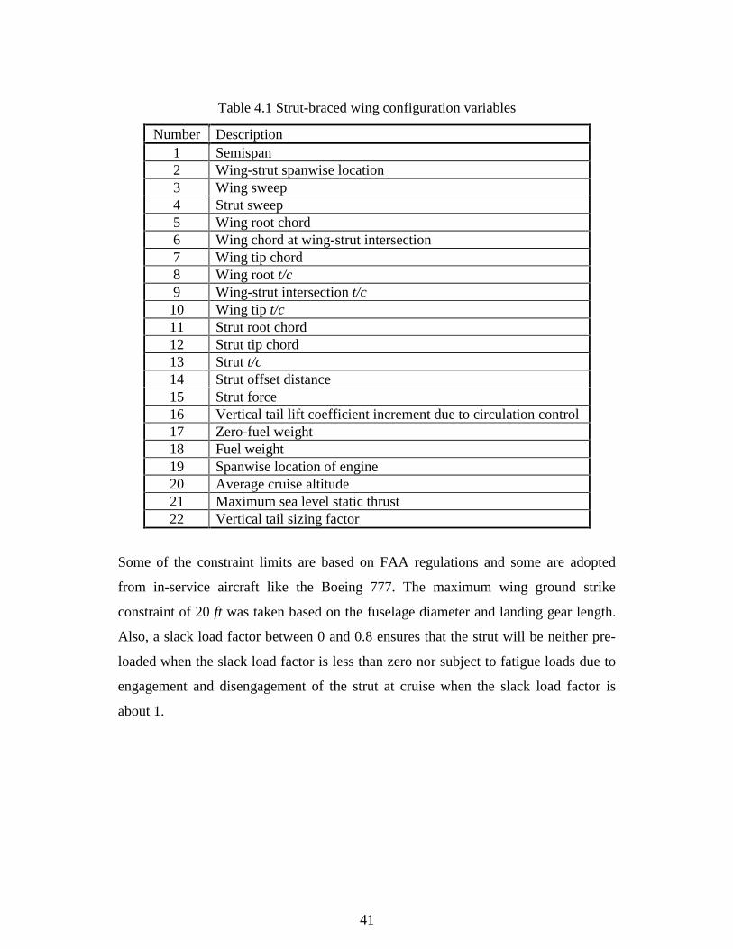
41
Table 4.1 Strut-braced wing configuration variables
Number Description1 Semispan2 Wing-strut spanwise location3 Wing sweep4 Strut sweep5 Wing root chord6 Wing chord at wing-strut intersection7 Wing tip chord8 Wing root t/c9 Wing-strut intersection t/c10 Wing tip t/c11 Strut root chord12 Strut tip chord13 Strut t/c14 Strut offset distance15 Strut force16 Vertical tail lift coefficient increment due to circulation control17 Zero-fuel weight18 Fuel weight19 Spanwise location of engine20 Average cruise altitude21 Maximum sea level static thrust22 Vertical tail sizing factor
Some of the constraint limits are based on FAA regulations and some are adopted
from in-service aircraft like the Boeing 777. The maximum wing ground strike
constraint of 20 ft was taken based on the fuselage diameter and landing gear length.
Also, a slack load factor between 0 and 0.8 ensures that the strut will be neither pre-
loaded when the slack load factor is less than zero nor subject to fatigue loads due to
engagement and disengagement of the strut at cruise when the slack load factor is
about 1.
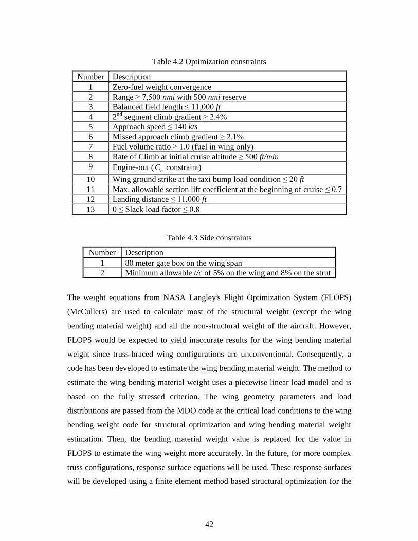
42
Table 4.2 Optimization constraints
Number Description1 Zero-fuel weight convergence2 Range ��������nmi with 500 nmi reserve3 Balanced field length ���������ft4 2nd segment climb gradient ������5 Approach speed ������kts6 Missed approach climb gradient ������7 Fuel volume ratio �������IXHO�LQ�ZLQJ�RQO\�8 Rate of Climb at initial cruise altitude ������ft/min9 Engine-out ( nC constraint)
10 Wing ground strike at the taxi bump load condition �����ft11 Max. allowable section lift coefficient at the beginning of cruise �����12 Landing distance ���������ft13 0 ��6ODFN�ORDG�IDFWRU������
Table 4.3 Side constraints
Number Description1 80 meter gate box on the wing span2 Minimum allowable t/c of 5% on the wing and 8% on the strut
The weight equations from NASA Langley’s Flight Optimization System (FLOPS)
(McCullers) are used to calculate most of the structural weight (except the wing
bending material weight) and all the non-structural weight of the aircraft. However,
FLOPS would be expected to yield inaccurate results for the wing bending material
weight since truss-braced wing configurations are unconventional. Consequently, a
code has been developed to estimate the wing bending material weight. The method to
estimate the wing bending material weight uses a piecewise linear load model and is
based on the fully stressed criterion. The wing geometry parameters and load
distributions are passed from the MDO code at the critical load conditions to the wing
bending weight code for structural optimization and wing bending material weight
estimation. Then, the bending material weight value is replaced for the value in
FLOPS to estimate the wing weight more accurately. In the future, for more complex
truss configurations, response surface equations will be used. These response surfaces
will be developed using a finite element method based structural optimization for the
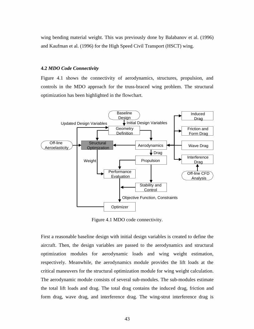
43
wing bending material weight. This was previously done by Balabanov et al. (1996)
and Kaufman et al. (1996) for the High Speed Civil Transport (HSCT) wing.
4.2 MDO Code Connectivity
Figure 4.1 shows the connectivity of aerodynamics, structures, propulsion, and
controls in the MDO approach for the truss-braced wing problem. The structural
optimization has been highlighted in the flowchart.
BaselineDesign
GeometryDefinition
Structural Optimization
Performance Evaluation
Aerodynamics
Stability andControl
Propulsion
Optimizer
Induced Drag
Friction and Form Drag
Wave Drag
Interference Drag
Off-line CFD Analysis
Off-line Aeroelasticity
Initial Design Variables
Objective Function, Constraints
Drag
Weight
Updated Design Variables
Figure 4.1 MDO code connectivity.
First a reasonable baseline design with initial design variables is created to define the
aircraft. Then, the design variables are passed to the aerodynamics and structural
optimization modules for aerodynamic loads and wing weight estimation,
respectively. Meanwhile, the aerodynamics module provides the lift loads at the
critical maneuvers for the structural optimization module for wing weight calculation.
The aerodynamic module consists of several sub-modules. The sub-modules estimate
the total lift loads and drag. The total drag contains the induced drag, friction and
form drag, wave drag, and interference drag. The wing-strut interference drag is
44
evaluated using an offline CFD solver. Moreover, the propulsion module reads the
drag from the aerodynamics module and calculates the required thrust and engine size
by rubber engine sizing. Tail sizing and circulation control for the engine-out
condition are performed in the stability and control module. Finally, the total drag and
wing weight are input to the performance evaluation module to calculate the aircraft
takeoff weight, the objective function for the optimizer. The constraints are also
evaluated in the same module. This procedure is iterated by the optimizer until an
optimum configuration is obtained.
A Lockheed Martin Aeronautical Systems’ (LMAS) mission profile is used to
generate the results. The takeoff gross weight was chosen as the objective function for
optimization. Nineteen out of 22 design variables for the tip-mounted engine design
and 20 out of 22 design variables for the under-wing engine design as well as 13
constraints are used to characterize the strut-braced wing configurations and bending
material weight estimation. For the current optimization cases, the strut t/c is fixed at
8% and the strut tip chord is set to be equal to the strut root chord based on the LMAS
suggestion.
45
Chapter 5 Results
All structural results obtained from the piecewise linear load method for different
strut-braced wing design configurations are tabulated and presented in this chapter.
Two sets of single-strut configurations are explored. The first set represents the
optimization results based on the tip-mounted engine configuration and the second set
indicates the optimization results based on the under-wing engine configuration. The
wing structure is partially assumed to be made of a composite material.
Also, the final design configurations are compared with the counterpart cantilever
wing configuration obtained from the same MDO methodology and technology to
evaluate the potential of the strut-braced wing. Some of the technology concepts that
are introduced are natural laminar flow, drag reduction techniques, and relaxed static
stability (Grasmeyer et al., 1998). Rubber engine sizing to match the engine size and
weight to the required thrust is also considered.
The advantage of using composite materials for bending load carrying panels is
evaluated by comparing the wing weights of metallic strut-braced wing configurations
to those of composite strut-braced wing configurations.
Finally, the variations of the wing weight and takeoff gross weight of the strut-braced
wing to changes in the strut force, strut offset length, and wing-strut intersection are
shown.
5.1 Material propeties
Two different materials are used in the wing weight estimation code to produce the
results. A high strength aluminum alloy and a graphite-epoxy composite laminate
with a [45/-45/0/90/0/-45/45] stacking sequence are considered. Material information
and properties were obtained from Torenbeek (1992) and Fielding et al., (1987) for
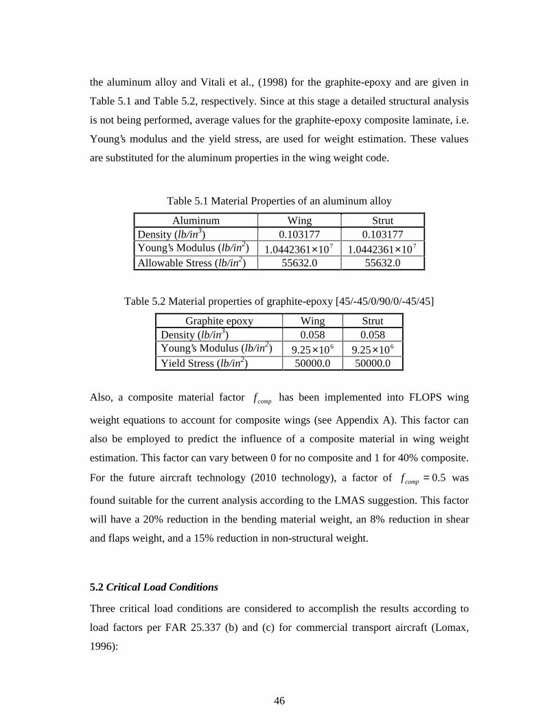
46
the aluminum alloy and Vitali et al., (1998) for the graphite-epoxy and are given in
Table 5.1 and Table 5.2, respectively. Since at this stage a detailed structural analysis
is not being performed, average values for the graphite-epoxy composite laminate, i.e.
Young’s modulus and the yield stress, are used for weight estimation. These values
are substituted for the aluminum properties in the wing weight code.
Table 5.1 Material Properties of an aluminum alloy
Aluminum Wing StrutDensity (lb/in3) 0.103177 0.103177Young’s Modulus (lb/in2) 7100442361.1 × 7100442361.1 ×Allowable Stress (lb/in2) 55632.0 55632.0
Table 5.2 Material properties of graphite-epoxy [45/-45/0/90/0/-45/45]
Graphite epoxy Wing StrutDensity (lb/in3) 0.058 0.058Young’s Modulus (lb/in2) 61025.9 × 61025.9 ×Yield Stress (lb/in2) 50000.0 50000.0
Also, a composite material factor compf has been implemented into FLOPS wing
weight equations to account for composite wings (see Appendix A). This factor can
also be employed to predict the influence of a composite material in wing weight
estimation. This factor can vary between 0 for no composite and 1 for 40% composite.
For the future aircraft technology (2010 technology), a factor of 5.0=compf was
found suitable for the current analysis according to the LMAS suggestion. This factor
will have a 20% reduction in the bending material weight, an 8% reduction in shear
and flaps weight, and a 15% reduction in non-structural weight.
5.2 Critical Load Conditions
Three critical load conditions are considered to accomplish the results according to
load factors per FAR 25.337 (b) and (c) for commercial transport aircraft (Lomax,
1996):
47
1. Maximum lift of 2 5 2. MTOW FS lbs distributed over the wing half-span. It
corresponds to a 2.5g upward maneuver.
2. Reversed lift of − MTOW FS 2 lbs distributed over the wing half span. It
corresponds to a 1.0g downward maneuver.
3. 2.0g taxi bump.
The bending material weight calculations are based on the above load conditions.
5.2.1 Landing Calculations
An inertia load factor of 2.5 is assumed for landing calculations. The following
landing loads are calculated from the output data which will be presented later in this
chapter for the tip-mounted engine configuration. Based on the material discussed in
chapter 3, section 3.3 one obtains:
),( 0.913,2442/2/ lbsWL L ==
),( 0.775,3002/)( lbsWWWnWn fwsLeL =+++
where eW is the engine weight, sW is the strut weight, fW is the fuel weight, LW is
the aircraft landing weight, and wW is the wing weight.
Comparing the downward loads with the upward lift shows that the resultant of the
downward loads is a little greater than the lift during landing. Because the wing is
designed for 2.5 and –1.0 maneuver load factors and 2.0 taxi bump load factor, the
bending moment distribution due the landing loads is not expected to be more critical
than those of the critical load conditions according to the above results. Consequently,
it can be concluded that landing would be less critical and was not considered as a
critical load case in this study. Similar conclusion can be carried out for the under-
wing engine configuration.
48
5.3 Strut-Braced Wing Optimum Configurations
The advanced technology optimum cantilever wing configuration and the advanced
technology optimum strut-braced wing configuration results are summarized in Table
5.3. These design configurations were created using the strut-braced wing MDO tool.
The strut-braced wing with tip-mounted engines exhibits a 9.2% reduction in the
takeoff gross weight, a 38.1% reduction in the wing weight, and an 8.2% reduction in
the fuel weight while the strut-braced wing with under-wing mounted engines shows a
9.4% reduction in the takeoff gross weight, an 18.2% reduction in the wing weight,
and a 15.2% reduction in the fuel weight compared to the cantilever configuration.
Although both strut-braced wing configurations have practically equal takeoff gross
weights, the under-wing configuration shows more reduction in the fuel weight which
makes it a more economical aircraft. This corresponds to a higher L/D for the under-
wing engine configuration. Moreover, notice that the wing weight of the under-wing
engine configuration is higher than the wing weight of the tip-mounted engine
configuration with practically equal takeoff gross weights, indicates that the tip-
mounted engine configuration is a structurally dominated design and the under-wing
engine configuration is an aerodynamically dominated design. The span and t/c’s of
the tip-mounted engine configuration are decreased and increased respectively to
decrease the wing weight while the span and t/c’s of the under-wing engine
configuration are increased and decreased respectively to increase the aircraft L/D by
taking advantage of induced and wave drag reductions.
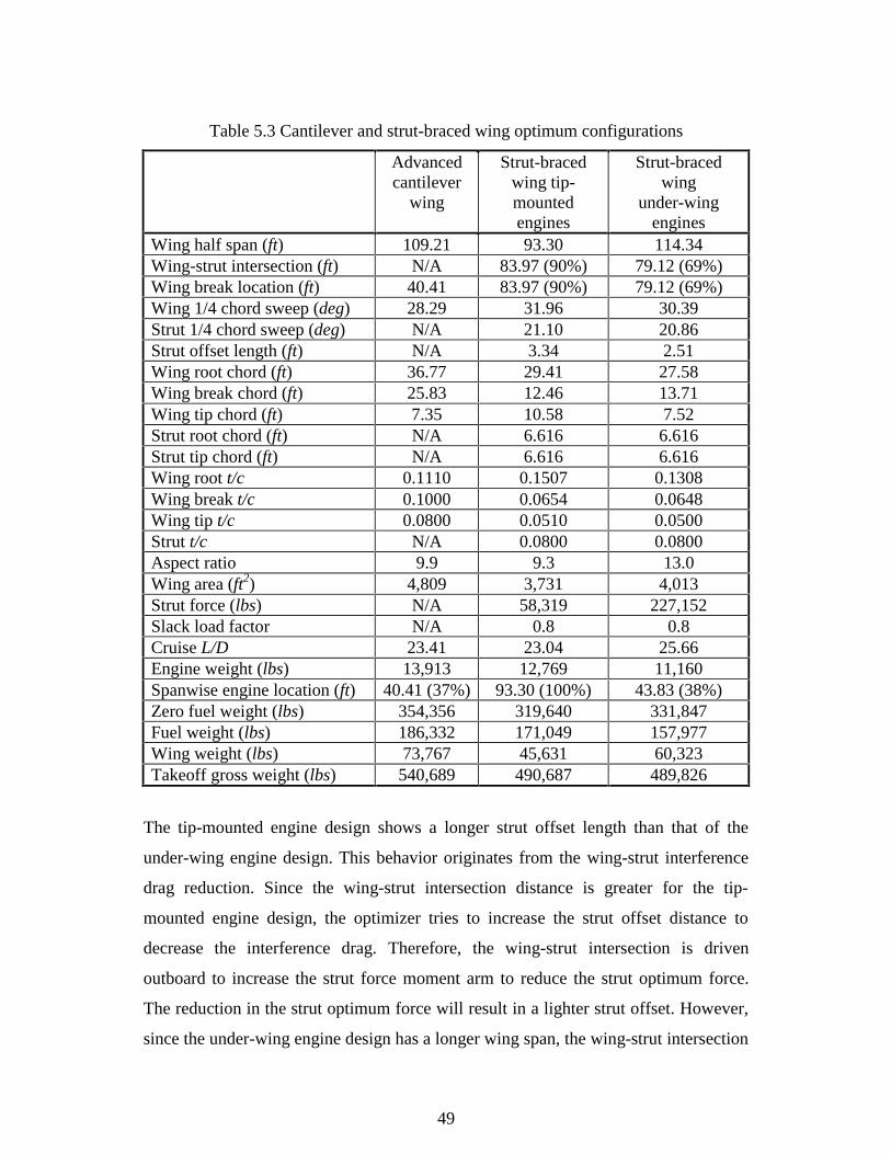
49
Table 5.3 Cantilever and strut-braced wing optimum configurations
Advancedcantilever
wing
Strut-bracedwing tip-mountedengines
Strut-bracedwing
under-wingengines
Wing half span (ft) 109.21 93.30 114.34Wing-strut intersection (ft) N/A 83.97 (90%) 79.12 (69%)Wing break location (ft) 40.41 83.97 (90%) 79.12 (69%)Wing 1/4 chord sweep (deg) 28.29 31.96 30.39Strut 1/4 chord sweep (deg) N/A 21.10 20.86Strut offset length (ft) N/A 3.34 2.51Wing root chord (ft) 36.77 29.41 27.58Wing break chord (ft) 25.83 12.46 13.71Wing tip chord (ft) 7.35 10.58 7.52Strut root chord (ft) N/A 6.616 6.616Strut tip chord (ft) N/A 6.616 6.616Wing root t/c 0.1110 0.1507 0.1308Wing break t/c 0.1000 0.0654 0.0648Wing tip t/c 0.0800 0.0510 0.0500Strut t/c N/A 0.0800 0.0800Aspect ratio 9.9 9.3 13.0Wing area (ft2) 4,809 3,731 4,013Strut force (lbs) N/A 58,319 227,152Slack load factor N/A 0.8 0.8Cruise L/D 23.41 23.04 25.66Engine weight (lbs) 13,913 12,769 11,160Spanwise engine location (ft) 40.41 (37%) 93.30 (100%) 43.83 (38%)Zero fuel weight (lbs) 354,356 319,640 331,847Fuel weight (lbs) 186,332 171,049 157,977Wing weight (lbs) 73,767 45,631 60,323Takeoff gross weight (lbs) 540,689 490,687 489,826
The tip-mounted engine design shows a longer strut offset length than that of the
under-wing engine design. This behavior originates from the wing-strut interference
drag reduction. Since the wing-strut intersection distance is greater for the tip-
mounted engine design, the optimizer tries to increase the strut offset distance to
decrease the interference drag. Therefore, the wing-strut intersection is driven
outboard to increase the strut force moment arm to reduce the strut optimum force.
The reduction in the strut optimum force will result in a lighter strut offset. However,
since the under-wing engine design has a longer wing span, the wing-strut intersection
50
lies at about 2/3 of the half span of the wing to prevent high strut and strut offset
weight due to the induced moment by the horizontal strut force component. Thus, the
strut offset length can be shorter without too much interference drag penalty.
The slack load factor for both cases is calculated to be 0.8 which is the specified
upper bound in the slack load factor constraint. This means that the strut engages at
0.8g. Hence, at the cruise condition the strut is active.
Also, several local optima, deviating between 0.6-3.5% from the obtained optima,
were found by changing the design variables initial guesses. Thus, the current
configurations are not guaranteed to be the global optimum designs. However, the
author did his best to discover the best design configurations based on minimum
takeoff gross weight. This was achieved by assigning the design variables initial
values close to the optimum values obtained from the previous run and then re-
optimizing.
5.4 Aerodynamic and Taxi bump Loads
Aerodynamic loads are imported into the structural optimization subroutine from the
aerodynamics subroutine (Grasmeyer et al. 1997). Figure 5.1 shows the lift
distributions at the 2.5g and 1.0g load conditions. A linear interpolation procedure is
used to interpolate the load distributions from the locations where the aerodynamic
loads are assumed onto the structural nodes. The structural nodes are assumed to be
independent of the aerodynamic nodes. A convergence study was performed to
determine a reasonable value for the number of structural nodes. The number of 82
nodes was found suitable. Also, the 2.0g taxi bump loads are obtained from the
procedure described in Section 3.2 and are shown in Figure 5.2. For these plots, the x-
axis represents the aerodynamic half-span in ft and the y-axis represents the amount of
load in lbs/ft.
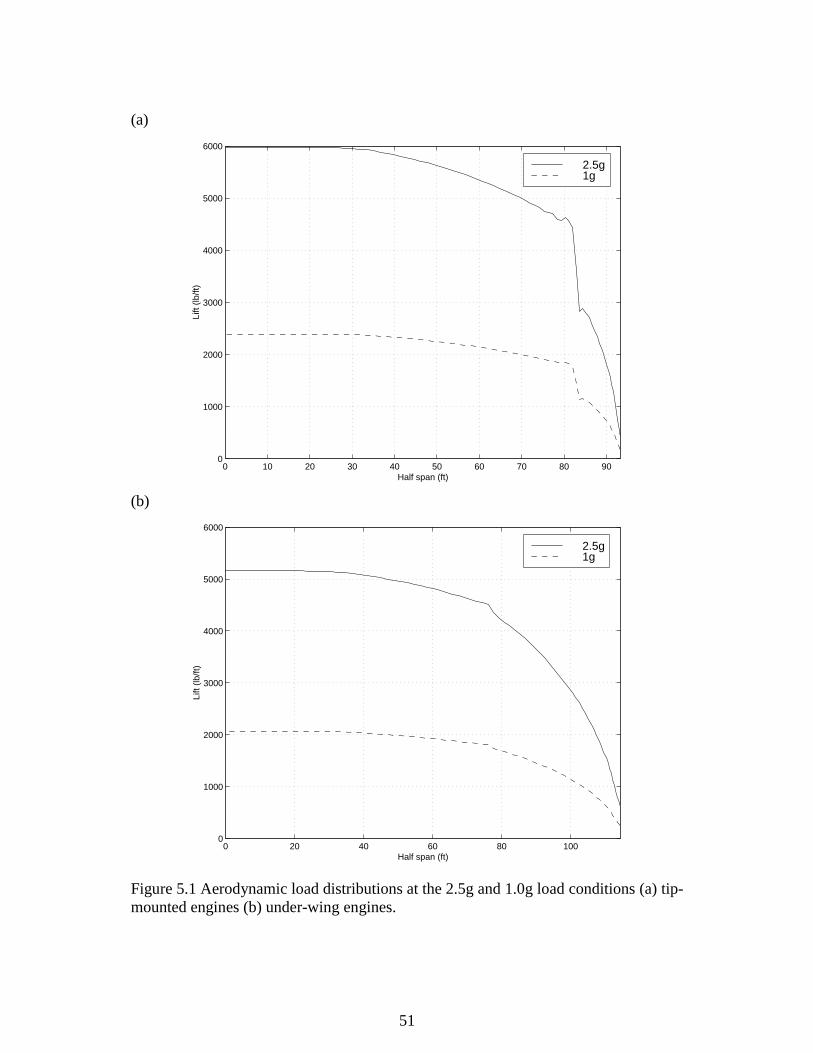
51
(a)
0 10 20 30 40 50 60 70 80 900
1000
2000
3000
4000
5000
6000
Half span (ft)
Lift
(lb/ft
)
2.5g1g
(b)
0 20 40 60 80 1000
1000
2000
3000
4000
5000
6000
Half span (ft)
Lift
(lb/ft
)
2.5g1g
Figure 5.1 Aerodynamic load distributions at the 2.5g and 1.0g load conditions (a) tip-mounted engines (b) under-wing engines.
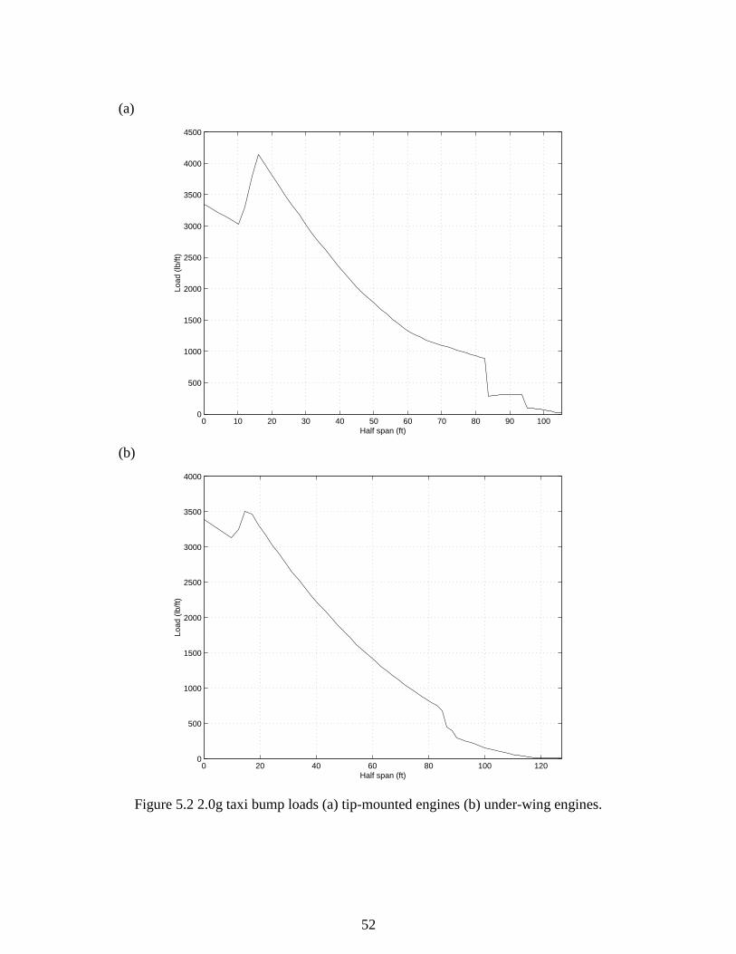
52
(a)
0 10 20 30 40 50 60 70 80 90 1000
500
1000
1500
2000
2500
3000
3500
4000
4500
Half span (ft)
Load
(lb
/ft)
(b)
0 20 40 60 80 100 1200
500
1000
1500
2000
2500
3000
3500
4000
Half span (ft)
Load
(lb
/ft)
Figure 5.2 2.0g taxi bump loads (a) tip-mounted engines (b) under-wing engines.
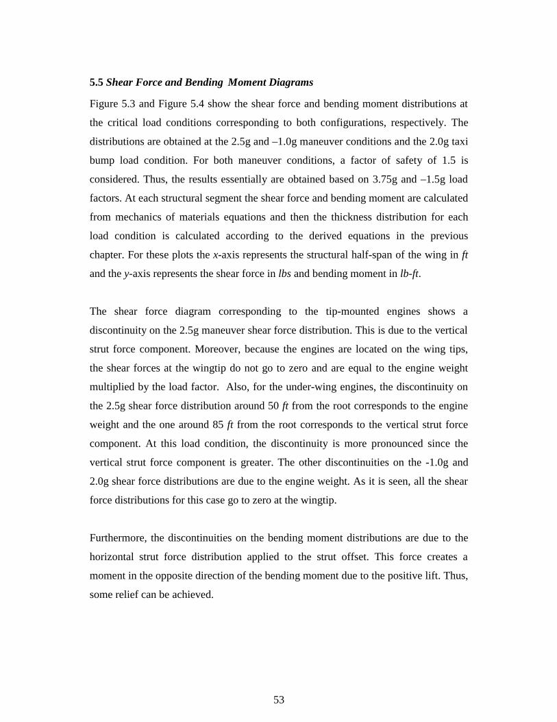
53
5.5 Shear Force and Bending Moment Diagrams
Figure 5.3 and Figure 5.4 show the shear force and bending moment distributions at
the critical load conditions corresponding to both configurations, respectively. The
distributions are obtained at the 2.5g and –1.0g maneuver conditions and the 2.0g taxi
bump load condition. For both maneuver conditions, a factor of safety of 1.5 is
considered. Thus, the results essentially are obtained based on 3.75g and –1.5g load
factors. At each structural segment the shear force and bending moment are calculated
from mechanics of materials equations and then the thickness distribution for each
load condition is calculated according to the derived equations in the previous
chapter. For these plots the x-axis represents the structural half-span of the wing in ft
and the y-axis represents the shear force in lbs and bending moment in lb-ft.
The shear force diagram corresponding to the tip-mounted engines shows a
discontinuity on the 2.5g maneuver shear force distribution. This is due to the vertical
strut force component. Moreover, because the engines are located on the wing tips,
the shear forces at the wingtip do not go to zero and are equal to the engine weight
multiplied by the load factor. Also, for the under-wing engines, the discontinuity on
the 2.5g shear force distribution around 50 ft from the root corresponds to the engine
weight and the one around 85 ft from the root corresponds to the vertical strut force
component. At this load condition, the discontinuity is more pronounced since the
vertical strut force component is greater. The other discontinuities on the -1.0g and
2.0g shear force distributions are due to the engine weight. As it is seen, all the shear
force distributions for this case go to zero at the wingtip.
Furthermore, the discontinuities on the bending moment distributions are due to the
horizontal strut force distribution applied to the strut offset. This force creates a
moment in the opposite direction of the bending moment due to the positive lift. Thus,
some relief can be achieved.
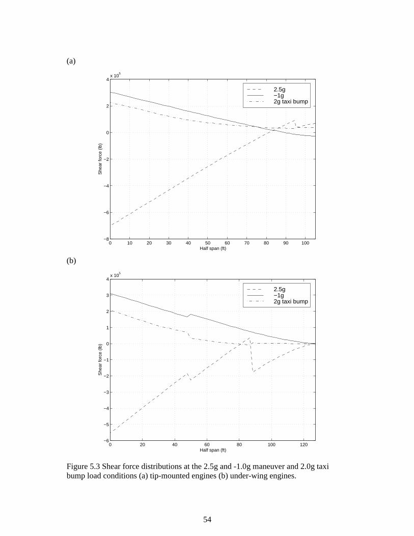
54
(a)
0 10 20 30 40 50 60 70 80 90 100−8
−6
−4
−2
0
2
4x 10
5
Half span (ft)
She
ar fo
rce
(lb)
2.5g −1g 2g taxi bump
(b)
0 20 40 60 80 100 120−6
−5
−4
−3
−2
−1
0
1
2
3
4x 10
5
Half span (ft)
She
ar fo
rce
(lb)
2.5g −1g 2g taxi bump
Figure 5.3 Shear force distributions at the 2.5g and -1.0g maneuver and 2.0g taxibump load conditions (a) tip-mounted engines (b) under-wing engines.
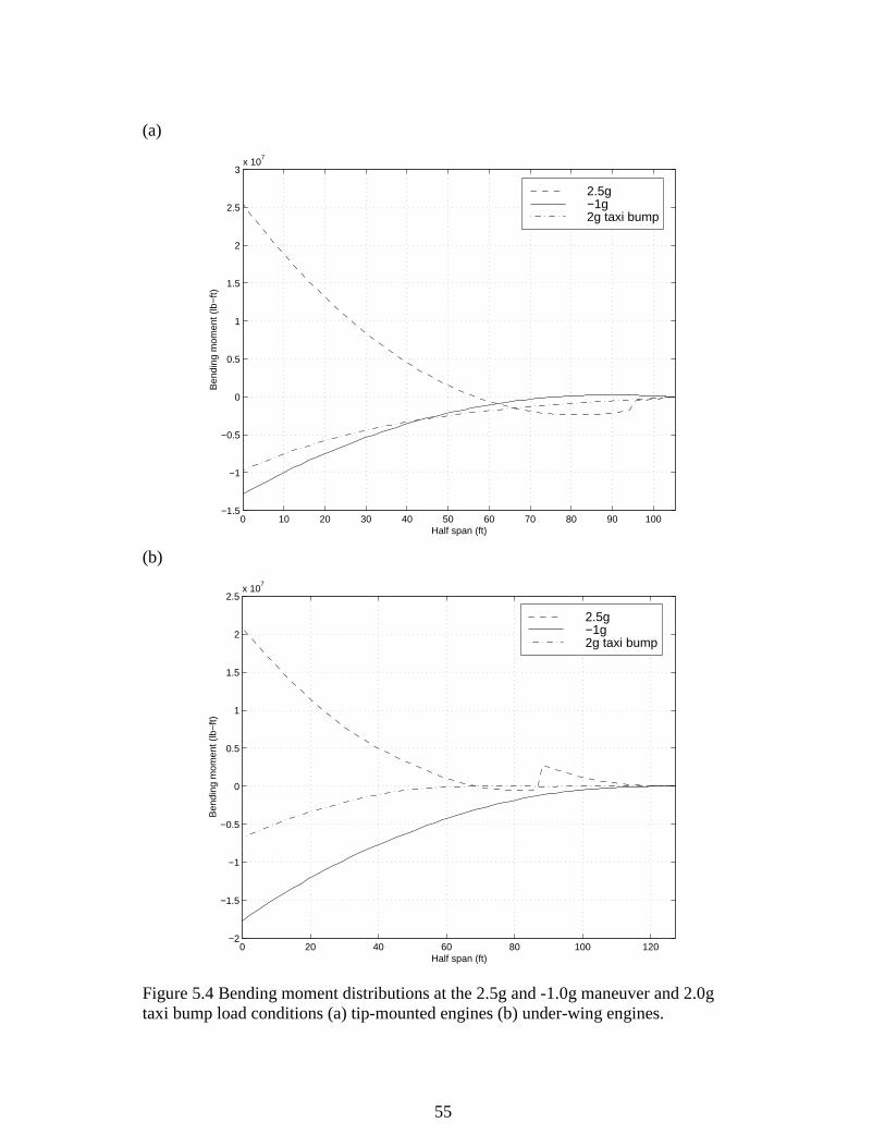
55
(a)
0 10 20 30 40 50 60 70 80 90 100−1.5
−1
−0.5
0
0.5
1
1.5
2
2.5
3x 10
7
Half span (ft)
Ben
ding
mom
ent (
lb−
ft)
2.5g −1g 2g taxi bump
(b)
0 20 40 60 80 100 120−2
−1.5
−1
−0.5
0
0.5
1
1.5
2
2.5x 10
7
Half span (ft)
Ben
ding
mom
ent (
lb−
ft)
2.5g −1g 2g taxi bump
Figure 5.4 Bending moment distributions at the 2.5g and -1.0g maneuver and 2.0gtaxi bump load conditions (a) tip-mounted engines (b) under-wing engines.
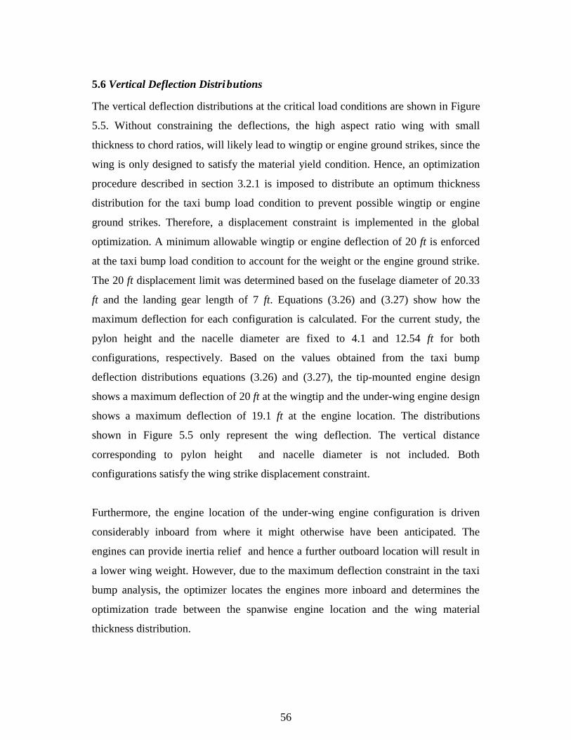
56
5.6 Vertical Deflection Distributions
The vertical deflection distributions at the critical load conditions are shown in Figure
5.5. Without constraining the deflections, the high aspect ratio wing with small
thickness to chord ratios, will likely lead to wingtip or engine ground strikes, since the
wing is only designed to satisfy the material yield condition. Hence, an optimization
procedure described in section 3.2.1 is imposed to distribute an optimum thickness
distribution for the taxi bump load condition to prevent possible wingtip or engine
ground strikes. Therefore, a displacement constraint is implemented in the global
optimization. A minimum allowable wingtip or engine deflection of 20 ft is enforced
at the taxi bump load condition to account for the weight or the engine ground strike.
The 20 ft displacement limit was determined based on the fuselage diameter of 20.33
ft and the landing gear length of 7 ft. Equations (3.26) and (3.27) show how the
maximum deflection for each configuration is calculated. For the current study, the
pylon height and the nacelle diameter are fixed to 4.1 and 12.54 ft for both
configurations, respectively. Based on the values obtained from the taxi bump
deflection distributions equations (3.26) and (3.27), the tip-mounted engine design
shows a maximum deflection of 20 ft at the wingtip and the under-wing engine design
shows a maximum deflection of 19.1 ft at the engine location. The distributions
shown in Figure 5.5 only represent the wing deflection. The vertical distance
corresponding to pylon height and nacelle diameter is not included. Both
configurations satisfy the wing strike displacement constraint.
Furthermore, the engine location of the under-wing engine configuration is driven
considerably inboard from where it might otherwise have been anticipated. The
engines can provide inertia relief and hence a further outboard location will result in
a lower wing weight. However, due to the maximum deflection constraint in the taxi
bump analysis, the optimizer locates the engines more inboard and determines the
optimization trade between the spanwise engine location and the wing material
thickness distribution.
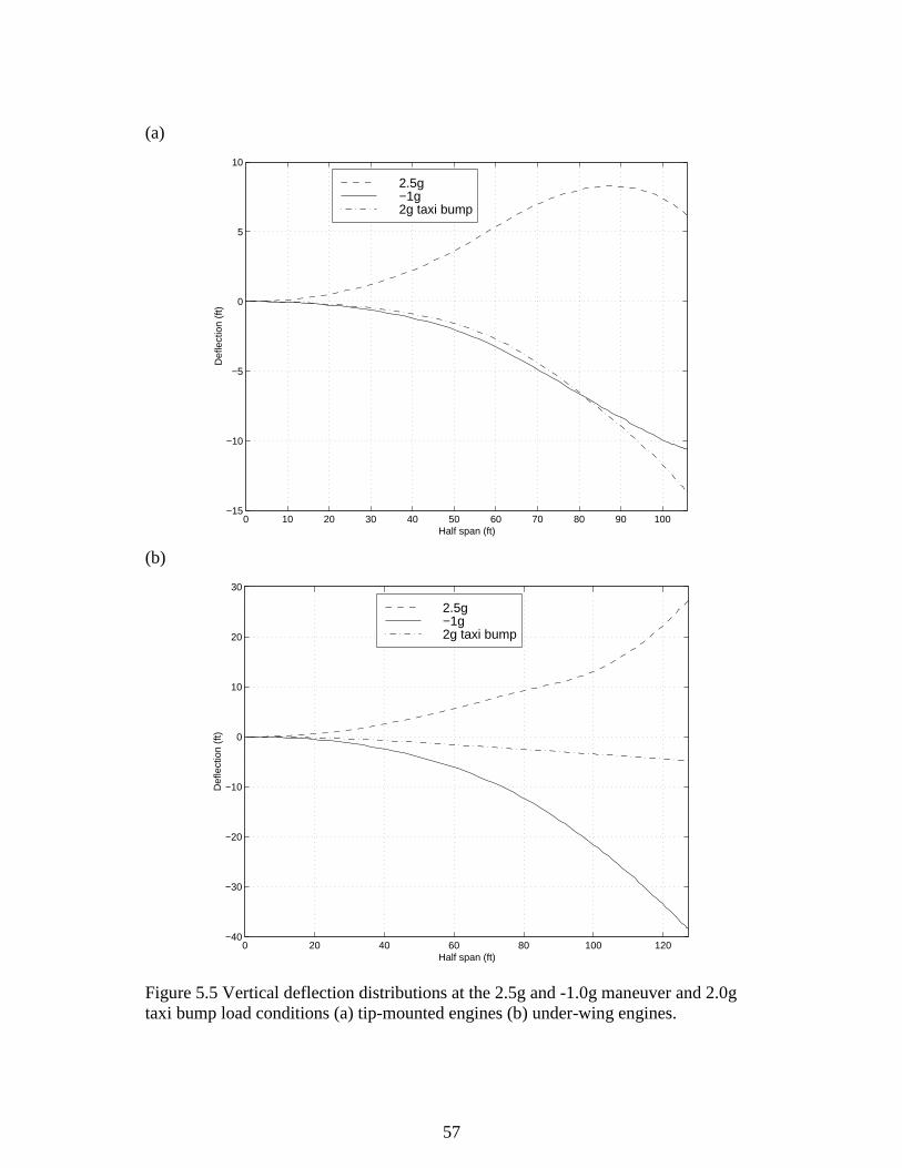
57
(a)
0 10 20 30 40 50 60 70 80 90 100−15
−10
−5
0
5
10
Half span (ft)
Def
lect
ion
(ft)
2.5g −1g 2g taxi bump
(b)
0 20 40 60 80 100 120−40
−30
−20
−10
0
10
20
30
Half span (ft)
Def
lect
ion
(ft)
2.5g −1g 2g taxi bump
Figure 5.5 Vertical deflection distributions at the 2.5g and -1.0g maneuver and 2.0gtaxi bump load conditions (a) tip-mounted engines (b) under-wing engines.

58
5.7 Material Thickness Distr ibutions
Figure 5.6 depicts the required wing box material thickness distributions due to
bending only at the 2.5g and -1.0g maneuver and 2.0g taxi bump load conditions.
These plots reveal that for some regions along the wing half span the -1.0g load
condition is the dominant load condition and for other regions the 2.5g load condition
is the dominant one. Thus, at each segment, the maximum thickness distribution on
the figure defines the required thickness. Two separate skin thickness distributions are
obtained for the taxi bump load condition. The dash-dotted line is the distribution due
to the material allowable stress and was obtained based on the fully stressed criterion
while the dotted line is the distribution due to the maximum displacement constraint
which was discussed in the previous chapter. Moreover, the taxi bump thickness
distributions show that the required skin thickness distribution due to this load
condition may violate the required skin thickness distribution due to the maneuver
conditions. This is avoided by adding the required extra thickness due to the taxi
bump load condition at the aforementioned wing locations to the required thickness
due to the maneuver conditions. A minimum gauge of 0.055 in is used as a lower
bound for the skin thickness distributions. For the current configurations, at the taxi
bump load condition, the material thickness distributions due to bending are only
exceeding the minimum gauge thickness and the one corresponding to the tip-
mounted engine configuration only violates the maneuver envelope. The material
thickness distribution due to the displacement constraint is not active for either
configuration. The outer thickness envelope in both figures show the design material
thickness. The two sharp changes on the thickness distributions at the 2.5g load
condition are due to the moments applied by the strut horizontal force component
acting on the strut offset as can be seen on the bending moment diagrams (Figure 5.4).
This is most likely the reason which prevents the material thickness distribution due
to the ground strike displacement constraint becoming critical.
59
(a)
0 10 20 30 40 50 60 70 80 90 1000
0.1
0.2
0.3
0.4
0.5
0.6
0.7
0.8
Half span (ft)
Pan
el th
ickn
ess
(in)
2.5g −1g 2g taxi bump Tip constraint
(b)
0 20 40 60 80 100 1200
0.1
0.2
0.3
0.4
0.5
0.6
0.7
0.8
0.9
Half span (ft)
Pan
el th
ickn
ess
(in)
2.5g −1g 2g taxi bump Tip constraint
Figure 5.6 Material thickness distributions at the 2.5g and -1.0g maneuver and 2.0gtaxi bump load conditions (a) tip-mounted engines (b) under-wing engines.
60
5.8 Load Alleviation
To further reduce the wing weight and thus to increase the overall aircraft
performance, modern electronic control systems in concert with the fly-by-wire
technology offer a considerable potential for active load alleviation.
The use of active load control has been investigated to understand the effects of load
alleviation on potential bending weight reduction. The aileron is used to shift
approximately 10% of the lift inboard at the maneuver load conditions. By deflecting
the aileron, the wing intends to wash out at the tip, thereby shifting the lift inboard
(Kulfan et al., 1978). Hence, this phenomenon produces a bending weight reduction at
the root since the lift distribution centroid is also moved inboard. Moreover, Young et
al. (1998) explains how trailing edge flaps are used for load alleviation on the F/A-
18E/F aircraft. As the aircraft pulls load factor, the trailing edge flap is scheduled
down by the flight control system as a function of load factor. The result is a
modification of the lift distribution with less lift on outboard and more on inboard.
This reduces wing bending moment, which results in a reduction in wing weight.
Table 5.4 summarizes the optimum configurations. The under-wing engine
configuration shows more improvements in both aerodynamics and structures than
those of the under-wing engine configuration without active load alleviation. Active
load alleviation is a practical means to reduce the structural weight. Because the
under-wing engine configuration is an aerodynamic driven design, active load
alleviation not only reduced the wing weight but also helped with aerodynamic
improvements (a higher L/D) due to its design behavior. Also, the tip-mounted engine
configuration shows a reduction in wing weight compared to that of the same
configuration without active load alleviation. However, aerodynamic improvements
are not observed for the tip-mounted engine configuration employing active load
alleviation compared to the case of the same configuration without active load
alleviation since it is a structurally driven design. In general, the results show that this
mechanism could assist in achieving a significant reduction in the bending weight.
Further discussion will follow in the next few sections.
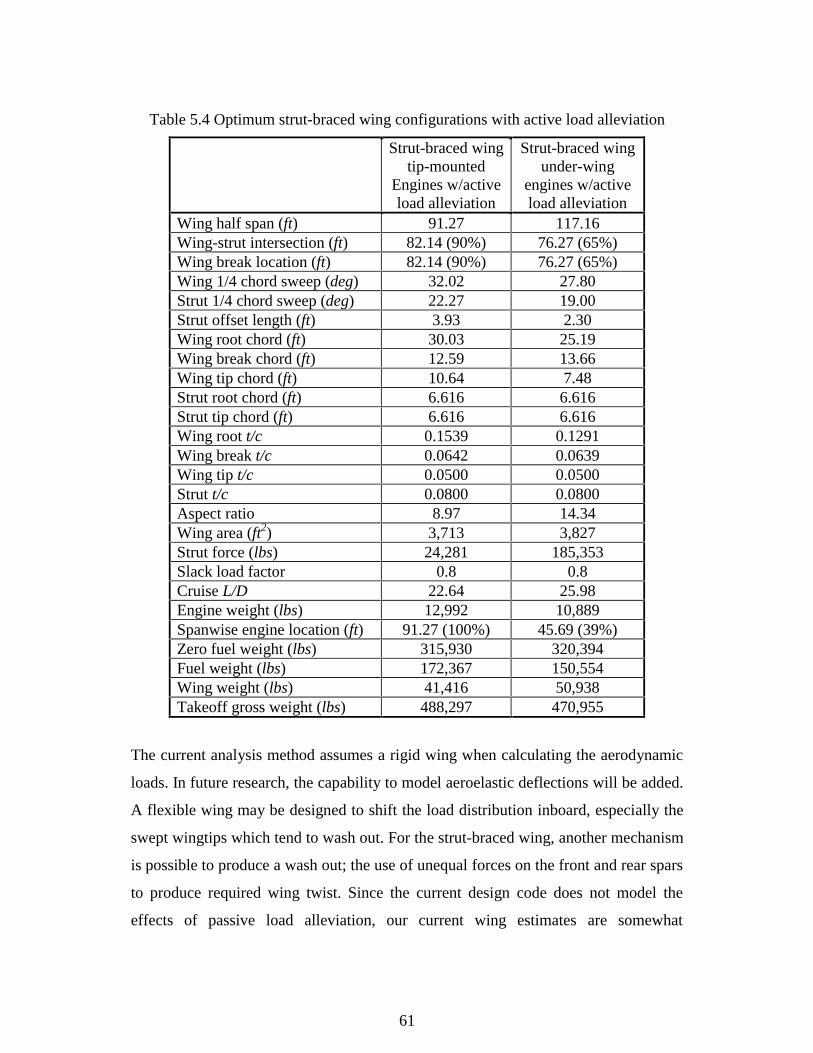
61
Table 5.4 Optimum strut-braced wing configurations with active load alleviation
Strut-braced wingtip-mounted
Engines w/activeload alleviation
Strut-braced wingunder-wing
engines w/activeload alleviation
Wing half span (ft) 91.27 117.16Wing-strut intersection (ft) 82.14 (90%) 76.27 (65%)Wing break location (ft) 82.14 (90%) 76.27 (65%)Wing 1/4 chord sweep (deg) 32.02 27.80Strut 1/4 chord sweep (deg) 22.27 19.00Strut offset length (ft) 3.93 2.30Wing root chord (ft) 30.03 25.19Wing break chord (ft) 12.59 13.66Wing tip chord (ft) 10.64 7.48Strut root chord (ft) 6.616 6.616Strut tip chord (ft) 6.616 6.616Wing root t/c 0.1539 0.1291Wing break t/c 0.0642 0.0639Wing tip t/c 0.0500 0.0500Strut t/c 0.0800 0.0800Aspect ratio 8.97 14.34Wing area (ft2) 3,713 3,827Strut force (lbs) 24,281 185,353Slack load factor 0.8 0.8Cruise L/D 22.64 25.98Engine weight (lbs) 12,992 10,889Spanwise engine location (ft) 91.27 (100%) 45.69 (39%)Zero fuel weight (lbs) 315,930 320,394Fuel weight (lbs) 172,367 150,554Wing weight (lbs) 41,416 50,938Takeoff gross weight (lbs) 488,297 470,955
The current analysis method assumes a rigid wing when calculating the aerodynamic
loads. In future research, the capability to model aeroelastic deflections will be added.
A flexible wing may be designed to shift the load distribution inboard, especially the
swept wingtips which tend to wash out. For the strut-braced wing, another mechanism
is possible to produce a wash out; the use of unequal forces on the front and rear spars
to produce required wing twist. Since the current design code does not model the
effects of passive load alleviation, our current wing estimates are somewhat
62
conservative. In the next section the weight results obtained by implimenting the
active load alleviation are presented.
5.9 Wing Weight Results and Comparison
The wing weight breakdowns of the aluminum and composite strut-braced and
cantilever wing configurations are tabulated in Table 5.5. The effect of active load
alleviation on the wing weight and takeoff gross weight is also reflected in the
tabulated data. Figure 5.7 and Figure 5.8 show the wing weight and takeoff gross
weight comparisons. The wing weight varies between 73,767 lbs for the cantilever
wing to 45,631 lbs for the strut-braced composite wing with tip-mounted engines.
Comparing the strut-braced wing weights with the cantilever wing shows that the
strut-bracing can reduce the wing weight and takeoff gross weight considerably. The
consequence is a 38% weight savings for the composite strut-braced wing with tip-
mounted engines and an 18% weight savings for the composite strut-braced wing with
under-wing engines compared to the composite cantilever wing. Also, the use of a
composite material has reduced the wing weight of the tip-mounted engine design by
18% and the under-wing engine design by 8%. As mentioned earlier, the tip-mounted
engine design is a structurally dominated design and thus a lighter wing with greater
drag is achieved. On the other hand, the under-wing engine design is an
aerodynamically dominated design and thus less drag and a heavier wing is obtained.
Moreover, active load alleviation via aileron deflection is considered. This is done by
transferring 10% of the lift inboard at the maneuver load conditions. Therefore, a
wing weight reduction and a total takeoff gross weight reduction are expected.
According to Table 5.5, the weight reduction corresponding to the under-wing engine
configuration is more pronounced than that corresponding to the tip-mounted engine
configuration. Since the strut-braced wing with under-wing engines is
aerodynamically more efficient, and according to Figure 5.6-(b) both maneuver cases
contribute to the weight more or less equally, the use of active load alleviation
increases the structural efficiency significantly without losing its aerodynamic
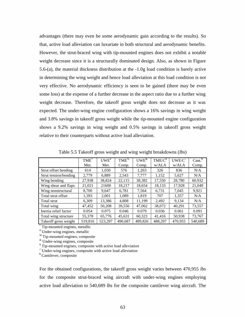
63
advantages (there may even be some aerodynamic gain according to the results). So
that, active load alleviation can luxuriate in both structural and aerodynamic benefits.
However, the strut-braced wing with tip-mounted engines does not exhibit a notable
weight decrease since it is a structurally dominated design. Also, as shown in Figure
5.6-(a), the material thickness distribution at the -1.0g load condition is barely active
in determining the wing weight and hence load alleviation at this load condition is not
very effective. No aerodynamic efficiency is seen to be gained (there may be even
some loss) at the expense of a further decrease in the aspect ratio due to a further wing
weight decrease. Therefore, the takeoff gross weight does not decrease as it was
expected. The under-wing engine configuration shows a 16% savings in wing weight
and 3.8% savings in takeoff gross weight while the tip-mounted engine configuration
shows a 9.2% savings in wing weight and 0.5% savings in takeoff gross weight
relative to their counterparts without active load alleviation.
Table 5.5 Takeoff gross weight and wing weight breakdowns (lbs)
TME*
Met.UWE#
Met.TME%
Comp.UWE&
Comp.TME/C$
w/ALAUWE/C+
w/ALACant.
Comp.Strut offset bending 614 1,030 576 1,263 326 836 N/AStrut tension/bending 2,779 6,889 2,543 7,777 1,152 5,627 N/AWing bending 27,938 38,824 22,115 38,382 17,550 28,780 60,932Wing shear and flaps 21,021 21600 18,217 18,654 18,133 17,928 21,049Wing nonstructural 8,700 9,647 6,781 7,564 6,731 7,045 9,921Total strut offset 1,393 2,001 1,089 1,819 707 1,357 N/ATotal strut 6,309 13,386 4,808 11,199 2,492 9,134 N/ATotal wing 47,452 50,208 39,556 47,062 38,072 40,291 73,557Inertia relief factor 0.054 0.075 0.046 0.079 0.036 0.061 0.091Total wing structure 55,378 65,776 45,631 60,323 41,416 50,938 73,767Takeoff gross weight 519,816 523,297 490,687 489,826 488,297 470,955 540,689
∗ Tip-mounted engines, metallic# Under-wing engines, metallic% Tip-mounted engines, composite& Under-wing engines, composite$ Tip-mounted engines, composite with active load alleviation+ Under-wing engines, composite with active load alleviation¶ Cantilever, composite
For the obtained configurations, the takeoff gross weight varies between 470,955 lbs
for the composite strut-braced wing aircraft with under-wing engines employing
active load alleviation to 540,689 lbs for the composite cantilever wing aircraft. The
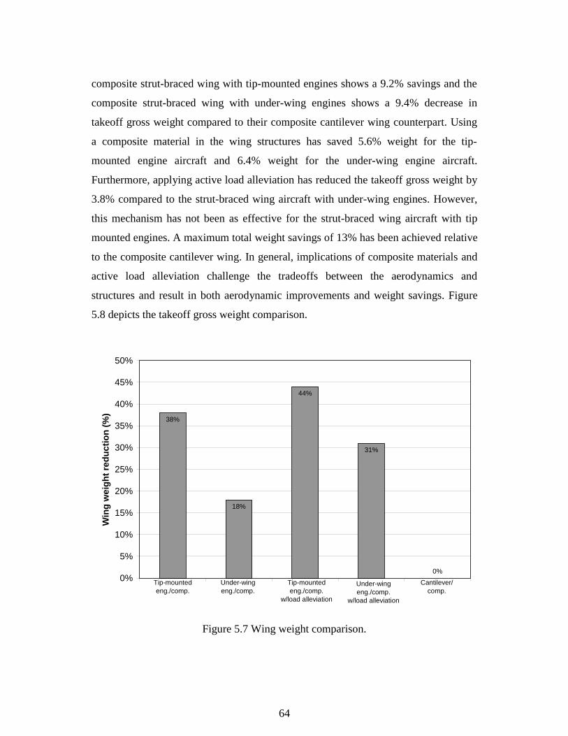
64
composite strut-braced wing with tip-mounted engines shows a 9.2% savings and the
composite strut-braced wing with under-wing engines shows a 9.4% decrease in
takeoff gross weight compared to their composite cantilever wing counterpart. Using
a composite material in the wing structures has saved 5.6% weight for the tip-
mounted engine aircraft and 6.4% weight for the under-wing engine aircraft.
Furthermore, applying active load alleviation has reduced the takeoff gross weight by
3.8% compared to the strut-braced wing aircraft with under-wing engines. However,
this mechanism has not been as effective for the strut-braced wing aircraft with tip
mounted engines. A maximum total weight savings of 13% has been achieved relative
to the composite cantilever wing. In general, implications of composite materials and
active load alleviation challenge the tradeoffs between the aerodynamics and
structures and result in both aerodynamic improvements and weight savings. Figure
5.8 depicts the takeoff gross weight comparison.
18%
44%
31%
0%
38%
0%
5%
10%
15%
20%
25%
30%
35%
40%
45%
50%
1 2 3 4 5
Win
g w
eig
ht
red
uct
ion
(%
)
Tip-mounted eng./comp.
Under-wing eng./comp.
Tip-mounted eng./comp.
w/load alleviation
Under-wing eng./comp.
w/load alleviation
Cantilever/comp.
Figure 5.7 Wing weight comparison.
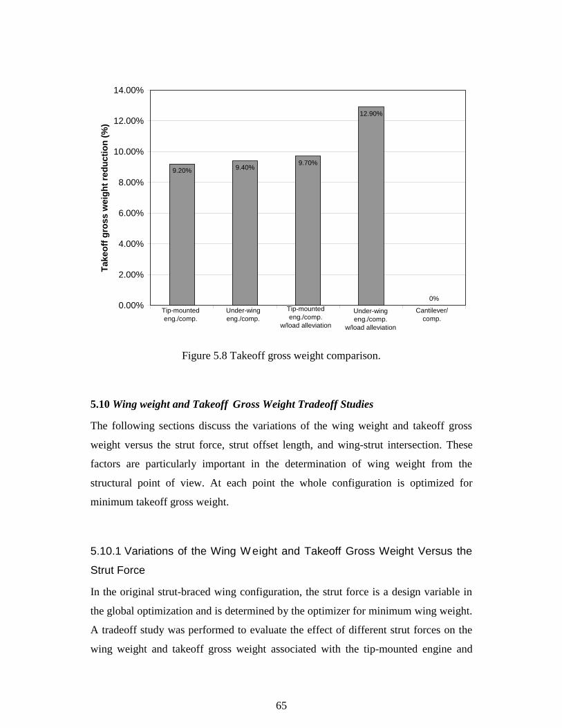
65
9.20% 9.40%9.70%
12.90%
0%0.00%
2.00%
4.00%
6.00%
8.00%
10.00%
12.00%
14.00%
1 2 3 4 5
Tak
eoff
gro
ss w
eig
ht
red
uct
ion
(%
)
Tip-mounted eng./comp.
Under-wing eng./comp.
Tip-mounted eng./comp.
w/load alleviation
Under-wing eng./comp.
w/load alleviation
Cantilever/comp.
Figure 5.8 Takeoff gross weight comparison.
5.10 Wing weight and Takeoff Gross Weight Tradeoff Studies
The following sections discuss the variations of the wing weight and takeoff gross
weight versus the strut force, strut offset length, and wing-strut intersection. These
factors are particularly important in the determination of wing weight from the
structural point of view. At each point the whole configuration is optimized for
minimum takeoff gross weight.
5.10.1 Variations of the Wing W eight and Takeoff Gross Weight Versus the
Strut Force
In the original strut-braced wing configuration, the strut force is a design variable in
the global optimization and is determined by the optimizer for minimum wing weight.
A tradeoff study was performed to evaluate the effect of different strut forces on the
wing weight and takeoff gross weight associated with the tip-mounted engine and
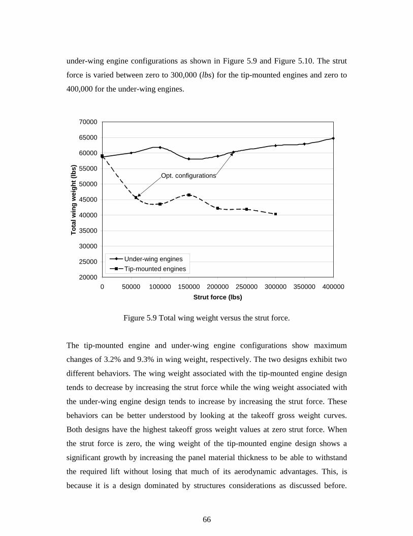
66
under-wing engine configurations as shown in Figure 5.9 and Figure 5.10. The strut
force is varied between zero to 300,000 (lbs) for the tip-mounted engines and zero to
400,000 for the under-wing engines.
20000
25000
30000
35000
40000
45000
50000
55000
60000
65000
70000
0 50000 100000 150000 200000 250000 300000 350000 400000
Strut force (lbs)
To
tal w
ing
wei
gh
t (l
bs)
Under-wing engines
Tip-mounted engines
Opt. configurations
Figure 5.9 Total wing weight versus the strut force.
The tip-mounted engine and under-wing engine configurations show maximum
changes of 3.2% and 9.3% in wing weight, respectively. The two designs exhibit two
different behaviors. The wing weight associated with the tip-mounted engine design
tends to decrease by increasing the strut force while the wing weight associated with
the under-wing engine design tends to increase by increasing the strut force. These
behaviors can be better understood by looking at the takeoff gross weight curves.
Both designs have the highest takeoff gross weight values at zero strut force. When
the strut force is zero, the wing weight of the tip-mounted engine design shows a
significant growth by increasing the panel material thickness to be able to withstand
the required lift without losing that much of its aerodynamic advantages. This, is
because it is a design dominated by structures considerations as discussed before.
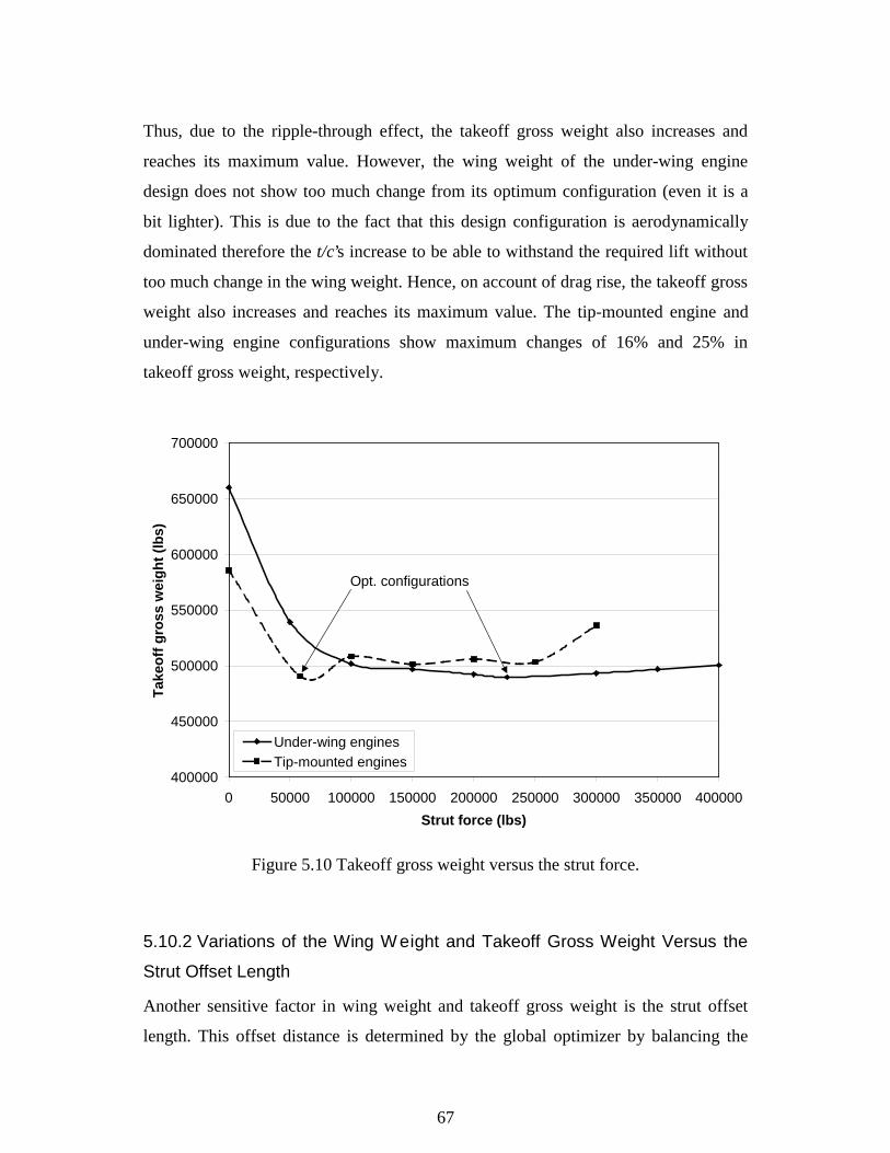
67
Thus, due to the ripple-through effect, the takeoff gross weight also increases and
reaches its maximum value. However, the wing weight of the under-wing engine
design does not show too much change from its optimum configuration (even it is a
bit lighter). This is due to the fact that this design configuration is aerodynamically
dominated therefore the t/c’s increase to be able to withstand the required lift without
too much change in the wing weight. Hence, on account of drag rise, the takeoff gross
weight also increases and reaches its maximum value. The tip-mounted engine and
under-wing engine configurations show maximum changes of 16% and 25% in
takeoff gross weight, respectively.
400000
450000
500000
550000
600000
650000
700000
0 50000 100000 150000 200000 250000 300000 350000 400000
Strut force (lbs)
Tak
eoff
gro
ss w
eig
ht
(lb
s)
Under-wing enginesTip-mounted engines
Opt. configurations
Figure 5.10 Takeoff gross weight versus the strut force.
5.10.2 Variations of the Wing W eight and Takeoff Gross Weight Versus the
Strut Offset Length
Another sensitive factor in wing weight and takeoff gross weight is the strut offset
length. This offset distance is determined by the global optimizer by balancing the
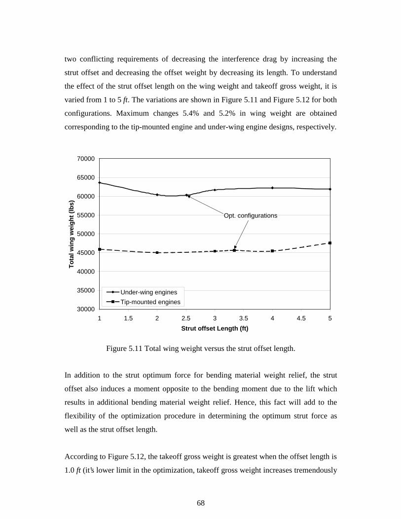
68
two conflicting requirements of decreasing the interference drag by increasing the
strut offset and decreasing the offset weight by decreasing its length. To understand
the effect of the strut offset length on the wing weight and takeoff gross weight, it is
varied from 1 to 5 ft. The variations are shown in Figure 5.11 and Figure 5.12 for both
configurations. Maximum changes 5.4% and 5.2% in wing weight are obtained
corresponding to the tip-mounted engine and under-wing engine designs, respectively.
30000
35000
40000
45000
50000
55000
60000
65000
70000
1 1.5 2 2.5 3 3.5 4 4.5 5
Strut offset Length (ft)
To
tal w
ing
wei
gh
t (l
bs)
Under-wing engines
Tip-mounted engines
Opt. configurations
Figure 5.11 Total wing weight versus the strut offset length.
In addition to the strut optimum force for bending material weight relief, the strut
offset also induces a moment opposite to the bending moment due to the lift which
results in additional bending material weight relief. Hence, this fact will add to the
flexibility of the optimization procedure in determining the optimum strut force as
well as the strut offset length.
According to Figure 5.12, the takeoff gross weight is greatest when the offset length is
1.0 ft (it’s lower limit in the optimization, takeoff gross weight increases tremendously

69
as the offset length is further reduced). The shorter the offset length is, the more
interference drag is produced. Within the range of 2.5 to 4.0 ft, the takeoff gross
weight remains practically unchanged. Consequently, it can be concluded that the
interference drag and the offset weight compensate for one another. When the offset
length is less than 2.5 ft, due to the increase in the interference drag, the takeoff gross
weight also increases. And, when the offset length is more than 4.0 ft due to the
increase in the offset weight and also other factors, the takeoff weight grows. The
maximum changes in takeoff gross weight associated with the tip-mounted engine and
under-wing engine designs are obtained 4.7% and 1.9%, respectively.
480000
485000
490000
495000
500000
505000
510000
515000
520000
1 1.5 2 2.5 3 3.5 4 4.5 5
Strut offset Length (ft)
Tak
eoff
gro
ss w
eig
ht
(lb
s)
Under-wing engines
Tip-mounted engines
Opt. configurations
Figure 5.12 Takeoff gross weight versus the strut offset length.
5.10.3 Variations of the Wing W eight and Takeoff Gross Weight Versus
Wing-Strut Intersection Location
To evaluate the influence of the wing-strut intersection location on the wing weight
and takeoff gross weight, a tradeoff study is performed. The wing-strut intersection
70
location is varied from 40% to 90% of the half span. Figure 5.13 and Figure 5.14
depict the variations of the wing weight and takeoff gross weight versus the wing-
strut intersection, respectively. This design variable plays an important role in
determining the strut offset length and the optimum strut force. A longer strut offset
may cause greater offset weight due to the induced bending moment by the horizontal
strut force component. This results in a smaller strut force. The smaller strut force can
regain its effect on reducing the bending material weight by an increase in the
moment arm (distance from the root to the wing-strut intersection). This is the
situation which most likely took place in the optimization trend associated with the
tip-mounted engine configuration. On the other hand, for the under-wing
configuration the wing-strut intersection was forced more inboard. This issue changes
the optimization trend associated with this design configuration. Hence, the strut
offset can further reduce to save its weight and then a greater strut force could be
applied.
Significant variations in the wing weight are seen for neither configuration. This is
mostly because of the tradeoff between this design variable, the strut offset length,
and the strut force. The tip-mounted engine design shows a maximum change of 5.3%
while the under-wing engine design shows that of 9.6% in wing weight.
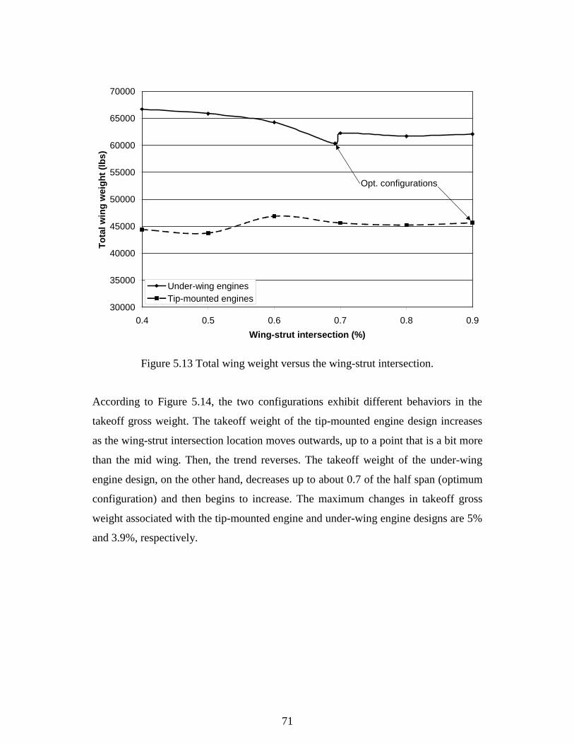
71
30000
35000
40000
45000
50000
55000
60000
65000
70000
0.4 0.5 0.6 0.7 0.8 0.9
Wing-strut intersection (%)
To
tal w
ing
wei
gh
t (l
bs)
Under-wing enginesTip-mounted engines
Opt. configurations
Figure 5.13 Total wing weight versus the wing-strut intersection.
According to Figure 5.14, the two configurations exhibit different behaviors in the
takeoff gross weight. The takeoff weight of the tip-mounted engine design increases
as the wing-strut intersection location moves outwards, up to a point that is a bit more
than the mid wing. Then, the trend reverses. The takeoff weight of the under-wing
engine design, on the other hand, decreases up to about 0.7 of the half span (optimum
configuration) and then begins to increase. The maximum changes in takeoff gross
weight associated with the tip-mounted engine and under-wing engine designs are 5%
and 3.9%, respectively.
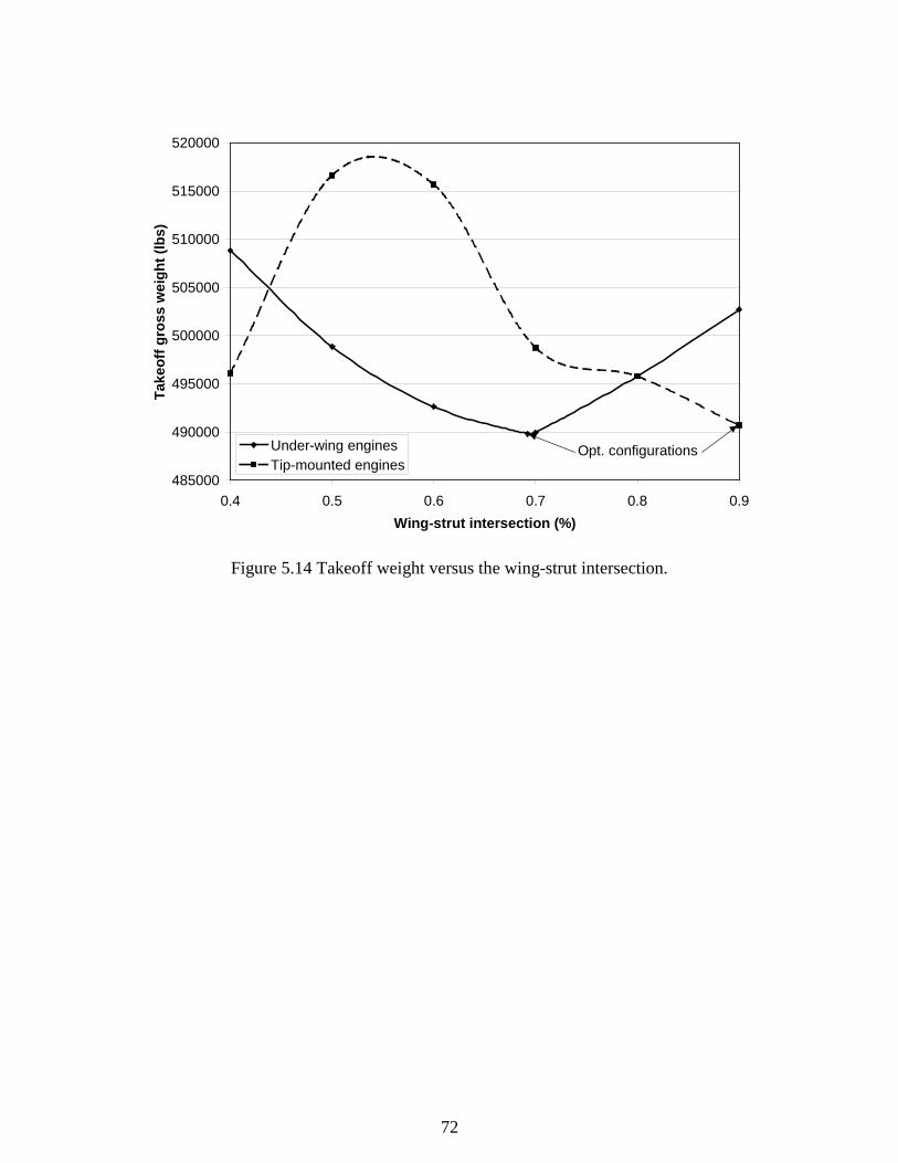
72
485000
490000
495000
500000
505000
510000
515000
520000
0.4 0.5 0.6 0.7 0.8 0.9
Wing-strut intersection (%)
Tak
eoff
gro
ss w
eig
ht
(lb
s)
Under-wing enginesTip-mounted engines
Opt. configurations
Figure 5.14 Takeoff weight versus the wing-strut intersection.
73
Chapter 6 A Preliminary Sta tic Aeroelastic Analysis of
the Strut-Braced Wing Using the Finite Element Method
To reduce weight, aircraft structural parts are commonly built with thin-walled
flexible structures. Thin-walled flexible structures such as wings, when encountering
significant aerodynamic loads, show large elastic deformations and may be prone to
flutter. The elastic deformations induce additional aerodynamic loads which can
strongly affect the aircraft stability and aerodynamic load distributions and thus the
overall performance while flutter results in catastrophic structural failure. Other
aeroelastic phenomena such as divergence and control effectiveness can also be
important. Hence, in aircraft conceptual and preliminary design phases special
attention should be paid to aeroelastic effects on structural design which yields to the
utilization of multidisciplinary design concepts and optimization strategies (Niu,
1988, Bisplinghoff et al., 1983, and Honlinger et al., 1998).
The truss-braced wing has a high aspect ratio made of thin airfoil sections.
Preliminary studies showed that the wing may undergo large deformations at critical
maneuver load conditions. Thus, static aeroelastic effects should be considered to
account for more realistic aerodynamic load distributions since significant differences
may occur in wing weight estimation compared to rigid wing weight estimation. The
introductory work for bending material weight estimation uses load distributions
obtained from the optimum spanload for minimum induced drag method (Grasmeyer,
1997) which does not account for static aeroelastic effects. Studying the aeroelastic
influences requires knowledge of the torsional stiffness distribution along the wing
semispan. Such a capability does not exist in the double-plate model. Therefore, the
MSC/NASTRAN aeroelastic module (Rodden and Johnson, 1994) is used to create a
NASTRAN finite element model for the strut braced wing. The MSC/NASTRAN
optimization module (Moore, 1994) will be integrated (future work) with the static
aeroelastic analysis to perform structural optimizations to produce bending material

74
weight response surfaces to be used in the truss-braced wing MDO code for different
truss-braced wing configurations. The work of Rais-Rohani (1991), Huang (1994),
and Balabanov (1997) can be mentioned in this category. The use of response
surfaces, as mentioned in previous sections, reduces high computational costs
associated with detailed CFD and FEM models. Response surfaces to represent
structural and aerodynamic responses have been used at Virginia Tech for designing
the High Speed Civil Transport (HSCT) with a considerable success for several years.
The reader can refer to Giunta et al., 1996, Giunta et al., 1997, Hutchison et al., 1994,
and Knill et al., 1998 for further information.
6.1 MSC/NASTRAN
MSC/NASTRAN is one of the most common multipurpose commercial finite-element
software packages that is used in the aircraft industry. NASTRAN was developed at
NASA during the late 1960’s period and was released for public use in 1970. Since
then, it has evolved and several different modules have been integrated to it.
MSC/NASTRAN has capabilities of performing linear static analysis, dynamic
analysis, non-linear analysis, aeroelastic analysis, design sensitivity and optimization,
numerical methods, and thermal analysis. For this study, aeroelastic and design
sensitivity and optimization analysis modules are used. The following is a brief
description of each.
6.1.1 MSC/NASTRAN Aeroelastic Analysis Module
The aeroelastic analysis module is capable of performing aeroelastic analyses in both
subsonic and supersonic regimes. The model can be simulated structurally and
aerodynamically with separate grid points. One subsonic and three supersonic lifting
surface aerodynamic theories as well as strip theory are available in this module. The
Doublet-Lattice theory which can account for interference among multiple lifting
surfaces and bodies is used for subsonic aerodynamics while supersonic theories are
the Mach Box method, Piston Theory, and the ZONA51 method for multiple
interfering lifting surfaces. Moreover, splining techniques for both lines and surfaces
75
are provided to interpolate the load distribution from the aerodynamic grid points to
structural degrees of freedom. Furthermore, the equations for static equilibrium are
solved to determine the structural load distribution on an elastic vehicle in trimmed
flight. The solution process leads to aerodynamic stability derivatives, lift and
moment curve slopes and lift and moment coefficients due to control surface rotation,
and trim variables, i.e. angle of attack and control surface setting, as well as
aerodynamic and structural loads, structural deflections, and element stresses (Rodden
and Johnson, 1995).
6.1.2 MSC/NASTRAN Design Sensitivity and Optimization Module
The design sensitivity and optimization module has several built-in numerical
optimization techniques. The optimization algorithms in MSC/NASTRAN belong to
the gradient-based optimization methods. For a general optimization problem, the
method of feasible directions is used. Moreover, finite difference approximations are
employed to evaluate the derivatives. Approximate design models are also included.
Output in design sensitivity and optimization may be generated from (1)
MSC/NASTRAN analysis, (2) design sensitivity analysis, (3) design optimization
(including optimization output), and (4) convergence tests and design model updates
(Moore, 1995).
6.2 MSC/NASTRAN Elemen t Discriptions Used for Wing Modeling
In this section, the MSC/NASTRAN finite element model details are explained. The
developed model uses the CQUAD4 and CTRIA3 membrane and shell elements and
the CROD truss element.
6.2.1 CQUAD4 Shell Element
The CQUAD4 element is a typical isoparametric quadrilateral plate and shell element.
Although there are variety of elements available in the MSC/NASTRAN library, the
CQUAD4 element is the most commonly used two-dimensional element. This
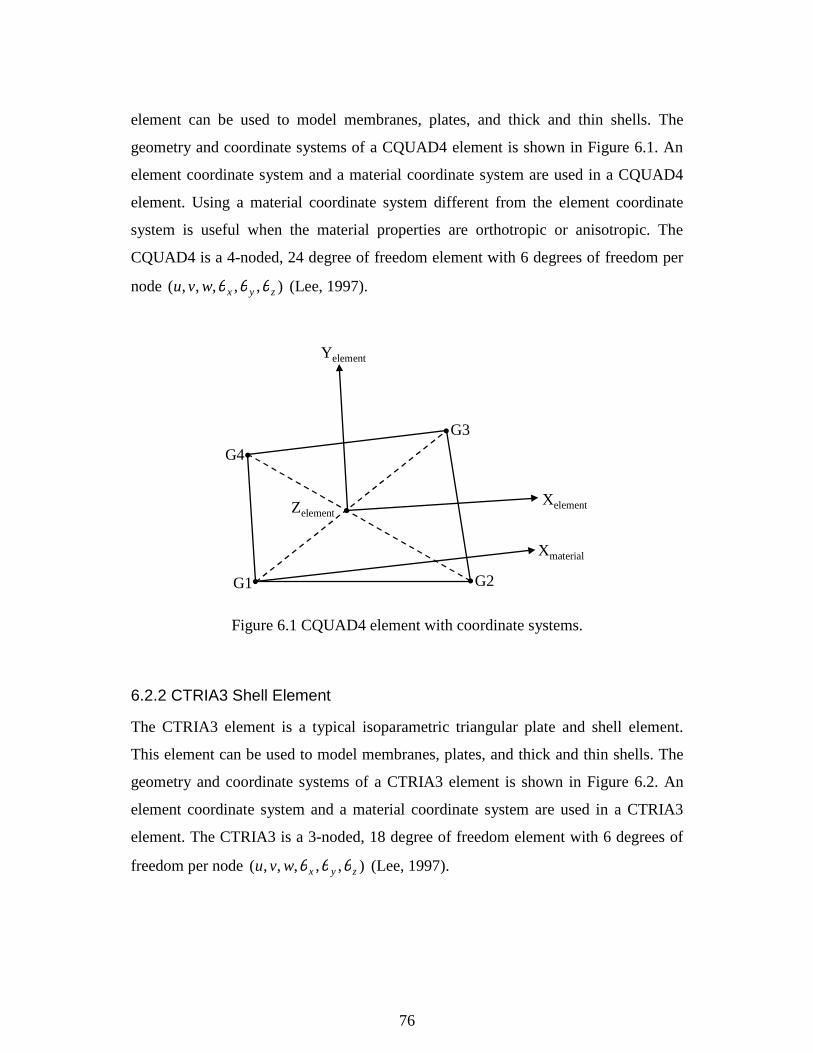
76
element can be used to model membranes, plates, and thick and thin shells. The
geometry and coordinate systems of a CQUAD4 element is shown in Figure 6.1. An
element coordinate system and a material coordinate system are used in a CQUAD4
element. Using a material coordinate system different from the element coordinate
system is useful when the material properties are orthotropic or anisotropic. The
CQUAD4 is a 4-noded, 24 degree of freedom element with 6 degrees of freedom per
node ),,,,,( zyxwvu θθθ (Lee, 1997).
..
. .
.
G1
G4
G2
G3
Xelement
Yelement
Xmaterial
Zelement
Figure 6.1 CQUAD4 element with coordinate systems.
6.2.2 CTRIA3 Shell Element
The CTRIA3 element is a typical isoparametric triangular plate and shell element.
This element can be used to model membranes, plates, and thick and thin shells. The
geometry and coordinate systems of a CTRIA3 element is shown in Figure 6.2. An
element coordinate system and a material coordinate system are used in a CTRIA3
element. The CTRIA3 is a 3-noded, 18 degree of freedom element with 6 degrees of
freedom per node ),,,,,( zyxwvu θθθ (Lee, 1997).

77
G1 G2
G3
. .
.
Xelement
Yelement
Xmaterial
Figure 6.2 CTRIA3 element with coordinate systems.
6.2.3 CROD Truss Element
The CROD element is a one-dimensional axial force and axial torsion (truss) element.
Figure 6.3 shows the geometry and coordinate system of a CROD element. The
CROD is a 2-noded, 6 degree of freedom element with 3 degrees of freedom per node
),,( xvu θ .
. .G1 G2Xelement
Figure 6.3 CROD element.
6.3 Strut-Braced Wing Finite Element Arrangement
Truss-braced wing configurations are highly unconventional. Thus, available weight
estimation software packages are not capable of performing weight analyses on such
wings. Also, analytical-based methods cannot be employed for structural analyses of
such structures as was used for the single-strut-braced wing. Consequently, numerical
techniques such as the finite element method should be used to perform structural
analyses and optimization of complex truss-braced wing configurations. For the time
being, only the strut-braced wing configuration with tip-mounted engines is
considered to develop the finite element model. This can be assumed as the first step
78
towards modeling more complex trusses. MSC/NASTRAN finite-element-based
structural optimization commercial software package was selected to perform
structural optimizations to provide the bending material weight for different truss-
braced wing configurations. The results from the structural optimizations will then be
used in the truss-braced wing MDO code via the response surface methodology.
Performing structural optimizations and customizing response surfaces should be
studied in the future.
A relatively simple finite element model with a fixed arrangement of spars, ribs, and
skin panels is employed. To prevent degree of freedom singularities, the wing skin
panels are modeled by CQUAD4 shell elements. Moreover, spar and rib caps are
modeled by CROD truss elements. Because spar and rib shear webs contribute to the
stiffness of the structure hence they should not be considered as pure shear elements.
Therefore, CQUAD4 membrane elements are used to model spar and rib shear webs.
Figure 6.4 shows a typical wing box cell that is used herein.
The wing box from top and side views is depicted in Figure 6.5 and Figure 6.6. The
front spar is located at 15% chord and the rear spar is located at 60% chord. Also, a
20-30 in spacing is considered for the ribs. Moreover, the wing ribs are assumed
perpendicular to the rear spar. This arrangement has structural advantages over the
case that the ribs are parallel to the flight path. The latter has too many structural
disadvantages (Niu, 1988) such as (1) the rib webs are subjected to chordwise bending
(2) additional twist is produced due to wing bending.
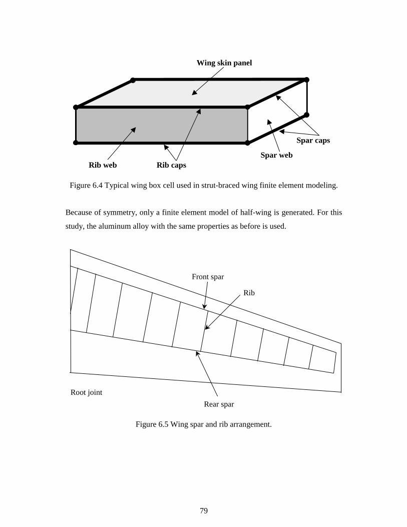
79
Spar caps
Rib caps
Wing skin panel
Spar webRib web
Figure 6.4 Typical wing box cell used in strut-braced wing finite element modeling.
Because of symmetry, only a finite element model of half-wing is generated. For this
study, the aluminum alloy with the same properties as before is used.
Front spar
Rear spar
Root joint
Rib
Figure 6.5 Wing spar and rib arrangement.
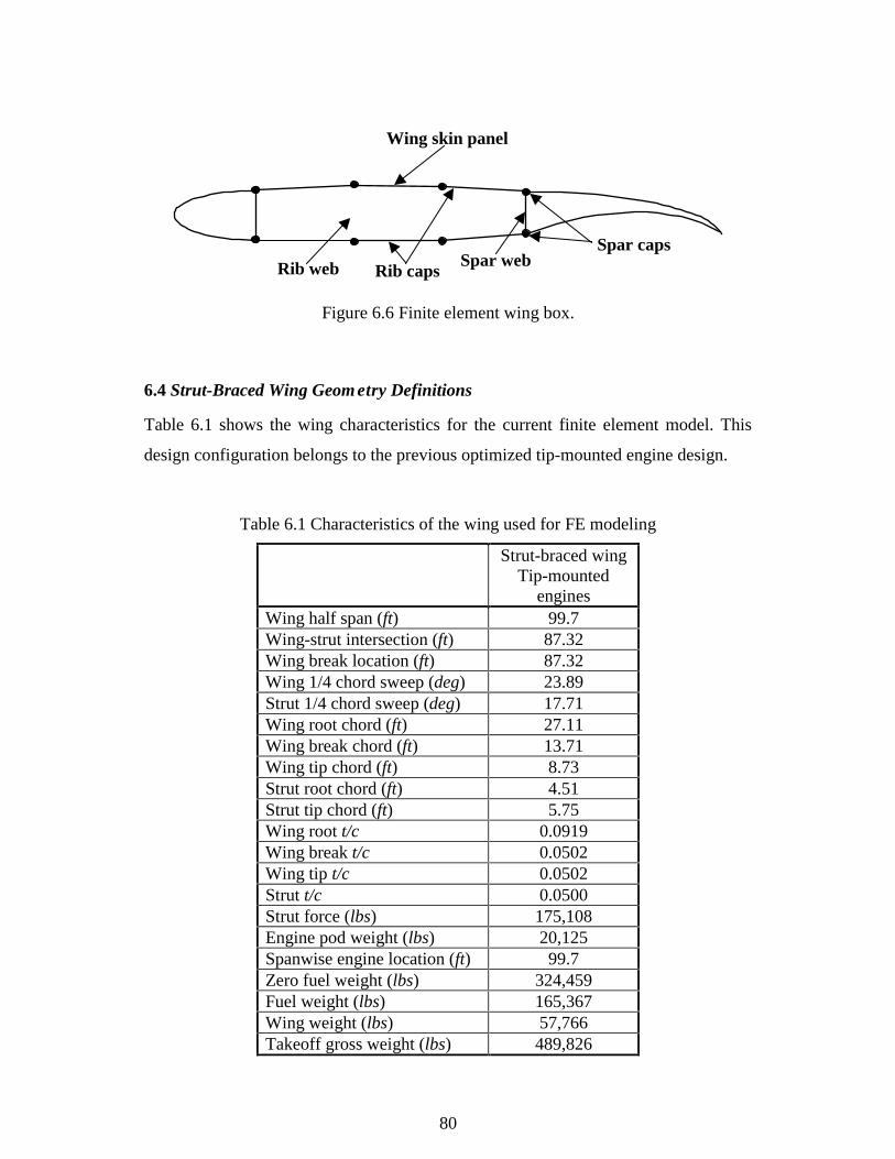
80
Spar caps
Rib caps
Wing skin panel
Spar webRib web
Figure 6.6 Finite element wing box.
6.4 Strut-Braced Wing Geom etry Definitions
Table 6.1 shows the wing characteristics for the current finite element model. This
design configuration belongs to the previous optimized tip-mounted engine design.
Table 6.1 Characteristics of the wing used for FE modeling
Strut-braced wingTip-mounted
enginesWing half span (ft) 99.7Wing-strut intersection (ft) 87.32Wing break location (ft) 87.32Wing 1/4 chord sweep (deg) 23.89Strut 1/4 chord sweep (deg) 17.71Wing root chord (ft) 27.11Wing break chord (ft) 13.71Wing tip chord (ft) 8.73Strut root chord (ft) 4.51Strut tip chord (ft) 5.75Wing root t/c 0.0919Wing break t/c 0.0502Wing tip t/c 0.0502Strut t/c 0.0500Strut force (lbs) 175,108Engine pod weight (lbs) 20,125Spanwise engine location (ft) 99.7Zero fuel weight (lbs) 324,459Fuel weight (lbs) 165,367Wing weight (lbs) 57,766Takeoff gross weight (lbs) 489,826
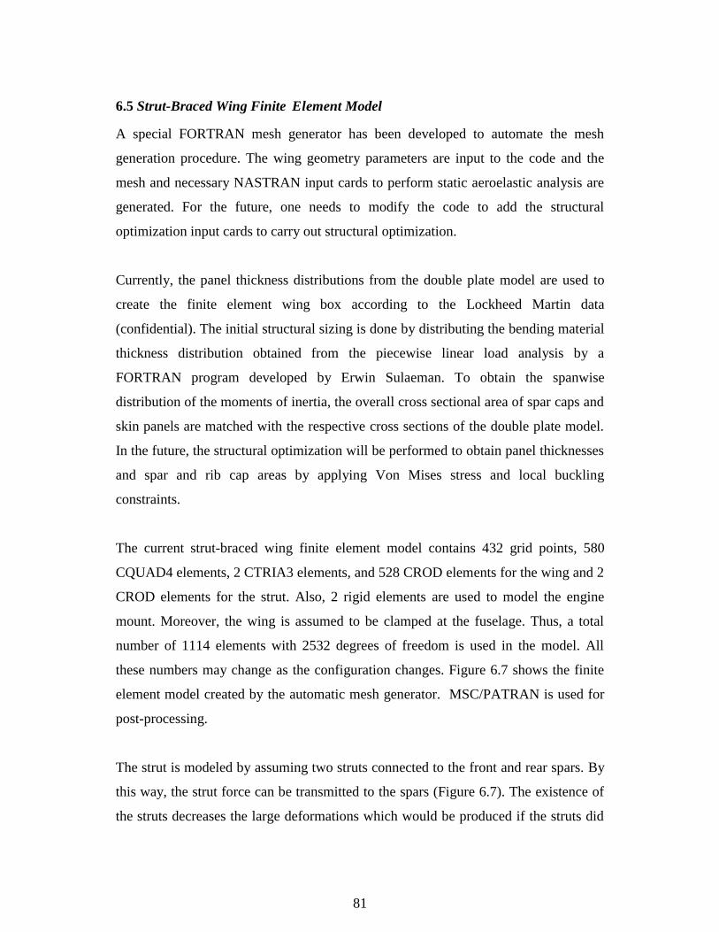
81
6.5 Strut-Braced Wing Finite Element Model
A special FORTRAN mesh generator has been developed to automate the mesh
generation procedure. The wing geometry parameters are input to the code and the
mesh and necessary NASTRAN input cards to perform static aeroelastic analysis are
generated. For the future, one needs to modify the code to add the structural
optimization input cards to carry out structural optimization.
Currently, the panel thickness distributions from the double plate model are used to
create the finite element wing box according to the Lockheed Martin data
(confidential). The initial structural sizing is done by distributing the bending material
thickness distribution obtained from the piecewise linear load analysis by a
FORTRAN program developed by Erwin Sulaeman. To obtain the spanwise
distribution of the moments of inertia, the overall cross sectional area of spar caps and
skin panels are matched with the respective cross sections of the double plate model.
In the future, the structural optimization will be performed to obtain panel thicknesses
and spar and rib cap areas by applying Von Mises stress and local buckling
constraints.
The current strut-braced wing finite element model contains 432 grid points, 580
CQUAD4 elements, 2 CTRIA3 elements, and 528 CROD elements for the wing and 2
CROD elements for the strut. Also, 2 rigid elements are used to model the engine
mount. Moreover, the wing is assumed to be clamped at the fuselage. Thus, a total
number of 1114 elements with 2532 degrees of freedom is used in the model. All
these numbers may change as the configuration changes. Figure 6.7 shows the finite
element model created by the automatic mesh generator. MSC/PATRAN is used for
post-processing.
The strut is modeled by assuming two struts connected to the front and rear spars. By
this way, the strut force can be transmitted to the spars (Figure 6.7). The existence of
the struts decreases the large deformations which would be produced if the struts did
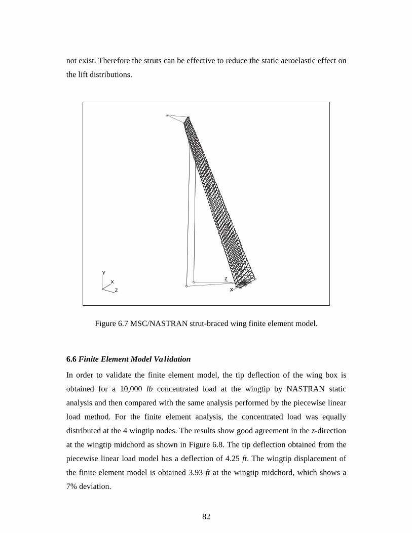
82
not exist. Therefore the struts can be effective to reduce the static aeroelastic effect on
the lift distributions.
X
Y
Z
16X
Y
Z32
X
Y
ZX
Y
Z
Figure 6.7 MSC/NASTRAN strut-braced wing finite element model.
6.6 Finite Element Model Va lidation
In order to validate the finite element model, the tip deflection of the wing box is
obtained for a 10,000 lb concentrated load at the wingtip by NASTRAN static
analysis and then compared with the same analysis performed by the piecewise linear
load method. For the finite element analysis, the concentrated load was equally
distributed at the 4 wingtip nodes. The results show good agreement in the z-direction
at the wingtip midchord as shown in Figure 6.8. The tip deflection obtained from the
piecewise linear load model has a deflection of 4.25 ft. The wingtip displacement of
the finite element model is obtained 3.93 ft at the wingtip midchord, which shows a
7% deviation.
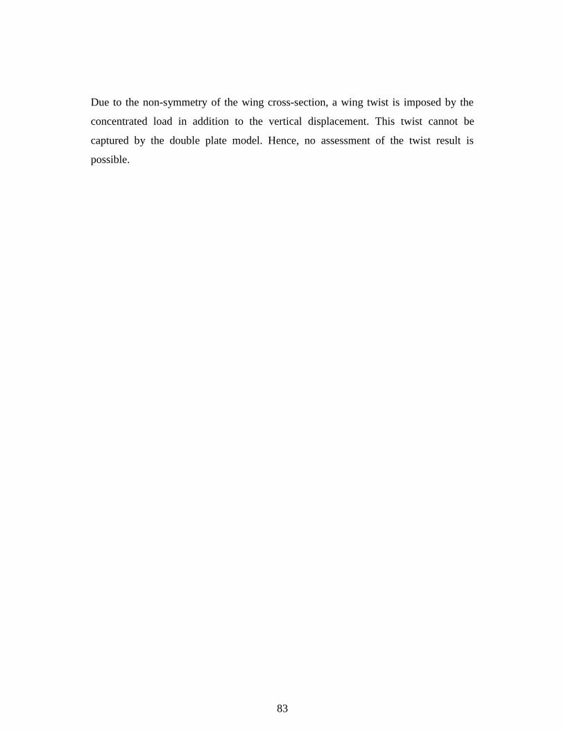
83
Due to the non-symmetry of the wing cross-section, a wing twist is imposed by the
concentrated load in addition to the vertical displacement. This twist cannot be
captured by the double plate model. Hence, no assessment of the twist result is
possible.
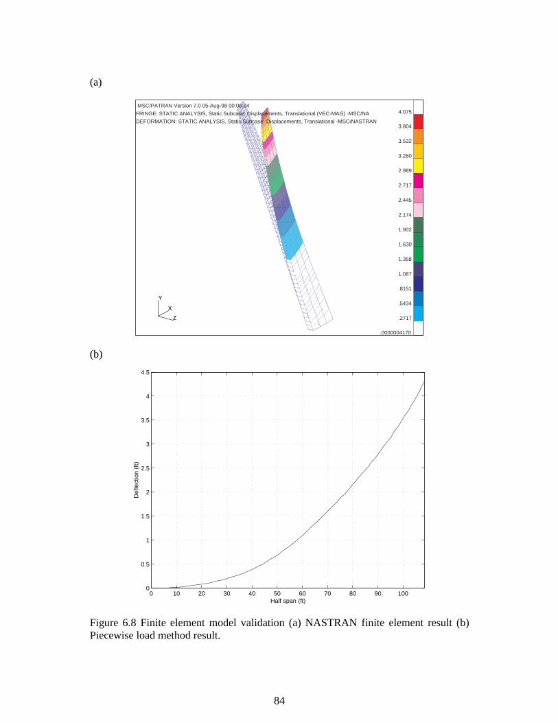
84
(a)
X
Y
Z
4.075
3.804
3.532
3.260
2.989
2.717
2.445
2.174
1.902
1.630
1.358
1.087
.8151
.5434
.2717
.0000004170
MSC/PATRAN Version 7.0 05-Aug-98 00:06:04
FRINGE: STATIC ANALYSIS, Static Subcase: Displacements, Translational (VEC-MAG) -MSC/NA
DEFORMATION: STATIC ANALYSIS, Static Subcase: Displacements, Translational -MSC/NASTRAN
X
Y
Z
(b)
0 10 20 30 40 50 60 70 80 90 1000
0.5
1
1.5
2
2.5
3
3.5
4
4.5
Half span (ft)
Def
lect
ion
(ft)
Figure 6.8 Finite element model validation (a) NASTRAN finite element result (b)Piecewise load method result.
85
6.7 Static Aeroelasticity Resu lts
Static aeroelastic analysis is performed for the 1g load condition. The subsonic
Doublet Lattice method is used to generate the aerodynamic lift loads on the wing
since the available version of MSC/NASTRAN is not capable of performing transonic
flow analyses. The rigid lift distribution is obtained by creating a wing structure of
very high rigidity. This is determined by having a high material elastic modulus. The
rigid and flexible aerodynamic load distributions are shown in Figure 6.9. The rigid
aerodynamic load distribution was expected to be close to an elliptical load
distribution but it is not. This can be cured by considering the wing jig-shape
correction or the wing twist in the finite element model (future work). The rigid wing
analysis will provide sufficient information to calculate the jig-shape twist.
0 10 20 30 40 50 60 70 80 90 1000
2000
4000
6000
8000
10000
12000
Half span (ft)
Lift
(lb/ft
)
Flexible wing Rigid wing (NASTRAN)
Figure 6.9 Rigid and flexible aerodynamic load distributions.
Figure 6.10 shows the strut-braced wing displacements due to the flexible
aerodynamic load distribution at the 1.0g load condition. The wing is subjected to a
86
considerable wing twist distribution due to non-symmetrical cross-sectional area and
chordwise lift pressure distribution. By adjusting the stiffnesses of the struts
(aeroelastic tailoring), it will be possible to produce a desirable twist distribution for
a drag reduction.
This chapter presented a brief introduction to the static aeroelastic analysis of a strut-
braced wing using the finite element method. In the future, an optimization capability
will be added for structural optimization. This will be done by using the built-in
MSC/NASTRAN Design Sensitivity and Optimization module (Moore, 1995).
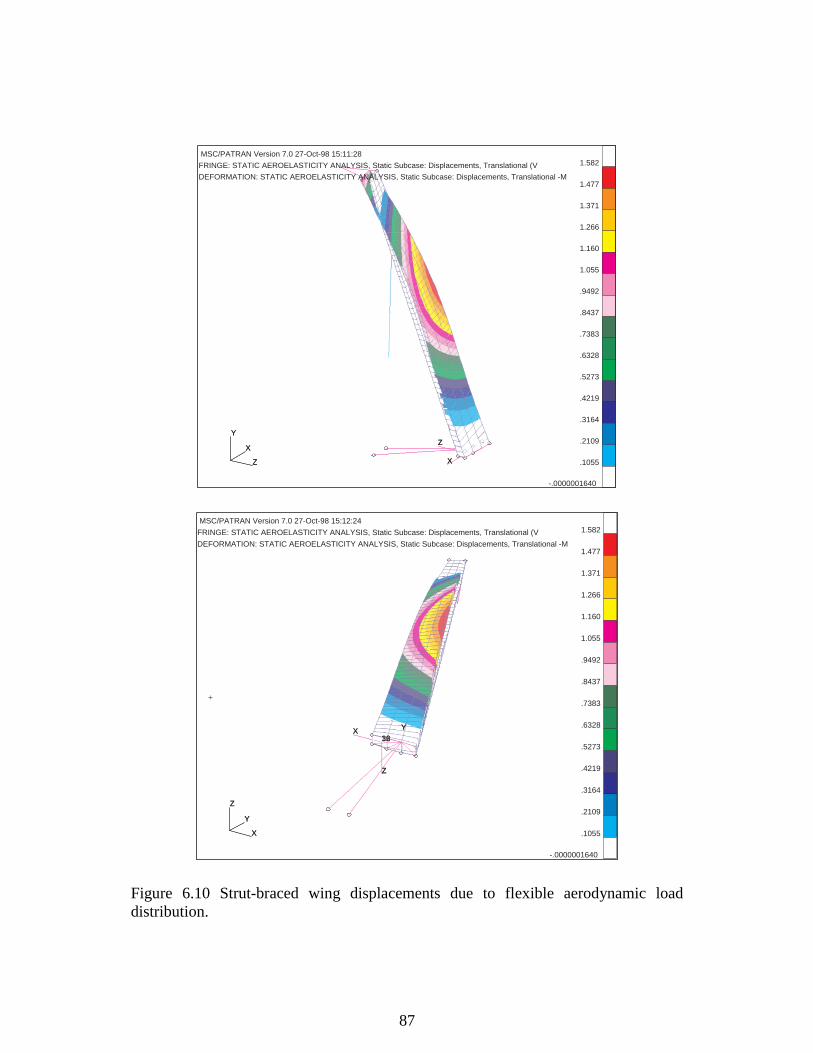
87
X
Y
Z XX
ZZ
1.582
1.477
1.371
1.266
1.160
1.055
.9492
.8437
.7383
.6328
.5273
.4219
.3164
.2109
.1055
-.0000001640
MSC/PATRAN Version 7.0 27-Oct-98 15:11:28
FRINGE: STATIC AEROELASTICITY ANALYSIS, Static Subcase: Displacements, Translational (V
DEFORMATION: STATIC AEROELASTICITY ANALYSIS, Static Subcase: Displacements, Translational -M
X
Y
Z
X
Y
Z
1632XX YY
ZZ
1.582
1.477
1.371
1.266
1.160
1.055
.9492
.8437
.7383
.6328
.5273
.4219
.3164
.2109
.1055
-.0000001640
MSC/PATRAN Version 7.0 27-Oct-98 15:12:24
FRINGE: STATIC AEROELASTICITY ANALYSIS, Static Subcase: Displacements, Translational (V
DEFORMATION: STATIC AEROELASTICITY ANALYSIS, Static Subcase: Displacements, Translational -M
X
Y
Z
Figure 6.10 Strut-braced wing displacements due to flexible aerodynamic loaddistribution.
88
Chapter 7 Concluding Remarks and Future Work
The advantages of a strut-braced wing over its cantilever wing counterpart were
explored. Multidisciplinary design optimization (MDO) was employed to integrate
different disciplines to construct a tool for conceptual aircraft design. A considerable
reduction in takeoff gross weight was obtained by applying the truss-braced wing
concepts in combination with advanced technologies and novel design innovations. In
this work, a preliminary structural analysis and optimization of a strut-braced wing
was investigated.
Two maneuver load conditions (2.5g and -1.0g × a factor of safety of 1.5), and a 2.0g
taxi bump load condition were used to determine the wing bending material weight.
An innovative design was considered to eliminate the significant weight penalty due
to strut buckling under the -1.0g pushover. Weight savings was accomplished by
considering a clamped wing for both positive and negative maneuvers while the strut
provides support at positive maneuvers and is inactive at negative maneuvers. This
was done by utilizing a telescoping sleeve mechanism. Moreover, the strut force was
optimized to provide the minimum wing bending material weight at the 2.5g
maneuver. Also, a strut offset member was designed and optimized to reduce
significant wing-strut interference drag. The results showed a significant weight
reduction.
Two sets of results corresponding to two different design configurations were
provided. The first design configuration assumes tip-mounted engines while the
second design configuration employs under-wing engines. Shear force, bending
moment, vertical deflection, and material thickness distributions were obtained for
both design configurations. Also, a composite material based on the future technology
was used by applying a technology factor to a state-of-the-art aluminum alloy. The
total wing weight results showed 18% and 8% savings associated with tip-mounted
engine and under-wing engine configurations, respectively compared to a thoroughly
89
metallic wing. Furthermore, the use of active load alleviation control was explored to
cut down the wing bending material weight. It showed good potential for future
investigation.
Overall, this preliminary study of a strut-braced wing showed a considerable weight
savings in takeoff gross weight compared to the cantilever wing counterpart without
sacrificing performance. The best strut-braced wing configuration exhibited a 18%
reduction in wing weight and an 9.4% reduction in takeoff gross weight.
It is recommended that the future work of this study showed focus on:
1. Implementation of two additional constraints, i.e. the inboard wing buckling
constraint and the engine location constraint, in the MDO code.
2. Implementation of a hexagonal wing box model in place of the double-plate
model. The model was suggested and provided by Lockheed Martin Aeronautical
Systems (LMAS). The new model provides higher geometrical accuracy.
3. Structural analysis and optimization of an arch-braced wing using geometrically
non-linear finite elements (Kapania and Li, 1998).
4. Structural analysis and optimization of more complex truss-braced wing
configurations using the finite element method. Also, other truss configurations
rather than the single-strut using the finite element method should be examined.
5. Complete static and dynamic aeroelastic optimization and analysis. One of the
main goals of strut braced wing designs is to decrease airfoil thickness and, as a
result, to reduce wave drag and increase laminar flow. This thickness reduction
results in a reduction of the wing-box torsional stiffness, rendering the aircraft
prone to aeroelastic instabilities. Therefore, aeroelastic and structural dynamic
analyses must be performed along with the MDO optimization.
90
References
1. Aerosoft, GASP The General Aerodynamic Simulation Program User’s Manual,Version 3, Aerosoft, Inc., Blacksburg, Virginia, 1996.
2. Balabanov, V., "Development of Approximations for HSCT Wing BendingMaterial Weight Using Response Surface Methodology, Ph.D. Dissertation,Virginia Polytechnic Institute and State University, Blacksburg, VA 24061,September 1997.
3. Balabanov, V., Kaufman, M., Knill, D.L., Giunta, A.A., Haftka, R.T., Grossman,B., Mason, W.H., and Watson, L.T., "Dependence of Optimum Structural Weighton Aerodynamic Shape for a High Speed Civil Transport," AIAA 96-4046,Proceedings of the 6th AIAA/NASA/ISSMO Symposium on MultidisciplinaryAnalysis and Optimization, pp. 599-612, Sept. 1996.
4. Bennett, J., Fenyes P., Haering W., and Neal M., "Issues in IndustrialMultidisciplinary Optimization," AIAA-98-4727, 1998.
5. Bisplinghoff, R.L., Ashley, H., and Halfman, R.L., Aeroelasticity, DoverPublications, Inc., 31 East 2nd Street, Mineola, N.Y. 11501, 1983.
6. Coster, J.E., and Haftka, R.T., "Preliminary Topology Optimization of a Truss-Braced Wing," University of Florida, December 1996.
7. Dudley, J., Huang, X., MacMillin, P.E., Grossman, B., Haftka, R.T., and Mason,W.H., "Multidisciplinary Optimization of the High-Speed Civil Transport,"AIAA-95-0124, January 1995.
8. Fielding, J. and Wild, F., "Aluminum Alloys in Aircraft--Present Status andFuture Potential," Aluminum Industry, Vol. 6, No. 4, pp 5-11, May 1987.
9. Gallman, J.W. and Kroo, I.M., "Structural Optimization for Joined-WingSyntheses," AIAA-92-4761-CP, 1992.
10. Gallman, J.W., Smith, S.C., and Kroo, I.M., "Optimization of Joined-WingAircraft," Journal of Aircraft, Vol. 30, No. 6, Nov.-Dec., 1993.
91
11. Giunta, A.A., Balabanov, V., Haim, D., Grossman, B., Mason, W.H., Watson,L.T., and Haftka, R.T., "Wing Design for a High-Speed Civil Transport Using aDesign of Experiments Methodology," AIAA, Virginia Polytechnic Institute andState University, Blacksburg, VA 24061, 1996.
12. Giunta, A.A., Balabanov, V., Haim, D., Grossman, B., Mason, W.H., Watson,L.T., and Haftka, R.T., "Multidisciplinary Optimization of a Supersonic TransportUsing Design of Experiments Theory and Response Surface Modeling," TheAeronautical Journal, pp. 347-356, October 1997.
13. Grasmeyer, J.M., "A Discrete Vortex Method for Calculating the MinimumInduced Drag and Optimum Load Distribution for Aircraft Configurations withNon-coplanar Surfaces," VPI-AOE-242, Multidisciplinary Analysis and DesignCenter for Advanced Vehicles, Department of Aerospace and Ocean Engineering,Virginia Polytechnic Institute and State University, Blacksburg, VA 24061,January 1997.
14. Grasmeyer, J.M., "Stability and Control Derivative Estimation and Engine-OutAnalysis," VPI-AOE-254, Multidisciplinary Analysis and Design Center forAdvanced Vehicles, Department of Aerospace and Ocean Engineering, VirginiaPolytechnic Institute and State University, Blacksburg, VA 24061, January 1998.
15. Grasmeyer, J.M., "Truss-Braced Wing Description and User’s Manual," VPI-AOE-255, Multidisciplinary Analysis and Design Center for Advanced Vehicles,Department of Aerospace and Ocean Engineering, Virginia Polytechnic Instituteand State University, Blacksburg, VA 24061, 1998.
16. Grasmeyer, J.M., Naghshineh-Pour, A.H., Tetrault, P.A., Grossman, B., Haftka,R.T., Kapania, R.K., Mason, and W.H., Schetz, "Multidisciplinary DesignOptimization of a Strut-Braced Wing Aircraft with Tip-Mounted Engines," MAD98-01-01, Multidisciplinary Analysis and Design Center for Advanced Vehicles,Virginia Polytechnic Institute and State University, Blacksburg, Virginia 24061,January 1998.
17. Grossman, B., Strauch, G.J., Eppard, W.M., Gurdal, Z., and Haftka, R.T.,"Integrated Aerodynamic/Structural Design of a Sailplane Wing," AIAA-86-2623, Dayton, Ohio, October 20-22, 1986.
18. Haftka, R.T. and Gurdal Z., Elements of Structural Optimization, KluwerAcademic Publishers, P.O. Box 17, 3300 AA Dordrecht, The Netherlands, 1992.
92
19. Hajela, P. and Chen J.L., "Optimum Structural Sizing of Conventional Cantileverand Joined-Wing Configurations Using Equivalent Beam Models," AIAA-86-2653, Dayton, Ohio, October 20-22, 1986.
20. Hoerner, S.F., "Fluid-Dynamic Drag: Practical Information on Aerodynamic Dragand Hydrodynamic Resistance," Midland Park, NJ, pp. 8-1-8-20, 1965.
21. Hönlinger, H.G., Krammer, J., and Stettner, M., "MDO Technology Needs inAeroelastic Structural Design," AIAA-98-4731, 1998.
22. Huang, X., Structural Optimization and Its Integration with AerodynamicOptimization for a High Speed Civil Transport, Ph.D. Dissertation, VirginiaPolytechnic Institute and State University, Blacksburg, VA 24061, September1994.
23. Hutchison, M.G., Unger, E.R., Mason, W.H., Grossman, B., Haftka, R.T.,"Variable Complexity Aerodynamic Optimization of a High Speed CivilTransport Wing," Journal of aircraft, Vol. 31, No. 1, pp. 110-116, 1994.
24. Joslin, R.D., "Aircraft Laminar Flow Control," Annual Review of FluidMechanics, Annual Reviews Inc., Vol. 30, pp. 1-29, Palo Alto, CA, 1998.
25. Kapania, R.K. and Li, J., "A Four-Noded 3-D Geometrically Nonlinear CurvedBeam Element with Large Displacements/Rotations, in Modeling and SimulationEngineering," Atluri, S.N., O'Dononghue (ed.), Technology Science Press, 679-784, 1998.
26. Kaufman, M., Balabanov, V., Burgee, S.L., Giunta, A.A., Grossman, B., Haftka,R.T., Mason, W.H., and Watson, L.T., "Variable-Complexity Response SurfaceApproximations for Wing Structural Weight in HSCT Design," ComputationalMechanics, Vol. 18, No. 2, pp. 112-126, June 1996.
27. Knill, D.L., Giunta, A.A., Baker, C.A., Grossman, B., Mason, W.H., Watson,L.T., and Haftka, R.T., "HSCT Configuration Design Using Response SurfaceApproximations of Supersonic Euler Aerodynamics," AIAA-98-0905, 1998.
28. Korte, J.J., Weston, R.P., and Zang, T.A., "Multidisciplinary OptimizationMethods for Preliminary Design," Multidisciplinary Optimization Branch, MS159, NASA Langley Research Center, 1998.
93
29. Kroo, I., "MDO Applications in Preliminary Design: Status and Directions," 38th
AIAA/ASME/ASCE/ASC Structures, Structural Dynamics, and MaterialsConference, Kissimme, Florida, April 7-10, 1997.
30. Kroo, I., Altus, S., Braun, R., Gage, P., and Sobieski, I., "MultidisciplinaryOptimization Methods for Aircraft Preliminary Design," AIAA-94-4325, 1994.
31. Kroo, I.M. and Gallman J.W., "Aerodynamic Structural Studies of Joined-WingAircraft," Journal of aircraft, Vol. 28, No. 1, pp. 74-81, May 7, 1990.
32. Kulfan, R.M., and Vachal, J.D., "Wing Planform Geometry Effects on LargeSubsonic Military Transport Airplanes," Boeing Commercial Airplane Company,AFFDL-TR-78-16, February 1978.
33. Lee, J.M., MSC/NASTRAN Linear Static Analysis User’s Guide Version 69,MacNeal-Schwendler Corporation, 1997.
34. Lomax, T.L., Structural Loads Analysis for Commercial Transport Aircraft:Theory and Practice, AIAA, Reston, Virginia, 1996.
35. McCullers, L.A., FLOPS User’s Guide, Release 5.81, NASA Langley ResearchCenter.
36. Moore, G.J., MSC/NASTRAN Design Sensitivity and Optimization User’s GuideVersion 68, MacNeal-Schwendler Corporation, 1995.
37. Niu, M.C.Y., Airframe Structural Design, Lockheed Aeronautical SystemsCompany, Burbank, California, 1988.
38. Parikh, P. and Pirzadeh, S., "A Fast Upwind Solver for the Euler Equations onThree-Dimensional Unstructured Meshes," AIAA-91-0102, Reno, Nevada,January 7-10, 1991.
39. Park, H. P., "The Effect on Block Fuel Consumption of a Strutted vs. CantileverWing for a Short Haul Transport Including Strut Aeroelastic Considerations,"AIAA-78-1454-CP, Los Angeles, California, Aug. 21-23, 1978.
94
40. Patel, H.D., "Multidisciplinary Design Optimization with Superelements inMSC/NASTRAN," AIAA-92-4732-CP, 1992.
41. Rais-Rohani, M., Integrated Aerodynamics-Structural-Control Wing Design,Ph.D. Dissertation, Virginia Polytechnic Institute and State University,Blacksburg, VA 24061, September 1991.
42. Raymer, D.P., Aircraft Design: A Conceptual Approach, AIAA, WashingtonD.C., 1992.
43. Rodden, W.P. and Johnson, E.H., MSC/NASTRAN Aeroelastic Analysis User’sGuide Version 68, MacNeal-Schwendler Corporation, 1995.
44. Selberg, B.P. and Cronin, D.L., "Aerodynamic-Structural Optimization ofPositive/Negative Stagger Joined-Wing Configurations," AIAA-86-2626, Dayton,Ohio, October 20-22, 1986.
45. Thomas, H.L., Shyy, Y-K., Vanderplaats, G.N., and Miura, H., "GENESIS - AModern Shape and Sizing Structural Design Tool," AIAA-92-2559-CP, 1991.
46. Torenbeek, E., "Development and Application of a Comprehensive, DesignSensitive Weight Prediction Method for Wing Structures of Transport CategoryAircraft," Delft University of Technology, Report LR-693, Sept. 1992.
47. Turriziani, R.V., Lovell, W.A., Martin, G.L., Price, J.E., Swanson, E.E., andWashburn, G.F., "Preliminary Design Characteristics of a Subsonic Business JetConcept Employing an Aspect Ratio 25 Strut Braced Wing," NASA CR-159361,October 1980.
48. Vanderplaats Research & Development, Inc., DOT User’s Manual, Version 4.20,Colorado Springs, CO, 1995.
49. Vanderplaats, G.N., "Automated Optimization Techniques for Aircraft Synthesis,"AIAA-76-909-CP, Dallas, Texas, September 27-29, 1976.
50. Venkayya, V.B., Tischler, V.A., and Bharatram, G., "Multidisciplinary Issues inAircraft Design," AIAA-96-1386-CP, 1996.

95
51. Vitali, R., Park, O., Haftka, R.T., Sankar, B.V., and Rose. C., "StructuralOptimization of a Hat Stiffened Panel," Department of Aerospace Engineering,Mechanics and Engineering Science, Gainesville, FL 32611-6250, 1998.
52. Wolkovitch, J., "The Joined Wing: An Overview," AIAA-85-0274-CP, Reno, NV,January 14-17, 1985.
53. Young, J.A., Anderson, R.D., and Yurkovich, R.N., "A Description of the F/A-18E/F Design and Design Process," AIAA-98-4701-CP, St. Louis, Missouri,September 2-4, 1998.
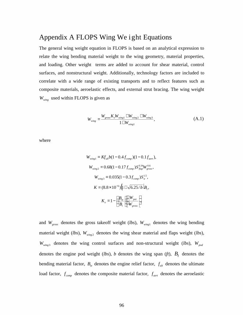
96
Appendix A FLOPS Wing We ight Equations
The general wing weight equation in FLOPS is based on an analytical expression to
relate the wing bending material weight to the wing geometry, material properties,
and loading. Other weight terms are added to account for shear material, control
surfaces, and nonstructural weight. Additionally, technology factors are included to
correlate with a wide range of existing transports and to reflect features such as
composite materials, aeroelastic effects, and external strut bracing. The wing weight
wingW used within FLOPS is given as
,1 1
321
wing
wingwingwingegrosswing W
WWWKWW
+++
= (A.1)
where
),1.01)(4.01(1 aertcompultwing ffbKfW −−=
,)17.01(68.0 6.034.02 grossflapcompwing WSfW −=
,)3.01(035.0 5.13 wcompwing SfW −=
( ) ,/25.61)108.8( 6tBbK +×= −
,1
−=
gross
pot
t
tee W
W
B
BK
and grossW denotes the gross takeoff weight (lbs), 1wingW denotes the wing bending
material weight (lbs), 2wingW denotes the wing shear material and flaps weight (lbs),
3wingW denotes the wing control surfaces and non-structural weight (lbs), podW
denotes the engine pod weight (lbs), b denotes the wing span (ft), tB denotes the
bending material factor, teB denotes the engine relief factor, ultf denotes the ultimate
load factor, compf denotes the composite material factor, aertf denotes the aeroelastic
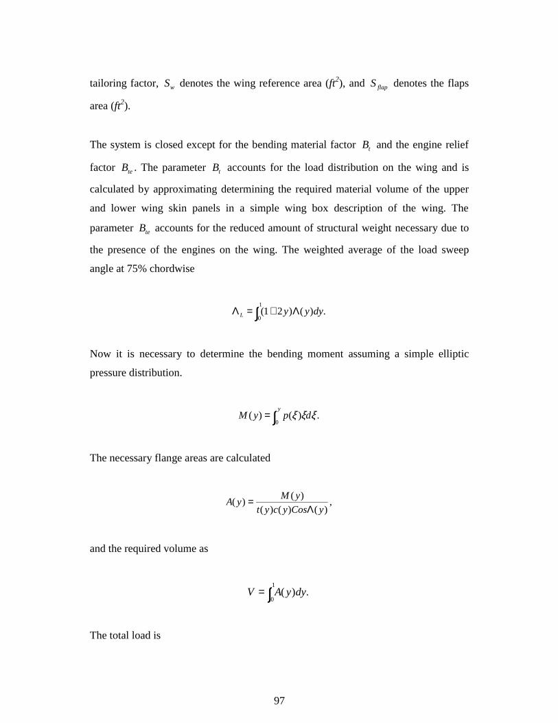
97
tailoring factor, wS denotes the wing reference area (ft2), and flapS denotes the flaps
area (ft2).
The system is closed except for the bending material factor tB and the engine relief
factor teB . The parameter tB accounts for the load distribution on the wing and is
calculated by approximating determining the required material volume of the upper
and lower wing skin panels in a simple wing box description of the wing. The
parameter teB accounts for the reduced amount of structural weight necessary due to
the presence of the engines on the wing. The weighted average of the load sweep
angle at 75% chordwise
∫ Λ+=Λ1
0.)()21( dyyyL
Now it is necessary to determine the bending moment assuming a simple elliptic
pressure distribution.
∫=y
dpyM0
.)()( ξξξ
The necessary flange areas are calculated
,)()()(
)()(
yCosycyt
yMyA
Λ=
and the required volume as
∫=1
0.)( dyyAV
The total load is
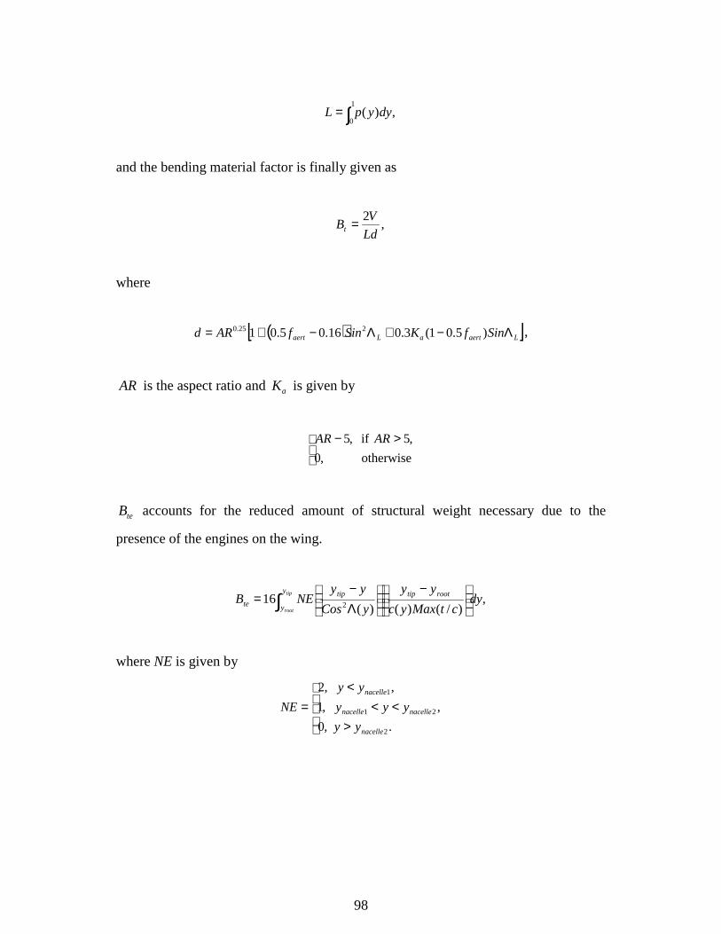
98
∫=1
0,)( dyypL
and the bending material factor is finally given as
,2Ld
VBt =
where
( )[ ]LaertaLaert SinfKSinfARd Λ−+Λ−+= )5.01(3.016.05.01 225.0 ,
AR is the aspect ratio and aK is given by
>−
otherwise ,0
,5 if ,5 ARAR
teB accounts for the reduced amount of structural weight necessary due to the
presence of the engines on the wing.
,)/()()(
162
dyctMaxyc
yy
yCos
yyNEB roottipy
y
tipte
tip
root
−
Λ−
= ∫
where NE is given by
><<
<=
. ,0
, ,1
, ,2
2
21
1
nacelle
nacellenacelle
nacelle
yy
yyy
yy
NE
99
Appendix B Wing.f Code Desc r iption
A FORTRAN code labeled wing.f has been provided to estimate the single-strut-
braced wing bending material weight. This appendix describes the code. For the full
description of the strut-braced wing MDO code, the reader may refer to Grasmeyer
(1998). All the necessary information, i.e. aerodynamic lift loads, fuel distribution,
and wing geometry parameters, is passed from the MDO code as shown in Figure 4.1.
The code is capable of estimating the bending material weight for both cantilever and
strut-braced wings at three different load conditions. Also, the code can be run
separately without running the MDO code at the same time by defining a parameter
set along with fuel and load information as separate input files. *.in provides the input
parameters, *.fuel provides the spanwise fuel distribution, and *.loads provides the
spanwise load distributions. The above input files are read by the wingin.f code and
passed to wing.f.
B.1 Wing.f Structure
The code consists of a main body and several subroutines. Figure B.1 shows the
wing.f flowchart. First, the wing parameters and the lift and fuel distributions are read
and then interpolated onto the structural nodes. The shear force and bending moment
distributions are calculated to estimate the bending material weight. The bending
material weight is substituted for the value in FLOPS to calculate the wing weight due
to the maneuver load conditions using FLOPS wing weight equations. The wing
weight along with the fuel weight distribution are combined to create the taxi loads.
The taxi analysis is performed to calculate the bending material weight due to the taxi
bump load condition. Finally, the bending material weight due to the maneuvers and
bending material weight due to the taxi bump condition are compared to calculate the
total bending material weight and to obtain the design material distribution.
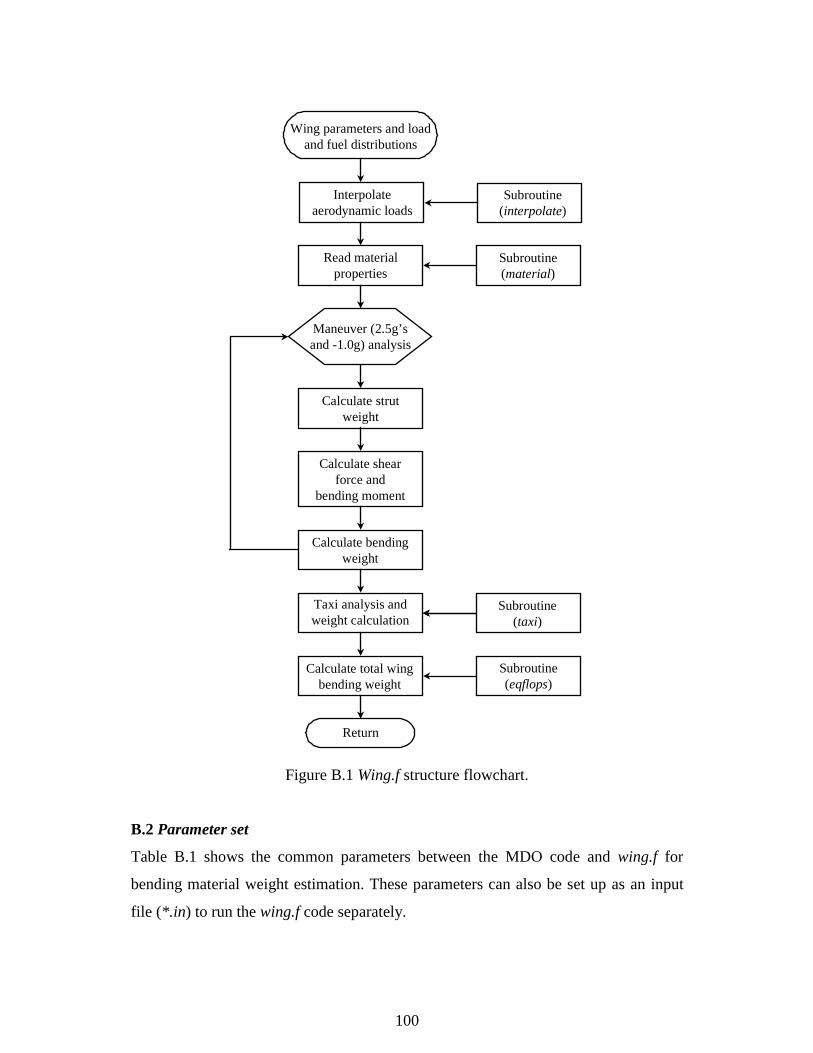
100
Return
Wing parameters and loadand fuel distributions
Interpolateaerodynamic loads
Subroutine(interpolate)
Read materialproperties
Subroutine(material)
Calculate strutweight
Maneuver (2.5g’sand -1.0g) analysis
Calculate shearforce and
bending moment
Calculate bendingweight
Taxi analysis andweight calculation
Subroutine(taxi)
Calculate total wingbending weight
Subroutine(eqflops)
Figure B.1 Wing.f structure flowchart.
B.2 Parameter set
Table B.1 shows the common parameters between the MDO code and wing.f for
bending material weight estimation. These parameters can also be set up as an input
file (*.in) to run the wing.f code separately.
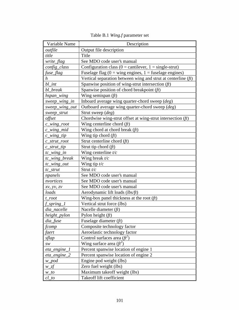
101
Table B.1 Wing.f parameter set
Variable Name Descriptionoutfile Output file descriptiontitle Titlewrite_flag See MDO code user’s manualconfig_class Configuration class (0 = cantilever, 1 = single-strut)fuse_flag Fuselage flag (0 = wing engines, 1 = fuselage engines)h Vertical separation between wing and strut at centerline (ft)bl_int Spanwise position of wing-strut intersection (ft)bl_break Spanwise position of chord breakpoint (ft)hspan_wing Wing semispan (ft)sweep_wing_in Inboard average wing quarter-chord sweep (deg)sweep_wing_out Outboard average wing quarter-chord sweep (deg)sweep_strut Strut sweep (deg)offset Chordwise wing-strut offset at wing-strut intersection (ft)c_wing_root Wing centerline chord (ft)c_wing_mid Wing chord at chord break (ft)c_wing_tip Wing tip chord (ft)c_strut_root Strut centerline chord (ft)c_strut_tip Strut tip chord (ft)tc_wing_in Wing centerline t/ctc_wing_break Wing break t/ctc_wing_out Wing tip t/ctc_strut Strut t/cnpanels See MDO code user’s manualnvortices See MDO code user’s manualxv, yv, zv See MDO code user’s manualloads Aerodynamic lift loads (lbs/ft)t_root Wing-box panel thickness at the root (ft)f_spring_1 Vertical strut force (lbs)dia_nacelle Nacelle diameter (ft)height_pylon Pylon height (ft)dia_fuse Fuselage diameter (ft)fcomp Composite technology factorfaert Aeroelastic technology factorsflap Control surfaces area (ft2)sw Wing surface area (ft2)eta_engine_1 Percent spanwise location of engine 1eta_engine_2 Percent spanwise location of engine 2w_pod Engine pod weight (lbs)w_zf Zero fuel weight (lbs)w_to Maximum takeoff weight (lbs)cl_to Takeoff lift coefficient
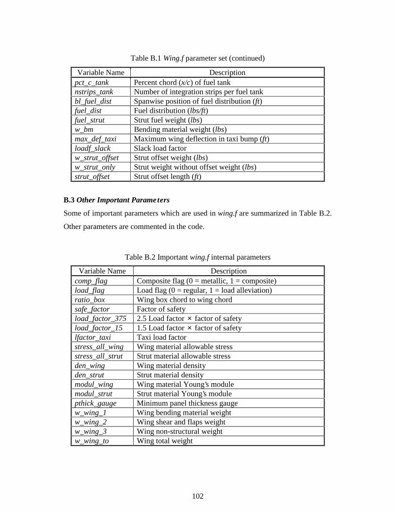
102
Table B.1 Wing.f parameter set (continued)
Variable Name Descriptionpct_c_tank Percent chord (x/c) of fuel tanknstrips_tank Number of integration strips per fuel tankbl_fuel_dist Spanwise position of fuel distribution (ft)fuel_dist Fuel distribution (lbs/ft)fuel_strut Strut fuel weight (lbs)w_bm Bending material weight (lbs)max_def_taxi Maximum wing deflection in taxi bump (ft)loadf_slack Slack load factorw_strut_offset Strut offset weight (lbs)w_strut_only Strut weight without offset weight (lbs)strut_offset Strut offset length (ft)
B.3 Other Important Parameters
Some of important parameters which are used in wing.f are summarized in Table B.2.
Other parameters are commented in the code.
Table B.2 Important wing.f internal parameters
Variable Name Descriptioncomp_flag Composite flag (0 = metallic, 1 = composite)load_flag Load flag (0 = regular, 1 = load alleviation)ratio_box Wing box chord to wing chordsafe_factor Factor of safetyload_factor_375 2.5 Load factor × factor of safetyload_factor_15 1.5 Load factor × factor of safetylfactor_taxi Taxi load factorstress_all_wing Wing material allowable stressstress_all_strut Strut material allowable stressden_wing Wing material densityden_strut Strut material densitymodul_wing Wing material Young’s modulemodul_strut Strut material Young’s modulepthick_gauge Minimum panel thickness gaugew_wing_1 Wing bending material weightw_wing_2 Wing shear and flaps weightw_wing_3 Wing non-structural weightw_wing_to Wing total weight
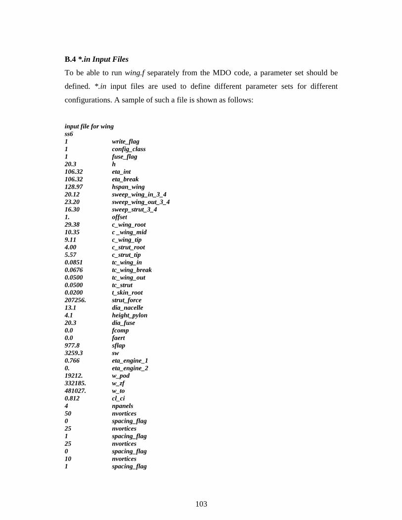
103
B.4 *.in Input Files
To be able to run wing.f separately from the MDO code, a parameter set should be
defined. *.in input files are used to define different parameter sets for different
configurations. A sample of such a file is shown as follows:
input file for wingss61 write_flag1 config_class1 fuse_flag20.3 h106.32 eta_int106.32 eta_break128.97 hspan_wing20.12 sweep_wing_in_3_423.20 sweep_wing_out_3_416.30 sweep_strut_3_41. offset29.38 c_wing_root10.35 c _wing_mid9.11 c_wing_tip4.00 c_strut_root5.57 c_strut_tip0.0851 tc_wing_in0.0676 tc_wing_break0.0500 tc_wing_out0.0500 tc_strut0.0200 t_skin_root207256. strut_force13.1 dia_nacelle4.1 height_pylon20.3 dia_fuse0.0 fcomp0.0 faert977.8 sflap3259.3 sw0.766 eta_engine_10. eta_engine_219212. w_pod332185. w_zf481027. w_to0.812 cl_ci4 npanels50 nvortices0 spacing_flag25 nvortices1 spacing_flag25 nvortices0 spacing_flag10 nvortices1 spacing_flag
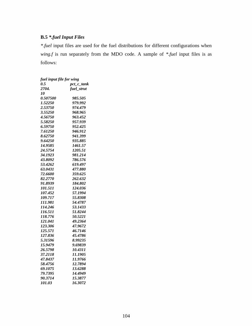
104
B.5 *.fuel Input Files
*.fuel input files are used for the fuel distributions for different configurations when
wing.f is run separately from the MDO code. A sample of *.fuel input files is as
follows:
fuel input file for wing0.5 pct_c_tank2704. fuel_strut100.507500 985.5051.52250 979.9922.53750 974.4793.55250 968.9654.56750 963.4525.58250 957.9396.59750 952.4257.61250 946.9128.62750 941.3999.64250 935.88514.9585 1461.5724.5754 1205.5134.1923 981.21443.8092 786.57653.4262 619.49763.0431 477.88072.6600 359.62582.2770 262.63291.8939 184.802101.511 124.036107.452 57.1994109.717 55.8308111.981 54.4787114.246 53.1433116.511 51.8244118.776 50.5221121.041 49.2364123.306 47.9672125.571 46.7146127.836 45.47865.31596 8.9923515.9479 9.6983926.5798 10.431137.2118 11.190547.8437 11.976658.4756 12.789469.1075 13.628879.7395 14.494990.3714 15.3877101.03 16.3072
105
The fist column represents the fuel spanwise location in (ft) and second column
represents the fuel distribution in (lbs/ft). For more details, the reader may refer to the
MDO User’s Manual (Grasmeyer, 1998).
B.6 *.loads Input Files
*.loads input files are used for the load distributions for different configurations when
wing.f is run separately from the MDO code. The two maneuver load conditions are
read from a *.loads input file. A sample is not given.
B.7 *.wing and *.dat Output Files
*.wing output files represent the calculated quantities by wing.f. The necessary data
for post-processing are produced in *.dat output files.
B.8 Post-Processing
A MATLAB code labeled wing.m has been provided for post-processing. This code
reads the output files produced by wing.f and generates the required plots. Samples of
the post-processing results are shown in Figures 5-1 to 5-6.
106
Vita
Amir H. Naghshineh-Pour was born on March 3, 1969 in Tehran, Iran. After
graduation from high school in Tehran in 1986, he entered Azad University in Tehran
and graduated with the Bachelor of Science in Mechanical Engineering. After two
years of working as an engineer in a consulting engineering company, he began his
post graduate studies in 1994 at North Carolina Agricultural and Technical State
University and completed his Master of Science degree in Mechanical Engineering in
1996. Due to his interest in aircraft and aerospace engineering he also decided to
pursue his education in the aerospace field. He joined the Aerospace and Ocean
Engineering Department at Virginia Polytechnic Institute and State University in
August 1996 and graduated with the Master of Science degree in Aerospace
Engineering in December 1998. He will join BFGoodrich, Aerospace, Aerostructures
Group located in San Diego, California.