Embed Size (px)
Citation preview
Strontium isotope tracing in animal teeth at the Neanderthal site of Les
Pradelles, Charante, France.
TEGAN E KELLY
Honours thesis submitted as part requirement of the B.Sc. (Hons) degree completed in the Department of Earth and Marine Sciences, in conjunction with the Research School of Earth Sciences, Australian
National University. 30th May 2007

Statement of Authorship I certify that this thesis is my original work. No other person’s work has been used without due acknowledgement in the text of this thesis. Except where reference is made in the text, this document contains no material presented elsewhere or extracted in whole or in part from a document presented by me for another qualification at this or any other institution. Name: Tegan Emma Kelly Date: 20th June 2007 Signature:
Tegan E Kelly 2007
i
Abstract Strontium isotope ratios (87Sr/86Sr) can be utilised in reconstructing the migration and
mobility of ancient animal and human populations. Strontium isotopes in fossil tooth
enamel are compared to a geological, bio-available strontium isotope map, to
determine whether teeth are from local or migrant individuals. This study was carried
out on the Upper Pleistocene site of Les Pradelles (Marillac-le-Franc, Charente,
France), which has yielded numerous faunal remains including an important
collection of Neanderthal pieces (Homo neanderthalensis). The surrounding area
consists of two main rock regions, the limestones of the Dordogne and the
metamorphic and granitoid rocks of the Massif Central, which yield differing average
strontium isotope ratios. Soil and plant samples were collected from 40 locations
across both rock regions. Soil samples were sieved and leached to ensure only
biologically available strontium would be measured. Plant samples were dried, ashed
and dissolved. All samples had total Sr concentration measured via solution ICP-MS
before Sr separation was undertaken via ion exchange chromatography. 87Sr/86Sr
ratios were measured via ICP-MS analysis. Despite some variation in 87Sr/86Sr within
each rock region, the two main regions are successfully differentiated on the basis of
Sr isotopes and a Sr isotope map of the area has been produced. The fossil faunal
samples from the site consisted of 27 teeth from seven species including both
herbivores and carnivores. Sr isotopes in the tooth enamel were measured via laser
ablation ICP-MS, resulting in high resolution records along the growth axis of the
enamel. The strontium isotope ratios do not vary significantly along the growth of the
tooth enamel, potentially indicating a lack of migration across the rock provinces
while the teeth were forming. However, the lack of seasonality may alternatively be
explained by reservoir effects and complexities in tooth mineralisation. Animals with
small feeding ranges are successfully linked to particular rock regions according to Sr
isotope ratio, whereas intermediate 87Sr/86Sr values in migrating animals suggest an
averaging of values from both units. This study forms the basis for an ongoing study
into Neanderthal migration.

Tegan E Kelly 2007
ii
Acknowledgements My honours year has been both challenging and enjoyable and would not have been
possible without the help and support of a whole team of people. Firstly I am hugely
indebted to my supervisor, Rainer Grün, whose enthusiasm, support and confidence in
my abilities continually encouraged me to try to achieve my best throughout all stages
of this project. Thanks also to my co-supervisors, Steve Eggins and Bradley Opdyke,
for your suggestions and advice. Also to Maxime Aubert, who, along with Rainer,
tramped around France collecting my samples and photographing the sites. I just wish
I’d been available to go with you too! Thanks also Max, for your help with my
methodology, and helping brainstorm explanations for my results. Additionally, merci
to Renaud Joannes-Boyau, for helping me decipher Google-translations of French
papers; nothing would have made sense otherwise!
Thankyou to Bruno Maureille at the University of Bordeaux, for providing the faunal
samples from Les Pradelles, as well as extensive information on the history,
stratigraphy, and significance of the site. Thankyou for allowing me to be a part of a
fantastic project. Thanks also to Manfred Thönnessen and Ulrich Radtke at the
University of Cologne, for processing the plant samples, which we otherwise couldn’t
have returned to Australia.
A huge thanks goes to Graham Mortimer, whose knowledge and expertise in
analytical geochemistry was indispensable. Thank you for not only showing me what
to do and how to do it, but always helping me to understand the principles behind the
procedures involved. Thank you to Les Kinsley, who, along with Steve and Graham,
helped me operate the ICP-MS; I would have been lost without you. Thanks also to
Jon Woodhead and the School of Earth Sciences at Melbourne University for
allowing me to visit and utilise your ICP-MS equipment while the Neptune at ANU
had broken down. It was hugely appreciated and gave me the excuse for a trip to
Melbourne in the middle of my honours!
Tegan E Kelly 2007
iii
To David Ellis and the Department of Earth and Marine Sciences at ANU: thankyou
for taking a chance on an unknown student based on the other side of campus, without
your support I could not have undertaken an honours project with the RSES. I also
appreciate the offer of a desk in the DEMS honours room, even if I hardly utilised it!
The Research School of Earth Sciences deserves special mention. Thank you for
taking me on and treating me as an RSES student even though I was technically
enrolled at DEMS. Thankyou to Gordon Lister for getting me started at RSES and
helping secure an Honours Scholarship at short notice, outside the normal application
period.
Last but certainly not least, extra special thanks to my boyfriend, Cluan Smith. Thank
you for all your help with the graphics in this thesis, but mostly for up and moving to
Canberra with me on such short notice to support me in undertaking this opportunity.
Your sincere love, friendship and support have helped get me through the year, thank
you for knowing when to provide encouragement, and when to provide a distraction!

Tegan E Kelly 2007
iv
Contents Abstract………………………………………………………………………………i Acknowledgements………………………………………………………………..ii Contents…………………………………………………………………………….iv List of Figures……………………………………………………………………..vii List of Tables……………………………………………………………………….ix
Chapter 1: Introduction 1 1.1. Significance of the research…………………………………......1 1.2. Aims…………………………………………………………………..1 1.3. Study area…………………………………………………………...2 1.3.1 Regional geology……………………………………………….....2
1.3.2. Les Pradelles……………………………………………………....3
1.4. Thesis overview.……………………………………………………6
Chapter 2: Background 7 2.1. Strontium as a tool for tracing migration……………………...7 2.1.1. General Sr chemistry……………………………………………...7
2.1.2. Geological Sr isotope mapping…………………………………..8
2.1.3. Sr in the food chain………………………………………………..9
2.1.4. Strontium migration tracing……………………………………….9 2.1.4.1. Applications………………………………………………………9
2.1.4.2. Techniques……………………………………………………..10
2.1.5. Biological availability……………………………………………..12
2.2. Teeth………………………………………………………………...14 2.2.1. Mammal tooth structure…………………………………………14
2.2.2. Dental enamel……………………………………………………15 2.2.2.1. Enamel composition…………………………………………...15
2.2.2.2. Enamel microstructure………………………………………...16
2.2.2.3. Enamel formation………………………………………………17
2.3. Study animals……………………………………………………..17 2.3.1. Reindeer…………………………………………………………..18
2.3.2. Aurochs/Bison…………………………………………………….19

Tegan E Kelly 2007
v
2.3.3. Horse………………………………………………………………21
2.3.4. Marmot…………………………………………………………….22
2.3.5. Beaver……………………………………………………………..23
2.3.6. Wolf………………………………………………………………..24
2.3.7. Fox…………………………………………………………………25
Chapter 3: Methods 26 3.1. Sample collection………………………………………………...26 3.1.1. Soil and plant sample collection………………………………..26
3.1.2. Animal sample collection………………………………………..28
3.2. Sample preparation………………………………………………28 3.2.1. Cleaning…………………………………………………………..29
3.2.2. Soil sample preparation…………………………………………29
3.2.3. Plant sample preparation………………………………………..30
3.2.4. Animal sample preparation……………………………………...31
3.2.5. Ion exchange chromatography…………………………………31
3.3. Sample analysis…………………………………………………..32 3.3.1. What is ICP-MS?....................................................................32
3.3.2. Measurement of Sr concentration……………………………...34
3.3.3. Measurement of Sr isotopes……………………………………35 3.3.3.1. Plant and soil Sr isotope measurement……………………….35
3.3.3.2. Animal Sr isotope measurement……………………………….35
3.4. Statistical analyses………………………………………………36
Chapter 4: Results 37 4.1. Soil and plant total Sr concentration………………………….37 4.2. Soil and plant Sr isotope ratios………………………………..40 4.2.1. Measurement results…………………………………………….40
4.2.2. Statistical analyses………………………………………………44 4.2.2.1. Soil and plant analyses………………………………………….45 4.2.2.1.1. Data exploration…………………………………………………..46
4.2.2.1.2. Analyses…………………………………………………………...46
4.2.2.2. Region analyses………………………………………………….48 4.2.2.2.1. Data exploration…………………………………………………..48

Tegan E Kelly 2007
vi
4.2.2.2.2. Five region analysis………………………………………………50
4.2.2.2.3. Three region analysis…………………………………………….50
4.2.2.3. Conclusion of statistical analyses results.……………………..51
4.2.3. Strontium isotope map…………………………………………..51
4.3. Animal Sr isotope ratios………………………………………...53
Chapter 5: Discussion 57 5.1. Soil and plant analyses: creating the map…………………..57 5.1.1. Variation within sites……………………………………………..58 5.1.1.1. Top and bottom soils…………………………………………….58
5.1.1.2. Soils and plants…………………………………………………..60
5.1.2. Variation within regions………………………………………….62 5.1.2.1. Limestone regions………………………………………………..62
5.1.2.2. Granitoid regions…………………………………………………64
5.1.2.3. Clay region………………………………………………………..64
5.1.2.4. River regions……………………………………………………...65
5.1.3. Variation between regions………………………………………65
5.2. Animal analyses: testing the map……………………………..66 5.2.1. Rodents……………………………………………………………67
5.2.2. Ruminants………………………………………………………...68
5.2.3. Carnivores………………………………………………………...70
5.2.4. Summary………………………………………………………….71
5.2.5. Implications……………………………………………………….71
Chapter 6: Conclusion 72 6.1. Future recommendations……………………………………….73
References 75
Appendices 81

Tegan E Kelly 2007
vii
List of Figures
Figure 1.1. Map of study area……………………………………………………2
Figure 1.2. Schematic Les Pradelles stratigraphic section..…..……………..5
Figure 1.3. Photograph of Les Pradelles stratigraphic section………………5
Figure 2.1. Periodic table of the elements……………………………………...7
Figure 2.2. Graph of 87Sr/86Sr evolution over geologic time………………….8
Figure 2.3. Map of the South Central Andes with geological strontium
isotope values………………………………………………………..9
Figure 2.4. 87Sr/86Sr graph of plant, whole soil and labile soil strontium
from the Sterkfontein Valley, South Africa………………………12
Figure 2.5. Generalised structure of a simple mammalian tooth…………...14
Figure 2.6. Permanent and deciduous dentitions of a ruminant (Bovid)......15
Figure 2.7. Simple schematic molar cross-section showing enamel
microstructure………………………………………………………16
Figure 2.8. Schematic diagram of enamel biomineralisation in five
stages...……………………………………………………………..17
Figure 2.9. Mountain reindeer (Rangifer tarandus tarandus)……………….19
Figure 2.10. a) Depiction of an Aurochs in Pleistocene cave art at the
site of Lascaux……………………………………………………..20
b) Modern aurochs, aka. cattle (Bos taurus)……………………20
c) European bison, aka. wisent (Bison bonasus)………………20
Figure 2.11. a) Depiction of a horse in Pleistocene cave art at the site
of Lascaux. …………………………………………………………22
b) Artists impression of a Pleistocene wild horse (Equus
lambei)………………………………………………………………22
c) Modern wild horse (Equus caballus przewalskii)……………22
Figure 2.12. Alpine marmot (Marmota marmota)…………………….………..23
Figure 2.13. European beaver (Castor fiber)…………………………………..23
Figure 2.14. Eurasian wolf (Canis lupus lupus)………………………………..24
Figure 2.15. Red fox (Vulpes vulpes)…………………………………………...25
Figure 3.1. Retsch shaking machine…………………………………………..29
Figure 3.2. Ion exchange chromatography columns………………………...31
Tegan E Kelly 2007
viii
Figure 3.3. Schematic diagram of quadropole ICP-MS connected to
a laser ablation cell………………………………………………...33
Figure 3.4. Schematic diagram of a double focussing magnetic
sector multi-collector ICP-MS. …………………………………...34
Figure 4.1. Graph of known 86Sr concentration of standards plotted
against the 86Sr count rate ICP-MS results……………………...37
Figure 4.2. Graph of 87Sr/86Sr results for all sites…………………………….42
Figure 4.3. ICP-MS 87Sr/86Sr results for SRM987 standards……………….43
Figure 4.4. Comparative box plots of 87Sr/86Sr results from each region….45
Figure 4.5. Comparative box-plots for soil and plant data…………………..46
Figure 4.6. Scatterplot of soil and plant values for each site……………….47
Figure 4.7. Normal QQ Probability Plots for all seven potential regions,
based on average Sr isotope values for each site……………..49
Figure 4.8. Map of the study area with average Sr isotope ratio results
for each site and for each region…………………………………52
Figure 4.9. Mean 87Sr/86Sr of animal teeth……………………………………53
Figure 4.10. 87Sr/86Sr of animals in comparison with region boxplots……….54
Figure 4.11. Sr isotope graphs for four animal samples……………………...55
Figure 4.12. Sr isotope histograms for four animal samples…………………55
Figure 4.13. LA-ICP-MS 87Sr/86Sr results for Tridacna standard…………….56
Figure 5.1. Flow diagram of a modern hydrogeochemical budget for
Sr for a local area…………………………………………………..58
Figure 5.2. 87Sr/86Sr ratios of a periglacial soil profile……………………….60
Figure 5.3. A best-estimate seawater strontium isotope curve covering
most of the last 210 m.y…………………………………………...63
Tegan E Kelly 2007
ix
List of Tables
Table 1.1. Stratigraphic correlations at Les Pradelles……………………….4
Table 2.1. Taxonomy of the study animals…………………………………..18
Table 2.2. Eruption table for permanent dentition of reindeer……………..18
Table 2.3. Timing of enamel formation and eruption in the molars
of Bos/Bison………………………………………………………...20
Table 2.4. Permanent premolar and molar mineralisation and eruption
in horses…………………………………………………………….21
Table 2.5. Tooth emergence stages for domestic dog……………………..24
Table 2.6. Tooth emergence stages for red fox……………………………..25
Table 3.1. Plant and soil sample list………………………………………….27
Table 3.2. Animal sample list………………………………………………….28
Table 3.3. Ion exchange chromatography procedure for strontium
separation…………………………………………………………..32
Table 4.1. Strontium concentration and count rate for standards…………37
Table 4.2. Strontium concentration and count rate for soil samples………38
Table 4.3. Strontium concentration and count rate for plant samples…….39
Table 4.4. Strontium isotope ratio results for soils and plants……………..41
Table 4.5. Sr isotope ICP-MS results for SRM987 standards……………..43
Table 4.6. Sr isotope ICP-MS results for the procedural blanks…………..44
Table 4.7. Univariate statistics for soil and plant data sets………………...46
Table 4.8. Correlation co-efficients and p-values for soil and plant non-
parametric correlation tests……………………………………….48
Table 4.9. Univariate statistics for all potential regions…………………….48
Table 4.10. p-value results for Mann-Whitney pair-wise comparisons of
five region analysis………………………………………………...50
Table 4.11. p-value results for Mann-Whitney pair-wise comparisons of
three region analysis………………………………………………51
Table 4.12. LA-ICP-MS Sr isotope averages for animal teeth………………53
Table 4.13. Univariate statistics for 87Sr/86Sr of some representative
animal samples…………………………………………………….54
Table 4.14. Sr isotope LA-ICP-MS results for the Tridacna standard……...56
Chapter 1: Introduction
Tegan E Kelly 2007
1
Chapter 1
INTRODUCTION
1.1. Significance of the research Strontium isotope tracing is a useful geochemical technique increasingly being
applied in palaeoecological and archaeological research. The creation of a geological
Sr isotope map allows current and future researchers to provenance fossil fauna from
in and around the area, thus revealing information regarding range, migration and
mobility. The map created in the current study is of particular significance, due to the
presence of a Pleistocene Neanderthal excavation site in the area. This is preliminary
research, providing a basis for future studies into the migration and mobility of
Neanderthals using Sr isotopes. Though this technique is regularly applied to
prehistoric human populations, it has not yet been applied to Neanderthals. The
current study also utilises relatively new methods involved in Sr migration tracing,
such as a focus on biologically available strontium and the use of laser ablation ICP-
MS for high resolution Sr isotope measurement in fossil tooth enamel.
1.2. Aims This study aims to:
i) Create a strontium isotope map (87Sr/86Sr) of a small region of southwestern France
in order to determine whether the two main rock-regions in the area can be
differentiated based on biologically available strontium isotope ratios.
ii) Test the utility of the created strontium isotope map, by determining the
provenance of various fossil fauna from a Neanderthal excavation site in the area,
based on the strontium isotope ratios of their tooth enamel.
iii) Provide a preliminary study as a basis for future research into the provenance of
Neanderthals from the excavation site, using the same technique as for the other fossil
fauna.

Chapter 1: Introduction
Tegan E Kelly 2007
2
1.3. Study area A region of approximately 46.6 km x 35 km in south western France was chosen. It is
roughly centred over the Pleistocene Neanderthal excavation site of Les Pradelles, just
north of the village of Marillac-le-Frank, in Charente (Fig 1.1.).
N
LimestoneRegion
GranitoidRegion
Les Pradelles
5 km
Figure 1.1: Map of the study area with a geological underlay, showing its location in France and the extent of the two main rock regions. Blue lines are rivers, red dots are sampling locations and the red dot ringed in purple is the site of Les Pradelles (adapted from BRGM 1983, 1984, 1985, 1986.)
1.3.1. Regional geology The study area includes the margin of the Dordogne region of the Aquitaine Basin and
the eastern edge of the Massif Central, encompassing two main rock-regions (Fig 1.1.;
BRGM 1983, 1984, 1985, 1986). The western region is mostly covered by low-lying
Chapter 1: Introduction
Tegan E Kelly 2007
3
agricultural fields and pastures and is dominated by the limestones of the Dordogne.
These consist of: Cretaceous (100–90 Ma) fossiliferous, bioclastic and argillaceous
limestones with some gravely areas, and Jurassic (165-150 Ma) chalky, oolitic,
fossiliferous reef limestones including argillaceous limestones and marl. The eastern
region is relatively elevated and more densely forested. It consists of Devonian (380-
350 Ma) granitoids of the Massif Central, which are mica-rich, fine- to coarse-grained
granites and granodiorites. Textures are predominantly equidimensional, tending to
porphyritic. There are also biotite-rich gneisses in this region, derived from
metamorphosed arenites and greywackes, which show mixing with the granites in some
areas. In addition to these two main regions, Tertiary and Quaternary clays are also
present within the study area, including colluvium and alluvium, clayey sands and
pisolithic red clays. The clays partially cover the underlying limestones and granitoids,
forming a layer up to 10 m thick in some areas.
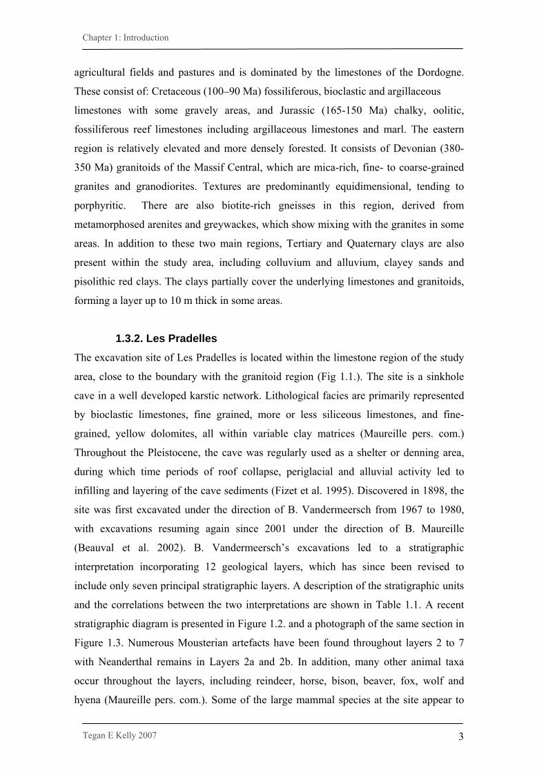
1.3.2. Les Pradelles The excavation site of Les Pradelles is located within the limestone region of the study
area, close to the boundary with the granitoid region (Fig 1.1.). The site is a sinkhole
cave in a well developed karstic network. Lithological facies are primarily represented
by bioclastic limestones, fine grained, more or less siliceous limestones, and fine-
grained, yellow dolomites, all within variable clay matrices (Maureille pers. com.)
Throughout the Pleistocene, the cave was regularly used as a shelter or denning area,
during which time periods of roof collapse, periglacial and alluvial activity led to
infilling and layering of the cave sediments (Fizet et al. 1995). Discovered in 1898, the
site was first excavated under the direction of B. Vandermeersch from 1967 to 1980,
with excavations resuming again since 2001 under the direction of B. Maureille
(Beauval et al. 2002). B. Vandermeersch’s excavations led to a stratigraphic
interpretation incorporating 12 geological layers, which has since been revised to
include only seven principal stratigraphic layers. A description of the stratigraphic units
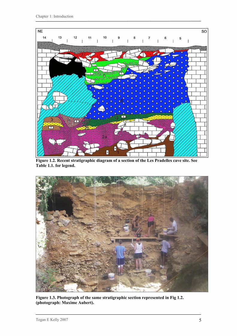
and the correlations between the two interpretations are shown in Table 1.1. A recent
stratigraphic diagram is presented in Figure 1.2. and a photograph of the same section in
Figure 1.3. Numerous Mousterian artefacts have been found throughout layers 2 to 7
with Neanderthal remains in Layers 2a and 2b. In addition, many other animal taxa
occur throughout the layers, including reindeer, horse, bison, beaver, fox, wolf and
hyena (Maureille pers. com.). Some of the large mammal species at the site appear to

Chapter 1: Introduction
Tegan E Kelly 2007
4
have been brought into the cave by the humans, while other species show anthropic
commensalism (Fizet 1995). The faunal assemblage indicates a cold, continental,
steppic and open environment and along with sedimentology, lithic industry and
Neanderthal presence, provides convergent evidence for dating the site to OIS 3,
approximately 40,000 - 50,000 years ago (Fizet 1995).
Table 1.1: Stratigraphic correlation of the layers determined during the Vandermeersch excavations and new analysis of the stratigraphic facies by Maureille (Maureille pers. com.).
Stratigraphy according to works coordinated by B. Vandermeersh New facies and sub-facies New facies and
sub-facies correlations Not correlated
Layer N° Nature of layer NE part Middle SO part
NE part Middle SO
part
of the cut of the
cut
1 Small gelifacted blocks 7 7 7 Matrix: brown sandy clays 2 Big blocks Matrix: clear clays and very small gravels 6 3 Limestone blocks (size very variable) Matrix: fine brown clays 4 Limestone blocks masked Matrix: yellow sands and brown clays 5 Limestone Blocks by 5 Matrix: yellow sands and brown clays 5 6 Blocks of limestone altered Matrix: more clay rich 7 Black limestone blocks material 8
8J Small blocks of limestone Yellow sandy silts 4 4 8 Big blocks of limestone Matrix: dark red clays 3
9a Altered blocks of limestone with a black colouration
Matrix: red clays 9b Like in 9a but with a red sandy clay matrix 2b 2b 2b
9b1 Like in 9a with a white colouration related to limestone
alteration 9c Like in 9a but More clay rich 3
10 Fine red sticky clays and non altered limestone blocks
10a Fine red sticky clays with small white fragments (altered limestone
blocks) 2a 2a 2a 11 Fine red clays with altered limestone blocks Base: very rich in coprolithes
Base 11-12 Broken stalagmitic floor Not found 12 Brown to black clays with flint nodules 1 1 1 No n° Brown to black very fine clays
Chapter 1: Introduction
Tegan E Kelly 2007
5
Figure 1.2. Recent stratigraphic diagram of a section of the Les Pradelles cave site. See Table 1.1. for legend.
Figure 1.3. Photograph of the same stratigraphic section represented in Fig 1.2. (photograph: Maxime Aubert).

Chapter 1: Introduction
Tegan E Kelly 2007
6
1.4. Thesis overview Chapter 2 provides background information relevant to the current study. It explains
the principles and techniques involved in strontium isotope tracing and presents some
examples of prior studies. A brief overview regarding the composition, structure and
formation of tooth enamel supplies information relevant to the sampling techniques
and results, while background information on each of the study species gives an
insight into the lives of the Pleistocene populations represented by the sample
material. Chapter 3 outlines the methodology of the study, from sample collection and
preparation to analysis and techniques. Chapter 4 presents all results, including
strontium measurements, statistical analyses and the resultant strontium isotope map.
Chapter 5 provides an in depth discussion of the meanings, complications and
implications of the results and Chapter 6 finishes off with a conclusionary summary
and suggestions for further research.
Chapter 2: Background
Tegan E Kelly 2007
7
Chapter 2
BACKGROUND 2.1. Strontium as a tool for tracing migration
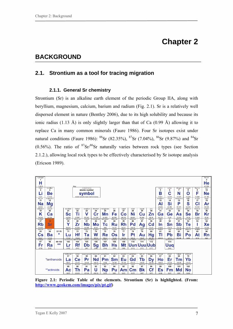
2.1.1. General Sr chemistry Strontium (Sr) is an alkaline earth element of the periodic Group IIA, along with
beryllium, magnesium, calcium, barium and radium (Fig. 2.1). Sr is a relatively well
dispersed element in nature (Bentley 2006), due to its high solubility and because its
ionic radius (1.13 Å) is only slightly larger than that of Ca (0.99 Å) allowing it to
replace Ca in many common minerals (Faure 1986). Four Sr isotopes exist under
natural conditions (Faure 1986): 88Sr (82.35%), 87Sr (7.04%), 86Sr (9.87%) and 84Sr
(0.56%). The ratio of 87Sr/86Sr naturally varies between rock types (see Section
2.1.2.), allowing local rock types to be effectively characterised by Sr isotope analysis
(Ericson 1989).
Figure 2.1: Periodic Table of the elements. Strontium (Sr) is highlighted. (From: http://www.geokem.com/images/pix/pt.gif)

Chapter 2: Background
Tegan E Kelly 2007
8
2.1.2. Geological Sr isotope mapping
All rock-types have a characteristic ratio of 87Sr/86Sr, generally ranging from 0.700 –
0.740. Although this range appears small, it is actually quite large relative to
analytical error (0.00001-0.00003) (Price et al. 1994a). The ratio is a function of a
rock’s age and its composition (Fig. 2.2.). The radioactive isotope 87Rb decays to form
radiogenic 87Sr (forming the basis of Rb-Sr dating; Faure 1986). Therefore, old rock
units are relatively higher in radiogenic 87Sr than younger rocks, leading to a higher 87Sr/86Sr ratio. It follows that rocks with high levels of Rb relative to Sr will also have
more 87Sr relative to 86Sr and hence, higher ratios (Price et al. 2002). By comparing
the Sr isotope ratios within and between geological regions of differing age and
composition, rock-types can be characterised by Sr isotope ratio and a geological
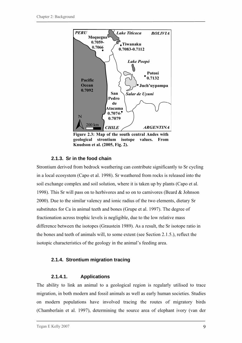
isotope map created. For example, Knudson et al. (2005) used soil and water isotope
ratios to infer local isotope signatures in an area of the south central Andes of South
America ( Fig. 2.3.). They then used this map to determine that two of the three
Juch’uypampa cave mummies found in the region had been locals to the area.
Figure 2.2: Evolution of 87Sr/86Sr over geologic time. A hypothetical granite that crystallised around 3.6 Ga ago form a mantle-derived melt (Granite I) evolves along a steep trajectory toward high 87Sr/86Sr values because of its high Rb/Sr ratio. Granite II also evolves along a steep trajectory, but its 87Sr/86Sr measured today is lower than that of granite I because it crystallised later. Two rocks of the same age but with different Rb/Sr ratios will evolve along different trajectories, with the lower Rb/Sr rock yielding a lower 87Sr/86Sr. From Capo et al. (1998, Fig. 2).
Chapter 2: Background
Tegan E Kelly 2007
9
Figure 2.3: Map of the south central Andes with geological strontium isotope values. From Knudson et al. (2005, Fig. 2).
2.1.3. Sr in the food chain Strontium derived from bedrock weathering can contribute significantly to Sr cycling
in a local ecosystem (Capo et al. 1998). Sr weathered from rocks is released into the
soil exchange complex and soil solution, where it is taken up by plants (Capo et al.
1998). This Sr will pass on to herbivores and so on to carnivores (Beard & Johnson
2000). Due to the similar valency and ionic radius of the two elements, dietary Sr
substitutes for Ca in animal teeth and bones (Grupe et al. 1997). The degree of
fractionation across trophic levels is negligible, due to the low relative mass
difference between the isotopes (Graustein 1989). As a result, the Sr isotope ratio in
the bones and teeth of animals will, to some extent (see Section 2.1.5.), reflect the
isotopic characteristics of the geology in the animal’s feeding area.
2.1.4. Strontium migration tracing
2.1.4.1. Applications The ability to link an animal to a geological region is regularly utilised to trace
migration, in both modern and fossil animals as well as early human societies. Studies
on modern populations have involved tracing the routes of migratory birds
(Chamberlain et al. 1997), determining the source area of elephant ivory (van der

Chapter 2: Background
Tegan E Kelly 2007
10
Merwe et al. 1990; Vogel et al. 1990) and tracking habitat use in African Elephants
(Koch et al. 1995). Studies on fossil animals have involved investigating the seasonal
mobility of prehistoric herders in South Africa, through the analysis of sheep tooth
enamel (Balasse et al. 2002), tracing major population migration events through
analysis of cattle teeth and bones (Scheissing & Grupe 2003), mapping the spatial
scale of fossil faunal assemblages (Porder et al. 2003) and tracking the migratory
behaviour of extinct animals such as mammoths and mastodons (Hoppe et al. 1999).
Sr isotope analysis has also been applied to historic human populations in both Europe
and the Americas. European studies have included an investigation into Bronze Age
migration near Stonehenge, in which three adult males were shown to have spent their
childhood in a different area to that of their burial, while the two juveniles from the
same grave were most likely locals (Evans et al. 2006). Grupe et al. (1997) studied the
mobility of the Bell Beaker people of southern Bavaria and found high levels of
mobility, with 17.5-25% of the 69 individuals studied having changed residence
during their lifetime. The famous alpine iceman found in a European glacier in 1991,
appears, based on Sr isotopes, to have migrated in later life after originating from
within 60 km south east of the discovery site (Hoogewerff et al. 2001; Müller et al.
2003). Studies based in the Americas have included the Mayan region of the south
central Andes, where Hodell et al. (2004) created a Sr isotope map, which Wright
(2005) used to determine that eight of 83 skeletons from Tikal, Guatemala, migrated
to their site of burial from distant geological zones. Studies have also focused on the
south west United States, where a complex pattern of immigration and settlement has
been demonstrated at the site of Grasshopper Pueblo, Arizona (Price et al. 1994b).
Ezzo & Price (2002) found that out of 70 adult individuals from the site, 33 were
locals, 13 non-locals from nearby regions and 24 non-locals from more distant areas.
Furthermore, Sr isotopes have also been utilised to study earlier human species, such
as those from the Sterkfontein Valley, South Africa, which involved the analysis of
ancient Australopithecus robustus and early Homo remains, which determined that
these early hominids did not source their food from riparian areas (Sillen et al. 1998).
2.1.4.2. Techniques A common method of determining migration is to compare Sr isotope ratios between
tooth and bone tissues within an individual. This technique is based on the fact that

Chapter 2: Background
Tegan E Kelly 2007
11
tooth enamel is formed during childhood and does not undergo resorption and
remodelling (Fincham et al. 1999) and therefore reflects the isotopic conditions of the
childhood feeding area. Bone tissue on the other hand is regularly replaced throughout
life, so isotopically reflects the feeding area of later life (Wright 2005). By comparing
the isotopic ratios of the two tissues, it is possible to determine whether an individual
has migrated during life (if the two are different), or whether they spent their later life
in the same area as their childhood (if the two are similar). This technique has been
used, for example, to investigate migration of humans from a Roman fortress in
Germany (Schweissing & Grupe 2003) and in the ancient city of Teotihuacan in
Mexico (Price et al. 2000) as well as in determining the source of horn core from a
long-horned ox at an early modern horn-core site in Austria (Schweissing & Grupe
2003).
Fossil enamel is often the best preserved of hard tissues due to its heavily mineralised
nature (see Section 2.2.; Hillson 1986) and is relatively resistant to contamination and
diagenesis (Budd et al. 2000). Bone on the other hand is much more liable to post-
depositional contamination (Price et al. 1994a) and does not always provide reliable
Sr isotope results. It is therefore desirable to use a method of Sr migration tracing that
focuses on tooth enamel and not the less reliable bone material. Evans et al. (2006)
achieved this by comparing the isotopes in tooth enamel of premolars with those in
molars from the same individual. These teeth grow at different times of childhood
(Hillson 1986), thus indicating any mobility which may have occurred during this
period.
A more comprehensive approach is to utilise a Sr isotope map of the local geology
(see Section 2.1.2.). By assuming the area of burial is indicative of the area of later
life habitation, isotope ratios can be measured in tooth enamel to see if the individual
was local to the area (if isotopes match the location of burial), migrated to the area
from somewhere nearby (if they match a different area of the map) or from
somewhere more distant (if they do not match anywhere on the map). This technique
is very effective and is used regularly to study mobility in fossil animal populations
(e.g. Balasse et al. 2002; Porder et al. 2003) and prehistoric humans (e.g. Bentley et
al. 2004; Chiardia et al. 2003; Ezzo & Price 2002; Grupe et al. 1997; Knudson et al.
2005).

Chapter 2: Background
Tegan E Kelly 2007
12
2.1.5. Biological availability It is important to be aware that the Sr isotope ratios in biological material can not be
assumed to be the same as the local bedrock, because little of the bedrock Sr is
biologically available to plants and animals (Capo et al. 1998; Price et al. 2002; Sillen
et al. 1998). Capo et al. (1998) wrote on the use of Sr isotopes as tracers of ecosystem
processes. They noted that only the exchangeable ions within a soil will be available
for transport in solution, which they called the ‘labile’ portion. Sillen et al. (1998)
investigated the difference between the labile portion, and the whole rock Sr (which
includes that locked-up in silicates) when determining local Sr isotope signatures.
While researching the use of Sr isotopes in the reconstruction of early hominid
behaviour in the Sterkfontein Valley in South Africa, they found a large difference in
Sr isotope composition between whole-soil Sr compared with both available soil Sr
and plant Sr (Fig. 2.4.). They went on to suggest that “any potential applications of 87Sr/86Sr relationships should use biologically available Sr as a starting point, rather
than substrate geology per se.”
Sr data from three sites at Swartkrans
0.7
0.72
0.74
0.76
0.78
0.8
0.82
0.84
0.86
0 1 2 3
87Sr
/86S
r
PlantWhole soilLabile soil
Figure 2.4: Comparison of 87Sr/86Sr for whole soil Sr, available soil Sr and plant Sr at three locations at Swatkrans in the Sterkfontein Valley, South Africa. (Adapted from data in Sillen et al. 1998).
Chapter 2: Background
Tegan E Kelly 2007
13
This has led a number of other researchers to use biologically available Sr when
creating isotope maps. When attempting to track the migration of mammoths and
mastodons across prehistoric North America, Hoppe et al. (1999) used plant and water
samples to create a Sr isotope map in one area, and modern rodent bones and teeth in
another. Porder et al. (2003) attempted to use Sr isotope mapping to determine the
spatial scale of Holocene, predator-accumulated, faunal assemblages in north-eastern
Yellowstone National Park, Wyoming. They compared Sr isotopes in soil, plant and
animal bones in addition to rocks, and in so doing, successfully differentiated between
different regions of the area.
Analysis of biologically available Sr can be achieved through analysing local
biological materials or by leaching available Sr from soils and rocks. Hodell et al.
(2004) created a Sr isotope map in the Maya region, through the analysis of plant and
water Sr isotopes in addition to rocks and soils. They found that although there was
significant variability between 87Sr/86Sr values within a region, it was not enough to
blur the distinction between regions. However, Hodell et al. (2004) did not separate
the biologically available portion of Sr in rocks and soils, but used bulk analyses
instead, thus incorporating non-biological Sr into their analyses. Price et al. (2002)
reviewed the use of various local Sr indicators (i.e. rock, soil, plant and animal
tissues) in a number of papers, and concluded that, if available, fossil teeth of small
animals will give the best indication of a local biologically available 87Sr/86Sr signal.
They went on to apply this technique at Grasshopper, Pueblo, Arizona (Ezzo & Price
2002), where they analysed rodent bones to determine local signals. Similarly,
Bentley & Knipper (2005) used archaeological domestic pigs for local signatures in
south west Germany, which, in a previous study (Bentley et al. 2004), had already
been shown to demonstrate a local signature due to their being raised in proximity to
the archaeological site. Alternatively, Budd et al. (2004) recommend labile soil Sr as a
reliable indicator of local biologically available Sr and as such a good basis for Sr
isotope mapping. The labile portion of soil Sr can be separated through ammonium
nitrate leaching of bulk soil (Prohaska et al. 2005). Labile soil Sr makes a better proxy
for local signatures than labile rock Sr, as leaching from rocks will not take into
account Sr derived from aeolian and fluvial sediments, which also contribute to the Sr
cycling of the ecosystem (Capo et al. 1998). As such, the analysis of labile soil Sr in
addition to plant Sr was chosen as the appropriate technique for the current study.
Chapter 2: Background
Tegan E Kelly 2007
14
2.2. Teeth
2.2.1 Mammal tooth structure
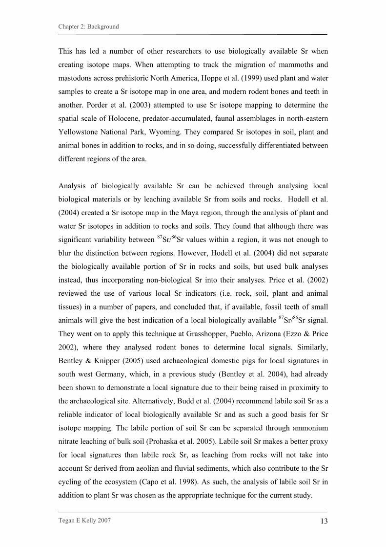
Mammalian teeth are composed of three main materials, dentine, enamel and
cementum (Hoppe et al. 2004). Dentine forms the main bulk of the tooth, and enamel
the hard protective cover, while cementum forms additional layers in some taxa (Fig
2.5.; Hillson 1986). Mammal teeth occur in many shapes and forms and a complex
descriptive terminology for tooth shape exists (Hillson 1986). The most complex
features of mammalian teeth are the crowns of molars, which can be folded into
diverse and complex shapes (Zhao et al. 2000). Molar form can be brachydont (low
crowns) or hypsodont (High crowns), with rounded cusps (bunodont) or sharp cusps
(secodont) and may have cusps coalesced into folds known as infindibulums
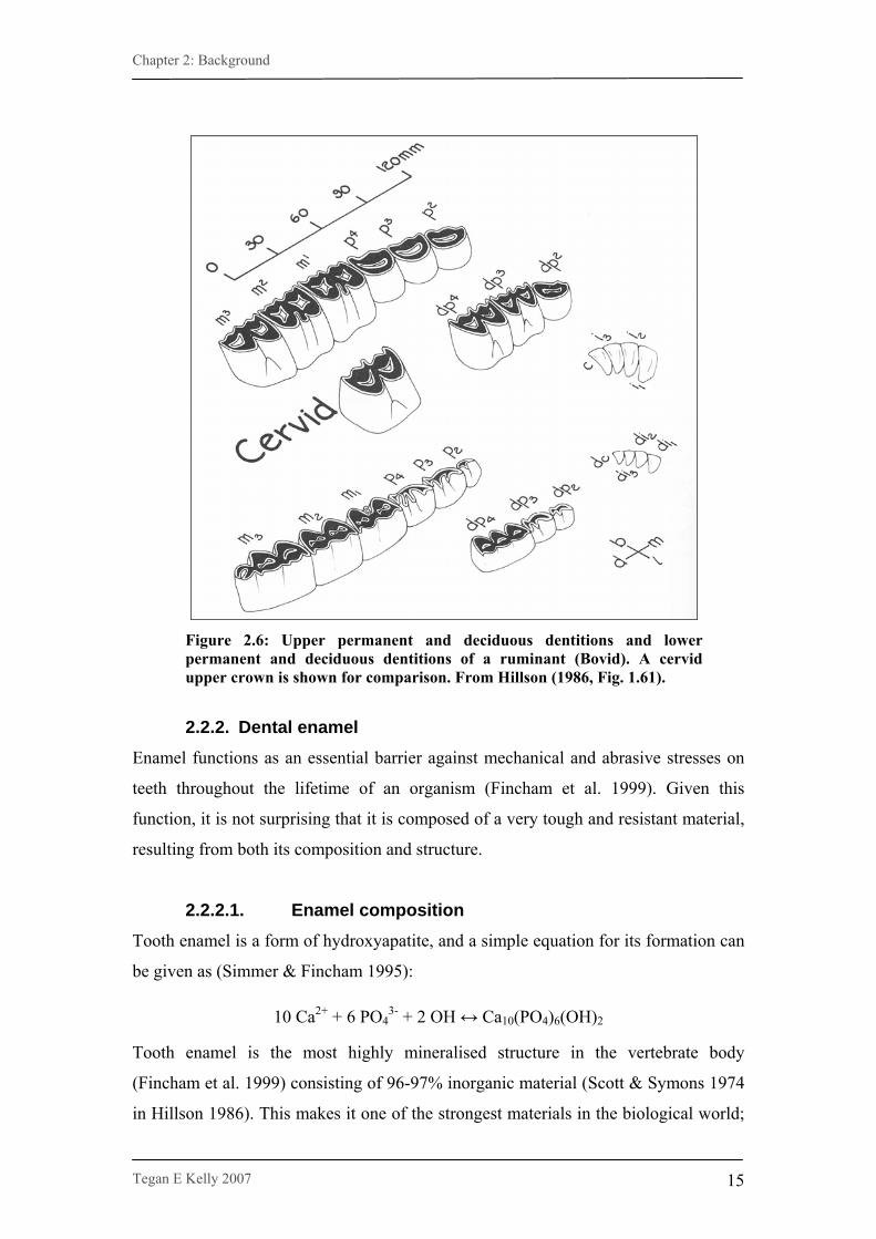
(selenodont; Hillson et al. 1986). The main study animals for this project are
ruminants (see Section 2.3.) which have spatulate incisors and canines (have a high
cutting edge) and selenodont molars with multiple infindibulums (Fig 2.6.; Hillson
1986).
Figure 2.5: Generalised structure of a simple mammalian tooth. From Hillson (1986, Fig. 1.1).
Chapter 2: Background
Tegan E Kelly 2007
15
Figure 2.6: Upper permanent and deciduous dentitions and lower permanent and deciduous dentitions of a ruminant (Bovid). A cervid upper crown is shown for comparison. From Hillson (1986, Fig. 1.61).
2.2.2. Dental enamel Enamel functions as an essential barrier against mechanical and abrasive stresses on
teeth throughout the lifetime of an organism (Fincham et al. 1999). Given this
function, it is not surprising that it is composed of a very tough and resistant material,
resulting from both its composition and structure.
2.2.2.1. Enamel composition Tooth enamel is a form of hydroxyapatite, and a simple equation for its formation can
be given as (Simmer & Fincham 1995):
10 Ca2+ + 6 PO43- + 2 OH ↔ Ca10(PO4)6(OH)2
Tooth enamel is the most highly mineralised structure in the vertebrate body
(Fincham et al. 1999) consisting of 96-97% inorganic material (Scott & Symons 1974
in Hillson 1986). This makes it one of the strongest materials in the biological world;
Chapter 2: Background
Tegan E Kelly 2007
16
with a hardness intermediate between iron and carbon steel (Simmer & Fincham
1995). This strength is in large part achieved through the systematic and well
organised microstructure of enamel.
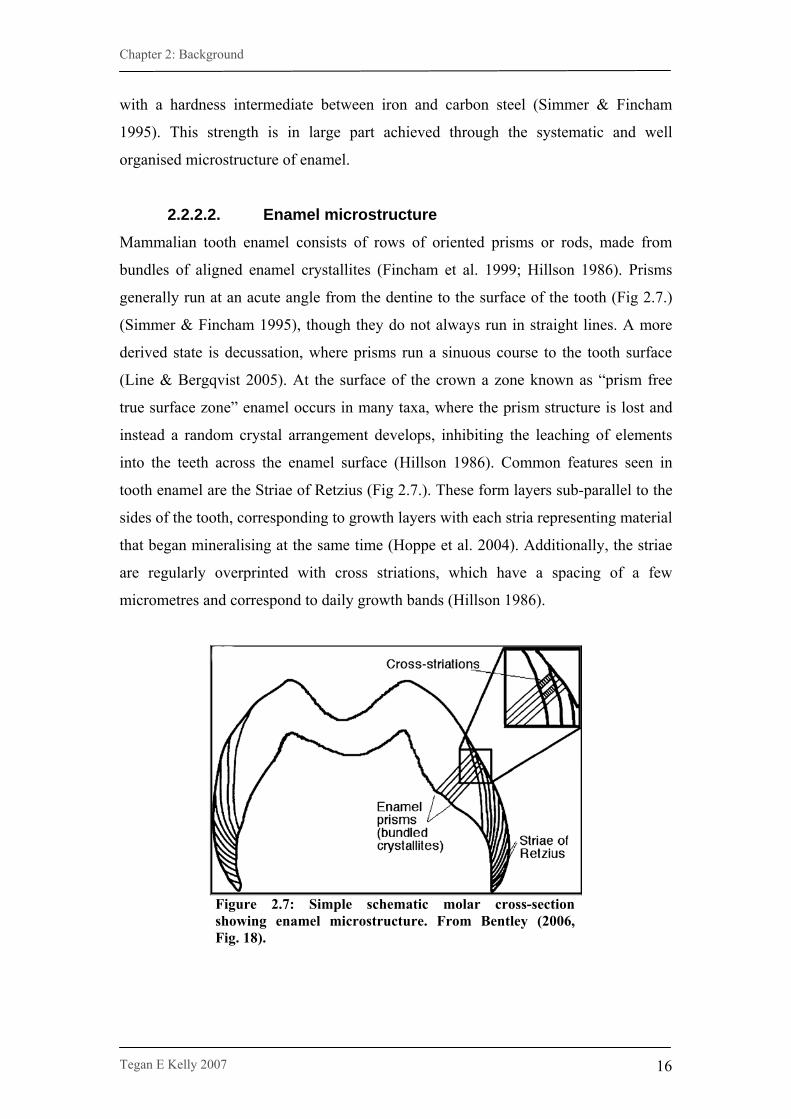
2.2.2.2. Enamel microstructure Mammalian tooth enamel consists of rows of oriented prisms or rods, made from
bundles of aligned enamel crystallites (Fincham et al. 1999; Hillson 1986). Prisms
generally run at an acute angle from the dentine to the surface of the tooth (Fig 2.7.)
(Simmer & Fincham 1995), though they do not always run in straight lines. A more
derived state is decussation, where prisms run a sinuous course to the tooth surface
(Line & Bergqvist 2005). At the surface of the crown a zone known as “prism free
true surface zone” enamel occurs in many taxa, where the prism structure is lost and
instead a random crystal arrangement develops, inhibiting the leaching of elements
into the teeth across the enamel surface (Hillson 1986). Common features seen in
tooth enamel are the Striae of Retzius (Fig 2.7.). These form layers sub-parallel to the
sides of the tooth, corresponding to growth layers with each stria representing material
that began mineralising at the same time (Hoppe et al. 2004). Additionally, the striae
are regularly overprinted with cross striations, which have a spacing of a few
micrometres and correspond to daily growth bands (Hillson 1986).
Figure 2.7: Simple schematic molar cross-section showing enamel microstructure. From Bentley (2006, Fig. 18).

Chapter 2: Background
Tegan E Kelly 2007
17
2.2.2.3. Enamel formation Amelogenesis, the process of enamel formation, occurs in two main phases (Hillson
1986), which can be further subdivided into five stages (see Fig 2.8.) (Fincham et al.
1999; Moradian-Oldak 2001). The first phase, matrix production, involves: i)
secretion of an organic matrix and ii) enamel crystal nucleation and assembly. The
second phase, enamel maturation, involves: iii) crystal elongation and prism
formation, iv) resorption of the organic matrix and v) maturation into heavily
mineralised enamel with an outer, prism-free zone (Fincham et al. 1999; Hillson
1986; Simmer & Fincham 1995). The enamel maturation phase can continue for some
time, both during and after tooth eruption in many mammal species (Hillson 1986).
Figure 2.8: Schematic diagram of enamel biomineralization in five stages. From Fincham et al. (1999, Fig 8).
2.3. Study animals Twenty three animal teeth, excavated from layers 2-5 at Les Pradelles, were analysed.
The primary study animals were ruminants, including 14 reindeer (Rangifer
tarandus), three horse (Equus caballus) and one aurochs/bison (Bos/Bison) specimen.
Three rodent incisors were also analysed: two marmots (Marmota marmota.) and one
Chapter 2: Background
Tegan E Kelly 2007
18
beaver (Castor sp.). Two carnivore samples were included as a comparison to the
herbivores: a wolf (Canis lupus) and a fox (Vulpes vulpes). The taxonomy of the study
animals is shown in Table 2.1.
Table 2.1: Taxonomy of study animals
Class
Order
Family
Genus & species
Common name
Cervidae Rangifer tarandus Reindeer Artiodactyla Bovidae Bos/ Bison sp. Aurochs/Bison
Perissodactyla Equidae Equus caballus Horse Scuridae Marmota marmota. Marmot Rodentia Castoridae Castor sp. Beaver
Canis lupus Wolf
Mammalia
Carnivora Canidae Vulpes vulpes. Fox
2.3.1. Reindeer Modern reindeer (or caribou in North America) have a northern circumpolar
distribution (Kurtén 1968) mostly inhabiting arctic tundra and the surrounding boreal
forests (Nowak & Paradiso 1983). Many herds are now semi-domesticated, but wild
herds still migrate through very large areas (Iacumin and Longinelli 2002) and are
almost constantly on the move. They sometimes travel up to 1,000 km between their
summer tundra range and forest wintering grounds (Nowak & Paradiso 1983), though
a distance of 100 - 300 km is more usual (Dannell et al. 2006). Their diet consists of a
variety of grasses, herbs and leaves in summer and fine twigs and lichen in winter
(Kurtén 1968; Nowak & Paradiso 1983). Reindeer calving usually occurs around mid
may, and calves are born with deciduous teeth already erupted (Hillson 1986). The
permanent dentition of reindeer continues to mineralise after eruption (Drucker et al.
2001; Table 2.2.).
Table 2.2: Eruption table for permanent dentition of reindeer
Eruption stage Age range (months) Possible season M1 3-5 mid-August -mid October M2 10-15 mid-March to mid-August M3 15-29 any time of year P 22-29 mid-March to mid-September Adapted from Hillson (1983).
Pleistocene reindeer had a much wider range in Europe than they do today, especially
during OIS 2 (Kurtén 1968). During this period, reindeer formed the main game
Chapter 2: Background
Tegan E Kelly 2007
19
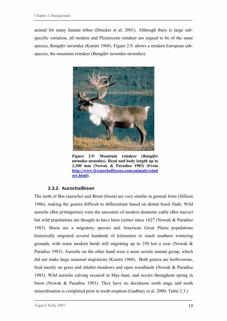
animal for many human tribes (Drucker et al. 2001). Although there is large sub-
specific variation, all modern and Pleistocene reindeer are argued to be of the same
species, Rangifer tarandus (Kurtén 1968). Figure 2.9. shows a modern European sub-
species, the mountain reindeer (Rangifer tarandus tarandus).
Figure 2.9: Mountain reindeer (Rangifer tarandus tarandus). Head and body length up to 2,200 mm (Nowak & Paradiso 1983) (From http://www.fresnochaffeezoo.com/animals/reindeer.html).
2.3.2. Aurochs/Bison The teeth of Bos (aurochs) and Bison (bison) are very similar in general form (Hillson
1986), making the genera difficult to differentiate based on dental fossil finds. Wild
aurochs (Bos primigenius) were the ancestors of modern domestic cattle (Bos taurus)
but wild populations are thought to have been extinct since 1627 (Nowak & Paradiso
1983). Bison are a migratory species and American Great Plains populations
historically migrated several hundreds of kilometres to reach southern wintering
grounds, with some modern herds still migrating up to 250 km a year (Nowak &
Paradiso 1983). Aurochs on the other hand were a more sessile animal group, which
did not make large seasonal migrations (Kurtén 1968). Both genera are herbivorous,
feed mostly on grass and inhabit meadows and open woodlands (Nowak & Paradiso
1983). Wild aurochs calving occured in May-June, and occurs throughout spring in
bison (Nowak & Paradiso 1983). They have no deciduous tooth stage and tooth
mineralisation is completed prior to tooth eruption (Gadbury et al. 2000; Table 2.3.)
Chapter 2: Background
Tegan E Kelly 2007
20
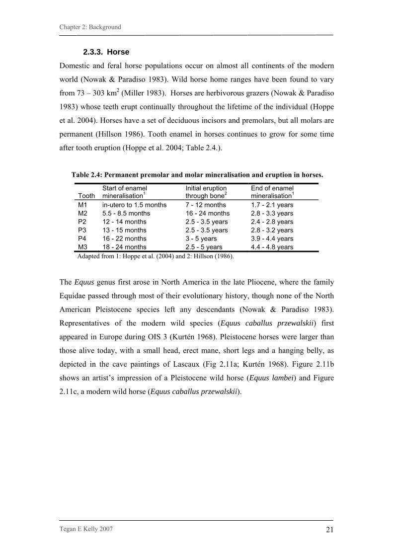
Table 2.3: Timing of enamel formation and tooth eruption in the molars of Bos/Bison. Tooth Formation1 Eruption2 M1 In-utero to several months of age 9-12 months M2 Birth to 13 months 18 months M3 9 months to 2 years 2.25-2.5 years
Adapted from 1: Gadbury et al. (2000) and 2: Hillson (1986).
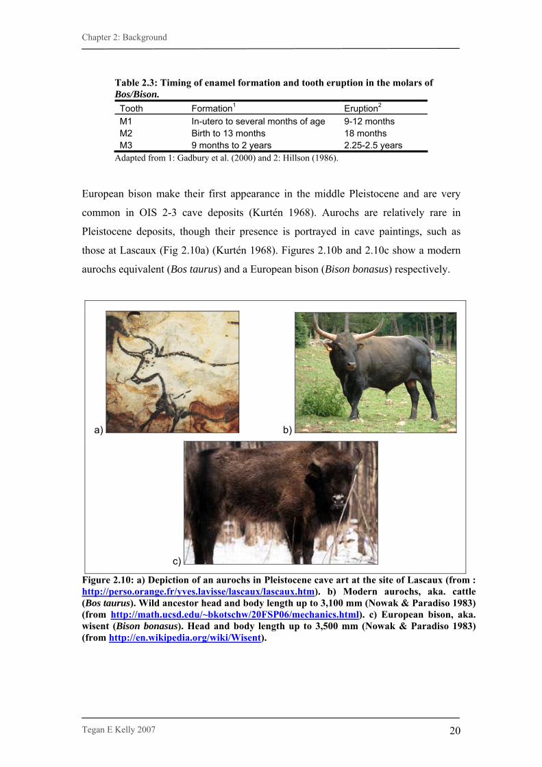
European bison make their first appearance in the middle Pleistocene and are very
common in OIS 2-3 cave deposits (Kurtén 1968). Aurochs are relatively rare in
Pleistocene deposits, though their presence is portrayed in cave paintings, such as
those at Lascaux (Fig 2.10a) (Kurtén 1968). Figures 2.10b and 2.10c show a modern
aurochs equivalent (Bos taurus) and a European bison (Bison bonasus) respectively.
a) b)
c)
Figure 2.10: a) Depiction of an aurochs in Pleistocene cave art at the site of Lascaux (from : http://perso.orange.fr/yves.lavisse/lascaux/lascaux.htm). b) Modern aurochs, aka. cattle (Bos taurus). Wild ancestor head and body length up to 3,100 mm (Nowak & Paradiso 1983) (from http://math.ucsd.edu/~bkotschw/20FSP06/mechanics.html). c) European bison, aka. wisent (Bison bonasus). Head and body length up to 3,500 mm (Nowak & Paradiso 1983) (from http://en.wikipedia.org/wiki/Wisent).
Chapter 2: Background
Tegan E Kelly 2007
21
2.3.3. Horse Domestic and feral horse populations occur on almost all continents of the modern
world (Nowak & Paradiso 1983). Wild horse home ranges have been found to vary
from 73 – 303 km2 (Miller 1983). Horses are herbivorous grazers (Nowak & Paradiso
1983) whose teeth erupt continually throughout the lifetime of the individual (Hoppe
et al. 2004). Horses have a set of deciduous incisors and premolars, but all molars are
permanent (Hillson 1986). Tooth enamel in horses continues to grow for some time
after tooth eruption (Hoppe et al. 2004; Table 2.4.).
Table 2.4: Permanent premolar and molar mineralisation and eruption in horses.
Tooth Start of enamel mineralisation1
Initial eruption through bone2
End of enamel mineralisation1
M1 in-utero to 1.5 months 7 - 12 months 1.7 - 2.1 years M2 5.5 - 8.5 months 16 - 24 months 2.8 - 3.3 years P2 12 - 14 months 2.5 - 3.5 years 2.4 - 2.8 years P3 13 - 15 months 2.5 - 3.5 years 2.8 - 3.2 years P4 16 - 22 months 3 - 5 years 3.9 - 4.4 years M3 18 - 24 months 2.5 - 5 years 4.4 - 4.8 years Adapted from 1: Hoppe et al. (2004) and 2: Hillson (1986).
The Equus genus first arose in North America in the late Pliocene, where the family
Equidae passed through most of their evolutionary history, though none of the North
American Pleistocene species left any descendants (Nowak & Paradiso 1983).
Representatives of the modern wild species (Equus caballus przewalskii) first
appeared in Europe during OIS 3 (Kurtén 1968). Pleistocene horses were larger than
those alive today, with a small head, erect mane, short legs and a hanging belly, as
depicted in the cave paintings of Lascaux (Fig 2.11a; Kurtén 1968). Figure 2.11b
shows an artist’s impression of a Pleistocene wild horse (Equus lambei) and Figure
2.11c, a modern wild horse (Equus caballus przewalskii).

Chapter 2: Background
Tegan E Kelly 2007
22
a) b)
c)
Figure 2.11: a) Depiction of a horse in Pleistocene cave art at the site of Lascaux (from: http://www.ifls-france.net/PHOTOS/Lascaux.jpeg). b) Artists impression of a Pleistocene wild horse (Equus lambei) (from http://www.virtualmuseum.ca/ Exhibitions/Herschel/English/Discoveries/discoveries01d.html). c) Modern wild horse (Equus caballus przewalskii). Can be up to 1,500 mm high at the shoulders (Nowak & Paradiso 1983) (from http://www.billybear4kids.com/animal/whose-toes/toes-88a-WildHorse.html).
2.3.4. Marmot Marmots are large rodents, which have a fragmented distribution over Europe and
North America, though their range was much larger in the Pleistocene (Kurtén 1968).
They occupy open habitats, such as steppes, alpine meadows, pastures and forest
edges (Nowak & Paradiso 1983) and tend to live on mountain sides above the timber
line (Kurtén 1968). Individual marmot territories may be 2,000 m2 (Nowak &
Paradiso 1983) and are centred around a subterranean den (Kurtén 1968). Marmots
are mainly herbivorous, eating seeds, nuts, stems, leaves roots and bulbs, though they
will eat insects and small vertebrates during the lead up to hibernation (Hillson 1986).
All rodent incisors are ever-growing (Hillson 1986), generally erupting at a rate equal
to the attrition of the tip (Rinaldi & Cole 2004). This makes rodent incisor enamel an
exception in isotope analysis, only reflecting Sr isotopes from the later stages of an
individuals feeding history, as the record of earlier stages are lost to wear. Evidence of
marmots have been found as early as OIS 6 but only become common in the late

Chapter 2: Background
Tegan E Kelly 2007
23
Pleistocene (Kurtén 1983). Figure 2.12. shows a modern European sub-species, the
alpine marmot (Marmota marmota).
Figure 2.12: Alpine marmot (Marmota marmota). Head and body length up to 600 mm (Nowak & Paradiso 1983) (from http://en.wikipedia.org/wiki/Alpine_Marmot).
2.3.5. Beaver Beavers are large semi-aquatic rodents, which build complex dams, canals and lodges
in streams and small lakes (Nowak & Paradiso 1983). Their dams are made from
branches of nearby trees, the bark of which forms their main food, though they also
feed on shore vegetation and water-plants in summer (Kurtén 1968). As with all
rodents, beaver incisors erupt continuously throughout life (Rinaldi & Cole 2004). In
addition to feeding, beaver incisors are used to fell trees (Hillson 1986) resulting in
especially rapid replacement growth (Stuart-Williams & Schwarcz 1997). Beaver
fossils occur as early as the Oligocene and show a continuous record throughout the
Pleistocene, at which stage all forms seem referable to the living species (Kurtén
1968). Figure 2.13. shows a modern European beaver (Castor fiber).
Figure 2.13: European beaver (Castor fiber). Head and body length up to 1,000 mm Nowak & Paradiso 1983) (from: http://www.flickr.com/photos/patries71/).

Chapter 2: Background
Tegan E Kelly 2007
24
2.3.6. Wolf Gray wolves (Canis lupus), the wild ancestors of domestic dogs (Canis familiaris),
are found in all habitats of the northern hemisphere except tropical forests and arid
deserts (Nowak & Paradiso 1983). A gregarious species, wolves hunt in packs to feed
primarily on prey larger than themselves (Kurtén 1968), though they will also
occasionally eat rodents and amphibians (Hillson 1986). Their home range size
depends on food availability, season and pack size, ranging from 18 km2 to 13,000
km2, with an average territory of 100-700 km2 (Nowak & Paradiso 1983). All dogs
have deciduous teeth which emerge within the first two months after birth and are
later replaced by permanent dentition (Hillson 1986; Table 2.5.). Wolves first appear
during the Middle Pleistocene and the wolves of the Late Pleistocene were slightly
larger than modern day wolves (Kurtén 1968). Figure 2.14. shows a modern Eurasian
wolf (Canis lupus lupus).
Table 2.5: Tooth emergence stages for domestic dog.
Stage Definition Suggested age Stage 1 Deciduous teeth emerge, i, c, then p. 1 - 2.5 months Stage 2 Permanent incisors emerge, permanent M1 & P1 emerge later in
this stage 2.5 - 4 months
Stage 3 Permanent M2, P2, P3 & P4 emerge. Permanent canines emerge during this stage or next.
5 - 6 months
Stage 4 Permanent M3 emerge. Canines may erupt in this stage. 6 - 7 months Adapted from Hillson (1986). See Appendix 2 for dental notation.
Figure 2.14: Eurasian wolf (Canis lupus lupus). Head and body length up to 1,600 mm (Nowak & Paradiso 1983) (from http://www.wolfdog.org/eng/articles/1357.htm).

Chapter 2: Background
Tegan E Kelly 2007
25
2.3.7. Fox Foxes rival the grey wolf for the greatest natural distribution of living terrestrial
mammals after humans (Nowak & Paradiso 1983) with a modern range covering
Europe, North Africa, most of Asia and North America as well as having been
introduced in Australia (Kurtén 1968). Their habitat ranges from deep forests to arctic
tundra (Nowak & Paradiso 1983). Foxes hunt by stalking (Kurtén 1968) and their
main prey are rodents, though they may also eat birds, amphibians, fish, insects and
fruit (Kurtén 1968; Nowak & Paradiso 1983). Home range size varies with food
availability and is largest in winter, ranging from 12 km2 (good habitat) to 50 km2
(bad habitat) and smallest during the birthing period (5 to 20 km2; Nowak & Paradiso
1983). Red fox dentition goes through a deciduous stage during the first few months
of life, with all permanent teeth having emerged after 6 months (Hillson 1986; Table
2.6.). Foxes are very common in both open air and cave sites of OIS 2-4 and the main
difference from modern populations is a smaller body size (Kurtén 1968). Figure 2.15.
shows a modern red fox (Vulpes vulpes).
Table 2.6: Tooth emergence stages for red fox. Stage Definition Suggested age Stage 1 All deciduous teeth emerged 1 - 2.5 months Stage 2 Permanent incisors and P1 emerge. Permanent canines
emerge during this stage or next. 2.5 - 4 months
Stage 3 Permanent M1, M2 and M3 emerge in order. Permanent P2, P3, and P4 emerge early in this stage. Canines may erupt in this stage.
4 - 5.5 or 6 months
Stage 4 All permanent teeth emerged Adapted from Hillson (1986). See Appendix 2 for dental notation.
Figure 2.15: Red fox (Vulpes vulpes). Head and body length up to 900 mm (Nowak & Paradiso 1983) (from http://en.wikipedia.org/wiki/Red_Fox).
Chapter 3: Methods
Tegan E Kelly 2007
26
Chapter 3
METHODS
3.1. Sample collection
3.1.1. Soil and plant sample collection Forty locations were sampled (Fig 1.1.) by Professor Rainer Grün and Mr Maxime
Aubert during June and July 2006. Sample sets consisted of plant material (grasses)
and one to two soil samples (a top soil sample at all sites and a bottom soil from lower
in the soil profile at nine sites). The sites were spread over the two main rock-regions
in the area, mainly at roadsides, with locations recorded by GPS. In addition to sample
sites representing the rocks of the two regions, samples were also collected from three
clay sites and 15 river sites: 11 in the limestone region and four in the granitoids.
Rock samples were also collected; however, they were not used in this study. The
choice to omit the rock samples was based on a number of factors: time constraints
limited the number of samples that could be prepared and measured, rock samples
were not available for all sites and additionally methodological ambiguities arose in
the determining of how to extract the biologically available portion of strontium from
the rock. Given the aim and scope of this project, it was decided that labile soil and
plant strontium would be sufficient to determine the biologically available strontium
in the regions. A full list of samples utilised in the study is provided in Table 3.1.
Chapter 3: Methods
Tegan E Kelly 2007
27
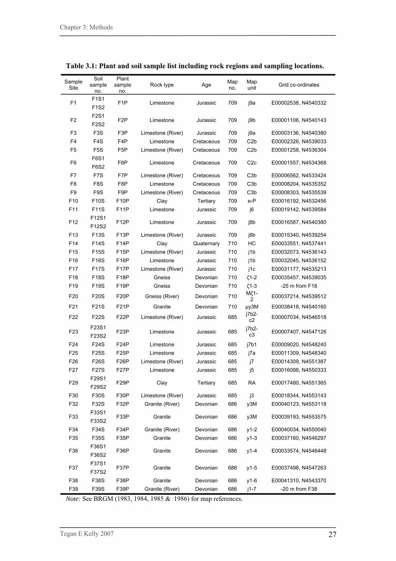
Table 3.1: Plant and soil sample list including rock regions and sampling locations.
Sample Site
Soil sample
no.
Plant sample
no. Rock type Age Map
no. Map unit Grid co-ordinates
F1S1 F1
F1S2 F1P Limestone Jurassic 709 j9a E00002538, N4540332
F2S1 F2
F2S2 F2P Limestone Jurassic 709 j9b E00001106, N4540143
F3 F3S F3P Limestone (River) Jurassic 709 j9a E00003136, N4540380 F4 F4S F4P Limestone Cretaceous 709 C2b E00002326, N4539033 F5 F5S F5P Limestone (River) Cretaceous 709 C2b E00001258, N4536304
F6S1 F6
F6S2 F6P Limestone Cretaceous 709 C2c E00001557, N4534368
F7 F7S F7P Limestone (River) Cretaceous 709 C3b E00006562, N4533424 F8 F8S F8P Limestone Cretaceous 709 C3b E00008204, N4535352 F9 F9S F9P Limestone (River) Cretaceous 709 C3b E00008303, N4535539 F10 F10S F10P Clay Tertiary 709 e-P E00016192, N4532456 F11 F11S F11P Limestone Jurassic 709 j6 E00019142, N4539584
F12S1 F12
F12S2 F12P Limestone Jurassic 709 j8b E00016587, N4540380
F13 F13S F13P Limestone (River) Jurassic 709 j8b E00015340, N4539254 F14 F14S F14P Clay Quaternary 710 HC E00033551, N4537441 F15 F15S F15P Limestone (River) Jurassic 710 j1b E00032073, N4536143 F16 F16S F16P Limestone Jurassic 710 j1b E00032045, N4536152 F17 F17S F17P Limestone (River) Jurassic 710 j1c E00031177, N4535213 F18 F18S F18P Gneiss Devonian 710 ζ1-2 E00035457, N4539035 F19 F19S F19P Gneiss Devonian 710 ζ1-3 -25 m from F18
F20 F20S F20P Gneiss (River) Devonian 710 Mζ1-2 E00037214, N4539512
F21 F21S F21P Granite Devonian 710 μy3M E00038418, N4540160
F22 F22S F22P Limestone (River) Jurassic 685 j7b2-c2 E00007034, N4546518
F23S1 F23
F23S2 F23P Limestone Jurassic 685 j7b2-
c3 E00007407, N4547126
F24 F24S F24P Limestone Jurassic 685 j7b1 E00009020, N4548240 F25 F25S F25P Limestone Jurassic 685 j7a E00011309, N4548340 F26 F26S F26P Limestone (River) Jurassic 685 j7 E00014309, N4551387 F27 F27S F27P Limestone Jurassic 685 j5 E00016098, N4550333
F29S1 F29
F29S2 F29P Clay Tertiary 685 RA E00017480, N4551365
F30 F30S F30P Limestone (River) Jurassic 685 j3 E00018344, N4553143 F32 F32S F32P Granite (River) Devonian 686 y3M E00040123, N4553118
F33S1 F33
F33S2 F33P Granite Devonian 686 y3M E00039193, N4553575
F34 F34S F34P Granite (River) Devonian 686 y1-2 E00040034, N4550040 F35 F35S F35P Granite Devonian 686 y1-3 E00037160, N4546297
F36S1 F36
F36S2 F36P Granite Devonian 686 y1-4 E00033574, N4546448
F37S1 F37
F37S2 F37P Granite Devonian 686 y1-5 E00037498, N4547263
F38 F38S F38P Granite Devonian 686 y1-6 E00041310, N4543370 F39 F39S F39P Granite (River) Devonian 686 j1-7 -20 m from F38
Note: See BRGM (1983, 1984, 1985 & 1986) for map references.
Chapter 3: Methods
Tegan E Kelly 2007
28
3.1.2. Animal sample collection
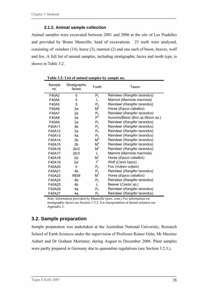
Animal samples were excavated between 2001 and 2006 at the site of Les Pradelles
and provided by Bruno Maureille, head of excavations. 23 teeth were analysed,
consisting of: reindeer (14), horse (3), marmot (2) and one each of bison, beaver, wolf
and fox. A full list of animal samples, including stratigraphic facies and tooth type, is
shown in Table 3.2.
Table 3.2: List of animal samples by sample no.
Sample no.
Stratigraphic facies Tooth Taxon
F40A2 5 P2 Reindeer (Rangifer tarandus) F40A4 5 I1 Marmot (Marmota marmota) F40A5 5 P2 Reindeer (Rangifer tarandus) F40A6 2a M2 Horse (Equus caballus) F40A7 2a P2 Reindeer (Rangifer tarandus) F40A8 2a P3 Aurochs/Bison (Bos sp./Bison sp.) F40A9 2a P2 Reindeer (Rangifer tarandus)
F40A11 4b P2 Reindeer (Rangifer tarandus) F40A12 2a P3 Reindeer (Rangifer tarandus) F40A13 4a P2 Reindeer (Rangifer tarandus) F40A14 2b M3 Reindeer (Rangifer tarandus) F40A15 2b M3 Reindeer (Rangifer tarandus) F40A16 2b/3 M3 Reindeer (Rangifer tarandus) F40A17 2b/3 I1 Marmot (Marmota marmota) F40A18 2a' M1 Horse (Equus caballus) F40A19 2a' I2 Wolf (Canis lupus) F40A20 5 P2 Fox (Vulpes vulpes) F40A21 4b P2 Reindeer (Rangifer tarandus) F40A23 REM M1 Horse (Equus caballus) F40A24 4b P2 Reindeer (Rangifer tarandus) F40A25 4b I1 Beaver (Castor sp.) F40A26 4a P2 Reindeer (Rangifer tarandus) F40A27 4a P2 Reindeer (Rangifer tarandus)
Note. Information provided by Maureille (pers. com.) For information on stratigraphic facies see Section 1.3.2. For interpretation of dental notation see Appendix 2.
3.2. Sample preparation Sample preparation was undertaken at the Australian National University, Research
School of Earth Sciences under the supervision of Professor Rainer Grün, Mr Maxime
Aubert and Dr Graham Mortimer, during August to December 2006. Plant samples
were partly prepared in Germany due to quarantine regulations (see Section 3.2.3.).

Chapter 3: Methods
Tegan E Kelly 2007
29
3.2.1. Cleaning Laboratory containers (new and used) were chemically cleaned before use. Savillex
PFA Teflon vials and caps were detergent and acid cleaned in a four step procedure.
They were immersed sequentially in 5% Decon, 10% HNO3, 10% HCl and Milli-Q
purified water (MQ-H2O) in a large glass beaker, at each step heated on a hotplate to
boiling point for 3 hours, then allowed to cool and to soak overnight. Between steps,
the vials and caps were individually rinsed in MQ- H2O. Finally, to remove any
residue, a small amount (~1 ml) of 2% HCl + 0.05% HF was added to each vial,
which was then capped and placed on a hot plate heated to approximately 60°C and
refluxed for two days. The vials and caps were finally rinsed in MQ-H2O and stored
in clean plastic bags, ready for use. Polypropylene pipet tips, tubes, vials and their
associated lids were cleaned by soaking in 10% HNO3 for three days, rinsed with MQ-
H2O then soaked in MQ-H2O for three days and rinsed once more. After drying in a
laminar-flow fume cupboard overnight, they were stored in clean plastic containers,
ready for use.
3.2.2. Soil sample preparation Soil samples were sieved to <2 mm and 1 g of the sieved portion collected in a 4 ml
vial. A small pipet was used to add 2.5 ml of 1M ammonium nitrate (NH4NO3) to
each. Ammonium ions displace loosely bound cations from the surface of the soil
particles, bringing them into solution (Prohaska et al. 2005). In order to allow this to
happen effectively, the vials containing the soil/NH4NO3 mixture were mounted in a
Retsch shaking machine and shaken continuously for 24 hours (Fig 3.1).
Figure 3.1: Retsch shaking machine. Each wooden sample holder holds 16 sample tubes.

Chapter 3: Methods
Tegan E Kelly 2007
30
Sample vials were then placed into a Clements GS150 centrifuge at 3,000 rpm for 5 to
10 minutes, to separate the solution from the sediment. 1-1.5 ml of solution was
extracted from each sample with a pipet, and placed into a clean teflon vial. These
were evaporated overnight on a 60°C hotplate in an extraction cupboard.
Subsequently, 15 drops of distilled concentrated nitric acid (65% HNO3) was added to
each vial to break down residual organic matter. These were capped and dissolved on
the hotplate for 1 hour, then evaporated for 3 hours with the cap removed. The
resultant residue was redissolved into 2 ml of 2M HNO3.
These samples were each divided into two sub-samples. 0.1 ml from each sample was
transferred with a pipet to a 10 ml vial containing 9.9 ml of 2% HNO3, ready for total
Sr concentration measurement via solution ICP-MS (see Section 3.3.2.). The
remaining sub-sample was used in ion exchange chromatography (see Section 3.2.5.)
in preparation for Sr isotope measurement with mass spectrometry (see Section
3.3.3.).
3.2.3. Plant sample preparation The initial stages of plant sample preparation were undertaken at the Universität zu
Köln (Cologne) in Germany, under the supervision of Dr. Manfred Thönnessen.
Samples were digested in 5 ml conc. nitric in a microwave digestion unit at 200°C and
a pressure of 7 MPa. This destroyed any organic material, satisfying Australian
quarantine standards. The samples were then diluted to 50 ml with double distilled
water before being mailed to ANU in 50 ml plastic vials.
A sub-sample was then removed and further diluted to 2% conc. nitric. 2 ml of each
sample was transferred by pipet to a 10 ml plastic vial and diluted with 8 ml MQ-H2O,
ready for total Sr measurement via solution-ICP-MS (see Section 3.3.2.). A further
sub-sample was removed for use in ion exchange chromatography (see Section 3.2.5)
before Sr isotope measurement with mass spectrometry (see Section 3.3.3.).
Some plant samples contained as little as 31 ppb strontium (see Section 4.1.) and as
only 1-2 ml of sample can be loaded into an ion exchange column (see Section 3.2.5.),
all plant samples first had a portion equivalent to 400 ng of Sr (1.36 ml to 12.74 ml,
see Section 4.1.) pipetted into Teflon beakers and evaporated on a 60°C hotplate

Chapter 3: Methods
Tegan E Kelly 2007
31
overnight. The residue was then dissolved in 1 ml of 2M HNO3, ready for use in ion
exchange chromatography (see Section 3.2.5.).
3.2.4. Animal sample preparation Animal teeth were sliced radially with a hand-held diamond saw to produce a
continuous slither of tooth enamel. Each sample was photographed before and after
removal, to record exactly where on the tooth the sample came from. They were then
flattened with wet P800 ‘wet’n’dry’ sandpaper before being mounted in a ‘blu-tack’
sample holder, in preparation for Sr isotope measurement via laser ablation ICP-MS
(LA-ICP-MS) (see Section 3.3.3.2.).
3.2.5. Ion exchange chromatography Before Sr isotope measurement, Sr has to be separated from matrix elements in the
sample. It is especially important to remove 87Rb, as it interferes with the 87Sr signal
in the ICP-MS. This was accomplished by ion exchange chromatography, using a Sr
specific resin. Three main steps are involved in this process: first sample solutions
containing dissolved ions are loaded into the resin. They are then rinsed with acid
washes to preferentially retain Sr in the resin while other elements, including Rb are
eluted and discarded. With further acid addition, a ‘breakthrough’ point is reached and
Sr is also eluted and able to be isolated in a sample beaker below the column (Fig.
3.2.).
Figure 3.2: Ion exchange chromatography columns during the eluting phase. The top of each column can hold 1 ml of solution, which slowly filters through the resin.

Chapter 3: Methods
Tegan E Kelly 2007
32
The standard Sr separation procedure used at RSES was applied to the prepared soil
and plant samples. Eighteen columns were prepared, containing an Eichrom Sr spec.
0.25 ml resin bed. These were re-cleaned and re-used up to six times. 10-18 samples
were eluted per day, over a period of six days. The separation procedure involved five
main parts, each incorporating a number of steps (Table 3.3.).
Table 3.3: Ion exchange chromatography procedure for strontium separation Acid added to column Volume No. repeats
0.02M HNO3 1 ml 3 8M HCl 1 ml 2 1. Cleaning resin
0.02M HNO3 1 ml 5 2. Conditioning column 2M HNO3 0.25 ml 3
3. Loading sample Various volumes depending on concentration (see Section 4.1, Tables 4.2 & 4.3) added in 0.2 ml aliquots*
2M HNO3 1 ml 1 4. Rinsing sample 2M HNO3 0.5 ml 3 5. Collecting sample 0.02M HNO3 1 ml 5
* Note: The amount of sample loaded varied per sample due to varying concentrations of strontium. A target of 400 ng strontium per end sample was chosen, in order to ensure a strong and relatively consistent Sr ion beam on the ICP-MS. Lists of ml per 400 ng for samples are provided in Tables 4.1. & 4.2. These volumes were used to determine how much soil sample to load into the columns, and how much plant sample to evaporate and redissolve in 1 ml HNO3 before loading into the columns (see Section 3.2.3.).
After each column procedure, one drop of phosphoric acid (H3PO4) was added to each
sample beaker and the samples evaporated overnight on a 60°C hotplate. Phosphoric
acid did not evaporate, keeping the residue moist. Each sample was redissolved in 2
ml of 2% conc. nitric and transferred to clean 4 ml autosampler vials, for
measurement via solution ICP-MS (see Section 3.3.3.).
3.3. Sample analysis
3.3.1 What is ICP-MS? Inductively Coupled Plasma – Mass Spectrometry (ICP-MS) arose from atomic
emission spectrometry (Jarvis et al. 1992), and pioneering work on the technique was
conducted in the early 1980s (e.g. Date & Gray 1981). Argon based ICP-MS runs at
7000 k, providing a very efficient and spectrally clean ion source (Eggins pers. com.).
Mass spectrometry is the measurement of elemental abundances through separating
atoms according to mass. “Inductively coupled plasma” refers to the emission source
for the mass spectrometers. Nebulised sample solution (in solution ICP-MS) or
vaporised sample particles (in laser ablation ICP-MS) are swept into a plasma (a
Chapter 3: Methods
Tegan E Kelly 2007
33
luminous volume of partially ionised gas) by a carrier gas (usually argon) and passed
through a sample cone orifice to accelerate into an expansion chamber. A skimmer
cone extracts ions from the chamber, which are focussed and shaped through the mass
spectrometer with ion lenses.
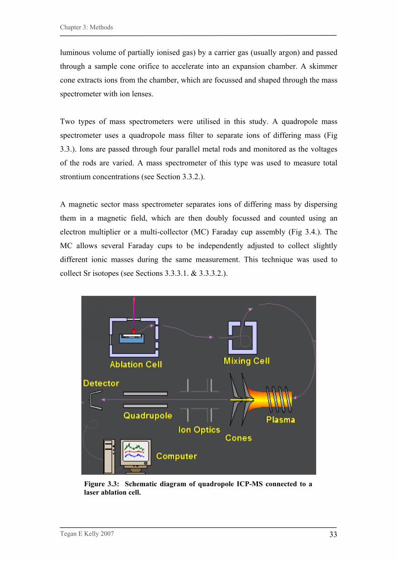
Two types of mass spectrometers were utilised in this study. A quadropole mass
spectrometer uses a quadropole mass filter to separate ions of differing mass (Fig
3.3.). Ions are passed through four parallel metal rods and monitored as the voltages
of the rods are varied. A mass spectrometer of this type was used to measure total
strontium concentrations (see Section 3.3.2.).
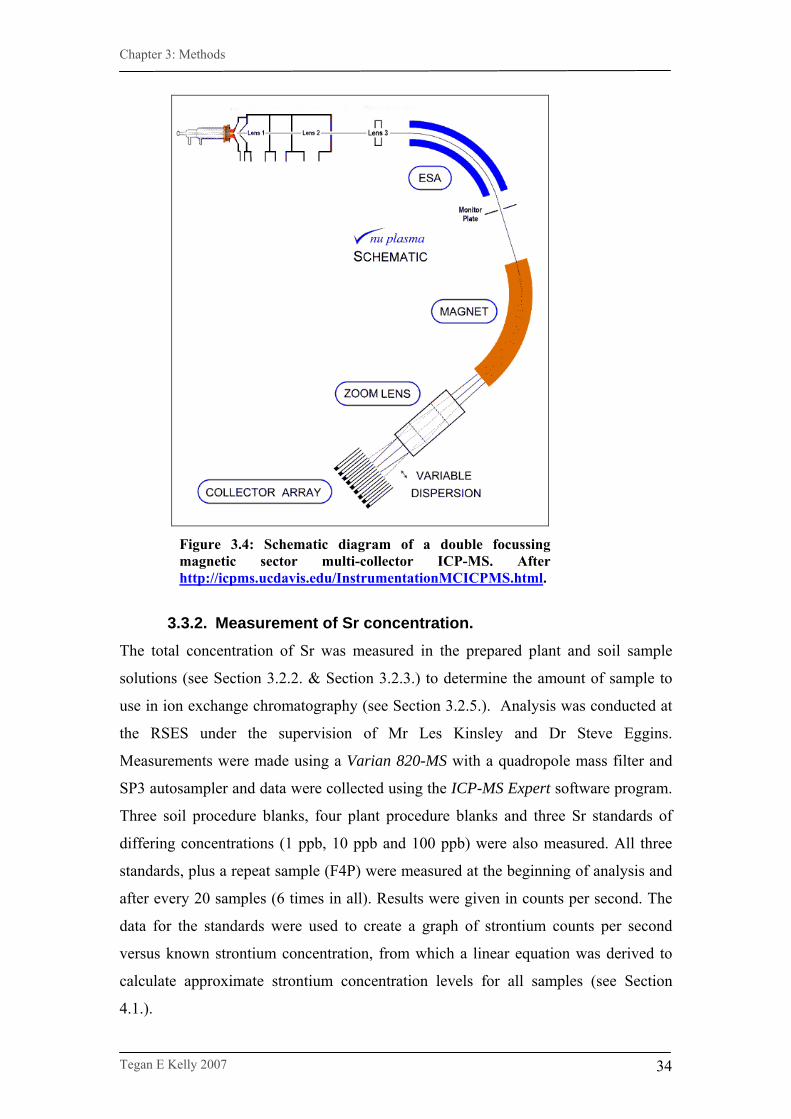
A magnetic sector mass spectrometer separates ions of differing mass by dispersing
them in a magnetic field, which are then doubly focussed and counted using an
electron multiplier or a multi-collector (MC) Faraday cup assembly (Fig 3.4.). The
MC allows several Faraday cups to be independently adjusted to collect slightly
different ionic masses during the same measurement. This technique was used to
collect Sr isotopes (see Sections 3.3.3.1. & 3.3.3.2.).
Figure 3.3: Schematic diagram of quadropole ICP-MS connected to a laser ablation cell.
Chapter 3: Methods
Tegan E Kelly 2007
34
Figure 3.4: Schematic diagram of a double focussing magnetic sector multi-collector ICP-MS. After http://icpms.ucdavis.edu/InstrumentationMCICPMS.html.
3.3.2. Measurement of Sr concentration.
The total concentration of Sr was measured in the prepared plant and soil sample
solutions (see Section 3.2.2. & Section 3.2.3.) to determine the amount of sample to
use in ion exchange chromatography (see Section 3.2.5.). Analysis was conducted at
the RSES under the supervision of Mr Les Kinsley and Dr Steve Eggins.
Measurements were made using a Varian 820-MS with a quadropole mass filter and
SP3 autosampler and data were collected using the ICP-MS Expert software program.
Three soil procedure blanks, four plant procedure blanks and three Sr standards of
differing concentrations (1 ppb, 10 ppb and 100 ppb) were also measured. All three
standards, plus a repeat sample (F4P) were measured at the beginning of analysis and
after every 20 samples (6 times in all). Results were given in counts per second. The
data for the standards were used to create a graph of strontium counts per second
versus known strontium concentration, from which a linear equation was derived to
calculate approximate strontium concentration levels for all samples (see Section
4.1.).

Chapter 3: Methods
Tegan E Kelly 2007
35
3.3.3. Measurement of Sr isotopes
3.3.3.1. Plant and soil Sr isotope measurement Strontium isotopes were measured at the RSES under the supervision of Dr Graham
Mortimer and Mr Les Kinsley. Measurements were conducted using a multi-collector
Finnigan MAT Neptune ICP-MS. This is a double focusing, magnetic sector mass
spectrometer, equipped with nine Faraday cups, eight of which are adjustable. The
sample solutions were introduced in 2% HNO3 and aspirated through an Apex
desolvator prior to introduction into the plasma.
All of the available cups were employed to collect ion currents at nominal masses
82.5, 83(Kr), 83.5, 84(Sr+Kr), 85(Rb), 86(Sr+Kr), 86.5, 87(Sr+Rb) and 88(Sr).
Krypton has the potential to be introduced with the carrier gas and interfere with the 84Sr and 86Sr signals, and rubidium was measured to apply corrections to 87Sr for 87Rb
interference, although Rb was in most cases effectively removed during ion exchange
chromatography (see Section 3.2.5.). The half-mass positions monitor the potential
contribution of doubly charged REE ions. A strontium isotope standard (SRM987,
U.S. National Institute of Standards and Technology standard reference material) was
measured one to two times each day to monitor the precision of measurements. A
reagent blank (consisting of 2% HNO3) was measured before each sample
measurement and subtracted from the immediately following sample, to remove
instrument memory of Rb and Sr and the minor constant Kr in the carrier gas. Each
result was also corrected for 87Rb and mass bias. A sequence of acid and detergent
washes was employed between each measurement to remove all but a trace of
previous sample solutions. Six procedural blanks were also measured, two each from
soil sample preparation, plant sample preparation and ion exchange chromatography.
3.3.3.2. Animal Sr isotope measurement Laser ablation ICP-MS measurements were carried out at the University of
Melbourne, School of Earth Sciences under the supervision of Dr Jon Woodhead. The
measurements were done with a HelEx 193 nm, Excimer laser ablation system
coupled to a Nu Plasma multi-collector ICP-MS.
Chapter 3: Methods
Tegan E Kelly 2007
36
The HelEx system involves an objective lens, which projects and demagnifies a laser-
illuminated aperture onto the sample. The use of helium as a carrier gas during
ablation maximises sample transmission to the ICP (Eggins et al. 1998). The Nu-
Plasma MC-ICP-MS is a double focussing, magnetic sector, mass spectrometer
equipped with 12 Faraday cups.
Eight of the 12 available Faraday cups were employed to collect currents at nominal
masses 81, 82, 83, 84, 85, 86, 87 and 88. A Tridacna shell was used as a strontium
standard. Doubly charged rare earth elements (REE) have the potential to interfere in
the region of Sr masses (Woodhead et al. 2005.) As such REE levels were first
measured in 2 samples (A2 and A24). The levels were very low, so it was assumed
that all samples would be the same in this regard, considering their similar material,
origin and source.
Background levels were measured for 90 seconds before each sample. Samples were
measured continuously along the length of the tooth enamel, with the laser run at 5 Hz
with an 85 μm spot size. Each result was corrected for background, 87Rb and mass
bias.
3.4. Statistical analyses All statistical tests were conducted using PAST versions 1.53 & 1.68, a
Palaeontological Statistics software package for education and data analysis (Hammer
et al. 2001). Variations in isotope ratios were compared within and between two
groups using F-tests, Student’s T tests and Welch tests for parametric comparisons,
and Mann-Whitney U tests and Kolmogorov-Smirnov tests for non-parametric
comparisons. For comparisons of three or more groups, Analysis of Variance
(ANOVA) analyses were conducted on parametric data and Kruskal-Wallis tests
undertaken on non-parametric data. The Shapiro-Wilk statistic was used to determine
whether data were parametric, as well as Normal QQ probability plots and
histograms. For correlation testing, Pearson’s Correlation Coefficent was used to
analyse parametric data and Spearmann’s Rank and Kendall’s Tau correlation
coefficients for non-parametric data.
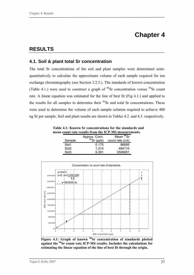
Chapter 4: Results
Tegan E Kelly 2007
37
Chapter 4
RESULTS
4.1. Soil & plant total Sr concentration The total Sr concentrations of the soil and plant samples were determined semi-
quantitatively to calculate the approximate volume of each sample required for ion
exchange chromatography (see Section 3.2.5.). The standards of known concentration
(Table 4.1.) were used to construct a graph of 86Sr concentration versus 86Sr count
rate. A linear equation was estimated for the line of best fit (Fig 4.1.) and applied to
the results for all samples to determine their 86Sr and total Sr concentrations. These
were used to determine the volume of each sample solution required to achieve 400
ng Sr per sample. Soil and plant results are shown in Tables 4.2. and 4.3. respectively.
Table 4.1: Known Sr concentrations for the standards and mean count rate results from the ICP-MS measurements.
Sample Approx. Conc.
86Sr (ppb)Mean 86Sr
count rate (c/s)Std1 0.175 86685Std2 1.214 484110Std3 9.281 3506651
0 1 2 3 4 5 6 7 8 9
86Sr concentration (ppb)
0
400,000
800,000
1,200,000
1,600,000
2,000,000
2,400,000
2,800,000
3,200,000
3,600,000
86Sr
cou
ntra
te(c
/s)
y=mx+cc=0, m=2,000,000
5.5 y=363636.3x
Concentration vs count rate of standards
Figure 4.1: Graph of known 86Sr concentration of standards plotted against the 86Sr count rate ICP-MS results. Includes the calculations for estimating the linear equation of the line of best fit through the origin.
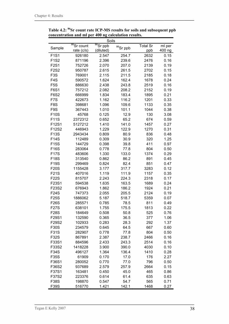
Chapter 4: Results
Tegan E Kelly 2007
38
Table 4.2: 86Sr count rate ICP-MS results for soils and subsequent ppb concentration and ml per 400 ng calculation results.
Soils
Sample 86Sr count rate (c/s)
86Sr ppb (diluted)
86Sr ppb Total Sr ppb
ml per 400 ng
F1S1 926180 2.547 254.7 2632 0.15 F1S2 871196 2.396 239.6 2476 0.16 F2S1 752726 2.070 207.0 2139 0.19 F2S2 950787 2.615 261.5 2702 0.15 F3S 769001 2.115 211.5 2185 0.18 F4S 590572 1.624 162.4 1678 0.24 F5S 886630 2.438 243.8 2519 0.16 F6S1 757212 2.082 208.2 2152 0.19 F6S2 666999 1.834 183.4 1895 0.21 F7S 422673 1.162 116.2 1201 0.33 F8S 398681 1.096 109.6 1133 0.35 F9S 367443 1.010 101.1 1044 0.38 F10S 45768 0.125 12.9 130 3.08 F11S 2372312 0.652 65.2 674 0.59 F12S1 5127212 1.410 141.0 1457 0.27 F12S2 446943 1.229 122.9 1270 0.31 F13S 2943434 0.809 80.9 836 0.48 F14S 112489 0.309 30.9 320 1.25 F15S 144729 0.398 39.8 411 0.97 F16S 283064 0.778 77.8 804 0.50 F17S 483606 1.330 133.0 1374 0.29 F18S 313540 0.862 86.2 891 0.45 F19S 299469 0.824 82.4 851 0.47 F20S 1155428 3.177 317.7 3283 0.12 F21S 407016 1.119 111.9 1157 0.35 F22S 815707 2.243 224.3 2318 0.17 F23S1 594538 1.635 163.5 1689 0.24 F23S2 676943 1.862 186.2 1924 0.21 F24S 747373 2.055 205.5 2124 0.19 F25S 1886062 5.187 518.7 5359 0.07 F26S 285571 0.785 78.5 811 0.49 F27S 638101 1.755 175.5 1813 0.22 F28S 184649 0.508 50.8 525 0.76 F29S1 132590 0.365 36.5 377 1.06 F29S2 102933 0.283 28.3 292 1.37 F30S 234579 0.645 64.5 667 0.60 F31S 282907 0.778 77.8 804 0.50 F32S 867891 2.387 238.7 2466 0.16 F33S1 884596 2.433 243.3 2514 0.16 F33S2 1418228 3.900 390.0 4030 0.10 F34S 496127 1.364 136.4 1410 0.28 F35S 61909 0.170 17.0 176 2.27 F36S1 280052 0.770 77.0 796 0.50 F36S2 937689 2.579 257.9 2664 0.15 F37S1 163481 0.450 45.0 465 0.86 F37S2 223376 0.614 61.4 635 0.63 F38S 198870 0.547 54.7 565 0.71 F39S 516770 1.421 142.1 1468 0.27

Chapter 4: Results
Tegan E Kelly 2007
39
Table 4.3: 86Sr count rate ICP-MS results for plants and subsequent ppb concentration and ml per 400 ng calculation results.
Plants
Sample 86Sr count rate (c/s)
86Sr ppb (diluted)
86Sr ppb Total Sr ppb
ml per 400 ng
F1P 357533 0.983 4.9 51 7.87 F2P 736889 2.026 10.1 105 3.82 F3P 1005818 2.766 13.8 143 2.80 F4P 512289 1.409 7.0 73 5.50 F5P 727503 2.001 10.0 103 3.87 F6P 898809 2.472 12.4 128 3.13 F7P 793805 2.183 10.9 113 3.55 F8P 465426 1.280 6.4 66 6.05 F9P 411724 1.132 5.7 58 6.84 F10P 402230 1.106 5.5 57 7.00 F11P 271636 0.747 3.7 39 10.36 F12P 662333 1.821 9.1 94 4.25 F13P 580779 1.597 8.0 83 4.85 F14P 220957 0.608 3.0 31 12.74 F15P 335803 0.923 4.6 48 8.38 F16P 342785 0.943 4.7 49 8.21 F17P 429371 1.181 5.9 61 6.56 F18P 433890 1.193 6.0 62 6.49 F19P 1270989 3.495 17.5 181 2.22 F20P 1630760 4.485 22.4 232 1.73 F21P 910188 2.503 12.5 129 3.09 F22P 355138 0.977 4.9 50 7.93 F23P 693673 1.908 9.5 99 4.06 F24P 1313943 3.613 18.1 187 2.14 F25P 1038613 2.856 14.3 148 2.71 F26P 272549 0.750 3.8 39 10.33 F27P 303500 0.835 4.2 43 9.28 F28P 471790.4 1.297 6.5 67 5.97 F29P 279356 0.768 3.8 40 10.08 F30P 577153 1.587 7.9 82 4.88 F32P 1515196 4.167 20.8 215 1.86 F33P 2076508 5.710 28.6 295 1.36 F34P 1176718 3.236 16.2 167 2.39 F35P 1224085 3.366 16.8 174 2.30 F36P 1762455 4.847 24.2 250 1.60 F37P 1073187 2.951 14.8 152 2.62 F38P 441505 1.214 6.1 63 6.38 F39P 716288 1.970 9.9 102 3.93 F40P 287034 0.789 4.0 41 9.81
Soil sample concentrations vary from 130 ppb (F10S) to 5,360 ppb (F25S) with a
mean of 1,520 ppb. Plant sample concentrations are generally lower, varying from 31
ppb (F14P) to 295 ppb (F33P) with a mean of 106 ppb. These results are not directly
indicative of the original Sr concentrations of the source material: although exactly
one gram of each soil sample was leached, differing volumes (1–2 ml) of the leachate
Chapter 4: Results
Tegan E Kelly 2007
40
of each was recovered for further processing, also differing volumes of material
(0.2213 – 0.2564 g) were ashed for each plant sample. Additionally, soil and plant
samples had different processing and dilution histories, so their respective
concentration results are not comparable to one another. The concentrations are,
however, sufficient for the purpose of calculating the ml of prepared solution required
to contain roughly 400 ng Sr in each end sample.
4.2. Soil and plant Sr isotope ratios
4.2.1. Measurement results Soil and plant Sr isotope ratios were measured on the Neptune mass spectrometer,
with 60 measurements of four second duration for each sample (see Section 3.3.3.1.).
The mean 87Sr/86Sr and standard error for each sample, along with the average 87Sr/86Sr for each site, are presented in Table 4.4. The error for each result is small and
some variability in 87Sr/86Sr occurs between samples. The same data are presented
graphically in Figure 4.2. and the range for Jurassic-Cretaceous (J/K) seawater 87Sr/86Sr for the time period of limestone formation (Jones et al. 1994) is represented
by the solid blue line. The variability within and between regions begins to become
apparent with this graph. Limestone sample results all sit at or above the J/K seawater
Sr ratio; though most also fall below 0.7100 whereas granitoid samples mostly fall
above. Clay samples appear to give similar results to the granitoids. The granitoid
results are more variable than the limestone results, with greater variability between
sites within the region and also larger differences between soil and plant results within
sites, notably at sites F19, F35 and F38, which have top soil values far exceeding any
other measurements on the graph. Two granitoid samples also show a difference
between top soil and bottom soil values (F36 & F37). The following section (4.2.2.)
provides a more detailed, statistical investigation of these results.

Chapter 4: Results
Tegan E Kelly 2007
41
Table 4.4: Sr isotope ratio results for soils and plants, including standard error for each sample and average for each site.
87Sr/86Sr
Region Site Top soil error Bottom
soil error Plant error Site
average
F10 0.711707 0.000018 0.711663 0.000012 0.7117F14 0.717422 0.000017 0.712530 0.000019 0.7150Clay F29 0.711377 0.000027 0.710539 0.000028 0.714409 0.000031 0.7121
F3 0.710860 0.000017 0.707769 0.000016 0.7093F5 0.708390 0.000016 0.708839 0.000015 0.7086F7 0.708339 0.000022 0.708293 0.000015 0.7083F9 0.708527 0.000024 0.708551 0.000013 0.7085F13 0.708839 0.000017 0.708747 0.000016 0.7088F15 0.708586 0.000019 0.709191 0.000031 0.7089F17 0.712148 0.000029 0.715163 0.000020 0.7137F22 0.708249 0.000021 0.708348 0.000016 0.7083F26 0.710565 0.000017 0.709275 0.000019 0.7099
River on limestone
F30 0.709464 0.000030 0.710970 0.000017 0.7102
F1 0.707890 0.000021 0.707505 0.000025 0.708277 0.000017 0.7079F2 0.707860 0.000024 0.707981 0.000034 0.712336 0.000012 0.7094F4 0.708020 0.000015 0.708270 0.000014 0.7081F6 0.707747 0.000025 0.707654 0.000021 0.707998 0.000027 0.7078F8 0.708463 0.000020 0.708362 0.000027 0.7084F11 0.708989 0.000013 0.708365 0.000014 0.7087F12 0.709577 0.000024 0.709331 0.000021 0.708292 0.000028 0.7091F16 0.708315 0.000024 0.708916 0.000028 0.7086F23 0.707562 0.000023 0.707762 0.000026 0.708401 0.000022 0.7079F24 0.707946 0.000021 0.707842 0.000020 0.7079F25 0.708311 0.000029 0.708841 0.000022 0.7086
Limestone
F27 0.708073 0.000024 0.708689 0.000023 0.7084
F20 0.718601 0.000019 0.716880 0.000025 0.7177F32 0.712955 0.000031 0.713128 0.000013 0.7130F34 0.707837 0.000015 0.710809 0.000020 0.7093
River on Granitoid
F39 0.719231 0.000019 0.718417 0.000021 0.7188
F19 0.735799 0.000026 0.718640 0.000029 0.7272F21 0.718825 0.000028 0.714003 0.000022 0.7164F33 0.710381 0.000025 0.709598 0.000025 0.709476 0.000022 0.7098F35 0.733289 0.000024 0.712701 0.000019 0.7230F36 0.715354 0.000022 0.711970 0.000028 0.712716 0.000018 0.7133F37 0.716564 0.000018 0.712040 0.000026 0.710744 0.000018 0.7131
Granitoid
F38 0.728507 0.000036 0.717070 0.000019 0.7228
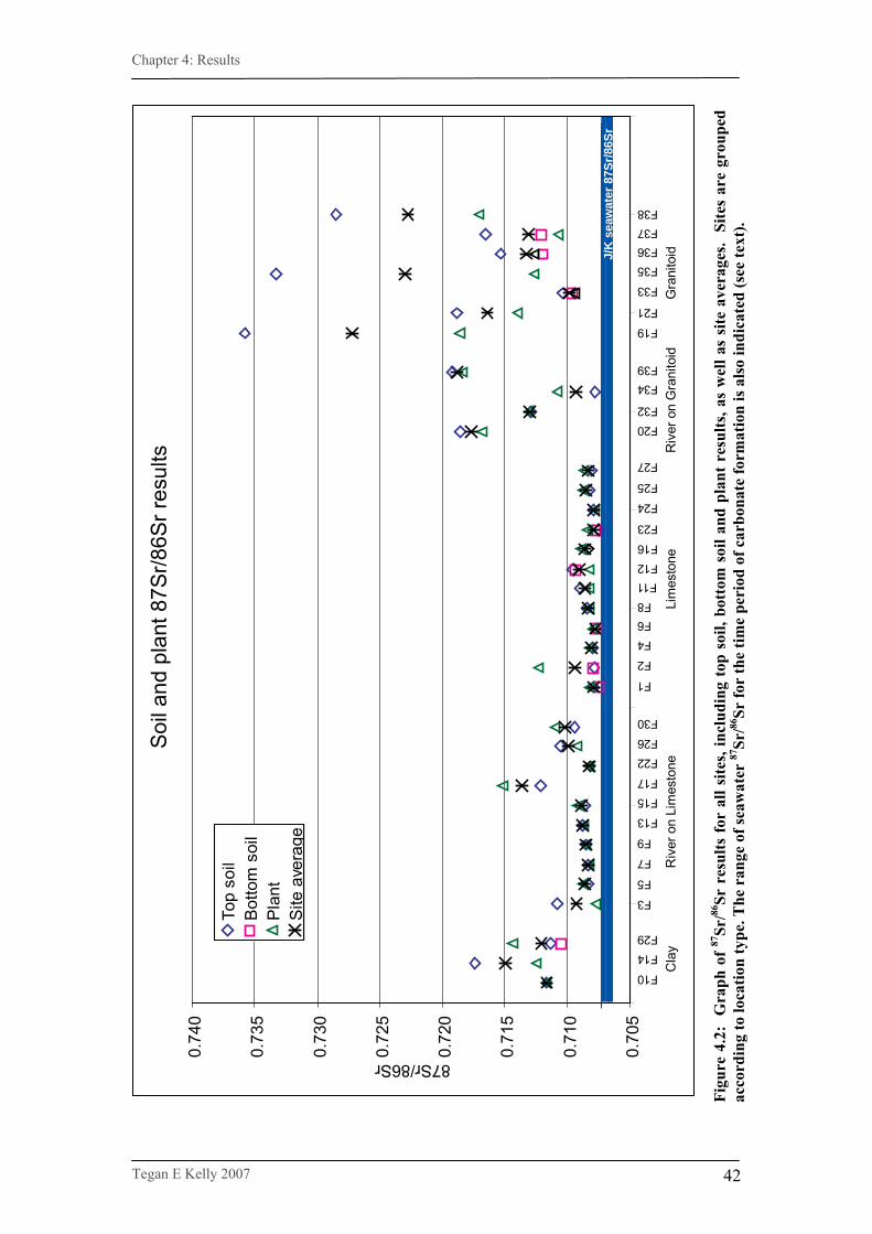
Chapter 4: Results
Tegan E Kelly 2007
42
J/K
sea
wat
er 8
7Sr/8
6Sr
0.70
5
0.71
0
0.71
5
0.72
0
0.72
5
0.73
0
0.73
5
0.74
0
Top
soil
Bot
tom
soil
Pla
ntS
iteav
erag
e
87Sr/86Sr
F10
F14F29
F3
F5
F7
F9
F13F15F17
F22F26F30
F1
F2
F4F6F8
F11F12F16F23
F24
F25
F27
F20F32
F34F39
F19
F21
F33
F35F36F37F38
Cla
yR
iver
on
Lim
esto
neLi
mes
tone
Riv
er o
n G
rani
toid
Gra
nito
id
Soi
l and
pla
nt 8
7Sr/8
6Sr r
esul
ts
Figu
re 4
.2:
Gra
ph o
f 87Sr
/86Sr
res
ults
for
all s
ites,
incl
udin
g to
p so
il, b
otto
m s
oil a
nd p
lant
res
ults
, as
wel
l as
site
ave
rage
s. S
ites
are
grou
ped
acco
rdin
g to
loca
tion
type
. The
ran
ge o
f sea
wat
er 87
Sr/86
Sr fo
r th
e tim
e pe
riod
of c
arbo
nate
form
atio
n is
als
o in
dica
ted
(see
text
).

Chapter 4: Results
Tegan E Kelly 2007
43
The results for the SRM987 standards are shown in Table 4.5. and Figure 4.3. The
bold horizontal line in Figure 4.3. shows the mean 87Sr/86Sr ratio of SRM987 as
stated in Hart et al. (2005), the bold dashed lines indicate their 2σ error. The thin
horizontal line shows the mean of the measurements in this study, and the thin dashed
lines, the error of the mean. The mean falls below that of Hart et al. 2005, but well
within their 2σ error, indicating high measurement precision.
Table 4.5: Sr isotope ICP-MS results, for the seven SRM987 standards measured over the five days of soil and plant sample measurement. Sample Date 88Sr (V) 87Sr/86Sr ± 87Sr/86Sr SRM987a 12-Feb-07 10.0 0.710193 0.000016 SRM987b 12-Feb-07 11.9 0.710194 0.000023 SRM987c 13-Feb-07 16.8 0.710199 0.000014 SRM987d 14-Feb-07 20.1 0.710187 0.000014 SRM987e 14-Feb-07 19.4 0.710174 0.000008 SRM987f 15-Feb-07 16.8 0.710198 0.000013 SRM987g 16-Feb-07 13.6 0.710168 0.000014
0.71010
0.71012
0.71014
0.71016
0.71018
0.71020
0.71022
0.71024
87Sr
/86S
r
87Sr/86Sr ICP-MS results for SRM987 Sr standard
Figure 4.3: 87Sr/86Sr ICP-MS results for the seven SRM987 standards measured over the five days of soil and plant sample measurement. The thin horizontal line shows the mean and the thin dashed lines the error of the mean. The bold horizontal line is the mean SRM987 value as stated in Hart et al. (2005), the bold dashed lines indicate their 2σ error.
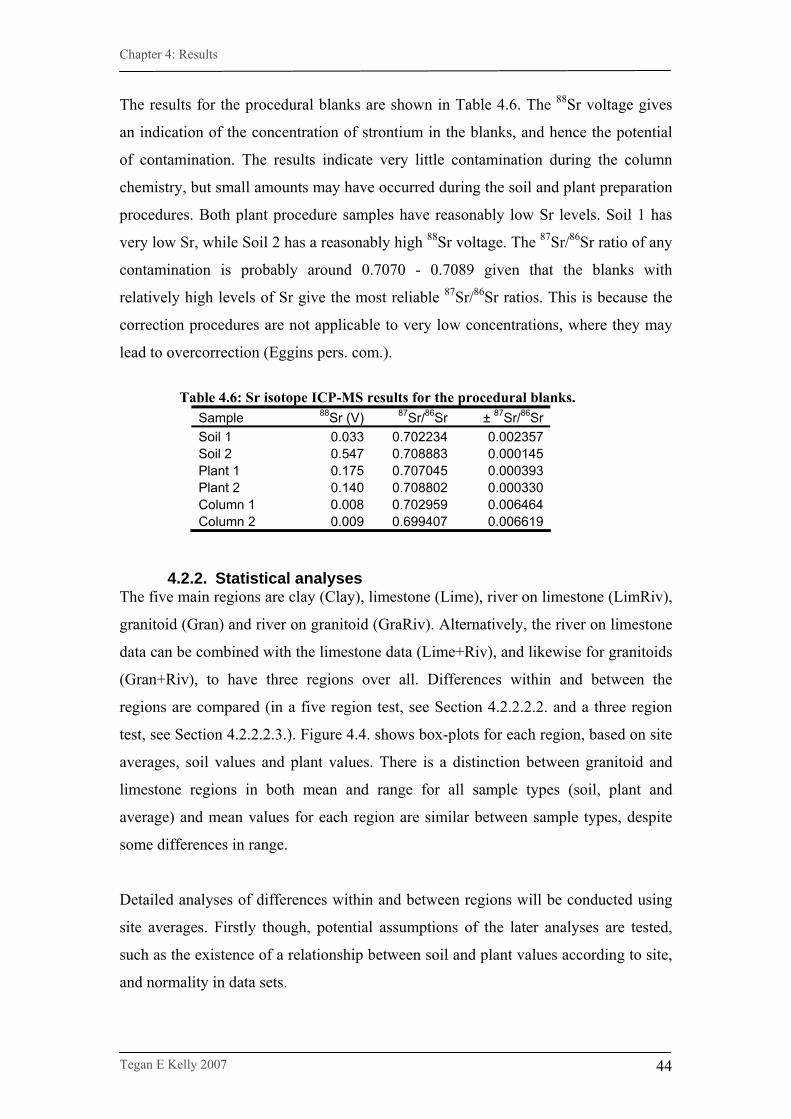
Chapter 4: Results
Tegan E Kelly 2007
44
The results for the procedural blanks are shown in Table 4.6. The 88Sr voltage gives
an indication of the concentration of strontium in the blanks, and hence the potential
of contamination. The results indicate very little contamination during the column
chemistry, but small amounts may have occurred during the soil and plant preparation
procedures. Both plant procedure samples have reasonably low Sr levels. Soil 1 has
very low Sr, while Soil 2 has a reasonably high 88Sr voltage. The 87Sr/86Sr ratio of any
contamination is probably around 0.7070 - 0.7089 given that the blanks with
relatively high levels of Sr give the most reliable 87Sr/86Sr ratios. This is because the
correction procedures are not applicable to very low concentrations, where they may
lead to overcorrection (Eggins pers. com.).
Table 4.6: Sr isotope ICP-MS results for the procedural blanks.
Sample 88Sr (V) 87Sr/86Sr ± 87Sr/86SrSoil 1 0.033 0.702234 0.002357Soil 2 0.547 0.708883 0.000145Plant 1 0.175 0.707045 0.000393Plant 2 0.140 0.708802 0.000330Column 1 0.008 0.702959 0.006464Column 2 0.009 0.699407 0.006619
4.2.2. Statistical analyses The five main regions are clay (Clay), limestone (Lime), river on limestone (LimRiv),
granitoid (Gran) and river on granitoid (GraRiv). Alternatively, the river on limestone
data can be combined with the limestone data (Lime+Riv), and likewise for granitoids
(Gran+Riv), to have three regions over all. Differences within and between the
regions are compared (in a five region test, see Section 4.2.2.2.2. and a three region
test, see Section 4.2.2.2.3.). Figure 4.4. shows box-plots for each region, based on site
averages, soil values and plant values. There is a distinction between granitoid and
limestone regions in both mean and range for all sample types (soil, plant and
average) and mean values for each region are similar between sample types, despite
some differences in range.
Detailed analyses of differences within and between regions will be conducted using
site averages. Firstly though, potential assumptions of the later analyses are tested,
such as the existence of a relationship between soil and plant values according to site,
and normality in data sets.

Chapter 4: Results
Tegan E Kelly 2007
45
Cla
y
Lim
Riv
Lim
e
Lim
e+R
iv
Gra
nRiv
Gra
n
Gra
n+R
iv
0.705
0.71
0.715
0.72
0.725
0.73
0.735
Region box-plots fordifferent sample types
0.705
0.71
0.715
0.72
0.725
0.73
0.735
0.705
0.71
0.715
0.72
0.725
0.73
0.735
Aver
age
Pla
ntS
oil
4.2.2.1. Soil and plant analyses
In order for analyses within and between regions to have any value, it first must be
shown that results within each site (i.e. the soil and plant values for each site) are
more coherent than between sites. This assumption can be tested by checking for a
correlation between soil and plant values according to site and also by comparing all
soil results with plant results to ensure there is no significant difference.
Figure 4.4. Comparative box plots of 87Sr/86Sr results from each region using site averages, soil values and plant values.
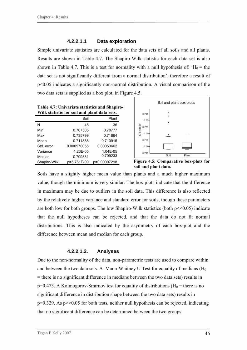
Chapter 4: Results
Tegan E Kelly 2007
46
4.2.2.1.1 Data exploration
Simple univariate statistics are calculated for the data sets of all soils and all plants.
Results are shown in Table 4.7. The Shapiro-Wilk statistic for each data set is also
shown in Table 4.7. This is a test for normality with a null hypothesis of: ‘H0 = the
data set is not significantly different from a normal distribution’, therefore a result of
p<0.05 indicates a significantly non-normal distribution. A visual comparison of the
two data sets is supplied as a box plot, in Figure 4.5.
Table 4.7: Univariate statistics and Shapiro-Wilk statistic for soil and plant data sets. Soil Plant
N 45 36 Min 0.707505 0.70777 Max 0.735799 0.71864 Mean 0.711888 0.710915 Std. error 0.000970055 0.00053662 Variance 4.23E-05 1.04E-05 Median 0.709331 0.709233
Shapiro-Wilk p=5.761E-09 p=0.00007298
Soils have a slightly higher mean value than plants and a much higher maximum
value, though the minimum is very similar. The box plots indicate that the difference
in maximum may be due to outliers in the soil data. This difference is also reflected
by the relatively higher variance and standard error for soils, though these parameters
are both low for both groups. The low Shapiro-Wilk statistics (both p<<0.05) indicate
that the null hypotheses can be rejected, and that the data do not fit normal
distributions. This is also indicated by the asymmetry of each box-plot and the
difference between mean and median for each group.
4.2.2.1.2. Analyses Due to the non-normality of the data, non-parametric tests are used to compare within
and between the two data sets. A Mann-Whitney U Test for equality of medians (H0
= there is no significant difference in medians between the two data sets) results in
p=0.473. A Kolmogorov-Smirnov test for equality of distributions (H0 = there is no
significant difference in distribution shape between the two data sets) results in
p=0.329. As p>>0.05 for both tests, neither null hypothesis can be rejected, indicating
that no significant difference can be determined between the two groups.
Figure 4.5: Comparative box-plots for soil and plant data.
Soil Plant0.705
0.71
0.715
0.72
0.725
0.73
0.735
87S
r/86S
r
Soil and plant box-plots
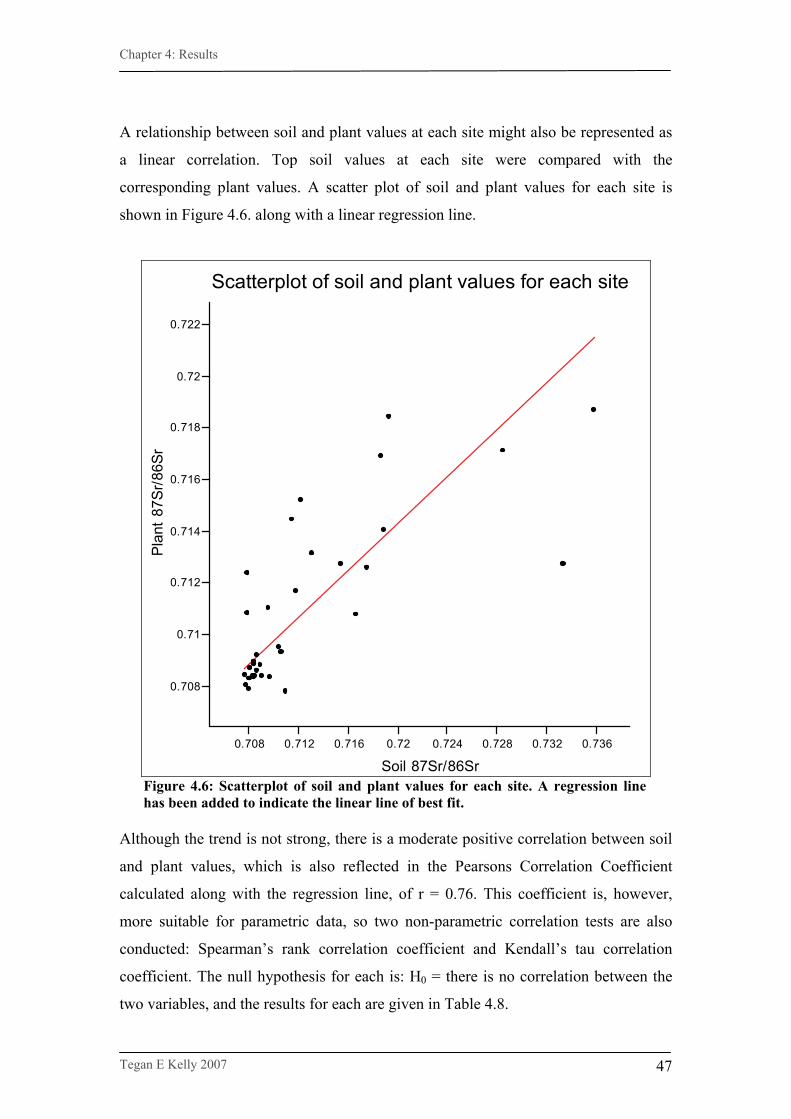
Chapter 4: Results
Tegan E Kelly 2007
47
A relationship between soil and plant values at each site might also be represented as
a linear correlation. Top soil values at each site were compared with the
corresponding plant values. A scatter plot of soil and plant values for each site is
shown in Figure 4.6. along with a linear regression line.
0.708 0.712 0.716 0.72 0.724 0.728 0.732 0.736
Soil 87Sr/86Sr
0.708
0.71
0.712
0.714
0.716
0.718
0.72
0.722
Plan
t87S
r/86S
r
Scatterplot of soil and plant values for each site
Figure 4.6: Scatterplot of soil and plant values for each site. A regression line has been added to indicate the linear line of best fit.
Although the trend is not strong, there is a moderate positive correlation between soil
and plant values, which is also reflected in the Pearsons Correlation Coefficient
calculated along with the regression line, of r = 0.76. This coefficient is, however,
more suitable for parametric data, so two non-parametric correlation tests are also
conducted: Spearman’s rank correlation coefficient and Kendall’s tau correlation
coefficient. The null hypothesis for each is: H0 = there is no correlation between the
two variables, and the results for each are given in Table 4.8.

Chapter 4: Results
Tegan E Kelly 2007
48
Table 4.8: Correlation coefficients and respective p-values for soil and plant non-parametric correlation tests. Spearmanns Rank Kendalls Tau Coefficient rs=0.73 τ = 0.55 p value 5.02E-7 2.14E-6
Though neither non-parametric correlation coefficient shows as strong a correlation,
p<<0.05 for both, firmly rejecting the null hypothesis and indicating that a correlation,
even if only moderate, is present.
4.2.2.2. Region analyses
4.2.2.2.1. Data exploration Each potential region (see Section 4.2.2.) first has univariate statistics calculated and
their normality tested via the Shapiro-Wilk statistic (p<0.05 = non-normal). Results
are shown for site averages in Table 4.9.
Table 4.9: Univariate statistics and Shapiro-wilk statistic for all potential regions, using site averages.
Clays LimRiv Lime GraRiv Gran Lime+Riv Gran+Riv
N 3 10 12 4 7 22 11
Min 0.7117 0.7083 0.7078 0.7093 0.7098 0.7078 0.7093
Max 0.7150 0.7115 0.7094 0.7188 0.7272 0.7115 0.7272
Mean 0.71293 0.70923 0.70853 0.71470 0.71794 0.70885 0.71676
Std. error 0.00104 0.00032 0.00016 0.00220 0.00243 0.00018 0.00174
Variance 3.24E-06 1.06E-06 3.11E-07 1.93E-05 4.14E-05 7.45E-07 3.33E-05
Median 0.71210 0.70885 0.70850 0.71535 0.71640 0.70860 0.71640
Shapiro-Wilk p value 0.2125 0.0675 0.3002 0.5581 0.5291 0.0102 0.5738
The mean values vary between the data sets and each median is similar to the
respective mean. Standard errors are low, and variance is very low. Most data sets
have a Shapiro-Wilk statistic of p> 0.05, and only Lime+Riv is significantly different
from normal, though some data sets are small, making their results somewhat
unreliable. However, a look at Normal QQ Probability plots for the same data (Fig
4.7.), indicates that the Clay, LimRiv and Lime+Riv regions all deviate substantially
from a linear relationship, indicating non-normal distributions.
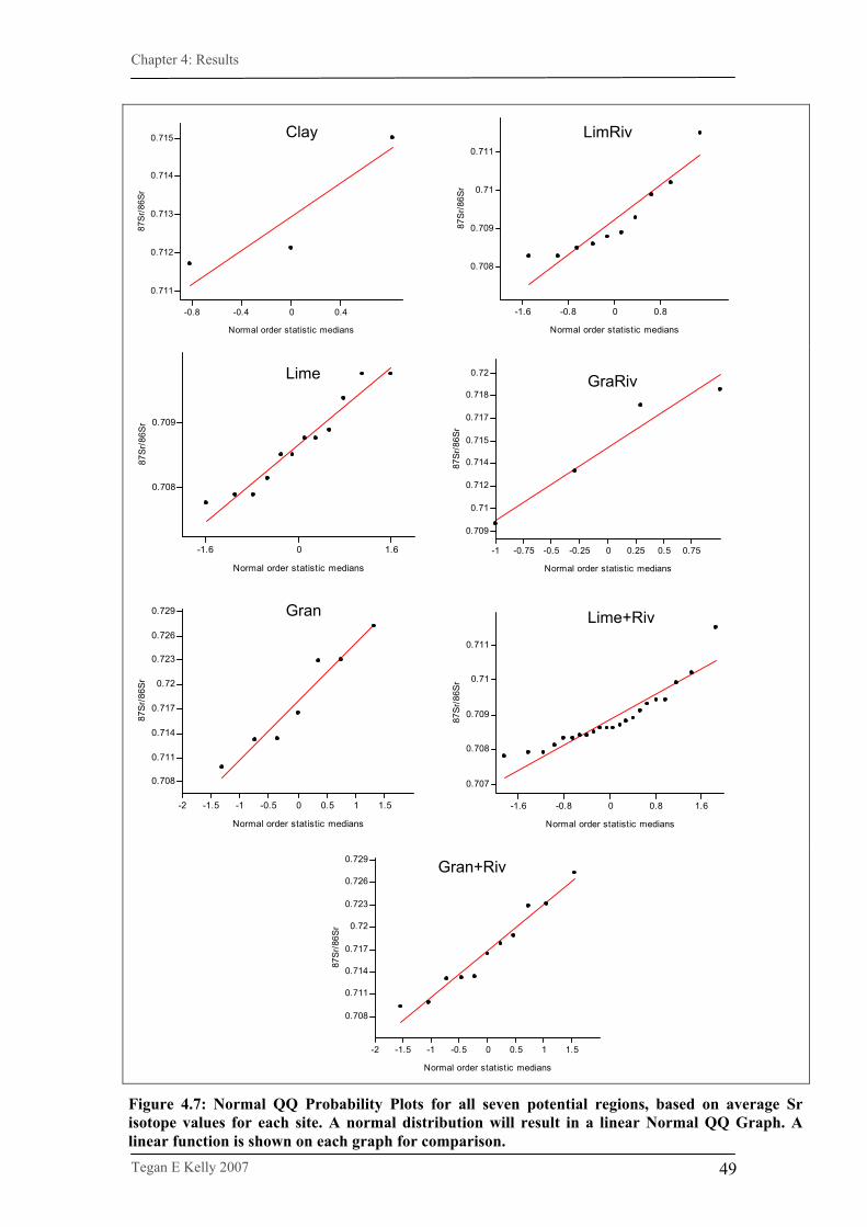
Chapter 4: Results
Tegan E Kelly 2007
49
-0.8 -0.4 0 0.4
Normal order statistic medians
0.711
0.712
0.713
0.714
0.71587
Sr/8
6Sr
-1.6 -0.8 0 0.8
Normal order statistic medians
0.708
0.709
0.71
0.711
87S
r/86S
r
-1.6 0 1.6
Normal order statistic medians
0.708
0.709
87S
r/86S
r
-1 -0.75 -0.5 -0.25 0 0.25 0.5 0.75
Normal order statistic medians
0.709
0.71
0.712
0.714
0.715
0.717
0.718
0.72
87S
r/86
Sr
-2 -1.5 -1 -0.5 0 0.5 1 1.5
Normal order statistic medians
0.708
0.711
0.714
0.717
0.72
0.723
0.726
0.729
87S
r/86
Sr
-1.6 -0.8 0 0.8 1.6
Normal order statistic medians
0.707
0.708
0.709
0.71
0.711
87Sr
/86S
r
-2 -1.5 -1 -0.5 0 0.5 1 1.5
Normal order statistic medians
0.708
0.711
0.714
0.717
0.72
0.723
0.726
0.729
87Sr
/86S
r
Clay
Lime
Gran
LimRiv
GraRiv
Lime+Riv
Gran+Riv
Figure 4.7: Normal QQ Probability Plots for all seven potential regions, based on average Sr isotope values for each site. A normal distribution will result in a linear Normal QQ Graph. A linear function is shown on each graph for comparison.
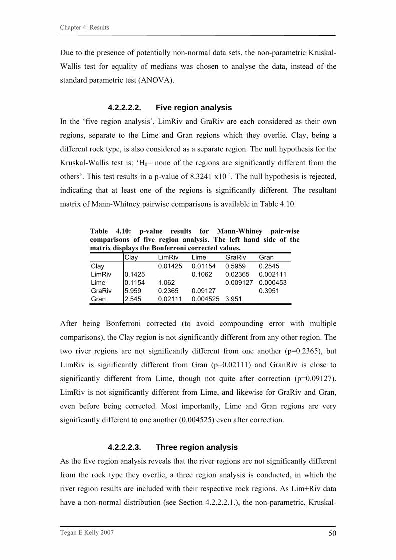
Chapter 4: Results
Tegan E Kelly 2007
50
Due to the presence of potentially non-normal data sets, the non-parametric Kruskal-
Wallis test for equality of medians was chosen to analyse the data, instead of the
standard parametric test (ANOVA).
4.2.2.2.2. Five region analysis In the ‘five region analysis’, LimRiv and GraRiv are each considered as their own
regions, separate to the Lime and Gran regions which they overlie. Clay, being a
different rock type, is also considered as a separate region. The null hypothesis for the
Kruskal-Wallis test is: ‘H0= none of the regions are significantly different from the
others’. This test results in a p-value of 8.3241 x10⁻⁵. The null hypothesis is rejected,
indicating that at least one of the regions is significantly different. The resultant
matrix of Mann-Whitney pairwise comparisons is available in Table 4.10.
Table 4.10: p-value results for Mann-Whiney pair-wise comparisons of five region analysis. The left hand side of the matrix displays the Bonferroni corrected values. Clay LimRiv Lime GraRiv Gran Clay 0.01425 0.01154 0.5959 0.2545 LimRiv 0.1425 0.1062 0.02365 0.002111 Lime 0.1154 1.062 0.009127 0.000453 GraRiv 5.959 0.2365 0.09127 0.3951 Gran 2.545 0.02111 0.004525 3.951
After being Bonferroni corrected (to avoid compounding error with multiple
comparisons), the Clay region is not significantly different from any other region. The
two river regions are not significantly different from one another (p=0.2365), but
LimRiv is significantly different from Gran (p=0.02111) and GranRiv is close to
significantly different from Lime, though not quite after correction (p=0.09127).
LimRiv is not significantly different from Lime, and likewise for GraRiv and Gran,
even before being corrected. Most importantly, Lime and Gran regions are very
significantly different to one another (0.004525) even after correction.
4.2.2.2.3. Three region analysis As the five region analysis reveals that the river regions are not significantly different
from the rock type they overlie, a three region analysis is conducted, in which the
river region results are included with their respective rock regions. As Lim+Riv data
have a non-normal distribution (see Section 4.2.2.2.1.), the non-parametric, Kruskal-
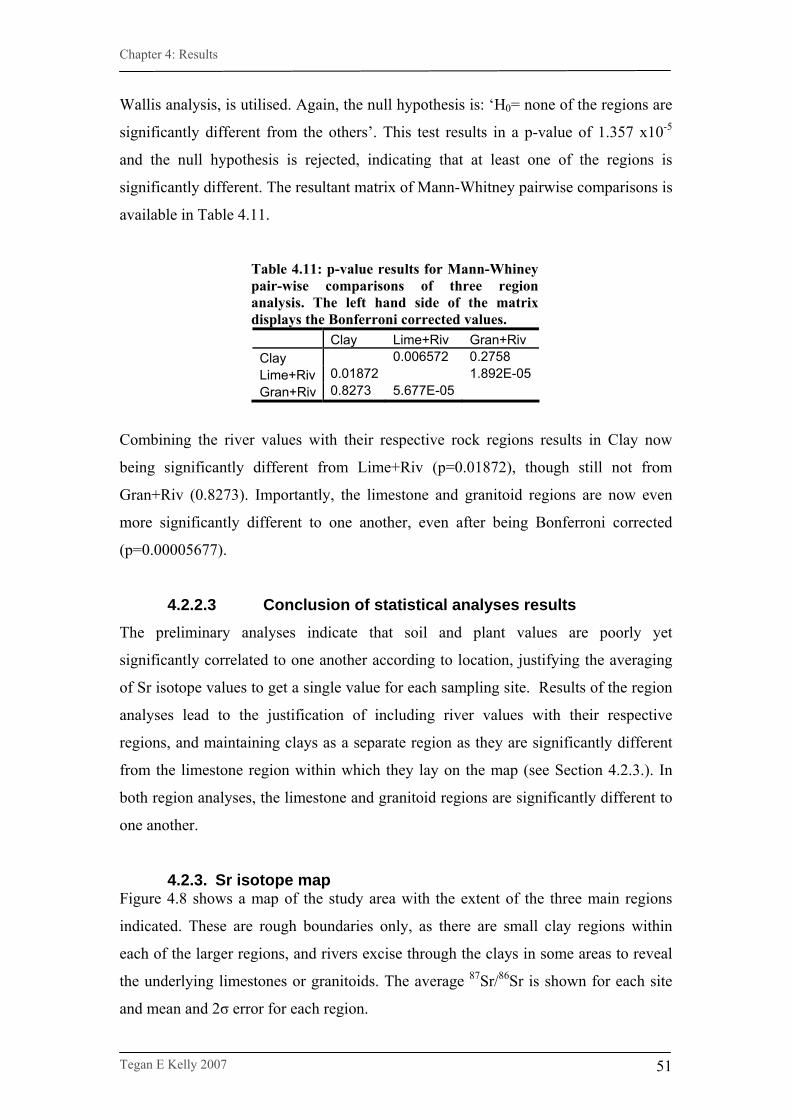
Chapter 4: Results
Tegan E Kelly 2007
51
Wallis analysis, is utilised. Again, the null hypothesis is: ‘H0= none of the regions are
significantly different from the others’. This test results in a p-value of 1.357 x10⁻⁵
and the null hypothesis is rejected, indicating that at least one of the regions is
significantly different. The resultant matrix of Mann-Whitney pairwise comparisons is
available in Table 4.11.
Table 4.11: p-value results for Mann-Whiney pair-wise comparisons of three region analysis. The left hand side of the matrix displays the Bonferroni corrected values.
Clay Lime+Riv Gran+Riv Clay 0.006572 0.2758 Lime+Riv 0.01872 1.892E-05 Gran+Riv 0.8273 5.677E-05
Combining the river values with their respective rock regions results in Clay now
being significantly different from Lime+Riv (p=0.01872), though still not from
Gran+Riv (0.8273). Importantly, the limestone and granitoid regions are now even
more significantly different to one another, even after being Bonferroni corrected
(p=0.00005677).
4.2.2.3 Conclusion of statistical analyses results The preliminary analyses indicate that soil and plant values are poorly yet
significantly correlated to one another according to location, justifying the averaging
of Sr isotope values to get a single value for each sampling site. Results of the region
analyses lead to the justification of including river values with their respective
regions, and maintaining clays as a separate region as they are significantly different
from the limestone region within which they lay on the map (see Section 4.2.3.). In
both region analyses, the limestone and granitoid regions are significantly different to
one another.
4.2.3. Sr isotope map Figure 4.8 shows a map of the study area with the extent of the three main regions
indicated. These are rough boundaries only, as there are small clay regions within
each of the larger regions, and rivers excise through the clays in some areas to reveal
the underlying limestones or granitoids. The average 87Sr/86Sr is shown for each site
and mean and 2σ error for each region.
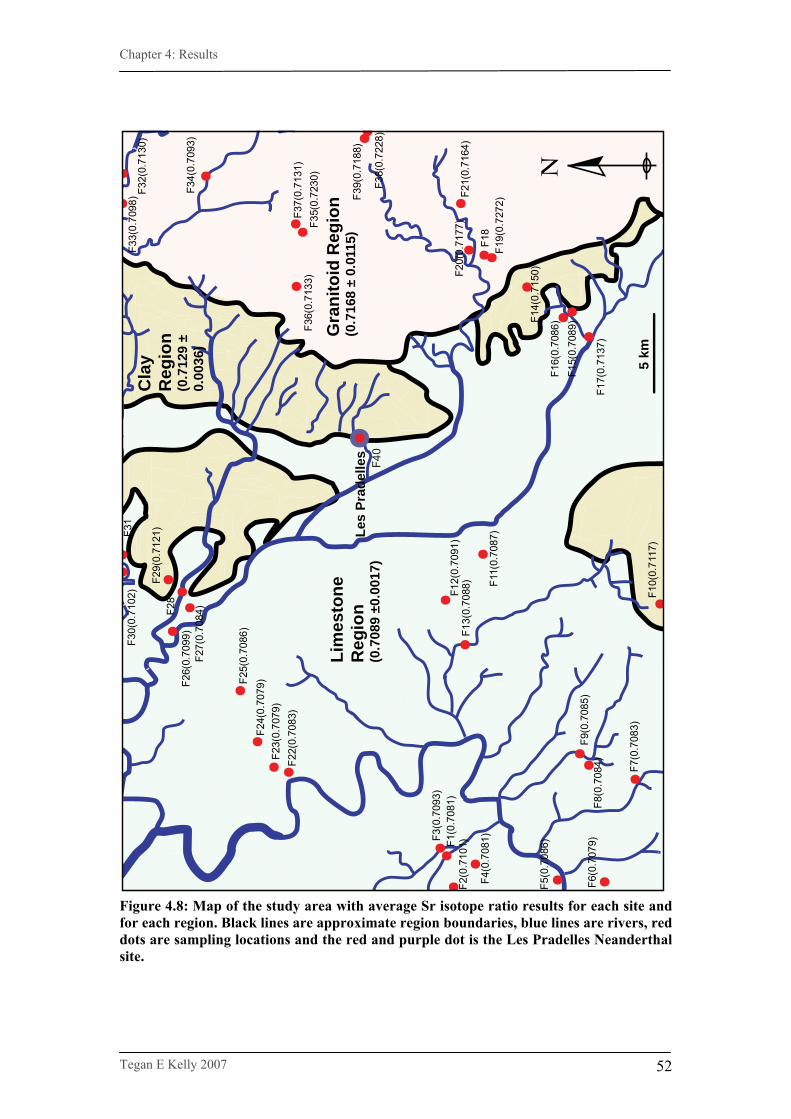
Chapter 4: Results
Tegan E Kelly 2007
52
Figure 4.8: Map of the study area with average Sr isotope ratio results for each site and for each region. Black lines are approximate region boundaries, blue lines are rivers, red dots are sampling locations and the red and purple dot is the Les Pradelles Neanderthal site.
F40
F11(
0.70
87)
F12(
0.70
91)
F13(
0.70
88)
Lim
esto
neR
egio
n(0
.708
9 ±0
.001
7)
Gra
nito
id R
egio
n(0
.716
8 ±
0.01
15)
Les
Prad
elle
s
F3(0
.709
3)
F4(0
.708
1)
F5(0
.708
6)
F6(0
.707
9)
F7(0
.708
3)
F8(0
.708
4)F9
(0.7
085)
F10(
0.71
17)
F14(
0.71
50)
F15(
0.70
89)
F16(
0.70
86)
F17(
0.71
37)
F18
F19(
0.72
72)
F20(
0.71
77)
F21(
0.71
64)
F22(
0.70
83)
F23(
0.70
79)
F24(
0.70
79)F2
5(0.
7086
)
F26(
0.70
99)
F27(
0.70
84)F2
8F2
9(0.
7121
)
F30(
0.71
02)
F31
F32(
0.71
30)
F33(
0.70
98) F3
4(0.
7093
)
F35(
0.72
30)
F36(
0.71
33)
F37(
0.71
31)
F38(
0.72
28)
F39(
0.71
88)
N
F1(0
.708
1)F2
(0.7
101)
Cla
yR
egio
n(0
.712
9 ±
0.00
36)
5 km
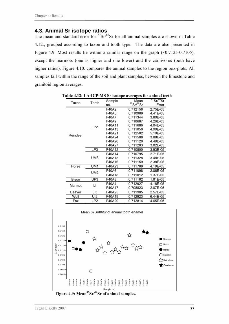
Chapter 4: Results
Tegan E Kelly 2007
53
4.3. Animal Sr isotope ratios The mean and standard error for 87Sr/86Sr for all animal samples are shown in Table
4.12., grouped according to taxon and tooth type. The data are also presented in
Figure 4.9. Most results lie within a similar range on the graph (~0.7125-0.7105),
except the marmots (one is higher and one lower) and the carnivores (both have
higher ratios). Figure 4.10. compares the animal samples to the region box-plots. All
samples fall within the range of the soil and plant samples, between the limestone and
granitoid region averages. Table 4.12: LA-ICP-MS Sr isotope averages for animal teeth
Taxon Tooth Sample no.
Mean 87Sr/86Sr
87Sr/86Sr Error
F40A2 0.712158 2.75E-05 F40A5 0.710969 4.41E-05 F40A7 0.711344 3.80E-05 F40A9 0.710687 4.26E-05 F40A11 0.711686 4.04E-05 F40A13 0.711050 4.90E-05 F40A21 0.712502 5.10E-05 F40A24 0.711508 3.88E-05 F40A26 0.711120 4.49E-05
LP2
F40A27 0.711283 3.82E-05 LP3 F40A12 0.710800 3.93E-05
F40A14 0.710795 2.71E-05 F40A15 0.711328 3.48E-05
Reindeer
UM3 F40A16 0.711159 2.38E-05
Horse UM1 F40A23 0.711769 4.19E-05 F40A6 0.711098 2.06E-05 UM2 F40A18 0.711012 1.37E-05
Bison UP3 F40A8 0.711162 1.81E-05 F40A4 0.712927 4.18E-05 Marmot LI F40A17 0.708823 2.07E-05
Beaver LI3 F40A25 0.711985 2.57E-05 Wolf UI2 F40A19 0.712923 6.44E-05 Fox LP2 F40A20 0.712814 4.65E-05
Figure 4.9: Mean87Sr/86Sr of animal samples.
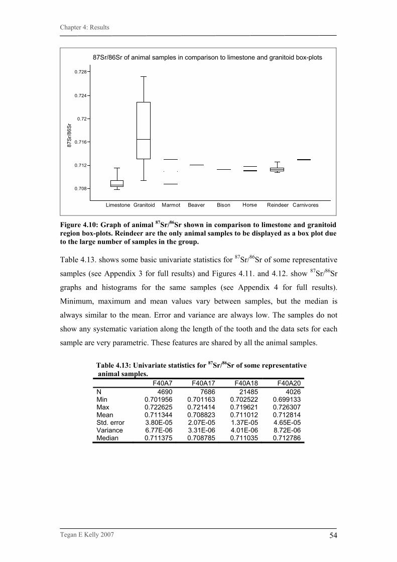
Chapter 4: Results
Tegan E Kelly 2007
54
Limestone Granitoid Marmot Beaver Bison Horse Reindeer Carnivores
0.708
0.712
0.716
0.72
0.724
0.72887
Sr/8
6Sr
87Sr/86Sr of animal samples in comparison to limestone and granitoid box-plots
Figure 4.10: Graph of animal 87Sr/86Sr shown in comparison to limestone and granitoid region box-plots. Reindeer are the only animal samples to be displayed as a box plot due to the large number of samples in the group. Table 4.13. shows some basic univariate statistics for 87Sr/86Sr of some representative
samples (see Appendix 3 for full results) and Figures 4.11. and 4.12. show 87Sr/86Sr
graphs and histograms for the same samples (see Appendix 4 for full results).
Minimum, maximum and mean values vary between samples, but the median is
always similar to the mean. Error and variance are always low. The samples do not
show any systematic variation along the length of the tooth and the data sets for each
sample are very parametric. These features are shared by all the animal samples.
Table 4.13: Univariate statistics for 87Sr/86Sr of some representative animal samples. F40A7 F40A17 F40A18 F40A20 N 4690 7686 21485 4026 Min 0.701956 0.701163 0.702522 0.699133 Max 0.722625 0.721414 0.719621 0.726307 Mean 0.711344 0.708823 0.711012 0.712814 Std. error 3.80E-05 2.07E-05 1.37E-05 4.65E-05 Variance 6.77E-06 3.31E-06 4.01E-06 8.72E-06 Median 0.711375 0.708785 0.711035 0.712786
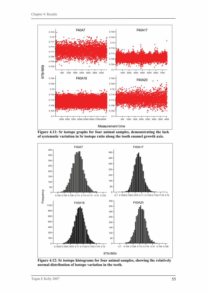
Chapter 4: Results
Tegan E Kelly 2007
55
600 1200 1800 2400 3000 3600 4200
0.702
0.705
0.708
0.711
0.714
0.717
0.72
0.723
1000 2000 3000 4000 5000 6000 70000.7
0.704
0.708
0.712
0.716
0.72
0.724
0.728
2500 5000 7500 100001250015000 17500200000.7
0.704
0.708
0.712
0.716
0.72
0.724
0.728
500 1000 1500 2000 2500 3000 3500 40000.7
0.704
0.708
0.712
0.716
0.72
0.724
0.72887Sr
/86S
r
Measurement time
F40A7 F40A17
F40A18 F40A20
Figure 4.11: Sr isotope graphs for four animal samples, demonstrating the lack of systematic variation in Sr isotope ratio along the tooth enamel growth axis.
0.702 0.705 0.708 0.711 0.714 0.717 0.72 0.7230
50
100
150
200
250
300
350
400
0.7 0.7025 0.7050.7075 0.71 0.7125 0.7150.7175 0.720
80
160
240
320
400
480
560
0.7025 0.7050.7075 0.71 0.7125 0.7150.7175 0.720
160
320
480
640
800
960
1120
0.7 0.704 0.708 0.712 0.716 0.72 0.724 0.7280
50
100
150
200
250
300
350
400
F40A7 F40A17
F40A18 F40A20
87Sr/86Sr
Freq
uenc
y
Figure 4.12: Sr isotope histograms for four animal samples, showing the relatively normal distribution of isotope variation in the teeth.
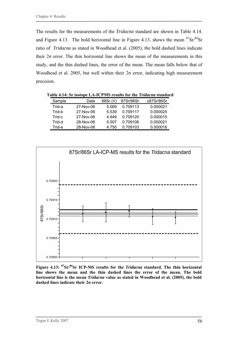
Chapter 4: Results
Tegan E Kelly 2007
56
The results for the measurements of the Tridacna standard are shown in Table 4.14.
and Figure 4.13. The bold horizontal line in Figure 4.13. shows the mean 87Sr/86Sr
ratio of Tridacna as stated in Woodhead et al. (2005), the bold dashed lines indicate
their 2σ error. The thin horizontal line shows the mean of the measurements in this
study, and the thin dashed lines, the error of the mean. The mean falls below that of
Woodhead et al. 2005, but well within their 2σ error, indicating high measurement
precision.
Table 4.14: Sr isotope LA-ICPMS results for the Tridacna standard
Sample Date 88Sr (V) 87Sr/86Sr ±87Sr/86Sr Trid-a 27-Nov-06 5.069 0.709113 0.000021Trid-b 27-Nov-06 5.539 0.709117 0.000025Trid-c 27-Nov-06 4.949 0.709120 0.000015Trid-d 28-Nov-06 5.007 0.709106 0.000021Trid-e 28-Nov-06 4.750 0.709103 0.000016
0.70900
0.70905
0.70910
0.70915
0.70920
87Sr/86Sr LA-ICP-MS results for the Tridacna standard
87S
r/86S
r
Figure 4.13: 87Sr/86Sr ICP-MS results for the Tridacna standard. The thin horizontal line shows the mean and the thin dashed lines the error of the mean. The bold horizontal line is the mean Tridacna value as stated in Woodhead et al. (2005), the bold dashed lines indicate their 2σ error.

Chapter 5: Discussion
Tegan E Kelly 2007 57
Chapter 5
DISCUSSION
5.1. Soil and plant analyses: creating the map The Sr isotope map (Fig. 4.8.) is based on 87Sr/86Sr analyses of soil and plant samples,
reliant on the assumption that 87Sr/86Sr cycling in an ecosystem is based on labile Sr
derived from the weathering of bedrock geology. This assumption is borne out by the
significantly different Sr isotope values from the two main rock regions; however,
there are also unexpected results in the data. These include variations within sites,
such as differences in 87Sr/86Sr ratios between top and bottom soils and between soils
and plants. Furthermore, variations within regions, such as the variability of 87Sr/86Sr
ratios in the granitoid samples and the difference between the limestone values and
those expected from seawater 87Sr/86Sr, also require explanation.
The procedural blanks indicate potential contamination during sample preparation
(see Section 4.2.1.) and the possible extent of this contamination deserves comment.
Both plant blanks show low levels of 88Sr (0.140 – 0.175 V). These levels could at
most account for 1.6% of the 88Sr signal, when applied to the plant sample with the
lowest voltage (10.7 V). This level of Sr contamination will therefore have little effect
on plant 87Sr/86Sr values. The soil blanks, however, tell a different story. Although
Soil 1 has an extremely low value (0.033 V), accounting for at most, 0.7% of the 88Sr
signal, Soil 2 has a much higher value (0.547 V), which, when applied to the range of
voltages received for the soil samples, could account for 5.1% - 12.2% of each 88Sr
signal. If any soil samples do indeed have contamination levels similar to this soil
blank, it could influence the measured 87Sr/86Sr result. As explained in Section 4.2.1.,
the Sr isotope ratio of the contamination appears to be around 0.7070-0.7089. This is
well within the range of the limestone soil results, but has the potential to decrease the
ratio in granitoid soil sample measurements. This must be kept in mind when
interpreting the data, however, it is not sufficient to explain the unexpected results
seen in some samples.
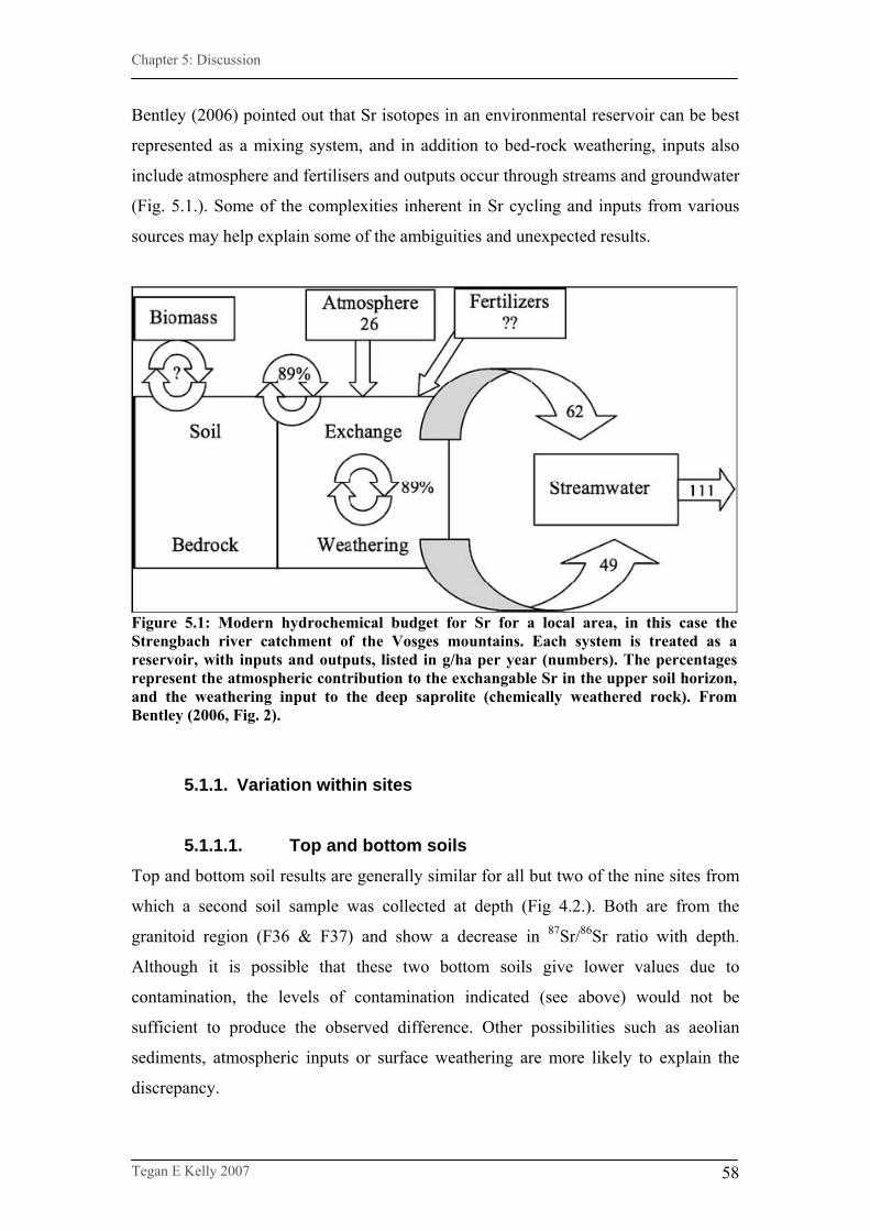
Chapter 5: Discussion
Tegan E Kelly 2007 58
Bentley (2006) pointed out that Sr isotopes in an environmental reservoir can be best
represented as a mixing system, and in addition to bed-rock weathering, inputs also
include atmosphere and fertilisers and outputs occur through streams and groundwater
(Fig. 5.1.). Some of the complexities inherent in Sr cycling and inputs from various
sources may help explain some of the ambiguities and unexpected results.
Figure 5.1: Modern hydrochemical budget for Sr for a local area, in this case the Strengbach river catchment of the Vosges mountains. Each system is treated as a reservoir, with inputs and outputs, listed in g/ha per year (numbers). The percentages represent the atmospheric contribution to the exchangable Sr in the upper soil horizon, and the weathering input to the deep saprolite (chemically weathered rock). From Bentley (2006, Fig. 2).
5.1.1. Variation within sites
5.1.1.1. Top and bottom soils Top and bottom soil results are generally similar for all but two of the nine sites from
which a second soil sample was collected at depth (Fig 4.2.). Both are from the
granitoid region (F36 & F37) and show a decrease in 87Sr/86Sr ratio with depth.
Although it is possible that these two bottom soils give lower values due to
contamination, the levels of contamination indicated (see above) would not be
sufficient to produce the observed difference. Other possibilities such as aeolian
sediments, atmospheric inputs or surface weathering are more likely to explain the
discrepancy.
Chapter 5: Discussion
Tegan E Kelly 2007 59
Aeolian dust (loess) deposits are widespread over much of western Europe, including
northern France (Gallet et al. 1998) and although the study area does not contain
significant loess deposits, dust could easily blow into the region from the north.
European loess has given 87Sr/86Sr ratios of 0.712-0.730 (Gallet et al. 1998) so could
potentially result in elevated surface ratios if present in top soil samples.
Alternatively, atmospheric inputs (i.e. rain) have been known to cause a trend in 87Sr/86Sr with depth. Poszwa et al. (2004) measured Sr in soil profiles in a boreal
forest ecosystem in northern Sweden, to a depth of 60 cm. They found the 87Sr/86Sr
ratio of labile Sr to generally increase in relation to depth. Probst et al. (2000) came to
similar conclusions in a 60 cm profile at a spruce forest site in north eastern France.
They each attributed the trend to atmospheric inputs at the surface, with a decrease in
the contribution of atmospheric inputs relative to mineral weathering with depth.
Prohaska et al. (2005) measured Sr in a periglacial soil profile in the Günzer
mountains of eastern Austria, to a depth of 2.5 m. As can be seen in Figure 5.2., they
got more complicated results, with an increase in the 87Sr/86Sr ratio of labile Sr for the
first 50 cm, while deeper examination of the profile showed a steady decrease.
Both bottom soil samples that display a decrease in 87Sr/86Sr ratio were collected from
a depth of more than 1 m, so appear to fit the above trends. However, the remainder of
the sites show very little difference in 87Sr/86Sr ratio between top and bottom soils,
even though bottom soils were collected from a range of depths, varying from 30 cm
to 4 m, spaning both the limestone and granitoid regions. Thus the limited data
suggest that at most sites, either, aeolian and atmospheric inputs provide a similar 87Sr/86Sr ratio to mineral weathering or they contribute little to the Sr cycling in the
ecosystem. Although some authors (e.g. Kennedy et al. 2002) have found
atmospheric inputs to be a major component in Sr cycling in an ecosystem, Bern et al.
(2005) showed that even a modest input of Sr from mineral weathering, driven by
erosion, can prevent atmospheric inputs from dominating the local Sr cycle. As such,
mineral weathering is usually the dominant contributor to soil and plant Sr (Bentley
2006).

Chapter 5: Discussion
Tegan E Kelly 2007 60
Figure 5.2: 87Sr/86Sr ratios of total digest and NH4NO3 extract (labile portion) in a periglacial soil profile from the Günzer Mountains in Eastern Austria. From Prohaska et al. (2005, Fig. 2).
If atmospheric inputs are not the cause of the variation in 87Sr/86Sr ratio with depth,
extensive surface weathering may be. Åberg (1995) explained how a decrease in
Sr87Sr/86 ratio with depth may be due to the depletion of easily weathered Ca-rich (and
therefore Sr-rich) minerals, and the resultant concentration of K-rich minerals, in the
uppermost soil layers. This effect may well explain the results for the granitoid
samples. Plagioclase feldspar is high in Ca and hence Sr, and is also low in Rb,
resulting in low 87Sr/86Sr ratios. Potassium feldspars on the other hand are very low in
Sr and high in Rb, resulting in much higher ratios (Bentley 2006). If the granite soils
are highly weathered, plagioclase feldspars may have been removed, resulting in
highly radiogenic labile 87Sr/86Sr ratios at the surface. Analysis of rock samples could
help to confirm this, if labile rock Sr is found to be similar to that of the bottom soil.
5.1.1.2. Soils and plants
The strontium isotope map (Fig 4.8.) has been based on Sr isotope ratios determined
from the average of soil and plant samples at each site. As suggested by Sillen et al.
(1998), all soil samples were leached in order to extract labile strontium for
measurement (see Sections 2.1.5. and 3.2.2.). If the laboratory leaching process
successfully reflects the leaching of labile strontium in the natural environment, soil
Chapter 5: Discussion
Tegan E Kelly 2007 61
ratios should be very similar to plant ratios from the same location (Fig 2.4.). As can
be seen in Figure 4.2., this is the case for many locations, especially those on
limestones or in either type of river. However, at four sites (F29, F17, F2 and F34) the
plant values are higher than the soils, and at eight sites (F14, F3 and all granitoid
locations except F33) the soil is higher.
Where plant values are higher than soil, it could potentially be due to soil
contamination (see above). This may indeed be the case at F17 and F34, where there
is no reason to expect the low soil values to be correct. Alternatively, at these
locations the differences may be due to the implications of being river sites (see
Section 5.1.2.4.). The other two sites (F29 and F2) show good agreement between top
and bottom soil values, making random soil contamination less likely and the elevated
plant value the anomaly. It is unclear why the plant values are elevated above the soil
in which they grow, unless they are receiving a higher 87Sr/86Sr input from elsewhere
(i.e. rainwater runoff or small tributaries not marked on the map), which is not altering
the ratios of the soil exchange system.
The granitoid samples are more liable to influence from the potential soil
contamination (see above), yet all granitoid sites showing a discrepancy (i.e. the
majority) give soil values higher than plants, rather than lower as would be expected
from contamination. Three of the granitoid samples give very high soil ratios (F19,
F35 & F36; Fig 4.2.), much more radiogenic than plant samples from the same
locations, or indeed any sample type from any location. They thus appear to represent
a different population. These samples may contain aeolian loess, or be from extremely
weathered and depleted granite soils, which, as explained above, will give elevated Sr
ratios relative to unweathered samples, (see Section 5.1.1.1.). Unfortunately, bottom
soil samples were not collected at these particular locations in order to test these
suggestions. Although extensive weathering and Ca depletion may explain high 87Sr/86Sr ratios in the soils, it is less clear why the elevated ratios are not being passed
on to the plants. Indeed, at the sites where a bottom soil was collected, the plant ratios
appear to more closely approximate that of the bottom soil, rather than the top soil.
Although it may be attractive to speculate that the plants did not derive their 87Sr/86Sr
isotopes from the topsoil, but from the lower layers of the profile, this is unlikely
given that most of the plants collected were shallow rooted grasses.

Chapter 5: Discussion
Tegan E Kelly 2007 62
Alternatively, insufficient leaching procedures may be the problem. Only three of the
deviations between soil and plant occur in samples from within the limestone region
(two of which are on rivers, see Section 5.1.2.4.), while nine are from clays or
granitoids. It may well be possible that the laboratory leaching procedures were not
generally applicable to all soils types. Limestone soils may leach more thoroughly due
to their soluble nature, whereas the technique may not sufficiently replicate the extent
of natural leaching in the granitoid system. Laboratory tests involving the leaching of
numerous soil types with leachates of varying severity (i.e. various solutes of differing
composition, concentration and/or leaching exposure time) and comparison of the
labile 87Sr/86Sr results with those of plants from the same location might shed light on
this issue. This is, however, outside the scope of the current study.
5.1.2. Variation within regions
5.1.2.1. Limestone regions Limestone rocks are high in Sr (due to high Ca levels) and relatively low in Rb (Capo
et al. 1998), and should generally yield low Sr isotope ratios (<0.7100). The site
average 87Sr/86Sr ratio results of the limestone samples (including those from rivers)
do indeed give relatively low 87Sr/86Sr results, with little variation (see Figs. 4.2. &
4.4.; 0.7089 ±0.0017 [2σ s.d.]) and most of the variation occurs in the river samples
(see Section 5.1.2.4.). Marine carbonate rocks reflect the isotopic composition of the
sea-water, from which they were precipitated (Ehrlich et al. 2001). The seawater 87Sr/86Sr at the time of formation of the limestones was low (0.7068-0.7075; Fig. 5.3.;
Jones et al. 1994), leading to the expectation that the rocks and soils would have
similarly low ratios. Yet all site averages for the limestone regions are higher (0.7078-
0.7137; Fig 4.2.). This is not entirely surprising as argillaceous limestones will have
higher 87Sr/86Sr than clean limestones. Additionally any in situ development of a soil
will involve some extent of weathering, and the development of clay minerals will
lead to higher Sr isotope ratios than the parent rocks. This could be tested by
separating the mineral components of soils before analysis, though the weighted
average labile 87Sr/86Sr of both together is the relevant value for ecosystem cycling.
Although this is the most likely explanation, alternative scenarios for the elevation of
limestone soil ratios should be considered.
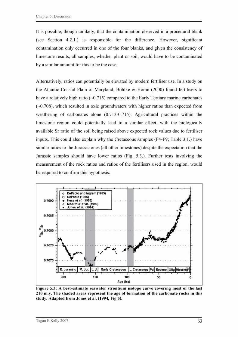
Chapter 5: Discussion
Tegan E Kelly 2007 63
It is possible, though unlikely, that the contamination observed in a procedural blank
(see Section 4.2.1.) is responsible for the difference. However, significant
contamination only occurred in one of the four blanks, and given the consistency of
limestone results, all samples, whether plant or soil, would have to be contaminated
by a similar amount for this to be the case.
Alternatively, ratios can potentially be elevated by modern fertiliser use. In a study on
the Atlantic Coastal Plain of Maryland, Böhlke & Horan (2000) found fertilisers to
have a relatively high ratio (~0.715) compared to the Early Tertiary marine carbonates
(~0.708), which resulted in oxic groundwaters with higher ratios than expected from
weathering of carbonates alone (0.713-0.715). Agricultural practices within the
limestone region could potentially lead to a similar effect, with the biologically
available Sr ratio of the soil being raised above expected rock values due to fertiliser
inputs. This could also explain why the Cretaceous samples (F4-F9; Table 3.1.) have
similar ratios to the Jurassic ones (all other limestones) despite the expectation that the
Jurassic samples should have lower ratios (Fig. 5.3.). Further tests involving the
measurement of the rock ratios and ratios of the fertilisers used in the region, would
be required to confirm this hypothesis.
Figure 5.3: A best-estimate seawater strontium isotope curve covering most of the last 210 m.y. The shaded areas represent the age of formation of the carbonate rocks in this study. Adapted from Jones et al. (1994, Fig 5).
Chapter 5: Discussion
Tegan E Kelly 2007 64
5.1.2.2. Granitoid regions Granites are high in rubidium (>100 ppm), resulting in high Rb/Sr ratios (Capo et al.
1998). This combined with the ancient age of the granitoid rocks (380-350 Ma) leads
to the expectation of relatively high 87Sr/86Sr ratios. The site average 87Sr/86Sr ratios
for the granitoid regions are indeed high (>0.710; Figs. 4.2. & 4.4.), but much
variation is present. Even discounting the three sites with exceptionally high ratios
(F19, F35 and F38; see Section 5.1.1.2.), there is still considerable variation between
the granitoid sites (Figs 4.2 & 4.4.), which range from 0.7093 (F34) to 0.7188 (F39)
(0.7139 ±0.0025 [2σ s.d.]).
This variability is probably due to the heterogeneous nature of the rock region, which
spans five different map units (Table 3.1.), including granites and granodiorites, as
well as gneissic terrains. The mineralogies of the samples vary, such as the types of
feldspar and the proportion of mafic minerals present, including biotite and pyroxene.
The effects of preferential weathering of feldspars are explained above (see Section
5.1.1.1.), and variable weathering conditions combined with varying proportions of
feldspars will lead to variations in 87Sr/86Sr ratios. Higher ratios will also occur in
biotite rich areas, due to high levels of K and therefore Rb, and low Sr. Textural
features such as grainsize and the presence and size of phenocrysts also vary,
influencing the labile 87Sr/86Sr ratio of soil samples. Smaller grains have a higher
surface to volume ratio, resulting in stronger weathering ability and the preferential
leaching of 87Sr from the more loosely bonded Rb sites, relative to 86Sr, which is more
tightly bonded to the lattice. This may result in lower Sr isotope ratios for fine-grained
samples (Åburg 1995). All of these features of the region are likely to have
contributed to the variable 87Sr/86Sr ratios.
5.1.2.3. Clay region Clays generally have high concentrations of potassium, and are not rich in calcium
and so by association, have high Rb/Sr ratios. This, in turn should result in relatively
high 87Sr/86Sr ratios. The results for the few clay samples in the study do indeed show
relatively high 87Sr/86Sr ratios. No comment can be made on the variation in these
values, as three samples are insufficient to display trends.
Chapter 5: Discussion
Tegan E Kelly 2007 65
5.1.2.4. River regions The 87Sr/86Sr ratios from the river sites are very similar to the rock regions they
overly, demonstrating that the labile Sr isotopes in the river sediments and plants are
principally derived from local weathering. A few river limestone sites give somewhat
elevated ratios (F17, F26 & F30) and one of the rivers in the granitoids gives a low
ratio (F34). This is reflected in the box plots of site averages in Figure 4.4., showing
the limestone rivers with slightly higher average values than the limestones, and the
granite rivers slightly lower averages than the granites. Additionally the two river
regions are not statistically different from one another (see Section 4.2.2.2.2.). This is
likely due to the mixing of 87Sr/86Sr ratios from different regions and potential inputs
from atmospheric sources.
Rivers carry a suspended load of weathering products, sourced from higher
topography undergoing erosion, resulting in a mix of rocks and solids from upstream
(Bentley 2006). The addition of Sr isotopes derived from upstream clays and
granitoids could account for the raised 87Sr/86Sr ratios in river sediments in the
limestone region relative to the majority of non-riverine limestone samples.
Atmospheric inputs into stream waters may also influence the 87Sr/86Sr ratios of the
river sediments. In a spruce forest study in north eastern France, Probst et al. (2000)
found 49-58% of dissolved Sr in stream waters was derived from atmospheric inputs.
This could potentially be influencing the 87Sr/86Sr ratios of the river sediments,
lowering ratios in the granitoid rivers and raising them in the limestone ones.
However, any mixing or atmospheric effects which are occurring do not appear to be
strong, and are not significantly altering the river sediment ratios from those of the
non-riverine equivalents (see Section 4.2.2.2.2.).
5.1.3. Variation between regions Even with these variations within each of the regions, it is apparent from Figures 4.2.
and 4.4. that the two main regions have distinctively different 87Sr/86Sr ratios, which
are statistically significant (see Section 4.2.2.2.), regardless of whether rivers are
included. As the river regions are not significantly different from their respective rock
regions, they do not need to be considered separately. The significant difference
between limestones and granitoids is easily explained, and the expectation of
Chapter 5: Discussion
Tegan E Kelly 2007 66
relatively low 87Sr/86Sr ratios in the limestones and relatively high 87Sr/86Sr ratios in
the granitoids has been covered in sections 5.1.2.1. & 5.1.2.2. (see above). Although
the clay samples did not provide significantly different 87Sr/86Sr ratios to the
granitoids, it makes sense to consider them separately, as they occur in pockets over
both the other regions of the map. As such, the study area can be successfully divided
into three Sr isotope regions (Figure 4.8.).
5.2. Animal analyses: testing the map 87Sr/86Sr ratios were measured along tooth growth axes, with the expectation of
seasonal trends. However all animal samples give normally distributed 87Sr/86Sr
results with relatively constant ratios along the growth axes of the teeth (see Section
4.3.1. and Appendix 4). This may imply that each individual animal did not range far
during enamel formation, or alternatively, may be the result of tooth growth periods
and reservoir effects combined with the incorporation of Sr isotopes from both
regions due to the feeding ranges of the animals (see below). Most results give Sr
isotope values intermediate between the two regions, rather than mapping directly to
one region or the other (Fig 4.10.), further suggesting reservoir and averaging effects,
rather than restricted range. Bentley (2006) explained that the averaging of 87Sr/86Sr
ratios up trophic levels will lead to a decrease in the variability of animal Sr isotopes
compared to the rocks and plants of an ecosystem, which is indeed the case in this
study.
In any geochemical study of fossil remains, it is important to address the potential of
diagenetic contamination. Fossil materials, including teeth, interact with soil moisture
and meteoric water in the burial soil, which can lead to secondary mineral
precipitation and leaching. Enamel is less porous than dentine or bone material, and as
such is less prone to the effects of diagenesis (Budd et al. 2000; Chiardia et al. 2003).
Horn et al. (1994) analysed material from a 675,000 ±75,000 year old fossil stag from
Mauer and found that tooth enamel preserved the original 87Sr/86Sr signal, whereas
bone and dentine did not. It is usually assumed that enamel samples are relatively free
of contamination, and acid washing procedures on bone samples may arguably
remove some contamination (e.g. Grupe et al. 1997; Price et al 1994a). In an
investigation of modern and fossil teeth in central Kenya, however, Kohn et al. (1999)

Chapter 5: Discussion
Tegan E Kelly 2007 67
found that while the PO4 component of tooth enamel was resistant to chemical
alteration, the OH component could be extensively altered, resulting in the alteration
of apatite in both dentine and enamel. They go on to suggest that the presence of U or
REEs may indicate the potential for this type of contamination (Kohn et al. 1999).
The samples in this study consisted of enamel only and had very low levels of REEs
and, as such, most likely contain the primary biological Sr signal. Additionally,
Prohaska et al. (2002) suggest that the high resolution capabilities of LA-ICP-MS
make it the method of choice over solution ICP-MS for potentially diagenetically
altered material.
5.2.1. Rodents The rodents (F40A4, F40A17, and F40A25) would have had small feeding ranges
(see Sections 2.3.4. & 2.3.5.) and the constant Sr ratios are probably a result of the
individuals remaining within a small region while the enamel was mineralising. Due
to the continuous growth and attrition of rodent incisors, the sections of enamel
measured reflect only the last few years at most, of the animals’ lives. The two
marmots give the most extreme mean Sr isotope ratios (Fig 4.10.), indicating that
F40A17 probably spent at least the later years of its life within the limestone region
(0.7088), while F40A4, within the granitoid region or a clay area (0.7129). The clay
region proximal to Les Pradelles is listed on the map as “Quaternary terrain with
undifferentiated Tertiary sectors”, which formed via the in situ decalcification of the
limestone substrate (BRGM 1983). As such, much of it probably did not exist when
this marmot was alive, making the granitoid region the closest likely source for the
animal. The beaver (F40A25) gives an intermediate ratio (0.7120). This could indicate
that the individual was from one of the less radiogenic areas of the granitoid region,
but is more likely due to beavers living and sourcing their food from in and around
streams. Sillen (1998) found streamside plants to reflect the 87Sr/86Sr ratio of the water
in the stream, so although the beaver had a small home range and is unlikely to have
fed from both regions of the map, the plants it ate may have incorporated 87Sr/86Sr
ratios from both, due to the mixing effects of the river in which it lived (see Section
5.1.2.4.). The beaver could potentially be from the river in the far north east corner of
the map, near site F32, which gives the most similar Sr isotope ratio (0.7130), but this
is speculation only, as the majority of rivers were not measured.
Chapter 5: Discussion
Tegan E Kelly 2007 68
5.2.2. Ruminants In contrast to the rodent incisors, all other tooth samples in the study record the 87Sr/86Sr consumed in the first few months to years of the animals’ lives. The
ruminant (reindeer, horse and bison) samples all give fairly similar average ratios
(Figures 4.9. & 4.10.), intermediate in value between the mean 87Sr/86Sr of the two
main rock regions. Once again this could potentially indicate that the teeth were
formed while the animals lived in a radiogenic-poor region of the granitoids, or is
alternatively due to the mixing of Sr incorporated from the two regions. Given the
relatively long period of tooth formation for each species (reindeer 2-3 years, horse 1-
2 years and bison about 1 year; see Section 2.3.) and large feeding ranges of the
animals (see below and Section 2.3.) the latter scenario is more likely.
Modern wild horses have been shown to have feeding ranges varying from 73-303
km2 (Miller 1983) and the horses sampled at Les Pradelles probably ranged across
both regions of the map. The reindeer and bison were almost certainly migratory, and
may have travelled hundreds of km within a single year (see Section 2.3.1. & 2.3.2.).
In modern reindeer, the population continues to migrate both during calving (1.1
km/day) and straight after (1.3 km/day; Ferguson & Elkie 2004). The new born
reindeer follows its mother on the continued migratory route within days, nibbling
leaves and buds almost straight away after birth (Danell et al. 2006). So why then,
given the fact that the animals were almost certainly migrating while the teeth were
forming, is there no sign of variation in the 87Sr/86Sr of the growing tooth enamel?
Balasse et al. (2002) found no pattern of seasonal variation in Sr isotope ratios in a
cow tooth from the south western cape of South Africa, though they found a clear
seasonal cycle in carbon and oxygen isotopes in the same sample. The lack of
variation therefore may not indicate a lack of migration and, if undertaken, carbon and
oxygen analyses could potentially demonstrate seasonal variation. It is more likely
due to mixing and reservoir effects. The Sr isotope composition of any particular
skeletal element is a concentration-weighted average of all dietary Sr ingested by the
individual while that skeletal component was being formed (Beard and Johnson
2000). As such the Sr isotopes in animal tissues are averaged over both space and
time.
Chapter 5: Discussion
Tegan E Kelly 2007 69
Sr isotopes can be averaged spatially due to the consumption of a variety of plants
from various regions. Danell et al. (2006) found that in Northern Sweden, modern
reindeer migrate into the mountains in summer and back to lower, less harsh altitudes
during winter. The Pleistocene reindeer from Les Pradelles may have had similar
behaviour, spending summer in the higher altitudes of the granitoid region and winter
in the lower limestone region. Modern reindeer have a clear annual cycle in appetite
and growth, with much higher metabolic demands in summer (Mathiesen et al. 2000).
Although limestone has higher concentrations of Sr, the granitoid region may still
have contributed substantially to a weighted average in the samples, due to the
increased food intake and higher metabolic demands of the summer period. Small
amounts of forage would have been consumed during the winter in the limestone, also
contributing to the Sr intake of the animals. For instance, some modern reindeer dig
through winter snow to reach the vegetation beneath, though where available, the
winter diet of most reindeer is primarily lichen (Drucker et al. 2001, Mathiesen et al.
2000). In an isotopic study of large herbivores in Pleistocene south-western France,
Drucker et al. (2003) found carbon isotope signatures to suggest that reindeer diet was
much enriched in lichens relative to other species such as Bos/Bison, perhaps to avoid
direct competition between the herbivores.
Isotopes also average temporally, due to the averaging of 87Sr/86Sr in the diet over the
time of formation of skeletal tissues. Although mammal teeth do show daily cross
striations, Hoppe et al. (2004) explain that a significant amount of time separates
matrix formation from the completion of enamel maturation and during the initial
stages of crown formation the enamel mineralisation front can extend over a vertical
distance of several cm. This means that any one spot of enamel may have taken
several months to fully mineralise. Reindeer migrating seasonally can cover hundreds
of miles just between early autumn and early winter (Bishop 1998), when they travel
up to 2.5 km/day (Ferguson & Elkie 2004). It is therefore likely that the animals were
crossing regions faster than their teeth were mineralising. Additionally, chemical ions
are stored in animal skeletons, to be released and mobilised rapidly in order to meet
metabolic requirements (Balasse et al. 2002). This storage and release of ions such as
Ca and Sr can create a reservoir effect, further weakening seasonal signals.
Chapter 5: Discussion
Tegan E Kelly 2007 70
The possibility that the lack of seasonal variation is due to a lack of migration cannot
be ruled out. Perhaps the horses had a range size at the low end of the spectrum of
modern ranges, and perhaps the Bos/Bison samples were actually non-migratory
aurochs. There are even some sedentary sub-species of modern reindeer, such as the
non-migratory reindeer of the Svalbard archipelago, which do not seasonally migrate
and show only limited migration between populations (Aanes et al. 2003). Since none
of the mean 87Sr/86Sr ratios of these species are outside the range of the granitoid
region, they may indeed have spent at least the first few years of their life only within
a low 87Sr/86Sr area of the region. Oxygen and carbon isotope analyses could be
utilised to confirm whether this is indeed the case (e.g. Balasse et al. 2005), but this is
outside the scope of the current study.
5.2.3. Carnivores The averaging effects described above also have implications for carnivore 87Sr/86Sr
ratios. Animals from higher trophic levels usually show lower variability in 87Sr/86Sr
than animals from lower trophic levels within the same ecosystem (Bentley 2006).
While the herbivores average out Sr from various regions, carnivores average out Sr
from various herbivores. Both carnivore samples give higher 87Sr/86Sr than the
majority of the herbivores, with a similar result to the marmot with the high ratio (Fig
4.11.). Foxes have relatively small home ranges and feed mainly on small animals as
well as fruit (see Section 2.3.7.). The high ratio therefore suggests that the fox spent
its youth in the granitoid region. Wolves on the other hand, usually have relatively
large ranges and feed primarily on large herbivores, though they do consume some
small prey as well (see Section 2.3.6.). The high ratio observed suggests that the wolf
spent the first year of its life well into the granitoid region. Wolf pups feed on milk
and then food regurgitated by the mother (Mech et al. 1999) who would most likely
have fed on herbivores which had large range sizes. Considering the averaging effect
of carnivorous feeding, the birthing area must have been well away from the
limestone region in order for the 87Sr/86Sr ratio to be higher than all the herbivores
measured in this study.
Chapter 5: Discussion
Tegan E Kelly 2007 71
5.2.4. Summary All animal samples show no sign of seasonal signals in Sr isotopes in the tooth
enamel. In the animals with small feeding ranges (marmots, beaver and fox) this is
most likely due to the animal consuming isotopes from within only one region of the
map. One of the marmots probably spent the last year or so of its life in the limestone
region and the other in the granitoid or clay region, due to the low and high mean
isotope ratios, respectively. The beaver may have inhabited a river from anywhere on
the map due to the mixing of Sr isotopes from both regions by water flow. The fox
probably spent at least the first six months of its life in the granitoid region. For the
animals with large feeding ranges, the results are more ambiguous. The lack of
seasonal signals is probably due to the averaging of isotopes from both regions due to
reservoir effects and the timing lapse between the onset of enamel mineralisation and
later maturation. The reindeer, horses and bison most likely roamed and fed over both
regions of the map, while the wolf probably spent at least the first year of its life
within the granitoid region some distance away from the limestone areas.
5.2.5. Implications The majority of the animal samples probably represent the remains of Neanderthal
meals, as indicated by the nature of the animal assemblage as well as cut marks on
bones at the site (Maureille pers. com.). Most samples do not provide much
information regarding the range of Neanderthal hunting: one marmot may have been
local, and the beaver may have lived in a nearby river. The horse, reindeer and bison
may also have been hunted near by the cave. The other marmot, however, indicates
that the Neanderthals probably travelled some distance when hunting, reaching the
granitoid region more than 5 km away. As such any of the other prey animals may
have been hunted some distance away also. The fox and wolf probably used the cave
as a den, independently of the Neanderthal occupation (Maureille pers. com.). The
carnivore results therefore reflect the independent migration of the canines, rather
than Neanderthal hunting range.
Chapter 6: Conclusion
Tegan E Kelly 2007
72
Chapter 6
CONCLUSIONS
The regional area surrounding the Neanderthal excavation site of Les Pradelles lent
itself well to strontium isotope mapping, with the two main rock regions easily
distinguished on the basis or Sr isotope ratios. The limestones gave relatively low
ratios (<0.710), though substantially higher than the sea-water values at the time of
carbonate precipitation, probably due to clay materials and potentially also fertiliser
inputs. The heterogeneous nature of the granitoid region led to more variable results,
though with relatively high ratios (>0.710). Limited overlap in Sr isotope ratios of the
two regions occurred at only a few river sites. Results indicate that river sediments are
primarily derived from the local bedrock, with only minor mixing of sediments from
the two regions. Aeolian and atmospheric inputs to the Sr soil reservoir appear to be
minimal. Extensive surface weathering may lead to elevated soil surface ratios in
some areas of the granitoid region.
The faunal teeth gave mixed results. Seasonal variation in 87Sr/86Sr was not apparent,
even though some (such as reindeer) almost certainly migrated across regions during
tooth formation. Animals with small feeding ranges could be mapped to specific
regions, whereas those with larger ranges gave intermediate values. These results
suggest an averaging of isotopes: both across the feeding range of the individuals, and
over the time period of enamel maturation. It is important to understand the behaviour
and nature of tooth development in study animals, to discriminate isotopes indicating
a specific region of provenance from the results of averaging effects.
The results of this study highlight some of the complexities inherent in Sr isotope
tracing in animal tissues. Bentley (2006) was correct when he pointed out that
“spatial heterogeneity and mixing relations must often be accounted for, rather than
simply ‘matching’ a measured strontium isotope value to a presumed single value
geologic source”. Nevertheless, Sr isotope tracing is a worthwhile exercise. The

Chapter 6: Conclusion
Tegan E Kelly 2007
73
marmot results gave an indication of Neanderthal hunting range, and migration was
determined in the wolf, despite the averaging effects of its feeding habits.
Analyses of Neanderthals from the Les Pradelles site are likely to be equally
illuminating. Although seasonal mobility is unlikely to be determined using Sr
isotopes, there is a great potential for discerning lifetime migration. The relative
abundance and diversity of fossil species at Les Pradelles suggest that it was a hunting
site (Maureille pers. com.). As such, it would be expected that local individuals would
provide 87Sr/86Sr signatures similar to those of the local herbivores, or perhaps a little
lower due to averaging with locally sourced vegetation and small game. Any
individuals with significantly higher ratios are likely to have spent their childhood in a
different area, similar to the wolf in this study.
Strontium isotope tracing is a very useful technique, regularly applied to faunal and
archaeological samples all over the world. Many of the conclusions of this study have
relevance to other researchers, regardless of study material or location. When
conducting this type of study, it is important to keep in mind the complexities of Sr
ecosystem cycling; bedrock geology is not the only source of Sr isotopes contributing
to the system. Even when bio-available Sr isotopes can provide a clear distinction
between rock regions, animals will not necessarily map to a particular region, instead
averaging the isotopes of the various sources from which they feed. None the less,
useful information regarding mobility is to be gleaned from the Sr isotopes of animal
teeth.
6.1. Future recommendations This was a preliminary study and a number of future recommendations became
apparent throughout the conduction of the research.
Bed rock samples were not analysed due to time constraints, but it is highly
recommended that they are in future. Knowledge of the labile rock Sr could help
confirm some of the assumptions made in this study, such as the influence of clay
materials and fertilisers in the limestones and surface weathering in the granitoids.

Chapter 6: Conclusion
Tegan E Kelly 2007
74
The analysis of biologically available Sr is essential. Laboratory studies into
various leaching procedures could be used to ensure the techniques utilised closely
approximate the natural system.
Laser ablation is a relatively quick and easy technique for the analysis of Sr
isotopes in tooth enamel. The high resolution results made it clear that ratios were
averaged during the formation of teeth and that no seasonal trends occurred; results
undeterminable via bulk methods.
The lack of seasonality in Sr data does not necessarily indicate that no migration
occurred. Alternate stable isotopes such as O and C could be utilised in conjunction
with Sr, to discover whether constant Sr ratios are due to averaging effects or a true
lack of migration (e.g. Balasse et al. 2002).
It is highly recommended that a similar study be carried out on Neanderthal
teeth from the Les Pradelles site. Sr isotope tracing has never before been attempted
on Neanderthal samples, and this study demonstrates the potential for success.
During the measurement of faunal Sr isotopes, total Sr concentration results are
also determined. If Ca were measured, Ca/Sr ratios could provide information
regarding trophic level (e.g. Blum et al. 2000). It would be interesting to investigate
Ca/Sr ratios in the Neanderthals at Les Pradelles, as δ15N and δ13C isotopes in samples
from the site have suggested carnivorous behaviour (Fizet et al. 1995) and though
speculative, cut marks on bones may potentially indicate cannibalism (Maureille pers.
com.).

Tegan E Kelly 2007
75
References Aanes, R., Sæther, B-E., Solberg, E. J., Aanes, S., Strand, O. & Øritsland, N. A. 2003. Synchrony in Svalbard reindeer population dynamics. Canadian Journal of Zoology. 81: 103-110. Åberg, G. 1995. The use of natural strontium isotopes as tracers in environmental studies. Water, Air and Soil Pollution. 79:309-322. Balasse, M., Ambrose, S, H., Smith, A. B. & Douglas-Price, T. 2002. The seasonal mobility model for prehistoric herders in the south-western cape of South Africa assessed by isotopic analysis of sheep tooth enamel. Journal of Archaeological Science. 29: 917–932. Beard, B. L. & Johnson, C. M. 2000. Strontium Isotope Composition of Skeletal Material Can Determine the Birth Place and Geographic Mobility of Humans and Animals. Journal of Forensic Science. 45 :1049–1061. Beauval, C., Bourguignon, L., Costamagno, S., Couchoud, I., Marquet, J-Cl., Maureille, B., Maignen, L., Mann, A. E., Texier, J-P. & Vandermeersch, B. 2002. Recent discoveries of Neandertal remains from Les Pradelles (Marillac-le-Franc, Charente, France). Journal of Human Evolution. 42: A5-A6. Bentley, R. A. 2006. Strontium Isotopes from the Earth to the Archaeological Skeleton: A Review. Journal of Archaeological Method and Theory. 13: 135-187. Bentley, R. A. & Knipper, C. 2005. Geographical patterns in biologically available strontium, carbon and oxygen isotope signatures in prehistoric SW Germany. Archaeometry. 47: 629-644. Bentley, R. A., Price, T. D. & Stephan, E. 2004. Determining the ‘local’ 87Sr/86Sr range for archaeological skeletons: a case study from Neolithic Europe. Journal of Archaeological Science. 31: 365-375. Bern, C. R., Townsend, A. R. & Farmer, G. L. 2005. Unexpected dominance of parent-material strontium in a tropical forest on highly weathered soils. Ecology. 86 : 626-632. Bishop, G. 1998. Meet the real Rudolph. Ranger Rick. 32: 16-17. Blum, J. D., Taliaferro, E. H., Weisse, M. T. & Holmes, R. T. 2000. Changes in Sr/Ca, Ba/Ca and 87Sr/86Sr ratios between trophic levels in two forest ecosystems in the northeastern U.S.A. Biogeochemistry. 49: 97-101. Böhlke, J. K. & Horan, M. 2000. Strontium isotope geochemistry of groundwaters and streams affected by agriculture, Locust Grove, MD. Applied Geochemistry. 15: 599-609. BRGM. 1983. Carte géologique de la France. La Rochefoucauold, A/50 000, Map 686. BRGM. 1984. Carte géologique de la France. Mansle, A/50 000, Map 685.

Tegan E Kelly 2007
76
BRGM. 1985. Carte géologique de la France. Angoulême, A/50 000, Map 709. BRGM. 1986. Carte géologique de la France. Montbron, A/50 000, Map 710. Budd, P., Montgomery, J., Berreiro, B. & Thomas, R. G. 2000. Differential diagenesis of strontium in archaeological human dental tissues. Applied Geochemistry. 15: 687-694. Budd, P., Millard, A., Chenery, C., Lucy, S. & Roberts, C. 2004. Investigating population movement by stable isotope analysis: a report from Britain. Antiquity. 78: 127-141. Capo, R. C., Stewart, B. W. & Chadwick, O. A. 1998. Strontium isotopes as tracers of ecosystem processes: theory and methods. Geoderma. 82: 197-225 Chamberlain, C. P., Blum, J. D., Holmes, R. T., Feng, X., Sherry, T. W. & Graves, G. R. 1997. The use of isotope tracers for identifying populations of migratory birds. Oecologia. 109:132–141 Chiaradia, M., Gallay, A. & Todt, W. 2003. Different contamination styles of prehistoric human teeth at a Swiss necropolis (Sion, Valais) inferred from lead and strontium isotopes. Applied Geochemistry. 18: 353-370. Danell, A. C., Andrén, H., Sergerström, P. & Franzén, R. 2006. Space use by Eurasian lynx in relation to reindeer migration. Canadian Journal of Zoology. 84: 546-555. Date, A. R. & Gray, A. L. 1981. Plasma source mass spectrometry using an inductively coupled plasma and a high resolution quadrupole mass filter. Analyst. 106: 1255-1267. Drucker, D., Bocherens, H., Pike-Tay, A. & Mariotti, A. 2001. Isotopic tracking of seasonal dietary change in dentine collagen: preliminary data from modern caribou. Earth and Planetary Sciences. 333: 303-309. Drucker, D. G., Bocherens, H. & Billiou, D. 2003. Evidence for shifting environmental conditions in Southwestern France from 33 000 to 15 000 years ago derived from carbon-13 and nitrogen-15 natural abundances in collagen of large herbivores. Earth and Planetary Science Letters. 216: 163-173. Eggins, S. M., Kinsley, L. P. J. & Shelley, J. M. G. 1998. Deposition and element fractionation processes during atmospheric pressure laser sampling for analysis by ICP-MS. Applied Surface Science, 127–129: 278–286. Ehrlich, S., Gavrieli, I., Dor, L-B. & Haliez, L. 2001. Direct high-precision measurements of the 87Sr/86Sr isotope ratio in natural water, carbonates and related materials by multiple collector inductively coupled plasma mass spectrometry (MC-ICP-MS). Journal of Analytical Atomic Spectrometry. 16: 1389-1392. Ericson, J. E. 1989. Some Problems and Potentials of Strontium Isotope Analysis for Human and Animal Ecology. In Rundel, P. W., Ehleringer, J. R. & Nagy, K. A. (Eds.) Stable Isotopes in Ecological Research. Springer-Verlag: New York.
Tegan E Kelly 2007
77
Evans, J. A., Chenerey, C. A. & Fitzpatrick, A. P. 2006. Bronze Age childhood migration of individuals near Stonehenge, revealed by strontium and oxygen isotope tooth enamel analysis. Archaeometry. 48: 309-321. Ezzo, J. A. & Price, T. D. 2002. Migration, regional reorganisation, and spatial group composition at Grasshopper Pueblo, Arizona. Journal of Archaeological Science. 29: 499-520 Faure, G. 1986. Principles of Isotope Geology (2nd ed.). John Wiley & Sons: New York. Ferguson, S. H. & Elkie, P. C. 2004. Seasonal movement patterns of woodland caribou (Rangifer tarandus caribou). Journal of Zoology, London. 262. 125-134. Fincham, A. G., Moradian-Oldak, J. & Simmer, J. P. 1999. The Structural Biology of the Developing Dental Enamel Matrix. Journal of Structural Biology. 126:270-299 Fizet, M., Mariotti, A. & Bocherens, H. 1995. Effect of Diet, Physiology and Climate on Carbon and Nitrogen Stable Isotopes of Collagen in a Late Pleistocene Anthropic Palaeoecosystem: Marillac, Charente, France. Journal of Archaeological Science. 22: 67-79. Gadbury, C., Todd, L., Jahren, A. H. & Amundsen R. 2000. Spatial and temporal variations in the isotopic composition of bison tooth enamel from the Early Holocene Hudson–Meng Bone Bed, Nebraska. Palaeogeography, Palaeoclimatology, Palaeoecology. 157: 79-93. Gallet, S., Jahn, B., Lanoë, B. V. V., Dia, E. & Rossello, E. 1998. Loess geochemistry and its imlications for particle origin and composition of the upper continental crust. Earth and Planetary Science Letters. 156: 157-172. Graustein, W. C. 1989. 87Sr/86Sr Ratios Measure the Sources and Flow of Strontium in Terrestrial Ecosystems. In Rundel, P. W., Ehleringer, J. R. & Nagy, K. A. (Eds.) Stable Isotopes in Ecological Research. Springer-Verlag: New York. Grupe, G., Price, T. D., Schröter, P., Söllner, F., Johnson, C. M. & Beard, B. L. 1997. Mobility of Bell Beaker people revealed by strontium isotope ratios of tooth and bone: a study of southern Bavarian skeletal remains. Applied Geochemistry. 12: 517-525. Hammer, Ø., Harper, D. A. T. & Ryan, P. 2001. Past: Paleontological statistics software package for education and data analysis. Palaeontoligica Electronica. 4: 1-9. Hart, S. R., Ball, L. & Jackson, M. 2005. Sr Isotopes by Laser Ablation Pimms: Application to CPX from Samoan Peridotite Xenoliths. WHOI Plasma Facility Open File Technical Report 11. http://www.whoi.edu/science/GG/people/shart/Open%20File%2011,%20revised%202-9-05-1.pdf Hauslabjoch: A Geochemical Approach Using Sr, C and O Isotopes and Trace Element Signatures. Journal of Archaeological Science. 28: 983–989. Hillson, S. 1986. Teeth. Cambridge University Press: Cambridge.
Tegan E Kelly 2007
78
Hodell, D. A., Quinn, R. L., Brenner, M. & Kamenov, G. 2004. Spatial variation of strontium isotopes (87Sr/86Sr) in the Maya region: a tool for tracking ancient human migration. Journal of Archaeological Science. 31: 585-601. Hoogewerff, J., Papesch, W., Kralik, M., Berger, M., Vroon, P., Miesbouer, H., Gaber, O., Künzel, K-H. & Kleinjans, J. 2001. The last domicile of the iceman from Hauslabjoch: a geochemical approach using Sr, C and O isotopes and trace element signatures. Journal of Archaeological Science. 28: 983-989. Hoppe, K. A., Koch, P. L., Carlson, R. W. & Webb, S. D. 1999. Tracking mammoths and mastodons: reconstruction of migratory behaviour using strontium isotope ratios. Geology. 27: 439-442. Hoppe, K, A., Stover, S. M., Pascoe, J. R. & Amundsen, R. 2004. Tooth enamel biomineralization in extant horses: implications for isotopic microsampling. Palaeogeography, Palaeoclimatology, Palaeoecology. 206: 355-365. Horn, P., Hölzl, S. & Storzer, D. 1994. Habitat determination on a fossil stag’s mandible from the site of Homo erectus heidelbergensis at Mauer by use of 87Sr/86Sr. Naturwissenschaften. 81: 360-362. Iacumin, P. & Longinelli, A. 2002. Relationship between δ18O values for skeletal apatite from reindeer and foxes and yearly mean δ18O values of environmental water. Earth and Planetary Science Letters. 201: 213-219. Jarvis, K. E., Gray, A. L. & Houk, R. S.1992. Handbook of Inductively Coupled Plasma Mass Spectrometry. Blackie: London. Jones, C. E., Jenkyns, H, C., Coe, A. L. & Hesselbo, S. P. 1994. Strontium isotopic variations in Jurassic and Cretaceous seawater. Geochimica et Cosmochimica Acta 58: 3061-30. Kennedy, M. J., Hedin, L. O. & Derry, L. A. Decoupling of unpolluted temperate forests from rock nutrient sources revealed by natural 87Sr/86SR and 84Sr tracer addition. Proceedings of the National Academy of Sciences (USA). 99: 9639-9644. Knudson, K. J., Tung, T. A., Nystrom, K. C., Douglas-Price, T. & Fullagar, P. D. 2005. The origin of the Juch’uypampa Cave mummies: strontium isotope analysis of archaeological human remains from Bolivia. Journal of Archaeological Science. 32: 903-913. Koch, P. L., Heisinger, J., Moss, C., Carlson, R. W., Fogel, M. L., Behrensmeyer, A. K. 1995. Isotopic tracking of change in diet and habitat use in African elephants. Science, 267: 1340-1343. Kohn, M. J., Schoeninger, M. J. & Barker, W. W. 1999. Altered states: effects of diagenesis on fossil tooth chemistry. Geochimica et Cosmochimica Acta. 63: 2737-2747. Kurtén, B. 1968. Pleistocene Mammals of Europe. Weidenfeld and Nicolson: London.

Tegan E Kelly 2007
79
Line, S, R, P. & Bergqvist, L. P. 2005. Enamel structure of paleocene mammals of the Sao José De Itaborai Basin, Brazil. ‘Condylarthra’ Litopterna, Notoungulata, Xenungulata, and Astrapotheria. Journal of Vertebrate Palaeontology 25: 924–928. Mathiesen, S. D., Sørmo, W., Haga, Ø. E., Norberg, H. J., Utsi, T. H. A. & Tyler, N. J. C. 2000. The oral anatomy of Arctic ruminants coping with seasonal changes. Journal of Zoology, London. 251: 119-128. Mech, D. L., Wolf, P. C. & Packard, J. M. 1999. Reguritative food transfer among wild wolves. Canadian Journal of Zoology. 77: 1192-1195. Miller, R. 1983. Seasonal Movements and Home Ranges of Feral Horse Bands in Wyoming’s Red Desert. Journal of Range Management. 36: 199-201. Moradian-Oldak, J. 2001. Amelogenins: assembly, processing and control of crystal morphology. Matrix Biology. 20: 293-305. Müller, W., Fricke, H., Halliday, A. N., McCulloch, M. T. & Wartho, J. 2003. Origin and migration of the alpine iceman. Science. 302: 862-866. Nowak, R. M. & Paradiso, J. L. (Eds). 1983. Walker’s Mammals of the World (4th Ed). The John Hopkins University Press: Baltimore. Porder, S., Paytan, A. & Hadly, E. A. 2003. Mapping the origin of faunal assemblages using strontium isotopes. Paleobiology. 29: 197-204. Price, T. D., Johnson, C. M., Ezzo, J. A, Ericson, J. & Burton, J. H. 1994a. Residential mobility in the prehistoric southwest United States: a preliminary study using strontium isotope analysis. Journal of Archaeological Science. 21: 315-330. Price, T. D., Grupe, G. & Schröter, P. 1994b. Reconstruction of migration patterns in the Bell Beaker period by stable strontium isotope analysis. Applied Geochemistry. 9: 413-417. Price, T. D., Mansanilla, L. & Middleton, W. 2000. Immigration and the ancient city of Teotihuacan in Mexico: a study using strontium isotope ratios in human bone and teeth. Journal of Archaeological Science. 27: 903-913. Price, T. G., Burton, J. H. & Bentley, R. A. 2002. The characterization of biologically available strontium isotope ratios for the study of prehistoric migration. Archaeometry. 44. 117-135. Poszwa, A., Ferry, B., Dambrine, E., Pollier, B., Wickman, T., Loubet, M. & Bishop, K. 2004. Variations of bioavailable Sr concentration and 87SR/86Sr ratio in boreal forest ecosystems: Role of biocycling, mineral weathering and depth of root uptake. Biogeochemistry. 67: 1-20. Probst, A., El Gh’mari, A., Aubert, D., Fritz, B. & McNutt, R. 2000. Strontium as a tracer of weathering processes in a silicate catchment polluted by acid atmospheric inputs, Strengbach, France. Chemical Geology. 170: 203-219.

Tegan E Kelly 2007
80
Prohaska, T., Latkoczy, C., Schultheis, G., Teschler-nicola, M. & Stingeder, G. 2002. Investigation of Sr isotope ratios in prehistoric human bones and teeth using laser ablation ICP-MS and ICP-MS after Rb/Sr separation. Journal of Analytic Atomic Spectrometry. 17: 887-891. Prohaska, T., Wenzel, W. W. & Stingeder, G. 2005. ICP-MS-based tracing of metal sources and mobility in a soil depth profile via the isotopic variation of Sr and Pb. International Journal of Mass Spectrometry. 242: 243-250. Rinaldi, C. & Cole, T. M. 2004. Environmental seasonality and incremental growth rates of beaver (Castor canadensis) incisors: implications for palaeobiology. Palaeogeography, Palaeoclimatology, Palaeoecology. 206: 289– 301. Scheissing, M. M. & Grupe, G. 2003. Tracing migration events in man and cattle by stable strontium isotope analysis of appositionally grown mineralized tissue. International Journal of Osteoarchaeology. 13: 96-103. Sillen, A., Hall, G., Richardson, S. & Armstrong, R. 1998. 87Sr/86Sr ratios in modern and fossil food-webs of the Sterkfontein Valley: implications for early hominid habitat preference. Geochimica et Cosmochimica Acta. 62: 2463-2473. Simmer, J. P. & Fincham, A. G. 1995. Molecular mechanisms of dental enamel formation. Critical Review of Oral Biology & Medicine. 6:84-108. Stuart-Williams, H. L. Q. & Schwarcz, H. P. 1997. Oxygen isotopic determination of climatic variation using phosphate from beaver bone, tooth enamel, and dentine. Geochimica et Cosmochimica Acta, 61: 2539-2550. van der Merwe, N. J., Lee-Thorp, J. A., Thackeray, J. F., Hall-Martin, A., Kruger, F. J., Coetzee, H., Bell, R. H. E. & Lindeque, M. 1990. Source-area determination of elephant ivory by isotopic analysis. Nature. 346: 744-746. Vogel, J. C., Eglington, B. & Auret, J. M. 1990. Isotope fingerprints in elephant bone and ivory. Nature. 346: 747-749. Woodhead, J., Hellstrom, J., Haas, R., Hergt, J., Shelley, M., Eggins, S. & Kemp, R. 2003. Geological applications of of the HelEx 193nm laser ablation system coupled to a New Plasma –ICPMS. Geochimica et Cosmochimica Acta. 67: A536-A356. Woodhead, J., Swearer, S, Hergt, J. & Maas, J. 2005. In situ Sr-isotope analysis of carbonates by LA-MC-ICP-MS: interference corrections, high spatial resolution and an example from otolith studies. Journal of Analytic Atomic Spectrometry. 20: 22-27. Wright, L. E. 2005. Identifying immigrants to Tikal, Guatemala: defining local variability in strontium isotope ratios of human tooth enamel. Journal of Archaeological Science. 32: 555-566. Zhao, Z., Weiss, K. M. & Stock, D. W. 2000. Development and evolution of dentition patterns and their genetic basis. In Teaford, M. F., Smith, M. M. & Ferguson, M. W. J. (Eds). Development, Function and Evolution of Teeth. Cambridge University Press: Cambridge.
81
Appendix 1: Glossary
Amelogenesis: The process of dental enamel formation.
Archaeology: The study of past human groups and cultures, primarily through
material remains.
Analysis of Variance (ANOVA): A statistical test used to determine whether several
univariate sample groups are taken from populations with equal means. Data should
be continuous and parametric.
Biologically available strontium: Exchangeable Sr ions on the surface of rocks and
soils, available for transport in solution and ecosystem circulation. May have a
different strontium isotope ratio to Sr ions locked up inside silicates in rocks and
soils, which are analysed in ‘whole rock’ or ‘whole soil’ analyses.
Bio-available strontium: see biologically available strontium.
F-test: A statistical test used to determine whether two univariate sample groups are
taken from populations with equal variances. Data should be parametric.
Geochemistry: The study of the distribution and amounts of chemical elements and
their isotopes in minerals, ores, rocks, soils, water and the atmosphere, and the study
of the circulation of the elements in nature.
Isotope: One of two or more species of the same chemical element, differing in their
atomic mass.
Kendall’s Tau Correlation Coefficient : A statistical test used to determine linear or
non-linear correlation between two variates. Data may be non-parametric.
Kolmogorov-Smirnov test: A statistical test used to compare the shapes of two
univariate distributions.
Kruskal-Wallis test: A statistical test used to determine whether several univariate
sample groups are taken from populations with equal medians. Data may be non-
parametric.
Labile strontium: see biologically available strontium.
Mann-Whitney U test: A statistical test used to determine whether two inviariate
sample groups are taken from populations with equal medians. Data may be non-
parametric.

82
Mousterian: European stone tool industry characterised by flakes struck from cores.
Generally associated with Neanderthals. Dates from around 150 ka to 35 ka.
Normal QQ Probability plot: A graph used for assessing whether data display a
normal distribution. Normally distributed data will form a straight line on a
probability plot.
Palaeoecology: The study of past ecosystems.
Parametric distribution: Data which fits a normal distribution curve (a.k.a. bell-
shaped curve, gaussian distribution).
Pearson’s Correlation Coefficient: Statistical test used to determine linear or non-
linear correlation between two variates. Data should be parametric.
Radioactive elements: Elements (or isotopes) which decay to emit energetic particles
and/or radiation. Leads to the formation of different elements or isotopes. (See also
radiogenic).
Radiogenic elements: Elements (or isotopes) formed via the radioactive decay of
radioactive elements.
Ruminant: A group of mammals which have four stomachs and chew their cud.
Includes cattle, deer, sheep, goats and camels.
Shapiro-Wilk statistic: A statistical test used to determine whether a given sample
group has been taken from a population with a normal distribution.
Spearman’s Rank Correlation Coefficient: Statistical test used to determine linear
or non-linear correlation between two variates. Data may be non-parametric.
Strontium isotope mapping: Creating a map of a region based on the strontium
isotope ratio of the materials of the region, such as rocks, water, soils, plants and
animals. Often used in strontium isotope tracing.
Strontium isotope ratio: The ratio of radiogenic 87Sr relative to 86Sr: (87Sr/86Sr).
Strontium isotope tracing: Measuring strontium isotope ratios in animal tissues with
the intention of tracing migration or mobility in the individual. Often involves the
utilisation of a strontium isotope map.
Student’s t-test: A statistical test used to determine whether two univariate samples
are taken from populations with equal means. Data should be parametric and have
equal variances.
Welch test: A statistical test used to determine whether two univariate samples are
taken from populations with equal means. Data should be parametric and but do not
require equal variances.

83
Appendix 2: Dental Notation The maximum number of teeth for a placental mammal (counting from centre front, along one side of the jaw) is: 3 incisors, 1 canine, 4 premolars and 3 molars.
Lower case: deciduous Superscript: upper jaw Upper case: permanent Subscript: lower jaw
Deciduous Permanent Upper Lower Upper Lower
First incisor i1 i1 I1 I1
Second incisor i2 i2 I2 I2
Third incisor i3 i3 I3 I3
Canine c1 c1 C1 C1
First premolar p1 p1 P1 P1
Second premolar p2 p2 P2 P2
Third premolar p3 p3 P3 P3
Fourth premolar p4 p4 P4 P4
First molar m1 m1 M1 M1
Second molar m2 m2 M2 M2
Third molar m3 m3 M3 M3 Note: Left and right hand sides are not specified here.
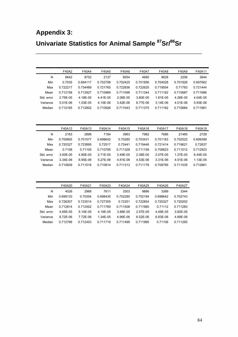
84
Appendix 3: Univariate Statistics for Animal Sample 87Sr/86Sr
F40A2 F40A4 F40A5 F40A6 F40A7 F40A8 F40A9 F40A11
N 6642 8752 2137 8054 4690 9628 2206 3644 Min 0.7035 0.694117 0.702799 0.702425 0.701956 0.704028 0.701926 0.697662 Max 0.722217 0.734489 0.721765 0.722836 0.722625 0.719554 0.71783 0.721444
Mean 0.712158 0.712927 0.710969 0.711098 0.711344 0.711162 0.710687 0.711686 Std. error 2.75E-05 4.18E-05 4.41E-05 2.06E-05 3.80E-05 1.81E-05 4.26E-05 4.04E-05 Variance 5.01E-06 1.53E-05 4.15E-06 3.42E-06 6.77E-06 3.14E-06 4.01E-06 5.93E-06
Median 0.712165 0.712902 0.710926 0.711043 0.711375 0.711162 0.710684 0.711661
F40A12 F40A13 F40A14 F40A15 F40A16 F40A17 F40A18 F40A19
N 2163 2896 7184 3963 7982 7686 21485 2728 Min 0.700805 0.701577 0.698642 0.70285 0.703431 0.701163 0.702522 0.699399 Max 0.720327 0.723895 0.72517 0.72441 0.719446 0.721414 0.719621 0.72637
Mean 0.7108 0.71105 0.710795 0.711328 0.711159 0.708823 0.711012 0.712923 Std. error 3.93E-05 4.90E-05 2.71E-05 3.49E-05 2.38E-05 2.07E-05 1.37E-05 6.44E-05 Variance 3.34E-06 6.95E-06 5.27E-06 4.81E-06 4.53E-06 3.31E-06 4.01E-06 1.13E-05
Median 0.710839 0.711018 0.710814 0.711313 0.711178 0.708785 0.711035 0.712861
F40A20 F40A21 F40A23 F40A24 F40A25 F40A26 F40A27
N 4026 2968 7611 3303 9886 3389 3344 Min 0.699133 0.70354 0.698435 0.702285 0.702194 0.698642 0.702743 Max 0.726307 0.723014 0.727355 0.72351 0.722854 0.720327 0.720202
Mean 0.712814 0.712502 0.711769 0.711508 0.711985 0.71112 0.711283 Std. error 4.65E-05 5.10E-05 4.19E-05 3.88E-05 2.57E-05 4.49E-05 3.82E-05 Variance 8.72E-06 7.72E-06 1.34E-05 4.96E-06 6.52E-06 6.83E-06 4.89E-06
Median 0.712786 0.712453 0.711719 0.711499 0.711985 0.71106 0.711265
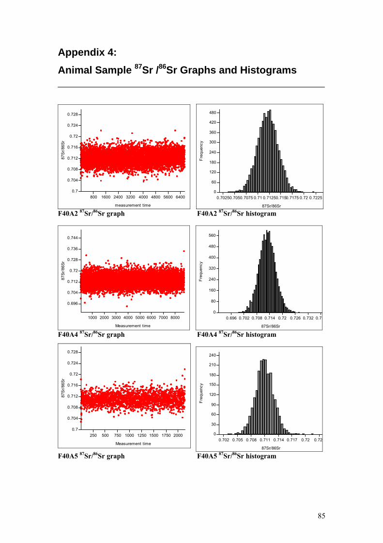
85
Appendix 4: Animal Sample 87Sr /86Sr Graphs and Histograms
800 1600 2400 3200 4000 4800 5600 6400
measurement time
0.7
0.704
0.708
0.712
0.716
0.72
0.724
0.728
87S
r/86
Sr
0.70250.7050.7075 0.71 0.71250.7150.7175 0.72 0.7225
87Sr/86Sr
0
60
120
180
240
300
360
420
480
Freq
uenc
y
F40A2 87Sr/86Sr graph F40A2 87Sr/86Sr histogram
1000 2000 3000 4000 5000 6000 7000 8000
Measurement time
0.696
0.704
0.712
0.72
0.728
0.736
0.744
87Sr
/86S
r
0.696 0.702 0.708 0.714 0.72 0.726 0.732 0.73
87Sr/86Sr
0
80
160
240
320
400
480
560
Fre
quen
cy
F40A4 87Sr/86Sr graph F40A4 87Sr/86Sr histogram
250 500 750 1000 1250 1500 1750 2000
Measurement time
0.7
0.704
0.708
0.712
0.716
0.72
0.724
0.728
87S
r/86S
r
0.702 0.705 0.708 0.711 0.714 0.717 0.72 0.72
87Sr/86Sr
0
30
60
90
120
150
180
210
240
Fre
quen
cy
F40A5 87Sr/86Sr graph F40A5 87Sr/86Sr histogram
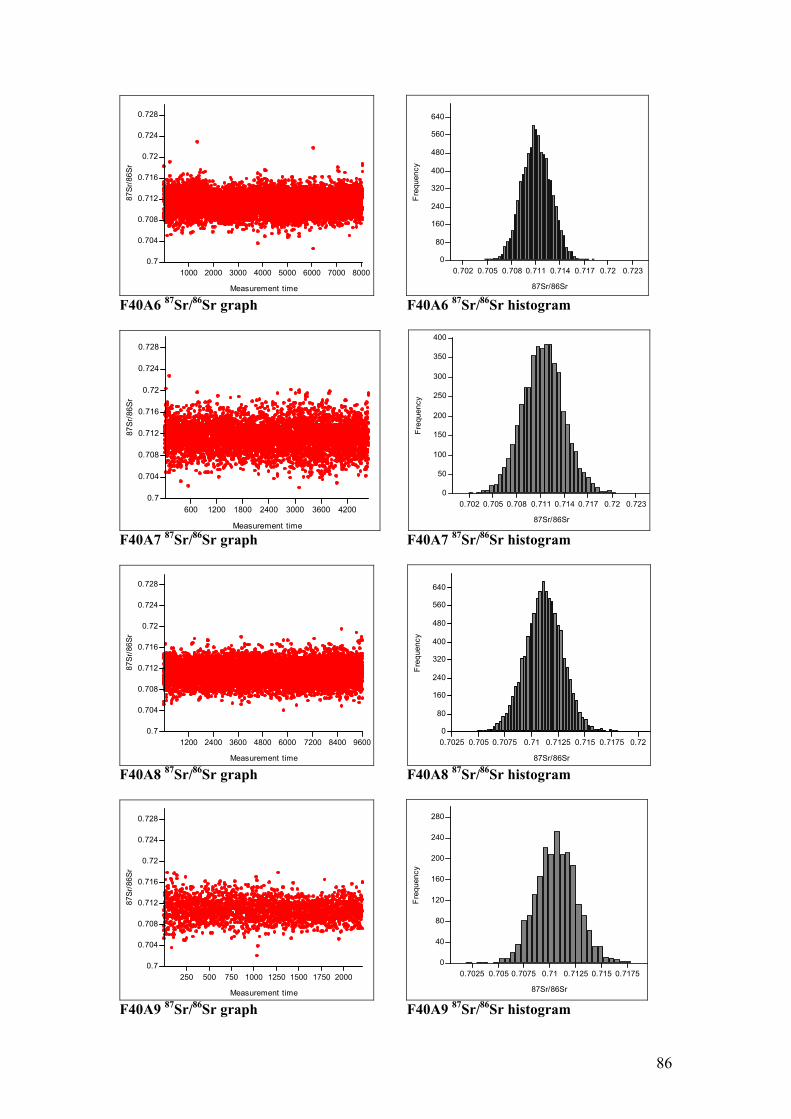
86
1000 2000 3000 4000 5000 6000 7000 8000
Measurement time
0.7
0.704
0.708
0.712
0.716
0.72
0.724
0.728
87S
r/86S
r
0.702 0.705 0.708 0.711 0.714 0.717 0.72 0.723
87Sr/86Sr
0
80
160
240
320
400
480
560
640
Freq
uenc
y
F40A6 87Sr/86Sr graph F40A6 87Sr/86Sr histogram
600 1200 1800 2400 3000 3600 4200
Measurement time
0.7
0.704
0.708
0.712
0.716
0.72
0.724
0.728
87Sr
/86S
r
0.702 0.705 0.708 0.711 0.714 0.717 0.72 0.723
87Sr/86Sr
0
50
100
150
200
250
300
350
400
Freq
uenc
y
F40A7 87Sr/86Sr graph F40A7 87Sr/86Sr histogram
1200 2400 3600 4800 6000 7200 8400 9600
Measurement time
0.7
0.704
0.708
0.712
0.716
0.72
0.724
0.728
87S
r/86S
r
0.7025 0.705 0.7075 0.71 0.7125 0.715 0.7175 0.72
87Sr/86Sr
0
80
160
240
320
400
480
560
640
Fre
quen
cy
F40A8 87Sr/86Sr graph F40A8 87Sr/86Sr histogram
250 500 750 1000 1250 1500 1750 2000
Measurement time
0.7
0.704
0.708
0.712
0.716
0.72
0.724
0.728
87S
r/86S
r
0.7025 0.705 0.7075 0.71 0.7125 0.715 0.7175
87Sr/86Sr
0
40
80
120
160
200
240
280
Freq
uenc
y
F40A9 87Sr/86Sr graph F40A9 87Sr/86Sr histogram
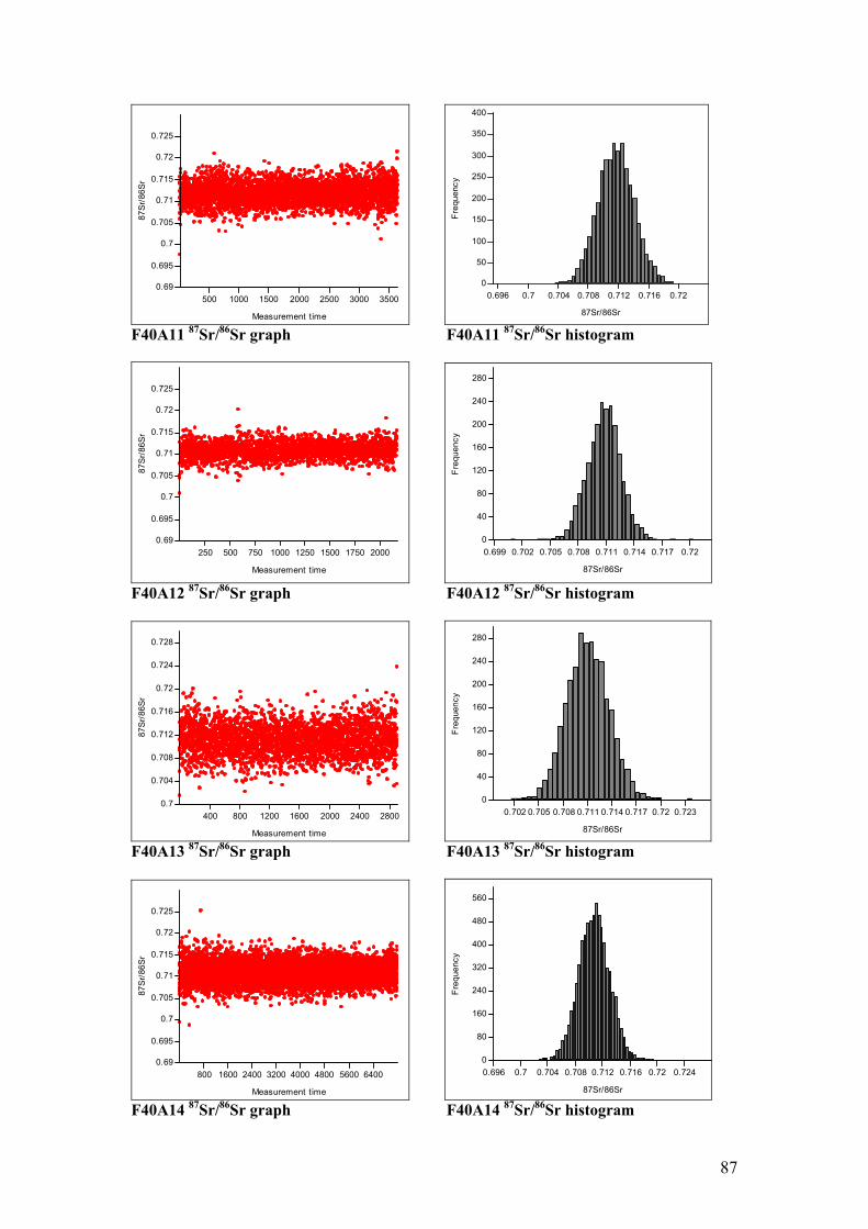
87
500 1000 1500 2000 2500 3000 3500
Measurement time
0.69
0.695
0.7
0.705
0.71
0.715
0.72
0.72587
Sr/8
6Sr
0.696 0.7 0.704 0.708 0.712 0.716 0.72
87Sr/86Sr
0
50
100
150
200
250
300
350
400
Freq
uenc
y
F40A11 87Sr/86Sr graph F40A11 87Sr/86Sr histogram
250 500 750 1000 1250 1500 1750 2000
Measurement time
0.69
0.695
0.7
0.705
0.71
0.715
0.72
0.725
87S
r/86
Sr
0.699 0.702 0.705 0.708 0.711 0.714 0.717 0.72
87Sr/86Sr
0
40
80
120
160
200
240
280
Fre
quen
cy
F40A12 87Sr/86Sr graph F40A12 87Sr/86Sr histogram
400 800 1200 1600 2000 2400 2800
Measurement time
0.7
0.704
0.708
0.712
0.716
0.72
0.724
0.728
87S
r/86S
r
0.702 0.705 0.708 0.711 0.714 0.717 0.72 0.723
87Sr/86Sr
0
40
80
120
160
200
240
280
Fre
quen
cy
F40A13 87Sr/86Sr graph F40A13 87Sr/86Sr histogram
800 1600 2400 3200 4000 4800 5600 6400
Measurement time
0.69
0.695
0.7
0.705
0.71
0.715
0.72
0.725
87S
r/86S
r
0.696 0.7 0.704 0.708 0.712 0.716 0.72 0.724
87Sr/86Sr
0
80
160
240
320
400
480
560
Fre
quen
cy
F40A14 87Sr/86Sr graph F40A14 87Sr/86Sr histogram
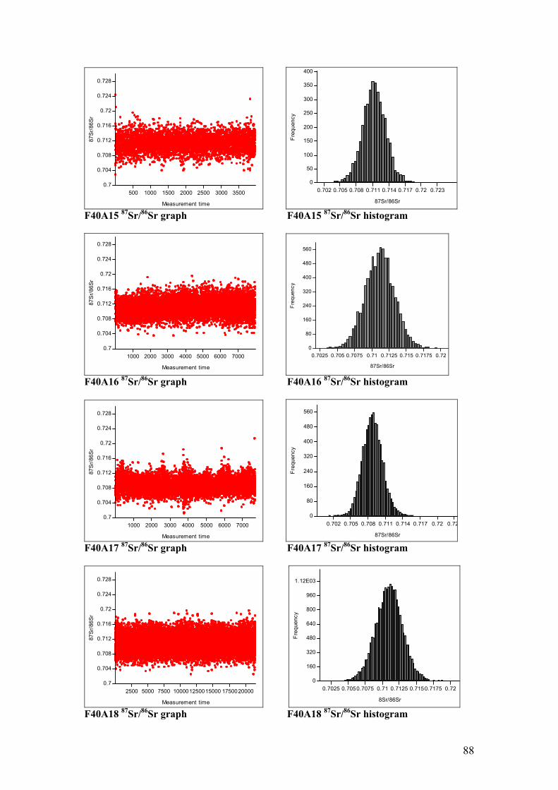
88
500 1000 1500 2000 2500 3000 3500
Measurement time
0.7
0.704
0.708
0.712
0.716
0.72
0.724
0.728
87S
r/86S
r
0.702 0.705 0.708 0.711 0.714 0.717 0.72 0.723
87Sr/86Sr
0
50
100
150
200
250
300
350
400
Fre
quen
cy
F40A15 87Sr/86Sr graph F40A15 87Sr/86Sr histogram
1000 2000 3000 4000 5000 6000 7000
Measurement time
0.7
0.704
0.708
0.712
0.716
0.72
0.724
0.728
87S
r/86
Sr
0.7025 0.705 0.7075 0.71 0.7125 0.715 0.7175 0.72
87Sr/86Sr
0
80
160
240
320
400
480
560
Fre
quen
cy
F40A16 87Sr/86Sr graph F40A16 87Sr/86Sr histogram
1000 2000 3000 4000 5000 6000 7000
Measurement time
0.7
0.704
0.708
0.712
0.716
0.72
0.724
0.728
87S
r/86S
r
0.702 0.705 0.708 0.711 0.714 0.717 0.72 0.72
87Sr/86Sr
0
80
160
240
320
400
480
560
Fre
quen
cy
F40A17 87Sr/86Sr graph F40A17 87Sr/86Sr histogram
2500 5000 7500 100001250015000 1750020000
Measurement time
0.7
0.704
0.708
0.712
0.716
0.72
0.724
0.728
87S
r/86S
r
0.7025 0.7050.7075 0.71 0.7125 0.7150.7175 0.72
8Sr/86Sr
0
160
320
480
640
800
960
1.12E03
Fre
quen
cy
F40A18 87Sr/86Sr graph F40A18 87Sr/86Sr histogram

89
400 800 1200 1600 2000 2400
Measurement time
0.69
0.695
0.7
0.705
0.71
0.715
0.72
0.72587
Sr/8
6Sr
0.7 0.704 0.708 0.712 0.716 0.72 0.724 0.728
87Sr/86Sr
0
40
80
120
160
200
240
280
Fre
quen
cy
F40A19 87Sr/86Sr graph F40A19 87Sr/86Sr histogram
500 1000 1500 2000 2500 3000 3500 4000
Measurement time
0.69
0.695
0.7
0.705
0.71
0.715
0.72
0.725
87S
r/86
Sr
0.7 0.704 0.708 0.712 0.716 0.72 0.724 0.728
87Sr/86Sr
0
50
100
150
200
250
300
350
400
Fre
quen
cy
F40A20 87Sr/86Sr graph F40A20 87Sr/86Sr histogram
400 800 1200 1600 2000 2400 2800
Measurement time
0.7
0.704
0.708
0.712
0.716
0.72
0.724
0.728
87S
r/86S
r
0.702 0.705 0.708 0.711 0.714 0.717 0.72 0.723
87Sr/86Sr
0
40
80
120
160
200
240
280
Fre
quen
cy
F40A21 87Sr/86Sr graph F40A21 87Sr/86Sr histogram
1000 2000 3000 4000 5000 6000 7000
Measurement time
0.69
0.695
0.7
0.705
0.71
0.715
0.72
0.725
87S
r/86S
r
0.696 0.7 0.704 0.708 0.712 0.716 0.72 0.724 0.728
87Sr/86Sr
0
80
160
240
320
400
480
560
Fre
quen
cy
F40A23 87Sr/86Sr graph F40A23 87Sr/86Sr histogram
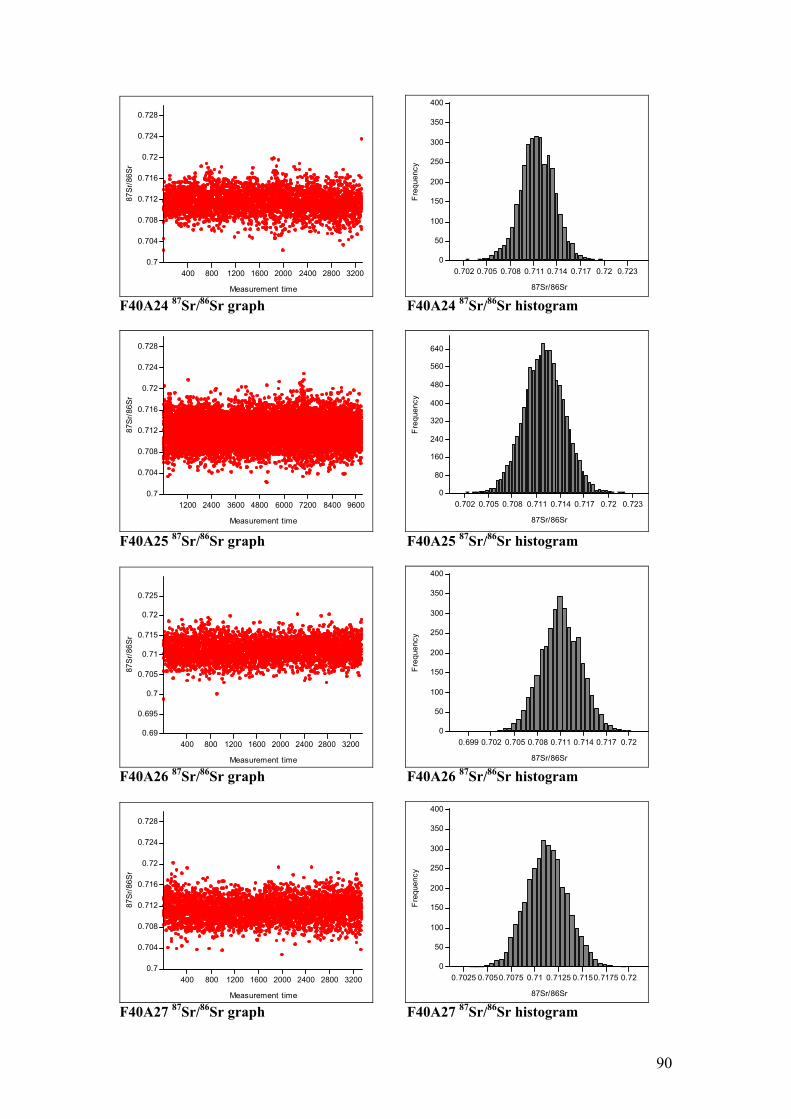
90
400 800 1200 1600 2000 2400 2800 3200
Measurement time
0.7
0.704
0.708
0.712
0.716
0.72
0.724
0.728
87S
r/86S
r
0.702 0.705 0.708 0.711 0.714 0.717 0.72 0.723
87Sr/86Sr
0
50
100
150
200
250
300
350
400
Fre
quen
cy
F40A24 87Sr/86Sr graph F40A24 87Sr/86Sr histogram
1200 2400 3600 4800 6000 7200 8400 9600
Measurement time
0.7
0.704
0.708
0.712
0.716
0.72
0.724
0.728
87S
r/86
Sr
0.702 0.705 0.708 0.711 0.714 0.717 0.72 0.723
87Sr/86Sr
0
80
160
240
320
400
480
560
640
Fre
quen
cy
F40A25 87Sr/86Sr graph F40A25 87Sr/86Sr histogram
400 800 1200 1600 2000 2400 2800 3200
Measurement time
0.69
0.695
0.7
0.705
0.71
0.715
0.72
0.725
87S
r/86S
r
0.699 0.702 0.705 0.708 0.711 0.714 0.717 0.72
87Sr/86Sr
0
50
100
150
200
250
300
350
400
Fre
quen
cy
F40A26 87Sr/86Sr graph F40A26 87Sr/86Sr histogram
400 800 1200 1600 2000 2400 2800 3200
Measurement time
0.7
0.704
0.708
0.712
0.716
0.72
0.724
0.728
87S
r/86S
r
0.7025 0.7050.7075 0.71 0.7125 0.7150.7175 0.72
87Sr/86Sr
0
50
100
150
200
250
300
350
400
Fre
quen
cy
F40A27 87Sr/86Sr graph F40A27 87Sr/86Sr histogram


![[A J S ., 1999, P. 589–610] STABLE ISOTOPE TRACING …earth.geology.yale.edu/~ajs/1999/07-09.1999.04Martens.pdfWe were seeking to measure concentration distributions of dissolved](https://img.pdfslide.us/doc/110x75/5aa686037f8b9a2f048ec984/a-j-s-1999-p-589610-stable-isotope-tracing-earth-ajs199907-09199904martenspdfwe.jpg)