Embed Size (px)
Citation preview
Strong Dipolar Effects in a ChromiumBose-Einstein Condensate
Diplomarbeitvorgelegt von
Bernd Fröhlich
Hauptberichter: Prof. Dr. Tilman PfauMitberichter: Prof. Dr. J. Wrachtrup
5. Physikalisches InstitutUniversität Stuttgart
13. Juli 2007

Contents
Zusammenfassung 1
1. Introduction 3
2. Scattering Theory and Feshbach Resonances 72.1. Collisional Dynamics of Ultra-Cold Atomic Gases . . . . . . . . . . . . . . . . 7
2.1.1. Scattering Theory . . . . . . . . . . . . . . . . . . . . . . . . . . . . . . 82.1.2. Low-Energy Limit . . . . . . . . . . . . . . . . . . . . . . . . . . . . . 11
2.2. Tuning the Scattering Length via Feshbach Resonances . . . . . . . . . . . . . 122.3. Theory of Feshbach Resonances . . . . . . . . . . . . . . . . . . . . . . . . . . 15
2.3.1. Formal Solution . . . . . . . . . . . . . . . . . . . . . . . . . . . . . . . 152.3.2. Derivation of the Scattering Properties . . . . . . . . . . . . . . . . . . 16
2.4. Feshbach Resonances of Chromium . . . . . . . . . . . . . . . . . . . . . . . . 18
3. Dipolar Bose-Einstein Condensates 233.1. Bose-Einstein Condensation . . . . . . . . . . . . . . . . . . . . . . . . . . . . 23
3.1.1. Statistical Description . . . . . . . . . . . . . . . . . . . . . . . . . . . 233.1.2. Mean-Field Approximation and Thomas-Fermi Limit . . . . . . . . . . 24
3.2. Hydrodynamic Description of the Condensate Dynamics . . . . . . . . . . . . 263.3. Dipole-Dipole Interaction in a Bose-Einstein Condensate . . . . . . . . . . . . 29
3.3.1. In-Trap Condensate Shape . . . . . . . . . . . . . . . . . . . . . . . . . 293.3.2. Expansion Dynamics . . . . . . . . . . . . . . . . . . . . . . . . . . . . 31
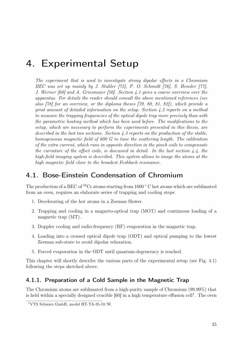
4. Experimental Setup 354.1. Bose-Einstein Condensation of Chromium . . . . . . . . . . . . . . . . . . . . 35
4.1.1. Preparation of a Cold Sample in the Magnetic Trap . . . . . . . . . . . 354.1.2. Forced Evaporation in the Optical Dipole Trap . . . . . . . . . . . . . 38
4.2. Measurement of the Trapping Frequencies . . . . . . . . . . . . . . . . . . . . 394.3. Producing a Homogeneous Magnetic Field of 600 Gauss . . . . . . . . . . . . . 42
4.3.1. Curvature Compensation . . . . . . . . . . . . . . . . . . . . . . . . . . 424.3.2. Technical Realization . . . . . . . . . . . . . . . . . . . . . . . . . . . . 454.3.3. Calibration of the Curvature Compensation . . . . . . . . . . . . . . . 464.3.4. Magnetic Field Gradient . . . . . . . . . . . . . . . . . . . . . . . . . . 50
4.4. High-Field Imaging System . . . . . . . . . . . . . . . . . . . . . . . . . . . . . 504.4.1. Imaging at Low Magnetic Fields . . . . . . . . . . . . . . . . . . . . . . 514.4.2. Imaging at High Magnetic Fields . . . . . . . . . . . . . . . . . . . . . 534.4.3. Fringe Reduction . . . . . . . . . . . . . . . . . . . . . . . . . . . . . . 55
5. Strong Dipolar Effects in a Chromium Bose-Einstein Condensate 575.1. Lifetime and Scattering Length Close to a Feshbach Resonance . . . . . . . . . 57
5.1.1. Lifetime of the Condensate . . . . . . . . . . . . . . . . . . . . . . . . . 585.1.2. Tuning the Scattering Length . . . . . . . . . . . . . . . . . . . . . . . 59
5.2. Strong Dipolar Effects . . . . . . . . . . . . . . . . . . . . . . . . . . . . . . . 615.2.1. Variation of the Condensate Aspect Ratio . . . . . . . . . . . . . . . . 615.2.2. Time-of-Flight Measurements . . . . . . . . . . . . . . . . . . . . . . . 63
6. Conclusion and Outlook 67
A. Two-Frequency Acousto-Optic Modulator Driver 71A.1. Introduction to Acousto-Optic Modulation . . . . . . . . . . . . . . . . . . . . 71A.2. Improving the Beam Stability with the Two-Frequency Method . . . . . . . . 73A.3. Technical Realization of a Two-Frequency Driver . . . . . . . . . . . . . . . . . 74A.4. Measurements of the Position Stability . . . . . . . . . . . . . . . . . . . . . . 76
B. Chromium 81B.1. General Properties . . . . . . . . . . . . . . . . . . . . . . . . . . . . . . . . . 81B.2. Feshbach Resonances . . . . . . . . . . . . . . . . . . . . . . . . . . . . . . . . 82
C. Mathematical Supplement 83C.1. Incomplete Elliptic Integral Function . . . . . . . . . . . . . . . . . . . . . . . 83C.2. Magnetic Field of a Cylindrically Symmetric Current Distribution . . . . . . . 84C.3. Dependence of the Optical Density of Linear Polarized Light to σ−-Light . . . 86
Bibliography 86
D. Danksagung 95
Zusammenfassung
Im Rahmen dieser Arbeit wurde erstmals eine Supraflüssigkeit realisiert, die eine starke Dipol-Dipol-Wechselwirkung zwischen ihren mikroskopischen Bestandteilen aufweist [1]. Diese Su-praflüssigkeit kann in Analogie zu klassischen Ferroflüssigkeiten eine Quanten-Ferroflüssigkeitgenannt werden. Die Dipol-Dipol-Wechselwirkung unterscheidet sich durch ihren anisotro-pen — also symmetriebrechenden — und langreichweitigen Charakter fundamental von derKontakt-Wechselwirkung, welche bisher in allen Experimenten mit ultra-kalten atomarenGasen dominierend war. Die Realisierung einer Quanten-Ferroflüssigkeit ist daher der ersteSchritt zur Untersuchung einer Fülle neuer physikalischer Phänomene in ultra-kalten Ga-sen [2].
Eine Supraflüssigkeit weist einige außerordentliche Eigenschaften auf, z.B. fliesst sie ohneReibung und hat eine unendliche thermische Leitfähigkeit. Diese Eigenschaften sind eine di-rekte Folge der bosonischen Natur ihrer Bestandteile. Das erste System in dem suprafluideEigenschaften beobachtet wurden war flüssiges Helium 1937 [3, 4]. Hierbei wurde das bosoni-sche Isotop 4He verwendet. Aber auch in flüssigem Helium bestehend aus dem fermionischenIsotop 3He wurde 35 Jahre später Suprafluidität nachgewiesen [5]. Dies ist durch eine Paar-bildung der 3He Atomen zu Bosonen möglich. Ein weiterer Meilenstein in der Untersuchungvon Supraflüssigkeiten war die Realisierung eines Bose-Einstein Kondensats in verdünntenatomaren Gasen 1995 [6, 7]. Diese Systeme erlauben einer hervorragende Kontrolle der expe-rimentellen Parameter und haben eine Vielzahl grundlegender Untersuchungen suprafluiderPhänomene erlaubt. Aber auch in fermionischen atomaren Gasen wurde zehn Jahre späterSuprafluidität nachgewiesen [8], die wiederum nur durch eine Paarbildung der Atome möglichist. In diesen Experimenten mit ultra-kalten bosonischen oder fermionische Gasen war bisherdie Kontakt-Wechselwirkung dominierend, deren Stärke durch einen einzigen Parameter, dieStreulänge a, beschrieben werden kann.
Trotz des vergleichsweise großen Dipolmoments von 6 µB von 52Cr Atomen ist die Kontakt-Wechselwirkung auch in einem Chrom Bose-Einstein Kondensat dominierend. Die Dipol-Dipol-Wechselwirkung kann als Störung in der Beschreibung des Kondensats berücksichtigtwerden. Das erste Chrom Bose-Einstein Kondensat wurde 2004 von Griesmaier und Mit-arbeitern realisiert [9]. Ein Jahr später konnte der Effekt der Dipol-Dipol-Wechselwirkungerstmalig anhand einer Modifizierung der Form des Kondensates nachgewiesen werden [10].
Eine Methode, die die Stärke der Dipol-Dipol-Wechselwirkung relativ zur Kontakt-Wechsel-wirkung erhöht, ist die Verwendung einer Feshbach Resonanz um die Streulänge und somitdie Stärke der Kontakt-Wechselwirkung zu verringern. Feshbach Resonanzen wurden 1998erstmals in einem ultra-kalten atomaren Gas nachgewiesen [11]. Sie erlauben es durch Anlegeneines Magnetfelds die Streulänge über einen weiten Bereich von positiven bis hin zu negativenWerten zu varriieren. Auch in einem ultra-kalten Gas aus 52Cr Atomen wurden im Jahr 2004Feshbach Resonanzen nachgewiesen [12].
Im Rahmen dieser Arbeit wird die breiteste dieser Resonanzen verwendet, um die Streulän-ge von Chrom auf ein Fünftel des ursprünglichen Wertes zu verringern. Diese Verringerung
1
Zusammenfassung
führt gleichzeitig zu einer Erhöhung der relativen Stärke der Dipol-Dipol-Wechselwirkungum einen Faktor fünf. Somit wird erstmals eine Supraflüssigkeit erzeugt, die stark durchden dipolaren Charakter ihrer Bestandteile beeinflusst ist. In einer Serie von Experimentenwird die Anwendbarkeit der Methode demonstriert, um diese Quanten-Ferroflüssigkeit zuuntersuchen. Diese Arbeit enthält neben einer ausführlichen Beschreibung der durchgeführ-ten Experimente eine Einführung in die theoretische Beschreibung von Feshbach Resonanzenund dipolaren Kondensaten, sowie eine Beschreibung der Modifikationen des Experiments,die nötig waren, um die Ergebnisse zu ermöglichen. Ein ausführlicher Anhang berichtet überden ebenfalls im Rahmen dieser Arbeit realisierten akusto-optischen Modulator (AOM) Trei-ber, welcher durch Verwenden von zwei verschiedenen Radiofrequenzsignalen die Stabilitätder Dipolfallen-Laserstrahlen signifikant erhöht [13].
2
1. Introduction
A superfluid is a quantum fluid. The quantum character of any microscopic particle, whichis usually not visible in macroscopic bodies, gives rise to their exceptional properties, likezero viscosity or infinite thermal conductivity. The quantum character is visible, because thephase relation between the quantum particles of which it is composed of is fixed, whereas itis random in classical bodies, leading on average to the classical properties. The collectivebehaviour of the quantum particles arises from the Bose statistics describing their many-bodystate [14]. The first system to show superfluid character was liquid helium in 1937 [3, 4]. Notonly the bosonic 4He undergoes the phase transition to a superfluid, also 3He condenses toa superfluid via a pairing mechanism of the fermionic atoms [5], analogous to the Cooperpairing responsible for superconductivity. The symmetry-breaking interaction in 3He, causedby the p-wave pairing, substantially enriches the physical properties of the 3He superfluidcompared to the 4He system [15].
A new system that allows to study superfluidity are quantum-degenerate bosonic or fermio-nic gases. The narrow path to cool down an atomic sample to a state which reveals thequantum nature — without solidifying the sample — has prevented the realization of suchsystems until 1995. First the group of Wieman and Cornell [6] and shortly afterwards thegroup of Ketterle [7] produced quantum-degenerate bosonic gases of 87Rb and 23Na atoms.These Bose-Einstein condensates (BECs) of dilute gases, later also realized with 7Li [16], spin-polarized hydrogen [17], 85Rb [18], metastable Helium [19], 41K [20], 133Cs [21], 174Yb [22],52Cr [9] and recently with 39K [23], led to many experiments on superfluid properties, forexample on collective oscillations [24] or vortices [25]. The dominant interaction underlyingthese experiments is the isotropic and short-range contact interaction, which for ultra-coldatoms is described by a single parameter, the scattering length a [26]. The tunability of thisparameter via Feshbach resonances [11] is an important tool to study a wide range of physicalregimes.
A quantum-degenerate gas of fermions, first realized in 1999 with potassium atoms [27],shows superfluidity via a pairing of the atoms like in 3He [8]. Two atoms in different spinstates form a weakly bound Cooper pair, which is a boson and can undergo condensation.The theory describing the paring was developed in 1957 mainly by Bardeen, Cooper andSchrieffer [28]. The condensed state of Cooper pairs is therefore called BCS state. Thepairing mechanism depends strongly on the interaction between the atoms. Like for bosonsthe dominant interaction is the contact interaction. Hence, it is tunable via Feshbach reso-nances [29, 30, 31], which allowed to study the crossover of the BCS state to a condensateof diatomic molecules [32, 33, 34]. A quantum gas of fermions is an ideal model systemto explore the formation of a superfluid made of paired fermions. Besides the interactionstrength, also the ratio of the atoms in different spin states can be controlled precisely. Thus,the formation is studied over a wide parameter range (see for example [35]).
Another interaction, which promises the realization of a new type of superfluid, is thedipole-dipole interaction. It attracts a large attention of theoreticians currently, apparent
3
1. Introduction
through about 60 publications on this topic over the last 5 years. Dipole-dipole interactionhas long-range character and is anisotropic. This distinguishes it significantly from contactinteraction. The symmetry-break corresponding to the anisotropy is predicted to give rise to avariety of new physical phenomena [2], similar to the enrichment of the physical properties of3He compared to 4He. Among these new phenomena are e.g. novel quantum phases in opticallattices, such as checkerboard or supersolid phases [36], or structured density profiles [37],including biconcave density distributions in pancake-shaped traps [38]. Dipolar effects shouldalso enrich the field of spinor physics [39, 40, 41]. Another interesting prediction for thesesystems is a roton-like excitation spectrum [42].
A superfluid with strong dipolar interaction can be called a quantum ferrofluid, in analogyto classical ferrofluids. Polar molecules in their vibrational ground state are a possibility torealize them with electric dipoles. Although progress has been made recently in slowing andtrapping of polar molecules (see for example [43]), the densities and temperatures reachedare still far from quantum-degeneracy. Polar molecules created from two ultra-cold atomicspecies via Feshbach resonances [44] are an actively explored alternative [45]. However, untilnow it is not possible to bring these molecules to their vibrational ground state [46]. Electricdipoles induced by dc electric fields [47] or by light [48] might be an alternative.
The first quantum ferrofluid was realized with magnetic dipoles [1] and is presented inthis thesis. Our experimental approach makes use of the large magnetic dipole moment of6µB of Chromium atoms to realize such a quantum system. Important steps that paved theway towards this development were the observation of Feshbach resonances in 2004 [12] andthe condensation of Chromium in 2004 [9]. Besides, experiments on the expansion dynamicsof Chromium showed in 2005 [10] for the first time dipolar effects in a BEC. However, therelative strength of the dipole-dipole interaction to the contact interaction in these measure-ments corresponded only to a small perturbation, although the dipole-dipole interaction is36 times larger than in standard alkali quantum gases. This is changed with the experimentsthat are a part of this thesis. By using a Feshbach resonance to tune the scattering lengtha, the relative strength of the dipole-dipole interaction is increased by a factor of 5. Thismodifies the condensate properties way beyond the perturbative regime and constitutes thefirst realization of a quantum ferrofluid.
This thesis is organized as follows:In chapter 2 the theory of Feshbach resonances is introduced. To provide a theoretical ba-sis to understand the physics of Feshbach resonances, the first section reports on scatteringtheory with a focus on the scattering properties of ultra-cold atomic gases. The second sec-tion discusses the phenomenological properties of Feshbach resonances, which supports thetheoretical description in section 3. The theoretical approach presented follows closely [44]and [49]. The last section describes the Feshbach resonances of Chromium, which have beenobserved in a series of measurements in 2004 [12].
Chapter 3 gives an introduction to the theoretical description of Bose-Einstein condensateswith dipole-dipole interaction. To introduce the theoretical methods used to describe BECs,and to allow a comparison of condensates with and without dipole-dipole interaction, the firsttwo sections take only contact interaction into account. The first section discusses importantproperties of the steady-state of BECs. The mean-field description with a macroscopic wavefunction and the Thomas-Fermi approximation are introduced. The second section reports
4
on the hydrodynamic description of the condensate dynamics. In the third section this hy-drodynamic theory is expanded to include dipole-dipole interaction. The main results of thistheory, which are used in the data analysis of the experiments on strong dipolar effects, arepresented.
The apparatus that is used for the experiments is described in chapter 4. The first sec-tion gives a coarse overview of the experiment, more details can be found for example in [50].The important steps to produce a quantum-degenerate gas of Chromium atoms are described.The second section reports on the measurements of the trapping frequencies of the opticaldipole trap, which are performed with a new method, that has not been used in our setupbefore. Next, I discuss modifications of the apparatus, which are done to perform the ex-periments presented in this thesis. The third section reports on the production of a stable,homogenous magnetic field at ∼ 600 G, which is needed to tune the scattering length a via aFeshbach resonance. Also described is the calibration of the curvature compensation, whichallows us to produce BECs at these high magnetic fields. The last section discusses thehigh-field imaging system, which is used to image the atoms at the high magnetic fields.
Finally, in chapter 5 the experimental results on strong dipolar effects in a quantum gasare presented. In the first section the broadest Feshbach resonance at 589.1 G is character-ized. This resonance is used to tune the scattering length a. Both measurements on thelifetime and the variation of a in the vicinity of the resonance are described. In the secondsection the observation of strong dipolar effects is discussed, which are apparent through achange of the condensate shape. In a time-of-flight series our control on the system is demon-strated.
An appendix provides additional information. In particular it reports on a two-frequencyacousto-optic modulator driver realized as a part of this thesis [13], which is included in thesetup to improve the stability of the optical dipole trap.
5

1. Introduction
6
2. Scattering Theory and FeshbachResonances
In the experiments presented in this thesis a Feshbach resonance is used to tune thecontact interaction strength. The theoretical description of Feshbach resonances isintroduced in this chapter. For a basic understanding of these resonances, scatter-ing theory is required. Hence, section 2.1 gives an overview on scattering theory,focusing on the collision dynamics of ultra-cold atoms. The presentation followsclosely [26] and chapter 8 in [51]. The partial wave decomposition for sphericallysymmetric potentials is not discussed. I chose a more general approach to preparethe theoretical description of Feshbach resonances and for brevity. For informationon the partial wave decomposition the reader is referred to the standard literatureon scattering theory [51, 52, 53]. In section 2.2 the physical process underlying aFeshbach resonance is discussed and their properties are described phenomenolog-ically. With this background, in section 2.3 the theory of Feshbach resonances isintroduced. The main steps to obtain an expression for the scattering length as afunction of the magnetic field B are presented. The last section 2.4 reports on theFeshbach properties of 52Cr.
2.1. Collisional Dynamics of Ultra-Cold Atomic Gases
A basic knowledge of collision physics is important to understand the properties of ultra-cold atomic gases. Elastic collisions for example ensure the thermalization of a gas, whichis crucial for evaporative cooling. A second example is the expansion of a BEC which isgoverned by the mean-field interaction. For a dilute gas the interaction range r0 betweentwo atoms (typically on the order of a few nm) is much smaller than the mean distancebetween them (typically a few 100 nm). This allows to reduce the theoretical descriptionof the collisions to the scattering problem of only two atoms [26]. They interact via theirmolecular potential, which consists of several contributions like the exchange interaction orthe van der Waals interaction. For ultra-cold atomic samples a detailed knowledge of themolecular potential is not needed to describe the collision process: The thermal de Brogliewavelength
λth =
√2π~2
mkBT, (2.1)
where m is the atomic mass and T is the temperature of the gas, is larger than r0 andthe details of the potential are not resolved. As we shall see, the scattering process is thenisotropic and is described by a single parameter, the scattering length a. The complicatedmolecular potential is replaced by a simple contact interaction potential.
7
2. Scattering Theory and Feshbach Resonances
V (r)
Scatteringpotential
Incomingparticle
Detector
ϑ∆Ω
x
z
y
rd
∆A
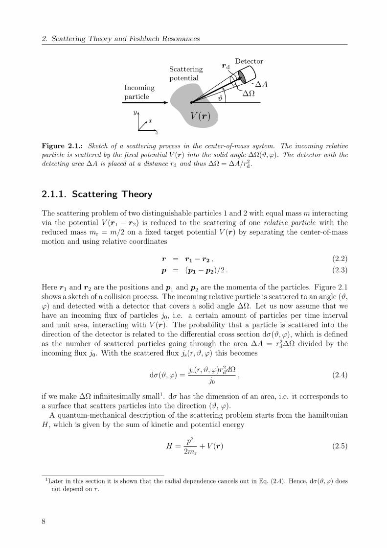
Figure 2.1.: Sketch of a scattering process in the center-of-mass system. The incoming relativeparticle is scattered by the fixed potential V (r) into the solid angle ∆Ω(ϑ, ϕ). The detector with thedetecting area ∆A is placed at a distance rd and thus ∆Ω = ∆A/r2d.
2.1.1. Scattering Theory
The scattering problem of two distinguishable particles 1 and 2 with equal mass m interactingvia the potential V (r1 − r2) is reduced to the scattering of one relative particle with thereduced mass mr = m/2 on a fixed target potential V (r) by separating the center-of-massmotion and using relative coordinates
r = r1 − r2 , (2.2)p = (p1 − p2)/2 . (2.3)
Here r1 and r2 are the positions and p1 and p2 are the momenta of the particles. Figure 2.1shows a sketch of a collision process. The incoming relative particle is scattered to an angle (ϑ,ϕ) and detected with a detector that covers a solid angle ∆Ω. Let us now assume that wehave an incoming flux of particles j0, i.e. a certain amount of particles per time intervaland unit area, interacting with V (r). The probability that a particle is scattered into thedirection of the detector is related to the differential cross section dσ(ϑ, ϕ), which is definedas the number of scattered particles going through the area ∆A = r2
d∆Ω divided by theincoming flux j0. With the scattered flux js(r, ϑ, ϕ) this becomes
dσ(ϑ, ϕ) =js(r, ϑ, ϕ)r2
ddΩ
j0, (2.4)
if we make ∆Ω infinitesimally small1. dσ has the dimension of an area, i.e. it corresponds toa surface that scatters particles into the direction (ϑ, ϕ).
A quantum-mechanical description of the scattering problem starts from the hamiltonianH, which is given by the sum of kinetic and potential energy
H =p2
2mr
+ V (r) (2.5)
1Later in this section it is shown that the radial dependence cancels out in Eq. (2.4). Hence, dσ(ϑ, ϕ) doesnot depend on r.
8
2.1. Collisional Dynamics of Ultra-Cold Atomic Gases
of the relative particle. With the time-independent Schrödinger equation
Hψk(r) = Ekψk(r) (2.6)
we can calculate the stationary scattering eigenstates of H. We are interested only in theasymptotic behavior of these states as the mean distance between the atoms is much largerthan the interaction range r0. To calculate the asymptotic behavior, Eq. (2.6) is written inthe form
(∆ + k2)ψk(r) = U(r)ψk(r) , (2.7)
with the notationsk2 =
2mrEk
~2, U(r) =
2mr
~2V (r) . (2.8)
The concept of Green’s functions, known e.g. from the theory of electrodynamics, is a pow-erful tool to tackle a differential equation of the form of Eq. (2.7). With the Green’s functionGk(r), which is defined through the following equation
(∆ + k2)Gk(r) = δ(r) , (2.9)
where δ(r) is the Dirac delta function, a formal solution of Eq. (2.7) is
ψk(r) = ψ0(r) +
∫d3r′Gk(r − r′)U(r′)ψk(r′) . (2.10)
The first term ψ0(r) on the right hand side is the solution of the homogeneous differentialequation
(∆ + k2)ψ0(r) = 0 . (2.11)
It describes the incoming particle in the asymptotic limit. We choose the easiest non-trivialsolution of Eq. (2.11), a plane wave traveling in z direction ψ0(r) = eikz, not taking intoaccount the normalization problem.
It can be shown (see for example [53]), that the Green’s functions has two linear indepen-dent solutions
G±k (r) = − 1
4π
e±ikr
r(2.12)
corresponding to an outgoing, respectively incoming, spherical wave. Only the outgoingspherical wave G+
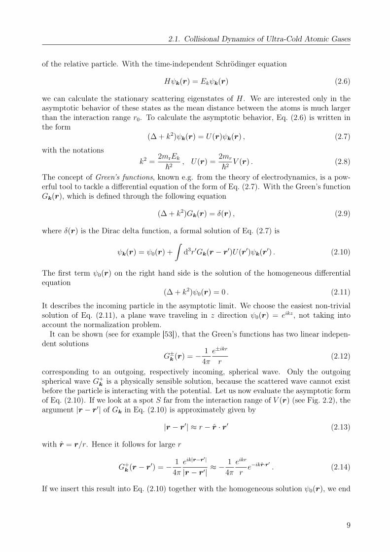
k is a physically sensible solution, because the scattered wave cannot existbefore the particle is interacting with the potential. Let us now evaluate the asymptotic formof Eq. (2.10). If we look at a spot S far from the interaction range of V (r) (see Fig. 2.2), theargument |r − r′| of Gk in Eq. (2.10) is approximately given by
|r − r′| ≈ r − r · r′ (2.13)
with r = r/r. Hence it follows for large r
G+k (r − r′) = − 1
4π
eik|r−r′|
|r − r′|≈ − 1
4π
eikr
re−ikr·r′ . (2.14)
If we insert this result into Eq. (2.10) together with the homogeneous solution ψ0(r), we end
9
2. Scattering Theory and Feshbach Resonances
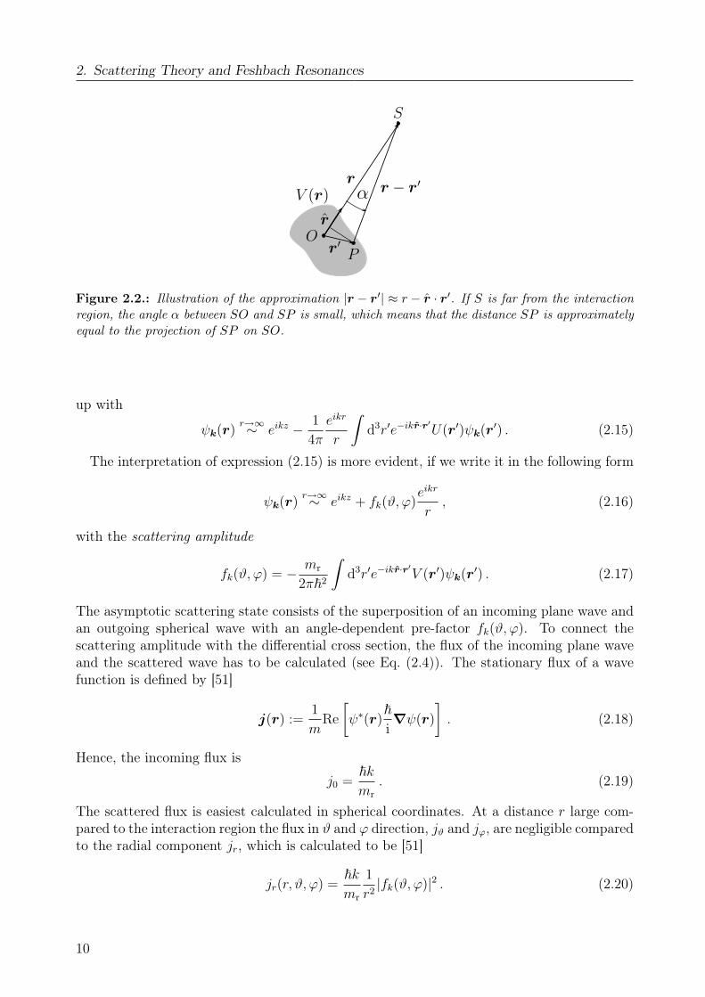
V (r)r
r − r′
r′
S
PO
α
r
Figure 2.2.: Illustration of the approximation |r − r′| ≈ r − r · r′. If S is far from the interactionregion, the angle α between SO and SP is small, which means that the distance SP is approximatelyequal to the projection of SP on SO.
up with
ψk(r)r→∞∼ eikz − 1
4π
eikr
r
∫d3r′e−ikr·r′U(r′)ψk(r′) . (2.15)
The interpretation of expression (2.15) is more evident, if we write it in the following form
ψk(r)r→∞∼ eikz + fk(ϑ, ϕ)
eikr
r, (2.16)
with the scattering amplitude
fk(ϑ, ϕ) = − mr
2π~2
∫d3r′e−ikr·r′V (r′)ψk(r′) . (2.17)
The asymptotic scattering state consists of the superposition of an incoming plane wave andan outgoing spherical wave with an angle-dependent pre-factor fk(ϑ, ϕ). To connect thescattering amplitude with the differential cross section, the flux of the incoming plane waveand the scattered wave has to be calculated (see Eq. (2.4)). The stationary flux of a wavefunction is defined by [51]
j(r) :=1
mRe
[ψ∗(r)
~i∇ψ(r)
]. (2.18)
Hence, the incoming flux is
j0 =~kmr
. (2.19)
The scattered flux is easiest calculated in spherical coordinates. At a distance r large com-pared to the interaction region the flux in ϑ and ϕ direction, jϑ and jϕ, are negligible comparedto the radial component jr, which is calculated to be [51]
jr(r, ϑ, ϕ) =~kmr
1
r2|fk(ϑ, ϕ)|2 . (2.20)
10
2.1. Collisional Dynamics of Ultra-Cold Atomic Gases
Inserting j0 and js(r, ϑ, ϕ) ≈ jr(r, ϑ, ϕ) into Eq. (2.4) results in a simple relation between thedifferential cross section and the scattering amplitude
dσ
dΩ(ϑ, ϕ) = |fk(ϑ, ϕ)|2 . (2.21)
The scattering amplitude is thus directly connected to the experiment.
2.1.2. Low-Energy Limit
Let us now discuss the low-energy limit and show that the scattering is isotropic in thisregime. In the low-energy limit the thermal de Broglie wavelength is large compared to theinteraction range (λth r0). In terms of the k-vector this is equivalent to k 1/r0. Themain contributions to the integral of Eq. (2.17) are given for |r′| . r0, where the potentialV (r) has significant values. The factor e−ikr·r′ in Eq. (2.17) is therefore approximately 1 askr · r′ . kr0 1 and hence
fk ≈ −mr
2π~2
∫d3r′V (r′)ψk(r′) . (2.22)
Consequently the interaction is isotropic, because the amplitude is independent of ϑ and ϕ.The integral equation (2.22) for fk is implicit, i.e. fk appears on both sides of Eq. (2.22)2.
The scattering length3 a is defined as
a := − limk→0
fk . (2.23)
It can be shown that a depends strongly on the details of V (r) and that a small variationin V (r) can lead to a divergence of a. This is the case e.g. for Feshbach resonances (seesection 2.2 and 2.3). For potentials with a finite a, the total cross section σ, given by theintegral of dσ/dΩ over the full 4π solid angle, is 4πa2. σ is thus equal to the scattering areaof a classical hard sphere with a radius given by twice the scattering length. This analogyhelps to get a descriptive understanding of a. However, it is only valid if a is positive, whichis not necessarily the case.
The total cross section changes, if the colliding particles are indistinguishable. In thiscase it cannot be distinguished which particle is going in which direction after the collision(see Fig. 2.3). Therefore the wave function ψk(r) has to be symmetrized (anti-symmetrized)for bosons (fermions) against particle exchange. For the scattering amplitude the particleexchange is equivalent to a substitution of (ϑ, ϕ) by (π−ϑ, ϕ+π) [26]. Hence the differentialcross section is
dσ
dΩ(ϑ, ϕ) = |fk(ϑ, ϕ) + εfk(π − ϑ, ϕ+ π)|2 , (2.24)
with ε = +1 for bosons and ε = −1 for fermions. Consequently, at low energies collisions arestrongly suppressed for fermions in the same quantum state and enhanced by a factor of 2
2This is changed with the Born approximation, where the scattered wave function ψk(r′) is replaced bythe incoming plane wave eikz (see for example [51] or [53]). The Born approximation is valid for weakinteracting particles. It cannot be applied in case of contact interaction, but is used to describe dipole-dipole interaction (see section 3.3).
3Equal to the s-wave scattering length in the description by partial waves if only l = 0 contributes.
11
2. Scattering Theory and Feshbach Resonances
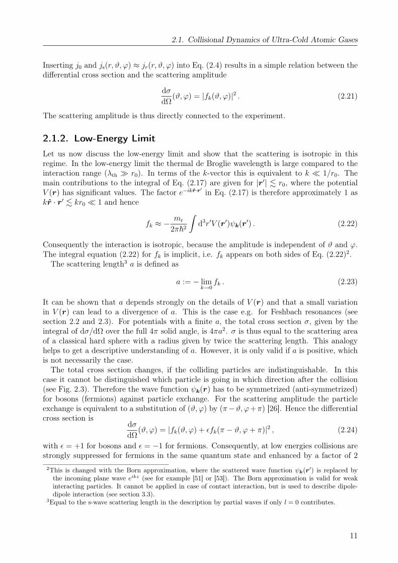
ϑ11
2
2π − ϑ
12
2
1
Figure 2.3.: Scattering of identical particles. For identical particles the two processes shown in thefigure are indistinguishable. The scattering amplitude fk(ϑ, ϕ) describing the left process is equal tofk(π − ϑ, ϕ+ π), which describes the right process.
for bosons, leading to a total cross section4 of 8πa2 instead of 4πa2.To obtain the macroscopic properties of an atomic gas from the microscopic theory of
binary collisions, a mean field description is used. The mean field description makes use ofa pseudo-potential, which replaces the complicated molecular potential between two atoms.This pseudo-potential must have the same scattering length a. A natural choice is a contactinteraction potential [26]
Vcontact(r) = gδ(r) . (2.25)
This potential has the same scattering length a for5
g =2π~2a
mr
=4π~2a
m. (2.26)
The form of the potential indicates the physical meaning of the sign of a, it determineswhether the contact interaction is attractive (a < 0) or repulsive (a > 0).
2.2. Tuning the Scattering Length via FeshbachResonances
The previous section has shown that the collisional properties in the low-energy limit arecompletely determined by a single parameter, the scattering length a. It has also been statedthat a small variation of the scattering potential can have a strong effect on a. This is thecase for Feshbach resonances, which allow to tune a with a magnetic field B over a widerange. To understand this phenomena, one needs to take a closer look at the atom-atominteraction. The molecular potential between two atoms depends on the internal atomicquantum states. For example, for two atoms with spin 1/2 the total spin can be either 0 or 1,leading to a singlet and a triplet potential with different strengths. To describe the physicsbehind a Feshbach resonance it is not enough to take into account only a single molecularpotential between the atoms, Feshbach resonances occur due to a coupling between differentpotentials.
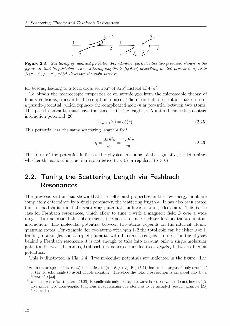
This is illustrated in Fig. 2.4. Two molecular potentials are indicated in the figure. The
4As the state specified by (ϑ, ϕ) is identical to (π− ϑ, ϕ+ π), Eq. (2.24) has to be integrated only over halfof the 4π solid angle to avoid double counting. Therefore the total cross section is enhanced only by afactor of 2 [54].
5To be more precise, the form (2.25) is applicable only for regular wave functions which do not have a 1/rdivergence. For none-regular functions a regularizing operator has to be included (see for example [26]for details).
12
2.2. Tuning the Scattering Length via Feshbach Resonances
Interatomic distance
Ene
rgy
Coupling
Kinetic energy
Open channel
Closed channelBound states
Figure 2.4.: Coupling between molecular potentials that leads to a Feshbach resonance. The asymp-totic value E∞ of the higher lying (blue) potential exceeds Ekin and can thus usually be neglected inthe description of a scattering process. If a bound state of this potential comes close to Ekin, thecoupling changes the scattering properties and the potential has to be taken into account.
lower lying (red) potential has an asymptotic energy E∞ = limr→∞ V (r) smaller than therelative kinetic energy Ekin of the atoms, for the other (blue) one E∞ > Ekin. Withoutcoupling only the lower lying potential would contribute to the scattering amplitude. Theinternal quantum states corresponding to a potential with E∞ < Ekin (E∞ > Ekin) define anopen (closed) channel. The situation with only one open channel is realistic for cold atomsexperiments, as the atoms are often prepared solely in one quantum state6.
With coupling, for example due to exchange interaction or spin-spin interaction, the scat-tering properties are determined also by the closed channel. However, the scattering lengtha is affected significantly only if a bound state of the closed channel is close to Ekin. If thisis not naturally the case, a difference in the magnetic moments of open and closed channelµres = µclosed − µopen can be used to vary the relative energy between the channels with amagnetic field B and to bring a bound state close to Ekin. The atoms can then undergo avirtual transition to this bound state. The duration of the transition scales with the inverseof the energy difference between bound state energy Eb and Ekin [49]. If Eb − Ekin is tunedwith B to small values, the virtual molecule lives long compared to the time the scatteringprocess takes. This has a dramatic effect on the scattering properties. In the vicinity of aresonance the scattering length a varies as
a(B) = abg
(1− ∆B
B −Bres
), (2.27)
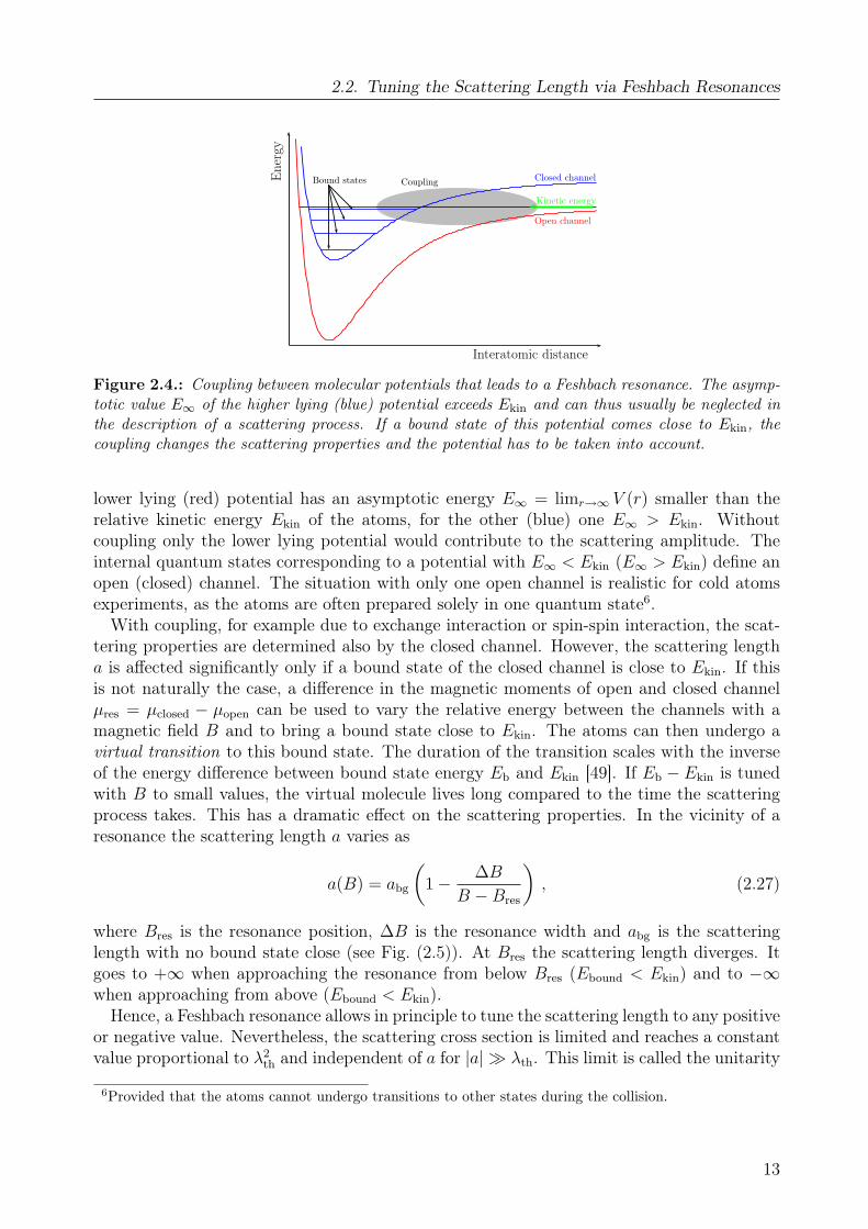
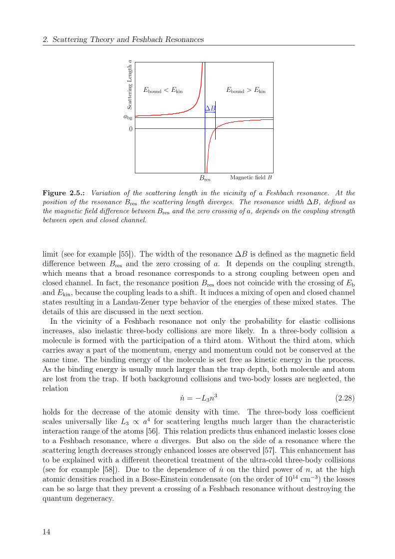
where Bres is the resonance position, ∆B is the resonance width and abg is the scatteringlength with no bound state close (see Fig. (2.5)). At Bres the scattering length diverges. Itgoes to +∞ when approaching the resonance from below Bres (Ebound < Ekin) and to −∞when approaching from above (Ebound < Ekin).
Hence, a Feshbach resonance allows in principle to tune the scattering length to any positiveor negative value. Nevertheless, the scattering cross section is limited and reaches a constantvalue proportional to λ2
th and independent of a for |a| λth. This limit is called the unitarity
6Provided that the atoms cannot undergo transitions to other states during the collision.
13
2. Scattering Theory and Feshbach Resonances
Magnetic field B
Scat
teri
ngLe
ngth
a
Bres
abg
0
∆B
Ebound < Ekin Ebound > Ekin
Figure 2.5.: Variation of the scattering length in the vicinity of a Feshbach resonance. At theposition of the resonance Bres the scattering length diverges. The resonance width ∆B, defined asthe magnetic field difference between Bres and the zero crossing of a, depends on the coupling strengthbetween open and closed channel.
limit (see for example [55]). The width of the resonance ∆B is defined as the magnetic fielddifference between Bres and the zero crossing of a. It depends on the coupling strength,which means that a broad resonance corresponds to a strong coupling between open andclosed channel. In fact, the resonance position Bres does not coincide with the crossing of Eb
and Ekin, because the coupling leads to a shift. It induces a mixing of open and closed channelstates resulting in a Landau-Zener type behavior of the energies of these mixed states. Thedetails of this are discussed in the next section.
In the vicinity of a Feshbach resonance not only the probability for elastic collisionsincreases, also inelastic three-body collisions are more likely. In a three-body collision amolecule is formed with the participation of a third atom. Without the third atom, whichcarries away a part of the momentum, energy and momentum could not be conserved at thesame time. The binding energy of the molecule is set free as kinetic energy in the process.As the binding energy is usually much larger than the trap depth, both molecule and atomare lost from the trap. If both background collisions and two-body losses are neglected, therelation
n = −L3n3 (2.28)
holds for the decrease of the atomic density with time. The three-body loss coefficientscales universally like L3 ∝ a4 for scattering lengths much larger than the characteristicinteraction range of the atoms [56]. This relation predicts thus enhanced inelastic losses closeto a Feshbach resonance, where a diverges. But also on the side of a resonance where thescattering length decreases strongly enhanced losses are observed [57]. This enhancement hasto be explained with a different theoretical treatment of the ultra-cold three-body collisions(see for example [58]). Due to the dependence of n on the third power of n, at the highatomic densities reached in a Bose-Einstein condensate (on the order of 1014 cm−3) the lossescan be so large that they prevent a crossing of a Feshbach resonance without destroying thequantum degeneracy.
14
2.3. Theory of Feshbach Resonances
2.3. Theory of Feshbach Resonances
To derive a theoretical description of Feshbach resonances, this section recapitulates scatter-ing theory taking into account a coupling between different molecular potentials. Only onebound state is considered, which is the single resonance approach. The presentation followsmainly [49] and [59]. For more details the reader is referred also to [54, 60].
2.3.1. Formal Solution
As explained in the previous section, a coupling between open and closed channel is crucialfor a Feshbach resonance. This coupling leads to a mixing of the open and the closed channelstate |ψop〉 and |ψcl〉. The scattering state has thus the following general form
|ψ〉 = α |ψop〉+ β |ψcl〉 . (2.29)
As was done in section 2.1, we calculate the stationary scattering eigenstate with the time-independent Schrödinger equation. Though, we now have two coupled differential equationsdue to the coupling [59]
Hop |ψop〉+ W |ψcl〉 =E |ψop〉 , (2.30)Hcl |ψcl〉+W |ψop〉 = E |ψcl〉 , (2.31)
and two scattering eigenstates7 |ψopk 〉 and
∣∣ψclk
⟩. Here Hop (respectively Hcl) is the Hamilton
operator for the open (respectively closed) channel without coupling and W denotes thecoupling. Hop is thus equal to Eq. (2.5).Hcl is of the same form as Hop, but its potential energy is given by the closed channel
potential Vcl(r). The eigenfunctions of interest of Hcl are all bound states, because theasymptotic energy of Vcl(r) is larger than the relative kinetic energy of the atoms. Hcl cantherefore be written as
Hcl =∑
ν
Eν |ψν〉 〈ψν | , (2.32)
with the bound states |ψν〉 and their energy Eν . This allows us to write Eq. (2.31) as∑ν
(E − Eν) |ψν〉 〈ψν | ψcl〉 = W |ψop〉 . (2.33)
We are interested in the behavior of a when a bound state is close to the relative kineticenergy Ekin of the atoms. Therefore we can neglect all eigenstates of Hcl other than |ψb〉, thebound state that is close to Ekin. Consequently Eq. (2.33) can be rewritten as
(E − Eb) |ψb〉 〈ψb| ψcl〉 = W |ψop〉 . (2.34)
This approach is called the single resonance approximation.To get to a formal solution of the coupled Schrödinger equations (2.30) and (2.31), the
concept of Green’s functions — in this case Green’s operators — is used like in the previous
7Also called dressed states.
15
2. Scattering Theory and Feshbach Resonances
section. With the Green’s operators
Gop(z) =1
z −Hop
, (2.35)
Gcl(z) =1
z −Hcl
, (2.36)
where z is a complex number with the dimension of an energy, the scattering states be-come [49]
|ψopk 〉 = |ψk〉+Gop(E + iε)W
∣∣ψclk
⟩, (2.37)∣∣ψcl
k
⟩= Gcl(E)W |ψop
k 〉 . (2.38)
Let us first discuss expression (2.37): |ψk〉 is the solution of Eq. (2.30) without coupling Wand therefore in position-space given by Eq. (2.15). The argument z = E + iε of the Green’soperator ensures that the second term has the asymptotic behaviour of an outgoing sphericalwave. Equation (2.38) has no scattered component8 for W = 0, because for Hcl exist onlybound states, as was stated above. In this equation we can include the single resonanceapproximation. The Green’s operator Gcl(E) becomes then
Gcl(E) =1
(E − Eb) |ψb〉 〈ψb|=|ψb〉 〈ψb|(E − Eb)
. (2.39)
Consequently∣∣ψcl
k
⟩is proportional to |ψb〉
∣∣ψclk
⟩= |ψb〉
〈ψb|W |ψopk 〉
E − Eb
. (2.40)
If we now insert (2.40) into (2.37), after some algebra an expression for |ψopk 〉 is obtained,
which depends only on the states |ψk〉 and |ψb〉
|ψopk 〉 = |ψk〉+Gop
W |ψb〉 〈ψb|WE − Eb − 〈ψb|WGopW |ψb〉
|ψk〉 . (2.41)
2.3.2. Derivation of the Scattering Properties
With Eq. (2.41) the scattering properties in the vicinity of a Feshbach resonance are deduced.Only zero-energy resonances are considered, which means Ekin = 0. Here the zero of energyis set as the dissociation threshold of the open channel. As already discussed above, the firstterm on the right hand side of Eq. (2.41) describes the scattering in the open channel withno coupling W . The scattering length corresponding to this is called background scatteringlength abg. The resonance behaviour of a is caused by the second term of Eq. (2.41). Thescattering amplitude, given by its asymptotic behaviour, diverges when the denominatorvanishes, i.e. if
E = Eb + 〈ψb|WGopW |ψb〉 . (2.42)
8Hence, z is chosen real.
16
2.3. Theory of Feshbach Resonances
For small E the second term on the right hand side of Eq. (2.42) becomes [49]
〈ψb|WGopW |ψb〉 = 〈ψb|W1
E −Hop + iεW |ψb〉
E→0≈
∑k
| 〈ψb|W |ψk〉 |2
−~2k2
2mr+ iε
:= ~∆0 . (2.43)
The approximate expression for 〈ψb|WGopW |ψb〉 has a form that is well-known from per-turbation theory9. The expression describes the shift of the resonance position due to secondorder coupling induced by W on |ψb〉. Consequently the resonance does not occur when Eb
is close to zero, but whenEres = Eb + ~∆0 = 0 . (2.44)
As was already stated in the previous section, the energy difference between open andclosed channel is tunable with a magnetic field B, if the two states have a difference inmagnetic moment µres = µclosed − µopen. Hence, Eb = Eb(B) = µres(B − Bb), where Bb isthe magnetic field value at which Eb = Ekin. Therefore the magnetic field value Bres thatcorresponds to the resonance position is defined by
Bres = Bb +~∆0
µres
. (2.45)
To get an expression for the total scattering amplitude ftot, we include Eq. (2.44) inEq. (2.41) and multiply with 〈r| from the left, which gives the total scattered wave function
ψopk (r) = 〈r| ψop
k 〉 = ψk(r) +〈r|GopW |ψb〉 〈ψb|W |ψk〉
E − Eres
. (2.46)
It takes some effort to calculate the asymptotic behaviour of this expression [49], hence I onlystate the result
ψop0 (r)
r→∞≈ ψ0(r) +
1
r
4π2mr
~2
| 〈ψ0|W |ψb〉 |2
Eres
, (2.47)
here E and k are set to zero. The factor behind 1/r is the contribution fres to the totalscattering amplitude, thus we finally get to Eq. (2.27) for the scattering length
a(B) = − limk→0
ftot = abg −4π2mr
~2
| 〈ψ0|W |ψb〉 |2
Eres
= abg
(1− ∆B
B −Bres
), (2.48)
with the width of the resonance
∆B =4π2mr
~2
| 〈ψ0|W |ψb〉 |2
abgµres
. (2.49)
It depends on the coupling strength W between open and closed channel, as already discussedin the previous section.
9Strictly speaking ∆0 has also an imaginary part due to iε. It can be shown that in the low-energy limit wecan neglect this part which would lead to a damping term, because the density of states of the continuumof Hop vanishes near k = 0 [49].
17
2. Scattering Theory and Feshbach Resonances
Magnetic field B
Ene
rgy
∆0
µres
BbBres
0
|ψb〉
|ψop〉|ψop〉
|ψb〉
Slope µres
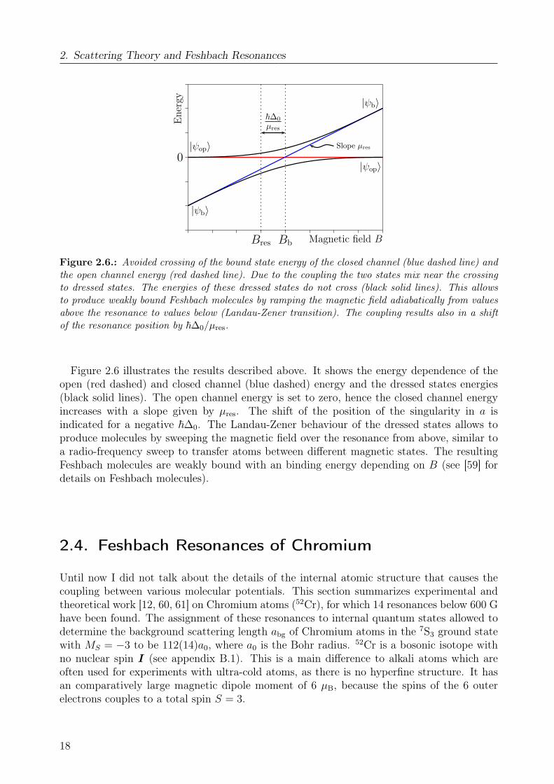
Figure 2.6.: Avoided crossing of the bound state energy of the closed channel (blue dashed line) andthe open channel energy (red dashed line). Due to the coupling the two states mix near the crossingto dressed states. The energies of these dressed states do not cross (black solid lines). This allowsto produce weakly bound Feshbach molecules by ramping the magnetic field adiabatically from valuesabove the resonance to values below (Landau-Zener transition). The coupling results also in a shiftof the resonance position by ~∆0/µres.
Figure 2.6 illustrates the results described above. It shows the energy dependence of theopen (red dashed) and closed channel (blue dashed) energy and the dressed states energies(black solid lines). The open channel energy is set to zero, hence the closed channel energyincreases with a slope given by µres. The shift of the position of the singularity in a isindicated for a negative ~∆0. The Landau-Zener behaviour of the dressed states allows toproduce molecules by sweeping the magnetic field over the resonance from above, similar toa radio-frequency sweep to transfer atoms between different magnetic states. The resultingFeshbach molecules are weakly bound with an binding energy depending on B (see [59] fordetails on Feshbach molecules).
2.4. Feshbach Resonances of Chromium
Until now I did not talk about the details of the internal atomic structure that causes thecoupling between various molecular potentials. This section summarizes experimental andtheoretical work [12, 60, 61] on Chromium atoms (52Cr), for which 14 resonances below 600 Ghave been found. The assignment of these resonances to internal quantum states allowed todetermine the background scattering length abg of Chromium atoms in the 7S3 ground statewith MS = −3 to be 112(14)a0, where a0 is the Bohr radius. 52Cr is a bosonic isotope withno nuclear spin I (see appendix B.1). This is a main difference to alkali atoms which areoften used for experiments with ultra-cold atoms, as there is no hyperfine structure. It hasan comparatively large magnetic dipole moment of 6 µB, because the spins of the 6 outerelectrons couples to a total spin S = 3.
18
2.4. Feshbach Resonances of Chromium
The molecular interaction potential of 52Cr atoms consists of the following contributions
Vmol =2∑
k=1
V kZ + VE + VvdW + VSS + VSO . (2.50)
The various terms are:
Zeeman interaction V kZ : The magnetic dipole moment of the atoms k = 1, 2 leads to a
shift of their energy if a magnetic field B is applied. It is given by the well-known formula
V kZ = −µk ·B = −µBgJMJ,kB . (2.51)
Here MJ,k is the projection of the total angular momentum Jk of atom k on the quantizationaxis defined by the magnetic field. The Landé-factor gJ of the 7S3 ground state of Chromiumis negative and close to the electron g factor, namely gJ = −2.00183 [62]. The Zeemaninteraction is crucial for Feshbach resonances, as it allows to shift molecular potentials withdifferent projections of the dipole moment relative to each other.
Exchange interaction VE: The electronic exchange interaction has no classical analogyand has therefore to be described quantum mechanically [63]. It arises from the fact thatthe valence electrons cannot be allocated to a specific atom any more if the electron cloudsoverlap. It is a short range interaction because this overlap decays exponentially with thedistance of the atoms. At small distances it is strongly repulsive because of the fermionicnature of electrons.
Van der Waals interaction VvdW: The atoms induce mutually an electric dipole momentif they are close. These dipole moments interact with each other, leading to an attractivepotential falling of as −C6/r
6. C6 is the van der Waals coefficient determining the interactionstrength. There exist also higher multipole contributions decaying as −Cn/r
n, with n = 8,10, . . ..
Spin-spin interaction VSS: Also referred to as dipole-dipole interaction in this thesis. VSS
is the most important coupling interaction for 52Cr, as coupling due to exchange interactiondoes not lead to Feshbach resonances (see below). The potential energy is dependent on therelative alignment of the dipoles and falls of with 1/r3. For a polarized sample it is given by
VSS =µ0µ
2
4π
(1− 3 cos2 θ
r3
), (2.52)
with the atomic dipole moment µ = gJµBMJ and with θ being the angle between the magneticfield and the connection line between the atoms.
Second order spin-orbit interaction VSO: Besides the direct spin-spin interaction VSS,there is an indirect interaction between the spins, the second-order spin-orbit interactionVSO. It occurs when the atomic charge clouds overlap as a molecule is formed, and the in-teraction between the ground state spins are modified due to couplings mediated through
19
2. Scattering Theory and Feshbach Resonances
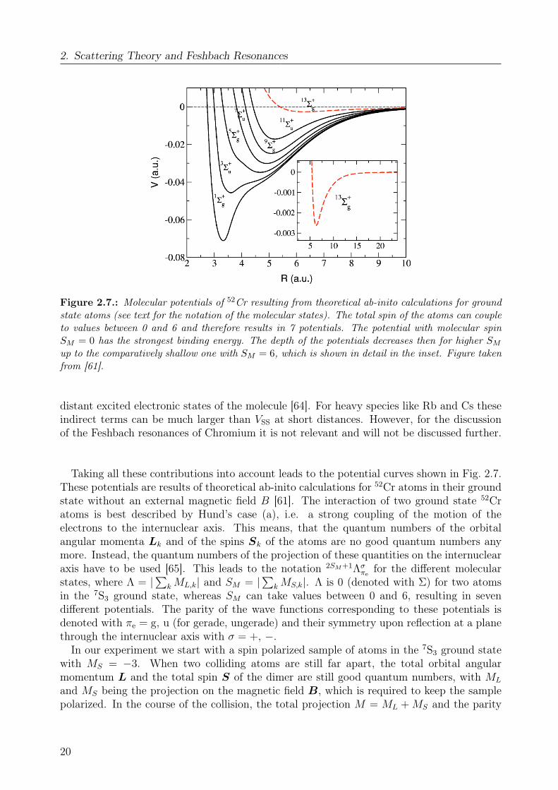
Figure 2.7.: Molecular potentials of 52Cr resulting from theoretical ab-inito calculations for groundstate atoms (see text for the notation of the molecular states). The total spin of the atoms can coupleto values between 0 and 6 and therefore results in 7 potentials. The potential with molecular spinSM = 0 has the strongest binding energy. The depth of the potentials decreases then for higher SM
up to the comparatively shallow one with SM = 6, which is shown in detail in the inset. Figure takenfrom [61].
distant excited electronic states of the molecule [64]. For heavy species like Rb and Cs theseindirect terms can be much larger than VSS at short distances. However, for the discussionof the Feshbach resonances of Chromium it is not relevant and will not be discussed further.
Taking all these contributions into account leads to the potential curves shown in Fig. 2.7.These potentials are results of theoretical ab-inito calculations for 52Cr atoms in their groundstate without an external magnetic field B [61]. The interaction of two ground state 52Cratoms is best described by Hund’s case (a), i.e. a strong coupling of the motion of theelectrons to the internuclear axis. This means, that the quantum numbers of the orbitalangular momenta Lk and of the spins Sk of the atoms are no good quantum numbers anymore. Instead, the quantum numbers of the projection of these quantities on the internuclearaxis have to be used [65]. This leads to the notation 2SM+1Λσ
πefor the different molecular
states, where Λ = |∑
k ML,k| and SM = |∑
k MS,k|. Λ is 0 (denoted with Σ) for two atomsin the 7S3 ground state, whereas SM can take values between 0 and 6, resulting in sevendifferent potentials. The parity of the wave functions corresponding to these potentials isdenoted with πe = g, u (for gerade, ungerade) and their symmetry upon reflection at a planethrough the internuclear axis with σ = +, −.
In our experiment we start with a spin polarized sample of atoms in the 7S3 ground statewith MS = −3. When two colliding atoms are still far apart, the total orbital angularmomentum L and the total spin S of the dimer are still good quantum numbers, with ML
and MS being the projection on the magnetic field B, which is required to keep the samplepolarized. In the course of the collision, the total projection M = ML +MS and the parity
20
2.4. Feshbach Resonances of Chromium
1st order 2nd order
∆L 0, ±2 0, ±2, ±4
∆ML 0, ±1, ±2 0, ±1, ±2, ±3, ±4
∆S 0, ±2 0, ±2, ±4
Table 2.1.: Selection rules for a first and second order dipole-dipole transition. ∆ML = 0 is notallowed for L = 0 → L′ = 0 in first order.
(a)
(b)
Scat
teri
ngle
ngth
[a0]
0 100 200 300 400 500 600 70095
100
105
110
115
Magnetic field [G]
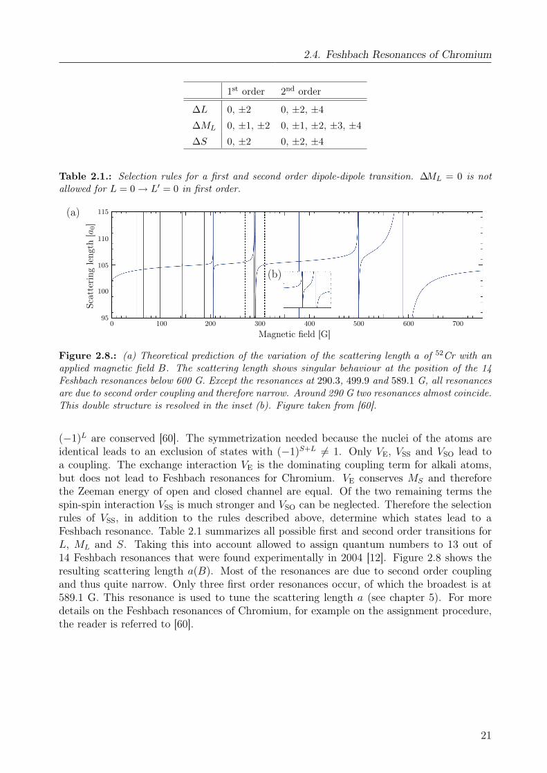
Figure 2.8.: (a) Theoretical prediction of the variation of the scattering length a of 52Cr with anapplied magnetic field B. The scattering length shows singular behaviour at the position of the 14Feshbach resonances below 600 G. Except the resonances at 290.3, 499.9 and 589.1 G, all resonancesare due to second order coupling and therefore narrow. Around 290 G two resonances almost coincide.This double structure is resolved in the inset (b). Figure taken from [60].
(−1)L are conserved [60]. The symmetrization needed because the nuclei of the atoms areidentical leads to an exclusion of states with (−1)S+L 6= 1. Only VE, VSS and VSO lead toa coupling. The exchange interaction VE is the dominating coupling term for alkali atoms,but does not lead to Feshbach resonances for Chromium. VE conserves MS and thereforethe Zeeman energy of open and closed channel are equal. Of the two remaining terms thespin-spin interaction VSS is much stronger and VSO can be neglected. Therefore the selectionrules of VSS, in addition to the rules described above, determine which states lead to aFeshbach resonance. Table 2.1 summarizes all possible first and second order transitions forL, ML and S. Taking this into account allowed to assign quantum numbers to 13 out of14 Feshbach resonances that were found experimentally in 2004 [12]. Figure 2.8 shows theresulting scattering length a(B). Most of the resonances are due to second order couplingand thus quite narrow. Only three first order resonances occur, of which the broadest is at589.1 G. This resonance is used to tune the scattering length a (see chapter 5). For moredetails on the Feshbach resonances of Chromium, for example on the assignment procedure,the reader is referred to [60].
21
2. Scattering Theory and Feshbach Resonances
22
3. Dipolar Bose-Einstein Condensates
Chromium has an comparatively large magnetic dipole moment of 6 µB. Hence, atheoretical description of a Chromium Bose-Einstein condensate has to include alsodipole-dipole interaction. This chapter discusses an extension of the mean-field the-ory for condensates with only contact interaction to dipolar condensates. In the firsttwo sections the theory including only contact interaction is described. Section 3.1reports on the in-trap properties of such a condensate. The mean-field approxima-tion and the Thomas-Fermi regime are introduced. The theoretical description ofthe condensate dynamics by hydrodynamic equations is discussed in section 3.2. Fi-nally, section 3.3 includes dipole-dipole interaction in this theory. All importantresults that are used for the data evaluation are presented.
3.1. Bose-Einstein Condensation
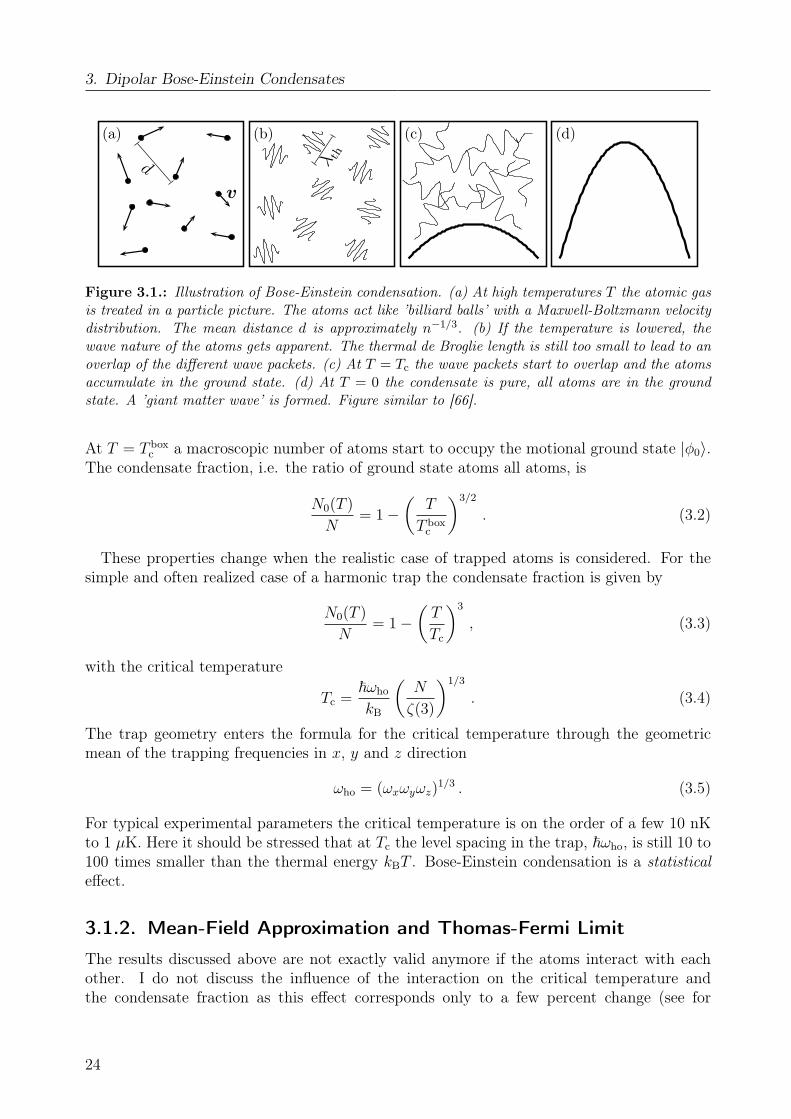
The new state of matter called Bose-Einstein condensate (BEC) that was first realized in 1995in the group of Wieman and Cornell [6] and shortly afterwards in the group of Ketterle [7],had been predicted already 70 years before by Einstein [14]. Bose-Einstein condensation isbased on the indistinguishability and wave nature of particles [66]. The phase transitionfrom a thermal gas of trapped bosonic atoms to a condensate appears, when the thermal deBroglie wavelength λth (Eq. (2.1)) starts to be on the order of the mean atomic distance (givenapproximately by n−1/3, where n is the particle density). Therefore the wave functions of theatoms start to overlap and the indistinguishability becomes important: Bosons accumulatein the ground state which leads to a collective macroscopic behaviour of the atoms (seeFig. 3.1). The sample can then be described by one macroscopic wave function with afixed phase throughout the whole sample. BECs are a macroscopic probe to study quantumphenomena, which explains the huge interest they have attracted over the last years.
3.1.1. Statistical Description
Before I introduce the mean-field description, I summarize important results of the statisticaldescription of Bose-Einstein condensation. For a derivation of these results see for exam-ple [54, 55, 67] or standard textbooks on statistical physics [68, 69]. For a Bose gas withoutinteractions in a box with periodic boundary conditions, the phase transition to a condensateappears when the phase space density, defined as ρ := nλ3
th, is equal to1 ζ(3/2) ≈ 2.612. Thiscorresponds to a critical temperature
T boxc =
2π~2
mkB
(n
ζ(3/2)
)2/3
. (3.1)
1Here ζ(x) is the Riemann Zeta function, defined as ζ(x) =∑∞
k=1 k−x.
23
3. Dipolar Bose-Einstein Condensates
(a) (b) (c) (d)
v
d λ th
Figure 3.1.: Illustration of Bose-Einstein condensation. (a) At high temperatures T the atomic gasis treated in a particle picture. The atoms act like ’billiard balls’ with a Maxwell-Boltzmann velocitydistribution. The mean distance d is approximately n−1/3. (b) If the temperature is lowered, thewave nature of the atoms gets apparent. The thermal de Broglie length is still too small to lead to anoverlap of the different wave packets. (c) At T = Tc the wave packets start to overlap and the atomsaccumulate in the ground state. (d) At T = 0 the condensate is pure, all atoms are in the groundstate. A ’giant matter wave’ is formed. Figure similar to [66].
At T = T boxc a macroscopic number of atoms start to occupy the motional ground state |φ0〉.
The condensate fraction, i.e. the ratio of ground state atoms all atoms, is
N0(T )
N= 1−
(T
T boxc
)3/2
. (3.2)
These properties change when the realistic case of trapped atoms is considered. For thesimple and often realized case of a harmonic trap the condensate fraction is given by
N0(T )
N= 1−
(T
Tc
)3
, (3.3)
with the critical temperature
Tc =~ωho
kB
(N
ζ(3)
)1/3
. (3.4)
The trap geometry enters the formula for the critical temperature through the geometricmean of the trapping frequencies in x, y and z direction
ωho = (ωxωyωz)1/3 . (3.5)
For typical experimental parameters the critical temperature is on the order of a few 10 nKto 1 µK. Here it should be stressed that at Tc the level spacing in the trap, ~ωho, is still 10 to100 times smaller than the thermal energy kBT . Bose-Einstein condensation is a statisticaleffect.
3.1.2. Mean-Field Approximation and Thomas-Fermi Limit
The results discussed above are not exactly valid anymore if the atoms interact with eachother. I do not discuss the influence of the interaction on the critical temperature andthe condensate fraction as this effect corresponds only to a few percent change (see for
24
3.1. Bose-Einstein Condensation
example [54]). Nevertheless, the interaction is important for the structure of a BEC. Themany-body hamiltonian of a cloud of interacting atoms includes the potential energy betweeneach pair of atoms. Typical BECs contain 104–106 atoms, it is clear that the many-bodyproblem can thus not be solved exactly. Because BECs are dilute gases with n|a|3 1for sufficiently small interaction, we can neglect the correlations between the atoms andassume that they move in a mean-field potential created by the other atoms. The mean-fieldpotential has to be defined in a self-consistent way. This mean-field approximation simplifiesthe theoretical description vastly.
In the fully condensed state (T = 0) all atoms occupy the same motional ground state|φ0〉. In the mean field approximation the whole condensate is then described by one wavefunction2. It is useful to define the wave function as
ψ(r) :=√Nφ0(r) , (3.6)
because then the particle density n(r) is given by |ψ(r)|2. A non-linear Schrödinger equationfor this wave function, the (time-independent) Gross-Pitaevskii equation (GPE), is obtainedby using variational methods [54](
− ~2
2m∇2 + Vext(r) + g|ψ(r)|2
)ψ(r) = µψ(r) . (3.7)
Here m is the atomic mass, Vext(r) is the confining potential and µ is the chemical potentialof the system, i.e. the energy needed to add a particle to the system. The derivation ofEq. (3.7) makes use of the simple pseudo-potential introduced in section 2.1 to describe theatom-atom interaction. This leads to the mean-field interaction term gn(r) = g|φ(r)|2. Asalready stated above, dipole-dipole interaction is first not taken into account. Equation (3.7)is the key tool in the mean field description of BECs.
The GPE simplifies a lot if the kinetic energy term is neglected. The kinetic energy iscaused by the confinement of the atoms due to the Heisenberg principle. It can be shown(see for example [54]) that for large atom numbers and repulsive interaction the kinetic energyis negligible3. This regime is called Thomas-Fermi limit, it is valid if
Na
aho
1 , (3.8)
where aho =√
~/(mωho) is the oscillator length of the trapping potential. In this case wedirectly obtain a solution of the GPE
n(r) = |ψ(r)|2 =
µ− Vext(r)
g: Vext(r) ≤ µ
0 : otherwise. (3.9)
The density profile of the BEC reflects the shape of the confining potential. For harmonictraps it is thus parabolic (see Fig. 3.2). With the Thomas-Fermi radii, which are defined by
2Please note that the wave function is the order parameter of the BEC phase transition.3It is intuitively clear that for repulsive interaction the size R of the BEC increases and hence the kinetic
energy (∼ ~2/(mR2)) decreases.
25
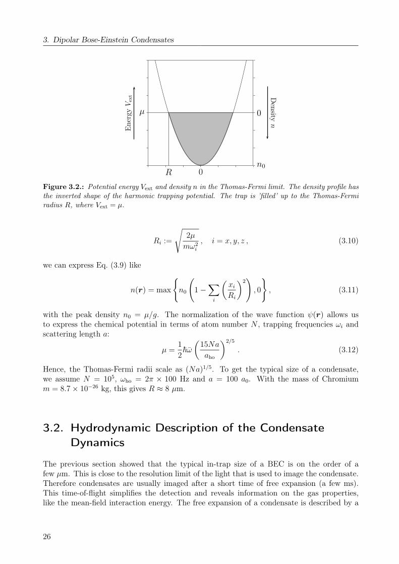
3. Dipolar Bose-Einstein Condensates
R 0
µ 0
n0
Density
nE
nerg
yV
ext
Figure 3.2.: Potential energy Vext and density n in the Thomas-Fermi limit. The density profile hasthe inverted shape of the harmonic trapping potential. The trap is ’filled’ up to the Thomas-Fermiradius R, where Vext = µ.
Ri :=
√2µ
mω2i
, i = x, y, z , (3.10)
we can express Eq. (3.9) like
n(r) = max
n0
(1−
∑i
(xi
Ri
)2), 0
, (3.11)
with the peak density n0 = µ/g. The normalization of the wave function ψ(r) allows usto express the chemical potential in terms of atom number N , trapping frequencies ωi andscattering length a:
µ =1
2~ω(
15Na
aho
)2/5
. (3.12)
Hence, the Thomas-Fermi radii scale as (Na)1/5. To get the typical size of a condensate,we assume N = 105, ωho = 2π × 100 Hz and a = 100 a0. With the mass of Chromiumm = 8.7× 10⁻²⁶ kg, this gives R ≈ 8 µm.
3.2. Hydrodynamic Description of the CondensateDynamics
The previous section showed that the typical in-trap size of a BEC is on the order of afew µm. This is close to the resolution limit of the light that is used to image the condensate.Therefore condensates are usually imaged after a short time of free expansion (a few ms).This time-of-flight simplifies the detection and reveals information on the gas properties,like the mean-field interaction energy. The free expansion of a condensate is described by a
26
3.2. Hydrodynamic Description of the Condensate Dynamics
scaling law. It is deduced by reformulating the time-dependent GPE
− i~∂
∂tψ(r, t) =
(− ~2
2m∇2 + Vext(r, t) + g|ψ(r, t)|2
)ψ(r, t) (3.13)
as a set of hydrodynamic equations. For this, we rewrite the condensate wave functionEq. (3.6) in polar form
ψ(r, t) =√n(r, t)eiα(r,t) , (3.14)
where α(r, t) is the phase of the condensate. After some algebra (see for example [67]) thefollowing expressions are obtained
∂n
∂t= −∇ · (nv) (3.15)
m∂v
∂t= −∇
(− ~2
2m
∆√n√n
+mv2
2+ Vext + gn
). (3.16)
Equation (3.15) has the form of a continuity equation and Eq. (3.16) is similar to the Eulerequation for a superfluid. The superfluid velocity v(r, t) is proportional to the gradient ofthe phase
v(r, t) =~m
∇α(r, t) . (3.17)
Hence, the condensate motion is equivalent to the potential flow of a superfluid4 in thepresence of Vext and the mean field potential gn. A difference in Eq. (3.16) to classicalhydrodynamics is the quantum pressure term
− ~2
2m
∆√n√n. (3.18)
It can be estimated by∆√n√n∼ 1
d2, (3.19)
where d denotes the typical length scale for the variation of the condensate density n(r) [67].Like the termmv2/2 it originates from the kinetic energy of the condensate, but it correspondsto a different physical effect: Whereas mv2/2 describes the kinetic energy of the particlemotion, Eq. (3.18) describes the zero point motion (hence the name quantum pressure) [54].For a moderate excitation of the condensate or in the course of ballistic expansion, d is onthe order of the size of the condensate itself. It can be shown that the quantum pressureterm is then negligible in the Thomas-Fermi regime [67].
Thus, the condensate motion is described by a set of classical hydrodynamic equations inthis regime. In this model each particle experiences a force
F (r, t) = −∇(Vext(r, t) + gn(r, t)) . (3.20)
At t = 0 the system is assumed to be in steady state, meaning that the density distributionis given by Eq. (3.9). If Vext is then switched off, the condensate motion corresponds to a
4The velocity potential is given by ~α/m.
27

3. Dipolar Bose-Einstein Condensates
(a)
Ry Rz
0 2 4 6 8 100
10
20
30
40
50
60
Time [ms]
Tho
mas
-Fer
mir
adii
[µm
](b)
0 2 4 6 8 100
0.5
1
1.5
Time [ms]
Asp
ect
rati
oA
yz
Figure 3.3.: (a) Thomas-Fermi radii Ry(t) and Rz(t) after sudden switch-off of a trap with(ωx, ωy, ωz) = 2π × (200, 200, 100) Hz. At approximately 2.3 ms the ellipticity of the condensateinverts. (b) The aspect ratio Ayz crosses 1 at this time.
dilatation of the cloud, with any small piece of the fluid moving along the trajectory
Ri(t) = λi(t)Ri(0) , (3.21)
where Ri(0) are the initial Thomas-Fermi radii. An exact solution of the dynamics of thecondensate can be calculated for harmonic potentials [70]. In this case the λi(t) fulfill thefollowing coupled differential equations5
λi =1
λxλyλz
ω2i (0)
λi
− ω2i (t)λi , i = x, y, z . (3.22)
Figure 3.3 (a) shows how the Thomas-Fermi radii Ry and Rz evolve after a sudden switch-off of a trap with (ωx, ωy, ωz) = 2π × (200, 200, 100) Hz. Starting at t = 0 with a quadraticbehavior, the radii increase almost linearly for times t > 1/ωi. The slope of Ry is steeper,leading to a crossing of the radii after approximately 2.3 ms: The condensate inverts itsellipticity. Unless the ratio ωy/ωz is initially exactly one, the condensate always inverts itsellipticity6, i.e. the aspect ratio Ayz(t) = Ry/Rz changes from values smaller (larger) thanone to values larger (smaller) than one (see Fig. (3.3) (b)). This is a ’smoking gun’ evidencefor quantum degeneracy. It can be easily understood in the classical hydrodynamics model.The density gradient ∇n(r) is larger in the direction of higher trapping frequencies, leadingto a faster acceleration in this direction (see Eq. (3.20)).
5The equations are exact not only for a sudden switch-off, but for any change of the external potential att = 0.
6If only contact interaction is present.
28
3.3. Dipole-Dipole Interaction in a Bose-Einstein Condensate
ϑr
B repulsive
attrac-tive
attrac-tive
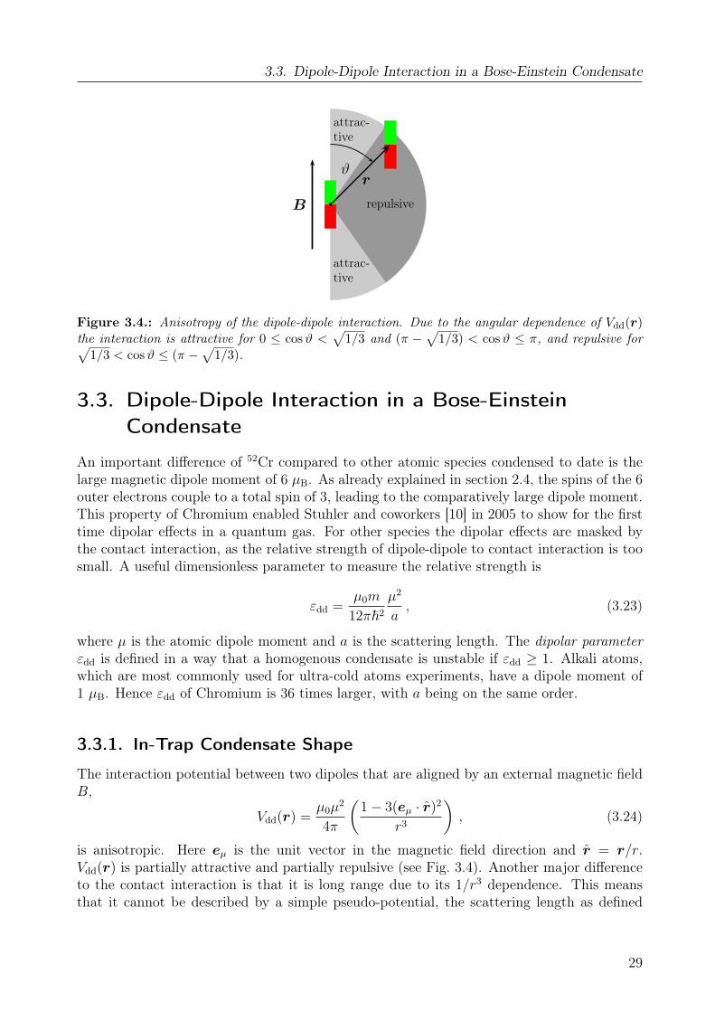
Figure 3.4.: Anisotropy of the dipole-dipole interaction. Due to the angular dependence of Vdd(r)the interaction is attractive for 0 ≤ cosϑ <
√1/3 and (π −
√1/3) < cosϑ ≤ π, and repulsive for√
1/3 < cosϑ ≤ (π −√
1/3).
3.3. Dipole-Dipole Interaction in a Bose-EinsteinCondensate
An important difference of 52Cr compared to other atomic species condensed to date is thelarge magnetic dipole moment of 6 µB. As already explained in section 2.4, the spins of the 6outer electrons couple to a total spin of 3, leading to the comparatively large dipole moment.This property of Chromium enabled Stuhler and coworkers [10] in 2005 to show for the firsttime dipolar effects in a quantum gas. For other species the dipolar effects are masked bythe contact interaction, as the relative strength of dipole-dipole to contact interaction is toosmall. A useful dimensionless parameter to measure the relative strength is
εdd =µ0m
12π~2
µ2
a, (3.23)
where µ is the atomic dipole moment and a is the scattering length. The dipolar parameterεdd is defined in a way that a homogenous condensate is unstable if εdd ≥ 1. Alkali atoms,which are most commonly used for ultra-cold atoms experiments, have a dipole moment of1 µB. Hence εdd of Chromium is 36 times larger, with a being on the same order.
3.3.1. In-Trap Condensate Shape
The interaction potential between two dipoles that are aligned by an external magnetic fieldB,
Vdd(r) =µ0µ
2
4π
(1− 3(eµ · r)2
r3
), (3.24)
is anisotropic. Here eµ is the unit vector in the magnetic field direction and r = r/r.Vdd(r) is partially attractive and partially repulsive (see Fig. 3.4). Another major differenceto the contact interaction is that it is long range due to its 1/r3 dependence. This meansthat it cannot be described by a simple pseudo-potential, the scattering length as defined
29
3. Dipolar Bose-Einstein Condensates
in Eq. (2.23) diverges7 [26]. Although the dipole-dipole interaction differs significantly fromcontact interaction, it is relatively easy to include in the mean-field description of BECs. Asstated in [71] (explicitly shown in [72]), the mean-field dipole-dipole potential entering theGPE has the intuitive form
V meandd (r) =
∫dr′3Vdd(r − r′)n(r′) . (3.25)
This equation corresponds to the Born approximation for binary collisions (see section 2.1)and is accurate for dipole moments on the order of 1 µB and far away from shape reso-nances [73].
It is remarkable that the parabolic density distribution is also a self-consistent solution ofthe GPE including V mean
dd , if εdd does not exceed one. This is shown by integrating (3.25) witha density distribution of the form (3.11). It turns out that the physical dipolar contributionsof V mean
dd are then also quadratic like the trapping potential Vext(r) = 1/2m∑
i ω2i x
2i and the
mean field energy gn(r) of the contact interaction [73]. Therefore, the GPE contains onlyparabolic and constant terms in the Thomas-Fermi limit and the inverted parabola profile isstill an exact solution of the problem. However, it is not trivial to obtain the condensate radiiwith dipole-dipole interaction present. Here I will only discuss the results, see for example [73]for details on the derivation.
The in-trap radii Ri for a magnetic field pointing in z direction are obtained by solvingthe following equations
ω2j =
(15N~2a
m2RxRyRz
)1
R2j
[1− εddf(Axz, Ayz) + εddAjz
∂f(Axz, Ayz)
∂Ajz
], j = x, y , (3.26)
ω2z =
(15N~2a
m2RxRyRz
)1
R2z
[1− εddf(Axz, Ayz)− εddAxz
∂f(Axz, Ayz)
∂Axz
− εddAyz∂f(Axz, Ayz)
∂Ayz
]. (3.27)
The function f(Axz, Ayz) of the aspect ratios Axz = Rx/Rz and Ayz = Ry/Rz depends on theincomplete elliptic integrals of the first and second kind and is discussed in appendix C.1.With the radii the mean-field potential can be calculated. I will not discuss the completeexpression here (for details see [10]), but discuss only the simpler case of a spherical con-densate with radius RTF. This example contains already the relevant main characteristics.Equation (3.25) integrated with a spherical density distribution is
V meandd (r) =
εddmω20
5r2(1− 3(ez · r)2) , r ≤ RTF . (3.28)
The potential has a saddle-shape with a negative curvature when moving along the z directionfrom the saddle point and a positive curvature when moving along x or y (see Fig. 3.5). Thismeans that compared to a condensate with only contact interaction, the dipolar condensateis elongated in the dipole direction and compressed in the directions perpendicular to it.This is a bit counterintuitive, as from the simple two-body interaction of dipoles (Eq. (3.24))
7In the description by a partial wave decomposition this means that all partial waves contribute.
30
3.3. Dipole-Dipole Interaction in a Bose-Einstein Condensate
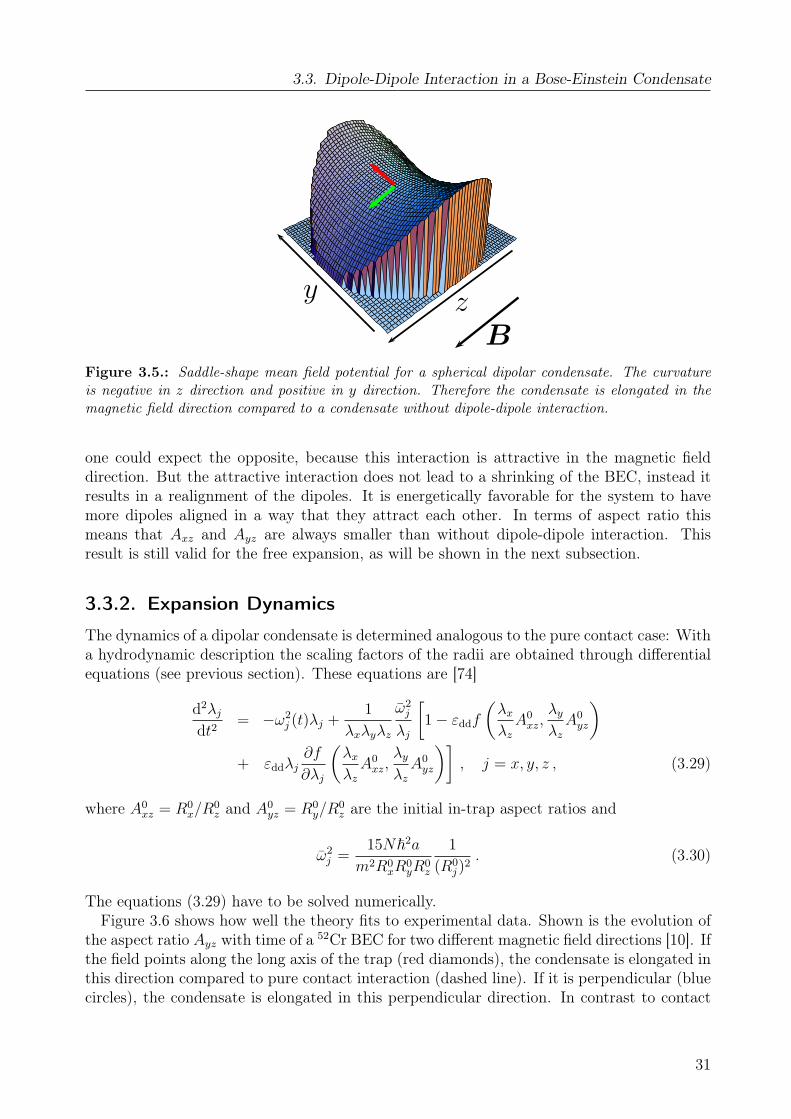
zy
BFigure 3.5.: Saddle-shape mean field potential for a spherical dipolar condensate. The curvatureis negative in z direction and positive in y direction. Therefore the condensate is elongated in themagnetic field direction compared to a condensate without dipole-dipole interaction.
one could expect the opposite, because this interaction is attractive in the magnetic fielddirection. But the attractive interaction does not lead to a shrinking of the BEC, instead itresults in a realignment of the dipoles. It is energetically favorable for the system to havemore dipoles aligned in a way that they attract each other. In terms of aspect ratio thismeans that Axz and Ayz are always smaller than without dipole-dipole interaction. Thisresult is still valid for the free expansion, as will be shown in the next subsection.
3.3.2. Expansion Dynamics
The dynamics of a dipolar condensate is determined analogous to the pure contact case: Witha hydrodynamic description the scaling factors of the radii are obtained through differentialequations (see previous section). These equations are [74]
d2λj
dt2= −ω2
j (t)λj +1
λxλyλz
ω2j
λj
[1− εddf
(λx
λz
A0xz,
λy
λz
A0yz
)+ εddλj
∂f
∂λj
(λx
λz
A0xz,
λy
λz
A0yz
)], j = x, y, z , (3.29)
where A0xz = R0
x/R0z and A0
yz = R0y/R
0z are the initial in-trap aspect ratios and
ω2j =
15N~2a
m2R0xR
0yR
0z
1
(R0j )
2. (3.30)
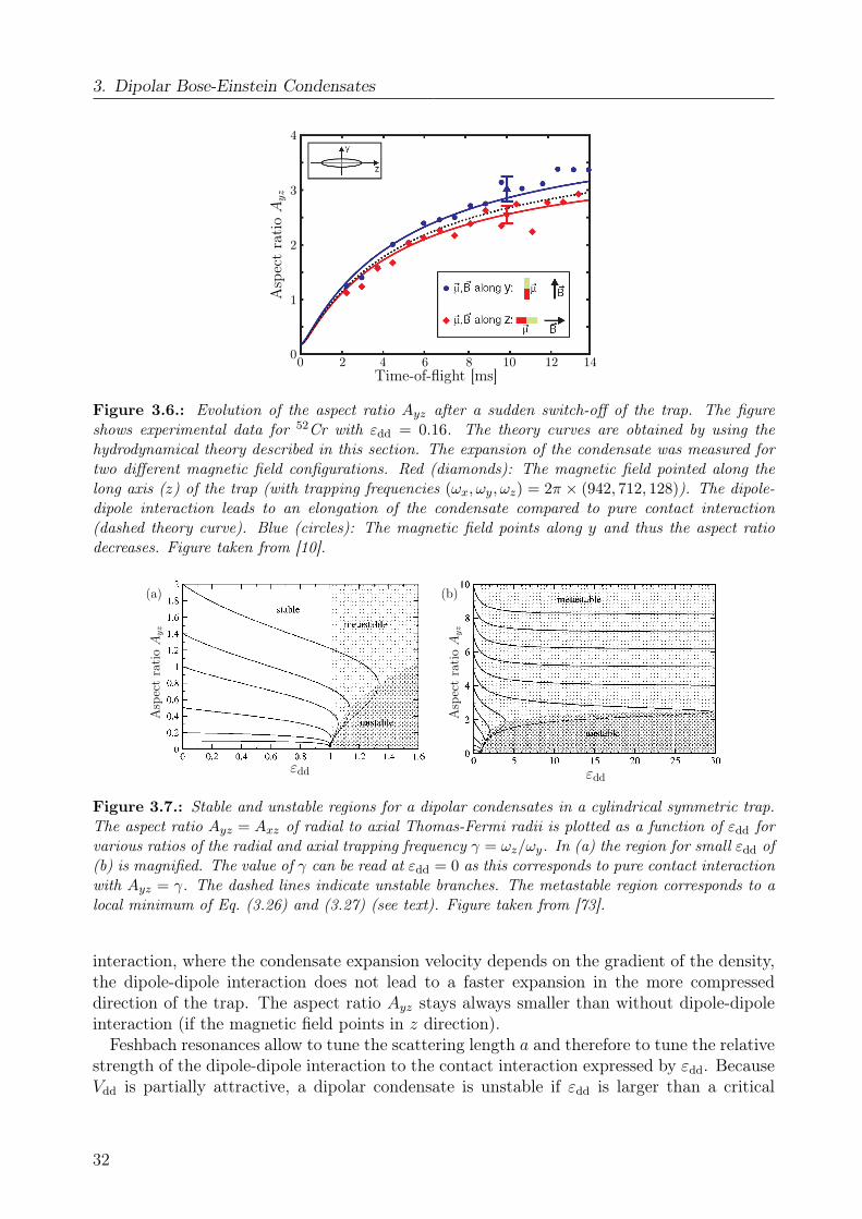
The equations (3.29) have to be solved numerically.Figure 3.6 shows how well the theory fits to experimental data. Shown is the evolution of
the aspect ratio Ayz with time of a 52Cr BEC for two different magnetic field directions [10]. Ifthe field points along the long axis of the trap (red diamonds), the condensate is elongated inthis direction compared to pure contact interaction (dashed line). If it is perpendicular (bluecircles), the condensate is elongated in this perpendicular direction. In contrast to contact
31
3. Dipolar Bose-Einstein Condensates
0 2 4 6 8 10 12 140
1
2
3
4
Time-of-flight [ms]
Asp
ect
rati
oA
yz
Figure 3.6.: Evolution of the aspect ratio Ayz after a sudden switch-off of the trap. The figureshows experimental data for 52Cr with εdd = 0.16. The theory curves are obtained by using thehydrodynamical theory described in this section. The expansion of the condensate was measured fortwo different magnetic field configurations. Red (diamonds): The magnetic field pointed along thelong axis (z) of the trap (with trapping frequencies (ωx, ωy, ωz) = 2π × (942, 712, 128)). The dipole-dipole interaction leads to an elongation of the condensate compared to pure contact interaction(dashed theory curve). Blue (circles): The magnetic field points along y and thus the aspect ratiodecreases. Figure taken from [10].
εdd
Asp
ect
rati
oA
yz
εdd
Asp
ect
rati
oA
yz
(a) (b)
Figure 3.7.: Stable and unstable regions for a dipolar condensates in a cylindrical symmetric trap.The aspect ratio Ayz = Axz of radial to axial Thomas-Fermi radii is plotted as a function of εdd forvarious ratios of the radial and axial trapping frequency γ = ωz/ωy. In (a) the region for small εdd of(b) is magnified. The value of γ can be read at εdd = 0 as this corresponds to pure contact interactionwith Ayz = γ. The dashed lines indicate unstable branches. The metastable region corresponds to alocal minimum of Eq. (3.26) and (3.27) (see text). Figure taken from [73].
interaction, where the condensate expansion velocity depends on the gradient of the density,the dipole-dipole interaction does not lead to a faster expansion in the more compresseddirection of the trap. The aspect ratio Ayz stays always smaller than without dipole-dipoleinteraction (if the magnetic field points in z direction).
Feshbach resonances allow to tune the scattering length a and therefore to tune the relativestrength of the dipole-dipole interaction to the contact interaction expressed by εdd. BecauseVdd is partially attractive, a dipolar condensate is unstable if εdd is larger than a critical
32
3.3. Dipole-Dipole Interaction in a Bose-Einstein Condensate
value εcritdd . Already with the equations (3.26) and (3.27) important predictions can be made
on the stability properties. This was done in [73] for a cylindrical symmetric trap with themagnetic field pointing in axial direction. Figure 3.7 shows stable and unstable regions forvarious trap geometries. In the Thomas-Fermi limit the trap geometry is the only parameterthat determines if a condensate is stable for a given εdd. It turns out that for 0 ≤ εdd < 1the solution of Eq. (3.26) and Eq. (3.27) corresponds to a global energy minimum and thecondensate is stable for all geometries. For εdd ≥ 1 and a ratio of radial to axial trappingfrequency γ = ωz/ωx = ωz/ωy ≤ 5.17 two solutions exist: While one is unstable, the otherone is only a local energy minimum and thus metastable. Above γ = 5.17 both solutions aremetastable for all εdd. For these extreme pancake-shaped (oblate) traps the repulsive partof Vdd leads to a stabilization. To summarize, cigar-shaped (prolate) traps with the dipolesaligned along the long axis are unstable for εdd ≥ 1, whereas for pancake traps larger εdd arepossible.
33
3. Dipolar Bose-Einstein Condensates
34
4. Experimental Setup
The experiment that is used to investigate strong dipolar effects in a ChromiumBEC was set up mainly by J. Stuhler [75], P. O. Schmidt [76], S. Hensler [77],J. Werner [60] and A. Griesmaier [50]. Section 4.1 gives a coarse overview over theapparatus. For details the reader should consult the above mentioned references (seealso [78] for an overview, or the diploma theses [79, 80, 81, 82]), which provide agreat amount of detailed information on the setup. Section 4.2 reports on a methodto measure the trapping frequencies of the optical dipole trap more precisely than withthe parametric heating method which has been used before. The modifications to thesetup, which are necessary to perform the experiments presented in this thesis, aredescribed in the last two sections. Section 4.3 reports on the production of the stable,homogeneous magnetic field of 600 G to tune the scattering length. The calibrationof the extra current, which runs in opposite direction in the pinch coils to compensatethe curvature of the offset coils, is discussed in detail. In the last section 4.4, thehigh-field imaging system is described. This system allows to image the atoms at thehigh magnetic field close to the broadest Feshbach resonance.
4.1. Bose-Einstein Condensation of Chromium
The production of a BEC of 52Cr atoms starting from 1600 C hot atoms which are sublimatedfrom an oven, requires an elaborate series of trapping and cooling steps:
1. Decelerating of the hot atoms in a Zeeman Slower.
2. Trapping and cooling in a magneto-optical trap (MOT) and continuous loading of amagnetic trap (MT).
3. Doppler cooling and radio-frequency (RF) evaporation in the magnetic trap.
4. Loading into a crossed optical dipole trap (ODT) and optical pumping to the lowestZeeman sub-state to avoid dipolar relaxation.
5. Forced evaporation in the ODT until quantum-degeneracy is reached.
This chapter will shortly describe the various parts of the experimental setup (see Fig. 4.1)following the steps sketched above.
4.1.1. Preparation of a Cold Sample in the Magnetic Trap
The Chromium atoms are sublimated from a high-purity sample of Chromium (99.99%) thatis held within a specially designed crucible [60] in a high temperature effusion cell1. The oven
1VTS Schwarz GmbH, model HT-TA-35-10/W.
35
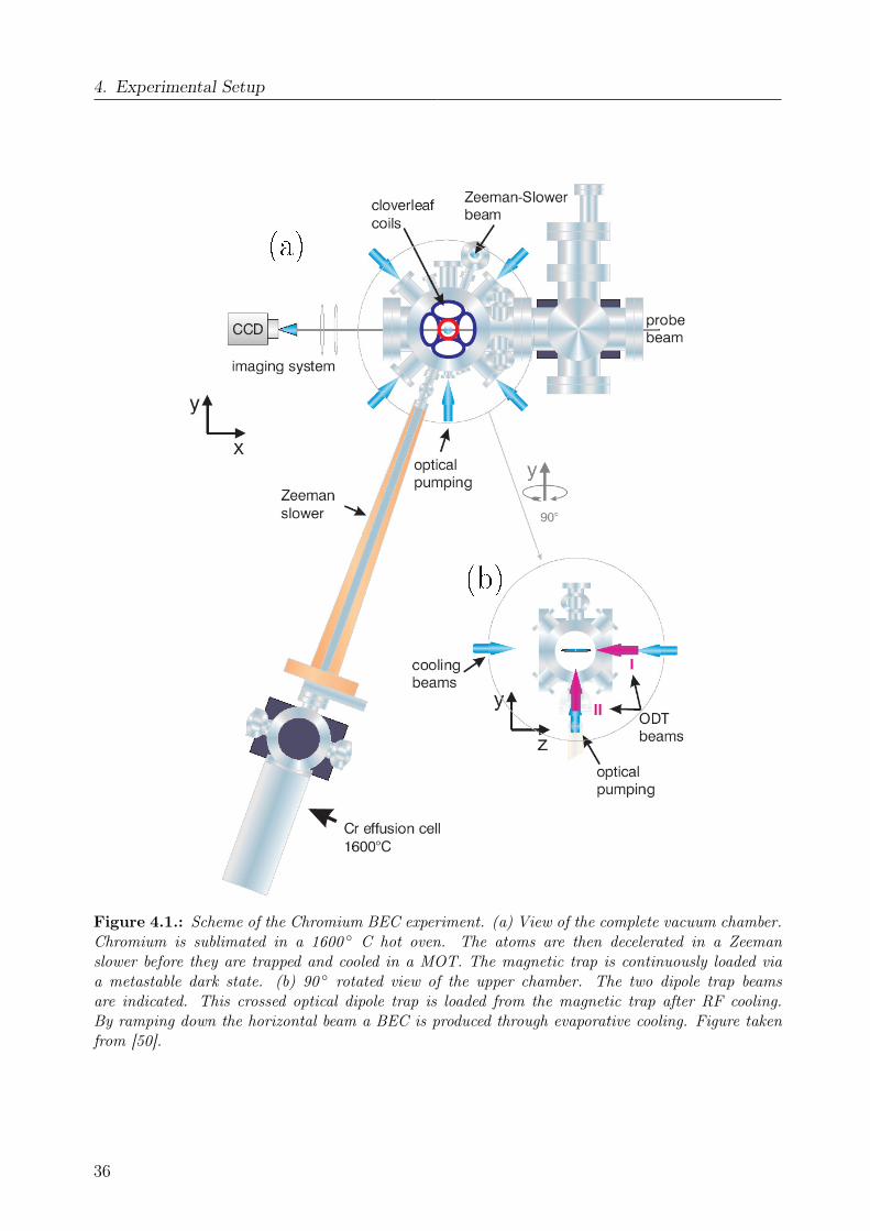
4. Experimental Setup
Figure 4.1.: Scheme of the Chromium BEC experiment. (a) View of the complete vacuum chamber.Chromium is sublimated in a 1600 C hot oven. The atoms are then decelerated in a Zeemanslower before they are trapped and cooled in a MOT. The magnetic trap is continuously loaded viaa metastable dark state. (b) 90 rotated view of the upper chamber. The two dipole trap beamsare indicated. This crossed optical dipole trap is loaded from the magnetic trap after RF cooling.By ramping down the horizontal beam a BEC is produced through evaporative cooling. Figure takenfrom [50].
36

4.1. Bose-Einstein Condensation of Chromium
is connected through an 80 cm long spin-flip Zeeman slower to the main chamber [81]. TheZeeman slower, which acts also as an differential pumping stage2, decelerates atoms with aninitial velocity smaller than ∼ 600 m/s to the capture velocity of the MOT (∼ 30 m/s). TheMOT is operated on the 7S3↔7P4 transition (see Figure 4.2 and appendix B.1 for details onthe level structure of 52Cr).
The magnetic fields for the MOT are provided by the coils of the Ioffe-Pritchard typemagnetic trap [81] (see also section 4.3). In MOT operation the cloverleaf coils create a radialgradient (x and y direction) of ∼ 10 G/cm and the pinch coils an axial curvature (z direction)of ∼ 15 G/cm2. The offset coils compensate the offset field of the pinch coils. Two orthogonalpairs of counter-propagating σ+/σ−-polarized laser beams confine and cool the atoms radially.In axial direction the magnetic field does not allow a MOT operation. Therefore the atomsare only Doppler-cooled in this direction using a σ+/σ+ optical molasses [76].
With a ratio of approximately 1/250000 the Chromium atoms do not decay back into the7S3 ground state, but into the metastable 5D4 or 5D3 states. These states have a magneticdipole moment of 6 µB and 4 µB, respectively. Atoms that are in a low-field seeking sub-stateand are sufficiently cool are thus trapped in the weak confining potential of the magnetic field.As these atoms are decoupled from the light field without a repumping laser, this allows tocontinuously load the magnetic trap. After about 10 s a steady-state is reached, where theloading rate of the magnetic trap is equal to the losses due to light-induced collisions [76]. Ifthe MOT beams are then switched-off and the atoms are pumped back into the ground statewith the repumper3 at 663 nm (shone in along the z axis), a sample of approximately 108
atoms is prepared in the MT close to the doppler temperature of 124 µK (phase spacedensity ∼ 10−9) [50]. The atoms are pumped back via the 7P3 state, as this allows fasterpumping than via the 7P4 state. Subsequently, the magnetic trap is compressed by rampingup the current in the cloverleaf, offset and pinch coils to 300 A. This leads to a heating of thecloud to ∼ 1 mK. At this stage the gas is Doppler cooled with the axial σ+/σ+ beams. Afterthe rethermalization of the sample the phase space density has increased by about 2 ordersof magnitude without atom loss. The current is then ramped down adiabatically to form amagnetic trap with the highest possible overlap to the trapping potential of the horizontaldipole trap beam. In this magnetic trap RF cooling is performed. Due to the high magneticmoment of Chromium atoms it is important to have a low magnetic offset field at this stage,otherwise spin-changing collisions lead to too high atom losses at the densities that arereached during RF cooling [77]. With an additional current running through the offset coils,offset fields on the order of a few 10 mG are reached, which allow to cool down the sample toa temperature of approximately 22 µK without too high inelastic losses. About 5×10⁶ atomsremain at a phase space density of 10−5. However, quantum-degeneracy cannot be reachedin this way. Hence, the sample is pumped into the lowest Zeeman state MS = −3, wherespin-changing collisions cannot occur. This is done with a σ−-polarized optical pumping laserat 427 nm, which pumps the atoms to the MS = −3 state via the 7P3 state (see Fig. 4.2 (b)).As the MS = −3 state is high-field seeking, the MT has to be switched off before. Thehorizontal ODT beam, which is on during the whole first part of the experimental sequence,provides then the trapping potential. After ramping up also the vertical ODT beam in 5 sabout 106 atoms remain trapped [50].
2Allowing to have a 2 orders of magnitude lower pressure in the upper science chamber (about 10−11 mbar).3The gain in atom number by repumping also the 5D3 state atoms is small compared to using only the
663 nm repumper. Thus the 5D3 atoms are not pumped back.
37
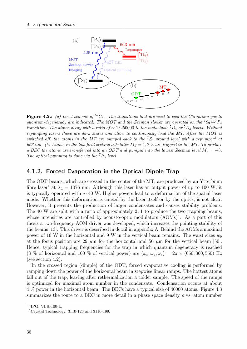
4. Experimental Setup
(a)
˛˛7S3
¸
˛˛7P4
¸
˛7P3
¸
˛5D4
¸˛˛5D3
¸425 nm
MOT
Zeeman slowerImaging
427 nmOptical pumping
663 nmRepumper
(b)
MJ=−3 −2 −1 0 1 2 3ODT
MT
Figure 4.2.: (a) Level scheme of 52Cr. The transitions that are used to cool the Chromium gas toquantum-degeneracy are indicated. The MOT and the Zeeman slower are operated on the 7S3↔7P4
transition. The atoms decay with a ratio of ∼ 1/250000 to the metastable 5D4 or 5D3 levels. Withoutrepumping lasers these are dark states and allow to continuously load the MT. After the MOT isswitched off, the atoms in the MT are pumped back to the 7S3 ground level with a repumper3 at663 nm. (b) Atoms in the low-field seeking substates MJ = 1, 2, 3 are trapped in the MT. To producea BEC the atoms are transferred into an ODT and pumped into the lowest Zeeman level MJ = −3.The optical pumping is done via the 7P3 level.
4.1.2. Forced Evaporation in the Optical Dipole Trap
The ODT beams, which are crossed in the center of the MT, are produced by an Ytterbiumfibre laser4 at λL = 1076 nm. Although this laser has an output power of up to 100 W, itis typically operated with ∼ 40 W. Higher powers lead to a deformation of the spatial lasermode. Whether this deformation is caused by the laser itself or by the optics, is not clear.However, it prevents the production of larger condensates and causes stability problems.The 40 W are split with a ratio of approximately 2 : 1 to produce the two trapping beams,whose intensities are controlled by acousto-optic modulators (AOMs)5. As a part of thisthesis a two-frequency AOM driver was developed, which increases the pointing stability ofthe beams [13]. This driver is described in detail in appendix A. Behind the AOMs a maximalpower of 16 W in the horizontal and 9 W in the vertical beam remains. The waist sizes w0
at the focus position are 29 µm for the horizontal and 50 µm for the vertical beam [50].Hence, typical trapping frequencies for the trap in which quantum degeneracy is reached(3 % of horizontal and 100 % of vertical power) are (ωx, ωy, ωz) = 2π × (650, 360, 550) Hz(see section 4.2).
In the crossed region (dimple) of the ODT, forced evaporative cooling is performed byramping down the power of the horizontal beam in stepwise linear ramps. The hottest atomsfall out of the trap, leaving after rethermalization a colder sample. The speed of the rampsis optimized for maximal atom number in the condensate. Condensation occurs at about4 % power in the horizontal beam. The BECs have a typical size of 40000 atoms. Figure 4.3summarizes the route to a BEC in more detail in a phase space density ρ vs. atom number
4IPG, VLR-100-L.5Crystal Technology, 3110-125 and 3110-199.
38
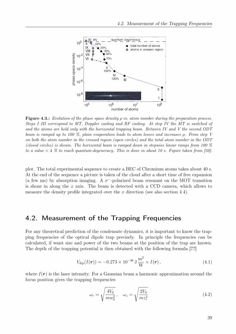
4.2. Measurement of the Trapping Frequencies
Figure 4.3.: Evolution of the phase space density ρ vs. atom number during the preparation process.Steps I–III correspond to MT, Doppler cooling and RF cooling. At step IV the MT is switched ofand the atoms are held only with the horizontal trapping beam. Between IV and V the second ODTbeam is ramped up to 100 %, plain evaporation leads to atom losses and increases ρ. From step Von both the atom number in the crossed region (open circles) and the total atom number in the ODT(closed circles) is shown. The horizontal beam is ramped down in stepwise linear ramps from 100 %to a value < 4 % to reach quantum-degeneracy. This is done in about 10 s. Figure taken from [50].
plot. The total experimental sequence to create a BEC of Chromium atoms takes about 40 s.At the end of the sequence a picture is taken of the cloud after a short time of free expansion(a few ms) by absorption imaging. A σ−-polarized beam resonant on the MOT transitionis shone in along the x axis. The beam is detected with a CCD camera, which allows tomeasure the density profile integrated over the x direction (see also section 4.4).
4.2. Measurement of the Trapping Frequencies
For any theoretical prediction of the condensate dynamics, it is important to know the trap-ping frequencies of the optical dipole trap precisely. In principle the frequencies can becalculated, if waist size and power of the two beams at the position of the trap are known.The depth of the trapping potential is then obtained with the following formula [77]
Vdip(I(r)) = −0.273× 10−36 Jm2
W× I(r) , (4.1)
where I(r) is the laser intensity. For a Gaussian beam a harmonic approximation around thefocus position gives the trapping frequencies
ωr =
√4V0
mw20
, ωz =
√2V0
mz2r
(4.2)
39
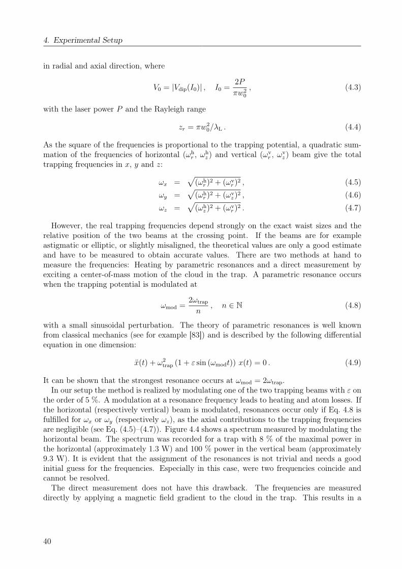
4. Experimental Setup
in radial and axial direction, where
V0 = |Vdip(I0)| , I0 =2P
πw20
, (4.3)
with the laser power P and the Rayleigh range
zr = πw20/λL . (4.4)
As the square of the frequencies is proportional to the trapping potential, a quadratic sum-mation of the frequencies of horizontal (ωh
r , ωhz ) and vertical (ωv
r , ωvz ) beam give the total
trapping frequencies in x, y and z:
ωx =√
(ωhr )2 + (ωv
r )2 , (4.5)
ωy =√
(ωhr )2 + (ωv
z )2 , (4.6)
ωz =√
(ωhz )2 + (ωv
r )2 . (4.7)
However, the real trapping frequencies depend strongly on the exact waist sizes and therelative position of the two beams at the crossing point. If the beams are for exampleastigmatic or elliptic, or slightly misaligned, the theoretical values are only a good estimateand have to be measured to obtain accurate values. There are two methods at hand tomeasure the frequencies: Heating by parametric resonances and a direct measurement byexciting a center-of-mass motion of the cloud in the trap. A parametric resonance occurswhen the trapping potential is modulated at
ωmod =2ωtrap
n, n ∈ N (4.8)
with a small sinusoidal perturbation. The theory of parametric resonances is well knownfrom classical mechanics (see for example [83]) and is described by the following differentialequation in one dimension:
x(t) + ω2trap (1 + ε sin (ωmodt)) x(t) = 0 . (4.9)
It can be shown that the strongest resonance occurs at ωmod = 2ωtrap.In our setup the method is realized by modulating one of the two trapping beams with ε on
the order of 5 %. A modulation at a resonance frequency leads to heating and atom losses. Ifthe horizontal (respectively vertical) beam is modulated, resonances occur only if Eq. 4.8 isfulfilled for ωx or ωy (respectively ωz), as the axial contributions to the trapping frequenciesare negligible (see Eq. (4.5)–(4.7)). Figure 4.4 shows a spectrum measured by modulating thehorizontal beam. The spectrum was recorded for a trap with 8 % of the maximal power inthe horizontal (approximately 1.3 W) and 100 % power in the vertical beam (approximately9.3 W). It is evident that the assignment of the resonances is not trivial and needs a goodinitial guess for the frequencies. Especially in this case, were two frequencies coincide andcannot be resolved.
The direct measurement does not have this drawback. The frequencies are measureddirectly by applying a magnetic field gradient to the cloud in the trap. This results in a
40
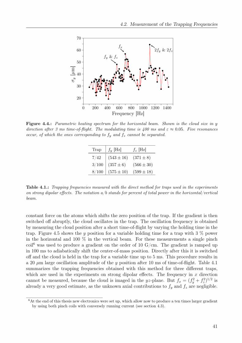
4.2. Measurement of the Trapping Frequencies
0 200 400 600 800 1000 1200 1400
20
30
40
50
60
70
Frequency [Hz]
σy
[µm
]
fy & fz
fx2fy & 2fz
Figure 4.4.: Parametric heating spectrum for the horizontal beam. Shown is the cloud size in ydirection after 3 ms time-of-flight. The modulating time is 400 ms and ε ≈ 0.05. Five resonancesoccur, of which the ones corresponding to fy and fz cannot be separated.
Trap fy [Hz] fz [Hz]
7/42 (543± 16) (371± 8)
3/100 (357± 6) (566± 30)
8/100 (575± 10) (599± 18)
Table 4.1.: Trapping frequencies measured with the direct method for traps used in the experimentson strong dipolar effects. The notation a/b stands for percent of total power in the horizontal/verticalbeam.
constant force on the atoms which shifts the zero position of the trap. If the gradient is thenswitched off abruptly, the cloud oscillates in the trap. The oscillation frequency is obtainedby measuring the cloud position after a short time-of-flight by varying the holding time in thetrap. Figure 4.5 shows the y position for a variable holding time for a trap with 3 % powerin the horizontal and 100 % in the vertical beam. For these measurements a single pinchcoil6 was used to produce a gradient on the order of 10 G/cm. The gradient is ramped upin 100 ms to adiabatically shift the center-of-mass position. Directly after this it is switchedoff and the cloud is held in the trap for a variable time up to 5 ms. This procedure results ina 20 µm large oscillation amplitude of the y position after 10 ms of time-of-flight. Table 4.1summarizes the trapping frequencies obtained with this method for three different traps,which are used in the experiments on strong dipolar effects. The frequency in x directioncannot be measured, because the cloud is imaged in the yz-plane. But fx = (f 2
y + f 2z )1/2 is
already a very good estimate, as the unknown axial contributions to fy and fz are negligible.
6At the end of this thesis new electronics were set up, which allow now to produce a ten times larger gradientby using both pinch coils with conversely running current (see section 4.3).
41
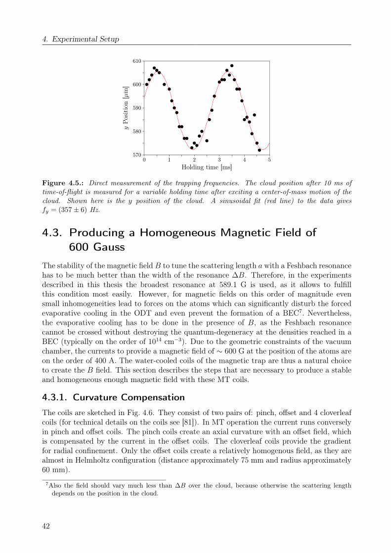
4. Experimental Setup
0 1 2 3 4 5570
580
590
600
610
Holding time [ms]
yPos
itio
n[µ
m]
Figure 4.5.: Direct measurement of the trapping frequencies. The cloud position after 10 ms oftime-of-flight is measured for a variable holding time after exciting a center-of-mass motion of thecloud. Shown here is the y position of the cloud. A sinusoidal fit (red line) to the data givesfy = (357± 6) Hz.
4.3. Producing a Homogeneous Magnetic Field of600 Gauss
The stability of the magnetic field B to tune the scattering length a with a Feshbach resonancehas to be much better than the width of the resonance ∆B. Therefore, in the experimentsdescribed in this thesis the broadest resonance at 589.1 G is used, as it allows to fulfillthis condition most easily. However, for magnetic fields on this order of magnitude evensmall inhomogeneities lead to forces on the atoms which can significantly disturb the forcedevaporative cooling in the ODT and even prevent the formation of a BEC7. Nevertheless,the evaporative cooling has to be done in the presence of B, as the Feshbach resonancecannot be crossed without destroying the quantum-degeneracy at the densities reached in aBEC (typically on the order of 1014 cm−3). Due to the geometric constraints of the vacuumchamber, the currents to provide a magnetic field of ∼ 600 G at the position of the atoms areon the order of 400 A. The water-cooled coils of the magnetic trap are thus a natural choiceto create the B field. This section describes the steps that are necessary to produce a stableand homogeneous enough magnetic field with these MT coils.
4.3.1. Curvature Compensation
The coils are sketched in Fig. 4.6. They consist of two pairs of: pinch, offset and 4 cloverleafcoils (for technical details on the coils see [81]). In MT operation the current runs converselyin pinch and offset coils. The pinch coils create an axial curvature with an offset field, whichis compensated by the current in the offset coils. The cloverleaf coils provide the gradientfor radial confinement. Only the offset coils create a relatively homogenous field, as they arealmost in Helmholtz configuration (distance approximately 75 mm and radius approximately60 mm).
7Also the field should vary much less than ∆B over the cloud, because otherwise the scattering lengthdepends on the position in the cloud.
42
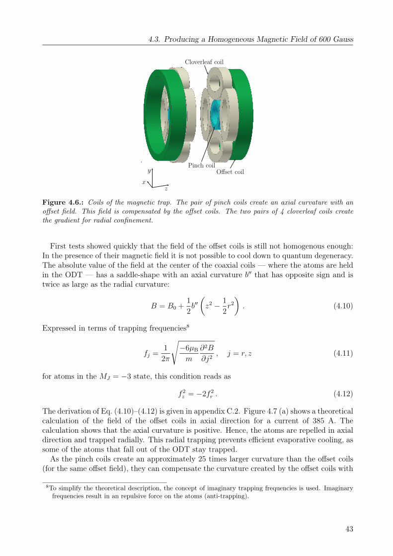
4.3. Producing a Homogeneous Magnetic Field of 600 Gauss
Pinch coilOffset coil
Cloverleaf coil
z
y
x
Figure 4.6.: Coils of the magnetic trap. The pair of pinch coils create an axial curvature with anoffset field. This field is compensated by the offset coils. The two pairs of 4 cloverleaf coils createthe gradient for radial confinement.
First tests showed quickly that the field of the offset coils is still not homogenous enough:In the presence of their magnetic field it is not possible to cool down to quantum degeneracy.The absolute value of the field at the center of the coaxial coils — where the atoms are heldin the ODT — has a saddle-shape with an axial curvature b′′ that has opposite sign and istwice as large as the radial curvature:
B = B0 +1
2b′′(z2 − 1
2r2
). (4.10)
Expressed in terms of trapping frequencies8
fj =1
2π
√−6µB
m
∂2B
∂j2, j = r, z (4.11)
for atoms in the MJ = −3 state, this condition reads as
f 2z = −2f 2
r . (4.12)
The derivation of Eq. (4.10)–(4.12) is given in appendix C.2. Figure 4.7 (a) shows a theoreticalcalculation of the field of the offset coils in axial direction for a current of 385 A. Thecalculation shows that the axial curvature is positive. Hence, the atoms are repelled in axialdirection and trapped radially. This radial trapping prevents efficient evaporative cooling, assome of the atoms that fall out of the ODT stay trapped.
As the pinch coils create an approximately 25 times larger curvature than the offset coils(for the same offset field), they can compensate the curvature created by the offset coils with
8To simplify the theoretical description, the concept of imaginary trapping frequencies is used. Imaginaryfrequencies result in an repulsive force on the atoms (anti-trapping).
43
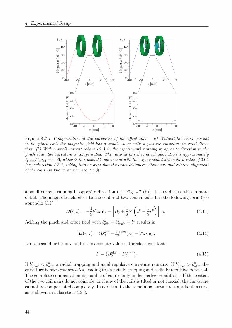
4. Experimental Setup
(a)
-100 -50 0 50 100300
400
500
600
700700
z [mm]
Mag
neti
cfie
ld[G
]
(b)
-100 -50 0 50 100300
400
500
600
700700
z [mm]
Mag
neti
cfie
ld[G
]
-10 -5 0 5 10590
595
600
605
610
z [mm]
Mag
neti
cfie
ld[G
]
-10 -5 0 5 10590
595
600
605
610
z [mm]M
agne
tic
field
[G]
Figure 4.7.: Compensation of the curvature of the offset coils. (a) Without the extra currentin the pinch coils the magnetic field has a saddle shape with a positive curvature in axial direc-tion. (b) With a small current (about 16 A in the experiment) running in opposite direction in thepinch coils, the curvature is compensated. The ratio in this theoretical calculation is approximatelyIpinch/Ioffset = 0.06, which is in reasonable agreement with the experimental determined value of 0.04(see subsection 4.3.3) taking into account that the exact distances, diameters and relative alignmentof the coils are known only to about 5 %.
a small current running in opposite direction (see Fig. 4.7 (b)). Let us discuss this in moredetail. The magnetic field close to the center of two coaxial coils has the following form (seeappendix C.2):
B(r, z) = −1
2b′′zr er +
[B0 +
1
2b′′(z2 − 1
2r2
)]ez . (4.13)
Adding the pinch and offset field with b′′offs = b′′pinch = b′′ results in
B(r, z) = (Boffs0 −Bpinch
0 ) ez − b′′zr er . (4.14)
Up to second order in r and z the absolute value is therefore constant
B = (Boffs0 −Bpinch
0 ) . (4.15)
If b′′pinch < b′′offs, a radial trapping and axial repulsive curvature remains. If b′′pinch > b′′offs, thecurvature is over-compensated, leading to an axially trapping and radially repulsive potential.The complete compensation is possible of course only under perfect conditions. If the centersof the two coil pairs do not coincide, or if any of the coils is tilted or not coaxial, the curvaturecannot be compensated completely. In addition to the remaining curvature a gradient occurs,as is shown in subsection 4.3.3.
44
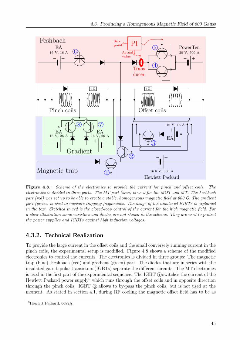
4.3. Producing a Homogeneous Magnetic Field of 600 Gauss
+−+−
+−
1Ω 1Ω
+ −
+ −+−
Pinch coils Offset coils
PowerTen20 V, 500 A
Hewlett Packard16.8 V, 300 A
EA16 V, 16 A
EA
16 V, 16 A
EA16 V, 26 A
EA16 V, 26 A
Feshbach
Magnetic trap
Gradient
PI
Trans-ducer
Set-point
Actualvalue
1
2
3
4
56
78
Figure 4.8.: Scheme of the electronics to provide the current for pinch and offset coils. Theelectronics is divided in three parts. The MT part (blue) is used for the MOT and MT. The Feshbachpart (red) was set up to be able to create a stable, homogeneous magnetic field at 600 G. The gradientpart (green) is used to measure trapping frequencies. The usage of the numbered IGBTs is explainedin the text. Sketched in red is the closed-loop control of the current for the high magnetic field. Fora clear illustration some varistors and diodes are not shown in the scheme. They are used to protectthe power supplies and IGBTs against high induction voltages.
4.3.2. Technical Realization
To provide the large current in the offset coils and the small conversely running current in thepinch coils, the experimental setup is modified. Figure 4.8 shows a scheme of the modifiedelectronics to control the currents. The electronics is divided in three groups: The magnetictrap (blue), Feshbach (red) and gradient (green) part. The diodes that are in series with theinsulated gate bipolar transistors (IGBTs) separate the different circuits. The MT electronicsis used in the first part of the experimental sequence. The IGBT©1 switches the current of theHewlett Packard power supply9 which runs through the offset coils and in opposite directionthrough the pinch coils. IGBT ©2 allows to by-pass the pinch coils, but is not used at themoment. As stated in section 4.1, during RF cooling the magnetic offset field has to be as
9Hewlett Packard, 6682A.
45
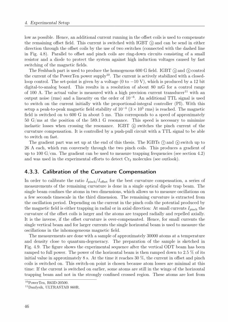
4. Experimental Setup
low as possible. Hence, an additional current running in the offset coils is used to compensatethe remaining offset field. This current is switched with IGBT ©3 and can be send in eitherdirection through the offset coils by the use of two switches (connected with the dashed linein Fig. 4.8). Parallel to offset and pinch coils are ring-down circuits consisting of a smallresistor and a diode to protect the system against high induction voltages caused by fastswitching of the magnetic fields.
The Feshbach part is used to produce the homogenous 600 G field. IGBT ©4 and ©5 controlthe current of the PowerTen power supply10. The current is actively stabilized with a closed-loop control. The set-point is given by a voltage (0 to −10 V), which is produced by a 12 bitdigital-to-analog board. This results in a resolution of about 80 mG for a control rangeof 100 A. The actual value is measured with a high precision current transducer11 with anoutput noise (rms) and a linearity on the order of 10−6. An additional TTL signal is usedto switch on the current initially with the proportional-integral controller (PI). With thissetup a peak-to-peak magnetic field stability of 10−4 (3× 10⁵ rms) is reached. The magneticfield is switched on to 600 G in about 5 ms. This corresponds to a speed of approximately50 G/ms at the position of the 589.1 G resonance. This speed is necessary to minimizeinelastic losses when crossing the resonance. IGBT ©6 switches the pinch current of thecurvature compensation. It is controlled by a push-pull circuit with a TTL signal to be ableto switch on fast.
The gradient part was set up at the end of this thesis. The IGBTs ©7 and ©8 switch up to26 A each, which run conversely through the two pinch coils. This produces a gradient ofup to 100 G/cm. The gradient can be used to measure trapping frequencies (see section 4.2)and was used in the experimental efforts to detect Cr2 molecules (see outlook).
4.3.3. Calibration of the Curvature Compensation
In order to calibrate the ratio Ipinch/Ioffset for the best curvature compensation, a series ofmeasurements of the remaining curvature is done in a single optical dipole trap beam. Thesingle beam confines the atoms in two dimensions, which allows us to measure oscillations ona few seconds timescale in the third dimension. The remaining curvature is extracted fromthe oscillation period. Depending on the current in the pinch coils the potential produced bythe magnetic field is either trapping in radial or in axial direction: At small currents Ipinch thecurvature of the offset coils is larger and the atoms are trapped radially and repelled axially.It is the inverse, if the offset curvature is over-compensated. Hence, for small currents thesingle vertical beam and for larger currents the single horizontal beam is used to measure theoscillations in the inhomogeneous magnetic field.
The measurements are done with a sample of approximately 30000 atoms at a temperatureand density close to quantum-degeneracy. The preparation of the sample is sketched inFig. 4.9. The figure shows the experimental sequence after the vertical ODT beam has beenramped to full power. The power of the horizontal beam is then ramped down to 2.5 % of itsinitial value in approximately 8 s. At the time it reaches 30 %, the current in offset and pinchcoils is switched on. This switch-on point is chosen because atom losses are minimal at thistime: If the current is switched on earlier, some atoms are still in the wings of the horizontaltrapping beam and not in the strongly confined crossed region. These atoms are lost from10PowerTen, R63D-20500.11Danfysik, ULTRASTAB 860R.
46
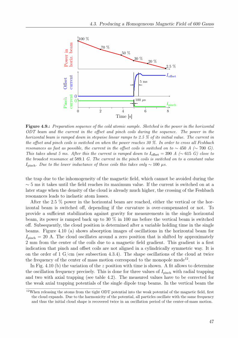
4.3. Producing a Homogeneous Magnetic Field of 600 Gauss
0 2 4 6 8Time [s]
100 %
70 %50 %
30 %20 %
2.5 %
Ioffset
0Ipinch
0
Pow
erin
hori
z.be
amO
ffset
curr
ent
Pin
chcu
rren
t
5 ms
100 µs
Figure 4.9.: Preparation sequence of the cold atomic sample. Sketched is the power in the horizontalODT beam and the current in the offset and pinch coils during the sequence. The power in thehorizontal beam is ramped down in stepwise linear ramps to 2.5 % of its initial value. The current inthe offset and pinch coils is switched on when the power reaches 30 %. In order to cross all Feshbachresonances as fast as possible, the current in the offset coils is switched on to ∼ 450 A (∼ 700 G).This takes about 5 ms. After this the current is ramped down to Ioffset = 390 A (∼ 615 G) close tothe broadest resonance at 589.1 G. The current in the pinch coils is switched on to a constant valueIpinch. Due to the lower inductance of these coils this takes only ∼ 100 µs.
the trap due to the inhomogeneity of the magnetic field, which cannot be avoided during the∼ 5 ms it takes until the field reaches its maximum value. If the current is switched on at alater stage when the density of the cloud is already much higher, the crossing of the Feshbachresonances leads to inelastic atom losses.
After the 2.5 % power in the horizontal beam are reached, either the vertical or the hor-izontal beam is switched off, depending if the curvature is over-compensated or not. Toprovide a sufficient stabilization against gravity for measurements in the single horizontalbeam, its power is ramped back up to 30 % in 100 ms before the vertical beam is switchedoff. Subsequently, the cloud position is determined after a variable holding time in the singlebeams. Figure 4.10 (a) shows absorption images of oscillations in the horizontal beam forIpinch = 20 A. The cloud oscillates around a zero position that is shifted by approximately2 mm from the center of the coils due to a magnetic field gradient. This gradient is a firstindication that pinch and offset coils are not aligned in a cylindrically symmetric way. It ison the order of 1 G/cm (see subsection 4.3.4). The shape oscillations of the cloud at twicethe frequency of the center of mass motion correspond to the monopole mode12.
In Fig. 4.10 (b) the variation of the z position with time is shown. A fit allows to determinethe oscillation frequency precisely. This is done for three values of Ipinch with radial trappingand two with axial trapping (see table 4.2). The measured values have to be corrected forthe weak axial trapping potentials of the single dipole trap beams. In the vertical beam the12When releasing the atoms from the tight ODT potential into the weak potential of the magnetic field, first
the cloud expands. Due to the harmonicity of the potential, all particles oscillate with the same frequencyand thus the initial cloud shape is recovered twice in an oscillation period of the center-of-mass motion.
47
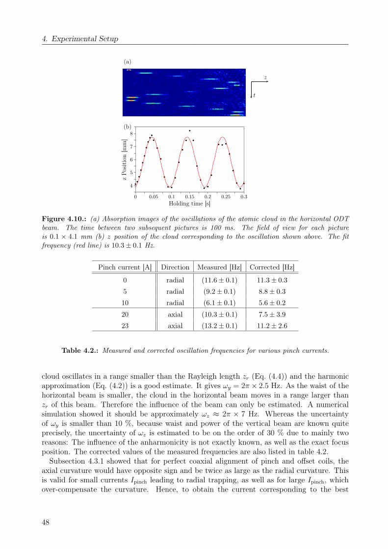
4. Experimental Setup
(a)
(b)
z
t
0 0.05 0.1 0.15 0.2 0.25 0.3
4
5
6
7
8
Holding time [s]
zPos
itio
n[m
m]
Figure 4.10.: (a) Absorption images of the oscillations of the atomic cloud in the horizontal ODTbeam. The time between two subsequent pictures is 100 ms. The field of view for each pictureis 0.1 × 4.1 mm (b) z position of the cloud corresponding to the oscillation shown above. The fitfrequency (red line) is 10.3± 0.1 Hz.
Pinch current [A] Direction Measured [Hz] Corrected [Hz]
0 radial (11.6± 0.1) 11.3± 0.3
5 radial (9.2± 0.1) 8.8± 0.3
10 radial (6.1± 0.1) 5.6± 0.2
20 axial (10.3± 0.1) 7.5± 3.9
23 axial (13.2± 0.1) 11.2± 2.6
Table 4.2.: Measured and corrected oscillation frequencies for various pinch currents.
cloud oscillates in a range smaller than the Rayleigh length zr (Eq. (4.4)) and the harmonicapproximation (Eq. (4.2)) is a good estimate. It gives ωy = 2π× 2.5 Hz. As the waist of thehorizontal beam is smaller, the cloud in the horizontal beam moves in a range larger thanzr of this beam. Therefore the influence of the beam can only be estimated. A numericalsimulation showed it should be approximately ωz ≈ 2π × 7 Hz. Whereas the uncertaintyof ωy is smaller than 10 %, because waist and power of the vertical beam are known quiteprecisely, the uncertainty of ωz is estimated to be on the order of 30 % due to mainly tworeasons: The influence of the anharmonicity is not exactly known, as well as the exact focusposition. The corrected values of the measured frequencies are also listed in table 4.2.
Subsection 4.3.1 showed that for perfect coaxial alignment of pinch and offset coils, theaxial curvature would have opposite sign and be twice as large as the radial curvature. Thisis valid for small currents Ipinch leading to radial trapping, as well as for large Ipinch, whichover-compensate the curvature. Hence, to obtain the current corresponding to the best
48
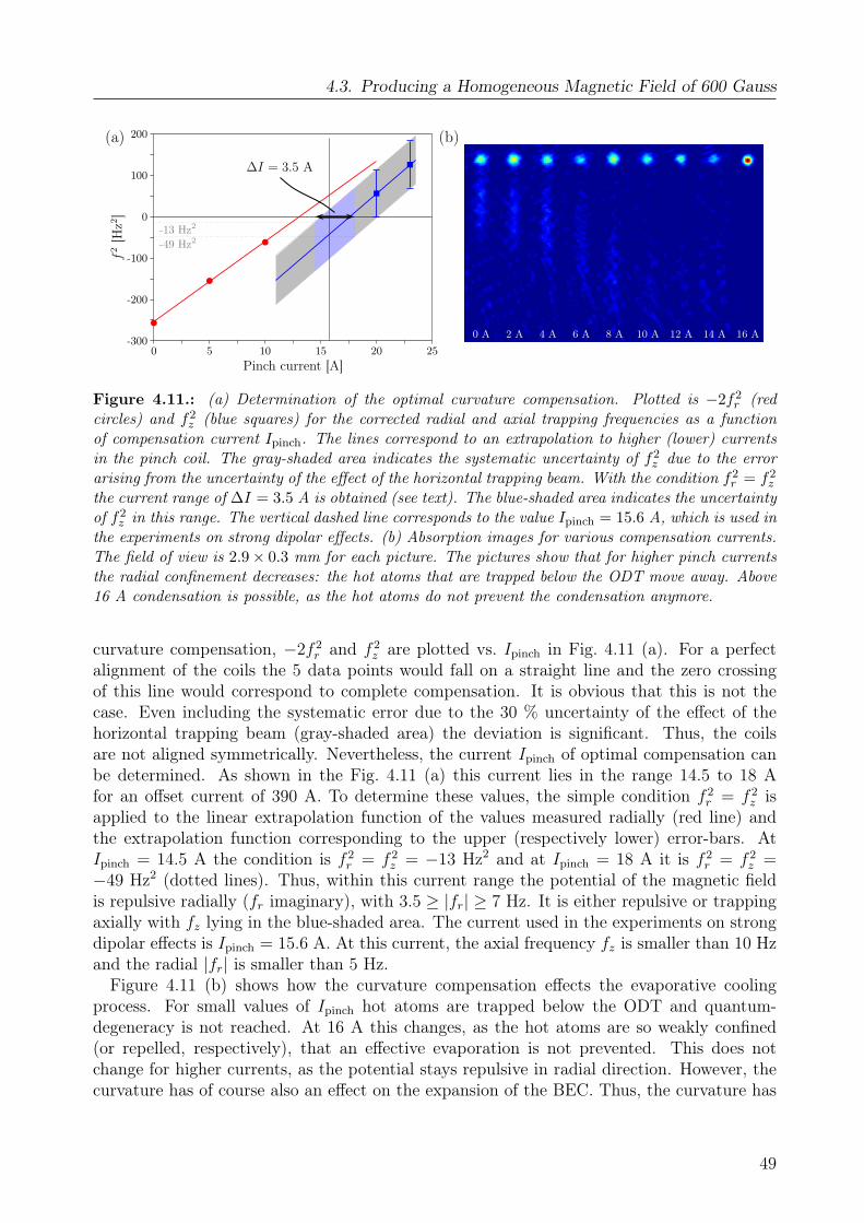
4.3. Producing a Homogeneous Magnetic Field of 600 Gauss
(a) (b)
0 5 10 15 20 25-300
-200
-100
0
100
200
Pinch current [A]
f2
[Hz2
]
0 A 2 A 4 A 6 A 8 A 10 A 12 A 14 A 16 A
∆I = 3.5 A
-13 Hz2
-49 Hz2
Figure 4.11.: (a) Determination of the optimal curvature compensation. Plotted is −2f2r (red
circles) and f2z (blue squares) for the corrected radial and axial trapping frequencies as a function
of compensation current Ipinch. The lines correspond to an extrapolation to higher (lower) currentsin the pinch coil. The gray-shaded area indicates the systematic uncertainty of f2
z due to the errorarising from the uncertainty of the effect of the horizontal trapping beam. With the condition f2
r = f2z
the current range of ∆I = 3.5 A is obtained (see text). The blue-shaded area indicates the uncertaintyof f2
z in this range. The vertical dashed line corresponds to the value Ipinch = 15.6 A, which is used inthe experiments on strong dipolar effects. (b) Absorption images for various compensation currents.The field of view is 2.9× 0.3 mm for each picture. The pictures show that for higher pinch currentsthe radial confinement decreases: the hot atoms that are trapped below the ODT move away. Above16 A condensation is possible, as the hot atoms do not prevent the condensation anymore.
curvature compensation, −2f 2r and f 2
z are plotted vs. Ipinch in Fig. 4.11 (a). For a perfectalignment of the coils the 5 data points would fall on a straight line and the zero crossingof this line would correspond to complete compensation. It is obvious that this is not thecase. Even including the systematic error due to the 30 % uncertainty of the effect of thehorizontal trapping beam (gray-shaded area) the deviation is significant. Thus, the coilsare not aligned symmetrically. Nevertheless, the current Ipinch of optimal compensation canbe determined. As shown in the Fig. 4.11 (a) this current lies in the range 14.5 to 18 Afor an offset current of 390 A. To determine these values, the simple condition f 2
r = f 2z is
applied to the linear extrapolation function of the values measured radially (red line) andthe extrapolation function corresponding to the upper (respectively lower) error-bars. AtIpinch = 14.5 A the condition is f 2
r = f 2z = −13 Hz2 and at Ipinch = 18 A it is f 2
r = f 2z =
−49 Hz2 (dotted lines). Thus, within this current range the potential of the magnetic fieldis repulsive radially (fr imaginary), with 3.5 ≥ |fr| ≥ 7 Hz. It is either repulsive or trappingaxially with fz lying in the blue-shaded area. The current used in the experiments on strongdipolar effects is Ipinch = 15.6 A. At this current, the axial frequency fz is smaller than 10 Hzand the radial |fr| is smaller than 5 Hz.
Figure 4.11 (b) shows how the curvature compensation effects the evaporative coolingprocess. For small values of Ipinch hot atoms are trapped below the ODT and quantum-degeneracy is not reached. At 16 A this changes, as the hot atoms are so weakly confined(or repelled, respectively), that an effective evaporation is not prevented. This does notchange for higher currents, as the potential stays repulsive in radial direction. However, thecurvature has of course also an effect on the expansion of the BEC. Thus, the curvature has
49
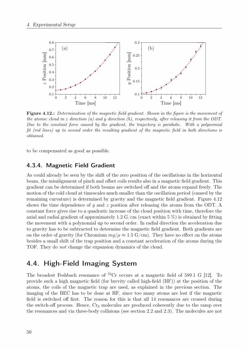
4. Experimental Setup
(a) (b)
0 2 4 6 8 10 12
0.1
0.2
0.3
0.4
0.5
0.6
0.7
0.8
Time [ms]
zPos
itio
n[m
m]
0 2 4 6 8 10 120.1
0.15
0.2
0.25
0.3
Time [ms]
yPos
itio
n[m
m]
Figure 4.12.: Determination of the magnetic field gradient. Shown in the figure is the movement ofthe atomic cloud in z direction (a) and y direction (b), respectively, after releasing it from the ODT.Due to the constant force caused by the gradient, the trajectory is parabolic. With a polynomialfit (red lines) up to second order the resulting gradient of the magnetic field in both directions isobtained.
to be compensated as good as possible.
4.3.4. Magnetic Field Gradient
As could already be seen by the shift of the zero position of the oscillations in the horizontalbeam, the misalignment of pinch and offset coils results also in a magnetic field gradient. Thisgradient can be determined if both beams are switched off and the atoms expand freely. Themotion of the cold cloud at timescales much smaller than the oscillation period (caused by theremaining curvature) is determined by gravity and the magnetic field gradient. Figure 4.12shows the time dependence of y and z position after releasing the atoms from the ODT. Aconstant force gives rise to a quadratic increase of the cloud position with time, therefore theaxial and radial gradient of approximately 1.2 G/cm (exact within 5 %) is obtained by fittingthe movement with a polynomial up to second order. In radial direction the acceleration dueto gravity has to be subtracted to determine the magnetic field gradient. Both gradients areon the order of gravity (for Chromium mg/µ ≈ 1.5 G/cm). They have no effect on the atomsbesides a small shift of the trap position and a constant acceleration of the atoms during theTOF. They do not change the expansion dynamics of the cloud.
4.4. High-Field Imaging System
The broadest Feshbach resonance of 52Cr occurs at a magnetic field of 589.1 G [12]. Toprovide such a high magnetic field (for brevity called high-field (HF)) at the position of theatoms, the coils of the magnetic trap are used, as explained in the previous section. Theimaging of the BEC has to be done at HF, since too many atoms are lost if the magneticfield is switched off first. The reason for this is that all 14 resonances are crossed duringthe switch-off process. Hence, Cr2 molecules are produced coherently due to the ramp overthe resonances and via three-body collisions (see section 2.2 and 2.3). The molecules are not
50
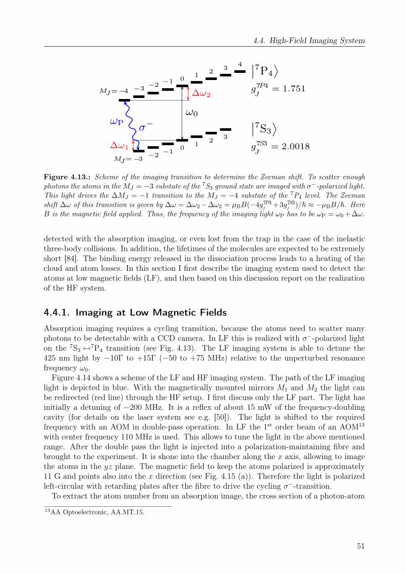
4.4. High-Field Imaging System
∆ω2
∆ω1
ω0
σ−ωP
MJ=−3 −2 −1 0 1 2 3
˛˛7S3
¸
g7S3J
= 2.0018
MJ=−4 −3 −2 −1 0 1 2 3 4 ˛7P4
¸
g7P4J
= 1.751
Figure 4.13.: Scheme of the imaging transition to determine the Zeeman shift. To scatter enoughphotons the atoms in the MJ = −3 substate of the 7S3 ground state are imaged with σ−-polarized light.This light drives the ∆MJ = −1 transition to the MJ = −4 substate of the 7P4 level. The Zeemanshift ∆ω of this transition is given by ∆ω = ∆ω2−∆ω2 = µBB(−4g7P4
J+3g7S3
J)/~ ≈ −µBB/~. Here
B is the magnetic field applied. Thus, the frequency of the imaging light ωP has to be ωP = ω0 +∆ω.
detected with the absorption imaging, or even lost from the trap in the case of the inelasticthree-body collisions. In addition, the lifetimes of the molecules are expected to be extremelyshort [84]. The binding energy released in the dissociation process leads to a heating of thecloud and atom losses. In this section I first describe the imaging system used to detect theatoms at low magnetic fields (LF), and then based on this discussion report on the realizationof the HF system.
4.4.1. Imaging at Low Magnetic Fields
Absorption imaging requires a cycling transition, because the atoms need to scatter manyphotons to be detectable with a CCD camera. In LF this is realized with σ−-polarized lighton the 7S3 ↔7P4 transition (see Fig. 4.13). The LF imaging system is able to detune the425 nm light by −10Γ to +15Γ (−50 to +75 MHz) relative to the unperturbed resonancefrequency ω0.
Figure 4.14 shows a scheme of the LF and HF imaging system. The path of the LF imaginglight is depicted in blue. With the magnetically mounted mirrors M1 and M2 the light canbe redirected (red line) through the HF setup. I first discuss only the LF part. The light hasinitially a detuning of −200 MHz. It is a reflex of about 15 mW of the frequency-doublingcavity (for details on the laser system see e.g. [50]). The light is shifted to the requiredfrequency with an AOM in double-pass operation. In LF the 1st order beam of an AOM13
with center frequency 110 MHz is used. This allows to tune the light in the above mentionedrange. After the double pass the light is injected into a polarization-maintaining fibre andbrought to the experiment. It is shone into the chamber along the x axis, allowing to imagethe atoms in the yz plane. The magnetic field to keep the atoms polarized is approximately11 G and points also into the x direction (see Fig. 4.15 (a)). Therefore the light is polarizedleft-circular with retarding plates after the fibre to drive the cycling σ−-transition.
To extract the atom number from an absorption image, the cross section of a photon-atom
13AA Optoelectronic, AA.MT.15.
51
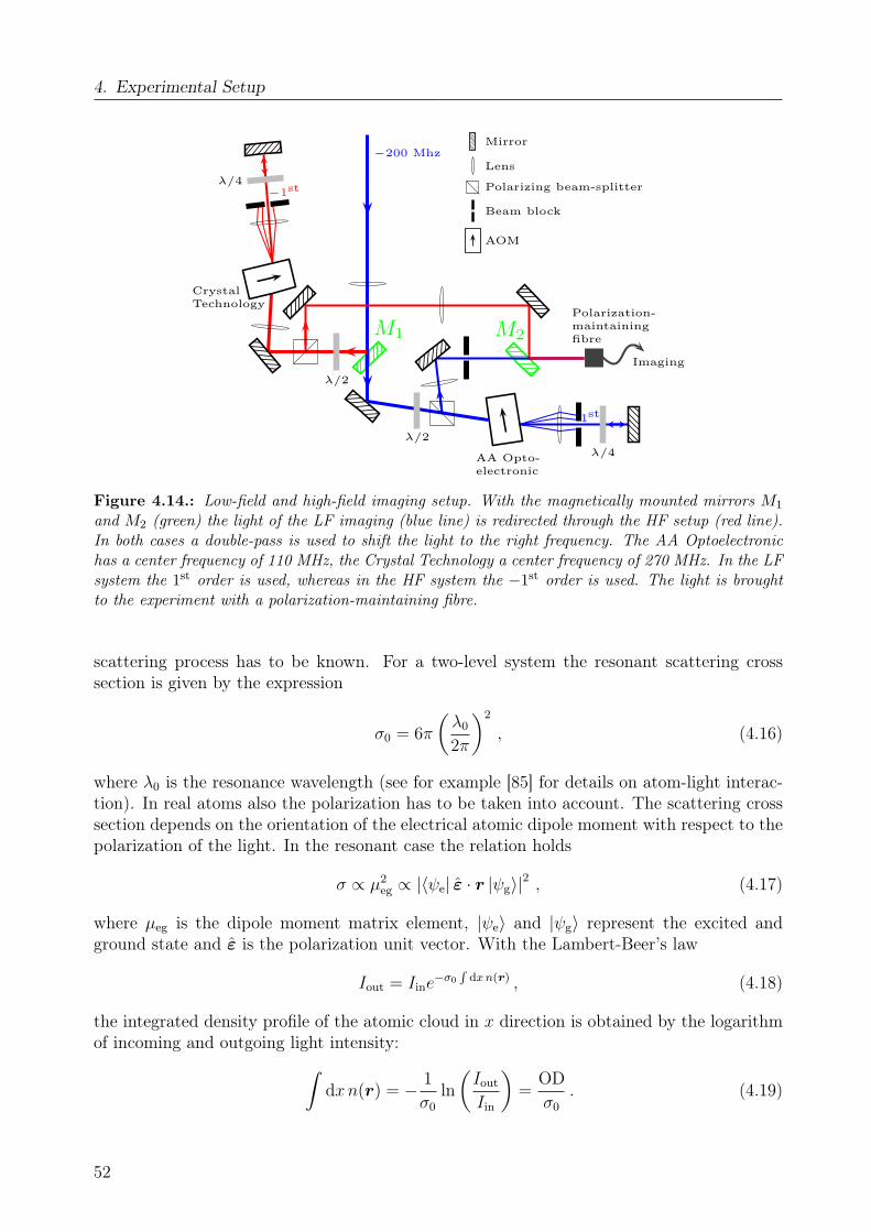
4. Experimental Setup
M1 M2
−200 Mhz
AA Opto-electronic
CrystalTechnology
Polarization-maintainingfibre
Imaging
λ/4λ/2
λ/2
λ/4
1st
−1st
Mirror
Lens
Polarizing beam-splitter
Beam block
AOM
Figure 4.14.: Low-field and high-field imaging setup. With the magnetically mounted mirrors M1
and M2 (green) the light of the LF imaging (blue line) is redirected through the HF setup (red line).In both cases a double-pass is used to shift the light to the right frequency. The AA Optoelectronichas a center frequency of 110 MHz, the Crystal Technology a center frequency of 270 MHz. In the LFsystem the 1st order is used, whereas in the HF system the −1st order is used. The light is broughtto the experiment with a polarization-maintaining fibre.
scattering process has to be known. For a two-level system the resonant scattering crosssection is given by the expression
σ0 = 6π
(λ0
2π
)2
, (4.16)
where λ0 is the resonance wavelength (see for example [85] for details on atom-light interac-tion). In real atoms also the polarization has to be taken into account. The scattering crosssection depends on the orientation of the electrical atomic dipole moment with respect to thepolarization of the light. In the resonant case the relation holds
σ ∝ µ2eg ∝ |〈ψe| ε · r |ψg〉|2 , (4.17)
where µeg is the dipole moment matrix element, |ψe〉 and |ψg〉 represent the excited andground state and ε is the polarization unit vector. With the Lambert-Beer’s law
Iout = Iine−σ0
Rdx n(r) , (4.18)
the integrated density profile of the atomic cloud in x direction is obtained by the logarithmof incoming and outgoing light intensity:∫
dxn(r) = − 1
σ0
ln
(Iout
Iin
)=
OD
σ0
. (4.19)
52
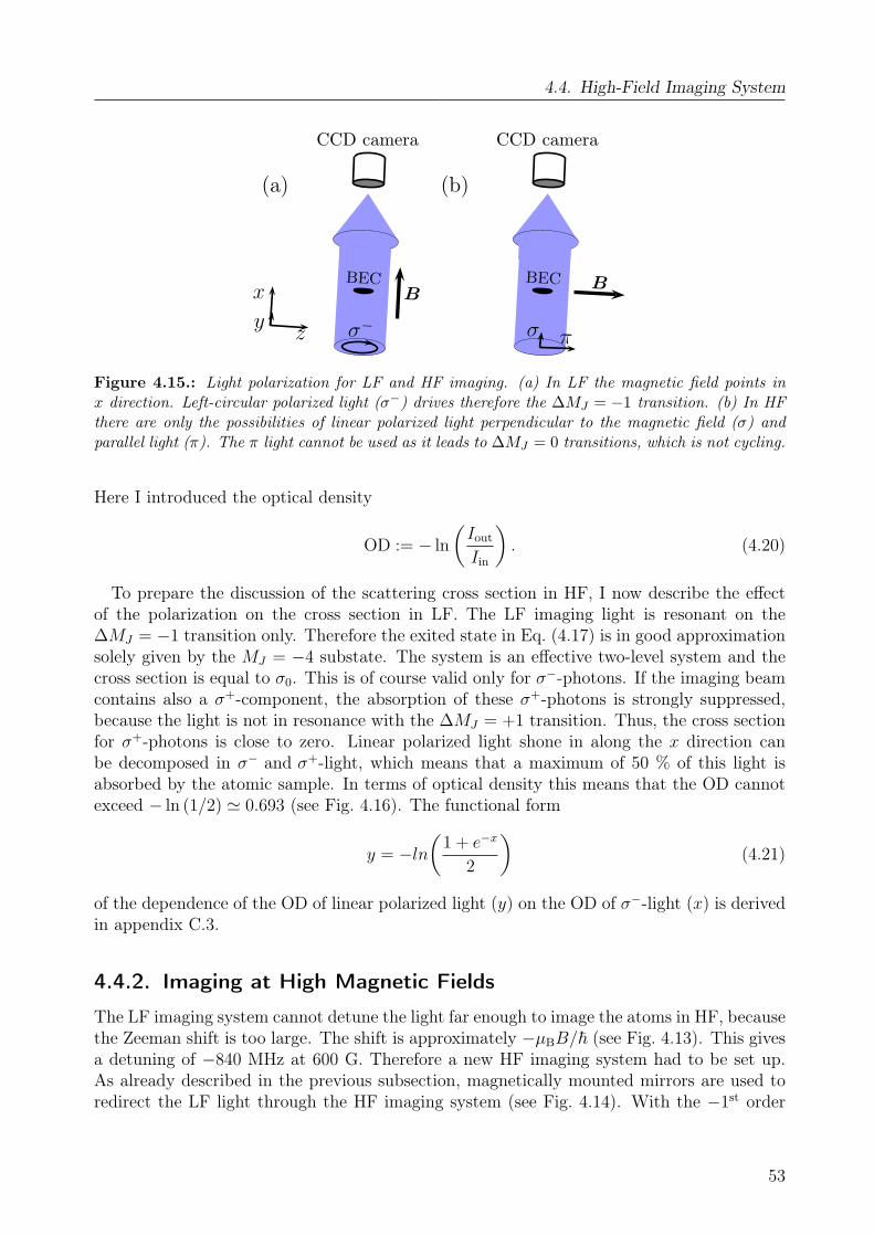
4.4. High-Field Imaging System
(a)
z
x
y
CCD camera
BECB
σ−
(b)
CCD camera
BEC B
πσ
Figure 4.15.: Light polarization for LF and HF imaging. (a) In LF the magnetic field points inx direction. Left-circular polarized light (σ−) drives therefore the ∆MJ = −1 transition. (b) In HFthere are only the possibilities of linear polarized light perpendicular to the magnetic field (σ) andparallel light (π). The π light cannot be used as it leads to ∆MJ = 0 transitions, which is not cycling.
Here I introduced the optical density
OD := − ln
(Iout
Iin
). (4.20)
To prepare the discussion of the scattering cross section in HF, I now describe the effectof the polarization on the cross section in LF. The LF imaging light is resonant on the∆MJ = −1 transition only. Therefore the exited state in Eq. (4.17) is in good approximationsolely given by the MJ = −4 substate. The system is an effective two-level system and thecross section is equal to σ0. This is of course valid only for σ−-photons. If the imaging beamcontains also a σ+-component, the absorption of these σ+-photons is strongly suppressed,because the light is not in resonance with the ∆MJ = +1 transition. Thus, the cross sectionfor σ+-photons is close to zero. Linear polarized light shone in along the x direction canbe decomposed in σ− and σ+-light, which means that a maximum of 50 % of this light isabsorbed by the atomic sample. In terms of optical density this means that the OD cannotexceed − ln (1/2) ' 0.693 (see Fig. 4.16). The functional form
y = −ln(
1 + e−x
2
)(4.21)
of the dependence of the OD of linear polarized light (y) on the OD of σ−-light (x) is derivedin appendix C.3.
4.4.2. Imaging at High Magnetic Fields
The LF imaging system cannot detune the light far enough to image the atoms in HF, becausethe Zeeman shift is too large. The shift is approximately −µBB/~ (see Fig. 4.13). This givesa detuning of −840 MHz at 600 G. Therefore a new HF imaging system had to be set up.As already described in the previous subsection, magnetically mounted mirrors are used toredirect the LF light through the HF imaging system (see Fig. 4.14). With the −1st order
53
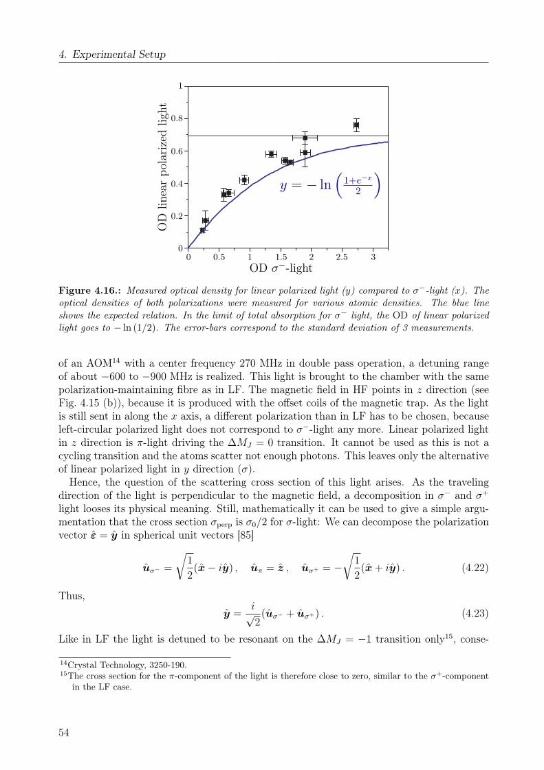
4. Experimental Setup
0 0.5 1 1.5 2 2.5 30
0.2
0.4
0.6
0.8
1
OD σ−-light
OD
linea
rpo
lari
zed
light
y = − ln(
1+e−x
2
)
Figure 4.16.: Measured optical density for linear polarized light (y) compared to σ−-light (x). Theoptical densities of both polarizations were measured for various atomic densities. The blue lineshows the expected relation. In the limit of total absorption for σ− light, the OD of linear polarizedlight goes to − ln (1/2). The error-bars correspond to the standard deviation of 3 measurements.
of an AOM14 with a center frequency 270 MHz in double pass operation, a detuning rangeof about −600 to −900 MHz is realized. This light is brought to the chamber with the samepolarization-maintaining fibre as in LF. The magnetic field in HF points in z direction (seeFig. 4.15 (b)), because it is produced with the offset coils of the magnetic trap. As the lightis still sent in along the x axis, a different polarization than in LF has to be chosen, becauseleft-circular polarized light does not correspond to σ−-light any more. Linear polarized lightin z direction is π-light driving the ∆MJ = 0 transition. It cannot be used as this is not acycling transition and the atoms scatter not enough photons. This leaves only the alternativeof linear polarized light in y direction (σ).
Hence, the question of the scattering cross section of this light arises. As the travelingdirection of the light is perpendicular to the magnetic field, a decomposition in σ− and σ+
light looses its physical meaning. Still, mathematically it can be used to give a simple argu-mentation that the cross section σperp is σ0/2 for σ-light: We can decompose the polarizationvector ε = y in spherical unit vectors [85]
uσ− =
√1
2(x− iy) , uπ = z , uσ+ = −
√1
2(x + iy) . (4.22)
Thus,
y =i√2(uσ− + uσ+) . (4.23)
Like in LF the light is detuned to be resonant on the ∆MJ = −1 transition only15, conse-
14Crystal Technology, 3250-190.15The cross section for the π-component of the light is therefore close to zero, similar to the σ+-component
in the LF case.
54
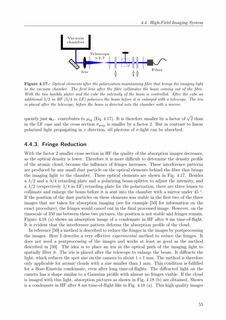
4.4. High-Field Imaging System
Fibreλ2
λ4
λ2
Telescope×2.7
Iris
Vacuumchamber
Figure 4.17.: Optical elements after the polarization-maintaining fibre that brings the imaging lightto the vacuum chamber. The first lens after the fibre collimates the beam coming out of the fibre.With the two lambda plates and the cube the intensity of the beam is controlled. After the cube anadditional λ/2 in HF (λ/4 in LF) polarizes the beam before it is enlarged with a telescope. The irisis placed after the telescope, before the beam is directed into the chamber with a mirror.
quently just uσ− contributes to µeg (Eq. 4.17). It is therefore smaller by a factor of√
2 thanin the LF case and the cross section σperp is smaller by a factor 2. But in contrast to linearpolarized light propagating in x direction, all photons of σ-light can be absorbed.
4.4.3. Fringe Reduction
With the factor 2 smaller cross section in HF the quality of the absorption images decreases,as the optical density is lower. Therefore it is more difficult to determine the density profileof the atomic cloud, because the influence of fringes increases. These interference patternsare produced by any small dust particle on the optical elements behind the fibre that bringsthe imaging light to the chamber. These optical elements are shown in Fig. 4.17. Besidesa λ/2 and a λ/4 retarding plate and a polarizing beam-splitter to adjust the intensity, anda λ/2 (respectively λ/4 in LF) retarding plate for the polarization, there are three lenses tocollimate and enlarge the beam before it is sent into the chamber with a mirror under 45 .If the position of the dust particles on these elements was stable in the first two of the threeimages that are taken for absorption imaging (see for example [50] for information on theexact procedure), the fringes would cancel out in the final processed image. However, on thetimescale of 350 ms between these two pictures, the position is not stable and fringes remain.Figure 4.18 (a) shows an absorption image of a condensate in HF after 8 ms time-of-flight.It is evident that the interference pattern deforms the absorption profile of the cloud.
In reference [50] a method is described to reduce the fringes in the images by postprocessingthe images. Here I describe a very effective experimental method to reduce the fringes. Itdoes not need a postprocessing of the images and works at least as good as the methoddescribed in [50]. The idea is to place an iris in the optical path of the imaging light tospatially filter it. The iris is placed after the telescope to enlarge the beam. It diffracts thelight, which reduces the spot size on the camera to about 1×1 mm. The method is thereforeonly applicable for atomic clouds with a size smaller than 1 mm. This condition is fulfilledfor a Bose-Einstein condensate, even after long time-of-flights. The diffracted light on thecamera has a shape similar to a Gaussian profile with almost no fringes visible. If the cloudis imaged with this light, absorption pictures as shown in Fig. 4.18 (b) are obtained. Shownis a condensate in HF after 8 ms time-of-flight like in Fig. 4.18 (a). This high quality images
55
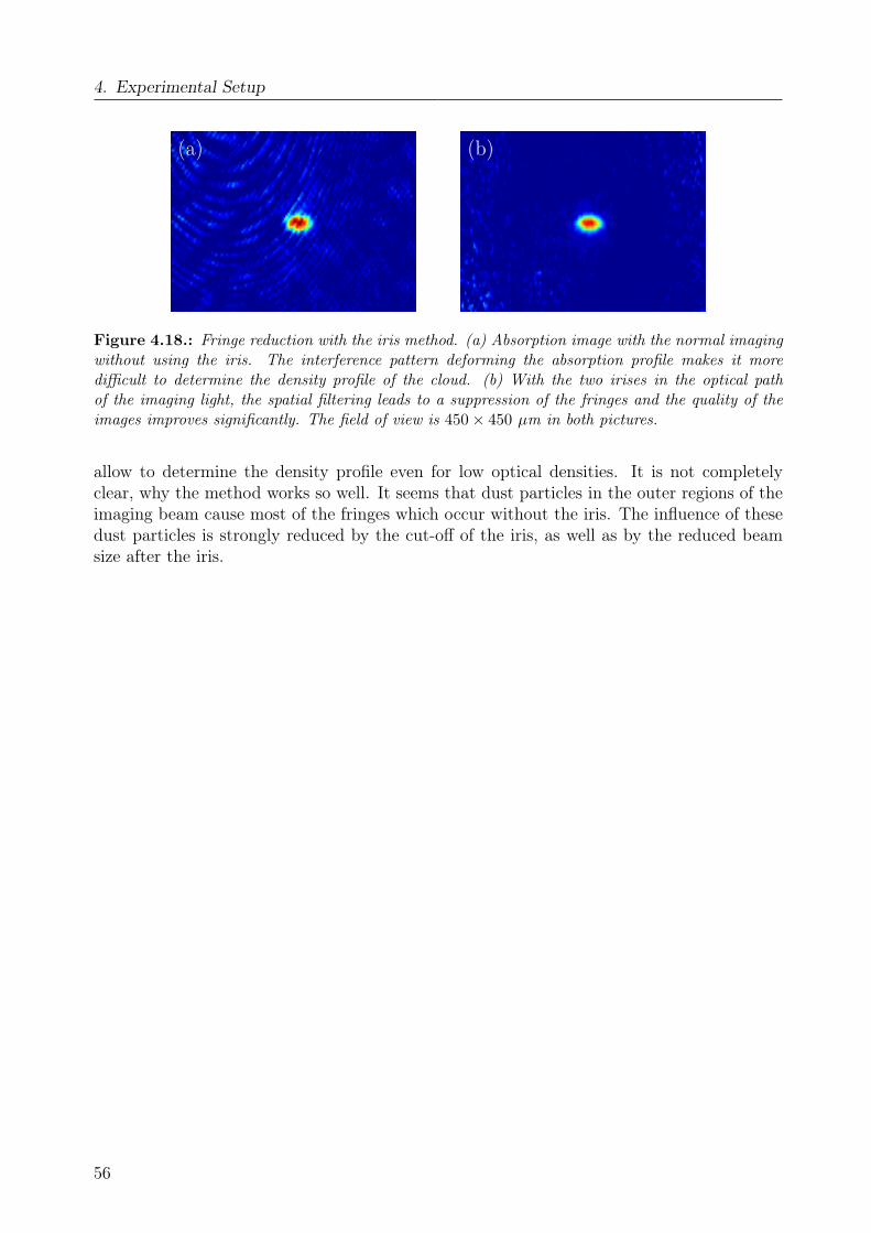
4. Experimental Setup
(a) (b)
Figure 4.18.: Fringe reduction with the iris method. (a) Absorption image with the normal imagingwithout using the iris. The interference pattern deforming the absorption profile makes it moredifficult to determine the density profile of the cloud. (b) With the two irises in the optical pathof the imaging light, the spatial filtering leads to a suppression of the fringes and the quality of theimages improves significantly. The field of view is 450× 450 µm in both pictures.
allow to determine the density profile even for low optical densities. It is not completelyclear, why the method works so well. It seems that dust particles in the outer regions of theimaging beam cause most of the fringes which occur without the iris. The influence of thesedust particles is strongly reduced by the cut-off of the iris, as well as by the reduced beamsize after the iris.
56
5. Strong Dipolar Effects in aChromium Bose-EinsteinCondensate
This chapter summarizes the experimental results on strong dipolar effects in a Bose-Einstein condensate. With a Feshbach resonance the scattering length is reduced byup to a factor of 5 and thus the dipolar parameter εdd is increased accordingly. Thismeans that the dipolar parameter is tuned close to one, where a dipolar collapse ofthe BEC is expected for the trap geometries used. Our experimental control on thesystem is demonstrated with a series of time-of-flight measurements for various rel-ative strengths of the dipole-dipole interaction. For the largest values reached it isshown, that even the standard ’smoking gun’ evidence for Bose-Einstein condensa-tion, an inversion of the ellipticity of the condensate during the free expansion, doesnot apply anymore. The results presented here constitute the first realization of aquantum-degenerate gas with such strong dipolar effects [1]. They are the first stepin the exploration of the unique properties of quantum ferrofluids. This chapter isorganized as follows: In section 5.1 the Feshbach resonance at 589.1 G is character-ized, which is used to tune the scattering length. Both the lifetime of the condensateand the scattering length close to the resonance are presented. In section 5.2 theenhancement of the relative strength of the dipole-dipole to the contact interaction isinvestigated. The dependence of the condensate aspect ratio on the dipolar parame-ter is discussed. Finally the series of time-of-flight measurements for various εdd ispresented.
5.1. Lifetime and Scattering Length Close to aFeshbach Resonance
The realization of a Bose-Einstein condensate at high magnetic fields (described in section 4.3)allows us to study the properties of the quantum-degenerate gas in the vicinity of the Feshbachresonance at 589.1 G. This resonance is chosen for the experiments, as it is predicted to havethe largest width (∆B = 1.7 G) of the 14 resonances found in 2004 [12]. Therefore therequirement on the magnetic field stability is least stringent and the condensate propertiesare measured with the highest precision. The absolute position Bres of the resonance is foundto coincide with the value measured in [12] by observing enhanced inelastic losses in a thermalcloud. The magnetic field is calibrated both with the knowledge of the position of lower lyingresonances, which have been determined precisely with RF spectroscopy in [12], and with themeasured optimal detuning of the high-field imaging system. The error in the determinationof the absolute position is approximately 1 %.
57
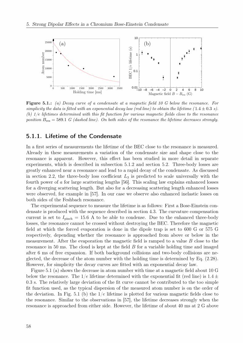
5. Strong Dipolar Effects in a Chromium Bose-Einstein Condensate
(a)
0 500 1000 1500 2000 2500 3000 35000
5000
10000
15000
20000
25000
Holding time [ms]
Ato
mnu
mbe
r(b)
0.01
0.1
1
10
–10 –8 –6 –4 –2 0 108642
BE
C1/
elif
etim
e(s
)
Magnetic field B −Bres (G)
Figure 5.1.: (a) Decay curve of a condensate at a magnetic field 10 G below the resonance. Forsimplicity the data is fitted with an exponential decay law (red line) to obtain the lifetime ( 1.4± 0.3 s).(b) 1/e lifetimes determined with this fit function for various magnetic fields close to the resonanceposition Bres = 589.1 G (dashed line). On both sides of the resonance the lifetime decreases strongly.
5.1.1. Lifetime of the Condensate
In a first series of measurements the lifetime of the BEC close to the resonance is measured.Already in these measurements a variation of the condensate size and shape close to theresonance is apparent. However, this effect has been studied in more detail in separateexperiments, which is described in subsection 5.1.2 and section 5.2. Three-body losses aregreatly enhanced near a resonance and lead to a rapid decay of the condensate. As discussedin section 2.2, the three-body loss coefficient L3 is predicted to scale universally with thefourth power of a for large scattering lengths [56]. This scaling law explains enhanced lossesfor a diverging scattering length. But also for a decreasing scattering length enhanced losseswere observed, for example in [57]. In our case we observe also enhanced inelastic losses onboth sides of the Feshbach resonance.
The experimental sequence to measure the lifetime is as follows: First a Bose-Einstein con-densate is produced with the sequence described in section 4.3. The curvature compensationcurrent is set to Ipinch = 15.6 A to be able to condense. Due to the enhanced three-bodylosses, the resonance cannot be crossed without destroying the BEC. Therefore the magneticfield at which the forced evaporation is done in the dipole trap is set to 600 G or 575 Grespectively, depending whether the resonance is approached from above or below in themeasurement. After the evaporation the magnetic field is ramped to a value B close to theresonance in 50 ms. The cloud is kept at the field B for a variable holding time and imagedafter 6 ms of free expansion. If both background collisions and two-body collisions are ne-glected, the decrease of the atom number with the holding time is determined by Eq. (2.28).However, for simplicity the decay curves are fitted with an exponential decay law.
Figure 5.1 (a) shows the decrease in atom number with time at a magnetic field about 10 Gbelow the resonance. The 1/e lifetime determined with the exponential fit (red line) is 1.4±0.3 s. The relatively large deviation of the fit curve cannot be contributed to the too simplefit function used, as the typical dispersion of the measured atom number is on the order ofthe deviation. In Fig. 5.1 (b) the 1/e lifetime is plotted for various magnetic fields close tothe resonance. Similar to the observations in [57], the lifetime decreases strongly when theresonance is approached from either side. However, the lifetime of about 40 ms at 2 G above
58
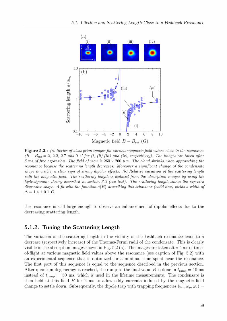
5.1. Lifetime and Scattering Length Close to a Feshbach Resonance
0.1
1
10
–10 –8 –6 –4 –2 0 108642
Scat
teri
ngle
ngth
a/a
bg
Magnetic field B −Bres (G)
(b)
(i)
(ii)
(iii) (iv)
(a)
z
y B
(i) (ii) (iii) (iv)
Figure 5.2.: (a) Series of absorption images for various magnetic field values close to the resonance(B − Bres = 2, 2.2, 2.7 and 9 G for (i),(ii),(iii) and (iv), respectively). The images are taken after5 ms of free expansion. The field of view is 260× 260 µm. The cloud shrinks when approaching theresonance because the scattering length decreases. Moreover a significant change of the condensateshape is visible, a clear sign of strong dipolar effects. (b) Relative variation of the scattering lengthwith the magnetic field. The scattering length is deduced from the absorption images by using thehydrodynamic theory described in section 3.3 (see text). The scattering length shows the expecteddispersive shape. A fit with the function a(B) describing this behaviour (solid line) yields a width of∆ = 1.4± 0.1 G.
the resonance is still large enough to observe an enhancement of dipolar effects due to thedecreasing scattering length.
5.1.2. Tuning the Scattering Length
The variation of the scattering length in the vicinity of the Feshbach resonance leads to adecrease (respectively increase) of the Thomas-Fermi radii of the condensate. This is clearlyvisible in the absorption images shown in Fig. 5.2 (a). The images are taken after 5 ms of time-of-flight at various magnetic field values above the resonance (see caption of Fig. 5.2) withan experimental sequence that is optimized for a minimal time spent near the resonance.The first part of this sequence is equal to the sequence described in the previous section.After quantum-degeneracy is reached, the ramp to the final value B is done in tramp = 10 msinstead of tramp = 50 ms, which is used in the lifetime measurements. The condensate isthen held at this field B for 2 ms to allow eddy currents induced by the magnetic fieldchange to settle down. Subsequently, the dipole trap with trapping frequencies (ωx, ωy, ωz) =
59
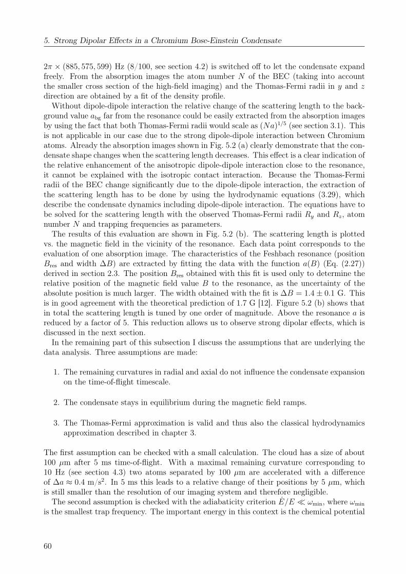
5. Strong Dipolar Effects in a Chromium Bose-Einstein Condensate
2π × (885, 575, 599) Hz (8/100, see section 4.2) is switched off to let the condensate expandfreely. From the absorption images the atom number N of the BEC (taking into accountthe smaller cross section of the high-field imaging) and the Thomas-Fermi radii in y and zdirection are obtained by a fit of the density profile.
Without dipole-dipole interaction the relative change of the scattering length to the back-ground value abg far from the resonance could be easily extracted from the absorption imagesby using the fact that both Thomas-Fermi radii would scale as (Na)1/5 (see section 3.1). Thisis not applicable in our case due to the strong dipole-dipole interaction between Chromiumatoms. Already the absorption images shown in Fig. 5.2 (a) clearly demonstrate that the con-densate shape changes when the scattering length decreases. This effect is a clear indication ofthe relative enhancement of the anisotropic dipole-dipole interaction close to the resonance,it cannot be explained with the isotropic contact interaction. Because the Thomas-Fermiradii of the BEC change significantly due to the dipole-dipole interaction, the extraction ofthe scattering length has to be done by using the hydrodynamic equations (3.29), whichdescribe the condensate dynamics including dipole-dipole interaction. The equations have tobe solved for the scattering length with the observed Thomas-Fermi radii Ry and Rz, atomnumber N and trapping frequencies as parameters.
The results of this evaluation are shown in Fig. 5.2 (b). The scattering length is plottedvs. the magnetic field in the vicinity of the resonance. Each data point corresponds to theevaluation of one absorption image. The characteristics of the Feshbach resonance (positionBres and width ∆B) are extracted by fitting the data with the function a(B) (Eq. (2.27))derived in section 2.3. The position Bres obtained with this fit is used only to determine therelative position of the magnetic field value B to the resonance, as the uncertainty of theabsolute position is much larger. The width obtained with the fit is ∆B = 1.4± 0.1 G. Thisis in good agreement with the theoretical prediction of 1.7 G [12]. Figure 5.2 (b) shows thatin total the scattering length is tuned by one order of magnitude. Above the resonance a isreduced by a factor of 5. This reduction allows us to observe strong dipolar effects, which isdiscussed in the next section.
In the remaining part of this subsection I discuss the assumptions that are underlying thedata analysis. Three assumptions are made:
1. The remaining curvatures in radial and axial do not influence the condensate expansionon the time-of-flight timescale.
2. The condensate stays in equilibrium during the magnetic field ramps.
3. The Thomas-Fermi approximation is valid and thus also the classical hydrodynamicsapproximation described in chapter 3.
The first assumption can be checked with a small calculation. The cloud has a size of about100 µm after 5 ms time-of-flight. With a maximal remaining curvature corresponding to10 Hz (see section 4.3) two atoms separated by 100 µm are accelerated with a differenceof ∆a ≈ 0.4 m/s2. In 5 ms this leads to a relative change of their positions by 5 µm, whichis still smaller than the resolution of our imaging system and therefore negligible.
The second assumption is checked with the adiabaticity criterion E/E ωmin, where ωmin
is the smallest trap frequency. The important energy in this context is the chemical potential
60
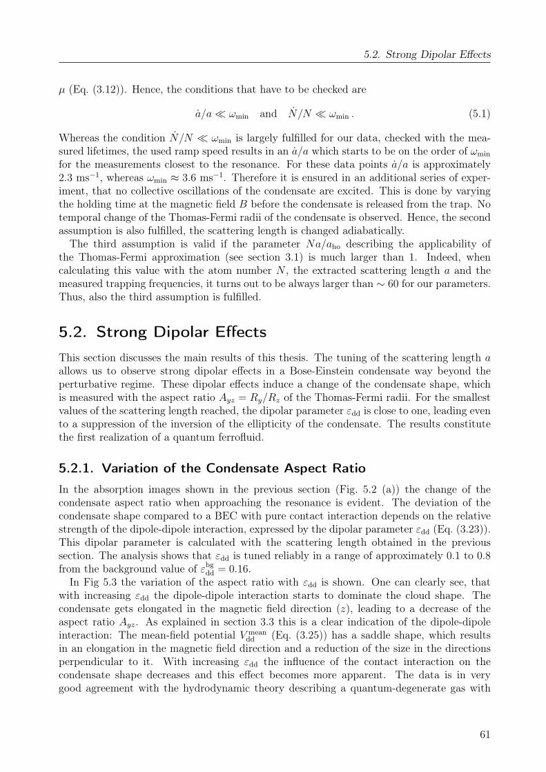
5.2. Strong Dipolar Effects
µ (Eq. (3.12)). Hence, the conditions that have to be checked are
a/a ωmin and N/N ωmin . (5.1)
Whereas the condition N/N ωmin is largely fulfilled for our data, checked with the mea-sured lifetimes, the used ramp speed results in an a/a which starts to be on the order of ωmin
for the measurements closest to the resonance. For these data points a/a is approximately2.3 ms−1, whereas ωmin ≈ 3.6 ms−1. Therefore it is ensured in an additional series of exper-iment, that no collective oscillations of the condensate are excited. This is done by varyingthe holding time at the magnetic field B before the condensate is released from the trap. Notemporal change of the Thomas-Fermi radii of the condensate is observed. Hence, the secondassumption is also fulfilled, the scattering length is changed adiabatically.
The third assumption is valid if the parameter Na/aho describing the applicability ofthe Thomas-Fermi approximation (see section 3.1) is much larger than 1. Indeed, whencalculating this value with the atom number N , the extracted scattering length a and themeasured trapping frequencies, it turns out to be always larger than ∼ 60 for our parameters.Thus, also the third assumption is fulfilled.
5.2. Strong Dipolar Effects
This section discusses the main results of this thesis. The tuning of the scattering length aallows us to observe strong dipolar effects in a Bose-Einstein condensate way beyond theperturbative regime. These dipolar effects induce a change of the condensate shape, whichis measured with the aspect ratio Ayz = Ry/Rz of the Thomas-Fermi radii. For the smallestvalues of the scattering length reached, the dipolar parameter εdd is close to one, leading evento a suppression of the inversion of the ellipticity of the condensate. The results constitutethe first realization of a quantum ferrofluid.
5.2.1. Variation of the Condensate Aspect Ratio
In the absorption images shown in the previous section (Fig. 5.2 (a)) the change of thecondensate aspect ratio when approaching the resonance is evident. The deviation of thecondensate shape compared to a BEC with pure contact interaction depends on the relativestrength of the dipole-dipole interaction, expressed by the dipolar parameter εdd (Eq. (3.23)).This dipolar parameter is calculated with the scattering length obtained in the previoussection. The analysis shows that εdd is tuned reliably in a range of approximately 0.1 to 0.8from the background value of εbg
dd = 0.16.In Fig 5.3 the variation of the aspect ratio with εdd is shown. One can clearly see, that
with increasing εdd the dipole-dipole interaction starts to dominate the cloud shape. Thecondensate gets elongated in the magnetic field direction (z), leading to a decrease of theaspect ratio Ayz. As explained in section 3.3 this is a clear indication of the dipole-dipoleinteraction: The mean-field potential V mean
dd (Eq. (3.25)) has a saddle shape, which resultsin an elongation in the magnetic field direction and a reduction of the size in the directionsperpendicular to it. With increasing εdd the influence of the contact interaction on thecondensate shape decreases and this effect becomes more apparent. The data is in verygood agreement with the hydrodynamic theory describing a quantum-degenerate gas with
61
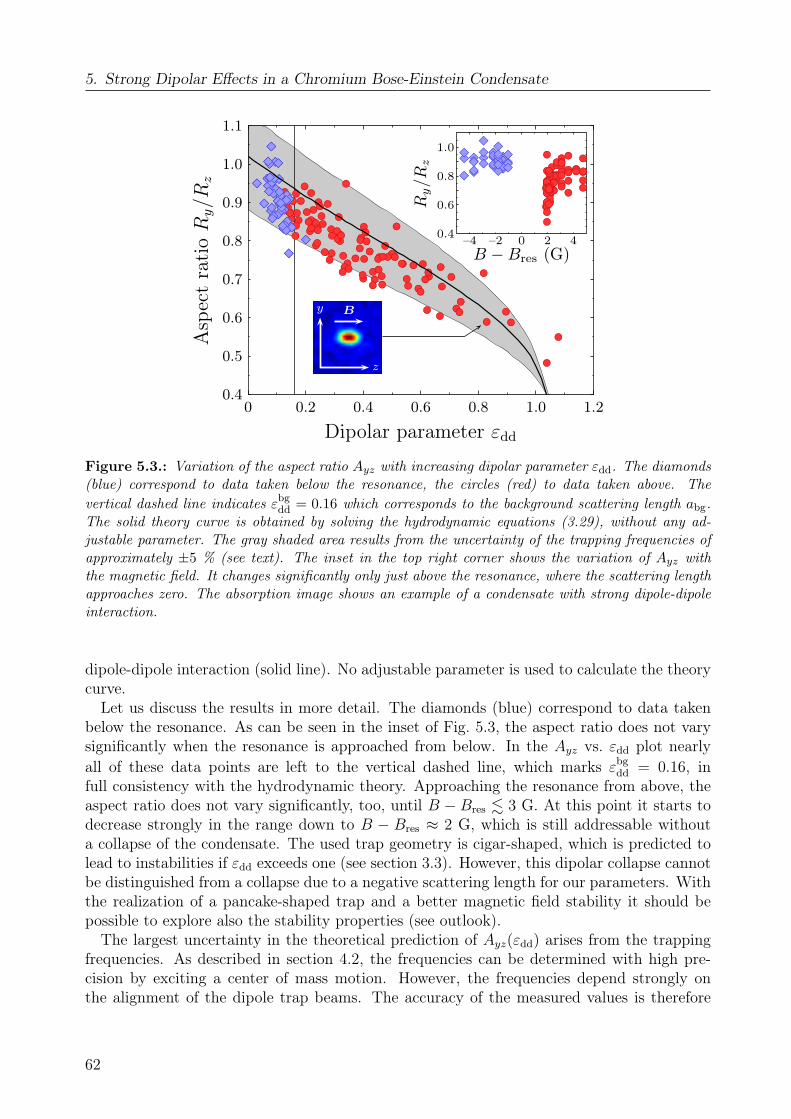
5. Strong Dipolar Effects in a Chromium Bose-Einstein Condensate
0.4
0.5
0.6
0.7
0.8
0.9
1.0
1.1
0 0.2 0.4 0.6 0.8 1.0 1.2
z
y B
Asp
ect
rati
oR
y/R
z
Dipolar parameter εdd
0.4
0.6
0.8
1.0
–4 –2 0 42
Ry/R
z
B −Bres (G)
Figure 5.3.: Variation of the aspect ratio Ayz with increasing dipolar parameter εdd. The diamonds(blue) correspond to data taken below the resonance, the circles (red) to data taken above. Thevertical dashed line indicates εbg
dd = 0.16 which corresponds to the background scattering length abg.The solid theory curve is obtained by solving the hydrodynamic equations (3.29), without any ad-justable parameter. The gray shaded area results from the uncertainty of the trapping frequencies ofapproximately ±5 % (see text). The inset in the top right corner shows the variation of Ayz withthe magnetic field. It changes significantly only just above the resonance, where the scattering lengthapproaches zero. The absorption image shows an example of a condensate with strong dipole-dipoleinteraction.
dipole-dipole interaction (solid line). No adjustable parameter is used to calculate the theorycurve.
Let us discuss the results in more detail. The diamonds (blue) correspond to data takenbelow the resonance. As can be seen in the inset of Fig. 5.3, the aspect ratio does not varysignificantly when the resonance is approached from below. In the Ayz vs. εdd plot nearlyall of these data points are left to the vertical dashed line, which marks εbg
dd = 0.16, infull consistency with the hydrodynamic theory. Approaching the resonance from above, theaspect ratio does not vary significantly, too, until B − Bres . 3 G. At this point it starts todecrease strongly in the range down to B − Bres ≈ 2 G, which is still addressable withouta collapse of the condensate. The used trap geometry is cigar-shaped, which is predicted tolead to instabilities if εdd exceeds one (see section 3.3). However, this dipolar collapse cannotbe distinguished from a collapse due to a negative scattering length for our parameters. Withthe realization of a pancake-shaped trap and a better magnetic field stability it should bepossible to explore also the stability properties (see outlook).
The largest uncertainty in the theoretical prediction of Ayz(εdd) arises from the trappingfrequencies. As described in section 4.2, the frequencies can be determined with high pre-cision by exciting a center of mass motion. However, the frequencies depend strongly onthe alignment of the dipole trap beams. The accuracy of the measured values is therefore
62
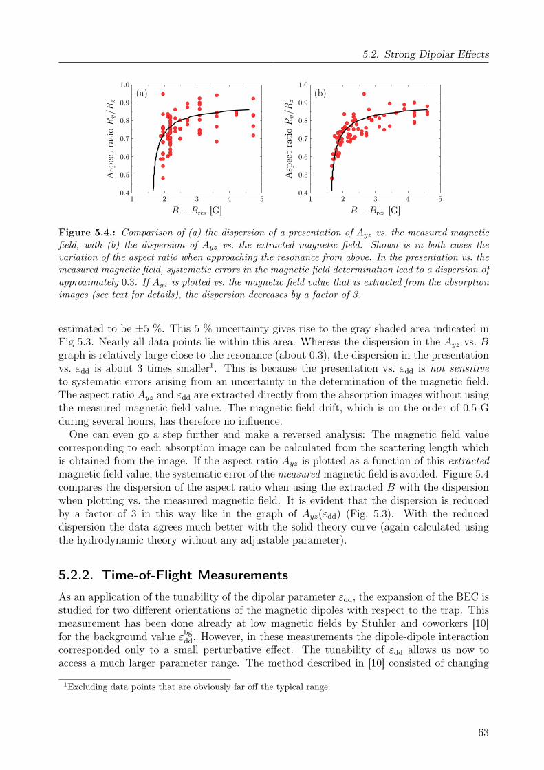
5.2. Strong Dipolar Effects
(a)
0.4
0.5
0.6
0.7
0.8
0.9
1.0
1 2 3 4 5
Asp
ect
rati
oR
y/R
z
B −Bres [G]
(b)
0.4
0.5
0.6
0.7
0.8
0.9
1.0
1 2 3 4 5
Asp
ect
rati
oR
y/R
z
B −Bres [G]
Figure 5.4.: Comparison of (a) the dispersion of a presentation of Ayz vs. the measured magneticfield, with (b) the dispersion of Ayz vs. the extracted magnetic field. Shown is in both cases thevariation of the aspect ratio when approaching the resonance from above. In the presentation vs. themeasured magnetic field, systematic errors in the magnetic field determination lead to a dispersion ofapproximately 0.3. If Ayz is plotted vs. the magnetic field value that is extracted from the absorptionimages (see text for details), the dispersion decreases by a factor of 3.
estimated to be ±5 %. This 5 % uncertainty gives rise to the gray shaded area indicated inFig 5.3. Nearly all data points lie within this area. Whereas the dispersion in the Ayz vs. Bgraph is relatively large close to the resonance (about 0.3), the dispersion in the presentationvs. εdd is about 3 times smaller1. This is because the presentation vs. εdd is not sensitiveto systematic errors arising from an uncertainty in the determination of the magnetic field.The aspect ratio Ayz and εdd are extracted directly from the absorption images without usingthe measured magnetic field value. The magnetic field drift, which is on the order of 0.5 Gduring several hours, has therefore no influence.
One can even go a step further and make a reversed analysis: The magnetic field valuecorresponding to each absorption image can be calculated from the scattering length whichis obtained from the image. If the aspect ratio Ayz is plotted as a function of this extractedmagnetic field value, the systematic error of the measured magnetic field is avoided. Figure 5.4compares the dispersion of the aspect ratio when using the extracted B with the dispersionwhen plotting vs. the measured magnetic field. It is evident that the dispersion is reducedby a factor of 3 in this way like in the graph of Ayz(εdd) (Fig. 5.3). With the reduceddispersion the data agrees much better with the solid theory curve (again calculated usingthe hydrodynamic theory without any adjustable parameter).
5.2.2. Time-of-Flight Measurements
As an application of the tunability of the dipolar parameter εdd, the expansion of the BEC isstudied for two different orientations of the magnetic dipoles with respect to the trap. Thismeasurement has been done already at low magnetic fields by Stuhler and coworkers [10]for the background value εbg
dd. However, in these measurements the dipole-dipole interactioncorresponded only to a small perturbative effect. The tunability of εdd allows us now toaccess a much larger parameter range. The method described in [10] consisted of changing
1Excluding data points that are obviously far off the typical range.
63
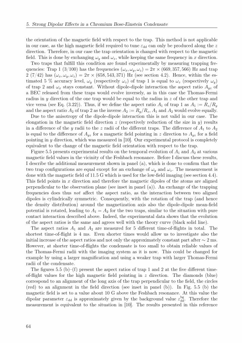
5. Strong Dipolar Effects in a Chromium Bose-Einstein Condensate
the orientation of the magnetic field with respect to the trap. This method is not applicablein our case, as the high magnetic field required to tune εdd can only be produced along the zdirection. Therefore, in our case the trap orientation is changed with respect to the magneticfield. This is done by exchanging ωy and ωz, while keeping the same frequency in x direction.
Two traps that fulfill this condition are found experimentally by measuring trapping fre-quencies: Trap 1 (3/100) has the frequencies (ωx, ωy, ωz) = 2π × (669, 357, 566) Hz and trap2 (7/42) has (ωx, ωy, ωz) = 2π × (658, 543, 371) Hz (see section 4.2). Hence, within the es-timated 5 % accuracy level, ωy (respectively ωz) of trap 1 is equal to ωz (respectively ωy)of trap 2 and ωx stays constant. Without dipole-dipole interaction the aspect ratio Ayz ofa BEC released from these traps would evolve inversely, as in this case the Thomas-Fermiradius in y direction of the one trap would be equal to the radius in z of the other trap andvice versa (see Eq. (3.22)). Thus, if we define the aspect ratio A1 of trap 1 as A1 := Rz/Ry
and the aspect ratio A2 of trap 2 as the inverse A2 := Ry/Rz, A1 and A2 would evolve equally.Due to the anisotropy of the dipole-dipole interaction this is not valid in our case. The
elongation in the magnetic field direction z (respectively reduction of the size in y) resultsin a difference of the y radii to the z radii of the different traps. The difference of A1 to A2
is equal to the difference of Ayz for a magnetic field pointing in z direction to Ayz for a fieldpointing in y direction, which was measured in [10]. Our experimental protocol is completelyequivalent to the change of the magnetic field orientation with respect to the trap.
Figure 5.5 presents experimental results on the temporal evolution of A1 and A2 at variousmagnetic field values in the vicinity of the Feshbach resonance. Before I discuss these results,I describe the additional measurement shown in panel (a), which is done to confirm that thetwo trap configurations are equal except for an exchange of ωy and ωz. The measurement isdone with the magnetic field of 11.5 G which is used for the low-field imaging (see section 4.4).This field points in x direction and therefore the magnetic dipoles of the atoms are alignedperpendicular to the observation plane (see inset in panel (a)). An exchange of the trappingfrequencies does thus not affect the aspect ratio, as the interaction between two aligneddipoles is cylindrically symmetric. Consequently, with the rotation of the trap (and hencethe density distribution) around the magnetization axis also the dipole-dipole mean-fieldpotential is rotated, leading to A1 = A2 for the two traps, similar to the situation with purecontact interaction described above. Indeed, the experimental data shows that the evolutionof the aspect ratios is the same and agrees well with the theory curve (black solid line).
The aspect ratios A1 and A2 are measured for 5 different time-of-flights in total. Theshortest time-of-flight is 4 ms. Even shorter times would allow us to investigate also theinitial increase of the aspect ratios and not only the approximately constant part after ∼ 2 ms.However, at shorter time-of-flights the condensate is too small to obtain reliable values ofthe Thomas-Fermi radii with the imaging system as it is now. This could be changed forexample by using a larger magnification and using a weaker trap with larger Thomas-Fermiradii of the condensate.
The figures 5.5 (b)–(f) present the aspect ratios of trap 1 and 2 at the five different time-of-flight values for the high magnetic field pointing in z direction. The diamonds (blue)correspond to an alignment of the long axis of the trap perpendicular to the field, the circles(red) to an alignment in the field direction (see inset in panel (b)). In Fig. 5.5 (b) themagnetic field is set to a value about 10 G above the Feshbach resonance. At this value thedipolar parameter εdd is approximately given by the background value εbg
dd. Therefore themeasurement is equivalent to the situation in [10]. The results presented in this reference
64
5.2. Strong Dipolar Effects
are recovered, the aspect ratios A1 and A2 differ due to the dipole-dipole interaction. Thehydrodynamic theory curves (red and blue solid line) are in good agreement with the data,without any adjustment of the parameters.
In the figures 5.5 (c)–(f) the magnetic field is subsequently set to values closer to the reso-nance (2.6, 2.5, 2.3 and 2.2 G respectively). With εdd approaching one, these measurementsare far beyond the perturbative regime. The deviation of A1 and A2 increases, indicatingthe enhancement of the relative strength of the dipole-dipole interaction. At εdd = 0.75(panel (f)) even the standard ’smoking gun’ evidence of quantum-degeneracy, an inversionof the ellipticity (see section 3.1) of the condensate, does not apply anymore. The dashedline indicating the inversion is not crossed by both the blue and the red line. Rz stays al-ways larger than Ry for both traps. The black solid line indicates the theory curve withoutdipole-dipole interaction. The large deviation of the data to this curve is evident. However,the hydrodynamic theory including dipole-dipole interaction does still describe the evolutionof the aspect ratios correctly.
In conclusion, the experiments demonstrate the first investigation of the unique propertiesof a quantum ferrofluid. We observe a strong modification of the condensate shape when thecontact interaction is reduced. In a series of time-of-flight measurements our control on thesystem is demonstrated. The hydrodynamic theory introduced in section 3.3 is in excellentagreement with the measured data.
65
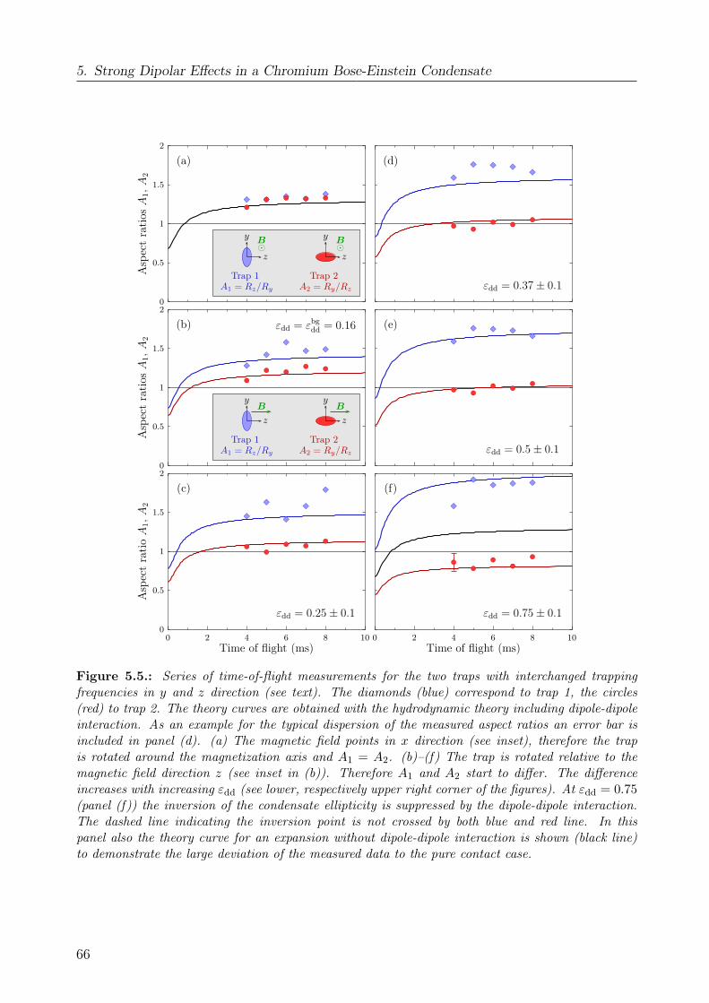
5. Strong Dipolar Effects in a Chromium Bose-Einstein Condensate
(f)
εdd = 0.75± 0.1
0 108642
Time of flight (ms)
(b) εdd = εbgdd = 0.16
0
0.5
1
1.5
2
Asp
ect
rati
osA
1,A
2
z
y
Trap 1A1 = Rz/Ry
z
y
Trap 2A2 = Ry/Rz
B B
(e)
εdd = 0.5± 0.1
(a)
0
0.5
1
1.5
2
z
y
Trap 1A1 = Rz/Ry
z
y
Trap 2A2 = Ry/Rz
B B
Asp
ect
rati
osA
1,A
2
(c)
εdd = 0.25± 0.1
0
0.5
1
1.5
2
0 108642
Asp
ect
rati
oA
1,A
2
Time of flight (ms)
(d)
εdd = 0.37± 0.1
Figure 5.5.: Series of time-of-flight measurements for the two traps with interchanged trappingfrequencies in y and z direction (see text). The diamonds (blue) correspond to trap 1, the circles(red) to trap 2. The theory curves are obtained with the hydrodynamic theory including dipole-dipoleinteraction. As an example for the typical dispersion of the measured aspect ratios an error bar isincluded in panel (d). (a) The magnetic field points in x direction (see inset), therefore the trapis rotated around the magnetization axis and A1 = A2. (b)–(f) The trap is rotated relative to themagnetic field direction z (see inset in (b)). Therefore A1 and A2 start to differ. The differenceincreases with increasing εdd (see lower, respectively upper right corner of the figures). At εdd = 0.75(panel (f)) the inversion of the condensate ellipticity is suppressed by the dipole-dipole interaction.The dashed line indicating the inversion point is not crossed by both blue and red line. In thispanel also the theory curve for an expansion without dipole-dipole interaction is shown (black line)to demonstrate the large deviation of the measured data to the pure contact case.
66
6. Conclusion and Outlook
This thesis presented an experimental demonstration of strong dipolar effects in a quantumgas. Such a quantum ferrofluid is a novel kind of superfluid that promises the discovery ofmany new physical phenomena. The approach used in this work is based on decreasing thecontact interaction with a Feshbach resonance, which results in an enhancement of the relativestrength of the dipole-dipole interaction. The parameter describing the relative strength, εdd,has been increased reliably by a factor of five to εdd = 0.8. This corresponds to dipolar effectsway beyond the perturbative regime.
The first two chapters introduced the theoretical concepts underlying the physical phenom-ena studied in this work. Chapter 2 discussed the theory of Feshbach resonances in generaland specialized on the resonances of Chromium. Chapter 3 reported on the properties ofdipolar quantum gases. After setting up this theoretical background, chapter 4 presented theapparatus that has been used to perform the experiments. The chapter focussed on the mod-ifications of the setup which have been necessary to tune the contact interaction at the highmagnetic fields. In addition, a method was described to measure the trapping frequencies ofour optical dipole trap with high precision.
Finally in chapter 5 the experiments on strong dipolar effects were presented. In the firstpart the broadest Feshbach resonance at 589.1 G was characterized. The measured width of1.4± 0.1 G was found to be in good agreement with the theoretical prediction of 1.7 G. Thelifetime of the condensate near the resonance was found to decrease rapidly probably due toenhanced three-body losses. By approaching the resonance from above, the scattering lengthhas been reduced by up to a factor of five. In the second part the effect of this reductionon the condensate properties was discussed. The condensate dynamics in this strong dipolarregime has been studied in a series of time-of-flight measurements.
The realization of a two-frequency acousto-optic modulator driver was another part of thisthesis. The measurements on its performance to improve the pointing stability of a laserbeam, were described in the appendix A. It has been shown that the stability is increasedby a factor of ∼ 20. Additionally it has been shown that also the laser power is stabilizedafter rapidly switching the RF driving power. Two of these drivers are now included in theexperimental setup to control the intensity of the optical dipole trap beams.
The future perspectives of the experiment are very promising. The realization of a quantumgas with strong dipolar effects opens up many avenues to study the properties of this system.The next step will be to study the stability properties of a dipolar condensate. To be ableto address a wide parameter range, a one-dimensional optical lattice has been set up, whichnow allows us to realize a stack of pancake-shaped traps. This lattice is produced by twolinearly polarized laser beams at 1064 nm sent in under an angle of about ±4 to the imagingaxis. The beams are produced with an Ytterbium fibre laser1 with a linewidth of 70 kHz.
1IPG, YLR-20-1064-LPSF.
67
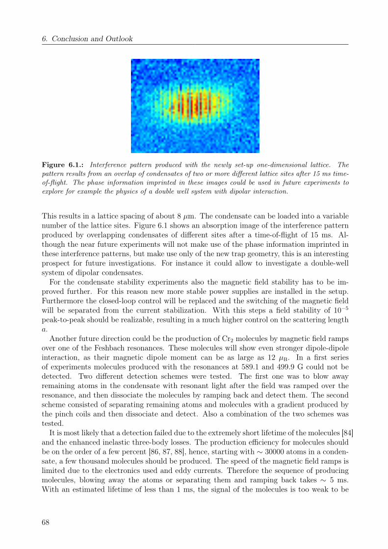
6. Conclusion and Outlook
Figure 6.1.: Interference pattern produced with the newly set-up one-dimensional lattice. Thepattern results from an overlap of condensates of two or more different lattice sites after 15 ms time-of-flight. The phase information imprinted in these images could be used in future experiments toexplore for example the physics of a double well system with dipolar interaction.
This results in a lattice spacing of about 8 µm. The condensate can be loaded into a variablenumber of the lattice sites. Figure 6.1 shows an absorption image of the interference patternproduced by overlapping condensates of different sites after a time-of-flight of 15 ms. Al-though the near future experiments will not make use of the phase information imprinted inthese interference patterns, but make use only of the new trap geometry, this is an interestingprospect for future investigations. For instance it could allow to investigate a double-wellsystem of dipolar condensates.
For the condensate stability experiments also the magnetic field stability has to be im-proved further. For this reason new more stable power supplies are installed in the setup.Furthermore the closed-loop control will be replaced and the switching of the magnetic fieldwill be separated from the current stabilization. With this steps a field stability of 10−5
peak-to-peak should be realizable, resulting in a much higher control on the scattering lengtha.
Another future direction could be the production of Cr2 molecules by magnetic field rampsover one of the Feshbach resonances. These molecules will show even stronger dipole-dipoleinteraction, as their magnetic dipole moment can be as large as 12 µB. In a first seriesof experiments molecules produced with the resonances at 589.1 and 499.9 G could not bedetected. Two different detection schemes were tested. The first one was to blow awayremaining atoms in the condensate with resonant light after the field was ramped over theresonance, and then dissociate the molecules by ramping back and detect them. The secondscheme consisted of separating remaining atoms and molecules with a gradient produced bythe pinch coils and then dissociate and detect. Also a combination of the two schemes wastested.
It is most likely that a detection failed due to the extremely short lifetime of the molecules [84]and the enhanced inelastic three-body losses. The production efficiency for molecules shouldbe on the order of a few percent [86, 87, 88], hence, starting with ∼ 30000 atoms in a conden-sate, a few thousand molecules should be produced. The speed of the magnetic field ramps islimited due to the electronics used and eddy currents. Therefore the sequence of producingmolecules, blowing away the atoms or separating them and ramping back takes ∼ 5 ms.With an estimated lifetime of less than 1 ms, the signal of the molecules is too weak to be
68
detectable. In the future the experiments could be redone with the use of the one-dimensionallattice. The quasi two-dimensional confinement in the stack of pancake traps could lead to astabilization of the molecules due to the repulsive interaction in the pancake plane.
69

6. Conclusion and Outlook
70
A. Two-Frequency Acousto-OpticModulator Driver
This appendix describes the two-frequency acousto-optic modulator (AOM) driverthat is used to improve the pointing stability of our optical dipole trap beams [13].Section A.1 gives an introduction to acousto-optic modulation. Based on this, theproblem of beam movement due to thermal effects is introduced in section A.2 and thetwo-frequency method is presented as a way to suppress this movement. Section A.3reports on the technical realization of a two-frequency driver, including the detailsof an electronic circuit used for it. The last section A.4 presents the measurementsthat were done to test the performance of the two-frequency method.
A.1. Introduction to Acousto-Optic Modulation
Acousto-optic modulators are an important tool to manipulate laser beams. They are usedmainly for three purposes: to deflect, to shift in frequency and to modulate the intensity ofa beam [89]. Technical applications exist among many others in telecommunications or laserprinting. In Atomic, Mesoscopic and Optical Physics (AMO) especially their ability to tunefrequencies and modulate intensities is widely used, for example in cold atoms experimentsthese parameters need to be controlled precisely for many laser beams. This section gives ashort introduction to the theory of acousto-optic modulation following mostly the treatmentin [90]. A more detailed description can be found also in [91].
The working principle of an AOM is Brillouin scattering [92], i.e. the diffraction of lightby a sound wave inside a crystal. A sound wave is a periodic density perturbation, whichcauses also a periodic change of the index of refraction. This ’grating’ with a lattice spacinggiven by the sound wavelength λs diffracts an incoming optical beam. In the limit of athick grating, i.e. the optical path length in the perturbed region is large compared to λs,a theoretical description is given by the Bragg diffraction analogous to the diffraction of X-rays in a crystal: If the path difference 2d between reflection on two adjacent acoustic wavefronts (see Fig. A.1) is an integer multiple m of the light wavelength λ1, the reflected beamsinterfere in phase, which leads to a bright diffraction peak. The angle of incidence at whichthis condition is fulfilled is called Bragg angle θB. It can be calculated by using d = sin θiλs,where θi is the angle between incoming beam and sound wave. Hence, the condition reads
2λs sin θB = mλ . (A.1)
In the Bragg limit it is possible to diffract up to 100% of the light in one order m, whereas in
1Actually one has to use the wavelength in the crystal λ/n, where n is the refractive index. But, due torefraction at the surface air - crystal, the n cancels out in the final equation for the Bragg angle and isnot taken into account.
71
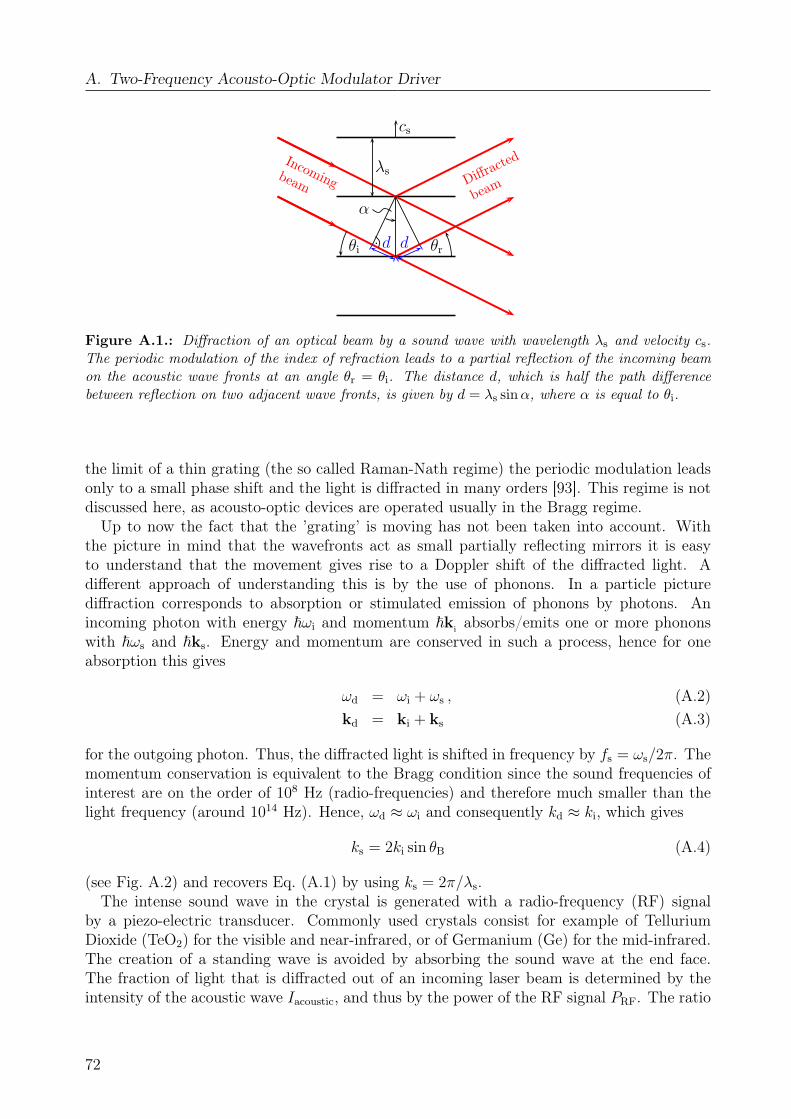
A. Two-Frequency Acousto-Optic Modulator Driver
Diffracted
beam
Incomingbeamλs
cs
θi θr
α
· d d
Figure A.1.: Diffraction of an optical beam by a sound wave with wavelength λs and velocity cs.The periodic modulation of the index of refraction leads to a partial reflection of the incoming beamon the acoustic wave fronts at an angle θr = θi. The distance d, which is half the path differencebetween reflection on two adjacent wave fronts, is given by d = λs sinα, where α is equal to θi.
the limit of a thin grating (the so called Raman-Nath regime) the periodic modulation leadsonly to a small phase shift and the light is diffracted in many orders [93]. This regime is notdiscussed here, as acousto-optic devices are operated usually in the Bragg regime.
Up to now the fact that the ’grating’ is moving has not been taken into account. Withthe picture in mind that the wavefronts act as small partially reflecting mirrors it is easyto understand that the movement gives rise to a Doppler shift of the diffracted light. Adifferent approach of understanding this is by the use of phonons. In a particle picturediffraction corresponds to absorption or stimulated emission of phonons by photons. Anincoming photon with energy ~ωi and momentum ~k
iabsorbs/emits one or more phonons
with ~ωs and ~ks. Energy and momentum are conserved in such a process, hence for oneabsorption this gives
ωd = ωi + ωs , (A.2)kd = ki + ks (A.3)
for the outgoing photon. Thus, the diffracted light is shifted in frequency by fs = ωs/2π. Themomentum conservation is equivalent to the Bragg condition since the sound frequencies ofinterest are on the order of 108 Hz (radio-frequencies) and therefore much smaller than thelight frequency (around 1014 Hz). Hence, ωd ≈ ωi and consequently kd ≈ ki, which gives
ks = 2ki sin θB (A.4)
(see Fig. A.2) and recovers Eq. (A.1) by using ks = 2π/λs.The intense sound wave in the crystal is generated with a radio-frequency (RF) signal
by a piezo-electric transducer. Commonly used crystals consist for example of TelluriumDioxide (TeO2) for the visible and near-infrared, or of Germanium (Ge) for the mid-infrared.The creation of a standing wave is avoided by absorbing the sound wave at the end face.The fraction of light that is diffracted out of an incoming laser beam is determined by theintensity of the acoustic wave Iacoustic, and thus by the power of the RF signal PRF. The ratio
72
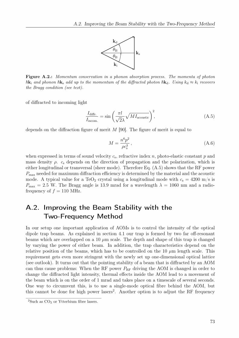
A.2. Improving the Beam Stability with the Two-Frequency Method
θB
θB
kd
ki
ks
Figure A.2.: Momentum conservation in a phonon absorption process. The momenta of photon~ki and phonon ~ks add up to the momentum of the diffracted photon ~kd. Using kd ≈ ki recoversthe Bragg condition (see text).
of diffracted to incoming light
Idiffr.
Iincom.
= sin
(πl√2λ
√MIacoustic
)2
, (A.5)
depends on the diffraction figure of merit M [90]. The figure of merit is equal to
M =n6p2
ρc3s, (A.6)
when expressed in terms of sound velocity cs, refractive index n, photo-elastic constant p andmass density ρ. cs depends on the direction of propagation and the polarization, which iseither longitudinal or transversal (sheer mode). Therefore Eq. (A.5) shows that the RF powerPmax needed for maximum diffraction efficiency is determined by the material and the acousticmode. A typical value for a TeO2 crystal using a longitudinal mode with cs = 4200 m/s isPmax = 2.5 W. The Bragg angle is 13.9 mrad for a wavelength λ = 1060 nm and a radio-frequency of f = 110 MHz.
A.2. Improving the Beam Stability with theTwo-Frequency Method
In our setup one important application of AOMs is to control the intensity of the opticaldipole trap beams. As explained in section 4.1 our trap is formed by two far off-resonantbeams which are overlapped on a 10 µm scale. The depth and shape of this trap is changedby varying the power of either beam. In addition, the trap characteristics depend on therelative position of the beams, which has to be controlled on the 10 µm length scale. Thisrequirement gets even more stringent with the newly set up one-dimensional optical lattice(see outlook). It turns out that the pointing stability of a beam that is diffracted by an AOMcan thus cause problems: When the RF power PRF driving the AOM is changed in order tochange the diffracted light intensity, thermal effects inside the AOM lead to a movement ofthe beam which is on the order of 1 mrad and takes place on a timescale of several seconds.One way to circumvent this, is to use a single-mode optical fibre behind the AOM, butthis cannot be done for high power lasers2. Another option is to adjust the RF frequency
2Such as CO2 or Ytterbium fibre lasers.
73
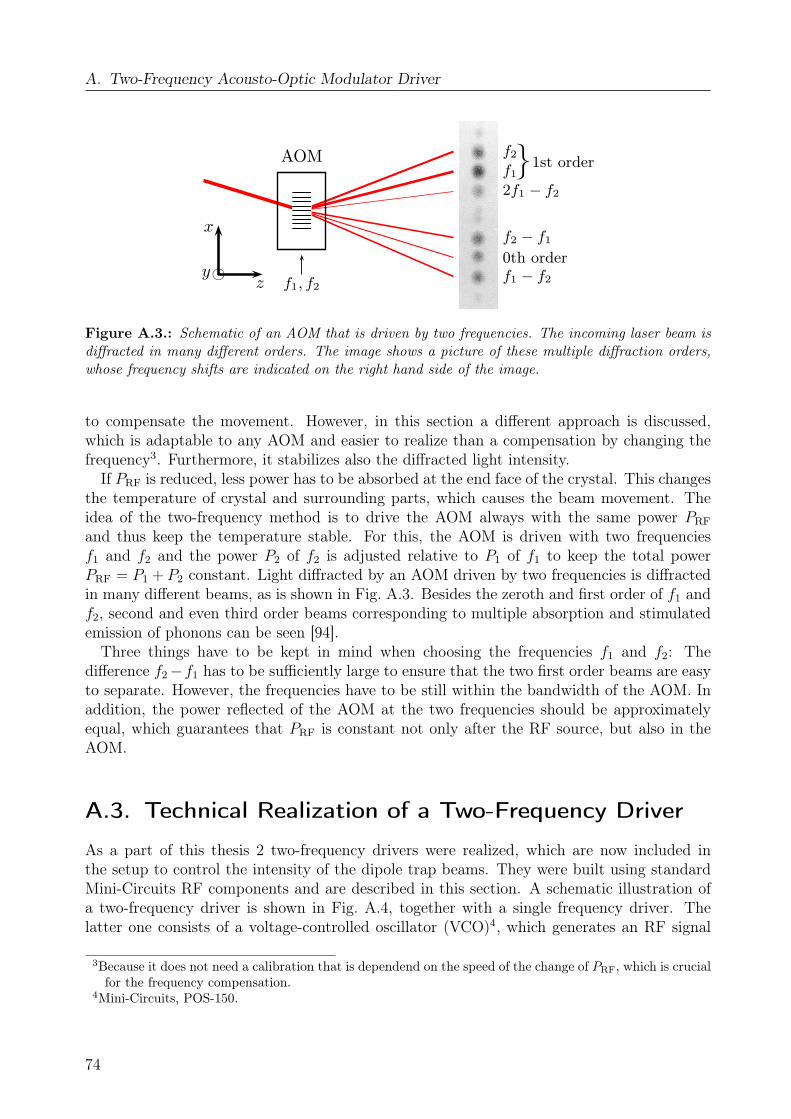
A. Two-Frequency Acousto-Optic Modulator Driver
0th orderf1 − f2
f2 − f1
f1
f21st order
2f1 − f2
AOM
f1, f2y
z
x
Figure A.3.: Schematic of an AOM that is driven by two frequencies. The incoming laser beam isdiffracted in many different orders. The image shows a picture of these multiple diffraction orders,whose frequency shifts are indicated on the right hand side of the image.
to compensate the movement. However, in this section a different approach is discussed,which is adaptable to any AOM and easier to realize than a compensation by changing thefrequency3. Furthermore, it stabilizes also the diffracted light intensity.
If PRF is reduced, less power has to be absorbed at the end face of the crystal. This changesthe temperature of crystal and surrounding parts, which causes the beam movement. Theidea of the two-frequency method is to drive the AOM always with the same power PRF
and thus keep the temperature stable. For this, the AOM is driven with two frequenciesf1 and f2 and the power P2 of f2 is adjusted relative to P1 of f1 to keep the total powerPRF = P1 + P2 constant. Light diffracted by an AOM driven by two frequencies is diffractedin many different beams, as is shown in Fig. A.3. Besides the zeroth and first order of f1 andf2, second and even third order beams corresponding to multiple absorption and stimulatedemission of phonons can be seen [94].
Three things have to be kept in mind when choosing the frequencies f1 and f2: Thedifference f2−f1 has to be sufficiently large to ensure that the two first order beams are easyto separate. However, the frequencies have to be still within the bandwidth of the AOM. Inaddition, the power reflected of the AOM at the two frequencies should be approximatelyequal, which guarantees that PRF is constant not only after the RF source, but also in theAOM.
A.3. Technical Realization of a Two-Frequency Driver
As a part of this thesis 2 two-frequency drivers were realized, which are now included inthe setup to control the intensity of the dipole trap beams. They were built using standardMini-Circuits RF components and are described in this section. A schematic illustration ofa two-frequency driver is shown in Fig. A.4, together with a single frequency driver. Thelatter one consists of a voltage-controlled oscillator (VCO)4, which generates an RF signal
3Because it does not need a calibration that is dependend on the speed of the change of PRF, which is crucialfor the frequency compensation.
4Mini-Circuits, POS-150.
74
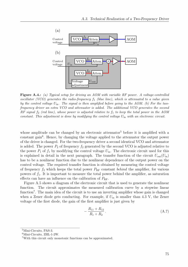
A.3. Technical Realization of a Two-Frequency Driver
(a)
AOMUin
Atten.VCOf1
Controlvoltage
(b)
Controlvoltage
+ AOMAtten.VCOf1
Atten.VCOf2
Voltageadjustment
Uout
Uin
Figure A.4.: (a) Typical setup for driving an AOM with variable RF power. A voltage-controlledoscillator (VCO) generates the radio-frequency f1 (blue line), which is attenuated to a value givenby the control voltage Uin. The signal is then amplified before going to the AOM. (b) For the two-frequency driver an extra VCO and attenuator is added. The additional VCO generates the secondRF signal f2 (red line), whose power is adjusted relative to f1 to keep the total power in the AOMconstant. This adjustment is done by modifying the control voltage Uin with an electronic circuit.
whose amplitude can be changed by an electronic attenuator5 before it is amplified with aconstant gain6. Hence, by changing the voltage applied to the attenuator the output powerof the driver is changed. For the two-frequency driver a second identical VCO and attenuatoris added. The power P2 of frequency f2 generated by the second VCO is adjusted relative tothe power P1 of f1 by modifying the control voltage Uin. The electronic circuit used for thisis explained in detail in the next paragraph. The transfer function of the circuit Uout(Uin)has to be a nonlinear function due to the nonlinear dependence of the output power on thecontrol voltage. The required transfer function is obtained by measuring the control voltageof frequency f2 which keeps the total power PRF constant behind the amplifier, for variouspowers of f1. It is important to measure the total power behind the amplifier, as saturationeffects can have an influence on the calibration of PRF.
Figure A.5 shows a diagram of the electronic circuit that is used to generate the nonlinearfunction. The circuit approximates the measured calibration curve by a stepwise linearfunction7. The main idea of the circuit is to use an inverting amplifier whose gain is changedwhen a Zener diode gets conducting. For example, if Uin is smaller than 4.3 V, the Zenervoltage of the first diode, the gain of the first amplifier is just given by
− R11 +R12
R1 +R2
. (A.7)
5Mini-Circuits, PAS-3.6Mini-Circuits, ZHL-1-2W.7With this circuit only monotonic functions can be approximated.
75
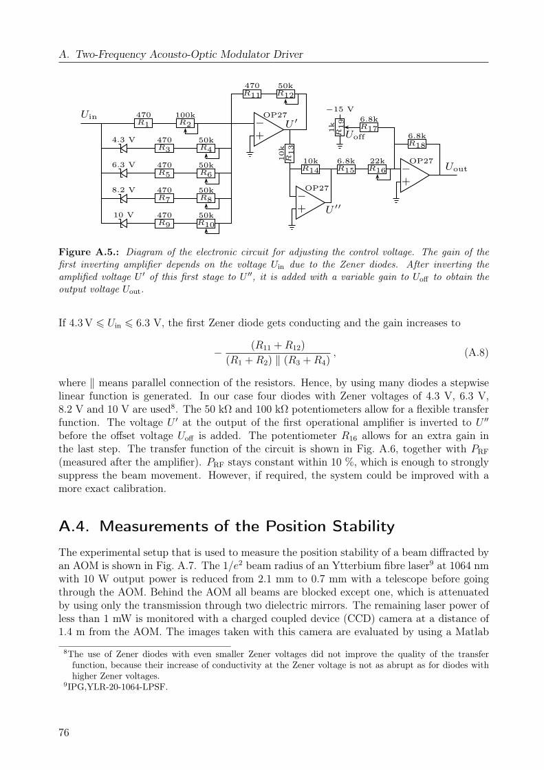
A. Two-Frequency Acousto-Optic Modulator Driver
R1470
R2100k
4.3 VR3470
R450k
6.3 VR5470
R650k
8.2 VR7470
R850k
10 VR9470
R1050k
−+
OP27U ′
R11470
R1250k
−+
OP27
U ′′
10k
R13
R1410k −
+
OP27R156.8k
R1622k
1k
R19
−15 V
UoffR176.8k
R186.8k
Uin
Uout
Figure A.5.: Diagram of the electronic circuit for adjusting the control voltage. The gain of thefirst inverting amplifier depends on the voltage Uin due to the Zener diodes. After inverting theamplified voltage U ′ of this first stage to U ′′, it is added with a variable gain to Uoff to obtain theoutput voltage Uout.
If 4.3 V 6 Uin 6 6.3 V, the first Zener diode gets conducting and the gain increases to
− (R11 +R12)
(R1 +R2) ‖ (R3 +R4), (A.8)
where ‖ means parallel connection of the resistors. Hence, by using many diodes a stepwiselinear function is generated. In our case four diodes with Zener voltages of 4.3 V, 6.3 V,8.2 V and 10 V are used8. The 50 kΩ and 100 kΩ potentiometers allow for a flexible transferfunction. The voltage U ′ at the output of the first operational amplifier is inverted to U ′′
before the offset voltage Uoff is added. The potentiometer R16 allows for an extra gain inthe last step. The transfer function of the circuit is shown in Fig. A.6, together with PRF
(measured after the amplifier). PRF stays constant within 10 %, which is enough to stronglysuppress the beam movement. However, if required, the system could be improved with amore exact calibration.
A.4. Measurements of the Position Stability
The experimental setup that is used to measure the position stability of a beam diffracted byan AOM is shown in Fig. A.7. The 1/e2 beam radius of an Ytterbium fibre laser9 at 1064 nmwith 10 W output power is reduced from 2.1 mm to 0.7 mm with a telescope before goingthrough the AOM. Behind the AOM all beams are blocked except one, which is attenuatedby using only the transmission through two dielectric mirrors. The remaining laser power ofless than 1 mW is monitored with a charged coupled device (CCD) camera at a distance of1.4 m from the AOM. The images taken with this camera are evaluated by using a Matlab
8The use of Zener diodes with even smaller Zener voltages did not improve the quality of the transferfunction, because their increase of conductivity at the Zener voltage is not as abrupt as for diodes withhigher Zener voltages.
9IPG,YLR-20-1064-LPSF.
76
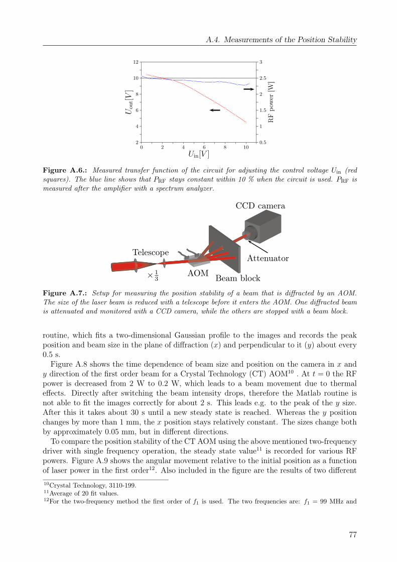
A.4. Measurements of the Position Stability
2
4
6
8
10
12
0 2 4 6 8 10
Uin[V ]
Uou
t[V
]
0.5
1
1.5
2
2.5
3
RF
pow
er[W
]
Figure A.6.: Measured transfer function of the circuit for adjusting the control voltage Uin (redsquares). The blue line shows that PRF stays constant within 10 % when the circuit is used. PRF ismeasured after the amplifier with a spectrum analyzer.
CCD camera
Attenuator
Beam blockAOM
Telescope
× 13
Figure A.7.: Setup for measuring the position stability of a beam that is diffracted by an AOM.The size of the laser beam is reduced with a telescope before it enters the AOM. One diffracted beamis attenuated and monitored with a CCD camera, while the others are stopped with a beam block.
routine, which fits a two-dimensional Gaussian profile to the images and records the peakposition and beam size in the plane of diffraction (x) and perpendicular to it (y) about every0.5 s.
Figure A.8 shows the time dependence of beam size and position on the camera in x andy direction of the first order beam for a Crystal Technology (CT) AOM10 . At t = 0 the RFpower is decreased from 2 W to 0.2 W, which leads to a beam movement due to thermaleffects. Directly after switching the beam intensity drops, therefore the Matlab routine isnot able to fit the images correctly for about 2 s. This leads e.g. to the peak of the y size.After this it takes about 30 s until a new steady state is reached. Whereas the y positionchanges by more than 1 mm, the x position stays relatively constant. The sizes change bothby approximately 0.05 mm, but in different directions.
To compare the position stability of the CT AOM using the above mentioned two-frequencydriver with single frequency operation, the steady state value11 is recorded for various RFpowers. Figure A.9 shows the angular movement relative to the initial position as a functionof laser power in the first order12. Also included in the figure are the results of two different10Crystal Technology, 3110-199.11Average of 20 fit values.12For the two-frequency method the first order of f1 is used. The two frequencies are: f1 = 99 MHz and
77
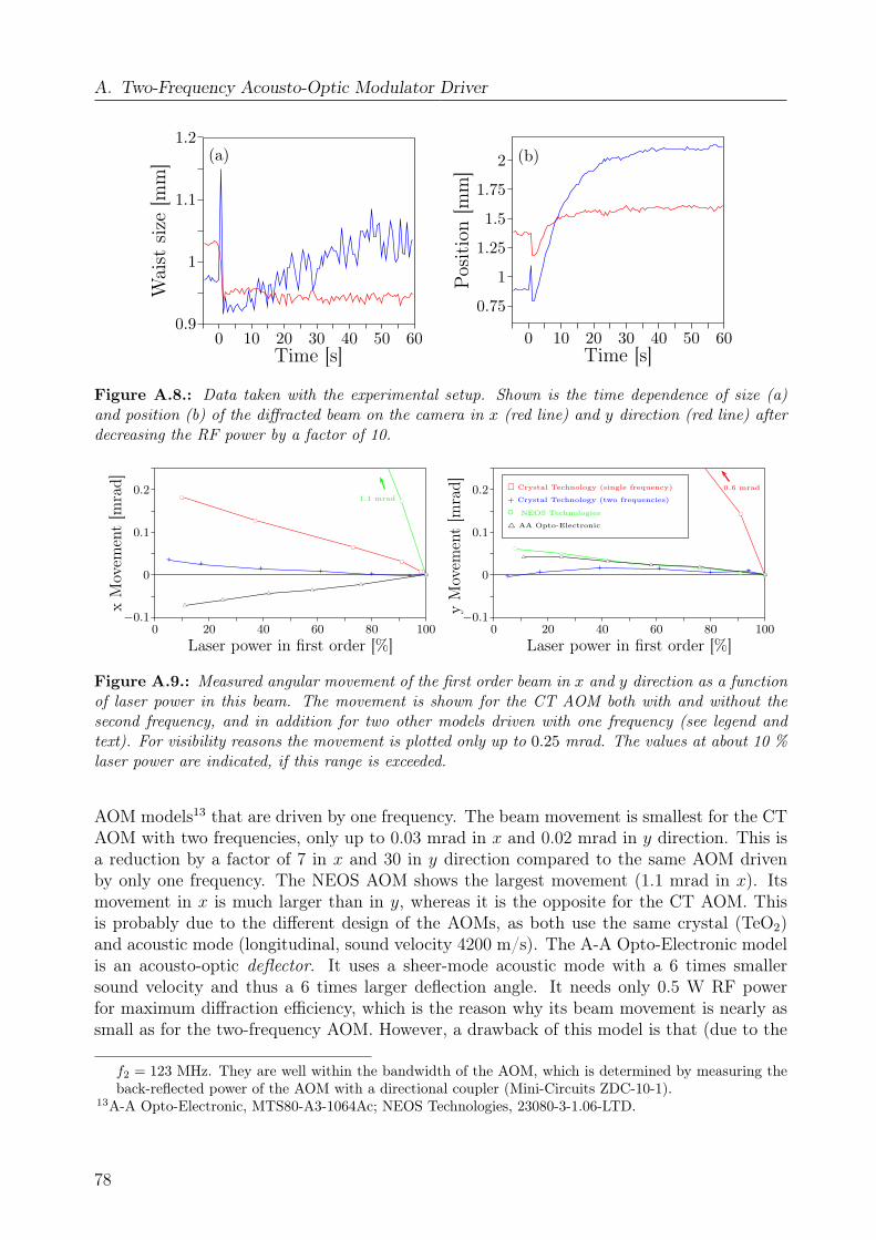
A. Two-Frequency Acousto-Optic Modulator Driver
(a)
0 10 20 30 40 50 600.9
1
1.1
1.2
Time [s]
Wai
stsi
ze[m
m] (b)
0 10 20 30 40 50 60
0.75
1
1.25
1.5
1.75
2
Time [s]
Pos
itio
n[m
m]
Figure A.8.: Data taken with the experimental setup. Shown is the time dependence of size (a)and position (b) of the diffracted beam on the camera in x (red line) and y direction (red line) afterdecreasing the RF power by a factor of 10.
−0.1
0
0.1
0.2
0 20 40 60 80 100
+++++++
Laser power in first order [%]
xM
ovem
ent
[mra
d]
1.1 mrad
−0.1
0
0.1
0.2
0 20 40 60 80 100
+++++++
0.6 mrad
Laser power in first order [%]
yM
ovem
ent
[mra
d] Crystal Technology (single frequency)
+ Crystal Technology (two frequencies)
NEOS Technologies
AA Opto-Electronic
Figure A.9.: Measured angular movement of the first order beam in x and y direction as a functionof laser power in this beam. The movement is shown for the CT AOM both with and without thesecond frequency, and in addition for two other models driven with one frequency (see legend andtext). For visibility reasons the movement is plotted only up to 0.25 mrad. The values at about 10 %laser power are indicated, if this range is exceeded.
AOM models13 that are driven by one frequency. The beam movement is smallest for the CTAOM with two frequencies, only up to 0.03 mrad in x and 0.02 mrad in y direction. This isa reduction by a factor of 7 in x and 30 in y direction compared to the same AOM drivenby only one frequency. The NEOS AOM shows the largest movement (1.1 mrad in x). Itsmovement in x is much larger than in y, whereas it is the opposite for the CT AOM. Thisis probably due to the different design of the AOMs, as both use the same crystal (TeO2)and acoustic mode (longitudinal, sound velocity 4200 m/s). The A-A Opto-Electronic modelis an acousto-optic deflector. It uses a sheer-mode acoustic mode with a 6 times smallersound velocity and thus a 6 times larger deflection angle. It needs only 0.5 W RF powerfor maximum diffraction efficiency, which is the reason why its beam movement is nearly assmall as for the two-frequency AOM. However, a drawback of this model is that (due to the
f2 = 123 MHz. They are well within the bandwidth of the AOM, which is determined by measuring theback-reflected power of the AOM with a directional coupler (Mini-Circuits ZDC-10-1).
13A-A Opto-Electronic, MTS80-A3-1064Ac; NEOS Technologies, 23080-3-1.06-LTD.
78
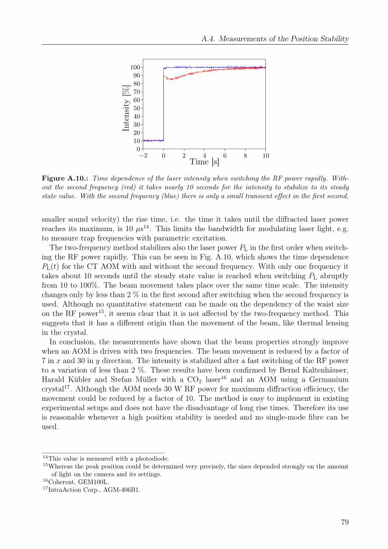
A.4. Measurements of the Position Stability
0
10
20
30
40
50
60
70
80
90
100
−2 0 2 4 6 8 10Time [s]
Inte
nsity
[%]
Figure A.10.: Time dependence of the laser intensity when switching the RF power rapidly. With-out the second frequency (red) it takes nearly 10 seconds for the intensity to stabilize to its steadystate value. With the second frequency (blue) there is only a small transient effect in the first second.
smaller sound velocity) the rise time, i.e. the time it takes until the diffracted laser powerreaches its maximum, is 10 µs14. This limits the bandwidth for modulating laser light, e.g.to measure trap frequencies with parametric excitation.
The two-frequency method stabilizes also the laser power PL in the first order when switch-ing the RF power rapidly. This can be seen in Fig. A.10, which shows the time dependencePL(t) for the CT AOM with and without the second frequency. With only one frequency ittakes about 10 seconds until the steady state value is reached when switching PL abruptlyfrom 10 to 100%. The beam movement takes place over the same time scale. The intensitychanges only by less than 2 % in the first second after switching when the second frequency isused. Although no quantitative statement can be made on the dependency of the waist sizeon the RF power15, it seems clear that it is not affected by the two-frequency method. Thissuggests that it has a different origin than the movement of the beam, like thermal lensingin the crystal.
In conclusion, the measurements have shown that the beam properties strongly improvewhen an AOM is driven with two frequencies. The beam movement is reduced by a factor of7 in x and 30 in y direction. The intensity is stabilized after a fast switching of the RF powerto a variation of less than 2 %. These results have been confirmed by Bernd Kaltenhäuser,Harald Kübler and Stefan Müller with a CO2 laser16 and an AOM using a Germaniumcrystal17. Although the AOM needs 30 W RF power for maximum diffraction efficiency, themovement could be reduced by a factor of 10. The method is easy to implement in existingexperimental setups and does not have the disadvantage of long rise times. Therefore its useis reasonable whenever a high position stability is needed and no single-mode fibre can beused.
14This value is measured with a photodiode.15Whereas the peak position could be determined very precisely, the sizes depended strongly on the amount
of light on the camera and its settings.16Coherent, GEM100L.17IntraAction Corp., AGM-406B1.
79

A. Two-Frequency Acousto-Optic Modulator Driver
80
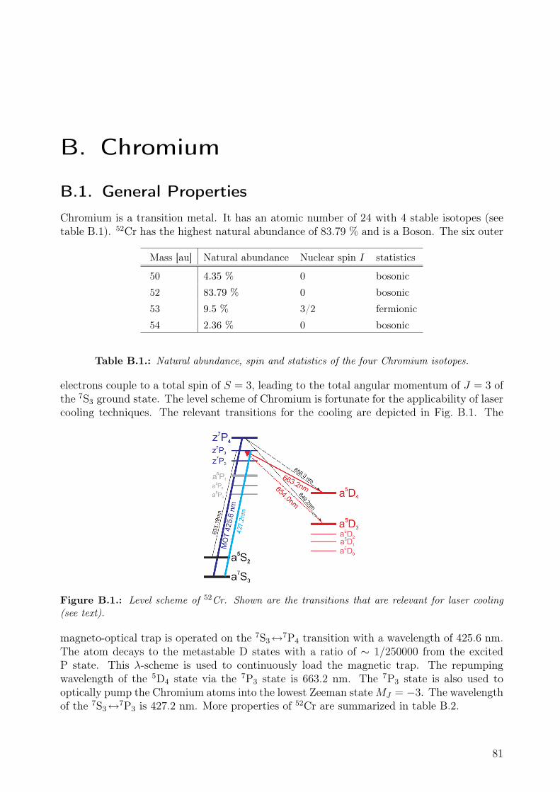
B. Chromium
B.1. General Properties
Chromium is a transition metal. It has an atomic number of 24 with 4 stable isotopes (seetable B.1). 52Cr has the highest natural abundance of 83.79 % and is a Boson. The six outer
Mass [au] Natural abundance Nuclear spin I statistics
50 4.35 % 0 bosonic
52 83.79 % 0 bosonic
53 9.5 % 3/2 fermionic
54 2.36 % 0 bosonic
Table B.1.: Natural abundance, spin and statistics of the four Chromium isotopes.
electrons couple to a total spin of S = 3, leading to the total angular momentum of J = 3 ofthe 7S3 ground state. The level scheme of Chromium is fortunate for the applicability of lasercooling techniques. The relevant transitions for the cooling are depicted in Fig. B.1. The
Figure B.1.: Level scheme of 52Cr. Shown are the transitions that are relevant for laser cooling(see text).
magneto-optical trap is operated on the 7S3↔7P4 transition with a wavelength of 425.6 nm.The atom decays to the metastable D states with a ratio of ∼ 1/250000 from the excitedP state. This λ-scheme is used to continuously load the magnetic trap. The repumpingwavelength of the 5D4 state via the 7P3 state is 663.2 nm. The 7P3 state is also used tooptically pump the Chromium atoms into the lowest Zeeman stateMJ = −3. The wavelengthof the 7S3↔7P3 is 427.2 nm. More properties of 52Cr are summarized in table B.2.
81
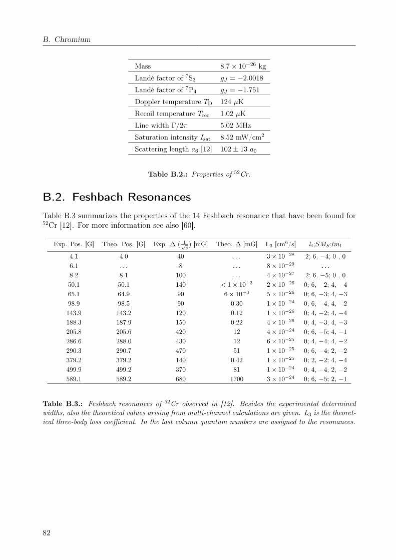
B. Chromium
Mass 8.7× 10⁻²⁶ kg
Landé factor of 7S3 gJ = −2.0018
Landé factor of 7P4 gJ = −1.751
Doppler temperature TD 124 µK
Recoil temperature Trec 1.02 µK
Line width Γ/2π 5.02 MHz
Saturation intensity Isat 8.52 mW/cm2
Scattering length a6 [12] 102± 13 a0
Table B.2.: Properties of 52Cr.
B.2. Feshbach Resonances
Table B.3 summarizes the properties of the 14 Feshbach resonance that have been found for52Cr [12]. For more information see also [60].
Exp. Pos. [G] Theo. Pos. [G] Exp. ∆ ( 1√e) [mG] Theo. ∆ [mG] L3 [cm6/s] li;SMS ;lml
4.1 4.0 40 . . . 3× 10⁻²⁸ 2; 6, −4; 0 , 06.1 . . . 8 . . . 8× 10⁻²⁹ . . .
8.2 8.1 100 . . . 4× 10⁻²⁷ 2; 6, −5; 0 , 050.1 50.1 140 < 1× 10⁻³ 2× 10⁻²⁶ 0; 6, −2; 4, −465.1 64.9 90 6× 10⁻³ 5× 10⁻²⁶ 0; 6, −3; 4, −398.9 98.5 90 0.30 1× 10⁻²⁴ 0; 6, −4; 4, −2143.9 143.2 120 0.12 1× 10⁻²⁶ 0; 4, −2; 4, −4188.3 187.9 150 0.22 4× 10⁻²⁶ 0; 4, −3; 4, −3205.8 205.6 420 12 4× 10⁻²⁴ 0; 6, −5; 4, −1286.6 288.0 430 12 6× 10⁻²⁵ 0; 4, −4; 4, −2290.3 290.7 470 51 1× 10⁻²⁵ 0; 6, −4; 2, −2379.2 379.2 140 0.42 1× 10⁻²⁵ 0; 2, −2; 4, −4499.9 499.2 370 81 1× 10⁻²⁴ 0; 4, −4; 2, −2589.1 589.2 680 1700 3× 10⁻²⁴ 0; 6, −5; 2, −1
Table B.3.: Feshbach resonances of 52Cr observed in [12]. Besides the experimental determinedwidths, also the theoretical values arising from multi-channel calculations are given. L3 is the theoret-ical three-body loss coefficient. In the last column quantum numbers are assigned to the resonances.
82
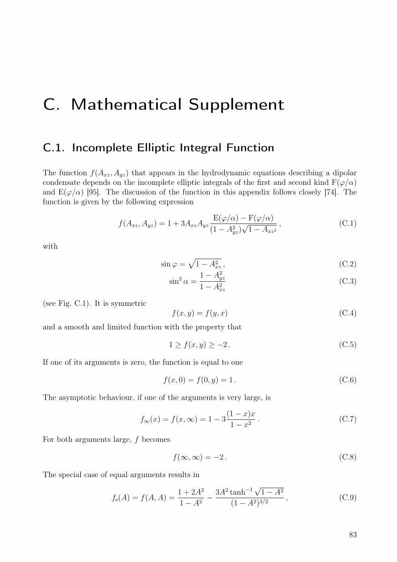
C. Mathematical Supplement
C.1. Incomplete Elliptic Integral Function
The function f(Axz, Ayz) that appears in the hydrodynamic equations describing a dipolarcondensate depends on the incomplete elliptic integrals of the first and second kind F(ϕ/α)and E(ϕ/α) [95]. The discussion of the function in this appendix follows closely [74]. Thefunction is given by the following expression
f(Axz, Ayz) = 1 + 3AxzAyzE(ϕ/α)− F(ϕ/α)
(1− A2yz)√
1− Axz2
, (C.1)
with
sinϕ =√
1− A2xz , (C.2)
sin2 α =1− A2
yz
1− A2xz
(C.3)
(see Fig. C.1). It is symmetricf(x, y) = f(y, x) (C.4)
and a smooth and limited function with the property that
1 ≥ f(x, y) ≥ −2 . (C.5)
If one of its arguments is zero, the function is equal to one
f(x, 0) = f(0, y) = 1 . (C.6)
The asymptotic behaviour, if one of the arguments is very large, is
f∞(x) = f(x,∞) = 1− 3(1− x)x
1− x2. (C.7)
For both arguments large, f becomes
f(∞,∞) = −2 . (C.8)
The special case of equal arguments results in
fs(A) = f(A,A) =1 + 2A2
1− A2− 3A2 tanh−1
√1− A2
(1− A2)3/2, (C.9)
83
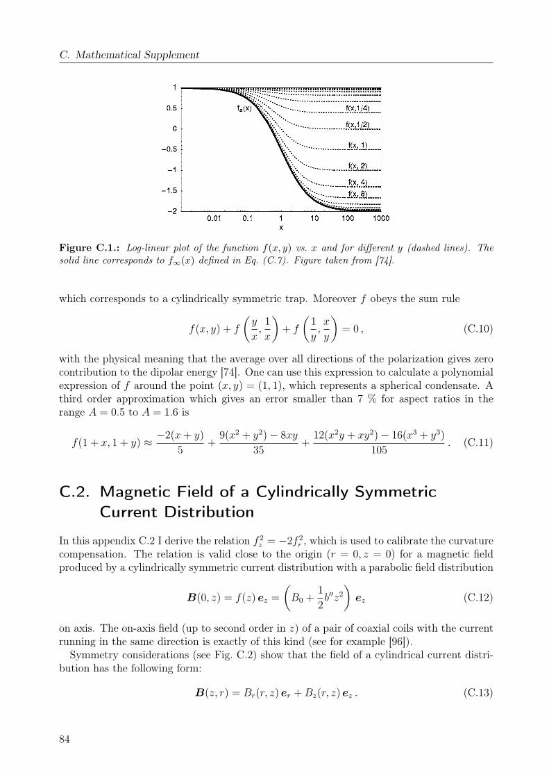
C. Mathematical Supplement
Figure C.1.: Log-linear plot of the function f(x, y) vs. x and for different y (dashed lines). Thesolid line corresponds to f∞(x) defined in Eq. (C.7). Figure taken from [74].
which corresponds to a cylindrically symmetric trap. Moreover f obeys the sum rule
f(x, y) + f
(y
x,1
x
)+ f
(1
y,x
y
)= 0 , (C.10)
with the physical meaning that the average over all directions of the polarization gives zerocontribution to the dipolar energy [74]. One can use this expression to calculate a polynomialexpression of f around the point (x, y) = (1, 1), which represents a spherical condensate. Athird order approximation which gives an error smaller than 7 % for aspect ratios in therange A = 0.5 to A = 1.6 is
f(1 + x, 1 + y) ≈ −2(x+ y)
5+
9(x2 + y2)− 8xy
35+
12(x2y + xy2)− 16(x3 + y3)
105. (C.11)
C.2. Magnetic Field of a Cylindrically SymmetricCurrent Distribution
In this appendix C.2 I derive the relation f 2z = −2f 2
r , which is used to calibrate the curvaturecompensation. The relation is valid close to the origin (r = 0, z = 0) for a magnetic fieldproduced by a cylindrically symmetric current distribution with a parabolic field distribution
B(0, z) = f(z) ez =
(B0 +
1
2b′′z2
)ez (C.12)
on axis. The on-axis field (up to second order in z) of a pair of coaxial coils with the currentrunning in the same direction is exactly of this kind (see for example [96]).
Symmetry considerations (see Fig. C.2) show that the field of a cylindrical current distri-bution has the following form:
B(z, r) = Br(r, z) er +Bz(r, z) ez . (C.13)
84
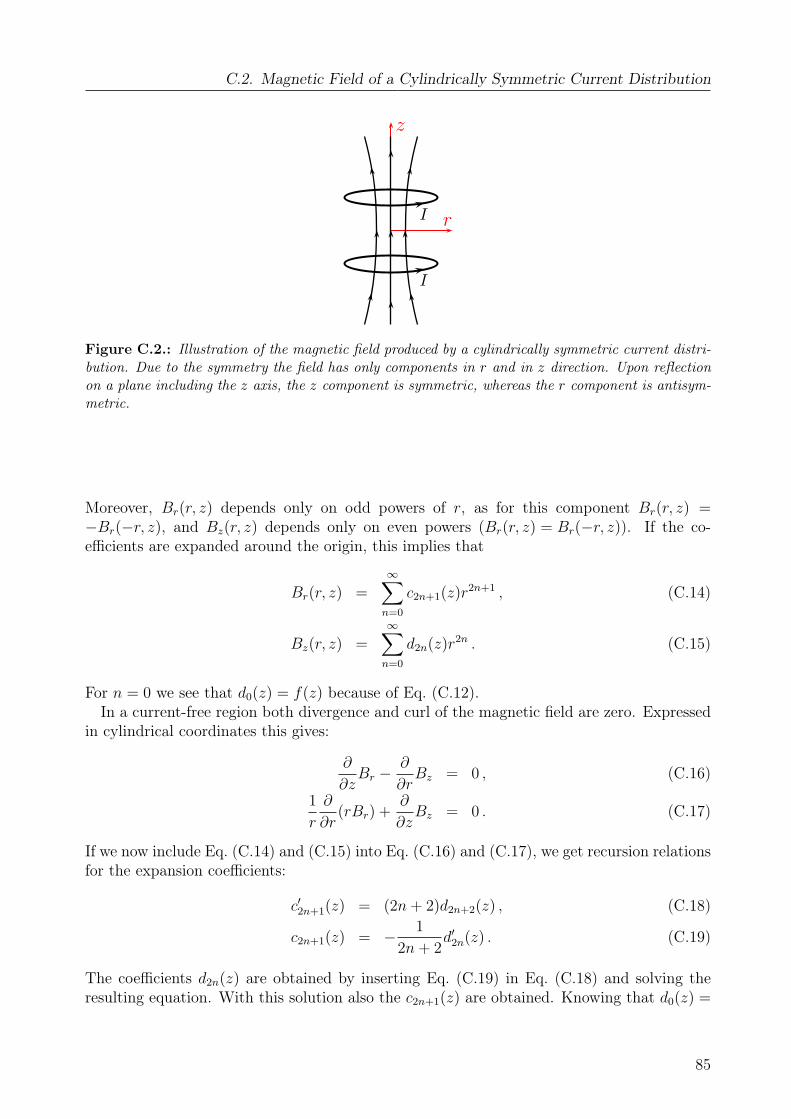
C.2. Magnetic Field of a Cylindrically Symmetric Current Distribution
r
z
I
I
Figure C.2.: Illustration of the magnetic field produced by a cylindrically symmetric current distri-bution. Due to the symmetry the field has only components in r and in z direction. Upon reflectionon a plane including the z axis, the z component is symmetric, whereas the r component is antisym-metric.
Moreover, Br(r, z) depends only on odd powers of r, as for this component Br(r, z) =−Br(−r, z), and Bz(r, z) depends only on even powers (Br(r, z) = Br(−r, z)). If the co-efficients are expanded around the origin, this implies that
Br(r, z) =∞∑
n=0
c2n+1(z)r2n+1 , (C.14)
Bz(r, z) =∞∑
n=0
d2n(z)r2n . (C.15)
For n = 0 we see that d0(z) = f(z) because of Eq. (C.12).In a current-free region both divergence and curl of the magnetic field are zero. Expressed
in cylindrical coordinates this gives:
∂
∂zBr −
∂
∂rBz = 0 , (C.16)
1
r
∂
∂r(rBr) +
∂
∂zBz = 0 . (C.17)
If we now include Eq. (C.14) and (C.15) into Eq. (C.16) and (C.17), we get recursion relationsfor the expansion coefficients:
c′2n+1(z) = (2n+ 2)d2n+2(z) , (C.18)
c2n+1(z) = − 1
2n+ 2d′2n(z) . (C.19)
The coefficients d2n(z) are obtained by inserting Eq. (C.19) in Eq. (C.18) and solving theresulting equation. With this solution also the c2n+1(z) are obtained. Knowing that d0(z) =
85
C. Mathematical Supplement
f(z), we get:
c2n+1(z) =(−1)n+1
22n+1(n+ 1)!n!f (2n+1)(z) , (C.20)
d2n(z) =(−1)n
22n(n!)2f (2n)(z) . (C.21)
Please note that these relations are of course valid also for an arbitrary function f(z).Let us now calculate Br and Bz up to second order in r and z for the parabolic field
distribution on axis. With Eq. (C.20) and (C.21) we directly obtain
Br(r, z) ≈ −1
2b′′zr , (C.22)
Bz(r, z) ≈ B0 +1
2b′′(z2 − 1
2r2
). (C.23)
Thus, B2 up to second order is
B2 = B2r +B2
z ≈ B2z ≈ B2
0 +B0b′′(z2 − 1
2r2
). (C.24)
Hence, finally we get to f 2z = −2f 2
r , if we recall that f 2z ∝ ∂2
zB and f 2r ∝ ∂2
rB and use
B = B0
√1 +
b′′
B0
(z2 − 1
2r2
)≈ B0 +
1
2b′′(z2 − 1
2r2
). (C.25)
C.3. Dependence of the Optical Density of LinearPolarized Light to σ−-Light
Linear polarized light traveling in the magnetic field direction can be decomposed in σ− andσ+-light. Thus the linear polarized light can be written in terms of the spherical unit vectorsintroduced in section 4.4
Ein = E0(uσ+ + uσ−) . (C.26)
Only the σ−-component is absorbed, which results in an outgoing electric field
Eout = E0(uσ+ + e−x2 uσ−) , (C.27)
where x denotes the optical density that is observed for σ−-light. With the definition of theoptical density (4.20) we get the dependence of the OD of linear polarized light (denotedwith y) on x:
y = −ln(Iout
Iin
)= −ln
(|Eout|2
|Ein|2
)= −ln
(1 + e−x
2
). (C.28)
86
Bibliography
[1] T. Lahaye, T. Koch, B. Fröhlich, M. Fattori, J. Metz, A. Griesmaier, S. Giovanazzi andT. Pfau, Strong dipolar effects in a quantum ferrofluid, Nature, 448, 672 (2007). 1, 4,57
[2] M. Baranov, Ł. Dobrek, K. Góral, L. Santos and M. Lewenstein, Ultracold Dipolar Gases— a Challenge for Experiments and Theory, Physica Scripta, 2002, 74–81 (2002). 1, 4
[3] P. Kapitza, Viscosity of liquid helium below the gimel-point, Nature, 141, 74 (1938). 1,3
[4] J. F. Allen and A. D. Misener, Flow phenomena in liquid helium II, Nature, 142, 643–644(1938). 1, 3
[5] D. D. Osheroff, R. C. Richardson and D. M. Lee, Evidence for a New Phase of SolidHe-3, Physical Review Letters, 28, 885 (1972). 1, 3
[6] M. H. Anderson, J. R. Ensher, M. R. Matthews, C. E. Wieman and E. A. Cornell,Observation of Bose-Einstein Condensation in a Dilute Atomic Vapor, Science, 269,198 (1995). 1, 3, 23
[7] K. B. Davis, M. O. Mewes, M. R. Andrews, N. J. van Druten, D. S. Durfee, D. M. Kurn,and W. Ketterle, Bose-Einstein Condensation in a Gas of Sodium Atoms, PhysicalReview Letters, 75, 3969 (1995). 1, 3, 23
[8] M. W. Zwierlein, J. R. Abo-Shaeer, A. Schirotzek, C. H. Schunck and W. Ketterle,Vortices and superfluidity in a strongly interacting Fermi gas, Nature, 435, 1047 (2005).1, 3
[9] A. Griesmaier, J. Werner, S. Hensler, J. Stuhler and T. Pfau, Bose-Einstein Condensa-tion of Chromium, Physical Review Letters, 94, 160401 (2005). 1, 3, 4
[10] J. Stuhler, A. Griesmaier, T. Koch, M. Fattori, S. Giovanazzi, P. Pedri, L. Santos andT. Pfau, Observation of Dipole-Dipole Interaction in a Degenerate Quantum Gas, Phys-ical Review Letters, 95, 150406 (2005). 1, 4, 29, 30, 31, 32, 63, 64
[11] S. Inouye, M. R. Andrews, J. Stenger, H.-J. Miesner, D. M. Stamper-Kurn and W. Ket-terle, Observation of Feshbach resonances in a Bose-Einstein condensate, Nature, 392,151 (1998). 1, 3
[12] J. Werner, A. Griesmaier, S. Hensler, J. Stuhler, T. Pfau, A. Simoni and E. Tiesinga, Ob-servation of Feshbach Resonances in an Ultracold Gas of 52Cr, Physical Review Letters,94, 183201 (2005). 1, 4, 18, 21, 50, 57, 60, 82
87
Bibliography
[13] B. Fröhlich, T. Lahaye, B. Kaltenhäuser, H. Kübler, S. Müller, T. Koch, M. Fattori andT. Pfau, Two-frequency acousto-optic modulator driver to improve the beam pointingstability during intensity ramps, Review of Scientific Instruments, 78, 043101 (2007). 2,5, 38, 71
[14] A. Einstein, Quantentheorie des einatomigen idealen Gases, Zweite Abhandlung,Sitzungsber. Kg. Preuss. Akad. Wiss., page 3 (1925). 3, 23
[15] D. Vollhardt and P. Wölfle, The Superfluid Phases of Helium 3, Taylor & Francis, London(1990). 3
[16] C. C. Bradley, C. A. Sackett, J. J. Tollett and R. G. Hulet, Evidence of Bose-EinsteinCondensation in an Atomic Gas with Attractive Interactions, Physical Review Letters,75, 1687 (1995). 3
[17] D. G. Fried, T. C. Killian, L. Willmann, D. Landhuis, S. C. Moss, D. Kleppner and T. J.Greytak, Bose-Einstein Condensation of Atomic Hydrogen, Physical Review Letters, 81,3811 (1998). 3
[18] S. L. Cornish, N. R. Claussen, J. L. Roberts, E. A. Cornell and C. E. Wieman, Stable 85RbBose-Einstein Condensates with Widely Tunable Interactions, Physical Review Letters,85, 1795–1798 (2000). 3
[19] A. Robert, O. Sirjean, A. Browaeys, J. Poupard, S. Nowak, D. Boiron, C. I. Westbrookand A. Aspect, A Bose-Einstein Condensate of Metastable Atoms, Science, 292, 461(2001). 3
[20] G. Modugno, G. Ferrari, G. Roati, R. J. Brecha, A. Simoni and M. Inguscio, Bose-Einstein Condensation of Potassium Atoms by Sympathetic Cooling, Science, 294, 1320(2001). 3
[21] T. Weber, J. Herbig, M. Mark, H.-C. Nägerl and R. Grimm, Bose-Einstein Condensationof Cesium, Science, 299, 232–235 (2003). 3
[22] Y. Takasu, K. Maki, K. Komori, T. Takano, K. Honda, M. Kumakura, T. Yabuzakiand Y. Takahashi, Spin-Singlet Bose-Einstein Condensation of Two-Electron Atoms,Physical Review Letters, 91, 040404 (2003). 3
[23] G. Roati, M. Zaccanti, C. D’Errico, J. Catani, M. Modugno, A. Simoni, M. Inguscioand G. Modugno, 39-K Bose-Einstein condensate with tunable interactions, Preprint at<http://arxiv.org/abs/cond-mat/0703714> (2007). 3
[24] D. S. Jin, J. R. Ensher, M. R. Matthews, C. E. Wieman and E. A. Cornell, CollectiveExcitations of a Bose-Einstein Condensate in a Dilute Gas, Physical Review Letters,77, 420–423 (1996). 3
[25] M. R. Matthews, B. P. Anderson, P. C. Haljan, D. S. Hall, C. E. Wieman and E. A.Cornell, Vortices in a Bose-Einstein Condensate, Physical Review Letters, 83, 2498–2501 (1999). 3
88
Bibliography
[26] J. Dalibard, Collisional dynamics of ultra-cold atomic gases, in M. Inguscio, S. Stringariand C. Wieman, editors, Proceedings of the International School of Physics - EnricoFermi, page 321, IOS Press (1999). 3, 7, 11, 12, 30
[27] B. DeMarco and D. S. Jin, Onset of Fermi Degeneracy in a Trapped Atomic Gas, Science,285, 1703 (1999). 3
[28] J. S. J. Bardeen, L. Cooper, Microscopic Theory of Superconductivity, Physical Review,106, 162–164 (1957). 3
[29] T. Loftus, C. A. Regal, C. Ticknor, J. L. Bohn and D. S. Jin, Resonant Control of ElasticCollisions in an Optically Trapped Fermi Gas of Atoms, Physical Review Letters, 88,173201 (2002). 3
[30] K. Dieckmann, C. A. Stan, S. Gupta, Z. Hadzibabic, C. H. S. W. and Ketterle, Decayof an Ultracold Fermionic Lithium Gas near a Feshbach Resonance, Phys. Rev. Lett.,89, 203201 (2002). 3
[31] K. M. O’Hara, S. L. Hemmer, M. E. Gehm, S. R. Granade and J. E. Thomas, Observationof a Strongly Interacting Degenerate Fermi Gas of Atoms, Science, 298, 2179 (2002). 3
[32] C. A. Regal, M. Greiner and D. S. Jin, Observation of Resonance Condensation ofFermionic Atom Pairs, Physical Review Letters, 92, 040403 (2004). 3
[33] M. W. Zwierlein, C. A. Stan, C. H. Schunck, S. M. F. Raupach, A. J. Kerman andW. Ketterle, Condensation of Pairs of Fermionic Atoms near a Feshbach Resonance,Physical Review Letters, 92, 120403 (2004). 3
[34] M. Greiner, C. A. Regal and D. S. Jin, Probing the excitation spectrum of a fermi gasin the BCS-BEC crossover regime, Physical Review Letters, 94, 070403 (2005). 3
[35] W. Ketterle and Y. il Shin, Fermi gases go with the superfluid flow, Physics World, 20,39–43 (2007). 3
[36] K. Goral, L. Santos and M. Lewenstein, Quantum Phases of Dipolar Bosons in OpticalLattices, Physical Review Letters, 88, 170406 (2002). 4
[37] O. Dutta and P. Meystre, Ground-state structure and stability of dipolar condensates inanisotropic traps, Preprint at <http://arxiv.org/abs/cond-mat/0703044> (2007). 4
[38] S. Ronen, D. C. E. Bortolotti and J. L. Bohn, Radial and Angular Rotons in TrappedDipolar Gases, Physical Review Letters, 98, 030406 (2007). 4
[39] Y. Kawaguchi, H. Saito and M. Ueda, Einstein–de Haas Effect in Dipolar Bose-EinsteinCondensates, Physical Review Letters, 96, 080405 (2006). 4
[40] L. Santos and T. Pfau, Spin-3 Chromium Bose-Einstein Condensates, Physical ReviewLetters, 96, 190404 (2006). 4
[41] S. Yi and H. Pu, Spontaneous Spin Textures in Dipolar Spinor Condensates, PhysicalReview Letters, 97, 020401 (2006). 4
89
Bibliography
[42] L. Santos, G. Shlyapnikov and M. Lewenstein, Roton-Maxon Spectrum and Stabilityof Trapped Dipolar Bose-Einstein Condensates, Physical Review Letters, 90, 250403(2003). 4
[43] R. K. J. Doyle, B. Friedrich and F. Masnou-Seeuws, Quo vadis, cold molecules?, Euro-pean Physical Journal D, 31, 149 (2004). 4
[44] M. Köhl, H. Moritz, T. Stöferle, K. Günter and T. Esslinger, Fermionic Atoms in a ThreeDimensional Optical Lattice: Observing Fermi Surfaces, Dynamics, and Interactions,Physical Review Letters, 94, 080403 (2005). 4
[45] C. Ospelkaus, S. Ospelkaus, L. Humbert, P. Ernst, K. Sengstock and K. Bongs, UltracoldHeteronuclear Molecules in a 3D Optical Lattice, Physical Review Letters, 97, 120402(2006). 4
[46] J. M. Sage, S. Sainis, T. Bergeman and D. DeMille, Optical Production of UltracoldPolar Molecules, Physical Review Letters, 94, 203001 (2005). 4
[47] M. Marinescu and L. You, Controlling Atom-Atom Interaction at Ultralow Temperaturesby dc Electric Fields, Physical Review Letters, 81, 4596–4599 (1998). 4
[48] S. Giovanazzi, D. O’Dell and G. Kurizki, Density Modulations of Bose-Einstein Con-densates via Laser-Induced Interactions, Physical Review Letters, 88, 130402 (2002).4
[49] J. C. Cohen-Tannoudji, Atom-Atom Interactions in Ultracold Quantum Gases— Lectures on Quantum Gases Institut Henri Poincaré, available online athttp://www.phys.ens.fr/∼castin/ (2007). 4, 13, 15, 16, 17
[50] A. Griesmaier, Dipole-dipole interaction in a degenerate quantum gas – Bose-Einsteincondensation of chromium atoms, Dissertation, University of Stuttgart (2006). 5, 35,36, 37, 38, 39, 51, 55
[51] J. C. Cohen-Tannoudji, Quantum mechanics 2, de Gruyter (1999). 7, 10, 11
[52] J. J. Sakurai, Modern Quantum Mechanics — Revised Edition, Addison-Wesley publish-ing Company (1994). 7
[53] W. Nolting, Quantenmechanik 2, Verlag Zimmermann-Neufang (1992). 7, 9, 11
[54] C. Pethick and H. Smith, Bose-Einstein Condensation in Dilute Gases, Cambridge Uni-versity Press (2004). 12, 15, 23, 25, 27
[55] L. Pitaevskii and S. Stringari, Bose-Einstein Condensation, Oxford Science Publications(2003). 14, 23
[56] E. Braaten and H. Hammer, Universality in Few-body Systems with Large ScatteringLength, Physics Reports, 428, 259–390 (2006). 14, 58
90
Bibliography
[57] J. Stenger, S. Inouye, M. R. Andrews, H.-J. Miesner, D. M. Stamper-Kurn and W. Ket-terle, Strongly Enhanced Inelastic Collisions in a Bose-Einstein Condensate near Fesh-bach Resonances, Physical Review Letters, 82 (1999). 14, 58
[58] V. A. Yurovsky and A. Ben-Reuven, Atom loss from Bose-Einstein condensates due toFeshbach resonances, Physical Review A, 60, R765 (1999). 14
[59] T. Köhler, K. Góral and P. S. Julienne, Production of cold molecules via magneticallytunable Feshbach resonances, Reviews of Modern Physics, 78, 1311 (2006). 15, 18
[60] J. Werner, Observation of Feshbach resonances in an ultracold gas of 52Cr, Dissertation,University of Stuttgart (2006). 15, 18, 21, 35, 82
[61] Z. Pavlovic, B. O. Roos, R. Cote and H. R. Sadeghpour, Collisional properties of trappedcold chromium atoms, Physical Review A (Atomic, Molecular, and Optical Physics), 69,030701 (2004). 18, 20
[62] W. J. Childs and L. S. Goodman, Electronic g Factors of Low-Lying Levels of Fe I, CrI and Mn I, Physical Review A (Atomic, Molecular, and Optical Physics), 140 (2A),A447 (1965). 19
[63] H. Haken and H. C. Wolf, Atom- und Quantenphysik, Springer-Verlag (1990). 19
[64] F. H. Mies, C. J. Williams, P. S. Julienne and M. Krauss, Estimating Bounds on Colli-sional Relaxation Rates of Spin-Polarized 87Rb Atoms at Ultracold Temperatures, Jour-nal of Research of the National Institute of Standards and Technology, 101, 521 (1996).20
[65] W. Demtröder, Molekülphysik, Oldenbourg Wissenschaftsverlag (2003). 20
[66] W. Ketterle, D. Durfee and D. Stamper-Kurn, Making, probing and understanding Bose-Einstein condensates, in M. Inguscio, S. Stringari and C. Wieman, editors, Proceedingsof the International School of Physics - Enrico Fermi, page 67, IOS Press (1999). 23, 24
[67] Y. Castin, Bose-Einstein condensates in atomic gases: simple theoretical results, avail-able online at http://www.phys.ens.fr/cours/notes-de-cours/castin/castin.pdf (2000).23, 27
[68] F. Schwabl, Statistische Mechanik, Springer-Lehrbuchverlag (2000). 23
[69] W. Greiner, Thermodynamik und Statistische Mechanik, Verlag Harri Deutsch (1987).23
[70] Y. Castin and R. Dum, Bose-Einstein Condensates in Time Dependent Traps, PhysicalReview Letters, 77, 5315 (1996). 28
[71] K. Goral, K. Rzazewski and T. Pfau, Bose-Einstein condensation with magnetic dipole-dipole forces, Physical Review A, 61, 051601 (2000). 30
[72] S. Yi and L. You, Trapped condensates of atoms with dipole interactions, Physical ReviewA, 63, 053607 (2001). 30
91
Bibliography
[73] C. Eberlein, S. Giovanazzi and D. H. J. O’Dell, Exact solution of the Thomas-Fermiequation for a trapped Bose-Einstein condensate with dipole-dipole interactions, PhysicalReview A, 71, 033618 (2005). 30, 32, 33
[74] S. Giovanazzi, P. Pedri, L.Santos, A. Griesmaier, M. Fattori, T. Koch, J. Stuhler andT. Pfau, Expansion dynamics of a dipolar Bose-Einstein condensate, Physical ReviewA, 74, 013621 (2006). 31, 83, 84
[75] J. Stuhler, Kontinuierliches Laden einer Magnetfalle mit lasergekühlten Chromatomen,Dissertation, University of Stuttgart (2001). 35
[76] P. O. Schmidt, Scattering properties of ultra-cold chromium atoms, Dissertation, Uni-versity of Stuttgart (2003). 35, 37
[77] S. Hensler, Wechselwirkung in ultrakalten dipolaren Gasen, Dissertation, University ofStuttgart (2004). 35, 37, 39
[78] A. Griesmaier, J. Stuhler and T. Pfau, Production of a chromium Bose-Einstein con-densate, Applied Physics B, 82, 211–216 (2006). 35
[79] J. Werner, Kontinuierliches Laden einer Magnetfalle mit lasergekühlten Chromatomen,Diplomarbeit, University of Stuttgart (2000). 35
[80] T. Binhammer, Verdampfungskühlung ultrakalter Chrom-Atome, Diplomarbeit, Univer-sity of Stuttgart (2002). 35
[81] A. Griesmaier, Aufbau einer kombinierten magneto-optischen Falle für Chrom und Ru-bidium, Diplomarbeit, University of Stuttgart (2002). 35, 37, 42
[82] S. Götz, Demagnetization cooling in an ultracold chromium gas, Diplomarbeit, Universityof Stuttgart (2006). 35
[83] L. D. Landau and E. M. Lifschitz, Lehrbuch der theoretischen Physik, Bd.1, Mechanik,Deutsch (Harri) (1997). 40
[84] E. A. Donley, N. R. Claussen, S. T. Thompson and C. E. Wieman, Atom-moleculecoherence in a Bose-Einstein condensate, Nature, 417, 529 (2002). 51, 68
[85] H. J. Metcalf and P. v. d. Straten, Laser Cooling and Trapping, Springer-Verlag (1999).52, 54
[86] K. Xu, T. Mukaiyama, J. R. Abo-Shaeer, J. K. Chin, D. E. Miller and W. Ketterle, For-mation of Quantum-Degenerate Sodium Molecules, Physical Review Letters, 91, 210402(2003). 68
[87] J. Herbig, T. Kraemer, M. Mark, T. Weber, C. Chin, H.-C. Nägerl and R. Grimm,Preparation of a Pure Molecular Quantum Gas, Science, 301, 1510 (2003). 68
[88] S. Dürr, T. Volz, A. Marte and G. Rempe, Observation of Molecules Produced from aBose-Einstein Condensate, Physical Review Letters, 92, 020406 (2004). 68
92
Bibliography
[89] A. P. Goutzoulis and D. Pape, editors, Design and Fabrication of Acousto-Optic Devices,CRC (1994). 71
[90] A. Yariv, Optical Electronics, Saunders College Publishers (1991). 71, 73
[91] M. Born and E. Wolf, Principles of Optics, Cambridge University Press (2003). 71
[92] L. Brillouin, Diffusion de la lumiére et des rayons X par un corps transparent homogéne,Ann. Physique, 17, 88 (1922). 71
[93] J. Eichler and H.-J. Eichler, Laser — Grundlagen, Systeme, Anwendungen, SpringerVerlag (1990). 72
[94] D. L. Hecht, Multifrequency Acoustooptic Diffraction, IEEE Transactions on Sonics andUltrasonics, SU-24 (1977). 74
[95] M. Abramowitz and I. A. Stegun, Handbook of Mathematical Functions with Formulas,Graphs and Mathematical Table, Dober Publications (1972). 83
[96] J. D. Jackson, Classical Electrodynamics, John Wiley and Sons, Inc. (1999). 84
93

Bibliography
94
D. Danksagung
Und zu guter Letzt möchte ich mich noch bei allen Leuten bedanken, die zum Gelingendieser Arbeit beigetragen haben. Ohne die Unterstützung von allen Seiten, wäre diese Arbeitso nicht möglich gewesen:
• An erster Stelle bedanke ich mich sehr herzlich bei Herrn Prof. T. Pfau, der meinenWeg an der Stuttgarter Universität von Anfang an begleitet hat. Angefangen mit demkleinen Laborpraktikum bei Chrom I und der zwei Jahre langen Hiwi Zeit, was mirinteressante Einblicke in die Welt eines Experimentalphysikers lieferte und auch sehrbeim Erstellen der Diplomarbeit geholfen hat, bis hin zur Diplomarbeit die ich an seinemInstitut machen durfte in dem meiner Meinung nach spannendsten Gebiet der Physik,das es momentan gibt. Insbesondere auch für die Unterstützung bei der Erstellung desAOM Artikels, die motivierenden Worte in der Weihnachtsansprache und das netteAngebot noch eine weitere Zeit hier arbeiten zu dürfen. Vielen Dank!
• Second, I thank of course Thierry Lahaye, from whose brilliancy I benefited so infinitelymuch! I learned so many things from him in this year that will serve me well in thefuture. Thank you for all the ’small calculations’ that taught me more than any bookcould have taught me, for the motivation to write the AOM article, for the supportin the lab, for explaining all things to me as often as I needed it, for making the niceresults possible described in this thesis. . . And of course for still proof-reading thisthesis, although already being in France and waiting for the baby!
• Bei Tobias Koch, dessen gute Ideen die Arbeit im Labor immer wieder voran gebrachthaben. Viele Dinge die in dieser Arbeit beschrieben sind, sind auf seinem ’Mist’ ge-wachsen. Natürlich auch für die Unterstützung während der ganzen Diplomarbeit unddie Korrekturen in letzter Minute!
• Bei Jonas Metz, für seine unermüdlichen Versuche mir einen besseren Schreibstil auf-zuprägen, ich hoffe es war nicht vollkommen umsonst!
• I thank Marco Fattori, for the short time I could work together with him. He also taughtme many things and his ’gute Laune’ made the work in the lab always enjoyable.
• Und dem ganzen Rest vom Institut ein herzliches Dankeschön! Es war sehr angenehmhier zu arbeiten. Axel Griesmeier, der mir schon im Laborpraktikum gezeigt hat wiemühsam Laborarbeit sein kann (Stichwort Faser einkoppeln). . . Aber natürlich auchfür das Beantworten aller Fragen zum Labor. Ulrich Raitzsch und Alexander Grei-ner für die Zeit kurz nach dem Mittagessen. Alexander Greiner und Jimmy Sebastianauch besonders für die Hilfe in der Hiwi-Zeit. Den restlichen Rubidis für den tollenSchraubenschrank. Björn Butscher auch besonders für das grösstenteils Übernehmender Weihnachtsfeier-Organisation. Da konntest du schon mal üben für das Greenhorn
95
D. Danksagung
Meeting. . . Und natürlich auch den anderen Chrom II Leute und den Leuten aus demdritten Stock, besonders Harald für das Lösen aller Computerprobleme. Und dann na-türlich auch Sylvia, Nadine und Karin!
• Von den Ehemaligen danke ich ganz besonders auch Sven Hensler, der mir in der HiwiZeit sehr geholfen hat, und Bernd Kaltenhäuser für die schöne Grafik im AOM Artikel.
• Bei Herrn Prof. Dr. Wrachtrup für die Teilnahme als Mitberichter.
• Bei meinen Eltern für die Unterstützung in jeglicher Hinsicht während meines ganzenStudium!
• Bei meinen Freunden für den Ausgleich neben der Arbeit, besonders natürlich bei Sebo,Erik, Domi, Christian und Anna. Bei Patrick, Ilona und Alex für die effektive Prüfungs-vorbereitung. Und bei den Chaoten, die es mir erlaubt haben hier in Stuttgart weiterMusik zu machen und dazu verbunden mit so viel Spaß!.
• Und last but absolutely not least bei meiner Freundin Denise für die Unterstützung undGeduld die sie aufgebracht hat, wenn es mal wieder später wurde, besonders natürlichin den letzten Wochen!
96