HAL Id: hal-01366646https://hal.archives-ouvertes.fr/hal-01366646v2

Submitted on 20 Feb 2017

HAL is a multi-disciplinary open accessarchive for the deposit and dissemination of sci-entific research documents, whether they are pub-lished or not. The documents may come fromteaching and research institutions in France orabroad, or from public or private research centers.

L’archive ouverte pluridisciplinaire HAL, estdestinée au dépôt et à la diffusion de documentsscientifiques de niveau recherche, publiés ou non,émanant des établissements d’enseignement et derecherche français ou étrangers, des laboratoirespublics ou privés.

Distributed under a Creative Commons Attribution - NonCommercial - NoDerivatives| 4.0International License

Stress and flux reconstruction in Biot’s poro-elasticityproblem with application to a posteriori error analysisRita Riedlbeck, Daniele Di Pietro, Alexandre Ern, Sylvie Granet, Kyrylo

Kazymyrenko

To cite this version:Rita Riedlbeck, Daniele Di Pietro, Alexandre Ern, Sylvie Granet, Kyrylo Kazymyrenko. Stressand flux reconstruction in Biot’s poro-elasticity problem with application to a posteriori erroranalysis. Computers & Mathematics with Applications, Elsevier, 2017, 73 (7), pp.1593-1610.10.1016/j.camwa.2017.02.005. hal-01366646v2

Stress and flux reconstruction in Biot’s poro-elasticity problem

with application to a posteriori error analysis

Rita Riedlbeck∗,1,3, Daniele A. Di Pietro1, Alexandre Ern2, Sylvie Granet3, and Kyrylo Kazymyrenko3

1University of Montpellier, Institut Montpellierain Alexander Grothendieck, 34095 Montpellier CEDEX 5,France

2University Paris-Est, CERMICS (ENPC), 6-8 avenue Blaise Pascal, 77455 Marne-la-Vallee CEDEX 2, France3EDF R&D, IMSIA, 7 boulevard Gaspard Monge, 91120 Palaiseau, France

February 20, 2017

Abstract

We derive equilibrated reconstructions of the Darcy velocity and of the total stress ten-sor for Biot’s poro-elasticity problem. Both reconstructions are obtained from mixed finiteelement solutions of local Neumann problems posed over patches of elements around meshvertices. The Darcy velocity is reconstructed using Raviart–Thomas finite elements and thestress tensor using Arnold–Winther finite elements so that the reconstructed stress tensor issymmetric. Both reconstructions have continuous normal component across mesh interfaces.Using these reconstructions, we derive a posteriori error estimators for Biot’s poro-elasticityproblem, and we devise an adaptive space-time algorithm driven by these estimators. Thealgorithm is illustrated on test cases with analytical solution, on the quarter five-spot prob-lem, and on an industrial test case simulating the excavation of two galleries.

Key words: a posteriori error estimate; equilibrated stress reconstruction; Arnold-Wintherfinite element space; Biot’s poro-elasticity problem

1 Introduction

Biot’s poro-elasticity problem was originally proposed by von Terzaghi [40] and Biot [6] todescribe the hydro-mechanical coupling between the displacement field u of a linearly elastic,porous material and the pressure p of an incompressible, viscous fluid saturating its pores. LetΩ ⊂ R2 be the simply connected polygonal region occupied by the porous material, and lettF > 0 denote the simulation time. For the sake of simplicity, we assume that the materialis clamped at its impermeable boundary, and fix the Biot–Willis coefficient equal to 1. Wealso assume that the deformation of the material is much slower than the flow rate, so that theproblem can be considered in quasi-static form. Then, the displacement field u : Ω×(0, tF )→ R2

∗Corresponding author, rita.riedlbeck@edf.fr

1

and the pore pressure p : Ω× (0, tF )→ R are determined by

−∇ · σ(u) +∇p = f in Ω× (0, tF ), (1.1a)

∂t(∇ · u+ c0p)−∇ · (κ∇p) = g in Ω× (0, tF ), (1.1b)

u = 0 on ∂Ω× (0, tF ), (1.1c)

κ∇p · nΩ = 0 on ∂Ω× (0, tF ), (1.1d)

u(·, 0) = u0 in Ω, (1.1e)

where f denotes the volumetric body force acting on the material, g a volumetric fluid source(which, if c0 = 0, is assumed to verify the compatibility condition

∫Ω g(x, t)dx = 0 for each

t ∈ (0, tF )), and the effective stress tensor σ is linked to the strain tensor ε through Hooke’s law

σ(u) = 2µε(u) + λtr(ε(u))I2, ε(u) =1

2(∇u+∇uT), (1.2)

where I2 is the two-dimensional identity matrix. The Lame parameters λ and µ, describing the

mechanical properties of the material, are assumed such that µ > 0 and λ+ 23µ > 0 uniformly

in Ω. The scalar field κ : Ω → R describes the mobility of the fluid and we assume that thereexist positive real numbers κ[ and κ] such that κ[ ≤ κ ≤ κ] a.e. in Ω. When the specific storagecoefficient c0 is zero, we enforce uniqueness of the pore-pressure in (1.1) by further requiringthat ∫

Ωp(·, t)dx = 0 in (0, tF ). (1.3)

On the other hand, for c0 > 0, we complement (1.1) by the following initial condition on thepressure:

p(·, 0) = p0 in Ω. (1.4)

In practice, even when c0 = 0, the initial velocity field u0 in (1.1e) is usually obtained by firstsetting p0 equal to the solution of a hydrostatic computation and then calculating u0 by solving(1.1a) with p = p0 (cf. Remark 2.1 in [33]). The well-posedness of Biot’s consolidation problemhas been analyzed in [38,41]. A suitable approximation method consists of using Taylor–HoodH1-conforming finite elements in space (using piecewise polynomials of order k ≥ 1 for thepressure and of order (k + 1) for the displacement) and a backward Euler scheme in time. Thecorresponding a priori error analysis can be found in [28–30]. This discretization strategy isadopted in the Code Aster1 software, which is used for the numerical examples presented in thiswork. Several other discretization methods have been studied in the literature, among whichwe cite, in particular, the fully coupled algorithm of [7], where the Hybrid High-Order methodof [12] is used for the elasticity operator, while the weighted discontinuous Galerkin methodof [13] is used for the Darcy operator.

The two governing equations (1.1a) and (1.1b) express, respectively, the conservation of me-chanical momentum and fluid mass. In particular, the Darcy velocity φ(p) := −κ∇p and thetotal stress tensor θ(u, p) := σ(u)− pI2 have continuous normal component across any interfacein the domain Ω, and the divergence of these fields is locally in equilibrium with the sources (andthe accumulation terms) in any control volume. It is well known that the use of H1-conformingfinite elements does not lead to discrete fluxes φ(pnh) and θ(unh, p

nh) (where (unh, p

nh) denotes the

discrete solution at a given discrete time tn) that satisfy the discrete counterpart of the aboveproperties across mesh interfaces and in mesh cells. The first contribution of this work is tofill this gap by reconstructing equilibrated fluxes from local mixed finite element solves on cell

1http://web-code-aster.org

2

patches around mesh vertices. The Darcy velocity reconstruction uses, as in [9,11,21], Raviart–Thomas mixed finite elements [35] on cell patches around vertices of the original mesh. Theconstruction we propose for the total stress tensor is, to our knowledge, novel and is based onthe use of the Arnold–Winther mixed finite element [4], again on the same vertex-based cellpatches. This construction provides, in particular, a symmetric total stress tensor. The Darcyvelocity and the total stress tensor are reconstructed at each discrete time, they have continuousnormal component across any mesh interface, and their divergence is locally in equilibrium withthe sources (averaged over the time interval) in any mesh cell. In steady-state linear elastic-ity, element-wise (as opposed to patch-wise) reconstructions of equilibrated tractions from localNeumann problems can be found in [2, 10, 25, 32], whereas direct prescription of the degrees offreedom in the Arnold–Winther finite element space is considered in [31].

The second contribution of this work is to perform an a posteriori error analysis of Biot’sporo-elasticity problem using the above reconstructed fluxes to compute the error indicators.Equilibrated-flux a posteriori error estimates for poro-elasticity appear to be a novel topic(residual-based error estimates can be found, e.g., in [18,27]). Equilibrated-flux a posteriori errorestimates offer several advantages. On the one hand, error upper bounds are obtained with fullycomputable constants. The idea can be traced back to [34] and was advanced amongst othersby [1,9,11,19,21,23,24,26,36]. Another interesting property is the polynomial-degree robustnessproved recently for the Poisson problem in [8,21]. A third attractive feature introduced in [20] isto distinguish among various error components, e.g., discretization, linearization, and algebraicsolver error components, and to equilibrate adaptively these components in the iterative solutionof nonlinear problems. This idea was applied to multi-phase, multi-components (possibly nonisothermal) Darcy flows in [14–16]. For simplicity, we consider in the present work a global errormeasure which lends itself naturally to the development of equilibrated-flux error estimators,and defined as the dual energy-norm of the residual of the weak formulation.

This paper is organized as follows. In Section 2, we introduce the weak and discrete formulationsof Biot’s poro-elasticity problem (1.1), along with some useful notation and preliminary results.In Section 3, we present the equilibrated reconstruction for the Darcy velocity and the totalstress tensor. In Section 4, we derive a fully computable upper bound on the residual dualnorm. We then distinguish two different error sources in the upper bound, namely the spatialand the temporal discretization, and we propose an algorithm adapting the mesh and the timestep so as to equilibrate these error sources. Finally, we show numerical results in Section 5.

2 Setting

In this section we introduce some notation, the weak formulation, and the discrete solution ofproblem (1.1).

2.1 Weak formulation

We denote by L2(Ω), L2(Ω) and L2(Ω) the spaces composed of square-integrable functions takingvalues in R, R2 and R2×2 respectively, and by (·, ·) and ‖·‖ the corresponding inner productand norm. We also let L2

0(Ω) := q ∈ L2(Ω) | (q, 1) = 0. H1(Ω) stands for the Sobolevspace composed of L2(Ω) functions with weak gradients in L2(Ω) and H1

0 (Ω) for its zero-tracesubspace. H(div,Ω) and H(div,Ω) denote the spaces composed of L2(Ω) and L2(Ω) functions

3

with weak divergence in L2(Ω) and L2(Ω), respectively, Hs(div,Ω) the subspace of H(div,Ω)composed of symmetric-valued tensors, and H0(div,Ω) := ϕ ∈ H(div,Ω) | ϕ · nΩ = 0 on ∂Ω.

We assume henceforth, for the sake of simplicity, that the volumetric body force f and thefluid source g lie in L2(0, tF ;L2(Ω)) and L2(0, tF ;L2

0(Ω)), respectively. In order to write a weakformulation of this poro-elastic problem, we define

U := H10 (Ω), P := H1(Ω), (2.1)

where in the case c0 = 0 we require additionally that P = H1(Ω) ∩ L20(Ω), and introduce the

following Bochner spaces:

X := L2(0, tF ;U)× L2(0, tF ;P ), (2.2a)

Y := H1(0, tF ;U)×H1(0, tF ;P ). (2.2b)

Let u, v ∈ U and p, q ∈ P . We define the bilinear forms

a(u, v) := (σ(u), ε(v)), (2.3a)

b(v, q) := −(q,∇ · v), (2.3b)

c(p, q) := (c0p, q), (2.3c)

d(p, q) := (κ∇p,∇q). (2.3d)

Then, we consider the following weak formulation: find (u, p) ∈ Y , verifying the initial condition(1.1e) with u0 ∈ H1

0 (Ω) and (1.4) with p0 ∈ H1(Ω) if c0 > 0, and such that, for a.e. t ∈ (0, tF ),

a(u(t), v) + b(v, p(t)) = (f(t), v) ∀v ∈ U, (2.4a)

−b(∂tu(t), q) + c(∂tp(t), q) + d(p(t), q) = (g(t), q) ∀q ∈ P. (2.4b)

The well-posedness of Biot’s consolidation problem in slightly different weak formulations isshown in [38, 41]. The uniqueness of the solution to (2.4) can be shown by energy arguments.Assuming the existence of the solution in Y , we denote by σ(u) the resulting effective stresstensor, by θ(u, p) = σ(u)− pI2 the total stress tensor and by φ(p) = −κ∇p the Darcy velocity.They verify the following properties:

θ(u, p) ∈ L2(0, tF ;Hs(div,Ω)), −∇ · θ(u, p) = f, (2.5a)

φ(p) ∈ L2(0, tF ;H0(div,Ω)), ∇ · φ(p) = g − ∂t(∇ · u+ c0p). (2.5b)

2.2 Discrete setting

For the time discretization, we consider a sequence of discrete times (tn)0≤n≤N such that ti <tj whenever i < j, t0 = 0, and tN = tF . For each 1 ≤ n ≤ N , let In := (tn−1, tn) andτn := tn − tn−1. For a space-time function v, we denote vn := v(·, tn) and define the backwarddifferencing operator ∂nt v = τ−1

n (vn − vn−1).

At each time step 1 ≤ n ≤ N , the space discretization is based on a conforming triangulationT nh of Ω, i.e. a set of closed triangles with union equal to Ω and such that, for any distinctT1, T2 ∈ T nh , the set T1 ∩ T2 is either a common edge, a vertex or the empty set. We assumethat T nh verifies the minimum angle condition, i.e., there exists αmin > 0 uniform with respect

4

to all considered meshes such that the minimum angle αT of each triangle T ∈ T nh satisfiesαT ≥ αmin. The set of vertices of the mesh is denoted by Vnh ; it is decomposed into interior

vertices Vn,inth and boundary vertices Vn,ext

h . For any subdomain ω ⊂ Ω we denote Vnω the setof vertices in ω. For all a ∈ Vnh , T na is the patch of elements sharing the vertex a, and ωa thecorresponding open subset of Ω. For all T ∈ T nh , VnT denotes the set of vertices of T , hT itsdiameter and nT its unit outward normal vector.

For all n ∈ N and all k ∈ N, we denote by Pk(T ) the space of bivariate polynomials in T ∈ T nh oftotal degree at most k and by Pk(T nh ) = ϕ ∈ L2(Ω) | ϕ|T ∈ Pk(T ) ∀T ∈ T nh the correspondingbroken space over T nh .

The following Poincare’s inequality holds for all T ∈ T nh :

‖v −Π0,T v‖T ≤ CP,ThT ‖∇v‖T ∀v ∈ H1(T ), (2.6)

where Π0,T : L1(T ) → P0(T ) is such that∫T (v − Π0,T v)dx = 0 and CP,T = 1/π owing to the

convexity of the mesh elements (see e.g. [5]). Let

RM := b+ c(x2,−x1)T | b ∈ R2, c ∈ R (2.7)

denote the space of rigid body motions. We have the following Korn’s inequality, again validfor all T ∈ T nh :

‖∇(v −ΠRM,T v)‖T ≤ CK,T ‖ε(v)‖T ∀v ∈ H1(T ), (2.8)

where ΠRM,T : H1(T )→ RM is such that∫T (v−ΠRM,T v)dx = 0 and

∫T rot(v−ΠRM,T v)dx = 0

(with rot(v) := ∂x1v2−∂x2v1), and the constant CK,T is bounded by√

2(sin(αT /4))−1 (cf [22]).Combining (2.6) and (2.8), and accounting for the bounds on the corresponding constants, weinfer that, for all T ∈ T nh ,

‖v −ΠRM,T v‖T ≤hTπ

√2

sin(αT /4)‖ε(v)‖T ∀v ∈ H1(T ). (2.9)

2.3 Discrete problem

We will focus on the conforming Taylor–Hood finite element method using for each time step1 ≤ n ≤ N the spaces

Unh := Pk+1(T nh ) ∩ U, Pnh := Pk(T nh ) ∩ P, (2.10)

with k ≥ 1. This method was first proposed in [39] for incompressible flows and is known toprovide stable pore pressure approximations (cf. [30] and [37, 43]) and is a classical choice forthe discretization of poro-mechanical problems by conforming finite elements.

Assumption 2.1 (Piecewise-constant-in-time source terms). For simplicity of exposition, weassume henceforth that the functions f and g are constant-in-time on each time interval In anddenote fn := f |In and gn := g|In.

Using the Taylor–Hood finite element spaces and a backward Euler scheme to march in time, thediscrete problem reads: given u0

h and, if c0 > 0, p0h, find (unh, p

nh) ∈ Unh × Pnh , for all 1 ≤ n ≤ N ,

such that

a(unh, vh) + b(vh, pnh) = (fn, vh) ∀vh ∈ Unh , (2.11a)

−b(∂tunhτ , qh) + c(∂tpnhτ , qh) + d(pnh, qh) = (gn, qh) ∀qh ∈ Pnh , (2.11b)

5

where we denote by uhτ , phτ the discrete space-time functions which are continuous and piece-wise affine in time, and such that, for each 0 ≤ n ≤ N , (uhτ , phτ )(·, tn) = (unh, p

nh), so that

∂tunhτ := ∂tuhτ |In = τ−1

n (unh − un−1h ) and ∂tp

nhτ := ∂tphτ |In = τ−1

n (pnh − pn−1h ).

3 Quasi-static flux reconstructions

In contrast to (2.5), we have in general θ(unh, pnh) /∈ Hs(div,Ω) and φ(pnh) /∈ H0(div,Ω). In

this section, we restore these properties by reconstructing H(div)-conforming discrete fluxes.These reconstructions are devised locally on patches of elements around mesh vertices. We firstpresent the reconstructions in an abstract setting; then we apply these reconstructions to Biot’sporo-elasticity problem. Since the time variable is irrelevant in devising the reconstructions, wedrop the index n in the abstract presentation.

3.1 Darcy velocity

We reconstruct the Darcy velocity using mixed Raviart–Thomas finite elements of order l ≥ 0.For each element T ∈ Th, the local Raviart–Thomas polynomial spaces are defined by

WT := Pl(T ) + xPl(T ), (3.1a)

QT = Pl(T ). (3.1b)

Figure 1 shows the corresponding degrees of freedom for l = 0 and l = 1. For each vertex a ∈ Vh,the mixed Raviart–Thomas finite element spaces on the patch domain ωa are then defined as

W ah := vh ∈ H(div, ωa) | vh|T ∈WT ∀T ∈ Ta, (3.2a)

Qah := qh ∈ L2(ωa) | qh|T ∈ QT ∀T ∈ Ta. (3.2b)

We need to consider the following subspaces associated with the setting where a zero normalcomponent is enforced on the velocity:

W ah := vh ∈ W a

h | vh · nωa = 0 on ∂ωa, (3.3a)

Qah := qh ∈ Qah | (qh, 1)ωa= 0. (3.3b)

The distribution of the degrees of freedom of functions in W ah is presented in Figure 2. Note

that we enforce the zero normal condition also on patches associated with boundary verticessince a zero normal Darcy velocity is prescribed in the exact problem; see Remark 3.3 for othertypes of boundary conditions.

Figure 1: The mixed Raviart–Thomas finite element for l = 0 (left) and l = 1 (right)

6

Construction 3.1 (Darcy velocity φh). For each a ∈ Vh, let γa ∈ L2(ωa) be such that(γa, 1)ωa

= 0, and let Γa ∈ L2(ωa). Consider the following constrained minimization problem:

ϕah = argminwh∈Wa

h , ∇·wh=ΠQahγa

‖wh − Γa‖ωa , (3.4)

where ΠQah

denotes the L2–orthogonal projection on Qah. Then, extending ϕah by zero outsideωa, set

φh :=∑a∈Vh

ϕah. (3.5)

Since functions in W ah have zero normal component on ∂ωa, condition (γa, 1)ωa

= 0 is crucial forthe well-posedness of the constrained minimization problem (3.4). This problem is classicallysolved by finding ϕah ∈W a

h and sah ∈ Qah such that(ϕah, wh

)ωa− (sah,∇ · wh)ωa

= (Γa, wh)ωa∀wh ∈W a

h , (3.6a)(∇ · ϕah, qh

)ωa

= (γa, qh)ωa∀qh ∈ Qah. (3.6b)

This problem is well-posed owing to the properties of mixed Raviart–Thomas finite elements,and we obtain the following result (cf. [9, 11,21]):

Lemma 3.2 (Properties of φh). Let φh be prescribed by Construction 3.1. Then, φh ∈ H0(div,Ω),and letting γh ∈ L2(Ω) be defined such that γh|T =

∑a∈VT γa for all T ∈ Th, we have

(γh −∇ · φh, q)T = 0 ∀q ∈ QT ∀T ∈ Th. (3.7)

Remark 3.3 (Other boundary conditions). Suppose that we are given a partition of the bound-ary as ∂Ω = ∂ΩN,P ∪ ∂ΩD,P (the subsets ∂ΩN,P and ∂ΩD,P are conventionally closed in ∂Ω,i.e., ∂ΩN,P ∩ ∂ΩD,P is the common boundary of the two subsets) and that an inhomogeneousNeumann condition is enforced on the flux φ(p) on ∂ΩN,P (and a Dirichlet condition is enforcedon p in ∂ΩD,P ). Assume that the mesh is fitted to the boundary partition, so that any mesh edgeon the boundary belongs to either ∂ΩN,P or ∂ΩD,P . As detailed in [17], this situation can be ac-commodated in Construction 3.1 up to minor modifications for all a ∈ Vext

h (the construction isunmodified for all a ∈ V int

h ). For the flux, we consider for the trial and test spaces, respectively,

W ah,N := wh ∈ W a

h | wh · nωa |∂ωa\∂Ω = 0, wh · nωa |∂ωa∩∂ΩN,P= Φa,N,

W ah,0 := wh ∈ W a

h | wh · nωa |∂ωa\∂Ω = 0, wh · nωa |∂ωa∩∂ΩN,P= 0,

with Φa,N related to the Neumann condition, whereas we set Qah := Qah if a lies on some edgein ∂ΩD,P and Qah as in (3.3b) otherwise.

aa

∂Ω

Figure 2: The degrees of freedom of the space W ah in the case l = 0 on a patch for a ∈ V int

h

(left) and a ∈ Vexth (right)

7

3.2 Total stress tensor

We reconstruct the total stress tensor using mixed Arnold–Winther finite elements of order m ≥1. One advantage of using these elements is that the reconstructed stress tensor is symmetric.For each element T ∈ Th, the local Arnold–Winther polynomial spaces are defined by

ΣT := Ps,m+1(T ) + τ ∈ Ps,m+2(T ) | ∇ · τ = 0 (3.8a)

= τ ∈ Ps,m+2(T ) | ∇ · τ ∈ Pm(T ),VT := Pm(T ), (3.8b)

where Ps,m(T ) denotes the subspace of Pm(T ) composed of symmetric-valued tensors. Figure3 shows the corresponding degrees of freedom in the cases m = 1 and m = 2. The dimensionof VT is (m + 1)(m + 2), and it is shown in [4] that dim(ΣT ) = (3m2 + 17m + 28)/2. For thelowest-order case m = 1, the 24 degrees of freedom in ΣT are

• The values of the three components of the (symmetric) stress tensor at each vertex of thetriangle (9 dofs);

• The values of the moments of degree 0 and 1 of the normal components of the stress tensoron each edge (12 dofs);

• The value of the moment of degree 0 of each component of the stress tensor on the triangle(3 dofs).

For each vertex a ∈ Vh, the mixed Arnold–Winther finite element spaces on the patch domainωa are defined as

Σah := τh ∈ Hs(div, ωa) | τh|T ∈ ΣT ∀T ∈ Ta, (3.9a)

V ah := vh ∈ L2(ωa) | vh|T ∈ VT ∀T ∈ Ta. (3.9b)

We need to consider subspaces where a zero normal component is enforced on the stress tensor.Since the boundary condition in the exact problem prescribes the displacement and not thenormal stress, we distinguish the case whether a is an interior vertex or a boundary vertex (seeRemark 3.6 for other types of boundary conditions). For a ∈ V int

h , we set

Σah := τh ∈ Σa

h | τhnωa = 0 on ∂ωa, τh(b) = 0 ∀b ∈ Vωa ∩ ∂ωa, (3.10a)

V ah := vh ∈ V a

h | (vh, z)ωa= 0 ∀z ∈ RM, (3.10b)

and for a ∈ Vexth , we set

Σah := τh ∈ Σa

h | τhnωa = 0 on ∂ωa\∂Ω, τh(b) = 0 ∀b ∈ Vωa ∩ (∂ωa\∂Ω), (3.11a)

V ah := V a

h . (3.11b)

Figure 3: Element diagrams for the pair (ΣT , VT ) in the cases m = 1 (left) and m = 2 (right)

8

Note that, as argued in [4], the nodal degrees of freedom on ∂ωa are set to zero if the vertexseparates two edges where the normal stress is enforced to be zero. The distribution of thedegrees of freedom in Σa

h is presented in Figure 4.

Construction 3.4 (Total stress tensor θh). For each a ∈ Vh, let λa ∈ L2(ωa) be such that

(λa, z)ωa= 0 for all z ∈ RM and all a ∈ V int

h , and let Λa ∈ L2(ωa). Consider the followingconstrained minimization problem:

ϑah = argminτh∈Σa

h, ∇·τh=ΠV ahλa

‖τh − Λa‖ωa , (3.12)

where ΠV ah

denotes the L2-orthogonal projection onto V ah . Then, extending ϑah by zero outside

ωa, set

θh :=∑a∈Vh

ϑah. (3.13)

The condition on λa for all a ∈ V inth ensures that the constrained minimization problem (3.12)

is well-posed. This problem is classically solved by finding ϑah ∈ Σah and sah ∈ V a

h such that(ϑah, τh

)ωa−(sah,∇ · τh

)ωa

=(Λa, τh

)ωa

∀τh ∈ Σah, (3.14a)(

∇ · ϑah, vh)ωa

= (λa, vh)ωa∀vh ∈ V a

h . (3.14b)

This problem is well-posed (see [4]), and we obtain the following result:

Lemma 3.5 (Properties of θh). Let θh be prescribed by Construction 3.4. Then, θh ∈ Hs(div,Ω),and letting λh ∈ L2(Ω) be defined such that λh|T =

∑a∈VT λa for all T ∈ Th, we have

(λh −∇ · θh, v)T = 0 ∀v ∈ VT ∀T ∈ Th. (3.15)

Proof. All the fields ϑah are in Hs(div, ωa) and satisfy appropriate zero normal conditions sothat their zero-extension to Ω is in Hs(div,Ω). Hence, θh ∈ Hs(div,Ω). Let us prove (3.15).

Let a ∈ V inth . Since (λa, z)ωa

= 0 for all z ∈ RM , we infer that (3.14b) actually holds for all

vh ∈ V ah . The same holds true if a ∈ Vext

h by definition of V ah . Hence,

(∇ · ϑah, vh

)ωa

= (λa, vh)ωa

for all vh ∈ V ah and all a ∈ Vh. Since V a

h is composed of piecewise polynomials that can bechosen independently in each cell T ∈ Ta, we conclude that (3.15) holds.

Remark 3.6 (Other boundary conditions). In the spirit of Remark 3.3 with the boundarypartition ∂Ω = ∂ΩN,U ∪ ∂ΩD,U , the minor modifications of Construction 3.4 are as follows for

a

∂Ω

Figure 4: The degrees of freedom of the space Σah in the case m = 1 on a patch for a ∈ V int

h

(left) and a ∈ Vexth (right)

9

all a ∈ Vexth (the construction is unmodified for all a ∈ V int

h ): For the stress tensor, we considerfor the trial and test spaces, respectively,

Σah,N := τh ∈ Σa

h | τhnωa |∂ωa\∂Ω = 0, τhnωa |∂ωa∩∂ΩN,U= Θa,N ,

τh(b) = 0 ∀b ∈ Vωa ∩ (∂ωa\∂Ω), τh(b) = θa,N ∀b ∈ Vωa ∩ (∂Ω \ ∂ΩD,U ),Σah,0 := τh ∈ Σa

h | τhnωa |∂ωa\∂Ω = 0, τhnωa |∂ωa∩∂ΩN,U= 0,

τh(b) = 0 ∀b ∈ Vωa ∩ (∂ωa\∂Ω), τh(b) = 0 ∀b ∈ Vωa ∩ (∂Ω \ ∂ΩD,U ),

with Θa,N and θa,N related to the Neumann condition, whereas we set V ah as in (3.11b) if a lies

on some edge in ∂ΩD,U and V ah as in (3.10b) otherwise.

Remark 3.7 (Extension to 3D). The extension of Construction 3.4 to three dimensions hingeson the existence of mixed finite element spaces producing three dimensional, H(div)-conforming,symmetric tensors. These were introduced in [3], but are complex to implement and requiresignificant computational effort, due to the high number of degrees of freedom per element (162for the stress tensor).

3.3 Application to Biot’s poro-elasticity problem

In this section, we apply the above constructions to the discrete Biot poro-elasticity prob-lem (2.11). The reconstructed Darcy velocity and total stress tensor are space-time functionsthat are piecewise constant in time, i.e. these functions are calculated at every time step. We useConstructions 3.1 and 3.4 where we now specify the data γa, Γa, λa, and Λa for each 1 ≤ n ≤ N .For this purpose, we consider for any mesh vertex a ∈ Vnh , the piecewise affine “hat” functionψa ∈ P1(Th) ∩H1(Ω) supported in ωa, which takes the value 1 at the vertex a and zero at thevertices lying on the boundary of ωa; cf. Figure 5. An important property for our constructionsis the following partition of unity:∑

a∈VnT

ψa|T = 1 ∀T ∈ T nh . (3.16)

Construction 3.8 (Darcy velocity and total stress reconstructions). Let 1 ≤ n ≤ N . Definefor all a ∈ Vnh ,

γa = ψagn − ψa∂t(∇ · uhτ + c0phτ )n +∇ψa · φ(pnh), Γa = ψaφ(pnh), (3.17a)

λa = −ψafn + θ(unh, pnh)∇ψa, Λa = ψaθ(u

nh, p

nh), (3.17b)

where we recall that φ(pnh) = −κ∇pnh and θ(unh, pnh) = σ(unh)−pnhI2. Then define φnh ∈ H0(div,Ω)

and θnh ∈ Hs(div,Ω) using Constructions 3.1 and 3.4, respectively, with l ∈ k−1, k and m = k,where k is the degree of the used Taylor–Hood element in (2.11).

a

ψa

Figure 5: Hat function

10

Remark 3.9 (Choice of l and m in Construction 3.8). The polynomial degree k in the Taylor–Hood finite element method (2.10) corresponds to degree k for the pressure and degree k + 1for the displacement, implying polynomial degree k − 1 for φ(ph) and k for θ(uh, ph). Thus, itseems reasonable that the polynomial degree for the reconstruction of the velocity is one lowerthan for the reconstruction of the total stress tensor. It has been shown in [8, 21] that k − 1 ork are suitable choices for the velocity reconstruction, and for k = 1 we can observe the expectedconvergence rates for l = 0 and m = 1 in the numerical test of Section 5.2.

Lemma 3.10 (Darcy velocity and total stress reconstructions). Construction 3.8 is well defined,and the following holds:

(−∇ · θnh , z)T = (fn, z)T ∀T ∈ T nh , ∀z ∈ RM, (3.18a)

(∇ · φnh, 1)T = (gn − ∂t(∇ · uhτ + c0phτ )n, 1)T ∀T ∈ T nh . (3.18b)

Proof. Construction 3.1 is well defined provided (γa, 1)ωa= 0 holds for all a ∈ Vh, and this

follows by taking qh = ψa in (2.11b) (this is possible since hat functions are contained in thediscrete space for the pressure). Construction 3.4 is well defined provided (λa, z)ωa

= 0 for all

z ∈ RM and all a ∈ Vn,inth , and this follows by taking vh = ψaz in (2.11a) (recall that k ≥ 1 in

(2.10), so that this choice is legitimate) and using that

(θ(unh, pnh), ε(ψaz)) = (θ(unh, p

nh),∇(ψaz)

T)

= (θ(unh, pnh), z(∇ψa)T) + (θ(unh, p

nh), ψa(∇z)T)

= (θ(unh, pnh), z(∇ψa)T).

Finally, the properties on the divergence follow from Lemmas 3.5 and 3.2 and the partition ofunity (3.16) which implies that

∑a∈Vn

T∇ψa|T = 0.

Remark 3.11 (Other boundary conditions). If inhomogeneous Neumann boundary conditionsφ(p) · nΩ = ΦN or θ(u, p)nΩ = ΘN are imposed on ∂ΩN,P and ∂ΩN,U , respectively, we modifythe constructions using Remarks 3.3 and 3.6. In particular, in Remark 3.3, Φa,N is the L2-projection of ψaΦN onto W a

h · nΩ, whereas in Remark 3.6, Θa,N is the L2-projection of ψaΘN

onto ΣahnΩ.

4 A posteriori error analysis and space-time adaptivity

In this section, we derive an a posteriori error estimate at every time step n based on the quasi-equilibrated flux reconstructions of Section 3.3 for Biot’s poro-elasticity problem. Using theseestimators, we devise an adaptive algorithm including the adaptive choice of the mesh size andof the time step.

4.1 A posteriori error estimate

To derive the a posteriori error estimate, we consider the residual of the weak formulation(2.4). To combine the two equations in (2.4) into a single residual, the two equations must bewritten using the same physical units. Therefore, we introduce a reference time scale t? anda reference length scale l? which we will use as scaling parameters together with the Young

11

modulus E = µ(3λ + 2µ)(λ + µ)−1. Defining the bilinear map B : Y ×X → L2(0, tF ;R) suchthat

B((u, p), (v, q))(t) := a(u, v)(t) + b(v, p)(t) + t? (−b(∂tu, q)(t) + c(∂tp, q)(t) + d(p, q)(t)) , (4.1)

we can restate (2.4) as follows: find (u, p) ∈ Y , verifying the initial condition (1.1e), and (1.4)if c0 > 0, and such that for a.e. t ∈ (0, tF ),

B((u, p), (v, q))(t) = (f, v)(t) + t?(g, q)(t) ∀(v, q) ∈ X. (4.2)

For any pair (uhτ , phτ ) ∈ Y , we define the residual R(uhτ , phτ ) ∈ X ′ of (4.2) as

〈R(uhτ , phτ ), (v, q)〉X′,X :=

∫ tF

0B((u− uhτ , p− phτ ), (v, q))(t)dt.

Its dual norm is defined as

‖R(uhτ , phτ )‖X′ := sup(v,q)∈X,‖(v,q)‖X=1

〈R(uhτ , phτ ), (v, q)〉X′,X ,

with

‖(v, q)‖2X :=

∫ tF

0(E‖ε(v)‖)2 + (l?‖∇q‖)2dt.

We first derive a local-in-time a posteriori error estimate. Let the time step 1 ≤ n ≤ N befixed. Let us set

Xn := L2(In;U)× L2(In;P ) and Yn := H1(In;U)×H1(In;P ),

and define the norm ‖·‖Xn on Xn in the same way as ‖·‖X on X. The local error measure forthe time step n is then defined as

en := sup(v,q)∈Xn,‖(v,q)‖Xn=1

∫In

B((u− uhτ , p− phτ ), (v, q))dt

= sup(v,q)∈Xn,‖(v,q)‖Xn=1

∫In

enU (v) + enP (q)dt,

(4.3)

with

enU (v) :=

∫In

(θ(u, p)− θ(uhτ , phτ ), ε(v))(t)dt, (4.4a)

enP (q) := t?∫In

(∂t(∇ · u+ c0p)− ∂t(∇ · uhτ + c0phτ ), q

)n(t)−

(φ(p)− φ(phτ ),∇q

)(t)dt,

(4.4b)

where we recall that In = (tn−1, tn) and that both uhτ and phτ are continuous, piecewise affinefunctions in time.

For all 1 ≤ n ≤ N , let φnh and θnh be the constant in time fields over In defined by Construc-tion 3.8. For all T ∈ T nh , we define the residual estimators ηnR,T,U , ηnR,T,P by

ηnR,T,U :=hTπ

√2

sin(αT /4)E−1‖fn +∇ · θnh‖T , (4.5a)

ηnR,T,P :=hTπ

t?

l?‖gn − ∂nt (∇ · uhτ + c0phτ )−∇ · φnh‖T , (4.5b)

12

where αT denotes the minimum angle of the triangle T , and the flux estimators ηnF,T,U (t),ηnF,T,P (t), t ∈ In, by

ηnF,T,U (t) := E−1‖θnh − θ(uhτ , phτ )(t)‖T , (4.6a)

ηnF,T,P (t) :=t?

l?‖φnh − φ(phτ )(t)‖T . (4.6b)

Theorem 4.1 (Local-in-time a posteriori error estimate). Let (u, p) ∈ Y be the weak solutionof (2.4) and let (uhτ , phτ ) ∈ Y be the discrete solution of (2.11). Let 1 ≤ n ≤ N . Let en bedefined by (4.3) with estimators defined by (4.5) and (4.6). Then the following holds:

en ≤

∫In

∑T∈T n

h

(ηnR,T,U + ηnF,T,U (t))2 + (ηnR,T,P + ηnF,T,P (t))2dt

1/2

. (4.7)

Proof. Let (v, q) ∈ Xn. Recalling (4.4a), we have

enU (v) =

∫In

(θ(u, p)− θ(uhτ , phτ ), ε(v)

)(t)dt

=

∫In

(f, v)(t)−

(θ(uhτ , phτ ), ε(v)

)(t)dt

=

∫In

((fn +∇ · θnh , v(t)

)︸ ︷︷ ︸T1(t)

+(θnh − θ(uhτ , phτ ), ε(v)

)(t)︸ ︷︷ ︸

T2(t)

)dt,

(4.8)

where we have used (2.4a) to pass to the second line and we have inserted (∇ · θnhτ , v) +(θnhτ , ε(v)) = 0 inside the integral to conclude. For the first term we have, for a.e. t ∈ (0, tF ),

|T1(t)| =

∣∣∣∣∣ ∑T∈T n

h

(fn +∇ · θnh , (v −ΠK,T v)(t))T

∣∣∣∣∣ ≤ ∑T∈T n

h

ηnR,T,UE‖ε(v)(t)‖T ,

where we have used (3.18a) to insert ΠK,T v inside the integral and (2.9) to conclude. For thesecond term, using the Cauchy–Schwarz inequality readily yields

|T2(t)| ≤∑T∈T n

h

‖θnh − θ(uhτ , phτ )(t)‖T ‖ε(v)(t)‖T =∑T∈T n

h

ηnF,T,U (t)E‖ε(v)(t)‖T .

Inserting these results into (4.8) and applying the Cauchy-Schwarz inequality yields

|eU (v)| ≤

∫In

∑T∈T n

h

(ηnR,T,U + ηnF,T,U (t))2dt

1/2

×(∫

In

(E‖ε(v)(t)‖)2dt

)1/2

.

Proceeding in a similar way for enP using (3.18b) and Poincare’s inequality (2.6) in place of(3.18a) and (2.9), respectively, we obtain

|eP (q)| ≤

∫In

∑T∈T n

h

(ηnR,T,P + ηnF,T,P (t))2dt

1/2

×(∫

In

(l?‖∇q(t)‖)2dt

)1/2

.

13

Combining these results and using again the Cauchy-Schwarz inequality yields

|eU (v) + eP (q)| ≤

∫In

∑T∈T n

h

(ηnR,T,U + ηnF,T,U (t))2 + (ηnR,T,P (t) + ηnF,T,P (t))2dt

1/2

× ‖(v, q)‖Xn ,

and passing to the supremum concludes the proof.

Remark 4.2 (Data oscillation). Lemmas 3.2 and 3.5, and the mixed finite element space prop-erty ∇ · Σn

h(T ) = V nh (T ) and ∇ ·Wn

h (T ) = Qnh(T ) for any T ∈ T nh imply

ηnR,T,U =hTπ

√2

sin(αT /4)E−1‖fn −ΠV n

h (T )f‖T ,

ηnR,T,P =hTπ

t?

l?‖gn − ∂nt (∇ · uhτ + c0phτ )−ΠQn

h(T )(gn − ∂nt (∇ · uhτ + c0phτ ))‖T .

For the sake of convenience, we assumed the source terms f and g to be piecewise constantin time. When this is not the case, an additional data time-oscillation term appears in theright-hand side of the bound (4.7).

Remark 4.3 (Other types of boundary conditions). If we consider inhomogeneous Neumannboundary conditions θ(u, p)nΩ = θN on ∂ΩN,U ⊆ ∂Ω and φ(p) · nΩ = φN on ∂ΩN,P ⊆ ∂Ω, twomore error estimators appear in (4.7). The details of how they are obtained for the hydraulicpart are shown in [17] and can be directly applied to linear elasticity. For each T ∈ T nh , let EN,UT

and EN,PT be the set of edges lying on ∂ΩN,U and ∂ΩN,P respectively, and let θnh and φnh be theflux reconstructions of Remarks 3.3 and 3.6. Then we set

ηnN,T,U =∑

e∈EN,UT

hT (2heCt)1/2

E sin(αT /4)|T |1/2‖θnhnΩ − θN‖e,

ηnN,T,P =∑

e∈EN,PT

t?hT (heCt)1/2

l?|T |1/2‖φnh · nΩ − φN‖e,

where Ct ≈ 0.77708, and (4.7) now reads

en ≤

∫In

∑T∈T n

h

(ηnR,T,U + ηnF,T,U (t) + ηnN,T,U )2 + (ηnR,T,P + ηnF,T,P (t) + ηnN,T,P )2dt

1/2

.

To define a global-in-time a posteriori error estimate, we additionally define the initial conditionerrors ηIC,T,U and ηIC,T,P by setting

ηIC,T,U :=

(1

2E−1t?

(σ(u0 − uhτ (·, 0)), ε(u0 − uhτ (·, 0))

)T

)1/2

, (4.9a)

ηIC,T,P :=

(1

2E−1(t?)2c0 ((p0 − phτ (·, 0)), p0 − phτ (·, 0))T

)1/2

, (4.9b)

and we set

eIC = ηIC =

∑T∈T 0

h

η2IC,T,U + η2

IC,T,P

1/2

. (4.10)

We define the global error ase := ‖R(uhτ , phτ )‖X′ + eIC. (4.11)

14

Corollary 4.4 (Global-in-time a posteriori error estimate). The following holds:

e ≤

N∑n=1

∫In

∑T∈T n

h

(ηnR,T,U + ηnF,T,U (t))2 + (ηnR,T,P + ηnF,T,P (t))2dt

1/2

+ ηIC. (4.12)

Proof. For each 1 ≤ n ≤ N , let ξn ∈ X be the Riesz-representative of Jn : Xn → R withJn(v, q) =

∫InB((u− uhτ , p− phτ ), (v, q))dt. Then the function ξ ∈ X defined by ξ|In := ξn will

be the Riesz-representative of J : X → R with (v, q) 7→∫ tF

0 B((u − uhτ , p − phτ ), (v, q))dt, sothat

‖R(uhτ , phτ )‖2X′ = ‖J‖2X′ = ‖ξ‖2X =

N∑n=1

‖ξn‖2Xn=

N∑n=1

‖Jn‖2X′n =

N∑n=1

(en)2. (4.13)

Inserting this result into (4.11) and applying Theorem 4.1 concludes the proof.

4.2 Distinguishing the space and time error components

The goal of this section is to elaborate the error estimate (4.7) so as to distinguish the errorcomponents resulting from the spatial and the temporal discretization. This is essential forthe development of Algorithm 4.6 below, where the space mesh and the time step are chosenadaptively. Therefore, we add and subtract the discrete fluxes in the flux estimators (4.6) andapply the triangle inequality. We obtain, for all T ∈ T nh , the following local spatial and temporaldiscretization error estimators:

ηnsp,T,U := ηnR,T,U + E−1‖θnh − θ(unh, pnh)‖T , (4.14a)

ηnsp,T,P := ηnR,T,P +t?

l?‖φnh − φ(pnh)‖T , (4.14b)

ηntm,T,U (t) := E−1‖θ(unh, pnh)− θ(uhτ , phτ )(t)‖T , (4.14c)

ηntm,T,P (t) :=t?

l?‖φ(pnh)− φ(phτ )(t)‖T . (4.14d)

For each of these local estimators we can define a global version by setting

ηn•,U,P(t) :=

2

∫In

∑T∈T n

h

(ηn•,T,U,P(t)

)2dt

1/2

. (4.15)

Inserting them into (4.7) and applying the triangle inequality yields the following result.

Theorem 4.5 (A posteriori error estimate distinguishing the error components). Let 1 ≤ n ≤N . Let (u, p) be the weak solution of (2.4) and let (uhτ , phτ ) ∈ Y n be the discrete solutionof (2.11). Let θnh , φnh be the equilibrated fluxes of Construction 3.8. Then the following holdsfor the error en defined by (4.3) with estimators defined by (4.14) and (4.15):

en ≤ ηnsp,U + ηnsp,P + ηntm,U + ηntm,P . (4.16)

15

4.3 Adaptive algorithm

Based on the error estimate of Theorem 4.5, we propose an adaptive algorithm where themesh size and time step are locally adapted. The idea is to compare the estimators for thetwo error sources with each other in order to concentrate the computational effort on reducingthe dominant one. Thus, both the spatial mesh and the time step are adjusted until spaceand time discretization contribute nearly equally to the overall error. For this purpose, letΓtm > 1 > γtm > 0 be user-given weights and critn, for all 0 ≤ n ≤ N , a chosen threshold thatthe error on the time interval In should not exceed. For each of the considered error sources wedefine the corresponding estimator as η• := η•,U + η•,P , so that (4.16) becomes

en ≤ ηnsp + ηntm (4.17)

Algorithm 4.6 (Adaptive algorithm).

1. Initialisation

(a) Choose an initial triangulation T 0h , an initial time step τ0, and set t0 := 0

(b) Initial mesh adaptation loop

• Calculate ηIC,U and ηIC,P

• Refine or coarsen the mesh T 0h such that the local initial condition error estima-

tors ηIC,T,• are distributed equally

End of the loop if ηIC ≤ crit0

2. Time loop

(a) Set n := n+ 1, T nh := T n−1h , and τn := τn−1

(b) Calculate (unh, pnh) and the estimators ηnsp and ηntm

(c) Space refinement loop

i. Space and time error balancing loop

A. if γtmηnsp > ηntm: Set τn := 2τn

B. if Γtmηnsp < ηntm: Set τn := 1

2τn

End of the space-time error balancing loop if

γtmηnsp ≤ ηntm ≤ Γtmη

nsp or τn ≤ τmin

ii. Refine or coarsen the mesh T nh such that the local spatial error estimators ηnsp,Tare distributed equally

End of the space refinement loop if

ηnsp + ηntm ≤ critn (4.18)

End of the time loop if tn ≥ tF

16

Owing to (4.11), (4.13), (4.17) and (4.18) the obtained discrete solution satisfies

e ≤

(N∑n=1

(critn)2

)1/2

+ crit0. (4.19)

In order to keep computational costs in the algorithm low, the initial mesh and time stepshould be chosen in a way that they match the criteria crit0 and crit1. This can be achievedby performing only one time step before running the whole computation, and by modifying theinitial discretization if they do not.

5 Numerical results

In this section we illustrate numerically our theoretical results on four test cases. For all testswe use the Taylor–Hood finite elements (2.10) with k = 1 and Construction 3.8 with l = 0and m = 1. In the first two test cases, analytical solutions are known; the first one is a purelyelastic, stationary problem and the second one a Biot’s poro-elasticity problem. We analyzethe convergence rates of the error estimators and compare them to those of an energy-typenorm of the analytical error. The third test is the quarter five-spot problem, where we comparethe results of the adaptive algorithm to a “standard” solution with fixed mesh and time steps.In the fourth test, the excavation of two parallel tunnels is simulated. It shows an industrialapplication of the error estimators used for remeshing and again compares the performance ofAlgorithm 4.6 to a standard resolution.

5.1 Purely mechanical analytical test

For this stationary, purely mechanical test we consider the mode I loading of a cracked plate,corresponding to pure tension at the top and the bottom applied at the infinity. Following [42],an analytical solution around the crack tip is given by

u(r, θ) =1 + ν

E√

2π

√r

(− cos( θ2)(3− 4ν − cos(θ))

sin( θ2)(3− 4ν − cos(θ))

), (5.1)

leading to a singularity of the stress tensor at the crack tip. For our test, we restrain ourselvesto the domain Ω = (−1

2 ,12) × (−1

2 ,12) with a straight crack from (−1

2 , 0) (cf. Figure 6), andimpose the analytical solution (5.1) as Dirichlet boundary condition on ∂Ω and the crack facesto obtain the discrete solution uh. The Young modulus and the Poisson ratio are set to E = 1and ν = 0, leading to the Lame parameters µ = 0.5 and λ = 0. Since in this purely mechanical

x

yr

θ

Figure 6: Loading of a cracked plate

17

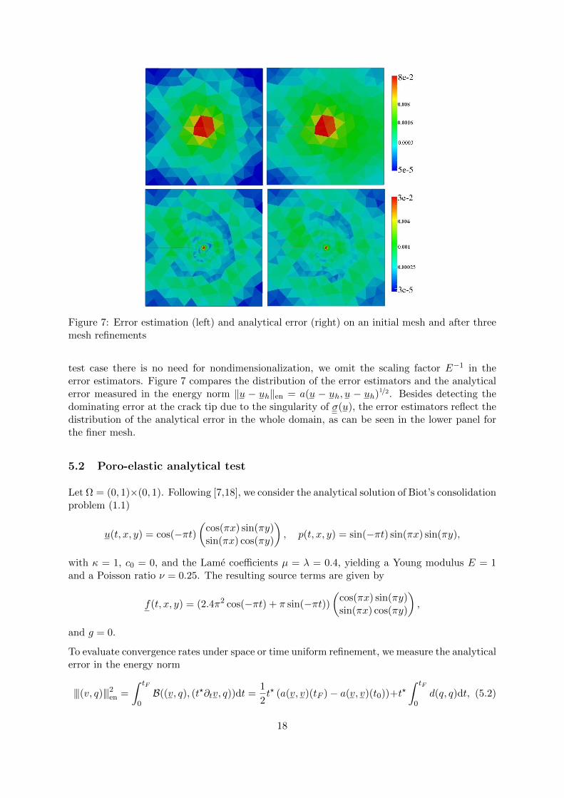
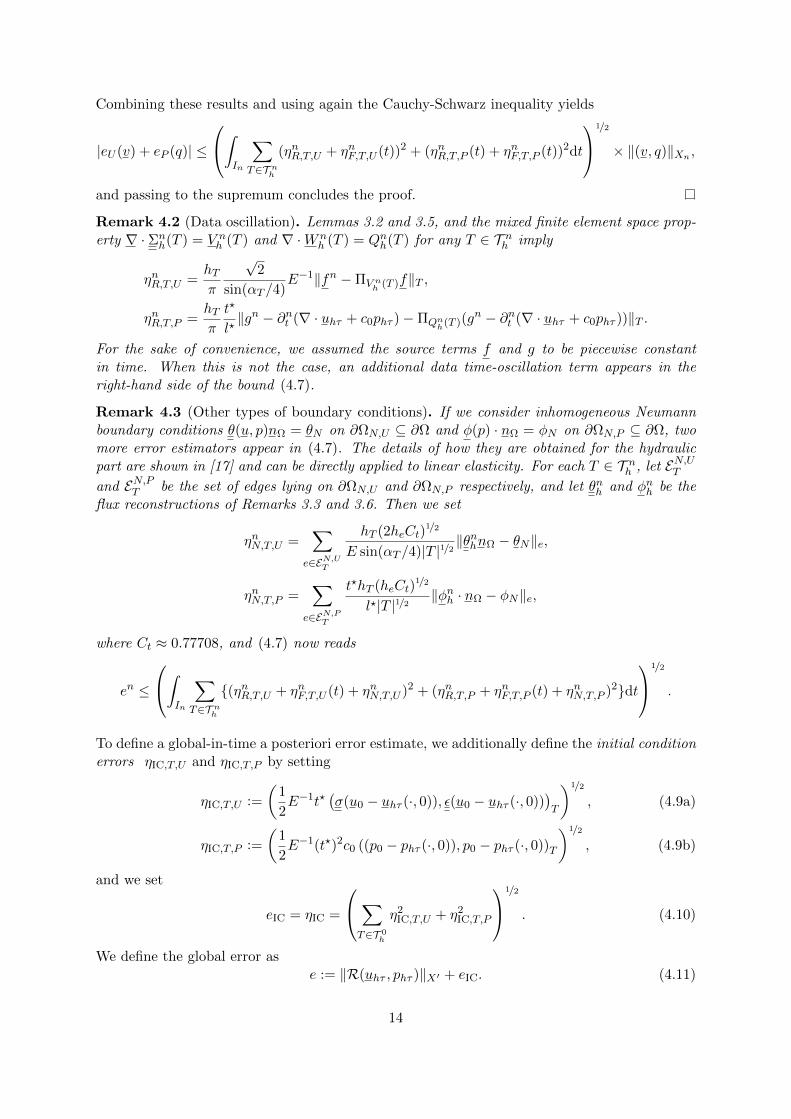
Figure 7: Error estimation (left) and analytical error (right) on an initial mesh and after threemesh refinements

test case there is no need for nondimensionalization, we omit the scaling factor E−1 in theerror estimators. Figure 7 compares the distribution of the error estimators and the analyticalerror measured in the energy norm ‖u − uh‖en = a(u − uh, u − uh)1/2. Besides detecting thedominating error at the crack tip due to the singularity of σ(u), the error estimators reflect thedistribution of the analytical error in the whole domain, as can be seen in the lower panel forthe finer mesh.

5.2 Poro-elastic analytical test

Let Ω = (0, 1)×(0, 1). Following [7,18], we consider the analytical solution of Biot’s consolidationproblem (1.1)

u(t, x, y) = cos(−πt)(

cos(πx) sin(πy)sin(πx) cos(πy)

), p(t, x, y) = sin(−πt) sin(πx) sin(πy),

with κ = 1, c0 = 0, and the Lame coefficients µ = λ = 0.4, yielding a Young modulus E = 1and a Poisson ratio ν = 0.25. The resulting source terms are given by

f(t, x, y) = (2.4π2 cos(−πt) + π sin(−πt))(

cos(πx) sin(πy)sin(πx) cos(πy)

),

and g = 0.

To evaluate convergence rates under space or time uniform refinement, we measure the analyticalerror in the energy norm

|||(v, q)|||2en =

∫ tF

0B((v, q), (t?∂tv, q))dt =

1

2t? (a(v, v)(tF )− a(v, v)(t0))+t?

∫ tF

0d(q, q)dt, (5.2)

18

h−1 ηsp,U ηsp,P ‖u− uhτ‖U ‖p− phτ‖P een Ieff

4 3.45e-2 — 1.58 — 3.44e-2 — 4.67e-1 — 5.12e-1 3.158 8.13e-3 2.09 7.62e-1 1.05 8.11e-3 2.08 2.33e-1 1.07 2.46e-1 3.1416 1.96e-3 2.05 3.76e-1 1.02 2.00e-3 2.02 1.10e-1 1.02 1.21e-1 4.0432 4.85e-4 2.01 1.87e-1 1.01 9.03e-4 1.15 5.46e-2 1.01 6.03e-2 3.16

Table 1: Error estimators and analytical errors under space refinement with tF = 0.5, τ = 5e-5

τ−1 ηtm,U ηtm,P ‖u− uhτ‖U ‖p− phτ‖P een Ieff

4 4.73e-1 — 2.54e-1 — 1.96e-1 — 2.09e-1 — 2.32e-1 3.348 2.40e-1 0.78 1.40e-1 0.86 9.88e-2 1.00 1.14e-1 0.87 1.27e-1 3.3516 1.20e-1 1.00 7.31e-2 0.94 4.94e-2 1.00 6.03e-2 0.92 6.94e-2 3.4632 6.00e-2 1.00 3.74e-2 0.97 2.47e-2 1.00 3.17e-2 0.93 3.85e-2 3.76

Table 2: Error estimators and analytical errors under time refinement with tF = 0.5, h = 1/128

and the mechanical and hydraulic parts separately in the following norms:

‖v‖2U =

∫ tF

0a(v, v)dt and ‖q‖2P =

∫ tF

0d(q, q)dt. (5.3)

where in this dimensionless test, the nondimensionalization parameters t? and l? are both equalto one, and we also omit the factor E.

Tables 1 and 2 compare the convergence rates under space and time refinement of the corre-sponding error estimators to the analytical error in the norms defined by (5.2) and (5.3). Thelast column shows the effectivity index defined by

Ieff :=ηsp,U + ηsp,P + ηtm,U + ηtm,P

|||(u− uhτ , p− phτ )|||en

. (5.4)

For both the spatial and the temporal refinement, we obtain the expected convergence ratesof the Taylor–Hood finite element method (2.10) with k = 1, and a backward Euler scheme intime. The last value of the analytical mechanical error under space refinement is due to theerror in time discretization which starts playing a role for the finest mesh. We observe thatthe orders of magnitude of the mechanical and hydraulic part are comparable in this test, andthat the effectivity index is dominated by the hydraulic part under space refinement, and bythe mechanical part under time refinement.

5.3 Quarter five-spot problem

In this standard configuration considered in petroleum engineering, the injection of water at thecenter of a square domain and the production at the four corners is simulated on a quarter ofthe domain. In our test, this quarter is a square of 100m side length, divided into two parts withdifferent mobilities; a circle around the injection point of radius 50m with κ = 8·10−9m2Pa−1s−1,and κ = 10−9m2Pa−1s−1 in the rest of the domain. The Young modulus and the Poisson ratioare given by E = 109Pa, ν = 0.3, and we set c0 = 0. The initial state is given by θ0 = 0,φ0 = 0 and p0 = 105Pa. During the computation time of 30 days, we set p = p0 in the top rightcorner and p = 4 · 105Pa in the bottom left corner, simulating the production and the injectionrespectively. The nondimensionalization parameters are l? = 140m and t? = 1h. The problemis dominated by hydraulic processes.

19

# space-time unknowns # iterations ηsp ηtm ηsp+ηtm

reference 13,754,520 120 0.204 0.315 0.519equivalent 973,620 45 1.14 1.54 2.68adaptive 846,174 71 0.462 0.507 0.969

Table 3: The three computations in our test for the quarter five-spot problem

0 20 40 60 80 100 120 140

1

2

3

4

·105

referenceequivalentadaptive

diagonal length (m)

Pre

ssu

reph

t = 30dt = 10dt = 6d

Figure 8: Left: Comparison of the pressure in the quarter five-spot problem along the diagonalbetween the three algorithms in Table 3. Right: An adapted mesh at time t = 10 days

We use Algorithm 4.6 to perform space-time adaptivity. We start with an initial mesh of 10,638vertices and with an initial time step of τ0 = 12h. For the space-time error balancing, we setγtm = 0.8 and Γtm = 1.3 and fix the error limit for each time step to critn = 0.005τn. Wecompare the performance of the adaptive algorithm to two static computations (i.e. with fixedmeshes and time steps), one, called equivalent, where the discretization is chosen in a way to haveapproximately the same number of space-time unknowns as in the adaptive algorithm, and onewhere the discretization is very fine, so its solution can be taken as a reference solution. Table 3compares the number of space-time unknowns and performed iterations (i.e. the number of timesteps, counting repetitions in the adaptive algorithm), and the values of the error estimators ofthe three computations.

The left graphic in Figure 8 shows the discrete pressure along the diagonal going from thebottom left to the top right of the domain (as indicated in the right graphic) at three differenttimes obtained by the static computations (solid and dotted lines) and the adaptive algorithm(dashed lines). The loosely dotted vertical line marks the edge between the two parts of Ω withdifferent permeabilities. At each of these times, the discrete solution of the adaptive algorithmis closer to the reference solution than the equivalent computation using a fixed mesh and timestep. At the last time step, all the results get closer as the solution converges in time to aconstant state.

20

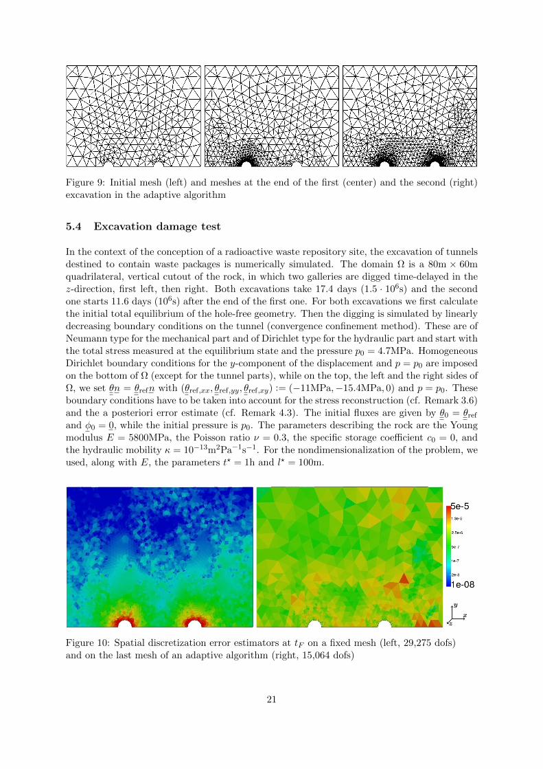
Figure 9: Initial mesh (left) and meshes at the end of the first (center) and the second (right)excavation in the adaptive algorithm

5.4 Excavation damage test

In the context of the conception of a radioactive waste repository site, the excavation of tunnelsdestined to contain waste packages is numerically simulated. The domain Ω is a 80m × 60mquadrilateral, vertical cutout of the rock, in which two galleries are digged time-delayed in thez-direction, first left, then right. Both excavations take 17.4 days (1.5 · 106s) and the secondone starts 11.6 days (106s) after the end of the first one. For both excavations we first calculatethe initial total equilibrium of the hole-free geometry. Then the digging is simulated by linearlydecreasing boundary conditions on the tunnel (convergence confinement method). These are ofNeumann type for the mechanical part and of Dirichlet type for the hydraulic part and start withthe total stress measured at the equilibrium state and the pressure p0 = 4.7MPa. HomogeneousDirichlet boundary conditions for the y-component of the displacement and p = p0 are imposedon the bottom of Ω (except for the tunnel parts), while on the top, the left and the right sides ofΩ, we set θn = θrefn with (θref,xx, θref,yy, θref,xy) := (−11MPa,−15.4MPa, 0) and p = p0. Theseboundary conditions have to be taken into account for the stress reconstruction (cf. Remark 3.6)and the a posteriori error estimate (cf. Remark 4.3). The initial fluxes are given by θ0 = θref

and φ0 = 0, while the initial pressure is p0. The parameters describing the rock are the Youngmodulus E = 5800MPa, the Poisson ratio ν = 0.3, the specific storage coefficient c0 = 0, andthe hydraulic mobility κ = 10−13m2Pa−1s−1. For the nondimensionalization of the problem, weused, along with E, the parameters t? = 1h and l? = 100m.

Figure 10: Spatial discretization error estimators at tF on a fixed mesh (left, 29,275 dofs)and on the last mesh of an adaptive algorithm (right, 15,064 dofs)

21

105 106

100

100.2

100.4

100.6

100.8

Total number of space-time unknowns

Err

or

esti

mat

ion

static algorithmadaptive algorithm

0 10 20 30 40 500

2

4

6

·10−3

time (days)

Err

or

esti

mato

rs

staticadaptive

Figure 11: Comparison between a static algorithm with fixed mesh and time step and theadaptive algorithm 4.6 for the excavation damage test

The performance of Algorithm 4.6 is tested on four different initial meshes with critn = 7·10−3τnfor the coarsest one and, with the mesh getting finer, critn = 4 · 10−3τn, critn = 2 · 10−3τn andcritn = 1 · 10−3τn. In all the calculations we fix γtm = 0.8, Γtm = 1.5 and τ0 = 3.9d. Figure 9illustrates the evolution of the second coarsest mesh with critn = 4 · 10−3τn. During the firstexcavation, the refinement takes only place around the left tunnel, whereas the area aroundthe right tunnel is only refined after the beginning of the second excavation. The calculationsresulting from the adaptive algorithm are compared to calculations with fixed meshes and timesteps. Each of these meshes is slightly finer around the tunnels than in the rest of Ω, and thetime steps are chosen in a way that ηsp ≈ ηtm. Figure 10 compares the spatial discretizationerror estimators at the final time tF of the static algorithm to those of the adaptive algorithm,which are much more evenly distributed over the domain. Furthermore, the left graphic inFigure 11 shows that in our test, the use of the adaptive algorithm reduces the number ofspace-time-unknowns for a similar value of the error estimator.

In the right graphic of Figure 11, we plot the evolution of the error estimators in the twocomputations circled in the left graphic. Each mark stands for an iteration and shows the errorestimate en of the current time interval divided by τn. For the plain algorithm, an iteration isequal to a time step. The adaptive algorithm recalculates the solution at a time step wheneverthe error estimate lies over critn (illustrated by the dashed line) by refining τn or the mesh(or both). Thus, only the square shaped points in the graphic contribute to the overall errorestimate. In the consolidation phase between the two excavations (from t = 17.4 days tot = 29 days), the mesh is slightly coarsened and the time step considerably increased, since thedominating error source in this phase is the spatial discretization.

5.5 Conclusion

The analytical test cases show that the distribution and convergence rates of our error estima-tors reflect those of the analytical error. The efficiency of Algorithm 4.6 has been illustratedin industrial tests, where the number of space-time unknowns is considerably decreased for acomparable overall error estimate. We also observe that the price for computing the flux re-constructions can be substantially reduced by pre-processing, a task that is fully parallelizable.

22

As shown in the first test, the stress reconstruction and a posteriori estimate presented in thiswork are directly applicable to pure linear elasticity problems. The second test shows that thepresented error estimate also delivers sharp bounds (as reflected by moderate effectivity indices)of more accessible error measures computed using energy-type norms. In the third and fourthtests, comparing the proportions of the estimators for the hydraulic and the mechanical partsreflects the physical properties of the problem: in the quarter five-spot test, the dominatingestimators are those for the hydraulic part; for the excavation damage test, they are approxi-mately of the same order of magnitude, with the mechanical estimator dominating in regionsof stress concentration.

Acknowledgements

The work of D. A. Di Pietro was supported by ANR grant HHOMM (ANR-15-CE40-0005)

References

References

[1] M. Ainsworth and J. T. Oden. A posteriori error estimation in finite element analysis. Pure and AppliedMathematics (New York), Wiley-Interscience [John Wiley & Sons], New York, 2000.

[2] M. Ainsworth and R. Rankin. Guaranteed computable error bounds for conforming and nonconformingfinite element analysis in planar elasticity. Internat. J. Numer. Methods Engrg, 82:1114–1157, 2000.

[3] D. N. Arnold, G. Awanou, and R. Winther. Finite elements for symmetric tensors in three dimensions.Math. Comp., 77:1229–1251, 2008.

[4] D. N. Arnold and R. Winther. Mixed finite elements for elasticity. Numer. Math., 92:401–419, 2002.

[5] M. Bebendorf. A note on the Poincare inequality for convex domains. Z. Anal. Anwendungen, 22:751–756,2003.

[6] M. A. Biot. General theory of three-dimensional consolidation. J. Appl. Phys., 12:155–169, 1941.

[7] D. Boffi, M. Botti, and D. A. Di Pietro. A nonconforming high-order method for the Biot problem on generalmeshes. SIAM J. Sci. Comput., 38(3):A1508–A1537, 2016.

[8] D. Braess, V. Pillwein, and J. Schoberl. Equilibrated residual error estimates are p-robust. Comput. MethodsAppl. Mech. Engrg., 198:1189–1197, 2009.

[9] D. Braess and J. Schoberl. Equilibrated residual error estimator for edge elements. Math. Comp.,77(262):651–672, 2008.

[10] L. Chamoin, P. Ladeveze, and F. Pled. An enhanced method with local energy minimization for the robusta posteriori construction of equilibrated stress field in finite element analysis. Comput. Mech., 49:357–378,2012.

[11] P. Destuynder and B. Metivet. Explicit error bounds in a conforming finite element method. Math. Comput.,68(228):1379–1396, 1999.

[12] D. A. Di Pietro and A. Ern. A hybrid high-order locking-free method for linear elasticity on general meshes.Comput. Meth. Appl. Mech. Engrg, 283:1–21, 2015.

[13] D. A. Di Pietro, A. Ern, and J.-L. Guermond. Discontinuous Galerkin methods for anisotropic semi-definitediffusion with advection. SIAM J. Numer. Anal., 46(2):805–831, 2008.

[14] D. A. Di Pietro, E. Flauraud, M. Vohralık, and S. Yousef. A posteriori error estimates, stopping criteria,and adaptivity for multiphase compositional Darcy flows in porous media. J. Comput. Phys., 276:163–187,2014.

[15] D. A. Di Pietro, M. Vohralık, and S. Yousef. An posteriori-based, fully adaptive algorithm for thermalmultiphase compositional flows in porous media with adaptive mesh refinement. Comput. and Math. withAppl., 68(12):2331–2347, 2014.

23

[16] D. A. Di Pietro, M. Vohralık, and S. Yousef. Adaptive regularization, linearization, and discretization anda posteriori error control for the two-phase Stefan problem. Math. Comp, 84(291):153–186, 2015.

[17] V. Dolejsı, A. Ern, and M. Vohralık. hp–adaption driven by polynomial-degree-robust a posteriori errorestimates for elliptic problems. SIAM J. Sci. Comput., 38(5):A3220–A3246, 2016.

[18] A. Ern and S. Meunier. A posteriori error analysis of Euler-Galerkin approximations to coupled elliptic-parabolic problems. ESAIM Math. Mod. Numer. Anal.., 43:353–375, 2009.

[19] A. Ern and M. Vohralık. A posteriori error estimation based on potential and flux reconstruction for theheat equation. SIAM J. Numer. Anal., 48(1):198–223, 2010.

[20] A. Ern and M. Vohralık. Adaptive inexact Newton methods with a posteriori stopping criteria for nonlineardiffusion PDEs. SIAM J. Sci. Comput., 35(4):A1761–A1791, 2013.

[21] A. Ern and M. Vohralık. Polynomial-degree-robust a posteriori estimates in a unified setting for conforming,nonconforming, discontinuous Galerkin, and mixed discretizations. SIAM J. Numer. Anal., 53(2):1058–1081,2015.

[22] Kwang-Yeon Kim. Guaranteed a posteriori error estimator for mixed finite element methods of linearelasticity with weak stress symmetry. SIAM J. Numer. Anal., 48:2364–2385, 2011.

[23] P. Ladeveze. Comparaison de modeles de milieux continus. PhD thesis, Universite Pierre et Marie Curie(Paris 6), 1975.

[24] P. Ladeveze and D. Leguillon. Error estimate procedure in the finite element method and applications.SIAM J. Numer. Anal., 20:485–509, 1983.

[25] P. Ladeveze, J. P. Pelle, and P. Rougeot. Error estimation and mesh optimization for classical finite elements.Engrg. Comp., 8(1):69–80, 1991.

[26] R. Luce and B. I. Wohlmuth. A local a posteriori error estimator based on equilibrated fluxes. SIAM J.Numer. Anal., 42:1394–1414, 2004.

[27] S. Meunier. Analyse d’erreur a posteriori pour les couplages hydro-Mecaniques et mise en œuvre dansCode Aster. PhD thesis, Ecole des Ponts ParisTech, 2007.

[28] M. A. Murad and A. F. D. Loula. Improved accuracy in finite element analysis of Biot’s consolidationproblem. Comput. Meth. Appl. Mech. Engrg., 95:359–382, 1992.

[29] M. A. Murad and A. F. D. Loula. On stability and convergence of finite element analysis of Biot’s consoli-dation problem. Internat. J. Numer. Methods Engrg., 37:645–667, 1994.

[30] M. A. Murad, V. Thomee, and A. F. D. Loula. Asymptotic behaviour of semidiscrete finite-element approx-imations of Biot’s consolidation problem. SIAM J. Numer. Anal., 33(3):1065–1083, 1996.

[31] S. Nicaise, K. Witowski, and B. Wohlmuth. An a posteriori error estimator for the lame equation based onH(div)-conforming stress approximations. IMA J. Numer. Anal., 28:331–353, 2008.

[32] S. Ohnimus, E. Stein, and E. Walhorn. Local error estimates of FEM for displacements and stresses in linearelasticity by solving local Neumann problems. Int. J. Numer. Meth. Engng., 52:727–746, 2001.

[33] P. J. Phillips and M. J. Wheeler. A coupling of mixed and continous Galerkin finite element methods forporoelasticity II: the discrete-in-time case. Comput Geosci, 11:145–158, 2007.

[34] W. Prager and J. L. Synge. Approximations in elasticity based on the concept of function space. Quart.Appl. Math., 5:241–269, 1947.

[35] P. A. Raviart and J. M. Thomas. A mixed finite element method for second order elliptic problems, volume606 of Lecture Notes in Math. Springer, 1975.

[36] S. I. Repin. A posteriori estimates for partial differential equations, volume 4 of Radon Series on Computa-tional and Applied Mathematics. Walter de Gruyter GmbH & Co. KG, Berlin, 2008.

[37] R. S. Sandhu and E. L. Wilson. Finite element analysis of seepage in elastic media. J. Engrg. Mech. Div.Amer. Soc. Civil. Engrg., 95:641–652, 1969.

[38] R. E. Showalter. Diffusion in poro-elastic media. J. Math. Anal. Appl., 251:310–340, 2000.

[39] C. Taylor and P. Hood. A numerical solution of the Navier-Stokes equations using the finite elementtechnique. Comput. & Fluids, 1:73–100, 1973.

[40] K. von Terzaghi. Theoretical soil mechanics. Wiley, New York, 1943.

[41] A. Zenısek. The existence and uniqueness theorem in Biot’s consolidation theory. Aplikace Matematiky,29:194–211, 1984.

[42] M. Williams. On the stress distribution at the base of a stationary crack. J. Appl. Mech., 24:109–114, 1957.

[43] Y. Yokoo, K. Yamagata, and H. Nagaoka. Finite element method applied to Biot’s consolidation theory.Soils and Foundations, 11:29–46, 1971.

24