Embed Size (px)
Citation preview

MASTER THESIS
STREAMLINING STORAGE OF
TEST EQUIPMENT AT SIEMENS
HENGELO: A CAPACITY BASED
APPROACH
G. H. van der Velde
2013, May.
MASTER
Industrial Engineering and Management
TRACK
Production and Logistic Management
FACULTY
School of Management and Governance
RESEARCH DEPARTMENT
Industrial Engineering and Business Information
Systems
EXAMINATION COMMITTEE
Dr. A. Al Hanbali
Dr. P.C. Schuur
EXTERNAL SUPERVISORS
H.-J. Klaver Bsc.
Ing. R. B. ten Velde

II G. H. van der Velde, Master Thesis, 2013, May.

G. H. van der Velde, Master Thesis, 2013, May. III
Management summary Siemens Hengelo assembles compressors and gas turbines for the oil and gas industry.
After the completion of the assembly, the compressor must be tested. Since a compressor
cannot run ‘dry’, a closed loop is created. The pipes used to connect the compressor to the
loop are the subject of this research. Every compressor is different; they are all uniquely
designed and engineered to fit exactly at the oil source were they will operate. Therefore
there are different pipes needed every time. The pipes differ in length, diameter and the
pressure they can handle. Hundreds of pipes with all kinds of different characteristics are in
stock to connect a compressor with the permanent installed pipe system. With every new
compressor test new pipes are manufactured and added to the warehouse, while the pipes
last forever and thus are never removed from the warehouse. The warehouse has reached its
capacity limits, storage space is a scarce resource at this facility located in the city centre of
Hengelo, and the capacity is likely to reduce due to road construction plans at the
warehouse location. This leads to two research questions for this thesis:
1) How can test pipes be removed from the warehouse in a systematic way?
2) Can we prevent the necessity of new test pipes?
The cost of one pipe runs from 3,000 to 7,400 euros. Currently there are at least 421 pipes
in stock. Only 15 loops per year are built. This leads to a warehouse with expensive parts
while 30% of the items, equalling 70% of the storage space, was not used in the past four
years.
To answer both problems, the historical usage data of all test pipes is analysed to search for
patterns that can be used to forecast usage. Main subjects of analysis are the diameter,
pressure capacity and length of a pipe. No relations between these characteristics and the
usage are found; therefore no forecasts based on these specifications can be made.
Nonetheless we find four pressure stages and five diameters that are used more often than
others. We conclude usage forecasts on item basis cannot be made, but we do know how
long an item is already in storage without any usage. This leads to two recommendations:
1. Refresh the warehouse inventory continuously, using the so-called knapsack
principle. Every time a new pipe must be stored, storage space must be created by
removing another pipe. An model is developed in Excel to decide what item must
be removed, based on the replacement value, the number of weeks the pipe is
unused in storage, and the number of square metres a pipe needs.
2. Manufacture new pipes according to the standards defined in this report, such that
the pipes can be used in many situations. We recommend four standard pressure
stages (out of the nine pressure stages currently in the warehouse) and five
standard diameters (out of the 19 diameters currently in the warehouse).
Furthermore we propose to use standardised pipe lengths: using a pre-defined set
of lengths all required distances can be created from a few pipes.
Obtained advantages of the knapsack principle are:
Due to the knapsack principle the warehouse capacity is fixed from now on,
eliminating the everlasting growth of storage costs and resulting in predictable
storage usage and costs.
To define the initial warehouse size lots of items are scrapped, saving 7,000 euros
per year of external warehousing costs and clearing up some back-log in the
internal warehouse.
IV G. H. van der Velde, Master Thesis, 2013, May.
The inventory will be up to date, items that are not used for all kind of unclear
reasons are automatically removed and replaced by new items.
Implementation costs are negligible.
Obtained advantages of the standardised test piping are:
Almost no need for new items anymore when all default pressure stage, diameter
and length combinations are in stock
Easier test loop design due to standard measurements
Less items need to be stored
Saving of 135,000 euros per year after an initial investment of 360,000 euros.
The standardisation of pipes requires an investment of 360,000 euros, in addition to the
currently recurring costs. The earn-back period depends on the investment period, it
depends on the number of loops that will be built per year in how many years the
investment is completed and the earn-back will start. On average a saving of 135,000 euros
per year is expected after five years.
With some further research even larger savings are possible. Our main recommendation for
further research concerns the use of retractable pipes. One retractable pipe can replace up to
30 standard length pipes a cost only three to four pipes, saving the purchases costs as well
as the warehouse costs of these pipes. This system is currently in use in the Siemens plant
in Duisburg, Germany, thus practical experience can be obtained from the German
colleagues.

G. H. van der Velde, Master Thesis, 2013, May. V
Index
Management summary ........................................................................................................................ III List of figures ........................................................................................................................................ VI List of Tables ...................................................................................................................................... VII Preface................................................................................................................................................... IX 1 Introduction: company, products and research setup .............................................................. 1
1.1 Company description: oil & gas compressors solutions ................................... 1 1.2 Test setup introduction ..................................................................................... 3 1.3 Research design & research questions .............................................................. 7
2 Current situation ........................................................................................................................ 11 2.1 Stakeholder analysis ........................................................................................11 2.2 Current storage usage ......................................................................................15 2.3 Conclusion on current situation .......................................................................17
3 Theoretical framework .............................................................................................................. 18 3.1 New part, store or not to store? ........................................................................18 3.2 Stored parts, when to scrap? ............................................................................21 3.3 Case studies .....................................................................................................24 3.4 Knapsack problem ...........................................................................................26 3.5 Conclusion on theoretical framework ..............................................................28
4 Data analysis ............................................................................................................................... 29 4.1 Data sources and data scope ............................................................................29 4.2 Pipe usage patterns ..........................................................................................31 4.3 Purchase price analysis ....................................................................................33 4.4 A, B, or C items? .............................................................................................35 4.5 Amount of pipes not used vs. storage space ....................................................37 4.6 Patterns in used/not used figures: grouping .....................................................38 4.7 Current storage costs .......................................................................................45 4.8 To stock or not to stock; seven factors ............................................................46 4.9 Conclusion on data analysis .............................................................................48
5 Decision model formulation ....................................................................................................... 50 5.1 Problem 1 solution selection: knapsack ...........................................................50 5.2 Implementation trajectory of the knapsack model ...........................................56 5.3 Financial effects of the knapsack model ..........................................................59 5.4 Problem 2 solution selection: standardisation ..................................................60 5.5 Working towards standardisation: 4 options ....................................................64 5.6 Influence of standardisation on inventory........................................................65 5.7 Financial effects of standardisation .................................................................68 5.8 Conclusion on decision model .........................................................................74
6 Conclusion & recommendation ................................................................................................. 75 6.1 Main recommendation 1: use the knapsack model ..........................................75 6.2 Main recommendation 2: use standardised test piping ....................................76 6.3 Other recommendations ...................................................................................77
References ............................................................................................................................................. 80 A Appendix A: purchase order analysis ....................................................................................... 82 B Appendix B: ABC log-normal relation ..................................................................................... 85 C Appendix C: usage tables ........................................................................................................... 86 D Appendix D: 3D graphs.............................................................................................................. 90 E Appendix E: list of items with different priorities ................................................................... 96

VI G. H. van der Velde, Master Thesis, 2013, May.
List of figures Figure 1: Example of a product assembled in Hengelo, an oil compressor train (Siemens
Hengelo, 2013) ...................................................................................................................... 1 Figure 2: Gas injection well (APEC, 2012) .......................................................................... 2 Figure 3: Compressor test: gas from exhaust back to intake ................................................. 3 Figure 4: Construction work at a test loop (left) .................................................................... 4 Figure 5: The loop: a compressor with some piping connected to the permanent pipe system
(right) ..................................................................................................................................... 4 Figure 6: Basic test setup ....................................................................................................... 4 Figure 7: Lack of storage space, pipes are blocking the aisles in the warehouse .................. 6 Figure 8: One compressor with four connections .................................................................. 6 Figure 9: Example of an item that is marked with ‘shred after use’ ...................................... 8 Figure 10: Illustrating problem 1, many pipes enter the warehouse while none leave .......... 9 Figure 11: Illustrating problem 2, can we prevent the need for new pipes? .......................... 9 Figure 12: To achieve a test on time, one needs to know the parts in advance ................... 12 Figure 13: Tree main causes for high storage costs ............................................................. 13 Figure 14: Processes related to test equipment .................................................................... 14 Figure 15: Current decisions and communication about storing or scrapping..................... 15 Figure 16: Internal warehouse ............................................................................................. 16 Figure 17: Pipes attic ........................................................................................................... 16 Figure 18: large pipes in the external warehouse ................................................................ 17 Figure 19: Data filters .......................................................................................................... 30 Figure 20: Gantt chart of usage data .................................................................................... 32 Figure 21: ABC plot ............................................................................................................ 37 Figure 22: Percentage of pipes that has not been used since a specific date ....................... 38 Figure 23: Number of items moved vs. not moved according to type ................................. 39 Figure 24: Number of items moved vs. not moved according to diameter .......................... 39 Figure 25: Number of items moved vs. not moved according to pressure stage ................. 40 Figure 26: Number of items moved vs. not moved according to length .............................. 40 Figure 27: Example how to read the ball graphs ................................................................. 41 Figure 28: Pressure stage / Diameter combinations usage................................................... 41 Figure 29: Close up Length / Diameter combination usage ................................................ 42 Figure 30: Pressure stage / Length combinations usage ...................................................... 42 Figure 31: 3D graph of item usage ...................................................................................... 44 Figure 32: Knapsack principle: one item leaves if another enters the warehouse ............... 50 Figure 33: New decisions and communication about storing or scrapping ......................... 58 Figure 34: Storage costs become fixed ................................................................................ 60 Figure 35: Comparison of pipes with coins ......................................................................... 60 Figure 36: Number of standard pipes required per total pipe length ................................... 66 Figure 37: Number of times standard pipes are used........................................................... 67 Figure 38: Straight pipes need to be split to standard lengths ............................................. 67 Figure 39: Initial double costs are encountered .................................................................. 69 Figure 40: Cost and savings of standardization accumulated for all projects ...................... 70 Figure 41: Cost and savings of standardization per project ................................................. 70 Figure 42: Many connections in the current situation ......................................................... 71 Figure 43: Investment spread over years, for 6/15/20 loops per year. ................................. 72 Figure 44: Investment spread over years, based on 2/4/7 pipes per loop ............................ 73 Figure 45: Log-normal ABC plot ........................................................................................ 85 Figure 46: 3D graph of usage .............................................................................................. 90 Figure 47: 3D graph of usage .............................................................................................. 91

G. H. van der Velde, Master Thesis, 2013, May. VII
List of Tables Table 1: Piping part types ...................................................................................................... 5 Table 2: Number of loops build per year ............................................................................... 7 Table 3: Value of pipes ........................................................................................................ 33 Table 4: Yearly value purchase orders test piping ............................................................... 34 Table 5: New bought pipes per loop .................................................................................... 35 Table 6: Example of the knapsack method .......................................................................... 54 Table 7: Results of two different priority calculations ......................................................... 55 Table 8: Break-even points based on the number of loops per year. ................................... 73 Table 8: Break-even points based on the number of pipes per loop. ................................... 73 Table 9: Welding work purchase orders per type ................................................................ 83 Table 10: Average price of flanges (based on # purchase orders) ....................................... 84 Table 11: Average price of small/regular flanges ................................................................ 84 Table 12: Average price of large flanges ............................................................................. 84 Table 13: Pressure / Diameter usage table ........................................................................... 86 Table 14: Length / Diameter usage table ............................................................................. 87 Table 15: pressure stage / length usage table ....................................................................... 88 Table 16: Source table of 3D graphs .................................................................................... 91 Table 17: Priority ranking of all items ................................................................................. 96

VIII G. H. van der Velde, Master Thesis, 2013, May.

G. H. van der Velde, Master Thesis, 2013, May. IX
Preface This report is the end result of my master thesis research project. In the framework of
completing the study Industrial Engineering and Management at the University of Twente,
I performed a research project at Siemens Hengelo into the usefulness and necessity of
permanent storage of test piping parts. Finishing this thesis, and
I would like to thank my supervisors of the University of Twente, Ahmad al Hanbali and
Peter Schuur for guiding me through the process of this master research project. I
appreciate all the time and effort you put into this research, especially during our meetings.
We had many interesting discussions during which I received lots of helpful feedback.
I would also like to thank Siemens Netherlands, location Hengelo for providing me the
opportunity to perform my research within this interesting organisation. From the first day I
felt very welcome in this organisation. I thank my supervisors, Henk-Jan Klaver and
Robbert ten Velde, for their continuous support and interest. We had lots of interesting
discussions that had a great influence on the quality of the end result as it is presented in
this report. I am also grateful to Roeland van den Bos, Wim Hoffer, Emil Pietersz and all
other colleagues for enabling me to perform my research within a very pleasant working
environment, and being willing to answer lots of questions on a daily basis about the
sometimes complex structures and working procedures of this organisation.
Thanks to Gerard Land for his support, since we performed our master assignments mainly
in the same timeframe he faced the same problems and was a great sparring partner. Thanks
to Freek van Eijndhoven, Karin van Ewijk, Benjamin Groenewolt, Gerard Land, Tycho
Lejeune and Kirsten van der Reest for proof-reading my thesis.
Last but not least I thank my girlfriend Kim Slikkerveer and my family Henriëtte, Mirna
and Jorinde van der Velde for their support and encouragements, not only during this
project but during my whole study career.
In remembrance of my father, who always loved to hear about my study projects and was of
great support in the first years of my study. Unfortunately he is not able to read this report
anymore.
Gerben van der Velde
2013, April

G. H. van der Velde, Master Thesis, 24-05-2013 1
1 Introduction: company, products and research
setup This report is the result of a seven month research project within Siemens Hengelo. It is
written to complete my master study Industrial Engineering & Management at the
University of Twente.
This chapter introduces the company Siemens, it provides a general problem description
and introduces the research questions. Section 1.1 describes the product Siemens delivers,
the compressor, as well as the setting where this product is used. This research focuses on a
specific part of the production process: the testing of the finished product. Therefore
Section 1.2 introduces the testing process. After this general description of the situation,
Section 1.3 introduces the research design & research questions.
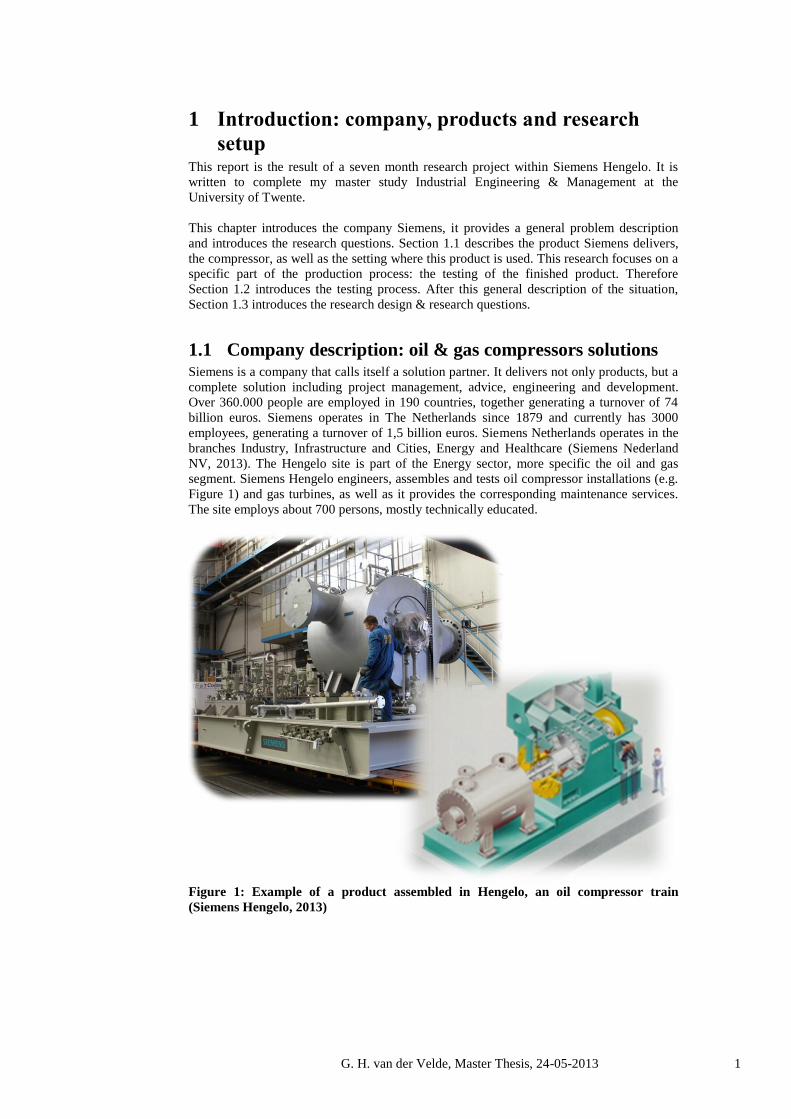
1.1 Company description: oil & gas compressors solutions Siemens is a company that calls itself a solution partner. It delivers not only products, but a
complete solution including project management, advice, engineering and development.
Over 360.000 people are employed in 190 countries, together generating a turnover of 74
billion euros. Siemens operates in The Netherlands since 1879 and currently has 3000
employees, generating a turnover of 1,5 billion euros. Siemens Netherlands operates in the
branches Industry, Infrastructure and Cities, Energy and Healthcare (Siemens Nederland
NV, 2013). The Hengelo site is part of the Energy sector, more specific the oil and gas
segment. Siemens Hengelo engineers, assembles and tests oil compressor installations (e.g.
Figure 1) and gas turbines, as well as it provides the corresponding maintenance services.
The site employs about 700 persons, mostly technically educated.
Figure 1: Example of a product assembled in Hengelo, an oil compressor train
(Siemens Hengelo, 2013)

2 G. H. van der Velde, Master Thesis, 2013, May.
1.1.1 Basic oil well description
The compressors of Siemens are used to retrieve oil from onshore as well as offshore oil
sources. An oil well always contains a mixture of oil and gas. In most locations in the world
this gas has no commercial value, since most countries do not use it a lot and it is expensive
to transport. One way of retrieving oil (there are multiple and the compressors are used in
other settings as well) is using the gas to ease the retrieval of oil. Basically, the gas is
pumped back into the well to keep a high pressure in the well. As long as there is a high
pressure in the oil field, the oil comes out relatively easy. Since oil is a thick and heavy
fluid, this is far more efficient than just using suction power to retrieve the oil. This is a
self-sustaining system that only needs a start-up: by pressing gas into the well a mixture of
oil and gas comes out, the gas is separated and pressed back in so this process repeats itself.
This process is illustrated in Figure 2. Siemens produces the compressors to push the gas
back into the well, and the gas turbines that drive these compressors.
Figure 2: Gas injection well (APEC, 2012)
1.1.2 Testing the products
Siemens Hengelo is an assembly site: almost all parts are delivered by suppliers and
assembled in Hengelo. The final products (compressors / turbines) can also be tested
extensively in Hengelo. A simple test to check if the compressor is working is always
performed. However, some customers demand a more extensive test. The demand for
extensive tests can be explained from the self-sustaining system illustrated in Figure 2 and
described in Section 1.1.1. Once this process gets interrupted, there will be no gas anymore
to keep a high pressure at the well. In the worst case, an unexpected interruption means that
a gas transport ship needs to deliver gas to the well in order to revise the pressure and get
the process running again. This can cause a long period (e.g. weeks) without production,
meaning lots of lost profit. Therefore the customers of Siemens want to perform every
possible test, just to be sure there will not be any complication if the compressor is used at
the final destination, even if this extra testing costs a couple of millions of euros extra. For
those customers, the compressor gets a full-load test in combination with the other
equipment used by the customer (the string: motor, gearbox, etc.). The total time from
accepting the order to finishing the simple compressor test is about one and a half year.
After that, a full string test can take a couple of months.

G. H. van der Velde, Master Thesis, 2013, May. 3
1.1.3 Siemens Hengelo figures
The annual turnover is currently approximately 200 million euros. In the strategic plan
‘vision 2015’ a turnover of 400 million euros is the target for 2015, so the production at the
site will grow substantially. At the time of writing, most recent orders were an order for six
gas turbine driven compressor trains for gas mining in South-Korea with a total value of 29
million euros (announced in June 2012), and an order for four electrically driven
compressor trains for a new Norwegian offshore oil platform with a total value of 27.5
million euros (announced in September 2012).
1.2 Test setup introduction As described in Section 1.1, a compressor needs to be tested after the assembly is finished.
This subsection describes the test setup and the number of tests performed.
1.2.1 The purpose of a test loop
A compressor cannot run ‘dry’; it is designed to run with a special mixture of gases. The
compressor is tested in a closed system, illustrated in Figure 3, in which a gas stream is
used. When the gas leaves the compressor it is cooled down and decompressed in a long
system of pipes. Thereafter the gas enters the compressor again and this process is repeated
for a certain period of time. Some examples of the system are illustrated in Figure 4 and
Figure 5. The piping required to create this closed loop is the main subject of this research.
Figure 3: Compressor test: gas from exhaust back to intake
Creating such a closed loop requires a lot of pipes, some sensors and some other special
equipment. As Figure 5 shows there is a permanent system of pipes mounted at the wall,
with several connection points. To test the compressor, the intake and exhaust have to be
mounted to the permanent wall loop connection points. Every compressor is unique, so it is
a puzzle every time to find out what pipes can be used to build the loop. The basic example
of a test setup is shown in Figure 6. Central we see the compressor. This compressor is
driven by a motor, whose energy is transmitted by a gearbox. From the intake and exhaust
of the compressor some pipes are connecting the compressor with the permanent
connection points. There are several types of pipes available to make the connection from
the compressor to the permanent loop system. For a better understanding of the terminology
throughout this research, the types of pipes are presented in Table 1.

4 G. H. van der Velde, Master Thesis, 2013, May.
Figure 4: Construction work at a test loop (left)
Figure 5: The loop: a compressor with some piping connected to the permanent pipe
system (right)
Figure 6: Basic test setup

G. H. van der Velde, Master Thesis, 2013, May. 5
Table 1: Piping part types
Flange:
A flange is a ring with holes welded to the end of a pipe and is
used to connect one pipe with another.
All piping parts within this research have flanges, no matter if this
is explicitly mentioned in the part description or not.
Pipe:
The basic pipe is just a straight tube and can be of all lengths and
diameters. The thickness of the material and the type of flange
determines the pressure a pipe can handle. This is expressed in the
“pressure stage”.
Elbow:
An elbow is a pipe with an angle.
Bladed elbow: If an elbow is bladed, it has some blades inside that
change the internal air flow.
Tee:
A tee pipe is a part where three flows come together.
Reducer:
A reducer is a pipe with different diameters or pressure classes on
both sides of the pipe, such that two pipes of different diameters
(or pressure stages) can be connected to each other via the reducer.
Measurement pipe:
A measurement pipe has small connectors for sensors all over it.
The exact locations of these sensor connectors are important and
can differ per test.
Since all compressors are different, it is unlikely that all required parts are already in stock.
So, at least some pipes need to be project-specifically manufactured to be able to create the
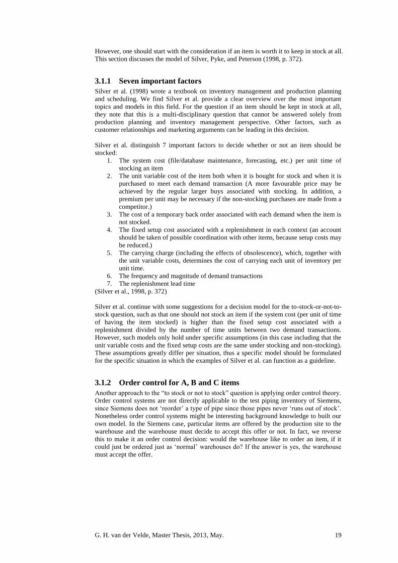
loop. For example, see the large differences between Figure 6 and Figure 8: Figure 8 shows
four instead of two compressor connections and uses far more pipes to connect the
compressor. The manufacturing of these pipes can be done internally, but due to personnel
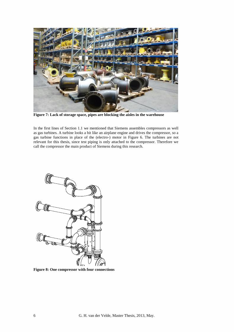
capacity constraints most of the time this is outsourced. At the moment, all of those pipes
are stored; this means with every compressor produced a few new pipes enter the
warehouse. At the same time, almost no pipe is ever permanently removed from the
warehouse. One can easily see that this is not a sustainable situation. Lots of items are
already blocking the aisles due to a lack of rack shelves, see Figure 7. To make it even
more critical, within a couple of years (depending on the speed of bureaucratic procedures
at the municipality) some warehouse space might be demolished according to plans of the
municipality of Hengelo to construct a new road at this location. This results in the research
objective as stated in the next section.
6 G. H. van der Velde, Master Thesis, 2013, May.
Figure 7: Lack of storage space, pipes are blocking the aisles in the warehouse
In the first lines of Section 1.1 we mentioned that Siemens assembles compressors as well
as gas turbines. A turbine looks a bit like an airplane engine and drives the compressor, so a
gas turbine functions in place of the (electro-) motor in Figure 6. The turbines are not
relevant for this thesis, since test piping is only attached to the compressor. Therefore we
call the compressor the main product of Siemens during this research.
Figure 8: One compressor with four connections

G. H. van der Velde, Master Thesis, 2013, May. 7
1.2.2 Basic figures about test loops
For this research there are in fact two basic relevant figures: how many loops per year are
build and how many pipes per test are used?
The number of test loops that are build is lower than the number of compressors delivered,
since many orders consist of up to four compressors of the same type. Those are tested one
after each other in the same test loop setting, or only one of the batch is tested extensively.
Table 2 shows the number of loops build in the last six years.
Table 2: Number of loops build per year
Year Loops
2007 6
2008 13
2009 19
2010 20
2011 12
2012 12
The number of pipes used per loop is not exactly known. As will be explained in Section
2.2, till a few months ago not all pipes were specified by the Test Engineering department
at the technical drawing. The Piping department used to have lots of freedom in choosing
their own parts and there is no single database with all parts per loop. Therefore we make
an estimation. Based on some recent technical drawings as well as interviews with two
employees from the Test Engineering department and one employee from the Piping
department we estimate 20 pipes per loop in most situations to 40 pipes per loop in some
more complex situations. All employees do stress there is a lot of variation per loop: they
state one test loop cannot be compared to another.
1.3 Research design & research questions This section discusses the research scope, objectives and questions. It starts with the
questions posed by Siemens, which are the starting point for this research. Then these
questions are translated into two research questions, where after these questions are divided
into several sub questions. Finally the scope and deliverables are defined.
1.3.1 Research objectives
The goal of this research is to develop a decision-support tool that suggests whether or not a
newly project-specific manufactured pipe should be permanently stored after the project
(e.g. Figure 9). This decision should be easy, i.e., based on criteria that any employee can
understand and measure, such as length and diameter. Preferably this decision is integrated
in the current way of working, such that it is not possible to continue the process without
this decision. So, we create an admission control policy to manage the inflow of test piping
to the warehouse. This policy will also be applied to the existing items in stock.

8 G. H. van der Velde, Master Thesis, 2013, May.
Figure 9: Example of an item that is marked with ‘shred after use’
1.3.2 Research questions
This research initiates from two questions posed by Siemens:
What is the economically most attractive way of storing test equipment?
What is the best way to cope with the planned elimination of some warehouse
space at the Hengelo site? (I.e., store fewer parts or use external warehouse space?)
‘Economically most attractive’ means that we need to focus on financial figures, of the
storage costs as well as the cost of producing new (replacement) parts.
After a basic exploration of the current situation at Siemens, as will be shown in Chapter 2,
in combination with several meetings with managers and employees from the involved
departments we find basically two problems to solve:
1. There are continuously new pipes entering the warehouse, but there is no system
to remove pipes from the warehouse. Thus the warehouse faces an overload of
items. Can we come up with a systematic approach to deal with this overload
problem? (Illustrated in Figure 10.)
2. The new pipes are created for a reason. Can we prevent the necessity for creating
new pipes? (Illustrated in Figure 11.)
Summarised, this leads to two research questions:
1. How can pipes be removed from the warehouse in a systematic way?
2. Can we prevent the necessity for creating new pipes?
To be able to answer these two questions, we need some information. Such as how often
the pipes are used, what types of pipe they are, their cost, etc.. Next to that we will explore
some literature to explore what models or approaches exist in literature that cope with this
kind of problems. All information we need is summarized in five sub-questions.

G. H. van der Velde, Master Thesis, 2013, May. 9
Figure 10: Illustrating problem 1, many pipes enter the warehouse while none leave
Figure 11: Illustrating problem 2, can we prevent the need for new pipes?
Sub-questions:
1. Current situation: Discussed in Chapter 2
a. What is the current way of working?
b. How much storage space is currently in use?
2. Theoretical framework: Discussed in Chapter 3.
a. If a new part is produced, should we keep it in stock for future use or not?
b. Once a part is in stock, when should it be permanently removed from
stock?
3. Usage analysis: Discussed in Chapter 4.
a. How often are the pipes used?
b. What patterns can be distinguished in the pipes usage?
4. Financial analysis: Discussed in Chapter 4.
a. What value of the test pipes can be defined?
b. What values of storage, transportation and other costs apply?
5. Decision model formulation: discussed in Chapter 5.
a. How can be decided what to keep and what not to keep?
b. How will this decision be integrated in the existing processes?
After these sub-questions, Chapter 6 will provide the conclusions and recommendations on
the main research questions.

10 G. H. van der Velde, Master Thesis, 2013, May.
1.3.3 Research scope
We limit our research to the test piping for the compressors. This piping can be stored in
any warehouse (internal and external). We focus on the pipes since the pipes are used
frequently and available in large amounts. Thus the other test equipment such as motors,
towing material, and others is out of the scope of this project.
1.3.4 Deliverables
The final deliverables of this project are:
This report, describing the situation and explaining what the most suitable way of
handling the problem is.
An easy to use decision tool for the warehouse management, such that the solution
suggested in this report is ready for daily use. E.g. by implementing the tool in an
Excel spread sheet.

G. H. van der Velde, Master Thesis, 2013, May. 11
2 Current situation In this chapter we create an overview of the current (‘as is’) situation of all processes
related to the test piping. We look at the stakeholders as well as at the process
characteristics. Section 2.1 describes the stakeholders and their interests. In Section 2.2 the
current storage usage is discussed.
2.1 Stakeholder analysis Since there are several stakeholders involved in the storage of test equipment, we create an
overview of them and their interests. It will become clear that part of the problem is the
lack of a problem owner. The engineering department is owner of the test equipment and
also decides on the storage and use of it. One of the problems is that they have no incentive
to demolish these units, since they do not have to pay the bill of the storage.
In this analysis we start with the end of the process: the requirements and thus the ‘voice’
of the external and the internal customer. We continue with the cause/effect relations and
the process flow relations.
2.1.1 Voice of the external customer: test at agreed date/time
The final customer is the organization who orders the test. These are large oil and gas
companies or contractors who operate on behalf of them. The customer wants a test of the
compressor. This test must be according to specifications and regulations. In addition to the
local laws, customers mostly demand products and tests to meet the API (American
Petroleum Institute) or ASME (American Society of Mechanical Engineers) standards. The
test must be on time and planned in advance (on average 2 weeks in advance), since the
customer hires external experts to witness the test, who are flown in from all over the world.
We can improve the quality, and thus make the customer happier, by having fewer tests
rescheduled.
2.1.2 Voice of the internal customer: parts, immediately
The internal customer is the piping department, who actually builds the test loop and thus
needs the testing equipment. This customer wants the test piping parts available at the right
place and at the right time. Sometimes he requires the pipes in a very short timeframe, since
there are frequent deviations from the construction plan occurring during the loop
construction work. Next to that, not every individual part is planned by the engineers. The
customer wants the parts available on demand without any bureaucratic hassle. We improve
the quality if we have more test equipment planned in advance by the engineers, such that
every necessary part is known beforehand by all departments. Thus, the planning
department can check exactly if any part is unavailable and fix a solution beforehand,
instead of having the piping department to find an ad hoc solution during the construction
work.
2.1.3 Voice of the customers flow down
In Figure 12 the cause/effect relations between all critical-to-quality (CTQ) issues from
both the internal and the external customer are displayed in a flow down diagram. This
diagram starts with the main wish of the customer: the test must take place at the agreed
date. Then we ask: what do we need to make this happen? The loop needs to be finished in
time, and there must be no unexpected technical errors. The latter are outside the scope of

12 G. H. van der Velde, Master Thesis, 2013, May.
this research, so we continue: what do we need to have the loop finished in time? The new
parts must be produced in time and the existing parts must be retrieved from the ware house
in time. To have the new parts ready in time we must order them in time, and for the
existing parts to be in time at the right location, we must give the internal transport a 48
hour notice. To make this happen, we need to know exactly which parts we need in advance.
We conclude that the setup drawing (that does or does not include all parts specified into
detail) is the most important aspect.
Test on time
(avg 14 day
notice)
Loop finished in
time
No technical
errors
Parts retrieved
from warehouse in
time
Parts ordered 48h
in advance
Necessary parts
exactly known in
advance
New parts
produced in time
New parts ordered
in time
Out of scope
Figure 12: To achieve a test on time, one needs to know the parts in advance
2.1.4 Voice of business: high storage costs
After having the voice of the internal and external customers discussed, it is important to
take the voice of the business into account. For the business, the main issue is that the
storage costs for test equipment are too high.
The simple statement that the costs are too high might be seen as a problem by the
management, but from a problem solving perspective it might not be the problem but only
the symptom. In order to find the root cause, the ‘5 times why’ method is introduced by
Toyoda in the Toyota Production System and now widely used by all kind of Lean Six
Sigma-based theories (Testa & Sipe, 2006).
In Figure 13 the flow down of the high storage costs is displayed. To analyse why these
‘high storage costs’ are there, the ‘5 times why’ method is used to derive the main cause.
First why: Why are the storage costs too high? Because much external space is hired. Why
is much external space hired? Because internal storage space is full. Why is the internal
space full? Because new parts arrive all the time and old parts are never thrown away. Why
are stored parts never thrown away? This is the 5th
layer, so we stop the questioning and
find three causes why parts are not thrown away:

G. H. van der Velde, Master Thesis, 2013, May. 13
The parts might be needed in a short timeframe (quicker than the production time
of a new part).
The parts are expensive.
The decision maker does not pay the storage costs.
Storage costs too
high
Much external
storage space
hired
Internal storage
space full
Stored parts are
never thrown
away
Parts might be
needed rapidly
Parts are
expensive
Decission maker
does not pay the
storage costs
Figure 13: Tree main causes for high storage costs
2.1.5 Process description: relations between stakeholders
Now we take a look at the relation between all stakeholders by visualizing the process flow.
Figure 14 shows the 5 departments that are involved in the testing process and their most
important relations. This is a high level overview, in practice there are even more and more
detailed information streams in the enterprise information system SAP and other channels.

14 G. H. van der Velde, Master Thesis, 2013, May.
Figure 14: Processes related to test equipment
Sometimes a pipe has such unique specifications that the test engineering department
decides it would not be useful to store this item. In that case, they list this at the technical
drawing. From an interview with an employee of the planning & control department we
conclude this is barely happening. Even if the protocol is not actively used, for this research
it is relevant to model the current decision and communication protocols that are in use for
the storage and scrapping process. We visualise this process into some more detail in
Figure 15.

G. H. van der Velde, Master Thesis, 2013, May. 15
Figure 15: Current decisions and communication about storing or scrapping
2.1.6 Conclusion on stakeholder analysis
From the previous sections we conclude that five departments are involved in the test
equipment usage, namely Test Engineering, Planning & Control, Purchasing, Piping and
Internal Transport. The usage process starts with the setup drawing of the Test Engineering
department, so they have a large impact. The ‘user’ of the test pipes is the Piping
department, so they have a large interest. There is no problem owner for research problem 1:
the lack of a systematic approach to remove pipes from the warehouse.
2.2 Current storage usage Currently more than 973 parts are stored, totalling about 1000 m
2 on site and 975 m
2
external. According to the enterprise information system SAP and the separately
documented internal transport orders, only 326 parts are used since 2008 January, so the
main part of the inventory is unused for years.
The internal storage is divided over two locations: the internal warehouse (Figure 16) and
the so-called pipes attic (Figure 17). The internal warehouse is the main storage location,
were most items are stored. The pipes attic is named after its location: it is literally an attic

16 G. H. van der Velde, Master Thesis, 2013, May.
above the production hall and it contains only the smallest pipes. Those small pipes are
used to complete the last decimetres of a loop. This working procedure results from history
when engineers were not used to design the test setup to the centimetre precise: until about
a year ago the production employees who built the loop were used to measure the
remaining gap when they have constructed all the prescribed pipes, then walked to the attic
to find a part fitting this length. The production employees themselves had total freedom in
the usage of these parts. For this reason the parts at the pipes attic are not managed by the
internal transport department nor registered in SAP. Thus there is no usage history of these
parts available. Since mid-2012 the engineering department prescribes every part to the last
centimetre. Therefore it is no longer necessary to make a distinction between the two
storage locations. Nevertheless the parts are still present and still not registered in SAP.
Figure 16: Internal warehouse
Figure 17: Pipes attic
The external warehouse is in use for all items that are too large to hold in the internal
warehouse. They do not fit on the regular pallets and must be stored at ground level, see
Figure 18.

G. H. van der Velde, Master Thesis, 2013, May. 17
Figure 18: large pipes in the external warehouse
2.3 Conclusion on current situation After the analysis of the current situation we conclude there are five departments involved
in the processes related to test piping. Most of the procedures, like the existence of the
pipes attic, have their roots in the past and do not create added value anymore. The storage
costs of Siemens Hengelo are high and this is the main reason for the management to
initiate this research. There seem to be three causes for the high costs: The part might be
needed rapidly, the parts are expensive, and the decision maker does not pay the storage
costs. The latter fact is at the same time the cause of another problem: there is no problem
owner for the problems of this research. Thus we must come up with a solution that can be
implemented without someone having direct interest in this change.

18 G. H. van der Velde, Master Thesis, 2013, May.
3 Theoretical framework This chapter searches for theoretical models that can be applied to the test piping storage
problem of Siemens. In Section 1.3 we conclude there are two problems to solve in this
research:
1. How can pipes be removed from the warehouse in a systematic way?
2. Can we prevent the necessity for creating new pipes?
The first question is a warehousing issue. Should the pipes be stored for a specific time
interval, for a certain number of usages, until a specific inventory size is reached, or maybe
not at all? In this chapter we describe available literature which we can use to create a
suitable model that can be applied for the situation at Siemens
The second question is more a Mechanical Engineering question; literature research to the
necessity (and thus physical characteristics) of pipes is out of the scope of this research.
However, the background of this question is related to warehousing issues: the original
target of the question is to reduce storage costs. Therefore we rephrase the question to:
If a new part is produced, should we keep it in stock for future use or not?
From the previous chapters, we conclude that we search for a model that can cope with the
following characteristics:
Expensive items with unknown exact value
No ‘consumption’ of items: item return to the warehouse and never depreciate.
Large items
Single items (in contrast to many of the same item in stock)
Binary intermittent demand
Intermittent demand means that “the demand for a product appears sporadically, with some
time periods showing no demand at all. When demand occurs, the demand size may be
constant or variable, perhaps highly so.” (M. Babai, Syntetos, A., Teunter, R., 2011). This
implicates a twofold forecasting problem: when will the next demand occur, and what will
be the demand volume? (M. Babai, Ali, & Nikolopoulos, 2012). In the case of Siemens the
demand size is always 0 or 1 since every pipe is unique, so the demand is binary.
Concluding, in this chapter we search for the answer to two different questions that might
be answered by one and the same theory but might as well be answered by two separate
models:
1. If a new part is produced, should we keep it in stock for future use or not?
2. Once a part is in stock, when should it be permanently removed from stock?
We start with describing the first question in Section 3.1. Then the second question is
explored in 3.2, although this section might as well include further information about the
first question since some literature covers both questions. Next to exploring literature, we
want to learn from other companies with similar problems. Therefore in Section 3.3 we
discuss some relevant case studies. One of those case studies suggests the usage of a so-
called knapsack model can be relevant for our research too, therefore Section 3.4 elaborates
on knapsack models.
3.1 New part, store or not to store? There are many models described in literature on inventory management. Those mostly
include decision models on replenishment moments and amounts, as well as stock levels.
G. H. van der Velde, Master Thesis, 2013, May. 19
However, one should start with the consideration if an item is worth it to keep in stock at all.
This section discusses the model of Silver, Pyke, and Peterson (1998, p. 372).
3.1.1 Seven important factors
Silver et al. (1998) wrote a textbook on inventory management and production planning
and scheduling. We find Silver et al. provide a clear overview over the most important
topics and models in this field. For the question if an item should be kept in stock at all,
they note that this is a multi-disciplinary question that cannot be answered solely from
production planning and inventory management perspective. Other factors, such as
customer relationships and marketing arguments can be leading in this decision.
Silver et al. distinguish 7 important factors to decide whether or not an item should be
stocked:
1. The system cost (file/database maintenance, forecasting, etc.) per unit time of
stocking an item
2. The unit variable cost of the item both when it is bought for stock and when it is
purchased to meet each demand transaction (A more favourable price may be
achieved by the regular larger buys associated with stocking. In addition, a
premium per unit may be necessary if the non-stocking purchases are made from a
competitor.)
3. The cost of a temporary back order associated with each demand when the item is
not stocked.
4. The fixed setup cost associated with a replenishment in each context (an account
should be taken of possible coordination with other items, because setup costs may
be reduced.)
5. The carrying charge (including the effects of obsolescence), which, together with
the unit variable costs, determines the cost of carrying each unit of inventory per
unit time.
6. The frequency and magnitude of demand transactions
7. The replenishment lead time
(Silver et al., 1998, p. 372)
Silver et al. continue with some suggestions for a decision model for the to-stock-or-not-to-
stock question, such as that one should not stock an item if the system cost (per unit of time
of having the item stocked) is higher than the fixed setup cost associated with a
replenishment divided by the number of time units between two demand transactions.
However, such models only hold under specific assumptions (in this case including that the
unit variable costs and the fixed setup costs are the same under stocking and non-stocking).
These assumptions greatly differ per situation, thus a specific model should be formulated
for the specific situation in which the examples of Silver et al. can function as a guideline.
3.1.2 Order control for A, B and C items
Another approach to the “to stock or not to stock” question is applying order control theory.
Order control systems are not directly applicable to the test piping inventory of Siemens,
since Siemens does not ‘reorder’ a type of pipe since those pipes never ‘runs out of stock’.
Nonetheless order control systems might be interesting background knowledge to built our
own model. In the Siemens case, particular items are offered by the production site to the
warehouse and the warehouse must decide to accept this offer or not. In fact, we reverse
this to make it an order control decision: would the warehouse like to order an item, if it
could just be ordered just as ‘normal’ warehouses do? If the answer is yes, the warehouse
must accept the offer.

20 G. H. van der Velde, Master Thesis, 2013, May.
Most models focus on answering questions like: how many items should be ordered and
when should that order be placed (including: should there be a safety stock, can we allow
backorders)?
Silver et al. distinct six categories of inventory management models that provide a good
basis for our research to focus on the right type of models (all are for individual item
inventories):
1. B-items, bulk: Order quantities when demand is approximately level.
2. B-items, bulk: Lot sizing for individual items with time varying demand.
3. B-items, bulk: individual items with probabilistic demand.
4. A-items.
5. C-items.
6. Style goods and perishable items.
As becomes clear from these categories, first we need to know if we deal with A, B or C
items. We will show in Section 4.4 that Siemens deals with class A items, and thus
elaborate on order control rules for Class A items.
3.1.3 A, B, and C items
Silver et al. (1998) distinguish Class A, B and C items in order to apply different inventory
policies to them. Class A items are the most important items and class C the least important
items. Important in this case means that the costs involved with replenishment, keeping
stock and shortages justify a sophisticated control system and/or the annual usage expressed
in dollars is high.
The A, B and C categorization is also frequently used to identify fast- and slow moving
items. As Herron (1976) described, the ABC curve is a common tool to make such a
categorization. So-called ‘A’ items have a high activity level. Thus, they need close
managerial attention and if the high activity is caused by a lot of movements they need to
be stored close to the usage location. The ‘B’ items show a medium activity level and the
‘C’ items show almost no activity. A high activity level in this context does not necessarily
mean a lot of movements of the item. The most used indicator for activity is the annual
dollar usage: the number of items used times their value in dollars. Nonetheless, ‘activity’
is also frequently replaced by ‘demand’ or ‘movements’, neglecting the value.
The typical ABC grouping is the grouping method as used by Herron: sort all items
according to their activity level, the items with the highest activity level on top. Calculate
the sum of the activity of all items. Now the A-items are the items on top of the list where
their activity sum equals 50% of all activity. The C-items are the bottom 50% of the
number of items (so not related to the activity level), and the B items are the items in
between. According to Herron (1976) the typical ABC curve shows that 20% of the items
are accountable for 80% of the activity.
To create the ABC curve, all items are ranked in ascending level of activity. Some authors,
i.e. Ramanathan (2006) propose methods to use multiple criteria combined into one
performance criterion instead of just activity. For example with the Analytic Hierarchy
Process the number of criteria can be large, as long as all are positively related to the
performance (i.e. the higher the number, the better). Also Herron (1976) uses two criteria as
he uses the ‘annual dollar activity’: the demand of an item per year multiplied by the value
of the item. Other options would include adding a ‘criticality’ factor and so on.
G. H. van der Velde, Master Thesis, 2013, May. 21
3.1.4 Most important (Class A) items
Class-A items are the items with a high annual dollar usage. This can be the case in two
situations: the item value is low and the demand is high, or the demand is low and the item
value is high. At Siemens we notice a low demand and a high item value, therefore we
classify the test piping items as class A items. The costs involved in replenishment,
carrying stock and shortages are so high that it justifies a sophisticated control system. For
these items, routine rules such frequently used for B-items do not apply anymore (Silver et
al., 1998). The high (financial) importance of the inventory requires special attention of the
management and one should try to estimate and influence demand as well as supply (Silver
et al., 1998, p. 317).
For slow moving items, there is the Order Point, Order Quantity (s, Q) system. For very
expensive slow moving items, there is a special measure (called B2) to calculate the reorder
point taking shortage costs into account and using order quantities of one. For the low-
value but high-demand items, Order-Point, Order-up-to-Level (s, S) systems are available.
3.1.5 Other order/inventory control systems
The models suggested by Silver et al. (1998) (such as (s, Q) or (R, S) systems) are mostly
cost-driven. In most situations the costs are simply the most relevant aspect for companies.
Therefore the systems are for example compared at cost results by Santoro (2007).
However newer systems have been developing in the last decades to reduce the costs even
more. Santoro shows the more recent development in the inventory management field: Just-
In-Time (JIT) delivery systems to reduce the inventory, and Kanban systems to prevent
stock-outs. Since JIT deliveries or Kanban systems share almost no characteristics with our
research case we do not describe this systems any further.
3.1.6 Conclusion on storing new parts
The seven factors described in Section 3.1.1 are important to include in the decision at
Siemens. Silver et al. show that there is no one-model-fits-all solution for to stock or not to
stock decisions. The example models by Silver et al. mainly show that holding costs should
not exceed reorder costs. Thus, we will not continue with a separate model for this situation
but include the seven factors in the final model.
We conclude order control models for class-A items are not directly applicable but might
function as a basis for new model building, while other systems like JIT and Kanban are
not applicable at Siemens.
3.2 Stored parts, when to scrap? In Section 3.1 we saw models that are applicable to answer the question: should we accept
this new item in the warehouse? If an item is accepted and thus stored, we also want to
decide for how long the parts should be kept in inventory. Thus we must know the expected
future usage of the parts, or, in other words: forecast the demand of the items. In literature,
no consensus has been found how to forecast intermittent demand. As Johnston and Boylan
(1996) point out, most widely used general forecast systems use the Exponentially
Weighted Moving Average (EWMA) to forecast the demand of an item. Croston (1972) has
written one of the most cited papers on forecasting in the case of intermittent demand. He
stresses that the EWMA is not applicable in the special case of intermittent demand since
the EWMA puts large emphasis on recent data. In the case of intermittent demand, many
periods can have a demand of zero, suddenly interrupted by a demand of a bunch of items
at once. Using the EWMA, the forecast will be high just after a request of the item and then

22 G. H. van der Velde, Master Thesis, 2013, May.
start declining, possibly to zero just before the next use. This will result in unnecessary high
stocks. To overcome this problem of zero-demand periods, several forecasting methods are
developed that we discuss in the next sections.
3.2.1 Method of Croston
Croston (1972) is seen as the first author (M. Babai et al., 2012) who researched forecasting
in case of intermittent demand. Croston deals with the zero-demand period problem by
focusing on the periods between to demand instances as well as the size of those instances.
By handling these two parameters independently he estimates the underlying demand and
creates a forecast of demand per time period. After the first paper of Croston a whole field
developed and many authors made extensions to the method of Croston. For example
Johnston and Boylan (1996) remark the method is extended with various decision rules for
inventory control in combination with lumpy (high volumes at once) demand. Also
Johnston and Boylan (1996) have improved the method by introducing an estimate of the
variability of the demand. Johnston and Boylan (1996) It is proven that this method
outperforms the EWMA as soon as the demand is less than 0.8 per period (or stated the
other way around: the inter-order interval is more than 1.25 times the forecast review period)
(Johnston & Boylan, 1996).
Teunter, Syntetos, and Babai (2011) notice that the method of Croston and its variants are
widely applied, including in software systems like SAP. However, they see two important
disadvantages: it is positively biased and updates its forecast only after a demand
occurrence. This causes a major issue in the case of obsolescence and thus ‘dead stock’:
“the forecast becomes outdated after (many) period with zero demand and unsuitable for
estimating the risk of obsolescence” (Teunter et al., 2011, p. 606).
3.2.2 Method of Teunter, Syntetos and Babai: coping with
obsolescence
Teunter et al. conclude that the subject of obsolescence (cf. the last paragraph of 3.2.1) is,
despite its importance, ill researched. As a solution they propose a new method, the Teunter,
Syntetos and Babai (TSB) method, and evaluate this method by a simulation study. An
important remark of Teunter et al., is that no system can prevent obsolescence. In fact, it
may be the task of the management to notice changes in demand rate. Nonetheless, with
hundreds or thousands of slow moving items it might be a problem to determine the items
that should be discontinued and thus the TSB method adjusts the forecast downwards after
long periods without demand to help identify these items. We discuss the TSB method
more in depth in the remainder of this section.
Teunter et al. (2011) introduce the following notation:
Yt: Demand for an item in period t.
Y’t: Estimate of mean demand per period at the end of period t for period t + 1.
zt: Actual demand size in period t.
z’t: Estimate of mean demand size at the end of period t.
pt: Demand occurrence indicator for period t, such that:
pt = 1 if demand occurs at time t (i.e.: Yt > 0), pt = 0 otherwise
p’t: Estimate of the probability of a demand occurrence at the end of period t.
α, β: Smoothing constants (0 ≤ α, β ≤ 1).
An important difference with the Croston method is that there are two smoothing constants,
since the demand probability is updated more often than the demand size.

G. H. van der Velde, Master Thesis, 2013, May. 23
The method starts:
If pt = 0: p’t = p’t-1 + β(0 - p’t-1) z’t = z’t-1 Y’t = p’tz’t
If pt = 1: p’t = p’t-1 + β(1 - p’t-1) z’t = z’t-1 + α(zt – z’t-1), Y’t = p’tz’t
In the case of Siemens, the demand size is never larger than 1 since all pipes are unique, so
z’t is always 1.
This simplifies the model:
If pt = 0: p’t = p’t-1 + β(0 - p’t-1) Y’t = p’t → Y’t = p’t-1 + β(0 - p’t-1)
If pt = 1: p’t = p’t-1 + β(1 - p’t-1) Y’t = p’t → Y’t = p’t-1 + β(1 - p’t-1)
This way we eliminated smoothing constant α.
Teunter et al. (2011) show that
0
t )1( p'Ei
i pp
Since in our case Y’t = p’t this results in p Y'E t .
Although there is variance and a smoothing factor included in the model, in the end a
decision to scrap an item or to keep it in storage will only be based on the moment that the
demand forecast gets below a certain threshold, which is probably when the forecast gets
close to zero. Thus, the non-integer forecasts of demand per period that result from the
model will not be used.
We conclude that due to these circumstances models like the model of Teunter et al. (2011)
do not provide added value for this setting. Since the smoothing factor and the ‘scrap-
threshold’ are chosen somewhat arbitrary, the result in the end will be almost equal to
somewhat arbitrary define a number of periods of non-usage after which a product should
be scrapped. Next to questionable added value for this setting the use of such a model
comes at a cost: it requires statistical formulas in a spreadsheet and thus a regular transition
of data from SAP to the spreadsheet. This regular transition is something that will easily be
‘forgotten’ or become a task of ‘low priority’ since it is hard to force the task execution into
the daily workflow. Moreover, not all people who have to deal with the model will
understand the model. Of course a spreadsheet can be made dummy-proof by hiding all
formulas and just ask an input and provide an output. Even then, we expect employees to
neglect the spreadsheet and continue their own way of working.
3.2.3 Aggregation
Another method to get rid of the many zero-demand periods is aggregating multiple
instances. This can be done in two ways: if one aggregates multiple periods within one
dataset of one product, thus aggregating demand in lower-frequency ‘time buckets’, thereby
reducing the presence of zero observations is called ‘ Temporal aggregation’. If one
aggregates the datasets of multiple products (thus combining multiple time series) this is
called Cross-Sectional Aggregation.
M. Babai et al. (2012, p. 713) provide three reasons why aggregating is attractive:
1. With temporal aggregation zero observations are gradually reduced or eliminated,
‘intermittence’ is reduced, and you eventually end up with a series which has ‘nicer’
properties.
2. Given the reduction of zero observations, a far richer arsenal of forecasting methods and
models are available to be employed for extrapolation (rather than just the Croston method
and its variations).
3. In an intermittent demand context, forecasters are interested in a cumulative forecast over
the lead time, rather than point forecasts over the same period; thus, there is no need to

24 G. H. van der Velde, Master Thesis, 2013, May.
disaggregate the aggregate forecast (as extrapolated in the series resulting from temporal
aggregation).
Empirical research performed by M. Babai et al. (2012) shows that the forecasts based on
temporal aggregated data outperforms the classical forecasting methods, including Crostons
method.
3.2.4 Conclusion on when to scrap stored parts
The most common methods for forecasting intermittent demand are the methods of Croston
(1972) and Teunter et al. (2011). The first one has an important disadvantage, the method
only updates at a demand occurrence. This pitfall is solved by the second one, but we
showed this model does not help us in the situation of Siemens. Since we cannot apply one
of those models directly, the use of aggregation might help us to find patterns in the part
usage.
3.3 Case studies Case studies can help us to learn from the successes and mistakes of other companies with
somewhat similar problems. In this section we summarize three case studies that deal with
problems that have similarities to the research problem in this thesis.
3.3.1 Belgium petrochemical company: EOQ vs. ABC
Gelders and Looy (1978) describe their case study in a large petrochemical company in
Belgium. The central warehouse of this company contains spare parts, as well as
consumption articles and tools. The authors state that the EOQ formula does not apply to
slow-moving parts, since the question is not ‘how much to order (/have in stock), but to
order zero or one items. Answers like 0.01 are irrelevant. Therefore they start with an ABC
analysis (cf. ABC theory in Section 3.1.3). First, they use a dataset of one year and notice
70% of the items in the warehouse have not been moved in this year. Second, they make
ABC groups according to the number of movements in that year (a fast moving item has a
demand rate > 24 per year, a slow moving item < 2 per year and normal moving is
everything in between.). Furthermore the authors divide all items in three price categories,
resulting in a 3x3 matrix. For the fast moving items, they recalculate the EOQ and save
hugely on the order costs. For the slow moving items, Gelders and Looy include a global
budget on request of the management. They develop a knapsack-type model to find the
optimal product mix according to certain objectives, under the global constraint. They also
include penalties for backorders. This model results in a 25% reduction of the slow-moving
inventory.
3.3.2 Belgium petrochemical company: Spare parts decision model
Molenaers, Baets, Pintelon, and Waeyenbergh (2012) describe a case study at the same
Belgium petrochemical company mentioned in Section 3.3.1. The company has, amongst
other types of inventory, a lot of spare parts which is the focus of this research. The authors
create a multi-criteria decision diagram. They state that the ABC method is only applicable
when the assortment differs mainly in terms of one criterion, while they consider their
spare-parts assortment to be far more heterogeneous. The Analytic Hierarchy Process (AHP)
is considered as too theoretical. The characteristics of the parts concerned are:
Value: high value.
Usage: more than half of the inventory has not moved in the last four years and no
information was available about the years before this period.

G. H. van der Velde, Master Thesis, 2013, May. 25
Business specific: more than half of the inventory concerns business-specific items
(i.e. non-catalogue items).
One of the parameters is the bill of material presence: the spare-parts need to be linked to
equipment via a bill of material.
Furthermore, Molenears et al. define several criteria: equipment criticality, probability of
item failure, replenishment time, number of potential suppliers, availability of technical
specifications and maintenance type. Via some sub-criteria all items are ranked on a 3–step
scale: vital, essential or desirable. All criteria have weights to express difference in
importance factor. Via a decision diagram the final result is having all items divided in four
categories: the criticality levels high, medium, low and no.
3.3.3 Machine supplier spare parts model
Ekanayake et al. (1977) describe an inventory control system for a company that developed
machines for industrial as well as domestic use. It concerns an inventory of more than
10.000 parts: spare parts were kept in stock until 8 years after production of the
corresponding machine had stopped. Complicating factor in this research were some errors
in historical usage data. The interchangeability requires special attention since standard
models did not cope with this: if a required spare part is not in stock technicians will look
for a random other part that might do the job, even if it is more expensive. In that case the
parts are interchangeable. Commonality also played a role: some parts are designed to be
used in multiple machines. As is the nature of spare parts, the demand of parts is
intermittent. Next to that, the company faces a long lead time: 14 weeks with a standard
deviation of 5 weeks.
Exponential smoothing appeared to be the best method to predict future demand. Based on
total three characteristics per item (future demand, time to the end of demand, and the shape
of the demand rate curve) a dynamic programming model was developed. Ekanayake et al.
(1977) summarize: “the system proposed used reorder levels, economic order quantities and
exponential smoothing corrected for trend, with extensive provision for manual override.
As in most inventory control studies, most of the approaches used were standard techniques
and most of the work consisted of routine data gathering and analysis.”
3.3.4 Conclusion on case studies
We have seen three different approaches for dealing with inventories with intermittent
demand; all of them provide useful hints. The EOQ model is once again turned down
(Gelders & Looy, 1978). We find that the knapsack model (with a global budget from the
management, as is the situation at Siemens) is worth further analysis.
From Molenaers et al. (2012) we learn spare-part models quickly turn into multi-criteria
models with criteria like criticality and maintenance type. For the test equipment at
Siemens, such criteria are not available: there only is one criterion, being the unknown
probability of demand.
Ekanayake et al. (1977) also dealt with a spare parts case, but exponential smoothing might
as well be applicable to one criterion instead of multiple criteria. From this case study we
are warned to take the effects of commonality and interchangeability into account, which
are very likely to occur at Siemens as well.
Since from these case studies the knapsack model looks the most promising to be applied
within Siemens, we describe the knapsack theory into more detail in the next section.

26 G. H. van der Velde, Master Thesis, 2013, May.
3.4 Knapsack problem Gelders and Looy (1978) introduced a knapsack model in their case study (see Section
3.3.1). Since this type of solution looks promising for Siemens, we describe some more
literature on this topic. A knapsack model is a combinatorial optimization problem,
meaning we want to find the optimal solution from a finite set of solution.
The knapsack problem can be explained by a small example. A knapsack model uses
literally the concept of a knapsack. The principle of this knapsack is simple: you want to go
for a hike and need several items for survival. You want to take the most important items
with you, but you can carry only a limited amount of kilograms, say 15 kilo. So decisions
must be made: should we bring multiple bottles of water, a tent and fire matches? Such
decisions are made based on some ‘criticality’ factor (will I survive if I don’t have this
item?) in relation to the weight of the item. Example: do we really need an air mattress of 3
kg? Probably not. But if it was only 0,5 kg, we might like the comfort of an air mattress.
3.4.1 Different types of knapsack problems
In literature, several variants of the knapsack problem are discussed. In the case of Siemens,
we deal with a binary knapsack problem: from all parts we can add 0 or 1 pieces to the
knapsack. Be aware that in literature the term binary knapsack problem is also in use for
variants with binary weights per item instead of a binary amount of items (c.f. Gorski,
Paquete, and Pedrosa (2012)). Other variants can be found in Chandra, Hirschberg, and
Wong (1976), such as the integer knapsack problem, in which one can choose to add
multiple pieces of the same item, and the integer multiple-choice knapsack problem, which
adds the restriction that a minimum amount per item must be added. It is also possible that
there are more restrictions next to the knapsack size, called the multi-dimensional knapsack
problem (Chandra et al., 1976) or the nested knapsack problem (Dudziński & Walukiewicz,
1987).
3.4.2 General ILP formulation of the binary knapsack problem
As example of the general integer linear programming formulation of the binary knapsack
problem we adhere to the notation of (Martello, Pisinger, & Toth, 2000), since using the
variables p, w and c is more intuitive than the frequently used a, b and c (Chandra et al.,
1976), (Dudziński & Walukiewicz, 1987).:
Notation: knapsack capacity c, profit pj, weight wj and binary decision variable xj with xj=1
if item j is selected and xj = 0 otherwise.
Maximize
n
j
jj xpz1
Subject to:
n
j
jj cxw1
1,0jx , nj ,...,1
In words: the goal is to maximize the total profit by selecting the items with the highest
profit per unit of weight and thus setting xi = 1 for those items, while the total weight of the
selected items must be smaller than or equal to the knapsack capacity (thus: until the
knapsack is full).

G. H. van der Velde, Master Thesis, 2013, May. 27
3.4.3 Methods to solve a knapsack problem
A knapsack problem can be solved in several ways. There are exact solutions, but these will
consume large amounts of time as the size of the problem grows. Heuristics provide a
solution in this case: they do not provide the optimal, but an acceptable good solution
within a short time frame. Next to that there is the ILP relaxation, which is easy to calculate
and provides an upper bound on the solution value. These methods are discussed in the next
paragraphs.
Exact solution
A binary knapsack problem is NP-complete (Dudziński & Walukiewicz, 1987), meaning
that there is no efficient way to compute the exact optimal solution, or as Chandra et al.
(1976) formulate it, “the computation time becomes prohibitively large as the size of the
problem grows”. Martello et al. (2000) state that a knapsack is NP-hard.
Independent of the problem characteristics, as long as the problem size is relatively small
the computation time is not that much of an issue and it is possible to solve the problem to
optimality.
Martello et al. (2000) differentiate three groups of exact algorithms:
Basic branch-and-bound algorithms
Core algorithms
Dynamic programming algorithms
Next to these three basic groups they list branch-and-bound with tighter bounds and
dynamic programming with tighter bounds as separate groups.
Linear relaxation
The exact solution, or ILP solution, gives only integer results: one can add an item to the
knapsack or not, but it is not possible to add an item partial. Removing this constraint, thus
allowing partial items, results in the linear relaxation.
The linear relaxation is one of the few problems for which an analytical expression for the
optimal solution exists (Dudziński & Walukiewicz, 1987). Since this solution is easy to
compute and runs in polynomial time, it provides an upper bound for the feasible solution.
This relaxation introduces the efficiency factor d, with dj = pj / wj. All items are sorted such
that d1 ≥ d2 ≥ … ≥ dn. Now we add the items with the highest efficiency till the capacity is
reached. (Note: Symbols pj and cj are translated from the original paper into the symbols
used in this thesis.)
Heuristics
Since most real-life problems are too large to compute an exact solution within a reasonable
amount of time, many heuristics, approximate algorithms or greedy algorithms are
developed, c.f. Gorski et al. (2012) and Chandra et al. (1976).
3.4.4 Knapsack for warehousing
Traditional knapsack problems, as frequently described in literature (see Chandra et al.
(1976), Dudziński and Walukiewicz (1987), and Gorski et al. (2012)), are designed to run
once. The model starts with a large set of items (sometimes all with different profits and
weights, sometimes multiple of the item are available). The ‘items’ are for example
investment opportunities. In this case the model runs and returns the highest available
profit within the given budget. So the investor knows what investments to choose (out of
the many available options), thus he invests his money and he is done. In our warehouse
28 G. H. van der Velde, Master Thesis, 2013, May.
situation, the knapsack model must not necessarily be designed for a one-time run. Next it
should not be designed to start with an empty knapsack, since we have a full warehouse.
Our application of a knapsack model for warehousing makes the knapsack dynamic: we
must be able to change the contents of the knapsack during the trip. The knapsack is already
full from the beginning (we start with a fully occupied warehouse), and during the trip we
find the new items one by one which we consider to carry with us. If we want to add a new
item, we have to leave behind one or more other items such that there is enough space
available in the knapsack to add the new item.
There is an alternative for this ‘dynamic’ view: solve a ‘new’ knapsack problem every time
a new item can be added. Thus, all existing items plus the new item form together a new set
of items that function as the input for a standard knapsack problem. Obviously this set of
items is only slightly larger than the knapsack (warehouse) capacity. The result of the
model will be that almost all items can be added, except for one or more with the total
weight of the new added item.
3.4.5 Conclusion on knapsack problems
The principle of a knapsack is easy and can be applied to many warehousing situations.
Whether the knapsack problem is solved via an (exact) algorithm or heuristic does mainly
depend on the size of the problem. The ILP relaxation provides an upper bound and a first
impression of what an ideal solution would look like.
3.5 Conclusion on theoretical framework In this chapter we performed a literature research to answer two questions:
1. If a new part is produced, should we keep it in stock for future use or not?
2. Once a part is in stock, when should it be permanently removed from stock?
For the first question, no ready-to-use theoretic models are found. Nonetheless, we
conclude class-A items justify the use of a sophisticated control system. We will build the
decision model tailor made to the Siemens situation. In this chapter we learned such a
control system should include all kind of involved costs, such as item costs, system
maintenance costs, storage costs and backorder costs.
For the second question, we conclude the knapsack model is most suitable for Siemens. The
main aspect of this model is the restricted warehouse capacity, such that once the
warehouse is full new items can only enter if other items leaves the warehouse. The
prioritizing of items, used to decide which item needs to leave, will be designed specifically
for the situation at Siemens.

G. H. van der Velde, Master Thesis, 2013, May. 29
4 Data analysis From Chapter 3 we conclude we are going to develop a knapsack model for the test piping
inventory of Siemens. Next to that, we want to develop a recommendation on the question
if a pipe should be allowed to the warehouse at all.
As a starting point of this model development we generate and analyse some characteristics
of the currently stored pipes. At first we are interested in some basic figures that will
describe our situation into more detail:
How often are the pipes used? See section 4.2.
What do the pipes costs? See section 4.3.
Based on these figures, we can classify the items according to the A, B, and C classes of
section 3.1.2.
Do we deal with Class A, B or C items? See section 4.4.
During the data gathering of the previous questions we will notice that many stored items
seem to be unused for years. This is relevant information for the systematic approach to
remove items from the warehouse, thus we will check this.
How many pipes are stored without recent usage? See Section 4.5
Now since there are many pipes unused, we want to know if there is any relation between
item characteristics and the usage, such that this can be used to predict future usage.
Are there any patterns/relations in the usage vs. physical characteristics? See
Section 4.6.
Of course this whole research would not be relevant if the storage of the pipes was free, but
the opposite seems to be trough: the high storage costs are of the main concerns for the
management. Of course we need the exact figures for this research.
What are the current storage costs? See Section 4.7.
Now we know the characteristics and the costs of the pipes, the question still is: to stock or
not to stock? We will use the seven important factors from Section 3.1.1 to answer this
question.
What are the answers to the seven factors of Silver et al. (cf. Section 3.1.1)? See
section 4.8.
Each of these questions will be answered in a separate section in this chapter. All together
this chapter can be used as fundament for the decision model that will be constructed in the
next chapter. Since all questions require some data, we first start describing the available
data sources in Section 4.1.
4.1 Data sources and data scope We have three data sources available. At first, the engineering department has a database of
all available parts, including all kind of technical characteristics. Secondly, all movements
of parts from the warehouse to the production site are stored in SAP. We use these
movement transactions of SAP from March 2008 till September 2012. Third, the piping
department uses transport forms to request a transport from the warehouse to the production
site and other way around. We use these forms from February 2008 till December 2011.

30 G. H. van der Velde, Master Thesis, 2013, May.
As specified in the scope in Chapter one, we only focus on the test piping, while the data
sources also include other types of parts. Figure 19 shows how the information from these
sources is filtered to 421 items, of which 43 items do not have usage data, so 378 items can
be used for extensive analysis. As can be seen we start with 733 items that are labelled as
permanent storage in SAP. As explained in the scope of this research, we only focus on the
piping parts and thus exclude all other types of equipment. By ‘piping’ parts we mean:
(bladed-) elbows, tees, measurement pipes, pipes, and reducers. For a better understanding
of these types, see Table 1.
Figure 19: Data filters

G. H. van der Velde, Master Thesis, 2013, May. 31
4.2 Pipe usage patterns To get familiar with the usage of the test piping parts, we use a visual representation. Figure
20 shows a Gantt chart of the item usage data. In this chart every horizontal line of one or
more green bars represents a part number. The green bars indicate usage: the part is at the
plant. The vertical gridlines represents half a year per line, the graph starts at 2008 January
1st and ends at 2012 December 31
th. As stated before, the dataset runs from March 2008 to
September 2012
4.2.1 Data source of the Gantt chart
As shown in the introduction of Chapter 4 the scope of this thesis contains 421 parts, of
which 156 parts have no usage data. Thus we have the pattern of the other 265 parts. We
filter out the parts with only one usage transaction, since we are only interested in
completed periods of use. If the first transaction of a part is a movement back from the
plant to the warehouse we remove this transaction for the same reason. Next we remove
parts with corrupted data, e.g. multiple transactions from the warehouse to the plant but
never a return transaction. This is not uncommon: data can be corrupted if there are
multiple parts using the same part number. We remain with 137 parts of which we plot the
usage data in the Gantt chart in Figure 20.
4.2.2 Conclusion of usage pattern
The Gantt chart enables us to quickly see if there are any clear patterns, such as a number of
usages per year or a usage length that more or less applies for all items or groups of items.
Unfortunately, the Gantt chart leaves us with a first impression of complete randomness.
There are however some important facts to be concluded from this graph. What
immediately pops out of this chart is the long usage period of quite a lot of parts: usage
periods of more than half a year appear frequently. From the business process perspective
this is strange, since a test seldom runs more than three months. We check this observation
by providing a sample of these part numbers to two employees who work regularly in the
plant, and ask if it can be true this part has been on the shop floor for such a long time.
Answers differ per item, from: “no, but this part is permanently attached to a cooler now
and will therefore not have any individual movements anymore” to “yes this is a commonly
used part and now has a special storage place within the permanent loop”. The common
sense is that there are a few parts that are in use for years indeed, but for the majority this is
not the case. Therefore we conclude the sample of 137 parts displayed in the Gantt chart in
Figure 20 contains several data errors.
An even more important conclusion cannot be drawn from the data in the graph, but from
the data that is not in the graph. Out of the originally 421 items, we were only able to plot a
pattern of 137 items. As mentioned in Section 4.2.1, 156 parts have no usage data since
they are not used. So, these are normal items that should be included in the Gantt chart but
will not show any green bar.
In conclusion, we question the reliability of the usage registration since lots of parts are
used for unlikely long periods. However if a pipe is used, it seems to be used repeatedly. So
in the next section we start searching for patterns that could explain why some pipes are
used frequently and others never.
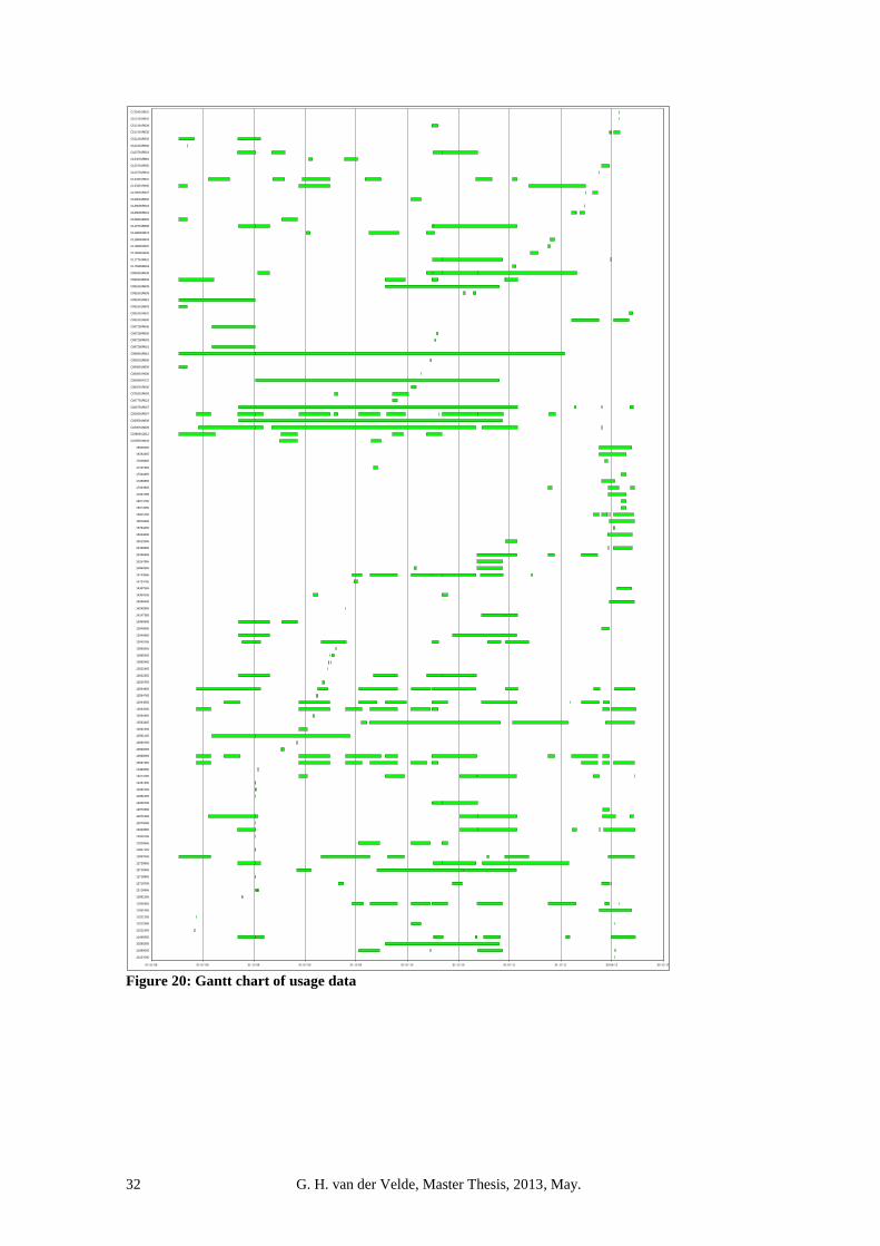
32 G. H. van der Velde, Master Thesis, 2013, May.
01-01-08 01-07-08 31-12-08 01-07-09 31-12-09 01-07-10 31-12-10 01-07-11 31-12-11 30-06-12 30-12-12
10137065
10289065
10289265
11449365
11511665
11511865
11521265
11651665
11906365
12681265
12716965
12718765
12718865
12719265
12729965
12857065
12857165
12929665
12929765
12929865
12970065
12970165
12970365
13059765
13281665
13282265
13287365
13374165
13380665
13587965
13588365
13590065
13590765
13591165
13591565
13593465
13594465
13594565
13594665
13594765
13594865
13629765
13632365
13632465
13895465
13895565
13895665
13940165
13940865
13946665
13960665
14147365
14242865
14246665
14354165
14357565
14734765
14743665
14869265
15157865
15436965
15438965
15513265
15634665
15784365
15879665
16941265
16974665
16974765
17034765
17034865
17280865
17544465
17747965
17828865
18284365
18655965
C025891N646
C038691Q612
C039091N606
C039591N608
C050691R607
C066791R607
C067791R623
C076391R605
C080291R606
C080890R122
C080891R606
C080891R609
C082091R606
C086891R610
C087290R601
C087290R603
C087290R605
C087290R606
C091691R600
C091691R601
C091691R603
C091691R610
C091691R635
C091691R639
C092591R639
C095291R639
C115990R604
C117791R431
C118090R609
C118890R602
C118890R603
C118890R878
C119791R608
C126891R602
C128690R601
C128690R603
C129091R606
C129091R607
C133391R600
C133391R601
C133791R601
C133791R605
C134091R884
C413791R601
C512191R600
C512191R602
C512191R635
C512191R639
C512191R642
C733491R601
Figure 20: Gantt chart of usage data

G. H. van der Velde, Master Thesis, 2013, May. 33
4.3 Purchase price analysis We now have a first impression of the usage pattern of the test pipes. The second step is to
analyse the value of these items. In the internal administration the current book value of all
pipes is 0 euro; all pipes are fully paid by the project that initially ordered the specific pipe.
Next to that, there is no initial purchase price known since pipes are almost never purchased
as a complete item. Until a couple of years ago most pipes were produced internal, a more
recent trend is that test pipe production is the first to be outsourced as soon as the welding
department is reaches its maximum workload capacity. Therefore in the next section we
examine if it is possible by other means to determine the value of the pipes.
4.3.1 Purchase order analysis
To make an estimation of the cost and therefore the value of an item, we analyse the
purchase orders. We filter the purchase orders to show only the orders of three categories:
Welding work (including witnessed test, as explained later in this section)
Flanges
Pipes (the tubes)
The welding work purchase orders of 2010 till 2012 concern 84 purchase orders. Engineers
suggest that pipes of a heavier pressure stage are more expensive than the light ones, since a
higher pressure stage leads to a ticker wall width and thus requires more welding work. A
larger diameter requires more welding work too. No need to say a Tee-part has three welds
instead of two, requiring half more welding work (for an explanation of the different pipe
types, see Table 1). In the same line of reasoning it makes sense that measurement pipes are
far more expensive than the other types of pipes, since a lot of sensor connectors need to be
welded at exact locations. We tabulate the purchase orders to type, diameter and pressure
stage in Appendix A. Unfortunately the amounts paid in the purchase orders differ greatly
and we found only one relation at all with type, pressure stage or diameter: there is a
difference between measurement pipes and all other types of pipes. We use the average of €
2500 for non-measurement pipes and € 5300 for measurement pipes.
Next to the welding work comes the raw material cost. As explained in Appendix A the
pipe tubes itself represent only a small share. Unfortunately we have no information about
these prices. The flanges are the most important material cost factor. Based on the purchase
orders that we have tabulated in Appendix A, we distinct two price categories. The
small/regular flanges are at maximum 600 pound / 20 inch and cost on average 500 euros
per two pieces. The heavier/larger flanges cost on average 2100 euros per two pieces.
This results in four price categories that are tabulated in Table 3.
Table 3: Value of pipes
Pipe category Price work + material Total price
Non-measurement pipe small/regular* € 2,500 + € 500 € 3,000
Non-measurement pipe large € 2,500 + € 2,100 € 4,600
Measurement pipe small/regular* € 5,300 + € 500 € 5,800
Measurement pipe large € 5,300 + € 2,100 € 7,400 *small/regular = maximum 600 pound and 20 inch
Some site notes to these purchase orders are important. At first, we cannot be sure if all
these purchase orders concern only the type of costs they are categorized in. Sometimes a
welding work order also includes raw materials. Second, the order can be including or
excluding a witnessed test (witnessed test: every pipe needs to be x-ray inspected, this
inspection needs to be witnessed by a third party inspection agency).

34 G. H. van der Velde, Master Thesis, 2013, May.
For further analysis, it would be interesting to derive not only an average price but also a
standard deviation per category. Unfortunately our sample is not large enough allow this,
some categories even include only one value and thus deriving a standard deviation is not
possible. Therefore we use only the average values in the remainder of this thesis.
4.3.2 Information from supplier
The purchase order analysis has resulted in four useful value categories. Nonetheless we
were expecting some more relationships between the welding work and the price, thus we
visit the most used supplier of test piping to gain some more insights. The supplier agrees
there is a relation between material costs / welding hours related to diameter and pressure
stage, but he states this is only a fraction of the total costs. The most important factors are:
Number of pipes ordered at the same time: every pipe needs to be certified by an
external inspection agency. They charge a fixed rate of about 500 euros for a visit
to the supplier, so if they can check multiple pipes at once this has a large
influence on the price per pipe.
Lead time: often Siemens asks for pipes that need to be delivered in a very short
timeframe. The materials required are not catalogue items that are in stock at every
metal wares shop, so normally these materials have a longer lead time than
required by Siemens. Lead time reduction leads to higher material costs.
The supplier even came up with an example of an order in recent history were Siemens
demanded a delivery time of two weeks, while the regular delivery time for the required
raw materials would be 10 weeks. Thus, the supplier needed to retrieve materials from a
company specialised in emergency deliveries for offshore oil platforms in order to meet the
Siemens lead time. These kinds of platform emergency companies have all materials that
can be necessary at an oil platform in stock to fly them immediately by helicopter to the
required location. In this specific example the charge for the raw material (pipe) was about
1000 euros, where the regular suppliers (with about 10 weeks delivery time, that is) would
have charged about 150 euros. Thus, lead time restrictions can have a influence accounting
for hundreds of euros at the amounts displayed in the tables of Appendix A.
4.3.3 How many new pipes are bought?
Throughout this report it is frequently stated that for every test several new pipes need to be
bought. Unfortunately no overview exists of how many pipes this concerns. Thus we derive
this number from secondary data sources.
Purchase value
We want to derive the total amount of pipes bought from the purchase order history. To
retrieve this, we filter the purchases orders for the name of the supplier of welding work,
and/or for a pipe type in the description (flange, elbow, pipe, m-pipe, or reducer). This
results in 445 purchase orders concerning the years 2010-2012 of which the values are
tabulated in Table 4.
Table 4: Yearly value purchase orders test piping
Year Purchase value
2010 € 109,250
2011 € 251,513
2012 € 155,506

G. H. van der Velde, Master Thesis, 2013, May. 35
Unfortunately we cannot be sure all purchase orders were for the purpose of test piping. It
is possible there are purchase orders for piping that is used at the compressor itself
(consumables) mixed up with the purchase orders for test piping (tools/storage goods).
There is no way to reengineer for what purpose a bought flange or pipe is used.
Now we calculate the number of pipes bought per loop. We combine these values with the
number of loops build per year as stated in Table 2 and the prices of pipes as listed in Table
3. However, this will not provide a full overview since not all work is listed in purchase
orders: frequently the welding work and testing is performed internally. We correct for the
missing internal costs by dividing only over the cheapest pipe category from Table 3: the
standard pipe of € 3,000. This results in the number of pipes bought per loop as listed in
Table 5.
Table 5: New bought pipes per loop
Year Purchase value Estimated #
pipes
(à € 3,000)
# loops Estimated # pipes
per loop
2010 € 109,250 36 20 1.8
2011 € 251,513 84 12 7.0
2012 € 155,506 52 12 4.34
average 4.4
This average of 4.4 pipes per loop is derived from many assumptions. This includes the
uncertainty in the total purchase value, a rough average of the price per pipe and thus the
uncertain number of pipes. Therefore we check our estimation with the Test Engineers.
They confirm the number of new pipes per loop differs greatly per loop but the four pipes
per loop can be a reasonable educated guess. Thus we will use the rounded estimation of
four pipes per loop in further calculations.
4.3.4 Conclusion of purchase price analysis
We solve the lack of exact purchase prices per item by deriving four easy applicable value
categories. Therefore we make a price distinction for two factors; the difference in price
between measurement pipes and all other types and the difference between regular and
large pipes.
Non-measurement pipe small/regular* € 3,000
Non-measurement pipe large € 4,600
Measurement pipe small/regular* € 5,800
Measurement pipe large € 7,400
(*small/regular is up to 600 pound / 20 inch)
Based on the total purchase value per year, the price category of pipes as just derived and
the number of loops per year we derive that on average 4 pipes per loop are bought.
4.4 A, B, or C items? In Section 3.1.2 we described the definitions of A, B and C items. At first we will define
the class of the test equipment in general. Next, we will make subsections within the test
equipment inventory. In Chapter 3.1.2 we mentioned different order control types for A, B
and C inventories. We start with the remark that independently of the category we pick, all
of these systems have in common that they expect a certain demand, thus need
replenishments in the warehouse to meet this demand. This is why these models are not

36 G. H. van der Velde, Master Thesis, 2013, May.
directly applicable to the Siemens test piping inventory: there are never any orders placed
for items that ‘should be’ on stock and the ‘demand’ is not of the consuming type.
4.4.1 Test equipment: A-items
From Section 4.2 we know the demand for the items is very low, peaking at about four
usages a year. In Section 4.3 it became clear that items do represent a high value. The high
value and low usage matches with the description of class A-items in Section 3.1.4. This
means the items require special attention of the management and it is justified to use
sophisticated control systems.
4.4.2 Order control based on category
In Chapter 3.1.4 several order control methods are mentioned that are generally suitable to
deal with class-A items. Since Siemens does not place orders to keep the inventory at the
desired level, such methods cannot be applied 1-to-1 to the case of this thesis. For slow
moving items (which we have) the Order Point, Order Quantity (s, Q) is advised. However,
we are not interested in the order point, since this is clear: an item is offered to the
warehouse as soon as a project starts or finishes. Also we are not interested in the Order
Quantity since this will always be one. For very expensive slow moving items the inclusion
of shortage costs is advised. Although this can be included, in our case it does not seem
efficient, since it makes the model more complicated while stock outs / shortage costs
barely happen.
This does not mean that these theories are useless. Perhaps the (s, Q) method (or an
adaption to that method) can be of use at a higher level, i.e., at groups of items instead of
specific items. For this we first need to know if there is any grouping method that makes
sense. This will be further discussed in Section 4.5.
4.4.3 Test equipment: sub-bins A, B and C
As we see in Section 4.2 there is a large variation in usage per year of the different items.
So, we can make an A, B and C classifications within this inventory. To categorize our
items in these bins we need to define an activity level for our items. In Section 3.1.3 we
saw that annual dollar usage is the most used activity but all kinds of activity indicators are
possible. We take the euro activity in our four-year period. By euro-activity, or “euros
moved”, we mean the number of times an item is moved times the value of the item as
specified in Section 4.3. For reasons of model simplification we assume storage costs,
criticality and other possible factors to be the same for all items. For criticality this is true,
for storage costs it is not true since items are charged per square metre as explained in
Section 4.7.
For the ABC-curve, Herron (1976) points out that the typical ABC-curve shows that 20%
of the items account for 80% of the movements. As shown in Figure 21, this rule does not
fully apply at the 378 items that are within the scope of this research. Nonetheless the
intention is still valid: 20% of the items cause 64% of the movements so a minority of the
items cause the majority of the movements. We use the ABC grouping method as used by
Herron: the A-items are the items representing the top 50% of the movements, the C-items
are the bottom 50% of the items, and the B items is the group between.

G. H. van der Velde, Master Thesis, 2013, May. 37
Figure 21: ABC plot
The tale of this graph immediately requests attention: 63% of the items accounts for 100%
of the movements. So, 37% of the items have not been used within the scope of this dataset
(i.e. last four years). In Appendix B we show via a log-normal relation plot that in fact the
problem already arises as soon as an item is moved less than 5 times in the four years scope.
4.4.4 Conclusion of A, B and C items
At first we have positioned the test piping inventory as a whole: it concerns items of a high
value with a low demand, thus A-items. Class-A in this case means that close attentions of
the management is necessary and the implementation of a sophisticated control system is
justified. Order control systems that are suggested in literature for class-A items can
however not be applied directly due to the special characteristics of this test piping
inventory.
Within the inventory we have made again the A, B and C classes. We notice almost all
items in the C-class have not moved at all.
4.5 Amount of pipes not used vs. storage space In Section 4.2.2 we concluded that we will focus on searching for an explanation why some
pipes are used and some are not. The research question of this thesis starts with a lack of
storage space issue, so in this section we check the influence of these pipes at the storage
space.
4.5.1 Unused inventory over time
As mentioned in Section 4.2, a lot of pipes have no usage data at all and a lot are not used
in recent history. We now plot how long parts have not been used and thus conclude how
much storage space could have been saved if the unused parts were not stored. Not only the
number of pipes, but more particular the amount of square metres that these pipes need is of
importance to this research. The amount of square metres that a pipe uses is not
administered by the company and measuring this for all items by hand would require many
days. During visits to the warehouse (see Figure 16) we notice however that most items are
stored at pallets that can vary in length but always have the same depth. Therefore we can
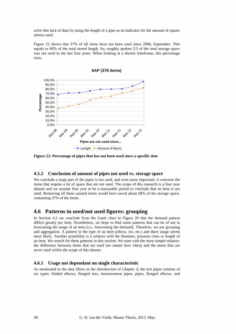
38 G. H. van der Velde, Master Thesis, 2013, May.
solve this lack of data by using the length of a pipe as an indicator for the amount of square
metres used.
Figure 22 shows that 37% of all items have not been used since 2008, September. This
equals to 68% of the total stored length. So, roughly spoken 2/3 of the total storage space
was not used in the last four years. When looking at a shorter timeframe, this percentage
rises.
SAP (378 items)
0,0%
10,0%
20,0%
30,0%
40,0%
50,0%
60,0%
70,0%
80,0%
90,0%
100,0%
Sep
-08
Mar
-09
Sep
-09
Mar
-10
Sep
-10
Mar
-11
Sep
-11
Mar
-12
Sep
-12
Pipes are not used since...
Perc
en
tag
e
Length Amount of items
Figure 22: Percentage of pipes that has not been used since a specific date
4.5.2 Conclusion of amount of pipes not used vs. storage space
We conclude a large part of the pipes is not used, and even more important: it concerns the
items that require a lot of space that are not used. The scope of this research is a four year
dataset and we assume four year to be a reasonable period to conclude that an item is not
used. Removing all these unused items would have saved about 68% of the storage space,
containing 37% of the items.
4.6 Patterns in used/not used figures: grouping In Section 4.2 we conclude from the Gantt chart in Figure 20 that the demand pattern
differs greatly per item. Nonetheless, we hope to find some patterns that can be of use in
forecasting the usage of an item (i.e., forecasting the demand). Therefore, we use grouping
and aggregation. A pattern in the type of an item (elbow, tee, etc.) and there usage seems
most likely. Another possibility is a relation with the diameter, pressure class or length of
an item. We search for these patterns in this section. We start with the most simple relation:
the difference between items that are used (no matter how often) and the items that are
never used within the scope of this dataset.
4.6.1 Usage not dependant on single characteristic
As mentioned in the data filters in the introduction of Chapter 4, the test pipes consists of
six types: bladed elbows, flanged tees, measurement pipes, pipes, flanged elbows, and

G. H. van der Velde, Master Thesis, 2013, May. 39
flanged reducers. Figure 23 shows that the unused items are distributed over all types, so
there is no relation between the type of item and the usage. Of course we do notice that the
percentage of unused parts is high at the pipes, tees and bladed elbows but also in the other
categories the percentages are high enough to justify further research.
Figure 23: Number of items moved vs. not moved according to type
An important characteristic of the test piping is the diameter. The diameters 12, 16 and 20
inch are the default sizes, that are also available in the permanent wall loop. Figure 24
shows however that other diameters are also widely used. From this graph we can conclude
the diameters 6, 8, 10, 12, 16, 18, 20 and 24 are commonly used. If there were no other
limitations this figure suggests removing all other diameters. However, also within the
commonly used diameters there are large amounts of unused items.
Figure 24: Number of items moved vs. not moved according to diameter
The pressure stage is the next important characteristic. Figure 25 shows that 150, 300, 600,
900 and 1500 pound are frequently used. On the other hand, there are large amounts of
unused items within these categories.

40 G. H. van der Velde, Master Thesis, 2013, May.
Figure 25: Number of items moved vs. not moved according to pressure stage
The last characteristic we analyse is the length of a pipe. We categorise all pipes in bins of
250 millimetres till 2500mm, and have a rest bin called 99999 gathering all longer parts.
This shows that there are far more short pipes than long pipes. Furthermore, in the rest bin
more parts are not moved than moved, so the long parts are not that popular.
Figure 26: Number of items moved vs. not moved according to length
4.6.2 Cross-sectional analysis
In Section 4.6.1 we did not find any non-usage explaining pattern between a single
characteristic and the non-usage of an item in the last couple of years. Therefore we
combine the previous graphs to graphs with two criteria.
First we plot the usage of all three combinations of pressure stage/diameter/length.
In Figure 28 till Figure 30 we have plotted the total amount of items of a particular
combination as a dark blue circle, and the number of items that have moved as a light blue
circle. Figure 27 shows an example of how to read these graphs: the dark blue surface is
twice as large as the light blue surface, thus the inventory is twice as large as the number of
items that are moved.
The plots in Figure 28 till Figure 30 are based on the tables shown in Appendix C. For
reasons of visibility, only the most common used diameters and pressure stages are plotted.
The tables in Appendix C contain the full dataset.

G. H. van der Velde, Master Thesis, 2013, May. 41
Figure 27: Example how to read the ball graphs
0
300
600
900
1200
1500
0 2 4 6 8 10 12 14 16 18 20 22 24 26 28 30 32 34 36
Diameter (inch)
Pre
ss
ure
sta
ge
(p
ou
nd
)
Inventory Moved
Figure 28: Pressure stage / Diameter combinations usage
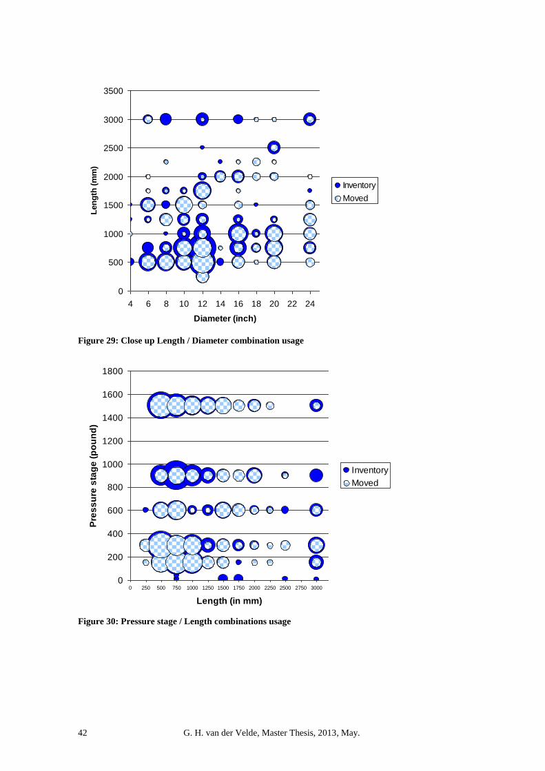
42 G. H. van der Velde, Master Thesis, 2013, May.
0
500
1000
1500
2000
2500
3000
3500
4 6 8 10 12 14 16 18 20 22 24
Diameter (inch)
Len
gth
(m
m)
Inventory
Moved
Figure 29: Close up Length / Diameter combination usage
0
200
400
600
800
1000
1200
1400
1600
1800
0 250 500 750 1000 1250 1500 1750 2000 2250 2500 2750 3000
Length (in mm)
Pre
ss
ure
sta
ge
(p
ou
nd
)
Inventory
Moved
Figure 30: Pressure stage / Length combinations usage
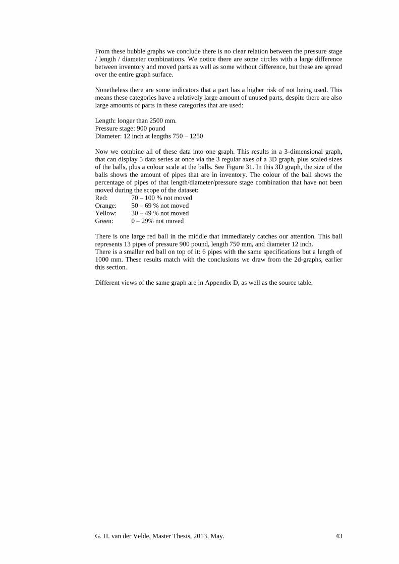
G. H. van der Velde, Master Thesis, 2013, May. 43
From these bubble graphs we conclude there is no clear relation between the pressure stage
/ length / diameter combinations. We notice there are some circles with a large difference
between inventory and moved parts as well as some without difference, but these are spread
over the entire graph surface.
Nonetheless there are some indicators that a part has a higher risk of not being used. This
means these categories have a relatively large amount of unused parts, despite there are also
large amounts of parts in these categories that are used:
Length: longer than 2500 mm.
Pressure stage: 900 pound
Diameter: 12 inch at lengths 750 – 1250
Now we combine all of these data into one graph. This results in a 3-dimensional graph,
that can display 5 data series at once via the 3 regular axes of a 3D graph, plus scaled sizes
of the balls, plus a colour scale at the balls. See Figure 31. In this 3D graph, the size of the
balls shows the amount of pipes that are in inventory. The colour of the ball shows the
percentage of pipes of that length/diameter/pressure stage combination that have not been
moved during the scope of the dataset:
Red: 70 – 100 % not moved
Orange: 50 – 69 % not moved
Yellow: 30 – 49 % not moved
Green: 0 – 29% not moved
There is one large red ball in the middle that immediately catches our attention. This ball
represents 13 pipes of pressure 900 pound, length 750 mm, and diameter 12 inch.
There is a smaller red ball on top of it: 6 pipes with the same specifications but a length of
1000 mm. These results match with the conclusions we draw from the 2d-graphs, earlier
this section.
Different views of the same graph are in Appendix D, as well as the source table.

44 G. H. van der Velde, Master Thesis, 2013, May.
Figure 31: 3D graph of item usage
4.6.3 Combining both parameter groups
We started in Section 4.6.1 with graphs divided to type: pipe, tee, elbow etc. Then we
continued in Section 4.6.2 with pipe characteristics: length, pressure stage and diameter. It
seems interesting to combine these data: we can create the 3D characteristics plot per pipe
type. Unfortunately this results in groups of only one or two pipes, being by far too less
data points to draw reasonable conclusions from such graphs.
4.6.4 Conclusion of patterns in used/not used pipes via grouping
In this the previous sections we searched for an explanation why a pipe is used (even if it
was only once) or not used at all. We started with the pipe categories: elbows, tees, etc.
There appears to be a noticeable difference in percentage of unused parts between those
categories, but all categories have high percentages.
We continued with 2D and 3D graphs of pipe characteristics; length, diameter etc. These
gave useful insights in what the popular combinations and the not-used combinations are.

G. H. van der Velde, Master Thesis, 2013, May. 45
However the used and unused combinations seem to be almost randomly spread over the
surface so we conclude there is no clear pattern.
4.7 Current storage costs One of the incentives for the start of this research is the management concern about the
high and ever rising storage costs. To indicate potential savings by new working methods,
at first we need to now how high exactly the current storage costs are. Since all locations
have different price settings, we make separate cost calculations per storage location. There
are three storage locations:
Internal warehouse
Pipes attic
External warehouse
The scope of this research contains only the internal and external warehouse. As explained
in Chapter 2, the pipes attic contains all small items and those are not logged or registered
in any system. Since we do not have any data about the pipes at the pipes attic, this location
is out of scope.
4.7.1 Internal warehouse costs
The internal warehouse consists of racks with pallets, as shown in Figure 16. Most racks
are five or six pallets in height. The pallets are not regular Europallets, although the depth is
the same as with Europallets since the racks have a Europallet depth. The length however
varies, so parts of different lengths fit at different pallets. Every part has its own dedicated
pallet since a custom made framework to support the (round) pipe is built at the pallet. Thus,
even if a part is in use, the location in the rack is still occupied by its (empty) pallet.
The internal warehouse measures 433m2. In the current rack setup this provides enough
space for:
36 places of 3.60 m length = 36 x 4 = 144 pcs of Europallets
20 places of 2.70 m length = 20 pcs of 2.5-metre pallets
168 places of 2.20 m length = 168 pcs of 2-metre pallets
In a place of 3.60 m length, one can fit 4 Europallets.
In the places of 2.70 m or 2.20 m length, generally only custom made long pallets are
stored.
The internal used storage rate is 3.50 euros per week per square metre. (For comparison
purposes: about 15.16 euros per month). This is an arbitrary chosen number, defined by the
business administration department, charged for the ground floor space, plus the effective
storage space of the rack shelves. When we calculate the effective storage space of the rack
shelves according to internal calculations rules, this equals to 1,000 square metres. Thus
warehouse costs 1,000 m2 x 3.50 euros/week/m
2= 3,500 euros per week = 182,000 euros
per year. Of course we need to keep in mind that these are internal costs (one department
pays to another), so in the end no saving will be achieved when this warehouse is not used.
4.7.2 External warehouse costs
The external warehouse is currently 800m2, but the size can vary per month. The rate is
4.50 euros per square metre per month, so the costs are 3,600 euros per month or 43,200
euros per year. This includes the external storage of items that are outside the scope of this
research, unfortunately we cannot define the share of items within the scope.

46 G. H. van der Velde, Master Thesis, 2013, May.
As explained in Section 2.2 and showed in Figure 18 the external warehouse is used for
items that do not fit in the internal racks. So there are no racks: there are only extremely
large items that are put next to each other at the ground.
4.7.3 Conclusion on storage costs
We conclude the price per square metre internal is at least three times as high as the
external storage price. Total storage costs are 182,000 + 43,200 = 225,200 euros per year,
although the internal storage costs are only paid from one department to another and thus
stay within the company.
4.8 To stock or not to stock; seven factors In the introduction of Chapter 4 (cf. Figure 19) we showed there are currently 421 items
with usage data. Are these 421 items worth it to stock them at all? In the literature chapter
we saw that Silver et al. (1998, p. 372) note that this is a multi-disciplinary question that
cannot be answered solely from production planning and inventory management
perspective. This is true in the case of Siemens: from a planning perspective it is possible to
store nothing and order every part every time again. From the overall plant planning,
management wishes to reduce the amount of storage space that is in use by test piping. The
proposal department however, argues that there is no budget in a project to buy all new test
piping for every project. They state the company gets orders only because they can offer a
reasonable price, and they can offer this price only if most of the test pipes are available
‘for free’.
4.8.1 Seven important factors
As discussed in Section 3.1.1, Silver et al. distinguish 7 important factors to decide whether
or not an item should be stocked (Silver et al., 1998, p. 372). Combining Chapters 1, 2, and
4 we have gathered enough insights in the situation to answer these questions. In this
subsection answer all of these seven questions separately.
1. The system cost (file maintenance, forecasting, etc.) per unit time of stocking an
item
Although not explicitly mentioned, from Section 2.1.5 we can derive there is no system
for the maintenance and forecasting of the test piping. Of course the items are listed in
SAP but as long as items are not used there is no time spend. Thus, the costs of system
maintenance or forecasting are zero. In the same section we notice there is a planning
department, these personnel costs could be labelled as forecasting costs. However the
main purpose of their forecasting is creating a floor plan to see what tests can
physically be done simultaneously. Since the bill of material (including test piping) is
already created for a test, the result of this forecast is automatically a forecast of what
test pipes are needed from the warehouse and what need to be produced. We conclude
a negligible part of the planning department and thus no costs can be assigned to the
test piping system costs.
The storage costs on the other hand, are high. In Section 4.7.1 we noticed the internal
storage costs are 3.50 euros per square metre per week and 4.50 euros per square metre
per month for external storage.
2. The unit variable cost of the item both when it is bought for stock and when it is
purchased to meet each demand transaction

G. H. van der Velde, Master Thesis, 2013, May. 47
As we conclude from Section 4.3, the item price ‘from stock’ is zero euros, since the
item has been paid by a previous project. At the same time we conclude in Section
4.3.1 that new items are expensive: from 3,000 to 7,400 euros.
3. The cost of a temporary back order associated with each demand when the item is
not stocked.
As long as the planning functions as it should, there is enough lead time and slack to
have every part delivered in time. If, for any reason, an item is late however, the test
has to be postponed which is very expensive.
4. The fixed setup cost associated with a replenishment in each context (an account
should be taken of possible coordination with other items, because setup costs may
be reduced.)
For new items, we learned from a supplier in Section 4.3.2 that ordering multiple items
at once reduces the unit price since for example the witnessed test costs are fixed and
can be shared. Thus these are setup costs.
For items from the warehouse there are no setup costs. One could argue that there need
to be forklift movements etc., but at least the same amount of movements are necessary
at the incoming goods department if an item is new so these costs do not make any
difference and can be ignored.
5. The carrying charge (including the effects of obsolescence), which, together with
the unit variable costs, determines the cost of carrying each unit of inventory per
unit time.
The storage costs are fixed per square metre per week (internal) or month (external), as
described in Section 4.7. Effects of obsolescence are not taken into account since all
items have a book value of zero euro, as described in Section 4.3.
6. The frequency and magnitude of demand transactions
As shown in Figure 20 in Section 4.3, the usage frequency differs a lot per item: from 0
to ca. 4 times a year. We call this quite infrequent. Since all pipes are unique, the
magnitude of demand is always 1. On the other hand, a test requires on average 20 to
40 piping parts as discussed in Section 1.2.2. So when they would all be ordered new,
the magnitude of the order would be between 20 and 40.
7. The replenishment lead time
The lead time can be anything and generally varies from 2 to 14 weeks. As we saw in
Section 4.3.2 the longer the lead time is, the cheaper the part will be.
4.8.2 Conclusion to stock or not to stock; on seven factors
We started this section with the remark that this question is multidisciplinary. Now we
know there is enough lead time to have all items ordered new, so from planning perspective
there is no reason to store. From customer relation management there is also no reason to
store the pipes: the customer is internal and only cares about the pipes being delivered in
time, independent of the source.
What is left is the financial question. The current storage costs are 225,200 euros per year
(Section 4.7.3). Assuming that there are 15 test loops build per years (Section 1.2.2) all
requiring at least 20 pipes per loop (Section 1.2.2) at an average cost of 3,000 euros per
pipe (Section 4.3.1), buying every pipe new would cost at least 900,000 euros per year. We
state “at least”, since we did not include the more expensive pipe categories that are listed
in Section 4.3.1. So clearly it is attractive to store at least some pipes.

48 G. H. van der Velde, Master Thesis, 2013, May.
4.9 Conclusion on data analysis In this chapter we have gathered a lot of information. Most questions are answered based
on the analysis of data sources like the movement transactions of the pipes between the
warehouse and the shop floor, but also financial sources like purchase orders for raw
materials. We summarise the answers to all questions that we posed in the introduction of
this chapter:
How often are the pipes used?
We have created a Gantt chart of the usage periods per pipe. We conclude the
usage data is not reliable and we cannot derive from this data how often pipes are
used. One fact we do conclude from the data is that a large amount of pipes has no
usage data at all, while other pipes seem to be used multiple times a year.
What do the pipes costs?
Since all pipes are different and original purchase prices are not available, we
estimate the value based on the type of pipe, the pressure class and the diameter.
These estimations are based on the analysis of purchase orders of raw materials
and outsourced activities. For the type we distinct between measurement pipes and
all other kind of pipes, for the pressure class and diameter we distinct between
small pipes that are below 600 pound and 20 inch and large pipes are above those
values. This way we distinct four price categories: 3,000 euros for small pipes,
4,600 euros for large pipes, 5,800 euros for small measurement-pipes and 7,400
euros for large measurement pipes. Based on the same purchase order analysis we
estimate 4 pipes per loop are bought new.
Do we deal with Class A, B or C items?
Fist we look at all test piping together as one class. This concerns expensive items
with a low demand, which are the characteristics of Class A items. Within the
group of test piping we can also distinct the classes A, B and C. We notice 20% of
the items account for 64% of the movements and 63% of the items already account
for 100% of the movements.
How many pipes are stored without recent usage?
As we saw in the previous question, 37% of the items have not moved in the last
four years. Even more interesting is that these items account for an estimated 68%
of the total storage space. When looking at last year only, about 70% of the items
are not used which equals about 80% of the storage space.
Are there any patterns/relations in the usage vs. physical characteristics?
We have compared the number of used vs the number of unused pipes filtered on
type of pipe, the diameter, pressure stage and length. This shows the usage does
not depends on a single characteristic. Combining the characteristics in 2D and
3D graphs still don’t show a clear pattern, although we now see three situations
with a relatively large amount of unused pipes:
o Length: longer than 2500 mm.
o Pressure stage: 900 pound
o Diameter: 12 inch at lengths 750 – 1250
What are the current storage costs?
Within the scope of this research there are two warehouses: the internal and the
external warehouse. The internal warehouse measures 1000 m2 and costs 3.50
euros per square metre per week, equalling 182,000 euros per year. The external
warehouse measures 800m2 and costs 4.50 euros per month, thus equaling 43,200

G. H. van der Velde, Master Thesis, 2013, May. 49
euros per year. In the external warehouse there are non-piping objects stored as
well.
What are the answers to the seven factors of Silver et al. (cf. Section 3.1.1)?
Via these seven factors we have checked the multidisciplinary facets of the
necessity of test piping storage. From planning perspective or customer relation
management there is no need to store pipes at all. The only reason to do so appears
to be a financial one: it is simply cheaper than producing them all again when
needed.
Concluding we now have all details we need to start developing a useful model, according
to the initial research questions of this thesis.

50 G. H. van der Velde, Master Thesis, 2013, May.
5 Decision model formulation Based on the models of Chapter 3 and the data of Chapter 4, in this chapter we formulate
the answer to the two problems that were formulated at the start of this research.
At first, in Section 5.1 we select and formulate the solution to problem 1 of Chapter 1.3.2:
‘There are continuously new pipes entering the warehouse, but there is no system to
remove pipes from the warehouse. Thus the warehouse faces an overload of items. Can we
come up with a systematic approach to deal with this overload problem?’ We recommend
the use of a knapsack model. Section 5.2 describes the implementation trajectory for this
solution.
Second, in Section 5.4 we answer problem 2 as formulated in Chapter 1.3.2: ‘The new pipes
are created for a reason. Can we prevent the necessity of creating new pipes?’ We
recommend standardisation of test piping. Since it is not possible to switch from the current
situation to the recommended situation at once, Section 5.5 describes the implementation
trajectory.
5.1 Problem 1 solution selection: knapsack One of the two main research problems in this thesis is if we can come up with a systematic
approach to cope with the warehouse overload. This leads to the question what kind of
inventory review system we can apply. From the theory in Chapter 3 we learned the
common models like the model of Croston (1972) and Teunter et al. (2011) are not relevant
for the situation at Siemens. We note that aggregation might be helpful from theoretical
perspective; however we did not find any data to aggregate. The data we would like to
aggregate is the usage data; unfortunately only for a small percentage of all items this data
is available and not corrupted, and within this small dataset most items have too few or
non-realistic demand occurrences to draw conclusions. Aggregation does not solve the lack
of reliability of the data.
In the case study of Gelders and Looy (1978) as introduced in Section 3.3.1 we saw the
knapsack-model for slow-moving items. The conditions for their model have many
commonalities with Siemens and this model provides a feasible solution regarding
implementation and system maintenance. In the next subsection we will elaborate on the
introduction of a knapsack model for Siemens. The basic idea of this system is that it
updates itself. Every time a new item is added to the warehouse, another item must leave to
create the required warehouse space. This basic principle is illustrated in Figure 32.
Figure 32: Knapsack principle: one item leaves if another enters the warehouse
G. H. van der Velde, Master Thesis, 2013, May. 51
5.1.1 Knapsack conditions at Siemens
As shown in Section 3.4 there are several ways to solve a knapsack problem. They all share
the basic characteristics of a knapsack problem: there is (at least) one knapsack capacity
(the restriction), all items have a ‘weight’ in terms of the knapsack capacity and all items
have a profit when added to the knapsack. In this section we will define these
characteristics for Siemens.
Knapsack capacity: Available space
The knapsack capacity is the number of square metres we have available in the warehouse.
In contrast to many other situations where companies face a physical restriction on the
warehouse capacity, Siemens has multiple storage locations and the total capacity can be
adapted to the requirements. From data analysis we know what parts are used in the past
four years. Management agrees that since Siemens was able to work for four years with this
amount of pipes, it is likely that it can survive with an equal amount of pipes in the coming
years. So we will calculate the amount of square metres that is necessary for storing only
the parts that are used in the past four years and take this as the knapsack capacity. From
the problem introduction in subsection 1.2.1 we know the warehouse capacity might change
in the near future, there are plans of the municipality to construct a road at the current
internal warehouse location. Therefore we stress that the warehouse capacity is a variable in
the knapsack model, which can vary without influencing the functionality of the model.
Knapsack item weight: pallet size
The weight of an item in the knapsack is the amount of square metres it requires. In the
internal warehouse the pipes are stored at pallets in racks. The current rack setup results in
five weight categories:
Europallet
2-metre pallet
2.5-metre pallet
3.4-metre pallet
Larger, does not fit on a pallet.
For items stored on pallets, the amount of square metres required is fixed per pallet size,
independent of the item size. The items that are larger than the largest pallet are stored
without pallet on the floor, in this case the exact amount of square metres required to store
the item represents the weight of the item.
Knapsack profit: stored euros per week
We use two values as a ‘profit’ that is obtained when an item is stored. First, the
replacement value: it is better to scrap (and if necessary reproduce later on) a cheap item
than an expensive item. Second: the usage intensity, we better store the items that are used
frequently and scrap the ones that are seldom used.
As shown in Chapter 4.3 we derived four price categories for the replacement value. So this
‘profit’ will be equal for many items.
For the usage intensity, it would be nice to have figures like ‘amount of times used per year
in the last x years’. Unfortunately we do not have these numbers. In theory these figures are
available from the SAP system, but from the Gantt chart in Figure 20 we saw that these
figures are not reliable and cannot be used to draw conclusions on the number of times an
item is used.

52 G. H. van der Velde, Master Thesis, 2013, May.
To cope with this lack of data, we use the length of the current storage period as a cost. This
has two major advantages. At first, it is easy measurable and the system is reliable for this
figure. Second, this parameter prefers items that are recently used. Test Engineers prefer to
use recently used items as well, so this is an indication for a higher change it will be used
again soon. At the same time, the lowest profit goes to the item that is already stored for
years without any usage so those items will be removed.
We need to take care for the correct use of these two profit parameters: for replacement
value it is the higher the better, for the current storage period it is the lower the better. Thus
we define the profit as replacement value divided by the storage period, resulting in the
intuitive setting where a higher profit is better.
5.1.2 Model selection
The easiest way to get an indication of the knapsack solution (and an upper bound of the
maximum profit) is the use of the relaxation of the ILP-problem, as described in Section
3.4.3. Due to the relaxation, the model will suggest to add a fraction of an item, which is
not feasible in practice. For large amounts of items this would be a problem, therefore lots
of heuristics have been developed. In our case however, there is in most of the cases only
one item that does not fit into the knapsack: the item that is new. So we do not face a
complicated knapsack. If an employee sees the results of the relaxation, he can easily point
out the item that should be removed. This is not necessarily the one with the lowest priority,
also the pallet size must fit. E.g. we cannot store an extra 3.4-metre pallet by removing two
2-metre pallets: the 3.4 metre pallet simply won’t fit in any of the two 2-metre rack places.
The other way around is possible although it results in unused space that the knapsack
model will not subtract from the capacity. In this case the problem is we cannot store a
Euro pallet in two small gaps of 50 centimetres when 2-metre pallets are stored in 2.5-metre
racks. On the other hand, in some cases it is possible to store larger pallets by removing
smaller ones: e.g. the euro pallets are generally stored in groups of four on a 3.4-metre
place. It can also happen that Euro pallets are stored in one of the other rack sizes.
Incorporating all of these factors results in a sophisticated software model that needs, next
to the mentioned costs and profits, the exact storage locations of all items. When using such
a system the risk for errors is huge since the storage locations will not always be right. In
case of an error the transport & storage employees are not able to manually check the result
of the model since they cannot oversee all the calculations.
Taking into account the considerations of the previous paragraph, we decide to implement
only the relaxed ILP problem and train the employees in the logic of this system and how to
make decisions according to the result.
5.1.3 Model formulation
From the description of the several elements of the model in the previous subsection, we
derive the labels, parameters and variables. This leads to the priority formula.
Labels:
i = item i
Parameters:
si = required storage space in m2
, in case of pallet usage this is the pallet size.
ti = length of the current storage period since the last usage moment, in weeks (if the item is
in storage) or 0 (if the item is in use).
vi = replacement value, in euros.

G. H. van der Velde, Master Thesis, 2013, May. 53
Variables:
di = priority of an item. The item with the lowest priority is the first to be scrapped.
pi = profit when adding item i to the knapsack
wi = weight (in terms of the knapsack capacity restriction) encountered when adding item i
to the knapsack.
In Section 3.4.3 the priority is defined as profit per unit of weight, thus di = pi / wi.
For the profit (pi) we derived in subsection 5.1.1 after sub-heading ‘profit’ that the profit in
our case exists of two parameters: the replacement value and the length of the current
storage period, the subsection concludes that profit = replacement value / storage period. In
our model notation this reads pi = vi / ti.
From the parameter definitions in the start of this subsection we know that ti equals zero if
the item is in use at the moment the model is executed. With the proposed profit formula
this would result in an error: we try to divide by zero. The objective of the profit formula is
to assign the highest profit to the items with the shortest storage period. A storage period of
zero weeks is the shortest possible, thus these items should provide the highest profit. It
also should result in the highest priority, since it is physically not possible to remove items
from the warehouse that are currently in use. Therefore we create a separate priority
formula for the case ti = 0.
The weight (wi) consists only of the required storage space si, as explained in 5.1.1 after
sub-heading ‘weight’.
Now can first calculate the priorities for all items that are in the warehouse (thus the current
storage period is larger than zero):
iwifwpd iiii 0 /
Then we assign the maximum of all calculated priorities to the items that are currently in
use, thus have a storage period of zero:
0max
ilil
i wifdd
Since we have:
pi = vi / ti
wi = si
this results in:
iwifstvd iiiii 0 /
and second step:
0max
ilil
i wifdd
Thus, the priority is set as the value of an item divided by the number of weeks the item is
already in storage per square metre.
A numerical example of this formula is shown in Table 6. The replacement value of the
items varies from 3,000 to 7,400 euros at the moment, but the system can handle any value.
The number weeks of the current storage period can be any number but will generally be
from 1 to about 400. The result is a priority on the scale of 0 to ( ii sv min/max ). The
example in Table 6 shows item A has a priority of 15, being the lowest priority in the list.
Thus, item A is the first in the row to be scrapped when a new item needs to be stored in

54 G. H. van der Velde, Master Thesis, 2013, May.
this warehouse. Item F appears to be zero weeks in storage, thus it is currently in use. A
very high priority is assigned to this item, thus items currently in use will never be scrapped.
Table 6: Example of the knapsack method
Item Value vi Weeks ti Space si Priority di
A 3000 100 2 15
B 5800 2 4 725
C 4600 80 2 29
D 3000 50 2 30
E 3000 30 6 17
F 3000 0 2 1500
5.1.4 Considerations in formulation of variables: alternatives
In subsection 5.1.3 we have defined the variables profit, weight and priority, where the
priority is always profit divided by weight. Since we deal with heuristics, there are different
possibilities for defining the other two variables. Therefore we discuss the alternatives for
both variables separately.
Weight
Expressing the knapsack size and thus the weight of items in square metres seems to be
obvious. Alternatives would be the number of pallet places, but those differ in sizes so this
is not desirable. The weight could also be expressed in storage costs (thus setting a storage
budget as restriction). However, the storage costs are directly related to the square metre
usage so this would not change the model.
Using storage costs as a weight is interesting when one wants to research on the difference
between storing in the internal and external warehouse, since both locations have different
rates per square metre. This is not the goal of this research however, and it would also
require including the transportation costs and thus the exact number of movements, which
makes the model far more complicated.
Profit
The profit is defined as the item value divided over the number of weeks an item is stored.
One could argue to divide this also over the required storage space, resulting in value per
week per square metre:
pi = vi / (ti. * si )
Since di = pi / wi is still valid, and as long as we do not change the weight, this results in:
di = vi / (ti. * si 2)
We notice the storage space si is now included twice. This places a larger emphasis on the
required storage space, at a cost of the emphasis on value and storage period.
Table 7 shows the difference between both formulas in the real dataset. An extended
version of this table is added in Appendix E. We do not tabulate the actual values of the
calculated priorities, but rather their ranking order. So number 1 is the item with the lowest
priority, number 421 (out of 421 items) is the item with the highest priority.
We notice the top three of lowest priority items is equal in both formulas, although in a
different order. So both models agree on the three items that should be scrapped first, the

G. H. van der Velde, Master Thesis, 2013, May. 55
sequence in which those three items will be scrapped is different but since new pipes will
be added shortly after each other all three will be scrapped soon. Thus this difference in
order is considered as not important.
For the more extreme cases we notice large differences. For example take a look at the
marked item, item number J. It is an item that lays unused in the warehouse for the longest
period of all items: since April 2009. In the original model, this long storage period places
high emphasis on the priority and thus it ends at position 9. The item requires only a small
storage location, which is more important in the alternative formula. Thus in the alternative
formula this item ends much higher on the list: priority place number 77. This shows that
using the alternative formula, this item will not be scrapped in the near future. We consider
this as undesirable behaviour of the model, an item that is not being used for years and is
not that expensive should not end up this high in the ranking. Therefore we conclude the
original system performs better than this alternative.
Table 7: Results of two different priority calculations
Priority
ranking of
model:
di = vi / ( ti. *
si )
Alternative
priority
ranking:
di = vi / (ti.
* si * si)
Item nr.
(i)
Surface
m2
(si) Value € (vi)
In storage
since
(#weeks
since then
= ti)
1 3 Item A 4.08 3,000 27-5-2011
2 1 Item G 5.56 4,600 27-5-2011
3 2 Item B 5.27 4,600 27-5-2011
4 5 Item F 2.40 3,000 12-1-2011
5 6 Item D 2.40 3,000 13-1-2011
6 7 Item E 2.40 3,000 13-1-2011
7 4 Item H 4.08 4,600 27-5-2011
8 10 Item C 2.40 3,000 27-5-2011
9 77 Item J 0.96 3,000 7-4-2009
10 14 Item I 2.40 4,600 12-1-2011
5.1.5 Model execution: dynamic vs. permanent parameter values
As becomes clear from the chosen parameters, only the number of weeks an item is in
storage needs to be updated every time the model is executed. The replacement value of an
item and the storage space required are not likely to change in short term. In the long term,
say once every 4 years, it is interesting to check if labour or steel prices have changed
significantly such that the replacement value of the items need to be updated. This makes it
easy to execute the model frequently: in practice only one column in Excel (the ‘stored
since’ date) needs to be updated and Excel returns the new priorities immediately.
5.1.6 Conclusion on problem 1 solution selection: knapsack
This section recommends the knapsack model as the solution for the lack of a systematic
approach to remove items from the warehouse. The model is easy to understand and to
execute: the warehouse capacity is fixed so for every new item that must be stored another
item must be removed. The model suggests which item should be removed based on the

56 G. H. van der Velde, Master Thesis, 2013, May.
replacement value, the current storage period and the storage surface. Due to the fixed
warehouse size the knapsack model creates predictability within the company and saves
costs.
5.2 Implementation trajectory of the knapsack model As with any inventory management system to work, it is important to implement the system
in the right way. During the stakeholder analysis in Section 2.1 we concluded there is a lack
of a problem owner. This is an implementation risk: when no one feels the urgent to adhere
to the knapsack model, nothing will change. New pipes will keep arriving at the warehouse,
but if no one decides what pipe can be removed from the warehouse the malfunctioning of
the system becomes a warehousing problem again. The warehousing department is just a
service department for the entire plant, they just store all kinds of items and cannot make
decisions concerning the content. So we must prevent that the problem is transferred to this
last-in-line department due to lack of interest of the other departments. Therefore this
subsection asses the decisions that must be taken and responsibilities that must be assigned
for a successful implementation.
The following steps must be implemented:
One time decision: size of the warehouse
For every new part: decide if it must be stored or not
If it must be stored:
o Add the new pipe to the knapsack model
o Decide what item must leave
o Remove the item from the warehouse
We start in Section 5.2.1 with the first and one-time step: defining the knapsack size, or the
size of the warehouse. The other three steps are recurring procedures, therefore we continue
in Section 5.2.2 till 5.2.4 with the daily operating procedures and responsibilities.
5.2.1 Defining the warehouse (/knapsack) size
From Section 4.5 it becomes clear that lots of pipes are unused for years, which implies that
the knapsack size can be defined smaller than the currently used storage space. To see how
small the knapsack size can be defined, all pipes are checked manually one by one to decide
if they must stay in the knapsack. This is done during a couple of inventory review sessions
with the Test Engineering department and the author of this thesis. The result is a one-time
reduction of the total inventory.
The intention of these inventory review meetings was to discuss every single item. During
the process this appeared not to be necessary. In the first meeting the items that are most
likely to be obsolete were discussed. Since from Figure 24 in Section 4.6.1 it appears that
items with a diameter larger than 24 inch are seldom used, we start discussing all items
larger than 24 inch. As a next step we discuss all large items, that is: all items stored at the
external warehouse. The remaining items are stored internal and they are not large in
diameter or length. Since this includes all popular items, we limit the discussion to all items
that have not been used for more than four years. For all newer items the Test Engineers
state they need to be kept anyways. The result of this manual inventory review meetings is
the removal of 94 pipes.
5.2.2 Identifying new and existing working procedures
There are two procedures that must be implemented:

G. H. van der Velde, Master Thesis, 2013, May. 57
Decision if a new pipe must be stored or not
Removal of an old pipe
In the current way of working, the test engineering department already specifies at the
technical drawing if the pipe must be stored for future use or not, although they do not do
this consequently. We prefer to adhere to existing procedures as much as possible, so we
opt for keeping this information on the technical drawings and stress that this procedure
must be performed always. When the standardisation of test piping as proposed in this
thesis is implemented, it will be even easier for the test engineers to make this decision and
list it at the drawing.
For removing a pipe from the warehouse, no procedure exists. During this research many
pipes are removed from the warehouse during sessions initiated by the author of this thesis
as discussed in Section 5.2.1. The author noticed that non-structured ad-hoc procedures
were used that differed from session to session, since it was unclear who was responsible
and from who the signatures were needed for the removal.
5.2.3 Assigning responsibilities
The most important implementation issue is assigning the responsibility: who will decide
what item must leave? The model provides a priority ranking, but the department that
works with the model must manually decide which item from the lowest priorities clears up
the right amount of space for the new item. To see which department can make this
decision best, we first model the current way of decision making. In Chapter 2 we already
modelled the relations between the departments in Figure 14 and Figure 15. Since Test
Engineering already maintains their database of all test pipes and this department decides
about the storage or scrapping, it seems plausible to let Test Engineering maintain the
knapsack system. The problem is they have no incentive to do so and they have currently
no communication with the other departments other than the technical drawing, so this
would be vulnerable for errors in the process. Other options are to host the model at the
Warehousing department or the Planning & Control department. To enter new items into
the model some technical characteristics (like length and pressure stage) must be known.
People at the Warehousing department do not have these insights and it is likely that they
are not always available in the item description. Forcing this information to be always
present in the description is vulnerable for errors. Thus the most suitable department is the
Planning & Control department. This department has already communication with both
Test Engineering and Warehousing. It also has already technical insights in the pipes and
sees new pipes coming upfront since it processes the drawings coming from Test
Engineering. In Figure 33 the proposed new process is displayed. It shows that Planning &
Control manages the model, and only asks Test Engineering for approval for scrapping an
item. Rules must be formulated on this approval, we suggest Test Engineering can only
disapprove if they can already specify a project where this item will be used at.

58 G. H. van der Velde, Master Thesis, 2013, May.
Figure 33: New decisions and communication about storing or scrapping

G. H. van der Velde, Master Thesis, 2013, May. 59
5.2.4 Model execution in practice
An Excel file will be developed containing all the values and storage requirements. Since
the number of new items per year is not that large, these can easily be added manually to
the Excel file. Furthermore the output of SAP containing the most recent warehouse entry
dates can directly be pasted into this sheet. Then the sheet provides a list of priorities that
are automatically calculated. Planning & Control employees will be trained to remove the
item with the lowest priority that creates a free space that fits the new item.
5.2.5 Conclusion on implementation trajectory of the knapsack model
We recommend to have the planning & control department responsible for the execution of
the knapsack model and the involved process steps. An Excel file is developed to help the
planning & control employees making the decisions easy.
5.3 Financial effects of the knapsack model The main financial effect of the knapsack model is the saving of storage costs. In Section
5.2.1 we achieve a one time inventory reduction of 94 pipes. In order to relate this amount
to the number of square meters that is saved, we estimate the storage surface based on the
length and diameter of a pipe. In the cases were these measurements are within a pallet size
we use the pallet size, if the item is larger we use the real surface plus some aisle space.
This results in a saving of 60 m2 in the internal warehouse and 130 m
2 in the external
warehouse. Multiplied with the internal storage rate of 3.50 euros per square meter per
week and the external storage rate of 4.50 euros per square metre per month (as explained
in Section 4.7) this saves:
Internal: 60 m2 * 3.50 euros/m
2/week * 52 weeks/year = 10,920 euros per year.
External: 130 m2 * 4.50 euros/m
2 /month * 12 months/year = 7,020 euros per year.
The internal savings will not be visible at the internal financial overviews. This is since we
just solved part of a backlog problem: lots of pallets are stored in the aisle since the racks
are full. Now at least some aisles are accessible. The aisle usage is not charged internally,
so it cannot be saved. Despite the non-visible financial benefits of the internal storage
reduction, there are indirect benefits such as the easier storage and retrieval of items in the
warehouse without pallets blocking the aisles and with more items stored at a specific rack
location instead of random in the aisle.
An indirect financial advantage of the knapsack model is that the amount of storage space is
fixed from now on. In the past, the total storage costs (especially the external storage costs)
have grown every year. So we save a growing amount of costs in the coming years, as
illustrated in Figure 34. This creates predictable expenses; predictability is of major
importance to Siemens.
The costs of the system are marginal. Every time a new pipe is added, an employee must
update the Excel sheet. This means loading a new export of SAP, adding a pipe and
removing a pipe. Taking into account that not all employees are Excel or SAP guru’s, we
estimate this process will take about 15 minutes. When multiple items are added at the
same time then the SAP export is needed only once, so it will take only a couple of minutes
extra per pipe.

60 G. H. van der Velde, Master Thesis, 2013, May.
Figure 34: Storage costs become fixed
5.4 Problem 2 solution selection: standardisation As became clear in 3D graph in Figure 31, there are many combinations of diameter,
pressure stage, and length. In fact, 176 combinations are represented in the graph.
Unnecessary to mention, this amount would be significantly larger if the length bins were
chosen smaller than the current 25 centimetre. Since the unused items are also spread over
many combinations, we conclude this diversification is the main reason for the storage and
non-used item problems. Since there are so many combinations and different test loop
setups with different characteristics designed in the past, there is a high risk that an item
will be used only once. This risk is stressed by the relative low amount of test loops build:
on average 15 loops per year using on average 20 to 25 items per loop (see Section 1.2.2).
In the ideal situation a set of pipes is introduced that can together fit in almost every
situation. The money system is a good example: with just a couple of different coins and
banknotes we can make any desired amount using just a few money ‘pieces’. If such a
system can be applied to the test piping, the research problem of this thesis is solved: the
amount of pipes is reduced and no new parts will be produced in the future, so no ‘to
store/not to store’ decisions are needed anymore (see Figure 35). In the next subsections we
will elaborate on this system for test piping, by defining what the possibilities and
limitations of standardisation are for the pressure stages, diameters, lengths, and types.
Figure 35: Comparison of pipes with coins
5.4.1 Pressure stage
As shown in Figure 25, currently there are nine different pressure stages available. Five of
them are available in large amounts of pipes.
G. H. van der Velde, Master Thesis, 2013, May. 61
Hypothetical optimum
From technical perspective, ‘pressure stages’ are a minimum requirement and pipes can
always be replaced by a pipe of a higher pressure stage. At the moment 1500 pound is the
highest pressure stage used, so in theory all loops can be constructed using only 1500
pound pipes.
Feasibility
The different pressure stages are there for financial and workload reasons. From
consultations with management and engineers as well, we conclude it is not feasible to
work with the highest pressure stage only. Management says the highest pressure stage
requires significantly higher investment costs than low pressure stages and constructing
loops with these heavy pipes requires significantly longer building time.
Recommendation
We conclude we need to keep working with several pressure stages for financial reasons.
Our recommendation is to maintain the 300, 600, 900 and 1500 pound classes. The 150
pound class can be discontinued. The 150 pound class exists only since the permanent loop
(which is permanently mounted at the wall, as shown in subsection 1.2.1) used to be 150
pound. About two years ago an entire new permanent loop was constructed, now the loop is
at 300 pound. Thus the 150 pound pipes have no added value anymore. The pressure
classes 300, 600 900 and 1500 pound are all frequently used and not attractive to replace by
a higher pressure class.
5.4.2 Diameter
As shown in Figure 24, currently there are 19 different diameters available, of which eight
are available in large amounts of pipes.
Hypothetical optimum
The three most used diameters are the three diameters of the permanent loop: 12, 16 and 20
inch. In an optimal situation all tests are possible with these three diameters.
Feasibility
From consultation with the engineers we learn using the right diameter is in some cases
necessary. For the measurement pipes there is no other option than using the exact diameter
as prescribed by the technical requirements of the compressor. With all other pipes, all
diameters can be used as long as the diameter is somewhat close to the compressor diameter.
A main constraint is one can never use a converter to a smaller diameter: the next diameter
must always be larger to prevent flow problems.
Engineers mention a larger diameter means a wider radius in the elbows, thus a test loop
with unnecessary large diameters would require more space in the test hall which is not
available.
Recommendation
Next to the three diameters of the standard loop, diameters 6, 8, and 10 inch are regularly
used. From this set we suggest to keep only the 8 inch pipes, since systems of 6 inch can
easily be converted to 8 inch and systems of 10 inch can easily be converted to 12 inch.
The diameter 24 inch is unavoidable since it is the largest and converting to a smaller
diameter causes technical problems. Diameters larger than 24 inch are seldom used and
therefore not attractive to store at all. This results in the recommendation to store 5 standard

62 G. H. van der Velde, Master Thesis, 2013, May.
diameters: 8, 12, 16, 20, and 24 inch. From this selection, it automatically follows that
converters from the discontinued diameters to the new standard diameters remain necessary.
5.4.3 Length
All kinds of lengths are available. In this thesis we have divided them in ten bins of 25
centimetre from zero to 2,5 metre, and an eleventh bin for all larger parts as shown in
Figure 26.
Hypothetical optimum
In the ideal situation there is a standardised set of lengths enabling us to create all possible
lengths with only a small amount of pieces. (Cf. the euro-coin system: with coins of 1, 2, 5,
20, 50 cents and 1 and 2 euro all amounts can easily be paid.)
Feasibility
The length of pipes always needs to fit within a margin of 1 centimetre and the required
total lengths can vary from 1 centimetre to a couple of metres. Distances up to 3 or 4 metres
are common practice, longer pipes are seldom used. To create a set of standard lengths, it
seems reasonable to create pipes of 1, 2, 5, 10 and 25 centimetres, half a metre, one metre
and 2 metre to form all distances. However the small parts cannot be produced, since the
flanges are a couple of centimetres in width and there must also be approximately 10
centimetres between the flanges to connect the stud bolts. The shortest length is not a strict
number: it depends on the pressure class and diameter of the pipe, thicker pipes and flanges
have a longer shortest length than small/thin pipes and flanges. For the lowest pressure
classes the shortest pipe is about 10 centimetres. One could easily think to resolve the
problem by creating the ‘connecting pipes’ not at 10, 5, 2 and 1 centimetres but instead at
these lengths plus minimum length 10, resulting in 20, 15, 12 and 11 centimetres. Now this
shows a problem: while in the old situation every length was creatable, e.g. 1 + 2 = 3, in
this new setting not every length is creatable (e.g. length 13 is not creatable from this set).
If the minimum length is not 1, one needs every length at the centimetre precise between
the minimum length and double the minimum length as individual parts.
Recommendation
The situation as described in the feasibility paragraph, leads for the low pressure class/
small diameter pipes to the set of standard lengths:
Small parts: all from minimum possible length to double the minimum length. (e.g.
for small pipes with minimum length 10: 10, 11, 12, 13, 14, 15, 16, 17, 18, 19 and
20 cm)
50 cm
100 cm
200 cm
For the high pressure classes or larger diameters the minimum length will be about 30 to 40
cm. In those cases the small-parts-set contains all lengths from the minimum length to
double the minimum length.
This recommendation still results in many small pipes that need to be bought and stored.
Although it is more efficient than the current way of working, from economical perspective
a retractable pipe provides a many times larger saving potential. One retractable pipe can
replace all small parts mentioned in this subsection. Such retractable pipes are already in
use in the Siemens plant in Duisburg, Germany. Unfortunately there are some technical
issues that need to be solved before they can be used in Hengelo. Those technical issues are

G. H. van der Velde, Master Thesis, 2013, May. 63
out of scope for this thesis. Therefore a recommendation for further research to the
retractable pipe is provided in Section 6.3.3.
5.4.4 Type
From the nature of the types, the physical different shapes are needed to construct a loop.
Since the type does have influence at the standardisation of the other characteristics
discussed in the previous subsections, we will now discuss this influence per type.
Pipe
For the standard pipe, all recommendations on lengths, diameters and pressure stages can
be applied.
Elbow
For the elbow, the different (small) lengths don’t make sense: it is not feasible to construct
an elbow of 10 cm. Besides, it is not necessary, the small lengths are to ‘fill the gap’ when
the loop is constructed of standard parts like standard elbows. Thus we recommend having
only two types of elbows per pressure stages/diameter combinations: long radius and short
radius. Of course the elbows of small diameters and low pressure class are physically
smaller than the ones of high pressure stages and pressure classes. For standardisation
purposes we recommend to create only symmetric elbows.
Tee
Just as with the elbows, it is not feasible to construct tees at small lengths and it is not
necessary to have them in all kind of lengths either. We recommend to keep only the
lengths that are larger than the small bin lengths.
Measurement pipe
Measurement pipes do require the exact specifications of the test, thus nothing can be
standardised here. Although this means that measurement pipes of non-standard diameters
or pressure classes must sometimes be created, we recommend to store only the pipes that
match the recommended standard diameter and pressure stage since changes are low that a
non-standard measurement pipe will be used again in any near future.
5.4.5 Conclusion on the optimal situation
In this paragraph we recommend to have a few parts stored, such that together these parts
can create almost all necessary test loops. The standard parts have the following
characteristics:
Pipes, elbows and tees:
Pressure stage: 300, 600, 900 and 1500 pound
Diameter: 8, 12, 16, 20 and 24 inch
Pipes:
Lengths: all from minimum to 2x minimum, 50 cm, 100 cm, and 200 cm. (shortest
bin depends on physical limitations of diameter and pressure stage)
Elbows:
Lengths: two sizes: small and large radius.
Tees:
Lengths: One size.
Measurement pipes:
No standardisation.

64 G. H. van der Velde, Master Thesis, 2013, May.
5.5 Working towards standardisation: 4 options There are several options to switch from the current situation to the recommended
standardised situation, for example: replace all pipes at once, replace all pipes in a fixed
number of years, replace pipes when they are used or never replace the existing pipes but
buy new pipes only according to the standards. In the next subsections we will discuss the
financial impact of these options.
5.5.1 Replace all pipes at once
In this case all pipes need to be bought new. From Chapter 4 we learned that we have 421
pipes at an average value of 3,000 euros, so this would cost on average 1,263,000 euros.
Unfortunately, the total costs will be even higher since there are also more expensive pipes,
the measurement pipes, and there are a lot of small pipes not included in the scope of this
research.
5.5.2 Replace all pipes in a fixed number of years
Since the investment costs for a one time replacement are high, it seems to make sense to
divide these costs over a couple of years. Also from production perspective, it makes sense
not to order 421 pipes at once since no supplier would be able to deliver this. For example
the order can be divided over 5 years, resulting in an investment of 252.600 euros a year,
plus the extra costs for the pipes that are outside the scope of this research. The advantage
of a multiple year plan is that the amount of pipes that need to be replaced might become
lower since in the upcoming years a part of the pipes will appear to be unnecessary for the
future and can be scrapped instead of replaced.
5.5.3 Replace pipes when they are used
Another variant is to work only with standardised piping from now on, meaning before
every test all required pipes are replaced by new pipes according to the standard. Since
there are about 20 pipes in a loop and 15 loops a year (see Section 1.2.2), this would result
in 300 pipes a year. Of course this amount will drop down quickly since a lot of pipes are
used multiple times a year, unfortunately we do not have the correct usage data to make a
meaningful estimation.
5.5.4 Never replace the existing pipes but buy new standardised pipes
only
The cheapest option is to keep working with the existing pipes as much as possible. Hence,
only when a pipe is missing a new pipe is ordered according to the standards. In the current
situation a pipe also needs to be ordered when it is missing in the existing set, so this does
not change the costs that much. Nonetheless there will be some extra costs: it is likely that
two or three pipes need to be ordered instead of one if it needs to be according to the
standard while the other pipes are not according to the standard.
5.5.5 Conclusion on working toward the optimal situation
We conclude the replacement of whole current piping set requires more than a million
euros. From management we learn this is not available, whether it is needed at once or
spread over a couple of years. Therefore we suggest working towards this goal in the
upcoming years by picking the option of 5.5.4: Never replace the existing pipes but buy

G. H. van der Velde, Master Thesis, 2013, May. 65
new standardised pipes only. The financial consequences of this implementation plan are
described in more detail in Section 5.7.
This implementation option means setting rules to production of new pipes: the current
available pipes can still be used, but every new pipe that is produced from now on must be
according to the new standards. In many situations this will lead to extra pipes produced.
For example, think of a situation where a normal pipe of 53 cm is needed of a small
diameter and low pressure stage. One faces the new rules stating that this length is not
allowed anymore. So, instead of one pipe of 53 cm, now three pipes of 20, 20 and 13 cm
are designed and manufactured. This way, the investment costs are spread in time and over
many project budgets. When the next time a pipe of 23, 30, 43 or 63 cm is needed, only one
part of 10cm needs to be manufactured.
Perhaps this rule can sometimes lead to extreme situations, requiring disproportional many
more new pipes instead of only one. In this case the management can decide to make an
exception. This will be a one-time exception and the resulting pipes are for one time use, so
not to be stored. This is where a second rule comes in place: the warehouse intake control
rule. The warehouse will not accept any new item anymore that does not comply to the
standardization rules. So, if an exception is made and a non-standard part is produced, one
knows beforehand this will be a one-time use item. This makes the part relatively more
expensive and thus makes it less attractive to produce non-standard parts.
5.6 Influence of standardisation on inventory In Section 5.5 we recommend to keep working with the current inventory, while having
new bought parts adhere to the new standards. How many standardised pipes will be
necessary before almost every loop can be constructed from inventory parts? In this section
we show the influence of the standardisation at the number of required pipes per distance
(Subsection 5.6.1) and we combine all figures known about the number of pipes required
per distance, the size of the current inventory and the number of new pipes per loop in
Subsection 5.6.2.
5.6.1 Number of standard pipes per total length
In section 5.5.5 we concluded the standardisation of pipe lengths will lead to the production
of extra pipes during the implementation phase. To make an estimation how many extra
pipes are required (compared to the current situation), we calculate the required number of
standard pipes to construct the most used lengths. First we define a standard pipes set for
this example. Based on interviews with Test Engineers, we know the minimum length of
the most used pipes is 30 cm. Thus we define as default pipes set:
small pipes of 30-60 cm
100 cm
200 cm
Next we define the lengths to construct in test setups. Based on some test setup drawings
we expect lengths longer than 400 cm will seldom occur.
Now Figure 36 shows the required number of pipes for all test setup distances from 30 to
400 cm. We notice that for short lengths (30 – 100 cm) only 1 or 2 pipes are needed, the
longer the distance gets the more pipes are needed on average to construct this length.
The table showing the exact number of pipes for all 370 lengths would be too large to print
here or in an appendix. Thus we just remark that the average number of pipes required to

66 G. H. van der Velde, Master Thesis, 2013, May.
construct a length (and thus the average in Figure 36) is 2.65 pipes. In test setups however,
short lengths occur much more often than long lengths. Thus the lengths requiring only one
pipe in the left part of Figure 36 occur much more often than the lengths requiring four
pipes in the right part. For the lengths from 30 to 200 cm, the average number of pipes
required is 2.09. Thus for calculating the expected number of pipes produced, 2.09 will be
closer to the real-life situation than 2.65.
During the first number of loops this average of 2.09 pipes will be required often. However
there are a few pipes that are used to create many other lengths, so these basic parts will be
in stock after the first few test loops. Figure 37 shows the number of times the standard
length pipes are used to create all lengths from 30 to 400 cm once. We conclude there are
four standard lengths very popular, so at least one of these four is used in most lengths.
After these four are in stock, the average number of required pipes will drop to only 1.09
per length.
Taking into account that we need on average 2.65 pipes per required length, but we use the
distances with average 2.09 pipes per length more often and this number will drop to 1.09
as soon as the four popular lengths are in stock, but it takes some time before the four
popular lengths in stock for all diameter/pressure stage combinations, we assume two pipes
per required length to be a reasonable and safe average.
Figure 36: Number of standard pipes required per total pipe length

G. H. van der Velde, Master Thesis, 2013, May. 67
Figure 37: Number of times standard pipes are used
5.6.2 Total number of required new pipes
In Section 5.6.1 we conclude we need on average 2 pipes per length in a loop, but how
many pipes do we need as total inventory?
The current inventory exists of:
230 pipes
181 elbows
232 reducers
44 tees
132 measurement pipes
Note that these numbers are higher than the amounts of pipes used for analysis in Chapter 4.
The list above includes all items, while in Chapter 4 only the items with usage statistics
were included (so excluding the pipes attic).
The main replacements need to be done for the straight pipes. Here, many lengths must be
replaced by two or more parts as shown in Figure 38.
Figure 38: Straight pipes need to be split to standard lengths
From Figure 23 in Section 4.6.1 we conclude that only one fifth of the straight pipes is used
in the last four years. Assuming this also holds for the pipes on the pipes attic, only 46
pipes are used in the last four years. Since the pipes attic mainly holds small pipes and
those are assumed to be used more frequent than the long pipes, we hold a safety margin:

68 G. H. van der Velde, Master Thesis, 2013, May.
we expect 100 pipes are used in the last four years. In the new system, these 100 pipes will
be replaced by about 200 pipes of standardised lengths.
Since we phase out a few diameters and pressure stages, some new reducers might be
necessary. Most elbows can be used, although they might still have non-standard (and non-
symmetrical) lengths. In a few situations the available elbow will have such odd
dimensions that a new elbow is necessary.
Adding up all these elements and including some safety margin we expect 300 new pipes to
be necessary.
5.6.3 Conclusion on influence of standardisation on inventory
We conclude we need on average two pipes to construct a required distance. Taking into
account that the current inventory will remain in use and including a safety margin we
conclude we need 300 new pipes before we can construct almost all loop situations directly
from inventory.
5.7 Financial effects of standardisation The standardisation results in large savings in the long term, but will require some
substantial investments to create the standardised pipes in the first place. Long term savings
are achieved since almost no pipes need to be bought anymore when all standard pipes are
present. In Section 5.5 we recommend not replacing the current inventory or buying all
standardised pipes at once, but implement the standardised system gradually by having only
the pipes that need to be newly produced anyway to adhere to the standards. To calculate
the investment and the savings, we must know how many pipes are bought per year and
what the influence of the standardisation on this amount will be. We start with the extra
costs per pipe. Then we derive the investment & earn back period for standardising all
pipes. Not only replacement costs are important, working with more pipes in a loop does
also mean more man hours in loop construction and other costs. All financial overviews
provided in this section are based on estimations, like the number of loops per year and the
number of pipes per loop. Therefore we conclude this section with an analysis of the
consequences if those numbers deviate from the historical average.
5.7.1 More pipes required for a straight length
Currently, on average four new pipes per test loop are necessary, as shown in Table 5 in
Section 4.3.3. This number is derived from the total value of the purchase orders and shows
a large variation.
Due to standardization restrictions this amount will be doubled, as illustrated by Figure 39.
Two small pipes cost twice as much as one longer pipe, since the length of a pipe has only a
minor influence on the costs. Major factors for determining the price are the flanges, the
welding work and inspection as explained in Section 4.3.1. This means the splitting of a
required pipe length into standard lengths as illustrated in Figure 39 doubles the costs.

G. H. van der Velde, Master Thesis, 2013, May. 69
Figure 39: Initial double costs are encountered
5.7.2 Investment & earn back period of extra pipes
According to Section 1.2.2 there are about fifteen loops build per year. In Section 4.3.3 we
showed that on average 4 pipes per loop are bought new. Thus currently there are bought:
15 loops per year * 4 pipes per loop = 60 pipes per year. As shown in Section 5.6.1 this
number is assumed to double due to standardisation. Section 4.3.1 shows the average price
of a small/regular pipe is € 3,000. Thus the investment for the extra pipes consists of 60
extra pipes * € 3,000 = € 180,000 per year, next to the 60 pipes and thus € 180,000 that is
already spend yearly.
After two years there are 240 new pipes bought. This includes all 30/60/100/200 cm parts
and a large amount of the small parts. Since all large parts are already available only small
parts need to be manufactured for missing lengths, thus equalling the regular amount of
new bought pipes. Therefore in the third year another 60 small parts will be bought. After
that almost all necessary sizes are expected to be in stock so almost no new pipes will be
bought anymore. We now have bought 120+120+60 = 300 new pipes according to the
standards. This is in line with the necessary 300 pipes as estimated in Section 5.6.2,
meaning almost all required standard pipes will be in stock now.
We save the manufacturing of 60 pipes * € 3,000 = € 180,000 per year from then on. Only
every now and then a missing pipe or new type measurement pipe must still be bought. We
estimate this to be five pipes per year, resulting in a recurring cost of € 15,000 per year.
This means after five years the initial extra costs are earned back and thus after five years a
saving of € 135,000 per year (continuous for all future years) will be achieved compared to
the current situation, as shown in Figure 40.
This seems a high investment but when looking at project level it is about 12,000 euros per
project extra in the first two years, as shown in Figure 41. When a project consists of
multiple compressors this means a couple of thousands per compressor.

70 G. H. van der Velde, Master Thesis, 2013, May.
-€ 400.000
-€ 350.000
-€ 300.000
-€ 250.000
-€ 200.000
-€ 150.000
-€ 100.000
-€ 50.000
€ 0
20
13
20
14
20
15
20
16
20
17
20
18
20
19
20
20 ,,,
Year
Eu
ro p
er
ye
ar
Cost current system
Cost standardised system
Figure 40: Cost and savings of standardization accumulated for all projects
€ 0
€ 5.000
€ 10.000
€ 15.000
€ 20.000
€ 25.000
€ 30.000
2013 2014 2015 2016 2017 2018 2019 2020 ,,,
Year
Eu
ro p
er
pro
jec
t
Cost current system
Cost standardised system
Figure 41: Cost and savings of standardization per project
5.7.3 Longer loop building time
The standardisation of pipe lengths leads to more piping parts, as illustrated in Figure 39.
This means more stud bolts must be connected, which takes time. This subsection will
estimate the influence of the extra parts on the workload. It is not possible to analyse the
amount of extra pipe connections in the standardised situation accurately by lack of data
(we don’t even have the exact number of pipes per loop as explained in Section 1.2.2, set
aside the length of those parts). Thus we make an estimation based on the figures we do
have.
A compressor nozzle needs to be connected via piping in three directions, x, y and z. Thus
there are at least three straight lengths per nozzle. We have shown in Section 5.6.1 that all
straight piping parts will on average be split into two parts due to the standardisation. Thus
if all straight lengths would exists of only one pipe in the current situation, we expect one
extra connection in all three directions. Of course this will not be the case. In some setups
there are more than three directions used (e.g. up on two different locations on one nozzle
as in Figure 42) and as shown in Figure 36 for some lengths we need up to four standard

G. H. van der Velde, Master Thesis, 2013, May. 71
pipes. On the other hand, in the current situation there is usually more than one pipe used to
create one straight length as well. Thus a lot of work on making connections is already
spend in the current situation as well. Frequently many ‘random’ parts are connected to
each other since they luckily add up to the correct length so no new part has to be produced.
For example see the setup in Figure 42. In the marked area we expect an equal amount or
even less connections due to standardisation. All this work on connecting ‘random’ parts
will be prevented by using the long standard lengths and be replaced by the number of
pipes (and thus connections) as shown in Section 5.6.1.
Concluding, for workload purposes we estimate we need on average one extra connection
per direction per nozzle, thus six extra connections for standard loops.
Figure 42: Many connections in the current situation
The amount of time required to create a connection depends on the diameter, which is an
indication for the number of stud bolts in the flange. For example, a 20 inch flange is
connected by 24 stud bolts. Employees estimate the connection of these 24 stud bolts take
about half an hour with two persons, thus equalling one man hour.
This results in a rough estimate of six extra construction hours when constructing a loop for
a compressor with two nozzles.
5.7.4 Other costs involved
Although the extra construction hours will be the most important cost factor, we need to
take in mind two extra costs: extra stud bolts and extra gaskets.
Since we assume more connections, more stud bolts are necessary. Although many
stud bolts are in stock, it is possible some extra need to be purchased.
Since we assume more connections, more gaskets are used. These do not last long,
so this means repeating extra costs.

72 G. H. van der Velde, Master Thesis, 2013, May.
5.7.5 Variability in financial effects of standardisation
In Section 5.7.2 we calculated the financial effects of buying new pipes based on the
current situation of 15 loops per year and four new pipes per test. However, these numbers
are not fixed. Table 2 in Section 1.2.2 showed that the number of loops varied from 6 to 20
in the last six years. The number of pipes per loop varies from 2 to 7 as shown in Table 5 in
Section 4.3.3. This section shows the result on the investment per year if one of these
figures changes.
5.7.6 Risk and consequences of variability in number of loops per year
As shown in Table 2 in Section 1.2.2 the number of loops per year varied from six to
twenty in the last six years. This is a large range and it seems likely that the number of
loops will not be exactly fifteen in the upcoming years. In Section 5.7.2 we calculated the
financial effects of buying new pipes based on the average situation of fifteen loops per
year. If the number of loops per year varies, we still need to achieve the number of 300
standardised pipes (cf. Section 5.6.2). If the number of loops build per year is low, the
number of pipes bought per year is low. Thus the investment for the required number of
standard pipes will be spread over a longer period, resulting in lower costs per year and a
longer earn-back period. Figure 43 shows the spread of the investment over the years, for
the average of fifteen loops per year as well as the minimum of six and the maximum of
twenty loops per year. The graph is based at buying four pipes per loop. Thus the yearly
costs in the current system are low if only six loops are build. In that case the investment it
takes seven years before all 300 standardised pipes are bought, so the earn-back period is
long. On the other hand, when many loop are build, many pipes are bought, and the
investment will be earned back within four years. Table 8 shows the earn-back period per
number of loops per year.
Spread of investment over the years
based on the number of test loops per year
-€ 550.000
-€ 500.000
-€ 450.000
-€ 400.000
-€ 350.000
-€ 300.000
-€ 250.000
-€ 200.000
-€ 150.000
-€ 100.000
-€ 50.000
€ 0
20
13
20
14
20
15
20
16
20
17
20
18
20
19
20
20
20
21
20
22
20
23
20
24
20
25
Year
Eu
ro p
er
ye
ar
Current
system, 6
loops p/y
Current
system, 15
loops p/y
Current
system, 20
loops p/y
Standardised,
6 loops p/y
Standardised,
15 loops p/y
Standardised,
20 loops p/y
Figure 43: Investment spread over years, for 6/15/20 loops per year.

G. H. van der Velde, Master Thesis, 2013, May. 73
Table 8: Break-even points based on the number of loops per year.
Loops per year Break-even after
6 13 years
15 5 years
20 4 years
5.7.7 Risk and consequences of variability in number of pipes per loop
From Table 5 in Section 4.3.3 we conclude that the number of pipes per loop can vary from
two to seven. The same reasoning as with the number of loops per year goes here: the same
300 pipes still need to be bought, so if there are bought more pipes per loop the investment
in the first year is higher, but the number of required pipes is reached sooner so the earn-
back period is shorter. Figure 44 shows the spread of the investment based on the average
of four pipes per loop, as well as the minimum of two and the maximum of seven pipes per
loop. Table 9 shows the break-even points.
Spread of investment over the years
based on the number of pipes per loop
-€ 700.000
-€ 650.000
-€ 600.000
-€ 550.000
-€ 500.000
-€ 450.000
-€ 400.000
-€ 350.000
-€ 300.000
-€ 250.000
-€ 200.000
-€ 150.000
-€ 100.000
-€ 50.000
€ 0
20
13
20
14
20
15
20
16
20
17
20
18
20
19
20
20
20
21
20
22
20
23
20
24
20
25
Year
Eu
ro p
er
year
Current
system, 2
pipes per loop
Current
system, 4
pipes per loop
Current
system, 7
pipes per loop
Standardised,
2 pipes per
loop
Standardised,
4 pipes per
lopo
Standardised,
7 pipes per
loop
Figure 44: Investment spread over years, based on 2/4/7 pipes per loop
Table 9: Break-even points based on the number of pipes per loop.
Pipes per loop Break-even after
2 11 years
4 6 years
7 3 years

74 G. H. van der Velde, Master Thesis, 2013, May.
5.7.8 Conclusion on financial effects of standardisation
To achieve standardisation, new pipes must be bought according to the standards. Since we
recommend not to replace the current inventory but only buy new, standardised, pipes when
a pipe needs to be bought anyway, the investment period and the earn-back period depend
on the number of loops that will be built in the upcoming years and the number of pipes
these loops need. After 300 pipes are bought we expect to start saving money since the
most used standardised pipes are in stock now. Compared to the historical average we need
an investment of 320,000 euros spread over two years, which will be earned back after the
fifth year. From the sixth year on we save 135,000 euros a year.
5.8 Conclusion on decision model In this chapter we recommend two models to implement. At first, we recommend the use of
the knapsack model. This means the total warehousing space reserved for test piping must
be fixed from now on, thus if a new item will be stored another item has to be scrapped to
free up storage space first. The decision on what item must be scrapped is based on a
priority formula. The Planning & Control department will manage this model. Second,
we recommend to produce only new items that adhere to the specified standards.

G. H. van der Velde, Master Thesis, 2013, May. 75
6 Conclusion & recommendation This research initiated from two questions posed by Siemens, as stated in Section 1.3.2:
What is the economically most attractive way of storing test equipment?
What is the best way to cope with the planned elimination of some warehouse
space at the Hengelo site? (I.e., store fewer parts or use external warehouse space?)
We have split these problems into two questions:
1. How can pipes be removed from the warehouse in a systematic way?
2. Can we prevent the necessity for creating new pipes?
The high storage costs are the main cause for the Siemens management to pose these
questions. The high costs are caused by the inefficient current way of working. Many
procedures have risen from the past but no added value anymore in the current way of
working. For example; the items are split over three locations, part of the items are in SAP
but some are not, they are registered in two different databases and the owner does not pay
the storage costs.
6.1 Main recommendation 1: use the knapsack model For the first question, ‘how can pipes be removed from the warehouse in a systematic
way?’, we recommend the use of the knapsack model. This model uses a fixed amount of
warehouse space; the target is that the amount of warehouse space will not change over the
years. When new items are developed and must be stored, other items must be removed
(scrapped) from the warehouse. A model is developed to support this system. The model
assigns priorities to all items in the warehouse based on the used storage space (in square
metres), the value bin (in euros) and the length of the current storage period (in days). An
Excel file is developed that automatically calculates the priorities based on those input
values. We recommend to have this sheet and the involved (communication-) processes
managed by the Planning & Control department. The operator of this department will run
the model in the Excel sheet resulting in a list of items sorted in ascending priority. The
item with the lowest priority must be scrapped, although the operator will manually check
if the storage location that becomes available by scrapping this item fits the new item. If not,
he will scrap the second lowest priority item or if this items also does not occupy a suitable
storage location the third item and so on.
To define the required size of the warehouse, all stored items are manually checked during
inventory review sessions. This results in a inventory reduction of 94 items. A significant
part of those items were stored externally, thus we achieved a saving of 7,020 euros per
year on the external storage costs. For the internal storage space there was already a storage
backlog: items are stored in the aisles due to a lack of shelf locations. Usage of (unofficial)
locations in the aisles are not charged, so no tangible saving are achieved. Due to the
inventory reduction part of the aisles are cleaned up resulting in a smoother warehouse
handling process.
One of the issue discussed in this paper is that many items are stored forever, since there
exists no procedure to remove them. The general believe is they must be kept since they are
expensive and might be of use some time. No one checks if they are not used anymore in
practise due to all kind of reasons like missing documents, odd specifications, damages and
so on. This issue is also solved by the knapsack model. Via the ‘current storage period’
variable in the model, items that are not used for a very long period will be removed
automatically.

76 G. H. van der Velde, Master Thesis, 2013, May.
The results of this model are:
Self-refreshing inventory (no 10-years not used items anymore)
Fixed and thus predictable inventory size (no ever expanding warehouse anymore)
Fixed and thus predictable storage costs (no ever growing costs anymore)
External storage costs saving of € 7,020 per year compared to current situation
Reduction of blocked aisles in the internal storage (smoother handling process).
6.2 Main recommendation 2: use standardised test piping For the second question, ‘can we prevent the necessity for creating new pipes?’, we
recommend to use standardised piping. We have developed a set of standards that will fit
almost all test setups. These standards include default pressure stages, diameters and
lengths.
We restrict all items to 4 pressure stages and 5 diameters, including:
Pressure stage: only 300, 600, 900 and 1500 pound
Diameter: only 8, 12, 16, 20 and 24 inch
Within these pressure stages and diameters we recommend the following restrictions per
pipe type:
Elbows; maximum 2 types of elbow (long radius/short radius) per
diameter/pressure stage combination
Tees; 1 type of tee per diameter/pressure stage combination
Pipes; per pressure stage/diameter combination a limited amount of lengths: all
lengths from minimum length to 2x minimum length, 50 cm, 100 cm, and 200 cm.
(minimum length differs per diameter and pressure stage combination due to
physical limitations)
Measurement pipes need to be according to test specifications and are therefore unrestricted.
However we encourage the Test Engineering department to adhere to the pressure stage and
diameter restrictions as much as possible.
Reducers can have one side within and one side without the pressure stage/diameter
restrictions, since the current inventory (that might be non-standard) will still be used and
must be connected to the standard pipes. Reducers must all have the same (standard) length.
The currently available pipes can still be used, we recommend that only the newly
developed piping must adhere to the standards. This way, in combination with the knapsack
model, in a few years most piping will be standard. Sometimes exceptional situations will
occur where a non-standard pipe is needed. In this case we recommend this pipe is
manufactured for one time use only, so only standardised pipes are accepted in the
warehouse.
The standardization of test piping requires an one time investment of € 360,000 above the
current spending on test piping. The earn back period of this investment largely depends on
the number of years over which this investment is spread; this can vary from three to
thirteen years. Next to this one time investment we expect six extra hours per test loop for
constructing a test loop with standardised pipes. After the earn-back period a recurring
saving of € 135,000 per year is expected compared to the current situation.
The results of the standardisation of test piping are:
Easier and faster test loop design due to only standard parts (no more puzzles)
Less items need to be stored (only a few standard lengths + lots of small parts)

G. H. van der Velde, Master Thesis, 2013, May. 77
Less items need to be bought new (less risk of delay due to delivery problems)
After a one-time investment of € 360,000 a recurring saving of € 135,000 per year.
6.3 Other recommendations During this research several issues popped up that felt outside the scope of this research,
but are of interest to the company. We list them shortly in this section and recommend
further research on these subjects.
6.3.1 Unique number per item
In the database systems (SAP as well as the engineering database) different items can have
the same item number. The issue here is that engineering labels an items as ‘the same’ if the
pressure stage and diameter are equal. But the length may vary. So there can be up to 30
items with the same number (or in SAP: inventory of the item is 30) while in fact every
item is unique since all lengths are different.
This causes confusion in the usage data en has reduced the dataset for this research. It also
creates a risk for errors in order picking. When the decision model as proposed in this
research is implemented, there is a high risk for errors in model execution if the current
number system is kept. Therefore we recommend relabeling al numbers that have multiple
items, such that every items receives a unique number.
6.3.2 Design freeze on time
From the interview with the supplier we learnt that quick deliveries are possible but at a
high cost. From a process point of view such short delivery times are not necessary since
the test setup drawing should be finished in an early phase. However this is not daily
practice at the moment: lots of changes in the setup are made last minute.
By having a test loop setup ‘design freeze’ milestone three months in advance we obtain
multiple advantages:
Test planning can detect in advance the requirement of a single item in multiple
simultaneously running tests.
Required extra items can be bought cheap
Production of extra items for multiple test can be bundled, such that the setup costs
(such as whiteness test costs) are shared.
6.3.3 Use retractable pipes
The model recommended in this research includes the storage of a set of ‘small length’
pipes, e.g. 10 till 20 cm. Having such sets at different pressure stages and diameters still
requires a lot of piping in the warehouse. In the Siemens factory in Duisburg (Germany),
retractable pipes are in use. When this system is copied to Siemens Hengelo, a lot of
warehousing space can be saved since all the ‘small length’ pipes can be scrapped.
Technical documentation for the retractable pipe is already created and a proposal is
delivered by the manufacturer. The price is just below € 10,000, so if it would prevent the
purchase of two extra pipes next to the pipe in whose place the retractable pipe is ordered it
is already profitable.

78 G. H. van der Velde, Master Thesis, 2013, May.
6.3.4 Internal storage cost system
There seems to be a flaw in the current internal storage cost system. The system is
introduced to encourage efficient use of the limited amount of square metres that are
available. Thus, throughout the entire plant (warehouse, production and all other locations)
3.50 euros per week per square metre need to be paid by the user of that square metre. This
is a model developed by the business administration department.
However, the internal transport & storage department has come up with its own
implementation of this procedure and decided to charge not only the square metres of
surface level, but also the square metres created by storage racks. This does not encourage
the efficient use: whenever it is possible to allocate items more efficient and by doing so
place an extra shelve in the rack, the storage costs will only rise since the extra shelve
creates extra square metres that will be charged. The other problem is that the internal rate
of 3.50 euros per square metre per week is already a high amount, but if items are stored
five levels high the costs will be even higher: five times 3.50 euros = 17.50 euros per
square metre per week. The external warehouse only charges 4.50 euros per month per
square metre at surface level. Thus the internal rate is in no proportion to the external
commercial rate and from this perspective it looks attractive to move all of the racks to the
external warehouse while putting the non-rack items in the internal warehouse. Thus this
mismatch between the objective of the business administration department and the practical
implementation of the storage department must be discussed and aligned.
6.3.5 Outsourcing test piping design and manufacturing
Simply ordering a new test pipe consumes resources of many departments in the company.
The test engineering department makes calculations on the required pipe thickness, flange
size, welding specifications and finally creates a technical drawing and bill of material. The
planning department schedules the order and places a purchase order with the purchasing
department. The purchasing department buys the separate raw materials from different
suppliers and, in some cases, outsources the welding and testing/certification process. The
different bills must be paid by the finance department. In the meantime the internal
transport department receives the raw materials, must administer this in the central database
and check to what department or third party the items must be forwarded. When the
welding work is done (intern or external) the Testing department must collect and
administer the paperwork: all raw materials and the welding work have received
certifications that result in a manufacturing data book which need to be checked again.
The supplier offered during our meeting to take over the whole process. The idea: Test
Engineering provides them with the length of the pipe, the pressure of the test and the gas
mixture used during the test. The manufacturer does all the calculations, creates the
technical drawing, orders the materials and in the end he delivers a pipe including complete
documentation.
It is easy to see this would save a lot of steps and thus man hours in the whole organization.
The manufacturer offers prices like 50 euros for calculations including technical drawing,
even without the purchasing and transport department the hourly wage of the internal
engineers are more expensive than the suppliers offer.
Next to that the supplier is PED certified and thus allowed to mark their products as CE
approved. This saves the external certification agency costs.

G. H. van der Velde, Master Thesis, 2013, May. 79
6.3.6 Single software system use
Lots of problems is this research have risen due to the multiple software systems that are in
place. Warehousing uses SAP to administer the inventory, movements and locations. Test
Engineering uses an Excel database to administer the technical details of all items. Planning
uses the Excel database as well as their own planning system to check what items will be in
use and what need to be manufactured.
This can cause problems like request of items that do not appear to be available, ‘ghost’
items, as well as confusion due to different SAP numbers and technical material numbers.
Lots of errors will be prevented if data of test pipes, from all departments, would be in one
single system. In one system the current location of items must be visible, the planned
usage of the items, as well as all the technical specifications.
This can be implemented in SAP since this is the main system of Siemens, but probably not
all desired features are available in the Siemens version of SAP so one should look for a
system with an automated synchronization function with SAP.

80 G. H. van der Velde, Master Thesis, 2013, May.
References APEC. (2012). Gas injection, retrieved March 01, 2013, from
http://irapec.com/news/en/show/id/128
Babai, M., Ali, M. M., & Nikolopoulos, K. (2012). Impact of temporal aggregation on
stock control performance of intermittent demand estimators: Empirical analysis.
Omega, 40(6), 713-721. doi: 10.1016/j.omega.2011.09.004
Babai, M., Syntetos, A., Teunter, R. (2011). Intermittent demand estimators:Empirical
performance and sensitivity to the smoothing constants used. Retrieved from
http://www.bem.edu/en../content/download/946/15182/file/138-
11+MZ+BABAI.pdf
Chandra, A. K., Hirschberg, D. S., & Wong, C. K. (1976). Approximate algorithms for
some generalized knapsack problems. Theoretical Computer Science, 3(3), 293-
304. doi: http://dx.doi.org/10.1016/0304-3975(76)90048-7
Croston, J. D. (1972). Forecasting and Stock Control for Intermittent Demands.
Operational Research Quarterly (1970-1977), 23(3), 289-303.
Dudziński, K., & Walukiewicz, S. (1987). Exact methods for the knapsack problem and its
generalizations. European Journal of Operational Research, 28(1), 3-21. doi:
http://dx.doi.org/10.1016/0377-2217(87)90165-2
Ekanayake, R. B., Norman, J. M., Ritchie, E., Smith, P. H., Taylor, B. R., & Wilcox, P.
(1977). Aspects of an inventory control study. European Journal of Operational
Research, 1(4), 225-229. doi: http://dx.doi.org/10.1016/0377-2217(77)90091-1
Gelders, L. F., & Looy, P. M., van. (1978). An Inventory Policy for Slow and Fast Movers
in a Petrochemical Plant: A Case Study. The Journal of the Operational Research
Society, 29(9), 867-874. doi: 10.2307/3009559
Gorski, J., Paquete, L., & Pedrosa, F. (2012). Greedy algorithms for a class of knapsack
problems with binary weights. Computers & Operations Research, 39(3), 498-
511. doi: http://dx.doi.org/10.1016/j.cor.2011.02.010
Herron, D. (1976). Industrial engineering applications of ABC curves. AIIE Trans, 8(2),
210-218.
Johnston, F. R., & Boylan, J. E. (1996). Forecasting for Items with Intermittent Demand.
The Journal of the Operational Research Society, 47(1), 113-121. doi:
10.2307/2584256
Martello, S., Pisinger, D., & Toth, P. (2000). New trends in exact algorithms for the 0-1
knapsack problem. European Journal of Operational Research, 123(2), 325-332.
doi: 10.1016/s0377-2217(99)00260-x
Molenaers, A., Baets, H., Pintelon, L., & Waeyenbergh, G. (2012). Criticality classification
of spare parts: A case study. International Journal of Production Economics,
140(2), 570-578. doi: 10.1016/j.ijpe.2011.08.013
Ramanathan, R. (2006). ABC inventory classification with multiple-criteria using weighted
linear optimization. Computers & Operations Research, 33(3), 695-700. doi:
10.1016/j.cor.2004.07.014
Santoro, M. C. F., G.; Hernandez, A. E. (2007). Inventory models comparison in variable
demand environments. Paper presented at the 19th International Conference on
Production Research, Valparaiso, Chile.
http://www.icpr19.cl/mswl/Papers/060.pdf
Siemens Nederland NV. (2013). Siemens in Nederland, from
http://www.corporate.siemens.nl/nl/siemens-in-nederland/index.htm
Siemens Hengelo. (2013). Internal documentation.
Silver, E., Pyke, D., & Peterson, R. (1998). Inventory Management and Production
Planning and Scheduling, 3rd Edition: Wiley.

G. H. van der Velde, Master Thesis, 2013, May. 81
Testa, M. R., & Sipe, L. J. (2006). A Systems Approach to Service Quality: Tools for
Hospitality Leaders. Cornell Hotel and Restaurant Administration Quarterly,
47(1), 36-48. doi: 10.1177/0010880405279173
Teunter, R. H., Syntetos, A. A., & Babai, M. Z. (2011). Intermittent demand: Linking
forecasting to inventory obsolescence. European Journal of Operational
Research, 214(3), 606-615. doi: 10.1016/j.ejor.2011.05.018

82 G. H. van der Velde, Master Thesis, 2013, May.
A Appendix A: purchase order analysis In Table 10 the average amounts of purchase orders per item type are shown. Amounts are
in euros. Most cells in the table are based on only one purchase order, some are the average
of two purchase orders. These orders mainly concern just the welding work. In some cases
however, material costs are also included. Unfortunately this is not separable in the
financial administration. We assume these averages to represent the welding work and non-
destructive research costs (third party witness tests).
Most important part of the material costs are the flanges. In Table 11 the purchase orders of
flanges bought are listed. Based on this table we decide to form two groups: the flanges up
to 12 inch and 600 pound are prices on average just below 200 euros as shown in Table 12.
The larger/heavier flanges face rapidly increasing prices, they average about 1,000 euros as
shown in Table 13.
Now only the pipe tubes are missing. The prices of this part mainly depends on the length,
however the length is not administered in the financial administration so we do not know
these costs. On average the costs of a pipe is about 100 euros, but small parts start already
from 10 euros. We neglect these costs and will take some margin by rounding up the other
price elements.
From these three tables we conclude we have four price differentiators: for the welding
work we distinct measurement pipes and all other pipes, for the material we differentiate
between small/regular sizes and large sizes.
Non-measurement pipe small/regular € 2,500 + € 500 = € 3,000
Non-measurement pipe large € 2,500 + € 2,100 = € 4,600
Measurement pipe small/regular € 5,300 + € 500 = € 5,800
Measurement pipe large € 5,300 + € 2,100 = € 7,400

G. H. van der Velde, Master Thesis, 2013, May. 83
Table 10: Welding work purchase orders per type
Purchase order value (euros)
Diameter (inch)
pressure
stage (pound) 8 12 16 20 average
fl-elbow
300 890 1,100 1,490 1,344 1,206
600 4,210 4,210
900 2,110 2,172 1,995 2,092
1500 2,150 2,150
fl-reducer
300 867 1,200 2,186 1,418
600
900 1,898 2,015 3,220 2378
1500 3,175 3,175
fl-tee
300 1,244 1,244
600
900 2,834 2,850 2,842
1500 1,800 1,800
fl-pipe
300 7,120 7,120
600 2,678 2,678
900 3,065 5,204 3,240 1,840 3,337
1500
average 2,159 2,806 2,561 1,841 2,458
m-pipe
300 1,700 1,700
600 2,400 2,400
900 5,645 7,330 8,030 7,002
1500 6,600 6,600
average 4,086 7,330 8,030 5,284

84 G. H. van der Velde, Master Thesis, 2013, May.
Table 11: Average price of flanges (based on # purchase orders)
Purchase price (euros)
Diameter (inch)
Pressure
(pound) 8 10 12 14 16 18 20 24 32 Total
150 50 (8) 46 (1) 63 (5) 114
(1)
144
(3)
154
(5)
282
(1)
98
300 67
(13)
111
(2)
179
(21)
191
(2)
335
(13)
387
(1)
334
(4)
1330
(2)
2023
(3)
328
600 107
(2)
218
(1)
259
(6)
524
(2)
276
900 297
(5)
569
(12)
562
(18)
845
(1)
932
(3)
1250
(1)
1680
(1)
1490
(1)
631
1500 1069
(8)
2233
(11)
1743
Total 106 457 419 335 1037 819 378 1108 2023 542
Table 12: Average price of small/regular flanges
Purchase price (euros)
Diameter (inch)
Pressure
(pound) 8 10 12 14 16 18 20 Total
150 50 46 63 114 144 154 90
300 67 111 179 191 335 387 334 202
600 107 218 259 524 276
Total 65 121 176 165 324 387 234 182
Table 13: Average price of large flanges
Purchase price (euros)
Diameter (inch)
Pressure
(pound) 8 10 12 14 16 18 20 24 32 Total
150 282 282
300 1,330 2,023 1,746
600 --
900 297 569 562 845 932 1,250 1,680 1,490 631
1500 1069 2,233 1,743
Total 297 569 718 845 1,954 1,250 1,680 1,108 2,023 1,024

G. H. van der Velde, Master Thesis, 2013, May. 85
B Appendix B: ABC log-normal relation Herron (1976) also shows that an ABC graph can be closely approximated by a log-normal
relation. Although the characteristics of this relation are not relevant for this research, we
show this graph for our data in 4.4.3 since it again immediately points our attention to the
part where our graph does not approximate the log-normal relation: the tale. This
approximation works as long as items have been used at least sometimes, storing items that
don’t move at all clearly doesn’t fit this model and the purpose of storing items without
some movements needs to be questioned. The lognormal approximation starts to deviate
from the 30% point on the x-axes (the number of the items). When we look up this point in
the original data table it appears to be the point with less than 5 movements in the total
scope (i.e., in the last four years).
Figure 45: Log-normal ABC plot

86 G. H. van der Velde, Master Thesis, 2013, May.
C Appendix C: usage tables The tables in this appendix (Table 14, Table 15, and Table 16) shows the number of items
that exist in the inventory (called ‘inventory’) and the number of items that have moved at
least once (called ‘moved’) within the scope of the dataset. On the axis we show the
pressure stage (in pound), the diameter (in inch) and/or the length (in mm). Based on these
tables Figure 28 till Figure 30 is created.
Table 14: Pressure / Diameter usage table
Pressure
Dia
met
er
Data 6
10
40
15
0
30
0
60
0
90
0
15
00
25
00
Grand Total
2 Inventory 1 1
Moved 0 0
3 Inventory 1 1
Moved 0 0
4 Inventory 4 1 1 6
Moved 2 0 0 2
6 Inventory 3 1 3 26 2 35
Moved 3 1 2 16 0 22
8 Inventory 2 11 4 10 10 37
Moved 0 8 4 5 6 23
10 Inventory 1 3 14 20 15 53
Moved 0 2 11 10 13 36
12 Inventory 14 39 11 27 14 105
Moved 13 22 9 9 11 64
14 Inventory 1 1 2 2 3 9
Moved 1 1 0 1 2 5
16 Inventory 1 14 4 10 24 53
Moved 1 13 2 5 16 37
18 Inventory 1 5 5 3 14
Moved 0 4 4 1 9
20 Inventory 24 9 4 7 44
Moved 22 9 0 5 36
24 Inventory 22 3 7 1 33
Moved 16 1 6 0 23
26 Inventory 1 1 2
Moved 1 0 1
30 Inventory 4 1 2 7
Moved 2 0 0 2
32 Inventory 3 1 4

G. H. van der Velde, Master Thesis, 2013, May. 87
Moved 3 0 3
36 Inventory 1 2 1 4
Moved 0 0 0 0
500 Inventory 1 1
Moved 0 0
1000 Inventory 1 8 9
Moved 0 0 0
28A Inventory 1 1
Moved 0 0
Total of Inventory 1 8 1 71 95 57 90 93 3 419
Total of Moved 0 0 0 55 67 37 40 64 0 263
Table 15: Length / Diameter usage table
Length
Dia
met
er
Dat
a
25
0
50
0
75
0
10
00
12
50
15
00
17
50
20
00
22
50
25
00
99
999
Grand
Total
2 Inventory 1 1
Moved 0 0
3 Inventory 1 1
Moved 0 0
4 Inventory 3 1 1 1 6
Moved 1 1 0 0 2
6 Inventory 13 5 2 9 1 1 4 35
Moved 8 0 1 9 1 1 2 22
8 Inventory 13 6 1 6 3 2 1 5 37
Moved 9 4 0 5 2 2 1 0 23
10 Inventory 11 17 6 6 11 2 53
Moved 7 11 3 3 11 1 36
12 Inventory 6 26 29 11 6 3 13 3 1 6 104
Moved 6 19 17 4 2 2 10 1 0 3 64
14 Inventory 2 1 5 1 9
Moved 0 1 4 0 5
16 Inventory 6 11 16 4 2 1 6 1 4 51
Moved 6 7 12 1 2 1 4 1 3 37
18 Inventory 1 4 3 1 2 2 1 14
Moved 1 2 1 0 2 2 1 9
20 Inventory 7 12 12 2 3 1 6 1 44
Moved 6 11 10 1 2 1 4 1 36
24 Inventory 3 6 6 6 4 1 1 6 33
Moved 3 4 5 5 3 0 1 2 23
26 Inventory 2 2

88 G. H. van der Velde, Master Thesis, 2013, May.
Moved 1 1
30 Inventory 3 1 2 6
Moved 1 0 0 1
32 Inventory 2 1 1 4
Moved 2 0 1 3
36 Inventory 1 1 2 4
Moved 0 0 0 0
500 Inventory 1 1
Moved 0 0
100
0 Inventory 1 3 3 1 1 9
Moved 0 0 0 0 0 0
Total of
Inventory 7 85 94 62 34 39 23 21 6 8 35 414
Total of Moved 6 60 57 39 18 29 15 15 5 4 14 262
Table 16: pressure stage / length usage table
Pressure stage
Length Data 6
10
40
15
0
30
0
60
0
90
0
15
00
25
00
Grand Total
250 Inventory 1 5 1 7
Moved 1 5 0 6
500 Inventory 13 26 9 14 23 85
Moved 11 19 7 6 17 60
750 Inventory 1 1 19 14 12 27 18 2 94
Moved 0 0 15 12 10 9 11 0 57
1000 Inventory 16 15 3 15 13 62
Moved 13 10 1 6 9 39
1250 Inventory 6 7 4 8 10 35
Moved 5 2 1 3 7 18
1500 Inventory 3 5 6 9 6 9 1 39
Moved 0 4 5 7 5 8 0 29
1750 Inventory 3 1 5 6 4 4 23
Moved 0 0 2 5 4 4 15
2000 Inventory 1 3 3 8 6 21
Moved 1 2 2 6 4 15
2250 Inventory 1 1 2 2 6
Moved 1 1 1 2 5
2500 Inventory 1 3 2 2 8
Moved 0 3 0 1 4
2750 Inventory 1 1 1 1 4
Moved 0 1 0 0 1

G. H. van der Velde, Master Thesis, 2013, May. 89
3000 Inventory 3 3 1 7
Moved 2 2 0 4
3250 Inventory 2 2 1 5
Moved 2 0 1 3
3500 Inventory 2 1 1 4
Moved 2 0 0 2
3750 Inventory 2 2
Moved 1 1
4000 Inventory 1 2 1 4
Moved 1 0 1 2
4250 Inventory 1 1
Moved 0 0
4500 Inventory 1 1 2
Moved 1 0 1
4750 Inventory 2 2
Moved 0 0
5000 Inventory 1 1
Moved 0 0
6250 Inventory 2 2
Moved 0 0
9000 Inventory 1 1
Moved 0 0
Total of Inventory 1 8 1 70 94 57 90 91 3 415
Total of Moved 0 0 0 54 67 37 40 64 0 262

90 G. H. van der Velde, Master Thesis, 2013, May.
D Appendix D: 3D graphs This appendix shows other views and the data source of the 3D graph in Section 4.6.1.
Figure 46: 3D graph of usage

G. H. van der Velde, Master Thesis, 2013, May. 91
Figure 47: 3D graph of usage
Table 17: Source table of 3D graphs
Pre
ssu
re (
po
nd)
Len
gth
(m
m)
Dia
met
er (
mm
)
Mo
ved
(p
cs)
Inv
ento
ry (
pcs
)
No
t M
ov
ed (
pcs
)
Per
cen
tag
e n
ot
mo
ved
(%
)
Co
lou
r P
erce
nta
ge
150 250 12 1 1 0 0.0 green
150 500 10 0 1 1 1.0 red
150 500 12 7 7 0 0.0 green
150 500 16 1 1 0 0.0 green
150 500 20 1 2 1 0.5 yellow
150 500 24 2 2 0 0.0 green
150 750 12 2 3 1 0.3 yellow
150 750 14 1 1 0 0.0 green

92 G. H. van der Velde, Master Thesis, 2013, May.
150 750 20 10 10 0 0.0 green
150 750 24 2 4 2 0.5 yellow
150 750 36 0 1 1 1.0 red
150 1000 18 0 1 1 1.0 red
150 1000 20 7 8 1 0.1 green
150 1000 24 5 5 0 0.0 green
150 1000 30 1 2 1 0.5 yellow
150 1250 20 1 1 0 0.0 green
150 1250 24 4 5 1 0.2 green
150 1500 12 1 1 0 0.0 green
150 1500 24 3 3 0 0.0 green
150 1500 30 0 1 1 1.0 red
150 1750 24 0 1 1 1.0 red
150 2000 20 1 1 0 0.0 green
150 2250 20 1 1 0 0.0 green
150 3000 8 0 2 2 1.0 red
150 3000 12 2 2 0 0.0 green
150 3000 20 1 1 0 0.0 green
150 3000 24 0 2 2 1.0 red
300 250 12 5 5 0 0.0 green
300 500 8 6 7 1 0.1 green
300 500 10 0 1 1 1.0 red
300 500 12 8 13 5 0.4 yellow
300 500 16 1 1 0 0.0 green
300 500 20 4 4 0 0.0 green
300 750 8 1 1 0 0.0 green
300 750 12 4 5 1 0.2 green
300 750 16 4 4 0 0.0 green
300 750 18 2 3 1 0.3 yellow
300 750 20 1 1 0 0.0 green
300 1000 12 2 4 2 0.5 yellow
300 1000 16 5 5 0 0.0 green
300 1000 20 1 1 0 0.0 green
300 1000 24 0 1 1 1.0 red
300 1000 30 0 1 1 1.0 red
300 1000 32 2 2 0 0.0 green
300 1000 36 0 1 1 1.0 red
300 1250 8 1 2 1 0.5 yellow
300 1250 12 0 4 4 1.0 red
300 1250 24 1 1 0 0.0 green
300 1500 6 3 3 0 0.0 green
300 1500 10 2 2 0 0.0 green
G. H. van der Velde, Master Thesis, 2013, May. 93
300 1500 12 0 1 1 1.0 red
300 1750 12 2 5 3 0.6 orange
300 2000 12 0 1 1 1.0 red
300 2000 14 1 1 0 0.0 green
300 2000 18 1 1 0 0.0 green
300 2250 18 1 1 0 0.0 green
300 2500 20 3 3 0 0.0 green
300 3000 8 0 1 1 1.0 red
300 3000 12 1 1 0 0.0 green
300 3000 16 3 3 0 0.0 green
300 3000 24 0 1 1 1.0 red
300 3000 26 1 1 0 0.0 green
300 3000 32 1 1 0 0.0 green
300 3000 36 0 1 1 1.0 red
600 250 2 0 1 1 1.0 red
600 500 10 2 3 1 0.3 yellow
600 500 12 2 2 0 0.0 green
600 500 14 0 1 1 1.0 red
600 500 16 1 1 0 0.0 green
600 500 18 1 1 0 0.0 green
600 500 24 1 1 0 0.0 green
600 750 10 4 4 0 0.0 green
600 750 12 4 4 0 0.0 green
600 750 16 0 1 1 1.0 red
600 750 20 0 1 1 1.0 red
600 750 24 2 2 0 0.0 green
600 1000 18 1 2 1 0.5 yellow
600 1000 20 0 1 1 1.0 red
600 1250 8 1 1 0 0.0 green
600 1250 10 0 1 1 1.0 red
600 1250 20 0 1 1 1.0 red
600 1500 6 1 1 0 0.0 green
600 1500 8 1 1 0 0.0 green
600 1500 10 5 5 0 0.0 green
600 1500 24 0 1 1 1.0 red
600 1500 32 0 1 1 1.0 red
600 1750 8 2 2 0 0.0 green
600 1750 10 0 1 1 1.0 red
600 1750 12 3 3 0 0.0 green
600 2000 16 1 2 1 0.5 yellow
600 2000 24 1 1 0 0.0 green
600 2250 14 0 1 1 1.0 red
94 G. H. van der Velde, Master Thesis, 2013, May.
600 2250 18 1 1 0 0.0 green
600 2500 12 0 1 1 1.0 red
600 2500 20 0 1 1 1.0 red
600 3000 12 0 1 1 1.0 red
600 3000 18 1 1 0 0.0 green
600 3000 24 2 2 0 0.0 green
600 3000 26 0 1 1 1.0 red
600 3000 36 0 1 1 1.0 red
900 500 4 1 2 1 0.5 yellow
900 500 6 0 1 1 1.0 red
900 500 8 1 3 2 0.7 orange
900 500 10 1 2 1 0.5 yellow
900 500 12 1 3 2 0.7 orange
900 500 14 0 1 1 1.0 red
900 500 16 1 1 0 0.0 green
900 500 20 1 1 0 0.0 green
900 750 8 1 2 1 0.5 yellow
900 750 10 4 9 5 0.6 orange
900 750 12 3 13 10 0.8 red
900 750 16 1 2 1 0.5 yellow
900 750 18 0 1 1 1.0 red
900 1000 4 1 1 0 0.0 green
900 1000 10 1 3 2 0.7 orange
900 1000 12 1 6 5 0.8 red
900 1000 16 1 3 2 0.7 orange
900 1000 20 2 2 0 0.0 green
900 1250 3 0 1 1 1.0 red
900 1250 4 0 1 1 1.0 red
900 1250 8 2 2 0 0.0 green
900 1250 10 1 3 2 0.7 orange
900 1250 16 0 1 1 1.0 red
900 1500 6 2 2 0 0.0 green
900 1500 8 1 1 0 0.0 green
900 1500 10 2 2 0 0.0 green
900 1500 18 0 1 1 1.0 red
900 1750 10 1 1 0 0.0 green
900 1750 12 3 3 0 0.0 green
900 2000 12 1 1 0 0.0 green
900 2000 14 1 1 0 0.0 green
900 2000 16 2 3 1 0.3 yellow
900 2000 18 1 1 0 0.0 green
900 2000 20 1 2 1 0.5 yellow

G. H. van der Velde, Master Thesis, 2013, May. 95
900 2500 20 1 2 1 0.5 yellow
900 3000 8 0 2 2 1.0 red
900 3000 12 0 1 1 1.0 red
900 3000 24 0 1 1 1.0 red
900 3000 30 0 2 2 1.0 red
1500 500 4 0 1 1 1.0 red
1500 500 6 8 12 4 0.3 yellow
1500 500 8 2 3 1 0.3 yellow
1500 500 10 4 4 0 0.0 green
1500 500 12 1 1 0 0.0 green
1500 500 16 2 2 0 0.0 green
1500 750 6 0 3 3 1.0 red
1500 750 8 2 3 1 0.3 yellow
1500 750 10 3 4 1 0.3 green
1500 750 12 4 4 0 0.0 green
1500 750 16 2 4 2 0.5 yellow
1500 1000 8 0 1 1 1.0 red
1500 1000 10 2 3 1 0.3 yellow
1500 1000 12 1 1 0 0.0 green
1500 1000 16 6 8 2 0.3 green
1500 1250 6 1 2 1 0.5 yellow
1500 1250 8 1 1 0 0.0 green
1500 1250 10 2 2 0 0.0 green
1500 1250 12 2 2 0 0.0 green
1500 1250 16 1 3 2 0.7 orange
1500 1500 6 3 3 0 0.0 green
1500 1500 8 0 1 1 1.0 red
1500 1500 10 2 2 0 0.0 green
1500 1500 12 1 1 0 0.0 green
1500 1500 16 2 2 0 0.0 green
1500 1750 6 1 1 0 0.0 green
1500 1750 12 2 2 0 0.0 green
1500 1750 16 1 1 0 0.0 green
1500 2000 6 1 1 0 0.0 green
1500 2000 12 0 1 1 1.0 red
1500 2000 14 2 3 1 0.3 yellow
1500 2000 16 1 1 0 0.0 green
1500 2250 8 1 1 0 0.0 green
1500 2250 16 1 1 0 0.0 green
1500 3000 6 2 4 2 0.5 yellow
1500 3000 12 0 1 1 1.0 red
1500 3000 16 0 1 1 1.0 red

96 G. H. van der Velde, Master Thesis, 2013, May.
E Appendix E: list of items with different priorities This appendix shows the inventory list and their according priorities in Table 18. For
reasons of simplification and easy understanding of the difference in both formulas, not the
real priority values but their ranking order number is shown.
The first column shows the priority ranking according to the alternative formula of Section
5.1.4. The second column shows the priority ranking according to the formula of the model,
as developed in Section 5.1.3.
Table 18: Priority ranking of all items
Alternative
priority
ranking:
di = vi / (ti. *
si * si )
Priority
ranking of
model:
di = vi / (ti. *
si)
Item nr.
(i)
Surface
(si)
Value
(vi)
In storage
since (ti)
3 1 13591165 4.08 3,000 27-5-2011
1 2 C100091R634 5.56 4,600 27-5-2011
2 3 C100091R633 5.27 4,600 27-5-2011
5 4 13591065 2.40 3,000 12-1-2011
6 5 C512191R633 2.40 3,000 13-1-2011
7 6 C733491R600 2.40 3,000 13-1-2011
4 7 C087290R607 4.08 4,600 27-5-2011
10 8 C092591R637 2.40 3,000 27-5-2011
77 9 C733491R601 0.96 3,000 7-4-2009
14 10 C091691R635 2.40 4,600 12-1-2011
15 11 11496665 2.40 4,600 12-1-2011
16 12 11511665 2.40 4,600 12-1-2011
17 13 C074991R604 2.40 4,600 12-1-2011
18 14 11664465 2.40 4,600 12-1-2011
19 15 12857165 2.40 4,600 13-1-2011
20 16 12857165 2.40 4,600 13-1-2011
21 17 C073091R610 2.40 4,600 13-1-2011
22 18 C512191R637 2.40 4,600 13-1-2011
24 19 13594165 2.40 4,600 19-4-2011
8 20 16978065 4.08 7,400 27-5-2011
9 21 C091691R602 4.08 7,400 27-5-2011
25 22 C100091R635 2.40 4,600 27-5-2011
26 23 C118090R610 2.40 5,800 10-12-2010
13 24 10289265 3.00 5,800 27-5-2011
28 25 13632465 2.40 5,800 12-1-2011
29 26 13960665 2.40 5,800 12-1-2011
30 27 C118090R604 2.40 5,800 12-1-2011
31 28 C092591R600 2.40 5,800 24-1-2011
32 29 12064365 2.40 4,600 6-7-2011
23 30 14734765 3.00 5,800 15-7-2011

G. H. van der Velde, Master Thesis, 2013, May. 97
33 31 15564765 2.40 4,600 28-7-2011
34 32 13632365 2.40 5,800 2-3-2011
11 33 13940165 4.08 7,400 7-9-2011
12 34 13940165 4.08 7,400 7-9-2011
56 35 C129091R605 1.97 4,600 27-5-2011
35 36 12328565 2.40 4,600 10-10-2011
36 37 C118890R878 2.40 4,600 10-10-2011
37 38 11759965 2.40 4,600 11-10-2011
27 39 13940665 3.00 5,800 11-10-2011
38 40 14869265 2.40 5,800 6-6-2011
39 41 10436265 2.40 7,400 12-1-2011
40 42 10436265 2.40 7,400 12-1-2011
41 43 13629465 2.40 7,400 12-1-2011
42 44 C045791R612 2.40 7,400 12-1-2011
43 45 C080891R608 2.40 7,400 12-1-2011
44 46 12476165 2.40 7,400 13-1-2011
45 47 C073091R608 2.40 7,400 13-1-2011
46 48 C129091R602 2.40 7,400 13-1-2011
47 49 C092591R602 2.40 5,800 6-7-2011
48 50 C092591R602 2.40 5,800 6-7-2011
49 51 C098091R600 2.40 5,800 6-7-2011
50 52 15394165 2.40 5,800 6-7-2011
95 53 13594265 0.96 3,000 13-1-2011
96 54 C080291R606 0.96 3,000 13-1-2011
97 55 C080291R606 0.96 3,000 13-1-2011
98 56 C080291R606 0.96 3,000 13-1-2011
99 57 C133791R601 0.96 3,000 13-1-2011
100 58 C118090R609 0.96 3,000 13-1-2011
101 59 13287365 0.96 3,000 13-1-2011
102 60 C051391R645 0.96 3,000 13-1-2011
103 61 C048191R637 0.96 3,000 13-1-2011
104 62 13590365 0.96 3,000 13-1-2011
105 63 13590565 0.96 3,000 13-1-2011
106 64 13593665 0.96 3,000 13-1-2011
107 65 11664665 0.96 3,000 13-1-2011
108 66 C095291R637 0.96 3,000 13-1-2011
109 67 C512191R634 0.96 3,000 13-1-2011
110 68 C512191R638 0.96 3,000 13-1-2011
51 69 13059765 2.40 5,800 15-7-2011
52 70 15429165 2.40 5,800 26-7-2011
114 71 C413791R601 0.96 3,000 7-3-2011
58 72 11992565 2.40 7,400 29-4-2011

98 G. H. van der Velde, Master Thesis, 2013, May.
59 73 C087290R606 2.40 4,600 12-1-2012
60 74 C087290R601 2.40 4,600 12-1-2012
61 75 C119791R608 2.40 5,800 10-10-2011
62 76 14242865 2.40 5,800 10-10-2011
63 77 13940865 2.40 5,800 10-10-2011
64 78 16046165 2.40 5,800 11-10-2011
65 79 C091691R603 2.40 7,400 27-5-2011

G. H. van der Velde, Master Thesis, 2013, May. 99