Strategies for Multigraph Edge Coloring · JOHNS HOPKINS APL TECHNICAL DIGEST, VOLUME 23, NUMBERS 2 and 3 (2002) 187 JOHNOS PSJKIAHKLTEOP HNCDKSG SK,AEAHPV I Strategies for Multigraph

JOHNS HOPKINS APL TECHNICAL DIGEST, VOLUME 23, NUMBERS 2 and 3 (2002) 187

STRATEGIES FOR MULTIGRAPH EDGE COLORING

I

Strategies for Multigraph Edge Coloring

Jeffrey M. Gilbert

n mathematical graph theory, coloring problems are ubiquitous. Dating back to the famous four-color map problem, both the theory and applications associated with graph coloring have a rich history. A standard problem in graph theory is to color a graph’s vertices with the fewest number of colors such that no two adjacent vertices have the same color. This article examines a complementary problem with important applications in communications and scheduling. In particular, it considers the problem of optimally color-ing a multigraph’s edges (where multiple edges are permitted between vertices) such that no edges incident at a given vertex share the same color. The article explores the theory surrounding the problem and surveys some algorithms that give nearly optimal solutions. Although powerful, these algorithms have important theoretical limitations. These limita-tions are discussed and recent conceptual and algorithmic techniques that appear to be promising candidates for circumventing the difficulties are reviewed.

INTRODUCTIONA multigraph is an abstract structure consisting of a

finite set of vertices together with a finite set of edges connecting pairs of those vertices. Generally a multi-graph permits multiple edges between the same pair of vertices. (Multigraphs also generally permit both end-point vertices of an edge to be the same, forming what is known as a “self-loop” and connecting a vertex to itself. However, self-loops are not relevant to the prob-lem at hand and are not considered here.) A mul-tigraph with at most one edge between any pair of vertices is called a simple graph. This article discusses a problem concerning multigraphs that is of both theo-retical and practical interest in the field of algorithmic graph theory. In particular, it examines the question of how to color the edges of a multigraph using the minimum number of colors such that no two edges

incident at the same vertex share the same color. Such a coloring is said to be proper. The minimum number of colors required to properly color a multigraph is called its chromatic index.

Multigraph edge coloring was first discussed in 1949 in a paper by Claude Shannon,1 the father of modern communication theory. In it, Shannon also presented an algorithm for approximately solving the problem and demonstrated an upper bound on the chromatic index. In 1964, V. G. Vizing2 devised a powerful edge-color-ing algorithm that improved on Shannon’s bound. In fact, for simple graphs he showed that it would always produce a coloring within one of the chromatic index. On the other hand, his bound for general multigraphs was much weaker and left open the question of whether better approximation algorithms might exist.

188 JOHNS HOPKINS APL TECHNICAL DIGEST, VOLUME 23, NUMBERS 2 and 3 (2002)

J. M. GILBERT

Holyer3 showed that the problem of determining a multigraph’s chromatic index is NP-complete, even when restricted to simple graphs, so an efficient algo-rithm for computing an optimal edge coloring is unlikely to exist. Nevertheless, as Vizing had shown, there are excellent approximation algorithms for certain classes of multigraphs and similar algorithms may exist for the general case. Indeed, Seymour4 conjectured a bound on the chromatic index for general multigraphs that is analogous to Vizing’s bound for simple graphs. The con-jectured bound suggests that, just like simple graphs, it may be possible to create an efficient algorithm for col-oring an arbitrary multigraph to within one of its chromatic index. Several approximation algorithms have been published with quantitative bounds that asymptotically approach Seymour’s conjectured bound. These include the algorithms of Goldberg5,6; Andersen7; Hochbaum, Nishizeki, and Shmoys8; and Nishizeki and Kashiwagi.9 Unfortunately, as their bounds improve, so does the complexity of these algorithms as well as the difficulty in implementing them. Thus the sequence does not appear to lead to an efficient algorithm that would achieve the conjectured bound.

The remainder of the introduction presents the reader with a simple example that is revisited through-out the text. After discussing a number of practical applications, the article develops some of the theoret-ical background and terminology surrounding multi-graph edge coloring. Next it turns to a discussion of algo-rithms for solving the problem. It examines implications of the problem’s NP-completeness. A general algorith-mic framework is then proposed for multigraph edge col-oring, within which specific approximation algorithms can be compared. Vizing’s algorithm and bound are discussed in detail within this framework. Conjectured bounds of Seymour and Goldberg are introduced and are related to an edge-coloring structure called a “chro-matic capsule.” The article then discusses the sequence of approximation algorithms that approaches Seymour’s bound. It points out the difficulties with these algo-rithms and introduces a concept referred to as “Declare Before Using,” which appears to hold promise for cir-cumventing those difficulties.

An ExampleConsider the problem of scheduling baseball games

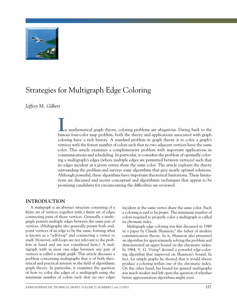
among a group of teams over the course of a season. Any pair of teams will be required to play each other a number of times (possibly zero). Each team is to play at most one game per day, with no special requirements or preferences regarding the days on which they play. Given the number of games to be played between each pair of teams, what is the minimum number of days needed to schedule all of the games? Table 1 gives an example showing the required games to be scheduled

among a league of nine teams. For example, Team 4 is to play Team 3 twice, whereas it is to have three games each with Teams 1, 5, and 6 and no games with any other teams.

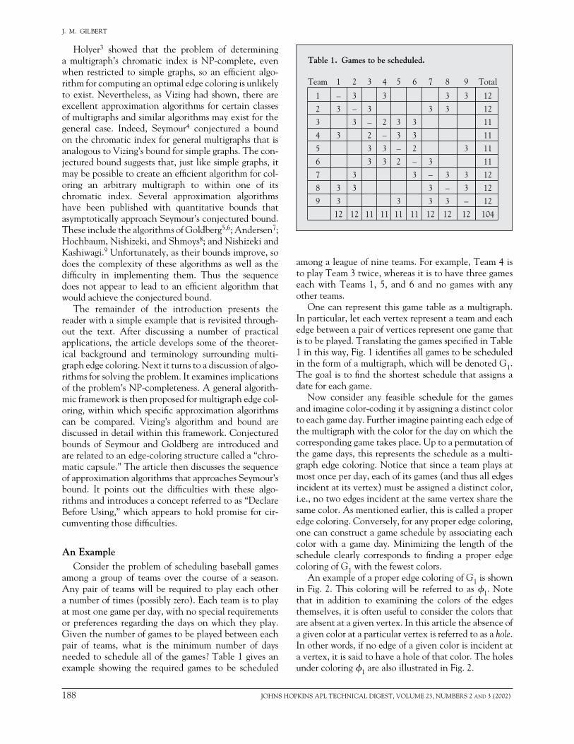
One can represent this game table as a multigraph. In particular, let each vertex represent a team and each edge between a pair of vertices represent one game that is to be played. Translating the games specified in Table 1 in this way, Fig. 1 identifies all games to be scheduled in the form of a multigraph, which will be denoted G1. The goal is to find the shortest schedule that assigns a date for each game.

Now consider any feasible schedule for the games and imagine color-coding it by assigning a distinct color to each game day. Further imagine painting each edge of the multigraph with the color for the day on which the corresponding game takes place. Up to a permutation of the game days, this represents the schedule as a multi-graph edge coloring. Notice that since a team plays at most once per day, each of its games (and thus all edges incident at its vertex) must be assigned a distinct color, i.e., no two edges incident at the same vertex share the same color. As mentioned earlier, this is called a proper edge coloring. Conversely, for any proper edge coloring, one can construct a game schedule by associating each color with a game day. Minimizing the length of the schedule clearly corresponds to finding a proper edge coloring of G1 with the fewest colors.

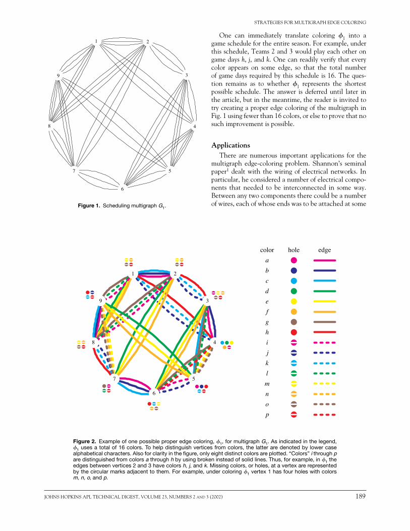
An example of a proper edge coloring of G1 is shown in Fig. 2. This coloring will be referred to as 1. Note that in addition to examining the colors of the edges themselves, it is often useful to consider the colors that are absent at a given vertex. In this article the absence of a given color at a particular vertex is referred to as a hole. In other words, if no edge of a given color is incident at a vertex, it is said to have a hole of that color. The holes under coloring 1 are also illustrated in Fig. 2.

Table 1. Games to be scheduled.

Team 1 2 3 4 5 6 7 8 9 Total

1 – 3 3 3 3 12

2 3 – 3 3 3 12

3 3 – 2 3 3 11

4 3 2 – 3 3 11

5 3 3 – 2 3 11

6 3 3 2 – 3 11

7 3 3 – 3 3 12

8 3 3 3 – 3 12

9 3 3 3 3 – 12

12 12 11 11 11 11 12 12 12 104



One can immediately translate coloring 1 into a game schedule for the entire season. For example, under this schedule, Teams 2 and 3 would play each other on game days h, j, and k. One can readily verify that every color appears on some edge, so that the total number of game days required by this schedule is 16. The ques-tion remains as to whether 1 represents the shortest possible schedule. The answer is deferred until later in the article, but in the meantime, the reader is invited to try creating a proper edge coloring of the multigraph in Fig. 1 using fewer than 16 colors, or else to prove that no such improvement is possible.

ApplicationsThere are numerous important applications for the

multigraph edge-coloring problem. Shannon’s seminal paper1 dealt with the wiring of electrical networks. In particular, he considered a number of electrical compo-nents that needed to be interconnected in some way. Between any two components there could be a number of wires, each of whose ends was to be attached at some Figure 1. Scheduling multigraph G1.

Figure 2. Example of one possible proper edge coloring, 1, for multigraph G1. As indicated in the legend, 1 uses a total of 16 colors. To help distinguish vertices from colors, the latter are denoted by lower case alphabetical characters. Also for clarity in the figure, only eight distinct colors are plotted. “Colors” i through p are distinguished from colors a through h by using broken instead of solid lines. Thus, for example, in 1 the edges between vertices 2 and 3 have colors h, j, and k. Missing colors, or holes, at a vertex are represented by the circular marks adjacent to them. For example, under coloring 1 vertex 1 has four holes with colors m, n, o, and p.

1 2

3

4

5

6

7

8

9

1 2

3

4

5

6

7

8

9

edgeholecolorabcdefghijklmnop


J. M. GILBERT

port on a component. Wires were bundled into cables and, in order to distinguish between them, one was to assign each wire a color such that no two wires arriv-ing at the same component had the same color. The goal was to minimize the number of colors needed to so wire the given network. Mapping components into vertices and wires into edges, this clearly corresponds to multigraph edge coloring.

Multigraph edge coloring can also be applied in many practical scheduling problems. For example, consider the task of coordinating scans among a set of similar active sensors {s1, s2, …, sS} over a set of targets {t1, t2, …, tT}. Assume that a sensor can only illuminate one target at a time. Also, to avoid mutual interference, assume that no two sensors should illuminate the same target simultaneously. Now, given a matrix M = [mi,j], where mi,j specifies the number of times sensor si is to measure target tj over the course of its scan, and assuming that each measurement takes time t, what is the minimum time needed to complete the scans of all sensors? To for-mulate the problem graph-theoretically, create a multi-graph with a vertex for each sensor and one for each target. Between any given sensor and target vertices, introduce an edge for every measurement that the sensor is required to take of the target. Thus for any i and j, there should be mi,j edges between the vertices for sensor si and target tj. If one assigns a color to each measure-ment interval, then any schedule for the sensor mea-surements can be mapped into a corresponding color-ing of the edges in this multigraph and vice versa. Also, since each target should be scanned by only one sensor at a time and since sensors illuminate only one target at a time, this edge coloring will be proper. Clearly, if the minimum number of colors needed in a proper edge coloring of the multigraph is , then the minimum time needed to complete all sensor scans is t.

As a third example (through which the author became interested in the problem), consider a commu-nications network linking a number of nodes. A node generally communicates directly with only a subset of the other nodes called its neighbors. Suppose that the network operates on a cyclic, time-division multiplexed schedule and that each node can communicate with only one neighboring node at a time. In any atomic time interval, or frame, nodes must thus be paired off with each other for communications. Assume that the net-work has a specified communications load such that for any pair of neighboring nodes one is given the number of frames in which they are required to communicate over the course of the schedule. Since the schedule is periodic, in order to maximize throughput, the goal is to construct a schedule that includes every required com-munication while minimizing its period, or length. Let-ting each node be a vertex and placing an edge between two nodes for each communication frame they require, one obtains a multigraph. Treating each color as a frame

in the schedule, an optimal proper edge coloring cor-responds to a minimum length schedule satisfying the communication requirements.

The multigraph edge-coloring problem is applicable in many other scheduling problems and has practical application in such diverse fields as statistical analysis and experimental design, file transfer protocols for com-puter networks, matrix algebra, and tensor calculus. The interested reader is referred to Fiorini and Wilson10 for an excellent summary of some of these applications.

THEORETICAL BACKGROUND

Definitions and NomenclatureBefore discussing the theory behind the multigraph

edge-coloring problem, some definitions and nomen-clature are needed. The concept of a multigraph, G = [V(G), E(G)] with vertex set V(G) and edge set E(G) was introduced above. The number of vertices it con-tains is called its order and is denoted here by n(G). The number of edges is denoted by m(G). The number of edges incident at a given vertex v is called the degree of v and will be denoted by dG(v). A vertex of degree 0 is said to be isolated. For any given pair of distinct vertices x and y, the number of edges joining them is called the edge multiplicity of x and y and is denoted by G(x, y). The maximum degree among all the vertices is denoted by (G). The maximum edge multiplicity over all pairs of vertices is denoted by (G).

A subgraph S of G is any multigraph whose vertex and edge sets, V(S) and E(S), are subsets, respectively, of V(G) and E(G). This is written S G. Suppose that two vertices, v and u, in G are connected by an alternat-ing sequence of edges and vertices (v = v0, e1, v1, e2, v2, …, eL, vL = u), where vi1 and vi are the endpoints of ei (1 ≤ i ≤ L) and where the vertices are all distinct, except possibly for u and v. A subgraph composed of these vertices and edges is called a simple path if u ≠ v or a simple cycle if u = v. Its length is the number of edges L it contains.

An edge coloring of G is a mapping of its edges into some set of colors C. It is said to be proper if no two edges incident at a common vertex share the same color. The minimum number of colors required for a proper edge coloring of G is called its chromatic index and is denoted by (G). For any color x, the edges assigned that color under a given coloring are referred to as x-edges. Also, as mentioned above, this article refers to the absence of a given color at a particular vertex as a hole. More for-mally, <v, x> is a hole of G with respect to if v is a vertex in V(G), x is a color in C, and there is no x-edge incident at v under . The number of holes at vertex v in G under will be denoted by hG,(v). Notice that for any proper coloring of any G, and for any v V(G), dG(v) + hG,(v) = k, where k is the number of colors in



C. A set of vertices with more than one hole of the same color is said to have a hole color duplication. (In the remainder of this article, note that the argument or subscript G appearing on various quantities like those defined above will often be omitted for notational con-venience if it is clear from the context.)

Chromatic Components and the Chromatic Adjacency Graph

Under a proper edge coloring of G, let X be any subset of the colors and imagine removing edges from G, keeping only those whose colors are in X. From a given vertex v, consider the set of all vertices and edges in the resulting multigraph that can be reached via a simple path. The subgraph of G consisting of these ver-tices and edges is called an X-chromatic component of G under . Chromatic components are sometimes called Kempe components after A. B. Kempe, who published the first attempted proof of the four-color map theo-rem.11 He made the simple but important observation that any permutation of colors within such a chromatic component yields another proper coloring. Using these chromatic component recolorings, he attempted to show that four colors were sufficient to color the regions of any map that can be drawn on a planar or spherical surface so that no two regions with a common bound-ary have the same color. Although his proof was flawed, Kempe’s chromatic component recolorings form the basis of many, if not most, algorithms for both vertex and edge-coloring problems.

Chromatic components involving pairs of colors will be of special interest in this article. Let x and y be any two distinct colors appearing in a proper edge col-oring of G and consider its {x, y}-chromatic compo-nents. Since there is at most one x-edge and at most one y-edge incident at any vertex, one can readily see that each {x, y}-chromatic component is either a simple path, a simple cycle, or an isolated vertex. Edges along the paths and cycles must alternate between the two colors of the component. Notice that a two-colored chro-matic component has only one recoloring, obtained by exchanging its two colors.

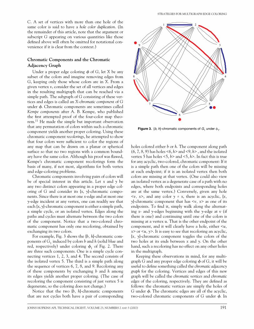
For example, Fig. 3 shows the {b, h}-chromatic com-ponents of G1 induced by colors b and h (solid blue and red, respectively) under coloring 1 of Fig. 2. There are three such components. One is a simple cycle con-necting vertices 1, 2, 3, and 4. The second consists of the isolated vertex 5. The third is a simple path along the sequence of vertices 6, 7, 8, and 9. Recoloring any of these components by exchanging b and h among its edges yields another proper coloring. (The case of recoloring the component consisting of just vertex 5 is degenerate, so the coloring does not change.)

Notice that the two {b, h}-chromatic components that are not cycles both have a pair of corresponding

holes colored either b or h. The component along path (6, 7, 8, 9) has holes <6, h> and <9, h> , and the isolated vertex 5 has holes <5, b> and <5, h>. In fact this is true for any acyclic, two-colored, chromatic component: If it is a simple path then one of the colors will be missing at each endpoint; if it is an isolated vertex then both colors are missing at that vertex. (One could also view an isolated vertex as a degenerate case of a path with no edges, where both endpoints and corresponding holes are at the same vertex.) Conversely, given any hole <v, x>, and any color y ≠ x, there is an acyclic, {x, y}-chromatic component that has <v, x> as one of its endpoints. To find it, simply walk along the alternat-ing x- and y-edges beginning with the y-edge at v (if there is one) and continuing until one of the colors is missing at a vertex u. That is the other endpoint of the component, and it will clearly have a hole, either <u, x> or <u, y>. It is easy to see that recoloring an acyclic, {x, y}-chromatic component toggles the colors of the two holes at its ends between x and y. On the other hand, such a recoloring has no effect on any other holes in the multigraph.

Keeping these observations in mind, for any multi-graph G and any proper edge coloring of G, it will be useful to define something called the chromatic adjacency graph for the coloring. Vertices and edges of this new graph will be called the chromatic vertices and chromatic edges of the coloring, respectively. They are defined as follows: the chromatic vertices are simply the holes of G under . The chromatic edges are all of the acyclic, two-colored chromatic components of G under . In

Figure 3. {b, h}-chromatic components of G1 under 1.

1 2

3

4

5

6

7

8

9


J. M. GILBERT

particular, for any distinct pair of colors x and y in the coloring, an acyclic, {x, y}-chromatic component will be referred to as an {x, y}-chromatic edge. The endpoints of a chromatic edge are the two holes associated with that chromatic component, which are guaranteed to exist by the observations made above. Two holes, = <v, x> and = <u, y>, are said to be chromatically adjacent if they are endpoints of a common chromatic edge. More spe-cifically, for distinct colors p and q, holes and will be said to be {p, q}-chromatically adjacent or chromatically adjacent via p and q if {x, y} {p, q} and the two holes are the endpoints of the same {p, q}-chromatic edge. As pointed out above, recoloring a {p, q}-chromatic edge toggles the colors of its endpoint holes, but leaves all other holes untouched.

Because of their central importance in the remainder of the article, it is worth emphasizing the distinction between the vertices and edges in multigraph G and the chromatic vertices and chromatic edges in its chromatic adjacency graph under a coloring . The vertices of G are the nodes of the multigraph, and its edges are the direct connections between them. The chromatic vertices, on the other hand, are the holes in G under . The chro-matic edges are not edges of G. Rather, they are simple paths or isolated vertices in G that correspond to its acy-clic, two-colored chromatic components under .

As an example, Fig. 3 shows four chromatic vertices, namely the holes <5, b>, <5, h>, <6, h>, and <9, h>. It shows two chromatic edges, one being the isolated vertex 5 and the other being the {b, h}-chromatic com-ponent along path (6, 7, 8, 9). The former chromatic edge connects the chromatic vertices (holes) <5, b> and <5, h>, and the latter connects holes <6, h> and <9, h>. Thus <5, b> and <5, h> are chromatically adja-cent, as are <6, h> and <9, h> (via the colors b and h).

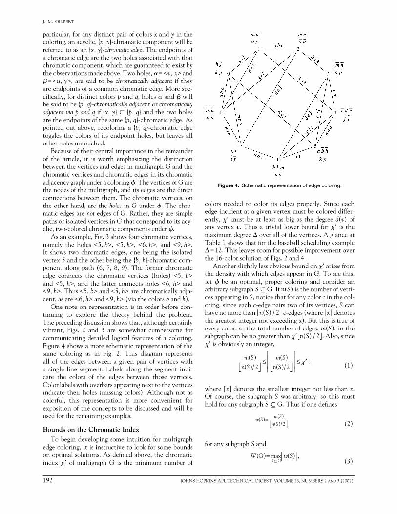
One note on representation is in order before con-tinuing to explore the theory behind the problem. The preceding discussion shows that, although certainly vibrant, Figs. 2 and 3 are somewhat cumbersome for communicating detailed logical features of a coloring. Figure 4 shows a more schematic representation of the same coloring as in Fig. 2. This diagram represents all of the edges between a given pair of vertices with a single line segment. Labels along the segment indi-cate the colors of the edges between those vertices. Color labels with overbars appearing next to the vertices indicate their holes (missing colors). Although not as colorful, this representation is more convenient for exposition of the concepts to be discussed and will be used for the remaining examples.

Bounds on the Chromatic IndexTo begin developing some intuition for multigraph

edge coloring, it is instructive to look for some bounds on optimal solutions. As defined above, the chromatic index of multigraph G is the minimum number of

colors needed to color its edges properly. Since each edge incident at a given vertex must be colored differ-ently, must be at least as big as the degree d(v) of any vertex v. Thus a trivial lower bound for is the maximum degree over all of the vertices. A glance at Table 1 shows that for the baseball scheduling example = 12. This leaves room for possible improvement over the 16-color solution of Figs. 2 and 4.

Another slightly less obvious bound on arises from the density with which edges appear in G. To see this, let be an optimal, proper coloring and consider an arbitrary subgraph S G. If n(S) is the number of verti-ces appearing in S, notice that for any color c in the col-oring, since each c-edge pairs two of its vertices, S can have no more than n(S) / 2 c-edges (where x denotes the greatest integer not exceeding x). But this is true of every color, so the total number of edges, m(S), in the subgraph can be no greater than n(S) / 2. Also, since is obviously an integer,

m S

n S

m S

n S

( )( )/

( )( )/

,2 2

≤

≤ ′� (1)

where ⎡x denotes the smallest integer not less than x. Of course, the subgraph S was arbitrary, so this must hold for any subgraph S G. Thus if one defines

w S

m S

n S( )

( )( )/

= 2 (2)

for any subgraph S and

W G w S

S G( ) max ( ) ,= ⊆ (3)

Figure 4. Schematic representation of edge coloring.



then certainly W = W(G) is another lower bound for . Unfortunately, since the number of subgraphs of G is exponential in n(G), this definition does not provide an efficient algorithm for computing W. However, any par-ticular subgraph or group of subgraphs can be examined to determine a lower bound on . In particular, for the baseball scheduling example, let S = G1. Again referring to Table 1, notice that the sum of all the game counts is 104. However, this counts each of the games twice (once for each team), so the total number of games to be played, and also the number of edges in G1, is m(G1) = 52. With n(G1) = 9 teams playing, w(G1) = 52/9/2 = 52/4 = 13. This shows that, even though no vertex in G1 has more than 12 neighbors, the density of its edges is too great to permit a solution with less than 13 colors. Of course, whether one can actually find a coloring that realizes this bound is another question and will be the subject of discussion in subsequent sections.

EDGE-COLORING ALGORITHMS

NP-CompletenessOne of the first questions typically asked when inves-

tigating a computational problem is whether it is tracta-ble. For practical purposes, the time an algorithm takes to compute a solution should not grow too rapidly with input size. Computer scientists formalize this notion as the computational complexity of the algorithm. One usually considers an algorithm to be efficient (from the theoretical standpoint) if its run time is bounded by some polynomial function of an appropriate measure of its input size. The class of problems that can be solved by algorithms running in polynomial time is called P. However, there is a large and important class of prob-lems, known as NP, for which no polynomial algorithms appear to exist. For such problems, it seems very likely that any algorithm solving them will require run times exceeding any polynomial function of their input size. A subclass of the problems in NP has the important property that if one were to find a polynomial algorithm for solving any one of them, then all other problems in NP could also be solved in polynomial time. Thus, in a sense, each of these problems, which are called NP-complete, is just as hard as any other problem in NP.

The standard vertex coloring problem had been chal-lenging mathematicians and computer scientists long before the early 1970s when these concepts were intro-duced, and not surprisingly was among the first prob-lems demonstrated to be NP-complete. In particular, Karp12 showed that the problem of finding an optimal vertex coloring for a graph is NP-complete. The issue was not resolved quite so quickly for edge colorings. Since edge adjacencies at vertices are more constrained than vertex adjacencies across edges, edge colorings are more highly structured than vertex colorings. One

might hope that with some ingenuity a clever algorithm could be developed to exploit this additional structure so as to find an optimal edge coloring efficiently.

Unfortunately, this is apparently not the case. Ulti-mately, the problem of finding an optimal edge color-ing for an arbitrary multigraph G was shown also to be NP-complete by Holyer3 in 1981. In fact, his construc-tion shows that the problem of determining is NP-complete even when G is a simple graph and its maxi-mum degree is no greater than 3. (One can better appreciate the elegance and simplicity of Holyer’s con-struction for proving the NP-completeness of edge col-oring by considering the difficulties described in an investigation13 of the same issue and published not long before his proof.)

At first glance, one might think that a result as strong as Holyer’s dashes all hope of finding a good multigraph edge-coloring algorithm. However, although it seems very unlikely that an efficient algorithm will ever be found to compute an optimal solution, one can never-theless look for approximation algorithms that can effi-ciently compute solutions that are nearly optimal. For-tunately, the structure imposed on edge coloring by adjacency constraints can be exploited to develop such approximation algorithms. Recall that no coloring can do better (use fewer) than max{, W} colors. It is of con-siderable practical and theoretical interest if an approx-imation algorithm can be shown to do no worse than some upper bound. The next several sections will dis-cuss this issue and provide upper bounds on several algo-rithms showing that, although not optimal, they pro-duce very good solutions efficiently.

An Algorithmic Framework for Edge ColoringBefore turning to this analysis, it is useful to provide

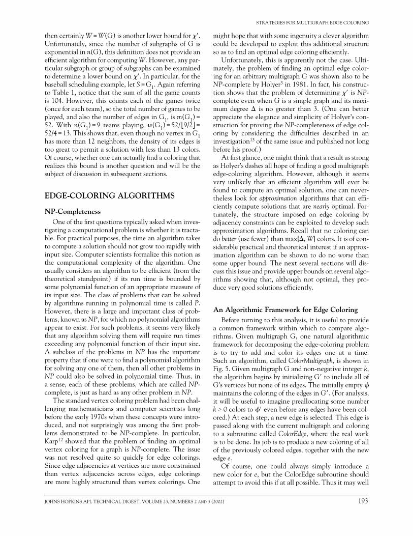
a common framework within which to compare algo-rithms. Given multigraph G, one natural algorithmic framework for decomposing the edge-coloring problem is to try to add and color its edges one at a time. Such an algorithm, called ColorMultigraph, is shown in Fig. 5. Given multigraph G and non-negative integer k, the algorithm begins by initializing G to include all of G’s vertices but none of its edges. The initially empty maintains the coloring of the edges in G. (For analysis, it will be useful to imagine preallocating some number k ≥ 0 colors to even before any edges have been col-ored.) At each step, a new edge is selected. This edge is passed along with the current multigraph and coloring to a subroutine called ColorEdge, where the real work is to be done. Its job is to produce a new coloring of all of the previously colored edges, together with the new edge e.

Of course, one could always simply introduce a new color for e, but the ColorEdge subroutine should attempt to avoid this if at all possible. Thus it may well


J. M. GILBERT

shuffle the colors among the previously processed edges to accommodate the new edge within the existing pal-ette of colors. This same basic algorithmic framework is used in all of the edge-coloring algorithms discussed in this article. The focus will be on exactly how the ColorEdge subroutine accomplishes its task.

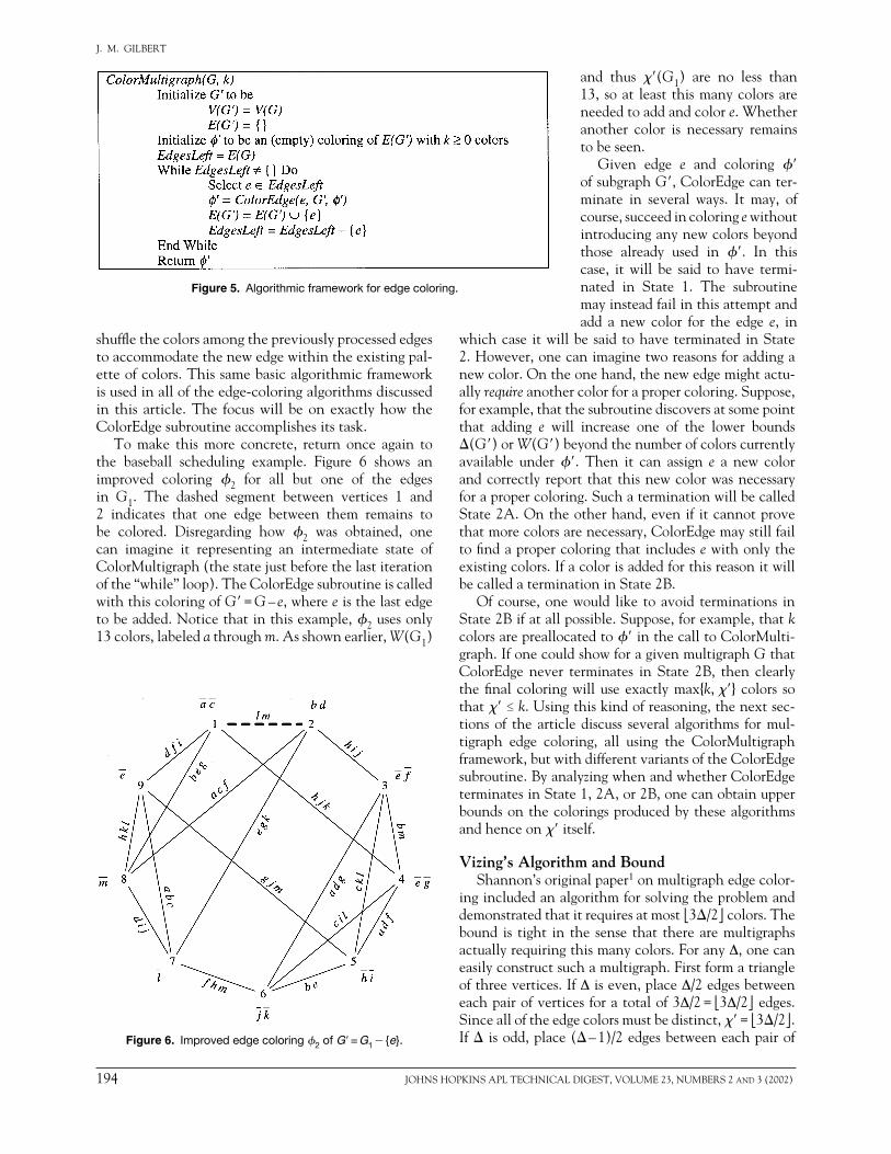
To make this more concrete, return once again to the baseball scheduling example. Figure 6 shows an improved coloring 2 for all but one of the edges in G1. The dashed segment between vertices 1 and 2 indicates that one edge between them remains to be colored. Disregarding how 2 was obtained, one can imagine it representing an intermediate state of ColorMultigraph (the state just before the last iteration of the “while” loop). The ColorEdge subroutine is called with this coloring of G = G – e, where e is the last edge to be added. Notice that in this example, 2 uses only 13 colors, labeled a through m. As shown earlier, W(G1)

and thus (G1) are no less than 13, so at least this many colors are needed to add and color e. Whether another color is necessary remains to be seen.

Given edge e and coloring of subgraph G, ColorEdge can ter-minate in several ways. It may, of course, succeed in coloring e without introducing any new colors beyond those already used in . In this case, it will be said to have termi-nated in State 1. The subroutine may instead fail in this attempt and add a new color for the edge e, in

Figure 5. Algorithmic framework for edge coloring.

Figure 6. Improved edge coloring 2 of G = G1 {e}.

which case it will be said to have terminated in State 2. However, one can imagine two reasons for adding a new color. On the one hand, the new edge might actu-ally require another color for a proper coloring. Suppose, for example, that the subroutine discovers at some point that adding e will increase one of the lower bounds (G) or W(G) beyond the number of colors currently available under . Then it can assign e a new color and correctly report that this new color was necessary for a proper coloring. Such a termination will be called State 2A. On the other hand, even if it cannot prove that more colors are necessary, ColorEdge may still fail to find a proper coloring that includes e with only the existing colors. If a color is added for this reason it will be called a termination in State 2B.

Of course, one would like to avoid terminations in State 2B if at all possible. Suppose, for example, that k colors are preallocated to in the call to ColorMulti-graph. If one could show for a given multigraph G that ColorEdge never terminates in State 2B, then clearly the final coloring will use exactly max{k, } colors so that ≤ k. Using this kind of reasoning, the next sec-tions of the article discuss several algorithms for mul-tigraph edge coloring, all using the ColorMultigraph framework, but with different variants of the ColorEdge subroutine. By analyzing when and whether ColorEdge terminates in State 1, 2A, or 2B, one can obtain upper bounds on the colorings produced by these algorithms and hence on itself.

Vizing’s Algorithm and BoundShannon’s original paper1 on multigraph edge color-

ing included an algorithm for solving the problem and demonstrated that it requires at most 3/2 colors. The bound is tight in the sense that there are multigraphs actually requiring this many colors. For any ∆, one can easily construct such a multigraph. First form a triangle of three vertices. If ∆ is even, place ∆/2 edges between each pair of vertices for a total of 3∆/2 = 3∆/2 edges. Since all of the edge colors must be distinct, = 3/2. If is odd, place ( – 1)/2 edges between each pair of



vertices and then add one more edge between any pair. Notice that the maximum degree is indeed and that there are 3( – 1)/2 + 1 = 3/2 edges, which again must all be distinct, so = 3/2.

Unfortunately, Shannon’s algorithm does not nat-urally fit the framework of ColorMultigraph. We will return to his bound momentarily, but, instead of look-ing at his algorithm, we will focus on a method devised 15 years later by Vizing.2 Vizing’s algorithm has the form of ColorMultigraph. His simple but important technique for the ColorEdge subroutine is perhaps the greatest single algorithmic contribution to edge- coloring problems. To see how it works, consider any call, ColorEdge(e, G, ), with proper coloring of subgraph G and with new edge e to be added. Let v0 and v1 be the endpoints of the uncolored edge e. Start-ing with edge e = e1, let F = (e1, e2, …, er) be a sequence of edges in E(G) {e}, each of which is incident at v0, but whose opposite endpoints are distinct. For all i, 2 ≤ i ≤ r, let vi denote the opposite endpoint of ei, and let ci denote the color of ei under , i.e., ci = (ei). Now, suppose that there is at least one hole <v0, c> at v0 and that for each edge ei, 2 ≤ i ≤ r, there is a hole <vi–1, ci> at the endpoint of the previous edge having the same color, ci, as edge ei. Then F is called a Vizing fan sequence. Figure 7a shows such a fan sequence.

In this particular fan sequence, notice that there happen to be holes of the same color c at v0 and vr. Viz-ing’s remarkable observation was that if there are any hole color duplications among the vertices in F (in other words, among VF = {v0, v1, …, vr}), then through a suitable recoloring of , the new edge e can be col-ored without introducing any new colors to the palette. Vizing provided a ColorEdge subroutine to accomplish this. In the terminology developed above, if VF contains any hole color duplications, then his ColorEdge routine terminates in State 1. To follow the algorithm, let and be two distinct holes in VF with the same color c. Since ≠ , they must obviously be at different vertices.

Consider the possible pairs of vertices where and can appear. First, suppose that one of the holes, say

, is at v0. By reducing r (truncating the fan sequence) if necessary, one can assume, without loss of generality, that appears at vr, the endpoint of the last edge. This is the situation illustrated in Fig. 7a, where = <v0, c> and = <vr, c>. In the simplest case, suppose that r = 1 so that color c is absent at both endpoints v0 and v1 of e. Then ColorEdge assigns edge e the color c and ter-minates in State 1. On the other hand, suppose that r > 1. Referring to Fig. 7a, notice that color c2 is missing at v1. ColorEdge removes it from edge e2 and shifts it to edge e1, leaving e2 uncolored. But color c3 is absent at v2, and ColorEdge in turn shifts it from edge e3 to color e2. Continuing in this way, a new coloring is obtained in which er is the uncolored edge. But now, since c is miss-ing at both v0 and vr, ColorEdge uses it to color er and again terminates in State 1. The new coloring , which includes the new edge, appears in Fig. 7b. This tech-nique is called a Vizing fan shift, for obvious reasons.

One can alternately view the fan shift starting with the last edge. Since a duplication of hole color c initially appears between the endpoints of edge er, the subrou-tine can recolor it with this color. Doing so produces holes of color cr appearing at v0 and vr. But now a dupli-cation of hole color cr arises between v0 and vr1, which ColorEdge uses to recolor edge er1. As seen from this standpoint, the Vizing fan shift is a process for migrating a hole color duplication that appears somewhere along the fan sequence back to the initial vertex pair v0 and v1, where it can be used to color the new edge e.

Using the Vizing fan shift shows that if the hole color duplication in VF involves any hole at v0, then Color-Edge terminates in State 1. A corollary to this observa-tion is that if any hole at v0 is not chromatically adjacent to every hole among the vertices VF – {v0}, then ColorEdge can again reach State 1. To see this, suppose that vi is the first vertex along the sequence for which there are two holes <v0, c> and <vi, ci> that are not chromatically adjacent. By recoloring the {c, ci}-chromatic edge beginning at <vi, ci>, ColorEdge obtains a new coloring with hole <vi, c>, while not otherwise affecting hole or edge colors along

Figure 7. Vizing fan sequence (a) and shift (b).

F = (e1, e2, …, ei). Then F is a Vizing fan sequence with a hole color duplication between vertices v0 and vi, and the subroutine uses the fan shift described above to color e and terminate in State 1.

The possibility remains that the hole color duplication does not involve any holes at v0. Then there are two distinct vertices vi and vj, 1 ≤ i < j ≤ r with holes of the same color, say = <vi, ci> and = <vj, cj>, where ci = cj = c*. Now consider the hole = <v0, c>. Clearly c ≠ c* since no hole color at v0 is duplicated in


J. M. GILBERT

VF. Notice that cannot be chromatically adjacent to both and , since the {c*, c}-chromatic edge beginning at has only one other endpoint. Since there is a hole in VF – {v0} that is not chromatically adjacent to , the above corollary applies, and once again ColorEdge ter-minates in State 1.

Notice the overall strategy employed by Vizing’s ColorEdge algorithm. It explores a structure (the fan sequence F) and searches for holes appearing at the ver-tices VF of that structure. If a hole color duplication is found among those vertices, a procedure is provided (the Vizing fan shift with possible chromatic edge recol-orings) to migrate the duplication back to vertices v0 and v1 where it can be exploited to color the new edge e. Abstracting this strategy provides a powerful paradigm for edge coloring. Many algorithms can be viewed as variants of the ColorEdge subroutine using this same underlying paradigm, but with different structures and procedures for migrating hole color duplications.

Using his ColorEdge subroutine as described, and apply-ing a clever pigeonhole argument, Vizing was able to dem-onstrate an upper bound on the chromatic index for a multigraph G. In particular, for any v V(G), define

d v d v v xG*

Gx V G

G( ) ( ) max ( , )( )

= +⊆

�

and let

Vizing G d vv V(G)

G*( ) max ( ).=

⊆

Vizing proved that for any G, his algorithm colors G with no more than Vizing(G) colors, and hence (G) ≤ Vizing(G). This result is known as Vizing’s theorem. For any multigraph, the bound is clearly no greater than the sum of the maximum degree and max-imum multiplicity, + . In the case of a simple graph, since ≤ 1, this gives the extremely strong result that ≤ ≤ + 1. Surprisingly, even though the question of computing is NP-complete, Vizing’s simple algo-rithm described above produces a coloring within one of the optimal number of colors.

Shannon’s triangles described earlier show that the situation is not so fortunate for multigraphs. Indeed, for these triangles, = 3/2 colors. On the other hand, it is not difficult to show (see, for example Fiorini and Wilson14) that Vizing’s theorem implies that no multi-graph requires more than this many colors.

Conjectures of Seymour and GoldbergNot all multigraphs need as many colors as Shan-

non’s bound allows. Consider again the coloring 2 shown in Fig. 6, which uses 13 colors. Even if one adds a new color to finish coloring G1, this is still less than the Shannon bound of 3(G1)/2 = 3 · 12/2 = 18. (For that matter, the original coloring shown in Figs.

2 and 4 used 16 colors, which was already less than Shannon’s bound.) Vizing’s algorithm also turns out to be of no assistance in trying to add the last edge in Fig. 6. Inspection of that illustration reveals that no hole color duplication appears on any fan sequence beginning with edge e. One might therefore ask whether improved recoloring algorithms and upper bounds on the chro-matic index can be found for this and other multigraphs.

In pursuing this question, researchers have been led to explore the reasons for which the chromatic index of a multigraph G would become elevated beyond the lower bounds or W. To discuss this, Goldberg6 refers to a multigraph for which = W as elementary. Over time, various infinite classes of nonelementary multigraphs have been found for which = + 1. On the other hand, every known multigraph for which > + 1 is elementary. This observation led Seymour4 to conjecture that for any multigraph, ≤ max{ + 1, W}. Goldberg6 strengthened this to con-jecture that (a) if > + 1, then = W and (b) if > W + 1, then = . [Part (a) is equivalent to Sey-mour’s conjecture.]

Suppose for the moment that Seymour’s conjecture is true. Then in analogy with Vizing’s theorem for simple graphs, any multigraph has a chromatic index within one color of the lower bound max{, W}. Furthermore, even if P ≠ NP, the NP-completeness of multigraph edge coloring does not preclude the possibility of find-ing an efficient approximation algorithm that uses at most max{ + 1, W} colors. For multigraphs in which W < + 1, even if the conjecture were true, the ques-tion of whether = or = + 1 would remain NP- complete and an efficient algorithmic answer seems unlikely. On the other hand, for multigraphs in which W ≥ + 1, the conjecture predicts that = W. One could conceivably find an efficient algorithm that would produce an optimal coloring for such multigraphs. For this reason, Seymour’s conjecture in the case of W ≥ + 1 has been the main focus of the author’s research into multigraph edge coloring and will be the central topic in the remainder of the article. (The reader less interested in the theoretical details may wish to skip the next two subsections and proceed directly to the discussion of “Specific Algorithms with Quantitative Edge-Coloring Bounds.”)

Chromatic CapsulesProceeding with the assumption that W ≥ + 1 and

thinking again in terms of the edge-by-edge coloring strategy used in ColorMultigraph, suppose the algorithm is at an intermediate stage and has an optimal coloring of some G for which (G) = W(G) = k colors. It is useful to consider the situation in which adding the next edge e to G increases W and thus . By study-ing this “straw” and how it breaks the camel’s back, one can begin to design a ColorEdge subroutine that is more



likely to terminate in the desirable States 1 and 2A and to avoid State 2B. If the new edge increases W, then certainly G must have a subgraph S* containing both endpoints of e and for which ⎡w(S*) = k, but where ⎡w(S* e) = k + 1. [Here, S* e means the multigraph with vertices V(S*) and edges E(S*) {e}.] But then,

m S

n Sk

m S e

n S e

m S

n S

( *)( *) /

( * )( * ) /

( *)( *) /

,

21 1

2

12

+ = + = ∪∪

= +

(4)

which can only be true if

m(S*) = k n(S*)/2 = (G) n(S*)/2 .

In this article, if (G) ≥ (G) + 1, a subgraph S* G for which m(S*) = (G) n(S*)/2 is called a chromatic capsule of G.

Chromatic capsules have some interesting features. While it is beyond the scope of this article to elaborate on all their properties, one important structural charac-teristic deserves mention. If S* is a chromatic capsule of G, it is not hard to show that under any optimal col-oring, among the holes within S* and the edges that leave S*, each color appears exactly once. To see this, consider any optimal coloring of G and notice that since (G) ≥ (G) + 1, there is at least one hole at each vertex. Suppose that S* has an even number of vertices. Then for each color c there are n(S*)/2 c-edges appearing in S* and pairing its vertices. This is impos-sible, since it would mean that each color is present at every vertex. Thus n(S*) must be odd. In this case, for each color c, there are n(S*)/2 c-edges in S* that pair all but one of its vertices. For that one unpaired vertex, the color c is either absent or there is a c-edge leaving S*; i.e., for any color c, S* contains exactly one c-hole or one c-edge leaving S*.

Since this is true of every optimal coloring of G, if both endpoints of e are in S*, then the ColorEdge sub-routine has no hope of introducing a hole color duplica-tion between those endpoints unless it adds a new color to the palette. In other words, having both endpoints of e in the same chromatic capsule of G is a sufficient condition to imply (G) < (G e). If Seymour’s conjecture is true and if (G) ≥ (G) + 1, then it is also a necessary condition. The sufficiency just noted is equivalent to the simple observation that led to the definition of W(G). However, it is useful to think of the property in terms of constraints on hole colors, since this maps naturally into the generic paradigm for the ColorEdge subroutine mentioned earlier.

A Family of Approximation AlgorithmsConsider again the subroutine call ColorEdge(e, G,

). Suppose that uses k colors and that G contains a subgraph S with e’s endpoints and no hole color dupli-cations. Then one can show that

′ ′ ∪ ≥ ′ ∪ ≥ ′ − +( ) ( )

( ( ) )( )

.G e G ek n S

n S1 2

(5)

In this case, if ColorEdge terminates in State 2B and adds a new color to the palette, the resulting coloring of G e uses k = k + 1 colors, where

(6)

Furthermore, since k is an integer,

k

n Sn S

G en Sn S

n Sn S

G en Sn S

≤−

′ ∪ + −−

≤−

′ ′ ∪ + −−

( )( )

( )( )( )

( )( )

( )( )( )

.

131

131

One can exploit this observation to design a family of ColorEdge algorithms and bound the number of colors they use on arbitrary multigraphs. The algo-rithms in this family follow a paradigm abstracted from the strategy used by Vizing. Under this paradigm, given a colored multigraph G and new edge e, a par-ticular ColorEdge algorithm has an associated explo-ration family = (e, G, ) of subgraphs of G e, together with a ranking function, , over . and satisfy several properties: Let Se denote the subgraph consisting of edge e and its endpoints. Then Se and it is the unique minimum of the ranking function, i.e., (Se) < (S) for all S – {Se}. Also, for all S , V(Se) V(S), and if V(Se) V(S*) for some chromatic capsule S*, then V(S) V(S*). Beginning with Se = S0, ColorEdge attempts to find a sequence of subgraphs S0, S1, S2, …, in , such that the number of vertices is strictly increasing.

Suppose one of these subgraphs, say Si, has a hole color duplication. Then it certifies that e’s endpoints are not contained in any chromatic capsule S* [since otherwise V(Si) V(S*), which is impossible because of the duplication]. In this case, ColorEdge calls a reduction procedure, Reduce, which (possibly) recolors G to produce another subgraph in the exploration family. The new subgraph, Reduce(Si), also contains

k = k +n S G e

n Sn S G e n S

n Sn S G e n S

n S

′ ≤ ′ ∪ −−

+

= ′ ∪ + −−

≤ ′ ′ ∪ + −−

12

11

31

31

( ) ( )( )

( ) ( ) ( )( )

( ) ( ) ( )( )

.


J. M. GILBERT

a duplication, but [Reduce(Si)] < (Si). ColorEdge repeats this reduction procedure until ultimately the duplication appears on Se, namely at the endpoints of e. Using the duplication to color e, it thereby colors G e with no new colors, and terminates in State 1.

Suppose instead that ColorEdge discovers a subgraph Si in the sequence having the same vertices as some chromatic capsule S*. In this case Si is said to cover S*. Since V(Se) V(Si) = V(S*), the endpoints of e are in the same chromatic capsule, which certifies that G e requires an additional color. The algorithm uses a new color for edge e and terminates in State 2A.

If ColorEdge could always continue the sequence of subgraphs, Si, until either a hole color duplication or a chromatic capsule were found, then it would never ter-minate in State 2B. As pointed out earlier, starting with k = (G) + 1 colors, ColorMultigraph(G, k) would then use at most max{(G) + 1, W(G)} colors, hence prov-ing Seymour’s conjecture. Unfortunately, no such algo-rithm is known. As the number of vertices increases, it becomes progressively more difficult to guarantee that the sequence can be extended. However, suppose that if no hole color duplication or chromatic capsule is encountered, a ColorEdge algorithm is guaranteed to extend the sequence as long as the number of vertices is less than some failure threshold, say . Then it will only terminate in State 2B if it finds a subgraph containing the endpoints of e with no hole color duplications and having at least vertices. But then by the observation made at the beginning of the section, after adding the new color, the resulting coloring uses no more than

−

′ ∪ + −−

≤

−′ ′ ∪ + −

−

1

31 1

31

( ) ( )G e G e

colors. Thus, again starting with k = (G) + 1 colors, ColorMultigraph(G, k) will color an arbitrary multi-graph G with at most

B G G( ) ( )=−

′ + −−

1

31

colors. Furthermore, if it uses more than

−

+ −−

1

31

( )G

colors then the last time a new color is added, ColorEdge must terminate in State 2A, so that the col-oring is optimal with exactly (G) = W(G) colors.

For example, in Vizing’s ColorEdge algorithm, (e, G, ) is the family of fan sequences in G begin-ning with edge e under coloring . Unless e’s endpoints

already have a hole color duplication, the fan sequence must obviously have at least two edges (and thus three vertices), so the failure threshold for this algorithm is at least 3. On the other hand, in Fig. 6, letting v0 = 2 gives an example in which no fan sequence has more than three vertices, has a hole color duplication, or covers a chromatic capsule. Thus the failure threshold for Viz-ing’s algorithm is exactly 3, so it is guaranteed to color an arbitrary multigraph with at most B3(G) = 3(G)/2 colors, which is precisely Shannon’s bound, as men-tioned earlier.

If Vizing’s algorithm encounters a maximal fan sequence at the failure threshold that does not cover a chromatic capsule and has no color duplications, it simply terminates in State 2B. However, one could imagine that by some searching or recoloring of G it might be possible to construct a fan sequence having more vertices. This procedure is called expansion and allows the sequence of subgraphs Si to continue. A series of algorithms has been devised that use expansion to increase the failure threshold , and thus improve the coloring bound B(G). However, most of these algorithms do not explore fan sequences. For these algorithms, the exploration family (e, G, ) is the collection of chromatic edges between pairs of holes at either endpoint of e. Unless e’s endpoints already have a hole color duplication, these chromatic edges must have an odd number of vertices, so that the failure threshold is odd.

Specific Algorithms with Quantitative Edge-Coloring Bounds

To review, suppose one can demonstrate that under any inputs, a ColorEdge algorithm terminates in State 2B only if it finds a set of at least vertices having no hole color duplications. Then the previous section shows that ColorMultigraph will produce a coloring of the entire multigraph using no more than

B G G( ) ( )=−

′ + −−

1

31

colors. As just mentioned, for Vizing’s algorithm this failure threshold is 3, and B is equivalent to Shannon’s bound. By giving expansion procedures for the chromatic edges between the holes at e’s endpoints, in 1973 Gold-berg5 demonstrated an algorithm with failure thresh-old = 5 to achieve coloring bound B5 = (5 + 2)/4. In 1975, Andersen7 gave an algorithm with = 7 and achieving bound B7 = (7 + 4)/6. This was improved by Goldberg6 (1984) and by Hochbaum, Nishizeki, and Shmoys8 (1986), who reached = 9 and thus bound B9 = (9 + 6)/8. Nishizeki and Kashiwagi9 later (1990) extended the techniques used in the 1986 paper to



guarantee a failure threshold of = 11, thus giving an algorithm that colors an arbitrary multigraph with at most B11 = (11 + 8)/10 colors. (Referring again to Fig. 6, notice that even bound B11 cannot guarantee that this algorithm will correctly decide whether a 14th color is necessary for G1.)

Bounds on the algorithms just mentioned are quite strong and show how an arbitrary multigraph can be col-ored nearly optimally. However, their techniques suffer important limitations. The expansion procedures these algorithms use to guarantee increasing failure thresholds rely on case-by-case analysis of all possible configura-tions of chromatic edges in (between holes at the endpoints of e) and having fewer than vertices. For each of these configurations, the analysis must show that unless the chromatic edge covers a chromatic cap-sule or has a hole color duplication, there is a recolor-ing of G having a strictly longer chromatic edge in . As increases, the number of cases that must be consid-ered increases rapidly. Thus, for example, Nishizeki and Kashiwagi examine at least 21 subcases, not to mention a number of supporting lemmas, to prove B11. At the least, this is very tedious. More seriously, the procedures used to accomplish expansion in the various cases tend to be ad hoc, specialized to the cases in which they are applied, and without any apparent pattern or strategy that unifies them. They are therefore of little assistance in designing algorithms with larger failure thresholds. With enough patience, these methods may succeed in increasing the failure threshold a step or two at a time, but it is questionable whether they will lead to a proof of Seymour’s conjecture.

The Declare-Before-Using ConceptIt appears that to move closer to this goal, algorithms

with richer exploration families need to be devised that can better explore subgraphs of G for chromatic capsules. One can use the characteristics of chromatic capsules to help construct exploration families with the necessary properties. The challenge then is to devise cor-responding ranking functions and reduction and expan-sion procedures to work with these families. In this vein the author coined a term for a concept that provides a powerful mechanism for exploring chromatic cap-sules. Borrowing a metaphor from computer program-ming languages, the concept is called Declare Before Using (DBU). Beginning with the endpoints of e, imag-ine constructing a subgraph of G by edge accretion so that each edge added has an endpoint in common with a previously added edge. (Of course, when an edge is accreted, any new endpoint will also be added to the vertex set.) During the accretion process, define the first hole encountered of a given color to be the declaration of that color. Accreting an edge with a given color to the structure constitutes a use of that color. Suppose

one requires that in building the structure, a color must always be declared before it is used. That is, an edge can be accreted only if there is already a hole in the struc-ture with the same color. Such a structure is said to have the DBU property. Obviously a DBU structure contains the endpoints of e. The key observation is that in an optimal coloring of G, if these endpoints are contained in a chromatic capsule, then so are all vertices in the DBU structure. To see this, suppose that e’s endpoints are both in a chromatic capsule S* and that the DBU structure departs from the vertices of S*. Let e* be its first edge (in the accretion process) that leaves S*. Because it is an optimally colored chromatic capsule, no hole within S* has the same color as e*. But this is impossible because of the DBU property. Thus a DBU structure never leaves an optimally colored chromatic capsule containing e’s endpoints.

Notice that Vizing fan sequences have the DBU property. As another example, consider the collection of simple paths in G e, beginning at e and having the DBU property. By the observation just made, this col-lection of subgraphs has the properties needed to be an exploration family (e, G, ) and will be called the simple DBU paths. Kierstead,15 who refers to them as -acceptable paths, devised a reduction procedure (rediscovered by the author) for any such path contain-ing a hole color duplication. It works by showing that a strictly shorter DBU path can always be constructed with a duplication. Suppose that (v0, v1, v2, …, vL) is the sequence of vertices along a simple DBU path having a hole color duplication, where v0 and v1 are the end-points of e and L is the length of the path. Truncating the path, if necessary, one may assume, without loss of generality, that it has exactly one hole color duplication and that the second hole in the duplication appears at vL. Then let = <vi, c> and = <vL, c> be holes with duplicate color c. Suppose, as show in Fig. 8 (top), that i < L 1 and let vj be any vertex on the path, strictly between vi and vL and prior to any c-edge of the path. Since c is absent from vi and no c-edges appear before vi, there must be some such vertex. Let = <vj, p> be any hole at vj, and suppose that and are not chro-matically adjacent (via c and p). Then recoloring the {c, p}-chromatic edge starting at changes the color of to c while leaving ’s color unchanged. Since no c- or p-edges appeared prior to vj, truncating the path there yields a strictly shorter DBU path with a duplication.

Suppose instead that is chromatically adjacent to . Then recoloring the {c, p}-chromatic edge between them exchanges their hole colors. In particular, the dec-laration of color c moves from at vi to at vj. On the other hand, since the recoloring affects no other holes, the color of is still c. Moreover, the only edges on the DBU path that could have changed colors are c- or p-edges. Moving along the path in the new coloring, both of these colors will have been declared by the


J. M. GILBERT

time one reaches vertex vj, and since no c- or p-edges [shown in bold in Fig. 8 (top)] appear before that point, the entire path still has the DBU property. Hence one obtains a new DBU path in which the holes of the dupli-cation are strictly closer. One iterates this process until either the DBU path is truncated (shortening the path) or the duplicated hole color, say c, appears at the last two vertices vL1 and vL. In the latter case, shown in Fig. 8 (bottom), let eL be the edge connecting them on the DBU path and suppose its current color is q. One can replace this color with c, so that vL1 and vL now both have holes colored q. But by the DBU property, color q must have been declared earlier on the path, say at vk. Hence truncating eL from the path, one obtains a strictly shorter DBU path that still has a hole color duplication. One continues this procedure, migrating the duplication to shorter and shorter DBU paths until eventually it appears on e where it is used to color that edge.

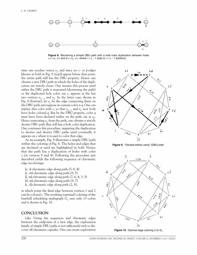
As an example, Fig. 9 illustrates a simple DBU path within the coloring of Fig. 6. The holes and edges that are declared or used are highlighted in bold. Notice that the path has a duplication of holes with color e (at vertices 9 and 4). Following the procedure just described yields the following sequence of chromatic edge recolorings:

{e, i}-chromatic edge along path (5, 6, 4) {e, m}-chromatic edge along path (9, 5) {l, m}-chromatic edge along path (7, 6, 4, 3, 5) {d, m}-chromatic edge along path (8, 7) {c, d}-chromatic edge along path (2, 8),

at which point the final edge between vertices 1 and 2 can be colored c. The resulting (optimal) coloring of the baseball scheduling multigraph G1 uses only 13 colors and is shown in Fig. 10.

CONCLUSIONLike Vizing fan sequences and chromatic edges

between the endpoints of a new edge, the exploration family of simple DBU paths is not sufficiently rich to dis-cover all chromatic capsules. One can create exploration

Figure 8. Recoloring a simple DBU path with a hole color duplication between holes = <vi , c> and = <vL, c>, where i < L 1 (top) or i = L 1 (bottom).

Figure 9. “Declare before using” (DBU) path.

Figure 10. Optimal edge coloring of G1.

v0 v1 vi vj vL

� ��

c cp c c p p c

v0 v1 vk vi vL

c cq q

eL



families that are guaranteed to find any chromatic cap-sule. However, no reduction procedure is known for any of these families that can be guaranteed to migrate an arbitrary hole color duplication back to the uncol-ored edge.

In 1989, Wu16 devised an exploration family using the DBU property to construct an algorithm having a failure threshold of = 13 and thus reaching bound B13 = (13 + 10)/12. Most recently (1998), Caprara and Rizzi17 showed a technique that can augment any of the algorithms in this family to lower the constant term in the numerator of the bound equation by 1. Although they were apparently unaware of Wu’s result, their tech-nique would appear to work with his algorithm, thus giving a slightly improved bound of B13 = (13 + 9)/12. This bound is the best known to the author for multi-graph edge coloring. Although a proof of Seymour’s or Goldberg’s conjecture remains elusive, the best hope for moving in this direction or for finding better bounds appears to be through the use of the DBU property or similar concepts that exploit the unique structural char-acteristics of chromatic capsules.

REFERENCES 1Shannon, C. E., “A Theorem on Coloring the Lines of a Network,”

J. Math. Phys. 28, 148–151 (1949). 2Vizing, V. G., “On an Estimate of the Chromatic Class of a p-Graph,”

Diskret. Analiz. 3, 25–30 (1964) (in Russian). 3Holyer, I., “The NP-Completeness of Edge-Coloring,” SIAM J.

Comput. 10(4), 718–720 (Nov 1981). 4Seymour, P. D., “On Multi-Colourings of Cubic Graphs, and Con-

jectures of Fulkerson and Tutte,” Proc. London Math. Soc. 38(3), 423–460 (1979).

5 Goldberg, M. K., “On Multigraphs of Almost Maximal Chromatic Class,” Diskret. Analiz. 23, 3–7 (1973) (in Russian).

6 Goldberg, M. K., “Edge-Coloring of Multigraphs: Recoloring Tech-nique,” J. Graph Theory 8, 123–137 (1984).

7 Andersen, L. D., Edge-Coloring of Simple and Non-Simple Graphs, Aarhus University, Denmark (1975).

8 Hochbaum, D. S., Nishizeki, T., and Shmoys, D. S., “A Better Than ‘Best Possible’ Algorithm to Edge Color Multigraphs,” J. Algorithms 7, 79–104 (1986).

9 Nishizeki, T., and Kashiwagi, K., “On the 1.1 Edge-Coloring of Mul-tigraphs,” SIAM J. Discrete Math. 3, 391–410 (1990).

10 Fiorini, S., and Wilson, R. J., Edge-Colourings of Graphs, Fearon- Pitman Publishers, San Francisco, CA, pp. 57–64 (1977).

11 Kempe, A. B., “On the Geographical Problems of the Four Colours,” Am. J. Math. 2, 193–200 (1879).

12 Karp, R. M., “Reducibility Among Combinatorial Problems,” in Com-plexity of Computer Computations, Miller and Thatcher (eds.), Plenum Press, New York, pp. 85–103 (1972).

13 Crane, T. B., An Investigation into the Complexity of Determining the Edge Chromatic Number of a Graph, M.S.E.E. Thesis, Northwestern University, Evanston, IL (Aug 1980).

14 Fiorini, S., and Wilson, R. J., “Edge-Colorings of Graphs,” Chap. 5, in Selected Topics in Graph Theory, L. W. Beineke and R. J. Wilson (eds.), Academic Press, New York, pp. 103–126 (1978).

15 Kierstead, H. A., “On the Chromatic Index of Multigraphs Without Large Triangles,” J. Comb. Theory Ser. B 36, 156–160 (1984).

16 Wu, M., Algorithms for Spanning Trees with Many Leaves and for Edge Colorings of Multigraph, Ph.D. Dissertation, University of South Caro-lina (1989).

17 Caprara, A., and Rizzi, R., “Improving a Family of Approximation Algorithms to Edge Color Multigraphs,” Inf. Proc. Lett. 68, 11–15 (1998).

ACKNOWLEDGMENTS: Parts of this work were funded by the Navy to sup-port development of the Cooperative Engagement Capability Data Distribution System (DDS). The author would like to thank Elinor Fong and Suzette Som-merer for their encouragement and support of investigating this problem and its applications. He also gratefully acknowledges the members of the DDS Network Control Working Group at APL, especially Bill Antosek and Eric Farmer for their time, comments, and suggestions and for the many invaluable discussions we have had regarding multigraph edge coloring.

THE AUTHOR

JEFFREY M. GILBERT graduated summa cum laude from Penn State University in 1983 with B.S. degrees in mathematics and electrical engineering. He earned an M.S. in computer science, summa cum laude, from the JHU Whiting School of Engineering in 1987. In 1984 Mr. Gilbert joined APL’s Fleet Systems Department in the Surface and Strike Warfare Systems Engineering Group, then transferred to ADSD’s Sensor Signal and Data Processing Group in 1997. He became a member of the Principal Professional Staff in 2000. Mr. Gilbert has developed requirements and simulated and analyzed network control algorithms for the Data Distribution System of the Navy’s Cooperative Engagement Capability. He is currently head of the APL Network Control Working Group and Supervisor of the Modeling and Analysis Section. His e-mail address is [email protected].

Documents

Strategies for Multigraph Edge Coloring · JOHNS HOPKINS APL TECHNICAL DIGEST, VOLUME 23, NUMBERS 2 and 3 (2002) 187 JOHNOS PSJKIAHKLTEOP HNCDKSG SK,AEAHPV I Strategies for Multigraph