Stock Market Valuation and Globalization

Geert Bekaert

Columbia University, New York, NY 10027 USA

National Bureau of Economic Research, Cambridge, MA 02138 USA

Campbell R. Harvey

Duke University, Durham, NC 27708 USA

National Bureau of Economic Research, Cambridge, MA 02138 USA

Christian T. Lundblad

University of North Carolina, Chapel Hill, NC 27599 USA

Stephan Siegel∗

University of Washington, Seattle, WA 98195 USA

May 2007Preliminary and Incomplete

∗ Send correspondence to: Campbell R. Harvey, Fuqua School of Business, Duke University, Durham,NC 27708. Phone: +1 919.660.7768, E-mail: cam.harvey@duke.edu .

Stock Market Valuation and Globalization

Abstract

We study the valuation of similar assets in different national markets and howthe valuation differentials have evolved through time. We focus on the impact ofglobalization and propose a (model free) measure of the degree of segmentation ofworld equity markets. We characterize which factors determine its cross-sectional andtime series variation. Our first goal is to link the measure to the de jure globalizationprocess using measures of capital and equity market restrictions on foreigners and tradeliberalization. We then consider other local fundamental factors including financialdevelopment, political risk, regulatory and labor market frictions, and push factorssuch as U.S. interest rate conditions. We also examine actual valuation differentials(with special emphasis on the emerging market discount) and their determinants, andcharacterize which industries appear the least and most integrated into global capitalmarkets.

1 Introduction

Why do different countries trade at very different valuation ratios? For example, among 13

developed countries, Table 1 shows the maximum price-earnings ratio (PE henceforth) at the

end of 2003 was 23.21 for the US, and the lowest was recorded for Ireland, with 10.76. For

emerging markets, the differences are even more extreme. Zimbabwe’s price-earnings ratio

was only 6.26, whereas Israel’s was 37.10. From an international finance perspective, these

large country valuation differentials are somewhat surprising. The removal of capital controls

in both developed countries (mostly during the eighties) and emerging markets (mostly at

the end of the eighties and the early nineties) has led to unparalleled financial openness across

the world. If openness leads to the consistent use of global discount rates, and discount rate

variation accounts for most of the variation in valuation ratios at the country level, we would

expect to see valuation differentials across countries converge. Similarly, multi-lateral trade

GATT (WTO) rounds, regional trade arrangements, and unilateral trade reforms have led to

increased trade openness. While the theoretical effects of trade openness on valuation are far

from clear, it is at least conceivable that a larger proportion of internationally active firms

would lead to a higher dependence of a country’s growth opportunities on world business

cycles.

Our main object of study in this article is the difference between a country’s PE and

its global counterpart, that is, the PE that would apply to the same industry basket at

world market multiples. We call this measure LEGO (see below). Controlling for industry

structure is important for multiple reasons. Most obviously, different industries trade a very

different multiples making country valuations difficult to compare without controlling for

industry composition. For example, the high PE for Israel in Table 1 is to a large extent

due to its concentration of the Israeli market in the high tech sector. Consequently, the

LEGO measure (roughly, the percent differential with world valuation) is smaller for Israel

than for Indonesia. Similarly, notice that for the developed countries, the most extreme PE

ratios (Ireland and the US) do not feature the largest valuation differentials. In addition, it

is natural to expect globalization to imply changes in sectoral allocations (see for instance

1

Carrieri, Errunza and Sarkissian (2007)), but we want to focus solely on pricing effects. We

propose the absolute value of LEGO as a measure of the degree of effective or de facto equity

market segmentation for a country, but we investigate the actual signed differential as well.

We then address several questions. First, we show that the effective degree of market

segmentation has on average indeed decreased and that the narrowing of valuation differ-

entials is related to the process of de jure globalization. Second, we use a panel regression

framework to determine the relative contribution of country-specific and global factors to the

cross-sectional and time series variation of LEGO and its absolute value. Under a strong

null of full market integration, established in a pricing model in Section 2 of the paper,

only leverage differences and measures of earnings volatility should help explain variation in

LEGO or its absolute value. However, under the alternative (i.e. some degree of market

segmentation), any country characteristic correlated with local global growth opportunities

or local discount rates may be a relevant factor.

While we do not establish causality, only association, determining which factors are of

first-order importance in explaining cross-country valuation differentials provides new in-

sights. There is a large literature in international finance studying the links between de jure

and de facto market integration (see e.g. Bekaert (1995), Lane and Milesi-Ferretti (2001),

Aizenman and Noy (2004), Nishiotis (2004), and Prasad, Rogoff, Wei, and Kose (2004)).

Country characteristics such as high political risk, an inefficient and illiquid stock market,

and poor corporate governance may keep out important institutional investors and lead to

de facto segmentation. In macro-economics, there is an enormous literature teasing out

which factors best predict differential growth rates across countries (see e.g. Barro (1997)).

The price earnings ratio of a country should reflect the country’s growth opportunities, and

Bekaert, Harvey, Lundblad, and Siegel (2007) show that a country’s PE ratio and its global

counterpart indeed predict future growth rates of real per capita GDP in a large panel of

countries. Consequently, one way to view the outcome of the regressions we run is to asses

which local growth determinants, for example the quality of institutions versus financial

development, are priced in the stock market, controlling for a country’s global growth op-

portunities represented by its industry mix. This may include measures of local product

market regulations or labor market conditions. While the majority of our factors are coun-

2

try characteristics that exhibit mostly low frequency variation, global investor behavior may

induce more temporary movements in valuation. We therefore include a number of factors

that (may) characterize the risk appetites of global investors or their attitude towards foreign

investments, such as the level of real rates, measures of global macroeconomic liquidity, etc.

The remainder of the paper is organized as follows. The second section introduces our

measure of market segmentation. The third section discusses our data and presents some

summary statistics. We also analyze the pure time-series variation in the degree of segmen-

tation. Section 4 contains the main empirical results on what factors determine the variation

in segmentation across countries and time. Section 5 focuses on valuation differentials in gen-

eral, and devotes special attention to the pricing of emerging markets relative to developed

markets (the so-called emerging market discount). The last section recognizes that different

industries may exhibit varying degrees of integration as they face different sets of regula-

tions, or competitive advantages, and analyzes differences in the degree of segmentation

across industries. In our conclusions, we also discuss some related literature.

2 Developing a measure of market segmentation

In this section, we develop a measure of the degree of segmentation for a particular stock

market. Our measure encompasses simultaneously economic and financial market integra-

tion and does not differentiate between the two, but it makes minimal assumptions and is

essentially model free. The main underlying assumption we make is that systematic risk

and growth opportunities are largely industry specific and the base unit of our model is a

country-industry portfolio.

2.1 A simple pricing model for industry portfolios

We begin by defining log earnings growth, ∆ ln(Earnt), with Earni,j,t the earnings level, in

country i, industry j as:

∆ ln(Earni,j,t) = GOw,j,t−1 + GOi,j,t−1 + εi,j,t. (1)

3

GOw,j,t represents the world-wide stochastic growth opportunity for each industry j which

does not depend on the country to which the industry belongs. In contrast, GOi,j,t is a

country and industry specific growth opportunity. For example, an industry’s growth oppor-

tunity may be curtailed by country-specific regulation or affected by country-specific factor

endowments. Finally, εi,j,t is a country and industry specific earnings growth disturbance,

which we assume to be N(0, σ2i,j). Because it has no persistence, it is not priced. Growth

opportunities themselves follow persistent stochastic processes:

GOw,j,t = µj + ϕjGOw,j,t−1 + εw,j,t (2)

GOi,j,t = µ̄i,j + ϕ̄ijGOi,j,t−1 + ε̄i,j,t.

We assume εw,j,t ∼ N(0, σ2w,j) and ε̄i,j,t ∼ N(0, σ̄2

i,j).

The discount rate for each industry in each country is affected by two factors:

δi,j,t = rf (1− βi,j − β̄i,j) + βi,jδw,t + β̄i,jδi,t. (3)

The constant term, with rf equal to the risk free rate, arises because the discount rates are

total not excess discount rates. An equation like (3) would follow from a logarithmic version

of the standard world CAPM. The world market discount rate process follows:

δw,t = dw + φwδw,t−1 + ηw,t, (4)

with ηw,t ∼ N(0, s2w). Likewise, the country-specific discount factor follows:

δi,t = di + φiδi,t−1 + ηi,t, (5)

with ηi,t ∼ N(0, s2i ). We assume the various shocks to be uncorrelated.

Assuming that each industry pays out all earnings, Earnt, each period, the valuation of

the industry under (1)-(5) is:

Vi,j,t = Et[∞∑

k=1

exp(−k−1∑

`=0

δi,j,t+`)Earni,j,t+k]. (6)

Given that we model earnings growth as in equation (1), the earnings process is non-

stationary. We must scale the current valuation by earnings, and impose a transversality

condition to obtain a solution:

PEi,j,t =Vi,j,t

Earni,j,t

= Et[∞∑

k=1

exp(k−1∑

`=0

−δi,j,t+` + ∆ ln(Earni,j,t+1+`))] (7)

4

Given the assumed dynamics for δw, δi, GOw,j, and GOi,j and normally distributed

shocks, the PE ratio can be shown to be an infinite sum of exponentiated affine functions

of the current realizations of the growth opportunity factors (with a positive sign) and the

discount rate factors (with a negative sign) (a detailed derivation is available upon request):

PEi,j,t =∞∑

k=1

exp(ai,j,k + bi,j,kδw,t + ci,j,kGOw,j,t + ei,j,kδi,t + fi,j,kGOi,j,t). (8)

In this model, the cash flows and discount rate processes governing the pricing of various

industries in particular countries may be affected by both local and global factors. Note that

the constant in the expression for the PE ratio is affected positively by the volatility of the

shocks to the discount rates, growth opportunities, and earnings growth rates.

The model nests the two polar cases of full integration and full segmentation. Assume

that the variance of the country-specific growth opportunity is zero and β̄i,j = 0 ∀ i, j. Also,

assume that industry systematic risk is the same across integrated countries; that is,

βi,j = βj. (9)

This assumption also implies that financial risk through leverage is identical across countries.

Under this assumption, we can rewrite (8) as:

PEi,j,t =∞∑

k=1

exp(ai,j,k + bj,kδw,t + cj,kGOw,j,t). (10)

An improvement in growth opportunities increases price earnings ratios for the industry

everywhere in the world, and the change in the PE ratio is larger when GOw,j,t is more

persistent. Similarly, a reduction in the world discount rate increases the PE ratio with the

magnitude of the response depending upon the persistence of the discount rate process and

the beta of the industry.

Alternatively, if βi,j = 0 ∀ i, j, that is local investors determine discount rates and

GOw,j,t has zero variance, country-specific persistent components will drive local industry

growth opportunities and discount rates. In that case, local industry PE ratios need not

be equivalent to global ratios for the same industry and price earnings ratios for each local

industry depend only on δi,t and GOi,j,t. While local and global factors may be correlated,

local industry PE ratios can now differ substantially from comparable global PE ratios.

5

2.2 A market segmentation measure

Following Bekaert, Harvey, Lundblad, and Siegel (2007), we view each country as a portfolio

of industries where an industry’s portfolio weight corresponds to the relative (equity) market

value of the industry. Define country i’s industry weights by IWi. Let EYi denote the vector

of industry earnings yields in country i and EYw the corresponding vector of world industry

earning yields. Combining these vectors for country i, we define local PE ratios (LGO) and

implied global PE ratios (GGO) for the same portfolio composition of industries, as follows:

LGOi,t = −ln[IW ′i,tEYi,t] (11)

GGOi,t = −ln[IW ′i,tEYw,t]. (12)

Note that the exponential of LGOi,t is simply the local market PE ratio, and GGOi,t repre-

sents the log PE ratio for the country’s mix of industries at global prices.1

The main variable of analysis in this article is the difference between these two price

earnings ratios:

LEGOi,t = LGOi,t −GGOi,t. (13)

Bekaert, Harvey, Lundblad, and Siegel (2007) introduce this variable as a measure of ”local

excess growth opportunities” (GO denotes growth opportunities), but it may of course also

reflect discount rate variation.

We propose the absolute value of LEGO as a measure of market segmentation. Under the

strong market integration concept introduced in Section 2.1, the time varying part of both

the numerator and denominator is identical, being driven by variation in the world discount

rate and world growth opportunities. However, the constant term may differ, because of

Jensen’s inequality terms. In our empirical work, we are careful to add a measure of local

earnings volatility to deal with this dependence. Because of the non-linearities, the volatility

terms may also lead to time-varying dependence on these global variables, but these effects

are likely to be second order (and in future work we will verify this directly). Consequently,

1Using earnings to derive industry weights and calculating an aggregate PE ratio as a weighted average

of industry PE ratios would not have this aggregation property, and leads to potentially negative weights

and the use of extreme PE values.

6

under the assumptions of the model |LEGO| should be small and constant for integrated

countries.

It is instructive to recall the assumptions going into the model so as to better interpret

the empirical work to follow. First, we assume a constant world interest rate. We will add

the world real interest rate as one of the potential determinants of LEGO.2 Note that it

is not likely that real rates account for much of the variation in price-earnings ratios. Nev-

ertheless, work by Gagnon and Unferth (1995) and Goldberg, Lothian, and Okunev (2003)

suggests that real interest rates are converging across countries and hence may themselves

contribute to lower |LEGO| values. Second, we assume that systematic risk is identical

across industries. While this is the typical textbook assumption, the industry classification

may not be homogenous enough to make this an acceptable assumption. We deal with this

in two ways. We use an industry classification that is quite granular compared to other work,

involving 38 different industries (see below). In addition, we will use this industry classifi-

cation on a large integrated market (e.g. the U.S.) and in future work verify that portfolios

within industries have comparable multiples.3 Third, we assume that the same industry in

different countries has identical financial risk. Surely, country specific circumstances will

induce different leverage ratios across countries. Therefore we will verify that our results are

robust to the inclusion of country-specific leverage ratios. Fourth, the market integration

concept is unusual in that it involves cash flows as well. Yet, the assumption that only world

factors drive growth opportunities is common. For example, recent articles by Rajan and

Zingales (1998) and Fisman and Love (2004), make this assumption quite explicitly, arguing

that growth opportunities primarily arise through technological shocks. Bekaert, Harvey,

Lundblad, and Siegel (2007) show that, in fact, GGO predicts growth for both developed

and emerging markets. Our approach then tests the degree to which local growth opportuni-

ties and other domestic factors matter for valuation once we have controlled for a country’s

global growth opportunities.

2In future work, we will also add local real interest rates, which should matter under the alternative of

(partial) segmentation.3It is conceivable that we may have to introduce other firm characteristics (such as size) to obtain a

homogeneous classification.

7

Even with these caveats, most countries will for sure be segmented according to this defi-

nition. We conjecture that a main driver of such segmentation is de jure segmentation: some

markets are simply legally closed for foreign investment. In that case, market segmentation

is associated with lower prices, because the absence of foreign investors and the inability to

invest abroad implies that local risks cannot be diversified away. In standard rational mod-

els, discount rates are higher as a result, yielding lower valuations. Consequently, LEGO is

negative.

Interestingly enough, the literature on financial openness is scarce compared to the vol-

umes of articles written on issues such as corporate governance. If a country suffers from

weak corporate governance, the managers stealing part of the cash flows will naturally lead to

lower valuations for the minority shareholders. As Albuquerque and Wang (2007) show, there

should also be a discount rate effect in equilibrium, which, on the one hand should lead to

even lower valuations, but, in the context of their model, reduces some of the over-investment

incentives induced by the manager’s pursuit of private benefits. In an international context,

there may be an additional discount rate effect which may be of first order. International

investors may shun markets with weak corporate governance, keeping discount rates local

and thus higher. There may also be interesting interaction effects between openness and

weak corporate governance, which partially undo this negative effect. A large literature on

ADRs shows that companies may try to bond themselves to the stronger corporate gover-

nance laws in the countries in which they cross-list and then become more highly valued,

although there exists much doubt about the exact source of the higher valuations (see, for

example, Doidge et al. (2004) and Siegel (2005)).

Weak corporate governance is only one of the many country characteristics that may lead

to effective segmentation. Alfaro et al. (2007) marshal direct evidence that only countries

with a high quality of local institutions attract significant FDI flows. Their measure of

the quality of institutions is a measure which we use below as well. It is in fact designed

to measure political risk, and we have argued before (see Bekaert, Harvey and Lundblad

(2005)) that some of its sub-components are related to the quality of institutions, some to

law and order, and others to pure political risk.

The effects discussed above so far associate segmentation with “low” prices. Yet, seg-

8

mentation need not have such asymmetric effects. For example, in markets with irrational

agents, segmentation could cause over-pricing (see Mei, Scheinkman and Xiong (2006) for

an argument how excessive speculation caused Chinese A shares, traded by locals, to be

over-priced relative to B-shares, traded by foreigners). Likewise, regulations may protect

local industries against foreign competition and improve cash flow prospects. Hence, we first

look at the absolute value of LEGO.

In section 5, we also investigate valuation differentials, LEGO, and their determinants.

Our results here are related to the analysis in a recent paper by Hail and Leuz (2006), in

which they study differences in expected returns across 40 countries, highlighting the effect

of legal institutions and securities market regulation. They mainly use accounting-based

valuation models to back out expected returns, and acknowledge that long-term differences in

growth opportunities may still matter for their results. While we do not differentiate between

expected returns and growth opportunities, we correct the local PE ratio for a multiple that

should reflect the discount rate and growth opportunities of the country’s industry basket

under a (strong) null of market integration. We then test which other factors are value-

relevant. These factors can reflect local growth opportunities or local discount rates. In the

terminology of Alfaro et al (2007), they can reflect local fundamentals (like human capital),

institutions, and capital market imperfections. For example, considerable research in asset

pricing now recognizes liquidity as a priced factor affecting discount rates. While financial

openness may improve liquidity, an asset pricing model with liquidity risk will necessarily

involve local factors (see Bekaert, Harvey, and Lundblad (2007)).

This reasoning also suggests the potential for interaction effects. More generally, as

openness increases over time, so may the relevance of GGO for local valuation. Likewise,

a well developed banking sector may be essential for efficient capital allocation but less so

in an open capital market (See Bekaert, Harvey, Lundblad, and Siegel (2007) for evidence

that financial openness, rather than a well-developed banking sector, is first-order in aligning

growth opportunities with growth). We will check for interaction effects in the final section.

Finally, we should point out that we explain valuation at the country level, which may

hide important inter-sectoral effects. As one example, the degree of integration may differ

across industries, so that the mix of a country’s industry basket itself may drive the valuation

9

effects of openness. Moreover, competitive effects induced by trade openness may lower val-

uations of certain industries while increasing the valuations of others, dampening the effect

of openness on the market’s PE. In the last section, we investigate industry specific devia-

tions from world valuations. This allows us to not only characterize the most “integrated”

and “segmented” industries, but also create useful alternative measures of integration at the

country level. For example, an equally weighted sum of absolute industry valuation differen-

tials would avoid the problem of over and undervaluation canceling each other and control

for a country’s initial industry mix.

3 Data and segmentation over time

3.1 Data construction

We construct the valuation differential, LEGO, for a sample of 51 countries, using monthly

data from Datastream as well as from Standard & Poors’ Emerging Market Data Base

(EMDB) between 1973 and 2005. While monthly LEGO measures are constructed (and are

presented in subsequent figures), we conduct our analysis at the annual frequency given the

availability of our candidate explanatory variables described below.

For 23 mainly developed countries, we collect equity market value data at the industry

level from Datastream, which typically covers about 85% of a country’s equity market. We

use the industry market value to determine a country’s industry composition in the form

of 38 portfolio weights that reflect the Industry Classification Benchmark (ICB) framework

employed by Datastream. For the same set of countries and industries, we also obtain

industry earnings yields from Datastream.4

We also obtain global industry earnings yields from Datastream. These global earnings

yields reflect a value weighted average of earnings yields from around the world. For the

remaining 28 countries, we use EMDB to obtain market value and trailing 12-month earnings

data at the firm level. After setting negative earnings to zero, we aggregate the firm level

4We calculate industry earnings yields as the inverse of an industry’s PE ratio. Datastream calculates

an industry PE ratio by dividing total market value by total (generally trailing) 12-month earnings where

negative earnings have been set to zero.

10

data to be compatible with the industry classification employed by Datastream.5 For each

industry and country, we calculate local earnings yields and portfolio weights.

By combining industry portfolio weights and local earnings yields, obtained from Datas-

tream and EMDB, we calculate LGO for each country and month for which data are avail-

able. Next, using the same industry portfolio weights, but global industry earnings yields

obtained from Datastream, we calculate GGO. We finally calculate LEGO = LGO−GGO,

yielding |LEGO| as our segmentation measure. Appendix Table 1 contains details on the

data source and availability for all 51 countries in our study.

Table 2 provides summary statistics for LEGO as well as the absolute value of LEGO.

In particular, we report the time series average and standard deviation for all countries in

our sample. We also report the corresponding statistics when Japan (JPN) is excluded from

the construction of these measures. Japanese log PE ratios are roughly 70% larger, on

average, than their global counterparts over the entire sample. As the first column shows,

the high Japanese PE ratios imply that the average value of LEGO is negative for 46 out of

51 countries. Using this metric, the Japanese market appears particularly segmented from

global capital markets. However, French and Poterba (1991) provide a detailed discussion

of the nature of Japanese earnings data showing that they artificially inflate Japanese price

earnings ratios. As Japan constitutes a large portion of the global equity market, we calculate

global industry PE ratios that do not include Japanese data, and proceed to exclude Japanese

data for the remainder of the article. All evidence presented below is available with Japanese

data upon request; the qualitative differences are in fact minimal.

Finally, at the bottom of the table, we report the cross-sectional averages of these statis-

tics for the set of industrialized, emerging, and all countries. The last column of the table

reflects the unbalanced nature of our panel data set. While we have 33 years of data for

most industrialized counties, the average number of years with data for emerging market

countries is about 17. Averaging the reported statistics across the set of industrialized as

well as emerging market countries, we observe that emerging markets on average exhibit

5We first aggregate firm level data to sub-industry level in the Global Industry Classification Standard

(GICS) used by EMDB. We then link GICS to ICB. The concordance between both classification systems

that we have developed is available upon request.

11

larger valuation discounts as well as larger fluctuations of LEGO over time. When focusing

on the absolute value of LEGO, our measure of market segmentation, we notice that indus-

trialized countries have lower time series averages. Probably not surprisingly, the US is the

least segmented country.

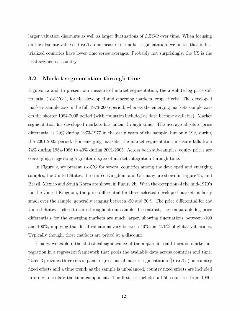
3.2 Market segmentation through time

Figures 1a and 1b present our measure of market segmentation, the absolute log price dif-

ferential (|LEGO|), for the developed and emerging markets, respectively. The developed

markets sample covers the full 1973-2005 period, whereas the emerging markets sample cov-

ers the shorter 1984-2005 period (with countries included as data become available). Market

segmentation for developed markets has fallen through time. The average absolute price

differential is 29% during 1973-1977 in the early years of the sample, but only 19% during

the 2001-2005 period. For emerging markets, the market segmentation measure falls from

74% during 1984-1988 to 40% during 2001-2005. Across both sub-samples, equity prices are

converging, suggesting a greater degree of market integration through time.

In Figure 2, we present LEGO for several countries among the developed and emerging

samples; the United States, the United Kingdom, and Germany are shown in Figure 2a, and

Brazil, Mexico and South Korea are shown in Figure 2b. With the exception of the mid-1970’s

for the United Kingdom, the price differential for these selected developed markets is fairly

small over the sample, generally ranging between -20 and 20%. The price differential for the

United States is close to zero throughout our sample. In contrast, the comparable log price

differentials for the emerging markets are much larger, showing fluctuations between -100

and 100%, implying that local valuations vary between 40% and 270% of global valuations.

Typically though, these markets are priced at a discount.

Finally, we explore the statistical significance of the apparent trend towards market in-

tegration in a regression framework that pools the available data across countries and time.

Table 3 provides three sets of panel regressions of market segmentation (|LEGO|) on country

fixed effects and a time trend; as the sample is unbalanced, country fixed effects are included

in order to isolate the time component. The first set includes all 50 countries from 1980-

12

2005, developed and emerging, where the regression is unbalanced, including the emerging

markets as data become available. As our measure of market segmentation is persistent, the

standard errors reflect a correction for serial correlation and cross-sectional SUR effects in

the regression errors. The coefficient on the time trend is negative and statistically signifi-

cant. Market segmentation declines across time for a broad set of developed and emerging

countries. We also consider a balanced sub-sample of 13 developed markets that extends

from 1973 to 2005. For this balanced sample, the regression coefficient on the time trend is

also negative and significant but somewhat smaller than for the full country sample. Finally,

in the unbalanced emerging market sample, the downward trend is considerably stronger.

In all three cases, the relatively large regression R2 is almost entirely attributable to the

country fixed effect. This feature of the data will be revisited in the next section.

Economically, the trend coefficient represents the decline in the (logarithmic) absolute

percentage differential between local and global PE ratios. Hence, from 2005 levels, the

developed markets price differential should converge by 2029 (2017 under the full sample re-

gression). In emerging markets, convergence is faster, but the total differential is much larger.

The regression implies full convergence by 2025 (2039 under the full sample regression).

4 Market segmentation dynamics

In this section, we explore the determinants of time variation and cross-sectional variation

in our measure of market segmentation, |LEGO|.

4.1 Exploratory regression and econometrics

We begin with an exploratory time-series fixed-effects regression:

|LEGO|i,t = αi + τt + ηi,t (14)

where |LEGO|i,t is the year t absolute price differential for country i, and αi and τt represent

country and year effects, respectively. Figure 3 graphs the year effects together with the time

trend estimated in Table 3. The convergence trend was notably interrupted following the

1997 South-East Asian crisis and the market turbulence in 1998 (the Russian debt crisis and

13

LTCM). The country fixed effects are of interest as well. The five largest fixed effects are

due to Kenya, Pakistan, Sri Lanka, Bangladesh, and Zimbabwe. The least integrated mar-

kets, on average, among industrialized countries are Finland, Norway, and Singapore. This

exploratory regression explains 42% of the total variation in |LEGO|. Most of the R2 (37%)

comes from the fixed effects, suggesting that country factors must be really dominant, and

that valuation differentials are very persistent6 In Table 3 (panel B), we report a regression

that combines a time trend and the initial |LEGO| for each country. This regression has

an R2 of only 17%, indicating that its initial |LEGO| is only a very noisy indicator of a

country’s fixed effect. The persistence coefficient is nonetheless large at 0.3.

To examine whether variation in measured economic variables can account for part of

|LEGO|’s variation, we estimate panel regressions for 50 countries on annual data from

1980-2003. We employ as much data as are available for our potential determinants so that

the panel is unbalanced. The regression we consider is

|LEGO|i,t = α + β′xi,t + ηi,t (15)

where |LEGO|i,t is the year t absolute price differential for country i, and xi,t represents the

various explanatory variables. We use two estimation techniques.7 The first specification

is pooled ordinary least squares (OLS). However, the standard errors incorporate a Newey-

West (1987) correction (with two lags) and cross-sectional SUR effects. These corrections

have the effect of increasing the standard errors relative to simple OLS.8

To address the serial correlation in the error term in an alternative fashion, we perform

a Prais-Winsten (1954) regression assuming that the autocorrelation coefficient of the error

term is the same for all countries. We follow Beck and Katz (1995) and report panel corrected

standard errors that allow for heteroscedasticity across countries as well as contemporaneous

6This is related to the results in Lemmon, Roberts and Zender (2006) documenting strong fixed effects

in firm’s corporate leverage ratios. However, as we shall see, we are more successful in explaining these fixed

effects than they are.7We have also considered the GMM estimator developed by Blundell and Bond (1998) to control for time-

invariant country effects. Unfortunately, the high persistence of the dependent variable often invalidates past

lagged regressors as instruments.8These standard errors are very similar to the standard errors we obtain when controlling for errors that

cluster by both country and year (Thompson (2006)).

14

correlation of the error term between countries.9 Generally, the results from the Prais-

Winsten regressions are in line with the OLS specifications.

4.2 Globalization and convergence

The most obvious cause of the downward trend in |LEGO| we observe is the de jure global-

ization process. To measure financial openness we use two different measures, one focusing on

the entire capital account and one focusing exclusively on equity markets. Because the two

measures are highly correlated (0.74), we use them separately in most of our regressions. The

capital account openness measure compiled in Quinn (1997) and Quinn and Toyoda (2004)

is based on information from the IMF. A value of 1 indicates full capital account openness,

a value of zero a closed capital account, and larger intermediate values indicate increasingly

fewer regulations on international capital flows. The equity market openness measure uses

data on foreign ownership restrictions to measure the degree of equity market openness.

Following Bekaert (1995) and Edison and Warnock (2003), the measure is based upon the

ratio of the market capitalization of the S&P investable to the S&P global indices in each

country. The S&P’s global stock index seeks to represent the local stock market whereas the

investable index corrects the market capitalization for foreign ownership restrictions. Hence,

a ratio of one means that all of the stocks in the local market are available to foreigners.

To measure trade openness, we obtain the trade liberalization dates developed in Wacziarg

and Welch (2003) (based on the earlier work of Sachs and Warner (1995)). Wacziarg and

Welch look at five criteria: high tariff rates, extensive non-tariff barriers, large black market

exchange rate premia, state monopolies on major exports, and socialist economic systems.

If a country meets any of these five criteria, it is classified with an indicator variable equal

to zero and deemed closed.

Table 4 shows the effect of these openness measures in both univariate and bivariate

regressions. Panel OLS coefficient and standard errors are reported; as above, the standard

errors reflect a correction for serial correlation and cross-sectional SUR effects in the regres-

9Given the unbalanced nature of our data set, we estimate the elements of the covariance matrix pairwise,

that is using for each pair of countries all years for which both countries have non-missing data.

15

sion errors. Bold coefficients denote statistical significant under both panel OLS and the

Prais-Winsten specifications. All coefficients are negative and significant, with the effect of

capital account openness the largest and trade openness the smallest. According to these

numbers, countries with completely open capital accounts (equity markets) feature valuation

differentials that are almost 50% (37%) smaller than those with completely closed capital

accounts (equity markets). Because trade and financial openness are positively correlated,

these coefficients decrease in bivariate regressions, but they remain statistically and econom-

ically significant. Notably, if we add a trend term to the regression, it obtains an insignificant

coefficient. In other words, globalization indeed explains the downward trend in LEGO. It

is also remarkable that the two globalization variables explain around 20% of the total vari-

ation in |LEGO|, or about half what the benchmark fixed effect regression explains. We will

now use these two bivariate regressions to assess the marginal significance of other potential

determinants of effective segmentation.

4.3 Determinants of market segmentation and univariate results

Next, we discuss seven different categories of potential determinants of |LEGO| and report

their marginal impact in a regression where the two globalization variables are already in-

cluded.10 Table 5 presents results for the case where de jure financial openness is measured

as equity market openness, but the general evidence is qualitatively similar when capital

account openness is used instead. Bold coefficients in the table indicate significance under

both panel OLS and the Prais-Winsten specification.

4.3.1 Other measures of openness

In addition to the de jure measures of financial and trade openness provided above, we also

consider two de facto measures of openness. First, we use a measure of the importance of

foreign direct investment (FDI), computed as the sum of the absolute values of inflows and

outflows of FDI relative to GDP. Second, we employ a de facto measure of trade openness,

computed as the sum of exports and imports as a share of gross domestic product. While

10See Appendix Table 2 for a detailed description of all relevant data items and their sources.

16

both the magnitude of FDI flows or the trade sector decrease segmentation, the effects are

not statistically significant in the presence of de jure measures of globalization.

4.3.2 Political risk and institutions

There are many additional country characteristics that may effectively segment markets other

than formal capital or trade restrictions. La Porta et al. (1997) emphasize the importance of

investor protection and, more generally, the quality of institutions and the legal environment.

Poor institutions and political instability may affect risk assessments of foreign investors

effectively segmenting capital markets (see Bekaert (1995)), and financial openness might

not suffice to attract foreign capital if the country is viewed as excessively risky.

To explore these effects, we consider several variables that measure different aspects of

the institutional environment. First, we consider the overall ICRG political risk rating - a

composite of twelve sub-indices ranging from political conditions, the quality of institutions,

socioeconomic conditions and conflict. Note that a high rating is associated with less risk.

We also consider several sub-indices of the political risk index: 1) the quality of institutions,

reflecting corruption, the strength and impartiality of the legal system (law and order), and

bureaucratic quality, and 2) the investment profile, reflecting the risk of expropriation, con-

tract viability, payment delays, and the ability to repatriate profits. This measure is closely

associated with the attractiveness of a country for FDI. We also separately consider the sub-

index for law and order, which measures both the quality of the legal system and whether

laws are actually enforced. It is likely closely associated with investor protection. Following

La Porta et al. (1998), we also consider their corporate governance measure of minority

shareholder rights. This measure is only available in the cross-section. Bhattacharya and

Daouk (2002) document the enactment of insider trading laws and the first prosecution of

these laws. We construct two indicator variables, where the first takes the value of one

following the introduction of an insider trading law and the second takes the value of one

after the law’s first prosecution. Finally, we consider the country’s legal origin (Anglo-Saxon,

French, and other), an often used instrument for corporate governance and a “good” legal

system.

17

The various measures of political risk and corporate governance extracted from the ICRG

data are all statistically significant, and improved conditions are associated with lower de-

grees of market segmentation. Yet, the financial openness measures remain statistically

significant. All the other variables have no significant effects on segmentation.

4.3.3 Financial development

Poorly developed financial systems may also be an important factor driving market segmen-

tation. For example, in a 1992 survey by Chuhan, equity market illiquidity was mentioned

as one of the main reasons that prevented foreign institutional investors from investing in

emerging markets. Moreover, poor liquidity as a priced local factor may lead to valuation

differentials. When markets are closed, efficient capital allocation should depend on finan-

cial development (see Wurgler (2000) and Fisman and Love (2004)). Because banks are still

the dominant financing source in many countries, poor banking sector development may

severely hamper growth prospects and lower valuations. We employ several measures to

quantify stock and banking sector development.

Our first equity market liquidity measure relies on the incidence of observed zero daily

returns. Lesmond, Ogden and Trzcinka (1999) argue that if the value of an information signal

is insufficient to outweigh the costs associated with transacting, then market participants

will elect not to trade, resulting in an observed zero return. Lesmond (2005) provides a

detailed analysis of emerging equity market trading costs, and confirms the usefulness of this

measure.

We also consider three additional measures of equity market trading and efficiency: (i)

turnover as the value trade relative to GDP, a standard measure of stock market development

(see Atje and Jovanovic (1989)); (ii) equity market return autocorrelation over the previous

five years computed using monthly returns; and (iii) equity market synchronicity (see Morck,

Yeung, and Yu (2000)), where the measure is an annual value-weighted local market model

R2 obtained from each firm’s returns regressed on the local market portfolio return for that

year. Last, we proxy for the development of the banking system by the amount of private

credit divided by GDP (see King and Levine (1993)). La Porta et al. (2002) and Dinc

18

(2005) correct the standard measures of banking development for the state ownership of

banks, viewing state control as synonymous with inefficient resource allocation. To explore

this alternative, we interpolate the state ownership ratios provided by La Porta et al. (2002)

for two years during our sample to the full period and create an adjusted measure of banking

development as private credit to GDP times (1 − ratio of state ownership).

The equity market illiquidity (zero return) measure is significantly associated with mar-

ket segmentation and its effect is economically large. A shift from the average level of zero

returns for the emerging markets to the average level for the developed markets would entail

a narrowing of the segmentation measure by almost five percentage points. Higher mar-

ket turnover, although a standard measure of stock market development, has no relation

with market segmentation. The market return autocorrelation measure has a borderline

significant relation with the market segmentation measure, but under the Prais-Winsten

specification it is no longer significant. Banking sector development reduces market segmen-

tation significantly, and the measure adjusted for state ownership has the strongest effects.

Perhaps surprisingly, the well-known stock market efficiency measure of Morck, Yeung, and

Yu has no significant relation with segmentation. In all these regressions, the equity market

openness measure has a remarkably robust and significant effect on segmentation. There is

only one instance where trade openness loses significance, albeit only in the Prais-Winsten

regression and in a regression with fewer observations than the full specification.

4.3.4 Accounting

Accounting standards that differ across countries may impact valuation differentials through

two channels. First, the earnings levels employed in the price-earnings ratios may exhibit

systematic differences due to country-specific accounting rules.11 Second, any perceived risks

associated with lax accounting standards or the opacity of corporate records may affect the

cost of capital across countries (see Hail and Leuz (2006)). To explore the effect of account-

ing standards on |LEGO|, we consider an index, constructed by La Porta, Lopez-de-Silanes,

11A concept like EBITDA (earnings before income tax and depreciation) may be more robust to measure-

ment issues, but unfortunately such data are no available for our full sample.

19

Shleifer, and Vishny (1998), of accounting standards (where larger numbers denote higher

standards) created by examining and rating companies’ annual reports on their inclusion

or omission of certain accounting items. These items relate to general information, income

statements, balance sheets, funds flow statements, accounting standards, stock data, and

other special items. In addition, we investigate the effects of corporate earnings manage-

ment (where larger numbers reflect greater levels of manipulation) due to Leuz, Nanda and

Wysocki (2003). Both variables are purely cross-sectional and only available for a smaller

set of countries in our study. While the regression coefficients for both variables have the

expected sign, they are not significantly different from zero. Note that the loss of significance

for the trade openness effect may well be due to the reduced sample.

4.3.5 Risk appetite and business cycles

We also consider a number of variables that capture potential push factors driving capi-

tal flows. Because all these variables are based on U.S. or global data, they exhibit only

time-series variation. An established literature argues that market conditions in developed

countries, such as the level of interest rates, may drive capital flows, and thus affect inter-

national valuation differentials (see e.g. Fernandez-Arias (1996)). In particular, low real

rates in the U.S. would cause capital flows into emerging markets bringing their valuations

closer to developed market levels. While the evidence on this effect is mixed (see Bekaert,

Harvey and Lumsdaine (2002)), we nonetheless try to capture it using the level of the real

interest rate in the U.S. Such a relation may reflect a behavioral search for yield, but it

is also possible that the level of interest rates is correlated with a change in risk appetite.

The direction of the relation between interest rates and risk aversion is not entirely clear.

Lower interest rates may increase wealth, and thus increase risk tolerance (see e.g. Sharpe

(1990), Bekaert, Engstrom and Grenadier (2006)). In this case, it is conceivable that risk

tolerant investors view foreign markets (erroneously) as attractive. Alternatively, real in-

terest rates may be pro-cyclical where low interest rates are associated with recessions. A

recession may cause an increase in societal risk aversion and change portfolio allocations.

Recessions could therefore cause a retreat from risky equity investments, including a retreat

20

from foreign markets that are (erroneously) viewed as riskier. These two effects are opposite

from one another. We therefore also include a more direct measure of U.S. risk aversion due

to Bekaert and Engstrom (2007) computed based on the parameter estimates of the habit

model in Campbell and Cochrane (1999). This measure tends to behave counter-cyclically.

Finally, low real rates may be an indicator of lax monetary policy and a surge in “global

liquidity.” Popular stories claim such global liquidity increases stock market valuations across

the world. An alternative global liquidity measure we use is the growth rate of the U.S.

money supply (M2). We also include world GDP growth, which may either act as a measure

of global growth opportunities or more generally as an indicator of the world business cycle.

The world business cycle may affect global discount rates, and consequently may affect the

pricing of all markets simultaneously.

Other measures more directly correlated with the risk appetite or sentiments of world

investors are the U.S. Corporate default spread and the VIX Option Index. The latter is

generally viewed as an indicator of market uncertainty and sudden increases in its level with

a flight to safety. Increases in these measures may lead to a retreat of U.S. capital from

foreign markets, leading to divergence in valuations. Alternatively, the VIX index is simply

a measure of the U.S. stock market’s volatility, which may be correlated with global discount

rates. Finally, we investigate one country-specific behavioral factor, the level of the lagged

country portfolio return over the last year to potentially proxy for return chasing effects by

international investors.

None of the measures we investigate has a significant effect on market segmentation,

and the effects of the globalization measures remain intact. Yet, there are a few relations

with coefficients that are borderline significant. For example, increases in the U.S. real rate

are associated with larger degrees of segmentation, consistent with the view that in low

interest rate environments markets move together more. The U.S. risk aversion measure has

a negative effect on the degree of market segmentation. This is perhaps surprising, as the

popular story would argue that when risk averse U.S. investors retreat from international

capital markets, local factors may become more important. Increases in uncertainty, as

measured by the VIX index marginally increase segmentation, as expected, whereas high

past local returns, unexpectedly, also marginally increase segmentation.

21

4.3.6 Regulatory conditions and other growth determinants

Imperfections in a country’s labor and goods markets can lead to effective segmentation if

these imperfections affect discount rates and/or growth opportunities. Using U.S. industry

data, Chen, Kacperzyk, and Ortiz-Molina (2006) find that the presence of labor unions is

associated with higher expected industry returns. To examine whether differences in the de-

gree of unionization across countries explain differences in integration, our analysis includes

an annual measure of union density that is available for 23 countries in our sample. Given

that certain sectors of the economy such as the telecommunications sector have long been

subject to regulation with often significant effects on the industry’s and the country’s devel-

opment and competitiveness, we also include a measure that captures regulatory conditions

with respect to market entry, ownership, and price controls in the following seven sectors:

airlines, telecommunications, electricity, gas, post, rail, and road freight. The measure is

available for 20 countries in our sample (see Conway and Nicoletti (2006) for details on this

measure).

More generally, it is possible that GGO is only a good proxy for growth opportunities in

well-developed countries with good institutions, health care, human capital, etc., and that

the less developed countries have growth opportunities more local in nature. We therefore

include some variables that appear in most empirical growth regressions, such as human

capital, as measured by secondary school enrollment, log life expectancy, population growth,

and, importantly, the log of real GDP per capita (reset every five years). We find that, with

the exception of population growth, these standard growth determinants, indeed significantly

reduce the degree of market segmentation. The significance of equity market openness is not

affected, whereas trade openness becomes insignificant in two Prais -Winsten specifications.

Both union density and a higher degree of product market regulation are also significantly

associated with greater levels of segmentation. However, these effects do not survive in

Prais-Winsten regressions. Also, we are forced to remove the trade openness variable from

the regression with product market regulations as for this small sample there was no longer

meaningful cross-sectional correlation in the openness measure. The limited data availability,

concentrated in developed markets, makes the results for the openness measures hard to

22

interpret.

4.3.7 Other

The model suggests including measures of earnings growth and discount rate volatility as

potential determinants. We include a measure of country-level earnings growth volatility by

taking the five-year rolling variance of the country-level quarterly log earnings growth rate.

Similarly, we also include a measure of the variance of the world market portfolio return.

Given the potential effect of leverage on price-earnings ratios, we construct an annual

financial leverage ratio for 46 countries in our sample. We obtain annual accounting data for

all public industrial firms contained in Bureau van Dijk’s OSIRIS data base. For each firm

and year, we calculate the ratio of long term interest bearing debt and current long term

debt to the sum of long term interest bearing debt, current long term debt, and book equity.

Weighting each observation by the relative size of the firm’s assets, we aggregate this ratio

across all firms in a given country and year at the industry as well as country level. The

average leverage ratio is 0.36 across all countries, with 0.32 for emerging markets and 0.37

for developed markets. These data are available from 1985 to 2003 in our sample.

We do not find a significant relationship between a country’s level of financial leverage and

its degree of market segmentation. Country-level earnings growth volatility is significantly

associated with larger segmentation measures. This effect is consistent with the theoretical

prediction in the valuation model. Finally, we do not find a significant relationship between

|LEGO| and the volatility of the world market portfolio return.

4.4 Multivariate analysis

4.4.1 Model selection and regression results

To determine which of the variables previously examined are the most important, we conduct

a multivariate regression analysis. Unfortunately, we have too many variables to include in

one regression. Moreover, many of the variables are highly correlated. Therefore, we conduct

our analysis in two different ways designed to reduce the size of the model. In our first

23

method, we select the most important variables from each of the seven categories detailed

above. The second method, using PcGets, relies on statistical model reduction techniques

to automatically select the optimal model.

In our first technique, we select the most important variables (in terms of statistical

significance) from each sub-group (quality of institutions, law and order, investment profile,

private credit, the U.S. real rate, Log GDP per capita, secondary school enrollment, and log

life expectancy). The political risk index is excluded as it is very highly correlated with the

quality of institutions index. Given the primacy of de jure globalization, financial and trade

openness are included in all specifications. While other variables appear to be important, we

select only those variables that are available for our full sample. We perform a preliminary

joint multivariate regression using the different variables described here. In this preliminary

specification, a variable is then removed if it has a t-statistic below one in the joint regression.

The resulting pared-down regression is re-run, and Table 6a shows the regressors used in the

final multivariate regression.

The resulting multivariate regression contains five independent variables (financial and

trade openness, the quality of institutions, private credit and the U.S. real interest rate). All

variables have the expected sign, but not all variables are statistically significant. While many

coefficients are borderline significant, equity market openness and the quality of institutions

have the most significant effect on market segmentation. Capital account openness does not

have a significant effect on market segmentation. Perhaps this is caused by its close relation

with other variables in the regression, such as trade liberalization. In fact, in the equity

market openness specification, the trade liberalization effect is statistically significant. The

evidence is broadly similar using the Prais-Winsten specification as denoted in bold.

The other results in Table 6a add variables to the chosen specification that were either

important in Table 5 or constitute important controls (like earnings volatility, leverage and

accounting standards) from the perspective of the pricing model, but for which we do not

have the full data set. The adjusted private credit to GDP variable has stronger effects than

the unadjusted measure and also weakens the openness effects somewhat in the equity market

specification. While equity market illiquidity is, by itself, not significant, its t-statistic is well

over 1 and it appears to also reduce the relative importance of the openness effects. The other

24

controls are not significant. Despite much smaller samples in some instances, the quality of

institutions variable is always significant using the OLS specification, and insignificant in

only one Prais-Winsten specification.

We also apply a general-to-specific search algorithm as described by Hendry (1995) and

as implemented in PcGets (see Hendry and Krolzig (2001) for a detailed description). The

algorithm is an application of a “testing down” process that eliminates variables with co-

efficient estimates that are not statistically significant and thereby leads to a parsimonious

un-dominated model. In particular, we formulate a general unrestricted model that contains

all available variables and that we estimate in a first step by OLS. PcGets then eliminates

variables that are statistically insignificant. The new model is then re-estimated, and a mul-

tiple reduction path search is used to find all terminal models, that is models in which all

variables have statistically significant coefficient estimates. Finally, if more than one termi-

nal model exists, the different terminal models are compared to each other and one is chosen

as the unique final model. In our application of PcGets, we initially consider 22 variables for

which we have data over the full sample. PcGets eliminates 13 variables, leaving us with a

final model that contains 11 variables. Appendix Table 3 lists the 22 input variables and the

selected variables. Notice that the selection depends on whether we include capital account

openness or equity market openness among the 22 initial variables. Table 6b provides the

final regression specifications.

In the PcGets system, more variables survive in addition to the ones used in out previous

specification presented in Table 6a. These variables include the Investment Profile, which

has the expected sign but is only borderline significant, the Insider Trading Law dummy,

which indicates that insider trading laws increase segmentation, the legal origin dummies,

where both English and French systems reduce segmentation relative to other systems, and

two additional “global risk” variables, U.S. Risk Aversion (with a surprising negative sign)

and the U.S. corporate default spread (with the expected positive sign). Again, local market

illiquidity seems the most important omitted variable in the base specification, and it seems

to be correlated with both equity and capital market openness, reducing their effects. The

Quality of Institutions variable again maintains significance in the bulk of the specifications.

25

4.4.2 Variance decomposition

With a multivariate regression, we can examine how much of the variation in the segmenta-

tion variable is explained by the right-hand side explanatory variables. We use a simple R2

concept computed asV ar( ˆ|LEGO|i,t)V ar(|LEGO|i,t) where ˆ|LEGO|i,t = α̂+ β̂xi,t. The denominator is defined

as

V ar(|LEGO|i,t) =1

N

N∑

i=1

1

Ti

Ti∑

t=1

(|LEGO|i,t − ¯|LEGO|)2 (16)

where ¯|LEGO| = 1N

∑Ni=1

1Ti

∑Tit=1 |LEGO|i,t. The numerator is defined analogously as

V ar( ˆ|LEGO|i,t) =1

N

N∑

i=1

1

Ti

Ti∑

t=1

( ˆ|LEGO|i,t −¯̂|LEGO|)2 (17)

where¯̂|LEGO| = 1

N

∑Ni=1

1Ti

∑Tit=1

ˆ|LEGO|i,t. These quantities are reported in Table 6c. We

find that across the regression specifications provided, the predicted market segmentation

explains about 20 to 30% of the variation of the observed market segmentation in the data.

We also examine the contributions of each of the independent variables to the overall

variation of the predicted market segmentation. For the two baseline specifications in Table

6a, we decompose the variance of the predicted market segmentation for explanatory variable

j as follows:

Cov( ˆ|LEGO|i,t, β̂jxi,j,t) =1

N

N∑

i=1

1

Ti

Ti∑

t=1

β̂j( ˆ|LEGO|i,t −¯̂|LEGO|)(xi,j,t − x̄j) (18)

where x̄j is defined analogously as above. Across all individual explanatory variables, these

covariance terms must exactly equal the variance of the predicted market segmentation.

In Table 6c, we report the ratio of each covariance term to the overall predicted market

segmentation variance,Cov( ˆ|LEGO|i,t,β̂jxi,j,t)

V ar( ˆ|LEGO|i,t), where each column must necessarily sum to 1. We

report this variance decomposition for each of the two regression specifications considered.

Across the various specifications considered, the explanatory variables that contribute the

largest to overall variation in the predicted market segmentation are equity market openness

(around 30%) and the quality of institutions (around 30 to 50%). Private credit to GDP

and trade openness contribute approximately 15% of the overall variation.

It is important to note that this measure of predicted segmentation variation captures

both time-series and cross-sectional effects. We further perform two decompositions of these

26

covariance terms into separate effects that capture each of these features. The first de-

composition splits the total covariation for each explanatory variable into a within-country

component and a pure cross-sectional between-country component:

Cov( ˆ|LEGO|i,t, β̂jxi,j,t) =1

N

N∑

i=1

1

Ti

Ti∑

t=1

β̂j( ˆ|LEGO|i,t −¯̂|LEGO|i)(xi,j,t − x̄i,j)

+1

N

N∑

i=1

β̂j(¯̂|LEGO|i −

¯̂|LEGO|)(x̄i,j − x̄j) (19)

where¯̂|LEGO|i = 1

Ti

∑Tit=1

ˆ|LEGO|i,t and x̄i,j = 1Ti

∑Tit=1 xi,j,t denote the within-country

means of the relevant variables.

The second decomposition splits the total covariation into a within-year component and

a pure time-series between-year component:

Cov( ˆ|LEGO|i,t, β̂jxi,j,t) =1

N

N∑

i=1

1

Ti

Ti∑

t=1

β̂j( ˆ|LEGO|i,t −¯̂|LEGO|t)(xi,j,t − x̄j,t)

+1

Ti

Ti∑

t=1

β̂j(¯̂|LEGO|t −

¯̂|LEGO|)(x̄j,t − x̄j) (20)

where¯̂|LEGO|t = 1

N

∑Ni=1

ˆ|LEGO|i,t and x̄j,t = 1N

∑Ni=1 xi,j,t denote the within-year means

of the relevant variables.

Table 6c reports both decompositions for both baseline multivariate specifications. All

covariance terms are again scaled by the variance of the predicted degree of segmentation,

V ar( ˆ|LEGO|i,t). Both decompositions suggest in both cases that the largest contribution to

the variation in predicted market segmentation is, by far, the cross-sectional component, the

between-country component in the case of the first decomposition (accounting for around

80% of the explained variation) and the within-year component in the case of the second

decomposition (accounting for 97%). This, of course, explains why the real rate was deemed

to explain only a very small part of the variation in predicted |LEGO|. In fact, even the

temporal variation is mostly accounted for by the openness variables and the quality of

institutions. The results are largely robust under the PcGets specification as the additional

variables retained only contribute trace amounts to the total variation.12 One problem with

12In the interests of space, we present the variance decomposition only for the specification based on equity

market openness.

27

our approach is that is difficult to assess the robustness and significance of these variance

contributions. In future work, we envision the following exercise. For each variable included,

we run 1,000 experiments where we choose K (with K random) variables among all other

available factors (no matter the data availability), run a regression on these variables, remove

variables with a t-statistic less than 1, re-run the regression and record coefficients, t-stats

and variance decomposition numbers. The 90% intervals of such an experiment should be

informative on the robustness of our results.

5 What drives pricing differentials? (incomplete)

So far, we have characterized market segmentation using the absolute difference between a

local and global PE ratio, corrected for industry structure. Now, we turn our attention to

LEGO itself, the actual valuation differential. While section 5.1 analyzes the full sample,

we focus specifically on the valuation differentials for emerging markets in section 5.2. For

emerging markets, it is well known that various direct and indirect barriers to investment

still exist, causing an ’emerging market discount.’ We study the emerging market discount

over time and analyze its determinants. In other words, we investigate the value-relevance

of local fundamentals, institutions, liquidity, etc. after correcting for global PE ratios that

apply to the country’s industry basket.

5.1 General analysis

In Table 7, we evaluate the effect of the openness variables on LEGO. We focus our discussion

again on the pooled OLS results. Not surprisingly, financial openness causes local price-

earnings ratios to increase relative to their (industry-adjusted) global counterparts. For

capital account and equity market openness, a move from closed to open is associated roughly

with a 20 to 30% change in the price earnings ratio differential. These results are related to

a large literature that has traced the effects of equity market liberalizations on the cost of

capital (see e.g. Bekaert and Harvey (2000) and Henry (2000) for early papers), typically

finding that liberalizations reduce the cost of capital. Trade openness also increases local

prices relative to global prices.

28

In bivariate regressions, the coefficients (standard errors) naturally decrease (increase)

but they remain significant in the equity openness specification, at least using the OLS stan-

dard errors. It is conceivable that forcing a coefficient of 1 on global valuations (GGO) is

not optimal. In particular, one would think that the relevance of GGO in local valuation

would depend on the degree of financial and trade openness. We defer the examination

of such interaction effects to the next draft of the paper, but Table 7 shows a regression

where the effect of GGO is unconstrained, and we find that it has a coefficient between 0.7

and 0.8, with the difference from one being highly statistically significant. Allowing this

additional flexibility considerably improves the R2, and does not alter the main effects of

financial openness, so we retain GGO as an additional regressor in our benchmark speci-

fication. Table 8 mimics the trivariate regressions presented for |LEGO| in Table 5. De

facto openness measures have no significant marginal impact on valuation. Surprisingly, of

all the Political risk/Institutions/Corporate governance variables, only law and order has an

important valuation effect. The effect is economically large as well.

Measured between 0 and 1, a typical emerging market has a rating of 0.52 on law and

order and a developed country a rating of 0.95. Consequently, achieving law and order levels

similar to a typical developed country would cause a 11% increase in local relative to global

prices for a typical emerging market.

Turning to panel C, improved liquidity, when measured using the zero returns, signifi-

cantly increases local price earnings ratios. The inclusion of the liquidity variable also renders

equity market openness insignificant. Also, countries with better developed banking sectors

also have significantly higher local PE ratios.

Higher levels of accounting standards are associated with larger local price earnings ratios

relative to the world, but the effect is only statistically significant at the 10% level. Higher

levels of earnings management are surprisingly associated with larger local price earnings

differentials; this is not the sign one would necessarily expect, but the sample is quite small.

Increases in the U.S. real rate lower LEGO across the world, consistent with a “push” or

“searching for yield” story, while the effect is significant in the OLS regression, it is not in

the Prais-Winsten specification. An increase in the U.S. money supply reduces local prices

rather than indicating that global macroeconomic liquidity drives up stock markets across

29

the world. Both higher VIX levels and a higher U.S. corporate default spread significantly

decrease local valuations. It is conceivable that all three effects simply stem from the opposite

effect occurring for the global valuation component, GGO, in the valuation differential,

LEGO, which has a large weighting in the U.S. equity market. To explore this further,

we run an additional specification where global log PE ratios for each country, GGO, are

regressed on U.S. risk aversion. These are the price earnings ratios for each country as

implied collectively by global equity markets at their industry compositions. This regression

(not reported) uncovers a negative effect, so that global market prices are indeed moving

in the opposite direction from U.S. risk aversion. Global prices are significantly affected by

risk aversion levels, whereas individual country prices (particularly emerging markets) are

less affected – this channel dominates the price differential regression, explaining the positive

overall effect in the price differential regressions. We find no significant valuation effects from

standard growth determinants and regulatory conditions. This is somewhat surprising as we

would expect these variables to be correlated with local growth opportunities. Larger country

market portfolio returns last year are associated with larger price-earnings ratio differentials.

To perhaps get a finer measurement, we also created a “local growth opportunity” measure as

follows. We take a standard Barro regression framework (with these four traditional growth

determinant variables, the size of the government sector, and financial and trade openness,

and run a panel regression of future average real per capita GDP growth over 5 years on these

growth determinants. We use the fitted value as a measure of local growth opportunities.

In unreported results, we find that the fitted local growth opportunities variable is positive

associated with relative valuations.

Last, neither country earnings growth rate volatility nor world market portfolio return

volatility are significantly associated with local price earnings differentials. Also, increased

levels of country-level financial leverage are, as expected, associated with lower price earnings

ratio differentials.

Because so many variables are borderline significant, a multivariate analysis is particular

imperative.

30

5.2 The emerging market discount (incomplete)

6 Industries and market integration (incomplete)

We add another dimension to our analysis by considering a variant of our segmentation

measure at the industry level. Remember from the construction of our country-specific

segmentation measure, |LEGO|, that for each country and year we have available local

earnings yield (EYi,j,t) data for up to 38 industries. Instead of aggregating these into a

country-level measure, we now calculate the absolute difference between the local earnings

yield and the corresponding global earnings yield (EYw,j,t). Notice that in contrast to the

country-specific measure, this measure at the industry level is expressed as the difference in

earnings yields as opposed to the difference in PE ratios. This allows us to deal with cases

where local earnings yields are zero.13

Table 9a contains a list of all 38 industries that can be part of a country’s equity market.

For each industry, we report the simple mean of our industry segmentation measure across

countries and time for the first five years of our sample period (1980-1984) as well as for

the last five years (2001-2005). For the majority of industries, the absolute value of the

yield differential has decreased over the last two decades. Consistent with the decrease in

dispersion of yield differentials across industries, we observe significant reductions in the

segmentation measure for those industries that appear least integrated in the earlier period

between 1980 and 1984. For the top four industries, Life Insurance, Banks, General Retailers,

and Nonlife Insurance, we also observe a relative increase in integration by their rank among

all industries.

Focusing on the bottom of list, we notice that Software and Computer Services, Electronic

& Electrical Equipment, and Technology Hardware and Equipment were and still are among

the most integrated industries. On the other hand, our results suggest that segmentation

has increased for Household and Personal Goods.

The last two columns of the table report results from a regression of annual average

13Note that the industry earnings yield data we obtain from Datastream are always nonnegative, as

negative earnings are set to zero in Datastream’s construction of industry earnings measures. We therefore

apply the same rule to the data we obtain from Standard & Poors’ EMDB.

31

industry yield differentials onto a linear time trend. These results confirm the overall decrease

in segmentation as well as the more pronounced effect for the previously less integrated

industries. Interestingly, several of the industries for which we observe a significantly negative

trend, such as Insurance, Banking, Electricity, and Telecommunication, have experienced

substantial deregulation and privatization in many countries over the last two decades.

To examine whether the variables that we have found to determine integration at the

country level have possibly different impacts on different industries, we repeat our analysis

from Table 3 at the industry level. For each industry j, we consider univariate regressions

of the form:

|EYi,j,t − EYw,j,t| = α + βxi,t + ηi,j,t. (21)

It is important to point out that all of our explanatory variables continue to be measured at

the country-level. For each variable and industry, we report the coefficient estimates from a

pooled OLS regression in Table 9b. Standard errors are robust to arbitrary heteroscedasticity

and clustering by country and year.14 Coefficient estimates that are significant at the 5%

level appear in bold.

Consistent with our findings so far, equity market openness, trade liberalization, the

quality of institutions, illiquidity, the ratio of private credit to GDP, and product market

regulation appear to significantly affect most industries in the expected way. While the

coefficients on investment profile, turnover, and union density generally have the expected

sign, only about half of them are statistically significant. The US real interest rate appears

to have a significantly positive effect on a few industries. US risk aversion is significantly

positively associated with segmentation in the case of Retailers, Industrial Engineering, Life

Insurance, and Media, but negatively in the case of Personal Goods and Tobacco.

7 Conclusion

We study valuation differentials across countries and through time. We view each country

as a basket of industries, which we price using local and global prices. Our measure of

market integration, the differential between these local and global PE ratios, will go to zero

14See Thompson (2006) for details.

32

when discount rates and growth opportunities are global in nature. Focusing on the absolute

value of this measure, we find that it has significantly trended downward from the early 1980s

onwards for both developed and emerging markets. We then examine the determinants of

the measure’s variation, finding that we can explain about 20% to 30% of its variation using

measures of financial openness, trade openness, the quality of institutions, local banking

sector and stock market development, and push factors. We find equity market openness

and the quality of institutions to be the most important explanatory variables, accounting

for over 50% of the explained variance. The remaining variation is primarily accounted for

by trade openness and local banking sector development. We also examine the determinants

of the magnitude of the valuation differential, with special emphasis on the emerging market

discount. Finally, we explore market segmentation at the industry level. Historically heavily

regulated industries, such as the banking, insurance, and electricity sectors, were among the

least integrated in 1980-1984 and are now among the most integrated industries.

33

8 References

Albuquerque, R., and N. Wang, 2007, Agency Conflicts, Investment, and Asset Pricing, Journalof Finance, forthcoming.

Aizenman, J., Noy, I., 2004. Endogenous financial and trade openness: efficiency and politicaleconomy considerations. Working paper, University of California, Santa Cruz.

Alfaro, L., Kalemlio-Ozcan S., and V. Volosovych, 2007, Why doesn’t capital flow from rich topoor countries? An empirical investigation, Review of Economics and Statistics, forthcoming.

Atje, R., and B. Jovanovic, 1989, Stock markets and development, European Economic Review37, 632-640.

Barro, R., 1997, Determinants of Economic Growth, MIT Press: Cambridge, MA.

Beck, N. and J. N. Katz, 1995, What to do (and not to do) with time-series cross-section data,American Political Sience Review, 89, 634-647.

Bekaert, G., 1995, Market integration and investment barriers in emerging equity markets,World Bank Economic Review 9, 75-107.

Bekaert, G. and E. Engstrom, 2007, Inflation and the Stock Market: Understanding the FedModel, working paper.

Bekaert, G., E. Engstrom, and S. Grenadier, 2006, Stock and Bond Returns with MoodyInvestors, working paper.

Bekaert, G., and C. R. Harvey, 1995, Time-varying world market integration, Journal of Finance50, 403-444.

Bekaert, G., and C. R. Harvey, 2000, Foreign speculators and emerging equity markets, Journalof Finance 55, 565-614.

Bekaert, G., and C. R. Harvey, 2005, Chronology of important economic, financial and politicalevents in emerging markets, http://www.duke.edu/∼charvey/chronology.htm

Bekaert, G., C. R. Harvey and R. Lumsdaine, 2002, The Dynamics of Emerging Market EquityFlows, Journal of International Money and Finance 21, 295–350.

Bekaert, G., C. R. Harvey, and C. Lundblad, 2001, Emerging equity markets and economicdevelopment, Journal of Development Economics 66, 465-504.

Bekaert, G., C. R. Harvey, and C. Lundblad, 2005, Does financial liberalization spur growth,Journal of Financial Economics, 77, 3-55.

Bekaert, G., C. R. Harvey, and C. Lundblad, 2007, Liquidity and Expected Returns: Lessonsfrom Emerging Markets, Review of Financial Studies, forthcoming.

Bekaert, G., C. R. Harvey, C. Lundblad and S. Siegel, 2007, Growth Opportunities and MarketIntegration, Journal of Finance, forthcoming.

Bhattacharya, U., and H. Daouk, 2002, The world price of insider trading, Journal of Finance

34

57, 75-108.

Blundell, R. W. and S. R. Bond, 1998, Initial conditions and Moment Conditions in DynamicPanel Data Models,Journal of Econometrics,87, 115-143.

Campbell, J. and J. Cochrane, 1999, By Force of Habit: A Consumption-Based Explanation ofAggregate Stock Market Behavior, Journal of Political Economy 107, 205–251.

Carrieri, F., V. Errunza, and S. Sarkissian, 2004, Industry Risk and Market Integration, Man-agement Science 50, 207–221.

Chen, H., M. Kacperzyk, and H. Ortiz-Molina, 2006, Labor Unions, Operating Leverage, andExpected Stock Returns, working paper.

Chuhan, P., 1992, Are Institutional Investors an Important Source of Portfolio Investment inEmerging Markets?, World Bank Working Paper N. 1243.

Conway, P. and G. Nicoletti, 2006, Product market regulation in non-manufacturing sectorsin OECD countries: measurement and highlights, OECD Economics Department WorkingPaper.

Carrieri, F., V. Errunza, and S. Sarkissian, 2007, The dynamics of geographic versus sectoraldiversification: Is there a link to the real economy?, Unpublished working paper, McGillUniversity.

Dinc, I. S., 2005. Politicians and banks: Political influences on government-owned banks inemerging markets, Journal of Financial Economics 77, 453–479.

Doidge C, Karolyi A., and R. Stulz, 2004, Why are foreign firms listed in the U.S. worth more?,Journal of Financial Economics 71, 205-238.

Edison, H., and F. Warnock, 2003, A simple measure of the intensity of capital controls, Journalof Empirical Finance 10, 81-103.

Fernandez-Arias, E., The new wave of private capital inflows: Push or pull?, Journal of Devel-opment Economics 48, 389–418.

Fisman, R., and I. Love, 2004, Financial development and intersector allocation: A new ap-proach, Journal of Finance 59, 2785-2807.

French, K. R., and J. M. Poterba, 1991, International diversification and international equitymarkets, American Economic Review 81, 222-26.

Gagnon, J., and M. Unferth, 1995, Is there a real world interest rate?, Journal of InternationalMoney and Finance 14, 845–855.

Goldberg, L., Lothian, J., and J. Okunev, 2003, Has international financial integration in-creased, Open Economies Review 14, 299-317.

Hail, L. and C. Leuz, 2006, International Differences in Cost of Capital: Do Legal Institutionsand Securities Regulation Matter?, Journal of Accounting Research, forthcoming.

Harvey, C. R., 1991, The world price of covariance risk, Journal of Finance 46, 111-157.

Hendry, D.F., 1995, Dynamic Econometrics, Oxford, Oxford University Press

35

Hendry, D. F., and H.-M. Krolzig, 2001, Automatic Econometric Model Selection, London.

Henry, P. B., 2000, Stock market liberalization, economic reform, and emerging market equityprices, Journal of Finance 55, 529-564.

King, R., and R. Levine, 1993, Finance and growth: Schumpeter might be right, QuarterlyJournal of Economics 108, 717-738.

La Porta, R., F. Lopez-de-Silanes, A. Shleifer, and R. W. Vishny, 1997, Legal determinants ofexternal finance, Journal of Finance 52, 1131-1150.

La Porta, R., F. Lopez-de-Silanes, A. Shleifer, and R.W. Vishny, 1998, Law and Finance,Journal of Political Economy 106, 1113-1155.

La Porta, R., F. Lopez-de-Silanes, A. Shleifer, and R.W. Vishny, 2000, Investor protection andcorporate governance, Journal of Financial Economics 58, 3-28.

La Porta, Rafael, Florencio Lopez-de-Silanes, and Andrei Shleifer, 2002. Government Owner-ship of Banks, Journal of Finance 57, 265–301.

Lane, P.R., Milesi-Ferretti, G., 2001. The external wealth of nations: measures of foreign assetsand liabilities for industrial and developing countries. Journal of International Economics55, 263–294.

Lemmon, M., Roberts M., and J. Zender, 2006, Back to the beginning: persistence and thecross-section of corporate capital structure, Working paper, University of Utah.

Lesmond, D. A., 2005, The Costs of Equity Trading in Emerging Markets, Journal of FinancialEconomics 77, 411–452.

Lesmond, David A., J. P. Ogden, C. Trzcinka, A New Estimate of Transaction Costs, Reviewof Financial Studies 12, 1113-1141.

Leuz, C., D. Nanda, P. Wysocki, 2003, Investor Protection and Earnings Management: AnInternational Comparison, Journal of Financial Economics 69, 505-527.

Lucas, R., 1990, Why doesn’t capital flow from rich to poor countries?, American EconomicReview 80, 92–96.

Mei, J., J. Scheinkman and W. Xiong, 2006, Speculative trading and Stock prices: Evidencefrom Chinese A-B Share premia, NBER working Paper 11362.

Morck, R., Yeung B., and W. Yu, 2000, The information content of stock markets: Why doemerging markets Have synchronous stock price movements?, Journal of Financial Eco-nomics 58, 215–260.

Newey, W., and K. West, 1987, A Simple, Positive Semi-Definite, Heteroskedasticity and Au-tocorrelation Consistent Covariance Matrix, Econometrica, 55, 703-708.

Nishiotis, G., 2004, Do Indirect Investment Barriers Contribute to Capital Market Segmenta-tion?, Journal of Financial and Quantitative Analysis 39, 613–630.

Obstfeld, M., 1994, Risk Taking, Global Diversification and Growth, American Economic Re-view 84, 1310-1329.

36

Prais, S. J. and C. B. Winsten, 1954, Trend Estimators and Serial Correlation, Cowles Com-mission Discussion Paper.

Prasad, E., Rogoff, K., Wei, S., Kose, M.A., 2004, Effects of financial globalization on developingcountries: some empirical evidence. Working paper, International Monetary Fund.

Quinn, D., 1997, The correlates of changes in international financial regulation, AmericanPolitical Science Review 91, 531-551.

Quinn, D., and A. M. Toyoda, 2001, How and where capital account liberalization leads togrowth, Unpublished working paper, Georgetown University.

Rajan, R. G., and L. Zingales, 1998, Financial dependence and growth, American EconomicReview, 88:3, 559-586.

Sachs, J. D. and A. M. Warner, 1995, Economic Reform and the Process of Global Integration,Brookings Papers on Economic Activity, 1-118.

Sharpe, W. F., 1990, Investor wealth measures and expected return, in Quantifying the mar-ket risk premium phenomenon for investment decision making, The Institute of CharteredFinancial Analysts, 29-37.

Siegel, J., 2005, Can foreign firms bond themselves effectively by renting U.S. securities laws?,Journal of Financial Economics 75, 319–359.

Tesar, L., and I. Werner, 1995, Home bias and high turnover, Journal of International Moneyand Finance 14, 467-92.

Thompson, Samuel B., Simple Formulas for Standard Errors that Cluster by Both Firm andTime, Unpublished working paper, Harvard University, 2006.

Wacziarg, Romain and Karen Horn Welch, 2003, Trade Liberalization and Growth: New Evi-dence, NBER Working Paper No. 10152

White, H., 1980, A heteroskedasticity-consistent covariance matrix estimator and a direct testfor heteroskedasticity, it Econometrica 48, 817-838.

Wurgler, J., 2000, Financial markets and the allocation of capital, Journal of Financial Eco-nomics 58, 187-214.

37

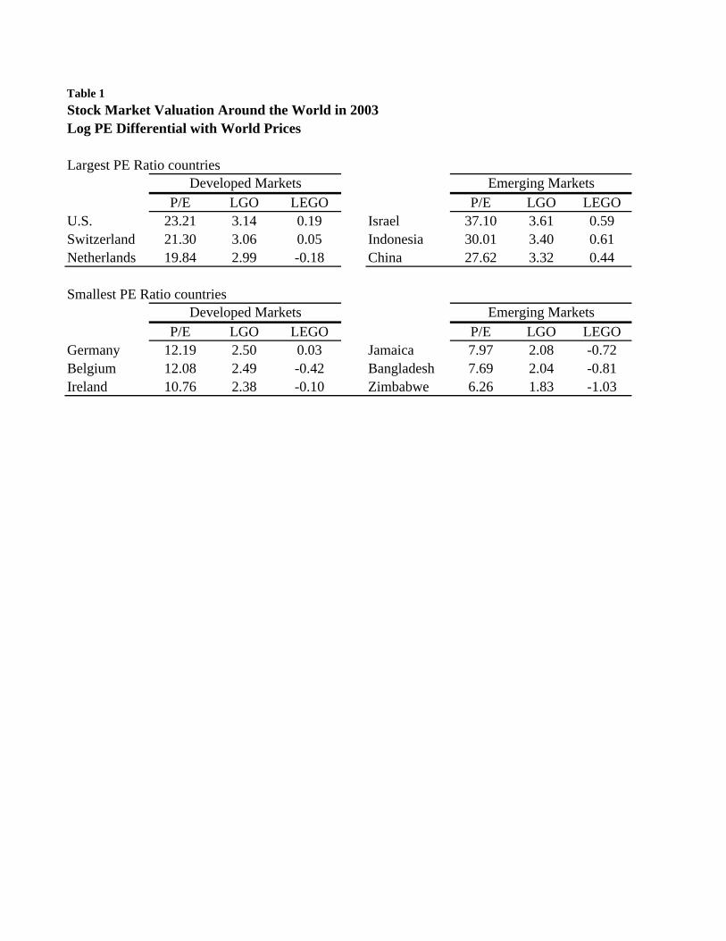
Table 1Stock Market Valuation Around the World in 2003Log PE Differential with World Prices

Largest PE Ratio countries

P/E LGO LEGO P/E LGO LEGOU.S. 23.21 3.14 0.19 Israel 37.10 3.61 0.59Switzerland 21.30 3.06 0.05 Indonesia 30.01 3.40 0.61Netherlands 19.84 2.99 -0.18 China 27.62 3.32 0.44

Smallest PE Ratio countries

P/E LGO LEGO P/E LGO LEGOGermany 12.19 2.50 0.03 Jamaica 7.97 2.08 -0.72Belgium 12.08 2.49 -0.42 Bangladesh 7.69 2.04 -0.81Ireland 10.76 2.38 -0.10 Zimbabwe 6.26 1.83 -1.03

Developed Markets Emerging Markets

Developed Markets Emerging Markets

Table 2Summary StatisticsLog Price Differential: LEGO

Country Sample Average Stdev Average Stdev Average Stdev Average Stdev Observations

ARG EM -0.506 0.632 0.614 0.521 -0.186 0.544 0.407 0.397 20AUS IND -0.215 0.198 0.245 0.158 0.018 0.141 0.106 0.093 33AUT IND -0.005 0.244 0.194 0.144 0.074 0.218 0.204 0.103 33BEL IND -0.257 0.266 0.322 0.178 0.003 0.188 0.150 0.110 33BGD EM -0.605 0.688 0.788 0.437 -0.361 0.637 0.630 0.330 10BRA EM -0.824 0.438 0.824 0.438 -0.541 0.386 0.541 0.386 20CAN IND -0.157 0.184 0.200 0.134 0.076 0.174 0.138 0.129 33CHE IND -0.194 0.209 0.228 0.170 -0.101 0.206 0.163 0.160 33CHL EM -0.423 0.601 0.491 0.543 -0.222 0.430 0.326 0.352 19CHN EM 0.311 0.312 0.346 0.270 0.463 0.280 0.466 0.275 13CIV EM -1.067 0.263 1.067 0.263 -0.703 0.193 0.703 0.193 10COL EM -0.443 0.453 0.506 0.378 -0.268 0.472 0.449 0.295 22DEU IND -0.210 0.179 0.225 0.159 0.012 0.157 0.127 0.091 33DNK IND -0.098 0.359 0.263 0.260 0.049 0.312 0.222 0.221 33EGY EM -0.575 0.576 0.720 0.350 -0.357 0.560 0.568 0.313 10ESP IND -0.273 0.340 0.337 0.273 -0.009 0.215 0.170 0.126 19FIN IND -0.366 0.491 0.496 0.351 -0.319 0.452 0.450 0.313 18FRA IND -0.287 0.169 0.296 0.153 -0.101 0.168 0.156 0.117 33GBR IND -0.302 0.215 0.302 0.215 -0.132 0.171 0.141 0.163 33GRC EM -0.312 0.507 0.447 0.385 -0.056 0.346 0.272 0.211 17IDN EM -0.064 0.479 0.364 0.304 0.259 0.474 0.417 0.334 17IND EM -0.200 0.396 0.370 0.234 0.090 0.421 0.371 0.202 20IRL IND -0.385 0.272 0.399 0.249 -0.205 0.206 0.217 0.193 33ISR EM -0.046 0.390 0.330 0.179 0.001 0.379 0.301 0.204 9ITA IND -0.076 0.206 0.180 0.121 0.130 0.165 0.164 0.129 20JAM EM -1.037 0.513 1.037 0.513 -0.814 0.468 0.814 0.468 10JOR EM -0.169 0.406 0.351 0.255 0.094 0.374 0.241 0.297 20JPN IND 0.785 0.278 0.786 0.273 - - - - 33KEN EM -0.538 0.518 0.597 0.440 -0.396 0.482 0.507 0.346 10KOR EM -0.039 0.437 0.352 0.249 0.179 0.517 0.467 0.267 20LKA EM -0.532 0.515 0.605 0.418 -0.403 0.549 0.539 0.404 13MAR EM -0.141 0.287 0.253 0.182 0.030 0.274 0.231 0.129 10MEX EM -0.527 0.381 0.530 0.376 -0.342 0.334 0.376 0.294 20MYS EM 0.218 0.337 0.344 0.198 0.343 0.391 0.455 0.242 22NGA EM -0.732 0.543 0.812 0.406 -0.537 0.500 0.672 0.283 22NLD IND -0.232 0.228 0.262 0.191 -0.188 0.173 0.215 0.137 33NOR IND -0.676 0.438 0.676 0.438 -0.281 0.386 0.372 0.295 26NZL IND -0.375 0.242 0.375 0.242 -0.184 0.153 0.198 0.134 18PAK EM -0.705 0.570 0.756 0.497 -0.391 0.541 0.510 0.424 20PHL EM -0.479 0.553 0.540 0.490 -0.292 0.545 0.419 0.449 20PRT EM -0.073 0.527 0.389 0.351 0.146 0.299 0.258 0.204 18SGP IND 0.154 0.373 0.312 0.251 0.323 0.375 0.399 0.290 33SWE IND -0.172 0.263 0.229 0.213 -0.064 0.250 0.201 0.156 24THA EM -0.280 0.347 0.379 0.227 -0.065 0.351 0.282 0.210 20TTO EM -0.206 0.202 0.216 0.190 -0.053 0.169 0.154 0.072 10TUN EM -0.260 0.275 0.330 0.172 -0.266 0.413 0.416 0.238 10TUR EM -0.341 0.722 0.542 0.578 -0.082 0.667 0.529 0.396 20USA IND -0.085 0.198 0.181 0.113 0.045 0.069 0.061 0.056 33VEN EM -0.554 0.545 0.654 0.412 -0.248 0.608 0.487 0.429 20ZAF EM -0.515 0.225 0.517 0.220 -0.220 0.196 0.249 0.157 33ZWE EM -0.973 0.737 1.093 0.532 -0.764 0.665 0.892 0.468 20IND -0.155 0.388 0.320 0.268 -0.036 0.271 0.196 0.191 587 / 554EM -0.407 0.568 0.551 0.430 -0.181 0.534 0.441 0.350 528

ALL -0.274 0.498 0.429 0.372 -0.107 0.427 0.316 0.306 1,115 / 1,082

LGO-GGO |LGO-GGO| LGO-GGO |LGO-GGO|Excluding Japan

Table 3Log Price DifferentialsTrends in |LEGO|?

Panel A

Trend Estimate

Standard Error

Number of

CountriesTrend

EstimateStandard

Error

Number of

CountriesTrend

EstimateStandard

Error

Number of

Countries

-0.0100 0.0020 50 -0.0050 0.0016 13 -0.0170 0.0038 31R-squared: 0.40 R-squared: 0.28 R-squared: 0.28

Panel B

Intial |LEGO|

Standard Error

Trend Estimate

Standard Error

Number of

Countries

0.3442 0.0471 -0.0044 0.0026 50R-squared: 0.20

1980-2005

All countries Developed Markets Emerging Markets1980-2005 1973-2005 1980-2005

All countries

Table 4Market Integration DeterminantsDependent Variable: |LEGO|50 countries1980-2003

Capital Account Openness

Equity Market Openness Trade Openness Trend

No of Countries / Country Years R2

-0.475 48 / 858 0.159(0.069)

-0.361 50 / 884 0.207(0.045)

-0.349 50 / 884 0.128(0.061)

-0.390 -0.156 48 / 858 0.179(0.072) (0.059)

-0.391 -0.158 0.001 48 / 858 0.179(0.073) (0.059) (0.003)

-0.293 -0.171 50 / 884 0.230(0.046) (0.058)

-0.295 -0.166 -0.001 50 / 884 0.231(0.046) (0.059) (0.003)

Table 5aMarket Integration DeterminantsDependent Variable: |LEGO|50 countries1980-2003

Panel A: OpennessEquity Market

Openness Trade Openness Gross FDI/GDP Trade/GDPNo of Countries /

Country Years R2

-0.285 -0.166 -0.233 50 / 879 0.227(0.047) (0.058) (0.231)

-0.300 -0.151 -0.077 50 / 884 0.237(0.046) (0.058) (0.051)

Panel B: Political Risk / Institutions / Corporate Governance

Equity Market Openness Trade Openness

Political Risk Index

Quality of Institutions

Investment Profile Law and Order

Minority Shareholder

RightsInsider Trading

LawInsider Trading

ProsecutionLegal Origin

(English)Legal Origin

(French)No of Countries /

Country Years R2

-0.202 -0.133 -0.416 50 / 884 0.247(0.053) (0.058) (0.152)

-0.170 -0.151 -0.343 50 / 884 0.263(0.051) (0.055) (0.091)

-0.268 -0.150 -0.190 50 / 884 0.241(0.046) (0.057) (0.076)

-0.195 -0.145 -0.256 50 / 884 0.255(0.049) (0.056) (0.075)

-0.244 -0.235 -0.061 40 / 771 0.235(0.054) (0.063) (0.086)

-0.296 -0.185 0.053 50 / 884 0.235(0.046) (0.058) (0.043)

-0.289 -0.169 -0.010 50 / 884 0.230(0.049) (0.058) (0.037)

-0.297 -0.179 -0.035 0.001 50 / 884 0.233(0.047) (0.058) (0.051) (0.050)

Table 5bMarket Integration DeterminantsDependent Variable: |LEGO|50 countries1980-2003

Panel C: Financial Development / Measurement

Equity Market Openness Trade Openness

Local Equity Market

IlliquidityLocal Equity

Market Turnover

Local Equity Market Return Autocorrelation

MYY R2

SynchronicityPrivate

Credit/GDP

Private Credit/GDP

(adj.)Accounting Standards

Earnings Management

No of Countries / Country Years R2

-0.217 -0.168 0.259 46 / 787 0.194(0.052) (0.057) (0.095)

-0.295 -0.170 0.010 50 / 884 0.230(0.048) (0.058) (0.028)

-0.228 -0.165 0.178 50 / 760 0.194(0.050) (0.059) (0.085)

-0.249 -0.172 -0.085 45 / 763 0.169(0.050) (0.060) (0.123)

-0.239 -0.156 -0.150 50 / 884 0.210(0.047) (0.055) (0.046)

-0.211 -0.164 -0.166 49 / 876 0.254(0.046) (0.054) (0.046)

-0.238 -0.163 -0.263 36 / 713 0.199(0.064) (0.076) (0.158)

-0.232 -0.089 0.095 28 / 591 0.131(0.067) (0.083) (0.074)

Panel D: Global Discount / Risk Appetite / Behavioral

Equity Market Openness Trade Openness U.S. Real Rate

U.S. Money Supply Growth

U.S. Risk Aversion

World GDP Growth

U.S. Corporate Default Spread

VIX Option Index

Past Local Equity Market

ReturnNo of Countries /

Country Years R2

-0.298 -0.165 1.258 50 / 884 0.234(0.047) (0.058) (0.725)

-0.295 -0.170 0.246 50 / 884 0.190(0.047) (0.058) (0.355)

-0.287 -0.168 -0.051 50 / 884 0.234(0.047) (0.058) (0.035)

-0.293 -0.170 0.243 50 / 884 0.230(0.047) (0.058) (0.822)

-0.294 -0.168 2.883 50 / 884 0.190(0.046) (0.058) (3.449)

-0.289 -0.173 0.194 50 / 884 0.232(0.047) (0.058) (0.156)

-0.281 -0.145 0.025 50 / 850 0.207(0.048) (0.060) (0.018)

Table 5cMarket Integration DeterminantsDependent Variable: |LEGO|50 countries1980-2003

Panel E: Traditional Growth / Factor Productivity Determinants

Equity Market Openness Trade Openness

Log GDP per capita

Secondary School

EnrollmentLog Life

ExpantancyPopulation

Growth Union DensityProduct Market

RegulationNo of Countries /

Country Years R2

-0.150 -0.129 -0.058 50 / 884 0.256(0.058) (0.058) (0.017)

-0.207 -0.134 -0.202 50 / 884 0.250(0.052) (0.058) (0.068)

-0.222 -0.107 -0.469 50 / 884 0.248(0.051) (0.059) (0.165)

-0.256 -0.160 2.961 50 / 884 0.236(0.049) (0.058) (1.945)

-0.441 -1.206 0.197 23 / 479 0.194(0.105) (0.230) (0.086)

-0.196 0.172 20 / 432 0.049(0.374) (0.066)

Panel F: Global Asset Pricing Model Implied Controls

Equity Market Openness Trade Openness

Corporate Financial

Leverage Ratio (1985-2003)

Local Market Earnings Growth

VolatilityWorld Equity

Market Volatility R2

-0.314 -0.096 0.089 46 / 652 0.152(0.053) (0.067) (0.103)

-0.299 -0.073 0.374 50 / 802 0.203(0.046) (0.059) (0.171)

-0.294 -0.170 -0.561 50 / 884 0.230(0.047) (0.058) (1.433)

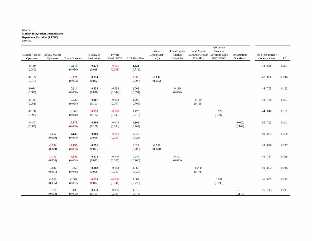
Table 6aMarket Integration DeterminantsDependent Variable: |LEGO|1980-2003

Capital Account Openness

Equity Market Openness Trade Openness

Quality of Institutions

Private Credit/GDP U.S. Real Rate

Private Credit/GDP

(adj.)

Local Equity Market

Illiquidity

Local Market Earnings Growth

Volatility

Corporate Financial

Leverage Ratio (1985-2003)

Accounting Standards

No of Countries / Country Years R2

-0.149 -0.118 -0.370 -0.075 1.823 48 / 858 0.241(0.080) (0.056) (0.098) (0.048) (0.716)

-0.165 -0.121 -0.314 1.606 -0.092 47 / 850 0.246(0.076) (0.054) (0.092) (0.697) (0.045)

-0.094 -0.114 -0.338 -0.034 1.008 0.139 44 / 763 0.183(0.083) (0.060) (0.096) (0.044) (0.691) (0.090)

-0.135 -0.030 -0.367 -0.054 1.590 0.189 48 / 780 0.201(0.083) (0.058) (0.101) (0.047) (0.706) (0.165)

-0.180 -0.060 -0.310 -0.080 1.475 0.122 44 / 640 0.192(0.090) (0.070) (0.102) (0.045) (0.710) (0.097)

-0.173 -0.171 -0.308 -0.045 1.162 -0.002 36 / 713 0.241(0.085) (0.066) (0.109) (0.048) (0.769) (0.169)

-0.160 -0.137 -0.300 -0.092 1.738 50 / 884 0.280(0.050) (0.054) (0.098) (0.049) (0.728)

-0.132 -0.150 -0.291 1.571 -0.110 49 / 876 0.277(0.049) (0.053) (0.093) (0.708) (0.048)

-0.108 -0.146 -0.312 -0.049 0.949 0.191 46 / 787 0.239(0.054) (0.054) (0.091) (0.045) (0.706) (0.093)

-0.180 -0.052 -0.282 -0.064 1.567 0.260 50 / 802 0.246(0.051) (0.056) (0.098) (0.047) (0.730) (0.176)

-0.174 -0.067 -0.314 -0.090 1.807 0.161 46 / 652 0.225(0.055) (0.062) (0.094) (0.044) (0.729) (0.096)

-0.126 -0.135 -0.330 -0.056 1.310 0.018 36 / 713 0.241(0.064) (0.072) (0.101) (0.048) (0.778) (0.170)

Table 6bMarket Integration DeterminantsDependent Variable: |LEGO|1980-2003

Panel A: General Unrestricted Model with Capital Account Openess

Capital Account Openness

Trade Openness

Quality of Institutions

Insider Trading Law

Legal Origin (English)

Legal Origin (French)

Private Credit/GDP U.S. Real Rate

U.S. Risk Aversion

U.S. Corporate

Default SpreadPopulation

Growth

Private Credit/GDP

(adj.)

Local Equity Market

Illiquidity

Local Market Earnings Growth Volatility

Financial Leverage

Ratio (1985-2003)

Accounting Standards

No of Countries / Country Years R2

-0.149 -0.088 -0.345 0.129 -0.135 -0.132 -0.126 1.848 -0.117 14.597 3.583 48 / 858 0.299(0.065) (0.081) (0.128) (0.047) (0.046) (0.038) (0.042) (0.729) (0.039) (4.760) (2.490)

-0.159 -0.094 -0.269 0.125 -0.121 -0.101 1.611 -0.122 15.700 4.620 -0.113 47 / 850 0.305(0.064) (0.083) (0.106) (0.048) (0.043) (0.036) (0.683) (0.038) (4.626) (2.627) (0.037)

-0.063 -0.105 -0.312 0.132 -0.141 -0.140 -0.090 1.020 -0.094 14.461 5.169 0.151 44 / 763 0.259(0.071) (0.079) (0.123) (0.036) (0.044) (0.039) (0.042) (0.695) (0.033) (4.198) (2.037) (0.082)

-0.136 0.011 -0.365 0.110 -0.119 -0.158 -0.110 1.741 -0.082 10.957 3.865 0.193 48 / 780 0.264(0.069) (0.055) (0.129) (0.040) (0.043) (0.040) (0.041) (0.783) (0.038) (4.521) (2.308) (0.176)

-0.121 -0.027 -0.376 0.103 -0.150 -0.154 -0.117 1.286 -0.127 8.589 4.370 0.115 44 / 640 0.253(0.071) (0.070) (0.161) (0.046) (0.053) (0.042) (0.048) (0.767) (0.093) (3.949) (2.534) (0.110)

-0.156 -0.145 -0.148 0.133 -0.182 -0.108 -0.059 0.930 -0.132 17.462 8.213 -0.131 36 / 713 0.331(0.069) (0.103) (0.121) (0.042) (0.051) (0.035) (0.042) (0.837) (0.042) (5.153) (1.918) (0.146)

Panel B: General Unrestricted Model with Equity Market Openess

Equituy Market

OpennessTrade

OpennessQuality of Institutions

Investment Profile

Insider Trading Law

Legal Origin (English)

Legal Origin (French)

Private Credit/GDP U.S. Real Rate

U.S. Risk Aversion

U.S. Corporate

Default Spread

Private Credit/GDP

(adj.)

Local Equity Market

Illiquidity

Local Market Earnings Growth Volatility

Financial Leverage

Ratio (1985-2003)

Accounting Standards

No of Countries / Country Years R2

-0.145 -0.120 -0.351 -0.155 0.098 -0.097 -0.112 -0.110 1.645 -0.091 12.740 50 / 884 0.318(0.062) (0.091) (0.118) (0.072) (0.051) (0.049) (0.040) (0.050) (0.765) (0.032) (4.855)

-0.114 -0.131 -0.341 -0.206 0.089 -0.079 -0.089 1.392 -0.094 13.975 -0.098 49 / 876 0.316(0.059) (0.090) (0.111) (0.069) (0.051) (0.048) (0.039) (0.694) (0.032) (4.766) (0.042)

-0.069 -0.151 -0.392 -0.158 0.108 -0.091 -0.131 -0.075 0.857 -0.073 12.602 0.205 46 / 787 0.290(0.062) (0.086) (0.124) (0.055) (0.037) (0.048) (0.042) (0.041) (0.688) (0.030) (4.592) (0.105)

-0.155 -0.032 -0.365 -0.129 0.076 -0.078 -0.129 -0.091 1.586 -0.057 8.477 0.227 50 / 802 0.281(0.058) (0.077) (0.123) (0.057) (0.045) (0.047) (0.041) (0.046) (0.827) (0.034) (5.003) (0.174)

-0.137 -0.053 -0.432 -0.156 0.103 -0.118 -0.137 -0.097 1.340 -0.121 8.562 0.117 46 / 652 0.276(0.067) (0.082) (0.121) (0.065) (0.049) (0.048) (0.041) (0.048) (0.721) (0.079) (4.324) (0.105)

-0.068 -0.142 -0.356 -0.232 0.129 -0.119 -0.094 -0.041 0.968 -0.113 19.061 -0.093 36 / 713 0.309(0.069) (0.101) (0.103) (0.065) (0.042) (0.056) (0.041) (0.038) (0.788) (0.039) (5.123) (0.172)

Panel C: General Unrestricted Model with Capital Account and Equity Market Openess

Equituy Market

OpennessQuality of Institutions

Investment Profile

Insider Trading Law

Legal Origin (English)

Legal Origin (French)

Private Credit/GDP U.S. Real Rate

U.S. Risk Aversion

U.S. Corporate

Default SpreadPopulation

Growth

Private Credit/GDP

(adj.)

Local Equity Market

Illiquidity

Local Market Earnings Growth Volatility

Financial Leverage

Ratio (1985-2003)

Accounting Standards

No of Countries / Country Years R2

-0.131 -0.349 -0.142 0.131 -0.135 -0.129 -0.109 1.983 -0.108 16.111 2.924 48 / 858 0.303(0.060) (0.098) (0.077) (0.045) (0.046) (0.034) (0.044) (0.698) (0.038) (5.121) (2.816)

-0.090 -0.310 -0.182 0.127 -0.122 -0.111 1.696 -0.116 17.780 4.185 -0.114 47 / 850 0.304(0.053) (0.097) (0.071) (0.046) (0.043) (0.032) (0.631) (0.039) (4.964) (2.796) (0.038)

-0.051 -0.358 -0.164 0.123 -0.145 -0.149 -0.070 1.073 -0.092 16.432 4.959 0.110 44 / 763 0.260(0.058) (0.108) (0.063) (0.034) (0.045) (0.038) (0.041) (0.647) (0.034) (4.338) (1.978) (0.082)

-0.117 -0.332 -0.097 0.121 -0.116 -0.137 -0.092 1.826 -0.073 11.916 3.114 0.232 48 / 780 0.272(0.055) (0.113) (0.059) (0.039) (0.042) (0.034) (0.041) (0.728) (0.036) (4.601) (2.533) (0.164)

-0.112 -0.383 -0.140 0.117 -0.152 -0.145 -0.093 1.214 -0.135 9.936 3.877 0.114 44 / 640 0.265(0.071) (0.120) (0.064) (0.050) (0.054) (0.035) (0.047) (0.749) (0.083) (4.484) (2.586) (0.101)

-0.084 -0.212 -0.210 0.121 -0.174 -0.109 -0.052 0.867 -0.132 20.790 8.430 -0.119 36 / 713 0.327(0.067) (0.113) (0.066) (0.040) (0.052) (0.036) (0.041) (0.751) (0.045) (5.729) (1.707) (0.152)

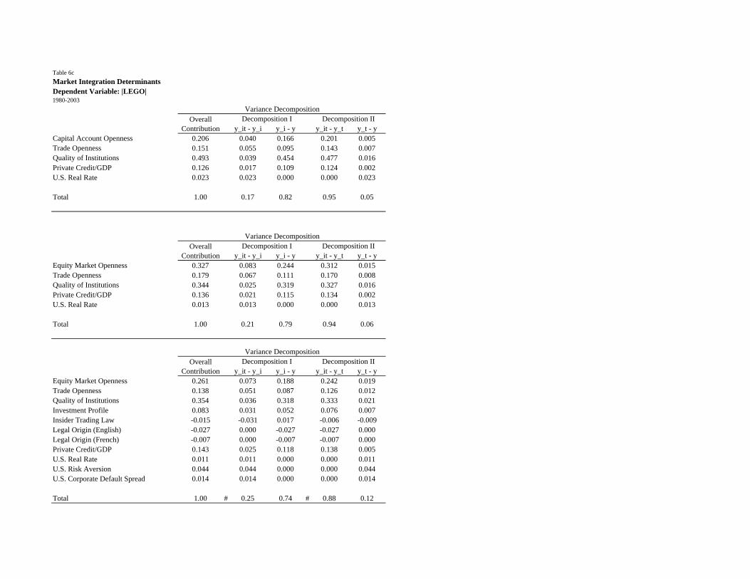
Table 6cMarket Integration DeterminantsDependent Variable: |LEGO|1980-2003

y_it - y_i y_i - y y_it - y_t y_t - yCapital Account Openness 0.206 0.040 0.166 0.201 0.005Trade Openness 0.151 0.055 0.095 0.143 0.007Quality of Institutions 0.493 0.039 0.454 0.477 0.016Private Credit/GDP 0.126 0.017 0.109 0.124 0.002U.S. Real Rate 0.023 0.023 0.000 0.000 0.023

Total 1.00 0.17 0.82 0.95 0.05

y_it - y_i y_i - y y_it - y_t y_t - yEquity Market Openness 0.327 0.083 0.244 0.312 0.015Trade Openness 0.179 0.067 0.111 0.170 0.008Quality of Institutions 0.344 0.025 0.319 0.327 0.016Private Credit/GDP 0.136 0.021 0.115 0.134 0.002U.S. Real Rate 0.013 0.013 0.000 0.000 0.013

Total 1.00 0.21 0.79 0.94 0.06

y_it - y_i y_i - y y_it - y_t y_t - yEquity Market Openness 0.261 0.073 0.188 0.242 0.019Trade Openness 0.138 0.051 0.087 0.126 0.012Quality of Institutions 0.354 0.036 0.318 0.333 0.021Investment Profile 0.083 0.031 0.052 0.076 0.007Insider Trading Law -0.015 -0.031 0.017 -0.006 -0.009Legal Origin (English) -0.027 0.000 -0.027 -0.027 0.000Legal Origin (French) -0.007 0.000 -0.007 -0.007 0.000Private Credit/GDP 0.143 0.025 0.118 0.138 0.005U.S. Real Rate 0.011 0.011 0.000 0.000 0.011U.S. Risk Aversion 0.044 0.044 0.000 0.000 0.044U.S. Corporate Default Spread 0.014 0.014 0.000 0.000 0.014

Total 1.00 # 0.25 0.74 # 0.88 0.12

Overall Contribution

Decomposition I Decomposition II

Variance DecompositionOverall

ContributionDecomposition I Decomposition II

Variance Decomposition

Variance DecompositionOverall

ContributionDecomposition I Decomposition II

Table 7Market Valuation Determinants Market Valuation DeterminantsDependent Variable: LEGO Dependent Variable: LEGO50 countries 50 countries1980-2003 1980-2003

Capital Account Openness

Equity Market Openness Trade Openness R2 GGO

Capital Account Openness

Equity Market Openness Trade Openness

No of Countries / Country Years R2

0.286 0.029 -0.216 0.314 48 / 858 0.046(0.118) (0.084) (0.118)

0.296 0.072 -0.237 0.308 50 / 884 0.091(0.074) (0.084) (0.073)

0.336 0.061 -0.232 0.349 50 / 884 0.079(0.091) (0.089) (0.091)

0.192 0.174 0.042 -0.224 0.217 0.182 48 / 858 0.060(0.125) (0.099) (0.086) (0.124) (0.099)

0.213 0.207 0.090 -0.246 0.222 0.215 50 / 884 0.110(0.078) (0.098) (0.086) (0.077) (0.097)

Table 8aMarket Valuation DeterminantsDependent Variable: LEGO50 countries1980-2003

Panel A: Openness

GGOEquity Market

Openness Trade Openness Gross FDI/GDP Trade/GDPNo of Countries /

Country Years R2

-0.276 0.204 0.201 0.490 50 / 879 0.107(0.084) (0.078) (0.098) (0.371)

-0.247 0.223 0.212 0.014 50 / 884 0.110(0.086) (0.077) (0.098) (0.086)

Panel B: Political Risk / Institutions / Corporate Governance

GGOEquity Market

Openness Trade OpennessPolitical Risk

IndexQuality of Institutions

Investment Profile Law and Order

Minority Shareholder

RightsInsider Trading

LawInsider Trading

ProsecutionLegal Origin

(English)Legal Origin

(French)No of Countries /

Country Years R2

-0.242 0.184 0.200 0.171 50 / 884 0.111(0.086) (0.091) (0.099) (0.259)

-0.227 0.162 0.205 0.166 50 / 884 0.114(0.086) (0.090) (0.097) (0.160)

-0.253 0.197 0.194 0.195 50 / 884 0.116(0.084) (0.078) (0.097) (0.129)

-0.241 0.127 0.191 0.247 50 / 884 0.122(0.084) (0.084) (0.096) (0.128)

-0.210 0.112 0.401 0.075 40 / 771 0.149(0.073) (0.081) (0.096) (0.124)

-0.286 0.219 0.199 0.064 50 / 884 0.113(0.090) (0.077) (0.099) (0.073)

-0.273 0.196 0.207 0.068 50 / 884 0.114(0.086) (0.080) (0.097) (0.063)

-0.252 0.203 0.234 -0.047 -0.110 50 / 884 0.119(0.086) (0.078) (0.097) (0.085) (0.084)

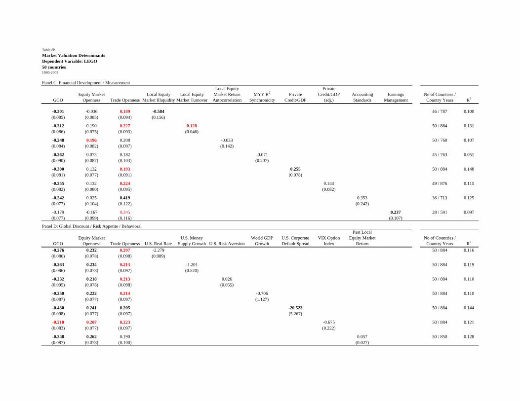
Table 8bMarket Valuation DeterminantsDependent Variable: LEGO50 countries1980-2003

Panel C: Financial Development / Measurement

GGOEquity Market

Openness Trade OpennessLocal Equity

Market IlliquidityLocal Equity

Market Turnover

Local Equity Market Return Autocorrelation

MYY R2

SynchronicityPrivate

Credit/GDP

Private Credit/GDP

(adj.)Accounting Standards

Earnings Management

No of Countries / Country Years R2

-0.301 -0.036 0.189 -0.584 46 / 787 0.100(0.085) (0.085) (0.094) (0.156)

-0.312 0.190 0.227 0.128 50 / 884 0.131(0.086) (0.075) (0.093) (0.046)

-0.248 0.196 0.208 -0.033 50 / 760 0.107(0.084) (0.082) (0.097) (0.142)

-0.262 0.073 0.182 -0.071 45 / 763 0.051(0.090) (0.087) (0.103) (0.207)

-0.300 0.132 0.193 0.255 50 / 884 0.148(0.081) (0.077) (0.091) (0.078)

-0.255 0.132 0.224 0.144 49 / 876 0.115(0.082) (0.080) (0.095) (0.082)

-0.242 0.025 0.419 0.353 36 / 713 0.125(0.077) (0.104) (0.122) (0.242)

-0.179 -0.167 0.345 0.237 28 / 591 0.097(0.077) (0.099) (0.116) (0.107)

Panel D: Global Discount / Risk Appetite / Behavioral

GGOEquity Market

Openness Trade Openness U.S. Real RateU.S. Money

Supply Growth U.S. Risk AversionWorld GDP

GrowthU.S. Corporate Default Spread

VIX Option Index

Past Local Equity Market

ReturnNo of Countries /

Country Years R2

-0.276 0.232 0.207 -2.279 50 / 884 0.116(0.086) (0.078) (0.098) (0.989)

-0.263 0.234 0.213 -1.201 50 / 884 0.119(0.086) (0.078) (0.097) (0.520)

-0.232 0.218 0.213 0.026 50 / 884 0.110(0.095) (0.078) (0.098) (0.055)

-0.250 0.222 0.214 -0.706 50 / 884 0.110(0.087) (0.077) (0.097) (1.127)

-0.430 0.241 0.205 -20.523 50 / 884 0.144(0.098) (0.077) (0.097) (5.267)

-0.210 0.207 0.223 -0.675 50 / 884 0.121(0.083) (0.077) (0.097) (0.222)

-0.248 0.262 0.190 0.057 50 / 850 0.128(0.087) (0.078) (0.100) (0.027)

Table 8cMarket Valuation DeterminantsDependent Variable: LEGO50 countries1980-2003

Panel E: Traditional Growth / Factor Productivity Determinants

GGOEquity Market

Openness Trade OpennessLog GDP per

capita

Secondary School

EnrollmentLog Life

ExpantancyPopulation

Growth Union DensityProduct Market

RegulationNo of Countries /

Country Years R2

-0.255 0.259 0.227 -0.015 50 / 884 0.111(0.087) (0.100) (0.099) (0.031)

-0.238 0.249 0.227 -0.065 50 / 884 0.111(0.087) (0.088) (0.099) (0.121)

-0.233 0.128 0.131 0.615 50 / 884 0.125(0.083) (0.085) (0.099) (0.273)

-0.247 0.230 0.218 0.685 50 / 884 0.110(0.086) (0.082) (0.098) (3.247)

-0.080 -0.484 1.649 -0.110 23 / 479 0.138(0.058) (0.145) (0.330) (0.118)

-0.091 -0.286 -0.146 20 / 432 0.013(0.066) (0.451) (0.116)

Panel F: Global Asset Pricing Model Implied Controls

GGOEquity Market

Openness Trade Openness

Corporate Financial

Leverage Ratio (1985-2003)

Local Market Earnings Growth

VolatilityWorld Equity

Market VolatilityNo of Countries /

Country Years R2

-0.244 0.190 0.050 -0.437 46 / 652 0.059(0.100) (0.081) (0.105) (0.151)

-0.275 0.253 0.104 0.060 50 / 802 0.102(0.085) (0.076) (0.098) (0.297)

-0.248 0.226 0.213 3.051 50 / 884 0.112(0.085) (0.077) (0.097) (2.276)

Table 9a |EYij - EYiw| per industry

Industry Code 1980 - 1984 2001-2005 Change1980 - 1984

2001 - 2005

Trend Estimate

Standard Error

Life Insurance LFINS 0.1421 0.0316 -0.1105 1 31 -0.0048 0.0015Banks BANKS 0.0906 0.0301 -0.0606 2 33 -0.0026 0.0003General Retailers GNRET 0.0823 0.0401 -0.0422 3 18 -0.0010 0.0008Nonlife Insurance NLINS 0.0761 0.0409 -0.0352 4 16 -0.0016 0.0004Chemicals CHMCL 0.0720 0.0704 -0.0016 5 2 -0.0008 0.0005Electricity ELECT 0.0658 0.0351 -0.0307 6 25 -0.0017 0.0003Industrial Metals INDMT 0.0650 0.0634 -0.0016 7 4 -0.0008 0.0004Automobiles & Parts AUTMB 0.0643 0.0497 -0.0146 8 7 -0.0005 0.0003Industrial Engineering INDEN 0.0631 0.0381 -0.0250 9 21 -0.0010 0.0004Fixed Line Telecommunications TELFL 0.0584 0.0379 -0.0205 10 22 -0.0017 0.0004Mobile Telecommunications TELMB 0.0562 0.0280 -0.0282 11 36 -0.0014 0.0005General Industrials GNIND 0.0550 0.0456 -0.0094 12 11 -0.0002 0.0005Oil & Gas Producers OILGP 0.0540 0.0436 -0.0103 13 14 -0.0011 0.0003Industrial Transportation INDTR 0.0523 0.0440 -0.0083 14 13 -0.0002 0.0005Forestry & Paper FSTPA 0.0514 0.0953 0.0439 15 1 -0.0002 0.0005Beverages BEVES 0.0505 0.0340 -0.0164 16 27 -0.0005 0.0004Construction & Materials CNSTM 0.0500 0.0446 -0.0054 17 12 -0.0006 0.0003Media MEDIA 0.0482 0.0306 -0.0177 18 32 -0.0005 0.0005Equity Investment Instruments EQINV 0.0446 0.0509 0.0063 19 6 0.0005 0.0004Leisure Goods LEISG 0.0444 0.0401 -0.0043 20 17 0.0000 0.0006Food & Drug Retailers FDRGR 0.0426 0.0291 -0.0135 21 34 -0.0003 0.0004Mining MNING 0.0405 0.0653 0.0248 22 3 0.0000 0.0007Real Estate RLEST 0.0403 0.0369 -0.0034 23 23 0.0002 0.0003Food Producers FOODS 0.0401 0.0496 0.0095 24 8 -0.0002 0.0003Tobacco TOBAC 0.0385 0.0335 -0.0050 25 28 -0.0003 0.0004Oil Equipment & Services OILES 0.0379 0.0396 0.0017 26 19 0.0003 0.0003Healthcare Equipment & Services HCEQS 0.0343 0.0383 0.0040 27 20 0.0006 0.0005Aerospace & Defense AERSP 0.0340 0.0255 -0.0085 28 37 0.0001 0.0004Pharmaceuticals & Biotechnology PHARM 0.0325 0.0345 0.0020 29 26 0.0002 0.0004General Financial GENFI 0.0320 0.0428 0.0108 30 15 0.0009 0.0004Support Services SUPSV 0.0305 0.0287 -0.0018 31 35 0.0001 0.0003Travel & Leisure TRLES 0.0290 0.0465 0.0174 32 10 0.0010 0.0005Gas, Water & Multiutilities GWMUT 0.0287 0.0356 0.0069 33 24 0.0002 0.0003Software & Computer Services SFTCS 0.0283 0.0199 -0.0084 34 38 -0.0005 0.0003Household Goods HHOLD 0.0278 0.0616 0.0339 35 5 0.0003 0.0005Electronic & Electrical Equipment ELTNC 0.0272 0.0328 0.0056 36 30 0.0000 0.0003Personal Goods PERSG 0.0241 0.0473 0.0232 37 9 0.0007 0.0006Technology Hardware & Equipment TECHD 0.0175 0.0332 0.0157 38 29 0.0006 0.0004

Mean 0.0493 0.0420 -0.0073Dispersion 0.0230 0.0143

Segmentation RankTrend Regression: 1980 - 2005Equally Weighted Mean of |EYij - EYiw|

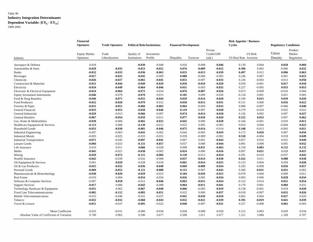
Table 9bIndustry Integration DeterminantsDependent Variable: |EYij - EYiw| 1980-2003

Financial Openness Trade Openness

IndustryEquity Market Openness

Trade Liberalization

Quality of Institutions

Investment Profile Illiquidity Turnover

Private Credit/GDP (adj.) US Real Rate

US Risk Aversion

Union Density

Product Market Regulation

Aerospace & Defense 0.018 -0.039 -0.049 0.026 -0.008 -0.046 0.139 0.004 0.058 0.069Automobiles & Parts -0.029 -0.033 -0.053 -0.055 0.076 -0.009 -0.025 0.396 0.003 -0.006 0.032Banks -0.032 -0.033 -0.036 -0.063 0.033 -0.013 -0.039 0.497 0.012 0.096 0.063Beverages -0.017 -0.025 -0.045 -0.009 0.088 -0.006 -0.002 0.246 0.007 0.001 0.023Chemicals -0.026 -0.027 -0.065 -0.045 0.053 -0.007 -0.033 0.236 -0.003 0.013 0.050Construction & Materials -0.031 -0.044 -0.049 -0.029 0.050 -0.010 -0.020 0.039 -0.001 0.017 0.018Electricity -0.034 -0.049 -0.064 -0.046 0.031 -0.003 -0.035 0.257 -0.005 0.033 0.053Electronic & Electrical Equipment -0.024 -0.064 -0.072 -0.034 0.076 -0.007 -0.026 0.073 -0.009 -0.010 0.004Equity Investment Instruments -0.046 -0.079 -0.070 0.015 0.105 0.009 -0.020 -0.124 0.001 0.021 0.005Food & Drug Retailers -0.046 -0.071 -0.055 -0.044 0.029 -0.014 -0.020 0.190 0.015 0.039 0.020Food Producers -0.032 -0.020 -0.070 -0.012 0.058 -0.013 -0.031 -0.151 0.000 0.016 0.022Forestry & Paper -0.031 -0.051 -0.066 -0.063 0.064 -0.004 -0.033 0.080 -0.007 -0.006 0.040General Financial -0.033 -0.053 -0.058 -0.046 0.110 -0.007 -0.028 0.279 -0.010 0.025 0.022General Industrials -0.029 -0.013 -0.066 -0.007 0.074 -0.014 -0.018 0.126 0.002 0.007 0.027General Retailers -0.067 -0.054 -0.059 -0.011 0.077 -0.018 -0.020 0.522 0.033 0.007 0.062Gas, Water & Multiutilities -0.039 -0.006 -0.065 -0.025 0.042 0.000 -0.028 -0.166 -0.001 0.010 0.011Healthcare Equipment & Services -0.113 0.008 -0.139 -0.012 0.052 0.005 -0.005 0.033 0.004 -0.004 0.023Household Goods -0.033 -0.030 -0.081 -0.046 0.075 -0.014 -0.014 0.348 -0.013 -0.003 0.021Industrial Engineering -0.007 -0.003 -0.043 -0.002 0.044 -0.005 -0.019 0.172 0.020 0.007 0.050Industrial Metals -0.005 -0.025 -0.033 -0.031 0.039 -0.009 -0.002 0.558 -0.004 0.018 0.049Industrial Transportation -0.071 -0.045 -0.097 -0.041 0.007 0.001 -0.043 0.057 0.010 0.025 0.049Leisure Goods -0.084 -0.023 -0.131 -0.057 0.037 0.008 -0.044 0.091 0.008 0.005 0.032Life Insurance 0.010 0.011 0.066 -0.028 0.008 -0.031 -0.063 0.158 0.083 0.132 0.132Media -0.045 -0.021 -0.038 -0.002 0.024 0.000 -0.016 0.097 0.021 0.028 0.021Mining -0.059 -0.072 -0.115 -0.084 0.130 -0.013 -0.054 0.291 -0.010 -0.037 0.042Nonlife Insurance -0.042 -0.039 -0.032 -0.008 0.037 -0.014 -0.030 0.432 0.011 0.088 0.038Oil Equipment & Services 0.001 0.029 -0.028 -0.018 0.065 -0.014 -0.025 -0.155 0.004 0.059 0.028Oil & Gas Producers -0.025 -0.032 -0.036 -0.040 0.069 -0.009 -0.034 0.183 -0.008 0.056 0.057Personal Goods -0.069 -0.052 -0.121 -0.088 0.115 -0.007 -0.043 0.360 -0.031 0.031 0.002Pharmaceuticals & Biotechnology -0.030 -0.020 -0.059 -0.023 0.104 -0.010 -0.015 -0.078 0.004 0.009 0.011Real Estate -0.010 0.004 -0.054 -0.024 0.026 0.005 -0.034 0.093 0.006 0.028 0.034Software & Computer Services -0.007 0.018 -0.012 -0.046 0.063 -0.015 -0.024 -0.152 0.014 0.055 0.054Support Services -0.017 0.006 -0.043 -0.008 0.064 -0.011 -0.041 0.170 0.001 0.084 0.031Technology Hardware & Equipment -0.031 0.002 -0.067 -0.040 0.066 -0.005 -0.019 -0.138 -0.001 0.018 0.028Fixed Line Telecommunications -0.082 -0.112 -0.083 -0.051 0.032 0.000 -0.037 -0.018 -0.007 0.033 0.026Mobile Telecommunications -0.033 -0.046 -0.031 -0.037 0.041 -0.010 -0.018 0.002 0.004 0.027 0.020Tobacco -0.032 -0.032 -0.068 -0.043 0.052 -0.022 -0.039 0.391 -0.019 0.041 0.039Travel & Leisure -0.051 -0.037 -0.095 -0.022 0.048 -0.007 -0.031 0.257 -0.008 0.063 -0.003

Mean Coefficient -0.035 -0.031 -0.060 -0.034 0.058 -0.008 -0.028 0.152 0.003 0.029 0.034Absolute Value of Coefficient of Variation 0.749 0.962 0.596 0.677 0.508 1.011 0.477 1.311 5.084 1.169 0.707

Political Risk/Institutions Financial DevelopmentRisk Appetite / Business Cycles Regulatory Conditions

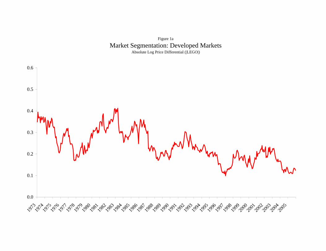
Figure 1a

Market Segmentation: Developed MarketsAbsolute Log Price Differential (|LEGO|)

0.0

0.1

0.2

0.3

0.4

0.5

0.6

1973

1974

1975

1976

1977

1978

1979

1980

1981

1982

1983

1984

1985

1986

1987

1988

1989

1990

1991

1992

1993

1994

1995

1996

1997

1998

1999

2000

2001

2002

2003

2004

2005

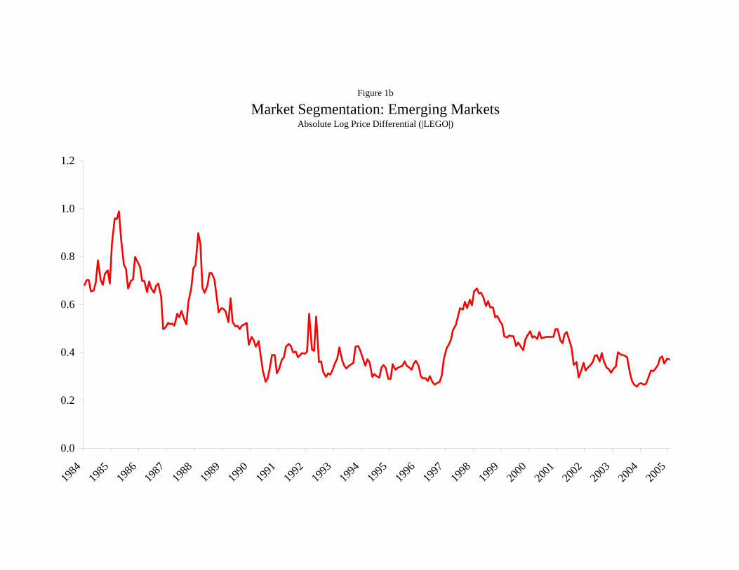
Figure 1b

Market Segmentation: Emerging MarketsAbsolute Log Price Differential (|LEGO|)

0.0

0.2

0.4

0.6

0.8

1.0

1.2

1984

1985

1986

1987

1988

1989

1990

1991

1992

1993

1994

1995

1996

1997

1998

1999

2000

2001

2002

2003

2004

2005

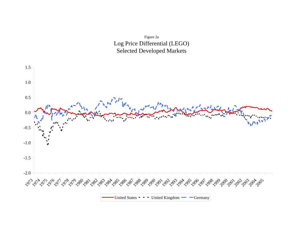
Figure 2a

Log Price Differential (LEGO)Selected Developed Markets

-2.0

-1.5

-1.0

-0.5

0.0

0.5

1.0

1.5

1973

1974

1975

1976

1977

1978

1979

1980

1981

1982

1983

1984

1985

1986

1987

1988

1989

1990

1991

1992

1993

1994

1995

1996

1997

1998

1999

2000

2001

2002

2003

2004

2005

United States United Kingdom Germany

Figure 2b

Log Price Differential (LEGO)Selected Emerging Markets

-2.0

-1.5

-1.0

-0.5

0.0

0.5

1.0

1.5

1973

1974

1975

1976

1977

1978

1980

1981

1982

1983

1984

1985

1987

1988

1989

1990

1991

1992

1994

1995

1996

1997

1998

1999

2001

2002

2003

2004

2005

Brazil Mexico Korea

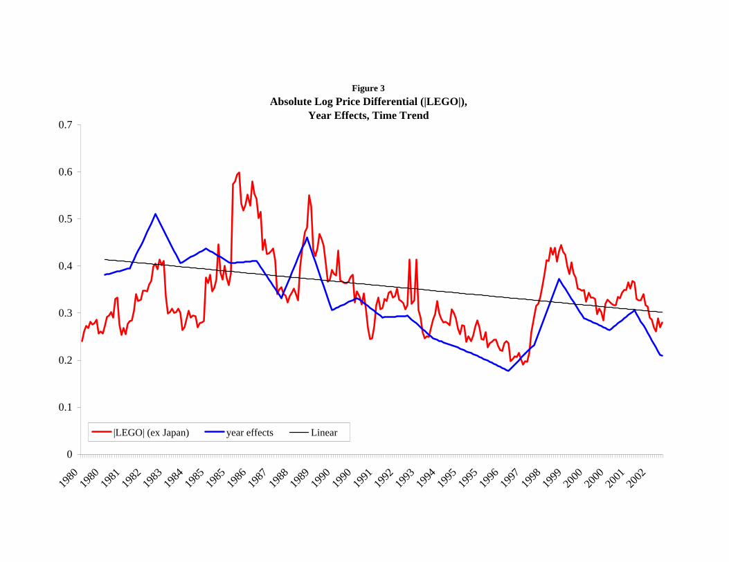
Figure 3 Absolute Log Price Differential (|LEGO|),

Year Effects, Time Trend

0

0.1

0.2

0.3

0.4

0.5

0.6

0.7

1980

1980

1981

1982

1983

1984

1985

1985

1986

1987

1988

1989

1990

1990

1991

1992

1993

1994

1995

1995

1996

1997

1998

1999

2000

2000

2001

2002

|LEGO| (ex Japan) year effects Linear

Figure 4

Emerging Market Discount (LEGO)

-1

-0.8

-0.6

-0.4

-0.2

0

0.2

0.4

1984

1984

1985

1986

1987

1988

1989

1989

1990

1991

1992

1993

1994

1994

1995

1996

1997

1998

1999

1999

2000

2001

2002

2003

2004

2004

2005

Appendix Table 1Data Availability

Source Code Name LGO data start Source Code Name LGO data startDS AUS Australia 197301 EMDB ARG Argentina 198604DS AUT Austria 197301 EMDB BGD Bangladesh 199601DS BEL Belgium 197301 EMDB BRA Brazil 198604DS CAN Canada 197301 EMDB CHL Chile 198601DS DNK Denmark 197301 EMDB CHN China 199301DS FIN Finland 198803 EMDB COL Colombia 198412DS FRA France 197301 EMDB CIV Cote d'Ivoire 199601DS DEU Germany 197301 EMDB EGY Egypt 199601DS IRL Ireland 197301 DS GRC Greece 198903DS ITA Italy 198601 EMDB IND India 198604DS JPN Japan 197301 EMDB IDN Indonesia 198912DS NLD Netherlands 197301 EMDB ISR Israel 199701DS NZL New Zealand 198801 EMDB JAM Jamaica 199601DS NOR Norway 198001 EMDB JOR Jordan 198607DS SGP Singapore 197301 EMDB KEN Kenya 199601DS ESP Spain 198703 EMDB KOR Korea 198601DS SWE Sweden 198201 EMDB MYS Malaysia 198412DS CHE Switzerland 197301 EMDB MEX Mexico 198604DS GBR United Kingdom 197301 EMDB MAR Morocco 199601DS USA United States 197301 EMDB NGA Nigeria 198412

EMDB PAK Pakistan 198601EMDB PHL Philippines 198412DS PRT Portugal 198809DS ZAF South Africa 197301EMDB LKA Sri Lanka 199301EMDB THA Thailand 198601EMDB TTO Trin. & Tobago 199601EMDB TUN Tunisia 199601EMDB TUR Turkey 198612EMDB VEN Venezuela 198601EMDB ZWE Zimbabwe 198601

Industrialized Emerging

Appendix Table 2Description of the VariablesAll data are employed at the annual frequency.

Variable Description

LEGO and |LEGO| LEGO measures the difference between a country's local market PE ratio and the corresponding global PE ratio, adjusted for the country's industry composition. |LEGO| is the absolute value of LEGO. Both variables are available for 51 countries. For details, see Section 2. Sources: Datastream and Standard & Poors' Emerging Market Data Base.

LEGO(exJ) and |LEGO(exJ)| In the construction of LEGO(exJ) and |LEGO(exJ)|, we have excluded Japanese data from the global PE ratios. For details, see Section 2. Sources: Datastream and Standard & Poors' Emerging Market Data Base.

Capital account openness Quinn’s capital account openness measure is also created from the text of the annual volume published by thInternational Monetary Fund (IMF), Exchange Arrangements and Exchange Restrictions. Rather than the indicator constructed by the IMF that takes a 1 if any restriction is in place, Quinn’s openness measure is scored 0-4, in half integer units, with 4 representing a fully open economy. The measure hence facilitates a more nuanced view of capital account openness than the usual 0/1 indicator as it can vary between 0 and 1, and is available for 48 countries in our study. We transform the measure into a 0 to 1 scale.

Equity market openness Following Bekaert (1995) and Edison and Warnock (2003), the equity market openness measure is based on the ratio of the market capitalization of the constituent firms comprising the IFC Investable index to those that comprise the IFC Global index for each country. The IFC Global index, subject to some exclusion restrictions, is designed to represent the overall market portfolio for each country, whereas the IFC Investable index is designed to represent a portfolio of domestic equities that are available to foreign investors. A ratio of one means that all of the stocks are available to foreign investors. Fully segmented countries have an intensity measure of zero, and fully liberalized countries have an intensity measure of one.

Gross FDI/GDP Gross foreign direct investment is the sum of the absolute values of inflows and outflows of foreign direct investment recorded in the balance of payments financial account. It includes equity capital, reinvestment of earnings, other long-term capital, and short-term capital. The indicator is calculated as a ratio to GDP. Source: World Bank Development Indicators .

Trade liberalization We obtain the trade liberalization dates developed in Wacziarg and Welch (2003). Wacziarg and Welch look at five factors: average tariff rates of 40% or more; nontariff barriers covering 40% or more of trade; a black market exchange rate that is depreciated by 20% or more relative to the official exchange rate, on average, during the 1970s or 1980s; a state monopoly on major exports; and a socialist economic system. If a country meets any of these five criteria, it is classified with indicator variable equal to zero and deemed closed.

Trade/GDP The sum of exports and imports of goods and services measured as a share of gross domestic product. Source: World Bank Development Indicators .

Political risk index The value of the the Political Risk Service (PRS) Group’s political risk indicator (which ranges between 0 and 100). The risk rating is a combination of 12 subcomponents. Overall, a political risk rating of 0.0% to 49.9% indicates a Very High Risk; 50.0% to 59.9% High Risk; 60.0% to 69.9% Moderate Risk; 70.0% to 79.9% Low Risk; and 80.0% or more Very Low Risk. The data are available from 1984 through 1997. For each country, we backfill the 1984 value to 1980. Source: Various issues of the International Country Risk Guide.

Quality of Institutions The sum of ICRG subcomponents: Corruption, Law and Order, and Bureaucratic Quality Corruption ICRG political risk sub-component. This is a measure of corruption within the political system. Such

corruption distorts the economic and financial environment, reduces the efficiency of government and business by enabling people to assume positions of power through patronage rather than ability, and introduces an inherent instability into the political process. The most common form of corruption met directly by business is financial corruption in the form of demands for special payments and bribes connected with import and export licenses, exchange controls, tax assessments, police protection, or loans. Although the PRS measure takes such corruption into account, it is more concerned with actual or potential corruption in the form of excessive patronage, nepotism, job reservations, “favor-for-favors,” secret party funding, and suspiciously close ties between politics and business. In PRS's view these sorts of corruption pose risk to foreign business, potentially leading to popular discontent, unrealistic and inefficient controls on the state economy, and encourage the development of the black market.

Law and Order ICRG political risk sub-component. PRS assesses Law and Order separately, with each sub-component comprising zero to three points. The Law sub-component is an assessment of the strength and impartiality of the legal system, while the Order sub-component is an assessment of popular observance of the law. Thus, a country can enjoy a high rating (3.0) in terms of its judicial system, but a low rating (1.0) if the law is ignored for a political aim.

Table 2(Continued)

Variable Description Bureaucratic Quality ICRG political risk sub-component. The institutional strength and quality of the bureaucracy can act as a

shock absorber that tends to minimize revisions of policy when governments change. Therefore, high points are given to countries where the bureaucracy has the strength and expertise to govern without drastic changes in policy or interruptions in government services. In these low-risk countries, the bureaucracy tends to be somewhat autonomous from political pressure and to have an established mechanism for recruitment and training. Countries that lack the cushioning effect of a strong bureaucracy receive low points because a change in government tends to be traumatic in terms of policy formulation and day-to-day administrative functions.

Minority Shareholder Rights An index aggregating different shareholder rights. The index is formed by adding 1 when: (1) the country allows shareholders to mail their proxy vote to the firm; (2) shareholders are not required to deposit their shares prior to the General Shareholders’ Meeting; (3) cumulative voting or proportional representation of minorities in the board of directors is allowed; (4) an oppressed minorities mechanism is in place; (5) the minimum percentage of share capital that entitles a shareholder to call for an Extraordinary Shareholders’ Meeting is less than or equal to 10 percent (the sample median); or (6) shareholders have preemptive rights that can only be waved by a shareholders’ vote. The index ranges from 0 to 6. This variable is purely cross-sectional, and available for 47 countries. Source: La Porta et al. (1998).

Insider Trading Law Bhattacharya and Daouk (2002) document the enactment of insider trading laws and the first prosecution of these laws. We construct two indicator variables. The first takes the value of one following the introduction oan insider trading law. The second takes the value of one after the law's first prosecution.

Legal origin Identifies the legal origin of the company law or commercial code of each country (English, French, Socialist, German, Scandinavian). We construct three indicators that take the value of one when the legal origin is Anglo-Saxon (English law), French (French law), or other (law other), and zero otherwise. This variable is purely cross-sectional and available for all countries. The source is La Porta, Lopez-di-Silanes, Shleifer, and Vishny (1999).

Illiquidity Following Lesmond, Ogden and Trzcinka (1999), Lesmond (2005), and Bekaert, Harvey, and Lundblad (2005), we construct the illiquidity measure as the proportion of zero daily returns observed over the relevant year for each equity market. We obtain daily returns data in local currency at the firm level from the Datastream research files. For each country, we observe daily returns (using closing prices) for a large collection of firms. The total number of firms available from the Datastream research files accounts for about 90%, on average, of the number of domestically listed firms reported by the World Bank's World Development Indicators. For each country, we calculate the capitalization-weighted proportion of zero daily returns across all firms, and average this proportion over the year

Equity market turnover The ratio of equity market value traded to the market capitalization. The data are available for 50 countries. Source: Standard and Poor's/International Finance Corporation's Emerging Stock Markets Factbook.

Market Return Autocorrleation For each country and year t , we estimate the autocorrelation of monthly equity market returns over the period between January of year t-4 and December of year t .

Private credit/GDP Private credit divided by gross domestic product. Credit to private sector refers to financial resources provided to the private sector, such as through loans, purchases of non-equity securities, and trade credits and other accounts receivable that establish a claim for repayment. Available for all countries. Source: World Bank Development Indicators CD-ROM. We also construct an adjusted private credit measure controlling for state ownership of the banking system. We interpolate the state ownership ratios provided by La Porta, Lopez de Silanes and Shleifer (2002) for two years during our sample to the full sample, and create a new measure of banking development as official private credit to GDP times (1- the ratio of state ownership).

Accounting Standards Index created by examining and rating companies' 1990 annual reports on their inclusion or omission of 90 items. These items fall into seven categories (general information, income statements, balance sheets, funds flow statements, accounting standards, stock data, and special items). A minimum of three companies in each country was studied. The companies represent a cross-section of various industry groups; industrial companies represented 70%, and financial companies represented the remaining 30%. This variable is purely cross-sectional and available for 39 countries. The source is La Porta, Lopez-di- Silanes, Shleifer, and Vishny(1998).

Earnings Management Leuz, Nanda and Wysocki (2003) develop a measure of corporate earnings management (where larger numbers reflect greater levels of management). The earnings management index reflects four subcomponentsthe country’s median ratio of the firm-level standard deviations of operating income and operating cash flow; the country’s Spearman correlation of the change in accruals and the change in cash flow from operations; thcountry’s median ratio of the absolute value of accruals and the absolute value of the cash flow from operations; and the number of “small profits” divided by the number of “small losses” for each country. Thivariable is purely cross-sectional.

U.S. Real Rate United States current real interest rate: the prime lending interest rate adjusted for inflation as measured by the GDP deflator. Source: World Bank Development Indicators .

U.S. Money Supply Growth Annual growth in money supply (M2) for the United States. Source: World Bank Development Indicators .

U.S. Risk Aversion We measure U.S. risk aversion based on the parameter estimates of the habit-persistence model from Campbell and Cochrane (1999). Source: Bekaert and Engstrom (2007)

World GDP Growth Growth of real world per capita gross domestic product. Source: World Bank Development Indicators .

Union Density We calculate union density as the ratio of union members over total employees as reported by the OECD. Source: OECD.

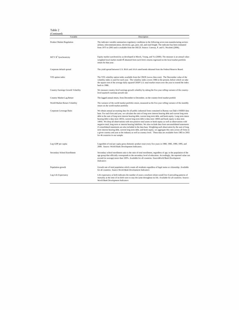
Table 2(Continued)

Variable Description

Product Market Regulation The indicator variable summarizes regulatory conditions in the following seven non-manufacturing sectors: airlines, telecommunication, electricity, gas, post, rail, and road freight. The indicator has been estimated from 1975 to 2003 and is available from the OECD. Source: Conway, P. and G. Nicoletti (2006).

MYY R2 Synchronicity Equity market synchronicity as developed in Morck, Yeung, and Yu (2000). The measure is an annual value-weighted local market model R2 obtained from each firm's returns regressed on the local market portfolio return for that year.

Corporate default spread The yield spread between U.S. BAA and AAA rated bonds obtianed from the Federal Reserve Board.

VIX option index The VIX volatility option index available from the CBOE (www.cboe.com). The Deecember value of the volatility index is used for each year. The volatility index covers 1986 to the present, before which we take the square root of the average daily squared CRSP U.S. total market return over the year to extend the index back to 1980.

Country Earnings Growth Volatility We measure country-level earnings growth volatility by taking the five-year rolling variance of the country-level quarterly earnings growth rate

Country Market Lag Return The lagged annual return, from December to December, on the country-level market portfoli

World Market Return Volatility The variance of the world market portfolio return, measured as the five-year rolling variance of the monthly return on the world market portfolio

Corporate Leverage Ratio We obtain annual accounting data for all public industrial firms contained in Bureau van Dijk's OSIRIS data base. For each firm and year, we calculate the ratio of long term interest bearing debt and current long term debt to the sum of long term interest bearing debt, current long term debt, and book equity. Long term interesbearing debt is data item 14016, current long term debt is data item 14004 and book equity is data item 14041. We drop all observations with non positive total assets or book equity as well as observations with negative total, long term or interest bearing liabilities. We also exclude data from unconsolidated statements if consolidated statements are also included in the data base. Weighting each observation by the sum of long term interest bearing debt, current long term debt, and book equity, we aggregate this ratio across all firms in a given country and year at the industry as well as country level. These data are available from 1985 to 2003 for 46 countries in our sample

Log GDP per capita Logarithm of real per capita gross domestic product reset every five years in 1980, 1985, 1990, 1995, and 2000. Source: World Bank Development Indicators.

Secondary School Enrollment Secondary school enrollment ratio is the ratio of total enrollment, regardless of age, to the population of the age group that officially corresponds to the secondary level of education. Accordingly, the reported value can exceed (or average) more than 100%. Available for all countries. Source: World Bank Development Indicators

Population growth Growth rate of total population which counts all residents regardless of legal status or citizenship. Available for all countries. Source: World Bank Development Indicators

Log Life Expectancy Life expectancy at birth indicates the number of years a newborn infant would live if prevailing patterns of mortality at the time of its birth were to stay the same throughout its life. Available for all countries. Source: World Bank Development Indicators

Appendix Table 3Selecting Independent Variables for Multivariate Regression

Potential Variables Countries Obs.

General Unrestriced

ModelSign of Selected

Variables

General Unrestriced

Model

Sign of Selected Variables

General Unrestriced

ModelSign of Selected

Variables

Capital Account Openness 48 858 X Minus XEquity Market Openness 50 884 X Minus X MinusTrade Openness 50 884 X Minus X Minus XGross FDI/GDP 50 879Trade/GDP 50 884 X X XPolitical Risk 50 884Quality of Institutions 50 884 X Minus X Minus X MinusInvestment Profile 50 884 X X Minus X MinusLaw and Order 50 884 X X XMinority Shareholder Rights 40 771Insider Trading Law 50 884 X Plus X Plus X PlusInsider Trading Prosecution 50 884 X X XLegal Origin (English) 50 884 X Minus X Minus X MinusLegal Origin (French) 50 884 X Minus X Minus X MinusLocal Equity Market Illiquidity 46 787Local Equity Market Turnover 50 884 X X XLocal Equity Market Return Autocorrelation 50 760MYY R2 Synchronicity 45 763Private Credit/GDP 50 884 X Minus X Minus X MinusPrivate Credit/GDP (adj.) 49 876Accounting Standards 36 713Earnings Management 28 591U.S. Real Rate 50 884 X Plus X Plus X PlusU.S. Money Supply Growth 50 884 X X XU.S. Risk Aversion 50 884 X Minus X Minus X MinusWorld GDP Growth 50 884 X X XU.S. Corporate Default Spread 50 884 X Plus X Plus X PlusVIX Option Index 50 884 X X XPast Local Equity Market Return 50 850World Equity Market Volatility 50 884 X X XInitial Log GDP 50 884 X X XSecondary School Enrollment 50 884 X X XLog Life Expantancy 50 884 X X XPopulation Growth 50 884 X Plus X X PlusPredicted Growth Opportunities 50 884Corporate Financial Leverage Ratio 46 652Local Market Earnings Growth Volatility 50 872

Number of variables 23 11 23 11 24 11

Capital Account Openness (858 observations)

General-to-specifc Modelling (PcGets)

Equity Market Openness (884 observations)

Equity Market and Capital Account Openness (858 observations)

Appendix Table 4Selecting Independent Variables for Multivariate Regression of LEGO

Potential Variables Countries Obs.

General Unrestriced

Model

Sign of Selected Variables

General Unrestriced

Model

Sign of Selected Variables

GGO 50 884 X Minus X MinusCapital Account Openness 48 858Equity Market Openness 50 884 X Plus X Plus X Plus X PlusTrade Openness 50 884 X Plus X Plus X Plus X PlusGross FDI/GDP 50 879Trade/GDP 50 884 X X X XPolitical Risk 50 884Quality of Institutions 50 884 X X X XInvestment Profile 50 884 X Plus X Plus X Plus X PlusLaw and Order 50 884 X X X XMinority Shareholder Rights 40 771Insider Trading Law 50 884 X X X Minus X MinusInsider Trading Prosecution 50 884 X X X Plus X PlusLegal Origin (English) 50 884 X X X XLegal Origin (French) 50 884 X Minus X Minus X Minus X MinusLocal Equity Market Illiquidity 46 787Local Equity Market Turnover 50 884 X X X Plus X PlusLocal Equity Market Return Autocorrelation 50 760MYY R2 Synchronicity 45 763Private Credit/GDP 50 884 X Plus X Plus X Plus X PlusPrivate Credit/GDP (adj.) 49 876Accounting Standards 36 713Earnings Management 28 591U.S. Real Rate 50 884 X Plus X Plus X XU.S. Money Supply Growth 50 884 X Minus X Minus X Minus X MinusU.S. Risk Aversion 50 884 X Plus X Plus X Plus X PlusWorld GDP Growth 50 884 X Plus X X XU.S. Corporate Default Spread 50 884 X Minus X Minus X Minus X MinusVIX Option Index 50 884 X Minus X Minus X Minus X MinusPast Local Equity Market Return 50 850World Equity Market Volatility 50 884 X Plus X Plus X XInitial Log GDP 50 884 X Minus X Minus X Minus X MinusSecondary School Enrollment 50 884 X Minus X Minus X XLog Life Expantancy 50 884 X Plus X Plus X Plus X PlusPopulation Growth 50 884 X X X XPredicted Growth Opportunities 50 884 X X XCorporate Financial Leverage Ratio 46 652Local Market Earnings Growth Volatility 50 872

Number of variables 24 15 23 14 25 15 25 15

Equity Market

General-to-specifc Modelling (PcGets)

Equity Market Openness Equity Market Equity Market