Policy Research Working Paper 8091

Financial Globalization and Market Volatility

An Empirical Appraisal

Tito CordellaAnderson Ospino Rojas

Development Economics Vice PresidencyOperations and Strategy TeamJune 2017

WPS8091P

ublic

Dis

clos

ure

Aut

horiz

edP

ublic

Dis

clos

ure

Aut

horiz

edP

ublic

Dis

clos

ure

Aut

horiz

edP

ublic

Dis

clos

ure

Aut

horiz

ed

Produced by the Research Support Team

Abstract

The Policy Research Working Paper Series disseminates the findings of work in progress to encourage the exchange of ideas about development issues. An objective of the series is to get the findings out quickly, even if the presentations are less than fully polished. The papers carry the names of the authors and should be cited accordingly. The findings, interpretations, and conclusions expressed in this paper are entirely those of the authors. They do not necessarily represent the views of the International Bank for Reconstruction and Development/World Bank and its affiliated organizations, or those of the Executive Directors of the World Bank or the governments they represent.

Policy Research Working Paper 8091

This paper is a product of the Operations and Strategy Team, Development Economics Vice Presidency. It is part of a larger effort by the World Bank to provide open access to its research and make a contribution to development policy discussions around the world. Policy Research Working Papers are also posted on the Web at http://econ.worldbank.org. The authors may be contacted at tcordella@worldbank.org and aospinorojas@worldbank.org.

This paper computes a new financial globalization index for a large sample of countries for 1992–2016. Unlike other measures, the financial globalization index cor-rects for the heteroscedasticity of global volatility. This leads to a downward adjustment of financial global-ization trends for developed, emerging, and frontier

markets. The paper also shows that financial globalization reduces market volatility (measured by the volatility of stock returns) in tranquil times, and increases it in tur-bulent ones. On average, the first effect dominates, so that financial globalization leads to a decrease in market volatility, which is more pronounced in frontier markets.

Financial Globalization and Market Volatility: an Empirical Appraisal*

Tito Cordella and Anderson Ospino Rojas

Development Economics (DEC), The World Bank, 1818 H St. NW, Washington, DC, 20433

Emails: tcordella@worldbank.org and aospinorojas@worldbank.org

Keywords: Financial Globalization, Financial Markets, Stock Market Volatility, Emerging Markets, Frontier Markets. JEL Classification Numbers: F15, F36, F65, G11, G15.

* We would like to thank Tatiana Didier, Poonam Gupta, Oliver Masetti and Ugo Panizza for comments and discussions. The usual disclaimers apply.

2

1. Introduction

Has the world become more financially integrated in the last decades? Are the patterns of financial globalization the same in developed, emerging, and frontier markets? Have they changed after the global financial crisis? More importantly, is financial globalization a stabilizing or a destabilizing force? To answer these important questions, we construct a new measure of financial globalization, the Financial Globalization Index (FGI). We compute it for a large sample of countries over the last quarter century, and study how it correlates with stock market volatility. Of course, we are not the first to propose a measure of financial integration.1 Our FGI is an asset price correlation measure that builds upon Pukthuanthong and Roll (2009). The main difference between our measure and Pukthuanthong and Roll’s is that, following Forbes and Rigobon (2002), we recognize that changes in the correlation between different countries’ stock markets partly reflect changes in global volatility and we correct for it. The main finding of our analysis of financial globalization is that, for the “average” country, it increased by 0.6 percentage points per year over the 1992-2016 period. Had we not controlled for changes in volatility, the figure would have been much larger, 1.3 percentage points. For the subsamples of developed, emerging, and frontier countries, the corrected figures are 0.5, 0.9, and 0.4 percentage points, respectively, compared with the uncorrected figures of 1.6, 1.5, and 0.6. The correction also alters our reading of the patterns of globalization during periods of financial turbulence and hence of the effects of the global financial crisis. Finally, when we compare the levels of financial globalization of developed, emerging, and frontier markets, we find that nowadays the average FGI of emerging and frontier markets is still a fraction (0.61 and 0.15) of that of the average developed market. Our analysis relates to a growing body of literature on international asset correlation. With respect to developed economies, using country-industry and country-style equity portfolios, Bekaert et al. (2009) do not find evidence of an increase in the correlation of countries’ stock market returns, with the notable exception of Europe. This makes them conclude that it is difficult to support the argument that global trends have led to permanent changes in the correlation of international assets. Pukthuanthong and Roll (2009), instead, find evidence of a financial integration trend in developed markets for the 1989-2009 period. Looking at pre-2011 data, Volosovych (2011) also points to a positive long-run trend in the co-movement of industrialized countries’ bond returns. With respect to emerging markets, looking at bilateral correlations of countries’ stock indices for the period 1988-1999, Saunders and Walter (2002) conclude that they have become so integrated with developed economies’ that they no longer represent a separate asset class. This, however, may well reflect episodes of financial turbulence over that period. Bekaert and Harvey (2014) look at the difference between the rates of returns at the industry level, and argue that the distinction between asset classes is still valid, though the correlation between developed and emerging markets has increased. Levy-Yeyati and Williams (2012) show that while emerging markets’ business cycles have partially decoupled from advanced economies’, financial integration has strengthened, leading to a

1 We refer the reader to Quinn et al. (2011) for a comprehensive survey of different measures of financial openness and integration, some of which we use in section 5.

2

“financial recoupling” within emerging markets. Dooley and Hutchinson (2009) examine the 2007-2009 period and find evidence of emerging markets’ financial decoupling prior to the crisis andrecoupling during the event. This suggests that the degree of financial integration may vary along the global financial cycle. Along the same lines, Öztek and Öcal (2017) find evidence of time-varying correlation between stock markets, agricultural, and precious metals commodity indices. With respect to frontier markets, the literature is much more limited. Speidell and Khrone (2007) have been the first to point out the appeal of frontier markets in terms of their diversification properties vis-à-vis advanced economies. Up to date, the most comprehensive analysis of frontier markets’ financial integration is Berger et al. (2011). Using Pukthuanthong and Roll’s (2009) measure of financial integration, they show that the integration between frontier and advanced economies has not increased substantially over time. Finally, looking at Central and Eastern European equity markets, Baele et al. (2015) find that smaller frontier markets provide much higher diversification opportunities than larger economies; however, differently from Berger et al. (2011), they find that the increase in correlation up to 2011 is a long-term phenomenon, which is not driven by increases in the volatility of global factors, such as the MSCI World index. In the second part of the paper, we use our index to discuss the relation between financial globalization and stock market volatility, contributing to the debate on whether financial globalization is a stabilizing force, allowing for more efficient risk sharing, or a destabilizing one, that is, a vehicle of contagion. Overall, the evidence is mixed. Some studies suggest that financial liberalization increases volatility (Bae et al., 2004) and leads to economic instability (Stiglitz, 2004). Others show that the liberalization of capital markets has increased the correlation between local and world market returns but not the volatility of local markets themselves (Bekaert and Harvey, 1997), and that financial liberalization leads to more efficient stock markets, with higher returns but no increase in volatility (Han Kim and Singal, 2000). Even if the degree of international risk sharing associated with greater financial globalization may have been at best modest, and only limited to developed economies (Kose et al. 2009), Umutlu et al. (2010) find a negative relation between financial liberalization and the volatility of stock market returns; Esqueda et al. (2012), instead, find evidence of a negative relation between financial integration and stock market volatility in emerging but not in developed economies. Perhaps, one of the reasons why the evidence is mixed is that the effects of financial globalization on stock market volatility are different in periods of global financial stability and instability. Indeed, using our index, we show that while in tranquil times financial globalization reduces the volatility of stock returns, the opposite happens in periods of high uncertainty. On average, we find that negative shocks of the magnitude required for financial globalization to yield an increase in financial instability are quite infrequent and thus that financial globalization is associated with an average decrease in stock market volatility. The paper is organized as follows: section 2 presents the data and the methodology; section 3 provides an analysis of financial globalization trends in developed, emerging, and frontier markets, before and after the global financial crisis; section 4 discusses the relation between financial globalization and stock market volatility; section 5 compares our index with traditional measures of financial integration; section 6 provides some robustness analysis and, finally, section 7 concludes. The Data Appendix provides a detailed description of our data set. All data files are available upon request.

2

2. Data and Methodology

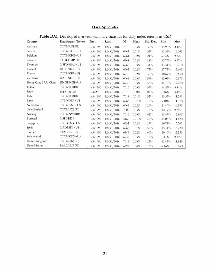
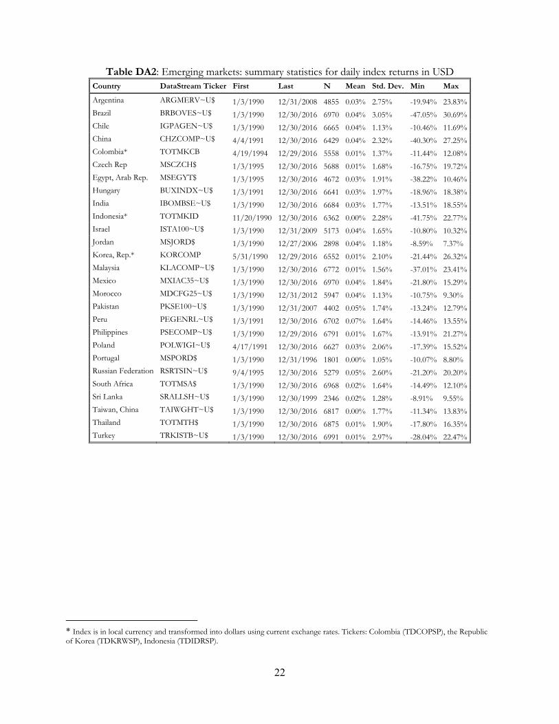
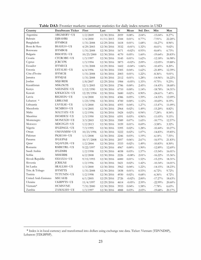
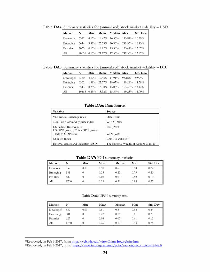
Our data set is an unbalanced panel of 84 countries: 21 advanced, 20 emerging, 36 frontier, and 7 that transitioned2 between groups during the 1991-2016 period, which we consider.3 Our main variables of interest are country stock market index returns. Country classification follows the MSCI baskets for emerging and developed markets. In the frontier markets category, instead, because of substantial heterogeneity among the MSCI and other indices, we include all countries that have been classified for at least one year as frontier by either MSCI, or by no less than two of the other indices providers.4 For all indices we ensure that they have adequate liquidity in local currency; hence, we only keep those country-year pairs with at least 150 non-return zeros. We refer the reader to tables DA1-DA5 in the Data Appendix for the list of countries, available observations, DataStream tickers, and descriptive statistics for daily stock market returns. Regarding the other data we use in our analysis, table DA6 provides information about the different sources. To measure financial globalization, we start from the methodology developed by Pukthuanthong and Roll (2009) and apply the adjustment proposed by Forbes and Rigobon (2002) to remove the variation caused by changes in the volatility of the global factor. Pukthuanthong and Roll (2009) perform their analysis in two stages. In the first stage, they run a principal component analysis of the daily stock market index returns,5 , , where denotes countries and days. They retain the first ten principal components, global factors (GFs), hereinafter. The analysis is performed year by year. One important detail is that the weights used to estimate the GFs in a given year are computed out of sample from the previous year’s correlation matrix of the returns.6 In the second stage, the daily returns of each country’s stock market index are regressed on the global factors estimated in the first stage. Thus, for each year and country , they estimate: = + ( ) + .(1) The R-squared of such regressions provides the country-year measures of financial globalization. We deviate from Pukthuanthong and Roll’s (2009) methodology in three ways. First, to estimate the GFs they use 17 countries for which stock market data are available on a daily basis starting from

2Portugal (1997), and Israel (2010) transitioned from emerging to frontier countries; Sri Lanka (2000), Jordan (2007), Pakistan (2008), Argentina (2009), and Morocco (2013) from emerging to frontier. 3 The choice of the time period is driven by the fact that the index for China, which we need to estimate the first principal component, is only available on Datastream starting from 1991. 4 Other providers are FTSE, S&P, and Russell. 5 Daily index returns are obtained from DataStream. When available, we use total returns price indices, including reinvestment of dividends, otherwise, we use simple price indices. All returns are measured in USD. DataStream provides an exchange rate conversion option to download the data in the desired currency. However, special care is needed when using it to avoid an artificial increase in the frequency of observations due to currency fluctuations. To deal with such a spurious source of variation, in our data set, returns are estimated only when the value of the index, expressed in local currency, differs from the previous business day. Using such a rule, we also omit holidays and stale values. We also exclude daily returns above 20 and below -20 percent. 6 The out of sample computation of the weights, as proposed by Pukthuanthong et Roll (2009), is motivated by the fact that, in the second stage, we estimate the FGIs for the very same countries that have been used to estimate the GFs. This may introduce a positive bias in the FGI estimates. While such a methodology does not rule out completely the bias, which could be still present because of stock market volatility auto-correlation, it certainly attenuates it.

3

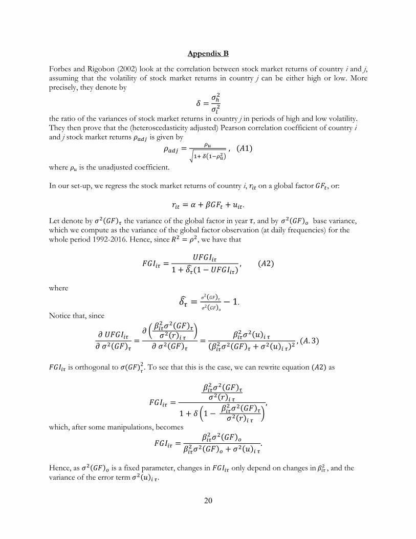
1973; instead, we look at the 20 biggest stock markets in 2006,7 a year in the middle of our period of analysis. The original basket includes mostly developed economies,8 while the new basket includes several developing economies, which are playing an increasingly important role in the global economy, and thus should enter in any meaningful index of globalization. Indeed, in 2012, the original basket accounted for 77 percent, while our basket for 94 percent of global stock market capitalization.9 Hence, the global factor that we estimate does not reflect the dynamics of developed economies only. The second difference is in the number of GFs used to estimate the R-squared: while Pukthuanthong and Roll (2009) consider the first ten GFs, we only retain the first one. The reason is that, since we deal with a heterogeneous set of countries, we expect some clustering in the GFs. It is thus likely that some of the GFs with lower eigenvalues capture only the dynamics of emerging or frontier markets. Since the focus of this paper is on global (rather than regional or within asset types) co-movements we decided to use the first GF only. Nonetheless, we also replicate our main results using ten GFs for comparability. Third, and more important, we correct Pukthuanthong and Roll’s index acknowledging that changes in the R-squared of regressions (1) may either reflect changes in the interlinkages between economies or changes in the volatility of the GF(s). This argument is based on Forbes and Rigobon (2002), which look at the Pearson correlation coefficients between stock market indices, and establishes that they are conditional on measures of volatility. More precisely, they show that during financial crises the increase in the correlation between different countries’ stock market indices may just reflect the increase in volatility. In the paper, they propose a correction for volatility, which we adapt to our framework to remove from the R-squared the variation driven by changes in the volatility of the GF. Denoting by UFGI the uncorrected index computed with one GF (and UFGI10, the one computed with ten), the corrected index (FGI) is equal to = 1 + (1 − )(2) with = ( )( ) − 1,

where ( ) is the variance of the global factor in year , and ( ) is the base variance of the global factor. As a measure of base variance, Forbes and Rigobon (2002) choose the variance in tranquil times that precede periods of financial turbulence. In this paper, we choose the variance of global factor daily observations over the entire sample period. Hence, in any given year, , can be positive or negative, and the FGI can be lower or higher than the UFGI.

We refer the reader to Appendix B for the derivation of equation (2) and additional technical details. Here, it is important to underscore that the FGI is not affected by changes in the variance of the global 7 This set includes Australia, Belgium, Brazil, Canada, France, Germany, Hong Kong SAR, China, India, Italy, Japan, Mexico, China, Singapore, South Africa, the Republic of Korea, Spain, Switzerland, the Netherlands, the United Kingdom, and the United States. 8 The only non-developed market included is South Africa. 9 These estimates are based on the stock market capitalization of domestically listed companies from WDI.

4

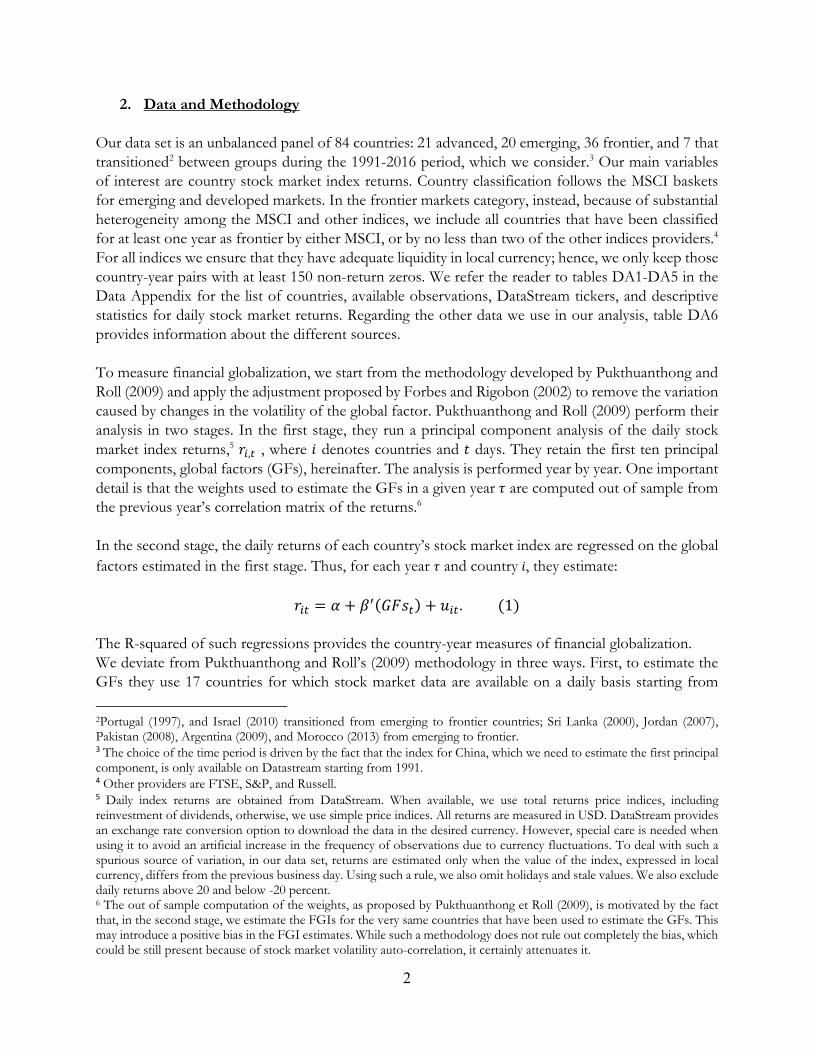
factor, and hence that its changes are driven by changes in and in the variance of the error term in equation (1).

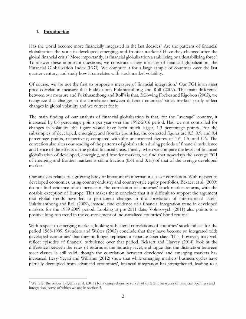
Figure 1: FGI versus UFGI

Source: Authors’ computation using Datastream.

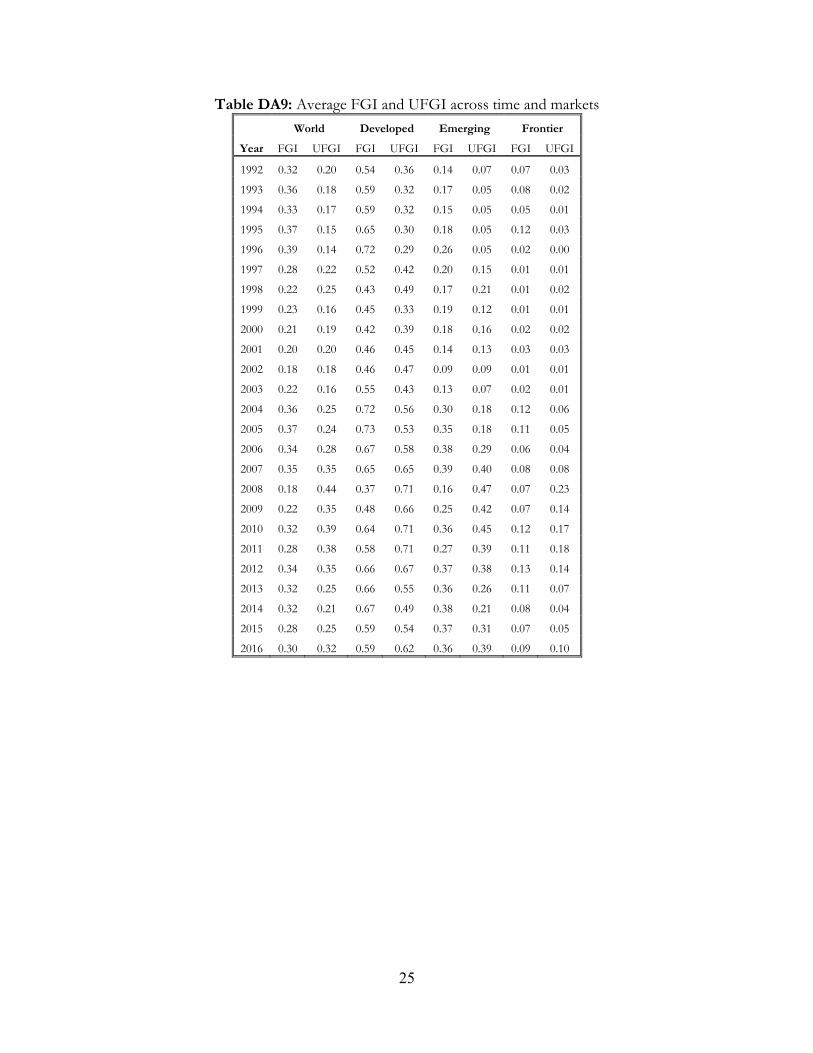
Data Appendix tables DA7-DA9 provide summary statistics for the FGI and UFGI in developed, emerging, and frontier markets. Our main findings are illustrated in Figure 1, where we plot the average FGI and UFGI for the different market groups. As it is evident from a simple inspection of the figure, the correction for the heteroscedasticity of the global factor affects substantially our measure of globalization, especially during financial crises.10 We discuss the correlations between UFGI, FGI, and UFGI 10 in section 5 below, where we also look at other measures of integration.

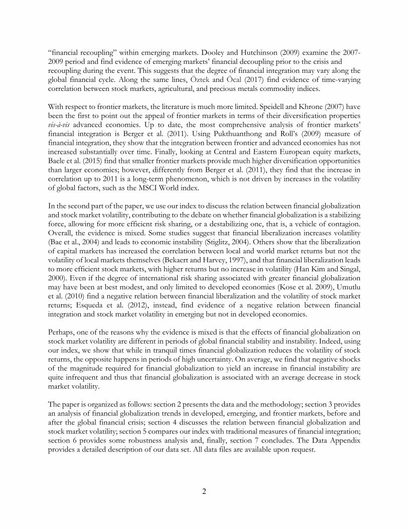
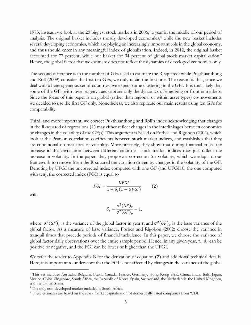
To offer the reader a better idea of the behavior of the FGIs, in Figure 2a we plot the FGI for a developed, Sweden, an emerging, Turkey, and a frontier market, Romania; while in Figure 2b, we plot the average value of the FGI, for developed, emerging, and frontier markets for the 1992-2016 period together with the volatility of the GF we estimated, a measure of financial turbulence. Figure 2 suggests that, once we control for the heteroscedasticity of the global factor, the process of financial globalization has a stop and go pattern, it increases in tranquil times and experiences setbacks during turbulent ones. This reflects the fact that, differently from other measures used in the literature (see section 5, below), our measure cleans the index from the spurious increases in correlation between stock markets due to increases in global volatility. It is also worth noticing that, while the patterns of financial globalization are similar for developed and emerging markets, frontier markets remain relatively isolated from global dynamics.11

10 Forbes and Rigobon (2002) also find an increase in conditional but not in unconditional correlations during the 1987 U.S. market crash, the Tequila, and the Asian crisis. 11 See Appendix tables DA7-DA9.

0.2

.4.6

.8

1992 1997 2002 2007 2012 2017year

All Countries

0.2

.4.6

.8

1992 1997 2002 2007 2012 2017year

Developed

0.2

.4.6

.8

1992 1997 2002 2007 2012 2017year

Emerging

0.2

.4.6

.81992 1997 2002 2007 2012 2017

year

Frontier

FGI UFGI

5

Figure 2: The Financial Globalization Index (FGI) 2 (a) 2 (b)

Source: Authors’ computations using Datastream.

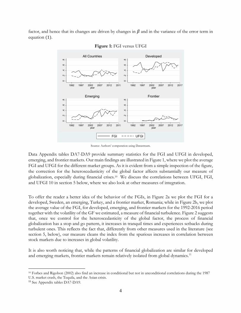
3. Financial globalization trends

To get more precise estimates of the financial globalization trends, we regress the FGIs on a time trend, controlling for country fixed effects. Our results are presented in table 1, which indicates that in the 1992-2016 period, financial globalization increased at an average rate of about 0.6 percentage points a year, see column 1. When we distinguish between developed, emerging and frontier markets, our estimates of the trend (column 4) are, respectively, 0.5, 0.9, and 0.4 percentage points per year. Notice that, had we not adjusted for heteroscedasticity, we would have substantially overestimated the trends, using one (column 2) or ten GFs (column 3).

Table 1: Financial globalization trends (1) (2) (3) (4) (5) (6)

FGI UFGI UFGI10 FGI UFGI UFGI10

Trend 0.006*** 0.013*** 0.011***

(0.001) (0.001) (0.001)

Trend×D 0.005*** 0.016*** 0.013***

(0.001) (0.001) (0.001)

Trend×E 0.009*** 0.015*** 0.013***

(0.002) (0.001) (0.002)

Trend×F 0.004*** 0.006*** 0.006***

(0.001) (0.001) (0.001)

Constant 0.211*** 0.091*** 0.296*** 0.213*** 0.107*** 0.308***

(0.012) (0.013) (0.012) (0.011) (0.010) (0.011)

Obs. 1,760 1,760 1,760 1,760 1,760 1,760

R-squared 0.097 0.325 0.270 0.117 0.371 0.297

Countries 84 84 84 84 84 84

Country FE Yes Yes Yes Yes Yes Yes

Clustered standard errors at country level in parentheses. *** p<0.01, ** p<0.05, * p<0.1.

0.5

11.

52

Glo

b Fa

ct V

olat

ility

(RH

S)

0.2

.4.6

.8FG

I

1992 1996 2000 2004 2008 2011 2015year

Sweden TurkeyRomania Glob Fact Volatility (RHS)

0.5

11.

52

Glo

b Fa

ct V

olat

ility

(RH

S)

0.2

.4.6

.8FG

I

1992 1996 2000 2004 2008 2011 2015year

World DevelopedEmerging FrontierGlob Fact Volatility (RHS)

6

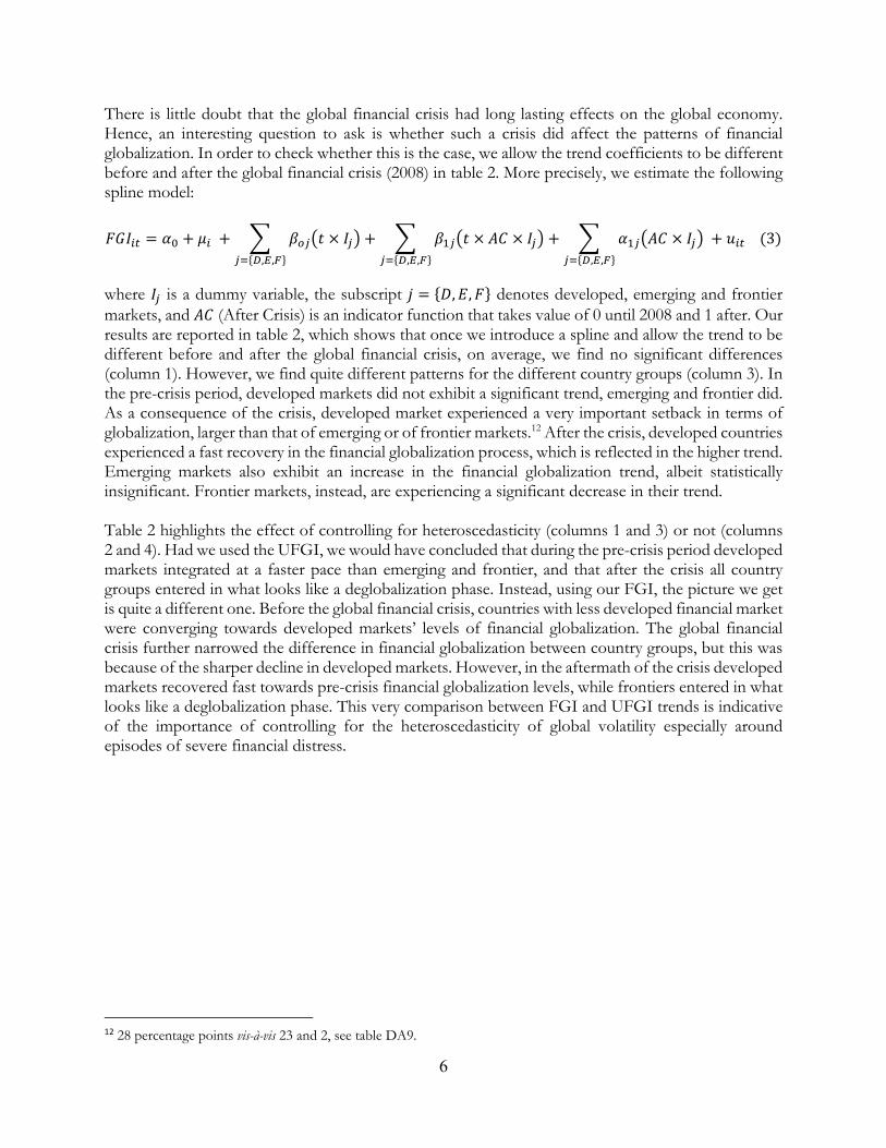
There is little doubt that the global financial crisis had long lasting effects on the global economy. Hence, an interesting question to ask is whether such a crisis did affect the patterns of financial globalization. In order to check whether this is the case, we allow the trend coefficients to be different before and after the global financial crisis (2008) in table 2. More precisely, we estimate the following spline model: = + + ×, , + × ×, , + ×, , + (3) where is a dummy variable, the subscript = , , denotes developed, emerging and frontier markets, and (After Crisis) is an indicator function that takes value of 0 until 2008 and 1 after. Our results are reported in table 2, which shows that once we introduce a spline and allow the trend to be different before and after the global financial crisis, on average, we find no significant differences (column 1). However, we find quite different patterns for the different country groups (column 3). In the pre-crisis period, developed markets did not exhibit a significant trend, emerging and frontier did. As a consequence of the crisis, developed market experienced a very important setback in terms of globalization, larger than that of emerging or of frontier markets.12 After the crisis, developed countries experienced a fast recovery in the financial globalization process, which is reflected in the higher trend. Emerging markets also exhibit an increase in the financial globalization trend, albeit statistically insignificant. Frontier markets, instead, are experiencing a significant decrease in their trend. Table 2 highlights the effect of controlling for heteroscedasticity (columns 1 and 3) or not (columns 2 and 4). Had we used the UFGI, we would have concluded that during the pre-crisis period developed markets integrated at a faster pace than emerging and frontier, and that after the crisis all country groups entered in what looks like a deglobalization phase. Instead, using our FGI, the picture we get is quite a different one. Before the global financial crisis, countries with less developed financial market were converging towards developed markets’ levels of financial globalization. The global financial crisis further narrowed the difference in financial globalization between country groups, but this was because of the sharper decline in developed markets. However, in the aftermath of the crisis developed markets recovered fast towards pre-crisis financial globalization levels, while frontiers entered in what looks like a deglobalization phase. This very comparison between FGI and UFGI trends is indicative of the importance of controlling for the heteroscedasticity of global volatility especially around episodes of severe financial distress.

12 28 percentage points vis-à-vis 23 and 2, see table DA9.

7

Table 2: Financial globalization trends

(1) (2) (3) (4)

FGI UFGI FGI UFGI

Trend 0.005*** 0.019***

(0.001) (0.001)

Trend×D 0.002 0.023***

(0.002) (0.002)

Trend×E 0.009*** 0.019***

(0.002) (0.002)

Trend×F 0.004*** 0.011***

(0.001) (0.002)

AC×Trend -0.001 -0.038***

(0.002) (0.003)

AC×Trend×D 0.009*** -0.045***

(0.003) (0.004)

AC×Trend×E 0.006 -0.038***

(0.004) (0.006)

AC×Trend×F -0.006* -0.027***

(0.003) (0.004)

AC 0.026 0.697***

(0.040) (0.055)

AC×D -0.15*** 0.821***

(0.059) (0.076)

AC×E -0.075 0.734***

(0.082) (0.107)

AC×F 0.148** 0.510***

(0.052) (0.085)

Constant 0.214*** 0.036** 0.219*** 0.062***

(0.016) (0.017) (0.014) (0.015)

0.214*** 0.036** 0.219*** 0.062***

Obs. 1,760 1,760 1,760 1,760

R-squared 0.098 0.444 0.125 0.475

Countries 84 84 84 84

Country FE Yes Yes Yes Yes

Clustered standard errors at country level in parentheses. *** p<0.01, ** p<0.05, * p<0.1.

4. Financial globalization and financial volatility

As we mentioned in the introduction, the question of whether financial globalization is a stabilizing force, allowing for more efficient risk sharing, or a destabilizing one, exposing countries to financial contagion, is an open one. While there are different ways of measuring financial market volatility, in the context of our analysis, the most natural is to look at the volatility of daily stock market returns. Hence, in what follows, we regress the annualized monthly volatility13 of stock market returns (σR) on 13 The volatility is computed for each month from the daily returns of the local stock markets. The same approach is used to estimate the volatility of the GF at monthly frequency.

8

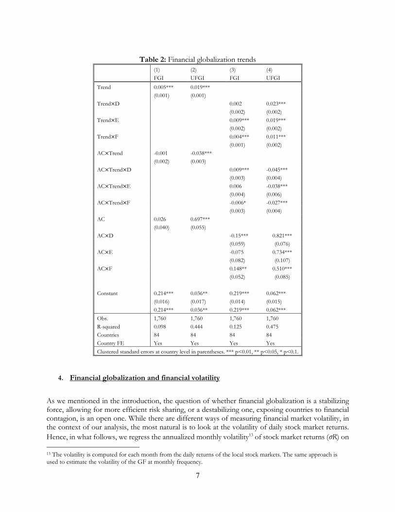
the FGI of the previous year, controlling (among other things) for financial turbulence, which we proxy by the annualized monthly volatility of the global factor we used to compute the FGI (σGF), which we plot in Figure 3 together with the VIX index, an alternative measure of global financial market volatility, which we use in the robustness section below.

Figure 3: Global factor volatility and VIX (monthly frequency)

Source: Authors’ computation using Datastream.

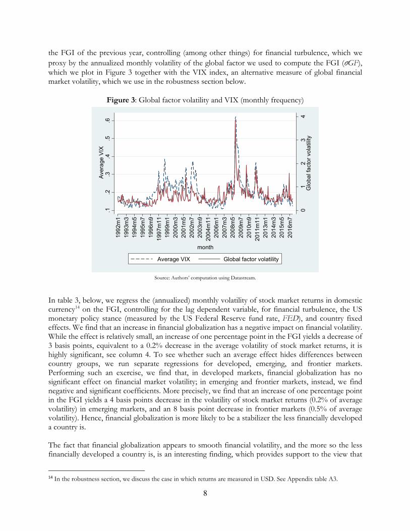
In table 3, below, we regress the (annualized) monthly volatility of stock market returns in domestic currency14 on the FGI, controlling for the lag dependent variable, for financial turbulence, the US monetary policy stance (measured by the US Federal Reserve fund rate, FED), and country fixed effects. We find that an increase in financial globalization has a negative impact on financial volatility. While the effect is relatively small, an increase of one percentage point in the FGI yields a decrease of 3 basis points, equivalent to a 0.2% decrease in the average volatility of stock market returns, it is highly significant, see column 4. To see whether such an average effect hides differences between country groups, we run separate regressions for developed, emerging, and frontier markets. Performing such an exercise, we find that, in developed markets, financial globalization has no significant effect on financial market volatility; in emerging and frontier markets, instead, we find negative and significant coefficients. More precisely, we find that an increase of one percentage point in the FGI yields a 4 basis points decrease in the volatility of stock market returns (0.2% of average volatility) in emerging markets, and an 8 basis point decrease in frontier markets (0.5% of average volatility). Hence, financial globalization is more likely to be a stabilizer the less financially developed a country is. The fact that financial globalization appears to smooth financial volatility, and the more so the less financially developed a country is, is an interesting finding, which provides support to the view that

14 In the robustness section, we discuss the case in which returns are measured in USD. See Appendix table A3.

01

23

4G

loba

l fac

tor v

olat

ility

.1.2

.3.4

.5.6

Ave

rage

VIX

1992

m1

1993

m3

1994

m5

1995

m7

1996

m9

1997

m11

1999

m1

2000

m3

2001

m5

2002

m7

2003

m9

2004

m11

2006

m1

2007

m3

2008

m5

2009

m7

2010

m9

2011

m11

2013

m1

2014

m3

2015

m5

2016

m7

month

Average VIX Global factor volatility

9

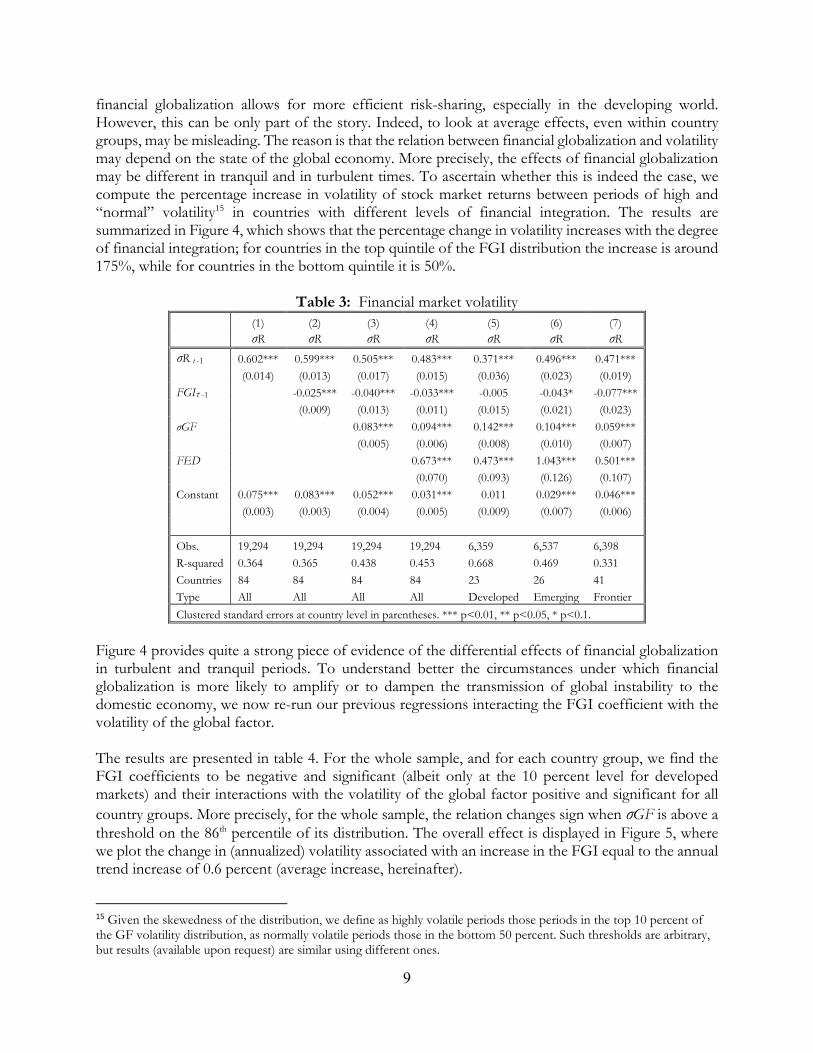
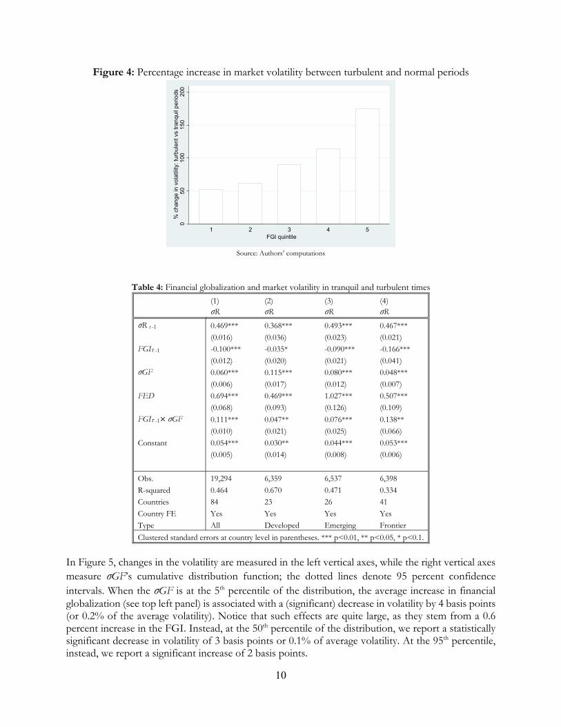
financial globalization allows for more efficient risk-sharing, especially in the developing world. However, this can be only part of the story. Indeed, to look at average effects, even within country groups, may be misleading. The reason is that the relation between financial globalization and volatility may depend on the state of the global economy. More precisely, the effects of financial globalization may be different in tranquil and in turbulent times. To ascertain whether this is indeed the case, we compute the percentage increase in volatility of stock market returns between periods of high and “normal” volatility15 in countries with different levels of financial integration. The results are summarized in Figure 4, which shows that the percentage change in volatility increases with the degree of financial integration; for countries in the top quintile of the FGI distribution the increase is around 175%, while for countries in the bottom quintile it is 50%.

Table 3: Financial market volatility (1) (2) (3) (4) (5) (6) (7)

σR σR σR σR σR σR σR

σR t -1 0.602*** 0.599*** 0.505*** 0.483*** 0.371*** 0.496*** 0.471***

(0.014) (0.013) (0.017) (0.015) (0.036) (0.023) (0.019) FGI-1 -0.025*** -0.040*** -0.033*** -0.005 -0.043* -0.077***

(0.009) (0.013) (0.011) (0.015) (0.021) (0.023)

σGF 0.083*** 0.094*** 0.142*** 0.104*** 0.059***

(0.005) (0.006) (0.008) (0.010) (0.007)

FED 0.673*** 0.473*** 1.043*** 0.501***

(0.070) (0.093) (0.126) (0.107)

Constant 0.075*** 0.083*** 0.052*** 0.031*** 0.011 0.029*** 0.046***

(0.003) (0.003) (0.004) (0.005) (0.009) (0.007) (0.006)

Obs. 19,294 19,294 19,294 19,294 6,359 6,537 6,398

R-squared 0.364 0.365 0.438 0.453 0.668 0.469 0.331

Countries 84 84 84 84 23 26 41

Type All All All All Developed Emerging Frontier

Clustered standard errors at country level in parentheses. *** p<0.01, ** p<0.05, * p<0.1.

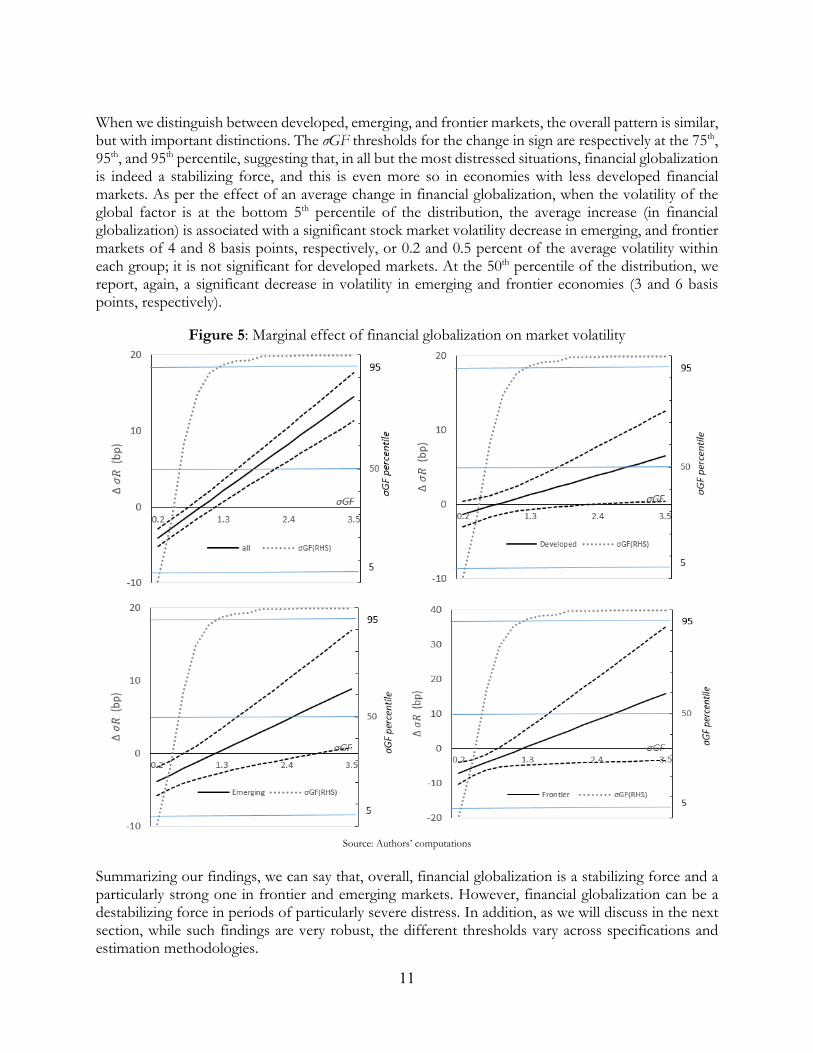
Figure 4 provides quite a strong piece of evidence of the differential effects of financial globalization in turbulent and tranquil periods. To understand better the circumstances under which financial globalization is more likely to amplify or to dampen the transmission of global instability to the domestic economy, we now re-run our previous regressions interacting the FGI coefficient with the volatility of the global factor. The results are presented in table 4. For the whole sample, and for each country group, we find the FGI coefficients to be negative and significant (albeit only at the 10 percent level for developed markets) and their interactions with the volatility of the global factor positive and significant for all country groups. More precisely, for the whole sample, the relation changes sign when σGF is above a threshold on the 86th percentile of its distribution. The overall effect is displayed in Figure 5, where we plot the change in (annualized) volatility associated with an increase in the FGI equal to the annual trend increase of 0.6 percent (average increase, hereinafter).

15 Given the skewedness of the distribution, we define as highly volatile periods those periods in the top 10 percent of the GF volatility distribution, as normally volatile periods those in the bottom 50 percent. Such thresholds are arbitrary, but results (available upon request) are similar using different ones.

10

Figure 4: Percentage increase in market volatility between turbulent and normal periods

Source: Authors’ computations

Table 4: Financial globalization and market volatility in tranquil and turbulent times

(1) (2) (3) (4)

σR σR σR σR

σR t -1 0.469*** 0.368*** 0.493*** 0.467***

(0.016) (0.036) (0.023) (0.021) FGI-1 -0.100*** -0.035* -0.090*** -0.166***

(0.012) (0.020) (0.021) (0.041) σGF 0.060*** 0.115*** 0.080*** 0.048***

(0.006) (0.017) (0.012) (0.007)

FED 0.694*** 0.469*** 1.027*** 0.507***

(0.068) (0.093) (0.126) (0.109) FGI-1× σGF 0.111*** 0.047** 0.076*** 0.138**

(0.010) (0.021) (0.025) (0.066)

Constant 0.054*** 0.030** 0.044*** 0.053***

(0.005) (0.014) (0.008) (0.006)

Obs. 19,294 6,359 6,537 6,398

R-squared 0.464 0.670 0.471 0.334

Countries 84 23 26 41

Country FE Yes Yes Yes Yes

Type All Developed Emerging Frontier

Clustered standard errors at country level in parentheses. *** p<0.01, ** p<0.05, * p<0.1.

In Figure 5, changes in the volatility are measured in the left vertical axes, while the right vertical axes measure σGF’s cumulative distribution function; the dotted lines denote 95 percent confidence intervals. When the σGF is at the 5th percentile of the distribution, the average increase in financial globalization (see top left panel) is associated with a (significant) decrease in volatility by 4 basis points (or 0.2% of the average volatility). Notice that such effects are quite large, as they stem from a 0.6 percent increase in the FGI. Instead, at the 50th percentile of the distribution, we report a statistically significant decrease in volatility of 3 basis points or 0.1% of average volatility. At the 95th percentile, instead, we report a significant increase of 2 basis points.

050

100

150

200

% c

hang

e in

vol

atilit

y: tu

rbul

ent v

s tra

nqui

l per

iods

1 2 3 4 5 FGI quintile

11

When we distinguish between developed, emerging, and frontier markets, the overall pattern is similar, but with important distinctions. The σGF thresholds for the change in sign are respectively at the 75th, 95th, and 95th percentile, suggesting that, in all but the most distressed situations, financial globalization is indeed a stabilizing force, and this is even more so in economies with less developed financial markets. As per the effect of an average change in financial globalization, when the volatility of the global factor is at the bottom 5th percentile of the distribution, the average increase (in financial globalization) is associated with a significant stock market volatility decrease in emerging, and frontier markets of 4 and 8 basis points, respectively, or 0.2 and 0.5 percent of the average volatility within each group; it is not significant for developed markets. At the 50th percentile of the distribution, we report, again, a significant decrease in volatility in emerging and frontier economies (3 and 6 basis points, respectively).

Figure 5: Marginal effect of financial globalization on market volatility

Source: Authors’ computations

Summarizing our findings, we can say that, overall, financial globalization is a stabilizing force and a particularly strong one in frontier and emerging markets. However, financial globalization can be a destabilizing force in periods of particularly severe distress. In addition, as we will discuss in the next section, while such findings are very robust, the different thresholds vary across specifications and estimation methodologies.

12

5. FGI and existing measures of financial integration

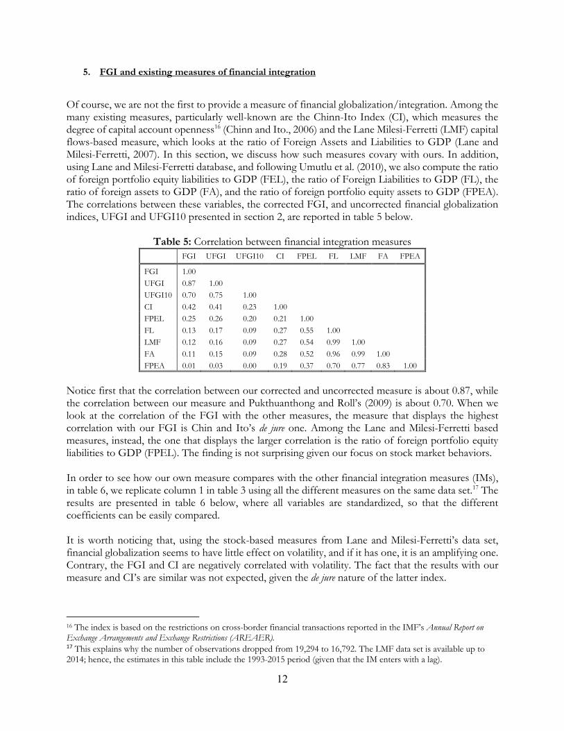
Of course, we are not the first to provide a measure of financial globalization/integration. Among the many existing measures, particularly well-known are the Chinn-Ito Index (CI), which measures the degree of capital account openness16 (Chinn and Ito., 2006) and the Lane Milesi-Ferretti (LMF) capital flows-based measure, which looks at the ratio of Foreign Assets and Liabilities to GDP (Lane and Milesi-Ferretti, 2007). In this section, we discuss how such measures covary with ours. In addition, using Lane and Milesi-Ferretti database, and following Umutlu et al. (2010), we also compute the ratio of foreign portfolio equity liabilities to GDP (FEL), the ratio of Foreign Liabilities to GDP (FL), the ratio of foreign assets to GDP (FA), and the ratio of foreign portfolio equity assets to GDP (FPEA). The correlations between these variables, the corrected FGI, and uncorrected financial globalization indices, UFGI and UFGI10 presented in section 2, are reported in table 5 below.

Table 5: Correlation between financial integration measures FGI UFGI UFGI10 CI FPEL FL LMF FA FPEA

FGI 1.00

UFGI 0.87 1.00

UFGI10 0.70 0.75 1.00

CI 0.42 0.41 0.23 1.00

FPEL 0.25 0.26 0.20 0.21 1.00

FL 0.13 0.17 0.09 0.27 0.55 1.00

LMF 0.12 0.16 0.09 0.27 0.54 0.99 1.00

FA 0.11 0.15 0.09 0.28 0.52 0.96 0.99 1.00

FPEA 0.01 0.03 0.00 0.19 0.37 0.70 0.77 0.83 1.00

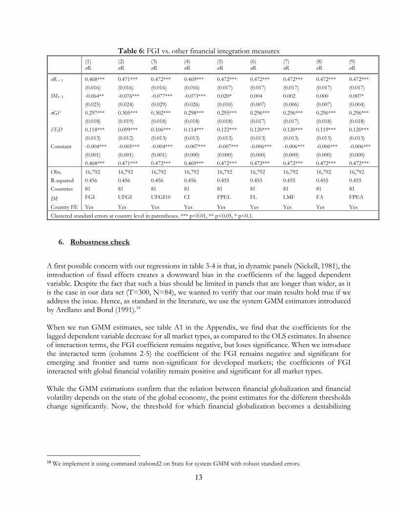
Notice first that the correlation between our corrected and uncorrected measure is about 0.87, while the correlation between our measure and Pukthuanthong and Roll’s (2009) is about 0.70. When we look at the correlation of the FGI with the other measures, the measure that displays the highest correlation with our FGI is Chin and Ito’s de jure one. Among the Lane and Milesi-Ferretti based measures, instead, the one that displays the larger correlation is the ratio of foreign portfolio equity liabilities to GDP (FPEL). The finding is not surprising given our focus on stock market behaviors. In order to see how our own measure compares with the other financial integration measures (IMs), in table 6, we replicate column 1 in table 3 using all the different measures on the same data set.17 The results are presented in table 6 below, where all variables are standardized, so that the different coefficients can be easily compared. It is worth noticing that, using the stock-based measures from Lane and Milesi-Ferretti’s data set, financial globalization seems to have little effect on volatility, and if it has one, it is an amplifying one. Contrary, the FGI and CI are negatively correlated with volatility. The fact that the results with our measure and CI’s are similar was not expected, given the de jure nature of the latter index.

16 The index is based on the restrictions on cross-border financial transactions reported in the IMF’s Annual Report on Exchange Arrangements and Exchange Restrictions (AREAER). 17 This explains why the number of observations dropped from 19,294 to 16,792. The LMF data set is available up to 2014; hence, the estimates in this table include the 1993-2015 period (given that the IM enters with a lag).

13

Table 6: FGI vs. other financial integration measures (1) (2) (3) (4) (5) (6) (7) (8) (9)

σR σR σR σR σR σR σR σR σR

σR t -1 0.468*** 0.471*** 0.472*** 0.469*** 0.472*** 0.472*** 0.472*** 0.472*** 0.472***

(0.016) (0.016) (0.016) (0.016) (0.017) (0.017) (0.017) (0.017) (0.017)

IM-1 -0.064** -0.076*** -0.077*** -0.073*** 0.020* 0.004 0.002 0.000 0.007*

(0.025) (0.024) (0.029) (0.026) (0.010) (0.007) (0.006) (0.007) (0.004)

σGF 0.297*** 0.305*** 0.302*** 0.298*** 0.295*** 0.296*** 0.296*** 0.296*** 0.296***

(0.018) (0.019) (0.018) (0.018) (0.018) (0.017) (0.017) (0.018) (0.018)

FED 0.118*** 0.099*** 0.106*** 0.114*** 0.122*** 0.120*** 0.120*** 0.119*** 0.120***

(0.013) (0.012) (0.013) (0.013) (0.013) (0.013) (0.013) (0.013) (0.013)

Constant -0.004*** -0.005*** -0.004*** -0.007*** -0.007*** -0.006*** -0.006*** -0.006*** -0.006***

(0.001) (0.001) (0.001) (0.000) (0.000) (0.000) (0.000) (0.000) (0.000)

0.468*** 0.471*** 0.472*** 0.469*** 0.472*** 0.472*** 0.472*** 0.472*** 0.472***

Obs. 16,792 16,792 16,792 16,792 16,792 16,792 16,792 16,792 16,792

R-squared 0.456 0.456 0.456 0.456 0.455 0.455 0.455 0.455 0.455

Countries 81 81 81 81 81 81 81 81 81

IM FGI UFGI UFGI10 CI FPEL FL LMF FA FPEA

Country FE Yes Yes Yes Yes Yes Yes Yes Yes Yes

Clustered standard errors at country level in parentheses. *** p<0.01, ** p<0.05, * p<0.1.

6. Robustness check

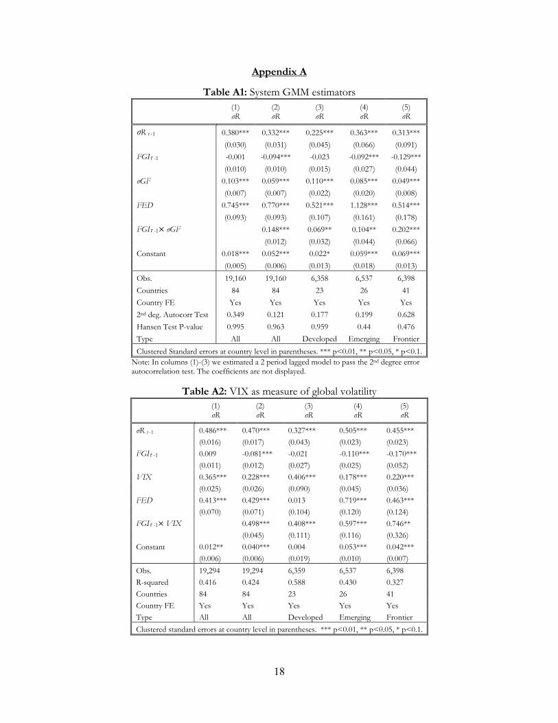
A first possible concern with our regressions in table 3-4 is that, in dynamic panels (Nickell, 1981), the introduction of fixed effects creates a downward bias in the coefficients of the lagged dependent variable. Despite the fact that such a bias should be limited in panels that are longer than wider, as it is the case in our data set (T=300, N=84), we wanted to verify that our main results hold true if we address the issue. Hence, as standard in the literature, we use the system GMM estimators introduced by Arellano and Bond (1991).18 When we run GMM estimates, see table A1 in the Appendix, we find that the coefficients for the lagged dependent variable decrease for all market types, as compared to the OLS estimates. In absence of interaction terms, the FGI coefficient remains negative, but loses significance. When we introduce the interacted term (columns 2-5) the coefficient of the FGI remains negative and significant for emerging and frontier and turns non-significant for developed markets; the coefficients of FGI interacted with global financial volatility remain positive and significant for all market types. While the GMM estimations confirm that the relation between financial globalization and financial volatility depends on the state of the global economy, the point estimates for the different thresholds change significantly. Now, the threshold for which financial globalization becomes a destabilizing

18 We implement it using command xtabond2 on Stata for system GMM with robust standard errors.

14

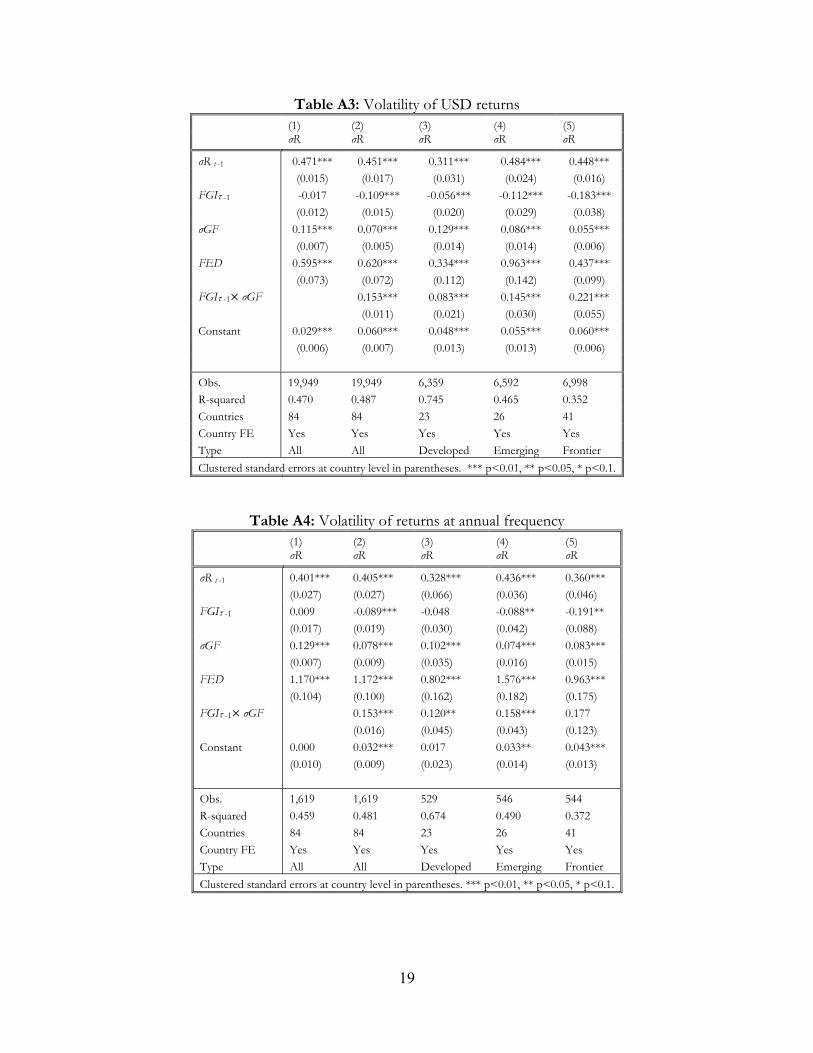
force is the 63th percentile of the distribution of global factor volatility for whole sample and the 15th, 85th, and 63th percentile for developed, emerging and frontier markets, respectively.19 A second possible concern regarding our analysis may stem from the fact that our measure of financial volatility is, by construction, correlated with the stock market volatility of the basket of countries that are used in the principal component analysis. Hence, we rerun our analysis using the VIX instead of σGF. The correlation between the two measures is 0.8. The results are presented in table A2 and indicate that the relation between financial globalization and financial volatility depends upon the state of the global economy as in our main specification. The thresholds for which financial globalization turns to be destabilizing are now the 42nd percentile for the whole sample, the 1st, 55th, and 74th percentiles of the VIX distribution for developed, emerging, and frontier markets, respectively. The fact that higher levels of financial globalization are associated with higher stock market volatility in developed markets, for virtually all levels of the VIX, may well reflect the fact that the VIX is indeed a measure of developed market (US) financial volatility. In our view, the right indicator to understand whether financial globalization affects financial volatility in a particular country is stock market volatility expressed in domestic currency. However, one may wonder what happens if the returns are computed in USD, hence incorporating the effects of exchange rate movements. The results are presented in table A3 and are very similar to those in local currency, although the coefficient of FGI in developed markets is now significant at 1%. The thresholds for which financial globalization becomes a destabilizing force are now the 74th percentile for the complete sample, and the 68th, 78th, and 82nd percentiles for developed, emerging, and frontier markets, respectively. This suggests that financial globalization is slightly less effective in reducing stock market volatility when expressed in USD rather than in domestic currency. This result could be driven by increases in exchange rate volatility correlated with deeper financial integration, as suggested by Donadelli and Paradiso (2014), and Caporale et al. (2011). In order to address endogeneity concerns, in the estimates of tables 3 and 4, we use current stock market volatility and the lagged value of the FGI. As it is well-known, the lagging strategy solves the endogeneity problem if the shocks to the independent variable are not auto-correlated. This, of course, may not be the case. Hence, to partially address the problem, we decided to introduce the dependent variable and the FGI at different frequencies, monthly for the former, annual for the latter. This reduces the likelihood that an FGI shock in the previous year is correlated with a stock market volatility shock in the current month. Nonetheless, we decided to look at how our results would be affected had we introduced the variables at the same frequency. The results are presented in table A4 where all variables are expressed at annual frequency, and are quite similar to the previous ones. The thresholds for which financial globalization contributes to increase stock market volatility are now the 48, 16th, 40th, and 92th percentiles of the distribution of global market volatility, for the whole sample, developed, emerging and frontier markets, respectively. Notice, however, that our estimation sample contains only 25 annual data points for σGF, in consequence the precision around these thresholds is lower.

19 Notice that, in the GMM estimations, to pass the second-order error autocorrelation test–for the whole sample and for developed markets–we had to introduce a second lag of the dependent variable. We also re-estimated tables 3 and 4 with this specification, and obtained virtually identical results, which are available upon request.

15

7. Conclusions

The picture on financial globalization that the existing literature provides is a mixed one that depends very much on the period(s) considered. While according to some (e.g., Berger et al. 2011, Levy Yeyati and Williams, 2012) the world is becoming increasing financially globalized, according to others, this could have been the case before the global financial crisis but not after. For instance, Kristin Forbes (Forbes, 2014) wonders whether “financial deglobalization [is not] a more accurate description of today than financial globalization.” To shed some new light on the patterns of financial globalization in the last quarter century, in this paper we compute a new measure of financial globalization. Our measure is based on the co-movements of countries’ stock return indices and a global financial factor. However, what sets our analysis apart from most of the existing literature is that we correct for the heteroscedasticity of such global factor. The correction has important implications for the patterns of financial globalization and shows that the latter has a stop and go pattern, it increases when global financial markets are calm and experiences set-backs when they become turbulent. Adjusting for changes in the variance of the global factor also affects our understanding of recent financial globalization trends. Without such an adjustment, one would be tempted to conclude that during the pre-crisis period developed markets integrated at a faster pace than emerging and frontier, and that after the crisis all country groups entered in a de-globalization phase. Instead, using our FGI, the picture is quite different. Before the global financial crisis, countries with less developed financial markets were converging towards those with more developed ones. The global financial crisis further narrowed the difference in financial globalization between country groups, but this was because of the sharper decline in developed markets. However, in the aftermath of the crisis, developed and emerging markets have recovered their pre-crisis financial globalization levels, while frontier markets apparently entered in a deglobalization phase. The second important issue we address in this paper is the relation between financial globalization and financial volatility. Our main finding is that the relation is different in tranquil and turbulent times, negative in the former and positive in the latter. In other words, financial globalization dampens turbulence when turbulence is low, and it amplifies it in periods of financial distress. On average, we find that the dampening effect dominates, but the magnitudes of the stabilizing (or destabilizing) effects are different across country groups and depend on the empirical specifications and estimation techniques. This being said, we find that financial globalization tends to reduce volatility in frontier and emerging markets more than in developed ones. One reason why the estimated effects of financial globalization can differ across countries is that they may be affected by the frequency and magnitude of domestic shocks relative to the external ones. When the former dominate, financial globalization provides diversification opportunities, when the latter do, it may instead be a source of instability. In developed economies, domestic shocks are likely to play a relatively smaller role than in emerging or frontier ones. This can be the reason why financial globalization, on average, is more likely to reduce stock market volatility in emerging and frontier than it does in developed markets. We plan to address this important issue in future work.

16

References Arellano, M., and Bond, S. (1991), “Some tests of specification for panel data: Monte Carlo evidence and an application to employment equations,” The review of economic studies 58: 277-297. Bae, K. H., Chan, K., and A. Ng (2004), “Investibility and return volatility,” Journal of Financial Economics, 71: 239-63. Baele, L., Bekaert, G., L. Schäfer (2015), “An Anatomy of Central and Eastern European Equity Markets,” Columbia Business School Research Paper No. 15-71. Bekaert, G., and C. R. Harvey (1997), “Emerging equity market volatility,” Journal of Financial Economics, 43: 29-77. Bekaert, G., and C. R. Harvey (2014), “Emerging equity markets in a globalizing world,” Netspar Discussion Paper No. 05/2014-024. Bekaert, G., Hodrick, R. J., and X. Zhang (2009), “International stock return comovements,” The Journal of Finance, 64: 2591-626. Berger, D., Pukthuanthong, K., and J.J. Yang (2011), “International diversification with frontier markets,” Journal of Financial Economics, 101: 227-42. Caporale, G. M., Hadj Amor, T., and C. Rault (2011), “Sources of real exchange rate volatility and international financial integration: A dynamic GMM panel approach,” CESifo Working Paper Series No. 3645. Chinn, M., and H. Ito (2006), “What matters for financial development? capital controls, institutions, and interactions,” Journal of Development Economics, 81: 163-92. Donadelli, M., and A. Paradiso (2014), “Does financial integration affect real exchange rate volatility and cross-country equity market returns correlation?” The North American Journal of Economics and Finance, 28: 206-20. Dooley, M., and M. Hutchison (2009), “Transmission of the US subprime crisis to emerging markets: evidence on the decoupling–recoupling hypothesis,” Journal of International Money and Finance, 28: 1331-149. Esqueda, O. A., Assefa, T. A., and A.V. Mollick (2012), “Financial globalization and stock market risk,” Journal of International Financial Markets, Institutions and Money, 22: 87-102. Forbes, K. J., and R. Rigobon (2002), “No contagion, only interdependence: measuring stock market comovements,” The Journal of Finance, 57: 2223-61. Forbes, K. (2014). “Financial ‘deglobalization?’: capital flows, banks, and the Beatles,” speech at Queen Mary University, London, November, 18, available on the internet at http://www.bankofengland.co.uk/publications/Pages/speeches/2014/777.aspx

17

Han Kim, E., and V. Singal (2000), “Stock market openings: experience of emerging economies,” The Journal of Business, 73: 25-66. Kose, M. A., Prasad, E. S., and M. E. Terrones (2009), “Does financial globalization promote risk sharing?” Journal of Development Economics, 89: 258-70. Lane, P. R., and G.M. Milesi-Ferretti (2007), “The external wealth of nations mark II: revised and extended estimates of foreign assets and liabilities, 1970–2004,” Journal of International Economics, 73: 223-50. Levy-Yeyati, E., and T. Williams (2012), “Emerging economies in the 2000s: real decoupling and financial recoupling,” Journal of International Money and Finance, 31: 2102-26. Nickell, S. (1981), “Biases in dynamic models with fixed effects,” Econometrica, 49: 1417-26. Öztek, M. F., and Öcal, N. (2017), “Financial crises and the nature of correlation between commodity and stock markets,” International Review of Economics & Finance, 48: 56-68. Quinn, D., Schindler, M., and A.M. Toyoda (2011), “Assessing measures of financial openness and integration,” IMF Economic Review, 59: 488-522. Pukthuanthong, K., and R. Roll (2009), “Global market integration: an alternative measure and its application,” Journal of Financial Economics, 94: 214-32. Saunders, A. and I. Walter (2002), “Are emerging market equities a separate asset class?” The Journal of Portfolio Management, 28: 102-14. Stiglitz, J. E. (2004), “Capital-market liberalization, globalization, and the IMF,” Oxford Review of Economic Policy, 20: 57-71. Speidell, L. S., and A. Krohne (2007), “The case for frontier equity markets,” The Journal of Investing, 16:12-22. Umutlu, M., Akdeniz, L., and Altay-Salih (2010), “The degree of financial liberalization and aggregated stock-return volatility in emerging markets,” Journal of Banking and Finance, 34: 509-21. Volosovych, V. (2011), “Measuring financial market integration over the long run: is there a U-shape?” Journal of International Money and Finance, 30: 1535-61.

18

Appendix A

Table A1: System GMM estimators (1) (2) (3) (4) (5)

σR σR σR σR σR

σR t -1 0.380*** 0.332*** 0.225*** 0.363*** 0.313***

(0.030) (0.031) (0.045) (0.066) (0.091)

FGI-1 -0.001 -0.094*** -0.023 -0.092*** -0.129***

(0.010) (0.010) (0.015) (0.027) (0.044)

σGF 0.103*** 0.059*** 0.110*** 0.085*** 0.049***

(0.007) (0.007) (0.022) (0.020) (0.008)

FED 0.745*** 0.770*** 0.521*** 1.128*** 0.514***

(0.093) (0.093) (0.107) (0.161) (0.178)

FGI-1× σGF 0.148*** 0.069** 0.104** 0.202***

(0.012) (0.032) (0.044) (0.066)

Constant 0.018*** 0.052*** 0.022* 0.059*** 0.069***

(0.005) (0.006) (0.013) (0.018) (0.013)

Obs. 19,160 19,160 6,358 6,537 6,398

Countries 84 84 23 26 41

Country FE Yes Yes Yes Yes Yes

2nd deg. Autocorr Test 0.349 0.121 0.177 0.199 0.628

Hansen Test P-value 0.995 0.963 0.959 0.44 0.476

Type All All Developed Emerging Frontier

Clustered Standard errors at country level in parentheses. *** p<0.01, ** p<0.05, * p<0.1. Note: In columns (1)-(3) we estimated a 2 period lagged model to pass the 2nd degree error autocorrelation test. The coefficients are not displayed.

Table A2: VIX as measure of global volatility (1) (2) (3) (4) (5)

σR σR σR σR σR

σR t -1 0.486*** 0.470*** 0.327*** 0.505*** 0.455***

(0.016) (0.017) (0.043) (0.023) (0.023) FGI-1 0.009 -0.081*** -0.021 -0.110*** -0.170***

(0.011) (0.012) (0.027) (0.025) (0.052)

VIX 0.365*** 0.228*** 0.406*** 0.178*** 0.220***

(0.025) (0.026) (0.090) (0.045) (0.036)

FED 0.413*** 0.429*** 0.013 0.719*** 0.463***

(0.070) (0.071) (0.104) (0.120) (0.124) FGI-1× VIX 0.498*** 0.408*** 0.597*** 0.746**

(0.045) (0.111) (0.116) (0.326)

Constant 0.012** 0.040*** 0.004 0.053*** 0.042***

(0.006) (0.006) (0.019) (0.010) (0.007)

Obs. 19,294 19,294 6,359 6,537 6,398

R-squared 0.416 0.424 0.588 0.430 0.327

Countries 84 84 23 26 41

Country FE Yes Yes Yes Yes Yes

Type All All Developed Emerging Frontier

Clustered standard errors at country level in parentheses. *** p<0.01, ** p<0.05, * p<0.1.

19

Table A3: Volatility of USD returns (1) (2) (3) (4) (5)

σR σR σR σR σR

σR t -1 0.471*** 0.451*** 0.311*** 0.484*** 0.448***

(0.015) (0.017) (0.031) (0.024) (0.016) FGI-1 -0.017 -0.109*** -0.056*** -0.112*** -0.183***

(0.012) (0.015) (0.020) (0.029) (0.038)

σGF 0.115*** 0.070*** 0.129*** 0.086*** 0.055***

(0.007) (0.005) (0.014) (0.014) (0.006)

FED 0.595*** 0.620*** 0.334*** 0.963*** 0.437***

(0.073) (0.072) (0.112) (0.142) (0.099) FGI-1× σGF 0.153*** 0.083*** 0.145*** 0.221***

(0.011) (0.021) (0.030) (0.055)

Constant 0.029*** 0.060*** 0.048*** 0.055*** 0.060***

(0.006) (0.007) (0.013) (0.013) (0.006)

Obs. 19,949 19,949 6,359 6,592 6,998

R-squared 0.470 0.487 0.745 0.465 0.352

Countries 84 84 23 26 41

Country FE Yes Yes Yes Yes Yes

Type All All Developed Emerging Frontier

Clustered standard errors at country level in parentheses. *** p<0.01, ** p<0.05, * p<0.1.

Table A4: Volatility of returns at annual frequency

(1) (2) (3) (4) (5)

σR σR σR σR σR

σR t -1 0.401*** 0.405*** 0.328*** 0.436*** 0.360***

(0.027) (0.027) (0.066) (0.036) (0.046) FGI-1 0.009 -0.089*** -0.048 -0.088** -0.191**

(0.017) (0.019) (0.030) (0.042) (0.088)

σGF 0.129*** 0.078*** 0.102*** 0.074*** 0.083***

(0.007) (0.009) (0.035) (0.016) (0.015)

FED 1.170*** 1.172*** 0.802*** 1.576*** 0.963***

(0.104) (0.100) (0.162) (0.182) (0.175) FGI-1× σGF 0.153*** 0.120** 0.158*** 0.177

(0.016) (0.045) (0.043) (0.123)

Constant 0.000 0.032*** 0.017 0.033** 0.043***

(0.010) (0.009) (0.023) (0.014) (0.013)

Obs. 1,619 1,619 529 546 544

R-squared 0.459 0.481 0.674 0.490 0.372

Countries 84 84 23 26 41

Country FE Yes Yes Yes Yes Yes

Type All All Developed Emerging Frontier

Clustered standard errors at country level in parentheses. *** p<0.01, ** p<0.05, * p<0.1.

20

Appendix B

Forbes and Rigobon (2002) look at the correlation between stock market returns of country i and j, assuming that the volatility of stock market returns in country j can be either high or low. More precisely, they denote by =

the ratio of the variances of stock market returns in country j in periods of high and low volatility. They then prove that the (heteroscedasticity adjusted) Pearson correlation coefficient of country i and j stock market returns is given by = ,( 1) where is the unadjusted coefficient. In our set-up, we regress the stock market returns of country i, on a global factor , or: = + + .

Let denote by ( ) the variance of the global factor in year , and by ( ) base variance, which we compute as the variance of the global factor observation (at daily frequencies) for the whole period 1992-2016. Hence, since = , we have that

= 1 + (1 − ) , ( 2)

where = 2( ) 2( ) − 1.

Notice that, since ( ) = ( )( ) ( ) = ( ) ( ( ) + ( ) ) , ( . 3)

is orthogonal to ( )2. To see that this is the case, we can rewrite equation ( 2) as

= ( )( ) 1 + 1 − ( )( ) , which, after some manipulations, becomes = ( )( ) + ( ) . Hence, as ( ) is a fixed parameter, changes in only depend on changes in , and the variance of the error term ( ) .

21

Data Appendix

Table DA1: Developed markets: summary statistics for daily index returns in USD

Country DataStream Ticker First Last N Mean Std. Dev. Min Max

Australia TOTMAU$(RI) 1/3/1990 12/30/2016 7016 0.03% 1.35% -15.95% 8.40% Austria TOTMKOE~U$ 1/3/1990 12/30/2016 6962 0.01% 1.33% -12.35% 10.26% Belgium TOTMKBG~U$ 1/3/1990 12/30/2016 6964 0.02% 1.21% -9.34% 9.72% Canada TTOCOMP~U$ 1/3/1990 12/30/2016 6968 0.02% 1.21% -13.79% 9.93% Denmark MSDNMKL~U$ 1/3/1990 12/30/2016 6960 0.03% 1.34% -13.51% 10.71% Finland HEXINDX~U$ 1/3/1990 12/30/2016 6965 0.02% 1.75% -17.73% 13.60% France TOTMKFR~U$ 1/3/1990 12/30/2016 6972 0.02% 1.35% -10.69% 10.65% Germany DAXINDX~U$ 1/3/1990 12/30/2016 6961 0.03% 1.54% -13.06% 12.37% Hong Kong SAR, China HNGKNGI~U$ 1/3/1990 12/30/2016 6948 0.03% 1.58% -14.72% 17.27% Ireland TOTMIR$(RI) 1/3/1990 12/30/2016 7016 0.03% 1.37% -14.53% 9.34% Israel ISTA100~U$ 1/4/2010 12/30/2016 1816 0.00% 1.07% -8.46% 4.45% Italy TOTMIT$(RI) 1/3/1990 12/30/2016 7014 0.01% 1.52% -13.35% 11.29% Japan TOKYOSE~U$ 1/3/1990 12/30/2016 6763 -0.01% 1.45% -9.10% 11.37% Netherlands TOTMKNL~U$ 1/3/1990 12/30/2016 6966 0.02% 1.29% -11.49% 10.19% New Zealand TOTMNZ$(RI) 1/3/1990 12/30/2016 7006 0.03% 1.18% -12.19% 9.29% Norway TOTMNW$(RI) 1/3/1990 12/30/2016 7016 0.03% 1.65% -13.57% 13.90% Portugal MSPORD$ 1/2/1997 12/30/2016 5160 -0.01% 1.42% -13.03% 11.82% Singapore TOTXTSG~U$ 1/3/1990 12/30/2016 6952 0.02% 1.27% -10.71% 13.70% Spain MADRIDI~U$ 1/3/1990 12/30/2016 6965 0.01% 1.50% -15.41% 15.22% Sweden SWSEALI~U$ 1/3/1990 12/30/2016 6846 0.02% 1.60% -10.10% 12.53% Switzerland TOTMKSW~U$ 1/3/1990 12/30/2016 6957 0.03% 1.10% -8.14% 9.04% United Kingdom TOTMUK$(RI) 1/3/1990 12/30/2016 7016 0.03% 1.22% -12.42% 11.84% United States S&ACOMP(RI) 1/3/1990 12/30/2016 6797 0.04% 1.13% -9.46% 10.96%

22

Table DA2: Emerging markets: summary statistics for daily index returns in USD Country DataStream Ticker First Last N Mean Std. Dev. Min Max

Argentina ARGMERV~U$ 1/3/1990 12/31/2008 4855 0.03% 2.75% -19.94% 23.83% Brazil BRBOVES~U$ 1/3/1990 12/30/2016 6970 0.04% 3.05% -47.05% 30.69% Chile IGPAGEN~U$ 1/3/1990 12/30/2016 6665 0.04% 1.13% -10.46% 11.69% China CHZCOMP~U$ 4/4/1991 12/30/2016 6429 0.04% 2.32% -40.30% 27.25% Colombia*20 TOTMKCB 4/19/1994 12/29/2016 5558 0.01% 1.37% -11.44% 12.08% Czech Rep MSCZCH$ 1/3/1995 12/30/2016 5688 0.01% 1.68% -16.75% 19.72% Egypt, Arab Rep. MSEGYT$ 1/3/1995 12/30/2016 4672 0.03% 1.91% -38.22% 10.46% Hungary BUXINDX~U$ 1/3/1991 12/30/2016 6641 0.03% 1.97% -18.96% 18.38% India IBOMBSE~U$ 1/3/1990 12/30/2016 6684 0.03% 1.77% -13.51% 18.55% Indonesia* TOTMKID 11/20/1990 12/30/2016 6362 0.00% 2.28% -41.75% 22.77% Israel ISTA100~U$ 1/3/1990 12/31/2009 5173 0.04% 1.65% -10.80% 10.32% Jordan MSJORD$ 1/3/1990 12/27/2006 2898 0.04% 1.18% -8.59% 7.37% Korea, Rep.* KORCOMP 5/31/1990 12/29/2016 6552 0.01% 2.10% -21.44% 26.32% Malaysia KLACOMP~U$ 1/3/1990 12/30/2016 6772 0.01% 1.56% -37.01% 23.41% Mexico MXIAC35~U$ 1/3/1990 12/30/2016 6970 0.04% 1.84% -21.80% 15.29% Morocco MDCFG25~U$ 1/3/1990 12/31/2012 5947 0.04% 1.13% -10.75% 9.30% Pakistan PKSE100~U$ 1/3/1990 12/31/2007 4402 0.05% 1.74% -13.24% 12.79% Peru PEGENRL~U$ 1/3/1991 12/30/2016 6702 0.07% 1.64% -14.46% 13.55% Philippines PSECOMP~U$ 1/3/1990 12/29/2016 6791 0.01% 1.67% -13.91% 21.27% Poland POLWIGI~U$ 4/17/1991 12/30/2016 6627 0.03% 2.06% -17.39% 15.52% Portugal MSPORD$ 1/3/1990 12/31/1996 1801 0.00% 1.05% -10.07% 8.80% Russian Federation RSRTSIN~U$ 9/4/1995 12/30/2016 5279 0.05% 2.60% -21.20% 20.20% South Africa TOTMSA$ 1/3/1990 12/30/2016 6968 0.02% 1.64% -14.49% 12.10% Sri Lanka SRALLSH~U$ 1/3/1990 12/30/1999 2346 0.02% 1.28% -8.91% 9.55% Taiwan, China TAIWGHT~U$ 1/3/1990 12/30/2016 6817 0.00% 1.77% -11.34% 13.83% Thailand TOTMTH$ 1/3/1990 12/30/2016 6875 0.01% 1.90% -17.80% 16.35% Turkey TRKISTB~U$ 1/3/1990 12/30/2016 6991 0.01% 2.97% -28.04% 22.47%

* Index is in local currency and transformed into dollars using current exchange rates. Tickers: Colombia (TDCOPSP), the Republic of Korea (TDKRWSP), Indonesia (TDIDRSP).

23

Table DA3: Frontier markets: summary statistics for daily index returns in USD Country DataStream Ticker First Last N Mean Std. Dev. Min Max

Argentina ARGMERV~U$ 1/2/2009 12/30/2016 2059 0.08% 2.04% -15.04% 8.27% Bahrain DJBAHR$ 1/4/2000 11/11/2015 3344 0.01% 0.77% -7.91% 22.20% Bangladesh IFFMBG$ 1/31/2008 12/29/2016 1618 0.01% 1.68% -16.27% 8.96% Bosn & Herz BSASX10~U$ 4/29/2003 12/30/2016 3532 -0.01% 1.32% -8.61% 9.02% Botswana IFFMBO$ 1/31/2008 12/30/2016 1671 -0.02% 0.93% -8.64% 6.73% Bulgaria BSSOFIX~U$ 10/23/2000 12/30/2016 4170 0.05% 1.60% -19.64% 20.83% Croatia CTCROBE~U$ 1/3/1997 12/30/2016 5145 0.01% 1.62% -12.18% 16.98% Cyprus JCRCYP$ 1/3/1994 12/30/2016 5873 -0.02% 2.09% -12.05% 19.88% Ecuador IFFMEC$ 1/31/2008 12/29/2016 1602 -0.04% 1.06% -10.45% 8.20% Estonia ESTALSE~U$ 6/4/1996 12/30/2016 5305 0.04% 1.62% -21.89% 12.39% Côte d’Ivoire IFFMCI$ 1/31/2008 12/30/2016 2003 0.01% 1.22% -8.36% 9.01% Jamaica IFFMJA$ 1/31/2008 12/30/2016 2112 0.01% 1.28% -14.96% 16.22% Jordan MSJORD$ 1/8/2007 12/29/2016 1984 -0.05% 1.33% -9.75% 9.23% Kazakhstan MSKZKT$ 12/1/2005 12/30/2016 2786 0.00% 2.45% -14.43% 18.68% Kenya NSEINDX~U$ 1/12/1990 12/30/2016 6710 0.00% 1.14% -18.78% 14.31% Kuwait KWKICGN~U$ 12/29/1994 12/30/2016 5680 0.02% 0.90% -24.61% 7.45% Latvia RIGSEIN~U$ 1/4/2000 12/30/2016 4386 0.05% 1.59% -14.53% 12.09% Lebanon21* LBBLOMI 1/23/1996 12/30/2016 4700 0.00% 1.12% -10.69% 8.19% Lithuania LNVILSE~U$ 1/3/2000 12/30/2016 4393 0.04% 1.27% -13.47% 11.09% Macedonia MCMBI10~U$ 1/4/2005 12/30/2016 2964 0.02% 1.49% -15.20% 8.82% Malta MALTAIX~U$ 1/2/1996 12/30/2016 5424 0.02% 0.94% -7.24% 8.54% Mauritius ISEMDEX~U$ 1/3/1990 12/30/2016 6591 0.03% 0.96% -11.03% 9.15% Montenegro MONEX20~U$ 3/3/2003 12/30/2016 3589 0.07% 1.65% -10.77% 12.57% Morocco MDCFG25~U$ 1/2/2013 12/30/2016 1039 0.01% 0.69% -3.58% 3.32% Nigeria IFGDNGL~U$ 7/3/1995 12/30/2016 5395 0.02% 1.28% -10.44% 10.27% Oman OMANMSM~U$ 10/23/1996 12/30/2016 5222 0.02% 1.07% -14.83% 19.85% Pakistan PKSE100~U$ 1/1/2008 12/30/2016 2246 0.03% 1.19% -6.14% 7.55% Panama IFGEPN$ 10/17/2008 12/30/2016 2057 0.06% 2.67% -16.97% 21.83% Qatar XQAFLDL~U$ 1/2/2004 12/30/2016 3333 0.02% 1.49% -10.83% 8.50% Romania RMBETRL~U$ 9/22/1997 12/30/2016 4967 0.00% 1.90% -12.89% 12.69% Saudi Arabia IFGDSB$ 1/2/1998 12/30/2016 4038 0.03% 1.57% -13.54% 16.01% Serbia MSSERB$ 6/2/2008 12/30/2016 2226 -0.08% 2.01% -16.22% 15.36% Slovak Republic SXSAX16~U$ 9/15/1993 12/30/2016 6000 0.01% 1.52% -15.23% 18.31% Slovenia JCRSLN$ 1/2/1996 12/30/2016 5421 0.02% 1.42% -10.34% 14.01% Sri Lanka SRALLSH~U$ 1/3/2000 12/30/2016 3962 0.04% 1.22% -14.15% 18.23% Trin. & Tobago IFFMTT$ 1/31/2008 12/30/2016 1838 0.01% 0.53% -6.72% 9.72% Tunisia TUTUNIN~U$ 1/2/1998 12/30/2016 4930 0.02% 0.68% -6.36% 4.72% United Arab Emirates MSUAEI$ 6/1/2005 12/29/2016 2726 -0.02% 2.00% -17.27% 18.63% Ukraine UKRPFTS~U$ 11/4/1997 12/29/2016 4614 -0.05% 2.59% -22.99% 20.60% Vietnam* HCMNVNE 7/31/2000 12/30/2016 3933 0.04% 1.58% -7.78% 6.63% Zambia ZAMALSH~U$ 1/3/1997 12/30/2016 4888 0.03% 2.03% -19.68% 20.17%

21 * Index is in local currency and transformed into dollars using exchange rate data. Ticker: Vietnam (TDVNDSP), Lebanon (TDLBPSP).

24

Table DA4: Summary statistics for (annualized) stock market volatility – USD

Market N Min Mean Median Max Std. Dev.

Developed 6372 4.17% 19.42% 16.56% 113.81% 10.79%

Emerging 6644 3.82% 25.35% 20.96% 249.55% 16.43%

Frontier 7035 0.15% 18.82% 15.30% 123.41% 13.07%

All 20051 0.15% 21.17% 17.56% 249.55% 13.97%

Table DA5: Summary statistics for (annualized) stock market volatility – LCU Market N Min Mean Median Max Std. Dev.

Developed 6360 4.17% 17.45% 14.91% 95.18% 9.99%

Emerging 6562 1.98% 22.37% 18.67% 149.28% 14.38%

Frontier 6543 0.29% 16.90% 13.05% 123.46% 13.14%

All 19465 0.29% 18.92% 15.57% 149.28% 12.90%

Table DA6: Data Sources Variable Source

VIX Index, Exchange rates Datastream

Non Fuel Commodity price index, WEO (IMF)

US Federal Reserve rate IFS (IMF) US GDP growth, China GDP growth, Trade to GDP ratio.

WDI (WB)

Chin Ito Index Chin-Ito website22

External Assets and Liabilities (USD) The External Wealth of Nations Mark II23

Table DA7: FGI summary statistics Market N Min Mean Median Max Std. Dev.

Developed 552 0.03 0.58 0.6 0.94 0.22

Emerging 581 0 0.25 0.22 0.79 0.20

Frontier 627 0 0.08 0.03 0.52 0.10

All 1760 0 0.29 0.21 0.94 0.27

Table DA8: UFGI summary stats.

Market N Min Mean Median Max Std. Dev.

Developed 552 0.03 0.51 0.5 0.93 0.24

Emerging 581 0 0.22 0.15 0.8 0.2

Frontier 627 0 0.08 0.02 0.61 0.12

All 1760 0 0.26 0.17 0.93 0.26

22Recovered, on Feb 6 2017, from: http://web.pdx.edu/~ito/Chinn-Ito_website.htm 23Recovered, on Feb 6 2017, from: https://www.imf.org/external/pubs/cat/longres.aspx?sk=18942.0

25

Table DA9: Average FGI and UFGI across time and markets

World Developed Emerging Frontier

Year FGI UFGI FGI UFGI FGI UFGI FGI UFGI

1992 0.32 0.20 0.54 0.36 0.14 0.07 0.07 0.03

1993 0.36 0.18 0.59 0.32 0.17 0.05 0.08 0.02

1994 0.33 0.17 0.59 0.32 0.15 0.05 0.05 0.01

1995 0.37 0.15 0.65 0.30 0.18 0.05 0.12 0.03

1996 0.39 0.14 0.72 0.29 0.26 0.05 0.02 0.00

1997 0.28 0.22 0.52 0.42 0.20 0.15 0.01 0.01

1998 0.22 0.25 0.43 0.49 0.17 0.21 0.01 0.02

1999 0.23 0.16 0.45 0.33 0.19 0.12 0.01 0.01

2000 0.21 0.19 0.42 0.39 0.18 0.16 0.02 0.02

2001 0.20 0.20 0.46 0.45 0.14 0.13 0.03 0.03

2002 0.18 0.18 0.46 0.47 0.09 0.09 0.01 0.01

2003 0.22 0.16 0.55 0.43 0.13 0.07 0.02 0.01

2004 0.36 0.25 0.72 0.56 0.30 0.18 0.12 0.06

2005 0.37 0.24 0.73 0.53 0.35 0.18 0.11 0.05

2006 0.34 0.28 0.67 0.58 0.38 0.29 0.06 0.04

2007 0.35 0.35 0.65 0.65 0.39 0.40 0.08 0.08

2008 0.18 0.44 0.37 0.71 0.16 0.47 0.07 0.23

2009 0.22 0.35 0.48 0.66 0.25 0.42 0.07 0.14

2010 0.32 0.39 0.64 0.71 0.36 0.45 0.12 0.17

2011 0.28 0.38 0.58 0.71 0.27 0.39 0.11 0.18

2012 0.34 0.35 0.66 0.67 0.37 0.38 0.13 0.14

2013 0.32 0.25 0.66 0.55 0.36 0.26 0.11 0.07

2014 0.32 0.21 0.67 0.49 0.38 0.21 0.08 0.04

2015 0.28 0.25 0.59 0.54 0.37 0.31 0.07 0.05

2016 0.30 0.32 0.59 0.62 0.36 0.39 0.09 0.10