Embed Size (px)
Citation preview
LUND UNIVERSITY
SCHOOL OF ECONOMICS AND MANAGEMENT
MASTER OF FINANCE
STOCK LIQUIDITY AS A DETERMINANT OF CREDIT DEFAULT SWAP SPREADS
MASTER THESIS IN FINANCE
Authors:
Mehmet Caglar Kaya, Radu-Dragomir Manac
Supervisors:
Prof. Hossein Asgharian, Prof. Ola Bengtsson
May 2013

1
ABSTRACT
This research investigates the effect of stock liquidity on credit default swap spreads. The
relationship between stock liquidity and CDS spreads is tested empirically using a panel data
of 82 companies spanning a period of 64 months. To ensure the accuracy of our findings, we
use three proxies for stock liquidity, namely the bid-ask spread, Amihud illiquidity measure
and the turnover ratio. When controlling for other known firm-level factors, we obtain a
relationship between stock liquidity measures and CDS spreads, indicating that higher stock
liquidity leads to lower CDS spread. This relation also holds when macroeconomic factors are
used as control variables. Thereby, we manage to find a link between the stock market and the
CDS market. This relationship helps predict the movement of CDS spreads by analyzing
stock liquidity in the developed equity market.
KEYWORDS: Credit Default Swaps, Stock Liquidity, Default Risk, Bid-Ask Spread,
Amihud Illliquidity, Turnover Ratio.

2
ACKNOWLEDGMENTS
We are grateful to Professor Hossein Asgharian and Professor Ola Bengtsson of Lund
University for their help, valuable suggestions and supervision. We also wish to thank other
professors for the knowledge gained from their courses which proved invaluable in writing
this thesis.
Mehmet Caglar Kaya Radu-Dragomir Manac

3
I. INTRODUCTION ................................................................................................................... 4
2. STOCK LIQUIDITY AND OTHER DETERMINANTS OF CDS SPREADS .................... 8
2.1. Credit Default Swaps..................................................................................................................... 8
2.2. Literature Review .......................................................................................................................... 9
2.3. Theoretical Framework ............................................................................................................... 11
2.3.1. Stock Liquidity ...................................................................................................................... 11
2.3.2. Control Variables ................................................................................................................. 15
3. METHODOLOGY ............................................................................................................... 21
3.1 Data .............................................................................................................................................. 21
3.1.1. CDS Data .............................................................................................................................. 21
3.1.2. Stock Liquidity Data ............................................................................................................. 22
3.1.3. Control Variables Data ......................................................................................................... 24
3.1.4. Descriptive Statistics ............................................................................................................ 26
3.2. Model .......................................................................................................................................... 29
4. EMPIRICAL ANALYSIS .................................................................................................... 39
5. CONCLUSION ..................................................................................................................... 51
6. REFERENCES ..................................................................................................................... 52
7. APPENDIX: .......................................................................................................................... 56
4
I. INTRODUCTION
Credit derivatives and credit default swaps are pioneered in the late 20th century and
after a period of steady development, the derivatives market grows tremendously in the
beginning of the 2000s. This rapid growth is believed to rise from the need of banks and
insurance companies to hedge their bond and loan exposures and by the desire of hedge funds
for highly liquid instruments to speculate on credit risk (Tang and Yan, 2008).
Hull (2003) defines credit derivatives as contracts in which the payoff depends on the
creditworthiness of one or more entities. Ericsson et al (2005) further explain that these types
of instruments allow default risk to be traded separately from other sources of uncertainty.
The most widely used type of credit derivatives are the credit default swaps. Hull (2003)
argues that credit default swaps are considered to be a type of insurance against the default
risk of a company. Das et al (2006) define credit default swaps as “a default insurance
contract in which the buyer pays the seller a periodic premium in return for compensation in
the event that a reference firm defaults”. Therefore, credit default swap spreads highlight the
market’s view on the financial stability of an entity (Annaert et al, 2010).
CDS spreads display information regarding the financial soundness of a firm. They are
related to a firm’s credit risk and more directly to default risk. In understanding a firm’s
financial standing and predicting its future financial reliability, the analysis of CDS spreads
and their movements emerges as a crucial study. The importance of capturing a firm’s credit
risk and default risk greatly increases after the recent financial crisis. Therefore, the
requirement of investigating and analyzing the factors determining credit risk (default risk)
and influencing CDS spreads is undisputed (Annaert et al, 2010). According to Merton Model
(1974), leverage, asset value and asset volatility constitute the theoretical factors determining
default risk of a firm. Other factors influencing CDS spreads are earnings, dividends of a firm
as well as macroeconomic dynamics such as GDP growth rate. Some of these factors such as
leverage and earnings are obtained from financial statements. Thus, their data availability is
not so frequent resulting in a drawback when estimating CDS spreads. On the other hand,
stock market related factors have the advantage of higher data frequency. Underlying
determinants for default risk such as asset value and asset volatility of a firm are not

5
observable. They are estimated with proxies based on the equity market: market value of
equity and volatility of stock return. Following up and analyzing these factors helps investors
understand the credit risk and default risk of a firm. Thereby, investors determine the pricing
of CDS.
Another important characteristic of the stock market besides return and volatility is
liquidity. It is known that stock volatility and return are market related factors influencing the
CDS spreads. However, the relationship between liquidity in the stock market and CDS
spreads is not sufficiently addressed. We believe that such a relationship exists. Our literature
search reveals only one study focusing on the effects of stock market liquidity on CDS
spreads.
In our study, we investigate comprehensively the relationship between stock liquidity
and credit default swap spreads. Our research of the effect of stock liquidity on CDS spread is
distinguished by taking into consideration the effects of well-known firm specific and
macroeconomic factors as control variables. In doing this, we try to extend the literature
concerning the effects of liquidity in credit markets and prove that stock liquidity is a factor
that needs to be taken into account in CDS pricing. Our analysis is of particular interest for
researchers and prudential authorities as they use CDS spreads to investigate any possible
warning signals regarding the financial health of an entity.
Prior to the rapid growth of the CDS market, most researches focusing on extracting
credit risk investigated the bond market (De Fonseca et al, 2012). Several studies such as
Collin-Dufresne et al (2001) and Chen et al (2007) document illiquidity of the bond market as
an important part of bond spreads. Related literature also focuses on the effects of overall
CDS market liquidity on CDS spreads (Arakelyan et al, 2012) and the relationship between
stock liquidity and credit risk (Rösch et al, 2012). To the best of our knowledge, the direct
relationship between stock liquidity and CDS spreads has only been investigated in the work
of Das and Hanouna (2008) who find strong evidence that “equity liquidity of the entity is
negatively related to the CDS spreads”. Several other researches highlight the different
impacts that certain variables have on credit default swaps. Benchmarks in credit default swap
literature are the studies undertaken by Ericsson et al (2005) who investigate the effects that
factors such as firm leverage, riskless interest rate and volatility have on the CDS premium.
6
Furthermore, Hull, Predescu and White (2004) investigate the impact of rating
announcements on credit default swap pricing.
Strong evidence is found in the researches of Chen et al (2007) and Goldstein et al
(2006) that illiquidity of bond market is a component of bond spreads. Since the underlying
instrument behind the CDS contracts are bonds, we expect to find a similar liquidity effect on
CDS spreads stemming from the stock market. However, as Das et al (2008) argues,
dissimilarity exists between corporate bond liquidity and CDS liquidity stemming from the
different uses of these instruments. As corporate bonds are used mainly for portfolio reasons
and trade seldom, CDS are used in arbitrage and risk management. Therefore, this liquidity
phenomenon on CDS spreads needs to be investigated separately (Das et al, 2008).
Das et al (2008:2) argue that CDS contract sellers “actively hedge their exposures
through the equity markets and through the use of options and debt-related instruments”.
When the overall liquidity in the equity markets falls, the hedging costs “related to taking
short positions in equity or long positions in put options” that CDS contract sellers have to
bear increase. These increased hedging costs are recovered through increased CDS spreads,
even when illiquidity is not systematic. (Das et al, 2008:2).
A further motivation for investigating the relationship between stock liquidity and
CDS spreads is the flight-to-quality or flight-to-liquidity phenomenon (Ericsson and Renault,
2007). This relates to the tendency of high credit quality assets to become more liquid than
low credit quality assets, especially in periods of crisis. This is mainly due to investor
preference of shifting their portfolio weights towards safer assets in periods of market
turbulence (Rösch et al, 2012). Rösch et al (2012) conclude in their research that investment
grade stocks have lower liquidity costs than speculative stocks. This is in line with the idea
that the more risky an asset is the more liquidity costs it incurs. According to this theory, we
expect companies with a higher stock liquidity to have lower CDS spreads than companies
with low stock liquidity.
Credit default swaps can be viewed as insurance premiums against the default risk of a
firm (Hull, 2003). When a firm’s asset value decreases, its credit risk increases. Thus, the firm
gets closer to the default point. Under these circumstances, the demand for that firm’s shares

7
in the market decreases, implying less trade for these shares. This stock illiquidity triggers
signals regarding the solvency of the firm to the bond market and CDS market. The CDS
market requires a higher premium to insure against the default of that firm leading to an
increase in the CDS spread. Investors somewhat compensate the increased insurance cost due
the illiquidity in the stock market by increasing CDS spreads.
In our research, we use monthly data on 82 firms, encompassing a period of 64
months, starting from December 2007 until March 2013. We are limited to using this time
window because CDS data is not available before December 2007 in the Datastream.
Furthermore, for the accounting data used such as leverage and operating margin, we face
with the limitation that these variables are only available with yearly frequency. We address
this problem by using interpolation.
To investigate the effect of stock liquidity on CDS spreads we use a panel data
regression in which the dependent variable is the CDS spread and the independent variable is
stock liquidity. We use as control variables: stock return, stock return volatility, equity value,
leverage and operating margin. In our analysis, we use three proxies for liquidity: the bid-ask
spread, Amihud illiquidity measure and the turnover ratio. We prove that stock liquidity has a
significant role in explaining the variation in CDS spreads when accounting for the above
mentioned variables. Therefore, we manage to link the CDS market and stock market which
are both ultimately assessing the performance of a firm.
In Section 2 of this paper, we discuss in detail the stock liquidity and other
determinants of CDS spreads, by focusing on the credit default swaps (Section 2.1), literature
review (Section 2.2) and the theoretical framework reasoning the impact of stock liquidity on
CDS spreads and the choice of control variables (Section 2.3). Section 3 is devoted to the
methodology behind our research. In this section, we investigate the data we use (Section 3.1)
and the model we adopt in testing our hypothesis (Section 3.2). Empirical analysis is
presented in Section 4, while Section 5 is finally dedicated to the conclusions of our study.
8
2. STOCK LIQUIDITY AND OTHER DETERMINANTS OF CDS SPREADS
2.1. Credit Default Swaps
Credit derivatives emerge in the 1990s and after a period of steady growth, the
derivatives market expands in the 2000s with the International Swaps and Derivatives
Association reporting a growth in CDS notional amounts from $632 billion in 2001 to over
$45 trillion by midyear 2007; annual growth rate exceeding 100 percent from 2004 through to
2006 (Mengle, 2007). Moreover, even after the turmoil due to the 2008 financial crisis, data
provided by the International Organization of Securities Commission shows that the amount
of CDS trading continues to increase even with the expansion of risk management practices
(IOSCO, 2012).
Tang and Yan (2012) further argue that the multi trillion dollar CDS contracts market
plays an increasingly important role in the financial world, being a stepping stone in the
analysis of market participants and regulators. Many important market participants such as
Deutsche Bank, Bloomberg or Moody’s use CDS spreads as measures of financial strength of
corporations and sovereigns. For instance, Deutsche Bank provides an “online mapping from
CDS spreads to default probabilities for sovereign entities”, while Moody’s calculates default
frequencies based on implied CDS (Tang and Yan, 2012:1). However, the criticism regarding
this new financial derivative instrument continues, Jarrow (2012) pointing out several
problems with using CDS as a measure of default probabilities.
CDS are traded over-the counter, transactions being facilitated by inter-dealer brokers.
Even though some companies CDS are traded daily or even multiple times within a day, a
large amount of contracts are traded every few days or even weekly (Tang and Yan, 2012).
Tang and Yan (2012) further argue that this issue should raise awareness regarding the
information content of CDS and also shows the importance of liquidity in CDS pricing.
Das et al. (2006:1) defines that “the periodic payment or spread, taken as a percentage
of the notional value of the CDS contract, is a metric of the credit risk of the reference firm
and it is also a forecast of the expected loss on a reference bond issued by the reference
issuer”. A firm defaults when it is not able to meet its obligations against its debt holders.
Thus, default risk causes lenders to ask a spread over the risk-free rate of interest from
9
borrowing firms. Higher default risk implies a higher spread for a borrower in the borrowing
fund as well as a higher CDS spread. In other words, spread is an increasing function of the
default risk (Merton, 1974 and Vassalou & Xing, 2004).
2.2. Literature Review
Throughout the past years several researches are undertaken concerning the different
impacts that certain variables have on credit default swaps. Such notable researches include
Ericsson, Jacobs and Oviedo (2005); Benkert (2004); Annaert, De Ceuster, Van Roy and
Vespro (2010); Kapar and Olmo (2011); Das and Hanouna (2008); de Jong and Driessen
(2005); Alexander and Kaeck (2007); Norden (2008); Byström (2005); Callen, Livnat and
Segal (2008); Hull, Predescu and White (2004); Daniels and Jensen (2005).
Ericsson, Jacobs and Oviedo (2005) investigate using CDS data the relationship
between the market CDS premium and factors such as firm leverage, riskless interest rate and
volatility. By using linear regressions, they find that the coefficients of all of these three
determinants are significant both statistically and economically. With regards to volatility, a
previous research is undertaken by Benkert (2004) using panel data of credit default swaps on
120 companies. His findings reveal that “option-implied volatility is a more important factor
in explaining variation in credit default swap premiums than historical volatility” (Benkert,
2004).
Annaert, De Ceuster, Van Roy and Vespro (2010) determine the impact of certain
credit risk drivers inspired by the Merton model on CDS spread changes of 31 European
Banks. Their article also examines and compares how the determinants of CDS spreads
change before and after the financial crisis. They find that these determinants vary widely
across time implying that in order to get the whole picture; the models, which test the
determinants of CDS spread changes, have to be estimated frequently. Another finding refers
to the CDS market liquidity which plays an important part in explaining Euro-area bank CDS
changes both before and after the financial crisis, while variables suggested by credit risk
models become considerably more significant after the onset of the financial crisis (Annaert et
al, 2010).

10
The conclusions of Annaert et al (2010) are also confirmed by the research of Kapar
and Olmo (2011) which makes the distinction between non-financial and financial firms.
They argue that before the financial crisis, credit risk in the CDS market is enough to explain
overall credit risk; during the financial crisis, non-financial CDS contracts are still tightly
related to the counterparty credit risk, while financial contracts are not. Kapar and Olmo
(2011) suggest that this is mainly due to the fact that in case of default of a financial firm,
investors would expect government intervention in order to avoid a possible domino effect
and systemic risk.
Das and Hanouna (2008) find a direct relationship between stock liquidity and CDS
spreads in the context of the Merton Model (1974) framework. Their result is robust to
different measures of liquidity. Special attention is being given to the transmission mechanism
of illiquidity from equity markets to CDS spread. In many respects, the paper of Das and
Hanouna (2008) is similar to the work of de Jong and Driessen (2005) who prove that equity
market illiquidity is priced into bond spreads.
Alexander and Kaeck (2007) demonstrate that CDS spreads “display pronounced
regime specific behavior”. Their study shows that during CDS market turbulences the spreads
are highly sensitive to stock volatility while in ordinary periods the spreads are more sensitive
to stock returns rather than stock volatility. Their study also reveals that interest rates, stock
returns and implied volatility have a significant effect on CDS spreads. These findings are in
line with previous researches undertaken by Ericsson et al (2004) and Byström (2005).
Norden (2008) investigates in his study whether and how private and public
information affects the CDS market’s response to rating announcements. His findings show
that there are significant announcement effects for reviews of downgrades and to a smaller
extent for downgrades, whilst there are significant anticipation effects for downgrades rather
than for reviews of ratings. The research of Norden (2008) is closely related to the works of
Daniels and Jensen (2005) and Hull, Predescu and White (2004) which investigate the impact
of rating announcements on credit default swap pricing. Their findings show that reviews for
downgrades contain significant information for the pricing of CDS while actual downgrades
and negative outlooks do not. Another interesting observation pointed out by Hull, Predescu

11
and White (2004) is that the results for positive rating events are much less significant than
those for negative rating events.
Callen, Livnat and Segal (2009) investigate the impact of earnings on credit risk in the
CDS market. They conclude that the earnings of reference firms are significantly negatively
correlated with the CDS premiums. This result is in line with the fact that earnings display
information regarding the credit risk of firms. Moreover, Callen et al (2008) find that CDS
premiums are more correlated with earnings of low rated firms rather than with earnings of
higher rated firms.
2.3. Theoretical Framework
Our study is tightly related to the above mentioned researches. We investigate the
impact of stock liquidity on CDS spreads while controlling for other known determinants. The
independent control variables we use in our analysis are: stock return, market value of equity,
stock return volatility, leverage, operating margin, GDP growth rate and risk-free rate.
Findings of Annaert et al (2010) suggest that these drivers change in significance throughout
time. Their research shows that before 2006 credit risk drivers are the major determinants of
CDS spreads while in the period just preceding the financial crisis and during the financial
crisis, these drivers are not enough to explain the variation in CDS spreads, while liquidity
and overall perception of bank stability explain an important part of this variation. We
investigate in more detail the characteristics of stock liquidity and of the control variables.
2.3.1. Stock Liquidity
Based on the interaction between the stock market and the debt market, which both
evaluate the solvency of a firm, we expect to find a relation between stock liquidity and CDS
spreads and we aim to analyze the significance and direction of this relationship. To clarify
the concept of stock liquidity, we appeal to the definition of De Jong & Driessen (2006: 11)
who state that “a stock is defined to be liquid if large volumes can be traded without
generating much price impact”. It is thought that this definition of stock liquidity is captured
well by the liquidity measure of bid-ask spread.
12
Credit risk and default risk are correlated with the firm’s stock movements in the stock
market. We conceptualize that if a firm’s assets have a higher liquidity in the equity market,
the firm have a lower spread for its CDS derivatives. When a firm has a higher default risk,
not only the debt market reacts to this but also the equity market adjusts itself by a decrease in
the transaction of the shares in the stock market. Firm stock illiquidity is viewed as increased
credit risk, resulting in an increased CDS spread of that firm. One of the main sources of
default (bankruptcy) risk relates to idiosyncratic factors (Opler & Titman, 1994; Asquith et al,
1994). In addition, the research of Spiegel and Wang (2005) confirms the negative relation
between stock idiosyncratic risk and stock liquidity. This finding is in line with other previous
studies.
Investors and debt holders have a chance to observe stock markets easier than debt
markets because the former one is more developed and more liquid. For instance, Gunther et
al (2001) argue that the stock market is a source of information for bank supervisors. They
find that “markets for common shares are fairly liquid, so the quality of the price signals is
reasonably high. Moreover, equity values are sensitive to changes in the condition of the
issuing firm, making those changes easier to observe in share prices” (Gunther et al, 2001:3).
The stock and debt markets are dependent on each other. For instance, De Jong and
Driessen (2006) point out the correlation between the returns on corporate bond, the returns
on the Treasury bond market and the returns on the stock market. This argument is also
emphasized in the work of Kwan (1996) which describes corporate bonds as a hybrid of the
firm’s stock and default-free bonds. Thereby, CDS as a derivative financial instrument
developed over default risk of corporate bonds has to be related to equity market liquidity.
The reasoning behind this is that “by controlling market risk using stock market index and
equity index volatility, corporate bond returns are positively related to changes in the equity
and bond market liquidity measures” (De Jong and Driessen, 2006: 2). The study of Fung et al
(2008) gives us a direct relationship between stock market and CDS market especially with
respect to volatility and pricing. They investigate the mutual feedback of information between
two markets and argue that stock market tends to lead the investment-grade CDS market in
terms of pricing. We think that if the volatility of stock market has an interaction with CDS
13
market, the relationship between the CDS market and another characteristic of stock market,
liquidity deserves to be analyzed.
In their study, Rösch et al (2012) search for the existence of a liquidity cost spread in
the stock market between companies with a high credit quality and companies with a low
credit quality. They find that “investment grade stocks have liquidity costs that are roughly
5% less than those of speculative grade stocks, indicating that stock market liquidity costs
increase with credit risk” (Rösch, 2008: 18). This finding is in line with our expectation.
Higher credit risk in a firm leads to illiquidity in that firm’s stock. Investors in the CDS
market who observe this movement ask a higher CDS spread for that firm. Rösch et al (2008)
comments that during crisis periods, credit risk intensifies and investors become more risk
averse, thereby choosing liquid instruments. This leads us to believe that the magnitude of the
relationship between liquidity in the stock market and CDS market increases (Rösch et al,
2008). In our study, we argue that liquidity of a firm’s shares in the stock market is an
implication of lower credit risk for that firm.
CDS are regarded as insurance premiums against the default risk of a firm; an
insurance against any possible decrease in the firm’s asset value (Hull, 2003). The shares of a
firm, whose asset value is believed to be decreasing, create less demand for the stock in the
stock market. Investors with long positions in shares of a firm experiencing financial distress
and/or close to bankruptcy are stuck with their stocks. This is due to the fact that the market
demand for this firm’s shares drops and the volume of traded shares decreases. Thereby, stock
illiquidity signals higher credit risk. Less frequently traded stocks increase the need of
insurance on the asset value of that firm which implies an increase in CDS spread.
The relationship between stock liquidity and CDS spread is not analyzed until now to
the best of our knowledge except for one study written by Das and Hanouna (2008:1, 10-11).
They theorize and confirm that “credit default swap spreads are directly related to equity
market liquidity; equity market illiquidity is a component of CDS spreads at the individual
firm level and this illiquidity component increases as the credit quality of the firm declines”.
Das et al (2008) argue that a common procedure in the financial world is the active hedging of
CDS contracts, which induces hedging costs to be incurred indifferent of whether liquidity
risk is systematic or not. Therefore, we expect a transmission of these illiquidity costs from

14
equity markets into CDS spreads. Evidence of a relationship between default risk and
liquidity risk is also documented in the findings of Acharya et al (2007) who present a model
in which declining credit quality is strongly linked with the drying up of liquidity in corporate
debt markets (Das et al, 2008).
We argue that liquidity of a stock is a determining factor of the CDS spreads. Stock
markets are more developed and more reactive to any new information regarding a firm or
any changes in the performance of a firm in comparison to debt markets. Therefore, equity
market leads the debt market by reacting to deteriorating credit quality in a firm which stems
from a firm specific factor such as worsening business activity or an industry level factor such
as changes in legislation which lead to narrowing profit margins in the sector. Both equity
market and debt market are taking into consideration the riskiness of a firm –business risk for
stock market, credit risk for debt market- by analyzing the changes in the firm’s value.
Business risk refers to asset risk which is defined by Crosbie and Bohn (2003:6) as “the
uncertainty or risk of the asset value and which is a measure of a firm’s business or industry
risk.” Because the value of the firm is estimated and uncertain, it is always likely to be
understood in the context of the business or asset risk of the firm (Crosbie and Bohn, 2003).
The stock and bond markets reflect this riskiness to the stock and bond prices as well as
liquidity of the two assets. To sum up, all the ideas and research findings mentioned above
bring about the hypothesis that there is a negative relationship between stock liquidity and
CDS spreads.
Liquidity is a subtle concept in the sense that it is not directly observable and it is
composed of numerous aspects which are not captured in one measure (Amihud, 2000).
Therefore, in order to analyze in detail the effect of stock liquidity on CDS spreads, we use
three measures of liquidity. These are: the bid-ask spread, the Amihud measure of illiquidity
and the turnover ratio. Amihud (2000) argues that the bid-ask spread is a liquidity measure
related to price impact. By using the classification of Spiegel and Wang (2005), the bid-ask
spread is considered a cost based measure of liquidity that examines the loss a trader incurs
from a transaction. A high bid-ask spread implies illiquidity in a particular stock. As defined
by Spiegel and Wang (2005), a second type of liquidity class called reflective measures is
distinguished. Reflective measures of liquidity, such as those that include volume of traded
15
shares, are associated to different characteristics. These reflective measures focus on the
volume, ignoring the costs associated to trading that share (Spiegel and Wang, 2005). Both
Amihud’s measure of illiquidity and the turnover ratio include the volume of traded shares in
their formulas. However, Amihud’s measure of illiquidity also touches upon the price impact
by taking into account the dollar or euro volume of traded shares as well as the absolute value
of returns in its calculation. On the other hand, the turnover ratio relies solely on the volume
of traded shares and number of total shares outstanding to magnify liquidity. A higher
Amihud illiquidity measure implies a higher CDS spread, whereas a higher turnover ratio
denotes higher liquidity and thus a lower CDS spread.
2.3.2. Control Variables
The choice of control variables is made in line with previous researches. Stock return,
equity value, equity (stock return) volatility, firm leverage, operating margin, risk-free rate
and GDP growth rate are typical credit risk factors. Theory suggests that they are reflected in
the CDS spreads. All of these factors are previously tested and results of the researches are in
line one with another in that they all have a significant impact on the CDS spreads.
Stock Return
We select stock returns as a control variable because returns reflect a company’s
future prospects such as earnings and cash flows. By using equity returns as a proxy for asset
returns in the Merton Model (1974), we test whether the equity market information has an
effect on CDS spreads. Based on the Merton (1974) model, we expect that the higher the
stock returns the lower the probability of default and as a result, we expect a lower CDS
spread. A similar analysis is done by Annaert et al (2010). Articles such as Zhu (2006) show
that CDS spreads are quite responsive to changes in stock returns.
Equity Value
A second independent control variable that we choose in our analysis is the equity
value. Alexander and Kaeck (2007) argue that when the market value of a firm increases, the
probability of default decreases. Since the firm value is not observed directly, we use as a

16
proxy for firm value the equity value of the firm. Such an analysis is made by Alexander and
Kaeck (2007) who argue that changes in a firm’s equity value are the main determinant of
changes in the firm value and the structural models indicate that upward trends in equity level
are accompanied by decreases in the CDS spread.
Equity Volatility
As underlined by Alexander and Kaeck (2007), firm volatility is another theoretical
determinant of CDS spreads as it is clear that the probability of default increases as the firm
value fluctuations are more frequent and larger in scale.
The Merton Model (1974) bases its foundation on the option pricing model of Black
and Scholes from 1973. The Black-Scholes model allows only two types of liabilities: a single
class of debt and a single class of equity. Thereby, it becomes possible to compute the market
value of total assets, which is not directly observable, based on following equations.
𝑉𝑒 = 𝑉𝐴* N (𝑑1) – ( 𝑒−𝑟(𝑇−𝑡)) *D(t)*N(𝑑2)
𝑑1= 𝐼𝑛�𝑉𝐴𝐷 �+(𝑟+𝜎𝐴
2
2 )∗(𝑇−𝑡)
𝜎𝐴∗√𝑇
𝑑2 = 𝑑1- 𝜎𝐴 ∗ �(𝑇 − 𝑡)
𝜎𝑒 = 𝑉𝐴𝑉𝑒∗ 𝑁(𝑑1) ∗ 𝜎𝐴
where 𝐷(𝑡) is the value of debt at time t with a maturity time T, 𝑉𝑒 is the market value of
equity at time t, 𝑉𝐴 is market the value of assets at time t, r is the risk free rate, 𝜎𝐴 is the
volatility of assets, T is the maturity time of debt.
As with firm value, firm volatility is not observed directly. However, the positive
relationship between equity volatility and firm volatility (asset volatility) is depicted by Ito’s
Lemma existing in the Merton Model:
𝜎𝑒 = 𝑉𝐴𝑉𝑒∗ 𝑁(𝑑1) ∗ 𝜎𝐴

17
We use this relationship as a motivation for choosing equity volatility as a determinant
for CDS spreads. Ericsson et al (2005) also follows the idea found in the Merton (1974)
model which states that a firm defaults if the firm value falls below a certain threshold. As
equity volatility increases, then this threshold is more easily reached and thus the firm has a
higher chance of default. Furthermore, Hull and White (2004) argue that the Merton (1974)
framework views equity as a call option on the underlying firm’s assets and with a strike price
equal to the face value of debt while debt is viewed as a put option on a firm’s assets.
Therefore, an increase in volatility decreases the value of risky debt and increase the CDS
spread (Greatrex, 2008). In conclusion, we expect a positive relationship between equity
volatility, asset volatility and the CDS spreads, a hypothesis which is in line with the research
of Alexander and Kaeck (2008).
In this research, we follow the same procedure as in previous studies (i.e., Alexander
& Kaeck, 2008) and we calculate the volatility of stock returns monthly to obtain equity
volatility values in our model.
Operating Margin
Based on the Merton Model (1974), higher asset value implies lower distance-to-
default and therefore lower default risk. Lower default risk implies lower credit spread and
lower CDS spreads altogether. A company’s earnings are the main financing sources for its
asset growth. As a consequence, operating profit is the essential component of a company’s
future prospects. These ideas are researched by Callen, Livnat and Segal (2008:2) who find in
their study that “earnings of firms are negatively and significantly correlated with the level of
CDS premiums, consistent with earnings (cash flows, accruals) conveying information about
default risk.”
In addition, the profit margin of a publicly owned company reflects its stock price
performance and its stock return volatility, two of the control variables in our study. The
paper of Irvine and Pontiff (2009) reveals that over the period 1964-2003, the volatility of the
average stock return drastically outpaces total market volatility which implies an increase in
idiosyncratic return volatility. Their study documents a significant increase over 40-year
period in the idiosyncratic volatility of firm-level earnings, cash flows and sales.
18
We choose operating profit as a proxy for a company’s earnings because operating
profit is an accounting data free from the effects of financing and taxes. It is the main profit or
loss figure of a company’s performance from its core business activities. We prefer to use it as
a ratio by dividing it to sales (revenues) in order to cope with size differences between
different companies and to get a better comparison across companies.
Leverage
Leverage is regarded as the central determinant of CDS spreads in all credit risk
models (Ericsson et al., 2005). In general sense, equity and debt (liabilities) are claims on the
firm’s assets that constitute firm value. Merton Model (1974) interprets equity as a call option
written on the firm value, whereas debt is regarded as a short put option written on the firm
value. As a structural model, the Merton Model (1974) defines the state of default when the
asset value of a firm is less than the value of its debt at maturity. Thereby, default becomes a
function of capital structure (Greatrex, 2008). Capital structure and debt structure specifically
give signals about the credit quality of a firm. The research performed by Rauh and Sufi
(2008) reveals that low credit quality firms are more likely to have a multi-tiered capital
structure consisting of both secured bank debt with tight covenants and subordinated non-
bank debt with loose covenants rather than good quality firms.
In short, leverage is a core factor in determining the default risk and ultimately the
CDS spread. As the leverage of a firm increases, its default risk increases and consequently,
we expect the CDS spread to increase accordingly.
As the Merton (1974) model theoretically suggests, leverage is calculated based on the
market value of debt rather than book value in order to not be restricted by accounting data.
However, the market value of debt is not easily observable and due to the different types of
debt that firms have on the balance sheet (with differences in convertibility, maturity and
seniority), computing a total market value for all these types of debt is difficult. Therefore, in
practice we use book values as the Merton (1974) model itself adopts.
We use three proxies for firm leverage. These are debt to equity ratio, total debt to
assets ratio and interest coverage ratio. “The debt to equity ratio indicates the relative uses of
19
debt and equity as sources of capital to finance the company’s assets, evaluated using book
values of capital resources. On the other hand, the total debt to assets ratio shows the
proportion of assets that are financed with debt. The interest coverage is the ratio of the
earnings available to the interest obligation” (Drake, 2013). The first two of them are main
capital structure ratios which are based on balance sheet figures, whereas the last one is an
income statement ratio that provides information as to what extent the firm can pay its interest
expenses with its earnings before interest (EBIT). The interest coverage ratio gains more
attention in regards to firm’s solvency especially when firms are under financial distress
and/or they are close to the default point.
Risk-free Interest Rate
One of the major theoretical determinants of CDS spreads is the risk-free interest rate
which we introduce in our analysis. There are two reasons why we expect the risk-free
interest rate to affect the CDS spreads. Firstly, Annaert et al (2010:9) argues that in the
Merton (1974) model, “the risk free rate constitutes the drift in the risk neutral world” and
thus the higher it becomes the lower is the chance of default and the lower the CDS spread.
Ericsson et al (2004) find consistent results with the structural models suggesting that there is
a negative relationship between the risk free rate and the risk-adjusted default probabilities.
Secondly, from a macro-economic perspective, interest rates are positively linked to economic
growth and ceteris paribus, higher growth leads to lower risk of default (Annaert et al, 2010
and Tang and Yan, 2006). In conclusion, we expect to find an inverse relationship between
risk free rate and CDS spreads.
In this research, we use three proxies for the risk-free interest rate. The first one is the
one year interbank rate in the respective country where the firm in the sample is
headquartered. The rationale for selecting the interbank rate is that in the debt market, banks
determine the interest rate in corporate lending based on this rate. If a borrower company has
a higher credit risk, a spread over this interbank rate is charged to that firm. The interbank rate
becomes a benchmark risk-free rate. For instance, Brooks and Yan (1999) argue that London
Interbank Offer Rate (LIBOR) is the most commonly used proxy for the risk-free rate.
Furthermore, Grbac and Papapantol (1999) use the interbank rate as risk-free rate in their
20
research regarding default risk and CDS. As second and third risk-free rate proxies, we
choose the five-year and ten-year government bond yields of the countries in our sample. We
note that the choice of five-year bond yield is also in line with CDS data’s five-year maturity
in our analysis.
GDP Growth Rate
The last control variable included in our analysis is the GDP growth rate. Since the
GDP growth is an indicator of economic growth, we expect periods with higher GDP growth,
implying an economic boom phase, to be linked with lower default risk of companies. Thus,
we expect a negative relationship between the two variables: CDS spreads and GDP growth
rate. Similar analysis are performed by Tang and Yan (2010) and Suh and Lee (2011) who
discover that credit spreads and CDS spreads decrease as GDP growth increases and vice-
versa.
21
3. METHODOLOGY
3.1 Data
3.1.1. CDS Data
In gathering the data for credit default swap spreads, we use the Thomson Reuters
source found in the Datastream database. Our sample consists of 82 firms’ data encompassing
a period of 5 years and 4 months from December 2007 to March 2013, resulting in a total of
5248 observations for each variable. We select the firms based on two criteria: the firms
which have the longest CDS history and the firms which operate in non-financial sectors. We
exclude banks and insurance companies from our sample, because they have different
financial reporting standards and distinct business risk types than the firms in other sectors.
This is likely to create problems when comparing them to other non-financial firms especially
with regards to the calculation of leverage and operating margin. The list of firms included in
our analysis, together with the countries in which they are headquartered is presented in
Appendix (35).
The firms chosen are all part of the well known European iTraxx index. We prefer to
base our analysis on this index since “the iTraxx CDS index family consists of the most liquid
single-name CDSs in the European and Asian markets” (Alexander and Kaeck, 2007:2). The
European iTraxx index consists of 125 equally weighted single firm investment grade CDSs.
These indices are reviewed every six months when a new series is introduced to ensure that
the most liquid CDSs are included in the index replacing defaulted, merged, sector changed or
downgraded entities (Alexander and Kaeck, 2007). Many researchers use the iTraxx index in
different analysis on CDS spreads and CDS spreads changes. One such notable research is
carried out by Byström (2005) who finds that iTraxx index CDS spreads tend to increase
when stock prices rise and vice versa.
These 82 firms are selected in our analysis since they are the only firms included in
the iTraxx index for which we find CDS data for the desired period from Thomson Reuters in
Datastream. The currency used in our analysis is Euro since the vast majority of the firms
have CDS contracts traded in this currency. We use CDS spreads with five-year maturity
22
since these are regarded as the most actively traded CDS contracts. Researchers such as Meng
and Gwilym (2008) prove that CDS with five-year maturity are the most liquid type of CDS.
In our research, we use CDS data with monthly frequency, even though daily
frequency is the most common type of CDS spread frequency adopted in literature. For
instance, researchers who use daily CDS spread data are Norden and Weber (2004) and
Ericsson et al (2005). On the other hand, we prefer to use monthly frequency and choose the
CDS spread of the last work day of each month. Our reasoning behind this decision is that we
observe that CDS spread data does not change drastically from one day to the next. Tang and
Yan (2012) confirm this observation by highlighting the fact that many companies’ CDS
contracts are traded every few days or even weekly instead of daily. Therefore, we think that
if we choose daily data, we come across with a large amount of noise in our data. By
computing monthly frequency, we reach 64 monthly observations which are considered
sufficient for a panel data analysis. Researches which don’t use daily frequency CDS data
include Annaert et al (2010) and Das et al (2008).
After collecting the monthly CDS spread data, we take the logarithm of the CDS
spread values. The reasoning behind this decision is that the CDS spreads are depicted in
basis points so we want to correct for the large values that exist for some of the companies,
thereby smoothing the CDS spreads data before we run the regressions. A second reason is
that taking logarithm of the CDS spreads (the dependent variable in our regression) helps
eliminate prospective heteroskedasticity when we perform the regressions (Kennedy, 2009).
The study of Das and Hanouna (2008:7) also uses logarithm of CDS spreads because “spreads
are exponential functions of the state variables in the popular class of affine models”.
3.1.2. Stock Liquidity Data
The data collection of our independent variable is founded on daily observations of
stock prices as well as daily volume of traded stocks. We use three proxies for stock liquidity
which are based on bid-ask spread, volume of traded stocks and the total number of
outstanding shares.

23
We collect daily bid and ask prices for each stock to compute the bid-ask spread
measure of liquidity. Data on the bid (bid price offered at close of market) and ask (ask price
quoted at close of market) prices of the stocks is available on Datastream. After calculating
the daily bid-ask spreads divided by their average, we average these values over a month to
obtain monthly frequency data. In the calculation of the bid-ask spread, we use the formula
below:
Bid-Ask Spread Measure as a proxy of stock liquidity:
𝐵𝑎𝑠𝑖𝑚 = 1𝐷𝑖𝑚 � ∗��[𝑎𝑏𝑠 (𝑏𝑖𝑑 𝑝𝑖𝑚𝑡 − 𝑎𝑠𝑘 𝑝𝑖𝑚𝑡)] �
𝑏𝑖𝑑 𝑝𝑖𝑚𝑡 + 𝑎𝑠𝑘 𝑝𝑖𝑚𝑡2
�� �𝐷𝑖𝑚
𝑡=1
where 𝐵𝑎𝑠𝑖𝑚 is the bid-ask spread measure of stock i for month m; 𝐷𝑖𝑚 is the number of
days for which data are available for stock i in month m; 𝑏𝑖𝑑 𝑝𝑖𝑚𝑡 is the bid price of stock i
offered at the close of market on day t of month m; 𝑎𝑠𝑘 𝑝𝑖𝑚𝑡 is the asking price of stock i
quoted at the close of market on day t of month m.
With regards to Amihud illiquidity measure, we collect the volume of traded shares
and the closing price on a particular day from Datastream. After this, we calculate the euro
volume of traded shares by multiplying the price of the stock quoted in Euro with the volume
of traded shares. The absolute returns are calculated by taking the absolute values of daily log
returns. When we calculate the Amihud illiquidity, we take the average of each month to
obtain a monthly frequency for this variable. We base our computation on the study of
liquidity measures developed by Amihud (2000).
Amihud Illiquidity Measure as a proxy of stock illiquidity:
𝐼𝑙𝑙𝑖𝑞𝑖𝑚 = 1𝐷𝑖𝑚 � ∗�{[𝑎𝑏𝑠 (𝑅𝑖𝑚𝑡)] 𝑉𝑜𝑙𝑒𝑖𝑚𝑡⁄ }
𝐷𝑖𝑚
𝑡=1
where 𝐼𝑙𝑙𝑖𝑞𝑖𝑚 is the Amihud measure of illiquidity of stock i for month m; 𝐷𝑖𝑚 is the number
of days for which data are available for stock i in month m; 𝑅𝑖𝑚𝑡 is the return on stock i on the
day t of month m; 𝑉𝑜𝑙𝑒𝑖𝑚𝑡 is the respective daily volume in euros which is the multiplication
of volume of traded shares with the closing price of stock i at the day t of month m.
24
Turnover ratio is the third proxy for stock liquidity used in our study. We collect the
volume of traded shares and the total outstanding shares for each firm on a particular day.
Both data sets are available in Datastream on a daily basis. In the calculation of this measure
we first compute the daily ratios of volume of traded shares over the total number of shares
and then average these ratios over a month.
Turnover ratio measure:
𝑇𝑟𝑛𝑣𝑟𝑖𝑚 = 1𝐷𝑖𝑚 � ∗�[𝑉𝑜𝑙𝑠ℎ𝑟𝑠𝑖𝑚𝑡 𝑁𝑠ℎ𝑟𝑠𝑖𝑚𝑡⁄ ]
𝐷𝑖𝑚
𝑡=1
where 𝑇𝑟𝑛𝑣𝑟𝑖𝑚 is the turnover ratio of stock i for month m, 𝐷𝑖𝑚 is the number of days for
which data are available for stock i in month m; 𝑉𝑜𝑙𝑠ℎ𝑟𝑠𝑖𝑚𝑡 is the trading volume in shares of
stock i on day t in month m; 𝑁𝑠ℎ𝑟𝑠𝑖𝑚𝑡 is the number of shares outstanding of stock i on
particular day t of month m.
3.1.3. Control Variables Data
The independent variables that we use as control variables are: stock return, market
value of equity, equity (stock return) volatility, leverage, operating margin, risk-free rate and
the GDP growth rate. Literature considers these variables as significant factors in explaining
the CDS spreads.
Stock prices are collected from Thomson Reuters with a daily frequency and are the
official closing prices for the respective stock. We use these stock prices to calculate
logarithmic daily returns using the formula: LN (Pt/Pt-1) in Excel. We use log returns rather
than normal returns due to a few reasons. Firstly, log returns are interpreted as continuously
compounded returns, thus facilitating comparisons across assets; secondly, log returns have
symmetrical normal distribution. (Brooks, 2008) Articles such as Knaup and Wagner (2008)
and Alexander and Kaeck (2007) use daily frequency stock returns in their analysis on CDS
spreads.
As a proxy for firm value we use the market value of equity. This data is directly
collected from Datastream. Since the firm value is not directly observable, we need to use the
25
Merton Model’s two main equations based on the Black Scholes Model structure. Due to the
fact that using these equations requires a number of assumptions and calculating the option
values is cumbersome, we use equity value as a proxy for firm value. The market value of
equity on a daily basis is already calculated by Datastream as the share price multiplied by the
number of ordinary shares in issue. Because in our analysis we use monthly frequency of the
variables, we collect the market value of the firms at the closing date of each month. To adjust
the large numbers in the market value, we take natural logarithm of these values before using
them in regressions.
The third control variable that we use in our model is equity volatility. It is a proxy for
asset volatility in the Merton Model. We calculate stock return volatility to represent equity
volatility. We compute monthly standard deviations of daily stock returns using Excel
formula of STDEV.
To analyze leverage, we use three types of measures based on accounting data. Firstly,
we divide total debt by common equity (levde).
𝑙𝑒𝑣𝑑𝑒 = [(𝐿𝑜𝑛𝑔 𝑇𝑒𝑟𝑚 𝐷𝑒𝑏𝑡
+ 𝑆ℎ𝑜𝑟𝑡 𝑇𝑒𝑟𝑚 𝐷𝑒𝑏𝑡 & 𝐶𝑢𝑟𝑟𝑒𝑛𝑡 𝑃𝑜𝑟𝑡𝑖𝑜𝑛 𝑜𝑓 𝐿𝑜𝑛𝑔 𝑇𝑒𝑟𝑚 𝐷𝑒𝑏𝑡)
/ 𝐶𝑜𝑚𝑚𝑜𝑛 𝐸𝑞𝑢𝑖𝑡𝑦 ] ∗ 100
A second measure for the leverage ratio is found by dividing total debt to total assets (levdta).
𝑙𝑒𝑣𝑑𝑡𝑎 = [(𝐿𝑜𝑛𝑔 𝑇𝑒𝑟𝑚 𝐷𝑒𝑏𝑡
+ 𝑆ℎ𝑜𝑟𝑡 𝑇𝑒𝑟𝑚 𝐷𝑒𝑏𝑡 & 𝐶𝑢𝑟𝑟𝑒𝑛𝑡 𝑃𝑜𝑟𝑡𝑖𝑜𝑛 𝑜𝑓 𝐿𝑜𝑛𝑔 𝑇𝑒𝑟𝑚 𝐷𝑒𝑏𝑡)
/ (𝑇𝑜𝑡𝑎𝑙 𝐸𝑞𝑢𝑖𝑡𝑦
+ 𝑆ℎ𝑜𝑟𝑡 𝑇𝑒𝑟𝑚 𝐷𝑒𝑏𝑡 & 𝐶𝑢𝑟𝑟𝑒𝑛𝑡 𝑃𝑜𝑟𝑡𝑖𝑜𝑛 𝑜𝑓 𝐿𝑜𝑛𝑔 𝑇𝑒𝑟𝑚 𝐷𝑒𝑏𝑡) ] ∗ 100
A third and final measure for firm leverage that we include in our analysis is the interest
coverage ratio (levintcov). This is calculated by dividing EBIT to interest expense.
𝑙𝑒𝑣𝑖𝑛𝑡𝑐𝑜𝑣 = [𝐸𝑎𝑟𝑛𝑖𝑛𝑔𝑠 𝐵𝑒𝑓𝑜𝑟𝑒 𝐼𝑛𝑡𝑒𝑟𝑒𝑠𝑡 𝑎𝑛𝑑 𝑇𝑎𝑥𝑒𝑠 𝐼𝑛𝑡𝑒𝑟𝑒𝑠𝑡 𝐸𝑥𝑝𝑒𝑛𝑠𝑒⁄ ] ∗ 100
All the financial statement data used is collected on a yearly basis as that is the only frequency
available on Datastream. Since we assume that the previous period’s leverage ratio affects the

26
borrowing conditions of the firms in the coming period, we take the leverage of previous year
(year y-1) as the leverage for the next year (year y) throughout our sample. We follow the
procedure used by Ericsson et al (2005) and interpolate to obtain monthly figures to suit to
other variables’ frequencies.
As a measure of firm profitability, we collect operating margin from Datastream.
Operating margin is already calculated by Datastream as the ratio of operating income over
net sales. The result is shown in percentages and on a yearly basis. Since operating margin is
also an accounting variable, we follow the same logic as we do in the case of leverage by
using the previous year’s (year y-1) operating margin figures for the following year (year y).
We adopt the same method when dealing with leverage in that we interpolate to obtain
monthly figures. The operating margin formula used in our study is shown below:
𝑂𝑝𝑒𝑟𝑎𝑡𝑖𝑛𝑔 𝑃𝑟𝑜𝑓𝑖𝑡 𝑀𝑎𝑟𝑔𝑖𝑛 = [𝑂𝑝𝑒𝑟𝑎𝑡𝑖𝑛𝑔 𝐼𝑛𝑐𝑜𝑚𝑒 𝑁𝑒𝑡 𝑆𝑎𝑙𝑒𝑠 𝑜𝑟 𝑅𝑒𝑣𝑒𝑛𝑢𝑒𝑠⁄ ] ∗ 100
We choose three proxies for the risk free rate to reflect whether CDS spreads manifest
different relationships with different risk-free rate maturities. Thus, as risk free rate measures
for each country, we use the one-year interbank interest rate, the five-year government bond
yield and the ten-year government bond yield. Interbank interest rates are collected with a
monthly frequency from Thomson Datastream, while government bond yields are obtained
from the countries’ national central banks.
To obtain the GDP growth rates, we collect GDP data of the countries in which the
companies are headquartered, and then calculate growth rates using simple returns. We collect
the country GDP data from Datastream on a quarterly basis. We interpolate the quarterly GDP
growth rates to obtain monthly frequencies.
3.1.4. Descriptive Statistics
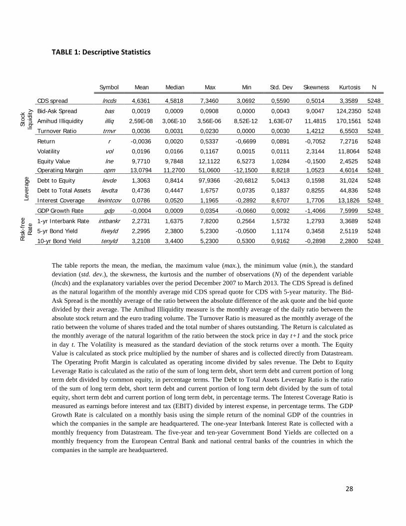
Table 1 reports summary statistics for all variables used in our analysis. We observe
that the firms in our sample have an average negative return throughout the 64 months. We
also note that the Amihud illiquidity measure shows very small values for the mean, median,
maximum and minimum values. This is due to the way it is calculated, the ratio having a
denominator (dollar trading volume) which is much larger than the numerator (absolute stock

27
return). A further observation is made regarding the GDP growth rate which shows a negative
mean throughout the sample period, in line with the turbulent times in European economies
caused by the financial crisis. Finally, when analyzing the risk-free rate proxies used, we note
that the higher the maturity of the risk-free rate the higher the yield. Furthermore, the standard
deviation of the risk-free rates decreases with maturity. The Jarque-Bera test (not reported)
rejects the normality assumption for all variables.
28
TABLE 1: Descriptive Statistics
Symbol Mean Median Max Min Std. Dev Skewness Kurtosis N
CDS spread lncds 4,6361 4,5818 7,3460 3,0692 0,5590 0,5014 3,3589 5248
Stoc
k liq
uidi
ty
Bid-Ask Spread bas 0,0019 0,0009 0,0908 0,0000 0,0043 9,0047 124,2350 5248
Amihud Illiquidity illiq 2,59E-08 3,06E-10 3,56E-06 8,52E-12 1,63E-07 11,4815 170,1561 5248
Turnover Ratio trnvr 0,0036 0,0031 0,0230 0,0000 0,0030 1,4212 6,5503 5248
Return r -0,0036 0,0020 0,5337 -0,6699 0,0891 -0,7052 7,2716 5248
Volatility vol 0,0196 0,0166 0,1167 0,0015 0,0111 2,3144 11,8064 5248
Equity Value lne 9,7710 9,7848 12,1122 6,5273 1,0284 -0,1500 2,4525 5248
Operating Margin opm 13,0794 11,2700 51,0600 -12,1500 8,8218 1,0523 4,6014 5248
Leve
rage
Debt to Equity levde 1,3063 0,8414 97,9366 -20,6812 5,0413 0,1598 31,024 5248
Debt to Total Assets levdta 0,4736 0,4447 1,6757 0,0735 0,1837 0,8255 44,836 5248
Interest Coverage levintcov 0,0786 0,0520 1,1965 -0,2892 8,6707 1,7706 13,1826 5248
GDP Growth Rate gdp -0,0004 0,0009 0,0354 -0,0660 0,0092 -1,4066 7,5999 5248
Ris
k-fr
ee
Rat
e 1-yr Interbank Rate intbankr 2,2731 1,6375 7,8200 0,2564 1,5732 1,2793 3,3689 5248
5-yr Bond Yield fiveyld 2,2995 2,3800 5,2300 -0,0500 1,1174 0,3458 2,5119 5248
10-yr Bond Yield tenyld 3,2108 3,4400 5,2300 0,5300 0,9162 -0,2898 2,2800 5248
The table reports the mean, the median, the maximum value (max.), the minimum value (min.), the standard deviation (std. dev.), the skewness, the kurtosis and the number of observations (N) of the dependent variable (lncds) and the explanatory variables over the period December 2007 to March 2013. The CDS Spread is defined as the natural logarithm of the monthly average mid CDS spread quote for CDS with 5-year maturity. The Bid-Ask Spread is the monthly average of the ratio between the absolute difference of the ask quote and the bid quote divided by their average. The Amihud Illiquidity measure is the monthly average of the daily ratio between the absolute stock return and the euro trading volume. The Turnover Ratio is measured as the monthly average of the ratio between the volume of shares traded and the total number of shares outstanding. The Return is calculated as the monthly average of the natural logarithm of the ratio between the stock price in day t+1 and the stock price in day t. The Volatility is measured as the standard deviation of the stock returns over a month. The Equity Value is calculated as stock price multiplied by the number of shares and is collected directly from Datastream. The Operating Profit Margin is calculated as operating income divided by sales revenue. The Debt to Equity Leverage Ratio is calculated as the ratio of the sum of long term debt, short term debt and current portion of long term debt divided by common equity, in percentage terms. The Debt to Total Assets Leverage Ratio is the ratio of the sum of long term debt, short term debt and current portion of long term debt divided by the sum of total equity, short term debt and current portion of long term debt, in percentage terms. The Interest Coverage Ratio is measured as earnings before interest and tax (EBIT) divided by interest expense, in percentage terms. The GDP Growth Rate is calculated on a monthly basis using the simple return of the nominal GDP of the countries in which the companies in the sample are headquartered. The one-year Interbank Interest Rate is collected with a monthly frequency from Datastream. The five-year and ten-year Government Bond Yields are collected on a monthly frequency from the European Central Bank and national central banks of the countries in which the companies in the sample are headquartered.
29
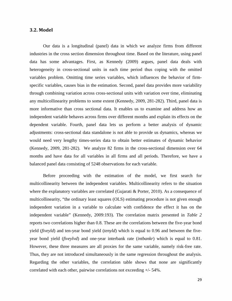
3.2. Model
Our data is a longitudinal (panel) data in which we analyze firms from different
industries in the cross section dimension throughout time. Based on the literature, using panel
data has some advantages. First, as Kennedy (2009) argues, panel data deals with
heterogeneity in cross-sectional units in each time period thus coping with the omitted
variables problem. Omitting time series variables, which influences the behavior of firm-
specific variables, causes bias in the estimation. Second, panel data provides more variability
through combining variation across cross-sectional units with variation over time, eliminating
any multicollinearity problems to some extent (Kennedy, 2009, 281-282). Third, panel data is
more informative than cross sectional data. It enables us to examine and address how an
independent variable behaves across firms over different months and explain its effects on the
dependent variable. Fourth, panel data lets us perform a better analysis of dynamic
adjustments: cross-sectional data standalone is not able to provide us dynamics, whereas we
would need very lengthy times-series data to obtain better estimates of dynamic behavior
(Kennedy, 2009, 281-282). We analyze 82 firms in the cross-sectional dimension over 64
months and have data for all variables in all firms and all periods. Therefore, we have a
balanced panel data consisting of 5248 observations for each variable.
Before proceeding with the estimation of the model, we first search for
multicollinearity between the independent variables. Multicollinearity refers to the situation
where the explanatory variables are correlated (Gujarati & Porter, 2010). As a consequence of
multicollinearity, “the ordinary least squares (OLS) estimating procedure is not given enough
independent variation in a variable to calculate with confidence the effect it has on the
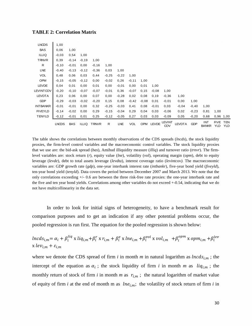
independent variable” (Kennedy, 2009:193). The correlation matrix presented in Table 2
reports two correlations higher than 0.8. These are the correlations between the five-year bond
yield (fiveyld) and ten-year bond yield (tenyld) which is equal to 0.96 and between the five-
year bond yield (fiveylvd) and one-year interbank rate (intbankr) which is equal to 0.81.
However, these three measures are all proxies for the same variable, namely risk-free rate.
Thus, they are not introduced simultaneously in the same regression throughout the analysis.
Regarding the other variables, the correlation table shows that none are significantly
correlated with each other, pairwise correlations not exceeding +/- 54%.
30
TABLE 2: Correlation Matrix
The table shows the correlations between monthly observations of the CDS spreads (lncds), the stock liquidity proxies, the firm-level control variables and the macroeconomic control variables. The stock liquidity proxies that we use are: the bid-ask spread (bas), Amihud illiquidity measure (illiq) and turnover ratio (trnvr). The firm-level variables are: stock return (r), equity value (lne), volatility (vol), operating margin (opm), debt to equity leverage (levde), debt to total assets leverage (levdta), interest coverage ratio (levintcov). The macroeconomic variables are: GDP growth rate (gdp), one-year interbank interest rate (intbankr), five-year bond yield (fiveyld), ten-year bond yield (tenyld). Data covers the period between December 2007 and March 2013. We note that the only correlations exceeding +/- 0.6 are between the three risk-free rate proxies: the one-year interbank rate and the five and ten year bond yields. Correlations among other variables do not exceed +-0.54, indicating that we do not have multicollinearity in the data set.
In order to look for initial signs of heterogeneity, to have a benchmark result for
comparison purposes and to get an indication if any other potential problems occur, the
pooled regression is run first. The equation for the pooled regression is shown below:
𝑙𝑛𝑐𝑑𝑠𝑖,𝑚= 𝛼𝑖 + 𝛽𝑖𝑙𝑖𝑞 x 𝑙𝑖𝑞𝑖,𝑚+𝛽𝑖𝑟 x 𝑟𝑖,𝑚 + 𝛽𝑖𝑒 x 𝑙𝑛𝑒𝑖,𝑚 +𝛽𝑖𝑣𝑜𝑙 x 𝑣𝑜𝑙𝑖,𝑚 +𝛽𝑖
𝑜𝑝𝑚 x 𝑜𝑝𝑚𝑖,𝑚 +𝛽𝑖𝑙𝑒𝑣 x 𝑙𝑒𝑣𝑖,𝑚 + 𝜀𝑖,𝑚
where we denote the CDS spread of firm i in month m in natural logarithm as 𝑙𝑛𝑐𝑑𝑠𝑖,𝑚 ; the
intercept of the equation as 𝛼𝑖 ; the stock liquidity of firm i in month m as 𝑙𝑖𝑞𝑖,𝑚 ; the
monthly return of stock of firm i in month m as 𝑟𝑖,𝑚 ; the natural logarithm of market value
of equity of firm i at the end of month m as 𝑙𝑛𝑒𝑖,𝑚; the volatility of stock return of firm i in
LNCDS 1,00
BAS 0,06 1,00
ILLIQ -0,03 0,54 1,00
TRNVR 0,39 -0,14 -0,19 1,00
R -0,10 -0,01 0,00 -0,16 1,00
LNE -0,40 -0,13 -0,12 -0,36 0,03 1,00
VOL 0,48 0,06 0,03 0,44 -0,25 -0,22 1,00
OPM -0,15 -0,05 -0,12 0,00 -0,02 0,26 -0,11 1,00
LEVDE 0,04 0,01 0,00 0,01 0,00 -0,01 0,00 0,01 1,00
LEVINTCOV -0,20 -0,10 -0,07 -0,07 -0,01 0,36 -0,07 0,15 -0,08 1,00
LEVDTA 0,23 0,06 0,00 0,07 0,00 -0,28 0,02 0,08 0,19 -0,36 1,00
GDP -0,29 -0,03 -0,02 -0,20 0,15 0,08 -0,42 -0,08 0,01 -0,01 0,00 1,00
INTBANKR -0,01 -0,01 0,00 0,32 -0,25 -0,03 0,41 0,08 -0,01 0,03 -0,04 -0,40 1,00
FIVEYLD -0,14 -0,02 0,00 0,29 -0,15 -0,04 0,29 0,04 0,03 -0,06 0,02 -0,23 0,81 1,00
TENYLD -0,12 -0,01 0,01 0,25 -0,12 -0,05 0,27 0,03 0,03 -0,09 0,05 -0,20 0,68 0,96 1,00
LEVDTA GDP INT BANKR
FIVEYLD
TENYLD
LEVINTCOVLNCDS BAS ILLIQ TRNVR R LNE VOL OPM LEVDE

31
month m as 𝑣𝑜𝑙𝑖,𝑚 ; the operating profit margin of firm i in month m as 𝑜𝑝𝑚𝑖,𝑚; the leverage
of firm i in month m as 𝑙𝑒𝑣𝑖,𝑚; the residual of firm i in month m as 𝜀𝑖,𝑚.
The output of this simple panel LS regression without any corrections is represented
in Appendix (1). From the data output of the pooled regression, we see that volatility and
leverage have a significant positive relation with the CDS spread, whereas equity value has a
negative relationship. Stock liquidity, return and operating margin are insignificant at the 5%
significance level. The regression’s goodness of fit (R2 = 0.335) is quite low. However, a
quick examination of the Durbin-Watson test statistic (0.2546) suggests significant
autocorrelation in the residuals.
To get an idea of whether heterogeneity is present in our data, we first plot the
residuals of the pooled regression and check whether they seem “homogenous”. The residuals
plot is depicted in Appendix (2). If the residuals constantly tend to be either below or above
zero, this is likely to be an indication of heterogeneity. This seems to be the case in our pooled
regression result. The variance of the errors seems not to be constant, indicating that
heteroskedasticity is likely to be an issue.
There are two main panel estimator approaches which are used in financial research.
These are the fixed effects model and the random effects model. The panel data provides us
with the option of controlling for cross-sectional heterogeneity and/or controlling for time-
specificity (Brooks, 2008). In regards to the cross-sectional heterogeneity, we fix the model in
the time-series dimension and we have a chance to examine the firm-specific variation of the
parameters by letting them vary cross firms (Brooks, 2008). Alternatively, when we fix the
model in the cross section dimension, we have a chance to isolate time-specificity and
therefore analyzing how the relationship among our variables changes through time (Brooks,
2008).
Both the random effects model (also called the variance components or error
components model) and the fixed effects model use different intercept terms for each entity.
These intercepts are assumed to be constant over time and the relationships between the
explanatory and explained variables are considered identical over time (Brooks, 2008). The
difference between the fixed and random effects models is that under the latter, “intercepts for

32
each cross-sectional unit are assumed to arise from a common intercept and a random variable
which is constant over time but varies cross-sectional” (Brooks, 2008:498). This random
variable measures the deviation of the individual intercept terms from the global intercept
term. With regards to the fixed effects models, the cross-sectional fixed effects model
decomposes the disturbance term in two separate parts: an individual specific effect and a
“remainder disturbance” which varies over time and cross sectional (Brooks, 2008). In the
time-fixed effects model, intercepts vary with time but don’t change across entities at each
given point in time (Brooks, 2008).
Since the random effects model saves degrees of freedom, it provides a more efficient
estimator of variable coefficients than the fixed effects model (Kennedy, 2009). For this
reason, we first investigate the presence of random effects in our model. To test whether we
need to include random effects, we perform the Correlated Random Effects - Hausman Test, a
specification test available in EViews. As we see from the results of the Hausman test shown
in Table 3, the p-value for both the cross-section and period random effects is 0.0000
indicating that we reject the assumption of cross-section and period random effects.
Therefore, we cannot apply the random effects model in our analysis.
TABLE 3: Correlated Random Effects – Hausman Test
HAUSMAN TEST Test Summary Chi-Sq. Statistic Chi-Sq. d.f. Prob.
Cross-section random 223,211557 6 0,0000 Period Random 143,032510 6 0,0000
Table 3 depicts the results of the Correlated Random Effects – Hausman Test for the
regression using bid-ask spread as a measure of stock liquidity. The first column denotes in
which dimension the test is performed. The Chi-squared test statistic and the degrees of
freedom are presented in the second and third column. The p-value (Prob.) is presented in the
fourth column. When the p-value for the Chi-Squared statistic is less than 0.05, we reject the
null hypothesis indicating the presence of random effects in the model in favor of the
alternative hypothesis suggesting that the random effects model is not applicable. The
probability (Prob.) of the Chi-Squared Statistic is 0.0000 for both cross-section and period
random effects. Therefore, we conclude that the specification using random effects is not
applicable for this regression.

33
We draw our attention towards investigating the presence of fixed effects in our
model. We estimate the model with dummy variables for cross-section units, then time
periods and finally test the dummies jointly for significance. Across the entire sample, the
mean of residuals is zero. However, if systematic average deviations from zero occur for each
cross-section unit or time period, by using dummies, which explain this average deviation, we
push the residuals back toward zero. The results of the regression with cross-section dummies
are presented in Appendix (3). The results of the regression with time dummies are shown in
Appendix (4) and finally the results of the regression with both cross-section and time
dummies are displayed in Appendix (5).
With regards to the estimation with both cross-section and time dummies, we find that
the variables’ significance and coefficients are now qualitatively different. The stock liquidity
is now significant and has a positive relationship with the CDS spread. Return, equity value,
volatility and leverage are as well significant, whereas operating margin remains insignificant.
We can also observe that the R2 increases; the goodness of fit of our regression now
reaching 0.8514. This is a result of both decreasing the variation of residuals and introducing
a large number of new explanatory variables (the dummies). We perform a redundant fixed
effects test, shown in Table 4 to check whether the specification using fixed effects is optimal
for our model.
TABLE 4: Redundant Fixed Effects Tests
REDUNDANT FIXED EFFECTS TESTS Effects Test Statistic d.f. Prob.
Cross-section F 157,943006 (81,5097) 0,0000 Cross-section Chi Square 6589,447595 81 0,0000 Period F 63,303449 (63,5097) 0,0000 Period Chi-Square 3033,267801 63 0,0000 Cross-Section/Period F 123,093060 (144,5097) 0,0000 Cross-Section/Period Chi-Square 7867,226465 144 0,0000
Table 4 presents the results of the redundant fixed effects tests for the regression using bid-ask
spread as a measure of stock liquidity. The first column denotes the fixed effects test we
perform (cross-section fixed effects, period fixed effects and simultaneous cross-section and
period fixed effects). The F and Chi-Squared Statistics are presented in the second column.
The degrees of freedom and the p-value (prob.) are presented in the third and fourth columns.

34
When the p-value for the F-statistic and Chi-Squared statistic is less than 0.05, we accept the
null hypothesis indicating the presence of fixed effects in the model and reject the alternative
hypothesis indicating that the fixed effects model is not applicable. The probability (Prob.) of
both the F statistic and Chi-Squared Statistic is 0.0000 for both cross-section and period fixed
effects. Therefore, we conclude that the specification using both cross-section and period
fixed effects is recommended.
We observe that both the F statistic and the Chi-Squared have a p-value of 0.0000 indicating
that both the cross section and period dummies are significant at the 5% significance level.
Thus, we need to account for heterogeneity in both dimensions and conclude that our model
needs to use fixed effects. We note that when checking for fixed effects individually in the
period dimension and individually in the cross-section dimension, we reach the same result in
that the dummy variables are highly significant and heterogeneity needs to be accounted for
both dimensions.
Therefore, the generic model that we use in this paper is of the following form:
𝑙𝑛𝑐𝑑𝑠𝑖,𝑚= 𝛼𝑖 +𝛽𝑖𝑙𝑖𝑞 x 𝑙𝑖𝑞𝑖,𝑚 +𝛽𝑖𝑟 x 𝑟𝑖,𝑚 + 𝛽𝑖𝑒 x 𝑙𝑛𝑒𝑖,𝑚 +𝛽𝑖𝑣𝑜𝑙 x 𝑣𝑜𝑙𝑖,𝑚 +𝛽𝑖
𝑜𝑝𝑚 x 𝑜𝑝𝑚𝑖,𝑚 +𝛽𝑖𝑙𝑒𝑣 x 𝑙𝑒𝑣𝑖,𝑚 + 𝐷𝑚+𝐷𝑖+ 𝜀𝑖,𝑚
where we denote the CDS spread of firm i in month m in natural logarithm as 𝑙𝑛𝑐𝑑𝑠𝑖,𝑚 ; the
intercept of the equation as 𝛼𝑖 ; the stock liquidity of firm i in month m as 𝑙𝑖𝑞𝑖,𝑚 ; the
monthly return of stock of firm i in month m as 𝑟𝑖,𝑚 ; the natural logarithm of market value
of equity of firm i at the end of month m as 𝑙𝑛𝑒𝑖,𝑚; the volatility of stock return of firm i in
month m as 𝑣𝑜𝑙𝑖,𝑚 ; the operating profit margin of firm i in month m as 𝑜𝑝𝑚𝑖,𝑚; the leverage
of firm i in month m as 𝑙𝑒𝑣𝑖,𝑚; the dummy variable used to control time-effects present in our
sample as 𝐷𝑚; the dummy variable used to control any cross-sectional (firm-specific) effects
present in our sample as 𝐷𝑖 ; the residual of firm i in month m as 𝜀𝑖,𝑚.
We use three proxies for the stock liquidity variable represented above by 𝑙𝑖𝑞𝑖,𝑚 .
These are: the stock liquidity of firm i at month m implied by bid-ask spread measure as
𝑏𝑎𝑠𝑖,𝑚; the stock illiquidity of firm i at month m implied by Amihud illiquidity measure as
𝑖𝑙𝑙𝑖𝑞𝑖,𝑚 ; the stock liquidity of firm i at month m implied by turnover ratio as 𝑡𝑟𝑛𝑣𝑟𝑖,𝑚 .
Similarly for the leverage variable represented above by 𝑙𝑒𝑣𝑖,𝑚 , we use three ratios: the
35
leverage of firm i calculated by the debt to equity ratio at month m as 𝑙𝑒𝑣𝑑𝑒𝑖,𝑚; the leverage
of firm i calculated by the debt to total assets ratio at month m as 𝑙𝑒𝑣𝑑𝑡𝑎𝑖,𝑚; the leverage of
firm i implied by the interest coverage ratio at month m as 𝑙𝑒𝑣𝑖𝑛𝑡𝑐𝑜𝑣𝑖,𝑚.
In our model we allow for heterogeneity, thus we want to capture any fixed time
effects across firms as well as any firm specific effects (cross sectional effects) across time.
This result is in line with the article of Annaert et al (2010) which suggests that the fixed
effects model needs to be used for two reasons. Firstly, all the firms included in the sample
have sufficient CDS quotes and have their stock listed at the stock market. As a result, we do
not state that our sample is random. Secondly, in the panel regression, we have many time-
series observations that enable us to use fixed effects model, because Hsiao (2005:37, cited in
Annaert et al, 2010) states “the GLS estimator for random effects converges to the OLS
estimator for fixed effects when the number of time-series observations grows.”
In the next step, we investigate the presence of heteroskedasticity in our model.
Heteroskedasticity implies that the variance of the error terms is not constant. To get an idea
of whether we have heteroskedasticity in our model, we first look at the residual graph of the
regression with cross-section and period fixed effects shown in Appendix (6). According to
this plot, we are not able to affirm with certainty whether heteroskedasticity is present in the
data. Thus, we manually perform a White heteroskedasticity test in EViews. The results of
this test are shown in Appendix (7) and summarized in Table 5.
TABLE 5: White Heteroskedasticity Test
WHITE TEST FOR HETEROSCEDASTICITY
Dependent Variable: Residual^2 R-Squared F-statistic Prob. (F-statistic)
Values 0,3667 111,922 0,0000 Table 5 presents summarized results of the White test for heteroskedasticity performed for the
model using bid-ask spread as proxy for stock liquidity. To perform the test, we select as
dependent variable the squared residuals (residual ^2), while we use as independent variables
all explanatory variables from the generic model, their squares and all cross-products. When
the p-value of the F-statistic (Prob.) is less than 0.05, then we reject the null hypothesis of
homoskedasticity in favor of the alternative hypothesis of heteroskedasticity. The p-value for
the test is 0.0000, indicating that heteroskedasticity is present in the model. A detailed

36
breakdown of the test together with the significance of all explanatory variables is presented in
Appendix (7).
The p-value of the White test is 0.0000 indicating the problem of heteroskedasticity.
By performing a Breusch-Pagan test presented in Appendix (8), we obtain the same result as
in the White test, confirming that heteroskedasticity exists. To solve the problem of
heteroskedasticity, we use the White (diagonal) standard errors in the regressions. Using
White standard errors also helps us cope with clustering within each firm through time. The
output of this regression of bid-ask spread stock liquidity using White diagonal standard
errors is shown in Appendix (9).
The bid-ask spread, which is the most commonly used liquidity proxy, is a “cost
based” measure of liquidity relying on transaction costs. To analyze the relation between
stock liquidity and CDS in detail, we investigate two other proxies for liquidity, classified as
“reflective” measures, which capture different characteristics of liquidity (Spiegel and Wong,
2005). These two measures are the Amihud illiquidity measure (illiq) and the turnover ratio
(trnvr). Both measures use volume of traded shares in their calculation, which shows cross-
sectional heterogeneity. We figure out that we have more outlier observations in volume data
across cross section. Hence, we use fixed cross-section effects and let the variables vary
across time. Because we use a model with only cross-section fixed effects, to account for
heteroskedasticity in the cross-sectional dimension, we also run the regressions using White
cross-section standard errors. If we use the model with both cross-section and time fixed
effects, we obtain counter-intuitive results with insignificant probabilities for these liquidity
measures.
In order to analyze whether stock liquidity remains significant when controlling for
macroeconomic variables, we perform a separate regression model. We perform this analysis
in a different regression because the macro level variables (GDP growth rate and risk-free
rate) are time-oriented variables. These variables vary according to countries, whereas CDS
spreads vary through firms. Therefore, the cross-section section dimension frequencies are not
identical. Accordingly, we are not able to introduce these variables together with other control
variables that vary across firms in the generic model, where we use time-fixed effects.
Following the same procedure above, we first examine the pooled regression below:

37
𝐼𝑛𝑐𝑑𝑠𝑖,𝑚= 𝛼𝑖 +𝛽𝑖𝑙𝑖𝑞 x 𝑙𝑖𝑞𝑖,𝑚+ 𝛽𝑔𝑑𝑝 x 𝑔𝑑𝑝𝑗,𝑚+ 𝛽𝑟𝑓 x 𝑟𝑓𝑗,𝑚 + 𝜀𝑖,𝑚
where we denote the CDS spread of firm i in month m in natural logarithm as 𝑙𝑛𝑐𝑑𝑠𝑖,𝑚 ; the
intercept of the equation as 𝛼𝑖 ; the stock liquidity of firm i in month m as 𝑙𝑖𝑞𝑖,𝑚 ; the average
GDP growth rate of country j where company i is located, in month m as 𝑔𝑑𝑝𝑗,𝑚; the risk-free
rate of country j where company i is located, in month m as 𝑟𝑓𝑗,𝑚; the residual of firm i in
month m as 𝜀𝑖,𝑚.
We use three proxies for the risk-free rate variable represented above by 𝑟𝑓𝑗,𝑚. These
are: the 1-year interbank interest rate of country j in month m as 𝑖𝑛𝑡𝑏𝑎𝑛𝑘𝑟𝑗,𝑚; the five-year
government bond yield of country j in month m as 𝑓𝑖𝑣𝑒𝑦𝑙𝑑𝑗,𝑚; the ten-year government yield
of country j in month m as 𝑡𝑒𝑛𝑦𝑙𝑑𝑗,𝑚.
We investigate the presence of heterogeneity in the model including macroeconomic
control variables through the residual graph presented in Appendix (10). We check for
heterogeneity in the data by first investigating random effects in the cross sectional
dimension. The Hausman test for random effects turns out to be invalid, indicating that the
specification using random effects is not applicable. Then, we examine the presence of fixed
effects in the cross-section dimension.
TABLE 6: Redundant Fixed Effects Test for the Model using Macroeconomic Variables
REDUNDANT FIXED EFFECTS TEST
Effects Test Statistic d.f. Prob.
Cross-section F 87,0962 (81,5163) 0,0000 Cross-section Chi Square 4520,4995 81 0,0000
Table 6 presents the results of the redundant fixed effects tests for the regression using bid-ask
spread as a measure of stock liquidity and macroeconomic factors as explanatory variables.
The first column denotes the fixed effects test we perform (cross-section fixed effects). The F
and Chi-Squared Statistics are presented in column two. The degrees of freedom and the p-
value (prob.) are presented in the third and fourth columns. When the p-value for the F-
statistic and Chi-Squared statistic is less than 0.05, we accept the null hypothesis indicating
the presence of fixed effects in the model and reject the alternative hypothesis indicating that
the fixed effects model is not applicable. The probability (Prob.) of both the F statistic and
38
Chi-Squared Statistic is 0.0000 for the cross-section fixed effects. Therefore, we conclude that
we apply cross-section fixed effects in our model with macroeconomic explanatory variables.
By conducting a redundant fixed effects test presented in Table 6, we obtain a p-value
for cross section fixed effects of 0.0000 indicating that the dummy variables are significant
and that we have to account for fixed effects in the cross-section dimension. As stated above,
we do not use fixed effects for the time-dimension. By interpreting the residual graph of the
regression of bid-ask spread stock liquidity with macroeconomic control variables using
cross-section fixed effects presented in Appendix (11), we ascertain that heteroskedasticity
has to be accounted for by using White cross-section standard errors. As a consequence, the
generic model for testing the significance of stock liquidity when controlling for
macroeconomic variables is shown below:
𝐼𝑛𝑐𝑑𝑠𝑖,𝑚= 𝛼𝑖 +𝛽𝑖𝑙𝑖𝑞 x 𝑙𝑖𝑞𝑖,𝑚+ 𝛽𝑟𝑓 x 𝑟𝑓𝑗,𝑚 + 𝛽𝑔𝑑𝑝 x 𝑔𝑑𝑝𝑗,𝑚+𝐷𝑖+ 𝜀𝑖,𝑚
where we denote the CDS spread of firm i in natural logarithm as 𝑙𝑛𝑐𝑑𝑠𝑖,𝑚; the intercept of
the equation as 𝛼𝑖 ; the stock liquidity of firm i at month m as 𝑙𝑖𝑞𝑖,𝑚; the risk free rate of
country j in month m as 𝑟𝑓𝑗,𝑚; the GDP growth rate of country j in month m as 𝑔𝑑𝑝𝑗,𝑚; the
dummy variable used to control any cross-sectional (firm-specific) effects present in our
sample as 𝐷𝑖; the residual of firm i at month m as 𝜀𝑖,𝑚.

39
4. EMPIRICAL ANALYSIS
According to the regression outputs, we make several interpretations. In the regression
where we use both cross-section and time fixed effects, by controlling for return, equity value,
volatility, operating margin and leverage measured by debt to equity ratio (levde), we observe
a significant positive relation between stock liquidity measured as bid-ask spread and CDS
spreads. The coefficients of the majority of the control variables confirm our intuition and the
literature, having significant probabilities (p<0.05). However, stock return shows a significant
positive relation with CDS spreads, which is counter intuitive and not in line with literature.
With regards to operating margin, we observe an expected negative relationship with CDS
spreads, however with an insignificant probability of 0.185. The R2, the most commonly used
goodness of fit statistic, has a value of 0.8514 which shows that our model fits the data well.
The result of the regression using fixed effects in both dimensions is presented in Table 7
together with the pooled regression and the regression using random effects for comparison
purposes. Detailed information of each regression is depicted in the Appendices (1, 12, and
5).
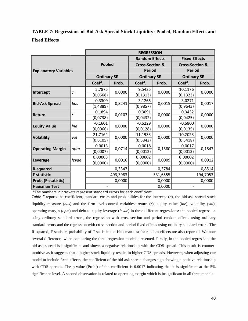
40
TABLE 7: Regressions of Bid-Ask Spread Stock Liquidity: Pooled, Random Effects and
Fixed Effects
REGRESSION
Explanatory Variables Pooled
Random Effects Fixed Effects Cross-Section &
Period Cross-Section &
Period Ordinary SE Ordinary SE Ordinary SE
Coeff. Prob. Coeff. Prob. Coeff. Prob.
Intercept c 5,7875 0,0000 9,5425 0,0000 10,1176 0,0000 (0,0668) (0,1313) (0,1323)
Bid-Ask Spread bas -0,3309 0,8241 3,1265 0,0015 3,0271 0,0017 (1,4889) (0,9857) (0,9643)
Return r 0,1894 0,0103 0,3091 0,0000 0,3432 0,0000 (0,0738) (0,0432) (0,0425)
Equity Value lne -0,1601 0,0000 -0,5229 0,0000 -0,5800 0,0000 (0,0066) (0,0128) (0,0135)
Volatility vol 21,7164 0,0000 11,1933 0,0000 10,2023 0,0000 (0,6105) (0,5343) (0,5418)
Operating Margin opm -0,0013 0,0714 -0,0018 0,1380 -0,0017 0,1847 (0,0007) (0,0012) (0,0013)
Leverage levde 0,00003
0,0016 0,00002
0,0009 0,00002
0,0012 (0,0000) (0,0000) (0,0000)
R-squared
0,3347 0,3784 0,8514 F-statistic 493,3983 531,6555 194,7053 Prob. (F-statistic) 0,0000 0,0000 0,0000 Hausman Test - 0,0000 - *The numbers in brackets represent standard errors for each coefficient.
Table 7 reports the coefficient, standard errors and probabilities for the intercept (c), the bid-ask spread stock
liquidity measure (bas) and the firm-level control variables: return (r), equity value (lne), volatility (vol),
operating margin (opm) and debt to equity leverage (levde) in three different regressions: the pooled regression
using ordinary standard errors, the regression with cross-section and period random effects using ordinary
standard errors and the regression with cross-section and period fixed effects using ordinary standard errors. The
R-squared, F-statistic, probability of F-statistic and Hausman test for random effects are also reported. We note
several differences when comparing the three regression models presented. Firstly, in the pooled regression, the
bid-ask spread is insignificant and shows a negative relationship with the CDS spread. This result is counter-
intuitive as it suggests that a higher stock liquidity results in higher CDS spreads. However, when adjusting our
model to include fixed effects, the coefficient of the bid-ask spread changes sign showing a positive relationship
with CDS spreads. The p-value (Prob.) of the coefficient is 0.0017 indicating that it is significant at the 5%
significance level. A second observation is related to operating margin which is insignificant in all three models.
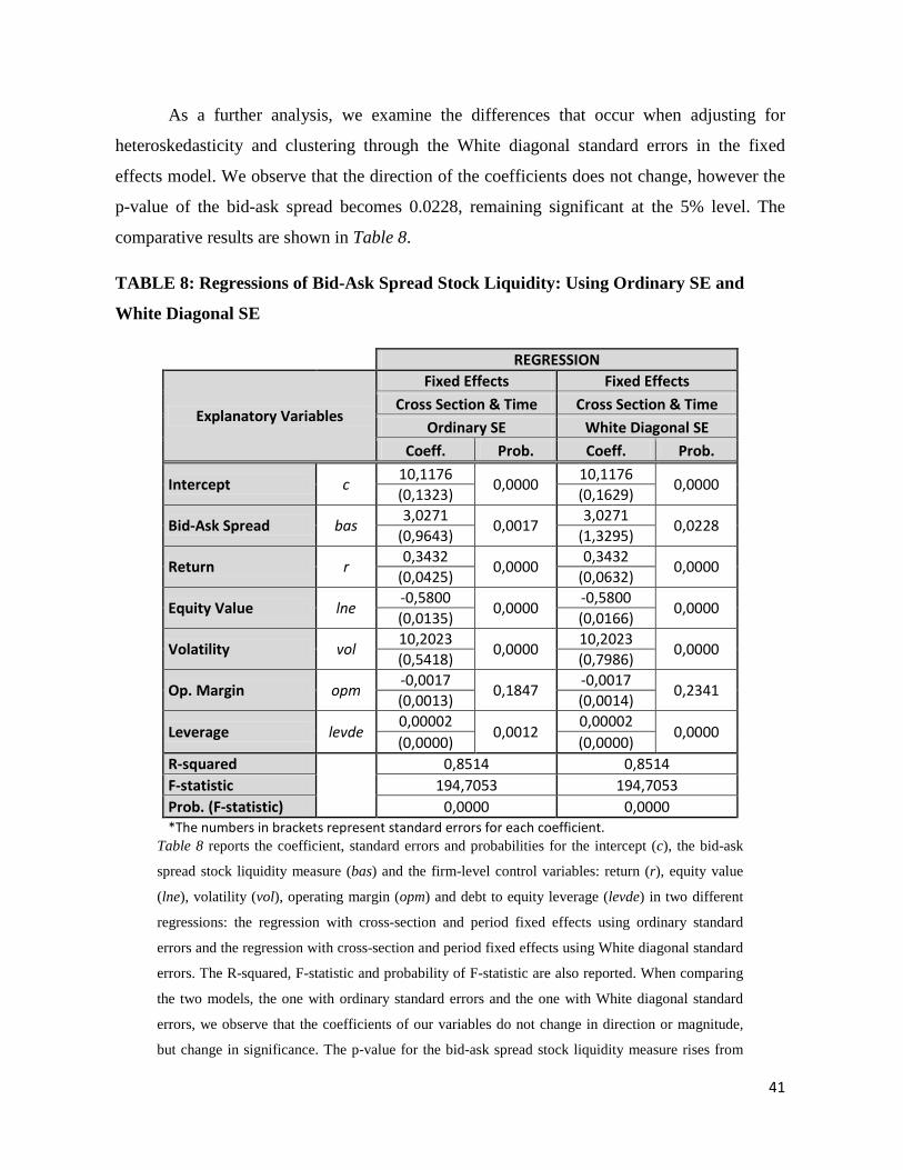
41
As a further analysis, we examine the differences that occur when adjusting for
heteroskedasticity and clustering through the White diagonal standard errors in the fixed
effects model. We observe that the direction of the coefficients does not change, however the
p-value of the bid-ask spread becomes 0.0228, remaining significant at the 5% level. The
comparative results are shown in Table 8.
TABLE 8: Regressions of Bid-Ask Spread Stock Liquidity: Using Ordinary SE and
White Diagonal SE
REGRESSION
Explanatory Variables
Fixed Effects Fixed Effects Cross Section & Time Cross Section & Time
Ordinary SE White Diagonal SE Coeff. Prob. Coeff. Prob.
Intercept c 10,1176 0,0000 10,1176 0,0000 (0,1323) (0,1629)
Bid-Ask Spread bas 3,0271 0,0017 3,0271 0,0228 (0,9643) (1,3295)
Return r 0,3432 0,0000 0,3432 0,0000 (0,0425) (0,0632)
Equity Value lne -0,5800
0,0000 -0,5800
0,0000 (0,0135) (0,0166)
Volatility vol 10,2023 0,0000 10,2023 0,0000 (0,5418) (0,7986)
Op. Margin opm -0,0017 0,1847 -0,0017 0,2341 (0,0013) (0,0014)
Leverage levde 0,00002
0,0012 0,00002
0,0000 (0,0000) (0,0000)
R-squared
0,8514 0,8514 F-statistic 194,7053 194,7053 Prob. (F-statistic) 0,0000 0,0000 *The numbers in brackets represent standard errors for each coefficient.
Table 8 reports the coefficient, standard errors and probabilities for the intercept (c), the bid-ask
spread stock liquidity measure (bas) and the firm-level control variables: return (r), equity value
(lne), volatility (vol), operating margin (opm) and debt to equity leverage (levde) in two different
regressions: the regression with cross-section and period fixed effects using ordinary standard
errors and the regression with cross-section and period fixed effects using White diagonal standard
errors. The R-squared, F-statistic and probability of F-statistic are also reported. When comparing
the two models, the one with ordinary standard errors and the one with White diagonal standard
errors, we observe that the coefficients of our variables do not change in direction or magnitude,
but change in significance. The p-value for the bid-ask spread stock liquidity measure rises from
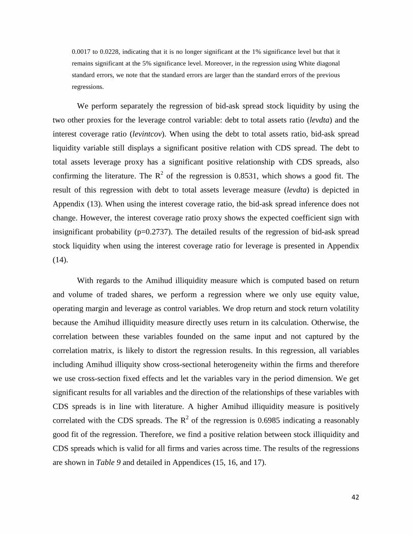
42
0.0017 to 0.0228, indicating that it is no longer significant at the 1% significance level but that it
remains significant at the 5% significance level. Moreover, in the regression using White diagonal
standard errors, we note that the standard errors are larger than the standard errors of the previous
regressions.
We perform separately the regression of bid-ask spread stock liquidity by using the
two other proxies for the leverage control variable: debt to total assets ratio (levdta) and the
interest coverage ratio (levintcov). When using the debt to total assets ratio, bid-ask spread
liquidity variable still displays a significant positive relation with CDS spread. The debt to
total assets leverage proxy has a significant positive relationship with CDS spreads, also
confirming the literature. The R2 of the regression is 0.8531, which shows a good fit. The
result of this regression with debt to total assets leverage measure (levdta) is depicted in
Appendix (13). When using the interest coverage ratio, the bid-ask spread inference does not
change. However, the interest coverage ratio proxy shows the expected coefficient sign with
insignificant probability (p=0.2737). The detailed results of the regression of bid-ask spread
stock liquidity when using the interest coverage ratio for leverage is presented in Appendix
(14).
With regards to the Amihud illiquidity measure which is computed based on return
and volume of traded shares, we perform a regression where we only use equity value,
operating margin and leverage as control variables. We drop return and stock return volatility
because the Amihud illiquidity measure directly uses return in its calculation. Otherwise, the
correlation between these variables founded on the same input and not captured by the
correlation matrix, is likely to distort the regression results. In this regression, all variables
including Amihud illiquity show cross-sectional heterogeneity within the firms and therefore
we use cross-section fixed effects and let the variables vary in the period dimension. We get
significant results for all variables and the direction of the relationships of these variables with
CDS spreads is in line with literature. A higher Amihud illiquidity measure is positively
correlated with the CDS spreads. The R2 of the regression is 0.6985 indicating a reasonably
good fit of the regression. Therefore, we find a positive relation between stock illiquidity and
CDS spreads which is valid for all firms and varies across time. The results of the regressions
are shown in Table 9 and detailed in Appendices (15, 16, and 17).
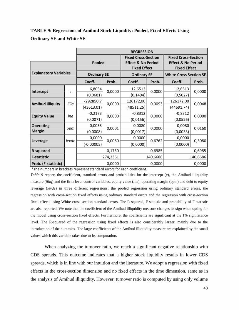
43
TABLE 9: Regressions of Amihud Stock Liquidity: Pooled, Fixed Effects Using
Ordinary SE and White SE
REGRESSION
Pooled
Fixed Cross-Section Effect & No Period
Fixed Effect
Fixed Cross-Section Effect & No Period
Fixed Effect Explanatory Variables Ordinary SE Ordinary SE White Cross Section SE
Coeff. Prob. Coeff. Prob. Coeff. Prob.
Intercept c 6,8054 0,0000 12,6513 0,0000 12,6513 0,0000 (0,0681) (0,1494) (0,5027)
Amihud Illiquity illiq -292850,7 0,0000 126172,00 0,0093 126172,00 0,0048 (43613,01) (48511,25) (44691,74)
Equity Value lne -0,2173 0,0000 -0,8312 0,0000 -0,8312 0,0000 (0,0071) (0,0156) (0,0526)
Operating Margin opm -0,0033 0,0001 0,0080 0,0000 0,0080 0,0160
(0,0008) (0,0017) (0,0033)
Leverage levde 0,0000
0,0060 0,0000
0,6762 0,0000
0,3080 (-0,00005) (0,0000) (0,0000)
R-squared
0,1730 0,6985 0,6985 F-statistic 274,2361 140,6686 140,6686 Prob. (F-statistic) 0,0000 0,0000 0,0000 *The numbers in brackets represent standard errors for each coefficient.
Table 9 reports the coefficient, standard errors and probabilities for the intercept (c), the Amihud illiquidity
measure (illiq) and the firm-level control variables: equity value (lne), operating margin (opm) and debt to equity
leverage (levde) in three different regressions: the pooled regression using ordinary standard errors, the
regression with cross-section fixed effects using ordinary standard errors and the regression with cross-section
fixed effects using White cross-section standard errors. The R-squared, F-statistic and probability of F-statistic
are also reported. We note that the coefficient of the Amihud illiquidity measure changes its sign when opting for
the model using cross-section fixed effects. Furthermore, the coefficients are significant at the 1% significance
level. The R-squared of the regression using fixed effects is also considerably larger, mainly due to the
introduction of the dummies. The large coefficients of the Amihud illiquidity measure are explained by the small
values which this variable takes due to its computation.
When analyzing the turnover ratio, we reach a significant negative relationship with
CDS spreads. This outcome indicates that a higher stock liquidity results in lower CDS
spreads, which is in line with our intuition and the literature. We adopt a regression with fixed
effects in the cross-section dimension and no fixed effects in the time dimension, same as in
the analysis of Amihud illiquidity. However, turnover ratio is computed by using only volume
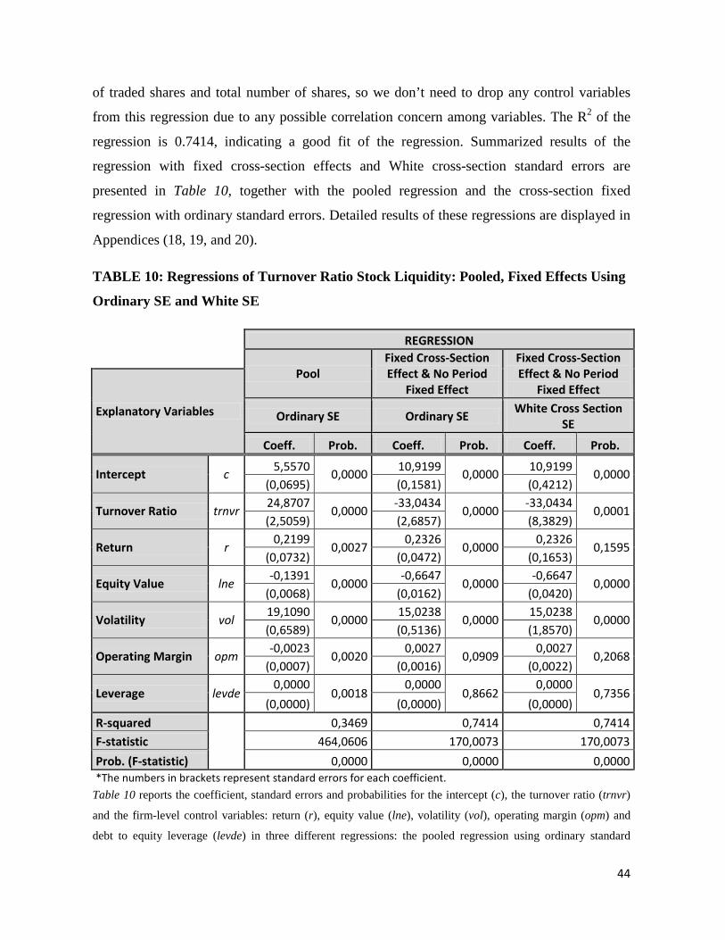
44
of traded shares and total number of shares, so we don’t need to drop any control variables
from this regression due to any possible correlation concern among variables. The R2 of the
regression is 0.7414, indicating a good fit of the regression. Summarized results of the
regression with fixed cross-section effects and White cross-section standard errors are
presented in Table 10, together with the pooled regression and the cross-section fixed
regression with ordinary standard errors. Detailed results of these regressions are displayed in
Appendices (18, 19, and 20).
TABLE 10: Regressions of Turnover Ratio Stock Liquidity: Pooled, Fixed Effects Using
Ordinary SE and White SE
REGRESSION
Pool
Fixed Cross-Section Effect & No Period
Fixed Effect
Fixed Cross-Section Effect & No Period
Fixed Effect
Explanatory Variables Ordinary SE Ordinary SE White Cross Section SE
Coeff. Prob. Coeff. Prob. Coeff. Prob.
Intercept c 5,5570 0,0000 10,9199 0,0000 10,9199 0,0000 (0,0695) (0,1581) (0,4212)
Turnover Ratio trnvr 24,8707 0,0000 -33,0434 0,0000 -33,0434 0,0001 (2,5059) (2,6857) (8,3829)
Return r 0,2199 0,0027 0,2326 0,0000 0,2326 0,1595 (0,0732) (0,0472) (0,1653)
Equity Value lne -0,1391 0,0000 -0,6647 0,0000 -0,6647 0,0000 (0,0068) (0,0162) (0,0420)
Volatility vol 19,1090 0,0000 15,0238 0,0000 15,0238 0,0000 (0,6589) (0,5136) (1,8570)
Operating Margin opm -0,0023 0,0020 0,0027 0,0909 0,0027 0,2068 (0,0007) (0,0016) (0,0022)
Leverage levde 0,0000
0,0018 0,0000
0,8662 0,0000
0,7356 (0,0000) (0,0000) (0,0000)
R-squared
0,3469 0,7414 0,7414 F-statistic 464,0606 170,0073 170,0073 Prob. (F-statistic) 0,0000 0,0000 0,0000 *The numbers in brackets represent standard errors for each coefficient.
Table 10 reports the coefficient, standard errors and probabilities for the intercept (c), the turnover ratio (trnvr)
and the firm-level control variables: return (r), equity value (lne), volatility (vol), operating margin (opm) and
debt to equity leverage (levde) in three different regressions: the pooled regression using ordinary standard
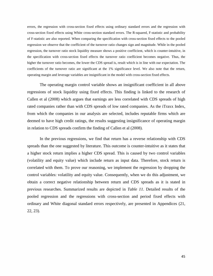
45
errors, the regression with cross-section fixed effects using ordinary standard errors and the regression with
cross-section fixed effects using White cross-section standard errors. The R-squared, F-statistic and probability
of F-statistic are also reported. When comparing the specification with cross-section fixed effects to the pooled
regression we observe that the coefficient of the turnover ratio changes sign and magnitude. While in the pooled
regression, the turnover ratio stock liquidity measure shows a positive coefficient, which is counter-intuitive, in
the specification with cross-section fixed effects the turnover ratio coefficient becomes negative. Thus, the
higher the turnover ratio becomes, the lower the CDS spread is, result which is in line with our expectation. The
coefficients of the turnover ratio are significant at the 1% significance level. We also note that the return,
operating margin and leverage variables are insignificant in the model with cross-section fixed effects.
The operating margin control variable shows an insignificant coefficient in all above
regressions of stock liquidity using fixed effects. This finding is linked to the research of
Callen et al (2008) which argues that earnings are less correlated with CDS spreads of high
rated companies rather than with CDS spreads of low rated companies. As the iTraxx Index,
from which the companies in our analysis are selected, includes reputable firms which are
deemed to have high credit ratings, the results suggesting insignificance of operating margin
in relation to CDS spreads confirm the finding of Callen et al (2008).
In the previous regressions, we find that return has a reverse relationship with CDS
spreads than the one suggested by literature. This outcome is counter-intuitive as it states that
a higher stock return implies a higher CDS spread. This is caused by two control variables
(volatility and equity value) which include return as input data. Therefore, stock return is
correlated with them. To prove our reasoning, we implement the regression by dropping the
control variables: volatility and equity value. Consequently, when we do this adjustment, we
obtain a correct negative relationship between return and CDS spreads as it is stated in
previous researches. Summarized results are depicted in Table 11. Detailed results of the
pooled regression and the regressions with cross-section and period fixed effects with
ordinary and White diagonal standard errors respectively, are presented in Appendices (21,
22, 23).
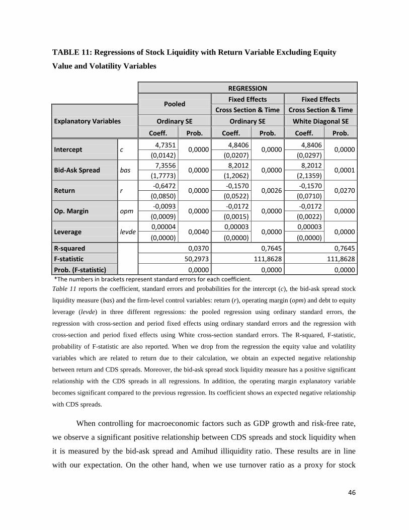
46
TABLE 11: Regressions of Stock Liquidity with Return Variable Excluding Equity
Value and Volatility Variables
REGRESSION
Pooled Fixed Effects Fixed Effects
Explanatory Variables Cross Section & Time Cross Section & Time
Ordinary SE Ordinary SE White Diagonal SE
Coeff. Prob. Coeff. Prob. Coeff. Prob.
Intercept c 4,7351 0,0000 4,8406 0,0000 4,8406 0,0000 (0,0142) (0,0207) (0,0297)
Bid-Ask Spread bas 7,3556 0,0000 8,2012 0,0000 8,2012 0,0001 (1,7773) (1,2062) (2,1359)
Return r -0,6472 0,0000 -0,1570 0,0026 -0,1570 0,0270 (0,0850) (0,0522) (0,0710)
Op. Margin opm -0,0093
0,0000 -0,0172
0,0000 -0,0172
0,0000 (0,0009) (0,0015) (0,0022)
Leverage levde 0,00004
0,0040 0,00003
0,0000 0,00003
0,0000 (0,0000) (0,0000) (0,0000)
R-squared
0,0370 0,7645 0,7645 F-statistic 50,2973 111,8628 111,8628 Prob. (F-statistic) 0,0000 0,0000 0,0000 *The numbers in brackets represent standard errors for each coefficient.
Table 11 reports the coefficient, standard errors and probabilities for the intercept (c), the bid-ask spread stock
liquidity measure (bas) and the firm-level control variables: return (r), operating margin (opm) and debt to equity
leverage (levde) in three different regressions: the pooled regression using ordinary standard errors, the
regression with cross-section and period fixed effects using ordinary standard errors and the regression with
cross-section and period fixed effects using White cross-section standard errors. The R-squared, F-statistic,
probability of F-statistic are also reported. When we drop from the regression the equity value and volatility
variables which are related to return due to their calculation, we obtain an expected negative relationship
between return and CDS spreads. Moreover, the bid-ask spread stock liquidity measure has a positive significant
relationship with the CDS spreads in all regressions. In addition, the operating margin explanatory variable
becomes significant compared to the previous regression. Its coefficient shows an expected negative relationship
with CDS spreads.
When controlling for macroeconomic factors such as GDP growth and risk-free rate,
we observe a significant positive relationship between CDS spreads and stock liquidity when
it is measured by the bid-ask spread and Amihud illiquidity ratio. These results are in line
with our expectation. On the other hand, when we use turnover ratio as a proxy for stock

47
liquidity, we obtain a counter-intuitive result, suggesting that a higher turnover ratio implies a
higher CDS spread. The results of the regression with turnover ratio as a measure of stock
liquidity and macroeconomic control variables are displayed in Appendix (24).
Regarding the control variables, we obtain the expected negative relationship between
them and the CDS spread. In all regressions, the coefficients of GDP growth rate and risk-free
rate are significantly negative. In regards to risk-free measures, we use all three proxies and
obtain the expected negative relationship between CDS spreads and risk-free rate. The
summarized results of regressions of bid-ask spread stock liquidity where we use the one-year
interbank interest rate and five-year government yield are presented in Table 12 and Table 13.
The R2 of the regressions using bid-ask spread stock liquidity range from 0.6217 to 0.6475,
indicating a good level of fit. Detailed estimation outputs of the pooled regressions and cross-
section fixed regressions using the one-year interbank interest rate and five-year bond yield
are shown in Appendices (26 – 31). The detailed results of the regression of bid-ask spread
stock liquidity using the ten-year bond yield and cross-section fixed effects is presented
Appendix (25). We note that the results are not qualitatively different. The regression of
Amihud stock liquidity using one-year interbank interest rate is shown in Table 14. The R2 of
the regression using Amihud illiquidity and cross-section fixed effects is 0.6166, indicating a
good level of fit. Detailed results of the regressions of Amihud stock liquidity using
macroeconomic controls are displayed in Appendices (32, 33, 34).
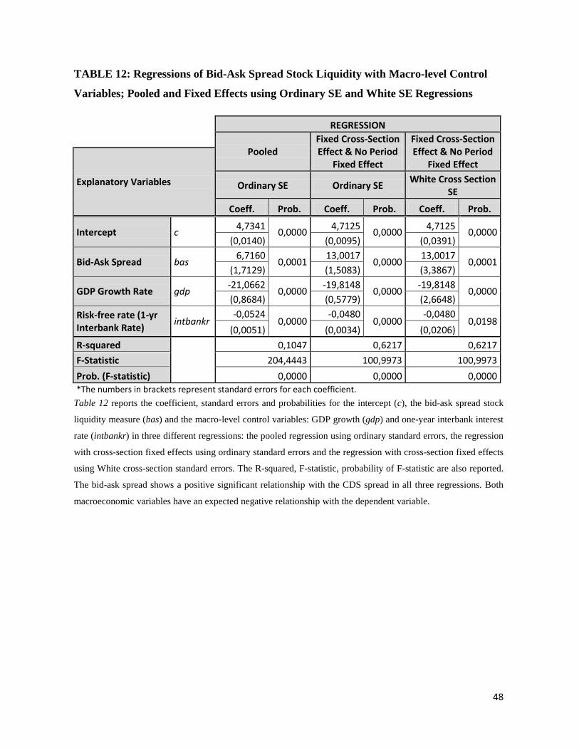
48
TABLE 12: Regressions of Bid-Ask Spread Stock Liquidity with Macro-level Control
Variables; Pooled and Fixed Effects using Ordinary SE and White SE Regressions
REGRESSION
Pooled
Fixed Cross-Section Effect & No Period
Fixed Effect
Fixed Cross-Section Effect & No Period
Fixed Effect
Explanatory Variables Ordinary SE Ordinary SE White Cross Section SE
Coeff. Prob. Coeff. Prob. Coeff. Prob.
Intercept c 4,7341 0,0000 4,7125 0,0000 4,7125 0,0000 (0,0140) (0,0095) (0,0391)
Bid-Ask Spread bas 6,7160 0,0001 13,0017 0,0000 13,0017 0,0001 (1,7129) (1,5083) (3,3867)
GDP Growth Rate gdp -21,0662 0,0000 -19,8148 0,0000 -19,8148 0,0000 (0,8684) (0,5779) (2,6648)
Risk-free rate (1-yr Interbank Rate) intbankr
-0,0524 0,0000
-0,0480 0,0000
-0,0480 0,0198
(0,0051) (0,0034) (0,0206) R-squared
0,1047 0,6217 0,6217 F-Statistic 204,4443 100,9973 100,9973 Prob. (F-statistic) 0,0000 0,0000 0,0000 *The numbers in brackets represent standard errors for each coefficient.
Table 12 reports the coefficient, standard errors and probabilities for the intercept (c), the bid-ask spread stock
liquidity measure (bas) and the macro-level control variables: GDP growth (gdp) and one-year interbank interest
rate (intbankr) in three different regressions: the pooled regression using ordinary standard errors, the regression
with cross-section fixed effects using ordinary standard errors and the regression with cross-section fixed effects
using White cross-section standard errors. The R-squared, F-statistic, probability of F-statistic are also reported.
The bid-ask spread shows a positive significant relationship with the CDS spread in all three regressions. Both
macroeconomic variables have an expected negative relationship with the dependent variable.
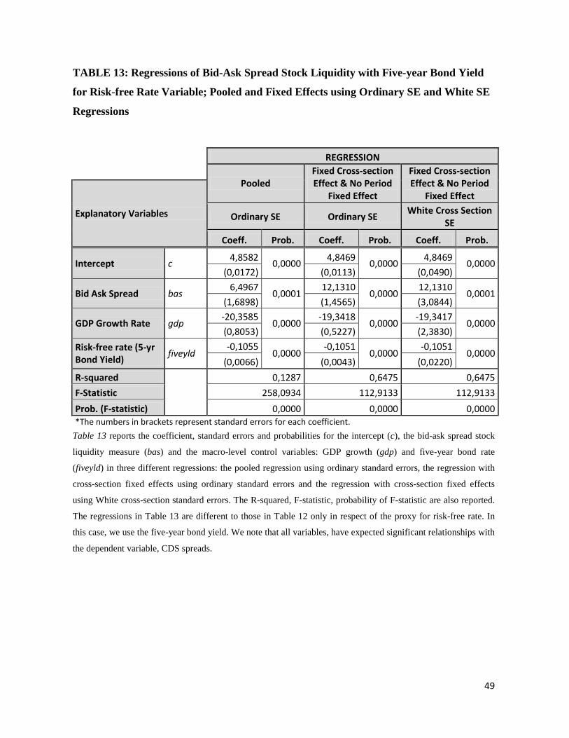
49
TABLE 13: Regressions of Bid-Ask Spread Stock Liquidity with Five-year Bond Yield
for Risk-free Rate Variable; Pooled and Fixed Effects using Ordinary SE and White SE
Regressions
REGRESSION
Pooled
Fixed Cross-section Effect & No Period
Fixed Effect
Fixed Cross-section Effect & No Period
Fixed Effect
Explanatory Variables Ordinary SE Ordinary SE White Cross Section SE
Coeff. Prob. Coeff. Prob. Coeff. Prob.
Intercept c 4,8582 0,0000 4,8469 0,0000 4,8469 0,0000 (0,0172) (0,0113) (0,0490)
Bid Ask Spread bas 6,4967 0,0001 12,1310 0,0000 12,1310 0,0001 (1,6898) (1,4565) (3,0844)
GDP Growth Rate gdp -20,3585
0,0000 -19,3418
0,0000 -19,3417
0,0000 (0,8053) (0,5227) (2,3830)
Risk-free rate (5-yr Bond Yield) fiveyld
-0,1055 0,0000
-0,1051 0,0000
-0,1051 0,0000
(0,0066) (0,0043) (0,0220) R-squared
0,1287 0,6475 0,6475 F-Statistic 258,0934 112,9133 112,9133 Prob. (F-statistic) 0,0000 0,0000 0,0000 *The numbers in brackets represent standard errors for each coefficient.
Table 13 reports the coefficient, standard errors and probabilities for the intercept (c), the bid-ask spread stock
liquidity measure (bas) and the macro-level control variables: GDP growth (gdp) and five-year bond rate
(fiveyld) in three different regressions: the pooled regression using ordinary standard errors, the regression with
cross-section fixed effects using ordinary standard errors and the regression with cross-section fixed effects
using White cross-section standard errors. The R-squared, F-statistic, probability of F-statistic are also reported.
The regressions in Table 13 are different to those in Table 12 only in respect of the proxy for risk-free rate. In
this case, we use the five-year bond yield. We note that all variables, have expected significant relationships with
the dependent variable, CDS spreads.

50
TABLE 14: Regressions of Amihud Stock Liquidity with Macro-level Control Variables; Pooled and Fixed Effects using Ordinary SE and White SE Regressions
REGRESSION
Pooled
Fixed Cross-Section Effect & No Period
Fixed Effect
Fixed Cross-Section Effect & No Period
Fixed Effect
Explanatory Variables Ordinary SE Ordinary SE White Cross Section SE
Coeff. Prob. Coeff. Prob. Coeff. Prob.
Intercept c 4,7520 0,0000 4,7353 0,0000 4,7353 0,0000 (0,0136) (0,0092) (0,0413)
Amihud Illiquidity illiq -134914,40 0,0027 117751,70 0,0318 117751,70 0,0551 (44883,86) (54821,41) (61373,85)
GDP Growth Rate gdp -21,2742 0,0000 -20,0190 0,0000 -20,0190 0,0000 (0,8685) (0,5831) (2,7188)
Risk-free rate (1-yr Interbank Rate) intbankr
-0,0532 0,0000
-0,0485 0,0000
-0,0485 0,0199
(0,0051) (0,0034) (0,0208) R-squared
0,1036 0,6166 0,6166 F-Statistic 202,0913 98,8354 98,8354 Prob. (F-statistic) 0,0000 0,0000 0,0000 *The numbers in brackets represent standard errors for each coefficient.
Table 14 reports the coefficient, standard errors and probabilities for the intercept (c), the Amihud illiquidity
measure (illiq) and the macro-level control variables: GDP growth (gdp) and one-year interbank interest rate
(intbankr) in three different regressions: the pooled regression using ordinary standard errors, the regression with
cross-section fixed effects using ordinary standard errors and the regression with cross-section fixed effects
using White cross-section standard errors. The R-squared, F-statistic, probability of F-statistic are also reported.
The Amihud illiquidity measure shows an expected positive relationship with the CDS spreads when using the
specification with cross-section fixed effects. However, when using White cross-section standard errors, the
significance of the illiquidity measure becomes 0.0551, which is insignificant at the 5% level. However, the
result is still significant at the 10% significance level. We also note that White cross-section standard errors are
larger than the ordinary standard errors.

51
5. CONCLUSION
This research studies the impact of stock liquidity on CDS spreads by taking into account the
effects of other known CDS spread determinants. Several researches are made on the impact
of bond market liquidity on bond spreads. However, the literature focusing on CDS spreads is
quite narrow and the direct effect of stock liquidity on CDS spreads, to the best of our
knowledge, is investigated only in the paper of Das and Hanouna (2008).
In this study, a panel data consisting of 82 firms on a 64-month time frame is used to examine
the relation between CDS spreads and stock liquidity. To investigate in detail the nature of
this relationship, we scrutinize three different liquidity measures: the bid-ask spread, Amihud
illiquidity measure and turnover ratio. High stock liquidity is determined by a low bid-ask
spread and a low Amihud illiquidity measure. On the other hand, a low turnover ratio implies
low stock liquidity. All three liquidity measures demonstrate a significant relationship with
the CDS spreads. The direction of the relationship indicates that a higher stock liquidity leads
to a lower CDS spread, result which is in line with our expectation. Therefore, the regressions
confirm that both “cost based” and “reflective” (Spiegel and Wang, 2005) liquidity measures
have a significant impact on CDS spreads, when other firm-level CDS spreads determinants
are controlled. This research also proves that stock liquidity is a significant constituent of
CDS spreads when controlling for macroeconomic variables, such as GDP growth rate and
risk-free rate.
This study builds up on the current literature by tying the developing CDS market with the
well developed stock market. Furthermore, we add value by comprehensively investigating
the scarcely researched relationship between stock liquidity and CDS spreads.
52
6. REFERENCES
Acharya, V., Schaefer, S., Zhang, Y. “Liquidity Risk and Correlation Risk: A Clinical
Study of General Motors and Ford Downgrade of May 2005”, 2007, Working Paper,
London Business School;
Alexander, C., Kaeck, A. “Regime Dependent Determinants of Credit Default Swap
Spreads”, 2007, Journal of Banking and Finance, Vol. 32, pp. 1008-1021;
Amihud, Y. “Illiquidity and Stock Returns: Cross-Section and Time-Series Effects”,
2000, Stern School of Business, New York University Working Papers Series no. FIN-
00-041;
Annaert, J., De Ceuster, M., Van Roy, P. Vespro, C. “What Determines Euro Area Bank
CDS Spreads?”, 2010, National Bank of Belgium Working Paper, Brussels;
Arakelyan, A., Serrano, P. “Liquidity in Credit Default Swap Markets”, 2012,
Department of Business Administration Publications, Universidad Carlos III de Madrid;
Asquith, P., Gertner, R., Sharfstein, D. “Anatomy of Financial Distress: An
Examination of Junk Bond Issuers”, 1994, Quarterly Journal of Economics, Vol. 109,
pp. 625-658;
Benkert, C. “Explaining Credit Default Swap Premia”, 2004, Journal of Futures
Markets, Vol. 24, Issue 1, pp. 71-92;
Black, F., Scholes, M. “The Pricing of Options and Corporate Liabilities”, 1973, The
Journal of Political Economy, Vol. 81, No. 3, pp.637-654, University of Chicago Press;
Brooks, C. “Introductory Econometrics for Finance”, 2008, Second Edition, Cambridge
University Press;
Byström, H.N.E. “Credit Default Swaps and Equity Prices. The iTraxx CDS Index
Market”, 2005, Working Papers 2005:24, Lund University Department of Economics;
Callen, J.L., Livnat, J., Segal, D. “The Impact of Earnings on the Pricing of Credit
Default Swaps”, 2009, American Accounting Association, The Accounting Review,
Vol. 84, No. 5, pp. 1363 – 1394;
Chen, L., Lesmond, D., Wei, J. “Corporate Yield Spread and Bond Liquidity”, 2007,
Journal of Finance, Vol. 62 (1), pp. 199-149;
53
Collin-Dufresne, P., Goldstein, R., Martin J.S. “The Determinants of Spread Changes”,
Journal of Finance, Vol. 56, pp. 2177-2207;
Crosbie, P. Bohn, J. “Modeling Default Risk. Modeling Methodology”, 2003, Moody’s
KMV;
Daniels, K.N., Jensen, M.S. “The Effect of Credit Ratings on Credit Default Swap
Spreads and Credit Spreads”, 2005, Journal of Fixed Income;
Das, S.R., Hanouna, P. “Hedging Credit: Equity Liquidity Matters”, 2008, Journal of
Financial Intermediation, Vol.18, No.1, pp.112-123;
Das, S.R., Hanouna, P., Sarin A. “Fundamentals-Based versus Market-Based Cross-
Sectional Models of CDS Spreads”, 2004, Unpublished Working Paper, Santa Clara
University;
De Jong, F. Driessen, J. “Liquidity Risk Premia in Corporate Bond Markets”, 2005,
Working Paper, University of Amsterdam;
Drake, P. “Financial Ratio Analysis”, 2013, Online Resource available at:
http://educ.jmu.edu/~drakepp/principles/module2/fin_rat.pdf
Ericsson, J., Jacobs, K Oviedo, R. “The Determinants of Credit Default Swap Premia”,
2005, Journal of Financial and Quantitative Analysis, forthcoming;
Ericsson, J., Renault, O. “Liquidity and Credit Risk”, 2002, EFA 2003 Glasgow
Working Paper Series;
Fung, H-G., Sierra, G. E., Yau, J., Zhang G. “Are the US Stock Market and Credit
Default Swap Market Related? Evidence from CDX Indices”, summer 2008, Journal of
Alternative Investments;
Goldstein, M., Hotchkiss, E., Sirri, E. “Transparency and Liquidity: A Controlled
Experiment on Corporate Bonds”, 2006, Working Paper, Boston College;
Gujarati, D. N., Porter D. C. “Essentials of Econometrics”, 2010, 4th Edition, McGraw
Hill Publication, Singapore;
Gunther, J.W., Levonian, M. E., Moore, R. R. “Can the Stock Market Tell Bank
Supervisors Anything They Don’t Already Know?”, 2001, Federal Reserve Bank of
Dallas Economic and Financial Review;
Hsiao, C. “Analysis of Panel Data”, 2005, Cambridge University Press, 2nd edition,
Cambridge;
54
Hull, J. “Options, Futures and Other Derivatives”, 2003, 5th edition, Prentice Hall;
Hull, J., Nelken, I., White, A. “Merton’s Model, Credit Risk and Volatility Skews”,
2004, Journal of Credit Risk, Vol.1, No. 1, pp. 3-28;
Hull, J., Predescu, M., White, A. “The Relationship between Credit Default Swap
Spreads, Bond Yields and Credit Rating Announcements”, 2004, Journal of Banking
and Finance, Vol. 28, Issue 11, pp. 2789-2811;
Irvine, P.J., Pontiff J. “Idiosyncratic Return Volatility, Cash Flows and Product Market
Competition”, 2009, The Review of Financial Studies, Vol. 22, No.3, pp.1149-1177;
Jarrow, R. “Problems with using CDS to imply default probabilities”, 2012, Journal of
Fixed Income Vol.21, Issue 4, pp. 6-12;
Kapar, B., Olmo, J. “The Determinants of Credit Default Swap Spreads in the Presence
of Structural Breaks and Counterparty Risk”, 2011, City University London,
Department of Economics Discussion Paper Series No. 11/02;
Kennedy, P. “A Guide to Econometrics”, 2009, 6th Edition, Blackwell Publishing,
Oxford UK;
Knaup, M., Wagner, W. “A Market-Based Measure of Credit Quality and Banks’
Performance during the Subprime Crisis”, 2008, European Banking Centre Discussion
Paper No 2009-06S, Tilburg University;
Kwan, S. “Firm-specific Information and the Correlation between Individual Stock and
Bonds”, 1996, Journal of Financial Economics, Vol. 40, pp. 63-80;
Meng, L., Gwilym, O. A. “The Determinants of CDS bid-ask spreads”, 2008, Journal of
Derivatives, Vol. 16, No. 1, pp. 70-80;
Mengle, D. “Credit Derivatives: An Overview”, 2007, Federal Reserve Bank of Atlanta,
presented at Atlanta Fed’s Financial Markets Conference “Credit Derivatives: Where’s
the Risk?”;
Merton, R.C. “On the Pricing of Corporate Debt: The Risk Structure of Interest Rates”,
1974, Journal of Finance, Vol. 29, pp. 449-470;
Norden, L. “Credit Derivatives, Corporate News and Credit Ratings”, 2008, University
of Mannheim, Deutsche Bundesbank;
55
Norden, L., Weber, M. “The Comovement of Credit Default Swap, Bond and Stock
Markets: An Empirical Analysis”, 2004, Centre for Financial Studies, Working Paper
No 2004/20, Goethe University, Frankfurt;
Opler, T., Titman, S. “Financial Distress and Corporate Performance”, 1994, Journal of
Finance, Vol. 549, pp. 1015-1040;
Rauh, J.D., Sufi, A. “Capital Structure and Debt Structure”, 2008, National Bureau of
Economic Research, Working Paper 14488;
Rösch, C. G., Kaserer, C. “Market Liquidity in the Financial Crisis: The Role of
Liquidity Commonality and Flight-to-quality”, 2012, Technische Universität Munchen,
Working Paper Series;
Spiegel, M., Wang, X. “Cross-sectional Variation in Stock Returns: Liquidity and
Idiosyncratic Risk”, Yale School of Management, International Center for Finance,
Yale University, Working Paper No. 05-13, EFA 2005 Moscow Meetings Paper;
Suh, C.B., Lee, Y. “Determinants of Banks’ CDS Spreads and Policy Implications”,
2011, Seoul Journal of Economics, Vol. 24, No.4, pp. 575-591;
Tang, D.Y., Yan, H. “Liquidity and Credit Default Swap Spreads”, 2008 EFA Athens
Meetings Paper, 2007 AFA Chicago Meetings Paper;
Tang, D.Y., Yan, H. “Market Conditions, Default Risk and Credit Spreads”, 2010,
Journal of Banking and Finance, Vol. 34, pp. 743-753;
Tang, D.Y., Yan, H. “What Moves CDS Spreads”, 2012, University of Hong Kong
Research Paper;
The Board of the International Organization of Securities Commission “The Credit
Default Swap Market Report”, 2012, FR05/12;
Vassalou, M., Xing, Y. “Default Risk in Equity Returns”, 2004, The Journal of Finance,
Vol. 59, No. 2, pp. 831-868;
Zhu, H. “An Empirical Comparison of Credit Spreads Between the Bond Market and
the Credit Default Swap Market”, 2006, Journal of Financial Services Research, Vol.
29, No. 3, pp. 211-235.
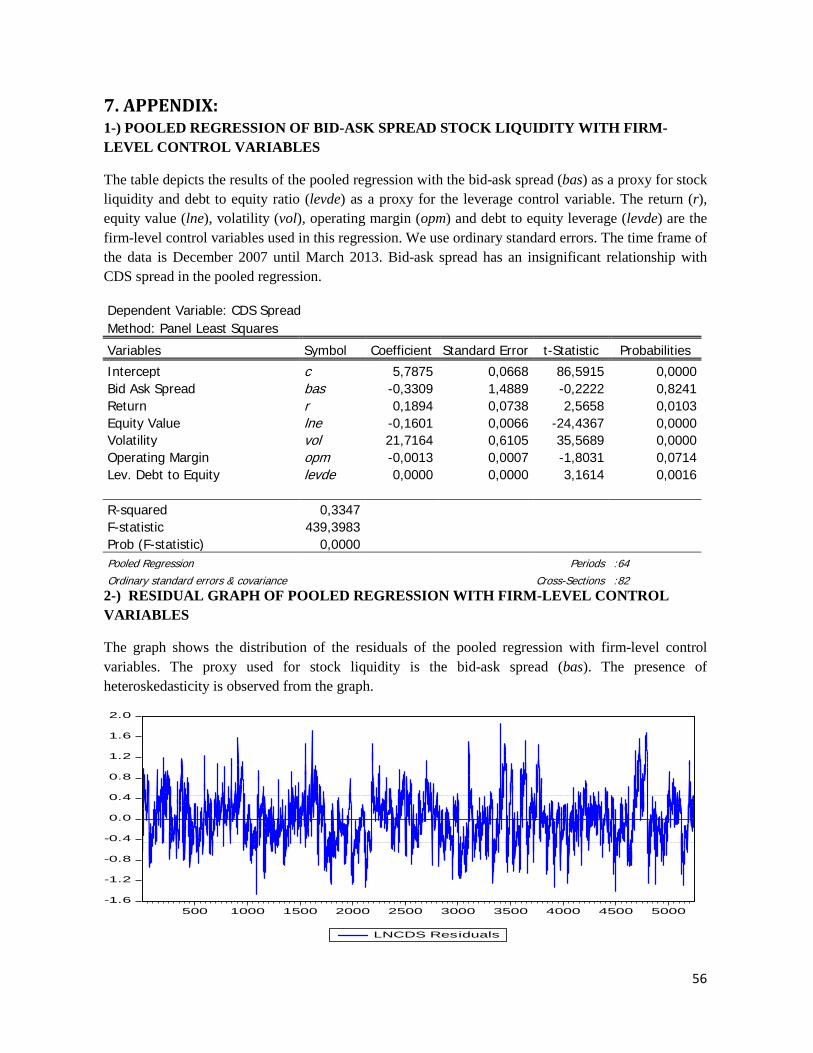
56
7. APPENDIX: 1-) POOLED REGRESSION OF BID-ASK SPREAD STOCK LIQUIDITY WITH FIRM-LEVEL CONTROL VARIABLES
The table depicts the results of the pooled regression with the bid-ask spread (bas) as a proxy for stock liquidity and debt to equity ratio (levde) as a proxy for the leverage control variable. The return (r), equity value (lne), volatility (vol), operating margin (opm) and debt to equity leverage (levde) are the firm-level control variables used in this regression. We use ordinary standard errors. The time frame of the data is December 2007 until March 2013. Bid-ask spread has an insignificant relationship with CDS spread in the pooled regression.
Dependent Variable: CDS Spread Method: Panel Least Squares
Variables Symbol Coefficient Standard Error t-Statistic Probabilities
Intercept c 5,7875 0,0668 86,5915 0,0000 Bid Ask Spread bas -0,3309 1,4889 -0,2222 0,8241 Return r 0,1894 0,0738 2,5658 0,0103 Equity Value lne -0,1601 0,0066 -24,4367 0,0000 Volatility vol 21,7164 0,6105 35,5689 0,0000 Operating Margin opm -0,0013 0,0007 -1,8031 0,0714 Lev. Debt to Equity levde 0,0000 0,0000 3,1614 0,0016 R-squared 0,3347
F-statistic 439,3983 Prob (F-statistic) 0,0000
Pooled Regression
Periods :64 Ordinary standard errors & covariance
Cross-Sections :82
2-) RESIDUAL GRAPH OF POOLED REGRESSION WITH FIRM-LEVEL CONTROL VARIABLES
The graph shows the distribution of the residuals of the pooled regression with firm-level control variables. The proxy used for stock liquidity is the bid-ask spread (bas). The presence of heteroskedasticity is observed from the graph.
-1.6
-1.2
-0.8
-0.4
0.0
0.4
0.8
1.2
1.6
2.0
500 1000 1500 2000 2500 3000 3500 4000 4500 5000
LNCDS Residuals
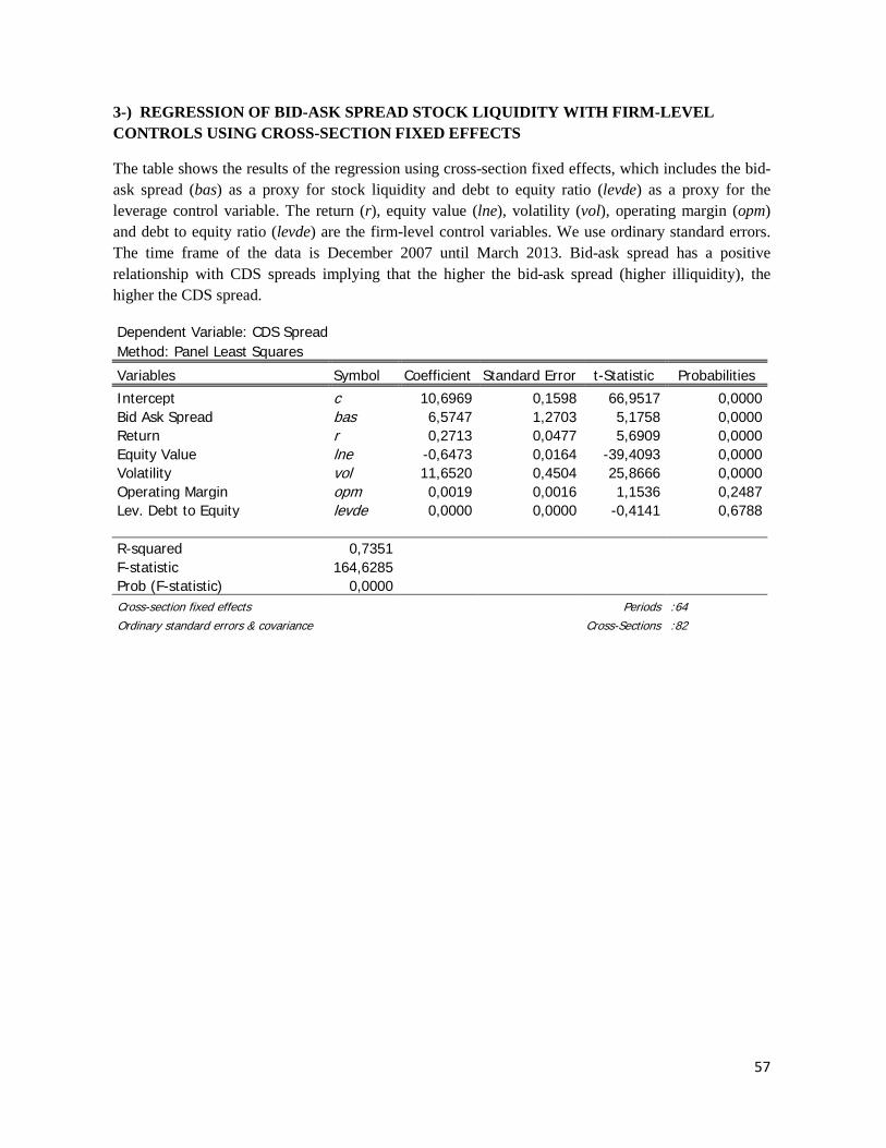
57
3-) REGRESSION OF BID-ASK SPREAD STOCK LIQUIDITY WITH FIRM-LEVEL CONTROLS USING CROSS-SECTION FIXED EFFECTS
The table shows the results of the regression using cross-section fixed effects, which includes the bid-ask spread (bas) as a proxy for stock liquidity and debt to equity ratio (levde) as a proxy for the leverage control variable. The return (r), equity value (lne), volatility (vol), operating margin (opm) and debt to equity ratio (levde) are the firm-level control variables. We use ordinary standard errors. The time frame of the data is December 2007 until March 2013. Bid-ask spread has a positive relationship with CDS spreads implying that the higher the bid-ask spread (higher illiquidity), the higher the CDS spread.
Dependent Variable: CDS Spread Method: Panel Least Squares
Variables Symbol Coefficient Standard Error t-Statistic Probabilities
Intercept c 10,6969 0,1598 66,9517 0,0000 Bid Ask Spread bas 6,5747 1,2703 5,1758 0,0000 Return r 0,2713 0,0477 5,6909 0,0000 Equity Value lne -0,6473 0,0164 -39,4093 0,0000 Volatility vol 11,6520 0,4504 25,8666 0,0000 Operating Margin opm 0,0019 0,0016 1,1536 0,2487 Lev. Debt to Equity levde 0,0000 0,0000 -0,4141 0,6788 R-squared 0,7351
F-statistic 164,6285 Prob (F-statistic) 0,0000
Cross-section fixed effects
Periods :64 Ordinary standard errors & covariance
Cross-Sections :82
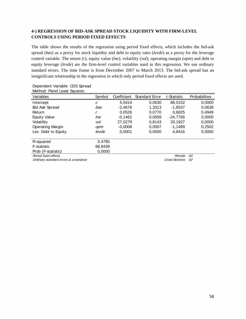
58
4-) REGRESSION OF BID-ASK SPREAD STOCK LIQUIDITY WITH FIRM-LEVEL CONTROLS USING PERIOD FIXED EFFECTS
The table shows the results of the regression using period fixed effects, which includes the bid-ask spread (bas) as a proxy for stock liquidity and debt to equity ratio (levde) as a proxy for the leverage control variable. The return (r), equity value (lne), volatility (vol), operating margin (opm) and debt to equity leverage (levde) are the firm-level control variables used in this regression. We use ordinary standard errors. The time frame is from December 2007 to March 2013. The bid-ask spread has an insignificant relationship in the regression in which only period fixed effects are used.
Dependent Variable: CDS Spread Method: Panel Least Squares
Variables Symbol Coefficient Standard Error t-Statistic Probabilities Intercept c 5,5414 0,0630 88,0152 0,0000 Bid Ask Spread bas -2,4678 1,3313 -1,8537 0,0638 Return r 0,0526 0,0770 0,6825 0,4949 Equity Value lne -0,1462 0,0059 -24,7765 0,0000 Volatility vol 27,0279 0,8143 33,1927 0,0000 Operating Margin opm -0,0008 0,0007 -1,1499 0,2502 Lev. Debt to Equity levde 0,0001 0,0000 4,8416 0,0000 R-squared 0,4785
F-statistic 68,8439 Prob (F-statistic) 0,0000
Period fixed effects
Periods :64 Ordinary standard errors & covariance
Cross-Sections :82
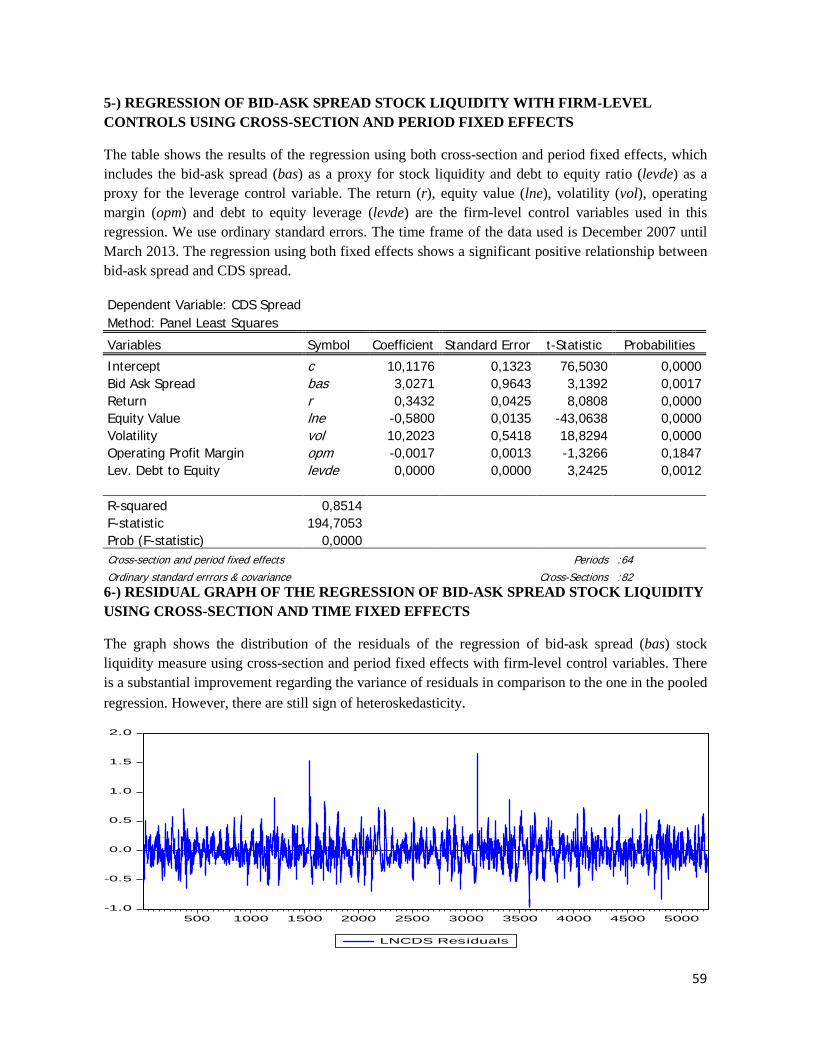
59
5-) REGRESSION OF BID-ASK SPREAD STOCK LIQUIDITY WITH FIRM-LEVEL CONTROLS USING CROSS-SECTION AND PERIOD FIXED EFFECTS
The table shows the results of the regression using both cross-section and period fixed effects, which includes the bid-ask spread (bas) as a proxy for stock liquidity and debt to equity ratio (levde) as a proxy for the leverage control variable. The return (r), equity value (lne), volatility (vol), operating margin (opm) and debt to equity leverage (levde) are the firm-level control variables used in this regression. We use ordinary standard errors. The time frame of the data used is December 2007 until March 2013. The regression using both fixed effects shows a significant positive relationship between bid-ask spread and CDS spread.
Dependent Variable: CDS Spread Method: Panel Least Squares
Variables Symbol Coefficient Standard Error t-Statistic Probabilities
Intercept c 10,1176 0,1323 76,5030 0,0000 Bid Ask Spread bas 3,0271 0,9643 3,1392 0,0017 Return r 0,3432 0,0425 8,0808 0,0000 Equity Value lne -0,5800 0,0135 -43,0638 0,0000 Volatility vol 10,2023 0,5418 18,8294 0,0000 Operating Profit Margin opm -0,0017 0,0013 -1,3266 0,1847 Lev. Debt to Equity levde 0,0000 0,0000 3,2425 0,0012 R-squared 0,8514
F-statistic 194,7053 Prob (F-statistic) 0,0000
Cross-section and period fixed effects
Periods :64 Ordinary standard errrors & covariance
Cross-Sections :82
6-) RESIDUAL GRAPH OF THE REGRESSION OF BID-ASK SPREAD STOCK LIQUIDITY USING CROSS-SECTION AND TIME FIXED EFFECTS
The graph shows the distribution of the residuals of the regression of bid-ask spread (bas) stock liquidity measure using cross-section and period fixed effects with firm-level control variables. There is a substantial improvement regarding the variance of residuals in comparison to the one in the pooled regression. However, there are still sign of heteroskedasticity.
-1.0
-0.5
0.0
0.5
1.0
1.5
2.0
500 1000 1500 2000 2500 3000 3500 4000 4500 5000
LNCDS Residuals
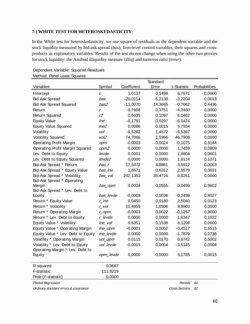
60
7-) WHITE TEST FOR HETEROSKEDASTICITY
In the White test for heteroskedasticity, we use square of residuals as the dependent variable and the stock liquidity measured by bid-ask spread (bas), firm-level control variables, their squares and cross-products as explanatory variables. Results of the test do not change when using the other two proxies for stock liquidity: the Amihud illiquidity measure (illiq) and turnover ratio (trnvr).
Dependent Variable: Squared Residuals Method: Panel Least Squares
Variables Symbol Coefficient Standard
Error t-Statistic Probabilities
Intercept c 1,0137 0,1498 6,7671 0,0000 Bid Ask Spread bas -20,0114 6,2138 -3,2204 0,0013 Bid Ask Spread Squared bas2 -11,0070 14,3665 -0,7662 0,4436 Return r -0,7608 0,1751 -4,3460 0,0000 Return Squared r2 0,6635 0,1097 6,0462 0,0000 Equity Value lne -0,1791 0,0297 -6,0424 0,0000 Equity Value Squared lne2 0,0086 0,0015 5,7934 0,0000 Volatility vol -9,5282 1,4572 -6,5387 0,0000 Volatility Squared vol2 74,7066 1,5966 46,7908 0,0000 Operating Profit Margin opm -0,0003 0,0024 -0,1075 0,9144 Operating Profit Margin Squared opm2 0,0000 0,0000 1,7459 0,0809 Lev. Debt to Equity levde 0,0001 0,0000 1,8804 0,0601 Lev. Debt to Equity Squared levde2 0,0000 0,0000 1,6114 0,1071 Bid-Ask Spread * Return bas_r 17,5472 4,8861 3,5912 0,0003 Bid-Ask Spread * Equity Value bas_lne 1,8671 0,6312 2,9579 0,0031 Bid-Ask Spread * Volatility bas_vol 242,1353 35,4716 6,8261 0,0000 Bid-Ask Spread * Operating Margin bas_opm 0,0028 0,0555 0,0499 0,9602 Bid-Ask Spread * Lev. Debt to Equity bas_levde -0,0009 0,0036 -0,2498 0,8027 Return * Equity Value r_lne 0,0450 0,0180 2,5040 0,0123 Return * Volatility r_vol 10,4955 1,0506 9,9903 0,0000 Return * Operating Margin r_opm -0,0003 0,0022 -0,1257 0,9000 Return * Lev. Debt to Equity r_levde 0,0000 0,0000 1,6347 0,1022 Equity Value * Volatility lne_vol 0,6351 0,1538 4,1298 0,0000 Equity Value * Operating Margin lne_opm -0,0001 0,0002 -0,4517 0,6515 Equity Value * Lev. Debt to Equity lne_levde 0,0000 0,0000 -1,7879 0,0738 Volatility * Operating Margin vol_opm 0,0115 0,0170 0,6742 0,5002 Volatility * Lev. Debt to Equity vol_levde -0,0015 0,0004 -3,5145 0,0004 Operating Margin * Lev. Debt to Equity opm_levde 0,0000 0,0000 3,1785 0,0015 R-squared 0,3667
F-statistic 111,9219 Prob (F-statistic) 0,0000
Pooled Regression
Periods :64
Ordinary standard errors & covariance
Cross-Sections :82
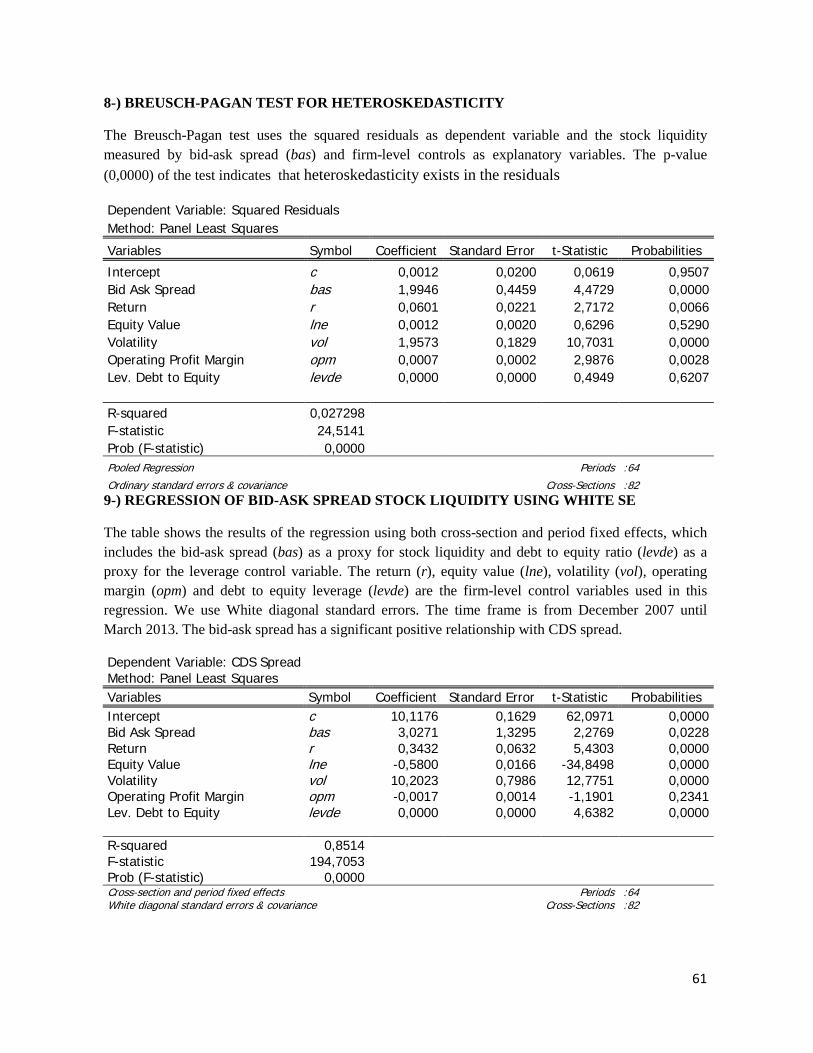
61
8-) BREUSCH-PAGAN TEST FOR HETEROSKEDASTICITY
The Breusch-Pagan test uses the squared residuals as dependent variable and the stock liquidity measured by bid-ask spread (bas) and firm-level controls as explanatory variables. The p-value (0,0000) of the test indicates that heteroskedasticity exists in the residuals
Dependent Variable: Squared Residuals Method: Panel Least Squares
Variables Symbol Coefficient Standard Error t-Statistic Probabilities
Intercept c 0,0012 0,0200 0,0619 0,9507 Bid Ask Spread bas 1,9946 0,4459 4,4729 0,0000 Return r 0,0601 0,0221 2,7172 0,0066 Equity Value lne 0,0012 0,0020 0,6296 0,5290 Volatility vol 1,9573 0,1829 10,7031 0,0000 Operating Profit Margin opm 0,0007 0,0002 2,9876 0,0028 Lev. Debt to Equity levde 0,0000 0,0000 0,4949 0,6207 R-squared 0,027298
F-statistic 24,5141 Prob (F-statistic) 0,0000
Pooled Regression
Periods :64 Ordinary standard errors & covariance
Cross-Sections :82
9-) REGRESSION OF BID-ASK SPREAD STOCK LIQUIDITY USING WHITE SE
The table shows the results of the regression using both cross-section and period fixed effects, which includes the bid-ask spread (bas) as a proxy for stock liquidity and debt to equity ratio (levde) as a proxy for the leverage control variable. The return (r), equity value (lne), volatility (vol), operating margin (opm) and debt to equity leverage (levde) are the firm-level control variables used in this regression. We use White diagonal standard errors. The time frame is from December 2007 until March 2013. The bid-ask spread has a significant positive relationship with CDS spread.
Dependent Variable: CDS Spread Method: Panel Least Squares
Variables Symbol Coefficient Standard Error t-Statistic Probabilities Intercept c 10,1176 0,1629 62,0971 0,0000 Bid Ask Spread bas 3,0271 1,3295 2,2769 0,0228 Return r 0,3432 0,0632 5,4303 0,0000 Equity Value lne -0,5800 0,0166 -34,8498 0,0000 Volatility vol 10,2023 0,7986 12,7751 0,0000 Operating Profit Margin opm -0,0017 0,0014 -1,1901 0,2341 Lev. Debt to Equity levde 0,0000 0,0000 4,6382 0,0000 R-squared 0,8514
F-statistic 194,7053 Prob (F-statistic) 0,0000
Cross-section and period fixed effects
Periods :64 White diagonal standard errors & covariance
Cross-Sections :82
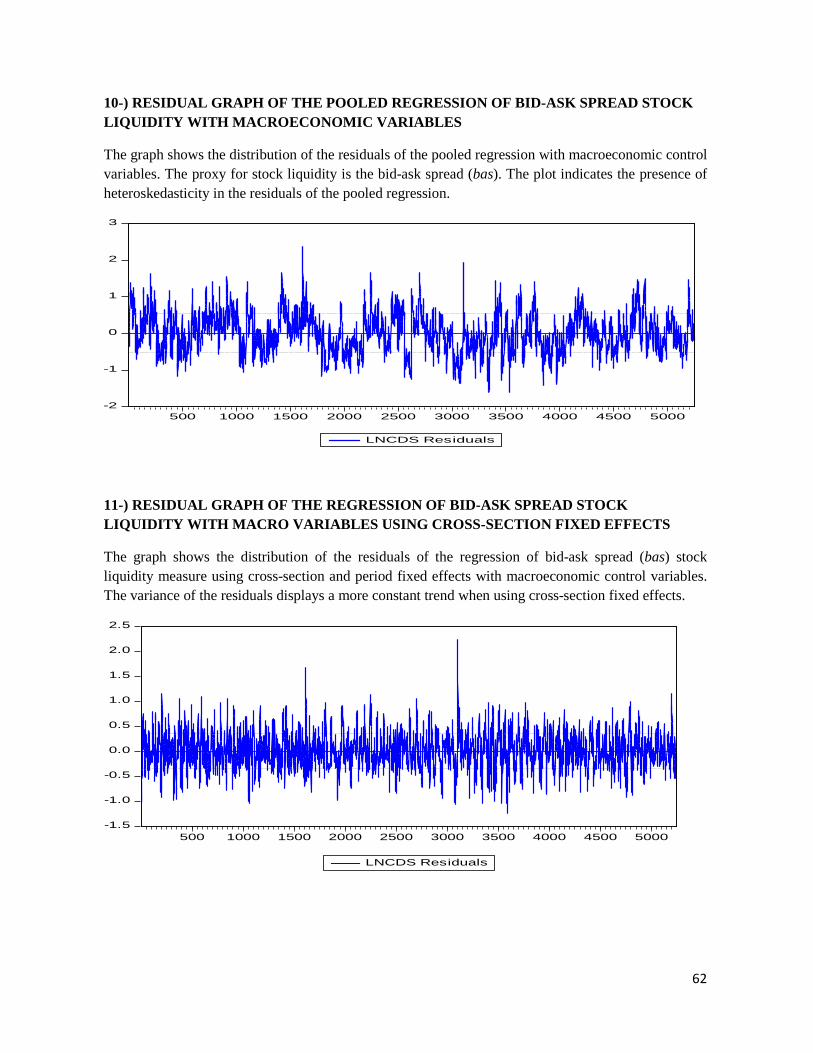
62
10-) RESIDUAL GRAPH OF THE POOLED REGRESSION OF BID-ASK SPREAD STOCK LIQUIDITY WITH MACROECONOMIC VARIABLES
The graph shows the distribution of the residuals of the pooled regression with macroeconomic control variables. The proxy for stock liquidity is the bid-ask spread (bas). The plot indicates the presence of heteroskedasticity in the residuals of the pooled regression.
11-) RESIDUAL GRAPH OF THE REGRESSION OF BID-ASK SPREAD STOCK LIQUIDITY WITH MACRO VARIABLES USING CROSS-SECTION FIXED EFFECTS
The graph shows the distribution of the residuals of the regression of bid-ask spread (bas) stock liquidity measure using cross-section and period fixed effects with macroeconomic control variables. The variance of the residuals displays a more constant trend when using cross-section fixed effects.
-2
-1
0
1
2
3
500 1000 1500 2000 2500 3000 3500 4000 4500 5000
LNCDS Residuals
-1.5
-1.0
-0.5
0.0
0.5
1.0
1.5
2.0
2.5
500 1000 1500 2000 2500 3000 3500 4000 4500 5000
LNCDS Residuals
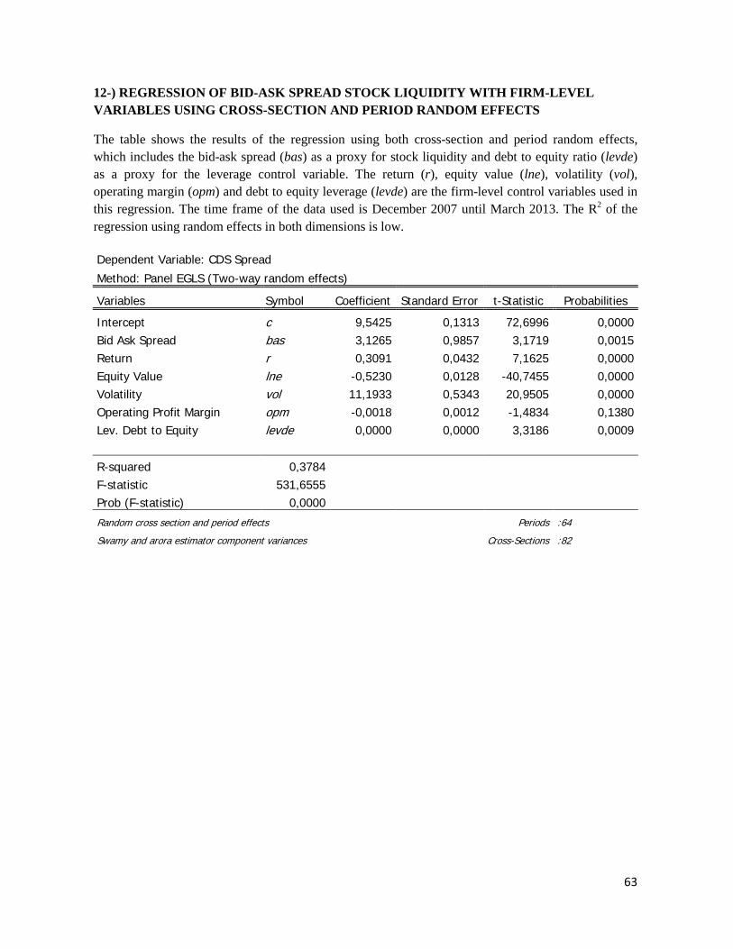
63
12-) REGRESSION OF BID-ASK SPREAD STOCK LIQUIDITY WITH FIRM-LEVEL VARIABLES USING CROSS-SECTION AND PERIOD RANDOM EFFECTS
The table shows the results of the regression using both cross-section and period random effects, which includes the bid-ask spread (bas) as a proxy for stock liquidity and debt to equity ratio (levde) as a proxy for the leverage control variable. The return (r), equity value (lne), volatility (vol), operating margin (opm) and debt to equity leverage (levde) are the firm-level control variables used in this regression. The time frame of the data used is December 2007 until March 2013. The R2 of the regression using random effects in both dimensions is low.
Dependent Variable: CDS Spread Method: Panel EGLS (Two-way random effects)
Variables Symbol Coefficient Standard Error t-Statistic Probabilities
Intercept c 9,5425 0,1313 72,6996 0,0000 Bid Ask Spread bas 3,1265 0,9857 3,1719 0,0015 Return r 0,3091 0,0432 7,1625 0,0000 Equity Value lne -0,5230 0,0128 -40,7455 0,0000 Volatility vol 11,1933 0,5343 20,9505 0,0000 Operating Profit Margin opm -0,0018 0,0012 -1,4834 0,1380 Lev. Debt to Equity levde 0,0000 0,0000 3,3186 0,0009 R-squared 0,3784
F-statistic 531,6555 Prob (F-statistic) 0,0000
Random cross section and period effects
Periods :64
Swamy and arora estimator component variances
Cross-Sections :82
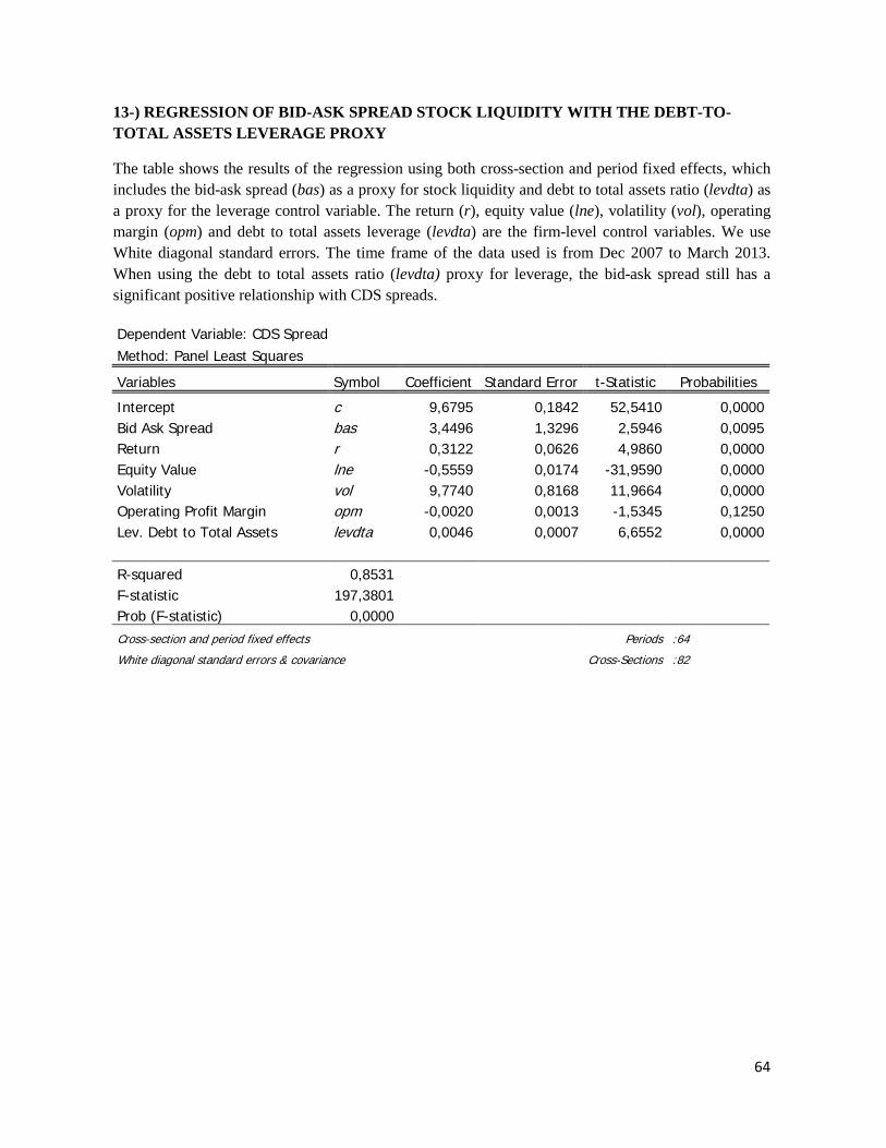
64
13-) REGRESSION OF BID-ASK SPREAD STOCK LIQUIDITY WITH THE DEBT-TO-TOTAL ASSETS LEVERAGE PROXY
The table shows the results of the regression using both cross-section and period fixed effects, which includes the bid-ask spread (bas) as a proxy for stock liquidity and debt to total assets ratio (levdta) as a proxy for the leverage control variable. The return (r), equity value (lne), volatility (vol), operating margin (opm) and debt to total assets leverage (levdta) are the firm-level control variables. We use White diagonal standard errors. The time frame of the data used is from Dec 2007 to March 2013. When using the debt to total assets ratio (levdta) proxy for leverage, the bid-ask spread still has a significant positive relationship with CDS spreads.
Dependent Variable: CDS Spread Method: Panel Least Squares
Variables Symbol Coefficient Standard Error t-Statistic Probabilities
Intercept c 9,6795 0,1842 52,5410 0,0000 Bid Ask Spread bas 3,4496 1,3296 2,5946 0,0095 Return r 0,3122 0,0626 4,9860 0,0000 Equity Value lne -0,5559 0,0174 -31,9590 0,0000 Volatility vol 9,7740 0,8168 11,9664 0,0000 Operating Profit Margin opm -0,0020 0,0013 -1,5345 0,1250 Lev. Debt to Total Assets levdta 0,0046 0,0007 6,6552 0,0000 R-squared 0,8531
F-statistic 197,3801 Prob (F-statistic) 0,0000
Cross-section and period fixed effects
Periods :64
White diagonal standard errors & covariance
Cross-Sections :82
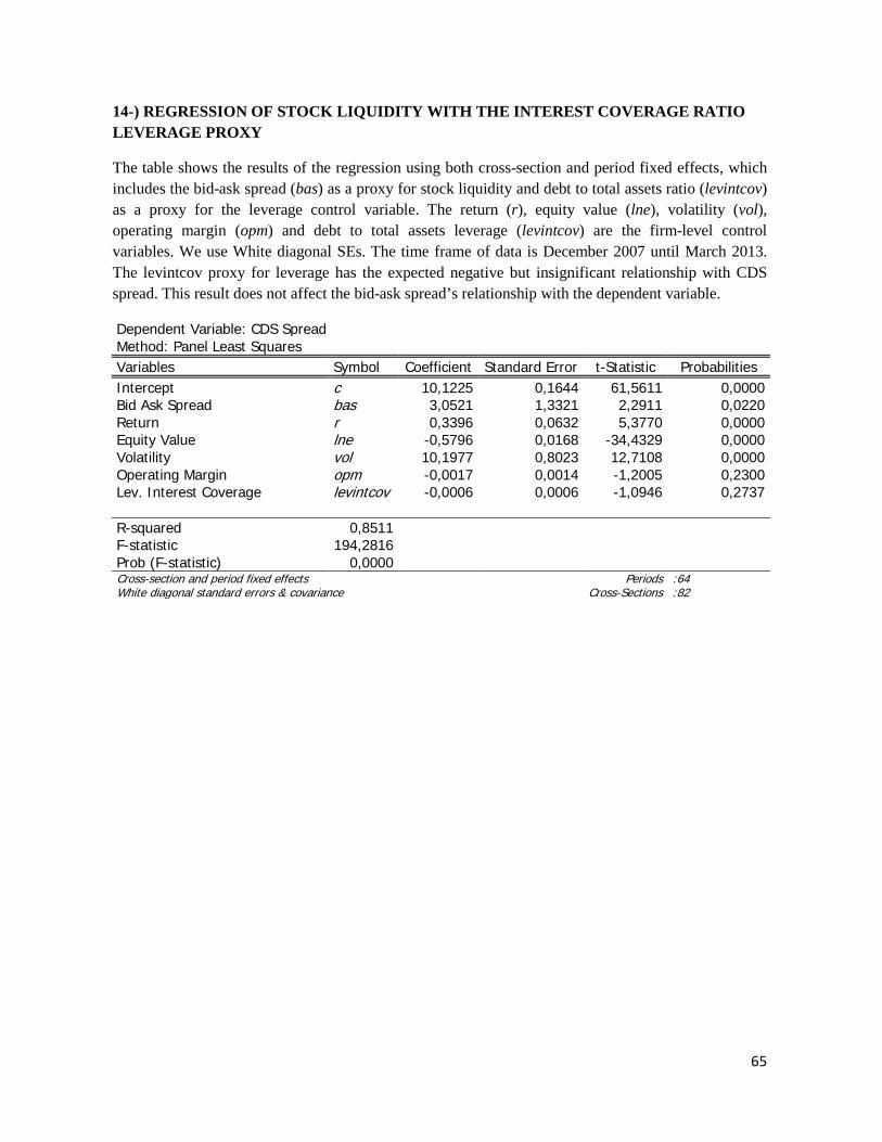
65
14-) REGRESSION OF STOCK LIQUIDITY WITH THE INTEREST COVERAGE RATIO LEVERAGE PROXY
The table shows the results of the regression using both cross-section and period fixed effects, which includes the bid-ask spread (bas) as a proxy for stock liquidity and debt to total assets ratio (levintcov) as a proxy for the leverage control variable. The return (r), equity value (lne), volatility (vol), operating margin (opm) and debt to total assets leverage (levintcov) are the firm-level control variables. We use White diagonal SEs. The time frame of data is December 2007 until March 2013. The levintcov proxy for leverage has the expected negative but insignificant relationship with CDS spread. This result does not affect the bid-ask spread’s relationship with the dependent variable.
Dependent Variable: CDS Spread Method: Panel Least Squares
Variables Symbol Coefficient Standard Error t-Statistic Probabilities Intercept c 10,1225 0,1644 61,5611 0,0000 Bid Ask Spread bas 3,0521 1,3321 2,2911 0,0220 Return r 0,3396 0,0632 5,3770 0,0000 Equity Value lne -0,5796 0,0168 -34,4329 0,0000 Volatility vol 10,1977 0,8023 12,7108 0,0000 Operating Margin opm -0,0017 0,0014 -1,2005 0,2300 Lev. Interest Coverage levintcov -0,0006 0,0006 -1,0946 0,2737 R-squared 0,8511
F-statistic 194,2816 Prob (F-statistic) 0,0000
Cross-section and period fixed effects
Periods :64 White diagonal standard errors & covariance
Cross-Sections :82
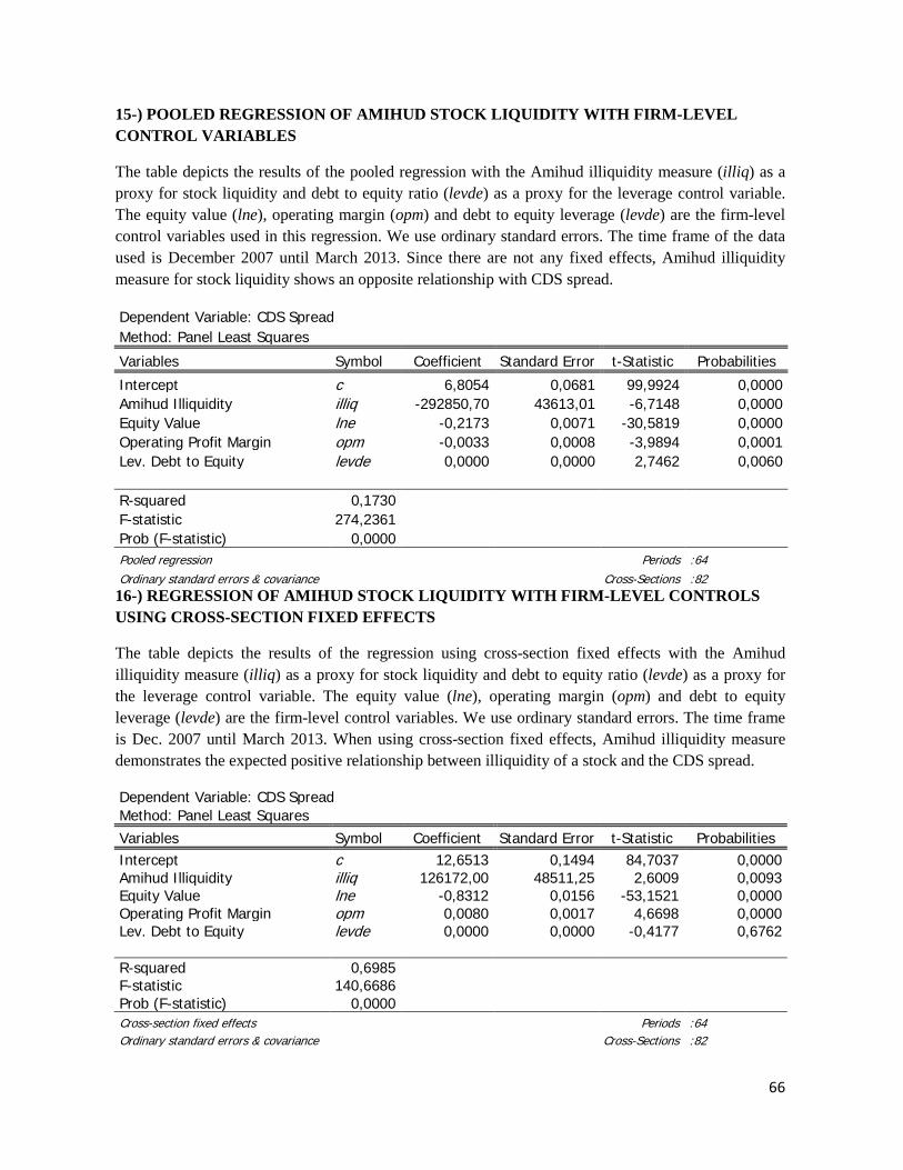
66
15-) POOLED REGRESSION OF AMIHUD STOCK LIQUIDITY WITH FIRM-LEVEL CONTROL VARIABLES
The table depicts the results of the pooled regression with the Amihud illiquidity measure (illiq) as a proxy for stock liquidity and debt to equity ratio (levde) as a proxy for the leverage control variable. The equity value (lne), operating margin (opm) and debt to equity leverage (levde) are the firm-level control variables used in this regression. We use ordinary standard errors. The time frame of the data used is December 2007 until March 2013. Since there are not any fixed effects, Amihud illiquidity measure for stock liquidity shows an opposite relationship with CDS spread.
Dependent Variable: CDS Spread Method: Panel Least Squares
Variables Symbol Coefficient Standard Error t-Statistic Probabilities
Intercept c 6,8054 0,0681 99,9924 0,0000 Amihud Illiquidity illiq -292850,70 43613,01 -6,7148 0,0000 Equity Value lne -0,2173 0,0071 -30,5819 0,0000 Operating Profit Margin opm -0,0033 0,0008 -3,9894 0,0001 Lev. Debt to Equity levde 0,0000 0,0000 2,7462 0,0060 R-squared 0,1730
F-statistic 274,2361 Prob (F-statistic) 0,0000
Pooled regression
Periods :64 Ordinary standard errors & covariance
Cross-Sections :82
16-) REGRESSION OF AMIHUD STOCK LIQUIDITY WITH FIRM-LEVEL CONTROLS USING CROSS-SECTION FIXED EFFECTS
The table depicts the results of the regression using cross-section fixed effects with the Amihud illiquidity measure (illiq) as a proxy for stock liquidity and debt to equity ratio (levde) as a proxy for the leverage control variable. The equity value (lne), operating margin (opm) and debt to equity leverage (levde) are the firm-level control variables. We use ordinary standard errors. The time frame is Dec. 2007 until March 2013. When using cross-section fixed effects, Amihud illiquidity measure demonstrates the expected positive relationship between illiquidity of a stock and the CDS spread.
Dependent Variable: CDS Spread Method: Panel Least Squares
Variables Symbol Coefficient Standard Error t-Statistic Probabilities Intercept c 12,6513 0,1494 84,7037 0,0000 Amihud Illiquidity illiq 126172,00 48511,25 2,6009 0,0093 Equity Value lne -0,8312 0,0156 -53,1521 0,0000 Operating Profit Margin opm 0,0080 0,0017 4,6698 0,0000 Lev. Debt to Equity levde 0,0000 0,0000 -0,4177 0,6762 R-squared 0,6985
F-statistic 140,6686 Prob (F-statistic) 0,0000
Cross-section fixed effects
Periods :64 Ordinary standard errors & covariance
Cross-Sections :82
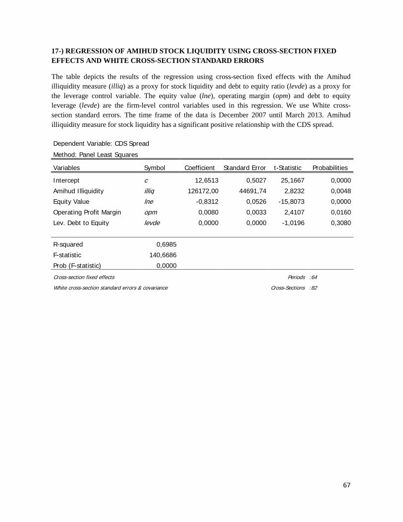
67
17-) REGRESSION OF AMIHUD STOCK LIQUIDITY USING CROSS-SECTION FIXED EFFECTS AND WHITE CROSS-SECTION STANDARD ERRORS
The table depicts the results of the regression using cross-section fixed effects with the Amihud illiquidity measure (illiq) as a proxy for stock liquidity and debt to equity ratio (levde) as a proxy for the leverage control variable. The equity value (lne), operating margin (opm) and debt to equity leverage (levde) are the firm-level control variables used in this regression. We use White cross-section standard errors. The time frame of the data is December 2007 until March 2013. Amihud illiquidity measure for stock liquidity has a significant positive relationship with the CDS spread.
Dependent Variable: CDS Spread Method: Panel Least Squares
Variables Symbol Coefficient Standard Error t-Statistic Probabilities
Intercept c 12,6513 0,5027 25,1667 0,0000
Amihud Illiquidity illiq 126172,00 44691,74 2,8232 0,0048
Equity Value lne -0,8312 0,0526 -15,8073 0,0000
Operating Profit Margin opm 0,0080 0,0033 2,4107 0,0160
Lev. Debt to Equity levde 0,0000 0,0000 -1,0196 0,3080
R-squared 0,6985 F-statistic 140,6686 Prob (F-statistic) 0,0000
Cross-section fixed effects
Periods :64
White cross-section standard errors & covariance
Cross-Sections :82
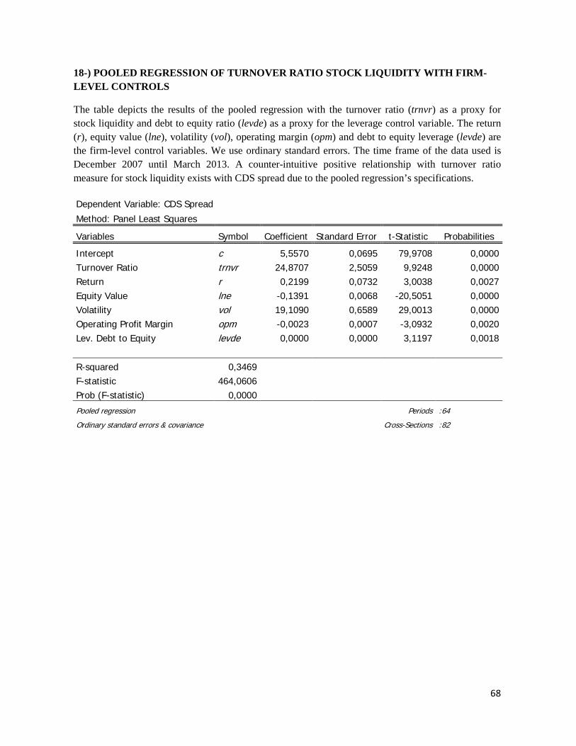
68
18-) POOLED REGRESSION OF TURNOVER RATIO STOCK LIQUIDITY WITH FIRM-LEVEL CONTROLS
The table depicts the results of the pooled regression with the turnover ratio (trnvr) as a proxy for stock liquidity and debt to equity ratio (levde) as a proxy for the leverage control variable. The return (r), equity value (lne), volatility (vol), operating margin (opm) and debt to equity leverage (levde) are the firm-level control variables. We use ordinary standard errors. The time frame of the data used is December 2007 until March 2013. A counter-intuitive positive relationship with turnover ratio measure for stock liquidity exists with CDS spread due to the pooled regression’s specifications.
Dependent Variable: CDS Spread Method: Panel Least Squares
Variables Symbol Coefficient Standard Error t-Statistic Probabilities
Intercept c 5,5570 0,0695 79,9708 0,0000 Turnover Ratio trnvr 24,8707 2,5059 9,9248 0,0000 Return r 0,2199 0,0732 3,0038 0,0027 Equity Value lne -0,1391 0,0068 -20,5051 0,0000 Volatility vol 19,1090 0,6589 29,0013 0,0000 Operating Profit Margin opm -0,0023 0,0007 -3,0932 0,0020 Lev. Debt to Equity levde 0,0000 0,0000 3,1197 0,0018 R-squared 0,3469
F-statistic 464,0606 Prob (F-statistic) 0,0000
Pooled regression
Periods :64
Ordinary standard errors & covariance
Cross-Sections :82
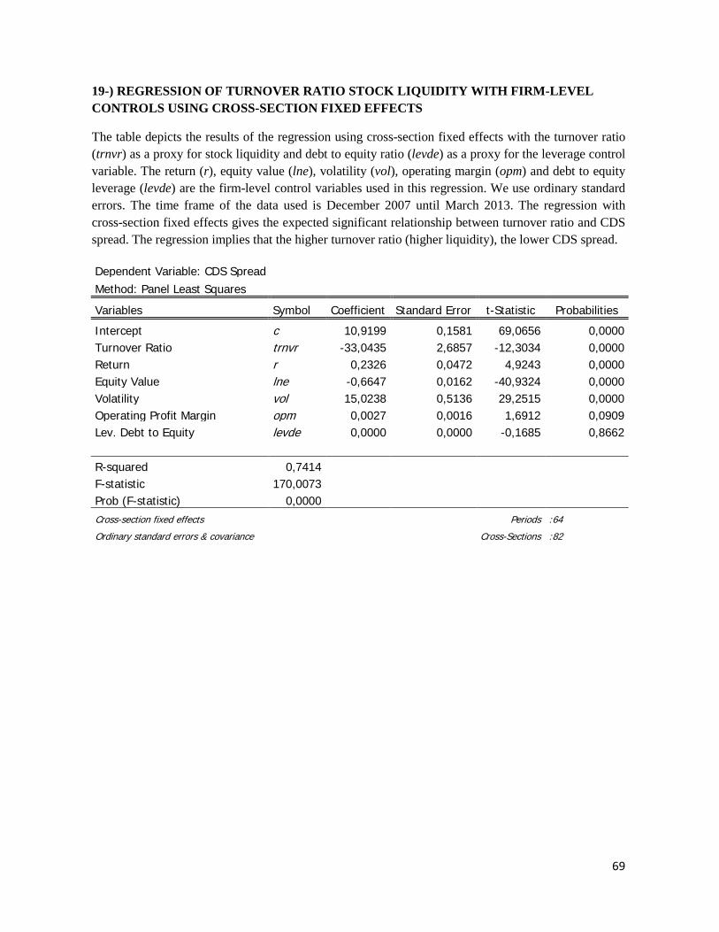
69
19-) REGRESSION OF TURNOVER RATIO STOCK LIQUIDITY WITH FIRM-LEVEL CONTROLS USING CROSS-SECTION FIXED EFFECTS
The table depicts the results of the regression using cross-section fixed effects with the turnover ratio (trnvr) as a proxy for stock liquidity and debt to equity ratio (levde) as a proxy for the leverage control variable. The return (r), equity value (lne), volatility (vol), operating margin (opm) and debt to equity leverage (levde) are the firm-level control variables used in this regression. We use ordinary standard errors. The time frame of the data used is December 2007 until March 2013. The regression with cross-section fixed effects gives the expected significant relationship between turnover ratio and CDS spread. The regression implies that the higher turnover ratio (higher liquidity), the lower CDS spread.
Dependent Variable: CDS Spread Method: Panel Least Squares
Variables Symbol Coefficient Standard Error t-Statistic Probabilities
Intercept c 10,9199 0,1581 69,0656 0,0000 Turnover Ratio trnvr -33,0435 2,6857 -12,3034 0,0000 Return r 0,2326 0,0472 4,9243 0,0000 Equity Value lne -0,6647 0,0162 -40,9324 0,0000 Volatility vol 15,0238 0,5136 29,2515 0,0000 Operating Profit Margin opm 0,0027 0,0016 1,6912 0,0909 Lev. Debt to Equity levde 0,0000 0,0000 -0,1685 0,8662 R-squared 0,7414
F-statistic 170,0073 Prob (F-statistic) 0,0000
Cross-section fixed effects
Periods :64
Ordinary standard errors & covariance
Cross-Sections :82
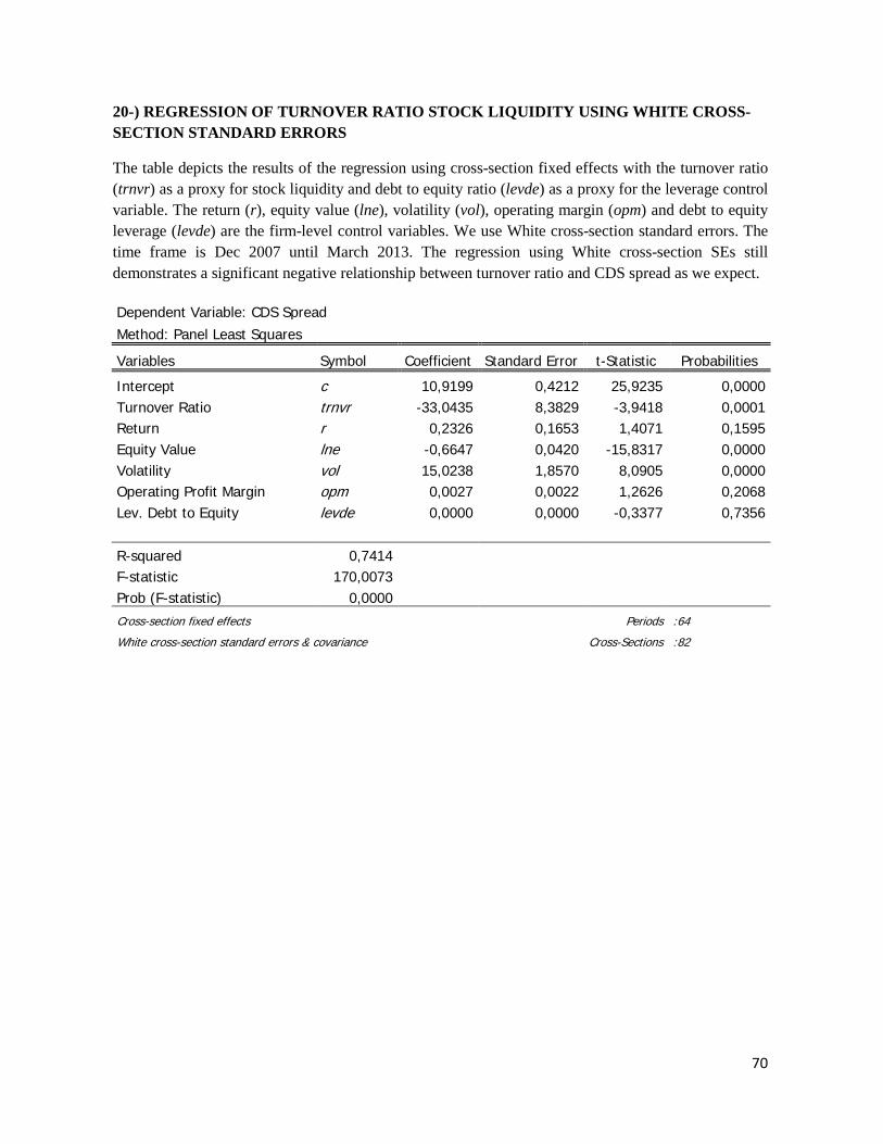
70
20-) REGRESSION OF TURNOVER RATIO STOCK LIQUIDITY USING WHITE CROSS-SECTION STANDARD ERRORS
The table depicts the results of the regression using cross-section fixed effects with the turnover ratio (trnvr) as a proxy for stock liquidity and debt to equity ratio (levde) as a proxy for the leverage control variable. The return (r), equity value (lne), volatility (vol), operating margin (opm) and debt to equity leverage (levde) are the firm-level control variables. We use White cross-section standard errors. The time frame is Dec 2007 until March 2013. The regression using White cross-section SEs still demonstrates a significant negative relationship between turnover ratio and CDS spread as we expect.
Dependent Variable: CDS Spread Method: Panel Least Squares
Variables Symbol Coefficient Standard Error t-Statistic Probabilities
Intercept c 10,9199 0,4212 25,9235 0,0000 Turnover Ratio trnvr -33,0435 8,3829 -3,9418 0,0001 Return r 0,2326 0,1653 1,4071 0,1595 Equity Value lne -0,6647 0,0420 -15,8317 0,0000 Volatility vol 15,0238 1,8570 8,0905 0,0000 Operating Profit Margin opm 0,0027 0,0022 1,2626 0,2068 Lev. Debt to Equity levde 0,0000 0,0000 -0,3377 0,7356 R-squared 0,7414
F-statistic 170,0073 Prob (F-statistic) 0,0000
Cross-section fixed effects
Periods :64
White cross-section standard errors & covariance
Cross-Sections :82
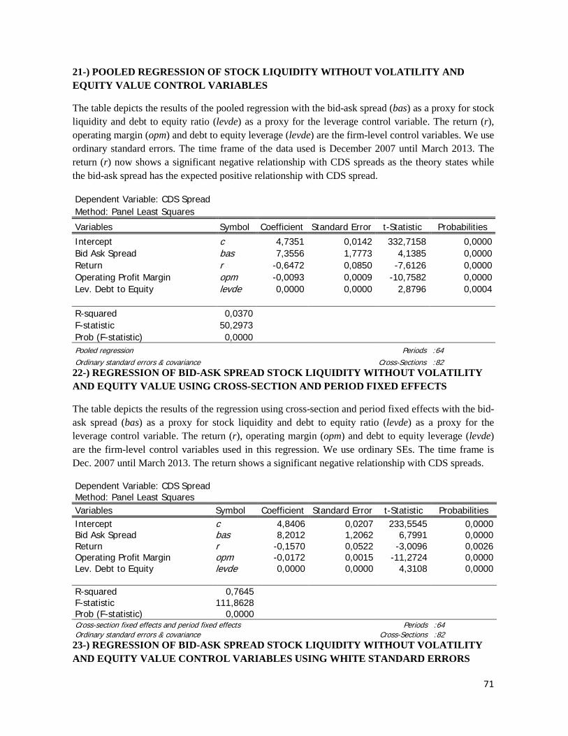
71
21-) POOLED REGRESSION OF STOCK LIQUIDITY WITHOUT VOLATILITY AND EQUITY VALUE CONTROL VARIABLES
The table depicts the results of the pooled regression with the bid-ask spread (bas) as a proxy for stock liquidity and debt to equity ratio (levde) as a proxy for the leverage control variable. The return (r), operating margin (opm) and debt to equity leverage (levde) are the firm-level control variables. We use ordinary standard errors. The time frame of the data used is December 2007 until March 2013. The return (r) now shows a significant negative relationship with CDS spreads as the theory states while the bid-ask spread has the expected positive relationship with CDS spread.
Dependent Variable: CDS Spread Method: Panel Least Squares
Variables Symbol Coefficient Standard Error t-Statistic Probabilities
Intercept c 4,7351 0,0142 332,7158 0,0000 Bid Ask Spread bas 7,3556 1,7773 4,1385 0,0000 Return r -0,6472 0,0850 -7,6126 0,0000 Operating Profit Margin opm -0,0093 0,0009 -10,7582 0,0000 Lev. Debt to Equity levde 0,0000 0,0000 2,8796 0,0004 R-squared 0,0370
F-statistic 50,2973 Prob (F-statistic) 0,0000
Pooled regression
Periods :64 Ordinary standard errors & covariance
Cross-Sections :82
22-) REGRESSION OF BID-ASK SPREAD STOCK LIQUIDITY WITHOUT VOLATILITY AND EQUITY VALUE USING CROSS-SECTION AND PERIOD FIXED EFFECTS
The table depicts the results of the regression using cross-section and period fixed effects with the bid-ask spread (bas) as a proxy for stock liquidity and debt to equity ratio (levde) as a proxy for the leverage control variable. The return (r), operating margin (opm) and debt to equity leverage (levde) are the firm-level control variables used in this regression. We use ordinary SEs. The time frame is Dec. 2007 until March 2013. The return shows a significant negative relationship with CDS spreads.
Dependent Variable: CDS Spread Method: Panel Least Squares
Variables Symbol Coefficient Standard Error t-Statistic Probabilities Intercept c 4,8406 0,0207 233,5545 0,0000 Bid Ask Spread bas 8,2012 1,2062 6,7991 0,0000 Return r -0,1570 0,0522 -3,0096 0,0026 Operating Profit Margin opm -0,0172 0,0015 -11,2724 0,0000 Lev. Debt to Equity levde 0,0000 0,0000 4,3108 0,0000 R-squared 0,7645
F-statistic 111,8628 Prob (F-statistic) 0,0000
Cross-section fixed effects and period fixed effects
Periods :64 Ordinary standard errors & covariance
Cross-Sections :82
23-) REGRESSION OF BID-ASK SPREAD STOCK LIQUIDITY WITHOUT VOLATILITY AND EQUITY VALUE CONTROL VARIABLES USING WHITE STANDARD ERRORS
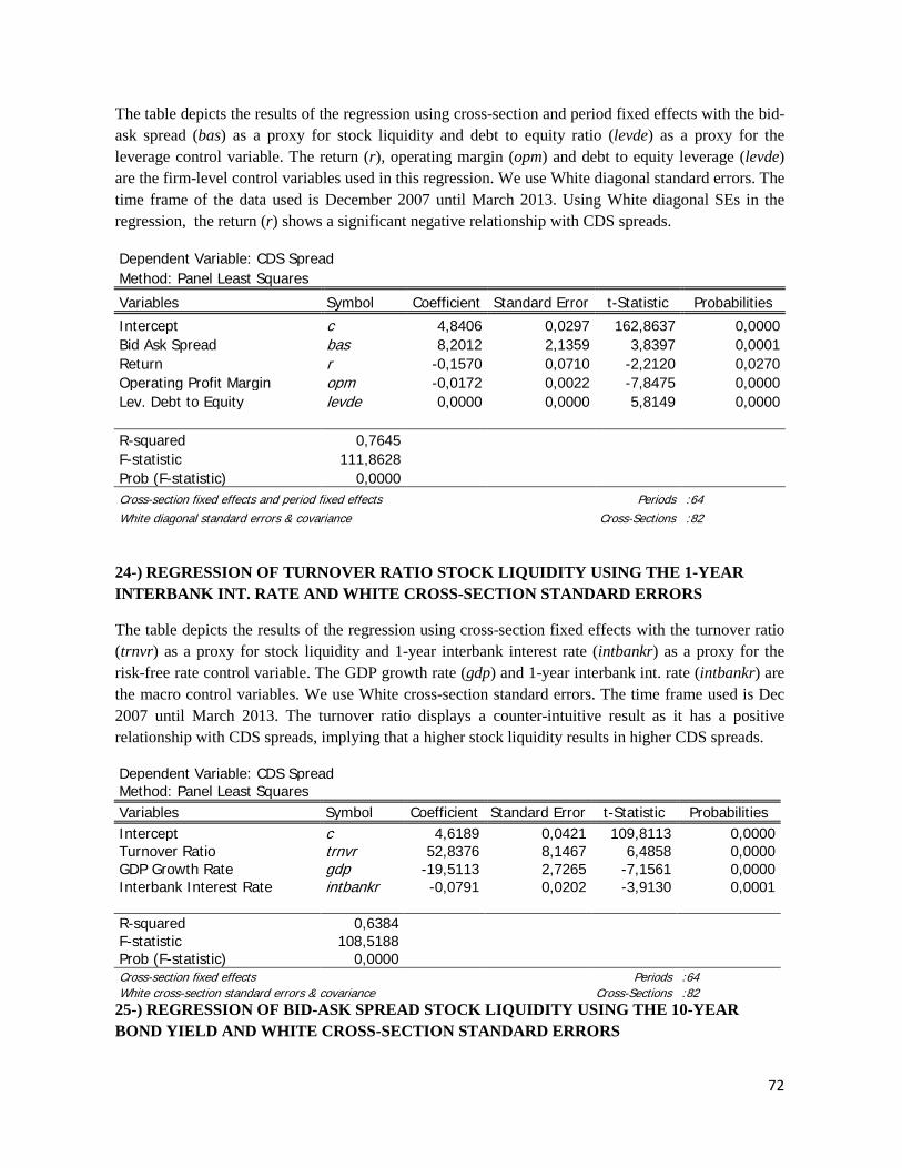
72
The table depicts the results of the regression using cross-section and period fixed effects with the bid-ask spread (bas) as a proxy for stock liquidity and debt to equity ratio (levde) as a proxy for the leverage control variable. The return (r), operating margin (opm) and debt to equity leverage (levde) are the firm-level control variables used in this regression. We use White diagonal standard errors. The time frame of the data used is December 2007 until March 2013. Using White diagonal SEs in the regression, the return (r) shows a significant negative relationship with CDS spreads.
Dependent Variable: CDS Spread Method: Panel Least Squares
Variables Symbol Coefficient Standard Error t-Statistic Probabilities
Intercept c 4,8406 0,0297 162,8637 0,0000 Bid Ask Spread bas 8,2012 2,1359 3,8397 0,0001 Return r -0,1570 0,0710 -2,2120 0,0270 Operating Profit Margin opm -0,0172 0,0022 -7,8475 0,0000 Lev. Debt to Equity levde 0,0000 0,0000 5,8149 0,0000 R-squared 0,7645
F-statistic 111,8628 Prob (F-statistic) 0,0000
Cross-section fixed effects and period fixed effects
Periods :64 White diagonal standard errors & covariance
Cross-Sections :82
24-) REGRESSION OF TURNOVER RATIO STOCK LIQUIDITY USING THE 1-YEAR INTERBANK INT. RATE AND WHITE CROSS-SECTION STANDARD ERRORS
The table depicts the results of the regression using cross-section fixed effects with the turnover ratio (trnvr) as a proxy for stock liquidity and 1-year interbank interest rate (intbankr) as a proxy for the risk-free rate control variable. The GDP growth rate (gdp) and 1-year interbank int. rate (intbankr) are the macro control variables. We use White cross-section standard errors. The time frame used is Dec 2007 until March 2013. The turnover ratio displays a counter-intuitive result as it has a positive relationship with CDS spreads, implying that a higher stock liquidity results in higher CDS spreads.
Dependent Variable: CDS Spread Method: Panel Least Squares
Variables Symbol Coefficient Standard Error t-Statistic Probabilities Intercept c 4,6189 0,0421 109,8113 0,0000 Turnover Ratio trnvr 52,8376 8,1467 6,4858 0,0000 GDP Growth Rate gdp -19,5113 2,7265 -7,1561 0,0000 Interbank Interest Rate intbankr -0,0791 0,0202 -3,9130 0,0001 R-squared 0,6384
F-statistic 108,5188 Prob (F-statistic) 0,0000
Cross-section fixed effects
Periods :64 White cross-section standard errors & covariance
Cross-Sections :82
25-) REGRESSION OF BID-ASK SPREAD STOCK LIQUIDITY USING THE 10-YEAR BOND YIELD AND WHITE CROSS-SECTION STANDARD ERRORS
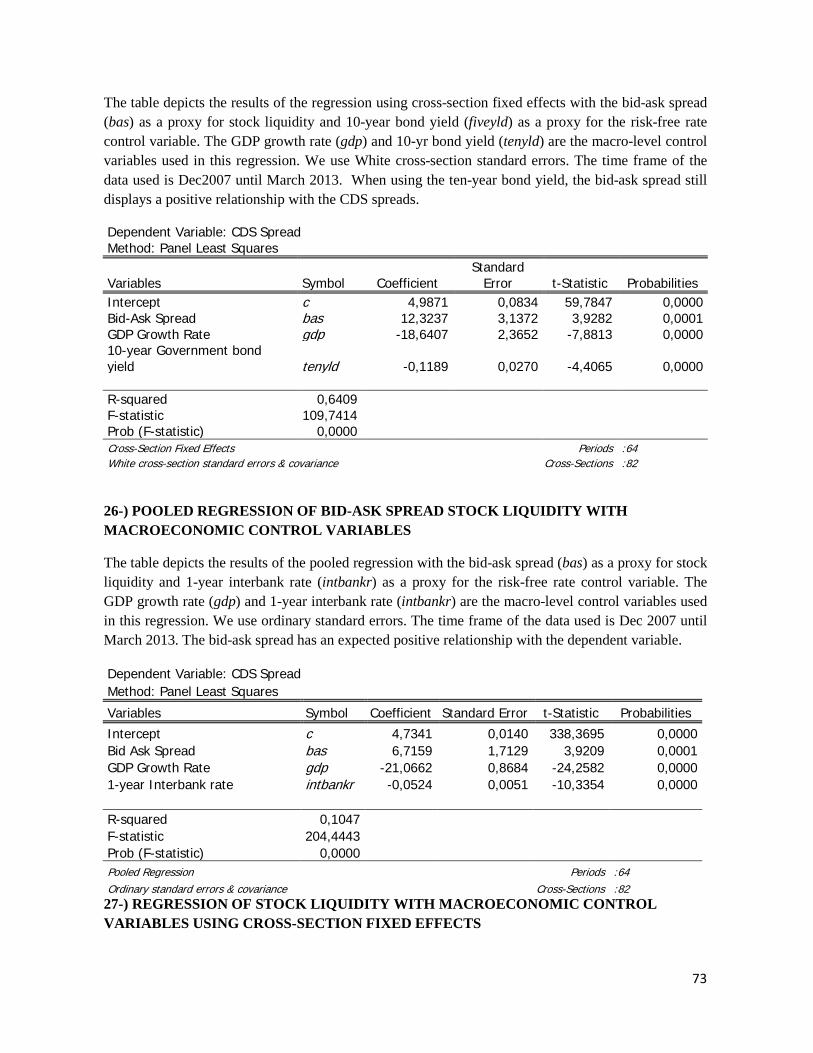
73
The table depicts the results of the regression using cross-section fixed effects with the bid-ask spread (bas) as a proxy for stock liquidity and 10-year bond yield (fiveyld) as a proxy for the risk-free rate control variable. The GDP growth rate (gdp) and 10-yr bond yield (tenyld) are the macro-level control variables used in this regression. We use White cross-section standard errors. The time frame of the data used is Dec2007 until March 2013. When using the ten-year bond yield, the bid-ask spread still displays a positive relationship with the CDS spreads.
Dependent Variable: CDS Spread Method: Panel Least Squares
Variables Symbol Coefficient Standard
Error t-Statistic Probabilities Intercept c 4,9871 0,0834 59,7847 0,0000 Bid-Ask Spread bas 12,3237 3,1372 3,9282 0,0001 GDP Growth Rate gdp -18,6407 2,3652 -7,8813 0,0000 10-year Government bond yield tenyld -0,1189 0,0270 -4,4065 0,0000 R-squared 0,6409
F-statistic 109,7414 Prob (F-statistic) 0,0000
Cross-Section Fixed Effects
Periods :64 White cross-section standard errors & covariance
Cross-Sections :82
26-) POOLED REGRESSION OF BID-ASK SPREAD STOCK LIQUIDITY WITH MACROECONOMIC CONTROL VARIABLES
The table depicts the results of the pooled regression with the bid-ask spread (bas) as a proxy for stock liquidity and 1-year interbank rate (intbankr) as a proxy for the risk-free rate control variable. The GDP growth rate (gdp) and 1-year interbank rate (intbankr) are the macro-level control variables used in this regression. We use ordinary standard errors. The time frame of the data used is Dec 2007 until March 2013. The bid-ask spread has an expected positive relationship with the dependent variable.
Dependent Variable: CDS Spread Method: Panel Least Squares
Variables Symbol Coefficient Standard Error t-Statistic Probabilities
Intercept c 4,7341 0,0140 338,3695 0,0000 Bid Ask Spread bas 6,7159 1,7129 3,9209 0,0001 GDP Growth Rate gdp -21,0662 0,8684 -24,2582 0,0000 1-year Interbank rate intbankr -0,0524 0,0051 -10,3354 0,0000 R-squared 0,1047
F-statistic 204,4443 Prob (F-statistic) 0,0000
Pooled Regression
Periods :64 Ordinary standard errors & covariance
Cross-Sections :82
27-) REGRESSION OF STOCK LIQUIDITY WITH MACROECONOMIC CONTROL VARIABLES USING CROSS-SECTION FIXED EFFECTS
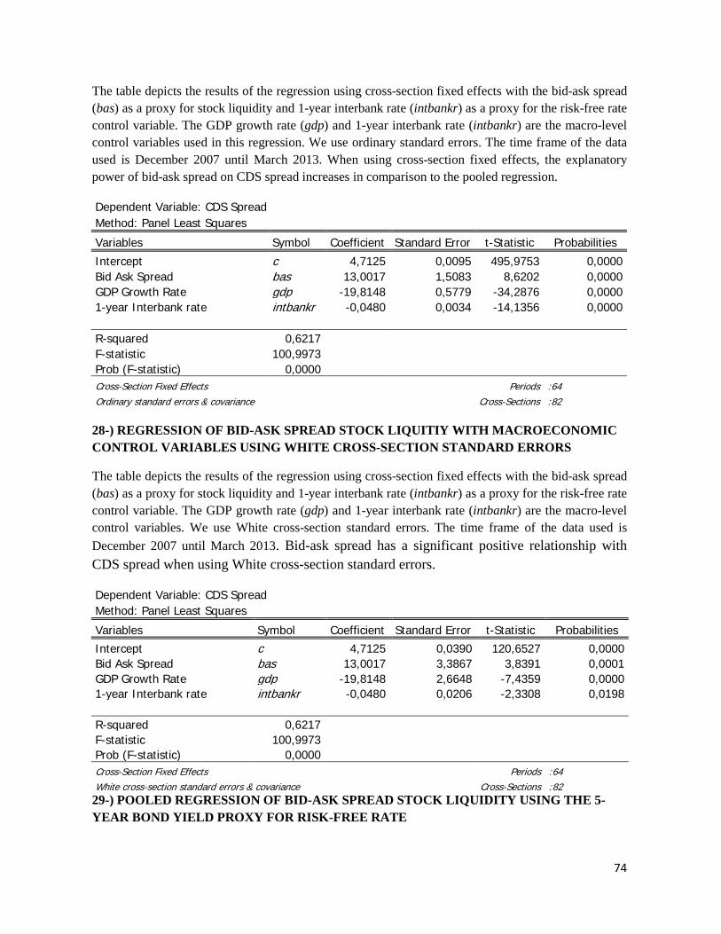
74
The table depicts the results of the regression using cross-section fixed effects with the bid-ask spread (bas) as a proxy for stock liquidity and 1-year interbank rate (intbankr) as a proxy for the risk-free rate control variable. The GDP growth rate (gdp) and 1-year interbank rate (intbankr) are the macro-level control variables used in this regression. We use ordinary standard errors. The time frame of the data used is December 2007 until March 2013. When using cross-section fixed effects, the explanatory power of bid-ask spread on CDS spread increases in comparison to the pooled regression.
Dependent Variable: CDS Spread Method: Panel Least Squares
Variables Symbol Coefficient Standard Error t-Statistic Probabilities
Intercept c 4,7125 0,0095 495,9753 0,0000 Bid Ask Spread bas 13,0017 1,5083 8,6202 0,0000 GDP Growth Rate gdp -19,8148 0,5779 -34,2876 0,0000 1-year Interbank rate intbankr -0,0480 0,0034 -14,1356 0,0000 R-squared 0,6217
F-statistic 100,9973 Prob (F-statistic) 0,0000
Cross-Section Fixed Effects
Periods :64 Ordinary standard errors & covariance
Cross-Sections :82
28-) REGRESSION OF BID-ASK SPREAD STOCK LIQUITIY WITH MACROECONOMIC CONTROL VARIABLES USING WHITE CROSS-SECTION STANDARD ERRORS
The table depicts the results of the regression using cross-section fixed effects with the bid-ask spread (bas) as a proxy for stock liquidity and 1-year interbank rate (intbankr) as a proxy for the risk-free rate control variable. The GDP growth rate (gdp) and 1-year interbank rate (intbankr) are the macro-level control variables. We use White cross-section standard errors. The time frame of the data used is December 2007 until March 2013. Bid-ask spread has a significant positive relationship with CDS spread when using White cross-section standard errors.
Dependent Variable: CDS Spread Method: Panel Least Squares
Variables Symbol Coefficient Standard Error t-Statistic Probabilities
Intercept c 4,7125 0,0390 120,6527 0,0000 Bid Ask Spread bas 13,0017 3,3867 3,8391 0,0001 GDP Growth Rate gdp -19,8148 2,6648 -7,4359 0,0000 1-year Interbank rate intbankr -0,0480 0,0206 -2,3308 0,0198 R-squared 0,6217
F-statistic 100,9973 Prob (F-statistic) 0,0000
Cross-Section Fixed Effects
Periods :64 White cross-section standard errors & covariance
Cross-Sections :82
29-) POOLED REGRESSION OF BID-ASK SPREAD STOCK LIQUIDITY USING THE 5-YEAR BOND YIELD PROXY FOR RISK-FREE RATE
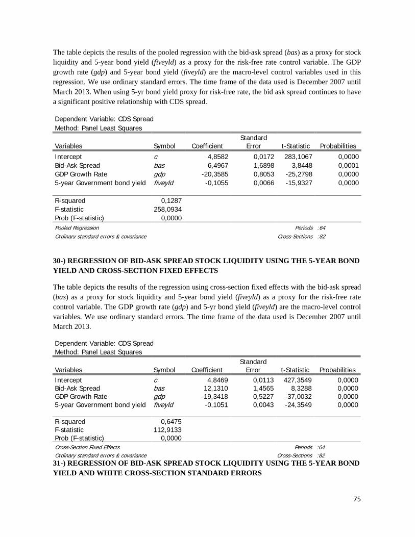
75
The table depicts the results of the pooled regression with the bid-ask spread (bas) as a proxy for stock liquidity and 5-year bond yield (fiveyld) as a proxy for the risk-free rate control variable. The GDP growth rate (gdp) and 5-year bond yield (fiveyld) are the macro-level control variables used in this regression. We use ordinary standard errors. The time frame of the data used is December 2007 until March 2013. When using 5-yr bond yield proxy for risk-free rate, the bid ask spread continues to have a significant positive relationship with CDS spread.
Dependent Variable: CDS Spread Method: Panel Least Squares
Variables Symbol Coefficient Standard
Error t-Statistic Probabilities
Intercept c 4,8582 0,0172 283,1067 0,0000 Bid-Ask Spread bas 6,4967 1,6898 3,8448 0,0001 GDP Growth Rate gdp -20,3585 0,8053 -25,2798 0,0000 5-year Government bond yield fiveyld -0,1055 0,0066 -15,9327 0,0000 R-squared 0,1287
F-statistic 258,0934 Prob (F-statistic) 0,0000
Pooled Regression
Periods :64 Ordinary standard errors & covariance
Cross-Sections :82
30-) REGRESSION OF BID-ASK SPREAD STOCK LIQUIDITY USING THE 5-YEAR BOND YIELD AND CROSS-SECTION FIXED EFFECTS
The table depicts the results of the regression using cross-section fixed effects with the bid-ask spread (bas) as a proxy for stock liquidity and 5-year bond yield (fiveyld) as a proxy for the risk-free rate control variable. The GDP growth rate (gdp) and 5-yr bond yield (fiveyld) are the macro-level control variables. We use ordinary standard errors. The time frame of the data used is December 2007 until March 2013.
Dependent Variable: CDS Spread Method: Panel Least Squares
Variables Symbol Coefficient Standard
Error t-Statistic Probabilities Intercept c 4,8469 0,0113 427,3549 0,0000 Bid-Ask Spread bas 12,1310 1,4565 8,3288 0,0000 GDP Growth Rate gdp -19,3418 0,5227 -37,0032 0,0000 5-year Government bond yield fiveyld -0,1051 0,0043 -24,3549 0,0000 R-squared 0,6475
F-statistic 112,9133 Prob (F-statistic) 0,0000
Cross-Section Fixed Effects
Periods :64 Ordinary standard errors & covariance
Cross-Sections :82
31-) REGRESSION OF BID-ASK SPREAD STOCK LIQUIDITY USING THE 5-YEAR BOND YIELD AND WHITE CROSS-SECTION STANDARD ERRORS
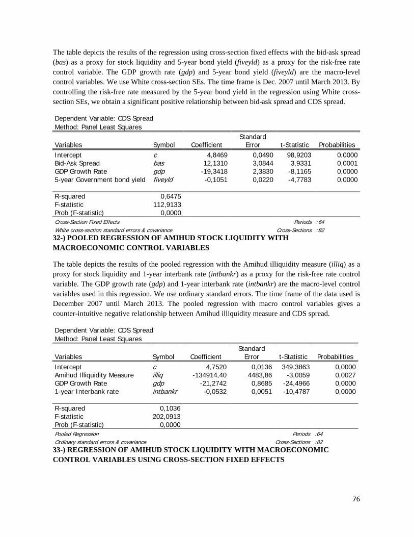
76
The table depicts the results of the regression using cross-section fixed effects with the bid-ask spread (bas) as a proxy for stock liquidity and 5-year bond yield (fiveyld) as a proxy for the risk-free rate control variable. The GDP growth rate (gdp) and 5-year bond yield (fiveyld) are the macro-level control variables. We use White cross-section SEs. The time frame is Dec. 2007 until March 2013. By controlling the risk-free rate measured by the 5-year bond yield in the regression using White cross-section SEs, we obtain a significant positive relationship between bid-ask spread and CDS spread.
Dependent Variable: CDS Spread Method: Panel Least Squares
Variables Symbol Coefficient Standard
Error t-Statistic Probabilities Intercept c 4,8469 0,0490 98,9203 0,0000 Bid-Ask Spread bas 12,1310 3,0844 3,9331 0,0001 GDP Growth Rate gdp -19,3418 2,3830 -8,1165 0,0000 5-year Government bond yield fiveyld -0,1051 0,0220 -4,7783 0,0000 R-squared 0,6475
F-statistic 112,9133 Prob (F-statistic) 0,0000
Cross-Section Fixed Effects
Periods :64 White cross-section standard errors & covariance
Cross-Sections :82
32-) POOLED REGRESSION OF AMIHUD STOCK LIQUIDITY WITH MACROECONOMIC CONTROL VARIABLES
The table depicts the results of the pooled regression with the Amihud illiquidity measure (illiq) as a proxy for stock liquidity and 1-year interbank rate (intbankr) as a proxy for the risk-free rate control variable. The GDP growth rate (gdp) and 1-year interbank rate (intbankr) are the macro-level control variables used in this regression. We use ordinary standard errors. The time frame of the data used is December 2007 until March 2013. The pooled regression with macro control variables gives a counter-intuitive negative relationship between Amihud illiquidity measure and CDS spread.
Dependent Variable: CDS Spread Method: Panel Least Squares
Variables Symbol Coefficient Standard
Error t-Statistic Probabilities Intercept c 4,7520 0,0136 349,3863 0,0000 Amihud Illiquidity Measure illiq -134914,40 4483,86 -3,0059 0,0027 GDP Growth Rate gdp -21,2742 0,8685 -24,4966 0,0000 1-year Interbank rate intbankr -0,0532 0,0051 -10,4787 0,0000 R-squared 0,1036
F-statistic 202,0913 Prob (F-statistic) 0,0000
Pooled Regression
Periods :64 Ordinary standard errors & covariance
Cross-Sections :82
33-) REGRESSION OF AMIHUD STOCK LIQUIDITY WITH MACROECONOMIC CONTROL VARIABLES USING CROSS-SECTION FIXED EFFECTS
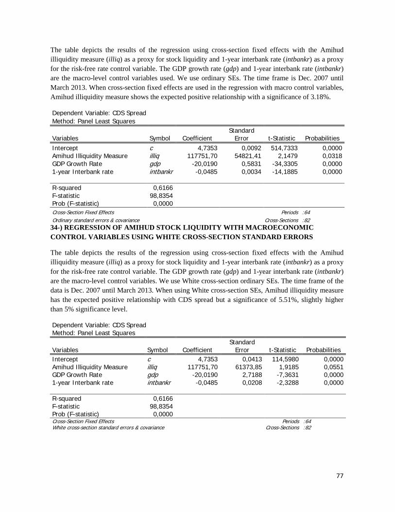
77
The table depicts the results of the regression using cross-section fixed effects with the Amihud illiquidity measure (illiq) as a proxy for stock liquidity and 1-year interbank rate (intbankr) as a proxy for the risk-free rate control variable. The GDP growth rate (gdp) and 1-year interbank rate (intbankr) are the macro-level control variables used. We use ordinary SEs. The time frame is Dec. 2007 until March 2013. When cross-section fixed effects are used in the regression with macro control variables, Amihud illiquidity measure shows the expected positive relationship with a significance of 3.18%.
Dependent Variable: CDS Spread Method: Panel Least Squares
Variables Symbol Coefficient Standard
Error t-Statistic Probabilities Intercept c 4,7353 0,0092 514,7333 0,0000 Amihud Illiquidity Measure illiq 117751,70 54821,41 2,1479 0,0318 GDP Growth Rate gdp -20,0190 0,5831 -34,3305 0,0000 1-year Interbank rate intbankr -0,0485 0,0034 -14,1885 0,0000 R-squared 0,6166
F-statistic 98,8354 Prob (F-statistic) 0,0000
Cross-Section Fixed Effects
Periods :64 Ordinary standard errors & covariance
Cross-Sections :82
34-) REGRESSION OF AMIHUD STOCK LIQUIDITY WITH MACROECONOMIC CONTROL VARIABLES USING WHITE CROSS-SECTION STANDARD ERRORS
The table depicts the results of the regression using cross-section fixed effects with the Amihud illiquidity measure (illiq) as a proxy for stock liquidity and 1-year interbank rate (intbankr) as a proxy for the risk-free rate control variable. The GDP growth rate (gdp) and 1-year interbank rate (intbankr) are the macro-level control variables. We use White cross-section ordinary SEs. The time frame of the data is Dec. 2007 until March 2013. When using White cross-section SEs, Amihud illiquidity measure has the expected positive relationship with CDS spread but a significance of 5.51%, slightly higher than 5% significance level.
Dependent Variable: CDS Spread Method: Panel Least Squares
Variables Symbol Coefficient Standard
Error t-Statistic Probabilities Intercept c 4,7353 0,0413 114,5980 0,0000 Amihud Illiquidity Measure illiq 117751,70 61373,85 1,9185 0,0551 GDP Growth Rate gdp -20,0190 2,7188 -7,3631 0,0000 1-year Interbank rate intbankr -0,0485 0,0208 -2,3288 0,0000 R-squared 0,6166
F-statistic 98,8354 Prob (F-statistic) 0,0000
Cross-Section Fixed Effects
Periods :64 White cross-section standard errors & covariance
Cross-Sections :82

78
35-) THE LIST OF 82 FIRMS USED IN THE SAMPLE:
* Company Name Country Company Name Country 1 Aktiebolaget Volvo Sweden 42 Next PLC UK 2 Akzo Nobel N.V. Netherlands 43 PPR France 3 Alstom France 44 Sabmiller PLC UK 4 Anglo American PLC UK 45 Suedzucker AG Mannheim Germany 5 Astrazeneca PLC UK 46 Tate & Lyle PLC UK 6 Atlantia S.P.A. Italy 47 Tesco PLC UK 7 BAE Systems PLC UK 48 Unilever UK 8 BASF SE UK 49 BP PLC UK 9 Bayer Aktiengesellschaft Germany 50 Centrica PLC UK
10 Bayerische Motoren Werke AG Germany 51 E.ON AG Germany 11 Bouygues France 52 Electricite de France (EDF) France 12 Compagnie de Saint-Gobain France 53 EnBW Energie Baden-Wuerttemberg AG Germany 13 Compagnie Financiere Michelin France 54 ENEL S.P.A. Italy 14 Daimler AG Germany 55 ENI S.P.A. Italy 15 Holcim Ltd Switzerland 56 Fortum Oyj Finland 16 Lanxess AG Germany 57 Gas Natural SDG S.A. Spain 17 Linde AG Germany 58 GDF Suez France 18 Rentokil Initial PLC UK 59 Iberdrola S.A. Spain 19 Rolls-Royce PLC UK 60 National Grid PLC UK 20 Sanofi France 61 Royal Dutch Shell PLC Netherlands 21 Siemens AG Germany 62 RWE AG Germany 22 Solvay Belgium 63 Total SA France 23 Valeo France 64 United Utilities PLC UK 24 Vinci France 65 Veolia Environment France 25 Volkswagen AG Germany 66 Aegon N.V. Netherlands 26 Xstrata PLC UK 67 British Telecommunications PLC UK 27 Accor France 68 Deutsche Telekom AG Germany 28 Aktiebolaget Electrolux Sweden 69 France Telecom France 29 Anheuser-Busch InBev Belgium 70 Koninklijke KPN N.V. Netherlands 30 British American Tobacco PLC UK 71 Pearson PLC UK 31 Carrefour France 72 Publicis Groupe SA France 32 Compass Group UK 73 STMicroelectronics N.V. France 33 Diageo PLC UK 74 Telecom Italia S.P.A. Italy 34 Experian Finance PLC UK 75 Telefonaktiebolaget LM Ericsson Sweden 35 Imperial Tobacco Group PLC UK 76 Telekom Austria AG Austria 36 Kingfisher PLC UK 77 Telenor ASA Norway 37 Koninklijke Ahold N.V. Netherlands 78 TeliaSonera Aktiebolaget Sweden 38 LVMH France 79 Vivendi France 39 Marks and Spencer PLC UK 80 Vodafone Group PLC UK 40 Metro AG Germany 81 Wolters Kluwer N.V. Netherlands 41 Nestle S.A. Switzerland 82 WPP 2005 Limited UK
Number of Companies per Country
United Kingdom 27 Sweden 3 France 19 Belgium 2 Germany 13 Switzerland 2 Netherlands 6 Norway 1 Italy 4 Finland 1 Spain 3 Austria 1 *The companies are selected from Markit iTraxx Europe Reference Portfolio